front propagation

Chapter 8

Front Propagation

8.1 Reaction-Diffusion Systems

We’ve studied simple N = 1 dynamical systems of the form

du

dt= R(u) . (8.1)

Recall that the dynamics evolves u(t) monotonically toward the first stable fixed pointencountered. Now let’s extend the function u(t) to the spatial domain as well, i.e. u(x, t),and add a diffusion term:

∂u

∂t= D∇

2u+R(u) , (8.2)

where D is the diffusion constant. This is an example of a reaction-diffusion system. If weextend u(x, t) to a multicomponent field u(x, t), we obtain the general reaction-diffusionequation (RDE)

∂ui∂t

= Dij∇2ui +Ri(u1, . . . , uN ) . (8.3)

Here, u is interpreted as a vector of reactants, R(u) describes the nonlinear local reaction

kinetics, and Dij is the diffusivity matrix . If diffusion is negligible, this PDE reduces todecoupled local ODEs of the form u = R(u), which is to say a dynamical system at eachpoint in space. Thus, any fixed point u∗ of the local reaction dynamics also describesa spatially homogeneous, time-independent solution to the RDE. These solutions may becharacterized as dynamically stable or unstable, depending on the eigenspectrum of theJacobian matrix Mij = ∂iRj(u

∗). At a stable fixed point, Re(λi) < 0 for all eigenvalues.

8.1.1 Single component systems

We first consider the single component system,

∂u

∂t= D∇

2u+R(u) . (8.4)

1

2 CHAPTER 8. FRONT PROPAGATION

Note that the right hand side can be expressed as the functional derivative of a Lyapunov

functional ,

L[u] =

∫

ddx

[

12D(∇u)2 − U(u)

]

, (8.5)

where

U(u) =

u∫

0

du′R(u′) . (8.6)

(The lower limit in the above equation is arbitrary.) Thus, eqn. 8.4 is equivalent to

∂u

∂t= − δL

δu(x, t). (8.7)

Thus, the Lyapunov functional runs strictly downhill, i.e. L < 0, except where u(x, t) solvesthe RDE, at which point L = 0.

8.1.2 Propagating front solutions

Suppose the dynamical system u = R(u) has two or more fixed points. Each such fixedpoint represents a static, homogeneous solution to the RDE. We now seek a dynamical,inhomogeneous solution to the RDE in the form of a propagating front , described by

u(x, t) = u(x− V t) , (8.8)

where V is the (as yet unknown) front propagation speed. With this Ansatz , the PDE ofeqn. 8.4 is converted to an ODE,

Dd2u

dξ2+ V

du

dξ+R(u) = 0 , (8.9)

where ξ = x − V t. With R(u) ≡ U ′(u) as in eqn. 8.6, we have the following convenientinterpretation. If we substitute u → q, ξ → t, D → m, and v → γ, this equation describesthe damped motion of a massive particle under friction: mq+γq = −U ′(q). The fixed pointsq∗ satisfy U ′(q∗) = 0 and are hence local extrema of U(q). The propagating front solutionwe seek therefore resembles the motion of a massive particle rolling between extrema ofthe potential U(q). Note that the stable fixed points of the local reaction kinetics haveR′(q) = U ′′(q) < 0, corresponding to unstable mechanical equilibria. Conversely, unstablefixed points of the local reaction kinetics have R′(q) = U ′′(q) > 0, corresponding to stable

mechanical equilibria.

A front solution corresponds to a mechanical motion interpolating between two equilibria atu(ξ = ±∞). If the front propagates to the right then V > 0, corresponding to a positive (i.e.usual) friction coefficient γ. Any solution, therefore must start from an unstable equilibriumpoint u∗I and end at another equilibrium u∗II. The final state, however, may be either a stableor an unstable equilibrium for the potential U(q). Consider the functions R(u) and U(u)in the left panels of fig. 8.1. Starting at ‘time’ ξ = −∞ with u = u∗I = 1, a particle with

8.1. REACTION-DIFFUSION SYSTEMS 3

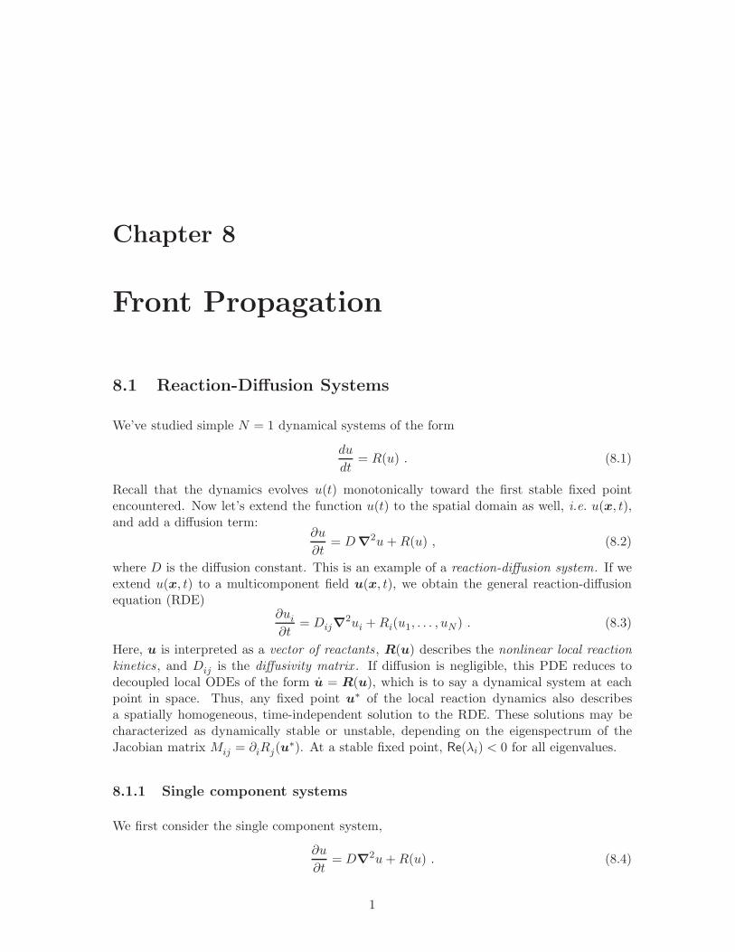
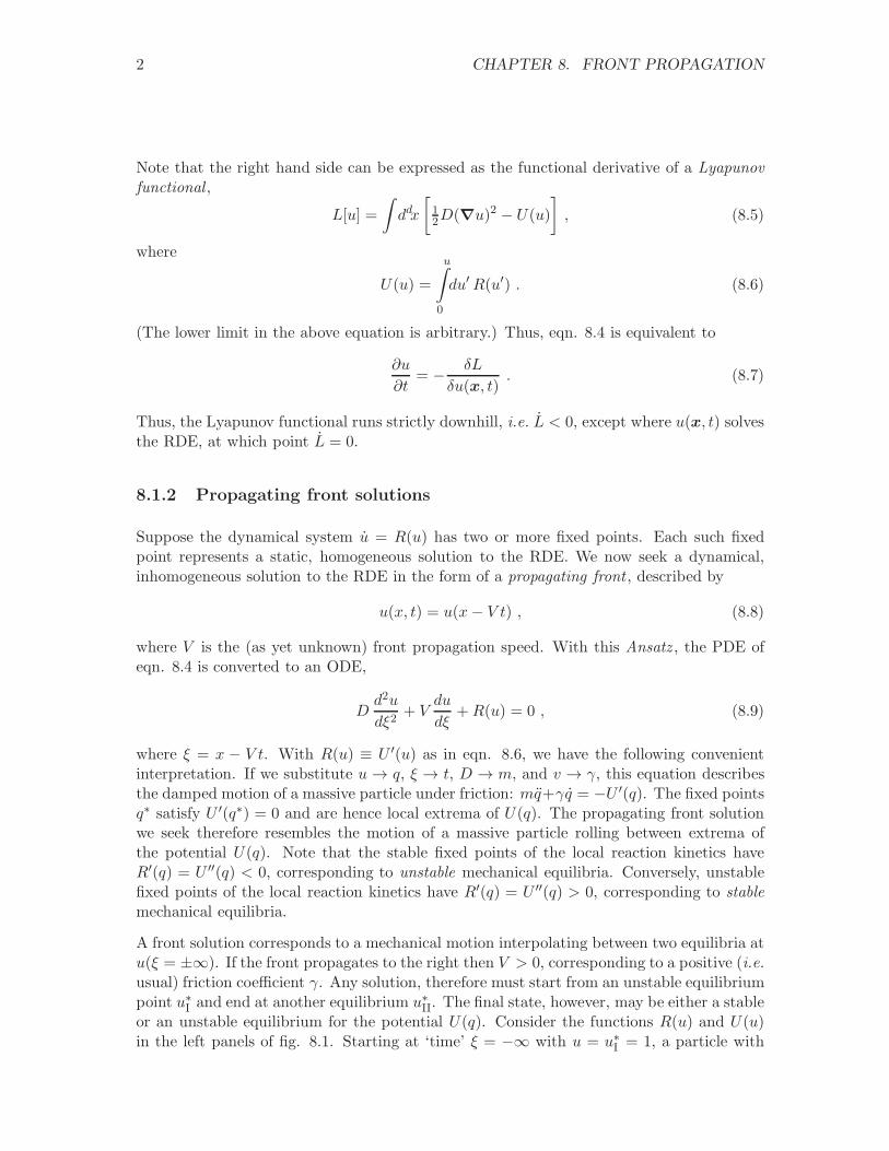
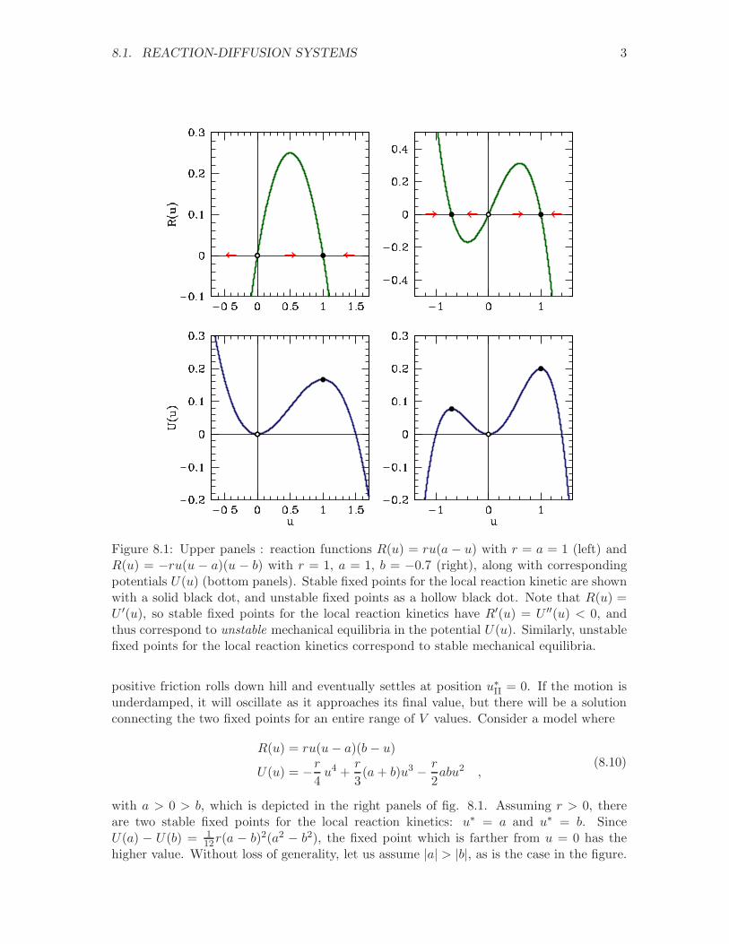
Figure 8.1: Upper panels : reaction functions R(u) = ru(a − u) with r = a = 1 (left) andR(u) = −ru(u − a)(u − b) with r = 1, a = 1, b = −0.7 (right), along with correspondingpotentials U(u) (bottom panels). Stable fixed points for the local reaction kinetic are shownwith a solid black dot, and unstable fixed points as a hollow black dot. Note that R(u) =U ′(u), so stable fixed points for the local reaction kinetics have R′(u) = U ′′(u) < 0, andthus correspond to unstable mechanical equilibria in the potential U(u). Similarly, unstablefixed points for the local reaction kinetics correspond to stable mechanical equilibria.

positive friction rolls down hill and eventually settles at position u∗II = 0. If the motion isunderdamped, it will oscillate as it approaches its final value, but there will be a solutionconnecting the two fixed points for an entire range of V values. Consider a model where

R(u) = ru(u− a)(b− u)

U(u) = −r4u4 +

r

3(a+ b)u3 − r

2abu2 ,

(8.10)

with a > 0 > b, which is depicted in the right panels of fig. 8.1. Assuming r > 0, thereare two stable fixed points for the local reaction kinetics: u∗ = a and u∗ = b. SinceU(a) − U(b) = 1

12r(a − b)2(a2 − b2), the fixed point which is farther from u = 0 has thehigher value. Without loss of generality, let us assume |a| > |b|, as is the case in the figure.


One can then roll off the peak at u∗ = a and eventually settle in at the local minimumu∗ = 0 for a range of c values, provided V is sufficiently large that the motion does not takeu beyond the other fixed point at u∗ = b. If we start at u∗ = b, then a solution interpolatingbetween this value and u∗ = 0 exists for any positive value of V . As we shall see, thismakes the issue of velocity selection a subtle one, as at this stage it appears a continuousfamily of propagating front solutions are possible. At any rate, for this type of front wehave u(ξ = −∞) = u∗I and u(ξ = +∞) = u∗II, where u

∗

I,II correspond to stable and unstablefixed points of the local dynamics. If we fix x and examine what happens as a function of t,we have ξ → ∓∞ as t→ ±∞, since V > 0, meaning that we start out in the unstable fixedpoint and eventually as the front passes over our position we transition to the stable fixedpoint. Accordingly, this type of front describes a propagation into an unstable phase. Notethat for V < 0, corresponding to left-moving fronts, we have negative friction, meaning wemove uphill in the potential U(u). Thus, we start at ξ = −∞ with u(−∞) = 0 and endup at u(+∞) = u∗I,II. But now we have ξ → ±∞ as t → ±∞, hence once again the stable

phase invades the unstable phase.

Another possibility is that one stable phase invades another. For the potential in the lowerright panel of fig. 8.1, this means starting at the leftmost fixed point where u(−∞) = aand, with V > 0 and positive friction, rolling down hill past u = 0, then back up the otherside, asymptotically coming to a perfect stop at u(+∞) = b. Clearly this requires that Vbe finely tuned to a specific value so that the system dissipates an energy exactly equal toU(a)−U(b) to friction during its motion. If V < 0 we have the time reverse of this motion.The fact that V is finely tuned to a specific value in order to have a solution means thatwe have a velocity selection taking place. Thus, if R(a) = R(b) = 0, then defining

∆U =

b∫

a

du R(u) = U(b)− U(a) , (8.11)

we have that u∗ = a invades u∗ = b if ∆U > 0, and u∗ = b invades u∗ = a if ∆U < 0.The front velocity in either case is fixed by the selection criterion that we asymptoticallyapproach both local maxima of U(u) as t→ ±∞.

For the equation

Du′′ + V u′ = ru(u− a)(u− b) , (8.12)

we can find an exact solution of the form

u(ξ) =

(

a+ b

2

)

+

(

b− a

2

)

tanh(Aξ) . (8.13)

Direct substitution shows this is a solution when

A = |a− b|( r

8D

)1/2(8.14)

V =

√

Dr

2(a+ b). (8.15)


8.1.3 Stability and zero mode

We assume a propagating front solution u(x−V t) connecting u(−∞) = uLand u(+∞) = u

R.

For |ξ| very large, we can linearize about the fixed points uL,R

. For ξ → −∞ we writeR(u

L+ δu) ≈ R′(u

L) δu and the linearized front equation is

D δu′′ + V δu′ +R′(uL) δu = 0 . (8.16)

This equation possesses solutions of the form δu = AeκLξ, where

Dκ2L+ V κ

L+R′(u

L) = 0 . (8.17)

The solutions are

κL= − V

2D±

√

(

V

2D

)2

− R′(uL)

D. (8.18)

We assume that uLis a stable fixed point of the local dynamics, which means R′(u

L) < 0.

Thus, κL,− < 0 < κ

L,+, and the allowed solution, which does not blow up as ξ → −∞ isto take κ

L= κ

L+. If we choose ξL< 0 such that κ+ξL << −1, then we can take as initial

conditions u(ξL) = u

L+ A

LeκL

ξL and u′(x

L) = κ

LA

LeκL

ξL . We can then integrate forward

to ξ = +∞ where u′(+∞ = 0) using the ‘shooting method’ to fix the propagation speed V .

For ξ → +∞, we again linearize, writing u = uR+ δu and obtaining

D δu′′ + V δu′ +R′(uR) δu = 0 . (8.19)

We find

κR= − V

2D±

√

(

V

2D

)2

− R′(uR)

D. (8.20)

If we are invading another stable (or metastable) phase, then R′(uR) < 0 and we must

choose κR= κ

R,− in order for the solution not to blow up as ξ → +∞. If we are invadingan unstable phase, however, then R′(u

R) > 0 and there are two possible solutions, with

κR,− < κ

R,+ < 0. In the ξ → ∞ limit, the κR,+ mode dominates, hence asymptotically we

have κR= κ

R,+, however in general both solutions are present asymptotically, which meansthe corresponding boundary value problem is underdetermined.

Next we investigate stability of the front solution. To do this, we must return to our originalreaction-diffusion PDE and linearize, writing

u(x, t) = u(x− V t) + δu(x, t) , (8.21)

where f(ξ) is a solution to Du′′ + V u′ +R(u) = 0. Linearizing in δu, we obtain the PDE

∂ δu

∂t= D

∂2δu

∂x2+R′

(

u(x− V t))

δu . (8.22)

While this equation is linear, it is not autonomous, due to the presence of u(x−V t) on thein the argument of R′ on the right hand side.


Let’s shift to a moving frame defined by ξ = x− V t and s = t. Then

∂

∂x=∂ξ

∂x

∂

∂ξ+∂s

∂x

∂

∂s=

∂

∂ξ(8.23)

∂

∂t=∂ξ

∂t

∂

∂ξ+∂s

∂t

∂

∂s= −V ∂

∂ξ+

∂

∂s. (8.24)

So now we have the linear PDE

δus = D δuξξ + V δuξ +R′(

u(ξ))

δu . (8.25)

This equation, unlike eqn. 8.22, is linear and autonomous. We can spot one solutionimmediately. Let δu(ξ, s) = u′(ξ), where C is a constant. Then the RHS of the aboveequation is

RHS = Duξξξ + V uξξ +R′(u)uξ (8.26)

=d

dξ

[

Duξξ + V uξ +R(u)]

= 0 ,

by virtue of the front equation for u(ξ) itself. This solution is called the zero mode. It iseasy to understand why such a solution must exist. Due to translation invariance in spaceand time, if u(x, t) = u(x− V t) is a solution, then so must u(x − a, t) = u(x − a − V t) bea solution, and for all values of a. Now differentiate with respect to a and set a = 0. Theresult is the zero mode, u′(x− V t).

If we define (writing t = s)

δu(ξ, t) = e−V ξ/2D ψ(ξ, t) , (8.27)

then we obtain a Schrodinger-like equation for ψ(ξ, t):

−ψt = −Dψξξ +W (ξ)ψ , (8.28)

where

W (ξ) =V 2

4D−R′

(

u(ξ))

. (8.29)

The Schrodinger equation is separable, so we can write ψ(ξ, t) = e−Et φ(ξ), obtaining

E φ = −Dφξξ +W (ξ)φ . (8.30)

Since the zero mode solution δu = u′(ξ) is an E = 0 solution, and since u′(ξ) must benodeless, the zero mode energy must be the ground state for this system, and all othereigenvalues must lie at positive energy. This proves that the front solution u(x − V t) isstable, provided the zero mode lies within the eigenspectrum of eqn. 8.30.

For ξ → −∞ we have u → uLwith R′(u

L) < 0 by assumption. Thus, W (−∞) > 0 and all

E > 0 solutions are exponentially decaying. As ξ → +∞, the solutions decay exponentiallyif R′(u

R) < 0, i.e. if u

Ris a stable fixed point of the local dynamics. If on the other hand u

R


is an unstable fixed point, then R′(uR) > 0. We see immediately that propagation velocities

with V < Vc = 2√

DR′(uR) are unstable, since W (+∞) < 0 in such cases. On the other

hand, for V > Vc, we have that

ψ(ξ) = eV ξ/2D δu(ξ) ∼ ARexp

(

√

V 2 − V 2c ξ/2D

)

, (8.31)

which is unnormalizable! Hence, the zero mode is no longer part of the eigenspectrum –translational invariance has been lost! One possible resolution is that V = Vc, where thethreshold of normalizability lies. This is known as the Fisher velocity .

8.1.4 Fisher’s equation

If we take R(u) = ru(1 − u), the local reaction kinetics are those of the logistic equationu = ru(1− u). With r > 0, this system has an unstable fixed point at u = 0 and a stablefixed point at u = 1. Rescaling time to eliminate the rate constant r, and space to eliminatethe diffusion constant D, the corresponding one-dimensional RDE is

∂u

∂t=∂2u

∂x2+ u(1− u) , (8.32)

which is known as Fisher’s equation (1937), originally proposed to describe the spreading ofbiological populations. Note that the physical length scale is ℓ = (D/r)1/2 and the physicaltime scale is τ = r−1. Other related RDEs are the Newell-Whitehead Segel equation, forwhich R(u) = u(1−u2), and the Zeldovich equation, for which R(u) = u(1−u)(a−u) with0 < a < 1.

To study front propagation, we assume u(x, t) = u(x− V t), resulting in

d2u

dξ2+ V

du

dξ= −U ′(u) , (8.33)

whereU(u) = −1

3u3 + 1

2u2 . (8.34)

Let v = du/dξ. Then we have the N = 2 dynamical system

du

dξ= v (8.35)

dv

dξ= −u(1− u)− V v , (8.36)

with fixed points at (u∗, v∗) = (0, 0) and (u∗, v∗) = (1, 0). The Jacobian matrix is

M =

(

0 12u∗ − 1 −V

)

(8.37)

At (u∗, v∗) = (1, 0), we have det(M) = −1 and Tr(M) = −V , corresponding to a saddle.At (u∗, v∗) = (0, 0), we have det(M) = 1 and Tr(M) = −V , corresponding to a stable nodeif V > 2 and a stable spiral if 0 < V < 2. If u(x, t) describes a density, then we must haveu(x, t) ≥ 0 for all x and t, and this rules out 0 < V < 2 since the approach to the u∗ = 0fixed point is oscillating (and damped).


Figure 8.2: Evolution of a blip in the Fisher equation. The initial configuration is shown inred. Progressive configurations are shown in orange, green, blue, and purple. Asymptoti-cally the two fronts move with speed V = 2.

8.1.5 Velocity selection and stability

Is there a preferred velocity V ? According to our analysis thus far, any V ≥ Vc = 2 willyield an acceptable front solution with u(x, t) > 0. However, Kolmogorov and collaboratorsproved that starting with the initial conditions u(x, t = 0) = Θ(−x), the function u(x, t)evolves to a traveling wave solution with V = 2, which is the minimum allowed propagationspeed. That is, the system exhibits velocity selection.

We can begin to see why if we assume an asymptotic solution u(ξ) = Ae−κξ as ξ → ∞.Then since u2 ≪ u we have the linear equation

u′′ + V u′ + u = 0 ⇒ V = κ+ κ−1 . (8.38)

Thus, any κ > 0 yields a solution, with V = V (κ). Note that the minimum allowed valueis Vmin = 2, achieved at κ = 1. If κ < 1, the solution falls off more slowly than for κ = 1,and we apparently have a propagating front with V > 2. However, if κ > 1, the solutiondecays more rapidly than for κ = 1, and the κ = 1 solution will dominate.

We can make further progress by deriving a formal asymptotic expansion. We start withthe front equation

u′′ + V u′ + u(1− u) = 0 , (8.39)

and we define z = ξ/V , yielding

ǫd2u

dz2+du

dz+ u(1 − u) = 0 , (8.40)

with ǫ = V −2 ≤ 14 . We now develop a perturbation expansion:

u(z ; ǫ) = u0(z) + ǫ u1(z) + . . . , (8.41)

and isolating terms of equal order in ǫ, we obtain a hierarchy. At order O(ǫ0), we have

u′0 + u0 (1− u0) = 0 , (8.42)

8.2. MULTI-SPECIES REACTION-DIFFUSION SYSTEMS 9

which is to saydu0

u0(u0 − 1)= d ln

(

u−10 − 1

)

= dz . (8.43)

Thus,

u0(z) =1

exp(z − a) + 1, (8.44)

where a is a constant of integration. At level k of the hierarchy, with k > 1 we have

u′′k−1 + u′k + uk −k

∑

l=0

ul uk−l = 0 , (8.45)

which is a first order ODE relating uk at level k to the set {uj} at levels j < k. Separatingout the terms, we can rewrite this as

u′k + (1− 2u0)uk = −u′′k−1 −k−1∑

l=1

ul uk−l . (8.46)

At level k = 1, we haveu′1 + (1− 2u0)u1 = −u′′0 . (8.47)

Plugging in our solution for u0(z), this inhomogeneous first order ODE may be solved viaelementary means. The solution is

u1(z) = − ln cosh(

z−a2

)

2 cosh2(

z−a2

) . (8.48)

Here we have adjusted the constant of integration so that u1(a) ≡ 0. Without loss ofgenerality we may set a = 0, and we obtain

u(ξ) =1

exp(ξ/V ) + 1− 1

2V 2

ln cosh(ξ/2V )

cosh2(ξ/2V )+O(V −4) . (8.49)

At ξ = 0, where the front is steepest, we have

−u′(0) = 1

4V+O(V −3) . (8.50)

Thus, the slower the front moves, the steeper it gets. Recall that we are assuming V ≥ 2here.

8.2 Multi-Species Reaction-Diffusion Systems

We’ve already introduced the general multi-species RDE,

∂ui∂t

= Dij∇2ui +Ri(u1, . . . , uN ) . (8.51)


We will be interested in stable traveling wave solutions to these coupled nonlinear PDEs.We’ll start with a predator-prey model,

∂N1

∂t= rN1

(

1− N1

K

)

− αN1N2 +D1

∂2N1

∂x2(8.52)

∂N2

∂t= βN1N2 − γN2 +D2

∂2N2

∂x2. (8.53)

Rescaling x, t, N1, and N2, this seven parameter system can be reduced to one with onlythree parameters, all of which are assumed to be positive:

∂u

∂t= u (1− u− v) +D ∂2u

∂x2(8.54)

∂v

∂t= av (u− b) +

∂2v

∂x2. (8.55)

The interpretation is as follows. According to the local dynamics, species v is parasitic inthat it decays as v = −abv in the absence of u. The presence of u increases the growthrate for v. Species u on the other hand will grow in the absence of v, and the presence ofv decreases its growth rate and can lead to its extinction. Thus, v is the predator and u isthe prey.

Before analyzing this reaction-diffusion system, we take the opportunity to introduce somenotation on partial derivatives. We will use subscripts to denote partial differentiation, e.g.

φt =∂φ

∂t, φxx =

∂2φ

∂x2, φxxt =

∂3φ

∂x2 ∂t, etc. (8.56)

Thus, our two-species RDE may be written

ut = u (1− u− v) +D uxx (8.57)

vt = av (u− b) + vxx . (8.58)

We assume 0 < b < 1, in which case there are three fixed points:

empty state: (u∗, v∗) = (0, 0)

prey at capacity: (u∗, v∗) = (1, 0)

coexistence: (u∗, v∗) = (b, 1− b) .

We now compute the Jacobian for the local dynamics:

M =

(

uu uvvu vv

)

=

(

1− 2u− v −uav a(u− b)

)

. (8.59)

We now examine the three fixed points.


• At (u∗, v∗) = (0, 0) we have

M(0,0) =

(

1 00 −b

)

⇒ T = 1− b , D = −b , (8.60)

corresponding to a saddle.

• At (u∗, v∗) = (1, 0),

M(1,0) =

(

−1 −10 a(1 − b)

)

⇒ T = a(1− b)− 1 , D = −a(1− b) , (8.61)

which is also a saddle, since 0 < b < 1.

• Finally, at (u∗, v∗) = (b, 1− b),

M(b,1−b) =

(

−b −ba(1− b) 0

)

⇒ T = −b , D = ab(1− b) . (8.62)

Since T < 0 and D > 0 this fixed point is stable. For D > 14T

2 it correspondsto a spiral, and otherwise a node. In terms of a and b, this transition occurs ata = b/4(1− b). That is,

stable node: a <b

4(1− b), stable spiral: a >

b

4(1 − b). (8.63)

The local dynamics has an associated Lyapunov function,

L(u, v) = ab

[

u

b− 1− ln

(

u

v

)

]

+ (1− b)

[

v

1− b− 1− ln

(

v

1− b

)

]

. (8.64)

The constants in the above Lyapunov function are selected to take advantage of the relationx − 1 − lnx ≥ 0; thus, L(u, v) ≥ 0, and L(u, v) achieves its minimum L = 0 at the stablefixed point (b, 1 − b). Ignoring diffusion, under the local dynamics we have

dL

dt= −a(u− b)2 ≤ 0 . (8.65)

8.2.1 Propagating front solutions

We now look for a propagating front solution of the form

u(x, t) = u(x− V t) , v(x, t) = v(x− V t) . (8.66)

This results in the coupled ODE system,

D u′′ + V u′ + u(1− u− v) = 0 (8.67)

v′′ + V v′ + av(u− b) = 0 , (8.68)


where once again the independent variable is ξ = x− V t. These two coupled second orderODEs may be written as an N = 4 system.

We will make a simplifying assumption and take D = D1/D2 = 0. This is appropriate if onespecies diffuses very slowly. An example might be plankton (D1 ≈ 0) and an herbivorousspecies (D2 > 0). We then have D = 0, which results in the N = 3 dynamical system,

du

dξ= −V −1 u (1− u− v) (8.69)

dv

dξ= w (8.70)

dw

dξ= −av (u− b)− V w , (8.71)

where w = v′. In terms of the N = 3 phase space ϕ = (u, v, w), the three fixed points are

(u∗, v∗, w∗) = (0, 0, 0) (8.72)

(u∗, v∗, w∗) = (1, 0, 0) (8.73)

(u∗, v∗, w∗) = (b, 1 − b, 0) . (8.74)

The first two are unstable and the third is stable. We will look for solutions where the stablesolution invades one of the two unstable solutions. Since the front is assumed to propagateto the right, we must have the stable solution at ξ = −∞, i.e. ϕ(−∞) = (b, 1− b, 0). Thereare then two possibilities: either (i) ϕ(+∞) = (0, 0, 0), or (ii) ϕ(+∞) = (1, 0, 0). We willcall the former a type-I front and the latter a type-II front.

For our analysis, we will need to evaluate the Jacobian of the system at the fixed point. Ingeneral, we have

M =

−V −1(1− 2u∗ − v∗) V −1u∗ 00 0 1

−av∗ −a(u∗ − b) −V

. (8.75)

We now evaluate the behavior at the fixed points.

• Let’s first look in the vicinity of ϕ = (0, 0, 0). The linearized dynamics then give

dη

dξ=Mη , M =

−V −1 0 00 0 10 ab −V

, (8.76)

where ϕ = ϕ∗ + η. The eigenvalues are

λ1 = −V −1 , λ2,3 = −12V ± 1

2

√

V 2 + 4ab . (8.77)

We see that λ1,2 < 0 while λ3 > 0.


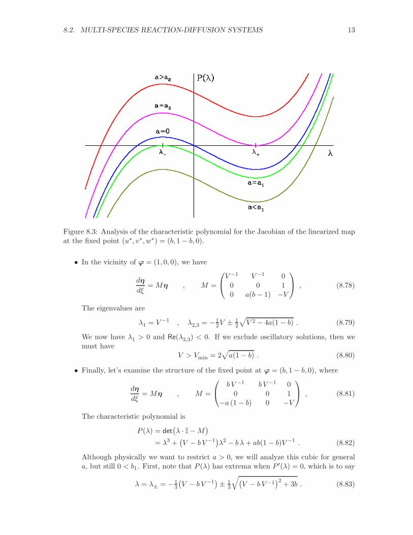
Figure 8.3: Analysis of the characteristic polynomial for the Jacobian of the linearized mapat the fixed point (u∗, v∗, w∗) = (b, 1− b, 0).

• In the vicinity of ϕ = (1, 0, 0), we have

dη

dξ=Mη , M =

V −1 V −1 00 0 10 a(b− 1) −V

, (8.78)

The eigenvalues are

λ1 = V −1 , λ2,3 = −12V ± 1

2

√

V 2 − 4a(1 − b) . (8.79)

We now have λ1 > 0 and Re(λ2,3) < 0. If we exclude oscillatory solutions, then wemust have

V > Vmin = 2√

a(1− b) . (8.80)

• Finally, let’s examine the structure of the fixed point at ϕ = (b, 1− b, 0), where

dη

dξ=Mη , M =

b V −1 b V −1 00 0 1

−a (1− b) 0 −V

, (8.81)

The characteristic polynomial is

P (λ) = det(

λ · I−M)

= λ3 +(

V − b V −1)

λ2 − b λ+ ab(1− b)V −1 . (8.82)

Although physically we want to restrict a > 0, we will analyze this cubic for generala, but still 0 < b1. First, note that P (λ) has extrema when P ′(λ) = 0, which is to say

λ = λ± = −13

(

V − b V −1)

± 13

√

(

V − b V −1)2

+ 3b . (8.83)


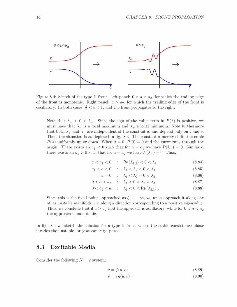
Figure 8.4: Sketch of the type-II front. Left panel: 0 < a < a2, for which the trailing edgeof the front is monotonic. Right panel: a > a2, for which the trailing edge of the front isoscillatory. In both cases, 1

2 < b < 1, and the front propagates to the right.

Note that λ− < 0 < λ+. Since the sign of the cubic term in P (λ) is positive, wemust have that λ− is a local maximum and λ+ a local minimum. Note furthermorethat both λ+ and λ− are independent of the constant a, and depend only on b and c.Thus, the situation is as depicted in fig. 8.3. The constant a merely shifts the cubicP (λ) uniformly up or down. When a = 0, P (0) = 0 and the curve runs through theorigin. There exists an a1 < 0 such that for a = a1 we have P (λ−) = 0. Similarly,there exists an a2 > 0 such that for a = a2 we have P (λ+) = 0. Thus,

a < a1 < 0 : Re (λ1,2) < 0 < λ3 (8.84)

a1 < a < 0 : λ1 < λ2 < 0 < λ3 (8.85)

a = 0 : λ1 < λ2 = 0 < λ3 (8.86)

0 < a < a2 : λ1 < 0 < λ2 < λ3 (8.87)

0 < a2 < a : λ1 < 0 < Re (λ2,3) . (8.88)

Since this is the fixed point approached as ξ → −∞, we must approach it along oneof its unstable manifolds, i.e. along a direction corresponding to a positive eigenvalue.Thus, we conclude that if a > a2 that the approach is oscillatory, while for 0 < a < a2the approach is monotonic.

In fig. 8.4 we sketch the solution for a type-II front, where the stable coexistence phaseinvades the unstable ‘prey at capacity’ phase.

8.3 Excitable Media

Consider the following N = 2 system:

u = f(u, v) (8.89)

v = ǫ g(u, v) , (8.90)

8.3. EXCITABLE MEDIA 15

Figure 8.5: Sketch of the nullclines for the dynamical system described in the text.

where 0 < ǫ ≪ 1. The first equation is ‘fast’ and the second equation ‘slow’. We assumethe nullclines for f = 0 and g = 0 are as depicted in fig. 8.5. As should be clear from thefigure, the origin is a stable fixed point. In the vicinity of the origin, we can write

f(u, v) = −au− bv + . . . (8.91)

g(u, v) = +cu− dv + . . . , (8.92)

where a, b, c, and d are all positive real numbers. The equation for the nullclines in thevicinity of the origin is then au + bv = 0 for the f = 0 nullcline, and cu − dv = 0 for theg = 0 nullcline. Note that

M ≡ ∂(u, v)

∂(u, v)

∣

∣

∣

∣

(0,0)

=

(

−a −bǫc −ǫd

)

. (8.93)

We then have TrM = −(a+ ǫd) < 0 and detM = ǫ(ad+ bc) > 0. Since the trace is negativeand the determinant positive, the fixed point is stable. The boundary between spiral andnode solutions is detM = 1

4(TrM)2, which means

|a− ǫd| > 2√ǫbc : stable node (8.94)

|a− ǫd| < 2√ǫbc : stable spiral . (8.95)

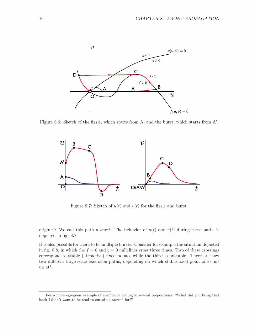
Although the trivial fixed point (u∗, v∗) = (0, 0) is stable, it is still excitable in the sense thata large enough perturbation will result in a big excursion. Consider the sketch in fig. 8.6.Starting from A, v initially increases as u decreases, but eventually both u and v get suckedinto the stable fixed point at O. We call this path the fizzle. Starting from A′, however, ubegins to increase rapidly and v increases slowly until the f = 0 nullcline is reached. Atthis point the fast dynamics has played itself out. The phase curve follows the nullcline,since any increase in v is followed by an immediate readjustment of u back to the nullcline.This state of affairs continues until C is reached, at which point the phase curve makes alarge rapid excursion to D, following which it once again follows the f = 0 nullcline to the


Figure 8.6: Sketch of the fizzle, which starts from A, and the burst, which starts from A′.

Figure 8.7: Sketch of u(t) and v(t) for the fizzle and burst.

origin O. We call this path a burst . The behavior of u(t) and v(t) during these paths isdepicted in fig. 8.7.

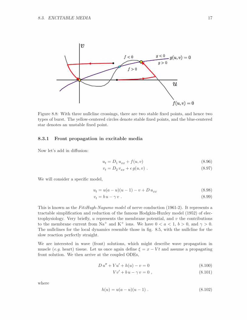
It is also possible for there to be multiple bursts. Consider for example the situation depictedin fig. 8.8, in which the f = 0 and g = 0 nullclines cross three times. Two of these crossingscorrespond to stable (attractive) fixed points, while the third is unstable. There are nowtwo different large scale excursion paths, depending on which stable fixed point one endsup at1.

1For a more egregious example of a sentence ending in several prepositions: “What did you bring that

book I didn’t want to be read to out of up around for?”


Figure 8.8: With three nullcline crossings, there are two stable fixed points, and hence twotypes of burst. The yellow-centered circles denote stable fixed points, and the blue-centeredstar denotes an unstable fixed point.

8.3.1 Front propagation in excitable media

Now let’s add in diffusion:

ut = D1 uxx + f(u, v) (8.96)

vt = D2 vxx + ǫ g(u, v) . (8.97)

We will consider a specific model,

ut = u(a− u)(u− 1)− v +Duxx (8.98)

vt = b u− γ v . (8.99)

This is known as the FitzHugh-Nagumo model of nerve conduction (1961-2). It represents atractable simplification and reduction of the famous Hodgkin-Huxley model (1952) of elec-trophysiology. Very briefly, u represents the membrane potential, and v the contributionsto the membrane current from Na+ and K+ ions. We have 0 < a < 1, b > 0, and γ > 0.The nullclines for the local dynamics resemble those in fig. 8.5, with the nullcline for theslow reaction perfectly straight.

We are interested in wave (front) solutions, which might describe wave propagation inmuscle (e.g. heart) tissue. Let us once again define ξ = x − V t and assume a propagatingfront solution. We then arrive at the coupled ODEs,

Du′′ + V u′ + h(u) − v = 0 (8.100)

V v′ + b u− γ v = 0 , (8.101)

where

h(u) = u(a− u)(u− 1) . (8.102)


Figure 8.9: Excitation cycle for the FitzHugh-Nagumo model.

Once again, we have an N = 3 dynamical system:

du

dξ= w (8.103)

dv

dξ= −b V −1 u+ γ V −1 v (8.104)

dw

dξ= −D−1 h(u) +D−1 v − V D−1 w , (8.105)

where w = u′.

We assume that b and γ are both small, so that the v dynamics are slow. Furthermore,v remains small throughout the motion of the system. Then, assuming an initial value(u0, 0, 0), we may approximate

ut ≈ Duxx + h(u) . (8.106)

With D = 0, the points u = 1 and u = 1 are both linearly stable and u = a is linearlyunstable. For finite D there is a wave connecting the two stable fixed points with a uniquespeed of propagation.

The equationDu′′+V u′ = −h(u) may again be interpreted mechanically, with h(u) = U ′(u).Then since the cubic term in h(u) has a negative sign, the potential U(u) resembles aninverted asymmetric double well, with local maxima at u = 0 and u = 1, and a localminimum somewhere in between at u = a. Since

U(0) − U(1) =

1∫

0

du h(u) = 112(1− 2a) , (8.107)

hence if V > 0 we must have a < 12 in order for the left maximum to be higher than the


Figure 8.10: Sketch of the excitation pulse of the FitzHugh-Nagumo model..

right maximum. The constant V is adjusted so as to yield a solution. This entails

V

∞∫

−∞

dξ u2ξ = V

1∫

0

duuξ = U(0) − U(1) . (8.108)

The solution makes use of some very special properties of the cubic h(u) and is astonishinglysimple:

V = (D/2)1/2 (1− 2a) . (8.109)

We next must find the speed of propagation on the CD leg of the excursion. There we have

ut ≈ Duxx + h(u)− vC, (8.110)

with u(−∞) = uD and u(+∞) = uC. The speed of propagation is

V = (D/2)1/2(

uC− 2u

P+ u

D

)

. (8.111)

We then set V = V to determine the location of C. The excitation pulse is sketched in fig.8.10

Calculation of the wave speed

Consider the second order ODE,

L(u) ≡ Du′′ + V u′ +A(u− u1)(u2 − u)(u− u3) = 0 . (8.112)

We assume u1,2,3 are all distinct. Remarkably, a solution may be found. We claim that if

u′ = λ(u− u1)(u− u2) , (8.113)


then, by suitably adjusting λ, the solution to eqn. 8.113 also solves eqn. 8.112. To showthis, note that under the assumption of eqn. 8.113 we have

u′′ =du′

du· dudξ

= λ (2u− u1 − u2)u′

= λ2(u− u1)(u− u2)(2u− u1 − u2) . (8.114)

Thus,

L(u) = (u− u1)(u− u2)[

λ2D(2u− u1 − u2) + λV +A(u3 − u)]

= (u− u1)(u− u2)[

(

2λ2D −A)

u+(

λV +Au3 − λ2D(u1 + u2))

]

. (8.115)

Therefore, if we choose

λ = σ

√

A

2D, V = σ

√

AD

2

(

u1 + u2 − 2u3)

, (8.116)

with σ = ±1, we obtain a solution to L(u) = 0. Note that the velocity V has been selected .

The integration of eqn. 8.113 is elementary, yielding the kink solution

u(ξ) =u2 + u1 exp [λ(u2 − u1)(ξ − ξ0)]

1 + exp [λ(u2 − u1)(ξ − ξ0)](8.117)

= 12(u1 + u2) +

12 (u1 − u2) tanh

[

12λ(u2 − u1)(ξ − ξ0)

]

,

where ξ0 is a constant which is the location of the center of the kink. This front solutionconnects u = u1 and u = u2. There is also a front solution connecting u1 and u3:

u(ξ) = 12(u1 + u3) +

12 (u1 − u3) tanh

[

12λ(u3 − u1)(ξ − ξ0)

]

, (8.118)

with the same value of λ = σ√

A/2D, but with a different velocity of front propagationV = σ(AD/2)1/2(u1 + u3 − 2u2), again with σ = ±1.

It is instructive to consider the analogue mechanical setting of eqn. 8.112. We write D →Mand V → γ, and u→ x, giving

Mx+ γ x = A(x− x1)(x− x2)(x− x3) ≡ F (x) , (8.119)

where we take x1 < x2 < x3. Mechanically, the points x = x1,3 are unstable equilibria. Afront solution interpolates between these two stationary states. If γ = V > 0, the frictionis of the usual sign, and the path starts from the equilibrium at which the potential U(x)is greatest. Note that

U(x1)− U(x3) =

x3

∫

x1

dxF (x) (8.120)

= 112(x3 − x1)

2[

(x2 − x1)2 − (x3 − x2)

2]

. (8.121)


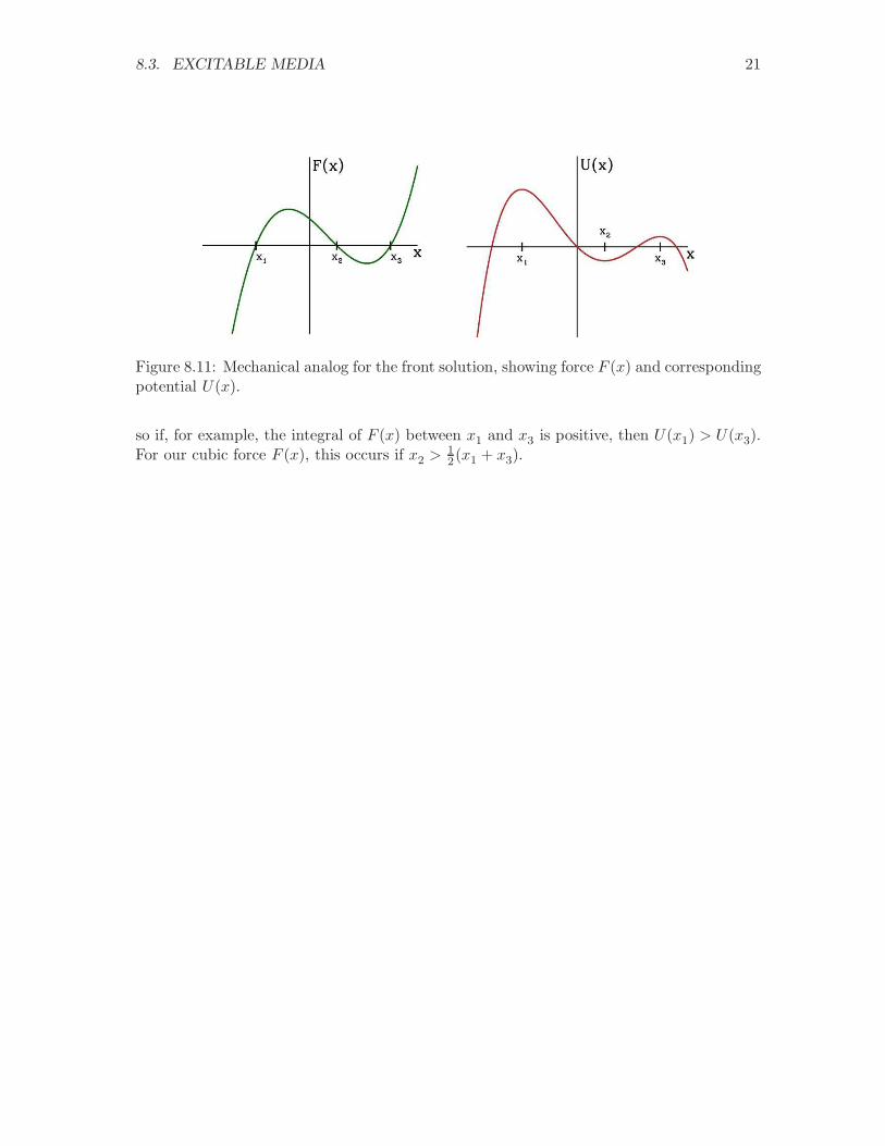
Figure 8.11: Mechanical analog for the front solution, showing force F (x) and correspondingpotential U(x).

so if, for example, the integral of F (x) between x1 and x3 is positive, then U(x1) > U(x3).For our cubic force F (x), this occurs if x2 >

12(x1 + x3).

front propagation

Documents