frst 557 forest operations module lecture 3c optimum...

FRST 557

Forest Operations Module

Lecture 3c

Optimum Road Standards

Special Case Study: No Timber Developed

1.0 Lesson Overview:

The preceding parts of this lecture assumed that the entire road is developing harvestable

timber adjacent to it. There are cases however where a section of road may not develop

timber. Often this occurs in situations where, due to physical differences in construction,

costs also vary significantly from those used for the rest of the road network.

Very difficult construction through a canyon where the numbers change significantly may

even have the indicated road class reduced for the section.

FRST 557 – Lecture 3c – Special Case Study: No Timber Developed

2

2.0 Lesson Preparation:

Review the last two lessons and be certain that you understand the concept of finding the

optimum road standard.

3.0 Lesson Objective:

On completion of this lesson, you will know how to adapt the approach to finding an

optimal solution to one example of a variation in physical conditions..

4.0 The Problem:

Optimum Road Standards (using the non-uniform road system method) have already been

developed for the following illustration with the exception of a short section between km

14.8 and km 16.0:

L = 66 km

v = 22,000 m3 / km

Summary:

Class 1 km 0 to km 45.1 (45.1 km)

Class 2 km 45.1 to km 59 (13.9 km)

Class 3 km 59 to km 66 (7.0 km)

V M = 220,000 m 3

Mainline

Sort Yard

Class 1? Class 2?

Class 3?

km 55

km 59

Branch B

Branch C

km 66

VC = 210,000 m3

VB = 250,000 m3

km 14.8 to km 16.0

Steep rock canyon requiring

drilling & blasting and end haul.

No timber developed (v = 0)


3

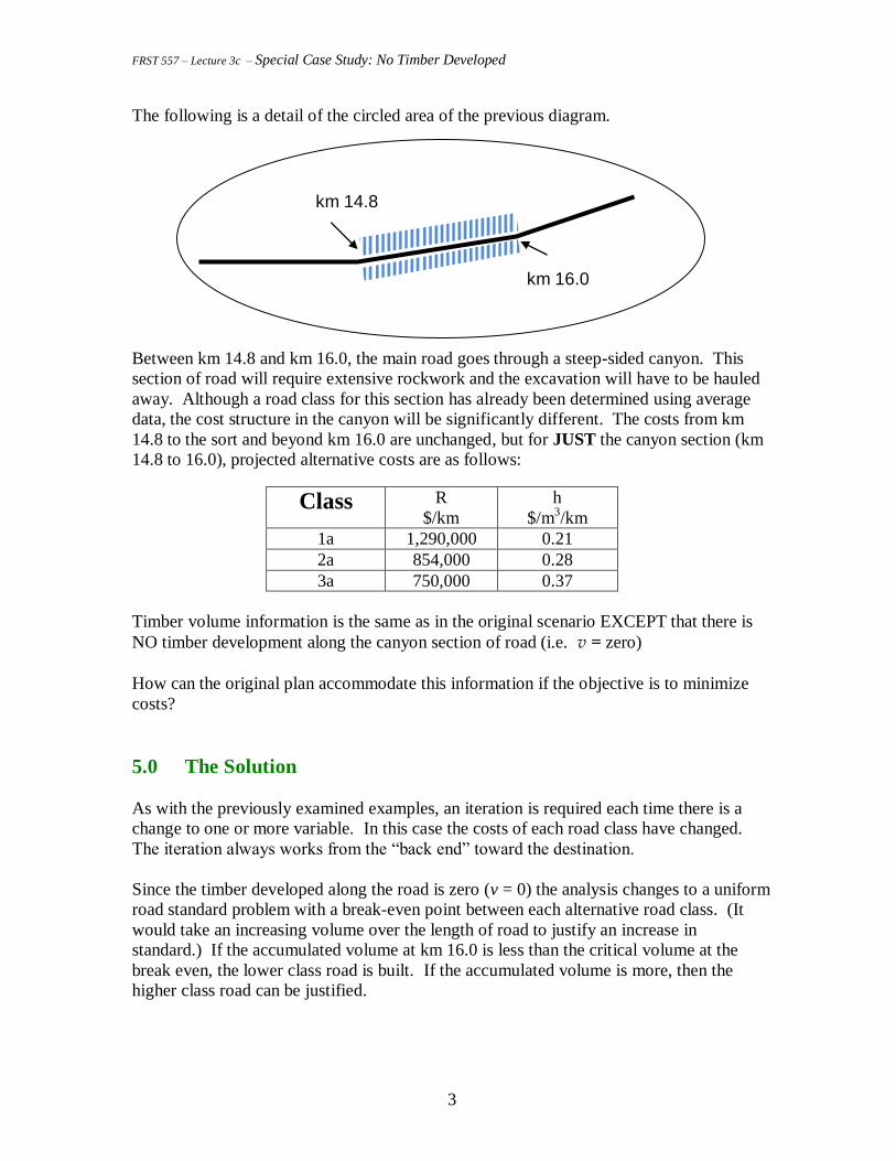
The following is a detail of the circled area of the previous diagram.

Between km 14.8 and km 16.0, the main road goes through a steep-sided canyon. This

section of road will require extensive rockwork and the excavation will have to be hauled

away. Although a road class for this section has already been determined using average

data, the cost structure in the canyon will be significantly different. The costs from km

14.8 to the sort and beyond km 16.0 are unchanged, but for JUST the canyon section (km

14.8 to 16.0), projected alternative costs are as follows:

Timber volume information is the same as in the original scenario EXCEPT that there is

NO timber development along the canyon section of road (i.e. v = zero)

How can the original plan accommodate this information if the objective is to minimize

costs?

5.0 The Solution

As with the previously examined examples, an iteration is required each time there is a

change to one or more variable. In this case the costs of each road class have changed.

The iteration always works from the “back end” toward the destination.

Since the timber developed along the road is zero (v = 0) the analysis changes to a uniform

road standard problem with a break-even point between each alternative road class. (It

would take an increasing volume over the length of road to justify an increase in

standard.) If the accumulated volume at km 16.0 is less than the critical volume at the

break even, the lower class road is built. If the accumulated volume is more, then the

higher class road can be justified.

Class R

$/km

h

$/m3/km

1a 1,290,000 0.21

2a 854,000 0.28

3a 750,000 0.37

km 14.8

km 16.0


4

CT(N) = CT(N+1)

where:

CT is the total cost of construction and ongoing costs

N is the class of road

or specifically, in this case, CT(1) = CT(2) and CT(2) = CT(3)

The following chart is a general illustration of the cumulative costs for increasing volumes

with each of three classes of road.

The actual total volume (V) is entering the section of road at km 16.0 so call it V16.

The total cost of either alternative is equal to the construction cost (the cost per km times

the length) plus the operating costs (volume times $/m3/km times length).

CT(N) = RNL + VhNL So if the breakeven is where:

CT(N) = CT(N+1) then:

RNL + VChNL = RN+1L + VChN+1L

Where the break even volume (or critical volume) is identified as VC

Tota

l Co

st p

er

km o

f R

oa

d

Cumulative Volume Hauled (m3)

Cumulative Cost per km vs Cumulative Volume Hauled

Class 1

Class 2

Class 3

Class 2 breakeven

Class 1 breakeven


5

Solving the equation for VC:

Using the data from Section 4.0, the actual volume at km 16.0 is:

V16 = VM + VC + VB+ v(66 – 16.0) = 1,780,000 m3

For the first iteration at km 16.0, look at the critical volume to justify Class 2a over

Class 3a (VC2a)

=

=

= 1,155,556 m

3

Since V16 > , at least Class 2a is justified.

But Class 1a should also be checked as a possibility, so what is the critical volume ( to justify Class 1a?

=

=

= 6,228,571 m

3

Since V16 < , there is not sufficient volume to justify a Class 1a road.

Conclusion: km 14.8 to km 16.0 will be constructed to a Class 2a standard.

Summary for the entire road:

Class 1 km 0 to km 14.8 (14.8 km)

Class 2a km 14.8 to km 16.0 (1.2 km)

Class 1 km 16.0 to km 45.1 (29.1 km)

Class 2 km 45.1 to km 59.0 (13.9 km)

Class 3 km 59.0 to km 66.0 (7.0 km)

The following chart illustrates the data for the actual example. Since the actual

cumulative volume at km 16.0 is 1,780,000 m3, the optimum choice is the Class 2a road.


6

6.0 Other Applications

This case study is but one of many unique situations that can occur. To find an optimal

solution for a range of choices, the objective must be identified along with the critical

variable, the input variables determined, and the appropriate approach – usually

comparing two alternatives at a time in an iterative process. Where the choice is between

two alternatives (i.e. all one or all the other) it will be a break even analysis. If the choice

is an appropriate combination of the alternatives, the optimal choice will be indicated as a

minimum total cost of all combinations of the alternatives.

$0

$500,000

$1,000,000

$1,500,000

$2,000,000

$2,500,000

$3,000,000

$3,500,000

$4,000,000

$4,500,000

$5,000,000

Tota

l Co

st p

er k

m o

f R

oa

d

Cumulative Volume Hauled (m3)

Cumulative Cost per km vs Cumulative Volume Hauled

Class 1a

Class 2a

Class 3a

Class 2a breakeven

1,155,556 m3

Class 1a breakeven

6,228,571 m3

Class 1a optimum

Class 2a optimum

Class 3a optimum


7

Low timber developed will happen. Zero is a number that may present problems in a

denominator and make you apply some creative thinking.

Off-Highway Logging Truck – Princess Royal Island (Cedar Creek)

frst 557 forest operations module lecture 3c optimum...

Documents