Fully 3D list-mode time-of-flight PET image reconstruction onGPUs using CUDA

Jing-yu CuiDepartment of Electrical Engineering, Stanford University, Stanford, California 94305

Guillem PratxDepartment of Radiation Oncology, Stanford University, Stanford, California 94305

Sven PrevrhalPhilips Healthcare, San Jose, California 95134

Craig S. Levina)

Departments of Radiology, Electrical Engineering, Physics, and Molecular Imaging Program at Stanford(MIPS), Stanford University, Stanford, California 94305

(Received 31 May 2011; revised 28 September 2011; accepted for publication 22 October 2011;

published 1 December 2011)

Purpose: List-mode processing is an efficient way of dealing with the sparse nature of positron

emission tomography (PET) data sets and is the processing method of choice for time-of-flight

(ToF) PET image reconstruction. However, the massive amount of computation involved in for-

ward projection and backprojection limits the application of list-mode reconstruction in practice,

and makes it challenging to incorporate accurate system modeling.

Methods: The authors present a novel formulation for computing line projection operations on

graphics processing units (GPUs) using the compute unified device architecture (CUDA) frame-

work, and apply the formulation to list-mode ordered-subsets expectation maximization (OSEM)

image reconstruction. Our method overcomes well-known GPU challenges such as divergence of

compute threads, limited bandwidth of global memory, and limited size of shared memory, while

exploiting GPU capabilities such as fast access to shared memory and efficient linear interpolation

of texture memory. Execution time comparison and image quality analysis of the GPU-CUDA

method and the central processing unit (CPU) method are performed on several data sets acquired

on a preclinical scanner and a clinical ToF scanner.

Results: When applied to line projection operations for non-ToF list-mode PET, this new GPU-

CUDA method is >200 times faster than a single-threaded reference CPU implementation. For

ToF reconstruction, we exploit a ToF-specific optimization to improve the efficiency of our parallel

processing method, resulting in GPU reconstruction >300 times faster than the CPU counterpart.

For a typical whole-body scan with 75� 75� 26 image matrix, 40.7 million LORs, 33 subsets, and

3 iterations, the overall processing time is 7.7 s for GPU and 42 min for a single-threaded CPU.

Image quality and accuracy are preserved for multiple imaging configurations and reconstruction

parameters, with normalized root mean squared (RMS) deviation less than 1% between CPU and

GPU-generated images for all cases.

Conclusions: A list-mode ToF OSEM library was developed on the GPU-CUDA platform. Our

studies show that the GPU reformulation is considerably faster than a single-threaded reference

CPU method especially for ToF processing, while producing virtually identical images. This new

method can be easily adapted to enable more advanced algorithms for high resolution PET recon-

struction based on additional information such as depth of interaction (DoI), photon energy, and

point spread functions (PSFs). VC 2011 American Association of Physicists in Medicine.

[DOI: 10.1118/1.3661998]

Key words: PET image reconstruction, time-of-flight PET, list-mode, OSEM, CUDA, GPU,

line projections, high performance computing, acceleration

I. INTRODUCTION

Positron emission tomography (PET) image reconstruction

methods based on list-mode acquisition have many advan-

tages compared with those using sinograms, especially for

time-of-flight (ToF),1–3 high resolution,4,5 and dynamic6

PET data. List-mode data can be reconstructed using itera-

tive algorithms such as maximum likelihood expectation

maximization (MLEM) (Ref. 7) and ordered-subsets expec-

tation maximization (OSEM).8–12 However, these algorithms

require forward and backprojection between individual lines

of response (LORs) and voxels and, therefore, have much

6775 Med. Phys. 38 (12), December 2011 0094-2405/2011/38(12)/6775/12/$30.00 VC 2011 Am. Assoc. Phys. Med. 6775

higher computational cost. For example, it requires tens of

minutes up to hours of CPU time to reconstruct a typical 3D

PET image, even on high-end CPUs with highly optimized

algorithms.3,13,14 Yet, within a cycle of forward and back-

projection, LORs can be processed independently, allowing

data-parallel processing on multiprocessor hardware.

Programmable graphics processing units (GPUs) have

emerged as a popular alternative to multi-CPU computer clus-

ters for high performance computation because of potential

savings of cost, space, and power.15 A significant research

effort has been devoted to exploiting GPU technology for

x-ray computed tomography (CT),16,17 digital tomosynthe-

sis,18 radiation treatment planning,19 dose calculation,20 and

other medical physics applications.21 Compared with multi-

CPU clusters,22 the faster speed and lower cost of communi-

cation between GPU cores makes scaling easier for applica-

tions that involve internode communication. This is true for

most of the iterative algorithms, which require the result of

the previous step to be broadcasted to all the nodes before the

next iteration can begin.

In a previous article, we reported a GPU formulation of 3D

list-mode OSEM using the OpenGL graphics library.13 Using

a graphics library for general-purpose parallel computing has

several drawbacks: The code is difficult to develop and main-

tain since the algorithm must be implemented as a graphics

rendering process; performance may be compromised by the

lack of access to all the capabilities of the GPU, for example,

shared memory; and code portability is a challenge because

the graphics code needs to be customized for specific graphics

cards for best performance.

In this paper, we present our recent work in reformulating

and accelerating fully 3D list-mode ToF PET image recon-

struction on GPUs using the compute unified device archi-

tecture (CUDA) framework.23

CUDA makes the highly parallel architecture of the GPU

cores available to the developers in a C-like programming par-

adigm.23 Compared to OpenGL, CUDA gives the program-

mer direct access to GPU features that are not available from

OpenGL, such as shared memory, thus, potentially could be

more efficient for certain applications. Briefly, the execution

model organizes individual threads into thread blocks. The

significance of a thread block is that its members can commu-

nicate through fast block-specific shared memory, whereas

threads in different blocks run independently. If interblock

communication is necessary, it must use much slower off-chip

global memory. Atomic operations and thread synchroniza-

tion primitives are further provided to allow threads in each

thread block to coordinate memory access and execution.

CUDA code has sufficient flexibility to manipulate the sched-

uling of the computation, yet the programmer does not need

to be concerned with the details of the hardware implementa-

tion since they are automatically handled by the run-time

environment. Once the CUDA code is written, it can run on

future graphics cards, automatically exploiting their advanced

capability without requiring code modifications.

We reformulated the OSEM algorithm to map it effi-

ciently to the NVIDIA Fermi GPU architecture and the CUDA

framework. When applied to line projection operations for

non-ToF list-mode PET, this method is >200 times faster

than a single-threaded reference CPU implementation. For

ToF reconstruction, since each LOR intersects fewer voxels,

the method is greater than 300-fold faster than the CPU

counterpart. Image quality and quantification are preserved

with negligible difference between CPU and GPU-generated

images.

This paper describes detailed formulations to enable 3D

list-mode OSEM acceleration using the GPU-CUDA plat-

form. This formulation can be applied to any PET and single

photon emission computed tomography (SPECT) system

configuration. In this work, we mainly focus on exploiting

this novel technique for image reconstruction for ToF-PET.

The contributions of this formulation are as follows:

(1) Spatial and temporal locality is exploited by caching the

image volume in faster shared memory and reformulat-

ing the projections to access the image slice-by-slice.

(2) LORs are partitioned into groups according to their

orientations, thus, the intersection of the tube of response

(TOR) and the slice has a fixed footprint, which can be

accessed using a fixed-bound for-loop to avoid GPU

thread divergence.

(3) For ToF reconstruction, events are further sorted accord-

ing to their ToF centers to reduce unnecessary

computation.

(4) The list-mode data are organized into structure of arrays

(SoA) in the global memory to enable coalesced parallel

access from different GPU threads.

(5) For forward projection, a line-driven approach with no

data race condition is proposed, with the sparseness of

the system matrix exploited.

(6) For backprojection, the pros and cons of the line- and

voxel-driven approaches are analyzed and discussed, and

the selected line-driven approach with hardware atomic

operations is presented because it exploits the sparseness

of the system matrix, while having relatively small over-

head imposed by the atomic operations.

(7) Multiplicative update is performed on the GPU in situwithout additional CPU-GPU communication.

(8) Several other optimizations are utilized, including free

interpolation of the texture memory, loop unrolling, fast

math, etc.

(9) The proposed method is a general framework which can

be easily adapted to incorporate more information such

as depth of interaction (DoI), photon energy, and point

spread functions (PSFs) into the image reconstruction

algorithm.

II. MATERIALS AND METHODS

II.A. Image reconstruction

The MLEM algorithm7 can be used to reconstruct a tomo-

graphic image based on a set of projective measurements.

The iterative algorithm can be summarized as

x kþ1ð Þ ¼ x kð Þ� 1

AT1� AT y

Ax kð Þ þ c

� �; (1)

6776 Cui et al.: Fully 3D list-mode time-of-flight PET on GPU-CUDA 6776

Medical Physics, Vol. 38, No. 12, December 2011

where A is the system matrix, whose elements Aij denote the

probability that a positron decay occurring in the jth voxel

gets detected in the ith LOR; y is the LOR measurement; c is

the additive correction term, usually the sum of the estimated

scatter correction s and random correction r; x(k) is the image

estimate at the k th step; � is the Hadamard (element-wise)

product, and �� is the element-wise division. In the OSEM

algorithm,8 only a subset of all LORs are used for each

update. For list-mode OSEM,10 the subsets are usually time-

ordered, and y¼ 1.

The system matrix A is usually very big.24,25 Researchers

have been working on reducing its size by exploiting its

sparse and symmetric structures.26–28 Several alternatives

exist for calculating the system matrix on-the-fly, including

Siddon’s29 and Joseph’s method.30 However, theses methods

are limited to thin, ideal lines that do not accurately represent

the physics of the photon detection in PET. Instead, we use a

TOR approach to represent PET projective measurement

because it provides more flexibility for accurately modeling

the system response. In this paper, the shape of the system

response is modeled using a shift-invariant kernel. It is a

straightforward extension of this work to change the inner-

most loop of the algorithm to incorporate a shift-varying

kernel.

II.B. Reformulation and implementation for the CUDAplatform

The bottleneck of iterative reconstruction algorithms lies

in the forward and backprojection operations that are respon-

sible for calculating the summed contributions of all voxels

to all LORs, and the summed contributions of all LORs to

all voxels, respectively. Both operations are intrinsically par-

allel, but in order to implement the algorithm efficiently on

the GPU, special consideration is required to match the com-

putation to the hardware architecture.

Some key principles for efficient CUDA programming

include increasing arithmetic intensity, that is the ratio of

arithmetic to memory operations; hiding global memory

latency by maximizing thread occupancy, which let the sched-

uler replace threads waiting for memory transactions with

ready threads; using caches, texture memory, and shared

memory; ensuring thread coherence to avoid serialization of

diverging execution paths; and minimizing the use of atomic

operations, which are required to guarantee correctness in the

presence of data race conditions.

In Secs. II B 1-II B 11, we will introduce the steps we

took to formulate and implement the MLEM and OSEM

algorithms to run efficiently on GPUs.

II.B.11. Global memory layout

We layout the data structure in GPU global memory in

such a way that the memory accesses of threads within a

half-warp are coalesced into one transaction, thereby pre-

serving global memory bandwidth. More specifically, a

structure of arrays (SoA) instead of an array of structures(AoS) is used to store data elements of events.23 The first

data element of all events is stored in a continuous block of

memory, followed by the second element of all events, and

so forth.

II.B.2. Caching with shared memory

Projection operations typically have low arithmetic inten-

sity: they access a large number of voxels and LORs but

only perform simple calculations with them. This fact

suggests that global memory access is a bottleneck of the

algorithm, and must be reduced as much as possible.

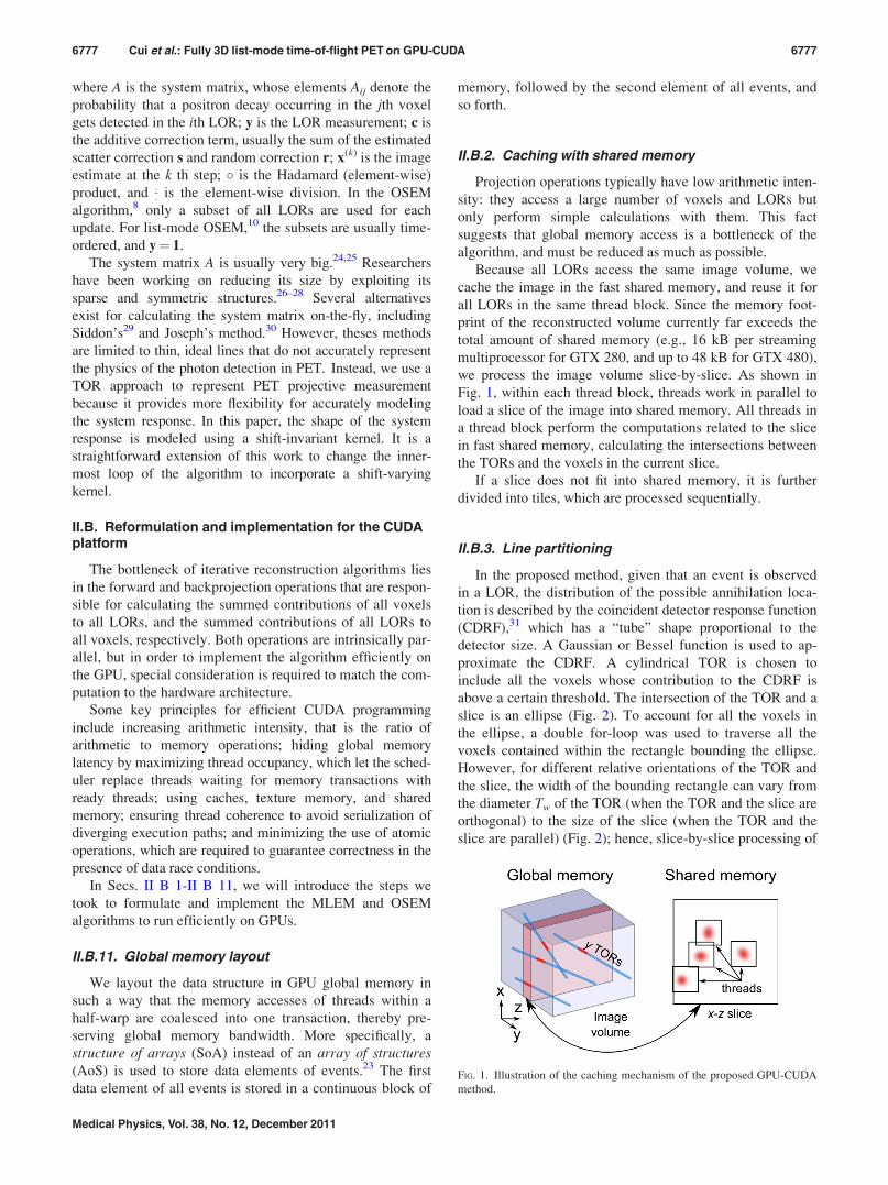
Because all LORs access the same image volume, we

cache the image in the fast shared memory, and reuse it for

all LORs in the same thread block. Since the memory foot-

print of the reconstructed volume currently far exceeds the

total amount of shared memory (e.g., 16 kB per streaming

multiprocessor for GTX 280, and up to 48 kB for GTX 480),

we process the image volume slice-by-slice. As shown in

Fig. 1, within each thread block, threads work in parallel to

load a slice of the image into shared memory. All threads in

a thread block perform the computations related to the slice

in fast shared memory, calculating the intersections between

the TORs and the voxels in the current slice.

If a slice does not fit into shared memory, it is further

divided into tiles, which are processed sequentially.

II.B.3. Line partitioning

In the proposed method, given that an event is observed

in a LOR, the distribution of the possible annihilation loca-

tion is described by the coincident detector response function

(CDRF),31 which has a “tube” shape proportional to the

detector size. A Gaussian or Bessel function is used to ap-

proximate the CDRF. A cylindrical TOR is chosen to

include all the voxels whose contribution to the CDRF is

above a certain threshold. The intersection of the TOR and a

slice is an ellipse (Fig. 2). To account for all the voxels in

the ellipse, a double for-loop was used to traverse all the

voxels contained within the rectangle bounding the ellipse.

However, for different relative orientations of the TOR and

the slice, the width of the bounding rectangle can vary from

the diameter Tw of the TOR (when the TOR and the slice are

orthogonal) to the size of the slice (when the TOR and the

slice are parallel) (Fig. 2); hence, slice-by-slice processing of

FIG. 1. Illustration of the caching mechanism of the proposed GPU-CUDA

method.

6777 Cui et al.: Fully 3D list-mode time-of-flight PET on GPU-CUDA 6777

Medical Physics, Vol. 38, No. 12, December 2011

the TORs will introduce severe thread divergence, serializ-

ing the calculations on the GPU.

In order to prevent the execution of the threads from

diverging within thread blocks, we categorize the lines within

each subset into three classes according to their predominant

direction. More specifically, the predominant direction is the

direction selected from x, y, and z that has the largest absolute

value of inner product with the line direction. Here directions

x and y span the transaxial image plane, and direction z is

along the scanner axis. For each class of lines, the slices are

selected to be orthogonal to the predominant line direction.

For example, for lines whose predominant direction is along

y, the slice is chosen to be parallel to the x-z plane (Fig. 1).

This categorization step can be performed very efficiently on

the GPU using the partition primitive,23 which partitions a set

of items into two groups based on the output of a binary func-

tion, for example, whether or not the predominant direction of

an LOR is x. This step needs to be performed only once for all

the iterations with very small time cost. For example, on a

GTX 480 GPU, it takes 12 ms to categorize 1 million

randomly-generated LORs.

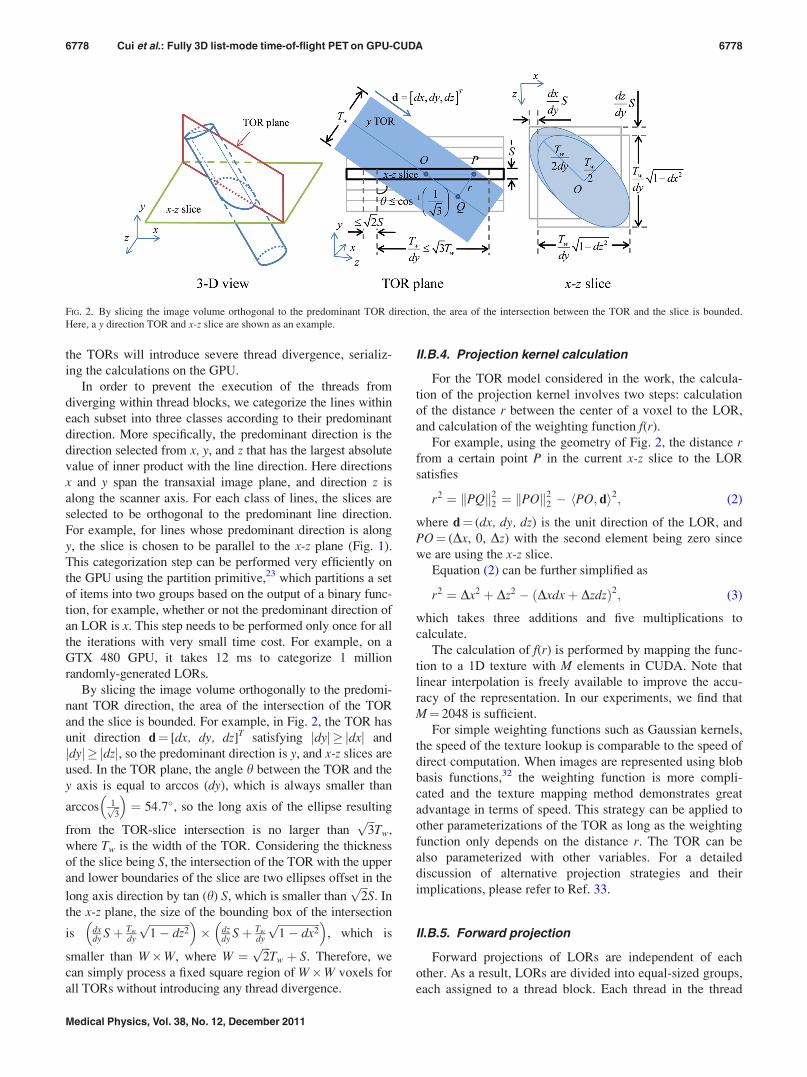
By slicing the image volume orthogonally to the predomi-

nant TOR direction, the area of the intersection of the TOR

and the slice is bounded. For example, in Fig. 2, the TOR has

unit direction d¼ [dx, dy, dz]T satisfying jdyj � jdxj and

jdyj � jdzj, so the predominant direction is y, and x-z slices are

used. In the TOR plane, the angle h between the TOR and the

y axis is equal to arccos (dy), which is always smaller than

arccos 1ffiffi3p� �

¼ 54:7�, so the long axis of the ellipse resulting

from the TOR-slice intersection is no larger thanffiffiffi3p

Tw,

where Tw is the width of the TOR. Considering the thickness

of the slice being S, the intersection of the TOR with the upper

and lower boundaries of the slice are two ellipses offset in the

long axis direction by tan (h) S, which is smaller thanffiffiffi2p

S. In

the x-z plane, the size of the bounding box of the intersection

is dxdy Sþ Tw

dy

ffiffiffiffiffiffiffiffiffiffiffiffiffiffiffi1� dz2p� �

� dzdy Sþ Tw

dy

ffiffiffiffiffiffiffiffiffiffiffiffiffiffiffi1� dx2p� �

, which is

smaller than W�W, where W ¼ffiffiffi2p

Tw þ S. Therefore, we

can simply process a fixed square region of W�W voxels for

all TORs without introducing any thread divergence.

II.B.4. Projection kernel calculation

For the TOR model considered in the work, the calcula-

tion of the projection kernel involves two steps: calculation

of the distance r between the center of a voxel to the LOR,

and calculation of the weighting function f(r).

For example, using the geometry of Fig. 2, the distance rfrom a certain point P in the current x-z slice to the LOR

satisfies

r2 ¼ PQk k22 ¼ POk k2

2 � PO; dh i2; (2)

where d¼ (dx, dy, dz) is the unit direction of the LOR, and

PO¼ (Dx, 0, Dz) with the second element being zero since

we are using the x-z slice.

Equation (2) can be further simplified as

r2 ¼ Dx2 þ Dz2 � Dxdxþ Dzdzð Þ2; (3)

which takes three additions and five multiplications to

calculate.

The calculation of f(r) is performed by mapping the func-

tion to a 1D texture with M elements in CUDA. Note that

linear interpolation is freely available to improve the accu-

racy of the representation. In our experiments, we find that

M¼ 2048 is sufficient.

For simple weighting functions such as Gaussian kernels,

the speed of the texture lookup is comparable to the speed of

direct computation. When images are represented using blob

basis functions,32 the weighting function is more compli-

cated and the texture mapping method demonstrates great

advantage in terms of speed. This strategy can be applied to

other parameterizations of the TOR as long as the weighting

function only depends on the distance r. The TOR can be

also parameterized with other variables. For a detailed

discussion of alternative projection strategies and their

implications, please refer to Ref. 33.

II.B.5. Forward projection

Forward projections of LORs are independent of each

other. As a result, LORs are divided into equal-sized groups,

each assigned to a thread block. Each thread in the thread

FIG. 2. By slicing the image volume orthogonal to the predominant TOR direction, the area of the intersection between the TOR and the slice is bounded.

Here, a y direction TOR and x-z slice are shown as an example.

6778 Cui et al.: Fully 3D list-mode time-of-flight PET on GPU-CUDA 6778

Medical Physics, Vol. 38, No. 12, December 2011

block processes a line independently as shown in Algorithm

1. Because the computation tasks are divided according to

the output, this step is a gather operation34 and there is no

data race condition.

If the image is represented using multiple sets of basis

functions, for example using two sets of blobs arranged in

even–odd body-centered cubic (BCC) grids,32 the forward

projection accumulates values from both grids into the same

set of LORs.

II.B.6. Backprojection

To avoid data races, backprojection must be performed as

a gather operation, i.e., the computation must be distributed

according to the voxels. However, because the interactions

of the TORs and the voxels are very sparse, and the list-

mode events are not ordered, this method would launch

many empty threads, and the computational efficiency would

suffer.

In our method, we use a line-driven scheme similar to the

forward projection. In this case, multiple lines may write to

the same location in shared memory simultaneously, so

atomic operations must be used to ensure correctness of the

reconstructed image. The floating point atomic operations

are available in hardware in the Fermi architecture, and can

be implemented in software for GPUs that do not support

hardware floating point atomic operations. The backprojec-

tion algorithm is detailed in Algorithm 2.

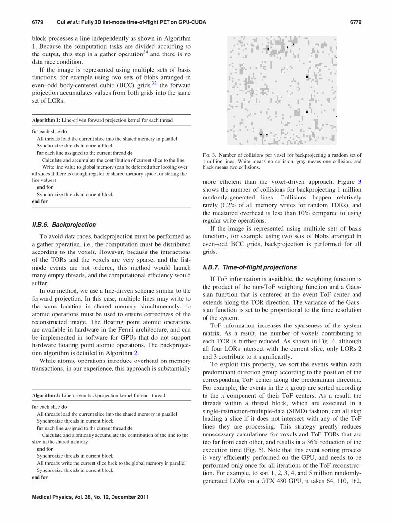
While atomic operations introduce overhead on memory

transactions, in our experience, this approach is substantially

more efficient than the voxel-driven approach. Figure 3

shows the number of collisions for backprojecting 1 million

randomly-generated lines. Collisions happen relatively

rarely (0.2% of all memory writes for random TORs), and

the measured overhead is less than 10% compared to using

regular write operations.

If the image is represented using multiple sets of basis

functions, for example using two sets of blobs arranged in

even–odd BCC grids, backprojection is performed for all

grids.

II.B.7. Time-of-flight projections

If ToF information is available, the weighting function is

the product of the non-ToF weighting function and a Gaus-

sian function that is centered at the event ToF center and

extends along the TOR direction. The variance of the Gaus-

sian function is set to be proportional to the time resolution

of the system.

ToF information increases the sparseness of the system

matrix. As a result, the number of voxels contributing to

each TOR is further reduced. As shown in Fig. 4, although

all four LORs intersect with the current slice, only LORs 2

and 3 contribute to it significantly.

To exploit this property, we sort the events within each

predominant direction group according to the position of the

corresponding ToF center along the predominant direction.

For example, the events in the x group are sorted according

to the x component of their ToF centers. As a result, the

threads within a thread block, which are executed in a

single-instruction-multiple-data (SIMD) fashion, can all skip

loading a slice if it does not intersect with any of the ToF

lines they are processing. This strategy greatly reduces

unnecessary calculations for voxels and ToF TORs that are

too far from each other, and results in a 36% reduction of the

execution time (Fig. 5). Note that this event sorting process

is very efficiently performed on the GPU, and needs to be

performed only once for all iterations of the ToF reconstruc-

tion. For example, to sort 1, 2, 3, 4, and 5 million randomly-

generated LORs on a GTX 480 GPU, it takes 64, 110, 162,

Algorithm 1: Line-driven forward projection kernel for each thread

for each slice do

All threads load the current slice into the shared memory in parallel

Synchronize threads in current block

for each line assigned to the current thread do

Calculate and accumulate the contribution of current slice to the line

Write line value to global memory (can be deferred after looping over

all slices if there is enough register or shared memory space for storing the

line values)

end for

Synchronize threads in current block

end for

FIG. 3. Number of collisions per voxel for backprojecting a random set of

1 million lines. White means no collision, gray means one collision, and

black means two collisions.

Algorithm 2: Line-driven backprojection kernel for each thread

for each slice do

All threads load the current slice into the shared memory in parallel

Synchronize threads in current block

for each line assigned to the current thread do

Calculate and atomically accumulate the contribution of the line to the

slice in the shared memory

end for

Synchronize threads in current block

All threads write the current slice back to the global memory in parallel

Synchronize threads in current block

end for

6779 Cui et al.: Fully 3D list-mode time-of-flight PET on GPU-CUDA 6779

Medical Physics, Vol. 38, No. 12, December 2011

210, and 262 ms, respectively. The complexity of the sorting

algorithm is O(nlogn), where n is the number of LORs being

sorted.

II.B.8. Multiplicative update

In the multiplicative update step, the previously estimated

image is multiplied by two matrices element-wise: the back-

projection result AT y

Ax kð Þþc, and the precomputed element-

wise reciprocal of the normalization map 1AT 1

. These two

matrices were preloaded on the GPU, so this step requires no

data transfer between the CPU and GPU, and take a negligi-

ble portion of the total execution time.

Note that multiplying the image by 1AT 1

and dividing it by

AT1 are mathematically equivalent. However, when the nor-

malization map AT1 contains zeros or very small values,

dividing by AT1 will be numerically unstable. This can be

easily fixed if we use the first method, and set the corre-

sponding values in 1AT 1

to zero.

II.B.9. Fast math

NVIDIA GPUs have intrinsic arithmetic operations imple-

mented in hardware. These operations perform common arith-

metic computations faster but less accurately. This feature can

be activated through the compiler flag nvcc� use fast math.

Our experiment shows that enabling fast math marginally

affects the final image accuracy, while saving computa-

tion time depending on the size of the TOR.

II.B.10. Loop unrolling

Loop unrolling can reduce the number of dynamic

instructions by avoiding extra comparisons and branches. It

provides additional opportunities for instruction level paral-

lelism since more independent instructions are exposed.

However, aggressive unrolling can introduce more static

instructions and higher register usage; the former increases

the instruction load time, and the latter forces some of the

registers to be spilled to L1 cache or global memory. The

#pragma unroll compiler directive informs the compiler of

potential loops to be unrolled, and the compiler decides

whether or not to unroll based on the trade-offs above.

II.B.11. Bank conflicts

CUDA shared memory is organized in equal-sized mem-

ory banks. Any n simultaneous memory accesses that fall

into n different banks can be served simultaneously, while

memory accesses in the same bank have to be serialized.

No bank conflicts occur when image slices are transferred

from global memory to shared memory, since for 32-bit float-

ing point numbers, no two threads access the same memory

bank simultaneously as long as the stride s is an odd number:23

shared float shared½ �;shared½offsetþ s � threadIdx:x� ¼ some value;

However, when projection operations access the cached

image slice in shared memory, the access pattern is not regu-

lar, and bank conflicts are inevitable to some extent. But

even with bank conflicts, the main bottleneck for the GPU-

CUDA method remains the global memory access, and the

penalty imposed by slight bank conflict is negligible.

II.C. Evaluation

II.C.1. CPU and GPU hardware

We compare the speed of the GPU-CUDA method with a

baseline CPU implementation running in single thread mode

on an Core 2 Duo E6600 2.4 GHz CPU (Intel, Santa Clara,

CA, 2006). Of note, the baseline CPU implementation is not

part of or equivalent to the manufacture’s product.

The GPU-CUDA code runs on a GeForce GTX 480 GPU

(NVIDIA, Santa Clara, CA, 2010), with 480 programmable cores

grouped into 15 streaming multiprocessors (SMs), running at

1.45 GHz clock frequency. The GPU has 1.5 GB on-board

memory, accessible from the CPU via the PCI-E 2.0� 16 bus.

For comparison, the GPU-CUDA implementation was also

run on a GeForce GTX 285 GPU (NVIDIA, Santa Clara, CA,

2009), with 240 programmable cores grouped into 30 SMs,

FIG. 5. Cumulative contributions of different optimization strategies to the

overall speedup of the GPU-CUDA method compared to the CPU-based

code. Simple GPU implementation refers to the method that directly maps

the computation to the GPU hardware without using the subsequent optimi-

zations listed in this figure.

FIG. 4. With the ToF information, fewer LOR-slice pairs need to be proc-

essed. Four LORs are shown intersecting the current slice. The dots on each

line denote the ToF center, and the bell shapes denote the ToF kernels. Only

LORs 2 and 3 contribute to the current slice significantly.

6780 Cui et al.: Fully 3D list-mode time-of-flight PET on GPU-CUDA 6780

Medical Physics, Vol. 38, No. 12, December 2011

running at 1.45 GHz clock frequency. Compared with the

GTX 480, the GTX 285 has only 1 GB of on-board memory,

and hardware floating point atomic operations are not avail-

able. The CUDA driver and runtime 3.2 are used to access the

functionalities of both GPUs.

II.C.2. Processing time analysis

The processing time for the CPU and GPU-CUDA meth-

ods are measured. For the GPU-CUDA method, contribu-

tions of different optimization strategies are analyzed.

Important parameters of the GPU-CUDA method, such as

the size of the thread block and the number of thread blocks,

are varied to analyze their impact on the performance.

II.C.3. Imaging experiments and reconstructionparameters

A cylindrical hot rod phantom (Micro Deluxe phantom,

Data Spectrum, Durham, NC), comprising rods of different

diameters spaced by twice their diameter (1.2, 1.6, 2.4, 3.2,

4.0, and 4.8 mm) was filled with 110 lCi of radioactive solu-

tion of Na18F, and 25.3 million events were acquired on a GE

eXplore Vista DR system35 for 20 min. A 103� 103� 36 vol-

umetric image of 0.65� 0.65� 0.65 mm3 voxels was recon-

structed using the list-mode 3D OSEM algorithm with 2

iterations and 40 subsets, both on the GPU and on the CPU.

For simplicity, the data corrections for photon scatter, random

coincidences, photon attenuation, and detector efficiency nor-

malization were not applied.

A mouse was injected with Na18F, a bone tracer, and 28.8

million events were acquired on the GE eXplore Vista DR

system.35 Reconstruction of a 72� 72� 51 image with

1 mm3 voxels was performed with three iterations and five

subsets of list-mode OSEM using the CPU and the GPU.

For simplicity, no data corrections were applied.

A clinical whole-body scan acquired on a Philips Gemini

TF 64 PET=CT scanner36 was also reconstructed after acquir-

ing 40.7 million events with ToF information. Consistently

with the vendor’s standard reconstruction method, the image

was represented using two sets of 75� 75� 26 blob basis

functions32 of radius 2.5 mm, and reconstructed using 33 sub-

sets and 3 iterations. The time resolution is 636 ps. The Gaus-

sian ToF kernel is truncated at 3 times the standard deviation.

Corrections for photon scatter, random events, photon attenua-

tion, and normalization were applied.

For all experiments, the voxel-by-voxel difference

between the images generated using the GPU and the CPU is

measured using the normalized root mean squared (RMS)

deviation, which is defined as the RMS divided by the range

of the voxel values. The contrast between two regions of

interest (ROIs) is calculated as the ratio of the mean voxel

value in the two ROIs. The noise of a ROI is calculated as

the standard deviation of the voxel values in it.

III. RESULTS

III.A. Processing time

The GPU execution time for backprojection, forward pro-

jection, and multiplicative update of 1 million random LORs

in a 75� 75� 26 image using the CUDA-GPU method is 95

ms for non-ToF reconstruction, and 61 ms for ToF recon-

struction. This is >200 times faster than the reference CPU-

based code for non-ToF, and >300 times faster for ToF. A

breakdown of the contributions of the different optimization

steps is shown in Fig. 5. Note that reducing the cost of mem-

ory transactions plays the most important role among all the

contributions.

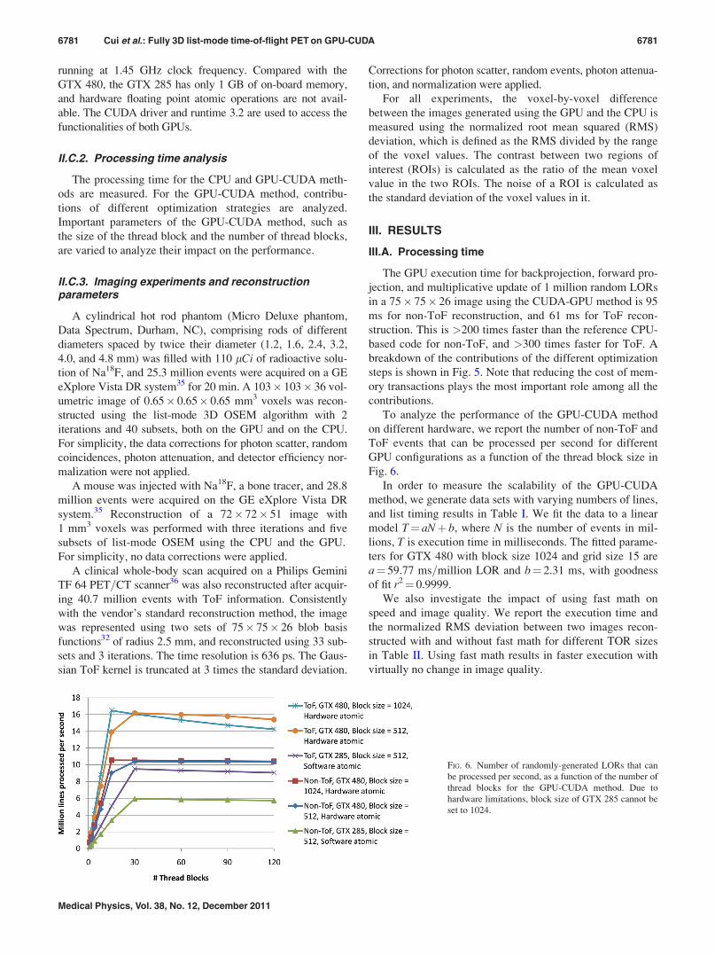
To analyze the performance of the GPU-CUDA method

on different hardware, we report the number of non-ToF and

ToF events that can be processed per second for different

GPU configurations as a function of the thread block size in

Fig. 6.

In order to measure the scalability of the GPU-CUDA

method, we generate data sets with varying numbers of lines,

and list timing results in Table I. We fit the data to a linear

model T¼ aNþ b, where N is the number of events in mil-

lions, T is execution time in milliseconds. The fitted parame-

ters for GTX 480 with block size 1024 and grid size 15 are

a¼ 59.77 ms=million LOR and b¼ 2.31 ms, with goodness

of fit r2¼ 0.9999.

We also investigate the impact of using fast math on

speed and image quality. We report the execution time and

the normalized RMS deviation between two images recon-

structed with and without fast math for different TOR sizes

in Table II. Using fast math results in faster execution with

virtually no change in image quality.

FIG. 6. Number of randomly-generated LORs that can

be processed per second, as a function of the number of

thread blocks for the GPU-CUDA method. Due to

hardware limitations, block size of GTX 285 cannot be

set to 1024.

6781 Cui et al.: Fully 3D list-mode time-of-flight PET on GPU-CUDA 6781

Medical Physics, Vol. 38, No. 12, December 2011

To understand how the algorithm scales with more voxels

in the image and bigger TOR, detailed analysis is performed

and the results are presented in Tables III–V. When the num-

ber of the voxels in the reconstructed image increases, we

keep the physical dimension of the TOR constant by increas-

ing the number of voxels in the TOR, and the execution time

as a function of image size is shown in Table III. We also

show the execution time for varying number of voxels in the

reconstructed image while fixing the other parameters in

Table IV, and the execution time for varying TOR width Tw

while fixing the number of voxels to be 75� 75� 26 in

Table V.

III.B. Image reconstruction accuracy

Transaxial slices of the hot rod phantom reconstructed

using the CPU and the GPU are quantitatively identical

(Fig. 7), with normalized RMS deviation between the two

images being 0.05% after two iterations, which is negligible

compared to the statistical variance of the voxel values in a

typical PET scan (>10%, from Poisson statistics). The pro-

file through the hot rods [Fig. 7(e)] and the contrast and

noise measurements [Fig. 7(f)] are virtually the same for the

two images.

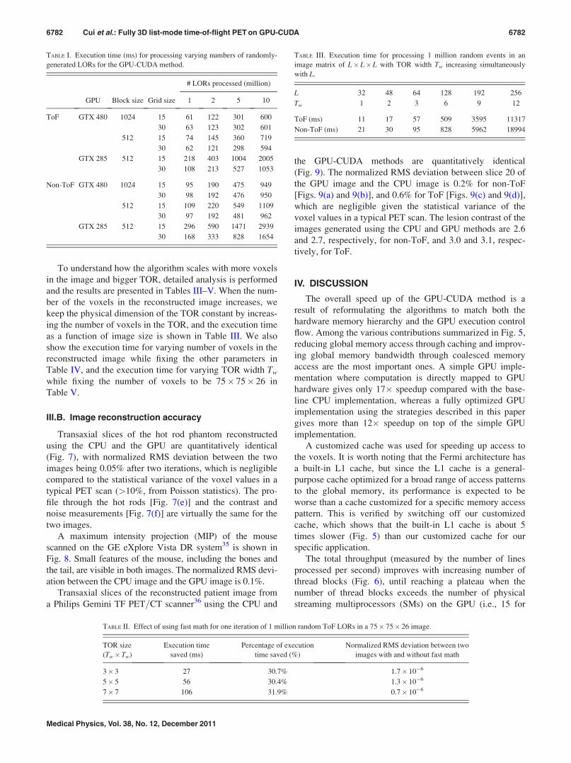
A maximum intensity projection (MIP) of the mouse

scanned on the GE eXplore Vista DR system35 is shown in

Fig. 8. Small features of the mouse, including the bones and

the tail, are visible in both images. The normalized RMS devi-

ation between the CPU image and the GPU image is 0.1%.

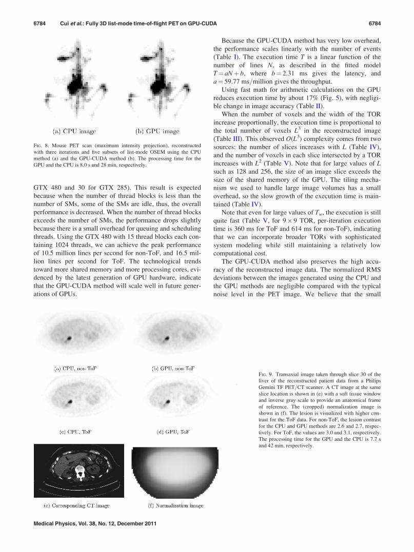
Transaxial slices of the reconstructed patient image from

a Philips Gemini TF PET=CT scanner36 using the CPU and

the GPU-CUDA methods are quantitatively identical

(Fig. 9). The normalized RMS deviation between slice 20 of

the GPU image and the CPU image is 0.2% for non-ToF

[Figs. 9(a) and 9(b)], and 0.6% for ToF [Figs. 9(c) and 9(d)],

which are negligible given the statistical variance of the

voxel values in a typical PET scan. The lesion contrast of the

images generated using the CPU and GPU methods are 2.6

and 2.7, respectively, for non-ToF, and 3.0 and 3.1, respec-

tively, for ToF.

IV. DISCUSSION

The overall speed up of the GPU-CUDA method is a

result of reformulating the algorithms to match both the

hardware memory hierarchy and the GPU execution control

flow. Among the various contributions summarized in Fig. 5,

reducing global memory access through caching and improv-

ing global memory bandwidth through coalesced memory

access are the most important ones. A simple GPU imple-

mentation where computation is directly mapped to GPU

hardware gives only 17� speedup compared with the base-

line CPU implementation, whereas a fully optimized GPU

implementation using the strategies described in this paper

gives more than 12� speedup on top of the simple GPU

implementation.

A customized cache was used for speeding up access to

the voxels. It is worth noting that the Fermi architecture has

a built-in L1 cache, but since the L1 cache is a general-

purpose cache optimized for a broad range of access patterns

to the global memory, its performance is expected to be

worse than a cache customized for a specific memory access

pattern. This is verified by switching off our customized

cache, which shows that the built-in L1 cache is about 5

times slower (Fig. 5) than our customized cache for our

specific application.

The total throughput (measured by the number of lines

processed per second) improves with increasing number of

thread blocks (Fig. 6), until reaching a plateau when the

number of thread blocks exceeds the number of physical

streaming multiprocessors (SMs) on the GPU (i.e., 15 for

TABLE I. Execution time (ms) for processing varying numbers of randomly-

generated LORs for the GPU-CUDA method.

# LORs processed (million)

GPU Block size Grid size 1 2 5 10

ToF GTX 480 1024 15 61 122 301 600

30 63 123 302 601

512 15 74 145 360 719

30 62 121 298 594

GTX 285 512 15 218 403 1004 2005

30 108 213 527 1053

Non-ToF GTX 480 1024 15 95 190 475 949

30 98 192 476 950

512 15 109 220 549 1109

30 97 192 481 962

GTX 285 512 15 296 590 1471 2939

30 168 333 828 1654

TABLE II. Effect of using fast math for one iteration of 1 million random ToF LORs in a 75� 75� 26 image.

TOR size

(Tw�Tw)

Execution time

saved (ms)

Percentage of execution

time saved (%)

Normalized RMS deviation between two

images with and without fast math

3� 3 27 30.7% 1.7� 10�6

5� 5 56 30.4% 1.3� 10�6

7� 7 106 31.9% 0.7� 10�6

TABLE III. Execution time for processing 1 million random events in an

image matrix of L�L�L with TOR width Tw increasing simultaneously

with L.

L 32 48 64 128 192 256

Tw 1 2 3 6 9 12

ToF (ms) 11 17 57 509 3595 11317

Non-ToF (ms) 21 30 95 828 5962 18994

6782 Cui et al.: Fully 3D list-mode time-of-flight PET on GPU-CUDA 6782

Medical Physics, Vol. 38, No. 12, December 2011

TABLE IV. Execution time for processing 1 million random events in an

image matrix of L�L�L with fixed TOR width 3� 3.

L 32 48 64 128 256

# voxels (L3) 3.3� 104 1.1� 105 2.6� 105 2.1� 106 1.7� 107

ToF (ms) 29 42 57 232 1387

Non-ToF (ms) 53 73 95 367 2119

TABLE V. Execution time for processing 1 million random LORs in an

image matrix of 75� 75� 26 for different TOR width Tw. T2w is the maxi-

mum number of voxels in a TOR-slice intersection.

Tw 1 3 5 7 9 11 13 15

T2w 1 9 25 49 81 121 169 225

ToF (ms) 24 61 128 226 360 529 731 968

Non-ToF (ms) 44 95 215 382 614 906 1256 1668

FIG. 7. Hot rod phantom (a) acquired on a preclinical PET scanner and reconstructed with 2 iterations and 40 subsets of list-mode OSEM, using (c) CPU

method and (d) GPU-CUDA method. (b) The normalization map. Profiles of (c) and (d) through the centers of the hot rods, depicted in (a), are shown in (e).

Contrast between the two ROIs in (a) and noise as functions of the number of iterations are shown in (f). The method for computing contrast and noise are

explained in Sec. II C 3. The processing time for the GPU and the CPU is 7.0 s and 23 min, respectively.

6783 Cui et al.: Fully 3D list-mode time-of-flight PET on GPU-CUDA 6783

Medical Physics, Vol. 38, No. 12, December 2011

GTX 480 and 30 for GTX 285). This result is expected

because when the number of thread blocks is less than the

number of SMs, some of the SMs are idle, thus, the overall

performance is decreased. When the number of thread blocks

exceeds the number of SMs, the performance drops slightly

because there is a small overhead for queuing and scheduling

threads. Using the GTX 480 with 15 thread blocks each con-

taining 1024 threads, we can achieve the peak performance

of 10.5 million lines per second for non-ToF, and 16.5 mil-

lion lines per second for ToF. The technological trends

toward more shared memory and more processing cores, evi-

denced by the latest generation of GPU hardware, indicate

that the GPU-CUDA method will scale well in future gener-

ations of GPUs.

Because the GPU-CUDA method has very low overhead,

the performance scales linearly with the number of events

(Table I). The execution time T is a linear function of the

number of lines N, as described in the fitted model

T¼ aNþ b, where b¼ 2.31 ms gives the latency, and

a¼ 59.77 ms=million gives the throughput.

Using fast math for arithmetic calculations on the GPU

reduces execution time by about 17% (Fig. 5), with negligi-

ble change in image accuracy (Table II).

When the number of voxels and the width of the TOR

increase proportionally, the execution time is proportional to

the total number of voxels L3 in the reconstructed image

(Table III). This observed O(L3) complexity comes from two

sources: the number of slices increases with L (Table IV),

and the number of voxels in each slice intersected by a TOR

increases with L2 (Table V). Note that for large values of Lsuch as 128 and 256, the size of an image slice exceeds the

size of the shared memory of the GPU. The tiling mecha-

nism we used to handle large image volumes has a small

overhead, so the slow growth of the execution time is main-

tained (Table IV).

Note that even for large values of Tw, the execution is still

quite fast (Table V, for 9� 9 TOR, per-iteration execution

time is 360 ms for ToF and 614 ms for non-ToF), indicating

that we can incorporate broader TORs with sophisticated

system modeling while still maintaining a relatively low

computational cost.

The GPU-CUDA method also preserves the high accu-

racy of the reconstructed image data. The normalized RMS

deviations between the images generated using the CPU and

the GPU methods are negligible compared with the typical

noise level in the PET image. We believe that the small

FIG. 8. Mouse PET scan (maximum intensity projection), reconstructed

with three iterations and five subsets of list-mode OSEM using the CPU

method (a) and the GPU-CUDA method (b). The processing time for the

GPU and the CPU is 8.0 s and 28 min, respectively.

FIG. 9. Transaxial image taken through slice 30 of the

liver of the reconstructed patient data from a Philips

Gemini TF PET=CT scanner. A CT image at the same

slice location is shown in (e) with a soft tissue window

and inverse gray scale to provide an anatomical frame

of reference. The (cropped) normalization image is

shown in (f). The lesion is visualized with higher con-

trast for the ToF data. For non-ToF, the lesion contrast

for the CPU and GPU methods are 2.6 and 2.7, respec-

tively. For ToF, the values are 3.0 and 3.1, respectively.

The processing time for the GPU and the CPU is 7.7 s

and 42 min, respectively.

6784 Cui et al.: Fully 3D list-mode time-of-flight PET on GPU-CUDA 6784

Medical Physics, Vol. 38, No. 12, December 2011

deviation we measured was caused by small variations in

how the arithmetic operations are performed on the CPU and

GPU. For example, we have observed that the exponential

function produces slightly different results on different plat-

forms. The fast math operations and approximate nature of

the linear interpolation in texture memory in the GPU also

contributes slightly to the difference. Since the image is

reconstructed by solving an ill-posed inverse problem with a

poorly conditioned system matrix, these small differences

could be amplified.

Because the CUDA framework is design to be forward

compatible with future GPUs, the proposed method can be

directly applied to new generations of hardware without any

modification. Of course, the performance comparison would

change depending on how much faster the new GPU and

CPU are compared with the ones used in the paper. However,

given the speed improvement using the proposed method and

the rapid development of the GPU technology, using GPU for

data-intensive image reconstruction applications would still

make sense, at least in the foreseeable future.

V. CONCLUSION

A list-mode time-of-flight OSEM library was developed

on the GPU-CUDA platform. Our studies show that the GPU

reformulation of 3D list-mode OSEM is >200 times faster

than a CPU reference implementation for non-ToF recon-

struction, and >300 times faster for ToF processing. This is

more than 12� faster than a simple GPU implementation

that does not use the optimization strategies proposed in this

paper. The images produced by the GPU-CUDA method are

virtually identical to those produced on the CPU.

The proposed method can be easily adapted to allow

researchers to use more advanced algorithms for high resolu-

tion PET reconstruction, based on additional information

such as depth of interaction (DoI) and photon energy. The

GPU-CUDA method naturally supports arbitrarily broad

LORs, thus can be used for more accurate reconstruction

methods that incorporate shift-varying system point spread

functions (PSFs).37

ACKNOWLEDGMENTS

The authors would like to thank Peter Olcott and Garry

Chinn at Stanford University for helpful discussions and

comments, and NVIDIA for providing a GTX 285 GPU. This

work was sponsored by a research grant from Philips

Healthcare.

a)Author to whom correspondence should be addressed. Electronic mail:

cslevin@stanford.edu1S. Surti, S. Karp, L. M. Popescu, E. Daube-Witherspoon, and M. Werner,

“Investigation of time-of-flight benefit for fully 3D PET,” IEEE Trans.

Med. Imaging 25, 529–538 (2006).2J. S. Karp, S. Surti, Margaret E. Daube-Witherspoon, and G. Muehllehner,

“Benefit of time-of-flight in PET: Experimental and clinical results,” J.

Nucl. Med. 49, 462–470 (2008).3S. Matej, S. Surti, S. Jayanthi, M. E. Daube-Witherspoon, R. M. Lewitt,

and J. S. Karp, “Efficient 3D TOF PET reconstruction using view-grouped

histo-images: DIRECT-direct image reconstruction for TOF,” IEEE Trans.

Med. Imaging 28, 739–751 (2009).

4M. Watanabe, H. Uchida, H. Okada, K. Shimizu, N. Satoh, E. Yoshikawa,

T. Ohmura, T. Yamashita, and E. Tanaka, “A high resolution PET for ani-

mal studies,” IEEE Trans. Med. Imaging 11, 577–580 (1992).5S. R. Cherry, Y. Shao, R. W. Silverman, K. Meadors, S. Siegel, A.

Chatziioannou, J. W. Young, W. Jones, J. C. Moyers, D. Newport, A.

Boutefnouchet, T. H. Farquhar, M. Andreaco, M. J. Paulus, D. M.

Binkley, R. Nutt, and M. E. Phelps, “MicroPET: A high resolution PET

scanner for imaging small animals,” IEEE Trans. Nucl. Sci. 44,

1161–1166 (1997).6J.-Y. Peng, J. A. D. Aston, R. N. Gunn, C.-Y. Liou, and J. Ashburner,

“Dynamic positron emission tomography data-driven analysis using

sparse bayesian learning,” IEEE Trans. Med. Imaging 27, 1356–1369

(2008).7L. A. Shepp and Y. Vardi, “Maximum likelihood reconstruction for emis-

sion tomography,” IEEE Trans. Med. Imaging 1, 113–122 (1982).8H. M. Hudson and R. S. Larkin, “Accelerated image reconstruction using

ordered subsets of projection data,” IEEE Trans. Med. Imaging 13,

601–609 (1994).9A. J. Reader, K. Erlandsson, M. A. Flower, and R. J. Ott, “Fast accurate

iterative reconstruction for low-statistics positron volume imaging,” Phys.

Med. Biol. 43, 835–846 (1998).10L. Parra and H. H. Barrett, “List-mode likelihood: EM algorithm and

image quality estimation demonstrated on 2-D PET,” IEEE Trans. Med.

Imaging 17, 228–235 (1998).11L. M. Popescu, S. Matej, and R. M. Lewitt, “Iterative image reconstruction

using geometrically ordered subsets with list-mode data,” Nuclear ScienceSymposium Conference Record, Vol. 6 (IEEE, Rome, Italy, 2004), pp.

3536–3540.12A. Rahmim, M. Lenox, A. J. Reader, C. Michel, Z. Burbar, T. J. Ruth, and

V. Sossi, “Statistical list-mode image reconstruction for the high resolu-

tion research tomograph,” Phys. Med. Biol. 49, 4239 (2004).13G. Pratx, P. D. Olcott, G. Chinn, and C. S. Levin, “Fast, accurate and

shift-varying line projections for iterative reconstruction using the GPU,”

IEEE Trans. Med. Imaging 28, 435–445 (2009).14I. K. Hong, S. T. Chung, H. K. Kim, Y. B. Kim, Y. D. Son, and Z. H. Cho,

“Ultra fast symmetry and SIMD-based projection-backprojection (SSP)

algorithm for 3D PET image reconstruction,” IEEE Trans. Med. Imaging

26, 789–803 (2007).15F. Xu and K. Mueller, “Accelerating popular tomographic reconstruction

algorithms on commodity PC graphics hardware,” IEEE Trans. Nucl. Sci.

52, 654–663 (2005).16F. Xu and K. Mueller, “Real-time 3D computed tomographic reconstruc-

tion using commodity graphics hardware,” Phys. Med. Biol. 52, 3405

(2007).17H. G. Hofmann, B. Keck, C. Rohkohl, and J. Hornegger, “Comparing

performance of many-core CPUs and GPUs for static and motion com-

pensated reconstruction of C-arm CT data,” Med. Phys. 38, 468–473

(2011).18F. Xu, A. Khamene, and O. Fluck, “High performance tomosynthesis

enabled via a GPU-based iterative reconstruction framework,” Proc. SPIE

7258, pp. 72585A (2009).19R. Jacques, J. Wong, R. Taylor, and T. McNutt, “Real-time dose computa-

tion: GPU-accelerated source modeling and superposition=convolution,”

Med. Phys. 38, 294–305 (2011).20S. Hissoiny, B. Ozell, H. Bouchard, and P. Despres, “GPUMCD: A new

GPU-oriented Monte Carlo dose calculation platform,” Med. Phys. 38,

754–764 (2011).21G. Pratx and L. Xing, “GPU computing in medical physics: A review,”

Med. Phys. 38, 2685–2697 (2011).22Z. Hu, W. Wang, E. E. Gualtieri, M. J. Parma, E. S. Walsh, D. Sebok, Y.

L. Hsieh, C. H. Tung, J. J. Griesmer, J. A. Kolthammer, L. M. Popescu,

M. Werner, J. S. Karp, A. Bucur, J. van Leeuwen, and D. Gagnon,

“Dynamic load balancing on distributed listmode time-of-flight image

reconstruction,” IEEE Nuclear Science Symposium Conference Record(IEEE, San Diego, California, 2006), pp. 3392–3396.

23NVIDIA, NVIDIA CUDA Programming Guide 3.0 (2010).

24E. Veklerov, J. Llacer, and E. J. Hoffman, “MLE reconstruction of a brain

phantom using a Monte Carlo transition matrix and a statistical stopping

rule,” IEEE Trans. Nucl. Sci. 35, 603–607 (1988).25R. H. Huesman, G. J. Klein, W. W. Moses, J. Qi, B. W. Reutter, and P. R.

G. Virador, “List-mode maximum-likelihood reconstruction applied to

positron emission mammography (PEM) with irregular sampling,” IEEE

Trans. Med. Imaging 19, 532–537 (2000).

6785 Cui et al.: Fully 3D list-mode time-of-flight PET on GPU-CUDA 6785

Medical Physics, Vol. 38, No. 12, December 2011

26C. A. Johnson, Y. Yan, R. E. Carson, R. L. Martino, and M. E. Daube-

Witherspoon, “A system for the 3D reconstruction of retracted-septa PET

data using the EM algorithm,” Nuclear Science Symposium and MedicalImaging Conference Record, Vol. 3 (IEEE, Norfolk, Virginia, 1994), pp.

1325–1329.27J. Qi, R. M. Leahy, S. R Cherry, A. Chatziioannou, and T. H. Farquhar,

“High-resolution 3D bayesian image reconstruction using the microPET

small-animal scanner,” Phys. Med. Biol. 43, 1001 (1998).28L. Zhang, S. Staelens, R. V. Holen, J. D. Beenhouwer, J. Verhaeghe, I.

Kawrakow, and S. Vandenberghe, “Fast and memory-efficient Monte

Carlo-based image reconstruction for whole-body PET,” Med. Phys. 37,

3667–3676 (2010).29R. L. Siddon, “Fast calculation of the exact radiological path for a three-

dimensional CT array,” Med. Phys. 12, 252–255 (1985).30P. M. Joseph, “An improved algorithm for reprojecting rays through pixel

images,” IEEE Trans. Med. Imaging 1, 192–196 (1982).31G. Pratx and C. Levin, “Online detector response calculations for

high-resolution PET image reconstruction,” Phys. Med. Biol. 56, 4023

(2011).

32S. Matej and R. M. Lewitt, “Practical considerations for 3D image recon-

struction using spherically symmetric volume elements,” IEEE Trans.

Med. Imaging 15, 68–78 (1996).33P. Aguiar, M. Rafecas, J. E. Ortuno, G. Kontaxakis, A. Santos, J. Pavıa,

and D. Ros, “Geometrical and Monte Carlo projectors in 3D PET

reconstruction,” Med. Phys. 37, 5691–5702 (2010).34M. Herlihy and N. Shavit, The Art of Multiprocessor Programming

(Morgan Kaufmann, Waltham, Massachusetts, 2008).35Y. Wang, J. Seidel, B. M. W. Tsui, J. J. Vaquero, and M. G. Pomper,

“Performance evaluation of the GE Healthcare eXplore VISTA dual-ring

small-animal PET scanner,” J. Nucl. Med. 47, 1891–1900 (2006).36S. Surti, A. Kuhn, M. E. Werner, A. E. Perkins, J. Kolthammer, and J. S.

Karp, “Performance of Philips Gemini TF PET=CT scanner with special

consideration for its time-of-flight imaging capabilities,” J. Nucl. Med. 48,

471–480 (2007).37A. M. Alessio, C. W. Stearns, S. Tong, S. G. Ross, S. Kohlmyer, A. Ganin,

and P. E. Kinahan, “Application and evaluation of a measured spatially

variant system model for PET image reconstruction,” IEEE Trans. Med.

Imaging 29, 938–949 (2010).

6786 Cui et al.: Fully 3D list-mode time-of-flight PET on GPU-CUDA 6786

Medical Physics, Vol. 38, No. 12, December 2011