Fully Connected Object Proposals for Video Segmentation

Federico Perazzi1,2 Oliver Wang2 Markus Gross1,2 Alexander Sorkine-Hornung2

1ETH Zurich 2Disney Research Zurich

Abstract

We present a novel approach to video segmentation using

multiple object proposals. The problem is formulated as a

minimization of a novel energy function defined over a fully

connected graph of object proposals. Our model combines

appearance with long-range point tracks, which is key to en-

sure robustness with respect to fast motion and occlusions

over longer video sequences. As opposed to previous ap-

proaches based on object proposals, we do not seek the best

per-frame object hypotheses to perform the segmentation.

Instead, we combine multiple, potentially imperfect propos-

als to improve overall segmentation accuracy and ensure

robustness to outliers. Overall, the basic algorithm consists

of three steps. First, we generate a very large number of

object proposals for each video frame using existing tech-

niques. Next, we perform an SVM-based pruning step to re-

tain only high quality proposals with sufficiently discrimina-

tive power. Finally, we determine the fore- and background

classification by solving for the maximum a posteriori of

a fully connected conditional random field, defined using

our novel energy function. Experimental results on a well

established dataset demonstrate that our method compares

favorably to several recent state-of-the-art approaches.

1. Introduction

Video object segmentation refers to the partitioning of

a video into two disjoint sets of pixels representing a fore-

ground object and background regions. The abundance of

available literature on video segmentation reflects the im-

portance of the topic, which is an essential building block

for numerous applications including video editing and post-

processing, video retrieval, analysis of large video collec-

tions, activity recognition, and many more. Many existing

approaches are based on background subtraction, tracking

of feature points and homogeneous regions, spatiotempo-

ral graph-cuts, or hierarchical clustering. Recently, meth-

ods leveraging advances in object recognition have gained

popularity. These methods make use of per-frame object

proposals and employ different techniques to select a set of

temporally coherent segments, one per frame, typically by

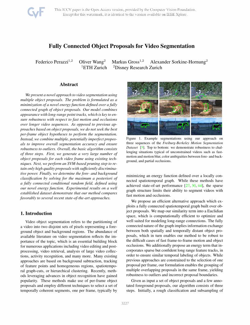
Figure 1. Example segmentations using our approach on

three sequences of the Freiburg-Berkeley Motion Segmentation

Dataset [5]. Top to bottom: we demonstrate robustness to chal-

lenging situations typical of unconstrained videos such as fast-

motion and motion blur, color ambiguities between fore- and back-

ground, and partial occlusions.

minimizing an energy function defined over a locally con-

nected spatiotemporal graph. While these methods have

achieved state-of-art performance [27, 30, 44], the sparse

graph structure limits their ability to segment videos with

fast motion and occlusions.

We propose an efficient alternative approach which ex-

ploits a fully connected spatiotemporal graph built over ob-

ject proposals. We map our similarity term into a Euclidian

space, which is computationally efficient to optimize and

well suited for modeling long-range connections. The fully

connected nature of the graph implies information exchange

between both spatially and temporally distant object pro-

posals, which in turn enables our method to be robust to

the difficult cases of fast frame-to-frame motion and object

occlusions. We additionally propose an energy term that in-

corporates sparse but confident long range feature tracks, in

order to ensure similar temporal labeling of objects. While

previous approaches are constrained to the selection of one

proposal per frame, our formulation enables the grouping of

multiple overlapping proposals in the same frame, yielding

robustness to outliers and incorrect proposal boundaries.

Given as input a set of object proposals and a few anno-

tated foreground proposals, our algorithm consists of three

steps. Initially, a rough classification and subsampling of

13227

the data is performed using a self-trained Support Vector

Machine (SVM) classifier in order to reduce the size of

the proposal space while preserving a large pool of can-

didate foreground proposals. Next, maximum a posteriori

(MAP) inference is performed on a fully connected condi-

tional random field (CRF) to determine the final labeling

of the candidate proposals. Finally, each labeled proposal

casts a vote to all pixels that it overlaps. The aggregate re-

sult yields the final foreground-background segmentation.

We compare our results with an existing benchmark dataset

and show that our method outperforms several state-of-the-

art approaches.

2. Related Work

In this section we provide an overview of commonly em-

ployed approaches and discuss works most related to ours.

Background Subtraction. Many established video

segmentation algorithms are based on background subtrac-

tion. These approaches assume that the background is

known a priori, and that the camera is stationary [12, 14]

or undergoes a predictable, parametric motion [20, 22, 38].

While this family of methods cannot handle non-rigid cam-

era movements, they are well suited to specific application

scenarios such as surveillance systems [6]. In contrast our

method is designed to handle unconstrained videos with ar-

bitrary camera motion and non-rigid background.

Tracking-based Methods. Significant progress has

been achieved by methods designed to track keypoints over

time and, more recently, over image regions [4, 27, 41].

These methods, however, only consider two consecutive

frames of video and cannot handle sudden motion and ap-

pearance changes (i.e. due to lighting). Related to tracking

systems, Brox et al. propose an approach to segment motion

by spectral clustering of long term point trajectories based

on their motion affinity [5] and a variational approach [31]

to turn the resulting sparse trajectory clusters into dense re-

gions. By defining the pairwise distance between trajecto-

ries as the maximum difference of their motion, they as-

sume a translational motion model. Despite this being a

reasonable approximation for spatially close point trajecto-

ries, these methods have difficulties to segment articulated

bodies following non-rigid motion. In this work, we exploit

point-tracks to increase stability for long term temporal con-

nections. However, we avoid motion clustering and do not

make any assumption on the underlying object motion.

Oversegmentation. Unconstrained motion can be han-

dled by supervoxel based methods [19,21,43]. These meth-

ods generate an oversegmentation of the video into space-

time homogeneous, perceptually distinct regions. They are

important for early stage video preprocessing, but do not

directly solve the problem of video object segmentation as

they do not provide any principled approach to flatten the hi-

erarchical decomposition of the video into a binary segmen-

tation [32]. In Section 6 we formulate the problem of re-

ducing overlapping segments into a foreground-background

partition by minimizing a novel energy function which we

solve optimally by inference on a CRF.

Video Object Segmentation. Recently, closely related

to our work, a family of methods for solving the problem of

segmenting the dominant moving object in a video gained

popularity. Papazouglo and Ferrari [32] describe a fully

automatic approach that efficiently identifies closed motion

boundaries to determine the object position, and propagates

the labeling through a spatiotemporal extension of Grab-

Cut [39]. Ramakanth and Babu [37] extend work on video-

retargeting [40] to propagate labels through connected low-

energy paths. Despite its ability to accurately segment ob-

ject boundaries, this method cannot handle complete oc-

clusions and fast motion, as it operates locally. To over-

come this problem [17] propose a non-local consensus vot-

ing scheme defined over a globally connected graph. This

method shares similarities with ours (fully connected graph,

weighted voting), but differs as their graph is built over non-

overlapping pixel regions and they use a random-walk tran-

sition matrix to update their prediction iteratively until con-

vergence. Relying on saliency detection this method might

encounter difficulties to segment complex objects of multi-

ple colors. To overcome this problem, Banica et al. [2] link

figure-ground hypotheses instead of superpixels, to form

temporal chains representing the object, based on saliency

metrics and appearance similarity.

Proposal-based approaches. Recent advances in state-

of-the-art image analysis [8, 18, 28] have motivated the use

of object proposals [1, 9, 16, 24] in video object segmen-

tation. Lee et al. [26] discover clusters of key-segments

in videos, coupling the notion of objectness and appear-

ance similarity. Hypotheses are later ranked and the top

scoring one is automatically selected for video segmenta-

tion. Their work is well suited to determine groups of seg-

ments with consistent appearance and motion, but disre-

gards spatial and temporal relations between segments. Ma

and Latecky [30] account for these by imposing the selec-

tion of one proposal in every frame, formulating the prob-

lem as finding a maximum weighted clique in a locally con-

nected graph with mutex constraints. However, the strict

assumptions that the object should appear in every frame

limits their efficacy in real world scenarios. Similar to [30],

Zhang et al. [44] create a layered Directed Acyclic Graph

(DAG) which combines unary edges measuring the object-

ness of the object proposal and pairwise edges modeling

affinities. A shortest path determines the video object seg-

mentation. Both [30,44] formulate the problem on a locally

connected graph structure, requiring that objects appear in

every frame. In contrast, we exploit a fully connected graph

to robustly model long range relations required to handle

fast motion or occlusions.

3228

3. Overview

Our method consists of three stages. Given an input

video V , for each frame Vt we compute a large set of ob-

ject proposals St = {sti}, using existing techniques [24].

The goal of this step is to generate a wide range of different

proposals, such that a sufficient number of segments over-

lap with the object (Section 4). Then our method learns an

SVM-based classifier in order to resample S into a smaller

set of higher quality proposals S (Section 5). Finally we re-

fine this classification by solving for the maximum a poste-

riori inference on a densely connected CRF (Section 6). The

fully connected graph structure is coupled with a novel en-

ergy function that considers overlap between point-tracks in

the pairwise potentials, exploits temporal information, and

ensures robustness to fast motion and occlusions.

4. Object Proposal Generation

Algorithms for computing object proposals are generally

designed to have a high recall, proposing at least one region

for as many objects in the image as possible. While the

set of candidates must remain of limited size, the task of

selecting positive samples is left to later stages, and the ratio

of regions that truly belong to an object, i.e. precision, is

usually not considered a measure of performance.

While other approaches leverage the high recall property

by assuming that there is one good proposal per-frame, our

goal is to exploit the redundancy in the data of multiple pro-

posals with a high degree of overlap with the foreground ob-

ject. In order to have a significant amount of such positive

instances, we modified the parameters of [24] that control

seed placement and level set selection to generate around

twenty thousands proposals per frame. Otherwise we con-

sider the proposal generator as a black box, and other object

proposal methods could be used instead.

It is important to note, however, that the resulting set of

proposals is likely imbalanced, with potentially many more

proposals on background regions than on foreground, de-

pending on object size. Furthermore, many proposals will

cover both foreground and background. These issues neg-

atively impact segmentation, both in terms of quality and

efficiency. To overcome this problem we self-train an SVM

classifier and resample the pool of proposals.

5. Candidate Proposal Pruning

We introduce a per-frame pruning step with the goal of

rebalancing the set of proposals and selecting only those

with higher discriminative power, i.e. those that do not over-

lap both with foreground and background. The choice of the

SVM is justified by its proven robustness to skewed vector

spaces resulting from class imbalance [42] and relatively

fast performance. We train an SVM classifier which oper-

ates on elements of S , separating those that overlap with

foreground from those that belong to the background (Sec-

tion 5.1), and then resample the set (Section 5.2). Finally,

we use the output of the SVM to initialize the unaries of the

CRF (Section 6.1).

5.1. Feature Extraction and Training

Features. From each of the proposals we extract a set of

features that characterize its appearance, motion and object-

ness as summarized in Table 1. The global appearance and

spatial support are defined in terms of average color, av-

erage position and area. The local appearance is encoded

with Histogram of Oriented Gradients (HOG) [29] com-

puted over the proposal bounding box rescaled to 64x64

pixels and divided into 8x8, 50% overlapping cells quan-

tized into 9 bins. The motion is defined with Histogram

of Oriented Optical Flow (HOOF) [10] extracted from the

proposal bounding box also rescaled to 64x64 pixels and

quantized into 32 bins. The objectness is measured in terms

of region boundaries encoded by 8x8 normalized gradients

patches [11]. The set of features is aggregated into a 1398

dimensional descriptor xi ∈ X .

Training. The classifier is trained from a small set of

proposals S known to belong to the foreground object. This

set S = {si} may be either determined using automatic

approaches such as salient object detectors [34], based on

objectness [16, 26], manually using interactive video edit-

ing tools, or a combination thereof. In our experiments

we manually annotated 1 or 2 foreground proposals per-

sequence. S is augmented with all proposals that spatially

overlap with one of its initial elements by a factor of more

than a threshold τ (0.95 in our experiments). All remain-

ing proposals are marked background. A binary SVM clas-

sifier with linear kernel and soft margins is trained on the

labeled data yielding the score function C(xi) = wTxi + b

which measures the distance of the proposal si with associ-

ated feature vector xi from the decision surface w⊥. While

sign(C(xi)) is enough to classify proposals as either fore-

or background, in Section 6 we can additionally include the

distance from the hyperplane wTxi+b ∈ [−∞,+∞] as the

posterior probability P (yi|xi) ∈ [0, 1] in order to initialize

the unary potentials of the CRF. We use Platt Scaling [35]

to fit a logistic regressor Q to the output of the SVM and

the true class labels, such that Q(C(xi)) : R → P (yi|xi).Parameters of the SVM are reported in Section 7.

Feature Description Dim

(ACC) Area, centroid, average color 6

(HOOF) Histogram of Oriented Optical Flow 32

(NG) Objectness via normalized gradients 64

(HOG) Histogram of oriented gradients 1296

Table 1. Set of features extracted from each object proposal by the

SVM classifier and corresponding dimensionality.

3229

5.2. Classification and Resampling

Given the trained classifier C, we aim to roughly sub-

divide the set of object proposals St extracted at frame tinto two spatially disjoint sets St+ and St− such that

⋃St+

lies within the foreground region and⋃St− on the back-

ground. Initially we form St+ = {sti|P (yi|xi) > 0.5}.

Next, we select elements from the set of proposals classi-

fied as background such that they do not overlap with St+,

i.e., St− = {sti| |St+ ∩ sti| < ǫ}. The slack variable ǫ is nec-

essary to avoid St− = ∅, which can happen in videos where

the foreground object occupies most of the frame. We ini-

tially set ǫ to 0 and iteratively increment it with steps of

20 until the constraint |St−| > 500 is satisfied or the total

amount of background proposal is reached. In our experi-

ments we retain ∼ 10% of the proposals generated (roughly

2000 proposals per-frame).

The positive impact of our pruning and resampling step

on the quality of the video segmentation is shown in Sec-

tion 8. The resulting classification can still be imprecise,

but serves the purpose of rebalancing positive and nega-

tive instances. The union of the two newly generated sets

St = St+ ∪ St− forms the input S = {St} to the follow-

ing step, which then provides a global solution considering

spatial and temporal information jointly with the color ap-

pearance. Note that for ease of notation we refer to S as Sthroughout the remaining part of paper.

6. Fully Connected Proposal Labeling

In order to accurately classify elements of S , we must

enforce a smoothness prior that says that similar proposals

should be similarly classified. Conditional random fields

provide a natural framework to incorporate all mutual spa-

tiotemporal relationships between proposals as well as our

initial proposal confidences.

6.1. Inference

Let us define a set of labels L = {bg = 0, fg = 1}, cor-

responding to background and foreground regions respec-

tively. Let F = {f i} be a newly generated set of features

extracted from each element in S , as defined in Eq. (3). Let

us define the set of random variables Y = {yi}, yi ∈ L.

Consider a fully-connected random field (Y,X ∪ F) de-

fined over a graph G = (V, E) whose nodes correspond

to object proposals. Let Z(X ,F) be the partition function.

The posterior probability for this model is P (Y |X ,F) =1

Z(F)exp(−E(Y |X ,F)) with the corresponding Gibbs en-

ergy defined over the set of all unary and pairwise cliques:

E(Y |X ,F) =∑

i∈V

ψu(yi;X ) +∑

i,j∈E

ψp(yi, yj ;F) . (1)

Unary Potentials. The unary term ψu is directly inferred

from the output of the SVM and the set of annotated pro-

posals S . We formulate an updated conditional probability

P (yi|xi) = λ · Q(C(xi)) +(1−λ)

2 , with the user-defined

parameter λ ∈ [0, 1] modulating the influence of the SVM

prediction on the CRF initialization. For all experiments,

we set the parameter λ to 0.1. We define ψu as a piecewise

function

e−ψu(yi,X ) =

{li + ǫ, li ∈ L si ∈ S

P (yi|xi) si /∈ S. (2)

Pairwise Potentials. We define the label compatibil-

ity function µ to be the Potts model µ(yi, yj) = [yi 6=

yj ], a Gaussian kernel k∗(x) = exp(− x2

2σ2∗

), and scalar

weights ω∗. In order to distinguish proposals that have sim-

ilar appearance but belong to different image regions we

define the pairwise potential ψp to be a linear combination

of several terms that jointly incorporate color, spatial and

temporal information:

ψp(yi, yj ;F) = [yi 6= yj ] ·(ωckc(Dc(ci, cj))︸ ︷︷ ︸

appearance kernel

+

ωsks(Ds(si, sj))︸ ︷︷ ︸

spatial kernel

+ωpkp(Dp(pi, pj))︸ ︷︷ ︸

trajectory kernel

+ωtkt(|ti − tj |)︸ ︷︷ ︸

temporal kernel

).

(3)

The color appearance Dc is defined in terms of the chi-

squared kernel χ2(ci, cj) where ci and cj are normalized

RGB color histograms of proposals si and sj , respectively,

with 20 bins per dimension. The spatial relation between

any pairs of proposals is defined in terms of the intersection-

over-union: Ds(si, sj) = 1 − |si∩sj ||si∪sj |

. The last two kernels

establish temporal connectivity among proposals, reducing

the penalty of assigning different labels to those that are not

intersected by the same trajectory or that belong to a differ-

ent frame. The trajectory kernel exploits that the proposals

we use consist of compact sub-regions in the form of super-

pixels. Let pi ⊂ si and pj ⊂ sj be the set of superpixels that

share at least one point-track (computed using [5]) with sjor si, respectively. We define Dp based on the area that is in-

tersected by common trajectories Dp(pi, pj) = 1− |pi∪pj ||si∪sj |

.

In the last term, ti and tj are the corresponding frame num-

bers of proposals si and sj , which reduces penalty for as-

signing different labels to proposals that are distant in time.

The maximum a posteriori (MAP) labeling of the random

field Y ∗ = argmaxY ∈LP (Y |X ,F) minimizing the Gibbs

energy E(Y |X ,F) produces the segmentation of the video.

To efficiently recover Y ∗ we use the framework of

Krahenbuhl and Koltun [23], which provides a linear time

O(N) algorithm for the inference of N variables on a fully-

connected graph based on a mean field approximation to

the CRF distribution. The efficiency of the method comes

with the limitation that the pairwise potential must be ex-

pressed as a linear combination of Gaussian kernels having

3230

the form:

ψp(yi, yj ,F) = µ(yi, yj)K∑

m=1

wmkm(f i, f j) (4)

where each Gaussian kernel defined as:

km(f i, f j) = exp

(

−1

2(f i − f j)

TΛm(f i − f j)

)

. (5)

We now describe the embedding techniques we employ to

project F into Euclidean space in order to overcome this

limitation.

6.2. Euclidean Embedding

To enable the use of arbitrary pairwise potentials we seek

a new representation of the data in which the l2-norm is a

good approximation to the distance of the original nonlinear

space. In practice, given the original set of features F we

seek a new embedding F into the Euclidean space Rd s.t.:

D(f i, f j) ≈∣∣∣

∣∣∣f i − f j

∣∣∣

∣∣∣2. (6)

Campbell et al. [7] have demonstrated the effectiveness

of Landmark Multidimensional Scaling (LMDS) [15] in a

context similar to ours. LMDS is an efficient variant of

Multidimensional Scaling [13] that uses the Nystrom ap-

proximation [3] to reduce the complexity from O(N3) to

O(Nmk +m3) where N is the number of points, m is the

number of landmarks and k the dimensionality of the new

space. We refer the reader to [7, 36] for more details.

We use LMDS to conform the pairwise potential to

Eq. (4). We express pairwise potentials ψp in Eq. (3) as

a linear combination of several terms. For better control of

the resulting embedding error, we separately embed each of

the components. For each D∗ term of Eq. (3), we empiri-

cally determine the dimensionality of the embedding space

from the analysis of their dissimilarity matrix eigenvalues.

The resulting pairwise potential conforming to Eq. (4) is:

ψp(yi, yj ; F) = [yi 6= yj ](ωckc(ci, cj)+

ωsks(si, sj) + ωpkp(pi, pj) + ωtkt(ti, tj)). (7)

The features c, s, p are Euclidean vectors of 10, 20 and

50 dimensions respectively. Note that the temporal term t is

already Euclidean, and so it does not require embedding.

6.3. Segmentation

The final video segmentation is computed as the sum

of the proposals weighted by the conditional probability

P (y = fg|X , F) and scaled to range [0, 1] on a per-frame

basis. As a final post-processing step, we refine the segmen-

tation with a median filter of width 3 applied along the di-

rection of the optical flow [5]. This has the effect of remov-

ing temporal instability that arises from different per-frame

object proposal configurations. The final segmentation can

then be thresholded by β to achieve a binary mask.

Stage Time (seconds)

Optical flow 113.1

Object Proposals 55.6

Feature Extraction 541.7

SVM Classification 42.7

MDS Embedding 78.4

CRF Inference 260.0

Video Segmentation 1091.5

Table 2. Running time in seconds for each individual stage to seg-

ment a video of 75 frames and spatial resolution 960x540.

7. Implementation Details

We conducted all experiments on a machine with 2 Intel

Xeon 2.20 GHz processors with 8 cores each. The algo-

rithm has been implemented in Python. For the SVM-based

pruning we employ the implementation of scikit-learn [33].

Most of the components of our algorithm are parallelizable.

Those that are not, such as MDS and the CRF, are relatively

efficient. In Table 2 we report the time consumption of each

individual component for a sample video of 75 frames and

resolution of 960x540. It takes about 20 minutes to com-

plete the segmentation which is about 16 seconds per frame.

The running time performance of our algorithm is compa-

rable to the fastest existing methods such as [17, 32, 37].

The weights of the CRF pairwise potential ψp of Eq. (3)

are specific to the dataset. For FBMS we used ωc = 1.0,

ωs = 0.15, ωp = 0.3 and ωt = 0.2, while for SegTrack

we reduced the impact of spatial-temporal relationships be-

tween proposals setting ωs = ωt = 0.01. The proposal

generation step uses 200 seeds, 200 level sets, with the re-

jection overlap set to 0.95. The only necessary modification

of parameters was a reduction of the number of proposals

for the evaluation of the CRF step only (without proposal

pruning), which we discuss in detail below. For that exper-

iment, we reduced the number of proposals using 30 seeds,

30 level sets and rejection threshold of 0.88.The parameter

β that binarizes the final segmentation is set empirically to

0.03 for FBMS and 0.07 for SegTrack.

8. Results

We quantitatively evaluate our approach and its com-

ponents with respect to various state-of-the-art techniques

on the Freiburg-Berkeley Motion Segmentation Dataset

(FBMS [5]), see Fig. 2. Please also refer to the supplemen-

tal material for details.

FBMS Results. The FBMS dataset consists of 59

sequences featuring typical challenges of unconstrained

videos such as fast motion, motion blur, occlusions, and ob-

ject appearance changes. The dataset is split into a training

and testing set. Since none of the methods we compare with

requires a training phase, we measure performance on both

3231

Figure 2. Top to bottom, left to right: qualitative video object segmentation results on six sequences (horses05, farm01, cats01, cars4,

marple8 and people5) from the FBMS dataset [5]. Our method demonstrates reasonable segmentation quality for challenging cases, e.g.,

non-rigid motion and considerable appearance changes (horse05, cats01). The rich set of features of the SVM and the pairwise potentials

of the CRF make our method robust to cluttered background (farm1, cars4), while the fully connected graph on which we perform

inference provides robustness to partial and full occlusions (marple8). The aggregation of object proposals is also effective for complex,

multi-colored objects (people05).

sets. Due to running-time and memory constraints of the

prior approaches that we compare to, we limit the length of

the videos to 75 frames. For the purpose of testing segmen-

tation quality in the presence of fast motion we temporally

subsample frames from videos exhibiting slow motion. We

report the speed-up factor of each sequence in the supple-

mentary material. In videos that have multiple objects we

manually selected the one with dominant motion. Similar to

previous works [17, 27] we measure the segmentation qual-

ity in terms of intersection-over-union, which is invariant to

image resolution and to the size of the foreground object.

We compare our method (FCP) with several recent state-

of-the-art approaches [17, 32, 37, 44]. These methods have

been selected based on their quality of results, underlying

approaches, and availability of their source code. SeamSeg

(SEA, [37]), seeks connected paths of low energy to track

the object boundaries. Zhang et al. (DAG, [44]) integrate

objectness and appearance similarity in a directly acyclic

graph whose shortest-path corresponds to a video segmenta-

tion. Under the assumption that the object moves differently

from the background Papazoglou and Ferrari (FST, [32])

find the closed motion boundary and propagate the initial

estimate using a spatio-temporal optimization. Finally, Fak-

tor and Irani (NLC, [17]) consolidate an initial foreground

estimate based on saliency using a Markov chain.

Our method and SEA are semi-supervised while the oth-

ers are unsupervised. For a more informative and fairer

comparison, we therefore removed any of the videos from

the comparison in Table 3, for which at least one of these

unsupervised methods did not detect the object.We report

detailed sequence evaluation for the test set and the average

for the training set. Please also refer to the supplementary

material for a more detailed evaluation. We separately eval-

uate the steps of our algorithm: SVM only, CRF only, and

the full approach FCP. Corresponding precision, recall, and

f-measure plots are shown in Fig. 3. As discussed in the

implementation section, in the CRF experiment we modi-

fied the parameters generating object proposals to produce

roughly the same number of proposals that are retained dur-

ing the pruning step.

Results in Table 3 demonstrates that our method con-

sistently produces a good segmentation yielding roughly a

10% improvement over the current state-of-the-art in terms

of average performance. The importance of combining both

the SVM and CRF steps is also apparent.

Limitations. Our approach is designed to work with

real-world video sequences with fast object motion, and oc-

clusions. In particular, since our method is based on ob-

ject proposals, it requires a sufficiently high video reso-

lution such that the computation of proposals using exist-

ing techniques produces meaningful results. This becomes

clear in Table 4, when running our approach on lower reso-

lution video such as the SegTrack benchmark1 [26, 32]. We

additionally compare with (TMF, [27]), (KEY, [26]) and

(HVS, [19]). In this dataset, very few proposals overlap

with the foreground object due to the limited image resolu-

tion (highest is 414x320) and the small size of the objects,

so our approach, which is based on aggregating multiple

object hypothesis works less well. For example the training

set of the birdfall video has a ratio of 1:4000 foreground and

background proposals, with only 13 proposals on the object.

The lack of positive samples weakens the self-training of

1In accordance with prior works we do not evaluate ’penguin’

3232

0.65 0.70 0.75 0.80 0.85 0.90 0.95 1.00

Recall0.4

0.5

0.6

0.7

0.8

0.9

1.0

Pre

cisi

on FCP

FCP\{Dc}FCP\{Dp}FCP\{Ds}FCP\{t}

SVM

SVM\{Hoof}

SVM\{ACC}

SVM\{Hog}

SVM\{NG}SV

M

SVM\{

Hoof}

SVM\{

ACC}

SVM\{

Hog}

SVM\{

NG}FC

P

FCP\

{Dc}

FCP\

{Dp}

FCP\

{Ds}

FCP\

{t}

0.4

0.5

0.6

0.7

0.8

0.9

1.0

F-s

core

F-Score Avg

F-Score Max

F-Score Min

Figure 3. Left: Precision-Recall curves and F-score isolines (β2=

0.3) for the SVM and CRF classification of object proposals into

foreground and background, obtained by varying the minimum

amount of overlap τ required for a proposal to be considered fore-

ground. The SVM classification (SVM) is less precise but has

better recall, preventing the removal of foreground proposals, with

which the CRF can perform the final classification (FCP). The plot

also evaluates the individual importance of the SVM features of

Table 1 and the CRF potentials of Eq. (3) in terms of the resulting

loss if they were removed during the classification. Right: Av-

erage, maximum and minimum F-score. Our solution FCP out-

performs the SVM only classification. Note that the best scores,

respectively SVM and FCP, are obtained when all features and po-

tentials are employed.

the SVM and, as consequence, the effectiveness of the CRF

is severely limited. While some of the results are compara-

ble with other approaches, these limitations are the reason

why our method performs significantly better on the FBMS

dataset.

9. Conclusion

We presented a novel approach to segment objects in un-

constrained videos, which provides state-of-the-art perfor-

mance on challenging video data. In general we believe

that, due to the constant increase in terms of video res-

olution and quality, even more complex benchmarks than

FBMS are required to provide real-world application sce-

narios for evaluating video segmentation algorithms. How-

ever, methods based on object proposals appear to be a

great candidate for addressing the computational challenges

arising from higher resolution video data, since the use of

proposals greatly reduces computational complexity, allow-

ing us to employ a fully connected CRF over a complete

video sequence. A similar, fully connected formulation at

the pixel level would be infeasible. There exist several fur-

ther opportunities for followup work. For example, to im-

prove the final segmentation accuracy, it would be inter-

esting to investigate approaches to combine the prediction

of the CRF in a more principled manner (e.g., incorporat-

ing higher-order potentials), or to employ bilateral filtering

techniques to refine the proposal-based segmentation to the

pixel level.

Sequence FCP CRF SVM SEA FST DAG NLC

cars1 0.69 0.80 0.68 (0.83) 0.82 0.10 0.27

cats01 ( 0.83) 0.68 0.76 0.62 0.80 0.34 0.71

cats03 0.39 0.00 0.11 0.17 (0.53) 0.32 0.12

dogs01 0.55 0.22 0.39 0.38 0.53 (0.56) 0.54

goats01 0.82 (0.84) 0.78 0.53 (0.84) 0.79 0.58

horses05 (0.77) 0.66 0.47 0.69 0.34 0.44 0.38

lion01 (0.84) 0.74 0.80 0.73 0.80 0.77 0.67

marple2 0.59 0.57 0.71 (0.78) 0.65 0.56 0.60

marple4 (0.88) 0.73 0.87 0.69 0.15 0.45 0.19

marple6 0.77 0.64 0.77 (0.86) 0.24 0.18 0.48

people1 0.68 0.64 0.22 0.58 0.54 0.69 (0.85)

people2 0.81 0.78 0.76 0.77 (0.92) 0.48 0.77

rabbits02 0.66 0.11 0.33 0.42 0.65 0.32 (0.71)

rabbits03 0.43 0.40 0.23 0.42 0.41 0.22 (0.44)

rabbits04 0.29 0.00 0.12 0.23 (0.38) 0.12 0.20

tennis 0.48 0.27 0.41 0.55 0.30 0.51 (0.64)

Avg. Test (0.65) 0.51 0.53 0.58 0.56 0.43 0.51

Avg. Training (0.77) 0.62 0.61 0.71 0.68 0.60 0.56

Table 3. Intersection-over-union comparisons on a subset of the

FBMS dataset. The columns SVM and CRF correspond to the

results obtained using either only our SVM-based classification,

or only our CRF-based labeling, respectively. Our full approach

(FCP) is generally (close to) the best performing one (highlighted

in bold), and achieves the highest average values of all methods.

Sequence FCP NLC FST DAG TMF KEY HVS

birdfall 0.25 (0.74) 0.59 0.71 0.62 0.49 0.57

cheetah 0.49 (0.69) 0.28 0.4 0.37 0.44 0.19

girl 0.54 (0.91) 0.73 0.82 0.89 0.88 0.32

monkeydog 0.64 0.78 (0.79) 0.75 0.71 0.74 0.68

parachute 0.91 0.94 0.91 0.94 0.93 (0.96) 0.69

Average 0.57 (0.81) 0.66 0.72 0.70 0.70 0.49

Table 4. Intersection-over-union computed on the SegTrack

dataset. On low resolution video, there are insufficient foreground

proposals generated for our method to work well.

Acknowledgements This work was supported by an

SNF award (200021 143598).

References

[1] P. A. Arbelaez, J. Pont-Tuset, J. T. Barron, F. Marques, and

J. Malik. Multiscale combinatorial grouping. In Proc. CVPR,

2014. 2

[2] D. Banica, A. Agape, A. Ion, and C. Sminchisescu. Video

object segmentation by salient segment chain composition.

In The IEEE International Conference on Computer Vision

(ICCV) Workshops, December 2013. 2

[3] S. Belongie, C. Fowlkes, F. R. K. Chung, and J. Malik. Spec-

tral partitioning with indefinite kernels using the nystrom ex-

tension. In Proc. ECCV, 2002. 5

[4] W. Brendel and S. Todorovic. Video object segmentation by

tracking regions. In Proc. ICCV, 2009. 2

[5] T. Brox and J. Malik. Object segmentation by long term

analysis of point trajectories. In Proc. ECCV, 2010. 1, 2, 4,

5, 6

3233

[6] S. Brutzer, B. Hoferlin, and G. Heidemann. Evaluation of

background subtraction techniques for video surveillance. In

Proc. CVPR, 2011. 2

[7] N. D. F. Campbell, K. Subr, and J. Kautz. Fully-connected

crfs with non-parametric pairwise potential. In Proc. CVPR,

2013. 5

[8] J. Carreira, F. Li, and C. Sminchisescu. Object recognition

by sequential figure-ground ranking. IJCV, 98(3):243–262,

2012. 2

[9] J. Carreira and C. Sminchisescu. CPMC: automatic object

segmentation using constrained parametric min-cuts. IEEE

TPAMI, 34(7):1312–1328, 2012. 2

[10] R. Chaudhry, A. Ravichandran, G. D. Hager, and R. Vidal.

Histograms of oriented optical flow and binet-cauchy ker-

nels on nonlinear dynamical systems for the recognition of

human actions. In Proc. CVPR, 2009. 3

[11] M. Cheng, Z. Zhang, W. Lin, and P. H. S. Torr. BING: bina-

rized normed gradients for objectness estimation at 300fps.

In Proc. CVPR, 2014. 3

[12] S.-C. S. Cheung and C. Kamath. Robust techniques for back-

ground subtraction in urban traffic video. In Visual Commu-

nications and Image Processing, volume 5308, pages 881–

892, 2004. 2

[13] T. Cox and M. Cox. Multidimensional Scaling. Chapman &

Hall, London, 1994. 5

[14] A. Criminisi, G. Cross, A. Blake, and V. Kolmogorov. Bi-

layer segmentation of live video. In Proc. CVPR, 2006. 2

[15] V. de Silva and J. B. Tenenbaum. Global versus local meth-

ods in nonlinear dimensionality reduction. In S. Becker,

S. Thrun, and K. Obermayer, editors, Proc. NIPS, 2002. 5

[16] I. Endres and D. Hoiem. Category-independent object pro-

posals with diverse ranking. IEEE TPAMI, 36(2):222–234,

2014. 2, 3

[17] A. Faktor and M. Irani. Video segmentation by non-local

consensus voting. In Proc. BMVC, 2014. 2, 5, 6

[18] R. B. Girshick, J. Donahue, T. Darrell, and J. Malik. Rich

feature hierarchies for accurate object detection and semantic

segmentation. In Proc. CVPR, 2014. 2

[19] M. Grundmann, V. Kwatra, M. Han, and I. A. Essa. Effi-

cient hierarchical graph-based video segmentation. In Proc.

CVPR, 2010. 2, 6

[20] E. Hayman and J. Eklundh. Statistical background subtrac-

tion for a mobile observer. In Proc. ICCV, 2003. 2

[21] S. Hickson, S. Birchfield, I. A. Essa, and H. I. Christensen.

Efficient hierarchical graph-based segmentation of RGBD

videos. In Proc. CVPR, 2014. 2

[22] M. Irani and P. Anandan. A unified approach to moving ob-

ject detection in 2d and 3d scenes. IEEE TPAMI, 20(6):577–

589, 1998. 2

[23] P. Krahenbuhl and V. Koltun. Efficient inference in fully

connected crfs with gaussian edge potentials. In Proc. NIPS,

2011. 4

[24] P. Krahenbuhl and V. Koltun. Geodesic object proposals. In

Proc. ECCV, 2014. 2, 3

[25] J. D. Lafferty, A. McCallum, and F. C. N. Pereira. Con-

ditional random fields: Probabilistic models for segmenting

and labeling sequence data. In ICML, 2001.

[26] Y. J. Lee, J. Kim, and K. Grauman. Key-segments for video

object segmentation. In Proc. ICCV, 2011. 2, 3, 6

[27] F. Li, T. Kim, A. Humayun, D. Tsai, and J. M. Rehg. Video

segmentation by tracking many figure-ground segments. In

Proc. ICCV, 2013. 1, 2, 6

[28] T. Lin, M. Maire, S. Belongie, J. Hays, P. Perona, D. Ra-

manan, P. Dollar, and C. L. Zitnick. Microsoft COCO: com-

mon objects in context. In Proc. ECCV, 2014. 2

[29] D. G. Lowe. Distinctive image features from scale-invariant

keypoints. IJCV, 60(2):91–110, 2004. 3

[30] T. Ma and L. J. Latecki. Maximum weight cliques with

mutex constraints for video object segmentation. In Proc.

CVPR, 2012. 1, 2

[31] P. Ochs and T. Brox. Object segmentation in video: A hi-

erarchical variational approach for turning point trajectories

into dense regions. In Proc. ICCV, 2011. 2

[32] A. Papazoglou and V. Ferrari. Fast object segmentation in

unconstrained video. In Proc. ICCV, 2013. 2, 5, 6

[33] F. Pedregosa, G. Varoquaux, A. Gramfort, V. Michel,

B. Thirion, O. Grisel, M. Blondel, P. Prettenhofer, R. Weiss,

V. Dubourg, J. Vanderplas, A. Passos, D. Cournapeau,

M. Brucher, M. Perrot, and E. Duchesnay. Scikit-learn: Ma-

chine learning in Python. Journal of Machine Learning Re-

search, 12:2825–2830, 2011. 5

[34] F. Perazzi, P. Krahenbuhl, Y. Pritch, and A. Hornung.

Saliency filters: Contrast based filtering for salient region

detection. In Proc. CVPR, 2012. 3

[35] J. C. Platt. Probabilistic outputs for support vector machines

and comparisons to regularized likelihood methods. In Ad-

vances in large margin classifiers, pages 61–74, 1999. 3

[36] J. C. Platt. Fastmap, metricmap, and landmark mds are all

nystrom algorithms. In Proc. Workshop on Artificial Intelli-

gence and Statistics, pages 261–268, 2005. 5

[37] S. A. Ramakanth and R. V. Babu. Seamseg: Video object

segmentation using patch seams. In Proc. CVPR, 2014. 2, 5,

6

[38] Y. Ren, C. Chua, and Y. Ho. Statistical background model-

ing for non-stationary camera. Pattern Recognition Letters,

24(1-3):183–196, 2003. 2

[39] C. Rother, V. Kolmogorov, and A. Blake. ”grabcut”: inter-

active foreground extraction using iterated graph cuts. ACM

Trans. Graph., 23(3):309–314, 2004. 2

[40] M. Rubinstein, A. Shamir, and S. Avidan. Improved seam

carving for video retargeting. ACM Trans. Graph., 27(3),

2008. 2

[41] D. Varas and F. Marques. Region-based particle filter for

video object segmentation. In Proc. CVPR, 2014. 2

[42] B. X. Wang and N. Japkowicz. Boosting support vector ma-

chines for imbalanced data sets. In Proc. ISMIS, 2008. 3

[43] C. Xu and J. J. Corso. Evaluation of super-voxel methods for

early video processing. In Proc. CVPR, 2012. 2

[44] D. Zhang, O. Javed, and M. Shah. Video object segmentation

through spatially accurate and temporally dense extraction of

primary object regions. In Proc. CVPR, 2013. 1, 2, 6

3234