fully secure functional encryption with general relations … · fully secure functional encryption...

Fully Secure Functional Encryption with General

Relations from the Decisional Linear Assumption∗

Tatsuaki OkamotoNTT

[email protected]

Katsuyuki TakashimaMitsubishi Electric

[email protected]

December 22, 2011

Abstract

This paper presents a fully secure functional encryption scheme for a wide class of re-lations, that are specified by non-monotone access structures combined with inner-productrelations. The security is proven under a standard assumption, the decisional linear (DLIN)assumption, in the standard model. The proposed functional encryption scheme covers, asspecial cases, (1) key-policy, ciphertext-policy and unified-policy (of key and ciphertext poli-cies) attribute-based encryption with non-monotone access structures, and (2) (hierarchical)predicate encryption with inner-product relations and functional encryption with non-zeroinner-product relations.

∗An extended abstract was presented at Advances in Cryptology – CRYPTO 2010, LNCS 6223, pages 191-208.This is the full paper.

1

Contents

1 Introduction 31.1 Background . . . . . . . . . . . . . . . . . . . . . . . . . . . . . . . . . . . . . . . 31.2 Our Result . . . . . . . . . . . . . . . . . . . . . . . . . . . . . . . . . . . . . . . 41.3 Notations . . . . . . . . . . . . . . . . . . . . . . . . . . . . . . . . . . . . . . . . 6

2 Dual Pairing Vector Spaces by Direct Product of Symmetric Pairing Groups 6

3 Functional Encryption with General Relations 83.1 Span Programs and Non-Monotone Access Structures . . . . . . . . . . . . . . . 83.2 Key-Policy Functional Encryption with General Relations . . . . . . . . . . . . . 93.3 Ciphertext-Policy Functional Encryption with General Relations . . . . . . . . . 103.4 Unified-Policy Functional Encryption with General Relations . . . . . . . . . . . 11

4 Decisional Linear (DLIN) Assumption 11

5 Lemmas for the Proofs of Main Theorems 12

6 KP-FE Scheme 136.1 Construction . . . . . . . . . . . . . . . . . . . . . . . . . . . . . . . . . . . . . . 136.2 Security . . . . . . . . . . . . . . . . . . . . . . . . . . . . . . . . . . . . . . . . . 14

7 CP-FE Scheme 217.1 Construction . . . . . . . . . . . . . . . . . . . . . . . . . . . . . . . . . . . . . . 217.2 Security . . . . . . . . . . . . . . . . . . . . . . . . . . . . . . . . . . . . . . . . . 23

8 UP-FE Scheme 288.1 Construction . . . . . . . . . . . . . . . . . . . . . . . . . . . . . . . . . . . . . . 288.2 Security . . . . . . . . . . . . . . . . . . . . . . . . . . . . . . . . . . . . . . . . . 31

9 Fully Secure (CCA Secure) CP-FE Scheme 319.1 Strongly Unforgeable One-Time Signatures . . . . . . . . . . . . . . . . . . . . . 319.2 Construction . . . . . . . . . . . . . . . . . . . . . . . . . . . . . . . . . . . . . . 329.3 Security . . . . . . . . . . . . . . . . . . . . . . . . . . . . . . . . . . . . . . . . . 33

Appendices 37

A Dual Pairing Vector Spaces (DPVS) 37A.1 Summary . . . . . . . . . . . . . . . . . . . . . . . . . . . . . . . . . . . . . . . . 37A.2 Dual Pairing Vector Spaces by Direct Product of Asymmetric Pairing Groups . . 38

B Proofs of Lemmas 1 and 2 39B.1 Outline . . . . . . . . . . . . . . . . . . . . . . . . . . . . . . . . . . . . . . . . . 39B.2 Preliminary Lemmas . . . . . . . . . . . . . . . . . . . . . . . . . . . . . . . . . . 40B.3 Proof of Lemma 1 . . . . . . . . . . . . . . . . . . . . . . . . . . . . . . . . . . . 42B.4 Proof of Lemma 2 . . . . . . . . . . . . . . . . . . . . . . . . . . . . . . . . . . . 45

C Proof of Lemma 3 47

D Problems 3, 4 and 5 for CCA-Secure CP-FE 48

2

E Generalized Version of Lemma 3 50

F How to Relax the Restriction that ρ̃ Is Injective 51F.1 The Modified CP-FE Scheme . . . . . . . . . . . . . . . . . . . . . . . . . . . . . 51F.2 Security . . . . . . . . . . . . . . . . . . . . . . . . . . . . . . . . . . . . . . . . . 51

G Special Cases 52G.1 KP-ABE with Non-Monotone Access Structures . . . . . . . . . . . . . . . . . . 52G.2 CP-ABE with Non-Monotone Access Structures . . . . . . . . . . . . . . . . . . . 53G.3 PE for Inner Products . . . . . . . . . . . . . . . . . . . . . . . . . . . . . . . . . 53

G.3.1 Construction . . . . . . . . . . . . . . . . . . . . . . . . . . . . . . . . . . 54G.3.2 (Weakly) Attribute-Hiding Security . . . . . . . . . . . . . . . . . . . . . 54

H HIPE Schemes 58H.1 Key Idea in Constructing the Proposed HIPEs . . . . . . . . . . . . . . . . . . . 58H.2 Special Notations for the Proposed HIPEs . . . . . . . . . . . . . . . . . . . . . . 58H.3 Efficient Payload-Hiding HIPE Scheme . . . . . . . . . . . . . . . . . . . . . . . . 59

H.3.1 Construction . . . . . . . . . . . . . . . . . . . . . . . . . . . . . . . . . . 59H.3.2 Security . . . . . . . . . . . . . . . . . . . . . . . . . . . . . . . . . . . . . 59

H.4 Attribute-Hiding HIPE Scheme . . . . . . . . . . . . . . . . . . . . . . . . . . . . 61H.4.1 Construction . . . . . . . . . . . . . . . . . . . . . . . . . . . . . . . . . . 61H.4.2 Equivalence of Delegated and Freshly-Generated Keys . . . . . . . . . . . 62H.4.3 Security . . . . . . . . . . . . . . . . . . . . . . . . . . . . . . . . . . . . . 63

1 Introduction

1.1 Background

Although numerous encryption systems have been developed over several thousand years, anytraditional encryption system before the 1970’s had a great restriction on the relation between aciphertext encrypted by an encryption-key and the decryption-key such that these keys shouldbe equivalent. The innovative notion of public-key cryptosystems in the 1970’s relaxed thisrestriction, where these keys differ and the encryption-key can be published.

Recently, a new innovative class of encryption systems, functional encryption (FE), hasbeen extensively studied. FE provides more sophisticated and flexible relations between thekeys where a secret key, skΨ, is associated with a parameter, Ψ, and message m is encryptedto a ciphertext Enc(m, pk,Υ) using system public key pk along with another parameter Υ.Ciphertext Enc(m, pk,Υ) can be decrypted by secret skΨ if and only if a relation R(Ψ,Υ) holds.FE has various applications in the areas of access control for databases, mail services, andcontents distribution [3, 8, 10, 17, 18, 23, 24, 25, 26, 28].

When R is the simplest relation or equality relation, i.e., R(Ψ,Υ) holds iff Ψ = Υ, it isidentity-based encryption (IBE) [4, 5, 6, 7, 11, 13, 14, 16].

As a more general class of FE, attribute-based encryption (ABE) schemes have been proposed[3, 8, 10, 17, 18, 23, 24, 25, 26, 28], where either one of the parameters for encryption and secretkey is a tuple of attributes, and the other is an access structure or (monotone) span programalong with a tuple of attributes, e.g., Υ is a general access structure (M̂, (v1, . . . , vi)) (or a tupleof attributes (x1, . . . , xi), resp.) for encryption and Ψ := (x1, . . . , xi) (or Ψ := (M̂, (v1, . . . , vi)),resp.) for a secret key. Here, some elements of the tuples may be empty. R(Ψ,Υ) holds iff thetruth-value vector of (T(x1 = v1), . . . ,T(xi = vi)) is accepted by M̂ , where T(ψ) := 1 if ψ is

3

true, and T(ψ) := 0 if ψ is false (For example, T(x = v) := 1 if x = v, and T(x = v) := 0 ifx �= v).

If parameter Ψ for a secret key is access structure (policy) (M̂, (v1, . . . , vi)), it is called key-policy ABE (KP-ABE). If parameter Υ for encryption is (M̂, (v1, . . . , vi)), it is ciphertext-policyABE (CP-ABE).

Inner-product encryption (IPE) [18] is also a class of FE, where each parameter for en-cryption and secret key is a vector over a field or ring (e.g., −→x := (x1, . . . , xn) ∈ F

nq and−→v := (v1, . . . , vn) ∈ F

nq for encryption and secret key, respectively), and R(−→v ,−→x ) holds iff−→x · −→v = 0, where −→x · −→v is the inner-product of −→x and −→v . The inner-product relation repre-

sents a wide class of relations including equality, conjunction and disjunction (more generally,CNF and DNF) of equality relations and polynomial relations.

There are two types of secrecy in FE, attribute-hiding and payload-hiding [18]. Roughlyspeaking, attribute-hiding requires that a ciphertext conceal the associated attribute as wellas the plaintext, while payload-hiding only requires that a ciphertext conceal the plaintext.Attribute-hiding FE is called predicate encryption (PE) [18]. Anonymous IBE and hidden-vector encryption (HVE) [10] are a class of PE and covered by predicate IPE, or PE withinner-product relations.

Although many ABE and IPE schemes have been presented over the last several years, noadaptively-secure (or fully-secure) scheme has been proposed in the standard model except [19].The ABE scheme in [19] supports monotone access structures with equality relations and issecure under non-standard assumptions over composite order pairing groups. The IPE schemein [19] supports inner-product relations and is secure under a non-standard assumption, whosesize depends on some parameter that is not the security parameter.

No adaptively-secure (or fully-secure) ABE (even for monotone access structures) or IPEscheme has been proposed under a standard assumption in the standard model, and no adaptively-secure (or fully-secure) ABE scheme with non-monotone access structures has been proposed(even under non-standard assumptions) in the standard model. In addition, to the best of ourknowledge, no FE scheme (even with selective security) has been presented that supports moregeneral relations than those for ABE, i.e., access structures with equality relations, and thosefor IPE, i.e., inner-product relations.

1.2 Our Result

• This paper proposes an adaptively secure functional encryption (FE) scheme for a wideclass of relations, that are specified by non-monotone access structures combined withinner-product relations. More precisely, either one of the parameters for encryptionand a secret key is a tuple of attribute vectors and the other is a non-monotone ac-cess structure or span program M̂ := (M,ρ) along with a tuple of attribute vectors, e.g.,Υ := (−→x 1, . . . ,

−→x i) ∈ Fn1+···+niq for encryption, and Ψ := (M̂, (−→v 1, . . . ,

−→v i) ∈ Fn1+···+niq )

for a secret key. The component-wise inner-product relations for attribute vector compo-nents, e.g., {−→x t · −→v t = 0 or not }t∈{1,...,i}, are input to span program M̂ , and R(Ψ,Υ)holds iff the truth-value vector of (T(−→x 1 ·−→v 1 = 0), . . . ,T(−→x i ·−→v i = 0)) is accepted by spanprogram M̂ . Note that in this paper (e.g., Section 6), parameter (−→x 1, . . . ,

−→x i) above is ex-pressed by Γ := {(t,−→x t) | 1 ≤ t ≤ d}, where 1 ≤ t ≤ d means that t is an element of somesubset of {1, . . . , d}, and parameter (M̂, (−→v 1, . . . ,

−→v i)) above is expressed by S := (M,ρ),where ρ in S is abused as ρ in M̂ combined with (−→v 1, . . . ,

−→v i) (see Definition 4),

Similarly to ABE, we propose two types of FE schemes, the KP-FE and CP-FE schemes(in Sections 6 and 7), where parameter Ψ for a secret key is access structure (policy)S := (M,ρ) in KP-FE, and parameter Υ for encryption is S in CP-FE.

4

In addition, we show a generalized notion of KP-FE and CP-FE, unified-policy FE (UP-FE) in Section 8, where a parameter for a secret key or encryption is a combination ofaccess structure (policy) S and attributes Γ, and a ciphertext can be decrypted by a secretkey when the both policies for the secret key and encryption are satisfied simultaneously.(The notion of UP-ABE and the first UP-ABE scheme were proposed by Attrapadungand Imai [1].)

Since the class of relations supported by the proposed FE scheme is more general thanthat for ABE and IPE, the proposed FE scheme includes the following schemes as specialcases:

1. The (KP, CP and UP)-ABE schemes for non-monotone access structures with equal-ity relations. Here, the underlying attribute vectors of the FE scheme, {−→x t}t∈{1,...,d}and {−→v t}t∈{1,...,d}, are specialized to two-dimensional vectors for the equality rela-tion, e.g., −→x t := (1, xt) and −→v t := (vt,−1), where −→x t · −→v t = 0 iff xt = vt (seeAppendices G.1 and G.2 for KP-ABE and CP-ABE).

2. The (zero-)IPE and non-zero-IPE schemes, where a non-zero-IPE scheme is a classof FE with R(−→v ,−→x ) iff −→x · −→v �= 0. Here, the underlying access structure S ofthe FE scheme is specialized to the 1-out-of-1 secret sharing. The IPE scheme, is‘weakly-attribute-hiding,’ where a type of key queries are not allowed in ‘weakly-attribute-hiding’ (see the definition in [19]), while there is no such restriction in‘fully-attribute-hiding’ ([18]). See Appendix G.3 for our (weakly-attribute-hiding)IPE scheme, which is slightly modified from a straightforward IPE-specialization ofour FE scheme for improving efficiency.

3. If the underlying access structure is specialized to the d-out-of-d secret sharing, ourFE scheme can be specialized to a hierarchical zero/non-zero-IPE scheme by addingdelegation and rerandomization mechanisms. We show two hierarchical (zero-)IPE(HIPE) schemes in Appendix H, where one is payload-hiding and the other (weakly)attribute-hiding.

• The proposed FE scheme with such a wide class of relations is proven to be adaptivelysecure (adaptively payload-hiding against CPA) under a standard assumption, the de-cisional linear (DLIN) assumption (over prime order pairing groups), in the standardmodel.

Note that even for FE with the simplest relations or the equality relations, i.e., IBE, onlya few IBE schemes are known to be adaptively secure under standard assumptions; theWaters IBE scheme [27] under the DBDH assumption, and the Waters IBE scheme [29]under the DBDH and DLIN assumptions.

• To prove the security, this paper elaborately combines the dual system encryption method-ology proposed by Waters [29] and the concept of dual pairing vector spaces (DPVS)proposed by Okamoto and Takashima [21, 22], in a manner similar to that in [19]. SeeSection 2 for the concept and actual construction of DPVS.

This paper also develops a new technique to prove the security based on the DLIN as-sumption. This provides a new methodology of employing a simple assumption defined onprimitive groups to prove a complicated scheme that is designed on a higher level concept,DPVS.

In our methodology, the top level of the security proof (based on the dual system encryp-tion methodology) directly employs only top level assumptions (assumptions by Problems

5

1 and 2), that are defined on DPVS. The methodology bridges the top level assumptionsand the primitive one, the DLIN assumption, in a hierarchical manner, where severallevels of assumptions are constructed hierarchically. Such a modular way of proof greatlyclarifies the logic of a complicated security proof.

• The efficiency of the proposed FE scheme is comparable to that of the existing ABE andIPE schemes. For example, if the proposed FE scheme is specialized to IPE, the keyand ciphertext sizes of our IPE scheme (Appendix G.3) are (3n+ 2) · |G|, while they are(2n+3) · |G| for the IPE scheme in [19], where n is the dimension of the attribute vectors,and |G| denotes the size of an element of prime order pairing group G, e.g., 256 bits.

• It is easy to convert the (CPA-secure) proposed FE scheme to a CCA-secure FE schemeby employing an existing general conversion such as that by Canetti, Halevi and Katz [12]or that by Boneh and Katz [9] (using additional 7-dimensional dual spaces (Bd+1,B

∗d+1)

with nd+1 := 2 on the proposed FE scheme, and a strongly unforgeable one-time signaturescheme or message authentication code with encapsulation). That is, we can present a fullysecure (adaptively payload-hiding against CCA) FE scheme for the same class of relationsin the standard model under the DLIN assumption as well as a strongly unforgeable one-time signature scheme or message authentication code with encapsulation (see Section9).

1.3 Notations

When A is a random variable or distribution, y R← A denotes that y is randomly selected fromA according to its distribution. When A is a set, y U← A denotes that y is uniformly selectedfrom A. y := z denotes that y is set, defined or substituted by z. When a is a fixed value,A(x) → a (e.g., A(x) → 1) denotes the event that machine (algorithm) A outputs a on inputx. A function f : N→ R is negligible in λ, if for every constant c > 0, there exists an integer nsuch that f(λ) < λ−c for all λ > n.

We denote the finite field of order q by Fq, and Fq \ {0} by F×q . A vector symbol denotes

a vector representation over Fq, e.g., −→x denotes (x1, . . . , xn) ∈ Fnq . For two vectors −→x =

(x1, . . . , xn) and −→v = (v1, . . . , vn), −→x · −→v denotes the inner-product∑n

i=1 xivi. The vector−→0 is abused as the zero vector in F

nq for any n. XT denotes the transpose of matrix X.

I� and 0� denote the � × � identity matrix and the � × � zero matrix, respectively. A boldface letter denotes an element of vector space V, e.g., x ∈ V. When bi ∈ V (i = 1, . . . , n),span〈b1, . . . , bn〉 ⊆ V (resp. span〈−→x 1, . . . ,

−→x n〉) denotes the subspace generated by b1, . . . , bn(resp. −→x 1, . . . ,

−→x n). For vectors −→x := (x1, . . . , xN ),−→y := (y1, . . . , yN ) ∈ FNq and bases B :=

(b1, . . . , bN ),B∗ := (b∗1, . . . , b∗N ), (−→x )B (= (x1, . . . , xN )B) denotes linear combination∑N

i=1 xibi,and (−→y )B∗ (= (y1, . . . , yN )B∗) denotes

∑Ni=1 yib

∗i . For a format of attribute vectors −→n :=

(d;n1, . . . , nd) that indicates dimensions of vector spaces, −→e t,j denotes the canonical basis vector

(

j−1︷︸︸︷0 · · · 0, 1,

nt−j︷︸︸︷0 · · · 0) ∈ F

ntq for t = 1, . . . , d and j = 1, . . . , nt.

2 Dual Pairing Vector Spaces by Direct Product of SymmetricPairing Groups

Definition 1 “Symmetric bilinear pairing groups” (q,G,GT , G, e) are a tuple of a prime q,cyclic additive group G and multiplicative group GT of order q, G �= 0 ∈ G, and a polynomial-

6

time computable nondegenerate bilinear pairing e : G×G→ GT i.e., e(sG, tG) = e(G,G)st ande(G,G) �= 1.

Let Gbpg be an algorithm that takes input 1λ and outputs a description of bilinear pairinggroups (q,G,GT , G, e) with security parameter λ.

In this paper, we concentrate on the symmetric version of dual pairing vector spaces [21, 22]constructed using symmetric bilinear pairing groups given in Definition 1.

Definition 2 “Dual pairing vector spaces (DPVS)” (q,V,GT ,A, e) by a direct product of sym-metric pairing groups (q,G,GT , G, e) are a tuple of prime q, N -dimensional vector space V :=

N︷︸︸︷G× · · · ×G over Fq, cyclic group GT of order q, canonical basis A := (a1, . . . ,aN ) of V, where

ai := (i−1︷︸︸︷

0, . . . , 0, G,N−i︷︸︸︷

0, . . . , 0), and pairing e : V× V→ GT .The pairing is defined by e(x,y) :=

∏Ni=1 e(Gi, Hi) ∈ GT where x := (G1, . . . , GN ) ∈ V

and y := (H1, . . . , HN ) ∈ V. This is nondegenerate bilinear i.e., e(sx, ty) = e(x,y)st and ife(x,y) = 1 for all y ∈ V, then x = 0. For all i and j, e(ai,aj) = e(G,G)δi,j where δi,j = 1 ifi = j, and 0 otherwise, and e(G,G) �= 1 ∈ GT .

DPVS also has linear transformations φi,j on V s.t.φi,j(aj) = ai and φi,j(ak) = 0 if k �= j,

which can be easily achieved by φi,j(x) := (i−1︷︸︸︷

0, . . . , 0, Gj ,N−i︷︸︸︷

0, . . . , 0) where x := (G1, . . . , GN ). Wecall φi,j “distortion maps”.

DPVS generation algorithm Gdpvs takes input 1λ (λ ∈ N) and N ∈ N, and outputs a descrip-tion of paramV := (q,V,GT ,A, e) with security parameter λ and N -dimensional V. It can beconstructed using Gbpg.

For the asymmetric version of DPVS, (q,V,V∗,GT ,A,A∗, e), see Appendix A.2. The above

symmetric version is obtained by identifying V = V∗ and A = A

∗ in the asymmetric version.We describe random dual orthonormal basis generator Gob below, which is used as a sub-

routine in the proposed FE scheme.

Gob(1λ,−→n := (d;n1, . . . , nd)) : paramG := (q,G,GT , G, e)R← Gbpg(1λ), ψ

U← F×q ,

N0 := 5, Nt := 3nt + 1 for t = 1, . . . , d,for t = 0, . . . , d,

paramVt:= (q,Vt,GT ,At, e) := Gdpvs(1λ, Nt, paramG),

Xt :=

⎛⎜⎝−→χ t,1

...−→χ t,Nt

⎞⎟⎠ := (χt,i,j)i,jU← GL(Nt,Fq),

⎛⎜⎝−→ϑ t,1...−→

ϑ t,Nt

⎞⎟⎠ := (ϑt,i,j)i,j := ψ · (XTt )−1,

bt,i := (−→χ t,i)At =∑Nt

j=1 χt,i,jat,j for i = 1, . . . , Nt, Bt := (bt,1, . . . , bt,Nt),

b∗t,i := (−→ϑ t,i)At =

∑Ntj=1 ϑt,i,jat,j for i = 1, . . . , Nt, B

∗t := (b∗t,1, . . . , b∗t,Nt

),

gT := e(G,G)ψ, param−→n := ({paramVt}t=0,...,d, gT ),

return (param−→n , {Bt,B∗t }t=0,...,d).

We note that gT = e(bt,i, b∗t,i) for t = 0, . . . , d; i = 1, . . . , Nt.

7

3 Functional Encryption with General Relations

3.1 Span Programs and Non-Monotone Access Structures

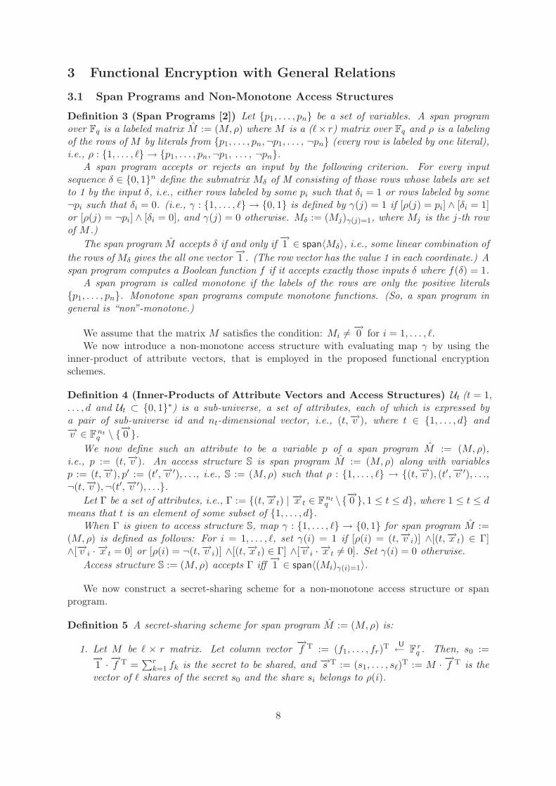
Definition 3 (Span Programs [2]) Let {p1, . . . , pn} be a set of variables. A span programover Fq is a labeled matrix M̂ := (M,ρ) where M is a (�× r) matrix over Fq and ρ is a labelingof the rows of M by literals from {p1, . . . , pn,¬p1, . . . , ¬pn} (every row is labeled by one literal),i.e., ρ : {1, . . . , �} → {p1, . . . , pn,¬p1, . . . , ¬pn}.

A span program accepts or rejects an input by the following criterion. For every inputsequence δ ∈ {0, 1}n define the submatrix Mδ of M consisting of those rows whose labels are setto 1 by the input δ, i.e., either rows labeled by some pi such that δi = 1 or rows labeled by some¬pi such that δi = 0. (i.e., γ : {1, . . . , �} → {0, 1} is defined by γ(j) = 1 if [ρ(j) = pi] ∧ [δi = 1]or [ρ(j) = ¬pi] ∧ [δi = 0], and γ(j) = 0 otherwise. Mδ := (Mj)γ(j)=1, where Mj is the j-th rowof M .)

The span program M̂ accepts δ if and only if−→1 ∈ span〈Mδ〉, i.e., some linear combination of

the rows of Mδ gives the all one vector−→1 . (The row vector has the value 1 in each coordinate.) A

span program computes a Boolean function f if it accepts exactly those inputs δ where f(δ) = 1.A span program is called monotone if the labels of the rows are only the positive literals

{p1, . . . , pn}. Monotone span programs compute monotone functions. (So, a span program ingeneral is “non”-monotone.)

We assume that the matrix M satisfies the condition: Mi �= −→0 for i = 1, . . . , �.We now introduce a non-monotone access structure with evaluating map γ by using the

inner-product of attribute vectors, that is employed in the proposed functional encryptionschemes.

Definition 4 (Inner-Products of Attribute Vectors and Access Structures) Ut (t = 1,. . . , d and Ut ⊂ {0, 1}∗) is a sub-universe, a set of attributes, each of which is expressed bya pair of sub-universe id and nt-dimensional vector, i.e., (t,−→v ), where t ∈ {1, . . . , d} and−→v ∈ F

ntq \ {

−→0 }.

We now define such an attribute to be a variable p of a span program M̂ := (M,ρ),i.e., p := (t,−→v ). An access structure S is span program M̂ := (M,ρ) along with variablesp := (t,−→v ), p′ := (t′,−→v ′), . . ., i.e., S := (M,ρ) such that ρ : {1, . . . , �} → {(t,−→v ), (t′,−→v ′), . . .,¬(t,−→v ),¬(t′,−→v ′), . . .}.

Let Γ be a set of attributes, i.e., Γ := {(t,−→x t) | −→x t ∈ Fntq \{

−→0 }, 1 ≤ t ≤ d}, where 1 ≤ t ≤ d

means that t is an element of some subset of {1, . . . , d}.When Γ is given to access structure S, map γ : {1, . . . , �} → {0, 1} for span program M̂ :=

(M,ρ) is defined as follows: For i = 1, . . . , �, set γ(i) = 1 if [ρ(i) = (t,−→v i)] ∧[(t,−→x t) ∈ Γ]∧[−→v i · −→x t = 0] or [ρ(i) = ¬(t,−→v i)] ∧[(t,−→x t) ∈ Γ] ∧[−→v i · −→x t �= 0]. Set γ(i) = 0 otherwise.

Access structure S := (M,ρ) accepts Γ iff−→1 ∈ span〈(Mi)γ(i)=1〉.

We now construct a secret-sharing scheme for a non-monotone access structure or spanprogram.

Definition 5 A secret-sharing scheme for span program M̂ := (M,ρ) is:

1. Let M be � × r matrix. Let column vector−→f T := (f1, . . . , fr)T

U← Frq . Then, s0 :=

−→1 · −→f T =

∑rk=1 fk is the secret to be shared, and −→s T := (s1, . . . , s�)T := M · −→f T is the

vector of � shares of the secret s0 and the share si belongs to ρ(i).

8

2. If span program M̂ := (M,ρ) accept δ, or access structure S := (M,ρ) accepts Γ, i.e.,−→1 ∈ span〈(Mi)γ(i)=1〉 with γ : {1, . . . , �} → {0, 1}, then there exist constants {αi ∈ Fq |i ∈ I} such that I ⊆ {i ∈ {1, . . . , �} | γ(i) = 1} and

∑i∈I αisi = s0. Furthermore, these

constants {αi} can be computed in time polynomial in the size of matrix M .

3.2 Key-Policy Functional Encryption with General Relations

Definition 6 (Key-Policy Functional Encryption : KP-FE) A key-policy functional en-cryption scheme consists of four algorithms.

Setup This is a randomized algorithm that takes as input security parameter and format −→n :=(d;n1, . . . , nd) of attributes. It outputs public parameters pk and master secret key sk.

KeyGen This is a randomized algorithm that takes as input access structure S := (M,ρ), pk andsk. It outputs a decryption key skS.

Enc This is a randomized algorithm that takes as input message m, a set of attributes, Γ :={(t,−→x t)|−→x t ∈ F

ntq \ {

−→0 }, 1 ≤ t ≤ d}, and public parameters pk. It outputs a ciphertext

ctΓ.

Dec This takes as input ciphertext ctΓ that was encrypted under a set of attributes Γ, decryptionkey skS for access structure S, and public parameters pk. It outputs either plaintext m orthe distinguished symbol ⊥.

A KP-FE scheme should have the following correctness property: for all (pk, sk) R← Setup(1λ,−→n ), all access structures S, all decryption keys skS

R← KeyGen(pk, sk,S), all messages m, allattribute sets Γ, all ciphertexts ctΓ

R← Enc(pk, m,Γ), it holds that m = Dec(pk, skS, ctΓ) withoverwhelming probability, if S accepts Γ.

Definition 7 The model for proving the adaptively payload-hiding security of KP-FE underchosen plaintext attack is:

Setup The challenger runs the setup algorithm, (pk, sk) R← Setup(1λ, −→n ), and gives publicparameters pk to the adversary.

Phase 1 The adversary is allowed to adaptively issue a polynomial number of queries, S, tothe challenger or oracle KeyGen(pk, sk, ·) for private keys, skS associated with S.

Challenge The adversary submits two messages m(0),m(1) and a set of attributes, Γ, providedthat no S queried to the challenger in Phase 1 accepts Γ. The challenger flips a coinb

U← {0, 1}, and computes ct(b)Γ

R← Enc(pk,m(b),Γ). It gives ct(b)Γ to the adversary.

Phase 2 The adversary is allowed to adaptively issue a polynomial number of queries, S, tothe challenger or oracle KeyGen(pk, sk, ·) for private keys, skS associated with S, providedthat S does not accept Γ.

Guess The adversary outputs a guess b′ of b.

The advantage of adversary A in the above game is defined as AdvKP-FE,PHA (λ) := Pr[b′ =

b] − 1/2 for any security parameter λ. A KP-FE scheme is adaptively payload-hiding secure ifall polynomial time adversaries have at most a negligible advantage in the above game.

9

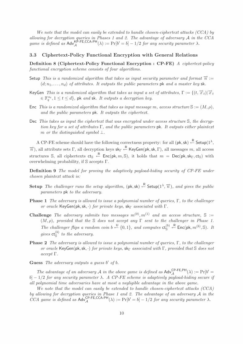
We note that the model can easily be extended to handle chosen-ciphertext attacks (CCA) byallowing for decryption queries in Phases 1 and 2. The advantage of adversary A in the CCAgame is defined as AdvKP-FE,CCA-PH

A (λ) := Pr[b′ = b]− 1/2 for any security parameter λ.

3.3 Ciphertext-Policy Functional Encryption with General Relations

Definition 8 (Ciphertext-Policy Functional Encryption : CP-FE) A ciphertext-policyfunctional encryption scheme consists of four algorithms.

Setup This is a randomized algorithm that takes as input security parameter and format −→n :=(d;n1, . . . , nd) of attributes. It outputs the public parameters pk and a master key sk.

KeyGen This is a randomized algorithm that takes as input a set of attributes, Γ := {(t,−→x t)|−→x t∈ F

ntq , 1 ≤ t ≤ d}, pk and sk. It outputs a decryption key.

Enc This is a randomized algorithm that takes as input message m, access structure S := (M,ρ),and the public parameters pk. It outputs the ciphertext.

Dec This takes as input the ciphertext that was encrypted under access structure S, the decryp-tion key for a set of attributes Γ, and the public parameters pk. It outputs either plaintextm or the distinguished symbol ⊥.

A CP-FE scheme should have the following correctness property: for all (pk, sk) R← Setup(1λ,−→n ), all attribute sets Γ, all decryption keys skΓ

R← KeyGen(pk, sk,Γ), all messages m, all accessstructures S, all ciphertexts ctS

R← Enc(pk,m,S), it holds that m = Dec(pk, skΓ, ctS) withoverwhelming probability, if S accepts Γ.

Definition 9 The model for proving the adaptively payload-hiding security of CP-FE underchosen plaintext attack is:

Setup The challenger runs the setup algorithm, (pk, sk) R← Setup(1λ,−→n ), and gives the publicparameters pk to the adversary.

Phase 1 The adversary is allowed to issue a polynomial number of queries, Γ, to the challengeror oracle KeyGen(pk, sk, ·) for private keys, skΓ associated with Γ.

Challenge The adversary submits two messages m(0),m(1) and an access structure, S :=(M,ρ), provided that the S does not accept any Γ sent to the challenger in Phase 1.The challenger flips a random coin b

U← {0, 1}, and computes ct(b)S

R← Enc(pk,m(b),S). Itgives ct

(b)S

to the adversary.

Phase 2 The adversary is allowed to issue a polynomial number of queries, Γ, to the challengeror oracle KeyGen(pk, sk, ·) for private keys, skΓ associated with Γ, provided that S does notaccept Γ.

Guess The adversary outputs a guess b′ of b.

The advantage of an adversary A in the above game is defined as AdvCP-FE,PHA (λ) := Pr[b′ =

b] − 1/2 for any security parameter λ. A CP-FE scheme is adaptively payload-hiding secure ifall polynomial time adversaries have at most a negligible advantage in the above game.

We note that the model can easily be extended to handle chosen-ciphertext attacks (CCA)by allowing for decryption queries in Phase 1 and 2. The advantage of an adversary A in theCCA game is defined as AdvCP-FE,CCA-PH

A (λ) := Pr[b′ = b]− 1/2 for any security parameter λ.

10

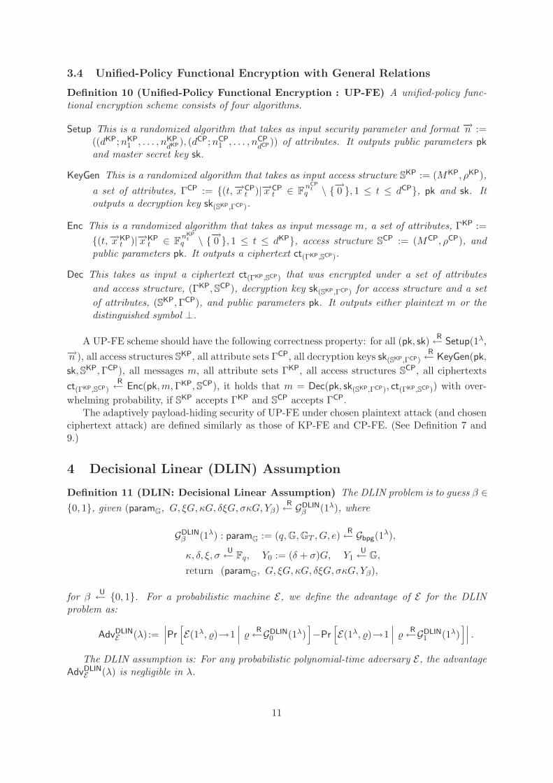
3.4 Unified-Policy Functional Encryption with General Relations

Definition 10 (Unified-Policy Functional Encryption : UP-FE) A unified-policy func-tional encryption scheme consists of four algorithms.

Setup This is a randomized algorithm that takes as input security parameter and format −→n :=((dKP;nKP

1 , . . . , nKPdKP), (dCP;nCP

1 , . . . , nCPdCP)) of attributes. It outputs public parameters pk

and master secret key sk.

KeyGen This is a randomized algorithm that takes as input access structure SKP := (MKP, ρKP),

a set of attributes, ΓCP := {(t,−→x CPt )|−→x CP

t ∈ FnCP

tq \ {−→0 }, 1 ≤ t ≤ dCP}, pk and sk. It

outputs a decryption key sk(SKP,ΓCP).

Enc This is a randomized algorithm that takes as input message m, a set of attributes, ΓKP :={(t,−→x KP

t )|−→x KPt ∈ F

nKPt

q \ {−→0 }, 1 ≤ t ≤ dKP}, access structure SCP := (MCP, ρCP), and

public parameters pk. It outputs a ciphertext ct(ΓKP,SCP).

Dec This takes as input a ciphertext ct(ΓKP,SCP) that was encrypted under a set of attributesand access structure, (ΓKP,SCP), decryption key sk(SKP,ΓCP) for access structure and a setof attributes, (SKP,ΓCP), and public parameters pk. It outputs either plaintext m or thedistinguished symbol ⊥.

A UP-FE scheme should have the following correctness property: for all (pk, sk) R← Setup(1λ,−→n ), all access structures S

KP, all attribute sets ΓCP, all decryption keys sk(SKP,ΓCP)R← KeyGen(pk,

sk,SKP,ΓCP), all messages m, all attribute sets ΓKP, all access structures SCP, all ciphertexts

ct(ΓKP,SCP)R← Enc(pk,m,ΓKP,SCP), it holds that m = Dec(pk, sk(SKP,ΓCP), ct(ΓKP,SCP)) with over-

whelming probability, if SKP accepts ΓKP and S

CP accepts ΓCP.The adaptively payload-hiding security of UP-FE under chosen plaintext attack (and chosen

ciphertext attack) are defined similarly as those of KP-FE and CP-FE. (See Definition 7 and9.)

4 Decisional Linear (DLIN) Assumption

Definition 11 (DLIN: Decisional Linear Assumption) The DLIN problem is to guess β ∈{0, 1}, given (paramG, G, ξG, κG, δξG, σκG, Yβ)

R← GDLINβ (1λ), where

GDLINβ (1λ) : paramG := (q,G,GT , G, e)

R← Gbpg(1λ),

κ, δ, ξ, σU← Fq, Y0 := (δ + σ)G, Y1

U← G,

return (paramG, G, ξG, κG, δξG, σκG, Yβ),

for β U← {0, 1}. For a probabilistic machine E, we define the advantage of E for the DLINproblem as:

AdvDLINE (λ) :=

∣∣∣Pr[E(1λ, �)→1

∣∣∣ � R←GDLIN0 (1λ)

]−Pr

[E(1λ, �)→1

∣∣∣ � R←GDLIN1 (1λ)

]∣∣∣ .The DLIN assumption is: For any probabilistic polynomial-time adversary E, the advantage

AdvDLINE (λ) is negligible in λ.

11

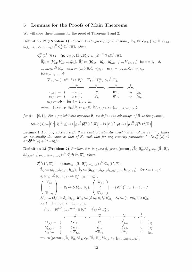
5 Lemmas for the Proofs of Main Theorems

We will show three lemmas for the proof of Theorems 1 and 2.

Definition 12 (Problem 1) Problem 1 is to guess β, given (param−→n ,B0, B̂∗0, eβ,0, {Bt, B̂∗t , eβ,t,1,

et,i}t=1,...,d;i=2,...,nt)R← GP1

β (1λ,−→n ), where

GP1β (1λ,−→n ) : (param−→n , {Bt,B∗t }t=0,...,d)

R← Gob(1λ,−→n ),

B̂∗0 := (b∗0,1, b

∗0,3, .., b

∗0,5), B̂

∗t := (b∗t,1, .., b

∗t,nt

, b∗t,2nt+1, .., b∗t,3nt+1) for t = 1, .., d,

ω, z0, γ0U← Fq, e0,0 := (ω, 0, 0, 0, γ0)B0 , e1,0 := (ω, z0, 0, 0, γ0)B0 ,

for t = 1, . . . , d;−→e t,1 := (1, 0nt−1) ∈ F

ntq , −→z t U← F

ntq , γt

U← Fq,

nt︷︸︸︷ nt︷︸︸︷ nt︷︸︸︷ 1︷︸︸︷e0,t,1 := ( ω−→e t,1, 0nt , 0nt , γt )Bt ,e1,t,1 := ( ω−→e t,1, −→z t, 0nt , γt )Bt ,

et,i := ωbt,i for i = 2, . . . , nt,

return (param−→n ,B0, B̂∗0, eβ,0, {Bt, B̂∗t , eβ,t,1, et,i}t=1,...,d;i=2,...,nt),

for β U← {0, 1}. For a probabilistic machine B, we define the advantage of B as the quantity

AdvP1B (λ) :=

∣∣∣Pr[B(1λ, �)→1

∣∣∣� R←GP10 (1λ,−→n )

]−Pr

[B(1λ, �)→1

∣∣∣� R←GP11 (1λ,−→n )

]∣∣∣ .Lemma 1 For any adversary B, there exist probabilistic machines E, whose running timesare essentially the same as that of B, such that for any security parameter λ, AdvP1

B (λ) ≤AdvDLIN

E (λ) + (d+ 6)/q.

Definition 13 (Problem 2) Problem 2 is to guess β, given (param−→n , B̂0,B∗0,h∗β,0, e0, {B̂t,B∗t ,

h∗β,t,i, et,i}t=1,...,d;i=1,...,nt)R← GP2

β (1λ,−→n ), where

GP2β (1λ,−→n ) : (param−→n , {Bt,B∗t }t=0,...,d)

R← Gob(1λ,−→n ),

B̂0 := (b0,1, b0,3, .., b0,5), B̂t := (bt,1, .., bt,nt , bt,2nt+1, .., bt,3nt+1) for t = 1, .., d,

δ, δ0, ωU← Fq, τ, u0

U← F×q , z0 := u−1

0 ,⎛⎜⎝−→z t,1

...−→z t,nt

⎞⎟⎠ := ZtU← GL(nt,Fq),

⎛⎜⎝−→u t,1

...−→u t,nt

⎞⎟⎠ := (Z−1t )T for t = 1, .., d,

h∗0,0 := (δ, 0, 0, δ0, 0)B∗0, h∗1,0 := (δ, u0, 0, δ0, 0)B∗

0, e0 := (ω, τz0, 0, 0, 0)B0 ,

for t = 1, . . . , d; i = 1, . . . , nt;−→e t,i := (0i−1, 1, 0nt−i) ∈ F

ntq ,

−→δ t,i

U← Fntq ,

nt︷︸︸︷ nt︷︸︸︷ nt︷︸︸︷ 1︷︸︸︷h∗0,t,i := ( δ−→e t,i, 0nt ,

−→δ t,i, 0 )B∗

t

h∗1,t,i := ( δ−→e t,i, −→u t,i, −→δ t,i, 0 )B∗

t

et,i := ( ω−→e t,i, τ−→z t,i, 0nt , 0 )Bt ,

return (param−→n , B̂0,B∗0,h∗β,0, e0, {B̂t,B∗t ,h∗β,t,i, et,i}t=1,..,d;i=1,..,nt),

12

for β U← {0, 1}. For a probabilistic adversary B, the advantage of B for Problem 2, AdvP2B (λ), is

similarly defined as in Definition 12.

Lemma 2 For any adversary B, there exists a probabilistic machine E, whose running timeis essentially the same as that of B, such that for any security parameter λ, AdvP2

B (λ) ≤AdvDLIN

E (λ) + 5/q.

Lemma 3 For p ∈ Fq, let Cp := {(−→x ,−→v )|−→x ·−→v = p} ⊂ V ×V ∗ where V is n-dimensional vectorspace F

nq , and V ∗ its dual. For all (−→x ,−→v ) ∈ Cp, for all (−→r ,−→w ) ∈ Cp, Pr [−→x U = −→r ∧ −→v Z = −→w ]

= Pr [−→x Z = −→r ∧ −→v U = −→w ] = 1/� Cp, where Z U← GL(n,Fq), U := (Z−1)T.

6 KP-FE Scheme

6.1 Construction

We define function ρ̃ : {1, . . . , �} → {1, . . . , d} by ρ̃(i) := t if ρ(i) = (t,−→v ) or ρ(i) = ¬(t,−→v ),where ρ is given in access structure S := (M,ρ). In the proposed scheme, we assume that ρ̃ isinjective for S := (M,ρ) with decryption key skS. We will show how to relax the restriction inAppendix F.

In the description of the scheme, we assume that input vector, −→x t := (xt,1, . . . , xt,nt), isnormalized such that xt,1 := 1. (If −→x t is not normalized, change it to a normalized one by(1/xt,1) · −→x t, assuming that xt,1 is non-zero).

Random dual basis generator Gob(1λ,−→n ) is defined at the end of Section 2. We refer toSection 1.3 for notations on DPVS.

Setup(1λ, −→n := (d;n1, . . . , nd)) : (param−→n , {Bt,B∗t }t=0,...,d)R← Gob(1λ,−→n ),

B̂0 := (b0,1, b0,3, b0,5), B̂t := (bt,1, .., bt,nt , bt,3nt+1) for t = 1, .., d,

B̂∗0 := (b∗0,1, b

∗0,3, b

∗0,4), B̂

∗t := (b∗t,1, .., b

∗t,nt

, b∗t,2nt+1, .., b∗t,3nt

) for t = 1, .., d,

pk := (1λ, param−→n , {B̂t}t=0,...,d), sk := {B̂∗t }t=0,...,d,

return pk, sk.

KeyGen(pk, sk, S := (M,ρ)) :−→f

U← Frq ,−→s T := (s1, . . . , s�)T := M · −→f T, s0 :=

−→1 · −→f T, η0

U← Fq,

k∗0 := (−s0, 0, 1, η0, 0)B∗0,

for i = 1, . . . , �,

if ρ(i) = (t,−→v i := (vi,1, . . . , vi,nt) ∈ Fntq \ {

−→0 }), θi

U← Fq,−→η i U← F

ntq ,

nt︷︸︸︷ nt︷︸︸︷ nt︷︸︸︷ 1︷︸︸︷k∗i := ( si

−→e t,1 + θi−→v i, 0nt , −→η i, 0 )B∗

t,

if ρ(i) = ¬(t,−→v i), −→η i U← Fntq ,

nt︷︸︸︷ nt︷︸︸︷ nt︷︸︸︷ 1︷︸︸︷k∗i := ( si

−→v i, 0nt , −→η i, 0 )B∗t,

return skS := (S,k∗0,k∗1, . . . ,k

∗� ).

Enc(pk, m, Γ := {(t,−→x t := (xt,1, .., xt,nt) ∈ Fntq \ {

−→0 }) | 1 ≤ t ≤ d, xt,1 := 1}) :

ω, ϕ0, ϕt, ζU← Fq for (t,−→x t) ∈ Γ,

c0 := (ω, 0, ζ, 0, ϕ0)B0 ,

13

nt︷︸︸︷ nt︷︸︸︷ nt︷︸︸︷ 1︷︸︸︷ct := ( ω−→x t, 0nt , 0nt , ϕt )Bt for (t,−→x t) ∈ Γ,

cd+1 := gζTm, ctΓ := (Γ, c0, {ct}(t,−→x t)∈Γ, cd+1),return ctΓ.

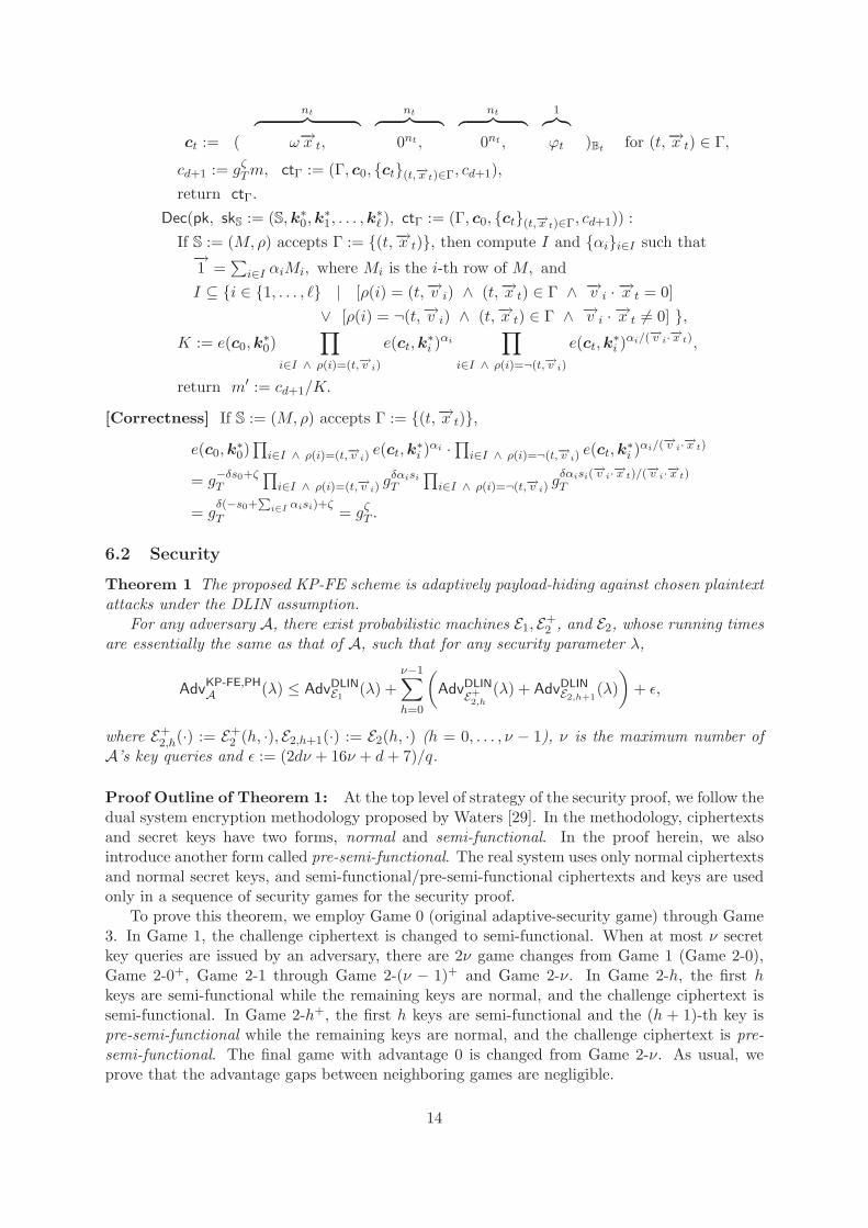
Dec(pk, skS := (S,k∗0,k∗1, . . . ,k

∗� ), ctΓ := (Γ, c0, {ct}(t,−→x t)∈Γ, cd+1)) :

If S := (M,ρ) accepts Γ := {(t,−→x t)}, then compute I and {αi}i∈I such that−→1 =

∑i∈I αiMi, where Mi is the i-th row of M, and

I ⊆ {i ∈ {1, . . . , �} | [ρ(i) = (t,−→v i) ∧ (t,−→x t) ∈ Γ ∧ −→v i · −→x t = 0]∨ [ρ(i) = ¬(t,−→v i) ∧ (t,−→x t) ∈ Γ ∧ −→v i · −→x t �= 0] },

K := e(c0,k∗0)

∏i∈I ∧ ρ(i)=(t,−→v i)

e(ct,k∗i )αi

∏i∈I ∧ ρ(i)=¬(t,−→v i)

e(ct,k∗i )αi/(−→v i·−→x t),

return m′ := cd+1/K.

[Correctness] If S := (M,ρ) accepts Γ := {(t,−→x t)},e(c0,k

∗0)∏i∈I ∧ ρ(i)=(t,−→v i)

e(ct,k∗i )αi ·∏i∈I ∧ ρ(i)=¬(t,−→v i)

e(ct,k∗i )αi/(−→v i·−→x t)

= g−δs0+ζT

∏i∈I ∧ ρ(i)=(t,−→v i)

gδαisiT

∏i∈I ∧ ρ(i)=¬(t,−→v i)

gδαisi(

−→v i·−→x t)/(−→v i·−→x t)

T

= gδ(−s0+

Pi∈I αisi)+ζ

T = gζT .

6.2 Security

Theorem 1 The proposed KP-FE scheme is adaptively payload-hiding against chosen plaintextattacks under the DLIN assumption.

For any adversary A, there exist probabilistic machines E1, E+2 , and E2, whose running times

are essentially the same as that of A, such that for any security parameter λ,

AdvKP-FE,PHA (λ) ≤ AdvDLIN

E1 (λ) +ν−1∑h=0

(AdvDLIN

E+2,h(λ) + AdvDLIN

E2,h+1(λ)

)+ ε,

where E+2,h(·) := E+

2 (h, ·), E2,h+1(·) := E2(h, ·) (h = 0, . . . , ν − 1), ν is the maximum number ofA’s key queries and ε := (2dν + 16ν + d+ 7)/q.

Proof Outline of Theorem 1: At the top level of strategy of the security proof, we follow thedual system encryption methodology proposed by Waters [29]. In the methodology, ciphertextsand secret keys have two forms, normal and semi-functional. In the proof herein, we alsointroduce another form called pre-semi-functional. The real system uses only normal ciphertextsand normal secret keys, and semi-functional/pre-semi-functional ciphertexts and keys are usedonly in a sequence of security games for the security proof.

To prove this theorem, we employ Game 0 (original adaptive-security game) through Game3. In Game 1, the challenge ciphertext is changed to semi-functional. When at most ν secretkey queries are issued by an adversary, there are 2ν game changes from Game 1 (Game 2-0),Game 2-0+, Game 2-1 through Game 2-(ν − 1)+ and Game 2-ν. In Game 2-h, the first hkeys are semi-functional while the remaining keys are normal, and the challenge ciphertext issemi-functional. In Game 2-h+, the first h keys are semi-functional and the (h + 1)-th key ispre-semi-functional while the remaining keys are normal, and the challenge ciphertext is pre-semi-functional. The final game with advantage 0 is changed from Game 2-ν. As usual, weprove that the advantage gaps between neighboring games are negligible.

14

For skS := (S,k∗0,k∗1, . . . ,k∗� ) and ctΓ := (Γ, c0, {ct}(t,−→x t)∈Γ, cd+1), we focus on−→k ∗

S:=

(k∗0,k∗1, . . . ,k∗� ) and −→c Γ := (c0, {ct}(t,−→x t)∈Γ), and ignore the other part of skS and ctΓ (and callthem secret key and ciphertext, respectively) in this proof outline. In addition, we ignore anegligible factor in the (informal) descriptions of this proof outline. For example, we say “A isbounded by B” when A ≤ B + ε(λ) where ε(λ) is negligible in security parameter λ.

A normal secret key,−→k ∗ norm

S(with access structure S), is the correct form of the secret

key of the proposed FE scheme, and is expressed by Eq. (1). Similarly, a normal ciphertext(with attribute set Γ), −→c norm

Γ , is expressed by Eq. (2). A semi-functional secret key,−→k ∗ semi

S,

is expressed by Eq. (8), and a semi-functional ciphertext, −→c semiΓ , is expressed by Eqs. (3)-(5).

A pre-semi-functional secret key,−→k ∗ pre-semi

S, and pre-semi-functional ciphertext, −→c pre-semi

Γ , areexpressed by Eq. (6) and Eqs. (3), (7) and (5), respectively.

To prove that the advantage gap between Games 0 and 1 is bounded by the advantage ofProblem 1 (to guess β ∈ {0, 1}), we construct a simulator of the challenger of Game 0 (or 1)(against an adversary A) by using an instance with β

U← {0, 1} of Problem 1. We then showthat the distribution of the secret keys and challenge ciphertext replied by the simulator isequivalent to those of Game 0 when β = 0 and those of Game 1 when β = 1. That is, theadvantage of Problem 1 is equivalent to the advantage gap between Games 0 and 1 (Lemma4). The advantage of Problem 1 is proven to be equivalent to that of the DLIN assumption(Lemma 1).

The advantage gap between Games 2-h and 2-h+ is similarly shown to be bounded bythe advantage of Problem 2 (i.e., advantage of the DLIN assumption) (Lemmas 5 and 2).Here, we introduce special forms of pre-semi-functional keys and ciphertexts,

−→k ∗ spec.pre-semi

S

and −→c spec.pre-semiΓ , respectively, such that they are equivalent to pre-semi-functional keys and

ciphertexts,−→k ∗ pre-semi

Sand −→c pre-semi

Γ , respectively, except that w0r0 = a0 :=∑r

k=1 gk and r0U←

Fq (note that r0, w0U← Fq for

−→k ∗ pre-semi


Γ ). These forms of keys and ciphertexts,−→k ∗ spec.pre-semi

Sand −→c spec.pre-semi

Γ , are simulated using Problem 2 with β = 1. From the definitionof these forms,


Scan decrypt −→c spec.pre-semi

Γ for any Γ when S accepts Γ, i.e., itis hard for simulator B+

2 to tell (−→k ∗ spec.pre-semi

S, −→c spec.pre-semi

Γ ) for Game 2-h+ from (−→k ∗ norm

S,−→c semi

Γ ) for Game 2-h under the assumption of Problem 2. On the other hand, a0(= w0r0) isindependently distributed from the other variables when S does not accept Γ (shown in Proofof Claim 1 by using Lemma 3). That is, the joint distribution of

−→k ∗ pre-semi


Γ isequivalent to that of



Γ , when S does not accept Γ (i.e., B+2 ’s

simulation using Problem 2 with β = 1 is the same distribution as that of Game 2-h+ fromthe adversary’s view). In other words, w0 and r0 in



Γ (given byB+

2 ’s simulation using Problem 2 with β = 1) are correlated for the case that S accepts Γ orfor simulator B+

2 ’s view, but adversary A cannot notice the correlation since A’s queries shouldsatisfy the condition that S does not accept Γ.

The advantage gap between Games 2-h+ and 2-(h+ 1) is similarly shown to be bounded bythe advantage of Problem 2, i.e., advantage of the DLIN assumption (Lemmas 6 and 2).

Finally we show that Game 2-ν can be conceptually changed to Game 3 (Lemma 7).

Proof of Theorem 1 : To prove Theorem 1, we consider the following (2ν + 3) games. InGame 0, a part framed by a box indicates coefficients to be changed in a subsequent game. Inthe other games, a part framed by a box indicates coefficients which were changed in a gamefrom the previous game.

Game 0 : Original game. That is, the reply to a key query for S := (M,ρ) with �× r matrix

15

M is:

k∗0 := (−s0, 0 , 1, η0, 0)B∗0,

for i = 1, . . . , �,

if ρ(i) = (t,−→v i), k∗i := (si−→e t,1 + θi−→v i, 0nt , −→η i, 0)B∗

t,

if ρ(i) = ¬(t,−→v i), k∗i := (si−→v i, 0nt , −→η i, 0)B∗t,

⎫⎪⎪⎪⎪⎪⎬⎪⎪⎪⎪⎪⎭(1)

where−→f

U← Frq ,−→s T := (s1, . . . , s�)T := M · −→f T, s0 :=

−→1 · −→f T, θi, η0


ntq ,−→e t,1 =

(1, 0, . . . , 0) ∈ Fntq , and −→v i ∈ F

ntq \ {

−→0 }. The challenge ciphertext for challenge plaintexts

(m(0),m(1)) and Γ := {(t,−→x t) | 1 ≤ t ≤ d} is:

c0 := (δ, 0 , ζ , 0, ϕ0)B0 ,

ct := (δ−→x t, 0nt , 0nt , ϕt)Bt for (t,−→x t) ∈ Γ,

cd+1 := gζTm(b),

⎫⎪⎪⎬⎪⎪⎭ (2)

where b U← {0, 1}; δ, ζ, ϕ0, ϕtU← Fq, and −→x t ∈ F

ntq \ {

−→0 }.

Game 1 : Same as Game 0 except that the challenge ciphertext is:

c0 := (δ, r0 , ζ, 0, ϕ0)B0 , (3)

ct := (δ−→x t, −→r t , 0nt , ϕt)Bt for (t,−→x t) ∈ Γ, (4)

cd+1 := gζTm(b), (5)

where r0U← Fq,

−→r t U← Fntq , and all the other variables are generated as in Game 0.

Game 2-h+ (h = 0, . . . , ν − 1) : Game 2-0 is Game 1. Game 2-h+ is the same as Game 2-hexcept the reply to the (h+ 1)-th key query for S := (M,ρ) with �× r matrix M , and ct of thechallenge ciphertext are:

k∗0 := (−s0, w0 , 1, η0, 0)B∗0,

for i = 1, . . . , �,

if ρ(i) = (t,−→v i),k∗i := (si−→e t,1 + θi

−→v i, (ai−→e t,1 + πi−→v i) · Zt , −→η i, 0)B∗

t,

if ρ(i) = ¬(t,−→v i),k∗i := (si−→v i, ai

−→v i · Zt , −→η i, 0)B∗t,

⎫⎪⎪⎪⎪⎪⎪⎪⎪⎪⎪⎬⎪⎪⎪⎪⎪⎪⎪⎪⎪⎪⎭(6)

ct := (δ−→x t, −→x t · Ut , 0nt , ϕt)Bt for (t,−→x t) ∈ Γ, (7)

where w0U← Fq,

−→g U← Frq ,−→a T := (a1, . . . , a�)T := M · −→g T, πi

U← Fq (i = 1, . . . , �), ZtU←

GL(nt,Fq), Ut := (Z−1t )T for t = 1, . . . , d, and all the other variables are generated as in Game

2-h.Game 2-(h + 1) (h = 0, . . . , ν − 1) : Game 2-(h+ 1) is the same as Game 2-h+ except thereply to the (h+ 1)-th key query for S := (M,ρ) with �× r matrix M , and ct of the challengeciphertext are:

k∗0 := (−s0, w0, 1, η0, 0)B∗0,

for i = 1, . . . , �,

if ρ(i) = (t,−→v i), k∗i := (si−→e t,1 + θi−→v i, 0nt , −→η i, 0)B∗

t,

if ρ(i) = ¬(t,−→v i), k∗i := (si−→v i, 0nt , −→η i, 0)B∗t,

⎫⎪⎪⎪⎪⎪⎬⎪⎪⎪⎪⎪⎭(8)

16

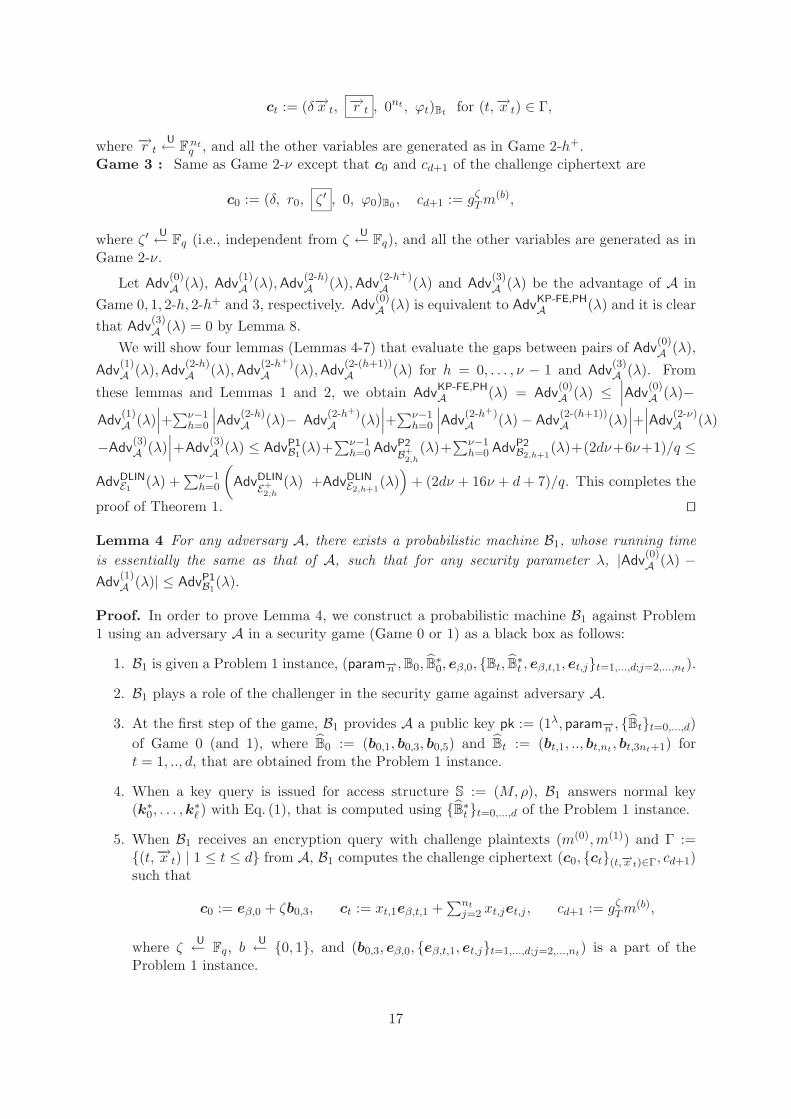
ct := (δ−→x t, −→r t , 0nt , ϕt)Bt for (t,−→x t) ∈ Γ,

where −→r t U← Fntq , and all the other variables are generated as in Game 2-h+.

Game 3 : Same as Game 2-ν except that c0 and cd+1 of the challenge ciphertext are

c0 := (δ, r0, ζ ′ , 0, ϕ0)B0 , cd+1 := gζTm(b),

where ζ ′ U← Fq (i.e., independent from ζU← Fq), and all the other variables are generated as in

Game 2-ν.

Let Adv(0)A (λ), Adv

(1)A (λ),Adv

(2-h)A (λ),Adv

(2-h+)A (λ) and Adv

(3)A (λ) be the advantage of A in

Game 0, 1, 2-h, 2-h+ and 3, respectively. Adv(0)A (λ) is equivalent to AdvKP-FE,PH

A (λ) and it is clearthat Adv

(3)A (λ) = 0 by Lemma 8.

We will show four lemmas (Lemmas 4-7) that evaluate the gaps between pairs of Adv(0)A (λ),

Adv(1)A (λ),Adv

(2-h)A (λ),Adv

(2-h+)A (λ),Adv

(2-(h+1))A (λ) for h = 0, . . . , ν − 1 and Adv

(3)A (λ). From

these lemmas and Lemmas 1 and 2, we obtain AdvKP-FE,PHA (λ) = Adv

(0)A (λ) ≤

∣∣∣Adv(0)A (λ)−

Adv(1)A (λ)

∣∣∣+∑ν−1h=0

∣∣∣Adv(2-h)A (λ)− Adv

(2-h+)A (λ)

∣∣∣+∑ν−1h=0

∣∣∣Adv(2-h+)A (λ)− Adv

(2-(h+1))A (λ)

∣∣∣+∣∣∣Adv(2-ν)A (λ)

−Adv(3)A (λ)

∣∣∣+Adv(3)A (λ) ≤ AdvP1

B1(λ)+

∑ν−1h=0 AdvP2

B+2,h

(λ)+∑ν−1

h=0 AdvP2B2,h+1

(λ)+(2dν+6ν+1)/q ≤

AdvDLINE1 (λ) +

∑ν−1h=0

(AdvDLIN

E+2,h

(λ) +AdvDLINE2,h+1

(λ))

+ (2dν + 16ν + d+ 7)/q. This completes the

proof of Theorem 1. ��

Lemma 4 For any adversary A, there exists a probabilistic machine B1, whose running timeis essentially the same as that of A, such that for any security parameter λ, |Adv

(0)A (λ) −

Adv(1)A (λ)| ≤ AdvP1

B1(λ).

Proof. In order to prove Lemma 4, we construct a probabilistic machine B1 against Problem1 using an adversary A in a security game (Game 0 or 1) as a black box as follows:

1. B1 is given a Problem 1 instance, (param−→n ,B0, B̂∗0, eβ,0, {Bt, B̂∗t , eβ,t,1, et,j}t=1,...,d;j=2,...,nt).

2. B1 plays a role of the challenger in the security game against adversary A.

3. At the first step of the game, B1 provides A a public key pk := (1λ, param−→n , {B̂t}t=0,...,d)of Game 0 (and 1), where B̂0 := (b0,1, b0,3, b0,5) and B̂t := (bt,1, .., bt,nt , bt,3nt+1) fort = 1, .., d, that are obtained from the Problem 1 instance.

4. When a key query is issued for access structure S := (M,ρ), B1 answers normal key(k∗0, . . . ,k∗� ) with Eq. (1), that is computed using {B̂∗t }t=0,...,d of the Problem 1 instance.

5. When B1 receives an encryption query with challenge plaintexts (m(0),m(1)) and Γ :={(t,−→x t) | 1 ≤ t ≤ d} from A, B1 computes the challenge ciphertext (c0, {ct}(t,−→x t)∈Γ, cd+1)such that

c0 := eβ,0 + ζb0,3, ct := xt,1eβ,t,1 +∑nt

j=2 xt,jet,j , cd+1 := gζTm(b),

where ζU← Fq, b

U← {0, 1}, and (b0,3, eβ,0, {eβ,t,1, et,j}t=1,...,d;j=2,...,nt) is a part of theProblem 1 instance.

17

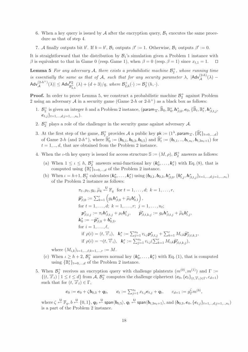
6. When a key query is issued by A after the encryption query, B1 executes the same proce-dure as that of step 4.

7. A finally outputs bit b′. If b = b′, B1 outputs β′ := 1. Otherwise, B1 outputs β′ := 0.

It is straightforward that the distribution by B1’s simulation given a Problem 1 instance withβ is equivalent to that in Game 0 (resp. Game 1), when β = 0 (resp.β = 1) since xt,1 = 1. ��Lemma 5 For any adversary A, there exists a probabilistic machine B+

2 , whose running timeis essentially the same as that of A, such that for any security parameter λ, |Adv

(2-h)A (λ) −

Adv(2-h+)A (λ)| ≤ AdvP2

B+2,h

(λ) + (d+ 3)/q, where B+2,h(·) := B+

2 (h, ·).

Proof. In order to prove Lemma 5, we construct a probabilistic machine B+2 against Problem

2 using an adversary A in a security game (Game 2-h or 2-h+) as a black box as follows:

1. B+2 is given an integer h and a Problem 2 instance, (param−→n , B̂0,B

∗0,h∗β,0, e0, {B̂t,B∗t ,h∗β,t,j ,

et,j}t=1,...,d;j=1,...,nt).

2. B+2 plays a role of the challenger in the security game against adversary A.

3. At the first step of the game, B+2 provides A a public key pk := (1λ, param−→n , {B̂′t}t=0,...,d)

of Game 2-h (and 2-h+), where B̂′0 := (b0,1, b0,3, b0,5) and B̂

′t := (bt,1, .., bt,nt , bt,3nt+1) for

t = 1, .., d, that are obtained from the Problem 2 instance.

4. When the ι-th key query is issued for access structure S := (M,ρ), B+2 answers as follows:

(a) When 1 ≤ ι ≤ h, B+2 answers semi-functional key (k∗0, . . . ,k∗� ) with Eq. (8), that is

computed using {B∗t }t=0,...,d of the Problem 2 instance.(b) When ι = h+1, B+

2 calculates (k∗0, . . . ,k∗� ) using (b0,1, b0,3,h∗β,0, {b∗t,j ,h∗β,t,j}t=1,...,d;j=1,...,nt)

of the Problem 2 instance as follows:

πt, μt, gk, μ̃kU← Fq for t = 1, . . . , d; k = 1, . . . , r,

p̃∗β,0 :=∑r

k=1

(gkh

∗β,0 + μ̃kb

∗0,1

),

for t = 1, . . . , d; k = 1, . . . , r; j = 1, . . . , nt;p∗β,t,j := πth

∗β,t,j + μtb

∗t,j , p̃∗β,t,k,j := gkh

∗β,t,j + μ̃kb

∗t,j ,

k∗0 := −p̃∗β,0 + b∗0,3,for i = 1, . . . , �,

if ρ(i) = (t,−→v i), k∗i :=∑nt

j=1 vi,jp∗β,t,j +

∑rk=1Mi,kp̃

∗β,t,k,1,

if ρ(i) = ¬(t,−→v i), k∗i :=∑nt

j=1 vi,j(∑r

k=1Mi,kp̃∗β,t,k,j),

where (Mi,k)i=1,...,�;k=1,...,r := M .(c) When ι ≥ h+ 2, B+

2 answers normal key (k∗0, . . . ,k∗� ) with Eq. (1), that is computedusing {B∗t }t=0,...,d of the Problem 2 instance.

5. When B+2 receives an encryption query with challenge plaintexts (m(0),m(1)) and Γ :=

{(t,−→x t) | 1 ≤ t ≤ d} from A, B+2 computes the challenge ciphertext (c0, {ct}(t,−→x t)∈Γ, cd+1)

such that for (t,−→x t) ∈ Γ,

c0 := e0 + ζb0,3 + q0, ct :=∑nt

j=1 xt,jet,j + qt, cd+1 := gζTm(b),

where ζ U← Fq, bU← {0, 1}, q0

U← span〈b0,5〉, qtU← span〈bt,3nt+1〉, and (b0,3, e0, {et,j}t=1,..,d;j=1,..,nt)

is a part of the Problem 2 instance.

18

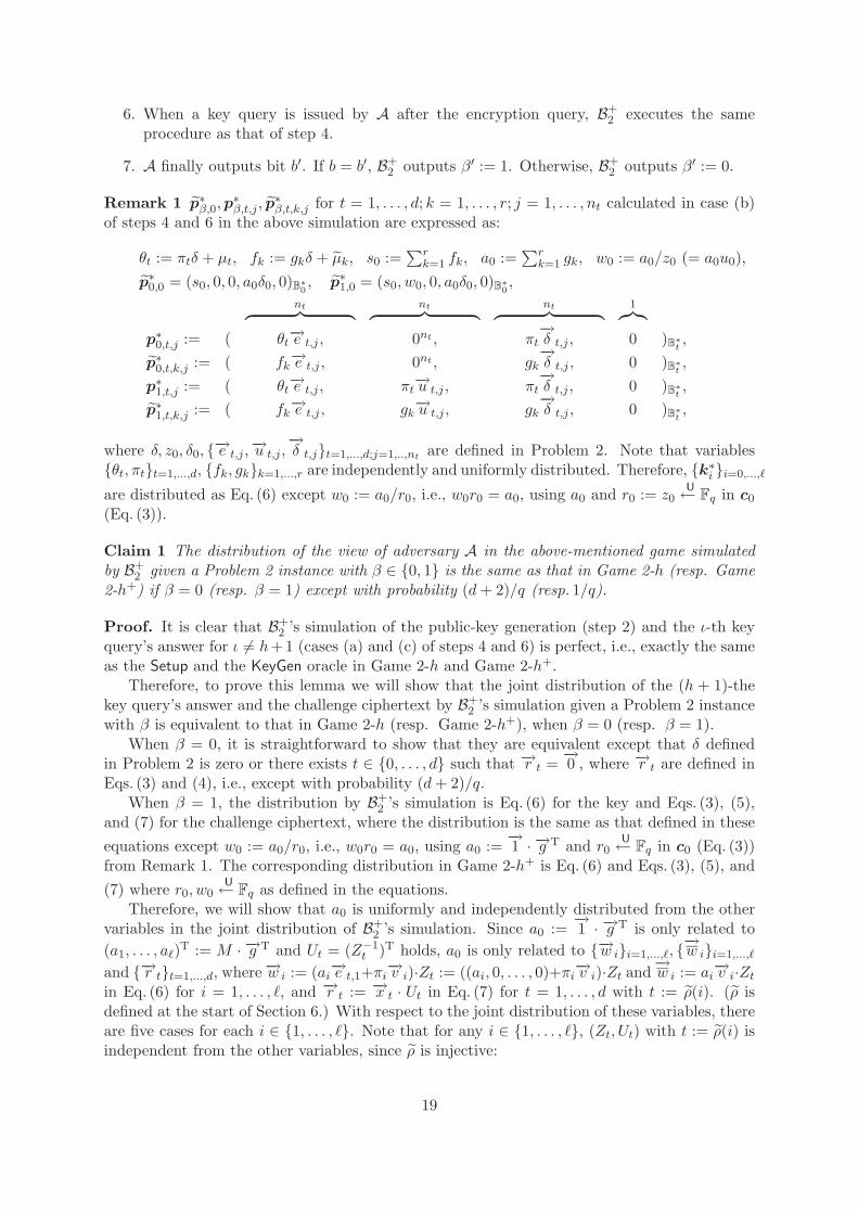
6. When a key query is issued by A after the encryption query, B+2 executes the same

procedure as that of step 4.

7. A finally outputs bit b′. If b = b′, B+2 outputs β′ := 1. Otherwise, B+

2 outputs β′ := 0.

Remark 1 p̃∗β,0,p∗β,t,j , p̃

∗β,t,k,j for t = 1, . . . , d; k = 1, . . . , r; j = 1, . . . , nt calculated in case (b)

of steps 4 and 6 in the above simulation are expressed as:

θt := πtδ + μt, fk := gkδ + μ̃k, s0 :=∑r

k=1 fk, a0 :=∑r

k=1 gk, w0 := a0/z0 (= a0u0),p̃∗0,0 = (s0, 0, 0, a0δ0, 0)B∗

0, p̃∗1,0 = (s0, w0, 0, a0δ0, 0)B∗

0,

nt︷︸︸︷ nt︷︸︸︷ nt︷︸︸︷ 1︷︸︸︷p∗0,t,j := ( θt

−→e t,j , 0nt , πt−→δ t,j , 0 )B∗

t,

p̃∗0,t,k,j := ( fk−→e t,j , 0nt , gk

−→δ t,j , 0 )B∗

t,

p∗1,t,j := ( θt−→e t,j , πt

−→u t,j , πt−→δ t,j , 0 )B∗

t,

p̃∗1,t,k,j := ( fk−→e t,j , gk

−→u t,j , gk−→δ t,j , 0 )B∗

t,

where δ, z0, δ0, {−→e t,j ,−→u t,j ,−→δ t,j}t=1,...,d;j=1,..,nt are defined in Problem 2. Note that variables{θt, πt}t=1,...,d, {fk, gk}k=1,...,r are independently and uniformly distributed. Therefore, {k∗i }i=0,...,�

are distributed as Eq. (6) except w0 := a0/r0, i.e., w0r0 = a0, using a0 and r0 := z0U← Fq in c0

(Eq. (3)).

Claim 1 The distribution of the view of adversary A in the above-mentioned game simulatedby B+

2 given a Problem 2 instance with β ∈ {0, 1} is the same as that in Game 2-h (resp. Game2-h+) if β = 0 (resp. β = 1) except with probability (d+ 2)/q (resp. 1/q).

Proof. It is clear that B+2 ’s simulation of the public-key generation (step 2) and the ι-th key

query’s answer for ι �= h+1 (cases (a) and (c) of steps 4 and 6) is perfect, i.e., exactly the sameas the Setup and the KeyGen oracle in Game 2-h and Game 2-h+.

Therefore, to prove this lemma we will show that the joint distribution of the (h + 1)-thekey query’s answer and the challenge ciphertext by B+

2 ’s simulation given a Problem 2 instancewith β is equivalent to that in Game 2-h (resp. Game 2-h+), when β = 0 (resp. β = 1).

When β = 0, it is straightforward to show that they are equivalent except that δ definedin Problem 2 is zero or there exists t ∈ {0, . . . , d} such that −→r t =

−→0 , where −→r t are defined in

Eqs. (3) and (4), i.e., except with probability (d+ 2)/q.When β = 1, the distribution by B+

2 ’s simulation is Eq. (6) for the key and Eqs. (3), (5),and (7) for the challenge ciphertext, where the distribution is the same as that defined in theseequations except w0 := a0/r0, i.e., w0r0 = a0, using a0 :=

−→1 · −→g T and r0

U← Fq in c0 (Eq. (3))from Remark 1. The corresponding distribution in Game 2-h+ is Eq. (6) and Eqs. (3), (5), and(7) where r0, w0

U← Fq as defined in the equations.Therefore, we will show that a0 is uniformly and independently distributed from the other

variables in the joint distribution of B+2 ’s simulation. Since a0 :=

−→1 · −→g T is only related to

(a1, . . . , a�)T := M · −→g T and Ut = (Z−1t )T holds, a0 is only related to {−→w i}i=1,...,�, {−→w i}i=1,...,�

and {−→r t}t=1,...,d, where−→w i := (ai−→e t,1+πi−→v i)·Zt := ((ai, 0, . . . , 0)+πi−→v i)·Zt and−→w i := ai

−→v i·Ztin Eq. (6) for i = 1, . . . , �, and −→r t := −→x t · Ut in Eq. (7) for t = 1, . . . , d with t := ρ̃(i). (ρ̃ isdefined at the start of Section 6.) With respect to the joint distribution of these variables, thereare five cases for each i ∈ {1, . . . , �}. Note that for any i ∈ {1, . . . , �}, (Zt, Ut) with t := ρ̃(i) isindependent from the other variables, since ρ̃ is injective:

19

1. γ(i) = 1 and [ρ(i) = (t,−→v i) ∧ (t,−→x t) ∈ Γ ∧ −→v i · −→x t = 0].

Then, from Lemma 3, the joint distribution of (−→w i,−→r t) is uniformly and independently

distributed on Cai := {(−→w ,−→r )|−→w · −→r = ai} (over ZtU← GL(nt,Fq)).

2. γ(i) = 1 and [ρ(i) = ¬(t,−→v i) ∧ (t,−→x t) ∈ Γ ∧ −→v i · −→x t �= 0].


distributed on C(−→v i·−→x t)·ai(over Zt

U← GL(nt,Fq)).

3. γ(i) = 0 and [ρ(i) = (t,−→v i) ∧ (t,−→x t) ∈ Γ] (i.e., −→v i · −→x t �= 0).


distributed on C(−→v i·−→x t)·πt+ai(over Zt

U← GL(nt,Fq)) where πt is defined in Remark1. Since πt is uniformly and independently distributed on Fq, the joint distribution of(−→w i,

−→r t) is uniformly and independently distributed over F2ntq .

4. γ(i) = 0 and [ρ(i) = ¬(t,−→v i) ∧ (t,−→x t) ∈ Γ] (i.e., −→v i · −→x t = 0).


distributed on C0 (over ZtU← GL(nt,Fq)).

5. [ρ(i) = (t,−→v i) ∧ (t,−→x t) �∈ Γ] or [ρ(i) = ¬(t,−→v i) ∧ (t,−→x t) �∈ Γ].

Then, the distribution of −→w i is uniformly and independently distributed on Fntq (over

ZtU← GL(nt,Fq)).

We then observe the joint distribution (or relation) of a0, {−→w i}i=1,...,�, {−→w i}i=1,...,� and{−→r t}t=1,...,d. Those in cases 3-5 are obviously independent from a0. Due to the restrictionof adversary A’s key queries,

−→1 �∈ span〈(Mi)γ(i)=1〉. Therefore, a0 :=

−→1 · −→g T is independent

from the joint distribution of {ai := Mi · −→g T | γ(i) = 1} (over the random selection of −→g ),which can be given by (−→w i,

−→r t) in case 1 and (−→w i,−→r t) in case 2. Thus, a0 is uniformly and

independently distributed from the other variables in the joint distribution of B+2 ’s simulation.

Therefore, the view of adversary A in the game simulated by B+2 given a Problem 2 instance

with β = 1 is the same as that in Game 2-h+ except that δ defined in Problem 2 is zero i.e.,except with probability 1/q. ��

This completes the proof of Lemma 5. ��


(2-h+)A (λ) −

Adv(2-(h+1))A (λ)| ≤ AdvP2

B2,h+1(λ) + (d+ 3)/q, where B2,h+1(·) := B2(h, ·).

Proof. In order to prove Lemma 6, we construct a probabilistic machine B2 against Problem2 using an adversary A in a security game (Game 2-h+ or 2-(h+ 1)) as a black box. B2 acts inthe same way as B+

2 in the proof of Lemma 5 except the following two points:

1. In case (b) of step 4; k∗0 is calculated as

k∗0 := −p̃∗β,0 + r′0b∗0,2 + b∗0,3,

where r′0U← Fq, p̃∗β,0 is calculated from h∗β,0 and b∗0,1 as in the proof of Lemma 5, and

B∗ := (b∗0,1, b∗0,2, b∗0,3) is in the Problem 2 instance.

2. In the last step; if b = b′, B2 outputs β′ := 0. Otherwise, B2 outputs β′ := 1.

20

When β = 0, it is straightforward that the distribution by B2’s simulation is equivalent tothat in Game 2-(h+ 1) except that δ defined in Problem 2 is zero, i.e., except with probability1/q. When β = 1, the distribution by B2’s simulation is equivalent to that in Game 2-h+ exceptthat δ defined in Problem 2 is zero or there exists t ∈ {0, . . . , d} such that −→r t =

−→0 are defined

in Eqs. (3) and (4), i.e., except with probability (d+ 2)/q. ��

Lemma 7 For any adversary A, Adv(3)A (λ) ≤ Adv

(2-ν)A (λ) + 1/q.

Proof. To prove Lemma 7, we will show distribution (param−→n , {B̂t}t=0,...,d, {sk(j)∗S}j=1,...,ν , c) in

Game 2-ν and that in Game 3 are equivalent, where sk(j)∗S

is the answer to the j-th key query,and c is the challenge ciphertext. By definition, we only need to consider elements on V0 or V

∗0.

We define new bases D0 of V0 and D∗0 of V

∗0 as follows: We generate θ U← Fq, and set

d0,2 := (0, 1,−θ, 0, 0)B = b0,2 − θb0,3, d∗0,3 := (0, θ, 1, 0, 0)B = b∗0,3 + θb∗0,2.

We set D0 := (b0,1,d0,2, b0,3, b0,4, b0,5), D∗0 := (b∗0,1, b∗0,2,d∗0,3, b∗0,4, b∗0,5). We then easily verify

that D0 and D∗0 are dual orthonormal, and are distributed the same as the original bases, B0

and B∗0.

The V0 components ({k(j)∗0 }j=1,...,ν , c0) in keys and challenge ciphertext ({sk(j)∗

S}j=1,...,ν , ctΓ)

in Game 2-ν are expressed over bases B0 and B∗0 as k

(j)∗0 = (−s(j)0 , w

(j)0 , 1, η(j)

0 , 0)B∗0, c0 =

(δ, r0, ζ, 0, ϕ0)B0 . Then,

k(j)∗0 = (−s(j)0 , w

(j)0 , 1, η(j)

0 , 0)B∗0

= (−s(j)0 , w(j)0 + θ, 1, η(j)

0 , 0)D∗0

= (−s(j)0 , ϑ(j)0 , 1, η(j)

0 , 0)D∗0,

where ϑ(j)0 := w

(j)0 + θ which are uniformly, independently distributed since w(j)

0U← Fq.

c0 = (δ, r0, ζ, 0, ϕ0)B0 = (δ, r0, ζ + r0θ, 0, ϕ0)D0 = (δ, r0, ζ ′, 0, ϕ0)D0

where ζ ′ := ζ + r0θ which is uniformly, independently distributed since θ U← Fq.In the light of the adversary’s view, both (B0,B

∗0) and (D0,D

∗0) are consistent with public

key pk := (1λ, param−→n , {B̂t}t=0,...,d). Therefore, {sk(j)∗S}j=1,...,ν and ctΓ can be expressed as keys

and ciphertext in two ways, in Game 2-ν over bases (B0,B∗0) and in Game 3 over bases (D0,D

∗0).

Thus, Game 2-ν can be conceptually changed to Game 3 if r0 �= 0, i.e., except with probability1/q. ��

Lemma 8 For any adversary A, Adv(3)A (λ) = 0.

Proof. The value of b is independent from the adversary’s view in Game 3. Hence, Adv(3)A (λ) =

0. ��

7 CP-FE Scheme

7.1 Construction

ρ̃ : {1, . . . , �} → {1, . . . , d} is defined at the start of Section 6. In the proposed scheme, weassume that ρ̃ is injective for S := (M,ρ) with ciphertext ctS. We will show how to relax therestriction in Appendix F.

In the description of the scheme, we assume that input vector −→x t := (xt,1, . . . , xt,nt) isnormalized such that xt,1 := 1. (If −→x t is not normalized, change it to a normalized one by

21

(1/xt,1) · −→x t assuming that xt,1 is non-zero). In addition, we assume that input vector −→v i :=(vi,1, . . . , vi,nt) satisfies that vi,nt �= 0.

Random dual basis generator Gob(1λ,−→n ) is defined at the end of Section 2. We refer toSection 1.3 for notations on DPVS.


B̂0 := (b0,1, b0,3, b0,5), B̂t := (bt,1, . . . , bt,nt , bt,3nt+1) for t = 1, . . . , d,

B̂∗0 := (b∗0,1, b

∗0,3, b

∗0,4), B̂

∗t := (b∗t,1, . . . , b

∗t,nt

, b∗t,2nt+1, . . . , b∗t,3nt

) for t = 1, . . . , d,

pk := (1λ, param−→n , {B̂t}t=0,...,d), sk := {B̂∗t }t=0,...,d,

return pk, sk.

KeyGen(pk, sk, Γ := {(t,−→x t := (xt,1, . . . , xt,nt) ∈ Fntq \ {

−→0 }) | 1 ≤ t ≤ d, xt,1 := 1}) :

δ, ϕ0U← Fq,

−→ϕ tU← F

ntq such that (t,−→x t) ∈ Γ,

k0 := (δ, 0, 1, ϕ0, 0)B∗0,

nt︷︸︸︷ nt︷︸︸︷ nt︷︸︸︷ 1︷︸︸︷k∗t := ( δ−→x t, 0nt , −→ϕ t, 0 )B∗

tfor (t,−→x t) ∈ Γ,

skΓ := (Γ,k∗0, {k∗t }(t,−→x t)∈Γ),return skΓ.

Enc(pk, m, S := (M,ρ)) :−→f

R← Frq ,−→s T := (s1, . . . , s�)T := M · −→f T, s0 :=

−→1 · −→f T, η0, ηi, θi, ζ

U← Fq (i = 1, .., �),c0 := (−s0, 0, ζ, 0, η0)B0 ,

for i = 1, . . . , �,if ρ(i) = (t,−→v i := (vi,1, . . . , vi,nt) ∈ F

ntq \ {

−→0 }) (vi,nt �= 0),

nt︷︸︸︷ nt︷︸︸︷ nt︷︸︸︷ 1︷︸︸︷ci := ( si

−→e t,1 + θi−→v i, 0nt , 0nt , ηi )Bt ,

if ρ(i) = ¬(t,−→v i),nt︷︸︸︷ nt︷︸︸︷ nt︷︸︸︷ 1︷︸︸︷

ci := ( si−→v i, 0nt , 0nt , ηi )Bt ,

cd+1 := gζTm, ctS := (S, c0, c1, . . . , c�, cd+1),return ctS.

Dec(pk, skΓ := (Γ,k∗0, {k∗t }(t,−→x t)∈Γ), ctS := (S, c0, c1, . . . , c�, cd+1)) :If S := (M,ρ) accepts Γ := {(t,−→x t)}, then compute I and {αi}i∈I such that−→1 =


I ⊆ {i ∈ {1, . . . , �}| [ρ(i) = (t,−→v i) ∧ (t,−→x t) ∈ Γ ∧ −→v i · −→x t = 0]∨ [ρ(i) = ¬(t,−→v i) ∧ (t,−→x t) ∈ Γ ∧ −→v i · −→x t �= 0] },

K := e(c0,k∗0)

∏i∈I ∧ ρ(i)=(t,−→v i)

e(ci,k∗t )αi ·

∏i∈I ∧ ρ(i)=¬(t,−→v i)

e(ci,k∗t )αi/(−→v i·−→x t),


[Correctness] If S := (M,ρ) accepts Γ := {(t,−→x t)},

22

e(c0,k∗0)∏i∈I ∧ ρ(i)=(t,−→v i)

e(ci,k∗t )αi ·∏i∈I ∧ ρ(i)=¬(t,−→v i)e(ci,k∗t )αi/(

−→v i·−→x t)

= g−δs0+ζT

∏i∈I ∧ ρ(i)=(t,−→v i)

gδαisiT

∏i∈I ∧ ρ(i)=¬(t,−→v i)

gδαisi(

−→v i·−→x t)/(−→v i·−→x t)

T

= gδ(−s0+

Pi∈I αisi)+ζ

T = gζT .

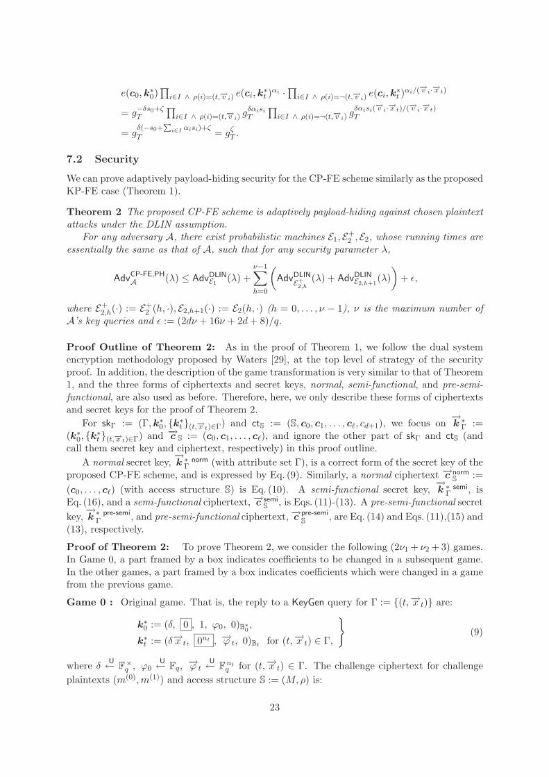
7.2 Security

We can prove adaptively payload-hiding security for the CP-FE scheme similarly as the proposedKP-FE case (Theorem 1).

Theorem 2 The proposed CP-FE scheme is adaptively payload-hiding against chosen plaintextattacks under the DLIN assumption.

For any adversary A, there exist probabilistic machines E1, E+2 , E2, whose running times are

essentially the same as that of A, such that for any security parameter λ,

AdvCP-FE,PHA (λ) ≤ AdvDLIN

E1 (λ) +ν−1∑h=0

(AdvDLIN

E+2,h

(λ) + AdvDLINE2,h+1

(λ))

+ ε,


2 (h, ·), E2,h+1(·) := E2(h, ·) (h = 0, . . . , ν − 1), ν is the maximum number ofA’s key queries and ε := (2dν + 16ν + 2d+ 8)/q.

Proof Outline of Theorem 2: As in the proof of Theorem 1, we follow the dual systemencryption methodology proposed by Waters [29], at the top level of strategy of the securityproof. In addition, the description of the game transformation is very similar to that of Theorem1, and the three forms of ciphertexts and secret keys, normal, semi-functional, and pre-semi-functional, are also used as before. Therefore, here, we only describe these forms of ciphertextsand secret keys for the proof of Theorem 2.

For skΓ := (Γ,k∗0, {k∗t }(t,−→x t)∈Γ) and ctS := (S, c0, c1, . . . , c�, cd+1), we focus on−→k ∗Γ :=

(k∗0, {k∗t }(t,−→x t)∈Γ) and −→c S := (c0, c1, . . . , c�), and ignore the other part of skΓ and ctS (andcall them secret key and ciphertext, respectively) in this proof outline.

A normal secret key,−→k ∗ norm

Γ (with attribute set Γ), is a correct form of the secret key of theproposed CP-FE scheme, and is expressed by Eq. (9). Similarly, a normal ciphertext −→c norm

S:=

(c0, . . . , c�) (with access structure S) is Eq. (10). A semi-functional secret key,−→k ∗ semi

Γ , isEq. (16), and a semi-functional ciphertext, −→c semi

S, is Eqs. (11)-(13). A pre-semi-functional secret

key,−→k ∗ pre-semi

Γ , and pre-semi-functional ciphertext, −→c pre-semiS

, are Eq. (14) and Eqs. (11),(15) and(13), respectively.

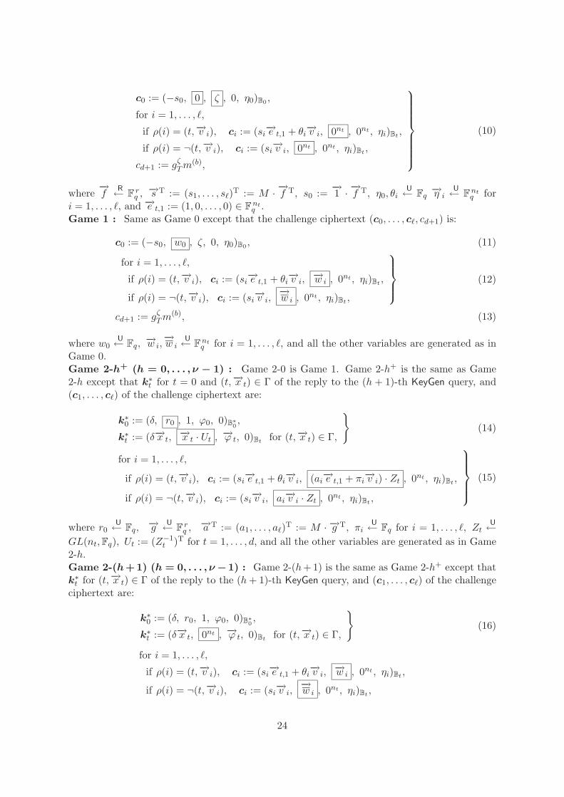
Proof of Theorem 2: To prove Theorem 2, we consider the following (2ν1 + ν2 + 3) games.In Game 0, a part framed by a box indicates coefficients to be changed in a subsequent game.In the other games, a part framed by a box indicates coefficients which were changed in a gamefrom the previous game.

Game 0 : Original game. That is, the reply to a KeyGen query for Γ := {(t,−→x t)} are:

k∗0 := (δ, 0 , 1, ϕ0, 0)B∗0,

k∗t := (δ−→x t, 0nt , −→ϕ t, 0)Bt for (t,−→x t) ∈ Γ,

}(9)

where δ U← F×q , ϕ0

U← Fq,−→ϕ t

U← Fntq for (t,−→x t) ∈ Γ. The challenge ciphertext for challenge

plaintexts (m(0),m(1)) and access structure S := (M,ρ) is:

23

c0 := (−s0, 0 , ζ , 0, η0)B0 ,

for i = 1, . . . , �,

if ρ(i) = (t,−→v i), ci := (si−→e t,1 + θi−→v i, 0nt , 0nt , ηi)Bt ,

if ρ(i) = ¬(t,−→v i), ci := (si−→v i, 0nt , 0nt , ηi)Bt ,

cd+1 := gζTm(b),

⎫⎪⎪⎪⎪⎪⎪⎪⎬⎪⎪⎪⎪⎪⎪⎪⎭(10)

where−→f

R← Frq ,−→s T := (s1, . . . , s�)T := M · −→f T, s0 :=

−→1 · −→f T, η0, θi

U← Fq−→η i U← F

ntq for

i = 1, . . . , �, and −→e t,1 := (1, 0, . . . , 0) ∈ Fntq .

Game 1 : Same as Game 0 except that the challenge ciphertext (c0, . . . , c�, cd+1) is:

c0 := (−s0, w0 , ζ, 0, η0)B0 , (11)

for i = 1, . . . , �,

if ρ(i) = (t,−→v i), ci := (si−→e t,1 + θi−→v i, −→w i , 0nt , ηi)Bt ,

if ρ(i) = ¬(t,−→v i), ci := (si−→v i, −→w i , 0nt , ηi)Bt ,

⎫⎪⎪⎬⎪⎪⎭ (12)

cd+1 := gζTm(b), (13)

where w0U← Fq,

−→w i,−→w i

U← Fntq for i = 1, . . . , �, and all the other variables are generated as in

Game 0.Game 2-h+ (h = 0, . . . , ν − 1) : Game 2-0 is Game 1. Game 2-h+ is the same as Game2-h except that k∗t for t = 0 and (t,−→x t) ∈ Γ of the reply to the (h + 1)-th KeyGen query, and(c1, . . . , c�) of the challenge ciphertext are:

k∗0 := (δ, r0 , 1, ϕ0, 0)B∗0,

k∗t := (δ−→x t, −→x t · Ut , −→ϕ t, 0)Bt for (t,−→x t) ∈ Γ,

}(14)

for i = 1, . . . , �,

if ρ(i) = (t,−→v i), ci := (si−→e t,1 + θi−→v i, (ai−→e t,1 + πi

−→v i) · Zt , 0nt , ηi)Bt ,

if ρ(i) = ¬(t,−→v i), ci := (si−→v i, ai−→v i · Zt , 0nt , ηi)Bt ,

⎫⎪⎪⎪⎬⎪⎪⎪⎭ (15)

where r0U← Fq,

−→g U← Frq ,−→a T := (a1, . . . , a�)T := M · −→g T, πi

U← Fq for i = 1, . . . , �, ZtU←

GL(nt,Fq), Ut := (Z−1t )T for t = 1, . . . , d, and all the other variables are generated as in Game

2-h.Game 2-(h+1) (h = 0, . . . , ν −1) : Game 2-(h+1) is the same as Game 2-h+ except thatk∗t for (t,−→x t) ∈ Γ of the reply to the (h+ 1)-th KeyGen query, and (c1, . . . , c�) of the challengeciphertext are:

k∗0 := (δ, r0, 1, ϕ0, 0)B∗0,


}(16)

for i = 1, . . . , �,



24

where −→w i,−→w i

U← Fntq for i = 1, . . . , �, and all the other variables are generated as in Game 2-h+.

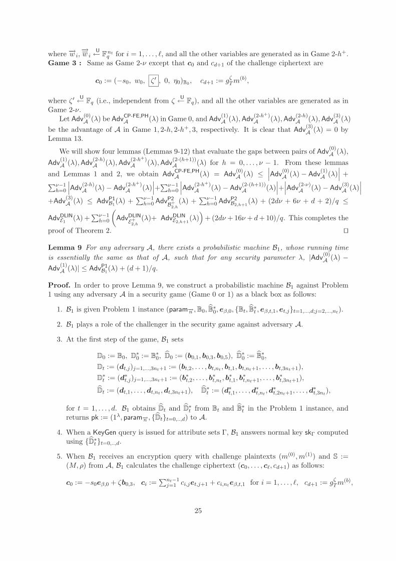
Game 3 : Same as Game 2-ν except that c0 and cd+1 of the challenge ciphertext are

c0 := (−s0, w0, ζ ′ , 0, η0)B0 , cd+1 := gζTm(b),

where ζ ′ U← Fq (i.e., independent from ζU← Fq), and all the other variables are generated as in

Game 2-ν.Let Adv

(0)A (λ) be AdvCP-FE,PH

A (λ) in Game 0, and Adv(1)A (λ),Adv

(2-h+)A (λ),Adv

(2-h)A (λ),Adv

(3)A (λ)

be the advantage of A in Game 1, 2-h, 2-h+, 3, respectively. It is clear that Adv(3)A (λ) = 0 by

Lemma 13.

We will show four lemmas (Lemmas 9-12) that evaluate the gaps between pairs of Adv(0)A (λ),

Adv(1)A (λ),Adv

(2-h)A (λ),Adv

(2-h+)A (λ),Adv

(2-(h+1))A (λ) for h = 0, . . . , ν − 1. From these lemmas

and Lemmas 1 and 2, we obtain AdvCP-FE,PHA (λ) = Adv

(0)A (λ) ≤

∣∣∣Adv(0)A (λ)− Adv

(1)A (λ)

∣∣∣ +∑ν−1h=0

∣∣∣Adv(2-h)A (λ)− Adv

(2-h+)A (λ)

∣∣∣+∑ν−1h=0

∣∣∣Adv(2-h+)A (λ)− Adv

(2-(h+1))A (λ)

∣∣∣+∣∣∣Adv(2-ν)A (λ)− Adv

(3)A (λ)

∣∣∣+Adv

(3)A (λ) ≤ AdvP1

B1(λ) +

∑ν−1h=0 AdvP2

B+2,h

(λ) +∑ν−1

h=0 AdvP2B2,h+1

(λ) + (2dν + 6ν + d + 2)/q ≤

AdvDLINE1 (λ) +

∑ν−1h=0

(AdvDLIN

E+2,h

(λ)+ AdvDLINE2,h+1

(λ))

+ (2dν + 16ν + d+ 10)/q. This completes the

proof of Theorem 2. ��


(0)A (λ) −

Adv(1)A (λ)| ≤ AdvP1

B1(λ) + (d+ 1)/q.

Proof. In order to prove Lemma 9, we construct a probabilistic machine B1 against Problem1 using any adversary A in a security game (Game 0 or 1) as a black box as follows:

1. B1 is given Problem 1 instance (param−→n ,B0, B̂∗0, eβ,0, {Bt, B̂∗t , eβ,t,1, et,j}t=1,...,d;j=2,...,nt).

2. B1 plays a role of the challenger in the security game against adversary A.

3. At the first step of the game, B1 sets

D0 := B0, D∗0 := B

∗0, D̂0 := (b0,1, b0,3, b0,5), D̂

∗0 := B̂

∗0,

Dt := (dt,j)j=1,...,3nt+1 := (bt,2, . . . , bt,nt , bt,1, bt,nt+1, . . . , bt,3nt+1),D∗t := (d∗t,j)j=1,...,3nt+1 := (b∗t,2, . . . , b

∗t,nt

, b∗t,1, b∗t,nt+1, . . . , b

∗t,3nt+1),

D̂t := (dt,1, . . . ,dt,nt ,dt,3nt+1), D̂∗t := (d∗t,1, . . . ,d

∗t,nt

,d∗t,2nt+1, . . . ,d∗t,3nt

),

for t = 1, . . . , d. B1 obtains D̂t and D̂∗t from Bt and B̂

∗t in the Problem 1 instance, and

returns pk := (1λ, param−→n , {D̂t}t=0,..,d) to A.

4. When a KeyGen query is issued for attribute sets Γ, B1 answers normal key skΓ computedusing {D̂∗t }t=0,..,d.

5. When B1 receives an encryption query with challenge plaintexts (m(0),m(1)) and S :=(M,ρ) from A, B1 calculates the challenge ciphertext (c0, . . . , c�, cd+1) as follows:

c0 := −s0eβ,0 + ζb0,3, ci :=∑nt−1

j=1 ci,jet,j+1 + ci,nteβ,t,1 for i = 1, . . . , �, cd+1 := gζTm(b),

25

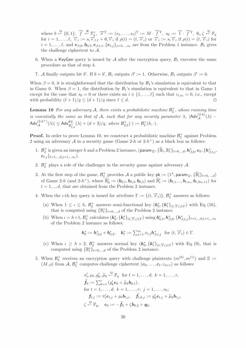
where b U← {0, 1}, −→f R← Frq ,−→s T := (s1, . . . , s�)T := M · −→f T, s0 :=

−→1 · −→f T, θi, ζ

U← Fq

for i = 1, . . . , �, −→c i := si−→e t,1 + θi

−→v i if ρ(i) = (t,−→v i) or −→c i := si−→v i if ρ(i) = (t,−→v i) for

i = 1, . . . , �, and eβ,0, b0,3, eβ,t,1, {et,j}j=2,...,nt are from the Problem 1 instance. B1 givesthe challenge ciphertext to A.

6. When a KeyGen query is issued by A after the encryption query, B1 executes the sameprocedure as that of step 4.

7. A finally outputs bit b′. If b = b′, B1 outputs β′ := 1. Otherwise, B1 outputs β′ := 0.

When β = 0, it is straightforward that the distribution by B1’s simulation is equivalent to thatin Game 0. When β = 1, the distribution by B1’s simulation is equivalent to that in Game 1except for the case that s0 = 0 or there exists an i ∈ {1, . . . , �} such that ci,nt = 0, i.e., exceptwith probability (�+ 1)/q ≤ (d+ 1)/q since � ≤ d. ��

Lemma 10 For any adversary A, there exists a probabilistic machine B+2 , whose running time

is essentially the same as that of A, such that for any security parameter λ, |Adv(2-h)A (λ) −

Adv(2-h+)A (λ)| ≤ AdvP2

B+2,h

(λ) + (d+ 3)/q, where B+2,h(·) := B+

2 (h, ·).

Proof. In order to prove Lemma 10, we construct a probabilistic machine B+2 against Problem

2 using an adversary A in a security game (Game 2-h or 2-h+) as a black box as follows:

1. B+2 is given an integer h and a Problem 2 instance, (param−→n , {B̂t,B∗t }t=0,..,d,h

∗β,0, e0, {h∗β,t,j ,

et,j}t=1,..,d;j=1,..,nt).

2. B+2 plays a role of the challenger in the security game against adversary A.

3. At the first step of the game, B+2 provides A a public key pk := (1λ, param−→n , {B̂′t}t=0,...,d)

of Game 2-h (and 2-h+), where B̂′0 := (b0,1, b0,3, b0,5) and B̂

′t := (bt,1, .., bt,nt , bt,3nt+1) for

t = 1, .., d, that are obtained from the Problem 2 instance.

4. When the ι-th key query is issued for attribute Γ := {(t,−→x t)}, B+2 answers as follows:

(a) When 1 ≤ ι ≤ h, B+2 answers semi-functional key (k∗0, {k∗t }(t,−→x t)∈Γ) with Eq. (16),

that is computed using {B∗t }t=0,...,d of the Problem 2 instance.

(b) When ι = h+1, B+2 calculates (k∗0, {k∗t }(t,−→x t)∈Γ) using b∗0,3,h∗β,0, {h∗β,t,j}t=1,..,d;j=1,..,nt

of the Problem 2 instance as follows:

k∗0 := h∗β,0 + b∗0,3, k∗t :=∑nt

j=1 xt,jh∗β,t,j for (t,−→x t) ∈ Γ.

(c) When ι ≥ h + 2, B+2 answers normal key (k∗0, {k∗t }(t,−→x t)∈Γ) with Eq. (9), that is

computed using {B∗t }t=0,...,d of the Problem 2 instance.

5. When B+2 receives an encryption query with challenge plaintexts (m(0),m(1)) and S :=

(M,ρ) from A, B+2 computes challenge ciphertext (c0, . . . , c�, cd+1) as follows:

π′t, μt, g′k, μ̃k

U← Fq for t = 1, . . . , d; k = 1, . . . , r,

f̃0 :=∑r

k=1 (g′ke0 + μ̃kb0,1) ,for t = 1, . . . , d; k = 1, . . . , r; j = 1, . . . , nt;

ft,j := π′tet,j + μtbt,j , f̃t,k,j := g′ket,j + μ̃kbt,j ,

ζU← Fq, c0 := −f̃0 + ζb0,3 + q0,

26

for i = 1 . . . , �,if ρ(i) = (t,−→v i), ci :=

∑ntj=1 vi,jft,j +

∑rk=1Mi,kf̃t,k,1 + qi,

if ρ(i) = ¬(t,−→v i), ci :=∑nt

j=1 vi,j(∑r

k=1Mi,kf̃t,k,j) + qi,

cd+1 := gζTm(b),

where (Mi,k)i=1,...,�;k=1,...,r := M , q0U← span〈b0,5〉, and qi

U← span〈bt,3nt+1〉 and (b0,1, b0,3,e0, {et,j}t=1,...,d;j=1,...,nt) is a part of the Problem 2 instance. B+

2 gives the challengeciphertext to A.

6. When a KeyGen query is issued by A after the encryption query, B+2 executes the same

procedure as that of step 4.

7. A finally outputs bit b′. If b = b′, B+2 outputs β′ := 1. Otherwise, B+

2 outputs β′ := 0.

Remark 2 f̃0,ft,j , f̃t,k,j for t = 1, . . . , d; k = 1, . . . , r; j = 1, . . . , nt calculated in the step 5 inthe above simulation are expressed as:

πt := τπ′t, θt := πtω + μt, gk := τg′k, fk := gkω + μ̃k,

s0 :=∑r

k=1 fk, a0 :=∑r

k=1 gk, w0 := a0/u0 (= a0z0),

f̃0 = (s0, w0, 0, 0, 0)B0 ,nt︷︸︸︷ nt︷︸︸︷ nt︷︸︸︷ 1︷︸︸︷

ft,j := ( θt−→e t,j , πt

−→z t,j , 0nt , 0 )Bt ,

f̃t,k,j := ( fk−→e t,j , gk

−→z t,j , 0nt , 0 )Bt ,

where τ, ω, u0, {−→e t,j ,−→z t,j}t=1,...,d;j=1,...,nt are defined in Problem 2. Note that variables {θt, πt}t=1,...,d,{fk, gk}k=1,...,r are independently and uniformly distributed. Therefore, {ci}i=0,...,� are dis-

tributed as (11) and (15) except w0 := a0/r0, i.e., w0r0 = a0, using a0 and r0 := u0U← Fq in k∗0

(Eq. (14)).

Claim 2 The distribution of the view of adversary A in the above-mentioned game simulatedby B+

2 given a Problem 2 instance with β ∈ {0, 1} is the same as that in Game 2-h (resp. Game2-h+) if β = 0 (resp. β = 1) except with probability (d+ 2)/q (resp. 1/q).

Proof. It is clear that B+2 ’s simulation of the public-key generation (step 3) and the ι-th key

query’s answer for ι �= h+ 1 (cases (a) and (c) of step 4) is perfect, i.e., exactly the same as theSetup and the KeyGen oracle in Game 2-h and Game 2-h+.

Therefore, to prove this lemma we will show that the joint distribution of the (h + 1)-thkey query’s answer and the challenge ciphertext by B+

2 ’s simulation given a Problem 2 instancewith β is equivalent to that in Game 2-h (resp. Game 2-h+), when β = 0 (resp. β = 1).

When β = 0, it is straightforward to show that they are equivalent except that δ definedin Problem 2 is zero or there exists i ∈ {0, . . . , �} such that −→w i =

−→0 with ρ(i) = (t,−→v i) or−→

w i =−→0 with ρ(i) = ¬(t,−→v i), where −→w i and

−→w i are defined in Eqs. (11) and (12), i.e., except

with probability (�+ 2)/q ≤ (d+ 2)/q since � ≤ d.When β = 1, the distribution by B+

2 ’s simulation is Eq. (14) for the key and Eqs. (11), (13),and (15) for the challenge ciphertext, where the distribution is the same as that defined in theseequations except w0 := a0/r0, i.e., w0r0 = a0, using a0 :=

−→1 · −→g T and r0

U← Fq in k∗0 (Eq. (14))from Remark 2. The corresponding distribution in Game 2-h+ is Eq. (14) and Eqs. (11), (13),and (15) where r0, w0

U← Fq as defined in the equations.

27

Moreover, similarly as in the proof of Claim 1, we can show that a0 is uniformly andindependently distributed from the other variables in the joint distribution of B+

2 ’s simulation.Therefore, the view of adversary A in the game simulated by B+

2 given a Problem 2 instancewith β = 1 is the same as that in Game 2-h+ except that δ defined in Problem 2 is zero i.e.,except with probability 1/q. ��

This completes the proof of Lemma 10. ��Lemma 11 For any adversary A, there exists a probabilistic machine B2, whose running timeis essentially the same as that of A, such that for any security parameter λ, |Adv

(2-h+)A (λ) −

Adv(2-(h+1))A (λ)| ≤ AdvP2

B2,h+1(λ) + (d+ 3)/q, where B2,h+1(·) := B2(h, ·).

Proof. The proof of Lemma 11 is similar to that of Lemma 6. ��

Lemma 12 For any adversary A, Adv(2-ν)A (λ) ≤ Adv

(3)A (λ) + 1/q.

Proof. The proof of Lemma 12 is similar to that of Lemma 7. ��


8 UP-FE Scheme

8.1 Construction

In order to obtain a UP-FE scheme, we combine the KP-FE scheme in Section 6 and the CP-FE scheme in Section 7 using the first vector space V0 of dimension 8, instead of dimension5. In the security proof, the semi-functional form of secret keys (resp. ciphertexts) has 2-dimensional random component in span〈b∗0,3, b∗0,4〉 (resp. span〈b0,3, b0,4〉). For our KP-FE andCP-FE schemes, the corresponding random components are in 1-dimensional subspace of V0

(see Sections 6 and 7).ρ̃ : {1, . . . , �} → {1, . . . , d} is defined at the start of Section 6. In the proposed scheme, we

assume that ρ̃ is injective for S := (M,ρ), where S := SKP,SCP.

In the description of the scheme, we assume that input vectors, −→x KPt := (xKP

t,1 , . . . , xKPt,nt

)and −→x CP

t := (xCPt,1 , . . . , x

CPt,nt

), are normalized such that xKPt,1 := 1 and xCP

t,1 := 1. (If −→x KPt

(resp.−→x CPt ) is not normalized, change it to a normalized one by (1/xKP

t,1 ) · −→x KPt (resp. (1/xCP

t,1 ) ·−→x CPt ), assuming that xKP

t,1 (resp.xCPt,1 ) is non-zero). In addition, we assume that input vector

−→v CPt := (vCP

i,1 , . . . , vCPi,nt

) satisfies that vCPi,nt�= 0.

We refer to Section 1.3 for notations on DPVS, e.g., (x1, . . . , xN )B, (y1, . . . , yN )B∗ for xi, yi ∈Fq

For a format of attribute vectors −→n := ((dKP;nKP1 , . . . , nKP

dKP), (dCP;nCP1 , . . . , nCP

dCP)) thatindicates dimensions of vector spaces, −→e KP

t,j (resp.−→e CPt,j ) denotes the canonical basis vector

(

j−1︷︸︸︷0 · · · 0, 1,

nKPt −j︷︸︸︷

0 · · · 0) ∈ FnKP

tq for j = 1, . . . , nKP

t (resp. (

j−1︷︸︸︷0 · · · 0, 1,

nCPt −j︷︸︸︷

0 · · · 0) ∈ FnCP

tq for j = 1, . . . , nCP

t ).We describe random dual orthonormal basis generator GUP

ob below, which is used as a sub-routine in the proposed UP-FE scheme.

GUPob (1λ,−→n := ((dKP;nKP

1 , . . . , nKPdKP), (dCP;nCP

1 , . . . , nCPdCP)) :

paramG := (q,G,GT , G, e)R← Gbpg(1λ), ψ

U← F×q ,

N0 := 8, NKPt := 3nKP

t + 1 for t = 1, . . . , dKP, NCPt := 3nCP

t + 1 for t = 1, . . . , dCP,

paramV0:= (q,V0,GT ,A0, e) := Gdpvs(1λ, N0, paramG),

28

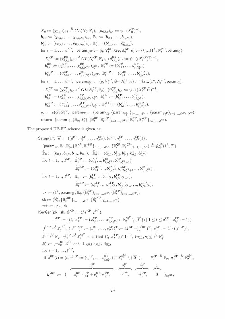
X0 := (χ0,i,j)i,jU← GL(N0,Fq), (ϑ0,i,j)i,j := ψ · (XT

0 )−1,

b0,i := (χ0,i,1, . . . , χ0,i,N0)A0 , B0 := (b0,1, . . . , b0,N0),b∗0,i := (ϑ0,i,1, . . . , ϑ0,i,N0)A0 , B

∗0 := (b∗0,1, . . . , b∗0,N0

),

for t = 1, . . . , dKP, paramVKP

t:= (q,VKP

t ,GT ,AKPt , e) := Gdpvs(1λ, NKP

t , paramG),

XKPt := (χKP

t,i,j)i,jU← GL(NKP

t ,Fq), (ϑKPt,i,j)i,j := ψ · ((XKP

t )T)−1,

bKPt,i := (χKP

t,i,1, . . . , χKPt,i,NKP

t)

AKPt, B

KPt := (bKP

t,1 , . . . , bKPt,NKP

t),

b∗KPt,i := (ϑKP

t,i,1, . . . , ϑKPt,i,NKP

t)

AKPt, B∗KPt := (b∗KP

t,1 , . . . , b∗KPt,NKP

t),

for t = 1, . . . , dCP, paramVCP

t:= (q,VCP

t ,GT ,ACPt , e) := Gdpvs(1λ, NCP

t , paramG),

XCPt := (χCP

t,i,j)i,jU← GL(NCP

t ,Fq), (ϑCPt,i,j)i,j := ψ · ((XCP

t )T)−1,

bCPt,i := (χCP

t,i,1, . . . , χCPt,i,NCP

t)

ACPt, B

CPt := (bCP

t,1 , . . . , bCPt,NCP

t),

b∗CPt,i := (ϑCP

t,i,1, . . . , ϑCPt,i,NCP

t)

ACPt, B∗CPt := (b∗CP

t,1 , . . . , b∗CPt,NCP

t),

gT := e(G,G)ψ, param−→n := (paramV0, {param

VKPt}t=1,...,dKP , {param

VCPt}t=1,...,dCP , gT ),

return (param−→n , {B0,B∗0}, {BKP

t ,B∗KPt }t=1,...,dKP , {BCP

t ,B∗CPt }t=1,...,dCP).

The proposed UP-FE scheme is given as:

Setup(1λ, −→n := ((dKP;nKP1 , . . . , nKP

dKP), (dCP;nCP1 , . . . , nCP

dCP))) :

(param−→n ,B0,B∗0, {BKP

t ,B∗KPt }t=1,...,dKP , {BCP

t ,B∗CPt }t=1,...,dCP) R← GUP

ob (1λ,−→n ),

B̂0 := (b0,1, b0,2, b0,5, b0,8), B̂∗0 := (b∗0,1, b

∗0,2, b

∗0,5, b

∗0,6, b

∗0,7),

for t = 1, .., dKP, B̂KPt := (bKP

t,1 , .., bKPt,nKP

t, bKPt,3nKP

t +1),

B̂∗KPt := (b∗KP

t,1 , .., b∗KPt,nKP

t, b∗KPt,2nKP

t +1, .., b∗KP

t,3nKPt

),

for t = 1, .., dCP, B̂CPt := (bCP

t,1 , .., bCPt,nCP

t, bCPt,3nCP

t +1),

B̂∗CPt := (b∗CP

t,1 , .., b∗CPt,nCP

t, b∗CPt,2nCP

t +1, .., b∗CP

t,3nCPt

),

pk := (1λ, param−→n , B̂0, {B̂KPt }t=1,...,dKP , {B̂CP

t }t=1,...,dCP),

sk := (B̂∗0, {B̂∗KPt }t=1,...,dKP , {B̂∗CP

t }t=1,...,dCP),return pk, sk.

KeyGen(pk, sk, SKP := (MKP, ρKP),

ΓCP := {(t,−→x CPt := (xCP

t,1 , . . . , xCPt,nCP

t) ∈ F

nCPt

q \ {−→0 }) | 1 ≤ t ≤ dCP, xCPt,1 := 1})

−→f KP U← F

rKP

q , (−→s KP)T := (sKP1 , . . . , sKP

�KP)T := MKP · (−→f KP)T, sKP0 :=

−→1 · (−→f KP)T,

δCP U← Fq,−→η CPt

U← FnCP

tq such that (t,−→x CP

t ) ∈ ΓCP, (η0,1, η0,2)U← F

2q ,

k∗0 := (−sKP0 , δCP, 0, 0, 1, η0,1, η0,2, 0)B∗

0,

for i = 1, . . . , �KP,

if ρKP(i) = (t,−→v KPi := (vKP

i,1 , . . . , vKPi,nKP

t) ∈ F

nKPt

q \ {−→0 }), θKPi

U← Fq,−→η KPi

U← FnKP

tq ,

nKPt︷︸︸︷ nKP

t︷︸︸︷ nKPt︷︸︸︷ 1︷︸︸︷

k∗KPi := ( sKP

i−→e KPt,1 + θKP

i−→v KPi , 0n

KPt , −→η KP

i , 0 )B∗KP

t,

29

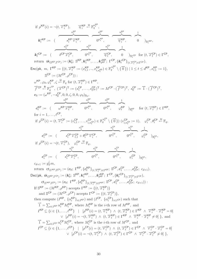
if ρKP(i) = ¬(t,−→v KPi ), −→η KP

iU← F

nKPtq ,


t︷︸︸︷ nKPt︷︸︸︷ 1︷︸︸︷

k∗KPi := ( sKP

i−→v KPi , 0n

KPt , −→η KP

i , 0 )B∗KP

t,

nCPt︷︸︸︷ nCP

t︷︸︸︷ nCPt︷︸︸︷ 1︷︸︸︷

k∗CPt := ( δCP−→x CP

t , 0nCPt , −→η CP

t , 0 )B∗CP

tfor (t,−→x CP

t ) ∈ ΓCP,

return sk(SKP,ΓCP) := (k∗0; SKP,k∗KP

1 , . . . ,k∗KP�KP ; ΓCP, {k∗CP

t }(t,−→x CPt )∈ΓCP).

Enc(pk, m, ΓKP := {(t,−→x KPt := (xKP

t,1 , .., xKPt,nKP

t) ∈ F

nKPt

q \ {−→0 }) | 1 ≤ t ≤ dKP, xKPt,1 := 1},

SCP := (MCP, ρCP)) :

ωKP, ϕ0, ϕKPt , ζ

U← Fq for (t,−→x KPt ) ∈ ΓKP,

−→f CP R← F

rCP

q , (−→s CP)T := (sCP1 , . . . , sCP

�CP)T := MCP · (−→f CP)T, sCP0 :=

−→1 · (−→f CP)T,

c0 := (ωKP,−sCP0 , 0, 0, ζ, 0, 0, ϕ0)B0 ,


t︷︸︸︷ nKPt︷︸︸︷ 1︷︸︸︷

cKPt := ( ωKP−→x KP

t , 0nKPt , 0n

KPt , ϕKP

t )BKP

tfor (t,−→x KP

t ) ∈ ΓKP,

for i = 1, . . . , �CP,

if ρCP(i) = (t,−→v CPi := (vCP

i,1 , . . . , vCPi,nCP

t) ∈ F

nCPt

q \ {−→0 }) (vCPi,nCP

t:= 1), ϕCP

i , θCPi

U← Fq,


t︷︸︸︷ nCPt︷︸︸︷ 1︷︸︸︷

cCPi := ( sCP

i−→e CPt,1 + θCP

i−→v CPi , 0n

CPt , 0n

CPt , ϕCP

i )BCP

t,

if ρCP(i) = ¬(t,−→v CPi ), ϕCP

iU← Fq,


t︷︸︸︷ nCPt︷︸︸︷ 1︷︸︸︷

cCPi := ( sCP

i−→v CPi , 0n

CPt , 0n

CPt , ϕCP

i )BCP

t,

cd+1 := gζTm,

return ct(ΓKP,SCP) := (c0; ΓKP, {cKPt }(t,−→x KP

t )∈ΓKP ; SCP, cCP

1 , . . . , cCP�CP ; cd+1).

Dec(pk, sk(SKP,ΓCP) := (k∗0; SKP,k∗KP

1 , . . . ,k∗KP�KP ; ΓCP, {k∗CP

t }(t,−→x CPt )∈ΓCP),

ct(ΓKP,SCP) := (c0; ΓKP, {cKPt }(t,−→x KP

t )∈ΓKP ; SCP, cCP

1 , . . . , cCP�CP ; cd+1)) :

If SKP := (MKP, ρKP) accepts ΓKP := {(t,−→x KP

t )}and S

CP := (MCP, ρCP) accepts ΓCP := {(t,−→x CPt )},

then compute (IKP, {αKPi }i∈IKP) and (ICP, {αCP

i }i∈ICP) such that−→1 =

∑i∈IKP αKP

i MKPi , where MKP

i is the i-th row of MKP, and

IKP ⊆ {i ∈ {1, . . . , �KP} | [ρKP(i) = (t,−→v KPi ) ∧ (t,−→x KP

t ) ∈ ΓKP ∧ −→v KPi · −→x KP

t = 0]∨ [ρKP(i) = ¬(t,−→v KP

i ) ∧ (t,−→x KPt ) ∈ ΓKP ∧ −→v KP

i · −→x KPt �= 0] }, and

−→1 =

∑i∈ICP αCP

i MCPi , where MCP

i is the i-th row of MCP, and

ICP ⊆ {i ∈ {1, . . . , �CP} | [ρCP(i) = (t,−→v CPi ) ∧ (t,−→x CP

t ) ∈ ΓCP ∧ −→v CPi · −→x CP

t = 0]∨ [ρCP(i) = ¬(t,−→v CP

i ) ∧ (t,−→x CPt ) ∈ ΓCP ∧ −→v CP

i · −→x CPt �= 0] },

30

K := e(c0,k∗0) ·∏

i∈IKP ∧ ρKP(i)=(t,−→v KPi )

e(cKPt ,k∗KP

i )αKPi

∏i∈IKP ∧ ρKP(i)=¬(t,−→v KP

i )

e(cKPt ,k∗KP

i )αKPi /(−→v KP

i ·−→x KPt ) ·

∏i∈ICP ∧ ρCP(i)=(t,−→v CP

i )

e(cCPt ,k∗CP

i )αCPi

∏i∈ICP ∧ ρCP(i)=¬(t,−→v CP

i )

e(cCPt ,k∗CP

i )αCPi /(−→v CP

i ·−→x CPt ),


[Correctness] If SKP := (MKP, ρKP) accepts ΓKP := {(t,−→x KP

t )} and SCP := (MCP, ρCP) accepts

ΓCP := {(t,−→x CPt )},

e(c0,k∗0) ·∏

i∈IKP ∧ ρKP(i)=(t,−→v KPi ) e(c

KPt ,k∗KP

i )αKPi ·∏i∈IKP ∧ ρKP(i)=¬(t,−→v KP

i ) e(cKPt ,k∗KP

i )αKPi /(−→v KP

i ·−→x KPt ) ·∏

i∈ICP ∧ ρCP(i)=(t,−→v CPi ) e(c

CPt ,k∗CP

i )αCPi ·∏i∈ICP ∧ ρCP(i)=¬(t,−→v CP

i ) e(cCPt ,k∗CP

i )αCPi /(−→v CP

i ·−→x CPt )

= g−(ωKPsKP

0 +δCPsCP0 )+ζ

T · gωKP(

Pi∈IKP α

KPi sKP

i )

T · gδCP(

Pi∈ICP α

CPi sCP

i )

T = gζT .

8.2 Security

The following theorem can be proved similarly as Theorems 1 and 2.

Theorem 3 The proposed UP-FE scheme is adaptively payload-hiding against chosen plaintextattacks under the DLIN assumption.

9 Fully Secure (CCA Secure) CP-FE Scheme

We can transform the proposed (KP, CP and UP)-FE schemes to CCA secure (KP, CP andUP)-FE schemes, respectively, by using the Canetti-Halevi-Katz (CHK) transformation [12] orthe Boneh-Katz (BK) transformation [9].

This section shows a CCA secure CP-FE scheme, that is modified from the CP-FE scheme inSection 7 through the CHK transformation, in which a strongly unforgeable one-time signaturescheme (Gen,Sig,Ver) is employed.

We can similarly apply the CHK transformation to our KP-FE scheme and the BK trans-formation to the FE schemes.

9.1 Strongly Unforgeable One-Time Signatures

Definition 14 (Signatures) A signature scheme consists of three algorithms.

Gen This is a randomized algorithm that takes as input the security parameter 1λ. It outputs averification key verk and a signing key sigk.

Sig This is a randomized algorithm that takes as input a signing key sigk and a message m (insome implicit message space). It outputs a signature σ.

Ver This takes as input a verification key verk, a message m, and a signature σ, and outputs aboolean value accept := 1 or reject := 0.

A signature scheme should have the following correctness property: for all (verk, sigk) R←Gen(1λ), all messages m, and all signatures σ R← Sig(sigk,m), it holds that 1 = Ver(verk,m, σ)with probability 1.

31

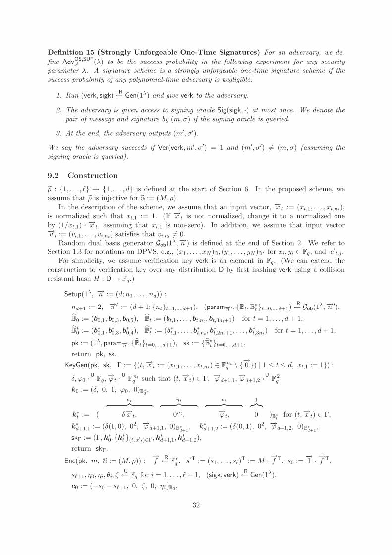
Definition 15 (Strongly Unforgeable One-Time Signatures) For an adversary, we de-fine AdvOS,SUF

A (λ) to be the success probability in the following experiment for any securityparameter λ. A signature scheme is a strongly unforgeable one-time signature scheme if thesuccess probability of any polynomial-time adversary is negligible:

1. Run (verk, sigk) R← Gen(1λ) and give verk to the adversary.

2. The adversary is given access to signing oracle Sig(sigk, ·) at most once. We denote thepair of message and signature by (m,σ) if the signing oracle is queried.

3. At the end, the adversary outputs (m′, σ′).

We say the adversary succeeds if Ver(verk,m′, σ′) = 1 and (m′, σ′) �= (m,σ) (assuming thesigning oracle is queried).

9.2 Construction

ρ̃ : {1, . . . , �} → {1, . . . , d} is defined at the start of Section 6. In the proposed scheme, weassume that ρ̃ is injective for S := (M,ρ).

In the description of the scheme, we assume that an input vector, −→x t := (xt,1, . . . , xt,nt),is normalized such that xt,1 := 1. (If −→x t is not normalized, change it to a normalized oneby (1/xt,1) · −→x t, assuming that xt,1 is non-zero). In addition, we assume that input vector−→v t := (vi,1, . . . , vi,nt) satisfies that vi,nt �= 0.

Random dual basis generator Gob(1λ,−→n ) is defined at the end of Section 2. We refer toSection 1.3 for notations on DPVS, e.g., (x1, . . . , xN )B, (y1, . . . , yN )B∗ for xi, yi ∈ Fq, and −→e t,j .

For simplicity, we assume verification key verk is an element in Fq. (We can extend theconstruction to verification key over any distribution D by first hashing verk using a collisionresistant hash H : D→ Fq.)

Setup(1λ, −→n := (d;n1, . . . , nd)) :

nd+1 := 2, −→n ′ := (d+ 1; {nt}t=1,...,d+1), (param−→n ′ , {Bt,B∗t }t=0,...,d+1)R← Gob(1λ,−→n ′),

B̂0 := (b0,1, b0,3, b0,5), B̂t := (bt,1, . . . , bt,nt , bt,3nt+1) for t = 1, . . . , d+ 1,

B̂∗0 := (b∗0,1, b

∗0,3, b

∗0,4), B̂

∗t := (b∗t,1, . . . , b

∗t,nt

, b∗t,2nt+1, . . . , b∗t,3nt

) for t = 1, . . . , d+ 1,

pk := (1λ, param−→n , {B̂t}t=0,...,d+1), sk := {B̂∗t }t=0,...,d+1,

return pk, sk.

KeyGen(pk, sk, Γ := {(t,−→x t := (xt,1, . . . , xt,nt) ∈ Fntq \ {

−→0 }) | 1 ≤ t ≤ d, xt,1 := 1}) :

δ, ϕ0U← Fq,

−→ϕ tU← F

ntq such that (t,−→x t) ∈ Γ, −→ϕ d+1,1,

−→ϕ d+1,2U← F

2q

k0 := (δ, 0, 1, ϕ0, 0)B∗0,

nt︷︸︸︷ nt︷︸︸︷ nt︷︸︸︷ 1︷︸︸︷k∗t := ( δ−→x t, 0nt , −→ϕ t, 0 )B∗


k∗d+1,1 := (δ(1, 0), 02, −→ϕ d+1,1, 0)B∗d+1, k∗d+1,2 := (δ(0, 1), 02, −→ϕ d+1,2, 0)B∗

d+1,

skΓ := (Γ,k∗0, {k∗t }(t,−→x t)∈Γ,k∗d+1,1,k

∗d+1,2),

return skΓ.

Enc(pk, m, S := (M,ρ)) :−→f

R← Frq ,−→s T := (s1, . . . , s�)T := M · −→f T, s0 :=

−→1 · −→f T,

s�+1, η0, ηi, θi, ζU← Fq for i = 1, . . . , �+ 1, (sigk, verk) R← Gen(1λ),

c0 := (−s0 − s�+1, 0, ζ, 0, η0)B0 ,

32

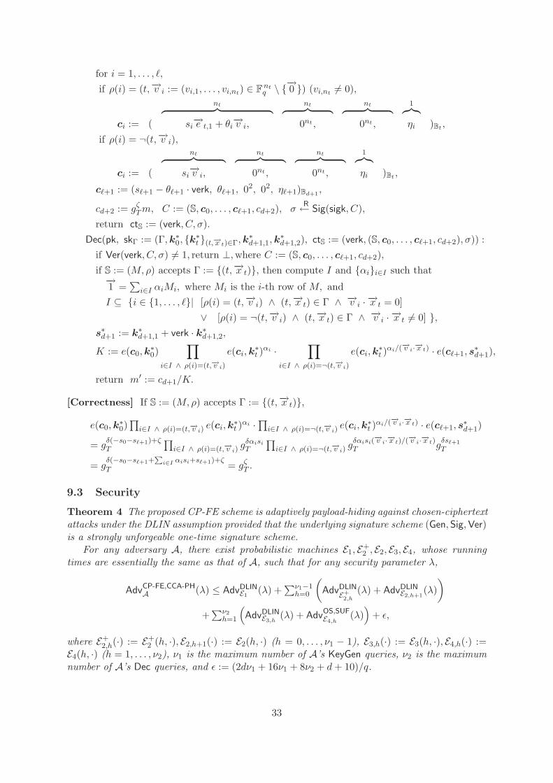
for i = 1, . . . , �,if ρ(i) = (t,−→v i := (vi,1, . . . , vi,nt) ∈ F

ntq \ {

−→0 }) (vi,nt �= 0),

nt︷︸︸︷ nt︷︸︸︷ nt︷︸︸︷ 1︷︸︸︷ci := ( si

−→e t,1 + θi−→v i, 0nt , 0nt , ηi )Bt ,

if ρ(i) = ¬(t,−→v i),nt︷︸︸︷ nt︷︸︸︷ nt︷︸︸︷ 1︷︸︸︷

ci := ( si−→v i, 0nt , 0nt , ηi )Bt ,

c�+1 := (s�+1 − θ�+1 · verk, θ�+1, 02, 02, η�+1)Bd+1,

cd+2 := gζTm, C := (S, c0, . . . , c�+1, cd+2), σR← Sig(sigk, C),

return ctS := (verk, C, σ).Dec(pk, skΓ := (Γ,k∗0, {k∗t }(t,−→x t)∈Γ,k

∗d+1,1,k

∗d+1,2), ctS := (verk, (S, c0, . . . , c�+1, cd+2), σ)) :

if Ver(verk, C, σ) �= 1, return ⊥,where C := (S, c0, . . . , c�+1, cd+2),if S := (M,ρ) accepts Γ := {(t,−→x t)}, then compute I and {αi}i∈I such that−→1 =


I ⊆ {i ∈ {1, . . . , �}| [ρ(i) = (t,−→v i) ∧ (t,−→x t) ∈ Γ ∧ −→v i · −→x t = 0]∨ [ρ(i) = ¬(t,−→v i) ∧ (t,−→x t) ∈ Γ ∧ −→v i · −→x t �= 0] },

s∗d+1 := k∗d+1,1 + verk · k∗d+1,2,

K := e(c0,k∗0)

∏i∈I ∧ ρ(i)=(t,−→v i)

e(ci,k∗t )αi ·

∏i∈I ∧ ρ(i)=¬(t,−→v i)

e(ci,k∗t )αi/(−→v i·−→x t) · e(c�+1, s

∗d+1),


[Correctness] If S := (M,ρ) accepts Γ := {(t,−→x t)},

e(c0,k∗0)∏i∈I ∧ ρ(i)=(t,−→v i)

e(ci,k∗t )αi ·∏i∈I ∧ ρ(i)=¬(t,−→v i)e(ci,k∗t )αi/(

−→v i·−→x t) · e(c�+1, s∗d+1)

= gδ(−s0−s�+1)+ζT

∏i∈I ∧ ρ(i)=(t,−→v i)

gδαisiT

∏i∈I ∧ ρ(i)=¬(t,−→v i)

gδαisi(

−→v i·−→x t)/(−→v i·−→x t)

T gδs�+1

T

= gδ(−s0−s�+1+

Pi∈I αisi+s�+1)+ζ

T = gζT .

9.3 Security

Theorem 4 The proposed CP-FE scheme is adaptively payload-hiding against chosen-ciphertextattacks under the DLIN assumption provided that the underlying signature scheme (Gen,Sig,Ver)is a strongly unforgeable one-time signature scheme.

For any adversary A, there exist probabilistic machines E1, E+2 , E2, E3, E4, whose running

times are essentially the same as that of A, such that for any security parameter λ,

AdvCP-FE,CCA-PHA (λ) ≤ AdvDLIN

E1 (λ) +∑ν1−1

h=0

(AdvDLIN

E+2,h

(λ) + AdvDLINE2,h+1

(λ))

+∑ν2

h=1

(AdvDLIN

E3,h(λ) + AdvOS,SUF

E4,h(λ)

)+ ε,


2 (h, ·), E2,h+1(·) := E2(h, ·) (h = 0, . . . , ν1 − 1), E3,h(·) := E3(h, ·), E4,h(·) :=E4(h, ·) (h = 1, . . . , ν2), ν1 is the maximum number of A’s KeyGen queries, ν2 is the maximumnumber of A’s Dec queries, and ε := (2dν1 + 16ν1 + 8ν2 + d+ 10)/q.

33

Proof Outline of Theorem 4: To prove Theorem 4, we consider the following (2ν1 +ν2 +3)games. In Game 0, a part framed by a box indicates coefficients to be changed in a subsequentgame. In the other games, a part framed by a box indicates coefficients which were changed ina game from the previous game.Game 0 : Original game. That is, the reply to a KeyGen query for Γ := {(t,−→x t)} are:

k∗0 := (δ, 0 , 1, ϕ0, 0)B∗0,


k∗d+1,1 := (δ(1, 0), 02, −→ϕ d+1,1, 0)B∗d+1, k∗d+1,2 := (δ(0, 1), 02, −→ϕ d+1,2, 0)B∗

d+1,

where δ U← F×q , ϕ0

U← Fq,−→ϕ t

U← Fntq for (t,−→x t) ∈ Γ, −→ϕ d+1,1,

−→ϕ d+1,2U← F

2q . In answering

Dec query for ctS := (verk, (S, c0, . . . , c�+1, cd+2), σ) when Ver(verk, C, σ) = 1, where C :=(S, c0, . . . , c�+1, cd+2), the used key for Γ := {(t,−→x t)} such that S accepts Γ are:

k∗0 := (δ̃, 0 , 1, ϕ̃0, 0)B∗0,

k∗t := (δ̃−→x t, 0nt ,−→̃ϕ t, 0)Bt for (t,−→x t) ∈ Γ,

s∗d+1 := (δ̃(1, verk), 02 ,−→̃ϕ d+1, 0)B∗

d+1,

where δ̃ U← F×q , ϕ̃0

U← Fq,−→̃ϕ t

U← Fntq for (t,−→x t) ∈ Γ,

−→̃ϕ d+1

U← F2q .

The challenge ciphertext for challenge plaintexts (m(0),m(1)) and access structure S :=(M,ρ) is:

c0 := (−s0 − s�+1, 0 , ζ , 0, η0)B0 ,

for i = 1, . . . , �,if ρ(i) = (t,−→v i), ci := (si−→e t,1 + θi

−→v i, 0nt , 0nt , ηi)Bt ,

if ρ(i) = ¬(t,−→v i), ci := (si−→v i, 0nt , 0nt , ηi)Bt ,

c�+1 := (s�+1 − θ�+1 · verk, θ�+1, 02 , 02, η�+1)Bd+1,

cd+2 := gζTm(b),

where−→f

R← Frq ,−→s T := (s1, . . . , s�)T := M · −→f T, s0 :=

−→1 · −→f T, s�+1, ζ, η0, ηi, θi

U← Fq fori = 1, . . . , �+ 1, and −→e t,1 := (1, 0, . . . , 0) ∈ F

ntq .

Game 1 : Same as Game 0 except that the challenge ciphertext for challenge plaintexts(m(0),m(1)) and access structure S := (M,ρ) is:

c0 := (−s0 − s�+1, w0 , ζ, 0, η0)B0 ,

for i = 1, . . . , �,



c�+1 := (s�+1 − θ�+1 · verk, θ�+1,−→w �+1 , 02, η�+1)Bd+1

,

where w0U← Fq,

−→w i,−→w i

U← Fntq for i = 1, . . . , �, −→w �+1

U← F2q , and all the other variables are

generated as in Game 0.Game 2-h+ (h = 0, . . . , ν1 − 1) and Game 2-(h +1) (h = 0, . . . , ν1 − 1) are the same asGame 2-h+ and Game 2-(h + 1) in the proof of Theorem 2, respectively.

34

Game 3-h (h = 1, . . . , ν2) : Game 3-0 is Game 2-ν1. Game 3-h is the same as Game 3-(h−1)except that k∗0, s∗d+1 of the key used in answering the h-th Dec query when Ver(verk, C, σ) = 1are:

k∗0 := (δ̃, r̃0 , 1, ϕ̃0, 0)B∗0,

s∗d+1 := (δ̃(1, verk),−→̃r d+1 ,

−→̃ϕ d+1, 0)B∗

d+1,

where r̃0U← Fq,

−→̃r d+1

U← F2q , and all the other variables are generated as in Game 3-(h− 1).

Game 4 : Same as Game 3-ν2 except that c0 in the challenge ciphertext is:

c0 := (−s0 − s�+1, w0, ζ ′ , 0, η0)B0 ,

where ζ ′ U← Fq (i.e., independent from all the other variables), and all the other variables aregenerated as in Game 3-ν2.

We follow the argument in [12] used for the chosen ciphertext security, and the rest of theproof of Theorem 4 is similar to that of Theorem 2.

Let Adv(0)A (λ) be AdvCP-FE,CCA-PH

A (λ) in Game 0, and Adv(1)A (λ),Adv

(2-h+)A (λ),Adv

(2-h)A (λ),

Adv(3-h)A (λ),Adv

(4)A (λ) be the advantage of A in Game 1, 2-h, 2-h+, 3-h, 4, respectively. (Adv

(4)A (λ)

= 0.) We can evaluate the gaps between pairs of Adv(0)A (λ),Adv

(1)A (λ),Adv

(2-h)A (λ),Adv

(2-h+)A (λ),

Adv(2-(h+1))A (λ) for h = 0, . . . , ν1 − 1 using Problems 3 and 4 (given in Appendix D) as in the

proof of Theorem 2.Moreover, we can evaluate the gaps between pairs of Adv

(3-h)A (λ) and Adv

(3-(h+1))A (λ) for

h = 0, . . . , ν2 − 1 using Problem 5 in Appendix D. ��

References

[1] Attrapadung, N., Imai, H.: Dual-policy attribute-based encryption: Simultaneous accesscontrol with ciphertext and key policies. IEICE Trans. Fundamentals, E93-A, no. 1, pp.116–125 (2010)

[2] Beimel, A., Secure schemes for secret sharing and key distribution. PhD Thesis, IsraelInstitute of Technology, Technion, Haifa, Israel, (1996)

[3] Bethencourt, J., Sahai, A., Waters, B.: Ciphertext-policy attribute-based encryption. In:2007 IEEE Symposium on Security and Privacy, pp. 321–334. IEEE Press, Los Alamitos(2007)

[4] Boneh, D., Boyen, X.: Efficient selective-ID secure identity based encryption without ran-dom oracles. In: Cachin, C., Camenisch, J. (eds.) EUROCRYPT 2004. LNCS, vol. 3027, pp.223–238. Springer, Heidelberg (2004)

[5] Boneh, D., Boyen, X.: Secure identity based encryption without random oracles. In:Franklin, M.K. (ed.) CRYPTO 2004. LNCS, vol. 3152, pp. 443–459. Springer, Heidelberg(2004)

[6] Boneh, D., Boyen, X., Goh, E.: Hierarchical identity based encryption with constant size ci-phertext. In: Cramer, R. (ed.) EUROCRYPT 2005. LNCS, vol. 3494, pp. 440–456. Springer,Heidelberg (2005)

35

[7] Boneh, D., Franklin, M.: Identity-based encryption from the Weil pairing. In: Kilian, J.(ed.) CRYPTO 2001. LNCS, vol. 2139, pp. 213–229. Springer, Heidelberg (2001)

[8] Boneh, D., Hamburg, M.: Generalized identity based and broadcast encryption scheme. In:Pieprzyk, J. (ed.) ASIACRYPT 2008. LNCS, vol. 5350, pp. 455–470. Springer, Heidelberg(2008)

[9] Boneh, D., Katz, J., Improved efficiency for CCA-secure cryptosystems built using iden-tity based encryption. In: Menezes, A. (ed.) CT-RSA 2005. LNCS, vol. 3376, pp. 87–103.Springer, Heidelberg (2005)

[10] Boneh, D., Waters, B.: Conjunctive, subset, and range queries on encrypted data. In:Vadhan, S.P. (ed.) TCC 2007. LNCS, vol. 4392, pp. 535–554. Springer, Heidelberg (2007)

[11] Boyen, X., Waters, B.: Anonymous hierarchical identity-based encryption (without randomoracles). In: Dwork, C. (ed.) CRYPTO 2006. LNCS, vol. 4117, pp. 290–307. Springer,Heidelberg (2006)

[12] Canetti, R., Halevi S., Katz J.: Chosen-ciphertext security from identity-based encryption.In: Cachin, C., Camenisch, J.L. (eds.) EUROCRYPT 2004. LNCS, vol. 3027, pp. 207–222.Springer, Heidelberg (2004)

[13] Cocks, C.: An identity based encryption scheme based on quadratic residues. In: Honary,B. (ed.) IMA Int. Conf. LNCS, vol. 2260, pp. 360–363. Springer, Heidelberg (2001)

[14] Gentry, C.: Practical identity-based encryption without random oracles. In: Vaudenay, S.(ed.) EUROCRYPT 2006. LNCS, vol. 4004, pp. 445–464. Springer, Heidelberg (2006)

[15] Gentry, C., Halevi, S.: Hierarchical identity-based encryption with polynomially manylevels. In: Reingold, O. (ed.) TCC 2009. LNCS, vol. 5444, pp. 437–456. Springer, Heidelberg(2009)

[16] Gentry, C., Silverberg, A.: Hierarchical ID-based cryptography. In: Zheng, Y. (ed.) ASI-ACRYPT 2002. LNCS, vol. 2501, pp. 548–566. Springer, Heidelberg (2002)

[17] Goyal, V., Pandey, O., Sahai, A., Waters, B.: Attribute-based encryption for fine-grainedaccess control of encrypted data. In: ACM Conference on Computer and CommunicationSecurity 2006, pp. 89–98, ACM, New York (2006)

[18] Katz, J., Sahai, A., Waters, B.: Predicate encryption supporting disjunctions, polynomialequations, and inner products. In: Smart, N.P. (ed.) EUROCRYPT 2008. LNCS, vol. 4965,pp. 146–162. Springer, Heidelberg (2008)

[19] Lewko, A., Okamoto, T., Sahai, A., Takashima, K., Waters, B.: Fully secure functionalencryption: Attribute-based encryption and (hierarchical) inner product encryption, In:Gilbert, H. (ed.) EUROCRYPT 2010. LNCS, vol. 6110, pp. 62–91. Springer, Heidelberg(2010)

[20] Lewko, A.B., Waters, B.: New techniques for dual system encryption and fully secure HIBEwith short ciphertexts. In: Micciancio, D. (ed.) TCC 2010. LNCS, vol. 5978, pp. 455–479.Springer, Heidelberg (2010)

[21] Okamoto, T., Takashima, K.: Homomorphic encryption and signatures from vector de-composition. In: Galbraith, S.D., Paterson, K.G. (eds.) Pairing 2008. LNCS, vol. 5209, pp.57–74. Springer, Heidelberg (2008)

36

[22] Okamoto, T., Takashima, K.: Hierarchical predicate encryption for inner-products, In:Matsui, M. (ed.) ASIACRYPT 2009. LNCS, vol. 5912, pp. 214–231. Springer, Heidelberg(2009)

[23] Ostrovsky, R., Sahai, A., Waters, B.: Attribute-based encryption with non-monotonicaccess structures. In: ACM Conference on Computer and Communication Security 2007,pp. 195–203, ACM, New York (2007)

[24] Pirretti, M., Traynor, P., McDaniel, P., Waters, B.: Secure attribute-based systems. In:ACM Conference on Computer and Communication Security 2006, pp. 99–112, ACM, NewYork (2006)

[25] Sahai, A., Waters, B.: Fuzzy identity-based encryption. In: Cramer, R. (ed.) EURO-CRYPT 2005. LNCS, vol. 3494, pp. 457–473. Springer, Heidelberg (2005)

[26] Shi, E., Waters, B.: Delegating capability in predicate encryption systems. In: Aceto, L.,Damg̊ard, I., Goldberg, L.A., Halldørsson, M.M., Ingølfsdøttir, A., Walukiewicz, I. (eds.)ICALP (2) 2008. LNCS, vol. 5126, pp. 560–578. Springer, Heidelberg (2008)

[27] Waters, B.: Efficient identity based encryption without random oracles. In: Cramer, R.(ed.) EUROCRYPT 2005. LNCS, vol. 3494, pp. 114–127. Springer, Heidelberg (2005)

[28] Waters, B.: Ciphertext-policy attribute-based encryption: an expressive, efficient, andprovably secure realization. ePrint, IACR, http://eprint.iacr.org/2008/290

[29] Waters, B.: Dual system encryption: realizing fully secure IBE and HIBE under simpleassumptions. In: Halevi, S. (ed.) CRYPTO 2009. LNCS, vol. 5677, pp. 619–636. Springer,Heidelberg (2009)

A Dual Pairing Vector Spaces (DPVS)

A.1 Summary

We now briefly explain our approach, DPVS, constructed on symmetric pairing groups (q,G,GT ,G, e), where q is a prime, G and GT are cyclic groups of order q, G is a generator of G,e : G × G → GT is a non-degenerate bilinear pairing operation, and e(G,G) �= 1. Here wedenote the group operation of G by addition and GT by multiplication, respectively. Note thatthis construction also works on asymmetric pairing groups (in this paper, we use symmetricpairing groups for simplicity of description).

Vector space V: V :=

N︷︸︸︷G× · · · ×G, whose element is expressed by N -dimensional vector,

x := (x1G, . . . , xNG) (xi ∈ Fq for i = 1, . . . , N).

Canonical base A: A := (a1, . . . ,aN ) of V, where a1 := (G, 0, . . . , 0),a2 := (0, G, 0, . . . , 0),. . . ,aN := (0, . . . , 0, G).

Pairing operation: e(x,y) :=∏Ni=1 e(xiG, yiG) = e(G,G)

PNi=1 xiyi = e(G,G)

−→x ·−→y ∈ GT ,where x := (x1G, . . . , xNG) = x1a1 + · · · + xNaN ∈ V, y := (y1G, . . . , yNG) = y1a1 +· · · + yNaN ∈ V, −→x := (x1, . . . , xN ) and −→y := (y1, . . . , yN ). Here, x and y can beexpressed by coefficient vector over basis A such that (x1, . . . , xN )A = (−→x )A := x and(y1, . . . , yN )A = (−→y )A := y.

37

Base change: Canonical basis A is changed to basis B := (b1, . . . , bN ) of V using a uni-formly chosen (regular) linear transformation, X := (χi,j)

U← GL(N,Fq), such thatbi =

∑Nj=1 χi,jaj , (i = 1, . . . , N). A is also changed to basis B

∗ := (b∗1, . . . , b∗N ) of V,such that (ϑi,j) := (XT )−1, b∗i =

∑Nj=1 ϑi,jaj , (i = 1, . . . , N). We see that e(bi, b∗j ) =

e(G,G)δi,j , (δi,j = 1 if i = j, and δi,j = 0 if i �= j) i.e., B and B∗ are dual orthonormal

bases of V.

Here, x := x1b1 + · · · + xNbN ∈ V and y := y1b∗1 + · · · + yNb∗N ∈ V can be ex-

pressed by coefficient vectors over B and B∗ such that (x1, . . . , xN )B = (−→x )B := x and

(y1, . . . , yN )B∗ = (−→y )B∗ := y, and e(x,y) = e(G,G)PN

i=1 xiyi = e(G,G)−→x ·−→y ∈ GT .

Intractable problem: One of the most natural decisional problems in this approach is thedecisional subspace problem [21]. It is to tell v := vN2+1bN2+1 + · · · + vN1bN1 (=(0, . . . , 0, vN2+1, . . . , vN1)B), from u := v1b1 + · · · + vN1bN1 (= (v1, . . . , vN1)B), where(v1, . . . , vN1)

U← FN1q and N2 + 1 < N1.

Trapdoor: Although the decisional subspace problem is assumed to be intractable, it can beefficiently solved using trapdoor t∗ ∈ span〈b∗1, . . . , b∗N2

〉. Given v := vN2+1bN2+1 + · · · +vN1bN1 or u := v1b1 + · · ·+ vN1bN1 , we can tell v from u using t∗ since e(v, t∗) = 1 ande(u, t∗) �= 1 with high probability.

Advantage of this approach: Higher dimensional vector treatment of bilinear pairing groupshave been already employed in literature especially in the areas of IBE, ABE and BE(e.g., [6, 3, 8, 11, 17, 25]). For example, in a typical vector treatment, two vector formsof P := (x1G, . . . , xNG) and Q := (y1G, . . . , yNG) are set and pairing for P and Q isoperated as e(P,Q) :=

∏Ni=1 e(xiG, yiG). Such treatment can be rephrased in this ap-

proach such that P = x1a1 + · · ·+ xNaN (= (x1, . . . , xN )A), and Q = y1a1 + · · ·+ yNaN(= (y1, . . . , yN )A) over canonical basis A.

The major drawback of this approach is the easily decomposable property over A (i.e., thedecisional subspace problem is easily solved). That is, it is easy to decompose xiai =(0, . . . , 0, xiG, 0, . . . , 0) from P := x1a1 + · · ·xNaN = (x1G, . . . , xNG).

In contrast, our approach employs basis B, which is linearly transformed from A using asecret random matrix X ∈ F

n×nq . A remarkable property over B is that it seems hard to

decompose xibi from P ′ := x1b1 + · · ·xNbN (and the decisional subspace problem seemsintractable). In addition, the secret matrix X (and the dual orthonormal basis B

∗ of V)can be used as a source of the trapdoors to the decomposability (and distinguishability forthe decisional subspace problem through the pairing operation over B and B

∗ as mentionedabove). The hard decomposability (and indistinguishability) and its trapdoors are ones ofthe key tricks in this paper. Note that composite order pairing groups are often employedwith similar tricks such as hard decomposability (and indistinguishability) of a compositeorder group to the prime order subgroups and its trapdoors through factoring (e.g., [18,26]).

A.2 Dual Pairing Vector Spaces by Direct Product of Asymmetric PairingGroups

Definition 16 “Asymmetric bilinear pairing groups” (q,G1,G2,GT , G1, G2, e) are a tuple ofa prime q, cyclic additive groups G1,G2 and multiplicative group GT of order q, G1 �= 0 ∈G1, G2 �= 0 ∈ G2, and a polynomial-time computable nondegenerate bilinear pairing e : G1 ×G2 → GT i.e., e(sG1, tG2) = e(G1, G2)st and e(G1, G2) �= 1.

38

Let Gbpg be an algorithm that takes input 1λ and outputs a description of bilinear pairinggroups paramG := (q,G1,G2,GT , G1, G2, e) with security parameter λ.

Definition 17 “Dual pairing vector spaces (DPVS)” (q,V,V∗,GT ,A,A∗, e) by direct product of

asymmetric pairing groups paramG := (q,G1,G2,GT , G1, G2, e) are a tuple of a prime q, two N -

dimensional vector spaces V :=

N︷︸︸︷G1 × · · · ×G1 and V

∗ :=

N︷︸︸︷G2 × · · · ×G2 over Fq, a cyclic group

GT of order q, and their canonical bases i.e., A := (a1, . . . ,aN ) of V and A∗ := (a∗1, . . . ,a∗N )

of V∗, where ai := (

i−1︷︸︸︷0, . . . , 0, G1,

N−i︷︸︸︷0, . . . , 0) and a∗i := (

i−1︷︸︸︷0, . . . , 0, G2,

N−i︷︸︸︷0, . . . , 0), and pairing e :

V× V∗ → GT .

The pairing is defined by e(x,y) :=∏Ni=1 e(Di, Hi) ∈ GT where x := (D1, . . . , DN ) ∈ V

and y := (H1, . . . , HN ) ∈ V∗. This is nondegenerate bilinear i.e., e(sx, ty) = e(x,y)st and if

e(x,y) = 1 for all y ∈ V, then x = 0. For all i and j, e(ai,a∗j ) = gδi,jT where δi,j = 1 if i = j,

and 0 otherwise, and e(G1, G2) �= 1 ∈ GT .DPVS also has linear transformations φi,j on V s.t.φi,j(aj) = ai and φi,j(ak) = 0 if k �= j,

which can be easily achieved by φi,j(x) := (i−1︷︸︸︷

0, . . . , 0, Dj ,

N−i︷︸︸︷0, . . . , 0) where x := (D1, . . . , DN ).

Moreover, linear transformation φ∗i,j on V∗ s.t.φ∗i,j(a

∗j ) = a∗i and φ∗i,j(a

∗k) = 0 if k �= j can be

easily achieved by φ∗i,j(y) := (i−1︷︸︸︷

0, . . . , 0, Hj ,

N−i︷︸︸︷0, . . . , 0) where y := (H1, . . . , HN ). We call φi,j and

φ∗i,j “distortion maps”.DPVS generation algorithm Gdpvs takes input 1λ (λ ∈ N), N ∈ N and a description of

bilinear pairing groups paramG, and outputs a description of paramV := (q,V,V∗,GT ,A,A∗, e)

constructed above with security parameter λ and N -dimensional (V,V∗).

B Proofs of Lemmas 1 and 2

B.1 Outline

The DLIN Problem is reduced to (complicated) Problems 1 and 2 through several intermediatesteps, or intermediate problems, as indicated below (See Figure 1):

1. DLIN Problem (in Definition 11)

2. Basic Problem 0 with three-dimensional DPVS (in Definition 18)

3. Basic Problems 1 and 2 with −→n := (d;n1, . . . , nd) (in Definitions 19 and 20)

4. Problems 1 and 2 with −→n (in Definitions 12 and 13)

We will explain how the simplest problem, DLIN, is sequentially transformed to more com-plicated ones according to parameter −→n , which indicates degree of complexity.

DLIN → Basic Problem 0 : Basic Problem 0 uses three-dimensional DPVS. In this firstreduction step, a DLIN instance on (symmetric) pairing group is transformed to a BasicProblem 0 instance on the DPVS, i.e., higher level concept. It is proven in Lemma 15.

Basic Problem 0 → Basic Problems 1 and 2 : Format −→n := (d;n1, . . . , nd) correspondsto d + 1 DPVSs, Vt (t = 0, . . . , d). The dimension of V0 is 5, and the dimensions of Vt

are 3nt + 1 for t = 1, . . . , d. In this reduction step, vector elements (and additional group

39

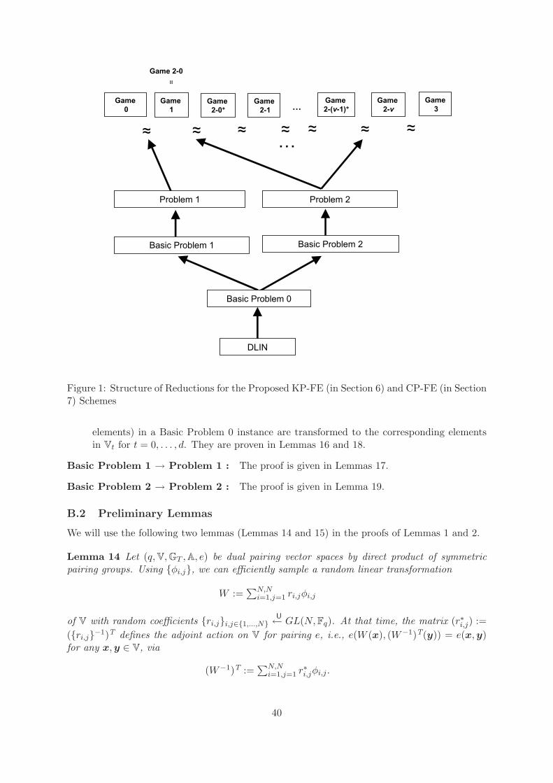
Problem 2

Game0

Game 1

Game 2-0+

Game2-1

Game 2-(v-1)+

Game 2-v

Game 2-0

=

DLIN

…

…Game

3

~~~~~~~~~~~~~~

Basic Problem 2

Problem 1

Basic Problem 0

Basic Problem 1

Figure 1: Structure of Reductions for the Proposed KP-FE (in Section 6) and CP-FE (in Section7) Schemes

elements) in a Basic Problem 0 instance are transformed to the corresponding elementsin Vt for t = 0, . . . , d. They are proven in Lemmas 16 and 18.

Basic Problem 1 → Problem 1 : The proof is given in Lemmas 17.

Basic Problem 2 → Problem 2 : The proof is given in Lemma 19.

B.2 Preliminary Lemmas

We will use the following two lemmas (Lemmas 14 and 15) in the proofs of Lemmas 1 and 2.

Lemma 14 Let (q,V,GT ,A, e) be dual pairing vector spaces by direct product of symmetricpairing groups. Using {φi,j}, we can efficiently sample a random linear transformation

W :=∑N,N

i=1,j=1 ri,jφi,j

of V with random coefficients {ri,j}i,j∈{1,...,N} U← GL(N,Fq). At that time, the matrix (r∗i,j) :=({ri,j}−1)T defines the adjoint action on V for pairing e, i.e., e(W (x), (W−1)T(y)) = e(x,y)for any x,y ∈ V, via

(W−1)T :=∑N,N

i=1,j=1 r∗i,jφi,j .

40

Definition 18 (Basic Problem 0) Basic Problem 0 is to guess β ∈ {0, 1}, given (paramBP0,

B̂,B∗,y∗β ,f , κG, ξG, δξG) R← GBP0β (1λ), where

GBP0β (1λ) : paramG := (q,G,GT , G, e)

R← Gbpg(1λ),

paramV := (q,V,GT ,A, e) := Gdpvs(1λ, 3, paramG),

X :=

⎛⎝ −→χ 1−→χ 2−→χ 3

⎞⎠ := (χi,j)i,jU← GL(3,Fq), (ϑi,j)i,j :=

⎛⎜⎝−→ϑ 1−→ϑ 2−→ϑ 3

⎞⎟⎠ := (XT)−1, κ, ξU← F

×q ,

bi := κ(−→χ i)A = κ∑3

j=1 χi,jaj for i = 1, 3, B̂ := (b1, b3),

b∗i := ξ(−→ϑ i)A = ξ

∑3j=1 ϑi,jat,j for i = 1, 2, 3, B

∗ := (b∗1, b∗2, b∗3),

gT := e(G,G)κξ, paramBP0 := (paramV, gT )

δ, σ, ωU← Fq, ρ, τ

U← F×q ,

y∗0 := (δ, 0, σ)B∗ , y∗1 := (δ, ρ, σ)B∗ , f := (ω, τ, 0)B,

return (paramBP0, B̂,B∗,y∗β ,f , κG, ξG, δξG).

for β U← {0, 1}. For a probabilistic machine D, we define the advantage of D for Basic Problem0, AdvBP0

D (λ), is similarly defined as in Definition 12.

Lemma 15 For any adversary D, there is a probabilistic machine E, whose running timeis essentially the same as that of E, such that for any security parameter λ, AdvBP0

D (λ) ≤AdvDLIN

E (λ) + 5/q.

Proof. Given a DLIN instance

(paramG, G, ξG, κG, δξG, σκG, Yβ),

E calculates

paramV := (q,V,GT ,A, e) := Gdpvs(1λ, 3, paramG),

gT := e(κG, ξG)(= e(G,G)κξ

), paramBP0 := (paramV, gT ).

E sets 3× 3 matrices Π∗,Π as follows:

Π∗ :=

⎛⎝ ξ 11

κ 1

⎞⎠ , Π :=

⎛⎝ κ−κ −ξ κξ

ξ

⎞⎠ ,

Then, Π · (Π∗)T = κξ · I3. By using matrices Π and Π∗, E sets

u∗1 := (ξ, 0, 1)A, u∗2 := (0, 0, 1)A, u∗3 := (0, κ, 1)A,

u1 := (κ, 0, 0)A, u2 := (−κ,−ξ, κξ)A, u3 := (0, ξ, 0)A,

E can compute u∗i for i = 1, 2, 3 and ui for i = 1, 3 from the above DLIN instance. Let bases

U := (ui)i=1,2,3, U∗ := (u∗i )i=1,2,3 of V. E then generates η, ϕ U← Fq such that η �= 0, and sets

v := (ϕG,−ηG, η(κG)) (= (ϕ,−η, ηκ)A) and w∗β := (δξG, σκG, Yβ).

E generates random linear transformation W on V given in Lemma 14, then calculates

41

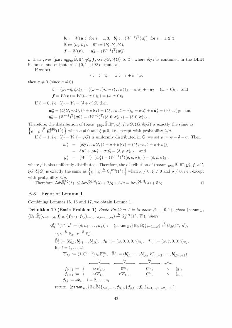
bi := W (ui) for i = 1, 3, b∗i := (W−1)T(u∗i ) for i = 1, 2, 3,B̂ := (b1, b3). B

∗ := (b∗1, b∗2, b∗3),

f = W (v), y∗β = (W−1)T(w∗β)

E then gives (paramBP0, B̂,B∗,y∗β ,f , κG, ξG, δξG) to D, where δξG is contained in the DLIN

instance, and outputs β′ ∈ {0, 1} if D outputs β′.If we set

τ := ξ−1η, ω := τ + κ−1ϕ,

then τ �= 0 (since η �= 0),

v = (ϕ,−η, ηκ)A = ((ω − τ)κ,−τξ, τκξ)A = ωu1 + τu2 = (ω, τ, 0)U, andf = W (v) = W ((ω, τ, 0)U) = (ω, τ, 0)B.

If β = 0, i.e., Yβ = Y0 = (δ + σ)G, then

w∗0 = (δξG, σκG, (δ + σ)G) = (δξ, σκ, δ + σ)A = δu∗1 + σu∗3 = (δ, 0, σ)U∗ andy∗0 = (W−1)T(w∗0) = (W−1)T((δ, 0, σ)U∗) = (δ, 0, σ)B∗ .

Therefore, the distribution of (paramBP0, B̂,B∗,y∗0,f , κG, ξG, δξG) is exactly the same as{

�∣∣∣ � R← GBP0

0 (1λ)}

when κ �= 0 and ξ �= 0, i.e., except with probability 2/q.If β = 1, i.e., Yβ = Y1 (= ψG) is uniformly distributed in G, we set ρ := ψ − δ − σ. Then

w∗1 = (δξG, σκG, (δ + ρ+ σ)G) = (δξ, σκ, δ + ρ+ σ)A

= δu∗1 + ρu∗2 + σu∗3 = (δ, ρ, σ)U∗ , andy∗1 = (W−1)T(w∗1) = (W−1)T((δ, ρ, σ)U∗) = (δ, ρ, σ)B∗ ,

where ρ is also uniformly distributed. Therefore, the distribution of (paramBP0, B̂,B∗,y∗1,f , κG,

ξG, δξG) is exactly the same as{�∣∣∣ � R← GBP0

1 (1λ)}

when κ �= 0, ξ �= 0 and ρ �= 0, i.e., exceptwith probability 3/q.

Therefore, AdvBP0D (λ) ≤ AdvDLIN

E (λ) + 2/q + 3/q = AdvDLINE (λ) + 5/q. ��

B.3 Proof of Lemma 1

Combining Lemmas 15, 16 and 17, we obtain Lemma 1.

Definition 19 (Basic Problem 1) Basic Problem 1 is to guess β ∈ {0, 1}, given (param−→n ,{Bt, B̂∗t }t=0,...,d,fβ,0, {fβ,t,1,ft,i}t=1,...,d;i=2,...,nt)

R← GBP1β (1λ, −→n ), where

GBP1β (1λ,−→n := (d;n1, . . . , nd)) : (param−→n , {Bt,B∗t }t=0,...,d)

R← Gob(1λ,−→n ),

ω, γU← Fq, τ

U← F×q ,

B̂∗0 := (b∗0,1, b

∗0,3, .., b

∗0,5), f0,0 := (ω, 0, 0, 0, γ)B0 , f1,0 := (ω, τ, 0, 0, γ)B0 ,

for t = 1, . . . , d,−→e t,1 := (1, 0nt−1) ∈ F

ntq , B̂

∗t := (b∗t,1, . . . , b

∗t,nt

, b∗t,nt+2, . . . , b∗t,3nt+1),

nt︷︸︸︷ nt︷︸︸︷ nt︷︸︸︷ 1︷︸︸︷f0,t,1 := ( ω−→e t,1, 0nt , 0nt , γ )Bt ,f1,t,1 := ( ω−→e t,1, τ−→e t,1, 0nt , γ )Bt ,

ft,i := ωbt,i i = 2, . . . , nt,

return (param−→n , {Bt, B̂∗t }t=0,...,d,fβ,0, {fβ,t,1,ft,i}t=1,...,d;i=2,...,nt).

42

for βU← {0, 1}. For a probabilistic adversary C, the advantage of C for Basic Problem 1,

AdvBP1C (λ), is similarly defined as in Definition 12.

Lemma 16 For any adversary C, there is a probabilistic machine D, whose running time isessentially the same as that of C, such that for any security parameter λ, AdvBP1

C (λ) ≤ AdvBP0D (λ)

for any −→n := (d; {nt}) := (d;n1, . . . , nd).

Proof. D is given a Basic Problem 0 instance

(paramBP0, B̂,B∗,y∗β ,f , κG, ξG, δξG).

By using paramG := (q,G,GT , G, e) underlying paramBP0, D calculates

param0 := (q,V0,GT ,A0, e) := Gdpvs(1λ, 5, paramG),paramt := (q,Vt,GT ,At, e) := Gdpvs(1λ, 3nt + 1, paramG) for t = 1, . . . , d,param−→n := ({paramt}t=0,...,d, gT ),

where gT is contained in paramBP0. D generates random linear transformation Wt on Vt (t =0, . . . , d) given in Lemma 14, then sets

d0,ι := W0(b∗ι , 0, 0) for ι = 1, 2, d0,3 := W0(0, 0, 0, ξG, 0),d0,4 := W0(b∗3, 0, 0), d0,5 := W0(0, 0, 0, 0, ξG),d∗ι := (W−1

0 )T(bι, 0, 0) for ι = 1, 2, d∗0,3 := (W−10 )T(0, 0, 0, κG, 0),

d∗0,4 := (W−10 )T(b3, 0, 0) d∗0,5 := (W−1

0 )T(0, 0, 0, 0, κG),gβ,0 := W0(y∗β , 0, 0),for t = 1, . . . , d,

dt,1 := Wt(b∗1, 0Nt−3), dt,nt+1 := Wt(b∗2, 0

Nt−3), dt,Nt := Wt(b∗3, 0Nt−3),

otherwise, dt,i := Wt(0ι, ξG, 0Nt−ι−1) where{ι := i+ 1 if i ∈ {2, . . . , nt},ι := i if i ∈ {nt + 2, . . . , Nt − 1},

d∗t,1 := (W−1t )T(b1, 0Nt−3), d∗t,nt+1 := (W−1

t )T(b2, 0Nt−3), d∗t,Nt:= (W−1

t )T(b3, 0Nt−3),

otherwise, d∗t,i := (W−1t )T(0ι, κG, 0Nt−ι−1) where

{ι := i+ 1 if i ∈ {2, . . . , nt},ι := i if i ∈ {nt + 2, . . . , Nt − 1},

gβ,t,1 := Wt(y∗β , 0Nt−3), gt,i := Wt(0i+1, δξG, 0Nt−i−2) for i = 2, . . . , nt,

where (v, 0Nt−3) := (G̃1, G̃2, G̃3, , 0Nt−3) for any v := (G̃1, G̃2, G̃3) ∈ V = G3. Then, D0 :=

(d0,i)i=1,...,5 and D∗0 := (d∗0,i)i=1,...,5, Dt := (dt,i)i=1,...,3nt+1 and D

∗t := (d∗t,i)i=1,...,3nt+1 are dual

orthonormal bases. D can compute Dt for t = 0, . . . , d, D̂∗0 := (d∗0,1,d∗0,3, . . . ,d∗0,5), D̂

∗t :=

(d∗t,1, . . . ,d∗t,nt,d∗t,nt+2, . . . ,d

∗t,3nt+1) for t = 1, . . . , d from B̂ := (b1, b3), B

∗, κG, and ξG. D thengives (param−→n , {Dt, D̂

∗t }t=0,...,d, gβ,0, {gβ,t,1, gt,i}t=1,...,d;i=2,...,nt) to C, and outputs β′ ∈ {0, 1} if

C outputs β′.We can see that

g0,0 := (ω′, 0, 0, 0, γ′)D0 , g1,0 := (ω′, τ ′, 0, 0, γ′)D0 ,

for t = 1, . . . , d,nt︷︸︸︷ nt︷︸︸︷ nt︷︸︸︷ 1︷︸︸︷

g0,t,1 := ( ω′−→e t,1, 0nt , 0nt , γ′ )Dt ,g1,t,1 := ( ω′−→e t,1, τ ′−→e t,1, 0nt , γ′ )Dt ,

gt,i := ω′dt,i for i = 2, . . . , nt,

43

where ω′ := δ, γ′ := σ, and τ ′ := ρ which are distributed uniformly in Fq. Therefore, thedistribution of (param−→n , {Dt, D̂

∗t }t=0,...,d, gβ,0, {gβ,t,1, gt,i}t=1,...,d;i=2,...,nt) is exactly the same as{

�∣∣∣ � R← GBP1

β (1λ,−→n )}

. ��

Lemma 17 For any adversary B, there is a probabilistic machine C, whose running timeis essentially the same as that of B, such that for any security parameter λ, AdvP1

B (λ) ≤AdvBP1

C (λ) + (d+ 1)/q.

Proof. Given a Basic Problem 1 instance

(param−→n , {Bt, B̂∗t }t=0,...,d,fβ,0, {fβ,t,1,ft,i}t=1,...,d;i=2,...,nt),

C calculates

rtU← span〈bt,3nt+1〉, eβ,t,1 := fβ,t,1 + rt for t = 1, . . . , d.

C generates u0U← F

×q ,

⎛⎜⎝−→u t,1

...−→u t,nt

⎞⎟⎠ := UtU← GL(nt,Fq) for t = 1, . . . , d. C then calculates

d0,2 := (0, u0, 0, 0, 0)B0 ,nt︷︸︸︷ nt︷︸︸︷ nt︷︸︸︷ 1︷︸︸︷

dt,nt+i := ( 0nt , −→u t,i, 0nt , 0 )Bt for t = 1, . . . , d; i = 1, . . . , nt,

C then sets dual orthonormal basis vectors

d∗0,2 := (0, u−10 , 0, 0, 0)B∗

0,

nt︷︸︸︷ nt︷︸︸︷ nt︷︸︸︷ 1︷︸︸︷d∗t,nt+i

:= ( 0nt , −→z t,i, 0nt , 0 )B∗t

for t = 1, . . . , d; i = 1 . . . , nt,

where

⎛⎜⎝−→z t,1

...−→z t,nt

⎞⎟⎠ := (U−1t )T. C cannot calculate above d∗0,2 and d∗t,i for i = nt + 1, . . . , 2nt

because of lack of b∗0,2 and b∗t,nt+1. C then sets

D0 := (b0,1,d0,2, b0,3, b0,4, b0,5), D∗0 := (b∗0,1,d

∗0,2, b

∗0,3, b

∗0,4, b

∗0,5), D̂

∗0 := (b∗0,1, b

∗0,3, b

∗0,4, b

∗0,5),

Dt := (bt,1, . . . , bt,nt ,dt,nt+1, . . . ,dt,2nt , bt,2nt+1, . . . , bt,3nt+1),D∗t := (b∗t,1, . . . , b

∗t,nt

,d∗t,nt+1, . . . ,d∗t,2nt

, b∗t,2nt+1, . . . , b∗t,3nt+1)

D̂∗t := (b∗t,1, . . . , b

∗t,nt

, b∗t,2nt+1, . . . , b∗t,3nt+1).

C gives (param−→n , {Dt, D̂∗t }t=0,..,d,fβ,0, {eβ,t,1,ft,i}t=1,...,d;i=2,...,nt) to B, and outputs β′ ∈ {0, 1}

if B outputs β′.Then, with respect to Dt,D

∗t (instead of Bt,B

∗t , respectively), the above answer to B has the

same distribution as the Problem 1 instance, i.e., the above instance has the same distributionas the one given by generator GP1

β (1λ,−→n ) if z0 in Problem 1 is not equal to 0 and (zt,1, . . . , zt,nt)

in Problem 1 is not equal to−→0 for any t = 1, . . . , d, i.e., except with probability (d + 1)/q for

β = 1. ��

44

B.4 Proof of Lemma 2

Combining Lemmas 15, 18 and 19, we obtain Lemma 2.

Definition 20 (Basic Problem 2) Basic Problem 2 is to guess β ∈ {0, 1}, given (param−→n ,{B̂t,B∗t }t=0,..,d,y

∗β,0,f0, {y∗β,t,i,ft,i}t=1,..,d;i=1,..,nt)

R← GBP2β (1λ,−→n ), where

GBP2β (1λ,−→n := (d;n1, . . . , nd)) : (param−→n , {Bt,B∗t }t=0,...,d)

R← Gob(1λ,−→n ),

B̂0 := (b0,1, b0,3, . . . , b0,5),

B̂t := (bt,1, . . . , bt,nt , bt,2nt+1, . . . , bt,3nt+1) for t = 1, . . . , d,

δ, δ0, ωU← Fq, ρ, τ

U← F×q ,

y∗0,0 := (δ, 0, 0, δ0, 0)B∗0, y∗1,0 := (δ, ρ, 0, δ0, 0)B∗

0, f0 := (ω, τ, 0, 0, 0)B0 ,

for t = 1, . . . , d, i = 1, . . . , nt;−→e t,i := (0i−1, 1, 0nt−i) ∈ F

ntq ,

nt︷︸︸︷ nt︷︸︸︷ nt︷︸︸︷ 1︷︸︸︷y∗0,t,i := ( δ−→e t,i, 0nt , δ0

−→e t,i, 0 )B∗t

y∗1,t,i := ( δ−→e t,i, ρ−→e t,i, δ0−→e t,i, 0 )B∗

t

ft,i := ( ω−→e t,i, τ−→e t,i, 0nt , 0 )Bt ,

return (param−→n , {B̂t,B∗t }t=0,..,d,y∗β,0,f0, {y∗β,t,i,ft,i}t=1,..,d;i=1,..,nt).

for β U← {0, 1}. For a probabilistic machine C, we define the advantage of C for Basic Problem2, AdvBP2

C (λ), as in Definition 12.

Lemma 18 For any adversary C, there is a probabilistic machine D, whose running time isessentially the same as that of C, such that for any security parameter λ, AdvBP2

C (λ) = AdvBP0D (λ)

for any −→n := (d; {nt}) := (d;n1, . . . , nd).

Proof. D is given a Basic Problem 0 instance

(paramBP0, B̂,B∗,y∗β ,f , κG, ξG, δξG).

By using paramG := (q,G,GT , G, e) underlying paramBP0, D calculates

param0 := (q,V0,GT ,A0, e) := Gdpvs(1λ, 5, paramG),paramt := (q,Vt,GT ,At, e) := Gdpvs(1λ, 3nt + 1, paramG) for t = 1, . . . , d,param−→n := ({paramt}t=0,...,d, gT ),

where gT is contained in paramBP0. D generates random linear transformation Wt on Vt (t =0, . . . , d) given in Lemma 14, then sets

d0,ι := W0(bι, 0, 0) for ι = 1, 2, d0,3 := W0(0, 0, 0, κG, 0),d0,4 := W0(b3, 0, 0), d0,5 := W0(0, 0, 0, 0, κG),d∗ι := (W−1

0 )T(b∗ι , 0, 0) for ι = 1, 2, d∗0,3 := (W−10 )T(0, 0, 0, ξG, 0),

d∗0,4 := (W−10 )T(b∗3, 0, 0) d∗0,5 := (W−1

0 )T(0, 0, 0, 0, ξG),

p∗β,0 := (W−10 )T(y∗β , 0, 0), g0 := W0(f , 0, 0),

for t = 1, . . . , d,dt,(ι−1)nt+i := Wt(03(i−1), bι, 03(nt−i), 0) for ι = 1, 2, 3; i = 1, . . . , nt,

dt,3nt+1 := Wt(03nt , κG),

d∗t,(ι−1)nt+i:= (W−1

t )T(03(i−1), b∗ι , 03(nt−i), 0) for ι = 1, 2, 3; i = 1, . . . , nt,

45

d∗t,3nt+1 := (W−1t )T(03nt , ξG),

p∗β,t,i := (W−1t )T(03(i−1),y∗β , 0

3(nt−i), 0) for i = 1, . . . , nt,

gt,i := Wt(03(i−1),f , 03(nt−i), 0) for i = 1, . . . , nt.

where (0l1 ,v, 0l2) := (0l1 , G̃1, G̃2, G̃3, 0l2) for any v := (G̃1, G̃2, G̃3) ∈ V = G3 and l1, l2 ∈

Z≥0. Then, D0 := (d0,i)i=1,...,5 and D∗0 := (d∗0,i)i=1,...,5, Dt := (dt,i)i=1,...,3nt+1 and D

∗t :=

(d∗t,i)i=1,...,3nt+1 for t = 1, . . . , d are dual orthonormal bases. D can compute

D̂0 := (d0,1,d0,3, . . . ,d0,5), D∗0 := (d∗0,1, . . . ,d

∗0,5),

for t = 1, . . . , d, D̂t := (dt,1, . . . ,dt,nt ,dt,2nt+1, . . . ,dt,3nt+1), D∗t := (d∗t,1, . . . ,d

∗t,3nt+1),

from B̂ := (b1, b3),B∗, κG, and ξG. D then gives (param−→n , {D̂t,D∗t }t=0,...,d,p

∗β,0, g0, {p∗β,t,i,

gt,i}t=1,...,d;i=1,...,nt) to C, and outputs β′ ∈ {0, 1} if C outputs β′.We can see that

p∗0,0 = (δ, 0, 0, δ0, 0)D∗0, p∗1,0 = (δ, ρ, 0, δ0, 0)D∗

0, g0 = (ω, τ, 0, 0, 0)D0 ,

nt︷︸︸︷ nt︷︸︸︷ nt︷︸︸︷ 1︷︸︸︷p∗0,t,i = ( δ−→e t,i, 0nt , δ0

−→e t,i, 0 )D∗t

p∗1,t,i = ( δ−→e t,i, ρ−→e t,i, δ0−→e t,i, 0 )D∗

t

gt,i = ( ω−→e t,i, τ−→e t,i, 0nt , 0 )Dt ,t = 1, . . . , d; i = 1, . . . , nt,

Therefore, the distribution of (param−→n , {D̂t,D∗t }t=0,...,d,p

∗β,0, g0, {p∗β,t,i, gt,i}t=1,...,d;i=1,...,nt) is ex-

actly the same as{�∣∣∣ � R← GBP2

β (1λ, (d, {nt}))}

. ��Lemma 19 For any adversary B, there is a probabilistic machine C, whose running time isessentially the same as that of B, such that for any security parameter λ, AdvP2

B (λ) = AdvBP2C (λ).

Proof. Given a Basic Problem 2 instance

(param−→n , {B̂t,B∗t }t=0,..,d,y∗β,0,f0, {y∗β,t,i,ft,i}t=1,..,d;i=1,..,nt),

C calculates

r∗t,iU← span〈b∗t,2nt+1, . . . , b

∗t,3nt〉, h∗β,t,i := y∗β,t,i + r∗t,i.

C then generates z′0U← F

×q and

⎛⎜⎝−→z ′t,1

...−→z ′t,nt

⎞⎟⎠ := Z ′tU← GL(nt,Fq), for t = 1, . . . , d, and calculates

d∗0,2 := (0, z′0, 0, 0, 0)B∗0,

nt︷︸︸︷ nt︷︸︸︷ nt︷︸︸︷ 1︷︸︸︷d∗t,nt+i

:= ( 0nt , −→z ′t,i, 0nt , 0 )B∗t

for t = 1, . . . , d; i = 1 . . . , nt.

C then sets z0 := ρ−1z′0, u0 := z−10 ,

⎛⎜⎝−→z t,1

...−→z t,nt

⎞⎟⎠ := Zt := ρ−1Z ′t and

⎛⎜⎝−→u t,1

...−→u t,nt

⎞⎟⎠ := (Z−1t )T,

where ρ is defined in Basic Problem 2. Then,

d∗0,2 = (0, ρz0, 0, 0, 0)B∗0,

nt︷︸︸︷ nt︷︸︸︷ nt︷︸︸︷ 1︷︸︸︷d∗t,nt+i

= ( 0nt , ρ−→z t,i, 0nt , 0 )B∗t

for t = 1, . . . , d; i = 1 . . . , nt.

46

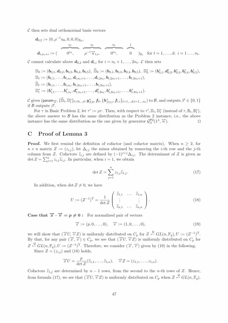
C then sets dual orthonormal basis vectors

d0,2 := (0, ρ−1u0, 0, 0, 0)B0 ,nt︷︸︸︷ nt︷︸︸︷ nt︷︸︸︷ 1︷︸︸︷

dt,nt+i := ( 0nt , ρ−1−→u t,i, 0nt , 0 )Bt for t = 1, . . . , d; i = 1 . . . , nt.

C cannot calculate above d0,2 and dt,i for i = nt + 1, . . . , 2nt. C then sets

D0 := (b0,1,d0,2, b0,3, b0,4, b0,5), D̂0 := (b0,1, b0,3, b0,4, b0,5), D∗0 := (b∗0,1,d

∗0,2, b

∗0,3, b

∗0,4, b

∗0,5),

Dt := (bt,1, . . . , bt,nt ,dt,nt+1, . . . ,dt,2nt , bt,2nt+1, . . . , bt,3nt+1),

D̂t := (bt,1, . . . , bt,nt , bt,2nt+1, . . . , bt,3nt+1),D∗t := (b∗t,1, . . . , b

∗t,nt

,d∗t,nt+1, . . . ,d∗t,2nt

, b∗t,2nt+1, . . . , b∗t,3nt+1).

C gives (param−→n , {D̂t,D∗t }t=0,..,d,y

∗β,0,f0, {h∗β,t,i,ft,i}t=1,..,d;i=1,..,nt) to B, and outputs β′ ∈ {0, 1}

if B outputs β′.For τ in Basic Problem 2, let τ ′ := ρτ . Then, with respect to τ ′,Dt,D

∗t (instead of τ,Bt,B∗t ),

the above answer to B has the same distribution as the Problem 2 instance, i.e., the aboveinstance has the same distribution as the one given by generator GP2

β (1λ,−→n ). ��

C Proof of Lemma 3

Proof. We first remind the definition of cofactor (and cofactor matrix). When n ≥ 2, forn × n matrix Z := (zi,j), let Δi,j the minor obtained by removing the i-th row and the j-thcolumn from Z. Cofactors z̃i,j are defined by (−1)i+jΔi,j . The determinant of Z is given asdetZ =

∑nj=1 zi,j z̃i,j . In particular, when i = 1, we obtain

detZ =n∑j=1

z1,j z̃1,j . (17)

In addition, when detZ �= 0, we have

U := (Z−1)T =1

detZ

⎛⎜⎝ z̃1,1 . . . z̃1,n...

...z̃n,1 . . . z̃n,n

⎞⎟⎠ . (18)

Case that −→x · −→v = p �= 0 : For normalized pair of vectors

−→x := (p, 0, . . . , 0), −→v := (1, 0, . . . , 0), (19)

we will show that (−→x U,−→v Z) is uniformly distributed on Cp for Z U← GL(n,Fq), U := (Z−1)T.By that, for any pair (−→x ,−→v ) ∈ Cp, we see that (−→x U,−→v Z) is uniformly distributed on Cp for

ZU← GL(n,Fq), U := (Z−1)T. Therefore, we consider (−→x ,−→v ) given by (19) in the following.Since Z = (zi,j) and (18) holds,

−→x U =p

detZ(z̃1,1, . . . , z̃1,n), −→v Z = (z1,1, . . . , z1,n).

Cofactors z̃1,j are determined by n − 1 rows, from the second to the n-th rows of Z. Hence,

from formula (17), we see that (−→x U,−→v Z) is uniformly distributed on Cp when Z U← GL(n,Fq).

47

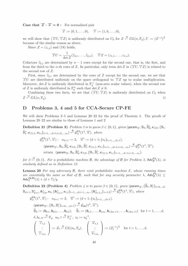
Case that −→x · −→v = 0 : For normalized pair−→x := (0, 1, . . . , 0), −→v := (1, 0, . . . , 0),

we will show that (−→x U,−→v Z) is uniformly distributed on C0 for Z U← GL(n,Fq), U := (Z−1)T

because of the similar reason as above.Since Z = (zi,j) and (18) holds,

−→x U =1

detZ(z̃2,1, . . . , z̃2,n), −→v Z = (z1,1, . . . , z1,n).

Cofactors z̃2,j are determined by n − 1 rows except for the second one, that is, the first, andfrom the third to the n-th rows of Z. In particular, only term detZ in (−→x U,−→v Z) is related tothe second row of Z.

First, since z̃2,1 are determined by the rows of Z except for the second one, we see that−→x U are distributed uniformly on the space orthogonal to −→v Z up to scalar multiplication.Moreover, detZ is uniformly distributed in F

×q (non-zero scalar values), when the second row

of Z is uniformly distributed in Fnq such that detZ �= 0.

Combining these two facts, we see that (−→x U,−→v Z) is uniformly distributed on C0 whenZ

U← GL(n,Fq). ��

D Problems 3, 4 and 5 for CCA-Secure CP-FE

We will show Problems 3–5 and Lemmas 20–22 for the proof of Theorem 4. The proofs ofLemmas 20–22 are similar to those of Lemmas 1 and 2

Definition 21 (Problem 3) Problem 3 is to guess β ∈ {0, 1}, given (param−→n ,B0, B̂∗0, eβ,0, {Bt,

B̂∗t , eβ,t,1, et,i}t=1,...,d+1;i=2,...,nt)

R← GP3β (1λ,−→n ), where

GP3β (1λ,−→n ) : nd+1 := 2, −→n ′ := (d+ 1; {nt}t=1,...,d+1),

(param−→n ′ ,B0, B̂∗0, eβ,0, {Bt, B̂∗t , eβ,t,1, et,i}t=1,...,d+1;i=2,...,nt)

R← GP1β (1λ,−→n ′),

return (param−→n ,B0, B̂∗0, eβ,0, {Bt, B̂∗t , eβ,t,1, et,i}t=1,...,d+1;i=2,...,nt).

for β U← {0, 1}. For a probabilistic machine B, the advantage of B for Problem 3, AdvP3B (λ), is


Lemma 20 For any adversary B, there exist probabilistic machine E, whose running timesare essentially the same as that of B, such that for any security parameter λ, AdvP3

B (λ) ≤AdvDLIN

E (λ) + (d+ 7)/q.

Definition 22 (Problem 4) Problem 4 is to guess β ∈ {0, 1}, given (param−→n , {B̂t,B∗t }t=0,..,d,

Bd+1,B∗d+1,h

∗β,0, e0, {h∗β,t,i, et,i}t=1,..,d;i=1,..,nt , {h∗d+1,i}i=1,2)


GP4β (1λ,−→n ) : nd+1 := 2, −→n ′ := (d+ 1; {nt}t=1,...,d+1),

(param−→n ′ , {Bt,B∗t }t=0,...,d+1)R← Gob(1λ,−→n ′),

B̂0 := (b0,1, b0,3, . . . , b0,5), B̂t := (bt,1, . . . , bt,nt , bt,2nt+1, . . . , bt,3nt+1) for t = 1, . . . , d,

δ, δ0, ωU← Fq, u0, τ

U← F×q , z0 := u−1

0 ,⎛⎜⎝−→z t,1

...−→z t,nt

⎞⎟⎠ := ZtU← GL(nt,Fq),

⎛⎜⎝−→u t,1

...−→u t,nt

⎞⎟⎠ := (Z−1t )T for t = 1, . . . , d,

48

h∗0,0 := (δ, 0, 0, δ0, 0)B∗0, h∗1,0 := (δ, u0, 0, δ0, 0)B∗

0, e0 := (ω, τz0, 0, 0, 0)B0 ,

for t = 1, . . . , d; i = 1, . . . , nt;−→e t,i := (0i−1, 1, 0nt−i) ∈ F

ntq ,

−→δ t,i

U← Fntq ,

nt︷︸︸︷ nt︷︸︸︷ nt︷︸︸︷ 1︷︸︸︷h∗0,t,i := ( δ−→e t,i, 0nt ,

−→δ t,i, 0 )B∗

t,

h∗1,t,i := ( δ−→e t,i, −→u t,i, −→δ t,i, 0 )B∗

t,

et,i := ( ω−→e t,i, τ−→z t,i, 0nt , 0 )Bt

h∗d+1,i := δb∗d+1,i for i = 1, 2,

return (param−→n , {B̂t,B∗t }t=0,..,d,Bd+1,B∗d+1,h

∗β,0, e0, {h∗β,t,i, et,i}t=1,..,d;i=1,..,nt , {h∗d+1,i}i=1,2).



Lemma 21 For any adversary B, there exists a probabilistic machine E, whose running timeis essentially the same as that of B, such that for any security parameter λ, AdvP4

B (λ) ≤AdvDLIN

E (λ) + 5/q.

Definition 23 (Problem 5) Problem 5 is to guess β ∈ {0, 1}, given (param−→n , {B̂t,B∗t }t=0,d+1,

{Bt,B∗t }t=1,..,d,h∗β,0, e0, {h∗t,i}t=1,..,d;i=1,..,nt , {h∗β,d+1,i, ed+1,i}i=1,2)


GP5β (1λ,−→n ) : nd+1 := 2, −→n ′ := (d+ 1; {nt}t=1,...,d+1),

(param−→n ′ , {Bt,B∗t }t=0,...,d+1)R← Gob(1λ,−→n ′),

B̂0 := (b0,1, b0,3, . . . , b0,5), B̂d+1 := (bd+1,1, bd+1,2, bd+1,5, . . . , bd+1,7),

δ, δ0, ωU← Fq, u0, τ

U← F×q , z0 := u−1

0 ,

h∗0,0 := (δ, 0, 0, δ0, 0)B∗0, h∗1,0 := (δ, u0, 0, δ0, 0)B∗

0, e0 := (ω, τz0, 0, 0, 0)B0 ,

h∗t,i := δb∗t,i for t = 1, . . . , d; i = 1, . . . , nt,( −→z d+1,1−→z d+1,2

):= Zd+1

U← GL(2,Fq),( −→u d+1,1−→u d+1,2

):= (Z−1

d+1)T,

for i = 1, 2,−→e d+1,i := (0i−1, 1, 02−i) ∈ F

2q ,−→δ d+1,i

U← F2q ,

2︷︸︸︷ 2︷︸︸︷ 2︷︸︸︷ 1︷︸︸︷h∗0,d+1,i := ( δ−→e d+1,i, 02,

−→δ d+1,i, 0 )B∗

d+1,

h∗1,d+1,i := ( δ−→e d+1,i,−→u d+1,i,

−→δ d+1,i, 0 )B∗

d+1,

ed+1,i := ( ω−→e d+1,i, τ−→z d+1,i, 02, 0 )Bd+1,

return (param−→n , {B̂t,B∗t }t=0,d+1, {Bt,B∗t }t=1,..,d,

h∗β,0, e0, {h∗t,i}t=1,..,d;i=1,..,nt , {h∗β,d+1,i, ed+1,i}i=1,2),



Lemma 22 For any adversary B, there is a probabilistic machine E, whose running timeis essentially the same as that of B, such that for any security parameter λ, AdvP5

B (λ) ≤AdvDLIN

E (λ) + 5/q.

49

E Generalized Version of Lemma 3

Let V is n-dimensional vector space Fnq , and V ∗ its dual. For −→p := (p1, . . . , ps) ∈ F

sq , let

C−→p :={

(−→x ,−→v 1, . . . ,−→v s)

∣∣∣∣ −→x �= −→0 , −→x · −→v i = pi for i = 1, . . . , s{−→v i}i=1,...,s are linearly independent over Fq,

}⊂ V × (V ∗)s.

Lemma 23 For all −→p such that C−→p �= ∅, for all (−→x ,−→v 1, . . . ,−→v s) ∈ C−→p , and (−→r ,−→w 1, . . . ,

−→w s) ∈C−→p ,

PrZ

U← GL(n,Fq),

[−→x U = −→r ∧ −→v iZ = −→w i for i = 1, . . . , s] =1

� C−→p,

where U := (Z−1)T.

Proof. Case that there exists an i such that −→x · −→v i = pi �= 0 : We can assumethat pi �= 0 for i = 1, . . . , t, pi = 0 for i = t + 1, . . . , s through an appropriate change of orderof coordinates. Then t ≥ 1.

For normalized tuple of vectors

−→x = (p1, . . . , pt, 0, . . . , 0), −→v i := (i−1︷︸︸︷

0, . . . , 0, 1,n−i︷︸︸︷

0, . . . , 0) for i = 1, . . . , s, (20)

we will show that (−→x U,−→v 1Z, . . . ,−→v sZ) is uniformly distributed on C−→p for Z U← GL(n,Fq), U :=

(Z−1)T. By that, for any pair (−→x ,−→v 1, . . . ,−→v s) ∈ C−→p , we see that (−→x U,−→v 1Z, . . . ,

−→v sZ)

is uniformly distributed on C−→p for Z U← GL(n,Fq), U := (Z−1)T. Therefore, we consider(−→x ,−→v 1, . . . ,

−→v s) given by (20) in the following.Since Z = (zi,j) and (18) holds,

−→x U =1

detZ

t∑i=1

pi(z̃i,1, . . . , z̃i,n), −→v iZ = (zi,1, . . . , zi,n) for i = 1, . . . , s.

Cofactors z̃i,j are determined by n− 1 rows of Z except for the i-th one. Hence, from formula

(17), we see that (−→x U,−→v 1Z, . . . ,−→v sZ) is uniformly distributed on C−→p when Z U← GL(n,Fq).

Case that pi = −→x · −→v i = 0 for all 1 ≤ i ≤ s : For normalized tuple

−→x = (s︷︸︸︷

0, . . . , 0, 1,n−s−1︷︸︸︷

0, . . . , 0), −→v i := (i−1︷︸︸︷

0, . . . , 0, 1,n−i︷︸︸︷

0, . . . , 0) for i = 1, . . . , s,

we will show that (−→x U,−→v 1Z, . . . ,−→v sZ) is uniformly distributed on C−→

0for Z U← GL(n,Fq), U :=

(Z−1)T because of the similar reason as above (where−→0 := (0, . . . , 0)).

Since Z = (zi,j) and (18) holds,

−→x U =1

detZ(z̃s+1,1, . . . , z̃s+1,n), −→v iZ = (zi,1, . . . , zi,n) for i = 1, . . . , s.

Cofactors z̃s+1,j are determined by n− 1 rows of Z except for the (s+ 1)-th one. In particular,only term detZ in (−→x U,−→v 1Z, . . . ,

−→v sZ) is related to the (s+ 1)-th row of Z.First, since z̃s+1,j are determined by the rows of Z except for the (s + 1)-th one, we see

that −→x U is distributed uniformly on the space orthogonal to span〈−→v 1Z, . . . ,−→v sZ〉 up to scalar

multiplication. Moreover, detZ is uniformly distributed in F×q (non-zero scalar values), when

the (s+ 1)-th row of Z is uniformly distributed in Fnq such that detZ �= 0.

Combining these two facts, we see that (−→x U,−→v 1Z, . . . ,−→v sZ) is uniformly distributed on

C−→0

when Z U← GL(n,Fq). ��

50

F How to Relax the Restriction that ρ̃ Is Injective

We assume that ϕ ∈ N is given in the system. For any access structure S := (M,ρ) for ciphertextin the CP-FE scheme, ϕ ≥ maxdt=1 #{i | ρ̃(i) = t}. (In the proposed CP-FE scheme in Section7, we assume that ϕ := 1.)

We will show how to modify the CP-FE scheme to allow ϕ > 1 with preserving the securityof the CP-FE scheme in Section 7.

We can also show the similar modification of the KP-FE scheme to allow ϕ > 1.

F.1 The Modified CP-FE Scheme

1. As for Setup, given (1λ, −→n := (d;n1, . . . , nd)), execute Setup(1λ, −→n ′ := (d;n′1, . . . , n′d))such that n′t := nt + ϕ for t = 1, . . . , d.

2. As for KeyGen, given (pk, sk, Γ := {(t,−→x t := (xt,1, . . . , xt,nt) ∈ Fntq ) | 1 ≤ t ≤ d}) execute

the same procedure as KeyGen except that:

n′t︷︸︸︷ n′

t︷︸︸︷ n′t︷︸︸︷ 1︷︸︸︷

k∗t := ( δ−→x t, 0ϕ 0n′t , −→ϕ t, 0 )B∗


3. As for Enc, given (pk, m, S := (M,ρ)), execute the same procedure as Enc except that:

if ρ(i) = (t,−→v i := (vi,1, . . . , vi,nt) ∈ Fntq ) ηi, τi

U← Fq,

n′t︷︸︸︷ n′

t︷︸︸︷ n′t︷︸︸︷ 1︷︸︸︷

ci := ( si−→e t,1 + θi

−→v i, 0κ−1, τi, 0ϕ−κ, 0n′t , 0n

′t , ηi )Bt

if ρ(i) = ¬(t,−→v i), ηi, τiU← Fq,

n′t︷︸︸︷ n′

t︷︸︸︷ n′t︷︸︸︷ 1︷︸︸︷

ci := ( si−→v i, 0κ−1, τi, 0ϕ−κ, 0n

′t , 0n

′t , ηi )Bt ,

where i is the κ-th index such that ρ̃(i) = t and �{j < i | ρ̃(j) = t} = κ− 1.

F.2 Security

We can prove the security of the modified CP-FE scheme in a manner similar to that of Theorem2 except that Problem 2 is changed to Modified Problem 2, Lemma 10 is changed, where B+

2 ’ssimulation is executed on Modified Problem 2, Game 2-h+ is changed to Modified Game 2-h+,and Claim 2 is proven based on Lemma 23 in place of Lemma 3.

Here we only show the essence of the change by using Modified Game 2-h+. The ModifiedGame 2-h+ is the same as Game 2-h+ except that Zt

U← GL(n′t,Fq), Ut := (Z−1t )T for t =

1, . . . , d, where for each t such that {iκ | ρ̃(iκ) = t, 1 ≤ κ ≤ ϕ}} is not empty, and forκ = 1, . . . , ϕ, the framed part by a box in k∗t in Eq. (14) is (−→x t, 0ϕ) ·Ut, and the framed parts bya box in ci (:= ciκ) in Eq. (15) are (ai−→e t,1+πi−→v i, 0κ−1, τ ′i , 0

ϕ−κ)·Zt and (ai−→v i, 0κ−1, τ ′i , 0ϕ−κ)·Zt,

where τ ′iU← Fq for i = 1, . . . , �. By using Modified Problem 2, B+

2 can simulate the ciphertexts,ciκ . By applying Lemma 23, we can prove Claim 2 for the changed simulation by B+

2 in amanner similar to the proof of Claim 2.

51

G Special Cases

This section describes special cases, KP-ABE and CP-ABE, of the proposed FE schemes givenin Sections 6 and 7. Here, the underlying attribute vectors, {−→x t}t∈{1,...,d} and {−→v i}i∈{1,...,�},are specialized to two-dimensional vectors for the equality relation, e.g., −→x t := (1, xt) and−→v i := (vi,−1), where −→x t ·−→v i = 0 iff xt = vi. These schemes are also adaptively payload-hidingunder the DLIN assumption.

G.1 KP-ABE with Non-Monotone Access Structures

Setup(1λ, −→n := (d; 2, . . . , 2)) : (param−→n , {Bt,B∗t }t=0,...,d)R← Gob(1λ,−→n ),

B̂0 := (b0,1, b0,3, b0,5), B̂t := (bt,1, bt,2, bt,7) for t = 1, .., d,

B̂∗0 := (b∗0,1, b

∗0,3, b

∗0,4), B̂

∗t := (b∗t,1, b

∗t,2, b

∗t,5, b

∗t,6) for t = 1, .., d,

return pk := (1λ, param−→n , {B̂t}t=0,...,d), sk := {B̂∗t }t=0,...,d,

KeyGen(pk, sk, S := (M,ρ)) :−→f

U← Frq ,−→s T := (s1, . . . , s�)T := M · −→f T, s0 :=

−→1 · −→f T, η0

U← Fq,

k∗0 := (−s0, 0, 1, η0, 0)B∗0,

for i = 1, . . . , �,

if ρ(i) = (t,−→v i := (vi,−1) ∈ F2q \ {

−→0 }), θi


2q ,

2︷︸︸︷ 2︷︸︸︷ 2︷︸︸︷ 1︷︸︸︷k∗i := ( si + θivi, −θi, 0, 0, −→η i, 0 )B∗

t,

if ρ(i) = ¬(t,−→v i), −→η i U← F2q ,

2︷︸︸︷ 2︷︸︸︷ 2︷︸︸︷ 1︷︸︸︷k∗i := ( sivi, −si, 0, 0, −→η i, 0 )B∗

t,

return skS := (S,k∗0,k∗1, . . . ,k

∗� ).

Enc(pk, m, Γ := {(t,−→x t := (1, xt) ∈ F2q \ {

−→0 }) | 1 ≤ t ≤ d}) :

ω, ϕ0, ϕt, ζU← Fq for (t,−→x t) ∈ Γ,

c0 := (ω, 0, ζ, 0, ϕ0)B0 ,2︷︸︸︷ 2︷︸︸︷ 2︷︸︸︷ 1︷︸︸︷

ct := ( ω, ωxt, 0, 0, 0, 0, ϕt )Bt for (t,−→x t) ∈ Γ,

cd+1 := gζTm, ctΓ := (Γ, c0, {ct}(t,−→x t)∈Γ, cd+1),return ctΓ.

Dec(pk, skS := (S,k∗0,k∗1, . . . ,k

∗� ), ctΓ := (Γ, c0, {ct}(t,−→x t)∈Γ, cd+1)) :

If S := (M,ρ) accepts Γ := {(t,−→x t)}, then compute I and {αi}i∈I such that−→1 =


I ⊆ {i ∈ {1, . . . , �} | [ρ(i) = (t,−→v i) ∧ (t,−→x t) ∈ Γ ∧ vi = xt]∨ [ρ(i) = ¬(t,−→v i) ∧ (t,−→x t) ∈ Γ ∧ vi �= xt] },

K := e(c0,k∗0)

∏i∈I ∧ ρ(i)=(t,−→v i)

e(ct,k∗i )αi

∏i∈I ∧ ρ(i)=¬(t,−→v i)

e(ct,k∗i )αi/(vi−xt),


52

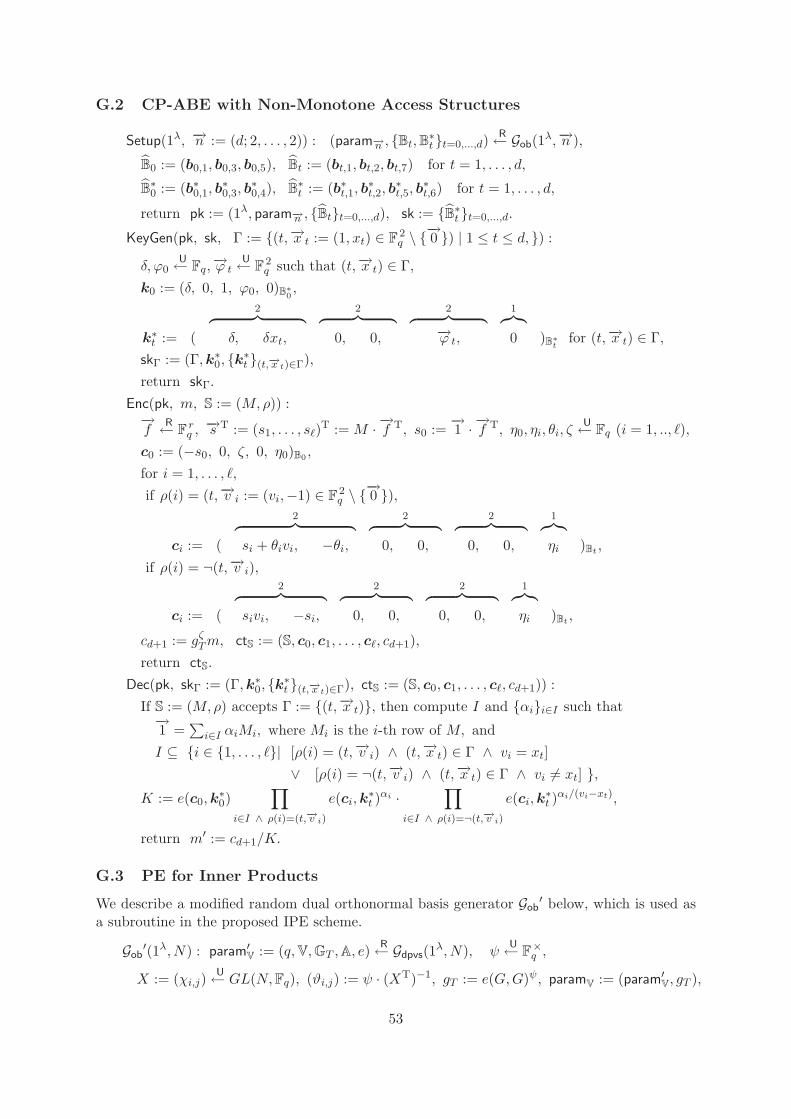
G.2 CP-ABE with Non-Monotone Access Structures

Setup(1λ, −→n := (d; 2, . . . , 2)) : (param−→n , {Bt,B∗t }t=0,...,d)R← Gob(1λ,−→n ),

B̂0 := (b0,1, b0,3, b0,5), B̂t := (bt,1, bt,2, bt,7) for t = 1, . . . , d,

B̂∗0 := (b∗0,1, b

∗0,3, b

∗0,4), B̂

∗t := (b∗t,1, b

∗t,2, b

∗t,5, b

∗t,6) for t = 1, . . . , d,

return pk := (1λ, param−→n , {B̂t}t=0,...,d), sk := {B̂∗t }t=0,...,d.

KeyGen(pk, sk, Γ := {(t,−→x t := (1, xt) ∈ F2q \ {

−→0 }) | 1 ≤ t ≤ d, }) :

δ, ϕ0U← Fq,

−→ϕ tU← F

2q such that (t,−→x t) ∈ Γ,

k0 := (δ, 0, 1, ϕ0, 0)B∗0,

2︷︸︸︷ 2︷︸︸︷ 2︷︸︸︷ 1︷︸︸︷k∗t := ( δ, δxt, 0, 0, −→ϕ t, 0 )B∗


skΓ := (Γ,k∗0, {k∗t }(t,−→x t)∈Γ),return skΓ.

Enc(pk, m, S := (M,ρ)) :−→f

R← Frq ,−→s T := (s1, . . . , s�)T := M · −→f T, s0 :=

−→1 · −→f T, η0, ηi, θi, ζ

U← Fq (i = 1, .., �),c0 := (−s0, 0, ζ, 0, η0)B0 ,

for i = 1, . . . , �,if ρ(i) = (t,−→v i := (vi,−1) ∈ F

2q \ {

−→0 }),

2︷︸︸︷ 2︷︸︸︷ 2︷︸︸︷ 1︷︸︸︷ci := ( si + θivi, −θi, 0, 0, 0, 0, ηi )Bt ,

if ρ(i) = ¬(t,−→v i),2︷︸︸︷ 2︷︸︸︷ 2︷︸︸︷ 1︷︸︸︷

ci := ( sivi, −si, 0, 0, 0, 0, ηi )Bt ,

cd+1 := gζTm, ctS := (S, c0, c1, . . . , c�, cd+1),return ctS.

Dec(pk, skΓ := (Γ,k∗0, {k∗t }(t,−→x t)∈Γ), ctS := (S, c0, c1, . . . , c�, cd+1)) :If S := (M,ρ) accepts Γ := {(t,−→x t)}, then compute I and {αi}i∈I such that−→1 =


I ⊆ {i ∈ {1, . . . , �}| [ρ(i) = (t,−→v i) ∧ (t,−→x t) ∈ Γ ∧ vi = xt]∨ [ρ(i) = ¬(t,−→v i) ∧ (t,−→x t) ∈ Γ ∧ vi �= xt] },

K := e(c0,k∗0)

∏i∈I ∧ ρ(i)=(t,−→v i)

e(ci,k∗t )αi ·

∏i∈I ∧ ρ(i)=¬(t,−→v i)

e(ci,k∗t )αi/(vi−xt),


G.3 PE for Inner Products

We describe a modified random dual orthonormal basis generator Gob′ below, which is used as

a subroutine in the proposed IPE scheme.

Gob′(1λ, N) : param′V := (q,V,GT ,A, e)

R← Gdpvs(1λ, N), ψU← F

×q ,

X := (χi,j)U← GL(N,Fq), (ϑi,j) := ψ · (XT)−1, gT := e(G,G)ψ, paramV := (param′V, gT ),

53

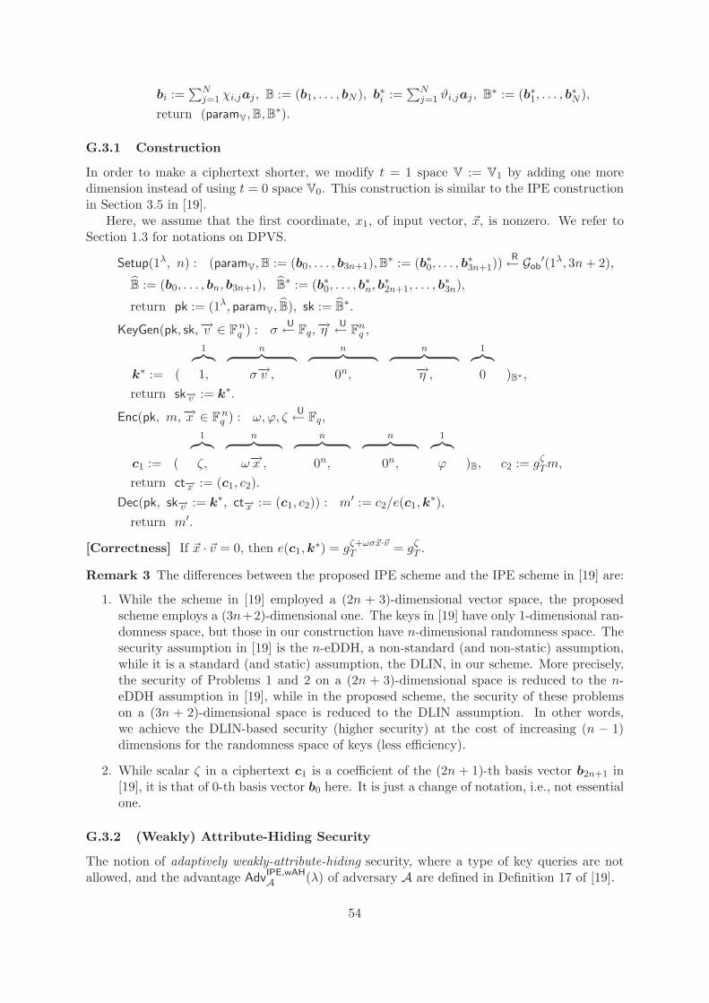
bi :=∑N

j=1 χi,jaj , B := (b1, . . . , bN ), b∗i :=∑N

j=1 ϑi,jaj , B∗ := (b∗1, . . . , b∗N ),

return (paramV,B,B∗).

G.3.1 Construction

In order to make a ciphertext shorter, we modify t = 1 space V := V1 by adding one moredimension instead of using t = 0 space V0. This construction is similar to the IPE constructionin Section 3.5 in [19].

Here, we assume that the first coordinate, x1, of input vector, �x, is nonzero. We refer toSection 1.3 for notations on DPVS.

Setup(1λ, n) : (paramV,B := (b0, . . . , b3n+1),B∗ := (b∗0, . . . , b∗3n+1))

R← Gob′(1λ, 3n+ 2),

B̂ := (b0, . . . , bn, b3n+1), B̂∗ := (b∗0, . . . , b

∗n, b∗2n+1, . . . , b

∗3n),

return pk := (1λ, paramV, B̂), sk := B̂∗.

KeyGen(pk, sk,−→v ∈ Fnq ) : σ

U← Fq,−→η U← F

nq ,

1︷︸︸︷ n︷︸︸︷ n︷︸︸︷ n︷︸︸︷ 1︷︸︸︷k∗ := ( 1, σ−→v , 0n, −→η , 0 )B∗ ,

return sk−→v := k∗.

Enc(pk, m,−→x ∈ Fnq ) : ω, ϕ, ζ

U← Fq,

1︷︸︸︷ n︷︸︸︷ n︷︸︸︷ n︷︸︸︷ 1︷︸︸︷c1 := ( ζ, ω−→x , 0n, 0n, ϕ )B, c2 := gζTm,

return ct−→x := (c1, c2).Dec(pk, sk−→v := k∗, ct−→x := (c1, c2)) : m′ := c2/e(c1,k

∗),return m′.

[Correctness] If �x · �v = 0, then e(c1,k∗) = gζ+ωσ�x·�vT = gζT .

Remark 3 The differences between the proposed IPE scheme and the IPE scheme in [19] are:

1. While the scheme in [19] employed a (2n + 3)-dimensional vector space, the proposedscheme employs a (3n+2)-dimensional one. The keys in [19] have only 1-dimensional ran-domness space, but those in our construction have n-dimensional randomness space. Thesecurity assumption in [19] is the n-eDDH, a non-standard (and non-static) assumption,while it is a standard (and static) assumption, the DLIN, in our scheme. More precisely,the security of Problems 1 and 2 on a (2n + 3)-dimensional space is reduced to the n-eDDH assumption in [19], while in the proposed scheme, the security of these problemson a (3n + 2)-dimensional space is reduced to the DLIN assumption. In other words,we achieve the DLIN-based security (higher security) at the cost of increasing (n − 1)dimensions for the randomness space of keys (less efficiency).

2. While scalar ζ in a ciphertext c1 is a coefficient of the (2n + 1)-th basis vector b2n+1 in[19], it is that of 0-th basis vector b0 here. It is just a change of notation, i.e., not essentialone.

G.3.2 (Weakly) Attribute-Hiding Security

The notion of adaptively weakly-attribute-hiding security, where a type of key queries are notallowed, and the advantage AdvIPE,wAH

A (λ) of adversary A are defined in Definition 17 of [19].

54

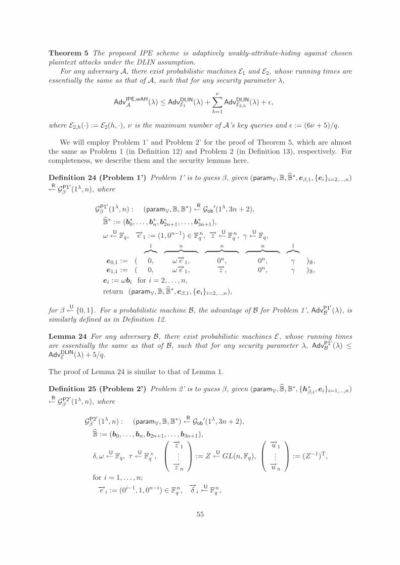
Theorem 5 The proposed IPE scheme is adaptively weakly-attribute-hiding against chosenplaintext attacks under the DLIN assumption.

For any adversary A, there exist probabilistic machines E1 and E2, whose running times areessentially the same as that of A, such that for any security parameter λ,

AdvIPE,wAHA (λ) ≤ AdvDLIN

E1 (λ) +ν∑h=1

AdvDLINE2,h

(λ) + ε,

where E2,h(·) := E2(h, ·), ν is the maximum number of A’s key queries and ε := (6ν + 5)/q.

We will employ Problem 1’ and Problem 2’ for the proof of Theorem 5, which are almostthe same as Problem 1 (in Definition 12) and Problem 2 (in Definition 13), respectively. Forcompleteness, we describe them and the security lemmas here.

Definition 24 (Problem 1’) Problem 1’ is to guess β, given (paramV,B, B̂∗, eβ,1, {ei}i=2,...,n)

R← GP1′β (1λ, n), where

GP1′β (1λ, n) : (paramV,B,B

∗) R← Gob′(1λ, 3n+ 2),

B̂∗ := (b∗0, . . . , b

∗n, b∗2n+1, . . . , b

∗3n+1),

ωU← Fq,

−→e 1 := (1, 0n−1) ∈ Fnq ,−→z U← F

nq , γ

U← Fq,

1︷︸︸︷ n︷︸︸︷ n︷︸︸︷ n︷︸︸︷ 1︷︸︸︷e0,1 := ( 0, ω−→e 1, 0n, 0n, γ )B,e1,1 := ( 0, ω−→e 1,

−→z , 0n, γ )B,

ei := ωbi for i = 2, . . . , n,return (paramV,B, B̂

∗, eβ,1, {ei}i=2,...,n),

for β U← {0, 1}. For a probabilistic machine B, the advantage of B for Problem 1’, AdvP1′B (λ), is


Lemma 24 For any adversary B, there exist probabilistic machines E, whose running timesare essentially the same as that of B, such that for any security parameter λ, AdvP1′

B (λ) ≤AdvDLIN

E (λ) + 5/q.

The proof of Lemma 24 is similar to that of Lemma 1.

Definition 25 (Problem 2’) Problem 2’ is to guess β, given (paramV, B̂,B∗, {h∗β,i, ei}i=1,...,n)

R← GP2′β (1λ, n), where

GP2′β (1λ, n) : (paramV,B,B

∗) R← Gob′(1λ, 3n+ 2),

B̂ := (b0, . . . , bn, b2n+1, . . . , b3n+1),

δ, ωU← Fq, τ

U← F×q ,

⎛⎜⎝−→z 1...−→z n

⎞⎟⎠ := ZU← GL(n,Fq),

⎛⎜⎝−→u 1...−→u n

⎞⎟⎠ := (Z−1)T,

for i = 1, . . . , n;−→e i := (0i−1, 1, 0n−i) ∈ F

nq ,−→δ i

U← Fnq ,

55

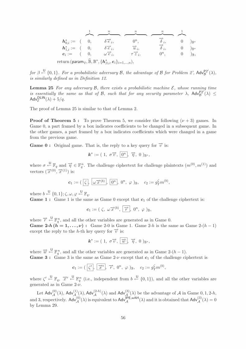
1︷︸︸︷ n︷︸︸︷ n︷︸︸︷ n︷︸︸︷ 1︷︸︸︷h∗0,i := ( 0, δ−→e i, 0n,

−→δ i, 0 )B∗

h∗1,i := ( 0, δ−→e i, −→u i, −→δ i, 0 )B∗

ei := ( 0, ω−→e i, τ−→z i, 0n, 0 )B,

return (paramV, B̂,B∗, {h∗β,i, ei}i=1,...,n),

for β U← {0, 1}. For a probabilistic adversary B, the advantage of B for Problem 2’, AdvP2′B (λ),

is similarly defined as in Definition 12.

Lemma 25 For any adversary B, there exists a probabilistic machine E, whose running timeis essentially the same as that of B, such that for any security parameter λ, AdvP2′

B (λ) ≤AdvDLIN

E (λ) + 5/q.

The proof of Lemma 25 is similar to that of Lemma 2.

Proof of Theorem 5 : To prove Theorem 5, we consider the following (ν + 3) games. InGame 0, a part framed by a box indicates coefficients to be changed in a subsequent game. Inthe other games, a part framed by a box indicates coefficients which were changed in a gamefrom the previous game.

Game 0 : Original game. That is, the reply to a key query for −→v is:

k∗ := ( 1, σ−→v , 0n , −→η , 0 )B∗ ,

where σ U← Fq and −→η ∈ Fnq . The challenge ciphertext for challenge plaintexts (m(0),m(1)) and

vectors (−→x (0),−→x (1)) is:

c1 := ( ζ , ω−→x (b) , 0n , 0n, ϕ )B, c2 := gζTm(b),

where b U← {0, 1}; ζ, ω, ϕ U← Fq.Game 1 : Game 1 is the same as Game 0 except that c1 of the challenge ciphertext is:

c1 := ( ζ, ω−→x (b), −→r , 0n, ϕ )B,

where −→r U← Fnq , and all the other variables are generated as in Game 0.

Game 2-h (h = 1, . . . , ν) : Game 2-0 is Game 1. Game 2-h is the same as Game 2-(h − 1)except the reply to the h-th key query for −→v is:

k∗ := ( 1, σ−→v , −→w , −→η , 0 )B∗ ,

where −→w U← Fnq , and all the other variables are generated as in Game 2-(h− 1).

Game 3 : Game 3 is the same as Game 2-ν except that c1 of the challenge ciphertext is

c1 := ( ζ ′ , −→x ′ , −→r , 0n, ϕ )B, c2 := gζTm(b),

where ζ ′ U← Fq,−→x ′ U← F

nq (i.e., independent from b

U← {0, 1}), and all the other variables aregenerated as in Game 2-ν.


(1)A (λ),Adv

(2-h)A (λ) and Adv

(3)A (λ) be the advantage of A in Game 0, 1, 2-h,

and 3, respectively. Adv(0)A (λ) is equivalent to AdvIPE,wAH

A (λ) and it is obtained that Adv(3)A (λ) = 0

by Lemma 29.

56

We will show three lemmas (Lemmas 26–28) that evaluate the gaps between pairs of Adv(0)A (λ),

Adv(1)A (λ),Adv

(2-h)A (λ) for h = 1, . . . , ν and Adv

(3)A (λ). From these lemmas and Lemmas 24 and

25, we obtain AdvIPE,wAHA (λ) = Adv

(0)A (λ) ≤

∣∣∣Adv(0)A (λ)− Adv

(1)A (λ)

∣∣∣ +∑ν

h=1

∣∣∣Adv(2-(h−1))A (λ)−

Adv(2-h)A (λ)

∣∣∣ +∣∣∣Adv

(2-ν)A (λ)− Adv

(3)A (λ)

∣∣∣ + Adv(3)A (λ) ≤ AdvP1′

B1(λ) +

∑νh=1 AdvP2′

B2,h(λ) + ν/q ≤

AdvDLINE1 (λ) +

∑νh=1 AdvDLIN

E2,h(λ) + (6ν + 5)/q. This completes the proof of Theorem 5. ��


(0)A (λ) −

Adv(1)A (λ)| = AdvP1′

B1(λ).

Proof. In order to prove Lemma 26, we construct a probabilistic machine B1 against Problem1’ by using any adversary A in a security game (Game 0 or 1) as a black box.

The construction of B1 is the same as the machine B0 in the proof of Lemma 24 in [19] exceptfor step 5. In the step, when B1 gets challenge plaintexts (m(0),m(1)) and challenge attributes(−→x (0),−→x (1)) (from A), B1 calculates and returns (c1, c2) such that c1 := ζb0 + x

(b)1 eβ,1 +∑n

i=2 x(b)i ei and c2 := gζTm

(b) where e1 and {ei}i=2,...,n are from the Problem 1’ instance B1

obtained, ζ U← Fq and b U← {0, 1}.Similar to Lemma 24 in [19], if β = 0, the distribution of (c1, c2) generated in step 5 is the

same as that in Game 0. If β = 1, the distribution of (c1, c2) generated in step 5 is the same asthat in Game 1.

Therefore, |Adv(0)A (λ)− Adv

(1)A (λ)| = AdvP1′

B1(λ). This completes the proof of Lemma 26. ��


(2-(h−1))A (λ)−

Adv(2-h)A (λ)| ≤ AdvP2′

B2,h(λ) + 1

q , where B2,h(·) := B2(h, ·).Proof. In order to prove Lemma 27, we construct a probabilistic machine B2 against Problem2’ by using any adversary A in a security game (Game 2-(h− 1) or 2-h) as a black box.

The construction of B2 is the same as the machine B(:= Bk) in the proof of Lemma 25 in[19] except for the order of basis vectors. That is, while in the IPE scheme in [19], scalar ζ is acoefficient of the (2n + 1)-th basis vector b2n+1 in c1, in our IPE scheme, the scalar ζ is thatof the 0-th basis vector b0 in c1 (item 2 of Remark 3). Except for such a notational difference,the simulation of B2 is the same as that of B in the proof of Lemma 25 in [19].

Similar to Lemma 25 in [19], the pair of secret key k∗ generated in case (b) of step 4 or6 and ciphertext c1 generated in step 5 has the same distribution as that in Game 2-(h − 1)(resp. Game 2-h) when β = 0 (resp.β = 1) except with probability 1

q .

Therefore, |Adv(2-(h−1))A (λ) − Adv

(2-h)A (λ)| ≤ AdvP2′

B2,h(λ) + 1

q . This completes the proof ofLemma 27. ��Lemma 28 For any adversary A, Adv

(2-ν)A (λ) = Adv

(3)A (λ).

Proof. To prove Lemma 28, we will show distribution (paramV, B̂, {k(j)∗}j=1,...,ν , c1, c2) inGame 2-ν and that in Game 3 are equivalent. The proof is the same as that of Lemma 26 in[19] (except for a notational difference in item 2 of Remark 3). ��


Proof. The value of b is independent from the adversary’s view in Game 3. Hence, Adv(3)A (λ) =

0. ��

57

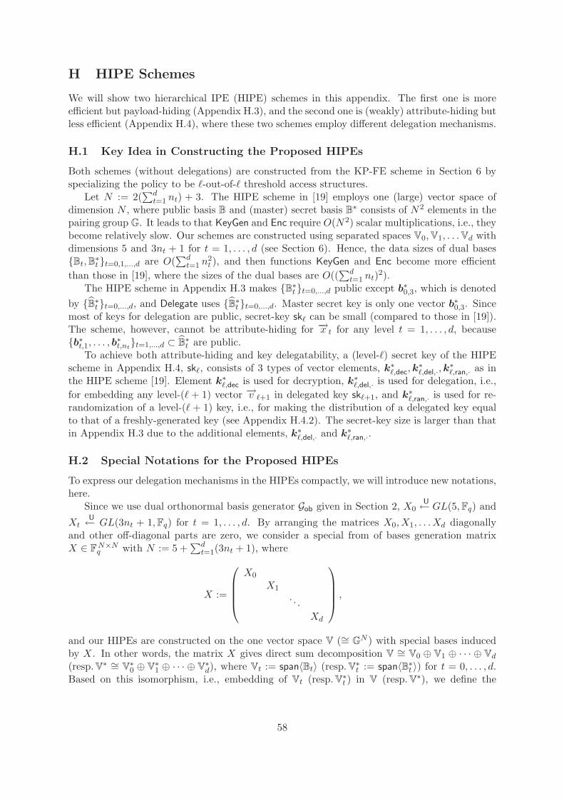
H HIPE Schemes

We will show two hierarchical IPE (HIPE) schemes in this appendix. The first one is moreefficient but payload-hiding (Appendix H.3), and the second one is (weakly) attribute-hiding butless efficient (Appendix H.4), where these two schemes employ different delegation mechanisms.

H.1 Key Idea in Constructing the Proposed HIPEs

Both schemes (without delegations) are constructed from the KP-FE scheme in Section 6 byspecializing the policy to be �-out-of-� threshold access structures.

Let N := 2(∑d

t=1 nt) + 3. The HIPE scheme in [19] employs one (large) vector space ofdimension N , where public basis B and (master) secret basis B

∗ consists of N2 elements in thepairing group G. It leads to that KeyGen and Enc require O(N2) scalar multiplications, i.e., theybecome relatively slow. Our schemes are constructed using separated spaces V0,V1, . . .Vd withdimensions 5 and 3nt + 1 for t = 1, . . . , d (see Section 6). Hence, the data sizes of dual bases{Bt,B∗t }t=0,1,...,d are O(

∑dt=1 n

2t ), and then functions KeyGen and Enc become more efficient

than those in [19], where the sizes of the dual bases are O((∑d

t=1 nt)2).

The HIPE scheme in Appendix H.3 makes {B∗t }t=0,...,d public except b∗0,3, which is denotedby {B̂∗t }t=0,...,d, and Delegate uses {B̂∗t }t=0,...,d. Master secret key is only one vector b∗0,3. Sincemost of keys for delegation are public, secret-key sk� can be small (compared to those in [19]).The scheme, however, cannot be attribute-hiding for −→x t for any level t = 1, . . . , d, because{b∗t,1, . . . , b∗t,nt

}t=1,...,d ⊂ B̂∗t are public.

To achieve both attribute-hiding and key delegatability, a (level-�) secret key of the HIPEscheme in Appendix H.4, sk�, consists of 3 types of vector elements, k∗�,dec,k

∗�,del,·,k

∗�,ran,· as in

the HIPE scheme [19]. Element k∗�,dec is used for decryption, k∗�,del,· is used for delegation, i.e.,for embedding any level-(� + 1) vector −→v �+1 in delegated key sk�+1, and k∗�,ran,· is used for re-randomization of a level-(� + 1) key, i.e., for making the distribution of a delegated key equalto that of a freshly-generated key (see Appendix H.4.2). The secret-key size is larger than thatin Appendix H.3 due to the additional elements, k∗�,del,· and k∗�,ran,·.

H.2 Special Notations for the Proposed HIPEs

To express our delegation mechanisms in the HIPEs compactly, we will introduce new notations,here.

Since we use dual orthonormal basis generator Gob given in Section 2, X0U← GL(5,Fq) and

XtU← GL(3nt + 1,Fq) for t = 1, . . . , d. By arranging the matrices X0, X1, . . . Xd diagonally

and other off-diagonal parts are zero, we consider a special from of bases generation matrixX ∈ F

N×Nq with N := 5 +

∑dt=1(3nt + 1), where

X :=

⎛⎜⎜⎜⎝X0

X1

. . .Xd

⎞⎟⎟⎟⎠ ,

and our HIPEs are constructed on the one vector space V (∼= GN ) with special bases induced

by X. In other words, the matrix X gives direct sum decomposition V ∼= V0 ⊕ V1 ⊕ · · · ⊕ Vd

(resp. V∗ ∼= V∗0 ⊕ V

∗1 ⊕ · · · ⊕ V

∗d), where Vt := span〈Bt〉 (resp. V∗t := span〈B∗t 〉) for t = 0, . . . , d.

Based on this isomorphism, i.e., embedding of Vt (resp. V∗t ) in V (resp. V∗), we define the

58

following notations as:

((−→x 0)B0 , . . . , (−→x d)Bd

) + ((−→y 0)B0 , . . . , (−→y d)Bd

) := ((−→x 0 +−→y 0)B0 , . . . , (−→x d +−→y d)Bd

)where ((−→x 0)B0 , . . . , (

−→x d)Bd), ((−→y 0)B0 , . . . , (

−→y d)Bd) ∈ V ∼= V0 ⊕ V1 ⊕ · · · ⊕ Vd,

(−→x )Bt := ((−→0 )B0 , · · · , (

−→0 )Bt−1 , (

−→x )Bt , (−→0 )Bt+1 , · · · , (

−→0 )Bd

) ∈ V,

((−→x 0)B0 , (−→x t)Bt : t = 1, . . . , �) := ((−→x 0)B0 , . . . , (

−→x �)B�) :=

∑�t=0(−→x t)Bt ∈ V,

((−→x 0)B0 , (−→x t)Bt : t = 1, . . . , �, (−→x τ )Bτ ) := ((−→x 0)B0 , . . . , (

−→x �)B�, (−→x τ )Bτ )

:=∑

t=0,...,�,τ (−→x t)Bt ∈ V,

e(c,k∗) :=∏dt=0 e(ct,k

∗t ) where c := (c0, . . . , cd) ∈ V0 ⊕ · · · ⊕ Vd,

k∗ := (k∗0, . . . ,k∗d) ∈ V

∗0 ⊕ · · · ⊕ V

∗d,

and −→e t,j := (

j−1︷︸︸︷0, . . . , 0, 1,

nt−j︷︸︸︷0, . . . , 0) ∈ F

ntq ,

and all the above notations are applied to the case with {B∗t }t=0,...,d instead of {Bt}t=0,...,d

H.3 Efficient Payload-Hiding HIPE Scheme

H.3.1 Construction



B̂∗0 := (b∗0,1, b

∗0,4), B̂

∗t := (b∗t,1, .., b

∗t,nt

, b∗t,2nt+1, .., b∗t,3nt

) for t = 1, .., d,

return pk := (1λ, param−→n , {B̂t, B̂∗t }t=0,...,d), sk := b∗0,3.

KeyGen(pk, sk, (−→v 1, . . . ,−→v �) ∈ F

n1q × · · · × F

n�q ) :

st, θtU← Fq for t = 1, . . . , �, s0 :=

∑�t=1 st,

−→η t U← Fntq for t = 0, . . . , �,

k∗� := ( ( −s0, 0, 1, η0, 0 )B∗0, ( st−→e t,1 + θt

−→v t, 0nt , −→η t, 0 )B∗t

: t = 1, . . . , �),return sk� := ((−→v 1, . . . ,

−→v �),k∗� ).Enc(pk,m ∈ GT , (−→x 1, . . . ,

−→x �) ∈ Fn1q × · · · × F

n�q ) :

ω, ϕ0, . . . , ϕ�U← Fq, c1 := ( (ω, 0, ζ, 0, ϕ0)B0 , (ω−→x t, 0nt , 0nt , ϕt)Bt : t = 1, . . . , �),

c2 := gζTm, ct := (c1, c2), return ct.

Dec(pk,k∗�,dec, ct) : m′ := c2/e(c1,k∗�,dec), return m′.

Delegate�(pk, sk�,−→v �+1 ∈ F

n�+1q ) :

sdel,t, θdel,tU← Fq for t = 1, . . . , �+ 1, sdel,0 :=

∑�+1t=1 sdel,t,

−→η del,tU← F

ntq for t = 0, . . . , �+ 1,

k∗del := ( ( −sdel,0, 0, 0, ηdel,0, 0 )B∗0,

( sdel,t−→e t,1 + θdel,t

−→v t, 0nt , −→η del,t, 0 )B∗t

: t = 1, . . . , �+ 1),k∗�+1 := k∗� + k∗del,

return sk�+1 := ((−→v 1, . . . ,−→v �+1),k∗�+1).

H.3.2 Security

The definition of adaptively payload-hiding security and the advantage AdvHIPE,PHA (λ) of adver-

sary A can be obtained through a straightforward extension of that of HIBE, e.g., [16], with

59

replacing ID-matching by vector-orthogonality.

Theorem 6 The proposed HIPE scheme is adaptively payload-hiding against chosen plaintextattacks under the DLIN assumption.

For any adversary A, there exist probabilistic machines, E1 and E2, whose running times areessentially the same as that of A, such that for any security parameter λ,

AdvHIPE,PHA (λ) ≤ AdvDLIN

E1 (λ) +ν∑h=1

AdvDLINE2,h

(λ) + ε,

where E2,h(·) := E2(h, ·), ν is the maximum number of adversary A’s key queries, and ε =(dν + 8ν + d+ 7)/q.

Proof Outline of Theorem 6 : To prove Theorem 6, we consider the following (ν + 3)games. In Game 0, a part framed by a box indicates coefficients to be changed in a subsequentgame. In the other games, a part framed by a box indicates coefficients which were changed ina game from the previous game.

Game 0 : Original game. That is, the reply to a key query consists of:

k∗� := ( ( −s0, 0 , 1, η0, 0 )B∗0, ( st−→e t,1 + θt

−→v t, 0nt , −→η t, 0 )B∗t

: t = 1, . . . , �).

The challenge ciphertext consists of:

c1 := ( (ω, 0 , ζ , 0, ϕ0)B0 , (ω−→x t, 0nt , 0nt , ϕt)Bt : t = 1, . . . , � ), c2 := gζTm.

Game 1 : Game 1 is the same as Game 0 except the following procedures.

1. When a create key query is issued by A, the challenger of the game only records thespecified predicates, and when a create delegated key query is issued, the challenger onlyrecords the specified keys and predicates. In this step, just the query is recorded, but nocorresponding key is created.

2. When a reveal key query is issued for a hierarchical (level-�) predicate (−→v 1, . . . ,−→v �) which

has been already recorded, the challenger creates the queried key by using KeyGen.


c1 := ( (ω, w0 , ζ, 0, ϕ0)B0 , (ω−→x t, −→w t , 0nt , ϕt)Bt : t = 1, . . . , � ), c2 := gζTm,

where w0U← Fq,

−→w tU← F

ntq .

Game 3-h (h = 1, . . . , ν) : Game 3-0 is Game 2. Game 3-h is the same as Game 3-(h− 1)except that the h-th reveal key query’s reply, k∗� , is:

k∗� := ( ( −s0, r0 , 1, η0, 0 )B∗0, ( st−→e t,1 + θt

−→v t, −→r t , −→η t, 0 )B∗t

: t = 1, . . . , �),

where r0U← Fq,

−→r t U← Fntq for t = 1, . . . , �, and the other variables are generated as in Game

3-(h− 1).

Game 4 : Game 4 is the same as Game 3-ν except that the challenge ciphertext is:

c1 := ( (ω,w0, ζ′ , 0, ϕ0)B0 , (ω−→x t,−→w t, 0nt , ϕt)Bt : t = 1, . . . , � ), c2 := gζTm,

60

where ζ, ζ ′ U← Fq.


(1)A (λ),Adv

(2)A (λ), Adv

(3-h)A (λ) and Adv

(4)A (λ) be the advantage of A in Game

0, Game 1, Game 2, Game 3-h and Game 4. It is obtained that Adv(4)A (λ) = 0.

We can evaluate the gaps between pairs of the above advantages using Problems 1 and 2 asin the proof of Theorem 1. ��

H.4 Attribute-Hiding HIPE Scheme

H.4.1 Construction



B̂∗0 := (b∗0,1, b

∗0,3), B̂

∗t := (b∗t,1, .., b

∗t,nt

) for t = 1, .., d,

return pk := (1λ, param−→n , {B̂t}t=0,...,d, b∗0,4, {b∗t,2nt+1, .., b

∗t,3nt}t=1,...,d), sk := {B̂∗t }t=0,...,d.

KeyGen(pk, sk, (−→v 1, . . . ,−→v �) ∈ F

n1q × · · · × F

n�q ) :

for j = 1, . . . , 2�; τ = �+ 1, . . . , d; ι = 1, . . . , nτ ;

ψ, sdec,t, sran,1,j,t, θdec,t, θran,1,j,tU← Fq for t = 1, . . . , �,

sdel,(τ,ι),t, sran,2,τ,t, θdel,(τ,ι),t, θran,2,τ,tU← Fq for t = 1, . . . , �+ 1,

sdec,0 :=∑�

t=1 sdec,t, sdel,(τ,ι),0 :=∑�+1

t=1 sdel,(τ,ι),t,

sran,1,j,0 :=∑�

t=1 sran,1,j,t, sran,2,τ,0 :=∑�+1

t=1 sran,2,τ,t,

−→η dec,t,−→η ran,1,j,t

U← Fntq for t = 0, . . . , �,

−→η del,(τ,ι),t,−→η ran,2,τ,t

U← Fntq , for t = 0, . . . , �+ 1,

k∗�,dec := ( ( −sdec,0, 0, 1, ηdec,0, 0 )B∗0,

( sdec,t−→e t,1 + θdec,t

−→v t, 0nt , −→η dec,t, 0 )B∗t

: t = 1, . . . , �),k∗�,del,(τ,ι) := ( ( −sdel,(τ,ι),0, 0, 0, ηdel,(τ,ι),0, 0 )B∗

0,

( sdel,(τ,ι),t−→e t,1 + θdel,(τ,ι),t

−→v t, 0nt , −→η del,(τ,ι),t, 0 )B∗t

: t = 1, . . . , �,( sdel,(τ,ι),�+1

−→e τ,1 + ψ−→e τ,ι, 0nτ , −→η del,(τ,ι),�+1, 0 )B∗τ),

k∗�,ran,1,j := ( ( −sran,1,j,0, 0, 0, ηran,1,j,0, 0 )B∗0,

( sran,1,j,t−→e t,1 + θran,1,j,t−→v t, 0nt , −→η ran,1,j,t, 0 )B∗

t: t = 1, . . . , �),

k∗�,ran,2,τ := ( ( −sran,2,τ,0, 0, 0, ηran,2,τ,0, 0 )B∗0,

( sran,2,τ,t−→e t,1 + θran,2,τ,t−→v t, 0nt , −→η ran,2,τ,t, 0 )B∗

t: t = 1, . . . , �,

( sran,2,τ,�+1−→e τ,1, 0nτ , −→η ran,2,τ,�+1, 0 )B∗

τ),

sk� := (k∗�,dec, {k∗�,del,(τ,ι)}τ=�+1,...,d; ι=1,...,nτ , {k∗�,ran,1,j , k∗�,ran,2,τ}j=1,...,2�; τ=�+1,...,d),return sk�.

Enc(pk,m ∈ GT , (−→x 1, . . . ,−→x �) ∈ F

n1q × · · · × F

n�q ) :

ω, ϕ0, . . . , ϕ�U← Fq, c1 := ( (ω, 0, ζ, 0, ϕ0)B0 , (ω−→x t, 0nt , 0nt , ϕt)Bt : t = 1, . . . , �),

c2 := gζTm, ct := (c1, c2), return ct.

Dec(pk,k∗�,dec, ct) : m′ := c2/e(c1,k∗�,dec), return m′.

Delegate�(pk, sk�,−→v �+1 := (v�+1,1, . . . , v�+1,n�+1

)) :for j′ = 1, . . . , 2(�+ 1); τ = �+ 2, . . . , d; ι = 1, . . . , nτ ;

61

φdel,(τ,ι), φran,2,τ , ψ′ U← Fq,

p∗dec,p∗del,(τ,ι),p

∗ran,1,j′ ,p

∗ran,2,τ

R← CoreDel�(pk, sk�,−→v �+1),

where CoreDel�(pk, sk�,−→v �+1) : σ, αj

U← Fq for j = 1, . . . , 2�+ 1,

return p∗ := σ(∑n�+1

i=1 v�+1,ik∗�,del,(�+1,i)) +

∑2�j=1 αjk

∗�,ran,1,j + α2�+1k

∗�,ran,2,�+1,

r∗dec, r∗ran,1,j′

U← span〈b∗0,4, {b∗t,2nt+i}t=1,...,�+1; i=1,...,nt〉,

r∗del,(τ,ι), r∗ran,2,τ

U← span〈b∗0,4, {b∗t,2nt+i}t=1,...,�+1,τ ; i=1,...,nt〉,

k∗�+1,dec := k∗�,dec + p∗dec + r∗dec,

k∗�+1,del,(τ,ι) := p∗del,(τ,ι) + φdel,(τ,ι)k∗�,ran,2,τ + ψ′k∗�,del,(τ,ι) + r∗del,(τ,ι),

k∗�+1,ran,1,j′ := p∗ran,1,j′ + r∗ran,1,j′ ,k∗�+1,ran,2,τ := p∗ran,2,τ + φran,2,τk

∗�,ran,2,τ + r∗ran,2,τ ,

sk�+1 := (k∗�+1,dec, {k∗�+1,del,(τ,ι)}τ=�+2,...,d; ι=1,...,nτ , {k∗�,ran,1,j′ , k∗�,ran,2,τ}j′=1,...,2(�+1); τ=�+2,...,d),return sk�+1.

H.4.2 Equivalence of Delegated and Freshly-Generated Keys

Lemma 30 If sk� is generated by KeyGen(pk, sk, (−→v 1, . . . ,−→v �)), the distribution of sk�+1 gener-

ated by Delegate(pk, sk�,−→v �+1) is equivalent to that of sk�+1 generated by KeyGen(pk, sk, (−→v 1, . . . ,−→v �,−→v �+1)) except with probability at most (2d− 2�+ 3)/q.

Proof. The distribution of (a part of) level-� key k∗�,J for J = dec, (ran, 1, 1), . . . , (ran, 1, 2�) isrepresented by that of the 2� coefficients, (sJ,1, . . . , sJ,�, θJ,1, . . . , θJ,�), of (−→e 1,1, . . . ,

−→e �,1,−→v 1, . . . ,−→v �) (and random-part coefficients, −→η J,t). The distribution of level-� key k∗�,J for J = (del, (�+1, 1)), . . . , (del, (d, nd)) (resp. J = (ran, 2, �+1), . . . , (ran, 2, d)) is represented by that of the 2�+2(resp. 2�+1) coefficients, (sJ,1, . . . , sJ,�, sJ,τ , θJ,1, . . . , θJ,�, ψ), of (−→e 1,1, . . . ,

−→e �,1,−→e τ,1,−→v 1, . . . ,−→v �,−→e τ,ι) (resp. (sJ,1, . . . , sJ,�, sJ,τ , θJ,1, . . . , θJ,�), of (−→e 1,1, . . . ,

−→e �,1,−→e τ,1,−→v 1, . . . ,−→v �)) (and random-

part coefficients, −→η J,t).Similarly, the distribution of level-(�+1) key k∗�+1,J is represented by that of the 2(�+1), 2(�+

1)+2 or 2(�+1)+1 coefficients, −→y J := (sJ,1, . . . , sJ,�, θJ,1, . . . , θJ,�), (sJ,1, . . . , sJ,�, sJ,τ , θJ,1, . . . ,θJ,�, ψ), or (sJ,1, . . . , sJ,�, sJ,τ , θJ,1, . . . , θJ,�).

Claim 3 shows the coefficients of delegated key is uniformly distributed in the first case.

Claim 3 If sk� is generated by KeyGen(pk, sk, (−→v 1, . . . ,−→v �)), the distribution of k∗�+1,ran,1,j′ gen-

erated in Delegate(pk, sk�,−→v �+1) is equivalent to that of k∗�+1,ran,1,j′ generated by KeyGen(pk, sk,

(−→v 1, . . . ,−→v �,−→v �+1)) except with probability at most 3/q.

Proof of Claim 3. The distribution of k∗�,J (J = (del, (τ, ι)), (ran, 1, j), (ran, 2, τ)) in sk� isrepresented by 2�+ 1-dimensional vectors as (except for ψ):

−→y �,J := (s�,J,1, . . . , s�,J,�, s�,J,τ , θ�,J,1, . . . , θ�,J,�) if J = (del, (τ, ι)),:= (s�,J,1, . . . , s�,J,�, 0, θ�,J,1, . . . , θ�,J,�) if J = (ran, 1, j),:= (s�,J,1, . . . , s�,J,�, s�,J,τ , θ�,J,1, . . . , θ�,J,�) if J = (ran, 2, τ).

The coefficients −→y �+1,ran,1,j′ of k∗�+1,ran,1,j′ except for that of −→v �+1 are given as:

−→y �+1,ran,1,j′ := (s�+1,ran,1,j′,1, . . . , s�+1,ran,1,j′,�+1, θ�+1,ran,1,j′,1, . . . , θ�+1,ran,1,j′,�)

= σran,1,j′∑n�+1

i=1 v�+1,i−→y �,del,(�+1,i) +

∑2�j=1 αran,1,j′,j

−→y �,ran,1,j + αran,1,j′,2�+1−→y �,ran,2,�+1

62

= σran,1,j′∑n�+1

i=1 v�+1,i−→y �,del,(�+1,i) +−→α ran,1,j′ · Y�,ran ∈ F

2�+1q ,

where −→α ran,1,j′ := (αran,1,j′,1, . . . , αran,1,j′,2�, αran,1,j′,2�+1)U← F

2�+1q ,

Y�,ran :=

⎛⎜⎜⎜⎝−→y �,ran,1,1

...−→y �,ran,1,2�−→y �,ran,2,�+1

⎞⎟⎟⎟⎠ ∈ F(2�+1)×(2�+1)q .

Moreover, the coefficient of −→v �+1 in kran,1,j′ of level-(�+1) is given by θ�+1,ran,1,j′,�+1 := σran,1,j′ ·ψ, where ψ is given in the level-� key and σran,1,j′ is generated in CoreDel� in the delegation.

We consider the joint distribution of −→y �+1,ran,1,j′ and θ�+1,ran,1,j′,�+1, i.e., {s�+1,ran,1,j′,t,θ�+1,ran,1,j′,t}t=1,...,�+1.

If the matrix Y�,ran is regular and ψ �= 0, since −→α ran,1,j′U← F

2�+1q , σran,1,j′

U← Fq, and variables−→α ran,1,j′ · Y�,ran and σran,1,j′ · ψ are independent, (−→y �+1,ran,1,j′ , θ�+1,ran,1,j′,�+1) ∈ F

2(�+1)q for j′ =

1, . . . , 2(�+ 1) are uniformly and independently distributed in F2(�+1)q .

Here, Y�,ran ((2�+ 1)× (2�+ 1) matrix) of sk� is regular and ψ �= 0 except with probabilityat most 2/q + 1/q = 3/q, from Claim 4. ��

Since k∗�+1,ran,1,j′ + b∗0,3 (j′ = 1, . . . , 2(� + 1)) has the same distribution as k∗�+1,dec, Lemma30 holds for k∗�+1,dec from Claim 3.

For k∗�+1,ran,2,τ (τ = �+2, . . . , d), the level-(�+1) coefficient s�+1,ran,2,τ,�+1 of −→e τ,1 is given byφran,2,τ ·s�,ran,2,τ,�+1 where φran,2,τ is generated in Delegate� and s�,ran,2,τ,�+1 the level-� coefficientof−→e τ,1. Therefore, Lemma 30 holds for k∗�+1,ran,2,τ from Claim 3 except for negligible probability,i.e., at most (d− �)/q.

Since k∗�+1,ran,2,τ + ψb∗τ,ι (τ = � + 2, . . . , d; ι = 1, . . . , nτ ) has the same distribution ask∗�+1,del,(τ,ι), Lemma 30 holds for k∗�+1,del,(τ,ι) from Claim 3 except for negligible probability,i.e., at most (d− �+ 1)/q.

Therefore, Lemma 30 holds except for negligible probability, i.e., at most (2d−2�+3)/q. ��

Claim 4 (Claim 4 in [19]) Let q > 2 and Δ := {M |detM �= 0} ⊂ Fl×lq . Then, |Δ|

ql2< 2

q .

H.4.3 Security

The definition of adaptively weakly-attribute-hiding security and the advantage AdvHIPE,wAHA (λ)

of adversary A are shown in Definition 47 of the full version of [19]. In the definition, the levels� and �′ of the two challenge vectors given by an adversary, (−→x (0)

i )i=1,...,� and (−→x (1)i )i=1,...,�′ ,

can be different, i.e., � �= �′ is allowed. The proposed HIPE scheme only satisfies the securitydefinition under the restriction that � = �′. Here, this restricted security ensures the anonymityof attributes of a ciphertext but with revealing the number of levels of attributes, while thesecurity definition in [19] ensures the anonymity of attributes as well as the number of levels.(The HIPE scheme in [19] satisfies the unrestricted security.) Our scheme can be modified tosatisfy the unrestricted security in [19] as: when generating a ciphertext in Enc, input vectors(−→x i)i=1,...,� are padded with random vectors (−→x i)i=�+1,...,d for a maximum level d, in the samemanner as the HIPE in [19].

Theorem 7 The proposed HIPE scheme is adaptively weakly-attribute-hiding against chosenplaintext attacks under the DLIN assumption.

63

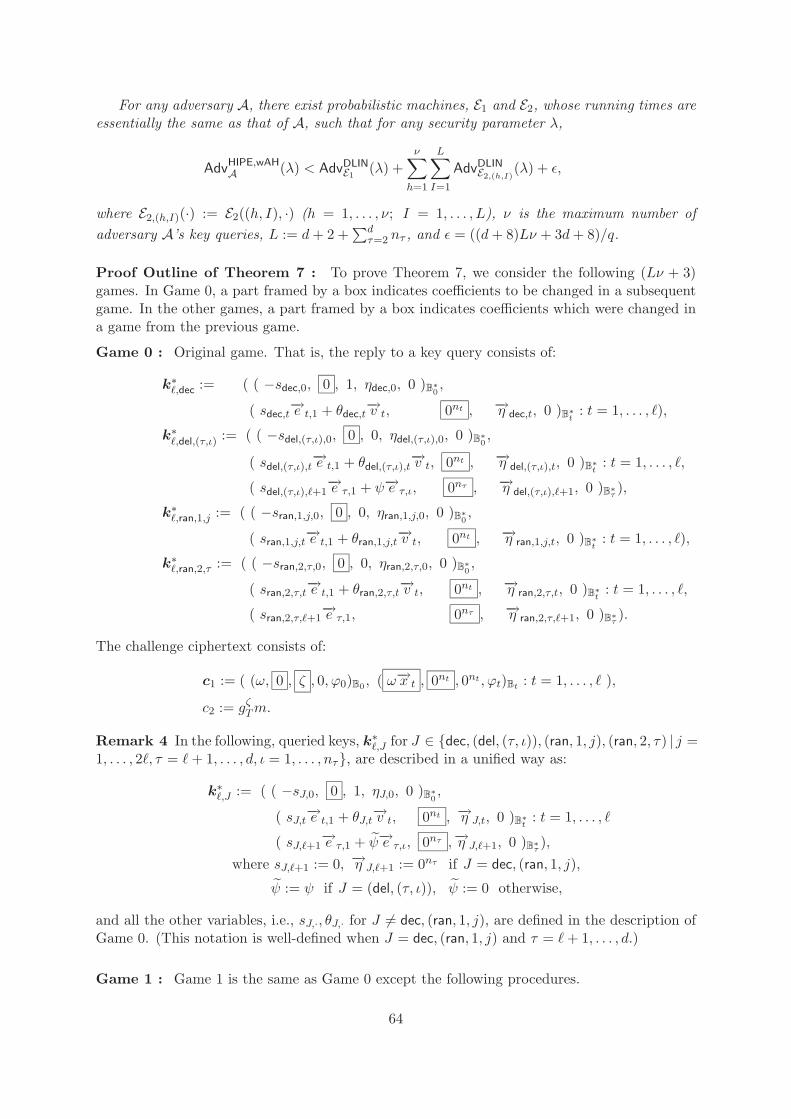
For any adversary A, there exist probabilistic machines, E1 and E2, whose running times areessentially the same as that of A, such that for any security parameter λ,

AdvHIPE,wAHA (λ) < AdvDLIN

E1 (λ) +ν∑h=1

L∑I=1

AdvDLINE2,(h,I)

(λ) + ε,

where E2,(h,I)(·) := E2((h, I), ·) (h = 1, . . . , ν; I = 1, . . . , L), ν is the maximum number ofadversary A’s key queries, L := d+ 2 +

∑dτ=2 nτ , and ε = ((d+ 8)Lν + 3d+ 8)/q.

Proof Outline of Theorem 7 : To prove Theorem 7, we consider the following (Lν + 3)games. In Game 0, a part framed by a box indicates coefficients to be changed in a subsequentgame. In the other games, a part framed by a box indicates coefficients which were changed ina game from the previous game.

Game 0 : Original game. That is, the reply to a key query consists of:

k∗�,dec := ( ( −sdec,0, 0 , 1, ηdec,0, 0 )B∗0,

( sdec,t−→e t,1 + θdec,t

−→v t, 0nt , −→η dec,t, 0 )B∗t

: t = 1, . . . , �),

k∗�,del,(τ,ι) := ( ( −sdel,(τ,ι),0, 0 , 0, ηdel,(τ,ι),0, 0 )B∗0,

( sdel,(τ,ι),t−→e t,1 + θdel,(τ,ι),t

−→v t, 0nt , −→η del,(τ,ι),t, 0 )B∗t

: t = 1, . . . , �,

( sdel,(τ,ι),�+1−→e τ,1 + ψ−→e τ,ι, 0nτ , −→η del,(τ,ι),�+1, 0 )B∗

τ),

k∗�,ran,1,j := ( ( −sran,1,j,0, 0 , 0, ηran,1,j,0, 0 )B∗0,

( sran,1,j,t−→e t,1 + θran,1,j,t−→v t, 0nt , −→η ran,1,j,t, 0 )B∗

t: t = 1, . . . , �),

k∗�,ran,2,τ := ( ( −sran,2,τ,0, 0 , 0, ηran,2,τ,0, 0 )B∗0,

( sran,2,τ,t−→e t,1 + θran,2,τ,t−→v t, 0nt , −→η ran,2,τ,t, 0 )B∗

t: t = 1, . . . , �,

( sran,2,τ,�+1−→e τ,1, 0nτ , −→η ran,2,τ,�+1, 0 )B∗

τ).

The challenge ciphertext consists of:

c1 := ( (ω, 0 , ζ , 0, ϕ0)B0 , ( ω−→x t , 0nt , 0nt , ϕt)Bt : t = 1, . . . , � ),

c2 := gζTm.

Remark 4 In the following, queried keys, k∗�,J for J ∈ {dec, (del, (τ, ι)), (ran, 1, j), (ran, 2, τ) | j =1, . . . , 2�, τ = �+ 1, . . . , d, ι = 1, . . . , nτ}, are described in a unified way as:

k∗�,J := ( ( −sJ,0, 0 , 1, ηJ,0, 0 )B∗0,

( sJ,t−→e t,1 + θJ,t−→v t, 0nt , −→η J,t, 0 )B∗

t: t = 1, . . . , �

( sJ,�+1−→e τ,1 + ψ̃−→e τ,ι, 0nτ ,−→η J,�+1, 0 )B∗

τ),

where sJ,�+1 := 0, −→η J,�+1 := 0nτ if J = dec, (ran, 1, j),

ψ̃ := ψ if J = (del, (τ, ι)), ψ̃ := 0 otherwise,

and all the other variables, i.e., sJ,·, θJ,· for J �= dec, (ran, 1, j), are defined in the description ofGame 0. (This notation is well-defined when J = dec, (ran, 1, j) and τ = �+ 1, . . . , d.)

Game 1 : Game 1 is the same as Game 0 except the following procedures.

64

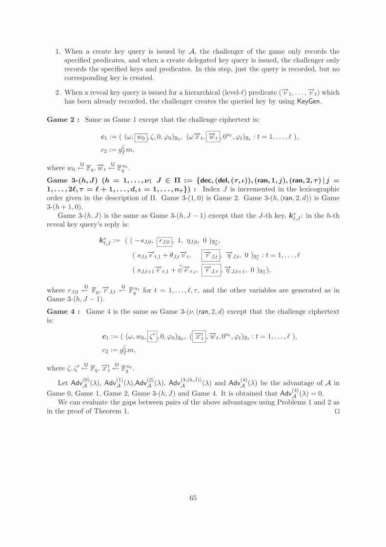
1. When a create key query is issued by A, the challenger of the game only records thespecified predicates, and when a create delegated key query is issued, the challenger onlyrecords the specified keys and predicates. In this step, just the query is recorded, but nocorresponding key is created.

2. When a reveal key query is issued for a hierarchical (level-�) predicate (−→v 1, . . . ,−→v �) which

has been already recorded, the challenger creates the queried key by using KeyGen.


c1 := ( (ω, w0 , ζ, 0, ϕ0)B0 , (ω−→x t, −→w t , 0nt , ϕt)Bt : t = 1, . . . , � ),

c2 := gζTm,

where w0U← Fq,

−→w tU← F

ntq .

Game 3-(h, J) (h = 1, . . . , ν; J ∈ Π := {dec, (del, (τ, ι)), (ran,1, j), (ran,2, τ ) | j =1, . . . ,2�, τ = � + 1, . . . , d, ι = 1, . . . , nfi }) : Index J is incremented in the lexicographicorder given in the description of Π. Game 3-(1, 0) is Game 2. Game 3-(h, (ran, 2, d)) is Game3-(h+ 1, 0).

Game 3-(h, J) is the same as Game 3-(h, J − 1) except that the J-th key, k∗�,J : in the h-threveal key query’s reply is:

k∗�,J := ( ( −sJ,0, rJ,0 , 1, ηJ,0, 0 )B∗0,

( sJ,t−→e t,1 + θJ,t−→v t, −→r J,t , −→η J,t, 0 )B∗

t: t = 1, . . . , �

( sJ,�+1−→e τ,1 + ψ̃−→e τ,ι, −→r J,τ ,−→η J,�+1, 0 )B∗

τ),

where rJ,0U← Fq,

−→r J,t U← Fntq for t = 1, . . . , �, τ , and the other variables are generated as in

Game 3-(h, J − 1).

Game 4 : Game 4 is the same as Game 3-(ν, (ran, 2, d) except that the challenge ciphertextis:

c1 := ( (ω,w0, ζ′ , 0, ϕ0)B0 , ( −→x ′t ,−→w t, 0nt , ϕt)Bt : t = 1, . . . , � ),

c2 := gζTm,

where ζ, ζ ′ U← Fq,−→x ′t U← F

ntq .


(1)A (λ),Adv

(2)A (λ), Adv

(3-(h,J))A (λ) and Adv

(4)A (λ) be the advantage of A in

Game 0, Game 1, Game 2, Game 3-(h, J) and Game 4. It is obtained that Adv(4)A (λ) = 0.

We can evaluate the gaps between pairs of the above advantages using Problems 1 and 2 asin the proof of Theorem 1. ��

65

fully secure functional encryption with general relations … · fully secure functional encryption...

Documents