Fun with Geometric Duality

Michael Junger Michael Schulz Wojciech Zychowicz

Dedicated to Jack Edmonds on the occasion of his 75th birthdayon April 5, 2009

Abstract

We present GEODUAL, a software for creating and solving geometricinstances of the Minimum Spanning Tree problem, the Perfect Matchingproblem, and the Traveling Salesman problem, along with visual proofsof optimality.

1 Introduction

Almost 20 years ago, William R. Pulleyblank and the first author started as-signing geometric interpretations to dual solutions of certain combinatorial op-timization problems. Among other things, this resulted in colorful pictures thatwere not only æsthetically pleasing but also of educational value, because certaintheorems can be appreciated visually without any formalism. The graphics soft-ware produced then by teams at Bellcore (“BINKY”), Simon Fraser University(“VisualMatching”) and the University of Cologne (“DUST” and “CATBOX”)does not run well on today’s systems, with the exception of VisualMatching byMichael Maguire [8] and the recent CATBOX-related Gato software [9] whoseemphasis is on teaching algorithms and that is restricted to Euclidean perfectpoint matching and spanning trees. For many years the first author has beensorry for not being able to spice up his lectures in the subject area with thepictures and animations provided by “DUST”. The GEODUAL software [10]closes this gap. Using the multi-platform Qt 4 open source library, it is a widelyusable tool for creating and solving geometric instances of the Minimum Span-ning Tree problem, the Perfect Matching problem, and the Traveling Salesmanproblem, along with visual proofs of optimality.

In this brief user guide, we explain GEODUAL’s functionality for beginners,followed by some remarks for specialists. But even for the beginners, we doassume basic knowledge of the theory of Linear Programming.

1

2 Basics

2.1 Perfect Point Matchings

Consider an even cardinality set P of n points in the plane. The distance ofany pair of points p and q with Cartesian coordinates (xp, yp) and (xq, yq) is theEuclidean distance dpq =

√|xp − xq|2 + |yp − yq|2.

A perfect point matching of the n points is a partitioning of the points intopairs. A perfect point matching is of minimum length if the sum of the distancesof all n

2 point pairs is minimum. This is a special version of the famous perfectmatching problem.

Here is a perfect point matching on six points:

Its total length is the sum of the lengths of all straight line segments con-necting the pairs. We claim it is not of minimum length, and we can easilyprove it by showing a shorter one:

Now we claim this is a minimum length perfect point matching. How canwe prove it?

Let us draw disks of radii rp centered at the points p ∈ P . The disks maytouch but not overlap (no two of them may have a common interior point):

2

Now take any perfect point matching. Each of its straight line segmentsconnecting pairs p and q is partially covered by the disks around p and q, so itslength dpq is at least the sum rp + rq. Each disk radius is accounted for exactlyonce. Therefore the total length of any perfect point matching is at least thesum of all n disk radii. Here is our perfect point matching along with a diskpacking whose sum of the radii equals the sum of the lengths of all representingline segments:

Therefore this perfect point matching is indeed of minimum length.Unfortunately, this technique does not always work. Consider this instance:

While the point matching is clearly the shortest possible, there is no way toconstruct a disk packing that proves this. An additional observation helps.While each point is touched by exactly one line, each odd cardinality subsetof the points is left by at least one line (that represents a pair one of whosemembers is not in the subset). That is, if we introduce moats that surroundodd cardinality sets of points and keep insisting on no overlaps, the sum of alldisk radii plus the widths of all moats is still a lower bound for the length ofany perfect point matching:

3

We omit a formal description of moat construction and just appeal to intu-ition, the details can be found in [5, 2]. Since the sum of the disk radii plusthe widths of the two three point moats equals the total length of our pointmatching, the picture “proves” that our point matching is indeed a shortestpossible.

This technique allows us to construct “graphic optimality proofs” for anyinstance of the perfect point matching problem. Some basic knowledge of thetheory of Linear Programming is needed here. Let us write rp for the radius ofthe disk surrounding point p ∈ P , and, for any odd cardinality subset S ⊂ Pof the points (3 ≤ |S| ≤ n

2 ), let wS denote the width of the moat around S.Then the problem of finding a feasible disk/moat packing that results in thebest possible lower bound on the total length of any perfect point matching canbe written as a linear programming problem as follows:

maximize∑p∈P

rp +∑

S⊂P, |S| odd and 3≤|S|≤n2

wS

such that

rp + rq +∑

|S∩{p,q}|=1

wS ≤ dpq for all p, q ∈ P, q 6= p,

rp ≥ 0 for all p ∈ P,

wS ≥ 0 for all S ⊂ P, |S| odd and 3 ≤ |S| ≤ n

2.

The restrictions make sure that the disks have non-negative radii and themoats have non-negative widths. They also guarantee that the disks and moatsare non-overlapping by stipulating that for any pair of points, the sum of theradii of the two associated disks plus the sum of the widths of all moats sep-arating them never exceeds their distance. The objective function asks for adisk/moat packing that provides the best possible lower bound on the length ofany perfect point matching.

We introduce(n2

)variables xpq for all pairs of distinct points p and q. The

dual of the above linear programming problem is then

minimize∑

p,q∈P, q 6=p

dpqxpq

such that ∑q∈P, q 6=p

xpq ≥ 1 for all p ∈ P,

∑|S∩{p,q}|=1

xpq ≥ 1 for all S ⊂ P, |S| odd and 3 ≤ |S| ≤ n

2,

xpq ≥ 0 for all p, q ∈ P, q 6= p.

We can represent any perfect point matching by setting xpq = 1 if p and qare matched and xpq = 0 otherwise. Then the xpq will satisfy all restrictions of

4

the latter linear programming problem. The “miracle” is that it follows fromthe groundbreaking work of Jack Edmonds [3, 4] and the geometric nature ofour problem that such “characteristic vectors” of perfect point matchings arethe only solutions that the simplex method for linear programming can return.This is way beyond “basics”. But once this result is accepted, it is clear that ourconstruction always works, and all we have to do is solve a linear programmingproblem (along with its dual). A second “miracle” (also beyond this exposition)is that there is no need to worry about the (exponentially) large set of variablesin the first and restrictions in the second linear programming problem. Indeed,both linear programming problems can be solved in polynomial time due to theresults of Jack Edmonds [3, 4].

Here is a 10 point example of a pair of optimum solutions to the primal/dualpair of linear programs.

Just by visual inspection, we can argue as follows:

• The black lines display indeed a perfect point matching. Therefore thedual solution is feasible for the dual linear program.

• The red disks and the orange moats are non-overlapping. On any straight-line connection between two points, the radii of the two disks assigned tothem plus the widths of the moats separating them add up to no more thanthe distance of the two points. Therefore the primal solution is feasiblefor the primal linear program.

Now we see the optimality of the perfect point matching by applying one oftwo basic theorems of Linear Programming:

5

1. The sum of all disk radii and all moat widths equals the sum of the lengthsof all black lines. Therefore we obtain optimality from the Weak DualityTheorem of Linear Programming.

2. For each black line, there is no white gap, i.e., whenever a variable xpq hasa positive value (=1), the associated primal constraint holds with equal-ity. And whenever a radius or a moat width is positive, it is traversed byexactly one black line, so the associated dual constraint holds with equal-ity. Therefore we obtain optimality from the Complementary SlacknessTheorem of Linear Programming.

“Geometric Duality” refers to assigning such geometric interpretations topairs of primal and dual solutions of certain linear programs.

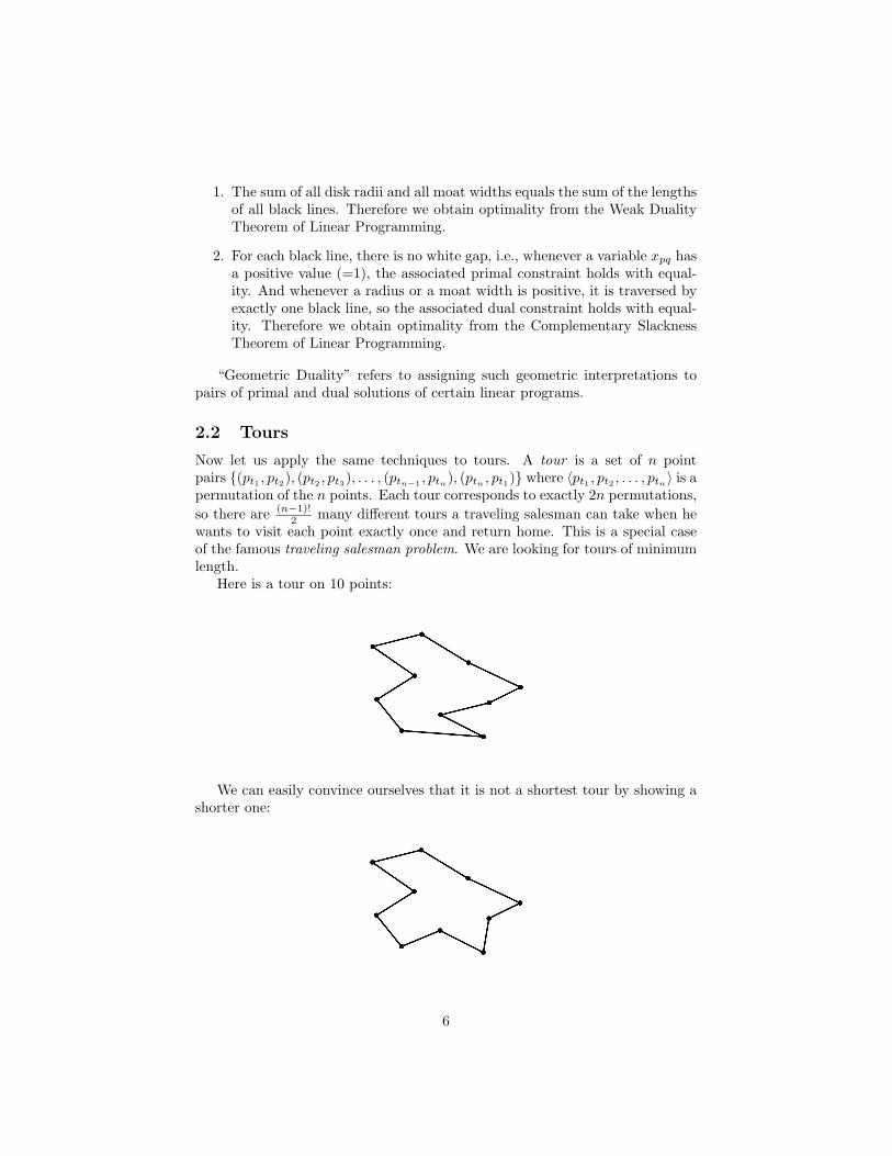
2.2 Tours

Now let us apply the same techniques to tours. A tour is a set of n pointpairs {(pt1 , pt2), (pt2 , pt3), . . . , (ptn−1 , ptn

), (ptn, pt1)} where 〈pt1 , pt2 , . . . , ptn

〉 is apermutation of the n points. Each tour corresponds to exactly 2n permutations,so there are (n−1)!

2 many different tours a traveling salesman can take when hewants to visit each point exactly once and return home. This is a special caseof the famous traveling salesman problem. We are looking for tours of minimumlength.

Here is a tour on 10 points:

We can easily convince ourselves that it is not a shortest tour by showing ashorter one:

6

This one is a shortest possible tour, and we can prove it by showing a non-overlapping system of disks:

Since each point is paired with exactly two other points, the disk surroundingit is traversed twice by any tour. Therefore, twice the sum of the radii of all ndisks is always at most the total length of any tour.

Like for perfect point matching, we can introduce moats as well, with theproviso that every moat is traversed at least twice, and there is no odd cardinal-ity restriction here. For the same 10 point example we used in our last perfectpoint matching example, we do need moats for an optimality proof:

7

The pair of linear programs for the tour problem look very similar to theone we gave for perfect point matching. The primal task is to

maximize 2∑p∈P

rp + 2∑

S⊂P, 3≤|S|≤n2

wS

such that

rp + rq +∑

|S∩{p,q}|=1

wS ≤ dpq for all p, q ∈ P, q 6= p,

rp ≥ 0 for all p ∈ P,

wS ≥ 0 for all S ⊂ P, 3 ≤ |S| ≤ n

2

and the dual task is to

minimize∑

p,q∈P, q 6=p

dpqxpq

such that ∑q∈P, q 6=p

xpq ≥ 2 for all p ∈ P,

∑|S∩{p,q}|=1

xpq ≥ 2 for all S ⊂ P, 3 ≤ |S| ≤ n

2,

xpq ≥ 0 for all p, q ∈ P, q 6= p.

However, unlike for perfect point matching, this construction does not alwayswork, in fact, it is quite unlikely to work for instances of more than, say, 20points. Again, the reason is beyond “basics”, see [5, 2, 1].

2.3 Spanning Trees

We wish to connect point pairs by straight lines, such that, if the lines werestreets, we could drive from any point to any other point. And we would likethe total length of all such lines to be minimum. We may assume that a solutioncannot have a cycle of the form {(pt1 , pt2), (pt2 , pt3), . . . , (ptk−1 , ptk

), (ptk, pt1)}

for some 1 ≤ k ≤ n because removing any of its point pairs would still be asolution of at most the same total length. Therefore, there should be no morethan n − 1 lines. On the other hand, we do need at least n − 1 lines, becauseotherwise at least one point would not be reachable from every other point. Sowe are looking for solutions consisting of n − 1 lines with no cycles, and theseare called spanning trees. Our problem is the minimum length spanning treeproblem, a special case of the minimum weight spanning tree problem.

There are several very efficient algorithms for solving this problem (in a moregeneral setting than considered here), and we shall concentrate on the one givenby Kruskal in 1956 [7]. Kruskal’s algorithm builds a minimum length spanning

8

tree by starting with the shortest line and then adding successively the shortestremaining line that produces no cycle. It stops as soon as n−1 lines are chosen.We shall mimic Kruskal’s algorithm for minimum length spanning trees on ahypothetical analog computer that is able to “blow up” disks around pointsand moats around point sets at uniform speed. Whenever there is a collision(i.e., blowing up further would produce overlapping disks/moats), we draw aline connecting two points causing the collision, and treat the newly connectedpoint set as a new unit around which a new moat is growing now. Let us runthe analog computer for our standard example on 10 points. We take snapshotswhenever a new line is produced, i.e., a total of 9 snapshots:

(1) (2)

(3) (4)

9

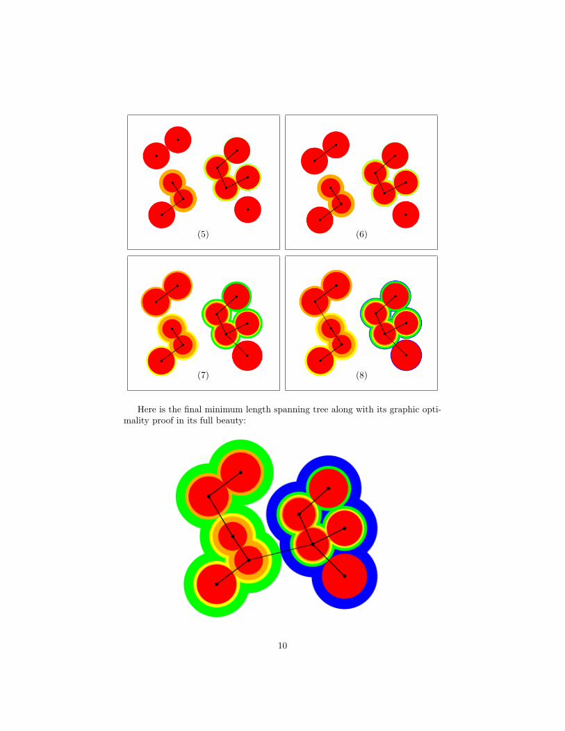
(5) (6)

(7) (8)

Here is the final minimum length spanning tree along with its graphic opti-mality proof in its full beauty:

10

The correctness of Kruskal’s algorithm (that is quite easy to see) makes surethat we have indeed found a minimum length spanning tree (whose correct con-struction is easily verified from the final picture). In addition, we can interpretthis picture like those for perfect point matchings and tours, yet we must takea little detour that is beyond “basics”. We will sketch it in Section 4.

2.4 Other Metrics

So far, we have considered Eulidean distances dpq =√|xp − xq|2 + |yp − yq|2

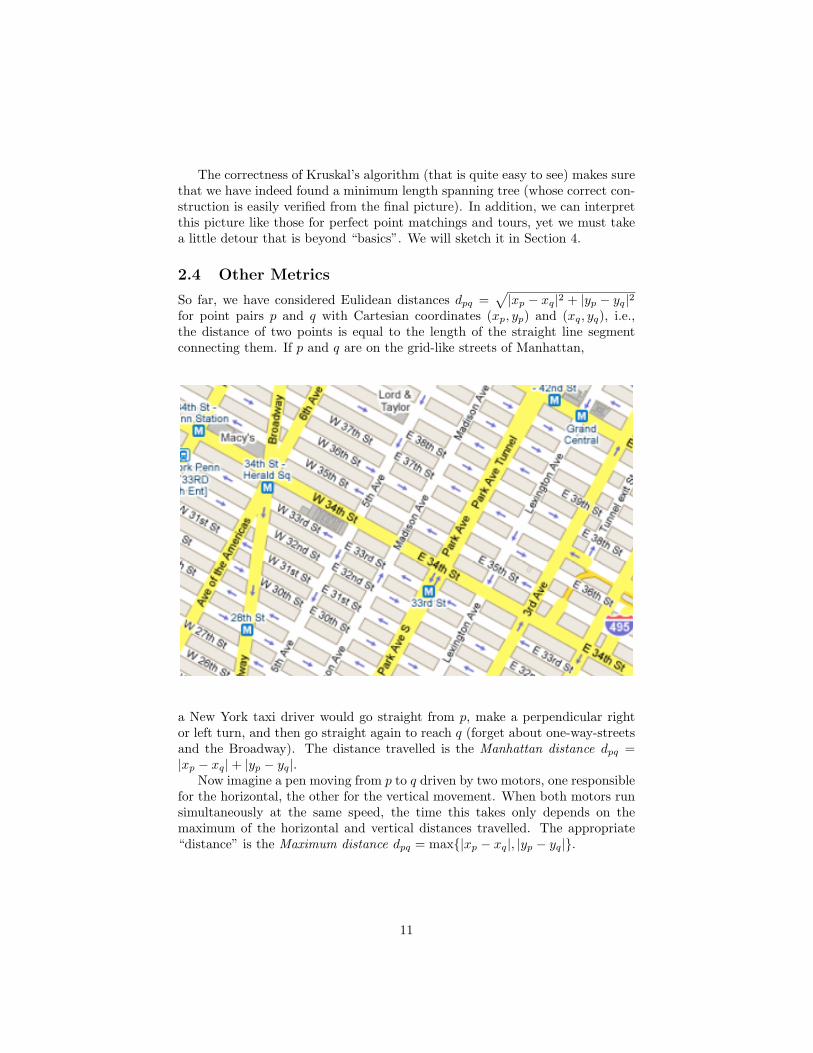
for point pairs p and q with Cartesian coordinates (xp, yp) and (xq, yq), i.e.,the distance of two points is equal to the length of the straight line segmentconnecting them. If p and q are on the grid-like streets of Manhattan,

a New York taxi driver would go straight from p, make a perpendicular rightor left turn, and then go straight again to reach q (forget about one-way-streetsand the Broadway). The distance travelled is the Manhattan distance dpq =|xp − xq|+ |yp − yq|.

Now imagine a pen moving from p to q driven by two motors, one responsiblefor the horizontal, the other for the vertical movement. When both motors runsimultaneously at the same speed, the time this takes only depends on themaximum of the horizontal and vertical distances travelled. The appropriate“distance” is the Maximum distance dpq = max{|xp − xq|, |yp − yq|}.

11

Here are the points of equal distance from a given point when distances aremeasured in Euclidean, Manhattan, and Maximum metric, respectively:

For distance 1, the sets of points on the circle, diamond, and square, re-spectively, are called the unit balls for the respective metrics. In fact, we canconsider infinitely many metrics called “Lk-metrics” in which p and q havedistance dpq = k

√|xp − xq|k + |yp − yq|k. The Manhattan metric is L1, the Eu-

clidean metric is L2, and the Maximum metric is L∞. For k ≥ 3, the unit ballslook like beer mats, and with increasing k, their shape converges to the square“unit ball” of the Maximum metric.

Everything said so far for the Euclidean metric applies to any of these metricsas well. We take a 20 point example to demonstrate this. Here is a Manhattan(L1) perfect point point matching with optimality proof:

12

It is not clear how to draw the “lines” for Lk with k ≥ 3. We use straightlines whose lengths equal the Lk-distances of their end points, that is why theremay be gaps at either end. Here is an L5 tour with optimality proof:

“L∞-lines” look almost like “L1-lines”, except that the segments represent-ing the longer of the horizontal and vertical distances (that determines the L∞-distance of the end points) are drawn solid and the others are drawn dotted.Here is a Maximum (L∞) spanning tree with optimality proof:

13

3 Using GEODUAL

When GEODUAL starts, it looks like this:

The application’s main window is divided into three parts, the largest of whichis the painting area. In addition, there are the groupbox at the left hand sideand the toolbar on top. In the following, we will explain each part.

3.1 Painting area

The painting area is the most important part of the application. All paintinghappens on the white canvas at a resolution of 500 × 500 pixels within thegrey rectangle that represents the unit square in the real plane. The only user-controlled interactions with the canvas are

• creating or deleting points,

• zooming in for a larger image,

• zooming out for a smaller image,

• switching a guiding grid on or off.

14

3.2 Groupbox

The groupbox provides the functionality for creating an instance consisting ofpoints in the unit square, specifying a metric for distance measurement, andchoosing the type of problem and solution. Finally, it displays status informa-tion.

There are two possibilities for creating an instance under “Choose Points”:

• The first push-button toggles between “Pick Points (Off)” and “PickPoints (On)”. In the latter mode the user may manually select pointsin the unit square by clicking the left mouse-button at the desired loca-tions. Selected points can be removed by clicking the right mouse-buttonclose to their location.

• An alternative way of generating an instance is provided by the “GeneratePoints” push-button. When pushed, the user is first asked for the numberof points, and subsequently for a random seed. Once these values areprovided, the program generates a pseudo-random instance and displaysit on the canvas.

Users should not try instances with more than 30 points for perfect pointmatching or tour computations: Larger instances are likely to result in a “notenough memory” message. Unfortunately, this may happen occasionally alsofor smaller instances, see also Section 4. For tour computations, no more than20 points should be tried, because a successful optimization is quite unlikely forlarger instances.

When an instance is available, the next step is to choose the desired metric.The “Choose Metric” part provides four radio-buttons, the first two for theManhattan (L1) and the Euclidean metric (L2). The third radio-button allowsto choose a metric in the range from L3 to L9 by adjusting the spinbox nextto the “L” at the radio-button. Finally there’s a fourth radio-button for theMaximum metric (L∞).

The next step is the specification of which problem the user wishes to solve.The section “Choose Type” provides radio-buttons for selecting one of the threeproblems: “Tree” for the spanning tree problem, “Matching” for the perfectpoint matching problem, and “Tour” for the tour problem.

In the “Choose Solution” section, the user can select which type of solutions/he wants to see. The default selection is the “Solution/Proof” option in whichoptimum solutions are displayed along with optimum disk/moat packings. Theother two choices are to display “Solution only” or “Proof only”. The former isof interest if the programs gives the “moats are not nested” error message (seeSection 4), the latter for æstetic reasons: disk/moat packings are beautiful bythemselves, even if nothing is proved.

The last section “Status” provides some information about the current in-stance and the state of solution display on the canvas. The point counter alwaysshows the current number of points on the canvas. For minimum length span-ning trees, “Phase” refers to the progress in terms of Kruskal’s algorithm as

15

explained in Section 2, i.e., there are n − 1 phases for an n point instance, ineach of which one line is drawn. For the perfect point matching problem andthe tour problem, there are no natural phases in the solution process, yet wehave introduced artificial phases that correspond to the “depths” of the disksand moats. We will see below how one can navigate between phases. When“0/0” is displayed, this simply means that no solution has been calculated yet.Calculation is triggered by any of the “ ”, “ ”, “ ”, “ ”, and “ ” buttonsin the toolbar, as well as when a radio-button in the groupbox is clicked.

Before we turn to the toolbar, we should discuss what can go wrong with agiven instance:

• The instance may be too large.

• It may not be possible to compute a shortest tour due to reasons explainedin Section 4.

• The calculation of a disk/moat packing may fail for perfect point match-ings or tours, even though an optimum solution has been found. This is aproblem that will be fixed in the next version of GEODUAL, see Section 4.When this happens, there is still the possibility to choose “Solution only”in the “Choose Solution” section.

3.3 Toolbar

The toolbar

supports the following actions:

“Load”: Load a set of stored points from a text file.“Save”: Save the current set of points to a text file.“Screenshot”: Take a screenshot of the current canvas.“Close”: Quit the application.“Previous”: Go to the previous phase.“Next”: Go to the next phase.“Start”: Return to the intial view, showing only the points

on the canvas.“Final”: Jump to the last phase and display the final result.“Play”: Run through the rest of the phases.“Stop”: Stop playing after the current phase is painted.“Clear”: Clear the canvas (including the point set).“Zoom in”: Zoom into the canvas.“Zoom out”: Zoom out of the canvas.

16

“Animation”: Switch animation on/off (if on, the symbolis pressed).

When animation is on, the transitions between phases are smooth,i.e., disks and moats “grow” rather than “jump” from one state tothe next.“Grid”: Switch the grid on/off (if on, the symbol is pressed).When the grid is visible and points are generated with the mouse,they will snap to the grid. This allows for regular patterns.“About”: Get information about the authors and the web site.“About Qt”: Get some information about Qt.

3.4 Example

Now we are ready to use GEODUAL. We generate a random instance by pushingthe “Generate Points” button followed by “20 〈return〉” for the number of pointsand “9 〈return〉” for the random seed. Twenty random points appear on thecanvas. We wish to see an optimum solution of the tour problem with proofwhen distances are measured in the Euclidean metric. Therefore we push the“Euclidean” radio-button, the “Tour” radio-button, and the “Solution/Proof”radio-button. We would like a nice animation in our first experiment. Therefore,we push the “ ” button as well. Now we push “ ” and watch a little moviethat ends like this:

17

4 Explanations for Experts

4.1 Geometric Duality and Spanning Trees

How can we interpret the disk and moat packings for minimum length spanningtrees of section 2 in terms of geometric duality? We give an interpretation thathas been introduced in [6]:

We choose an arbitrary point p and consider the following pair of dual linearprogramming problems. The primal task is to

maximize∑

∅6=S⊂P, p/∈S

2wS

such that ∑∅6=S⊂P, |S∩{p,q}|=1

wS ≤ dpq for all p, q ∈ P, q 6= p, (1)

∑∅6=S⊂P, p∈S

wS = α for all p ∈ P, (2)

wS ≥ 0 for all ∅ 6= S ⊂ P, (3)

and the dual task is to

minimize∑

p,q∈P, q 6=p

dpqxpq

such that ∑p,q∈P, q 6=p, |S∩{p,q}|=1

xpq +∑q∈S

yq ≥{

2 if p /∈ S0 if p ∈ S for all ∅ 6= S ⊂ P, (4)

∑q∈P

yq = 0, (5)

xpq ≥ 0 for all p, q ∈ P, q 6= p. (6)

The primal problem is another variant on the disk/moat packing problemswe have studied for perfect point matchings and tours:

(i) We drop the special treatment of cardinality one sets and treat the previ-ous disks as one point moats.

(ii) We can construct moats surrounding any set of points, not just odd sets.

(iii) We must “balance” the packing in that (2) requires that the sum of thewidths of the sets of moats surrounding each point be equal.

(iv) The objective function ignores the moats surrounding one point p (thechoice of which does not matter by (iii)), but doubles the rest.

18

Surprisingly, the dual problem is just the minimum length spanning treeproblem, slightly disguised. Kruskal’s algorithm with minor modifications willbuild optimum solutions to both linear programming problems.

For the primal problem, we will build a solution w as we perform Kruskal’salgorithm, starting with wS = 0 for all ∅ 6= S ⊂ P . At each stage, for eachtree T that we have built, all points p of T will satisfy

∑∅6=S⊂P, p∈S wS = α(T )

where α(T ) equals one half of the length of a longest line of T , respectivelyα(T ) = 0 if T has only one point.

Now suppose we add line t joining points p1 ∈ T1 and p2 ∈ T2. We constructa moat of width 1

2dp1p2 − α(Ti) around Ti for i = 1, 2. (Since dp1p2 is atleast as great as the length of the longest line in T1, resp. T2, these widths arenonnegative.) Let α(T ) = 1

2dp1p2 , where T is the new tree produced. It is clearthat when we terminate, w satisfies (1) and (2) with α(T ) equal to one half ofthe length of a longest line of T , the minimum length spanning tree produced.Notice that the solution w satisfies (1) with equality for every line of T .

Now we construct a feasible solution to the dual problem. Let xpq = 0 if(p, q) is not a line of T and let xpq = 1 if (p, q) is a line of T . Choose arbitrarilysome point p of T . Orient all lines of T towards p. For each q ∈ P , define yq

equal to the outdegree of q in T (i.e. the number of arrows leaving q) minusits indegree (i.e. the number of arrows entering q). Using induction on T , wecan prove that this is a feasible solution to the dual problem. Since xpq = 1only for lines in T , for every such pair p and q the inequality (1) holds withequality. Again, using induction, we can show that (4) holds with equality forall ∅ 6= S ⊆ P with wS > 0. (Show that it holds for two point trees, start withan arbitrary tree, remove one pendent point, apply induction.)

Therefore, these solutions satisfy the complementary slackness conditions foroptimality.

4.2 Implemented Algorithms

For the minimum length spanning trees, we implemented Kruskal’s algorithmwith the add-ons outlined above. It should always work, even for large point sets.For perfect point matchings and tours, we use cutting plane algorithms. Fortours, we had little choice, really. But for perfect point matchings, this is debat-able, of course. We could (should?) have used an implementation of Edmond’sblossom shrinking algorithm. The reason for our choice is that the cutting planeimplementations for perfect matchings and for traveling salesman tours are verysimilar. In the former, separation amounts to finding odd minimum capacitycuts, and in the latter, general minimum capacity cuts. The cutting plane ap-proach is flexible enough to give rise to our hope that the community will extendthe software with more examples of combinatorial optimization problems.

4.3 Shortcomings and Plans for the Future

Clearly, GEODUAL is bound to fail when trying to compute tours for instancesthat cannot be solved on the sub-tour relaxation of the traveling salesman prob-

19

lem. In this case an “optimization failed” message is rightfully issued. In fact,such a result is very likely for instances with more than 20 points. However,tour as well as perfect point matching computations may currently also fail withthe message “moats are not nested”. The reason is that, unlike for Edmonds’blossom shrinking algorithm, the cutting plane algorithms are not guaranteed tofind nested families of blossom/subtour constraints (our moats) for point match-ings or tours. Our current implementation (version 1.0) contains only primitiveheuristic measures to prevent this. But it is certainly possible to enforce nestedfamilies as required for our purposes, and we are currently working on the nextversion that will guarantee primal/dual optima for any perfect point matchinginstance (of reasonable size) and for any tour instance that can be solved on thesub-tour relaxation.

The amount of memory GEODUAL 1.0 allocates for perfect point matchingand tour computations only depends on the number of points. Even thoughthis works for most instances with no more than 30 points, there may be anoccasional memory overflow when too many cutting planes are generated.

GEODUAL 1.0 is available as Linux, Mac, and Windows executables. Forfurther developments, please see the “release notes” on page 21.

Beyond our own development efforts, we very much hope for contributionsfrom the Mathematical Programming Community!

References

[1] D. L. Applegate, R. E. Bixby, V. Chvatal, and W. J. Cook, The TravelingSalesman Problem: A Computational Study, Princeton Univ. Press, 2006.

[2] W. J. Cook, W. H. Cunningham, W. R. Pulleyblank, and A. Schrijver,Combinatorial Optimization, John Wiley and Sons, 1998.

[3] J. Edmonds, Paths, Trees, and Flowers, Can. J. Math. 17 (1965), 449–467.

[4] J. Edmonds, Maximum Matching and a Polyhedron with 0,1-Vertices, J.Res. Nat. Bur. Standards 69B (1965), 125–130.

[5] M. Junger and W. R. Pulleyblank, Geometric Duality and CombinatorialOptimization, in: Chatterji et al. (eds.), Jahrbuch Uberblicke Mathematik1993, Vieweg (1993), 1–24.

[6] M. Junger and W. R. Pulleyblank, New Primal and Dual Matching Heuris-tics, Algorithmica 13 (1995), 357–380.

[7] J. B. Kruskal, On the Shortest Spanning Subtree of a Graph and the Trav-eling Salesman Problem, in: Proceedings of the American MathematicalSociety 7 (1956), 48–50.

[8] http://www.math.sfu.ca/~goddyn/Courseware/Visual Matching.html

[9] http://www.gato.sourceforge.net

[10] http://www.informatik.uni-koeln.de/ls juenger/research/geodual

20

Release Notes

February 2010

GEODUAL 1.0 has been released in April 2009 on the occasion of Jack Ed-monds’ 75th birthday. One shortcoming that we could not fix by that time hasbothered us very much, namely the failure message “Moats are not nested.” Weare still working on an elegant solution, but for the time being, we have added an“untangling” post-processing step in release GEODUAL 1.1 of February 2010.You should be able to solve all matching instances up to about 100 points now.In any case, there should be no “Moats are not nested” message, neither formatching nor for tour computations.

In the meantime, Michael Schulz and Wojciech Zychowicz have left, andMartin Gronemann has joined the GEODUAL development team.

21