functional connectivity mapping using the ferromagnetic potts spin model

Functional Connectivity Mapping Using theFerromagnetic Potts Spin Model

Larissa Stanberry,1* Alejandro Murua,2 and Dietmar Cordes3

1Department of Statistics, University of Washington, Seattle, Washington2Department of Mathematics and Statistics, University of Montreal, Montreal, Quebec, Canada3Department of Radiology, University of Colorado Health Sciences Center, Denver, Colorado

Abstract: An unsupervised stochastic clustering method based on the ferromagnetic Potts spin modelis introduced as a powerful tool to determine functionally connected regions. The method provides anintuitively simple approach to clustering and makes no assumptions of the number of clusters in thedata or their underlying distribution. The performance of the method and its dependence on the intrin-sic parameters (size of the neighborhood, form of the interaction term, etc.) is investigated on the simu-lated data and real fMRI data acquired during a conventional periodic finger tapping task. The meritsof incorporating Euclidean information into the connectivity analysis are discussed. The ability of thePotts model clustering to uncover the hidden structure in the complex data is demonstrated throughits application to the resting-state data to determine functional connectivity networks of the anteriorand posterior cingulate cortices for the group of nine healthy male subjects. Hum Brain Mapp 29:422–440, 2008. VVC 2007 Wiley-Liss, Inc.

Key words: Potts model; functional connectivity; resting-state; fMRI; clustering

INTRODUCTION

Functionally connected regions of the brain exhibit syn-chronous blood flow fluctuations, which induce coherentlow-frequency (<0.12 Hz) signal intensity changes in fMRIdata. These coherent oscillations in different brain regionsimply the existence of neural connections between them[Biswal et al., 1995; Cordes et al., 2000; Friston, 1995; Loweet al., 1998; Stein et al., 2000; Xiong et al., 1999]. A varietyof model-independent methods that aim to determinefunctional networks specific to a given task have beenintroduced in the literature and include independent com-

ponent analysis (ICA) [McKeown and Sejnowski, 1998],

cluster analysis [Baumgartner et al., 1998; Cordes et al.,2002; Filzmoser et al., 1999; Goutte et al., 1999; Stanberry

et al., 2003], and principal component analysis [Friston

et al., 1993]. Most of the clustering methods (e.g. K-means,hierarchical clustering) require heavy assumptions such as

a known distribution of data in clusters, or the expected

number of clusters, while ICA produces spatially inde-pendent maps by optimizing a non-Gaussianity criterion

(e.g. negentropy) that cannot be easily translated in termsof a functional connectivity measure.Until now both model-dependent and model-independent

methods have been largely used to determine periodic task-specific activations and functional connections. However,establishing the existence of functional connections in theresting-state brain or during continuous (steady-state) stim-uli with any commonly used method has been a rather diffi-cult task. When dealing with such complex fMRI data,researchers often resort to a seed voxel analysis [Biswalet al., 1995], where a functional network of the region of in-terest is defined simply by thresholding the correlation map

*Correspondence to: Larissa Stanberry, Department of Statistics,University of Washington, Box 354322, Seattle, WA 98195-4322.E-mail: [email protected]

Received for publication 11 January 2006; Revised 25 January2007; Accepted 26 February 2007

DOI: 10.1002/hbm.20397Published online 11 May 2007 in Wiley InterScience (www.interscience.wiley.com).

VVC 2007 Wiley-Liss, Inc.

r Human Brain Mapping 29:422–440 (2008) r

associated with the mean time course of the pre-selectedseed voxels in that region. This method has been used tostudy functional connectivity of various brain regions duringresting-state [Biswal et al., 1995; Cordes et al., 2000; Loweet al., 1998, 2000; Stein et al., 2000] and continuous tasks[Hampson et al., 2002, 2004; Lowe et al., 2002]. Greiciuset al. [2003] followed a similar framework in their study offunctional connectivity of the cingulate cortex.The major disadvantage of the seed voxel approach is

that the resulting connectivity maps are conditionally de-pendent on the choice of the seed region. By the definitionof the method, the brain region of interest is represented bya small number of carefully chosen voxels whose mean timecourses serve as a reference function, and the resulting con-nectivity map is interpreted as being characteristic of theentire region of interest. However, to claim that the connec-tivity map obtained for a seed region reflects functional con-nections of the brain region from which the seed voxelswere chosen, one needs to demonstrate that the mean timecourse of the seed region is indeed representative of thebrain region of interest. In our studies [e.g. Stanberry et al.,2006], we observed that it is often the case that the structureof interest is comprised of several clusters, indicating inho-mogeneity of the temporal responses in the selected region.Therefore, seed-voxel connectivity maps can potentially beinaccurate as they could omit the connections from parts ofthe structure underrepresented in the seed region. Also, theseed voxel approach does not allow for the automatic identi-fication of the underlying functional dependencies, and, toget a full picture of the induced connections, one needs tosift through the entire set of brain regions, which is rathertedious and time consuming.In this paper we adapt a stochastic clustering method

based on the ferromagnetic Potts model to determine func-tional connectivity networks. The method was originallydeveloped by Blatt et al. [1996] and its physical aspectsand performance were rigorously studied in successivepublications [Blatt et al., 1997; Domany, 1999; Wisemanet al., 1998]. The Potts model is native of statistical physics[Wu, 1982] and models an inhomogeneous ferromagneticsystem where each data point is viewed as a marked ver-tex on the graph. The mark is a cluster label, or spin, asso-ciated with the vertex. The configuration of the system isdefined by the interactions between the vertices and a pa-rameter, T, called temperature. At low temperatures, alllabels are identical (spins are aligned), which is equivalentto the presence of a single cluster. As temperature rises thesingle cluster starts to split as the interactions betweenweakly coupled voxels vanish. In the statistical mechanicsliterature, the splitting corresponds to changes in entropy,while from a clustering viewpoint it is equivalent to thepartition of data into distinct groups containing objectswith similar characteristics. As the temperature continuesto climb, the remaining clusters split into a multitude ofsmaller clusters. This implicit behavior of the Potts modelcan be explained through its connection with the randomclusters model [Sokal, 1996; Murua et al., On Potts model

clustering, kernel K-means and density estimation, J Com-put Graph Stat, under review].One of the main advantageous of the Potts model clus-

tering is that the number of clusters and cluster member-ships are determined by consensus. That is, several possi-ble and likely clustering structures derived from the dataare combined to form cluster groups using the associatedconsensus graph (the definition is given later); the numberof clusters in the data is equal to the number of connectedcomponents of the consensus graph.The superparamagnetic clustering method, as it was

dubbed in the original paper, has been successfully appliedto different research problems [Agrawal and Domany, 2003;Domany, 2003; Domany et al., 1999; Einav et al., 2005; Getzet al., 2000a; Kullmann et al., 2000; Ott et al., 2004, 2005;Quiroga et al., 2004] and various extensions of the methodwere proposed, including the iterative coupled two-wayclustering [Getz et al., 2000b; Getz and Domany, 2003], themodified Hamiltonian and an improved version of the clus-ter update algorithm for the image segmentation problem[von Ferber and Woergoetter, 2000], a sequential extensionfor inhomogeneous clusters [Ott et al., 2004, 2005], and aspin-glass Hamiltonian for complex networks data [Reich-ardt and Bornholdt, 2004]. Murua et al. (On Potts modelclustering, kernel K-means and density estimation, J ComputGraph Stat, under review) related the Potts model basedclustering to kernel-based clustering methods and densityestimation and introduced yet another penalized Hamilto-nian to favor clusters of equal sizes.The remainder of the paper is structured as follows. In

the next section we briefly describe the Potts model clus-tering method. The performance of the method is studiedon the simulated data and data acquired from a conven-tional on-off finger tapping task. The method is applied tothe resting-state data to detect functional networks of theposterior and anterior cingulate cortices. The discussionand conclusions are presented in the last two sections.

METHODS

Potts Model Clustering

Consider a data set containing N voxels n1,. . .,nN. Wedefine the functional distance, fij, between two voxels niand nj as

fij ¼ 1� corrðni; njÞ ð1Þ

where the correlation coefficient, corr(ni, nj), measures thesimilarity of the acquired signals. Define the interaction,kij, between voxels ni and nj as

kij ¼ 1

K̂exp �

f 2ij

2a2

!ð2Þ

where K̂ is the average number of neighbors per voxel anda is the average nearest neighbor functional distance. Note

r Functional Connectivity via Potts Model Clustering r

r 423 r

that the interaction term (2) is in the form of an isotropicexponential kernel. Next, let S ¼ {s1,. . .,sN} denote thelabels or, equivalently, the cluster assignments of the datapoints. The probability density of the label assignments ata given temperature T, a purely abstract parameter, isgiven by the Boltzmann distribution

PðS;TÞ ¼ 1

Zexp �HðSÞ

T

� �ð3Þ

where Z is the normalizing constant and the Hamiltonian,H(S), defines the energy of the system

HðSÞ ¼Xði;jÞ

kij 1� dsisj

� �ð4Þ

The summation in (4) is over all neighboring sites ni and nj,and dsisj is the Kronecker’s delta, e.g. dsisj ¼ 1 if si ¼ sj anddsisj ¼ 0 otherwise. The Hamiltonian is defined by thebetween-cluster interactions, whereas pairs of voxelsbelonging to the same cluster (dsisj ¼ 1) do not contributeto it. Potts model clustering optimizes P(S; T), which canbe seen as a clustering figure-of-merit that penalizes theassignment of different labels to neighboring voxels.

Graph Structure

The graph, whose vertices are voxels of the fMRI imageand whose edges correspond to the 3D Euclidean spatialneighborhood system, defines a natural graph structure forsuch data. For large data sets, in the absence of a naturalgraph structure, or when a different similarity measure ismore appropriate, one may define a K-nearest neighborgraph where an object A is said to be a neighbor of anobject B, if and only if A is among the K-nearest neighborsof B.In context of the functional connectivity analysis, the

graph structure with edges determined by the functionalrather than Euclidean distances is more meaningful as itallows for links (i.e. edges) between disjoint brainregions. Pairwise interactions (2) can be thought of asweights thus transforming data into a weighted graph.Taking into consideration the size of a typical fMRI dataset, it is computationally advantageous and more rationalto construct a K-nearest neighbor graph rather than acomplete one. The construction of the K-nearest neighborgraph for N data points requires O(KN log N) operations[Vaidya, 1989], while Potts model clustering needs totrack NK interacting pairs of voxels. Clearly, large valuesof K will increase the computing time, however, smallvalues of K might affect the algorithm ability to accu-rately recover the underlying structure. Later in the pa-per we explore the performance of the method as a func-tion of the neighborhood size and give recommendationsfor the choice of the constant.

Distribution of Label Assignments

To find the likely label assignment S under the Boltz-mann distribution at a given temperature T we use theSwendsen–Wang [Swendsen and Wang, 1987] algorithm.This is an efficient Markov Chain Monte Carlo techniquespecifically developed for the Potts model. We define pij ¼1 – exp(�kij/T) and rewrite the Potts model density (3) as

PðSÞ ¼ Z�1 exp � 1

T

Xði;jÞ

kij 1� dsisj

� �0@

1A

¼ Z�1Yði;jÞ

ð1� pijÞ þ pijdsisj

� �ð5Þ

Applying the identity xþ y ¼P1b¼0 xdb;0 þ ydb;1 to the last

formula [Sokal, 1996] we can express the normalizationconstant Z as

Z ¼XfSg

Xfbijg

Yði;jÞ

ð1� pijÞð1� bijÞ þ pijbijdsisj

� �ð6Þ

where a Bernoulli variable bij defines the bond betweenvoxels ni and nj, and may take the value of one whenevervoxels ni and nj are neighbors and belong to the same clus-ter, and zero otherwise. The collection B ¼ {bij} defines thebond configuration of the system. Completely connectedgraphs formed by the unity bonds are subgraphs of theoriginal data graph and referred to as connected compo-nents of the original graph.The joint density of the label assignments and bond con-

figuration, known as the Fortuin–Kasteleyn–Swendsen–Wang model, is

pðS;BÞ ¼ Z�1Yði;jÞ

ð1� pijÞð1� bijÞ þ pijbijdsisj

� �ð7Þ

It can be shown [Sokal, 1996] that the marginal over allpossible bond assignments is exactly the Potts model, andthe marginal over all possible cluster assignments is therandom-cluster model.The samples from the Potts model are generated with a

Gibbs sampler [Swendsen and Wang, 1987] making use ofthe conditional distributions for the model in (7). It startswith randomly chosen label assignments (e.g. assigning allvoxels to the same cluster) and proceeds by alternatingbetween the two steps:

a. Given a label configuration, S, independently for eachbond, set bij ¼ 1 with probability pij ¼ 1 � exp(�kij/T), if voxels ni and nj are neighbors and have thesame label. Otherwise, set bij to zero.

b. Given a bond configuration, B, assign the same labelto all voxels in the same connected component. Thelabels are chosen independently of the other compo-nents and uniformly at random among all admissiblelabels.

r Stanberry et al. r

r 424 r

Clustering by Consensus

At any given temperature T, M simulated samples arecollected giving rise to M possible data partitions{S1,. . .,SM}. Under the Potts model, the probability of twogiven voxels having the same label assignment is esti-mated by

d̂ij ¼ 1

M

XMk¼1

dSkij ð8Þ

where dSkij takes the value of 1 if two voxels have the samelabel assignment under the partition Sk. The final clusterassignment is determined by consensus, i.e., two voxelsare assigned to the same cluster if the estimated probabil-ity exceeds a specified threshold, e.g. 0.5. The probabilitiesdefine the edges of a new graph called the consensusgraph. In this graph the edge between two voxels exists, ifand only if dSkij exceeds the prespecified threshold. The con-nected components of the consensus graph are exactly thedistinct clusters formed by consensus. By construction,clusters are specific to the given temperature T.

Identifying the Stable Phase

In general, according to the Potts model we wouldexpect to observe three distinct phases of the clusteringstructure depending on the temperature value. During thefirst phase corresponding to low temperatures, all pointsform a single cluster. When the system is in the secondphase, clusters of strongly interacting voxels are still pres-ent, but weak interactions have already been dissolved bythe rising temperature. During the third phase correspond-ing to high temperatures, clusters of strongly interactingvoxels disintegrate and the system is comprised of multi-ple small size clusters. Obviously, the phase of interestwith regard to clustering is the second phase.To properly determine the range of temperatures defin-

ing the second phase of the system, Blatt et al. [1997] sug-gested monitoring the changes in the system ‘‘magnet-ization’’ as a function of temperature, which in statisticalterms corresponds to the variance of the largest clustersize. However, it is not always the case that the largestcluster must split before others do. Therefore, it is moremeaningful to monitor the size changes of two to threelargest clusters. In this paper we study changes of thestandard deviations trajectories of the two to four largestclusters to determine the critical temperatures where thephase transitions occur.

Comparing Partitions

To monitor the stability of the clustering structure at anygiven phase, one could evaluate the agreement betweencluster assignments obtained by the model and the trueclustering structure (e.g. known in simulation studies, orfrom previous investigations). When the ground truth is

unknown, which is usually the case, one could comparepartitions at neighboring temperatures using some similar-ity statistic. Relating to the three different phases of theclustering structure one would intuitively expect the parti-tions to be stable during the second phase and differ sub-stantially when the phase transitions take place.In this paper we used the Hubert and Arabie’s [1985]

adjusted Rand index as a statistical measure of correspon-dence between two partitions, which is based on the clus-ter assignments of the pairs of data points.More precisely, consider two clustering partitions S and

S0 of the data set containing N points. Define Nij to be the

number of points that belong to the i-th cluster of S and to

the j-th cluster of S0; Nig (Ngj) will denote the number of

points in i-th cluster of S (j-th cluster of S0). Define A to be

the number of pairs placed in the same cluster in both

clusterings, B to be the number of pairs placed in the same

cluster in S, but in different clusters in S0, C to be the num-

ber of pairs placed in the same cluster in S0, but in differ-

ent clusters in S, and D to be the number of pairs placed

in different clusters in both clusterings. Clearly, A and D

can be interpreted as agreements between two partitions,

whereas B and C reflect disagreements between them. The

original Rand index [Rand, 1971] is a nonnegative similar-

ity measure, which attains 1 when the two partitions are

identical,

Rand: Index ¼ ðAþDÞ N

2

� �¼ N

2

� �þ 2

Xi;j

Nij

2

� �0@,

�Xi

Nig

2

� �þXj

Ngj

2

� �0@

1A1A, N

2

� �ð9Þ

The Rand index has a straightforward interpretation as theprobability of agreement between the two partitions. Theindex, however, is not corrected for randomness as it doesnot take on a constant value for two completely randompartitions. Given the number of clusters and objects ineach of the two partitions S and S0, the simplest nullmodel for randomness assumes that the I � J contingencytable is based on the generalized hypergeometric distribu-tion. Under the null hypothesis, the expected number ofobject pairs placed in the same cluster under two parti-tions is [Hubert and Arabie, 1985]

EXi;j

Nij

2

� �0@

1A ¼

Xi

Nig

2

� �Xj

Ngj

2

� �N

2

� ��ð10Þ

From here, the expected value of the Rand index is easy tocompute. Correcting the index (9) for randomness

Index� EðIndexÞmaxðIndexÞ � EðIndexÞ ð11Þ

we obtain the expression for the adjusted Rand index


r 425 r

Pij

Nij

2

� ��P

i

Nig

2

� �Pj

Ngj

2

� ��,N2

� �12

�Pi

Nig

2

� �þP

j

Ngj

2

� ��P

i

Nig

2

� �Pj

Ngj

2

� ��,N2

� � ð12Þ

It is easy to see that the adjusted index is bounded by 1and has expectation 0 under the null hypothesis of ran-domness. It achieves its maximum when the two partitionsare identical and the higher the value of the index themore alike the two partitions are.Milligan and Cooper [1986] have conducted a comprehen-

sive study investigating the effect of the density factor,dimensionality, and sample size on the performance of fivedifferent indices used to recover the true cluster structure.They found that the adjusted Rand index by Hubert andArabie [1985] had superior performance in the null case,when no cluster structure exists in the data. Specifically, themean value of the index in the null case was essentiallyzero, correctly indicating absence of the underlying groupingstructure in the data. Different density conditions andunequal cluster sizes have shown no effect on the meanindex value and only a mild influence on its variability.Other measures including the Rand index [Rand, 1971], Jac-card index [Downton and Brennan, 1980], Fowlkes and Mal-lows index [Fowlkes and Mallows, 1983], and the Moreyand Agresti [Morey and Agresti, 1984] adjusted Rand indexhad positive mean values in the null case and much largervariability when compared with the Hubert and Arabie’smeasure. In case of the nonoverlapping distinct groups inthe data, the adjusted Rand index correctly indicated nearperfect recovery of the clustering structure.

EXPERIMENTS

All structural and functional MR images used in thisresearch were collected in accordance with institutional

regulations (IRB approval) on a commercial 1.5T MR scan-ner (General Electric, Waukesha, WI) equipped with echo-speed gradients and a standard birdcage head coil.

Simulated Data

The simulated data set was composed of two circularclusters, each containing 37 voxels (Fig. 1, left), with dis-tinct signal profiles resembling an on-off design with peri-ods 20 and 60 s, respectively. The artificial signal templatesfor two clusters were obtained by convolving a box-carfunction with a canonical hemodynamic response functionas implemented in SPM2 (Wellcome Department of Imag-ing Neuroscience, London, UK) (Fig. 1, right panels). Thenoise component was estimated from the resting statefMRI data acquired with parameters FOV 24 cm � 24 cm,BW 662.5 KHz, TR 400 ms, Flip 508, slice thickness 7 mm,64 � 64 resolution, 750 time-points. The data were checkedfor subject motion using AFNI (Robert Cox, NIH) andband-pass filtered to retain frequencies in the 0.02–0.12 Hzrange. As a result, low-frequency noise, cardiac and respi-ratory artifacts were effectively eliminated from the dataacquired with a high sampling rate. Following theapproach of Beckmann and Smith [2004] we forgo theautocorrelation structure and assume the background noiseto be normally distributed. The preprocessed resting-statedata were used to estimate the noise parameters voxel-wise in the two symmetric regions chosen in the motorcortex (Fig. 1, left). Simulated Gaussian noise was thenadded to the artificial signal to complete the simulations.The signal and noise content was varied to produce datasets with a signal-to-noise ratio (SNR) ranging from about0.06 to 1.The Potts model clustering algorithm was applied to the

simulated data sets. For every temperature, 1,000 sweepsof the Swendsen–Wang algorithm were run. The initial 500sweeps were discarded from further analysis.

fMRI: Motor Task

The motor paradigm consisted of 30 identical cycles offinger tapping and rest with a period of 10 s (5 s on, 5 soff). Scanning was performed with the following EPI pa-rameters: four slices, FOV 24 cm � 24 cm, BW 662.5 KHz,TR 400 ms, Flip 508, slice thickness 7 mm, gap 2 mm, 64 �64 resolution, 750 time-points.

fMRI: Resting State

Resting-state data were collected on nine 30–45-year-oldhealthy men. Subjects were instructed to lay still with theireyes closed and refrain from any cognitive activity. Scan-ning was performed with the following acquisition param-eters: 20 axial slices, FOV 24 cm � 24 cm, BW 662.5 kHz,TR 2,000 ms, Flip 828, slice thickness 6 mm, gap 1 mm, re-solution 64 � 64, 186 time-points. The cardiac and respira-tory rates were digitally acquired with a sampling fre-

Figure 1.

Left: Two symmetric anatomical regions selected for the simula-

tion experiment; right: artificial signal profiles obtained by con-

volving box-car designs with 60- (top) and 20-s (bottom) periods

with the hemodynamic response function. The units on the hori-

zontal axes are in timeframes of TR 400 ms.


r 426 r

quency of 100 Hz using a pulse-oximeter and a respiratorybelt, respectively.

fMRI: Image Preprocessing

In each data set the motion was assessed using a 3-Dregistration algorithm in AFNI (Robert Cox, NIH). Voxelswith an SNR value in the first decile were discarded toeliminate voxels outside the brain as well as noisy timecourses associated with pulsating arteries and some por-tion of the cerebral spinal fluid. For each individual, thetime series were normalized to have a mean of zero andstandard deviation of 1. Since functionally connectedregions of the brain are characterized by synchronous sig-nal changes in the low-frequency range (0.02–0.12 Hz), thecross-correlation coefficients specific to this frequency

band were used in the analysis. To further reduce the sizeof the data set only voxels having low-frequency specificcorrelations of at least 0.3 with five or more voxels wereretained. For the resting-state data potential aliasing of thecardiac and respiratory rates was evaluated from digitallysampled physiological data.The Potts model clustering algorithm was applied to the

reduced data sets. The size of the neighborhood K was setto 10. For every temperature, 1,000 sweeps of the Swend-sen–Wang algorithm were run and the last 500 sweepswere retained for further analysis.

Group Functional Connectivity Maps

To obtain group connectivity maps for the resting statedata associated with anterior and posterior cingulate corti-

Figure 2.

Summary statistics as a function of temperature T (on the log

scale) for SNR ¼ 0.2 (left column), 0.25 (middle column), and

0.65 (right column). The peaks of the standard deviation tra-

jectories (first and second rows) correspond to critical temp-

eratures associated with significant changes in the clustering

structure. As temperature grows the number of clusters steadily

increases (third row). The adjusted Rand index (bottom row)

shows the existence of the stable phase during which the clus-

tering structure is perfectly uncovered for SNR > 0.2. For the

lowest SNR only the cluster containing low-frequency signals is

identified, while the high-frequency signals form multiple inde-

pendent groups.


r 427 r

ces, subject-specific cluster maps were coregistered to thestandardized brain using the FSL software (Image AnalysisGroup, FMRIB, Oxford, UK). The spatial extent of the pos-terior cingulate and anterior cingulate cortices was definedby warping them from the Automated Anatomical Label-ing system [Tzourio-Mazoyer et al., 2002] to the individualbrain using FSL Flirt. Cluster memberships of all the vox-els belonging to the anterior cingulate cortex were identi-fied for each subject. Subject-specific indicator maps wereconstructed to have a value of 1 at voxels that belong toany of the clusters comprising the anterior cingulate cor-tex, and zero, otherwise. Group connectivity maps for theanterior cingulate cortex were constructed by averagingindividual indicator maps across subjects on a voxel byvoxel basis. Group maps reflecting functional connectionsof the posterior cingulate cortex were constructed in thesame fashion. The group maps were smoothed with a 5-mm smoothing window using the SPM2 package (Well-come Department of Cognitive Neurology). Functionalconnectivity maps were overlaid on the standardizedbrain using MRIcro software (Chris Rorden, University ofNottingham).

RESULTS

Simulated Data

Algorithm illustration

To investigate the changes in the clustering structure asa function of temperature and signal-to-noise ratio charac-teristics we simulated three data sets as described earlierwith SNR ¼ 0.2, 0.25, 0.65. Figure 2 shows the standarddeviation trajectories of the size of the first (top row) andthe second (second row) largest clusters, number of clus-ters (third row), and adjusted Rand index of the clusterassignments (bottom row) as a function of temperature forthree different signal-to-noise ratios SNR ¼ 0.2 (left col-umn), 0.25 (center column), and 0.65 (right column). Theadjusted Rand index here measures the similarity betweenthe obtained clusterings and ground truth at each tempera-ture. The temperature parameter is shown on the log (basee) scale and will be further referred to as log T.At low temperatures voxels form a single cluster for all

three signal strengths. As temperature rises, the clusterbegins to split causing variations in the size of the clustersand an abrupt decrease of the adjusted Rand index. Thechanges in the standard deviations trajectories for the twolargest clusters occur at the same temperature, since thereduction in the size of the initial frozen cluster is equiva-lent to formation of another cluster(s). The temperature, atwhich changes in the system take place, varies for signalswith different SNR. For SNR ¼ 0.2, the frozen cluster im-mediately dissolves into 35 clusters at log T ¼ �4.6, withthe largest cluster containing 36 voxels with low-frequencytime courses (Fig. 1, right top panel). The remaining clus-ters contain at most two voxels with high-frequency sig-

nals (Fig. 1, right bottom panel). The clustering at log T ¼�4.6 is closest to the ground truth classification that so farhas been observed, which is manifested by the jump in thevalue of the adjusted Rand index to 0.43. As temperatureincreases to log T ¼ �4.45 the interactions between thelow-frequency signals vanish and the system crumblesinto 63 clusters. The system continues to dissolve, and atlog T > �1.4 we observe a complete chaos with each voxelforming an independent cluster.For the SNR ¼ 0.25, standard deviations of the two larg-

est clusters achieve their maximum at log T ¼ �5.35, whilevoxels are still being frozen together, indicating increasinginstability of the system and forecasting the upcomingchanges in the grouping structure. The first reorganizationof the system takes place at log T ¼ �5.65 when two clus-ters coinciding with the true underlying structure of thedata are formed (the adjusted Rand index is 1). However,the formation is not quite stable yet, and it is not until logT ¼ �5.2 that bonds between the two clusters vanish andwe observe a stable plateau, during which voxels formtwo clusters coinciding with the true grouping structure ofthe data. As interactions within clusters weaken (see localmaxima of the standard deviation trajectories at log T ¼�4.9) the system splits into nine clusters at log T ¼ �4.75,with a subsequent drop of the adjusted Rand index to0.82. The detrimental effect of rising temperature on thesystem structure continues as the number of clusters stead-ily increases to 74 singletons.The evolution of the system at SNR ¼ 0.65 is similar to

that of SNR ¼ 0.25. We would like to point out the follow-ing differences. First of all, stronger interactions betweenthe voxels require higher temperature to be broken down.First signs of the approaching changes appear at log T ¼�5.5 (compare to log T ¼ �5.65 for SNR ¼ 0.25) and thestable clusters are formed at log T ¼ �5.05 (compare tolog T ¼ �5.2 for SNR ¼ 0.25). Another important featureis the prolonged duration of the stable phase, which inthis case spans the interval of log T between �5.05 and�3.85 and is due to stronger interactions between thesimulated time courses with SNR ¼ 0.65. During the stablephase, both standard deviation trajectories steadily declineand spikes at log T ¼ �3.7 correspond to another changein the system structure when a single voxel was separatedfrom the cluster containing high-frequency signals. Thiscluster continues to dissolve and at log T ¼ �3.1 the sys-tem experiences yet another drastic change in its organiza-tion, when the high-frequency cluster completely dissolves,while the low-frequency cluster remains largely intact dueto stronger correlations between the signals that compriseit. The remaining low-frequency cluster finally dissipatesat log T ¼ �2.9 into a multitude of clusters containing pre-dominantly a single voxel.

Effect of K on algorithm performance

In general, the size of the neighborhood in imagingapplications is dictated by the intrinsic characteristics of


r 428 r

the image. For example, a four- or a eight-neighbor sys-tems are naturally used for the regular rectangular latticeof sites and a six-neighbor system is common for the regu-lar hexagonal lattice. In the current paper we operate in ahigh dimensional space and, therefore, the choice of thesize of the neighborhood is not entirely obvious. Choosingthe right value of K is similar to the problem of choosingthe proper bandwidth in the kernel density estimation, i.e.too large values of K tend to conceal fine clustering struc-tures in the data, while too small values of K would leadto spurious groupings. There is no strict rule for theproper choice of K and one should decide on it using dataat hand.To illustrate the effect of K on the accuracy of clustering

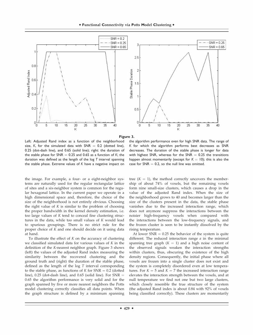
we classified simulated data for various values of K in thedefinition of the K-nearest neighbor graph. Figure 3 shows(left) the values of the adjusted Rand index measuring thesimilarity between the recovered clustering and theground truth and (right) the duration of the stable phase,defined as the length of the log T interval correspondingto the stable phase, as functions of K for SNR ¼ 0.2 (dottedline), 0.25 (dot-dash line), and 0.65 (solid line). For SNR ¼0.65 the algorithm performance is very solid and for thegraph spanned by five or more nearest neighbors the Pottsmodel clustering correctly classifies all data points. Whenthe graph structure is defined by a minimum spanning

tree (K ¼ 1), the method correctly uncovers the member-ship of about 74% of voxels, but the remaining voxelsform nine small-size clusters, which causes a drop in thevalue of the adjusted Rand index. When the size ofthe neighborhood grows to 40 and becomes larger than thesize of the clusters present in the data, the stable phasevanishes due to the increased interaction range, whichdoes not anymore suppress the interactions between thenoisier high-frequency voxels when compared withthe interactions between the low-frequency signals, andthe frozen cluster is seen to be instantly dissolved by therising temperature.At lower SNR ¼ 0.25 the behavior of the system is quite

different. The reduced interaction range a in the minimalspanning tree graph (K ¼ 1) and a high noise content ofthe observed signals weaken the interaction strengthswithin clusters, thus, obscuring the existence of the highdensity regions. Consequently, the initial phase where allvoxels are frozen into a single cluster does not exist andthe system is completely disordered even at low tempera-tures. For K ¼ 5 and K ¼ 7 the increased interaction rangeelevates the interaction strength between the voxels, and atnull temperature we find not one but two large clusters,which closely resemble the true structure of the system(the adjusted Rand index is about 0.84 with 92% of voxelsbeing classified correctly). These clusters are momentarily

Figure 3.

Left: Adjusted Rand index as a function of the neighborhood

size, K, for the simulated data with SNR ¼ 0.2 (dotted line),

0.25 (dot-dash line), and 0.65 (solid line); right: the duration of

the stable phase for SNR ¼ 0.25 and 0.65 as a function of K; the

duration was defined as the length of the log T interval spanning

the stable phase. Extreme values of K have a negative impact on

the algorithm performance even for high SNR data. The range of

K for which the algorithm performs best decreases as SNR

decreases. The duration of the stable phase is longer for data

with highest SNR, whereas for the SNR ¼ 0.25 the transitions

happen almost momentarily (except for K ¼ 10); this is also the

case for SNR ¼ 0.2, so the null line was omitted.


r 429 r

dissolved by rising temperature for K ¼ 7 but survive lon-ger for K ¼ 10 (the log T interval spanning the stablephase is [�5.29, �4.61], see also Fig. 3, right) before thesystem plunges into chaos. For 15 � K < 30 the frozencluster formed at low temperatures dissolves into a clustercontaining low-frequency voxels and a number of smallclusters with high-frequency signals. For larger K � 30, thestable phase vanishes and the system goes from the frozeninto chaotic state in a single jump.Reducing SNR to 0.2 we observe small changes in the

behavior of the system. For K < 5 a completely disorderedsystem exists even at low temperatures and the frozenstate of the system is not observed until K ¼ 7. For K ¼ 5at the null limit there exists a number of predominantlysingle-voxel clusters formed by the high-frequency signalsand a large cluster containing all the low-frequencysignals (the adjusted Rand index is 0.38), which instantlydissolves by rising temperature. The observed durationof the stable phase for the SNR ¼ 0.2 is essentially zerofor the entire range of K values and was not plotted onFigure 3 (right).

Comparison with other clustering methods

We used the simulated data to compare the Potts modelbased clustering to hierarchical clustering empowered bythe dendrogram sharpening previously used in fMRI con-nectivity analysis [Stanberry et al., 2003, 2006]. The two

clustering methods are similar in that they do not requirea priori assumptions of the number or nature of clusterspresent in the data and, therefore, the comparison shouldbe fair. Figure 4 (left) shows the performance of the twomethods as a function of SNR. Both methods were foundto be equally effective in distinguishing between the differ-ent signal profiles for an SNR of 0.25 and higher. The den-drogram based method appears to be more sensitivecorrectly classifying voxels with an SNR as low as 0.2,while the Potts model clustering at SNR ¼ 0.2 preservesthe low-frequency cluster and splits the high-frequencyone. This seemingly superior performance of the hierarchi-cal algorithm is explained by its definition. The method,by default, classifies all the voxels by assigning them tothe closest cluster core identified in the data set reducedby sharpening. Thus, the number of clusters in the data isstrictly less than the number of data points.As we have seen in the Potts model based method, clus-

ters formed by signals with low SNR are very unstableand melt into a multitude of single-point clusters, whereasclusters with high SNRs are preserved. Single-voxel clus-ters often do not have a meaningful interpretation, i.e.their occurrence in fMRI data is hardly justifiable from thebiological standpoint. To address this issue we impose alower bound on the size of the final clusters. This modifi-cation also makes the performance of the algorithm duringthe chaotic phase to be alike to the single linkage methodwith the number of clusters determined as a function of

Figure 4.

Adjusted Rand index as a function of SNR to compare the per-

formance of the Potts model clustering (solid line) to that of the

hierarchical clustering with dendrogram sharpening (dotted line).

The hierarchical clustering based method was more sensitive at

SNR ¼ 0.2 when compared with the Potts model based cluster-

ing with the minimum cluster size set to one (left). The Potts

model clustering with the minimum allowable cluster size set to

five (right) outperforms the hierarchical method for SNR ¼ 0.13

and gives reliable outcome for SNR ¼ 0.2 by correctly identify-

ing cluster membership of 92% of voxels. Both methods proved

to be effective in recovering the clustering structure for SNR >0.25.


r 430 r

the minimum allowable cluster size. Restricting any clusterto contain at least five voxels, Potts model clustering out-performs the hierarchical method for SNR ¼ 0.13 in termsof the adjusted Rand index and gives reliable outcome forSNR ¼ 0.2 by correctly identifying cluster membership of92% of voxels while misclassifying only a few high-fre-quency signals.

fMRI Data

Motor paradigm

We applied the Potts model clustering to the motor taskdata twice, first imposing no restriction on the size of thesmallest cluster, and then reclustering the data with thesize of the smallest cluster set to 50. Figure 5 showschanges in the size of the three largest clusters (top plot),the number of clusters in the data (middle plot), and theadjusted Rand index comparing partitions at neighboringtemperatures as a function of temperature (on the logscale); the minimum allowed cluster size was one. Initially

Figure 5.

Figure 6.

Clustering results for the motor-task experiment determined at

log T ¼ �5.95; minimum cluster size was set to one. Clusters

were color-coded and overlaid on high-resolution anatomical

images. The largest cluster (red) corresponds to the motor cor-

tex and supplementary motor area engaged in the motor task;

the remaining clusters predominantly contain a single voxel.

[Color figure can be viewed in the online issue, which is available

at www.interscience.wiley.com.]

Figure 5.

Top: The standard deviation trajectories of the three largest

clusters; center: number of clusters; and bottom: adjusted Rand

index as functions of temperature (log scale) for the motor task

experiment (the minimum cluster size set to one). The adjusted

Rand index measures the similarity of cluster assignments at

given and preceding temperatures. Phase transitions are identi-

fied by the peaks of standard deviation trajectories and abrupt

changes of the adjusted Rand index. The stable phase spans the

log T interval of [�6.25, �5.95], which is reflected by the simi-

larity of neighboring partitions in this temperature range

(bottom plot). Relatively high rate of the task presentation (�0.1

Hz) suppresses the signal changes, masking the transition to the

chaotic state, so the number of clusters increases monotonically

with rising temperatures. [Color figure can be viewed in the

online issue, which is available at www.interscience.wiley.com.]


r 431 r

all voxels form a single cluster, but as the temperatureincreases the system becomes increasingly unstable. Thepeaks of the standard deviation trajectories forecast signifi-cant changes in the clustering structure (i.e. the division oflarge clusters and subsequent formation of smaller clus-ters). At log T ¼ �7.4 the frozen cluster begins to splitwith a single voxel breaking away. The most extremechanges in the size of the two largest clusters observed at

Figure 8.

Figure 7.

Top: The standard deviation trajectories of the three largest

clusters; center: number of clusters; and bottom: adjusted Rand

index as functions of temperature (log scale) for the motor task

experiment (the minimum cluster size set to 50). The adjusted

Rand index measures the similarity between the cluster assign-

ments at the given and preceding temperatures. The changes in

the clustering structure are now more apparent and take place

at higher temperatures. During the stable phase, which is

spanned by a log T interval of [�1.49, �0.86] and is twice as

wide as the one observed in Figure 5, cluster assignments

remain robust (the adjusted Rand index is about 0.8). Since the

number of clusters present in the system is bounded above the

number of clusters and the similarity between the neighboring

partitions stabilize during the chaotic phase (log T > �0.6).

[Color figure can be viewed in the online issue, which is avail-

able at www.interscience.wiley.com.]

Figure 8.

Top: Clustering results for the stable phase at log T ¼ �0.98

(minimum cluster size is 50) identify the largest cluster (red)

corresponding to the motor cortex and supplementary motor

area. The remaining clusters could be attributed to the motion

component and vascular contributions; bottom: disordered state

at log T ¼ �0.86; the imposed cluster size restriction accentu-

ates strong dependencies between voxels in the immediate Eu-

clidean neighborhood. [Color figure can be viewed in the online

issue, which is available at www.interscience.wiley.com.]


r 432 r

log T ¼ �6.25 precede the meltdown of the system at logT ¼ �6.1 into about 500 clusters containing at most twovoxels, except one 450-voxel cluster. The content of thelargest cluster remains approximately the same as log Tincreases to �5.95, but it literally crumbles as noisy voxelsseparate from it to form independent groups as tempera-ture rises. Consequently, the number of clusters in the sys-tem steadily increases and the similarity index drops. Thelargest cluster (red) identified at log T ¼ �5.95 corre-sponds to the motor cortex and supplementary motor areaengaged in the motor task, while the remaining clusterspredominantly contain a single voxel (Fig. 6, the clusterswere color-coded to agree with the previous figure andoverlaid on high-resolution anatomical images).

Imposing the restriction on the size of the smallest clusterto contain at least 50 voxels, consistently with our expecta-tions we observe (Fig. 7, top plot) more pronounced changesin the standard deviation trajectories of the first two largestclusters at log T ¼ �1.61 and at log T ¼ �0.92, forecastingupcoming changes in the clustering structure. At log T ¼�1.49, the system splits into four clusters (Fig. 7, middleplot), causing the immediate drop in the adjusted Randindex (Fig. 7, bottom plot). During the stable phase of thesystem the size of the clusters and their content remainapproximately unchanged, which is reflected by the plateauof the standard deviation trajectories and relatively high val-ues of the adjusted Rand index, which are on the order of 0.8being equivalent to the change in cluster assignments for less

Figure 9.

Fourier and wavelet spectra (using the continuous Morlet trans-

form) for the three largest clusters identified for the periodic

motor task (minimum cluster size is 50). The largest contribu-

tion to the mean time course of the first largest cluster, corre-

sponding to the motor cortex and supplementary motor area,

comes from the paradigm frequency of 0.1 Hz (dashed lines on

Fourier spectra plots). The contributions are persistent through

the task and mimic the paradigm design [see the high periodic

values (dark red spots) at 0.1 Hz on the wavelet spectrum]. This

frequency contributes to the mean time courses of the other

two clusters, but is not dominant. Note that respiratory artifacts

were accurately localized (0.4 Hz oscillations in the second row)

into a separate cluster. [Color figure can be viewed in the online

issue, which is available at www.interscience.wiley.com.]

r 433 r


than 6% of voxels. The transition from the stable to chaoticstate occurs immediately after the second peak of the stand-ard deviation trajectories (log T ¼ �0.86) as the system splitsinto 10 clusters each containing 50–200 voxels. This changein the system structure is accompanied by the sharp decreaseof the adjusted Rand index (<0.2, corresponding to thechange of cluster assignments of 35% of voxels). As tempera-ture increases, the system gradually dissolves. However, theminimum cluster size condition restricts the number of clus-ters present in the system and, therefore, for higher tempera-tures (log T > �0.6) the number of clusters stabilizes and thesimilarity between the neighboring partitions increases.Figure 8 (top plot) shows the clustering results for the

stable phase at log T ¼ �0.98; the clusters were color-coded to match with color map on Figure 7 and overlaidon high-resolution anatomical images. The large red clus-ter corresponds to the motor cortex and supplementarymotor area engaged in the motor task. The remaining clus-ters could be attributed to a motion component or vascularcontributions. Frequency spectra and wavelet power spec-tra of the mean time courses of the three largest clusters(see Fig. 9) show a strong influence of the paradigm fre-quency (0.1 Hz) to the time courses of all, but the third,clusters. As expected, the power of the task frequency

closely mimics the task design in the motor areas (Fig. 9,top right). Respiratory artifacts are noticeable in the secondlargest cluster (Fig. 9, second row) as the periodic spikes ataround 0.4 Hz. The cluster partition at log T ¼ �0.86 (seeFig. 7) shows that at higher temperatures the red clusterassociated with the motor task splits into multiple clustersof considerably smaller sizes.

Resting-state connectivity

Figure 10 shows the standard deviations trajectories ofthe three largest cluster sizes for nine subjects under rest-ing-state conditions. The lower limit for the cluster sizewas set to 50. The standard deviation profiles are similarto those observed in the previous experiment. The trajecto-ries vary across subjects both in shape and magnitude. Therange of temperatures spanning the stable clustering phaseis much shorter for the resting state data than for themotor paradigm data. The temperature scale is approxi-mately the same, suggesting the equivalent interactionstrength among all nine data sets.The temperature corresponding to the last peak in the var-

iation of the size of the second largest cluster was used todetermine the consensus clustering structure for each sub-ject. Group connectivity maps show that at rest the anterior

Figure 10.

Standard deviation trajectories of the three largest clusters for the resting state data vary across

subjects both in shape and magnitude. The low signal strength reduces the duration of the stable

phase, which, nevertheless, is clearly visible. [Color figure can be viewed in the online issue,

which is available at www.interscience.wiley.com.]


r 434 r

cingulate cortex is functionally connected to the bilateralinferior, superior and middle frontal orbital cortex, superiormedial frontal cortex, bilateral parahippocampal gyrus, bilat-eral fusiform gyrus, right hippocampus, bilateral middletemporal gyrus, thalamus, posterior cingulum, and left post-central gyrus (see Fig. 11); whereas functional connections ofthe posterior cingulate cortex (see Fig. 12) extend to the thala-mus, anterior cingulate cortex, left postcentral gyrus, bilat-

eral inferior frontal gyrus, hippocampus, orbital frontalgyrus, left fusiform gyrus, and right parahippocampal gyrus.Figure 13 shows the group spectral density estimates andchanges in the frequency content over time for the meantime courses of the anterior and posterior cingulate cortices.The group estimates were obtained by averaging frequencyhistograms and time-frequency spectra across individuals.The spectra look fairly similar for the two structures. The

Figure 11.

Group functional connectivity maps of (obtained by Potts model

clustering) of the anterior cingulate cortex show its connections

to the inferior, superior, and middle frontal orbital cortex, para-

hippocampal gyrus, fusiform gyrus, right hippocampus, middle

temporal gyrus, thalamus, posterior cingulate cortex, superior

medial frontal cortex, and left postcentral gyrus in the resting-

state data. [Color figure can be viewed in the online issue, which

is available at www.interscience.wiley.com.]

Figure 12.

Group functional connectivity maps (obtained by Potts model

clustering) of the posterior cingulate cortex during rest include

the thalamus, anterior cingulate cortex, left postcentral gyrus,

bilateral inferior frontal gyrus, hippocampus, orbital frontal, left

fusiform, and right parahippocampal gyri. [Color figure can be

viewed in the online issue, which is available at www.interscience.

wiley.com.]


r 435 r

Figure 13.

Group Fourier and wavelet spectra (using the continuous Morlet

transform) for the anterior cingulated cortex (ACC, top row)

and posterior cingulate cortex (PCC, bottom row) obtained by

averaging frequency and time-frequency spectra of the cortices

across the nine subjects. [Color figure can be viewed in the


Figure 14.

Clustering results for the periodic motor task obtained by

extending the K-nearest neighbor graph to include edges with

immediate spatial neighbors in six orthogonal directions are sim-

ilar to those observed with a K-nearest neighbor graph based

only on functional distances. [Color figure can be viewed in the



r 436 r

dominant component of the oscillations corresponds to thelow-frequency range below 0.12 Hz, and the magnitude ofthese oscillations varies with time, exhibiting a strongincrease closer to the end of the task.

Incorporating spatial information in

connectivity analysis

We explored the possibility to incorporate spatial informa-tion from the Euclidean neighborhood via extending the K -nearest neighbor graph to include edges of the six immediate(in 3-D) neighboring voxels. That is for any two voxels iden-tified as spatial neighbors in a conventional Euclidean sense,but not as K - nearest neighbors, the edge was added to theexisting K-nearest neighbor graph and the correspondinginteraction term was computed as in (2). The standard devia-tion trajectories were rather similar to those observed previ-ously slightly differing only in the temperature scale. Thequality of the obtained connectivity maps (see Fig. 14) werealso alike to those described earlier with the biggest identi-fied cluster corresponding to the motor activity.

DISCUSSION

We have demonstrated the use of the Potts model basedclustering as an automatic tool to determine functional connec-tivity networks during periodic stimuli and in resting-statedata. The rational for the method stems from the ideas of sta-tistical mechanics and information theory. The method has avery intuitive physical interpretation and gives the solution interms of a probability distribution of the possible clusterassignments, which is then used to determine a unique grouplabeling. Another advantage of the Potts model based methodis its stochastic formulation, which allows it to be incorporatedinto hierarchical probabilistic models.In contrast to the seed voxel based connectivity approach

the method is totally automatic, i.e., there is no need forexpert intervention to construct the connectivity maps.Moreover, it is exhaustive in the sense that there is no omis-sion of seemingly connected brain regions. The Potts modelclustering is a kernel-based method [see Murua et al. (OnPotts model clustering, kernel K-means and density estima-tion, J Comput Graph Stat, under review) for connectionbetween the Potts model clustering and weighted kernelK-means] and, as such, shares the flexibility and good per-formance of kernel-based clustering methods includingkernel K-means [Girolami, 2002] and the multiway normal-ized cut [Meila and Xu, 2003]. However, in contrast to theK-means algorithm one makes no assumption on the distri-bution of the data or the expected number of clusters.Commonly to other clustering techniques the method

uses the dissimilarity measure between the objects. Inaddition, the interaction kernel and the number of nearestneighbors K to create a graph structure are required to bespecified. Once the samples from the underlying probabil-ity model are acquired it remains to identify the range oftemperatures corresponding to the stable partitioning

phase and determine the final cluster assignment. Weexplored the performance of the method and its sensitivityto various parameters on simulated data and recapitulatethe main findings later.

Effect of Parameters on Method Performance

The choice of the similarity measure

The Potts model clustering is based on the dissimilaritymeasure and avoids the explicit modeling of the observedsignals. In this paper, the interactions were computed fromthe low frequency specific correlations. A paradigmdesign, stimuli administration, and physiological processesmight induce spurious correlations that could potentiallylead to erroneous connectivity maps. The problem can becircumvented by, for example, using first- or higher orderpartial correlations [Jobson, 1992] to account for potentialconfounders, or by defining the interactions between thefeature vectors derived from the data rather than rawobservations [Goutte et al., 2001]. The use of the correla-tion coefficient in this study was justified by the prepro-cessing of the data, absence of the task-related confoundersin the resting-state data, and restricted spatial coverage ofthe brain volume for the motor task experiment. It is of in-terest to note that although the paradigm frequency indu-ces notable signal changes not just in the motor area but invoxels attributed to various artifacts (Fig. 9), the lowerends of the frequency spectra were substantially differentand, as a result, voxels were assigned to separate clusters.

The effect of the form of the interaction kernel

The effect of the form of the interaction kernel onalgorithm performance has been experimentally shownto be negligible by previous researchers [Wiseman et al.,1998]. In particular, the standard deviation trajectoriesfor the power law interactions, interactions specified bythe Gaussian kernel, and interactions specified by theexponential kernel were found to be similar and differonly in the range of temperatures where the changes inthe system occur. The irrelevance of the interactionform can also be seen through the connection of thePotts model based clustering to the kernel density esti-mation problem [Silverman, 1986; Murua et al., On Pottsmodel clustering, kernel K-means and density estima-tion, J Comput Graph Stat, under review), for which ithas been established both theoretically and experimen-tally [Epanechnikov, 1969] that the choice of the kernelhas negligible effect on the performance of the estima-tion method.

Effect of K

The Potts model was originally considered on a systemof spins confined to the regular lattice [Wu, 1982]. In thiswork, we did not view data as acquired on a regular lat-tice corresponding to the 3D representation of the brain;


r 437 r

rather, we ‘‘mapped’’ the data into a functional spacewhere the distances between voxels were defined by thesimilarity of the observed time courses. The transformeddata were not forming a regular lattice anymore and thedefinition of the neighborhood structure was not straight-forward. One of the possible choices in this situation wasto identify neighbors using the K-neighborhood criterion.Choosing K too big or too small would either smooth outthe important features in the data or make its structureappear too noisy. The effect of K was not found to be cru-cial to the performance of the clustering procedure for amany-cluster model with noise [Wiseman et al., 1998],however, the size of the neighborhood considered in thatpaper did not vary considerably (K ¼ 6, 12, 14, 18, and theVoronoi cell structure were studied), the contrast to noiseratio of the image, though not specified, appeared to bereasonably high, and the performance of the algorithmwas measured in terms of accuracy, a measure that is lessconservative than the adjusted Rand index.Our experiments on simulated data indicate a notable

effect of the extreme values of K on the algorithm perform-ance, which varies with SNR of the data. For high SNRs,when clusters are clearly distinguishable, the influence ofK is negligible as the algorithm perfectly uncovers thestructure for a large range of values. However, extremelysmall values of K produce completely disordered (noisy)systems, whereas too large values of the parameter inflatethe interaction strength even between points from differentclusters completely annihilating the stable phase. Theseeffects are amplified by the deteriorating signal strengthsince interactions grow rapidly as dissimilarity betweenthe voxels increases. Hence, the range of K where the algo-rithm performs well shortens as signal content weakens.Based on our experimental results, we settled for K ¼ 10for fMRI data collected at 1.5 T.

Comparison with other clustering methods

Previous studies have shown [Blatt et al., 1997; Muruaet al., On Potts model clustering, kernel K-means and den-sity estimation, J Comput Graph Stat, under review)] supe-rior performance of the Potts model clustering for real andsimulated data in comparison with other clustering techni-ques including the hierarchical single linkage, complete link-age, minimal spanning tree, directed graph method [Fuku-naga, 1990], etc. Our study shows that a minimum clustersize restriction improves the results of the method, whichperforms better or as good as a hierarchical clustering withdendrogram sharpening for a wide range of SNRs. The anal-ysis of the fMRI motor task data with and without a clustersize restriction demonstrated other advantages of this condi-tion including the increased duration of the stable phaseand more apparent phase transitions.

Mapping Connectivity in Functional MRI Data

We have demonstrated how the Potts model clusteringmethod can be applied to the functional connectivity prob-

lem using data from a conventional box-design motor taskand a more complex resting-state condition. Following thechanges in the data clustering structure over the extendedtemperature range we observed a clear transition from thefrozen to the stable state. The observed steady monotoneincrease in the number of identified clusters (see Fig. 5) isdue to a relatively high frequency of the on-off task design(0.1 Hz), which subdues the contrast between the ‘‘on’’and ‘‘off’’ images [Hathout et al., 1999].By imposing the lower limit on the size of the clusters,

we force the system to remain in any present state for alonger range of temperatures, and higher temperatureswere required for the bonds to be broken. Consequently,the phase transitions were taking place at higher tempera-tures, the stable phase became more pronounced, and therange of the temperatures spanning the stable phaseincreased. The restriction on the size of the smallest clusteris equivalent to the condition on the largest number ofclusters to be present in the system at any given tempera-ture. Therefore, once the transition to the chaotic phaseoccurs, clusters containing only a few voxels are forced tojoin together, which explains why the number of clustersin the system and the similarity index of neighboringassignments are stabilized at high temperatures (Fig. 7,middle and bottom plots).Relative robustness of the clustering solutions within the

stable phase allows one to select a partition correspondingto any log T within the stable phase interval as a final clus-tering solution. Alternatively, one could construct an aug-mented partition for the stable phase by estimating the pro-portion of times each pair of voxel was assigned to the samecluster and then thresholding it to get a unique labeling.

Resting state connectivity

The resulting functional connectivity maps for the ante-rior and posterior cingulate cortices during rest are consist-ent with earlier findings by Greicius et al. [2003] obtainedwith a seed voxel approach. In particular, Greicius et al.[2003] showed the connectivity of the posterior cingulatecortex with the medial prefrontal cortex, and found theventral anterior cingulate cortex to be connected to the pos-terior cingulate and medial prefrontal cortex, including or-bital frontal cortex and hypothalamus. However, there aresome notable differences between the connectivity maps ofGreicius et al. [2003] and ours. Our findings show the pos-terior cingulate cortex to be connected to both the rightparahippocampal gyrus and the bilateral hippocampus,whereas Greicius et al. [2003] only found a connection tothe left parahippocampal gyrus. We also found the poste-rior and anterior cingulate cortices to be connected to theleft and bilateral fusiform gyrus, respectively. These differ-ences could be in part due to the reduction of the signalsfrom the entire brain structure (anterior or posterior cingu-late cortices) to the sole mean time course of the region inthe seed-voxel approach implemented in Greicius et al.[2003].


r 438 r

Incorporating spatial information into analysis

Conceptually, it would be beneficial to account for theEuclidean neighborhood system in the analysis, providedit improves the results. Spatial information can be incorpo-rated in a number of ways, the simplest being to consideronly a nearest-neighbor Euclidean system not regardingthe similarity of the observed signals. With regard to thefunctional connectivity problem, a simple presumption ofthe conventional Euclidean neighborhood structure is falla-cious considering complicated folding patterns of graymatter, though one could try and solve the clusteringproblem on the flattened cortical surface where theassumption of the Euclidean spatial dependences seemsmore appropriate (note that this approach would excludestructures deep inside the brain from the analysis).Another way to account for the natural 3D structure is, asit was done in the paper, to augment the existing K-nearestneighbor graph structure with edges defined by spatialproximities. Alternatively, one could redefine the distancemeasure as a weighted combination of the Euclidean dis-tances and the similarity measure of interest or update theinteraction term to include morphometric characteristics ofthe brain structures.Although, our experiments did not indicate the effect of the

combined neighborhood structure on clustering results, itwould be of general interest to pursue this venue and furtherexplore the use of spatial informationwith the goal to increasethe sensitivity and accuracy of the clusteringmethod.

CONCLUSIONS

We introduced an unsupervised stochastic clusteringmethod based on the ferromagnetic Potts model, whichprovides a powerful alternative to study coherent signalchanges and can be effectively used as an automatic toolto determine functional connectivity networks under vari-ous complex conditions such as the resting-state and con-tinuous stimuli. We demonstrated the specifics of themethod by applying it to the simulated data and a conven-tional on-off finger tapping paradigm. The method shownin the literature to be insensitive to the choice of the inter-action kernel was found to give a robust performance fordata with SNR as low as 0.2. The ability of the method torecover a hidden clustering structure depends on the sizeof the neighborhood and one should avoid using theextreme values of K. Our experiments showed the stabilityof the resulting clustering solutions in the sense that therewas little variation of the cluster assignments within thestable phase. We observed that a lower bound on the sizeof the smallest cluster slows the changes in the clusteringstructure, increases the duration of the stable phase, andimproves the clustering results for low SNR data. Spatialinformation was not found to enhance the clustering solu-tions, though additional research on this topic is encour-aged. Functional connections of the anterior and posteriorcingulate cortices for a group of nine healthy subjects dur-

ing rest corroborate previous findings, therefore, attestingto the ability of the Potts model clustering to operate onthe complex data sets.Potts model based method provides an elegant way for

functional connectivity mapping since it makes no assump-tion with regard to the underlying grouping structure ofthe data and can simultaneously identify functional networkspresent in the data. To our knowledge, Potts model cluster-ing and ICA [Beckman and Smith, 2005; Cordes et al., 1999]are so far the only two methods reported in the literaturethat are capable of simultaneous identification of connectiv-ity networks in resting-state data.

ACKNOWLEDGMENTS

The authors would like to thank Dr. Tilmann Gneitingat the University of Washington for his valuable sugges-tions and the anonymous referees whose comments helpedto enhance the quality of the manuscript. This researchwas in part supported by a special multidisciplinary cen-ter grant P50-33812 from the National Institute of ChildHealth and Human Development (NIHCD) and by a fel-lowship from the National Science Foundation programfor Vertical Integration of Research and Education in theMathematical Sciences (VIGRE).

REFERENCES

Agrawal H, Domany E (2003): Potts ferromagnets on coexpressedgene networks: Identifying maximally stable partitions. PhysRev Let 90:158102.

Baumgartner R, Windischberger C, Moser E (1998): Quantificationin functional magnetic resonance imaging: Fuzzy clustering vs.correlation analysis. Magn Reson Imaging 16:115–125.

Beckmann CF, Smith SM (2005): Tensorial extensions of independ-ent component analysis for group fMRI data analysis. Neuro-image 25:294–311.

Biswal B, Yetkin F, Haughton V, Hyde J (1995): Functional connec-tivity in the motor cortex of resting human brain using echo-planar MRI. Magn Reson Med 34:537–541.

Blatt M, Wiseman S, Domany E (1996): Superparamagnetic cluster-ing of data. Phys Rev Let 76:3251–3254.

Blatt M, Wiseman S, Domany E (1997): Data clustering using amodel granular magnet. Neural Comput 9:1805–1842.

Cordes D, Carew J, Eghbalnia H, Meyerand E, Quigley M, Arfana-kis K, Assadi A, Turski P, Haughton V (1999): Resting-statefunctional connectivity study using independent componentanalysis, In: Proceedings International Society for MagneticResonance in Medicine, 7th Annual Meeting, Philadelphia.

Cordes D, Haughton V, Arfanakis K, Wendt G, Turski P, MoritzC, Quigley M, Meyerand M (2000): Mapping functionallyrelated regions of the brain with functional connectivity MRimaging. Am J Neuroradiol 21:1636–1644.

Cordes D, Haughton V, Carew J, Arfanakis K, Maravilla K (2002):Hierarchical clustering to measure connectivity in fMRI rest-ing-state data. Magn Reson Imaging 20:305–317.

Domany E (1999): Superparamagnetic clustering of data—Thedefinitive solution of an ill-posed problem. Phys A 263:158–169.

Domany E (2003): Cluster analysis of gene expression data. J StatPhys 110:1117.


r 439 r

Domany E, Blatt M, Gdalyahu Y, Weinshall D (1999): Superpara-magnetic clustering of data: Application to computer vision.Comp Phys Commun 121/122:5–12.

Downton M, Brennan T (1980): Comparing classifications: An evalu-ation of several coefficients of partition agreement. Paper pre-sented at themeeting of the Classification Society, Boulder, CO.

Einav U, Tabach Y, Getz G, Yitzhaky A, Ozbek U, Amarglio N,Izraeli S, Rechavi G, Domany E (2005): Gene expression analy-sis reveals a strong signature of an interferon-induced pathwayin childhood lymphoblastic leukemia as well as in breast andovarian cancer. Oncogene 24:6367–6375.

Epanechnikov VA (1969): Non-parametric estimation of a multi-variate probability density. Theory Prob Applic 14:153–158.

Filzmoser P, Baumgartner R, Moser E (1999): A hierarchical clus-tering method for analyzing functional MR images. MagnReson Imaging 17:817–816.

Fowlkes EB, Mallows CL (1983): A method for comparing twohierarchical clusterings, (with comments and rejoinder). J AmStat Assoc 78:553–584.

Friston KJ (1995): Functional and effective connectivity in neuroi-maging: A synthesis. Hum Brain Mapp 2:56–78.

Friston KJ, Frith C, Liddle FP, Frackowiak RSJ (1993): Functionalconnectivity: The principal-component analysis of large (PET)data sets. J Cereb Blood Metab 13:5–14.

Fukunaga K (1990): Introduction to Statistical Pattern Recognition.San Diego: Academic Press.

Getz G, Domany E (2003): Coupled two-way clustering server.Bioinformatics 19:1153–1154.

Getz G, Levine E, Domany E, Zhang M (2000a): Super-paramagneticclustering of yeast gene expression profiles. Phys A 279:457–464.

Getz G, Levine E, Domany E (2000b): Coupled two-way clusteringanalysis of gene microarray data. Proc Natl Acad Sci USA97:12079–12084.

Girolami M (2002): Mercer kernel based clustering in featurespace. IEEE Trans Neur Net 13:669–688.

Goutte C, Toft P, Rostrup E, Nielsen FA, Hansen, LK (1999): Onclustering fMRI time series. Neuroimage 9:298–310.

Goutte C, Hansen LK, Liptrot MK, Rostrup E (2001): Feature-spaceclustering for fMRI meta-analysis. Hum Brain Mapp 13:165–183.

Greicius M, Krasnow B, Reiss A, Menon V (2003): Functional con-nectivity in the resting brain: A network analysis of the defaultmode hypothesis. Proc Natl Acad Sci USA 100:253–258.

Hampson M, Peterson B, Skudlarski P, Gatenby J, Gore J (2002):Detection of functional connectivity using temporal correlationsin MR images. Hum Brain Mapp 15:247.

Hampson M, Olson I, Leung H, Skudlarski P, Gore J (2004):Changes in functional connectivity of human MT/V5 with vis-ual motion input. Neuroreport 15:1315–1319.

Hathout GM, Copi RK, Bandettini P, Gambhir SS (1999): The lag ofcerebral hemodynamics with rapidly alternating periodic stimula-tion: Modeling for functional MRI. Magn Reson Imaging 17:9–20.

Hubert L, Arabie P (1985): Comparing partitions. J Classif 2:193–218.Jobson JD (1992): Applied Multivariate Data Analysis, Vol. 2. New

York: Springer-Verlag.Kullmann L, Kertesz J, Mantegna RN (2000): Identification of clus-

ters of companies in stock indices via Potts super-paramagnetictransitions. Phys A 287:412–419.

Lowe M, Mock B, Sorenson J (1998): Functional connectivity insingle and multislice echoplanar imaging using resting-statefluctuations. Neuroimage 7:119–132.

Lowe M, Dzemidzic M, Lurito J, Mathew V, Phillips M (2000):Correlations in low-frequency BOLD fluctuations reflect cor-tico-cortical connections. Neuroimage 12:582–587.

Lowe M, Phillips M, Lurito J, Mattson D, Dzemidzic M, MathewsV (2002): Multiple sclerosis: Low-frequency temporal blood ox-ygen level-dependent fluctuations indicate reduced functionalconnectivity—Initial results. Radiology 224:184–192.

McKeownMJ, Sejnowski TJ (1998): Independent component analysisof fMRI data: Examining the assumptions. Hum Brain Mapp6:368–372.

Meila M, Xu L (2003): Multiway cuts and spectral clustering.,Department of Statistics, University of Washington: Seattle,WA. Technical report No 442.

Milligan G, Cooper M (1986): A study of the comparability ofexternal criteria for hierarchical cluster analysis. MultivariateBehav Res 21:441–458.

Morey L, Agresti A (1984): The measurement of classificationagreement: An adjustment to the Rand statistic for chanceagreement. Educ Psychol Meas 44:33–37.

Ott T, Kern A, Schuffenhauer A, Popov M, Acklin P, Jacoby E,Stoop R (2004): Sequential superparamagnetic clustering forunbiased classification of high-dimensional chemical data.J Chem Inf Comput Sci 44:1358–1364.

Ott T, Kern A, Steeb W, Stoop R (2005): Sequential clustering:tracking down the most natural clusters. J Stat Mech 11:P11014.

Quiroga RQ, Nadasdy Z, Ben-Shaul Y (2004): Unsupervised spikedetection and sorting with wavelets and superparamagneticclustering. Neural Comput 16:1661–1687.

Rand WM (1971): Objective criteria for the evaluation of clusteringmethods. J Am Stat Assoc 66:846–850.

Reichardt J, Bornholdt S (2004): Detecting fuzzy communities in com-plex networks with a Potts model. Phys Rev Lett 93: 218701.

Silverman BW (1986): Density estimation for statistics and dataanalysis, London, New York, Chapman and Hall.

Sokal AD (1996): Monte-Carlo methods in statistical mechanics:Foundations and new algorithms. In: Lectures at the CargeseSummer School on ‘‘Functional Integration: Basics and Applica-tions.’’

Stanberry L, Nandy R, Cordes D (2003): Cluster analysis of fMRI Datausing dendrogram sharpening. HumBrainMapp 20:201–219.

Stanberry L, Richards T, Berninger VW, Nandy R, Aylward E,Maravilla K, Cordes D (2006): Low frequency signal changesreflect differences in functional connectivity between goodreaders and dyslexics during continuous phoneme mapping.Magn Reson Imaging 24:217–229.

Stein T, Moritz C, Quigley M, Cordes D, Haughton V, MeyerandE (2000): Functional connectivity in the thalamus and hippo-campus studied with functional MR imaging. Am J Neurora-diol 21:1397–1401.

Swendsen RH, Wang JS (1987): Nonuniversal critical dynamics inMonte Carlo simulations. Phys Rev Lett 58:86–88.

Tzourio-Mazoyer N, Landeau B, Papathanassiou DF, Crivello F, EtardO, Delcroix N, Mazoyer B, Joliot M (2002): Automated anatomicallabeling of activations in SPM using a macroscopic anatomical par-cellation of the MNI MRI single-subject brain. NeuroImage 15(1):273–289.

Vaidya PM (1989): An O(n log n) algorithm for the all-nearest-neighbors problem. Disc Comp Geom 4:101–115.

von Ferber C, Worgoetter F (2000): Cluster update algorithm andrecognition. Phys Rev E62(Part A):1461–1464.

Wiseman S, Blatt M, Domany E (1998): Superparamagnetic cluster-ing of data. Phys Rev E 57:3767–3783.

Wu FY (1982): The Potts model. Rev Mod Phys 54:235–268.Xiong J, Parsons L, Gao J, Fox P (1999): Interregional connectivity

to primary motor cortex revealed using MRI resting-stateimages. Hum Brain Mapp 8:151–156.


r 440 r

functional connectivity mapping using the ferromagnetic potts spin model

Documents