functional mock-up interface for model exchange and co ... · functional mock-up interface for...
TRANSCRIPT
Functional Mock-up Interface for Model Exchange and Co-Simulation Document version: 2.0 July 25, 2014 This document defines the Functional Mock-up Interface (FMI), version 2.0. FMI is a tool independent standard to support both model exchange and co-simulation of dynamic models using a combination of xml-files and C-code (either compiled in DLL/shared libraries or in source code). The first version, FMI 1.0, was published in 2010. The FMI development was initiated by Daimler AG with the goal to improve the exchange of simulation models between suppliers and OEMs. As of today, development of the standard continues through the participation of 16 companies and research institutes. FMI 1.0 is supported by over 45 tools and is used by automotive and non-automotive organizations throughout Europe, Asia and North America.
On the Downloads page (https://www.fmi-standard.org/downloads), this specification, as well as supporting C-header and xml schema files, and an FMI compliance checker is provided. In addition, sample models (exported from different tools in FMI format) are provided to assist tool vendors to ensure compatibility with other tools, as well as a test suite to check whether connected FMUs are appropriately handled by a tool.
Contact the FMI development group at [email protected].

Functional Mock-up Interface 2.0 July 25, 2014 Page 2 of 126
History / Road Map
Version Date Remarks
1.0 2010-01-26 First version of FMI for Model Exchange
1.0 2010-10-12 First version of FMI for Co-Simulation
2.0 2014-07-25 Second version of FMI for Model Exchange and Co-Simulation
Please, report issues that you find with this specification to the public FMI issue tracking system: https://trac.fmi-standard.org
Functional Mock-up Interface 2.0 July 25, 2014 Page 3 of 126
License of this document Copyright © 2008-2011 MODELISAR consortium and 2012-2014 Modelica Association Project “FMI” This document is provided “as is" without any warranty. It is licensed under the CC-BY-SA (Creative Commons Attribution-Sharealike 4.0 International) license, which is the license used by Wikipedia. Human-readable summary of the license text from http://creativecommons.org/licenses/by-sa/4.0/:
You are free to:
Share — copy and redistribute the material in any medium or format
Remix — remix, transform, and build upon the material
for any purpose, even commercially.
The licensor cannot revoke these freedoms as long as you follow the license terms.
Under the following terms:
Attribution — You must give appropriate credit, provide a link to the license, and indicate if changes were made. You may do so in any reasonable manner, but not in any way that suggests the licensor endorses you or your use.
Share Alike — If you remix, transform, or build upon the material, you must distribute your contributions under the same license as the original.
The legal license text and disclaimer is available at:
http://creativecommons.org/licenses/by-sa/4.0/legalcode
Note: Article (3a) of this license requires that modifications of this work must clearly label, demarcate or otherwise identify that changes were made.
The C header and XML-schema files that accompany this document are available under the BSD 2-Clause license (http://www.opensource.org/licenses/bsd-license.html) with the extension that modifications must be also provided under the BSD 2-Clause license.
Attention is drawn to the possibility that some of the elements of this document may be the subject of patent rights. Modelica Association shall not be held responsible for identifying such patent rights.
If you have improvement suggestions, please send them to the FMI development group at mailto:[email protected].

Functional Mock-up Interface 2.0 July 25, 2014 Page 4 of 126
Abstract
This document defines the Functional Mock-up Interface (FMI), version 2.0 to (a) exchange dynamic models between tools and (b) define tool coupling for dynamic system simulation environments.
FMI for Model Exchange (chapter 3) The intention is that a modeling environment can generate C code of a dynamic system model that can be utilized by other modeling and simulation environments. Models are described by differential, algebraic and discrete equations with time-, state- and step-events. If the C code describes a continuous system, then this system is solved with the integrators of the environment where it is used. The models to be treated by this interface can be large for usage in offline or online simulation, or can be used in embedded control systems on micro-processors.
FMI for Co-Simulation (chapter 4) The intention is to provide an interface standard for coupling of simulation tools in a co-simulation environment. The data exchange between subsystems is restricted to discrete communication points. In the time between two communication points, the subsystems are solved independently from each other by their individual solver. Master algorithms control the data exchange between subsystems and the synchronization of all simulation solvers (slaves). Both, rather simple master algorithms, as well as more sophisticated ones are supported. Note, that the master algorithm itself is not part of the FMI standard.
FMI Common Concepts (chapter 2) The two interface standards have many parts in common. In particular, it is possible to utilize several instances of a model and/or a co-simulation tool and to connect them together. The interfaces are independent of the target environment because no header files are used that depend on the target environment (with exception of the data types of the target platform). This allows generating one dynamic link library that can be utilized in any environment on the same platform. A model, a co-simulation slave or the coupling part of a tool, is distributed in one zip file called FMU (Functional Mock-up Unit) that contains several files:
(1) An XML file contains the definition of all exposed variables in the FMU and other static information. It is then possible to run the FMU on a target system without this information, in other words with no unnecessary overhead.
(2) All needed model equations or the access to co-simulation tools are provided with a small set of easy to use C functions. A new caching technique allows a more efficient evaluation of the model equations than in other approaches. These C functions can either be provided in source and/or binary form. Binary forms for different platforms can be included in the same FMU zip file.
(3) The model equations or the co-simuation tool can be either provided directly in the FMU, or the FMU contains only a generic communication module that communicates with an external tool that evaluates or simulates the model. In the XML file information about the capabilities of the FMU are present, for example to characterize the ability of a co-simulation slave to support advanced master algorithms such as the usage of variable communication step sizes, higher order signal extrapolation, or others.
(4) Further data can be included in the FMU zip file, especially a model icon (bitmap file), documentation files, maps and tables needed by the FMU, and/or all object libraries or dynamic link libraries that are utilized.
A growing set of tools supports FMI. The actual list of tools is available at:
https://www.fmi-standard.org/tools
Functional Mock-up Interface 2.0 July 25, 2014 Page 5 of 126
About FMI 2.0 This version 2.0 is a major enhancement compared to FMI 1.0, where the FMI 1.0 Model Exchange and Co-Simulation standards have been merged, and many improvements have been incorporated, often due to practical experience when using the FMI 1.0 standards. New features are usually optional (need neither be supported by the tool that exports an FMU, nor by the tool that imports an FMU). Details are provided in appendix A.3.1. The appendix of the FMI 1.0 specification has been mostly moved in an extended and improved form to a companion document
“FunctionalMockupInterface-ImplementationHints.pdf”
where practical information for the implementation of the FMI standard is provided.
Conventions used in this Document • Non-normative text is given in square brackets in italic font: [especially examples are defined in this
style.].
• Arrays appear in two forms:
o In the end-user/logical view, one- and two-dimensional arrays are used. Here the convention of linear algebra, the control community and the most important tools in this area is utilized, in other words the first element along one dimension starts at index one. In all these cases, the starting index is also explicitly mentioned at the respective definition of the array. Example: In the modelDescription.xml file, the set of exposed variables is defined as ordered sets where the first element is referenced with index one (these indices are, for example, used to define the sparseness structure of partial derivative matrices).
o In the implementation view, one-dimensional C-arrays are used. In order to access an array element the C-convention is used. For example, the first element of input argument x for function setContinuousStates(..) is x[0].
FMI 2.0 Implementation Help If you plan to export or import models in FMI 2.0 format, you may find the following tools/models helpful for your development (available from https://fmi-standard.org/downloads):
• FMU Compliance Checker Free software to check whether an FMI model is compliant to the FMI standard.
• FMUs from other tools In order to test the import of FMI models from other vendors in your tool, a set of test FMUs are provided.
• Library to test connected FMUs Free Modelica library to test difficult cases of connected FMI models.
• FMU Software Development Kit Free software development kit by QTronic to demonstrate basic use of FMI.
• FMI Library Free software package by Modelon that enables integration of FMI models in applications.
Functional Mock-up Interface 2.0 July 25, 2014 Page 6 of 126
Contents
1. Overview ............................................................................................................................ 8
1.1 Properties and Guiding Ideas ................................................................................................... 9 1.2 Acknowledgements ................................................................................................................. 12
2. FMI Common Concepts for Model Exchange and Co-Simulation ................................ 13
2.1 FMI Application Programming Interface .................................................................................. 13 2.1.1 Header Files and Naming of Functions........................................................................ 13 2.1.2 Platform Dependent Definitions (fmi2TypesPlatform.h ) .............................................. 15 2.1.3 Status Returned by Functions ..................................................................................... 16 2.1.4 Inquire Platform and Version Number of Header Files ................................................ 18 2.1.5 Creation, Destruction and Logging of FMU Instances ................................................. 18 2.1.6 Initialization, Termination, and Resetting an FMU ....................................................... 21 2.1.7 Getting and Setting Variable Values ............................................................................ 23 2.1.8 Getting and Setting the Complete FMU State .............................................................. 24 2.1.9 Getting Partial Derivatives ........................................................................................... 25
2.2 FMI Description Schema......................................................................................................... 28 2.2.1 Definition of an FMU (fmiModelDescription) ................................................................ 29 2.2.2 Definition of Units (UnitDefinitions) .............................................................................. 33 2.2.3 Definition of Types (TypeDefinitions) ........................................................................... 38 2.2.4 Definition of Log Categories (LogCategories) .............................................................. 42 2.2.5 Definition of a Default Experiment (DefaultExperiment) .............................................. 43 2.2.6 Definition of Vendor Annotations (VendorAnnotations) ................................................ 43 2.2.7 Definition of Model Variables (ModelVariables) ........................................................... 44 2.2.8 Definition of the Model Structure (ModelStructure) ...................................................... 55 2.2.9 Variable Naming Conventions (variableNamingConvention) ....................................... 64
2.3 FMU Distribution ..................................................................................................................... 65
3. FMI for Model Exchange ................................................................................................. 69
3.1 Mathematical Description ....................................................................................................... 69 3.2 FMI Application Programming Interface .................................................................................. 79
3.2.1 Providing Independent Variables and Re-initialization of Caching ............................... 79 3.2.2 Evaluation of Model Equations .................................................................................... 80 3.2.3 State Machine of Calling Sequence ............................................................................. 82 3.2.4 Pseudo Code Example ................................................................................................ 86
3.3 FMI Description Schema......................................................................................................... 88 3.3.1 Model Exchange FMU (ModelExchange) .................................................................... 89 3.3.2 Example XML Description File ..................................................................................... 91
4. FMI for Co-Simulation ..................................................................................................... 93
4.1 Mathematical Description ....................................................................................................... 94 4.1.1 Basics .......................................................................................................................... 94 4.1.2 Mathematical Model .................................................................................................... 96
4.2 FMI Application Programming Interface .................................................................................. 99 4.2.1 Transfer of Input / Output Values and Parameters ...................................................... 99

Functional Mock-up Interface 2.0 July 25, 2014 Page 7 of 126
4.2.2 Computation .............................................................................................................. 100 4.2.3 Retrieving Status Information from the Slave ............................................................ 102 4.2.4 State Machine of Calling Sequence from Master to Slave ......................................... 103 4.2.5 Pseudo Code Example .............................................................................................. 106
4.3 FMI Description Schema....................................................................................................... 108 4.3.1 Co-Simulation FMU (CoSimulation) ........................................................................... 108 4.3.2 Example XML Description File ................................................................................... 111
5. Literature ....................................................................................................................... 114
Appendix A FMI Revision History .................................................................................. 115
A.1 Version 1.0 – FMI for Model Exchange ................................................................................. 115 A.2 Version 1.0 – FMI for Co-Simulation ..................................................................................... 116 A.3 Version 2.0 – FMI for Model Exchange and Co-Simulation ................................................... 117
A.3.1 Overview ................................................................................................................... 117 A.3.2 Main changes ............................................................................................................ 118 A.3.3 Contributors ............................................................................................................... 122
Appendix B Glossary ...................................................................................................... 124
Functional Mock-up Interface 2.0 July 25, 2014 Page 8 of 126
1. Overview
The FMI (Functional Mock-up Interface) defines an interface to be implemented by an executable called FMU (Functional Mock-up Unit). The FMI functions are used (called) by a simulation environment to create one or more instances of the FMU and to simulate them, typically together with other models. An FMU may either have its own solvers (FMI for Co-Simulation, chapter 4) or require the simulation environment to perform numerical integration (FMI for Model Exchange, chapter 3). The goal of this interface is that the calling of an FMU in a simulation environment is reasonably simple. No provisions are provided in this document how to generate an FMU from a modeling environment. Hints for implementation can be found in the companion document “FunctionalMockupInterface-ImplementationHints.pdf“.
The FMI for Model Exchange interface defines an interface to the model of a dynamic system described by differential, algebraic and discrete-time equations and to provide an interface to evaluate these equations as needed in different simulation environments, as well as in embedded control systems, with explicit or implicit integrators and fixed or variable step-size. The interface is designed to allow the description of large models.
The FMI for Co-Simulation interface is designed both for the coupling of simulation tools (simulator coupling, tool coupling), and coupling with subsystem models, which have been exported by their simulators together with its solvers as runnable code. The goal is to compute the solution of time dependent coupled systems consisting of subsystems that are continuous in time (model components that are described by differential-algebraic equations) or time-discrete (model components that are described by difference equations, for example discrete controllers). In a block representation of the coupled system, the subsystems are represented by blocks with (internal) state variables x(t) that are connected to other subsystems (blocks) of the coupled problem by subsystem inputs u(t) and subsystem outputs y(t).
In case of tool coupling, the modular structure of coupled problems is exploited in all stages of the simulation process beginning with the separate model setup and pre-processing for the individual subsystems in different simulation tools. During time integration, the simulation is again performed independently for all subsystems restricting the data exchange between subsystems to discrete communication points. Finally, also the visualization and post-processing of simulation data is done individually for each subsystem in its own native simulation tool.
The two interfaces have large parts in common. These parts are defined in chapter 2. In particular:
• FMI Application Programming Interface (C) All needed equations or tool coupling computations are evaluated by calling standardized “C” functions. “C” is used, because it is the most portable programming language today and is the only programming language that can be utilized in all embedded control systems.
• FMI Description Schema (XML) The schema defines the structure and content of an XML file generated by a modeling environment. This XML file contains the definition of all variables of the FMU in a standardized way. It is then possible to run the C code in an embedded system without the overhead of the variable definition (the alternative would be to store this information in the C code and access it via function calls, but this is neither practical for embedded systems nor for large models). Furthermore, the variable definition is a complex data structure and tools should be free how to represent this data structure in their programs. The selected approach allows a tool to store and access the variable definitions (without any memory or efficiency overhead of standardized access functions) in the programming language of the simulation environment, such as C++, C#, Java, or Python. Note, there are many free and commercial libraries in different programming languages to read XML files into an appropriate data structure, see for example http://en.wikipedia.org/wiki/XML#Parsers, and especially

Functional Mock-up Interface 2.0 July 25, 2014 Page 9 of 126
the efficient open source parser SAX (http://sax.sourceforge.net/, http://en.wikipedia.org/wiki/Simple_API_for_XML).
An FMU (in other words a model without integrators, a runnable model with integrators, or a tool coupling interface) is distributed in one zip file. The zip file contains (more details are given in section 2.3):
• The FMI Description File (in XML format).
• The C sources of the FMU, including the needed run-time libraries used in the model, and/or binaries for one or several target machines, such as Windows dynamic link libraries (.dll) or Linux shared object libraries (.so). The latter solution is especially used if the FMU provider wants to hide the source code to secure the contained know-how or to allow a fully automatic import of the FMU in another simulation environment. An FMU may contain physical parameters or geometrical dimensions, which should not be open. On the other hand, some functionality requires source code.
• Additional FMU data (like tables, maps) in FMU specific file formats.
A schematic view of an FMU is shown in the next figure:
Figure 1: Data flow between the environment and an FMU. For details, see chapters 3 and 4.
Blue arrows: Information provided by the FMU. Red arrows: Information provided to the FMU.
Publications for FMI are available from https://www.fmi-standard.org/literature, especially Blochwitz et.al. 2011 and 2012.
1.1 Properties and Guiding Ideas
In this section, properties are listed and some principles are defined that guided the low-level design of the FMI. This shall increase self consistency of the interface functions. The listed issues are sorted, starting from high-level properties to low-level implementation issues.
Expressivity: The FMI provides the necessary features that Modelica®, Simulink® and SIMPACK® models1 can be transformed to an FMU.
Stability: FMI is expected to be supported by many simulation tools world wide. Implementing such support is a major investment for tool vendors. Stability and backwards compatibility of the FMI has therefore high priority. To support this, the FMI defines 'capability flags' that will be used by
1 Modelica is a registered trademark of the Modelica Association, Simulink is a registered trademark of the MathWorks Inc.,
SIMPACK is a registered trademark of SIMPACK AG.
u y
Enclosing Model
v 0 0, ,inital values (a subset of ( ))t tp v
t time p parameters of type Real, Integer, Boolean, String u inputs of type Real, Integer, Boolean, String v all exposed variables y outputs of type Real, Integer, Boolean, String FMU instance
(model exchange or co-simulation)
Functional Mock-up Interface 2.0 July 25, 2014
Page 10 of 126
future versions of the FMI to extend and improve the FMI in a backwards compatible way, whenever feasible.
Implementation: FMUs can be written manually or can be generated automatically from a modeling environment. Existing manually coded models can be transformed manually to a model according to the FMI standard.
Processor independence: It is possible to distribute an FMU without knowing the target processor. This allows to run an FMU on a PC, a Hardware-in-the-Loop simulation platform or as part of the controller software of an ECU, e. g. as part of an AUTOSAR SWC. Keeping the FMU independent of the target processor increases the usability of the FMU and is even required by the AUTOSAR software component model. Implementation: using a textual FMU (distribute the C source of the FMU).
Simulator independence: It is possible to compile, link and distribute an FMU without knowing the target simulator. Reason: The standard would be much less attractive otherwise, unnecessarily restricting the later use of an FMU at compile time and forcing users to maintain simulator specific variants of an FMU. Implementation: using a binary FMU. When generating a binary FMU, e. g. a Windows dynamic link library (.dll) or a Linux shared object library (.so), the target operating system and eventually the target processor must be known. However, no run-time libraries, source files or header files of the target simulator are needed to generate the binary FMU. As a result, the binary FMU can be executed by any simulator running on the target platform (provided the necessary licenses are available, if required from the model or from the used run-time libraries).
Small run-time overhead: Communication between an FMU and a target simulator through the FMI does not introduce significant run time overhead. This is achieved by a new caching technique (to avoid computing the same variables several times) and by exchanging vectors instead of scalar quantities.
Small footprint: A compiled FMU (the executable) is small. Reason: An FMU may run on an ECU (Electronic Control Unit, for example a micro processor), and ECUs have strong memory limitations. This is achieved by storing signal attributes (names, units, etc.) and all other static information not needed for model evaluation in a separate text file (= Model Description File) that is not needed on the micro processor where the executable might run.
Hide data structure: The FMI for Model Exchange does not prescribe a data structure (a C struct) to represent a model. Reason: the FMI standard shall not unnecessarily restrict or prescribe a certain implementation of FMUs or simulators (whoever holds the model data), to ease implementation by different tool vendors.
Support many and nested FMUs: A simulator may run many FMUs in a single simulation run and/or multiple instances of one FMU. The inputs and outputs of these FMUs can be connected with direct feed through. Moreover, an FMU may contain nested FMUs.
Numerical Robustness: The FMI standard allows that problems which are numerically critical (for example time and state events, multiple sample rates, stiff problems) can be treated in a robust way.
Hide cache: A typical FMU will cache computed results for later reuse. To simplify usage and to reduce error possibilities by a simulator, the caching mechanism is hidden from the usage of the FMU. Reason: First, the FMI should not force an FMU to implement a certain caching policy. Second, this helps to keep the FMI simple. Implementation: The FMI provides explicit methods (called by the FMU environment) for setting properties that invalidate cached data. An FMU that chooses to implement a cache may maintain a set of 'dirty' flags, hidden from the simulator. A get method,
Functional Mock-up Interface 2.0 July 25, 2014
Page 11 of 126
e. g. to a state, will then either trigger a computation, or return cached data, depending on the value of these flags.
Support numerical solvers: A typical target simulator will use numerical solvers. These solvers require vectors for states, derivatives and zero-crossing functions. The FMU directly fills the values of such vectors provided by the solvers. Reason: minimize execution time. The exposure of these vectors conflicts somewhat with the 'hide data structure' requirement, but the efficiency gain justifies this.
Explicit signature: The intended operations, argument types and return values are made explicit in the signature. For example an operator (such as 'compute_derivatives') is not passed as an int argument but a special function is called for this. The 'const' prefix is used for any pointer that should not be changed, including 'const char*' instead of 'char*'. Reason: the correct use of the FMI can be checked at compile time and allows calling of the C code in a C++ environment (which is much stricter on ‘const’ as C is). This will help to develop FMUs that use the FMI in the intended way.
Few functions: The FMI consists of a few, 'orthogonal' functions, avoiding redundant functions that could be defined in terms of others. Reason: This leads to a compact, easy to use, and hence attractive API with a compact documentation.
Error handling: All FMI methods use a common set of methods to communicate errors.
Allocator must free: All memory (and other resources) allocated by the FMU are freed (released) by the FMU. Likewise, resources allocated by the simulator are released by the simulator. Reason: this helps to prevent memory leaks and runtime errors due to incompatible runtime environments for different components.
Immutable strings: All strings passed as arguments or returned are read-only and must not be modified by the receiver. Reason: This eases the reuse of strings.
Named list elements: All lists defined in the fmiModelDescription.xsd XML schema file have a String attribute name to a list element. This attribute must be unique with respect to all other name attributes of the same list.
Use C: The FMI is encoded using C, not C++. Reason: Avoid problems with compiler and linker dependent behavior. Run FMU on embedded target.
This version of the functional mock-up interface does not have the following desirable properties. They might be added in a future version:
• The FMI for Model Exchange is for ordinary differential equations in state space form (ODE). It is not for a general differential-algebraic equation system. However, algebraic equation systems inside the FMU are supported (for example the FMU can report to the environment to re-run the current step with a smaller step size since a solution could not be found for an algebraic equation system).
• Special features as might be useful for multi-body system programs, like SIMPACK, are not included.
• The interface is for simulation and for embedded systems. Properties that might be additionally needed for trajectory optimization, for example derivatives of the model with respect to parameters during continuous integration, are not included.
• No explicit definition of the variable hierarchy in the XML file.
• The number of states and number of event indicators are fixed for an FMU and cannot be changed.

Functional Mock-up Interface 2.0 July 25, 2014
Page 12 of 126
1.2 Acknowledgements
Until Dec. 2011, this work was carried out within the ITEA2 MODELISAR project (project number: ITEA 2–07006, https://itea3.org/project/modelisar.html).
Daimler AG, DLR, ITI GmbH, Martin Luther University Halle-Wittenberg, QTronic GmbH and SIMPACK AG thank BMBF for partial funding of this work within MODELISAR (BMBF Förderkennzeichen: 01lS0800x).
Dassault Systèmes (Sweden) thanks the Swedish funding agency VINNOVA (2008-02291) for partial funding of this work within MODELISAR.
LMS Imagine and IFPEN thank DGCIS for partial funding of this work within MODELISAR.
Since Sept. 2012 until Nov. 2015, this work is partially carried out within the ITEA2 MODRIO project (project number: ITEA 2–11004, https://itea3.org/project/modrio.html).
• DLR, ITI GmbH, QTronic GmbH and SIMPACK AG thank BMBF for partial funding of this work within MODRIO (BMBF Förderkennzeichen: 01IS12022E).
• Dassault Systèmes (Sweden), Linköping University and Modelon AB thank the Swedish funding agency VINNOVA (2012--01157) for partial funding of this work within MODRIO.
• Siemens PLM Software (France) and IFPEN thank DGCIS for partial funding of this work within MODRIO.
Functional Mock-up Interface 2.0 July 25, 2014
Page 13 of 126
2. FMI Common Concepts for Model Exchange and Co-Simulation
In this chapter, the concepts are defined that are common for “model exchange” and for “co-simulation”. In both cases, FMI defines an input/output block of a dynamic model where the distribution of the block, the platform dependent header file, several access functions, as well as the schema files are identical. The definitions that are specific to the particular case are defined in chapters 3 and 4.
Below, the term FMU (Functional Mock-up Unit) will be used as common term for a model in the “FMI for model exchange” format, or a co-simulation slave in the “FMI for co-simulation” format. Note, the interface supports several instances of one FMU.
2.1 FMI Application Programming Interface
This section contains the common interface definitions to execute functions of an FMU from a C program.
Note, the following general properties hold for an FMU:
• FMI functions of one instance don't need to be thread safe. [For example, if the functions of one instance of an FMU are accessed from more than one thread, the multi-threaded environment that uses the FMU must guarantee that the calling sequences of functions defined in section 3.2.3 and section 4.2.4. are used. The FMU itself does not implement any services to support this.]
• FMI functions must not change global settings which affects other processes/threads. An FMI function may change settings of the process/thread in which it is called (such as floating point control registers), provided these changes are restored before leaving the function or before a callback function is called. [So functions of different FMU instances can be called safely in any order. Additionally, they can be called in parallel provided the functions are called in different process/threads. If an FMI function changes for example the floating point control word of the CPU, it must restore the previous value before return of the function. For x86 CPUs, the floating point control word is set using the fldcw instruction. This can be used to switch on additional exceptions such as "floating point division by zero". An FMU might temporarily change the floating point control word and get notified on floating point exceptions internally, but has to restore the flag and clear the floating point status word before return of the respective FMI function.]
2.1.1 Header Files and Naming of Functions
Three header files are provided that define the interface of an FMU. In all header files the convention is used that all C function and type definitions start with the prefix “fmi2”:
• “fmi2TypesPlatform.h” contains the type definitions of the input and output arguments of the functions. This header file must be used both by the FMU and by the target simulator. If the target simulator has different definitions in the header file (for example “typedef float fmi2Real” instead of “typedef double fmi2Real”), then the FMU needs to be re-compiled with the header file used by the target simulator. Note, the header file platform for which the model was compiled can be inquired in the target simulator with fmi2GetTypesPlatform, see section 2.1.4. [Example for a definition in this header file: typedef double fmi2Real; ]

Functional Mock-up Interface 2.0 July 25, 2014
Page 14 of 126
• “fmi2FunctionTypes.h“ contains typedef definitions of all function prototypes of an FMU. When dynamically loading an FMU, these definitions can be used to type-cast the function pointers to the respective function definition. [Example for a definition in this header file: typedef fmi2Status fmi2SetTimeTYPE(fmi2Component, fmi2Real); ]
• “fmi2Functions.h” contains the function prototypes of an FMU that can be accessed in simulation environments and that are defined in chapters 2, 3, and 4. This header file includes “fmi2TypesPlatform.h” and “fmi2FunctionTypes.h”. Note, the header file version number for which the model was compiled, can be inquired in the target simulator with fmi2GetVersion, see section 2.1.4. [Example for a definition in this header file2: FMI2_Export fmi2SetTimeTYPE fmi2SetTime; ]
The goal is that both textual and binary representations of FMUs are supported and that several FMUs might be present at the same time in an executable (for example FMU A may use an FMU B). In order for this to be possible, the names of the functions in different FMUs must be different or function pointers must be used. To support the first variant macros are provided in “fmi2Functions.h” to build the actual function names by using a function prefix that depends on how the FMU is shipped. Typically, FMU functions are used as follows:
// FMU is shipped with C source code, or with static link library #define FMI2_FUNCTION_PREFIX MyModel_ #include "fmi2Functions.h" < usage of the FMU functions >
// FMU is shipped with DLL/SharedObject #include "fmi2Functions.h" < usage of the FMU functions >
A function that is defined as “fmi2GetReal” is changed by the macros to the following function name:
• FMU is shipped with C source code, or with static link library: The constructed function name is “MyModel_fmi2GetReal”, in other words the function name is prefixed with the model name and an “_”. As FMI2_FUNCTION_PREFIX the “modelIdentifier” ”attribute defined in <fmiModelDescription><ModelExchange>, or <fmiModelDescription><CoSimulation> is used, together with “_” at the end (see sections 3.3.1 and 4.3.1). A simulation environment can therefore construct the relevant function names by generating code for the actual function call. In case of a static link library, the name of the library is MyModel.lib on Windows, and libMyModel.a on Linux, in other words the “modelIdentifier” attribute is used as library name.
• FMU is shipped with DLL/SharedObject: The constructed function name is “fmi2GetReal”, in other words it is not changed. A simulation environment will then dynamically load this library and will explicitly import the function symbols by providing the FMI function names as strings. The name of the library is MyModel.dll on Windows or MyModel.so on Linux, in other words the “modelIdentifier” attribute is used as library name.
2 For Microsoft and Cygwin compilers, “FMI2_Export“ is defined as “__declspec(dllexport)“ and for Gnu-
Compilers “FMI2_Export“ is defined as “__attribute__((visibility("default")))“ in order to export the name for dynamic loading. Otherwise it is an empty definition.
Functional Mock-up Interface 2.0 July 25, 2014
Page 15 of 126
[An FMU can be optionally shipped so that it basically contains only the communication to another tool (needsExecutionTool = true, see section 4.3.1). This is particularily common for co-simulation tasks. In FMI 1.0, the function names are always prefixed with the model name and therefore a DLL/Shared Object has to be generated for every model. FMI 2.0 improves this situation since model names are no longer used as prefix in case of DLL/Shared Objects: Therefore one DLL/Shared Object can be used for all models in case of tool coupling. If an FMU is imported into a simulation environment, this is usually performed dynamically (based on the FMU name, the corresponding FMU is loaded during execution of the simulation environment) and then it does not matter whether a model name is prefixed or not.]
Since “modelIdentifier” is used as prefix of a C-function name it must fulfill the restrictions on C-function names (only letters, digits and/or underscores are allowed). [For example if modelName = “A.B.C“, then modelIdentifier might be “A_B_C“]. Since “modelIdentifier” is also used as name in a file system, it must also fulfill the restrictions of the targeted operating system. Basically, this means that it should be short. For example the Windows API only supports full path-names of a file up to 260 characters (see: http://msdn.microsoft.com/en-us/library/aa365247%28VS.85%29.aspx).
2.1.2 Platform Dependent Definitions (fmi2TypesPlatform.h )
To simplify porting, no C types are used in the function interfaces, but the alias types defined in this section. All definitions in this section are provided in the header file “fmi2TypesPlatform.h”.
#define fmi2TypesPlatform "default"
A definition that can be inquired with fmi2GetTypesPlatform. It is used to uniquely identify the header file used for compilation of a binary. [The “default” definition below is suitable for most common platforms. It is recommended to use this “default” definition for all binary FMUs. Only for source code FMUs, a change might be useful in some cases.]: fmi2Component : an opaque object pointer fmi2ComponentEnvironment: an opaque object pointer fmi2FMUstate : an opaque object pointer fmi2ValueReference : value handle type fmi2Real : real data type fmi2Integer : integer data type fmi2Boolean : datatype to be used with fmi2True and fmi2False fmi2Char : character data type (size of one character) fmi2String : pointer to a vector of fmi2Char characters ('\0' terminated, UTF8 encoded) fmi2Byte : smallest addressable unit of the machine (typically one byte)
typedef void* fmi2Component; This is a pointer to an FMU specific data structure that contains the information needed to
process the model equations or to process the co-simulation of the respective slave. This data structure is implemented by the environment that provides the FMU, in other words the calling environment does not know its content and the code to process it must be provided by the FMU generation environment and must be shipped with the FMU.
typedef void* fmi2ComponentEnvironment; This is a pointer to a data structure in the simulation environment that calls the FMU. Via this
pointer, data from the modelDescription.xml file [(for example mapping of valueReferences to variable names)] can be transferred between the simulation environment and the logger function (see section 2.1.5).
typedef void* fmi2FMUstate;

Functional Mock-up Interface 2.0 July 25, 2014
Page 16 of 126
This is a pointer to a data structure in the FMU that saves the internal FMU state of the actual or a previous time instant. This allows to restart a simulation from a previous FMU state (see section 2.1.8)
typedef unsigned int fmi2ValueReference; This is a handle to a (base type) variable value of the model. Handle and base type (such as
fmi2Real) uniquely identify the value of a variable. Variables of the same base type that have the same handle, always have identical values, but other parts of the variable definition might be different [(for example min/max attributes)].
All structured entities, like records or arrays, are “flattened” into a set of scalar values of type fmi2Real, fmi2Integer etc. An fmi2ValueReference references one such scalar. The coding of fmi2ValueReference is a “secret” of the environment that generated the FMU. The interface to the equations only provides access to variables via this handle. Extracting concrete information about a variable is specific to the used environment that reads the Model Description File in which the value handles are defined.
If a function in the following sections is called with a wrong “fmi2ValueReference” value [(for example setting a constant with a fmi2SetReal(..) function call)], then the function has to return with an error (fmi2Status = fmi2Error, see section 2.1.3).
typedef double fmi2Real ; // Data type for floating point real numbers typedef int fmi2Integer; // Data type for signed integer numbers typedef int fmi2Boolean; // Data type for Boolean numbers // (only two values: fmi2False, fmi2True) typedef char fmi2Char; // Data type for one character typedef const fmi2Char* fmi2String; // Data type for character strings // (′\0′ terminated, UTF8 encoded) typedef char fmi2Byte; // Data type for the smallest addressable // unit, typically one byte #define fmi2True 1 #define fmi2False 0
These are the basic data types used in the interfaces of the C functions. More data types might be included in future versions of the interface. In order to keep flexibility, especially for embedded systems or for high performance computers, the exact data types or the word length of a number are not standardized. Instead, the precise definition (in other words the header file “fmi2TypesPlatform.h”) is provided by the environment where the FMU shall be used. In most cases, the definition above will be used. If the target environment has different definitions and the FMU is distributed in binary format, it must be newly compiled and linked with this target header file.
If an fmi2String variable is passed as input argument to a FMI function and the FMU needs to use the string later, the FMI function must copy the string before it returns and store it in the internal FMU memory, because there is no guarantee for the lifetime of the string after the function has returned.
If an fmi2String variable is passed as output argument from a FMI function and the string shall be used in the target environment, the target environment must copy the whole string (not only the pointer). The memory of this string may be deallocated by the next call to any of the FMI interface functions (the string memory might also be just a buffer, that is reused)
2.1.3 Status Returned by Functions
This section defines the “status” flag (an enumeration of type fmi2Status defined in file “fmi2FunctionTypes.h”) that is returned by all functions to indicate the success of the function call:
Functional Mock-up Interface 2.0 July 25, 2014
Page 17 of 126
typedef enum { fmi2OK, fmi2Warning, fmi2Discard, fmi2Error, fmi2Fatal, fmi2Pending } fmi2Status; Status returned by functions. The status has the following meaning
fmi2OK – all well
fmi2Warning – things are not quite right, but the computation can continue. Function “logger” was called in the model (see below) and it is expected that this function has shown the prepared information message to the user.
fmi2Discard – this return status is only possible, if explicitly defined for the corresponding function3 (ModelExchange: fmi2SetReal, fmi2SetInteger, fmi2SetBoolean, fmi2SetString, fmi2SetContinuousStates, fmi2GetReal, fmi2GetDerivatives, fmi2GetContinuousStates, fmi2GetEventIndicators; CoSimulation: fmi2SetReal, fmi2SetInteger, fmi2SetBoolean, fmi2SetString, fmi2DoStep, fmiGetXXXStatus): For “model exchange”: It is recommended to perform a smaller step size and evaluate the model equations again, for example because an iterative solver in the model did not converge or because a function is outside of its domain (for example sqrt(<negative number>)). If this is not possible, the simulation has to be terminated. For “co-simulation”: fmi2Discard is returned also if the slave is not able to return the required status information. The master has to decide if the simulation run can be continued. In both cases, function “logger” was called in the FMU (see below) and it is expected that this function has shown the prepared information message to the user if the FMU was called in debug mode (loggingOn = fmi2True). Otherwise, “logger” should not show a message.
fmi2Error – the FMU encountered an error. The simulation cannot be continued with this FMU instance. If one of the functions returns fmi2Error, it can be tried to restart the simulation from a formerly stored FMU state by calling fmi2SetFMUstate. This can be done if the capability flag canGetAndSetFMUstate is true and fmu2GetFMUstate was called before in non-erroneous state. If not, the simulation cannot be continued and fmi2FreeInstance or fmi2Reset must be called afterwards.4 Further processing is possible after this call; especially other FMU instances are not affected. Function “logger” was called in the FMU (see below) and it is expected that this function has shown the prepared information message to the user.
fmi2Fatal – the model computations are irreparably corrupted for all FMU instances. [For example, due to a run-time exception such as access violation or integer division by zero during the execution of an fmi function]. Function “logger” was called in the FMU (see below) and it is expected that this function has shown the prepared information message to the user. It is not possible to call any other function for any of the FMU instances.
fmi2Pending – is returned only from the co-simulation interface, if the slave executes the function in an
3 Functions fmi2SetXXX are usually not performing calculations but just store the passed values in internal buffers. The actual
calculation is performed by fmi2GetXXX functions. Still fmi2SetXXX functions could check whether the input arguments are in their validity range. If not, these functions could return with fmi2Discard.
4 Typically, fmi2Error return is for non-numerical reasons, like „disk full“. There might be cases where the environment can fix such errors (eventually with the help oft the user), and then simulation can continue at the last consistent state defined with fmi2SetFMUstate.

Functional Mock-up Interface 2.0 July 25, 2014
Page 18 of 126
asynchronous way. That means the slave starts to compute but returns immediately. The master has to call fmi2GetStatus(..., fmi2DoStepStatus) to determine, if the slave has finished the computation. Can be returned only by fmi2DoStep and by fmi2GetStatus (see section 4.2.3).
2.1.4 Inquire Platform and Version Number of Header Files
This section documents functions to inquire information about the header files used to compile its functions.
const char* fmi2GetTypesPlatform(void);
Returns the string to uniquely identify the “fmi2TypesPlatform.h” header file used for compilation of the functions of the FMU. The function returns a pointer to a static string specified by “fmi2TypesPlatform” defined in this header file. The standard header file, as documented in this specification, has fmi2TypesPlatform set to “default” (so this function usually returns “default”).
const char* fmi2GetVersion(void); Returns the version of the “fmi2Functions.h” header file which was used to compile the
functions of the FMU. The function returns “fmiVersion” which is defined in this header file. The standard header file as documented in this specification has version “2.0” (so this function usually returns “2.0”).
2.1.5 Creation, Destruction and Logging of FMU Instances
This section documents functions that deal with instantiation, destruction and logging of FMUs.
fmi2Component fmi2Instantiate(fmi2String instanceName, fmi2Type fmuType, fmi2String fmuGUID, fmi2String fmuResourceLocation, const fmi2CallbackFunctions* functions, fmi2Boolean visible, fmi2Boolean loggingOn); typedef enum {fmi2ModelExchange, fmi2CoSimulation }fmi2Type;
The function returns a new instance of an FMU. If a null pointer is returned, then instantiation failed. In that case, “functions->logger” was called with detailed information about the reason. An FMU can be instantiated many times (provided capability flag canBeInstantiatedOnlyOncePerProcess = false).
This function must be called successfully, before any of the following functions can be called. For co-simulation, this function call has to perform all actions of a slave which are necessary before a simulation run starts (for example loading the model file, compilation...).
Argument instanceName is a unique identifier for the FMU instance. It is used to name the instance, for example in error or information messages generated by one of the fmi2XXX functions. It is not allowed to provide a null pointer and this string must be non-empty (in other words must have at least one character that is no white space). [If only one FMU is simulated, as instanceName attribute modelName or <ModelExchange/CoSimulation modelIdentifier=”..”> from the XML schema fmiModelDescription might be used.]
Argument fmuType defines the type of the FMU:

Functional Mock-up Interface 2.0 July 25, 2014
Page 19 of 126
• = fmi2ModelExchange: FMU with initialization and events; between events simulation of continuous systems is performed with external integrators from the environment (see section 3).
• = fmi2CoSimulation: Black box interface for co-simulation (see section 4).
Argument fmuGUID is used to check that the modelDescription.xml file (see section 2.3) is compatible with the C code of the FMU. It is a vendor specific globally unique identifier of the XML file (for example it is a “fingerprint” of the relevant information stored in the XML file). It is stored in the XML file as attribute “guid” (see section 2.2.1) and has to be passed to the fmi2Instantiate function via argument fmuGUID. It must be identical to the one stored inside the fmi2Instantiate function. Otherwise the C code and the XML file of the FMU are not consistent to each other. This argument cannot be null.
Argument fmuResourceLocation is an URI according to the IETF RFC3986 syntax to indicate the location to the “resources” directory of the unzipped FMU archive. The following schemes must be understood by the FMU: • Mandatory: “file” with absolute path (either including or omitting the authority component) • Optional: “http”, “https”, “ftp” • Reserved: “fmi2” for FMI for PLM. [Example: An FMU is unzipped in directory “C:\temp\MyFMU”, then fmuResourceLocation = "file:///C:/temp/MyFMU/resources" or "file:/C:/temp/MyFMU/resources". Function fmi2Instantiate is then able to read all needed resources from this directory, for example maps or tables used by the FMU.]
Argument functions provides callback functions to be used from the FMU functions to utilize resources from the environment (see type fmi2CallbackFunctions below).
Argument visible = fmi2False defines that the interaction with the user should be reduced to a minimum (no application window, no plotting, no animation, etc.), in other words the FMU is executed in batch mode. If visible = fmi2True, the FMU is executed in interactive mode and the FMU might require to explicitly acknowledge start of simulation / instantiation / initialization (acknowledgment is non-blocking).
If loggingOn=fmi2True, debug logging is enabled. If loggingOn=fmi2False, debug logging is disabled. [The FMU enable/disables LogCategories which are useful for debugging according to this argument. Which LogCategories the FMU sets is unspecified.]
typedef struct { void (*logger)(fmi2ComponentEnvironment componentEnvironment, fmi2String instanceName, fmi2Status status, fmi2String category, fmi2String message, ...);
void* (*allocateMemory)(size_t nobj, size_t size); void (*freeMemory) (void* obj); void (*stepFinished) (fmi2ComponentEnvironment componentEnvironment, fmi2Status status); fmi2ComponentEnvironment componentEnvironment; } fmi2CallbackFunctions; The struct contains pointers to functions provided by the environment to be used by the
FMU. It is not allowed to change these functions between fmi2Instantiate(..) and fmi2Terminate(..) calls. Additionally, a pointer to the environment is provided (componentEnvironment) that needs to be passed to the “logger” function, in order that the
Functional Mock-up Interface 2.0 July 25, 2014
Page 20 of 126
logger function can utilize data from the environment, such as mapping a valueReference to a string. In the unlikely case that fmi2Component is also needed in the logger, it has to be passed via argument componentEnvironment. Argument componentEnvironment may be a null pointer. The componentEnvironment pointer is also passed to the stepFinished(..) function in order that the environment can provide an efficient way to identify the slave that called stepFinished(..).
In the default fmi2FunctionTypes.h file, typedefs for the function definitions are present to simplify the usage. This is non-normative. The functions have the following meaning:
Function logger: Pointer to a function that is called in the FMU, usually if a fmi2XXX function does not behave as desired. If “logger” is called with “status = fmi2OK”, then the message is a pure information message. “instanceName” is the instance name of the model that calls this function. “category” is the category of the message. The meaning of “category” is defined by the modeling environment that generated the FMU. Depending on this modeling environment, none, some or all allowed values of “category” for this FMU are defined in the modelDescription.xml file via element “<fmiModelDescription><LogCategories>”, see section 2.2.4. Only messages are provided by function logger that have a category according to a call to fmi2SetDebugLogging (see below). Argument “message” is provided in the same way and with the same format control as in function “printf” from the C standard library. [Typically, this function prints the message and stores it optionally in a log file.]
All string-valued arguments passed by the FMU to the logger may be deallocated by the FMU directly after function logger returns. The environment must therefore create copies of these strings if it needs to access these strings later.
The logger function will append a line break to each message when writing messages after each other to a terminal or a file (the messages may also be shown in other ways, for example as separate text-boxes in a GUI). The caller may include line-breaks (using "\n") within the message, but should avoid trailing line breaks.
Variables are referenced in a message with “#<Type><ValueReference>#” where <Type> is “r” for fmi2Real, “i” for fmi2Integer, “b” for fmi2Boolean and “s” for fmi2String. If character “#”shall be included in the message, it has to be prefixed with “#”, so “#” is an escape character. [Example:
A message of the form “#r1365# must be larger than zero (used in IO channel ##4)”
might be changed by the logger function to “body.m must be larger than zero (used in IO channel #4)”
if “body.m” is the name of the fmi2Real variable with fmi2ValueReference = 1365.]
Function allocateMemory: Pointer to a function that is called in the FMU if memory needs to be allocated. If attribute “canNotUseMemoryManagementFunctions = true” in <fmiModelDescription><ModelExchange / CoSimulation>, then function allocateMemory is not used in the FMU and a void pointer can be provided. If this attribute has a value of “false” (which is the default), the FMU must not use malloc, calloc or other memory allocation functions. One reason is that these functions might not be available for embedded systems on the target machine. Another reason is that the environment may have optimized or specialized memory allocation functions. allocateMemory returns a
Functional Mock-up Interface 2.0 July 25, 2014
Page 21 of 126
pointer to space for a vector of nobj objects, each of size “size” or NULL, if the request cannot be satisfied. The space is initialized to zero bytes [(a simple implementation is to use calloc from the C standard library)].
Function freeMemory: Pointer to a function that must be called in the FMU if memory is freed that has been allocated with allocateMemory. If a null pointer is provided as input argument obj, the function shall perform no action [(a simple implementation is to use free from the C standard library; in ANSI C89 and C99, the null pointer handling is identical as defined here)]. If attribute “canNotUseMemoryManagementFunctions = true” in <fmiModelDescription><ModelExchange / CoSimulation>, then function freeMemory is not used in the FMU and a null pointer can be provided.
Function stepFinished: Optional call back function to signal if the computation of a communication step of a co-simulation slave is finished. A null pointer can be provided. In this case the master must use fmiGetStatus(..) to query the status of fmi2DoStep. If a pointer to a function is provided, it must be called by the FMU after a completed communication step.
void fmi2FreeInstance(fmi2Component c);
Disposes the given instance, unloads the loaded model, and frees all the allocated memory and other resources that have been allocated by the functions of the FMU interface. If a null pointer is provided for “c”, the function call is ignored (does not have an effect).
fmi2Status fmi2SetDebugLogging(fmi2Component c, fmi2Boolean loggingOn,
size_t nCategories, const fmi2String categories[]);
If loggingOn=fmi2True, debug logging is enabled, otherwise it is switched off. If loggingOn=fmi2True and nCategories > 0, then only debug messages according to the categories argument shall be printed via the logger function. Vector categories has nCategories elements. The allowed values of “category” are defined by the modeling environment that generated the FMU. Depending on the generating modeling environment, none, some or all allowed values for “categories” for this FMU are defined in the modelDescription.xml file via element “fmiModelDescription.LogCategories”, see section 2.2.4.
2.1.6 Initialization, Termination, and Resetting an FMU
This section documents functions that deal with initialization, termination, and resetting of an FMU.
fmi2Status fmi2SetupExperiment(fmi2Component c, fmi2Boolean toleranceDefined, fmi2Real tolerance, fmi2Real startTime, fmi2Boolean stopTimeDefined, fmi2Real stopTime); Informs the FMU to setup the experiment. This function can be called after
fmi2Instantiate and before fmi2EnterInitializationMode is called. Arguments toleranceDefined and tolerance depend on the FMU type: fmuType = fmi2ModelExchange:
If “toleranceDefined = fmi2True” then the model is called with a numerical integration scheme where the step size is controlled by using “tolerance” for error

Functional Mock-up Interface 2.0 July 25, 2014
Page 22 of 126
estimation (usually as relative tolerance). In such a case, all numerical algorithms used inside the model (for example to solve non-linear algebraic equations) should also operate with an error estimation of an appropriate smaller relative tolerance.
fmuType = fmi2CoSimulation: If “toleranceDefined = fmi2True” then the communication interval of the slave is controlled by error estimation. In case the slave utilizes a numerical integrator with variable step size and error estimation, it is suggested to use “tolerance” for the error estimation of the internal integrator (usually as relative tolerance). An FMU for Co-Simulation might ignore this argument.
The arguments startTime and stopTime can be used to check whether the model is valid within the given boundaries or to allocate memory which is necessary for storing results. Argument startTime is the fixed initial value of the independent variable5 [if the independent variable is “time”, startTime is the starting time of initializaton]. If stopTimeDefined = fmi2True, then stopTime is the defined final value of the independent variable [if the independent variable is “time”, stopTime is the stop time of the simulation] and if the environment tries to compute past stopTime the FMU has to return fmi2Status = fmi2Error. If stopTimeDefined = fmi2False, then no final value of the independent variable is defined and argument stopTime is meaningless.
fmi2Status fmi2EnterInitializationMode(fmi2Component c); Informs the FMU to enter Initialization Mode. Before calling this function, all variables with
attribute <ScalarVariable initial = "exact" or "approx"> can be set with the “fmi2SetXXX” functions (the ScalarVariable attributes are defined in the Model Description File, see section 2.2.7). Setting other variables is not allowed. Furthermore, fmi2SetupExperiment must be called at least once before calling fmi2EnterInitializationMode, in order that startTime is defined.
fmi2Status fmi2ExitInitializationMode(fmi2Component c);
Informs the FMU to exit Initialization Mode. For fmuType = fmi2ModelExchange, this function switches off all initialization equations and the FMU enters implicitely Event Mode, that is all continuous-time and active discrete-time equations are available.
fmi2Status fmi2Terminate(fmi2Component c); Informs the FMU that the simulation run is terminated. After calling this function, the final
values of all variables can be inquired with the fmi2GetXXX(..) functions. It is not allowed to call this function after one of the functions returned with a status flag of fmi2Error or fmi2Fatal.
fmi2Status fmi2Reset(fmi2Component c); Is called by the environment to reset the FMU after a simulation run. The FMU goes into the
same state as if fmi2Instantiate would have been called. All variables have their default values. Before starting a new run, fmi2SetupExperiment and fmi2EnterInitializationMode have to be called.
5 The variable that is defined with causality = ″independent″ in the fmiModelDescription.xml file.

Functional Mock-up Interface 2.0 July 25, 2014
Page 23 of 126
2.1.7 Getting and Setting Variable Values
All variable values of an FMU are identified with a variable handle called “value reference”. The handle is defined in the modelDescription.xml file (as attribute “valueReference” in element “ScalarVariable”). Element “valueReference” might not be unique for all variables. If two or more variables of the same base data type (such as fmi2Real) have the same valueReference, then they have identical values but other parts of the variable definition might be different [(for example min/max attributes)].
The actual values of the variables that are defined in the modelDescription.xml file can be inquired after calling fmi2EnterInitializationMode with the following functions:
fmi2Status fmi2GetReal (fmi2Component c, const fmi2ValueReference vr[],
size_t nvr, fmi2Real value[]); fmi2Status fmi2GetInteger(fmi2Component c, const fmi2ValueReference vr[],
size_t nvr, fmi2Integer value[]); fmi2Status fmi2GetBoolean(fmi2Component c, const fmi2ValueReference vr[],
size_t nvr, fmi2Boolean value[]); fmi2Status fmi2GetString (fmi2Component c, const fmi2ValueReference vr[],
size_t nvr, fmi2String value[]); Get actual values of variables by providing their variable references. [These functions are
especially used to get the actual values of output variables if a model is connected with other models. Since state derivatives are also ScalarVariables, it is possible to get the value of a state derivative. This is useful when connecting FMUs together. Furthermore, the actual value of every variable defined in the modelDescription.xml file can be determined at the actually defined time instant (see section 2.2.7).] • Argument “vr” is a vector of “nvr” value handles that define the variables that shall be
inquired. • Argument “value” is a vector with the actual values of these variables. • The strings returned by fmi2GetString must be copied in the target environment, because
the allocated memory for these strings might be deallocated by the next call to any of the fmi2 interface functions or it might be an internal string buffer that is reused.
• Note for ModelExchange: fmi2Status = fmi2Discard is possible for fmi2GetReal only, but not for fmi2GetInteger, fmi2GetBoolean, fmi2GetString, because these are discrete-time variables and their values can only change at an event instant where fmi2Discard does not make sense.
It is also possible to set the values of certain variables at particular instants in time using the following functions:
fmi2Status fmi2SetReal (fmi2Component c, const fmi2ValueReference vr[],
size_t nvr, const fmi2Real value[]); fmi2Status fmi2SetInteger(fmi2Component c, const fmi2ValueReference vr[],
size_t nvr, const fmi2Integer value[]); fmi2Status fmi2SetBoolean(fmi2Component c, const fmi2ValueReference vr[],
size_t nvr, const fmi2Boolean value[]); fmi2Status fmi2SetString (fmi2Component c, const fmi2ValueReference vr[],
size_t nvr, const fmi2String value[]); Set parameters, inputs, start values and re-initialize caching of variables that depend on these
variables (see section 2.2.7 for the exact rules on which type of variables fmi2SetXXX can be called, as well as section 3.2.3 in case of ModelExchange and section 4.2.4 in case of CoSimulation).

Functional Mock-up Interface 2.0 July 25, 2014
Page 24 of 126
• Argument “vr” is a vector of “nvr” value handles that define the variables that shall be set. • Argument “value” is a vector with the actual values of these variables. • All strings passed as arguments to fmi2SetString must be copied inside this function,
because there is no guarantee of the lifetime of strings, when this function returns. • Note: fmi2Status = fmi2Discard is possible for the fmi2SetXXX functions.
For co-simulation FMUs, additional functions are defined in section 4.2.1 to set and inquire derivatives of variables with respect to time in order to allow interpolation.
2.1.8 Getting and Setting the Complete FMU State
The FMU has an internal state consisting of all values that are needed to continue a simulation. This internal state consists especially of the values of the continuous-time states, iteration variables, parameter values, input values, delay buffers, file identifiers and FMU internal status information. With the functions of this section, the internal FMU state can be copied and the pointer to this copy is returned to the environment. The FMU state copy can be set as actual FMU state, in order to continue the simulation from it.
[Examples, for using this feature:
For variable step-size control of co-simulation master algorithms (get the FMU state for every accepted communication step; if the follow-up step is not accepted, restart co-simulation from this FMU state).
For nonlinear Kalman filters (get the FMU state just before initialization; in every sample period, set new continuous states from the Kalman filter algorithm based on measured values; integrate to the next sample instant and inquire the predicted continuous states that are used in the Kalman filter algorithm as basis to set new continuous states).
For nonlinear model predictive control (get the FMU state just before initialization; in every sample period, set new continuous states from an observer, initialize and get the FMU state after initialization. From this state, perform many simulations that are restarted after the initialization with new input signals proposed by the optimizer).]
Furthermore, the FMU state can be serialized and copied in a byte vector: [This can be, for example used to perform an expensive steady-state initialization, copy the received FMU state in a byte vector and store this vector on file. Whenever needed, the byte vector can be loaded from file, can be deserialized and the simulation is restarted from this FMU state, in other words from the steady-state initialization.]
fmi2Status fmi2GetFMUstate (fmi2Component c, fmi2FMUstate* FMUstate); fmi2Status fmi2SetFMUstate (fmi2Component c, fmi2FMUstate FMUstate); fmi2Status fmi2FreeFMUstate(fmi2Component c, fmi2FMUstate* FMUstate);
fmi2GetFMUstate makes a copy of the internal FMU state and returns a pointer to this copy (FMUstate). If on entry *FMUstate == NULL, a new allocation is required. If *FMUstate != NULL, then *FMUstate points to a previously returned FMUstate that has not been modified since. In particular, fmi2FreeFMUstate had not been called with this FMUstate as an argument. [Function fmi2GetFMUstate typically reuses the memory of this FMUstate in this case and returns the same pointer to it, but with the actual FMUstate.]
fmi2SetFMUstate copies the content of the previously copied FMUstate back and uses it as actual new FMU state. The FMUstate copy does still exist.
fmi2FreeFMUstate frees all memory and other resources allocated with the fmi2GetFMUstate call for this FMUstate. The input argument to this function is the FMUstate to be freed. If a null pointer is provided, the call is ignored. The function returns a null pointer in argument FMUstate.

Functional Mock-up Interface 2.0 July 25, 2014
Page 25 of 126
These functions are only supported by the FMU, if the optional capability flag <fmiModelDescription> <ModelExchange / CoSimulation canGetAndSetFMUstate in = "true"> in the XML file is explicitly set to true (see sections 3.3.1 and 4.3.1).
fmi2Status fmi2SerializedFMUstateSize(fmi2Component c, fmi2FMUstate FMUstate, size_t *size); fmi2Status fmi2SerializeFMUstate (fmi2Component c, fmi2FMUstate FMUstate, fmi2Byte serializedState[], size_t size); fmi2Status fmi2DeSerializeFMUstate (fmi2Component c, const fmi2Byte serializedState[], size_t size, fmi2FMUstate* FMUstate); fmi2SerializedFMUstateSize returns the size of the byte vector, in order that FMUstate can
be stored in it. With this information, the environment has to allocate an fmi2Byte vector of the required length size.
fmi2SerializeFMUstate serializes the data which is referenced by pointer FMUstate and copies this data in to the byte vector serializedState of length size, that must be provided by the environment.
fmi2DeSerializeFMUstate deserializes the byte vector serializedState of length size, constructs a copy of the FMU state and returns FMUstate, the pointer to this copy. [The simulation is restarted at this state, when calling fmi2SetFMUState with FMUstate.]
These functions are only supported by the FMU, if the optional capability flags canGetAndSetFMUstate and canSerializeFMUstate in <fmiModelDescription><ModelExchange / CoSimulation> in the XML file are explicitly set to true (see sections 3.3.1 and 4.3.1).
2.1.9 Getting Partial Derivatives
It is optionally possible to provide evaluation of partial derivatives for an FMU. For Model Exchange, this means computing the partial derivatives at a particular time instant. For Co-Simulation, this means to compute the partial derivatives at a particular communication point. One function is provided to compute directional derivatives. This function can be used to construct the desired partial derivative matrices.
fmi2Status fmi2GetDirectionalDerivative(fmi2Component c, const fmi2ValueReference vUnknown_ref[], size_t nUnknown, const fmi2ValueReference vKnown_ref[] , size_t nKnown, const fmi2Real dvKnown[], fmi2Real dvUnknown[]) This function computes the directional derivatives of an FMU. An FMU has different Modes and in
every Mode an FMU might be described by different equations and different unknowns. The precise definitions are given in the mathematical descriptions of Model Exchange (section 3.1) and Co-Simulation (section 4.1). In every Mode, the general form of the FMU equations are:
𝐯𝑢𝑛𝑘𝑛𝑜𝑤𝑛 = 𝐡(𝐯𝑘𝑛𝑜𝑤𝑛,𝐯𝑟𝑒𝑠𝑡) where • 𝐯𝑢𝑛𝑘𝑛𝑜𝑤𝑛 is the vector of unknown Real variables computed in the actual Mode:
‒ Initialization Mode: The exposed unknowns listed under <ModelStructure><InitialUnknowns> that have type Real.
‒ Continuous-Time Mode (ModelExchange): The continuous-time outputs and state derivatives (= the variables listed under <ModelStructure><Outputs> with type Real and variability = ″continuous″ and the variables listed as state derivatives under <ModelStructure><Derivatives>).

Functional Mock-up Interface 2.0 July 25, 2014
Page 26 of 126
‒ Event Mode (ModelExchange): The same variables as in the Continuous-Time Mode and additionally variables under <ModelStructure><Outputs> with type Real and variability = ″discrete″.
‒ Step Mode (CoSimulation): The variables listed under <ModelStructure><Outputs> with type Real and variability = ″continuous″ or ″discrete″. If <ModelStructure><Derivatives> is present, also the variables listed here as state derivatives.
• 𝐯𝑘𝑛𝑜𝑤𝑛 is the vector of Real input variables of function h that changes its value in the actual Mode. Details are described in the description of element dependencies on page 61 [for example continuous-time inputs in Continuous-Time Mode. If a variable with causality = ″independent″ is explicitely defined under ScalarVariables, a directional derivative with respect to this variable can be computed. If such a variable is not defined, the directional derivative with respect to the independent variable cannot be calculated].
• 𝐯𝑟𝑒𝑠𝑡 is the set of input variables of function h that either changes its value in the actual Mode but are non-Real variables, or do not change their values in this Mode, but change their values in other Modes [for example discrete-time inputs in Continuous-Time Mode].
If the capability attribute “providesDirectionalDerivative” is true, fmi2GetDirectionalDerivative computes a linear combination of the partial derivatives of h with respect to the selected input variables 𝐯𝑘𝑛𝑜𝑤𝑛:
∆𝐯𝑢𝑛𝑘𝑜𝑤𝑛 =𝜕𝐡
𝜕𝐯𝑘𝑛𝑜𝑤𝑛𝐯𝑘𝑛𝑜𝑤𝑛
Accordingly, it computes the directional derivative vector ∆𝐯𝑢𝑛𝑘𝑛𝑜𝑤𝑛 (dvUnknown) from the seed vector ∆𝐯𝑘𝑛𝑜𝑤𝑛(dvKnown). [The variable relationships are different in different modes. For example, during Continuous-Time Mode, a continuous-time output y does not depend on discrete-time inputs (because they are held constant between events). However, at Event Mode, y depends on discrete-time inputs.]
The function may compute the directional derivatives by numerical differentiation taking into account the sparseness of the equation system, or (preferred) by analytic derivatives. Example: Assume an FMU has the output equations
�𝑦1𝑦2� = �𝑔1
(𝑥,𝑢1,𝑢3,𝑢4)𝑔2(𝑥,𝑢1) �
and this FMU is connected, so that 𝑦1,𝑢1,𝑢3 appear in an algebraic loop. Then the nonlinear solver needs a Jacobian and this Jacobian can be computed (without numerical differentiation) provided the partial derivative of 𝑦1 with respect to 𝑢1 and 𝑢3 is available. Depending on the environment where the FMUs are connected, these derivatives can be provided
(a) with one wrapper function around function fmi2GetDirectionalDerivative to compute the directional derivatives with respect to these two variables (in other words 𝑣𝑢𝑛𝑘𝑛𝑜𝑤𝑛 = 𝑦1, 𝑣𝑘𝑛𝑜𝑤𝑛 = {𝑢1,𝑢3}) and then the environment calls this wrapper function with ∆𝑣𝑘𝑛𝑜𝑤𝑛 ={1,0} to compute the partial derivative with respect to 𝑢1 and ∆𝑣𝑘𝑛𝑜𝑤𝑛 = {0,1} to compute the partial derivative with respect to 𝑢3, or
(b) with two direct function calls of fmi2GetDirectionalDerivative (in other words 𝑣𝑢𝑛𝑘𝑛𝑜𝑤𝑛 = 𝑦1, 𝑣𝑘𝑛𝑜𝑤𝑛 = 𝑢1, ∆𝑣𝑘𝑛𝑜𝑤𝑛 = 1; and 𝑣𝑢𝑛𝑘𝑛𝑜𝑤𝑛 = 𝑦1, 𝑣𝑘𝑛𝑜𝑤𝑛 = 𝑢3, ∆𝑣𝑘𝑛𝑜𝑤𝑛 = 1).
Note, a direct implementation of this function with analytic derivatives provides: (a) The directional derivative for all input variables;
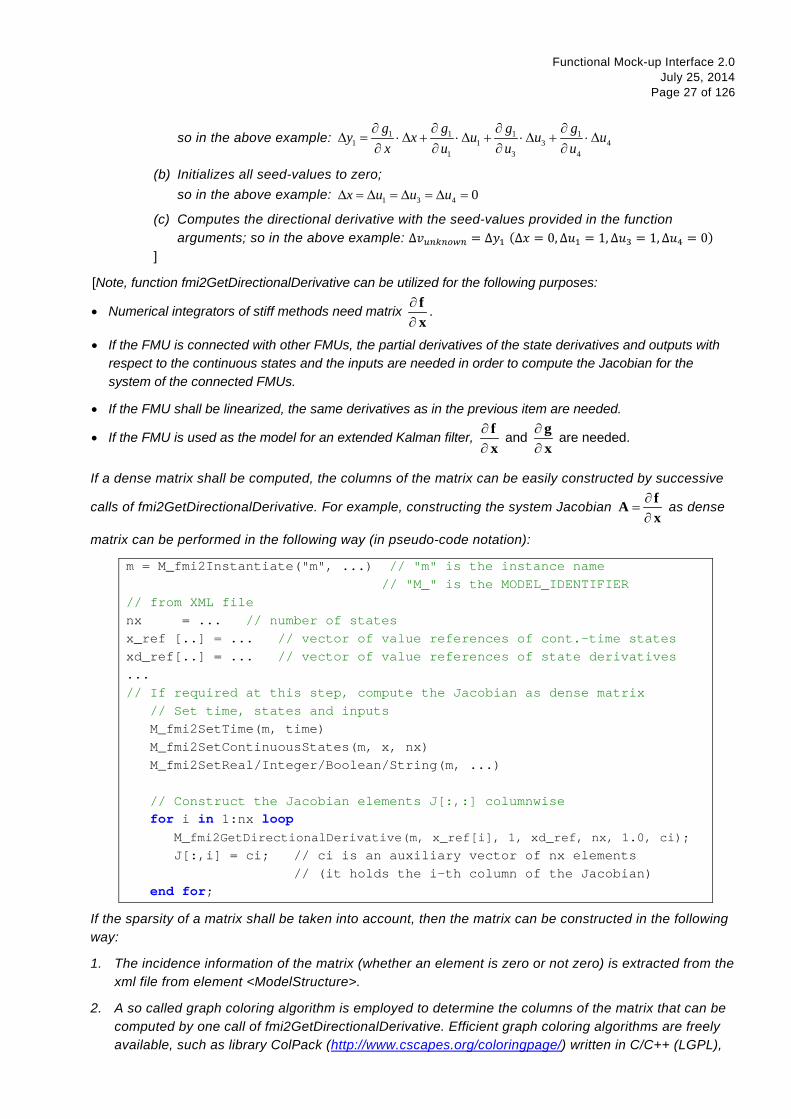
Functional Mock-up Interface 2.0 July 25, 2014
Page 27 of 126
so in the above example: 1 1 1 11 1 3 4
1 3 4
∂ ∂ ∂ ∂∆ = ⋅ ∆ + ⋅ ∆ + ⋅ ∆ + ⋅ ∆
∂ ∂ ∂ ∂g g g gy x u u ux u u u
(b) Initializes all seed-values to zero; so in the above example: 1 3 4 0∆ = ∆ = ∆ = ∆ =x u u u
(c) Computes the directional derivative with the seed-values provided in the function arguments; so in the above example: ∆𝑣𝑢𝑛𝑘𝑛𝑜𝑤𝑛 = ∆𝑦1 (∆𝑥 = 0,∆𝑢1 = 1,∆𝑢3 = 1,∆𝑢4 = 0)
]
[Note, function fmi2GetDirectionalDerivative can be utilized for the following purposes:
• Numerical integrators of stiff methods need matrix ∂∂
fx
.
• If the FMU is connected with other FMUs, the partial derivatives of the state derivatives and outputs with respect to the continuous states and the inputs are needed in order to compute the Jacobian for the system of the connected FMUs.
• If the FMU shall be linearized, the same derivatives as in the previous item are needed.
• If the FMU is used as the model for an extended Kalman filter, ∂∂
fx
and ∂∂
gx
are needed.
If a dense matrix shall be computed, the columns of the matrix can be easily constructed by successive
calls of fmi2GetDirectionalDerivative. For example, constructing the system Jacobian ∂
=∂
fAx
as dense
matrix can be performed in the following way (in pseudo-code notation):
m = M_fmi2Instantiate("m", ...) // "m" is the instance name // "M_" is the MODEL_IDENTIFIER // from XML file nx = ... // number of states x_ref [..] = ... // vector of value references of cont.-time states xd_ref[..] = ... // vector of value references of state derivatives ... // If required at this step, compute the Jacobian as dense matrix // Set time, states and inputs M_fmi2SetTime(m, time) M_fmi2SetContinuousStates(m, x, nx) M_fmi2SetReal/Integer/Boolean/String(m, ...) // Construct the Jacobian elements J[:,:] columnwise for i in 1:nx loop M_fmi2GetDirectionalDerivative(m, x_ref[i], 1, xd_ref, nx, 1.0, ci); J[:,i] = ci; // ci is an auxiliary vector of nx elements // (it holds the i-th column of the Jacobian) end for;
If the sparsity of a matrix shall be taken into account, then the matrix can be constructed in the following way:
1. The incidence information of the matrix (whether an element is zero or not zero) is extracted from the xml file from element <ModelStructure>.
2. A so called graph coloring algorithm is employed to determine the columns of the matrix that can be computed by one call of fmi2GetDirectionalDerivative. Efficient graph coloring algorithms are freely available, such as library ColPack (http://www.cscapes.org/coloringpage/) written in C/C++ (LGPL),

Functional Mock-up Interface 2.0 July 25, 2014
Page 28 of 126
or the routines by Coleman, Garbow, Moré: “Software for estimating sparse Jacobian matrices”, ACM Transactions on Mathematical Software - TOMS , vol. 10, no. 3, pp. 346-347, 1984. See e.g. http://www.netlib.org/toms/618.
3. For the columns determined in (2), one call to fmi2DirectionalDerivative is made. After each such call, the elements of the resulting directional derivative vector are copied into their correct locations of the partial derivative matrix.
More details and implementational notes are available from (Akesson et.al. 2012).
]
2.2 FMI Description Schema
All static information related to an FMU is stored in the text file modelDescription.xml in XML format. Especially, the FMU variables and their attributes such as name, unit, default initial value etc. are stored in this file. The structure of this XML file is defined with the schema file “fmiModelDescription.xsd”. This schema file utilizes the following helper schema files:
fmi2Annotation.xsd fmi2AttributeGroups.xsd fmi2ScalarVariable.xsd fmi2Type.xsd fmi2VariableDependency.xsd fmi2Unit.xsd
In this section these schema files are discussed. The normative definition are the above mentioned schema files6. Below, optional elements are marked with a “dashed” box. The required data types (like: xs:normalizedString) are defined in the XML-schema standard: http://www.w3.org/TR/XMLschema-2/. The types used in the fmi2 schema files are:
XML Description (http://www.w3.org/TR/XMLschema-2/) Mapping to C xs:double IEEE double-precision 64-bit floating point type
[In order to not loose precision, a number of this type should be stored on an XML file with at least 16 significant digits; for example 2/3 should be stored as 0.6666666666666667]
double
xs:int Integer number with maximum value 2147483647 and minimum value -2147483648 (32 bit Integer)
int
xs:unsignedInt Integer number with maximum value 4294967295 and minimum value 0 (unsigned 32 bit Integer)
unsigned int
xs:boolean Boolean number. Legal literals: false, true, 0, 1 char xs:string Any number of characters char* xs:normalizedString String without carriage return, line feed, and tab characters char* xs:dateTime Date, time and time zone (for details see the link above).
Example: 2002-10-23T12:00:00Z (noon on October 23, 2002, Greenwich Mean Time)
tool specific
The first line of an XML file, such as modelDescription.xml, must contain the encoding scheme of the XML file. It is required that the encoding scheme is always UTF-8: 6 Note, the screenshots of this section have been generated from the schema files with the tool “Altova XMLSpy”
(www.altova.com). With the enterprise edition of XMLSpy it is possible to automatically generate C++, C# and Java code that reads an XML file of fmiModelDescription.xsd. An efficient open source XML parser is SAX (http://sax.sourceforge.net/, http://en.wikipedia.org/wiki/Simple_API_for_XML). All data from the XML file is only defined via “attributes” and not via “elements”. Therefore, only an “attribute” handler needs to be defined for a SAX parser.
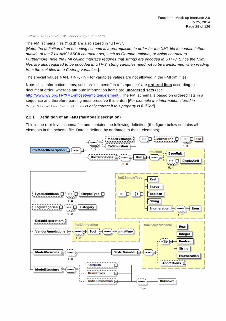
Functional Mock-up Interface 2.0 July 25, 2014
Page 29 of 126
<?xml version="1.0" encoding="UTF-8"?>
The FMI schema files (*.xsd) are also stored in “UTF-8”. [Note, the definition of an encoding scheme is a prerequisite, in order for the XML file to contain letters outside of the 7 bit ANSI ASCII character set, such as German umlauts, or Asian characters. Furthermore, note the FMI calling interface requires that strings are encoded in UTF-8. Since the *.xml files are also required to be encoded in UTF-8, string variables need not to be transformed when reading from the xml-files in to C string variables.].
The special values NAN, +INF, -INF for variables values are not allowed in the FMI xml files.
Note, child information items, such as “elements” in a “sequence” are ordered lists according to document order, whereas attribute information items are unordered sets (see http://www.w3.org/TR/XML-infoset/#infoitem.element). The FMI schema is based on ordered lists in a sequence and therefore parsing must preserve this order. [For example the information stored in ModelVariables.Derivatives is only correct if this property is fulfilled].
2.2.1 Definition of an FMU (fmiModelDescription)
This is the root-level schema file and contains the following definition (the figure below contains all elements in the schema file. Data is defined by attributes to these elements):
Functional Mock-up Interface 2.0 July 25, 2014
Page 30 of 126
On the top level, the schema consists of the following elements (see figure above7):
Element-Name Description
ModelExchange If present, the FMU is based on “FMI for Model Exchange” [(in other words the FMU includes the model or the communication to a tool that provides the model, and the environment provides the simulation engine)].
CoSimulation If present, the FMU is based on “FMI for Co-Simulation” [(in other words the FMU includes the model and the simulation engine, or a communication to a tool that provides the model and the simulation engine, and the environment provides the master algorithm to run coupled FMU co-simulation slaves together)].
UnitDefinitions A global list of unit and display unit definitions [for example to convert display units into the units used in the model equations]. These definitions are used in the XML element “ModelVariables”.
TypeDefinitions A global list of type definitions that are utilized in “ModelVariables”.
LogCategories A global list of log categories that can be set to define the log information that is supported from the FMU.
DefaultExperiment
Providing default settings for the integrator, such as stop time and relative tolerance.
VendorAnnotations Additional data that a vendor might want to store and that other vendors might ignore.
ModelVariables The central FMU data structure defining all variables of the FMU that are visible/accessible via the FMU functions.
ModelStructure Defines the structure of the model. Especially, the ordered lists of outputs, continuous-time states and initial unknowns (the unknowns during Initialization Mode) are defined here. Furthermore, the dependency of the unkowns from the knowns can be optionally defined. [This information can be, for example used to compute efficiently a sparse Jacobian for simulation or to utilize the input/output dependency in order to detect that in some cases there are actually no algebraic loops when connecting FMUs together].
At least one element of ModelExchange or CoSimulation must be present to identify the type of the FMU. If both elements are defined, different types of models are included in the FMU. The details of these elements are defined in section 3.3.1 and section 4.3.1.
The XML attributes of fmiModelDescription are:
7 Note, elements <ModelVariables> and <ModelStructure> are mandatory, whereas <UnitDefinitions>, <TypeDefinitions>, <LogCategories>, <DefaultExperiment>, <VendorAnnotation> are optional. If an optional element is present and defines a list (such as <UnitDefinitions>), the list must have at least one element (such as <Unit>).

Functional Mock-up Interface 2.0 July 25, 2014
Page 31 of 126
Attribute-Name Description
fmiVersion Version of “FMI for Model Exchange or Co-Simulation” that was used to generate the XML file. The value for this version is “2.0”. Future minor revisions are denoted as “2.0.1”, “2.0.2”, …
modelName The name of the model as used in the modeling environment that generated the XML file, such as “Modelica.Mechanics.Rotational.Examples.CoupledClutches”.
guid The “Globally Unique IDentifier” is a string that is used to check that the XML file is compatible with the C functions of the FMU. Typically when
Functional Mock-up Interface 2.0 July 25, 2014
Page 32 of 126
generating the XML file, a fingerprint of the “relevant” information is stored as guid and in the generated C-function.
description Optional string with a brief description of the model.
author Optional string with the name and organization of the model author.
version Optional version of the model, for example “1.0”.
copyright Optional information on the intellectual property copyright for this FMU. [Example: copyright = “© My Company 2011”].
license Optional information on the intellectual property licensing for this FMU. [Example: license = “BSD license <license text or link to license>”].
generationTool Optional name of the tool that generated the XML file.
generationDateAndTime Optional date and time when the XML file was generated. The format is a subset of “xs:dateTime” and should be: “YYYY-MM-DDThh:mm:ssZ" (with one “T” between date and time; “Z” characterizes the Zulu time zone, in other words Greenwich meantime). [Example: "2009-12-08T14:33:22Z"].
variableNamingConvention
Defines whether the variable names in “ModelVariables / ScalarVariable / name” and in “TypeDefinitions / Type / name” follow a particular convention. For the details, see section 2.2.9. Currently standardized are: • “flat”: A list of strings (the default). • “structured“: Hierarchical names with “.” as hierarchy separator,
and with array elements and derivative characterization.
numberOfEventIndicators The (fixed) number of event indicators for an FMU based on FMI for Model Exchange. For Co-Simulation, this value is ignored.
[The attribute “numberOfContinuousStates” available in FMI 1.0 has been removed for FMI 2.0, since this information can be deduced from the remaining data in the XML file]

Functional Mock-up Interface 2.0 July 25, 2014
Page 33 of 126
2.2.2 Definition of Units (UnitDefinitions)
[In this section the units of the variables are (optionally) defined. Unit support is important for technical systems since otherwise it is very easy for errors to occur. Unit handling is a difficult topic and there seems to be no method available that is really satisfactory for all applications such as unit check, unit conversion, unit propagation or dimensional analysis. In FMI a pragmatic approach is used that takes into account that every software system supporting units has potentially its own specific technique to describe and utilize units. The approach used here is slightly different to FMI 1.0 to reduce the need for standardized string representations.]
Element “UnitDefinitions” of fmiModelDescription is defined as:
It consists of zero or more Unit definitions8. A Unit is defined by its name attribute such as “N.m” or “N*m” or “Nm”, which must be unique with respect to all other defined elements of the UnitDefinitions list. If a variable is associated with a Unit, then the value of the variable has to be provided with the fmi2SetXXX functions or is returned by the fmi2GetXXX functions with respect to this Unit. [The purpose of the name is to uniquely identify a unit and, for example use it to display the unit in menus or in plots. Since there is no standard to represent units in strings, and there are different ways how this is performed in different tools, no specific string representation of the unit is required.]
Optionally, a value given in unit Unit can be converted to a value with respect to unit BaseUnit utilizing the conversion factor and offset attributes:
8 If no units are defined, element <UnitDefinitions> must not be present. If 1 or more units are defined, this element
must be present.

Functional Mock-up Interface 2.0 July 25, 2014
Page 34 of 126
Besides factor and offset, the BaseUnit definition consists of the exponents of the 7 SI base units “kg”, “m”, “s”, “A”, “K”, “mol”, “cd”, and of the exponent of the SI derived unit “rad”. [Depending on the analysis/operation carried out, the SI derived unit “rad” is or is not utilized, see discussion below. The additional “rad” base unit helps to handle the often occurring quantities in technical systems that depend on an angle.]
A value with respect to Unit (abbreviated as “Unit_value”) is converted with respect to BaseUnit (abbreviated as “BaseUnit_value”) by the equation:
BaseUnit_value = factor*Unit_value + offset
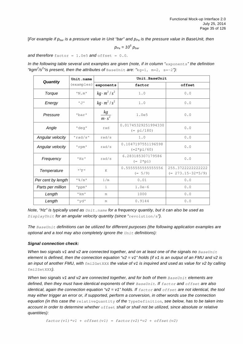
Functional Mock-up Interface 2.0 July 25, 2014
Page 35 of 126
[For example if pbar is a pressure value in Unit “bar” and pPa is the pressure value in BaseUnit, then
pPa = 105 pbar
and therefore factor = 1.0e5 and offset = 0.0.
In the following table several unit examples are given (note, if in column “exponents” the definition “kgm2/s2“is present, then the attributes of BaseUnit are: “kg=1, m=2, s=-2”):
Quantity Unit.name (examples)
Unit.BaseUnit
exponents factor offset
Torque "N.m" 2 2/kg m s⋅
1.0 0.0
Energy "J" 2 2/kg m s⋅
1.0 0.0
Pressure "bar" 2
kgm s⋅
1.0e5 0.0
Angle "deg" rad 0.01745329251994330
(= pi/180) 0.0
Angular velocity "rad/s" rad/s 1.0 0.0
Angular velocity "rpm" rad/s 0.1047197551196598
(=2*pi/60) 0.0
Frequency "Hz" rad/s 6.283185307179586
(= 2*pi) 0.0
Temperature "oF" K 0.5555555555555556
(= 5/9) 255.3722222222222 (= 273.15-32*5/9)
Per cent by length "%/m" 1/m 0.01 0.0
Parts per million "ppm" 1 1.0e-6 0.0
Length "km" m 1000 0.0
Length "yd" m 0.9144 0.0
Note, “Hz” is typically used as Unit.name for a frequency quantity, but it can also be used as DisplayUnit for an angular velocity quantity (since “revolution/s”).
The BaseUnit definitions can be utilized for different purposes (the following application examples are optional and a tool may also completely ignore the Unit definitions):
Signal connection check:
When two signals v1 and v2 are connected together, and on at least one of the signals no BaseUnit element is defined, then the connection equation “v2 = v1” holds (if v1 is an output of an FMU and v2 is an input of another FMU, with fmi2GetXXX the value of v1 is inquired and used as value for v2 by calling fmi2SetXXX).
When two signals v1 and v2 are connected together, and for both of them BaseUnit elements are defined, then they must have identical exponents of their BaseUnit. If factor and offset are also identical, again the connection equation “v2 = v1” holds. If factor and offset are not identical, the tool may either trigger an error or, if supported, perform a conversion, in other words use the connection equation (in this case the relativeQuantity of the TypeDefinition, see below, has to be taken into account in order to determine whether offset shall or shall not be utilized, since absolute or relative quantities):
factor(v1)*v1 + offset(v1) = factor(v2)*v2 + offset(v2)

Functional Mock-up Interface 2.0 July 25, 2014
Page 36 of 126
As a result, wrong connections can be detected (for example connecting a force with an angle signal would trigger an error) and conversions between, say, US and SI units can be either automatically performed or, if not supported, an error is triggered as well. Note, this approach is not satisfactory for variables belonging to different quantities that have, however, the same BaseUnit, such as quantities “Energy” and “Torque”, or “AngularVelocity” and “Frequency”. To handle such cases quantity definitions have to be taken into account (see TypeDefinitions) and quantity names need to be standardized.
This approach allows a general treatment of units, without being forced to standardize the grammar and allowed values for units (for example in FMI 1.0, a unit could be defined as “N.m” in one FMU and as “N*m” in another FMU and a tool would have to reject a connection, since the units are not identical, In FMI 2.0 the connection would be accepted, provided both elements have the same BaseUnit definition).
Dimensional analysis of equations:
In order to check the validity of equations in a modeling language, the defined units can be used for dimensional analysis, by using the BaseUnit definition of the respective unit. For this purpose, the BaseUnit “rad” has to be treated as “1”. Example:
J*α = τ → [kg.m2]*[rad/s2] = [kg.m2/s2]). // o.k. (“rad” is treated as “1”) J*α = f → [kg.m2]*[rad/s2] = [kg.m/s2]). // error, since dimensions do not agree
Unit propagation:
If unit definitions are missing for signals, they might be deduced from the equations where the signals are used. If no unit computation is needed, “rad” is propagated. If a unit computation is needed and one of the involved units has “rad” as a BaseUnit, then unit propagation is not possible. Examples:
• a = b + c, and Unit of c is provided, but not Unit of a and b: The Unit definition of c (in other words Unit.name, BaseUnit, DisplayUnit) is also used for a and b. For example if BaseUnit(c) = “rad/s”, then BaseUnit(a) = BaseUnit(b) = “rad/s”.
• a = b*c, and Unit of a and of c is provided, but not Unit of b: If “rad” is either part of the BaseUnit of “a” and/or of “c”, then the BaseUnit of b cannot be deduced (otherwise it can be deduced). Example: If BaseUnit(a)=”kg.m/s2” and BaseUnit(c)=”m/s2”, then the BaseUnit(b) can be deduced to be “kg”. In such a case Unit.name of b cannot be deduced from the Unit.name of a and c, and a tool would typically construct the Unit.name of b from the deduced BaseUnit.
]
Additionally to the unit definition, optionally a set of display units can be defined that can be utilized for input/output of a value:

Functional Mock-up Interface 2.0 July 25, 2014
Page 37 of 126
A DisplayUnit is defined by name, factor and offset. The attribute name must be unique with respect to all other names of the DisplayUnit definitions of the same Unit [(different Unit elements may have the same DisplayUnit names)]. A value with respect to Unit (abbreviated as “Unit_value”) is converted with respect to DisplayUnit (abbreviated as “DisplayUnit_value”) by the equation:
DisplayUnit_value = factor*Unit_value + offset
[“offset” is, for example needed for temperature units.]
[For example if TK is the temperature value of Unit.name (in “K”) and TF is the temperature value of DisplayUnit (in “oF”), then
TF = (9/5) * (TK - 273.15 ) + 32
and therefore factor = 1.8 (=9/5) and offset = -459.67 (= 32 – 273.15*9/5).
Both the DisplayUnit.name definitions as well as the Unit.name definitions are used in the ScalarVariable elements. Example for a definition:
<Unit name="rad/s"> <BaseUnit s="-1" rad="1"/> <DisplayUnit name="deg/s" factor= "57.29577951308232"/> <DisplayUnit name="rev/min" factor= "9.549296585513721"/> </Unit>
<Unit name="bar"> <BaseUnit kg="1", m="-1", s="-2", factor="1.0e5", offset="0"/> </Unit>
<Unit name="Re"> <BaseUnit/> // unit = "1" //(dimensionless, all exponents of BaseUnit are zero) </Unit>
<Unit name="Euro/PersonYear"/> // no mapping to BaseUnit defined
]
The schema definition is present in a separate file “fmi2Unit.xsd”.

Functional Mock-up Interface 2.0 July 25, 2014
Page 38 of 126
2.2.3 Definition of Types (TypeDefinitions)
Element “TypeDefinitions” of fmiModelDescription is defined as:
This element consists of a set of “SimpleType” definitions according to schema “fmi2SimpleType” in file “fmi2Type.xsd”. One “SimpleType” has a type “name” and “description" as attributes. Attribute “name” must be unique with respect to all other elements of the TypeDefinitions list. Furthermore, “name” of a “SimpleType” must be different to all “name” attributes of ScalarVariables [if the same names would be used, then this would nearly always give problems when importing the FMU in an environment such as Modelica, where a type name cannot be used as instance name].Additionally, one of the elements Real, Integer, Boolean, String, or Enumeration must be present. They have the following definitions:
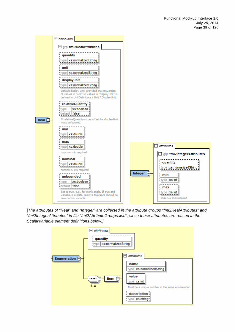
Functional Mock-up Interface 2.0 July 25, 2014
Page 39 of 126
[The attributes of “Real” and “Integer” are collected in the attribute groups “fmi2RealAttributes” and “fmi2IntegerAttributes” in file “fmi2AttributeGroups.xsd”, since these attributes are reused in the ScalarVariable element definitions below.]

Functional Mock-up Interface 2.0 July 25, 2014
Page 40 of 126
These definitions are used as default values in element ScalarVariables[, in order that, say, the definition of a “Torque” type does not have to be repeated over and over again]. The attributes and elements have the following meaning:
Name Description
quantity Physical quantity of the variable, for example “Angle”, or “Energy”. The quantity names are not standardized.
unit Unit of the variable defined with UnitDefinitions.Unit.name that is used for the model equations [, for example “N.m”: in this case a Unit.name = "N.m" must be present under UnitDefinitions].
displayUnit Default display unit. The conversion to the “unit” is defined with the element “<fmiModelDescription><UnitDefinitions>”. If the corresponding “displayUnit” is not defined under <UnitDefinitions> <Unit>
<DisplayUnit>, then displayUnit is ignored. It is an error if displayUnit is defined in element Real, but unit is not, or unit is not defined under <UnitDefinitions><Unit>.
relativeQuantity If this attribute is true, then the “offset” of “displayUnit” must be ignored (for example 10 degree Celsius = 10 Kelvin if “relativeQuantity = true” and not 283,15 Kelvin).
min Minimum value of variable (variable Value ≥ min). If not defined, the minimum is the largest negative number that can be represented on the machine. The min definition is an information from the FMU to the environment defining the region in which the FMU is designed to operate, see also comment after this table.
max Maximum value of variable (variableValue ≤ max). If not defined, the maximum is the largest positive number that can be represented on the machine. The max definition is an information from the FMU to the environment defining the region in which the FMU is designed to operate, see also comment after this table.
nominal Nominal value of variable. If not defined and no other information about the nominal value is available, then nominal = 1 is assumed. [The nominal value of a variable can be, for example used to determine the absolute tolerance for this variable as needed by numerical algorithms: absoluteTolerance = nominal*tolerance*0.01 where tolerance is, e.g., the relative tolerance defined in <DefaultExperiment>, see section 2.2.5.]
unbounded If true, indicates that the variable gets during time integration much larger than its nominal value nominal. [Typical examples are the monotonically increasing rotation angles of crank shafts and the longitudinal position of a vehicle along the track in long distance simulations. This information can, for example, be used to increase numerical stability and accuracy by setting the corresponding bound for the relative error to zero (relative tolerance = 0.0), if the corresponding variable or an alias of it is a continuous state variable.]
Item Items of an enumeration as a sequence of “name” and “value” pairs. The values can be any integer number, but must be unique within the same enumeration (in order that the mapping between “name” and “value” is bijective). An Enumeration element must have at least one Item.

Functional Mock-up Interface 2.0 July 25, 2014
Page 41 of 126
[Attributes „min“ and „max“ can be set for variables of type Real, Integer or Enumeration. The question is how fmi2SetReal, fmi2SetInteger, fmi2GetReal, fmi2GetInteger shall utilize this definition. There are several conflicting requirements: Avoiding forbidden regions (e.g. if „u“ is an input and „sqrt(u)“ is computed in the FMU, min=0 on „u“ shall guarantee that only values of „u“ in the allowed regions are provided). Numerical algorithms (ODE-solver, optimizers. nonlinear solvers) do not guarantee constraints. If a variable is outside of the bounds, the solver tries to bring it back into the bounds. As a consequence, calling fmi2GetReal during an iteration of such a solver might return values that are not in the defined min/max region. After the iteration is finalized, it is only guaranteed that a value is within its bounds upto a certain numerical precision. In debug mode checks on min/max should be performed. For maximum performance on a real-time system the checks might not be performed. The approach in FMI is therefore that min/max definitions are an information from the FMU to the environment defining the region in which the FMU is designed to operate. The environment is free to utilize this information (typically, in debug mode of the environment the min/max is checked in the cases as stated above). In any case, it is expected that the FMU handles variables appropriately where the region definition is critical. For example, dividing by an input (so the input should not be in a small range of zero) or taking the square root of an input (so the input should not be negative) may either result in fmi2Error, or the FMU is able to handle this situation in other ways. If the FMU is generated so that min/max shall be checked whenever meaningful (e.g. for debug purposes) then the following strategy should be used:
If fmi2SetReal or fmi2SetInteger is called violating the min/max attribute settings of the corresponding variable, the following actions are performed:
• On a fixed or tunable parameter fmi2Status = fmi2Discard is returned.
• On an input, the FMU decides what to return (If no computation is possible, it could return fmi2Status = fmi2Discard, in other situations it may return fmi2Warning or fmi2Error, or fmi2OK, if it is uncritical).
If an FMU defines min/max values for Integer and Enumerations (local and output variables), then the expected behavior of the FMU is that fmi2GetInteger returns values in the defined range.
If an FMU defines min/max values for Reals, then the expected behavior of the FMU is that fmi2GetReal returns values at the solution (accepted steps of the integrators) in the defined range with a certain uncertainty related to the tolerances of the numerical algorithms. ]

Functional Mock-up Interface 2.0 July 25, 2014
Page 42 of 126
2.2.4 Definition of Log Categories (LogCategories)
Element “LogCategories” of “fmiModelDescription is defined as:
LogCategories defines an unordered set of category strings that can be utilized to define the log output via function “logger”, see section 2.1.5. A tool is free to use any normalizedString for a category value. The “name” attribute of “Category” must be unique with respect to all other elements of the LogCategories list.
There are the following standardized names for “Category” and these names should be used if a tool supports the corresponding log category. If a tool supports one of these log categories and wants to expose it, then an element Category with this name should be added to LogCategories [To be clear: only the Category names listed under LogCategories in the xml-file are known to the environment in which the FMU is called.]
Category name Description
logEvents Log all events (during initialization and simulation).
logSingularLinearSystems Log the solution of linear systems of equations if the solution is singular (and the tool picked one solution of the infinitely many solutions).
logNonlinearSystems Log the solution of nonlinear systems of equations.
logDynamicStateSelection Log the dynamic selection of states.
logStatusWarning Log messages when returning fmi2Warning status from any function.
logStatusDiscard Log messages when returning fmi2Discard status from any function.
logStatusError Log messages when returning fmi2Error status from any function.
logStatusFatal Log messages when returning fmi2Fatal status from any function.
logStatusPending Log messages when returning fmi2Pending status from any function.
logAll Log all messages.
The optional attribute description shall contain a description of the respective log category. [Typically, this string can be shown by a tool if more details for a log category shall be presented.]
[This approach to define LogCategories has the following advantages: 1. A simulation environment can present the possible log categories in a menu and the user can select the
desired one (in the FMI 1.0 approach, there was no easy way for a user to figure out from a given FMU what log categories could be provided). Note, since element <LogCategories> is optional, an FMU does not need to expose its log categories.
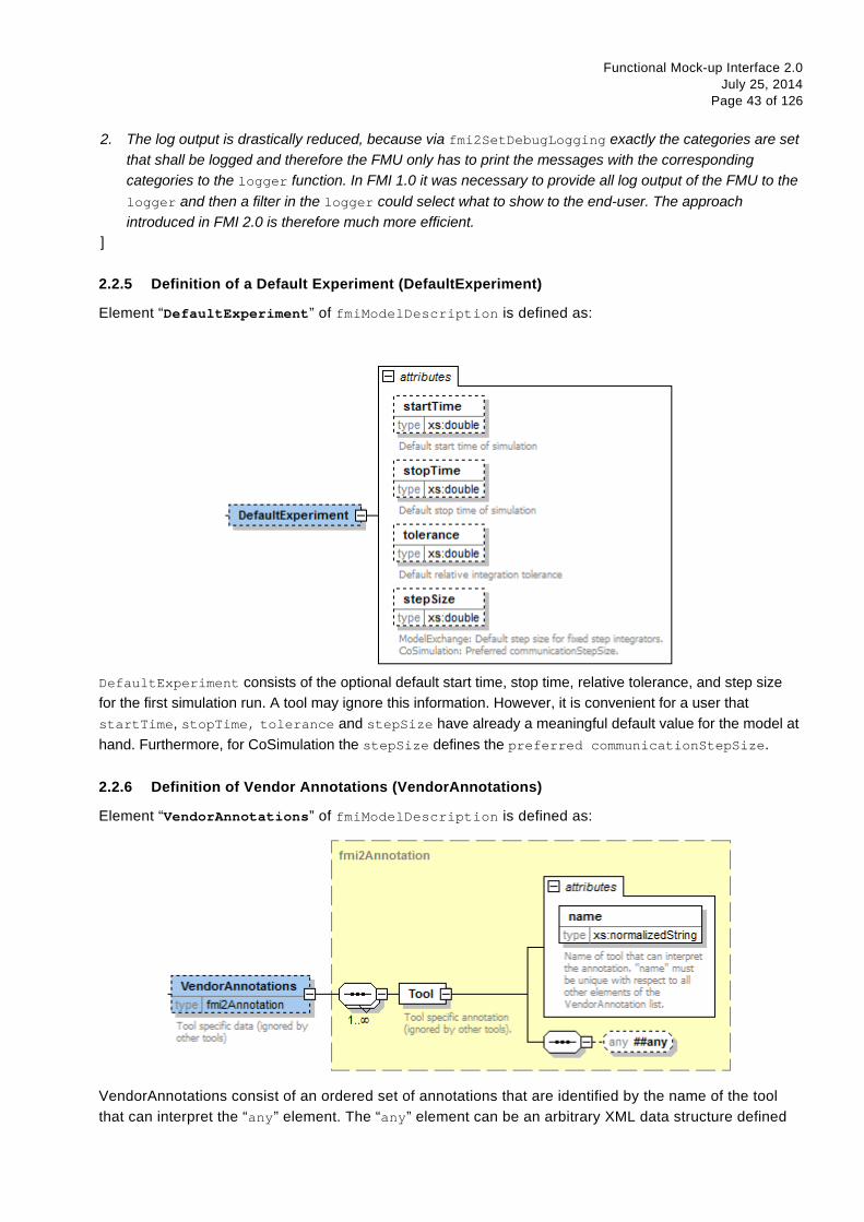
Functional Mock-up Interface 2.0 July 25, 2014
Page 43 of 126
2. The log output is drastically reduced, because via fmi2SetDebugLogging exactly the categories are set that shall be logged and therefore the FMU only has to print the messages with the corresponding categories to the logger function. In FMI 1.0 it was necessary to provide all log output of the FMU to the logger and then a filter in the logger could select what to show to the end-user. The approach introduced in FMI 2.0 is therefore much more efficient.
]
2.2.5 Definition of a Default Experiment (DefaultExperiment)
Element “DefaultExperiment” of fmiModelDescription is defined as:
DefaultExperiment consists of the optional default start time, stop time, relative tolerance, and step size for the first simulation run. A tool may ignore this information. However, it is convenient for a user that startTime, stopTime, tolerance and stepSize have already a meaningful default value for the model at hand. Furthermore, for CoSimulation the stepSize defines the preferred communicationStepSize.
2.2.6 Definition of Vendor Annotations (VendorAnnotations)
Element “VendorAnnotations” of fmiModelDescription is defined as:
VendorAnnotations consist of an ordered set of annotations that are identified by the name of the tool that can interpret the “any” element. The “any” element can be an arbitrary XML data structure defined

Functional Mock-up Interface 2.0 July 25, 2014
Page 44 of 126
by the tool. Attribute “name” must be unique with respect to all other elements of the VendorAnnotation list.
2.2.7 Definition of Model Variables (ModelVariables)
The “ModelVariables” element of fmiModelDescription is the central part of the model description. It provides the static information of all exposed variables and is defined as:
The “ModelVariables” element consists of an ordered set of “ScalarVariable” elements (see figure above). The first element has index = 1, the second index=2, etc. This ScalarVariable index is used in element ModelStructure to uniquely and efficiently refer to ScalarVariable definitions. A “ScalarVariable” represents a variable of primitive type, like a real or integer variable. For simplicity, only scalar variables are supported in the schema file in this version and structured entities (like arrays or records) have to be mapped to scalars. The schema definition is present in a separate file “fmi2ScalarVariable.xsd”. The attributes of “ScalarVariable” are:

Functional Mock-up Interface 2.0 July 25, 2014
Page 45 of 126
Attribute-Name Description
name
The full, unique name of the variable. Every variable is uniquely identified within an FMU instance by this name or by its ScalarVariable index (the element position in the ModelVariables list; the first list element has index=1).
valueReference A handle of the variable to efficiently identify the variable value in the model interface. This handle is a secret of the tool that generated the C functions. It is not required to be unique. The only guarantee is that valueReference is sufficient to identify the
,-----------------fmi2ScalarVariable
B__sttributes
name type I x s:normalizedString
Identifter of variable,. e.g. •a.b.mocf)AJ.'#123'.c•, •name• rrMJSt be unQJe with respect to a:ll otller elements of tile ModEN aria bles list
valueReference
type I x s:unsignedlnt
Identifter for variable vc:lue in FM:2 function ca:lls {not re::essarily unQJe with respect to a:ll variables)
·-----------dJ : descr iption ,
:_ty~~ 0~~~t!i!l~_: :-~~~:,_i itY-------------------------------------------------- f : type xs:normalizedString ; : en urn parameter calculatedParameter input output local independent , : default local ' ~ derived By restriction
I '
parameter: independent parameter c.a:lculatedParameter: ca:lcul=ted parameter input/OLrtput: can be used in connections locaJ: variable cakulated from other variables independent: independent variable (USl.IC:Ity time)
r :-~~~i;bilitY-----------------------------------
• type xs:normalizedString : en urn constant fiXed tunable discrete continuous • default continuous
~derive<! By restriction
constant: vc:lue never changes ft»:d: valle ft»:d after initia.liz.ation tunable: vc:lue constant between external events discrete: valle constant between internaJ events continuous: no restriction on va:lue changes
:- i~iii:,_j----------------------- f : type xs:normalizedString ; : en urn exact approx calculate<! ,
:_~-~~~~-~y restriction ' ~-~-~-~-~-~-~-~-~-~-~-~-~-~-~-~-~-~-~-~-'
exact: initia.lized with start valle cpprox: iteration variable that stotts with Stolt va:lue
ScalarVar iable _dL..l. c.ckulated: c.ckulated from other variables. If not providecl, initiaJ is deduced from c.cusa:lity end variability (deta.ils see
type 1 fmi2ScalarVariable U i spedfcation)
------------------------------------i1 : canHandleMult iple SetPerTim elnstant l
I ~type I xs:boolean ~ I
I Only for Mode!~nge and onty for variables with variability = • lflput": If present with vc:lue = fa:lse, tllen onty one fmi2:SetXlO( ca:ll is c:!lowed a t one super
I dense time instant. ! n otller words, this input is not a:!lowed to c ppear in en a~ebrai: loop.
I
Functional Mock-up Interface 2.0 July 25, 2014
Page 46 of 126
respective variable value in the call of the C functions. This implies that it is unique for a particular base data type (Real, Integer/Enumeration, Boolean, String) with exception of variables that have identical values (such variables are also called “alias” variables). This attribute is “required”.
description An optional description string describing the meaning of the variable.
causality Enumeration that defines the causality of the variable. Allowed values of this enumeration:
• "parameter": Independent parameter (a data value that is constant during the simulation and is provided by the environment and cannot be used in connections). variability must be "fixed" or "tunable". initial must be exact or not present (meaning exact).
• "calculatedParameter": A data value that is constant during the simulation and is computed during initialization or when tunable parameters change. variability must be "fixed" or "tunable". initial must be "approx", "calculated" or not present (meaning calculated).
• "input": The variable value can be provided from another model or slave. It is not allowed to define initial.
• "output": The variable value can be used by another model or slave. The algebraic relationship to the inputs is defined via the dependencies attribute of <fmiModelDescription><ModelStructure><Outputs><Unknown>.
• "local": Local variable that is calculated from other variables or is a continuous-time state (see section 2.2.8). It is not allowed to use the variable value in another model or slave.
• "independent": The independent variable (usually “time”). All variables are a function of this independent variable. variability must be "continuous". At most one ScalarVariable of an FMU can be defined as "independent". If no variable is defined as "independent", it is implicitely present with name = "time" and unit = "s". If one variable is defined as "independent", it must be defined as "Real" without a "start" attribute. It is not allowed to call function fmi2SetReal on an "independent" variable. Instead, its value is initialized with fmi2SetupExperiment and after initialization set by fmi2SetTime for ModelExchange and by arguments currentCommunicationPoint and communicationStepSize of fmi2DoStep for CoSimulation. [The actual value can be inquired with fmi2GetReal.]
The default of causality is “local”. A continuous-time state must have causality = "local" or "output", see also section 2.2.8. [causality = "calculatedParameter" and causality = "local" with variability = "fixed" or "tunable" are similar. The difference is that a calculatedParameter can be used in another model or slave, whereas a local variable cannot. For example, when importing an FMU in a Modelica environment, a "calculatedParameter" should be imported in a public section as final parameter, whereas a "local" variable should be imported in a protected section of the model.]
variability Enumeration that defines the time dependency of the variable, in other words it defines the time instants when a variable can change its value. [The purpose of this attribute is
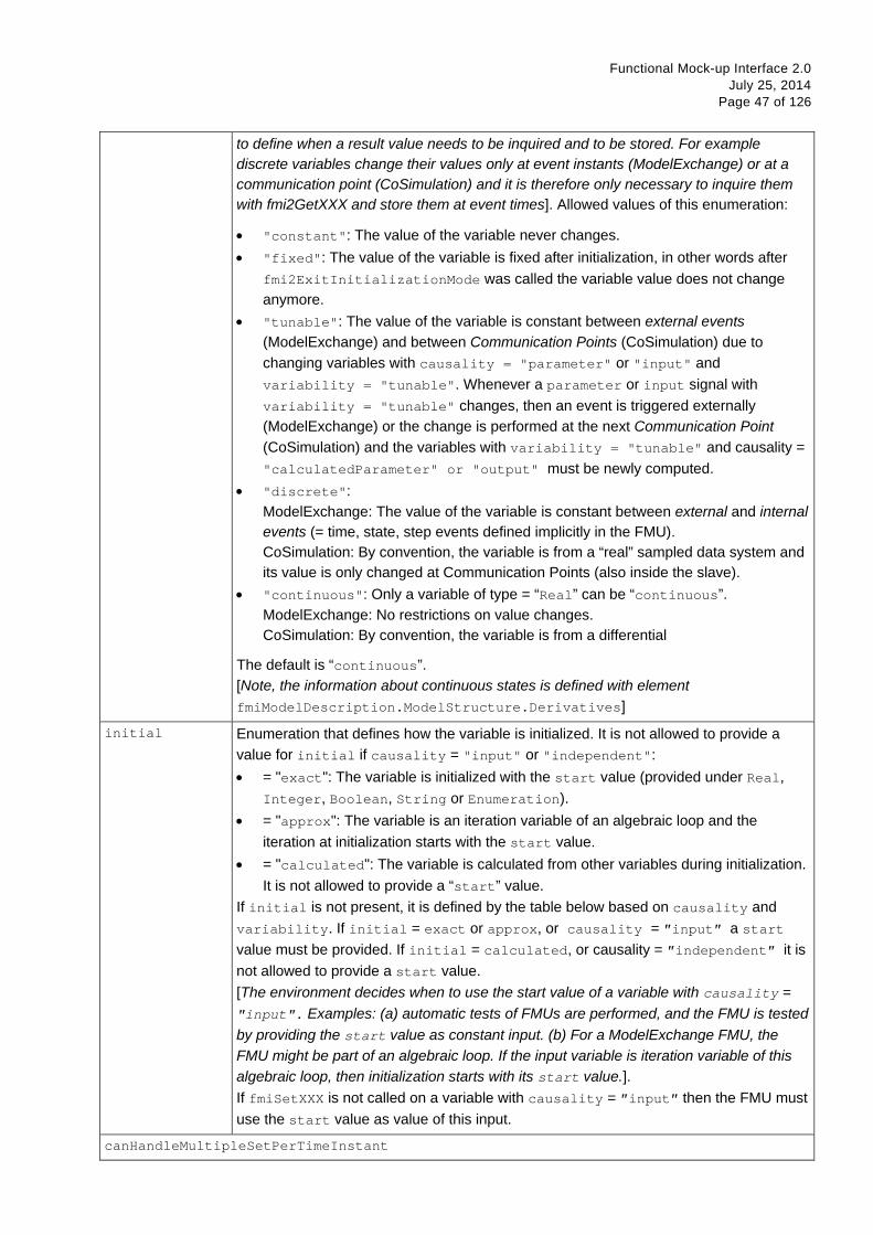
Functional Mock-up Interface 2.0 July 25, 2014
Page 47 of 126
to define when a result value needs to be inquired and to be stored. For example discrete variables change their values only at event instants (ModelExchange) or at a communication point (CoSimulation) and it is therefore only necessary to inquire them with fmi2GetXXX and store them at event times]. Allowed values of this enumeration:
• "constant": The value of the variable never changes. • "fixed": The value of the variable is fixed after initialization, in other words after
fmi2ExitInitializationMode was called the variable value does not change anymore.
• "tunable": The value of the variable is constant between external events (ModelExchange) and between Communication Points (CoSimulation) due to changing variables with causality = "parameter" or "input" and variability = "tunable". Whenever a parameter or input signal with variability = "tunable" changes, then an event is triggered externally (ModelExchange) or the change is performed at the next Communication Point (CoSimulation) and the variables with variability = "tunable" and causality = "calculatedParameter" or "output" must be newly computed.
• "discrete": ModelExchange: The value of the variable is constant between external and internal events (= time, state, step events defined implicitly in the FMU). CoSimulation: By convention, the variable is from a “real” sampled data system and its value is only changed at Communication Points (also inside the slave).
• "continuous": Only a variable of type = “Real” can be “continuous”. ModelExchange: No restrictions on value changes. CoSimulation: By convention, the variable is from a differential
The default is “continuous”. [Note, the information about continuous states is defined with element fmiModelDescription.ModelStructure.Derivatives]
initial Enumeration that defines how the variable is initialized. It is not allowed to provide a value for initial if causality = "input" or "independent": • = "exact": The variable is initialized with the start value (provided under Real,
Integer, Boolean, String or Enumeration). • = "approx": The variable is an iteration variable of an algebraic loop and the
iteration at initialization starts with the start value. • = "calculated": The variable is calculated from other variables during initialization.
It is not allowed to provide a “start” value. If initial is not present, it is defined by the table below based on causality and variability. If initial = exact or approx, or causality = ″input″ a start value must be provided. If initial = calculated, or causality = ″independent″ it is not allowed to provide a start value. [The environment decides when to use the start value of a variable with causality = ″input″. Examples: (a) automatic tests of FMUs are performed, and the FMU is tested by providing the start value as constant input. (b) For a ModelExchange FMU, the FMU might be part of an algebraic loop. If the input variable is iteration variable of this algebraic loop, then initialization starts with its start value.]. If fmiSetXXX is not called on a variable with causality = ″input″ then the FMU must use the start value as value of this input.
canHandleMultipleSetPerTimeInstant
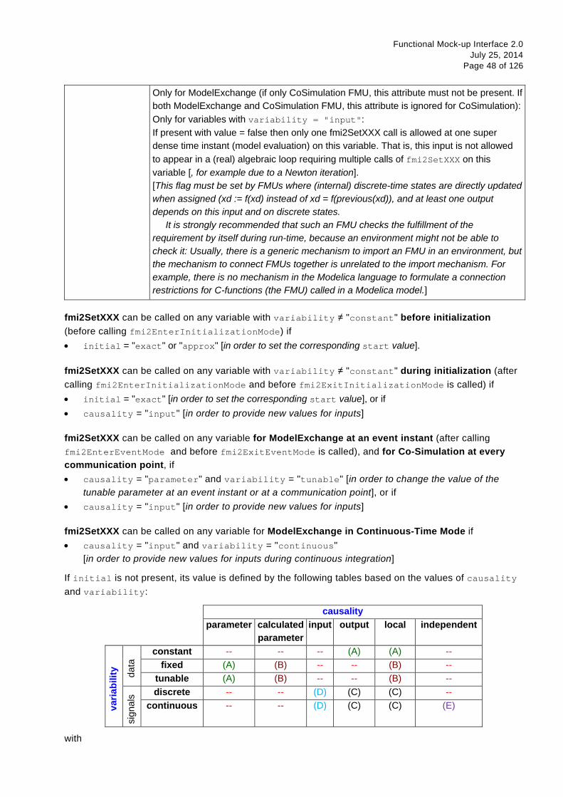
Functional Mock-up Interface 2.0 July 25, 2014
Page 48 of 126
Only for ModelExchange (if only CoSimulation FMU, this attribute must not be present. If both ModelExchange and CoSimulation FMU, this attribute is ignored for CoSimulation): Only for variables with variability = "input": If present with value = false then only one fmi2SetXXX call is allowed at one super dense time instant (model evaluation) on this variable. That is, this input is not allowed to appear in a (real) algebraic loop requiring multiple calls of fmi2SetXXX on this variable [, for example due to a Newton iteration]. [This flag must be set by FMUs where (internal) discrete-time states are directly updated when assigned (xd := f(xd) instead of xd = f(previous(xd)), and at least one output depends on this input and on discrete states. It is strongly recommended that such an FMU checks the fulfillment of the requirement by itself during run-time, because an environment might not be able to check it: Usually, there is a generic mechanism to import an FMU in an environment, but the mechanism to connect FMUs together is unrelated to the import mechanism. For example, there is no mechanism in the Modelica language to formulate a connection restrictions for C-functions (the FMU) called in a Modelica model.]
fmi2SetXXX can be called on any variable with variability ≠ "constant" before initialization (before calling fmi2EnterInitializationMode) if • initial = "exact" or "approx" [in order to set the corresponding start value].
fmi2SetXXX can be called on any variable with variability ≠ "constant" during initialization (after calling fmi2EnterInitializationMode and before fmi2ExitInitializationMode is called) if • initial = "exact" [in order to set the corresponding start value], or if • causality = "input" [in order to provide new values for inputs]
fmi2SetXXX can be called on any variable for ModelExchange at an event instant (after calling fmi2EnterEventMode and before fmi2ExitEventMode is called), and for Co-Simulation at every communication point, if • causality = "parameter" and variability = "tunable" [in order to change the value of the
tunable parameter at an event instant or at a communication point], or if • causality = "input" [in order to provide new values for inputs]
fmi2SetXXX can be called on any variable for ModelExchange in Continuous-Time Mode if • causality = "input" and variability = "continuous"
[in order to provide new values for inputs during continuous integration]
If initial is not present, its value is defined by the following tables based on the values of causality and variability:
causality parameter calculated
parameter input output local independent
varia
bilit
y data
constant -- -- -- (A) (A) -- fixed (A) (B) -- -- (B) --
tunable (A) (B) -- -- (B) --
sign
als discrete -- -- (D) (C) (C) --
continuous -- -- (D) (C) (C) (E)
with
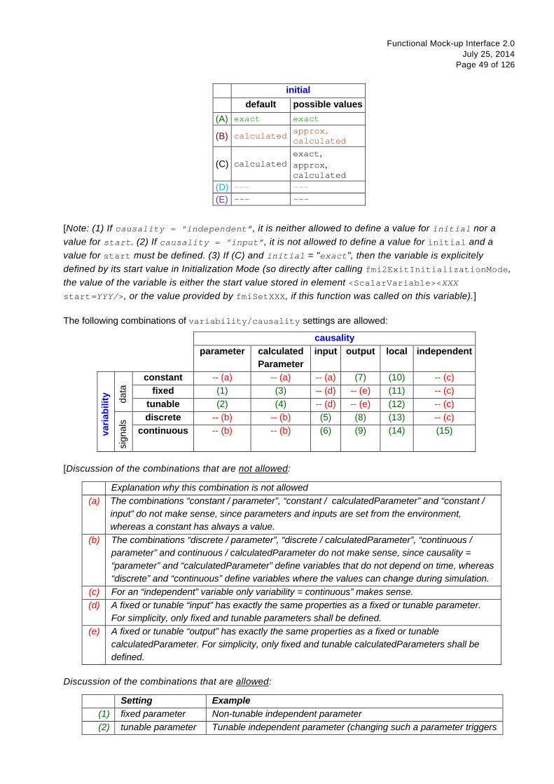
Functional Mock-up Interface 2.0 July 25, 2014
Page 49 of 126
initial default possible values (A) exact exact
(B) calculated approx, calculated
(C) calculated exact, approx, calculated
(D) --- ---
(E) --- ---
[Note: (1) If causality = "independent”, it is neither allowed to define a value for initial nor a value for start. (2) If causality = "input”, it is not allowed to define a value for initial and a value for start must be defined. (3) If (C) and initial = "exact", then the variable is explicitely defined by its start value in Initialization Mode (so directly after calling fmi2ExitInitializationMode, the value of the variable is either the start value stored in element <ScalarVariable><XXX start=YYY/>, or the value provided by fmiSetXXX, if this function was called on this variable).]
The following combinations of variability/causality settings are allowed:
causality parameter calculated
Parameter input output local independent
varia
bilit
y data
constant -- (a) -- (a) -- (a) (7) (10) -- (c) fixed (1) (3) -- (d) -- (e) (11) -- (c)
tunable (2) (4) -- (d) -- (e) (12) -- (c)
sign
als discrete -- (b) -- (b) (5) (8) (13) -- (c)
continuous -- (b) -- (b) (6) (9) (14) (15)
[Discussion of the combinations that are not allowed:
Explanation why this combination is not allowed (a) The combinations “constant / parameter”, “constant / calculatedParameter” and “constant /
input” do not make sense, since parameters and inputs are set from the environment, whereas a constant has always a value.
(b) The combinations “discrete / parameter”, “discrete / calculatedParameter”, “continuous / parameter” and continuous / calculatedParameter do not make sense, since causality = “parameter” and “calculatedParameter” define variables that do not depend on time, whereas “discrete” and “continuous” define variables where the values can change during simulation.
(c) For an “independent” variable only variability = continuous” makes sense. (d) A fixed or tunable “input” has exactly the same properties as a fixed or tunable parameter.
For simplicity, only fixed and tunable parameters shall be defined. (e) A fixed or tunable “output” has exactly the same properties as a fixed or tunable
calculatedParameter. For simplicity, only fixed and tunable calculatedParameters shall be defined.
Discussion of the combinations that are allowed:
Setting Example (1) fixed parameter Non-tunable independent parameter (2) tunable parameter Tunable independent parameter (changing such a parameter triggers
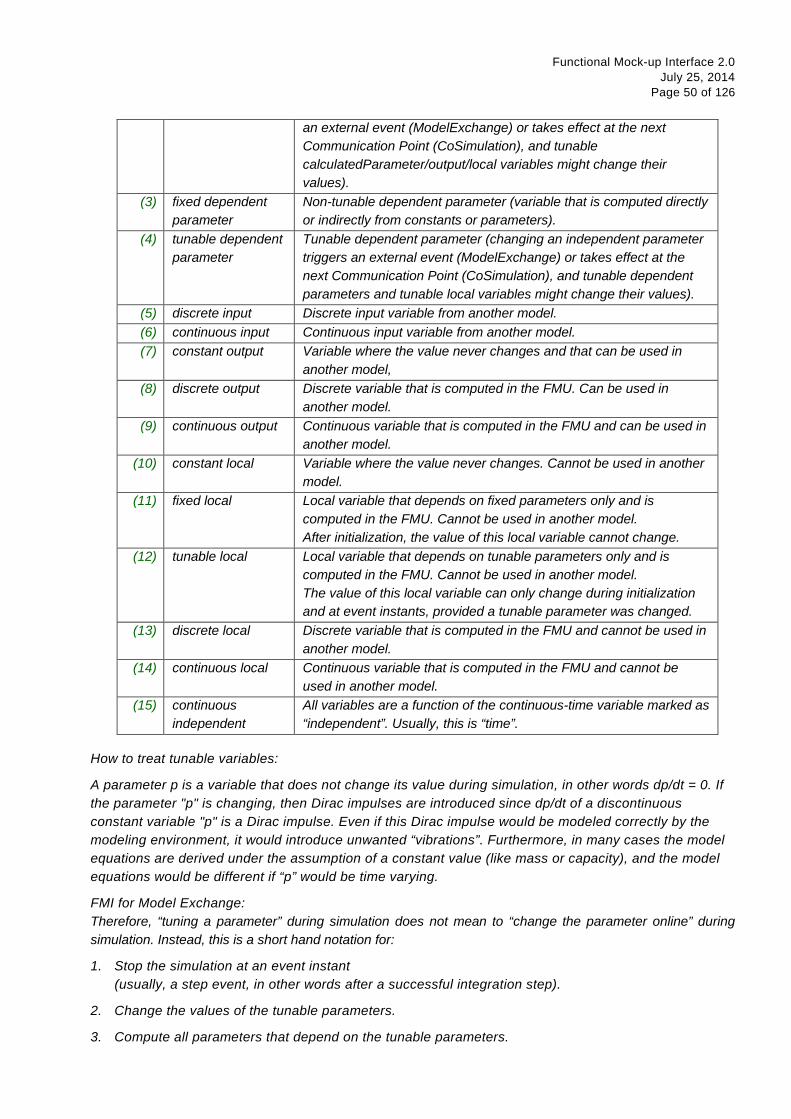
Functional Mock-up Interface 2.0 July 25, 2014
Page 50 of 126
an external event (ModelExchange) or takes effect at the next Communication Point (CoSimulation), and tunable calculatedParameter/output/local variables might change their values).
(3) fixed dependent parameter
Non-tunable dependent parameter (variable that is computed directly or indirectly from constants or parameters).
(4) tunable dependent parameter
Tunable dependent parameter (changing an independent parameter triggers an external event (ModelExchange) or takes effect at the next Communication Point (CoSimulation), and tunable dependent parameters and tunable local variables might change their values).
(5) discrete input Discrete input variable from another model. (6) continuous input Continuous input variable from another model. (7) constant output Variable where the value never changes and that can be used in
another model, (8) discrete output Discrete variable that is computed in the FMU. Can be used in
another model. (9) continuous output Continuous variable that is computed in the FMU and can be used in
another model. (10) constant local Variable where the value never changes. Cannot be used in another
model. (11) fixed local Local variable that depends on fixed parameters only and is
computed in the FMU. Cannot be used in another model. After initialization, the value of this local variable cannot change.
(12) tunable local Local variable that depends on tunable parameters only and is computed in the FMU. Cannot be used in another model. The value of this local variable can only change during initialization and at event instants, provided a tunable parameter was changed.
(13) discrete local Discrete variable that is computed in the FMU and cannot be used in another model.
(14) continuous local
Continuous variable that is computed in the FMU and cannot be used in another model.
(15) continuous independent
All variables are a function of the continuous-time variable marked as “independent”. Usually, this is “time”.
How to treat tunable variables:
A parameter p is a variable that does not change its value during simulation, in other words dp/dt = 0. If the parameter "p" is changing, then Dirac impulses are introduced since dp/dt of a discontinuous constant variable "p" is a Dirac impulse. Even if this Dirac impulse would be modeled correctly by the modeling environment, it would introduce unwanted “vibrations”. Furthermore, in many cases the model equations are derived under the assumption of a constant value (like mass or capacity), and the model equations would be different if “p” would be time varying.
FMI for Model Exchange: Therefore, “tuning a parameter” during simulation does not mean to “change the parameter online” during simulation. Instead, this is a short hand notation for:
1. Stop the simulation at an event instant (usually, a step event, in other words after a successful integration step).
2. Change the values of the tunable parameters.
3. Compute all parameters that depend on the tunable parameters.
Functional Mock-up Interface 2.0 July 25, 2014
Page 51 of 126
4. Newly start the simulation using as initial values the current values of all previous variables and the new values of the parameters.
Basically this means that a new simulation run is started from the previous FMU state with changed parameter values. With this interpretation, changing parameters online is “clean”, as long as these changes appear at an event instant.
FMI for Co-Simulation: Changing of tunable parameters is allowed before an fmi2DoStep call (so whenever an input can be set with fmi2SetXXX) and before fmi2ExitInitializationMode is called (so before and during Initialization Mode). The FMU internally carries out event handling if necessary. ]
Variables of the same base type (like fmi2Real) that have identical valueReference definitions are called “alias” variables. The main purpose of “alias” variables is to enhance efficiency. If two variables a and b are alias variables, then this is only allowed if the behavior of the FMU would be exactly the same, as if a and b would not be treated as alias variables (that is, would have different valueReferences). This requirement leads naturally to the following restrictions:
1. Variables a and b that can both be set with fmi2SetXXX, or variable a that can be set with fmiSetXXX and variable b that is defined with causality = ″independent″, cannot be alias variables [since these variables are “independent” variables and alias means that there is a constraint equation between variables (= the values are the same), and then the variables are no longer “independent”. For example if variables a and b have causality = "parameter", then the value references of a and b must be different. However, if variable a has causality = "parameter" and b has causality = "calculatedParameter" and b := a, then a and b can have the same value reference.].
2. At most one variable of the same alias set of variables with variability ≠ "constant" can have a start attribute. [since “start” variables are independent initial values.]
3. A variable with variability = "constant" can only be aliased to another variable with variability = "constant". It is then required that the start values of all aliased (constant) variables are identical.
4. All variables of the same alias set must all have either no <Unit> element defined or all of them must have the same <Unit name> and the same <Unit><BaseUnit> definitions.
The aliasing of variables only means that the “value” of the variables is always identical. However, aliased variables may have different attributes, like min/max/nominal values or description texts. [For example if v1, v2 are two alias variables with v1=v2 and v1.max=10 and v2.max=5, then the FMU will trigger an error if either v1 or v2 becomes larger than 5.]
[The dependency definition in fmiModelDescription.ModelStructure is completely unrelated to the alias definition. In particular, the “direct dependency” definition can be a super set of the “real” direct dependency definition, even if the “alias” information shows that this is too conservative. For example if it is stated that the output y1 depends on input u1 and the output y2 depends on input u2, and y1 is an alias to y2, then this definition is fine, although it can be deduced that in reality neither y1 nor y2 depend on any input.].
Type specific properties are defined in the required choice element, where exactly one of “Real”, “Integer”, “Boolean”, “String”, “Enumeration” must be present in the XML file:
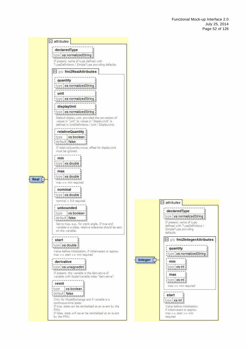
Functional Mock-up Interface 2.0 July 25, 2014
Page 52 of 126
E1 attributes I .---------------------n : declaredType
: typ~~J.~~~~-~-~!!!~.;~~~~!!-~~~~-~ If present, name of rype def.ned with TypeDeflnitions I Simple Type provid"mg defaults.
E1 grp fm i2Rea1Attributes I .---------------------n : quantity
: typ~J.~~~ n_ o_r!'!a.;li~~ ~!~i~ ~~-g :-~-n-i1 ----------------u : typ~J.~~~ n_ o_r!'!a.;li~~ ~!~i~ ~~-g .---------------------n : displayUnit
: typ~~J.~~~~-~-~!!!~.;~~~~!!-~~1-~ Default display unit, provided tile conversion of vc:lues in •unit• to va:lues in •ctsplayunit• is defined in UnitDef.rutions I Unit I Disp!ayUnit.
,-----------------' relative Quantity ' • type I xs:boolean
~ d ~~t~-~-~L!!~~~-~-~-~-~-~ If rel=tiveQuc:ntiry= true, offset for disp!ayUnit ...,., be ~nored.
:- ;.,;i~ --------u : typ~J.~~~d_o_u_~~~~-g :-~~--------n
Real 8- : typ~~~~'d_o_u_b]~-~ max>= min req.Wed
:-~-~~i~~i ---- -D : type 1 xs:double n
nominal > 0.0 req.Wed ,----------------- E1 attributes I ' unbounded ' • type I xs:boolean ~ defaun I false
.---------------------n : declaredType
: typ~~J.~~~~-~-~!!!~.;~~~~!!-~~1-~ Set to true, e.g., for aonk angle. !f true a:nd variable is a state, relative tolerance snoutd be zero on tNs variable.
If present, name of rype defmedw~hTypeOefmhbns / Simple Type providing defaults.
,--------------D : s tart El grp fm i21ntegerAttributes
: type 1 xs:double n Va:W before initi=:lization,. if initiaJ=exact or approx. max>= start>= min req.Wed
.---------------------n : quantity
: typ~J.~~~n_o_r!'!~.;~~~~!!-~~1-~ :- -d-;;i~;ti~~------] 1 : type I xs:unsignedlnt •
Integer 8- ---------]] ' . ' ' mm '
b.Yp_e_l_"s~ ~n!] J If present, this variable is the deriva tive of variable with Sca:larVarisble index •deriva tive•,
:-~~i~i;-----------
• type I xs:boolean
---------]1 ' ' ' m ax ' ' '
~ ~.P-~_L~~:~~!J I max>= min req.Wed
~ d ~~~t~-~-~L!!~~~-~-~-~-~-~ Only for Mode!Exha:nge a:nd if variable is a continuous-time state:
---------]1 : s tart : ' '
~ ~.P-~_L~~:~~!J I If true,. state can be reinitia.lized a t a:n event by the FMU If fa:!se, state d never be reinitia.lized a t a:n event
Vaile before initialization,. if initiaJ= exact or a pprox. max>= start>= min
by tne FMU ._m
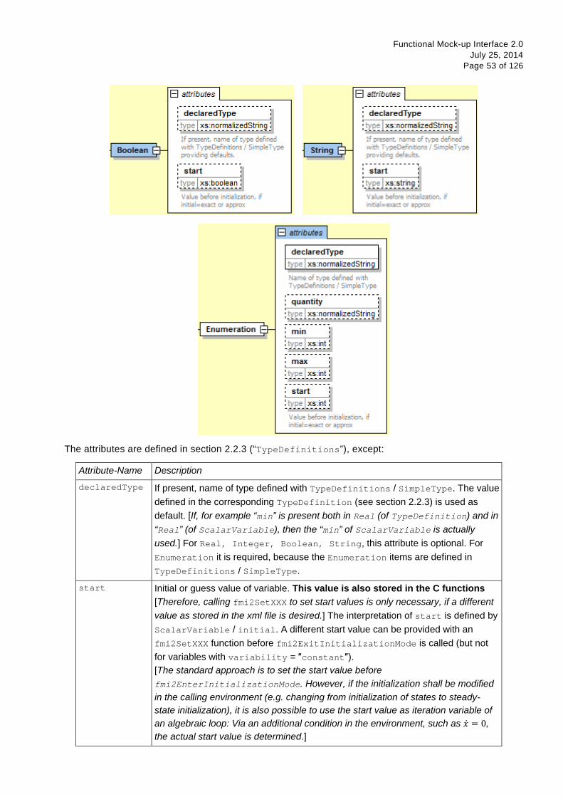
Functional Mock-up Interface 2.0 July 25, 2014
Page 53 of 126
The attributes are defined in section 2.2.3 (“TypeDefinitions”), except:
Attribute-Name Description
declaredType If present, name of type defined with TypeDefinitions / SimpleType. The value defined in the corresponding TypeDefinition (see section 2.2.3) is used as default. [If, for example “min” is present both in Real (of TypeDefinition) and in “Real” (of ScalarVariable), then the “min” of ScalarVariable is actually used.] For Real, Integer, Boolean, String, this attribute is optional. For Enumeration it is required, because the Enumeration items are defined in TypeDefinitions / SimpleType.
start Initial or guess value of variable. This value is also stored in the C functions [Therefore, calling fmi2SetXXX to set start values is only necessary, if a different value as stored in the xml file is desired.] The interpretation of start is defined by ScalarVariable / initial. A different start value can be provided with an fmi2SetXXX function before fmi2ExitInitializationMode is called (but not for variables with variability = ″constant″). [The standard approach is to set the start value before fmi2EnterInitializationMode. However, if the initialization shall be modified in the calling environment (e.g. changing from initialization of states to steady-state initialization), it is also possible to use the start value as iteration variable of an algebraic loop: Via an additional condition in the environment, such as �̇� = 0, the actual start value is determined.]

Functional Mock-up Interface 2.0 July 25, 2014
Page 54 of 126
If initial = ″exact″ or ″approx″ or causality = ″input″, a start value must be provided. If initial = ″calculated″ or causality = ″independent″, it is not allowed to provide a start value. Variables with causality = "parameter" or "input", as well as variables with variability = "constant", must have a "start" value. • If causality = "parameter", the start-value is the value of it. • If causality = "input", the start value is used by the model as value of
the input, if the input is not set by the environment. • If variability = "constant", the start value is the value of the constant. • If causality = "output" or "local" then the start value is either an
“initial” or a “guess” value, depending on the setting of attribute "initial".
derivative If present, this variable is the derivative of variable with ScalarVariable index "derivative". [For example, if there are 10 ScalarVariables and derivative = 3 for ScalarVariable 8, then ScalarVariable 8 is the derivative of ScalarVariable 3 with respect to the independent variable (usually time). This information might be especially used if an input or an output is the derivative of another input or output, or to define the states.] The state derivatives of an FMU are listed under element <ModelStructure><Derivatives>. All ScalarVariables listed in this element must have attribute derivative (in order that the continuous-time states are uniquely defined).
reinit Only for ModelExchange (if only CoSimulation FMU, this attribute must not be present. If both ModelExchange and CoSimulation FMU, this attribute is ignored for CoSimulation): Can only be present for a continuous-time state. If true, state can be reinitialized at an event by the FMU If false, state will not be reinitialized at an event by the FMU
min / max The optional attributes “min” and “max” in element “Enumeration” restrict the allowed values of the enumeration. The min/max definitions are an information from the FMU to the environment defining the region in which the FMU is designed to operate, see also comment in section 2.2.3. [If, for example an Enumeration is defined with “name1 = -4”, “name2 = 1”, “name3 = 5”, “name4 = 11” and min=-2, max = 5, then only “name2” and “name3” are allowed].
With element “Annotations” additional, tool specific data can be defined:

Functional Mock-up Interface 2.0 July 25, 2014
Page 55 of 126
With Tool.name the name of the tool is defined that can interpret the “any” element. The “any” element can be an arbitrary XML data structure defined by the tool. [Typically, additional data is defined here how to build up the menu for the variable, including the graphical layout and enabling/disabling an input field based on the values of other parameters.]
2.2.8 Definition of the Model Structure (ModelStructure)
The structure of the model is defined in element “ModelStructure” within “fmiModelDescription”. This structure is with respect to the underlying model equations, independently how these model equations are solved. [For example, when exporting a model both in Model-Exchange and in Co-Simulation format, then the model structure is identical in both cases. The Co-Simulation FMU has either an integrator included that solves the model equations, or the discretization formula of the integrator and the model equations are solved together (“inline integration”). In both cases the model has the same continuous-time states. In the second case the internal implementation is a discrete-time system, but from the outside this is still a continuous-time model that is solved with an integration method.]
The required part defines an ordering of the outputs and of the (exposed) derivatives, and defines the unknowns that are available during Initialization [Therefore, when linearizing an FMU, every tool will use the same ordering for the outputs, states, and derivatives for the linearized model. The ordering of the inputs should be performed in this case according to the ordering in ModelVariables.] A ModelExchange FMU must expose all derivatives of its continuous-time states in element <Derivatives>. A Co-Simulation FMU need not to expose these state derivatives. [If a Co-Simulation FMU exposes its state derivatives, they are usually not utilized for the co-simulation, but, e.g., to linearize the FMU at a communication point.]
The optional part defines in which way derivatives and outputs depend on inputs, and continuous-time states at the current super dense time instant (ModelExchange) or at the current Communication Point (CoSimulation). [A simulation environment can utilize this information to improve the efficiency, e.g., when connecting FMUs together, or when computing the partial derivative of the derivatives with respect to the states in the simulation engine.].
ModelStructure has the following definition:

Functional Mock-up Interface 2.0 July 25, 2014
Page 56 of 126
fmi2VariableDependency is defined as

Functional Mock-up Interface 2.0 July 25, 2014
Page 57 of 126
Elements of the InitialUnknowns list:
Functional Mock-up Interface 2.0 July 25, 2014
Page 58 of 126
Note, that attribute dependenciesKind for element InitialUnknowns has less enumeration values as dependenciesKind in the other lists.
ModelStructure consists of the following elements (see also figures above; the symbols of the mathematical equations describing the dependency are defined in section 3.1):
Element-Name Description
Outputs Ordered list of all outputs, in other words a list of ScalarVariable indices where every corresponding ScalarVariable must have causality = "output" (and every variable with causality=”output” must be listed here). [Note, all output variables are listed here, especially discrete and continuous outputs. The ordering of the variables in this list is defined by the exporting tool. Usually, it is best to order according to the declaration order in the source model, since then the <Outputs> list does not change, if the declaration order of outputs in the source model is not changed. This is e.g. important for linearization, in order that the interpretation of the output vector does not change for a re-exported FMU.]. Attribute dependencies defines the dependencies of the outputs from the knowns at the current super dense time instant in Event and in Continuous-Time Mode (ModelExchange) and at the current Communication Point (CoSimulation). The functional dependency is defined as (dependencies of variables that are fixed in Event and Continuous-Time Mode and at Communication Points are not shown):
(𝐲𝑐 ,𝐲𝑑) ≔ 𝐟𝑜𝑢𝑡𝑝𝑢𝑡(𝐱𝑐 ,𝒖𝑐 ,𝒖𝑑 , 𝑡,𝒑𝑡𝑢𝑛𝑒)
Derivatives Ordered list of all state derivatives, in other words a list of ScalarVariable indices where every corresponding ScalarVariable must be a state derivative. [Note, only continuous Real variables are listed here. If a state or a derivative of a state shall not be exposed from the FMU, or if states are not statically associated with a variable (due to dynamic state selection), then dummy ScalarVariables have to be introduced, for example x[4], or xDynamicStateSet2[5]. The ordering of the variables in this list is defined by the exporting tool. Usually, it is best to order according to the declaration order of the states in the source model, since then the <Derivatives> list does not change, if the declaration order of states in the source model is not changed. This is e.g. important for linearization, in order that the interpretation of the state vector does not change for a re-exported FMU.]. The corresponding continuous-time states are defined by attribute derivative of the corresponding ScalarVariable state derivative element. [Note, higher order derivatives must be mapped to first order derivatives but the mapping definition can be preserved due to attribute
derivative. Example: 𝑑𝑠𝑑𝑡
= 𝑣, 𝑑𝑣𝑑𝑡
= 𝑓(. . ), then �𝑣, 𝑑𝑣𝑑𝑡�is the vector of state
derivatives and attribute derivative of 𝑣 references 𝑠, and attribute
derivative of 𝑑𝑣𝑑𝑡
references 𝑣.]
For Co-Simulation, element “Derivatives” is ignored if capability flag providesDirectionalDerivative has a value of false, in other words cannot be computed [which is the default. If an FMU supports both ModelExchange and CoSimulation, then the “Derivatives” element might be present, since it is needed for ModelExchange. If the above flag is set to false for the CoSimulation case, then the “Derivatives” element is ignored for CoSimulation. If “inline integration” is used for a CoSimulation slave, then the model still has continuous-time states and just a special solver is used (internally the implementation results in a discrete-

Functional Mock-up Interface 2.0 July 25, 2014
Page 59 of 126
time system, but from the outside, it is still a continuous-time system)]. Attribute dependencies defines the dependencies of the state derivatives
from the knowns at the current super dense time instant in Event and in Continuous-Time Mode (ModelExchange) and at the current Communication Point (CoSimulation). The functional dependency is defined as (dependencies of variables that are fixed in Event and Continuous-Time Mode and at Communication Points are not shown):
�̇�𝑐 ≔ 𝐟𝑑𝑒𝑟(𝐱𝑐 ,𝒖𝑐 ,𝒖𝑑 , 𝑡,𝒑𝑡𝑢𝑛𝑒)
Functional Mock-up Interface 2.0 July 25, 2014
Page 60 of 126
InitialUnknowns Ordered list of all exposed Unknowns in Initialization Mode. This list consists of all variables with (1) causality = "output" and (initial="approx" or "calculated"), and (2) causality = "calculatedParameter" and (3) all continuous-time states and all state derivatives (defined with element
<Derivatives> from <ModelStructure>) with initial="approx" or "calculated" [if a Co-Simulation FMU does not define the <Derivatives> element, (3) cannot be present.].
The resulting list is not allowed to have duplicates (e.g. if a state is also an output, it is included only once in the list). The Unknowns in this list must be ordered according to their ScalarVariable index (for example if for two variables A and B the ScalarVariable index of A is less than the index of B, then A must appear before B in InitialUnknowns).
Attribute dependencies defines the dependencies of the Unknowns from the Knowns in Initialization Mode at the initial time. The functional dependency is defined as:
𝐯𝐼𝑛𝑖𝑡𝑖𝑎𝑙𝑈𝑛𝑘𝑛𝑜𝑤𝑛𝑠 ≔ 𝐟𝑖𝑛𝑖𝑡(𝒖𝑐,𝒖𝑑 , 𝑡0,𝐯𝑖𝑛𝑖𝑡𝑖𝑎𝑙=𝑒𝑥𝑎𝑐𝑡) Since outputs, continuous-time states and state derivatives are either present as Knowns (if initial="exact") or as Unknowns (if initial="approx" or "calculated"), they can be inquired with fmiGetXXX in InitializationMode. [Example: Assume an FMU is defined in the following way:
(𝐲c+d, �̇�c) ≔ 𝐟𝑖𝑛𝑖𝑡(𝐱c,𝐮c+d, t0,𝐩) (𝐲c+d, �̇�c) ≔ 𝐟𝑠𝑖𝑚(𝐱c,𝐮c+d, ti,𝐩)
Therefore, the initial state 𝐱c(t0) has initial="exact" and the initial state derivative �̇�c(t0) has initial="calculated". The environment can still initialize this FMU in steady-state, by using 𝐱c(t0) as iteration variables and adding the equations �̇�c(t0) = 𝟎 in the environment.]
Unknown An element of one of the lists above defining the unknown with a reference to the corresponding ScalarVariable element. It is assumed that at a super-dense time instant 𝑡 = (𝑡𝑅 , 𝑡𝐼) (ModelExchange) and at a Communication Point (CoSimulation) the following relationship holds:
𝑣𝑢𝑛𝑘𝑛𝑜𝑤𝑛 = ℎ(𝐯𝑘𝑛𝑜𝑤𝑛,𝐯𝑓𝑟𝑒𝑒𝑧𝑒) where • 𝑣𝑢𝑛𝑘𝑛𝑜𝑤𝑛 is the unknown variable defined with this element [for example an
output or a state derivative]. • 𝐯𝑘𝑛𝑜𝑤𝑛 is the vector of input arguments of function h that changes its value in
the actual Mode [for example continuous-time inputs in Continuous-Time Mode].
• 𝐯𝑓𝑟𝑒𝑒𝑧𝑒 is the set of input arguments of function h that do not change their values in this Mode, but change their values in other Modes [for example fixed parameters in Continuous-Time Mode].
Attribute dependencies of Unknown defines the dependency of 𝑣𝑢𝑛𝑘𝑛𝑜𝑤𝑛 with respect to 𝐯𝑘𝑛𝑜𝑤𝑛. [If for example a continuous-time output 𝑦2 is a function of the continuous-time inputs 𝑢3 and 𝑢5 and these inputs have changed then fmi2SetXXX on 𝑢3 and 𝑢5 must always be called before calling fmi2GetXXX on 𝑦2.]
Functional Mock-up Interface 2.0 July 25, 2014
Page 61 of 126
Element Unknown in Outputs, Derivatives and InitialUnknowns has the following attributes:
Attribute-Name Description
index The ScalarVariable index of the Unknown 𝑣𝑢𝑛𝑘𝑛𝑜𝑤𝑛. [For example, if there are 10 ScalarVariables and index = 3, then the third ScalarVariable is the unknown defined with this element.]
dependencies Optional attribute defining the dependencies of the unknown 𝑣𝑢𝑛𝑘𝑛𝑜𝑤𝑛 (directly or indirectly via auxiliary variables) with respect to 𝐯𝑘𝑛𝑜𝑤𝑛. If not present, it must be assumed that the Unknown depends on all Knowns. If present as empty list, the Unknown depends on none of the Knowns. Otherwise the Unknown depends on the Knowns defined by the given ScalarVariable indices. The indices are ordered according to magnitude, starting with the smallest index.
Knowns 𝐯𝑘𝑛𝑜𝑤𝑛 in Event and Continuous-Time Mode (ModelExchange) and at Communication Points (CoSimulation) for elements Outputs, Derivatives: • inputs (variables with causality = "input") • continuous-time states • independent variable (usually time; causality = "independent"). If an
independent variable is not explicitely defined under ScalarVariables, it is assumed that the Unknown depends explicitely on the independent variable.
Knowns 𝐯𝑘𝑛𝑜𝑤𝑛 in Initialization Mode (for elements InitialUnknowns): • inputs (variables with causality = "input") • variables with initial = "exact"
[for example independent parameters or initial states.] • independent variable (usually time; causality = "independent"). If an
independent variable is not explicitely defined under ScalarVariables, it is assumed that the Unknown depends explicitely on the independent variable.
For Co-Simulation, ”dependencies” does not list the dependency on continuous-time, if the capability flag providesDirectionalDerivative has a value of false, in other words the respective partial derivatives cannot be computed.
dependenciesKind If not present, it must be assumed that the Unknown 𝑣𝑢𝑛𝑘𝑛𝑜𝑤𝑛 depends on the Knowns 𝐯𝑘𝑛𝑜𝑤𝑛 without a particular structure. Otherwise, the corresponding Known 𝑣𝑘𝑛𝑜𝑤𝑛,𝑖 enters the equation as: If "dependenciesKind" is present, "dependencies" must be present and must have the same number of list elements.
= dependent: no particular structure, ℎ(. . , 𝑣𝑘𝑛𝑜𝑤𝑛,𝑖,..)
Only for Real unknowns 𝑣𝑢𝑛𝑘𝑛𝑜𝑤𝑛:
= constant: constant factor, 𝑐 ∙ 𝑣𝑘𝑛𝑜𝑤𝑛,𝑖 where 𝑐 is an expression that is evaluated before fmi2EnterInitializationMode is called.
Only for Real unknowns 𝑣𝑢𝑛𝑘𝑛𝑜𝑤𝑛 in Event and Continuous-Time Mode (ModelExchange) and at Communication Points (CoSimulation), and not for InitialUnknowns for Initialization Mode:

Functional Mock-up Interface 2.0 July 25, 2014
Page 62 of 126
= fixed: fixed factor, 𝑝 ∙ 𝑣𝑘𝑛𝑜𝑤𝑛,𝑖 where 𝑝 is an expression that is evaluated before fmi2ExitInitializationMode is called.
= tunable: tunable factor, 𝑝 ∙ 𝑣𝑘𝑛𝑜𝑤𝑛,𝑖 where 𝑝 is an expression that is evaluated before fmi2ExitInitializationMode is called and in Event Mode due to an external event (ModelExchange) or at a Communication Point (CoSimulation)
= discrete: discrete factor, 𝑑 ∙ 𝑣𝑘𝑛𝑜𝑤𝑛,𝑖 where 𝑑 is an expression that is evaluated before fmi2ExitInitializationMode is called and in Event Mode due to an external or internal event or at a Communication Point (CoSimulation).
If "dependenciesKind" is present, "dependencies" must be present and must have the same number of list elements.
[Example 1:
An FMU is defined by the following equations:
𝑑𝑑𝑡�𝑥1𝑥2𝑥3� = �
𝑓1(𝑥2)𝑓2(𝑥1) + 3 ∙ 𝑝2 ∙ 𝑥2 + 2 ∙ 𝑢1 + 3 ∙ 𝑢3
𝑓3(𝑥1, 𝑥3,𝑢1,𝑢2,𝑢3)�
𝑦 = 𝑔1(𝑥2, 𝑥3)
where 𝑢1 is a continuous-time input (variability=”continuous”), 𝑢2 is any type of input, 𝑢3 is a Real discrete-time input (variability=”discrete”), and 𝑝 is a fixed parameter (variability=”fixed”). The initialization is defined by:
𝑥1 = 1.1,𝑑𝑥2𝑑𝑡
= 0,𝑦 = 3.3
and therefore the initialization equations are:
𝑥2 =1
3 ∙ 𝑝2∙ (𝑓2(𝑥1) + 2 ∙ 𝑢1 + 3 ∙ 𝑢3)
𝑥3 = 𝑔1−1(𝑥2,𝑦)
This equation system can be defined as:
<ModelVariables> <ScalarVariable name="p" , ...> … </ScalarVariable> <!—index="1" --> <ScalarVariable name="u1" , ...> … </ScalarVariable> <!—index="2" --> <ScalarVariable name="u2" , ...> … </ScalarVariable> <!—index="3" --> <ScalarVariable name="u3" , ...> … </ScalarVariable> <!—index="4" --> <ScalarVariable name="x1" , ...> … </ScalarVariable> <!—index="5" --> <ScalarVariable name="x2" , ...> … </ScalarVariable> <!—index="6" --> <ScalarVariable name="x3" , ...> … </ScalarVariable> <!—index="7" --> <ScalarVariable name="der(x1)", ...> … </ScalarVariable> <!—index="8" --> <ScalarVariable name="der(x2)", ...> … </ScalarVariable> <!—index="9" --> <ScalarVariable name="der(x3)", ...> … </ScalarVariable> <!—index="10" --> <ScalarVariable name="y" , ...> … </ScalarVariable> <!—index="11" --> </ModelVariables> <ModelStructure> <Outputs> <Unknown index="11" dependencies="6 7" /> </Outputs>
Functional Mock-up Interface 2.0 July 25, 2014
Page 63 of 126
<Derivatives> <Unknown index="8" dependencies="6" /> <Unknown index="9" dependencies="2 4 5 6" dependenciesKind="constant constant dependent fixed"/> <Unknown index="10" dependencies="2 3 4 5 6" /> </Derivatives> <InitialUnknowns> <Unknown index="6" dependencies="2 4 5" /> <Unknown index="7" dependencies="2 4 5 11" /> <Unknown index="8" ... /> <Unknown index="10" ... /> </InitialUnknowns> </ModelStructure>
Example 2:
𝑦 = �2 ∙ 𝑢 if 𝑢 > 03 ∙ 𝑢 else
where 𝑢 is a continuous-time input with index=”1” and 𝑦 is a continuous-time output with index=”2”. The definition of the model structure is then:
<ModelStructure> <Outputs> <Unknown index="2" dependencies="1" dependenciesKind="discrete"/> </Outputs> </ModelStructure>
Note, 𝑦 = 𝑑 ∙ 𝑢 where 𝑑 changes only during Event Mode (𝑑 = 2 ∙ 𝑢 or 3 ∙ 𝑢 depending on relation 𝑢 > 0 that changes only at Event Mode). Therefore dependenciesKind="discrete".
Example 3:
𝑦 = �2 if 𝑢 > 03 else
where 𝑢 is a continuous-time input with index=”1” and 𝑦 is a continuous-time output with index=”2”. The definition of the model structure is then:
<ModelStructure> <Outputs> <Unknown index="2" dependencies="1" dependenciesKind="dependent"/> </Outputs> </ModelStructure>
Note, 𝑦 = 𝑐 where 𝑐 changes only during Event Mode (𝑐 = 2 or 3 depending on relation 𝑢 > 0 that changes only at Event Mode). Therefore dependenciesKind="dependent" because it is not a linear relationship on 𝑢.
Defining FMU features with the dependencies list:
Note, via the dependencies list the supported features of the FMU can be defined. Examples:
• If a state derivative der_x is a function of a parameter p (so of a start value of a variable with causality = "parameter" and variability = "fixed"), and the FMU does not support an iteration over p during InitializationMode (e.g. to iterate over p such that the state derivative der_x is zero), then the dependencies list of der_x should not include p. If an FMU is imported in an environment and such an iteration is setup, then the tool can figure out that the resulting algebraic system of equations is structurally singular and therefore can reject such a definition.

Functional Mock-up Interface 2.0 July 25, 2014
Page 64 of 126
• For standard CoSimulation FMUs it is common that no algebraic loops over the input/output variables nor over start-values is supported. In such a case, all dependencies lists for output variables under the InitialUnknowns element should be defined as empty lists defining that the setting of inputs and/or of start values does not influence the outputs. As a result, it is not possible to formulate algebraic loops of connected FMUs during InitializationMode.
]
2.2.9 Variable Naming Conventions (variableNamingConvention)
With attribute “variableNamingConvention” of element “fmiModelDescription”, the convention is defined how the ScalarVariable.names have been constructed. If this information is known, the environment may be able to represent the names in a better way (for example as tree and not as a linear list).
In the following definitions, the EBNF is used:
= production rule [ ] optional { } repeat zero or more times | or
The following conventions for scalar names are defined:
variableNamingConvention = "flat"
name = Unicode-char { Unicode-char } // identical to xs:normalizedString Unicode-char = any Unicode character without carriage return (#xD), line feed (#xA) nor tab (#x9)
The names must be unique, non-empty strings. [It is recommended that the names are visually clearly different from each other; but it is not required.]
variableNamingConvention = "structured"
Structured names are hierarchical using “.” as a separator between hierarchies. A name consists of “_”, letters and digits or may consist of any characters enclosed in single apostrophes. A name may identify an array element on every hierarchical level using “[...]” to identify the respective array index. A derivative of a variable is defined with “der(name)” for the first time derivative and “der(name,N)” for the N-th derivative. Examples:
vehicle.engine.speed resistor12.u v_min robot.axis.′motor #234′ der(pipe[3,4].T[14],2) // second time derivative of pipe[3,4].T[14]
The precise syntax is9:.
name = identifier | "der(" identifier ["," unsignedInteger ] ")" identifier = B-name [ arrayIndices ] {"." B-name [ arrayIndices ] } B-name = nondigit { digit | nondigit } | Q-name nondigit = "_" | letters "a" to "z" | letters "A" to "Z" digit = "0" | "1" | "2" | "3" | "4" | "5" | "6" | "7" | "8" | "9" Q-name = "’" ( Q-char | escape ) { Q-char | escape } "’" Q-char = nondigit | digit | "!" | "#" | "$" | "%" | "&" | "(" | ")" | "*" | "+" | "," | "-" | "." | "/" | ":" |
9 This definition is identical to the syntax of an identifier in Modelica version 3.2.

Functional Mock-up Interface 2.0 July 25, 2014
Page 65 of 126
";" | "<" | ">" | "=" | "?" | "@" | "[" | "]" | "^" | "{" | "}" | "|" | "~" | " " escape = "\’" | "\"" | "\?" | "\\" | "\a" | "\b" | "\f" | "\n" | "\r" | "\t" | "\v" arrayIndices = "[" unsignedInteger {"," unsignedInteger} "]" unsignedInteger = digit { digit }
The tree of names is mapped to an ordered list of ScalarVariable.name’s in depth-first order. Example:
vehicle transmission ratio outputSpeed engine inputSpeed temperature
is mapped to the following list of ScalarVariable.name’s:
vehicle.transmission.ratio vehicle.transmission.outputSpeed vehicle.engine.inputSpeed vehicle.engine.temperature
All array elements are given in a consecutive sequence of ScalarVariables. Elements of multi-dimensional arrays are ordered according to “row major” order that is elements of the last index are given in sequence.
[For example the vector “centerOfMass” in body “arm1” is mapped to the following ScalarVariables:
robot.arm1.centerOfMass[1] robot.arm1.centerOfMass[2] robot.arm1.centerOfMass[3]
For example, a table T[4,3,2] (first dimension 4 entries, second dimension 3 entries, third dimension 2 entries) is mapped to the following ScalarVariables:
T[1,1,1] T[1,1,2] T[1,2,1] T[1,2,2] T[1,3,1] T[1,3,2] T[2,1,1] T[2,1,2] T[2,3,1] …
]
It might be that not all elements of an array are present. If they are present, they are given in consecutive order in the XML file.
2.3 FMU Distribution
An FMU description consists of several files. An FMU implementation may be distributed in source code and/or in binary format. All relevant files are stored in a zip file with a pre-defined structure. The implementation must either implement all the functions of FMI for Model Exchange or all the functions of FMI for Co-Simulation or both. The extension of the zip file must be “.fmu”, for example “HybridVehicle.fmu”. The compression method used for the zip file must be “deflate” [(most free tools, for example zlib, offer only the common compression method "deflate")].

Functional Mock-up Interface 2.0 July 25, 2014
Page 66 of 126
Every FMU is distributed with its own zip file. This zip file has the following structure:
// Structure of zip file of an FMU modelDescription.xml // Description of FMU (required file) model.png // Optional image file of FMU icon documentation // Optional directory containing the FMU documentation index.html // Entry point of the documentation <other documentation files> sources // Optional directory containing all C sources // all needed C sources and C header files to compile and link the FMU // with exception of: fmi2TypesPlatform.h , fmi2FunctionTypes.h and fmi2Functions.h // The files to be compiled (but not the files included from these files) // have to be reported in the xml-file under the structure // <ModelExchange><SourceFiles> … and <CoSimulation><SourceFiles> binaries // Optional directory containing the binaries win32 // Optional binaries for 32-bit Windows <modelIdentifier>.dll // DLL of the FMI implementation // (build with option "MT" to include run-time environment) <other DLLs> // The DLL can include other DLLs // Optional object Libraries for a particular compiler VisualStudio8 // Binaries for 32-bit Windows generated with // Microsoft Visual Studio 8 (2005) <modelIdentifier>.lib // Binary libraries gcc3.1 // Binaries for gcc 3.1. ... win64 // Optional binaries for 64-bit Windows ... linux32 // Optional binaries for 32-bit Linux <modelIdentifier>.so // Shared library of the FMI implementation ... linux64 // Optional binaries for 64-bit Linux ... resources // Optional resources needed by the FMU < data in FMU specific files which will be read during initialization; also more folders can be added under resources (tool/model specific). In order for the FMU to access these resource files, the resource directory must be available in unzipped form and the absolute path to this directory must be reported via argument ″fmuResourceLocation″ via fmi2Instantiate. >
An FMU has to implement all common functions (according to tables in sections 3.2.3 and 4.2.4). ModelExchange FMUs have to provide additionally the respective Model Exchange function, CoSimulation FMUs the Co-Simulation functions.
The FMU must be distributed with at least one implementation, in other words either sources or one of the binaries for a particular machine. It is also possible to provide the sources and binaries for different target machines together in one zip file. The following names are standardized: For Windows: “win32”, “win64”- For Linux: “linux32”, “linux64”. For Mac: “darwin32“, “darwin64” Futhermore, also the names “VisualStudioX” and “gccX” are standardized and define the compiler with which the binary has been generated [, for example VisualStudio8]. Further names can be introduced by vendors. Dynamic link libraries must include all referenced resources that are not available on a standard target machine [for example DLLs on Windows machines must be built with option “MT” to include the run-time environment of VisualStudio in the DLL, and not use the option “MD” where this is not the case]. When compiling a shared object on Linux, RPATH=“$ORIGIN“ has to be set when generating the shared object in order that shared objects used from it, can be dynamically loaded.
Typical scenarios are to provide binaries only for one machine type (for example on the machine where the target simulator is running and for which licenses of run-time libraries are available) or to provide only

Functional Mock-up Interface 2.0 July 25, 2014
Page 67 of 126
sources (for example for translation and download for a particular micro-processor). If run-time libraries cannot be shipped due to licensing, special handling is needed, for example by providing the run-time libraries at appropriate places by the receiver.
FMI provides the means for two kinds of implementation: needsExecutionTool=true and needsExecutionTool=false. In the first case a tool specific wrapper DLL/SharedObject has to be provided as the binary, in the second a compiled or source code version of the model with its solver is stored (see section 4.3.1 for details).
In an FMU both a version for ModelExchange and for CoSimulation might be present. If in both cases the executable part is provided as DLL/SharedObject, then two different or only one library can be provided. The library names are defined in the modelIdentifier attribute of elements “fmiModelDescription.ModelExchange” and “fmiModelDescription.CoSimulation”:
[Example for different libraries: binaries win32 MyModel_ModelExchange.dll // ModelExchange.modelIdentifier = // "MyModel_ModelExchange" MyModel_CoSimulation.dll // CoSimulation.modelIdentifier = // "MyModel_CoSimulation" ]
The usual distribution of an FMU will be with DLLs/SharedObjects because then further automatic processing [(for example importing into another tool)] is possible.
If run-time libraries are needed by the FMU that have to be present on the target machine, then automatic processing is likely impossible. The requirements and the expected processing should be documented in the “documentation” directory in this case.
A source-based distribution might require manual interaction in order that it can be utilized. The intention is to support platforms that are not known in advance (such as HIL-platforms or micro-controllers). Typically, in such a case the complete source code in ANSI-C is provided (for example one C source file that includes all other needed C files with the “#include” directive). All C source file names that need to be defined in a compiler directive have to be defined in the xml-file under structure <ModelExchange><SourceFiles> and <CoSimulation><SourceFiles>. These files may include other files. #include directive with “” should be used for header-filers distributed in the FMU instead of using <…>. If default options of the compiler are sufficient, it might be then possible to automatically process such source code FMUs. An exporting tool should give documentation how to build an executable, either via a documentation file and/or a template makefile for a particular platform, from which a user can construct the makefile for his/her target platform. This documentation should be stored in the “documentation” directory, possibly with a link to the template makefile (stored in the “sources” directory). [As template makefile, CMake (www.cmake.org), a cross-platform, open-source build system might be used.]
In directory “resources”, additional data can be provided in FMU specific formats, typically for tables and maps used in the FMU. This data must be read into the model at latest during initialization (that is before “fmi2ExitInitializationMode” is called). The actual file names in the zip file to access the data files can either be hard-coded in the generated FMU functions, or the file names can be provided as string parameters via the “fmi2SetString” function. [Note, the absolute file name of the resource directory is provided by the initialization functions]. In the case of a co-simulation implementation of needsExecutionTool=true type, the “resources“ directory can contain the model file in the tool specific file format.
[Note, the header files fmi2TypesPlatform.h and fmi2FunctionTypes.h/fmi2Functions.h are not included in the FMU due to the following reasons:
fmi2TypesPlatform.h makes no sense in the “sources” directory, because if sources are provided, then the target simulator defines this header file and not the FMU. This header file is not included in the “binaries” directory, because it is implicitly defined by the platform

Functional Mock-up Interface 2.0 July 25, 2014
Page 68 of 126
directory (for example win32 for 32-bit machine or linux64 for 64-bit machine). Furthermore, the version that was used to construct the FMU can also be inquired via function fmi2GetTypesPlatform().
fmi2FunctionTypes.h/fmi2Functions.h are not needed in the “sources” directory, because they are implicitly defined by attribute fmiVersion in file modelDescription.xml. Furthermore, in order that the C-compiler can check for consistent function arguments, the header file from the target simulator should be used when compiling the C sources. It would therefore be counter productive (unsafe), if this header file would be present. These header files are not included in the “binaries” directory, since they are already utilized to build the target simulator executable. Via attribute fmiVersion in file modelDescription.xml or via function call fmi2GetVersion() the version number of the header file used to construct the FMU can be deduced. ]
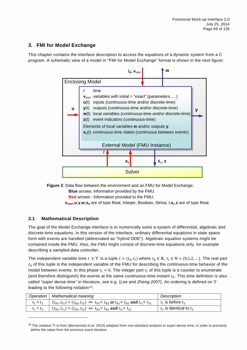
Functional Mock-up Interface 2.0 July 25, 2014
Page 69 of 126
3. FMI for Model Exchange
This chapter contains the interface description to access the equations of a dynamic system from a C program. A schematic view of a model in “FMI for Model Exchange” format is shown in the next figure:
3.1 Mathematical Description
The goal of the Model Exchange interface is to numerically solve a system of differential, algebraic and discrete-time equations. In this version of the interface, ordinary differential equations in state space form with events are handled (abbreviated as “hybrid ODE”). Algebraic equation systems might be contained inside the FMU. Also, the FMU might consist of discrete-time equations only, for example describing a sampled-data controller.
The independent variable time 𝑡 ∈ 𝕋 is a tuple 𝑡 = (𝑡𝑅, 𝑡𝐼) where 𝑡𝑅 ∈ ℝ, 𝑡𝐼 ∈ ℕ = {0,1,2, … }. The real part 𝑡𝑅 of this tuple is the independent variable of the FMU for describing the continuous-time behavior of the model between events. In this phase 𝑡𝐼 = 0. The integer part 𝑡𝐼 of this tuple is a counter to enumerate (and therefore distinguish) the events at the same continuous-time instant 𝑡𝑅. This time definition is also called “super dense time” in literature, see e.g. (Lee and Zheng 2007). An ordering is defined on 𝕋 leading to the following notation10:
Operation Mathematical meaning Description 𝑡1 < 𝑡2 (𝑡𝑅1, 𝑡𝐼1) < (𝑡𝑅2, 𝑡𝐼2) ⇔ 𝑡𝑅1< 𝑡𝑅2 or 𝑡𝑅1= 𝑡𝑅2 𝐚𝐧𝐝 𝑡𝐼1< 𝑡𝐼2 𝑡1 is before 𝑡2 𝑡1 = 𝑡2 (𝑡𝑅1, 𝑡𝐼1) = (𝑡𝑅2, 𝑡𝐼2) ⇔ 𝑡𝑅1= 𝑡𝑅2 𝐚𝐧𝐝 𝑡𝐼1= 𝑡𝐼2 𝑡1 is identical to 𝑡2
10 The notation 𝑡 ● is from (Benveniste et.al. 2010) adapted from non-standard analysis to super-dense time, in order to precisely
define the value from the previous event iteration.
Solver
u y
Enclosing Model
xc
t
w
t time vstart variables with initial = “exact” (parameters, …) u(t) inputs (continuous-time and/or discrete-time) y(t) outputs (continuous-time and/or discrete-time) w(t) local variables (continuous-time and/or discrete-time) z(t) event indicators (continuous-time)
Elements of local variables w and/or outputs y: xc(t) continuous-time states (continuous between events)
External Model (FMU Instance)
t0, vstart
�̇�𝑐 , 𝐳
Figure 2: Data flow between the environment and an FMU for Model Exchange: Blue arrows: Information provided by the FMU. Red arrows : Information provided to the FMU. vstart,u,y,w,xd are of type Real, Integer, Boolean, String; t,xc,z are of type Real.
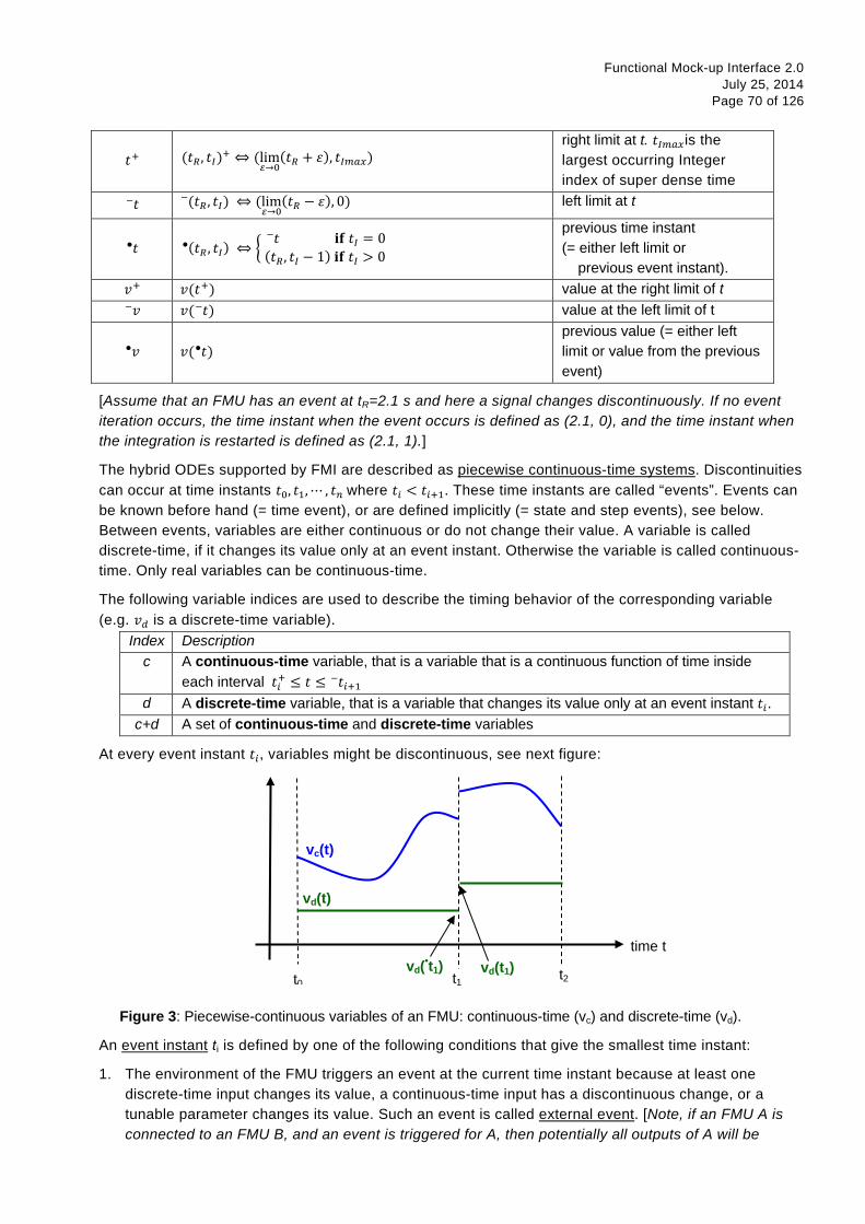
Functional Mock-up Interface 2.0 July 25, 2014
Page 70 of 126
𝑡+ (𝑡𝑅, 𝑡𝐼)+ ⇔ (lim𝜀→0
(𝑡𝑅 + 𝜀), 𝑡𝐼𝑚𝑎𝑥) right limit at t. 𝑡𝐼𝑚𝑎𝑥is the largest occurring Integer index of super dense time
𝑡 − (𝑡𝑅, 𝑡𝐼) − ⇔ (lim
𝜀→0(𝑡𝑅 − 𝜀), 0) left limit at t
𝑡 ● (𝑡𝑅 , 𝑡𝐼) ● ⇔ �
𝑡 − 𝐢𝐟 𝑡𝐼 = 0 (𝑡𝑅, 𝑡𝐼 − 1) 𝐢𝐟 𝑡𝐼 > 0
previous time instant (= either left limit or previous event instant).
𝑣+ 𝑣(𝑡+) value at the right limit of t 𝑣 − 𝑣( 𝑡 − ) value at the left limit of t
𝑣 ● 𝑣( 𝑡 ● ) previous value (= either left limit or value from the previous event)
[Assume that an FMU has an event at tR=2.1 s and here a signal changes discontinuously. If no event iteration occurs, the time instant when the event occurs is defined as (2.1, 0), and the time instant when the integration is restarted is defined as (2.1, 1).]
The hybrid ODEs supported by FMI are described as piecewise continuous-time systems. Discontinuities can occur at time instants 𝑡0, 𝑡1,⋯ , 𝑡𝑛 where 𝑡𝑖 < 𝑡𝑖+1. These time instants are called “events”. Events can be known before hand (= time event), or are defined implicitly (= state and step events), see below. Between events, variables are either continuous or do not change their value. A variable is called discrete-time, if it changes its value only at an event instant. Otherwise the variable is called continuous-time. Only real variables can be continuous-time.
The following variable indices are used to describe the timing behavior of the corresponding variable (e.g. 𝑣𝑑 is a discrete-time variable).
Index Description c A continuous-time variable, that is a variable that is a continuous function of time inside
each interval 𝑡𝑖+ ≤ 𝑡 ≤ 𝑡 − 𝑖+1 d A discrete-time variable, that is a variable that changes its value only at an event instant 𝑡𝑖.
c+d A set of continuous-time and discrete-time variables
At every event instant 𝑡𝑖, variables might be discontinuous, see next figure:
Figure 3: Piecewise-continuous variables of an FMU: continuous-time (vc) and discrete-time (vd).
An event instant ti is defined by one of the following conditions that give the smallest time instant:
1. The environment of the FMU triggers an event at the current time instant because at least one discrete-time input changes its value, a continuous-time input has a discontinuous change, or a tunable parameter changes its value. Such an event is called external event. [Note, if an FMU A is connected to an FMU B, and an event is triggered for A, then potentially all outputs of A will be
time t
t0 t1 t2
vc(t)
vd(t)
vd(•t1) vd(t1)

Functional Mock-up Interface 2.0 July 25, 2014
Page 71 of 126
discontinuous at this time instant. It is therefore adviceable to trigger an external event for B at this time instant too, if an output of A is connected to B. This means to call fmi2EnterEventMode on B.] All the following events are internal events.
2. At a predefined time instant ti = (Tnext(ti-1), 0) that was defined at the previous event instant ti-1 by the FMU. Such an event is called time event.
3. At a time instant, where an event indicator zj(t) changes its domain from zj > 0 to zj ≤ 0 or from zj ≤ 0 to zj > 0 (see Figure 4 below). More precisely: An event t = ti occurs at the smallest time instant “min t” with t > ti-1 where “(zj(t) > 0) ≠ (zj(ti-1) > 0)”. Such an event is called state event11. All event indicators are piecewise continuous and are collected together in one vector of real numbers z(t).
Figure 4: An event occurs when the event indicator changes its domain from z > 0 to z ≤ 0 or vice versa.
4. At every completed step of an integrator, fmi2CompletedIntegratorStep must be called (provided the capability flag ModelDescription.completedIntegratorStepNotNeeded = false). An event occurs at this time instant, if indicated by the return argument nextMode = EventMode. Such an event is called step event. [Step events are, for example, used to dynamically change the (continuous) states of a model internally in the FMU, because the previous states are no longer suited numerically.]
An FMI Model-Exchange model is described by the following variables:
Variable Description t Independent variable time ∈ 𝕋. (Variable defined with causality = "independent"). v A vector of all exposed variables (all variables defined in element <ModelVariables>,
see section 2.2.7). Via a subscript, a subset of the variables is selected. Example: vinitial=exact are variables defined with attribute initial = "exact", see section 2.2.7. These are independent parameters and start values of other variables, such as initial values for states, state derivatives or outputs.
p Parameters that are constant during simulation. The symbol without a sub-script references independent parameters (variables with causality = "parameter"). Dependent parameters (variables with causality = "calculatedParameter") are denoted as 𝐩𝑐𝑎𝑙𝑐𝑢𝑙𝑎𝑡𝑒𝑑.
u(t) Input variables. The values of these variables are defined outside of the model. Variables of this type are defined with attribute causality = "input". Via attribute variability = "discrete" or "continuous" it is defined whether the input is a discrete-time or continuous-time variable, see section 2.2.7.
y(t) Output variables. The values of these variables are computed in the FMU and they are designed to be used in a model connection. So output variables might be used in the environment as input values to other FMUs or other submodels. Variables of this type are
11 This definition is slightly different from the standard definition of state events: “zj(t)·zj(ti-1) ≤ 0”. This often used definition has the
severe drawback that zj(ti-1) ≠ 0 is required in order to be well-defined and this condition cannot be guaranteed.
time
t0 t1 t2
z(t) z > 0
z ≤ 0
Functional Mock-up Interface 2.0 July 25, 2014
Page 72 of 126
defined with attribute causality = "output". Via attribute variability = "discrete" or "continuous" it is defined whether the output is a discrete-time or continuous-time variable, see section 2.2.7.
w(t) Local variables of the FMU that cannot be used for FMU connections. Variables of this type are defined with attribute causality = "local", see section 2.2.7.
z(t) A vector of real continuous-time variables utilized to define state events, see below. 𝐱𝑐(t) A vector of real continuous-time variables representing the continuous-time states.
For notational convenience, a continuous-time state is conceptually treated as a different type of variable as an output or a local variable for the mathematical description below. In reality, a continuous-time state is however part of the outputs y or the local variables w of an FMU.
𝐱𝑑(𝑡) 𝐱 ● 𝑑(𝑡)
𝐱𝑑(𝑡) is a vector of (internal) discrete-time variables (of any type) representing the discrete states. 𝐱 ● 𝑑(𝑡) is the value of 𝐱𝑑(𝑡) at the previous super dense time instant, so 𝐱 ● 𝑑(𝑡) = 𝐱𝑑( 𝑡 ● ).
Given the previous values of the discrete-time states, 𝐱 ● 𝑑(𝑡), at the actual time instant t, all other discrete-time variables, especially the discrete states 𝐱𝑑(𝑡), can be computed. Discrete states are not visible in the interface of an FMU and are only introduced here to clarify the mathematical description. Formally, a discrete state is part of the outputs y or the local variables w of an FMU.
𝑇𝑛𝑒𝑥𝑡(𝑡𝑖) At initialization or at an event instant, an FMU can define the next time instant 𝑇𝑛𝑒𝑥𝑡, at which the next event occurs (see also the definition of events above). Note, every event removes automatically a previous definition of 𝑇𝑛𝑒𝑥𝑡, and it must be explicitely defined again, if a previously defined 𝑇𝑛𝑒𝑥𝑡 was not triggered at the current event instant.
𝐫(𝑡𝑖) A vector of Boolean variables with 𝑟𝑖 ≔ 𝑧𝑖 > 0. When entering Continuous-Time Mode all relations reported via the event indicators 𝐳 are fixed and during this Mode these relations are replaced by 𝐫. Only during Initialization or Event Mode the domains 𝑧𝑖 > 0 can be changed. For notational convenience, 𝐫 ≔ 𝐳 > 0 is an abbreviation for 𝐫 ≔ {𝑧1 > 0, 𝑧2 > 0, … }. [For more details, see “Remark 3” below.]
Computing the solution of an FMI model means to split the solution process in different phases and in every phase different equations and solution methods are utilized. The phases can be categorized according to the following modes:
1. Initialization Mode: This mode is used to compute at the start time 𝑡0 initial values for continuous-time states, 𝐱𝑐(𝑡0), and for the previous (internal) discrete-time states, 𝐱 ● 𝑑(𝑡0) , by utilizing extra equations not present in the other modes (for example equations to define the start value for a state or for the derivative of a state).
2. Continuous-Time Mode: This mode is used to compute the values of all (real) continuous-time variables between events by numerically solving ordinary differential and algebraic equations. All discrete-time variables are fixed during this phase and the corresponding discrete-time equations are not evaluated.
3. Event Mode: This mode is used to compute new values for all continuous-time variables, as well as for all discrete-time variables that are activated at the current event instant 𝑡, given the values of the variables from the previous instant 𝑡 • . This is performed by solving algebraic equations consisting of all continuous-time and all active discrete-time equations. In FMI 2.0 there is no mechanism that the FMU can provide the information whether a discrete-time variable is active or is not active (is not computed) at an event instant. Therefore, the environment has to assume that at an event instant always all discrete-time variables are computed, although internally in the FMU only a subset might be newly computed.
Functional Mock-up Interface 2.0 July 25, 2014
Page 73 of 126
When connecting FMUs together, loop structures can occur that lead to particular difficulties because linear or non-linear algebraic systems of equations in Real variables but also in Boolean or Integer variables might be present. In order to solve such systems of equations over FMUs efficiently the dependency information is needed stating, for example, which outputs depend directly on inputs. This data is optionally provided in the xml file under element <ModelStructure>. If this data is not provided, the worst case must be assumed (for example, all output variables depend algebraically on all input variables).
[Example: In the next Figure two different types of connected FMUs are shown (the “dotted lines” characterize the dependency information):
In the upper diagram FMU1 and FMU2 are connected in such a way that by an appropriate sequence of fmi2SetXXX and fmi2GetXXX calls the FMU variables can be computed.
In the lower diagram FMU3 and FMU4 are connected in such a way that a “real” algebraic loop is present. This loop might be solved iteratively with a Newton method. In every iteration the iteration variable 𝑢4 is provided by the solver and via the shown sequence of fmi2SetXXX and fmi2GetXXX calls the residue is computed and is provided back to the solver. Based on the residue a new value of 𝑢4 is provided. The iteration is terminated when the residue is close to zero.
These types of artifical or real algebraic loops can occur in all the different modes, Initialization Mode, Event Mode, and Continuous-Time Mode. Since different variables are computed in every Mode and the
FMU1
FMU2
FMU3
FMU4
𝑢2𝑎
𝑢2𝑏
𝑦2𝑎
𝑦2𝑏
𝑢1 𝑦1
artifical algebraic loop
“real” algebraic loop
𝑢4 𝑦4
𝑢3 𝑦3
fmiSetXXX(m2,< u2a>, …) y2a ≔ fmiGetXXX(m2, ...) fmiSetXXX(m1, < u1 ≔ y2a >, ...) y1 ≔ fmiGetXXX(m1,..) fmiSetXXX(m2, < u2b ≔ y1 >, ...) y2b ≔ fmiGetXXX(m2, ...)
sequential calling sequence:
iterative calling sequence:
In every Newton iteration evaluate: input: u4 // provided by solver output: residue // provided to solver fmiSetXXX(m4,< u4>, …) y4 ≔ fmiGetXXX(m4, ...) fmiSetXXX(m3, < u3 ≔ y4 >, ...) y3 ≔ fmiGetXXX(m3,..) residue ≔ u4 − y3
Figure 5: Calling sequences for FMUs that are connected in a loop.
Functional Mock-up Interface 2.0 July 25, 2014
Page 74 of 126
causality of variable computation can be different in Initialization Mode as with respect to the other two Modes, it might be necessary to solve different kinds of loops in the different Modes. ]
In Table 1 the equations are defined that can be evaluated in the respective Mode. The following color coding is used in the table:
grey If a variable in an argument list is marked in grey, then this variable is not changing in this mode and just the last calculated value from the previous mode is internally used. For an input argument it is not allowed to call fmi2SetXXX. For an output argument, calling fmi2GetXXX on such a variable returns always the same value in this mode.
green Functions marked in green are special functions to enter or leave a mode. blue Equations and functions marked in blue define the actual computations to be
performed in the respective mode.
Function fmi2SetXXX is an abbreviation for functions fmi2SetReal, fmi2SetBoolean, fmi2SetInteger and fmi2SetString respectively. Function fmi2GetXXX is an abbreviation for functions fmi2GetReal, fmi2GetBoolean, fmi2GetInteger and fmi2GetString respectively.
[In the following table the setting of the super dense time,(𝑡𝑅, 𝑡𝐼), is precisely described. Tools will usually not have such a representation of time. However, super-dense time defines precisely when a new "model evaluation" starts and therefore which variable values belong to the same "model evaluation" at the same (super dense) time instant and should be stored together. ]
Equations FMI functions
Equations before Initialization Mode Set independent variable time 𝑡𝑅0 and define 𝑡0: = (𝑡𝑅0, 0) fmi2SetupExperiment
Set variables 𝐯𝑖𝑛𝑖𝑡𝑖𝑎𝑙=𝑒𝑥𝑎𝑐𝑡 and 𝐯𝑖𝑛𝑖𝑡𝑖𝑎𝑙=𝑎𝑝𝑝𝑟𝑜𝑥 that have a start value (initial = "exact" or "approx")
fmi2SetXXX
Equations during Initialization Mode Enter Initialization Mode at 𝑡 = 𝑡0 (activate initialization, discrete-time and continuous-time equations)
fmi2EnterInitializationMode
Set variables 𝐯𝑖𝑛𝑖𝑡𝑖𝑎𝑙=𝑒𝑥𝑎𝑐𝑡 that have a start value with initial="exact" (independent parameters 𝐩 and continuous-time states with start values 𝐱𝑐,𝑖𝑛𝑖𝑡𝑖𝑎𝑙=𝑒𝑥𝑎𝑐𝑡 are included here)
fmi2SetXXX
Set continuous-time and discrete-time inputs 𝐮(𝑡0) fmi2SetXXX
𝐯𝐼𝑛𝑖𝑡𝑖𝑎𝑙𝑈𝑛𝑘𝑛𝑜𝑤𝑛𝑠 ≔ 𝐟𝑖𝑛𝑖𝑡(𝒖𝑐 ,𝒖𝑑, 𝑡0,𝐯𝑖𝑛𝑖𝑡𝑖𝑎𝑙=𝑒𝑥𝑎𝑐𝑡) fmi2GetXXX, fmi2GetContinuousStates
Exit Initialization Mode (de-activate initialization equations) fmi2ExitInitializationMode
Equations during Event Mode Enter Event Mode at 𝑡 = 𝑡𝑖 with 𝑡𝑖 ∶= (𝑡𝑅, 𝑡𝐼 + 1) if 𝑒𝑥𝑡𝑒𝑟𝑛𝑎𝑙𝐸𝑣𝑒𝑛𝑡 𝐨𝐫 𝑛𝑒𝑥𝑡𝑀𝑜𝑑𝑒 ≡ 𝐸𝑣𝑒𝑛𝑡𝑀𝑜𝑑𝑒 𝐨𝐫
𝑡𝑖 = (𝑇𝑛𝑒𝑥𝑡(𝑡𝑖−1) ,0) 𝐨𝐫 min𝑡>𝑡𝑖−1
𝑡: �𝑧𝑗(𝑡) > 0 ≠ 𝑧𝑗(𝑡𝑖−1) > 0�
(activate discrete-time equations)
fmi2EnterEventMode
(only from Continuous-Time Mode or after calling fmi2SetTime if FMU has no continuous-time equations)
Set independent tunable parameters 𝐩𝑡𝑢𝑛𝑒 fmi2SetXXX

Functional Mock-up Interface 2.0 July 25, 2014
Page 75 of 126
(and do not set other parameters 𝐩𝑜𝑡ℎ𝑒𝑟) Set continuous-time and discrete-time inputs 𝐮(𝑡𝑖) fmi2SetXXX
Set continuous-time states 𝐱𝑐(𝑡𝑖) fmi2SetXXX, fmi2SetContinuousStates
(𝐲𝑐+𝑑 , �̇�𝑐 ,𝒘𝑐+𝑑 , 𝐳, 𝐱𝑐,𝑟𝑒𝑖𝑛𝑖𝑡) ≔ 𝐟𝑠𝑖𝑚(𝐱𝑐 ,𝒖𝑐+𝑑 , 𝑡𝑖 ,𝐩𝑡𝑢𝑛𝑒 ,𝐩𝑜𝑡ℎ𝑒𝑟)
𝐟𝑠𝑖𝑚 is also a function of the internal variables 𝐱 ●𝑑
fmi2GetXXX, fmi2GetContinuousStates, fmi2GetDerivatives fmi2GetEventIndicators
Increment super dense time and define with newDiscreteStatesNeeded whether a new event iteration is required.
𝐢𝐟 𝐧𝐨𝐭 newDiscreteStatesNeeded 𝐭𝐡𝐞𝐧 𝑇𝑛𝑒𝑥𝑡 ≔ 𝑇𝑛𝑒𝑥𝑡(𝐱𝑐 , 𝐱 ●
𝑑 , 𝒖𝑐+𝑑 , 𝑡𝑖 ,𝐩𝑡𝑢𝑛𝑒,𝐩𝑜𝑡ℎ𝑒𝑟)𝐞𝐧𝐝 𝐢𝐟𝑡 ∶= (𝑡𝑅, 𝑡𝐼 + 1)𝐱 ●𝑑 ∶= 𝐱𝑑
fmi2NewDiscreteStates
Set independent variable time 𝑡𝑖 ∶= (𝑇𝑛𝑒𝑥𝑡 , 0) fmi2SetTime
(if no continuous-time equations)
Equations during Continuous-Time Mode Enter Continuous-Time Mode:
// de-activate discrete-time equations// "freeze" variables: 𝐫 ≔ 𝐳 > 0 // all relations 𝐲𝑑,𝒘𝑑 // all discrete - time variables
fmi2EnterContinuousTimeMode
Set independent variable time 𝑡 (> 𝑡𝑒𝑛𝑡𝑒𝑟 𝑚𝑜𝑑𝑒): 𝑡 ∶= (𝑡𝑅, 0) fmi2SetTime
Set continuous-time inputs 𝐮𝑐(𝑡) fmi2SetXXX
Set continuous-time states 𝐱𝑐(𝑡) fmi2SetXXX, fmi2SetContinuousStates
(𝐲𝑐 ,𝐲𝑑 , �̇�𝑐 ,𝒘𝑐 ,𝒘𝑑, 𝐳, 𝐱𝑐,𝑟𝑒𝑖𝑛𝑖𝑡) ≔ 𝐟𝑠𝑖𝑚(𝐱𝑐 ,𝒖𝑐 ,𝒖𝑑 , 𝑡,𝐩𝑡𝑢𝑛𝑒,𝐩𝑜𝑡ℎ𝑒𝑟)
𝐟𝑠𝑖𝑚 is also a function of the internal variables 𝐱 ●𝑑 , 𝐫.
fmi2GetXXX, fmi2GetDerivatives, fmi2GetEventIndicators
Complete integrator step and return enterEventMode fmi2CompletedIntegratorStep
Data types 𝑡 ∈ ℝ,𝐩 ∈ ℙ𝑛𝑝,𝐮(𝑡) ∈ ℙ𝑛𝑢, 𝐲(𝑡) ∈ ℙ𝑛𝑦, 𝐱𝑐(𝑡) ∈ ℝ𝑛𝑥𝑐 , 𝐱𝑑(𝑡) ∈ ℙ𝑛𝑥𝑑 ,𝐰(𝑡) ∈ ℙ𝑛𝑤, 𝐳(𝑡) ∈ ℝ𝑛𝑧
ℝ: real variable,ℙ: real or Boolean or integer or enumeration or string variable 𝐟𝑖𝑛𝑖𝑡 , 𝐟𝑠𝑖𝑚 ∈ 𝐶0 (= continuous functions with respect to all input arguments inside the respective mode).
Table 1: Mathematical description of an FMU for Model Exchange.
[Remark 1 – Calling Sequences: In the table above, for notational convenience in every Mode one function call is defined to compute all output arguments from all inputs arguments. In reality, every scalar output argument is computed by one fmi2GetXXX function call. Additionally, the output argument need not be a function of all input arguments, but of only a subset from it, as defined in the xml file under <ModelStructure>. This is essential when FMUs are connected in a loop, as shown in Figure 6: For example, since 𝑦2a depends only on 𝑢1a, but not on 𝑢1b, it is possible to call fmi2SetXXX to set 𝑢1a, and then inquire 𝑦2a with fmi2GetXXX without setting 𝑢1b beforehand.
Functional Mock-up Interface 2.0 July 25, 2014
Page 76 of 126
It is non-trivial to provide code for fmi2SetXXX, fmi2GetXXX, if the environment can call fmi2SetXXX on the inputs in quite different orders. A simple remedy is to provide the dependency information not according to the “real” functional dependency, but according to the sorted equations in the generated code. Example
Assume an FMU is described by the following equations (u1,u2 are inputs, y1,y2 are outputs, w1,w2 are internal variables):
w1 = w2 + u1 w2 = u2 y1 = w1 y2 = w2
Sorting of the equations might result in (this ordering is not unique):
w2 := u2 y2 := w2 w1 := w2 + u1 y1 := w1
With this ordering, the dependency should be defined as y2 = f(u2), y1 = f(u1,u2). When y2 is called first with fmi2GetXXX, then only u2 must be set first (since y2 = f(u2)), and the first two equations are evaluated. If later y1 is inquired as well, then the first two equations are not evaluated again and only the last two equations are evaluated. On the other hand, if y1 is inquired first, then u1 and u2 must be set first (since y1 = f(u1,u2)) and then all equations are computed. When y2 is inquired afterwards, the cached value is returned.
If sorting of the equations in this example would instead result in the following code:
w2 := u2 w1 := w2 + u1 y1 := w1 y2 := w2
then the dependency should be defined as y2 = f(u1,u2), y1 = f(u1,u2), because u1 and u2 must be first set, before y2 can be inquired with fmi2GetXXX when executing this code.
Remark 2 – Mathematical Model of Discrete-Time FMUs: There are many different ways discrete-time systems are described. For FMI the following basic mathematical model for discrete-time systems is used (other description forms must be mapped, as sketched below):
while 𝑇𝑛𝑒𝑥𝑡 ≤ 𝑡𝑒𝑛𝑑 loop 𝑡𝑅 ≔ 𝑇𝑛𝑒𝑥𝑡 𝑡𝐼 ≔ 0 𝑡 ≔ ( 𝑡𝑅, 𝑡𝐼) 𝐥𝐨𝐨𝐩 // super dense time iteration (e.g. since state machine in FMU) repeat // algebraic loop iteration (due to connected FMUs) // either sequence or solve algebraic loops over FMUs iteratively 𝐱𝑑 ≔ 𝐟( 𝐱 • 𝑑 ,𝐮𝑑) 𝐲𝑑 ≔ 𝐠( 𝐱 • 𝑑,𝐮𝑑) until <algebraic loops solved> // function fmi2NewDiscreteStates: 𝑇𝑛𝑒𝑥𝑡 ≔ 𝑇( 𝐱 • 𝑑,𝐮𝑑) if 𝐱𝑑 ≡ 𝐱 • 𝑑 then exit 𝐱 • 𝑑 ≔ 𝐱𝑑 𝑡 ∶= (𝑡𝑅 , 𝑡𝐼 + 1) end loopend while
Functional Mock-up Interface 2.0 July 25, 2014
Page 77 of 126
At an event instant, the discrete system is described by algebraic equations as function of the previous (internal) discrete-time states 𝐱 • 𝑑 and the discrete-time inputs 𝐮𝑑. If FMUs are connected in a loop, these algebraic equations are called iteratively, until the solution is found. If the actual discrete-time states 𝐱𝑑 and the previous discrete-time states 𝐱 • 𝑑 are not identical, the discrete-time states are updated, the Integer part of the time is incremented and a new event iteration is performed. Other discrete-time models must be mapped to this description form. Examples:
• Synchronous systems: A synchronous system, such as Lucid Synchrone (Pouzet 2006) or Modelica 3.3 (Modelica 2012), is called periodically and at every sample instant the discrete-time equations are evaluated exactly once. An FMU of this type can be implemented by activating the model equations only at the first event iteration and returning always 𝑛𝑒𝑤𝑁𝑒𝑤𝐷𝑖𝑠𝑐𝑟𝑒𝑡𝑒𝑆𝑡𝑎𝑡𝑒𝑠𝑁𝑒𝑒𝑑𝑒𝑑 ≔ 𝑓𝑎𝑙𝑠𝑒 from fmi2NewDiscreteStates. Furthermore, the discrete-time states are not updated by fmi2NewDiscreteStates, but as first action before the discrete-time equations are evaluated, in order that 𝐱 • 𝑑 (= value at the previous clock tick) and 𝐱𝑑 (value at the latest clock tick) have reasonable values between clock ticks.
• State machines with one memory location for a state: In such a system there is only one memory location for a discrete-time state and not two, and therefore a discrete-time state is updated in the statement where it is assigned (and not in fmi2NewDiscreteStates). As a result, fmi2NewDiscreteStates is basically just used to start a new (super dense) time instant. This is unproblematic, as long as no algebraic loops occur. FMUs of this type can therefore not be used in “real” algebraic loops if the involved variables depend on a discrete-time state. This restriction is communicated to the environment of the FMU by the ScalarVariable definition of the corresponding input with flag canHandleMultipleSetPerTimeInstant=false (so an input with this flag is not allowed to be called in an algebraic loop).
Remark 3 – Event Indicators / Freezing Relations: In the above table vector r is used to collect all relations together that are utilized in the event indicators z. In Continuous-Time Mode all these relations are “frozen” and do not change during the evaluations in the respective Mode. This is indicated in the table above by computing r when entering the Continuous-Time Mode and providing r as (internal) input argument to the evaluation functions. Example:
An equation of the form
y = if x1 > x2 or x1 < x3 then +1 else -1;
can be implemented in the FMU as:
z1 := x1 – x2; z2 := x3 – x1; if InitializationMode or EventMode then r1 := z1 > 0; r2 := z2 > 0; end if; y = if r1 or r2 then +1 else -1
Therefore, the original if-clause is evaluated in this form only during Initialization and Event Mode. In Continuous-Time Mode this equation is evaluated as:
z1 = x1 – x2; z2 = x3 – x1 y = if r1 or r2 then +1 else -1;
and when entering Continuous-Time Mode r1 and r2 are computed as

Functional Mock-up Interface 2.0 July 25, 2014
Page 78 of 126
r1 = z1 > 0 r2 = z2 > 0
When z1 changes from z1 > 0 to z1 <= 0 or vice versa, or z2 correspondingly, the integration is halted and the environment must call fmi2EnterEventMode.
An actual implementation will pack the code in an impure function, say Greater(...), resulting in:
y = if Greater(x1-x2,...) or Greater(x3-x1,...) then +1 else -1;
Furthermore, a hysteresis should be added for the event indicators. For more details see the companion document FunctionalMockupInterface-ImplementationHints.docx.
Remark 4 – Pure Discrete-Time FMUs: If an FMU has only discrete-time equations (and no variables with variability = “continuous”), then the environment need not to call fmi2EnterContinuousTimeMode but can directly call fmi2SetTime to set the value of the next event instant, before fmi2EnterEventMode is called.
]
An FMU is initialized in Initialization Mode with 𝐟𝑖𝑛𝑖𝑡(… ). The input arguments to this function consist of the input variables (= variables with causality = ″input″), of the independent variable (= variable with causality = ″independent″; usually the default value ″time″) and of all variables that have a start value with (explicitely or implicitely) initial = ″exact″ in order to compute the continuous-time states and the output variables at the initial time t0. In the above table, the variables with initial = exact are collected together in variable 𝐯𝑖𝑛𝑖𝑡𝑖𝑎𝑙=𝑒𝑥𝑎𝑐𝑡. For example initialization might be defined by providing initial start values for the states, 𝐱𝑐0, or by stating that the state derivatives are zero (�̇�𝑐 = 𝟎). Initialization is a difficult topic by itself and it is required that an FMU solves a well-defined initialization problem inside the FMU in Initialization Mode.
After calling fmi2ExitInitializationMode the FMU is implicitely in Event Mode and all discrete-time and continuous-time variables at the initial time instant (𝑡𝑅, 0) can be calculated, if needed also iteratively due to an algebraic loop. Once finalized, fmi2NewDiscreteStates must be called, and depending on the value of the return argument, the FMU either continues the event iteration at the initial time instant or switches to Continuous-Time Mode.
After switching to Continuous-Time Mode, the integration is started. Basically, in this phase the derivatives of the continuous states are computed. If FMUs and/or submodels are connected together, then the inputs of these models are the outputs of other models and therefore the corresponding FMU outputs must be computed. Whenever result values shall be stored, usually at output points defined before the start of the simulation, the fmi2GetXXX function with respect to the desired variables must be called.
Continuous integration is stopped at an event instant. An event instant is determined by a time, state, or step event, or by an external event triggered by the environment. In order to determine a state event, the event indicators z have to be inquired at every completed integrator step. Once the event indicators signal a change of their domain, an iteration over time is performed between the previous and the actual completed integrator step, in order to determine the time instant of the domain change up to a certain precision.
After an event is triggered, the FMU needs to be switched to Event Mode. In this mode systems of equations over connected FMUs might be solved (similarily as in Continuous-Time Mode). Once convergence is reached, fmi2NewDiscreteStates(..) must be called to increment super dense time (and conceptually update the discrete-time states defined internally in the FMU by 𝐱 • 𝑑 ≔ 𝐱𝑑). Depending on the discrete-time model, a new event iteration might be needed (e.g. because the FMU describes internally a state machine, and transitions are still able to fire, but new inputs shall be taken into account).
The function calls in the table above describe precisely, which input arguments are needed to compute the desired output argument(s). There is no 1:1 mapping of these mathematical functions to C functions. Instead, all input arguments are set with fmi2SetXXX(..) C-function calls and then the result argument(s) can be determined with the C functions defined in the right column of the above table. This technique is discussed in

Functional Mock-up Interface 2.0 July 25, 2014
Page 79 of 126
detail in section 3.2.1. [In short: For efficiency reasons, all equations from the table above will usually be available in one (internal) C-function. With the C functions described in the next sections, input arguments are copied into the internal model data structure only when their value has changed in the environment. With the C functions in the right column of the table above, the internal function is called in such a way, that only the minimum needed equations are evaluated. Hereby, variable values calculated from previous calls can be reused. This technique is called “caching” and can significantly enhance the simulation efficiency of real-world models.]
3.2 FMI Application Programming Interface
This section contains the interface description to evaluate different model parts from a C program.
3.2.1 Providing Independent Variables and Re-initialization of Caching
Depending on the situation, different variables need to be computed. In order to be efficient, it is important that the interface requires only the computation of variables that are needed in the present context. For example during the iteration of an integrator step, only the state derivatives need to be computed, provided the output of a model is not connected. It might be that at the same time instant other variables are needed. For example if an integrator step is completed, the event indicator functions need to be computed as well. For efficiency it is then important that in the call to compute the event indicator functions, the state derivatives are not newly computed, if they have been computed already at the present time instant. This means, the state derivatives shall be reused from the previous call. This feature is called “caching of variables” in the sequel.
Caching requires that the model evaluation can detect when the input arguments, like time or states, have changed. This is achieved by setting them explicitly with a function call, since every such function call signals precisely a change of the corresponding variables. For this reason, this section contains functions to set the input arguments of the equation evaluation functions. This is unproblematic for time and states, but is more involved for parameters and inputs, since the latter may have different data types.
fmi2Status fmi2SetTime(fmi2Component c, fmi2Real time); Set a new time instant and re-initialize caching of variables that depend on time, provided the
newly provided time value is different to the previously set time value (variables that depend solely on constants or parameters need not to be newly computed in the sequel, but the previously computed values can be reused).
fmi2Status fmi2SetContinuousStates(fmi2Component c, const fmi2Real x[],
size_t nx); Set a new (continuous) state vector and re-initialize caching of variables that depend on the
states. Argument nx is the length of vector x and is provided for checking purposes (variables that depend solely on constants, parameters, time, and inputs do not need to be newly computed in the sequel, but the previously computed values can be reused). Note, the continuous states might also be changed in Event Mode. Note: fmi2Status = fmi2Discard is possible.
fmi2Status fmi2SetXXX(..);
Set new values for (independent) parameters, start values and inputs and re-initialize caching of variables that depend on these variables. The details of these functions are defined in section 2.1.7.
[The functions above have the slight drawback that values must always be copied, for example a call to “fmi2SetContinuousStates” will provide the actual states in a vector and this function has to copy the values in to the internal model data structure “c” so that subsequent evaluation calls can utilize these

Functional Mock-up Interface 2.0 July 25, 2014
Page 80 of 126
values. If this turns out to be an efficiency issue, a future release of FMI might provide additional functions to provide the address of a memory area where the variable values are present.]
3.2.2 Evaluation of Model Equations
This section contains the core functions to evaluate the model equations. Before one of these functions can be called, the appropriate functions from the previous section have to be used, to set the input arguments to the current model evaluation.
fmi2Status fmi2EnterEventMode(fmi2Component c);
The model enters Event Mode from the Continuous-Time Mode and discrete-time equations may become active (and relations are not “frozen”).
fmi2Status fmi2NewDiscreteStates(fmi2Component c, fmi2EventInfo* fmi2eventInfo); typedef struct{ fmi2Boolean newDiscreteStatesNeeded; fmi2Boolean terminateSimulation; fmi2Boolean nominalsOfContinuousStatesChanged; fmi2Boolean valuesOfContinuousStatesChanged; fmi2Boolean nextEventTimeDefined; fmi2Real nextEventTime; // next event if nextEventTimeDefined=fmi2True } fmi2EventInfo; The FMU is in Event Mode and the super dense time is incremented by this call.
If the super dense time before a call to fmi2NewDiscreteStates was (tR, tI) then the time instant after the call is (tR, tI + 1).
If return argument fmi2eventInfo->newDiscreteStatesNeeded = fmi2True, the FMU should stay in Event Mode and the FMU requires to set new inputs to the FMU (fmi2SetXXX on inputs), to compute and get the outputs (fmi2GetXXX on outputs) and to call fmi2NewDiscreteStates again. Depending on the connection with other FMUs, the environment shall • call fmi2Terminate, if terminateSimulation = fmi2True is returned by at least one
FMU, • call fmi2EnterContinuousTimeMode if all FMUs return newDiscreteStatesNeeded =
fmi2False. • stay in Event Mode otherwise. When the FMU is terminated, it is assumed that an appropriate message is printed by the logger function (see section 2.1.5) to explain the reason for the termination.
If nominalsOfContinuousStatesChanged = fmi2True then the nominal values of the states have changed due to the function call and can be inquired with fmi2GetNominalsOfContinuousStates.
If valuesOfContinuousStatesChanged = fmi2True then at least one element of the continuous state vector has changed its value due to the function call. The new values of the states can be inquired with fmi2GetContinuousStates. If no element of the continuous state vector has changed its value, valuesOfContinuousStatesChanged must return fmi2False. [if fmi2True would be returned in this case, an infinite event loop may occur.]
If nextEventTimeDefined = fmi2True, then the simulation shall integrate at most until time = nextEventTime, and shall call fmi2EnterEventMode at this time instant. If integration is stopped before nextEventTime, for example due to a state event, the definition of nextEventTime becomes obsolete.
fmi2Status fmi2EnterContinuousTimeMode(fmi2Component c);

Functional Mock-up Interface 2.0 July 25, 2014
Page 81 of 126
The model enters Continuous-Time Mode and all discrete-time equations become inactive and all relations are “frozen”.
This function has to be called when changing from Event Mode (after the global event iteration in Event Mode over all involved FMUs and other models has converged) into Continuous-Time Mode.
[This function might be used for the following purposes: • If the FMU stores results internally on file, then the results after the initialization and/or the
event has been processed can be stored. • If the FMU contains dynamically changing states, then a new state selection might be
performed with this function. ]
fmi2Status fmi2CompletedIntegratorStep(fmi2Component c, fmi2Boolean noSetFMUStatePriorToCurrentPoint, fmi2Boolean* enterEventMode, fmi2Boolean* terminateSimulation); This function must be called by the environment after every completed step of the integrator
provided the capability flag completedIntegratorStepNotNeeded = false. Argument noSetFMUStatePriorToCurrentPoint is fmi2True if fmi2SetFMUState will no longer be called for time instants prior to current time in this simulation run [the FMU can use this flag to flush a result buffer].
The function returns enterEventMode to signal to the environment if the FMU shall call fmi2EnterEventMode, and it returns terminateSimulation to signal if the simulation shall be terminated. If enterEventMode = fmi2False and terminateSimulation = fmi2False the FMU stays in Continuous-Time Mode without calling fmi2EnterContinuousTimeMode again.
When the integrator step is completed and the states are modified by the integrator afterwards (for example correction by a BDF method), then fmi2SetContinuousStates(..) has to be called with the updated states before fmi2CompletedIntegratorStep(..) is called.
When the integrator step is completed and one or more event indicators change sign (with respect to the previously completed integrator step), then the integrator or the environment has to determine the time instant of the sign change that is closest to the previous completed step up to a certain precision (usually a small multiple of the machine epsilon). This is usually performed by an iteration where time is varied and state variables needed during the iteration are determined by interpolation. Function fmi2CompletedIntegratorStep must be called after this state event location procedure and not after the successful computation of the time step by the integration algorithm. The intended purpose of the function call is to indicate to the FMU that at this stage all inputs and state variables have valid (accepted) values.
After fmi2CompletedIntegratorStep is called, it is still allowed to go back in time (calling fmi2SetTime) and inquire values of variables at previous time instants with fmi2GetXXX [for example to determine values of non-state variables at output points]: However, it is not allowed to go back in time over the previous completedIntegratorStep or the previous fmi2EnterEventMode call.
[This function might be used, for example for the following purposes: 1. Delays:
All variables that are used in a “delay(..)” operator are stored in an appropriate buffer and the function returns with nextMode = fmi2ContinuousTimeMode.
2. Dynamic state selection: It is checked whether the dynamically selected states are still numerically appropriate. If yes, the function returns with enterEventMode = fmi2False otherwise with enterEventMode
Functional Mock-up Interface 2.0 July 25, 2014
Page 82 of 126
= fmi2True. In the latter case, fmi2EnterEventMode(..) has to be called and the states are dynamically changed by a subsequent fmi2NewDiscreteStates(..).
Note, this function is not used to detect time or state events, e.g., by comparing event indicators of the previous with the current call of fmi2CompletedIntegratorStep(..). These types of events are detected in the environment and the environment has to call fmi2EnterEventMode(..) in these cases, independently whether the return argument enterEventMode of fmi2CompletedIntegratorStep(..) is fmi2True or fmi2False. ]
fmi2Status fmi2GetDerivatives (fmi2Component c, fmi2Real derivatives[],
size_t nx); fmi2Status fmi2GetEventIndicators(fmi2Component c, fmi2Real eventIndicators[],
size_t ni); Compute state derivatives and event indicators at the current time instant and for the current
states. The derivatives are returned as a vector with “nx” elements. A state event is triggered when the domain of an event indicator changes from zj > 0 to zj ≤ 0 or vice versa. The FMU must guarantee that at an event restart zj ≠ 0, for example by shifting zj with a small value. Furthermore, zj should be scaled in the FMU with its nominal value (so all elements of the returned vector “eventIndicators” should be in the order of “one”). The event indicators are returned as a vector with “ni” elements.
The ordering of the elements of the derivatives vector is identical to the ordering of the state vector (for example derivatives[2] is the derivative of x[2]). Event indicators are not necessarily related to variables on the Model Description File.
Note: fmi2Status = fmi2Discard is possible for both functions.
fmi2Status fmi2GetContinuousStates(fmi2Component c, fmi2Real x[], size_t nx); Return the new (continuous) state vector x. This function has to be called directly after calling
function fmi2EnterContinuousTimeMode if it returns with eventInfo->valuesOfContinuousStatesChanged = fmi2True (indicating that the (continuous-time) state vector has changed).
fmi2Status fmi2GetNominalsOfContinuousStates(fmi2Component c,
fmi2Real x_nominal[], size_t nx); Return the nominal values of the continuous states. This function should always be called after
calling function fmi2NewDiscreteStates if it returns with eventInfo-> nominalsOfContinuousStatesChanged = fmi2True since then the nominal values of the continuous states have changed [e.g. because the association of the continuous states to variables has changed due to internal dynamic state selection]. If the FMU does not have information about the nominal value of a continuous state i, a nominal value x_nominal[i] = 1.0 should be returned. Note, it is required that x_nominal[i] > 0.0 [Typically, the nominal values of the continuous states are used to compute the absolute tolerance required by the integrator. Example:
absoluteTolerance[i] = 0.01*tolerance*x_nominal[i];]
3.2.3 State Machine of Calling Sequence
Every implementation of the FMI must support calling sequences of the functions according to the following state chart:
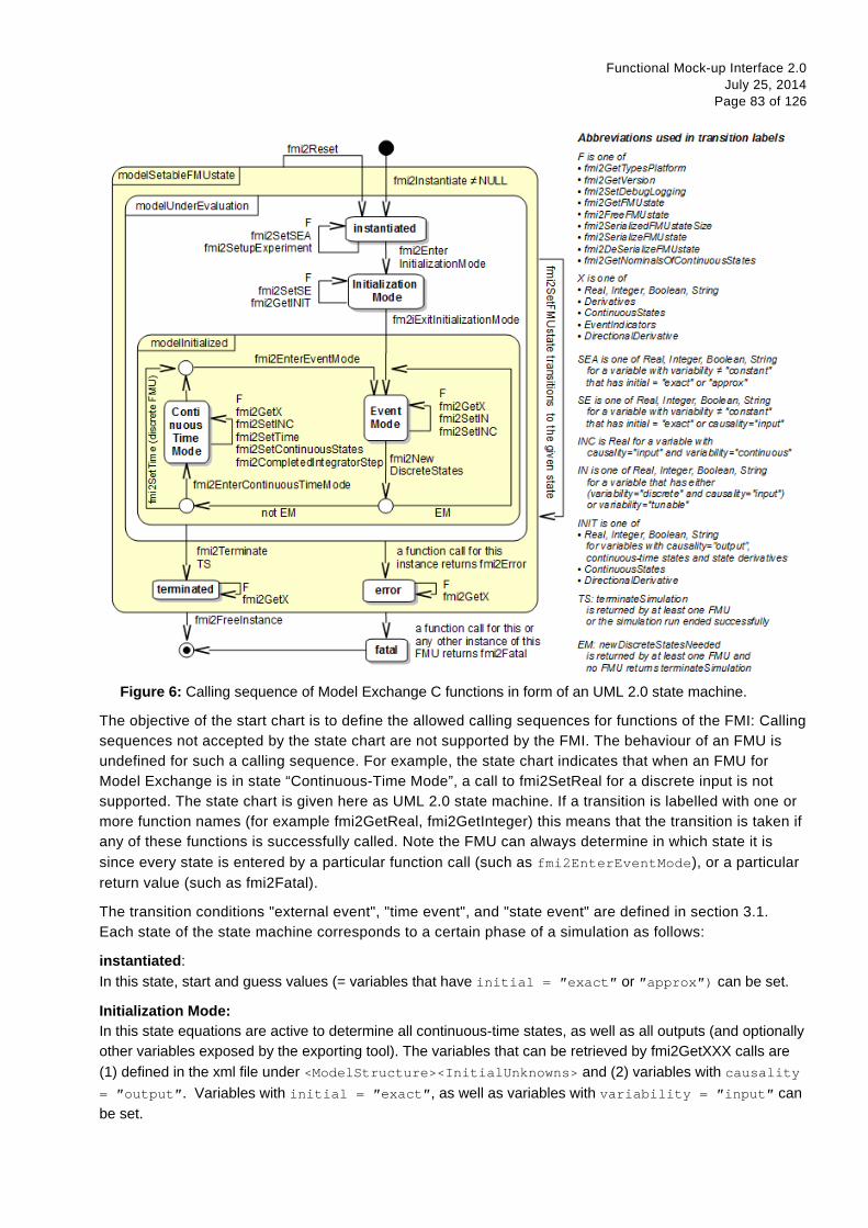
Functional Mock-up Interface 2.0 July 25, 2014
Page 83 of 126
Figure 6: Calling sequence of Model Exchange C functions in form of an UML 2.0 state machine.
The objective of the start chart is to define the allowed calling sequences for functions of the FMI: Calling sequences not accepted by the state chart are not supported by the FMI. The behaviour of an FMU is undefined for such a calling sequence. For example, the state chart indicates that when an FMU for Model Exchange is in state “Continuous-Time Mode”, a call to fmi2SetReal for a discrete input is not supported. The state chart is given here as UML 2.0 state machine. If a transition is labelled with one or more function names (for example fmi2GetReal, fmi2GetInteger) this means that the transition is taken if any of these functions is successfully called. Note the FMU can always determine in which state it is since every state is entered by a particular function call (such as fmi2EnterEventMode), or a particular return value (such as fmi2Fatal).
The transition conditions "external event", "time event", and "state event" are defined in section 3.1. Each state of the state machine corresponds to a certain phase of a simulation as follows:
instantiated: In this state, start and guess values (= variables that have initial = ″exact″ or ″approx″) can be set.
Initialization Mode: In this state equations are active to determine all continuous-time states, as well as all outputs (and optionally other variables exposed by the exporting tool). The variables that can be retrieved by fmi2GetXXX calls are (1) defined in the xml file under <ModelStructure><InitialUnknowns> and (2) variables with causality = ″output″. Variables with initial = ″exact″, as well as variables with variability = ″input″ can be set.

Functional Mock-up Interface 2.0 July 25, 2014
Page 84 of 126
Continuous-Time Mode: In this state the continuous-time model equations are active and integrator steps are performed. The event time of a state event may be determined if a domain change of at least one event indicator is detected at the end of a completed integrator step.
Event Mode: If an event is triggered in Continuous-Time Mode, then Event Mode is entered by calling fmi2EnterEventMode. In this mode all continuous-time and discrete-time equations are active and the unknowns at an event can be computed and retrieved. After an event is completely processed, fmi2NewDiscreteStates must be called and depending on the return argument, newDiscreteStatesNeeded, the state chart stays in Event Mode or switches to Continuous-Time Mode. When the Initialization Mode is terminated with fmi2ExitInitializationMode, then Event Mode is directly entered, and the continuous-time and discrete-time variables at the initial time are computed based on the initial continuous-time states determined in the Initialization Mode.
terminated: In this state, the solution at the final time of a simulation can be retrieved.
Note, that simulation backward in time is only allowed over continuous time intervals. As soon as an event occured (fmi2EnterEventMode was called) going back in time is forbidden, because fmi2EnterEventMode/fmi2NewDiscreteStates can only compute the next discrete state, not the previous one.
Note, during Initialization, Event, and Continuous-Time Mode input variables can be set with fmi2SetXXX and output variables can be get with fmi2GetXXX interchangeably according to the model structure defined under element <ModelStructure> in the xml-file. [For example if one output y1 depends on two inputs u1, u2, then these two inputs must be set, before y1 can be get. If additionally an output y2 depends on an input u3, then u3 can be set and y2 can be get afterwards. As a result, artificial or “real” algebraic loops over connected FMUs in any of these three modes can be handled by using appropriate numerical algorithms.]
The allowed function calls in the respective states are summarized in the following table (functions marked in “yellow” are only available for “Model Exchange”, the other functions are available both for “Model Exchange” and “Co-Simulation”):
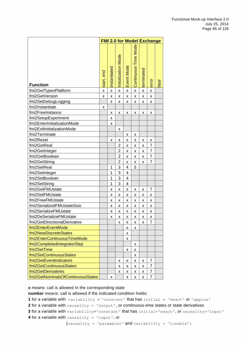
Functional Mock-up Interface 2.0 July 25, 2014
Page 85 of 126
FMI 2.0 for Model Exchange
Function star
t, en
d
inst
antia
ted
Initi
aliz
atio
n M
ode
Even
t Mod
e
Con
tinuo
us-T
ime
Mod
e
term
inat
ed
erro
r
fata
l
fmi2GetTypesPlatform x x x x x x x fmi2GetVersion x x x x x x x fmi2SetDebugLogging x x x x x x fmi2Instantiate x fmi2FreeInstance x x x x x x fmi2SetupExperiment x
fmi2EnterInitializationMode x fmi2ExitInitializationMode x fmi2Terminate x x fmi2Reset x x x x x x fmi2GetReal 2 x x x 7 fmi2GetInteger 2 x x x 7 fmi2GetBoolean 2 x x x 7 fmi2GetString 2 x x x 7 fmi2SetReal 1 3 4 5 fmi2SetInteger 1 3 4 fmi2SetBoolean 1 3 4 fmi2SetString 1 3 4 fmi2GetFMUstate x x x x x 7 fmi2SetFMUstate x x x x x x fmi2FreeFMUstate x x x x x x fmi2SerializedFMUstateSize x x x x x x fmi2SerializeFMUstate x x x x x x fmi2DeSerializeFMUstate x x x x x x fmi2GetDirectionalDerivative x x x x 7 fmi2EnterEventMode x x fmi2NewDiscreteStates x fmi2EnterContinuousTimeMode x fmi2CompletedIntegratorStep x fmi2SetTime x x fmi2SetContinuousStates x fmi2GetEventIndicators x x x x 7 fmi2GetContinuousStates x x x x 7 fmi2GetDerivatives x x x x 7
fmi2GetNominalsOfContinuousStates x x x x 7
x means: call is allowed in the corresponding state number means: call is allowed if the indicated condition holds: 1 for a variable with variability ≠ "constant" that has initial = "exact" or "approx" 2 for a variable with causality = "output", or continuous-time states or state derivatives 3 for a variable with variability≠"constant" that has initial="exact", or causality="input" 4 for a variable with causality = "input", or (causality = "parameter" and variability = "tunable")
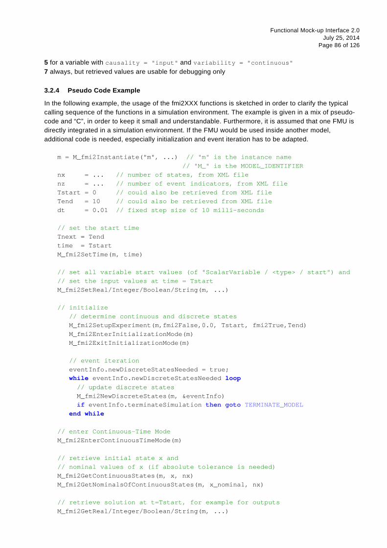
Functional Mock-up Interface 2.0 July 25, 2014
Page 86 of 126
5 for a variable with causality = "input" and variability = "continuous" 7 always, but retrieved values are usable for debugging only
3.2.4 Pseudo Code Example
In the following example, the usage of the fmi2XXX functions is sketched in order to clarify the typical calling sequence of the functions in a simulation environment. The example is given in a mix of pseudo-code and “C”, in order to keep it small and understandable. Furthermore, it is assumed that one FMU is directly integrated in a simulation environment. If the FMU would be used inside another model, additional code is needed, especially initialization and event iteration has to be adapted.
m = M_fmi2Instantiate("m", ...) // "m" is the instance name // "M_" is the MODEL_IDENTIFIER nx = ... // number of states, from XML file nz = ... // number of event indicators, from XML file Tstart = 0 // could also be retrieved from XML file Tend = 10 // could also be retrieved from XML file dt = 0.01 // fixed step size of 10 milli-seconds // set the start time Tnext = Tend time = Tstart M_fmi2SetTime(m, time) // set all variable start values (of "ScalarVariable / <type> / start") and // set the input values at time = Tstart M_fmi2SetReal/Integer/Boolean/String(m, ...) // initialize // determine continuous and discrete states M_fmi2SetupExperiment(m,fmi2False,0.0, Tstart, fmi2True,Tend) M_fmi2EnterInitializationMode(m) M_fmi2ExitInitializationMode(m) // event iteration eventInfo.newDiscreteStatesNeeded = true; while eventInfo.newDiscreteStatesNeeded loop // update discrete states M_fmi2NewDiscreteStates(m, &eventInfo) if eventInfo.terminateSimulation then goto TERMINATE_MODEL end while // enter Continuous-Time Mode M_fmi2EnterContinuousTimeMode(m) // retrieve initial state x and // nominal values of x (if absolute tolerance is needed) M_fmi2GetContinuousStates(m, x, nx) M_fmi2GetNominalsOfContinuousStates(m, x_nominal, nx) // retrieve solution at t=Tstart, for example for outputs M_fmi2GetReal/Integer/Boolean/String(m, ...)

Functional Mock-up Interface 2.0 July 25, 2014
Page 87 of 126
while time < Tend loop // compute derivatives M_fmi2GetDerivatives(m, der_x, nx) // advance time h = min(dt, Tnext-time) time = time + h M_fmi2SetTime(m, time) // set inputs at t = time M_fmi2SetReal/Integer/Boolean/String(m, ...) // set states at t = time and perform one step x = x + h*der_x // forward Euler method M_fmi2SetContinuousStates(m, x, nx) // get event indicators at t = time M_fmi2GetEventIndicators(m, z, nz) // detect events, if any time_event = abs(time - Tnext) <= eps state_event = ... // compare sign of z with previous z // inform the model about an accepted step M_fmi2CompletedIntegratorStep(m, fmi2True, &enterEventMode, &terminateSimulation) if terminateSimulation then goto TERMINATE_MODEL // handle events if entertEventMode or time_event or state_event then M_fmi2EnterEventMode(m) // event iteration eventInfo.newDiscreteStatesNeeded = true; while eventInfo.newDiscreteStatesNeeded loop // update discrete states M_fmi2NewDiscreteStates(m, &eventInfo) if eventInfo.terminateSimulation then goto TERMINATE_MODEL end while // enter Continuous-Time Mode M_fmi2EnterContinuousTimeMode(m) // retrieve solution at simulation restart M_fmi2GetReal/Integer/Boolean/String(m, ...) if eventInfo.valuesOfContinuousStatesChanged == fmi2True then //the model signals a value change of states, retrieve them M_fmi2GetContinuousStates(m, x, nx) end if if eventInfo.nominalsOfContinuousStatesChanged = fmi2True then

Functional Mock-up Interface 2.0 July 25, 2014
Page 88 of 126
//the meaning of states has changed; retrieve new nominal values M_fmi2GetNominalsOfContinuousStates(m, x_nominal, nx) end if if eventInfo.nextEventTimeDefined then Tnext = min(eventInfo.nextEventTime, Tend) else Tnext = Tend end if end if end while // terminate simulation and retrieve final values TERMINATE_MODEL: M_fmi2Terminate(m) M_fmi2GetReal/Integer/Boolean/String(m, ...) // cleanup M_fmi2FreeInstance(m)
Above, errors are not handled. Typically, fmi2XXX function calls are performed in the following way:
status = M_fmi2GetDerivatives(m, der_x, nx); switch ( status ) { case fmi2Discard: ....; break; // reduce step size and try again case fmi2Error : ....; break; // cleanup and stop simulation case fmi2Fatal : ....; } // stop using the model The switch statement could also be stored in a macro to simplify the code.
3.3 FMI Description Schema
This is defined in 2.2. Additionally, the “Model Exchange” specific element “ModelExchange” is defined in the next section.

Functional Mock-up Interface 2.0 July 25, 2014
Page 89 of 126
3.3.1 Model Exchange FMU (ModelExchange)
If the XML file defines an FMU for Model Exchange, element “ModelExchange” must be present. It is defined as:
-----------------~ ModeiExchange
I . '
The FMU includes a model or the col'l\O"M.ri:ation to a tool that provides a model. The envi"onment provOes the simulation engine for the model.
- : SourceFiles
E1 attributes I
modeUdentif ier
type I xs:normalizedString
Short class name according to Csyntax. e.g. •A_B_c · . Used as prefix for FM! functions if the functions ate provided in C scuce coCe or in SUitic: libraries, but not if the functions are provided by a DUJSharedObject:. rnode!Identifter is a:lso used as name of the sutc library or DU!SharedObject.
·--------------------, ' needsExecutionTool ' : type I xs:boolean : defaun I false
!f true, a tool is needed to e»:a.rte the model and the FMU just contains the co~tion to this tool.
' ------------------------------------' completedlntegratorStepNotNeeded ' • type I xs:boolean :_~!f_a_u_~J_f~!_s_e _________________________
---------------------------------------- ' ' canBelnstantiatedOnlyOncePerProcess
: type I xs:boolean : defaun I false
:-~~-N-~t-u-;~i~-~~-~.:Yi~~~~-9-~~-~~tF~~~ii~~-s- i • type I xs:boolean I
' ~ defaun I false : ·-----------------------, ' canGetAnd SetFMUstate ' : type I xs:boolean
~ ~~!'!~~l!_a;.~~ ----------- -~ ·---------------------, ' can Ser ializeFMUstate ' : type I xs:boolean : defaun I false
------------------------------' providesOirectionaiDer ivative ' : type I xs:boolean
: _!l_e!~.~.~.L!~~~------------------
~ -f-$~~-r~~-Fi l_e_; -$. -{-J-~
Lrst of SOI.K'Ce file names that are present m the .,SOI.K'Ces• 0..-ectory of the FMU a:nd need to be compiled in ordEr to generate the bmary of the FMU (only ~M for sooo:e coee FMUs),
El alttibut&s
name ll type I xs:normaizedstring U N.a""'E! of the file Jl"ld..l::ln; the pa.th relatr\ e ro the SCU'CES
ffflctxy, us.ng the forv.Md slash as.......,., (for exa,.pie, """"' • 1'1"1\'FMU.Cfii ,...,.,.,. • mcde:leochi~e.cj
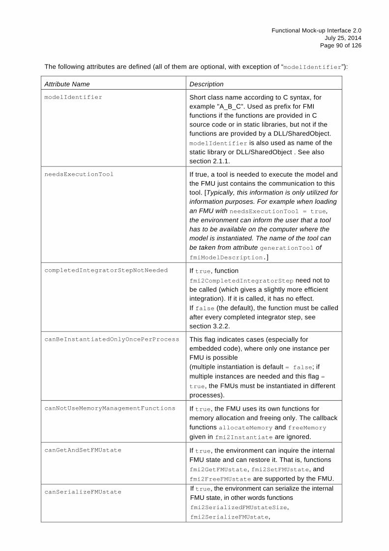
Functional Mock-up Interface 2.0 July 25, 2014
Page 90 of 126
The following attributes are defined (all of them are optional, with exception of “modelIdentifier”):
Attribute Name Description
modelIdentifier Short class name according to C syntax, for example "A_B_C". Used as prefix for FMI functions if the functions are provided in C source code or in static libraries, but not if the functions are provided by a DLL/SharedObject. modelIdentifier is also used as name of the static library or DLL/SharedObject . See also section 2.1.1.
needsExecutionTool If true, a tool is needed to execute the model and the FMU just contains the communication to this tool. [Typically, this information is only utilized for information purposes. For example when loading an FMU with needsExecutionTool = true, the environment can inform the user that a tool has to be available on the computer where the model is instantiated. The name of the tool can be taken from attribute generationTool of fmiModelDescription.]
completedIntegratorStepNotNeeded If true, function fmi2CompletedIntegratorStep need not to be called (which gives a slightly more efficient integration). If it is called, it has no effect. If false (the default), the function must be called after every completed integrator step, see section 3.2.2.
canBeInstantiatedOnlyOncePerProcess This flag indicates cases (especially for embedded code), where only one instance per FMU is possible (multiple instantiation is default = false; if multiple instances are needed and this flag = true, the FMUs must be instantiated in different processes).
canNotUseMemoryManagementFunctions If true, the FMU uses its own functions for memory allocation and freeing only. The callback functions allocateMemory and freeMemory given in fmi2Instantiate are ignored.
canGetAndSetFMUstate If true, the environment can inquire the internal FMU state and can restore it. That is, functions fmi2GetFMUstate, fmi2SetFMUstate, and fmi2FreeFMUstate are supported by the FMU.
canSerializeFMUstate If true, the environment can serialize the internal FMU state, in other words functions fmi2SerializedFMUstateSize, fmi2SerializeFMUstate,

Functional Mock-up Interface 2.0 July 25, 2014
Page 91 of 126
fmi2DeSerializeFMUstate are supported by the FMU. If this is the case, then flag canGetAndSetFMUstate must be true as well.
providesDirectionalDerivative If true, the directional derivative of the equations can be computed with fmi2GetDirectionalDerivative(..)
The flags have the following default values.
boolean: false unsignedInt: 0
3.3.2 Example XML Description File
When generating an FMU from the hypothetical model “MyLibrary.SpringMassDamper”, the XML file may have the following content:
<?xml version="1.0" encoding="UTF8"?> <fmiModelDescription fmiVersion="2.0" modelName="MyLibrary.SpringMassDamper" guid="{8c4e810f-3df3-4a00-8276-176fa3c9f9e0}" description="Rotational Spring Mass Damper System" version="1.0" generationDateAndTime="2011-09-23T16:57:33Z" variableNamingConvention="structured" numberOfEventIndicators="2"> <ModelExchange modelIdentifier="MyLibrary_SpringMassDamper"/> <UnitDefinitions> <Unit name="rad"> <BaseUnit rad="1"/> <DisplayUnit name="deg" factor="57.2957795130823"/> </Unit> <Unit name="rad/s"> <BaseUnit s="-1" rad="1"/> </Unit> <Unit name="kg.m2"> <BaseUnit kg="1" m="2"/> </Unit> </UnitDefinitions> <TypeDefinitions> <SimpleType name="Modelica.SIunits.Inertia"> <Real quantity="MomentOfInertia" unit="kg.m2" min="0.0"/> </SimpleType> <SimpleType name="Modelica.SIunits.Torque"> <Real quantity="Torque" unit="N.m"/> </SimpleType> <SimpleType name="Modelica.SIunits.AngularVelocity"> <Real quantity="AngularVelocity" unit="rad/s"/> </SimpleType> <SimpleType name="Modelica.SIunits.Angle"> <Real quantity="Angle" unit="rad"/> </SimpleType> </TypeDefinitions>
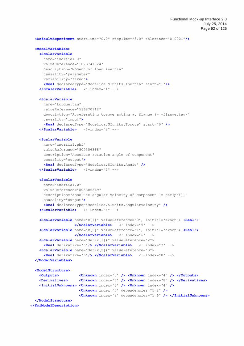
Functional Mock-up Interface 2.0 July 25, 2014
Page 92 of 126
<DefaultExperiment startTime="0.0" stopTime="3.0" tolerance="0.0001"/> <ModelVariables> <ScalarVariable name="inertia1.J" valueReference="1073741824" description="Moment of load inertia" causality="parameter" variability="fixed"> <Real declaredType="Modelica.SIunits.Inertia" start="1"/> </ScalarVariable> <!—index="1" --> <ScalarVariable name="torque.tau" valueReference="536870912" description="Accelerating torque acting at flange (= -flange.tau)" causality="input"> <Real declaredType="Modelica.SIunits.Torque" start="0" /> </ScalarVariable> <!—index="2" --> <ScalarVariable name="inertia1.phi" valueReference="805306368" description="Absolute rotation angle of component" causality="output"> <Real declaredType="Modelica.SIunits.Angle" /> </ScalarVariable> <!—index="3" --> <ScalarVariable name="inertia1.w" valueReference="805306369" description="Absolute angular velocity of component (= der(phi))" causality="output"> <Real declaredType="Modelica.SIunits.AngularVelocity" /> </ScalarVariable> <!—index="4" --> <ScalarVariable name="x[1]" valueReference="0", initial="exact"> <Real/> </ScalarVariable> <!—index="5" --> <ScalarVariable name="x[2]" valueReference="1", initial="exact"> <Real/> </ScalarVariable> <!—index="6" --> <ScalarVariable name="der(x[1])" valueReference="2"> <Real derivative="5"/> </ScalarVariable> <!—index="7" --> <ScalarVariable name="der(x[2])" valueReference="3"> <Real derivative="6"/> </ScalarVariable> <!—index="8" --> </ModelVariables> <ModelStructure> <Outputs> <Unknown index="3" /> <Unknown index="4" /> </Outputs> <Derivatives> <Unknown index="7" /> <Unknown index="8" /> </Derivatives> <InitialUnknowns> <Unknown index="3" /> <Unknown index="4" /> <Unknown index="7" dependencies="5 2" /> <Unknown index="8" dependencies="5 6" /> </InitialUnknowns> </ModelStructure> </fmiModelDescription>
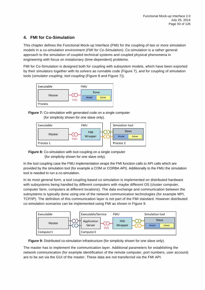
Functional Mock-up Interface 2.0 July 25, 2014
Page 93 of 126
4. FMI for Co-Simulation
This chapter defines the Functional Mock-up Interface (FMI) for the coupling of two or more simulation models in a co-simulation environment (FMI for Co-Simulation). Co-simulation is a rather general approach to the simulation of coupled technical systems and coupled physical phenomena in engineering with focus on instationary (time-dependent) problems.
FMI for Co-Simulation is designed both for coupling with subsystem models, which have been exported by their simulators together with its solvers as runnable code (Figure 7), and for coupling of simulation tools (simulator coupling, tool coupling (Figure 8 and Figure 7)).
Figure 7: Co-simulation with generated code on a single computer (for simplicity shown for one slave only).
Figure 8: Co-simulation with tool coupling on a single computer (for simplicity shown for one slave only).
In the tool coupling case the FMU implementation wraps the FMI function calls to API calls which are provided by the simulation tool (for example a COM or CORBA API). Additionally to the FMU the simulation tool is needed to run a co-simulation.
In its most general form, a tool coupling based co-simulation is implemented on distributed hardware with subsystems being handled by different computers with maybe different OS (cluster computer, computer farm, computers at different locations). The data exchange and communication between the subsystems is typically done using one of the network communication technologies (for example MPI, TCP/IP). The definition of this communication layer is not part of the FMI standard. However distributed co-simulation scenarios can be implemented using FMI as shown in Figure 9.
Figure 9: Distributed co-simulation infrastructure (for simplicity shown for one slave only).
The master has to implement the communication layer. Additional parameters for establishing the network communication (for example identification of the remote computer, port numbers, user account) are to be set via the GUI of the master. These data are not transferred via the FMI API.

Functional Mock-up Interface 2.0 July 25, 2014
Page 94 of 126
4.1 Mathematical Description
4.1.1 Basics
Co-simulation exploits the modular structure of coupled problems in all stages of the simulation process beginning with the separate model setup and preprocessing for the individual subsystems in different simulation tools (which can be powerful simulators as well as simple C programs). During time integration, the simulation is again performed independently for all subsystems restricting the data exchange between subsystems to discrete communication points tci. For simulator coupling, also the visualization and post-processing of simulation data is done individually for each subsystem in its own native simulation tool. In different contexts, the communication points tci, the communication steps tci → tci+1 and the communication step sizes hci := tci+1 - tci are also known as sampling points (synchronization points), macro steps and sampling rates, respectively. The term “communication point” in FMI for Co-Simulation refers to the communication between subsystems in a co-simulation environment and should not be mixed with the output points for saving simulation results to file.
FMI for Co-Simulation provides an interface standard for the solution of time dependent coupled systems consisting of subsystems that are continuous in time (model components that are described by instationary differential equations) or time-discrete (model components that are described by difference equations like, for example discrete controllers). In a block representation of the coupled system, the subsystems are represented by blocks with (internal) state variables x(t) that are connected to other subsystems (blocks) of the coupled problem by subsystem inputs u(t) and subsystem outputs y(t). In this framework, the physical connections between subsystems are represented by mathematical coupling conditions between the inputs u(t) and the outputs y(t) of all subsystems, Kübler and Schiehlen (2000).
Figure 10: Data flow at communication points.
For co-simulation two basic groups of functions have to be realized:
functions for the data exchange between subsystems and 1.
functions for algorithmic issues to synchronize the simulation of all subsystems and to proceed in 2.
communication steps tci → tci+1 from initial time tc0 := tstart to end time tcN := tstop.
y
Co-Simulation Master
v
Solver
t time m discrete states (constant between events) p parameters of type Real, Integer, Boolean, String u inputs of type Real, Integer, Boolean, String v all exposed variables x continuous states (continuous between events) y outputs of type Real, Integer, Boolean, String z event indicators
Model
t0, p, v0
Co-Simulation Slave (FMU Instance)
x t ,x z
u
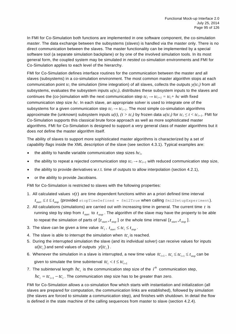
Functional Mock-up Interface 2.0 July 25, 2014
Page 95 of 126
In FMI for Co-Simulation both functions are implemented in one software component, the co-simulation master. The data exchange between the subsystems (slaves) is handled via the master only. There is no direct communication between the slaves. The master functionality can be implemented by a special software tool (a separate simulation backplane) or by one of the involved simulation tools. In its most general form, the coupled system may be simulated in nested co-simulation environments and FMI for Co-Simulation applies to each level of the hierarchy.
FMI for Co-Simulation defines interface routines for the communication between the master and all slaves (subsystems) in a co-simulation environment. The most common master algorithm stops at each communication point tci the simulation (time integration) of all slaves, collects the outputs y(tci) from all subsystems, evaluates the subsystem inputs u(tci), distributes these subsystem inputs to the slaves and continues the (co-)simulation with the next communication step tci → tci+1 = tci+ hc with fixed communication step size hc. In each slave, an appropriate solver is used to integrate one of the subsystems for a given communication step tci → tci+1. The most simple co-simulation algorithms approximate the (unknown) subsystem inputs u(t), (t > tci) by frozen data u(tci) for tci ≤ t < tci+1. FMI for Co-Simulation supports this classical brute force approach as well as more sophisticated master algorithms. FMI for Co-Simulation is designed to support a very general class of master algorithms but it does not define the master algorithm itself.
The ability of slaves to support more sophisticated master algorithms is characterized by a set of capability flags inside the XML description of the slave (see section 4.3.1). Typical examples are:
• the ability to handle variable communication step sizes hci,
• the ability to repeat a rejected communication step tci → tci+1 with reduced communication step size,
• the ability to provide derivatives w.r.t. time of outputs to allow interpolation (section 4.2.1),
• or the ability to provide Jacobians.
FMI for Co-Simulation is restricted to slaves with the following properties:
1. All calculated values )(tv are time dependent functions within an a priori defined time interval
start stopt t t≤ ≤ (provided stopTimeDefined = fmi2True when calling fmi2SetupExperiment). 2. All calculations (simulations) are carried out with increasing time in general. The current time t is
running step by step from startt to stopt . The algorithm of the slave may have the property to be able
to repeat the simulation of parts of ],[ stopstart tt or the whole time interval ],[ stopstart tt .
3. The slave can be given a time value itc , start i stopt tc t≤ ≤ .
4. The slave is able to interrupt the simulation when itc is reached. 5. During the interrupted simulation the slave (and its individual solver) can receive values for inputs
)( itcu and send values of outputs )( itcy .
6. Whenever the simulation in a slave is interrupted, a new time value 1+itc , 1i i stoptc tc t+≤ ≤ can be
given to simulate the time subinterval 1i itc t tc +< ≤
7. The subinterval length ihc is the communication step size of the thi communication step,
iii tctchc −= +1 . The communication step size has to be greater than zero.
FMI for Co-Simulation allows a co-simulation flow which starts with instantiation and initialization (all slaves are prepared for computation, the communication links are established), followed by simulation (the slaves are forced to simulate a communication step), and finishes with shutdown. In detail the flow is defined in the state machine of the calling sequences from master to slave (section 4.2.4).

Functional Mock-up Interface 2.0 July 25, 2014
Page 96 of 126
4.1.2 Mathematical Model
This section contains a formal mathematical model of a Co-Simulation FMU. The following fundamental assumptions are made:
The slave simulators are seen by the master simulator as purely sampled-data systems. Such a sampled-data system can be
• either a “real” sampled-data system (so a sampled discrete controller; the inputs and outputs can be of type Real, Integer, Boolean, String, or enumeration. Variables of this type are defined with variability = "discrete"; the smallest sample period as accessible by the outside of the FMU is defined by attribute stepSize in element DefaultExperiment).
• or a hybrid ODE that is integrated between communication points (known as “sampled access to time continuous systems”) where internal events may occur and be handled, but events are not visible from the outside of the FMU. It is assumed here that all inputs and all outputs of this hybrid ODE are Real signals (defined with variability = "continuous"),
• or a combination of the systems above.
The communication between the master and a slave takes only place at a discrete set of time instants, called communication points.
An FMI Co-Simulation model is described by the following variables:
Variable Description 𝑡
Independent variable time ∈ ℝ. (Variable defined with causality = "independent"). The i-th communication point is denoted as 𝑡 = 𝑡𝑐𝑖 The communication step size is denoted as ℎ𝑐𝑖 = 𝑡𝑐𝑖+1 − 𝑡𝑐𝑖
𝐯 A vector of all exposed variables (all variables defined in element <ModelVariables>, see section 2.2.7). Via a subscript, a subset of the variables is selected. Example: vinitial=exact are variables defined with attribute initial = "exact", see section 2.2.7. These are independent parameters and start values of other variables, such as initial values for states, state derivatives or outputs.
𝐩 Parameters that are constant during simulation. The symbol without a sub-script references independent parameters (variables with causality = "parameter"). Dependent parameters (variables with causality = "calculatedParameter") are denoted as 𝐩𝑐𝑎𝑙𝑐𝑢𝑙𝑎𝑡𝑒𝑑 and tunable parameters (variables with causality = "parameter" and variability = "tunable") are denoted as 𝐩𝒕𝒖𝒏𝒆.
𝐮(𝑡𝑐𝑖) Input variables. The values of these variables are defined outside of the model. Variables of this type are defined with attribute causality = "input". Via attribute variability = "discrete" or "continuous" it is defined whether the input is a discrete-time or continuous-time variable, see section 2.2.7.
𝐲(𝑡𝑐𝑖) Output variables. The values of these variables are computed in the FMU and they are designed to be used in a model connection. So output variables might be used in the environment as input values to other FMUs or other submodels. Variables of this type are defined with attribute causality = "output". Via attribute variability = "discrete" or "continuous" it is defined whether the output is a discrete-time or continuous-time variable, see section 2.2.7.
𝐰(𝑡𝑐𝑖) Local variables of the FMU that cannot be used for FMU connections. Variables of this type are defined with attribute causality = "local", see section 2.2.7.
𝐱𝑐(t) A vector of real continuous-time variables representing the continuous-time states. For notational convenience, a continuous-time state is conceptually treated as a different type of variable as an output or a local variable for the mathematical description

Functional Mock-up Interface 2.0 July 25, 2014
Page 97 of 126
below. However, at a communication point a continuous-time state is part of the outputs 𝐲 or the local variables 𝐰 of an FMU.
𝐱𝑑(𝑡) 𝐱 ● 𝑑(𝑡)
𝐱𝑑(𝑡) is a vector of (internal) discrete-time variables (of any type) representing the (internal) discrete states. 𝐱 ● 𝑑(𝑡) is the value of 𝐱𝑑(𝑡) at the previous sample time instant, so 𝐱 ● 𝑑(𝑡) = 𝐱𝑑( 𝑡 ● ).
Given the previous values of the discrete-time states, 𝐱 ● 𝑑(𝑡), at the actual time instant t, all other discrete-time variables, especially the discrete states 𝐱𝑑(𝑡), can be computed. Discrete states are not visible in the interface of an FMU and are only introduced here to clarify the mathematical description. Formally, a discrete state is part of the outputs y or the local variables w of an FMU.
When the transient simulation of the coupled system through co-simulation is completed, the sequence of evaluations is the following (here 𝐱 = [𝒙𝑐; 𝐱𝑑]𝑇 is the combined vector of continuous-time and discrete-time states, and 𝐲 = [𝒚𝑐;𝐲𝑑]𝑇) is the combined vector of continuous-time and discrete-time outputs):
for 𝑖 = 0,⋯ ,𝑛 − 1 �𝐱𝑖+1 = Φ𝑖 �𝐱𝑖 , �𝐮𝑖
(𝑗)�𝑗=0,⋯,𝑚𝑖𝑑𝑜
,𝐩𝑡𝑢𝑛𝑒,𝑖 ,ℎ𝑐𝑖�
��𝐲𝑖+1(𝑗) �
𝑗=0,⋯,𝑚𝑜𝑑𝑜,𝐰𝑖+1� = 𝚪𝑖 �𝐱𝑖 , �𝐮𝑖
(𝑗)�𝑗=0,⋯,𝑚𝑖𝑑𝑜
,𝐩𝑡𝑢𝑛𝑒,𝑖 ,ℎ𝑐𝑖� (4.1)
where 𝚽𝑖 and 𝚪𝑖 define the system behavior for the time interval 𝑡𝑐𝑖 ≤ 𝑡 < 𝑡𝑐𝑖+1, with 𝑡𝑐𝑖 = 𝑡𝑐0 + ∑ ℎ𝑐𝑘𝑖−1𝑘=0
[For the part of the co-simulation slave that is based on an ODE, a differential equation is solved between communication points:
�̇�𝑐 = 𝛗(𝐱𝑐(𝑡),𝐮𝑐(𝑡),𝒑𝑡𝑢𝑛𝑒)
In this case, the following relationship should hold (note the use of 𝐱𝑖+1 here): 𝜕𝚽𝑖
𝜕ℎ𝑐𝑖= 𝛗�𝐱𝑐,𝑖+1 ,� 𝐮𝑐,𝑖
(𝑗) ℎ𝑐𝑖𝑗
𝑗!
𝑚𝑖𝑑𝑜
𝑗=0,𝐩𝑡𝑢𝑛𝑒,𝑖�
This relation is in practice inexact due to using finite precision on machines and stopping iterations early. The slave simulators are responsible for implementing 𝚽𝑖 and 𝚪𝑖; e.g. to handle stiff differential equations as:
𝚽𝑖 �𝐱𝑐,𝑖 , �𝐮𝑐,𝑖(𝑗)�
𝑗=0,⋯,𝑚𝑖𝑑𝑜,𝐩𝑡𝑢𝑛𝑒,𝑖 , 𝑡𝑐𝑖� = 𝐱𝑐,𝑖 + �𝐈 − ℎ𝑐𝑖
𝜕𝛗𝜕𝐱𝑐
�−1
ℎ𝑐𝑖𝛗�𝐱𝑐,𝑖 ,𝐮𝑐,𝑖 ,𝐩𝑡𝑢𝑛𝑒,𝑖� + 𝑂(ℎ𝑐𝑖2).
]
Definition (4.1) is consistent with the definition of co-simulation by (Kübler, Schiehlen 2000): • At the communication points, the master provides generalized inputs to the slave, which can be:
o the current input variables 𝐮𝑖(0) of the subsystem (i.e. the input variables of the model contained in
the slave simulator, in the sense of system-level simulation), along with some of their successive derivatives �𝐮𝑖
(𝑗)�𝑗=1,⋯,𝑚𝑖𝑑𝑜
(in case of continuous-time variables),
o varying parameters 𝐩𝑡𝑢𝑛𝑒,𝑖, also known as tunable parameters. • The slave provides generalized outputs to the master, which are:
o the current output variables 𝒚𝑖+1(0) of the subsystem (same remark as above), along with some of
their successive derivatives �𝐲𝑖+1(𝑗) �
𝑗=1,⋯,𝑚𝑜𝑑𝑜(in case of continuous-time variables),
o observation variables and “calculated” varying parameters 𝐰𝑖+1, along with directional derivatives estimated at 𝑡 = 𝑡𝑐𝑖+1 (in case of continuous-time variables).
• Initialization: The slave being a sampled-data system, its internal states (being either continuous-time or discrete-time, it does not matter) need to be initialized at 𝑡 = 𝑡𝑐0. This is performed through an auxiliary function [this relationship is defined in the xml-file under <ModelStructure><InitialUnknowns>]:
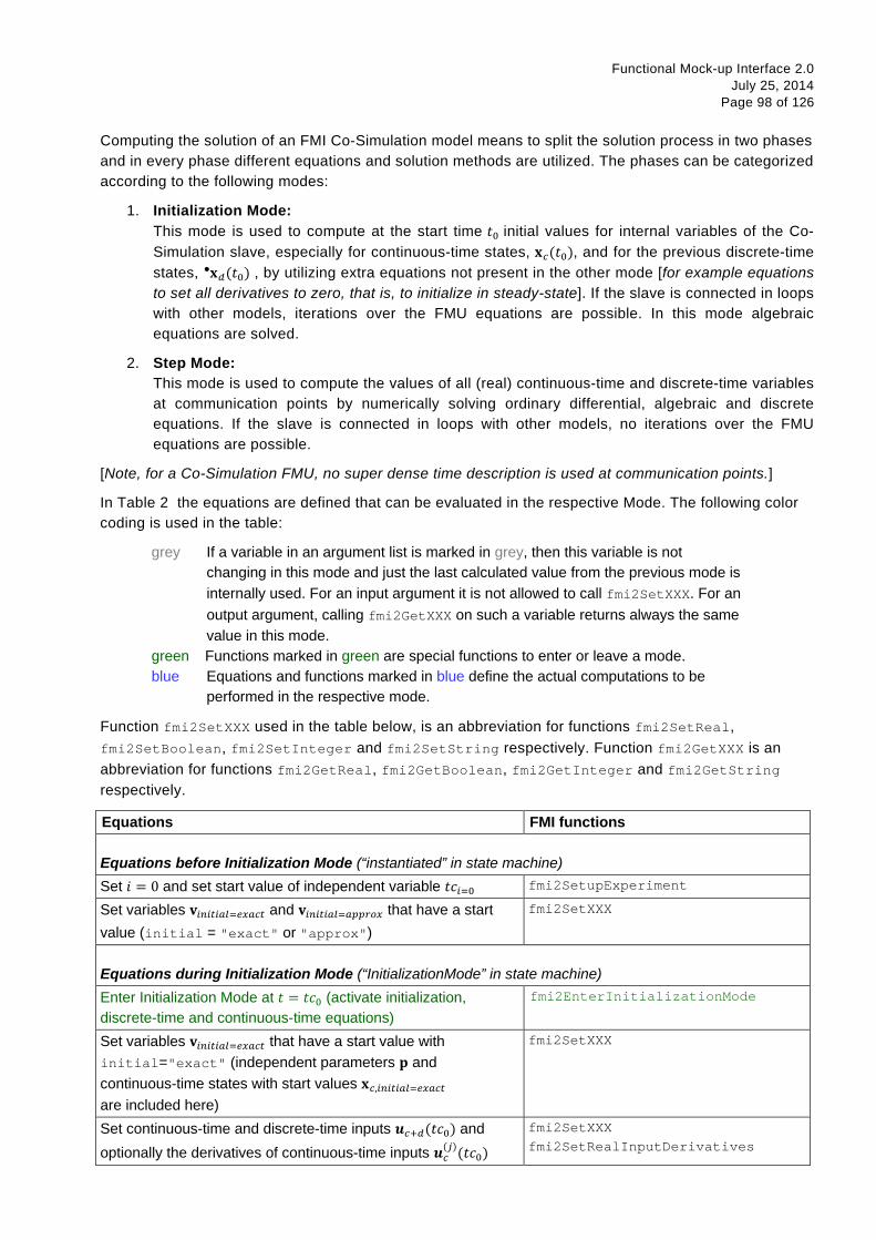
Functional Mock-up Interface 2.0 July 25, 2014
Page 98 of 126
Computing the solution of an FMI Co-Simulation model means to split the solution process in two phases and in every phase different equations and solution methods are utilized. The phases can be categorized according to the following modes:
1. Initialization Mode: This mode is used to compute at the start time 𝑡0 initial values for internal variables of the Co-Simulation slave, especially for continuous-time states, 𝐱𝑐(𝑡0), and for the previous discrete-time states, 𝐱 ● 𝑑(𝑡0) , by utilizing extra equations not present in the other mode [for example equations to set all derivatives to zero, that is, to initialize in steady-state]. If the slave is connected in loops with other models, iterations over the FMU equations are possible. In this mode algebraic equations are solved.
2. Step Mode: This mode is used to compute the values of all (real) continuous-time and discrete-time variables at communication points by numerically solving ordinary differential, algebraic and discrete equations. If the slave is connected in loops with other models, no iterations over the FMU equations are possible.
[Note, for a Co-Simulation FMU, no super dense time description is used at communication points.]
In Table 2 the equations are defined that can be evaluated in the respective Mode. The following color coding is used in the table:
grey If a variable in an argument list is marked in grey, then this variable is not changing in this mode and just the last calculated value from the previous mode is internally used. For an input argument it is not allowed to call fmi2SetXXX. For an output argument, calling fmi2GetXXX on such a variable returns always the same value in this mode.
green Functions marked in green are special functions to enter or leave a mode. blue Equations and functions marked in blue define the actual computations to be
performed in the respective mode.
Function fmi2SetXXX used in the table below, is an abbreviation for functions fmi2SetReal, fmi2SetBoolean, fmi2SetInteger and fmi2SetString respectively. Function fmi2GetXXX is an abbreviation for functions fmi2GetReal, fmi2GetBoolean, fmi2GetInteger and fmi2GetString respectively.
Equations FMI functions
Equations before Initialization Mode (“instantiated” in state machine) Set 𝑖 = 0 and set start value of independent variable 𝑡𝑐𝑖=0 fmi2SetupExperiment
Set variables 𝐯𝑖𝑛𝑖𝑡𝑖𝑎𝑙=𝑒𝑥𝑎𝑐𝑡 and 𝐯𝑖𝑛𝑖𝑡𝑖𝑎𝑙=𝑎𝑝𝑝𝑟𝑜𝑥 that have a start value (initial = "exact" or "approx")
fmi2SetXXX
Equations during Initialization Mode (“InitializationMode” in state machine) Enter Initialization Mode at 𝑡 = 𝑡𝑐0 (activate initialization, discrete-time and continuous-time equations)
fmi2EnterInitializationMode
Set variables 𝐯𝑖𝑛𝑖𝑡𝑖𝑎𝑙=𝑒𝑥𝑎𝑐𝑡 that have a start value with initial="exact" (independent parameters 𝐩 and continuous-time states with start values 𝐱𝑐,𝑖𝑛𝑖𝑡𝑖𝑎𝑙=𝑒𝑥𝑎𝑐𝑡 are included here)
fmi2SetXXX
Set continuous-time and discrete-time inputs 𝒖𝑐+𝑑(𝑡𝑐0) and optionally the derivatives of continuous-time inputs 𝒖𝑐
(𝑗)(𝑡𝑐0)
fmi2SetXXX fmi2SetRealInputDerivatives

Functional Mock-up Interface 2.0 July 25, 2014
Page 99 of 126
𝐯𝐼𝑛𝑖𝑡𝑖𝑎𝑙𝑈𝑛𝑘𝑛𝑜𝑤𝑛𝑠 ≔ 𝐟𝑖𝑛𝑖𝑡(𝒖𝑐,𝒖𝑑 , 𝑡0,𝐯𝑖𝑛𝑖𝑡𝑖𝑎𝑙=𝑒𝑥𝑎𝑐𝑡) fmi2GetXXX fmi2GetDirectionalDerivative
Exit Initialization Mode (de-activate initialization equations) fmi2ExitInitializationMode
Equations during Step Mode (“stepComplete”, “stepInProgress” in state machine) Set independent tunable parameters 𝐩𝑡𝑢𝑛𝑒 (and do not set other parameters 𝐩𝑜𝑡ℎ𝑒𝑟)
fmi2SetXXX
Set continuous-time and discrete-time inputs 𝒖𝑐+𝑑(𝑡𝑐𝑖) and optionally the derivatives of continuous-time inputs 𝒖𝑐
(𝑗)(𝑡𝑐𝑖)
fmi2SetXXX fmi2SetRealInputDerivatives
𝑡𝑐𝑖+1 ≔ 𝑡𝑐𝑖 + ℎ𝑐𝑖
(𝐲𝑐+𝑑 ,𝒚𝒄(𝒋),𝒘𝑐+𝑑)𝑡𝑐𝑖+1 ≔ 𝐟𝑑𝑜𝑆𝑡𝑒𝑝 �𝒖𝑐+𝑑 ,𝒖𝑐
(𝑗), 𝑡𝑐𝑖 ,ℎ𝑐𝑖 ,𝐩𝑡𝑢𝑛𝑒,𝐩𝑜𝑡ℎ𝑒𝑟�𝑡𝑐𝑖
𝑡𝑐𝑖 ≔ 𝑡𝑐𝑖+1
𝐟𝑑𝑜𝑆𝑡𝑒𝑝 is also a function of the internal variables 𝐱𝑐 , 𝐱 ●𝑑
fmi2DoStep fmi2GetXXX fmi2GetRealOutputDerivatives fmi2GetDirectionalDerivative
Data types 𝑡, 𝑡𝑐,ℎ𝑐 ∈ ℝ,𝐩 ∈ ℙ𝑛𝑝,𝐮(𝑡𝑐) ∈ ℙ𝑛𝑢, 𝐲(𝑡𝑐) ∈ ℙ𝑛𝑦, 𝐱𝑐(𝑡) ∈ ℝ𝑛𝑥𝑐 , 𝐱𝑑(𝑡) ∈ ℙ𝑛𝑥𝑑 ,𝐰(𝑡𝑐) ∈ ℙ𝑛𝑤
ℝ: real variable,ℙ: real or Boolean or integer or enumeration or string variable 𝐟𝑖𝑛𝑖𝑡 , 𝐟𝑜𝑢𝑡 ∈ 𝐶0 (= continuous functions with respect to all input arguments inside the respective mode).
Table 2: Mathematical description of an FMU for Co-Simulation.
[Remark – Calling Sequences:
In the table above, for notational convenience in Initialization Mode one function call is defined to compute all output arguments from all inputs arguments. In reality, every scalar output argument is computed by one fmi2GetXXX function call.
In Step Mode the input arguments to 𝒇𝑑𝑜𝑆𝑡𝑒𝑝 are defined by calls to fmi2SetXXX and fmi2SetRealInputDerivatives functions. The variables computed by 𝒇𝑑𝑜𝑆𝑡𝑒𝑝 can be inquired by fmi2GetXXX function calls.]
4.2 FMI Application Programming Interface
This section contains the interface description to access the in/output data and status information of a co-simulation slave from a C program.
4.2.1 Transfer of Input / Output Values and Parameters
Input and output variables and variables are transferred via the fmi2GetXXX and fmi2SetXXX functions, defined in section 2.1.7.
In order to enable the slave to interpolate the continuous real inputs between communication steps the derivatives of the inputs with respect to time can be provided. To allow higher order interpolation also higher derivatives can be set. Whether a slave is able to interpolate and therefore needs this information is provided by the capability attribute canInterpolateInputs.
fmi2Status fmi2SetRealInputDerivatives(fmi2Component c,
const fmi2ValueReference vr[], size_t nvr, const fmi2Integer order[], const fmi2Real value[]);
Sets the n-th time derivative of real input variables. Argument “vr” is a vector of value

Functional Mock-up Interface 2.0 July 25, 2014
Page 100 of 126
references that define the variables whose derivatives shall be set. The array “order” contains the orders of the respective derivative (1 means the first derivative, 0 is not allowed). Argument “value” is a vector with the values of the derivatives. “nvr” is the dimension of the vectors. Restrictions on using the function are the same as for the fmi2SetReal function.
Inputs and their derivatives are set with respect to the beginning of a communication time step.
To allow interpolation/approximation of the real output variables between communication steps (if they are used as inputs for other slaves) the derivatives of the outputs with respect to time can be read. Whether the slave is able to provide the derivatives of outputs is given by the unsigned integer capability flag MaxOutputDerivativeOrder. It delivers the maximum order of the output derivative. If the actual order is lower (because the order of integration algorithm is low), the retrieved value is 0.
Example: If the internal polynomial is of order 1 and the master inquires the second derivative of an output, the slave will return zero.
The derivatives can be retrieved by:
fmi2Status fmi2GetRealOutputDerivatives (fmi2Component c,
const fmi2ValueReference vr[], size_t nvr, const fmi2Integer order[], fmi2Real value[]);
Retrieves the n-th derivative of output values. Argument “vr” is a vector of “nvr” value references that define the variables whose derivatives shall be retrieved. The array “order” contains the order of the respective derivative (1 means the first derivative, 0 is not allowed). Argument “value” is a vector with the actual values of the derivatives. Restrictions on using the function are the same as for the fmi2GetReal function.
The returned outputs correspond to the current slave time. E. g. after a successful fmi2DoStep(...) the returned values are related to the end of the communication time step.
This standard supports polynomial interpolation and extrapolation as well as more sophisticated signal extrapolation schemes like rational extrapolation, see the companion document “FunctionalMockupInterface-ImplementationHints.pdf”.
4.2.2 Computation
The computation of time steps is controlled by the following function.
fmi2Status fmi2DoStep(fmi2Component c, fmi2Real currentCommunicationPoint, fmi2Real communicationStepSize, fmi2Boolean noSetFMUStatePriorToCurrentPoint);
The computation of a time step is started. Argument currentCommunicationPoint is the current communication point of the master (𝑡𝑐𝑖) and argument communicationStepSize is the communication step size (ℎ𝑐𝑖). The latter must be > 0.0. The slave must integrate until time instant 𝑡𝑐𝑖+1 = 𝑡𝑐𝑖 + ℎ𝑐𝑖. [The calling environment defines the communication points and fmi2DoStep must synchronize to these points by always integrating exactly to 𝑡𝑐𝑖 + ℎ𝑐𝑖. It is up to fmi2DoStep how to achieve this.] At the first call to fmiDoStep after fmi2ExitInitializationMode was called currentCommunicationPoint must be equal to startTime as set with

Functional Mock-up Interface 2.0 July 25, 2014
Page 101 of 126
fmi2SetupExperiment. [Formally argument currentCommunicationPoint is not needed. It is present in order to handle a mismatch between the master and the FMU state of the slave: The currentCommunicationPoint and the FMU state of the slaves defined by former fmi2DoStep or fmi2SetFMUState calls have to be consistent with respect to each other. For example, if the slave does not use the update formula for the independent variable as required above, 𝑡𝑐𝑖+1 = 𝑡𝑐𝑖 + ℎ𝑐𝑖 (using argument 𝑡𝑐𝑖 = currentCommunicationPoint of fmi2DoStep) but uses internally an own update formula, such as 𝑡𝑐𝑠,𝑖+1 = 𝑡𝑐𝑠,𝑖 + ℎ𝑐𝑠,𝑖 then the slave could use as time increment ℎ𝑐𝑠,𝑖: = (𝑡𝑐𝑖 − 𝑡𝑐𝑠,𝑖) + ℎ𝑐𝑖 (instead of ℎ𝑐𝑠,𝑖: = ℎ𝑐𝑖,) to avoid a mismatch between the master time 𝑡𝑐𝑖+1 and the slave internal time 𝑡𝑐𝑠,𝑖+1 for large i.]
Argument noSetFMUStatePriorToCurrentPoint is fmi2True if fmi2SetFMUState will no longer be called for time instants prior to currentCommunicationPoint in this simulation run [the slave can use this flag to flush a result buffer].
The function returns: fmi2OK - if the communication step was computed successfully until its end. fmi2Discard – if the slave computed successfully only a subinterval of the communication step. The master can call the appropriate fmi2GetXXXStatus functions to get further information. If possible, the master should retry the simulation with a shorter communication step size. [Redoing a step is only possible if the FMU state has been recorded at the beginning of the current (failed) step with fmi2GetFMUState. Redoing a step is performed by calling fmi2SetFMUState and afterwards calling fmi2DoStep with the new communicationStepSize. Note, it is not possible to change currentCommunicationPoint in such a call.] fmi2Error – the communication step could not be carried out at all. The master can try to repeat the step with other input values and/or a different communication step size in the same way as described in the fmi2Discard case above. fmi2Fatal – if an error occurred which corrupted the FMU irreparably. [The master should stop the simulation run immediatlely.] See section 2.1.3 for details. fmi2Pending – is returned if the slave executes the function asynchronously. That means the slave starts the computation but returns immediately. The master has to call fmi2GetStatus(...,fmi2DoStep,...) to find out, if the slave is done. An alternative is to wait until the callback function fmi2StepFinished is called by the slave. fmi2CancelStep can be called to cancel the current computation. It is not allowed to call any other function during a pending fmi2DoStep.
fmi2Status fmi2CancelStep(fmi2Component c); Can be called if fmi2DoStep returned fmi2Pending in order to stop the current
asynchronous execution. The master calls this function if for example the co-simulation run is stopped by the user or one of the slaves. Afterwards it is only allowed to call fmi2Reset or fmi2FreeInstance.
It depends on the capabilities of the slave which parameter constellations and calling sequences are allowed (see 4.3.1)
Functional Mock-up Interface 2.0 July 25, 2014
Page 102 of 126
4.2.3 Retrieving Status Information from the Slave
Status information is retrieved from the slave by the following functions:
fmi2Status fmi2GetStatus (fmi2Component c, const fmi2StatusKind s, fmi2Status* value); fmi2Status fmi2GetRealStatus (fmi2Component c, const fmi2StatusKind s, fmi2Real* value); fmi2Status fmi2GetIntegerStatus(fmi2Component c, const fmi2StatusKind s, fmi2Integer* value); fmi2Status fmi2GetBooleanStatus(fmi2Component c, const fmi2StatusKind s, fmi2Boolean* value); fmi2Status fmi2GetStringStatus (fmi2Component c, const fmi2StatusKind s, fmi2String* value);
Informs the master about the actual status of the simulation run. Which status information is to be returned is specified by the argument fmi2StatusKind. It depends on the capabilities of the slave which status information can be given by the slave (see 4.3.1). If a status is required which cannot be retrieved by the slave it returns fmi2Discard.
typedef enum {fmi2DoStepStatus, fmi2PendingStatus, fmi2LastSuccessfulTime, fmi2Terminated } fmi2StatusKind; Defines which status is inquired.
The following status information can be retrieved from a slave:
Status Type of retrieved value
Description
fmi2DoStepStatus fmi2Status Can be called when the fmi2DoStep function returned fmi2Pending. The function delivers fmi2Pending if the computation is not finished. Otherwise the function returns the result of the asynchronously executed fmi2DoStep call.
fmi2PendingStatus fmi2String Can be called when the fmi2DoStep function returned fmi2Pending. The function delivers a string which informs about the status of the currently running asynchronous fmi2DoStep computation.
fmi2LastSuccessfulTime fmi2Real Returns the end time of the last successfully completed communication step. Can be called after fmi2DoStep(...) returned fmi2Discard.
fmi2Terminated fmi2Boolean Returns true, if the slave wants to terminate the simulation. Can be called after fmi2DoStep(...) returned fmi2Discard. Use fmi2LastSuccessfulTime to determine the time instant at which the slave terminated.

Functional Mock-up Interface 2.0 July 25, 2014
Page 103 of 126
4.2.4 State Machine of Calling Sequence from Master to Slave
The following state machine defines the supported calling sequences.
Figure 11: Calling sequence of Co-Simulation C functions in form of an UML 2.0 state machine.
Each state of the state machine corresponds to a certain phase of a simulation as follows:
instantiated: In this state, start and guess values (= variables that have initial = “exact” or “approx.”) can be set.
Initialization Mode: In this state equations are active to determine all outputs (and optionally other variables exposed by the exporting tool). The variables that can be retrieved by fmi2GetXXX calls are (1) defined in the xml file under <ModelStructure><InitialUnknowns> and (2) variables with causality = ″output″. Variables with initial = ″exact″, as well as variables with variability = ″input″ can be set.
slaveInitialized: In this state the slave is initialized and the co-simulation computation is performed. The calculation until the next communication point is performed with function “fmi2DoStep”. Depending on the return value, the slave is in a different state (step complete, step failed, step canceled).
terminated: In this state, the solution at the final time of the simulation can be retrieved.
Note, in Initialization Mode input variables can be set with fmi2SetXXX and output variables can be get with fmi2GetXXX interchangeably according to the model structure defined under element <ModelStructure><InitialUnknowns> in the xml-file. [For example if one output y1 depends on two
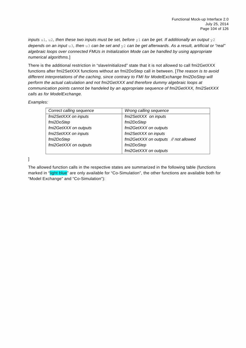
Functional Mock-up Interface 2.0 July 25, 2014
Page 104 of 126
inputs u1, u2, then these two inputs must be set, before y1 can be get. If additionally an output y2 depends on an input u3, then u3 can be set and y2 can be get afterwards. As a result, artificial or “real” algebraic loops over connected FMUs in Initialization Mode can be handled by using appropriate numerical algorithms.]
There is the additional restriction in “slaveInitialized” state that it is not allowed to call fmi2GetXXX functions after fmi2SetXXX functions without an fmi2DoStep call in between. [The reason is to avoid different interpretations of the caching, since contrary to FMI for ModelExchange fmi2DoStep will perform the actual calculation and not fmi2GetXXX and therefore dummy algebraic loops at communication points cannot be handeled by an appropriate sequence of fmi2GetXXX, fmi2SetXXX calls as for ModelExchange.
Examples:
Correct calling sequence Wrong calling sequence fmi2SetXXX on inputs fmi2DoStep fmi2GetXXX on outputs fmi2SetXXX on inputs fmi2DoStep fmi2GetXXX on outputs
fmi2SetXXX on inputs fmi2DoStep fmi2GetXXX on outputs fmi2SetXXX on inputs fmi2GetXXX on outputs // not allowed fmi2DoStep fmi2GetXXX on outputs
]
The allowed function calls in the respective states are summarized in the following table (functions marked in “light blue” are only available for “Co-Simulation”, the other functions are available both for “Model Exchange” and “Co-Simulation”):
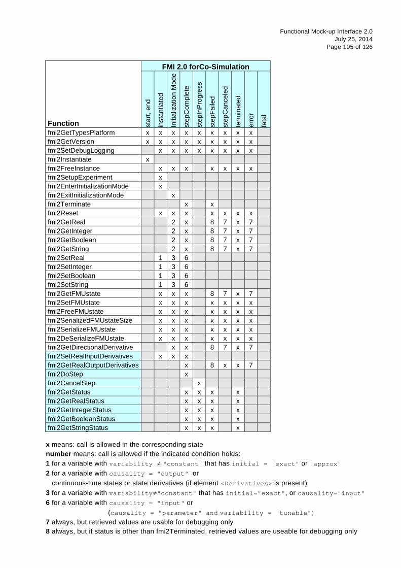
Functional Mock-up Interface 2.0 July 25, 2014
Page 105 of 126
FMI 2.0 forCo-Simulation
Function star
t, en
d
inst
antia
ted
Initi
aliz
atio
n M
ode
step
Com
plet
e
step
InPr
ogre
ss
step
Faile
d
step
Can
cele
d
term
inat
ed
erro
r
fata
l
fmi2GetTypesPlatform x x x x x x x x x fmi2GetVersion x x x x x x x x x fmi2SetDebugLogging x x x x x x x x fmi2Instantiate x fmi2FreeInstance x x x x x x x fmi2SetupExperiment x
fmi2EnterInitializationMode x fmi2ExitInitializationMode x fmi2Terminate x x fmi2Reset x x x x x x x fmi2GetReal 2 x 8 7 x 7 fmi2GetInteger 2 x 8 7 x 7 fmi2GetBoolean 2 x 8 7 x 7 fmi2GetString 2 x 8 7 x 7 fmi2SetReal 1 3 6 fmi2SetInteger 1 3 6 fmi2SetBoolean 1 3 6 fmi2SetString 1 3 6 fmi2GetFMUstate x x x 8 7 x 7 fmi2SetFMUstate x x x x x x x fmi2FreeFMUstate x x x x x x x fmi2SerializedFMUstateSize x x x x x x x fmi2SerializeFMUstate x x x x x x x fmi2DeSerializeFMUstate x x x x x x x fmi2GetDirectionalDerivative x x 8 7 x 7 fmi2SetRealInputDerivatives x x x fmi2GetRealOutputDerivatives x 8 x x 7 fmi2DoStep x fmi2CancelStep x fmi2GetStatus x x x x fmi2GetRealStatus x x x x fmi2GetIntegerStatus x x x x fmi2GetBooleanStatus x x x x fmi2GetStringStatus x x x x
x means: call is allowed in the corresponding state number means: call is allowed if the indicated condition holds: 1 for a variable with variability ≠ "constant" that has initial = "exact" or "approx" 2 for a variable with causality = "output" or continuous-time states or state derivatives (if element <Derivatives> is present) 3 for a variable with variability≠"constant" that has initial="exact", or causality="input" 6 for a variable with causality = "input" or (causality = "parameter" and variability = "tunable") 7 always, but retrieved values are usable for debugging only 8 always, but if status is other than fmi2Terminated, retrieved values are useable for debugging only
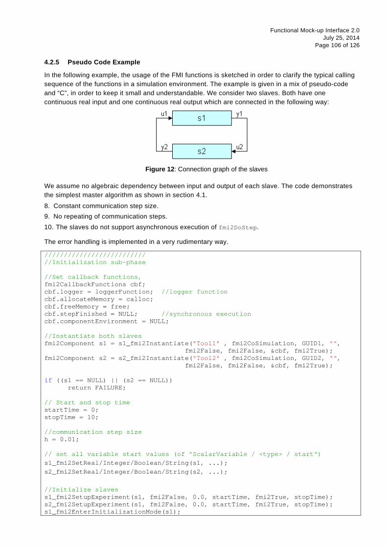
Functional Mock-up Interface 2.0 July 25, 2014
Page 106 of 126
4.2.5 Pseudo Code Example
In the following example, the usage of the FMI functions is sketched in order to clarify the typical calling sequence of the functions in a simulation environment. The example is given in a mix of pseudo-code and “C”, in order to keep it small and understandable. We consider two slaves. Both have one continuous real input and one continuous real output which are connected in the following way:
Figure 12: Connection graph of the slaves
We assume no algebraic dependency between input and output of each slave. The code demonstrates the simplest master algorithm as shown in section 4.1.
8. Constant communication step size. 9. No repeating of communication steps. 10. The slaves do not support asynchronous execution of fmi2DoStep.
The error handling is implemented in a very rudimentary way.
////////////////////////// //Initialization sub-phase //Set callback functions, fmi2CallbackFunctions cbf; cbf.logger = loggerFunction; //logger function cbf.allocateMemory = calloc; cbf.freeMemory = free; cbf.stepFinished = NULL; //synchronous execution cbf.componentEnvironment = NULL; //Instantiate both slaves fmi2Component s1 = s1_fmi2Instantiate("Tool1" , fmi2CoSimulation, GUID1, "", fmi2False, fmi2False, &cbf, fmi2True); fmi2Component s2 = s2_fmi2Instantiate("Tool2" , fmi2CoSimulation, GUID2, "", fmi2False, fmi2False, &cbf, fmi2True); if ((s1 == NULL) || (s2 == NULL)) return FAILURE; // Start and stop time startTime = 0; stopTime = 10; //communication step size h = 0.01; // set all variable start values (of "ScalarVariable / <type> / start") s1_fmi2SetReal/Integer/Boolean/String(s1, ...); s2_fmi2SetReal/Integer/Boolean/String(s2, ...); //Initialize slaves s1_fmi2SetupExperiment(s1, fmi2False, 0.0, startTime, fmi2True, stopTime); s2_fmi2SetupExperiment(s1, fmi2False, 0.0, startTime, fmi2True, stopTime); s1_fmi2EnterInitializationMode(s1);

Functional Mock-up Interface 2.0 July 25, 2014
Page 107 of 126
s2_fmi2EnterInitializationMode(s2); // set the input values at time = startTime s1_fmi2SetReal/Integer/Boolean/String(s1, ...); s2_fmi2SetReal/Integer/Boolean/String(s2, ...); s1_fmi2ExitInitializationMode(s1); s2_fmi2ExitInitializationMode(s2);
////////////////////////// //Simulation sub-phase
tc = startTime; //Current master time while ((tc < stopTime) && (status == fmi2OK)) { //retrieve outputs s1_fmi2GetReal(s1, ..., 1, &y1); s2_fmi2GetReal(s2, ..., 1, &y2); //set inputs s1_fmi2SetReal(s1, ..., 1, &y2); s2_fmi2SetReal(s2, ..., 1, &y1); //call slave s1 and check status status = s1_fmi2DoStep(s1, tc, h, fmi2True); switch (status) { case fmi2Discard: fmi2GetBooleanStatus(s1, fmi2Terminated, &boolVal); if (boolVal == fmi2True) printf("Slave s1 wants to terminate simulation."); case fmi2Error: case fmi2Fatal: terminateSimulation = true; break; } if (terminateSimulation) break; //call slave s2 and check status as above status = s2_fmi2DoStep(s2, tc, h, fmi2True); ... //increment master time tc += h; }
////////////////////////// //Shutdown sub-phase
if ((status != fmi2Error) && (status != fmi2Fatal)) { s1_fmi2Terminate(s1); s2_fmi2Terminate(s2); } if (status != fmi2Fatal) {
s1_fmi2FreeInstance(s1); s2_fmi2FreeInstance(s2); }

Functional Mock-up Interface 2.0 July 25, 2014
Page 108 of 126
4.3 FMI Description Schema
This is defined in 2.2. Additionally, the co-simulation specific element “Implementation” is defined in the next section.
4.3.1 Co-Simulation FMU (CoSimulation)
If the XML file defines an FMU for Co-Simulation, element “CoSimulation” must be present. It is defined as:
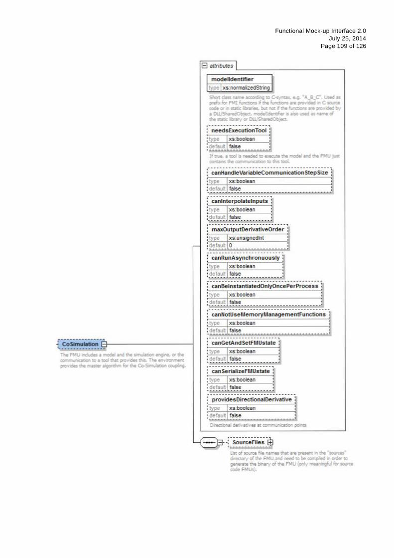
Functional Mock-up Interface 2.0 July 25, 2014
Page 109 of 126
~- -c~si.;;-;.;tk;.;-~E·:~--------------t ................ -~ -~ FMll rc:J...cl,w a \OOej and the ~iltorl tll'lgi"Je « tN! ~---~ :0 • tool Nc provdM d'& The env~ ;rev des the"*'-·~ for the eo.s.r.....~ (l).;l)in;.
E1 attributes I modelldentifier
type I xs:normaizedStmg
Short class n.:t'""E a:catfn;: :o Csyrltax. e.g. • A_ 8 _c-. Us.! .s p-efcc fer R-": f. ..:x:icns if me L .mctions ¥e o-o ~ ce:: 1l""l C ~ CDOe « n s::::tic.llltr"..cies. tx..."t ncx if tne ~ ¥e p-ovdled bv a DlL 5'-zec:O:.}:c"" ... ...-o:e::a:n........:e- is a.so used .s T">il'":e r:l tne s:::::l: flll:X3tY « Dl.L ~;ect.
:. ~~~d~E;;~~tk;.; T~i :1 :type I xs:boolean :
: ~t~~~~~--------- = If m...e.. a ::oo. s ~ ::o e:e:...--:e tne '"'"ICIOe. a'"ld d-e FMIJ ,.ctn"!af'IS ::ne CO"'""..,....~::on ::oms ":lXII-
r ~-~H~~dj~Vt;ri~bi;c~.;;~~-~i~ti~·~st;psi·~; 1 ;type j xs :boolean i :_default false ___________ J :· -~-~~~t~~~i~t~~~-p~;; .. :type I xs:boolean
:,~-~f~~~l!~~~----------: maxOutputDer ivativeOrder ~
: type I xs:unsignedlnt 1 :~~~~~~~~~--~,! : defaun I 0
: canRunAsynchronuously )
: type I xs:boolean : : ~_e_f~~~J!~~~ ______________ :
: canBelnstantiatedOnlyOncePerProcess ~
i type I xs:boolean i I ; default. false ____ J
:· ~~-,~-~.u·;;M·~;,.;~;yM~~~g~;,.;~;,tF~;,cti~~-s- i
l~;f:_~~J.~;:;~~-·~---------------------------i :-~~G"~tA:~cts~ifi.iu~i~t-;j : type I xs:boolean l ; defaull false :
.---------------------. : canSerializefMUstate 01
:type I xs:boolean -~
! d~t~'!.~ l false :
: providesDirectionaiDerivative ~
itype l xs:boolean j : defaul false ~ .
Drec:o"'..=l cer.v.::wes at o:wr ..... ...:nJ:a-:aa pol!'iS
.: . 5;,~-r~-F.I~; -~
List of SCK.Jrt:e 'ile names that a.-e present m the ~· drec:ay of the FMU and need 10 be~ n cnlor 10 gene<ate the bma<y of the FMU (only mearnngful foo- """* code FMUs).

Functional Mock-up Interface 2.0 July 25, 2014
Page 110 of 126
These attributes have the following meaning (all attributes are optional with exception of “modelIdentifier”):
Attribute Name Description
modelIdentifier Short class name according to C syntax, for example “A_B_C”. Used as prefix for FMI functions if the functions are provided in C source code or in static libraries, but not if the functions are provided by a DLL/SharedObject. modelIdentifier is also used as name of the static library or DLL/SharedObject . See also section 2.1.1.
needsExecutionTool If true, a tool is needed to execute the model. The FMU just contains the communication to this tool (see Figure 8). [Typically, this information is only utilized for information purposes. For example a co-simulation master can inform the user that a tool has to be available on the computer where the slave is instantiated. The name of the tool can be taken from attribute generationTool of fmiModelDescription. ]
canHandleVariableCommunicationStepSize The slave can handle variable communication step size. The communication step size (parameter communicationStepSize of fmi2DoStep(...) ) has not to be constant for each call.
canInterpolateInputs The slave is able to interpolate continuous inputs. Calling of fmi2SetRealInputDerivatives(...) has an effect for the slave.
maxOutputDerivativeOrder The slave is able to provide derivatives of outputs with maximum order. Calling of fmi2GetRealOutputDerivatives(...) is allowed up to the order defined by maxOutputDerivativeOrder.
canRunAsynchronuously This flag describes the ability to carry out the fmi2DoStep(...) call asynchronously.
Functional Mock-up Interface 2.0 July 25, 2014
Page 111 of 126
canBeInstantiatedOnlyOncePerProcess This flag indicates cases (especially for embedded code), where only one instance per FMU is possible (multiple instantiation is default = false; if multiple instances are needed, the FMUs must be instantiated in different processes).
canNotUseMemoryManagementFunctions If true, the slave uses its own functions for memory allocation and freeing only. The callback functions allocateMemory and freeMemory given in fmi2Instantiate are ignored.
canGetAndSetFMUstate If true, the environment can inquire the internal FMU state and can restore it. That is, fmi2GetFMUstate, fmi2SetFMUstate, and fmi2FreeFMUstate are supported by the FMU.
canSerializeFMUstate If true, the environment can serialize the internal FMU state, in other words fmi2SerializedFMUstateSize, fmi2SerializeFMUstate, fmi2DeSerializeFMUstate are supported by the FMU. If this is the case, then flag canGetAndSetFMUstate must be true as well.
providesDirectionalDerivative If true, the directional derivative of the equations at communication points can be computed with fmi2GetDirectionalDerivative(..)
The flags have the following default values. boolean: false unsignedInt: 0
Note, if needsExecutionTool = true, then it is required that the original tool is available to be executed in co-simulation mode. If needsExecutionTool = false, the slave is completely contained inside the FMU in source code or binary format (DLL/SharedObject).
4.3.2 Example XML Description File
The example below is the same one as shown in section 3.3.2 for a ModelExchange FMU. The only difference is the replacement of element ModelExchange by element CoSimulation (with additional attributes) and the removed local variables which are associated with continuous states and their derivatives. The XML file may have the following content:
<?xml version="1.0" encoding="UTF8"?> <fmiModelDescription fmiVersion="2.0" modelName="MyLibrary.SpringMassDamper" guid="{8c4e810f-3df3-4a00-8276-176fa3c9f9e0}" description="Rotational Spring Mass Damper System" version="1.0"

Functional Mock-up Interface 2.0 July 25, 2014
Page 112 of 126
generationDateAndTime="2011-09-23T16:57:33Z" variableNamingConvention="structured"> <CoSimulation modelIdentifier="MyLibrary_SpringMassDamper" canHandleVariableCommunicationStepSize="true" canInterpolateInputs="true"/> <UnitDefinitions> <Unit name="rad"> <BaseUnit rad="1"/> <DisplayUnit name="deg" factor="57.2957795130823"/> </Unit> <Unit name="rad/s"> <BaseUnit s="-1" rad="1"/> </Unit> <Unit name="kg.m2"> <BaseUnit kg="1" m="2"/> </Unit> </UnitDefinitions> <TypeDefinitions> <SimpleType name="Modelica.SIunits.Inertia"> <Real quantity="MomentOfInertia" unit="kg.m2" min="0.0"/> </SimpleType> <SimpleType name="Modelica.SIunits.Torque"> <Real quantity="Torque" unit="N.m"/> </SimpleType> <SimpleType name="Modelica.SIunits.AngularVelocity"> <Real quantity="AngularVelocity" unit="rad/s"/> </SimpleType> <SimpleType name="Modelica.SIunits.Angle"> <Real quantity="Angle" unit="rad"/> </SimpleType> </TypeDefinitions> <DefaultExperiment startTime="0.0" stopTime="3.0" tolerance="0.0001"/> <ModelVariables> <ScalarVariable name="inertia1.J" valueReference="1073741824" description="Moment of load inertia" causality="parameter" variability="fixed"> <Real declaredType="Modelica.SIunits.Inertia" start="1"/> </ScalarVariable> <ScalarVariable name="torque.tau" valueReference="536870912" description="Accelerating torque acting at flange (= -flange.tau)" causality="input"> <Real declaredType="Modelica.SIunits.Torque" start="0"/> </ScalarVariable> <ScalarVariable name="inertia1.phi" valueReference="805306368" description="Absolute rotation angle of component" causality="output"> <Real declaredType="Modelica.SIunits.Angle" />
Functional Mock-up Interface 2.0 July 25, 2014
Page 113 of 126
</ScalarVariable> <ScalarVariable name="inertia1.w" valueReference="805306369" description="Absolute angular velocity of component (= der(phi))" causality="output"> <Real declaredType="Modelica.SIunits.AngularVelocity" /> </ScalarVariable> </ModelVariables> <ModelStructure> <Outputs> <Unknown index="3"/> <Unknown index="4"/> </Outputs> <InitialUnknowns> <Unknown index="3"/> <Unknown index="4"/> </InitialUnknowns> </ModelStructure> </fmiModelDescription>
Functional Mock-up Interface 2.0 July 25, 2014
Page 114 of 126
5. Literature
Åkesson J., Braun W., Lindholm P., and Bachmann B. (2012): Generation of Sparse Jacobians for the Functional Mockup Interface 2.0. 9th International Modelica Conference, Munich, 2012. http://www.ep.liu.se/ecp/076/018/ecp12076018.pdf
Benveniste A., Caillaud B., Pouzet M. (2010): The Fundamentals of Hybrid Systems Modelers. In 49th IEEE International Conference on Decision and Control (CDC), Atlanta, Georgia, USA, December 15-17. http://www.di.ens.fr/~pouzet/bib/cdc10.pdf
Blochwitz T., Otter M., Arnold M., Bausch C., Clauß C., Elmqvist H., Junghanns A., Mauss J., Monteiro M., Neidhold T., Neumerkel D., Olsson H., Peetz J.-V., Wolf S. (2011): The Functional Mockup Interface for Tool independent Exchange of Simulation Models. 8th International Modelica Conference, Dresden 2011. http://www.ep.liu.se/ecp/063/013/ecp11063013.pdf
Blochwitz T., Otter M., Akesson J., Arnold M., Clauß C., Elmqvist H., Friedrich M., Junghanns A., Mauss J,, Neumerkel D., Olsson H., Viel A. (2012): Functional Mockup Interface 2.0: The Standard for Tool independent Exchange of Simulation Models. 9th International Modelica Conference, Munich, 2012. http://www.ep.liu.se/ecp/076/017/ecp12076017.pdf
Kübler R., Schiehlen, W. (2000): Two methods of simulator coupling. Mathematical and Computer Modeling of Dynamical Systems 6 pp. 93-113.
Lee E.A., Zheng H. (2007): Leveraging Synchronous Language Principles for Heterogeneous Modeling and Design of Embedded Systems. EMSOFT’07, Sept. 30 - Oct. 3, 2007, Salzburg, Austria. http://ptolemy.eecs.berkeley.edu/publications/papers/07/unifying/LeeZheng_SRUnifying.pdf
Lee E.A., Zheng H. (2007): Leveraging Synchronous Language Principles for Heterogeneous Modeling and Design of Embedded Systems. EMSOFT’07, September 30–October 3, Salzburg, Austria. http://doi.acm.org/10.1145/1289927.1289949
Modelica (2012): Modelica, A Unified Object-Oriented Language for Systems Modeling. Language Specification, Version 3.3, May 9, 2012. https://www.modelica.org/documents/ModelicaSpec33.pdf
MODELISAR Glossary (2009): MODELISAR WP2 Glossary and Abbreviations. Version 1.0, June 9, 2009.
Pouzet M. (2006): Lucid Synchrone, Version 3.0, Tutorial and Reference Manual. http://www.di.ens.fr/~pouzet/lucid-synchrone/
XML: www.w3.org/XML, en.wikipedia.org/wiki/XML

Functional Mock-up Interface 2.0 July 25, 2014
Page 115 of 126
Appendix A FMI Revision History
This appendix describes the history of the FMI design and its contributors. The current version of this document is available from https://www.fmi-standard.org.
The Functional Mock-up Interface development was initiated and organized by Daimler AG (from Bernd Relovsky and others) as subproject inside the ITEA2 MODELISAR project.
The development of versions 1.0 and 2.0 was performed within WP200 of MODELISAR, organized by the WP200 work package leader Dietmar Neumerkel from Daimler.
A.1 Version 1.0 – FMI for Model Exchange
Version 1.0 of FMI for Model Exchange was released on Jan. 26, 2010.
The subgroup “FMI for Model Exchange” was headed by Martin Otter (DLR-RM). The essential part of the design of this version was performed by (alphabetical list):
Torsten Blochwitz, ITI, Germany Hilding Elmqvist, Dassault Systèmes, Sweden Andreas Junghanns, QTronic, Germany Jakob Mauss, QTronic, Germany Hans Olsson, Dassault Systèmes, Sweden Martin Otter, DLR-RM, Germany.
This version was evaluated with prototypes implemented for (alphabetical list):
Dymola by Peter Nilsson, Dan Henriksson, Carl Fredrik Abelson, and Sven Erik Mattson, Dassault Systèmes, JModelica.org by Tove Bergdahl, Modelon AB, Silver by Andreas Junghanns, and Jakob Mauss, QTronic.
These prototypes have been used to refine the design of “FMI for Model Exchange”.
The following MODELISAR partners participated at FMI design meetings and contributed to the discussion (alphabetical list):
Ingrid Bausch-Gall, Bausch-Gall GmbH, Munich, Germany Torsten Blochwitz, ITI GmbH, Dresden, Germany Alex Eichberger, SIMPACK AG, Gilching, Germany Hilding Elmqvist, Dassault Systèmes, Lund, Sweden Andreas Junghanns, QTronic GmbH, Berlin, Germany Rainer Keppler, SIMPACK AG, Gilching, Germany Gerd Kurzbach, ITI GmbH, Dresden, Germany Carsten Kübler, TWT, Germany Jakob Mauss, QTronic GmbH, Berlin, Germany Johannes Mezger, TWT, Germany Thomas Neidhold, ITI GmbH, Dresden, Germany Dietmar Neumerkel, Daimler AG, Stuttgart, Germany Peter Nilsson, Dassault Systèmes, Lund, Sweden Hans Olsson, Dassault Systèmes, Lund, Sweden Martin Otter, German Aerospace Center (DLR), Oberpfaffenhofen, Germany Antoine Viel, LMS International (Imagine), Roanne, France Daniel Weil, Dassault Systèmes, Grenoble, France

Functional Mock-up Interface 2.0 July 25, 2014
Page 116 of 126
The following people outside of the MODELISAR consortium contributed with comments:
Johan Akesson, Lund University, Lund, Sweden Joel Andersson, KU Leuven, The Netherlands Roberto Parrotto, Politecnico di Milano, Italy
A.2 Version 1.0 – FMI for Co-Simulation
Version 1.0 of FMI for Co-Simulation was released on Oct. 10, 2010.
FMI for Co-Simulation was developed in three subgroups: “Solver Coupling” headed by Martin Arnold (University Halle) and Torsten Blochwitz (ITI), “Tool Coupling” headed by Jörg-Volker Peetz (Fraunhofer SCAI), and “Control Logic” headed by Manuel Monteiro (Atego). The essential part of the design of this version was performed by (alphabetical list):
Martin Arnold, University Halle, Germany Constanze Bausch, Atego Systems GmbH, Wolfsburg, Germany Torsten Blochwitz, ITI GmbH, Dresden, Germany Christoph Clauß, Fraunhofer IIS EAS, Dresden, Germany Manuel Monteiro, Atego Systems GmbH, Wolfsburg, Germany Thomas Neidhold, ITI GmbH, Dresden, Germany Jörg-Volker Peetz, Fraunhofer SCAI, St. Augustin, Germany Susann Wolf, Fraunhofer IIS EAS, Dresden, Germany
This version was evaluated with prototypes implemented for (alphabetical list):
SimulationX by Torsten Blochwitz and Thomas Neidhold (ITI GmbH), Master algorithms by Christoph Clauß (Fraunhofer IIS EAS)
The following MODELISAR partners participated at FMI design meetings and contributed to the discussion (alphabetical list):
Martin Arnold, University Halle, Germany Jens Bastian, Fraunhofer IIS EAS, Dresden, Germany Constanze Bausch, Atego Systems GmbH, Wolfsburg, Germany Torsten Blochwitz, ITI GmbH, Dresden, Germany Christoph Clauß, Fraunhofer IIS EAS, Dresden, Germany Manuel Monteiro, Atego Systems GmbH, Wolfsburg, Germany Thomas Neidhold, ITI GmbH, Dresden, Germany Dietmar Neumerkel, Daimler AG, Böblingen, Germany Martin Otter, DLR, Oberpfaffenhofen, Germany Jörg-Volker Peetz, Fraunhofer SCAI, St. Augustin, Germany Tom Schierz, University Halle, Germany Klaus Wolf, Fraunhofer SCAI, St. Augustin, Germany
Functional Mock-up Interface 2.0 July 25, 2014
Page 117 of 126
A.3 Version 2.0 – FMI for Model Exchange and Co-Simulation
FMI 2.0 for Model Exchange and Co-Simulation was released on July 25, 2014.
A.3.1 Overview
This section gives an overview about the changes with respect to versions 1.0 for Model Exchange and 1.0 for Co-Simulation:
• FMI 2.0 is not backwards compatible to FMI 1.0.
• The documents, schema and header files for Model Exchange and for Co-Simulation have been merged. Due to the merging, some conflicts had to be resolved leading to some non-backwards compatible changes with respect to FMI 1.0.
• Parameters can be declared to be “tunable” in the FMU, in other words during simulation these parameters can be changed (if supported by the simulation environment).
• When enabling logging, log categories to be logged can be defined, so that the FMU needs to only generate logs of the defined categories (in FMI 1.0, logs had to be generated for all log categories and they had to be filtered afterwards). Log categories that are supported by an FMU can be optionally defined in the XML file so that a simulation environment can provide them to the user for selection.
• In order that tools can more simply support importing both FMI 1.0 and 2.0, all file and function names of FMI 2.0 start with “fmi2”, whereas they start with “fmi” for FMI 1.0.
• FMI function names are no longer prefixed with the “modelIdentifier” if used in a DLL/sharedObject. As a result, FMUs that need a tool, can use a generic communication DLL, and the loading of DLLs is no longer FMU dependent.
• The different modes of an FMU are now clearly signaled with respective function calls (fmi2EnterInitializationMode, fmi2EnterEventMode, fmi2EnterContinuousTimeMode).
• The interfaces have been redesigned, in order that algebraic loops over connected FMUs with Real, Integer, or Boolean unknowns can now be handled reasonably not only in Continuous Time Mode, but also in Initialization and Event Mode. In FMI 1.0, algebraic loops in Initialization and Even Mode could not be handled.
• The termination of every global event iteration over connected FMUs must be reported by a new function call (fmi2EnterContinuousTimeMode).
• The unit definitions have been improved: The tool-specific unit-name can optionally be expressed as function of the 7 SI base units and the SI derived unit “rad”. It is then possible to check units when FMUs are connected together (without standardizing unit names), or to convert variable values that are provided in different units (for the same physical quantity).
• Enumerations have an arbitrary (but unique) mapping to integers (in FMI 1.0, the mapping was automatically to 1,2,3,...).
• Explicit alias/negatedAlias variable definitions have been removed, to simplify the interface: If variables of the same base type (like fmi2Real) have the same valueReference, they have identical values. A simulation environment may ignore this completely (this was not possible in FMI 1.0), or can utilize this information to more efficiently store results on file.
• When instantiating an FMU, the absolute path to the FMU resource directory is now reported also in Model Exchange, in order that the FMU can read all of its resources (for example maps, tables, ...) independently of the “current directory” of the simulation environment where the FMU is used.

Functional Mock-up Interface 2.0 July 25, 2014
Page 118 of 126
• An ordering is defined for input, output, and state variables in the XML file of an FMU, in order for this order to be defined in the FMU, and not (arbitrarily) selected by the simulation environment. This is essential, for example when linearizing an FMU, or when providing “sparsity” information (see below).
• Several optional features have been added:
− The complete FMU state can be saved, restored, and serialized to a byte vector (that can be stored on file). As a result, a simulation (both for Model Exchange and for Co-Simulation) can be restarted from a saved FMU state. Rejecting steps for variable step-size Co-Simulation master algorithms is now performed with this feature (instead of the less powerful method of FMI 1.0).
− The dependency of state derivatives and of output variables from inputs and states can be defined in the XML file, in other words the sparsity pattern for Jacobians can be defined. This allows simulating stiff FMUs with many states (> 1000 states) since sparse matrix methods can be utilized in the numerical integration method. Furthermore, it can be stated whether this dependency is linear (this allows to transform nonlinear algebraic equation systems into linear equation systems when connecting FMUs).
− Directional derivatives can be computed for derivatives of continuous-time states and for outputs. This is useful when connecting FMUs and the partial derivatives of the connected FMU shall be computed. If the exported FMU performs this computation analytically, then all numerical algorithms based on these partial derivatives (for example the numerical integration method or nonlinear algebraic solvers) are more efficient and more reliable.
− Every scalar variable definition can have an additional “annotation” data structure that is arbitrary (“any” element in XML). A tool vendor can store tool-dependent information here (that other tools can ignore), for example to store the graphical layout of parameter menus. The VendorAnnotations element was also generalized from (name, value) pairs to any XML data structure.
• Many smaller improvements have been included, due to the experience in using FMI 1.0 (for example the causality/variability attributes have been changed and more clearly defined, the fmi2ModelFunctions.h header has been split into two header files (one for the function signature, and one for the function names), in order that the header files can be directly used both for DLLs and for source code distribution).
A.3.2 Main changes
This section gives the details about the changes with respect to versions 1.0 for Model Exchange and 1.0 for Co-Simulation:
In this version, the documents of version 1.0 for Model Exchange and for Co-Simulation have been merged and several new features have been added.
The following changes in FMI 2.0 are not backwards compatible due to the merging:
File fmiModelTypes.h (in FMI for Model Exchange) has been renamed to fmi2TypesPlatform.h (the file name used in FMI for Co-Simulation).
File fmiModelFunctions.h (in FMI for Model Exchange) has been renamed to fmi2Functions.h (the file name used in FMI for Co-Simulation), and the function prototypes in this header files have been merged from “Model Exchange” and from “Co-Simulation”). Additionally, a new header files has been added, fmi2FunctionTypes.h that contains a definition of the function signatures. This header file is also used in fmi2Functions.h (so the signature is not duplicated). The benefit is that fmi2FunctionTypes.h can
Functional Mock-up Interface 2.0 July 25, 2014
Page 119 of 126
be directly used when loading a DLL/sharedObject (in FMI 1.0, the tool providers had to provide this header file by themselves).
Fixing ticket #47: In FMI 1.0 for Model Exchange the fmiModelDescription.version was defined as string, whereas in Co-Simulation it was defined as integer. This has been changed, so that version is a string.
The following backwards compatible improvements have been made in FMI 2.0:
The FMI 1.0 documents have been merged (for example all common definitions have been placed in the new chapter 2).
The following not backwards compatible improvements have been made in FMI 2.0:
Element “fmiModelDescription.Implementation” in the model description schema file has been replaced by a different structure where one hierarchical level is removed. There are now 2 elements directly under fmiModelDescription: “ModelExchange” and “CoSimulation”. File “fmiImplementation.xsd” has been removed. New capability flags have been introduced both for ModelExchange and for CoSimulation, such as canGetAndSetFMUstate, canSerializeFMUstate etc. Attribute modelIdentifier has been moved from an fmiModelDescription attribute to an attribute in ModelExchange and CoSimulation. This allows providing different identifiers, and then an FMU may contain both distribution types with different DLL names (which correspond to the modelIdentifier names). A new attribute needsExecutionTool has been introduced both in ModelExchange and in CoSimulation in order to define whether a tool is needed to execute the FMU. The previous elements in CoSimulation_Tool have been removed.
The state machines of ModelExchange and CoSimulation have been improved. Especially, the entering of the states in this state machine are now clearly marked by corresponding function calls (fmi2EnterInitializationMode, fmi2EnterEventMode, fmi2EnterContinuousTimeMode).
Fixing ticket #9: A new element LogCategory was introduced in fmiModelDescription. This is an unordered set of strings representing the possible values of the log categories of the FMU (for example logEvent). Function fmi2SetDebugLogging has two new arguments to define the categories (from LogCategory) to be used in log messages.
Fixing ticket #33: The causality and variability attributes of a ScalarVariable have not been fully clear. This has been fixed by changing the enumeration values of variability from “constant, parameter, discrete, continuous" to "constant, fixed, tunable, discrete, continuous" and causality from “input output internal none” to “parameter, input, output, local”. This change includes now also the support of parameters that can be tuned (changed) during simulation.
Fixing ticket #35: In order to simplify implementation (for example no longer an “element event handler” needed in SAX XML parser), the only location where data is not defined by attributes, is changed to an attribute definition: Element DirectDependency in ScalarVariable is removed. The same information can now be obtained from the InputDependency attribute inside <fmiModelDescription><ModelStructure><Outputs>.

Functional Mock-up Interface 2.0 July 25, 2014
Page 120 of 126
Fixing ticket #37: The new status flag fmi2Terminate is added to the Co-Simulation definition. This allows a slave to terminate the simulation run before the stop time is reached without triggering an error.
Fixing ticket #39: Wrong example in the previous section 2.10 of Co-Simulation has been fixed.
Fixing ticket #41: New types introduced in fmi2TypesPlatform.h : fmi2ComponentEnvironment, fmi2FMUstate, fmi2Byte. Struct fmi2CallbackFunctions gets a new last argument: fmi2ComponentEnvironment componentEnvironment The first argument of function logger is changed from type fmi2Component to fmi2ComponentEnvironment. By these changes, a pointer to a data structure from the simulation environment is passed to the logger and allows the logger, for example to transform a valueReference in the log message to a variable name.
Fixing ticket #42: Enumerations defined in fmi2Type.xsd are now defined with (name, value) pairs. An enumeration value must be unique within the same enumeration (to have a bijective mapping between enumeration names and values, in order that results can optionally be presented with names and not with values). Furthermore, the min/max values of element Enumeration in TypeDefinition have been removed, because they are meaningless.
Fixing ticket #43: The previous header file fmiFunctions.h is split into 2 header files, fmi2FunctionTypes.h and fmi2Functions.h, in order to simplify the dynamic loading of an FMU (the typedefs of the function prototypes defined in fmi2FunctionTypes.h can be used to type case the function pointers of the dynamic loading).
Fixing ticket #45: Contrary to the ticket proposal, no new function fmiResetModel is added. Instead 6 new functions are added to get and set the internal FMU state via a pointer and to serialize and deserialize an FMU state via a byte vector provided by the environment. For details, see section 2.1.8. This feature allows, for example to support more sophisticated co-simulation master algorithms which require the repetition of communication steps. Additionally, two capability flags have been added (canGetAndSetFMUstate, canSerializeFMUstate) in order to define whether these features are supported by the FMU.
Fixing ticket #46: The unit definitions have been enhanced by providing an optional mapping to the 7 SI base units and the SI derived unit “rad”, in order for a tool to be able to check whether a signal provided to the FMU or inquired by the FMU has the expected unit.
Fixing ticket #48: The definition of fmiBoolean in fmiTypesPlatform.h for “standard32” was changed from char to int. The main reason is to avoid unnecessary casting of Boolean types when exporting an FMU from a Modelica environment or when importing it into a Modelica environment. The current definition of char for a Boolean was not meaningful, since, for example for embedded code generation usually Booleans are packed on integers and char for one Boolean would also not be used. It is planned to add more supported data types to an FMU in the future, which should then also include support for packed Booleans.
Fixing ticket #49: Argument fmiComponent in function pointer stepFinished was changed to

Functional Mock-up Interface 2.0 July 25, 2014
Page 121 of 126
fmi2ComponentEnvironment (when stepFinished is called from a co-simulation slave and provides fmi2ComponentEnvironment, then this data structure provided by the environment can provide environment specific data to efficiently identify the slave that called the function).
Fixing ticket #54: In section 2.3 it is now stated, that the FMU must include all referenced resources. This means especially that for Microsoft VisualStudio the option “MT” has to be used when constructing a DLL in order to include the run-time environment of VisualStudio in the DLL.
Fixing ticket #75: Since states are now explicitly defined in the xml-file, function fmiGetStateValueReferences is no longer needed, as well as the special type fmiUndefinedValueReference that might be used as return value of this function. Therefore, both elements have been removed in FMI 2.0.
Fixing ticket #85: New argument noSetFMUStatePriorToCurrentPoint to function fmi2CompletedIntegratorStep, similarly to fmi2DoStep, in order that the FMU can flush a result buffer if necessary.
Fixing ticket #86: The fmi2TypesPlatform.h header file has been slightly changed: The default value of fmi2TypesPlatform is changed from “standard32” to “default”, since this definition holds for most platforms and compilers. Furthermore, the default type of fmi2ValueReference has been changed from “unsigned int” to “size_t”.
Fixing ticket #88: The definition of fmi2Functions.h slightly changed to improve portability (the header file can now be utilized both for Microsoft and gnu compilers, and the danger of name conflicts has been reduced).
Fixing ticket #95: FMI xml-files need to be UTF-8 encoded (as are xml schema files and strings in the C-API), in order to simplify reading of xml-files.
Fixing ticket #113: Changed function name “fmiTerminateSlave” to “fmi2Terminate” in order to be consistent with the other function definitions (fmi2EnterSlaveInitializationMode, fmi2Terminate).
Fixing ticket #115: Clarification added, that the special values NAN, +INF, -INF, are not allowed in the FMI xml-files.
Fixing ticket #127: Added clarifications in section 2.1, that all C-API functions are not thread safe and that FMUs must not influence each other.
Fixing ticket #218: Changed all name prefixes from fmi to fmi2 in *.h, *.xsd, *.png files and in the specification to avoid compiler and linker problems when supporting both FMI 1.0 and 2.0 in the same program.
Function fmiInitialize was split into two functions: fmi2EnterInitializationMode and fmi2ExitInitializationMode in order that artificial or “real” algebraic loops over connected FMUs can be handled in an efficient way.
Function stepEvent in struct fmi2CallbackFunctions had different locations in the FMI documentation and in the header file. This inconsistency has been corrected by using the location in the header file (at the end of the struct).
The struct fmi2CallbackFunctions is provided as a pointer to the struct when instantiating an FMU, and not as the struct itself. This simplifies the importing of an FMU into a Modelica environment.
Functional Mock-up Interface 2.0 July 25, 2014
Page 122 of 126
Defined how to utilize the min/max attributes for fmi2SetReal, fmi2SetInteger, fmi2GetReal, fmi2GetInteger calls.
Attributes “numberOfScalarVariables”, “numberOfContinuousStates”, “numberOfInputs”, “numberOfOutputs” available in FMI 1.0 have been removed, because they can be deduced from the remaining xml file (so in FMI 2.0 this would have been redundant information).
A.3.3 Contributors
The development group for this version was headed by Torsten Blochwitz (ITI). The essential part of the design of this version was performed by (alphabetical list):
Johan Akesson, Modelon, Sweden Martin Arnold, University Halle, Germany Torsten Blochwitz, ITI, Germany Christoph Clauss, Fraunhofer IIS EAS, Germany Hilding Elmqvist, Dassault Systèmes, Sweden Rüdiger Franke, ABB AG, Germany Markus Friedrich, SIMPACK AG, Germany Lev Greenberg, IBM Research, Israel Andreas Junghanns, QTronic, Germany Jakob Mauss, QTronic, Germany Iakov Nakhimovski, Modelon, Sweden Dietmar Neumerkel, Daimler AG, Germany Hans Olsson, Dassault Systèmes, Sweden Martin Otter, DLR RMC-SR, Germany Antoine Viel, Siemens PLM Software, France
The FMI 2.0 document was edited by Martin Otter (DLR), Torsten Blochwitz (ITI), and Martin Arnold (Uni Halle). The State Machines and tables for the Calling Sequences for Model Exchange and Co-Simulation are from Jakob Mauss (QTronic).
This version was evaluated with prototypes implemented for (alphabetical list):
Dymola by Peter Nilsson, Karl Wernersson, and Sven Erik Mattson, Dassault Systèmes, Sweden FMI Compliance Checker by Iakov Nakhimovski, Modelon AB, Sweden LMS Imagine.Lab AMESim by Antoine Viel, Siemens PLM Software, France MapleSim, by Kaska Kowalska, Maplesoft, Canada Silver by Andreas Junghanns, QTronic, Germany SimulationX by Torsten Blochwitz, ITI, Germany SCALEXIO and VEOS by Irina Zacharias, Andreas Pillekeit, dSPACE GmbH, Germany xMOD by Mongi ben Gaid, Bertrand Hugon, Bruno Léty, and Fabien Debertolis, IFPEN, France
These prototypes have been used to refine the design of “FMI 2.0 for Model Exchange and Co-Simulation”.
The open source FMITest library (https://svn.fmi-standard.org/fmi/branches/public/Test_FMUs/_FMIModelicaTest/FMITest/help/FMITest.html) to test difficult cases of connected FMUs was implemented by Martin Otter (DLR, Germany) based on suggestions by Hilding Elmqvist (Dassault Systèmes, Sweden) and Torsten Blochwitz (ITI, Germany).

Functional Mock-up Interface 2.0 July 25, 2014
Page 123 of 126
The following partners participated at FMI 2.0 design meetings and contributed to the discussion (alphabetical list):
Johan Akesson, Modelon, Sweden Christian Andersson, Modelon, Sweden Martin Arnold, University Halle, Germany Adeel Asghar, PELAB, Sweden Mongi Ben-Gaid, IFP, France Christian Bertsch, Robert Bosch GmbH, Germany Torsten Blochwitz, ITI, Germany Christoph Clauss, Fraunhofer IIS EAS, Germany Alex Eichberger, SIMPACK AG, Germany Hilding Elmqvist, Dassault Systèmes, Sweden Rüdiger Franke, ABB AG, Germany Markus Friedrich, SIMPACK AG, Germany Peter Fritzson, PELAB, Sweden Rafael Gilles (Erbacher), dSPACE GmbH, Germany Lev Greenberg, IBM Research, Israel Anton Haumer, Modelon, Germany Andreas Junghanns, QTronic, Germany Karsten Krügel, dSPACE GmbH, Germany Edward Lee, Berkeley University, U.S.A. Bruno Loyer, Siemens PLM Software, France Petter Lindholm, Modelon, Sweden Kristin Majetta, Fraunhofer IIS EAS, Germany Sven Erik Mattsson, Dassault Systèmes, Sweden Jakob Mauss, QTronic, Germany Monika Mühlbauer, Siemens AG, Germany Dietmar Neumerkel, Daimler AG, Germany Peter Nilsson, Dassault Systèmes, Sweden Hans Olsson, Dassault Systèmes, Sweden Martin Otter, DLR RMC-SR, Germany Nicolas Pernet, IFPEN, France Andreas Pillekeit, dSPACE GmbH, Germany Bernd Relovsky, Daimler AG, Germany Tom Schierz, University Halle, Germany Chad Schmitke, Maplesoft, Canada Stefan-Alexander Schneider, BMW, Germany Klaus Schuch, AVL List GmbH, Austria Bernhard Thiele, DLR RMC-SR, Germany Antoine Viel, Siemens PLM Software, France Karl Wernersson, Dassault Systèmes, Sweden Irina Zacharias, dSPACE GmbH, Germany
The following people contributed with comments (alphabetical list):
Peter Aaronsson, MathCore, Sweden Bernhard Bachmann, University of Bielefeld, Germany Andreas Pfeiffer, DLR RMC-SR

Functional Mock-up Interface 2.0 July 25, 2014
Page 124 of 126
Appendix B Glossary
This glossary is a subset of (MODELISAR Glossary, 2009) with some extensions.
Term Description algorithm A formal recipe for solving a specific type of problem. application programming interface (API)
A set of functions, procedures, methods or classes together with type conventions/declarations (for example C header files) that an operating system, library or service provides to support requests made by computer programs.
AUTOSAR AUTomotive Open System Architecture (www.autosar.org). Evolving standard of the automotive industry to define the implementation of embedded systems in vehicles including communication mechanisms. An important part is the standardization of C functions and macros to communicate between software components. AUTOSAR is targeted to built on top of the real-time operating system OSEK (www.osek-vdx.org, de.wikipedia.org/wiki/OSEK). The use of the AUTOSAR standard requires AUTOSAR membership.
communication points Time grid for data exchange between master and slaves in a co-simulation environment (also known as “sampling points” or “synchronization points”).
communication step size Distance between two subsequent communication points (also known as “sampling rate” or “macro step size”).
co-simulation Coupling (in other words dynamic mutualexchange and utilization of intermediate results) of several simulation programs including their numerical solvers in order to simulate a system consisting of several subsystems.
co-simulation platform Software used for coupling several simulation programs for co-simulation. ECU Electronic Control Unit (Microprocessor that is used to control a sub-system in a
vehicle). event Something that occurs instantaneously at a specific time or when a specific
condition occurs. At an event, numerical integration is suspended and variables may change their values discontinuously.
FMI Functional Mock-up Interface: Interface of a functional mock-up in form of a model. In analogy to the term digital mock-up (see mock-up), functional mock-up describes a computer-based representation of the functional behaviour of a system for all kinds of analyses.
FMI for Co-Simulation Functional Mock-up Interface for Co-Simulation: One of the MODELISAR functional mock-up interfaces. It connects the master solver component with one or more slave solvers.
FMI for Model Exchange Functional Mock-up Interface for Model Exchange: One of the MODELISAR functional mock-up interfaces. It consists of the model description interface and the model execution interface. It connects the external model component with the solver component.
FMU Functional Mock-up Unit: A “model class” from which one or more “model instances” can be instantiated for simulation. An FMU is stored in one zip file as defined in section 2.3 consisting basically of one XML file that defines the model variables and a set of C functions (see section 2.1), in source or binary form, to execute the model equations or the simulator slave. In case of tool execution, additionally, the original simulator is required to perform the co-simulation (compare section 4.3.1)
integration algorithm The numerical algorithm to solve differential equations.
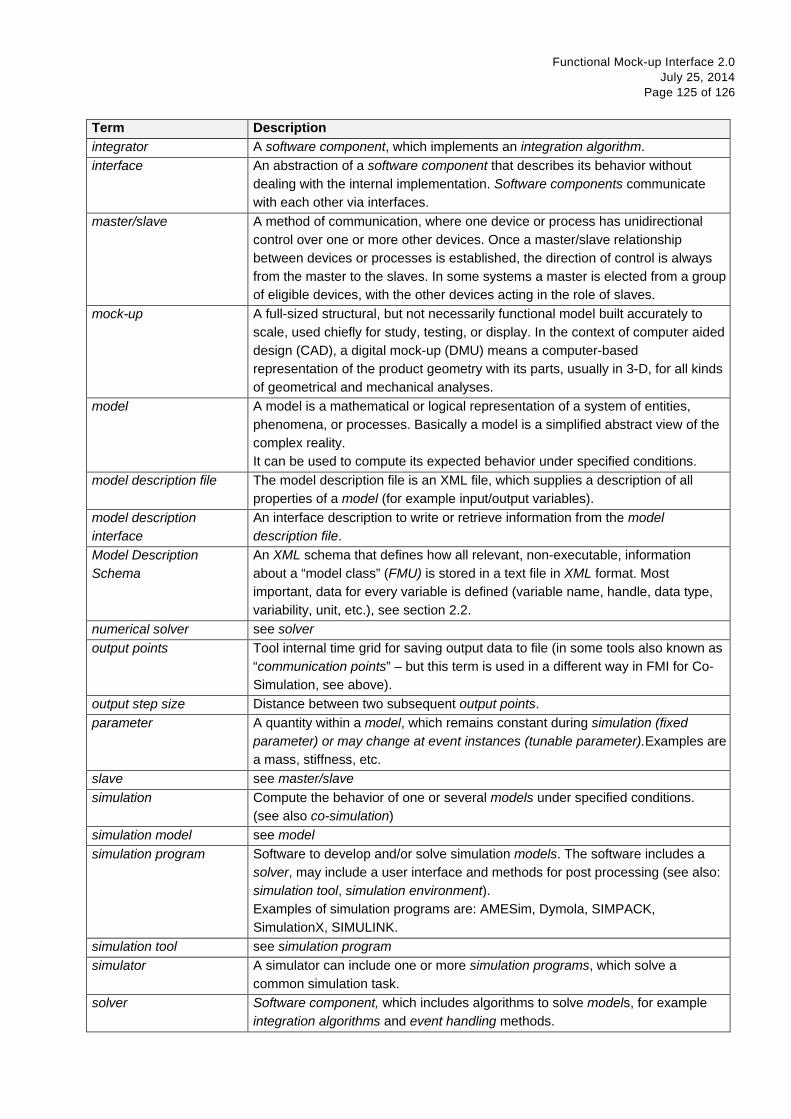
Functional Mock-up Interface 2.0 July 25, 2014
Page 125 of 126
Term Description integrator A software component, which implements an integration algorithm. interface An abstraction of a software component that describes its behavior without
dealing with the internal implementation. Software components communicate with each other via interfaces.
master/slave A method of communication, where one device or process has unidirectional control over one or more other devices. Once a master/slave relationship between devices or processes is established, the direction of control is always from the master to the slaves. In some systems a master is elected from a group of eligible devices, with the other devices acting in the role of slaves.
mock-up A full-sized structural, but not necessarily functional model built accurately to scale, used chiefly for study, testing, or display. In the context of computer aided design (CAD), a digital mock-up (DMU) means a computer-based representation of the product geometry with its parts, usually in 3-D, for all kinds of geometrical and mechanical analyses.
model A model is a mathematical or logical representation of a system of entities, phenomena, or processes. Basically a model is a simplified abstract view of the complex reality. It can be used to compute its expected behavior under specified conditions.
model description file The model description file is an XML file, which supplies a description of all properties of a model (for example input/output variables).
model description interface
An interface description to write or retrieve information from the model description file.
Model Description Schema
An XML schema that defines how all relevant, non-executable, information about a “model class” (FMU) is stored in a text file in XML format. Most important, data for every variable is defined (variable name, handle, data type, variability, unit, etc.), see section 2.2.
numerical solver see solver output points Tool internal time grid for saving output data to file (in some tools also known as
“communication points” – but this term is used in a different way in FMI for Co-Simulation, see above).
output step size Distance between two subsequent output points. parameter A quantity within a model, which remains constant during simulation (fixed
parameter) or may change at event instances (tunable parameter).Examples are a mass, stiffness, etc.
slave see master/slave simulation Compute the behavior of one or several models under specified conditions.
(see also co-simulation) simulation model see model simulation program Software to develop and/or solve simulation models. The software includes a
solver, may include a user interface and methods for post processing (see also: simulation tool, simulation environment). Examples of simulation programs are: AMESim, Dymola, SIMPACK, SimulationX, SIMULINK.
simulation tool see simulation program simulator A simulator can include one or more simulation programs, which solve a
common simulation task. solver Software component, which includes algorithms to solve models, for example
integration algorithms and event handling methods.

Functional Mock-up Interface 2.0 July 25, 2014
Page 126 of 126
Term Description state The “continuous states” of a model are all variables that appear differentiated in
the model and are independent from each other. The “discrete states” of a model are time-discrete variables that have two values in a model: The value of the variable from the previous event instant, and the value of the variable at the actual event instant.
state event Event that is defined by the time instant where the domain z > 0 of an event indicator variable z is changed to z ≤ 0, or vice versa. This definition is slightly different from the usual standard definition of state events: “z(t)*z(ti-1) ≤ 0” which has the severe drawback that the value of the event indicator at the previous event instant, z(ti-1) ≠ 0, must be non-zero and this condition cannot be guaranteed. The often used term “zero crossing function” for z is misleading (and is therefore not used in this document), since a state event is defined by a change of a domain and not by a zero crossing of a variable.
step event Event that might occur at a completed integrator step. Since this event type is not defined by a precise time or condition, it is usually not defined by a user. A program may use it, for example to dynamically switch between different states. A step event is handled much more efficiently than a state event, because the event is just triggered after performing a check at a completed integrator step, whereas a search procedure is needed for a state event.
super dense time A precise definition of time taking into account iterations at an event. For an FMU, the independent variable time 𝑡 ∈ 𝕋 is a tuple 𝑡 = (𝑡𝑅, 𝑡𝐼) where 𝑡𝑅 ∈ ℝ,𝑡𝐼 ∈ ℕ = {0,1,2, … }. The real part 𝑡𝑅 of this tuple is the independent variable of the FMU for describing the continuous-time behavior of the model between events. In this phase 𝑡𝐼 = 0. The integer part 𝑡𝐼 of this tuple is a counter to enumerate (and therefore distinguish) the events at the same continuous-time instant 𝑡𝑅.
time event Event that is defined by a predefined time instant. Since the time instant is known in advance, the integrator can select its step size so that the event point is directly reached. Therefore, this event can be handled efficiently.
user interface The part of the simulation program that gives the user control over the simulation and allows watching results.
value reference The value of a scalar variable of an FMU is identified with an Integer handle called value reference. This handle is defined in the modelDescription.xml file (as attribute valueReference in element ScalarVariable). Element valueReference might not be unique for all variables. If two or more variables of the same base data type (such as fmi2Real) have the same valueReference, then they have identical values but other parts of the variable definition might be different (for example min/max attributes).
XML eXtensible Markup Language (www.w3.org/XML, en.wikipedia.org/wiki/XML) – An open standard to store information in text files in a structured form.