functional mri user's guide - university of california,...
TRANSCRIPT

Functional MRI User's Guide
Michael A. Yassa
● The Division of Psychiatric Neuroimaging ●● Department of Psychiatry and Behavioral Sciences ●
● The Johns Hopkins School of Medicine ●● Baltimore, MD ●
1
Document written in OpenOffice.org Writer 2.0 by Sun MicrosystemsPublication date: June 2005 (1st edition)
Online versions available at http://pni.med.jhu.edu/intranet /fmriguide/
Acknowledgments: This document relies heavily on expertise and advice from the following individualsand/or groups: John Ashburner, Karl Friston, and Will Penny (FIL-UCL: London), KalinaChristoff (UBC: Canada), Matthew Brett (MRC-CBU: Cambridge), and Tom Nichols(SPH-UMichigan, Ann Arbor). Some portions of this document are adapted or copiedverbatim from other sources, and are referenced as such.
Supplemental Reading:
Frackowiak RS, Friston K, Frith C, Dolan RJ, Price CJ, Zeki S, Ashburner J, & Perchey G(2004). Human Brain Function, 2nd edition, Elsevier Academic Press, San Diego, CA.
Huettel SA, Song AW, McCarthy, G. (2004) Functional Magnetic Resonance Imaging.Sinaur Associates, Sunderland, MA.
2
Table of ContentsMagnetic Resonance Physics..............................................................................6
How the MR Signal is Generated.............................................................................6The BOLD Contrast Mechanism..............................................................................8Hemodynamic Modeling.........................................................................................10Signal and Noise in fMRI........................................................................................12
Thermal Noise.......................................................................................................12Cardiac and respiratory artifacts............................................................................12N/2 Ghost..............................................................................................................12Subject motion.......................................................................................................12Draining veins........................................................................................................13Scanner drift..........................................................................................................13Susceptibility artifacts............................................................................................13
Experimental Design...........................................................................................14Cognitive subtractions ...........................................................................................14Cognitive Conjunctions...........................................................................................14Parametric Designs................................................................................................14Multi-factorial Designs............................................................................................15Optimizing fMRI Studies.........................................................................................15
Signal Processing..................................................................................................15Confounding Factors.............................................................................................15
Control task............................................................................................................16Latent (hidden) factor.............................................................................................16Randomization and Counterbalancing...................................................................16Nonlinear Hemodynamic Effects............................................................................16
Epoch (Blocked) and Event-Related Designs .......................................................17Spatial and Temporal Pre-Processing...............................................................18
Overview................................................................................................................18Raw Data ...............................................................................................................18Getting Started.......................................................................................................18Requirements.........................................................................................................19
Hardware Requirements........................................................................................19Software Requirements.........................................................................................19
Software Set-up......................................................................................................19The SPM Environment...........................................................................................20Data Transfer from Godzilla...................................................................................20Volume Separation and Analyze headers .............................................................21Buffer Removal.......................................................................................................24Slice Timing Correction (For event-related data)...................................................24
To Correct or Not to Correct..................................................................................24Philips Slice Acquisition Order...............................................................................25Which Slice to Use as a Reference Slice...............................................................25
Timing Parameters.................................................................................................26Rigid-Body Registration (Correction for Head Motion)...........................................26
3
Creating a Mean Image.........................................................................................26Realignment...........................................................................................................27
Anatomical Co-registration (Optional)....................................................................29Co-registering Whole Brain Volumes.....................................................................30Co-registering Partial Brain Volumes.....................................................................30
Spatial Normalization to Standard Space..............................................................30Correcting Scan Orientation..................................................................................31Normalization Defaults...........................................................................................31Normalization to a Standard EPI Template............................................................32Gaussian Smoothing.............................................................................................33
Summary of Pre-processing Steps........................................................................34Statistical Analysis using the General Linear Model.......................................35
Modeling and Inference in SPM.............................................................................35Model Specification and the SPM Design Matrix ..................................................35
Setting Up fMRI Defaults.......................................................................................36Model Specification................................................................................................36Estimating a Specified Model................................................................................39
Global Intensity Normalization................................................................................40Temporal Filtering...................................................................................................40
Results and Statistical Inference............................................................................42Contrast Specification............................................................................................42Thresholding and Inference ..................................................................................43
Rejecting the Null Hypothesis.................................................................................43Type I Error (Multiple Comparison Correction).......................................................44Spatial Extent Threshold (Cluster analysis) ...........................................................46
Viewing Results using Maximum Intensity Projection ...........................................46Small Volume Correction and Regional Hypotheses.............................................48Extracting Results and Talairach Labeling.............................................................48Time-Series Extraction and Local Eigenimage Analysis .......................................49Plotting Responses and Parameter Estimates......................................................50Anatomical Overlays..............................................................................................53Editing, Printing and Exporting SPM output...........................................................55
Region of Interest (ROI) Analyses......................................................................56Anatomical vs. Functional ROIs ............................................................................56MarsBaR (MARSeille Boîte À Région d'Intérêt) ....................................................57
Overview of the Toolbox........................................................................................57ROI Definition........................................................................................................57Running an ROI Analysis ......................................................................................59
Group-Level Analysis and Population-level Inferences...................................63Inter-subject Analyses............................................................................................63Fixed-Effects Analysis............................................................................................63Random-Effects Analysis.......................................................................................64Conjunction Analysis .............................................................................................66Nonparametric Approaches....................................................................................67False Discovery Rate.............................................................................................68
4

Special Topics.....................................................................................................68Cost Function Masking for Lesion fMRI.................................................................68Advanced Spatial Normalization Methods.............................................................69Using a Subject-Specific HRF in analysis .............................................................70Guidelines for Presenting fMRI Data......................................................................73
5

Magnetic Resonance Physics
How the MR Signal is GeneratedThe magnetic resonance (MR) signal arises from hydrogen nuclei, which are the only
dipoles abundant enough to be measured with reasonably high spatial resolution. The humanbody is made up mostly of water (mainly hydrogen atoms). Hydrogen atoms possess amagnetic property called spin which can be thought of as a small magnetic field. Spin is afundamental property of some nuclei (not all nuclei possess spin) and has two importantparameters: (1) size; spin comes in multiples of ½ and (2) charge; spin can be positive ornegative. Paired opposite-charged particles, e.g. protons and electrons can eliminate eachother's spin effects. An unpaired proton (e.g. in the case of hydrogen) has a spin of +½.
In an external magnetic field, a particle with non-zero spin will experience a torque whichaligns the particle with the field, by precessing (wobbling) aroundthe magnetic field axis (see figure on the left). The particle developsan angular momentum, which is empirically related to itsgyromagnetic ratio (γ) (the ratio of the magnetic dipole moment tothe angular momentum of the particle). This value is unique to thenucleus of each element (For Hydrogen, γ = 42.58 MHz/T). Thevalue's derivation is too complex to explain here. Instead we willdescribe its relationship to the precession angular frequency (ω)of a proton. Angular frequency is a scalar measure of how fast aparticle is rotating around an axis (see figure on the right)
ωLarmor = γ Β
The above is known as the Larmor Equation namedafter Joseph Larmor, an Irish physicist (1857-1942). Itdescribes the relationship between the angular frequency (ω)of precession and the strength of the magnetic field B. There
are two possible configurations forproton alignment; one configurationpossesses higher energy than theother (see figure on the left). Aproton can undergo a transitionbetween the two energy states byabsorbing a photon that hasenough energy to match the energy
6

difference between the two states. This energy E is related to the photon's frequency ν byPlanck's constant h (6.626 x 10⁻³⁴ J-sec)
E = h ν
This frequency is associated with a spin flip and is often used to describe the Larmor frequencyas well.
ωLarmor = ν
In the context of MRI, a radio-frequency (RF) pulse is applied perpendicular to the staticmagnetic field (B0). This pulse, which has a frequency equal to the Larmor frequency, shiftsprotons into a higher energy state. When the RF pulse (BRF) stops, the protons return toequilibrium such that their magnetic moment is parallel again to B0. During this process ofnuclear relaxation, the nuclei lose energy by emitting their own RF signal. This is referred to asa free-induction decay (FID) response signal. The FID response signal is measured by a fieldRF coil, and has the characteristic shape shown in the figure below.
The Rf coil measure the relaxationof the dipoles in two dimensions. TheTime-1 (T1) constant measures thetime for the longitudinal relaxation inthe direction of the B0 field (shownbelow on the left). It is referred to asspin-lattice relaxation.
The Time-2 (T2) constantmeasures the time it takes for thetransverse relaxation of the dipole inthe plane perpendicular to the B0 field(shown below on the right). It isreferred to as spin-spin relaxation.
The T2 relaxation process is affected by molecular interactions and variations in B0. Thecombined time constant (in physiological tissue) is called T2* (T2 star). In the case of MRI, wetake advantage of the fact that physiological tissue does not contain not a homogeneousmagnetic field, and thus the transverse relaxation is much faster. The size of theseinhomogeneities depends on physiological processes, such as the composition of the localblood supply.
7

The BOLD Contrast MechanismThis mechanism is employed in most fMRI studies. The idea is that neural activity
changes the relative concentration of oxygenated and deoxygenated hemoglobin in the localblood supply. Deoxyhemoglobin (dHb) is paramagnetic (changes the MR signal), whileoxyhemoglobin is diamagnetic (does not change the MRI signal). An increase in dHb causes theT2* constant to decrease. This was first noticed by Ogawa et al. In 1990 1 in the rodent brain,and over the following few years became the mainstay of functional MRI. The BOLD Contrastrefers to the difference in T2* signal between oxygenated (HbO2) and dexoygenated (dHB)hemoglobin.
The above figure illustrates the physiological events that underlie our recording of the MRsignal. Upon stimulation, neural activation occurs, which pulls oxygen from the local bloodsupply. Theoretically, as the paramagnetic dHb increases, the field inhomogeneities areenhanced and the BOLD signal is reduced. However, the dHb increase is tightly coupled with asurge in cerebral blood flow (CBF) which compensates for the decrease in oxygen, delivering alarger supply of oxygenated blood. The result is a net increase in cerebral blood volume (CBV)and in Hb oxygenation, which decreases the susceptibility-related dephasing, increasing T2*signal and in turn enhancing the BOLD contrast.1 Ogawa S., Lee T.M., Nayak A.S., Glynn P. (1990). Oxygenation-sensitive contrast in magnetic resonance image
of rodent brain at high magnetic fields. Magn Reson Med 14:68-78.
8

The BOLD response can be thought of as the combination of four processes: (1) An initial decrease (dip) in signal caused by a combination of a negative metabolic and
non-metabolic BOLD effect. The local flow change as a result of the immediate oxygenextraction leads to a negative metabolic BOLD effect, while the vasodilation leads to anon-metabolic (or volumetric) negative BOLD effect.
(2) A sustained signal increase or positive BOLD effect due to the significantly increasedblood flow and the corresponding shift in the deoxy/oxy hemoglobin ratio. As the bloodoxygenation level increases, the signal continues to increase.
(3) A sustained signal decrease which is induced by the return to normal flow and normaldeoxy/oxy hemoglobin ratios.
(4) A post-stimulus undershoot caused by the slow recovery in cerebral blood volume.
9

Hemodynamic ModelingThe BOLD response is very complex. The signal depends on the total of dHb, which
means that the total blood volume is also a factor. Another factor is the amount of oxygenleaving the blood to enter the tissue (metabolic changes), which also changes the bloodoxygenation level. Finally, due to the elasticity of vascular tissue, increasing blood flow, changesblood volume. All these factors have to be modeled adequately in order for us to estimate theneural signal. The model currently employed in research and literature uses a canonicalhemodynamic response function that linearly transforms neural activity to the observed MRsignal. However, being able to get the true neural signal based on the hemodynamic counterpartis a bigger problem.
Ideally, we would like to evaluate how well our linear transform model allows us toestimate the actual neural signal. This can be done using simultaneous measurements of theneural and BOLD signals.
Source: Logothetis and Wandell 2004 2
The above figure shows these simultaneous measurements in a monkey brain, usingextracellular field potential recording, together with fMRI. (a) the black trace is the meanextracellular field potential (mEFP) signal; the red trace is the BOLD response. (b) spike activity
2 Logothetic NK, Wandell BA. (2004). Interpreting the BOLD signal. Ann Rev Physiol 66:735-69
10
derived from the mEFP. (c) frequency band separation of the mEFP (d) estimated temporalpulse response function relating the neurophysiological and BOLD measurements in monkeys.Even though these recordings are problematic due to their invasive nature (cannot be done inhumans) and due to sampling bias, they provided useful evidence for the coupling of the neuralsignal and the hemodynamic response.
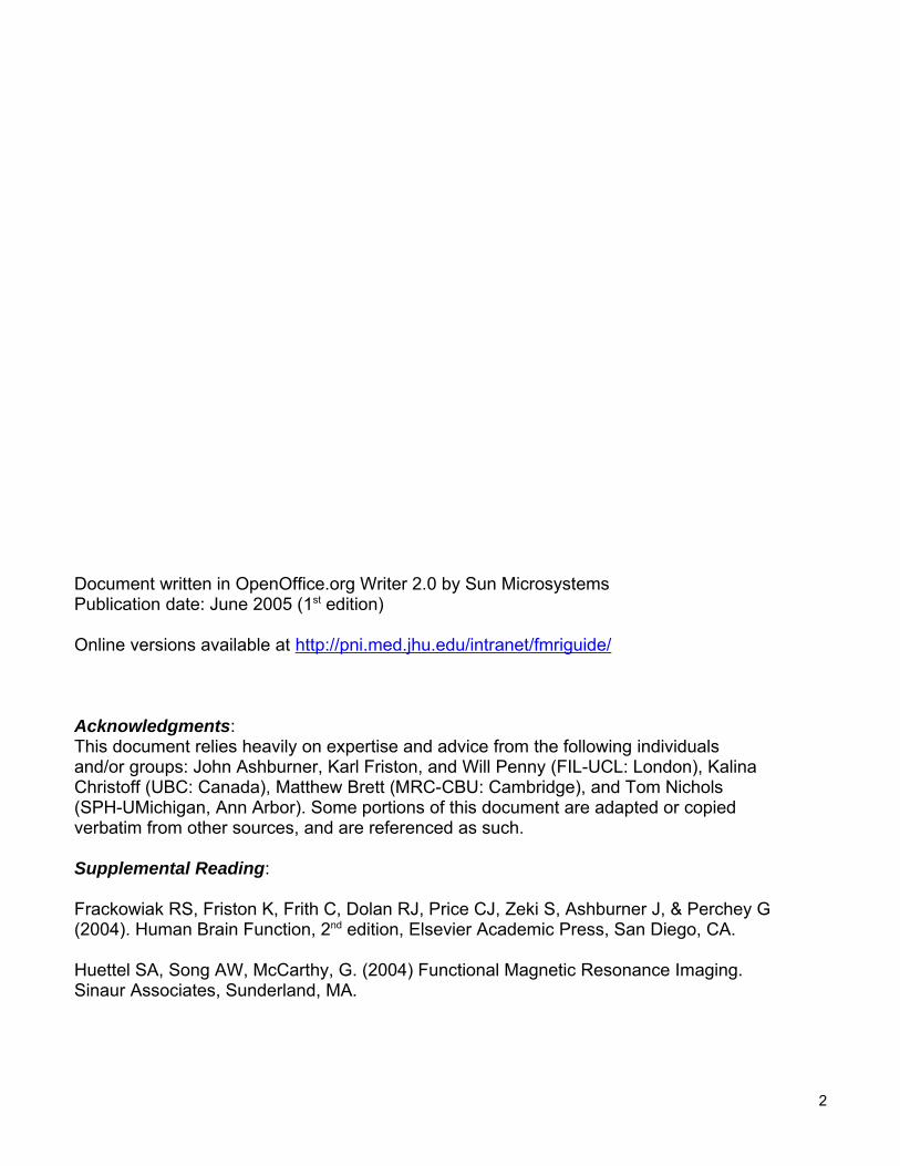
In human fMRI, we can estimate the hemodynamic response function, using known taskswith known and expected specific neural activation, e.g. visual, motor, etc... Results that areconsistent with what we already know about specific structures' involvement in cognitiveprocesses may provide some insight (even though it is at best speculative) into the neural
activation and the related hemodynamicresponse. Over recent years, a moredescriptive canonical hemodynamicresponse function has been developed thataccounts for the timing delay (temporalderivative) as well as the duration (dispersionderivative) of the response. This set offunctions is what SPM uses to estimate theneural signal. The mathematics behind thehemodynamic model are too complicated toexplain here, but more details are given inthe fMRI analysis section.
It is important to understand however thatthis model is a 'best fit' model, which meansit does a good job of explaining variance inthe hemodynamic response after neuralstimulation. However, it does not explain allthe parameters. The metabolic and neuralprocesses that couple action potentials toblood flow are still not well understood, andare the subject of much of today's fMRIresearch.
Animal research is attempting to carry outmore multi-modal experiments to produce empirical data to support or reject this model, andhuman research is getting better at the deconvolution of the neural impulse using higher ordermathematical modeling.
From the above we can see the entire cycle takes about 30 seconds to complete. Earlyevent-related studies were limited by this, and thus had to use very long inter-stimulus intervalsto allow the response to return to baseline before another one started. If the hemodynamicresponses were perfectly linear, then they should not have been hindered by this, as the linearsummation of HRFs can be deconvolved easily. However, BOLD response non-linearities exist,and pose a problem. This non-linearity can be thought of as a “saturation” effect where theresponse to a series of events is smaller than would be predicted by the sum of the BOLDresponses from the individual events. Empirically, it has been found that for SOA3 of below ~8seconds, the degree of saturation increases as the SOA decreases. However, for SOA of 2-4
3 SOA: Stimulus Onset Asynchrony – This is the amount of delay between the presentation of one experimentalstimulus to another.
11
seconds, the magnitude of saturation is small. This is important to think about in designing anfMRI experiment, and is particularly of importance in discussing rapid event-related fMRI.
To summarize, the general shape of the hemodynamic response is the same acrossindividuals and cortical areas. However, the precise shape varies from individual to individualand from area to area. Canonical modeling however offers us a powerful tool to be able toreasonably estimate the neural signal, based on the observed changes in regional cerebralblood flow.
Signal and Noise in fMRIThe magnitude of the BOLD response signal we are trying to measure in fMRI is very
small compared to the overall MR signal. We can improve our signal detection ability byincreasing the amplitude of the signal or reducing the amplitude of the noise. The type of controlis referred to as signal-to-noise ratio or SNR. There are many different sources of noise thatproduce artifacts in the scanner. Here is a brief description of some of the most commonproblems:
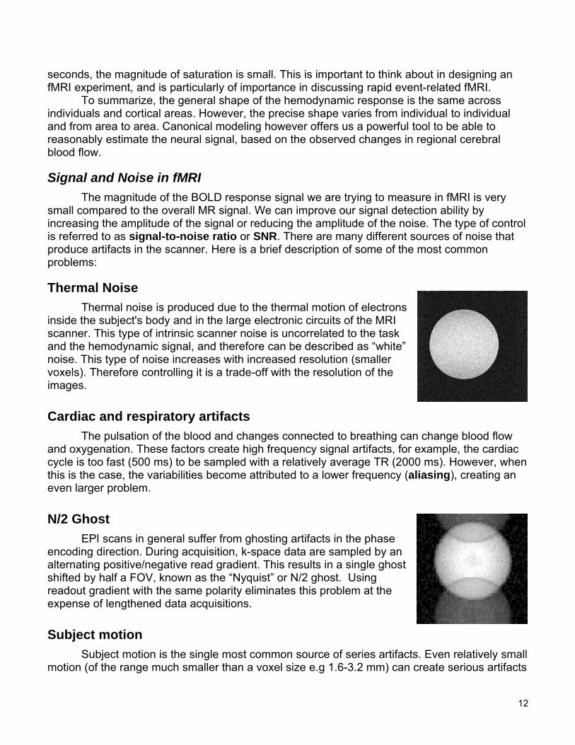
Thermal NoiseThermal noise is produced due to the thermal motion of electrons
inside the subject's body and in the large electronic circuits of the MRIscanner. This type of intrinsic scanner noise is uncorrelated to the taskand the hemodynamic signal, and therefore can be described as “white”noise. This type of noise increases with increased resolution (smallervoxels). Therefore controlling it is a trade-off with the resolution of theimages.
Cardiac and respiratory artifactsThe pulsation of the blood and changes connected to breathing can change blood flow
and oxygenation. These factors create high frequency signal artifacts, for example, the cardiaccycle is too fast (500 ms) to be sampled with a relatively average TR (2000 ms). However, whenthis is the case, the variabilities become attributed to a lower frequency (aliasing), creating aneven larger problem.
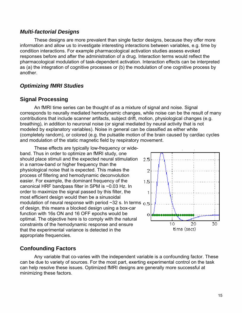
N/2 GhostEPI scans in general suffer from ghosting artifacts in the phase
encoding direction. During acquisition, k-space data are sampled by analternating positive/negative read gradient. This results in a single ghostshifted by half a FOV, known as the “Nyquist” or N/2 ghost. Usingreadout gradient with the same polarity eliminates this problem at theexpense of lengthened data acquisitions.
Subject motionSubject motion is the single most common source of series artifacts. Even relatively small
motion (of the range much smaller than a voxel size e.g 1.6-3.2 mm) can create serious artifacts
12

due to the partial volume effects. Typically motion of about half a voxel in size will render thedata useless. Subjects should be instructed not to move, with their heads restrained securely.The task design should also minimize the possibility of task related movements.
Draining veinsLarge vessels draining in the brain could induce a hemodynamic signal, that may not be
easily differentiated from the hemodynamic responses related to the neural signal. This is hardto control, thus caution should be taken in considering activation occurring close to visible largevessels.
Scanner driftDrift is created most probably by the small instability of scanner gradients. It can create
slow changes in voxel intensity over time. Even though the magnet contains hugesuperconducting coils to maintain its magnetic field, the stability of this magnetic field isoccasionally drifts. This type of spatial distortion can also be caused by non-system factors, e.g.the subject's head slowly moving downwards due to a possible leak in the vacuum pack holdingthe head in place.
Susceptibility artifactsThe EPI images are very sensitive to the changes of the
magnetic susceptibility. In effect the signal from regions close to sinusesand bottom of the brain may disappear. This can also be caused by thepresence of magnetic material in proximity of the gradients, e.g.Implants, braces, buttons, or even another human body moving in theroom.
13

Experimental DesignThis section deals with the different designs that can be employed in neuroimaging
studies. Designs in general can be subdivided into categorical (or parametric) designs and multi-factorial designs, with the latter being more complicated than the former.
Cognitive subtractions These are one type of categorical design, which rely on the premise that the difference
between two tasks can be qualified as a separate cognitive components that is distinct in spaceand therefore can be separated as an individual component of the hemodynamic response. Anexample is a study in which visual and motor stimulation are combined in the experimental taskor condition, while the control task or condition consist of only the visual or only the motorstimulation. Subtracting the activation in one condition from the other is expected to show onlythe activation relevant to the specific type of stimulation. The problem with these designs is theunderlying assumption that the neural processes underlying behavior are additive in nature. Dueto the complexity of neural responses and the significant functional integration between variousbrain structures, this assumption may not always hold true.
Cognitive ConjunctionsThese designs can be thought of as a series of subtractions. Instead of testing a single
hypothesis pertaining to the activation in one task over the other, conjunctions test severalhypotheses at a time, asking whether all activations are jointly significant. For example, if we areinterested in verbal working memory, then we can use a series of tasks that have that cognitivecomponent in common, but nothing else in common. The conjunction of these tasks shouldshow only the structures that are involved in verbal working memory. Conjunction analysesallow us to demonstrate neural responses independent of context.
Note: Testing joint significance using conjunctions is a notion that we will return to when wediscuss group fMRI analysis.
Parametric DesignsThe underlying premise in these designs is that regional activation will vary systematically
with the degree of cognitive processing. For example, an fMRI study of hemodynamicresponses and performance on a cognitive task illustrates the utility of this design. Correlationsor neurometric functions may or may not be linear. Clinical neuroscience can use parametricdesigns by looking for neuronal correlates of clinical ratings over subjects (e.g. symptomseverity, IQ, performance on QNE, etc..). The statistical design then can be viewed as a multiplelinear regression model. However, if one needed to investigate several clinical scores that arecorrelated, we have a problem with running the regression model, since variables are notorthogonal. In this case, factor analysis, or principal components analysis (PCA) is used toreduce the number of possible explanatory variables, and render them orthogonal to each other.
14
Multi-factorial DesignsThese designs are more prevalent than single factor designs, because they offer more
information and allow us to investigate interesting interactions between variables, e.g. time bycondition interactions. For example pharmacological activation studies assess evokedresponses before and after the administration of a drug. Interaction terms would reflect thepharmacological modulation of task-dependent activation. Interaction effects can be interpretedas (a) the integration of cognitive processes or (b) the modulation of one cognitive process byanother.
Optimizing fMRI Studies
Signal ProcessingAn fMRI time series can be thought of as a mixture of signal and noise. Signal
corresponds to neurally mediated hemodynamic changes, while noise can be the result of manycontributions that include scanner artifacts, subject drift, motion, physiological changes (e.g.breathing), in addition to neuronal noise (or signal mediated by neural activity that is notmodeled by explanatory variables). Noise in general can be classified as either white(completely random), or colored (e.g. the pulsatile motion of the brain caused by cardiac cyclesand modulation of the static magnetic field by respiratory movement.
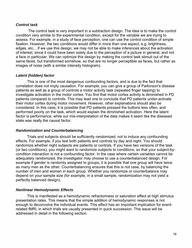
These effects are typically low-frequency or wide-band. Thus in order to optimize an fMRI study, oneshould place stimuli and the expected neural stimulationin a narrow-band or higher frequency than thephysiological noise that is expected. This makes theprocess of filtering and hemodynamic deconvolutioneasier. For example, the dominant frequency of thecanonical HRF bandpass filter in SPM is ~0.03 Hz. Inorder to maximize the signal passed by this filter, themost efficient design would then be a sinusoidalmodulation of neural response with period ~32 s. In termsof design, this means a blocked design using a box-carfunction with 16s ON and 16 OFF epochs would beoptimal. The objective here is to comply with the naturalconstraints of the hemodynamic response and ensurethat the experimental variance is detected in theappropriate frequencies.
Confounding FactorsAny variable that co-varies with the independent variable is a confounding factor. These
can be due to variety of sources. For the most part, exerting experimental control on the taskcan help resolve these issues. Optimized fMRI designs are generally more successful atminimizing these factors.
15
Control task The control task is very important in a subtraction design. The idea is to make the control
condition very similar to the experimental condition, except for the variable we are trying toassess. For example, in a study of face perception, one can use the control condition of simplefixation. However, the two conditions would differ in more than one aspect, e.g. brightness,edges, etc... If we use this design, we may not be able to make inferences about the activationof interest, since it could have been solely due to the perception of a picture in general, and nota face in particular. We can optimize this design by making the control task stimuli out of thesame faces, but transformed somehow, so that are no longer perceptible as faces, but rather asimages of noise (with a similar intensity histogram).
Latent (hidden) factorThis is one of the most dangerous confounding factors, and is due to the fact that
correlation does not imply causation. For example, you can give a group of Parkinson's diseasepatients as well as a group of controls a motor activity task (repeated finger tapping) toinvestigate activation in the motor cortex. You find that motor cortex activity is diminished in PDpatients compared to controls. This may lead one to conclude that PD patients under-activatetheir motor cortex during motor movement. However, other explanations should also beconsidered. In this case, it is possible that PD patients pressed the buttons less often, andperformed poorly on the task, which would explain the diminished activation. Here the latentfactor is performance, while our mis-interpretation of the data makes it seem like the diseasedstate was really the causal factor.
Randomization and CounterbalancingTrials and subjects should be sufficiently randomized, not to induce any confounding
effects. For example, if you test both patients and controls by day and night. You shouldrandomize whether night subjects are patients or controls. If you have two versions of the task(or two conditions), you might want to randomize subjects to conditions, so that your subject-by-condition interaction is not a confounding factor. In the case where certain variables cannot beadequately randomized, the investigator may choose to use a counterbalanced design. Forexample if gender is randomly assigned to groups, it is possible that one group will have twiceas many men as the other. Counterbalancing ensures that this is not case, by balancing thenumber of men and women in each group. Whether you randomize or counterbalance maydepend on your sample size (for example, in a small sample, randomization may not yield aperfectly balanced design).
Nonlinear Hemodynamic EffectsThis is manifested as a hemodynamic refractoriness or saturation effect at high stimulus
presentation rates. This means that the simple addition of hemodynamic responses is notenough to deconvolve the individual events. This effect has an important implication for event-related fMRI, in which trials are usually presented in quick succession. This issue will beaddressed in detail in the following section.
16

Epoch (Blocked) and Event-Related Designs Typically, fMRI experimental design can be classified into two types: a blocked design
(epoch-related) and a single event design (event-related). Blocked designs are the moretraditional type and involve the presentation of stimuli as blocks containing many stimuli of thesame type. For example, one may use a blocked design for a sustained attention task, wherethe subject is instructed to press the button every time he or she sees an X on the screen.Typically blocks of stimulation are separated from each other by equivalent blocks of rest (wherethe subject may be instructed to passively attend to a fixation cross on the screen. This type ofdesign is depicted below.
Blocked designs are simple to design and implement. They also have the addedadvantage that we can present a large number of stimuli, and thus increase our signal to noiseratio. It has excellent detection power, but is insensitive to the shape of the hemodynamicresponse. We also have to assume a single mode of activity at a constant level duringstimulation. In other words, we cannot infer any information regarding the individual events. Thisprecludes us from being able to investigate interesting questions, such as the relationship ofactivation to accuracy and performance or reaction time. We use blocked designs if we plan touse a cognitive subtraction or conjunction to analyze our data.
The alternative to epoch designs is a more powerful estimation method. Event-relatedfMRI has emerged as a much more informative method that allows for a number of otheranalyses to be conducted. Rapid, randomized, event-related fMRI is the newest improvementon this concept. The idea is to present individual stimuli of various condition types in randomizedorder, with variable stimulus onset asynchrony (SOA). This provides us with enough informationfor time-series deconvolution using a canonical or individual-derived HRF, and allows us toconduct post-hoc analyses with trial sorting (accuracy, performance, etc...). This design is moreefficient, because the built-in randomization (jittering) ensures that preparatory or anticipatoryeffects (which are common in blocks designs) do not confound event-related responses. Atypical event-related design is depicted below.
Mixed designs are also possible (combining aspects of blocked and event-relateddesigns, however they are much more complicated to design and analyze. They usually containblocks of control and experimental stimuli, however within each block are multiple types ofstimuli. It allows us to simultaneously examine state-related processes (best evaluated using ablock design) and item-related processes (best evaluated using an event-related design).
17

Spatial and Temporal Pre-Processing
OverviewFunctional MRI (fMRI) pre-processing is designed to accomplish several purposes. It
corrects for head motion artifacts during the scan (realignment), adjusts the data to a standardanatomical template (normalization) and convolves the data with a smooth function suitable foranalysis (smoothing). The pre-processing is done within the Statistical Parametric Mapping(SPM) environment which is a MATLAB package with a graphical user interface (GUI).Additional MATLAB functions will be used and will be described in detail. Depending on thecomputer speed and dataset size, pre-processing can take several hours or days.
Pre-processing also requires a lot of hard drive space, for example if a single subject’sdataset is 1000 MB (1GB) in size, you will need 5000 MB (5GB) of space to pre-process thesubject’s data. Of course once the pre-processing is done, a lot of the data generated in theintermediate steps can be deleted, and this can be used to save hard drive space. The pre-processing directory should be either (1) an internal drive at 7200 RPM or more (RAID-0 SATAor 10-15K SCSI preferred) or (2) an external drive at high throughput rates. FireWire is therecommended medium, due to its reliability and high throughput rates (800 Mbps on machinesthat support 1394b). Pre-processing, in general should not be done over the network (i.e. writingimages to a mapped network drive), as it takes longer, and makes the process more prone tocrashing (this is severely affected by network traffic). However, you may run pre-processing onanother computer on the network, using remote desktop (and the pre-processing computer'snative Matlab/SPM). For instructions on how to set up the remote desktop, please seehttp://www.microsoft.com/windowsxp/using/mobility/default.mspx
Raw Data fMRI datasets are saved at the point of origin (Philips scanner) as combinations of
.par/rec files. This data is saved on Godzilla (large capacity UNIX-based server, maintained bythe F.M. Kirby Research Center: for questions about Godzilla or to set up a user account,please contact its administrator, Joe Gillen ([email protected]). Data is usually saved as acombination of the subject’s last name and the reverse date of the scan, followed by the scannumber (scans are numbered in the same order in which they were acquired), e.g.“yassa050103_3.rec”. You may let the technicians know to save the files using a different name(HIPAA regulations somewhat preclude saving these files with the subject last name).
Getting StartedTo start a new analysis on your computer, first you must create a new working directory
for storing all of the data files in your dataset. You have to make sure the drive on which yousave the data has enough space to contain all the images. Then you should create a directory(without spaces in the directory name), e.g. “C:\fmri\subjID\” to contain all of the subject’s fMRIdata. It is a good idea to keep your imaging data organized by project and by subject. fMRI datainvolves potentially thousands of files and thousands of data points, so it is essential to keepeverything organized and document this organizational structure somewhere safe.
18
Requirements
Hardware RequirementsYou must have the following hardware requirements before you begin:- Windows XP Professional or Windows 2000 or Redhat Linux 9.0 and above.- At least 20 GB of free space (60 recommended)- At least 1 GB of RAM (2 – 4 GB recommended)- 4 GB of swap space (also known as paging file on Windows)- Dual processors recommended.
Software RequirementsYou must have the following software on your computer, before you begin:- Matlab 6.0 or higher with SPM99 and its latest updates (download)- Secure Shell SSH Software
If you do not have any of these requirements, you should contact Arnold Bakker or Mike Yassato make sure you have the correct setup.
Software Set-upInstall Matlab 6.1 (or above) in its default directory. If you’re using a network installation
of Matlab, you may need to be on an enabled Matlab client (we have a limited number of clientlicenses). We also have a personal licensed version of Matlab which is more convenient andcan be installed without the need for network setup.
Download SPM99 from http://www.fil.ion.ucl.ac.uk/spm/ and extract it in a suitabledirectory, e.g. “C:\spm99” or “C:\Matlab6p1\spm99”. Find the file “r2a.m” under\\Soma\Matlab_functions . If you do not have access to Soma, contact Mike Yassa or ArnoldBakker to get a copy of r2a. Copy and paste the file in your SPM99 directory.
Open Matlab 6.1 and add SPM99’s directory to the Matlab path, by going to File> SetPath, and adding the SPM99 folder. Save the appended path, and close the “Set path“ window.To check that everything has been installed correctly, type “spm fmri” in the Matlab console andwait for the SPM windows to pop up. If you get error messages at this point, then yourinstallation was unsuccessful or your options are not set correctly.
Note regarding SPM use: SPM is a very resource-hungry program that can be verytemperamental. Make sure you close other open windows and other “memory hogging”programs, before you start pre-processing or analyzing using SPM. At times it may alsospontaneously suffer from an internal error and indicate this by printing a verbose and crypticoutput to the Matlab command window. It may also crash or lock up your Windows systementirely. If this happens, then shut down SPM and restart Matlab (restarting Matlab clears itscache memory, and is necessary before you start the same process again).
19

The SPM EnvironmentStatistical Parametric Mapping (SPM)
main panel allows you to select between twointerfaces, one for fMRI and one forPET/SPECT modeling. In order to bring up thisscreen, type >spm at the Matlab console. Clickon <fMRI Time-series> to bring up the fMRIinterface. If you are running spm2 as well, makesure that the spm99 directory is prepended tothe top of the Matlab path. Matlab will runwhichever instance of spm it finds in its pathfirst.
Three SPM windows should appear. TheUpper window will be referred to as the fMRIswitchboard. The lower left window is the SPMinput window, and the right window is the SPMgraphics output window. The switchboardconsists of a spatial preprocessing panel withoption for processing fMRI data. The statisticalanalysis panel containing the different linearmodels that can be applied to the data. Andfinally, the bottom panel contains useful tools fordisplaying images, changing directories,creating means, changing defaults, writingheaders, and running different toolbox options.Toolboxes are installed in \\spm99\toolbox. The<Defaults> button changes the defaults only forthe current session. If you close and restartSPM or Matlab, those changes will be lost. Youcan make permanent changes to fMRI defaultsby editing the spm_defaults.m file (or creatingan alternate version for your lab, and placing itin the Matlab path before the spm directory.
Data Transfer from GodzillaGodzilla is a large RAID array, acting as a storage server at the F.M. Kirby Research
Center at Kennedy Krieger Institute. It is the default image repository. We use this server totransfer subject data from the scanner to our laboratory. Once a subject's data is acquired, it isexported from the scanner database to a specific directory on Godzilla. Usually this is under oneof the two main disks (g1 or g2). Each investigator has a directory for storage and transfer, e.g.\\g1\myassa. Open Secure Shell (SSH) File Transfer Window, and connect to Godzilla(godzilla.kennedykrieger.org) using your username and password. Once connected, in the topmenu bar go to <Operation> and Select <Go to Folder>. In the folder window enter the folder
20
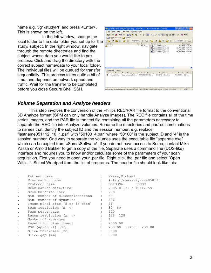
name e.g. “/g1/studyPI” and press <Enter>.This is shown on the left.
In the left window, change thelocal folder to the data folder you set up for thestudy/ subject. In the right window, navigatethrough the remote directories and find thesubject whose data you would like to pre-process. Click and drag the directory with thecorrect subject name/date to your local folder.The individual files will be queued for transfersequentially. This process takes quite a bit oftime, and depends on network speed andtraffic. Wait for the transfer to be completedbefore you close Secure Shell SSH.
Volume Separation and Analyze headers This step involves the conversion of the Philips REC/PAR file format to the conventional
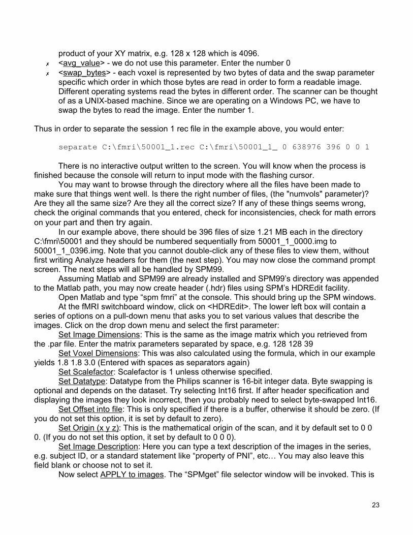
3D Analyze format (SPM can only handle Analyze images). The REC file contains all of the timeseries images, and the PAR file is the text file containing all the parameters necessary toseparate the REC file into Analyze volumes. Rename the directories and par/rec combinationsto names that identify the subject ID and the session number, e.g. replace“lastname051112_10_1.par” with “50100_4.par” where “50100” is the subject ID and “4” is thesession number. One way to separate the volumes uses the executable file “separate.exe”which can be copied from \\Soma\Software\. If you do not have access to Soma, contact MikeYassa or Arnold Bakker to get a copy of the file. Separate uses a command line (DOS-like)interface and requires you to know and/or calculate some of the parameters of your scanacquisition. First you need to open your .par file. Right click the .par file and select “OpenWith…”. Select Wordpad from the list of programs. The header file should look like this:
. Patient name : Yassa,Michael
. Examination name : #-#/g1/myassa/yassa050131
. Protocol name : Bold396 SENSE
. Examination date/time : 2005.01.31 / 10:12:59
. Scan Duration [sec] : 798
. Max. number of slices/locations : 39
. Max. number of dynamics : 396
. Image pixel size [8 or 16 bits] : 16
. Scan resolution (x, y) : 80 80
. Scan percentage : 100
. Recon resolution (x, y) : 128 128
. Number of averages : 1
. Repetition time [msec] : 2000.00
. FOV (ap,fh,rl) [mm] : 230.00 117.00 230.00
. Slice thickness [mm] : 3.00
. Slice gap [mm] : 0.00
21

The header file above has been truncated to only show the parameters of interest. TheRecon resolution is the reconstructed image matrix, and is what defines the image space. In thecase above, the matrix is 128 x 128 voxels (in the “x” and “y” planes). The plane of acquisition isplane “z” and is determined by the Number of Slices parameter, which in this case is 39. Thusthe image matrix is 128 x 128 x 39.
The Number of dynamics parameter determines the number of functional scans or timepoints in your series, for example 396 dynamics, means your rec file will be separated into 396Analyze volumes.
The FOV (ap, fh, rl) parameter describes the field of view in three dimensions (“ap” isanterior-posterior, “fh” is foot-head, and “rl” is right-left). Since the direction of acquisition of thisscan is axial (foot-head) that means the “fh” parameter (in this case, it is 117.00) is in the zorientation.
The voxel dimensions can be calculated from the image matrix and the field of view usingthe following formula:
Voxel size = FOV (mm) e.g. 230 x 230 x 117 = 1.8 x 1.8 x 3.0 mm Matrix (voxels) 128 x 128 x 39 voxel
Once you locate the file “separate.exe” copy it to your “C:\Windows” or “C:\WINNT”
directory. Now click on Start>Run and type “cmd” to display the command prompt. Test that thefile is in the right location and works by typing “separate” at the console, then hitting enter. Youshould get the following usage notification with a list of the arguments needed to separatevolumes.
Splits a set of volumes into individual filesUsage: separate <input_file_name> <output_filename> <head_bytes><volsize> <numvols> <bufsize> <avg value> <swap bytes? 0 or 1>
Here is an explanation of each of these arguments:✗ <input_file_name> - this is the name of the .rec file you would like to separate. You have
to type the full location of the file e.g. “C:\my_fmri\scan1.rec”. Separate also does not likespaces in folder or filenames.
✗ <output_file_name> - this is the root filename for the separated scans, for example“scan1_sess1_”. Output files would be appended with the dynamic number, e.g.scan1_sess1_0001.img etc…
✗ <head_bytes> - this is the number of bytes preceding the actual scan. Unless you havespecified this for your scan before acquisition, this parameter should be set to zero.
✗ <volsize> - this is the size of each volume in voxels, which is calculated from theinformation retrieved from the header. This is the equivalent of the image matrix, e.g. 128x 128 x 39. The product of those three numbers is the <volsize> parameter, which in thiscase is 638976 voxels.
✗ <numvols> - this is the number of volumes in the dataset, which is also the number ofdynamics, e.g. 396. This is the number of volumes your dataset will be split into.
✗ <bufsize> - this is the number of blank “buffer” voxels you may add to the beginning andend of each dynamic. We mostly do not use this parameter, but if you wanted to buffereach dynamic with a two-dimensional slice you would enter a number equivalent to the
22
product of your XY matrix, e.g. 128 x 128 which is 4096. ✗ <avg_value> - we do not use this parameter. Enter the number 0✗ <swap_bytes> - each voxel is represented by two bytes of data and the swap parameter
specific which order in which those bytes are read in order to form a readable image.Different operating systems read the bytes in different order. The scanner can be thoughtof as a UNIX-based machine. Since we are operating on a Windows PC, we have toswap the bytes to read the image. Enter the number 1.
Thus in order to separate the session 1 rec file in the example above, you would enter:
separate C:\fmri\50001_1.rec C:\fmri\50001_1_ 0 638976 396 0 0 1
There is no interactive output written to the screen. You will know when the process isfinished because the console will return to input mode with the flashing cursor.
You may want to browse through the directory where all the files have been made tomake sure that things went well. Is there the right number of files, (the "numvols" parameter)?Are they all the same size? Are they all the correct size? If any of these things seems wrong,check the original commands that you entered, check for inconsistencies, check for math errorson your part and then try again.
In our example above, there should be 396 files of size 1.21 MB each in the directoryC:\fmri\50001 and they should be numbered sequentially from 50001_1_0000.img to50001_1_0396.img. Note that you cannot double-click any of these files to view them, withoutfirst writing Analyze headers for them (the next step). You may now close the command promptscreen. The next steps will all be handled by SPM99.
Assuming Matlab and SPM99 are already installed and SPM99’s directory was appendedto the Matlab path, you may now create header (.hdr) files using SPM’s HDREdit facility.
Open Matlab and type “spm fmri” at the console. This should bring up the SPM windows. At the fMRI switchboard window, click on <HDREdit>. The lower left box will contain a
series of options on a pull-down menu that asks you to set various values that describe theimages. Click on the drop down menu and select the first parameter:
Set Image Dimensions: This is the same as the image matrix which you retrieved fromthe .par file. Enter the matrix parameters separated by space, e.g. 128 128 39
Set Voxel Dimensions: This was also calculated using the formula, which in our exampleyields 1.8 1.8 3.0 (Entered with spaces as separators again)
Set Scalefactor: Scalefactor is 1 unless otherwise specified.Set Datatype: Datatype from the Philips scanner is 16-bit integer data. Byte swapping is
optional and depends on the dataset. Try selecting Int16 first. If after header specification anddisplaying the images they look incorrect, then you probably need to select byte-swapped Int16.
Set Offset into file: This is only specified if there is a buffer, otherwise it should be zero. (Ifyou do not set this option, it is set by default to zero).
Set Origin (x y z): This is the mathematical origin of the scan, and it by default set to 0 00. (If you do not set this option, it set by default to 0 0 0).
Set Image Description: Here you can type a text description of the images in the series,e.g. subject ID, or a standard statement like “property of PNI”, etc… You may also leave thisfield blank or choose not to set it.
Now select APPLY to images. The “SPMget” file selector window will be invoked. This is
23

the standard way of selecting files in SPM. You can change the present directory fromC:\Matlab\work to the directory where your images are kept, and select all the *.img which youwrote using the separate function. You will notice that SPM does not list all of the files, butinstead it abbreviates the files with similar names and uses only the common root while thenumber of files sharing this root are marked with subscript numbers to the left of the name, e.g.39650001_1_*.img. In this case click on the filename root, and you should see that files 1-396were selected (turns blue). You can select more than one file and more than one series to writeheaders to. Once you have selected all the files for which you would like to write Analyzeheaders, click Done. SPM will create header files for each image file you selected, using thesame filename as the image file, but using the extension .hdr instead. You will see the progressin the bottom left window.
You can check that the headers were written correctly by double-clicking an image file,and displaying it in MRIcro. If the images do not display correctly, it is possible that yourdatatype should have been byte-swapped or that one or more of your parameters duringseparation and/or header creation was incorrect.
Buffer RemovalIn most fMRI acquisitions, the first few volumes acquired can be removed from the series
to be excluded from the analysis. This is done for two reasons. We have to make sure that thenet magnetization has reached steady state condition, and we also have to account for possiblehemodynamic effects that may be related to the start of the experiment, e.g. Scanner noise,shifting stimulus, etc... If these scans are included in the analysis there will be a large change insignal that is not related to experimental conditions per se, which should be avoided.
Before you remove any volumes, you have to make sure that these volumes wereacquired during rest (or fixation) and be sure that your model or design accounts for the lag thatwill result in the timing parameters. If you would rather not use the first few scans as a buffer,you can also use dummy scans to get magnetization to reach steady state before you start theactual experiment. This can be specified in your MRI protocol on the Philips scanner. Checkwith the MRI technician to make sure that enough dummy scans are included before the trigger.
Slice Timing Correction (For event-related data)
To Correct or Not to CorrectFunctional MRI data from the Philips scanner are acquired slice-wise so that a small
amount of time elapses between the acquisition of consecutive (or in the Philips case inter-leaving) slices. Given a TR of 2000 ms, for example, in a 20-slice acquisition, each slice wouldroughly take 100 ms to be acquired. This becomes an issue only in event-related designs whereone typically uses stimulus durations that elicit BOLD responses lasting only a couple ofseconds. For these designs it is critical that an appropriate temporal model is used, as anydifference between the expected and actual onset times may decrease the sensitivity of theanalysis. For short TR's (i.e. less than 3 seconds), slice timing correction can be used to remedythis problem. Essentially this pre-processing step will determine the midpoint slice in theacquisition and temporally interpolate all the other slices to this point.
Note: If slice timing correction is used, then one can use a naïve HRF model in theanalysis. If slice timing correction is not possible or is not performed, one can still model event-
24

related data using HRF derivatives (more information on this in the analysis section).
Philips Slice Acquisition OrderIn order to perform slice timing correction, click on the <Slice timing correction> button in
the SPM fMRI switchboard. Select all images in the series you would like to correct. Under<Sequence type> select <user specified>. The Philips scanner acquires slices in an odd-evensinterleaved pattern (i.e. 1, 3, 5, 7, … 2, 4, 6, 8, …). In the empty box enter the correct slice orderfrom your acquisition. For example, if you acquire 20 slices, enter: 1 3 5 7 9 11 13 15 17 19 2 46 8 10 12 14 16 18 20 . Numbers should be separated by a single space, and all slices in theacquisition should be included. Once you’re done click enter.
Note regarding slice acquisition order: At the point of scanning, you can specify andlet the MR technician know that you would like to acquire the scans in a sequential order (this isthe Kirby center default). If you do not change it, then they will be acquired according to thePhilips default (interleaved, odds then evens).
Which Slice to Use as a Reference SliceThe next prompt will be for the <Reference slice>. Enter the slice you want to consider as
a reference point. All other slices will be corrected to what they would have been if they wereacquired when the reference slice was acquired. The default is the middle slice (although,please make sure the default value given is indeed the middle slice for the number of slices youhave).
The logic behind selecting the middle slice as a reference point for slice timing correctionis that this way there will be a minimum total shifting in time required, and therefore anyinterpolation introduced by the correction procedure would be minimized. Some may argue thatin a perfect slice timing correction, the interpolation to any slice in the temporal sequence is thesame, and thus it doesn’t make any difference which slice you choose (even if it is in the spaceoutside the brain). However, SPM’s algorithm is not perfect and is worse for longer TR’s (more
10 as the reference slice.Note: When the first slice in time is NOT used as a reference during correction, the defaultsampled bin must be adjusted prior to analysis. More details in the analysis section.
25
Timing ParametersOnce you’ve specified the reference slice, SPM will prompt you for <Repetition Time
(TR)>. This parameter is in your .par file, and is quite simply the amount of time it takes thescanner to acquire a full volume. SPM will suggest a suitable TR by default, but this may not bethe correct TR. You must specify the correct TR for slice timing correction to work properly;otherwise temporal artifacts may be induced.
Next, SPM will ask you to input <Acquisition time (TA)>, which is the time between thebeginning of acquisition of the first slice and the beginning of acquisition of the last slice of onescan. Typically, this is calculated using the formula TA = (TR/#slices)*(#slices – 1). Forexample, if TR = 2, #slices = 39, TA = 1.949. This default value is calculated by SPM for you,and is displayed in the input box. You may accept this default value, but you may want toconfirm that it is indeed correct. This step will produce a* files, which are acquisition corrected. Ittypically takes 20 minutes or so to correct a typical session (300 scans).
Rigid-Body Registration (Correction for Head Motion)
Image registration is very important in fMRI, since signal changes due to hemodynamicresponses can be masked by signal changes resulting from subject movement. Although, thesubject’s head is restrained as much as possible in the scanner, head motion cannot becompletely eliminated, thus retrospective motion correction (i.e. Realignment in SPM-speak) isan essential pre-processing step. Image registration involves estimating a transformation matrixthat maps image A (the source image) onto image B (reference image (or target), which isassumed to be stationary). A rigid-body transformation is defined by six parameters: 3translations (x, y, z) and 3 rotations (x, y, z). This type of transformation is a subset of the moregeneral affine (linear) transformations.
Creating a Mean ImageMotion correction involves registering a source image to a target image. The target image
can be the first image in the series or it could be a mean image based on the entire series.Since the subject could undergo some motion at the beginning of the scan session whichsubsides as the scan goes on, it is better to calculate a mean image for the series and use thisimage as the realignment target.
The output of the function spm_mean_ui.m is written to the current working directory, soyou should change this to your fmri directory before you create a mean. In the fMRI switchboardclick on the <Utils> drop down menu and select <CD> to change the current working directory.Using the SPM folder selector window, navigate to the correct folder and select it. SPM shoulddisplay an alert with the new working directory name. Once this is done, you can click on the<Means> drop down menu and select <Mean>. You will be prompted to select the images to beaveraged. Select all of your (slice timing corrected if event related) functional images. If youhave several sessions, you may want to select all images or a representative subset of imagesfrom each session (MATLAB may crash if you try to average more than a few hundred imagesat the same time). This process has no progress bar, but the output is printed to the MATLABscreen. The mean image is written to the working directory. You can display the mean using<Display> to see if it came out OK.
26
RealignmentClick on <Realign> in the spatial pre-processing tab in the fMRI switchboard. Under
<number of subjects> type 1 (you can also realign more than one subject at once). Under<number of sessions> type the correct number of sessions. You will be asked to select theappropriate files for each session. Here you should first select the mean image followed by therest of the series. This will instruct SPM to realign all images to the first image select (mean).Under <Which option?> Select <Coregister Only>. This will cause all files to be realigned bycreating transformation .mat files that contain the realignment parameters that need to beapplied to the corresponding images. Since reslicing causes the images to lose some resolution,it is recommended only after normalization in the next step. Of course, it is still OK to select<Coregister and reslice> if you wanted to output motion corrected volumes to be saved or forother pre-processing. The logic here is that normalization will take into account the motioncorrection parameters (written to .mat files), so that reslicing has to be performed only once.
Note that if you select <Coregister and Reslice> you will be given an option of the resliceinterpolation method. Here’s a brief description of these methods:
1. Trilinear Interpolation : this is the process of linearly interpolating points within a 3dimensional box given the values at the vertices of the box. For example given theintensities at the vertices of the three dimensional grid of voxels, one can interpolate theintensity at a point inside the grid.
2. Sinc Interpolation : This involves convolving the image with a sinc function centered onthe point to be resampled. A true sinc interpolation would use every voxel in the image tointerpolate a single point, but due to time and speed considerations, an approximationusing a limited number of nearest neighbors, 'window' is used instead.
3. Fourier space interpolation : This is an implementation of rigid-body rotations executed asa series of shears, which are performed in Fourier space. This method can only beapplied to images with cubic voxels. For more information on this see Eddy et al.4 The best quality interpolation is given by the 'windowed' sinc interpolation (SPM selects
this option as the default). You may also use trilinear interpolation; however, the quality will bedegraded. Once you select an interpolation mode you will be asked for which images you wouldlike to create. Here you can select <All Images> or <Images 2..n> (remember that image 1 wasthe mean you already created). If you choose not to output resliced files, you can create just themean image, and leave the other files without reslicing to prevent degradation of image quality.
Next, SPM will ask whether or not you want to <Adjust sampling errors>. This is a datedfunction that works well with simulated data, but unfortunately not with real data. It is anadditional adjustment that is made to the data that removes a tiny amount of movement-relatedconfounds. It is based on the assumption that most of the realignment errors are frominterpolation artifacts, which does not appear to be the case. For this option, it is best to select<No>.
During realignment, SPM 99 eliminates unnecessary voxels (voxels offering the leastinformation about intensity differences between images), before performing the realignmentusing the best voxels to resample, i.e. the ones that provide the most information about theregistration, e.g. edge information. Realignment is SPM’s most time-consuming step. Dependingon the amount of data being realigned, this can take anywhere from an hour to several hours. Italso has a tendency to crash MATLAB and occasionally run out of memory. Be sure to shut
4 Eddy, W. F., Fitzgerald, M., & Noll, D. C. (1996) Improved image registration by using Fourier interpolation, MagnReson Med. 36(6):923-931.
27
down all major programs while realignment is in progress. Realignment works in two stages. First, the first image from each session is realigned to
the first file of the first session that you selected (mean.img). Second, within each session, therest of the images (2..n) images are realigned to the first image. As a consequence, afterrealignment, all files are realigned to the first file select (mean.img).
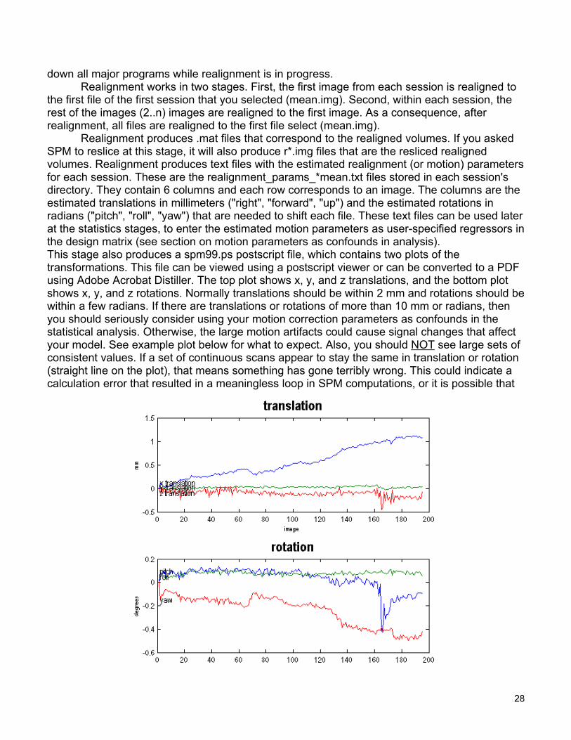
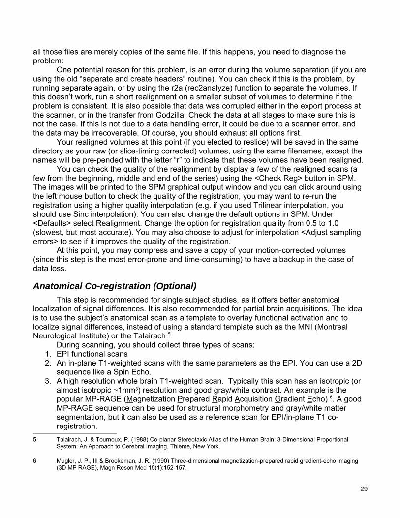
Realignment produces .mat files that correspond to the realigned volumes. If you askedSPM to reslice at this stage, it will also produce r*.img files that are the resliced realignedvolumes. Realignment produces text files with the estimated realignment (or motion) parametersfor each session. These are the realignment_params_*mean.txt files stored in each session'sdirectory. They contain 6 columns and each row corresponds to an image. The columns are theestimated translations in millimeters ("right", "forward", "up") and the estimated rotations inradians ("pitch", "roll", "yaw") that are needed to shift each file. These text files can be used laterat the statistics stages, to enter the estimated motion parameters as user-specified regressors inthe design matrix (see section on motion parameters as confounds in analysis).This stage also produces a spm99.ps postscript file, which contains two plots of thetransformations. This file can be viewed using a postscript viewer or can be converted to a PDFusing Adobe Acrobat Distiller. The top plot shows x, y, and z translations, and the bottom plotshows x, y, and z rotations. Normally translations should be within 2 mm and rotations should bewithin a few radians. If there are translations or rotations of more than 10 mm or radians, thenyou should seriously consider using your motion correction parameters as confounds in thestatistical analysis. Otherwise, the large motion artifacts could cause signal changes that affectyour model. See example plot below for what to expect. Also, you should NOT see large sets ofconsistent values. If a set of continuous scans appear to stay the same in translation or rotation(straight line on the plot), that means something has gone terribly wrong. This could indicate acalculation error that resulted in a meaningless loop in SPM computations, or it is possible that
28
all those files are merely copies of the same file. If this happens, you need to diagnose theproblem:
One potential reason for this problem, is an error during the volume separation (if you areusing the old “separate and create headers” routine). You can check if this is the problem, byrunning separate again, or by using the r2a (rec2analyze) function to separate the volumes. Ifthis doesn’t work, run a short realignment on a smaller subset of volumes to determine if theproblem is consistent. It is also possible that data was corrupted either in the export process atthe scanner, or in the transfer from Godzilla. Check the data at all stages to make sure this isnot the case. If this is not due to a data handling error, it could be due to a scanner error, andthe data may be irrecoverable. Of course, you should exhaust all options first.
Your realigned volumes at this point (if you elected to reslice) will be saved in the samedirectory as your raw (or slice-timing corrected) volumes, using the same filenames, except thenames will be pre-pended with the letter “r” to indicate that these volumes have been realigned.
You can check the quality of the realignment by display a few of the realigned scans (afew from the beginning, middle and end of the series) using the <Check Reg> button in SPM.The images will be printed to the SPM graphical output window and you can click around usingthe left mouse button to check the quality of the registration, you may want to re-run theregistration using a higher quality interpolation (e.g. if you used Trilinear interpolation, youshould use Sinc interpolation). You can also change the default options in SPM. Under<Defaults> select Realignment. Change the option for registration quality from 0.5 to 1.0(slowest, but most accurate). You may also choose to adjust for interpolation <Adjust samplingerrors> to see if it improves the quality of the registration.
At this point, you may compress and save a copy of your motion-corrected volumes(since this step is the most error-prone and time-consuming) to have a backup in the case ofdata loss.
Anatomical Co-registration (Optional)This step is recommended for single subject studies, as it offers better anatomical
localization of signal differences. It is also recommended for partial brain acquisitions. The ideais to use the subject’s anatomical scan as a template to overlay functional activation and tolocalize signal differences, instead of using a standard template such as the MNI (MontrealNeurological Institute) or the Talairach 5
During scanning, you should collect three types of scans:1. EPI functional scans2. An in-plane T1-weighted scans with the same parameters as the EPI. You can use a 2D
sequence like a Spin Echo. 3. A high resolution whole brain T1-weighted scan. Typically this scan has an isotropic (or
almost isotropic ~1mm3) resolution and good gray/white contrast. An example is thepopular MP-RAGE (Magnetization Prepared Rapid Acquisition Gradient Echo) 6. A goodMP-RAGE sequence can be used for structural morphometry and gray/white mattersegmentation, but it can also be used as a reference scan for EPI/in-plane T1 co-registration.
5 Talairach, J. & Tournoux, P. (1988) Co-planar Stereotaxic Atlas of the Human Brain: 3-Dimensional ProportionalSystem: An Approach to Cerebral Imaging. Thieme, New York.
6 Mugler, J. P., III & Brookeman, J. R. (1990) Three-dimensional magnetization-prepared rapid gradient-echo imaging(3D MP RAGE), Magn Reson Med 15(1):152-157.
29

Co-registering Whole Brain VolumesIn this step, you co-register the in-plane T1 to the high resolution 3 dimensional T1 scan.
Click on the <Coregister> button in the fMRI switchboard. Select <1> for <number of subjects>.Select <Coregister only> under <Which option?>. Select <target – T1 MRI> for <modality of firsttarget> and <object – T1 MRI> for <modality of first object image>. In the SPM selector window,select the high resolution 3-D T1 scan as your target scan. Select the 2-D in-plane T1 scan asyour object scan. You will be prompted to select other images for your subject. Here you canselect the entire volume of motion-corrected EPI scans (or alternatively you can select you’rethe mean EPI image (other images can be registered at a later point if you desire). Once SPM isdone, you will see the results of the registration in the graphics window. You can also use the<Check Reg> button to check that the images are registered well.
This procedure works well, because your subject will not move too much between theEPI scans and the in-plane T1, so the transformation matrix required to bring the in-plane T1 inregister with the high resolution scan can also be used to register the EPI’s.
Co-registering Partial Brain VolumesIf your in-plane T1 and functional scans have partial brain coverage, you can use a
similarity criterion such as Mutual Information (MI)7 to estimate the cost function for theregistration parameters between the in-plane T1 and the high resolution T1. Mutual informationis an information theoretic approach which measures the dependence of one image on anotherand can be considered to be the distance between joint distribution (dependence) and thedistribution assuming complete independence. When the two distributions are identical, thisdistance (and the mutual information) is zero. Logically, MI works best when there is mostoverlap between images, and thus it is ironically less effective at handling partial volumeacquisitions, but it is better than simpler approaches (e.g. minimizing entropy).
To use MI, you must change the SPM defaults to use MI in coregistration. First click<Defaults> and select <Coregistration> under <Defaults area?>. Select <Use MutualInformation Registration> when prompted. Mutual Information is a robust similarity criterionwhich will eliminate voxels that are not in both images (i.e. not in the partial in-plane T1 but inthe whole brain high resolution acquisition) from the cost function calculations. Now you can gothrough the steps in 11.1 exactly the same way as before, but changing this default option willenable you to co-register a partial brain volume.
Spatial Normalization to Standard SpaceSpatial normalization is the process of warping scans from several subjects into roughly
the same standard space to allow for signal average and evaluating results in a group, ratherthan an individual. Spatial normalization in fMRI gives us two important advantages:
1. We can determine what typically or generally happens in a group2. We can report locations of activation (or signal differences) according to Euclidean
coordinates within a standard space, e.g. Talairach and Tournoux space.Spatial Normalization in SPM is a two-step process. The first involves determining the
optimal 9 or 12 parameter affine transformation that registers the images together. This isfollowed by an iterative non-linear spatial normalization using functions that describe global
7 Wells, W. M., III, Viola, P., Atsumi, H., Nakajima, S., & Kikinis, R. (1996) Multi-modal volume registration bymaximization of mutual information, Med Image Anal 1(1):35-51.
30
shape differences (not accounted for by affine transformation). The initial affine transform yieldbetter starting estimates for the nonlinear normalization, which in this case performs well andachieves a good registration with only a few iterations.
Correcting Scan OrientationBefore normalization, you need to make sure that your scans are in the same orientation
as the template to which you are going to normalize. In SPM 99 and SPM 2, you can set thedefaults to flip the images when being displayed. Because this is just the display mode and notthe actual orientation, I suggest displaying one of your scans in another program that can tellyou the true orientation of the scan, e.g. MRIcro or Measure. In SPM, you want the top left boxto have the coronal view, the top right box to have the sagittal view, and the bottom box to havethe axial view. The eyes in both the sagittal and the axial views should be aimed towards thecoronal view. This means that your scans are in radiological orientation (your left is the subject’sright, and vice versa), which is SPM’s normalization default, and the default for the EPItemplate. It is important that you get your scans in this orientation before you normalize. Thecorrect orientation should be known before you start pre-processing. Many investigators chooseto use a fiducial marker on the right temple (a small object that is visible on high resolutionscans, to always tell what the subject’s right is). There are two ways of doing this:
1. Reorienting images using <Display>Click <Display> and select one of the EPI images. If the orientation is incorrect, you mayuse defined rotations in pitch, roll and yaw to get it in the right orientation. The mostcommon issue is the sagittal facing away from the coronal. This can be remedied using a“pi” orientation in <yaw>. This may take a bit of playing around to get it just right, butremember that doing this without having a fiducial and knowing the true orientation isuseless. Once you find the correct rotations needed, click on <Reorient images> andselect the rest of the functionals. This will create .mat files for all the functionals with thenew orientation information.
2. Changing the normalization starting estimate defaultsYou can also change the defaults for normalization by clicking <Defaults> and selecting<Spatial normalization> under <Defaults area…?>. Select <defaults for parameterestimation>. In the estimates options, you can select <Neurological> if that is the correctorientation of your scan. You can also select custom affine parameters. You can use thisto tell SPM to flip the scans along certain axes. For example [ 0 0 0 0 0 0 1 1 1 0 0 0] isneurological (R is R), while [0 0 0 0 0 0 -1 1 1 0 0 0] is radiological.
Normalization DefaultsThis is a brief explanation of all of SPM’s normalization defaults, for reference only. In
most cases, the defaults preset by SPM will be sufficient for our purposes. Remember that anychanges to SPM defaults will be undone every time you restart SPM. You can access thenormalization defaults, by clicking <Defaults> and selecting <Defaults for parameterestimation>. The first set of options defines the affine starting estimates and was described indetail above. The next set of options asks you to select whether or not you would like to allow<customized normalization>. This basically includes an option to customize the normalizationoptions (in case you forget to set the defaults). The default is set to <disallow>.
The <number of nonlinear basis functions> is used to further specify how many functionsshould be used to warp the scan. The default is 7 x 8 x 7 which for most purposes will be
31
sufficient. You may use more or less, depending on the quality of normalization and the scans. Ifyou choose [ 0 0 0 ] basis functions, SPM will only carry out the affine normalization only,without using any nonlinear basis functions. You are also given the option to specify the<number of iterations>. This is the number of iterations of nonlinear spatial normalization. 12 isthe default and in most cases will be enough. If the quality of the normalization is not great, thisnumber can be increased.
The next set of options have to do with <nonlinear regularization> which is used tominimize the sum of squared difference between the template and the warped image, whilesimultaneously minimizing some function of the deformation field. This is necessary, as withoutit, it is possible to introduce deformations that only reduce the residual sum of squares by aminiscule amount (which can potentially make the algorithm run infinitely). The default here<medium regularization> is in most cases adequate. If normalization needs more warping, youcan decrease the amount of regularization needed.
The next option <Mask brain when registering> is used to estimate spatial normalizationparameters from a specific region (e.g. a brain mask) or the whole volume. If your signal fromskull and dura is very low, then you can get away with not using a brain mask, but if you want toexclude any signal from skull and dura, you should select the default brain mask, which is theimage saved in the “apriori” directory of the spm99 directory called “brainmask.img” or a specificmask (to be specified by you, e.g. a study specific brain mask)
You are also asked if you would like to <Mask object brain when registering?> which isused in case you want to estimate the normalization parameters from only a limited region of theobject images. This can be used for normalizing brains with lesions (see section 12.3) byincorporating weighting via an image with values between 0 and 1 that matches the space of theobject image (e.g. an MRIcro mask).
You also have another set of defaults for writing normalized files. Select <Defaults>again, and select <Spatial Normalization> followed by <Defaults for writing normalized>. Thefirst option is to specify the bounding box, which is the definition of the volume of the normalizedimage that is written (mm relative to the anterior commissure). Leave this as the default [-78:78-112:76 -50:85]. Under <voxel sizes?> you are given options of the voxel sizes for thenormalized images. The default is 2 x 2 x 2 mm (isotropic) and is in general ok to use for moststudies.
Normalization to a Standard EPI TemplateClick <Normalize> and select <Determine parameters only>. Type 1 for <# subjects>. In
the SPMget window, select the first motion corrected functional image in the series (or the meanfunctional). You will then be prompted for the <template image>, which should be an EPItemplate. You can use the EPI template (MNI) that comes with the SPM99 distribution. This willproduce a single normalized file and a set of normalization parameters (*_sn3d.mat file). Youwill see the quality of the normalization in the SPM graphics window on the right. If it looks ok,you can apply it to the rest of the images. If not, then your orientation may be incorrect and/oryou may need to modify your normalization defaults. Assuming everything looks ok, you cannow click <Normalize> again but this time select <Write normalized only>. When you areprompted, you can select the normalization parameter set or the *_sn3d.mat file that wasproduced in the previous step. In the next window, select the rest of the functional scans.
32
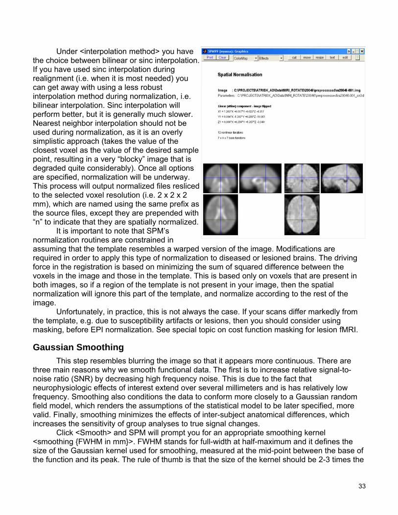
Under <interpolation method> you havethe choice between bilinear or sinc interpolation.If you have used sinc interpolation duringrealignment (i.e. when it is most needed) youcan get away with using a less robustinterpolation method during normalization, i.e.bilinear interpolation. Sinc interpolation willperform better, but it is generally much slower.Nearest neighbor interpolation should not beused during normalization, as it is an overlysimplistic approach (takes the value of theclosest voxel as the value of the desired samplepoint, resulting in a very “blocky” image that isdegraded quite considerably). Once all optionsare specified, normalization will be underway.This process will output normalized files reslicedto the selected voxel resolution (i.e. 2 x 2 x 2mm), which are named using the same prefix asthe source files, except they are prepended with“n” to indicate that they are spatially normalized.
It is important to note that SPM’snormalization routines are constrained inassuming that the template resembles a warped version of the image. Modifications arerequired in order to apply this type of normalization to diseased or lesioned brains. The drivingforce in the registration is based on minimizing the sum of squared difference between thevoxels in the image and those in the template. This is based only on voxels that are present inboth images, so if a region of the template is not present in your image, then the spatialnormalization will ignore this part of the template, and normalize according to the rest of theimage.
Unfortunately, in practice, this is not always the case. If your scans differ markedly fromthe template, e.g. due to susceptibility artifacts or lesions, then you should consider usingmasking, before EPI normalization. See special topic on cost function masking for lesion fMRI.
Gaussian SmoothingThis step resembles blurring the image so that it appears more continuous. There are
three main reasons why we smooth functional data. The first is to increase relative signal-to-noise ratio (SNR) by decreasing high frequency noise. This is due to the fact thatneurophysiologic effects of interest extend over several millimeters and is has relatively lowfrequency. Smoothing also conditions the data to conform more closely to a Gaussian randomfield model, which renders the assumptions of the statistical model to be later specified, morevalid. Finally, smoothing minimizes the effects of inter-subject anatomical differences, whichincreases the sensitivity of group analyses to true signal changes.
Click <Smooth> and SPM will prompt you for an appropriate smoothing kernel<smoothing {FWHM in mm}>. FWHM stands for full-width at half-maximum and it defines thesize of the Gaussian kernel used for smoothing, measured at the mid-point between the base ofthe function and its peak. The rule of thumb is that the size of the kernel should be 2-3 times the
33

size of the voxel. If you input only one number, SPM will assume an isotropic resolution and usethis value in all three planes. For anisotropic resolutions, you should input a 3 value vector, e.g.4 4 8, if you desired more smoothing in the in-plane direction (mostly the case). Select all yournormalized functionals to smooth. Smoothing will produce files corresponding to all thenormalized files you selected, prepended with “s” to indicate that they are smoothed.
Keep in mind that now that your data is smoothed, the effective voxel size is different (ifyour original voxel size is 3mm and you smoothed with a 6mm kernel, you now have aneffective voxel size of 9mm for conceptual purposes). This is important to keep in mind duringthe analysis step, to evaluate the true effect size of activation based on your acquisition voxels.
Summary of Pre-processing StepsTo summarize, the raw time series undergoes a series of pre-processing steps to prepare
the images for statistical analysis. The typical sequence is slice timing correction (for event-related data), followed by correction for head motion, normalization to a standard template, andfinally smoothing with a Gaussian kernel. This sequence may need to be altered for a specifictype of study (e.g. a single subject study may not need to normalize and reslice the timeseries.), but for most cases, this order should serve as a good reference.
34
Statistical Analysis using the General Linear Model
Disclaimer: Statistical analysis in SPM is inherently dangerous! SPM is one of theeasiest fMRI analysis packages to use. However, due to its apparent simplicity, many willattempt to use it without the required training. SPM STATISTICS ARE NOT SIMPLE eventhough it may seem so at first glance. You need to understand the concepts behind thebuttons before you push them. Please use only as a reference and with great caution.
Modeling and Inference in SPMStatistical parametric mapping (SPM) commonly refers to use of general linear equations
to model parametric distributions. An SPM analysis computes evidence against a nullhypothesis at each voxel.
The general linear model can be thought of as a linear combination of explanatoryvariables plus a well-behaved (independently and identically distributed) error term. For exampleit can measure a response variable (observation) at a particular voxel Yj, where j = 1, …, J.
For each observation we have a set of L (L < J) explanatory variables denoted by xjl
where l = 1, …, L. Explanatory variables may be continuous or discrete variables or covariates.βl are unknown parameters, corresponding to the explanatory variables. The error terms areassumed to be independent and identically distributed normal random variables.
Yj = xj1 β1 +…+ xjl βl +…+ xjL βL + єj iid
This can be written in matrix notation as Y = Xβ + є, where Y is the column vector ofobservations, X is the design matrix, β is the column vector of parameters, and є is the columnvector of error terms. The design matrix should be a full description of the model, with theremainder being in the error term. This is where all experimental knowledge about the expectedsignal is quantified.
Parameter estimation in SPM is done using ordinary least-squares (OLS) fitting. Say youhave a set of parameter estimates β* = [β*1,...,β*L]. Based on these estimates, fitted responsevalues are calculated so that Y* = [Y*1,...,Y*L]. The differences between the actual and fittedvalues (Y – Y*) are the residual errors e = [e1,...eL]. The residual sum of squares is the sum of thesquare differences between the actual and fitted values, which can be denoted by Σj
j=1 ej2. This
value is a measure of how well the model fits the actual data. The OLS estimates are thoseparameter estimates which minimize the residual sum of squares.
Inference in SPM is based on deriving t and F statistics that test for a linear combinationof effects (contrasts), e.g. ON minus OFF. During testing, effects of no interest can be removed.The idea in SPM is to enter all known information about the effect of interest in the designmatrix, and test the validity of our assumptions using OLS fitting under the general linear model.The following will be a walkthrough of how this is done in practice.
Model Specification and the SPM Design Matrix The idea from model specification is to specify the different conditions (or blocks) of
interest in each functional run, and specify the timing parameters that allow SPM to separate
35
their temporal effects. SPM uses a graphical user interface that requests several types ofinformation to specify and estimate this model. Once SPM has specified the statistical model,based on the information you provide, it creates a file in your current working directory calledSPM_fMRIDesMtx.mat, which is a design matrix file that can be estimated using the subject'spre-processed data.
Setting Up fMRI DefaultsBefore specifying a model, you may need to change some of the default parameters for
statistical analysis in SPM. If you performed slice-timing correction on your data, then you needto adjust the sampled time bin parameter to reflect that. SPM divides the TR into a number oftime bins (the default is 16). By default, SPM will sample the first time bin in the TR, e.g. If yourTR is 2 seconds, it will only sample the first 125ms. Since slice timing correction involves thereconstruction of the time series in the real order, the first 125 ms could reflect activation in adifferent slice. During slice timing correction we selected the middle slice as our reference slice,therefore, we should change the SPM defaults so that the sampled time bin is the middle bin (8).
To do this, click on <Defaults> and select <Statistics – fMRI>. Use default options for theUpper tail F prob. Threshold, and for the number of bins. However, you should change thesampled bin to 8, instead of the default (16). Remember that these changes are only valid forthe analysis session in context. If you restart SPM, these changes will be lost.
Model SpecificationThis section will go through specifying a model for a single subject. Note that if all your
subjects underwent the same testing conditions with the same timing parameters (e.g. in anepoch design), then the process of model specification needs to be done only once. The saveddesign matrix file can be applied to any of your subjects.
In the fMRI switchboard, click on “fMRI models” and select “Specify a model”. You will beasked to specify the <inter-scan interval> (another term for TR or your repetition time). Enteryour TR here in seconds. On the next prompt for <scans per session>, you have to input thenumber of functionals per run and the number of runs, e.g. if you ran 3 sessions with 360timepoints in each, you would enter [360 360 360] without the square brackets. You are thenasked if <conditions are replicated>. If you are using the same conditions in all sessions forexample, you would hit <yes>. You are then asked if <timing/parameters are the same> in allsessions. If different sessions had different timing parameters (for example, if you had form Aand form B of the task for two consecutive runs), you would hit <no>. In the latter case, you willhave to repeat the following steps for each session separately.
You are then asked to specify the <number of conditions or trials>. This number dependson how many conditions you would like to analyze. For example, if you had a memory task thatinvolves both encoding and recall, you may choose to specify 3 conditions (encoding, recall,rest) or 2 conditions (active memory, rest). Remember that the idea in matrix design is toprovide SPM with all relevant modeling information. In the above case, it is always better toanalyze 3 separate conditions, unless you had reason to believe that there is absolutely nodifference in activation between the two memory conditions.
You are then asked to specify the names of both conditions. If conditions were replicated,then you only have to do this one. If not, then you have to specify them for each session.
The next step is to specify whether or not you want to use a <stochastic design>. Click<No>. This type of design defines a variable probability of a given event type at each stimulus
36

onset point. For example, the underlying probability of events can be modeled using a sinewave. The other option is to use a 'deterministic' model, which is the default for an epochdesign. By deterministic we mean that the events are assumed to occur at a pre-specified timeor within a specific block of time. Stochastic designs are only used when a deterministic modelis not possible or inefficient, for example in the context of event-related fMRI. For moreinformation on this topic, please see Friston et al. (1999)8.
The next prompt will be for <SOA (Stimulus Onset Asynchrony)>. If your conditions allhave the same length, and the inter-trial interval between presentation of trials of the same typeis always the same, then you can select <Fixed>. If you have more than 2 conditions, or if youhave variable timing parameters, select <Variable>. For each condition you specified, you willbe prompted for two things: Stimulus onset vectors and durations. <SOA (scans) forcondition_1> should be specified in scan numbers. This can be thought of as the number of theimage (from your entire dataset) where your condition starts. This can be calculated from yourtiming parameters (divide your onset time (in seconds) by your TR and you will get scans. Forexample, if blocks of condition 1 start at 8, 24 and 64 seconds, and your TR is 2 seconds, youwould enter [4 12 32] as your onset time vector.
If you selected a fixed SOA, SPM will prompt you for <time to 1st trial>, where you shouldinput the amount of time (in scans like above) until the 1st trial of this type. Typically this will bethe first parameter in your SOA vector of onset times for this condition. If you selected variableSOA, SPM will inquire whether you are using <Variable Durations> or not. If you want to limityour analysis to the duration between stimulation and response, then you can say <Yes> andenter a behavioral response vector (e.g. reaction time) in the next prompt for <durations(scans)>. If you do not wish to use variable durations, click <no>.
You are then asked whether or not you would like to use <parametric modulation>. Formost cases, click <none>. This is only done to test the effect of a parametric vector on yourconditions, e.g. If you had reason to believe that you reaction times had a direct effect on youractivation, you can enter your reaction time as a modulator. You can model linear or simplefunction non-linear (e.g. exponential, quadratic, etc...) relationships.
Next, you will be prompted for your <trial type>. Here the model specification differsdepending on the type of analysis you want. If your design is blocked, select <epoch>, andunder <type of response> select the most basic <fixed response: box-car function>. Thisfunction describes the blocks using a square function modeled by Y = c (constant) for a < x < band 0 otherwise.
If your design is event-related, select <events> and under type of response. If you didnot perform slice timing correction, then you should select <hrf with time derivatives>. If slicetiming correction was performed, you can use a naïve hrf model (i.e. hrf <alone>). HRF is a
8 Firston, K.J., Zarahn, E., Josephs, O., Henson, R.N., Dale, A.M. (1999) Stochastic designs in event-related fMRI”.Neuroimage 10(5):607-619.
37

canonical hemodynamic response function that accounts for the lag between the stimulation andthe BOLD signal (see figure below). It is modeled as the difference of two gamma densityfunctions9.
It is important to note thateach individual hemodynamicresponse varies markedly from oneanother, but is relatively stable withinan individual 10. It may be preferableto use empirically derive a subject-specific HRF during analysis. Detailson this method will be describedlater.
If you selected an epochdesign, SPM will ask you separatelyabout convolving with the hrf and itsderivatives. Modeling temporalderivatives may be helpful to includein a model to account for smalldelays (or small differences) betweenthe model and the data, i.e. betterleast squares fit, but in most cases, itdecreases the analysis' power. In
other words, if you have no good reason why you should use the time derivatives, it is safest tostay with a naïve HRF model. Also, these lags are 'tiny' compared with the length of a block, sothat you can always get away with using a naïve HRF model in an epoch design. It may behelpful to model the time derivatives in an event-related analysis, since timing is more crucial.
If you selected an epoch design, you will be asked for the <epoch length> or the numberof scans per specified condition (durations), if you selected a fixed SOA. You will then be askedif you want to model <interactions among trials (Volterra)>. This option is useful if you want toregress our the effect of the interaction from successive trials of the same type, e.g. priming, butit should be used with caution. The last prompt will ask you for your <user specified regressors>.This is where you can specify any potential confounds in your analysis, so you can regress themout of the model. In most cases, you will enter [0]. However, you can model behavioral orepidemiological variables as covariates. Another good practice is using your motion correctionparameters as confounds. These covariates was saved earlier on during realignment, but canbe entered into the model at this stage (see note on the next page).
In essence, what SPM modeling is doing is calculating a cross-correlation evaluatingthe strength of the relationship between your predicted hemodynamic response and the rawhemodynamic signal (after filtering and adjusting for global variation).
9 Glover, G.H. (1999). Deconvolution of impulse response in event-related BOLD fMRI. Neuroimage, 9:416-429.
10 Aguirre, G. K., Zarahn, E., & D'Esposito, M. (1998). The variability of human, BOLD hemodynamic responses. Neuroimage,8(4), 360-369.
38

Including motion parameters as regressors of no interest (optional)When SPM asks you for user-specified regressors, type 6. Then it will prompt you for the
values – type spm_load in the box. You can then select the realignment_params.txt filefor the session you're currently specifying. The six regressors for each session correspond tothe six columns from the realignment_params.txt file, which are the estimated motion params inthe following directions:, "right", "forward", "up", "pitch", "roll", and "yaw". During the analysis,you would have 6 more regressors (and 6 more zeros when it comes to specifying the contrast).
Your design matrix will now be displayed in the SPM graphics window. Check it to makesure all your parameters are correct. There should be a regressor (β) in the model for eachcondition specified. There is also a constant regressor (µ) containing the global cerebral bloodflow values to normalize the mean signal value. Your canonical response basis set should bedisplayed. You can use the <Explore fMRI design> to browse between sessions and conditions,and make sure model is specified correctly. Below is an example of a specified design matrix foran event-related design, with five conditions of interest, and a constant global regressor.
The design orthogonality graph can be thought of a matrix of correlations. Perfectcorrelations are indicated by black. Correlations between 0 and 1 are indicated by some shadeof gray (white being a zero correlation). Each parameter perfectly correlates with itself (the blackdiagonal). The rest of the matrix describes how correlated the variables are with each other.Only the top half of the matrix is shown since the bottom is essentially a replication of the top.
Estimating a Specified ModelAfter you have reviewed your design matrix and determined that it look ok, it is time to
regress the model on the subject's actual data. Select <fMRI models> and select <estimate aspecified model> from the options. In the SPMget file selector window, select theSPMfMRIDesMtx.mat file from the working directory. Once you hit done, you will be prompted toselect the scans for each subject and session.
39
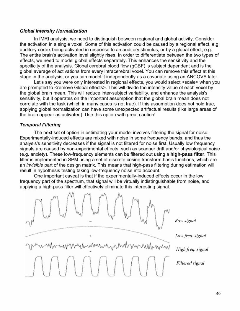
Global Intensity NormalizationIn fMRI analysis, we need to distinguish between regional and global activity. Consider
the activation in a single voxel. Some of this activation could be caused by a regional effect, e.g.auditory cortex being activated in response to an auditory stimulus, or by a global effect, e.g.The entire brain's activation level slightly rises. In order to differentiate between the two types ofeffects, we need to model global effects separately. This enhances the sensitivity and thespecificity of the analysis. Global cerebral blood flow (gCBF) is subject dependent and is theglobal average of activations from every intracerebral voxel. You can remove this effect at thisstage in the analysis, or you can model it independently as a covariate using an ANCOVA later.
Let's say you were only interested in regional effects, you would select <scale> when youare prompted to <remove Global effects>. This will divide the intensity value of each voxel bythe global brain mean. This will reduce inter-subject variability, and enhance the analysis'ssensitivity, but it operates on the important assumption that the global brain mean does notcorrelate with the task (which in many cases is not true). If this assumption does not hold true,applying global normalization can have some unexpected artifactual results (like large areas ofthe brain appear as activated). Use this option with great caution!
Temporal FilteringThe next set of option in estimating your model involves filtering the signal for noise.
Experimentally-induced effects are mixed with noise in some frequency bands, and thus theanalysis's sensitivity decreases if the signal is not filtered for noise first. Usually low frequencysignals are caused by non-experimental effects, such as scanner drift and/or physiological noise(e.g. anxiety). These low-frequency elements can be filtered out using a high-pass filter. Thisfilter is implemented in SPM using a set of discrete cosine transform basis functions, which arean invisible part of the design matrix. This means that high-pass filtering during estimation willresult in hypothesis testing taking low-frequency noise into account.
One important caveat is that if the experimentally-induced effects occur in the lowfrequency part of the spectrum, that signal will be virtually indistinguishable from noise, andapplying a high-pass filter will effectively eliminate this interesting signal.
40
Raw signal
Low freq. signal
High freq. signal
Filtered signal
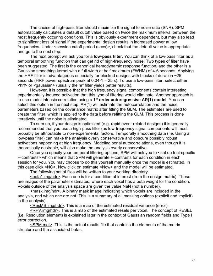
The choise of high-pass filter should maximize the signal to noise ratio (SNR). SPMautomatically calculates a default cutoff value based on twice the maximum interval between themost frequently occuring conditions. This is obviously experiment dependent, but may also leadto significant loss of signal if the experimental design results in increased power at lowfrequencies. Under <session cutoff period (secs)>, check that the default value is appropriateand go to the next step.
The next prompt will ask you for a low-pass filter. You can think of a low-pass filter as atemporal smoothing function that can get rid of high-frequency noise. Two types of filter havebeen suggested. The first is the canonical hemodynamic response function, and the other is aGaussian smoothing kernel with a full-width at half maximum (FWHM) of 4-6 seconds. Applyingthe HRF filter is advantageous especially for blocked designs with blocks of duration ~25seconds (HRF power spectrum peak at 0.04-1 = 25 s). To use a low-pass filter, select either<hrf> or <gaussian> (usually the hrf filter yields better results).
However, it is possible that the high frequency signal components contain interestingexperimentally-induced activation that this type of filtering would eliminate. Another approach isto use model intrinsic correlation using a 1st order autoregressive AR(1) model. You canselect this option in the next step. AR(1) will estimate the autocorrelation and the noiseparameters based on the covariance matrix after fitting the GLM. The estimates are used tocreate the filter, which is applied to the data before refitting the GLM. This process is doneiteratively until the noise is eliminated.
To sum up, if your design is optimized (e.g. rapid event-related designs) it is generallyrecommended that you use a high-pass filter (as low-frequency signal components will mostprobably be attributable to non-experimental factors. Temporally smoothing data (i.e. Using alow-pass filter) can make the analysis overly conservative and obscure possibly robustactivations happening at high frequency. Modeling serial autocorrelations, even though it istheoretically desirable, will also make the analysis overly conservative.
Once you specify your temporal filtering options, SPM will ask you to <set up trial-specificF-contrasts> which means that SPM will generate F-contrasts for each condition in eachsession for you. You may choose to do this yourself manually once the model is estimated. Inthis case click <NO>. Now click on estimate <Now> and the model will be estimated.
The following set of files will be written to your working directory. <beta*.img/hdr>. Each one is for a condition of interest (from the design matrix). These
are images of the parameter estimates, where each voxel has a beta weight for the condition.Voxels outside of the analysis space are given the value NaN (not a number).
<mask.img/hdr>. A binary mask image indicating which voxels are included in theanalysis, and which one are not. This is a summary of all masking options (explicit and implicit)in the analysis).
<ResMS.img/hdr>. This is a map of the estimated residual variance (error). <RPV.img/hdr>. This is a map of the estimated resels per voxel. The concept of RESEL
(i.e. Resolution element) is explained later in the context of Gaussian random fields and Type Ierror correction.
<SPM.mat>. This is the actual results file that contains the elements of the matrixstructure and the associated betas.
41

Results and Statistical Inference
Contrast SpecificationOnce the model is estimated on your data, you need to test for a specific effect of group
of effects, in order to be able to view 'results' so to speak. Remember that results in an SPManalysis consist of spatially mapped statistical image, where the intensity of individual voxelscorresponds to a t or F statistic. In order to view the effect of a specific condition or relationship,one needs to specify a “contrast”, which depends on the model specification and on the originalexperimental design. For example, if your task consisted of active and rest blocks, you maychoose to look at the 'Active > Rest' contrast. For this you have to construct and test a tcontrast. This process is simple, as a linear contrast is constructed using zeros and ones. Let'ssay that your modeled your motion parameters as covariates, and you have two conditions inthe experiment, denoted by ACTIVE and REST. Assuming you specified ACTIVE as your firstcondition and you want to look at activation that is present during the ACTIVE condition but notduring REST, you would enter 1 for ACTIVE and -1 for REST. You should also enter zeros forall of the motion parameters, however since those are at the end of the matrix (i.e. After theconditions of interest), you can input nothing, and SPM will automatically assume you want to
value of t against the likeliness of its value under the null hypothesis. The t statistic depends onthe standard deviation of the contrast of parameter estimates which depends on the variance inthe regressors. In other words, the t test's sensitivity for estimating a single component in thematrix is maximized when the rest of the regressors are de-correlated. This test is one-tailed,testing only for a positive or negative effect. In SPM, you can conduct two-tailed tests testing forthe joint probability of a positive or negative effect, using an F contrast. F contrasts are specifiedthe same way as t contrasts. A 'F-contrast' may look like
42
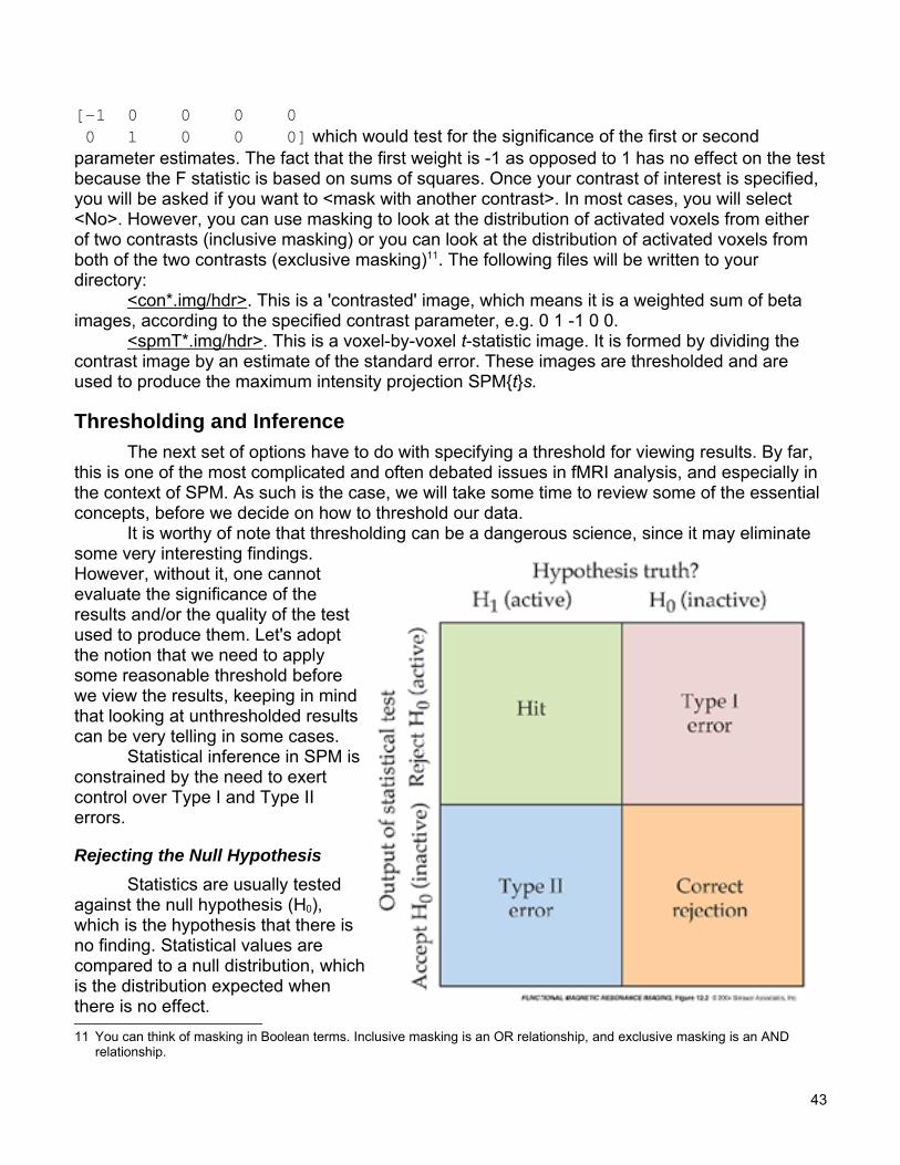
[-1 0 0 0 0 0 1 0 0 0] which would test for the significance of the first or secondparameter estimates. The fact that the first weight is -1 as opposed to 1 has no effect on the testbecause the F statistic is based on sums of squares. Once your contrast of interest is specified,you will be asked if you want to <mask with another contrast>. In most cases, you will select<No>. However, you can use masking to look at the distribution of activated voxels from eitherof two contrasts (inclusive masking) or you can look at the distribution of activated voxels fromboth of the two contrasts (exclusive masking)11. The following files will be written to yourdirectory:
<con*.img/hdr>. This is a 'contrasted' image, which means it is a weighted sum of betaimages, according to the specified contrast parameter, e.g. 0 1 -1 0 0.
<spmT*.img/hdr>. This is a voxel-by-voxel t-statistic image. It is formed by dividing thecontrast image by an estimate of the standard error. These images are thresholded and areused to produce the maximum intensity projection SPM{t}s.
Thresholding and Inference The next set of options have to do with specifying a threshold for viewing results. By far,
this is one of the most complicated and often debated issues in fMRI analysis, and especially inthe context of SPM. As such is the case, we will take some time to review some of the essentialconcepts, before we decide on how to threshold our data.
It is worthy of note that thresholding can be a dangerous science, since it may eliminatesome very interesting findings.However, without it, one cannotevaluate the significance of theresults and/or the quality of the testused to produce them. Let's adoptthe notion that we need to applysome reasonable threshold beforewe view the results, keeping in mindthat looking at unthresholded resultscan be very telling in some cases.
Statistical inference in SPM isconstrained by the need to exertcontrol over Type I and Type IIerrors.
Rejecting the Null HypothesisStatistics are usually tested
against the null hypothesis (H0),which is the hypothesis that there isno finding. Statistical values arecompared to a null distribution, whichis the distribution expected whenthere is no effect. 11 You can think of masking in Boolean terms. Inclusive masking is an OR relationship, and exclusive masking is an AND
relationship.
43

There are two kinds of errors that can be made in significance testing. The probability ofType I error is the probability of incorrectly rejecting a true null hypothesis (H0) and is denoted bythe greek letter alpa (α). This is called the Type I error rate. The probability of Type II error is theprobability of incorrectly accepting a false null hypothesis and is denoted by the greek letter beta(β). This is called the Type II error rate. A Type II error is only an error in the sense that anopportunity to reject the null hypothesis correctly was lost. It is not an error in the sense that anincorrect conclusion was drawn since no conclusion is drawn when the null hypothesis is notrejected. What this translates to in terms of fMRI statistics, is that we only need to correct forType I error, when testing for significance.
The situation in fMRI statistics is made more complicated because there are many voxelsin the brain, and thus many statistical values. The null hypothesis therefore refers to finding noeffect in the entire volume of the brain. Now we are asking the question of whether or not agroup (or 'family') of voxels is activated, and the chance of error that we are willing to accept isthe family-wise error (FWE).
Type I Error (Multiple Comparison Correction)Since the general linear model in SPM is used to test each voxel individually and
simultaneously, then several (hundred) tests are being conducted at once. This means that thecollective alpha (α) value increases. This increases Type I errors. In order to control for Type Ierror, we can adjust the alpha value of the individual tests to maintain an overall alpha value atan acceptable level. This is known as a 'correction for multiple comparisons'.
In theory, uncorrected p-values (significance of finding, without correcting for any multiplecomparisons), can only be used if the investigator had an a priori hypothesis that activationshould exist in a single pre-specified voxel (consider the same for every voxel that is tested).Since this usually not the case, but rather we would have some idea of which structures shouldbe activated, correction for multiple comparisons in the appropriate search volume is necessary.For example, if we expect to find a significant effect in the anterior cingulate cortex, we wouldcorrect for multiple comparisons in the volume of the anterior cingulate (using a prespecifiedmask or template). Sometimes, however, we have no idea where we expect to find activation inthe brain. In such a case, we have to correct for multiple comparisons across the entire volumeof the brain. In practice, this is done by choosing a corrected p-value.
Correction for multiple comparisons is possible using a Bonferroni correction. This typeof correction is too conservative, consequently resulting in an increase in Type II errors). It isalso inappropriate for our purposes because it assumes independence between voxels. Ifdatasets are spatially correlated (which is the case in fMRI), there are fewer independentobservations that need to be conducted.
The SPM alternative is using Random Field Theory (RFT), which provides a way ofcorrecting the p-value that takes into account the fact that neighboring voxels are notindependent by virtue of continuity in the smoothed functional data. RFT uses the expectedEuler characteristic for a smoothed statistical map. Calculating the expected Eulercharacteristic tells us the expected number of clusters above a given threshold, and thus givesus an appropriate height threshold. First the smoothness of the data is estimated (to figure outhow spatially correlated the statistical maps are). This allows us to calculate the expected Eulercharacteristics at different threshold levels. The effect of smoothness and the Eulercharacteristic is demonstrated below. Smoothness reduces the chance of noise passing throughthe threshold, consequently controlling for Type I errors.
44
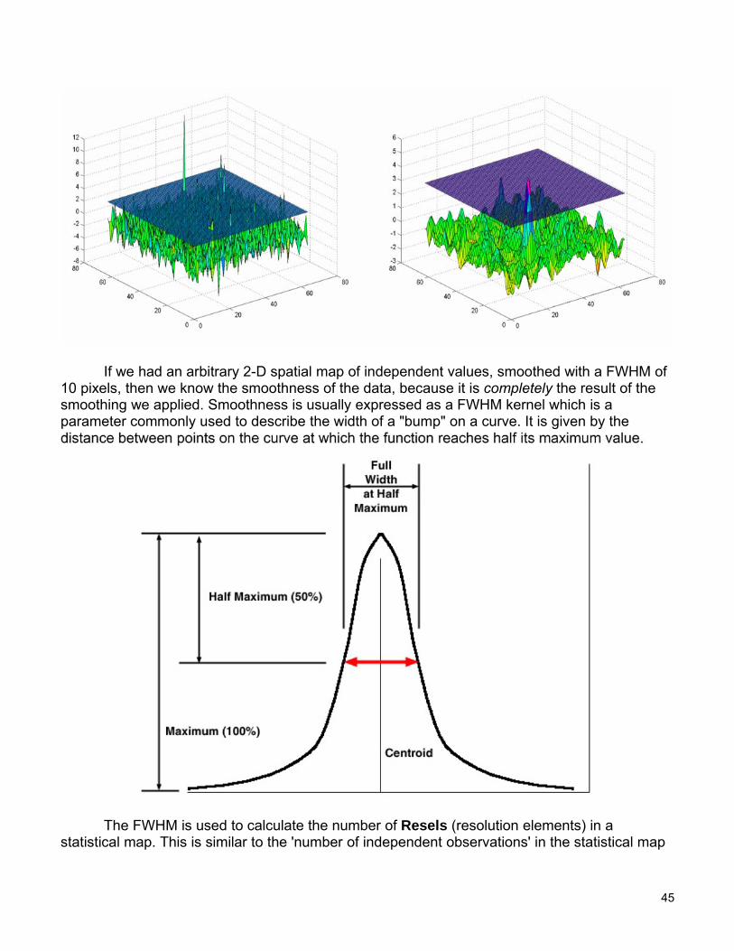
If we had an arbitrary 2-D spatial map of independent values, smoothed with a FWHM of10 pixels, then we know the smoothness of the data, because it is completely the result of thesmoothing we applied. Smoothness is usually expressed as a FWHM kernel which is aparameter commonly used to describe the width of a "bump" on a curve. It is given by the
The FWHM is used to calculate the number of Resels (resolution elements) in astatistical map. This is similar to the 'number of independent observations' in the statistical map
45

but is not exactly the same. A resel consists of the number of pixels it takes to create a FWHMblock. For example, if the FWHM kernel is 10 pixels, then a resel is a block of 100 pixels (10 x10). The number of resels is a useful characteristic to keep in mind when working with smoothedimages. This should be thought of as an alternative to thinking of images in terms of pixels, asthe latter assumes independence between the elements.
At high thresholds, the expected Euler characteristic is almost the same as the probabilityof familywise error. So, if we can calculate the expected Euler characteristic, we can predict thefamilywise error. Worsley et al. (1992) 12 came up with a formula to calculate the expected Eulercharacteristic based on the number of resels in an image. The mathematics are too complicatedto discuss here, but they are described in detail in the above referenced paper. For the mostpart, the Euler characteristic yields a good estimate of the error and gives us an adequatecorrection for Type I errors. .
In functional imaging it is a little more complicated, since we do not know the smoothnessof the original data (even though we know the smoothing kernel which was applied at the end ofpre-processing). Because we do not know the extent of spatial correlation in the original data,smoothness has to be calculated from the images themselves. This can be done using residualvalues from the statistical analysis. The method is described in detail in Kiebel et al. (1999) 13.
Spatial Extent Threshold (Cluster analysis) Another way to control errors is to use a minimum cluster size to specify significant
results. This relies on the assumption that areas of true activation will typically extend over morethan a single voxel. SPM asks you to specify an <extent threshold> or minimum cluster size. Forexample, if you specify 10, then all clusters less than 10 contiguous voxels in volume will berejected as false positives. This means that SPM provides two different ways to control for TypeI errors. Selecting the right threshold once again depends on the smoothness (correlation) of thevoxels. Smoothing increases the needed cluster size (large clusters only will pass thethreshold). However, if voxels are not spatially correlated (data is not sufficiently smooth), then asmaller cluster threshold is more appropriate. Even a cluster size of 3 reduces Type I error ratesignificantly.
Viewing Results using Maximum Intensity Projection In SPM you are given the option to set a height threshold as well as an extent threshold.
Once both are specified, results are printed in the SPM graphics window and the contrast youspecified is produced as a con_000*.img file to your working directory. The SPM glass brainsshow a spatial map of single voxels (or clusters in the case of extent thresholding) whichsurvived the height and extent threshold. You can print the statistics table to the graphicswindow by clicking on <volume> or <cluster> under p-values in the Results window. The tablecan also be printed to the Matlab console by right clicking on it and selecting <Print text table>.
The SPM 'glass brains' are viewed using maximum intensity projection (mip) of significantvoxels and clusters in three orthogonal views. The gray scale of the activation for each pixel ofeach view of the brain is proportional to the the largest value (be it Z score or F ratio), for the
12 Worsley KJ, Evans AC, Marrett S, Neelin P. (1992) A three-dimensional statistical analysis for CBF activationstudies in human brain. J Cereb Blood Flow Metab. 12(6):900-18.
13 Kiebel SJ, Poline, JB, Friston, KJ, Holmes, AP, Worsley, KJ. (1999) Robust smoothness estimation in statisticalparametric maps using standardized residuals from the general linear model. NeuroImage 10:756-766.
46

voxel with the maximum intensity, of all the voxels on a line going through the position of thatpixel, perpendicular to the plane of the page. Thus a dark cluster in the temporal lobe on thecoronal view, could be present anywhere from the front to the back of the brain. SPM glassbrains take a little getting used to. Note that you can navigate by clicking and dragging to thepointer to different coordinate sets. Each view allow you to navigate one of the three axes.
In order to see the SPM statistical table, click on <volume>. In the SPM graphics window,you will see that corrected p-values are derived for:
1. Set-level inferences: number of clusters above the height and volume threshold2. Cluster-level inferences: number of voxels in a particular cluster3. Voxel-level inferences: p-value for each voxel within a cluster
Set-level inferences are generally more powerful than cluster-level inferences andcluster-level inferences are generally more powerful than voxel-level inferences. However,voxel-level inferences are more capable of localizing precise activation (specificity), while set-level inferences are more sensitive to activation. Typically, one can use voxel-level inferencesas they specifies a high degree of anatomical precision.
Note: The SPM results table and MIP brains are surfable. Clicking a row will move the focus tothose coordinates in the MIPs. You can also move the cursor in the MIP to a cluster by clickingand dragging. Right click in the MIP to activate a context menu to jump to nearest and globalmaxima. You can also type the coordinates directly in the SPM results menu (lower left).
47

Small Volume Correction and Regional HypothesesWhen making regional inferences in SPM, we often have some idea of where to expect
activation. If our hypothesis involved a single voxel, then we can use an uncorrected p value asan appropriate alpha. However, more often than not, we make hypotheses involving regionsrather than specific voxels. For example, you could select a box or a sphere as yourhypothesized region of interest. You could also select a search volume based on a specificimage. Small volume correction is available in SPM using the <S.V.C.> button in the Resultsmenu. Click on <S.V.C> and select an appropriate search volume. For example, if you wantedto center your search volume around the set of coordinates indicated by the pointer, you canselect a box or sphere large enough to include the surrounding region. If you select nearestcluster, then you are essentially selecting a functional ROI, which may not be the best way toapproach an ROI analysis. The reason is that you're using results from your whole brainanalysis to guide your ROI analysis. To keep things fair, those two test should be conductedseparately and independently, as the hypotheses being tested in both are different (i.e. Is thereany activation in the brain? vs. is there activation in region X in the brain). More often, you willwant to select <image> and use a predefined region of interest binary mask, to specify thesearch region. The results printed to the SPM graphics window will include only clusters in thesearch volume space that survive the threshold. As a results, your corrected p-values will nowonly be corrected for the defined ROI search volume. This means your control over Type I erroris better, and your significance is thus increased.
Small volume correction is a way to conduct a pseudo-ROI analysis. Since it is still basedon the whole brain analysis, it is not completely blind to its findings. Ideally you would want theROI analysis to be conducted separately and independently of the SPM whole brain analysis.This can be done by masking your results before viewing them or by using another package toaverage values over an entire ROI (optimal). Such a functionality is available in the MarsBaRtoolbox which will be described separately in this guidebook.
Extracting Results and Talairach LabelingOne way you can anatomically label your results is using a standardized atlas like the
Talairach Atlas. This is a coordinate-based system that attaches labels to coordinates. However,the results in SPM are in MNI (Montreal Neurological Institute) space, which is a differentcoordinate system. Before we can attach Talairach labels to the results we need to convert theMNI coordinates to Talairach coordinates. This is typically done using formulas like below.
if z >=0 % This is at the anterior commissure x_tal = (.99*x); y_tal = (.9688*y + .0460*z); z_tal = (-.0485*y + .9189*z);else x_tal = (.99*x); y_tal = (.9688*y + .0420*z); z_tal = (-.0485*y + .8390*z);end
The above is how MNI2TAL works. This simple function, written by Matthew Brett can bedownloaded as \\Soma\Software\Matlab\mni2tal.m . An easy way to utilize this script and apply
48

it to the entire set of results to prepare a set of Talairach coordinates for further processing is byusing the extractresults script, which can also be downloaded from our internal server as\\Soma\Software\Matlab\extractresults.m . You need to put both files in your matlab path, andthen in the matlab console, type > extractresults to save all of your local maxima andtheir coordinates. The script will produce three text files to the current working directory, (1) thespm table of results, (2) the extracted SPM (MNI) coordinates, and (3) the correspondingTalairach coordinates. The coordinate files are in tab delimited format, for easy formatting.
The next step is to attach anatomical labels to the Talairach coordinates. For this we canuse the Talairach Daemon Java server or client. The client resides on your computer, andmaintains a database of coordinates and their corresponding labels, while the server is anonline tool you can use to plug into a net server to download the labels. We often use the clientversion, since it does not require a network or Internet connection to work. This can bedownloaded from: http://ric.uthscsa.edu/projects/talairachdaemon.html . The Talairach DaemonClient will read tab or space delimited records from text files containing lists of Talairachcoordinates arranged in x-y-z order. Or, using the Single Point Processing dialog, one can inputin a single coordinate to label. It will then look up the coordinate in the Talairach Daemondatabase for the Talairach label. There are options to search for the single point, search rangeor nearest gray matter. The output is written to a file which can be viewed in the program, athird-party text editor or imported into a third-party spreadsheet.
Once you install the Talairach Daemon, open it, and click on <File>. Select <Open> andselect the text file containing the Talairach coordinates that you produced using extractresults.Now click on <Option> and select <Database options>. Here you can specify whether you wantto search for the nearest gray matter or specify a search range. This means that if the set ofcoordinates does not coincide with a gray matter label (e.g. if the coordinates are in white matteror CSF), you have the choice of being able to specify a neighboring search range. Lancaster etal. 14 showed that a 5mm gray matter search range enhances the program's localization ability.
Once the options are set, click on <Process>. A new text file will be saved to your diretorywith the extension .td. The file will contain your Talairach coordinates and the correspondinganatomical labels. Labeling uses the Talairach Atlas five level labeling. Levels 1 thru 5adequately describe anatomical locations using gross and specific labels. Level 1 defines leftand right cerebra, cerebella and brainstems. Level 2 defines lobes, while level 3 defines the 55Talairach structures (e.g. anterior cingulate, hippocampus, etc...). Level 4 is a tissue classdefinition of gray matter, white matter, or CSF. Level 5 defines Brodmann areas. The Talairachdaemon will give you all 5 labels for each set of coordinates. Results can then be formatted toinclude only relevant data. For example, if you set a specific threshold, you may not need to listall of the significance values for each set of coordinates.
Time-Series Extraction and Local Eigenimage Analysis You can extract the raw time series data using the <V.O.I> button (Volume of Interest)
from the Results menu. Click <VOI> and give the region you would like to plot an appropriatename. This will use the SPM function spm_regions.m to extract the time series of adjusteddata (also known as local eigenimage analysis). Select <don't adjust> if you want to look at theraw unadjusted timecourse. Next SPM will ask you if you want to apply a filter to the data. Iftemporal filtering has already been applied to the data, then you do not need to apply any more
14 Lancaster et al. (2000) Automated Talairach atlas labels for functional brain mapping. Hum Brain Mapp.10(3):120-31.
49

filtering. Select <none>. Now you have to defineyour VOI in space. If you select a <sphere> ofradius <0> SPM will extract the results for thecurrent voxel. You can also select anothergeometric shape, e.g. <box> or <sphere> or<cluster>. The cluster option will select all thevoxels in the nearest cluster for local eigenimageanalysis. SPM will display a graph of the firsteigenvariate of the data centered around thevoxel of 'focus' or the nearest voxel that survivedthe threshold. The 1st eigenvariate can be thoughtof as a weighted mean of the signal intensity inthe specified space. Extracted VOI data aresaved using the VOI name in the workingdirectory. For example, if you named the VOI'areaX', the file VOI_areaX_1.mat would be savedto your working directory. The variable 'Y' storedin the Matlab workspace contains all of theeigenvariate values at every time point in the VOI.
Plotting Responses and Parameter EstimatesPlotting in SPM allows us to attach
numbers to our pretty images. This is veryimportant as we can pick up on interestingpatterns that the general activation MIPs will notshow. Click <plot> under <visualization> in theSPM results GUI. Select <contrast of parameterestimates> and select one or all effects ofinterest. A bar graph similar to the one shown onthe left will be printed to the SPM graphicswindow. This bar graph tells us how much of thevariance is explained by this particular contrast(effect size) and the direction of the relationship(sign) at this particular voxel. The red error barsare the standard error at the voxel. The size of theeffect is shown as a mean-corrected parameterestimate. A negative value here does not indicatea deactivation, but rather a negative deviation(decrease) from the global mean signal.
When you display a plot in SPM, you canexert some control on how it is displayed. Checking <hold> in the plot controls menu, will keepthe plot on the screen, so you can overlay another on top of it. Checking <grid> will turn on thegrid. Unchecking <box> will get rid of the black border around the graph. You can use the <text>controls to change the title and x and y labels. The <attrib> options can be used to change the xand y axes or return the handle of the current figure to the Matlab console. You can also extractthe numerical data used to build this graph, i.e. beta weights by typing beta in the Matlab
50

console. The beta weights will be printed in asa column vector to the Matlab console. Anadditional 'large' number will also be printed atthe end of the vector. This number is thesession mean at this voxel. You can type SEin the console to extract the standard errors.
Click <plot> again and this time select<fitted and adjusted responses>. Select thecontrast of interest. Usually you will want toplot the effect against time/scan (especially fora blocked design) to see how well the modelfits your data. However, if you have an event-related design, this type of plot may be lessuseful. Select the condition or effect you wantto plot from the list of parameters from thedesign matrix. The plot, similar to the oneshown on the right, should show the fittedresponses in red and the adjusted responsesin blue. Adjusted data is data adjusted forconfounding effects like gCBF and hi/lo pass filters. You can extract the adjusted values bytyping 'y' in the Matlab console. Fitted data is the best fit for the specified model with the actualdata. You can extract the fitted values by typing 'Y' in the Matlab console.
You can also plot the individual time components of the series using epoch/event-relatedplotting. Click <plot> again but this time select <event/epoch-related responses>. You havefour options. The first option plots the <fitted response>. This is a linear combination of theregressor (particular condition) multiplied by its parameter estimate. If you choose to plot <fittedresponse +/- standard error>, your graph will also include standard error plots. The event-related fitted response is the sum of each basis function multiplied by its parameter estimate.
51

Now select <fitted response andadjusted data>. Select your condition ofinterest, and SPM will plot the fitted waveform(solid line) and the individual data points(adjusted for confounds). This summary ofthe data is helpful, but it should be noted thatthis is not the way the SPM analysis is done.This graph is created by plotting time pointsaccording to the regressor of interest aroundthe fitted waveform (shape of the modeledresponse). This is helpful in evaluating howwell the response model fits the actual data.The fitted response is based on the data inthe sense that it is the best fit that the modelhas with the data, but changes by model orcontrast. Therefore it helps to be able to plotthe actual adjusted data points against it toget an idea about its accuracy.
The last option is plotting the <fittedresponse and the PTSH>. PTSH is the peri-stimulus time histogram, which gives the meanBOLD signal within a time window after theoccurrence of each event. This models thewaveform of the response. The plot shows themean response at each binned time point alongwith standard error bars. The fitted response isthe dash-dot line while the PSTH is the solid line.Essentially this is a plot of the mean regressorand the mean signal +/- standard error. There isalso no 'baselining' in this plot, meaning that theamplitude of the waveform for the controlcondition has not been subtracted from theexperimental condition. Peri-stimulus time, or thetime that passed since the last presentation ofan event of that particular type is measured inTR's but to simplify SPM scales it in seconds forplotting purposes.
Note: Stimulus timing in SPM is computed using stimulus pulse functions, representing theonset time and duration of each stimulus type. Onset times and durations are specified by theexperimenter in SPM. The user has the option of specifying a finite duration of the stimulus. Bydefault, however, stimuli are modeled as having zero duration (pulse) and depicted as 'deltaspikes' on the pulse function.
52

Anatomical OverlaysSPM offers many way to display your results. The MIP maps on the glass brains are
handy because they show a complete picture of the activation. Another way to show activationis by using anatomical overlays, which places the activation in a neurological context. However,one should be careful interpreting overlaid results, because they do not show a complete pictureof the results. In the SPM results window click on <overlays>.
Here you can select whether you would like to present data in the SPM graphics windowon a 3-D whole brain rendering, individual slices (in the z-direction) or using orthogonal sections.For the rendering, you can use a template from \\spm99\render\. Viewing sections or slices canbe done using any Analyze image. For display purposes you should use a standardizedtemplate, e.g. MNI single subject template under \\spm99\canonical\. Below are somerenderings of activation on anatomical overlays. The slice overlay by z axis is produced usingthe script m_slice, written by Kalina Christoff, and can be downloaded from\\Soma\Software\Matlab\ and is a nice way to represent activation through an entire section ofthe brain.
53
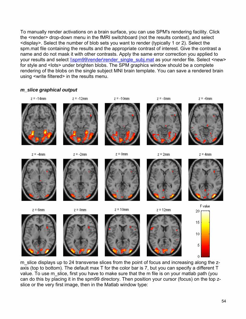
To manually render activations on a brain surface, you can use SPM's rendering facility. Clickthe <render> drop-down menu in the fMRI switchboard (not the results context), and select<display>. Select the number of blob sets you want to render (typically 1 or 2). Select thespm.mat file containing the results and the appropriate contrast of interest. Give the contrast aname and do not mask it with other contrasts. Apply the same error correction you applied toyour results and select \\spm99\render\render_single_subj.mat as your render file. Select <new>for style and <lots> under brighten blobs. The SPM graphics window should be a completerendering of the blobs on the single subject MNI brain template. You can save a rendered brainusing <write filtered> in the results menu.
m_slice graphical output
m_slice displays up to 24 transverse slices from the point of focus and increasing along the z-axis (top to bottom). The default max T for the color bar is 7, but you can specify a different Tvalue. To use m_slice, first you have to make sure that the m file is on your matlab path (youcan do this by placing it in the spm99 directory. Then position your cursor (focus) on the top z-slice or the very first image, then in the Matlab window type:
54
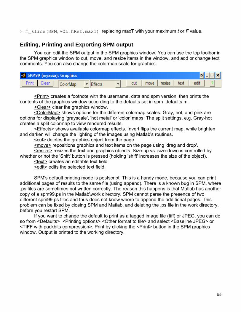
> m_slice(SPM,VOL,hRef,maxT) replacing maxT with your maximum t or F value.
Editing, Printing and Exporting SPM outputYou can edit the SPM output in the SPM graphics window. You can use the top toolbor in
the SPM graphics window to cut, move, and resize items in the window, and add or change textcomments. You can also change the colormap scale for graphics.
<Print> creates a footnote with the username, data and spm version, then prints thecontents of the graphics window according to the defaults set in spm_defaults.m.
<Clear> clear the graphics window.<ColorMap> shows options for the different colormap scales. Gray, hot, and pink are
options for displaying 'grayscale', 'hot metal' or 'color' maps. The split settings, e.g. Gray-hotcreates a split colormap to view rendered results.
<Effects> shows available colormap effects. Invert flips the current map, while brightenand darken will change the lighting of the images using Matlab's routines.
<cut> deletes the graphics object from the page.<move> repositions graphics and text items on the page using 'drag and drop'.<resize> resizes the text and graphics objects. Size-up vs. size-down is controlled by
whether or not the 'Shift' button is pressed (holding 'shift' increases the size of the object).<text> creates an editable text field.<edit> edits the selected text field.
SPM's default printing mode is postscript. This is a handy mode, because you can printadditional pages of results to the same file (using append). There is a known bug in SPM, where.ps files are sometimes not written correctly. The reason this happens is that Matlab has anothercopy of a spm99.ps in the Matlab\work directory. SPM cannot parse the presence of twodifferent spm99.ps files and thus does not know where to append the additional pages. Thisproblem can be fixed by closing SPM and Matlab, and deleting the .ps file in the work directory,before you restart SPM.
If you want to change the default to print as a tagged image file (tiff) or JPEG, you can doso from <Defaults> <Printing options> <Other format to file> and select <Baseline JPEG> or<TIFF with packbits compression>. Print by clicking the <Print> button in the SPM graphicswindow. Output is printed to the working directory.
55

Region of Interest (ROI) AnalysesIn many cases, when we perform an fMRI experiment, we have a specific region of
interest that we hope to activate to a maximal degree using our optimized paradigm. In thiscase, using a voxel-wise analysis to look for significance throughout the entire brain isunnecessary, and decreases our detection ability. Thus, for experiments where we have aspecific regional hypothesis, we require a more targeted analysis.
Anatomical vs. Functional ROIs One important distinction in our choice of ROI is whether we want to use the subject's (or
atlas) anatomy to determine the relevant voxels for the analysis, or whether we want to use anactual activation map for this purpose. Functional ROIs, in most cases, should be driven byindependent data. For example, say you conduct an experiment to make sure the hippocampusis activated during a verbal memory task, and using unbiased analytical methods (whole-brain),you find robust activation in a locus of the anterior hippocampus or in a region encompassingthe hippocampus and surrounding areas, you can use this activation map as a template ROI fora different kind of analysis, e.g. Do patients activate their hippocampi to a lesser extent thancontrols in response to this task?
Anatomical ROI's are either manually drawn on the individualsubject's anatomical scan (which was acquired in the same session asthe functional scans), and then registered to the EPI scan, or isextracted from an atlas of brain structures, and placed on the EPI(after registering the EPI to the atlas space). One such atlas of ROIlabels is the Talairach and Tournoux atlas (shown on the right). Atlas-based ROI's are error-prone, because of the three-dimensionalwarping that has to be performed before we can apply atlas labels toan individual subject's brain. The Talairach brain is not an optimal fit,since it is based on a single (possibly abnormal) brain scan. Analternative template is the MNI single subject (scanned 17 times), forwhich a labeling atlas is available (The Automated AnatomicalLabeling Atlas – AAL). Manually-drawn ROIs are far more superiorthan atlas-based ROI's, but they are much more time-consuming and require expert training toidentify the anatomical markers for a specific brain structure.
Functional ROI's can also be a powerful method, especially for domains where clearneuroanatomical boundaries are not apparent. A perfect example of this is Nancy Kanwisher'sfamous functional “face area”15 which apparently exists in the fusiform gyrus. This functionalROI, even though somewhat arbitrary proved useful to alter research using face stimuli.
The MarsBaR toolbox (http://marsbar.sourceforge.net) for SPM uses the AAL labels toconduct ROI analyses. It also enables us to create functional ROI's based on SPM maps.
15 Kanwisher, N., McDermott, J., Chun, M. (1997) The fusiform face area: A module in human extrastriate cortexspecialized for the perception of faces. J. Neurosci. 17, 4302-4311.
56

MarsBaR (MARSeille Boîte À Région d'Intérêt) MarsBaR (MARSeille Boîte À Région d'Intérêt) 16 is a toolbox for SPM which provides
routines for region of interest analysis. Features include region of interest definition, combinationof regions of interest with simple algebra, extraction of data for regions with and without SPMpreprocessing (scaling, filtering), and statistical analyses of ROI data using the SPM statisticsmachinery.
Overview of the ToolboxInstallation instructions and tutorials are available on the MarsBaR website at
http://marsbar.sourceforge.net which is also a reference for frequently asked questions. Here Iwill only highlight specific features of this package and demonstrate how to conduct a basic ROIanalysis.
First make sure the toolbox directory is onyour Matlab path, and run the command marsbarfrom the command prompt. If SPM is already upand running, the MarsBar window will pop-up ontop of the SPM windows. If SPM is not running,MarsBaR will start as a standalone toolbox. TheMarsBaR window is shown on the right. The newversion of the MarsBaR does not disable any of theSPM functionalities. This means that it can runalongside SPM.
ROI DefinitionClick on the ROI definition menu and you
should get the following options: View displays one or ROIs on a structural image.
Draw calls up a Matlab interface for drawing ROIs.
Get SPM cluster(s) uses the SPM results interface to select and save clusters as ROIs.
Build gives an interface to various methods for defining ROIs, using shapes (boxes,spheres), activation clusters, and binary images. Transform offers a GUI for combining ROIs, and for flipping the orientation of an ROI to theright or left side of the brain. Import allows you to import all SPM activations as ROIs, or to import ROIs from clusterimages, such as those written by the SPM results interface, or from images where ROIs aredefined by number labels (ROI 1 has value 1, ROI 2 has value 2, etc.). Export writes ROIs as images for use in other packages, such as MRIcro.
16 Matthew Brett, Jean-Luc Anton, Romain Valabregue, Jean-Baptiste Poline. Region of interest analysis using anSPM toolbox [abstract] Presented at the 8th International Conferance on Functional Mapping of the HumanBrain, June 2-6, 2002, Sendai, Japam. Available on CD-ROM in NeuroImage, Vol 16, No 2.
57

The following section will show you how to create a functional ROI. Creating ananatomical ROI is not very different. In fact it is a lot easier than the functional ROIs.
Select <Get SPM cluster(s)...> from the menu. This runs the standard SPM resultsinterface. Use the file selection window that SPM offers to navigate to the your SPM analysisdirectory. Select the SPM.mat file and click Done. Choose a contrast from the SPM contrastmanager, click Done. Then use the same thresholds you used for visualization before. Youshould get the familiar glass-brain output in the SPM-graphics window.
Now there should be a new menu in the SPM-input window named <Write ROI(s)>. Youcan use this to write single clusters (the one your have selected using the arrows), or to write allclusters in the SPM. By default MarsBaR saves ROI using the contrast name and coordinates.Each ROI is then saved as a separate .mat file.
You can now reviewthe ROI by selecting <View>from the <ROI definition>menu. The ROI should bedisplayed in a single solidcolor on an averagestructural image.
The view utility allowsyou to click around the imageto review the ROI in thestandard orthogonal views.You can select multiple ROIsto view on the samestructural. The list box to theleft of the axial view allowsyou to move to a particularROI (if you have more thanone). When the cross-hairsare in the ROI, theinformation panel will showdetails for that ROI, such ascenter of mass, and volumein mm. The default structuralimage is the MNI 152 T1average brain; you canchoose any image to displayROIs on by clicking on the<Options> menu in theMarsBaR window, thenchoosing <Edit Options>,followed by <Defaultstructural>. Now we see thatthe cluster includes visualcortex, but there also seems
58

to be some connected activation lateral and inferior to the primary visual cortex. The cross-hairsare between the voxels which seem to be in primary visual cortex and the more lateral voxels.Ideally we would like to restrict the ROI to voxels in the primary visual cortex. We can do this bydefining a box ROI that covers the area we are interested in, and combining this with theactivation cluster. You can define a box ROI using the <Build> option from the <ROI Definition>menu.
You can create a box ROI encompassing your interesting activation, and combine it withyour functional cluster using <Transform> from the <ROI Definition> menu. Select <CombineROIs> and select the two ROIs. The combine function should be one of the following. You canany other mathematical operator also.
r1 & r2 (r1 AND r2)
r1 | r2 (r1 OR r2)
r1 &~ r2 (r1 NOT r2)
Now you can write the ROI as an image to use in any other software. Click on <ROIDefinition> followed by <Export>. Select <image> from the menu and choose the ROI to export.You can select the space for ROI image from the following options:
<Base space for ROIs> this is set by default to the MNI template space but can bechanged from the MarsBaR options.
<From image> here you can specify an individual subject's brain scan for example<ROI native space> this is the MNI template space. Use only with normalized data.
Running an ROI Analysis Assuming all the data is preprocessed in SPM, you can use the MarsBaR options to run
the GLM analysis in the same way you would use SPM for this purpose. Under the <Designmenu> you can select <fMRI models>. Here is a summary of the interface (shown on the nextpage). The design menu offers options for creating, reviewing, estimating and processing SPM /MarsBaR designs. Set design from file option will ask for a design file, and load the specified design intoMarsBaR. The loaded design then becomes the default design. MarsBaR will from now onassume that you want to work with this design, unless you tell it otherwise by loading adifferent design. Save design to file will save the current default design to a file.
Set design from estimated; as we will see later, when MarsBaR estimates a design, itstores the estimated design in memory. Sometimes it is useful to take this estimated designand set it to be the default design, in order to be able to use the various of these menuoptions to review the design.PET models, FMRI models, and Basic models will use the SPM design routines tomake a design, and store it in memory as the default design. Explore runs the SPM interface for reviewing and exploring designs.
59

Frequencies (event+data) can be usefulfor FMRI designs. The option gives a plot ofthe frequencies present in ROI data and thedesign regressors for a particular FMRI event.This allows you to choose a high-pass filterthat will not remove much of the frequencies inthe design, but will remove low frequencies inthe data, which are usually dominated bynoise.Add images to FMRI design allows youto specify images for an FMRI design that doesnot yet contain images. SPM and MarsBaRcan create FMRI designs without images. Ifyou want to extract data using the design, youmay want to add images to the design usingthis menu item. Add/edit filter for FMRI designgives menu options for specifying high passand possibly (SPM99) low-pass filters, as wellas autocorrelation options (SPM2). Check images in the design looks forthe images names in a design, and simplychecks if they exist on the disk, printing out amessage on the matlab console window. Acommon problem in using saved SPM designsis that the images specified in the design havesince moved or deleted; this option is a usefulcheck to see it that has occurred. Change path to images allows you tochange the path of the image filenames saved in the SPM design, to deal with the situationwhen images have moved since the design was saved. Convert to unsmoothed takes the image names in a design, and changes them so thatthey refer to the unsmoothed version of the same images – in fact it just removes the “s”prefix from the filenames. This can be useful when you want to use an SPM design that wasoriginally run on smoothed images, but your ROI is very precise, so you want to avoid runningthe ROI analysis on smoothed data, which will blur unwanted signal into your ROI.
For our purposes, all we need to do is set the design file. MarsBaR allows us to directlyimport SPM results files (after running the GLM on the individual subject's preprocessed timeseries) and extract the ROI data from them. This can be done from the <Data> menu. Here is asummary of the options.Extract ROI data (default) takes one or more ROI files and a design, and extractsthe data within the ROI(s) for all the images in the design. As for the default design,MarsBaR stores the data in memory for further use.
60

Extract ROI data (full options) allows you to specify any set of images to extract datafrom, and will give you a full range of image scaling options for extracting the data.Default region is useful when you have extracted data for more than one ROI. In thiscase you may want to restrict the plotting functions (below) to look only at one of theseregions; you can set which region to use with thisoption. If you do not specify, MarsBaR willassume you want to look at all regions.Plot data (simple) draws time courseplots of the ROI data to the SPM graphicswindow. Plot data (full) has options for filteringthe data with the SPM design filter beforeplotting, and for other types of plots, such asFrequency plots or plots of autocorrelationcoefficients. Import data allows you to import data foranalysis from matlab, text files or spreadsheets.With Export data you can export data tomatlab variables, text files or spreadsheets. Split regions into files is useful in thesituation where you have extracted data frommore than one ROI, but you want to estimatewith the data from only one of these ROIs. Thiscan be a good idea for SPM2 designs, because,like SPM2, MarsBaR will pool the data from allROIs when calculating autocorrelation. This maynot be valid, as different brain regions can havedifferent levels of autocorrelation. Splitregions into files takes the current set ofdata and saves the data for each ROI as aseparate MarsBaR data file. Merge data files reverses the process, by taking a series of ROI data files and makingthem into one set of data with many ROIs.Set data from file will ask for a MarsBaR data file (default suffix '_mdata.mat') andload it into memory as the current set of data. Save data to file will save the currentset of data to a MarsBaR data file.
For our simple purposes, once again, select <Extract ROI data (default)> and select theROI of interest. Once MarsBaR is finished calculating the ROI timecourses, it will calculate anew summary timecourse for each ROI. This is made up of the means of all the voxel values inthe ROI. Now you can estimate the model on the ROI data using <Results> <Estimate Results>.You will then be asked to specify a contrast and the analysis will be conducted. You can viewthe results by clicking on <Statistics Table> in the <Results> menu. You should see something
61

like this:
At the left you see the contrast name. Under this, and to the right, MarsBaR has printedthe ROI label that you entered a while ago. The t statistic is self explanatory, and theuncorrected p value is just the one-tailed p value for this t statistic given the degrees of freedomfor the analysis. The corrected p is the uncorrected p value, with a Bonferroni correction for thenumber of regions in the analysis. In this case, we only analysed one region, so the corrected pvalue is the same as the uncorrected p value. MarsBaR (like SPM), will not attempt to correctthe p value for the number of contrasts, because the contrasts may not be orthogonal, and thiswill make a Bonferroni correction too conservative.
There is also a column called Contrast value. For a t statistic, as here, this value isan effect size. Remember that a t statistic consists of an effect size, divided by the standarddeviation of this effect. The value of this parameter will be the best-fitting slope of the linerelating the height of the HRF regressor to the FMRI signal. This effect size measure is thenumber that SPM stores for each voxel in the con_0001.img, con_0002.img ... series, and theseare the values that are used for standard second level / random effect analyses.
More detailed information on how to conduct ROI analyses are available on the MarsBaRwebsite and in the MarsBaR tutorial (from which this section is extracted).
62
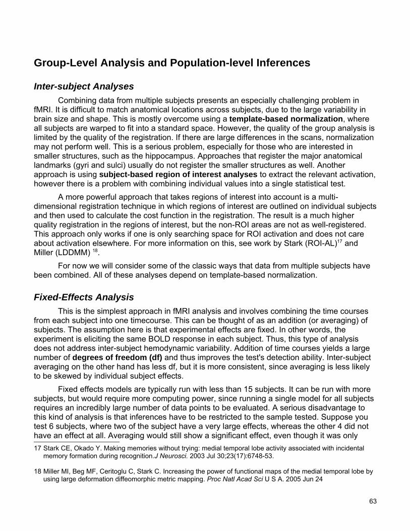
Group-Level Analysis and Population-level Inferences
Inter-subject AnalysesCombining data from multiple subjects presents an especially challenging problem in
fMRI. It is difficult to match anatomical locations across subjects, due to the large variability inbrain size and shape. This is mostly overcome using a template-based normalization, whereall subjects are warped to fit into a standard space. However, the quality of the group analysis islimited by the quality of the registration. If there are large differences in the scans, normalizationmay not perform well. This is a serious problem, especially for those who are interested insmaller structures, such as the hippocampus. Approaches that register the major anatomicallandmarks (gyri and sulci) usually do not register the smaller structures as well. Anotherapproach is using subject-based region of interest analyses to extract the relevant activation,however there is a problem with combining individual values into a single statistical test.
A more powerful approach that takes regions of interest into account is a multi-dimensional registration technique in which regions of interest are outlined on individual subjectsand then used to calculate the cost function in the registration. The result is a much higherquality registration in the regions of interest, but the non-ROI areas are not as well-registered.This approach only works if one is only searching space for ROI activation and does not careabout activation elsewhere. For more information on this, see work by Stark (ROI-AL)17 andMiller (LDDMM) 18.
For now we will consider some of the classic ways that data from multiple subjects havebeen combined. All of these analyses depend on template-based normalization.
Fixed-Effects AnalysisThis is the simplest approach in fMRI analysis and involves combining the time courses
from each subject into one timecourse. This can be thought of as an addition (or averaging) ofsubjects. The assumption here is that experimental effects are fixed. In other words, theexperiment is eliciting the same BOLD response in each subject. Thus, this type of analysisdoes not address inter-subject hemodynamic variability. Addition of time courses yields a largenumber of degrees of freedom (df) and thus improves the test's detection ability. Inter-subjectaveraging on the other hand has less df, but it is more consistent, since averaging is less likelyto be skewed by individual subject effects.
Fixed effects models are typically run with less than 15 subjects. It can be run with moresubjects, but would require more computing power, since running a single model for all subjectsrequires an incredibly large number of data points to be evaluated. A serious disadvantage tothis kind of analysis is that inferences have to be restricted to the sample tested. Suppose youtest 6 subjects, where two of the subject have a very large effects, whereas the other 4 did nothave an effect at all. Averaging would still show a significant effect, even though it was only17 Stark CE, Okado Y. Making memories without trying: medial temporal lobe activity associated with incidental
memory formation during recognition.J Neurosci. 2003 Jul 30;23(17):6748-53.
18 Miller MI, Beg MF, Ceritoglu C, Stark C. Increasing the power of functional maps of the medial temporal lobe byusing large deformation diffeomorphic metric mapping. Proc Natl Acad Sci U S A. 2005 Jun 24
63
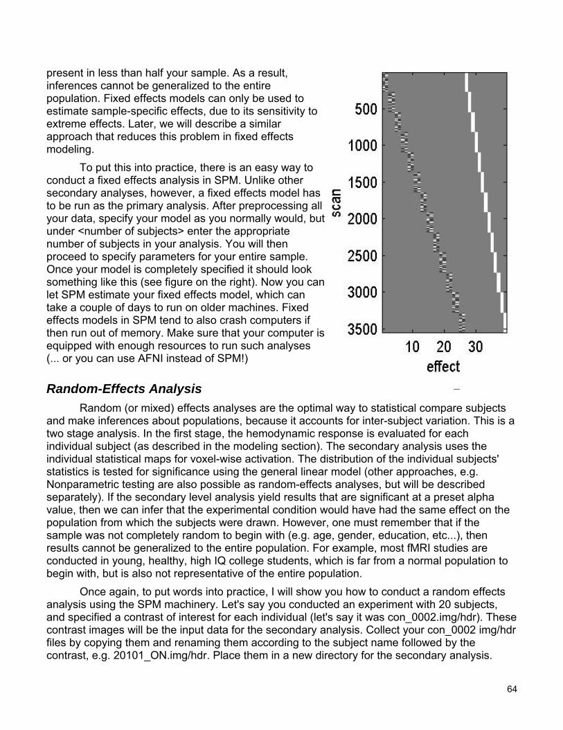
present in less than half your sample. As a result,inferences cannot be generalized to the entirepopulation. Fixed effects models can only be used toestimate sample-specific effects, due to its sensitivity toextreme effects. Later, we will describe a similarapproach that reduces this problem in fixed effectsmodeling.
To put this into practice, there is an easy way toconduct a fixed effects analysis in SPM. Unlike othersecondary analyses, however, a fixed effects model hasto be run as the primary analysis. After preprocessing allyour data, specify your model as you normally would, butunder <number of subjects> enter the appropriatenumber of subjects in your analysis. You will thenproceed to specify parameters for your entire sample.Once your model is completely specified it should looksomething like this (see figure on the right). Now you canlet SPM estimate your fixed effects model, which cantake a couple of days to run on older machines. Fixedeffects models in SPM tend to also crash computers ifthen run out of memory. Make sure that your computer isequipped with enough resources to run such analyses(... or you can use AFNI instead of SPM!)
Random-Effects AnalysisRandom (or mixed) effects analyses are the optimal way to statistical compare subjects
and make inferences about populations, because it accounts for inter-subject variation. This is atwo stage analysis. In the first stage, the hemodynamic response is evaluated for eachindividual subject (as described in the modeling section). The secondary analysis uses theindividual statistical maps for voxel-wise activation. The distribution of the individual subjects'statistics is tested for significance using the general linear model (other approaches, e.g.Nonparametric testing are also possible as random-effects analyses, but will be describedseparately). If the secondary level analysis yield results that are significant at a preset alphavalue, then we can infer that the experimental condition would have had the same effect on thepopulation from which the subjects were drawn. However, one must remember that if thesample was not completely random to begin with (e.g. age, gender, education, etc...), thenresults cannot be generalized to the entire population. For example, most fMRI studies areconducted in young, healthy, high IQ college students, which is far from a normal population tobegin with, but is also not representative of the entire population.
Once again, to put words into practice, I will show you how to conduct a random effectsanalysis using the SPM machinery. Let's say you conducted an experiment with 20 subjects,and specified a contrast of interest for each individual (let's say it was con_0002.img/hdr). Thesecontrast images will be the input data for the secondary analysis. Collect your con_0002 img/hdrfiles by copying them and renaming them according to the subject name followed by thecontrast, e.g. 20101_ON.img/hdr. Place them in a new directory for the secondary analysis.
64
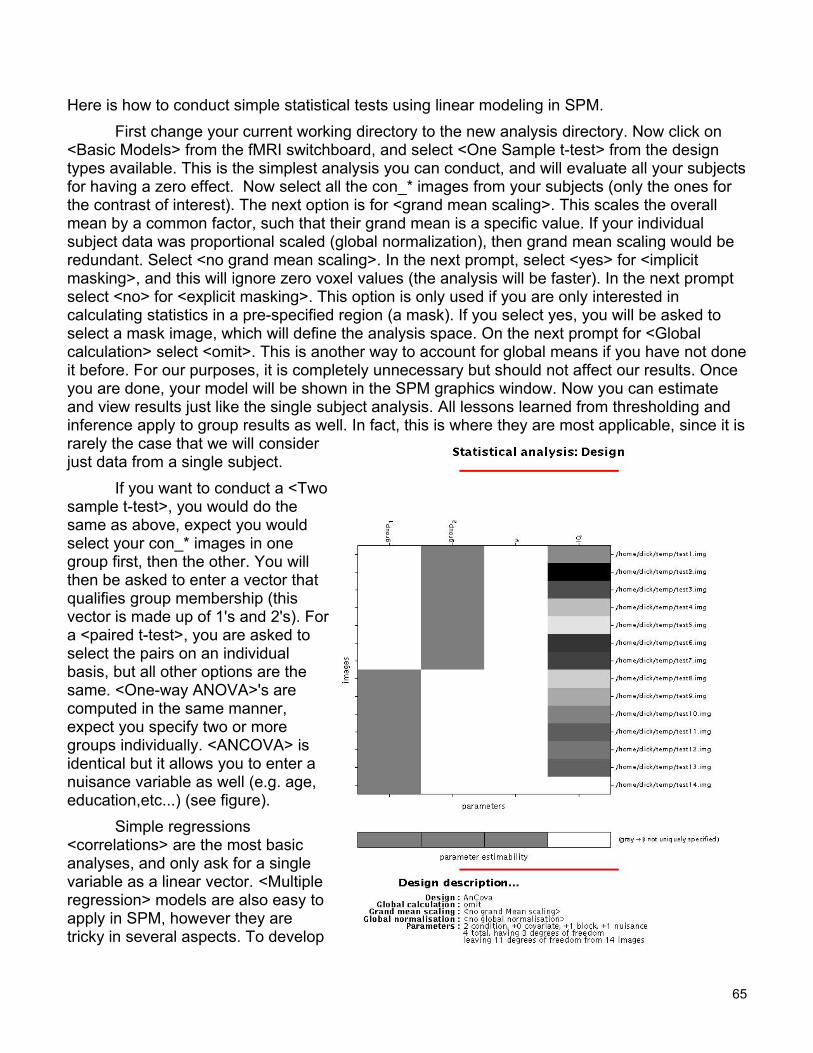
Here is how to conduct simple statistical tests using linear modeling in SPM. First change your current working directory to the new analysis directory. Now click on
<Basic Models> from the fMRI switchboard, and select <One Sample t-test> from the designtypes available. This is the simplest analysis you can conduct, and will evaluate all your subjectsfor having a zero effect. Now select all the con_* images from your subjects (only the ones forthe contrast of interest). The next option is for <grand mean scaling>. This scales the overallmean by a common factor, such that their grand mean is a specific value. If your individualsubject data was proportional scaled (global normalization), then grand mean scaling would beredundant. Select <no grand mean scaling>. In the next prompt, select <yes> for <implicitmasking>, and this will ignore zero voxel values (the analysis will be faster). In the next promptselect <no> for <explicit masking>. This option is only used if you are only interested incalculating statistics in a pre-specified region (a mask). If you select yes, you will be asked toselect a mask image, which will define the analysis space. On the next prompt for <Globalcalculation> select <omit>. This is another way to account for global means if you have not doneit before. For our purposes, it is completely unnecessary but should not affect our results. Onceyou are done, your model will be shown in the SPM graphics window. Now you can estimateand view results just like the single subject analysis. All lessons learned from thresholding andinference apply to group results as well. In fact, this is where they are most applicable, since it israrely the case that we will considerjust data from a single subject.
If you want to conduct a <Twosample t-test>, you would do thesame as above, expect you wouldselect your con_* images in onegroup first, then the other. You willthen be asked to enter a vector thatqualifies group membership (thisvector is made up of 1's and 2's). Fora <paired t-test>, you are asked toselect the pairs on an individualbasis, but all other options are thesame. <One-way ANOVA>'s arecomputed in the same manner,expect you specify two or moregroups individually. <ANCOVA> isidentical but it allows you to enter anuisance variable as well (e.g. age,education,etc...) (see figure).
Simple regressions<correlations> are the most basicanalyses, and only ask for a singlevariable as a linear vector. <Multipleregression> models are also easy toapply in SPM, however they aretricky in several aspects. To develop
65
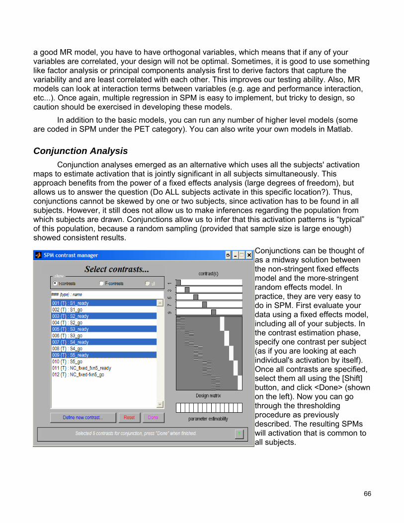
a good MR model, you have to have orthogonal variables, which means that if any of yourvariables are correlated, your design will not be optimal. Sometimes, it is good to use somethinglike factor analysis or principal components analysis first to derive factors that capture thevariability and are least correlated with each other. This improves our testing ability. Also, MRmodels can look at interaction terms between variables (e.g. age and performance interaction,etc...). Once again, multiple regression in SPM is easy to implement, but tricky to design, socaution should be exercised in developing these models.
In addition to the basic models, you can run any number of higher level models (someare coded in SPM under the PET category). You can also write your own models in Matlab.
Conjunction Analysis Conjunction analyses emerged as an alternative which uses all the subjects' activation
maps to estimate activation that is jointly significant in all subjects simultaneously. Thisapproach benefits from the power of a fixed effects analysis (large degrees of freedom), butallows us to answer the question (Do ALL subjects activate in this specific location?). Thus,conjunctions cannot be skewed by one or two subjects, since activation has to be found in allsubjects. However, it still does not allow us to make inferences regarding the population fromwhich subjects are drawn. Conjunctions allow us to infer that this activation patterns is “typical”of this population, because a random sampling (provided that sample size is large enough)showed consistent results.
Conjunctions can be thought ofas a midway solution betweenthe non-stringent fixed effectsmodel and the more-stringentrandom effects model. Inpractice, they are very easy todo in SPM. First evaluate yourdata using a fixed effects model,including all of your subjects. Inthe contrast estimation phase,specify one contrast per subject(as if you are looking at eachindividual's activation by itself).Once all contrasts are specified,select them all using the [Shift]button, and click <Done> (shownon the left). Now you can gothrough the thresholdingprocedure as previouslydescribed. The resulting SPMswill activation that is common toall subjects.
66
Nonparametric ApproachesNonparametric approach were introduced as a potential way to assess significance in
fMRI data, because they remove the need to assume that voxels are normally distributed(Gaussian). This distribution-free procedure is always valid, but requires a lot of computations.However, by today's standards, these computations are not so time consuming any more.
One such approach uses voxel-level permutation and randomization to investigateindependent observations in neuroimaging studies. SnPM (Statistical NonparametricMapping) is a package that was developed by Andrew Holmes and Tom Nichols as a toolboxfor SPM to conduct these kinds of nonparametric analyses. SnPM uses the GLM to construct t-images (or pseudo-t images), which are assessed using standard nonparametric multiplecomparisons procedure. This approach works best for analyses with low degrees of freedom. Inthis case, SnPM uses the weighted locally pooled variance estimates (a process known asvariance smoothing), making the approach much more powerful than conventionalapproaches that are limited by degrees of freedom.
SPM makes the assumption that data are derived from Gaussian random fields and thatthe data is sufficiently smooth and that its properties can be approximated by a continuousrandom field. In PET and multi-subject fMRI studies, we have the added problem of low degreesof freedom, which results in noisy images , due to our inability to estimate variance well from lowdf). This affects the t-distribution of the continuous field, against which voxel values arecompared for significance, resulting in a conservative test (underestimates significance).
SnPM is very simple in concept and only makes minimal assumptions regarding the data.We will consider the multi-subject fMRI example, since it is of most interest to us. In order to testour hypothesis that there is no experimental effect (null hypothesis), we consider all possible re-labellings of subjects and conditions. For example, if we are comparing patients and controls,we would carry out a randomization test, in which each subject would be reallocated to eachgroup (resampling). Considering the statistical images associated with all possible re-labellingsof the data, we can derive the statistical distribution of statistic images possible for the data.Now we test the hypothesis that the result would be an equally plausible statistical image (thereis no experimental effect – the null hypothesis), by comparing the actual labellings of theexperiment with this distribution and compute significance values. Here, SnPM only assumesexchangeability under the null hypothesis (subjects can be re-labelled if there is no experimentaleffect).
Variance smoothing is another powerful tool that we can use in nonparametric testing,since it allows us to pool variance estimates over neighboring voxels, giving us additionaldegrees of freedom. The pseudo-t statistics which smoothed variance have an increased SNRthan the low df t-statistic images. This is another reason why the nonparametric approach ismore powerful.
For a practical guide to SnPM, and to download the software, visit the SnPM mainwebsite at http://www.sph.umich.edu/ni-stat/SnPM/
67
False Discovery RateFalse Discovery Rate (FDR) is a new approach to the Multiple Comparisons Problem
(MCP). Instead of controlling the chance of any false positives (as Bonferroni or random fieldmethods do), FDR controls the expected proportion of false positives among suprathresholdvoxels (rejected tests). A FDR threshold is determined from the observed p-value distribution,and hence is adaptive to the amount of signal in your data.
FDR is more sensitive than traditional methods simply because it is using a more lenientmetric for false positives. However, if there is truly no signal anywhere in the brain, a FDR-controlling method has the same control as standard methods. That is, if the null hypothesis istrue everywhere, a FDR procedure will control the chance of a false positive anywhere in thebrain at the specified level. FDR methods therefore exhibit weak control of Family-wise error(FWE).
The Benjamini and Hochberg FDR method is a straightforward solution to the fMRI MCPproblem, and is implemented in SPM2 and SnPM2. For more details on FDR adjustment, pleasesee http://www.sph.umich.edu/~nichols/FDR
68

Special Topics
Cost Function Masking for Lesion fMRIThis method was developed by Matthew Brett 19 and is explained in detail in the following
section (adapted from Matthew's website). If your functional images differ from the SPM EPItemplate that is used for normalization, errors occur in normalization, especially when nonlinearwarping is carried out. To avoid this, you can mask out regions of your functional images youhave the artifacts (or lesions). These areas will not be taken into account during thenormalization. You may want to use the structural images to decide which areas of yourfunctional images are affected by susceptibility. To do this, co-register your in-plane structuralimage to your mean functional image as previously described, and reslice.
Open the images in MRIcro. The easiest way to do this is to double-click on the meanimage and your co-registered structural image in the 'Windows explorer' - this shouldautomatically open 2 windows of MRIcro, one showing the mean image and the other thecoregistered structural. Yoke both images by ticking the box <Yoke> in the toolbar section<Slice Viewer>. In the window that shows the coregistered structural, tick the box <Xbars> inthe toolbar section <Slice Viewer>. If you now click on a brain area in the functional image youwill see the corresponding area in the structural (indicated by the crosshairs). Go through all theslices and mask the lesioned areas in each affected slice. These are areas where you see brainin your structural images but not your functional images.
To change slices use the scroll bar or the text box immediately under the title ‘SliceViewer'. To mask a region, choose the buttons under 'Region of interest'. Find the four lowestbuttons on the right. When you click the first button on the left, the 'closed pen tool' is enabled.You can draw an outline around a region you wish to mask. If you press the 'shift'-key, you candelete the outline. When you click the third button on the left, you enable the 'filling tool'. Thisallows to fill an outlined region. If you press the 'shift'-key, you can delete the filled area and itsoutline.
Alternatively (and more quickly), use the left and right mouse buttons for masking. Firstclick the 'closed pen tool' (or press F3). Then use the left mouse button to draw an outline andthe right mouse button to fill the outline. If you click into the textbox that specifies the slicenumber (underneath the title 'Slice Viewer') you can use the arrow keys of your keyboard tochange slices.
To save the mask, chose "File", "Export ROI as smoothed analyze image". In the nextsmall window you can choose the smoothing. Choose 8 mm, since this is the smoothing SPMapplies during normalization. The threshold should be 0.001. Keep the default "Adjust sides inZ-plane only" and make sure that the final drop down box is set for "ROI is 0 [SPM object mask].You will then be asked to save the roi. Afterwards the mask is saved with the prefix "m" (thusmmean*.img).
Note that earlier versions of MRIcro do not write mat-files. These contain informationabout the image orientation, e.g. the flipping. Therefore it is crucial to provide such a mat-file forthe mask image (the mmean*.img). Copy the mat-file of the mean image (mean*.mat) into thedirectory that contains the mask image and rename it by adding the prefix "m". After doing this
19 Brett, M., Leff, A. P., Rorden, C., & Ashburner, J. (2001) Spatial normalization of brain images with focal lesions usingcost function masking, Neuroimage 14(2):486-500.
69
you should now have a mask image, header and mat-file with the same name (a mmeana*.img,a mmeana*.hdr and a mmeana*.mat).
Now you may change the normalization defaults in SPM to allow for object masking. Clickon the <Defaults> button, choose <Spatial normalization>, then <Defaults for parameterestimation>. Accept all the defaults, except the last two. For the <Mask brain when registering?> choose <No brain mask>. For the question <Mask object brain when registering?> choose<Mask object>. Now you can go through the regular normalization steps as above. You will beasked to select an object masking image, in which case you should select the mmean.img thatyou created in MRIcro. This will weigh out the object area and improve the quality of yournormalization.
Advanced Spatial Normalization MethodsIn-plane anatomical
This procedure is typically used if the EPI scans have a lot of artifacts. You can choose tofirst normalize your in-plane anatomical T1 scan to the standard template, then use thoseparameters to normalize the functional scans. Since the T1 was acquired using the same sliceprescription as the functionals, the estimates should be reasonably accurate. To do this, youwould normalize as you normally do, but you would select the in-plane T1 as the image todetermine parameters from, and SPM’s T1 template (under templates) as your target image. Ifthe normalization quality is reasonable, you can apply the same parameters to the rest of thefunctionals. Here you should always use sinc interpolation (9x9x9) even though it is more time-consuming.
Gray matter segmentNormalizing from gray matter can sometimes increase accuracy, especially for deep
cortical structures, such as the basal ganglia. You can use SPM’s segmentation routines toproduce reasonably accurate estimates of gray and white matter. Click <Segment> in the fMRIswitchboard, and type 1 for <number of subjects>. Select the in-plane MRI scan, and hit<Done>. When asked <Are they spatially normalized?>, select <No>. Select <T1 MRI> formodality. You can let SPM attempt to correct for intensity inhomogeneities, since this scan didnot undergo any intensity correction before. Use <lots of inhomogeneity correction> and savethe corrected images. This step will produce three segment files *_seg1, *_seg2, *_seg3 and thecorrected image corr*.img.
Check if you can see skull around the gray matter in seg1 using <Display>. If there is alot of skull or dura, you can try to get rid of some of it using SPM’s brain extraction tool. Click on<Render> and select <Xtract Brain>. Select the gray and white matter segment images, and hitdone. Save the extracted brain. SPM will save it as brain_*.img in the same directory as thesegments. Display the new image to see how much of the skull is gone. If the image seemsreasonable you can use it to mask out the skull from the gray matter segment image (seg1).
Click on <ImCalc> and select first the seg1 image, and then the brain_* image, and hitdone. Name the output filename <*_seg1_noskull.img>. Evaluate the function i1.*i2 (matrixproduct of the two images). This will produce a new file with the above filename in the workingdirectory. You can view it using <Display> to evaluate. If you determine that the segmentation issuccessful, you can now normalize the gray matter segment (*_seg1_noskull.img) to SPM’s<gray.img> template under spm99/apriori. Use the normalization parameter set to normalize thein-plane functional scans using sinc interpolation.
70
Using a Subject-Specific HRF in analysis
The following method is written by Kalina Christoff and describes a method for empiricallyderiving a subject-specific HRF based on the work by Aguirre 20 and D'Esposito 21. For thismethod to work you must have Kalina's ROI toolbox installed. This can be downloaded athttp://www-psych.stanford.edu/~kalina/SPM99/Tools/roi.html. Installation and usage instructionsare also available on the same page.
During event-related statistical analysis, SPM99 uses a canonical hemodynamicresponse function (HRF) to model the occurence of each event. Instead of using a canonicalHRF, identical across subjects, it may be desirable to use a subject-specific HRF in order toaccount for differences in HRF across subjects. Since the HRF varies substantially acrosspeople, but is relatively stable for a given person, using a subject-specific HRF may improve theoverall sensitivity of analysis and may be useful in reducing undesirable systematic differencesin HRF between groups (for example, when comparing patients and healthy subjects).
Empirically deriving a subject-specific HRFInclude at the end of your experiment a session during which the subject has to perform a
simple motor or visual task (e.g., finger tapping or watching at a flashing checkboard). This taskshould be performed once every 30 seconds, for a brief period of time, e.g., 1 second. Forinstance, present a flashing checkerboard for 1 second and a dark screen for the remaining 29seconds. Instruct your subject to simply look at the screen throughout the session. You couldalso instruct the subject to press his thumb and index fingers, for the same duration and with thesame strength, every time he sees the checkerboard, and to remain motionless for the 29seconds following the checkboard. This should produce robust event-related response in theprimary visual and primary motor cortices. At 3 Tesla, it it is usually sufficient to have 20-30 such30-second blocks
Once the data have been collected, use the following preprocessing steps: slice timingcorrection, realignment with reslicing, and then smoothing. After this, specify and estimate thestatistical model: select no global scaling, high-pass filter 66 sec, low-pass filter 'Gaussian', anda Windowed Fourier set as basis function set (3rd order and 16 sec window length).
After estimating, open SPM99, and from the RESULTS button, select F-contrasts, andselect 001{F}:effect of interest, hit DONE. Do not mask with other contrasts. Select anuncorrected height threshold. Use a high F value (e.g., 50). Find an F-value that will give acluster in the motor or the visual cortex of approximately 10 cubic cm (e.g., for voxel size 3.75 x3.75 x 7 mm, a cluster of 100 voxels would be 9.84 cubic cm). After displaying the results withthe chosen F-value, position the cursor on the selected cluster (e.g., the visual cortex), and usethe ROI button with ROI->SAVE COORDS to save the list of coordinates in a file.
20 Aguirre, G. K., Zarahn, E., & D'Esposito, M. (1998). The variability of human, BOLD hemodynamic responses. Neuroimage,8(4), 360-369.
21 D'Esposito, M., Zarahn, E., Aguirre, G. K., & Rypma, B. (1999). The effect of normal aging on the coupling of neural activityto the bold hemodynamic response. Neuroimage, 10(1), 6-14.
71

Then use ROI->PST PLOT andenter 'y' to the preprocessing option.Now go to the matlab console andtype at the prompt:
>>hrf = Cond.Ypr_pst_avg'>>save visual hrf
Don't forget to put the apostrophe at theend of the first line. An [n x 1] vector of hrf valueswil be saved, in a variable called hrf in a filevisual.mat in the current directory. This will beneeded during the next stage.
Using the subject-specific HRF duringanalysis
Now perform the analysis of your main task, as you would have otherwise, but instead ofselecting 'HRF alone' as a basis function, select the empirically derived HRF. This can be doneeither from the interface, or in batch mode. For this option to be available, you will need themodified spm_get_bf.m which can be downloaded from Kalina's website at http://www-psych.stanford.edu/~kalina/SPM99/Tools/spm_get_bf.m. Place this file in your matlab pathbefore spm's original distribution. (It is best to leave the original spm distirbution unchanged,and install the file in a different directory.)
When working from the interface, load the visual.mat file before specifying the model(type load visual at the matlab prompt before hitting the fMRI MODELS button) and then enterthe values from the hrf variable when prompted for estimated HRF (simply type hrf).
After specifying the model, but before estimating, please use the EXPLORE DESIGNbutton and the design submenu to display the design matrix and basis function for one of theconditions in order to verify that everything went well. The basis function displayed should havethe same shape as the average plot produced earlier in step 1.
Practical Examples The benefit from using subject-specific HRF would depend on the extent to which a given
subject's HRF differs from the canonical HRF. In addition, the extent to which this approachwould be beneficial depends on the extent to which the HRF across the entire brain can bepredicted on the basis of the HRF-estimate from the primary visual or motor cortices.
The approach described here uses an estimate of the hemodynamic response in primaryvisual or motor cortex to model the the hemodynamic response across the entire brain.
Using subject-specific HRF estimated from primary visual or motor cortex has thepotential problem of inter-region variability. Using a specific function determined from earlycortex doesn't necessarily buy you much unless that's the particular region you are interested in.
To demonstrate, here is data from 9 subjects, for which the hemodynamic response inthe primary visual and primary motor cortices is available. This figure shows the heterogeneityof the subject-specific HRF from different cortices.
72
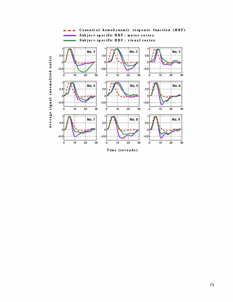
73

Guidelines for Presenting fMRI Data
This section is copied from the webpage maintained by Tom Nichols at U. Michigan,http://www.sph.umich.edu/~nichols/NIpub/ , which is a summary of the discussions on the SPMmailing list regarding establishing these guidelines. This is a collection of thoughts from activefMRI researchers, and should be treated as recommendations and not absolute requirements.However, more and more journals and referees are moving towards making them (at least inpart) a requirement.
At the end of this topic is an example methods section that I wrote to clarify how ourmethods should be reported. The reason I did this is because most of the analyses you will beconducting will take on a simpler form than described in these guidelines, so a lot of thisinformation may not be completely necessary and/or relevant to your study. Please use theexample section as a guide for the “typical” PNI fMRI study.
Note: Tom’s page is still a work in progress. Please take a moment to visit his site to make sureyou have the most updated version of the guidelines.
General Goal
The goal of this document is to have all neuroimaging papers have sufficient well-reportedmethodological detail such that a reader, if presented with an author's data, could reproduce thesame results presented in the paper. A closely related goal is to recommend aspects of theresults that should be reported. The primary goal stated first regards reporting in the methodssection. The secondary goal regards the content of the results section, and possibly an on-linerepository for supplementary data.
Methods: Experimental Design
Number of blocks, trials or experimental units per session and/or subject.
Methods: Data Collection and Processing
Image properties - As acquired✗ For voxel data (fMRI/PET/SPECT) image dimensions and voxel size.✗ For fMRI data, additionally, magnet strength (Tesla), TE and TR, FOV, and inter-slice
skip if any; image orientation (axial, sagittal, coronal, oblique; if axials are co-planar w/AC-PC, the volume coverage in terms of Z in mm); order of acquisition of slices(sequential or interleaved). Number of experimental sessions and volumes per session.
Pre-processing: General✗ For voxel data, type of motion correction used (minimally, software version; ideally, image
similarity metric and optimization method used) and interpolation method.✗ For fMRI, use of slice timing correction (minimally, software version; ideally, order and
type of interpolant used and reference slice).✗ For fMRI, use of EPI motion-susceptibility correction (minimally, software version).
74

✗ The order of the pre-processing steps should be recorded.
Pre-processing: Inter-subject registration✗ Inter-subject registration method used and software version✗ Affine? 9 or 12 parameters?✗ Non-linear? Deformation parameterization?✗ Non-linear regularization? (E.g. in SPM, e.g. "a little"). ✗ Interpolation method? ✗ Object Image information. (Image used to determine transformation to atlas)✗ Anatomical MRI? Image properites (see above) ✗ Co-planar with functional acquisition?✗ Segmented grey image? ✗ Atlas information✗ Brain image template space, name, modality and resolution. (E.g. "SPM2's MNI, T1
2x2x2"; "SPM2's MNI Gray Matter template 2x2x2")✗ Coordinate space? Typically Talairach, MNI, or MNI converted to Talairach.✗ If MNI converted to Talairach, what method? E.g. Brett's mni2tal?✗ How were anatomical locations (e.g. Brodmann areas) determined? (e.g. Talairach
Daemon, Talairach atlas, manual inspection of individuals' anatomy, etc.)
Pre-processing: Smoothing✗ What size smoothing kernel?✗ What type of kernel (especially if non-Gaussian, or non-stationary).✗ Is smoothing done separate at 1st and 2nd levels?
Statistical Modeling: Intra-subject fMRI
✗ Statistical model and software version used (e.g. Multiple regression model with SPM2,updates as of xx/xx/xx).
✗ Block or event; if block, duration of blocks.✗ Hemodynamic response function (HRF) assumed or estimated? If HRF used, which (e.g.
SPM's canonical HRF; SPM's gamma basis; Gamma HRF of Glover).✗ Additional regressors used (e.g. motion, behavioral covariates)✗ Drift modeling (e.g. DCT with cut off of X seconds; cubic polynomial)✗ Autocorrelation modeling ✗ Estimation method: OLS, OLS with variance-correction (G-G correction or equivalent), or
whitening.✗ Contrast construction. Exactly what terms are subtracted from what? It might be useful to
always define abstract names (e.g. AUDSTIM, VISSTIM) instead of underlyingpsychological concepts.
Statistical Modeling: 2-level, modality-generic
✗ Statistical model and software version used (e.g. 1-sample t on intrasubject contrast data,SPM2 with updates as of xx/xx/xx).
75

✗ Whether first level intersubject variances are assumed to be homogeneous (SPM &simple summary stat methods: yes; FSL: no).
✗ If multiple measurements per subject, method to account for within subject correlation.(e.g. SPM: 'Within-subject variance-covariance matrix estimated at F-significant voxels(P<0.001), then pooled over whole brain')
✗ Variance correction corresponding to within-subject variance-covariance matrix, sosimply some measure of nonsphericity.)
Statistical Modeling: Inference on Statistic Image (thresholding)
✗ Type of search region considered, and the volume in voxels or mm.✗ If not whole brain, how region was found; method for constructing region should be
independent of present statistic image.✗ If threshold used for inference and threshold used for visualization in figures is different,
clearly state so and list each.✗ Uncorrected inference is not acceptable, unless a single voxel can be a priori identified.✗ Voxel-wise significance? Corrected for Family-wise Error (FWE) or False Discovery Rate
(FDR).✗ If FWE found by random field theory (e.g. with SPM) list the smoothness in mm FWHM
and the RESEL count.✗ If not uniquely specified by use a given software package and version, the method for
finding significance should be described or cited ✗ Cluster-wise significance? If so, list cluster-defining threshold (e.g. P=0.01), and what the
corrected cluster significance was (e.g. "Statistic images assessed for cluster-wisesignificance; with a cluster-defining threshold of P=0.01 the 0.05 FWE-corrected criticalcluster size was 103.")
✗ Again, if significance determined with random field theory, then smoothness and RESELcount must be supplied.
Results
✗ Unthresholded Statistic Maps: Thresholded statistic maps can be seriously misleading.Both because they exclude sub-threshold but possibly broad patterns, and because theyimmediately reveal the mask. A reader automatically equates an absence ofsuprathreshold blob with no activation, yet they would think differently if they found therewas no data in that entire region (possible due to susceptibility artifacts) 22
✗ Time Course Plots: For event-related analyses minimally, and all analyses perhaps,waveforms should be plotted as figures or supplemental materials.
✗ Plotting interactions: If significant interactions (e.g., Group x Condition) or othercomplex contrasts are observed, barplots of % signal change or the like would be helpful.If bar plots are used, error bars should be included. If the contrast is within-subjects(repeated-measures) the appropriate within-subjects (repeated-measures) errors shouldbe used
✗ Hemisphere Effects: Inferences about significant hemispheric asymmetry require formal
22 Jernigan, T. L., Gamst, A. C., Fennema-Notestine, C., & Ostergaard, A. L. (2003) More "mapping" in brain mapping:statistical comparison of effects. Hum.Brain Mapp., 19(2):90-95.
76

tests of the Hemisphere x Condition (or Hemisphere x Group) interaction23. It isinappropriate to infer from main effects (of condition or group) that are significant in onlyone hemisphere that there is a significant asymmetry.
✗ Correlation Effects: Analyses of zero-order, partial, or part correlations between brainactivity and other measures (e.g., paper-and-pencil measures, task performance)mandate the inclusion of scatter plots, preferably with CIs.
✗ Maps of Standard Deviation or Confidence Interval Length: There is also a wealth ofinformation in the variance or standard deviation. A confidence interval for the primaryeffect is a scalar multiple of the standard deviation image (or, even if the CI is desired forthe BOLD %change, it's very easy to compute).
✗ ROI Mask Data: The exact values in a ROI mask can be critically evaluated to see if theregions covered make sense.
✗ Statistical Diagnostics: To assess if the data satisfy the statistical assumptions, showthe diagnostic statistics that assess Normality and white noise (possibly after whitening)assumptions.
✗ Design Matrices & Contrasts: When complex designs are used, a graphicalrepresentation of the matrix and a description of contrasts in term of columns could beprovided as supplementary information.
Acknowledgments
The following people have made contributions to this effort. Max Gunther started the thread onthe SPM list, and Karsten Specht, Russ Polldrack, Kent Kiel, Mauro Pesenti, Jesper Andersson,Iain Johnstone, Robert Welsh, Dara Ghahremani, Alexa Morcom, and Lena Katz, Daniel (akaJack) Kelly, Cyril Pernet and Alex Shackman followed with more suggestions.
Last modified: Tue Mar 8 09:32:53 EST 2005 Tom Nichols [email protected], UM Biostatistics
23 Davidson, R. J., Shackman, A. J., & Maxwell, J. S. (2004). Asymmetries in face and brain related to emotion. TrendsCogn. Sci. 8(9):389-391.
77

Sample fMRI Methods Section
Scan acquisition
Data were acquired on a 3 Tesla Philips Intera system (Philips MedicalSystems, Best, The Netherlands) at the F.M. Kirby Functional Imaging ResearchCenter (Kennedy Krieger Institute, Baltimore MD). The system is equipped with dualQuasar gradients (80mT/m at 110 mT/m/s or 40 mT/m at 220 mT/m/s). A standardhead coil was used to limit head motion. A sagittal scout (localizer) scan was collectedto pinpoint the exact location of the brain. Functional scans were collected usingecho-planar imaging (EPI) and a blood oxygenation level dependent (BOLD)technique with repetition time (TR)=1000 ms, echo time (TE)=34 ms, flip angle(θ)=90o, field-of-view (FOV) 240 mm2 in the xy plane, and matrix size =64x64,reconstructed to 128x128. Thirty four coronal slices were acquired with a 2.5 mmthickness and an inter-slice gap of 0.5 mm, oriented perpendicular to the anterior-posterior commisure (AC-PC) line. Slices were acquired sequentially along the z-axis;yielding total volume coverage of 119 mm. Functional scanning was performed in twosessions, each with 360 timepoints. Total functional acquisition time was 12 minutes.A high resolution whole-brain anatomical scan was obtained using a T1-weighted, 3DMP-RAGE (Magnetization Prepared Rapid Acquisition Gradient Echo) sequence withthe following parameters: TR=8.6 ms, TE=3.9 ms, FOV=240 mm, θ=8o, matrix size=256x256, slice thickness=1.5 mm, 124 slices.
Data pre-processing
Data pre-processing was conducted on a Windows XP workstation, equippedwith dual processors and 2GB of RAM. Statistical Parametric Mapping (SPM99,Wellcome Department of Imaging Neuroscience, University College, London, UK)was used, under the MATLAB 6.1 (The Mathworks, Sherborn, MA, USA)programming and runtime environment. Slice timing correction was conducted usingthe middle slice (#16) as the reference slice, and sinc-interpolation. Rigid-bodyregistration (motion correction) was performed by realigning the scans from bothsessions to the mean image of all the functionals in both sessions. This was conductedusing a 6-parameter affine transformation (3 translations and 3 rotations in x,y, and zaxes), followed by reslicing using a ‘windowed’ sinc-interpolation. Realignment outputplots and realigned volumes were checked for motion artifacts and size oftransformations. Affine (12 parameter) and nonlinear normalization using 7x8x7 basisfunctions and medium nonlinear regularization were conducted to deform eachsubject’s data into standard space (Montreal Neurologic Institute (MNI), McGillUniversity, Montreal, Canada) . Template space was defined by SPM’s standard EPItemplate (MNI). Data were resliced to isotropic voxels (2mm3) using trilinearinterpolation, and spatially smoothed with a full-width at half-maximum (FWHM)isotropic Gaussian kernel of 5mm3.
78
Statistical Modeling and Analysis
Individual subject-level analysis
Individual time series analysis was conducted using the general linear modelwithin the framework of statistical parametric mapping (SPM99). Data were modeledas event-related, and convolved with SPM’s canonical hemodynamic responsefunction (HRF) to account for the lag between stimulation and the BOLD signal.Motion correction parameters were entered into the model as covariates. The modelwas estimated using SPM’s standard ordinary least squares (OLS). Stimulus onset timesand corresponding reaction times were used to define two conditions (ON and OFF).The contrast of interest subtracted activation during the OFF condition from the ONcondition.
Whole brain random effects
A 1-sample t-test was conducted using the unthresholded contrast image (ONminus OFF) from each individual using SPM99’s basic modeling facility. Voxel-wisethreshold for inference and visualization using SPM's maximum intensity projectionsto p=0.05, corrected for family-wise error (FWE) (5 mm FWHM smoothing and 4016RESELS), with a spatial extent threshold k of 100 voxels. A Monte Carlo simulation(AFNI, AlphaSim) was conducted on each threshold pairing (height and extent) todetermine the level of alpha significance. Unthresholded statistical maps were alsoproduced to check any broad patterns excluded by the thresholding process. Thecoordinates of voxels that survived the statistical threshold were produced in MNIspace and converted to Talairach space (Talairach & Tournoux 1988) to facilitateanatomical labeling, which was conducted using the Talairach Daemon software(Lancaster et al. 1997) with an adaptive gray matter search range of 5mm3 (Lancaster etal. 2000). Labels were manually checked with the Talairach and Tournoux atlas(Talairach & Tournoux 1988)
Region of interest analysis
A 1-sample t-test was independently conducted on the unthresholded SPMcontrast images using the MarsBar toolbox for SPM99 (Brett et al. 2002). This analysiswas limited to a specified region of interest, defined by a robust manual segmentationof the left and right hippocampus by an expert rater (see Honeycutt et al. (1998) fordetails on the method's validity and reliability) on an average T1-weighted template ofall subjects in the study (normalized to SPM space and smoothed with a 4mm kernel).The model evaluated voxels for significance above a p<0.05 threshold and presenceinside the search region space. Results were corrected for multiple comparisons withinthe ROI search region (384 voxels in the left hippocampal space, and 356 voxels in theright hippocampal space).
79

Notes
-----------------------------------------------------------------------------------------------------------------------------------------------------------------------------------------------------------------------------------------------------------------------------------------------------------------------------------------------------------------------------------------------------------------------------------------------------------------------------------------------------------------------------------------------------------------------------------------------------------------------------------------------------------------------------------------------------------------------------------------------------------------------------------------------------------------------------------------------------------------------------------------------------------------------------------------------------------------------------------------------------------------------------------------------------------------------------------------------------------------------------------------------------------------------------------------------------------------------------------------------------------------------------------------------------------------------------------------------------------------------------------------------------------------------------------------------------------------------------------------------------------------------------------------------------------------------------------------------------------------------------------------------------------------------------------------------------------------------------------------------------------------------------------------------------------------------------------------------------------------------------------------------------------------------------------------------------------------------------------------------------------------------------------------------------------------------------------------------------------------------------------------------------------------------------------------------------------------------------------------------------------------------------------------------------------------------------------------------------------------------------------------------------------------------------------------------------------------------------------------------------------------------------------------------------------------------------------------------------------------------------------------------------------------------------------------------------------------------------------------------------------------------------------------------------------------------------------------------------------------------------------------------------------------------------------------------------------------------------------------------------------------------------------------------------------------------------------------------------------------------------------------------------------------------------------------------------------------------------------------------------------------------------------------------------------------------------------------------------------------------------------------------------------------------------------------------------------------------------------------------------------------------------------------------------------------------------------------------------------------------------------------------------------------------------------------------------------------------------------------------------------------------------------------------------------------------------------
80