- 1 -

TEL AVIV UNIVERSITY The Iby and Aladar Fleischman Faculty of Engineering

Functional Optical Imaging of Tissue

based on Fluorescence Lifetime

Measurement

A thesis submitted toward the degree of

Master of Science in Biomedical Engineering

by Izhar Ron

This research was carried out in the Department of Biomedical Engineering under the

supervision of Dr. Israel Gannot

January 2004

- 2 -

1 Introduction

1.1 Fluorescence

The phenomenon of photoluminescence has been known for over a century now, and

the ability to use it for spectroscopic methods is growing, especially within the last

few decades. This section deals with the physical aspects of fluorescence, which is the

more spectroscopically applied branch of photoluminescence (relative to

phosphorescence), in order to background its usage in the application represented in

this thesis.

1.1.1 Basis of fluorescence

Luminescence is the emission of photons from electronically excited states [1]. The

type of luminescence process that occurs is determined by the nature of the ground

and excited states of the molecule. Most organic molecules have an even number of

electrons. In the ground state, the electrons fill the atomic orbitals with the lower

energy levels, whereas their spins must be in opposite directions, so the net spin

equals 0. This is known as the singlet state. Upon excitation of a molecule, an electron

from the highest occupied orbital travels to an unoccupied orbital, where it can exist

in an opposite orientation to the electron left in the previous orbital (singlet excited

state), or having the same orientation (triplet excited state). The latter configuration

has a net spin of 1. Returning of an electron from a singlet excited state to the lower

orbital of its paired electron is allowed, quantum mechanically speaking, and takes

place on a very short time scale (emissive rates of 108 sec-1). This is the process of

fluorescence. In order to return from a triplet excited state to the singlet ground state,

the electron must experience a spin reversal. This forbidden process is usually the

basis to phosphorescence, a much less rapid process that may last from milliseconds

to seconds.

Before excitation occurs, at equilibrium, the molecules are distributed thermally at the

lowest vibrational and rotational energy levels of the ground state, S0. Upon

excitation, the molecule absorbs energy and is elevated to one of the excited singlet

states, Sn (n=1,2,…). The molecule then undergoes a vibrational relaxation (VR) to

the lowest vibronic level of the corresponding excited state, a process that is

- 3 -

accompanied by releasing of thermal energy to the surrounding medium. Emission

from higher vibronic levels may occur only under special conditions (such as low

pressure), but usually not in condensed matter (such as tissue).

Before fluorescent emission occurs, an additional process usually takes place: the

internal conversion (IC) of the molecule from the Sn excited state to Sn-1 excited state

and so on, until (in combination with VR processes) emission will occur in most cases

from the lower excited state (S1). The S1→ S0 may occur non-radiatively (through IC

and VR) or radiatively – through fluorescence. The emitted photon energy carries the

information of the energy gap between S1 to the vibronic levels of the ground state.

The alternative scenario of returning to ground state involves a change in spin

multiplicity – which enables the transition from some excited singlet state, Si to some

excited triplet state, Ti. This process is known as intersystem crossing (ISC). The

molecule can relax to T1 through IC and VR and then return to ground state non-

radiatively (through ISC) or radiatively – phosphorescence.

Fig.1-1 Jablonski’s energy diagram

A less common process of luminescence that might occur is delayed fluorescence. If a

transition of T1 → Si occurs, conventional fluorescence can take place, but with longer

lifetime (the time a molecule spends in the excited state). Of course, this kind of

- 4 -

transition requires additional activation energy, which originates usually from thermal

events or interaction between pairs of triplet state molecules. A schematic

representation of the above processes was well described by Alexander Jablonski,

who is considered the father of fluorescence spectroscopy, in his energy diagram

shown in figure 1-1 [2].

1.1.2 Parameters of fluorescence

A fluorescent molecule is first characterized by its absorption and emission spectra.

The absorption spectrum holds information on the vibrational frequencies of the

molecule’s excited state, and the emission spectrum on those of the molecule’s

ground state. Relying on the Franck-Condon principle, which states that electronic

transitions are too fast to allow for a nuclear rearrangement (since the atomic nuclei is

much heavier), the transition is said to be vertical, and the two spectra are

approximately mirror images of each other (figure 1-2). Since the molecule undergoes

two periods of vibrational relaxations within the excitation process (from vibronic

states of the excited state to the lowest excited state and from vibronic states of the

ground state to the lowest ground state), thermal dissipation of energy occurs and the

emission is of a lower quanta of energy, hence the photon is of a longer wavelength.

This red shift is known as Stokes’ shift.

- 5 -

Fig. 1-2 The Franck-Condon Principle: Energy Vs. nuclear distance (top) The mirror image relation

between absorption and emission spectra (bottom)

Upon excitation with polarized light, a fluorophore will preferentially absorb those

photons whose electric vector is parallel to its transition dipole. This kind of angle

between transition moments of absorption and emission, θ, determines the maximum

measured anisotropy. Fluorescence anisotropy and polarization are defined as

follows:

⊥

⊥

+

−=

IIII

r2||

|| (1.1)

⊥

⊥

+

−=

IIII

P||

|| (1.2)

Where Eq. 1.1 represents anisotropy, r, by the vertically (⊥ ) and horizontally (║)

emission intensities, and Eq. 1.2 represents polarization using the same factors. Since

molecules undergo rotational diffusion during the excited state, and can rotate in any

angle prior to emission, the polarization of emission might change in time.

Fluorescence polarization is irrelevant for the case of turbid media, since the major

part of light entering this media shortly becomes non coherent.

Under defined conditions, the molecule exhibit a defined luminescent sensitivity

which is determined by the ratio between the number of emitted (luminescent)

photons to the number of absorbed exciting photons. This ratio is known as the

quantum efficiency (or quantum yield) of the molecule. This parameter may be also

- 6 -

expressed in terms of rate of fluorescent decay (Γ) and rate of radiationless decay (k),

as in the form presented in Eq. 1.3, and in terms of fluorescent lifetime, which will be

described in the following section.

kF +Γ

Γ=Φ (1.3)

1.1.3 Fluorescence lifetime

Fluorescence lifetime is defined as the average time the molecule spends in the

excited state following excitation, before returning to the ground state [2]. Since

fluorescence is decaying exponentially, the lifetime is sometimes defined as the time

from intensity peak (the rise in response to an excitation pulse) to 1/e in the decay

curve. A fluorophore has its intrinsic natural lifetime that is defined for FΦ =1, that is

when no radiationless decay occurs. This lifetime is defined by τ0 as shown in Eq. 1.4,

and may be used to define quantum efficiency, when measured lifetime is given, as in

Eq. 1.5.

Γ= 10τ (1.4)

0ττ=Φ F (1.5)

The fluorescence lifetime of organic molecules is of the order of 10-9-10-7 seconds. A

single exponential decay curve is of the form shown in Eq. 1.6:

)exp()( 0 τtItI −= (1.6)

For this kind of decaying, 63% of the molecules decay at t < τ and only 37% decay at

t > τ. A decay of a molecule may be also analyzed as bi-exponential or multi-

exponential, and weights should then be assigned to the different populations

consisting this decay.

- 7 -

1.1.4 Fluorescence quenching and photobleaching

In addition to fluorophores’ intrinsic parameters, these two fluorescence-related

phenomena are sometimes used to characterize fluorophores or as distinguishing tools

in fluorescence spectroscopy.

Photobleaching is the destruction of the photosensitizer/fluorophore after exposure to

light. The basis of this process lies in the energy transfer from the excited probe to an

Oxygen molecule (in its ordinary triplet state), which in turn shifts to a singlet state, a

highly oxidative form which attacks, among others, the fluorophore molecule and

causes a change in its conformation. This leads to a reduction in fluorescence intensity

with excitation time. It may be used deliberately as a measured factor, in a technique

called fluorescence recovery after photobleaching (FRAP) in which the fluorescence

is measured after a boost of excitation light, and the recorded data may describe

diffusive processes of the photobleached molecules, but in most methods it is

considered an artifact, and should be avoided as much as possible, or at least taken

into account in planning the intensity and time of excitation.

Bleaching is actually a private case of a larger phenomenon called quenching of

fluorescence, which refers to any process that decreases the intensity of measured

fluorescence [2]. Some of the processes that can cause quenching are excited-state

reactions, molecular rearrangements, energy transfer, ground-state complex formation

and collisional quenching. In dynamic quenching, a quencher molecule diffuses to the

fluorophore while it is in its excited state, and if a physical encounter occurs, the

fluorophore returns to the ground state without the emission of a photon. Static

quenching is caused when a complex between the fluorophore and the quencher is

formed. In both cases, contact must exist, and no permanent damage is caused to the

molecules. Quenching measurements are used to study fluorophores’ localization in

proteins and membranes and membranes permeability to quenchers, and hence may

be used as a source of information on conformational changes of the above.

Collisional quenching of fluorescence usually results in a shorter lifetime than the

actual lifetime of the fluorophore [3]. This rate of energy transfer usually depends on

concentrations of different ions in a solution, hence the effect of quenching on the

measured fluorescent decay rate (lifetime) may be used also to probe these

concentrations (figure 1-3).

- 8 -

Fig. 1-3 Effect of quenching on lifetime

1.1.5 Fluorescent dyes

Fluorescent substances are divided into two main groups: intrinsic and extrinsic (or

endogenous and exogenous). The first refers to nucleotides, proteins and other

macromolecules consisting in the living cell/tissue, and the latter to synthesized or

organic materials which are introduced to biological or artificial samples and whose

luminescence gives information about the sample’s status, conformation, molecular

structure, environmental conditions and more parameters.

Regarding this work, exogenous fluorescent markers are of uppermost relevance.

There are thousands of manufactured fluorophores nowadays. These molecules may

be used in several applications in biological/live samples: labeling proteins

(covalently or non-covalently), labeling membranes, probing membrane potential,

labeling DNA sequences, chemical sensing of ions [2, 4]. Some unique classes of

fluorophores exist such as fluorescent proteins, viscosity probes, fluorescent lifetime

probes, fluorogenic probes, molecular beacons, Lanthanides – fluorescent metals with

long lifetimes, photo-activatable (caged) probes and more. The labeling of proteins

with fluorophores is usually performed through coupling of various reactive groups of

the probes with amine, sulfhydryl or histidine side chains of the protein [5],

covalently, or non-covalently by probes that are usually less fluorescent when not

bound to the protein. Labeling of membranes can be performed by introducing water-

insoluble probes to the nonpolar side of the membrane [2] and probing membrane

potential is done by using probes that are sensitive to potential changes due to their

reorientation, aggregation in the membrane or sensitivity to electrical field. Labeling

DNA is performed using the classical DNA probes – Ethidium Bromide or Acridine

orange, which spontaneously bind to DNA helices [6] or by incorporating DNA base

- 9 -

analogs to the sequence and thus rendering it fluorescent. More novel techniques

include the use of what is known as a molecular beacon – which is designed to probe

the level of presence of a specific DNA sequence in a sample [7]. This is achieved by

creating a DNA sequence with both ends complementary to the desired sequence’s

ends. Attaching the fluorophore molecule to one end while a suitable quencher is

attached to the other end allows this species to form a loop when no DNA is present,

thus no or little fluorescence will be observed, since quenching will take place. Upon

binding to a sequence, the fluorophore and the quencher are separated, and the

sequence can then fluoresce to a degree corresponding to its level in the sample.

Fluorogenic probes are dyes that become fluorescent following a chemical or

biological event, such as enzymatic cleavage or hydrolysis. These dyes are used to

measure activity of several enzymes in the cell [8]. Another class of special probes is

that of photoactivatable (caged) probes that are originally designed to allow

controlling (spatially and temporally) the release of active biological substances and

reagents, by means of flash photolysis of the caged probe [9, 10]. Later, this principle

was used to design fluorophores that undergo activation following a flash of light,

thus allowing measurements of activated fluorescence against the dark background.

1.1.6 Mechanisms of sensing molecules and ions through fluorescence

A very large group of dyes is that of fluorescent indicators. These include acid-base

indicators, oxidation-reduction indicators, adsorption indicators and a large variety of

ion indicators. These dyes usually consist of a fluorophore and a site for analyte (or

metabolite) recognition. The basic method of sensing is the detection of changes in

intensity in correlation with the concentration of the analyte of interest, whereas these

changes originate from collisional quenching. Intensity changes are not totally

reliable, since concentration of the probe may change with diffusion processes.

Furthermore, photobleaching affects the intensity regardless of the analyte

concentration.

Wavelength ratiometric probes exhibit spectral shifts upon analyte binding. It is

possible to conclude about the analyte’s concentration from the ratio of intensities of

measurements with two excitation/emission wavelengths (depending on the dye

properties). This kind of measurement is independent of the dye concentration. Some

analytes exist that change the polarization of the probe. It is also possible to measure

- 10 -

anisotropy that changes when the measured analyte replaces a labeled analyte bound

to an antibody.

Various mechanisms allow the sensing of concentrations through measuring different

fluorescent parameters. Collisional quenching causes a decrease in intensity and

shortens the fluorescent lifetime. Resonance Energy Transfer (RET) – the closer the

donor and acceptor are, the lower the measured fluorescent intensity and lifetime of

the donor, due to transferring the energy between both. Hence, the concentration of an

analyte on which the acceptor’s absorption spectrum is dependent, can be calculated

through measuring the intensity of the donor.

Some probes exhibit an on-off mode of operation, when equilibrium exists between

an analyte-bound probe and a free probe in the solution, and only one of the forms is

fluorescent. An alternative method is that when both forms are fluorescent, but with

differences in quantum efficiency or in the emission spectrum. A spectral shift is

typical for pH probes and cations probes. These dyes allow for ratiometric

measurements.

Collisional quenching-based probe may use for oxygen concentration calculation

given that the probe is sensitive for quenching by oxygen molecules. Collisional

quenching is usually described by the Stern–Volmer equation, as shown in Eq. 1.7:

][1][1 000 QKQK

FF

q +=+== τττ

(1.7)

Where F0 and τ0 are the probe’s natural intensity and lifetime, respectively, and F and

τ are the probe’s measured intensity and lifetime with analyte presence, Kq is the

quenching constant and [Q] is the quencher concentration. Choosing a probe with a

relatively long lifetime (in the absence of analyte) will result in a high sensitivity to

the analyte concentration, since the ratio τ0/ τ will increase more rapidly with

quenching. In general, it is said that for lifetime-based sensors, the longer the lifetime

is, the stronger is the effect of the quencher.

Lifetime-based sensors have also the advantage of overcoming fluctuations of

intensity, when these have no experimental significance. The lifetime tends to remain

stable even when 5-fold fluctuations in intensity occur [11].

In energy transfer-based sensing, designing of the probe is made simpler. The donor

and acceptor may be two separate molecules, and the donor should be adjusted

- 11 -

according to the excitation wavelength. Only the acceptor should be uniquely

sensitive to the analyte. Probes with absorption dependence on pH of the acceptor

exist, which exhibit a decrease in donor’s intensity/lifetime with increasing of pH

value (the acceptor absorbs in its basic form).

Sensing of pH is based on changes either in fluorescence intensity, emission

wavelength or lifetime. The fluorescing form may be the ionized (A-) or non-ionized

(AH) form of the molecule [4]. In general, the binding of a proton to the base form of

a dye molecule will change the confinement of electrons from mobile status to bond

formation, which effects the electronic state of the molecule, and hence its spectrum.

When choosing or designing a dye, several criteria should be fulfilled: high quantum

yield, low or none photo-bleaching, no photo-sensitizing effects (unless Photo-

dynamic Therapy is the issue), hydrophilicity and low toxicity of the dye, large

stokes’ shift, and a spectroscopic profile in the near IR range is also an advantage

(will be discussed in tissue optical properties section). The next step in executing the

experiment, is delivering the probe to the region of interest. This issue is described in

the next section.

1.1.7 Delivering the fluorescent probe

Fluorescent dyes are designed not only to exhibit spectral changes in response to all

kind of chemical and physiological events, but also to allow its successive

introduction to the sample for proper functioning. The considerations behind this

procedure include the diffuse behavior of the dye, its membrane permeability, its

affinity to the substances it is monitoring – when the dye is delivered independently,

and the possibilities to conjugate the dye to affinity ligands or antibodies in cases

where the dye is introduced through an intermediate. The important criteria to be

addressed when designing the probe are its delivery in a way that maintains the

physiological and structural integrity of the cell, its selective targeting to the species

of interest, maintaining the spectroscopic characteristics of the probe and a detectable

fluorescent response of the probe upon interaction with the investigated species [12].

Several approaches exist for selectively introducing the probe to the sample: one is to

create fluorescent analogues to lipids or receptor ligands [13]. Another is to couple

fluorophores with targeting groups in a way that interaction with the targeted species

- 12 -

will result in a detectable spectral/intensity change [14]. The recognition of the green

fluorescent protein’s capabilities made the last approach even simpler, since by means

of genetic engineering it is possible to insert the gene encoding to GFP to cells and

obtain the desired proteins attached to GFP [15]. Probes may be introduced to the

sample carried in a structural support (e.g. silicon-based) that will allow the diffusion

of the analyte of interest and prevent the interference of undesired factors from the

environment. Targeting a probe by means of attaching it to a specific antibody will be

discussed as a spectroscopic method (known as fluorescence labeled antibody

imaging) in a later section.

1.2 Light and tissue

1.2.1 Optical properties of tissue

Any substance that is not transparent will scatter photons upon incidence of light on

it. A biological tissue (in vivo or even excised) is termed a turbid (cloudy) medium for

light, and is a strong scatterer. The tissue is defined isotropic and homogenous only

within the algorithms that deal with assessing the dynamics and behavior of light

penetrating it, but is far from behaving as such in practice. The elements that absorb

light within tissue are termed “Chromophores”. Scattering may occur upon photon

hitting other elements. Tissue absorbs relatively weakly in the so-called “Diagnostic

window” (600-1000nm), which is practically the only range where spectroscopic

practice and analysis is feasible. Within the limits of this window, scattering becomes

significantly dominant over absorption, an important fact for later discussions. The

main absorbers working within this window are melanin, hemoglobin (both forms)

and water, but not at its peaks.

Tissue is characterized optically by several parameters: The index of refraction, n(λ),

describes the change in direction of light which crosses the surface (and is not

reflected) according to Snell’s law, and allows to calculate the transmission by T =

4n1n2/(n1+n2)2, and the reflection from the surface R = 1-T (which is different from

diffuse reflection), and generally holds values in the range 1.33-1.6 for biological

tissues [16]. The absorption coefficient, µa, is related to the probability of a photon to

be absorbed by a chromophore (in cm-1) and µa-1 is the mean free path of a photon

before absorption occurs. In a similar manner, scattering is characterized by the

- 13 -

scattering coefficient, µs, which leads to knowing the mean free path of a photon

between scattering events.

In the near IR region (the therapeutic window), where tissue absorption is relatively

low and multiple scattering events occur, the penetration of photon deeper within

tissue is enabled (figure 1-4). The sources for this multiple scattering lie in the

microscopic heterogeneities within tissue structures that result in frequent fluctuations

in the indices of refraction. The tissue scatters mainly in the forward direction, as

exhibited by the high values of the anisotropy parameter, g, to be around 0.69-0.995

(the average cosine of the scattering angle) [17]. We usually refer to elastic scattering

(no energy loss or gain upon a scattering event) that is described by Mie or Rayleigh

theories, depending on the wavelength to scaterrer’s size ratio. Scattering coefficients

are in the range of 10-1000cm-1 and absorption power is also characterized by the

molar extinction coefficient, ε, defined in units of [cm/mM].

Fig. 1-4 Tissue absorption in the near-IR region

- 14 -

1.2.2 Describing photon propagation in turbid media

When coming to mathematically treat the interaction of light with tissue, a

combination of classic description of light (as a wave), that defines mathematically

the dynamics of light transport (e.g., calculate scattering cross sections) and discrete

(photonic) description of light (that explains processes such as molecular transitions,

absorption, luminescence and Raman scattering) is looked for. Because of the

multiple scattering in turbid media such as tissue, the use of electromagnetic wave

theory would be too complex. Rather, Radiation Transport (RT) theory may fulfill the

requirements of the different models, under certain assumptions [18]. RT ignores

wave properties such as polarization and interference, and refers only to the transport

of light energy. The multiply scattered light is referred to as the incoherent fraction of

the scattered field (displaying random relations of the phase with time and position),

and therefore eliminates interference effects. The radiation transport equation

(Boltzman equation) describes the propagation of original energy (as a collection of

incoherent photons), which, depending on the time and direction, is losing energy

with absorption and scattering events, while gaining energy from other scattering

events. The diffusive fraction of the field is usually of interest, being the component

that penetrates in tissue and causes processes such as diffuse reflectance (reflection

from areas beneath the surface) that holds information on the media properties. In the

RT model, the total mean free path is simply defined through the total attenuation

coefficient: lt = 1/(µa+µs). However, for realistic cases such as tissue surfaces,

heterogeneities and complex geometries, more sophisticated analytical solutions are

needed. For the limiting case of dominant scattering (µs>>µa), also known as the

diffusion limit, the particles (photons) travel in a series of steps, each having a random

length and direction, and are thus subjected to the Random Walk (RW) regime. In the

random walk theory, each step starts with a scattering event, and has equal probability

of traveling in any direction [19]. This leads to an isotropic regime of photon

dispersion, even when only a few photons have entered the system. As the number of

photons increases, its density may be described as a continuous function whose

dynamics are described by the diffusion equation, where the diffusion constant holds

the information of media optical properties. Here, the effective total mean free path is

defined in terms of µs’, rather than µs, as: lt’ = 1/(µa+µs’). The lowest order (first order)

approximation to the diffusion equation is used in this dominant scattering limiting

- 15 -

case, and is practically suggesting that photons flow according to a density gradient in

space in the steepest possible line.

Numerical approaches have also been developed for cases that are beyond the

capabilities of analytical solutions (mainly complex geometries, but also tissue

characters and different types of light sources). The Kubelka-Munk model may be

used for describing a planar, homogenous, ideal diffusive medium irradiated from one

direction with monochromatic diffusive light. The light beam is described to lose

intensity due to absorption and scattering events, and gain intensity from other

scattering events (retrieving photons into the beam). Other assumptions underlying

this model are that reflectance and absorbance are constant over the area of

illumination and through the sample’s thickness. Although this model is frequently

used for calculating optical properties of diffuse media, and sometimes even for

quantitative analysis of optical biopsies methods, it is practically limited to simple

slab geometries. For all kinds of complex geometries, and varying light sources and

tissue types, the most common approach is using Monte Carlo-based algorithms. This

theory, possessing a random behavior by name, is a forward tool used to simulate

propagation of photons within media for a variety of given parameters (considered the

most flexible theory for realistic multi parameter cases), and is especially useful in RT

problems. The distribution of probabilities along the length and angle of path in every

scattering event is statistically sampled. As the number of simulated photons

increases, a better approximation to the RT model exact solution is achieved [20].

1.2.3 Optical phantoms

Tissue-like optical phantoms are test objects that mimic the optical properties of tissue

and on which calibration of the instrument, algorithm’s refinement and preliminary

measurements are being executed. When coming to evaluate the performance of an

experimental system and to validate the credibility of theoretical predictions (forward

algorithms), a reproducible model whose characteristics are well understood and

controllable is desired. A tissue-like phantom is, in most cases, a homogenous

substance with a simple geometry. Indeed, the heterogeneity and morphological

complexity of a biological tissue will not be expressed through the use of such

phantom. However, the phantom may be produced to possess, with a high fidelity,

optical properties that resemble those of a tissue. Moreover, a solid (jelly-like)

- 16 -

phantom usually exhibits mechanical properties (mostly a gelatinous texture) that

allow it to conveniently fit into most experimental setups. These properties enable one

to cut, using simple means, the phantom to a desired shape and size and to cast it into

various templates.

Designing a phantom starts with selecting the ground material (or base material) that

will determine the phantom’s structural, chemical and mechanical properties. The

important factors to be considered are its stability, handling safety and compatibility

with the other constituents of the phantom. It is also desired that it will not interfere

with the spectral properties that one wishes to obtain. Commonly used ground

materials for solid phantoms preparation are polymerizing agents such as agar,

polyacrilamide (PAA), gelatin and more [21]. The temporal stability of the material’s

physical parameters should be taken into account in order to minimize phenomena

such as evaporation of solvents, aging of polymers and degradation of constituents by

bacteria (Sodium Azide may be added in preparation process to protect from the

latter).

The next factor to be considered is the scattering medium. The most common

scatterers are fat emulsions, such as Intralipids, Nutralipids and Liposin. Intralipids

are known as intravenously introduced substances for patients. These materials are

suspensions of roughly spherical fat droplets dispersed in water [22]. Estimations of

the mean size of the scattering oil droplets range from 125-425nm [23, 24]. This

parameter is important when predictions regarding the wavelength dependence of the

scattering and reduced scattering coefficients are being made. Intralipids’ measured

optical properties tend to underestimate the value of anisotropy, g, relative to tissue,

therefore when designing such phantom, a reduced scattering coefficient (which is a

function of both g and µs) similar to that of a tissue should be obtained, rather than

scattering coefficient. Intralipids are considered colloidal systems (where particles of

one substance are found in a suspension of a second substance), and hence may be

subjected to aggregation over time with dramatic changes of pH or ion content of the

diluent. The resulting reduced scattering coefficient of Intralipid-based phantoms is

dependent on the amount of the gelling agent (effect that might be caused either by

the increased temperature during phantom preparation or by structural changes of the

scatterers, induced by interactions with the polymer).

- 17 -

1.3 Current spectroscopy methods

1.3.1 Fluorescence labeled antibody imaging

The advantages of targeting a fluorescent dye by means of coupling it to specific

antibodies for diagnostic biomedical purposes may be intuitively understood: staining

only the regions of interest within suspected tissue increases the specificity of the

measurement even before interpreting the measured spectral signals. The contrast of

detection or imaging is also significantly increased when the concentration of the dye

remains high where high affinity binding has occurred, while the circulating fraction

is washed out after some time. For better localization and spatial resolution of

detecting the bound dyes, the technique was improved towards the use of engineered

antibody fragments or synthetic peptides (in place of full-size antibody molecules)

that maintain the same high affinity. The use of fluorescence labeled antibodies in

specific targeting of dyes in vivo is often used in the same manner as in radio-labeled

diagnostic techniques, without the undesired disadvantages of the latter, including

ionizing radiation, bond breaking and other types of chemical and biological

alterations.

The basic structure of immunoglobulins (Ig’s) contains two light polypeptide chains

and two heavy polypeptide chains. This structure may be treated enzymatically to

produce several fragments, some of which contain the antigen-recognizing areas

(figure 1-5). The fragments that retain the antigen-binding activity are called Fab

fragments. The complementary fragment of the Fabs relative to the native Ig is known

as the Fc fragment. The area in a macromolecule that is recognized by an antibody is

termed antigenic determinant or epitope. For research and diagnostic purposes,

monoclonal antibodies, which are specific for only one type of epitope, are produced.

The interaction of antibody and antigen is a bimolecular association, similar to an

enzyme-substrate interaction, with the exception of being a reversible process (no

permanent chemical changes are found in either the antibody or antigen). This

interaction is of exquisite specificity compared to almost all kinds of chemical

reactions. The high affinity is expressed through an extremely high degree of

complementarity between the two interacting surfaces. This can be demonstrated by

the almost complete exclusion of water from the interface, implying that the cavities

that exist between the two surfaces are too small to accommodate a water molecule

- 18 -

[25]. Other characteristics of this type of interaction are high matching of charges

between the molecules (charge neutralization), a specific hydrogen bond arrangement

and the potential of every accessible region of the antigen to become antigenic[26].

The basic structure is presented in figure 1-5.

Figure 1-5 Prototype structure of IgG: L – light chain; H – heavy chain

The use of labeled antibodies in tumor localization requires primarily information

regarding the possible targets. Common targets are over-expressed, altered or

selectively accessible [27] receptors for specific ligands such as somatostatin (SST),

bombesin and vasoactive intestinal peptide (VIP) [28]. All components that are

present at high ratios due to angiogenesis, a common feature of tumors, are also

optional targets. In addition, receptors that are found on T cells that infiltrate in

response to tumor development may be used for this purpose [29]. It was proposed

that the extracellular matrix should be explored as a target following the observation

that antibodies targeted to the cell’s membrane were bound also to the extracelular

- 19 -

fluid and matrix [30]. It is important to realize that in vitro specificity does not

necessarily predict in vivo specificity. Purification or engineering of the chosen

antibody is then required, and of course the ability to conjugate it to the preferable dye

needs to be considered. When introducing the complex to tissue in vivo, the main

limitation is a pharmacokinetic one. In humans, a relatively long time is required for a

sufficient fraction of circulating blood to access small tumors, and methods to

increase blood flow or vascular permeability of the tumor area are sometimes used

[31, 32]. During that time, the conjugate may settle in other organs for a long time in

what is known as non-specific retention. A relatively short clearance time of unbound

conjugates should also be obtained.

The use of fluorophores as labeling agents possesses several advantages over the

traditional use of radioisotopes, namely: multiple cycles of excitation and emission;

use of a light signal whose focusing is made simple using lenses (thus permitting

whole field imaging with a good resolution); and, as often claimed, improved

sensitivity and resolution.

Two main groups of dyes have been used for these purposes: fluorescein and cyanine.

Both fluorescein and the fluorescein derivative fluorescein-isothiocyanate (FITC) are

mentioned in many works of labeled antibody imaging. Cyanine dyes enjoy growing

attractiveness, especially with the trend of Near-IR spectroscopy.

1.3.2 Fluorescence lifetime imaging

Fluorescence Lifetime Imaging (FLI) and Fluorescence Lifetime Imaging Microscopy

(FLIM) are becoming leading technologies in molecular, cellular and tissue imaging

in biomedical applications, but also in chemical applications in the materials science

and industry. The highlighted advantages of the lifetime parameter are its claimed

independency on probe concentration, photobleaching and photon pathlengths, and its

dependence on environmental conditions. The alternative way to avoid concentration

influence is using wavelength-ratiometric probes (see section 1.1.4), but nowadays

there appears to be a larger number of commercially available lifetime-based probes

(and moreover, ratiometric probes require the use of two excitation wavelengths).

The concept of lifetime imaging is the generation of lifetime values contrast images.

Steady-state fluorescent measurements may show equal intensity for two points in a

sample, whereas time-domain measurements of the same points may result in a

- 20 -

different lifetime, suggesting spatial differences in a sample that are not detectable

through measuring only the intensity. The motivation to establish imaging techniques

with lifetime as the contrast agent originates also from the fact that time-resolved

fluorescence measurements hold information regarding dynamics of biological

processes, that is not available from non-temporal techniques.

Various techniques of lifetime measuring (with emphasis on Time-Correlated Single

Photon Counting, TCSPC), analysis and applications are described in the following

sections.

1.3.2.1 Means of time-resolved fluorescence spectroscopy

Both time-domain and frequency-domain methods are used to measure fluorescent

lifetime. The two techniques are equivalent and related through Fourier transform.

The instrumentation, appearance of data and analysis differ between both methods.

Time-domain – The fluorescence is excited by a short light pulse, followed by

measuring the emission rate relative to the number of excited molecules. In other

words, the lifetime, τ, may be extracted from the change in population of the excited

state as a function of time, t, following a short excitation pulse, according to equation

1-10:

)()()( tnkdt

tdnnr+Γ−= (1-10)

Where, Г is the emission rate, knr is the non-radiative decay rate and n is the number

of molecules that populate the excited state. τ may then be expressed as follows:

1)( −+Γ= nrkτ (1-11)

And τ-1 is actually the sum of emissive rates that depopulate the excited state.

Several sampling methods are used in lifetime measurements. These methods use

gated detection of fluorescent signals. The commonly used Boxcar method [2, 33, 34]

is based on excitation of a sample with a periodical pulse train, with each pulse

- 21 -

followed by turning on a signal recording device for a very short duration, ∆t, with

some delay after the pulse. This delay is right shifted with every pulse and the above

is repeated for a set of delays, until the entire decay curve is sampled. Full images are

taken for every delay, and each pixel at the final image is constructed by collecting all

the signals recorded at this pixel (at different delays). This method was taken a step

forward with the development of the gated image intensifier. This device retains the

basic principles of boxcar sampling, but with synchronously detecting all points of the

sample (whole-field imaging), thus eliminating the need for scanning processes and

significantly reducing acquisition time. The device utilizes a photocathode for

primary detection of the photons emitted from an excited sample, while preserving the

pattern of fluorophores in the sample. The photons are further amplified by a

single/chain of MCP-PMT’s and the resulting photoelectrons finally hit a phosphor

screen that is observed by a CCD camera. The gating actions are performed on the

photocathode.

While in methods where scanning of the sample is involved, the scanning device is

synchronized with the data acquisition software (hence, every pixel corresponds to a

known point in the sample), in non-scanning methods there is a need to generate a

spatial sensitivity for the detection instrumentation. This is usually done by designing

anodes (the terminal stage of every PMT) that are able to provide information on the

spatially origin of each signal at the sample. Common designs include delay line

anodes (DL) which outputs a ∆t between arriving time of the signal to both ends of

the anode and translating it to the location of the hitting of photoelectrons on the

anode (for linear position resolution), quadrant anode (based on a similar principle)

for 2D position resolution and multi-anode (MA-MCP-PMT), an array of individual

anodes (spatially separated), where the location of each corresponds to the spatial

origin of the signal it receives.

Streak cameras were developed for cases of picosecond luminescence monitoring, in

times where sufficiently fast photo-tubes were not available, and are still commonly

used in lifetime measurements. Some of these devices are said to have instrument

response functions of 400fs, which is faster than for TCSPC operating with MCP-

PMTs. Streak cameras operate by dispersing the photoelectrons across an imaging

screen. This is accomplished by accelerating the photoelectrons into a deflection field.

The beam is then swept linearly in time across an MCP electron amplifier that

- 22 -

preserves the spatial information. The amplified electron beam strikes a phosphor

screen that can, in turn, be detected by a CCD camera. Streak cameras can provide

simultaneous wavelength and time-resolved decays (the dispersion is also by

wavelength).

Frequency-domain – Frequency –domain (FD)-based methods rely on the concept of

exciting fluorophores with harmonic modulated light with a given angular frequency,

and observing the phase lag and decrease of modulation of the resulting emitted signal

[2, 35, 36]. These changes have been shown to depend on the lifetime components of

the emission signal [37, 38]. Comparing to TD methods, a modulated light replaces

the pulsed light, gating pulses are replaced with high-frequency gain modulation

(corresponding to the frequency of excitation) in different phases, the image

intensifier in use is a modulated (instead of gated) one, and the construction is of

images in different phases (rather than different time delays). The FD measurement

concept is illustrated in figure 1- 6.

- 23 -

Figure 1-6 Principle of frequency-domain lifetime measurement

Many technological advances regarding FD techniques have evolved through the last

decade, and will not be discussed here.

Measuring lifetime through recording the complete fluorescent decay curve is

performed using TCSPC. This method is described separately in the following

section.

1.3.2.2 Time-correlated single photon counting

Time Correlated Single Photon Counting (TCSPC) is one of the more frequently used

time-domain techniques for measuring lifetimes of both endogenous and exogenous

fluorophores. The scale of fluorescent lifetime (ps-ns), its accuracy and resolution has

made its measurement a prefered technique for imaging biological processes. The

TCSPC method is based on the detection of single photons of a periodical light signal,

measurement of the detection times of the individual photons and the reconstruction

of the waveform from the individual time measurements. The accuracy does not

depend on the fluorophore’s concentration or exclusive position, or on the width of

the detector pulse (due to eliminating its jitter using a constant fraction discriminator).

- 24 -

Hence, TCSPC is considered intensity-independent, and is especially effective in

analyzing the low light levels present in fluorescence decay time studies.

The technique is of a digital nature, which makes data acquisition and analysis more

simple and accurate. The method basic principle is as follows:

The fast laser source pulses excite a fluorescent sample. Each source pulse reaches the

TCSPC through a synchronization channel (a fast photodiode that receives a portion

of the pulse) to create the start signal. This signal triggers the Time to Amplitude

converter (TAC) that is a ramp voltage generator. The first photon from a fluorescent

event that reaches the detector is delivered to the Constant Fraction Discriminator

(CFD) as the stop signal. The instrumentation noise is filtered by setting a lower level

threshold to the CFD and pulse pile-up (detecting more than on photon at a time) is

avoided by determining the CFD upper level threshold, so that only signals with an

amplitude in the defined range are accepted. The TAC voltage that had been reached

at this point is translated to a time address to which an Analog to Digital Converter

(ADC) adds 1 with every “legal” photon that arrives. The CFD eliminates the pulse

jitter by adding a delayed inverted pulse to the original pulse and by the zero cross

point between them it determines the exact point of arriving time, thus making the

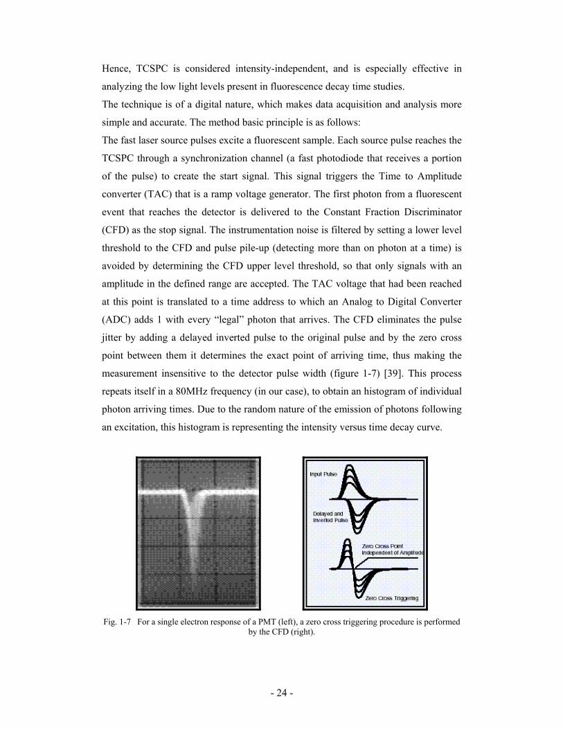
measurement insensitive to the detector pulse width (figure 1-7) [39]. This process

repeats itself in a 80MHz frequency (in our case), to obtain an histogram of individual

photon arriving times. Due to the random nature of the emission of photons following

an excitation, this histogram is representing the intensity versus time decay curve.

Fig. 1-7 For a single electron response of a PMT (left), a zero cross triggering procedure is performed

by the CFD (right).

- 25 -

In our system we are using a reversed TAC operation mode. Since the TAC has to

reset after every photon detection or every time it reaches the end of its time window

(when no photon is detected), when working with high frequency excitation this reset

dead time becomes a source for lost data or long measurement times. Since a photon

is reaching the detector only once in n periods, the TAC start pulse rate can be

decreased by a factor of n if we switch the start and stop inputs of the TAC. This is

obtained by adding a delay module to the sync channel. The excitation pulse starts

going through this delay line. At the same time it excites the sample, and without a

delay in the emission channel a fluorescent photon arrives sometime to create the start

signal. The stop signal will always reach at the same time (at the end of the delay line)

so that the variable is the ∆t between start and stop signals. Indeed the time axis has to

be reversed for a proper representation. A block diagram of TCSPC in a reversed

start-stop mode is shown in figure 1-8.

Fig. 1-8 Block diagram of the B&H TCSPC module.

TCSPC, originally described as a non-imaging technique for lifetime measurement,

enjoys some serious benefits over the other described methods, in particular the single

photon sensitivity (leading to high temporal resolution), the wide dynamic range –

allows to measure various levels of signals, and is especially important when

measuring the low levels and a relatively high SNR. This is in comparison with the

other described method, with emphasis on improved sensitivity and temporal

resolution with respect to gating methods, and improved SNR and wider dynamic

range with respect to a streak camera. Inevitably, disadvantages exist as well. When

- 26 -

applying TCSPC for imaging, the amount of individual recordings (and of data) is the

same as for examining several thousands of samples – a complete decay curve for

every pixel is required. This, of course, requires time. So in terms of acquisition time

TCSPC is not the fastest method. Even after the TAC reset dead time (on the order of

microseconds) was solved by the reversed start-stop mode, and pile-up effects are

avoided electronically (setting threshold to the constant fraction discriminator), the

count rate is usually limited to 1% of the excitation source frequency. This means that

for acquiring a 256X256 pixels lifetime image with 103 photons in each curves, will

take around ten minutes, if the count rate is on the order of 105. This is for the case

where fast excitation source is used (80MHz) – if one works with lower frequencies,

acquisition time will increase. However, we are working with relatively short

lifetimes and 80MHz in TCSPC allows measuring lifetimes of up to 2-3ns, so in this

application we enjoy the benefits more than we suffer from the limitations.

1.3.3.3 Analysis of time-resolved data

Various approaches are used in Fluorescence Lifetime Imaging Microscopy (FLIM)

data analysis in attempt to find the optimal balance for each application between SNR,

spatial resolution of the image, acquisition time and computational expenses

(hardware) and time (software).

In general, the acquisition of data for multiple pixel images, its analyzing and

processing for image display may take a few minutes. This is the main draw back of

imaging methods that do not use whole-field detection devices (i.e. that work on

pixel-by-pixel basis). There is always a search for methods that will enable one to

create images within a reasonable period of time, in order to compete with other

practical imaging methods and be able to deal with rapid and temporally short

processes.

Several analysis methods exist for FD-based FLIM [40, 41] that claim to allow the

acquiring, processing and displaying of lifetime-resolved images in quasi-real time.

However, before discussing the analysis of a collection of measurements and the

process of creating a digital image, it is important to review the common methods of

analysis of each pixel in this picture. For time-resolved fluorescence measurement,

when observing the decay curve form, the key features that may hold significant

information are the rise time, the position in time and intensity of the peak, and of

- 27 -

course the relaxation time (lifetime). The rise time reflects the rate in which the

excited state is being populated, and thus may shed light on the vibrational behavior

of the molecule [1]. The intensity and waveform of the fluorescent decay curve may

be used to define quantum yields, and the decay time gives a measure of the

molecule’s interactions with the surrounding.

Usually, the first action operated upon a fluorescent decay curve is fitting it to an

exponent (by regular means, present in most graphical softwares). When doing so,

one should decide what order of exponent is most suitable. When working with one

type of extrinsic fluorescent probe, and the spectral arrangement of the experimental

setup merely allows to detect fluorescent signals coming from sources other than this

probe, a monoexponential fit may be acceptable. This may be verified by observing a

linear slope of a semi-logarithmic representation of the decay curve. A single lifetime

and single amplitude of the exponential decaying are then obtained. When the

detection is of intrinsic fluorophores, autofluorescence of multiple molecules is

expected, which cannot be spectrally isolated with the same efficiency as near IR

extrinsic fluorophores, and fitting to higher order exponents is performed in attempt to

isolate the component of interest (this sometimes requires primary knowledge of the

lifetime). In such cases, for example when fitting to a second order exponent, one

might compare between different samples (or different points within the same sample)

using only the slower lifetime, or the ratio between the slow component and the fast

component’s amplitudes.

The most commonly applied method for obtaining the real decay curve from the

observed decay curve (especially for single photon counting data) is the least-squares

analysis technique. In this method, values of amplitude and lifetime (α and τ,

respectively) of decaying are iteratively assumed, until a best fit to the measured

decay is obtained. It is actually a minimizing procedure of the squares of deviations

between the experimental and the calculated data. The convolution integral for the

measured decay with the light source response is calculated with those best fit values

to obtain the actual decay function [2]. The quality of the fit may be inspected using

the square-chi test, or graphically by plotting the deviations between the two curves

for each time channel on the time axis. In this representation, fluctuations of these

residuals around zero indicate a good fit. Another method of analyzing decay uses the

convolution theorem and performs the analysis in the Laplace domain, where the

result is a product of the two functions, rather than their convolution. The analysis

- 28 -

retains the function in the Laplace domain since inverse transform to the calculated

function might be too difficult.

The above techniques refer to a single decay curve, as mentioned. In imaging

modalities, there is a need to rapidly analyze a large amount of data.

When applying the convolution operator, it should be pointed out that, in practice, the

instrument response is measured for the excitation wavelength (providing a temporal

excitation profile). This, however, has been shown not to distort the calculations, but

rather provide a good time resolution and satisfying fitting capabilities. It is important

to measure this function for every experiment, individually.

In the least-squares fitting method, χ2 is used as a measure of mismatch between the

experimental data and the fitted function. This parameter represents the summed (over

data points) square ratio between actual deviation (between experimental and fitted

data) and statistical expected deviation (e.g., noise). This ratio is also known as the

weighted residuals. A minimum deviation will be displayed as equality between the

actual and expected deviations, rendering χ2 equal (or with close proximity) to the

number of data points, N. However, since the number of fitted parameters, ν, creates

degrees of freedom in the calculation, χ2 should be compared to (N- ν) for accuracy.

A logarithmic representation tends to exaggerate features in the lower part of the

decay, at the expense of those around the peak. Displaying the weighted residuals

below the time axis provides clear visual information on where misfits exist,

displayed in statistical manner (standard deviation) and normalized.

The analysis of the substantial amount of data resulting from imaging procedures,

with the consideration of minimizing the time for analysis, may be performed in

several ways. One is to reduce a stack of images to a lower number of images by

means of reconstruction algorithms. In a two-gate measuring system, the lifetime

from each point may be rapidly calculated from the two measured intensities at the

two time windows (knowing the two delays) [42]. Two representative approaches for

fast FLIM analysis assume a fixed parameter while fitting to data: global-analysis

algorithm constrains that the lifetime parameter in all pixels will be equal, thus

reducing the number of fitted parameters and improving the fit quality [41]. Another

approach, derived from the above is invariant-fit, where a-priory known lifetime

values are fixed during the fit, and other features of the decay (amplitudes, intensity

fractions) are calculated [43].

- 29 -

1.3.2.4 Selected FLIM applications

Fluorescence lifetime imaging methods, both time-domain and frequency-domain,

have been used over the last decade in a broad range of applications, including

biomedical and diagnostic methods, cellular and molecular imaging, characterizing

substances in analytical chemistry and more. Combining of the technology with

modern microscopes and microscopy techniques is already well established, rendering

it a popular tool for many applications that are submitted to microscopic research

methods. Technologically speaking, FLIM was combined with scanning near-field

optical microscopy (SNOM) for FRET measurements, where the energy transfer

between dye molecules embedded in polyvinyl alcohol films or bound to cell surface

was detected through the SNOM tip by a time-resolved measuring system [44];

combination of FLIM with whole field microscope, where signals were detected by a

gated MCP image intensifier (combined with an intensified CCD) yielded 2D FLIM

images for each component of the fluorescent lifetime, with optical sectioning (for 3D

imaging) obtained in the same system using structured illumination configuration

[45]; another FRET-FLIM combination is described in [46] where the acquisition of

time-resolved images of the donor in the presence and absence of the acceptor is

performed by a gated high-speed camera. The combination of FRET and FLIM is

indeed a very popular one and is said to enable resolution in the order of 1-10nm, one

order of magnitude better than regular SNOM; Becker et al. (from Becker&Hickl,

GmbH, Berlin) described the integration of his TCSPC products within various

imaging systems, such as the Zeiss LSM-510 NLO laser scanning microscope [47]

and other laser scanning microscopes, wide-field microscopes and fluorescence

correlation spectroscopy techniques [3]. In all systems TCSPC-based detection

devices were used to replace the classical intensity detectors.

For the relevant research topics in which fluorescence lifetime imaging has been

combined, the list is even longer. Spatial distribution maps of the intracellular

concentration of ions and analytes have been obtained using the above systems.

Lifetime-based pH imaging was demonstrated by several researchers and was shown

to be superior compared to wavelength- ratiometric techniques, whose calibration is

less comfortable and the time for imaging is much longer [48-54]. The ability to

assess intracellular calcium by FLIM techniques was also demonstrated [55-57].

Other cellular ions that were subjects of such researches are Sodium [58], Zinc and

- 30 -

other metal-ions [59, 60]. Oxygen concentration in a sample (and also tissue

oxygenation) are attractive subjects for fluorescent-based sensing, in general, and

specifically for lifetime-based sensing, due to the dynamic quenching effects of

oxygen on the lifetime of various fluorescent probes [61, 62]. A work was described

that measures both oxygen pressure on a surface and oxygen flux through a permeable

diffusion barrier using FD lifetime measurement of ruthenium complexes (Ru(II))

incorporated into a polymer layer system [63]. These parameters may simulate

oxygen partial pressure on skin surface and oxygen flux through skin, respectively.

Additional complexes of ruthenium (ruthenium diimine complexes) were described as

lifetime-based sensors for a wide variety of blood gases, electrolytes and enzyme

substrates including pH, oxygen, carbon dioxide, potassium, sodium, calcium,

chloride, ammonia, urea and glucose [64]. These complexes are known for their

relatively long lifetime.

The clinical applications of FLIM in diagnosis and detection of diseases, mainly

cancers will be discussed in section 1.4.

1.4 Optical diagnostics and biopsies

Biopsy is the removal and examination of tissue, cells or fluids from the living body

[65] and is a commonly implemented procedure in cases where cancer development is

suspected, being the gold standard in cancer detection. The will to avoid the

invasiveness of this method is a principal motivation in the development of non- or

minimally-invasive methods, of which optical techniques play an important role. Few

are the methods whose out-coming assessment is valid without the encouragement of

a traditional biopsy, still there is a strong incentive to reach such abilities with the

rapid progress in the development of optical methods.

Endogenous fluorescent specimens that are altered with the development of cancer are

numerous: Pyridoxine (vitamin B6) metabolism is sometimes defected in tumors [66].

Protoporphyrin was found in advanced ulcerated Squamous Cell Carcinoma (SCC)

and its red fluorescence was marked as potentially diagnostic [67]. The amino acid

tryptophan is a fluorescent indicator of protein level. Two more aromatic amino acids,

tyrosine and phenylalanine, also contribute to protein fluorescence. NADH and FAD

are important factors in cellular metabolism, and changes in their fluorescence

- 31 -

properties may reflect the status of tissue oxygenation. The structural proteins

collagen and elastin, found in connective tissues, exhibit autofluorescence.

Flavins and porphyrins also contribute to tissue fluorescence and are supposed to

exhibit spectral changes with alterations in the environment that are characteristics to

cancerous tissues. Porphyrins are frequently recognized by red tumor fluorescence.

Exogenous fluorescent dyes that are widely used in clinical applications include

BCECF (a ratiometric probe used to map tumor pH), Hematoporphyrin and its

derivative (HpD), sulphonated phthalocyanine and indocyanine green (ICG), a

popular near-IR contrast agent..

Among the organs that were subjected to researches involving fluorescence

spectroscopy, one can find the colon, cervix, breast, oral cavity, lung, skin and brain.

Some examples are described below.

Brancaleon et al. investigated an in vivo method for the detection of non-melanoma

skin cancer in humans [68]. The endogenous fluorescence of tryptophan residues was

shown to increase in tumoral regions whereas collagen fluorescence decreased. The

high fluorescent signal was attributed to hyperactivity or epidermal hyperproliferation

[69] – increased activity or thickening of the epidermis is accompanied with a

transient higher protein content, hence a higher tryptophan fluorescent signal, while

the connective tissue surrounding the tumor nest is destroyed – leading to a decreased

level of elastin and collagen (tumor-specific colagenase were claimed responsible for

this process). This decrease is part of a general phenomenon of erosion of connective

tissue in NMSC. However, in SqCC there appears to be lesser invasion into the

dermis (and as a result, less erosion of connective tissue occurs). In contrast, when

emission spectra was collected from excised normal tissue and tumors of the

esophagus in wavelengths similar to the emission of tryptophan, tumors exhibited

smaller intensity relative to that of normal tissue, and reduced level of tryptophan was

suggested due to tumor necrosis [70]. Another example of opposite influence can be

seen in malignant breast where the level of fluorescence from connective tissue

adjacent to the tumor was increased. This emphasizes the importance of considering

all simultaneous processes that take place within a tumor environment.

Collecting fluorescence emission spectra from ovarian tissues is potentially capable to

distinguish ovarian cancers from normal ovarian structures [71]. Zheng et al. have

studied 5-ALA-induced protoporphyrin IX fluorescent endoscopic images from

patients with suspected premalignant and malignant oral cavity lesions, and found that

- 32 -

suspicious lesions displayed bright reddish fluorescence, while normal mucosas

exhibited blue background in the fluorescence images [72]. They have developed

algorithms for diagnostics based on the red-to-blue and red-to-green intensity ratio

that were proved to have sensitivity and specificity of 95% and 97%, respectively, in

oral cancer diagnosis, thus improving the accuracy of the method that was studied in a

similar research described elsewhere [73]. Autofluorescence quantitative mapping

was also used on animal models to image different stages of SqCC malignancy of the

aerodigestive tract. The fluorescence spectra of biopsy specimens taken from

clinically suspicious lesions and normal-appearing oral mucosa was compared in

order to determine the excitation wavelength where most significant spectral changes

exist, in view of possible in vivo implementations [74]. Contrast in autofluorescence

intensities in the green spectral range between healthy oral mucosa or benign lesions

and dysplastic or malignant tissue sample was also shown [75]. Fluorescence

spectrum was shown to differ also between normal and malignant breast tissues either

in vitro, in cell lines or in vivo.

The use of exogenous probes for similar applications is well documented. ICG was

used for contrast enhancement of images obtained from near-IR diffuse optical

tomography (DOT) of a human breast in vivo [76]. In vivo fluorescent NIR

reflectance images of ICG were acquired for the discrimination of spontaneous canine

adenocarcinoma from normal mammary tissues [77]. ICG- structurally related

cyanine dyes were developed for improved contrast in biomedical optical imaging

[78]. The pharmacokinetic properties were studied in both cases, including wash-in

and wash-out time, uptake rate and tumor to tissue concentration gradient in different

time after i.v. administration, and were used to evaluate the efficacy of the dye as

contrast enhancing agent in fluorescent images.

Kennedy et al. recently described targeting a fluorescent probe that is attached to folic

acid, to folate-receptor over-expressive metastatic tumors, which allowed a sharp

distinction from normal tissue that displayed little or no fluorescent signal hence

eliminating the need for image processing and enhancement [79].

In the context of time-resolved technology, a great body of literature exists that

describe the implementation of this technique in diseased and neoplastic tissue

diagnosis. The two “hot” fields on which this technology is applied are atherosclerosis

and cancer.

- 33 -

Methods that detect atherosclerotic lesions of arterial wall were described that rely on

either the fraction of the long-lived decay component of autofluorescence [80], the

identification of lipid-rich plaques that have necrotic cores in atherosclerotic lesions

through spectro-temporal profiles [81] and differences between the fast decay

components of normal, calcified and fibrous atherosclerotic plaques [82].

Experiments that attempt to distinguish malignant from normal tissues and other

malfunctioning or damaged tissues from the corresponding healthy ones are common

for ex vivo samples. For example, the dimerization states of epidermal growth factor

receptor (EGFR) on the surface of live human epidermoid carcinoma cells were

investigated through a FRET-FLIM measurement of fluorescein- and rhodamine-

labeled EGF molecules [83], and many researches describing FLIM microscopy have

also shown images with impressive contrast of ex vivo specimen. Transcutaneous

sensing of lifetime changes of an oxygen-sensitive dye was demonstrated by detecting

the signal after it had passed through layers of chicken skin [84] using phase

fluorometry. This method was suggested to be compatible for non-invasive oxygen

measurement in vivo. Cubeddu et al. have demonstrated time-gated imaging (using an

intensified CCD video camera) of tumor-bearing mice, sensitized with

hematoporphyrin derivative, by associating a gray-shade scale to the decay time

matrix of each mouse, and showing that the decay time of an exogenous dye in a

tumor is always longer than in normal tissue [85]. They also described a technique for

detection of skin cancer using ALA-induced ProtoporphyrinIX (PpIX) fluorescence,

which is of a much longer lifetime than observed in normal tissue (where the rise in

the content of the fluorophore is much less pronounced) [86].

Mycek et al. reported on a time-resolved spectrometer they used to measure

autofluorescence decay times from patients in vivo, and declared a sensitivity of 85%

of this data in distinguishing adenomatous from non-adenomatous polyps (adenomas

decay faster) [87]. They also tested new algorithms for recognizing artifacts that

appear in the time-resolved emission data originating from highly scattering media

[88]. FLIM was also tested for its applicability in histopathological assessment of

breast cancer tissue, where the average lifetimes of different tissue regions were

compared and found to differ with a microscopic resolution (although for a small

number of patients) [89]. A (spatial) 3D, wavelength-resolved, lifetime imaging

system was applied to human teeth to obtain a lifetime contrast between enamel,

dentin and caries [90].

- 34 -

Other researches, exploring the abilities of such methods to image live tissues and

organs, are conducted and reviewed by Hebden, Delpy and Arridge, who have special

interest in optical tomography through time-resolved (non-fluorescent) signals, for

mapping functional properties of newborn infant brain and of organs in adults as well

[91, 92]. In the above mentioned work by Das and Alfano [82], time-resolved

transmission measurements performed on several tissue samples from human breast

are described, of which the values of absorption lengths and transport mean free path

are calculated and used to evaluate the proportion of the different constituents that

may represent a neoplastic tissue (fibrous, glandular and fatty tissue).

These are only a few examples from this flourishing area of research, and what is

common to all is the recognition of the advantages of time-resolved optical and

fluorescence spectroscopy for tissue imaging.

- 35 -

2. Hypothesis and experimental part

2.1 Study goal

The research work in this thesis intends to develop a spectroscopic method for

biomedical diagnostic purposes, with a special emphasis on the importance of

minimally invasive diagnostics and the ability in early detection of diseases, as part of

the useful preventive medicine.

The method uniquely combines the use of near-IR, lifetime-based fluorescent probes,

the relying on physiological parameters that are known to alter in cancerous tissue

from a very early stage of tumor development, the ability to resolve this changes

through the leading edge technology of TCSPC, and the use of advanced algorithms

that will allow interpreting signals coming from depth of more than a few millimeters.

This still doesn’t mean that the method will be restricted to dermal and subcutaneous

tissue since by combining the method with endoscopy it is made suitable for mucous

tissue of several internal organs.

The envisioned application consists of identifying molecules that mark newly formed

tumors (either by massive infiltration to tumor area or by over expression of tumor

cells), selectively targeting fluorescent dyes to these cells by conjugation with specific

antibodies, scanning the tissue with excitation source within the time window where

only specific binding exist, recording a fluorescent decay curve for each pixel,

extracting the actual fluorescent lifetime value from each decay curve with respect to

the actual position (depth and XY plane coordinate), assigning a physiological value

for each pixel relying on calibration measurements for determining the lifetime

dependence on the parameter of interest, obtaining a distribution map of the desired

physiological parameter that reflects the morphology and stage of the tumor (and may

be compared with histopathological examination during research).

This work is dealing with primarily building the experimental system that will allow

both calibration and in vivo measurements, performing calibration measurements for

scaling the lifetime values with pH and temperature values, testing the inverse

algorithm capabilities of extracting the actual lifetime as well as the position of its

source and refining it according to correlation with experimental results, and testing

the system for in vivo measurements.

- 36 -

2.2 Means and methods

2.2.1 The probe

Two potential dyes were selected as potential probes for this research, IRD38 and

IRD41 (LI-COR, Inc., USA). The dyes’ chemical structure and absorption and

emission spectrum are shown in figure 2-1.

Fig. 2-1 Molecular structure and spectra of IRD38 (top) and IRD41 (bottom).

IRD38 has an absorption peak at 778nm and emission peak at 806nm. Its quantum

efficiency is 34.5% (in methanol). IRD 41 absorbs maximally at 786 and emits at 812.

Its quantum efficiency is 14.1% (in methanol). Both dyes are said to have a natural

lifetime of approximately 600ps, still no further characterization of this parameter is

available by the manufacturer (this is a common problem when trying to reveal the

potential of near-IR, lifetime-based new probes).

- 37 -

As shown later in the results, these two dyes are deemed not suitable for our

application. By contacting Prof. Gabor Patonay from Georgia State University (GSU),

who is scientifically involved with Li-Cor, Inc., we were provided with two newly

synthesized dyes, namely IRD700DX and IRD800CW, a-priory evaluated to fulfill

our spectral and hopefully even the kinetic requirements. We were the first to explore

their pH-dependent, time-resolved behavior. The absorption and emission spectra of

both dyes is shown in figure 2-2.

Fig. 2-2 Absorption and emission spectra of 700DX (left) and 800CW (right)

2.2.2 Diagnostic parameters

It is well established today that several important properties of tumors in vivo differ in

value from normal tissue properties. Some of these changes are extracellular pH

(pHe) distribution, blood flow, tissue oxygen and nutrient supply, bioenergetic status

and temperature. Some of these changes are derived from the heterogeneity in tumor

vascularization [93], which leads also to a reduction in the efficiency of disposal of

waste products (e.g., hydrogen ions, lactic acid, necrosis products etc.). These changes

can be useful tools in prognosis of malignancies and in the development of techniques

- 38 -

for drug targeting in tumors. This introduction will focus on the altered properties

(mainly pH and thermo-tolerance) as indicators in the diagnosis of tumors.

pHe in a tumor micro environment tends to exhibit a more acidic value than that of a

normal tissue. This property, referred to as acidosis, is thought to be due to a high

metabolic rate in a rapidly growing tumor (either glycolytic or lactic acid production),

accompanied by an insufficient drainage by convective and/or diffusive transport.

Thus, while the intracellular pH is maintained at a more physiologically normal pH by

self regulating systems such as using ion exchangers Na+/H+ antiport and Na+-

dependent HCO3-/Cl- exchanger, the extracellular matrix in a tumor becomes more

acidic than normal, creating a pH gradient inversed to the normal state (in which pHe

is less acidic) [94, 95].

The pHe in many solid tumors exhibit a low value that can decrease to 5.6 in contrast

to the pHe range in normal tissue that is 7.2-7.6 [96]. The average decrease in pHe is

0.3-0.5 pH units.

pH measurements were done in various studies both in animal models for human

tumors and in a variety of human tumors [97, 98]. In these studies a spectrum of

malignant tumors was taken in in vivo conditions and pHe was measured. The

findings clearly showed that there was a positive correlation between the tumor size

and the decrease in pHe. The decrease in pHe was detected even in small tumors.

The measurement methods used in research vary from pH-sensitive

mini/microelectrodes [97], to a PET-based technique, and 1H NMR spectroscopy

using 31P and 19F as probes [99]. These methods are either invasive or involve a use of

harmful materials for the measurement procedure.

Tumor temperature is usually higher than in surrounding normal tissue. The rapid

growth of vascularized tissue mass at a relatively high temperature and a high heat

dissipation capacity (because of the large blood perfusion rates) is one of the main

causes for this regional hyperthermia, and, in fact, several investigators have featured

ultrasound and other methods that prove the increased blood flow inside a malignant

tumor [100, 101].

Tumor temperature is 0.5-4.0ºC higher than that of the normal tissue [102].

Neoplastic tissue also displayed a different pattern of temperature distribution during

hyperthermia from that of normal tissue [103].

When investigating the existence of a thermal distinction between malignant tumors

and inflammatory benign lesions [104] using thermometric measurements, a positive

- 39 -

correlation was found between ∆t and degree of angiogenesis. Values of ∆t greater

than 1ºC can estimate with high accuracy a malignant tumor and the increase of

temperature difference by one degree triples the odds of a patient having a malignant

tumor.

2.2.3 Expected dependence of lifetime on parameters

Temperature - the temperature dependence of fluorescence properties, including

decaying characteristics has been widely investigated [105]. The rate of decaying was

usually shown to increase at elevated temperatures. This was demonstrated for

fluorescenated DNA oligomers at temperature range of 5-45ºc [106], some tryptophan

dipeptides [107] in the range of 10-35ºc, for Indole in polar solvents such as water in

the range –15-75ºc [108], for the ion-pairs of α,ω-diphenylpolyenylic at extreme low

temperatures [109] and for several more luminescent species in different studies

[110]. The described trend is often attributed to a decrease in the rate of non-radiative

decay at lower temperatures. In addition, fluorescence quenching by molecular

oxygen is known to be directly proportional to temperature [111], and quenching is a

possible factor of reduced lifetime. Another indirect effect of temperature may occur

through the increase in pH (the next parameter to be discussed) with decreasing

temperature (a phenomena that is known to occur in many conventional cases). In

such cases, a lifetime-based pH sensitive dye might exhibit changes in decaying

behavior without actually being temperature sensitive. These indirect effects may

interrupt as artifacts in experimental results and thus require that each parameter will

be controlled separately from all other possible effecting factors (e.g., changing pH

with temperature held constant before investigating temperature effects with no data

on the influence of pH). Furthermore, exceptions to most of the described trends

(changes in quantum yield and spectra) do exist, and it safest to investigate every

molecule by itself. The suggested mechanisms may only help in predicting and

attempting to control the desired and undesired effects. The effect of temperature on

lifetime is consistent in all the references.

pH – the effect of pH on fluorescent lifetime vary to a great extent, and opposite

influences may be observed using different probes. The effect is often dependent on

chemical functional groups bound to the dye molecule, rather than on the

- 40 -

chromophore itself. For a diethylaminomethyl pyrene molecule, designed specifically

as a stable optical pH sensor, it was proposed that the probability of electron transfer

from the amino group to the pyrene, when the molecule is in its excited state,

competes with fluorescence emission and hence influences the decay time [112]. The

electron transfer rate was shown to increase with pH (in an unprotonated form), and

thus shortening the decay time in basic environments. The protonated form of the

nitrogen in acidic pH has a positive charge, which tends to impede this electron

transfer [113]. Acid-base chemistry does not occur when the molecule is in the ground

state, which contributes to the stability of the probe during experiments [114].

Without anymore contradicting examples, it is best simply to explore the behavior of

each dye experimentally.

2.2.4 Artificial model

An agarose-based gel served as the optical phantom for testing and calibration

measurements. The phantom is prepared by dissolving 0.8g Agarose (SeaKem HE

Agarose, FMC Bioproducts) in 36.6ml of phosphate-buffered saline (J.T. Baker,

catalog no.5656) on a heating plate (while stirred) for 5 min. until the solution

appeared transparent and bubble-free. After cooling the solution to 70°c, 3.4ml of

Intralipid (Intralipid 20%, Pharmacia and Upjohn, catalog no.406563A) was added

using a syringe and the 50ml tube was gently shaken for homogeneity. The solution,

right after the preparation, is poured to a template of choice – usually a round petri

dish (plastic or glass). In order to simulate semi-infinite dimensions, to avoid

reflections from the vessel’s walls and exiting of photons from the sample, a glass

petri dish with a diameter of 64mm and depth of 40mm is used (picture 2-1).

- 41 -

Picture 2-1 Agarose-based optical phantom in a petri dish and a tube (left) and Delrin phantom with

holes on top surface (right)

For simulation of different environmental pH, a buffer solution of the desired pH

value replaced the phosphate-buffered saline in the above preparation step. For

simulation of temperature changes, a PID temperature controller (model 2216E,

Eurotherm, USA) was used to controllably heat a square 5cmX5cm heating plate

(picture 2-2), from which a thermocouple feedback line was connected back to the

controller (M.R.C., Israel). An additional wire thermocouple was used to get a

measurement directly from the sample. The sample was placed on the heating plate

(or attached to it in the perpendicular setup configuration) for temperature-related

measurements. Simulation of depth of fluorophores was achieved by placing slabs of

the phantom (with known thickness) on the sample’s surface.

- 42 -

Picture 2-2 Heat plate connected to a PID temperature controller

As an alternative phantom, bulks of DelrinTM were used. These round bulks are

available with small cylindrical holes that allow the placement of small volume

aqueous samples (picture 2-1, right). These phantoms are not suitable for temperature-

related measurements due to their poor heat conductance. They were used to measure

pH-related differences, where the sample was in a buffer solution and the optical

properties of the phantom was identical in each well, regardless of the pH of the

buffer.

An alternative way of performing the temperature-related measurements was to cast

small white silicon wells on the heating plate. The wells are opaque to diffusion of the

dye solution and are good heat conductors, and the high reflection from the silicon

yields a strong fluorescent signal (optical properties are, of course, not taken into

consideration in this measurement, only the temperature dependence).

In this part, the dyes were used in conjugation to micro-beads in order to prevent their

diffusion within the phantom.

2.2.5 Biological model

The biological model for in vivo experiments relies on induced Squamous Cell

Carcinoma (SqCC) in mice. SqCC, an immunogenic tumor, is usually characterized

by asymptomatic early lesions, which are therefore often misdiagnosed. The work that

- 43 -

was done by G. Gannot [29] established the immune cell infiltrate profile at different

stages of lesions. The immunohistochemical analysis of the tongue infiltrating cells

revealed an increase of the proportion of T cells, B cells and macrophages with

progressing of the epithelial lesions towards a more malignant phenotype. The general

characterization of SqCC was with a massive infiltrate of a larger number of cells, a

large portion of which is occupied by lymphocytes. Some of these potential disease-

specific markers are CD3 and CD19 positive cells. In the current research, the

fluorescent dyes are conjugated to antibodies with high specificity to these molecules,

and the tumor is simulated by injection of a cell-line of spontaneously induced SqCC

to BALB/c mice tongues, where lesions are developed within 10-14 days after

injection, and the animals survive 6-8 weeks after injection. In order to determine the

time window in which only specific binding of the conjugates exist in vivo, a

mathematical model was developed in a related project in our lab, that calculates the

diffusion, binding and dissociation rate constants.

2.2.6 Experimental system

2.2.6.1 Light source

The light source in use is a Titanium:Sapphire, mode-locked pulsed laser (Tsunami,

Spectra-Physics Lasers, USA) pumped by a high power, diode-pumped, all solid-state

CW laser (Millenia Vs., Spectra-Physics Lasers, USA). The pumping laser can output

more than 5W of CW 532nm light, utilizing a neodymium yttrium vanadate

(Nd:YVO4) crystal as the gain medium [115]. The output beam is blocked and

released by an electronically controlled mechanical shutter.

The Tsunami laser consists of a Titanium-dopped Sapphire crystalline material that is

produced by introducing Ti2O3 into a melt of Al2O3, where Ti3+ ions (which are

responsible for the lasing action) are substituted for a small percentage of the Al3+

ions [116]. The energy level structure of Ti3+ ions in Sapphire is shown in figure 2-2.

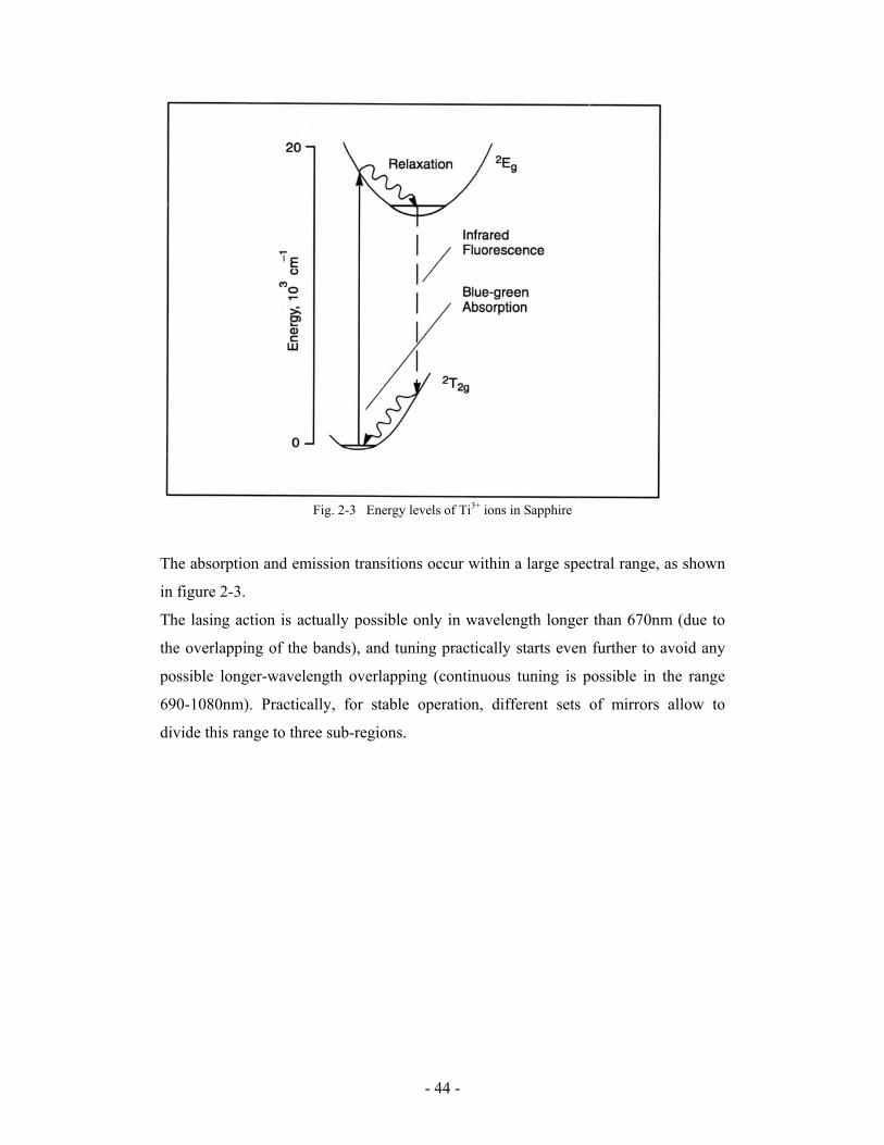
- 44 -

Fig. 2-3 Energy levels of Ti3+ ions in Sapphire

The absorption and emission transitions occur within a large spectral range, as shown

in figure 2-3.

The lasing action is actually possible only in wavelength longer than 670nm (due to

the overlapping of the bands), and tuning practically starts even further to avoid any

possible longer-wavelength overlapping (continuous tuning is possible in the range

690-1080nm). Practically, for stable operation, different sets of mirrors allow to

divide this range to three sub-regions.

- 45 -

Fig. 2-4 Absorption and emission spectra Ti:Sapphire

Besides the Ti:Sapphire rod, the laser consists of the optics that form the resonator

cavity and include pump beam mirrors, an output coupler (OC), a high reflector (HR),

beam folding mirrors (the cavity is a folded one to allow the required beam path-

length for mode-locking in a minimal device size), dispersion control elements and

tuning elements. A scheme of the beam path within the cavity is shown in figure 2-5.

The mode-locking (coordinating the phases between the different longitudinal modes

within the laser oscillator cavity) is performed actively, where the modulator (an

apparatus that functions as a shutter that closes and reopens at a frequency precisely

equal to the reciprocal of the round trip time in the laser cavity) is an acousto-optic

modulator (AOM), which is driven by a regeneratively-derived rf signal. In the

femtosecond configuration, wavelength tuning is performed using a prism sequence

and a slit. The sequence allows to spatially resolve the wavelengths in the cavity, and

changing the slit’s position selects the output wavelength. The slit’s width is also

controlled so that variations in bandwidth and temporal width of the output pulses

may be achieved. The pulse width selection is performed using prism pairs. The fs

configuration tuning curves are shown in figure 2-6.

- 46 -

Fig. 2-5 Beam path in the laser cavity (fs configuration)

Fig. 2-6 Tuning curves (fs configuration)

2.2.6.2 Optical set-up

A complete experimental setup was built for lifetime measurements of all the above

models. The light source’s output meets first a splitting mirror that directs a fraction

of the beam to a fast photodiode (see TCSPC system). Afterwards, coated neutral

density (N.D.) filters are used where laser attenuation is needed. A highly reflecting

mirror folds the laser beam onto the point of probe position in the phantom. The

emitted light reaches a collective lens (f=50mm) and right after a bandpass filter (with

a cutoff at 790nm, custom made by Omega Filters, USA). The signal is focused by the

- 47 -

lens to the entrance slit of a single grating monochromator (CM110, CVI Laser

Corporation, USA) with a resolution of 1200grooves/mm. The monochromator is

attached to the photomultiplier (PMT) in a way that prevents light leakage from

outside the desired light path. The PMT is connected to the TCSPC system in the

computer as described in the next section.

Two main configurations of this setup were used: one in which the sample is placed

perpendicularly with the monochromator working in a straight through configuration

(picture 2-3) and the other with the sample placed horizontally with the

monochromator working in a right angle configuration (picture 2-4). The reflecting

mirror (for beam directing), the sample and the lens & filter apparatus are all mounted

on micrometers for position control. All components following the splitting mirror are

placed in a black-painted wooden box to avoid as much as possible light from the

surrounding.

Scanning the sample with the laser is made possible by replacing the beam-folding

reflecting mirror with a dual axis optical scanner (6800HP, Cambridge Technologies

Inc. (CTI), USA). The scanner consists of two mirrors, each is controlled by a

galvanometric motor (Picture 2-5). The motors are controlled by two separate servo

drivers (series 650x, CTI), which are in turn controlled by a dual axis digital

controller (model 6760, CTI).

The experimental setup scheme is given in figure 2-7.

- 48 -

Picture 2-3 Experimental setup with the monochromator working in a straight through configuration

Picture 2-4 Experimental setup with the monochromator working in a right angle configuration

- 49 -

Fig. 2-7 Experimental setup scheme

Picture 2-5 Dual axis optical scanner

MONO-CHROMATOR

PMT

LensFilter

Sample

Fast Photodiode

TCSPC

SYNC CFD

Heating plate

Ti:Sapph @740nm,80MHz

- 50 -

2.2.6.3 The TCSPC system

The heart of the system is the electronics of signal processing and large memory

integrated on a PCI board (SPC-730, Becker&Hickl GmbH (B&H), Germany) and the

controlling software (SPCM7.5, B&H). Synchronization of the light source is

performed by a fast photodiode that receives a fraction of the laser beam (PHD-400,

B&H). The photodiode has a rise time of 200ps, FWHM of 400ps, detection area of

0.25mm2 and an analog output current scale. A fiber optic cable is delivering the

output signal to the SYNC input of the SPC board. The fluorescent signal is detected

by a fast PMT (H7422P-50, Hamamatsu, Japan). The PMT contains a Gallium

Arsenide (GaAs) Cathode, and has a high sensitivity in the spectral range 380-890nm,

with a maximal quantum efficiency of 12% at 800nm. The PMT is thermoelectrically

cooled by a Peltier element. Minimal rise time is 200ps, maximal output signal is

2µA, but this is further amplified by an up to 26dB amplifier (HFAC26, B&H). The

amplifier enables working with the detector with relatively low currents and long

cables, and it also contains a protection circuit to prevent overload of the detector.

The instrument response of the detector has a minimum FWHM of 240ps. Its output is

connected to the CFD input of the SPC.

The SPC-730 works in a reversed start-stop mode, allowing the use of high

frequencies. Its maximal operating frequency is 200MHz. The maximal time axis

resolution is 4096 bits (time channels), and with a maximal resolution gain

(“stretching “ the time window), each bit represents 813fs. Data acquisition times vary

from 1ms to 1000s. It is possible to measure several periods of a periodical signal or

simply measure single decay curves. The system has several modes of operation,

making feasible a continuous measurement, sampling in constant time intervals (thus

functioning as an optical oscilloscope), measurement for varying external parameters

(wavelength scanning, samples scanning) and measurement for imaging purposes (to

create images of up to 256X256 pixels). Recording of the light source in a single

mode is presented in figure 2-8.

- 51 -

Fig. 2-8 Laser pulses train as recoded in a single mode, 4 periods per window (Freq. Divider =4)

As can be seen, controlling the important parameters of the measurement is available

in the main window of SPCM. The building of the histogram is displayed in a chosen

display rate while the rate of photon counts per second by each of the components

(Sync, TAC, CFD, ADC) is presented continuously. The Sync rate is a good

indication for the mode-locking of the light source. The CFD is the indicator of

intensity of the signal. Other controllable parameters are the upper and lower

threshold voltages of the CFD (for pile-up effect preventing and noise eliminating,

respectively), data acquisition times and repetition rate of measurements (for

consecutive recordings), time window size and resolution and graphical amplification

(by count increment).

After a decay curve has been recorded, it may be graphically manipulated using the

“display parameters” control window (figure 2-9), where graphical representation in a

semi-logarithmic scale is optional, and determining the threshold of counts (for noise

cutting) is also possible. 2D data processing window (figure 2-10) also allows

performing simple operations such as smoothing by averaging adjacent points,

adding, subtracting, multiplying or dividing the curve by constants, interpolating

selected sections of the curve, shifting in x and y directions and more.

- 52 -

Fig. 2-9 Display parameters control window of SPCM

Fig. 2-10 2D data processing window of SPCM

- 53 -

2.2.6.4 Electrodes for reference measurements

In order to measure the actual pH and temperature values of a sample or a live model

for reference, a system of electrodes and data loggers was combined. The system

includes glass tip (90-110µm in diameter) pH and temperature sensitive electrodes,

where the pH is measured in combination with a reference electrode (PH100, TP100

and Ref100, respectively, Unisense, Denmark). The pH and reference electrodes are

connected to a high internal resistance (1014 ohms) pH meter (PHM210, Radiometer

Analytical, supplied by Unisense). The temperature electrode is connected to a

thermocouple thermometer (T301, Unisense). Both meters are connected through an

analog to digital converter (Adc-101, Pico Technology, supplied by Unisense) to data

acquisition software (PicoScope, Pico Technology, supplied by Unisense). Calibration

of the instruments is performed by measuring a sample of known pH and temperature

(e.g. buffer solution, thermally controlled) and creating a look up table that scales the

mV values that appear on the meters to the corresponding known pH and temperature

values.

The electrodes are placed on a micromanipulator apparatus (MM33, Unisense) for

precise positioning. The system’s components are shown in picture 2-6.

Picture 2-6 pH and reference electrode attached to a micromanipulator during measurement (left) pH

and temperature meters connected to a PC through an A-D converter (right)

- 54 -

2.2.7 Inverse algorithm for extracting actual lifetime

The mathematical framework for simulating and analyzing the experiments within

this work was developed by Amir. H. Gandbakhche and co-workers in the Laboratory

of Integrative Medical Biophysics at the NIH [117]. Based on RWT, expressions that

describe the probability of a photon arriving at any point and time, given the starting

point and time, were derived, allowing to distinguish between delay times of the

photons resulting from scattering events and distorted pathlengths, and the delay times

of photons resulting from the stay in an excited state (lifetime of a fluorescent event).

The tissue/media is modeled for this purpose as a 3D cubic lattice with a localized

(finite) fluorophore. The absorbing boundary of the lattice corresponds to the tissue

surface, and the lattice spacing corresponds to (µs’)-1, which is the transport-corrected

mean photon scattering distance (used to describe non-isotropically scattered photons

by an isotropic scattering model). This spacing is usually 0.5-1mm at NIR

wavelength.

Traveling of photons in a RWT model may be described by three dimensionless

parameters, ρ, n and µ, representing the probability of motion, the number of steps

and the probability of absorption per lattice step. Photons may move from each point

within the lattice to one of six adjacent points with a probability of 1/6. Knowing the

number of states, n, taken by a photon enables one to know the actual pathlength the

photon had traveled between two points. 2D Schematic representation of the model is

shown in figure 2-11.

Fig. 2-11 2D scheme of the RWT model

- 55 -

Regardless of the fluorophore characteristics, description of photons that are involved

in the process consists of two parts: the traveling to the fluorophore site and the

traveling from the fluorophore to the detector. The joint probability of these two

events can be represented by the product of two Green functions. Taking the

fluorophore’s characteristics into consideration, the probability of a fluorescent

photon from a site, s, arriving at a detector at a point, r, can be expressed as shown in

equation 2-1:

)1(),(),(),,( 21

tiGGsrω

ωβωαηφω

−=Γ ±

∧

±

∧

(2-1)

Where ω is the frequency of the photon source, Φ is the quantum efficiency of the

fluorophore, η is the probability of an interaction of a photon (that arrived at a

fluorescent site) with the fluorophore and τ is the fluorescent lifetime. This expression

allows the extraction of fluorescent lifetime from frequency-domain measurements.

For time-resolved data (fluorescent intensity as a function of time following a short

pulse of excitation light), Eq. 2-1 can be rewritten as shown in equation 2-2:

)1()],(),(),(),([

),,('

ωτβαβαβαβαηφ

ωµµ

µω

ieHHHH

srse

ae

seci

−+−−

=Γ

−

++−++−−− (2-2)

Where c is the speed of light in the tissue, the indices i and e specify the wavelength

of the coefficient (incidence/excitation and emission) and H terms are defined in

equation 2-3:

⎥⎥

⎦

⎤

⎢⎢

⎣

⎡

⎟⎟⎠

⎞⎜⎜⎝

⎛++⎟

⎟⎠

⎞⎜⎜⎝

⎛+−

=''''21),( sese

ae

sisi

ai

ci

ci

eHµω

µµ

βµω

µµ

α

αββα (2-3)

where

- 56 -

2222'])2([

43

sisi

fff zyx µµ

α ±++=±

2222 '])22()()[(43

sesese

fff zyyxx µµµ

β ±++−+−=±

Here the dimensionless α is a function of the distance from the photon source, located

at the origin, to a fluorophore site centered at the mean (xf, yf, zf) point, and the

dimensionless β is a function of the distance from the florophore site to the detector

located at the mean (x, y, 0), according to the geometry shown in figure 2-12.

Fig. 2-12 Imaging geometry

Existence of a closed-form time-domain solution, which is the Laplace transform of

equation 2-2, requires the existence of a closed-form time-domain solution for the

inverse Laplace transform of equation 2-3. This enforces to average the two

absorption coefficients (which are different because of wavelength dependence), but

since the scattering coefficient dominates, the solution seems insensitive to this

averaging. Performing the averaging and transforming Eq. 2-3 results in equation 2-4,

'

')(2

3'

),( s

as

ct

tc

s et

ch µ

µβα

µ

παββαµ

βα−+−+

⎟⎟⎠

⎞⎜⎜⎝

⎛= (2-4)

- 57 -

And transforming Eq. 2-2 results in equation 2-5,

⎥⎦⎤

⎢⎣⎡ ∆−=

dtdW

tWsrt ttηφγ ),,( (2-5)

Where ∆t describes the photon delay due to remaining of the fluorophore in the

excited state (fluorescent lifetime). Wt acts as a point spread function in an imaging

system, and is of the form shown in equation 2-6:

)],(h),(h),(h),(h[Wt ++−++−−− +−−= βαβαβαβα (2-6)

The PSF has also a derivative with a closed-form solution, as shown in equations 2-7

and 2-8:

=dt

dWt )],('),('),('),('[ ++−++−−− +−− βαβαβαβα hhhh (2-7)

Where

')(

''27

' 2

2)/3242)((

),(' s

as

ct

tc

ss ect

tc

h µµ

βαµ

παβµβαβαβαµ

βα−+−−+++

⎟⎟⎠

⎞⎜⎜⎝

⎛= (2-8)

This enables to simulate the effect of different fluorescent lifetimes on the photon

arrival times. It has been shown that longer lifetimes cause a delay in photon arrival

times, which is observed as a shift in the peak of the photon arrival curve.

This solution suits for short lifetime cases, unless the distances between source,

detector and fluorophore site are relatively large (e.g. the fluorophore is embedded

deeply in tissue).

Some important technical notes are concluded from the simulations. One is that

pathlengths have a significant effect on intensity, an effect that is minimized when the

fluorophore is centered between the source and the detector. Another conclusion is

- 58 -

that the solution works best for fluorophores with lifetimes shorter than 1ns,

embedded in depth of 10-30 mean photon scattering lengths in a turbid medium. The

main indication of changes in lifetime will be in the form of a temporal shift in the

intensity peak of arriving photons.

- 59 -

3. Measurements and results

3.1 System setup

Establishing the system for lifetime measurements started with installing all the

TCSPC components in a way that allows safe operation of the PMT. Since the laser is

the most intense source of light in the experimental region, and since it is of known

properties (waveform, width and temporal characteristics) it is desired to be able to

record laser pulses (before even getting to the system impulse response). The PMT

was positioned in such way to minimize dark counts rate, and the laser pulses were

gradually introduced into the optical setup through attenuating components until the

first photons were detected by the PMT. Afterwards, tuning the attenuation of the

laser was performed until a narrow pulse of light could be rapidly recorded.

Recording of the laser pulses relies on three main parameters: first, the Sync count

rate should display 8X107 counts/sec. when working with 80MHz pulse frequency.

Second, when recording more than one signal period per window (the frequency

divider parameter in the software was set to 4), one can observe the 12.5ns intervals

between pulses, that account for the actual frequency and third, a minimal full width

at half maximum (FWHM, representing pulse width) should be observed. The latter is

somewhat problematic since, as noted before, the PMT’s FWHM limit is 240ps,

suggesting that the actual pulse width of a femtosecond laser is not detectable using

this detector. A pulse with FWHM of 240ps was successfully recorded.

The next step was to set the system to measure a fluorescent signal from the type of

samples used in this work. First, an Agarose slab was placed with no fluorescent

marker in the sample’s position. At this stage the sample is placed perpendicular to

the optical table and the laser beam is directed to be incident on its center (with some

angle). The bandpass filter was placed before the PMT on the optical axis, and a

recording was taken to see the level of counts (accounting for photonic noise in the

system, after electrical noise was eliminated in the previous step). At this stage the

laser was set to 778nm (the absorption peak of IRD38), where the filter’s cutoff is

said to be at 790nm. Noting the relatively high scattering of the phantom and its white

color, it is understood that a strong signal of temporally broadened pulse was

recorded. At this stage, the problem of leakage from the filter spectrum was

recognized, since no filter is steep enough to separate fractions of light of such close

- 60 -

wavelengths. The cutoff of the filter cannot be chosen to be much further right on the

nm scale, remembering the small stokes’ shift of the dye (with an emission peak at

806nm, see p.35). Considering that the fluorescent signal is always weaker than the

light source, it was preferable to shift the laser to a lower wavelength and retaining the

emission channel to work according the emission peak. In addition, a monochromator

(set to 806nm) was added after the filter on the optical axis of detection, and a lens

was placed respectively to collect the light to its entrance slit. With the laser emitting

at 740nm, a very low level of photons was collected from a non-fluorescing phantom

in this setup, over a long integration time, allowing to try and get a fluorescent signal.

Adding 1µl of solution containing IRD38 conjugated to microbeads from a stock

(with concentration of 8X108 beads/ml) already resulted in an observable decay

signal. The laser beam was shifted across the sample while the lens was centered

according to the excitation point on the sample, until a maximal intensity (CFD count

rate) was reached. In order to measure a single period of decay, the offset parameter

was changed until all the photons were in the measurement window, and time gain

was set to 5, resulting in a 10ns time axis. Measurements can then be taken until a

peak of at least 45000 photons is collected, so that thresholding the curve by cutting

up to 10000 photons is possible while still having the whole part of the curve from

peak to 1/e of intensity (photon counts).

3.2 System’s impulse response

In time-resolved fluorescent lifetime measurements, the measured decay curve is

actually a convolution of the actual decay with the impulse response (or instrument

function) of the system. The impulse response can be practically defined as the effect

of the system’s configuration and components on a laser pulse with known waveform

and width. This effect is expected to apply on every kind of signal that is formed in

the experiments (e.g. a fluorescent decay curve), therefore a deconvolution action on

the measured data with the impulse response should be able to extract the actual

decaying form that has occurred.

In order to know how the fluorescent signal, emerging from the phantom, would be

influenced by the optical setup, the laser pulse is measured by placing a reflecting

mirror in place of the phantom’s surface. In this way the pulse is introduced to the

detection channel in exactly the same path as the fluorescent signal will travel. The

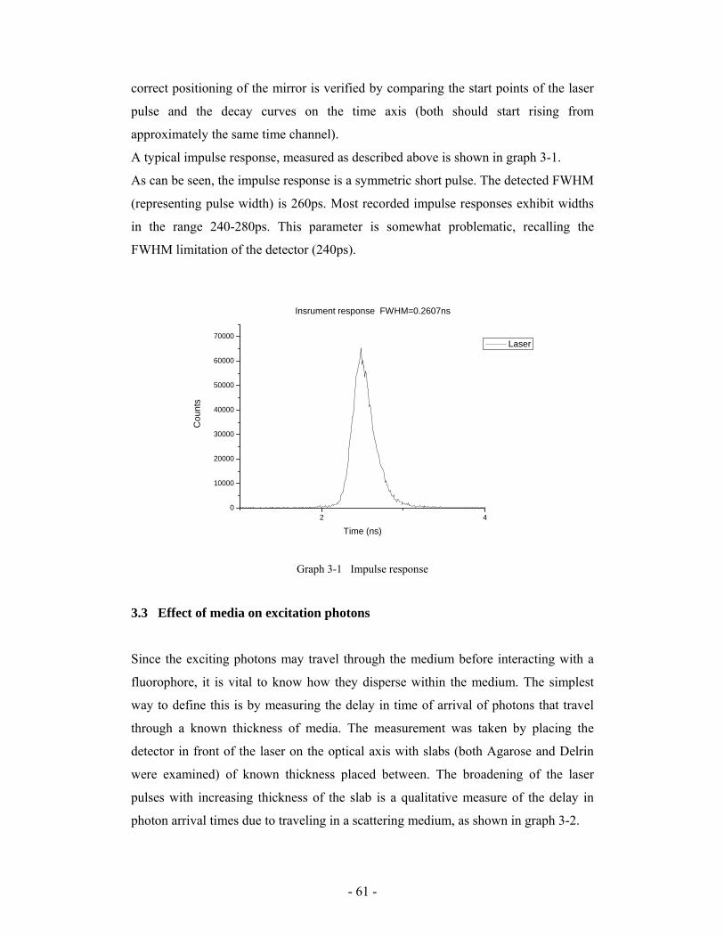
- 61 -

correct positioning of the mirror is verified by comparing the start points of the laser

pulse and the decay curves on the time axis (both should start rising from

approximately the same time channel).

A typical impulse response, measured as described above is shown in graph 3-1.

As can be seen, the impulse response is a symmetric short pulse. The detected FWHM

(representing pulse width) is 260ps. Most recorded impulse responses exhibit widths

in the range 240-280ps. This parameter is somewhat problematic, recalling the

FWHM limitation of the detector (240ps).

2 40

10000

20000

30000

40000

50000

60000

70000

Cou

nts

Time (ns)

Laser

Insrument response FWHM=0.2607ns

Graph 3-1 Impulse response

3.3 Effect of media on excitation photons

Since the exciting photons may travel through the medium before interacting with a

fluorophore, it is vital to know how they disperse within the medium. The simplest

way to define this is by measuring the delay in time of arrival of photons that travel

through a known thickness of media. The measurement was taken by placing the

detector in front of the laser on the optical axis with slabs (both Agarose and Delrin

were examined) of known thickness placed between. The broadening of the laser

pulses with increasing thickness of the slab is a qualitative measure of the delay in

photon arrival times due to traveling in a scattering medium, as shown in graph 3-2.

- 62 -

100

10000

20000

30000

40000

50000

60000

70000

Cou

nts

Time (ns)

0mm 2.8mm 6mm 9.2mm 12mm

transit time through delrin

Graph 3-2 Broadening of laser pulse going through slabs of Delrin

The effect of this scattering media on the excitation photons may use to demonstrate

one of the classical descriptions of light propagation in time through turbid media.

Photons are categorized as ballistic, with no scattering events, as “snake” – with

minor deviations from the ballistic axis, and as diffusive – where multiple scattering

occurs and diffusion-like propagation of photons through media is observed. We can

see that enough ballistic photons may be collected, but since the diffusive photons

appear before the peak (the peak, where most ballistic photons are found is right-

shifted in time), a delay in the rise time of the decay curve may be expected (see

section 3-7).

3.4 Measuring optical properties

Optical properties of a sample are calculated through a random walk-based algorithm

(named Coefs), developed at the laboratory for integrative medical biophysics at the

NIH. The algorithm receives as inputs the normalized values of diffuse reflectance,

diffuse transmittance, and the thickness of the sample. The measurements of these

values are performed as schematically shown in figure 3-1.

The light source used in this experiment is a Titanium-Sapphire CW laser, tunable in

the near-IR range (model 3900s, Spectra-Physics Lasers, USA). The integration

- 63 -

sphere is coated on the inside with BaSO3 (for high reflectance) and has front and

rear ports and a power detector, positioned perpendicular to these ports, connected to

the controller (Integration sphere and integration sphere system controller SC5500,

Labsphere, USA). The laser beam is directed to the front port of the sphere by a set of

reflecting mirrors and a shutter. The beam should be aligned properly until it exits

through the rear port’s pinhole. Then, the energy is measured for a configuration of

closed rear port and open front port (with no sample) and the measured energy is

referred to as the reference value. A round slab of phantom with known thickness is

excised and placed in an apparatus used to position the sample in the selected port.

Diffuse reflectance is measured by placing the sample in the rear port and diffuse

transmittance is measured with the sample placed in the front port with the rear port

closed. The measured energy values are divided by the reference value for

normalization, and the resulting values are fed into the algorithm along with the

thickness of the sample. The algorithm outputs values of absorption coefficient and

reduced scattering coefficient for each sample (µa and µs’, respectively, in cm-1). The

controller is calibrated for several wavelengths and, by tuning the laser, measuring

optical properties at more than one wavelength is possible (usually the measurement

is for excitation wavelength and the determined emission wavelength). An alternative

way of calculating the coefficients through the measured parameters is offered by the

inverse adding-doubling algorithm. This algorithm is available as a web-based

calculator from the Oregon Medical Laser Center (OMLC) website, and provides a

means for comparing the resulting coefficients from both methods [118].

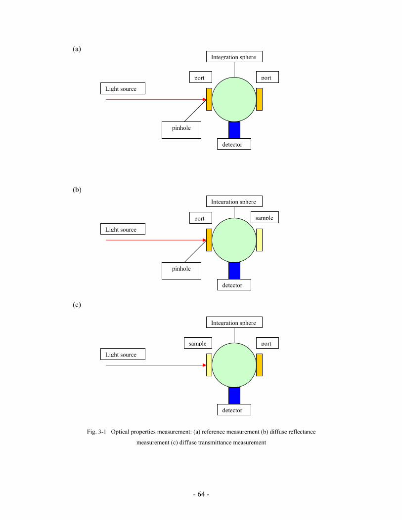
- 64 -

(a)

(b)

(c)

Fig. 3-1 Optical properties measurement: (a) reference measurement (b) diffuse reflectance

measurement (c) diffuse transmittance measurement

Integration sphere

Light source

pinhole

detector

portport

Integration sphere

detector

Light source

pinhole

sampleport

Integration sphere

Light source

detector

portsample

- 65 -

The measured and calculated values in both methods are shown in tables 3-1 and 3-2.

The measurements were taken with 775nm, 36-39mW light source. Normalized

values (of raw data) are also shown.

Table 3-1 Optical properties of Agarose in 775nm, calculated through Coefs

Depth Pinhole

2mm

Reference R

(norm)

T

(norm)

µs’ µa

8.5mm - 0.372e-1 0.492 0.3199 4.991342e-001 2.196190e-003

8.5mm + 0.376e-1 0.471 0.340 4.824964e-001 7.719942e-004

10.5mm - 0.341e-1 0.481 0.209 4.444671e-001 1.622305e-002

10.5mm + 0.375e-1 0.467 0.192 4.444671e-001 1.973434e-002

12mm - 0.360e-1 0.475 0.192 4.006938e-001 1.714970e-002

12mm + 0.370e-1 0.486 0.181 4.124790e-001 1.769535e-002

Table 3-2 Optical properties of Agarose in 775nm, calculated through inverse adding-doubling

(OMLC)

Depth Pinhole

2mm

Reference R

(norm)

T

(norm)

µs’ µa

8.5mm - 0.372e-1 0.492 0.3199 3.84e-001 6.87e-003

8.5mm + 0.376e-1 0.471 0.340 3.44e-001 6.95e-003

10.5mm - 0.341e-1 0.481 0.209 4.19e-001 1.085e-002

10.5mm + 0.375e-1 0.467 0.192 4.27e-001 1.24e-002

12mm - 0.360e-1 0.475 0.192 3.81-001 1.05e-002

12mm + 0.370e-1 0.486 0.181 4.08e-001 1.05e-002

Results from the two calculations methods are merely distinguishable, in terms of the

required sensitivity. Note that, as explained in section 2.2.6, the theory is not very

sensitive to averaging the absorption and scattering coefficients, in cases of dominant

scattering, hence we tolerate the deviations of the shown scale, at least as long as the

ratio between both coefficients (as shown in both methods) is maintained. However, a

suspicion has risen during the preparation of the different pH phantoms, that they

- 66 -

might possess different optical properties. For this reason, measurements were taken

for these phantoms as well. The results are shown in table 3-3.

Table 3-3 Optical properties (calculated through Coefs) for Agarose with different pHs

pH µa µs’

4 6.869542*exp(-03) 1.025305*exp(00)

7 2.973384*exp(-03) 1.025305*exp(00)

10 7.542472*exp(-05) 7.542472*exp(-01)

The only significant difference here between different pHs is the lower absorption of

pH10, relative to the other two. The theory should take into account a difference of

that order.

An example of measured optical properties for Delrin is given in table 3-4.

Table 3-4 Optical properties of Delrin slabs

Delrin thickness µa µs’

2.8mm 1.161675*exp(-04) 1.161675*exp(00)

6mm 5.656854*exp(-05) 5.656854*exp(-01)

9.2mm 9.469082*exp(-04) 9.469082*exp(-01)

The above values demonstrate a technical problem with the Coefs sub-routine, where

exactly the same amplitudes are yielded for both coefficients. However, the orders of

magnitude remain significant.

3.5 Source-detector separation

Measurements in attempt to reveal the effect of the medium on the traveling of

exciting and emitted photons laterally through the phantom were performed in

combination with all other parameters considered in this work. Since the algorithm

works best with the fluorophore centered between the source and the detector (as

mentioned in earlier section), the measurement was taken according to the scheme in

figure 3-2.

- 67 -

This was performed by shift of the beam for a distance of Xmm on the sample (using

the reflecting mirror), and moving the sample by X/2mm (using the micrometer to

which it is attached). Another consideration that makes the algorithm’s work simpler

is to measure for both source-detector separation and depth of the fluorophore, where

the depth is half the source-detector distance in each measurement. These results will

be presented later.

Fig. 3-2 Source-detector separation scheme

The results for changing the source-detector distance for various pH phantoms are

shown in the graphs 3-3 to 3-9:

Source

Excitation

PMT

Lens

Fluorophore

X

- 68 -

2 4 6

10000

Cou

nts

Time (ns)

0mm 1mm 2mm 3mm 4mm 5mm 6mm 7mm

Graph 3-3 Source-detector separation effects on decay curve for pH4

2 4 6

10000

0mm 1mm 2mm 3mm 4mm 5mm 6mm 7mm

Cou

nts

Time (ns)

Graph 3-4 Source-detector separation effects on decay curve for pH5

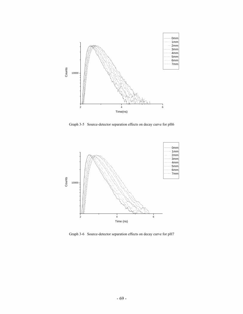
- 69 -

2 4 6

10000

0mm 1mm 2mm 3mm 4mm 5mm 6mm 7mm

Cou

nts

Time(ns)

Graph 3-5 Source-detector separation effects on decay curve for pH6

2 4 6

10000

0mm 1mm 2mm 3mm 4mm 5mm 6mm 7mm

Cou

nts

Time (ns)

Graph 3-6 Source-detector separation effects on decay curve for pH7

- 70 -

2 4 6

10000

0mm 1mm 2mm 3mm 4mm 5mm 6mm 7mm

Cou

nts

Time (ns)

Graph 3-7 Source-detector separation effects on decay curve for pH8

2 4 6

10000

0mm 1mm 2mm 3mm 4mm 5mm 6mm 7mm

Cou

nts

Time (ns)

Graph 3-8 Source-detector separation effects on decay curve for pH9

- 71 -

2 4 6

10000

0mm 1mm 2mm 3mm 4mm 5mm 6mm 7mm

Cou

nts

Time (ns)

Graph 3-9 Source-detector separation effects on decay curve for pH10

The FWHM values (in [ns]) are presented in table 3-5.

Table 3-5 FWHM values (ns) for source-detector separation measurements

SDS (mm) pH4 pH5 pH6 pH7 pH8 pH9 pH10

0 0.6782 0.6982 0.6064 0.6445 0.6104 0.6133 0.6838

1 0.7313 0.7247 0.6284 0.7247 0.7071 0.7534 0.7232

2 0.7803 0.792 0.7192 0.7906 0.7605 0.8331 0.8245

3 0.845 0.8396 0.7329 0.9049 0.8208 0.794 0.7772

4 0.8934 0.8417 0.8136 0.9545 0.9106 0.9584 0.8588

5 0.9153 0.9089 0.895 1.0208 0.9315 0.9463 0.8658

6 0.9907 0.9922 0.9509 1.0496 1.0466 1.0385 0.8797

7 1.0028 0.9863 0.9122 1.1496 1.0543 1.0757 0.9768

Plotting the above values results in Graph 3-10.

- 72 -

0

0.2

0.4

0.6

0.8

1

1.2

1.4

0 2 4 6Source-detector separation (mm)

FWH

M

pH4pH5pH6pH7pH8pH9pH10

Graph 3-10 Curve width (FWHM) as a function of source-detector separation for different pH

phantoms

A tendentious increase of FWHM is clear for all samples and is expected since the

rise time becomes less sharp due to excitation pulse traveling a distance before

fluorescent event and decay also lasts longer because the fluorescent photons travel

before exiting towards the detector, as well. Noticing the measure by which graphs

resemble each other, one may predict the problems we are about to experience when

coming to explore the pH dependence.

3.6 Depth dependence

This stage follows the same steps as described for source-detector separation, only

with the depth of the fluorophore changed between every measurement. It is possible

that lateral traveling of photons occurs since excitation light impinges with an angle

upon the sample, but lateral traveling may occur when light crosses a given thickness

of media, even if the incidence is perpendicular to the surface of the sample, because

of scattering. These measurements were taken on a localized fluorophore placed on

the surface of Agarose phantom, and covered with slabs of different thickness of the

same material (e.g., with the corresponding pH for each sample). The results are

shown in graphs 3-11 to 3-16:

- 73 -

2 4 6 81000

10000

Cou

nts

Time (ns)

0mm 1mm 2mm 3mm 4mm 5mm

Graph 3-11 Decay curves for pH4 at different depths

2 4 6 81000

10000

0mm 1mm 2mm 3mm 4mm 5mm

Time (ns)

Cou

nts

Time (ns)

Graph 3-12 Decay curves for pH5 at different depths

- 74 -

2 4 6 81000

10000

0mm 1mm 2mm 3mm 4mm 5mm

Cou

nts

Time (ns)

Graph 3-13 Decay curves for pH6 at different depths

2 4 6 81000

10000

0mm 1mm 2mm 3mm 4mm 5mm

Cou

nts

Time (ns)

Graph 3-14 Decay curves for pH7 at different depths

- 75 -

2 4 6 81000

10000

0mm 1mm 2mm 3mm 4mm 5mm

Cou

nts

Time (ns)

Graph 3-15 Decay curves for pH8 at different depths

2 4 6 81000

10000

0mm 1mm 2mm 3mm

Cou

nts

Time (ns)

Graph 3-16 Decay curves for pH10 at different depths

The FWHM values of the above measurements are summarized in table 3-6.

- 76 -

Table 3-6 FWHM values (ns) for depth measurements

Depth (mm) pH4 pH5 pH6 pH7 pH8 pH10

0 0.6782 0.6982 0.6064 0.6445 0.6104 0.6838

1 0.7922 0.85 0.8371 0.79 1.0113 1.0672

2 1.1171 1.0456 0.9982 1.0023 1.2918 1.3025

3 1.2494 1.1030 1.0294 1.2106 1.0955 1.3155

4 1.2674 1.0215 1.1817 1.1131 1.1561 -

5 1.3198 1.1691 1.233 1.3442 1.3747 -

Plotting FWHM against depth for the different pH in a search for trend is shown in

graph 3-17.

00.20.40.60.8

11.21.41.6

0 1 2 3 4 5

Depth (mm)

FWH

M

pH4pH5pH6pH7pH8pH10

Graph 3-17 Curve width (FWHM) as a function of depth for different pH phantoms

Again, the effect of traveling through scattering media is pronounced primarily by a

moderation of the rising part of the curve, and later through the arriving of the delayed

photons. The trend of increasing curve width with increasing depth is most

remarkable for the higher (basic) pH values, again arising the suspicion of varying

optical properties of the different samples that affect the arriving time of photons

regardless of the pH value of the surrounding.

- 77 -

3.7 Combination of source-detector separation and depth

As noted earlier, for preliminary correlations between simulations performed by the

algorithm and the measurements, it is preferable to measure for variant combinations

of source-detector separation and depth where the latter is half the size of the first.

Such measurements performed on pH7 phantom are shown in graph 3-18.

2 4 6

10000

Cou

nts

Time (ns)

laser sds=0,z=0 sds=6,z=3 sds=10,z=5 sds=14,z=7

Graph 3-18 Decay curves for different combinations of source-detector separation (sds) and depth (z)

for a pH7 phantom

Now, being familiar with the curves of sections 3.5 and 3.6, one may find it difficult

to distinguish between the different influences. This is allegedly justified, since for

unequipped eye the effect of depth is not distinguishable from the effect of source-

detector separation, and even though the effect of their combination looks more

dramatic, it is not necessarily simple to extract from it the two different components

accurately. This issue will to be dealt with in the discussion.

- 78 -

3.8 pH dependence

At this stage of the work, it was already clear that pH has a minor effect on lifetime of

the selected dyes. Therefore, it is useless to present the above measurements by

isolating the pH as the only parameter (e.g., plotting all pHs for depth=1mm, etc.).

Attempts were made to define the dependence that does exist, and to use this

measurement for examining the algorithm’s capability of accurately predicting the

shape of decaying.

The pH effect was first measured for a localized fluorophore in Agarose phantoms

with different fixed pH values. 1µl of fluorophore-microsphere complex from stock

was placed on the surface of the phantom in a marked point (for alignment with

detection optical axis), and recordings were taken to a defined counts peak (for

normalization) of 45,000 photons. The results are shown in graph 19.

2 41000

10000

Cou

nts

Time (ns)

pH4 pH7 pH10 laser

Graph 3-19 pH effects in Agarose

The measured FWHM values of the above recordings are shown in the table 3-7:

- 79 -

Table 3-7 FWHM values for different pH values in Agarose

Phantom pH FWHM (ns)

4 0.5289

7 0.4707

10 0.4292

Two immediate conclusions may be derived from the above result: first, there appears

to be a linear change in the measured width of the decay curve with the change in pH

value of the phantom. This change may be quantitatively defined as ~50ps per 3 pH

units. This change is the maximal change observed in these experiments, and is hardly

distinguishable from the normal fluctuations in repeating a decay curve recording of

the same sample. The second conclusion arises from the measurement of optical

properties of the different pH phantoms, which has shown a significantly lower

absorption coefficient for pH 10 than other pH values (see table 3-3). This could be

revealed even from observing the different texture of a pH10 phantom relative to

other phantoms, and may be explained by the effect of the basic environment on agar

polymerization and/or Intralipid integration in the medium. This is, however, a

definite artifact in this kind of experiments since live tissue is not predicted to change

its optical properties in response to changes of physiological pH, while these

variations of absorption/scattering coefficients clearly affect the arrival times of

photons, regardless of the effect of pH on the actual lifetime. Although the theoretical

prediction tools are designed to weigh the optical properties among other parameters,

it is an undesired byproduct in this stage of preliminary characterization of the dye. In

order to circumvent this problem, a simplified experiment was designed which utilizes

DelrinTM disk as a phantom, where 0.5µl of IRD41 from stock was mixed with 1µl of

buffer solution and the resulting aqueous sample was placed within a small hole in the

phantom. In this way, samples have different pH values due to the buffer, but are

surrounded with medium holding the same optical properties for all samples. The

resulting recordings are shown in graph 3-20:

- 80 -

2 4 61000

10000

Cou

nts

Time (ns)

pH4 pH7 pH10 laser

Graph 3-20 pH effects in Delrin

The FWHM values of the decay curves are presented in table 3-8.

For these measurements, a linear scaling between FWHM and pH seems to exist with

a scaling factor of ~70ps for 3 pH units. However, as opposed to the same experiment

in Agarose, it can be seen here that the pH10 sample holds the longest value and pH4

sample shows the shortest. This fact may provide the necessary information regarding

the effect of protonation of the dye, solely, without the interference of other photon

arrival-time-delays causing factors.

Table 3-8 FWHM values for different pH values in Delrin

Phantom pH FWHM (ns)

4 0.7982

7 0.8673

10 0.9351

It should also be noted that in general the lifetime appears to be longer than in

measurement in Agarose, but not necessarily due to phantom effects, rather due to

longer accumulated excitation times (several measurements were taken before the

presented recording, whereas in the previous experiment the recording was taken for a

“fresh” marker which usually tends to display a very short decaying, possibly due to

- 81 -

quenching before spreading evenly through the medium and also because

phtobleaching is yet to affect at the first excitations). This is the reason for the

changes not being remarkable in the graphical representation – the decaying lasts

longer, making the differences relatively smaller.

We then moved to start working on the new dye supplied by Li-Cor, Inc.,

IRD800CW. Again, no preliminary data was available regarding the temporal

behavior of these probes (in fact, we are sharing with Li-Cor any data we obtain with

these dyes). We started with IRD800CW, which does not require changing the

spectral settings of the system (light source, filters) thanks to its spectrum (see section

2.2.1) that resembles that of IRD38. We managed to absolutely separate excitation

light from the emission channel even with the laser tuned to 770nm and the

monochromator set to 795nm, both corresponding to the absorption and emission

peaks of the dye. Stocks of the dye dissolved in different pH buffer solutions (ranging

from 4 to 10) were then prepared, but with different concentrations. The concentration

was not strictly calculated to be equal at this stage since it is not expected to affect the

measured lifetime. As the optical phantom, Delrin bulks were used with small wells

served to contain 4µl from each stock in a well. Eight decay curves were recorded as a

first step for each sample and the resulting FWHM values in [ns] were averaged to

yield graph 3-21:

IRD800cw

0.20.40.60.8

11.2

4 5 6 7 8 9 10

pH units

FWH

M

Graph 3-21 Average of 8 FWHM (ns) values for IRD800CW in different pHs

- 82 -

Additional three measurements were taken after 30 minutes for comparison and

averaging of the resulting FWHM values was performed again, as shown in graph 3-

22:

IRD800cw

0.2

0.4

0.6

0.8

1

1.2

4 5 6 7 8 9 10

pH units

FWH

M

Graph 3-22 Average of 3 FWHM (ns) values for IRD800CW in different pHs

The resulting dependence is not linear or systematic in an observable way, hence we

decided to measure while eliminating any possible interaction of the sample solution

with the Delrin bulk, keeping the material to behave only as the surrounding media.

We used the plastic caps of PCR tubes to contain the sample, while these caps were

placed within the Delrin wells, and repeated the same experiment. Four decay curves

were measured and averaged for each sample (of 5µl of the dye dissolved in a buffer

of the nominal pH value). The results are shown in graph 5-3.

- 83 -

0.6

0.65

0.7

0.75

0.8

4 5 6 7 8 9 10

pH units

FWH

M

Graph 3-23 Average of 4 FWHM (ns) values of IRD800CW in different pH solutions (in PCR caps)

We refer to this result as the more reliable one regarding this material, being

measured at optimal conditions of isolating the pH values. It can be seen that the

lifetime may be scaled at the range of interest (i.e., pH between 6 and 8) linearly with

50ps lengthening of decaying for an increase by one pH unit. The same trend in this

specific range appears also (and with a similar scaling) in graph 3-22, however it may

not provide us with the pH resolution we wish to achieve (especially with such a

narrow range of interest).

3.9 Temperature effects

Measuring the influence temperature might have on fluorescence lifetime specifically,

or on all fluorescence properties in general is a complicated task. Temperature,

opposed to pH, is a hardly fixed parameter, especially when the type of sample is

relatively large in size and cannot be thermally isolated from the environment (the

sample must be exposed to excitation light). In addition, laser irradiation is involved

which carries quanta of thermal energy, and is incident on a small spot size, the region

of interest for each measurement, making the effect of heating by the laser a

potentially dramatic one. Since quantifying the thermal effect of the laser irradiation

on the inclusion of interest is a complex issue, and since for every point of

measurement the effect is not supposed to differ (the intensity and excitation times are

- 84 -

almost equal), than this side effect is disregarded at first stage. In addition, monitoring

the temperature at the point of measurement is performed continuously though the

feedback thermocouple (which regulates the temperature controller operation) – and

for calibration measurements this measured value is the important one. In such a way,

measurement is taken when the temperature has reached the desired value, and the

short time of measurement does not allow significant fluctuations of the temperature.

Agarose-based gel samples in medium size petri dishes (35mm in diameter) were first

used, to allow for fast thermal conductivity. In this measurement, the same point is

excited repeatedly while controllably changing the temperature of the entire sample.

The results are shown in graph 3-24.

00.10.20.30.40.50.60.70.80.9

23 26 29 32 35 38 41 44 47

Temperature (c)

FWH

M

FWHM

- 85 -

0

0.2

0.4

0.6

0.8

1

24 26 28 30 32 34 36 38 40 42

Temperature (c)

FWH

M

FWHM (ns)

Graph 3-24 Curve width (FWHM) in different temperatures for IRD38 in a pH7 phantom (top) and in

a pH6 phantom (bottom)

As can be seen, the range of fluctuations is about 200ps for the whole range of

temperatures that was examined in this experiment, which is far wider than the

physiological range. Especially in the range of 37-42ºc, very small changes are

observed. To eliminate the influence of accumulated excitation time (and the

potentially following photobleaching), it was desirable to repeat this measurement for

identical samples, each serves for one measurement only at a given temperature. To

achieve such condition, the samples were placed either in small metal caps on the

heating plate or in small white silicon wells that were formed to contain a small

volume sample (without permeation of the fluid sample). The good heat conductivity

of both apparatus enabled to give rise to fast changes of temperature around the

sample. The results were not qualitatively different from what is shown so far (data

not shown) and at this stage the temperature-related measurements were ceased.

3.10 In vivo measurements

Measurements of lifetime in vivo were performed only on the level of testing the

system’s readiness for this stage of the work. Since the calibration and forward

experiments were yet to be completed, and since the scanning system was not fully

combined into the experimental setup, it was useless to start working on animal

models. However, since these models were available from a related project, taking

- 86 -

place at the lab [119], there was an opportunity to examine the ability to yield a decay

curve from an animal model in this setup. The animals that were used are BALB/c

mice that were injected with 50µl of SqCC cell line to the tongue. At varying time

intervals after injection (in days), the mice were anesthetized and injected with 50µl

of anti-CD3-IRD38 or with anti-CD19-IRD38 conjugates (see section 2.2.4). After

sufficient time has passed since the injection of the fluorescent conjugates (to assure

that non-linked markers had washed out), a measurement may be taken (data not

shown). We verified that the control group (healthy mice injected with fluorescent-

antibodies conjugates) yielded practically no signal and mice from the experimental

group that were measured within the same interval after injection exhibited a strong,

clear fluorescent decay curve with a high count rate that allows its measuring in a

very short time. This is enabled in the same setup where the sample holder is replaced

with a custom-designed bed that prevents head movements of the anesthetized mouse

(picture 3-1). Although it is impossible to position two different mice at exactly the

same point, it should be simple to maintain the optical setup, the sample holder (bed)

coordinate and the scanning starting point of the light source (excitation), in a way

that will allow, by covering the whole surface of the tongue, to analyze and compare

quantitatively the signal emerging from two different mice.

Picture 3-1 Custom design animal holder (left) pH measurement in vivo (right)

- 87 -

3.11 Data analysis

The results I collected were used for examining the mathematical tools for solving the

forward and inverse problems as part of the wider group effort. I present this part as

an integral stage in the complete envisioned procedure, and provide some examples of

comparison between the experimental data and the computational simulations. In

general, this application requires treatment of experimental data in two levels: first, a

simple deconvolution procedure between the measured decay curve and the system’s

impulse response should be performed in order to obtain the actual decay curve, as

occurred physically (without the effect of the optics and detection system). Next, and

more complicated, the theory should distinguish between the delay times that

originate from photon transit time through the medium (affected by scattering) and

delay times that are attributed to the fluorescent event. The first step was simply done

using a standard Fast Fourier Transform (FFT) algorithm. In order to compare

between experimental data and theory predictions, a MATLAB code was written that

simulates a decay curve based on the analytical solutions and the given values of the

different considered parameters – absorption and scattering coefficients, position of

the fluorophore (depth and source-detector separation) and the known natural lifetime.

This simulation should be compared to the deconvoluted experimental data (since

theory does not treat the optics of the experimental system). The theory is tested for

correctness by matching to raw data for a single changed parameter (e.g., depth) with

all other parameters held constant.

Some examples of such correlations are presented in graphs 3-25 to 3-27.

- 88 -

Graph 3-25 Comparison of experimental data (deconvoluted) with simulation for pH7, depth=3mm

Graph 3-26 Comparison of experimental data (deconvoluted) with simulation for pH7, depth=5mm

- 89 -

Graph 3-27 Comparison of experimental data (deconvoluted) of different pH values with simulation

3.12 Scanned sample measurements

We started operating the optical scanner within the steady-state fluorescence imaging

system that was developed in a related project. This system is challenged by the

spatial resolution, i.e., the ability to resolve fluorescent foci that are very close to each

other within the phantom/sample, especially if depth of the foci is also involved. If

two fluorophores are positioned deeper within the phantom, then the point spread

function of the reconstruction algorithm is put to test – in other words, there is a need

to determine the spatial resolution in terms of the minimal distance between two

fluorophore that may be resolved when in maximal depth. To examine this, samples

with embedded fluorophores in a high proximity should be prepared. We used Delrin

with 5 points of dye (IRD38), linearly scanned in 1Hz and image acquiring time of 5

seconds to obtain the fluorescent image shown in picture 3-2.

- 90 -

Picture 3-2 Fluorescent image of a scanned Delrin bulk with five fluorophore targets on the surface

The non-uniform intensity of different foci will require considering how to apply the

same emission time for each point in a scanned sample with acquisition time of a few

seconds, since here the first excited inclusion experiences a longer emission time until

the image acquisition is ceased. One idea was to start a second measurement from the

opposite side, apply the same acquisition time and average the two images. The next

step will be to perform an image acquisition of a sample with identical inclusions of

flurophores, separated by a minimal distance and covered with slabs of phantoms of

varying thickness. The significance of the functional imaging will be illustrated in the

future, when a TCSPC lifetime image of the described sample, with every point

having a different pH (or other chosen value that will be sensed through lifetime

measurement) will be color-coded.

- 91 -

4. Discussion and prospective

This work is the basis of a functional imaging method. By the time of writing these

lines, the steps discussed in the results were completed. The meaning of it is that at

the moment, a TCSPC lifetime measurement system is ready for fast and simple

lifetime measurement for several kinds of samples – fluorescent solutions, fluorescent

gels, local fluorophores surrounded by turbid media (Delrin, agar etc.), and animal

models injected with fluorescent substances. All the situations we needed to simulate

for calibration and evaluation of the forward problem solution are achieved through

the experimental setup: phantoms and samples with different pH values, different

temperature values and different optical properties; varying positions of the

fluorophore with respect to the light source and the detector; and fluorescent dyes of

which at least one is expected to behave in a satisfying manner for our needs, hence

will become the contrast agent in this method.

Even though a calibration of the contrast agent is still not accomplished, it is due to

the simple reason of not finding the proper probe, and not because of technical

obstacles related to the experimental setup or the type of samples that are used. In

view of the technical aspect of the work, it would be responsible to say that mistakes

were made and learned from, and efforts towards maximal elimination of artifacts or

misleading results are constantly kept in mind at the highest priority. Thanks to this

approach, experiments are strictly designed to avoid variations between different

samples that are not related to the controlled parameters. In every measurement,

questions arise such as: had the temperature of the sample changed during the data

acquisition time? Does the fluid content of the sample evaporate during this short

time? Does this affect the processes the photons are undergoing on their way to

detection (through modification of the surrounding)? Well, in such moments I think

that it should be reminded that the goal is to work with biological models, where

variance is unavoidable, and artifacts will certainly interrupt (in the best case scenario,

when they are unraveled). For this reason I believe that wherever subjects from the

life and medical sciences are the case, a successful method should start with a

pronounced effect or phenomena; the forward steps should be as accurate as possible

– a reliable calibration is a must in order to be able to solve the inverse problems, but

once a pronounced effect is observed, the rest of the forward stage may be achieved

by means of precise and systematic work. The varying optical behavior of the

- 92 -

Agarose phantom in different pH values is an example of an artifact that is limited to

the artificial model (even if a soft tissue alters its optical properties with response to

pH changes, it will be very difficult to examine it, as in any case of measuring optical

properties of a live tissue), and is a technical aspect that arises during experiments.

That leaves us in the quest for an appropriate probe, being the limiting factor of the

research from moving on to the next stages. Designing a dye for a specific application

is a challenge even for experienced chemists, which we are not, so we can only keep

searching through trial and error (the price of trying something new), or find a source

of collaboration as is formed nowadays with Li-Cor and Prof. Gabor Patonay from

GSU. This collaboration looks promising and complementary to the two sides

involved in this work.

The dyes we were using so far, though they might not be chosen to serve as contrast

agents in future experiments, allowed us to quantify some of the effects that have to

be explored before approaching the inverse problem. Since the forward theory deals

with separate parameters, one at a time, the source-detector separation and depth-

related measurements provided the raw data required for testing and refining the

simulations, and the good agreement between experimental and computational curves,

as shown in section 3.11, is an outcome of this work.

Since the current estimation is that once a suitable dye is found, the forward step may

be completed within a short time, efforts were taking place in other fronts of the work,

as well. This include the combination of the optical scanner and its introduction to the

TCSPC system, a step that will be completed within weeks and will allow to perform

fast 2D scanning of a sample while recording a complete decay curve for each pixel.

The data of such a measurement is presented at first in a three dimensional graph -

counts versus time and coordinate. Since imaging is the issue, there is a need to be

able to display the array of scanned sample coordinates (resulting in an array of decay

curves) as an array of colored pixels, linearly scaled to the calculated lifetime which

in turn should be scaled to the parameter of interest. We need to design samples in

which a pH gradient is spread over the sample with a high spatial resolution. The

spatial resolution in itself is not a problem for 2D measurements (as opposed to what

is explained in section 3.12 for the measurements with the fluorescent camera) since it

depends on the laser spot size and on the scanning resolution, which are supposed to

be satisfactory. The best imaging software for this data is SPCImage, offered by

Becker&Hickl GmbH, which requires as inputs the system impulse response, the

- 93 -

measured decay curve and synchronization with the scanning program, and outputs a

color image of the color-scaled extracted lifetime (from the deconvolution process).

This still does not hold information regarding the parameters we are interested in, it is

strictly a lifetime map, and we should add our own scaling factor in order to obtain a

map of functional values. Spatial position was not mentioned yet. SPCImage knows

which coordinate is excited at each moment, but since we are dealing with a turbid

medium, additional set of computations should be combined as well to extract the

actual lifetime. The theory is further challenged, as mentioned in the results, by the

difficulty to resolve between the effect of source-detector separation and that of the

depth of fluorophore. For simplification, this may be done by shifting the sample in

the desired 2D scanning program, instead of scanning the laser over the sample. The

optical relations (geometry) are maintained fixed in this way, and there is no need to

account for source-detector separation. It may not suit an animal model, though,

unless robust fixing of the model to the moving plate is achieved. Depth is another

issue. At the current stage, theory should be provided with information about the

depth of each curve in order to extract the component in delay of photons arriving

time that is derived from the depth component of fluorophore position. Since

algorithms exist that were developed by the group mentioned above, for 3D

reconstruction of a 2D fluorescent image of the same model with steady-state

fluorescence spectroscopy (see ref. 119), we intend to perform our analysis in two

stages: the animal model will be imaged in the steady-state system, and the 3D

reconstruction method will be applied to determine the depth of each pixel. The same

model will then be measured in the TCSPC lifetime system, and with the condition of

matched coordinates between the two systems fulfilled, the theory is then provided

with the depth information for each pixel. In any case, the theory is expected to be

able to extract depth directly from lifetime measurements.

Some considerations regarding the in vivo experiments were examined through the

work. One aspect is the ability to perform reference measurement of the parameters of

choice (e.g., pH, temperature etc.) in vivo for comparison with the obtained lifetime

data. The electrodes that are currently used were found insufficient for this purpose.

The fragility of this electrode does not allow it to tolerate even the slightest movement

of the organ it is positioned in, and attempts to fix firmly this organ were a source of

great efforts. Since the relevant range of pH values that we wish to resolve is

relatively small, it is crucial to monitor it with high precision in order to evaluate the

- 94 -

accuracy of the lifetime map in reflecting the actual pH values. A solution to this

problem has to be found. The other reference measurements to which lifetime maps

should be compared are based on histopathological examinations. A protocol exists

and was practiced through the work. Generally, the procedure involves removing the

tongue and preserving it in a gelatinous substance, forming a cubical stained sample.

The sample is sliced in a cryostat and the formed preparations are examined under a

fluorescent microscope. A filter cube, matching the spectral properties of the IRDyes,

was already purchased and is being prepared for use in a related project. We enjoy the

support of the Oral Pathology laboratory staff in Tel Aviv University, school of

medicine, for this part of the work. The 2D image of stained areas in each slice is a

measure of tumor stage and size and direction of slicing is easily controlled to

correspond to the direction of image acquisition.

To summarize, this research work leaves us with a strong motivation to map the pH

distribution in vivo with a high resolution, considering it a good marker for tumor

development and other malfunctions of the tissue that is observable from the early

stages of the process. A fluorescent dye that will exhibit lifetime changes of 300ps

and more for a change of one pH unit may serve well for this purpose (and this is not

farfetched, considering pH sensitive lifetime-based probes that exist in other parts of

the spectrum). We are also motivated to reach the ability of analyzing and interpreting

signals coming from deeper positions within the media, with respect to the current

abilities of the theoretical models dealing with time-resolved propagation of photons

through turbid media. If these attempts are fruitful, then the resulting method may be

considered a breakthrough in using this leading edge optical technology to detect

small physiological changes within the physiological range of changing. To my

knowledge, lifetime-based pH sensitive probes are not applied to map physiological

changes of pH and are not applied in the near-IR region in vivo.

The other parameter that was considered seems less promising at the moment.

Temperature is a much more dynamic parameter, that is harder to simulate and control

through an experiment and may be distorted by many factors. Current thermography

method are performed mainly using Infra-Red thermal cameras, possessing a thermal

resolution of 0.02ºC, and this stands for a direct measurements with the device in a

close proximity to the patient’s body (usually breast). However, in case a proper

contrast agent for temperature sensing is found, even with a much lower resolution

than this, the advantage lies in the potential to couple the described method to

- 95 -

endoscopy (this refers to all other parameters as well). Although optical fibers are not

currently used in our work, it may be feasible to combine fibers in the excitation and

emission channels, thus taking the method one step further – from imaging a few mm

inside subcutaneous tissue to imaging a few mm inside mucous tissue of internal

organs (e.g., uterus, intestine, esophagus and more). Wherever exogenous dyes are

used, a way must be found to inject them to such organs, but until then – a long way is

still ahead.

- 96 -

5. References

1. Biomedical Applications of Fluorescence, in Handbook of Biomedical

Photonics, T. Vo-Dinh, Editor. 2003, CRC Press.

2. Lacowicz, J. R., Principles of Fluorescence Spectroscopy. 2 ed. 1999, New

York: Plenum Press.

3. Becker, W. and Bergmann, A., Lifetime imaging techniques for optical

microscopy. 2003, Becker & Hickl GmbH, www.becker-hickl.com.

4. White, C. E. and Argauer, R. J., Fluorescence Analysis - A Practical

approach. 1970, New York: Marcel Dekker, Inc.

5. Waggoner, A., Covalent labeling of proteins and nucleic acids with

fluorophores. Methods Enzymol., 1995. 246: p. 362-373.

6. Ausubel, F. M., Current protocols in molecular biology. 3rd ed. 1995: John

Wiley & Sons.

7. Tyagi, S. and Kramer, F. R., Molecular beacons: Probes that fluoresce upon

hybridization. Nature Biotechnology, 1996. 14(3): p. 303-308.

8. Haugland, R. P. and Johnson, I. D., Detecting enzymes in living cells using

fluorogenic substrates. Journal of Fluorescence, 1993. 3: p. 119-127.

9. McCray, J. A. and Trentham, D. R., Properties and uses of photoreactive

caged compounds. Annu. Rev. Biophys. Biophys. Chem., 1989. 18: p. 239-

270.

10. Haugland, R. P., Handbook of fluorescent probes and research chemicals.

1996: Molecular Probes , Inc., Eugene, Oregon.

11. Lakowicz, J. R., Topics in Fluorescence Spectroscopy. Vol. 1. 1991, New

York: Plenum Press.

12. Johnson, I., Fluorescent probes for living cells. Histochemical Journal, 1998.

30(3): p. 123-140.

13. Wang, Y.-L., Fluorescent analog cytochemistry: tracing functional protein

components in living cells. Methods in cell biology, 1989. 29: p. 1-12.

14. Giuliano, K. A., Post, P. L., Hahn, K. M., and Taylor, D. L., Fluorescent

Protein Biosensors - Measurement of Molecular-Dynamics in Living Cells.

Annual Review of Biophysics and Biomolecular Structure, 1995. 24: p. 405-

434.

- 97 -

15. Chalfie, M., Tu, Y., Euskirchen, G., Ward, W. W., and Prasher, D. C., Green

fluorescent protein as a marker for gene expression. Science, 1994. 263: p.

802-805.

16. Cheong, W. F., Prahl, S. A., and Welch, A. J., A review of the optical

properties of biological tissues. IEEE J. Quantum Electron., 1990. 26: p. 2166.

17. Welch, A. J. and Gemert, M. J. C. v., Optical-thermal response of laser-

irradiated tissue. 1995, New York: Plenum Press.

18. Ishimaru, A., Wave propagation and scattering in ramdom media. 1978, New

York: Academic Press.

19. Gandbakhche, A. H. and Weiss, G. H., Randon walk and diffusion-like models

of phtotn migration in turbid media, in Progress in Optics XXXIV, E. Wolf,

Editor. 1995, Elsevier Science B.V.

20. Prahl, S. A., Calculations of light distributions and optical properties of

tissue`, in Biomedical Engineering. 1988: University of Texas, Austin.

21. Pravdin, A. B., Chernova, S. P., Papazoglou, T. G., and Tuchin, V. V., Tissue

hantoms, in Handbook of optical Biomedical Diagnostics, V.V. Tuchin,

Editor. 2002, SPIE Press.

22. Wagnieres, G., Cheng, S. G., Zellweger, M., Utke, N., Braichotte, D., Ballini,

J. P., and vandenBergh, H., An optical phantom with tissue-like properties in

the visible for use in PDT and fluorescence spectroscopy. Physics in Medicine

and Biology, 1997. 42(7): p. 1415-1426.

23. Choukeife, J. E. and L'Huillier, J. P., Measurements of scattering effects

within tissue-like media at two wavelengths of 632.8 nm and 680 nm. Lasers in

Medical Science, 1999. 14(4): p. 286-296.

24. Driver, I., Feather, J. W., King, P. R., and Dawson, J. B., The Optical-

Properties of Aqueous Suspensions of Intralipid, a Fat Emulsion. Physics in

Medicine and Biology, 1989. 34(12): p. 1927-1930.

25. Davies, D. R., Sheriff, S., and Padlan, E. A., Antibody-antigen complexes. The

journal of biological chemistry, 1988. 263(22): p. 10541-10544.

26. Kuby, J., Immunology. 3 ed. 1997, New York: W.H. Freeman and Company.

27. Bodey, B., Siegel, S. E., and Kaiser, H. E., Human cancer detection and

immunotherapy with conjugated and non-conjugated monoclonal antibodies.

Anticancer Research, 1996. 16(2): p. 661-674.

- 98 -

28. Goldsmith, S. J., Receptor imaging: competitive or complementary to antibody

imaging? Semin. Nucl. Med., 1997. 27: p. 85.

29. Gannot, G., Gannot, I., Vered, H., Buchner, A., and Keisari, Y., Increase in

immune cell infiltration with progression of oral epithelium from

hyperkeratosis to dysplasia and carcinoma. British Journal of Cancer, 2002.

86(9): p. 1444-1448.

30. Lin, K., Nagy, J. A., Xu, H. H., Shockley, T. R., Yarmush, M. L., and Dvorak,

H. F., Compartmental Distribution of Tumor-Specific Monoclonal-Antibodies

in Human-Melanoma Xenografts. Cancer Research, 1994. 54(8): p. 2269-

2277.

31. Ballou, B., Fisher, G. W., Hakala, T. R., and Farkas, D. L., Tumor detection

and visualization using cyanine fluorochrome-labeled antibodies.

Biotechnology Progress, 1997. 13(5): p. 649-658.

32. Goldenberg, D. M., Larson, S. M., Reisfeld, R. A., and Schlom, J., Targeting

Cancer with Radiolabeled Antibodies. Immunology Today, 1995. 16(6): p.

261-264.

33. PCS-150/PCI-200 High Speed Boxcar Module - Operating manual: Becker &

Hickl GmbH.

34. Demas, J. N., Excited state lifetime measurements. 1983, New York:

Academic Press.

35. Gratton, E. and Limkeman, M., A Continuously Variable Frequency Cross-

Correlation Phase Fluorometer with Picosecond Resolution. Biophysical

Journal, 1983. 44(3): p. 315-324.

36. Lakowicz, J. R. and Maliwal, B. P., Construction and Performance of a

Variable-Frequency Phase-Modulation Fluorometer. Biophysical Chemistry,

1985. 21(1): p. 61-78.

37. Lakowicz, J. R. and Berndt, K. W., Lifetime-Selective Fluorescence Imaging

Using an Rf Phase-Sensitive Camera. Review of Scientific Instruments, 1991.

62(7): p. 1727-1734.

38. Szmacinski, H., Lakowicz, J. R., and Johnson, M. L., Fluorescence Lifetime

Imaging Microscopy - Homodyne Technique Using High-Speed Gated Image

Intensifier, in Numerical Computer Methods, Pt B. 1994. p. 723-748.

39. SPC-134 Through SPC-730 TCSPC Modules - Operating Manual: Becker &

hickl, GmbH.

- 99 -

40. Schneider, P. C. and Clegg, R. M., Rapid acquisition, analysis, and display of

fluorescence lifetime-resolved images for real-time applications. Review of

Scientific Instruments, 1997. 68(11): p. 4107-4119.

41. Verveer, P. J., Squire, A., and Bastiaens, P. I. H., Global analysis of

fluorescence lifetime imaging microscopy data. Biophysical Journal, 2000.

78(4): p. 2127-2137.

42. Chan, S. P., Fuller, Z. J., Demas, J. N., and DeGraff, B. A., Optimized gating

scheme for rapid lifetime determinations of single-exponential luminescence

lifetimes. Analytical Chemistry, 2001. 73(18): p. 4486-4490.

43. Squire, A., Verveer, P. J., and Bastiaens, P. I. H., Multiple frequency

fluorescence lifetime imaging microscopy. Journal of Microscopy-Oxford,

2000. 197: p. 136-149.

44. Kirsch, A. K., Subramaniam, V., Jenei, A., and Jovin, T. M., Fluorescence

resonance energy transfer detected by scanning near-field optical microscopy.

Journal of Microscopy-Oxford, 1999. 194(2/3): p. 448-454.

45. Cole, M. J., Siegel, J., Webb, S. E. D., Jones, R., Dowling, K., Dayel, M. J.,

Parsons-Karavassilis, D., French, P. M. W., Lever, M. J., Sucharov, L. O. D.,

Neil, M. A. A., Juskaitis, R., and Wilson, T., Time-domain whole-field

fluorescence lifetime imaging with optical sectioning. Journal of Microscopy-

Oxford, 2001. 203: p. 246-257.

46. Elangovan, M., Day, R. N., and Periasamy, A., Nanosecond fluorescence

resonance energy transfer-fluorescence lifetime imaging microscopy to

localize the protein interactions in a single living cell. Journal of Microscopy-

Oxford, 2002. 205: p. 3-14.

47. Becker, W., Bergmann, A., and Weiss, G. Lifetime Imaging with the Zeiss

LSM-510. in Proceedings of the SPIE. 2002.

48. Szmacinski, H. and Lakowicz, J. R., Optical Measurements of Ph Using

Fluorescence Lifetimes and Phase-Modulation Fluorometry. Analytical

Chemistry, 1993. 65(13): p. 1668-1674.

49. Sanders, R., Draaijer, A., Gerritsen, H. C., Houpt, P. M., and Levine, Y. K.,

Quantitative Ph Imaging in Cells Using Confocal Fluorescence Lifetime

Imaging Microscopy. Analytical Biochemistry, 1995. 227(2): p. 302-308.

- 100 -

50. Srivastava, A. and Krishnamoorthy, G., Time-resolved fluorescence

microscopy could correct for probe binding while estimating intracellular pH.

Analytical Biochemistry, 1997. 249(2): p. 140-146.

51. Lin, H. J., Szmacinski, H., and Lakowicz, J. R., Lifetime-based pH sensors:

Indicators for acidic environments. Analytical Biochemistry, 1999. 269(1): p.

162-167.

52. Vroom, J. M., De Grauw, K. J., Gerritsen, H. C., Bradshaw, D. J., Marsh, P.

D., Watson, G. K., Birmingham, J. J., and Allison, C., Depth penetration and

detection of pH gradients in biofilms by two-photon excitation microscopy.

Applied and Environmental Microbiology, 1999. 65(8): p. 3502-3511.

53. Andersson, R. M., Carlsson, K., Liljeborg, A., and Brismar, H.,

Characterization of probe binding and comparison of its influence on

fluorescence lifetime of two pH-sensitive benzo c xanthene dyes using

intensity-modulated multiple-wavelength scanning technique. Analytical

Biochemistry, 2000. 283(1): p. 104-110.

54. Lin, H. J., Herman, P., Kang, J. S., and Lakowicz, J. R., Fluorescence lifetime

characterization of novel low-pH probes. Analytical Biochemistry, 2001.

294(2): p. 118-125.

55. Lakowicz, J. R., Szmacinski, H., and Johnson, M. L., Calcium imaging using

fluorescence lifetime and long-wavelengths probes. Journal of Fluorescence,

1992. 2: p. 47.

56. Lakowicz, J. R., Szmacinski, H., Lederer, W. J., Kirby, M. S., Johnson, M. L.,

and Nowaczyk, K., Fluorescence Lifetime Imaging of Intracellular Calcium in

Cos Cells Using Quin-2. Cell Calcium, 1994. 15(1): p. 7-27.

57. Oliver, A. E., Baker, G. A., Fugate, R. D., Tablin, F., and Crowe, J. H., Effects

of temperature on calcium-sensitive fluorescent probes. Biophysical Journal,

2000. 78(4): p. 2116-2126.

58. Despa, S., Vecer, J., Steels, P., and Ameloot, M., Fluorescence lifetime

microscopy of the Na+ indicator Sodium Green in HeLa cells. Analytical

Biochemistry, 2000. 281(2): p. 159-175.

59. Birch, D. J. S., Holmes, A. S., and Darbyshire, M., Intelligent Sensor for

Metal-Ions Based on Fluorescence Resonance Energy-Transfer. Measurement

Science & Technology, 1995. 6(2): p. 243-247.

- 101 -

60. Thompson, R. B., Maliwal, B. P., and Fierke, C. A., Selectivity and sensitivity

of fluorescence lifetime-based metal ion biosensing using a carbonic

anhydrase transducer. Analytical Biochemistry, 1999. 267(1): p. 185-195.

61. Holst, G., Kohls, O., Klimant, I., Konig, B., Kuhl, M., and Richter, T., A

modular luminescence lifetime imaging system for mapping oxygen

distribution in biological samples. Sensors and Actuators B-Chemical, 1998.

51(1-3): p. 163-170.

62. Holst, G. and Grunwald, B., Luminescence lifetime imaging with transparent

oxygen optodes. Sensors and Actuators B-Chemical, 2001. 74(1-3): p. 78-90.

63. Hartmann, P., Ziegler, W., Holst, G., and Lubbers, D. W., Oxygen flux

fluorescence lifetime imaging. Sensors and Actuators B-Chemical, 1997. 38(1-

3): p. 110-115.

64. Wolfbeis, O. S., Klimant, I., Werner, T., Huber, C., Kosch, U., Krause, C.,

Neurauter, G., and Durkop, A., Set of luminescence decay time based chemical

sensors for clinical applications. Sensors and Actuators B-Chemical, 1998.

51(1-3): p. 17-24.

65. Merriam-Webster's Medical Dictionary. 1995: Merriam Webster, Inc., MA,

USA.

66. Ink, S. L. and Henderson, L. M., Vitamin-B6 Metabolism. Annual Review of

Nutrition, 1984. 4: p. 455-470.

67. Richards-Kortum, R. and Sevick-Muraca, E., Quantitative optical

spectroscopy fr tissue diagnosis. Annual Review of Physical Chemistry, 1996.

47: p. 555-606.

68. Brancaleon, L., Durkin, A. J., Tu, J. H., Menaker, G., Fallon, J. D., and

Kollias, N., In vivo fluorescence spectroscopy of nonmelanoma skin cancer.

Photochemistry and Photobiology, 2001. 73(2): p. 178-183.

69. Brancaleon, L., Lin, G., and Kollias, N., The in vivo fluorescence of

tryptophan moieties in human skin increases with UV exposure and is a

marker for epidermal proliferation. Journal of Investigative Dermatology,

1999. 113(6): p. 977-982.

70. Lycette, R. M. and Leslie, R. B., Fluorescence of Malignant Tissue. Lancet,

1965. 2(7409): p. 436-&.

71. Brewer, M., Utzinger, U., Silva, E., Gershenson, D., Bast, R. C., Follen, M.,

and Richards-Kortum, R., Fluorescence spectroscopy for in vivo

- 102 -

characterization of ovarian tissue. Lasers in Surgery and Medicine, 2001.

29(2): p. 128-135.

72. Zheng, W., Soo, K. C., Sivanandan, R., and Olivo, M., Detection of squamous

cell carcinomas and pre-cancerous lesions in the oral cavity by quantification

of 5-aminolevulinic acid induced fluorescence endoscopic images. Lasers in

Surgery and Medicine, 2002. 31(3): p. 151-157.

73. Gillenwater, A., Jacob, R., Ganeshappa, R., Kemp, B., El-Naggar, A. K.,

Palmer, J. L., Clayman, G., Mitchell, M. F., and Richards-Kortum, R.,

Noninvasive diagnosis of oral neoplasia based on fluorescence spectroscopy

and native tissue autofluorescence. Archives of Otolaryngology-Head & Neck

Surgery, 1998. 124(11): p. 1251-1258.

74. Ingrams, D. R., Dhingra, J. K., Roy, K., Perrault, D. F., Bottrill, I. D., Kabani,

S., Rebeiz, E. E., Pankratov, M. M., Shapshay, S. M., Manoharan, R., Itzkan,

I., and Feld, M. S., Autofluorescence characteristics of oral mucosa. Head and

Neck-Journal for the Sciences and Specialties of the Head and Neck, 1997.

19(1): p. 27-32.

75. Betz, C. S., Mehlmann, M., Rick, K., Stepp, H., Grevers, G., Baumgartner, R.,

and Leunig, A., Autofluorescence imaging and spectroscopy of normal and

malignant mucosa in patients with head and neck cancer. Lasers in Surgery

and Medicine, 1999. 25(4): p. 323-334.

76. Ntziachristos, V., Yodh, A. G., Schnall, M., and Chance, B., Concurrent MRI

and diffuse optical tomography of breast after indocyanine green

enhancement. Proceedings of the National Academy of Sciences of the United

States of America, 2000. 97(6): p. 2767-2772.

77. Gurfinkel, M., Thompson, A. B., Ralston, W., Troy, T. L., Moore, A. L.,

Moore, T. A., Gust, J. D., Tatman, D., Reynolds, J. S., Muggenburg, B.,

Nikula, K., Pandey, R., Mayer, R. H., Hawrysz, D. J., and Sevick-Muraca, E.

M., Pharmacokinetics of ICG and HPPH-car for the detection of normal and

tumor tissue using fluorescence, near-infrared reflectance imaging: A case

study. Photochemistry and Photobiology, 2000. 72(1): p. 94-102.

78. Licha, K., Riefke, B., Ntziachristos, V., Becker, A., Chance, B., and Semmler,

W., Hydrophilic cyanine dyes as contrast agents for near-infrared tumor

imaging: Synthesis, photophysical properties and spectroscopic in vivo

characterization. Photochemistry and Photobiology, 2000. 72(3): p. 392-398.

- 103 -

79. Kennedy, M. D., Jallad, K. N., Thompson, D. H., Ben-Amotz, D., and Low, P.

S., Optical imaging of metastatic tumors using a folate-targeted fluorescent

probe. Journal of Biomedical Optics, 2003. 8(4): p. 636-641.

80. Anderssonengels, S., Johansson, J., Stenram, U., Svanberg, K., and Svanberg,

S., Malignant-Tumor and Atherosclerotic Plaque Diagnosis Using Laser-

Induced Fluorescence. Ieee Journal of Quantum Electronics, 1990. 26(12): p.

2207-2217.

81. Marcu, L., Maarek, J.-M. I., and Grundfest, W. S. Time-resolved laser induced

fluorescence of lipids involved in development of atherosclerotic lesion lipid-

rich core. in Optical Biopsy II. 1998. San Jose, California.

82. Das, B. B., Liu, F., and Alfano, R. R., Time-resolved fluorescence and photon

migration studies in biomedical and model random media. Reports on

Progress in Physics, 1997. 60(2): p. 227-292.

83. Gadella, T. W. J. and Jovin, T. M., Oligomerization of Epidermal Growth-

Factor Receptors on A431 Cells Studied by Time-Resolved Fluorescence

Imaging Microscopy - a Stereochemical Model for Tyrosine Kinase Receptor

Activation. Journal of Cell Biology, 1995. 129(6): p. 1543-1558.

84. Bambot, S. B., Rao, G., Romauld, M., Carter, G. M., Sipior, J., Terpetchnig,

E., and Lakowicz, J. R., Sensing Oxygen through Skin Using a Red Diode-

Laser and Fluorescence Lifetimes. Biosensors & Bioelectronics, 1995. 10(6-

7): p. 643-652.

85. Cubeddu, R., Pifferi, A., Taroni, P., Valentini, G., and Canti, G., Tumor

detection in mice by measurement of fluorescence decay time matrices. Optics

Letters, 1995. 20(24): p. 2553-2555.

86. Cubeddu, R., Comelli, D., D'Andrea, C., Taroni, P., and Valentini, G., Time-

resolved fluorescence imaging in biology and medicine. Journal of Physics D-

Applied Physics, 2002. 35(9): p. R61-R76.

87. Mycek, M. A., Schomacker, K. T., and Nishioka, N. S., Colonic polyp

differentiation using time-resolved autofluorescence spectroscopy.

Gastrointestinal Endoscopy, 1998. 48(4): p. 390-394.

88. Vishwanath, K., Pogue, B., and Mycek, M. A., Quantitative fluorescence

lifetime spectroscopy in turbid media: comparison of theoretical, experimental

and computational methods. Physics in Medicine and Biology, 2002. 47(18):

p. 3387-3405.

- 104 -

89. Tadrous, P. J., Siegel, J., French, P. M. W., Shousha, S., Lalani, E. N., and

Stamp, G. W. H., Fluorescence lifetime imaging of unstained tissues: early

results in human breast cancer. Journal of Pathology, 2003. 199(3): p. 309-

317.

90. Webb, S. E. D., Leveque-Fort, S., Elson, D. S., Siegel, J., Watson, T., Lever,

M. J., Booth, M., Juskaitis, R., Neil, M. A. A., Sucharov, L. O., Wilson, T.,

and French, P. M. W., Wavelength-resolved 3-dimensional fluorescence

lifetime imaging. Journal of Fluorescence, 2002. 12(2): p. 279-283.

91. Hillman, E. M., Hebden, J. C., Schweiger, M., Dehghani, H., Schmid, F. E.,

Delpy, D. T., and Arridge, S. R., Time resolved optical tomography of the

human forearm. Physics in Medicine and Biology, 2001. 46(4): p. 1117-1130.

92. Hebden, J. C., Veenstra, H., Dehghani, H., Hillman, E. M., Schweiger, M.,

Arridge, S. R., and Delpy, D. T., Three-dimensional time-resolved optical

tomography of a conical breast phantom. Applied Optics, 2001. 40(19): p.

3278-3287.

93. Vaupel, P. F. K. P. O., Blood Flow, Oxygen and Nutrient Supply, and

Metabolic Microenvironment of Human Tumors: A Review. Cancer Research,

1989. 49: p. 6449-6465.

94. Boyer, M. J. and Tannock, I. F., Regulation of Intracellular Ph in Tumor-Cell

Lines - Influence of Microenvironmental Conditions. Cancer Research, 1992.

52(16): p. 4441-4447.

95. Wahl, M. L., Pooler, P. M., Briand, P., Leeper, D. B., and Owen, C. S.,

Intracellular pH regulation in a nonmalignant and a derived malignant

human breast cell line. Journal of Cellular Physiology, 2000. 183(3): p. 373-

380.

96. Griffiths, J. R., Are Cancer-Cells Acidic. British Journal of Cancer, 1991.

64(3): p. 425-427.

97. Engin, K., Leeper, D. B., Cater, J. R., Thistlethwaite, A. J., Tupchong, L., and

McFarlane, J. D., Extracellular Ph Distribution in Human Tumors.

International Journal of Hyperthermia, 1995. 11(2): p. 211-216.

98. Kallinowski, F. and Vaupel, P., Ph Distributions in Spontaneous and

Isotransplanted Rat-Tumors. British Journal of Cancer, 1988. 58(3): p. 314-

321.

- 105 -

99. Garcia-Martin, M. L., Herigault, G., Remy, C., Farion, R., Ballesteros, P.,

Coles, J. A., Cerdan, S., and Ziegler, A., Mapping extracellular pH in rat

brain gliomas in vivo by H-1 magnetic resonance spectroscopic imaging:

Comparison with maps of metabolites. Cancer Research, 2001. 61(17): p.

6524-6531.

100. Moeller, U. and Bojsen, J., Heat Transfer and Blood Flow in Experimental

Tumors in Rats Compared with the Circadian Rhythm Temperature of the

Body. Ann. NY Acad. Sci, 1980. 335: p. 22-32.

101. Gullino, P. M., Influence of Blood Supply on Thermal Properties and

Metabolism of Mammary Carcinomas. Ann. NY Acad. Sci, 1980: p. 1-17.

102. Pierart, J., Burmeister, R., Steinberg, J., Schalper, J., and Cid, L., Use of

Thermography in the Differential-Diagnosis of Phylloides Tumor. British

Journal of Surgery, 1990. 77(7): p. 783-784.

103. Jain, R. K., Temperature Distributions in Normal and Neoplastic Tissues

During Normothermia and Hyperthermia. . NY Acad. Sci, 1980. 335: p. 48-

62.

104. Stefanadis, C., Chrysochoou, C., Markou, D., Petraki, K., Panagiotakos, D. B.,

Fasoulakis, C., Kyriakidis, A., Papadimitriou, C., and Toutouzas, P. K.,

Increased temperature of malignant urinary bladder tumors in vivo: The

application of a new method based on a catheter technique. Journal of Clinical

Oncology, 2001. 19(3): p. 676-681.

105. Grattan, K. T. V. and Zhang, Z. Y., Fiber optic fluorescence thermometry.

Sensor physics and technology 2. 1995: Chapman & Hall.

106. Kumke, M. U., Shu, L. C., McGown, L. B., Walker, G. T., Pitner, J. B., and

Linn, C. P., Temperature end quenching studies of fluorescence polarization

detection of DNA hybridization. Analytical Chemistry, 1997. 69(3): p. 500-

506.

107. Brancaleon, L., Gasparini, G., Manfredi, M., and Mazzini, A., A model for the

explanation of the thermally induced increase of the overall fluorescence in

tryptophan-X peptides. Archives of Biochemistry and Biophysics, 1997.

348(1): p. 125-133.

108. Lee, J. and Robinson, G. W., Indole - a Model System for One-Photon

Threshold Photoionization in Polar Media. Journal of Chemical Physics,

1984. 81(3): p. 1203-1206.

- 106 -

109. Young, R. N., Brocklehurst, B., and Oliver, C. E., The temperature

dependence of the fluorescence lifetimes of the ion pairs of alpha,omega-

diphenylpolyenylic carbanions. Journal of Photochemistry and Photobiology

a-Chemistry, 1997. 102(2-3): p. 163-172.

110. Kamalov, V. F., Struganova, I. A., and Yoshihara, K., Temperature dependent

radiative lifetime of J-aggregates. Journal of Physical Chemistry, 1996.

100(21): p. 8640-8644.

111. Eftink, M. R. and Ghiron, C. A., Temperature and Viscosity Dependence of

Fluorescence Quenching by Oxygen in Model Systems. Photochemistry and

Photobiology, 1987. 45(6): p. 745-748.

112. Draxler, S. and Lippitsch, M. E., Ph Sensors Using Fluorescence Decay Time.

Sensors and Actuators B-Chemical, 1995. 29(1-3): p. 199-203.

113. Draxler, S. and Lippitsch, M. E., Time-resolved fluorescence spectroscopy for

chemical sensors. Applied Optics, 1996. 35(21): p. 4117-4123.

114. Lippitsch, M. E. and Draxler, S. A family of lifetime sensors for medical

purposes. in Proc. SPIE. 1995.

115. Millenia Vs. - Diode-Pumped, All-Solid-State Laser: User's Manual. 1999:

Spectra-Physics, CA.

116. Tsunami - mode-Locked Ti:apphire Laser: User's manual. 1999: Spectra-

Physics, CA.

117. Hattery, D., Chernomordik, V., Loew, M., Gannot, I., and Gandjbakhche, A.,

Analytical solutions for time-resolved fluorescence lifetime imaging in a

turbid medium such as tissue. Journal of the Optical Society of America a-

Optics Image Science and Vision, 2001. 18(7): p. 1523-1530.

118. Prahl, S. A., Van-Gemert, M. J. C., and Welch, A. J., Determining the optical

properties of turbid media by using the adding doubling method. Applied

Optics, 1993. 32: p. 559-568.

119. Gannot, I., Garashi, A., Gannot, G., Chernomordik, V., and Gandbakhche, A.,

In Vivo quantitative three-dimensional localization of tumor labeled with

exogenous specific fluorescent markers. Applied Optics, 2003. 42(16): p.

3073-3080.

- 107 -