functions for improving diagnostic resolution in an lsi ... · functions for improving diagnostic...

Functions for improving diagnostic resolution in an LSI environment*

by MADHUKUMAR A. MEHTA

GTE A utomatic Electric Laboratories Incorporated Northlake, Illinois

and

HENRY P. lVIESSINGER

Illinois Institute of Technology Chicago, Illinois

and

WILLIAM B. SMITH

Bell Telephone Laboratories Incorporated Holmdel, New Jersey

INTRODUCTION

LSI implementation of digital circuitry opens the door to the consideration of dramatically new approaches to the design of system fault diagnosis. 1 New constraints have been added, such as the difficulty of inserting test access points internal to large pieces of circuitry. At the same time, failure modes seem to be changing with bonding lead failures increasing in importance.2•3 This paper presents an approach that leans heavily on the assumption that adding additional logic to a circuit is of little consequence, whereas it is important to reduce the access provided for testing capability. As the practicality of the proposed approach has not been examined in detail, the concept is primiarly presented to stimulate further study into the special problems and opportunities involved in diagnosis of LSI systems.

The approach discussed here is to incorporate on each least replaceable unit CLRU) a special combinational

* Parts of this paper are excerpts from Dr. Mehta's Ph.D. Thesis. Dr. Messinger of Illinois Institute of Technology served as an academic adviser during the course of the thesis, while Dr. Smith of Bell Telephone Laboratories acted as a thesis adviser. Dr. Mehta is with GTE Automatic Electric Laboratories which also supported the thesis.

1079

test circuit that will identify, by observation of the output alone, any stuck at "0" or "1" input failures to the particular input involved. Such a test circuit is termed an "Ambiguity Resolver" CAR) function, and proof of its existence for any number of inputs ,vill be presented. The identification of a failure to a particular input in general actually only isolates the failure to the bus that is connected to that input because of the propagating tendency of failures on a bus. Thus, all LRU's connected to the bus implicated are equal candidates to have failures on their bus connections. A capability such as provided by AR functions would obviously be of little use in a situation in which buses tend to be common to a group of LRU's. However, when the observable points are restricted to the functional outputs, conventional methods usually do not provide resolution of input/output faults to a unique bus. This feature is conveniently provided by the usage of AR functions.

Let us define some of the terms and clarify the notations used in this article.

DEFINITIONS AND NOTATIONS

Observable Points: points at which the outcome of an applied test procedure can be observed.

From the collection of the Computer History Museum (www.computerhistory.org)

1080 Spring Joint Computer Conference, 1972

BONDING LEADS

F1 : THE BASIC FUNCTION

Fll : THE DUPLICATED FUNCTION

F2 : A COMPARE FUNCTION

Figure I-One way to use redundancy

Z SPECIAL

Failure Exclusive Points: a set of points only one of which is affected by anyone assumed failure.

Independent Inputs: two inputs are independent iff (if and only if) the logic state of either can be changed without affecting the logic state of the other.

Sensitized Path: a path between a point in a combinational circuit and the output is sensitized if a change of logic conditions at that point results in a change of logic conditions at the output while other inputs are not changed.

Output Vector: the ordered set of (binary) outputs that result from the application of a test procedure (a sequence of tests). The output vector corresponding to no-fault conditions is called the normal output vector and is denoted by ~n; also ~f denotes the output vector for the same test procedure when fault f is present.

Complementary Failures: Stuck-at-O (s-a-O) and Stuck-at-1 (s-a-1) failures at a particular point (input or output) are called complementary.

Least Replaceable Unit (LRU): the smallest subsystem which will be completely replaced if a fault is located at the terminals of, or inside, the subsystem.

Capital letters of the English alphabet are used to denote the inputs and the outputs of a circuit. Usually the early letters (A, B, C) are used for the inputs while the later letters are reserved for the outputs (Z, Y, X, W). Exceptions in these notations are made when dealing with networks to avoid duplicate labeling for connections (buses). Subscripts are used to identify

the inputs or the outputs. A distinction is made between the inputs to the circuit (Ai) and the leads which carry these inputs to the circuit. Small letters with identical subscripts (ai) designate the corresponding leads for any input. Similar notations are used to distinguish the outputs and the output leads. A fault at the input lead is fed back to the input (output of the driving gate) only if it is a propagating fault (i.e., if it affects the entire bus). A lead ai with a s-a-O fault, in tables and figures, is denoted by symbol aP; ail similarly denotes the same lead with a s-a-1 fault.

AMBIGUITY RESOLVER (AR) FUNCTION

Since LSI implementation makes redundant logic economic to use, we examine the possible ways of using redundancy (internal to a LSI circuit) to simplify fault diagnosis of digital systems.

One of the ways to use the redundancy is the conventional approach of duplicate and compare (Figure 1). Two disadvantages prevent this scheme from being attractive. First, the required redundancy is excessive; it takes more than double the circuitry to implement this approach. Second, the approach simplifies the diagnosis of only the internal faults. For the diagnosis of the faults at the bonding leads one has to still resort to other approaches. Unfortunately, a predominant failure mode in systems composed of LSI, that have been in systems which are in operation for awhile, is due to bond failures. 2 •3 Therefore, the approach of

BONDING LEADS

METALLIZATIONS

F....r---_A

Zm

ZSPECIAL

AMBIGUITY RESOLVER (AR) FUNCTION

Figure 2-Another way. to use redundancy


Figure 1 does not represent an efficient usage of redundancy.

The proposed approach (Figure 2) consists of a specialized single output test function (F) for simplifying the diagnosis of input faults. These Ambiguity Resolver (AR) functions are combinational logic functions which have the property that input/output faults can be resolved to a unique bus through the observation of the output alone. We will show that such functions exist and that they are simple in comparison to the normal function (FI). AR functions simplify the fault diagnosis of digital systems implemented with LSI circuits because:

(1) A predominant failure mode in operating IC's is bond failures which result in input/ output faults. The AR functions simplify the diagnosis of only the input faults; however, the output faults will become input faults of the driven LRU's and therefore will be diagnosed by their AR functions. It is reasonable to assume that the faults of the unused outputs do not affect the system performance.

(2) AR functions permit resolution of input/output faults to a unique bus. Such resolution is not always available by the use of conventional test procedures when the observable points are restricted to the functional outputs.

(3) Only one point need be observed for diagnosis.

(4) Since the AR function (F) is unrelated to the basic function F I , its design is completely independent; for example, FI may be a sequential function, yet F can be a simple combinational function. Due to this independence, often diagnosis using AR functions requires fewer tests in comparison to a conventional test procedure.

Although the AR approach simplifies fault diagnosis of LSI implemented systems, it is certainly not the complete answer. For example, the AR approach requires testing, and thus does not provide an on-line detection of faults. Also AR function provides neither fault detection nor diagnosis of faults within an LRU. Therefore, in any practical application, the AR approach would probably be augmented with other, more conventional methods.

Since the AR function can be independently designed, in the following sections, we will disregard the basic function. We will concern ourselves only with single output combinational functions which have the AR

Functions for Improving Diagnostic Resolution IORI

T ABLE I-Outcomes of a Test for Complementary Failures at the Input ak and their Implications

Test Input Conditions Normal Possi- ako ak1

A1- - - - -An Output bility

CTi CTi

2 CTi iii

3 Ui CTi

4 Ui iii

property. We will assume:

1. Only input/output faults. 2. Only s-a-I, s-a-O faults. 3. One fault at a time.

Implications for the test

CXki = 0 or 1 fault in-sensitive

CXki = 0

(Xki = 1

Not re-alizable

4. Access to only the inputs of the function. That is, only the inputs can be controlled externally.

5. Output is the only observable p:::>int, i.e., the performance of the function, during the test procedure, can be observed only at the output.

In order to clarify some of the concepts presented here, Section 8 presents an example of the use of AR functions along with a conventional scheme for comparison.

COMPLEMENTARY FAILURES

Understanding the constraints that are imposed on circuits being tested is required before we can gointo a discussion of the existence of AR functions. An important constraint is on the allowable outputs for complementary input failures.

Consider a test ti that applies the input aIia2i ... ani

to a circuit, and consider a particular input lead ak (see Table I). If the output of the circuit is (Ji under the test ti, then the output can be either (J i or a- i for ak s-a-O and similarly for ak s-a-l. If the output is (Ji for ak both s-a-O and s-a-l, then the output is fault insensitive to ak. If the output is a-i for ak s-a-O and (Ji for ak s-a-I, then it is clear that ak must have a "I" input for this test ti. A similar story is true for output (J i for ak s-a-O and a-i for ak s-a-l (ak has a "0" input). However, it is not possible to have an output a- i for both kinds of failures because this would imply that a- i is always the



output for ak with either 0 or 1 input, which contradicts the original assumption. Theorems 1 and 2 state the results just given, which are proved elsewhere in detaiL7 They are given below because the results will be used later.

Theorem 1:

The outcome of a test ti cannot be different from normal case under both a s-a-O and a s-a-1 failure at the same input.

Theorem 2:

If the outcome of the test ti is different from the normal case for the fault ii, then the outcome of the test ti for the complementary failure is identical to the normal case.

Finally, each detectable failure must produce a non-normal output for at least one of the tests. For that test, by Theorem 2, the complementary failure must have normal output. Therefore" the resulting output vectors for complementary failures cannot be the same. Thus, although this is not necessary for localization of input faults to a unique bus, complementary failures of AR function will always be distinguishable. Having established this, we are now in a position to formally define the AR function.

DEFINITION AND PROPERTIES OF AR FUNCTIONS

Definition: An n-input AR function is a combinational function of n variables with a single output with the following properties:

1. All faults are detectable, i.e., there exists a test procedure T containing p tests such that 1 ~ p ~ 2n

and ~n~ ~fi for any fault fi. 2. All faults produce unique output vectors for the

test procedure T, i.e., ~fi= ~fi iff fi=fj.

Any such set of p tests will be referred to as Test Pattern of the AR function (under the fault assumptions made earlier) .

Some elementary properties are easily derived from the basic definition of the AR function. Clearly, the output faults yield either an all D's (s-a-O) or an all l's (s-a-1) output vector. Also, the normal output vector for the test pattern has to be non-zero and non-all l's since output faults are to produce non-

normal output vectors. Finally, each input fault must yield a unique, non-zero and non-all l's output vector.

Theorem 3:

If the permissible failure modes include complementary faults at the inputs and at the outputs, then the complement of the normal output vector for an AR function is different from the resulting output vectors for all permissible failures.

Proof:

Since the normal output vector is non-zero, non-all l's, the complement of the normal output vector (~ii) is also non-zero, non-all l's. Thus ~ii is different from the resulting output vectors for the output faults.

N ext assume that the resulting output vector for an input fault fi is identical to ~ii. This implies that the outcome for each test tj (1 ~j ~ p) for the fault fi is different from the normal case. Now consider the complementary failure Ji. By Theorem 1, for any test tj the outcome for both failures at the same input cannot have different performance from the normaL Therefore (by Theorem 2), the outcome for each test tj (1 ~j ~ p) for the fault Ji must be identical to the normal case. Thus the resulting output vector for the fault Ji for the test pattern T will be identical to the normal case. But this is a contradiction since the fault Ji during the test pattern T must produce a unique output vector different from the normal case. Thus the resulting output vector of an input fault of an AR function also cannot be identical to ~ii. (Q.E.D.)

N ext we examine other properties of AR functions which will permit synthesis of new AR functions from

A1 a1 a2

A2 Zi

Zi

A3 a3

Figure 3a-N ot conformal because faults at aa violate condition 1


a1 a2 Fl

~ z Z a -- J 3 F2 a4

Figure 3b-Not conformal because faults at a2 violate condition 1

the available AR functions. It will be shown that the resulting functions have the AR property when certain structural constraints are observed. The concept of conformal structure, introduced next, provides one convenient way to produce new AR functions. It should be noted, however, that although conformal structures, as defined below, have the AR property, structures having the AR property need not be conformal.

Definition:

When a one output combinational function is generated by the use of AR functions and logic gates, the resulting structure is conformal iff

1. Each input failure of the resulting function results in a permissible input failure at one, and only one, of the AR functions,

2. No two input failures of the resulting function result in an identical input failure condition at any AR function,

°1 Fl z

°2 °3

Figure 3c-Not conformal because s-a-O faults at a2 and a3 violate condition 2

z

Functions for Improving Diagnostic Resolution 1083

"0" °1 A2 °2 F2

°3 A3 z Z

A4 °4 °5 Fl A5

Figure 3d-Not conformal because the test pattern for F2 may not be possible (condition 3)

3. Application of the test pattern for each AR function is possible by control of the inputs of the resulting function, and

4. For the output of each AR function, a sensitized path to the output of the resulting function exists.

Figure 3, where Fl and F2 are AR functions, illustrates a number of structures which are not conformal for one or more reasons.

The motivation for the use of various conditions in the above definition can be intuitively explained at this point. Condition 1 insures that each input fault can be made distinguishable from the other faults by the test pattern of one of the AR functions. The second part of the condition ("only one") prevents one input fault

°1 °2 Fl -Z1

°3 Z2 1\ °4 F2 z

°5 Ll

Figure 3e--Not conformal because the output Zl violates condition 4

z



from affecting more than one AR function. The resulting output vectors of each AR function need a sensitized path to the final output to be observable under normal, as well as under various failure conditions. One of the ways to provide such a path is to maintain a unique combination of the inputs at the remaining AR functions (which provides a sensitized path) during the testing of each AR function. Following this procedure, in addition, permits distinguishability of the input faults of one AR function from the input faults of other AR functions as we will see. If an input fault of the resulting structure affected more than one AR function, this procedure may not be possible in all cases. Condition 2 prevents multiple input failures from having identical output vectors, thereby permitting the required localization. Condition 3 assures the ability to apply test patterns to various AR functions, and the condition 4 makes the resulting output vector available at the final output of the resulting structure.

Having established some structural constraints and some intuitive basis for them, we proceed to prove the AR property of conformal structures.

Theorem 4:

A conformal structure implemented with AR functions and logic gates results in an AR function.

Proof:

Let F1, F2, ••• Fn be the n AR functions used in the conformal structure. We will refer to these functions as component AR functions. Let Zi be the output of the function F i and let Z be the output of the resulting function F with conformal structure.

To prove the AR property of the resulting conformal structure, we will show the existence of a test procedure which provides the distinguishability of the input/output faults of F.

As the structure is conformal, each input fault of the resulting structure results in a permissible input fault at one (and only one) AR function. Thus the set of input faults of the resulting structure is a subset of the input faults of the component AR functions. Also due to the second condition of conformality, these input faults of F produce unique input faults at the component AR functions. Thus if the input faults of the component AR functions are distinguishable, then the input faults of the resulting function are also distinguishable.

Consider a test procedure wherein we apply the test pattern to each component AR function, one after

another, by control of some of the inputs while maintaining the remaining inputs at some logic conditions so as to provide a sensitized path to the output Z throughout the test pattern. The conformality of the structure accounts for the feasibility of such a test procedure. We will show that this test procedure provides the required distinguishability.

To show the distinguishability, we will follow these steps. First we will show that input faults of any F i are distinguishable from the other input faults of the same AR function. Next we will show that these faults are distinguishable from the faults at the output Z. Then we will show the distinguishability of these faults from the input faults of the other AR functions. Note that the distinguishability is symmetric, i.e., if a is distinguishable from b, then b is distinguishable from a. Therefore, the distinguishability of the output (Z) faults from the input faults of the resulting structure is easily established. Finally, we will show the distinguishability of the output faults from each other.

During the test procedure, the test pattern Ti is applied to F i, and a sensitized path to the final output for the output Z i is provided. As F i is an AR function, its input faults produce unique non-normal output vectors at Zi for the test pattern Ti which due to the availability of the sensitized path are transmitted to the output Z. (The normal output at Z may be the same as, or could be the complement of, the output at Zi during the test pattern Ti as sensitization does not guarantee the polarity of the output. But as the uniqueness is what we are concerned with, and as uniqueness is preserved under complementation, we do not worry about the polarity.) Note that due to the conformality of the structure during the test pattern T i only permissible faults (s-a-O or s-a-l) exist at the inputs of the function Fi . Further, as we consider only a single failure, when we are considering the distinguishability of the two input faults of F i, the path sensitization can be assumed to be failure free. Thus the input faults of Fi produce unique output vectors at the output Zi, which in turn, produce unique output vectors at the output Z. Therefore, the input faults of Fi are distinguishable from the other input faults of the same AR function F i, when test pattern T i is applied as a part of the proposed test procedure by observing Z. Also, as the resulting output vector at the output Z for each input fault is different from normal, the input faults are detectable.

N ow consider the distinguishability of the input faults of the function F i from the output faults at the output Z. Observe that when the test pattern Ti is applied, as a part of the test procedure, the observed output vector for the faults at the output Z will be either all


O's or all l's. While the input fault of the function Fi results in a non-normal, non-zero, non all l's output vector at the output Zi, and will be transmitted to the output Z due to availability of a sensitized path. Also as all the properties (non-normal, non-zero, non all1's) of the output vector are preserved even under complementation, the resulting output vectors at the output Z, for the input faults of the AR function F i, are nonnormal, non-zero and non all l's. Therefore, the input faults of F i are distinguishable from the faults at the output Z when the test pattern T i is applied.

N ow consider the distinguishability of the input faults of one AR function, say F i, from those at the inputs of the other AR functions, say F j where i~j. The two AR functions, Fi and Fj, do have independent inputs* due to condition 1 of the conformal structure. Therefore, during the testing of F i by the test pattern T i, to provide a sensitized path a single combination of the inputs of Fj can be used throughout the test pattern T i . The input faults of the function F j would result in one of four cases during the test pattern Ti •

1. It does not affect the final output. 2. It makes the final output a complement of what

should be (changes the polarity of sensitization), i.e., fails all tests in T i .

3. Makes the final output a logic 0 for all tests. 4. Makes the final output a logic 1 for all tests.

In the first case, the resulting output is normal; in the second case, it is always the complement of the normal; in the third and the fourth cases it is at a permanent logic condition for the test pattern T i .

Since the input faults of F i, on the other hand, result in unique, non-normal, non-zero, non all l's output vectors, they are distinguishable from the input faults of F j in cases 1, 3, and 4. Further, by Theorem 3, the complement of the normal output vector cannot be the same as any output vector for the input faults. Therefore, the input faults of the functions Fi and F j are distinguishable.

As we repeat the procedure for each AR function, each input fault of every component AR function will be distinguishable from other input faults and from the output faults at Z.

Finally, as the property of distinguishability is symmetric, the output faults are distinguishable from the input faults. Also as the output faults produce an all O's or all l's output vector and as normal output vector has a logic 0 and a logic 1 element, the output

* An input fault of F only affects one of the F /s.


faults are detectable and distinguishable from one another.

Therefore, as the test procedure considered, provides unique, non-normal, output vectors for various faults, the resulting conformal structure has the AR property and the test procedure is its test pattern. (Q.E.D.)

It becomes apparent that the formulation of conformal structure provides us with a great flexibility in generating new AR functions. Of these, three are worthy of specific mention.

Corollary 1: The complement of an AR function is an AR function.

Corollary 2: The AND function of AR functions is an AR function if the resulting structure is conformal.

Corollary 3: The OR function of AR functions is an AR function if the resulting structure is conformal.

EXISTENCE OF A GENERAL N-INPUT AR FUNCTION

There are a number of ways by which we can prove the existence of an n-input AR function, for any n. For instance, it is easy to show that a parity network* with any number of inputs has the AR property. However, for three or more inputs other functions, apparently less complex, also exhibit the AR property. We, therefore, will create simple two- and three-input AR functions and use them in a constructional proof for proving the existence of a general AR function. This proof is preferred because it also provides a scheme for generating relatively simple AR functions.

Existence of a 2-input AR function

Figure 4 shows a two input exclusive OR function. Also shown are the resulting functions for various faults. Note the uniqueness of the resulting function for each fault. As the resulting function for each fault is unique and non-normal the exclusive OR function is an AR function. Table II shows a test pattern for the AR function. That this is a test pattern can be shown by generating the resulting output vectors for various conditions and showing their uniqueness.

Existence of a 3-input AR function

Figure 5 shows a three input function. Also shown are the resulting functions for various faults. As the result-

* A single output network using exclusive OR gates.



fa BONDING LEAD

a I {METALLIZATION

Zt (NORMAL) = 01 02 + 01 02

Zt (ZtO) = ° Zt (olt) = 02 Z1 (z 11 ) 1 Z1 (020) = 01 Zt (a to) = 02 Zt ( 021) = at

Figure 4-A 2-Input AR function

ing function for each fault is unique and non-normal the function has the AR property. Note that the function of Figure 5 is simple compared to a three input parity network. Table III shows a test pattern for the AR function of Figure 5. That this is a test pattern can be shown by generating the resulting output vectors for various conditions.

Having shown the existence of 2- and 3-input AR functions we now show the existence of a general n-input AR function for n ~ 2.

Theorem 5:

There exists an n-input AR function for any finite n~2.

TABLE II-A Test Pattern for the 2-Input AR Function of Figure 4

Inputs Test No. Normal Output

Al A2

1 0 0 0 2 0 1 1 3 1 0 1

\ BONDING LEAD

; r METALLIZATION 01

Zl (NORMAL)

Zl (Z10)

=01 0 2+'01 0 3

= ° Zl (02°) = 01 03

Z1 (Z11)

Zl(010)

Zl (all)

Proof:

1 Z1 (021) = 01 +°1 03 = 01 +03.

03 Zl (030) =01 0 2

= 02 Z1 (031) = 01 02+°1 =02+01

Figure 5-A 3-Input AR function

We have already shown the existence of 2-input and 3-input AR functions. Consider any integer n>3, then it is always possible to find integers q and r (25:. q 5:. n/2 and 05:.r5:.1) such that n=2q+3r. In other words, for all even integers, we have r=O, and q= (n/2) while for odd integers r=l and q=[(n-3)/2J.

Since the OR function of AR functions is an AR function by Theorem 4 (Corollary 3), we can generate an n-input AR function for n > 3 by generating an OR function of q 2-input AR functions and r 3-input AR functions with conformal structure. Therefore, n-input AR function exists for any finite n~2. (Q.E.D.)

THE CONVERGENCE PROPERTY

In the previous sections, we examined few techniques to generate new AR functions. The functions, thus

TABLE III-A Test Pattern for the 3-Input AR Function of Figure 5

Inputs Test No. Normal Output

Al A2 A3

1 0 1 0 0 2 0 0 1 1 3 1 0 1 0 4 1 1 0 1


generated, had the property of failure localization to a single bus for the input/output faults of the resulting function. To that extent, these new functions can be used internal to the LRU to provide the failure localization capability. If we provide an AR function in each LR U, the special output (the output of the AR function) of each LRU must be made observable. Does the possibility of reducing the total number of observable points exist? To answer this, we consider if convergence of AR functions by an AR function preserves the failure localization property.

First, let us illustrate what we mean by a converging connection. Let F I , F2,' • " Fn be n AR functions. Further, let each Fi have mi inputs and one output. Also let Fe be an AR function with n inputs. Now consider a configuration, shown in Figure 6, where the output Zi of each Fi is connected to the ith input of Fe. Let Z be the output of Fe. The resulting structure will be termed a converging connection.

It can be shown7 that when the inputs to a converging connection are independent and failure exclusive, the input/output faults of each component AR function (F/s or Fe) are locatable by observing Z alone. Thus a test procedure exists which produces unique output vectors at the final output Z for each of the faults at the inputs (aij; 1:::; i:::; n, l:::;j:::; mi) or at the outputs (Z/s or Zc). Further, it can be shown that

Ant An2

Anm

1

2

n

° it °12

Fl Zl

°lm1 -

°21 Oct -°22 F2

Z2 °c2 Fc Zc

°2m2 °cn --=.:...:.-

Z

I I I

ant I

°n2 Fn Zn -

°nmn F

Figure 6-A convergent structure


Zi = A1A2 A3

Z2= Al+A2+A3

Figure 7-A simple LRU for example subsystem

the length of such a test procedure does not exceed the sum of the tests in the test patterns of the component AR functions. The detailed proof of this result, which follows a similar line of reasoning as that of Theorem 4, is rather lengthy and is, therefore, not included.

N ext we demonstrate the application of converging connections in reducing the number of points which must be observable. Note that in Figure 6 if all AR functions Fi were used in different LRU, all of the n outputs Z/s must be made observable. In that case, the test pattern Ti however, can be applied simultaneously to each AR function F i. Thus the number of tests would be equal to the maximum of the number of tests in the test patterns T/s. On the other hand, by the use of a converging connection we are able to reduce the number of points which must be made observable to one (from n). But the length of the test procedure to obtain the same degree of diagnostic resolution· is now equal to (or less than) the sum of the number of tests in all the test patterns T i (1:::; i:::; n) and the number of tests in the test pattern Tc for the AR function Fc.

AN ILLUSTRATIVE EXAMPLE

To illustrate the application of AR functions, a very elemental LRU (Figure 7) is selected as a building block of a simple subsystem (Figure 8). Realistic systems, of course, would be considerably more complex. A comparison is made of the AR approach with present day techniques in terms of the required number of



A

B a 11 C a12 Fll

0 a13

E a 21

F a22 F12 G a23

zll

z12

z21

z22

Zl1

Z12 a 31

a32 F13

Z21 a33

Z22

Z31 = A+BCD+E+F+G

Z32= ABCD (E+F+G)

Figure 8-An illustrative subsystem

* z31

z32

Z31

Z32

* The points which are to be observable are identified by the arrowhead

observable points and the length of the required test procedure.

A conventional approach

As can be easily inferred from the functions for Z31 and ZS2, if the observable points are restricted to the final outputs (Z31 and ZS2) , all faults cannot be localized. For instance, the s-a-O faults at all, a12 and alS and s-a-1 fault at Zl1 are indistinguishable. Similarly, the s-a-1 faults at a2l, a22, and a2S and s-a-O fault at Z22 are indistinguishable. The distinguishability of these faults can be obtained if the outputs Z12 and Z2l are made observable. Thus to obtain a complete localization we need four observable points.

Table IV shows a conventional test procedure for the subsystem generated by the use of well-known techniques. (4,5,6) The first four tests provide the testing of the faults at the inputs of FH • The conditions at the other inputs are maintained as prescribed to provide a sensitized path to the output ZSl. One of these tests also provides an all zero test for F 12. The next three tests similarly provide the testing of the faults at the inputs of F 12. Note that the input combinations for FH , to provide a sensitized path for the output Z22 during these tests, are carefully chosen to simultaneously provide the tests for FH when the output Z12 is observable. The eighth test provides partly for the testing of the input aSl. Observe that so far only a subset of the total tests required is applied (indirectly) to F IS• The conditions corresponding to the remaining tests are applied by the tests 9 through 12. Note the use of care-

fully chosen input combination at the inputs of F12 to· simultaneously provide the required test combinations if the output Z2l was observable. Finally test 13 is necessary to provide the remaining test combination for F12 when output Z2l is made observable. Thus we see that a total of thirteen tests and four observable points are required for localization of all faults.

The proposed approach

N ext, consider the use of a three-input AR function (FAR) as shown in Figure 9, which is the function discussed in Section 6. One output is to be added to the LRU to make the output of the AR function observable.

Consider the implementation of the subsystem using LRU's with AR functions as shown in Figure 10. Table V shows the required test procedure to locate all faults, except the ones at the outputs ZSl and ZS2, by observing only the outputs of the three AR functions (ZlS, Z2S, Zss).

Outputs ZSl and ZS2 will be inputs to some other LRU's and therefore their faults will be localized by the AR function of those LRU's. Recall that for each AR function four tests are required (Table III). If the

TABLE IV-A Test Procedure for the Subsystem of Figure 8 (Without AR Functions)

Test Test Procedure Inputs to F13 No.

A B C D E F G A Zll Z22

1 1 0 1 1 0 0 0 1 1 1

2 1 1 0 1 0 0 0 1 1 1

3 1 1 1 0 0 0 0 1 1 1

4 1 1 1 1 0 0 0 1 0 1

5 1 0 0 1 0 0 1 1 1 0

6 1 0 1 0 0 1 0 1 1 0

7 1 1 0 0 1 0 0 1 1 0

8 0 0 0 0 0 0 0 0 1 1

9 0 1 1 1 0 0 0 0 0 1

10 0 1 0 0 1 1 0 1 0

11 1 1 1 1 1 0 1 1 0 0 12 0 1 1 1 1 1 0 0 0 0

13 1 1 0


-

-

-

01 F2 1'0- .......

a ....... "-2 "-r"""_ .... --~- FAR 1--- ____

03

Zl= A1A2 A3

Z2= Al +A2 + A3

Zl r-- Zl

z2 ~ Z2

z3 Z3

Figure 9-The LRU with AR function

conditions corresponding to this test pattern are applied to each of the AR functions, then the fault localization will be achieved. The first four tests provide the conditions for the test pattern of the AR functions in F21 and F 22• In so doing, by applying appropriate conditions at the input A we also manage to provide the conditions corresponding to two of the four tests for F23• The last two tests provide the remaining tests for F 23. Note that we use the results at the output Z33

only if we have determined that no input fault exists at F21 and F22 i.e., when Z13 and Z23 do not show a

A

B °Il Zll

zll C °12 F21 z12 Z12 D °13 z13 Z13 ° 31 z31 Z31

°32 F23 z32 Z32

°33 z33 Z33 Z21

E ° 21 z21 Z22

F °22 F22 z22 G °23 z23 Z23

Figure IO-Implementation of the subsystem using LRU's with AR functions


TABLE V-A Test Procedure for the Subsystem of Figure 10 with AR Functions

Test Test Procedure Inputs to F 23

No. A B C D E F G A Zll Z22

1 0 0 1 0 0 1 0 0 1 0 2 0 0 0 1 0 0 1 0 1 0 3 1 1 0 1 0 1 1 0 4 1 1 1 0 0 0

5 0 1 1 1 0 0 0 0 0 1 6 1 1 1 1 0 0 0 0 1

failure. Thus the output Z33 is used only to detect and locate the input faults of F 23•

Thus a test procedure with six tests and three observable points is sufficient to localize the failures. If we would like to reduce the number of observable points further, we can use a converging (Section 7) AR function Fa such as the 2-input AR function of an earlier section (Figure 11).3 The points \vhich must be observed are the outputs Z33 and Z41. But \vhen we reduce the number of observable points by converging we pay a penalty in the length of test sequence. Recall that, as per upper bound it would take 11 tests to test the convergent structure (as a two input AR function requires three tests). Two additional tests will be required to provide the remaining tests for the AR function F 23 as before. And thus a total of 13 tests may be necessary. However, as shown in the test procedure of Table VI, the actual number of tests required for the converging connection is only eight, and therefore, a total of nine tests are required (Tests 1 and 5 are identical). Note that the required test pattern for the

A

Zll B °11 z11 °31 z31 Z31

C °12 F21 z12 °32 F23 z32 Z32

D °13 z13 °33 z33 Z33

E Z21 °21 z21 °41 F °22 F22 z22 F3 z41

Z41 Z22

G 023 z23 °42 Z23

Figure ll-Use of a converging connection to reduce the points which must be made observable



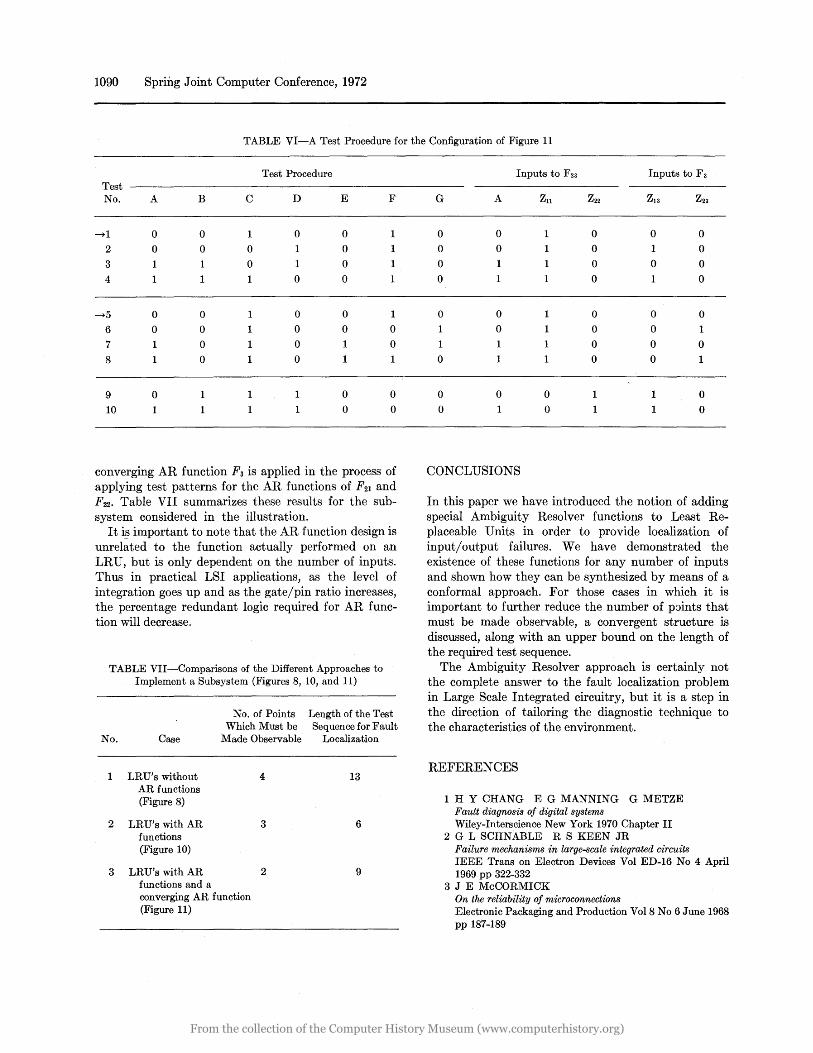
TABLE VI-A Test Procedure for the Configuration of Figure 11

Test Procedure Test No. A B C D E F

-+1 0 0 1 0 0 1

2 0 0 0 0 1

3 1 0 1 0 1

4 1 1 1 0 0 1

-+5 0 0 1 0 0 1

6 0 0 1 0 0 0

7 1 0 1 0 1 0

8 1 0 1 0 1 1

9 0 1 1 1 0 0

10 1 1 1 1 0 0

converging AR function Fa is applied in the process of applying test patterns for the AR functions of F21 and F22• Table VII summarizes these results for the subsystem considered in the illustration.

It iEl important to note that the AR function design is unrelated to the function actually performed on an LRU, but is only dependent on the number of inputs. Thus in practical LSI applications, as the level of integration goes up and as the gate/pin ratio increases, the percentage redundant logic required for AR function will decrease.

TABLE VII-Comparisons of the Different Approaches to Implement a Subsystem (Figures 8, 10, and 11)

No. of Points Length of the Test Which Must be Sequence for Fault

No. Case Made Observable Localization

1 LRU's without 4 13 AR functions (Figure 8)

2 LRU's with AR 3 6 functions (Figure 10)

3 LRU's with AR 2 9 functions and a converging AR function (Figure 11)

Inputs to F23 Inputs to F3

G A Zn Z22 Z13 Z23

0 0 1 0 0 0

0 0 1 0 1 0

0 1 1 0 0 0

0 1 1 0 1 0

0 0 1 0 0 0

1 0 1 0 0 1

1 1 0 0 0 0 1 1 0 0 1

0 0 0 1 1 0

0 1 0 1 1 0

CONCLUSIONS

In this paper we have introduced the notion of adding special Ambiguity Resolver functions to Least Replaceable Units in order to provide localization of input/ output failures. We have demonstrated the existence of these functions for any number of inputs and shown how they can be synthesized by means of a conformal approach. For those cases in which it is important to further reduce the number of pJints that must be made observable, a convergent structure is discussed, along with an upper bound on the length of the required test sequence.

The Ambiguity Resolver approach is certainly not the complete answer to the fault localization problem in Large Scale Integrated circuitry, but it is a step in the direction of tailoring the diagnostic technique to the characteristics of the environment.

REFERENCES

1 H Y CHANG E G MANNING G METZE Fault diagnosis of digital systems Wiley-Interscience New York 1970 Chapter II

2 G L SCHN ABLE R SKEEN JR Failure mechanisms in large-scale integrated circuits IEEE Trans on Electron Devices Vol ED-16 No 4 April 1969 pp 322-332

3 J E McCORMICK On the reliability of microconnections Electronic Packaging and Production Vol 8 No 6 June 1968 pp 187-189


4 D B ARMSTRONG On finding a nearly minimal set of fault detection tests for combinational logic nets IEEE Trans on Electronic Computers EC-15 February 1966 pp 66-73

5 J P ROTH Diagnois of automata failures-A calculus and a method IBM Journal of Research and Development 10 1966 pp 278-291


6 W H KAUTZ

Fault testing and diagnosis in combinational digital circuits IEEE Trans on Computers EC-17 pp 352-366

7 M A MEHTA

A method for optimizing the diagnostic resolution of input-output faults in digital circuits PhD Thesis Illinois Institute of Technology 1971


functions for improving diagnostic resolution in an lsi ... · functions for improving diagnostic...

Documents