________________________________

MATLAB Functions for Mie Scattering and Absorption

Christian Mätzler

________________________________

Research Report No. 2002-08 June 2002

Institut für Angewandte Physik Mikrowellenabteilung __________________________________________________________

Sidlerstrasse 5 Tel. : +41 31 631 89 11 3012 Bern Fax. : +41 31 631 37 65 Schweiz E-mail : matzler@iap.unibe.ch

1

MATLAB Functions for Mie Scattering and Absorption

Christian Mätzler, Institute of Applied Physics, University of Bern, June 20021 List of Contents

Abstract ...................................................................................................................1 1 Introduction..........................................................................................................2 2 Formulas for a homogeneous sphere ...................................................................2

2.1 Mie coefficients and Bessel functions................................................................................. 2 2.2 Mie efficiencies and cross sections ..................................................................................... 3 2.3 The scattered far field........................................................................................................... 4 2.4 The internal field .................................................................................................................. 5 2.5 Computation of Qabs, based on the internal field ................................................................ 6

3 The MATLAB Programs.........................................................................................7 3.1 Comments ............................................................................................................................. 7 3.2 The Function Mie_abcd ....................................................................................................... 8 3.3 The Function Mie ................................................................................................................. 8 3.4 The Function Mie_S12......................................................................................................... 9 3.5 The Function Mie_xscan...................................................................................................... 10 3.6 The Function Mie_tetascan.................................................................................................. 10 3.7 The Function Mie_pt............................................................................................................ 11 3.8 The Function Mie_Esquare.................................................................................................. 11 3.9 The Function Mie_abs.......................................................................................................... 12

4 Examples and Tests............................................................................................13 4.1 The situation of x=1, m=5+0.4i........................................................................................... 13 4.2 Large size parameters........................................................................................................... 15 4.3 Large refractive index .......................................................................................................... 16

5 Conclusion, and outlook to further developments .............................................18 References..............................................................................................................18

Abstract A set of Mie functions has been developed in MATLAB to compute the four Mie coefficients an, bn, cn and dn, efficiencies of extinction, scattering, backscattering and absorption, the asymmetry parameter, and the two angular scattering func-tions S1 and S2. In addition to the scattered field, also the absolute-square of the internal field is computed and used to get the absorption efficiency in a way inde-pendent from the scattered field. This allows to test the computational accuracy. This first version of MATLAB Mie Functions is limited to homogeneous dielectric spheres without change in the magnetic permeability between the inside and out-side of the particle. Required input parameters are the complex refractive index, m= m’+ im”, of the sphere (relative to the ambient medium) and the size parameter, x=ka, where a is the sphere radius and k the wave number in the ambient medium.

1 Equation on p. 16 corrected, April 2006

2

1 Introduction This report is a description of Mie-Scattering and Mie-Absorption programs written in the numeric computation and visualisation software, MATLAB (Math Works, 1992), for the improvement of radiative-transfer codes, especially to account for rain and hail in the microwave range and for aerosols and clouds in the submillimeter, infrared and visible range. Excellent descriptions of Mie Scattering were given by van de Hulst (1957) and by Bohren and Huffman (1983). The present programs are related to the formalism of Bohren and Huffman (1983). In addition an extension (Section 2.5) is given to describe the radial dependence of the internal electric field of the scattering sphere and the absorption resulting from this field. Except for Section 2.5, equation numbers refer to those in Bohren and Huffman (1983), in short BH, or in case of missing equation numbers, page numbers are given. For a description of computational problems in the Mie calculations, see the notes on p. 126-129 and in Appendix A of BH.

2 Formulas for a homogeneous sphere

2.1 Mie coefficients and Bessel functions

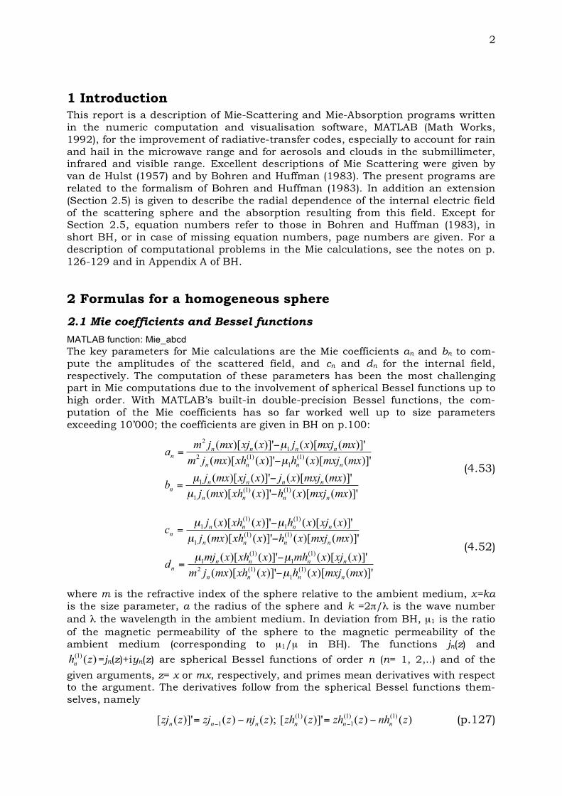
MATLAB function: Mie_abcd The key parameters for Mie calculations are the Mie coefficients an and bn to com-pute the amplitudes of the scattered field, and cn and dn for the internal field, respectively. The computation of these parameters has been the most challenging part in Mie computations due to the involvement of spherical Bessel functions up to high order. With MATLAB’s built-in double-precision Bessel functions, the com-putation of the Mie coefficients has so far worked well up to size parameters exceeding 10’000; the coefficients are given in BH on p.100:

)]'()[()]'()[(

)]'()[()]'()[(

)]'()[()]'()[(

)]'()[()]'()[(

)1()1(

1

1

)1(

1

)1(2

1

2

mxmxjxhxxhmxj

mxmxjxjxxjmxjb

mxmxjxhxxhmxjm

mxmxjxjxxjmxjma

nnnn

nnnnn

nnnn

nnnnn

!

!=

!

!=

µ

µ

µ

µ

(4.53)

)]'()[()]'()[(

)]'()[()]'()[(

)]'()[()]'()[(

)]'()[()]'()[(

)1(

1

)1(2

)1(

1

)1(

1

)1()1(

1

)1(

1

)1(

1

mxmxjxhxxhmxjm

xxjxmhxxhxmjd

mxmxjxhxxhmxj

xxjxhxxhxjc

nnnn

nnnnn

nnnn

nnnnn

µ

µµ

µ

µµ

!

!=

!

!=

(4.52)

where m is the refractive index of the sphere relative to the ambient medium, x=ka is the size parameter, a the radius of the sphere and k =2π/λ is the wave number and λ the wavelength in the ambient medium. In deviation from BH, µ1 is the ratio of the magnetic permeability of the sphere to the magnetic permeability of the ambient medium (corresponding to µ1/µ in BH). The functions jn(z) and

)()1( zhn

=jn(z)+iyn(z) are spherical Bessel functions of order n (n= 1, 2,..) and of the

given arguments, z= x or mx, respectively, and primes mean derivatives with respect to the argument. The derivatives follow from the spherical Bessel functions them-selves, namely

)()()]'([);()()]'([ )1()1(

1

)1(

1 znhzzhzzhznjzzjzzj nnnnnn !=!= !! (p.127)

3

For completeness, the following relationships between Bessel and spherical Bessel functions are given:

)(2

)( 5.0 zJz

zj nn +=!

(4.9)

)(2

)( 5.0 zYz

zy nn +=!

(4.10)

Here, Jν and Yν are Bessel functions of the first and second kind. For n=0 and 1 the spherical Bessel functions are given (BH, p. 87) by

zzzzzyzzzy

zzzzzjzzzj

/sin/cos)(;/cos)(

/cos/sin)(;/sin)(

2

10

2

10

!!=!=

!==

and the recurrence formula

)(12

)()( 11 zfz

nzfzf nnn

+=+ +! (4.11)

where fn is any of the functions jn and yn. Taylor-series expansions for small argu-ments of jn and yn are given on p. 130 of BH. The spherical Hankel functions are linear combinations of jn and yn. Here, the first type is required

)()()()1( ziyzjzh nnn += (4.13)

The following related functions are also used in Mie theory (although we try to avoid them here):

)()();()();()( )1( zzhzzzyzzzjz nnnnnn =!== "#$ (p.101, 183)

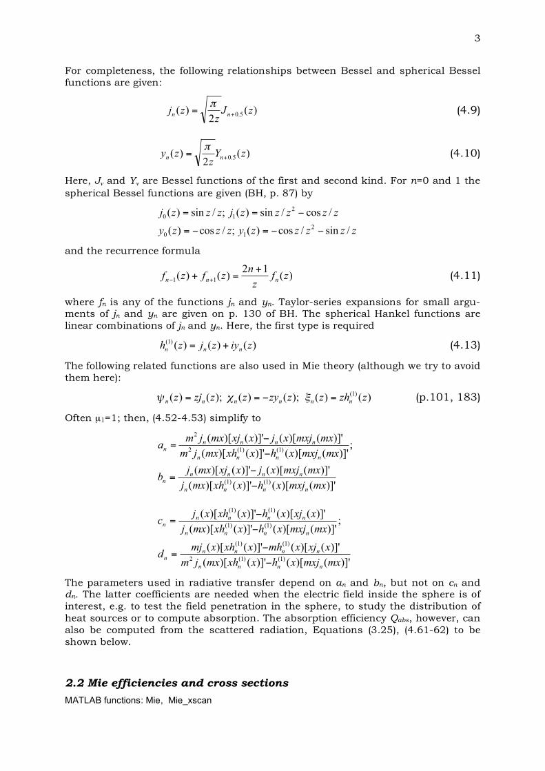
Often µ1=1; then, (4.52-4.53) simplify to

)]'()[()]'()[(

)]'()[()]'()[(

;)]'()[()]'()[(

)]'()[()]'()[(

)1()1(

)1()1(2

2

mxmxjxhxxhmxj

mxmxjxjxxjmxjb

mxmxjxhxxhmxjm

mxmxjxjxxjmxjma

nnnn

nnnnn

nnnn

nnnnn

!

!=

!

!=

)]'()[()]'()[(

)]'()[()]'()[(

;)]'()[()]'()[(

)]'()[()]'()[(

)1()1(2

)1()1(

)1()1(

)1()1(

mxmxjxhxxhmxjm

xxjxmhxxhxmjd

mxmxjxhxxhmxj

xxjxhxxhxjc

nnnn

nnnnn

nnnn

nnnnn

!

!=

!

!=

The parameters used in radiative transfer depend on an and bn, but not on cn and dn. The latter coefficients are needed when the electric field inside the sphere is of interest, e.g. to test the field penetration in the sphere, to study the distribution of heat sources or to compute absorption. The absorption efficiency Qabs, however, can also be computed from the scattered radiation, Equations (3.25), (4.61-62) to be shown below.

2.2 Mie efficiencies and cross sections

MATLAB functions: Mie, Mie_xscan

4

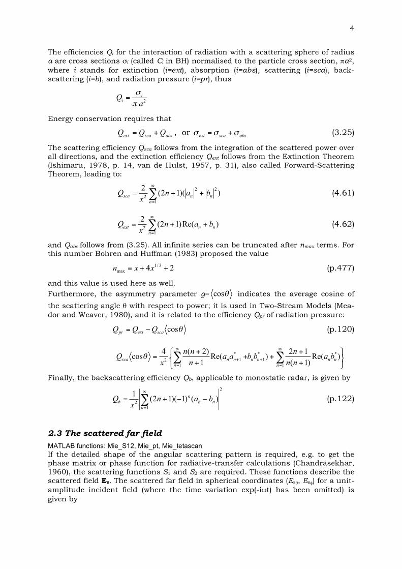
The efficiencies Qi for the interaction of radiation with a scattering sphere of radius a are cross sections σi (called Ci in BH) normalised to the particle cross section, πa2, where i stands for extinction (i=ext), absorption (i=abs), scattering (i=sca), back-scattering (i=b), and radiation pressure (i=pr), thus

2a

Q ii

!

"=

Energy conservation requires that

absscaext QQQ += , or absscaext

!!! += (3.25)

The scattering efficiency Qsca follows from the integration of the scattered power over all directions, and the extinction efficiency Qext follows from the Extinction Theorem (Ishimaru, 1978, p. 14, van de Hulst, 1957, p. 31), also called Forward-Scattering Theorem, leading to:

!"

=

++=1

22

2))(12(

2

n

nnsca banx

Q (4.61)

!"

=

++=1

2)Re()12(

2

n

nnext banx

Q (4.62)

and Qabs follows from (3.25). All infinite series can be truncated after nmax terms. For this number Bohren and Huffman (1983) proposed the value

243/1

max++= xxn (p.477)

and this value is used here as well.

Furthermore, the asymmetry parameter g= !cos indicates the average cosine of

the scattering angle θ with respect to power; it is used in Two-Stream Models (Mea-dor and Weaver, 1980), and it is related to the efficiency Qpr of radiation pressure:

!cosscaextpr QQQ "= (p.120)

!"#

$%&

+

+++

+

+= ''

(

=

+

(

=

+

1

**

1

1

*

12)Re(

)1(

12)Re(

1

)2(4cos

n

nnnn

n

nnsca bann

nbbaa

n

nn

xQ )

Finally, the backscattering efficiency Qb, applicable to monostatic radar, is given by

2

12

)()1)(12(1!"

=

##+=n

nn

n

b banx

Q (p.122)

2.3 The scattered far field

MATLAB functions: Mie_S12, Mie_pt, Mie_tetascan If the detailed shape of the angular scattering pattern is required, e.g. to get the phase matrix or phase function for radiative-transfer calculations (Chandrasekhar, 1960), the scattering functions S1 and S2 are required. These functions describe the scattered field Es. The scattered far field in spherical coordinates (Esθ, Esφ) for a unit-amplitude incident field (where the time variation exp(-iωt) has been omitted) is given by

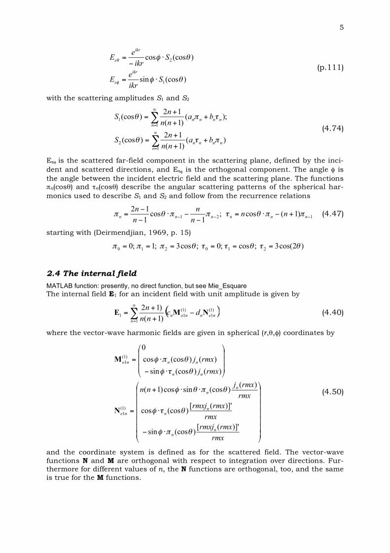
5

)(cossin

)(coscos

1

2

!"

!"

"

!

Sikr

eE

Sikr

eE

ikr

s

ikr

s

#=

#$

=

(p.111)

with the scattering amplitudes S1 and S2

!

!"

=

"

=

++

+=

++

+=

1

2

1

1

)()1(

12)(cos

;)()1(

12)(cos

n

nnnn

n

nnnn

bann

nS

bann

nS

#$%

$#%

(4.74)

Esθ is the scattered far-field component in the scattering plane, defined by the inci-dent and scattered directions, and Esφ is the orthogonal component. The angle φ is the angle between the incident electric field and the scattering plane. The functions πn(cosθ) and τn(cosθ) describe the angular scattering patterns of the spherical har-monics used to describe S1 and S2 and follow from the recurrence relations

121 )1(cos;1

cos1

12!!! +!"=

!!"

!

!=

nnnnnnnn

n

n

n

n##$%##$# (4.47)

starting with (Deirmendjian, 1969, p. 15)

)2cos(3;cos;0;cos3;1;0 210210 !"!""!### ======

2.4 The internal field

MATLAB function: presently, no direct function, but see Mie_Esquare The internal field E1 for an incident field with unit amplitude is given by

( )!"

=

#+

+=

1

)1(

1

)1(

11)1(

)12

n

nennondc

nn

nNME (4.40)

where the vector-wave harmonic fields are given in spherical (r,θ,φ) coordinates by

!!!!!!!

"

#

$$$$$$$

%

&

'(

'

''+

=

!!!

"

#

$$$

%

&

'(

'=

rmx

rmxrmxj

rmx

rmxrmxj

rmx

rmxjnn

rmxj

rmxj

nn

nn

nn

ne

nn

nnno

)]'([)(cossin

)]'([)(coscos

)()(cossincos)1(

)()(cossin

)()(coscos

0

)1(

1

)1(

1

)*+

),+

)*)+

),+

)*+

N

M

(4.50)

and the coordinate system is defined as for the scattered field. The vector-wave functions N and M are orthogonal with respect to integration over directions. Fur-thermore for different values of n, the N functions are orthogonal, too, and the same is true for the M functions.

6

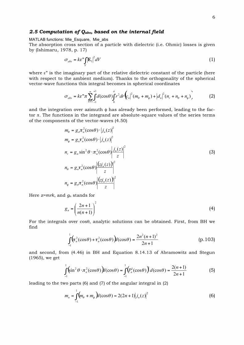
2.5 Computation of Qabs, based on the internal field

MATLAB functions: Mie_Esquare, Mie_abs The absorption cross section of a particle with dielectric (i.e. Ohmic) losses is given by (Ishimaru, 1978, p. 17)

dVk

V

abs !=2

1" E"# (1)

where ε” is the imaginary part of the relative dielectric constant of the particle (here with respect to the ambient medium). Thanks to the orthogonality of the spherical vector-wave functions this integral becomes in spherical coordinates

( )!" "#

=

+

$

++++=1

1

1 0

222 )()()(cos"n

a

rnnabsnnndmmcdrrdk %&%&&'() (2)

and the integration over azimuth φ has already been performed, leading to the fac-tor π. The functions in the integrand are absolute-square values of the series terms of the components of the vector-waves (4.50)

( )

( ) 22

2

2

2

22

22

22

')()(cos

')()(cos

)()(cossin

)()(cos

)()(cos

z

zzjgn

z

zzjgn

z

zjgn

zjgm

zjgm

nnn

nnn

nnnr

nnn

nnn

!"

!#

!"!

!#

!"

$

!

$

!

=

=

%=

%=

%=

(3)

Here z=mrk, and gn stands for

2

)1(

12!!"

#$$%

&

+

+=

nn

ngn

(4)

For the integrals over cosθ, analytic solutions can be obtained. First, from BH we find

( )12

)1(2)(cos)(cos)(cos

221

1

22

+

+=+!

"n

nnd

nn##$#% (p.103)

and second, from (4.46) in BH and Equation 8.14.13 of Abramowitz and Stegun (1965), we get

( ) ( )12

)1(2)(cos)(cos)(cos)(cossin

1

1

21

1

1

22

+

+==! ""

##n

ndPd

nn$$$$%$ (5)

leading to the two parts (6) and (7) of the angular integral in (2)

( ) 21

1

)()12(2)(cos zjndmmm nn +=+= !"

#$# (6)

7

( )!"

!#$

!%

!&'

+++=++= ()

221

1

')()()1()12(2)(cos)(

z

zzj

z

zjnnndnnnn nn

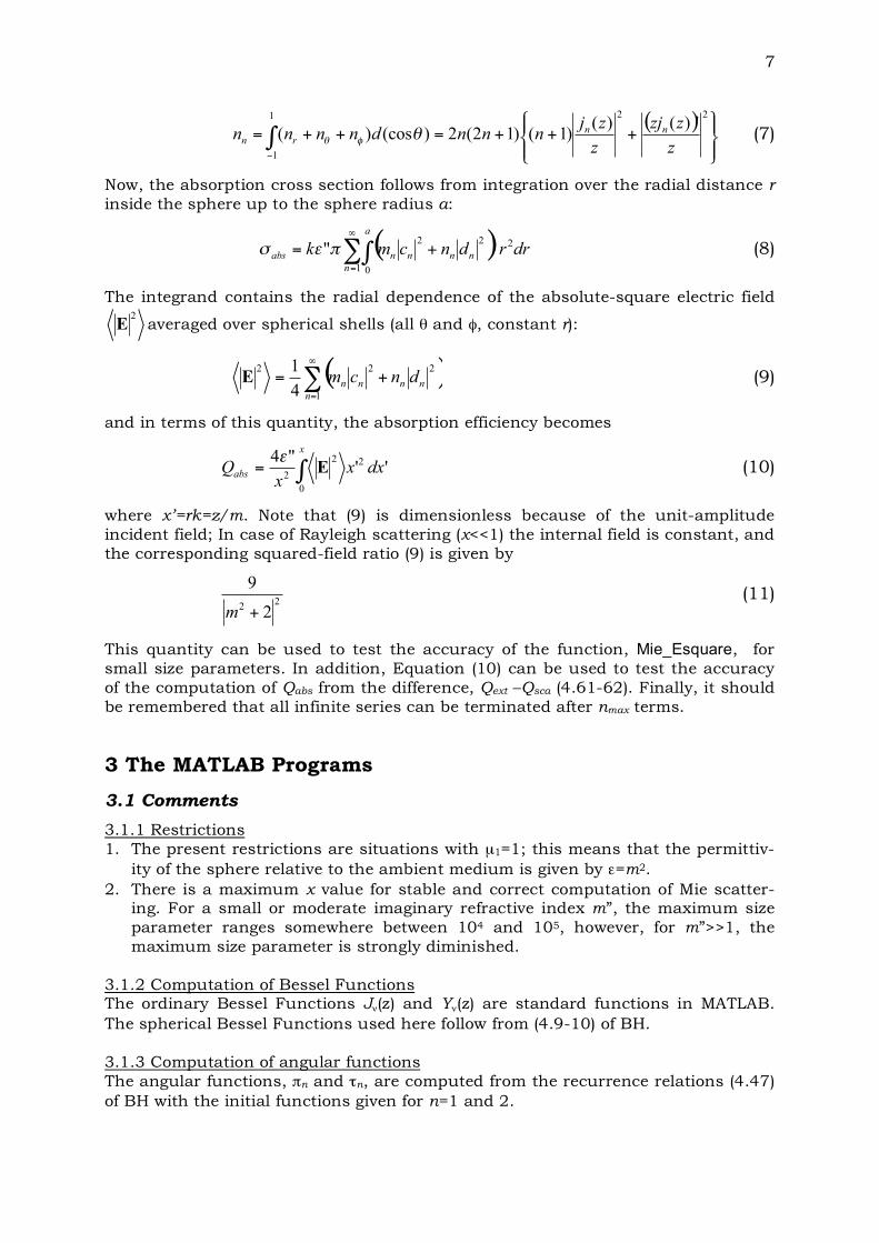
rn *+* (7)

Now, the absorption cross section follows from integration over the radial distance r inside the sphere up to the sphere radius a:

( )!"#

=

$+=1 0

222

"

n

a

nnnnabsdrrdncmk %&' (8)

The integrand contains the radial dependence of the absolute-square electric field 2

E averaged over spherical shells (all θ and φ, constant r):

( )!"

=

+=1

222

4

1

n

nnnndncmE (9)

and in terms of this quantity, the absorption efficiency becomes

!=

x

abs dxxx

Q0

22

2''

"4E

" (10)

where x’=rk=z/m. Note that (9) is dimensionless because of the unit-amplitude incident field; In case of Rayleigh scattering (x<<1) the internal field is constant, and the corresponding squared-field ratio (9) is given by

222

9

+m

(11)

This quantity can be used to test the accuracy of the function, Mie_Esquare, for small size parameters. In addition, Equation (10) can be used to test the accuracy of the computation of Qabs from the difference, Qext –Qsca (4.61-62). Finally, it should be remembered that all infinite series can be terminated after nmax terms.

3 The MATLAB Programs

3.1 Comments

3.1.1 Restrictions 1. The present restrictions are situations with µ1=1; this means that the permittiv-

ity of the sphere relative to the ambient medium is given by ε=m2. 2. There is a maximum x value for stable and correct computation of Mie scatter-

ing. For a small or moderate imaginary refractive index m”, the maximum size parameter ranges somewhere between 104 and 105, however, for m”>>1, the maximum size parameter is strongly diminished.

3.1.2 Computation of Bessel Functions The ordinary Bessel Functions Jν(z) and Yν(z) are standard functions in MATLAB. The spherical Bessel Functions used here follow from (4.9-10) of BH. 3.1.3 Computation of angular functions The angular functions, πn and τn, are computed from the recurrence relations (4.47) of BH with the initial functions given for n=1 and 2.

8

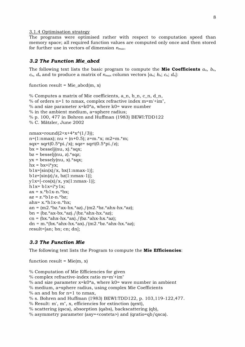
3.1.4 Optimisation strategy The programs were optimised rather with respect to computation speed than memory space; all required function values are computed only once and then stored for further use in vectors of dimension nmax.

3.2 The Function Mie_abcd

The following text lists the basic program to compute the Mie Coefficients an, bn, cn, dn and to produce a matrix of nmax column vectors [an; bn; cn; dn]: function result = Mie_abcd(m, x) % Computes a matrix of Mie coefficients, a_n, b_n, c_n, d_n, % of orders n=1 to nmax, complex refractive index m=m'+im", % and size parameter x=k0*a, where k0= wave number % in the ambient medium, a=sphere radius; % p. 100, 477 in Bohren and Huffman (1983) BEWI:TDD122 % C. Mätzler, June 2002 nmax=round(2+x+4*x^(1/3)); n=(1:nmax); nu = (n+0.5); z=m.*x; m2=m.*m; sqx= sqrt(0.5*pi./x); sqz= sqrt(0.5*pi./z); bx = besselj(nu, x).*sqx; bz = besselj(nu, z).*sqz; yx = bessely(nu, x).*sqx; hx = bx+i*yx; b1x=[sin(x)/x, bx(1:nmax-1)]; b1z=[sin(z)/z, bz(1:nmax-1)]; y1x=[-cos(x)/x, yx(1:nmax-1)]; h1x= b1x+i*y1x; ax = x.*b1x-n.*bx; az = z.*b1z-n.*bz; ahx= x.*h1x-n.*hx; an = (m2.*bz.*ax-bx.*az)./(m2.*bz.*ahx-hx.*az); bn = (bz.*ax-bx.*az)./(bz.*ahx-hx.*az); cn = (bx.*ahx-hx.*ax)./(bz.*ahx-hx.*az); dn = m.*(bx.*ahx-hx.*ax)./(m2.*bz.*ahx-hx.*az); result=[an; bn; cn; dn];

3.3 The Function Mie

The following text lists the Program to compute the Mie Efficiencies: function result = Mie(m, x) % Computation of Mie Efficiencies for given % complex refractive-index ratio m=m'+im" % and size parameter x=k0*a, where k0= wave number in ambient % medium, a=sphere radius, using complex Mie Coefficients % an and bn for n=1 to nmax, % s. Bohren and Huffman (1983) BEWI:TDD122, p. 103,119-122,477. % Result: m', m", x, efficiencies for extinction (qext), % scattering (qsca), absorption (qabs), backscattering (qb), % asymmetry parameter (asy=<costeta>) and (qratio=qb/qsca).

9

% Uses the function "Mie_abcd" for an and bn, for n=1 to nmax. % C. Mätzler, May 2002. if x==0 % To avoid a singularity at x=0 result=[real(m) imag(m) 0 0 0 0 0 0 1.5]; elseif x>0 % This is the normal situation nmax=round(2+x+4*x^(1/3)); n1=nmax-1; n=(1:nmax);cn=2*n+1; c1n=n.*(n+2)./(n+1); c2n=cn./n./(n+1); x2=x*x; f=mie_abcd(m,x); anp=(real(f(1,:))); anpp=(imag(f(1,:))); bnp=(real(f(2,:))); bnpp=(imag(f(2,:))); g1(1:4,nmax)=[0; 0; 0; 0]; % displaced numbers used for g1(1,1:n1)=anp(2:nmax); % asymmetry parameter, p. 120 g1(2,1:n1)=anpp(2:nmax); g1(3,1:n1)=bnp(2:nmax); g1(4,1:n1)=bnpp(2:nmax); dn=cn.*(anp+bnp); q=sum(dn); qext=2*q/x2; en=cn.*(anp.*anp+anpp.*anpp+bnp.*bnp+bnpp.*bnpp); q=sum(en); qsca=2*q/x2; qabs=qext-qsca; fn=(f(1,:)-f(2,:)).*cn; gn=(-1).^n; f(3,:)=fn.*gn; q=sum(f(3,:)); qb=q*q'/x2; asy1=c1n.*(anp.*g1(1,:)+anpp.*g1(2,:)+bnp.*g1(3,:)+bnpp.*g1(4,:)); asy2=c2n.*(anp.*bnp+anpp.*bnpp); asy=4/x2*sum(asy1+asy2)/qsca; qratio=qb/qsca; result=[real(m) imag(m) x qext qsca qabs qb asy qratio]; end;

3.4 The Function Mie_S12

The following text lists the program to compute the two complex scattering ampli-tudes S1 and S2: function result = Mie_S12(m, x, u) % Computation of Mie Scattering functions S1 and S2 % for complex refractive index m=m'+im", % size parameter x=k0*a, and u=cos(scattering angle), % where k0=vacuum wave number, a=sphere radius; % s. p. 111-114, Bohren and Huffman (1983) BEWI:TDD122 % C. Mätzler, May 2002 nmax=round(2+x+4*x^(1/3)); abcd=Mie_abcd(m,x); an=abcd(1,:);

10

bn=abcd(2,:); pt=Mie_pt(u,nmax); pin =pt(1,:); tin=pt(2,:); n=(1:nmax); n2=(2*n+1)./(n.*(n+1)); pin=n2.*pin; tin=n2.*tin; S1=(an*pin'+bn*tin'); S2=(an*tin'+bn*pin'); result=[S1;S2];

3.5 The Function Mie_xscan

The following text lists the program to compute the a matrix of Mie efficiencies and to plot them as a function of x: function result = Mie_xscan(m, nsteps, dx) % Computation and plot of Mie Efficiencies for given % complex refractive-index ratio m=m'+im" % and range of size parameters x=k0*a, % starting at x=0 with nsteps increments of dx % a=sphere radius, using complex Mie coefficients an and bn % according to Bohren and Huffman (1983) BEWI:TDD122 % result: m', m", x, efficiencies for extinction (qext), % scattering (qsca), absorption (qabs), backscattering (qb), % qratio=qb/qsca and asymmetry parameter (asy=<costeta>). % C. Mätzler, May 2002. nx=(1:nsteps)'; x=(nx-1)*dx; for j = 1:nsteps a(j,:)=Mie(m,x(j)); end; output_parameters='Real(m), Imag(m), x, Qext, Qsca, Qabs, Qb, <costeta>, Qb/Qsca' m1=real(m);m2=imag(m); plot(a(:,3),a(:,4:9)) % plotting the results legend('Qext','Qsca','Qabs','Qb','<costeta>','Qb/Qsca') title(sprintf('Mie Efficiencies, m=%g+%gi',m1,m2)) xlabel('x') result=a;

3.6 The Function Mie_tetascan

The following text lists the program to compute the a matrix of Mie scattering

intensities 2

1S and

2

2S as a function of u=cosθ, and to display the result as a

polar diagram of θ with 2

1S in the upper half circle (0<θ<π) and

2

2S in the lower

half circle (π<θ<2π). Both functions are symmetric with respect to both half circles: function result = Mie_tetascan(m, x, nsteps)

11

% Computation and plot of Mie Power Scattering function for given % complex refractive-index ratio m=m'+im", size parameters x=k0*a, % according to Bohren and Huffman (1983) BEWI:TDD122 % C. Mätzler, May 2002. nsteps=nsteps; m1=real(m); m2=imag(m); nx=(1:nsteps); dteta=pi/(nsteps-1); teta=(nx-1).*dteta; for j = 1:nsteps, u=cos(teta(j)); a(:,j)=Mie_S12(m,x,u); SL(j)= real(a(1,j)'*a(1,j)); SR(j)= real(a(2,j)'*a(2,j)); end; y=[teta teta+pi;SL SR(nsteps:-1:1)]'; polar(y(:,1),y(:,2)) title(sprintf('Mie angular scattering: m=%g+%gi, x=%g',m1,m2,x)); xlabel('Scattering Angle') result=y;

3.7 The Function Mie_pt

The following text lists the program to compute a matrix of πn and τn functions for n=1 to nmax: function result=Mie_pt(u,nmax) % pi_n and tau_n, -1 <= u= cosθ <= 1, n1 integer from 1 to nmax % angular functions used in Mie Theory % Bohren and Huffman (1983), p. 94 - 95 p(1)=1; t(1)=u; p(2)=3*u; t(2)=3*cos(2*acos(u)); for n1=3:nmax, p1=(2*n1-1)./(n1-1).*p(n1-1).*u; p2=n1./(n1-1).*p(n1-2); p(n1)=p1-p2; t1=n1*u.*p(n1); t2=(n1+1).*p(n1-1); t(n1)=t1-t2; end; result=[p;t];

3.8 The Function Mie_Esquare

The following text lists the program to compute and plot the (θ, φ) averaged absolute-square E-field as a function of x’=rk (for r<0<a): function result = Mie_Esquare(m, x, nj)

12

% Computation of nj+1 equally spaced values within (0,x) % of the mean-absolute-square internal % electric field of a sphere of size parameter x, % complex refractive index m=m'+im", % where the averaging is done over teta and phi, % with unit-amplitude incident field; % Ref. Bohren and Huffman (1983) BEWI:TDD122, % and my own notes on this topic; % k0=2*pi./wavelength; % x=k0.*radius; % C. Mätzler, May 2002 nmax=round(2+x+4*x^(1/3)); n=(1:nmax); nu =(n+0.5); m1=real(m); m2=imag(m); abcd=Mie_abcd(m,x); cn=abcd(3,:);dn=abcd(4,:); cn2=abs(cn).^2; dn2=abs(dn).^2; dx=x/nj; for j=1:nj, xj=dx.*j; z=m.*xj; sqz= sqrt(0.5*pi./z); bz = besselj(nu, z).*sqz; % This is jn(z) bz2=(abs(bz)).^2; b1z=[sin(z)/z, bz(1:nmax-1)]; % Note that sin(z)/z=j0(z) az = b1z-n.*bz./z; az2=(abs(az)).^2; z2=(abs(z)).^2; n1 =n.*(n+1); n2 =2.*(2.*n+1); mn=real(bz2.*n2); nn1=az2; nn2=bz2.*n1./z2; nn=n2.*real(nn1+nn2); en(j)=0.25*(cn2*mn'+dn2*nn'); end; xxj=[0:dx:xj]; een=[en(1) en]; plot(xxj,een); legend('Radial Dependence of (abs(E))^2') title(sprintf('Squared Amplitude E Field in a Sphere, m=%g+%gi x=%g',m1,m2,x)) xlabel('r k') result=een;

3.9 The Function Mie_abs

The following text lists the program to compute the absorption efficiency, based on Equation (9): function result = Mie_abs(m, x) % Computation of the Absorption Efficiency Qabs % of a sphere of size parameter x,

13

% complex refractive index m=m'+im", % based on nj internal radial electric field values % to be computed with Mie_Esquare(nj,m,x) % Ref. Bohren and Huffman (1983) BEWI:TDD122, % and my own notes on this topic; % k0=2*pi./wavelength; % x=k0.*radius; % C. Mätzler, May 2002 nj=5*round(2+x+4*x.^(1/3))+160; e2=imag(m.*m); dx=x/nj; x2=x.*x; nj1=nj+1; xj=(0:dx:x); en=Mie_Esquare(m,x,nj); en1=0.5*en(nj1).*x2; % End-Term correction in integral enx=en*(xj.*xj)'-en1; % Trapezoidal radial integration inte=dx.*enx; Qabs=4.*e2.*inte./x2; result=Qabs;

4 Examples and Tests

4.1 The situation of x=1, m=5+0.4i

The execution of the command line >> m =5 + 0.4i; x = 1; mie_abcd(m,x) leads to column vectors [an; bn; cn; dn] for n=1 to nmax=7: ans = Columns 1 through 4 (for n=1 to 4) 0.2306 - 0.2511i 0.0055 - 0.0354i 0.0000 - 0.0008i 0.0000 - 0.0000i 0.0627 + 0.1507i 0.0159 + 0.0262i 0.0004 - 0.0006i 0.0000 - 0.0000i -0.6837 + 0.0128i -0.3569 + 0.2199i 0.0752 + 0.0339i 0.0076 + 0.0000i -1.1264 + 0.0093i 0.2135 + 0.1212i 0.0180 + 0.0003i 0.0023 - 0.0004i Columns 5 through 7 (for n=5 to 7) 0.0000 - 0.0000i 0.0000 - 0.0000i 0.0000 - 0.0000i 0.0000 - 0.0000i 0.0000 - 0.0000i 0.0000 - 0.0000i 0.0010 - 0.0002i 0.0002 - 0.0000i 0.0000 - 0.0000i 0.0003 - 0.0001i 0.0001 - 0.0000i 0.0000 - 0.0000i >> mie(m,x) ans = Columns 1 through 7 (for m’, m”, x, Qext, Qsca, Qabs, Qb)

14

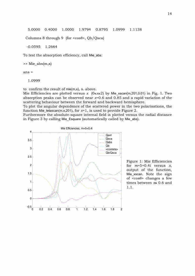
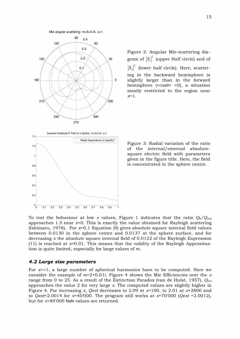
5.0000 0.4000 1.0000 1.9794 0.8795 1.0999 1.1138 Columns 8 through 9 (for <cosθ>, Qb/Qsca) -0.0595 1.2664 To test the absorption efficiency, call Mie_abs: >> Mie_abs(m,x) ans = 1.0999 to confirm the result of mie(m,x), s. above. Mie Efficiencies are plotted versus x (0≤x≤2) by Mie_xscan(m,201,0.01) in Fig. 1. Two absorption peaks can be observed near x=0.6 and 0.85 and a rapid variation of the scattering behaviour between the forward and backward hemisphere. To plot the angular dependence of the scattered power in the two polarisations, the function Mie_tetascan(m,x,201), for x=1, is used to provide Figure 2. Furthermore the absolute-square internal field is plotted versus the radial distance in Figure 3 by calling Mie_Esquare (automatically called by Mie_abs).

0 0.2 0.4 0.6 0.8 1 1.2 1.4 1.6 1.8 2-0.5

0

0.5

1

1.5

2

2.5

3

3.5

4

Mie Efficiencies, m=5+0.4i

x

Qext

Qsca

Qabs

Qb

<costeta>

Qb/Qsca

Figure 1: Mie Efficiencies for m=5+0.4i versus x, output of the function, Mie_xscan. Note the sign of <cosθ> changes a few times between x≅ 0.6 and 1.1.

15

0.1

0.2

0.3

0.4

30

210

60

240

90

270

120

300

150

330

180 0

Mie angular scattering: m=5+0.4i, x=1

Scattering Angle

Figure 2: Angular Mie-scattering dia-

gram of 2

1S (upper Half circle) and of

2

2S (lower half circle). Here, scatter-

ing in the backward hemisphere is slightly larger than in the forward hemisphere (<cosθ> <0), a situation mostly restricted to the region near x=1.

0 0.1 0.2 0.3 0.4 0.5 0.6 0.7 0.8 0.9 10

0.2

0.4

0.6

0.8

1

1.2

1.4Squared Amplitude E Field in a Sphere, m=5+0.4i, x=1

r k

Radial Dependence of (abs(E))2

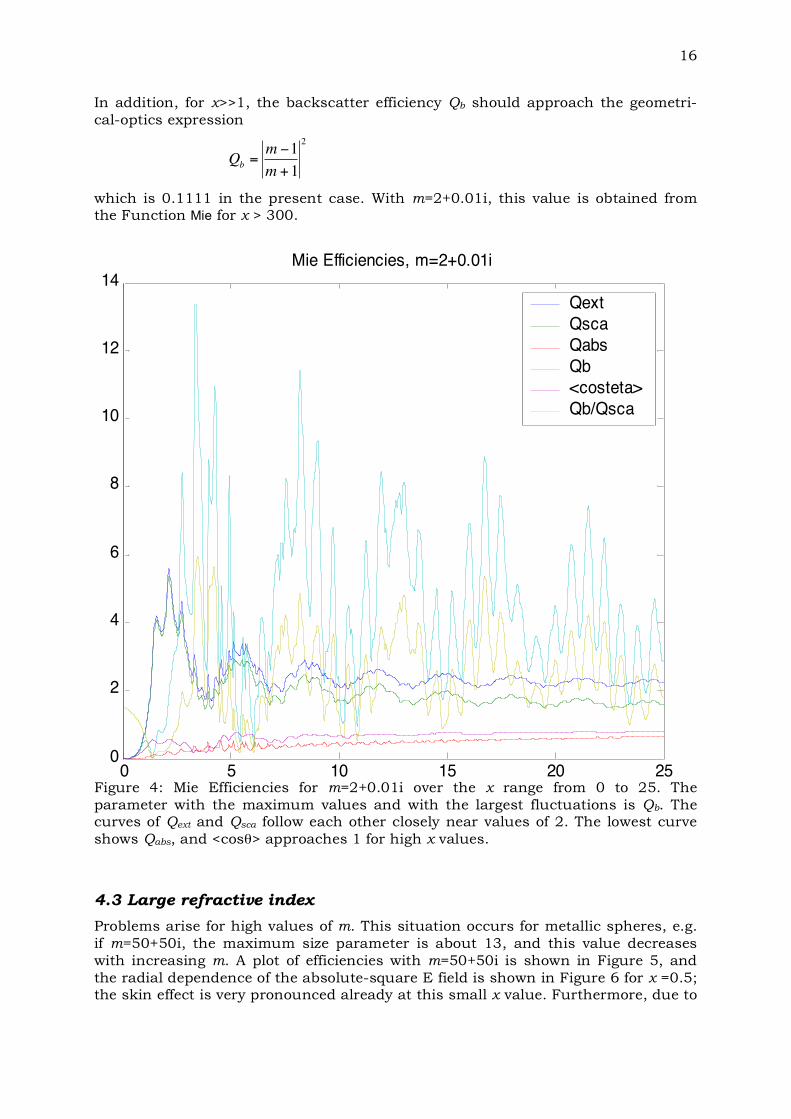
Figure 3: Radial variation of the ratio of the internal/external absolute-square electric field with parameters given in the figure title. Here, the field is concentrated in the sphere centre.

To test the behaviour at low x values, Figure 1 indicates that the ratio Qb/Qsca approaches 1.5 near x=0. This is exactly the value obtained for Rayleigh scattering (Ishimaru, 1978). For x=0.1 Equation (9) gives absolute square internal field values between 0.0130 in the sphere centre and 0.0137 at the sphere surface, and for decreasing x the absolute square internal field of 0.0122 of the Rayleigh Expression (11) is reached at x=0.01. This means that the validity of the Rayleigh Approxima-tion is quite limited, especially for large values of m.

4.2 Large size parameters

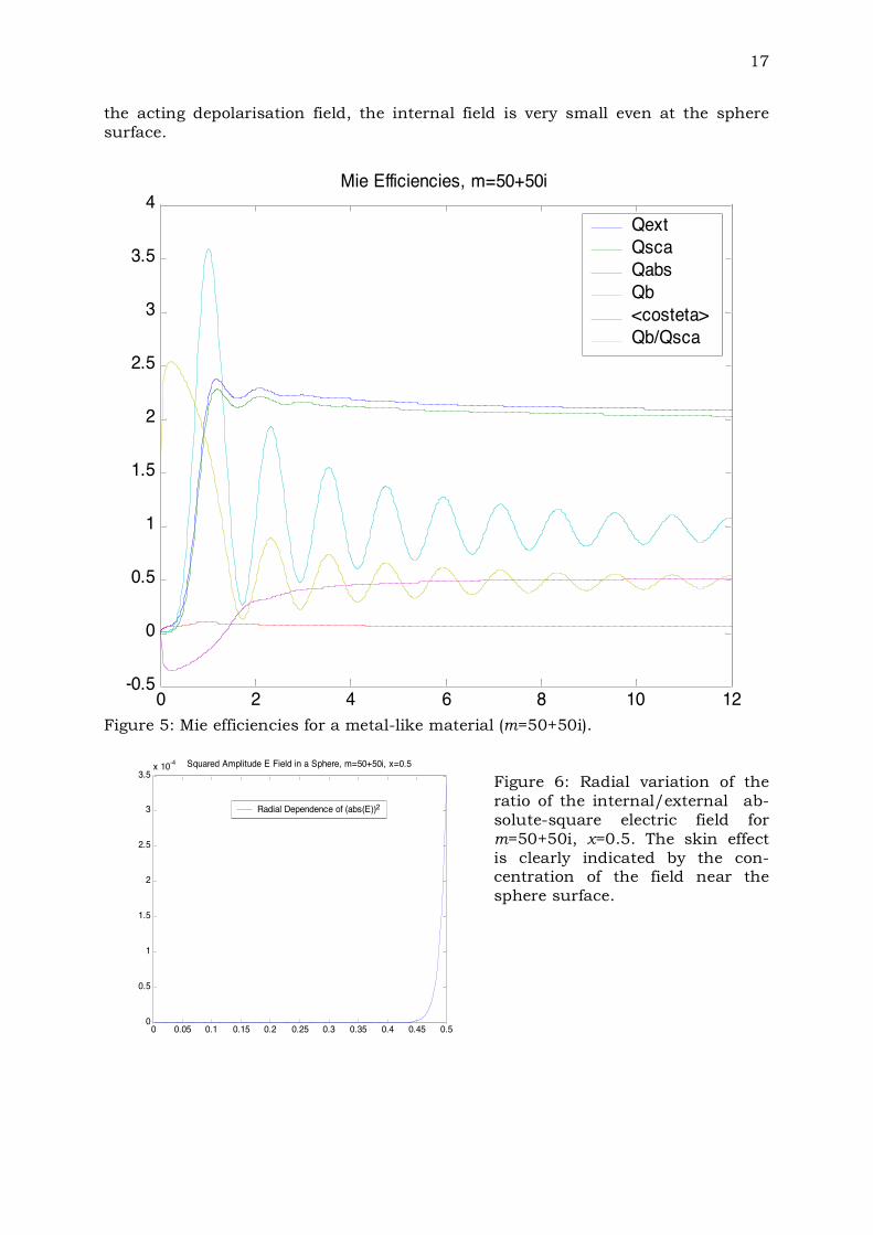
For x>>1, a large number of spherical harmonics have to be computed. Here we consider the example of m=2+0.01i. Figure 4 shows the Mie Efficiencies over the x range from 0 to 25. As a result of the Extinction Paradox (van de Hulst, 1957), Qext approaches the value 2 for very large x. The computed values are slightly higher in Figure 4. For increasing x, Qext decreases to 2.09 at x=100, to 2.01 at x=2800 and to Qext=2.0014 for x=40’000. The program still works at x=70'000 (Qext =2.0012), but for x>80'000 NaN values are returned.

16

In addition, for x>>1, the backscatter efficiency Qb should approach the geometri-cal-optics expression

!

Qb =m "1

m +1

2

which is 0.1111 in the present case. With m=2+0.01i, this value is obtained from the Function Mie for x > 300.

0 5 10 15 20 250

2

4

6

8

10

12

14

Mie Efficiencies, m=2+0.01i

x

Qext

Qsca

Qabs

Qb

<costeta>

Qb/Qsca

Figure 4: Mie Efficiencies for m=2+0.01i over the x range from 0 to 25. The parameter with the maximum values and with the largest fluctuations is Qb. The curves of Qext and Qsca follow each other closely near values of 2. The lowest curve shows Qabs, and <cosθ> approaches 1 for high x values.

4.3 Large refractive index

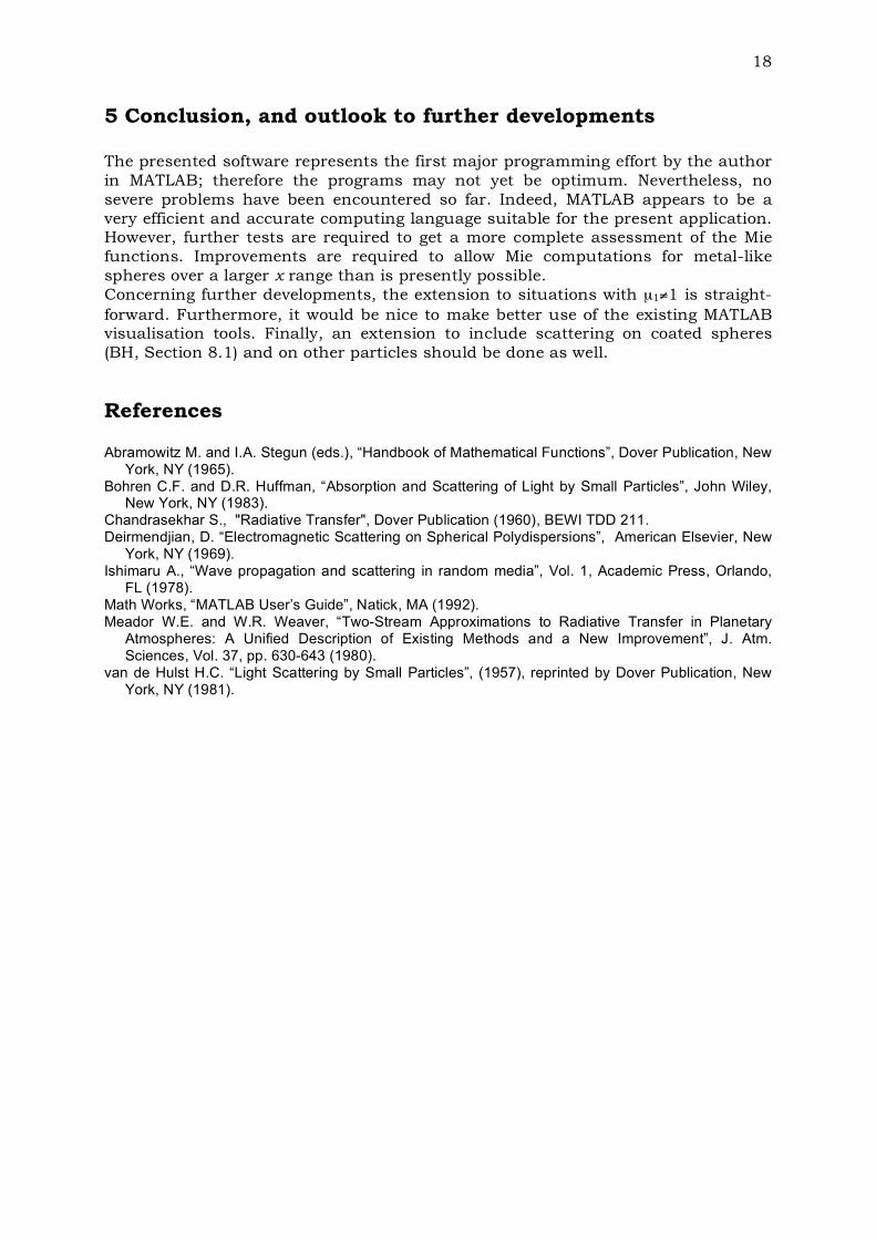
Problems arise for high values of m. This situation occurs for metallic spheres, e.g. if m=50+50i, the maximum size parameter is about 13, and this value decreases with increasing m. A plot of efficiencies with m=50+50i is shown in Figure 5, and the radial dependence of the absolute-square E field is shown in Figure 6 for x =0.5; the skin effect is very pronounced already at this small x value. Furthermore, due to

17

the acting depolarisation field, the internal field is very small even at the sphere surface.

0 2 4 6 8 10 12-0.5

0

0.5

1

1.5

2

2.5

3

3.5

4

Mie Efficiencies, m=50+50i

x

Qext

Qsca

Qabs

Qb

<costeta>

Qb/Qsca

Figure 5: Mie efficiencies for a metal-like material (m=50+50i).

0 0.05 0.1 0.15 0.2 0.25 0.3 0.35 0.4 0.45 0.50

0.5

1

1.5

2

2.5

3

3.5x 10

-4 Squared Amplitude E Field in a Sphere, m=50+50i, x=0.5

r k

Radial Dependence of (abs(E))2

Figure 6: Radial variation of the ratio of the internal/external ab-solute-square electric field for m=50+50i, x=0.5. The skin effect is clearly indicated by the con-centration of the field near the sphere surface.

18

5 Conclusion, and outlook to further developments The presented software represents the first major programming effort by the author in MATLAB; therefore the programs may not yet be optimum. Nevertheless, no severe problems have been encountered so far. Indeed, MATLAB appears to be a very efficient and accurate computing language suitable for the present application. However, further tests are required to get a more complete assessment of the Mie functions. Improvements are required to allow Mie computations for metal-like spheres over a larger x range than is presently possible. Concerning further developments, the extension to situations with µ1≠1 is straight-forward. Furthermore, it would be nice to make better use of the existing MATLAB visualisation tools. Finally, an extension to include scattering on coated spheres (BH, Section 8.1) and on other particles should be done as well.

References Abramowitz M. and I.A. Stegun (eds.), “Handbook of Mathematical Functions”, Dover Publication, New

York, NY (1965). Bohren C.F. and D.R. Huffman, “Absorption and Scattering of Light by Small Particles”, John Wiley,

New York, NY (1983). Chandrasekhar S., "Radiative Transfer", Dover Publication (1960), BEWI TDD 211. Deirmendjian, D. “Electromagnetic Scattering on Spherical Polydispersions”, American Elsevier, New

York, NY (1969). Ishimaru A., “Wave propagation and scattering in random media”, Vol. 1, Academic Press, Orlando,

FL (1978). Math Works, “MATLAB User’s Guide”, Natick, MA (1992). Meador W.E. and W.R. Weaver, “Two-Stream Approximations to Radiative Transfer in Planetary

Atmospheres: A Unified Description of Existing Methods and a New Improvement”, J. Atm. Sciences, Vol. 37, pp. 630-643 (1980).

van de Hulst H.C. “Light Scattering by Small Particles”, (1957), reprinted by Dover Publication, New York, NY (1981).