1 Fundamental Methods of Extrapolation

Fundamental Methods of Numerical

Extrapolation

With Applications

Eric Hung-Lin Liu

Keywords: numerical analysis, extrapolation, richardson, romberg, numerical differentiation, numerical integration

Abstract

Extrapolation is an incredibly powerful technique for increasing speed and accuracy in various numerical tasks in scientific computing. As we will see, extrapolation can transform even the most mundane of algorithms (such as the Trapezoid Rule) into an extremely fast and accurate algorithm, increasing the rate of convergence by more than one order of magnitude. Within this paper, we will first present some background theory to motivate the derivation of Richardson and Romberg Extrapolation and provide support for their validity and stability as numerical techniques. Then we will present examples from differentiation and integration to demonstrate the incredible power of extrapolation. We will also give some MATLAB code to show some simple implentation methods in addition to discussing error bounds and differentiating between ”‘true”’ and ”‘false”’ convergence.

1 Introduction

Extrapolation is an extremely powerful tool available to numerical analysts for improving the performance of a wide variety of mathematical methods. Since many “interesting” problems cannot be solved analytically, we often have to use computers to derive approximate solutions. In order to make this process efficient, we have to think carefully about our implementations: this is where extrapolation comes in. We will examine some examples in greater detail later, but we will briefly survey them now. First, consider numeric differentiation: in theory, it is performed by tending the step-size to zero. The problem is that modern computers have limited precision; as we will see, decreasing the step-size past 10−8 severely worsens the performance because of floating point round-off errors. The choice of step-size in integration is also important but for a different reason. Having a tiny step-size means more accurate results, but it also requires more function evaluations–this could be very expensive depending on the application at hand. The large numbers of floating point operations associated with a small step-size has the negative effect of magnifying the problems of limited precision (but it is not nearly as serious as with differentiation). Another example is the evaluation of (infinite) series. For slowly converging series, we will need to sum a very large number of terms to get an accurate result; the problem is that this could be very slow and again limited precision comes into play.

Extrapolation attempts to rectify these problems by computing “weighted averages” of

∑

2 Liu

relatively poor estimates to eliminate error modes–specifically, we will be examining various forms of Richardson Extrapolation. Richardson and Richardson-like schemes are but a subset of all extrapolation methods, but they are among the most common. They have numerous applications and are not terribly difficult to understand and implement. We will demonstrate that various numerical methods taught in introductory calculus classes are in fact insufficient, but they can all be greatly improved through proper application of extrapolation techniques.

1.1 Background: A Few Words on Series Expansions

We are very often able to associate some infinite sequence {An} with a known function A(h). For example, A(h) may represent a first divided differences scheme for differentiation, where h is the step-size. Note that h may be continuous or discrete. The sequence {An} is described by: An = A(hn), n ∈ N for a monotonically decreasing sequence {hn} that converges to 0 in the limit. Thus limh→0+ A(h) = A and similarly, limn→∞ An = A. Computing A(0) is exactly what we want to do–continuing the differentiation example, roughly speaking A(0) is the ”point” where the divided differences ”becomes” the derivative.

Interestingly enough, although we require that A(y) have an asymptotic series expansion, we need not determine it uniquely. In fact we will see that knowing the pn is sufficient. Specifically, we will examine functions with expansions that take this form:

s

A(h) = A + αkhpk + O(hps+1 ) as h 0+ (1) →

k=1

where pn 6= 0 ∀n, p1 < p2 < ... < ps+1, and all the αk are independent of y. The pn can in fact be imaginary, in which case we compare only the real parts. Clearly, having p1 > 0 guarantees the existence of limh→0+ A(h) = A. In the case where that limit does not exist, A is the antilimit of A(h), and then we know that at pi ≤ 0 for at least i = 1. However, as long as the sequence {pn} is monotonically increasing such that limk→∞ pk = +∞, (1) exists and A(h)

∑

∞has the expansion A(h) ∼ A + k=1 αkhpk . We do not need to declare any conditions on the

convergence of the infinite series. We do assume that the hk are known, but we do not need to know the αk, since as we will see, these constant factors are not significant.

Now suppose that p1 > 0 (hence it is true ∀p), then when h is sufficiently small, A(y) approximates A with error A(h) − A = O(hp1 ). In most cases, p1 is not particularly small (i.e. p1 < 4), so it would appear that we will need to decrease h to get useful results. But as previously noted, this is almost always prohibitive in terms of round-off errors and/or function evaluations.

We should not despair, because we are now standing on the doorstep of the fundamental idea behind Richardson Extrapolation. That idea is to use equation (1) to somehow eliminate the hp1 error term, thus obtaining a new approximation A1(h)−A = O(hh2 ). It is obvious that | A1(h)−A |<| A(h)−A | since p2 > p1. As we will see later, this is accomplished by taking a ”weighted average” of A(h) and A(h

s ).

2 Simple Numerical Differentiation and Integration Schemes

Before continuing with our development of the theory of extrapolation, we will briefly review differentiation by first divided differences and quadrature using the (composite) trapezoid and midpoint rules. These are among the simplest algorithms; they are straightforward enough

( )

Fundamental Methods of Extrapolation 3

to be presented in first-year calculus classes. Being all first-order approximations, their error modes are significant, and they have little application in real situations. However as we will see, applying a simple extrapolation scheme makes these simple methods extremely powerful, convering difficult problems quickly and achieving higher accuracy in the process.

2.1 Differentiation via First Divided Differencs

Suppose we have an arbitrary function f(x) ∈ C1[x0 − ǫ, x0 + ǫ] for some ǫ > 0. Then apply a simple linear fit to f(x) in the aforementioned region to approximate the f ′(x). We can begin by assuming the existence of additional derivatives and computing a Taylor Expansion:

1 f(x) = f(x0) + f ′ (x0)(x − x0) + f ′′ (x0)(x − x0)

2 + O(f(h3)) 2

where h = x − x0 and 0 < h ≤ ǫ

f ′ (x0) = f(x + h

h

) − f(x) − 12 f ′′ (x)h + O(h2)

Resulting in:

f ′ (x0) = f(x0 + h) − f(x0)

(2) h

From the Taylor Expansion, it would seem that our first divided difference approximation has truncation error on the order of O(h). Thus one might imagine that allowing h 0 will yield →O(h) 0 at a rate linear in h. Unfortunately, due the limitations of finite precision arithmetic, →performing h 0 can only decrease truncation error a certain amount before arithmetic error →becomes dominant. Thus selecting a very small h is not a viable solution, which is sadly a misconception of many Calculus students. Let us examine exactly how this arithmetic error arises. Note that because of the discrete nature of computers, a number a is represented as a(1 + ǫ1) where ǫ1 is some error.

(a − b) = a(1 + ǫ1) − b(1 + ǫ2)

= (a − b) + (aǫ1 − bǫ2) + (a − b)ǫ3

= (a − b)(1 + ǫ3) + (| a | + | b |)ǫ4

Thus the floating point representation of the difference numerator, fl[f(x + h) − f(x)] is f(x + h)− f(x) + 2f(x)ǫ + ... where 2f(x)ǫ represents the arithmetic error due to subtraction. So the floating point representation of the full divided difference is:

f ′ (x) = fl[ f(x + h) − f(x)

] + 2f(x)ǫ 1

h h −

2 f ′′ (x)h + ... (3)

Again, 2f(h

x)ǫ is the arithmetic error, while 12f ′′(x)h is the truncation error from only taking the

linear term of the Taylor Expansion. Since one term acts like h 1 and the other like h, there

exists an optimum choice of h such that the total error is minimized:

1

f(x) 2

h ≈ 2 f ′′(x)

ǫ (4)

log

(err

or)

10

4 Liu

From equation (4), it is evident that hoptimum ∼√

ǫm where ǫm is machine precision, which is

roughly 10−16 in the IEEE double precision standard. Thus our best error is 4(f ′′(x)f(x)ǫ) 1 ∼2

10−8 . This is rather dismal, and we certainly can do better. Naturally it is impossible to modify arithemtic error: it is a property of double precision representations. So we look to the truncation error: a prime suspect for extrapolation.

Failure of First Divided Differences

−16 −14 −12 −10 −8 −6 −4 −2 0

1

0

−1

−2

−3

−4

−5

−6

−7

−8

log (dx)10

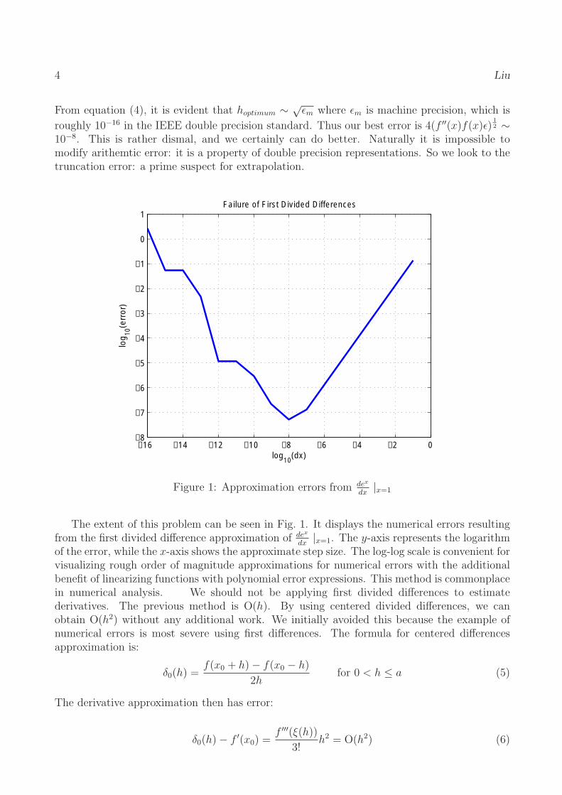
Figure 1: Approximation errors from dex |dx x=1

The extent of this problem can be seen in Fig. 1. It displays the numerical errors resulting dex

from the first divided difference approximation of dx

|x=1. The y-axis represents the logarithm of the error, while the x-axis shows the approximate step size. The log-log scale is convenient for visualizing rough order of magnitude approximations for numerical errors with the additional benefit of linearizing functions with polynomial error expressions. This method is commonplace in numerical analysis. We should not be applying first divided differences to estimate derivatives. The previous method is O(h). By using centered divided differences, we can obtain O(h2) without any additional work. We initially avoided this because the example of numerical errors is most severe using first differences. The formula for centered differences approximation is:

δ0(h) = f(x0 + h) − f(x0 − h)

for 0 < h ≤ a (5) 2h

The derivative approximation then has error:

δ0(h) − f ′ (x0) = f ′′′(ξ(h))

h2 = O(h2) (6) 3!

( ) ∑

∑

∫ ∫ ∑ ∏

∑

Fundamental Methods of Extrapolation 5

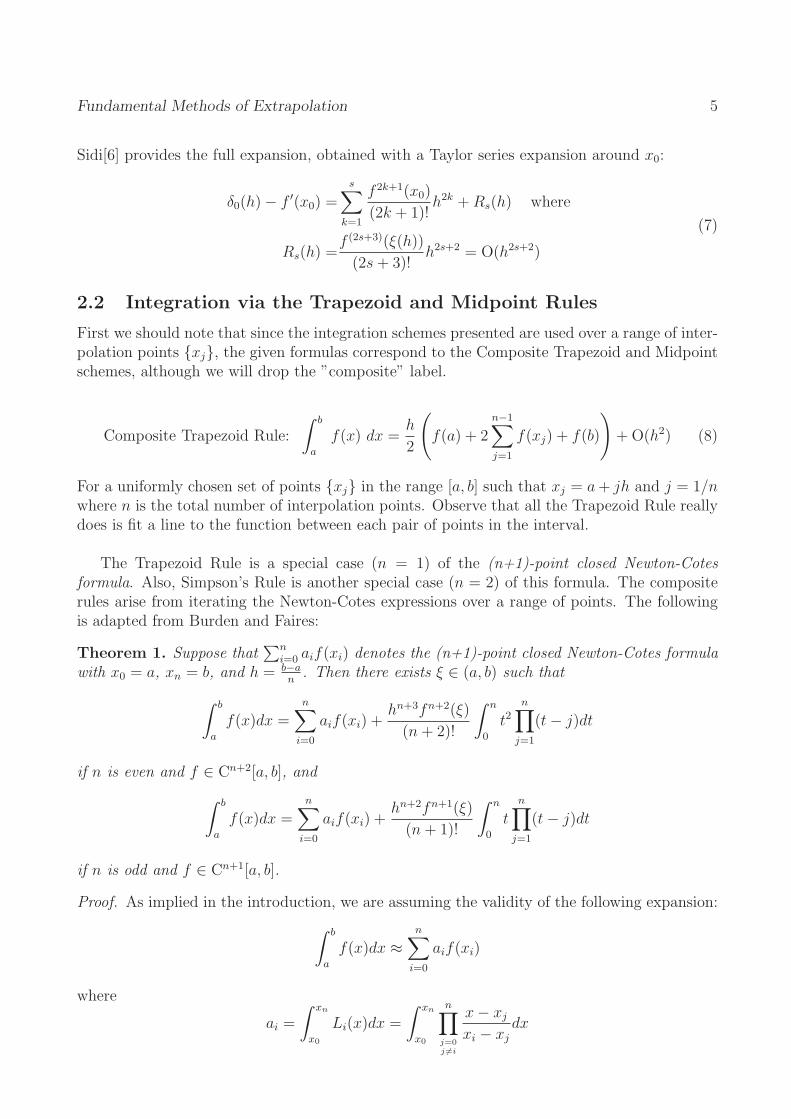
Sidi[6] provides the full expansion, obtained with a Taylor series expansion around x0:

s ∑ f 2k+1(x0)

δ0(h) − f ′ (x0) = (2k + 1)!

h2k + Rs(h) where k=1 (7)

h2s+2 Rs(h) = f (2s+3)(ξ(h))

= O(h2s+2)(2s + 3)!

2.2 Integration via the Trapezoid and Midpoint Rules

First we should note that since the integration schemes presented are used over a range of inter­polation points {xj}, the given formulas correspond to the Composite Trapezoid and Midpoint schemes, although we will drop the ”composite” label.

∫ b n−1h

Composite Trapezoid Rule: f(x) dx = f(a) + 2 f(xj) + f(b) + O(h2) (8) 2a j=1

For a uniformly chosen set of points {xj} in the range [a, b] such that xj = a + jh and j = 1/n where n is the total number of interpolation points. Observe that all the Trapezoid Rule really does is fit a line to the function between each pair of points in the interval.

The Trapezoid Rule is a special case (n = 1) of the (n+1)-point closed Newton-Cotes formula. Also, Simpson’s Rule is another special case (n = 2) of this formula. The composite rules arise from iterating the Newton-Cotes expressions over a range of points. The following is adapted from Burden and Faires:

Theorem 1. Suppose that i

n

=0 aif(xi) denotes the (n+1)-point closed Newton-Cotes formula with x0 = a, xn = b, and h = b−

na . Then there exists ξ ∈ (a, b) such that

b n hn+3fn+2(ξ) n n

f(x)dx = aif(xi) + (n + 2)!

t2 (t − j)dt a i=0 0 j=1

if n is even and f ∈ Cn+2[a, b], and

∫ n ∫ nb ∑ hn+2fn+1(ξ) n

∏ f(x)dx = aif(xi) +

(n + 1)! t (t − j)dt

a i=0 0 j=1

if n is odd and f ∈ Cn+1[a, b].

Proof. As implied in the introduction, we are assuming the validity of the following expansion:

∫ b n

f(x)dx ≈ aif(xi) a i=0

where ∫ ∫ nxn xn

∏ ai = Li(x)dx =

x − xj dx

x0 x0 j=0 xi − xj

j 6=i

∑

6 Liu

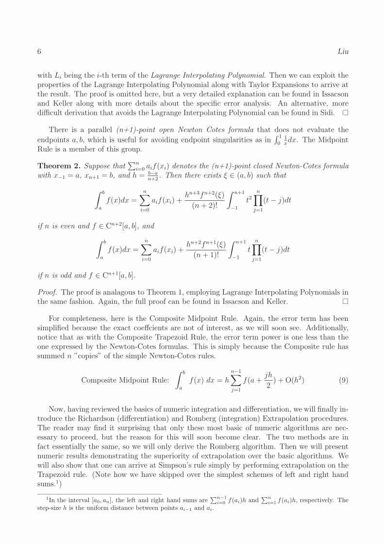
with Li being the i-th term of the Lagrange Interpolating Polynomial. Then we can exploit the properties of the Lagrange Interpolating Polynomial along with Taylor Expansions to arrive at the result. The proof is omitted here, but a very detailed explanation can be found in Issacson and Keller along with more details about the specific error analysis. An alternative, more difficult derivation that avoids the Lagrange Interpolating Polynomial can be found in Sidi.

There is a parallel (n+1)-point open Newton Cotes formula that does not evaluate the

endpoints a, b, which is useful for avoiding endpoint singularities as in ∫

0

1

x 1dx. The Midpoint

Rule is a member of this group.

Theorem 2. Suppose that i

n

=0 aif(xi) denotes the (n+1)-point closed Newton-Cotes formula with x−1 = a, xn+1 = b, and h = b−a . Then there exists ξ ∈ (a, b) such that

n+2

∫ n ∫ nb ∑ hn+3fn+2(ξ) n+1

∏ f(x)dx = aif(xi) +

(n + 2)! t2 (t − j)dt

a i=0 −1 j=1

if n is even and f ∈ Cn+2[a, b], and

∫ n ∫ nb ∑ hn+2fn+1(ξ) n+1

∏ f(x)dx = aif(xi) +

(n + 1)! t (t − j)dt

a i=0 −1 j=1

if n is odd and f ∈ Cn+1[a, b].

Proof. The proof is analagous to Theorem 1, employing Lagrange Interpolating Polynomials in the same fashion. Again, the full proof can be found in Issacson and Keller.

For completeness, here is the Composite Midpoint Rule. Again, the error term has been simplified because the exact coeffcients are not of interest, as we will soon see. Additionally, notice that as with the Composite Trapezoid Rule, the error term power is one less than the one expressed by the Newton-Cotes formulas. This is simply because the Composite rule has summed n ”copies” of the simple Newton-Cotes rules.

∫ b n−1 ∑ jh

Composite Midpoint Rule: f(x) dx = h f(a + ) + O(h2) (9) 2a j=1

Now, having reviewed the basics of numeric integration and differentiation, we will finally in­troduce the Richardson (differentiation) and Romberg (integration) Extrapolation procedures. The reader may find it surprising that only these most basic of numeric algorithms are nec­essary to proceed, but the reason for this will soon become clear. The two methods are in fact essentially the same, so we will only derive the Romberg algorithm. Then we will present numeric results demonstrating the superiority of extrapolation over the basic algorithms. We will also show that one can arrive at Simpson’s rule simply by performing extrapolation on the Trapezoid rule. (Note how we have skipped over the simplest schemes of left and right hand sums.1)

∑

n−1 ∑

n1In the interval [a0, an], the left and right hand sums are i=0 f(ai)h and

i=1 f(ai)h, respectively. The step-size h is the uniform distance between points ai−1 and ai.

( ) ∑

Fundamental Methods of Extrapolation 7

3 The Richardson and Romberg Extrapolation Technique

3.1 Conceptual and Analytic Approach

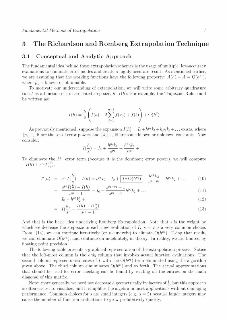
The fundamental idea behind these extrapolation schemes is the usage of multiple, low-accuracy evaluations to eliminate error modes and create a highly accurate result. As mentioned earlier, we are assuming that the working functions have the following property: A(h) − A = O(hp1 ), where p1 is known or obtainable.

To motivate our understanding of extrapolation, we will write some arbitrary quadrature rule I as a function of its associated step-size, h: I(h). For example, the Trapezoid Rule could be written as:

n−1 h

I(h) = f(a) + 2 f(xj) + f(b) + O(h2)2

j=1

As previously mentioned, suppose the expansion I(h) = I0+hp1 k1+hp2k2+ . . . exists, where {pi} ⊂ R are the set of error powers and {ki} ⊂ R are some known or unknown constants. Now consider:

h hp1 k1 hp2 k2I( ) = I0 + + + . . .

s sp1 sp2

To eliminate the hp1 error term (because it is the dominant error power), we will compute −I(h) + sp1 I(h).

s

hp2 k2I ′ (h) = sp1 I(

h ) − I(h) = sp1 I0 − I0 + 0 ∗ O(hp1 ) + − hp2 k2 + . . . (10)

sp1−p2ss

s = p1 I(h) − I(h)

= I0 + sp1−p2 − 1

hp2 k2 + . . . (11) sp1 sp1− 1 − 1

= I0 + hp2 k2 ′ + . . . (12)

h

s ) − I(h

s

)p1

−−I

1

(hs )

(13) = I(

And that is the basic idea underlying Romberg Extrapolation. Note that s is the weight by which we decrease the step-size in each new evaluation of I. s = 2 is a very common choice. From (14), we can continue iteratively (or recursively) to elimate O(hp2 ). Using that result, we can eliminate O(hp3 ), and continue on indefinitely, in theory. In reality, we are limited by floating point precision.

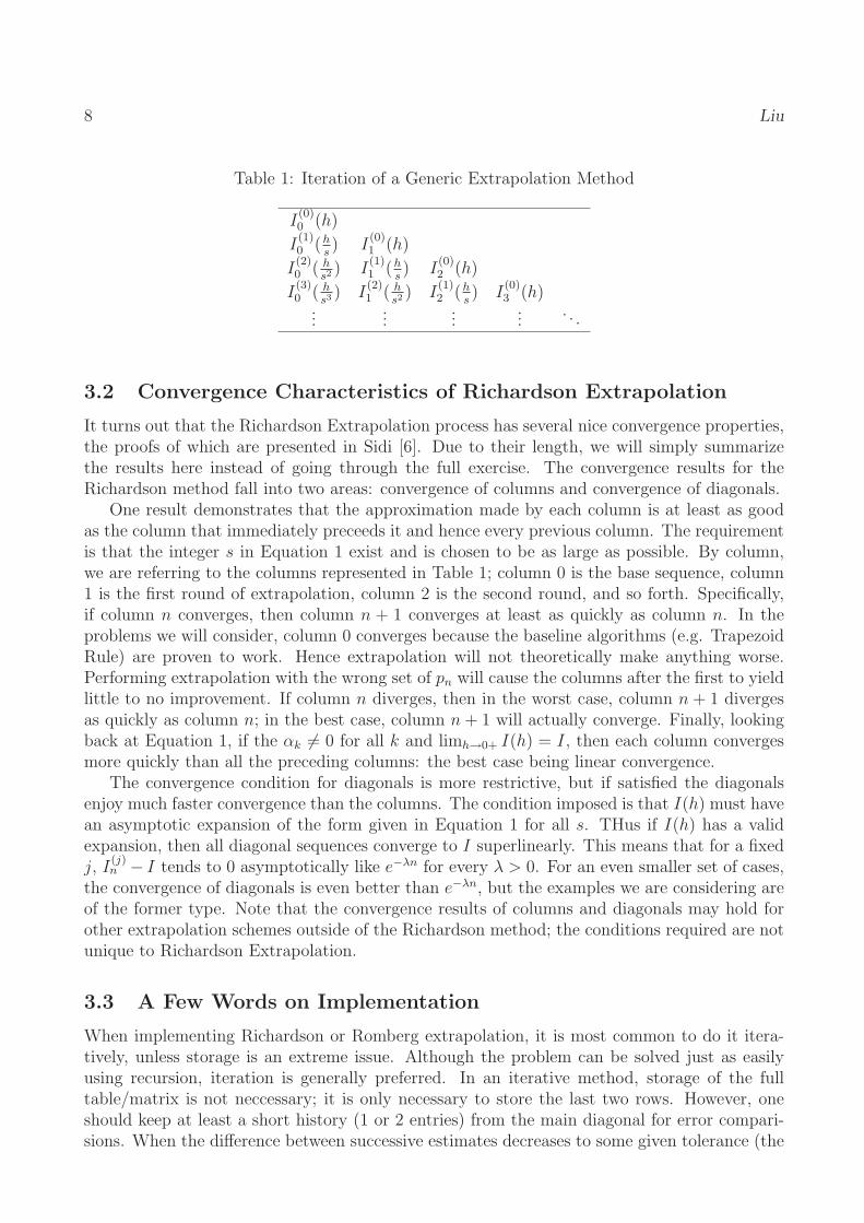
The following table presents a graphical representation of the extrapolation process. Notice that the left-most column is the only column that involves actual function evaluations. The second column represents estimates of I with the O(hp1 ) term eliminated using the algorithm given above. The third column elmiminates O(hp2 ) and so forth. The actual approximations that should be used for error checking can be found by reading off the entries on the main diagonal of this matrix.

Note: more generally, we need not decrease h geometrically by factors of 1 , but this approach s

is often easiest to visualize, and it simplifies the algebra in most applications without damaging performance. Common choices for s are small integers (e.g. s = 2) because larger integers may cause the number of function evaluations to grow prohibitively quickly.

6

8 Liu

Table 1: Iteration of a Generic Extrapolation Method

I0(0)

(h)

I0(1)

(h) I1(0)

(h)s

I0(2)

( h (1) 2 1) I (h) I2

(0) (h)

s s

I0(3)

(sh 3 ) I1

(2) (

sh 2 ) I2

(1) (h

s ) I3

(0) (h)

. . . . .. . . . .. . . . .

3.2 Convergence Characteristics of Richardson Extrapolation

It turns out that the Richardson Extrapolation process has several nice convergence properties, the proofs of which are presented in Sidi [6]. Due to their length, we will simply summarize the results here instead of going through the full exercise. The convergence results for the Richardson method fall into two areas: convergence of columns and convergence of diagonals.

One result demonstrates that the approximation made by each column is at least as good as the column that immediately preceeds it and hence every previous column. The requirement is that the integer s in Equation 1 exist and is chosen to be as large as possible. By column, we are referring to the columns represented in Table 1; column 0 is the base sequence, column 1 is the first round of extrapolation, column 2 is the second round, and so forth. Specifically, if column n converges, then column n + 1 converges at least as quickly as column n. In the problems we will consider, column 0 converges because the baseline algorithms (e.g. Trapezoid Rule) are proven to work. Hence extrapolation will not theoretically make anything worse. Performing extrapolation with the wrong set of pn will cause the columns after the first to yield little to no improvement. If column n diverges, then in the worst case, column n + 1 diverges as quickly as column n; in the best case, column n + 1 will actually converge. Finally, looking back at Equation 1, if the αk = 0 for all k and limh→0+ I(h) = I, then each column converges more quickly than all the preceding columns: the best case being linear convergence.

The convergence condition for diagonals is more restrictive, but if satisfied the diagonals enjoy much faster convergence than the columns. The condition imposed is that I(h) must have an asymptotic expansion of the form given in Equation 1 for all s. THus if I(h) has a valid expansion, then all diagonal sequences converge to I superlinearly. This means that for a fixed j, In

(j) − I tends to 0 asymptotically like e−λn for every λ > 0. For an even smaller set of cases, the convergence of diagonals is even better than e−λn, but the examples we are considering are of the former type. Note that the convergence results of columns and diagonals may hold for other extrapolation schemes outside of the Richardson method; the conditions required are not unique to Richardson Extrapolation.

3.3 A Few Words on Implementation

When implementing Richardson or Romberg extrapolation, it is most common to do it itera­tively, unless storage is an extreme issue. Although the problem can be solved just as easily using recursion, iteration is generally preferred. In an iterative method, storage of the full table/matrix is not neccessary; it is only necessary to store the last two rows. However, one should keep at least a short history (1 or 2 entries) from the main diagonal for error compari­sions. When the difference between successive estimates decreases to some given tolerance (the

Fundamental Methods of Extrapolation 9

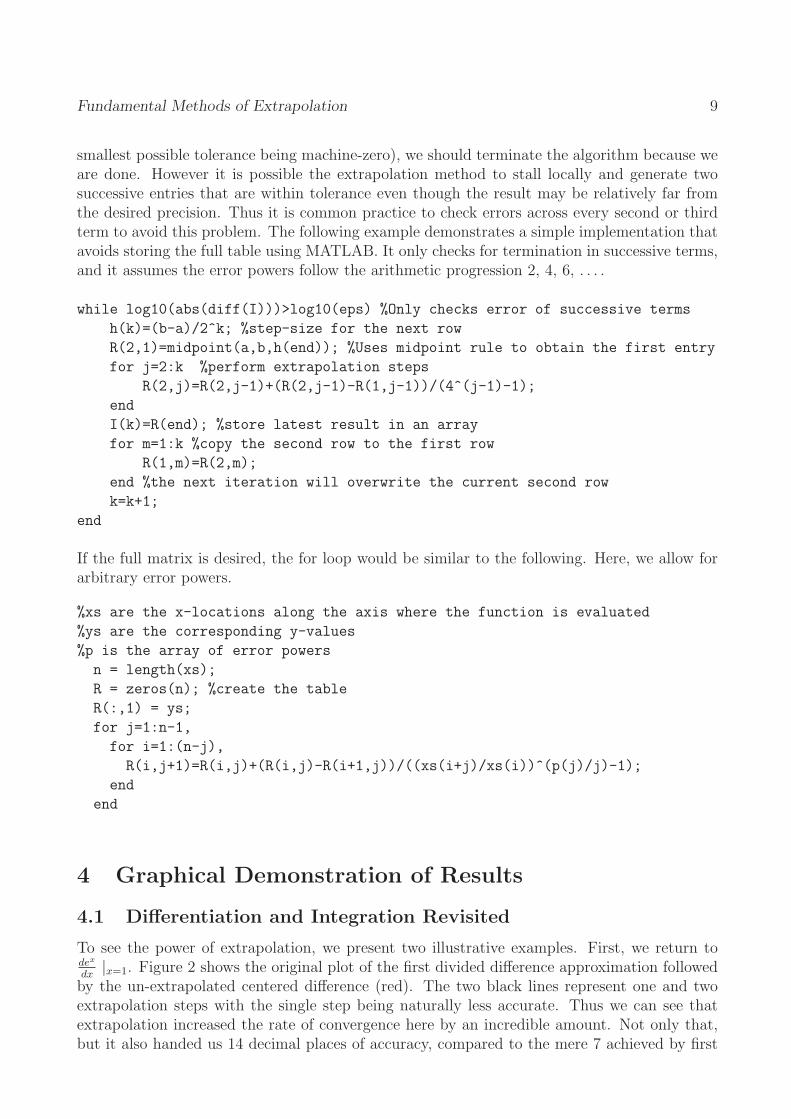
smallest possible tolerance being machine-zero), we should terminate the algorithm because we are done. However it is possible the extrapolation method to stall locally and generate two successive entries that are within tolerance even though the result may be relatively far from the desired precision. Thus it is common practice to check errors across every second or third term to avoid this problem. The following example demonstrates a simple implementation that avoids storing the full table using MATLAB. It only checks for termination in successive terms, and it assumes the error powers follow the arithmetic progression 2, 4, 6, . . . .

while log10(abs(diff(I)))>log10(eps) %Only checks error of successive terms h(k)=(b-a)/2^k; %step-size for the next row R(2,1)=midpoint(a,b,h(end)); %Uses midpoint rule to obtain the first entry for j=2:k %perform extrapolation steps

R(2,j)=R(2,j-1)+(R(2,j-1)-R(1,j-1))/(4^(j-1)-1);endI(k)=R(end); %store latest result in an arrayfor m=1:k %copy the second row to the first row

R(1,m)=R(2,m);end %the next iteration will overwrite the current second rowk=k+1;

end

If the full matrix is desired, the for loop would be similar to the following. Here, we allow for arbitrary error powers.

%xs are the x-locations along the axis where the function is evaluated %ys are the corresponding y-values %p is the array of error powers

n = length(xs);R = zeros(n); %create the tableR(:,1) = ys;for j=1:n-1,

for i=1:(n-j),R(i,j+1)=R(i,j)+(R(i,j)-R(i+1,j))/((xs(i+j)/xs(i))^(p(j)/j)-1);

endend

4 Graphical Demonstration of Results

4.1 Differentiation and Integration Revisited

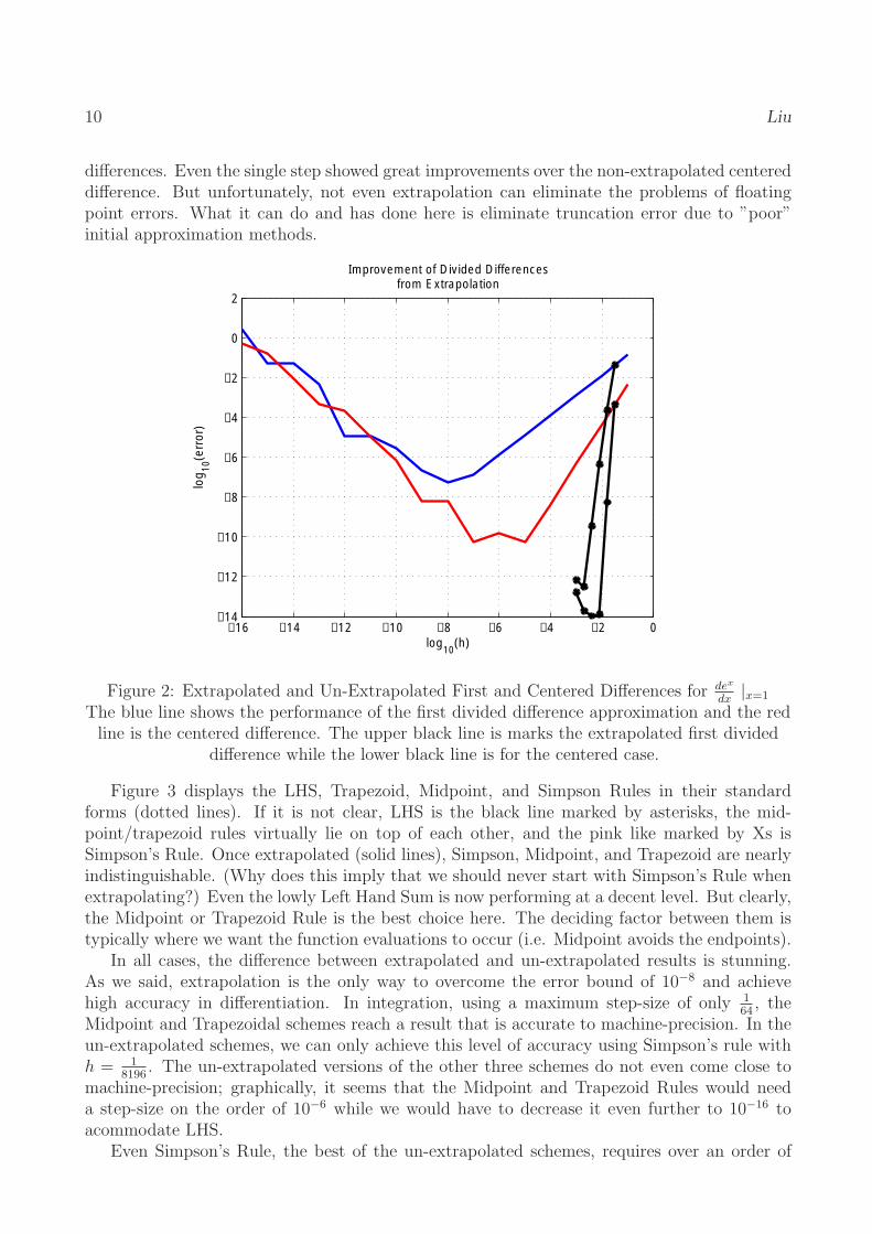
To see the power of extrapolation, we present two illustrative examples. First, we return to dex

dx |x=1. Figure 2 shows the original plot of the first divided difference approximation followed

by the un-extrapolated centered difference (red). The two black lines represent one and two extrapolation steps with the single step being naturally less accurate. Thus we can see that extrapolation increased the rate of convergence here by an incredible amount. Not only that, but it also handed us 14 decimal places of accuracy, compared to the mere 7 achieved by first

10 Liu

differences. Even the single step showed great improvements over the non-extrapolated centered difference. But unfortunately, not even extrapolation can eliminate the problems of floating point errors. What it can do and has done here is eliminate truncation error due to ”poor” initial approximation methods.

Improvement of Divided Differences from Extrapolation

−16 −14 −12 −10 −8 −6 −4 −2 0 −14

−12

−10

−8

−6

−4

−2

0

2

log 10

(err

or)

log (h)10

Figure 2: Extrapolated and Un-Extrapolated First and Centered Differences for dex

x=1 dx |

The blue line shows the performance of the first divided difference approximation and the red line is the centered difference. The upper black line is marks the extrapolated first divided

difference while the lower black line is for the centered case.

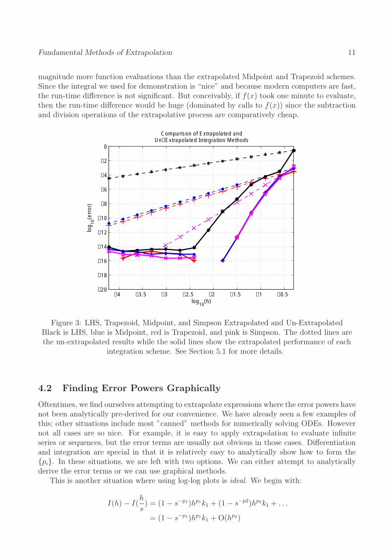
Figure 3 displays the LHS, Trapezoid, Midpoint, and Simpson Rules in their standard forms (dotted lines). If it is not clear, LHS is the black line marked by asterisks, the mid­point/trapezoid rules virtually lie on top of each other, and the pink like marked by Xs is Simpson’s Rule. Once extrapolated (solid lines), Simpson, Midpoint, and Trapezoid are nearly indistinguishable. (Why does this imply that we should never start with Simpson’s Rule when extrapolating?) Even the lowly Left Hand Sum is now performing at a decent level. But clearly, the Midpoint or Trapezoid Rule is the best choice here. The deciding factor between them is typically where we want the function evaluations to occur (i.e. Midpoint avoids the endpoints).

In all cases, the difference between extrapolated and un-extrapolated results is stunning. As we said, extrapolation is the only way to overcome the error bound of 10−8 and achieve high accuracy in differentiation. In integration, using a maximum step-size of only 1 , the

64

Midpoint and Trapezoidal schemes reach a result that is accurate to machine-precision. In the un-extrapolated schemes, we can only achieve this level of accuracy using Simpson’s rule with h = 1 . The un-extrapolated versions of the other three schemes do not even come close to

8196

machine-precision; graphically, it seems that the Midpoint and Trapezoid Rules would need a step-size on the order of 10−6 while we would have to decrease it even further to 10−16 to acommodate LHS.

Even Simpson’s Rule, the best of the un-extrapolated schemes, requires over an order of

11 Fundamental Methods of Extrapolation

magnitude more function evaluations than the extrapolated Midpoint and Trapezoid schemes. Since the integral we used for demonstration is “nice” and because modern computers are fast, the run-time difference is not significant. But conceivably, if f(x) took one minute to evaluate, then the run-time difference would be huge (dominated by calls to f(x)) since the subtraction and division operations of the extrapolative process are comparatively cheap.

Comparison of Extrapolated andUn−Extrapolated Integration Methods

−4 −3.5 −3 −2.5 −2 −1.5 −1 −0.5 −20

−18

−16

−14

−12

−10

−8

−6

−4

−2

0

log 10

(err

or)

log (h)10

Figure 3: LHS, Trapezoid, Midpoint, and Simpson Extrapolated and Un-Extrapolated Black is LHS, blue is Midpoint, red is Trapezoid, and pink is Simpson. The dotted lines are the un-extrapolated results while the solid lines show the extrapolated performance of each

integration scheme. See Section 5.1 for more details.

4.2 Finding Error Powers Graphically

Oftentimes, we find ourselves attempting to extrapolate expressions where the error powers have not been analytically pre-derived for our convenience. We have already seen a few examples of this; other situations include most ”canned” methods for numerically solving ODEs. However not all cases are so nice. For example, it is easy to apply extrapolation to evaluate infinite series or sequences, but the error terms are usually not obvious in those cases. Differentiation and integration are special in that it is relatively easy to analytically show how to form the {pi}. In these situations, we are left with two options. We can either attempt to analytically derive the error terms or we can use graphical methods.

This is another situation where using log-log plots is ideal. We begin with:

h ) = (1 − s −p1 )hp1 k1 + (1 − s −p2)hp2 k1 + . . . I(h) − I(

s = (1 − s −p1 )hp1 k1 + O(hp2 )

( )

12 Liu

From here, we would like to determine p1. We can do this by first assuming that for sufficently small values of h (in practice, on the order of 1 and smaller is sufficient), we can make the

100

approximation O(hp2 ) ≈ 0. Now we apply log10 to both sides; note that we will now drop the subscript p1 and assume that log means log10. So now we have:

h log(I(h) − I( )) = p log(h) + log(1 − s −p) + logk1 (14)

s

−p) 1 (

−p 1 −2p 1 −p + )

At this point, we can taylor expand log(1 − s = ln(10)

−s −2s −

3s . . . . We

have two options. If we believe that the error powers will be integers or ”simple” fractions (e.g. 1 1 1 and similarly simple ones), then we can make the additional approximation log(1−s−p) ≈2,

3,

4

log(1) = 0. As we will see, this series of approximations actually does not really harm our ability to determine p in most situations. The alternative is to retain more terms from the expansion of log(1 − s−p) and solve for p using the differences log(I(h)− I(h)). Proceeding with the first

s

option, we have: h

log(I(h) − I( )) = p log(h) + C (15) s

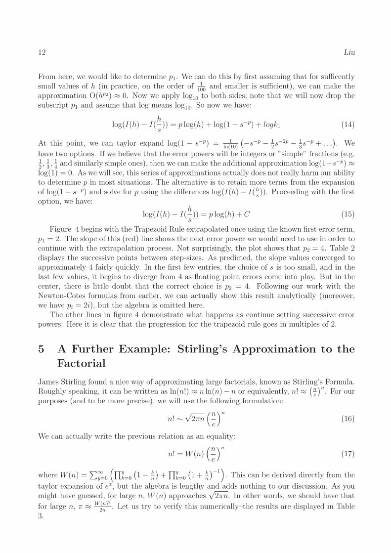
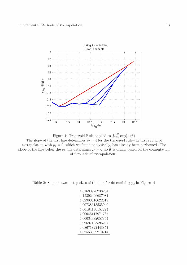
Figure 4 begins with the Trapezoid Rule extrapolated once using the known first error term, p1 = 2. The slope of this (red) line shows the next error power we would need to use in order to continue with the extrapolation process. Not surprisingly, the plot shows that p2 = 4. Table 2 displays the successive points between step-sizes. As predicted, the slope values converged to approximately 4 fairly quickly. In the first few entries, the choice of s is too small, and in the last few values, it begins to diverge from 4 as floating point errors come into play. But in the center, there is little doubt that the correct choice is p2 = 4. Following our work with the Newton-Cotes formulas from earlier, we can actually show this result analytically (moreover, we have pi = 2i), but the algebra is omitted here.

The other lines in figure 4 demonstrate what happens as continue setting successive error powers. Here it is clear that the progression for the trapezoid rule goes in multiples of 2.

5 A Further Example: Stirling’s Approximation to the

Factorial

James Stirling found a nice way of approximating large factorials, known as Stirling’s Formula. Roughly speaking, it can be written as ln(n!) ≈ n ln(n)−n or equivalently, n! ≈

( n )n

. For our e

purposes (and to be more precise), we will use the following formulation: ( )nn

n! ∼√

2πn (16) e

We can actually write the previous relation as an equality: ( )nn

n! = W (n) (17) e

∑

∞ ∏y

( k )

∏y (

k )

−1 where W (n) = y=0 k=0 1 −

n + k=0 1 +

n . This can be derived directly from the

taylor expansion of ex, but the algebra is lengthy and adds nothing to our discussion. As you might have guessed, for large n, W (n) approaches

√2πn. In other words, we should have that

for large n, π ≈ W (n)2

. Let us try to verify this numerically–the results are displayed in Table 2n

3.

13 Fundamental Methods of Extrapolation

log

(diff

(S))

10

Using Slope to Find Error Exponents

0

−2

−4

−6

−8

−10

−12

−14

−16

−18

−20

log (h)−4 −3.5 −3 −2.5 −2 −1.5 −1 −0.5

10

Figure 4: Trapezoid Rule applied to ∫ 1.25

exp(−x2)0.25

The slope of the first line determines p2 = 4 for the trapezoid rule–the first round of extrapolation with p1 = 2, which we found analytically, has already been performed. The

slope of the line below the p2 line determines p3 = 6, so it is drawn based on the computation of 2 rounds of extrapolation.

Table 2: Slope between step-sizes of the line for determining p2 in Figure 4

4.61680926238264 4.12392496687081 4.02980316622319 4.00738318535940 4.00184180151224 4.00045117971785 4.00034982057854 3.99697103596297 4.08671822443851 4.02553509210714

14 Liu

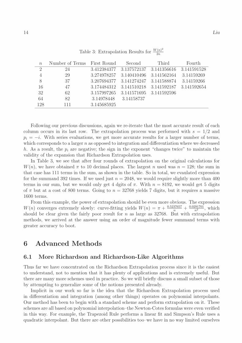
Table 3: Extrapolation Results for W

2(n

n)2

n Number of Terms First Round Second Third Fourth2 24 3.412384377 3.137572137 3.141356616 3.141591528 4 29 3.274978257 3.140410496 3.141562164 3.14159269 8 37 3.207694377 3.141274247 3.141588874 3.14159266 16 47 3.174484312 3.141510218 3.141592187 3.141592654 32 62 3.157997265 3.141571695 3.141592596 64 82 3.14978448 3.14158737 128 111 3.145685925

Following our previous discussions, again we re-iterate that the most accurate result of each column occurs in its last row. The extrapolation process was performed with s = 1/2 and pi = −i. With series evaluations, we get more accurate results for a larger number of terms, which corresponds to a larger n as opposed to integration and differentiation where we decreased h. As a result, the pi are negative; the sign in the exponent “changes twice” to maintain the validity of the expansion that Richardson Extrapolation uses.

In Table 3, we see that after four rounds of extrapolation on the original calculations for W (n), we have obtained π to 10 decimal places. The largest n used was n = 128; the sum in that case has 111 terms in the sum, as shown in the table. So in total, we evaulated expression for the summand 392 times. If we used just n = 2048, we would require slightly more than 400 terms in our sum, but we would only get 4 dgits of π. With n = 8192, we would get 5 digits of π but at a cost of 800 terms. Going to n = 32768 yields 7 digits, but it requires a massive 1600 terms.

From this example, the power of extrapolation should be even more obvious. The expression W (n) converges extremely slowly: curve-fitting yields W (n) = π + 0.5237657 + 0.0291701 , which 2n n

should be clear given the fairly poor result for n as large as 32768. But with extrapolation methods, we arrived at the answer using an order of magnitude fewer summand terms with greater accuracy to boot.

6 Advanced Methods

6.1 More Richardson and Richardson-Like Algorithms

Thus far we have concentrated on the Richardson Extrapolation process since it is the easiest to understand, not to mention that it has plenty of applications and is extremely useful. But there are many more schemes used in practice. So we will briefly discuss a small subset of those by attempting to generalize some of the notions presented already.

Implicit in our work so far is the idea that the Richardson Extrapolation process used in differentiation and integration (among other things) operates on polynomial interpolants. Our method has been to begin with a standard scheme and perform extrapolation on it. These schemes are all based on polynomial interpolation–the Newton-Cotes formulas were even verified in this way. For example, the Trapezoid Rule performs a linear fit and Simpson’s Rule uses a quadratic interpolant. But there are other possibilities too–we have in no way limited ourselves

∑

∑

∑ ∑

Fundamental Methods of Extrapolation 15

to polynomials. Bulirsch and Stoer [7] invented a rather elegant method for using rational functions. Here we begin the process by forming column 0 with rational, instead of polynomial interpolants; these could be found using the Pade Method for example. Then the other entries of the extrapolation table are computed as follows:

(j+1) n−1 n−1I(j) = I + ( I

(j+1) − I(j)

) (18) n n−1 (j+1) (j)hj In−1 −In−1

hj+n (j+1) (j+1) 1 −I −I

− 1 n−1 n−2

We will not derive this expression here; see Bulirsch and Stoer [7] for a very detailed discus­sion. Note that in this variation on the Richardson process, the notion of the step-size (still represented as h) need not be constant.

6.2 The First Generalization of the Richardson Process

The most immediate generalization of the Richardson process2 is to modify our initial assump­tion about the asymptotic expansion of A(h) given in Equation 1. Now instead of the summand being αkh

pk , we will be able to solve problems of the following form:

s

A(h) = A + αkφk(h) + O(φs+1(h)) as h 0+ (19) →k=1

where A(h) and φk(h) are assumed known, while again the values of αk are not required. φk(h) is an asymptotic sequence, so by definition it satisfies φk+1(h) = o(φk(y)) as h 0+. Similar →to the Richardson case we have been working with, if the above expansion holds for every s, then we have that A(h) ∼ A+

∑

∞

k=1 αkφk(h) as h → 0+. To see why our previous analysis is a special case of this generalization, consider the situation where φk(h) = hpk for k = 1, 2, 3, . . .. Again, here we do not make any assumptions or requirements concerning the structure of the φk(h). That is, they are not necessarily related to each other as in the case of the earlier differentiation and integration schemes.

If we have an I(h) as described above and a positive sequence ym on the domain of interest that decreases to 0, then the approximation to A can be written:

n

A(yl) = A(j) + βkφk(yl), for j ≤ l ≤ j + n (20) n

k=1

The set β1, . . . , βn are additional unknowns; the process that generates the An (j)

is called the First Generalization of the Richardson Extrapolation Process. One interesting example of when a function A(h) can arise in practice is given in Sidi [6]: Consider the integral I = ∫ 1

G(x)dx where G(x) = xslog(x)g(x), s has a real part larger than −1, and g(x) is infinitely 0

differentiable. If we write h = 1 , we can approximate I using the Trapezoid Rule: I(h) = ( ) n∑n−1 G(1) h j=1 G(jh) +

2 . Sidi [6] gives the (nontrivial) asymptotic expansion of I(h) as:

∞ ∞

I(h) ∼ I + aih2i + bih

s+i+1ρi(h) as h 0+ (21) →i=1 i=0

2Here our purpose is to survey the ideas of the First Generalization and then the E Algorithm, making note of concepts beyond the Richardson Method. We will skip over many of the details for brevity (i.e. stating rather than proving results), but more information can be found in the references.

{

16 Liu

where ρi(h) = ζ(−s − i)log(h) − ζ ′(−s − i). There are also analytic expressions for ai and bi, but since these correspond to the αk coefficients, their values are not of particular importance. From here we see that the φk(h) are known:

hs+i+1 if i = ⌊

2k ⌋ ,k = 1, 2, 4, 5, 7, 8, . . .

φk(h) = 3 (22) 2k h 3 if k = 3, 6, 9, . . .

6.3 The E Algorithm

The solution of the system in the First Generalization is the An (j)

which can be written as follows, using Cramer’s Rule:

A(nj) =

Γn (

(

j

j

)

)

(a) (23)

Γn (1)

For convenience, we have defined a(m) = A(ym), gk(m) = φ(ym), and Γ(a)n (j)

as the de­terminant of a matrix of n + 1 rows and n + 1 columns where the ith row looks like [g1(j + i − 1) g2(j + i − 1) gn(j + i − 1) a(j + i − 1)]. · · ·

(j)

Now define χ(j)

= Γp (b)

such that χ(j)

= A(j)

and we will also p (b) Γp

(j)(1)

p (a) p ,

need to let G(pj)

be the determinant of a p by p matrix with ith row given by

[g1(j + i − 1) g2(j + i − 1) gn(j + i − 1)] for p ≥ 1 and G(j)

= 1. Then we can use the · · · 0

Sylvester Determinant Identity to relate Γ and G:

Γ(j) (j+1) (j+1) p(j−

)1(b)G

(j+1) p (b)Gp−1 = Γp−1 (b)Gp

(j) − Γ p

Γ(j)

(b)G(j+1)

Then beginning from χp (j)

(b) = p p−1 and applying our relation of Γ and G, we arrive at (j) (j+1)

Γp (1)Gp−1

the final result of the E-Algorithm:

(j+1) (j) (j) (j+1)

χ(j)(b) = χp−1 (b)χp−1(gp) − χp−1(b)χp−1 (gp)

, (24) p (j) (j+1) χp−1(gp) − χp−1 (gp)

where b = a and b = gk for k = p + 1, p + 2, . . .. The intitial conditions are that χ0(j)

(b) = b(j). (j) χ

(j+1) (gp)

Note that we can save a considerable amount of computational work by setting wp = p

(−

j)1 :

χp−1(gp)

χ(j+1)

w(j)

χ(j)

χ(pj)(b) =

p−1 (b) − p

(j)

p−1(b) (25)

wp1 −

This forms the basis of the E Algorithm. Note that what we have presented here does not actually have much practical application. The E Algorithm solves systems of the form A(yl) =

An (j)

+ ∑n

k=1 βkφk(yl). By itself it is not an extrapolative scheme; we have to first create some conditions to specify the gk(m). Picking the gk(m) in a useful manner is by no means an easy task and there is ongoing research in that area. But given the generality of the E Algorithm, many extrapolative schemes are based on it.

∑ ∑

∑ ∑

Fundamental Methods of Extrapolation 17

7 Conclusion

Extrapolation allows us to achieve greater precision with fewer function evaluations than un­extrapolated methods. In some cases (as we saw with simple difference schemes), extrapolation is the only way to improve numeric behavior using the same algorithm (i.e. without switching to centered differences or something better). Using sets of poor estimates with small step-sizes, we can easily and quickly eliminate error modes, reaching results that would be otherwise unobtainable without significantly smaller step-sizes and function evaluations. Thus we turn relatively poor numeric schemes like the Trapezoid Rule into excellent performers. The material presented here is certainly not the limit of extrapolation methods as we attempted to show in the last section. Still as our examples demonstrate, the Richardson Extrapolation Process that we emphasized is more than sufficient for many applications including evaluating integrals, derivatives, infinite sums, infinite sequences, function approximations at a point (e.g. evaluating π or γ), and more.

7.1 Extrapolation: An Unsolved Problem

According to [1], it has been proven (by Delahaye and Germain-Bonne) that there cannot exist a general extrapolative scheme that works for all sequences. The concept of a working extrapolation scheme can be re-stated in the following way: if we apply an extrapolation method to a sequence Sn (for example, Si = trap(h/si)), the resulting sequence En must converge faster

En−Sthan Sn, meaning that limn→∞ Sn−S = 0. Thus the application of extrapolation for cases more

difficult than the fundamental examples presented here quite difficult, because for any given situation, we must first determine which scheme is best-suited for the problem. The metric for “best-suited” is not necessarily obvious either: it could be ease of implementation, number of function evaluations required, numeric stability, or others. Delahaye’s negative result also means that each new extrapolative scheme is interesting in its own right, since it has the potential to solve a wider class of problems which no other method can attack.

7.2 From Trapezoid to Simpson with Extrapolation

On a closing note, we will now quickly outline how Romberg extrapolation can be used to easily derive Simpson’s rule from the Trapezoid rule. More generally, extrapolating the n = i Closed Newton-Cotes Formula results in the n = i + 1 version. By now, this should not be all that surprising, but without knowledge of extrapolation, this relation between the ith and i + 1th formulas is not obvious at all. We start with s = 2 and p = 2; the choice of p is based on the error term from the Closed Newton-Cotes Formula. Alternatively, it could have been determined graphically, as shown earlier.

4trap(h) − trap(h)= Simp(

h2 )22 2− 1

( ) ( ) n−1 n−1

h h =

3 f(a) + 2 f(xj) + f(b) −

6 f(a) + 2 f(xj) + f(b)

j=1 j=1

n −1 n

h 2 2

= f(a) + 2 f(xj) + 4 f(xj) + f(b) 3

j=1 j=1

∑ ∑

18 Liu

Thus Simpson’s Rule is:

∫ n

−1 n b 2 2h

Simpson’s Rule: f(x) dx = f(a) + 2 f(xj) + 4 f(xj) + f(b) + O(h4) (26) 3a j=1 j=1

Lastly, to further reinforce the notion of how these processes are all tied together, if we instead choose s = 3 (while keeping the same choice of pn), we will arrive at Simpson’s 3

8ths Rule.

References

[1] Brezinski, Claude and Michela R. Zaglia, Extrapolation Methods: Theory and Practice, North-Holland. Amsterdam, 1991.

[2] Burden, R. and D. Faires, Numerical Analysis 8TH Ed, Thomson, 2005.

[3] Deuflhard, Peter and Andreas Hohmann. Numerical Analysis in Modern Scientific Com­puting, Springer. New York, 2003.

[4] Issacson, E. and H. B. Keller. Analysis of Numerical Methods, John Wiley and Sons. New York, 1966.

[5] Press, et. al. Numerical Recipes in C: The Art of Scientific Computing, Cambridge Uni­versity Press, 1992.

[6] Sidi, Avram, Practical Extrapolation Methods, Cambridge University Press, 2003.

[7] Stoer, J. and R. Burlirsch, Introduction to Numerical Analysis, Springer-Verlag, 1980.

[8] Sujit, Kirpekar, Implementation of the Burlirsch Stoer Extrapolation Method, U. Berkeley, 2003.