fundamental studies of biomass fluidization
TRANSCRIPT

Fundamental Studies of Biomass Fluidization
by
Gbenga Olatunde
A dissertation submitted to the Biosystems Engineering of Auburn University
in partial fulfillment of the requirements for the Degree of
Doctor of Philosophy
Auburn, Alabama December 12, 2015
Keyword: Biomass, loblolly pine, fluidization, particle size, particle shape, modeling
Copyright 2015 by Gbenga Olatunde
Approved by
Oladiran Fasina, Chair, Professor of Biosystems Engineering Sushil Adhikari, Associate Professor of Biosystems Engineering
Timothy McDonald, Associate Professor of Biosystems Engineering Steve Duke, Associate Professor of Chemical Engineering

Abstract
The world is presently at a point of making important decisions regarding how to minimize
disasters such as super storm, super earthquakes, and landslides that are caused by global
warming due to fossil fuel exploration and consumption. One route is to use varieties of
renewable energy resources such as solar, wind, biomass etc. to replace some of the fossil fuels
consumed. Biomass such as wood, energy plants (switchgrass, poplar, and willow) is the only
renewable energy that can be converted into liquid fuel. However, in the process of converting
biomass to fuel, there are numerous technical challenges that are encountered primarily due to
assumptions made in measuring values of physical properties of biomass grinds (e.g. size,
particle geometry, and voidage). These properties are utilized in the design and sizing of biomass
conversion and processing equipment and facilities. For example, the use of average (mean)
particle diameter in fluidization models and equation seems to imply that biomass ground
particles are uniformly sized, thus neglecting the size distribution of biomass. In addition, as
non-spherical particles, the use of a mean diameter is problematic because axis of measurement
significantly influences the value of diameter. Some mean diameter that can be obtained from
non-spherical particle include, the diameter of a sphere that has the same surface area to volume
ratio as a particle, Martins, Ferret and Sauter mean diameter. At present comprehensive
investigation on contribution of physical properties vis-a-vis particle size measurement scheme
on predictability of loblolly pine wood grind minimum fluidization velocity and other parameters
that are used in designing fluidized bed system is lacking in literature. Hence, this study
ii

investigated how the physical properties of loblolly pine wood influence the ability to predict
important design parameters and the behavior of biomass grinds during fluidization.
The result showed that loblolly pine wood grinds have mean particle density of 1460.6±7 kg/m3,
bulk density of 311± 37 kg/m3 and porosity of 0.787 ± 0.003. With regards to particle size, the
Ferret diameter was found to be higher than surface-volume diameter, Martin’s diameter and
chord diameter by 18.3, 23.6, and 7.03% respectively. Also, the shape characteristic based on the
sphericity value of biomass grinds ranges between 0.235 and 0.603, thus indicating that biomass
grinds have flat shape. The minimum fluidization velocity of ground loblolly pine wood
(unfractionated samples) was found to be 0.25 ±0.04 m/s. For fractionated samples, the
minimum fluidization velocity increased from 0.29 to 0.81 m/s as fractionating screen size
increased from 0.15 to 1.70 mm. Predictions of minimum fluidization velocity obtained from
selected equations were significantly different from the measured values. Moreover, increase in
moisture content increased the bulk density, particle density, and porosity but the particle size
coefficient of variation reduced from 90 at 8.46% MC to 42 at 27.02 % MC. Increase in moisture
content also increased the minimum fluidization velocity of unfractionated grinds from 0.20 to
0.32 m/s as moisture was increased from 8.45 to 27.02 % wet basis respectively. In addition, the
correlation developed predicted the experimental data for minimum fluidization velocity with
mean deviation less than 10%. For the modified Ergun equation, the coefficients K1 and K2 were
estimated to be 201 and 2.7 respectively. The overall mean relative deviation obtained between
the predicted and experimental pressure drop using loblolly pine wood grind and the equation
iii

developed in this study and the Ergun equation were -17.48 and 63.5 % respectively. Finally, an
evaluation of the interface exchange drag law equations (Gidaspow, Syamlal-Obrien, Wen & Yu
and non-spherical) showed that non-spherical drag law equation predicted the minimum
fluidization velocity with mean relative deviation of 4.5%. It was also observed that bed
entrainment occurred for all the drag law equation at 2 sec simulation time. The drag law
equations under-predicted the bed pressure drop, and mass entrainment above 0.2 m/s superficial
airflow velocity after bed material entrainment has begun. The incorporation of body force
improved the predictability of the non-spherical drag law equation but exhibited little impact on
the other drag law equations. Finally, this study has demonstrated the possibility of improving
prediction of important parameters of fluidize bed system when particles with non-uniform and
irregular geometry is used.
iv

Acknowledgments
First and foremost, I want to express my sincere thanks to God Almighty, the giver of life and
knowledge, for being with me from the start to the completion of this Ph.D. Degree program.
My sincere gratitude goes to my advisor, Dr. Oladiran Fasina for his unparalleled and relentless,
patience, advice, support, and timely guidance throughout the course of this work. I remembered
the first time I email you about the PhD position in your group; I told you that I would like to be
modeled after your research philosophy and style. These qualities which you have impacted in
me over the course of this program shall continue to grow with me until I become a researcher
and scientist of my desire.
I would also like to appreciate all my committee members, Dr. Sushil Adhikari, Dr. Timothy
McDonald, and Dr. Steve Duke. Their insightful comments, questions, and discussion have
significantly helped in increasing my curiosity level.
I want to use this medium to thank Christian Brodbeck, Jonathan, Jame Johnson, Boby Eplin,
Dawayne Flynn for their support during the laboratory work. They provided me with the material
and resource needed to carry out the test and their super quick response to assist was unique. Let
me say an heartfelt thank you to Sharon price, James Clark, Christopher Olds, for their help
during the time I was learning how to use HPCC for my simulation. Your assistance really made
a whole chapter of this work possible. Please accept my heart felt thank you.
v

I will also like to acknowledge my fellow graduate students who have significantly contributed
to my event-full years. I am deeply touched by your encouragement, support, and love. I can’t
but remember Anshu, Gurdeep, Jas, Omotolani, Tosin, Femi, Ujaain, Thomas, Dr.
Abdoulmoumine, Ewurama, Charles, Yusuf, Aurelie, Narendra, Bangpin.
Let me appreciate some of my family members for their support, encouragement and even
visitation to my humbly abode during this energy sapping degree: My father, Pastor Aderemi
Augustus Olatunde, Samuel Olatunde, Kolade Olatunde and Folashade Olatunde. My mother in-
law- Mrs. Ayoola, Prof. and Mrs Adeyemo. Dn. Dokun Olatunde, Mr. and Mrs Bamidele Falola,
Mr. Dehinde Olatunde, Pastor and Mrs. Adelekan, Mr. and Mrs. Idowu, Mrs. Oladunmoye,
Pastor and Mrs. Adedeji and Mr. and Mrs. Ajani. I will like to appreciate my families in Auburn-
Mrs Popoola, Dr. Yewande Fasina, Dr. & Mrs Shodeke. I appreciate their supports, constant
visits, and words of encouragements. Thank you and God bless you all.
I also want to appreciate the faculty staff of the department of Agricultural Engineering, Obafemi
Awolowo University, Ile-Ife. Especially Prof. O.K Owolarafe and Dr. B.S. Ogunsina, who
frequently called me and offer invaluable suggestions and advice on my work. Their words of
encouragement and support was noted and appreciated.
Finally, to my wife, Adesola and my son, Oreofe, I am moved by your priceless sacrifices,
sleepless nights, and support: spiritual and moral. I want to say you are indeed special to me and
everything you did contributed immensely to the successful completion of this work.
vi

Table of Contents
Abstract ........................................................................................................................................... ii Acknowledgments........................................................................................................................... v
Table of Contents .......................................................................................................................... vii List of Tables ................................................................................................................................ xii List of Figures ............................................................................................................................... xv
Chapter 1: Introduction .................................................................................................................. 1
1.1 Fossil fuel consumption and impact ............................................................................ 1
1.2 Research problem ........................................................................................................ 3
1.3 Hypothesis and objective ............................................................................................. 4
1.4 Organization of dissertation ........................................................................................ 5
1.5 References ................................................................................................................... 6
Chapter 2: Literature review ......................................................................................................... 9
2.1 Biomass resources ....................................................................................................... 9
2.2 Biomass conversion process ...................................................................................... 12
2.3 Introduction to fluidized bed system ......................................................................... 18
2.4 Advantages and disadvantages of fluidized bed ........................................................ 20
2.5 Fluidization phenomena and regimes ........................................................................ 20
2.6 Determination of minimum fluidization velocity (Umf) ............................................ 22
2.7 Problem with determination of minimum fluidization velocity of biomass grinds .. 23
2.8 Biomass material properties that influence its fluidization ....................................... 25
2.8.1 Particle size distribution ............................................................................................ 29
2.8.2 Particle size distribution measurement ...................................................................... 32
2.8.2.1 Particle size measurement using sieve analysis ............................................... 32 2.8.2.2 Particle size measurement using image analysis ............................................. 35
2.8.3 Particle shape factor .................................................................................................. 39
2.8.4 Density of biomass grinds ......................................................................................... 42
2.8.4.1 Bulk density ..................................................................................................... 42 2.8.4.2 Particle density ................................................................................................ 43
2.8.5 Moisture content ........................................................................................................ 45
vii

2.9 Fluidization models/ predicting equations ................................................................ 48
2.9.1 Pressure drop approach ............................................................................................. 48
2.9.2 Empirical model approach ......................................................................................... 50
2.9.3 Computational Fluid Dynamics approach ................................................................. 52
2.10 Summary ................................................................................................................... 59
2.11 References ................................................................................................................. 61
Chapter 3: Effect of Size on Physical Properties and Fluidization Behavior of Loblolly Pine Grinds ............................................................................................................................................ 75
3.1 Abstract ..................................................................................................................... 75
3.2 Introduction ............................................................................................................... 76
3.3 Material and Methods ................................................................................................ 82
3.3.1 Sample preparation .................................................................................................... 82
3.3.2 Particle size analysis .................................................................................................. 84
3.3.2.1 Whole sample (unfractionated sample A) ....................................................... 84 3.3.2.2 Fractionated sample (sample B) ...................................................................... 84
3.3.3 Particle size ................................................................................................................ 85
3.3.4 Particle density .......................................................................................................... 86
3.3.5 Bulk density ............................................................................................................... 86
3.3.6 Porosity ...................................................................................................................... 86
3.3.7 Fluidized bed system and fluidization test ................................................................ 87
3.3.8 Statistical analysis ..................................................................................................... 89
3.4 Result and Discussion ............................................................................................... 90
3.4.1 Physical properties of ground loblolly pine wood (Sample A and B) ....................... 90
3.4.1.1 Particle size ...................................................................................................... 90 3.4.1.2 Bulk, particle density and porosity .................................................................. 92 3.4.1.3 Particle shape ................................................................................................... 95
3.4.2 Geldart’s classification .............................................................................................. 95
3.4.3 Fluidization behavior of ground loblolly pine wood ................................................. 96
3.4.3.1 Validation of fluidization system .................................................................... 96 3.4.3.2 Fluidization behavior of unfractionated biomass grinds (Sample A) .............. 97 3.4.3.3 Fluidization behavior of fractionated biomass grinds (Sample B) .................. 99 3.4.3.4 Experimental determination of minimum fluidization velocity of samples A and B 101
viii

3.4.4 Effect of diameter measurement scheme on predicted values ................................ 106
3.4.5 Comparison between predicted and experimental values ....................................... 107
3.5 Conclusion ............................................................................................................... 111
3.6 Reference ................................................................................................................. 113
Chapter 4: Moisture Effect on Fluidization Behavior of Loblolly Pine Wood Grinds ............... 117
4.1 Abstract ................................................................................................................... 117
4.2 Introduction ............................................................................................................. 118
4.3 Material and methods .............................................................................................. 121
4.3.1 Material preparation ................................................................................................ 121
4.3.2 Particle size fractionation ........................................................................................ 122
4.3.3 Particle size measurement ....................................................................................... 123
4.3.4 Bulk density ............................................................................................................. 125
4.3.5 Particle density and porosity ................................................................................... 125
4.3.6 Fluidization test ....................................................................................................... 126
4.3.6.1 Experimental device ...................................................................................... 126 4.3.6.2 Fluidization test procedure ............................................................................ 126
4.3.7 Statistical analysis ................................................................................................... 126
4.4 Results and discussion ............................................................................................. 127
4.4.1 Particle size .............................................................................................................. 127
4.4.1.1 Effect of moisture content on the coefficient of variation of unfractionated (sample A) ....................................................................................................................... 127 4.4.1.2 Effect of measurement scheme on measured size ......................................... 128 4.4.1.3 Effect of moisture content on particle shape of loblolly pine wood grinds ... 134
4.4.2 Bulk and particle density ......................................................................................... 135
4.4.3 Fluidization studies .................................................................................................. 139
4.4.3.1 Minimum fluidization velocity ...................................................................... 139 4.4.3.2 Fluidization behavior of loblolly pine wood grinds ...................................... 142 4.4.3.3 Correlation of minimum fluidization velocity ............................................... 146 4.4.3.4 Verification of the Umf correlation. ............................................................... 149
4.5 Conclusion ............................................................................................................... 151
4.6 Reference ................................................................................................................. 152
Chapter 5: Air Flow through Packed Columns of Ground Loblolly Pine Wood: Revised Ergun Expression ................................................................................................................................... 156
ix

5.1 Abstract ................................................................................................................... 156
5.2 Introduction ............................................................................................................. 157
5.3 Methodology ........................................................................................................... 161
5.3.1 Material preparation ................................................................................................ 161
5.3.2 Particle size .............................................................................................................. 162
5.3.3 Particle density ........................................................................................................ 163
5.3.4 Bulk density ............................................................................................................. 163
5.3.5 Porosity .................................................................................................................... 163
5.3.6 Pressure drop and flow rate measurement test ........................................................ 163
5.3.7 Void fraction correlation modification: concept ..................................................... 164
5.3.8 Data analysis ............................................................................................................ 165
5.4 Experimental result and model derivation ............................................................... 166
5.4.1 Particle size and coefficient of variation ................................................................. 166
5.4.2 Bulk and particle densities ...................................................................................... 167
5.4.3 Porosity and sphericity ............................................................................................ 168
5.4.4 Pressure drop and flow rate measurement test ........................................................ 168
5.4.5 Void fraction correlation development: Ergun’s correlation .................................. 170
5.4.6 Modification of void fraction correlation ................................................................ 172
5.4.7 Model presentation .................................................................................................. 173
5.5 Model validation ...................................................................................................... 179
5.5.1 Performance of equation by experimental pressure drop data ................................ 179
5.5.2 Performance of equation for determination of minimum fluidization velocity ...... 184
5.5.3 Conclusion ............................................................................................................... 186
5.6 Reference ................................................................................................................. 186
Chapter 6: CFD modeling of ground Loblolly Pine Wood fluidization .................................... 191
6.1 Abstract ................................................................................................................... 191
6.2 Introduction ............................................................................................................. 193
6.3 Simulation steps and procedure ............................................................................... 199
6.3.1 Simulation condition ............................................................................................... 199
6.3.2 Particle size determination and particle injection file ............................................. 201
x

6.3.3 Governing equations and mathematical model ....................................................... 203
6.3.4 Formulation of body force correlation .................................................................... 205
6.3.5 Boundary and initial condition ................................................................................ 206
6.3.6 Solver related details ............................................................................................... 207
6.3.7 User defined function implementations .................................................................. 207
6.4 Result and discussion .............................................................................................. 208
6.4.1 Mesh convergence/ independent study .................................................................... 208
6.4.2 Effect of drag model on transient bed voidage profile ............................................ 212
6.4.3 Effect of drag model on pressure drop profile ........................................................ 219
6.4.4 Comparison of CFD simulation and experimental result ........................................ 221
6.4.5 Prediction of minimum fluidization velocity .......................................................... 223
6.4.6 Effect of void body force application on pressure drop profile .............................. 227
6.4.7 Prediction of minimum fluidization velocity .......................................................... 230
6.5 Conclusion ............................................................................................................... 231
6.6 Reference ................................................................................................................. 232
Chapter 7: Conclusion and Recommendation ............................................................................ 236
7.1 Conclusions ............................................................................................................. 236
7.2 Original contributions .............................................................................................. 238
7.3 Future work and recommendation ........................................................................... 239
7.3.1 Determining the hydrodynamics of the biomass under real hot condition .............. 239
7.3.2 Determining the effect of bed distributor to velocity distribution and pressure drop 239
7.3.3 Effect of bed width on fluidization .......................................................................... 239
7.3.4 Estimating the void fraction of ground biomass ..................................................... 240
Appendix 1: Additional data for Chapter 1................................................................................. 241
Appendix 2: Additional data for Chapter 3................................................................................. 243
Appendix 3: Additional data for Chapter 4................................................................................. 252
Appendix 4: Additional data for Chapter 6................................................................................. 261
Appendix 5: Additional data for Chapter 7................................................................................. 265
xi

List of Tables
Table 2.1: Different types of direct combustion system under thermal conversion method …....14
Table 2.2: Typical operating parameters for pyrolysis process ………………………………..16
Table 2.3: Selected work on solid-gas fluidization ………………………………………...……28
Table 2.4: Diameter type from sieve analysis and their field of application……………….……34
Table 2.5: Definition of the diameter types from image analysis software…………………..….37
Table 2.6 : Advantages and limitation of particle sizing instrument. …………………..……..…39
Table 2.7: Various forms of correlations for predicting Umf ……………………………………51
Table 2.8: Product yields (wt.%) of a type of red oak pyrolysis from experiment and simulation. ………………….……………………………………………………………………..55
Table 2.9: Some selected work that used Eulerian – Lagrangian with DDPM model ………….58
Table 3.1: Properties of powders in Geldart’s classification. …………………………………...80
Table 3.2: Schematic representation of size measuring scheme for non-spherical particle ..……………………………...………………………………………………………..81
Table 3.3: Sample preparation, groupings and identification based on sieve class. ……….……84
Table 3.4: Effect of measurement method on diameter of fractionated and unfractionated loblolly ground wood………… ………………………………………………………….……92
Table 3.5: Physical properties of unfractionated and fractionated loblolly pine wood………….94
Table 3.6: Geldart’s classification of un-fractionated and fractionated loblolly pine wood grinds as affected by diameter measurement schemes….........................................................96
Table 3.7: Experimentally determined minimum fluidization velocities of ground loblolly pine wood fractions …………………..…………………………………….…………….104
xii

Table 3.8: Selected fluidization equation used for predicting the experimental Umf of ground wood. ………………………………………………………………………………..105
Table 3.9: Effect of size measurement method and popular fluidization equation on predicted minimum fluidization velocity. …………………………..…………………………107
Table 3.10: Statistical evaluation of the effect of dameter type on predictive ability of different models of unfractionated sample. ……..…………………………………………….110
Table 4.1: Moisture content of loblolly pine wood grinds after fractionation………………….122
Table 4.2: Properties of particles extracted from the software of the Camsizer………………..124
Table 4.3: Effect of moisture content and diameter measurement scheme on the measured size of loblolly pine wood grinds. ………………………………………………………..…132
Table 4.4: Effect of moisture on geometric mean size of ground loblolly pine wood grinds.…133
Table 4.5: Effect of moisture on sphericity of loblolly pine wood grinds at different moisture content……………………………………………………………………………….134
Table 4.6: Effect of moisture on aspect ratio of loblolly pine wood grinds at different moisture content…………………………………………………………………………….....136
Table 4.7: Effect of moisture content on bulk densities ground loblolly pine wood (unfractionated and fractionated).……………………………………..……….…....137
Table 4.8: Effect of moisture content on particle densities ground loblolly pine wood (unfractionated and fractionated).……………………………………..………….....138
Table 4.9: Porosity of loblolly pine wood grinds at different moisture content level for both unfractionated and fractionated sample ………………………………………..……139
Table 4.10: Minimum fluidization velocity of fractionated loblolly pine wood as affected by moisture content. …………………………………………………………….…….142
Table 4.11: Particle characterization based on the coefficient of variation (COV) at the various moisture content levels…………………………………….……………………..… 147
Table 4.12: Effect of moisture contents and diameter measurement schemes on mean size of unfractionated loblolly pine wood grinds ………………………………………..….148
Table 4.13: Coefficient estimation at various diameter types……………………………….… 149
xiii

Table 4.14: Predicting and validating the Umf using Eqn. 4.4………………………………..…150
Table 5.1: Physical properties of loblolly pine wood grinds ground through different screen sized …………………………………………………………………………………….....167
Table 5.2: Estimation of slope and intercept parameters for loblolly pine wood at different particle sizes. ………………………………………………….…………….………170
Table 5.3: Comparison of K1 and K2 values with literature data……………………………… 178
Table 5.4: Physical properties of loblolly pine wood grind used for validation ………….……180
Table 5.5: Comparison of the overall relative mean deviation between predicted and the experimental data ……………………………………….………………………..…184
Table 5.6: Comparison of Eqn. 5.2, 5.24 and 5.27 for predicting the Umf …………………….185
Table 6.1: Discrete event collision setting parameter ………………………………………… 201
Table 6.2: Distribution characteristics of injected particle obtained from FLUENT® ………..202
Table 6.3: Governing equations and constitutive law of Eulerian Lagrangian, DDPM model for gas-solid flow ………………………………………………………………...……..205
Table 6.4: Meshing method and sizes obtained for mesh independent study ………………….209
Table 6.5: Mean relative deviation between predicted pressure drop using different drag equation and experimental data………………………………………………………………. 222
Table 6.7: Mean relative deviation between experimental and predicted pressure drop at different velocity and drag models. …………………………………………………………...228
xiv

List of Figures
Figure 2.1: Biomass resources and sources. ………………………………………….…………10
Figure 2.2: Pine tree at early stage of life (a) and established plantation (b) …………..………..12
Figure 2.3: Flow chart for biomass conversion to energy paths ……………………………...…13
Figure 2.4: Two different types of fixed bed reactors showing direction of flow of air and biomass into the bed……………….………………………………………..………..17
Figure 2.5: Schematics of a typical fluidized bed..…………………………………………….. .19
Figure 2.6: Different stages of gas –solid flow of a spherical uniform particle size. ………….. 21
Figure 2.7: Various experimental methods to determine minimum fluidization velocity. …….. 23
Figure 2.8: Geldart’s classification ………………………………………………………...……24
Figure 2.9: Particle size distribution for peanut hull grind …………………………...…………30
Figure 2.10: Comparisons between measures of central tendency……………………… ……...31
Figure 2.11: An elongated particle passing through a square sieve aperture. ………………..…33
Figure 2:12: Particle size distribution from image analysis using different diameter type ……..38
Figure 2:13: Comparison of the syngas composition in the case of dry and wet biomass gasification …………………………………………………………………………..46
Figure 3.1: Hammer mill used for size reduction process. ………………………….…………..82
Figure 3.2. Sieve shaker used for fractionating the samples. ………………………..………..…83
Figure 3.3: Schematic diagram of the system used for fluidization. ……………………………87
Figure 3.4: Particle size distribution of fractionated and unfractionated ground loblolly pine wood. ….......................................................................................................................90
Figure 3.5: Plot of pressure drop versus air velocity for sand particles. ……………………….. 97
Figure 3.6: Channeling during fluidization of ground biomass (unfractionated, sample A) impeded fluidization processes…………………………………………. …………..98
xv

Figure 3.7: Plugged flow during fluidization of ground biomass (unfractionated, sample A) because of particle interlocking...................................................................................98
Figure 3.8: Typical channeling behavior observed for B1, B2 and B3 samples during fluidization processes (the snapshot was that of B1 sample)..……………............……………..100
Figure 3.9: Typical channeling behavior observed for B4, B5 and B6 samples during fluidization processes (the snapshot was that of B5 sample)…………………………….……..100
Figure 3.10: Typical behavior of loblolly pine wood grinds during fluidization………………102
Figure 3.11: Variation in pressure drop with superficial gas velocity for unfractionated sample and Sample B (fractionated sample)……………………………….……………….103
Figure 4.1: Differences in size distributions obtained from using different diameter measurement schemes for loblolly pine wood grinds (8.40% MC wet basis). ………….……….129
Figure 4.2: Differences in size distributions obtained from using different diameter measurement schemes for loblolly pine wood grinds (14.86% MC wet basis)…………...………130
Figure 4.3: Differences in size distributions obtained from using different diameter measurement schemes for loblolly pine wood grinds (19.80% MC wet basis) …..………………130
Figure 4.4: Differences in size distributions obtained from using different diameter measurement schemes for loblolly pine wood grinds (27.02 % MC wet basis)……………….… 131
Figure 4.5: Pressure drop against superficial gas velocity for control sample at 8.40 % MC……………………………………………………………..…………………...140
Figure 4.6: Effect of moisture content on fluidization velocity of loblolly pine wood grinds. ………………………………………………………………………………...…….141
Figure 4.7: Fluidization behavior of 200g loblolly pine wood (8.46 %MC) with increasing gas…………………………………………………………………………….….....143
Fig 4.8: Fluidization behavior of 200g loblolly pine wood (19.8 %MC) with increasing gas velocity……………………………………………………………………...………144
Figure 4.9: Effect of particle size by fractionation method at different moisture content on fluidization of bed ………………………………………………………………….145
Fig 4.10: Schematic of fluidization behavior of ground loblolly pine wood grinds based on sequence of event ……………………………………………………………...…..146
xvi

Figure 4.11. Determination of the Umf correlation for whole sample of loblolly pine wood grinds ………………………………………………………………….……….…………..149
Figure 5.1: Particle size distribution for loblolly pine wood grinds obtained from hammer mill at different screen sizes. ………………………………………………………………166
Figure 5.2: Linear form of pressure–drop equation (Eqn.5.1 ) using loblolly pine wood grinds having different size and void fractions. ……………………………….………… 169
Figure 5.3: Dependence of viscous energy losses on fractional void volume correlation used in Ergun’s equation……………………………………………………………….…. 171
Figure 5.4: Dependence of kinetic energy losses on fractional void volume correlation used in Ergun’s equation ………………………………………………………………..…171
Figure 5.5: Dependence of kinetic energy losses on modified fractional void volume correlation used in Ergun’s equation (Eqn. 5.2)………………………………………………...172
Figure 5.6: A general plot for a single system having different void fraction using Ergun’s concept using chord diameter scheme…………………………………...…………176
Figure 5.7: A general plot for a single system having different void fraction using chord diameter scheme……………………………………………………………..………………..177
Figure 5.8: Pressure drop versus superficial velocity for loblolly pine wood grind……………181
Figure 5.9: Performance comparison of Eqn. 5.1, 5.24, and experimental pressure drop data using ground loblolly pine wood ground through 5/8 inches screen size. Particle size 2.28× 10⁻³m, coefficient of variation of 0.65, sphericity factor of 0.45, and porosity of 0.81 …………………………...…………………………………………..…...……181
Figure 5.10: Performance comparison of Eqn. 5.1, 5.24 and experimental pressure drop data using equations with ground loblolly pine wood ground through 1/4 inches screen size. Particle size 1.4× 10⁻³m, coefficient of variation of 0.73, sphericity factor of 0.47, and porosity of 0.81 …... ………………………………………………..….. 182
Figure 5.11: Performance comparison of Eqn. 5.1, 5.24, and experimental pressure drop data using ground loblolly pine wood ground through 1/2 inches screen size. Particle size 0.76 × 10⁻³ m, coefficient of variation of 0.60, sphericity factor of 0.46, and porosity of 0.80………………………..…………………………………………………..…182
Figure 6.1: Effect of particle size distribution on solid velocity measurement…………….…. 195
xvii

Figure 6.2: Schematic diagram of the fluidized bed and 3-D mesh (Cells (33728), Faces (103608), and Nodes (36305)) used for simulation. ………………………..…..….200
Figure 6.3: Particle size analysis and cumulative distribution plot of ground loblolly pine wood. ………………………………………………………………………………...…….202
Figure 6.4: Effect of using different mesh sizes on pressure drop across the bed with simulation time ……………………………………………………………………………..…210
Figure 6.5: Effect of using different mesh sizes on bed voidage with simulation time ……..…210
Figure 6.6: Flowchart showing scheme used for solving equations for multi-phase CFD model ……………………………………………………………………..….…………….212
Figure 6.7: Transient bed voidage profiles for velocities in the range of 0.08 -1.2 m/s for different drag law……………………………………………………….…………..213
Figure 6.8: Snapshots of transient solid volume fraction contours of the fluidized bed at 2.0 m/s ………………………………………………………………………………………215
Figure 6.9: Contour plot of volume fraction of solid on z-coordinate at 0.0, 0.01, 0.04, 0.10, and 0.15 mm at 0.2 m/s air velocity …………………………………………...………. 218
Figure 6.10: Evolution of pressure with simulation time at different velocity using Gidaspow drag law…………………………………………………………………….……….220
Figure 6.11: Determination of Umf using the plot of pressure drop against the airflow velocity ………………………………………………………………………………….….. 221
Figure 6.12: Comparison of predicted and experimental bed material entrainment as velocity increased………………………………………………………………...………….223
Figure 6.13: Pressure drop against velocity for determination of minimum fluidization velocity. ………………………………………………………………………………………224
Figure 6. 14: Particle traces colored by particle velocity magnitude using non-spherical drag law at 0.2 m/s ……………………………………………………………………...……225
Figure 6.15 Particle traces colored by particle velocity magnitude using non-spherical drag law at 0.4 m/s………………………………………………………………………………226
Figure 6.16: Pressure drop obtained at different velocities after application of body force correlation………………………………………………………………. …………227
xviii

Figure 6.17: Comparison of pressure drop obtained from modeling with and without application of body force at different drag law and velocity of 0.1 m/s air velocity……………229
Figure 6.18 Comparison of pressure drop obtained from modeling with and without application of body force at different drag law and velocity of 0.4 m/s air velocity. ………......229
Figure 6.19: Comparison of predicted and experimental bed material entrainment as velocity increased under application of body force…………………………………….……230
Figure 6.20: Pressure drop against velocity for determination of minimum fluidization velocity of bed having body force applied………………………………………...…………231
xix

Chapter 1: Introduction
1.1 Fossil fuel consumption and impact
Currently, fossil fuels such as crude oil, coal, and natural gas represent the major energy source
in U.S. (account for 90 Quadrillion BTU of energy per year ) and in the world (account for 600
Quadrillion BTU of energy per year) (Arastoopour, 2001). In the United States, about 8.43
million barrels of crude oil is imported daily from countries such as Mexico, Venezuela, and Iraq
where economic and political instability often lead to disruption in fuel supplies. These
instabilities threaten energy security and price stability (Nair, 2002; Sawin, 2006; Siedlecki et al.,
2010). In addition, the insatiable appetite for crude oil consumption in the US is being threatened
by crude oil reserve depletion that has been forecasted to occur around 2050 and 2075 (Van
Wachem et al., 2001). Furthermore, emission and greenhouse gases generated during exploration
and consumption of fossil fuels are believed to have environmental impacts (global warming,
pollution, acid rain, and smog) and contribute to the frequent occurrence of natural disasters such
as super storm, super earthquakes, and landslides (Cherubini, 2010).
It is therefore important that we optimize alternative energy production using varieties of
renewable energy resources (e.g. solar, wind, biomass) as a potential replacement for fossil fuels.
Biomass such as wood, energy plants (switchgrass, poplar, and willow) combine CO2 with water
and sunlight to produce carbohydrates molecules and oxygen. The carbohydrate molecule stored
in the plant cells can be extracted and processed into fuels, chemicals, and products, thus making
biomass the only renewable resource of carbon (Climent et al., 2014).
Biomass is a large and sustainable potential that can be grown and obtained locally. This local
availability reduces the risk of dependency on other parts of the world for petroleum. In fact,
Perlack et al. (2005) and Downing et al. (2011) reported that United States can produce 1.3
billion tons of dry biomass per year from forest and agricultural resources. This quantity of
biomass resources is enough to produce 60 billion gallons of bio-ethanol representing about 30%
of the current petroleum consumption. A large portion of this biomass resources is expected to
come from the southern U.S. because the region supplies about 60 % (by volume) of the U.S.
total timber harvest (Hanson et al., 2010). Loblolly pine wood is one of the predominant wood
specie grown in this region.
Therefore, exploring various option for converting this woody species to biofuel and coproducts
production would improve local economy and contribute toward achieving the renewable energy
goal of 36 billion US gallons of biofuels annually by 2022 as stated in the Energy Independence
and Security Act of 2007. In addition 16 billion of the 36 billion gallons is expected to come
from cellulosic ethanol while 5 billion US gallons will be obtained from biomass-based diesel
and other advanced biofuels (Sissine, 2007).
Biomass is converted to biofuels through two routes: thermo-chemical and bio-chemical
conversion methods (Damartzis and Zabaniotou, 2011; Srirangan et al., 2012; Zhang et al.,
2013). These two conversion methods are well known and established chemical processes but are
not well adapted to handle the variability in properties of biomass feedstock. Some of the
problems are evident in small biomass conversion pilot projects that have faced problems such as
solid entrainments/ carry over, incomplete combustion of particles, temperature variation,
feeding bottlenecks, and design inflexibility to feedstock moisture variation (James et al., 2013;
San Miguel et al., 2012; Siedlecki et al., 2010; Verma et al., 2012; Wiltsee, 2000).
Thermochemical conversion method is the most preferred method because it is better suited for
feedstocks with high variability in physical properties (Chen et al., 2012; Verma et al., 2012).
2

The most common thermochemical conversion methods are gasification and pyrolysis.
Gasification convert biomass feedstock into syngas by exposing the material to controlled
amount of oxygen and/ or steam at high temperatures (>700 °C). In pyrolysis, biomass is
thermally decomposed at temperatures between 200-550 oC in the absence of oxygen (Mohan et
al., 2006; Verma et al., 2012). In both conversion routes, a fluidized bed reactor is often used to
change the state of granular material from solid-like state to a dynamic fluid-like state by
suspending them in a gas stream (a process typically referred to as fluidization). Some of the
advantages of fluidization includes high heat transfer rates between bed material and the
feedstock, uniform temperature gradient across the bed, good bed temperature control, uniform
particle mixing and adaptability to wide variety of feedstocks (Damartzis and Zabaniotou, 2011;
M'Chirgui et al., 1997; Papadikis et al., 2010).
1.2 Research problem
In the process of fluidizing ground biomass, there are numerous technical challenges that are
encountered primarily due to assumptions made in measuring the physical properties of biomass
grinds (e.g. size, particle geometry, and voidage) that are used to design and size processing and
conversion equipment and facilities. For example, the use of average (mean) particle diameter in
fluidization models and equation (Abdullah et al., 2003; Abrahamsen and Geldart, 1980; Ergun,
1952; Leva, 1959; Miller and Logwinuk, 1951) seems to imply that biomass ground particles are
uniformly sized thus neglecting the size distribution of biomass (Jiliang et al., 2013; Ray et al.,
1987). Also, as non-spherical particles, the use of a mean diameter is problematic because axis of
measurement significantly influence the value of diameter obtained. Mean diameters that are
used to describe size of non-spherical particles include the diameter of a sphere that has the same
surface area to volume ratio as a particle (Ortega-Rivas et al., 2006; Rhodes, 2008). Martins
3

diameter (Yang, 2007), Ferret diameter (Ortega-Rivas et al., 2006) and Sauter mean diameter
(Abdullah et al., 2003; McMillan et al., 2007). At present comprehensive investigation on
contribution of physical properties vis-a-vis particle size measurement method on predictability
of loblolly pine wood grind minimum fluidization velocity and other parameters that are used in
designing fluidized bed system is lacking in literature.
1.3 Hypothesis and objective
The main hypothesis of this project is that physical properties of biomass grinds affect its
fluidization behavior. The overall objective was to investigate how the properties of ground
biomass influence the behavior of particle in fluidization environment.
To achieve this main objective, the following specific objectives were pursued:
Objective 1:
Experimentally investigate the effect of physical properties (particle size, particle density, shape,
and moisture content) fluidization behavior (bed expansion, pressure drop, minimum fluidization
velocity) of biomass grinds.
Hypothesis: biomass grinds physical properties significantly affect fluidization behavior.
Objective 2:
Develop and validate a revised Ergun equation that predicts pressure drop across a bed of
biomass grinds at different airflow velocities.
Hypothesis: biomass shape and size distribution influences porosity hence affect predicting equation.
Objective 3:
Develop a 3-D Computational Fluid Dynamics model for fluidization of biomass grinds using
Discrete Element Method and Dense Discrete Phase Model in Fluent ANSYS software.
4

Hypothesis: associated drag laws for solid-gas modeling cannot be used for ground biomass unless they are modified.
1.4 Organization of dissertation
This dissertation is subtitled into seven chapters. A brief description of each chapters is as
follows. Chapter 1 presents a brief introduction of biomass fluidization challenges and research
problems that were addressed in this dissertation. The chapter also presents the statement of
objectives and the relevant hypothesis. Chapter 2 includes comprehensive literature review of
biomass as a feedstock for biofuels and coproducts production. In addition, the rationale for
choice of feedstock used in this study was also discussed. Included also, is the challenges faced
with fluidizing biomass grinds and physical properties of biomass that impede homogeneous
fluidization, and a review of various fluidization models that have been used to predict important
fluidization parameters. Finally, review of Computational Fluid Dynamics modeling using Fluent
ANSYS software was presented in this chapter. Chapter 3 detailed the effect of diameters
obtained from different measurement schemes on minimum fluidization velocity of loblolly pine
wood grinds. In chapter 4, the effects of moisture content on fluidization behavior of loblolly
pine wood grinds were detailed and empirical correlation used for predicting minimum
fluidization velocity was developed and validated. Chapter 5 presents a new correlation for
predicting pressure drop across a bed of loblolly pine wood grinds at varying fluid flow
velocities. The correlation is an equation similar to Ergun’s expression but included a new term
for particle size distribution, void fraction correlation, and coefficients (K1 and K2). Chapter 6
presents a detailed fluidization behavior of ground biomass particle using Computational Fluid
Dynamics, Dense Discrete Phase Model in Fluent ANSYS software. Finally, the overall
conclusion and recommendation for future work based on the study were presented in Chapter 7.
5

Chapters 3 to 6 were presented using standard technical report format consisting of the Abstract,
Introduction, Methodology, Result & discussion, Conclusion and References. Where necessary,
additional data or analysis is referred to in the appendix, which is arranged on chapter basis. The
American Society of Agricultural and Biological Engineering (ASABE) style guide was used for
literature citing and for references listing.
1.5 References
Abdullah, M. Z., Z. Husain, and S. L. Yin Pong. 2003. Analysis of cold flow fluidization test results for various biomass fuels. Biomass and Bioenergy 24(6):487-494. Abrahamsen, A., and D. Geldart. 1980. Behaviour of gas-fluidized beds of fine powders part I. Homogeneous expansion. Powder Technology 26(1):35-46. Arastoopour, H. 2001. Numerical simulation and experimental analysis of gas/solid flow systems: 1999 Fluor-Daniel Plenary lecture. Powder Technology 119(2–3):59-67. Chen, X., W. Zhong, X. Zhou, B. Jin, and B. Sun. 2012. CFD–DEM simulation of particle transport and deposition in pulmonary airway. Powder Technology 228(0):309-318. Cherubini, F. 2010. The biorefinery concept: Using biomass instead of oil for producing energy and chemicals. Energy Conversion and Management 51(7):1412-1421. Climent, M. J., A. Corma, and S. Iborra. 2014. Conversion of biomass platform molecules into fuel additives and liquid hydrocarbon fuels. Green Chemistry 16(2):516-547. Damartzis, T., and A. Zabaniotou. 2011. Thermochemical conversion of biomass to second generation biofuels through integrated process design: A review. Renewable and Sustainable Energy Reviews 15(1):366-378. Downing, M., L. M. Eaton, R. L. Graham, M. H. Langholtz, R. D. Perlack, A. F. Turhollow Jr, B. Stokes, and C. C. Brandt. 2011. US Billion-Ton Update: Biomass supply for a bioenergy and bioproducts industry. Oak Ridge National Laboratory (ORNL). Ergun, S. 1952. Fluid flow through packed columns. Chem. Eng. Prog. 48:89-94. Hanson, C., L. Yonavjak, C. Clarke, S. Minnemeyer, L. Biosrobert, A. Leach, and K. Schleeweis. 2010. Southern forests for the future. World Resources Institute. Washington, DC
6

James, A. K., R. W. Thring, P. M. Rutherford, and S. S. Helle. 2013. Characterization of biomass bottom ash from an industrial scale fixed-bed boiler by fractionation. Energy and Environment Research 3(2):21. Jiliang, M., C. Xiaoping, and L. Daoyin. 2013. Minimum fluidization velocity of particles with wide size distribution at high temperatures. Powder Technology 235(0):271-278. Leva, M. 1959. Fluidization. McGraw-Hill Chemical Engineering Series. McGraw-Hill, London M'Chirgui, A., L. Tadrist, and J. Pantaloni. 1997. Influence of particle-size distribution on entrainment solid rate in fluidized bed. AIChE Journal 43(1):260-262. McMillan, J., C. Briens, F. Berruti, and E. W. Chan. 2007. Study of High Velocity Attrition Nozzles in a Fluidized Bed. In The 12th International Conference on Fluidization - New Horizons in Fluidization Engineering. F. Berruti, X. Bi, and T. Pugsley, eds. Vancouver, Canada: Engineering Conferences International. Miller, C. O., and A. Logwinuk. 1951. Fluidization studies of solid particles. Industrial & Engineering Chemistry 43(5):1220-1226. Mohan, D., C. U. Pittman, and P. H. Steele. 2006. Pyrolysis of wood/biomass for bio-oil: A critical review. Energy & Fuels 20(3):848-889. Nair, P. K. R. 2002. Our fragile world: Challenges and opportunities for sustainable development. Forerunner to the encyclopedia of life support systems (M. K. Tolba, Editor), Vols I and II. Agroforestry Systems 54(3):251-251. Ortega-Rivas, Enrique, P. Juliano, and H. Yan. 2006. Food powders: physical properties, processing, and functionality. 1st ed. Springer, New York, Philadelphia. Papadikis, K., S. Gu, and A. V. Bridgwater. 2010. Computational modelling of the impact of particle size to the heat transfer coefficient between biomass particles and a fluidised bed. Fuel Processing Technology 91(1):68-79. Perlack, R. D., L.L. Wright, A.F. Turhollow, R.L. Graham, B.J. Stokes, and D. C. Erbach. 2005. Biomass as feedstocks for a bioenergy and bioproducts industry: The technical feasibility of a billion -ton annual supply. http://www1.eere.energy.gov/biomass/pdfs/final_billionton_vision_report2.pdf: U.S. Department of Energy. Available at: http://www1.eere.energy.gov/biomass/pdfs/final_billionton_vision_report2.pdf. Ray, Y.-C., T.-S. Jiang, and C. Y. Wen. 1987. Particle attrition phenomena in a fluidized bed. Powder Technology 49(3):193-206. Rhodes, M. 2008. Particle size analysis. Introduction to Particle Technology. 1 ed. John Wiley & Sons, Ltd, Hoboken, NJ.
7

San Miguel, G., M. P. Domínguez, M. Hernández, and F. Sanz-Pérez. 2012. Characterization and potential applications of solid particles produced at a biomass gasification plant. Biomass and Bioenergy 47(0):134-144. Sawin, J. 2006. National policy instruments: Policy lessons for the advancement & diffusion of renewable energy technologies around the world. Renewable Energy. A Global Review of Technologies, Policies and Markets. Siedlecki, M., W. De Jong, and A. H. M. Verkooijen. 2010. Fluidized bed gasification as a mature and reliable technology for the production of bio-syngas and applied in the production of liquid transportation fuels: A review. Energies 4(3):389-434. Sissine, F. 2007. Energy Independence and Security Act of 2007: A summary of major provisions. DTIC Document. Srirangan, K., L. Akawi, M. Moo-Young, and C. P. Chou. 2012. Towards sustainable production of clean energy carriers from biomass resources. Applied Energy 100(0):172-186. Van Wachem, B., J. Schouten, C. Van den Bleek, R. Krishna, and J. Sinclair. 2001. CFD modeling of gas‐fluidized beds with a bimodal particle mixture. AIChE Journal 47(6):1292-1302. Verma, M., S. Godbout, S. Brar, O. Solomatnikova, S. Lemay, and J. Larouche. 2012. Biofuels production from biomass by thermochemical conversion technologies. International Journal of Chemical Engineering 2012(0):1-18. Wiltsee, G. 2000. Lessons learned from existing biomass power plants. National Renewable Energy Lab., Golden, CO (US) NREL/SR-570-26946. Colorado US. Yang, W.-C. 2007. Modification and re-interpretation of Geldart's classification of powders. Powder Technology 171(2):69-74. Zhang, K., J. Chang, Y. Guan, H. Chen, Y. Yang, and J. Jiang. 2013. Lignocellulosic biomass gasification technology in China. Renewable Energy 49(0):175-184.
8

Chapter 2: Literature review
2.1 Biomass resources Biomass are organic materials that are plant or animal based (ANSI/ASABE, 2011). Interest in
utilization of biomass feedstock such as agricultural and forest residues and dedicated energy
plants, as feedstock for fuel and products production is gaining attention of the general public.
Researchers and policy makers are vigorously working on technologies that can convert non-
food biomass feedstock sources to minimize the complicated ethical and moral issue of using
food materials. This non-food sources also have limitless renewable potential and at the same
time have less environmental impacts (Lu et al., 2015) during harvesting, processing, and
consumption. At present, conversion of non-food sources to fuels, chemicals, and products
appears as the best and most logical alternative. Figure 2.1 showed different sources of biomass
resources from where fuel and products can be obtained.

Figure 2.1: Biomass resources and sources
One of the advantages of biomass is its availability in most locations in the world. One form/type
of biomass could be obtained in commercial quantities in virtually every country of the world.
For example United States can produce 278 million dry tons biomass annually from forestlands
and 194 million dry tons annually from croplands and about 254 million tons from municipal
waste etc. (Perlack and Stokes, 2011). Obviously, this is a huge potential. In fact, gathering about
a billion tons of biomass just from agriculture and forest resources in a sustainable manner was
proved sufficient to be able to displace 30% or more of the country’s present petroleum
consumption by year 2030 (Downing et al., 2011). In order to optimally utilize the available
billion-ton biomass and get a good return on investment, every available biomass must be
carefully harvested and judiciously utilized.
10

In this study, our focus is on woody biomass specifically loblolly pine wood. The next paragraph
will provide basic information on this specie and subsequent focus of this work would center on
this biomass feedstock.
The forests of the South region account for 30 percent of the unreserved forest area of the United
States and 27 percent of all forestland (Smith et al., 2009). Pine tree (Fig 2.2) - the most
commonly available woody specie in this region was identified as a potential feedstock because
it occupies about 55 million acres or nearly one-fourth of all southern forests and about 60% of
the timber products manufactured in the United States. (Morris et al., 2010; NCSSF, 2005; Smith
et al., 2009). Pine species are predominantly found in the southeast stretching from Virginia in
the north to Florida in the south and to Oklahoma and Texas in the west (Allen et al., 1990;
Munsell and Fox, 2010; Nelson et al., 2013). In addition over 95% of loblolly pine grown in the
southern state are genetically modified hence lowering time to flowering and crossing from 8-10
years to 3-5 years and reducing selection age from 10-12 years to 4 – 5 years. This has resulted
in gain in volume production of about 10% per generation over three generations (McKeand,
2014).
11

(a) (b)
Figure 2.2: Pine tree at early stage of life (a) and established plantation (b)
2.2 Biomass conversion process Figure 2.3 highlights four pathways that are used to convert biomass into fuels, products, and
chemicals. Biochemical conversion method is used to produce ethanol and biogas by utilizing
bacteria, microorganism, and enzymes through fermentation and anaerobic digestion pathways.
Anaerobic digestion pathway produces methane, carbon dioxide, and hydrogen sulfide by
breaking down biomass in absence of oxygen. Usually, animal waste, human waste and other
waste with high moisture contents are preferred feedstock. Also agricultural crops such as
sugarcane, cassava, sorghums corn etc. can be decomposed using bacterial and yeast to produce
ethanol. The second pathway uses mechanical means to extract oil from oil-bearing kernels and
then use trans-esterification chemical conversion process to obtain bio-diesel.
12

Figure 2.3: Flow chart for biomass conversion to energy paths.
In thermal conversion method (examples are presented in Table 2.1), biomass is directly burnt in
the presence of excess air to convert the chemical energy stored in the biomass to produce heat
(Clark and Deswarte, 2014). Direct combustion cannot be used to produce liquid fuel but can be
used to generate heat, drive turbine for generation of electricity or other mechanical power etc.
One of the disadvantages of direct combustion is that at surplus airflow rate (when air supplied is
greater than the theoretically needed airflow for combustion), combustion temperature decreases,
and thermal efficiency reduces (Bhaskar et al., 2011; Quaak et al., 1999).
13

Table 2.1: Different types of direct combustion system under thermal conversion method Combustion method Typical example Features
Fixed bed
Spreader-stoker Under screw and through screw system Static and inclined grates
Air is supplied through the grate from below.
Thus initial biomass combustion occurs with
biomass closer to the grate.
The biomass used in this system must be low in
ash content. Because, the ash will simply block
the airflow into the chamber.
Typical combustion temperature ranges between
850 – 1400 oC.
Moving bed
Forward and reverse moving grate Step grate
This was designed such that the biomass is fed
from the top and moves downward during
combustion and the ash is removed by dropping
to the bottom.
Material residence time is fixed with the rate at
which the grate element moves.
Typical combustion temperature ranges between
500 – 1200 oC.
(Bhaskar et al., 2011; Christensen, 2011; Quaak et al., 1999)
Lastly, thermochemical conversion pathway includes hydrothermal liquefaction, combustion,
pyrolysis, and gasification. Each of the pathways will be briefly described.
Hydrothermal liquefaction (HTL), also called hydrous pyrolysis, is a process for converting
biomass into crude oil and other chemicals by mimicking the natural geological processes
thought to be involved in the production of fossil fuels (Elliott et al., 2015). The process involves
14

processing the feedstock in a hot, pressurized liquid environment for sufficient time to break
down the solid biopolymeric structure to mainly liquid components. Hydrothermal processing
conditions is typically carried out at temperatures of 300–400 oC and pressures of 4 to 22 MPa
(Brown et al., 2010; Elliott et al., 2015). This process is used to treat wet biomass because it
access ionic reaction conditions by maintaining a liquid water processing medium (Elliott et al.,
2015). HTL is an expensive process and the heavy oil obtained from the liquefaction process is a
viscous tarry lump, which is sometimes difficult to handle (Demirbaş, 2000; Marcilla et al.,
2013).
Pyrolysis is another thermo-chemical conversion method that thermally decompose biomass in
the absence of oxygen at 400–500°C to produce liquid oils, char, and small amount of gases.
Depending on the operating condition, pyrolysis can be classified into three main categories,
conventional (slow), fast and flash pyrolysis. The operating condition based on the pyrolysis
classification also influence relative distribution of products (Table 2.2). The most common form
of pyrolysis is the slow or conventional method (heating rate of 2 -10 oC/s min until 700 oC is
attained) (Goyal et al., 2008). However, high residence time required for complete thermal
decomposition of biomass adversely affect bio-oil yield and quality. In addition, long residence
time demands extra energy input (Jahirul et al., 2012). Fast pyrolysis process is carried out at
high heating rate (10 -300 oC/s) (Luo et al., 2004) with very short residence time, rapid cooling
of vapors and aerosol for high bio-oil yield and close control of reaction temperature. In flash
pyrolysis, biomass is reacted at temperature ranged between 700 – 1100 oC and very short
residence time of less than 1 second (Aguado et al., 2002; Gerçel, 2002). However, poor thermal
stability, corrosiveness of the oil, and particulates/solids mixed with the oil are some of the
drawback of the flash pyrolysis process (Jahirul et al., 2012).
15

Table 2.2: Typical operating parameters for pyrolysis process
Pyrolysis types
Operating conditions Conventional Fast Flash
Pyrolysis temperature (oC) 400 – 600 500 – 660 650 – 1000
Heating rate (oC/s) 2 – 10 10 – 300 > 1000
Particle size (mm) 5–50 < 1 < 0.2
Solid residence time (s) 450–550 0.5–10 < 0.5 Source: (Demirbas and Arin, 2002; Jahirul et al., 2012)
In gasification method, biomass is converted into synthesis gas also known as syngas by reacting
the biomass feedstock at high temperatures usually above 700°C with a controlled amount of
oxygen and with or without steam. Syngas is composed mostly of H2, CO, CO2, CH4, water
vapor, and trace impurities (Damartzis and Zabaniotou, 2011; Skoulou et al., 2008). Gasification
process can be divided into four steps namely drying, pyrolysis, combustion/oxidation, and
reduction. The biomass moisture is evaporated in the drying section of the gasifier (temperature
range of 100 to 150 o C). Pyrolysis step occur in the devolatilization zone (temperature range of
200 to 500 oC) where the volatiles are removed in form of light and long chain (tar)
hydrocarbons, CO and CO2. Damartzis and Zabaniotou (2011) reported that tar production
depends on the properties of feedstock and operating conditions. In the combustion section
(temperature range of 800 to 1200 oC), the char are further processes to produce more gaseous
products. Finally, the reduction zone (temperature ranged between 650 and 900 oC), the material
is decomposed into gas (syngas) and other products through a series of endothermic reactions.
Gasification reactors can be classified into three main categories; fluidized bed, fixed bed and
entrained flow reactors base on solid movement and position in the bed during operation. Large-
scale (industrial) applications usually employ entrained flow or fluidized bed gasifiers in which
16

solid material are consistently suspended in gas stream. More detail on fluidized bed would be
presented in next section. Fixed bed gasifiers are used for small-scale gasification but solid
suspension is not part of the requirement. Fixed bed can be either countercurrent or co-current
based on the fuel and airflow direction into the bed (Fig 2.4). In both instances, the biomass
enters the vessel from the top section. Air enters from the bottom and exits from the top side of
the countercurrent bed while in concurrent bed, the air enters from the side close to the top of the
gasifier and exits from the side close to the base of the bed. Due to the different mixing and flow
conditions in each of these configurations, the final product may be greatly different in terms of
temperature and composition, tar and particulates content and thermal efficiency (McKendry,
2002; Warnecke, 2000).
(a) Countercurrent flow (b) Cocurrent flow
Figure 2.4: Two different types of fixed bed reactors showing direction of flow of air and biomass into the bed.
17

In summary, biomass resources are huge. Lignocellulosic biomass such as wood and herbaceous
plants are typically processed using gasification and pyrolysis conversion methods. The
conversion occurs inside the gassifier through the concept of fluidization. Although the
conversion methods are well-known thermo-chemical processes, but there are challenges in
using biomass grinds as feedstock in this established processes. Before the biomass can be used
in conversion process, the feedstock requires reconditioning/ preprocessing steps in order to
obtain a particle size suitable for the reactor to handle and to ensure optimum conversion with
good product quality. The size reduction however result in grinds properties that make
homogeneous fluidization of biomass very difficult to achieve. The next section introduces the
fluidized bed system and draws a parallel to how biomass feedstocks behave when compared to
the conventional 1feedstock.
2.3 Introduction to fluidized bed system Fluidized beds reactors are piece of equipment /parts in a thermochemical conversion system
where particulates materials are suspended in fluid streams in presence of heat with the aim of
causing thermal degradation of the particulate material. Usually, the key component/section of
fluidized bed includes a plenum, a distributor, bed region, and a freeboard region (Fig 2.5). The
plenum is where the fluid enters the bed. The fluid then passes through the distributor plate,
which uniformly redistribute the fluid flowing into the bed section. The particulate material to be
fluidized is usually fed to the bed region supported by the distributor plate that is located on top
of the plenum. Above the bed section is the freeboard where particles that have been entrained
from the bed usually suspended. As fluid flow velocity through the bed increase, bed behavior
could be classified into seven recognizable regimes, which are describe in section 2.5.
1 Conventional feedstock here means materials with shapes that are nearly spherical and have normal size distribution
18

Figure 2.5: Schematic of a typical fluidized bed
19

2.4 Advantages and disadvantages of fluidized bed Fluidized bed systems are particularly favored because of higher throughput than fixed bed
gasification, improved heat and mass transfer, reduced char, and intense mixing of solids (fuel
and bed material) that favors isothermal condition throughout the reactor. Some of the
disadvantages of fluidized beds include, increase reactor vessel size to achieve complete
fluidization, particle entrainment, increase-pumping requirement for gas flow, and uncontrollable
pressure fluctuation that could lead to higher energy cost and bed instability. However, lack of
complete understanding of particle behavior (especially those of biomass grinds) in the bed
makes it difficult to predict and to calculate complex heat and mass flow within the bed
(Simanjuntak and Zainal, 2015; Yates, 2013; Yin et al., 2012).
2.5 Fluidization phenomena and regimes Raju (2011) reported that there are seven regimes of gas-solid fluidization. This include (a) fixed
bed; (b) particulate fluidization; (c) bubbling fluidization; (d) slugging fluidization; (e) turbulent
fluidization ; (f) fast fluidization; and (g) pneumatic conveyance. Fig. 2.6 shows the pictorial
depiction of the bed condition at these fluidization regimes. When the gas flow rate is low, the
fluids merely pass through the void spaces and the bed remains at its initial position (Fig 2.6a).
This is called the fixed bed. As the fluid flow rate increases, the drag force between the fluid and
particles becomes larger and the bed begins to expand in volume. Eventually a limit is reach
when the drag force is in balance with the gravitational force and weight of particles resulting in
suspension of the particle in the gas streams. At this point, the velocity is considered to be the
minimum fluidization velocity and the bed is considered to be at the minimum fluidization state
(Fig 2.6 b) (Davidson et al., 1977; Drake, 2011; Kunii and Levenspiel, 1991).
20

Figure 2.6: Different stages of gas –solid flow for spherical and uniformly sized particles.
When the fluid flow velocity is further increased, the excess gas starts to form bubbles within the
bed (Fig. 2.6 c). The bubbles coalesce as they rise through the bed, increasing in their average
diameter. As the bubble diameter expansion approaches the reactor diameter as a result of further
increase in fluid flow velocity, a situation is reached when the bubbles can no longer grows, and
slugging takes over (Constantineau et al., 2007). Thus slugging bed could be seen as a special
case of bubbling where the bubble size is physically constrained by the wall of the fluidized bed
system (Fig 2.6 d). Yang (2003) reported that slugging causes large pressure fluctuation,
deteriorate bed mixing and gas-solid contact in fluidized bed. Turbulent fluidization occurs when
the gas velocity is increased further still to a point where the bubbles and slugs breaks down and
no longer appear distinct. Clusters and void with different sizes and shapes move about intensely.
These movements limit the ability to distinguish between continuous and discontinuous phases in
the bed (Fig 2.6 e). Velocity at this condition is called turbulent velocity. When the fluid velocity
is further increased, the fast fluidization velocity is achieved. In the fast fluidization regime, solid
particles are thrown outside of the bed as the materials are in dilute phase with the fluid. Further
a Fixed bed
b Minimum fluidization
c Bubbling
bed
d Slugging
bed
e Turbulent bed
g Pneumatic transport
Increasing fluid velocity
f Fast
fluidization
21

increase in fluid velocity will result in the pneumatic transport of the particles – this fluid
velocity is called pneumatic transport velocity. (Fig 2.6 g).
One of the areas of fluidization regimes studies attracting attention of researchers is the
determination of the minimum fluidization velocity (Umf). The Umf is velocity at the point of
transition between a fixed bed and bubbling fluidization regime. It is an important parameter
because of its critical role in the design, operation, and characterization of fluidized beds (Ramos
et al., 2002; Sánchez-Delgado et al., 2011; Suarez, 2003). Pressure drop at Umf indicates the
amount of drag force per unit area necessary to attain solid suspension in the gas phase. Also,
Umf is used as a reference for the evaluation of intensity of the fluidization regime (Yang, 2003).
Therefore, in the next section discussions about how the Umf is determined and the impact of
biomass properties on Umf are presented.
2.6 Determination of minimum fluidization velocity (Umf) Usually, Umf is obtained experimentally through the plots of pressure drop, bed voidage or the
wall heat transfer coefficient against the superficial gas velocities (Gupta and Sathiyamoorthy,
1999). Fig. 2.7 shows the schematics describing different experimental methods for determining
Umf of a particulate material. On the y-axis are the bed pressure drop, voidage, or wall heat
transfer coefficient, while, fluid flow velocity is on the x-axis. Using the bed pressure drop
approach for Umf determination, the velocity at which increasing bed pressure terminates and
then reaches a constant pressure is the Umf of the sample. This method is most widely used
because the setup of the system to measure pressure drop and gas velocity can easily be carried
out. In this research, this method was used to determine the Umf of loblolly pine wood grinds. In
the voidage method, the velocity at which the bed starts to expand as superficial gas velocity
increases represents the Umf. However, it is be difficult to measure and identify the point at
22

which expansion of bed of packed samples starts. In addition, the sophisticated instrumentation
needed for experimental setup limits the usage of this method. Finally, in heat transfer method,
the heat transfer coefficient of the wall with increase velocities is measured. The velocity where
the heat transfer coefficient increases rapidly is regarded as the Umf. However, this method
requires expensive experimental setup and personnel in order to measure heat transfer data under
transient state of fluidized bed.
Figure 2.7: Various experimental methods to determine minimum fluidization velocity. a) Pressure drop method; b) bed voidage variation; and c) heat transfer method (Gupta and Sathiyamoorthy, 1999)
2.7 Problem with determination of minimum fluidization velocity of biomass grinds Earlier works on behavior of solid during the determination of Umf of particle could be traced to
several researcher among which is Geldart (1973) who examined the behavior of solids in a
fluidized bed system and categorized them according to density differences (ps - pf) and mean
particle sizes into four clearly recognizable groups. The key findings are presented in Fig 2.8.
Geldart’s classification requires that the average diameter of the material to be fluidized be
known. For spherical materials, a single diameter value is obtained by measuring the size,
23

surface area or volume of the particle. This is not the case for non-spherical particles because the
diameter measured depends strongly on the particle orientation during measurement (i.e. the
measurement method or scheme used). In addition, Geldart’s assumption underestimated the
impact of multi-component beds material where the mean diameter may not be adequate in
quantifying the size of all particles in the bed.
Figure 2.8: Geldart’s classification (Geldart, 1973)
Similar notable authors have agreed that complete characterization of fluidized bed can never be
captured with only mean particle diameter. They also expressed that the distribution of particle
sizes about its mean also play a very important role on bed behaviors such as bed expansion,
decreased incipient fluidization velocity and, increased minimum bubbling velocity (Gauthier et
al., 1999; Grace and Sun, 1991; Jiliang et al., 2013; Khoe et al., 1991; Lv et al., 2004; Reddy and
Mahapatra, 1999; Sun and Grace, 1992; Tanfara et al., 2002; Wang et al., 2007).
Furthermore, some other authors reported specific factors that affect the determination of
minimum fluidization velocity (Umf). For instance. Gunn and Hilal (1997) investigated
fluidization of glass beads of 100 µm particle size using two different bed with internal diameter
24

(ID) of 0.09 and 0.29 m and obtained a Umf of 0.025 and 0.017 m/s respectively. The author
concluded that the wall effect is stronger in bed with 0.09 m ID and this was responsible for
higher Umf. Furthermore, the author adjusted the samples in the bed to different height (0.02 –
0.05) and found that the Umf is independent of the bed height.
Ramos et al. (2002) also used glass beads with particle size:160–250, 250 – 400, 490–700 μm in
a column made by Perspex sheets with dimension of 1.0×0.2×0.012 m . The Umf was determined
by pressure drop method and found to be 0.05, 0.17 and 0.35 m/s respectively. The author also
measured the Umf for different bed heights (2, 4, 8, 16, 20, 40 and 60×10−2 m) as well as for
different bed widths (6, 7, 9 and 12 m). The author found that Umf depends on the particle
diameter, and column width, and that the friction of the bed at the wall increases as bed height,
and particle diameter increase, and the bed width decreases.
In summary, particle fluidization using a bed consisting of particle with uniform particle size and
density may appear easy. But when the fluidizing bed is comprised of non-uniform and non-
spherical particles as is typically the case for biomass grinds, the behavior of particle at the
various fluidization regimes becomes difficult to determine because of the possibility of
occurence of one or more regimes at a given airflow rate.
2.8 Biomass material properties that influence its fluidization In order to understand and apply the established principle of fluidization to biomass grind
fluidization, it is necessary to determine important factors affecting the fluidization of solids,
particularly the point at which movement of particles is initiated. Table 2.3 showed some
selected work on fluidization of biomass grinds and their key findings on influence of biomass
material properties on fluidization.
25

Table 2.3: Selected work on solid-gas fluidization
Material/ properties
Diameter scheme
Fluidizing Umf (m/s)
Key finding Reference Issue identified
Coffee husk 1.6 mm 2.6 mm 2.0 mm
Sieve analysis; Sauter mean
Air 0.37 0.52 0.92
Particle size and Umf has power relationship Suarez (2003)
Particle size
Rice husk 0.93 0.66 0.40 Sawdust 0.66 0.40 Groundnut shell 0.93 0.66 0.4
Sauter mean Air 0.54 0.50 0.48 0.54 0.48 0.62 0.48 0.54
Particle elutriate at velocity greater than 0.65 m/s Increase in fluidizing velocity resulted in less segregation Huge differences between predicted and observed values of Umf using 7 different fluidization equations
Rao and Reddy (2010)
Size distribution Predicting equations Gas flow velocity
Walnut 856 µm Corn 1040 µm
Sauter mean Air 0.55 0.61
Predicted values from selected fluidization equations underestimated actual data.
Paudel and Feng (2013)
Predicting equations
Bagasse Sieve screen 335 – 125 µm
Median / effective diameter
Air 0.10 – 0.15
Higher diameter ratio (inert/biomass) caused more pronounced bed segregation About 40% relative error between actual and predicted values
Oliveira et al. (2013)
Shape Predicting equations
Quart Sand Sauter mean Air Ergun equation assumes that pressure drop occurs Jiliang et al. Temperature
26

0.5 mm Bottom Ash 1.29 mm
0.75 solely due to gas-particle drag force, neglecting the effects of inter-particle forces. Umf reduced with increase in temperature. Wide size distribution lowers Umf as a result of small particle infilling between bigger particles and in the process gives lubricate effect Correlations fail completely for giving unacceptably high errors (> 50%)
(2013) Particle size distribution Predicting equations
Rice husk 1100 µm Bagasse 1250 µm Sawdust 530 µm
Mean Air 0.155 0.153 0.145
Higher proportion of biomass in mixture with sand negatively affects fluidization. Predicted values from selected fluidization equations underestimated actual data
Karmakar et al. (2013)
Mix ratio Predicting equations
Tobacco stem 17.5 mm
Arithmetic mean size (Vernier caliper)
Air 0.22 TS particles could not be fluidized even at the highest superficial gas velocity of 1.48 m/s A good mixing behavior was maintained when the superficial gas velocity was less than five times of the Umf
Zhang et al. (2012)
Shape Gas flow velocity
Olive pits: 1540 µm
Sauter mean Air 0.66 Top and bottom fluidization due to difference in particle size and density
Formisani et al. (2014)
Density/size
Beech: 0.0134m Balsa: 0.0076 m
Equivalent spherical
Air 1.54 0.59
Partial segregation of wood with 20 – 50% floated at the bed surface. When the velocity was low (< 3 Umf), the biomass particles tended to be more segregated than when the
Cluet et al. (2015)
Density Particle size
27

velocity was higher than 3 Umf
Pine: 1 mm
Screen size
Air
0.48
The superficial velocity thus corresponds to 4–10 times of minimum fluidization velocity.
Jae et al. (2014)
Fluidizing velocity
River sands 282.5 µm 450.0 µm 900.0 µm 1425.0 µm 1800.0 µm
Sauter mean
Air 0.06 0.12 0.58 0.92 1.12
Bed transition from one fluidization regime to the other depends strongly on particle size distribution. Prediction of Umf of 450.0 µm sample resulted in 50 % error deviation while others were below 50%. The author attributed the error to substantial difference in properties of the samples mixed in equal proportion.
Gauthier et al. (1999)
Size distribution Predicting equations
Sawdust 0.63 mm 82% MC 54% MC 45% MC 33% MC 26% MC 8% MC
Sauter mean 0.41 0.43 0.32 0.32 0.27 0.25
Sawdust by itself does not achieve adequate fluidization at moisture contents of 8–82 wt% on a dry basis
Clarke et al. (2005b)
Moisture content
Coal 104 µm
Martins
Air 0.06
Increase moisture causes inhomogeneous and sluggish formation of the fluidized bed over the entire velocity range
Merzsch et al. (2013)
Moisture content
Palm frond 1.83 mm
Arithmetic mean (Vernier caliper)
Air 0.7 An average percentage error calculated for all the 32 data points was more than 50%
Puspasari et al. (2013)
Predicting equations Shapes
28

In summary, particle size and distribution including diameter measurement scheme,
particle shape, density, moisture content, and predicting equations are some of the major
factors that are attracting attention in fluidization research. The next sections delve more
on each factors and why they are important in biomass fluidization.
2.8.1 Particle size distribution
Lignocellulosic biomass requires size reduction before conversion process can commence
because available technologies for converting biomass to biofuel cannot handle the
harvest sizes of biomass feedstocks (Khanal, 2010; Mosier et al., 2005; Takara et al.,
2010). Particle size is therefore one of the important parameters that influence the design
and sizing of fluidized bed reactor and supporting facilities (Barakat et al., 2013; Schell
and Harwood, 1994).
However, size reduction of biomass feedstock inevitably results in particles with non-
uniform size distribution and non-spherical particle shapes. For instance, Fasina (2008),
reported that the size range of peanut hull ground through 3.18 mm screen was between
0.10 and 3.40 mm nominal screen size. The size distribution was lognormal with
geometric mean diameter (dgw) and geometric standard deviation (sgw) of 0.65 and 0.75
mm respectively. Fig 2.9 shows the size distribution profile of peanut grinds. This is
similar to particle size distributions that have been reported for other biomass grinds
(Chevanan et al., 2011; Gil et al., 2013; Vaezi et al., 2013). The plot has a tail toward the
right hand side showing that certain portion within the sample has particle size greater
than 3.0 mm while other particle size are less than 0.1 mm.
29

Figure 2.9 : Particle size distribution for peanut hull grind Fasina (2008).
In another study, Gil et al. (2013) used a hammer mill fitted with 2 mm screen size and
obtained a dgw and sgw of 0.30 and 2.60 mm respectively for ground polar wood and 0.26
and 2.66 mm for ground cornstover. Fasina (2006) ground switchgrass through hammer
mill fitted with 0.8, 1.6 or 3.2 mm screen sizes and obtained a lognormal particle size
distribution with dgw of 0.17, 0.23, 0.39 mm and sgw of 0.15, 0.19 and 0.36 mm
respectively. Also, using a hammer mill fitted with 2.4 and 4.6 mm screen size, Kaliyan
and Morey (2009) ground switchgrass and obtained dgw of 0.49 and 0.64 mm and sgw 0.31
and 0.30 mm respectively. Similarly, Mani et al. (2004) obtained 0.25 and 0.43 mm for
dgw and sgw respectively when switchgrass particle were ground through 0.8 mm screen
size.
When particle size varied significantly, the question becomes how to determine the most
appropriate mean particle size to represent the distribution since equipment design,
facilities development, and modeling equation would require that the mean size be
known. Fig. 2.10 showed comparisons of various types of mean diameter that can be
30

obtained from particles with lognormal size distribution. It can be seen that the estimated
mean diameter from the sample is dependent on how the mean diameter is computed.
This also implies that adoption of a particular mean value may over/under estimate the
sample parameters and result in error. It appears that most published articles that attempt
to predict the fluidization velocity used particle Sauter mean diameter (Paudel and Feng,
2013; Rao and Reddy, 2010). Loth et al. (2004) attributed the reasons for wide
acceptability of Sauter mean diameter in fluidization to its ability to better estimate the
average effect of net gravitational and drag force. Presently, there are no published works
on the comparisons of different mean estimates on biomass grinds process operation
prediction.
Figure 2.10: Comparisons between measures of central tendency
31

2.8.2 Particle size distribution measurement
2.8.2.1 Particle size measurement using sieve analysis
Sieve analysis uses set of nested sieves arranged with decreasing size of the screens of
the sieves. The last sieve in the set/column is a round pan, called the receiver. Appendix
2.1 shows sieve classification for the US standard and Tyler series systems. In order to
perform a sieve analysis, about 100 g of the sample is placed into the first sieve which is
the largest screen size (ANSI/ASABE, 2012). The column is typically placed in a
mechanical sieve shaker such as Tyler Ro-Tap2. The shaker shakes the column, usually
for some 15 minutes. For hand-sieving, the nest of test sieves is inclined at an angle of
about 20° with the point at which the sieve is held in the lower position, and the sieve (or
nest) is tapped for approximately 120 times a minute with the other hand. After tapping,
the sieve is returned to a horizontal position (90°) and tap until the mass on each sieve at
1-min intervals changes by 0.1% or less (ANSI/ASABE, 2012). After sieving operation,
the mass fraction retained on each sieve is measured and midpoint of each interval chosen
as the representative particle diameter. The process of obtaining sieve diameter is
laborious and time consuming because of the time involved in selecting and weighing the
sieves. Also, the choice of sieve set that is used may be subjective and may influence the
calculated mean diameter (Mora et al., 1998).
In addition, one of the dimension of the particle passing through a sieve can be larger
than the size of the aperture. Fig 2.11, shows that an elongated particle having its length
greater than the aperture size can pass through the sieve without any difficulties.
2 Registered trade name
32

Therefore, the sieve aperture size is a measure of the lateral dimensions of the particles
only.
Figure 2.11 An elongated particle passing through a square sieve aperture (Mora et al., 1998).
To illustrate data obtained from sieve analysis, a plot of either the percentage of sample
(on mass basis) retained on each sieve or a cumulative distribution of mass as a function
of sieve size can be displayed. When the sieving result is plotted on a 3-cycle log paper,
and a linear plot is obtained for the entire data range, then the material is characterized as
a lognormal distribution. When the line is curved and consists of two or more linear
segments, then the distribution is polymodal (Brittain, 2002).
Several mean diameter estimate could be obtained from sieve analysis result such as the
surface /Sauter mean diameter (dm) (Eqn. 2.1), mean volume diameter (Eqn. 2.2),
geometric mean diameter (dgw) (Eqn. 2.3), and median diameter (d50). Depending on the
intended use one mean value can have more significance to the analyst than another
(Brittain, 2002). Table 2.4 shows the diameter schemes that can be obtained from sieving
method and typical applications of each diameter scheme.
33

Table 2.4: Diameter type from sieve analysis and their field of application Mean diameter Field of application Reference
Median Atomization, mass transfer, agglomeration Turchiuli et al. (2013)
Surface Adsorption Azzopardi (2011)
Volume Evaporation, molecular diffusion Liu (2012)
Sauter Efficiency studies, mass transfer, reaction Gelves et al. (2014)
Geometric Statistical characterization Hinds (2012)
∑=
i
im
dx
d 1 (2.1)
3 3
1
∑=
i
iv
dx
d (2.2)
where,
dm = Sauter mean diameter or surface mean diameter (dm) (mm)
di = arithmetic mean of the aperture (opening) of adjacent sieves (mm)
xi = mass fraction on ith sieve
dv = volume diameter (dv) (mm)
( )
=
=−=
∑
∑
n
iiW
n
iidiW
gwd
1
1log
1log (2.3)
( )
=
=
−=
∑∑
=
=
16loglog
loglog50
50
84
21
1
1
2
log dd
dd
W
ddWS n
i i
n
i wgii (2.4)
( )[ ] [ ]16841
log1
log1
21loglog
21 ddSSdS gwgw −=−=
−−− (2.5)
34

where,
dgw = geometric mean diameter or median size of particles by mass, (mm) or id =
1+× idid
di = nominal sieve aperture size of the ith sieve (mm)
di+1 = nominal sieve aperture size in next larger than ith sieve (just above in a set) (mm)
Slog = geometric standard deviation of log normal distribution by mass in ten-based
logarithms, dimensionless.
Sgw = geometric standard deviation diameter of particles by mass, mm
Wi = mass on ith sieve (g)
n = the number of sieves +1 (pan)
d84 = particle diameter at 84% probability (mm)
d50 = particle diameter at 54% probability = median diameter (mm)
d16 = particle diameter at 16% probability (mm)
2.8.2.2 Particle size measurement using image analysis
Image analysis is the process of extracting size information from digitized image of
particles by analyzing the pixel array (Nazar et al., 1996). Image measurement technique
uses digital camera and image analysis software to acquire and analyze image. The
characterization of particle using image analysis involves five procedures: image
acquisition, preprocessing, segmentation, data extraction and representation (Nazar et al.,
1996). This technique has been widely used in applications such as agriculture (Cardoso
et al., 2013; Miller and Henderson, 2010), pharmaceutical (Heinicke and Schwartz,
2004), and combustion analysis (Mason et al., 2015).
35

The captured images are then further processed by computer software to extract useful
information, which is then used to produce the size distribution, numbers of detected
particles and the various mean particles diameters (Table 2.5). Some of the diameter
schemes that are obtainable from software used to analyze images of non-spherical
shaped particles include Martin, Ferret, chord, and projected area diameters. Furthermore,
image analysis can provide detailed information on particle size distribution for each of
these different diameter schemes (Figure 2.12). In addition, the diameter schemes that are
obtained from sieve analysis method can also be obtained from image analysis methods
(see Eqn. 2.1 -2.5).
36

Table 2.5: Definition of the diameter types from image analysis software.
Symbol Diameter scheme Formula and definition Representation
XMa
Martins
Length of the chord through
the centroid which bisects
area of the particle into two
equal halves.
GmbH (2011)
XFe
Ferret
Longest distance between
parallel tangents touching
opposite side of the object.
GmbH (2011)
Xc
Chord
The distance between two
points on the contour,
measured exactly across the
center of gravity of the
projection area. Chord
length can be divided into
minimum and maximum.
GmbH (2011)
Xarea
Area
Particle diameter calculated
from the projected area (A)
of particle
πAX area
4=
37

Figure 2:12: Particle size distribution from image analysis using different diameter type
Data obtained from the schemes used to measure the size of irregular-shape particles
have been shown to be different and not in agreement (Trottier and Dhodapkar, 2014).
Apart from imaging technologies, every other particle characterization technologies
provide measurement of an equivalent spherical diameter as the particle pass through
restricted volume or channels under the influence of gravity or centrifugal force field or
interaction with some form of radiation or ultrasonic waves dynamic (Allen, 2003). For
non-spherical particles, Trottier and Dhodapkar (2014), concluded that image analysis
offered the best measurement in terms of accuracy, precision, resolution, capital cost,
skill level and analysis time (Table 2.6). However, particle orientation in measurement
field affect the result of image analysis as irregular particle can potentially present
different cross section depending on orientation. Next section presents information on
particle shape factor.
38

Table 2.6 : Advantages and limitation of particle size measurement techniques
Source (Trottier and Dhodapkar, 2014).
2.8.3 Particle shape factor
Shape factor is a dimensionless number used to characterize the shape of an object
(Bouwman et al., 2004; Saad et al., 2011). Shape of a particle or geometry can be
described by two or more shape factors namely form, roundness, irregularity aspect ratio
and sphericity (Blott and Pye, 2008; Bouwman et al., 2004). Sneed and Folk (1958) used
the term form to describe shape factor by finding the ratios of its three linear dimensions:
length, breadth, and thickness. Blott and Pye (2008) defined roundness as angularity or
sharpness of corners and edges of particles. Irregularity relates to the deviation of
external expression of an object from that of a regular body due to indentations (Blott and
Pye, 2008). In addition, the authors defined sphericity as a measure of the degree to
which the shape of a particle approximates that of a true sphere and is dependent on both
39

form and roundness. Gantenbein et al. (2011) defined the aspect ratio (AR) of a particle
as the proportional relationship between its width and its height.
Shape fof a non spherical particle has been widely repored using a scaled number from 0
to 1. For instance, Cui and Grace (2007) classified flatness of particles based on their
sphericity. Sphericities of φ < 0.5 indicates an extremely flat particles, φ > 0.5 indicates
flat particles and φ > ~ 0.8 is nearly spherical particles. Similarly, Lucas et al. (1986) also
classified sphericity of particles into three categories namely, round (0.8 ≤ φ ≤ 1), sharp
(0.5 ≤ φ ≤ 0.8) and others (0.1 < φ < 0.5). Recently, ISO 9276-6 defines the aspect ratio
as the ratio of the Feret’s minimum length to the Feret’s maximum length. This is done to
scale the aspect ratio such that the value is always in the range, 0 < AR ≤ 1 (Olson, 2011).
Sphericity (De Diego et al., 2002; Gil et al., 2014) and aspect ratio (Guo et al., 2012; Lu
et al., 2010) are popularly used in characterizing the shape of biomass grinds. Since
biomass grinds are not spherical, the effect of non-sphericity may cause discrepancies in
estimating mean size results (Gil et al., 2014). For instance, Lees (1964) reported
considerably deviation in average volume of particle retained on any sieve between
spherical and non-spherical particle of the same material. This was also corroborated by
Fernlund (1998) who used railroad aggregate with fraction ranged between 32 – 64 mm
and concluded that the probability of particles passing through screens of a sieve depend
strongly upon the shape of the particles. De Diego et al. (2002) studied devolatilization
time of pine chips having particle size ranging from 7 to 37 mm with shape factor
sphericity of 0.40 – 0.75, at temperature ranging from 650 and 950 oC. The author
concluded that the models developed for spherical particles can be applied to particles of
40

different shapes by replacing the particle dimension in the model with the equivalent
particle diameter multiplied by the shape factor.
When the particles are not spherical, the particles present more points of contact between
each other and therefore make relative motion very difficult (Gil et al., 2013). In addition,
as the point of contact within particles increased the friction between particles
accordingly. If the bed consists of particles that are elongated, then the tendency of the
particles in the bed to interlock is increased (Mattsson and Kofman, 2002; Paulrud et al.,
2002).
In summary, a single measurement (mean diameter) may not be adequate to describe a
typical non-spherical particle with particle size distributions. There are various
definitions of size measurement schemes and standardized shape factors can provide
additional descriptors to a particle population, which may be necessary to consider in
particle characterization for model development and validation. These measurement
schemes and shape factors can be measured using dynamic image analysis. However, like
all measurement techniques, there are limitations and possible sources of error. These
limitations can be minimized with a thorough understanding of the various diameter
measurement scheme and shape factor definitions and how they can be used to improve
the particle characterization and measurement.
41

2.8.4 Density of biomass grinds
2.8.4.1 Bulk density
Bulk density is the ratio of the mass of a bulk material to its bulk volume. Bulk density is
an important parameter in material handling, storage, and transport, (Mani et al., 2006)
and in designing and sizing of facilities for biomass conversion. For biological materials,
the bulk density is affected by particle size, particle shape, moisture content, and
specie/type of biomass. In fluidization, bulk density also influences the void spaces
between particles, thus, affecting inter-particle movement and air penetration through the
bed (Abdullah et al., 2003; Paudel and Feng, 2013).
Several studies have been conducted to quantify the bulk density of various biological
material and its relationship with other properties of the material. Firstly, studies show
that bulk density generally decreases with increase in particle size. This is because, void
spaces within particle increases when bulk product particles do not fit together partly due
to shape irregularity, size distribution, particle orientation, or packing arrangement
(Klieger and Lamond, 1994). Hence, when particle size increase, void spaces increases
and bulk density reduces. For instance, when the dgw of wheat straw increased from 0.25
to 1.43 mm, the bulk density reduced from 115 to 77 kg/m3 (Mani et al., 2004). Also,
when the dgw of switchgrass increase from 0.17 to 0.39 mm, bulk density reduced from
294 to 243 kg/m3 (Fasina, 2006).
However, some studies have also showed that bulk density increases with increase in size
up to a certain size limit. For instance, as the size of fluid cracking catalyst (FCC)
increased from 6 to 25 µm, Abdullah and Geldart (1999) found that bulk density first
increased from 400 to 700 kg/m3 with increase in particle size up to 80 µm. The author
42

attributed this behavior to weakening of inter-particle force as particle size decreased for
particle less than 25 µm resulting in less dense condition and decrease in bulk density.
Also, Mani et al. (2004) reported similar behavior in which the bulk density of wheat
straw grind increased from 104 to 115 kg/m3 as size increase from 0.18 to 0.25 mm
before reducing to 77 kg/m3 when particle size were further increase to 1.43 mm. The
author attributed higher density to the ability of fine particles to repel and create more
void spaces. Chevanan et al. (2011) also reported that bulk density of corn stover,
significantly increased (p < 0.05) by approximately 50% when particle size increased
from 3.26 to 12.79 mm. This was attributed to packing effect of non-spherical shape of
the grind in which at certain particle size, particles tend to repel, creating more void space
(Mani et al., 2004).
Furthermore, moisture content of a feedstock has been reported to affect the bulk density.
Generally, increase in moisture content results in decrease in bulk density. Increase in
moisture increases the particle weight but the increment rate is lower compared with the
resulting volumetric expansion of the bulk (Oginni, 2014). For instance, Littlefield et al.
(2011) reported that the bulk density of pecan shells reduced from 460.3 to 396.7 kg/m3
when moisture content increased from 4.4% to 24.7% wet basis. The author attributed
this to moisture addition that increased the volume of the bulk pecan shells at a faster rate
compared to the increase in mass of the pecan shells.
2.8.4.2 Particle density
Particle density is the ratio of the average mass to the average volume of particles that
form the bulk solid. Particle density affects the state of dispersion and settling velocity of
43

particles (Onwulata, 2005). It is also important in understanding and determination of
bulk solid structure (Ortega-Rivas et al., 2006).
Particle densities of several biological material has been reported in the literature, for
example, Gil et al. (2013) reported that the particle density of ground poplar varied
between 1293 and 1457 kg/m3 as particle size reduced from 5 mm to 2 mm. Also, Hehar
et al. (2014) classified loblolly pine ground wood into four groups namely unfractionated
(< 420 μm), coarse (180–420 μm medium (90–180 μm) and fine (< 90 μm) and
measured their particle densities to be 1437.9, 1423.6, 1448.3 and 1443.6 kg/m3
respectively. Mani et al. (2004) also measured the particle density of wheat straw, barley
straw, corn stover and switchgrass as 1030.0, 890.0, 1170.0 and 950.0 kg/m3 respectively.
The various studies on woody biomass grinds have shown that their particle densities
tend to be higher than that of herbaceous straw biomass. Wang (2014) concluded that
biomass with high particle density offer better flowability but low inner porosity that
could limit gas-solid interaction during fluidization.
Particle density is an important parameter in fluidization studies because it is the main
factor that causes segregation and defluidization (Zhang et al., 2009). When there are
substantial variations in particle densities of bulk material to be fluidized, the less heavy
particles are first fluidized while the heavier ones are still un- fluidized. Formisani et al.
(2008) concluded that segregation constitutes a serious obstacle to predicting the state of
mixing of the solids of the bed at a known regime of fluidization. Accordingly, potential
advantages such as uniform thermal conditions and good product quality that are
associated with proper regulation and control of mixing cannot be adequately exploited in
fluidized bed system.
44

2.8.5 Moisture content
Moisture content (MC) is one of the major causes of the high variability in properties of
biomass feedstock. This is because moisture influences flowablility, compressibility,
cohesion and adhesion of particles as a result of formation of inter-particle bonds in
biomass grinds (Fasina, 2008; Mani et al., 2004; Probst et al., 2013). For a bio-refinery
plant, biomass feedstock may come from various sources with significant differences in
time of harvest, specie of biomass and storage time. As a result biomass feedstock do not
arrive at biorefinery plant at the same moisture content. Therefore, drying or rewetting
may be necessary for preparing a material for conversion (Wright et al., 2006).
Impact of moisture content on fluidization processes has attracted attentions of several
researchers. Some workers looked at the effect of moisture on the yield and products
composition obtained from gasification /fluidization process. For instance Brammer and
Bridgwater (2002) studied the influence of moisture before and after drying on the
performance and cost of a fluidized bed gasifier engine for the combined generation of
heat and electricity. They discovered that as moisture content increased from 45 to 100 %
dry basis, overall efficiency reduced from 70 to 60% and cost of electricity increased
from 10.5 to 12.0 c/kWh. This was attributed use of to heat/thermal energy to evaporate
water contained in the biomass before actual conversion started.
Demirbas (2002) also investigated the relationship between heating value and lignin,
moisture, ash and extractive content of biomass fuels. The author observed that heating
value of biomass decreases with increase in moisture content. Similar result was also
obtained by Antonopoulos et al. (2012) who reported that when moisture content of the
45

olive, miscanthus and cardoon increased by 40%, the lower heating value of the syngas
obtained from a downdraft gasifier reduced by about 1 MJ/m3.
Similarly, Plis and Wilk (2011) investigated the influence of moisture content (7.0 and
13.0 % wet basis) using wood pellet having cylindrical shape, with a diameter of 6 mm
and a length of 10-30 mm on syngas production. The study found that the CO content in
the syngas reduced from 27.47 to 16.44 % vol. dry basis as moisture content increased.
Similar reductions were also obtained for the remaining combustible components in the
syngas as moisture content increased (Fig 2.13).
Figure 2:13: Comparison of the syngas composition in the case of dry and wet biomass gasification
Furthermore, some author have studied the impact of feedstock moisture on the fluidized
bed hydrodynamics behavior. Clarke et al. (2005a) fluidized sawdust having 0.63 mm
mean particle size. The sawdust moisture content was varied between 8 and 82 %-wet
basis. The bed material used was glass sphere with particle size range 0.32 to 1.04 mm.
46

The Umf was determined using pressure drop approach and was found to increase from
0.25 to 0.63 m/s as moisture content of the sawdust increased. They also observed that
when moisture content exceeded 33 %, channeling became predominant in the bed and
made determination of Umf difficult to determine experimentally.
Wormsbecker and Pugsley (2008) linked poor fluidization states (channeling,
entrainment, segregation) to feedstock moisture content. When particles are wet, a high
fluid velocity is required to avoid segregation, defluidization and channeling due to
dominant cohesive forces exerted by wetted surfaces and this could also cause top layer
of the bed to be fully fluidized while the particles at the bottom were still stationary
(Syahrul et al., 2003).
Hartman et al. (2006) investigated the impediment to incipient fluidization in wet bed of
porous ceramsite and lignite in a cold model fluidized bed. They found that as the
moisture content in the bed increased from 15 to 30 % by mass, the limiting air velocity
increased from 0.05 to 1.05 m/s. However, they observed that the equilibrium of the bed
is affected by presence of free surface liquid that tends to hold the particles together.
Gröger et al. (2003) explained this phenomenon as the inter-particle cohesion that
enhanced the capillary forces arising from formation of liquid bridges between particles
in contact.
In summary, because feedstock particles have extreme shapes, wide size distribution,
non-uniform densities and significant moisture variations, estimation of parameters
needed to develop facilities for fluidizing biomass feedstock pose technical challenge as
to which properties is most important and must be given high priority. However,
47

conducting an experiment under certain operating conditions for fluidized bed system
may be difficult and require elaborate experimental setup and technical expertise. Hence,
it is usual to rely on equations and correlations earlier developed for other feedstock in
order to estimate the parameters. However, because those equations were developed
under certain condition, adapting them may require some modification. Next section
discusses some of the equations used in estimating fluidization parameter and basic
assumptions used in developing them.
2.9 Fluidization models/ predicting equations In this section, the mathematical modeling studies related to prediction of minimum
fluidization velocity, and computational fluid dynamic models that has been used to
predict the state of bed during fluidization is reviewed and presented.
Predicting minimum fluidization velocity (Umf) and the state of the bed has been
performed for decades using models that vary from simple equation of motion to highly
sophisticated three-dimensional unsteady models that utilize fluidization hydrodynamics
through coupling of fundamentals mass, momentum and energy balance equations. In
predicting Umf, modeling approaches can be divided into the following categories: (1)
pressure drop approach, (2) empirical model approach, and (3) Computational Fluid
Dynamics (CFD) modeling approach. In the following section, each category will be
described and discussed.
2.9.1 Pressure drop approach
Pressure drop approach is the most widely used method of predicting minimum
fluidization velocity of a bed material. The pressure drop (ΔP) derived from a force
48

balance for the bed is related to the weight of the bed and the cross sectional area, (A).
Conceptually, when flow velocity is increased, the pressure drop increases until the
weight of material in the bed counter balance with the updraft created from the airflow.
At this point, the bed is supposed to be in fluidized state provided that (Yerushalmi et al.,
1976)
a) all solid particles are in densely packed,
b) clusters are spherical,
c) there are no walls or acceleration effects,
d) clusters have a voidage equal to that at minimum fluidization, and
e) clusters are discretely distributed in the bed.
The established correlation that is mostly used in the pressure-drop approach estimation
method is the Ergun (1952) equation (Eqn. 2.6):
( )p
mg
p
mg
dU
dU
LP 2
323
2 175.11150ρ
εεµ
εε −
+−
=∆ (2.6)
Also using the pressure – weight per unit area balance, the pressure drop can be written
as:
( )( )gLP
gs ρρε −−=∆ 1 (2.7)
where, P∆ Pressure drop (Pa)
L Bed length (m)
ε Void fraction
gµ Viscosity of gas (Pa s)
mU Superficial gas velocity (m/s)
49

pd Particle mean diameter (m) g Gravitational force (m/s)
sρ Solid density (kg/m3)
gρ Fluid density (kg/m3)
However, the determination of Umf from pressure drop approach required detailed
knowledge of void fraction, which is difficult to determine in a real system. In addition,
the equation assumes that the particles are spherical and therefore does not account for
samples that contain numerous particle sizes (i.e. have significant size distribution )
which is typically the case for biomass grinds (Cloete et al., 2015; Dolejs and Machac,
1995; Jing et al., 2000; Mawatari et al., 2003; Nemec et al., 2001).
2.9.2 Empirical model approach
Several, researchers have developed various correlations for predicting the Umf of
particles in fluidized bed systems. Correlations were developed in other to circumvent
estimating those particle properties (especially, shape factor and porosity) that are
difficult to determine. The empirical correlations rely on experimental data, particle size,
particle and gas densities, and viscosity. However, because the correlations are specific
to a system, they are valid under the conditions of the specific system (Shao et al., 2013).
Table 2.7 shows various forms of correlations that have been developed for biomass
fluidization.
50

Table 2.7: Various forms of correlations for predicting Umf Model Equation Material Rao et al. (2001)
( )g
geffeffmf
gdU
µρρ
1650
2 −=
Rice husk, sawdust and groundnut shell powder
Abdullah et al. (2003)
( )88.006.0
94.083.10093.0
gg
gspmf
dU
µρ
ρρ −=
Sawdust, Rice husk, peanut shell, coal
Shao et al. (2013) ( )
356.02.1231028.1
−×= −
g
eff
g
geffeffmf
dU
ρρ
µρρ
Silica sand Rough rice Wood sticks
Zhong et al. (2008) ( ) 363.02.12
31045.1
−×= −
g
eff
g
geffeffmf
dU
ρρ
µρρ
Wood chip, mung bean, millet, corn stalk, and cotton stalk
Abrahamsen and Geldart (1980)
( )[ ] 87.0066.0934.08.14109 −−−−×= ggggspdmfU µρρρ Literature data
where, gµ Viscosity of gas (Pa.s)
mfU Minimum fluidization velocity (m/s)
pd Particle mean diameter (m)
g Gravitational force (m/s) sρ Solid density (kg/m3)
gρ Fluid density (kg/m3)
effd Effective diameter (m)
effρ Effective density (kg/m3)
It is obvious that these correlations can be divided into two generic forms as shown in
Eqns. 2.8 and 2.9. The categories of Eqn. 2.8 are generally used for all particles/ bed
materials irrespective of the properties, those in Eqn. 2.9 have been developed for
multicomponent bed material exclusively. At present, there are no documented evidence
in scientific literatures the use of equations of the form shown in Eqn. 2.9 to predict the
Umf of biomass grinds. This is partly because, all the authors assumed biomass to be one
51

of the bed component (for instance sand and ground biomass is assumed to be two
component bed). The properties of biomass that made it behave like a multicomponent
material was clearly not factored into their assumptions.
( )xg
mgsm
smf dKUρρρ −
×= (2.8)
( ) α
ρρ
µρρ
−=
23.12
g
s
g
fseffmf
gdkU (2.9)
2.9.3 Computational Fluid Dynamics approach
Computational Fluid Dynamics (CFD) is a powerful tool used for modelling fluid-solid
system. Depending on the simulation type, two or three dimensional partial conservation
equations of mass, momentum, and energy can be combined and solved for a bed using
drag laws over the defined domain. The domain is usually discretized, into numerous
meshes using finite difference, finite volume, or finite element methods.
The CFD model has been applied for fluidized bed gasification of biomass grinds but due
to properties of biomass, CFD model are still not optimally predicting non-spherical and
complex behavior of particle especially in a fluidized bed system. For instance, Sun et al.
(2010) experimentally and computationally pyrolysed ground rice husk and sawdust in an
entrained flow reactor at different temperatures (700 -1000 oC). At 900 oC, the author
reported 20% under-prediction of CO2 yield at the first sampling point, while the yield of
CH4 was over-predicted for 21-28% at the early stage of pyrolysis. Backreedy et al.
(2005) performed a simulation for comparing the burnout properties vis-à-vis drag
coefficient of biomass and coal. The author found that the biomass remain (longer time)
52

in the combustion zone before it falls down into the ash hopper and he attributed this to
the non-spherical shape of biomass particles that caused the drag to increase. Yin et al.
(2004) also reported that the biomass particle experience increased dispersion due to lift
forces imposed by the shape making them to heat up and combust faster than a spherical
particle with same mass due to the larger surface area.
Despite CFD biomass gasification model challenges, it still predicted better the
gasification behavior of biomass grinds when compared to other model approaches (Witt
et al., 1997). The author observed that most reported predicted error falls within 20% of
the experimental values whereas other models typically resulted in high prediction error.
Zitney and Guenther (2005) said that using CFD model for gasification is better
compared with other models because of its ability to predict syngas composition based on
fluid flow, heat and mass transfer, and chemical reactions in the specified geometry and
at the specified boundary/operating conditions. On the other hand, other models must be
tuned by specifying temperature in the restricted equilibrium reactor models. However,
the most significant drawback of the CFD model is because of its sophistication,
computational time for 3D modelling are significantly longer and required special
training before it can be effectively deployed.
Therefore, the prediction of minimum fluidization is mostly carried out with pressure
drop and empirical models approaches. However, when the focus is to understand the
conditions of bed at different flow condition, the CFD is the only available modelling
tools that can be used to accomplish this goal. There are two different CFD approaches
that can be used to model biomass fluidization behavior: the Eulerian – Eulerian (E-E)
and Eulerian – Lagrangian (E-L) approach (Adamczyk et al., 2014a; FLUENT, 2012;
53

Huilin and Gidaspow, 2003; Rajeswari et al., 2011; Zhuang et al., 2014). The E-E model
is also referred to as the two-fluid model (TFM). This approach considers the solid and
fluid phases to be continuous and fully interpenetrating, and employs the Navier–Stokes
equations for solving the interacting continua. The kinetic theory of granular flow is used
to describe the gas–solid two-phase flow behavior, while the drag laws and constitutive
equations are used to account for the effect of particle interactions (Gao et al., 2012;
Sande and Ray, 2014).The E-E is most widely used in literature for gas-solid simulation
because it does not calculate the motion of individual particles resulting in less
computational time. The considerable reduction in computational time makes the E-E
approach the preferred CFD method for modelling fluidized bed (Chen et al., 2013; Gao
et al., 2012; Limayem and Ricke, 2012; Reddy and Yang, 2007; Zhuang et al., 2014).
E-E approach has been widely used use for modeling pilot scale and industrial scale
fluidized bed reactors (Gao et al., 2012; Shi et al., 2010; Zhuang et al., 2014). In such
cases, the particles is usually modeled using a single value for mean particle size, which
is clearly far from the reality of the typical biomass grinds in a biomass fluidization
reactor (Helland et al., 2000; Huilin and Gidaspow, 2003) and the system are sometimes
restricted to fewer particles (Brandani and Zhang, 2006; Jenkins and Savage, 1983).
When a non-uniform size distribution particle is modeled as a uniform distribution using
a single mean particle diameter, the reliability and the accuracy of these models are
doubtful (Wang et al., 2014). For instance Xue et al. (2012) performed both 2D and 3D
simulation using E-E model. For experimental validation, a ground red oak sieved
through screen size ranged of 250–400μm was used while for simulation, a single
diameter was used for simulation (Table 2.8). The author then used the result as a means
54

to validate the experimental setup and subsequently extracted several other simulation
data. It was not surprising that the authors suggested that the bio-oil yield was under-
predicted with high biomass loss and concluded that particle size distribution should be
included in the model in order to improve the study.
Table 2.8: Product yields (wt.%) of a type of red oak pyrolysis from experiment and simulation. Method Bio-oil Char Temperature (°C)
Experiment 71.7 13.0 500 Simulation (dp = 250, 2D) 60.5 12.3 497 Simulation (dp = 325, 2D) 62.4 14.1 498 Simulation (dp = 325, 3D) 61.5 12.9 499 Simulation (dp = 400, 2D) 63.4 15.1 499
The Eulerian –Lagrangian (E-L) approach is therefore particularly favored for solving
and determining motion for individual particles in a fluidizing system. The E-L scheme
uses Newtonian equations of motion by taking into account the effects of particle
collisions such as soft-sphere or hard-sphere models and forces acting on the particle by
the gas (Garg et al., 2012; Li et al., 2012). In addition, the gas phase is treated as a
continuum coupled to the motion of particles through an interphase exchange interaction
terms for momentum, mass and energy. Since individual particle can be tracked, it is easy
to assign a particular particle with its corresponding particle properties. However, due to
computation time required for tracking individual particle, low volume fraction of solid
phase is usually impose on the system,
However, for a system in which particle loading is high as typically the case for fluidized
bed, low volume fraction restriction does not represent the reality. Hence, Dense Discrete
Phase Model (DDPM) scheme in E-L approach is usually used. (Adamczyk et al., 2014a;
55

FLUENT, 2012). The DDPM is used to model the solid phase of the E-L model by
accounting for the volume excluded by the particle in the gas phase by using conservation
equations (FLUENT, 2012). Also, in DDPM model, a numerical particle is defined as a
group of particles sharing the same properties so that density, shape, size. Particle-
particle collision forces are simulated by means of a spatial gradient, using a particle
stress model to describe particle collisions. Examples of published studies that have used
DDPM models and their key findings are presented in Table 2.9.
56

Table 2.9: Some selected work that used Eulerian – Lagrangian with DDPM model Material properties Particle
distribution # of particle
Model type Key finding Reference
Sand: ρp = 2650 g/m3, dp = 0.7mm alumina: ρp = 1350 kg/m3, dp =1.2 mm, Gas velocity: ug = 6.5 m/s
Mixture 7000 E-L At 1.2 second simulation time all the injected large particles remain in the riser, whereas 16.1% of small particles flow out
Zhou et al. (2002)
Coarse glass beads ρp = 2500 kg/m³, d23 = 0.84 mm ug= 18.5 m/s
Mono-disperse n/a E-L + DDPM model
DDPM performed better than other model (DEM, Granular and DP) because of the ability to capture part-particle and particle to wall collision
Pirker et al. (2010)
Mimic Geldart A particles ρp = 1500 g/m3, dp = 100 μm ug= 5 m/s.
Uniform distribution
10 E-L +DDPM,
Two fluid model
Poor prediction obtained from using DDPM model without granular temperature transport
Cloete et al. (2012)
Coal
ρp= 1300 kg/m3, dp= 450 µm ug=6.5 m/s
Rosin-Rammler 8 DDPM + Eddy Dissipation Mode
Simulation over predicted experimental data (Temperature)
Adamczyk et al. (2014b)
57

Coal
ρp= not specified, dp= 1.19 mm ug=288 kg/h
Rosin-Rammler distribution
N/a DDPM It has been also observed that the applied time step led to wrong prediction of carbon conversion.
Klimanek et al. (2015)
Carbon capture system ρp= 1300 kg/m3, dp= 450 µm ug = (5.5- 12.6) cm/s.
Not specified N/a DDPM The Wen-Yu drag model as the optimal model input parameters and values.
Lane et al. (2014)
Spherical glass bead ρp= 2500 kg/m3 dp= 275 μm ug= 0.025–0.51m/s
Size vary between 250 and 300 mm diameter
DDPM, compare Fluent and MFIX software simulation
Prediction obtained from E-L using DDPM, with Syamlal and Gidaspow drag law predicted experimental data
Herzog et al. (2012)
58

2.10 Summary In this chapter, the importance of biomass as a feedstock and replacement option for
fossil fuel production/ consumption was discussed. The rationale for the choice of
loblolly pine wood as feedstock in this work was also explained. Lignocellulosic
biomass can be converted to fuels and products through thermochemical conversion.
Gasification has been most favored due to advantages highlighted in the review.
Furthermore, the reactor inside the gasifier houses the fluidized bed where the
fluidization and actual reaction occurs. Inside the fluidized bed, the feedstock is
suspended in a gas stream for optimal exposure to thermal decomposition into
intermediate products and gases. Before biomass can be used as a feedstock in fluidized
bed system, the size must be reduced to a range that the fluidized bed can effectively
process. But size reduction inevitable result in non-uniform size distribution having non-
spherical particle shapes and non-uniform densities. Properties variations therefore create
a problem in determining important parameter needed to design the fluidized bed and
auxiliary facilities. For a non-spherical particle, the axis and choice of a particular
diameter scheme over another must be carefully evaluated for specific operation.
Thus, utilizing equations for predicting parameter needed for fluidization seems to
provide an easy route. But majority of the available equation are developed with
assumption specifically for material that has properties and fluidizing behavior clearly
different from ground biomass. In this review, the three types of approaches to predict
fluidization properties and behavior of grind were identified as pressure-drop, empirical
and computational fluid dynamics approach. Pressure drop approaches based on the first
principle are widely used for varying material. The empirical equations are however,
59

material specific and unless the conditions are similar to which the equation was
developed, a wrong prediction would be obtain if applied to a different material and
under different condition. The most sophisticated of the approaches is the CFD approach.
For fluidized bed CFD simulation, Eulerian - Eulerian approach is popular and used
widely because of less computational time. However, with inability to track individual
particle the results obtained from E-E are doubtful, hence, the application of Dense
Discrete Phase Model using Eulerian –Lagrangian framework to fluidized beds.
However, since this model is new, it must be carefully evaluated for fluidized bed
application especially for fluidized beds that contains biomass grinds.
60

2.11 References
Abdullah, E. C., and D. Geldart. 1999. The use of bulk density measurements as flowability indicators. Powder Technology 102(2):151-165. Abdullah, M. Z., Z. Husain, and S. L. Yin Pong. 2003. Analysis of cold flow fluidization test results for various biomass fuels. Biomass and Bioenergy 24(6):487-494. Abrahamsen, A., and D. Geldart. 1980. Behaviour of gas-fluidized beds of fine powders part I. Homogeneous expansion. Powder Technology 26(1):35-46. Adamczyk, W. P., A. Klimanek, R. A. Białecki, G. Węcel, P. Kozołub, and T. Czakiert. 2014a. Comparison of the standard Euler–Euler and hybrid Euler–Lagrange approaches for modeling particle transport in a pilot-scale circulating fluidized bed. Particuology 15(0):129-137. Adamczyk, W. P., P. Kozołub, G. Węcel, A. Klimanek, R. A. Białecki, and T. Czakiert. 2014b. Modeling oxy-fuel combustion in a 3D circulating fluidized bed using the hybrid Euler–Lagrange approach. Applied Thermal Engineering 71(1):266-275. Aguado, R., M. Olazar, B. Gaisán, R. Prieto, and J. Bilbao. 2002. Kinetic study of polyolefin pyrolysis in a conical spouted bed reactor. Industrial & engineering chemistry research 41(18):4559-4566. Allen, H., P. Dougherty, and R. Campbell. 1990. Manipulation of water and nutrients—practice and opportunity in southern US pine forests. Forest Ecology and Management 30(1):437-453. Allen, T. 2003. 2 - Data presentation and interpretation. In Powder Sampling and Particle Size Determination, 56-141. T. Allen, ed. Amsterdam: Elsevier. ANSI/ASABE.2011.S593.1: Terminology and Definitions for Biomass Production, Harvesting and Collection, Storage, Processing, Conversion and Utilization. St. Joseph, MI 49085-9659, USA: American Society of Agricultural and Biological Engineers. ANSI/ASABE.2012.S319.4: Method of Determining and Expressing Fineness of Feed Materials by Sieving. Ml 49085-9659, USA,: American Society of Agricultural and Biological Engineers. Antonopoulos, I. S., A. Karagiannidis, A. Gkouletsos, and G. Perkoulidis. 2012. Modelling of a downdraft gasifier fed by agricultural residues. Waste Management 32(4):710-718. Azzopardi, B. J. 2011. Dropsize measurement: Sauter mean diameter. Thermopedia TM. DOI 10.
61

Backreedy, R., L. Fletcher, J. Jones, L. Ma, M. Pourkashanian, and A. Williams. 2005. Co-firing pulverised coal and biomass: a modeling approach. Proceedings of the Combustion Institute 30(2):2955-2964. Barakat, A., H. de Vries, and X. Rouau. 2013. Dry fractionation process as an important step in current and future lignocellulose biorefineries: A review. Bioresource Technology 134(0):362-273. Bhaskar, T., B. Bhavya, R. Singh, D. V. Naik, A. Kumar, and H. B. Goyal. 2011. Thermochemical conversion of biomass to biofuels. Biofuels. Academic Press, Burlington:51-77. Blott, S. J., and K. Pye. 2008. Particle shape: a review and new methods of characterization and classification. Sedimentology 55(1):31-63. Bouwman, A. M., J. C. Bosma, P. Vonk, J. A. Wesselingh, and H. W. Frijlink. 2004. Which shape factor(s) best describe granules? Powder Technology 146(1–2):66-72. Brammer, J. G., and A. V. Bridgwater. 2002. The influence of feedstock drying on the performance and economics of a biomass gasifier engine CHP system. Biomass and Bioenergy 22(4):271-281. Brandani, S., and K. Zhang. 2006. A new model for the prediction of the behaviour of fluidized beds. Powder Technology 163(1):80-87. Brittain, H. G. 2002. Particle-size distribution, part III: determination by analytical sieving. Pharmaceutical technology 26(12):56-64. Brown, T. M., P. Duan, and P. E. Savage. 2010. Hydrothermal liquefaction and gasification of Nannochloropsis sp. Energy & Fuels 24(6):3639-3646. Cardoso, C. R., T. J. P. Oliveira, J. A. Santana Junior, and C. H. Ataíde. 2013. Physical characterization of sweet sorghum bagasse, tobacco residue, soy hull and fiber sorghum bagasse particles: Density, particle size and shape distributions. Powder Technology 245(0):105-114. Chen, X., J. Wang, and J. Li. 2013. Coarse grid simulation of heterogeneous gas–solid flow in a CFB riser with polydisperse particles. Chemical Engineering Journal 234:173-183. Chevanan, N., A. Womac, V. Bitra, and S. Sokhansanj. 2011. Effect of Particle Size Distribution on Loose-Filled and Tapped Densities of Selected Biomass after Knife Mill Size Reduction. Applied Engineering in Agriculture 27(4):631-644.
62

Christensen, T. H. 2011. Solid waste technology & management. Wiley West Sussex, UK. Clark, J. H., and F. Deswarte. 2014. Introduction to chemicals from biomass. 1 ed. John Wiley & Sons, Wiley West Sussex, UK. Clarke, K. L., T. Pugsley, and G. A. Hill. 2005a. Fluidization of moist sawdust in binary particle systems in a gas–solid fluidized bed. Chemical Engineering Science 60(24):6909-6918. Clarke, K. L., T. Pugsley, and G. A. Hill. 2005b. Fluidization of moist sawdust in binary particle systems in a gas solid fluidized bed. Chemical Engineering Science 60(24):6909-6918. Cloete, S., S. T. Johansen, and S. Amini. 2012. Performance evaluation of a complete Lagrangian KTGF approach for dilute granular flow modelling. Powder Technology 226(0):43-52. Cloete, S., S. T. Johansen, and S. Amini. 2015. Grid independence behaviour of fluidized bed reactor simulations using the Two Fluid Model: Effect of particle size. Powder Technology 269(0):153-165. Cluet, B., G. Mauviel, Y. Rogaume, O. Authier, and A. Delebarre. 2015. Segregation of wood particles in a bubbling fluidized bed. Fuel Processing Technology 133(0):80-88. Constantineau, J. P., J. R. Grace, C. J. Lim, and G. G. Richards. 2007. Generalized bubbling–slugging fluidized bed reactor model. Chemical engineering science 62(1–2):70-81. Cui, H., and J. R. Grace. 2007. Fluidization of biomass particles: A review of experimental multiphase flow aspects. Chemical Engineering Science 62(1):45-55. Damartzis, T., and A. Zabaniotou. 2011. Thermochemical conversion of biomass to second generation biofuels through integrated process design—A review. Renewable and Sustainable Energy Reviews 15(1):366-378. Davidson, J. F., D. Harrison, and J. Carvalho. 1977. On the liquidlike behavior of fluidized beds. Annual Review of Fluid Mechanics 9(1):55-86. De Diego, L., F. Garcıa-Labiano, A. Abad, P. Gayan, and J. Adanez. 2002. Coupled drying and devolatilisation of non-spherical wet pine wood particles in fluidised beds. Journal of Analytical and Applied Pyrolysis 65(2):173-184. Demirbas, A. 2002. Relationships Between Heating Value and Lignin, Moisture, Ash and Extractive Contents of Biomass Fuels. Energy, Exploration & Exploitation 20(1):105-111.
63

Demirbaş, A. 2000. Mechanisms of liquefaction and pyrolysis reactions of biomass. Energy Conversion and Management 41(6):633-646. Demirbas, A., and G. Arin. 2002. An overview of biomass pyrolysis. Energy Sources 24(5):471-482. Dolejs, V., and I. Machac. 1995. Pressure drop during the flow of a Newtonian fluid through a fixed bed of particles. Chemical Engineering and Processing: Process Intensification 34(1):1-8. Downing, M., L. M. Eaton, R. L. Graham, M. H. Langholtz, R. D. Perlack, A. F. Turhollow Jr, B. Stokes, and C. C. Brandt. 2011. US Billion-Ton Update: Biomass supply for a bioenergy and bioproducts industry. Oak Ridge National Laboratory (ORNL). Drake, J. B. a. H., Theodore J. 2011. The repeatability and uniformity of 3D fluidized beds. Powder Technology 213(13):148-154. Elliott, D. C., P. Biller, A. B. Ross, A. J. Schmidt, and S. B. Jones. 2015. Hydrothermal liquefaction of biomass: Developments from batch to continuous process. Bioresource Technology 178(0):147-156. Ergun, S. 1952. Fluid flow through packed columns. Chem. Eng. Prog. 48:89-94. Fasina, O. 2006. Flow and physical properties of switchgrass, peanut hull, and poultry litter. Transactions of the ASABE 49(3):721-728. Fasina, O. O. 2008. Physical properties of peanut hull pellets. Bioresource Technology 99(5):1259-1266. Fernlund, J. M. R. 1998. The effect of particle form on sieve analysis: a test by image analysis. Engineering Geology 50(1–2):111-124. FLUENT, M. 2012. ANSYS Release Version 14.5, ANSYS Inc. Documentation. Formisani, B., R. Girimonte, and T. Longo. 2008. The fluidization process of binary mixtures of solids: Development of the approach based on the fluidization velocity interval. Powder Technology 185(2):97-108. Formisani, B., R. Girimonte, and V. Vivacqua. 2014. The interaction between mixture components in the mechanism of binary fluidization. Powder Technology 266(0):228-235.
64

Gantenbein, D., J. Schoelkopf, G. P. Matthews, and P. A. C. Gane. 2011. Determining the size distribution-defined aspect ratio of rod-like particles. Applied Clay Science 53(4):538-543. Gao, X., C. Wu, Y.-w. Cheng, L.-j. Wang, and X. Li. 2012. Experimental and numerical investigation of solid behavior in a gas–solid turbulent fluidized bed. Powder Technology 228(0):1-13. Garg, R., J. Galvin, T. Li, and S. Pannala. 2012. Open-source MFIX-DEM software for gas–solids flows: Part I—Verification studies. Powder Technology 220:122-137. Gauthier, D., S. Zerguerras, and G. Flamant. 1999. Influence of the particle size distribution of powders on the velocities of minimum and complete fluidization. Chemical Engineering Journal 74(3):181-196. Geldart, D. 1973. Types of gas fluidization. Powder Technology 7(5):285-292. Gelves, R., A. Dietrich, and R. Takors. 2014. Modeling of gas–liquid mass transfer in a stirred tank bioreactor agitated by a Rushton turbine or a new pitched blade impeller. Bioprocess and biosystems engineering 37(3):365-375. Gerçel, H. F. 2002. Production and characterization of pyrolysis liquids from sunflower-pressed bagasse. Bioresource Technology 85(2):113-117. Gil, M., D. Schott, I. Arauzo, and E. Teruel. 2013. Handling behavior of two milled biomass: SRF poplar and corn stover. Fuel Processing Technology 112(0):76-85. Gil, M., E. Teruel, and I. Arauzo. 2014. Analysis of standard sieving method for milled biomass through image processing. Effects of particle shape and size for poplar and corn stover. Fuel 116(0):328-340. Goyal, H. B., D. Seal, and R. C. Saxena. 2008. Bio-fuels from thermochemical conversion of renewable resources: A review. Renewable and Sustainable Energy Reviews 12(2):504-517. Grace, J. R., and G. Sun. 1991. Influence of particle size distribution on the performance of fluidized bed reactors. The Canadian Journal of Chemical Engineering 69(5):1126-1134. Gröger, T., U. Tüzün, and D. M. Heyes. 2003. Modelling and measuring of cohesion in wet granular materials. Powder Technology 133(1–3):203-215. Gunn, D. J., and N. Hilal. 1997. The expansion of gas-fluidised beds in bubbling fluidisation. Chemical Engineering Science 52(16):2811-2822.
65

Guo, Q., X. Chen, and H. Liu. 2012. Experimental research on shape and size distribution of biomass particle. Fuel 94(0):551-555. Gupta, C. K., and D. Sathiyamoorthy. 1999. Fluid bed technology in materials processing. CRC Press, Boca Raton, Fla. Hartman, M., O. Trnka, and K. Svoboda. 2006. Impediment to incipient fluidization in wet beds of porous nonspherical particles. Chemical Engineering Communications 193(1):100-115. Hehar, G., O. Fasina, S. Adhikari, and J. Fulton. 2014. Ignition and volatilization behavior of dust from loblolly pine wood. Fuel Processing Technology 127(0):117-123. Heinicke, G., and J. B. Schwartz. 2004. Particle size distributions of inert spheres and pelletized pharmaceutical products by image analysis. Pharmaceutical development and technology 9(4):359-367. Helland, E., R. Occelli, and L. Tadrist. 2000. Numerical study of cluster formation in a gas–particle circulating fluidized bed. Powder Technology 110(3):210-221. Herzog, N., M. Schreiber, C. Egbers, and H. J. Krautz. 2012. A comparative study of different CFD-codes for numerical simulation of gas–solid fluidized bed hydrodynamics. Computers & Chemical Engineering 39(0):41-46. Hinds, W. C. 2012. Aerosol technology: properties, behavior, and measurement of airborne particles. John Wiley & Sons, Wiley West Sussex, UK. Huilin, L., and D. Gidaspow. 2003. Hydrodynamics of binary fluidization in a riser: CFD simulation using two granular temperatures. Chemical Engineering Science 58(16):3777-3792. Jae, J., R. Coolman, T. J. Mountziaris, and G. W. Huber. 2014. Catalytic fast pyrolysis of lignocellulosic biomass in a process development unit with continual catalyst addition and removal. Chemical Engineering Science 108(0):33-46. Jahirul, M. I., M. G. Rasul, A. A. Chowdhury, and N. Ashwath. 2012. Biofuels production through biomass pyrolysis—a technological review. Energies 5(12):4952-5001. Jenkins, J., and S. Savage. 1983. A theory for the rapid flow of identical, smooth, nearly elastic, spherical particles. Journal of Fluid Mechanics 130:187-202. Jiliang, M., C. Xiaoping, and L. Daoyin. 2013. Minimum fluidization velocity of particles with wide size distribution at high temperatures. Powder Technology 235(0):271-278.
66

Jing, S., Q. Hu, J. Wang, and Y. Jin. 2000. Fluidization of coarse particles in gas–solid conical beds. Chemical Engineering and Processing: Process Intensification 39(4):379-387. Kaliyan, N., and R. Morey. 2009. Densification characteristics of corn stover and switchgrass. Transactions of the ASABE 52(3):907-920. Karmakar, M. K., S. Haldar, and P. K. Chatterjee. 2013. Studies on fluidization behaviour of sand and biomass mixtures. Int. J. Emerg. Technol. Adv. Eng. 3. Khanal, S. K. 2010. Bioenergy and biofuel from biowastes and biomass. ASCE Publications, Reston Virginia. Khoe, G. K., T. L. Ip, and J. R. Grace. 1991. Rheological and fluidization behaviour of powders of different particle size distribution. Powder Technology 66(2):127-141. Klieger, P., and J. F. Lamond. 1994. Significance of tests and properties of concrete and concrete-making materials. ASTM International. Klimanek, A., W. Adamczyk, A. Katelbach-Woźniak, G. Węcel, and A. Szlęk. 2015. Towards a hybrid Eulerian–Lagrangian CFD modeling of coal gasification in a circulating fluidized bed reactor. Fuel 152(0):131-137. Kunii, D., and O. Levenspiel. 1991. Fluidization engineering. Butterworth-Heinemann Boston. Lane, W. A., C. B. Storlie, C. J. Montgomery, and E. M. Ryan. 2014. Numerical modeling and uncertainty quantification of a bubbling fluidized bed with immersed horizontal tubes. Powder Technology 253(0):733-743. Lees, G. 1964. The measurement of particle shape and its influence in engineering materials. British Granite and Whinstone Federation. Li, T., P. Gopalakrishnan, R. Garg, and M. Shahnam. 2012. CFD–DEM study of effect of bed thickness for bubbling fluidized beds. Particuology 10(5):532-541. Limayem, A., and S. C. Ricke. 2012. Lignocellulosic biomass for bioethanol production: current perspectives, potential issues and future prospects. Progress in Energy and Combustion Science 38(4):449-467. Littlefield, B., O. O. Fasina, J. Shaw, S. Adhikari, and B. Via. 2011. Physical and flow properties of pecan shells—Particle size and moisture effects. Powder Technology 212(1):173-180. Liu, B. Y. 2012. Fine particles: Aerosol generation, measurement, sampling, and analysis. Elsevier.
67

Loth, E., T. O'Brien, M. Syamlal, and M. Cantero. 2004. Effective diameter for group motion of polydisperse particle mixtures. Powder Technology 142(2–3):209-218. Lu, H., E. Ip, J. Scott, P. Foster, M. Vickers, and L. L. Baxter. 2010. Effects of particle shape and size on devolatilization of biomass particle. Fuel 89(5):1156-1168. Lu, X., M. R. Withers, N. Seifkar, R. P. Field, S. R. H. Barrett, and H. J. Herzog. 2015. Biomass logistics analysis for large scale biofuel production: Case study of loblolly pine and switchgrass. Bioresource Technology 183(0):1-9. Lucas, A., J. Arnaldos, J. Casal, and L. Puigjaner. 1986. Improved equation for the calculation of minimum fluidization velocity. Industrial & Engineering Chemistry Process Design and Development 25(2):426-429. Luo, Z., S. Wang, Y. Liao, J. Zhou, Y. Gu, and K. Cen. 2004. Research on biomass fast pyrolysis for liquid fuel. Biomass and Bioenergy 26(5):455-462. Lv, P. M., Z. H. Xiong, J. Chang, C. Z. Wu, Y. Chen, and J. X. Zhu. 2004. An experimental study on biomass air-steam gasification in a fluidized bed. Bioresource Technology 95(1):95-101. Mani, S., L. G. Tabil, and S. Sokhansanj. 2004. Grinding performance and physical properties of wheat and barley straws, corn stover and switchgrass. Biomass and Bioenergy 27(4):339-352. Mani, S., L. G. Tabil, and S. Sokhansanj. 2006. Effects of compressive force, particle size and moisture content on mechanical properties of biomass pellets from grasses. Biomass and Bioenergy 30(7):648-654. Marcilla, A., L. Catalá, J. C. García-Quesada, F. J. Valdés, and M. R. Hernández. 2013. A review of thermochemical conversion of microalgae. Renewable and Sustainable Energy Reviews 27(0):11-19. Mason, P. E., L. I. Darvell, J. M. Jones, M. Pourkashanian, and A. Williams. 2015. Single particle flame-combustion studies on solid biomass fuels. Fuel 151:21-30. Mattsson, J. E., and P. D. Kofman. 2002. Method and apparatus for measuring the tendency of solid biofuels to bridge over openings. Biomass and Bioenergy 22(3):179-185. Mawatari, Y., Y. Tatemoto, and K. Noda. 2003. Prediction of minimum fluidization velocity for vibrated fluidized bed. Powder Technology 131(1):66-70. McKeand, S. 2014. The Success of Tree Breeding in the Southern US. BioResources 10(1):1-2.
68

McKendry, P. 2002. Energy production from biomass (part 1): overview of biomass. Bioresource Technology 83(1):37-46. Merzsch, M., S. Lechner, and H. J. Krautz. 2013. Heat-transfer from single horizontal tubes in fluidized beds: Influence of tube diameter, moisture and diameter-definition by Geldart C fines content. Powder Technology 235(0):1038-1046. Miller, N., and J. Henderson. 2010. Quantifying sand particle shape complexity using a dynamic, digital imaging technique. Agronomy journal 102(5):1407-1414. Mora, C. F., A. K. H. Kwan, and H. C. Chan. 1998. Particle size distribution analysis of coarse aggregate using digital image processing. Cement and Concrete Research 28(6):921-932. Morris, A. D., D. A. Miller, and M. C. Kalcounis-Rueppell. 2010. Use of Forest Edges by Bats in a Managed Pine Forest Landscape. The Journal of Wildlife Management 74(1):26-34. Mosier, N., C. Wyman, B. Dale, R. Elander, Y. Y. Lee, M. Holtzapple, and M. Ladisch. 2005. Features of promising technologies for pretreatment of lignocellulosic biomass. Bioresource Technology 96(6):673-686. Munsell, J. F., and T. R. Fox. 2010. An analysis of the feasibility for increasing woody biomass production from pine plantations in the southern United States. Biomass and Bioenergy 34(12):1631-1642. Nazar, A. M., F. A. Silva, and J. J. Ammann. 1996. Image processing for particle characterization. Materials Characterization 36(4–5):165-173. NCSSF. 2005. Global Markets Forum. Summary report of the National Commission on Science for Sustainable Forestry. Washington, D.C., USA.: National Commission on Science for Sustainable Forestry. Nelson, C. D., G. F. Peter, S. E. McKeand, E. J. Jokela, R. B. Rummer, L. H. Groom, and K. H. Johnsen. 2013. 20 Pines. Nemec, D., G. Berčič, and J. Levec. 2001. The hydrodynamics of trickling flow in packed beds operating at high pressures. The relative permeability concept. Chemical Engineering Science 56(21–22):5955-5962. Oginni, O. J. 2014. Contribution of particle size and moisture content to flowability of fractionated ground loblolly pine. M.S thesis. Auburn University, Biosystems Engineering Department, Auburn Alabama.
69

Oliveira, T. J. P., C. R. Cardoso, and C. H. Ataíde. 2013. Bubbling fluidization of biomass and sand binary mixtures: Minimum fluidization velocity and particle segregation. Chemical Engineering and Processing: Process Intensification 72(0):113-121. Olson, E. 2011. Particle Shape Factors and Their Use in Image Analysis Part 1: Theory. Journal of GXP Compliance 15(3):85. Onwulata, C. 2005. Encapsulated and powdered foods. . ed. CRC Press, Boca Raton. Ortega-Rivas, Enrique, P. Juliano, and H. Yan. 2006. Food powders: physical properties, processing, and functionality. 1st ed. Springer, New York, Philadelphia. Paudel, B., and Z.-G. Feng. 2013. Prediction of minimum fluidization velocity for binary mixtures of biomass and inert particles. Powder Technology 237(0):134-140. Paulrud, S., J. E. Mattsson, and C. Nilsson. 2002. Particle and handling characteristics of wood fuel powder: effects of different mills. Fuel Processing Technology 76(1):23-39. Perlack, R. D. a., and B. J. Stokes. 2011. U.S. Billion-Ton Update: Biomass Supply for a Bioenergy and Bioproducts Industry. Department of Energy Oak Ridge, TN: Oak Ridge National Laboratory. Pirker, S., D. Kahrimanovic, C. Kloss, B. Popoff, and M. Braun. 2010. Simulating coarse particle conveying by a set of Eulerian, Lagrangian and hybrid particle models. Powder Technology 204(2–3):203-213. Plis, P., and R. K. Wilk. 2011. Theoretical and experimental investigation of biomass gasification process in a fixed bed gasifier. Energy 36(6):3838-3845. Probst, K., A. Kingsly, R. Pinto, R. Bali, P. Krishnakumar, and K. Ileleji. 2013. The effect of moisture content on the grinding performance of corn and corncobs by hammermilling. Transactions of the ASABE 56(3):10251-11033. Puspasari, I., M. Z. M. Talib, W. R. W. Daud, and S. M. Tasirin. 2013. Fluidization characteristics of oil palm frond particles in agitated bed. Chemical Engineering Research and Design 91(3):497-507. Quaak, P., H. Knoef, and H. E. Stassen. 1999. Energy from biomass: a review of combustion and gasification technologies. World Bank Publications. Rajeswari, M. S. R., K. Azizli, S. Hashim, M. Abdullah, M. A. Mujeebu, and M. Abdullah. 2011. CFD simulation and experimental analysis of flow dynamics and grinding performance of opposed fluidized bed air jet mill. International Journal of Mineral Processing 98(1):94-105.
70

Raju, K. 2011. Fluid mechanics, Heat transfer, and Mass transfer: Chemical Engineering Practice. 1 ed. John Wiley & Sons, Hoboken, New Jersey. Ramos, C. G., M. Garcı́a Ruiz, J. J. Prieto Marqués, and J. Guardiola Soler. 2002. Minimum fluidization velocities for gas–solid 2D beds. Chemical Engineering and Processing: Process Intensification 41(9):761-764. Rao, K., and G. Reddy. 2010. Cold flow studies of rice husk, saw dust, and groundnut shell fuels in a fluidized bed. Energy Sources, Part A: Recovery, Utilization, and Environmental Effects 32(18):1701-1711. Rao, R., T. Ram, and J. V. Bheemarasetti. 2001. Minimum fluidization velocities of mixtures of biomass and sands. Energy 26(6):633-644. Reddy, G. V., and S. K. Mahapatra. 1999. Effect of coal particle size distribution on agglomerate formation in a fluidized bed combustor (FBC). Energy Conversion and Management 40(4):447-458. Reddy, N., and Y. Yang. 2007. Natural cellulose fibers from switchgrass with tensile properties similar to cotton and linen. Biotechnology and Bioengineering 97(5):1021-1027. Saad, M., A. Sadoudi, E. Rondet, and B. Cuq. 2011. Morphological characterization of wheat powders, how to characterize the shape of particles? Journal of Food Engineering 102(4):293-301. Sánchez-Delgado, S., J. A. Almendros-Ibáñez, N. García-Hernando, and D. Santana. 2011. On the minimum fluidization velocity in 2D fluidized beds. Powder Technology 207(1–3):145-153. Sande, P., and S. Ray. 2014. Mesh size effect on CFD simulation of gas-fluidized Geldart A particles. Powder Technology 264:43-53. Schell, D., and C. Harwood. 1994. Milling of lignocellulosic biomass. Applied biochemistry and biotechnology 45-46(1):159-168. Shao, Y., B. Ren, B. Jin, W. Zhong, H. Hu, X. Chen, and C. Sha. 2013. Experimental flow behaviors of irregular particles with silica sand in solid waste fluidized bed. Powder Technology 234(0):67-75. Shi, D.-P., Z.-H. Luo, and A.-Y. Guo. 2010. Numerical simulation of the gas− solid flow in fluidized-bed polymerization reactors. Industrial & engineering chemistry research 49(9):4070-4079.
71

Simanjuntak, J. P., and Z. A. Zainal. 2015. Experimental study and characterization of a two-compartment cylindrical internally circulating fluidized bed gasifier. Biomass and Bioenergy 77(0):147-154. Skoulou, V., A. Zabaniotou, G. Stavropoulos, and G. Sakelaropoulos. 2008. Syngas production from olive tree cuttings and olive kernels in a downdraft fixed-bed gasifier. International Journal of Hydrogen Energy 33(4):1185-1194. Smith, W. B., P. D. Miles, C. H. Perry, and S. A. Pugh. 2009. Forest resources of the United States, 2007: a technical document supporting the forest service 2010 RPA Assessment. General Technical Report-USDA Forest Service(WO-78). Sneed, E. D., and R. L. Folk. 1958. Pebbles in the lower Colorado River, Texas a study in particle morphogenesis. The Journal of Geology 66(2): 114-150. Suarez, J. A. 2003. Physical Properties of Cuban Coffee Husk for Use as an Energy Source. Energy Sources 25(10):953-959. Sun, G., and J. R. Grace. 1992. Effect of particle size distribution in different fluidization regimes. AIChE Journal 38(5): 716-722. Sun, S., H. Tian, Y. Zhao, R. Sun, and H. Zhou. 2010. Experimental and numerical study of biomass flash pyrolysis in an entrained flow reactor. Bioresource Technology 101(10):3678-3684. Syahrul, S., I. Dincer, and F. Hamdullahpur. 2003. Thermodynamic modeling of fluidized bed drying of moist particles. International Journal of Thermal Sciences 42(7):691-701. Takara, D., P. Shrestha, and S. K. Khanal. 2010. Lignocellulosic biomass pretreatment. Biofuel and bioenergy from biowastes and lignocellulosic biomass. American Society of Civil Engineers, Reston. Tanfara, H., T. Pugsley, and C. Winters. 2002. Effect of particle size distribution on local voidage in a bench-scale conical fluidized bed dryer. Drying Technology 20(6):1273. Trottier, R., and S. Dhodapkar. 2014. A Guide to Characterizing Particle Size and Shape. Chemical Engineering Progress 110(7):36-46. Turchiuli, C., R. Smail, and E. Dumoulin. 2013. Fluidized bed agglomeration of skim milk powder: analysis of sampling for the follow-up of agglomerate growth. Powder Technology 238:161-168. Vaezi, M., V. Pandey, A. Kumar, and S. Bhattacharyya. 2013. Lignocellulosic biomass particle shape and size distribution analysis using digital image processing for pipeline hydro-transportation. Biosystems Engineering 114(2):97-112.
72

Wang, L. 2014. Sustainable bioenergy production. CRC Press. Wang, Q., T. Niemi, J. Peltola, S. Kallio, H. Yang, J. Lu, and L. Wei. 2014. Particle size distribution in CPFD modeling of gas–solid flows in a CFB riser. Particuology(0). Wang, Y., Y. Cheng, Y. Jin, and H. T. Bi. 2007. On impacts of solid properties and operating conditions on the performance of gas-solid fluidization systems. Powder Technology 172(3):167-176. Warnecke, R. 2000. Gasification of biomass: comparison of fixed bed and fluidized bed gasifier. Biomass and Bioenergy 18(6):489-497. Witt, P., H. Perry, and M. Schwartz. 1997. Application of CFD to fluidised bed systems. In Proceedings of International conference on CFD in Minerals and Metals Processing and Power Generation. CSIRO Minerals Melbourne, Australia. Wormsbecker, M., and T. Pugsley. 2008. The influence of moisture on the fluidization behaviour of porous pharmaceutical granule. Chemical Engineering Science 63(16):4063-4069. Wright, C. T., P. A. Pryfogle, N. A. Stevens, J. R. Hess, and C. W. Radtke. 2006. Value of distributed preprocessing of biomass feedstocks to a bioenergy industry. Idaho National Laboratory. Xue, Q., D. Dalluge, T. J. Heindel, R. O. Fox, and R. C. Brown. 2012. Experimental validation and CFD modeling study of biomass fast pyrolysis in fluidized-bed reactors. Fuel 97(0):757-769. Yang, W. 2003. Handbook of Fluidization and Fluid-particle Systems. CRC Press. Yates, J. 2013. Fundamentals of Fluidized-Bed Chemical Processes: Butterworths Monographs in Chemical Engineering. Butterworth-Heinemann. Yerushalmi, J., N. T. Cankurt, D. Geldart, and B. Liss. 1976. Flow regimes in vertical gas-solid contact systems. Yin, C., L. Rosendahl, S. K. Kær, and T. J. Condra. 2004. Use of numerical modeling in design for co-firing biomass in wall-fired burners. Chemical Engineering Science 59(16):3281-3292. Yin, R., R. Liu, J. Wu, X. Wu, C. Sun, and C. Wu. 2012. Influence of particle size on performance of a pilot-scale fixed-bed gasification system. Bioresource technology 119(0):15-21.
73

Zhang, K., B. Yu, J. Chang, G. Wu, T. Wang, and D. Wen. 2012. Hydrodynamics of a fluidized bed co-combustor for tobacco waste and coal. Bioresource Technology 119(0):339-348. Zhang, Y., B. Jin, and W. Zhong. 2009. Experimental investigation on mixing and segregation behavior of biomass particle in fluidized bed. Chemical Engineering and Processing: Process Intensification 48(3):745-754. Zhong, W., B. Jin, Y. Zhang, X. Wang, and R. Xiao. 2008. Fluidization of Biomass Particles in a Gas−Solid Fluidized Bed. Energy & Fuels 22(6):4170-4176. Zhou, H., G. Flamant, D. Gauthier, and J. Lu. 2002. Lagrangian approach for simulating the gas-particle flow structure in a circulating fluidized bed riser. International Journal of Multiphase Flow 28(11):1801-1821. Zhuang, Y.-Q., X.-M. Chen, Z.-H. Luo, and J. Xiao. 2014. CFD–DEM modeling of gas–solid flow and catalytic MTO reaction in a fluidized bed reactor. Computers & Chemical Engineering 60(0):1-16. Zitney, S. E., and C. Guenther. 2005. Gasification CFD modeling for advanced power plant simulations. National Energy Technology Laboratory (NETL), Pittsburgh, PA, Morgantown, WV, and Albany, OR.
74

Chapter 3: Effect of Size on Physical Properties and Fluidization Behavior of
Loblolly Pine Grinds
3.1 Abstract
This study investigated the effect of particle size on physical properties and fluidization
behavior of loblolly pine wood grinds and the effect of size distribution on its fluidization
properties. Wood chips was ground through 1/8 inch screen size (3.18 mm) and were
fractionated using seven standard sieves that ranged between 0.053 - 3.2 mm. Particle
density, bulk density, sphericities and particle size diameters of each fraction were
measured. Effect of particle size distribution on minimum fluidization velocities (Umf)
was investigated by measuring bed-pressure drops as a function of superficial air velocity
for each of the fraction in a cold flow fluidization bed chamber. The results of the
experiment were compared with the predicted values obtained from some selected
equations for predicting minimum fluidization velocities. The result showed that the
loblolly pine wood grinds have mean particle density of 1460.6±7 kg/m3, bulk density of
311± 37 kg/m3 and porosity of 0.787 ± 0.003. With regards to particle size, the Ferret
diameter was found to be higher than surface-volume diameter, Martin’s diameter and
chord diameter by 18.3, 23.6, and 7.03% respectively. Also, the shape characteristic
based on the sphericity value of biomass grinds ranges between 0.235 and 0.603, an
indication that they have a flat shape. The minimum fluidization velocity of ground
loblolly pine wood (unfractionated samples) was found to be 0.25 ±0.04 m/s. For
fractionated samples, the minimum fluidization velocity increased from 0.29 to 0.81 m/s
as fractionating screen size increased from 0.15 to 1.7 mm. Predictions of minimum
fluidization velocity from selected equations were significantly different from
experimentally measured minimum fluidization velocity values.

3.2 Introduction
Lignocellulosic biomass feedstock such as woody biomass require size reduction before
they can be converted because the available technology for converting biomass to fuels,
products and chemicals cannot handle feedstock in the form they are harvested (Khanal,
2010; Mosier et al., 2005; Takara et al., 2010). In addition, the physical and chemical
structures of the biomass need to be adjusted so as to influence parameters such as
particle surface area, pore size, and rates of heat and mass transfer between the bed
material so as to achieve optimum conversion efficiencies (Zhu et al., 2009).
Furthermore, particle size is an important design parameter in fluidized bed reactor sizing
and in estimating residence time in gasification systems (Barakat et al., 2013; Schell and
Harwood, 1994).
However, size reduction of biomass material inevitably results in samples that are
composed of several sizes of particles with non-spherical shapes. Fasina (2008), reported
that the size range of peanut hull ground through 3.18 mm screen was between 0.10 and
3.40 mm nominal sieve size. The size distribution was log normal with geometric mean
diameter (dgw) and geometric standard deviation (sgw) of 0.65 and 0.75 mm respectively.
Also, Gil et al. (2013) used a hammer mill fitted with 2.0 mm screen size and obtained a
dgw and sgw of 0.30 and 2.60 mm respectively for ground polar wood. Mani et al. (2004)
reported that using hammer mill fitted with screen sizes that ranged between 0.8 and 3.2
mm, the particle density of wheat straw grinds varied between 1030 and 1340 kg/ m3,
barley straw grinds varied between 890 and 1250 kg/m3, corn stover grinds varied
between 1170 and 1340 kg/m3 and switchgrass grinds varied between 950 and 1170
76

kg/m3. Also, Adapa et al. (2009) measured the particle densities of ground wheat straw
and ground canola straw to be between 1631 and 1539 kg/m3, and 1504 and 1589 kg/m3
respectively.
The non-uniformity in size, geometry, and density of ground biomass impedes
homogeneous mixing of bed during fluidization. Phenomena such as channeling,
segregations, and plug flow that have been attributed to multicomponent nature of ground
biomass and the differences in the properties of the fractions that constitute the
multicomponent are prevalent. For instance, Wang et al. (2014) fluidized sawdust with
different size ranges (0–0.25, 0.25–0.36, 0.36–0.43, 0.43–0.50, 0.50–0.60, 0.60–0.71, and
0.71–0.85 mm). The author found that samples from 0–0.25 mm and 0.71–0.85 mm
could not be properly fluidized because of channeling and slugging. Liu et al. (2008b)
observed that glass ballotini (particle diameter: 0.57 – 0.24 mm and particle density: 2510
– 8750 kg/m3) and coal (particle diameter: 2–40 mm and mean density: 1340 kg/m3)
segregate during fluidization because of substantial differences in the density of particles
and distribution of particle size within the bulk material. Also, Sharma et al. (2013)
reported that channelization caused ineffective fluidization when gasifier residue
(0.080 ± 0.03 mm), sand (0.35 ± 0.02 mm) and switchgrass grinds (0.10 ± 0.02 mm) were
combined in a cold flow fluidization system (ratio of 95% total bed weight for both sand
and residues and the remaining 5% for switchgrass).
Owing to this heterogeneous nature of ground biomass, it is important to study the
appropriateness of the models and equations used for describing fluidization behavior of
biomass grinds. One of the earlier researchers who studied the behavior of particulate
materials as influenced by fluidizing medium and the mean particle size (dp), of a sample
77

during fluidization is Geldart (1973). His key findings are presented in Table 3.1.
However, these classification groupings require that the average diameter of the material
to be fluidized be known. For spherical materials, a single diameter value is obtained by
measuring the size, surface area, or volume of the particle. This is not the case for non-
spherical particles such as biomass grinds. Examples of the size measurement scheme
that can be measured from non-spherical particles are listed in Table 3.2. The method
used to measure the size of a particle is dependent on the process/unit operation the
material will be subjected. For example, the diameter of a sphere that has the same
surface area to volume ratio as a particle is used in grain chemical reaction kinetics
calculations (Ortega-Rivas et al., 2006; Rhodes, 2008). Chord, Martins diameter and
Ferret diameter (Ortega-Rivas et al., 2006; Yang, 2007) are used as statistical diameter
for particle characterization and modeling while Sauter mean diameter (Abdullah et al.,
2003; McMillan et al., 2007) are used in combustion systems and fluidization models.
Although the Sauter mean diameter is typically used in fluidization studies, there has not
been a study conducted on the effectiveness of Sauter mean diameter and other diameter
types in predicting fluidization behavior of biomass grinds.
Furthermore, the equations that are commonly used for predicting fluidization velocity
(Abdullah et al., 2003; Abrahamsen and Geldart, 1980; Ergun, 1952; Leva, 1959; Miller
and Logwinuk, 1951) are based on average values of material properties such as density,
sphericity and particle diameter. These equations were developed with the underlying
principle that mono-component bed having uniformly sized particles is being fluidized.
Several studies in the literature have documented that this assumption is responsible for
the significant deviation of experimental from predicted fluidization velocity when these
78

equations are applied to biological materials. For instance, using sand (particle size varies
between 0.26 and 0.36 mm), and sawdust (particle size varies between 0.8 and 10 mm),
Rao et al. (2001) obtained a relative percent error of 48% between experimental and
predicted value. A relative error of up 88% was also obtained when Aznar et al. (1992)
correlation was used to predict the fluidization velocity of sand (varies between 0.13 and
0.20 mm) and sawdust. One of the reasons why these correlations failed was because the
author neglected the impact of multi-component nature of biomass grinds in formulating
the predicting equations.
Therefore, the ability of commonly used equations and models to predict fluidization
velocity must be re-examined. In this study, the particle properties (particle & bulk
density, porosity, shape, and size distribution) of loblolly pine wood grind were
thoroughly investigated. The particle sizes of the grind were quantified using different
diameter measurement schemes for fractionated and unfractionated loblolly pine grind.
Finally, the measured properties were plugged into some selected fluidization equations
to predict the Umf of loblolly pine wood grinds that were earlier determined
experimentally using a bench scale fluidized bed system. The impact of particle size
fraction on channel, plug flow, de-fluidization and minimum fluidization velocity
prediction were also investigated.
79

Table 3.1: Properties of powders in Geldart’s classification Geldart (1973)
Properties and behavior of particles during fluidization Geldart's Grouping
Particle size (µm)
Particle density (kg/m3)
Bed expansion behavior Bubbling formation
A 20 and 100 < 1400 Bed expands considerably before bubbling commences and collapse slowly at the rate of 0.3 – 0.6 cm/s when gas supply is suddenly cut off.
In freely bubbling beds, the velocity of small bubbles (< 4 cm) appears to be about 30 – 40 cm/s regardless of bubble size.
B 40 < dp <500
1400 – 4000 Small bed expansion and rapid collapse of bed when gas supply is cut off.
Bubble size increases linearly with both bed height and excess gas velocity (U - Uo).
C dp < 20 200 – 1200 Powder lifts as a plug in a small diameter tube or formation of channel extending from distributor to the bed surface. Bed collapses slowly when gas supply is cut off.
Inter-particle forces are generally higher than forces exerted by fluid on the particle due to small particle size, strong electrostatic charges and or wet or sticky material, making bubbling formation difficult.
D dp > 1000 > 400 Bed expansion is low and it is characterized by combination of steady slug motion and intense irregular particles motion. Bed collapse rapidly when gas supply is cut off.
Instead of bubbling, spouted bed can easily form
80

Table 3.2: Schematic representation of selected size measuring schemes for non-spherical particles.
Symbol Diameter scheme Formula and definition Representation
XMa
Martins
Length of the chord through
the centroid which bisects
area of the particle into two
equal halves.
GmbH (2011)
XFe
Ferret
Longest distance between
parallel tangents touching
opposite side of the object.
GmbH (2011)
Xc
Chord
The distance between two
points on the contour,
measured exactly across the
center of gravity of the
projection area. Chord
length can be divided into
minimum and maximum.
GmbH (2011)
81

3.3 Material and Methods
3.3.1 Sample preparation
Loblolly pine wood chips were obtained from a forest plantation in Alabama, U.S. The
chips were ground using a hammer mill (Model 358, New Holland, Pa.) fitted with 3.18
mm diameter round holes screen (Fig. 3.1). After grinding, the moisture content of the
sample was determined using ASTM standard E871-82 ASTM (2007) procedure. This
involves placing about 10 g sample in a convective oven at 105 ± 2 oC for 24 hrs. The
mass loss of the sample was used to calculate the sample moisture content in wet basis.
Figure 3.1: Hammer mill used for size reduction process
The ground samples were divided into two groups: whole (i.e. un-fractionated sample A)
and fractionated sample (B). Whole sample serves as the control sample. About 100 g of
group B sample was weighed and fractionated into seven fractions by screening through
the following sieves (US) # 12 (1.7 mm), # 14 (1.4 mm), # 18 (1 mm), # 30 (600 µm), #
50 (300 µm), #100 (150 µm), # 270 (53 µm). A sieve shaker (model Rx 29, Tyler, Inc.,
82

Mentor, Ohio) was used for fractionating the samples for 15 minutes (Fig 3.2). Particles
retained on each sieve were collected for subsequent test (see Table 3.3 for particle
groupings and identification). The fractionation process was repeated until an average of
1.5 kg samples were obtained for each of the fractions.
Figure 3.2: Sieve shaker used for fractionating the samples
83

Table 3.3: Sample preparation, groupings and identification based on sieve class
US sieve #
Sample nomenclature Pass through Retained on
- 12 (1.7 mm) B1
12 14 (1.4 mm) B2
14 18 (1.0 mm) B3
18 30 (600 µm) B4
30 50 (300 µm) B5
50 100 (150 µm) B6
100 270 (53 µm) B7
3.3.2 Particle size analysis
3.3.2.1 Whole sample (unfractionated sample A)
Particle size analysis was carried out on sample A by placing 100 g of sample on the
volume based image analysis (Camsizer®, Retsch Technology, Haan, Germany)
following the method described in the section 3.3.3. The distribution data obtained from
the software of the instrument was used to determine the geometric mean diameter (dgw)
of the particles as outlined in ASABE S319.3 standard procedure (ASABE, 2006).
3.3.2.2 Fractionated sample (sample B)
Eqn. 3.1 was used to determine the geometric mean diameters (dgw) of all the sample
(ASABE, 2006) using the data obtained from the volume based image analysis (describe
in the next section).
( )
=
=−=
∑
∑
n
iiW
n
iidiW
gwd
1
1log
1log (3.1)
84

( )21
1
12loglog
log
=
= −=
∑
∑ni iW
ni wgdidiW
S (3.2)
where,
di = nominal aperture size of the ith sieve, mm
id = 1+× idid
Wi = mass on ith sieve, g
n = the number of sieves +1 (pan)
dgw = geometric mean diameter by mass, mm
Slog = geometric standard deviation of log normal distribution by mass in ten-based
logarithms, dimensionless
3.3.3 Particle size
An image analysis system (Camsizer®, Retsch Technology, Haan, Germany) was used to
measure the Martin, chord and minimum Ferret diameters of all the samples. In addition,
the software provided by the image analysis system was used to obtain the average
specific surface area (Sssa) and mean sphericity (φ) values of these samples. Sssa was then
used to calculate the surface to volume equivalent sphere diameter dsv (Eqn. 3.3) (Rhodes,
2008). It is also important to state that chord diameter is the default diameter scheme on
the Camsizer instrument. Hence, particle size distribution data were reported based on
chord diameter unless stated otherwise.
ssaSsvd 6= (3.3)
85

3.3.4 Particle density
A gas pycnometer (Accupyc 1330, Micromeritics Instrument Corp., Norcross, Ga.) was
used to measure the particle densities of all the samples. The gas pycnometer, uses
helium to estimate the pressure difference between a reference cell and a cell containing
the sample. The pressure difference was used by the pycnometer to estimate the volume
of a known mass of sample.
The particle density was computed using Eqn. (3.4)
p
pp v
m=ρ (3.4)
where, ρp is particle density (kg/m3), mp is sample mass (kg) of particle, and vp is sample
volume (m3) of particle.
3.3.5 Bulk density
Bulk densities of all the samples were determined using an apparatus that consists of a
funnel through which the sample freely falls onto 1137 mm3 cup. Bulk density was
estimated as the ratio of the mass of the sample in the container to the volume of the
container.
3.3.6 Porosity
The inter – granular porosity (ε) of the ground wood sample was calculated from the
measured values of bulk density and particle density as follows;
p
b
ρρ
ε −=1 (3.5)
where ρb is bulk density (kg/m3) and ρp is particle density (kg/m3).
86

3.3.7 Fluidized bed system and fluidization test
Fig. 3.3 shows a schematic diagram of the fluidized bed system that was used to measure
the minimum fluidization velocity of all the samples. The bed is composed of an acrylic
cylindrical pipe with internal diameter of 101.6 mm and a height of 1000 mm. The
system is also fitted with a distributor that has 100 µm uniformly distributed perforations
(Purolator, Model UNS 530403, Sacramento, CA 95828). The distributor supported the
samples to be fluidized. Fluidized gas (air) was supplied by a blower (Black and Decker,
Model LH5000, Antioch, CA). Air speed was regulated by a fan speed controller (Lutron
electronic, MFG part S2-LFSQH-WH Monroe, NJ) and measured by a vane anemometer
(FM Metal Vane anemometer, model 407113, Nashua, NH 03063) (see appendix 3 for
equipment specification) located at 0.7 m from the blower and was connected to a
computer through a RS-232 PC interface was used to transmit the recording on the
computer monitor. The software (Vane anemometer data logger, model 47001, version
4.0) provided by the manufacturer was used to measure the airflow rate and display the
result on the computer monitor. Pressure drop across the bed was measured by
connecting a U-tube manometer into the upper (800 mm above the distributor) and lower
(200 mm below the distributor) pressure taps. In order to quantify the pressure drop
across the distributor at no load conditions, the pressure drop (∆Pempty) across the bed and
the corresponding air velocity were respectively measured and recorded with the
manometer and vane anemometer (Fig 3.3). The flow patterns and bed mixing behavior
at different operating conditions with time were studied from recordings made using a
digital camera (Nikon, Model S3100 Melville, NY 11747-3064) that was installed at the
front of the fluidized bed.
87
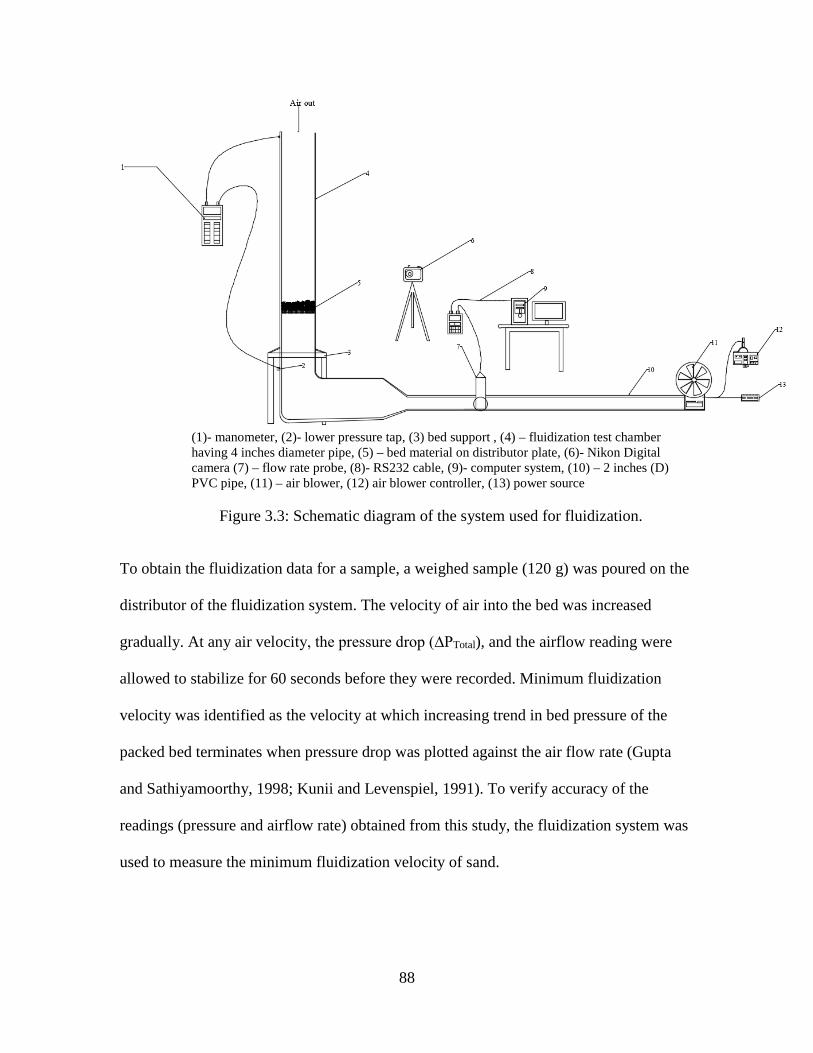
(1)- manometer, (2)- lower pressure tap, (3) bed support , (4) – fluidization test chamber having 4 inches diameter pipe, (5) – bed material on distributor plate, (6)- Nikon Digital camera (7) – flow rate probe, (8)- RS232 cable, (9)- computer system, (10) – 2 inches (D) PVC pipe, (11) – air blower, (12) air blower controller, (13) power source
Figure 3.3: Schematic diagram of the system used for fluidization.
To obtain the fluidization data for a sample, a weighed sample (120 g) was poured on the
distributor of the fluidization system. The velocity of air into the bed was increased
gradually. At any air velocity, the pressure drop (∆PTotal), and the airflow reading were
allowed to stabilize for 60 seconds before they were recorded. Minimum fluidization
velocity was identified as the velocity at which increasing trend in bed pressure of the
packed bed terminates when pressure drop was plotted against the air flow rate (Gupta
and Sathiyamoorthy, 1998; Kunii and Levenspiel, 1991). To verify accuracy of the
readings (pressure and airflow rate) obtained from this study, the fluidization system was
used to measure the minimum fluidization velocity of sand.
88

3.3.8 Statistical analysis
All experiments were conducted in triplicates. The results were presented in relevant
section as mean values and standard deviation. The effect of sample size obtained from
the different size measurement scheme on bulk density, particle density and particle size
diameter were analyzed using a generalized linear model from SAS statistical software
(SAS, 2011). In addition, a pairwise t-test using least squares means procedure with tukey
multiple comparison test was computed for each effect and their interactions. All the test
were considered to be statistical significant when p ≤0.05. The difference between
predicted (minimum fluidization velocity based on equations and diameter types) and
observed (minimum fluidization velocity obtained from laboratory experiment) were
evaluated by determining the mean relative deviation (MRD) following the method used
by (Nemec and Levec, 2005).
( ) ∑=
−=
N
i i
icalc
NMRD
1 exp.
exp..11001%λ
λλ (3.6)
where
calc.1λ is calculated Umf from predicting equation (m/s)
exp.iλ is experimentally obtained Umf (m/s) N is the numbers of data points
89

3.4 Result and Discussion
3.4.1 Physical properties of ground loblolly pine wood (Sample A and B)
3.4.1.1 Particle size
Particle size distributions of the unfractionated and the seven fractionated ground loblolly
pine wood samples obtained from the particle size imaging system are shown in Fig 3.4.
There was skewness in the distributions of the ground sample, which is typical of ground
biological materials. The skewness however reduces with increase in class size. For
instance, particle retained on nominal screen size of 1.7 mm was almost normally
distributed around 1.7 mm particle size. While particle retained on 0.15 mm had a long
tail positive skewness. The estimated geometric mean diameters for the samples are given
in Table 3.4.
*Numbers in the legend are the nominal diameters (mm) of the screen used for fractionation.
Figure 3.4: Particle size distribution of fractionated and unfractionated loblolly
pine wood.
90

The measured diameter using the different measurement schemes is shown in Table 3.4.
For sample A, the measured diameters varied between 0.58 and 1.07 mm. The highest
value was obtained from the minimum Ferret diameter (84.4% higher than the lowest
measured diameter – Sauter mean diameter). Similarly, for Group B samples, particle
size based on Ferret’s diameter was the highest (Table 3.4). For instance, sample B3, the
value of minimum Ferret diameter was higher than the surface-volume diameter, the
Martin diameter, and the chord diameter by 18.3%, 23.6%, and 7.03% respectively.
These highest values of Ferret diameter is because the measurement scheme is based on
the longest distance between parallel tangents (Table 3.2). Furthermore, Fig. 3.4 shows
that the group B samples retained their lognormal size distribution profile even after
fractionation. This confirmed that the lognormal size distribution property is an inherent
property of biomass grinds. Statistical analysis affirmed that particle sizes of samples in
group B were significantly (p <0.05) affected by the choice of the diameter measurement
scheme.
91

Table 3.4: Effect of measurement scheme on diameter of fractionated and unfractionated loblolly pine wood grinds.
Sieve number
4-12 12-14 14-18 18-30 30-50 50-100 100-270
Fractionated samples
Diameter schemes A B1 B2 B3 B4 B5 B6 B7 Geometric mean+ (mm)
0.83 (0.32) *
2.12A,2 (1.73) *
1.89B,1 (1.53) *
1.54C,1 (1.35) *
1.12D,1 (0.39) *
0.73E,1 (0.34) *
0.35F 2,1 (0.83) *
0.17G,3 (0.88) *
Chord (mm)
1.002 (0.05)
2.11 A, 2 (0.03)
1.68 B, 2
(0.01) 1.39 C, 2
(0.01) 1.04 D, 2 (0.02)
0.63 E, 3 (0.02)
0.55 F, 2,1 (0.26)
0.51 F, 1 (0.10)
Min. Ferret (mm)
1.07 (0.05)
2.24 A, 1 (0.04)
1.80 B, 2,1 (0.01)
1.49 C, 1 (0.01)
1.13 D, 1 (0.03)
0.69 E, 2,1 (0.03)
0.59 E,1 (0.27)
0.54 E, 1 (0.10)
Martins (mm)
0.83 (0.04)
1.83 A, 3 (0.02)
1.42 B, 3 (0.01)
1.10 C, 4 (0.06)
0.80 D, 3 (0.01)
0.45 E,F, 4 (0.01)
0.52 E, 2,1 (0.13)
0.36 F, 2 (0.09)
Surface-volume (mm)
0.79 (0.04)
1.83 A, 3 (0.02)
1.47 B, 3 (0.01)
1.19 C, 3 (0.03)
0.84 D, 4 (0.01)
0.45 E, 4 (0.01)
0.24 F, 2 (0.01)
0.27 F 2,3 (0.04)
Values are means of triplicates and numbers in parentheses are standard deviation Means with the different superscript (alphabet) in a row are significantly different (p<0.05) Means with the different superscript (numeric) in a column are significantly different (p<0.05) + Values are obtained from ASABE S319.3 analysis method. *Geometric mean standard deviation obtained from Eqn. 3.2 A acronym for Unfractionated samples 3.4.1.2 Bulk, particle density and porosity
The particle density of whole sample obtained in this study was 1469.5 kg/m3 and the
result was comparable to the value of 1440.0 kg/m3 obtained by Hehar et al. (2014) for
loblolly pine wood grinds. In addition, there were no visible trends between particle
densities and particle size of fractionated samples (Table 3.5). This suggests that voids
within individual particle were not affected by the grinding (ground through 3.12 mm
screen size) process and by particle size. The bulk densities of group B samples however
decreased from 278 kg/m3 to 166 kg/m3 as nominal screen reduced from 1.7 mm (sieve
number 12) to 0.15 mm (sieve number 100) with the bulk densities of samples B1, B2,
92

B3, B4 and B5 being significantly different (p <0.05) from bulk densities obtained for B6
and B7. The reduction in bulk density with reduction in size could be attributed to
biomass grinds collected after fractionation exhibit different packing because of particles
having similar sizes as compared to the unfractionated biomass grinds which comprises
of different particle size range. Similar result was obtained by Oginni (2014) using
loblolly pine wood grinds and Liu et al. (2008a) using unlubricated ibuprofen size
fraction. Statistical analysis also revealed that the bulk densities were significantly
affected by particle size (p < 0.05).
93

Table 3.5: Physical properties of unfractionated and fractionated loblolly ground wood.
Sieve #
4-12 12-14 14-18 18-30 30-50 50-100 100-270
Fractionated samples
Properties A B1 B2 B3 B4 B5 B6 B7
Bulk density (kg/m3)
311.1 A (7.9)
278.0 C (1.0)
277.7 C (2.1)
320.7 A (2.1)
290.3 B (7.6)
234.3 D (1.5)
169.3 E (2.5)
166.3 E (1.2)
Particle Density (kg/m3)
1469.0 C (7.0)
1471.6 B (0.8)
1466.1C,B (7.4)
1470.7 B (12.3)
1468.2 C,B (6.7)
1486.9 B (11.5)
1512.7 A (17.7)
1524.3 A (19.4)
Porosity
0.79 E (0.01)
0.92 C (0.01)
0.81 C (0.01)
0.78 E (0.01)
0.79 D (0.01)
0.84 B (0.01)
0.89 A 0.01)
0.89 A (0.01)
Sphericity
0.52 D (0.02)
0.60 A (0.01)
0.57 B,A (0.01)
0.55 B,C (0.03)
0.51 C,D (0.01)
0.41 E 0.01)
0.23 F (0.01)
0.43 E (0.03)
Values are means of triplicates and numbers in parentheses are standard deviation Means with the different superscript (alphabet) in a row are significantly different (p<0.05) A acronym for Unfractionated samples
Table 3.5 also shows that the void spaces within the fractionated samples were high
(0.78-0.91). Other authors have reported similarly high porosity values for biomass
feedstock. Lam et al. (2008) found that the porosity of switchgrass decreased from 0.87
to 0.82 as particle size increased from 0.10 mm to 2.00 mm. Naimi et al. (2007) reported
that the porosity of switchgrass decreased with increase in particle size from 0.71 to 2.80
mm. Manickam and Suresh (2011) measured the porosity of coir pith to vary between
0.62 to 0.86 within the particle size range of 0.075 to 3.00 mm. Fasina (2006) concluded
that it will be difficult to justify the transportation of biomass grinds because the porosity
of switchgrass, peanut hull, and poultry litter varies between 0.62 to 0.83. Although high
94

void fraction should enhance easy fluid penetration through the packed bed, they can also
aid in formation of channeling as airflow under pressure entrain smaller particles, create
bigger holes as bed structure rearranges, and ultimately cause particle segregation during
fluidization.
3.4.1.3 Particle shape
The sphericity (φ) of the samples varied from 0.24 to 0.60 and generally decreased
(P < 0.05) with reduction in particle size (Table 3.5). Cui and Grace (2007) classified
flatness of particles based on their sphericity. Sphericities of φ < 0.5 indicates an
extremely flat particles, φ > 0.5 indicates flat particles and φ > ~ 0.8 is nearly spherical
particles. Similarly, Lucas et al. (1986) also classified sphericity of particles into three
categories namely, round (0.8 ≤ φ ≤ 1), sharp (0.5 ≤ φ ≤ 0.8) and others (0.1 < φ < 0.5).
Therefore, based on these classifications, the sphericities of ground loblolly pine wood is
flat and sharp.
3.4.2 Geldart’s classification
Table 3.6 shows the effect of diameter measurement scheme on Geldart’s classification
of unfractionated and fractionated loblolly pine wood grinds. Owing to the influence of
diameter measurement scheme on measured size, the Geldart’s classifications of
unfractionated grinds was either Group B or Group D. Group B and D particles in Geldart
classification (Table 3.1) have distinct and opposite behavior. Therefore, the method used
for size measurement can potentially affect the interpretation of how biomass grinds and
similar non-spherical particles will respond in fluidization. In addition, prediction of
minimum fluidization velocity and other design parameters such as equipment selection
for fluidizing biomass material that require the size of the fluidizing biomass be known,
95

would be significantly affected by particle measurement method. For fractionated
loblolly pine grinds, fractions B1, B2, and B3 had similar classification (Group D), while
B4, B5, and B6 varied between Groups D, B, and A. This confirms that the wide range in
size of particles in biomass grind sample is partly responsible for the unpredictable
fluidization behavior of biomass grinds. Therefore, Geldart classification should be
applied with caution for sample with multi-component and multi-sized particles such as
ground biomass.
Table 3.6: Geldart’s classification of unfractionated and fractionated loblolly pine wood grinds as affected by diameter measurement schemes.
Sieve #
4-12 12-14 14-18 18-30 30-50 50-100 100-270
Diameter
Fractionated samples Scheme Unfractionated B1 B2 B3 B4 B5 B6 B7
Chord D D D D D B B B Ferret D D D D D B B B
Martins B D D D B B B A Sur.-vol. B D D D B B A A
The mean diameter value used for the classification is presented in Table 3.4. The particle density for each data is presented in Table 3.5 Geldart plot used for the classification is in Appendix 2 Unfractionated sample was previously referred to as sample A
3.4.3 Fluidization behavior of ground loblolly pine wood
3.4.3.1 Validation of fluidization system
Based on the plot of pressure drop across the bed of sand particles against the air
velocity as shown in Fig. 3.5. The minimum fluidization velocity of sand was measured
to be 0.28 ± 0.002 (m/s). The minimum fluidization velocity was identified as the
intersection between the rising and constant bed pressure drop (Gupta and
Sathiyamoorthy, 1998). It can be seen from the figure that duplicate runs for the sample
are essentially the same. This result is comparable to values of 0.35 m/s and 0.34 m/s
96

obtained for minimum fluidization velocity of sand as reported by Sánchez-Delgadoa et
al. (2011) and Patil et al. (2005) respectively. This validates the pressure drop – velocity
data obtained from the fluidization setup of Fig. 3.3.
Figure 3.5: Plot of pressure drop versus air velocity for sand particles
3.4.3.2 Fluidization behavior of unfractionated biomass grinds (Sample A)
Figs. 3.6 and 3.7 show some of the behaviors that were observed when Sample A (whole
sample) was fluidized. Plug-flow, channeling, top fluidization, and de-fluidization were
observed before fluidization was eventually achieved. When air flow through the bed
reached a velocity at which the updraft created from the air flow was sufficient to lift the
bed entirely (suggesting the Umf was attained at 0.16 to 0.30 m/s, smaller particles
entrained in the air stream were either deposited in another location in the bed or carried
out of the bed. This rearrangement caused the airflow to concentrate in a particular region
(region that offered least resistance to airflow) thus causing channels of various sizes
which can vary from multiple small channels (less than 0.01m diameter) to a channel
with diameter that is almost half of the bed (0.05 m) (Fig 3.6).
97

Figure 3.6: Channeling during fluidization of ground biomass (unfractionated, sample
A) impeded fluidization processes.
Further increase in air velocity resulted in bigger particles settling at the base in an
interlock position. In between the interlocked particles (mostly bigger particles) are
smaller particles that made air penetration through the bed difficult. All of these
rearrangements of particle resulted in the bed rising in a plug (Fig 3.7).
Figure 3.7: Plugged flow during fluidization of ground biomass (unfractionated, sample
A) because of particle interlocking.
98

The plug was disentangled by increasing the airflow rate. It is also important to mention
that after the bed collapse due to plug flow breakage, smaller particles trapped within the
bigger particle network escape thereby creating another stage for channeling and
entrainment. Defluidization was another phenomenon that was observed after complete
fluidization velocity of bed was achieved. Defluidization occurs after significant
entrainment of smaller particles from the bed resulting in a situation where the remaining
large particles require higher flow rate to fluidize. At this particular condition, a
multicomponent bed was turned into almost mono-component bed. This suggests that the
fluidization state of a bed that is composed of non-uniform and non-spherical particles is
constantly evolving.
3.4.3.3 Fluidization behavior of fractionated biomass grinds (Sample B)
Figs. 3.8 and 3.9 showed some of the behaviors that were observed when group B
samples (fractionated samples) were fluidized. The behavior observed can be
categorized into two based on the class size. For sample B1, B2 and B3, channelings
were seen more often before fluidization state was achieved. The channeling formation
could be attributed to networks of void spaces that simply grew with increase in airflow
into bigger channels. However, the channel breaks up once the updraft is sufficient to lift
the bed entirely. In addition, particle entrainment out of the bed were minimal or not
observed until the whole bed were in intensive mixing and at this stage, the minimum
fluidization velocity has been achieved. Since bed channeling were rampant, bed
expansion were not uniform too (Figure 3.8).
99

Figure 3.8: Typical channeling behavior observed for B1, B2 and B3 samples during fluidization processes (the snapshot was that of B1 sample).
The second category of behavior were obtained from B4, B5, and B6 samples. As airflow
increased, channelings were observed but sometimes the channeling disperse quickly.
However, at B5 samples, the cohesive force between particles causes channels to evolve
into different shapes (Fig 3.9). Unless the bed mixes intensely, entrainment out of the bed
was limited.
Figure 3.9: Typical channeling behavior observed for B4, B5 and B6 samples during fluidization processes (the snapshot was that of B5 sample).
100

In summary, there were notable differences in behavior of fractionated and unfractionated
samples to airflow. For instance, the plug flow in fractionated samples could be
problematic to break up while the unfractionated sample disentangled with relative ease
as airflow increase. The difference in behavior is principally due to wide particle size
distribution in unfractionated sample compared with fractionated samples.
3.4.3.4 Experimental determination of minimum fluidization velocity of samples A and B
Fig 3.10 shows the stages of fluidization during the experimental determination of the
minimum fluidization velocity. At stage 1, which is the initial state, about 120 g sample is
weighed and poured on the distributor in the bed chamber. The air velocity was increased
slowly, and the corresponding pressure drop across the bed was recorded at each flow
increment. Eventually a limit was reach after which three or four consecutive increase in
airflow did not result in appreciable increase in pressure drop (stage 2). Then at this
point, the velocity was considered to be the minimum fluidization velocity and the bed
was considered to be at minimum fluidization state (Fig 3.8 b) (Davidson et al., 1977;
Drake, 2011; Kunii and Levenspiel, 1991). Further increase in the superficial gas velocity
to about 4 ×Umf resulted in complete fluidization of the bed (stage 3).
Several measures were taken to prevent data collection from been compromised by poor
fluidization behavior as previously discussed. For instance, plug flow were stopped by
gently knocking on the wall or increase the airflow velocity and but in few cases that the
plug refused to break, the airflow velocity would be cutoff and the experiment restarted
with a new set of sample. For channeling, the air velocity was reduced so that particle can
fall into their natural position. Afterward the velocity was ramped up again and when
101

channel persisted, the flow velocity is increased by ~50% of the last flow velocity. As
previously stated, the channel usually disintegrated. However, at some occasions, we
notice recalcitrant channels that refuse to break with increase in airflow (B6 samples). In
such a situation, the airflow is stopped and the bed material is evacuated for fresh sample.
It is also important to add that when bed entrainment increased because of increase in
airflow velocity, the corresponding pressure drop data could be compromised (lower)
because of reduction in bed inventory. When this occurred before minimum fluidization
state were achieved, then the experiment is discarded and restarted.
(a) Stage 1 (b) Stage 2 (c) stage 3 Figure 3.10: Typical behavior of loblolly pine wood grinds during fluidization. First test from left side is the initial states (a) initial stage, (b) fluidization stage, (c) complete fluidization.
The plot of pressure drop against air velocity for sample A (unfractionated) and samples
from group B fractionated (sample B) is shown in Fig. 3.11. The minimum fluidization
velocity of sample A (un-fractionated ground loblolly pine wood) was measured to be
0.25±0.04 m/s. The nature of the pressure drop curve with increase in the superficial gas
velocity showed a deviation from that of Fig. 3.5. The wobbling line where constant
pressure line is expected could be attributed to the non-uniformity in size, shape and size
102

distribution of grinds (Woodcock and Mason, 2013). However, it can also be seen that
the instability in the line of constant pressure gradually reduced with narrower size
distribution group (Sample B).
*Numbers in the legend are the nominal diameters (mm) of the screen used for fractionation. Figure 3.11: Variation in pressure drop with superficial gas velocity for unfractionated
sample and Sample B (fractionated sample).
All of the ‘B’ samples have Umf greater than 0.25 m/s (the minimum fluidization velocity
of unfractionated sample) with the minimum fluidization of larger particles being about 3
times of the smaller particles (Table 3.7). This explains the fundamental reason why large
particles in ground samples remain un-fluidized whereas smaller particles are fluidized
and often ejected out of fluidization chamber. Similar observation was made by Liu et al.
(2008b) when a raw steam coal (a kind of bituminite usually used in industrial chain grate
boilers) between > 2 mm to 40 mm was fluidized. They found that about half of the coal
mass was blown out of the bed; some were entrained at the top section while the
103

remainder was at the bottom section of the bed after applying air at superficial gas
velocity of 3.0 m/s for 10 min. This variation in the Umf of multi-component materials
such as biomass grinds will affect their optimal performance during fluidization. The
same view was also expressed by Gauthier et al. (1999), Khoe et al. (1991) and Reina et
al. (2000) when they determined the minimum fluidization velocity of river sand, spent
fluid catalytic cracking catalyst (FCC) and scrap-wood particles respectively.
Table 3.7: Experimentally determined minimum fluidization velocities of ground loblolly pine wood fractions
Sample Tag US sieve # Minimum fluidization
velocity (m/s) Pass through Retained on
B1 - 12 0.81±0.007
B2 12 14 0.63±0.035
B3 14 18 0.53±0.11
B4 18 30 0.40±0.07
B5 30 50 0.27±0.02
B6 50 100 0.29±0.01
The experimentally determined minimum fluidization velocities of the sample were
compared with predicted velocities that were obtained from four commonly used
fluidization equations (listed in Table 3.8). All of these equations only require
measurement of physical properties of the material to be fluidized and the gas to be used
for fluidization. Microsoft Excel® goal seek function was used to estimate the minimum
fluidization velocity in equation 3.7 after substituting the appropriate values of the
properties (Table 3.5). It is important to point out that the Eqn. 3.7 has a sphericity term
and is different from the original Ergun equation in eqn. 2.6. The Umf obtained from
Eqns 3.8 -10 were obtained by direct substitution of physical properties of a fraction on
104

the right side of the equations. Physical properties of each fraction used in the equations
were obtained from Table 3.5. All of the diameters (Martins, chord, geometric mean,
minimum Ferret, and surface-volume diameter) were used in the equations to predict Umf.
Table 3.8: Selected fluidization equation used for predicting the experimental Umf of ground wood
Equation Eqn. # Label Reference
( )( )
( )( )ps
g
ps
g
dU
dU
LP
φρ
εε
φµ
εε 2
323
2 174.11150 −+
−=
∆ 3.7 Mod-
Ergun Ergun (1952)
( )06.088.0
94.082.10093.0
gg
gpmmf
dU
ρµρρ −
= 3.8 Leva Leva (1959)
( )
−−×=g
gggspdmfU
µ
ρρρ 1.19.0231025.1
3.9 Miller Miller and Logwinuk (1951)
( )[ ] 87.0066.0934.08.14109 −−−−×= ggggspdmfU µρρρ 3.10 Geldart Abrahamsen and Geldart (1980)
*Mod-Ergun has sphericity term while Original Ergun equation does not where,
Umf = Minimum fluidization velocity (m/s) dm = Sauter mean diameter (m) U = Superficial velocity (m/s) ρs = Density of particle (kg/m3) ρg = Density of gas (kg/m3) µg = Dynamic viscosity of fluidization gas (Pa s) dp = Surface volume mean diameter of particle (m) ε = Void fraction of bed φs = Sphericity of particle ∆P = Pressure drop (Pa) L = Length (m) g = Acceleration due to gravity (m/s2)
105

3.4.4 Effect of diameter measurement scheme on predicted values
Table 3.9 shows the effect of diameter measurement scheme on the predicted Umf from
the four equations listed in Table 3.8. The actual predicted values are shown in Appendix
2. For the unfractionated sample (A), when the mean diameter used in the equations was
changed from surface-volume (least) diameter, to minimum Ferret diameter (highest), the
predicted value obtained changed by 16.4%, 72.6 %, 73.7 %, 16.5 % and 83.4 % for
Ergun, Geldart, Leva, Mod-Ergun, and Miller equations respectively. Although there
were differences in the actual predicted values obtained when Ergun and Mod-Ergun
were used, the difference resulted in the same percent change in predicted value. The
least percent change in predicted values was obtained using Ergun equation. This could
be could be attributed to the structure and the underlying assumption made during
computation/ development of Ergun’s equation. Firstly, Ergun and Mod-Ergun equations
required more parameter than all other equation before Umf can be estimated. For
instance, Ergun has correlation for void fraction – a parameter that influence air
movement /penetration through the bed. Particles are expected to have a voidage equal to
the voidage at minimum fluidization (Ergun assumptions, see section 2.9.1). This is not
the case for biomass grinds because the minimum fluidization velocity iof the particles
that comprise the biomass grinds are different. Larachi et al. (1999) also made similar
observation by attributing poor prediction between experimental and predicted data to the
mathematical structure of the correlations and also alluded that the equation could not
embrace the high variability inherent in the properties of the material. Secondly, the
minimum fluidization velocities were estimated by balancing the pressure drop parameter
between fixed beds and fluidize bed state. Therefore, in order to obtain a velocity value,
Ergun equation essentially is computed from the bed weight/unit area.
106

Table 3.9: Effect of size measurement method and popular fluidization equation on predicted minimum fluidization velocity.
Measurement scheme
Size (% change)*
Percent change in predicted value
Sample Maximum Minimum
Ergun Geldart+ Leva+ Mod-Ergun+ Miller+ A Ferret Sur-vol. 35.4 16.4 72.6 73.7 16.5 83.4 B1 Ferret Martins 22.4 10.6 43.9 44.5 10.6 49.8 B2 Geometric Martins 33.1 15.4 67.3 68.3 15.4 77.2 B3 Geometric Martins 40.0 18.3 83.2 84.5 18.4 96.0 B4 Ferret Martins 41.3 18.9 86.2 87.5 18.9 99.5 B5 Geometric Martins 62.2 27.5 138.9 141.2 27.7 163.2 B6 Ferret Sur-vol. 145.8 57.1 404.8 414.0 59.9 504.3 B7 Ferret Sur-vol. 100.0 41.7 248.2 253.1 41.9 300.0
*% change obtained by the ratio of change in maximum and minimum diameter value to minimum diameter value. +Nomenclatures referred to Table 3.8. ├Ergun obtained from original Ergun equation expressed in Eqn. 2.9 having no sphericity factor.
For fractionated samples, percent change in the predicted value increased with decrease
in size. This could be attributed to the sensitivity of smaller particle to measurement
method because smaller particle has the least shape factor (sphericity of 0.4 from Table
3.5). In general, both Ergun and Mod-Ergun equation prediction gave a consistent lower
percent change in predicted value between highest and least diameter. Therefore, we can
safely conclude that measurement scheme has significant influence on measured
parameters and eventually the predicted values. However, it appears that Ergun equation
offer the best fluidization equation that can handle the changes in size due to
measurement scheme used.
3.4.5 Comparison between predicted and experimental values
The mean relative deviations (MRD) between experimental and predicted Umf values
using the fluidization equations (Eqn. 3.7 -10) are shown in Table 3.10. For
unfractionated sample, Miller had the least mean deviation irrespective of the
107

measurement scheme. In overall, prediction obtained using Ergun equations (Ergun and
Mod-Ergun) are significantly different from other equations. For instance, using surface
to volume diameter, the MRD obtained from Ergun and Mod-Ergun was 142.9 and 217.8
% respectively while Leva, Geldart, and Miller equation was 6.9, 24.8 and -3.85 %
respectively. Geldart, Leva and Miller equation were developed through experimental
correlations and have similar structure as depicted in Eqn. 3.11.
( )yn
g
xgp
lm
mfg
KdU
ρµ
ρρ −= (3.11)
Where k, l, x, n and, y represent different coefficient obtained from the fitting process.
Ergun equation required more material specific parameter (e.g. porosity and sphericity),
that probably increased the error obtained. For instance, a constant porosity value was
assumed in estimating Umf even though several authors and observation from this study
show that bed porosity changes with velocity (Vejahati et al., 2009).
For fractionated samples, the deviation between predicted, and the experimental data
reduced with reduction in size for all the equation considered. When the sample size was
greater than 1.00 mm, Miller equation produced the least MRD with values of -25.4, -
6.11, 0.57, and -2.83 % for B1, B2, B3 and B4 using Martins diameter. However, for
sample below 1.00 mm, Leva gave the least MRD. Reduction in prediction in MRD with
size could be attributed to the fact that size distribution reduced with reduction in size
(see Table 3.4, for geometric mean and geometric standard deviation of particles).
Significant prediction difference between Ergun and Mod-Ergun equation could be
attributed to the fact that Ergun equation derivation did not include sphericity factor. If
108

this factor is to be added so as to improve Ergun predictions, than Ergun equation has to
be refitted with sphericity factor. In addition, prediction obtained when Martins and
surface to volume mean diameter was used in the fluidization equation resulted in the
least MRD between predicted and actual value for sample B1,B2, B3, and B4 for all
equations used. Martins diameter is difficult to determine in a laboratory unless through
image analysis. Several procedure has been established and statistically verified for
surface- volume diameter. In fact, surface-volume mean diameter is liberally used in
fluidization equation. However, for sample B5, B6 and B7, the MRD were less than 15%
for all diameter schemes used with Leva, Geldart and Miller equation. This suggests that
reduction in size to certain diameter may neutralize the effect of non-sphericity on
predictive equation. Finally, the result also revealed that the effect of size distribution is
presently not captured in the equations, hence the high MRD obtained in unfractionated
sample. However, since in a real preprocessing plant, average properties of
unfractionated sample is typically used (not fractionated sample properties) then surface
to volume diameter offers the best diameter scheme with least MRD.
109

Table 3.10: Predictability of fluidization model for unfractionated woood grinds and effect of diameter measurement scheme.
Sample id Diameter types/ Ergun Mod-Ergun Leva Geldart Miller
dp (mm) MRD (%)
Martins 0.83 147.7 224.5 12.2 32.6 0.4
Sample A Chord 1.01 168.2 252.8 38.9 72.3 21.8
Ferret 1.07 174.6 261.7 48.8 87.2 29.6
Surf-vol. 0.79 142.9 217.8 6.9 24.8 -3.8
Geometric 0.83 147.7 224.5 12.2 32.6 0.4
Martins 1.83 -76.7 -110.7 -41.9 -85.2 -25.3 Sample B1 Chord 2.11 -85.3 -121.9 -66.2 -126.4 -44.4
Ferret 2.24 -89.2 -126.8 -78.4 -147.6 -54.0
Surf-vol. 1.83 -76.7 -110.7 -41.9 -85.2 -25.3
Geometric 2.12 -85.6 -122.2 -67.1 -128.0 -45.1
Martins 1.42 -64.2 -96.5 -16.2 -39.8 -6.1
Sample B2 Chord 1.68 -72.9 -108.0 -34.6 -69.7 -20.6
Ferret 1.80 -76.7 -113.0 -43.9 -85.2 -27.9
Surf-vol. 1.47 -66.1 -98.8 -19.0 -45.2 -8.7
Geometric 1.89 -79.5 -116.7 -51.2 -97.6 -33.7
Sample B3 Martins 1.1 -48.5 -75.9 -1.6 -14.2 4.4
Chord 1.39 -58.3 -89.1 -18.5 -40.6 -8.9
Ferret 1.49 -61.4 -93.3 -25.0 -51.1 -14.1
Surf-vol. 1.19 -51.7 -80.2 -6.5 -21.7 0.6
Geometric 1.54 -62.9 -95.4 -28.4 -56.6 -16.8
Martins 0.8 -39.0 -62.7 2.4 -3.1 5.7 Sample B4 Chord 1.04 -47.3 -74.3 -8.2 -19.1 -2.8
Ferret 1.13 -50.2 -78.3 -12.9 -26.1 -6.5
Surf-vol. 0.84 -40.4 -64.7 0.8 -5.5 4.4
Geometric 1.12 -49.8 -77.9 -12.3 -25.0 -6.0
110

Table 3.10 Continued: Statistical evaluation of the effect of diameter type on predictive ability of different models of unfractionated sample
Sample id Diameter types Ergun Mod-Ergun Leva Geldart Miller
dp (mm) MRD (%)
Martins 0.45 -23.3 -45.0 8.8 7.6 9.9
Sample B5 Chord 0.63
-30.4 -56.1 3.6 0.6 5.7
Ferret 0.69 -32.5 -59.4 1.5 -2.2 4.0
Surf-vol. 0.45 -23.3 -45.0 8.8 7.6 9.9
Geometric 0.73 -33.9 -61.5 0.1 -4.3 2.9
Martins 0.52 -17.5 -53.3 7.0 5.2 8.4
Sample B6 Chord 0.55
-18.4 -55.2 6.1 4.0 7.7
Ferret 0.59 -19.6 -57.7 4.9 2.4 6.7
Surf-vol. 0.24 -6.6 -31.3 13.0 12.9 13.3
Geometric 0.35 -11.4 -41.0 11.1 10.5 11.7
Martins 0.36 -31.7 -46.9 5.8 5.3 6.6
Sample B7 Chord 0.51
-39.7 -57.8 2.2 0.5 3.6
Ferret 0.54 -41.2 -59.8 1.4 -0.5 2.9
Surf-vol. 0.27 -26.0 -39.2 7.5 7.3 7.9
Geometric 0.37 -32.3 -47.7 5.6 5.0 6.4
3.5 Conclusion
In this chapter, the results of an experimental study on the physical and fluidization
properties of ground loblolly pine wood relevant to fluidized bed system were measured.
The result showed that a ground loblolly pine wood sample has mean particle density of
1460.6±7 kg/m3, bulk density of 311± 37 kg/m3 and porosity of 0.787 ± 0.003. The
Ferret diameter was found to be higher than surface-volume diameter, Martin’s diameter
and chord diameter by 18.3, 23.6, and 7.03% respectively. Also, the shape characteristic
based on the sphericity value showed that the particle is flat and ranges between 0.23
111

and 0.60. The minimum fluidization velocity of loblolly pine wood grinds
(unfractionated sample ground through 3.175 hammer mill screen) was found to be 0.25
±0.04 m/s. However, fractionated samples had their minimum fluidization velocity
higher than 0.25 m/s –the velocity of un-fractionated sample. Prediction error were
found to be significant (p<0.05) and increase with increase in particle size. The use of
different diameter types in fluidization equation had a significant effect on prediction
(Umf) obtained. Generally, Ergun equation (with or without sphericity factor) gave the
highest MRD. Although, change in diameter measurement scheme has little effect on
prediction of experimental minimum fluidization velocity. Other predicting equation
resulted in lower MRD but change of diameter scheme significantly influences the
predictability of those equations. Even though Martins diameter generally exhibited the
least MRD values, surface to volume diameter appeared to be the most practical in the
equation since standard experimental procedure has been established when image
analysis is not available.
112

3.6 Reference
Abdullah, M. Z., Z. Husain, and S. L. Yin Pong. 2003. Analysis of cold flow fluidization test results for various biomass fuels. Biomass and Bioenergy 24(6):487-494.
Abrahamsen, A., and D. Geldart. 1980. Behaviour of gas-fluidized beds of fine powders part I. Homogeneous expansion. Powder Technology 26(1):35-46.
Adapa, P., L. Tabil, and G. Schoenau. 2009. Compaction characteristics of barley, canola, oat and wheat straw. Biosystems Engineering 104(3):335-344.
ASABE. 2006. ASAE S319. 3—method of determining and expressing fineness of feed materials by sieving, ASABE Standards, 602–605, American Society of Agricultural and Biological Engineers, St. Joseph, MI.
ASTM. 2007. Standard test methods for direct moisture content measurement of wood and wood-base materials. American Society for Testing Materials. ASTM International West Conshohocken, PA.
Aznar, M. P., F. A. Gracia-Gorria, and J. Corella. 1992. Minimum and maximum velocities for fluidization for mixtures of agricultural and forest residues with a second fluidized solid. II. Experimental results for different mixtures. International chemical engineering 32(1):103-113.
Barakat, A., H. de Vries, and X. Rouau. 2013. Dry fractionation process as an important step in current and future lignocellulose biorefineries: A review. Bioresource Technology 134(0):362-273.
Cui, H., and J. R. Grace. 2007. Fluidization of biomass particles: A review of experimental multiphase flow aspects. Chemical Engineering Science 62(1):45-55.
Davidson, J. F., D. Harrison, and J. Carvalho. 1977. On the liquidlike behavior of fluidized beds. Annual Review of Fluid Mechanics 9(1):55-86.
Drake, J. B. a. H., Theodore J. 2011. The repeatability and uniformity of 3D fluidized beds. Powder Technology 213(13):148-154.
Ergun, S. 1952. Fluid flow through packed columns. Chem. Eng. Prog. 48:89-94.
Fasina, O. 2006. Flow and physical properties of switchgrass, peanut hull, and poultry litter. Transactions of the ASABE 49(3):721-728.
Fasina, O. O. 2008. Physical properties of peanut hull pellets. Bioresource Technology 99(5):1259-1266.
113

Gauthier, D., S. Zerguerras, and G. Flamant. 1999. Influence of the particle size distribution of powders on the velocities of minimum and complete fluidization. Chemical Engineering Journal 74(3):181-196.
Geldart, D. 1973. Types of gas fluidization. Powder Technology 7(5):285-292.
Gil, M., D. Schott, I. Arauzo, and E. Teruel. 2013. Handling behavior of two milled biomass: SRF poplar and corn stover. Fuel Processing Technology 112(0):76-85.
GmbH, S. 2011. Particle shape. Clausthal-Zellerfeld, Germany: Am Pulverhaus Available at: http://www.sympatec.com/EN/Science/Characterisation/05_ParticleShape.html.
Gupta, C. K., and D. Sathiyamoorthy. 1998. Fluid bed technology in materials processing. CRC.
Hehar, G., O. Fasina, S. Adhikari, and J. Fulton. 2014. Ignition and volatilization behavior of dust from loblolly pine wood. Fuel Processing Technology 127(0):117-123.
Khanal, S. K. 2010. Bioenergy and biofuel from biowastes and biomass. ASCE Publications, Reston Virginia.
Khoe, G. K., T. L. Ip, and J. R. Grace. 1991. Rheological and fluidization behaviour of powders of different particle size distribution. Powder Technology 66(2):127-141.
Kunii, D., and O. Levenspiel. 1991. Fluidization engineering. Butterworth-Heinemann Boston.
Lam, P., S. Sokhansanj, X. Bi, C. Lim, T. JayaShankar, G. Rezaie, and L. Naimi. 2008. The Effect of Particle Size and Shape on Physical Properties of Biomass Grinds. In An ASABE Meeting Presentation. Paper.
Larachi, F., I. Iliuta, O. Rival, and B. P. A. Grandjean. 1999. Prediction of Minimum Fluidization Velocity in Three-Phase Fluidized-Bed Reactors. Industrial & engineering chemistry research 39(2):563-572.
Leva, M. 1959. Fluidization. McGraw-Hill Chemical Engineering Series. McGraw-Hill, London
Liu, L. X., I. Marziano, A. C. Bentham, J. D. Litster, E.T.White, and T. Howes. 2008a. Effect of particle properties on the flowability of ibuprofen powders. International Journal of Pharmaceutics 362(1–2):109-117.
Liu, X., G. Xu, and S. Gao. 2008b. Fluidization of extremely large and widely sized coal particles as well as its application in an advanced chain grate boiler. Powder Technology 188(1):23-29.
114

Lucas, A., J. Arnaldos, J. Casal, and L. Puigjaner. 1986. Improved equation for the calculation of minimum fluidization velocity. Industrial & Engineering Chemistry Process Design and Development 25(2):426-429.
Mani, S., L. G. Tabil, and S. Sokhansanj. 2004. Grinding performance and physical properties of wheat and barley straws, corn stover and switchgrass. Biomass and Bioenergy 27(4):339-352.
Manickam, I. N., and S. Suresh. 2011. Effect of moisture content and particle size on bulk density, porosity, particle density and coefficient of friction of coir pith. International Journal of Engineering Science 3.
McMillan, J., C. Briens, F. Berruti, and E. W. Chan. 2007. Study of High Velocity Attrition Nozzles in a Fluidized Bed. In The 12th International Conference on Fluidization - New Horizons in Fluidization Engineering. F. Berruti, X. Bi, and T. Pugsley, eds. Vancouver, Canada: Engineering Conferences International.
Miller, C. O., and A. Logwinuk. 1951. Fluidization studies of solid particles. Industrial & Engineering Chemistry 43(5):1220-1226.
Mosier, N., C. Wyman, B. Dale, R. Elander, Y. Y. Lee, M. Holtzapple, and M. Ladisch. 2005. Features of promising technologies for pretreatment of lignocellulosic biomass. Bioresource Technology 96(6):673-686.
Naimi, L., S. Sokhansanj, X. Bi, C. Lim, S. Mani, M. Hoque, P. Lam, and A. Womac. 2007. Modeling and Characterization of Biomass Size Reduction. In ASAE Annual Meeting.
Nemec, D., and J. Levec. 2005. Flow through packed bed reactors: 1. Single-phase flow. Chemical Engineering Science 60(24):6947-6957.
Oginni, O. J. 2014. Contribution of particle size and moisture content to flowability of fractionated ground loblolly pine. M. S thesis. Auburn University, M. S thesis, Bisoystems Engineering Department, Auburn Alabama
Ortega-Rivas, Enrique, P. Juliano, and H. Yan. 2006. Food powders: physical properties, processing, and functionality. 1st ed. Springer, New York, Philadelphia.
Patil, K., T. Bowser, D. Bellmer, and R. Huhnke. 2005. Fluidization characteristics of sand and chopped switchgrass-sand mixtures. International Commission of Agricultural Engineering 7.
Rao, R., T. Ram, and J. V. Bheemarasetti. 2001. Minimum fluidization velocities of mixtures of biomass and sands. Energy 26(6):633-644.
Reina, J., E. Velo, and L. Puigjaner. 2000. Predicting the minimum fluidization velocity of polydisperse mixtures of scrap-wood particles. Powder Technology 111(3):245-251.
115

Rhodes, M. 2008. Introduction to particle technology. Wiley.
Sánchez-Delgadoa, S., J. A. Almendros-Ibáñez, N. García-Hernando, and C. Santana. 2011. On the minimum fluidization velocity in 2D fluidized beds. Powder Technology 207(1-3):145-153.
SAS. 2011. The SAS system for Windows. Ver. Release 9.2. Cary, NC.: SAS Institute.
Schell, D., and C. Harwood. 1994. Milling of lignocellulosic biomass. Applied biochemistry and biotechnology 45-46(1):159-168.
Sharma, A. M., A. Kumar, K. N. Patil, and R. L. Huhnke. 2013. Fluidization characteristics of a mixture of gasifier solid residues, switchgrass and inert material. Powder Technology 235(0):661-668.
Takara, D., P. Shrestha, and S. K. Khanal. 2010. Lignocellulosic biomass pretreatment. Biofuel and bioenergy from biowastes and lignocellulosic biomass. American Society of Civil Engineers, Reston.
Vejahati, F., N. Mahinpey, N. Ellis, and M. B. Nikoo. 2009. CFD simulation of gas–solid bubbling fluidized bed: A new method for adjusting drag law. The Canadian Journal of Chemical Engineering 87(1):19-30.
Wang, Q., T. Niemi, J. Peltola, S. Kallio, H. Yang, J. Lu, and L. Wei. 2014. Particle size distribution in CPFD modeling of gas–solid flows in a CFB riser. Particuology(0).
Woodcock, C., and J. Mason. 2013. Bulk solids handling: an introduction to the practice and technology. Springer Science & Business Media.
Yang, W.-C. 2007. Modification and re-interpretation of Geldart's classification of powders. Powder Technology 171(2):69-74.
Zhu, J., X. Pan, G. Wang, and R. Gleisner. 2009. Sulfite pretreatment (SPORL) for robust enzymatic saccharification of spruce and red pine. Bioresource Technology 100(8):2411-2418.
116

Chapter 4: Moisture Effect on Fluidization Behavior of Loblolly Pine Wood
Grinds
4.1 Abstract
The objective of this study was to quantify the effect of moisture contents on minimum
fluidization velocity of ground loblolly pine wood. Loblolly pine wood chips were
ground and screened through a 1/8-inch screen. Samples were adjusted to four moisture
contents that varied between 8 and 25 wt. % wet basis. Each of the samples was divided
into two groups (unfractionated and fractionated that consisted seven fractions). The
particle distribution parameter, particle size, bulk, and particle densities of the samples
were determined while their minimum fluidization velocities were determined from the
plot of pressure drop across the bed versus air velocity through the bed. Physical
properties results show that the bulk density, particle density, and porosity of grinds
increased with increase in moisture content. However, with an increase in moisture
content, the variations in sizes of particle within a sample reduced with coefficient of
variation value that ranged from 90 at 8.45% MC to 40 at 27.02% MC. Generally, as
moisture content increased the minimum fluidization velocity values increased. The
minimum fluidization velocity (Umf) was found to be 0.2 m/s for 8% MC, 0.24 m/s at
14.86% MC, 0.28 m/s at 19.86 % MC and 0.32 m/s for 27.02% MC. The correlation
developed predicted the experimental data with mean relative deviation that was less than
10%.

4.2 Introduction
The United States has the potential to produce more than one billion tons of biomass that
can be processed to replace 30% of current petroleum consumption by year 2030
(Downing et al., 2011). About 33% (330 million) of these vast quantity of biomass is
expected to come from forest and forest residues. This strategically positions the southern
region of the U.S. as a key stakeholder to achieving the 2030 biofuel goal because it
currently supplies about 60% of the U.S. total timber harvest by volume (Wear and Gries,
2011). With the U.S. pulp and paper manufacturing industry increasingly moving
overseas, a significant amount of woody biomass resource is now available for
conversion into fuels and products (Wilkinson, 1995). Loblolly pine is the most abundant
wood species - accounting for 83% of all woody species in the southern region of the U.S
(Smith et al., 2009).
Biomass conversion to fuels, chemical and products can be achieved through a
biochemical or a thermochemical platform. Biochemical conversion involves the use of
bacteria, microorganisms and enzymes to breakdown biomass into gaseous or liquid fuels
(e.g. biogas and ethanol). Thermochemical platform uses heat and chemical processes to
convert biomass to fuels, chemicals, and power via pyrolysis, gasification, and/or
combustion processes. Interest in thermochemical platform continues including
optimizing the fluidized bed system (FBS) that is typically used for this conversion
method. Among the reasons why FBS is gaining attention is the vigorous mixing of
feedstock and gasifying fluids (typically air) such that hotspots in the gassifier are
minimized and the likelihood of uniform temperature distribution in the bed is high
(Oliveira et al., 2013; Rousset et al., 2012).
118

FBS has been successfully used for various applications (drying, combusting, coating,
and coagulating) in the coal and pharmaceutical industries. After harvest, biomass must
be pre-processed before it can be fed into a fluidized bed system (Khanal, 2010). The
preprocessing steps however result in feedstock properties that create technical and
operational challenges during fluidization. Some of the properties include, bulk density,
particle density, particle porosity, and particle size and distribution. Since there are
numerous types of biomass that are harvested at different season of the year, and that the
harvested biomasses are stored at different conditions, biomass moisture content varies
tremendously. Moisture content (MC) also affect affects biomass properties thus
worsening the variability in biomass feedstock properties (Wright et al., 2006).
Moisture influence on the flow-ability, compressibility, cohesion, and adhesion of
particles is mostly due to enhancement of inter-particle bonds of the particles of biomass
grinds (Fasina, 2008; Mani et al., 2004; Probst et al., 2013). This causes operational
challenges during fluidization process. In fact, Wormsbecker and Pugsley (2008) linked
poor fluidization conditions (channeling, entrainment, segregation) to moisture content in
pharmaceutical granules. When the particles are wet, high fluid velocity is required to
prevent segregation, defluidization and channeling due to dominant cohesive forces of the
wetted surfaces (Mujumdar, 2006). But increasing velocity can be problematic for
reaction kinetic, and excessive air flow rate can lead to particle entrainment, channeling
and segregation (Clarke et al., 2005). In addition, cycle efficiency and net power output
from a biomass gasifier was shown to reduce with feedstock having MC above 30% (wet
basis) in a fluidized bed gassifier that was operated between 850°C - 1000 °C (Hughes
and Larson, 1997). Similarly, Kenney et al. (2013) reported that processes and facilities
119

that use feedstock with high variation in biomass properties barely achieve 40 % of their
capacity in the first year due to handling difficulties.
Based on the aforementioned, it is obvious that moisture content strongly affects the
properties of biomass grinds, hence its fluidization behavior, conversion, and product
yields. At present, there are no information on effect of moisture on the fluidization
properties of loblolly pine wood grinds. If loblolly pine wood is to be commercially
utilized for biofuel and bioproducts production, it is important to investigate how
moisture content of loblolly pine wood grinds contributes to its fluidization properties.
Firstly, physical properties such as size, shape, densities, and porosities of loblolly pine
grinds at different moisture contents must be quantified. In addition, the appropriateness
of the schemes used to measure the size of non-spherical particles such as biomass grinds
must be determined (Oliveira et al., 2013).
Therefore, the focus of this study was to investigate whether moisture content affects the
appropriateness of the scheme used to measure the shape and size of loblolly pine wood
grinds. The study also investigated the contribution of fractions and the moisture content
of the fraction on the fluidization behavior (bed expansion, channeling, and minimum
fluidization velocity) of loblolly pine grinds.
120

4.3 Material and methods
4.3.1 Material preparation
Clean loblolly pine wood chips with initial moisture content of 55 % wet basis were
obtained from a forest plantation in the southern part of the state of Alabama, U.S. The
wood chips were dried at room temperature to a moisture content of 8 % wet basis. About
200 kg of the wood chips were ground using a hammer mill (Arthur H. Thomas Co.,
Philadelphia, PA) that was fitted with a 3.175 mm screen. The ground samples were
divided into four subsamples. The moisture content of the first subsample was not
adjusted while the other remaining subsamples were adjusted to 15, 20 and 25 % wet
basis. Moisture adjustment following the method used by Rhén et al. (2005). This process
involves spraying of a sample (having initial moisture content of 8.40 % wet basis) with
calculated volume of water (to increase the moisture content of samples). The adjusted
moisture samples were then kept in a refrigerator at temperature of about 4 0C for at least
7 days for moisture equilibration. The sample to be used for experiment was removed 24
h before experimentation to allow for equilibration at room temperature. Moisture content
of the sample were determined before use and found to be 14.86, 19.80 and 27.02 %
(w.b.) using ASTM (2006) E871-82 standard procedure. When a sample of a particular
moisture content was selected, a portion was reserved for the control study experiment
and the remaining quantity was fractionated into six fractions using the method described
below.
121

4.3.2 Particle size fractionation
Fractionation were carried out by repeatedly using a sieve shaker (model Rx 29, Tyler,
Inc., Mentor, Ohio) to fractionate about 100 g of a sample on a set of US standard sieves
with US number #12 (1.7 mm), #14 (1.4 mm), #18 (1 mm), #30 (600 µm), #50 (300 µm)
and #100 (150 µm) for 10 minutes. After the sieving operation, the materials retained on
each sieve were collected and separately kept in clearly marked polyethylene bags. The
fractionation process was stopped when at least 800 g of each fractionated samples was
obtained. The moisture content of the fractionation samples were determined following
the method described earlier. The result of moisture content of loblolly pine wood is
presented in Table 4.1. It can be seen that the moisture content of the adjusted
unfractionated samples were very close to the targeted value. However, as fractionating
screen size reduced, the moisture content achieved gradually increase and increasingly
higher than the targeted values. This showed that the smaller particles hold more moisture
than the bigger particle.
Table 4.1: Moisture content of loblolly pine wood grinds after fractionation Target Achieved
Unfractionated #12 (1.7 mm)
#14 (1.4 mm)
#18 (1 mm)
#30 (600 µm)
#50 300 µm)
#100 (150 µm)
8.4 (1.2) 8.5 (0.6) 8.4 (0.8) 8.3 (0.6) 8.4 (0.4) 8.3 (0.3) 8.9 (0.2) 15.0 14.9 (2.2) 14.7 (0.1) 14.6 (0.3) 14.9 (0.4) 15.2 (0.2) 15.6 (1.2) 15.6 (1.2) 20.0 19.8 (1.4) 19.7 (0.3) 19.9 (0.6) 21.0 (0.2) 20.9 (0.1) 21.2 (0.7) 21.4 (0.2) 25.0 27.0 (2.0) 27.1 (1.3) 27.3 (0.9) 28.1 (0.9) 28.2(1.2) 29.6 (0.5) 29.8 (0.3)
122

4.3.3 Particle size measurement
An image analysis system (Camsizer, Retsch Technology GmbH, 42781 Haan, Germany)
was used for particle size measurement. About 100 g (~ 1 million particles) of a sample
was placed in the hopper of the equipment and was then transported to the measurement
field through a feeder controlled by the amplitude of vibration of the feeder. As the
particles fall through the measurement field which is located between a light source and
two full-frame digital cameras, the first camera measures the parameter of the bigger
particles (300 µm-30 mm), while the parameters of smaller particles are measured by the
smaller camera (30µm–3mm). Table 4.2 shows the list of particle properties obtained
from the Camsizer software.
123

Table 4.2: Properties of particles extracted from the software of the Camsizer
Parameters Definition Particle distribution
d50 Particle diameter at 50% probability d84 Particle diameter at 84% probability Allen (1997)
Based on chord length (mm)
d16 Particle diameter at 16% probability
% retained and passing Coefficient of variation
(COV) 5050
1684 ×−
=d
ddCOV
Diameter scheme
Ferret Two tangents are perpendicularly to the direction of measurement of a convex particle.
Martins The length of a bisector determined by dividing the projected area of the particle into two equal parts.
Chord The shortest length of a bisector that passes through the centroid of the convex particle.
Area equivalent
πA4
A is area of particle projection
Surface to volume
ssasv S
d 6=
Rhodes (2008)Rhodes (2008)
Geometric mean From distribution plot S319.4 (ASABE, 2006).
Particle properties
Specific surface VolumesurfaceSssa =
Rhodes (2008)
Aspect ratio
imum
imum
FeretChord
lbASP
max
min==
Sphericity 2
4P
ASPHT π=
P – measured perimeter/circumference of a particle projection A – measured area covered by a particle projection
124

4.3.4 Bulk density
The bulk densities of each sample were determined using a bulk density measuring
apparatus. This involved allowing the sample to freely fall through a funnel onto a
standard cup (volume of 1137 mm3). The material was then leveled across the surface of
the container and weighed using a digital balance with a 0.001g precision (Model
AR3130, Ohaus Corp, Pinebrook, NJ). The bulk density was then estimated as the ratio
of the mass of the sample in the container to the volume of the container.
4.3.5 Particle density and porosity
The particle densities of each of the samples were measured using a gas pycnometer
(Accupyc 1330, Micromeritics Instrument Corp., Norcross, Ga.). This involves
measuring the pressure difference between a reference cell and a cell containing the
measured sample. The pressure was generated by allowing helium to flow from the
reference cell into the cell containing the sample. The pycnometer then calculates the
volume of the material in the sample cell using equations that are based on ideal gas law.
The particle density was computed from the ratio of the sample mass to the measured
particle volume. The bulk and particle density values were used to calculate the
theoretical inter – granular porosity (ε) of the wood grinds (Eqn. 4.1)
p
bPorosityρρ
−= 1 (4.1)
where ρb is bulk density (kg/m3) and ρp is particle density (kg/m3).
125

4.3.6 Fluidization test
4.3.6.1 Experimental device
A description of this experimental setup can be found in section 3.3.6.
4.3.6.2 Fluidization test procedure
Fluidization experiments were conducted using a 4 × 7 factorial experimental design
(with 3 replicates). The factors considered were moisture content (8.40, 14.86, 19.80, and
27.02 % wet basis) and particle size (six fractionated and one unfractionated samples).
For a particular fluidization test, about 200 g of sample was measured, poured onto the
distribution plate of the fluidization chamber. The blower was then turned on and the fan
speed controller was used to gradually increase the airflow rate through the bed. At each
airflow velocity, 60 seconds was allowed for stabilization before recording the pressure
drop across the chamber and the corresponding air velocity through the bed was recorded.
The pressure drop across the chamber was determined for each superficial gas velocity
starting from fixed bed condition until turbulent regime of fluidization was achieved. The
flow patterns and bed mixing behavior at different operating conditions with time were
studied from a recording made using a digital camera (Nikon, Model S3100 Melville, NY
11747-3064) located in front of the fluidized bed.
4.3.7 Statistical analysis
All experiments were conducted in triplicates. The results were presented in relevant
section as mean values and standard deviation. Graphs were plotted using Microsoft
Excel®, version 2013. Test of significance of the variables (diameter type, bulk density,
126

particle porosity, sphericity, aspect ratio and coefficient of variation) were conducted
using the analysis of variance (ANOVA) procedures performed through SAS statistical
software (SAS, 2011). A pairwise t-test using least squares means procedure with Tukey
multiple comparison test was computed for each effect and their interactions. All the test
were considered to be statistical significant when p ≤0.05. The difference between
predicted (minimum fluidization velocity based on equations and diameter types) and
observed (minimum fluidization velocity obtained from laboratory experiment) were
evaluated by determining the mean relative deviation (MRD) following the method used
by (Nemec and Levec, 2005).
( ) ∑=
−=
N
i i
icalc
NMRD
1 exp.
exp..11001%λ
λλ (4.2)
where
calc.1λ is calculated Umf from predicting equation (m/s)
exp.iλ is experimentally obtained Umf (m/s) N is the numbers of data points
4.4 Results and discussion
4.4.1 Particle size
4.4.1.1 Effect of moisture content on the coefficient of variation of unfractionated (sample A)
The COV of sample using chord diameter measurement reduced as moisture content
increased. At 8.40, 14.86, 19.80, and 27.02 % wet basis, the COV obtained were 90, 65,
58, and 42% respectively –a reduction of 52 % when moisture content increased from
127

8.40 to 27.02 % (w.b.). (Appendix 4 showed particle size distribution at different
moisture content using different diameter measurement scheme). It can be seen that
irrespective of the diameter measurement scheme used, the particle distributions are log-
normal and different from one another. We suspect that the reduction in COV with
increase in moisture content could be attributed to increase in cohesiveness between fine
particles making them to stick together and form bigger particle and in essence reduce
size variability. The substantial variation in particle distribution in COV of samples
confirm the problems such as excessive dust generation, clogging of filters and
pneumatic transfer lines that are encountered during the processing and handling of
biomass grinds (Kenney et al., 2013).
4.4.1.2 Effect of measurement scheme on measured size
Figs. 4.1 - 4.4 shows the particle distribution profile of samples using the various
diameter measurement schemes at each of the four moisture content levels. Irrespective
of the moisture content and the diameter measurement scheme, the distribution is
positively skewed with the tail towards the right hand size. This is a log-normal
distribution that is typical of ground biological materials (Fasina, 2006). The profile
obtained using Ferret diameter was the farthest from the chord, area, and Martins
diameter measurement schemes irrespective of the moisture content. However, at 14.86
% and 19.80 % MC (Fig 4.2 and 4.2 respectively) the variation between Martins and
chord diameter reduced significantly to such a point that the percent retained profile
nearly overlay but Ferret and area diameter type were noticeably separated. Reduction in
variation between distribution profiles obtained from using Martins and chord diameter
could be attributed to the bisector line drawn by the camsizer software tending toward the
128

same value (Table 3.2). While the bisector drawn must pass through the centroid in chord
diameter, this line has to pass through the centerline in which the particle is divided into
two equal halves in Martins. Thus, at certain particle size, the bisector drawn by the
digital image software tends to be equal and hence responsible for the tendency of
Martins and chord diameters particle size distribution profile to overlay.
Figure 4.1: Differences in size distributions obtained from using different diameter
measurement schemes for loblolly pine wood grinds (8.40% MC wet basis).
129

Figure 4.2: Differences in size distributions obtained from using different diameter
measurement schemes for loblolly pine wood grinds (14.86% MC wet basis).
Figure 4.3: Differences in size distributions obtained from using different diameter
measurement schemes for loblolly pine wood grinds (19.80% MC wet basis).
130

Figure 4.4: Differences in size distributions obtained from using different diameter measurement schemes for loblolly pine wood grinds (27.02 % MC wet basis).
In addition, the different diameter measurement schemes produced significantly (p <0.05)
different measured size because of change of measurement orientation or axis (Table
4.3). This suggest that the particles are not spherical and the decision to adopt a particular
diameter measurement scheme has to be made in relation to the effectiveness of the
measured axis (used in determining the diameter) to the unit operation of interest.
131

Table 4.3: Effect of moisture content and diameter measurement scheme on the measured size of loblolly pine wood grinds.
Screen Size (#)
MC Diameter types (mm) (% w.b) Area Chord Ferret Martin Surface-vol.
Un- fractionated
8.40 2.87 a, 2(0.41) 1.01 a,2 3(0.36) 4.90 a,1(0.76) 1.59 a, 3,4(0.30) 0.82 b,4(0.04) 14.86 2.42 a, 2(0.12) 1.43 b c,3(0.26) 4.18 a, 1(0.11) 1.18 c b,4(0.01) 0.57 c, 4(0.03) 19.80 1.89 b, 2(0.03) 1.30 c, 3(0.03) 3.10 b, 1(0.06) 1.03 c, 4(0.02) 0.71 b c, 5(0.02
27.02 2.48 a, 2(0.27) 1.83 b a, 3
(0.26) 4.11 a, 1( 0.48) 1.37 b, 2(0.15) 1.05 a, 4(0.19)
12
8.40 3.53 b, 2(0.1) 2.17 b, 3(0.10) 6.15b, 1(0.24) 1.83 a, 5(0.03) 1.86 b, 4(0.01) 14.86 3.75b, 2(0.1) 2.31 a, 3(0.10) 6.72 a, 1(0.04) 1.88 a, 5(0.16) 1.92 a, 4(0.02) 19.80 3.54 a, 2(0.1) 2.16 b, 3(0.04) 6.09 c, 1(0.15) 1.89 a, 5(0.02) 1.89 b, 4(0.01) 27.02 3.37 c, 2(0.1) 2.1 b, 3(0.01) 5.72 d, 1(0.04) 1.88 a, 4(0.01) 1.83 c, 5(0.01)
12 - 14
8.40 2.75 a, 2(0.03) 1.75 b,3(0.02) 4.87 b, 1(0.10) 1.37 a, 5(0.01) 1.46 a, 4(0.01) 14.86 2.8 a,2(0.01) 1.79 a, 3(0.02) 5.07 a, 1(0.03) 1.37 a, 5(0.15) 1.44b a, 4(0.03) 19.80 2.63 b, 2(0.01) 1.61 c, 3(0.01) 4.53 c, 1(0.10) 1.36 a, 4(0.01) 1.42 b, 4(0.01) 27.02 2.42c, 2(0.02) 1.48d, 3(0.02) 4.22d, 1(0.04) 1.28 b, 4(0.01) 1.31 c, 4(0.01)
14 - 18
8.40 2.63 a, 2(0.25) 1.54 a, 3(0.05) 4.13 b, 1(0.14) 1.13a, 4(0.02) 1.18 a, 4(0.01) 14.86 2.25 b, 2(0.07) 1.48 a, 3(0.04) 4.09 a, 1(0.01) 1.09 b, 4(0.02) 1.14 b a, 4(0.01 19.80 2.06 b, 2(0.01) 1.29 b, 3(0.01) 3.65 c, 1(0.02) 1.05b, 5(0.01) 1.11b, 4(0.04) 27.02 1.8c, 2(0.03) 1.19 c, 3(0.03) 3.17 d, 1(0.10) 0.94 b, 4(0.01) 0.96 c, 4(0.01)
18 - 30
8.40 1.91b, 2(0.38) 1.20 b, 3(0.02) 3.41b, 1(0.68) 0.9 2, 3c(0.20) 0.84 b, 3(0.01)
14.86 1.57b c,
2(0.02) 1.10 b c,
3(0.02) 2.77 c, 1(0.45) 1.03 b, 3(0.03) 0.79 c, 3(0.02)
19.80 1.34 c, 2(0.01) 0.89 d, 3(0.01) 2.3 c, 1(0.03) 0.69 c, 4(0.01) 0.71d, 4(0.01) 27.02 2.99 a, 2(0.02) 2.59 a, 3(0.02) 4.69 a, 1(0.02) 1.89 a, 4(0.03) 1.35 a, 5(0.01)
30 - 50
8.40 1.36 a, 2(0.94) 1.38 a, 2(0.47) 2.96 a, 1(1.03) 0.88 b, 2(0.32) 0.53 a, 2(0.04) 14.86 1.10b, 2(0.10) 0.85b, 3(0.06) 1.87b,1(0.05) 0.55a, 3 (0.11) 0.47 b, 4(0.01) 19.80 0.71b, 2(0.01) 0.51b, 3(0.02) 1.16 b, 1(0.01) 0.36 c, 5(0.02) 0.36 c, 4(0.02) 27.02 n/a n/a n/a n/a n/a
50 - 100
8.40 2.84 a, 1(0.02) 2.25a, 2 1(0.03) 2.31a, 2 1(0.10) 1.56 a, 2.3(0.23) 0.93 a, 3(0.22) 14.86 1.52 a, 2(0.02) 1.25 a, 3(0.02) 2.25 a, 1(0.01) 2.25 a, 1(0.01) 0.66 a, 4(0.06) 19.80 2.00 a, 1(0.08) 1.62 a, 1(0.89) 2.77a, 1(0.02) 1.11a, 1(0.61) 0.64a, 1(0.21) 27.02 n/a n/a n/a n/a n/a
N/a result not available from measurement equipment due to stickiness of the particle
132

Values are means of triplicates and numbers in parentheses are geometric standard deviation calculated from Eqn. 2.5 Means with the different superscript (alphabet) in a row at a particular screen range are significantly different (p<0.05) Means with the different superscript (numeric) in a column at a particular screen range are significantly different (p<0.05)
Furthermore, the geometric mean diameter (dgw) is shown in Table 4.4. The values inside
parenthesis are the geometric mean standard deviations (Sgw) which gives indication on
the distribution of the particles size. As moisture content increased, Swg also reduced.
This showed that the variability in particle size reduced with an increase in moisture
content.
Table 4.4: Effect of moisture on geometric mean size of ground loblolly pine wood grinds
US sieve # Moisture content (% w.b)
Pass through Retained on 8.40 14.86 19.80 27.02
Unfractionated 0.64a (0.63) 0.54 a (0.89) 0.75 a (0.74) 1.09b (0.97)
- 12 2.25 b (0.71) 2.78 a (0.74) 2.32 b (0.59) 2.24 b (0.59)
12 14 1.75 ab (0.54) 2.00a (0.67) 1.76 a,b (0.36) 1.63 b (0.35)
14 18 0.76 b (0.67) 1.37 a (0.66) 1.36 a (0.37) 1.38 a (0.41)
18 30 0.73 b (0.68) 0.94 b (0.49) 0.89 b (0.31) 1.54 a (1.64)
30 50 0.39 b (0.40) 0.63 a (0.51) 0.43 b (0.25) N/a
50 100 0.37 b (0.20) 0.67 a (0.47) 0.65 a (0.96) N/a N/a result not available from measurement equipment due to stickiness of the particle Values are means of triplicates and numbers in parentheses are geometric standard deviation calculated from Eqn. 2.5 Means with the different superscript (alphabet) in a row are significantly different (p<0.05)
133

4.4.1.3 Effect of moisture content on particle shape of loblolly pine wood grinds
Table 4.5 shows the sphericity of ground loblolly pine wood (unfractionated and
fractionated) at different moisture content levels. As moisture content increased, the
sphericity first increased from 0.37 to 0.47 before decreasing to 0.42. Deshpande et al.
(1993) also found that the sphericity of soybeans increased linearly with moisture content
up to 20%. Beyond 20% MC, we suspect that the volumetric expansion resulted in
uneven expansion thus sphericity reduced. Furthermore, it can be seen from Table 4.5
that the mean sphericity reduced as the particle size reduced. The effects of moisture and
particle size are significant on sphericity value (p < 0.05).
Table 4.5: Effect of moisture on sphericity of loblolly pine wood grinds at different moisture content.
Screen size (#) Moisture content (% w.b) Pass
through Retained
on 8.40 14.86 19.80 27.02
Unfractionated 0.37 B,3 (0.02) 0.45 D,12 (0.01) 0.47 D,1 (0.01) 0.42 C,2 (0.03)
- 12 0.57 A,2 (0.01) 0.54A,3 (0.01) 0.58 A,12 (0.01) 0.59 A,1 (0.01) 12 14 0.53 A,2 (0.01) 0.51 B,3 (0.01) 0.56 B,1 (0.01) 0.56 BA,1 (0.01) 14 18 0.49 A,2 (0.01) 0.49 CB, 2(0.02) 0.54 C,1 (0.01) 0.53 B,1 (0.01) 18 30 0.46 BA,3 (0.01) 0.48C,2 (0.02) 0.54 C,1 (0.01) n/a 30 50 0.28 C,3 (0.1) 0.33 E,2 (0.1) 0.4 E,1 (0.01) n/a 50 100 n/a 0.43 (0.01) 0.34 (0.05) n/a
N/a result not available from measurement equipment due to stickiness of the particle Values are means of triplicates and numbers in parentheses are standard deviation, Means with the different superscript (numeric) in a row are significantly different (p<0.05) Means with the different superscript (alphabet) in a column are significantly different (p<0.05)
Based on Cui and Grace (2007) classification, (φ < 0.5 indicates an extremely flat
particles, φ > 0.5 indicates flat particles and φ > ~ 0.8 is nearly spherical particles).
Particles varied from flat to extremely flat in shape. The flatness of the particles in the
ground samples was confirmed in the result of aspect ratio (Table 4.6). The aspect ratio
134

was uniformly distributed between 0.38 and 0.52. We observed that aspect ratio of
particles retained between screen # 50 increased. We suspect that this is due to increase in
inter-particle cohesion at small particle size (Oginni, 2014)
In summary, when particle shapes are not spherical but pin-like, the tendency for particle
bridging during fluidization is increased (Mattsson and Kofman, 2002) and when
sphericity shape factor is between 0.1 and 0.5, particles will be difficult to fluidize (Yu
and Standish, 1993).
Table 4.6: Effect of moisture on aspect ratio of loblolly pine wood grinds at different moisture content
Screen size (#) Moisture content (% w.b)
Pass through Retained on 8.40 14.86 19.80 27.02
Unfractionated 0.48 1B (0.01) 0.43 2,B (0.01) 0.47 1,B (0.01) 0.48 1,A (0.01)
12 0.39 1,D (0.01) 0.38 2,D C (0.02) 0.40 1,D (0.01) 0.40 1,CB (0.01)
12 14 0.39 1,D (0.02) 0.43 2 D (0.1) 0.39 12,E (0.01) 0.38 12,B (0.01) 14 18 0.39 2,D (0.01) 0.39 2,C (0.02) 0.39 2,E(0.01) 0.411,B (0.01) 18 30 0.43 1C (0.01) 0.44 2,B(0.02) 0.45 3,C(0.01) n/a 30 50 0.50 2,A (0.01) 0.49 1,A (0.01) 0.52 3,A(0.01) n/a 50 100 n/a 0.59 (0.01) 0.58 (0.01) n/a N/a result not available from measurement equipment due to stickiness of the particle Values are means of triplicates and numbers in parentheses are standard deviation, Means with the different superscript (alphabet) in a row are significantly different (p<0.05) Means with the different superscript (numeric) in a column are significantly different (p<0.05)
4.4.2 Bulk and particle density
The bulk density of the grinds at different moisture content is presented in Table 4.7.
Bulk density varied from 135.14 to 278.91 kg/m3 (p < 0.05) and decreased as moisture
content increased from 8.40 % to 27.02 % wet basis. Lower bulk density at high moisture
content could be attributed to particle swelling as moisture content increased (Table 4.3).
135

The effect of moisture content on bulk density is similar to other biological material
reported in literature such as wheat straw, barley straw, corn stover and switchgrass by
Mani et al. (2004), and corn stover by Zhou et al. (2008). Furthermore, bulk density
increased with increase in particle size. For example, at 8.40 % moisture content, bulk
density increased from 152.70 to 278.91 kg/m3 for particle retained on screen size
numbers 100 and 12 respectively. When particle of similar sizes are poured into a given
container, the particle shape and orientation of particles affect inter-granular spaces.
However, when particle consisting of wide distribution is poured into similar container,
smaller particle occupy spaces between bigger particles hence improve packing density.
Therefore, increase in bulk density as fractionating screen size increase could be
attributed to similarity in size that affects packing density, increase porosity and lowered
bulk density. It is also important to point out that in this study, clean loblolly pine wood
was used whereas the sample used in Chapter 3 was dirty loblolly pine chips (i.e. clean
chip with bark attached) Hence, a careful look at the result of bulk density in Table 4.7
showed that a lower bulk density compared with Table 3.5. For a bed consisting of wide
particle sizes, air penetration through the bed become very difficult because, the voids
needed for easy penetration of air is blocked by the small particle size. Hence, a problem
in fluidization of biomass grinds.
136

Table 4.7: Effect of moisture content on bulk densities of loblolly pine wood grinds (unfractionated and fractionated).
US sieve # Moisture content (% wet basis )
Pass through
Retained on 8.40 14.86 19.80 27.02
Unfractionated 253.96 c, 1 (3.2) 233.22 b, 2 (1.6) 214.00 b,3 (2.1) 208.31 b, 4 (3.9) - 12 278.91 a, 1 (3.7) 242.95 a, 2 (6.5) 225.55 a, 3 (6.0) 226.19a, 3 (10.48)
12 14 272.65 b, 1 (4.5) 229.36 c, 2 (2.5) 215.67 b, 3 (1.7) 210.70 b, 3 (2.5) 14 18 266.85 b, 1 (2.0) 214.31 d 2 (0.9) 196.39 c, 3 (1.1) 185.37c, 4 (4.04) 18 30 231.92 d, 1 (4.8) 185.31 e, 2 (0.2) 167.32 d, 3 (1.8) 150.57d, 4 (0.2) 30 50 183.06 e, 1 (2.9) 160.79 f, 2 (0.1) 143.06 e, 3 (1.1) 138.46 e, 4 (1.3) 50 100 152.70 f, 1 (1.8) 139.28 g, 2 (0.5) 135.14 f, 3 (0.3) N/a
N/a result not available from measurement equipment due to stickiness of the particle Values are means of triplicates and numbers in parentheses are standard deviation, Means with the different superscript (alphabet) in a row are significantly different (p<0.05) Means with the different superscript (numeric) in a column are significantly different (p<0.05)
The particle densities at various moisture levels are presented in Table 4.8. Particle
density reduced as moisture content increased up to 20% moisture level. Further increase
in moisture content appears to increase the particle density. Manickam and Suresh (2011)
reported an increase in particle density of coir pith as moisture content increased from
10.0 to 60.2 % wt. wet basis. Similarly result was reported by Raigar and Mishra (2015)
using Bengal flour with moisture varied between 3.2 and 13.06 % wet basis. Sudden
increase in particle density at 20% moisture level (p <0.05) could be attributed to
apparent point of fiber saturation of woody biomass that has been identified to occur
between 17.5 – 22.5 % moisture content wet basis (Huntinton, 1924).When sample
moisture is at fiber saturation point, all the moisture are in the cell but as moisture
137

increases, the cell wall becomes flooded and causes increase in particle weight per unit
volume.
Table 4.8: Effect of moisture content on particle densities ground loblolly pine wood (unfractionated and fractionated).
US sieve # Moisture content (% wet basis ) Pass
through Retained
on 8.40 14.86 19.80 27.02
Unfractionated 1453.1 a, 1 (5.4) 1409.2 a, 2 (6.15) 1404 bc, 2 (5.6) 1360.3 ba, 3 (6.2) 50 100 1437.5 a, 1 (1.3) 1415.1 a, 1 (3.2) 1454.7 c 1 (2.6) n/a 30 50 1439.3 a, 1 (1.1) 1431.7 a, 1 (6.9) 1392.9 c, 1 (5.2) 1447.3 a, 1 (3.45) 18 30 1434.0 a, 1 (8.1) 1421.6 a, 12 (7.3) 1388.3 c, 3 (7.1) 1408.2 ab, 23 (6.3) 14 18 1469.7 a, 1 (7.7) 1428.1 a, 2 (11.4) 1392.6 c, 3 (9.6) 1394.5 ab, 3 (8.6) 12 14 1441.1 a, 1 (8.4) 1405.4 a, 2 (3.9) 1409.8 b c, 2 (0.5) 1371.6 ab, 3 (5.1) - 12 1427.0 a, 1 (0.6) 1434.5 a, 1 (0.5) 1420.4 b, 1 (7.9) 1338.93 b, 2 (5.5)
N/a result not available from measurement equipment due to stickiness of the particle Values are means of triplicates and numbers in parentheses are standard deviation, Means with the different superscript (alphabet) in a row are significantly different (p<0.05) Means with the different superscript (numeric) in a column are significantly different (p<0.05)
The porosity values computed from bulk and particle densities of unfractionated
sample is shown in Table 4.9. The porosity values slightly increased with increase in
moisture content and fractionation screen size. At low moisture content, inter-particle
force and electrostatic force within bulk material increased bulk density and in essence
increased the void fraction. In addition, presence of moisture causes smaller particle to
cluster and form bigger particle thus increasing the voids spaces. While normal spherical
particle has porosity value of about 0.4 (Woodcock and Mason, 1988), non-spherical
particle void space are expected to increase. The result of the void fraction confirmed that
loblolly pine wood grind are highly irregular in shape (see Table 4.5). The result of high
138

porosity was similar to other published work from Oginni (2014) on loblolly pine wood
grinds and Lam et al. (2008) on switchgrass grinds.
Table 4.9: Porosity of loblolly pine wood grinds at different moisture content level for both unfractionated and fractionated sample
US sieve # Moisture content (% wet basis ) Pass Retained
8.4 14.86 19.8 27.02 through on
Unfractionated 0.83 C 4 (0.002)
0.83 B 6
(0.001) 0.85 A, 6 (0.001)
0.85 A,4 (0.004)
50 100 0.89 C 1
(0.0001) 0.90 B 1
(0.0001) 0.90 A 1
(0.0001) na
30 50 0.87 C 2
(0.001) 0.89 B 2
(0.001) 0.89 A 2 (0.001)
0.90 A,1 (0.001)
18 30 0.84 D 3
(0.002) 0.86 C 3
(0.0004) 0.88 B 3 (0.001)
0.89 A,2
(0.001)
14 18 0.82 D 5
(0.002) 0.85 C 4
(0.001) 0.86 B 4
(0.001) 0.87A 3 (0.0002)
12 14 0.81 C 6
(0.003) 0.84 B 5
(0.002) 0.85 A 5 (0.001)
0.85 A 4
(0.002)
- 12 0.81 C 7
(0.003) 0.83 B 7
(0.001) 0.84 A 7 (0.002)
0.83 B,5 (0.001)
N/a result not available from measurement equipment due to stickiness of the particle Values are means of triplicates and numbers in parentheses are standard deviation, Means with the different superscript (alphabet) in a row are significantly different (p<0.05) Means with the different superscript (numeric) in a column are significantly different (p<0.05) 4.4.3 Fluidization studies
4.4.3.1 Minimum fluidization velocity
The plots of pressure drop across the sample bed against the airflow velocity of loblolly
pine wood at 8.4 % moisture content are shown in Fig 4.5. The intersection of increasing
pressure drop (representing fixed bed) and constant pressure drop (representing fluidized
bed) was used to estimate the minimum fluidization velocity (Umf). The minimum
fluidization was obtained by computing W/A (the pressure drop) and finding the air
velocity that correspond to the calculated W/A (0.24 kPa) values. The value of Umf from
139

the graph is 0.2 (0.01) m/s. The Umf obtained is lower but comparable with the result
obtained in Chapter 3. Similarly, Abdullah et al. (2003) determined the Umf of sawdust
with mean particle size of 0.8 mm to be 0.22 m/s . However, it can be seen that the
pressure drop exceeded the expected W/A (0.24 kPa). This suggests that other forces
such as particle – particle cohesive force and particle- wall interactions contributed to the
increase in pressure (Srivastava and Sundaresan, 2002; Tsinontides and Jackson, 1993).
Figure 4.5: Pressure drop against superficial gas velocity for unfractionated sample at 8.40 % MC.
Plots of minimum fluidization velocity against the sample various moisture content is
shown in Fig. 4.6. The plot showed a linear relationship (R2 =0.99) exists between the
Umf and moisture content of loblolly pine wood. As moisture increased particle inter-
particles cohesiveness increase, hence higher air velocity would be needed to fluidize the
material.
140

Figure 4.6: Effect of moisture content on fluidization velocity of unfractionated loblolly pine wood For the fractionated samples, the Umf, for a bed height of 0.106 m (200g sample) is
presented in Table 4.10. At 8% MC, the Umf of particles retained on 1.7 mm screen (#12)
was 60% higher than that required to fluidize particle retained on 300µm (#50) sieves.
Similarly, the differences for grinds at moisture contents at 14.86 and 19.86 % MC were
42 % and 70% respectively. This shows that particles that constitute biomass grinds have
varying fluidization velocity. When there are substantial variations in Umf of particles in
the bed, this result in a situation where smaller particle are entrained when the bigger
particles are yet to fluidize.
141

Table 4.10: Minimum fluidization velocity of fractionated loblolly pine wood as affected by moisture content.
Moisture content (% wet basis)
8.40 14.86 19.80 27.02
Pass through (US sieve #)
Retained on (US sieve #)
30 50 0.25 (0.06) 0.38 (0.18) 0.2 (0.06) N/A*
18 30 0.43 (0.01) 0.45 (0.09) 0.39 (0.04) 0.26 - 0.6*
14 18 0.68 (0.16) 0.56 (0.07) 0.56 (0.11) 0.52 (0.09)
12 14 0.89 (0.07) 0.58 (0.04) 0.72 (0.06) 0.62 (0.02)
- 12 0.59 (0.02) 0.65 (0.10) 0.78 (0.02) 0.76 (0.28) *Cohesive nature of sample (high moisture and fine particle size) impede accurate determination of Umf
4.4.3.2 Fluidization behavior of loblolly pine wood grinds
The condition of bed of 8.4% MC of loblolly pine wood grinds (unfractionated) at
minimum fluidization condition is shown in Fig 4.7 a –d. The Umf was estimated to be
0.20 m/s and it correspond to bed behavior between Figs. 4.7 a and b. Although the bed
slightly expanded (Fig 4.7 b) by 11 % of initial bed height, the figure shows a crack
across the bed – an indication that the expansion may not be uniform within the bed and
that the bed was mostly still at static condition. The bed expansion corresponds to the
condition where the updraft created as result of the airflow became equal to bed weight.
However, this condition did not support bed mixing and particle suspension in the gas
stream. Further increase in the velocity resulted in the whole bed been carried up in plug
flow (Fig. 4.7 c). At this point, the goal was to limit the entrainment of bed inventory
been carried out of the bed in plug flow. This process entailed, gentle knocking on the
bed wall, or reducing the air velocity and at certain instances the air source were stopped
142

completely and the experiment restarted. Fig 4.7 d showed a bed in complete fluidization
stage. The velocity at this stage was far greater than the velocity at Umf. (Also, see
Section 3.4.3.4).
(a) (b) (c) (d) Figure 4.7: Fluidization behavior of 200 g unfractionated loblolly pine wood (8.46 %MC)
with increasing gas velocity. (a) initial bed; (b) velocity at 0.30 m/s; (c) velocity at 0.45 m/s; (d) velocity at 0.60 m/s.
The bed behavior for 19.80 % wet basis is shown in Fig 4.8. The Umf for this sample is
0.30 m/s and occurred between Fig 4.8 a and b. As the gas velocity increased, channeling,
plug flow was observed before complete fluidization was achieved. For a fluidized bed
system, a velocity whereby all particles within the bed are sufficiently fluidized needs be
determined. In this study, it was found that loblolly pine wood grinds would completely
fluidize at a velocity of 4×Umf. Gauthier et al. (1999) reported 2×Umf for a bed consisting
of two different fraction of sizes of sand having a mean diameter of 0.28 and 1.8 mm.
Also, using cylindrical shaped cotton stalk (5 mm) and sand particle (0.5 mm), Zhang et
al. (2009) found that 5×Umf promote bed mixing.
143

(a) (b) (c) (d) (e)
Fig 4.8: Fluidization behavior of unfractionated loblolly pine wood (19.8 %MC) with increasing gas velocity (a) initial bed; (b) velocity at 0.3 m/s; (c) velocity at 0.45 m/s; (d) velocity > 0.6 m/s.
When the fractionated samples were fluidized, the behavior observed was dependent
upon if the particle size was greater or less than 1 mm nominal screen size. When
particles being fluidized were greater than 1 mm nominal screen size (Fig. 4.9 a),
channeling was the predominant phenomenon that was observed. Kunii and Levenspiel
(1991) reported that beds of large uniformly sized particles often fluidized poorly because
of the absence of fine particles that gives the lubricating effect needed for fluidization
quality enhancement. We suspected that inter-connected pores within particles allowed
easier passage of air without resistance. The pore channels quickly propagated into big
channels (Figure 4.9 b) before complete fluidization were achieved. However, when
particles being fluidized were less than 1 mm nominal screen size (Fig 4.9 c d and e),
plug-low and channeling were prevalently observed in the bed. This is because, smaller
particles have higher cohesive forces especially at the higher moisture levels. However, it
was noticed that plug flow collapsed easily without aid (shaking or tapping the bed)
unlike when bigger particles are fluidized. This suggests that particle interlocking effects
were not significant when smaller particles are fluidized.
144

(a) (b) (c) (d) (e) Figure 4.9: Effect of particle size by fractionation method at different moisture content on fluidization of bed (a) 1.7 mm 8% MC; (b) 600 mm 8% MC; (c) 600 mm 15% MC; (d) 600mm 19% MC; (d) 600mm 27.02% MC. *diameters were reported as nominal screen size
In summary, the fluidization behavior of loblolly pine grinds is strongly linked to the
physical properties of the grinds (moisture content, size, particle shape etc.). Fig. 4.10
schematically present sequence of various fluidization behavior that can be seen in a bed
consisting of loblolly pine wood grinds. The typical behavior can occur in a seven-stage
sequence with increasing airflow velocity. Stage 1 is the initial bed charge; Stage 2 shows
bed rising in plug flow; Stage 3 shows bed collapse; Stage 4 shows bed segregation;
Stage 5 shows bed channeling formation; Stage 6 shows a partial fluidized bed, and Stage
7 shows complete fluidized bed. Experimentally, Umf occurs at stage 2 when the airflow
velocity results in updraft sufficient to counterbalance the weight of the bed inventory.
When sample moisture is sufficiently low, bed behavior may skip stages 2 and 3 because
of density differences when grinds contains substantial amount of small particle that
elutriate out of the bed. However, particle entrainment is always a constant phenomenon
for stages above 4.
145
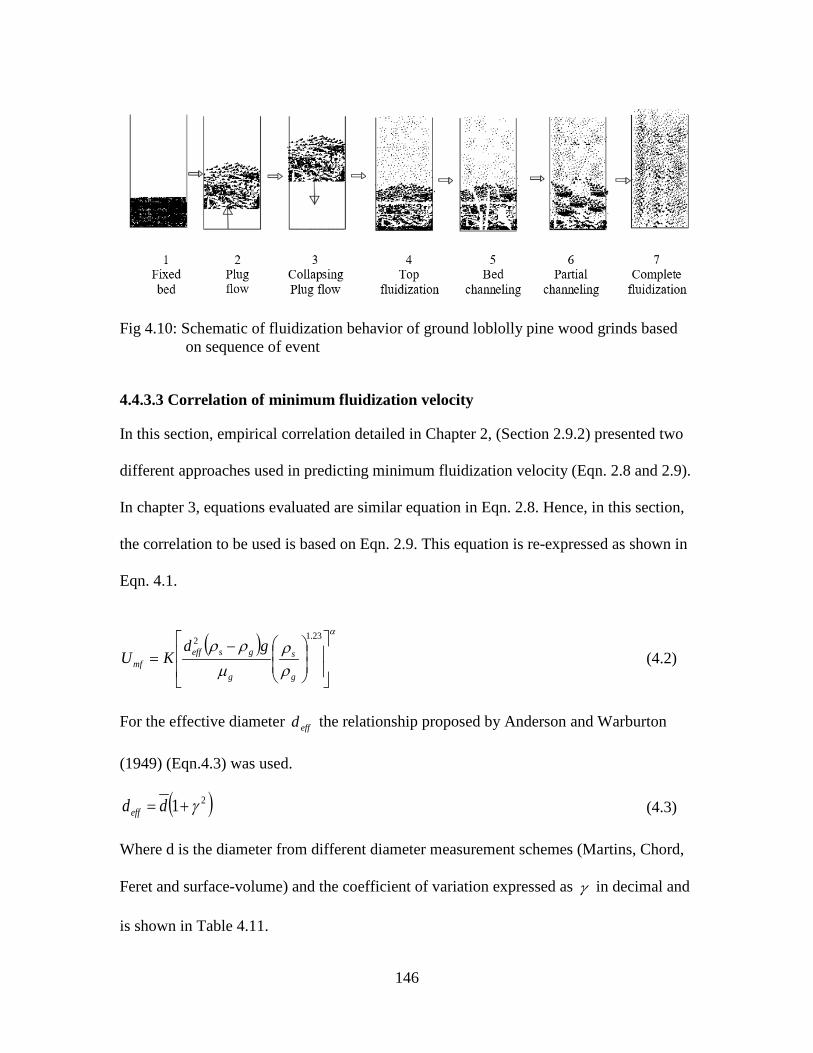
Fig 4.10: Schematic of fluidization behavior of ground loblolly pine wood grinds based
on sequence of event
4.4.3.3 Correlation of minimum fluidization velocity
In this section, empirical correlation detailed in Chapter 2, (Section 2.9.2) presented two
different approaches used in predicting minimum fluidization velocity (Eqn. 2.8 and 2.9).
In chapter 3, equations evaluated are similar equation in Eqn. 2.8. Hence, in this section,
the correlation to be used is based on Eqn. 2.9. This equation is re-expressed as shown in
Eqn. 4.1.
( )α
ρρ
µρρ
−=
23.12
g
s
g
gseffmf
gdKU (4.2)
For the effective diameter effd the relationship proposed by Anderson and Warburton
(1949) (Eqn.4.3) was used.
( )21 γ+= ddeff (4.3)
Where d is the diameter from different diameter measurement schemes (Martins, Chord,
Feret and surface-volume) and the coefficient of variation expressed as γ in decimal and
is shown in Table 4.11.
146

Table 4.11: Particle characterization based on the coefficient of variation (COV) at the
various moisture content levels
Screen size (mm) MC (wet basis) COV=γ
Unfractionated
8.40 0.90 (0.05)a 14.86 0.65 (0.02)b 19.80 0.58(0.04) b 27.02 0.42 (0.02)c
The coefficient of variation were measured based on chord diameter scheme Means with the different superscript (alphabet) in a column are significantly different (p<0.05)
In addition, moisture content term, ψ (in decimal) and particle sphericity terms, ϕ were
included in Eqn. 4.2 as follows
( ) ( )α
ρρ
µρρψϕγ
−+=
23.12222 1
g
p
g
gseffmf
gdKU (4.4)
Eqn. 4.4 can be simplified into
αKXU mf = (4.5)
Where
( ) ( ) 23.12222 1
−+=
g
p
g
gseff gdX
ρρ
µρρψϕγ
(4.6)
Umf Minimum fluidization velocity (m/s) MC, ψ Moisture content (%) d Mean diameter (m) dsv Surface – volume diameter (m) γ Coefficient of variation
sρ Solid density (kg/m3)
Sgw Geometric mean standard deviation (m) effd Effective diameter
gµ Dynamic viscosity (kg /ms) K, α Empirical constants ϕ Sphericity
147

Regression analysis was applied to the plot of the experimental values of the Umf on y-
axis against the parameters X (Eqn. 4.5) on x-axis. The particle diameter (size) used in
estimating the parameter X were obtained from different diameter measurement schemes
presented in Table 4.12. From the regression line in Fig. 4.11, the coefficient K and α
presented in Table 4.13 were obtained using the trendline capability in MS Excel®. Also,
Fig. 4.11 shows the significant effect of size measurement scheme on prediction of Umf.
The steepness reduced with increase in size with Feret and surface-volume diameter
having the least and highest slope respectively. Table 4.12 showed that the measured
values of α reduced in magnitude with reduction in actual size measured as follows i.e.
Feret, Area, Chord, Martins, and surface-volume diameter. About 76% increase in the K
value was estimated when the diameter changed from Ferret to surface-volume diameter,
representing highest and least mean diameter respectively.
Table 4.12: Effect of moisture contents and diameter measurement schemes on mean size
of unfractionated loblolly pine wood grinds
MC (% w.b) Diameter (mm)
Area Chord Ferret Martin Surface-vol.
Unfractionated
8.40 2.87 a, 2
(0.41) 1.01 a, 2,3
(0.36) 4.90 a,1
(0.76) 1.59 a, 3,4
(0.30) 0.82 b,4
(0.04)
14.86 2.42 a, 2
(0.12) 1.43 b c,3
(0.26) 4.18 a, 1
(0.11) 1.18 c b,4
(0.01) 0.57 c, 4
(0.03)
19.80 1.89 b, 2
(0.03) 1.30 c, 3
(0.03) 3.10 b, 1
(0.06) 1.03 c, 4
(0.02) 0.71 b c, 5
(0.02)
27.02 2.48 a, 2
(0.27) 1.83 b a, 3
(0.26) 4.11 a, 1
(0.48) 1.37 b, 2
(0.15) 1.05 a, 4
(0.19) Values are means of three data points and numbers in parentheses are standard deviation, Means with the different superscript (numeric) in a row are significantly different (p<0.05) Means with the different superscript (alphabet) in a column are significantly different (p<0.05)
148

Figure 4.11. Determination of the Umf correlation for unfractionated sample of loblolly
pine wood grinds
Table 4.13: Coefficient estimation at various diameter types
Diameter measurement scheme K α R2 Ferret 0.0056 0.251 0.92 Area 0.0082 0.243 0.98
Chord 0.016 0.205 0.98 Martin 0.0183 0.203 0.99
Surface –volume 0.0234 0.201 0.99
4.4.3.4 Verification of the Umf correlation.
To verify the suitability of equation 4.4, data presented in Chapter 3 were used. The
sample had moisture content of 9.40%, mean sphericity of 0.52, and coefficient of
variation of 0.65 (Please refer to Table 3.4 and 3.5). The Umf of the sample was estimated
to be 0.25 (0.02) m/s (see Section 3.4.3.3). Using Eqn. 4.4 and the coefficients estimated
149

for various diameter schemes, the predicted values of the Umf obtained for the samples
are given in Table 4.14.
Table 4.14: Predicting and validating the Umf using Eqn. 4.4 Measurement
scheme
Density (kg/m3)
Umf (m/s)
MRD (%)
Measured value (mm)
effd ×10-3 (m) pρ gρ X Predicted
Actual
Ferret 4.07 3.01 1469.0 1.23 5008349.0 0.26 0.25
(0.04)
3.8 Chord 1.00 0.74 1469.0 1.23 303557.7 0.21 -7.4 Martin 0.83 0.61 1469.0 1.23 205785.0 0.22 -6.1
Sur.- vol. 0.79 0.58 1469.0 1.23 186313.8 0.27 3.6 Parameters of X calculated from calculated from Eqn. 4.4 and Table 4.11 Sur.-vol. means surface-volume diameter MRD: mean relative deviation calculated from eqn. 4.2.
The mean relative deviations between experimental data and the predicted data using the
Feret, Chord, Martins, and surface-volume mean diameter scheme were 3.8, -7.4, -6.1,
and 3.6 % respectively. The error obtained were lower than to that of Zhong et al. (2008)
who obtained about 13.2 % error between predicted and experimental data using rice
husk and sawdust. Rao et al. (2001) obtained about 48% MRD from predicting the
experimental values of Umf using sand and sawdust (15% fraction) mixture. Also, about
33.05 % MRD was obtained using sand and sawdust (28%) mixture (Aznar et al., 1992).
Therefore, since the percent deviation obtained using the measurement schemes are less
than 20% (Zhong et al., 2008), then all the equation performed satisfactorily. However,
surface –volume diameter produced the least MRD and it would be adjudged most
preferred. Also, most fluidization studies used surface –volume diameter for prediction
standard laboratory determination in absence of image analysis system has be developed.
In addition, this new correlation addressed the deficiencies of selected fluidization
150

equation shown in Table 3.9 and 3.10 principally inability to adapt to change of diameter
measurement scheme and over prediction obtained with MRD greater than 15%.
4.5 Conclusion
Moisture content significantly affects the physical properties of biological material (bulk
density, particle density, porosity, and particle size distribution) that are critical in
determination of minimum fluidization velocity. We investigated the effect of moisture
contents on properties that influences the determination of minimum fluidization velocity
of ground loblolly pine wood. The result shows that as moisture content increased the
bulk density, particle density, and porosity increased. However, with increase in moisture
content, the particle size distribution reduced with coefficient of variation that ranges
from 90 at 8.46% MC to 42 at 27.02 % MC. Also, as moisture content increased the
minimum fluidization velocity values also increased. The minimum fluidization velocity
(Umf) of loblolly pine wood ground was found to be 0.20, 0.24, 0.28 and 0.32 m/s for
moisture content of 8.45, 14.86, 19.86 and 27.02 % wet basis respectively. The grinds
were found to be completely fluidized at 4Umf. The correlation developed predicted the
experimental data with mean relative deviation less than 20%.
151

4.6 Reference
Abdullah, M. Z., Z. Husain, and S. L. Yin Pong. 2003. Analysis of cold flow fluidization test results for various biomass fuels. Biomass and Bioenergy 24(6):487-494. Allen, T. 1997. Particle Size Measurement: Volume 2: Surface Area and Pore Size Determination. Springer. Anderson, S., and F. Warburton. 1949. 46—The porous plug and fibre diameter measurement. Effect of fibre orientation and use of plugs of randomized fibres. Journal of the Textile Institute Transactions 40(11):T749-T758. ASABE. 2006. ASAE S319. 3—method of determining and expressing fineness of feed materials by sieving, ASABE Standards, 602–605, American Society of Agricultural and Biological Engineers, St. Joseph, MI. ASTM. 2006. Standard Test Method for Moisture Analysis of Particulate Wood Fuels," ASTM International, West Conshohocken, PA, 2006, DOI: 10.1520/E0870-82R06. Aznar, M. P., F. A. Gracia-Gorria, and J. Corella. 1992. Minimum and maximum velocities for fluidization for mixtures of agricultural and forest residues with a second fluidized solid. II. Experimental results for different mixtures. International chemical engineering 32(1):103-113. Clarke, K. L., T. Pugsley, and G. A. Hill. 2005. Fluidization of moist sawdust in binary particle systems in a gas solid fluidized bed. Chemical Engineering Science 60(24):6909-6918. Cui, H., and J. R. Grace. 2007. Fluidization of biomass particles: A review of experimental multiphase flow aspects. Chemical Engineering Science 62(1):45-55. Deshpande, S. D., S. Bal, and T. P. Ojha. 1993. Physical Properties of Soybean. Journal of Agricultural Engineering Research 56(2):89-98. Downing, M., L. M. Eaton, R. L. Graham, M. H. Langholtz, R. D. Perlack, A. F. Turhollow Jr, B. Stokes, and C. C. Brandt. 2011. US Billion-Ton Update: Biomass supply for a bioenergy and bioproducts industry. Oak Ridge National Laboratory (ORNL). Fasina, O. 2006. Flow and physical properties of switchgrass, peanut hull, and poultry litter. Transactions of the ASABE 49(3):721-728. Fasina, O. O. 2008. Physical properties of peanut hull pellets. Bioresource Technology 99(5):1259-1266.
152

Gauthier, D., S. Zerguerras, and G. Flamant. 1999. Influence of the particle size distribution of powders on the velocities of minimum and complete fluidization. Chemical Engineering Journal 74(3):181-196. Hughes, W. E., and E. D. Larson. 1997. Effect of fuel moisture content on biomass -IGCC performance In International Gas Turbine and Aeroengine Congress and Exhibition. ASME, ed: American Society of Mechanical Engineers. Huntinton, C. 1924. The Idaho Forester. In A preliminary study of shrinkage in Idaho confers, 58. Moscow Idaho: university of Idaho. Kenney, K. L., W. A. Smith, G. L. Gresham, and T. L. Westover. 2013. Understanding biomass feedstock variability. Biofuels 4(1):111-127. Khanal, S. K. 2010. Bioenergy and biofuel from biowastes and biomass. ASCE Publications, Reston Virginia. Kunii, D., and O. Levenspiel. 1991. Fluidization engineering. Butterworth-Heinemann Boston. Lam, P., S. Sokhansanj, X. Bi, C. Lim, L. Naimi, M. Hoque, S. Mani, A. Womac, S. Narayan, and X. Ye. 2008. Bulk density of wet and dry wheat straw and switchgrass particles. Applied Engineering in Agriculture 24(3):351-358. Mani, S., L. G. Tabil, and S. Sokhansanj. 2004. Grinding performance and physical properties of wheat and barley straws, corn stover and switchgrass. Biomass and Bioenergy 27(4):339-352. Manickam, I. N., and S. Suresh. 2011. Effect of moisture content and particle size on bulk density, porosity, particle density and coefficient of friction of coir pith. International Journal of Engineering Science 3. Mattsson, J. E., and P. D. Kofman. 2002. Method and apparatus for measuring the tendency of solid biofuels to bridge over openings. Biomass and Bioenergy 22(3):179-185. Mujumdar, A. S. 2006. Handbook of industrial drying. 3rd ed. CRC Press, Florida US. Nemec, D., and J. Levec. 2005. Flow through packed bed reactors: 1. Single-phase flow. Chemical Engineering Science 60(24):6947-6957. Oginni, O. J. 2014. Contribution of particle size and moisture content to flowability of fractionated ground loblolly pine. M.S thesis. Auburn University, Biosystems Engineering Department, Auburn Alabama. Oliveira, T. J. P., C. R. Cardoso, and C. H. Ataíde. 2013. Bubbling fluidization of biomass and sand binary mixtures: Minimum fluidization velocity and particle
153

segregation. Chemical Engineering and Processing: Process Intensification 72(0):113-121. Probst, K., A. Kingsly, R. Pinto, R. Bali, P. Krishnakumar, and K. Ileleji. 2013. The effect of moisture content on the grinding performance of corn and corncobs by hammermilling. Transactions of the ASABE 56(3):10251-11033. Raigar, R., and H. Mishra. 2015. Effect of Moisture Content and Particle Sizes on Physical and Thermal Properties of Roasted Bengal Gram Flour. Journal of Food Processing and Preservation. Rao, R., T. Ram, and J. V. Bheemarasetti. 2001. Minimum fluidization velocities of mixtures of biomass and sands. Energy 26(6):633-644. Rhén, C., R. Gref, M. Sjöström, and I. Wästerlund. 2005. Effects of raw material moisture content, densification pressure and temperature on some properties of Norway spruce pellets. Fuel Processing Technology 87(1):11-16. Rhodes, M. 2008. Introduction to particle technology. Wiley. Rousset, P., T. Petithuguenin, T. Rodrigues, and A.-C. Azevedo. 2012. The fluidization behaviour of torrefied biomass in a cold model. Fuel 102(0):256-263. SAS. 2011. The SAS system for Windows. Ver. Release 9.2. Cary, NC.: SAS Institute. Smith, W. B., P. D. Miles, C. H. Perry, and S. A. Pugh. 2009. Forest resources of the United States, 2007: a technical document supporting the forest service 2010 RPA Assessment. General Technical Report-USDA Forest Service(WO-78). Srivastava, A., and S. Sundaresan. 2002. Role of wall friction in fluidization and standpipe flow. Powder Technology 124(1):45-54. Tsinontides, S., and R. Jackson. 1993. The mechanics of gas fluidized beds with an interval of stable fluidization. Journal of Fluid Mechanics 255:237-274. Wear, D., and J. Gries. 2011. The Southern Forest Futures Project. Technical Report. USDA Forest Service, General Technical Report SRS, Asheville, North Carolina. Wilkinson, D. 1995. Determination of minimum fluidization velocity by pressure fluctuation measurement. The Canadian Journal of Chemical Engineering 73(4):562-565. Woodcock, C., and J. Mason. 1988. Bulk solids handling: an introduction to the practice and technology. Springer.
154

Wormsbecker, M., and T. Pugsley. 2008. The influence of moisture on the fluidization behaviour of porous pharmaceutical granule. Chemical Engineering Science 63(16):4063-4069. Wright, C. T., P. A. Pryfogle, N. A. Stevens, J. R. Hess, and C. W. Radtke. 2006. Value of distributed preprocessing of biomass feedstocks to a bioenergy industry. Idaho National Laboratory. Yu, A., and N. Standish. 1993. Characterisation of non-spherical particles from their packing behaviour. Powder Technology 74(3):205-213. Zhang, Y., B. Jin, and W. Zhong. 2009. Experimental investigation on mixing and segregation behavior of biomass particle in fluidized bed. Chemical Engineering and Processing: Process Intensification 48(3):745-754. Zhong, W., B. Jin, Y. Zhang, X. Wang, and R. Xiao. 2008. Fluidization of Biomass Particles in a Gas−Solid Fluidized Bed. Energy & Fuels 22(6):4170-4176. Zhou, B., K. Ileleji, and G. Ejeta. 2008. Physical property relationships of bulk corn stover particles. Transactions of the ASABE 51(2):581-590.
155

Chapter 5: Air Flow through Packed Columns of Ground Loblolly Pine Wood:
Revised Ergun Expression
5.1 Abstract Existing model equations that may be used for predicting pressure drop as a result of
fluid flow through beds of granular materials non-uniform particle size are limited
because the void correlation used were developed using uniformly sized particles. Also,
the equation do not have terms to account for the influence of size distribution on air flow
and penetration through the bed. In this study, Ergun equation was modified by revising
the viscous and kinetic energy losses correlations and incorporating a term for coefficient
of variation of particles of ground loblolly pine wood. In addition, a new frictional factor
relating Reynold number to kinetic and viscous energy losses were proposed and tested.
Furthermore, a revised Ergun’s equation was proposed, tested and validated using ground
loblolly pine wood, and data from other published work. The coefficient K1 and K2 was
determined by methods of least square to be 201 and 2.7 respectively. The overall relative
mean deviation obtained between the predicted and experimental pressure drop using
ground loblolly pine wood and the equation developed in this study and the Ergun
equation were -17.48 % and 63.5 % respectively.

5.2 Introduction Fluidization is a process by which a bed of solids is transformed into a condition similar
to fluid flow by suspending the solids in a stream of fluid. The goal is to enhance contact
between fluid and solids, by increasing the surface area of solids exposed to the fluid – a
desire feature in applications such as drying, adsorption, combustion, carbonation, and
gasification. Depending on the objectives of the application, the solids may consist of
multicomponent particles that have differing behavior to gas/liquid fluidization
(Formisani et al., 2011). Examples of fluidizing behaviors that have been observed for
multicomponent particles include entrainment (Hrenya and Sinclair, 1997), segregation,
channeling, pressure fluctuation and un-controllable bed expansion due to the formation
of bubbles, slugging, plug flow and poor bed mixing (Das et al., 2008; Hoffmann et al.,
1993; Hrenya and Sinclair, 1997; Liu et al., 2008; Seu‐Kim and Arastoopour, 1995;
Zhang et al., 2008, 2009). These undesirable behaviors have limited the ability of
scientists and engineers to predict the state of bed during fluidization. As a result,
advantages associated with proper mixing such as uniform thermal concentration gradient
cannot be adequately exploited.
Fluidization of bed that consist of multicomponent particles have received attention of
several researchers in the past (Abrahamsen and Geldart, 1980; Ergun, 1952; Geldart,
1972; Kumar and SenGupta, 1974; Obata et al., 1982; Reina et al., 2000; Rowe and
Nienow, 1975; Wen and Yu, 1966). These researchers reported the influence of fluid
flow velocity on pressure losses and particle-fluid behaviors. These studies used the fluid
properties and averaged properties of solids (e.g. average density and average particle
157

size) to develop analytical/empirical expressions for predicting the pressure drop and
velocity of a fluidized bed system.
One of the most widely used analytical expression for representing the relationship
between pressure drop at different fluid flow in packed bed is Ergun’s expression
(henceforth refers to Ergun) (Wang, 2014). Ergun equation was developed with the
recognition of additive effect of the viscous and kinetic energy losses in a packed bed and
smooth transition from a viscous dominated to kinetic dominated effects as fluid flow
rate increased in a bed. Starting from Eqn. 5.1, which states that pressure drop across a
granular bed, is proportional to the fluid velocity at low flow rate and to the square of the
velocity at high flow rates. Ergun plotted ΔP/LU against ρU, using a bed of crushed coke
packed to different fractional void volume. Assuming a continuous function for the
relationship between pressure drop and fluid flow rate. The author added Poiseuilles’s
expression and his earlier developed void fraction correlations (viscous and kinetic)
(Ergun, 1951). A fit of experimental data to the Ergun’s expression for crushed coke
resulted in Ergun constants K1 = 150 and K2 = 1.75. The first term on the right-hand side
of Eqn. 5.2 represents viscous energy at low fluid flow rate while the second term on the
right hand side represent kinetic energy loss due to high fluid flow rate.
2UbUaLP ρµ +=
∆ (5.1)
( )
p
mf
p
m
dU
KdU
KLP 2
3223
2
111 ρ
εεµ
εε −
+−
=∆ (5.2)
where, ΔP/L= pressure gradient across channel (Pa/m),
Um = superficial velocity (m/s),
158

µ = fluid viscosity (Pa.s),
ρf = fluid density (kg/m3),
ε = porosity, and
dp = particle diameter (m).
Ergun identified the rate of fluid flow, viscosity and density of fluid, closeness and
orientation, size, shape, surface area and bed void fraction as factors that influence the
relationship between pressure drop and fluid flow velocity. When a bed consists of
particle with uniform shape and size distribution, Ergun’s expression has been proven to
perform satisfactorily in predicting pressure drop data at different gas flow rates. For
instance, using a bed consisting of spherical shaped alumina and glass beads, Nemec et
al. (2001) and Mawatari et al. (2003) obtained 4.2% and 5% error deviation between
experimental and predicted pressure drop data. Similar conclusion were made by Cloete
et al. (2015), Jing et al. (2000), Dolejs and Machac (1995) and Lippens and Mulder
(1993).
For a bed that consist of non-spherical particles with non-uniform particle size
distribution typical of biomass grinds, there is a need to modify Ergun’s equation before a
good prediction can be made. For instance, Dolejs and Machac (1995) obtained 72.6 and
24.9 % mean relative deviation for a bed consisting of polyhedral and cubes respectively.
Using a bed of Zeolite having a mean particle size of 6 mm and shape factor of 0.8,
Çarpinlioğlu and Özahi (2008) obtained a 28% deviation of experimental data from
predicted pressure drop. When bed is composed of cylindrical particles, the pressure drop
obtained was 35% higher than the experimental (Gunarathne et al., 2014). Luckos and
Bunt (2011) predicted the pressure drop in individual reaction zones in a commercial
Sasol-Lurgi gasifier. The author obtained about 70% error in the predicted and
159

experimental pressure drop in the combustion and gasification zones and the author
attributed the high deviation to voidage and Ergun equation inability to capture the effect
of particle size distribution within the zones. Kim and Han (2006) obtained 50%
deviation between predicted and experiment Umf. The author attributed the discrepancy to
high cohesive force between fine particles in phosphor which Ergun equation expression
was unable to capture. Hence, it can be concluded that Ergun equation in its original
form cannot be reliably used to predict pressure drop in beds that consist of non-spherical
particles.
In order to modify Ergun equation, the focus should not only be on changing Ergun’s
constants but also estimating appropriate void fraction at different flow velocity (laminar
or turbulent). This is because, as fluid velocity passed through the bed increase, small
particles are entrain, while larger and heavier particles are yet to be fluidized. In addition,
size and shape of non-spherical particle depends on several factors such as particle
orientation, measuring technology, and moisture content (Bouwman et al., 2004). These
issues have resulted in limited success in improving Ergun equation for non-spherical and
non-uniform particles size bed (Dolejs and Machac, 1995; Gunarathne et al., 2014;
Innocentini et al., 1999).
Some authors have attempted to refit Ergun’s equation and obtain new value for constant
(K1 and K2) but retain Ergun’s equation structure. Cloete et al. (2015) proposed K1 = 250
and K2 = 2.5 respectively for cylindrical particle of γ-Al2O3 Quinn (2014) proposed 267
for K1 while K2 is dependent on type of material. For leadshot, glass beads and white
sand, the K2 values were obtained to be 2.14, 2.51, 4.02 respectively. Also, Ozahi et al.
(2008) proposed a constant of K1 =160 and K2 = 1.61 for zeolite and chickpeas. In all
160

these studies, no attempt was made at changing or modifying the void fraction
correlation. In addition, these authors used spherical particles having uniform particle
size with void fraction that was less than 0.5. These conditions were sometimes imposed
on particles so as to satisfy Ergun assumptions (see section 2.9.1). Hence, the studies
were simply validating Ergun equation for other materials. However, for biomass grinds,
having high void fraction usually up to 0.8, lognormal size distribution, and non-spherical
particle shapes. Ergun’s structures and assumption has to be reexamined before good
prediction can be obtained.
In light of the limitations highlighted, the overall goal of this study is to propose and
validate a revised Ergun’s equation suitable for non-spherical materials with non-uniform
particle size distribution such as biomass grinds. First, a suitable void fraction correlation
will be derived for predicting kinetic and viscous fractional void correlation. Second,
Ergun’s equation will be revised using the void fraction correlation obtained and adapted
to loblolly pine wood grinds by accounting for the shape, porosity, and particle size
distribution using the coefficient of variation.
5.3 Methodology 5.3.1 Material preparation Clean loblolly pine wood chips were obtained from a forest plantation in Alabama, U.S.
The moisture content was determined to be 8.45 % using ASTM standard E871-82
ASTM (2007). The chips were ground through hammer mill (Model No. 10HBLPK,
Sheldon Manufacturing, Tiffin, OH) fitted with screen size of 22.23 mm (7/8 inches),
19.05 mm (3/4 inches), 15.88 mm (5/8 inches), 12.7 mm, (1/2 inches), 9.53 mm (3/8
inches), 6.35 mm (1.4 inches), or 3.18 mm (1/8 inches). This resulted in seven samples
161

with different bulk densities. The physical properties of each sample were determined as
described below.
5.3.2 Particle size
Particle size distribution of each sample was determined using a particle size analyzer
(Camsizer®, Retsch Technology, Haan, Germany). For this analysis, about 100g of each
of the sample was poured into the hopper from where it was conveyed through the
vibratory feeder to the measurement chamber of the system. In the chamber, images of
the falling particles were taken using two cameras located at the measurement field. The
software attached to the instrument then use the images recorded and the result was used
to plot the size distribution. In addition, Ferret, Martins, area, surface to volume and
chord diameter measurement schemes were recorded from the software. The surface to
volume diameter measurement scheme was estimated from the specific surface data
(Rhodes, 2008). The sphericity (φ) values of the particles were obtained from the
software using ISO 9276-6 standard procedure (ISO/9276-6, 2008). For each particle size
distribution data, particle characteristic needed (X84, X16, X50) to compute the coefficient
of variation (COV) (Eqn. 5.3) were recorded from the software.
50
168450X
XXCOV
−= (5.3)
where;
X85 is particle diameter at 84% probability (mm)
X16 is particle diameter at 16% probability (mm)
X50 is particle diameter at 50% probability (mm)
162

5.3.3 Particle density The particle density of sample were determined using a gas pycnometer (Accupyc 1330,
Micromeritics Instrument Corp., Norcross, Ga.). The gas pycnometer, uses helium to
estimate the pressure difference between a reference cell and a cell containing the sample.
The pressure difference was used by the pycnometer to estimate the volume of a known
mass of sample. A digital weighing scale (Model AR3130, Ohaus Corp, Pinebrook, NJ)
was used to measure the sample mass. Particle density was estimated as the ratio of the
mass of the sample in the cell and the volume estimated by the pycnometer.
5.3.4 Bulk density Bulk density was determined using an apparatus that consists of a funnel through which
the sample freely falls onto 1137 mm3 cup. The ratio of the mass of the sample in the
container to the volume of the container was used to compute the estimated bulk density.
5.3.5 Porosity The inter – granular porosity (ε) of the ground wood sample was calculated from the
measured values of bulk density and particle density as follows;
p
bρρ
ε −=1 (5.4)
where ρb is bulk density (kg/m3) and ρp is particle density (kg/m3).
5.3.6 Pressure drop and flow rate measurement test A description of this experimental setup can be found in section 3.3.6.
163

5.3.7 Void fraction correlation modification: concept Understanding Ergun’s argument would aid improving the void fraction correlation in
Eqn. 5.2. In a packed bed, the solid and void fractions are related using Eqn. 5.5, 5.6, and
5.7.
solidair
airvoid VV
V+
=ε (5.5)
( ) solidvoidvoidair VV εε =−1 (5.6)
airvoid
voidsolid VV
εε−
=1
(5.7)
where, voidε is the void faction
airV is the volume occupied by air (m3)
solidV volume occupied by solid (m3)
Earlier researchers (Hatch, 1943; Leva et al., 1951) suggested a non-linear expression of
the void fraction ( )
−n
m
εε1 as a function of fluid velocity, where m and n are positive
integer with values 1 (lamina) and 3 (turbulent) for bed with uniform particles sizes.
Using this concept, Ergun stated that the entropy in a bed at low (viscous) and high
(kinetic) fluid flow rate should be different and be proportional to the coefficients a and b
in Eqn. 5.1 respectively. In other word, coefficients a and b should be directly
proportional to ( )n
m
εε−1 at certain combinations of values of m and n for viscous and
turbulent flow for the theory to be valid. Then changing the value of m and n until such a
164

point that the value of R2 is maximum would result in the appropriate void correlation.
Hence, this approach would be used in this study to modify the void fraction correlations
of Ergun equation for loblolly pine wood grinds.
5.3.8 Data analysis All experiments were conducted in triplicates and results are presented in the relevant
sections as mean values and standard deviation. Test of significance of the variables
(screen size, porosity, particle and bulk density, particle size, sphericity and coefficient of
variation) were conducted using the analysis of variance (ANOVA) procedures (SAS,
2011). Tukey multiple range test (using the same software) was used to compare means
of each properties. Differences were considered to be statistically significant when p <
0.05. Statistical Mean Relative Deviation (MRD) (Eqn. 5.8) was used as statistical
indicator to compare the predictive ability of the equations (Original Ergun and modified
Ergun (Nemec and Levec, 2005).
( ) ∑=
−=
N
i i
icalci
NMRD
1 exp.
exp..1001%λ
λλ (5.8)
exp.iλ is experimental values
cali.λ is calculated/predicted
N is number of data points
165

5.4 Experimental result and model derivation 5.4.1 Particle size and coefficient of variation The particle size distributions obtained by grinding the sample through different screen
size are shown in Fig. 5.1. Similar to particle size of ground biological material, the
distribution show positive skewness which indicates that the tail on the right side is
longer than the left side. The estimated geometric mean diameter for each of the sample
is given in Table 5.1. The values obtained for the sample coefficient of variations was
greater than 60%, which further demonstrated that the particle size within the sample
varied widely. However, screen size did not significantly affect the coefficient of
variation of particle (p < 0.05).
Figure 5.1: Particle size distribution for loblolly pine wood grinds obtained from hammer
mill at different screen sizes.
166

Table 5.1: Physical properties of loblolly pine wood grinds ground through different
screen sizes. Screen Size (mm)
Diameter Sur.-vol.
(mm) Sphericity
Bulk density (kg/m3)
Particle density (kg/m3)
Porosity COV
6.35 0.79 c (0.10) 0.37c (0.10)
250.89 b (2.40)
1453.30 ab (44.10)
0.83b (0.01)
72.60 bc (0.01)
9.53 0.91 ba (0.10) 0.37 a (0.10)
252.80 b (2.80)
1420.40b (12.10)
0.84ab (0.01)
72.80 c
(0.1)
15.88 0.98a (0.10) 0.39 b (0.10)
229.93d (1.60)
1448.20ab (3.03)
0.84ab (0.01)
72.50 abc
(0.1)
19.05 0.94a (0.03) 0.42 a (0.10)
228.27d (2.90)
1424.90b (12.15)
0.84ab (0.01)
67.90c
(0.06)
22.23 0.98a (0.03) 0.41 a (0.01)
222.72e (3.30)
1438.80ab (11.70)
0.85a (0.01)
64.00 c
(0.02) Values are means of triplicates experimental runs Numbers in parentheses are standard deviation Means with the different superscript (alphabet) in a column are significantly different (p<0.05) COV means coefficient of variations (calculated using Eqn. 5.3) Sauter means surface to volume mean diameter (calculated using 6/specific surface obtained from CamSizer®)
5.4.2 Bulk and particle densities The result showed that the bulk densities decreased (p <0.05) as particle size increased
(Table 5.1). This has been attributed to reduction in voids between the particles as
particle size decreased (see values of porosity in Table 5.1) (Gil et al., 2013; Ryu et al.,
2006). Lam et al. (2008) also reported that bulk density of wet and dry wheat straw and
switchgrass particles reduced with increase in nominal screen size. It is also important to
point out that the bulk density result is opposite of Table 4.7. The sample in the present
study composed of different particle sizes and smaller size particles occupy spaces
between the bigger particles. Therefore, reduction in particle size produced more smaller
size fraction resulting in increase in bulk density. However, particle density did not
significantly vary with increase in particle size (p < 0.05). This could be that the exposure
167

of pores spaces as a result of size reduction process within the screen size ranged in this
aspect of the study were not significant.
5.4.3 Porosity and sphericity Table 5.1 shows that the reduction in porosity was less than 5 % as mean diameter
reduced from 2.10 to 1.19 mm and this reduction was not statistically significant
(p<0.05). Marginal reduction in porosity value can be attributed to the particle
distribution and the particle shape. As bigger particles reduced in size, the smaller
particles in the sample increase and occupy some of the void in between the larger
particles. In addition, particle shape (Table 5.1) influence the packing density as an
irregularly shaped particle having a pin-like structure can bend and interlock with other
particles within the sample, blocking available spaces and creating a more dense bed. The
results also showed that the mean sphericity of particles increased by 20 % as particle
size increased.
5.4.4 Pressure drop and flow rate measurement test The plots of ratio of pressure gradient to velocity against air mass flow rate (Eqn. 5.1) are
shown in Fig 5.2 for loblolly pine wood grinds that were prepared with different screen
sizes are linear. This plot is similar to what Ergun obtained using crushed coke (Ergun,
1952). Also, it can be deduced from the plot that reduction in particle size resulted in
higher pressure losses because air was forced through the packed bed. This could be
attributed to the fact that as particle size reduced, void fraction reduced thereby reducing
the airflow and increasing pressure gradient.
168

Figure 5.2: Linear form of pressure–drop equation (Eqn.5.1) using loblolly pine wood grinds having different size and void fractions.
The slopes, intercepts and the corresponding R2 value of each plots in Fig 5.2 is
summarized in Table 5.2. When the nominal screen size reduced by 89.8%, the slope and
intercept increased by 67.7 and 38.2 % respectively. Since the intercept and slopes are
related to viscous and kinetic energy losses respectively (Ergun, 1952), increases in the
value of intercept or slope indicate that resistance of the bed material to stress-shear
deformation at viscous level and bed entropy (particle-particle collision per unit area due
to kinetic energy) increased with reduction in size.
169

Table 5.2: Estimation of slope and intercept parameters for loblolly pine wood at different particle sizes.
Screen size (mm) +Slope +Intercept +R2 1Viscous 2Kinetic
6.35 mm 1/4 inches 3346.2 883.2 0.90 0.053 0.31
9.53 mm 3/8 inches 3248.3 811.1 0.95 0.046 0.28
15.88 mm 5/8 inches 3053.4 687.7 0.93 0.042 0.27
19.05 mm 3/4 inches 3071.1 670.5 0.98 0.041 0.26
22.23 mm 7/8 inches 2999.8 633.1 0.97 0.039 0.25
+Values obtained from Fig. 4 1values estimated from porosity data Table 5.2 and viscous void fraction correlation ( ) 321 εε−
2values estimated from porosity data Table 5.2 and kinetic void fraction correlation ( ) 31 εε−
5.4.5 Void fraction correlation development: Ergun’s correlation
Fig. 6.3 and 6.4 show the plot of slope and intercept (from Table 6.2) against viscous,
( ) 321 εε− and kinetic fractional correlation, ( ) 31 εε− used by Ergun respectively. It
can be seen that the R2 values from viscous energy void correlation is 0.9528 while that
of kinetic energy correlation 0.611. Hence, the Ergun’s kinetic energy correlation does
not appear to be adequate for loblolly pine wood grinds.
170

Figure 5.3: Dependence of viscous energy losses on fractional void volume correlation
used in Ergun’s equation.
Figure 5.4: Dependence of kinetic energy losses on fractional void volume correlation
used in Ergun’s equation
171

5.4.6 Modification of void fraction correlation In order to refit the void fraction correlations for kinetic energy losses, the Microsoft
Excel® nonlinear solver was employed to minimize the error sum of square between
predicted (void correlation data) and the corresponding actual data (slope data). While
iterating, the solver simultaneously change the parameters of m and n until a solution in
which all-internal solver constraint and optimality conditions are satisfied (in this case the
solver minimized the error sum of square). At this point, the value of m and n was then
chosen as the modified correlation as shown in Eqn. 5.9. Fig 6.5 show the plot of slope
values (Table 6.2) against the new kinetic fractional void correlation obtained. It can be
seen that the modified kinetic (R2=0.94) fractional correlation resulted in 35 %
improvement over R2 obtained from Ergun’s kinetic fractional void correlation (Fig. 6.4).
( )4.3
3.01εε−
=kinetic (R2 = 0.94) (5.9)
Figure 5.5: Dependence of kinetic energy losses on modified fractional void volume correlation used in Ergun’s equation (Eqn. 1)
172

5.4.7 Model presentation
In this section the particle size, shape, particle distribution using coefficient of variation
would now be included in the model.
Combining Eqn. 5.1 and the derived void fractional correlations (Fig. 5.3 and 5.5)
( ) ( ) 24.3
3.0
3
2 11 UbUaLP ii ρ
εεµ
εε −
+−
=∆
(5.10)
Also, comparing Eqn. 5..10 with Eqn. 5.2 ( ) ( ) 2
4.3
3.0
223
2
111 U
dKU
dK
LP
fρεεµ
εε −
+−
=∆ (5.11)
The relationship proposed by Anderson and Warburton (1949) was adopted for the
coefficient of variation term as shown in Eqn. 5.12
( )21 cvdd += (5.12)
Where d is the mean diameter (m) and cv is the coefficient of variation (in decimal)
Inserting Eqn. 5.12 and sphericity term into Eqn. 5.11
( )( )( )
( )( )
224.3
3.0
2223
2
1 11
11 U
cvdKU
cvdK
LP
fρε
εµε
ε+
−+
+
−=
∆ (5.13)
In order to incorporate the effect of shape of the particle, several researchers multiply the
diameter with the sphericity factor (Zhong et al., 2015).
( )( )( )
( )( )
224.3
3.0
2223
2
1 11
11 U
cvdKU
cvdK
LP
fρϕεεµ
ϕε
ε+
−+
+
−=
∆ (5.14)
whereϕ is the sphericity of the particle
Converting Eqn. 5.14 into a linear form result in
( )( )
( )( ) µεε
ϕρ
εµϕε
7.14.0
2
212
22223
11
11
−
++=
−+∆ cvUd
KKcvdLU
P f (5.15)
173

where,
µρUdN =Re
and ( )21 cvdd +=
then, Eqn. 17 can be re-expressed as
( ) ( ) 7.14.0Re
212
23
11 εεεµε
−+=
−
∆ NKKd
LUP (5.16)
Since the viscous term was used in the denominator of Eqn. 5.16, the left hand side of
Eqn. 5.16 can then be defined as the ratio of pressure drop to the viscous energy term and
will be designated by fv
( )223
1 εµε−
∆=
dLU
Pfv (5.17)
( ) 7.14.0Re
21 1 εε −+=
NKKfv (5.18)
According to Eqn. 5.18, a linear relationship exist between fv and ( ) 7.14.0
Re
1 εε −N
Similar to Eqn. 5.18, the Ergun version of the expression of ratio of pressure drop to the
viscous energy term is expressed as follows
ε−+=− 1
Re21
NKKf Ergunv (5.19)
It can be seen that Eqns. 5.18 and 5.19 are comparable because they are both related to
void fraction. Furthermore, when kinetic term was used in denominator of Eqn. 5.20, and
the left hand side can then be defined as the ratio of pressure drop to the viscous energy
term and will be designated by fk
( )( )
( )( ) 21
4.07.1
13.02
24.3
11
11 KK
UcvdK
Ucvd
LUP
ff
++
−=
−+∆
ρϕµεε
ερε (5.20)
174

( )( ) 3.02
24.3
11
ερε
−+∆
=U
cvdLU
Pff
k (5.21)
( )21
Re
7.14.0 1 KKN
fk +−
=εε (5.22)
Similar to Eqn. 5.19, the Ergun version of the expression of ratio of pressure drop to the
kinetic energy term, kf is expressed as follows
2Re
11 KN
Kf Ergunk +−
=−ε (5.23)
Based on Eqn. 5.19, Ergun stated that a linear relationship existed between fv-Ergun and
ε−1ReN
Therefore, a plot of all the data in Fig. 5.2 using Eqn. 5.19 should result in a single value
with intercept K1 and slope K2. Using Ergun’s methodology, we plotted fv against
ερ−1U
and this resulted in the plot shown in Fig 5.6. A fit of a linear equation to the data
presented in Fig 5.6 resulted in a negative intercept of -67.8. Ergun first assumption was
to recognize the additive effect of the viscous and kinetic energy losses in a packed bed
and the smooth transition from a viscous dominated to kinetic dominated effects as fluid
flow rate increased. In addition, it can be seen that the data fall on different lines with
respect to their screen sizes. Similar observation was made by Quinn (2014) who
attributed the inability to align all data on a single line using Ergun’s procedure to the
imbalance created as a result of absence of diameter and viscosity terms as expected in
Eqn. 5.19.
175

Figure 5.6: A general plot for a single system having different void fraction using
Ergun’s concept using chord diameter scheme.
When fv was plotted against( ) 7.14.0
Re
1 εε −N (Eqn. 5.18), Fig. 5.7 shows that all data
essentially fell on a straight line with R2 value of 0.95 when chord diameter measurement
scheme was used. The plots for other diameter measurement scheme are presented in
appendix 5. From Fig 5.7, the estimated values K1 = 201.6 and K2 = 2.7. These K1 and K2
values are comparable to the values obtained by other author who had earlier remodified
Ergun equation reported (Table 5.3). Inserting the coefficient values into Eqn. 5.14
results in eqn. 5.24.
176

( )( )( )
( )( )
224.3
3.0
223
2
117.2
1
1201 Ucvd
UcvdL
Pfρ
ϕεεµ
ϕε
ε+
−+
+
−=
∆ (5.24)
Figure 5.7: A general plot for a single system having different void fraction using chord
diameter measurement scheme.
177

Table 5.3: Comparison of K1 and K2 values with literature data K1 K2 Reference
201.6 2.7 Ground loblolly pine wood In this study
250 2.5 Polylobed particles (Nemec and Levec, 2005)
160 1.61 Glass beads (Ozahi et al., 2008)
160.4 2.8 Coal char (Koekemoer and Luckos, 2015)
180 1.8 Literature data (Macdonald et al., 1979)
250 2.5 γ-Al2O Cloete et al. (2015)
267 2.14,
2.51,
4.02
Leadshot, Glass beads and white
sand
Quinn (2014)
From Eqn. 5.18, following Ergun’s procedure the normalized viscous energy losses vf
can be expressed as
( ) 7.14.0Re
17.2201
εε −+=
Nfv (5.25)
Similarly, the normalized kinetic energy losses kf is shown in Eqn. 5.22 can now be re-
expressed as
( ) 7.21201Re
7.14.0
+−
=N
fkεε (5.26)
178

5.5 Model validation 5.5.1 Performance of equation by experimental pressure drop data
Validation of modified equation (Eqn. 5.26) was carried out by comparing the prediction
obtained with Ergun equation expressed in Eqn. 5.27.
( )p
mf
p
m
dU
Kd
UK
LP
ϕρ
εε
ϕµ
εε 2
32223
2
111 −
+−
=∆ (5.27)
where, ΔP/L= pressure gradient across channel (Pa/m),
Um = superficial velocity (m/s),
µ = fluid viscosity (Pa.s),
ρf = fluid density (kg/m3),
ε = porosity,
dp = particle diameter (m), and
φ = sphericity factor
A new set of loblolly pine wood chips were acquired with the initial moisture content
were determined to be 9.45 % using ASTM standard E871-82 ASTM (2007). The chips
were ground through hammer mill (Model No. 10HBLPK, Sheldon Manufacturing,
Tiffin, OH) fitted with screen sizes 15.88 mm (5/8 inches), 12.7 mm, (1/2 inches), 9.53
(3/8 inches), 6.35 mm (1/4 inches), or 3.18 (1/8 inches). The physical properties of each
these samples were determined as described Section 5.3 and the result of the physical
properties is presented as follows;
179

Table 5.4: Physical properties of loblolly pine wood grinds used for validation
Screen size Diameter (mm) Density kg/m3
Porosity Sphericity
COV Sur-vol. Particle Bulk
15.8 mm (5/8 inches)
2.28a
(0.30) 1437.70a
(4.97) 275.38c (2.62)
0.81a
0.45a
(0.003) 60.03a (4.49)
12.7 mm (½ inches)
2.04a
(0.20) 1436.40a
(9.08) 282.36c (4.25)
0.80a
0.46a (0.01)
60.52a (2.77)
9.53 mm (3/8 inches)
1.37b
(0.16) 1433.20a (10.33)
297.85 b (10.43)
0.79b
0.46a (0.01)
63.72a (4.37)
6.35 mm (¼ inches)
0.79c (0.03)
1422.30ba (2.45)
311.14ab (1.57)
0.78c
0.38cb (0.01)
65.48a (11.94)
3.18 mm (1/8 inches)
0.68 c (0.01)
1426.83a (4.93)
312.19a (0.88)
0.78c
0.43cb (0.01)
61.87a (2.42)
Values are means of triplicates experimental runs Numbers in parentheses are standard deviation Means with the different superscript (alphabet) in a column are significantly different (p<0.05) Sauter means surface to volume mean diameter (calculated using 6/specific surface obtained from CamSizer®) COV means coefficient of variations (calculated using Eqn. 5.3)
Fig 5.8 shows pressure drop per unit length against airflow velocity. The pressure drop
increased as airflow velocity increased. Similar profile was obtained by Mayerhofer et al.
(2011) who investigated pressure drop across a packed bed of irregular shaped wood
particles and Li et al. (2015) who used sand bed materials. Fig 5.8 – 5.10, shows
comparison between the experimental data and the predictions of pressure drop at various
airflow velocities obtained from Ergun equation (Eqn. 5.2) (the Ergun expression used
has sphericity term) and the equation developed in this study (Eqn. 5.24). Figure 5.9
shows that the prediction obtained when the loblolly pine wood was ground through 5/8
inches screen size was used. It can be seen that the predicting equations (Ergun and
modified) under predicted the pressure drop at any air velocity. However, modified
equation predictions were closer to experimental data. Similar profile was obtained from
sample ground through ¼ inch screen size (Fig 5.9). However, in Fig. 5.11, modified
equation over predicted the experimental data.
180

Figure 5.8: Pressure drop versus superficial velocity for loblolly pine wood grind.
Figure 5.9: Performance comparison of Eqn. 5.1, 5.24 and experimental pressure drop data using ground loblolly pine wood ground through 5/8 inches screen size. Particle size 2.28× 10⁻³m, coefficient of variation of 0.65, sphericity factor of 0.45, and porosity of 0.81.
181

Figure 5.10: Performance comparison of Eqn. 5.1, 5.24 and experimental pressure drop data using equations with ground loblolly pine wood ground through 1/4 inches screen size. Particle size 1.4× 10⁻³m, coefficient of variation of 0.73, sphericity factor of 0.47, and porosity of 0.81
Figure 5.11: Performance comparison of Eqn. 5.1, 5.24, and experimental pressure drop data using ground loblolly pine wood ground through 1/2 inches screen size. Particle size 0.76 × 10⁻³ m, coefficient of variation of 0.60, sphericity factor of 0.46, and porosity of 0.80.
182

Table 5.5 showed the comparison between the predicted pressure drop and the
experimental data set. Only the prediction obtained from grinding loblolly pine wood
through ¼-inch screen size produced a MRD less than 20%. Hence, there is a need to
tune up the modified equation for better prediction. However, comparing the relative
mean deviation, from Table 5.5, the equation developed in this study improved capability
to predict pressure drop of loblolly pine wood using Ergun equation concept. Although
the MRD obtained were high (up to 50%), some authors also recorded similar high
deviation between experimental and predicted pressure drop after refitting Ergun’s
equation for a particular material. For instance Nemec and Levec (2005) used neutral
network approach to modify Ergun using material shaped into various geometry sphere
(size ranged between 1.66 – 3.50 mm, porosity 0.4 – 0.44), cylinder (size ranged between
2.62 – 3.50 , porosity 0.32 – 0.68) and Quadralobes (size 2.13 porosity 0.47 – 0.50) and
obtained MRD of 42.2, 20.6 and 60.0%. The author attributed it to sensitivity of the
correlations for the Ergun on absolute particle size and bed porosities. Harrison et al.
(2013) refitted Ergun’s expression and obtained 119.8 for K1 and K2 to be 4.63 and
author validated the equation over a wide range of Reynold numbers and tube-diameter to
particle diameter ratio. The author reported an absolute mean relative deviation of up to
50.7 %.
183

Table 5.5: Comparison of the overall relative mean deviation between predicted and the experimental data
Screen size
(inches)
Present study
(%) Eqn. 5.24
Ergun Equation
(%), Eqn. 5.27
1/4" -18.4 -56.7
7/8" -32.8 -76.9
3/4" -31.2 -76.6
1/2" 44.1 -25.5
5/8" -49.1 -81.8
5.5.2 Performance of equation for determination of minimum fluidization velocity To verify the ability of equation 5.24 to predict Umf, data presented in chapter 4 were
used. The sample had varying initial moisture contents (see Table 4.1), particle sizes
(Table 4.11), coefficient of variations (Table 4.10) sphericities (Table 4.5), bulk densities
(Table 4.7), and particle densities (Table 4.8). The experimental data was used to
estimate the Umf of the samples 0.20, 0.24, 0.28 and 0.32 m/s for 8.40, 14.86, 19.80,
27.02 % MC wet basis. The predicted data is in appendix 5. The percent error between
experimental and predicted Umf obtained from Eqn. 5.24, Eqn. 5.2, and Eqn. 5.27 is
presented in Table 5.6.
184

Table 5.6: Comparison of Eqn. 5.2, 5.24 and 5.27 for predicting the Umf
Diameter
MRD (%) measurement
scheme Experimental
Umf (m/s) Present study Ergun Ergun+
Eqn. 5.24 Eqn. 5.2 Eqn. 5.27
0.20 64.3 283.6 135.9
Area 0.24 31.5 197.2 104.1
0.28 8.3 131.6 65.2
0.32 18.0 131.7 60.0
0.20 50.1 242.3 54.8
0.24 10.3 133.4 40.3
Chord 0.28 -3.2 96.2 8.2
0.32 7.8 103.6 5.0
0.20 101.4 391.5 121.6 Ferret 0.24 59.0 280.3 133.4
0.28 26.4 187.5 54.9
0.32 38.5 187.3 41.8
0.20 32.2 190.1 29.5 Martin 0.24 3.5 113.1 26.5
0.28 -9.6 76.4 -2.5
0.32 -0.8 79.9 -6.2
0.20 3.4 106.7 -11.4 Surface-volume 0.24 -19.0 45.8 -17.6
0.28 -19.0 47.5 -18.0
0.32 -8.0 60.1 -15.8
+ Ergun equation with sphericity value Generally, Ergun equation 5.2 (without sphericity factor) gave the highest MRD when
Area, chord, Ferret, and Martins diameter measurement scheme were used in the
equations. This confirms the inability of Ergun equation to predict minimum fluidization
velocity of non-spherical unless an adjustment is made. Furthermore, it can be seen that
using area, chord, Feret and Martins diameter measurement scheme in Eqn. 5.24 gave the
185

least overall mean relative deviation. Hence, the newly developed equation in this study
improved the prediction of Umf.
5.5.3 Conclusion
Ergun’s equation has attracted the attention of several researchers since it was first
developed. Some of the authors showed that the equation is best suited for uniformly
sized particles while others concluded that the void fraction correlation, the coefficients
(K1 and K2) and a term of introducing the effect of size distribution need to be carefully
determined before Ergun’s equation can be used for a bed consisting of non-uniform
particles having non-spherical shape. In this study, we introduced a new concept of
determining the void fraction correlation suitable for non-uniform particle size
distribution. We also incorporated coefficient of variation to capture the effect of particle
distribution. Accordingly, we estimated a new coefficient K1 and K2 to be 201.6 and 2.7
respectively. We also proposed new frictional loss equation using ground loblolly pine
wood. The result showed that the new equation resulted in lower overall mean relative
deviation of pressure drop data compared with original Ergun equation. Also, when
predicting the minimum fluidization velocity, lower mean relative deviation were
obtained varied with the diameter measurement scheme used.
5.6 Reference
Abrahamsen, A., and D. Geldart. 1980. Behaviour of gas-fluidized beds of fine powders part I. Homogeneous expansion. Powder Technology 26(1):35-46. Anderson, S., and F. Warburton. 1949. 46—The porous plug and fibre diameter measurement. Effect of fibre orientation and use of plugs of randomized fibres. Journal of the Textile Institute Transactions 40(11):T749-T758.
186

ASTM. 2007. Standard test methods for direct moisture content measurement of wood and wood-base materials. American Society for Testing Materials. ASTM International West Conshohocken, PA. Bouwman, A. M., J. C. Bosma, P. Vonk, J. A. Wesselingh, and H. W. Frijlink. 2004. Which shape factor(s) best describe granules? Powder Technology 146(1–2):66-72. Çarpinlioğlu, M. Ö., and E. Özahi. 2008. A simplified correlation for fixed bed pressure drop. Powder Technology 187(1):94-101. Cloete, S., S. T. Johansen, and S. Amini. 2015. Grid independence behaviour of fluidized bed reactor simulations using the Two Fluid Model: Effect of particle size. Powder Technology 269(0):153-165. Das, M., B. C. Meikap, and R. K. Saha. 2008. Characteristics of axial and radial segregation of single and mixed particle system based on terminal settling velocity in the riser of a circulating fluidized bed. Chemical Engineering Journal 145(1):32-43. Dolejs, V., and I. Machac. 1995. Pressure drop during the flow of a Newtonian fluid through a fixed bed of particles. Chemical Engineering and Processing: Process Intensification 34(1):1-8. Ergun, S. 1951. Determination of Particle Density of Crushed Porous Solids. Analytical Chemistry 23(1):151-156. Ergun, S. 1952. Fluid flow through packed columns. Chem. Eng. Prog. 48:89-94. Formisani, B., R. Girimonte, and V. Vivacqua. 2011. Fluidization of mixtures of two solids differing in density or size. AIChE Journal 57(9):2325-2333. Geldart, D. 1972. The effect of particle size and size distribution on the behaviour of gas-fluidised beds. Powder Technology 6(4):201-215. Gil, M., D. Schott, I. Arauzo, and E. Teruel. 2013. Handling behavior of two milled biomass: SRF poplar and corn stover. Fuel Processing Technology 112(0):76-85. Gunarathne, D. S., J. K. Chmielewski, and W. Yang. 2014. Pressure drop prediction of a gasifier bed with cylindrical biomass pellets. Applied Energy 113(0):258-266. Harrison, L. D., K. M. Brunner, and W. C. Hecker. 2013. A Combined Packed‐Bed Friction Factor Equation: Extension to Higher Reynolds Number with Wall Effects. AIChE Journal 59(3):703-706. Hatch, L. P. 1943. Flow of fluids through granular material: Filtration, expansion, and hindered settling. Eos, Transactions American Geophysical Union 24(2):536-547. Hoffmann, A., L. Janssen, and J. Prins. 1993. Particle segregation in fluidised binary mixtures. Chemical Engineering Science 48(9):1583-1592.
187

Hrenya, C. M., and J. L. Sinclair. 1997. Effects of particle‐phase turbulence in gas‐solid flows. AIChE Journal 43(4):853-869. Innocentini, M. D., V. R. Salvini, A. Macedo, and V. C. Pandolfelli. 1999. Prediction of ceramic foams permeability using Ergun's equation. Materials Research 2(4):283-289. ISO/9276-6.2008.9276-6: Representation of results of particle size analysis -- Part 6: Descriptive and quantitative representation of particle shape and morphology. Geneva: International Organization for Standardization. Jing, S., Q. Hu, J. Wang, and Y. Jin. 2000. Fluidization of coarse particles in gas–solid conical beds. Chemical Engineering and Processing: Process Intensification 39(4):379-387. Kim, J., and G. Y. Han. 2006. Effect of agitation on fluidization characteristics of fine particles in a fluidized bed. Powder Technology 166(3):113-122. Koekemoer, A., and A. Luckos. 2015. Effect of material type and particle size distribution on pressure drop in packed beds of large particles: Extending the Ergun equation. Fuel 158(0):232-238. Kumar, A., and P. SenGupta. 1974. Prediction of minimum fluidization velocity for multicomponent mixtures. 225-227. Council Scientific Industrial Research Publ & Info Directorate, New Delhi 110012, India. Lam, P., S. Sokhansanj, X. Bi, C. Lim, T. JayaShankar, G. Rezaie, and L. Naimi. 2008. The Effect of Particle Size and Shape on Physical Properties of Biomass Grinds. In An ASABE Meeting Presentation. Paper. Leva, M., M. Weintraub, M. Grummer, M. Pollchik, and H. Storch. 1951. Fluid flow through packed and fluidized systems. US Government Printing Office. Li, L., X. Zou, J. Lou, H. Li, and X. Lei. 2015. Pressure drops of single/two-phase flows through porous beds with multi-sizes spheres and sands particles. Annals of Nuclear Energy 85(0):290-295. Lippens, B. C., and J. Mulder. 1993. Prediction of the minimum fluidization velocity. Powder Technology 75(1):67-78. Liu, X., G. Xu, and S. Gao. 2008. Fluidization of extremely large and widely sized coal particles as well as its application in an advanced chain grate boiler. Powder Technology 188(1):23-29. Luckos, A., and J. R. Bunt. 2011. Pressure-drop predictions in a fixed-bed coal gasifier. Fuel 90(3):917-921.
188

Macdonald, I., M. El-Sayed, K. Mow, and F. Dullien. 1979. Flow through porous media-the Ergun equation revisited. Industrial & Engineering Chemistry Fundamentals 18(3):199-208. Mawatari, Y., Y. Tatemoto, and K. Noda. 2003. Prediction of minimum fluidization velocity for vibrated fluidized bed. Powder Technology 131(1):66-70. Mayerhofer, M., J. Govaerts, N. Parmentier, H. Jeanmart, and L. Helsen. 2011. Experimental investigation of pressure drop in packed beds of irregular shaped wood particles. Powder Technology 205(1):30-35. Nemec, D., G. Berčič, and J. Levec. 2001. The hydrodynamics of trickling flow in packed beds operating at high pressures. The relative permeability concept. Chemical Engineering Science 56(21–22):5955-5962. Nemec, D., and J. Levec. 2005. Flow through packed bed reactors: 1. Single-phase flow. Chemical Engineering Science 60(24):6947-6957. Obata, E., H. Watanabe, and N. Endo. 1982. Measurement of size and size distribution of particles by fluidization. Journal of Chemical Engineering of Japan 15(1):23-28. Ozahi, E., M. Y. Gundogdu, and M. Ö. Carpinlioglu. 2008. A Modification on Ergun's Correlation for Use in Cylindrical Packed Beds With Non-spherical Particles. Advanced Powder Technology 19(4):369-381. Quinn, H. M. 2014. A Reconciliation of Packed Column Permeability Data: Deconvoluting the Ergun Papers. Journal of Materials 2014. Reina, J., E. Velo, and L. Puigjaner. 2000. Predicting the minimum fluidization velocity of polydisperse mixtures of scrap-wood particles. Powder Technology 111(3):245-251. Rhodes, M. 2008. Introduction to particle technology. Wiley. Rowe, P. N., and A. W. Nienow. 1975. Minimum fluidisation velocity of multi-component particle mixtures. Chemical Engineering Science 30(11):1365-1369. Ryu, C., Y. B. Yang, A. Khor, N. E. Yates, V. N. Sharifi, and J. Swithenbank. 2006. Effect of fuel properties on biomass combustion: Part I. Experiments—fuel type, equivalence ratio and particle size. Fuel 85(7–8):1039-1046. SAS. 2011. The SAS system for Windows. Ver. Release 9.2. Cary, NC.: SAS Institute. Seu‐Kim, H., and H. Arastoopour. 1995. Simulation of FCC particles flow behavior in a CFB using modified kinetic theory. The Canadian Journal of Chemical Engineering 73(5):603-611. Wang, L. 2014. Sustainable bioenergy production. CRC Press.
189

Wen, C. Y., and Y. H. Yu. 1966. A generalized method for predicting the minimum fluidization velocity. AIChE Journal 12(3):610-612. Zhang, Y., B. Jin, and W. Zhong. 2008. Fluidization, mixing and segregation of a biomass-sand mixture in a fluidized bed. International Journal of Chemical Reactor Engineering 6(1). Zhang, Y., B. Jin, and W. Zhong. 2009. Experimental investigation on mixing and segregation behavior of biomass particle in fluidized bed. Chemical Engineering and Processing: Process Intensification 48(3):745-754. Zhong, W., X. Li, G. Tao, and T. Kagawa. 2015. Measurement and Determination of Friction Characteristic of Air Flow through Porous Media. Metals 5(1):336-349.
190

Chapter 6: CFD modeling of ground Loblolly Pine Wood fluidization
6.1 Abstract This study, the CFD modeling of solid –gas fluidized bed was performed using Eulerian
–Lagrangian frame work with Dense Discrete Phase Model. The simulation was carried
out using CFD commercial software package, Fluent ANSYS. The validation was carried
out using a bench scaled fluidized bed set up of 0.101 m internal diameter and 1.5 m
height. The interface exchange drag laws (Gidaspow, Syamlal-Obrien, Wen & Yu and
non-spherical) was evaluated for a bed consisting of particles similar to ground loblolly
pine wood that was ground using hammer mill fitted with 3.2 mm screen size. The
modeling was carried out at velocities ranging between 0.04 m/s to 1.2 m/s which covers
the velocity ranges at which biomass grinds have the minimum and complete fluidization.
For a particular case, pressure drop across the bed against time and void fraction against
time were plotted. The result showed that non-spherical drag law predicted the minimum
fluidization velocity. There was a need to modify other drag law before a good prediction
of Umf can be obtained. The body force correlation applied improved the non-spherical
drag law while other drag law showed little impact. It was also observed that bed
entrainment occurred for all drag law at 2 sec simulation time. Review of several
simulations case revealed differences between experimental and predicted, which further
proved that the drag laws must be modified before it can be used for ground biomass.

Nomenclature DC Drag coefficient
sε Void fraction of solid in dense phase
gε Void fraction of gas in dense phase
gρ Gas/ fluid density (kg m-3)
sρ Solid density (kg m-3)
sd Particle diameter (m)
gv Superficial fluid velocity (m/s)
sv Superficial solid velocity (m/s) f Drag function
sRe Reynold number based on solid fraction
sgk , β Momentum exchange coefficient (kg m-3s-1)
gµ Viscosity of gas (Pa s)
srv , Terminal velocity of solid (m/s)
sphRe Reynold computed with the diameter of a sphere having the same volume.
m Mass of particle (kg) dt Time step (s)
dragF Drag force (N)
pressureF Pressure force (N)
massvirtualF _ , gvmF ,
Virtual mass force (N)
ngravitatioF , gliftF ,
Gravitational force (N)
gtdF ,
Turbulent dispersion force based on fluid phase (N)
othersF Other force e.g. body force (N)
frictionF Frictional force (N)
normalF Normal force (N)
gS Fluid phase source term
sS Solid phase source term p∇ Pressure shared by all phases (N m-2)
gτ Fluid phase stress-strain tensor (N m-2)
sτ Particle relaxation time (s) g Gravitational acceleration (9.81 m s-2)
sF
Solid phase drag force
sp∇ Solid pressure (N/ m-2)
sa Particle acceleration (m/s) subscripts g, s Gas & solid phase
192

6.2 Introduction
Despite the popularity of fluidized bed technology, detailed understanding of particle
flow behavior during fluidized bed gasification has been limited. This can be attributed to
the harsh operating environments of a typical fluidization system ( e.g. high pressure,
high temperature, and dusty environment) that make physical and quick examination of
the state of the bed very challenging, expensive and complicated (Cloete et al., 2015).
Another reason is the biomass feedstock with particles that are non-uniform and non-
spherical. With advances in technology, computer models such as computational fluid
dynamics (CFD) can be used to explore and optimize the behavior of these particles in a
fluidized state thereby minimizing the requirement for elaborate experimental setup (Li et
al., 2014; Zhang et al., 2008).
Biomass grinds typically have non-uniform size distribution and the shapes of the grinds
are not spherical as illustrated in Chapters 3, 4 and 5. The grinds are obtained feedstock
that come from diverse sources having varying moisture contents (Chapter 4). These
properties have dramatic effect on the overall behavior of particulate flow thereby makes
modeling process very challenging (Rao et al., 2011; Wang et al., 2014). Unfortunately,
researchers have disregarded these unique properties of biomass grinds, and
computationally modeled a fluidizing bed as one consisting of particles that are uniform
and spherical, even though particle – particle collision, particle – fluid interaction and
particle to wall collision of spherical and uniformly sized particles are significantly
different to that of non-spherical and non-uniformly sized particles.
Drag equations are typically used to study and simulate solid-solid and solid-fluid
interactions. For instance Louge et al. (1991) investigated the interaction within particles
193

of uniform diameter in a solid-gas system and develop a numerical scheme for exchange
of momentum when particles collide with one another and between the particle and the
wall. Similarly, Hrenya and Sinclair (1997) investigated the interaction between particles
and interaction associated with collective motion of particles in a dense gas-solid flow
using two models. In the first model, the governing equations (force, momentum, and
continuity) were used to quantify the effect of particle phase on bed turbulence. In the
second model, the kinetic theory equations were used. The author found that laminar flow
contribution to solid-phase pressure was greater than turbulent flow contribution. This
effect was attributed to excessive sensitivity of particle phase to inelastic particle –
particle collisions in which a single-phase turbulent constant was used to describe the
phenomena of particle phase turbulence. In addition, the author concluded that first
model failed to adequately describe the behavior of gas-solid flows, while the second
predicted particle segregation and other salient features associated with such flows.
Owing to these limitations, several researchers have summarized that governing
equations alone cannot be used to describe particle- particle-fluid interaction (Pei et al.,
2012; Van Wachem et al., 2001; Yasuna et al., 1995).
Generally, the drag force acting on a particle in a fluid-solid system can be represented by
the product of a momentum transfer coefficient (β) and the slip velocity between the fluid
and solid phases sg vv − (Eqn.1):
( )sgdrag vvF −= β (6.1)
( )( )sggsgs
gsD vvfvv
dC
−−= ερε
β43 (6.2)
194

However, experimental determinations of relative velocity between two phases are
difficult to measure in a laboratory setting (Fig. 6.1). Hence, researchers rely on
empirically correlations of drag force in computing particle-particle and particle wall
interactions. When a bed consist of a single particles (Fig. 6.1a), high tech velocimetry
imaging technology can be used to study particle location as function of time in a known
fluid velocity. Also, when particle consist of many uniformly sized particles, an average
displacement can also be used to quantify the displacement at a given velocity and time
(Kumar et al., 2011). However, for a non-uniform size distribution particles, determining
particle location as a function to time in a fluid flow is problematic (Fig 6.1b) because
particle displacement are significantly affected by particle size and density.
Figure 6.1: Effect of particle size distribution on solid velocity measurement
Vejahati et al. (2009) developed correlations for β by using two types of experimental
data and verifying them using multi-fluid model in Fluent. The first type developed for
packed bed with high solid volume fractions, uses the packed-bed pressure drop data to
derive a drag function. This is similar to Ergun (1952) expression. In the second set of
data, the terminal velocity of the particle in fluidized bed was employed to derive the
195

drag function similar to the model of Richardson and Zaki (1954). For both models, drag,
β, obtained was a function of void fraction3.
One of the most widely used drag correlation in CFD simulation of gas-solid fluidized
beds is the Ergun-Wen-Yu model (Gidaspow, 1986) popularly called Gidaspow model
(Benzarti et al., 2012; Pei et al., 2012; Ye et al., 2005). This is the combination of two
equations but used at different simulation conditions. The Wen and Yu4 correlations
(Wen and Yu, 1966) is used to calculate the drag when the porosities are higher than 0.8
(Eqn. 6.3) and the well-known Ergun equation (Ergun, 1952) is employed for porosities
less than 0.8 (Eqn. 6.5)
65.2
43 −−= ggsD
s
ggs vvCd
ερεε
β , 8.0>gε (6.3)
( )[ ]687.0Re15.01Re
24sg
sgDC ε
ε+= (6.4)
( )s
gssg
sg
ggs
dvv
d
−
+−
=ερ
εµεε
β 75.11
150 2 , 8.0≤gε (6.5)
Where
g
gppggs
vvdµ
ρε −=Re (6.6)
Furthermore, Syamlal and O'Brien (1988) developed a drag correlation based on a single
spherical particle in a fluid, and with modified relative velocity (f), which is the terminal
settling velocity of a particle in a system divided by the terminal settling velocity of a
single sphere given by Garside and Al-Dibouni (1977). The author assumed that the
3 Most of the available drag functions are related to void fraction of the bed. 4 Definition of the parameters in this equation and other equation are presented in the table of nomenclature
196

Archimedes number in a single particle and multi-particle system are the same and can be
represented by
2,24
Re
sr
gsD
vC
fε
= (6.7)
2
,
Re7.463.0
+=
sr
sD
v
C (6.8)
gssr
sD
ssr
ggs vvv
Cdv
−
=
,2,
Re4
3 ρεεβ (6.9)
( ) ( )( )
+−++−= 22
, 2Re12.0Re06.0Re06.05.0 AABAv ssssr (6.10)
Where,g
gssgs
vvdµ
ρ −
=Re
14.4gA ε=
28.18.0 gB ε= 85.0≤gε
65.2gB ε= 85.0>gε
In the three previously discussed drag laws correlation, it is clear that particle shape and
particle size distribution were not taken into consideration. For instance, non-spherical
particles rotation is different from spherical particle during transport (Chen et al., 2012)
Non-spherical drag equation such as that given by Haider and Levenspiel (1989) can be
employed for particles with irregular shapes.
197

( )sph
sphbsph
sphD b
bbC
ReRe
Re1Re
24
4
31
2
+++= (6.11)
where, ( )21 4486.24581.63288.2exp ϕϕ +−=b
ϕ5565.00964.02 −=b ,
( )323 2599.104222.188944.13905.4exp ϕϕϕ −+−=b ,
( )323 8855.157322.202584.124681.1exp ϕϕϕ −+−=b
The shape factor φ, is defined as
Ss
=ϕ
where,
s, the surface area of a sphere having the same volume as the particle
S is the actual surface area of the particle.
sphRe is the Reynolds number computed with the diameter of a sphere having the same
volume.
Despite the abundance of various kinds of drag model in literature (Clift et al., 1978;
Huilin and Gidaspow, 2003; Morsi and Alexander, 1972; Syamlal and O’Brien, 1989;
Takamasa and Tomiyama, 1999), Vejahati et al. (2009) reported that care must be taken
in selecting a drag model for fluidized bed simulation. In fact, almost all available studies
dealt with Eulerian –Eulerian model that is incapable of handling particle with wide size
distribution and incapable of estimating the trajectories/collision of particles at a given
time. In addition, comparative studies of the appropriateness of various drag laws on
CFD modeling fluidize bed consisting of non-uniform particle size distribution with
irregular particle shapes using Eulerian – Lagrangian with DDPM framework is lacking
in literature. The objective of this work is to determine the appropriateness of drag laws
198

that are available in FLUENT 14.5 (FLUENT, 2012) for a 3-D bed consisting of non-
spherical particles having particle sizes that are log-normal distribution such as the
typical distribution for biomass grinds. In addition, the study proposed a body force
correlation that can be incorporated into the existing drag law model to improve
prediction and simulation of gas –solid fluidization of biomass grinds.
6.3 Simulation steps and procedure
6.3.1 Simulation condition The multiphase flow (solid – gas) in a fluidized bed is classified as turbulent, 3D system
in which the gas/fluid phase is considered continuous (primary) and solid phase is
regarded as secondary (FLUENT, 2012). This simulation was modelled after a bench
scale fluidized system with internal diameter of 101.6 mm and height of 1400 mm. The
system consists of velocity inlet, pressure outlets, and the stationary wall. At the inlet, the
distributor serves as the solid support boundary in which the solid cannot cross this
boundary. The whole system was modeled as a plane cylindrical block having the bed
height along the z- axis (Fig. 6.2). The ground particles was injected into the bed chamber
(Fig. 6.2 a), where there is an airflow modeled as a laminar or turbulent depending on the
velocity. In addition, the fluidized bed was not modeled as having a central axis
(symmetric flow) because the particles may be forced to obey the centerline axis and
affect particle flow and behavior. As the particles fluidize, when velocity is sufficiently
high to entrain a particle out of the bed and reach the outlet boundary, then the particle is
allowed to be discharged.
199
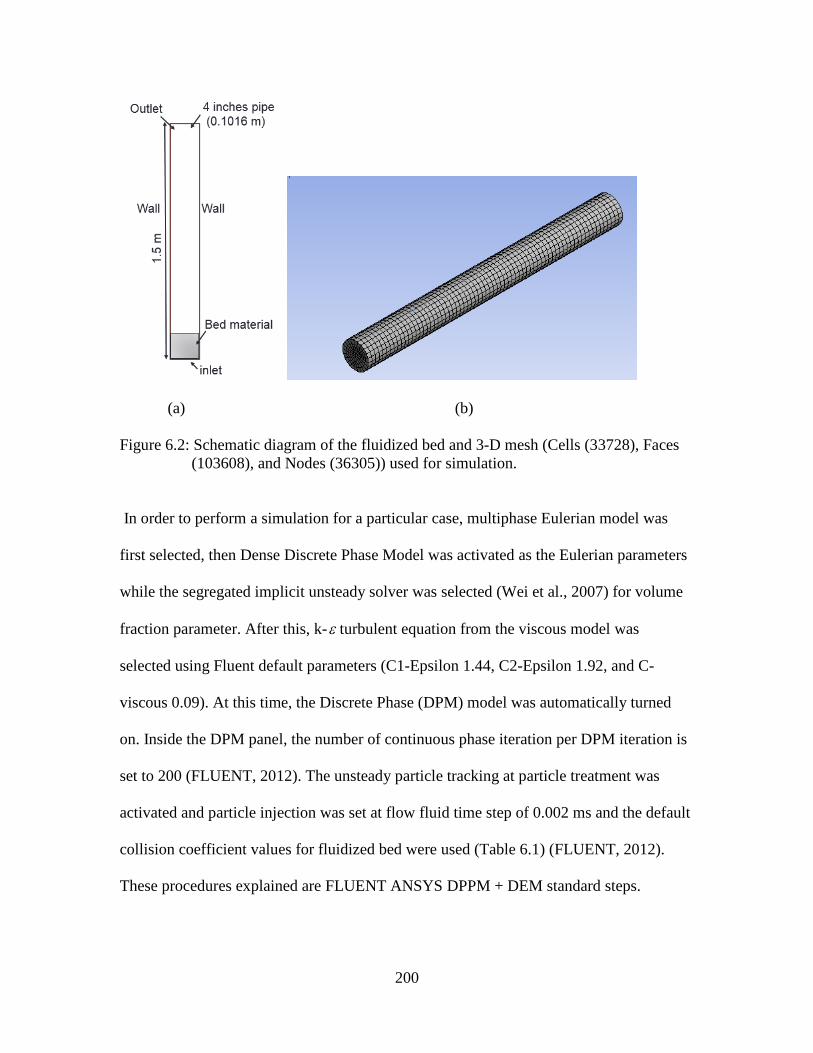
(a) (b)
Figure 6.2: Schematic diagram of the fluidized bed and 3-D mesh (Cells (33728), Faces (103608), and Nodes (36305)) used for simulation.
In order to perform a simulation for a particular case, multiphase Eulerian model was
first selected, then Dense Discrete Phase Model was activated as the Eulerian parameters
while the segregated implicit unsteady solver was selected (Wei et al., 2007) for volume
fraction parameter. After this, k-ε turbulent equation from the viscous model was
selected using Fluent default parameters (C1-Epsilon 1.44, C2-Epsilon 1.92, and C-
viscous 0.09). At this time, the Discrete Phase (DPM) model was automatically turned
on. Inside the DPM panel, the number of continuous phase iteration per DPM iteration is
set to 200 (FLUENT, 2012). The unsteady particle tracking at particle treatment was
activated and particle injection was set at flow fluid time step of 0.002 ms and the default
collision coefficient values for fluidized bed were used (Table 6.1) (FLUENT, 2012).
These procedures explained are FLUENT ANSYS DPPM + DEM standard steps.
200

Table 6.1: Discrete event collision setting parameter
Contact law Constants Spring-dashpot, k 100 Friction dashpot 0.5 µsticks 0.5 µglide 0.2 µlimit 0.1
Where
µsticks is the sticking friction coefficient
µglide is the gliding friction coefficient
µglide is the gliding velocity
6.3.2 Particle size determination and particle injection file Loblolly pine wood chips were obtained from a forest plantation in Alabama, U.S. The
chips were ground using a hammer mill (Model 358, New Holland, Pa.) fitted with 3.18
mm diameter round holes screen. After grinding, the moisture content of the sample was
determined, using ASTM standard E871-82 ASTM (2007) procedure, to be 8.45 % wet
basis. A particle size analyzer (Fig 6.3a) (Camsizer®, Retsch Technology, Haan,
Germany) was used to obtain particle size (based on chord diameter measurement
scheme) distribution in the form of cumulative particle size distribution plot (Fig 6.3 b).
In addition, the mean sphericity of the particles was extracted from the software of the
system. The cumulative distribution plot was subsequently converted to an injection file
using a python program (the python code is proprietary program provided by ANSYS
Fluent support). Table 6.2 shows the summary distribution characteristics of injected
particles.
201

(a) Camsizer: Particle size analyzer. (b) Cumulative distribution of particles Figure 6.3: Particle size analysis and cumulative distribution plot of ground loblolly pine
wood.
Table 6.2: Distribution characteristics of injected particle obtained from FLUENT®
Particle characteristics Values Total number of parcels 40824 Total number of particles 1.3e+08 Total mass 200 g Overall RR Spread Parameter 1.1 Maximum Error in RR fit 0.041 Overall RR diameter (D_RR) 0.00091 mm Maximum RMS distance from injector 0.23 mm Maximum particle diameter 0.11 mm Minimum particle diameter 0.000048 mm Overall mean diameter (D10) 0.00011 mm Overall mean surface area (D20) 0.00015 mm Overall mean volume (D30) 0.00022 mm Overall surface diameter(D21) 0.00020 mm Overall volume diameter(D31) 0.00031 mm Overall Sauter diameter(D32) 0.00048 mm Overall De Brouckere diameter (D43) 0.0011 mm
202

6.3.3 Governing equations and mathematical model The Eulerian-Lagrangian with Dense Discreet Phase model was used to simulate and
analyze the flow in the fluidized solid- air system. This was achieved by solving the set
of governing momentum and continuity equations for each phase (solid and fluid) and
coupling the two phases through pressure and interphase exchange coefficients. The solid
gas-solid interphase exchange coefficient was declared as a function of drag force. In
addition, optional body forces are coupled to the drag force in Fluent. The body forces
are localized forces on individual particles which the standard drag did not consider e.g.
virtual mass and lift (FLUENT, 2012). In order to consider virtual mass as a body force,
the density of the fluid must approach or exceed the density of the particles. In this case,
the ratio of solid density to fluid density was greater than 1000. Therefore the virtual
mass effect is insignificant (FLUENT, 2012; Rajeswari et al., 2011). Lift force is used for
submicron particles and often cause significant convergence problems (FLUENT, 2012),
thus inclusion of lift force was neglected. Body forces are typically applied to particle
with initial void fractions less than 0.6 with the assumption that particles with high void
fraction (void > 0.8) are not expected to have body forces application in Fluent.
Therefore, in order to obtain a reliable solution from simulation of biomass grinds with
void fraction that approximate to 0.8, this study present a void body force correlation.
The procedure used to capture the effect of body force using biomass grinds is discussed
in the next section. The body force developed was integrated into the Eulerian-
Lagrangian DDPM model for gas- solid (Eqn. 6.11– 20 Table 6.3). These equations were
chosen from the FLUENT CFD software, based on the aforementioned assumptions, as
they are found most suitable for modeling multiphase flow which consists of a primary
203

continuous phase (air) and a secondary phase (solid biomass) dispersed within the
continuous phase.
Table 6.3: Governing equations and constitutive law of Eulerian Lagrangian, DDPM model for gas-solid flow
Governing equation Detail Eqn. #
othersngravitatiomassvirtualpressuredrag FFFFFdtvdm ++++= _
vdtdx
=, othersF = frictionF , bodyF
Particle motion
6.12
normalfriction FF µ=
stickµµ = = sticking friction coefficient
glideµµ = , gliding friction coefficient
itlimµµ = , high velocity limit friction coefficient Friction coefficient plot is showed in Appendix 5
Frictional collision law
6.13
1=+ sg εε Volume fraction of the phases 6.14
( ) ( ) ( ) g
n
pgssgggggg Smmv
t+−=⋅∇+
∂∂ ∑
=1
ρερερ
Continuity equation for gas 6.15
( ) ( ) (n
pgssssss mmv
t−=⋅∇+
∂∂ ∑
=1
ρερερ
Continuity equation for solid 6.16
Momentum equation for gas 6.17
( ) ( ) ( )(
( )gtdgvmgliftg
n
ggssgsggssgggggggggggg
FFFF
vmvmvvKgpvvvt
,,,
1
++++
−+−++⋅∇+∇−=⋅∇+∂∂ ∑
=
ρετερερερ
Momentum equation for solid phase 6.18
( ) ( ) ( )( )
( )stdsvmslifts
N
lsgsggsgssggssssssssssssss
FFFF
vmvmvvKgppvvvt
,,,
1
++++
−+−++⋅∇+∇−∇−=⋅∇+∂∂ ∑
=
ρετερερερ
s
sssg
fKτρε
= , Solid-gas exchange coefficient 6.19
f
sss
dµ
ρτ
18
2
= Relaxation time 6.20
204

Syamlal-Obrien
vvv
Cdv
ksr
sD
ssr
llssl
−
=
,2,
Re4
3 ραα
2
,
Re7.463.0
+=
sr
sD
v
C
6.21
Wen & Yu 65.2
43 −−= llsD
s
llssl vvC
dk αραα
( )( )687.0Re15.01Re
24sl
slDC α
α+=
6.22
Gidaspow ( )s
lssl
sl
llssl d
vvd
k
−+
−=
αρα
µαα 75.11150 2
( )( )687.0Re15.01Re
24sl
slDC α
α+=
6.23
Non-spherical
65.2
43 −−= llsD
s
llssl vvC
dk αραα
( )sph
sphsph
sphD b
bbbC
ReRe
Re1Re
24
4
321 +++=
6.24
6.3.4 Formulation of body force correlation
In the formulation scheme for particle motion (Eqn. 6.12), body force is an optional force
embedded under the othersF . The contact force are due to particle to particle interaction,
whereas the body forces are any external force fields acting on the particles (Sen et al.,
2014). For fluent to implement a body force (bforce), an acceleration term must be
developed in the form of eqn. 6.21.
massforcebforce = (6.25)
Relating void fraction to the particle and fluid occupying a control volume
solidair
air
VVV+
=ε (6.26)
205

solidair VVε
ε−
=1
(6.27)
Expanding the force in relation to fluid volume and density
ss
airair
VaV
massforcebforce
ρρ
== (6.28)
solids
ssolidair
V
aV
massforcebforce
ρε
ερ
−== 1 (6.29)
Thus, the body force acting on a bed of material can be related to the porosity of air,
density of air, and particle.
amassforcebforce
s
air
εε
ρρ
−==
1 (6.30)
6.3.5 Boundary and initial condition
In order to obtain a well-posed system of equations, reasonable boundary condition for
the computational domain was implemented. At the inlet boundary, is a uniform air
velocity inlet while the outlet boundary is the pressure boundary condition set at zero
gauge pressure to model the opening of the system to the atmosphere. Also, mixture
boundary was also activated for the outlet boundary. Here, the discrete phase boundary
condition was set at escape boundary. This means that the particles that crossed the
boundary is eliminated. For the wall, boundary conditions were set at no-slip conditions
for gas phase and discrete event collision for the solid phase. At the initial condition, 0.2
kg of loblolly pine grinds with the following characteristics was injected: void fraction of
0.7 for ground loblolly pine wood, and sphericity of 0.45. For all simulations, the time
step, maximum iterations/time, and reporting interval were set at 1E-3 s, 20 sec, and 5
(frequency) respectively.
206

6.3.6 Solver related details The Eulerian-Lagrangian with Dense Discrete Phase Model( DDPM) equations were
implemented in FLUENT 14.5.7 solver employing finite volume solution method and
Phase Coupled SIMPLE (FLUENT, 2012) algorithm to solve the pressure–velocity
coupled equations in a discretization scheme. The unsteady state formulation employed
QUICK scheme solver for momentum and volume fraction for discretization. The
solution was initialized from solid inlet and air inlets and the convergence was monitored
approximately up to 10,000 iterations with residual convergence fixed between 1× 10⁻³
and 1 × 10⁻⁶.
6.3.7 User defined function implementations
To compute the bed voidage, it was mandatory to computationally designate which cells
belonged to the bed region (the region where particles reside). In order to discount the
very dilute suspension in the freeboard, only cells with > 0.01 solid volume fraction (ɛs)
were designated as belonging to the bed. This study used the Fluent UDF macro written
in the C programming language called DEFINE_EXECUTE_AT_END. This is a
general-purpose macro that is executed at the end of an iteration in a steady state run, or
at the end of a time step in a transient run (FLUENT, 2012). In addition, body force
correlation implementation used UDF macro DEFINE_DPM_BODY_FORCE. The UDF is
used to identify body force other than a gravitational or drag force on the particles. The
macro return the real value of the acceleration due to the body force (in m/s2) to the
ANSYS FLUENT solver. The UDFs for bed voidage and body force are presented in
Appendix 5.
207

6.4 Result and discussion 6.4.1 Mesh convergence/ independent study Mesh independent study are usually first conducted to reduce the error in CFD
calculations due to the usage of an incorrect mesh sizes (Rundle et al., 2011). Solutions
over a range of significantly different grid resolutions have to be presented to
demonstrate grid-independent or grid-convergent results. For mesh independent study,
five different mesh sizes that varies from 4000 to 65000 numbers of element were
considered (Table 6.4). When a particular mesh size is selected, about 200 g particles
were injected into the bed and airflow of 0.2 m/s was applied. Using a simulation time
step of 2000 corresponding to 2 seconds simulation time, the pressure drop, bed voidage
at each time step were extracted using the FLUENT programming user define function
(UDF) described in 7.2.7.
208

Table 6.4: Meshing method and sizes obtained for mesh independent study
Mesh type Program controlled
Sizing method Proximity and curvature
Mesh number 1 2 3 4 5
Numbers of node 4558 4730 33728 49248 67725
Numbers of Element 3570 3740 36304 45390 63510
It can be seen from Fig. 6.4 that the pressure drop profile at various mesh sizes behaved
similarly and reach steady state by 2-seconds of simulation time. For comparison
purposes, the theoretical pressure drop obtained that was calculated by dividing bed
weight by the cross-sectional area of the bed was 268 Pa. The percentage errors between
the theoretical pressure drop and predicted pressure drop for the number of elements
3570, 3740, 33728, 45390, and 63510 were 12.51 %, 15.8 %, 8.6 %, 9.2%, and 8.6%
respectively. Similarly, the plot of bed voidage with time showed similar profile for all
the mesh size. In addition, the bed voidage converged at 2-second simulation time.
209

Figure 6.4: Effect of using different mesh sizes on pressure drop across the bed with
simulation time
Figure 6.5: Effect of using different mesh sizes on bed voidage with simulation time
210

In general, the smaller the mesh size, the closer the simulation results were to the
theoretical pressure drop. When mesh size reduced, the total number of the control
volume increased (mesh total number). This also increased the number of governing
equations that must be solved for each mesh and hence the solution becomes more
precise (Pin et al., 2014). However, increase in number of mesh also increase the
computational effort (time and resources) needed for convergence and for producing
result. About 100 hours is required to complete a simulation case. However additional 2
hours existed between cases (based mesh size variation) using High-performance
computing cluster (HPCC) that consist of 512 cores @ 2.80 GHz X5560, 1.536TB shared
memory, and 20.48TB raw internal storage. HPCC Theoretical Performance calculated @
5.735 teraflops with memory bandwidth up to 90 GB/s. Therefore, with low deviation in
pressure drop and insignificant computational time compared to other mesh sizes, mesh
size of 33728 was chosen as the optimum mesh size. Subsequent simulations were
therefore carried out using this mesh size. Fig 6.6 shows the flow chart used to simulate
the solid-gas fluidized bed system that comprised of non-uniform and non-spherical
particles such as particles from loblolly pine grinds.
211

Figure 6.6: Flowchart showing scheme used for solving equations for multi-phase CFD model
6.4.2 Effect of drag model on transient bed voidage profile
Fig. 6.7 a – d illustrates transient bed voidage profile for velocities in the range of 0.08 –
1.2 m/s using Gidaspow, non-spherical, Syamlal-Obrien, and Wen & Yu drag model
respectively (FLUENT, 2012). For our system, velocity of interest is between 0.25 -1.0
m/s because the minimum and complete fluidization velocities respectively falls within
this range (Chapter 4 and 5). However, the choice simulating wider velocity range (0.08 –
1.2 m/s) was to enable the plotting of pressure drop-velocity profile for the sample.
212

Figure 6.7: Transient bed voidage profiles for velocities in the range of 0.08 -1.2 m/s for different drag law: (a) Gidaspow; (b) Non-spherical; (c) Syamlal-Obrien, and (d) Wen & Yu
The bed voidage profile using different drag equations and at different velocities showed
similar profile. Firstly, the initial bed was unstable until simulation time of 2.0. We
attribute this behavior to shock at bed startup (Chialvo et al., 2012; Sande and Ray,
2014). Initially when air is introduced into the packed bed, the air attempts to flow
through the void spaces within the bed: However, since the voids are not directly
connected, the tortuous movement of air and the flow velocity create a situation where
the air create its own path resulting in bed realignment intense mixing. As the air
establishes its own flow path, the void settles down (time at 2 sec to 10 seconds). Figure
213

6.8 a –d shows the snapshots of the contour plot of the transient solid volume fraction at
2.0 m/s air flow using the different drag equations.
(a) 0 sec 1 sec 2 sec 4 sec 6 sec 8 sec 10 sec
(b) 0 sec 1 sec 2 sec 4 sec 6 sec 8 sec 10 sec
214

(c) 0 sec 1 sec 2 sec 4 sec 6 sec 8 sec 10 sec
(d) 0 sec 1 sec 2 sec 4 sec 6 sec 8 sec 10 sec
Figure 6.8: Snapshots of transient solid volume fraction contours of the fluidized bed at 2.0 m/s: (a) Gidaspow: (b) Non-spherical; (c) Syamlal-Obrien: (d) Wen & Yu drag law
A careful look at the snapshot (Fig. 6.8) revealed a plug flow at simulation time of 1 sec.
This corroborated the initial resistance of the bed to air penetration as air attempt to
establish its path in the bed. It can be seen that the bed initially bubble sizes are almost
215

equal to the diameter of the bed which could be likened to a plug flow. Immediately after
this initial bed resistance, the bed resettled.
The bed perturbation was least when non-spherical drag law was used, while the rest
showed an extensive bed mixing. This observation was different from what was observed
by Sande and Ray (2014) and Zhang et al. (2008). These authors using a bed consisting
of uniformly sized particles and the simulation were carried out using Eulerian - Eulerian
simulation schemes. These authors reported that after the initial bed disturbance, the
whole bed return to the homogenous fluidization state. However, when a bed consists of
non-uniform particle size, small particles trapped between big particles could initially
offer resistance to fluid flow through the bed. Thus, part of the bed move in a plug flow.
Immediately afterwards, the bed collapses resulting in escape of small particle trapped
between the bigger particles. In addition, air flow causes structural realignment of the
bed, small particles that are light in weight are entrained out of their position to a new
place or some are entrained in the air. This movement of particles creates void/ channels
and various routes for air passage through the bed. We suspect that the entrainment of the
smaller particles out of the bed, makes the bed to consist more of bigger particles. An
increase in air velocity is then required before fluidization can occur. Thus an initial
perturbed bed simply resettled after some time. This behavior was experimentally
observed and details presented in Chapter 3.
216

Gidaspow
Non- spherical
Syamlal- Obrien
0.15 mm
0.10 mm
0.04 mm
0.01 mm

Wen & Yu
Initial state 1 sec 4 sec 10 sec Drag law Figure 6.9: Contour plot of volume fraction of solid on z-coordinate at 0.0, 0.01, 0.04, 0.10, and 0.15 mm at 0.2 m/s air velocity
0.0 mm
218

Similarly, Fig. 6.9 shows the contour plot of volume fraction of solid at 0.0, 0.01, 0.04,
0.10 and 0.15 mm and 0.2 m/s velocity (using different drag laws). Dark red represent
high concentration of material at the particular location while yellow signifies void
spaces. It can be seen that virtually all the model showed various size of channels and
particle realignments. As the simulation time increase, particle concentration at the base
of the bed increased for Gidaspow, non-spherical, and Wen & Yu models. This may be
attributed to structure of Syamlal drag law in which terminal velocity is used as particle
velocity in drag function.
6.4.3 Effect of drag model on pressure drop profile
Pressure drop across the bed is an important parameter to determine for proper scaling up
and reactor design. Traditionally, the pressure drop in a fluidized bed has always been
described by the buoyant weight (i.e. weight per unit cross-sectional area of bed) of the
suspension (Brandani and Zhang, 2006; Shi et al., 2010). Figure 6.10 shows the bed
pressure drop profile as a function of the flow time at various fluidizing velocity (using
Gidaspow drag law). Similar profiles were obtained for Syamlal-Obrien, Wen & Yu and
non-spherical drag laws (Appendix 5).

Figure 6.10: Evolution of pressure with simulation time at different velocity using
Gidaspow drag law Moreover, according to Figure 6.10, it is worth noting that four typical regions could be
identified (Shi et al., 2010). The startup stage is the initial pressure of the bed (at time 0
second). Slow drop stage (0 s < time < 1.5 s), vibration stage (1.5 s time < 4.0 s), and
stable fluidization stage (time > 4 s). The maximum bed pressure drop occurred at the
start-up point/ stage and the pressure is far greater than any other three stages because of
the inter-particle locking and bed cohesive forces that must be overcome. Afterward, the
bed pressure drop decreased slowly because of formation of the gas-phase flow field and
the looseness of the solid phase following the flow proceeding in the period of 0-1.5 s. In
the period of 1.5-4.0 s, air bubble formation was predominantly found that developed
with time; causing the bed pressure drop to fluctuate greatly. After the vibration stage, the
bed pressure drop fluctuates with time around a mean value corresponding to the gas flow
as shown in Figure 6.10, namely, the stable fluidization stage.
Since the bed achieve stable fluidization at later stage of the fluidization, the mean
pressure drop was obtained using the 10 sec time step simulation case file.
220

6.4.4 Comparison of CFD simulation and experimental result
Figure 6.11 showed the pressure drop against the airflow velocity of both experimental
and simulated data. The pressure profile behavior can be categorized into two different
behaviors based on the velocity, namely, before (0- 0.2 m/s) and after (0.2-1.0 m/s).
Figure 6.11: Determination of Umf using the plot of pressure drop against the airflow
velocity
Between 0– 0.2 m/s, air velocity and pressure increased progressively, and only non-
spherical drag matches the experimental data. When the velocity was greater than 0.2
m/s, the experimental pressure drop became constant, while the predicting drags law
started to decline progressively. The decline in pressure drop with increase velocity
above 0.2 m/s was traced to bed material entrainment and loss of inventory. This situation
is further investigated in subsequent section. In experimental situation at ~0.2 m/s,
particle distribution and particle forming network / interlocked offered additional
resistance to fluid flow apart from buoyant weight of the suspension. Thus, intra and
inter-particle bridging contributed to pressure addition hence the slight increase in
pressure drop (Zhuang et al., 2014). Furthermore, Table 6.5 showed the mean relative
deviation (MRD) between the predicted and the experimental pressure drop data. It can
221

be seen that all the drag laws under predicted the experimental data and the deviation
increased with increase in velocity.
Table 6.5: Mean relative deviation between predicted pressure drop using different drag
equation and experimental data. Mean Relative deviation (%)
Velocity (m/s) Gidaspow Wen & Yu Syamlal-Obrien Non-spherical 0.2 -3.9 -3.9 -4.1 -6.1 0.4 -3.3 -1.1 2.6 -3.3 0.6 -0.8 -3.7 -7.4 -12.2 0.8 -11.1 -4.4 -9.9 -18.2
This could be attributed to the bed channeling and particles entrainment out of the bed.
Eqn. 6.31 was used to calculate the bed entrainment after 10 seconds simulation time.
60×−
=t
MMtentrainmen fi 6.31
where
entrainment is (g/min)
iM is the initial mass (g)
fM is the final mass (g) at 10 sec (t) simulation time step.
Fig. 6.12 shows the comparison of predicted and experimental entrained bed material. At
0.2 m/s both experimental and predicted showed there were no bed material entrainments.
However, at 0.24 m/s, predicted and experimental bed material entrainments were
comparable. However, at 0.6 and 0.8 m/s the drag law significantly over-predicted the
bed entrainment. This can be attributed to inability of the drag laws to capture the
particles interaction because Fluent software see the particles as spherical and the
interlocking effect coupled with particle to particle friction of non-spherical particles
were not properly captured by the drag laws. Hence, the need to revise existing
222

equation/laws in order to effectively predict the bed expansion and material entrainment.
When the bed inventory reduced because of entrainment, the total weight of the bed
reduces with the corresponding reduction in pressure drop. Bed entrainment also caused
similar drop in pressure during the simulation as velocity increased. The detail is
presented in next section.
Figure 6.12: Comparison of predicted and experimental bed material entrainment as
velocity increased. 6.4.5 Prediction of minimum fluidization velocity
The minimum fluidization velocity was identified as the velocity at which increasing
trend in bed pressure of the packed bed terminates in the plot of pressure drop against the
airflow rate. This approach was used in chapter 4 and 5. From Figure 6.13, the minimum
fluidization velocity of the bed varied according to the drag law used. The experimental
Umf was 0.2 m/s while non-spherical and other drag laws predicted 0.2 m/s and less than
223

0.1 m/s respectively. Hence, the non-spherical seems to have successfully predicted the
experimental Umf.
Dash line represents the theoretical pressure drop defined as bed weight per unit cross-sectional area
Figure 6.13: Pressure drop against velocity for determination of minimum fluidization velocity.
In order to understand particle behavior at fluidization, it is important that we examine
the state of bed at velocity before (0.2 m/s) and after (0.4 m/s) the minimum fluidization
velocity. Fig 6.14 particle traces colored by particle velocity magnitude using non-
spherical drag law at 0.2 m/s. It can be seen that the bed was still in static position as
larger percentage of the bed was still in fixed bed. However, smaller particles were
increasingly entrained out of the bed area as simulation proceeds from 2 sec to 10 second.
Similarly, Figure 6.15 shows particle traces colored by particle velocity magnitude using
non-spherical drag law at 0.4 m/s. It can be seen that particle entrainment out of the bed
began after 2-second simulation time. Similar particle entrainments were observed while
using Gidaspow, Wen & Yu, and Syamlal-Obrien. (Appendix 7). In addition, from scale
in Fig 6.15, the smallest and the highest solid velocity was 1.1e-7 m/s, and 1.28 m/s
224

respectively. This wide difference in solid velocity is attributed to the wide variation in
the size and densities of particles in the bed. When particle size varied largely, bigger
particle settles while smaller particle entrained. This is important because residence time
for ground biomass is approximately 3 seconds (Capareda, 2013). Thus, operating the
fluidize bed at a velocity above Umf would result in particle carryover. Even as particle
entrained out of the bed, a large part of the solid was still on the distributor.
1 sec 2 sec 4 sec 6 sec 8 sec 10 sec Experimental Figure 6.14: Particle traces colored by particle velocity magnitude using non-spherical
drag law at 0.2 m/s
225

1 sec 2 sec 4 sec 6 sec 8 sec 10 sec Experimental
Figure 6.15 Particle traces colored by particle velocity magnitude using non-spherical
drag law at 0.4 m/s
226

6.4.6 Effect of void body force application on pressure drop profile
Table 6.16 shows the pressure drop at different air velocities after application of the body
force correlation. It can be seen that pressure drop first increased until velocity reached
0.2 m/s then reduced for all drag law considered. This relationship obtained between
pressure drop and velocity is similar to the relationship obtained when body force was not
applied (section 6.4.4). The reduction in pressure drop with increase in velocity was
earlier attributed to loss of bed material inventory. Also, it was observed that the least
pressure drop considering all the velocities was obtained when non-spherical drag was
used. For instance, about 46% difference were recorded between Gidaspow and non-
spherical at 0.04 m/s velocity.
Table 6.6: Pressure drop obtained at different velocities after application of body force correlation.
Figure 6.16: Pressure drop obtained at different velocities after application of body force correlation.
227
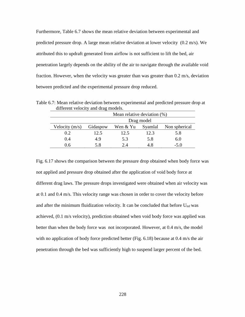
Furthermore, Table 6.7 shows the mean relative deviation between experimental and
predicted pressure drop. A large mean relative deviation at lower velocity (0.2 m/s). We
attributed this to updraft generated from airflow is not sufficient to lift the bed, air
penetration largely depends on the ability of the air to navigate through the available void
fraction. However, when the velocity was greater than was greater than 0.2 m/s, deviation
between predicted and the experimental pressure drop reduced.
Table 6.7: Mean relative deviation between experimental and predicted pressure drop at different velocity and drag models.
Mean relative deviation (%) Drag model
Velocity (m/s) Gidaspow Wen & Yu Syamlal Non spherical 0.2 12.5 12.5 12.3 5.8 0.4 4.9 5.3 5.8 6.0 0.6 5.8 2.4 4.8 -5.0
Fig. 6.17 shows the comparison between the pressure drop obtained when body force was
not applied and pressure drop obtained after the application of void body force at
different drag laws. The pressure drops investigated were obtained when air velocity was
at 0.1 and 0.4 m/s. This velocity range was chosen in order to cover the velocity before
and after the minimum fluidization velocity. It can be concluded that before Umf was
achieved, (0.1 m/s velocity), prediction obtained when void body force was applied was
better than when the body force was not incorporated. However, at 0.4 m/s, the model
with no application of body force predicted better (Fig. 6.18) because at 0.4 m/s the air
penetration through the bed was sufficiently high to suspend larger percent of the bed.
228

Figure 6.17: Comparison of pressure drop obtained from modeling with and without
application of body force at different drag law and velocity of 0.1 m/s air velocity.
Figure 6.18 Comparison of pressure drop obtained from modeling with and without
application of body force at different drag law and velocity of 0.4 m/s air velocity.
229

However, the bed entrainments were not significantly affected by application of body
force. It can be seen from Fig 6.19 that the mass entrainment increased with increase in
velocity. Particle entrainment increased under application of body force (Fig 6.19)
compared with when body force was not applied (Fig 6.12).
Figure 6.19: Comparison of predicted and experimental bed material entrainment as
velocity increased under application of body force.
6.4.7 Prediction of minimum fluidization velocity
The minimum fluidization velocity was identified by following the methods used in
section 6.4.5. The experimental Umf was found to be 0.2 m/s. while non-spherical drag
law predicted 0.1 m/s all other drag law under predicted the experimental data with more
than 50% error (Fig 6.20). In addition, the result of minimum fluidization velocity is
similar to the result obtained when body force was not applied (Fig. 6.13). The inability
of the drag laws to predict the Umf of loblolly pine wood confirms the need to modify
existing equations for loblolly pine wood grinds.
230

Figure 6.20: Pressure drop against velocity for determination of minimum fluidization velocity of bed having body force applied.
6.5 Conclusion The first part of the study investigated the effect of mesh size on predictive capability of
Eulerian-Lagrangian coupled with Dense Discreet Phase Model (DDPM) in a solid gas
flow fluidized bed consisting of particles having lognormal distribution. The
computational domain was of laboratory scale size and even numbers of mesh sizes
simulation ranging from 400 to 60000 were simulated and presented. The results of the
simulation were analyzed using pressure drop prediction and the ability of the voidage to
reach a stable profile with increase in simulation time. For pressure drop, the percentage
errors for each mesh were 12.51 %, 15.8 %, 8.6 %, 9.2%, and 8.6% for the 3570, 3740,
33728, 45390, and 63510 numbers of meshes respectively. Similarly, the plot of bed
voidage with time showed similar profile for all the mesh considered. In addition, the bed
voidage converged at 2-second simulation time. The percentage errors for each different
mesh size were 28.7 %, 15.3 %, 15.6 %, 15.3%, and 15.3 % for 3570, 3740, 33728,
45390, and 63510. However, for bed voidage, all equation converged nicely at 2 seconds
231

simulation time. Hence, due to least percent error in pressure drop prediction, 33728-
mesh size was used for subsequent study.
Simulation results showed that the drag models generally under predicted the pressure
drop with maximum mean relative deviation (MRD) obtained from non-spherical drag
law. In addition, the Gidaspow, Wen & Yu and Syamlal-Obrien failed to predict the
minimum fluidization velocity. When body force correlation was applied, we could not
resolve the convergence problem at 0.2 m/s. However, the body force application resulted
in reduction of MRD of the non-spherical drag law but no significant influence on other
drag equation in pressure drop prediction were observed. In addition, the body force
application did not improve the prediction of Umf of the all drag equations except the non-
spherical drag model. We also observed that particle entrainment occurred after
simulations time of 2 second and this was experimentally validated. It can be safely
concluded that there is a need to modify drag law equations if they are to be used to
simulate the fluidization of particles with lognormal particle size distribution.
6.6 Reference ASTM. 2007. Standard test methods for direct moisture content measurement of wood and wood-base materials. American Society for Testing Materials. ASTM International West Conshohocken, PA. Benzarti, S., H. Mhiri, and H. Bournot. 2012. Drag models for Simulation Gas-Solid Flow in the Bubbling Fluidized Bed of FCC particles. World Academy of Science, Engineering and Technology 61. Brandani, S., and K. Zhang. 2006. A new model for the prediction of the behaviour of fluidized beds. Powder Technology 163(1):80-87. Capareda, S. 2013. Introduction to biomass energy conversions. CRC Press.
232

Chen, X., W. Zhong, X. Zhou, B. Jin, and B. Sun. 2012. CFD–DEM simulation of particle transport and deposition in pulmonary airway. Powder Technology 228(0):309-318. Chialvo, S., J. Sun, and S. Sundaresan. 2012. Bridging the rheology of granular flows in three regimes. Physical Review E 85(2):021305. Clift, R., J. R. Grace, and M. E. Weber. 1978. Bubbles, drops, and particles. Accademic Press. Cloete, S., S. T. Johansen, and S. Amini. 2015. Grid independence behaviour of fluidized bed reactor simulations using the Two Fluid Model: Effect of particle size. Powder Technology 269(0):153-165. Ergun, S. 1952. Fluid flow through packed columns. Chem. Eng. Prog. 48:89-94. FLUENT, M. 2012. ANSYS Release Version 14.5, ANSYS Inc. Documentation. Garside, J., and M. R. Al-Dibouni. 1977. Velocity-voidage relationships for fluidization and sedimentation in solid-liquid systems. Industrial & Engineering Chemistry Process Design and Development 16(2):206-214. Gidaspow, D. 1986. Hydrodynamics of fiuidizatlon and heat transfer: Supercomputer modeling. Applied Mechanics Reviews 39(1):1-23. Haider, A., and O. Levenspiel. 1989. Drag coefficient and terminal velocity of spherical and nonspherical particles. Powder Technology 58(1):63-70. Hrenya, C. M., and J. L. Sinclair. 1997. Effects of particle‐phase turbulence in gas‐solid flows. AIChE Journal 43(4):853-869. Huilin, L., and D. Gidaspow. 2003. Hydrodynamics of binary fluidization in a riser: CFD simulation using two granular temperatures. Chemical Engineering Science 58(16):3777-3792. Kumar, N., S. Ramaswamy, and A. Sood. 2011. Symmetry properties of the large-deviation function of the velocity of a self-propelled polar particle. Physical Review Letters 106(11):118001. Li, T., A. Gel, S. Pannala, M. Shahnam, and M. Syamlal. 2014. Reprint of “CFD simulations of circulating fluidized bed risers, part I: Grid study”. Powder Technology. Louge, M., E. Mastorakos, and J. Jenkins. 1991. The role of particle collisions in pneumatic transport. Journal of Fluid Mechanics 231:345-359.
233

Morsi, S., and A. Alexander. 1972. An investigation of particle trajectories in two-phase flow systems. Journal of Fluid Mechanics 55(02):193-208. Pei, P., K. Zhang, and D. Wen. 2012. Comparative analysis of CFD models for jetting fluidized beds: The effect of inter-phase drag force. Powder Technology 221(0):114-122. Pin, S., W. Rashmi, M. Khalid, C. Chong, M. Woo, and L. Tee. 2014. Simulation of spray drying on Piper betle Linn extracts using Computational Fluid Dynamics. International Food Research Journal 21(3):1053-1060. Rajeswari, M. S. R., K. Azizli, S. Hashim, M. Abdullah, M. A. Mujeebu, and M. Abdullah. 2011. CFD simulation and experimental analysis of flow dynamics and grinding performance of opposed fluidized bed air jet mill. International Journal of Mineral Processing 98(1):94-105. Rao, A., J. S. Curtis, B. C. Hancock, and C. Wassgren. 2011. Classifying the fluidization and segregation behavior of binary mixtures using particle size and density ratios. AIChE Journal 57(6):1446-1458. Richardson, J. F., and W. N. Zaki. 1954. Sedimentation and fluidization (Part 1). Trans. Inst. Chem. Eng,. 32:35 -52. Rundle, C., M. Lightstone, P. Oosthuizen, P. Karava, and E. Mouriki. 2011. Validation of computational fluid dynamics simulations for atria geometries. Building and Environment 46(7):1343-1353. Sande, P., and S. Ray. 2014. Mesh size effect on CFD simulation of gas-fluidized Geldart A particles. Powder Technology 264:43-53. Sen, M., D. Barrasso, R. Singh, and R. Ramachandran. 2014. A multi-scale hybrid CFD-DEM-PBM description of a fluid-bed granulation process. Processes 2(1):89-111. Shi, D.-P., Z.-H. Luo, and A.-Y. Guo. 2010. Numerical simulation of the gas− solid flow in fluidized-bed polymerization reactors. Industrial & engineering chemistry research 49(9):4070-4079. Syamlal, M., and T. O'Brien. 1988. Simulation of granular layer inversion in liquid fluidized beds. International Journal of Multiphase Flow 14(4):473-481. Syamlal, M., and T. J. O’Brien. 1989. Computer simulation of bubbles in a fluidized bed. In AIChE Symp. Ser. Takamasa, T., and A. Tomiyama. 1999. Three-dimensional gas–liquid two-phase bubbly flow in a C-shaped tube. In Proceedings of the 1999 NURETH-9 Conference.
234

Van Wachem, B., J. Schouten, C. Van den Bleek, R. Krishna, and J. Sinclair. 2001. CFD modeling of gas‐fluidized beds with a bimodal particle mixture. AIChE Journal 47(6):1292-1302. Vejahati, F., N. Mahinpey, N. Ellis, and M. B. Nikoo. 2009. CFD simulation of gas–solid bubbling fluidized bed: A new method for adjusting drag law. The Canadian Journal of Chemical Engineering 87(1):19-30. Wang, Q., T. Niemi, J. Peltola, S. Kallio, H. Yang, J. Lu, and L. Wei. 2014. Particle size distribution in CPFD modeling of gas–solid flows in a CFB riser. Particuology(0). Wei, X., X. Meng, X. Ma, J. Zhang, and X. He. 2007. Design and Optimization of Fluid-bed Reactor of Biomass Pyrolysis System. In Challenges of Power Engineering and Environment, 1134-1138. K. Cen, Y. Chi, and F. Wang, eds: Springer Berlin Heidelberg. Wen, C. Y., and Y. H. Yu. 1966. A generalized method for predicting the minimum fluidization velocity. AIChE Journal 12(3):610-612. Yasuna, J. A., H. R. Moyer, S. Elliott, and J. L. Sinclair. 1995. Quantitative predictions of gas-particle flow in a vertical pipe with particle-particle interactions. Powder Technology 84(1):23-34. Ye, M., M. Van der Hoef, and J. Kuipers. 2005. The effects of particle and gas properties on the fluidization of Geldart A particles. Chemical Engineering Science 60(16):4567-4580. Zhang, K., S. Brandani, J. Bi, and J. Jiang. 2008. CFD simulation of fluidization quality in the three-dimensional fluidized bed. Progress in Natural Science 18(6):729-733. Zhuang, Y.-Q., X.-M. Chen, Z.-H. Luo, and J. Xiao. 2014. CFD–DEM modeling of gas–solid flow and catalytic MTO reaction in a fluidized bed reactor. Computers & Chemical Engineering 60(0):1-16.
235

Chapter 7: Conclusion and Recommendation
7.1 Conclusions
Importance of particle size in fluidization dynamics of ground loblolly pine wood and
switchgrass has been researched in this dissertation. In this regard, some light has been
shed on the fluidization parameter which are of importance to the design, operation and
control of fluidized bed systems. In chapter 3, it was shown that the use of mean particle
diameter in fluidization equation would result in wrong parameter estimation because the
particles of the material considered in this study are non-spherical and the distributions
are not normal. This was illustrated by experimental determination of Umf of ground
loblolly pine wood then employed some fluidization equation to predict the experimental
data. The result showed that Geldart model should be cautiously applied for biomass
material. Also, the fluidization equation used must be modified before a good prediction
can be obtained. Chapter 4 addressed the fluidization challenges faced with ground
switchgrass. Switchgrass shapes are extremely spiky, thin, and flexible. Several authors
have previously reported their inability to fluidize switchgrass. So we look at different
fluidization behavior of switchgrass grind at different airflow by using the principle of
pressure drop again superficial gas flow velocity. Swichgrass was ground multiple times
in order to see if there will be improvement in switchgrass size particles, however, the
result showed that size reduction by multiple grinding has no significant effect on
switchgrass physical properties. Furthermore, the Umf of switchgrass was found to be 0.3
m/s but fluidizing switchgrass at this velocity resulted in an un-fluidized bed.

Furthermore, the study examined the effect of particle size based on sieve fractions on the
determination of the Umf and found about 100 percent differences in Umf of the smallest
sized fraction compared to biggest sized fraction. Further still, this chapter examined the
behavior of fluidizing switchgrass with sand material addition at different proportion of
switchgrass. The Umf of the mixture and the sand component were equal. Whereas there
was a difference between the Umf of the switchgrass ground only and the switchgrass-
sand mixture. However, as switchgrass fraction increased, the pressure –velocity graph
start to exhibit some differences in profile. The issue of moisture content of ground
loblolly pine wood was on fluidization of biomass was the major focus of Chapter 5. The
result of the physical properties show that as moisture content increased the bulk density
and particle density increases. Also the value of porosity was found to increase from 0.81
to 0.91with an increase in moisture content. However, with an increase in moisture
content, the particle size distribution reduced with coefficient of variation value ranges
from 90 at 8.45% MC to 40 at 25% MC. The minimum fluidization velocity (Umf) was
found to be 0.2 m/s for 8% MC, 0.24 for 14.86% MC, 0.28 m/s for19.86 % MC and 0.32
m/s for 27.02% MC. Generally, as moisture content increase the minimum fluidization
velocity values also increases. Using a popular fluidization model scheme, model fitting
using different diameter types was performed, the correlations developed predicted the
experimental data with mean relative deviation that were less than 21%. In chapter 6,
since the correlation developed in chapter 5 were material specific and they are excellent
under the fitting condition, we developed a pressure drop velocity relationship using
Ergun’s equation as a springboard. In this study, a new void fraction correlation was
developed and model fitting was carried out by including terms for coefficient of
237

variation, and particle shape that was originally lacking in Ergun’s equation. The
behavior of ground loblolly pine wood particle were investigated using computational
fluid dynamics through the commercial code FLUENT ANSYS sopftware using
Eulerian-Lagraningian approach in Chapter 6. The proposed CFD model used particle
size distribution data obtained from Camsizer software® to generate an injection file that
served as input file. The study evaluate different drag laws in fluent for ground biomass
fluidized bed simulation specifically, the pressure drop at different air velocity were
estimated. The result showed that the drag laws in Fluent ansys need to be adjusted
before a reasonable prediction of minimum fluidization velocity could be obtained. The
result also showed that particle entrainment out of the bed occurs within by 2 seconds
simulation time.
7.2 Original contributions The novel aspects of this study are as follows:
a) Detailed study of moisture effect and size distribution on clod flow fluidization properties and behavior of non-uniform and non-spherical particles.
b) Develop an understanding of influence of diameter measurement scheme on ability of models to predict fluidization properties of non-uniform and non-spherical particles.
c) Developing a pressure – velocity model by modifying Ergun’s equation. This also includes redeveloping void fraction correlation of ground loblolly pine wood
d) Developing an Eulerian-Lagrangian (E-L) model for the numerical simulation of ground loblolly pine wood fluidized bed and validating the simulation results by experimental data. The impact of airflow velocity on bed inventory trajectories and mixing behavior of the fluidized bed was also scrutinized.
238

7.3 Future work and recommendation This research shed light on the impact of the irregular particles on the typical
characteristics of fluidized beds. In addition to the insight gained about the
characteristics, at different flow velocities, segregation and channeling now makes it
more clearer some of the aspects that calls for a more in-depth study
7.3.1 Determining the hydrodynamics of the biomass under real hot condition
It is well known that at a high temperature the volatiles loss and individual particle mass
reduction due to thermal decomposition will affect particle buoyancy, segregation and
some other fluidized bed behavior studied in this work. It is therefore important to
understand particle trajectory, bubble formation, particle entrainment, and segregation at
elevated temperatures and different fluidizing velocities.
7.3.2 Determining the effect of bed distributor to velocity distribution and
pressure drop
During the development of the cold flow fluidized bed, the choice of distributors vis-à-vis
pressure drop because of airflow were not considered. This eventually caused the pump
to overheat at high velocity. There are no published work that made attempt at optimizing
optimize particle size with the permeability of distributor in relation to the pressure drop.
7.3.3 Effect of bed width on fluidization
It was observed in this study that at certain bed mass (30 g) particle fluidization becomes
erratically unpredictable for instance bed material sometime settles at a particular size in
the bed and an already fluidized bed could be considered as defluidized. I suppose that
239

when the bed width was too wide for the sample causing fluidization behavior to change.
Hence looking at bed width may help in determining the critical load of biomass
7.3.4 Estimating the void fraction of ground biomass
There is a need to better understand how the bulk density and particle density of ground
biomass relates to it void fraction. This study has shown that the void fraction is high
(0.8). However, at 0.8 void fraction, it suggests that, 80% of every one unit volume
constitute the air space /void. In reality, this is not true. Hence the need to redefine the
void fraction of ground biomass.
240

Appendix 1: Additional data for Chapter 1 Table 2.2: Properties of powders in Geldart’s classification (Ajbar et al., 2002; Fan and
Zhu, 2005; Geldart, 1973; Geldart and Cranfield, 1972)
Properties and behavior of particles during fluidization Geldart's Grouping
Particle size (µm)
Particle density (kg/m3)
Bed expansion behavior Bubbling formation
A 20 and 100 < 1400 Bed expand considerably before bubbling commences and collapse slowly at the rate of 0.3 – 0.6 cm/s when gas supply is suddenly cut off.
In freely bubbling beds, the velocity of small bubbles (< 4 cm) appears to be about 30 – 40 cm/s regardless of bubble size.
B 40 < dp <500 1400 – 4000 Small bed expansion and
rapid collapse of bed when gas supply is cut off.
Bubble size increases linearly with both bed height and excess gas velocity (U - Uo).
C dp < 20 200 - 1200 Powder lifts as a plug in a
small diameter tube or formation of channel extending from distributor to the bed surface. Bed collapses slowly when gas supply is cut off.
Inter-particle forces are generally higher than forces exerted by fluid on the particle due to small particle size, strong electrostatic charges and or wet or sticky material, making bubbling formation difficult.
D dp > 1000 > 400 Bed expansion is low and it is characterized by combination of steady slug motion and intense irregular particles motion. Bed collapse rapidly when gas supply is cut off.
Instead of bubbling, spouted bed can easily form

Appendix 2.1: Aperture sizes for test sieves ISO 3310-1 Supplementary Sizes R40/3
US Sieve No.
US Sieve Opening
Tyler Designation
mm mm in. 4.75 4 4.76 0.187 4 3.35 6 3.36 0.132 6 2.36 8 2.38 0.0937 8 1.70 12 1.68 0.0661 10 1.18 16 1.19 0.0469 14 μm μm 850 20 841 0.0331 20 600 30 595 0.0234 28 425 40 420 0.0165 35 300 50 297 0.0117 48 212 70 210 0.0083 65 150 100 149 0.0059 100 106 140 105 0.0041 150 75 200 74 0.0029 200 53 270 53 0.0021 270 Pan
242

Appendix 2: Additional data for Chapter 3
Figure 1: Geldart’s classification Table : Range specification for FM Metal Vane anemometer, model 407113, Nashua, NH 03063
243

Actual minimum fluidization velocity for unfractionated and fractionated loblolly pine wood grids and effect of diameter measurement schem.
Ergun
Mod-Ergun Leva Geldart Miller
mininum Fluidization velocity (m/s)
Dimater scheme 0.96 1.52 0.37 0.30 0.50
Sample A
Martins 1.11 1.71 0.53 0.43 0.73 Chord 1.16 1.77 0.59 0.48 0.82 MFD 0.92 1.47 0.34 0.28 0.45 Surf-vol. 0.96 1.52 0.37 0.30 0.50 Geometric
Sample B1
Martins 2.28 3.02 1.64 1.26 2.50 Chord 2.46 3.24 2.12 1.63 3.33 MFD 2.54 3.34 2.37 1.82 3.75 Surf-vol. 2.28 3.02 1.64 1.26 2.50 Geometric 2.47 3.25 2.14 1.65 3.36
Martins 1.99 2.63 1.03 0.80 1.50
Sample B2
Chord 2.16 2.86 1.39 1.08 2.10 MFD 2.24 2.96 1.58 1.22 2.41 Surf-vol. 2.02 2.68 1.09 0.85 1.60 Geometric 2.29 3.03 1.73 1.34 2.65
Sample B3
Martins 1.57 2.12 0.63 0.51 0.88 Chord 1.77 2.38 0.97 0.77 1.41 MFD 1.83 2.47 1.10 0.87 1.62 Surf-vol. 1.63 2.20 0.73 0.58 1.04 Geometric 1.86 2.51 1.17 0.93 1.73
Martins 1.18 1.65 0.35 0.28 0.46
Sample B4
Chord 1.35 1.89 0.57 0.46 0.78 MFD 1.40 1.97 0.66 0.53 0.92 Surf-vol. 1.21 1.70 0.38 0.31 0.51 Geometric 1.40 1.96 0.65 0.52 0.91
Sample B5
Martins 0.77 1.20 0.12 0.10 0.15 Chord 0.91 1.42 0.23 0.19 0.29
244

MFD 0.95 1.49 0.27 0.22 0.34 Surf-vol. 0.77 1.20 0.12 0.10 0.15 Geometric 0.98 1.53 0.30 0.24 0.39
Sample B6
Martins 0.65 1.37 0.16 0.13 0.20 Chord 0.67 1.41 0.18 0.15 0.22 MFD 0.69 1.46 0.20 0.17 0.25 Surf-vol. 0.43 0.93 0.04 0.03 0.04 Geometric 0.53 1.12 0.08 0.07 0.09
Sample B7
Martins 0.84 1.14 0.08 0.07 0.09 Chord 1.00 1.36 0.15 0.13 0.19 MFD 1.02 1.40 0.17 0.15 0.21 Surf-vol. 0.72 0.99 0.05 0.04 0.05 Geometric 0.85 1.16 0.09 0.07 0.10
245

Picture of the fluidized bed used in this study
246

Sas code for analysis of variance on particle size measurement method data chapter3data; input size$ chord Ferret Martins Surface-volume Geometric; datalines; whol 0.821 0.821 0.821 0.821 0.821 whol 0.953 0.953 0.953 0.953 0.953 whol 0.83 0.83 0.83 0.83 0.83 17 2.101 2.231 1.812 1.833 2.125 17 2.086 2.214 1.815 1.81 2.122 17 2.152 2.287 1.847 1.854 2.133 14 1.691 1.807 1.428 1.475 1.805 14 1.686 1.801 1.417 1.46 1.805 14 1.676 1.789 1.415 1.466 2.061 1 1.381 1.486 1.029 1.188 1.561 1 1.392 1.5 1.134 1.191 1.548 1 1.389 1.494 1.142 1.195 1.512 0.6 1.045 1.138 0.796 0.84 1.104 0.6 1.06 1.151 0.804 0.845 1.13 0.6 1.013 1.098 0.788 0.822 1.145 0.3 0.632 0.689 0.448 0.444 0.824 0.3 0.648 0.706 0.454 0.452 0.661 0.3 0.608 0.665 0.436 0.4397 0.728 0.15 0.284 0.315 0.634 0.245 0.34 0.15 0.571 0.605 0.386 0.233 0.362 0.15 0.508 0.85 0.551 0.23 . 0.53 0.526 0.562 0.373 0.242 0.17 0.53 0.397 0.428 0.268 0.243 0.16 0.53 0.593 0.625 0.44 0.312 0.17 ; run; proc glm data = chapter3data; class size; model Xc Femin martin surface geom= size; means size/ duncan; run;
Analysis of variance with dependent Variable: Chord diameter Source DF Sum of Squares Mean Square F Value Pr > F
247

Source DF Sum of Squares Mean Square F Value Pr > F
Model 7 7.49385063 1.07055009 212.07 <.0001
Error 16 0.08077000 0.00504812
Corrected Total 23 7.57462062
R-Square Coeff Var Root MSE Chord Mean
0.989337 6.547647 0.071050 1.085125
Analysis of variance with dependent Variable: Femin Source DF Sum of Squares Mean Square F Value Pr > F
Model 7 8.14662996 1.16380428 103.37 <.0001
Error 16 0.18013200 0.01125825
Corrected Total 23 8.32676196
R-Square Coeff Var Root MSE Femin Mean
0.978367 9.080113 0.106105 1.168542
Analysis of variance with dependent Variable:: martin Source DF Sum of Squares Mean Square F Value Pr > F
Model 7 5.44331729 0.77761676 186.03 <.0001
Error 16 0.06688267 0.00418017
Corrected Total 23 5.51019996
R-Square Coeff Var Root MSE martin Mean
0.987862 7.046460 0.064654 0.917542
Analysis of variance with dependent Variable: Surface-volume diameter Source DF Sum of Squares Mean Square F Value Pr > F
Model 7 6.99128443 0.99875492 1017.67 <.0001
248

Source DF Sum of Squares Mean Square F Value Pr > F
Error 16 0.01570259 0.00098141
Corrected Total 23 7.00698702
R-Square Coeff Var Root MSE surface Mean
0.997759 3.509478 0.031327 0.892654 Sas code for analysis of variance on densities data chapter3data; input size$ Bulk particle porosity; datalines; 1.7 277 1474 0.812075984 1.7 278 1470.7 0.810974366 1.7 279 1470.3 0.810242808 1.4 280 1457.6 0.807903403 1.4 276 1469.5 0.812181014 1.4 277 1471.3 0.811731122 1 323 1484.7 0.782447633 1 320 1461.7 0.781076828 1 319 1465.7 0.782356553 0.6 297 1464.4 0.797186561 0.6 282 1464.3 0.807416513 0.6 292 1475.9 0.802154618 0.3 234 1482.5 0.842158516 0.3 236 1478.3 0.840357167 0.3 233 1500.1 0.844677022 0.15 169 1493.4 0.886835409 0.15 172 1516.8 0.886603376 0.15 167 1528.1 0.890713959 0.053 165 1510.6 0.890771879 0.053 167 1515.9 0.889834422 0.053 167 1546.5 0.892014226 whole 326.81 1448.3 0.774349237 whole 316.013 1447.7 0.781713753 whole 311.4 1449.6 0.785182119 ; run; proc glm data = chapter3data; class size; model Bulk particle porosity= size; means size/ duncan; run;
249

Analysis of variance with dependent Variable: Bulk Source DF Sum of Squares Mean Square F Value Pr > F
Model 7 78546.62817 11220.94688 638.67 <.0001
Error 16 281.10769 17.56923
Corrected Total 23 78827.73586
R-Square Coeff Var Root MSE Bulk Mean
0.996434 1.631959 4.191567 256.8426 Dependent Variable: particle
Source DF Sum of Squares Mean Square F Value Pr > F
Model 7 13663.29625 1951.89946 14.48 <.0001
Error 16 2157.00000 134.81250
Corrected Total 23 15820.29625
R-Square Coeff Var Root MSE particle Mean
0.863656 0.783903 11.61088 1481.163
Source DF Sum of Squares Mean Square F Value Pr > F
Model 7 0.04010476 0.00572925 611.34 <.0001
Error 16 0.00014995 0.00000937
Corrected Total 23 0.04025471
R-Square Coeff Var Root MSE porosity Mean
0.996275 0.370639 0.003061 0.825957
250

Sas code for analysis of variance on shapes data chapter3data; input size$ sphe aspect Symmetry; datalines; 1.7 0.599 0.403 0.853 1.7 0.599 0.402 0.852 1.7 0.599 0.403 0.853 1.4 0.572 0.389 0.843 1.4 0.572 0.388 0.845 1.4 0.573 0.39 0.854 1 0.548 0.381 0.828 1 0.547 0.38 0.827 1 0.554 0.384 0.833 0.6 0.519 0.4 0.796 0.6 0.515 0.411 0.797 0.6 0.539 0.393 0.814 0.3 0.409 0.465 0.686 0.3 0.414 0.448 0.688 0.3 0.455 0.483 0.745 0.15 0.239 0.496 0.659 0.15 0.244 0.493 0.656 0.15 0.235 0.486 0.684 0.053 0.43 0.602 0.705 0.053 0.47 0.596 0.704 0.053 0.436 0.606 0.724 whole 0.518 . 0.81 whole 0.502 . 0.795 whole 0.497 . 0.796 ; run; proc glm data = chapter3data; class size; model sphe aspect Symmetry= size; means size/ duncan; run;
251

Analysis of variance with dependent Variable: Sphericity Source DF Sum of Squares Mean Square F Value Pr > F
Model 7 0.27604394 0.03943485 211.91 <.0001
Error 14 0.00260533 0.00018610
Corrected Total 21 0.27864927
R-Square Coeff Var Root MSE sphe Mean
0.990650 2.835035 0.013642 0.481182
Appendix 3: Additional data for Chapter 4
Chord diameter
252

Ferret diameter
Martins diameter
253

Area diameter data chapter5data; input size$ M8M14 M20 M25; datalines; WHOLE 0.376 0.441 0.475 0.415 WHOLE 0.379 0.445 0.467 0.458 WHOLE 0.343 0.452 0.481 0.396 1.7 0.553 0.546 0.582 0.58 1.7 0.579 0.547 0.578 0.588 1.7 0.572 0.534 0.592 0.59 1.4 0.52 0.482 0.556 0.555 1.4 0.537 0.513 0.557 0.554 1.4 0.531 0.52 0.557 0.56 1 0.489 0.486 0.538 0.518 1 0.488 0.482 0.534 0.53 1 0.505 0.51 0.533 0.532 0.6 0.46 0.482 0.546 . 0.6 0.466 0.479 0.547 . 0.6 0.464 0.473 0.535 . 0.3 0.282 0.339 0.4 . 0.3 0.282 0.335 0.401 . 0.3 0 0.326 0.398 . ; run; proc glm data = chapter5data;
254

class size; model M8 M14 M20 M25= size; means size/ duncan; run;
Dependent Variable: M8 Source DF Sum of Squares Mean Square F Value Pr > F
Model 5 0.28992378 0.05798476 12.76 0.0002
Error 12 0.05452533 0.00454378
Corrected Total 17 0.34444911
R-Square Coeff Var Root MSE M8 Mean
0.841703 15.50391 0.067408 0.434778
Dependent Variable: M14 Source DF Sum of Squares Mean Square F Value Pr > F
Model 5 0.07860911 0.01572182 119.86 <.0001
Error 12 0.00157400 0.00013117
Corrected Total 17 0.08018311
R-Square Coeff Var Root MSE M14 Mean
0.980370 2.456511 0.011453 0.466222
Dependent Variable: M20 Source DF Sum of Squares Mean Square F Value Pr > F
Model 5 0.06785161 0.01357032 524.18 <.0001
Error 12 0.00031067 0.00002589
Corrected Total 17 0.06816228
R-Square Coeff Var Root MSE M20 Mean
0.995442 0.987238 0.005088 0.515389
Dependent Variable: M25 Source DF Sum of Squares Mean Square F Value Pr > F
Model 3 0.04528067 0.01509356 54.65 <.0001
Error 8 0.00220933 0.00027617
255

Source DF Sum of Squares Mean Square F Value Pr > F
Corrected Total 11 0.04749000
R-Square Coeff Var Root MSE M25 Mean
0.953478 3.177488 0.016618 0.523000 data chapter5data; input mc$ whol S1_7 S1_4 S1 S0_6 S0_3; datalines; M8 0.376 0.553 0.52 0.489 0.46 0.282 M8 0.379 0.579 0.537 0.488 0.466 0.282 M8 0.343 0.572 0.531 0.505 0.464 . M14 0.441 0.546 0.482 0.486 0.482 0.339 M14 0.445 0.547 0.513 0.482 0.479 0.335 M14 0.452 0.534 0.52 0.51 0.473 0.326 M20 0.475 0.582 0.556 0.538 0.546 0.4 M20 0.467 0.578 0.557 0.534 0.547 0.401 M20 0.481 0.592 0.557 0.533 0.535 0.398 M25 0.415 0.58 0.555 0.518 . . M25 0.458 0.588 0.554 0.53 . . M25 0.396 0.59 0.56 0.532 . . ; run; proc glm data = chapter5data; class MC; model whol S1_7 S1_4 S1 S0_6 S0_3= mc; means mc/ duncan; run;
Dependent Variable: whol Source DF Sum of Squares Mean Square F Value Pr > F
Model 3 0.01901400 0.00633800 17.03 0.0008
Error 8 0.00297667 0.00037208
Corrected Total 11 0.02199067
R-Square Coeff Var Root MSE whol Mean
0.864640 4.513915 0.019289 0.427333
Dependent Variable: S1_7
256

Source DF Sum of Squares Mean Square F Value Pr > F
Model 3 0.00366425 0.00122142 15.59 0.0011
Error 8 0.00062667 0.00007833
Corrected Total 11 0.00429092
R-Square Coeff Var Root MSE S1_7 Mean
0.853955 1.552512 0.008851 0.570083 Dependent Variable: S1_4
Source DF Sum of Squares Mean Square F Value Pr > F
Model 3 0.00552967 0.00184322 14.92 0.0012
Error 8 0.00098800 0.00012350
Corrected Total 11 0.00651767
R-Square Coeff Var Root MSE S1_4 Mean
0.848412 2.070113 0.011113 0.536833
Dependent Variable: S1 Source DF Sum of Squares Mean Square F Value Pr > F
Model 3 0.00432558 0.00144186 14.99 0.0012
Error 8 0.00076933 0.00009617
Corrected Total 11 0.00509492
R-Square Coeff Var Root MSE S1 Mean
0.849000 1.915013 0.009806 0.512083 Dependent Variable: S0_6
Source DF Sum of Squares Mean Square F Value Pr > F
Model 2 0.01069067 0.00534533 214.77 <.0001
Error 6 0.00014933 0.00002489
Corrected Total 8 0.01084000
R-Square Coeff Var Root MSE S0_6 Mean
0.986224 1.008533 0.004989 0.494667 Dependent Variable: S0_3
257

Source DF Sum of Squares Mean Square F Value Pr > F
Model 2 0.01731054 0.00865527 463.68 <.0001
Error 5 0.00009333 0.00001867
Corrected Total 7 0.01740388
R-Square Coeff Var Root MSE S0_3 Mean
0.994637 1.250957 0.004320 0.345375
258

Table 5.2: Particle characterization based on the coefficient of variation (COV)
Screen size (mm) MC (wet basis) D16 D50 D84 COV
Control
8.40 0.58 (0.02) 1.44 (0.10) 3.76 (0.1) 90.33a 14.86 0.39 (0.02) 1.08 (0.05) 2.31 (0.2) 65.56b 19.80 0.54 (0.01) 1.14 (0.03) 2.03 (0.05) 58.60b 27.02 0.87 (0.14) 1.58 (0.23) 3.17 (0.80) 42.20c
Fractionated sample US Sieve #
Pass through
Retained on
8.40 1.49 (0.01) 1.95 (0.02) 2.80 (0.02) 33.70a - 12 14.86 1.52 (0.01) 2.02 (0.2) 2.88 (0.1) 33.60a
19.80 1.54 (0.01) 2.00 (0.01) 2.67 (0.03) 32.20a
27.02 1.45 (0.01) 1.94 (0.01) 2.70 (0.02) 28.20b 8.40 1.15 (0.1) 1.54 (0.01) 2.32 (0.01) 37.99a
12 14 14.86 1.14 (0.02) 1.51 (0.02) 2.33 (0.1) 39.54a
19.80 1.17 (0.01) 1.49 (0.01) 1.89 (0.02) 24.33b
27.02 1.08 (0.01) 1.39 (0.01) 1.80 (0.03) 25.82b
8.40 0.83 (0.1) 1.25 (0.10) 1.95 (0.10) 44.90ba
14 18 14.86 0.88 (0.01) 1.21 (0.01) 2.07 (0.10) 49.20a
19.80 0.88 (0.01) 1.17 (0.01) 1.62 (0.03) 31.73b
27.02 0.77 (0.01) 1.07 (0.01) 1.58 (0.06) 37.77ba
8.40 0.63 (0.01) 0.94 (0.01) 1.82 (0.01) 64.03ba
18 30 14.86 0.60 (0.01) 0.88 (0.01) 1.61 (0.03) 57.10b
19.80 0.57 (0.01) 0.80 (0.01) 1.20 (0.02) 39.60c
27.02 1.07 (0.2) 2.53 (0.3) 4.56 (0.32) 74.05a
8.40 0.34 (0.01) 0.70 (0.1) 1.72 (0.01) 98.6a
30 50 14.86 0.33 (0.01) 0.63 (0.01) 1.24 (0.04) 73.03b
19.80 0.27 (0.01) 0.47 (0.01) 0.76 (0.01) 53.46c
27.02 0.75 (0.01) 1.97 (0.01) 4.25 (0.01) 70.80b
8.40 0.80 (0.1) 1.95 (0.01) 4.89 (0.02) 78.20a
50 100 14.86 0.52 (0.01) 1.16 (0.02) 1.96 (0.01) 61.60b 19.80 0.43 (0.2) 1.28 (0.3) 2.84 (1.8) 81.75a 27.02 na na na
na particle cohesiveness caused flow problem during measurement, thus data not available Data in parenthesis are standard deviation from means of triplicates COV means coefficient of variation Data in COV columns within the same screen size classification having the same alphabet are not significantly different
259

Table 4: Effect of moisture contents and diameter types on fractions from ground Screen size
MC Diameter types (mm) (% w.b) Area Chord Ferret Martin Surface-vol.
Whole
8.40 2.87 a, 2(0.41) 1.01 a,2 3(0.36) 4.90 a,1(0.76) 1.59 a, 3,4(0.30) 0.82 b,4(0.04) 14.86 2.42 a, 2(0.12) 1.43 b c,3(0.26) 4.18 a, 1(0.11) 1.18 c b,4(0.01) 0.57 c, 4(0.03) 19.80 1.89 b, 2(0.03) 1.30 c, 3(0.03) 3.10 b, 1(0.06) 1.03 c, 4(0.02) 0.71 b c, 5(0.02) 27.02 2.48 a, 2(0.27) 1.83 b a, 3(0.26) 4.11 a, 1( 0.48) 1.37 b, 2(0.15) 1.05 a, 4(0.19)
2.3 > dp < 1.7
8.40 3.53 b, 2(0.1) 2.17 b, 3(0.10) 6.15b, 1(0.24) 1.83 a, 5(0.03) 1.86 b, 4(0.01) 14.86 3.75b, 2(0.1) 2.31 a, 3(0.10) 6.72 a, 1(0.04) 1.88 a, 5(0.16) 1.92 a, 4(0.02) 19.80 3.54 a, 2(0.1) 2.16 b, 3(0.04) 6.09 c, 1(0.15) 1.89 a, 5(0.02) 1.89 b, 4(0.01) 27.02 3.37 c, 2(0.1) 2.1 b, 3(0.01) 5.72 d, 1(0.04) 1.88 a, 4(0.01) 1.83 c, 5(0.01)
1.7 > dp < 1.40
8.40 2.75 a, 2(0.03) 1.75 b,3(0.02) 4.87 b, 1(0.10) 1.37 a, 5(0.01) 1.46 a, 4(0.01) 14.86 2.8 a,2(0.01) 1.79 a, 3(0.02) 5.07 a, 1(0.03) 1.37 a, 5(0.15) 1.44b a, 4(0.03) 19.80 2.63 b, 2(0.01) 1.61 c, 3(0.01) 4.53 c, 1(0.10) 1.36 a, 4(0.01) 1.42 b, 4(0.01) 27.02 2.42c, 2(0.02) 1.48d, 3(0.02) 4.22d, 1(0.04) 1.28 b, 4(0.01) 1.31 c, 4(0.01)
1.4 > dp < 1.00
8.40 2.63 a, 2(0.25) 1.54 a, 3(0.05) 4.13 b, 1(0.14) 1.13a, 4(0.02) 1.18 a, 4(0.01) 14.86 2.25 b, 2(0.07) 1.48 a, 3(0.04) 4.09 a, 1(0.01) 1.09 b, 4(0.02) 1.14 b a, 4(0.01) 19.80 2.06 b, 2(0.01) 1.29 b, 3(0.01) 3.65 c, 1(0.02) 1.05b, 5(0.01) 1.11b, 4(0.04)
27.02 1.8c, 2(0.03) 1.19 c, 3(0.03) 3.17 d, 1(0.10) 0.94 b, 4(0.01) 0.96 c, 4(0.01)
1.0 > dp < 0.60
8.40 1.91b, 2(0.38) 1.20 b, 3(0.02) 3.41b, 1(0.68) 0.9 2, 3c(0.20) 0.84 b, 3(0.01) 14.86 1.57b c, 2(0.02) 1.10 b c, 3(0.02) 2.77 c, 1(0.45) 1.03 b, 3(0.03) 0.79 c, 3(0.02) 19.80 1.34 c, 2(0.01) 0.89 d, 3(0.01) 2.3 c, 1(0.03) 0.69 c, 4(0.01) 0.71d, 4(0.01) 27.02 2.99 a, 2(0.02) 2.59 a, 3(0.02) 4.69 a, 1(0.02) 1.89 a, 4(0.03) 1.35 a, 5(0.01)
0.6 > dp < 0.30
8.40 1.36 a, 2(0.94) 1.38 a, 2(0.47) 2.96 a, 1(1.03) 0.88 b, 2(0.32) 0.53 a, 2(0.04) 14.86 1.10b, 2(0.10) 0.85b, 3(0.06) 1.87b,1(0.05) 0.55a, 3 (0.11) 0.47 b, 4(0.01) 19.80 0.71b, 2(0.01) 0.51b, 3(0.02) 1.16 b, 1(0.01) 0.36 c, 5(0.02) 0.36 c, 4(0.02) 27.02 n/a n/a n/a n/a n/a
0.3 >dp <0.015
8.40 2.84 a, 1(0.02) 2.25a, 2 1(0.03) 2.31a, 2 1(0.10) 1.56 a, 2.3(0.23) 0.93 a, 3(0.22) 14.86 1.52 a, 2(0.02) 1.25 a, 3(0.02) 2.25 a, 1(0.01) 2.25 a, 1(0.01) 0.66 a, 4(0.06) 19.80 2.00 a, 1(0.08) 1.62 a, 1(0.89) 2.77a, 1(0.02) 1.11a, 1(0.61) 0.64a, 1(0.21) 27.02 n/a n/a n/a n/a n/a
* Values are means of three data points and numbers in parentheses are standard deviation, *values within a screen size in a column, having the same superscript (alphabet) are statistically not significant (p < 0.05) *values within a screen size in a row, with the same superscript (numeric) are statistically not significant (p < 0.05) *N/A means: readings at those point were not available on Camsizer
260

Appendix 4: Additional data for Chapter 6 Particle diameter 0.00182 m
Coefficient of variation 0.8
sphericity 0.38
porosity 0.84
viscosity 0.000015 Pa.s
Screen size 1/2"
Pressure (Inches of
H2O) Flow (m/s)
Pressure (Pa)
Present (Pa/m)
RMD (%)
Ergun (Pa/m)
RMD (%)
1.56 0.15 366.05 113.7 -68.9
48.8 -86.7 2.15 0.24 498.96 271.0 -45.7
94.1 -81.1
2.56 0.27 595.93 346.5 -41.8
114.1 -80.9 2.82 0.29 657.06 404.2 -38.5
129.0 -80.4
3.16 0.31 738.60 459.3 -37.8
142.9 -80.7 3.85 0.35 905.42 556.1 -38.6
166.8 -81.6
4.9 0.41 1156.38 777.6 -32.7
219.9 -81.0 5.33 0.42 1261.64 824.5 -34.6
230.9 -81.7
6.23 0.47 1477.55 1025.5 -30.6
277.5 -81.2 6.9 0.49 1641.38 1112.0 -32.2
297.2 -81.9
7.56 0.50 1804.53 1156.6 -35.9
307.3 -83.0 8.5 0.55 2031.62 1355.9 -33.3
352.2 -82.7
9.48 0.59 2268.12 1584.1 -30.2
402.8 -82.2 9.99 0.60 2393.24 1650.7 -31.0
417.5 -82.6
10.85 0.64 2601.05 1858.5 -28.5
463.0 -82.2 11.4 0.67 2732.24 2048.6 -25.0
504.3 -81.5
Overall RMD -36.6
-82.0
261

Particle diameter 0.00202 m
Coefficient of variation 0.68
sphericity 0.38
porosity 0.84
viscosity 0.000015 Pa.s
Screen size 3/4" Pressure
(Inches of H2O)
Flow (m/s)
Pressure (Pa)
Present (Pa/m)
RMD (%)
Ergun (Pa/m)
RMD (%)
1.83 0.22 421.50 217.0 -48.5
63.8 -84.9 2.31 0.27 534.29 303.5 -43.2
83.7 -84.3
2.88 0.31 669.04 410.9 -38.6
107.4 -83.9 3.29 0.34 766.74 484.5 -36.8
123.3 -83.9
3.81 0.37 891.02 579.3 -35.0
143.3 -83.9 4.61 0.43 1081.19 759.0 -29.8
180.6 -83.3
5.22 0.45 1230.07 830.4 -32.5
195.2 -84.1 6.23 0.49 1474.34 1002.7 -32.0
229.9 -84.4
7.1 0.53 1685.36 1147.8 -31.9
258.9 -84.6 8 0.58 1900.97 1372.3 -27.8
303.2 -84.1
8.7 0.60 2071.22 1492.0 -28.0
326.6 -84.2 9.4 0.63 2241.44 1616.7 -27.9
350.8 -84.3
10.01 0.64 2392.01 1668.0 -30.3
360.8 -84.9 10.82 0.69 2584.31 1950.4 -24.5
415.2 -83.9
11.8 0.71 2824.89 2078.2 -26.4
439.7 -84.4 12.9 0.73 3096.92 2165.6 -30.1
456.4 -85.3
-32.7
-84.3
262

Particle diameter 0.00209
Coefficient of variation 0.73
0.39 0.42 0.84 0.84 0.000015 0.000015 Screen size 5/8" Pressure (Inches of H2O)
Flow (m/s)
Pressure (Pa)
Present (Pa/m)
RMD (%)
Ergun (Pa/m)
RMD (%)
1.76 0.23 402.73 229.4 -43.0
71.2 -82.3 2.24 0.27 516.36 306.7 -40.6
89.9 -82.6
2.38 0.29 548.36 346.6 -36.8
99.4 -81.9 2.68 0.32 617.30 433.7 -29.7
119.5 -80.6
3.12 0.34 723.80 487.9 -32.6
131.8 -81.8 3.74 0.38 872.63 590.3 -32.4
154.7 -82.3
4.3 0.41 1005.94 710.8 -29.3
181.1 -82.0 4.71 0.44 1103.93 797.4 -27.8
199.9 -81.9
5.26 0.47 1236.42 898.3 -27.3
221.5 -82.1 6.04 0.49 1427.30 985.4 -31.0
240.0 -83.2
6.76 0.53 1599.89 1150.1 -28.1
274.7 -82.8 7.43 0.55 1762.71 1259.6 -28.5
297.5 -83.1
8.2 0.59 1949.07 1409.2 -27.7
328.5 -83.1 8.89 0.63 2112.49 1643.1 -22.2
376.5 -82.2
9.67 0.64 2306.05 1681.7 -27.1
384.4 -83.3 10.46 0.68 2496.75 1867.6 -25.2
422.2 -83.1
11.01 0.72 2626.40 2091.9 -20.3
467.5 -82.2
-30.0
-82.4
263

Table Comparison of Eqn. 5.2, 5.24 and 5.27 for predicting the Umf
Diameter Experimental Umf Present study Ergun Ergun measurement scheme (m/s) (%) (%) (%)
Eqn. 5.24 Eqn. 5.2 Eqn. 5.27
Area 0.20 0.46 1.33 0.74
0.24 0.39 1.19 0.74
0.28 0.33 1.02 0.65
0.32 0.44 1.16 0.70
Chord 0.30 0.40 1.17 0.63
0.28 0.29 0.88 0.51
0.42 0.26 0.82 0.49
0.52 0.37 0.98 0.57
Ferret 0.30 0.61 1.77 1.03
0.28 0.52 1.59 1.03
0.42 0.43 1.33 0.88
0.52 0.57 1.52 0.96
martin 0.30 0.33 0.96 0.48
0.28 0.26 0.78 0.43
0.42 0.23 0.71 0.40
0.52 0.32 0.83 0.46
Surface-volume 0.30 0.21 0.63 0.23
0.28 0.15 0.46 0.18
0.42 0.17 0.55 0.27
0.52 0.27 0.70 0.36
264

Appendix 5: Additional data for Chapter 7
UDF for bed voidage #include "udf.h" real vof; DEFINE_EXECUTE_AT_END(excecute_at_end) { Domain *d; Thread *t; Thread **pt; cell_t c; real bed_voidage =0.; real sum_v_s =0.; real sum_v_cell =0.; real current_time; current_time = RP_Get_Real("flow-time");
265

d = Get_Domain(1); mp_thread_loop_c(t, d, pt) { begin_c_loop_int(c, t) { if (C_VOF(c,pt[1])> 0.01) { sum_v_s += C_VOF(c,pt[1]) * C_VOLUME(c, t); sum_v_cell += C_VOLUME(c, t); pres_sum += C_P(c,t) * C_VOLUME(c,t); } } end_c_loop(c,t) } bed_voidage = sum_v_s/sum_v_cell; mp_thread_loop_c(t, d, pt) { begin_c_loop_int(c, t) { C_UDMI(c,t,0) = bed_voidage; } end_c_loop(c,t) } } UDF for body force DEFINE_DPM_BODY_FORCE(particle_body_force,p,i) { Domain *d; Thread *t=P_CELL_THREAD(p); cell_t c=P_CELL(p); Thread **pt = THREAD_SUB_THREADS(t); Thread *tp = pt[0]; /* initialize fluid phase (primary phase) */ Thread *tsk= pt[1]; /* initialize mixture phase for particle (secondary phase) */ real bforce; bforce= ( C_R(c,tp)/ C_R(c,tsk))*(C_VOF(c,tp)/(1.0 -C_VOF(c,tp)))*((P_VEL(p)[0]-P_VEL(p)[1])/CURRENT_TIMESTEP); return bforce;
266

}
Evolution of pressure drop with simulation time using non spherical drag law
Evolution of pressure drop with simulation time using spherical drag law
267

Evolution of pressure drop with simulation time using Syamlal - Obrien drag law
Evolution of pressure drop with simulation time using Wen & Yu drag law
268

Additional data at predicting minimum fluidization velocitysection
Figure 7.13: Particle traces colored by particle velocity magnitude using non-spherical
drag law at 0.4 m/s
269

Figure 7.13: Particle traces colored by particle velocity magnitude using Syamla-Obrien
drag law at 0.4 m/s
270

Figure 7.13: Particle traces colored by particle velocity magnitude using Wen & Yu drag
law at 0.4 m/s
271