fundamentals and basic methods for microstructure...

Part I

Fundamentals and Basic Methodsfor Microstructure Simulation

above the Atomic Scale

1 Computer Simulation of Diffusion Controlled PhaseTransformations

André Schneider and Gerhard Inden

The numerical treatment of diffusion controlled phase transformations becomes mandatoryin multi-component systems and for complex conditions like heat treatments. The treatmentpresented here is based on (a) the concept of sharp interfaces, (b) local equilibrium at theinterface, (c) thermodynamic driving forces derived from the CALPHAD approach for com-putational thermodynamics and (d) mobilities. It embraces isothermal and non-isothermalconditions, and various geometries. In order to treat microstructure formation and the com-petition between growing phases, volume may be subdivided into cells and regions which arecoupled by appropriate boundary conditions.

The class of materials studied will essentially be steels. For these materials thermody-namic databases as well as data for the kinetic parameters are available. Steels offer a largevariety of different transformation regimes owing to large differences in the kinetic parametersbetween different phases and between substitutional and interstitial elements. The regimes arereflected by typical boundary conditions: local equilibrium, local equilibrium with negligiblepartitioning and para-equilibrium. Several examples of diffusion controlled phase transforma-tions in binary, ternary and higher order systems will be discussed.

1.1 Introduction

The principles of diffusion controlled phase transformations have been known for a long time.Making simplifying assumptions and considering binary systems it was possible to deriveanalytical solutions which provided very valuable guidelines in the field of materials develop-ment. In practice, however, materials have to be very complex multi-component systems inorder to fulfill all the requirements under service conditions. In those cases the simplifyingassumptions can no longer be made. This holds particularly for the thermodynamic propertieswhich control driving forces, boundary conditions and kinetic parameters like diffusivities.The boundary conditions cannot be taken constant during the transformation, the diffusivitiesbecome complex functions of temperature and composition (and thus also of space), and dif-fusion can no longer be treated on the basis of concentration gradients. In multi-componentsystems up-hill diffusion is a frequent case. It is thus mandatory to move to computer assistedsolutions, provided the required input data are available.

A first important input is the thermodynamics of multi-component systems. About 35years ago computational thermodynamics started with the pioneering work of Larry Kaufman(Kaufman 1970), evolving to what is known today as the CALPHAD approach (Saunders

Continuum Scale Simulation of Engineering Materials: Fundamentals – Microstructures – Process Applications.

Edited by Dierk Raabe, Franz Roters, Frédéric Barlat, Long-Qing Chen

Copyright c© 2004 Wiley-VCH Verlag GmbH & Co. KGaA, Weinheim

ISBN: 3-527-30760-5

4 1 Computer Simulation of Diffusion Controlled Phase Transformations

and Miodownik 1998, Hack 1996). The method is based on the concept of deriving, by nu-merical optimization techniques, the thermodynamic functions of a system from all availableexperimental data. The thermodynamic functions are written as polynomials of compositionand temperature. The numerical values of the polynomial coefficients are the result of theoptimization. Although this method aims primarily at calculating complex phase diagrams,i.e. focusing on equilibrium states, the thermodynamic functions also provide information formetastable states. Such information is needed for the treatment of phase transformations.In multi-component systems the condition of local equilibrium at a moving interface differsvery much from the global equilibrium represented in a phase diagram. It is thus very impor-tant to get information about the thermodynamics of phases in their ranges of metastability.This is made available by the CALPHAD approach. Meanwhile, a variety of thermodynamicdatabases and software has been developed covering large parts of the wide field of materialsand phases: THERMO-CALC (Sundman et al. 1985), CHEMSAGE and FACTSAGE (Eriks-son and Hack 1990, Bale et al. 2002), PANDAT and MTDATA (Davies et al. 1990, 1994).In the present instance the thermodynamic calculations were performed with the softwareTHERMO-CALC coupled with the database SSOL.

A second major input is the kinetic parameters. The thermodynamics making availabletrue driving forces, mobilities may be taken as kinetic parameters instead of diffusivities. Thisreduces the number of parameters considerably. The numerical values of the mobilities can bemade available from diffusion constants and composition profiles in diffusion couples usingoptimization routines similar to those used in computational thermodynamics. The numeri-cal results presented here were obtained using the software DICTRA for solving the movingboundary problem and the database MOB2 for the mobilities. The concepts of numericaltreatments of diffusion in multi-component systems were outlined by (Andersson and Ågren1992) forming the basis of the DICTRA program (DICTRA). The treatment of the movingboundary problem in DICTRA is outlined in (Crusius et al. 1992 a,b). Applications are pre-sented in several review articles (Inden and Neumann 1996, Inden 1997, Borgenstam et al.2000, Inden 2002).

The aim of computer simulations of phase transformations is the prediction of (a) mi-crostructural changes in multi-component systems, (b) the effect of complex heat treatments,(c) the effect of alloying elements on the kinetics of phase formation, and (d) the behaviorunder long term service conditions. It is only by performing computer simulations that thesereactions can be described quantitatively. The numerical results often lead to unexpectedresults. It is only by making use of these techniques that the full spectrum of processingpossibilities can be explored.

In this report simulations will be made for steels. Small amounts of alloying elements mayhave a strong influence on the kinetics of phase transformations. The mobilities of alloyingelements may vary by orders of magnitude in different phases, e.g. in ferrite (α) compared toaustenite (γ), and there is a significant difference between the kinetic parameters of substitu-tional and interstitial elements. Therefore, steels offer a large variety of different transforma-tion regimes depending on time and temperature of a heat treatment. The regimes are reflectedby typical boundary conditions: local equilibrium (LE), local equilibrium with negligible par-titioning(LENP) and para-equilibrium (PE). Because of the fast kinetics, the formation anddissolution of metastable phases is possible. These processes occurring at intermediate stagesmay consume a large part of the available driving force, thus increasing the time to reach equi-

1.2 Numerical Treatment of Diffusion Controlled Transformations 5

librium. Consequently, in the case of high-temperature materials a degradation of e.g. creepproperties may appear during long term service.

Several examples will be presented in this report showing advantages and limitations ofsimulations of diffusion controlled phase transformations using DICTRA.

1.2 Numerical Treatment of Diffusion ControlledTransformations

1.2.1 Diffusion

Diffusion is generally treated on the basis of Fick’s equation, i.e. the movement of atomsin a concentration gradient, concentration ci of an element i being defined as the number ofmoles of i per molar volume Vm. Concentration is directly accessible by local analyticalmethods. In this case the kinetic parameters coupling concentration gradients with atomicfluxes are the diffusivities. From a thermodynamic point of view concentration gradients donot represent true forces. This becomes evident in e.g. the Darken experiment which clearlyshows the diffusion of atoms against their concentration gradient. In multi-component systemsthis effect is very common. The situation is even more complicated in the case of phaseswith several sublattices, the sublattices being specified by the preferential occupation of givenspecies. This case will not be treated here. A review of the treatment of diffusion in phaseswith several sublattices is given by Ågren (Ågren 1982a).

If a kinetic database is to be set up, this should not be done on the basis of diffusivities.One has to start with the fundamental equations relating fluxes to true thermodynamic forces.In this approach the kinetic parameters are the atomic mobilities. This reduces drastically thenumber of parameters to be stored and their composition and temperature dependence is muchless complex.

For small deviations from equilibrium the flux JX of an extensive quantity X may be takenproportional to the driving force given by the gradient of the intensive variable Φ conjugateto X (Onsager 1931): JX = −∑J LXJ∇ΦJ . In diffusion the most common variablesare X = V, S, nk and their conjugate potentials Φ = P , T , µk. For a choice of conjugatevariables and driving forces the L-matrix is symmetric: LXJ = LJX (Onsager 1931).The off-diagonal terms in the coefficient matrix LXJ describe the coupling of fluxes, e.g. a particleflux due to a temperature gradient (Soret effect) or the transport of heat due to concentrationgradients (Dufour effect). For the present purpose we will limit the discussion to isothermaland isobaric conditions. In this case the extensive quantities are the numbers nk of species kand the conjugate variables are the chemical potentials µk.

1.2.1.1 Lattice Fixed Reference Frame

Flux being defined as the number of species crossing a unit area per time, a reference framehas to be introduced defining the position of this unit area. We start with the lattice fixed(or Kirkendall) reference frame. Since in the solid state substitutional elements diffuse via avacancy exchange mechanism this reference frame is defined by

∑sk=1 JK

k + JKV = 0 where

s = number of substitutional elements, V = vacancy and K stands for Kirkendall. For the


fluxes we should then write

JKk = −

s+1∑j=1

LKkj

∂µj

∂ξwith j ∈ 1, 2, . . . , S, V and JK

I = −LKII∇µI

where I defines an interstitial element and ξ the distance (linear geometry assumed). If thevariation of lattice parameter with composition can be neglected ξ may be replaced simply bythe space variable z.

The matrix of coefficients LKij being symmetric, the relation defining the reference frame

allows to eliminate one flux equation. Usually the flux of vacancies is eliminated and one getsfor the substitutional elements

Jk = −{

s∑j=1

LKkj∇ (µj − µV )

}and JK

I = −LKII∇µI (1.1)

With a sufficient density of vacancy sources and sinks we may assume equilibrium for thevacancies and set µV = 0. In the lattice fixed frame of reference there is no or little couplingbetween diffusional steps of substitutional elements. Therefore, the corresponding cross termscan also be neglected.

We then end up with a set of flux equations

Jk = −LKkk∇µk for k ∈ 1, 2, . . . , S and JK

I = −LKII∇µI (1.2)

We may thus conclude: in the lattice fixed frame of reference elements diffuse only ac-cording to their own chemical potential gradient, and in an n-component system diffusion canbe described with n kinetic coefficients LK

kk.If instead of chemical potential gradients concentration gradients were used, one gets in-

stead of (1.2) the following expressions:

JKk = −LK

kk

n−1∑j=1

∂µk

∂cj

∂cj

∂z

= −n−1∑j=1

DKkj

∂cj

∂z(1.3)

where component n was chosen as the dependent composition variable (since∑n

j=1 cj =1/Vm). The diffusivity matrix DK

kj = LKkk

∂µk

∂cjis by no means diagonal due to the thermo-

dynamic coupling coming from the dependence of µk(c1, c2, . . . , cn−1) on all independentconcentrations. Furthermore, the diffusivity matrix is not symmetric. In this case, the treat-ment of diffusion in an n-component system requires (n − 1)(n − 1) diffusivities.

1.2.1.2 Mobilities

It thus turns out that in order to build up a most efficient database for kinetic parameters of n-component systems one should use the n parameters LK

kk describing the diffusion of k undera chemical potential gradient of k. The parameters LK

kk can be expressed as atomic mobilityMk using the definition

JKk = −Mkck

∂µk

∂z


The mobility contains terms related to the vacancy concentration and to the exchange rateof atoms with a vacancy. Both terms refer to thermally activated processes. Therefore, themobility will be given the form

Mk =M0

k

RTexp(−∆G∗

k

RT

)where M0

k is related to a frequency factor and ∆G∗k is a Gibbs energy barrier. Both terms de-

pend on composition. In the mobility database these terms are represented by a Redlich-Kisterpolynomial (see e.g. Hillert 1998) very much the same way as it is done for the thermodynamicfunctions in the corresponding databases. For magnetic systems a magnetic factor has also tobe introduced.

A kinetic database has been established covering a large number of elements and phases(Andersson and Ågren 1992, Jönsson 1994, Engström and Ågren 1996, Franke and Inden1997). It is now available as MOB2 (MOB2).

1.2.1.3 Change of Driving Forces

The coefficients Lkj are not uniquely defined. Due to the Gibbs-Duhem equation∑ni=1 xidµi = 0, the flux Jk does not change if Lkj is replaced by L′

kj = Lkj + Akxj .This fact can be used to eliminate the potential gradient ∇µn of the dependent variable n suchthat the fluxes become Jk =

∑n−1j=1 L′

kj (∇µj −∇µn). For this choice of driving forces thecoefficient Ak has to take the form Ak = −∑n

i=1 Lki in order to have conjugate fluxes anddriving forces. It is thus always possible to discuss diffusion in terms of (n − 1) independentdriving forces ∇ (µi − µn).

1.2.1.4 Number Fixed Reference Frame

So far we have treated diffusion in the Kirkendall reference frame. Experimentally, how-ever, diffusion is analyzed in other reference frames, e.g. a frame fixed with one end of asample. The DICTRA software treats diffusion in the number fixed frame. If the partialmolar volumes of the elements do not depend on composition this reference frame is equiv-alent to a volume fixed frame. In systems with interstitial elements no partial volume is usu-ally attributed to these elements. Volume is thus build up by the substitutional atoms only:V ∼= Vs = Vm/

∑k∈s xk. The concentration is then given by

ck =xk

Vm=

xk/∑k∈s

xk

Vs=

uk

Vs.

Therefore the reference frame is fixed by the number of substitutional atoms. The fluxes J ′k in

this new reference frame must fulfill the condition∑s

k=1 J ′k = 0.

The L′ij can be expressed in terms of the parameters LK

ij . The new frame moves with somevelocity v relative to the Kirkendall frame. Consequently the new fluxes J ′

k must contain acontribution coming from this movement: J ′

k = JKk − v xk

Vm= JK

k − v uk

Vs. The velocity is


obtained from the condition∑s

k=1 J ′k = 0, i.e.: v = Vs

∑si=1 JK

i . For the new fluxes onegets

J ′k = JK

k − uk

s∑i=1

JKi (1.4)

Introducing (1.2) into (1.4) gives

L′kj = δkj − ukLjj k ∈ 1, 2, . . . , S

L′Ij = −uILjj

(1.5)

For a quaternary system with S = A, B, C and an interstitial element I one gets

J ′A = − [(1 − uA)LAA∇µA − uALBB∇µB − uALCC∇µC ]

J ′B = − [−uBLAA∇µA + (1 − uB)LBB∇µB − uBLCC∇µC ]

J ′C = − [−uCLAA∇µA − uCLBB∇µB + (1 − uC) LCC∇µC ]

JI = − [−uILAA∇µA − uILBB∇µB − uILCC∇µC + LII∇µI ]

Performing the same conversion with Equation (1.3) for the diffusivities and defining D′jk in

the new reference frame by J ′k = −∑n−1

j=1 D′kj

∂cj

∂z , one obtains

J ′k = −

n−1∑j=1

DKkj

∂cj

∂z+ uk

s∑i=1

n−1∑j=1

DKij

∂cj

∂z

= − (1 − uk)n−1∑j=1

DKkj

∂cj

∂z+ uk

n−1∑j=1

(s∑

i �=k

DKij

)∂cj

∂z

and thus D′kj = (1 − uk)DK

kj − uk

∑si �=k DK

ij for k ∈ (1, 2, . . . , S) and D′Ij = DK

Ij −uk

∑si=1 DK

ij for the interstitial I .In summary, starting from n mobilities it is possible to calculate any kind of kinetic pa-

rameter like diffusivities. The advantage of working with the mobilities is three-fold: 1. thenumber of independent parameters is smaller compared to any other choice, 2. the utiliza-tion of true driving forces makes sure that effects like up-hill diffusion result automatically,3. the number of independent parameters to be varied while analyzing experimental data likediffusivities and composition profiles is smallest.

1.2.2 Boundary Conditions

In the numerical treatments of phase transformations volume is usually subdivided into twohalf spaces, one for the growing phase, the other for the shrinking phase, see Figure 1.1.The diffusion problem is then treated in each of these regions separately. In order to treatmore complex situations space is subdivided in the DICTRA program into cells with sizesto be defined. Various geometries are possible like linear, cylindrical, ellipsoidal or sphericalgeometry. The cells are then coupled by appropriate boundary conditions. Within each cell


regions may be defined which are also connected by boundary conditions. The boundariesbetween regions are mobile. Within each region a phase has to be specified. The regionwill grow or shrink during the diffusion process. The phase may be set dormant such that itappears only after a critical driving force is attained. The spatial coordinate is discretized bygrid points, either equidistant or with increasing density as obtained from a geometric series(Crusius 1992a). Figure 1.1 shows how position, cell size and particle size are defined in thisreport. In the case of two regions per cell, the symmetry in linear geometry reduces diffusioncalculations to the half cell.

Figure 1.1: Definition ofcell parameters in linearand spherical geometry.Here the case of tworegions within one cell isshown: the growing parti-cle α and the surroundingmatrix γ.

The mass balance at the moving interface controls its velocity. Let us consider a movingα/γ interface between two phases α and γ. The flux balance is given by

vα

V αS

uαk − vγ

V γS

uγk = Jα

k − Jγk k = 1, 2, . . . , n

By using the two relations∑

k∈S uk = 1 and∑

k∈S Jk = 0 one velocity and one flux equationcan be eliminated. We thus end up with n variables, the interface velocity v and (n − 1)independent flux equations:

v · (uαk − uγ

k) = Jαk − Jγ

k k = 1, 2, . . . , (n − 1) (1.6)

with the velocity v =def

vα

V αS

= vγ

V γS

.

In the case of interdiffusion, i.e. diffusion of substitutional elements on a common sublat-tice, the diffusion potential may be written Φk = µk − µn, where n is the selected dependentelement. In the case of an interstitial element the corresponding potential is Φk = µk. Dif-fusional equilibrium at an α/γ interface means Φα

k = Φγk , k = 1, 2, . . . , (n − 1). We may

thus fix one of the Φk and determine v and the (n− 2) remaining Φk by means of the (n− 1)Equations (1.6). It is to be emphasized that the solution will generally not lead to µα

k = µγk ,

the condition of (full) local equilibrium. This is schematically illustrated in Figure 1.2 for abinary substitutional system and in Figure 1.3 for a binary system like Fe-C with an interstitialcomponent.

In the case of substitutional elements the local diffusional equilibrium condition is metwith a parallel tangent construction. For a selected value of Φγ

B = µγB − µγ

A correspondingto a composition xγ/α > x0 at the interface, the corresponding composition xα/γ in α at theinterface is obtained by the parallel tangent. The driving force for diffusion in γ is related tothe difference Φγ/α

k −Φγk0 = µ

γ/αk −µγ

k0. It becomes evident from Figure 1.2 that this drivingforce increases the more xγ/α approaches xγ

e and increases further beyond xγe .


Figure 1.2: Boundary condition in thecase of a binary substitutional alloy.The broken lines define a local diffu-sional equilibrium at the interface.

The same situation is illustrated in Figure 1.3 for the case of an interstitial binary alloy. Inthis case diffusional equilibrium at the interface means µ

α/γC = µ

γ/αC .

The condition of local equilibrium applies to interfaces that are highly (or infinitely) mo-bile. All potentials being the same across the interface, there is no force acting on the interfaceand its movement is solely controlled by diffusion in the matrix phase γ.

Figure 1.3: Boundary condition in thecase of a binary interstitial alloy. Thebroken lines define a local diffusionalequilibrium at the interface. The ar-row ∆Gd

m represents the driving forcefor the transformation (per mole of fer-rite formed). ∆Gp

m represents the up-per limit of Gibbs energy stored in theC-composition profile within γ (evalu-ated under the assumption of a rectan-gular profile). The difference betweenthe two quantities defines the Gibbsenergy available for the transformationprocess.

In cases different from local equilibrium shown in Figure 1.3 there exists a chemical po-tential difference of Fe across the interface. This difference exerts a force on the interface. In


Figure 1.3 this force is directed in the growth direction towards γ and can be used to overcomea friction of the interface or to provide the force required to overcome a barrier.

In the case of a finite interface mobility the value of µγ/αC has to be selected such that the

C-flux at the interface leads to a velocity that is the same as that following from the potentialdifference across the interface. Such effects shall not be considered here. They require moresophisticated approaches (Hillert 1999) including concepts of diffuse interfaces.

Figure 1.4: Boundary condition at theinterfaces of a particle with one mobileand one pinned interface (linear geom-etry).

There is, however, one case where a velocity constraint is imposed. This situation is en-countered when a particle, precipitated at a grain boundary, grows asymmetrically, i.e. onlyinto one of the adjacent grains. Usually the interface with a high coherency exhibits a lowmobility or is even pinned, i.e. v = 0. At a pinned interface the fluxes on either side of theinterface must be equal such that the mass balance does not require an interface movement.The resulting conditions are schematically drawn in Figure 1.4. The deviation of the bound-ary condition from local equilibrium leads to a difference in diffusion potential through thegrowing particle α. There is, of course, a force exerted on the pinned interface given by thedifference in chemical potential of the substitutional component Fe, but due to the pinning thisforce does not lead to a movement.

This kind of situation is particularly interesting in the case of Fe-C since C diffuses about100 times faster in α than in γ The chemical potential (and thus composition) gradient throughα leads to a short-circuit diffusion such that the mobile interface moves twice as fast as it didif both interfaces were moving under LE conditions. Consequently, the growth rate of a grain


boundary allotriomorph with only one mobile interface is practically the same as that of asymmetrically growing particle.

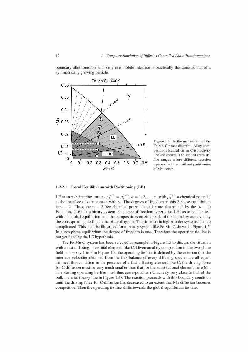
Figure 1.5: Isothermal section of theFe-Mn-C phase diagram. Alloy com-positions located on an C-iso-activityline are shown. The shaded areas de-fine ranges where different reactionregimes, with or without partitioningof Mn, occur.

1.2.2.1 Local Equilibrium with Partitioning (LE)

LE at an α/γ interface means µα/γk = µ

γ/αk , k = 1, 2, . . . , n, with µ

α/γk = chemical potential

at the interface of α in contact with γ. The degrees of freedom in this 2-phase equilibriumis n − 2. Thus, the n − 2 free chemical potentials and v are determined by the (n − 1)Equations (1.6). In a binary system the degree of freedom is zero, i.e. LE has to be identicalwith the global equilibrium and the compositions on either side of the boundary are given bythe corresponding tie-line in the phase diagram. The situation in higher order systems is morecomplicated. This shall be illustrated for a ternary system like Fe-Mn-C shown in Figure 1.5.In a two-phase equilibrium the degree of freedom is one. Therefore the operating tie-line isnot yet fixed by the LE hypothesis.

The Fe-Mn-C system has been selected as example in Figure 1.5 to discuss the situationwith a fast diffusing interstitial element, like C. Given an alloy composition in the two-phasefield α + γ say 1 to 3 in Figure 1.5, the operating tie-line is defined by the criterion that theinterface velocities obtained from the flux balance of every diffusing species are all equal.To meet this condition in the presence of a fast diffusing element like C, the driving forcefor C-diffusion must be very much smaller than that for the substitutional element, here Mn.The starting operating tie-line must thus correspond to a C-activity very close to that of thebulk material (heavy line in Figure 1.5). The reaction proceeds with this boundary conditionuntil the driving force for C-diffusion has decreased to an extent that Mn diffusion becomescompetitive. Then the operating tie-line shifts towards the global equilibrium tie-line.


The alloys 1 to 4 in Figure 1.5 all correspond to the same C-activity. The starting op-erating tie-line is thus the same for all these alloys. This tie-line requires a partitioning ofMn between α and γ since the Mn composition on either side of the interface is very muchdifferent. Therefore the velocity of transformation is essentially controlled by the substitu-tional diffusion leading to a slow reaction. In Figure 1.5 the range of compositions where thereaction requires partitioning is shown as shaded area labelled LE.

1.2.2.2 Local Equilibrium with Negligible Partitioning (LENP)

In the case of alloy 4 (Figure 1.5) the operating LE tie-line defines the same Mn content inboth phases. For this alloy and all compositions below the broken line a reaction withoutpartitioning of Mn is possible. This leads to a fast reaction and the boundary condition iscalled local equilibrium with negligible or no partitioning (LENP).

The dotted line in Figure 1.5 defines a sharp limit between the two regimes. This limit isgiven by the intersection of the line of constant Mn content (white broken line) with the lineof constant activity in γ.

These basic concepts of LE and LENP were introduced long ago (Hultgren 1920, Hillert1953, Kirkaldy 1962, Popov 1959, Darken 1961). For an overview see (Hillert 1998). With thenew computational instruments the kinetics of these phase transformations can be calculatedquantitatively for any given time-temperature profile and composition.

1.2.2.3 Para-Equilibrium (PE)

So far fast and slow reactions were the result of the thermodynamic conditions related to thecomposition of the alloy at a given temperature. There were no kinetic constraints involved.

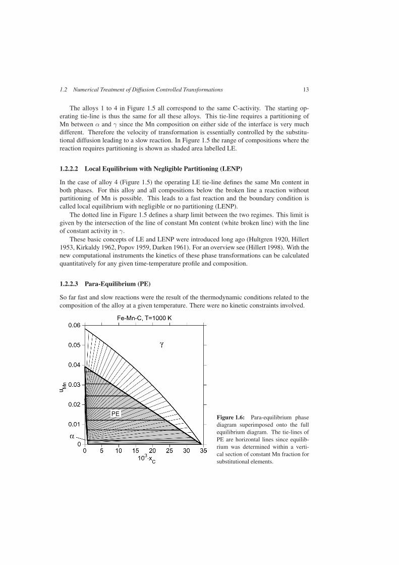
Figure 1.6: Para-equilibrium phasediagram superimposed onto the fullequilibrium diagram. The tie-lines ofPE are horizontal lines since equilib-rium was determined within a verti-cal section of constant Mn fraction forsubstitutional elements.


The situation becomes different if transformations at lower temperatures are consideredwhere substitutional atoms definitely become more and more immobile compared to the ve-locity of the interface. In that case equilibrium can no longer be established with respect tothese elements, but it may still be attained with respect to the fast diffusing interstitial el-ements. This situation was discussed by Hultgren in 1947 (Hultgren 1947). The resultingequilibrium he called para-equilibrium. Multicomponent systems like Fe-X-C are regardedas pseudo-binary systems M-C where all substitutional elements (Fe,. . . ) are replaced by oneaverage component M. The thermodynamic properties of M have to be constructed such thatthe Gibbs energy function of the pseudo-binary system M-C is identical to the Gibbs energyfunction within the corresponding vertical section of the system Fe-X-C.

The conditions for para-equilibrium are defined by the equations:

µαC = µγ

C

uαFeµ

αFe + uα

XµαX = uγ

FeµγFe + uγ

XµγX

The first equation imposes the local equilibrium for C, the second equation imposes the con-straint that this equilibrium has to be within a section of constant fraction of substitutionalelement X. The resulting phase diagram is shown in Figure 1.6. The tie-lines are horizontal ifu-fraction is used as coordinate for component X.

A reaction according to para-equilibrium cannot lead to the final global equilibrium. PEleads to phase fractions different from those of global equilibrium. It is important to noticethat PE gives equal chemical potentials of C on either side of the boundary, but not for thepotentials of substitutional components. This chemical potential difference exerts a force onthe interface, but the net force is zero.

The PE reaction in diffusion controlled phase transformations has been treated for variousexamples (e.g. Ghosh and Olson 2001, Hutchinson et al. 2003).

1.2.3 Cell Size

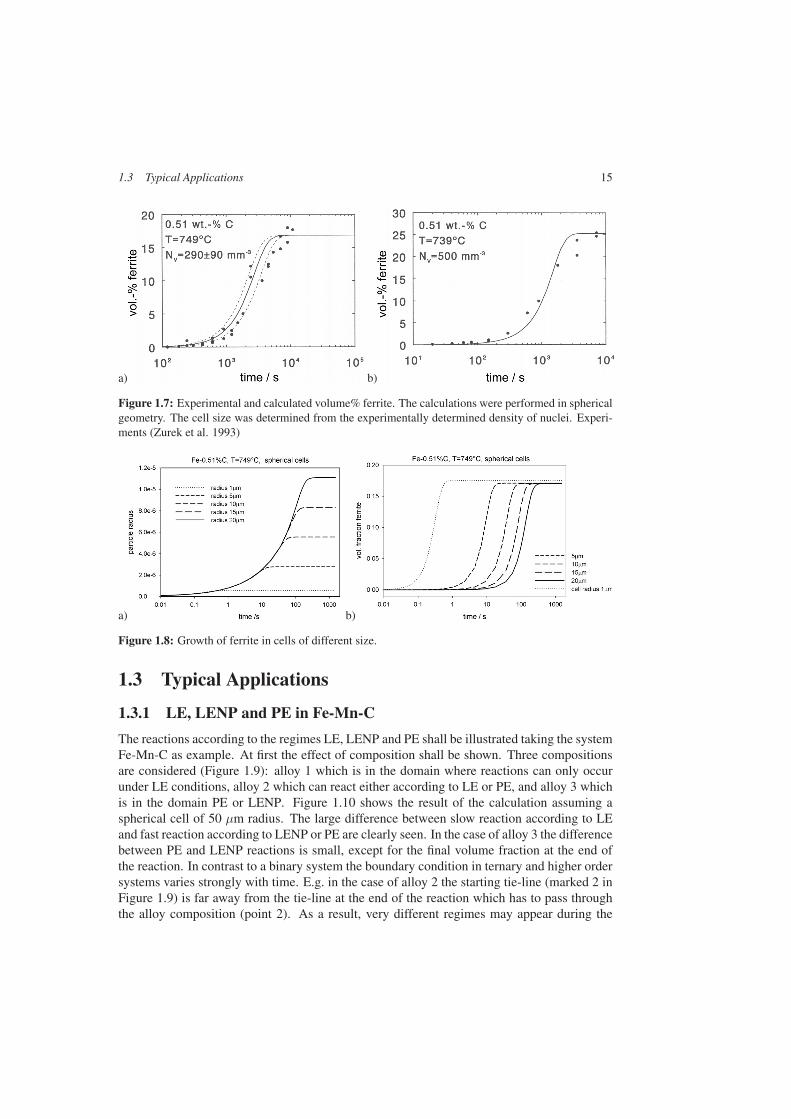
Cell size plays an important role in the kinetics of phase transformations. It is thus manda-tory to have a reliable value when it comes to comparison with experiments. In Figure 1.7the results for the binary Fe-C system are shown. Very good agreement is obtained betweenexperiment and calculation thanks a good knowledge of the density of nuclei obtained frommetallographic analysis of serial sections every 3 µm (Zurek et al. 1993). Using this informa-tion no fitting had to be applied to obtain this good agreement. The dotted lines in Figure 1.7arepresent the difference resulting from the indicated error range of the density of nuclei.

The importance of cell size becomes evident by means of Figure 1.8. A series of calcu-lations is shown for the same conditions as in Figure 1.7, however within cells of differentsizes. Looking at the particle sizes in Figure 1.8a one can see the common growth law and thelevelling off due to soft impingement of the C-composition profiles with the cell boundary. Ifinstead one looks at the volume fraction of ferrite formed the kinetic curves seem to suggest afaster kinetics. It is thus very important to make sure that when comparing experiments withcalculations the cell size corresponds to the particle distances in the experiments. Informationon the kinetics requires both quantities, average particle distance and volume fraction.

1.3 Typical Applications 15

a) b)

Figure 1.7: Experimental and calculated volume% ferrite. The calculations were performed in sphericalgeometry. The cell size was determined from the experimentally determined density of nuclei. Experi-ments (Zurek et al. 1993)

a) b)

Figure 1.8: Growth of ferrite in cells of different size.

1.3 Typical Applications

1.3.1 LE, LENP and PE in Fe-Mn-C

The reactions according to the regimes LE, LENP and PE shall be illustrated taking the systemFe-Mn-C as example. At first the effect of composition shall be shown. Three compositionsare considered (Figure 1.9): alloy 1 which is in the domain where reactions can only occurunder LE conditions, alloy 2 which can react either according to LE or PE, and alloy 3 whichis in the domain PE or LENP. Figure 1.10 shows the result of the calculation assuming aspherical cell of 50 µm radius. The large difference between slow reaction according to LEand fast reaction according to LENP or PE are clearly seen. In the case of alloy 3 the differencebetween PE and LENP reactions is small, except for the final volume fraction at the end ofthe reaction. In contrast to a binary system the boundary condition in ternary and higher ordersystems varies strongly with time. E.g. in the case of alloy 2 the starting tie-line (marked 2 inFigure 1.9) is far away from the tie-line at the end of the reaction which has to pass throughthe alloy composition (point 2). As a result, very different regimes may appear during the


evolution of the reaction. It is thus very important that the full thermodynamic information isincorporated, otherwise reliable results cannot be obtained.

Figure 1.9: Isothermal section of the sys-tem Fe-Mn-C showing the starting tie-linesfor three alloys according to their reactionregime.

Figure 1.10: Kinetics of transformation of alloys 1–3in Figure 1.9. Spherical geometry, cell radius 50 µm.

a) b)

Figure 1.11: Kinetics of ferrite formation from austenite: fast reaction at T = 1000 K.

Similar differences in the transformation regimes are obtained by variation of temperature.This is illustrated in Figure 1.11 and 1.12. From the phase diagrams, Figures 1.11a and 1.12a,it can be deduced that at 1000 K the LENP reaction is possible, while 50 K higher it is not.The composition profiles for various time steps in Figure 1.11b show that at 1000 K, duringthe first 1000 s, ferrite inherits the Mn-content of austenite. During this first LENP regimethe boundary condition is constant. After soft impingement of the C-profile with the cellboundary the reaction slows down and can proceed further only with Mn diffusion. During


this second LE regime the boundary condition varies considerably with time and eventuallyequilibrium is attained. On the contrary, at 1050 K the phase diagram Figure 1.12a shows thatthe LENP reaction is not possible. Therefore the reaction is slow from the beginning and canproceed only with Mn diffusion. The difference between the reactions at the two temperaturesare tremendous: at 1000 K, 63% of ferrite is formed within 1000s, while at 1050 K only0.2% is formed within 106 s. This shows the overwhelming possibilities of microstructurecontrol offered by appropriate heat treatments. There may be ways of selecting just the righttemperature in order to avoid the precipitation of an unwanted phase during heat treatmentswithin industrial time scales. Fast and slow reaction regimes are also obtained in the processof dissolution of phases. This has been treated in (Inden 1997).

a) b)

Figure 1.12: Kinetics of ferrite formation from austenite: slow reaction at T = 1050 K.

1.3.2 LE, LENP and PE in Fe-Si-C

1.3.2.1 Ferrite Precipitation in Fe-1.15Si-0.51C

First the precipitation of ferrite from austenite in a ternary Fe-1.15 %Si-0.5 %C (uSi =0.02272, uC = 0.02302) alloy at T = 749◦C shall be discussed. Figure 1.13 shows thecalculated isothermal section at equilibrium together with the diagram for para-equilibrium.It is clear that the alloy is located in the domain where both LENP and PE are thermodynam-ically possible. The corresponding tie-lines defining the respective boundary condition areindicated by thick lines.

Experiments were performed at this temperature and analyzed metallographically by serialsectioning. It was found that nucleation took place at grain vertices and the density of nucleiwas determined as 2200 ± 400/mm3. This density fixes the average cell size to be usedin the calculation (50 µm radius for spherical geometry or 80 µm half cell size in lineargeometry). This size controls the time at which soft-impingement of carbon starts reducingthe driving force for C diffusion, leading to a switch from LENP to LE. The results of DICTRAcalculations are shown in Figure 1.14 for linear and spherical geometry. The experiments areperfectly reproduced by the calculation for spherical geometry. Both calculations clearly show


Figure 1.13: Isothermal section of the Fe-Si-C system at 749◦C. Both the equilibrium(solid lines) and the para-equilibrium (bro-ken lines) diagrams are shown. The tie-lines defining the boundary condition are in-dicated.

Figure 1.14: Comparison between experimental dataand calculation. The calculation reveal the large dif-ference in the kinetic regimes, LENP and subsequentLE, showing that the plateau observed in industrial timescales, does not represent the final state. Equilibrium isonly attained after 2.5 years.

the existence of two reaction regimes. It shall be emphasized that the excellent agreement isobtained without any fitting. At the end of the fast regime the plateau defines an almostconstant volume fraction for very long times, far beyond industrial time scales.

Figure 1.15: Comparison ofthe precipitation kinetics ac-cording to PE and LENP withexperiments (lin. geom.).


It is interesting to check the second alternative: PE. The results of the PE calculationare shown in Figure 1.15. The PE calculations could only be performed in linear geometry.For comparison the LENP calculations are also shown for the same geometry. The resultsshow that there is very little difference between the kinetics of PE and LENP. The alloy isthus inappropriate for identifying whether the fast reaction regime might have been controlledby the PE condition or not. The reason for this becomes evident from the phase diagram inFigure 1.13. The tie-lines of both PE and LENP define C-compositions in austenite, whichare almost on the same iso-activity line. The driving force for C-diffusion is thus practicallythe same in both cases.

1.3.2.2 Ferrite Precipitation in Fe-1.73%Si-0.4%C

The thickening and lengthening kinetics of grain boundary allotriomorphic proeutectoid ferritewas measured by Bradley/Aaronson (Bradley and Aaronson 1981) at temperatures between725◦C and 825◦C. Some results are shown in Figure 1.16. The particle thickening shows theexpected parabolic growth behavior for diffusion controlled reactions.

a) b)

Figure 1.16: Thickening of grain boundary allotriomorphic ferrite.

DICTRA calculations were performed for both spherical and linear geometry and it turnsout that the thickening rate is best reproduced using linear geometry, as it may be expected forgrain boundary allotriomorph thickening.

At T = 725◦C and 775◦C the DICTRA calculations for linear geometry and LENP con-ditions agree rather well with the experimental data of ferrite thickening. At T = 825◦C theLENP regime is thermodynamically not possible, as can be seen from Figure 1.17. The endpoint of the tie-line for LENP corresponds to a C-activity which is just less than that of thematrix. Thus, C-diffusion in austenite is directed towards the growing ferrite instead of theaustenite bulk. Growth is not possible under this condition. In this instance the DICTRAcalculations which are based on the local equilibrium condition thus predict growth accordingto LE with a thickening rate very much less than obtained in the experiments.

The results at all temperatures are compared by means of the parabolic rate constant vs.temperature. This is shown in Figure 1.18. The LENP results cannot continue beyond the


limit of 822◦C, above which LENP is thermodynamically not possible. The PE calculationsshow excellent agreement with the growth constants in the whole temperature range. Below822◦C where LENP conditions are thermodynamically possible the LENP calculations arealso close to the results for PE conditions. This is again the effect of the small difference indriving force for C-diffusion in austenite for both LENP and PE, as seen in Figure 1.17. Thedifference between the results for LENP and PE condition differ by less than the error barsattributed to the data points in the original paper.

Figure 1.17: Calculated isothermal sec-tion of Fe-Si-C according to full equilib-rium and PE (dotted lines).

Figure 1.18: Comparison of experimental and calculatedparabolic growth rates for thickening of grain boundaryallotriomorphs of pro-eutectoid ferrite. The calculationsindicate a reaction according to PE. The limit of possibleLENP reaction is at 822◦C.

The experimental data of Bradley/Aaronson at 825◦C have to be interpreted as being dueto a reaction of PE type, since at this temperature LENP is thermodynamically not possible.However, the limit for LENP is very close and may be too close to the experimental temper-ature of 825◦C to draw a definitive conclusion. These results, however, show the way how toselect other compositions to have better conditions for drawing conclusions.

1.3.3 PE in Fe-Ni-C

The results presented so far give the impression that PE is rarely observed. In this contextthe recent experimental and theoretical work by Hutchinson (Hutchinson et al. 2003) has tobe mentioned which indicates that in fact PE plays an important role at early reaction times.The likelihood of experimentally observing PE depends on the range of interface velocitiesencountered. Since the PE reaction is very fast, special experimental techniques are requiredto fix the reaction steps. Hutchinson used a dilatometer instrument at IRSID/France allowingshort term heat treatments and quenching rates of more than 100/s. He analyzed five alloyswith compositions shown in Figure 1.19 in the isothermal section of the Fe-Ni-C system at700◦C, the temperature of the annealing experiments. The alloys are partly located in the field


PE/LENP, partly in the PE field. The experimental results obtained are shown in Figure 1.20.At the very beginning all alloys show a very rapid growth. This growth is consistent with thegrowth under PE conditions shown as solid lines in Figure 1.20. The most interesting effectis the levelling off of the growth of the three alloys with the highest Ni-contents. Obviously,in the very early stages the interface velocity is fast enough that the Ni atoms are virtuallyimmobile and a Ni-spike at the interface cannot develop. This regime continues until thevelocity has decreased to an extent that this criterion is no longer fulfilled. Once a Ni-spike isbuilt up, the reaction switches from PE to further growth under LE or LENP condition. Thistransient leads to the plateau in the thickening rate.

Following this reasoning it becomes clear why the plateau level is smaller the higher the Nicontent: the higher the Ni content is, the smaller is the driving force for C-diffusion leadingto slower interface velocities (given by the difference in C concentration between interfaceand bulk austenite) and the earlier is the moment when Ni diffusion can compete with theinterface velocity. In Figure 1.20 the calculated curves for the thickening under PE conditionsare also shown. They do not differ much at the early stages of reaction and they agree withthe experiments at short times.

Hutchinson did set up a program allowing for a continuous transition from a starting PEreaction to the subsequent continuation with LE or LENP. The results obtained describe wellthe experimental observations (Hutchinson et al. 2003) and in particular can explain the for-mation of small amounts of α in composition ranges above the LE/LENP boundary.

For the two alloys with lowest Ni-contents there are no data points available for longertimes. This is due to experimental difficulties since at longer time hard impingement effectsoccurred as a result of the small grain size used. However, measurements of the plateau αfraction formed agreed well with the LENP fractions, even though the early stage kinetics isconsistent with PE. This is considered as indirect evidence of a transition from PE to LENPduring growth.

1.3.4 Effect of Traces on the Growth of Grain Boundary Cementite

Si is an element that has little solubility in cementite Fe3C. In the current thermodynamicdatabases cementite is treated as a phase with no solubility for Si. Lateral growth of grainboundary cementite was studied experimentally by Ando and Krauss (Ando and Krauss 1981)on a (nominally) ternary Fe-2.26%Cr-1.06%C at 738◦C.

The experimental data are shown in Figure 1.21. The calculations were first performed forthe nominal composition. The starting tie-line corresponds to a fast LENP reaction. In orderto comply with the experimental situation in (Ando and Krauss 1981) a spherical cell withdiameter 70 µm was chosen, cementite growing from the outer shell of the spherical graintowards the center. The calculated results for short times are shown in Figure 1.21. For 0%Sithe time to reach a given layer thickness is more than an order of magnitude shorter than theexperiments. It is only after taking into account that the alloys contained a trace of 0.03%Sithat the calculations come close to the experimental data. The rejection of the little amount ofSi into the matrix slows drastically down the rate of reaction.

It is interesting to note that taking three times more Si, 0.1%Si, makes only little difference.This demonstrates the effectiveness that traces may have on the reaction rate. At the sametime, this shows nicely that higher amounts of such elements do not necessarily lead to highereffects.


Figure 1.19: Isothermal section of the Fe-Ni-Cphase diagram at 700◦C. Five alloys are indicatedwhich were analyzed experimentally by Hutchin-son (Hutchinson 2002).

Figure 1.20: Experimentally determined thick-ening of ferrite allotriomorphs in Fe-Ni-C. Thelines represent calculations for PE (by courtesy ofC.R. Hutchinson 2003).

Figure 1.21: Lateral growth of grainboundary cementite in Fe-2.26%Cr-1.06%Si at 738◦C. The alloys con-tained a trace of 0.03%Si.

1.3.5 Continuous Cooling

The phenomena discussed so far under isothermal conditions are also encountered during con-tinuous cooling or heating. In a cooling experiment an alloy enters first into the LE region of atwo phase field, then into the PE region well before it enters eventually into the LENP region.By continuous cooling it is thus possible to observe these regimes within one specimen.

Such experiments were performed with two alloys, a ternary Fe-1.5Mn-0.09C and a qua-ternary Fe-1.37Mn-0.42Si-0.18C with a cooling rate of 1◦C/s from the austenite region (Cugy


Figure 1.22: Volume fraction of fer-rite determined experimentally afterinterrupted continuous cooling fromaustenite. Cooling rate 1 K/s. Experi-ments courtesy IRSID (Cugy and Kan-del 2001). Calculations: linear geom-etry, cell size 10 µm.

and Kandel 2001)). The cooling experiments were interrupted at a given temperature to deter-mine the microstructures obtained. The fraction of ferrite was determined from metallographicanalysis. The experimental results are shown in Figure 1.22. Calculations were performed forthe same conditions using a cell size in accordance with the austenite grain size. The cal-culated temperatures of LE and PE are marked by arrows. The volume fraction precipitatedunder LE is negligibly small. The onset of LENP reaction is characterized by a sudden in-crease in volume fraction.

The experimental data were determined at temperatures below the LENP starting point.They are perfectly located on the calculated LENP branches. Since the growth rates of PEand LENP reactions are very similar, the PE reaction, if occurring, should have started at thecorresponding temperatures TPE indicated. The volume fraction curves would then be verymuch like those in Figure 1.22, but shifted parallel to higher temperatures. The results thusindicate that at the cooling rates employed, the reaction proceeds by LENP.

Several arguments can be put forward to explain this. The PE start temperatures beingrather high the condition of immobility of Mn and Fe (relative to the velocity of the interface)is not fulfilled. Furthermore, the driving force for nucleation within the vertical section of PEis very much less than that for LE.

1.3.6 Competitive Growth of Phases: Multi-Cell Calculations

Simultaneous growth of phases can be treated by defining different cells (with the same ge-ometry) and coupling them together by appropriate boundary conditions. Various options are


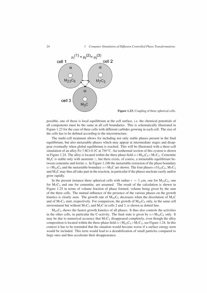
Figure 1.23: Coupling of three spherical cells.

possible, one of those is local equilibrium at the cell surface, i.e. the chemical potentials ofall components must be the same at all cell boundaries. This is schematically illustrated inFigure 1.23 for the case of three cells with different carbides growing in each cell. The size ofthe cells has to be defined according to the microstructure.

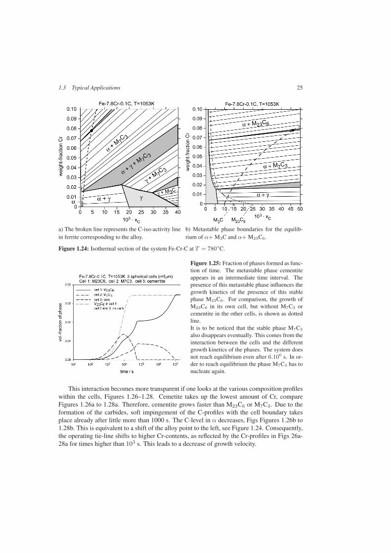
The multi-cell treatment allows for including not only stable phases present in the finalequilibrium, but also metastable phases which may appear at intermediate stages and disap-pear eventually when global equilibrium is reached. This will be illustrated with a three-cellsimulation of an alloy Fe-7.8Cr-0.1C at 780◦C. An isothermal section of this system is shownin Figure 1.24. The alloy is located within the three phase field α+M23C6+M7C3. CementiteM3C is stable only with austenite γ, but there exists, of course, a metastable equilibrium be-tween cementite and ferrite α. In Figure 1.24b the metastable extension of the phase boundaryα+M23C6 and the metastable boundary α+M3C are shown. The four phases αM23C6, M7C3

and M3C may thus all take part in the reaction, in particular if the phases nucleate easily and/orgrow rapidly.

In the present instance three spherical cells with radius r = 5 µm, one for M23C6, onefor M7C3 and one for cementite, are assumed. The result of the calculation is shown inFigure 1.25 in terms of volume fraction of phase formed, volume being given by the sumof the three cells. The mutual influence of the presence of the various phases on the growthkinetics is clearly seen. The growth rate of M23C6 decreases when the dissolution of M3Cand of M7C3 start, respectively. For comparison, the growth of M23C6 only, in the same cellenvironment but without M7C3 and M3C in cells 2 and 3, is shown as dotted line.

M23C6 shows the fastest growth kinetics of all phases. It thus also controls the activitiesin the other cells, in particular the C-activity. The final state is given by α+M23C6 only. Itmay be due to numerical accuracy that M7C3 disappeared completely, even though the alloycomposition is located within the three-phase field α+M23C6+M7C3, see Figure 1.24. In thiscontext it has to be reminded that the situation would become worse if a surface energy termwould be included. This term would lead to a destabilization of small particles compared tolarge ones and thus accelerate their disappearance.


a) The broken line represents the C-iso-activity linein ferrite corresponding to the alloy.

b) Metastable phase boundaries for the equilib-rium of α+ M3C and α+ M23C6.

Figure 1.24: Isothermal section of the system Fe-Cr-C at T = 780◦C.

Figure 1.25: Fraction of phases formed as func-tion of time. The metastable phase cementiteappears in an intermediate time interval. Thepresence of this metastable phase influences thegrowth kinetics of the presence of this stablephase M23C6. For comparison, the growth ofM23C6 in its own cell, but without M7C3 orcementite in the other cells, is shown as dottedline.It is to be noticed that the stable phase M7C3

also disappears eventually. This comes from theinteraction between the cells and the differentgrowth kinetics of the phases. The system doesnot reach equilibrium even after 6.106 s. In or-der to reach equilibrium the phase M7C3 has tonucleate again.

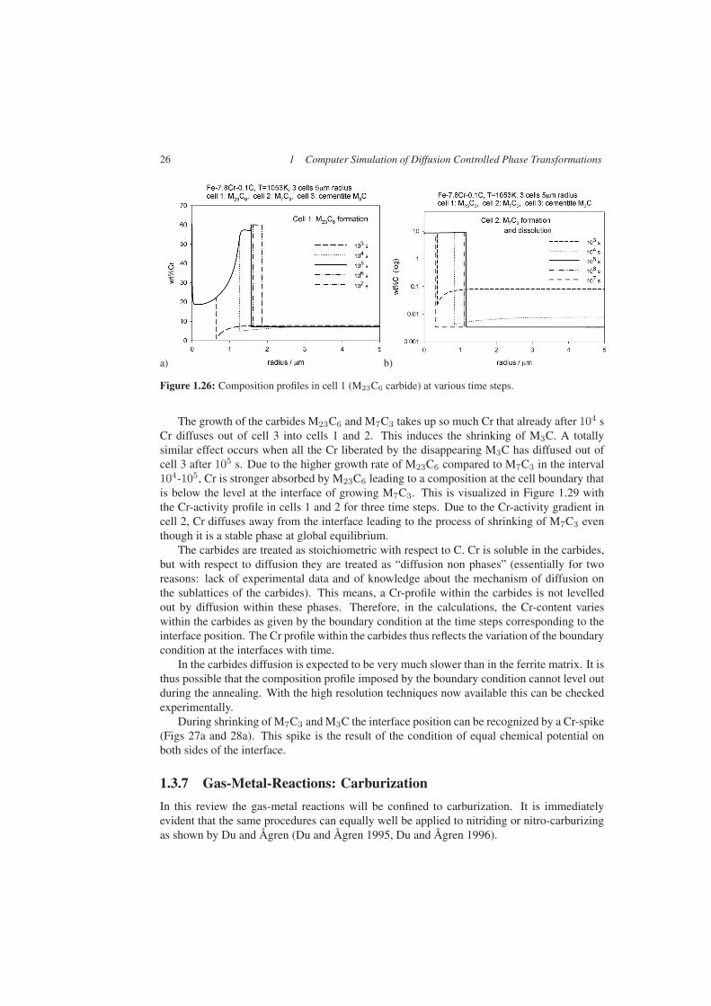
This interaction becomes more transparent if one looks at the various composition profileswithin the cells, Figures 1.26–1.28. Cemetite takes up the lowest amount of Cr, compareFigures 1.26a to 1.28a. Therefore, cementite grows faster than M23C6 or M7C3. Due to theformation of the carbides, soft impingement of the C-profiles with the cell boundary takesplace already after little more than 1000 s. The C-level in α decreases, Figs Figures 1.26b to1.28b. This is equivalent to a shift of the alloy point to the left, see Figure 1.24. Consequently,the operating tie-line shifts to higher Cr-contents, as reflected by the Cr-profiles in Figs 26a-28a for times higher than 103 s. This leads to a decrease of growth velocity.


a) b)

Figure 1.26: Composition profiles in cell 1 (M23C6 carbide) at various time steps.

The growth of the carbides M23C6 and M7C3 takes up so much Cr that already after 104 sCr diffuses out of cell 3 into cells 1 and 2. This induces the shrinking of M3C. A totallysimilar effect occurs when all the Cr liberated by the disappearing M3C has diffused out ofcell 3 after 105 s. Due to the higher growth rate of M23C6 compared to M7C3 in the interval104-105, Cr is stronger absorbed by M23C6 leading to a composition at the cell boundary thatis below the level at the interface of growing M7C3. This is visualized in Figure 1.29 withthe Cr-activity profile in cells 1 and 2 for three time steps. Due to the Cr-activity gradient incell 2, Cr diffuses away from the interface leading to the process of shrinking of M7C3 eventhough it is a stable phase at global equilibrium.

The carbides are treated as stoichiometric with respect to C. Cr is soluble in the carbides,but with respect to diffusion they are treated as “diffusion non phases” (essentially for tworeasons: lack of experimental data and of knowledge about the mechanism of diffusion onthe sublattices of the carbides). This means, a Cr-profile within the carbides is not levelledout by diffusion within these phases. Therefore, in the calculations, the Cr-content varieswithin the carbides as given by the boundary condition at the time steps corresponding to theinterface position. The Cr profile within the carbides thus reflects the variation of the boundarycondition at the interfaces with time.

In the carbides diffusion is expected to be very much slower than in the ferrite matrix. It isthus possible that the composition profile imposed by the boundary condition cannot level outduring the annealing. With the high resolution techniques now available this can be checkedexperimentally.

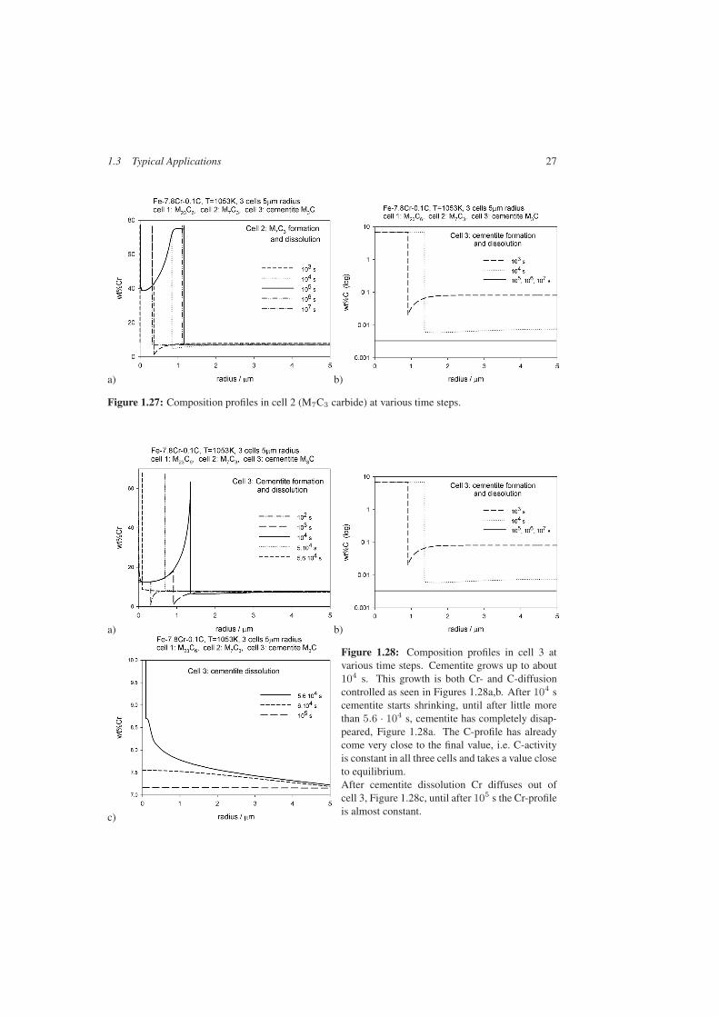
During shrinking of M7C3 and M3C the interface position can be recognized by a Cr-spike(Figs 27a and 28a). This spike is the result of the condition of equal chemical potential onboth sides of the interface.

1.3.7 Gas-Metal-Reactions: Carburization

In this review the gas-metal reactions will be confined to carburization. It is immediatelyevident that the same procedures can equally well be applied to nitriding or nitro-carburizingas shown by Du and Ågren (Du and Ågren 1995, Du and Ågren 1996).


a) b)

Figure 1.27: Composition profiles in cell 2 (M7C3 carbide) at various time steps.

a) b)

c)

Figure 1.28: Composition profiles in cell 3 atvarious time steps. Cementite grows up to about104 s. This growth is both Cr- and C-diffusioncontrolled as seen in Figures 1.28a,b. After 104 scementite starts shrinking, until after little morethan 5.6 · 104 s, cementite has completely disap-peared, Figure 1.28a. The C-profile has alreadycome very close to the final value, i.e. C-activityis constant in all three cells and takes a value closeto equilibrium.After cementite dissolution Cr diffuses out ofcell 3, Figure 1.28c, until after 105 s the Cr-profileis almost constant.


Figure 1.29: Cr-activity profile in thethree cells at time steps 5 · 104 s,6 · 104 s and 105 s.The rapid growth of M23C6 consumesso much Cr that after 105 s, whenthere is no more Cr supply from cell 3,the Cr-activity becomes lower at thecell boundary than at the interfaceα/M7C3. Consequently, Cr diffusesaway from the carbide M7C3 intocell 1. This leads to the shrinking andeventual disappearing of M7C3 eventhough it is a stable phase.

Gas carburization occurs in industrial furnaces with carbon activities aC < 1. Corrosivecarburization of high temperature alloys in carbon monoxide, methane or other hydrocarbonbearing gases at aC < 1 results in the formation of dispersed carbide particles, e.g. Cr-richcarbides in the case of Cr-alloys, leading to embrittlement of structural material. At activitiesaC � 1 the high temperature corrosion phenomenon, known as metal dusting (Grabke 2001),occurs.

Generally gas carburization of metals can be treated as follows (Sproge and Ågren 1988,Grabke 2001):

The carbon flux density from the gas to the metal depends on a mass transfer coefficient fand on the carbon activities in the gas and at the surface:

jC =1A

· dnC

dt= f · (agas

C − asurfaceC

).

The carbon diffusion in the metal matrix is driven by the gradient of the chemical potential ofcarbon:

jC = −MCcCdµC

dx= − DC

R · T cCdµC

dx.

The mass transfer coefficients of the various possible chemical surface reactions, e.g. the slowcarburizing gas mixture CH4 = C+2H2 or the fast carburizing mixture CO+H2 =C+H2O,have to be introduced. They have to be determined from experiments as function of tempera-ture and pressure. They are defined as f = k′

1 ·p3/2H2

or f = k′2 · pH2O

pH2, respectively. Numerical

values can be found in (Grabke 2001).

1.3.7.1 Carburization of pure Fe

Examples of slow and fast carburization simulations using DICTRA are shown in Figure 1.30.Slow carburization of an iron sample with 1 mm in thickness in a CH4–H2 gas mixture at700◦C at aC = 1 with a relatively low mass transfer coefficient f = 3.4 · 10−11 mol

cm2s leads to


a surface controlled carburization reaction, as shown in Figure 1.30a. The carbon activity atthe iron surface increases slowly with increasing time. The opposite situation is representedby carburization in a CO–H2–H2O mixture with a high mass transfer coefficient f = 3.4 ·10−6 mol

cm2s which leads to fast carbon transfer. In this case the carbon activity at the surfaceincreases very rapidly and the carburization reaction can be regarded as a diffusion controlledprocess (Figure 1.30b).

Carburization in H2S-containing atmospheres leads to a reduced kinetics due to a sulphurcoverage ΘS : jC = f · (1 − ΘS) · (agas

C − asurfaceC

).

Using this relationship the sulphur coverage can be determined indirectly by thermogravi-metric experiments where the carbon flux density is measured (Grabke 1977).

a) b)

Figure 1.30: Activity profiles obtained from DICTRA simulation for carburization of iron with 1 mm inthickness at 700◦C and aC = 1. a) slow carburization in a CH4-H2 mixture with f = 3.4·10−11 mol

cm2s,

b) fast carburization in a CO–H2–H2O mixture with f = 3.4 · 10−6 molcm2s

.

1.3.7.2 Carburization of Ni-Cr

The computer simulation of carburization of a Ni-25Cr high-temperature alloy was treatedby Engström et al. (Engström 1994). Since the conditions of the corresponding experimentsdefine a fast surface reaction, the DICTRA simulation is simplified taking the carbon activityat the alloy surface constant at aC = 1. In this instance a transfer coefficient need not to beintroduced into the calculation, consequently the reaction is just diffusion controlled. Afterbeing transferred to the material carbon diffuses within the matrix leading to precipitates ofM7C3 and M3C2. In order to treat this problem with DICTRA a special module for dispersedprecipitates was implemented (Engström 1994/2). The idea is to subdivide the carburizedmatrix into slices and to assume global equilibrium within every slice. The phase fractionsare obtained from the equilibrium calculation. Within a segment more than two phases mayprecipitate at the same time. During the first calculation step, the so-called diffusion step,diffusion in the matrix phase is treated as a one phase problem. Each diffusion step results in


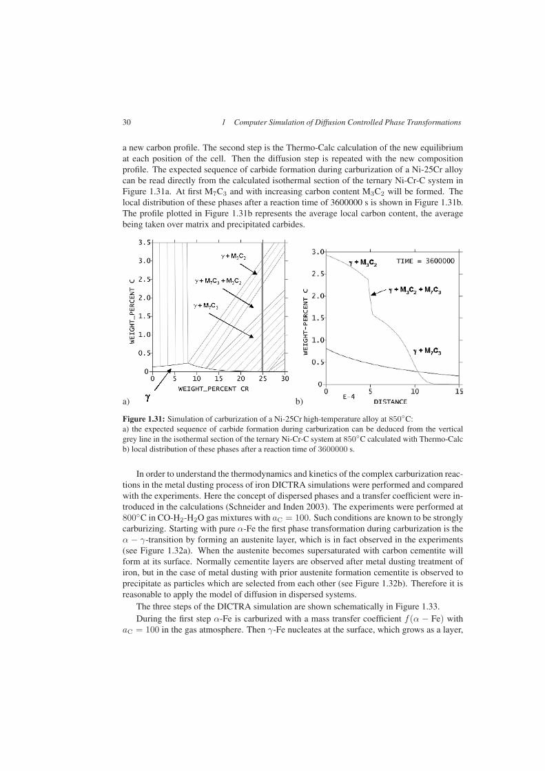
a new carbon profile. The second step is the Thermo-Calc calculation of the new equilibriumat each position of the cell. Then the diffusion step is repeated with the new compositionprofile. The expected sequence of carbide formation during carburization of a Ni-25Cr alloycan be read directly from the calculated isothermal section of the ternary Ni-Cr-C system inFigure 1.31a. At first M7C3 and with increasing carbon content M3C2 will be formed. Thelocal distribution of these phases after a reaction time of 3600000 s is shown in Figure 1.31b.The profile plotted in Figure 1.31b represents the average local carbon content, the averagebeing taken over matrix and precipitated carbides.

a) b)

Figure 1.31: Simulation of carburization of a Ni-25Cr high-temperature alloy at 850◦C:a) the expected sequence of carbide formation during carburization can be deduced from the verticalgrey line in the isothermal section of the ternary Ni-Cr-C system at 850◦C calculated with Thermo-Calcb) local distribution of these phases after a reaction time of 3600000 s.

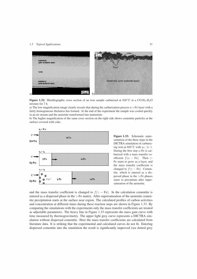
In order to understand the thermodynamics and kinetics of the complex carburization reac-tions in the metal dusting process of iron DICTRA simulations were performed and comparedwith the experiments. Here the concept of dispersed phases and a transfer coefficient were in-troduced in the calculations (Schneider and Inden 2003). The experiments were performed at800◦C in CO-H2-H2O gas mixtures with aC = 100. Such conditions are known to be stronglycarburizing. Starting with pure α-Fe the first phase transformation during carburization is theα − γ-transition by forming an austenite layer, which is in fact observed in the experiments(see Figure 1.32a). When the austenite becomes supersaturated with carbon cementite willform at its surface. Normally cementite layers are observed after metal dusting treatment ofiron, but in the case of metal dusting with prior austenite formation cementite is observed toprecipitate as particles which are selected from each other (see Figure 1.32b). Therefore it isreasonable to apply the model of diffusion in dispersed systems.

The three steps of the DICTRA simulation are shown schematically in Figure 1.33.During the first step α-Fe is carburized with a mass transfer coefficient f(α − Fe) with

aC = 100 in the gas atmosphere. Then γ-Fe nucleates at the surface, which grows as a layer,


a) b)

Figure 1.32: Metallographic cross section of an iron sample carburized at 800◦C in a CO-H2-H2Omixture for 7 h.a) The low magnification image clearly reveals that during the carburization process a γ-Fe layer with afairly homogeneous thickness has formed. At the end of the experiment the sample was cooled quicklyin an air stream and the austenite transformed into martensite.b) The higher magnification of the same cross section on the right side shows cementite particles at thesurface covered with coke.

Figure 1.33: Schematic repre-sentation of the three steps in theDICTRA simulation of carburiz-ing iron at 800◦C with aC � 1.During the first step α-Fe is car-burized with a mass transfer co-efficient f(α − Fe). Then γ-Fe starts to grow as a layer, andthe mass transfer coefficient ischanged to f(γ − Fe). Cemen-tite, which is entered as a dis-persed phase in the γ-Fe phasesstarts to precipitate after super-saturation of the austenite.

and the mass transfer coefficient is changed to f(γ − Fe). In the calculation cementite isentered as a dispersed phase in the γ-Fe matrix. After supersaturation of the austenite cemen-tite precipitation starts at the surface near region. The calculated profiles of carbon activitiesand concentration at different times during these reaction steps are shown in Figure 1.33. Bycomparing the simulations with the experiments only the mass transfer coefficients are treatedas adjustable parameters. The heavy line in Figure 1.33 represents the mass gain curve withtime measured by thermogravimetry. The upper light grey curve represents a DICTRA sim-ulation without dispersed cementite. Here the mass transfer coefficients are calculated fromliterature data. It is striking that the experimental and calculated curves do not fit. Enteringdispersed cementite into the simulation the result is significantly improved (see dotted grey


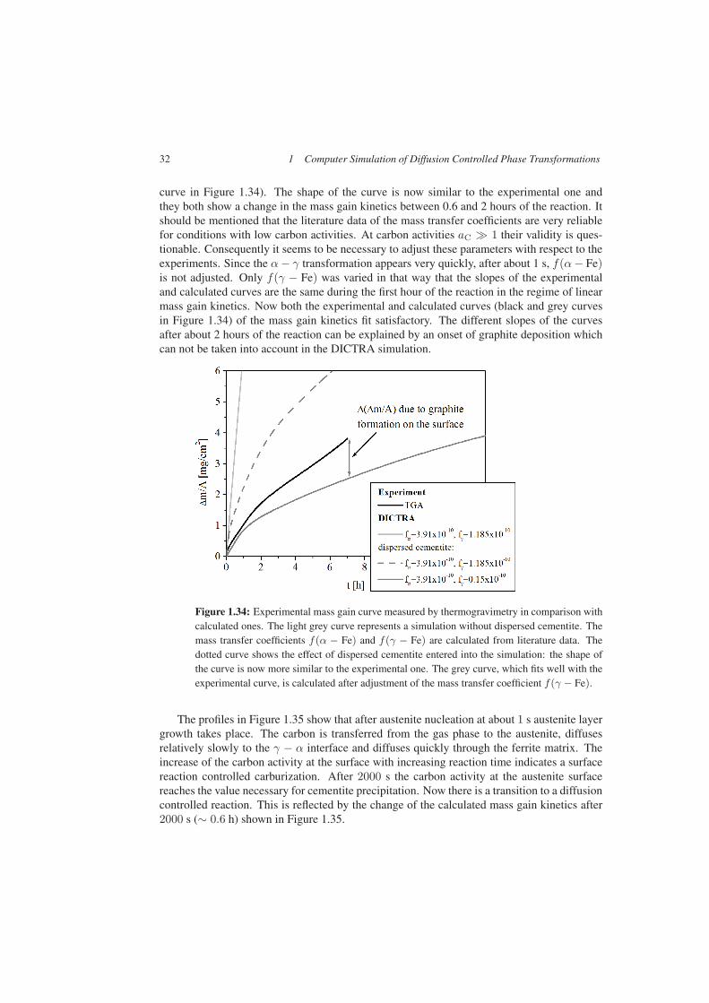
curve in Figure 1.34). The shape of the curve is now similar to the experimental one andthey both show a change in the mass gain kinetics between 0.6 and 2 hours of the reaction. Itshould be mentioned that the literature data of the mass transfer coefficients are very reliablefor conditions with low carbon activities. At carbon activities aC � 1 their validity is ques-tionable. Consequently it seems to be necessary to adjust these parameters with respect to theexperiments. Since the α − γ transformation appears very quickly, after about 1 s, f(α − Fe)is not adjusted. Only f(γ − Fe) was varied in that way that the slopes of the experimentaland calculated curves are the same during the first hour of the reaction in the regime of linearmass gain kinetics. Now both the experimental and calculated curves (black and grey curvesin Figure 1.34) of the mass gain kinetics fit satisfactory. The different slopes of the curvesafter about 2 hours of the reaction can be explained by an onset of graphite deposition whichcan not be taken into account in the DICTRA simulation.

Figure 1.34: Experimental mass gain curve measured by thermogravimetry in comparison withcalculated ones. The light grey curve represents a simulation without dispersed cementite. Themass transfer coefficients f(α − Fe) and f(γ − Fe) are calculated from literature data. Thedotted curve shows the effect of dispersed cementite entered into the simulation: the shape ofthe curve is now more similar to the experimental one. The grey curve, which fits well with theexperimental curve, is calculated after adjustment of the mass transfer coefficient f(γ − Fe).

The profiles in Figure 1.35 show that after austenite nucleation at about 1 s austenite layergrowth takes place. The carbon is transferred from the gas phase to the austenite, diffusesrelatively slowly to the γ − α interface and diffuses quickly through the ferrite matrix. Theincrease of the carbon activity at the surface with increasing reaction time indicates a surfacereaction controlled carburization. After 2000 s the carbon activity at the austenite surfacereaches the value necessary for cementite precipitation. Now there is a transition to a diffusioncontrolled reaction. This is reflected by the change of the calculated mass gain kinetics after2000 s (∼ 0.6 h) shown in Figure 1.35.

1.4 Outlook 33

These calculations are help understanding the complex driving forces of the gas-metalinteractions and simultaneous diffusion controlled phase transformations, e.g. during hightemperature corrosion.

a) b)

Figure 1.35: Calculated profiles of carbon activities (a) and concentration (b) at different times duringcarburization of iron at 800◦C with aC = 100.

1.4 Outlook

The results presented show that the numerical calculation of diffusion controlled phase trans-formations has reached a high level of accuracy and agreement with experimental data. Ithas become a valuable tool for research and alloy development. The limitations are comingfrom deficiencies in the thermodynamic description of phases which have previously been de-termined only for the purpose of phase diagram calculations, discarding any aspect relevantfor diffusion. Many of the phases are treated as so-called “diffusion-non-phase”, i.e. they arestoichiometric with respect to certain or even all components and do not allow diffusionaltransport within the phase. The mobilities can only be defined in accordance with the thermo-dynamic description. Consequently, they suffer from the same limitations. It can be expectedthat these limitations will be removed by future work.

There are other limitations which are obvious, e.g. the limit to geometries with one spatialcoordinate only. The distribution of particles may be such that a real 3-dimensional treatmentis required. e.g. experiments indicate that in ferritic steels the Laves phase nucleates prefer-entially at M23C6 particles. It is thus to be expected that the growth of Laves phase may isinfluenced by an exchange of elements between these phases. Such problems require methodslike phase field. The same is true for shape instabilities and elastic contributions.

Another limitation comes from the sharp interface concept which is the basis of the DIC-TRA-type approach. Effects like solute drag or solute trapping cannot really be treated prop-erly without opening the method to a diffuse interface.

34 References

The merit of the DICTRA method still is the sophisticated thermodynamic description.For many practical problems the thermodynamic part plays already a key-role and valuableresults for materials development can be obtained already from this approach. The reactions inmulti-component systems become extremely complex and can hardly be guessed in advance.The guidance offered by the quantitative predictions obtained with this concept have becomea valuable tool.

Acknowledgements

One of the authors (G.I.) wishes to thank the CNRS/France for making available a researchstay at Grenoble. This gave the opportunity for intense discussions with C. Hutchinson andY. Bréchet on para-equilibrium reactions and for a co-operation in that subject. Thanks aredue for the discussions and for making available results prior to publication.

ReferencesÅgren, J., 1982a. Diffusion in phases with several components and sublattices. J. Phys. Chem. Solids 43, 421–430.

Ågren, J., 1982b. Numerical treatment of diffusional reactions in multicomponent alloys. J. Phys. Chem. Solids 43,385–391.

Ågren, J., 2002. A graduate course in the theory of phase transformations. Stockholm.

Andersson, J.-O., Helander, T., Höglund, L., Shi, P., and Sundman, B., 2002. Thermo-Calc & DICTRA, computa-tional tools for materials science. CALPHAD 26, 273–312.

Andersson, J.-O. and Ågren, J. (1992) Models for numerical treatment of multicomponent diffusion in simple phases,J. Appl. Phys. 72, 1350–1355.

Ando, T. and Krauss, G. (1981) The isothermal thickening of cementite allotriomorphs in a 1.5Cr-1C steel, ActaMetall. 29, 351.

Bale, C. W., Chartrand, P., Degterov, S. A., Eriksson, G., Hack, K., Ben Mahfoud, R., Melancon, J., Pelton, A. D.and Petersen, S. (2002), CALPHAD, 26(2), 189–228.

Borgenstam, A., Engström, A., Höglund, L. and Ågren, J. (2000) DICTRA, a Tool for Simulation of DiffusionalTransformations in Alloys, J. Phase Equilibria 21, 269–280.

Bradley, J. R. and Aaronson, H. I. (1981) Metall. Trans. A 12A, 1729–1741.

Chen, S.-L., Daniel, S., Zhang, F., Chang, Y. A., Oates, W. A., R. Schmid-Fetzer (2001), “On the Calculation ofMulticomponent Stable Phase Diagrams”, J. Phase Equilibria 22, 373–378.

Crusius, S., Inden, G., Knoop, U., Höglund, L. and Ågren, J. (1992a) On the numerical treatment of moving boundaryproblems, Z. Metallkunde 83, 673–678.

Crusius, S., Höglund, L., Knoop, U., Inden, G. and Ågren, J. (1992b) On the growth of ferrite allotriomorphs in Fe-C,Z. Metallkunde 83, 729–738.

Cugy, P. and Kandel, M., IRSID/France, unpublished work, private communication.

Darken, L. S. (1961) Role of Chemistry in Metallurgical Research, Trans AIME 221, 654–671.

Davies, R. H., Dinsdale, A. T., Chart, T. G., Barry, T. I., Rand, M. (1990), “Application of MTDATA to the modellingof multicomponent equilibria”, High Temp. Science 26, 251–262.

Davies, R. H., Dinsdale, A. T., Gisby, J. A., Hodson, S. M., Ball, R. G. J. (1994), “Thermodynamic Modellingusing MTDATA: A Description showing applications involving oxides, alloys and aqueous solution”, Proc. Conf.ASM/TMS Fall Meeting: Applications of thermodynamics in the synthesis and processing of materials, Rosemont,IL, USA, 2–6 Oct 1994.

Du, H. and Ågren, J. (1995), “Gaseous nitriding iron – evaluation of diffusion data of N in γ′ and ε phases”, Z.Metallk. 86, 522–529.

References 35

Du, H. and Ågren, J. (1995), “Theoretical treatment of nitriding and nitrocarburizing of iron”, Metall. Trans. A 27,1073–1080.

Engström, A., Höglund, L. and Ågren, J. (1994a), “Computer simulations of carburization in multiphase systems”,Mater. Sci. Forum 163–165, 725–730.

Engström, A., Höglund, L. and Ågren, J. (1994b), “Computer Simulation of Diffusion in Multiphase Systems”,Metall. Mater. Trans. A 25A, 1127–1134.

Eriksson, G. and Hack, K. (1990), “ChemSage - A Computer Program for the Calculation of Complex ChemicalEquilibria”, Met. Trans. B, 21B, 1013–1023.

Engström, A. and Ågren, J. (1996) Assessment of Diffusional Mobilities in Face-centered Cubic Ni-Cr-Al Alloys, Z.Metallkunde 87, 92–97.

Franke, P. and Inden, G. (1997a) Diffusion Controlled Transformations in Multi-Particle Systems, Z. Metallkunde 88,917–924.

Franke, P. and Inden, G. (1997b) An assessment of the Si mobility and the application to phase transformations in Sisteels, Z. Metallkunde 88, 795–799.

Ghosh, G. and Olson, G. B. (2001) Simulation of Para-equilibrium Growth in Multicomponent Systems, Metall.Mater. Trans. 32A, 455.

Grabke, H. J., Petersen, E. M. and Srinivasan, S. R. (1977): “Influence of adsorbed sulphur on surface reactionkinetics and surface self diffusion on iron”, Surf. Sci. 67, 501–516.

Grabke, H. J., E. M. Müller-Lorenz, Schneider, A. (2001), “Carburization and metal dusting on iron”, ISIJ Int. 41,S1-S8.

The SGTE Casebook: Thermodynamics at Work, K. Hack Ed., The Institute of Materials, London 1996.

Hillert, M. (1953) Paraequilibrium, Internal Report, Swedish Institute of Metals Res., Stockholm.

Hillert, M. (1998) Phase Equilibria and Phase Transformations – Their Thermodynamic Basis, Cambridge UniversityPress.

Hillert, M. (1999) Drag, Solute Trapping and Diffusional Dissipation of Gibbs Energy, Acta mater. 47, 4481–4505.

Hultgren, A. (1920), A Metallographic Study of Tungsten Steels, John Wiley, New York NY.

Hultgren, A. (1947) Isothermal Transformation of Austenite, Trans ASM 36, 915–989.

Hutchinson, C. R., private communication.

Hutchinson, C. R., Fuchsmann, A. and Y. Bréchet (2003), “The Diffusional Formation of Ferrite from Austenite inFe-Ni-C Alloys”, Metall. Trans., in press.

Inden, G. and Neumann, P. (1996) “Simulation of diffusion controlled phase transformations in steels”, steel research67, 401–407.

Inden, G. (1997) Cinétique de transformation de phases dans des systèmes polyconstitutés - aspects thermody-namiques, Entropie 202/203, 6–14.

Inden, G. (2002) Computational Thermodynamics and Simulation of Phase Transformations, in CALPHAD and AlloyThermodynamics, Turchi, P. E., Gonis, A. and Shull, R. D. (Eds), The Minerals, Metals and Materials Soc (TMS),Warrendale/PA, 107–130.

Inden, G. (2003) Computer Modelling of Diffusion Controlled Transformations, in Thermodynamics, Microstructuresand Plasticity, A. Finel , D. Mazière, A. Olemskoï, M. Véron and P. Voorhees (Eds), Kluwer, 135–153.

Inden, G. and Hutchinson, C. R., presented at TMS Annual Meeting, Chicago 2003.

Jönsson, B. (1994) Ferromagnetic Ordering and Diffusion of Carbon and Nitrogen in bcc Cr-Fe-Ni Alloys, Z. Metall-kunde 85, 498–509.

Kaufman, L. and Bernstein, H. (1970), Computer Calculation of Phase Diagrams, Academic Press, New York.

Kirkaldy, J. S. (1962) Theory of Diffusional Growth in Solid-Solid Transformations, in Decomposition of Austeniteby Diffusionla Processes, Zackay, V. F. and Aaaronson, H. I. (Eds), Interscience Publ., New York, 39–130.

Onsager, L., 1931. Reciprocal relations in irreversible processes. Phys. Rev. 37, 405–426.

Popov, A. A. and Miller, M. S. (1959) On the kinetics of ferrite formation in the decarburization of carbon and alloysteels, Physics Metals Metallography 7, 36.

Sundman, B.; Jansson, B.; Andersson, J.-O.: CALPHAD 9 (1985a) 153/190.

36 References

Saunders, N. and Miodownik, A. P. (1998), CALPHAD, Pergamon Materials Series Vol. 1, Cahn, R. W. (Ed.), ElsevierScience, Oxford.

Schneider, A. and Inden, G. (2003), “Experiments and DICTRA simulations on carburization of iron at 800◦C athigh carbon activities”, in preparation.

Sundman, B., Jansson, B. and J.-O. Andersson (1985b) The Thermo-Calc databank system, CALPHAD 9, 153–190.

Jansson, B.; Schalin, M.; Sundman, B. (1993): Thermodynamic calculations made easy, J. Phase Equil. 14, 557–562.

Zurek, C., Thesis, TH-Aachen 1993, Hougardy, H. P., Inden, G., Knoop, U., Zurek, C., Final Report of COSMOSProject (1993); Knoop, U., Thesis Univ. Dortmund (1992).

Software THERMO-CALC: thermodynamic equilibrium calculations, developed at the Royal Institute of Technology,Stockholm. It is updated and implemented by the Foundation of Computational Thermodynamics, Royal Instituteof Technology, Stockholm/Sweden.

DICTRA: calculation of Diffusion Controlled TRAnsfromations. The first version was developed in 1988–1993 ina co-operation between the Royal Institute of Technology, Stockholm, (Group of Profs. M. Hillert and J. Ågren)and Max-Planck-Institut für Eisenforschung GmbH, Düsseldorf (Group of Prof. Inden) within a project (COS-MOS) supported by Volkswagen-Stiftung and Land Nordrhein-Westfalen. Since 1993 the software is updated andimplemented by the foundation THERMOCALC.

SSOL: Solid Solution Data Base provided by SGTE (Scientific Group Thermodata Europe).

PANDAT: Software for Multicomponent Phase Diagram Calculation, developed and maintained by ComputhermLLC, 437 S. Yellowstone Drive, Suite 217, Madison WI 53719, USA.

MTDATA: Thermodynamic equilibrium calculation. Software developed and maintained by the Thermodynamics andProcess Modeling Group, NPL Materials Centre, National Physical Laboratory, Teddington, Middlesex, TW110LW, UK.

CHEMSAGE, FACTSAGE: Thermodynamic equilibrium calculation, software developed and maintained by GTT-Technologies, Kaiserstraße 100, 52134 Herzogenrath/Germany and CRTC, Ecole Polytechnique de Mon-treal/Canada.

fundamentals and basic methods for microstructure...

Documents