fundamentals of numerical linear...
TRANSCRIPT
Fundamentals of Numerical LinearAlgebra
Seongjai Kim
Department of Mathematics and StatisticsMississippi State University
Mississippi State, MS 39762 USAEmail: [email protected]
Updated: November 30, 2016
Seongjai Kim, Department of Mathematics and Statistics, Missis-sippi State University, Mississippi State, MS 39762-5921 USA Email:[email protected]. The work of the author is supported in partby NSF grant DMS-1228337.
Prologue
In organizing this lecture note, I am indebted by Dem-mel [4], Golub and Van Loan [6], Varga [10], and Watkins[12], among others. Currently the lecture note is not fullygrown up; other useful techniques would be soon incor-porated. Any questions, suggestions, comments will bedeeply appreciated.
i

ii
Contents
1 Introduction to Matrix Analysis 11.1. Basic Algorithms and Notation . . . . . . . 2
1.1.1. Matrix notation . . . . . . . . . . . . 21.1.2. Matrix operations . . . . . . . . . . . 21.1.3. Vector notation . . . . . . . . . . . . 31.1.4. Vector operations . . . . . . . . . . . 41.1.5. Matrix-vector multiplication & “gaxpy” 41.1.6. The colon notation . . . . . . . . . . 51.1.7. Flops . . . . . . . . . . . . . . . . . 6
1.2. Vector and Matrix Norms . . . . . . . . . . 71.2.1. Vector norms . . . . . . . . . . . . . 71.2.2. Matrix norms . . . . . . . . . . . . . 91.2.3. Condition numbers . . . . . . . . . . 12
1.3. Numerical Stability . . . . . . . . . . . . . . 161.3.1. Stability in numerical linear algebra . 171.3.2. Stability in numerical ODEs/PDEs . 18
1.4. Homework . . . . . . . . . . . . . . . . . . 19
2 Gauss Elimination and Its Variants 212.1. Systems of Linear Equations . . . . . . . . 22
2.1.1. Nonsingular matrices . . . . . . . . 24
iii
iv Contents
2.1.2. Numerical solutions of differential equa-tions . . . . . . . . . . . . . . . . . . 26
2.2. Triangular Systems . . . . . . . . . . . . . . 302.2.1. Lower-triangular systems . . . . . . 312.2.2. Upper-triangular systems . . . . . . 33
2.3. Gauss Elimination . . . . . . . . . . . . . . 342.3.1. Gauss elimination without row inter-
changes . . . . . . . . . . . . . . . . 362.3.2. Solving linear systems by LU fac-
torization . . . . . . . . . . . . . . . 392.3.3. Gauss elimination with pivoting . . . 492.3.4. Calculating A−1 . . . . . . . . . . . . 56
2.4. Special Linear Systems . . . . . . . . . . . 582.4.1. Symmetric positive definite (SPD) ma-
trices . . . . . . . . . . . . . . . . . 582.4.2. LDLT and Cholesky factorizations . 632.4.3. M-matrices and Stieltjes matrices . . 67
2.5. Homework . . . . . . . . . . . . . . . . . . 68
3 The Least-Squares Problem 713.1. The Discrete Least-Squares Problem . . . 72
3.1.1. Normal equations . . . . . . . . . . 743.2. LS Solution by QR Decomposition . . . . . 78
3.2.1. Gram-Schmidt process . . . . . . . 783.2.2. QR decomposition, by Gram-Schmidt
process . . . . . . . . . . . . . . . . 813.2.3. Application to LS solution . . . . . . 91
3.3. Orthogonal Matrices . . . . . . . . . . . . . 94
Contents v
3.3.1. Householder reflection . . . . . . . . 953.3.2. QR decomposition by reflectors . . . 1063.3.3. Solving LS problems by Householder
reflectors . . . . . . . . . . . . . . . 1113.3.4. Givens rotation . . . . . . . . . . . . 1133.3.5. QR factorization by Givens rotation . 1193.3.6. Error propagation . . . . . . . . . . . 122
3.4. Homework . . . . . . . . . . . . . . . . . . 125
4 Singular Value Decomposition (SVD) 1274.1. Introduction to the SVD . . . . . . . . . . . 128
4.1.1. Algebraic Interpretation of the SVD . 1314.1.2. Geometric Interpretation of the SVD 1334.1.3. Properties of the SVD . . . . . . . . 1354.1.4. Computation of the SVD . . . . . . . 1414.1.5. Numerical rank . . . . . . . . . . . . 145
4.2. Applications of the SVD . . . . . . . . . . . 1474.2.1. Image compression . . . . . . . . . 1484.2.2. Rank-deficient least-squares prob-
lems . . . . . . . . . . . . . . . . . . 1514.2.3. Principal component analysis (PCA) 1584.2.4. Image denoising . . . . . . . . . . . 166
4.3. Homework . . . . . . . . . . . . . . . . . . 169
5 Eigenvalue Problems 1715.1. Definitions and Canonical Forms . . . . . . 1725.2. Perturbation Theory: Bauer-Fike Theorem . 1775.3. Gerschgorin’s Theorem . . . . . . . . . . . 182
vi Contents
5.4. Taussky’s Theorem and Irreducibility . . . . 1855.5. Nonsymmetric Eigenvalue Problems . . . . 189
5.5.1. Power method . . . . . . . . . . . . 1905.5.2. Inverse power method . . . . . . . . 1955.5.3. Orthogonal/Subspace iteration . . . 1985.5.4. QR iteration . . . . . . . . . . . . . . 2015.5.5. Making QR iteration practical . . . . 2035.5.6. Hessenberg reduction . . . . . . . . 2055.5.7. Tridiagonal and bidiagonal reduction 2145.5.8. QR iteration with implicit shifts – Im-
plicit Q theorem . . . . . . . . . . . . 2215.6. Symmetric Eigenvalue Problems . . . . . . 233
5.6.1. Algorithms for the symmetric eigen-problem – Direct methods . . . . . . 233
5.6.2. Tridiagonal QR iteration . . . . . . . 2365.6.3. Rayleigh quotient iteration . . . . . . 2415.6.4. Divide-and-conquer . . . . . . . . . 242
5.7. Homework . . . . . . . . . . . . . . . . . . 243
6 Iterative Methods for Linear Systems 2456.1. A Model Problem . . . . . . . . . . . . . . . 2466.2. Relaxation Methods . . . . . . . . . . . . . 2476.3. Krylov Subspace Methods . . . . . . . . . . 2486.4. Domain Decomposition Methods . . . . . . 2496.5. Multigrid Methods . . . . . . . . . . . . . . 2506.6. Homework . . . . . . . . . . . . . . . . . . 251
Chapter 1
Introduction to Matrix Analysis
1
2 CHAPTER 1. INTRODUCTION TO MATRIX ANALYSIS
1.1. Basic Algorithms and Notation
1.1.1. Matrix notation
Let R be the set of real numbers. We denote the vectorspace of all m× n matrices by Rm×n:
A ∈ Rm×n ⇔ A = (aij) =
a11 · · · a1n... ...am1 · · · amn
, aij ∈ R.
(1.1)The subscript ij refers to the (i, j) entry.
1.1.2. Matrix operations
• transpose (Rm×n → Rn×m)
C = AT ⇒ cij = aji
• addition (Rm×n × Rm×n → Rm×n)
C = A + B ⇒ cij = aij + bij
• scalar-matrix multiplication (R× Rm×n → Rm×n)
C = αA ⇒ cij = α aij
• matrix-matrix multiplication (Rm×p × Rp×n → Rm×n)
C = AB ⇒ cij =
p∑k=1
aikbkj
These are the building blocks of matrix computations.
1.1. Basic Algorithms and Notation 3
1.1.3. Vector notation
Let Rn denote the vector space of real n-vectors:
x ∈ Rn ⇔ x =
x1...xn
, xi ∈ R. (1.2)
We refer to xi as the ith component of x. We identify Rn
with Rn×1 so that the members of Rn are column vectors.On the other hand, the elements of R1×n are row vectors:
y ∈ R1×n ⇔ y = (y1, · · · , yn).
If x ∈ Rn, then y = xT is a row vector.
4 CHAPTER 1. INTRODUCTION TO MATRIX ANALYSIS
1.1.4. Vector operations
Assume a ∈ R and x, y ∈ Rn.
• scalar-vector multiplication
z = a x ⇒ zi = a xi
• vector addition
z = x + y ⇒ zi = xi + yi
• dot product (or, inner product)
c = xTy(= x · y) ⇒ c =
n∑i=1
xiyi
• vector multiply (or, Hadamard product)
z = x. ∗ y ⇒ zi = xiyi
• saxpy (“scalar a x plus y”): a LAPACK routine
z = a x + y ⇒ zi = a xi + yi
1.1.5. Matrix-vector multiplication & “gaxpy”
• gaxpy (“generalized saxpy”): a LAPACK routine
z = Ax + y ⇒ zi =
n∑j=1
aijxj + yi
1.1. Basic Algorithms and Notation 5
1.1.6. The colon notation
A handy way to specify a column or row of a matrix is withthe “colon” notation. Let A ∈ Rm×n. Then,
A(i, :) = [ai1, · · · , ain], A(:, j) =
a1j...amj
Example 1.1. With these conventions, the gaxpy can bewritten as
for i=1:m
z(i)=y(i)+A(i,:)x
end
(1.3)
or, in column version,
z=y
for j=1:n
z=z+x(j)A(:,j)
end
(1.4)
Matlab-code 1.2. The gaxpy can be implemented assimple as
z=A*x+y; (1.5)
6 CHAPTER 1. INTRODUCTION TO MATRIX ANALYSIS
1.1.7. Flops
A flop (floating point operation) is any mathematical op-eration (such as +, -, ∗, /) or assignment that involvesfloating-point numbers Thus, the gaxpy (1.3) or (1.4) re-quires 2mn flops.
The following will be frequently utilized in counting flops:n∑k=1
k =n(n + 1)
2,
n∑k=1
k2 =n(n + 1)(2n + 1)
6,
n∑k=1
k3 =( n∑k=1
k)2
=n2(n + 1)2
4.
(1.6)
1.2. Vector and Matrix Norms 7
1.2. Vector and Matrix Norms
1.2.1. Vector norms
Definition 1.3. A norm (or, vector norm) on Rn is afunction that assigns to each x ∈ Rn a nonnegative realnumber ‖x‖, called the norm of x, such that the followingthree properties are satisfied: for all x, y ∈ Rn and λ ∈ R,
‖x‖ > 0 if x 6= 0 (positive definiteness)
‖λx‖ = |λ| ‖x‖ (homogeneity)
‖x + y‖ ≤ ‖x‖ + ‖y‖ (triangle inequality)
(1.7)
Example 1.4. The most common norms are
‖x‖p =(∑
i
|xi|p)1/p
, 1 ≤ p <∞, (1.8)
which we call the p-norms, and
‖x‖∞ = maxi|xi|, (1.9)
which is called the infinity-norm or maximum-norm.
Two of frequently used p-norms are
‖x‖1 =∑
i |xi|, ‖x‖2 =(∑
i |xi|2)1/2
The 2-norm is also called the Euclidean norm, often de-noted by ‖ · ‖.Remark 1.5. One may consider the infinity-norm as thelimit of p-norms, as p→∞; see Homework 1.1.
8 CHAPTER 1. INTRODUCTION TO MATRIX ANALYSIS
Theorem 1.6. (Cauchy-Schwarz inequality) For allx, y ∈ Rn,∣∣∣ n∑
i=1
xiyi
∣∣∣ ≤ ( n∑i=1
x2i
)1/2( n∑i=1
y2i
)1/2
(1.10)
Note: (1.10) can be rewritten as
|x · y| ≤ ‖x‖ ‖y‖ (1.11)
which is clearly true.
Example 1.7. Given a positive definite matrix A ∈ Rn×n,define the A-norm on Rn by
‖x‖A = (xTAx)1/2
Note: When A = I, the A-norm is just the Euclideannorm. The A-norm is indeed a norm; see Homework 1.2.
Lemma 1.8. All p-norms on Rn are equivalent to eachother. In particular,
‖x‖2 ≤ ‖x‖1 ≤√n ‖x‖2
‖x‖∞ ≤ ‖x‖2 ≤√n ‖x‖∞
‖x‖∞ ≤ ‖x‖1 ≤ n ‖x‖∞
(1.12)
Note: For all x ∈ Rn,
‖x‖∞ ≤ ‖x‖2 ≤ ‖x‖1 ≤√n ‖x‖2 ≤ n ‖x‖∞ (1.13)
1.2. Vector and Matrix Norms 9
1.2.2. Matrix norms
Definition 1.9. A matrix norm on m× n matrices is avector norm on the mn-dimensional space, satisfying
‖A‖ ≥ 0, and ‖A‖ = 0 ⇔ A = 0 (positive definiteness)
‖λA‖ = |λ| ‖A‖ (homogeneity)
‖A + B‖ ≤ ‖A‖ + ‖B‖ (triangle inequality)(1.14)
Example 1.10.
• maxi,j|aij| is called the maximum norm.
• ‖A‖F ≡(∑
i,j
|aij|2)1/2
is called the Frobenius norm.
Definition 1.11. Let ‖ · ‖m×n be a matrix norm on m× nmatrices. The norms are called mutually consistent if
‖AB‖m×p ≤ ‖A‖m×n · ‖B‖n×p (1.15)
Definition 1.12. Lat A ∈ Rm×n and ‖ ·‖n is a vector normon Rn. Then
‖A‖mn = maxx∈Rn, x6=0
‖Ax‖m‖x‖n
(1.16)
is called an operator norm or induced norm or subor-dinate norm.
10 CHAPTER 1. INTRODUCTION TO MATRIX ANALYSIS
Lemma 1.13. Let A ∈ Rm×n and B ∈ Rn×p.
1. An operator norm of A is a matrix norm.
2. For all operator norms and the Frobenius norm,
‖Ax‖ ≤ ‖A‖ ‖x‖‖AB‖ ≤ ‖A‖ ‖B‖
(1.17)
3. For the induced 2-norm and the Frobenius norm,
‖PAQ‖ = ‖A‖ (1.18)
when P and Q are orthogonal, i.e., P−1 = P T andQ−1 = QT .
4. The max norm and the Frobenius norm are not oper-ator norms.
5. ‖A‖1 ≡ maxx 6=0
‖Ax‖1
‖x‖1= max
j
∑i
|aij|
6. ‖A‖∞ ≡ maxx 6=0
‖Ax‖∞‖x‖∞
= maxi
∑j
|aij|
7. ‖A‖2 ≡ maxx 6=0
‖Ax‖2
‖x‖2=√λmax(ATA),
where λmax denotes the largest eigenvalue.
8. ‖A‖2 = ‖AT‖2.
9. ‖A‖2 = maxi|λi(A)|, when ATA = AAT (normal).
1.2. Vector and Matrix Norms 11
Lemma 1.14. Let A ∈ Rn×n. Then
1√n‖A‖2 ≤ ‖A‖1 ≤
√n ‖A‖2
1√n‖A‖2 ≤ ‖A‖∞ ≤
√n ‖A‖2
1
n‖A‖∞ ≤ ‖A‖1 ≤ n ‖A‖∞
‖A‖1 ≤ ‖A‖F ≤√n ‖A‖2
(1.19)
Example 1.15. Let u, v ∈ Rn and let A = uvT . This is amatrix of rank one. Let’s prove
‖A‖2 = ‖u‖2 ‖v‖2 (1.20)
Proof.
12 CHAPTER 1. INTRODUCTION TO MATRIX ANALYSIS
1.2.3. Condition numbers
Definition 1.16. Let A ∈ Rn×n. Then
κ(A) ≡ ‖A‖ ‖A−1‖
is called the condition number of A, associated to thematrix norm.
Lemma 1.17.
1. κ(A) = κ(A−1)
2. κ(cA) = κ(A) for any c 6= 0.
3. κ(I) = 1 and κ(A) ≥ 1, for any induced matrix norm.
Theorem 1.18. If A is nonsingular and
‖δA‖‖A‖
≤ 1
κ(A), (1.21)
then A + δA is nonsingular.
1.2. Vector and Matrix Norms 13
Theorem 1.19. Let A ∈ Rn×n be nonsingular, and x andx = x + δx be the solutions of
Ax = b and A x = b + δb,
respectively. Then
‖δx‖‖x‖
≤ κ(A)‖δb‖‖b‖
. (1.22)
Proof. The equations
Ax = b and A(x + δx) = b + δb
imply Aδx = δb, that is, δx = A−1δb. Whatever vectornorm we have chosen, we will use the induced matrixnorm to measure matrices. Thus
‖δx‖ ≤ ‖A−1‖ ‖δb‖ (1.23)
Similarly, the equation b = Ax implies ‖b‖ ≤ ‖A‖ ‖x‖, orequivalently
1
‖x‖≤ ‖A‖ 1
‖b‖. (1.24)
The claim follows from (1.23) and (1.24).
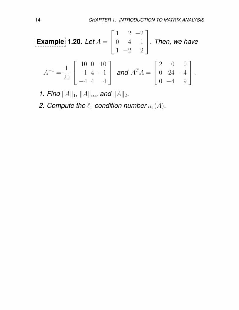
14 CHAPTER 1. INTRODUCTION TO MATRIX ANALYSIS
Example 1.20. Let A =
1 2 −2
0 4 1
1 −2 2
. Then, we have
A−1 =1
20
10 0 10
1 4 −1
−4 4 4
and ATA =
2 0 0
0 24 −4
0 −4 9
.1. Find ‖A‖1, ‖A‖∞, and ‖A‖2.
2. Compute the `1-condition number κ1(A).
1.2. Vector and Matrix Norms 15
Remark 1.21. Numerical analysis involving the condi-tion number is a useful tool in scientific computing. Thecondition number has been involved in analyses of
• Accuracy, due to the error involved in the data
• Stability of algebraic systems
• Convergence speed of iterative algebraic solvers
The condition number is one of most frequently-used mea-surements for matrices.
16 CHAPTER 1. INTRODUCTION TO MATRIX ANALYSIS
1.3. Numerical Stability
Sources of error in numerical computation:
Example: Evaluate a function f : R→ R at a given x.
• x is not exactly known
– measurement errors
– errors in previous computations
• The algorithm for computing f (x) is not exact
– discretization (e.g., it uses a table to look up)
– truncation (e.g., truncating a Taylor series)
– rounding error during the computation
The condition of a problem: sensitivity of the solutionwith respect to errors in the data
• A problem is well-conditioned if small errors in thedata produce small errors in the solution.
• A problem is ill-conditioned if small errors in the datamay produce large errors in the solution
1.3. Numerical Stability 17
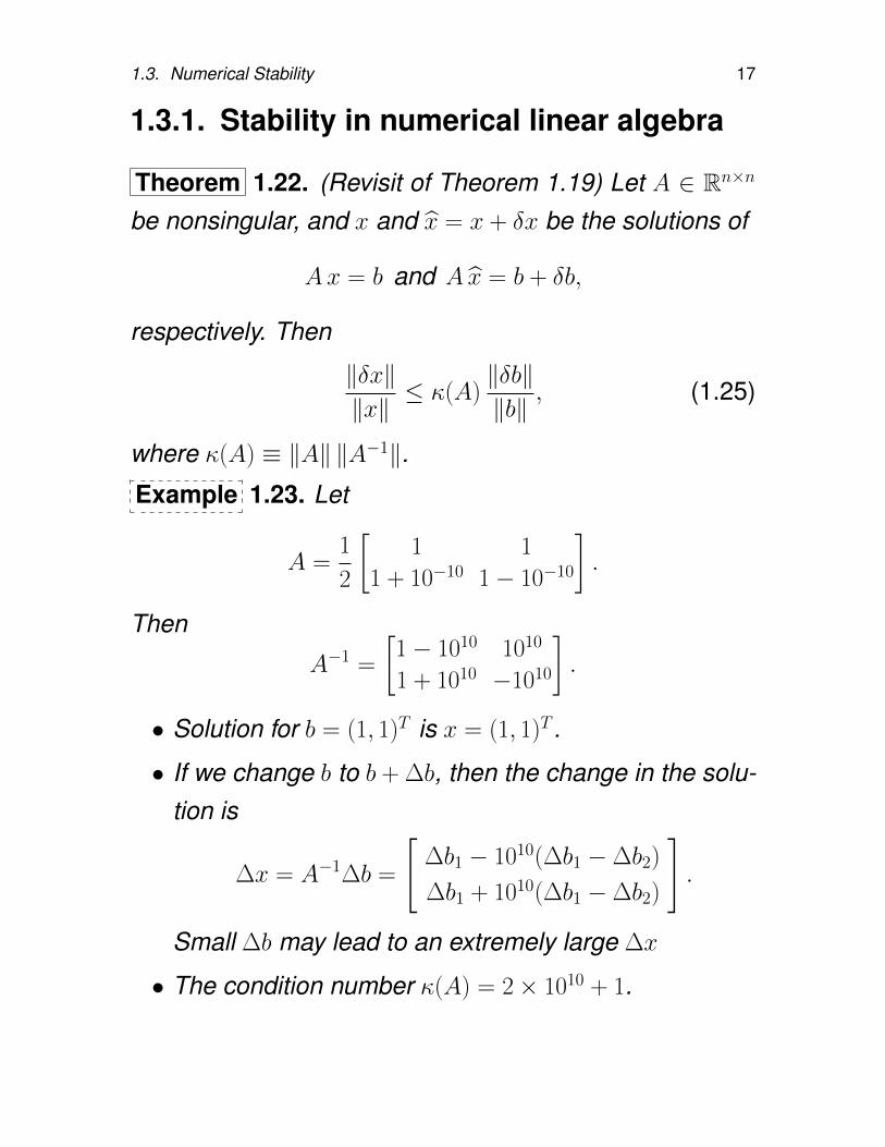
1.3.1. Stability in numerical linear algebra
Theorem 1.22. (Revisit of Theorem 1.19) Let A ∈ Rn×n
be nonsingular, and x and x = x + δx be the solutions of
Ax = b and A x = b + δb,
respectively. Then
‖δx‖‖x‖
≤ κ(A)‖δb‖‖b‖
, (1.25)
where κ(A) ≡ ‖A‖ ‖A−1‖.Example 1.23. Let
A =1
2
[1 1
1 + 10−10 1− 10−10
].
Then
A−1 =
[1− 1010 1010
1 + 1010 −1010
].
• Solution for b = (1, 1)T is x = (1, 1)T .
• If we change b to b + ∆b, then the change in the solu-tion is
∆x = A−1∆b =
[∆b1 − 1010(∆b1 −∆b2)
∆b1 + 1010(∆b1 −∆b2)
].
Small ∆b may lead to an extremely large ∆x
• The condition number κ(A) = 2× 10¹⁰ + 1.
18 CHAPTER 1. INTRODUCTION TO MATRIX ANALYSIS
1.3.2. Stability in numerical ODEs/PDEs
Physical Definition: A (FD) scheme is stable if a smallchange in the initial conditions produces a small changein the state of the system.
• Most aspects in the nature are stable.
• Some phenomena in the nature can be representedby differential equations (ODEs and PDEs), while theymay be solved through difference equations.
• Although ODEs and PDEs are stable, their approxi-mations (finite difference equations) may not be sta-ble. In this case, the approximation is a failure.
Definition: A differential equation is
• stable if for every set of initial data, the solution re-mains bounded as t→∞.
• strongly stable if the solution approaches zero ast→∞.
1.4. Homework 19
1.4. Homework1.1. This problem proves that the infinite-norm is the limit of the p-
norms as p→∞.
(a) Verify that
limp→∞
(1 + xp)1/p = 1, for each |x| ≤ 1
(b) Let x = (a, b)T with |a| ≥ |b|. Prove
limp→∞‖x‖p = |a| (1.26)
Equation (1.26) implies limp→∞‖x‖p = ‖x‖∞ for x ∈ R2.
(c) Generalize the above arguments to prove that
limp→∞‖x‖p = ‖x‖∞ for x ∈ Rn (1.27)
1.2. Let A ∈ Rn×n be a positive definite matrix, and R be its Choleskyfactor so that A = RTR.
(a) Verify that‖x‖A = ‖Rx‖2 for all x ∈ Rn (1.28)
(b) Using the fact that the 2-norm is indeed a norm on Rn, provethat the A-norm is a norm on Rn.
1.3. Prove (1.13).
1.4. Let A, B ∈ Rn×n and C = AB. Prove that the Frobenius norm ismutually consistent, i.e.,
‖AB‖F ≤ ‖A‖F ‖B‖F (1.29)
Hint: Use the definition cij =∑
k aikbkj and the Cauchy-Schwarzinequality.
1.5. The rank of a matrix is the dimension of the space spanned byits columns. Prove that A has rank one if and only if A = uvT forsome nonzero vectors u, v ∈ Rn.
20 CHAPTER 1. INTRODUCTION TO MATRIX ANALYSIS
1.6. A matrix is strictly upper triangular if it is upper triangular withzero diagonal elements. Show that if A ∈ Rn×n is strictly uppertriangular, then An = 0.
1.7. Let A = diagn(d−1, d0, d1) denote the n-dimensional tri-diagonalmatrix with ai,i−k = dk for k = −1, 0, 1. For example,
diag4(−1, 2,−1) =
2 −1 0 0−1 2 −1 0
0 −1 2 −10 0 −1 2
.Let B = diag10(−1, 2,−1). Use a computer software to solve thefollowing.
(a) Find condition number κ2(B).(b) Find the smallest (λmin) and the largest eigenvalues (λmax)
of B to compute the ratioλmax
λmin.
(c) Compare the above results.
Chapter 2
Gauss Elimination and Its Variants
One of the most frequently occurring problems in all ar-eas of scientific endeavor is that of solving a system of nlinear equations in n unknowns. The main subject of thischapter is to study the use of Gauss elimination to solvesuch systems. We will see that there are many ways toorganize this fundamental algorithm.
21
22 Chapter 2. Gauss Elimination and Its Variants
2.1. Systems of Linear Equations
Consider a system of n linear equations in n unknowns
a11x1 + a12x2 + · · · + a1nxn = b1
a21x1 + a22x2 + · · · + a2nxn = b2...
an1x1 + an2x2 + · · · + annxn = bn
(2.1)
Given the coefficients aij and the source bi, we wish tofind x1, x2, · · · , xn which satisfy the equations.
Since it is tedious to write (2.1) again and again, wegenerally prefer to write it as a single matrix equation
Ax = b, (2.2)
where
A =
a11 a12 · · · a1n
a21 a22 · · · a2n... ... ...an1 an2 · · · ann
, x =
x1
x2...xn
, and b =
b1
b2...bn
.
2.1. Systems of Linear Equations 23
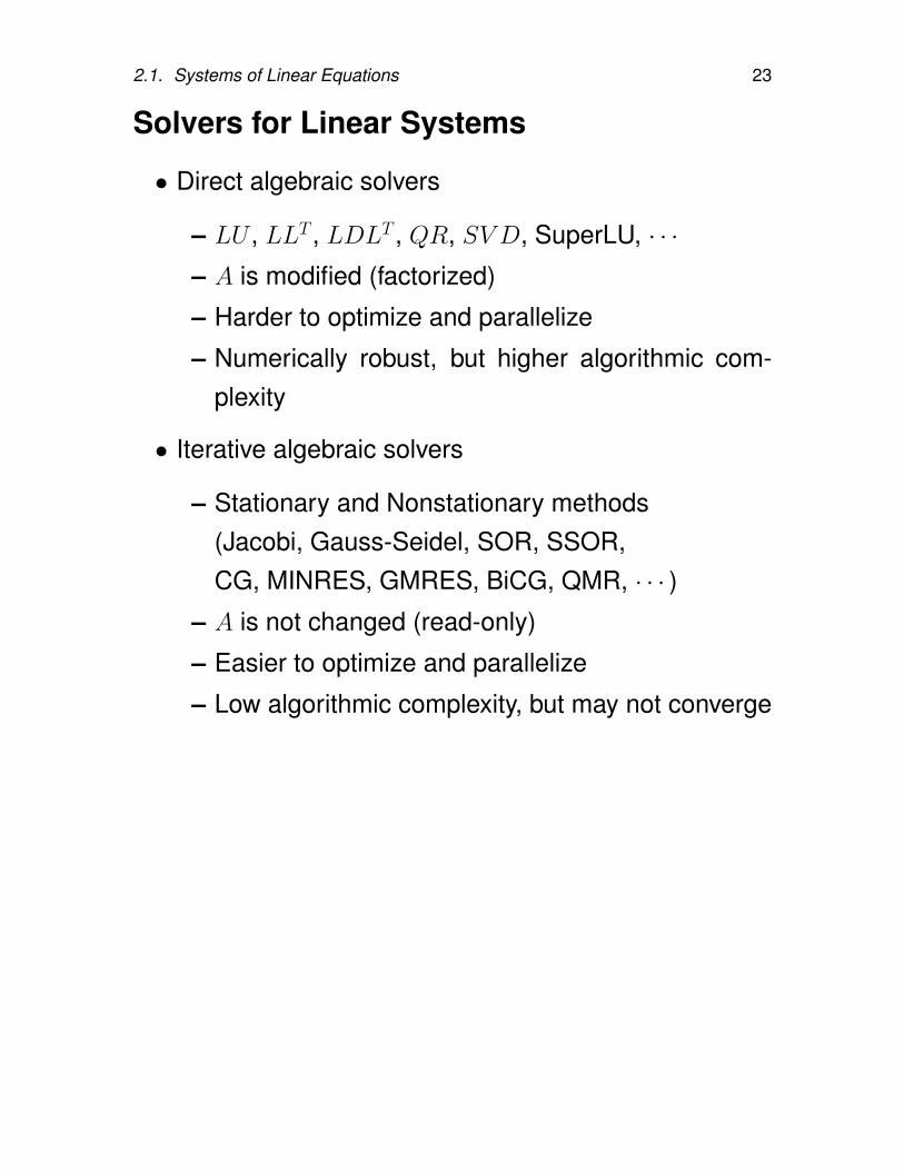
Solvers for Linear Systems
• Direct algebraic solvers
– LU , LLT , LDLT , QR, SV D, SuperLU, · · ·– A is modified (factorized)
– Harder to optimize and parallelize
– Numerically robust, but higher algorithmic com-plexity
• Iterative algebraic solvers
– Stationary and Nonstationary methods(Jacobi, Gauss-Seidel, SOR, SSOR,CG, MINRES, GMRES, BiCG, QMR, · · · )
– A is not changed (read-only)
– Easier to optimize and parallelize
– Low algorithmic complexity, but may not converge
24 Chapter 2. Gauss Elimination and Its Variants
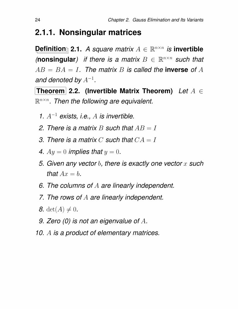
2.1.1. Nonsingular matrices
Definition 2.1. A square matrix A ∈ Rn×n is invertible(nonsingular) if there is a matrix B ∈ Rn×n such thatAB = BA = I. The matrix B is called the inverse of Aand denoted by A−1.
Theorem 2.2. (Invertible Matrix Theorem) Let A ∈Rn×n. Then the following are equivalent.
1. A−1 exists, i.e., A is invertible.
2. There is a matrix B such that AB = I
3. There is a matrix C such that CA = I
4. Ay = 0 implies that y = 0.
5. Given any vector b, there is exactly one vector x suchthat Ax = b.
6. The columns of A are linearly independent.
7. The rows of A are linearly independent.
8. det(A) 6= 0.
9. Zero (0) is not an eigenvalue of A.
10. A is a product of elementary matrices.
2.1. Systems of Linear Equations 25
Example 2.3. Let A ∈ Rn×n and eigenvalues of A be λi,i = 1, 2, · · · , n. Show that
det(A) =
n∏i=1
λi. (2.3)
Thus we conclude that A is singular if and only if 0 is aneigenvalue of A.
Hint: Consider the characteristic polynomial of A, φ(λ) =
det(A− λI), and φ(0).
26 Chapter 2. Gauss Elimination and Its Variants
2.1.2. Numerical solutions of differential equa-tions
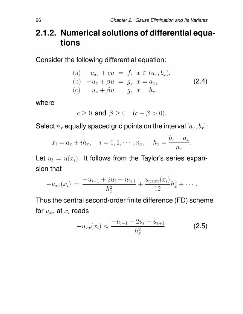
Consider the following differential equation:
(a) −uxx + cu = f, x ∈ (ax, bx),
(b) −ux + βu = g, x = ax,
(c) ux + βu = g, x = bx.
(2.4)
wherec ≥ 0 and β ≥ 0 (c + β > 0).
Select nx equally spaced grid points on the interval [ax, bx]:
xi = ax + ihx, i = 0, 1, · · · , nx, hx =bx − axnx
.
Let ui = u(xi). It follows from the Taylor’s series expan-sion that
−uxx(xi) =−ui−1 + 2ui − ui+1
h2x
+uxxxx(xi)
12h2x + · · · .
Thus the central second-order finite difference (FD) schemefor uxx at xi reads
−uxx(xi) ≈−ui−1 + 2ui − ui+1
h2x
. (2.5)
2.1. Systems of Linear Equations 27
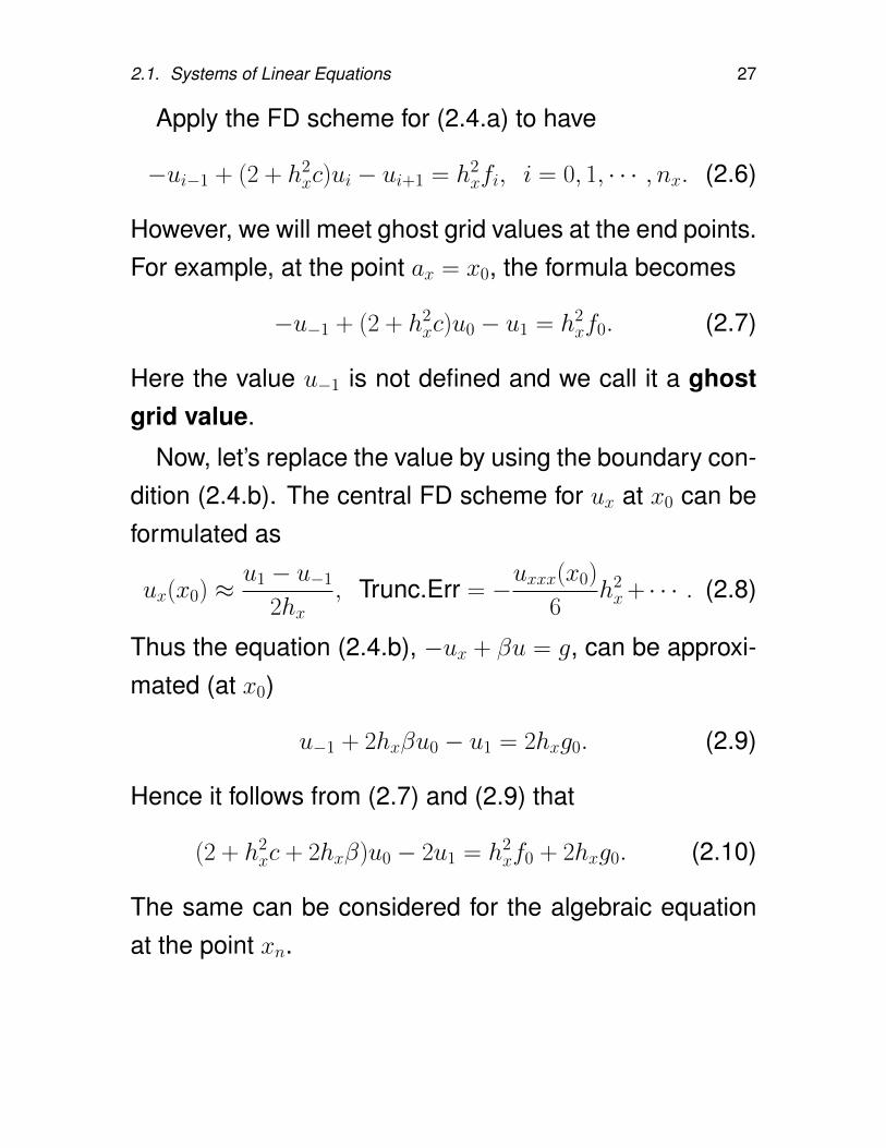
Apply the FD scheme for (2.4.a) to have
−ui−1 + (2 + h2xc)ui − ui+1 = h2
xfi, i = 0, 1, · · · , nx. (2.6)
However, we will meet ghost grid values at the end points.For example, at the point ax = x0, the formula becomes
−u−1 + (2 + h2xc)u0 − u1 = h2
xf0. (2.7)
Here the value u−1 is not defined and we call it a ghostgrid value.
Now, let’s replace the value by using the boundary con-dition (2.4.b). The central FD scheme for ux at x0 can beformulated as
ux(x0) ≈ u1 − u−1
2hx, Trunc.Err = −uxxx(x0)
6h2x+ · · · . (2.8)
Thus the equation (2.4.b), −ux + βu = g, can be approxi-mated (at x0)
u−1 + 2hxβu0 − u1 = 2hxg0. (2.9)
Hence it follows from (2.7) and (2.9) that
(2 + h2xc + 2hxβ)u0 − 2u1 = h2
xf0 + 2hxg0. (2.10)
The same can be considered for the algebraic equationat the point xn.
28 Chapter 2. Gauss Elimination and Its Variants
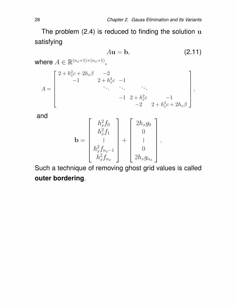
The problem (2.4) is reduced to finding the solution u
satisfyingAu = b, (2.11)
where A ∈ R(nx+1)×(nx+1),
A =
2 + h2
xc+ 2hxβ −2−1 2 + h2
xc −1. . . . . . . . .
−1 2 + h2xc −1
−2 2 + h2xc+ 2hxβ
,
and
b =
h2xf0
h2xf1...
h2xfnx−1
h2xfnx
+
2hxg0
0...0
2hxgnx
.Such a technique of removing ghost grid values is calledouter bordering.
2.1. Systems of Linear Equations 29
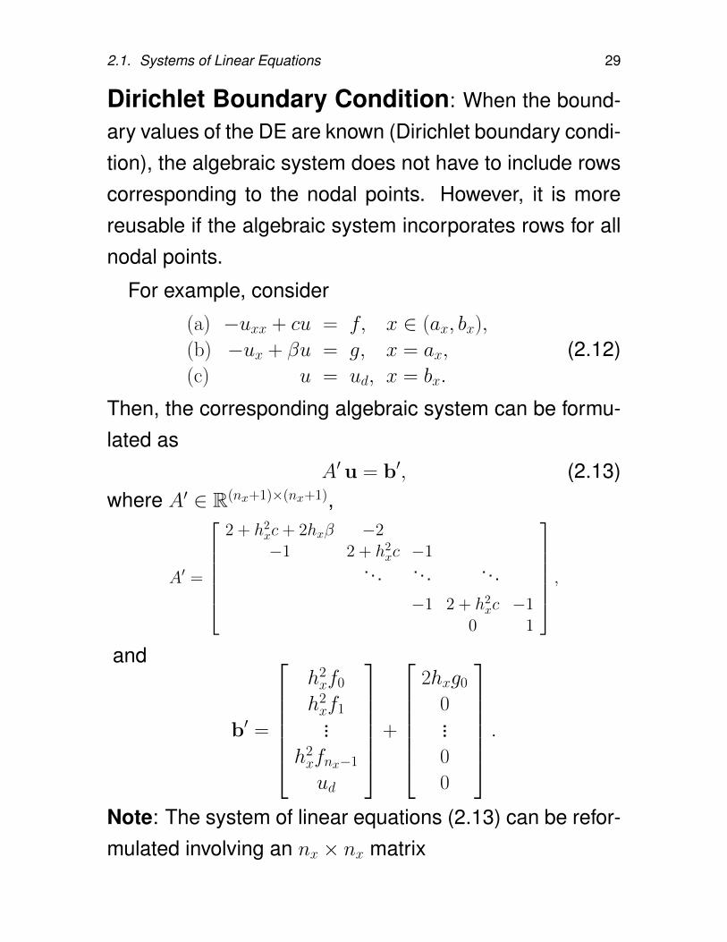
Dirichlet Boundary Condition: When the bound-ary values of the DE are known (Dirichlet boundary condi-tion), the algebraic system does not have to include rowscorresponding to the nodal points. However, it is morereusable if the algebraic system incorporates rows for allnodal points.
For example, consider
(a) −uxx + cu = f, x ∈ (ax, bx),
(b) −ux + βu = g, x = ax,
(c) u = ud, x = bx.
(2.12)
Then, the corresponding algebraic system can be formu-lated as
A′ u = b′, (2.13)where A′ ∈ R(nx+1)×(nx+1),
A′ =
2 + h2
xc+ 2hxβ −2−1 2 + h2
xc −1. . . . . . . . .
−1 2 + h2xc −1
0 1
,and
b′ =
h2xf0
h2xf1...
h2xfnx−1
ud
+
2hxg0
0...0
0
.Note: The system of linear equations (2.13) can be refor-mulated involving an nx × nx matrix
30 Chapter 2. Gauss Elimination and Its Variants
2.2. Triangular Systems
Definition 2.4.
1. A matrix L = (`ij) ∈ Rn×n is lower triangular if
`ij = 0 whenever i < j.
2. A matrix U = (uij) ∈ Rn×n is upper triangular if
uij = 0 whenever i > j.
Theorem 2.5. Let G be a triangular matrix. Then G isnonsingular if and only if gii 6= 0 for i = 1, · · · , n.
2.2. Triangular Systems 31
2.2.1. Lower-triangular systems
Consider the n× n system
Ly = b (2.14)
where L is a nonsingular, lower-triangular matrix (`ii 6= 0).It is easy to see how to solve this system if we write it indetail:
`11 y1 = b1
`21 y1 + `22 y2 = b2
`31 y1 + `32 y2 + `33 y3 = b3... ...
`n1 y1 + `n2 y2 + `n3 y3 + · · · + `nn yn = bn
(2.15)
The first equation involves only the unknown y1, whichcan be found as
y1 = b1/`11.
With y1 just obtained, we can determine y2 from the sec-ond equation:
y2 = (b2 − `21 y1)/`22.
Now with y2 known, we can solve the third equation for y3,and so on. In general, once we have y1, y2, · · · , yi−1, wecan solve for yi using the ith equation:
yi = (bi − `i1 y1 − `i2 y2 − · · · − `i,i−1 yi−1)/`ii
=1
`ii
(bi −
i−1∑j=1
`ij yj
) (2.16)
32 Chapter 2. Gauss Elimination and Its Variants
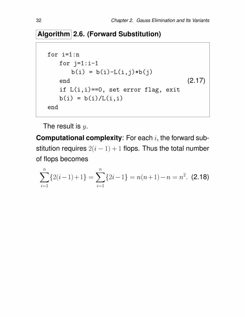
Algorithm 2.6. (Forward Substitution)
for i=1:n
for j=1:i-1
b(i) = b(i)-L(i,j)*b(j)
end
if L(i,i)==0, set error flag, exit
b(i) = b(i)/L(i,i)
end
(2.17)
The result is y.
Computational complexity: For each i, the forward sub-stitution requires 2(i− 1) + 1 flops. Thus the total numberof flops becomes
n∑i=1
2(i−1)+1 =
n∑i=1
2i−1 = n(n+1)−n = n2. (2.18)
2.2. Triangular Systems 33
2.2.2. Upper-triangular systems
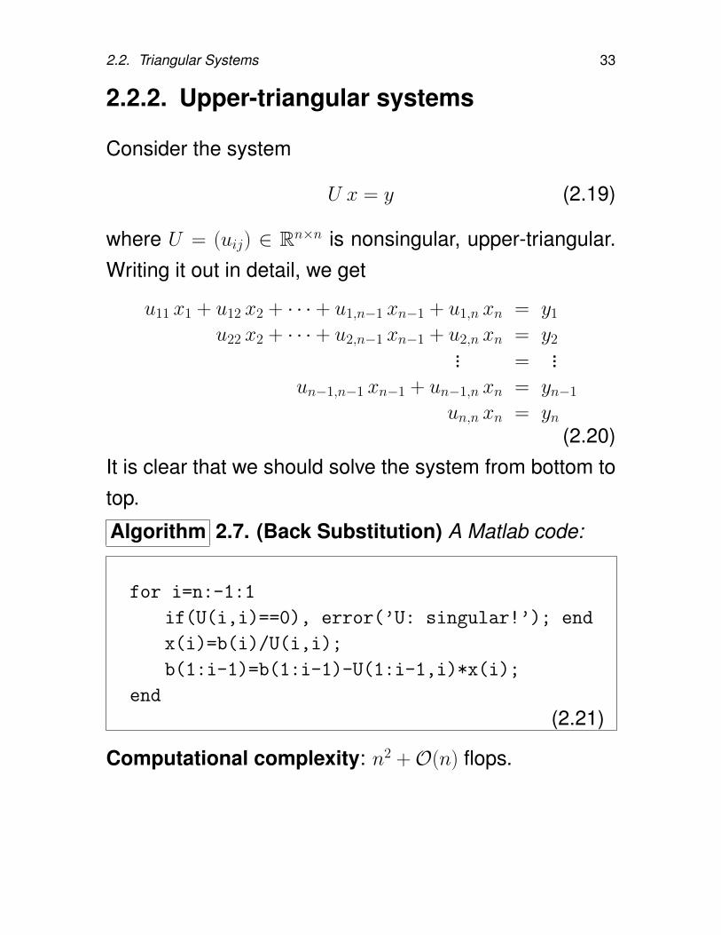
Consider the system
U x = y (2.19)
where U = (uij) ∈ Rn×n is nonsingular, upper-triangular.Writing it out in detail, we get
u11 x1 + u12 x2 + · · · + u1,n−1 xn−1 + u1,n xn = y1
u22 x2 + · · · + u2,n−1 xn−1 + u2,n xn = y2... = ...
un−1,n−1 xn−1 + un−1,n xn = yn−1
un,n xn = yn(2.20)
It is clear that we should solve the system from bottom totop.
Algorithm 2.7. (Back Substitution) A Matlab code:
for i=n:-1:1
if(U(i,i)==0), error(’U: singular!’); end
x(i)=b(i)/U(i,i);
b(1:i-1)=b(1:i-1)-U(1:i-1,i)*x(i);
end
(2.21)
Computational complexity: n2 +O(n) flops.
34 Chapter 2. Gauss Elimination and Its Variants
2.3. Gauss Elimination
— a very basic algorithm for solving Ax = b
The algorithms developed here produce (in the absenceof rounding errors) the unique solution of Ax = b when-ever A ∈ Rn×n is nonsingular.
Our strategy: Transform the system Ax = b to aequivalent system Ux = y, where U is upper-triangular.
It is convenient to represent Ax = b by an augmentedmatrix [A|b]; each equation in Ax = b corresponds to arow of the augmented matrix.
Transformation of the system: By means of threeelementary row operations applied on the augmentedmatrix.
Definition 2.8. Elementary row operations.
Replacement: Ri ← Ri + αRj (i 6= j)
Interchange: Ri ↔ Rj
Scaling: Ri ← βRi (β 6= 0)
(2.22)
2.3. Gauss Elimination 35
Proposition 2.9.
1. If [A | b] is obtained from [A |b] by elementary row op-erations (EROs), then systems [A |b] and [A | b] rep-resent the same solution.
2. Suppose A is obtained from A by EROs. Then A isnonsingular if and only if A is.
3. Each ERO corresponds to left-multiple of an elemen-tary matrix.
4. Each elementary matrix is nonsingular.
5. The elementary matrices corresponding to “Replace-ment” and “Scaling” operations are lower triangular.
36 Chapter 2. Gauss Elimination and Its Variants
2.3.1. Gauss elimination without row inter-changes
Let E1, E2, · · · , Ep be the p elementary matrices whichtransform A to an upper-triangular matrix U , that is,
EpEp−1 · · ·E2E1A = U (2.23)
Assume: No “Interchange” is necessary to apply. Then
• EpEp−1 · · ·E2E1 is lower-triangular and nonsingular
• L ≡ (EpEp−1 · · ·E2E1)−1 is lower-triangular.
• In this case,
A = (EpEp−1 · · ·E2E1)−1U = LU. (2.24)
2.3. Gauss Elimination 37
Example 2.10. Let A =
2 1 1
2 2 −1
4 −1 6
and b =
9
9
16
.
1. Perform EROs to obtain an upper-triangular system.
2. Identity elementary matrices for the EROs.
3. What are the inverses of the elementary matrices?
4. Express A as LU .
38 Chapter 2. Gauss Elimination and Its Variants
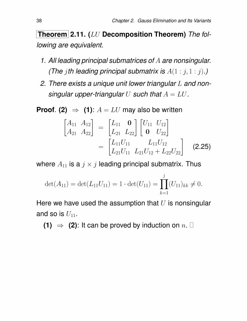
Theorem 2.11. (LU Decomposition Theorem) The fol-lowing are equivalent.
1. All leading principal submatrices ofA are nonsingular.(The jth leading principal submatrix is A(1 : j, 1 : j).)
2. There exists a unique unit lower triangular L and non-singular upper-triangular U such that A = LU .
Proof. (2) ⇒ (1): A = LU may also be written[A11 A12
A21 A22
]=
[L11 0
L21 L22
] [U11 U12
0 U22
]=
[L11U11 L11U12
L21U11 L21U12 + L22U22
](2.25)
where A11 is a j × j leading principal submatrix. Thus
det(A11) = det(L11U11) = 1 · det(U11) =
j∏k=1
(U11)kk 6= 0.
Here we have used the assumption that U is nonsingularand so is U11.
(1) ⇒ (2): It can be proved by induction on n.
2.3. Gauss Elimination 39
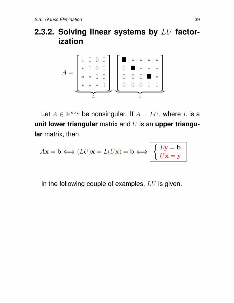
2.3.2. Solving linear systems by LU factor-ization
A =
1 0 0 0
∗ 1 0 0
∗ ∗ 1 0
∗ ∗ ∗ 1
︸ ︷︷ ︸
L
∗ ∗ ∗ ∗0 ∗ ∗ ∗0 0 0 ∗0 0 0 0 0
︸ ︷︷ ︸
U
Let A ∈ Rn×n be nonsingular. If A = LU , where L is aunit lower triangular matrix and U is an upper triangu-lar matrix, then
Ax = b⇐⇒ (LU)x = L(Ux) = b⇐⇒Ly = b
Ux = y
In the following couple of examples, LU is given.
40 Chapter 2. Gauss Elimination and Its Variants
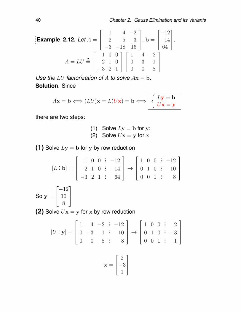
Example 2.12. Let A =
1 4 −22 5 −3−3 −18 16
, b =
−12−1464
.
A = LU∆=
1 0 02 1 0−3 2 1
1 4 −20 −3 10 0 8
Use the LU factorization of A to solve Ax = b.Solution. Since
Ax = b⇐⇒ (LU)x = L(Ux) = b⇐⇒Ly = bUx = y
there are two steps:
(1) Solve Ly = b for y;(2) Solve Ux = y for x.
(1) Solve Ly = b for y by row reduction
[L... b] =
1 0 0... −12
2 1 0... −14
−3 2 1... 64
→ 1 0 0
... −12
0 1 0... 10
0 0 1... 8
So y =
−12108
(2) Solve Ux = y for x by row reduction
[U... y] =
1 4 −2... −12
0 −3 1... 10
0 0 8... 8
→ 1 0 0
... 2
0 1 0... −3
0 0 1... 1
x =
2−31
2.3. Gauss Elimination 41
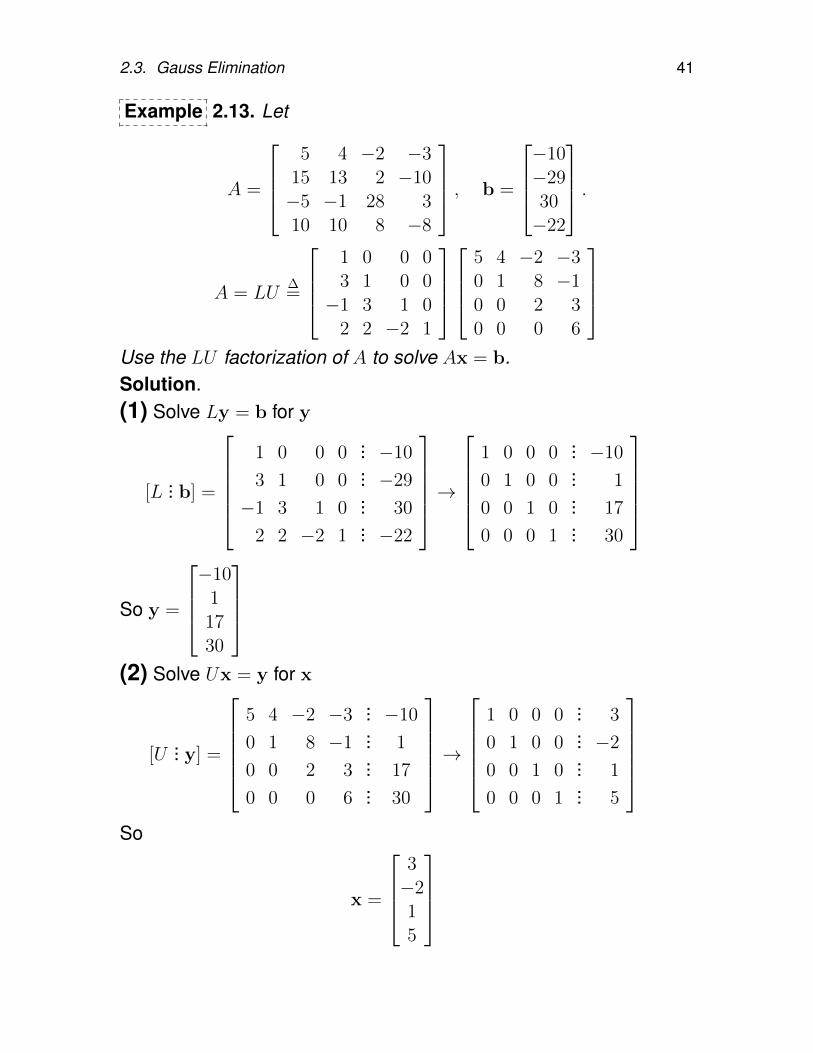
Example 2.13. Let
A =
5 4 −2 −3
15 13 2 −10−5 −1 28 310 10 8 −8
, b =
−10−2930−22
.
A = LU∆=
1 0 0 03 1 0 0−1 3 1 0
2 2 −2 1
5 4 −2 −30 1 8 −10 0 2 30 0 0 6
Use the LU factorization of A to solve Ax = b.Solution.(1) Solve Ly = b for y
[L... b] =
1 0 0 0
... −10
3 1 0 0... −29
−1 3 1 0... 30
2 2 −2 1... −22
→
1 0 0 0... −10
0 1 0 0... 1
0 0 1 0... 17
0 0 0 1... 30
So y =
−10
11730
(2) Solve Ux = y for x
[U... y] =
5 4 −2 −3
... −10
0 1 8 −1... 1
0 0 2 3... 17
0 0 0 6... 30
→
1 0 0 0... 3
0 1 0 0... −2
0 0 1 0... 1
0 0 0 1... 5
So
x =
3−215
42 Chapter 2. Gauss Elimination and Its Variants
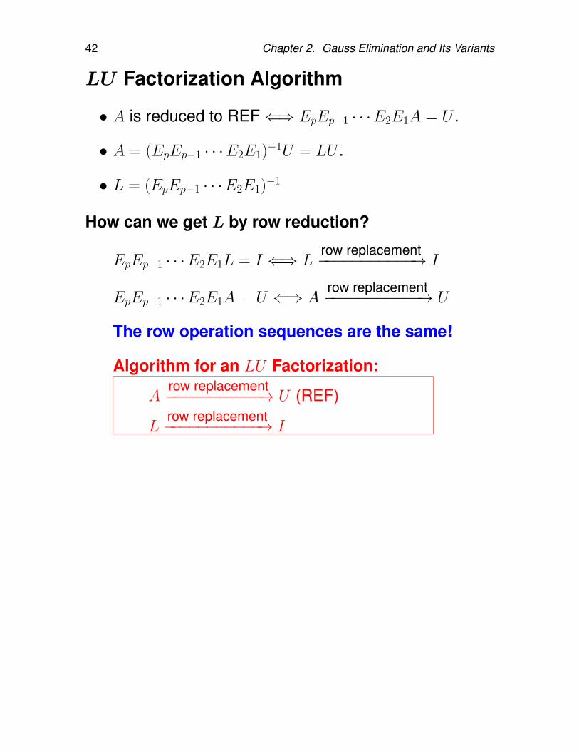
LU Factorization Algorithm
• A is reduced to REF⇐⇒ EpEp−1 · · ·E2E1A = U .
• A = (EpEp−1 · · ·E2E1)−1U = LU .
• L = (EpEp−1 · · ·E2E1)−1
How can we get L by row reduction?
EpEp−1 · · ·E2E1L = I ⇐⇒ Lrow replacement−−−−−−−−−−−→ I
EpEp−1 · · ·E2E1A = U ⇐⇒ Arow replacement−−−−−−−−−−−→ U
The row operation sequences are the same!
Algorithm for an LU Factorization:
Arow replacement−−−−−−−−−−−→ U (REF)
Lrow replacement−−−−−−−−−−−→ I
2.3. Gauss Elimination 43
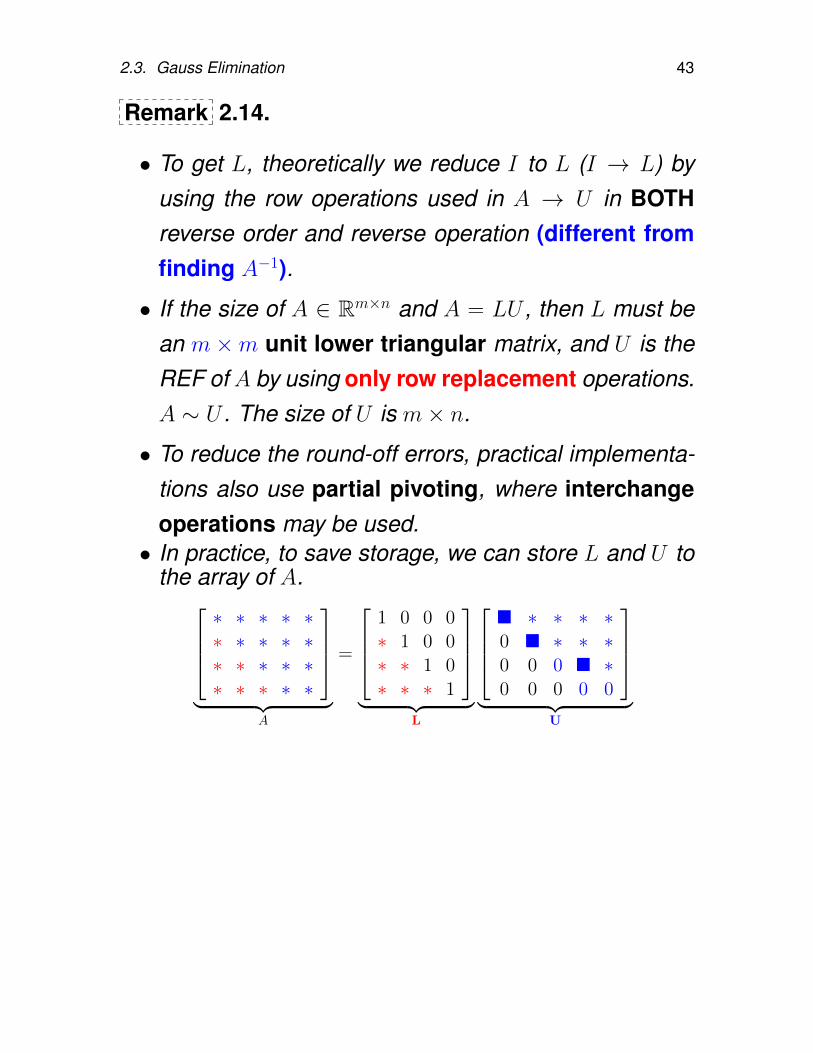
Remark 2.14.
• To get L, theoretically we reduce I to L (I → L) byusing the row operations used in A → U in BOTHreverse order and reverse operation (different fromfinding A−1).
• If the size of A ∈ Rm×n and A = LU , then L must bean m×m unit lower triangular matrix, and U is theREF of A by using only row replacement operations.A ∼ U . The size of U is m× n.
• To reduce the round-off errors, practical implementa-tions also use partial pivoting, where interchangeoperations may be used.• In practice, to save storage, we can store L and U to
the array of A.∗ ∗ ∗ ∗ ∗∗ ∗ ∗ ∗ ∗∗ ∗ ∗ ∗ ∗∗ ∗ ∗ ∗ ∗
︸ ︷︷ ︸
A
=
1 0 0 0∗ 1 0 0∗ ∗ 1 0∗ ∗ ∗ 1
︸ ︷︷ ︸
L
∗ ∗ ∗ ∗0 ∗ ∗ ∗0 0 0 ∗0 0 0 0 0
︸ ︷︷ ︸
U
44 Chapter 2. Gauss Elimination and Its Variants
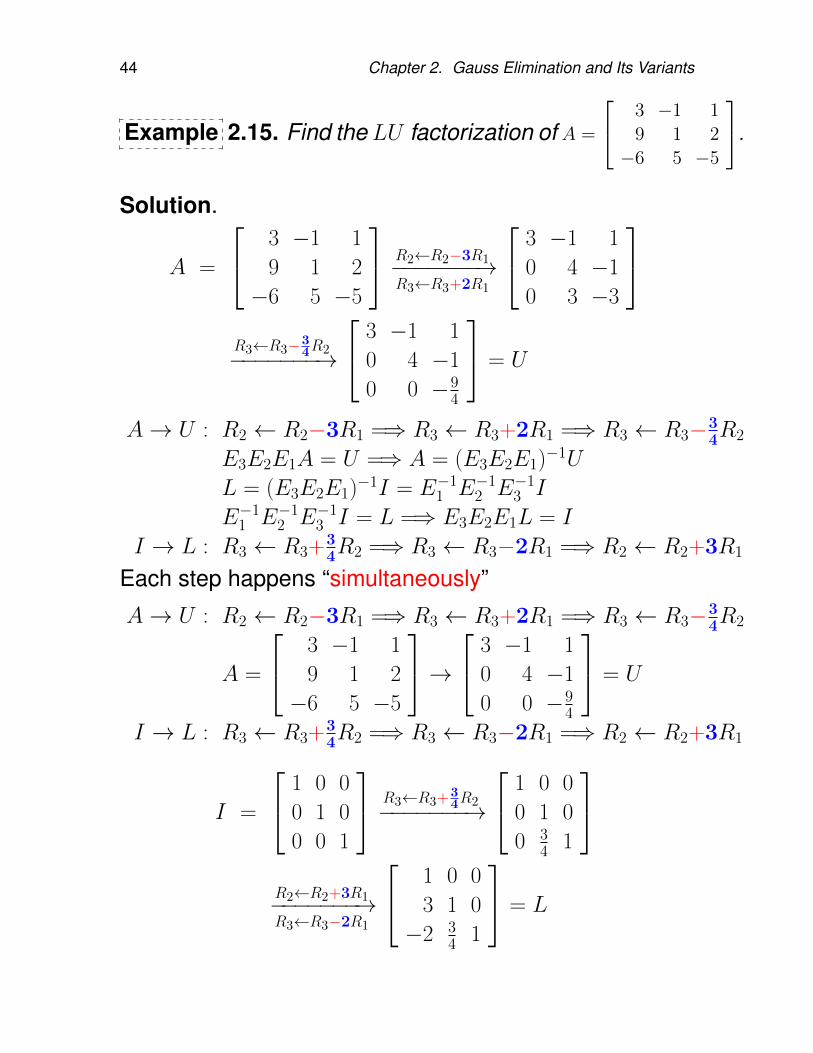
Example 2.15. Find the LU factorization of A =
3 −1 19 1 2−6 5 −5
.
Solution.
A =
3 −1 1
9 1 2
−6 5 −5
R2←R2−3R1−−−−−−−→R3←R3+2R1
3 −1 1
0 4 −1
0 3 −3
R3←R3−3
4R2−−−−−−−→
3 −1 1
0 4 −1
0 0 −94
= U
A→ U : R2 ← R2−3R1 =⇒ R3 ← R3+2R1 =⇒ R3 ← R3−34R2
E3E2E1A = U =⇒ A = (E3E2E1)−1U
L = (E3E2E1)−1I = E−11 E−1
2 E−13 I
E−11 E−1
2 E−13 I = L =⇒ E3E2E1L = I
I → L : R3 ← R3+34R2 =⇒ R3 ← R3−2R1 =⇒ R2 ← R2+3R1
Each step happens “simultaneously”
A→ U : R2 ← R2−3R1 =⇒ R3 ← R3+2R1 =⇒ R3 ← R3−34R2
A =
3 −1 1
9 1 2
−6 5 −5
→ 3 −1 1
0 4 −1
0 0 −94
= U
I → L : R3 ← R3+34R2 =⇒ R3 ← R3−2R1 =⇒ R2 ← R2+3R1
I =
1 0 0
0 1 0
0 0 1
R3←R3+34R2−−−−−−−→
1 0 0
0 1 0
0 34 1
R2←R2+3R1−−−−−−−→R3←R3−2R1
1 0 0
3 1 0
−2 34 1
= L
2.3. Gauss Elimination 45
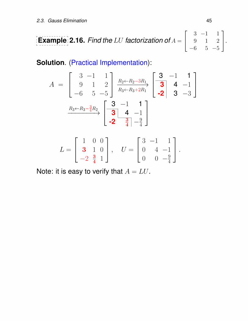
Example 2.16. Find the LU factorization of A =
3 −1 19 1 2−6 5 −5
.
Solution. (Practical Implementation):
A =
3 −1 1
9 1 2
−6 5 −5
R2←R2−3R1−−−−−−−→R3←R3+2R1
3 −1 13 4 −1
-2 3 −3
R3←R3−3
4R2−−−−−−−→
3 −1 13 4 −1
-2 34 −
94
L =
1 0 0
3 1 0
−2 34 1
, U =
3 −1 1
0 4 −1
0 0 −94
.Note: it is easy to verify that A = LU .
46 Chapter 2. Gauss Elimination and Its Variants
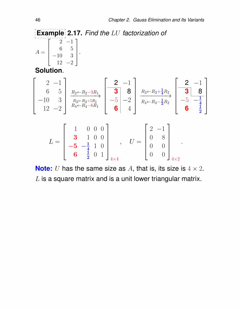
Example 2.17. Find the LU factorization of
A =
2 −16 5
−10 312 −2
.
Solution.2 −1
6 5
−10 3
12 −2
R2←R2−3R1−−−−−−−→R3←R3+5R1R4←R4−6R1
2 −1
3 8−5 −2
6 4
R3←R3+14R2−−−−−−−→
R4←R4−12R2
2 −1
3 8−5 −1
4
6 12
L =
1 0 0 0
3 1 0 0
−5 −14 1 0
6 12 0 1
4×4
, U =
2 −1
0 8
0 0
0 0
4×2
.
Note: U has the same size as A, that is, its size is 4× 2.L is a square matrix and is a unit lower triangular matrix.
2.3. Gauss Elimination 47
Numerical Notes: For an n× n dense matrix A (withmost entries nonzero) with n moderately large.
• Computing an LU factorization of A takes about 2n3/3
flops† (∼ row reducing [A b]), while finding A−1 re-quires about 2n3 flops.
• Solving Ly = b and Ux = y requires about 2n2 flops,because any n×n triangular system can be solved inabout n2 flops.
• Multiplying b by A−1 also requires about 2n2 flops, butthe result may not as accurate as that obtained fromL and U (due to round-off errors in computing A−1 &A−1b).
• If A is sparse (with mostly zero entries), then L and Umay be sparse, too. On the other hand, A−1 is likelyto be dense. In this case, a solution of Ax = b withLU factorization is much faster than using A−1.
† A flop is +, −, × or ÷.
48 Chapter 2. Gauss Elimination and Its Variants
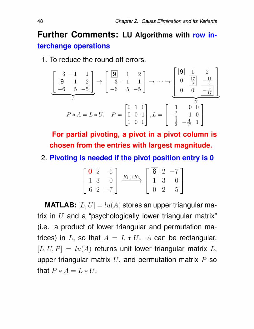
Further Comments: LU Algorithms with row in-terchange operations
1. To reduce the round-off errors. 3 −1 1
9 1 2−6 5 −5
︸ ︷︷ ︸
A
→
9 1 23 −1 1−6 5 −5
→ · · · →
9 1 2
0 173 −11
3
0 0 − 917
︸ ︷︷ ︸
U
P ∗ A = L ∗ U, P =
0 1 00 0 11 0 0
, L =
1 0 0−2
3 1 013 −
417 1
For partial pivoting, a pivot in a pivot column is
chosen from the entries with largest magnitude.
2. Pivoting is needed if the pivot position entry is 0 0 2 5
1 3 0
6 2 −7
R1↔R3−−−−→
6 2 −7
1 3 0
0 2 5
MATLAB: [L,U ] = lu(A) stores an upper triangular ma-
trix in U and a “psychologically lower triangular matrix”(i.e. a product of lower triangular and permutation ma-trices) in L, so that A = L ∗ U . A can be rectangular.[L,U, P ] = lu(A) returns unit lower triangular matrix L,upper triangular matrix U , and permutation matrix P sothat P ∗ A = L ∗ U .
2.3. Gauss Elimination 49
2.3.3. Gauss elimination with pivoting
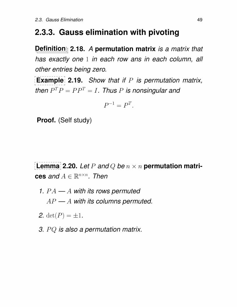
Definition 2.18. A permutation matrix is a matrix thathas exactly one 1 in each row ans in each column, allother entries being zero.
Example 2.19. Show that if P is permutation matrix,then P TP = PP T = I. Thus P is nonsingular and
P−1 = P T .
Proof. (Self study)
Lemma 2.20. Let P and Q be n× n permutation matri-ces and A ∈ Rn×n. Then
1. PA — A with its rows permutedAP — A with its columns permuted.
2. det(P ) = ±1.
3. PQ is also a permutation matrix.
50 Chapter 2. Gauss Elimination and Its Variants
Example 2.21. Let A ∈ Rn×n, and let A be a matrixobtained from scrambling the rows. Show that there is aunique permutation matrix P ∈ Rn×n such that A = PA.
Hint: Consider the row indices in the scrambled matrixA, say k1, k2, · · · , kn. (This means that for example,the first row of A is the same as the k1-th row of A.) Usethe index set to define a permutation matrix P .
Proof. (Self study)
2.3. Gauss Elimination 51
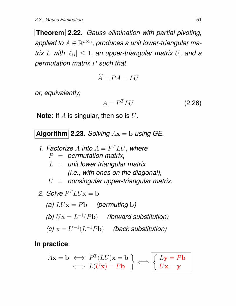
Theorem 2.22. Gauss elimination with partial pivoting,applied to A ∈ Rn×n, produces a unit lower-triangular ma-trix L with |`ij| ≤ 1, an upper-triangular matrix U , and apermutation matrix P such that
A = PA = LU
or, equivalently,A = P TLU (2.26)
Note: If A is singular, then so is U .
Algorithm 2.23. Solving Ax = b using GE.
1. Factorize A into A = P TLU , whereP = permutation matrix,L = unit lower triangular matrix
(i.e., with ones on the diagonal),U = nonsingular upper-triangular matrix.
2. Solve P TLUx = b
(a) LUx = Pb (permuting b)
(b) Ux = L−1(Pb) (forward substitution)
(c) x = U−1(L−1Pb) (back substitution)
In practice:
Ax = b ⇐⇒ P T (LU)x = b
⇐⇒ L(Ux) = Pb
⇐⇒
Ly = Pb
Ux = y
52 Chapter 2. Gauss Elimination and Its Variants
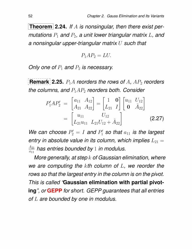
Theorem 2.24. If A is nonsingular, then there exist per-mutations P1 and P2, a unit lower triangular matrix L, anda nonsingular upper-triangular matrix U such that
P1AP2 = LU.
Only one of P1 and P2 is necessary.
Remark 2.25. P1A reorders the rows of A, AP2 reordersthe columns, and P1AP2 reorders both. Consider
P ′1AP′2 =
[a11 A12
A21 A22
]=
[1 0
L21 I
] [u11 U12
0 A22
]=
[u11 U12
L21u11 L21U12 + A22
](2.27)
We can choose P ′2 = I and P ′1 so that a11 is the largestentry in absolute value in its column, which implies L21 =A21a11
has entries bounded by 1 in modulus.
More generally, at step k of Gaussian elimination, wherewe are computing the kth column of L, we reorder therows so that the largest entry in the column is on the pivot.This is called “Gaussian elimination with partial pivot-ing”, or GEPP for short. GEPP guarantees that all entriesof L are bounded by one in modulus.
2.3. Gauss Elimination 53
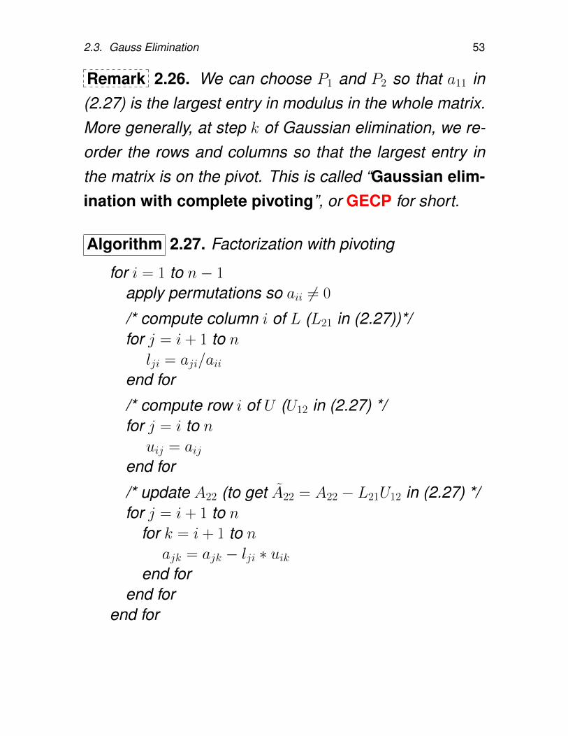
Remark 2.26. We can choose P1 and P2 so that a11 in(2.27) is the largest entry in modulus in the whole matrix.More generally, at step k of Gaussian elimination, we re-order the rows and columns so that the largest entry inthe matrix is on the pivot. This is called “Gaussian elim-ination with complete pivoting”, or GECP for short.
Algorithm 2.27. Factorization with pivoting
for i = 1 to n− 1
apply permutations so aii 6= 0
/* compute column i of L (L21 in (2.27))*/for j = i + 1 to n
lji = aji/aiiend for
/* compute row i of U (U12 in (2.27) */for j = i to n
uij = aijend for
/* update A22 (to get A22 = A22 − L21U12 in (2.27) */for j = i + 1 to n
for k = i + 1 to najk = ajk − lji ∗ uik
end forend for
end for
54 Chapter 2. Gauss Elimination and Its Variants
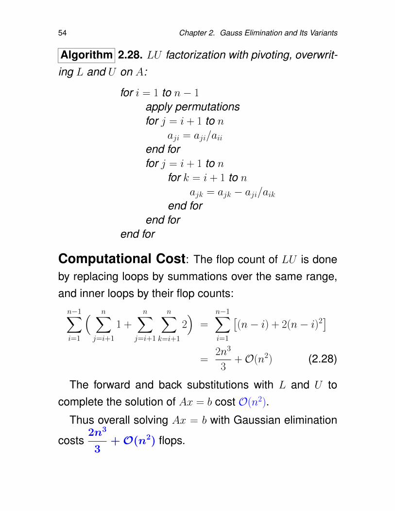
Algorithm 2.28. LU factorization with pivoting, overwrit-ing L and U on A:
for i = 1 to n− 1
apply permutationsfor j = i + 1 to n
aji = aji/aiiend forfor j = i + 1 to n
for k = i + 1 to najk = ajk − aji/aik
end forend for
end for
Computational Cost: The flop count of LU is doneby replacing loops by summations over the same range,and inner loops by their flop counts:n−1∑i=1
( n∑j=i+1
1 +
n∑j=i+1
n∑k=i+1
2)
=
n−1∑i=1
[(n− i) + 2(n− i)2
]=
2n3
3+O(n2) (2.28)
The forward and back substitutions with L and U tocomplete the solution of Ax = b cost O(n2).
Thus overall solving Ax = b with Gaussian elimination
costs2n3
3+O(n2) flops.
2.3. Gauss Elimination 55
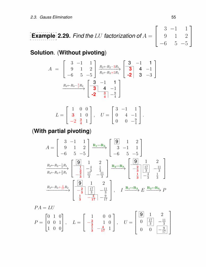
Example 2.29. Find the LU factorization ofA =
3 −1 1
9 1 2
−6 5 −5
Solution. (Without pivoting)
A =
3 −1 19 1 2−6 5 −5
R2←R2−3R1−−−−−−−→R3←R3+2R1
3 −1 13 4 −1
-2 3 −3
R3←R3− 3
4R2−−−−−−−→
3 −1 13 4 −1
-2 34 −
94
L =
1 0 03 1 0−2 3
4 1
, U =
3 −1 10 4 −10 0 −9
4
.(With partial pivoting)
A =
3 −1 19 1 2−6 5 −5
R1↔R2−−−−→
9 1 23 −1 1−6 5 −5
R2←R2− 1
3R1−−−−−−−→R3←R3+ 2
3R1
9 1 213 −
43
13
−23
173 −11
3
R2↔R3−−−−→
9 1 2
−23
173 −11
313 −
43
13
R3←R3+ 4
17R2−−−−−−−−→
9 1 2
−23
173 −11
313 − 4
17 −917
, IR1↔R2−−−−→ E
R2↔R3−−−−→ P
PA = LU
P =
0 1 00 0 11 0 0
, L =
1 0 0−2
3 1 013 −
417 1
, U =
9 1 2
0 173 −11
3
0 0 − 917
56 Chapter 2. Gauss Elimination and Its Variants
2.3.4. Calculating A−1
The program to solve Ax = b can be used to calculate theinverse of a matrix. Letting X = A−1, we have AX = I.This equation can be written in partitioned form:
A[x1 x2 · · · xn] = [e1 e2 · · · en] (2.29)
where x1, x2, · · · , xn and e1, e2, · · · , en are columns of Xand I, respectively.
Thus AX = I is equivalent to the n equations
Axi = ei, i = 1, 2, · · · , n. (2.30)
Solving these n systems by Gauss elimination with partialpivoting, we obtain A−1.
2.3. Gauss Elimination 57
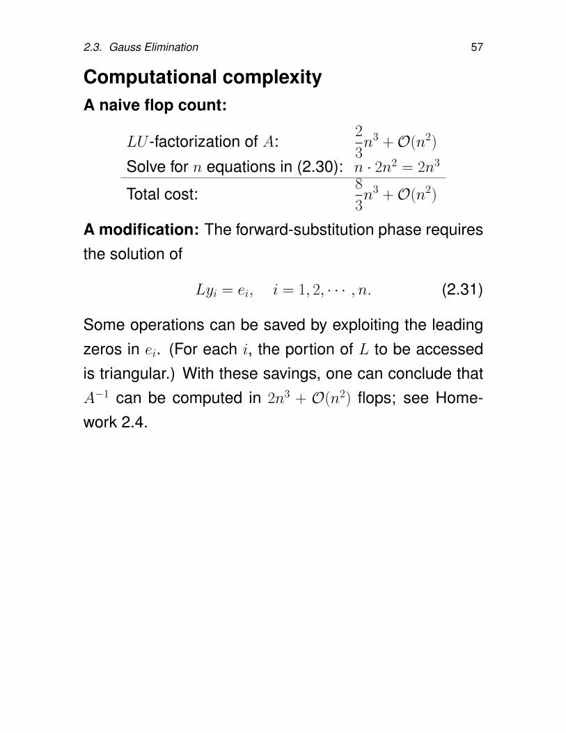
Computational complexityA naive flop count:
LU -factorization of A:2
3n3 +O(n2)
Solve for n equations in (2.30): n · 2n2 = 2n3
Total cost:8
3n3 +O(n2)
A modification: The forward-substitution phase requiresthe solution of
Lyi = ei, i = 1, 2, · · · , n. (2.31)
Some operations can be saved by exploiting the leadingzeros in ei. (For each i, the portion of L to be accessedis triangular.) With these savings, one can conclude thatA−1 can be computed in 2n3 + O(n2) flops; see Home-work 2.4.
58 Chapter 2. Gauss Elimination and Its Variants
2.4. Special Linear Systems
2.4.1. Symmetric positive definite (SPD) ma-trices
Definition 2.30. A real matrix is symmetric positivedefinite (s.p.d.) if A = AT and xTAx > 0, ∀x 6= 0.
Proposition 2.31. Let A ∈ Rn×n be a real matrix.
1. A is s.p.d. if and only if A = AT and all its eigenvaluesare positive.
2. If A is s.p.d and H is any principal submatrix of A(H = A(j : k, j : k) for some j ≤ k), then H is s.p.d.
3. If X is nonsingular, then A is s.p.d. if and only ifXTAX is s.p.d.
4. IfA is s.p.d., then all aii > 0, and maxij |aij| = maxi aii >
0.
5. A is s.p.d. if and only if there is a unique lower tri-angular nonsingular matrix L, with positive diagonalentries, such that A = LLT .
The decomposition A = LLT is called the Cholesky fac-torization of A, and L is called the Cholesky factor of A.
2.4. Special Linear Systems 59
Algorithm 2.32. Cholesky algorithm:
for j = 1 to n
ljj =(ajj −
j−1∑k=1
l2jk
)12
for i = j + 1 to n
lij =(aij −
j−1∑k=1
likljk
)/ljj
end for
end for
Derivation: See Homework 2.2.
Remark 2.33. The Cholesky factorization is mainly usedfor the numerical solution of linear systems Ax = b.
• For symmetric linear systems, the Cholesky decom-position (or its LDLT variant) is the method of choice,for superior efficiency and numerical stability.
• Compared with the LU -decomposition, it is roughlytwice as efficient (O(n3/3) flops).
60 Chapter 2. Gauss Elimination and Its Variants
Algorithm 2.34.
(Cholesky: Gaxpy Version) [6, p.144]
for j = 1 : n
if j > 1
A(j : n, j) = A(j : n, j)
−A(j : n, 1 : j − 1)A(j, 1 : j − 1)T
end
A(j : n, j) = A(j : n, j)/√A(j, j)
end
(Cholesky: Outer Product Version)
for k = 1 : n
A(k, k) =√A(k, k)
A(k + 1 : n, k) = A(k + 1 : n, k)/A(k, k)
for j = k + 1 : n
A(j : n, j) = A(j : n, j)− A(j : n, k)A(j, k)
end
end
• Total cost of the Cholesky algorithms: O(n3/3) flops.
• L overwrites the lower triangle of A in the above al-gorithms.
2.4. Special Linear Systems 61
Stability of Cholesky Process
•
A = LLT =⇒ l2ij ≤i∑
k=1
l2ik = aii, ||L||22 = ||A||2
• If x is the computed solution to Ax = b, obtainedvia any of Cholesky procedures, then x solves theperturbed system (A + E)x = b
• Example: [6] If Cholesky algorithm is applied to thes.p.d. matrix
A =
100 15 .01
15 2.26 .01
.01 .01 1.00
For round arithmetic, we get
l11 = 10, l21 = 1.5, l31 = .001,
andl22 = (a22 − l21
2)1/2 = .00
The algorithm then breaks down trying to compute l32.
By the way: The Cholesky factor of A is
L =
10.0000 0 0
1.5000 0.1000 0
0.0010 0.0850 0.9964
62 Chapter 2. Gauss Elimination and Its Variants
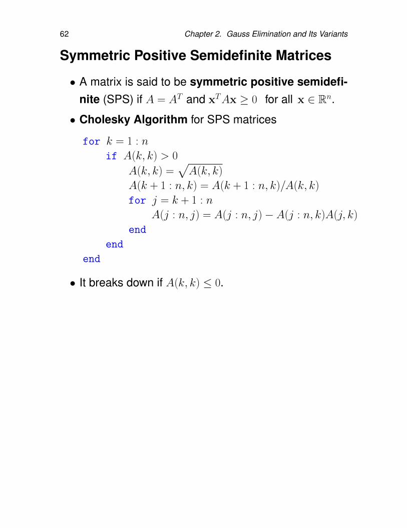
Symmetric Positive Semidefinite Matrices
• A matrix is said to be symmetric positive semidefi-nite (SPS) if A = AT and xTAx ≥ 0 for all x ∈ Rn.
• Cholesky Algorithm for SPS matrices
for k = 1 : n
if A(k, k) > 0
A(k, k) =√A(k, k)
A(k + 1 : n, k) = A(k + 1 : n, k)/A(k, k)
for j = k + 1 : n
A(j : n, j) = A(j : n, j)− A(j : n, k)A(j, k)
end
end
end
• It breaks down if A(k, k) ≤ 0.
2.4. Special Linear Systems 63
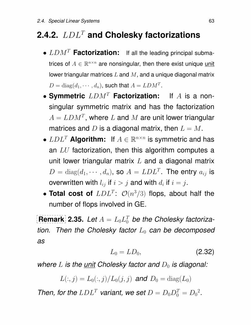
2.4.2. LDLT and Cholesky factorizations
• LDMT Factorization: If all the leading principal subma-
trices of A ∈ Rn×n are nonsingular, then there exist unique unit
lower triangular matrices L and M , and a unique diagonal matrix
D = diag(d1, · · · , dn), such that A = LDMT .
• Symmetric LDMT Factorization: If A is a non-singular symmetric matrix and has the factorizationA = LDMT , where L and M are unit lower triangularmatrices and D is a diagonal matrix, then L = M .
• LDLT Algorithm: If A ∈ Rn×n is symmetric and hasan LU factorization, then this algorithm computes aunit lower triangular matrix L and a diagonal matrixD = diag(d1, · · · , dn), so A = LDLT . The entry aij isoverwritten with lij if i > j and with di if i = j.
• Total cost of LDLT : O(n3/3) flops, about half thenumber of flops involved in GE.
Remark 2.35. Let A = L0LT0 be the Cholesky factoriza-
tion. Then the Cholesky factor L0 can be decomposedas
L0 = LD0, (2.32)
where L is the unit Cholesky factor and D0 is diagonal:
L(:, j) = L0(:, j)/L0(j, j) and D0 = diag(L0)
Then, for the LDLT variant, we set D = D0DT0 = D0
2.
64 Chapter 2. Gauss Elimination and Its Variants
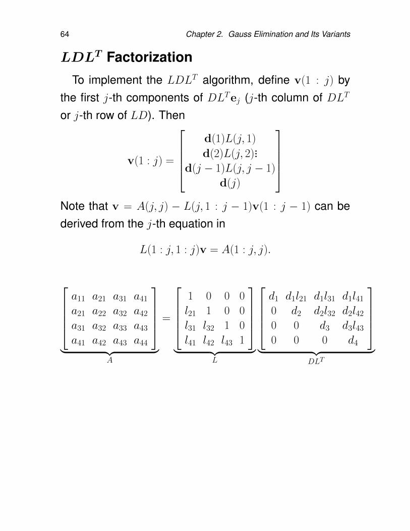
LDLT Factorization
To implement the LDLT algorithm, define v(1 : j) bythe first j-th components of DLTej (j-th column of DLT
or j-th row of LD). Then
v(1 : j) =
d(1)L(j, 1)
d(2)L(j, 2)...d(j − 1)L(j, j − 1)
d(j)
Note that v = A(j, j) − L(j, 1 : j − 1)v(1 : j − 1) can bederived from the j-th equation in
L(1 : j, 1 : j)v = A(1 : j, j).
a11 a21 a31 a41
a21 a22 a32 a42
a31 a32 a33 a43
a41 a42 a43 a44
︸ ︷︷ ︸
A
=
1 0 0 0
l21 1 0 0
l31 l32 1 0
l41 l42 l43 1
︸ ︷︷ ︸
L
d1 d1l21 d1l31 d1l41
0 d2 d2l32 d2l42
0 0 d3 d3l43
0 0 0 d4
︸ ︷︷ ︸
DLT
2.4. Special Linear Systems 65
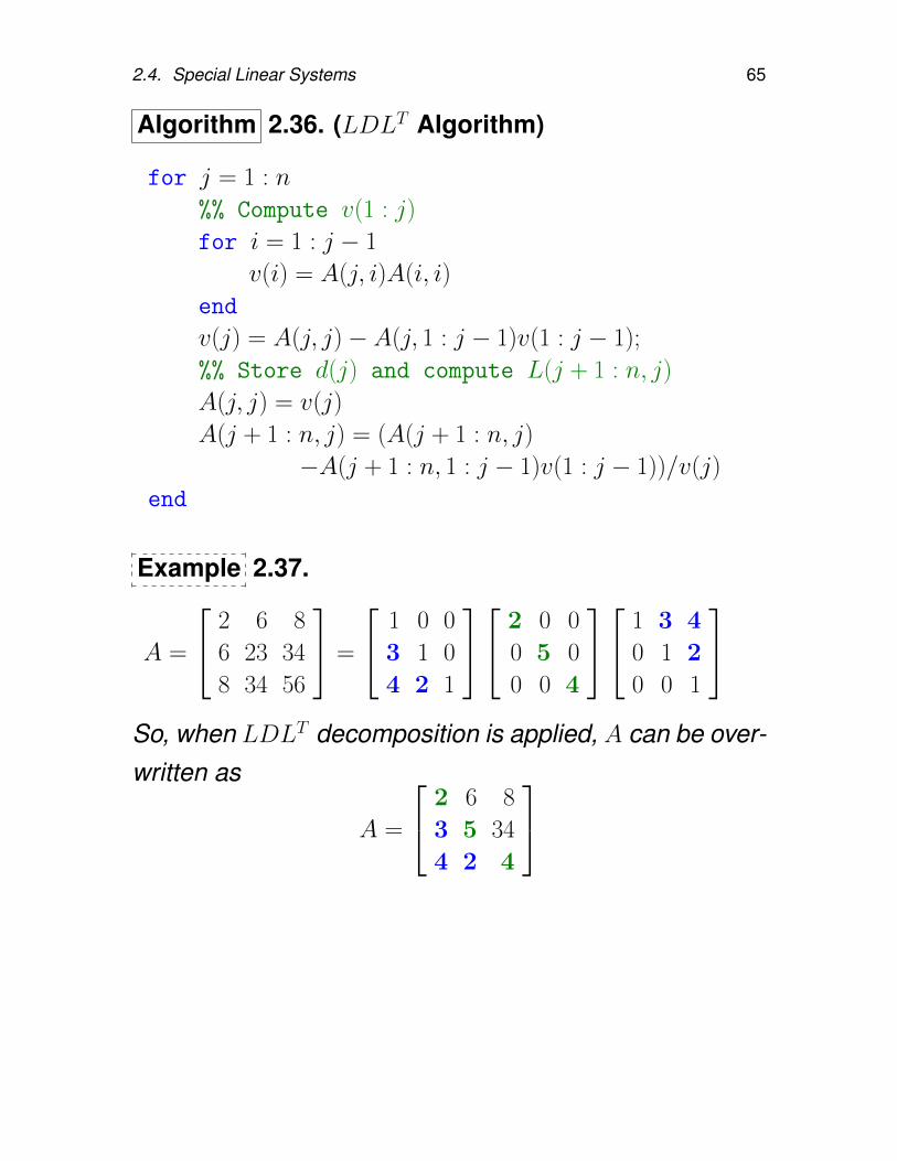
Algorithm 2.36. (LDLT Algorithm)
for j = 1 : n
%% Compute v(1 : j)
for i = 1 : j − 1
v(i) = A(j, i)A(i, i)
end
v(j) = A(j, j)− A(j, 1 : j − 1)v(1 : j − 1);
%% Store d(j) and compute L(j + 1 : n, j)
A(j, j) = v(j)
A(j + 1 : n, j) = (A(j + 1 : n, j)
−A(j + 1 : n, 1 : j − 1)v(1 : j − 1))/v(j)
end
Example 2.37.
A =
2 6 8
6 23 34
8 34 56
=
1 0 0
3 1 0
4 2 1
2 0 0
0 5 0
0 0 4
1 3 4
0 1 2
0 0 1
So, when LDLT decomposition is applied, A can be over-written as
A =
2 6 8
3 5 34
4 2 4
66 Chapter 2. Gauss Elimination and Its Variants
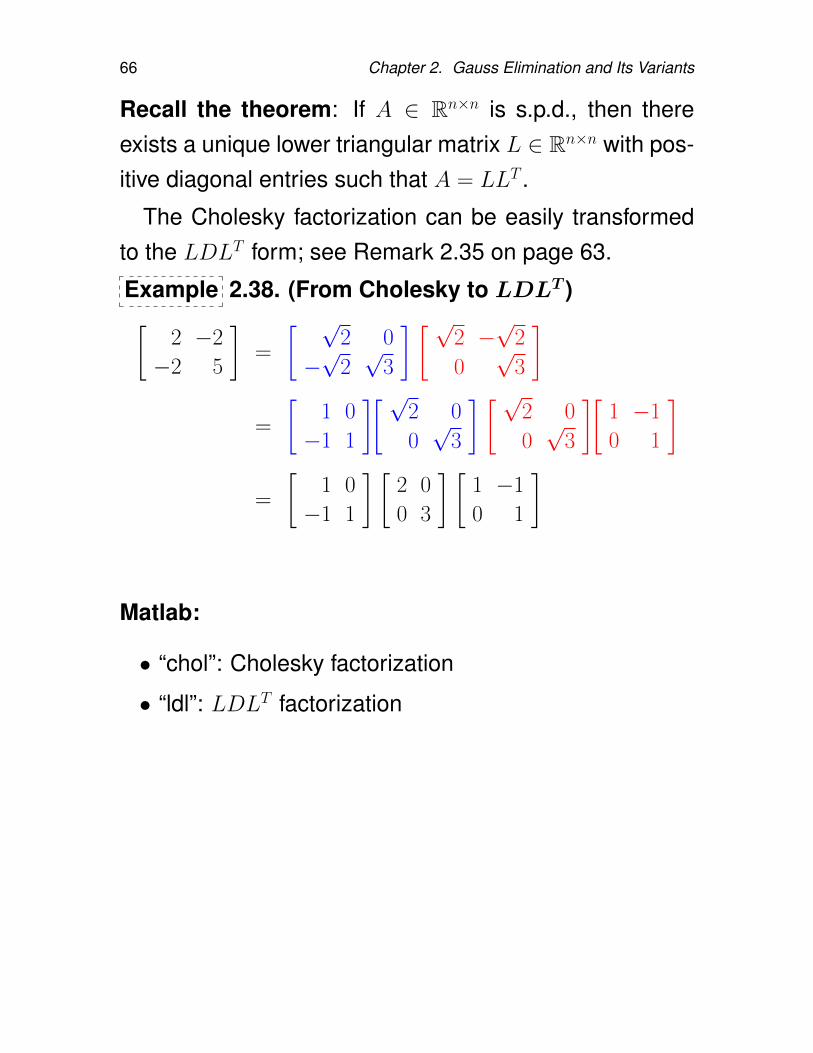
Recall the theorem: If A ∈ Rn×n is s.p.d., then thereexists a unique lower triangular matrix L ∈ Rn×n with pos-itive diagonal entries such that A = LLT .
The Cholesky factorization can be easily transformedto the LDLT form; see Remark 2.35 on page 63.
Example 2.38. (From Cholesky to LDLT )[2 −2
−2 5
]=
[ √2 0
−√
2√
3
] [ √2 −√
2
0√
3
]=
[1 0
−1 1
][ √2 0
0√
3
] [ √2 0
0√
3
][1 −1
0 1
]=
[1 0
−1 1
] [2 0
0 3
] [1 −1
0 1
]
Matlab:
• “chol”: Cholesky factorization
• “ldl”: LDLT factorization
2.4. Special Linear Systems 67
2.4.3. M-matrices and Stieltjes matrices
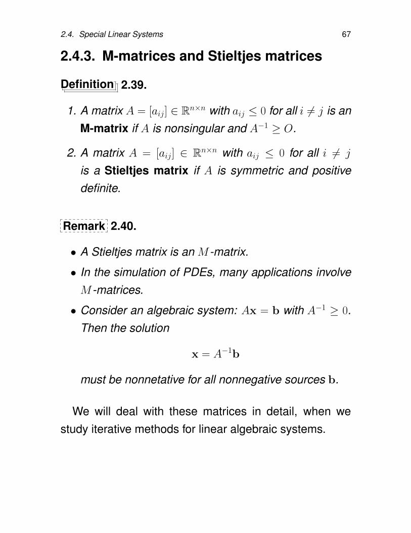
Definition 2.39.
1. A matrix A = [aij] ∈ Rn×n with aij ≤ 0 for all i 6= j is anM-matrix if A is nonsingular and A−1 ≥ O.
2. A matrix A = [aij] ∈ Rn×n with aij ≤ 0 for all i 6= j
is a Stieltjes matrix if A is symmetric and positivedefinite.
Remark 2.40.
• A Stieltjes matrix is an M -matrix.
• In the simulation of PDEs, many applications involveM -matrices.
• Consider an algebraic system: Ax = b with A−1 ≥ 0.Then the solution
x = A−1b
must be nonnetative for all nonnegative sources b.
We will deal with these matrices in detail, when westudy iterative methods for linear algebraic systems.
68 Chapter 2. Gauss Elimination and Its Variants
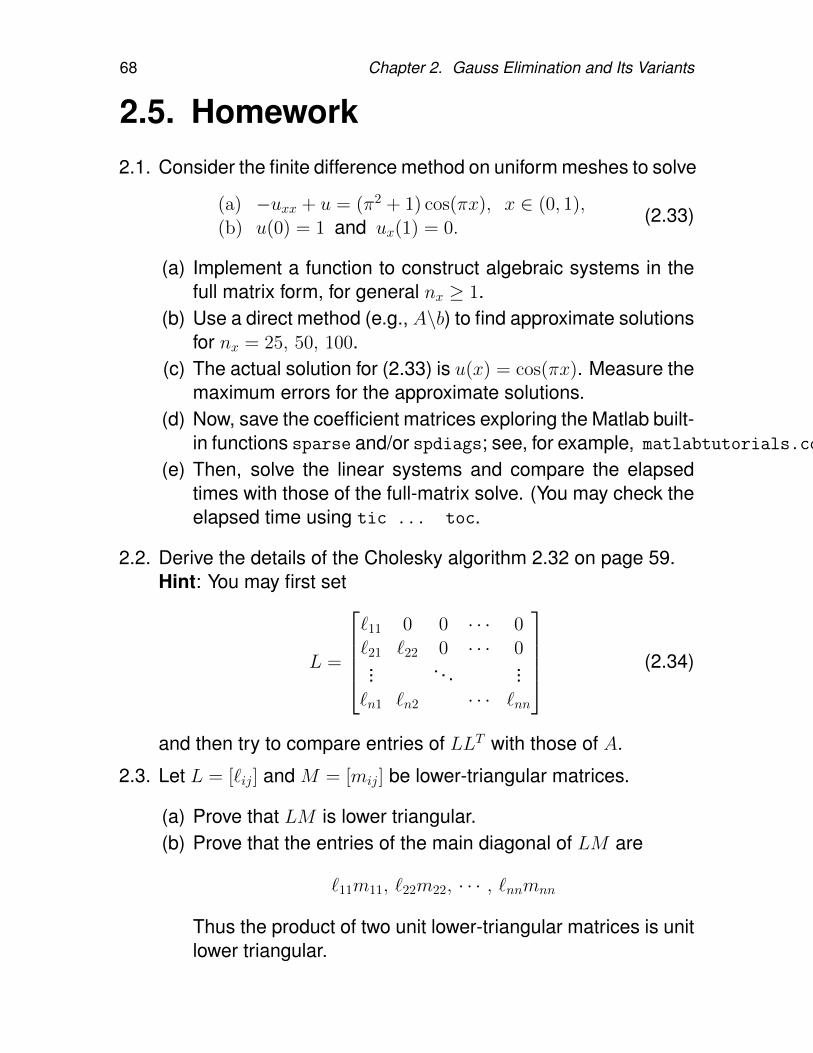
2.5. Homework2.1. Consider the finite difference method on uniform meshes to solve
(a) −uxx + u = (π2 + 1) cos(πx), x ∈ (0, 1),(b) u(0) = 1 and ux(1) = 0.
(2.33)
(a) Implement a function to construct algebraic systems in thefull matrix form, for general nx ≥ 1.
(b) Use a direct method (e.g., A\b) to find approximate solutionsfor nx = 25, 50, 100.
(c) The actual solution for (2.33) is u(x) = cos(πx). Measure themaximum errors for the approximate solutions.
(d) Now, save the coefficient matrices exploring the Matlab built-in functions sparse and/or spdiags; see, for example, matlabtutorials.com/howto/spdiags.
(e) Then, solve the linear systems and compare the elapsedtimes with those of the full-matrix solve. (You may check theelapsed time using tic ... toc.
2.2. Derive the details of the Cholesky algorithm 2.32 on page 59.Hint: You may first set
L =
`11 0 0 · · · 0`21 `22 0 · · · 0... . . . ...`n1 `n2 · · · `nn
(2.34)
and then try to compare entries of LLT with those of A.
2.3. Let L = [`ij] and M = [mij] be lower-triangular matrices.
(a) Prove that LM is lower triangular.(b) Prove that the entries of the main diagonal of LM are
`11m11, `22m22, · · · , `nnmnn
Thus the product of two unit lower-triangular matrices is unitlower triangular.
2.5. Homework 69
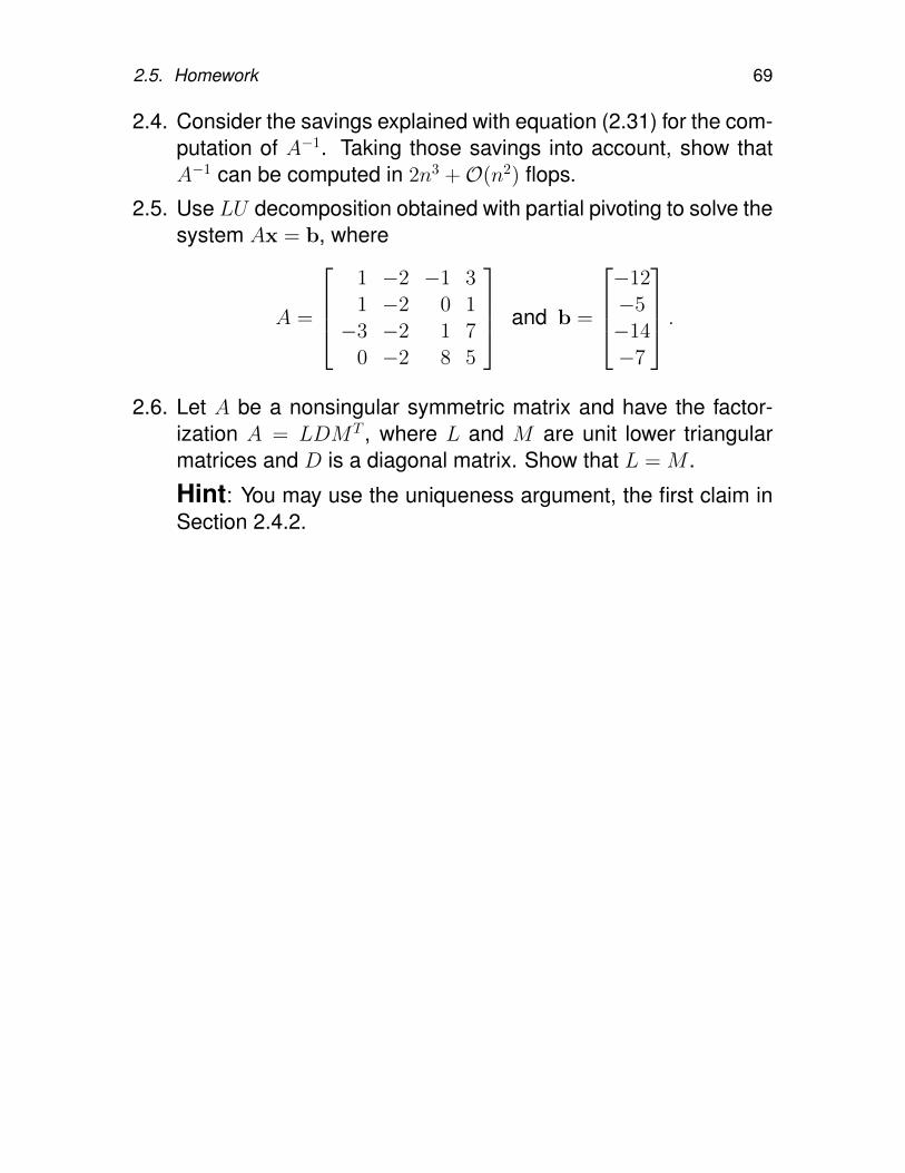
2.4. Consider the savings explained with equation (2.31) for the com-putation of A−1. Taking those savings into account, show thatA−1 can be computed in 2n3 +O(n2) flops.
2.5. Use LU decomposition obtained with partial pivoting to solve thesystem Ax = b, where
A =
1 −2 −1 31 −2 0 1−3 −2 1 7
0 −2 8 5
and b =
−12−5−14−7
.2.6. Let A be a nonsingular symmetric matrix and have the factor-
ization A = LDMT , where L and M are unit lower triangularmatrices and D is a diagonal matrix. Show that L = M .
Hint: You may use the uniqueness argument, the first claim inSection 2.4.2.

70 Chapter 2. Gauss Elimination and Its Variants
Chapter 3
The Least-Squares Problem
In this chapter, we study the least-squares problem, whicharises frequently in scientific and engineering computa-tions. After describing the problem, we will develop toolsto solve the problem:
• normal equation
• reflectors and rotators
• the Gram-Schmidt orthonormalization process
• the QR decomposition
• the singular value decomposition (SV D)
71
72 Chapter 3. The Least-Squares Problem
3.1. The Discrete Least-Squares Prob-lem
Definition 3.1. Let A ∈ Rm×n and b ∈ Rm. The linearleast-squares problem is to find x ∈ Rn which minimizes
||Ax− b||2 or, equivalently, ||Ax− b||22
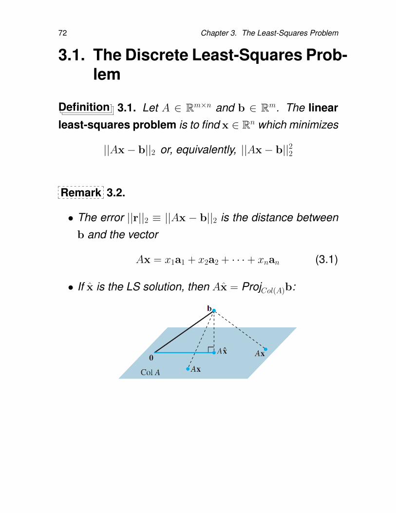
Remark 3.2.
• The error ||r||2 ≡ ||Ax − b||2 is the distance betweenb and the vector
Ax = x1a1 + x2a2 + · · · + xnan (3.1)
• If x is the LS solution, then Ax = ProjCol(A)b:
3.1. The Discrete Least-Squares Problem 73
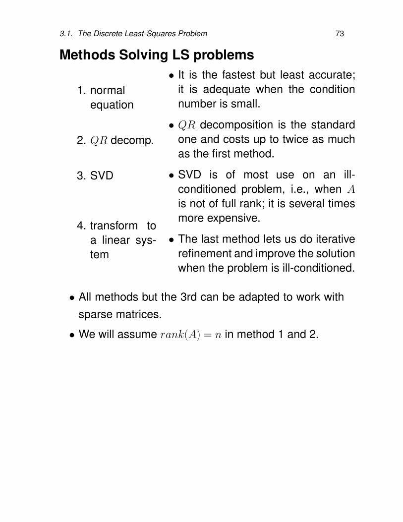
Methods Solving LS problems
1. normalequation
2. QR decomp.
3. SVD
4. transform toa linear sys-tem
• It is the fastest but least accurate;it is adequate when the conditionnumber is small.
• QR decomposition is the standardone and costs up to twice as muchas the first method.
• SVD is of most use on an ill-conditioned problem, i.e., when A
is not of full rank; it is several timesmore expensive.
• The last method lets us do iterativerefinement and improve the solutionwhen the problem is ill-conditioned.
• All methods but the 3rd can be adapted to work withsparse matrices.
• We will assume rank(A) = n in method 1 and 2.
74 Chapter 3. The Least-Squares Problem
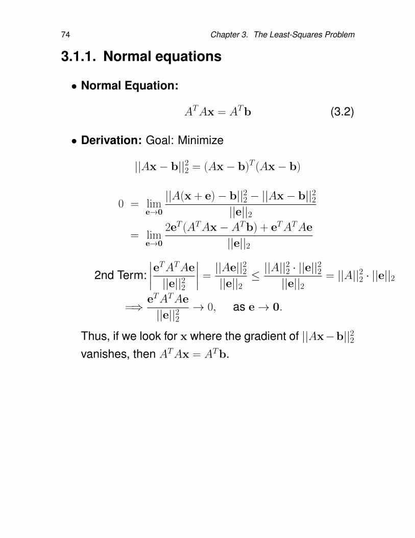
3.1.1. Normal equations
• Normal Equation:
ATAx = ATb (3.2)
• Derivation: Goal: Minimize
||Ax− b||22 = (Ax− b)T (Ax− b)
0 = lime→0
||A(x + e)− b||22 − ||Ax− b||22||e||2
= lime→0
2eT (ATAx− ATb) + eTATAe
||e||2
2nd Term:∣∣∣∣eTATAe
||e||22
∣∣∣∣ =||Ae||22||e||2
≤ ||A||22 · ||e||22||e||2
= ||A||22 · ||e||2
=⇒ eTATAe
||e||22→ 0, as e→ 0.
Thus, if we look for x where the gradient of ||Ax−b||22vanishes, then ATAx = ATb.
3.1. The Discrete Least-Squares Problem 75
Remark 3.3.
• Why x is the minimizer of ||Ax− b||22∆= f (x)?
∂f(x)
∂x= ∇xf(x) =
∂((Ax− b)T (Ax− b)
)∂x
=∂(xTATAx− 2xTATb
)∂x
= 2ATAx− 2ATb
Hf(x) =∂
∂x
(∂f(x)
∂x
)= 2ATA positive definite
(under the assumption that rank(A) = n)
So the function f is strictly convex, and any criticalpoint is a global minimum.1
• For A ∈ Rm×n, if rank(A) = n, then ATA is SPD;indeed,
– ATA is symmetric since (ATA)T = AT (AT )T = ATA.
– Since rank(A) = n, m ≥ n, and the columns of Aare linearly independent.
So Ax = 0 has only the trivial solution.
Hence, for any x ∈ Rn, if x 6= 0, then Ax 6= 0.
– For any 0 6= x ∈ Rn, xTATAx = (Ax)T (Ax) =
||Ax||22 > 0.
So the normal equation ATAx = ATb has a uniquesolution x = (ATA)−1ATb.
1Hf(x) is called Hessian matrix of f .
76 Chapter 3. The Least-Squares Problem
• If let x′ = x + e, where x is the minimizer, one caneasily verify the following
||Ax′−b||22 = ||Ax−b||22 + ||Ae||22 ≥ ||Ax−b||22 (3.3)
(See Homework 3.1.) Note that since A is of full-rank,Ae = 0 if and only if e = 0; which again proves theuniqueness of the minimizer x.
• Numerically, normal equation can be solved by theCholesky factorization. Total cost:
n2m +1
3n2 + O(n2) flops.
Since m ≥ n, the term n2m dominates the cost.
3.1. The Discrete Least-Squares Problem 77
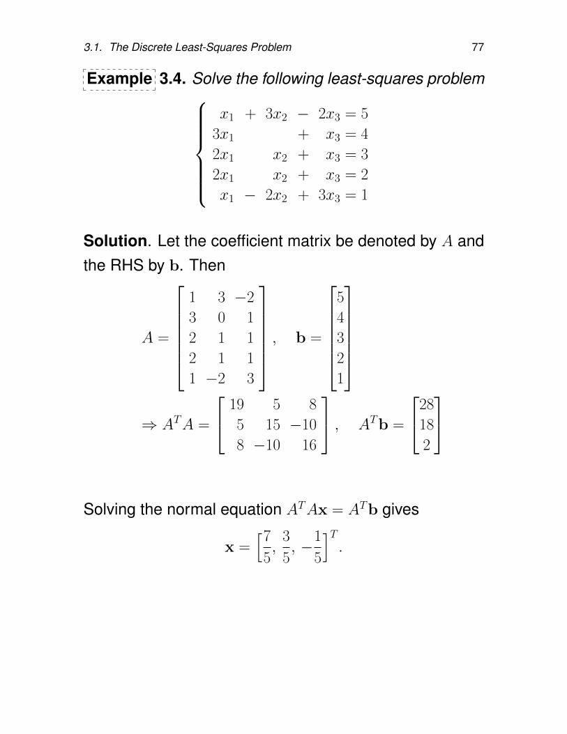
Example 3.4. Solve the following least-squares problem
x1 + 3x2 − 2x3 = 5
3x1 + x3 = 4
2x1 x2 + x3 = 3
2x1 x2 + x3 = 2
x1 − 2x2 + 3x3 = 1
Solution. Let the coefficient matrix be denoted by A andthe RHS by b. Then
A =
1 3 −2
3 0 1
2 1 1
2 1 1
1 −2 3
, b =
5
4
3
2
1
⇒ ATA =
19 5 8
5 15 −10
8 −10 16
, ATb =
28
18
2
Solving the normal equation ATAx = ATb gives
x =[7
5,
3
5, −1
5
]T.
78 Chapter 3. The Least-Squares Problem
3.2. LS Solution by QR Decomposi-tion
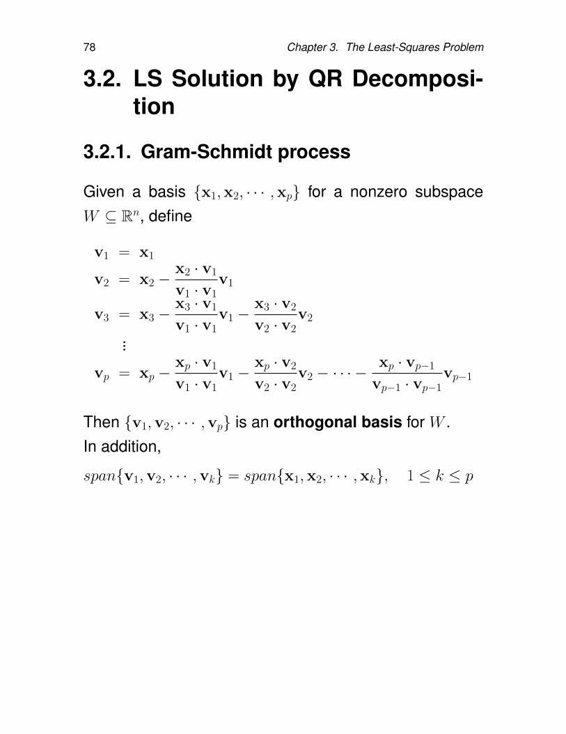
3.2.1. Gram-Schmidt process
Given a basis x1,x2, · · · ,xp for a nonzero subspaceW ⊆ Rn, define
v1 = x1
v2 = x2 −x2 · v1
v1 · v1v1
v3 = x3 −x3 · v1
v1 · v1v1 −
x3 · v2
v2 · v2v2
...
vp = xp −xp · v1
v1 · v1v1 −
xp · v2
v2 · v2v2 − · · · −
xp · vp−1
vp−1 · vp−1vp−1
Then v1,v2, · · · ,vp is an orthogonal basis for W .In addition,
spanv1,v2, · · · ,vk = spanx1,x2, · · · ,xk, 1 ≤ k ≤ p
3.2. LS Solution by QR Decomposition 79
Example 3.5. Let x1 =
1
0
−1
1
, x2 =
1
1
0
1
, x3 =
0
1
2
1
,
and x1,x2,x3 be a basis for a subspace W of R4. Con-struct an orthogonal basis for W .
Solution. Let v1 = x1. Then W1 = Spanx1 = Spanv1.
v2 = x2 −x2 · v1
v1 · v1v1 =
1
1
0
1
− 2
3
1
0
−1
1
=
13
12313
=1
3
1
3
2
1
,
v2 ⇐ 3v2 =
1
3
2
1
(for convenience)
Then,
v3 = x3 −x3 · v1
v1 · v1v1 −
x3 · v2
v2 · v2v2 =
0
1
1
1
− −1
3
1
0
−1
1
− 8
15
1
3
2
1
=1
5
−1
−3
3
4
,
v3 ⇐ 5v3 =
−1
−3
3
4
Then v1,v2,v3 is an orthogonal basis for W .
Note: Replacing v2 with 3v2, v3 with 5v3 does not breakorthogonality.
80 Chapter 3. The Least-Squares Problem
Definition 3.6. An orthonormal basis is an orthogonalbasis v1,v2, · · · ,vp with ||vi|| = 1, for all i = 1, 2 · · · , p.That is vi · vj = δij.
Example 3.7. Let v1 =
1
0
−1
, v2 =
3
3
3
,W = Spanv1,v2.
Construct an orthonormal basis for W .
Solution. It is easy to see that v1 · v2 = 0. So v1,v2 isan orthogonal basis for W . Rescale the basis vectors toform a orthonormal basis u1,u2:
u1 =1
||v1||v1 =
1√2
−1
0
1
=
−1√2
01√2
u2 =
1
||v2||v2 =
1
3√
3
3
3
3
=
1√3
1√3
1√3
3.2. LS Solution by QR Decomposition 81
3.2.2. QR decomposition, by Gram-Schmidtprocess
Theorem 3.8. (QR Decomposition) Let A ∈ Rm×n withm ≥ n. Suppose A has full column rank (rank(A) = n).Then there exist a unique m × n orthogonal matrix Q
(QTQ = In) and a unique n × n upper triangular matrixR with positive diagonals rii > 0 such that A = QR.
Proof. (Sketch) Let A = [a1 · · · an].
1. Construct an orthonormal basis q1,q2, · · · ,qn forW = Col(A) by Gram-Schmidt process, starting froma1, · · · , an
2. Q = [q1 q2 · · ·qn].
Spana1, a2, · · · , ak = Spanq1,q2, · · · ,qk, 1 ≤ k ≤ n
ak = r1kq1 + r2kq2 + · · · + rkkqk + 0 · qk+1 + · · · + 0 · qnNote: If rkk < 0, multiply both rkk and qk by −1.
3. Let rk = [r1k r2k · · · rkk 0 · · · 0]T . Then ak = Qrk fork = 1, 2, · · · , n. Let R = [r1 r2 · · · rn].
4. A = [a1 · · · an] = [Qr1 Qr2 · · · Qrn] = QR.
82 Chapter 3. The Least-Squares Problem
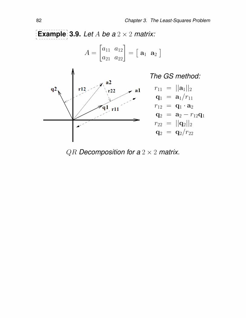
Example 3.9. Let A be a 2× 2 matrix:
A =
[a11 a12
a21 a22
]=[
a1 a2
]The GS method:
r11 = ||a1||2q1 = a1/r11
r12 = q1 · a2
q2 = a2 − r12q1
r22 = ||q2||2q2 = q2/r22
QR Decomposition for a 2× 2 matrix.
3.2. LS Solution by QR Decomposition 83
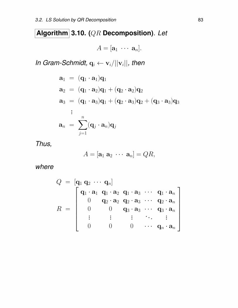
Algorithm 3.10. (QR Decomposition). Let
A = [a1 · · · an].
In Gram-Schmidt, qi ← vi/||vi||, then
a1 = (q1 · a1)q1
a2 = (q1 · a2)q1 + (q2 · a2)q2
a3 = (q1 · a3)q1 + (q2 · a3)q2 + (q3 · a3)q3
...
an =
n∑j=1
(qj · an)qj
Thus,A = [a1 a2 · · · an] = QR,
where
Q = [q1 q2 · · · qn]
R =
q1 · a1 q1 · a2 q1 · a3 · · · q1 · an
0 q2 · a2 q2 · a3 · · · q2 · an0 0 q3 · a3 · · · q3 · an... ... ... . . . ...0 0 0 · · · qn · an
84 Chapter 3. The Least-Squares Problem
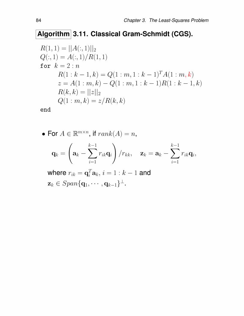
Algorithm 3.11. Classical Gram-Schmidt (CGS).
R(1, 1) = ||A(:, 1)||2Q(:, 1) = A(:, 1)/R(1, 1)
for k = 2 : n
R(1 : k − 1, k) = Q(1 : m, 1 : k − 1)TA(1 : m, k)
z = A(1 : m, k)−Q(1 : m, 1 : k − 1)R(1 : k − 1, k)
R(k, k) = ||z||2Q(1 : m, k) = z/R(k, k)
end
• For A ∈ Rm×n, if rank(A) = n,
qk =
(ak −
k−1∑i=1
rikqi
)/rkk, zk = ak −
k−1∑i=1
rikqi,
where rik = qTi ak, i = 1 : k − 1 andzk ∈ Spanq1, · · · ,qk−1⊥.
3.2. LS Solution by QR Decomposition 85
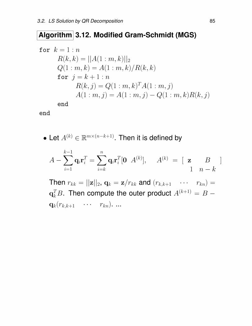
Algorithm 3.12. Modified Gram-Schmidt (MGS)
for k = 1 : n
R(k, k) = ||A(1 : m, k)||2Q(1 : m, k) = A(1 : m, k)/R(k, k)
for j = k + 1 : n
R(k, j) = Q(1 : m, k)TA(1 : m, j)
A(1 : m, j) = A(1 : m, j)−Q(1 : m, k)R(k, j)
end
end
• Let A(k) ∈ Rm×(n−k+1). Then it is defined by
A−k−1∑i=1
qirTi =
n∑i=k
qirTi [0 A(k)], A(k) = [ z B ]
1 n− k
Then rkk = ||z||2, qk = z/rkk and (rk,k+1 · · · rkn) =
qTkB. Then compute the outer product A(k+1) = B −qk(rk,k+1 · · · rkn). ...
86 Chapter 3. The Least-Squares Problem
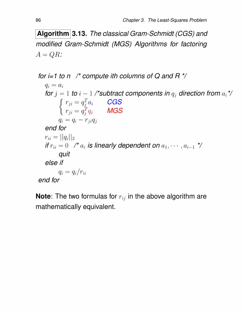
Algorithm 3.13. The classical Gram-Schmidt (CGS) andmodified Gram-Schmidt (MGS) Algorithms for factoringA = QR:
for i=1 to n /* compute ith columns of Q and R */qi = aifor j = 1 to i− 1 /*subtract components in qj direction from ai*/
rji = qTj ai CGSrji = qTj qi MGS
qi = qi − rjiqjend forrii = ||qi||2if rii = 0 /* ai is linearly dependent on a1, · · · , ai−1 */
quitelse if
qi = qi/riiend for
Note: The two formulas for rij in the above algorithm aremathematically equivalent.
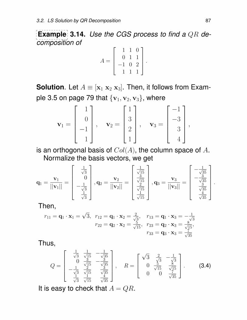
3.2. LS Solution by QR Decomposition 87
Example 3.14. Use the CGS process to find a QR de-composition of
A =
1 1 00 1 1−1 0 2
1 1 1
.Solution. Let A ≡ [x1 x2 x3]. Then, it follows from Exam-ple 3.5 on page 79 that v1,v2,v3, where
v1 =
1
0
−1
1
, v2 =
1
3
2
1
, v3 =
−1
−3
3
4
,is an orthogonal basis of Col(A), the column space of A.
Normalize the basis vectors, we get
q1 =v1
||v1||=
1√3
0
− 1√3
1√3
,q2 =v2
||v2||=
1√153√152√151√15
,q3 =v3
||v3||=
− 1√
35
− 3√353√354√35
.Then,r11 = q1 · x1 =
√3, r12 = q1 · x2 = 2√
3, r13 = q1 · x3 = − 1√
3
r22 = q2 · x2 = 5√15, r23 = q2 · x3 = 8√
15,
r33 = q3 · x3 = 7√35
Thus,
Q =
1√3
1√15− 1√
35
0 3√15− 3√
35
− 1√3
2√15
3√35
1√3
1√15
4√35
, R =
√
3 2√3− 1√
3
0 5√15
8√15
0 0 7√35
. (3.4)
It is easy to check that A = QR.
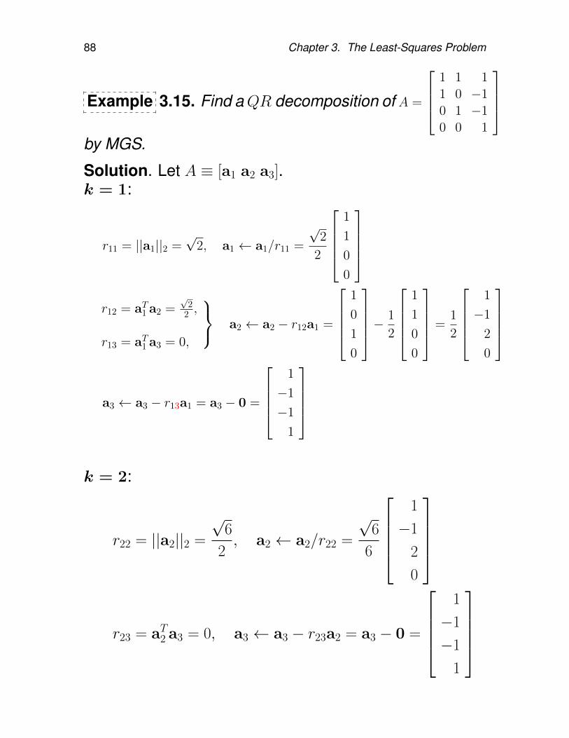
88 Chapter 3. The Least-Squares Problem
Example 3.15. Find aQR decomposition of A =
1 1 11 0 −10 1 −10 0 1
by MGS.
Solution. Let A ≡ [a1 a2 a3].k = 1:
r11 = ||a1||2 =√
2, a1 ← a1/r11 =
√2
2
1
1
0
0
r12 = aT1 a2 =
√2
2 ,
r13 = aT1 a3 = 0,
a2 ← a2 − r12a1 =
1
0
1
0
− 1
2
1
1
0
0
=1
2
1
−1
2
0
a3 ← a3 − r13a1 = a3 − 0 =
1
−1
−1
1
k = 2:
r22 = ||a2||2 =
√6
2, a2 ← a2/r22 =
√6
6
1
−1
2
0
r23 = aT2 a3 = 0, a3 ← a3 − r23a2 = a3 − 0 =
1
−1
−1
1
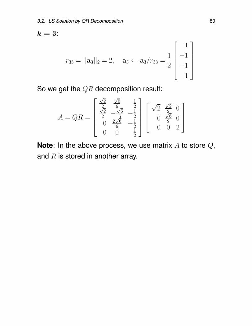
3.2. LS Solution by QR Decomposition 89
k = 3:
r33 = ||a3||2 = 2, a3 ← a3/r33 =1
2
1
−1
−1
1
So we get the QR decomposition result:
A = QR =
√
22
√6
612√
22 −
√6
6 −12
0 2√
66 −1
2
0 0 12
√
2√
22 0
0√
62 0
0 0 2
Note: In the above process, we use matrix A to store Q,and R is stored in another array.
90 Chapter 3. The Least-Squares Problem
Remark 3.16.
• CGS (classical Gram-Schmidt) method has very poornumerical properties in that there is typically a severeloss of orthogonality among the computed qi.
• MGS (Modified Grad-Schmidt) method yields a muchbetter computational result by a rearrangement of thecalculation.
• CGS is numerically unstable in floating point arith-metic when the columns of A are nearly linearly de-pendent. MGS is more stable but may still result in Qbeing far from orthogonal when A is ill-conditioned.
• Both CGS and MGS require O(2mn2) flops to com-pute a QR factorization of A ∈ Rm×n.
3.2. LS Solution by QR Decomposition 91
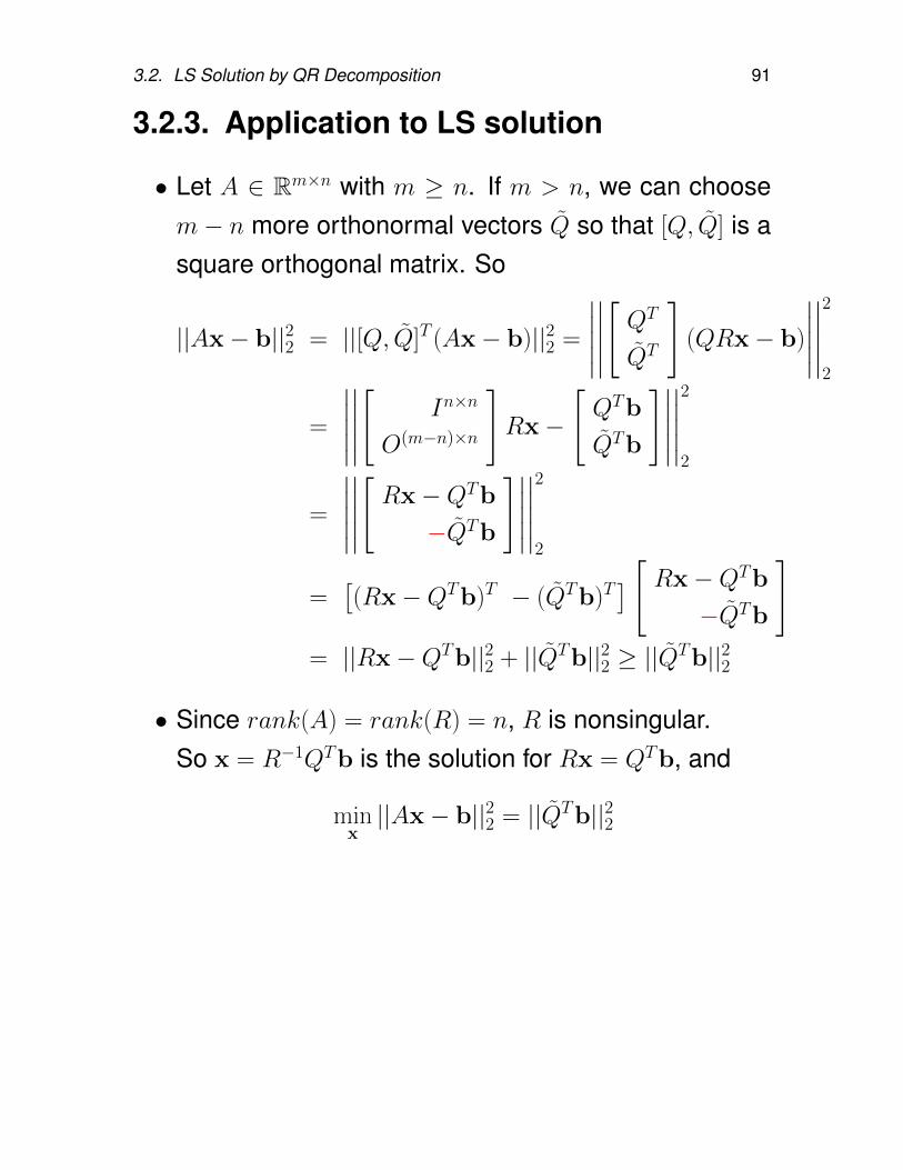
3.2.3. Application to LS solution
• Let A ∈ Rm×n with m ≥ n. If m > n, we can choosem− n more orthonormal vectors Q so that [Q, Q] is asquare orthogonal matrix. So
||Ax− b||22 = ||[Q, Q]T (Ax− b)||22 =
∣∣∣∣∣∣∣∣∣∣[QT
QT
](QRx− b)
∣∣∣∣∣∣∣∣∣∣2
2
=
∣∣∣∣∣∣∣∣∣∣[
In×n
O(m−n)×n
]Rx−
[QTb
QTb
]∣∣∣∣∣∣∣∣∣∣2
2
=
∣∣∣∣∣∣∣∣∣∣[Rx−QTb
−QTb
]∣∣∣∣∣∣∣∣∣∣2
2
=[(Rx−QTb)T − (QTb)T
] [ Rx−QTb
−QTb
]= ||Rx−QTb||22 + ||QTb||22 ≥ ||QTb||22
• Since rank(A) = rank(R) = n, R is nonsingular.So x = R−1QTb is the solution for Rx = QTb, and
minx||Ax− b||22 = ||QTb||22
92 Chapter 3. The Least-Squares Problem
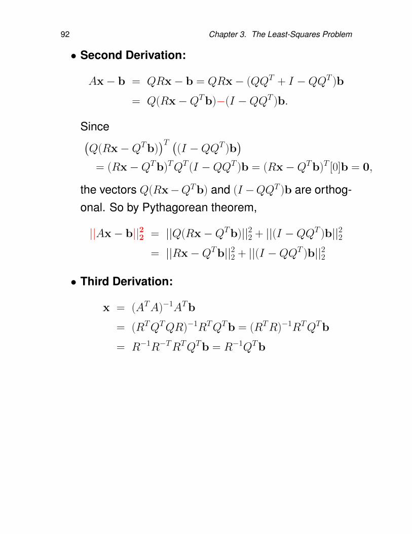
• Second Derivation:
Ax− b = QRx− b = QRx− (QQT + I −QQT )b
= Q(Rx−QTb)−(I −QQT )b.
Since(Q(Rx−QTb)
)T ((I −QQT )b
)= (Rx−QTb)TQT (I −QQT )b = (Rx−QTb)T [0]b = 0,
the vectors Q(Rx−QTb) and (I −QQT )b are orthog-onal. So by Pythagorean theorem,
||Ax− b||22 = ||Q(Rx−QTb)||22 + ||(I −QQT )b||22= ||Rx−QTb||22 + ||(I −QQT )b||22
• Third Derivation:
x = (ATA)−1ATb
= (RTQTQR)−1RTQTb = (RTR)−1RTQTb
= R−1R−TRTQTb = R−1QTb
3.2. LS Solution by QR Decomposition 93
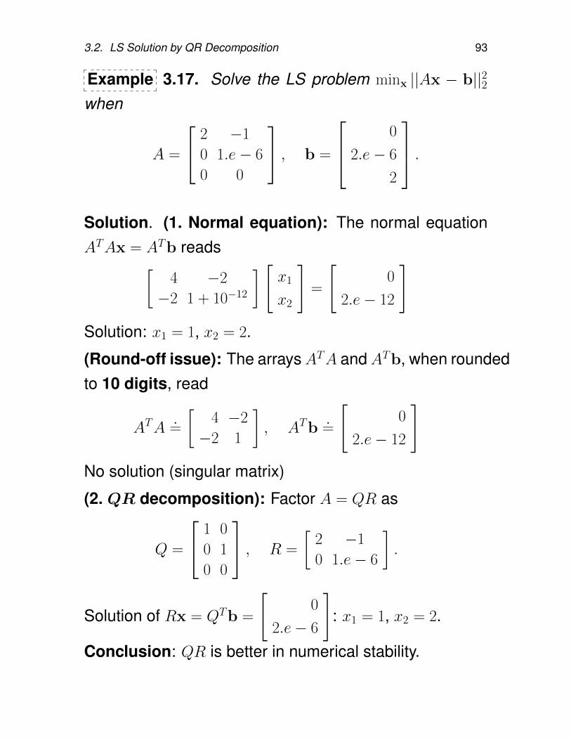
Example 3.17. Solve the LS problem minx ||Ax − b||22when
A =
2 −1
0 1.e− 6
0 0
, b =
0
2.e− 6
2
.Solution. (1. Normal equation): The normal equationATAx = ATb reads[
4 −2
−2 1 + 10−12
] [x1
x2
]=
[0
2.e− 12
]Solution: x1 = 1, x2 = 2.
(Round-off issue): The arraysATA andATb, when roundedto 10 digits, read
ATA.=
[4 −2
−2 1
], ATb
.=
[0
2.e− 12
]No solution (singular matrix)
(2. QR decomposition): Factor A = QR as
Q =
1 0
0 1
0 0
, R =
[2 −1
0 1.e− 6
].
Solution of Rx = QTb =
[0
2.e− 6
]: x1 = 1, x2 = 2.
Conclusion: QR is better in numerical stability.
94 Chapter 3. The Least-Squares Problem
3.3. Orthogonal Matrices
Approaches for orthogonal decomposition:
1. Classical Gram-Schmidt (CGS) andModified Gram-Schmidt (MGS) process (§3.2.2)
2. Householder reflection (reflector)
3. Givens rotation (rotator)
This section studies Householder reflection and Givensrotation in detail, in the use for QR decomposition.
3.3. Orthogonal Matrices 95
3.3.1. Householder reflection
The Householder reflection is also called “reflector”. Inorder to introduce the reflector, let’s begin with the projec-tion.
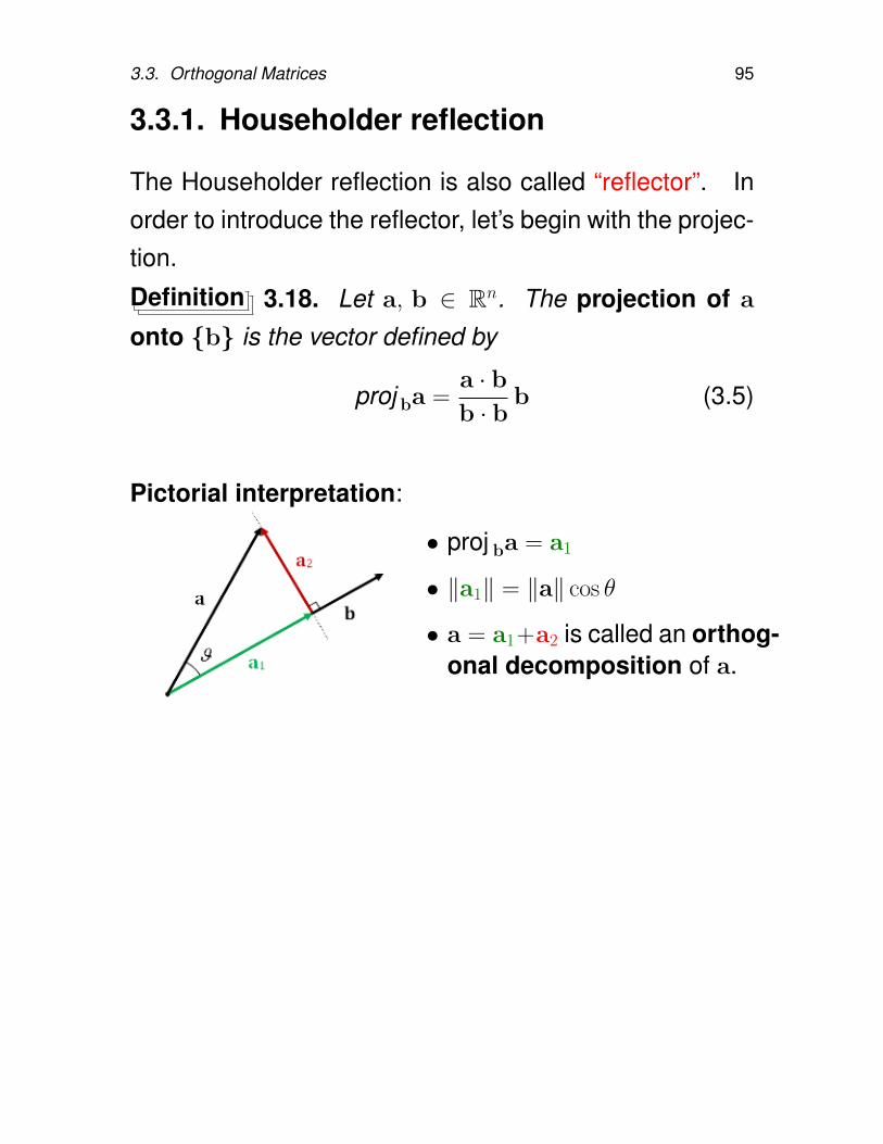
Definition 3.18. Let a, b ∈ Rn. The projection of a
onto b is the vector defined by
proj ba =a · bb · b
b (3.5)
Pictorial interpretation:
• proj ba = a1
• ‖a1‖ = ‖a‖ cos θ
• a = a1+a2 is called an orthog-onal decomposition of a.
96 Chapter 3. The Least-Squares Problem
Householder reflection (or, Householder transfor-mation, Elementary reflector) is a transformation that takesa vector and reflects it about some plane or hyperplane.Let u be a unit vector which is orthogonal to the hyper-plane. Then, the reflection of a point x about this hy-perplane is
x− 2 proj ux = x− 2(x · u)u. (3.6)
Note that
x− 2(x · u)u = x− 2(uuT )x = (I − 2uuT )x.
3.3. Orthogonal Matrices 97
Definition 3.19. Let u ∈ Rn with ‖u‖ = 1. Then thematrix P = I − 2uuT is called a Householder matrix (or,Householder reflector).
Proposition 3.20. Let P = I − 2uuT with ‖u‖ = 1.
1. Pu = −u
2. Pv = v, if u · v = 0
3. P = P T (P is symmetric)
4. P T = P−1 (P is orthogonal)
5. P−1 = P (P is an involution)
6. PP T = P 2 = I.
Indeed,
PP T = (I − 2uuT )(I − 2uuT ) = I − 4uuT + 4uuTuuT = I
98 Chapter 3. The Least-Squares Problem
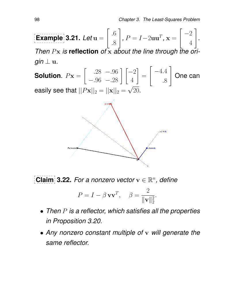
Example 3.21. Let u =
[.6
.8
], P = I−2uuT , x =
[−2
4
].
Then Px is reflection of x about the line through the ori-gin ⊥ u.
Solution. Px =
[.28 −.96
−.96 −.28
] [−2
4
]=
[−4.4
.8
]One can
easily see that ||Px||2 = ||x||2 =√
20.
Claim 3.22. For a nonzero vector v ∈ Rn, define
P = I − β vvT , β =2
‖v‖22
.
• Then P is a reflector, which satisfies all the propertiesin Proposition 3.20.
• Any nonzero constant multiple of v will generate thesame reflector.
3.3. Orthogonal Matrices 99
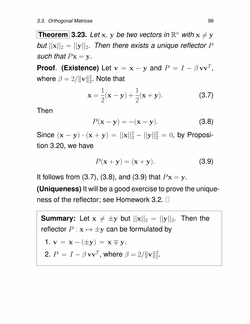
Theorem 3.23. Let x, y be two vectors in Rn with x 6= y
but ||x||2 = ||y||2. Then there exists a unique reflector Psuch that Px = y.
Proof. (Existence) Let v = x − y and P = I − β vvT ,where β = 2/‖v‖2
2. Note that
x =1
2(x− y) +
1
2(x + y). (3.7)
ThenP (x− y) = −(x− y). (3.8)
Since (x − y) · (x + y) = ||x||22 − ||y||22 = 0, by Proposi-tion 3.20, we have
P (x + y) = (x + y). (3.9)
It follows from (3.7), (3.8), and (3.9) that Px = y.
(Uniqueness) It will be a good exercise to prove the unique-ness of the reflector; see Homework 3.2.
Summary: Let x 6= ±y but ||x||2 = ||y||2. Then thereflector P : x 7→ ±y can be formulated by
1. v = x− (±y) = x∓ y.
2. P = I − β vvT , where β = 2/‖v‖22.
100 Chapter 3. The Least-Squares Problem
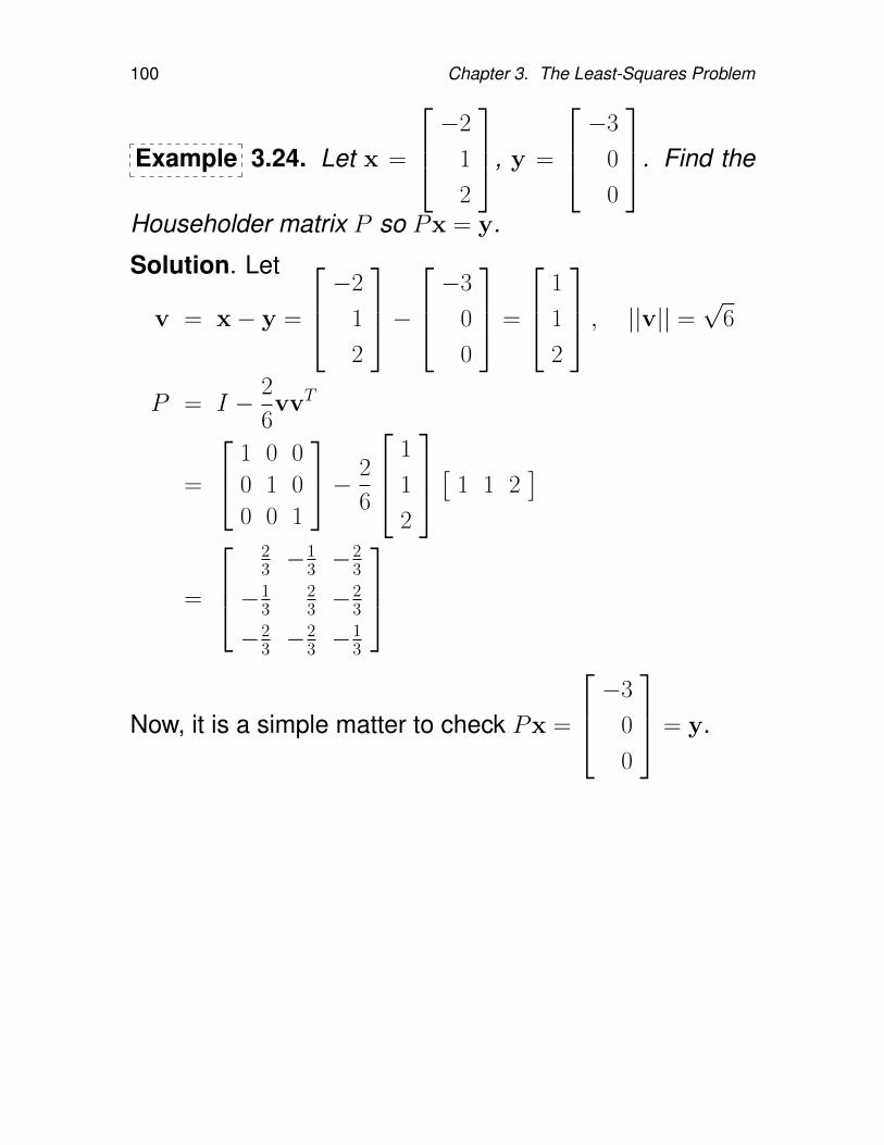
Example 3.24. Let x =
−2
1
2
, y =
−3
0
0
. Find the
Householder matrix P so Px = y.
Solution. Let
v = x− y =
−2
1
2
− −3
0
0
=
1
1
2
, ||v|| =√
6
P = I − 2
6vvT
=
1 0 0
0 1 0
0 0 1
− 2
6
1
1
2
[ 1 1 2]
=
23 −
13 −
23
−13
23 −
23
−23 −
23 −
13
Now, it is a simple matter to check Px =
−3
0
0
= y.
3.3. Orthogonal Matrices 101
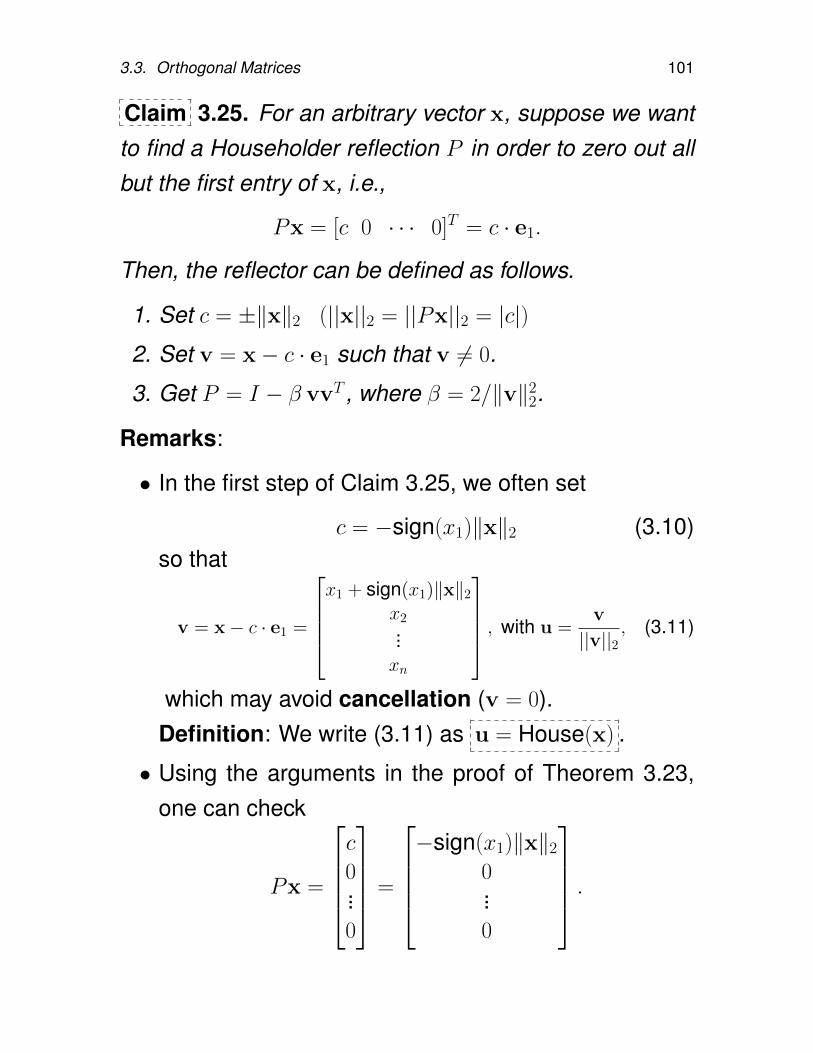
Claim 3.25. For an arbitrary vector x, suppose we wantto find a Householder reflection P in order to zero out allbut the first entry of x, i.e.,
Px = [c 0 · · · 0]T = c · e1.
Then, the reflector can be defined as follows.
1. Set c = ±‖x‖2 (||x||2 = ||Px||2 = |c|)
2. Set v = x− c · e1 such that v 6= 0.
3. Get P = I − β vvT , where β = 2/‖v‖22.
Remarks:
• In the first step of Claim 3.25, we often set
c = −sign(x1)‖x‖2 (3.10)so that
v = x− c · e1 =
x1 + sign(x1)‖x‖2
x2...xn
, with u =v
||v||2, (3.11)
which may avoid cancellation (v = 0).Definition: We write (3.11) as u = House(x) .
• Using the arguments in the proof of Theorem 3.23,one can check
Px =
c
0...0
=
−sign(x1)‖x‖2
0...0
.
102 Chapter 3. The Least-Squares Problem
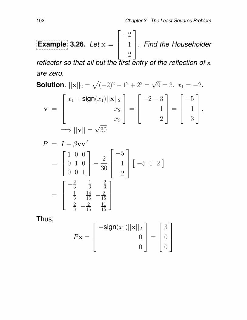
Example 3.26. Let x =
−2
1
2
. Find the Householder
reflector so that all but the first entry of the reflection of x
are zero.
Solution. ||x||2 =√
(−2)2 + 12 + 22 =√
9 = 3. x1 = −2.
v =
x1 + sign(x1)||x||2x2
x3
=
−2− 3
1
2
=
−5
1
3
,=⇒ ||v|| =
√30
P = I − βvvT
=
1 0 0
0 1 0
0 0 1
− 2
30
−5
1
2
[ −5 1 2]
=
−23
13
23
13
1415 −
215
23 −
215
1115
Thus,
Px =
−sign(x1)||x||20
0
=
3
0
0
3.3. Orthogonal Matrices 103
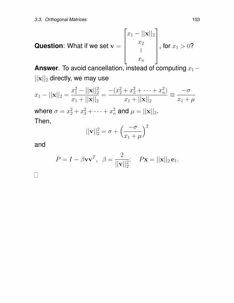
Question: What if we set v =
x1 − ||x||2
x2...xn
, for x1 > 0?
Answer. To avoid cancellation, instead of computing x1−||x||2 directly, we may use
x1 − ||x||2 =x2
1 − ||x||22x1 + ||x||2
=−(x2
2 + x23 + · · · + x2
n)
x1 + ||x||2≡ −σx1 + µ
where σ = x22 + x2
3 + · · · + x2n and µ = ||x||2.
Then,||v||22 = σ +
( −σx1 + µ
)2
and
P = I − βvvT , β =2
||v||22; Px = ||x||2 e1.
104 Chapter 3. The Least-Squares Problem
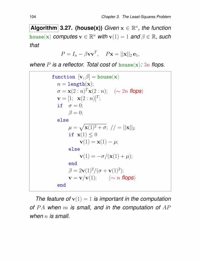
Algorithm 3.27. (house(x)) Given x ∈ Rn, the functionhouse(x) computes v ∈ Rn with v(1) = 1 and β ∈ R, suchthat
P = In − βvvT , Px = ||x||2 e1,
where P is a reflector. Total cost of house(x): 3n flops.
function [v, β] = house(x)
n = length(x);
σ = x(2 : n)Tx(2 : n); (∼ 2n flops)
v = [1; x(2 : n)]T ;
if σ = 0;
β = 0;
else
µ =√
x(1)2 + σ; // = ||x||2if x(1) ≤ 0
v(1) = x(1)− µ;
else
v(1) = −σ/(x(1) + µ);
end
β = 2v(1)2/(σ + v(1)2);
v = v/v(1); (∼ n flops)
end
The feature of v(1) = 1 is important in the computationof PA when m is small, and in the computation of APwhen n is small.
3.3. Orthogonal Matrices 105
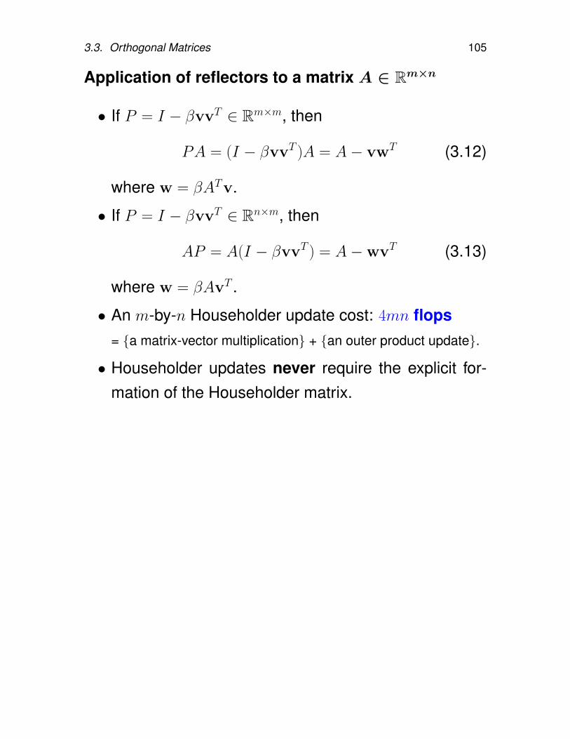
Application of reflectors to a matrix A ∈ Rm×n
• If P = I − βvvT ∈ Rm×m, then
PA = (I − βvvT )A = A− vwT (3.12)
where w = βATv.
• If P = I − βvvT ∈ Rn×m, then
AP = A(I − βvvT ) = A−wvT (3.13)
where w = βAvT .
• An m-by-n Householder update cost: 4mn flops= a matrix-vector multiplication + an outer product update.
• Householder updates never require the explicit for-mation of the Householder matrix.
106 Chapter 3. The Least-Squares Problem
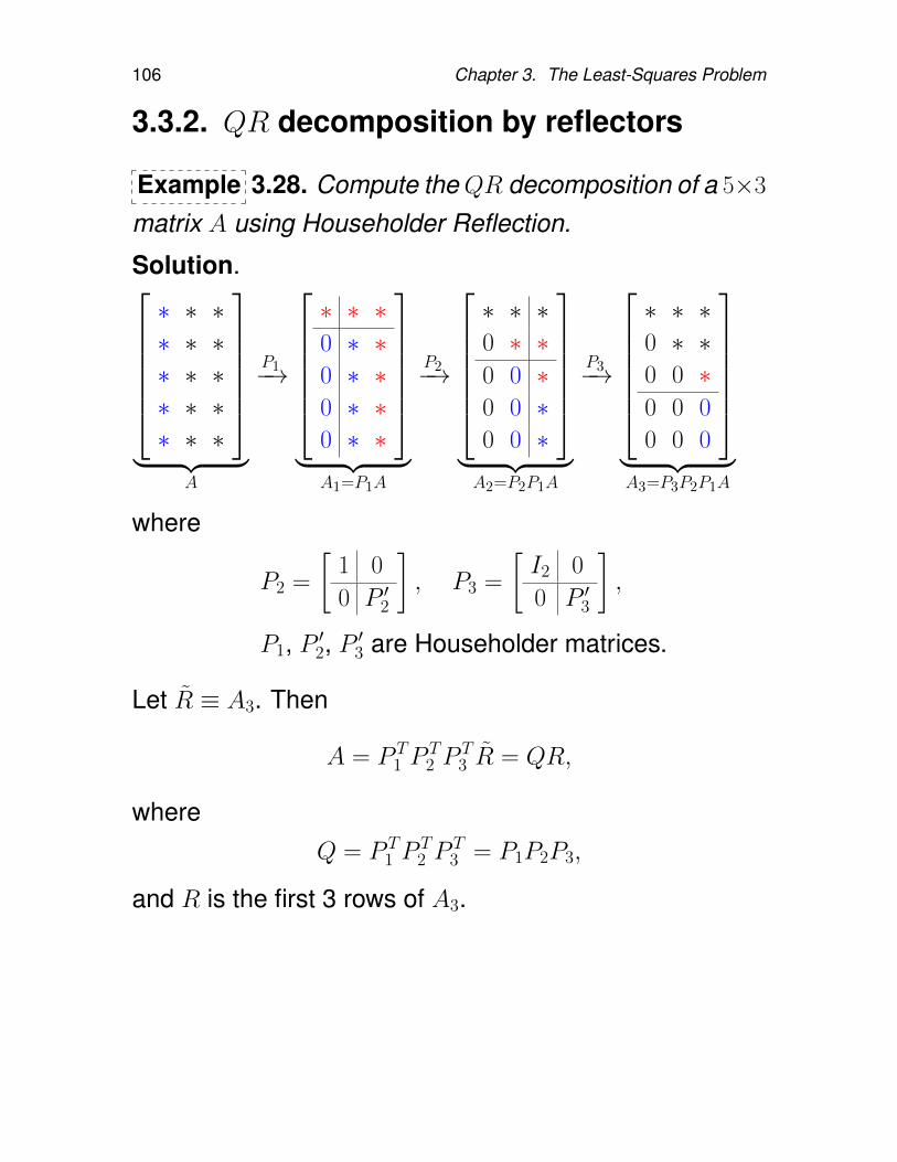
3.3.2. QR decomposition by reflectors
Example 3.28. Compute theQR decomposition of a 5×3
matrix A using Householder Reflection.
Solution.∗ ∗ ∗∗ ∗ ∗∗ ∗ ∗∗ ∗ ∗∗ ∗ ∗
︸ ︷︷ ︸
A
P1−→
∗ ∗ ∗0 ∗ ∗0 ∗ ∗0 ∗ ∗0 ∗ ∗
︸ ︷︷ ︸
A1=P1A
P2−→
∗ ∗ ∗0 ∗ ∗0 0 ∗0 0 ∗0 0 ∗
︸ ︷︷ ︸A2=P2P1A
P3−→
∗ ∗ ∗0 ∗ ∗0 0 ∗0 0 0
0 0 0
︸ ︷︷ ︸A3=P3P2P1A
where
P2 =
[1 0
0 P ′2
], P3 =
[I2 0
0 P ′3
],
P1, P ′2, P′3 are Householder matrices.
Let R ≡ A3. Then
A = P T1 P
T2 P
T3 R = QR,
whereQ = P T
1 PT2 P
T3 = P1P2P3,
and R is the first 3 rows of A3.
3.3. Orthogonal Matrices 107
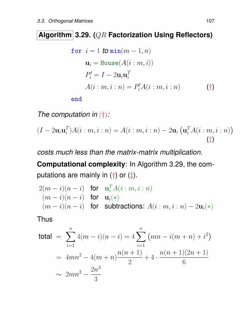
Algorithm 3.29. (QR Factorization Using Reflectors)
for i = 1 to min(m− 1, n)
ui = House(A(i : m, i))
P ′i = I − 2uiuTi
A(i : m, i : n) = P ′iA(i : m, i : n) (†)end
The computation in (†):
(I − 2uiuTi )A(i : m, i : n) = A(i : m, i : n)− 2ui
(uTi A(i : m, i : n)
)(‡)
costs much less than the matrix-matrix multiplication.
Computational complexity: In Algorithm 3.29, the com-putations are mainly in (†) or (‡).
2(m− i)(n− i) for uTi A(i : m, i : n)
(m− i)(n− i) for ui(∗)(m− i)(n− i) for subtractions: A(i : m, i : n)− 2ui(∗)
Thus
total =
n∑i=1
4(m− i)(n− i) = 4
n∑i=1
(mn− i(m + n) + i2
)= 4mn2 − 4(m + n)
n(n + 1)
2+ 4 · n(n + 1)(2n + 1)
6
∼ 2mn2 − 2n3
3
108 Chapter 3. The Least-Squares Problem
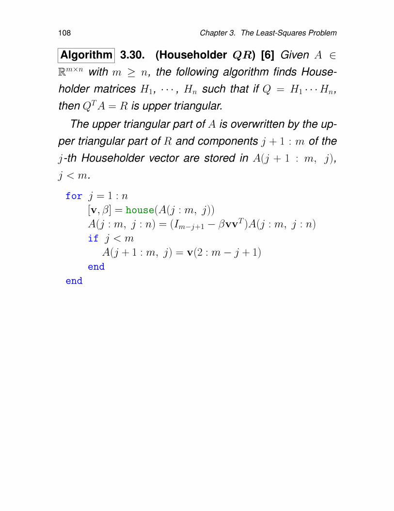
Algorithm 3.30. (Householder QR) [6] Given A ∈Rm×n with m ≥ n, the following algorithm finds House-holder matrices H1, · · · , Hn such that if Q = H1 · · ·Hn,then QTA = R is upper triangular.
The upper triangular part of A is overwritten by the up-per triangular part of R and components j + 1 : m of thej-th Householder vector are stored in A(j + 1 : m, j),j < m.
for j = 1 : n
[v, β] = house(A(j : m, j))
A(j : m, j : n) = (Im−j+1 − βvvT )A(j : m, j : n)
if j < m
A(j + 1 : m, j) = v(2 : m− j + 1)
end
end
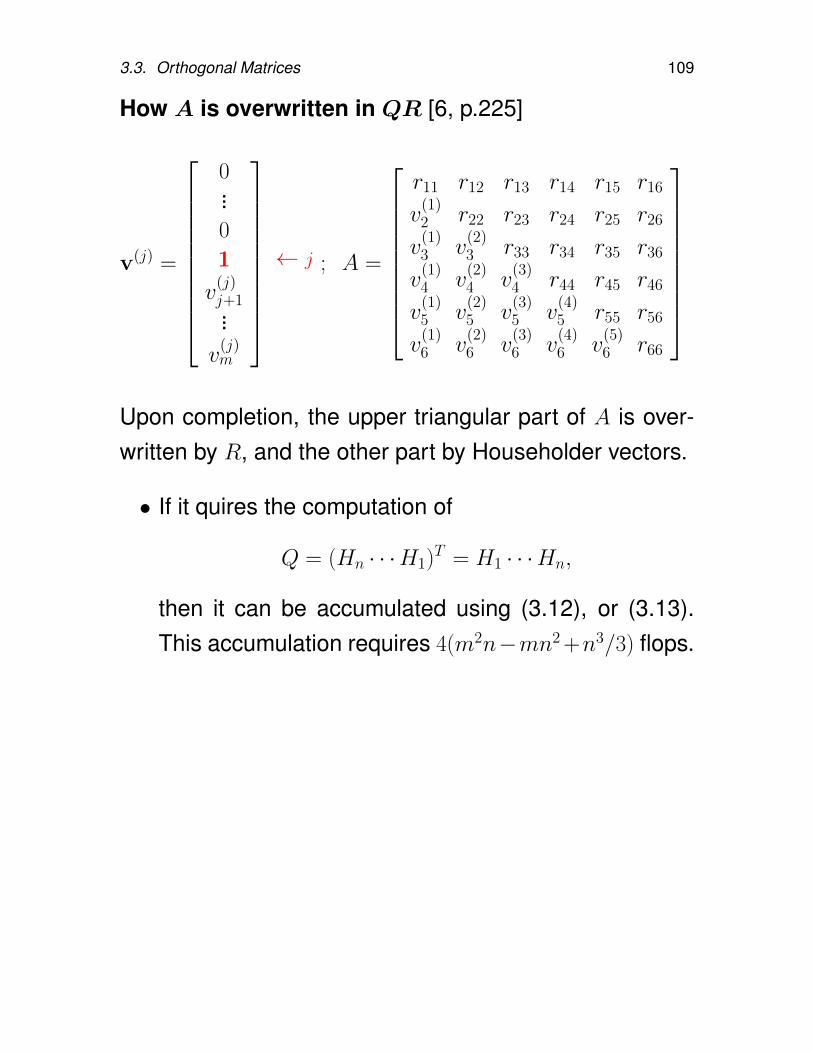
3.3. Orthogonal Matrices 109
How A is overwritten in QR [6, p.225]
v(j) =
0...0
1
v(j)j+1...v
(j)m
← j ; A =
r11 r12 r13 r14 r15 r16
v(1)2 r22 r23 r24 r25 r26
v(1)3 v
(2)3 r33 r34 r35 r36
v(1)4 v
(2)4 v
(3)4 r44 r45 r46
v(1)5 v
(2)5 v
(3)5 v
(4)5 r55 r56
v(1)6 v
(2)6 v
(3)6 v
(4)6 v
(5)6 r66
Upon completion, the upper triangular part of A is over-written by R, and the other part by Householder vectors.
• If it quires the computation of
Q = (Hn · · ·H1)T = H1 · · ·Hn,
then it can be accumulated using (3.12), or (3.13).This accumulation requires 4(m2n−mn2 +n3/3) flops.
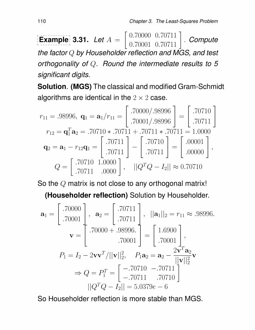
110 Chapter 3. The Least-Squares Problem
Example 3.31. Let A =
[0.70000 0.70711
0.70001 0.70711
]. Compute
the factor Q by Householder reflection and MGS, and testorthogonality of Q. Round the intermediate results to 5significant digits.
Solution. (MGS) The classical and modified Gram-Schmidtalgorithms are identical in the 2× 2 case.
r11 = .98996, q1 = a1/r11 =
[.70000/.98996
.70001/.98996
]=
[.70710
.70711
]r12 = qT1 a2 = .70710 ∗ .70711 + .70711 ∗ .70711 = 1.0000
q2 = a1 − r12q1 =
[.70711
.70711
]−
[.70710
.70711
]=
[.00001
.00000
],
Q =
[.70710 1.0000
.70711 .0000
], ||QTQ− I2|| ≈ 0.70710
So the Q matrix is not close to any orthogonal matrix!
(Householder reflection) Solution by Householder.
a1 =
[.70000
.70001
], a2 =
[.70711
.70711
], ||a1||2 = r11 ≈ .98996.
v =
[.70000 + .98996.
.70001
]=
[1.6900
.70001
],
P1 = I2 − 2vvT/||v||22, P1a2 = a2 −2vTa2
||v||22v
⇒ Q = P T1 =
[−.70710 −.70711
−.70711 .70710
]||QTQ− I2|| = 5.0379e− 6
So Householder reflection is more stable than MGS.
3.3. Orthogonal Matrices 111
3.3.3. Solving LS problems by Householderreflectors
• To solve the LS problem min ||Ax−b||22 using A = QR,we need to compute
QTb and Rx = QTb.
Since A→ PnPn−1 · · ·P1A = R, Q = (PnPn−1 · · ·P1)T ,
QTb = PnPn−1 · · ·P1b.
So we can apply exactly the same steps that wereapplied to A in the Householder QR algorithm:
112 Chapter 3. The Least-Squares Problem
• (Computing QTb)
for i = 1 to n
γ = −2 · uTi b(i : m)
b(i : m) = b(i : m) + γuiend for
• (Solving Rx = QTb)
R ≡ [R QTb]
for k = n : −1 : 1
R(k, n + 1) = R(k, n + 1)/R(k, k);
if k 6= 1
R(1 : k − 1, n + 1) = R(1 : k − 1, n + 1)− R(1 : k − 1, k)R(k, n + 1);
end if
end for
(Solution x overwrites the (n + 1)-th column of R.)
• Total cost in solving the LS problem:
2mn2 −2n3
3
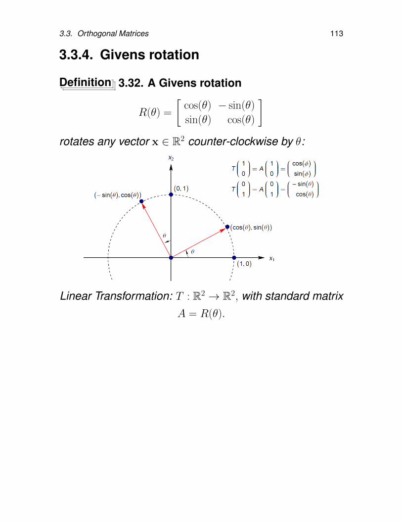
3.3. Orthogonal Matrices 113
3.3.4. Givens rotation
Definition 3.32. A Givens rotation
R(θ) =
[cos(θ) − sin(θ)
sin(θ) cos(θ)
]rotates any vector x ∈ R2 counter-clockwise by θ:
Linear Transformation: T : R2 → R2, with standard matrixA = R(θ).
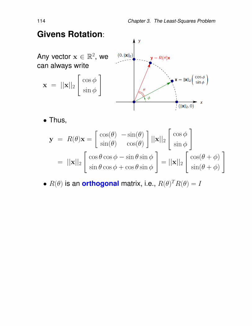
114 Chapter 3. The Least-Squares Problem
Givens Rotation:
Any vector x ∈ R2, wecan always write
x = ||x||2
[cosφ
sinφ
]
• Thus,
y = R(θ)x =
[cos(θ) − sin(θ)
sin(θ) cos(θ)
]||x||2
[cosφ
sinφ
]
= ||x||2
[cos θ cosφ− sin θ sinφ
sin θ cosφ + cos θ sinφ
]= ||x||2
[cos(θ + φ)
sin(θ + φ)
]
• R(θ) is an orthogonal matrix, i.e., R(θ)TR(θ) = I
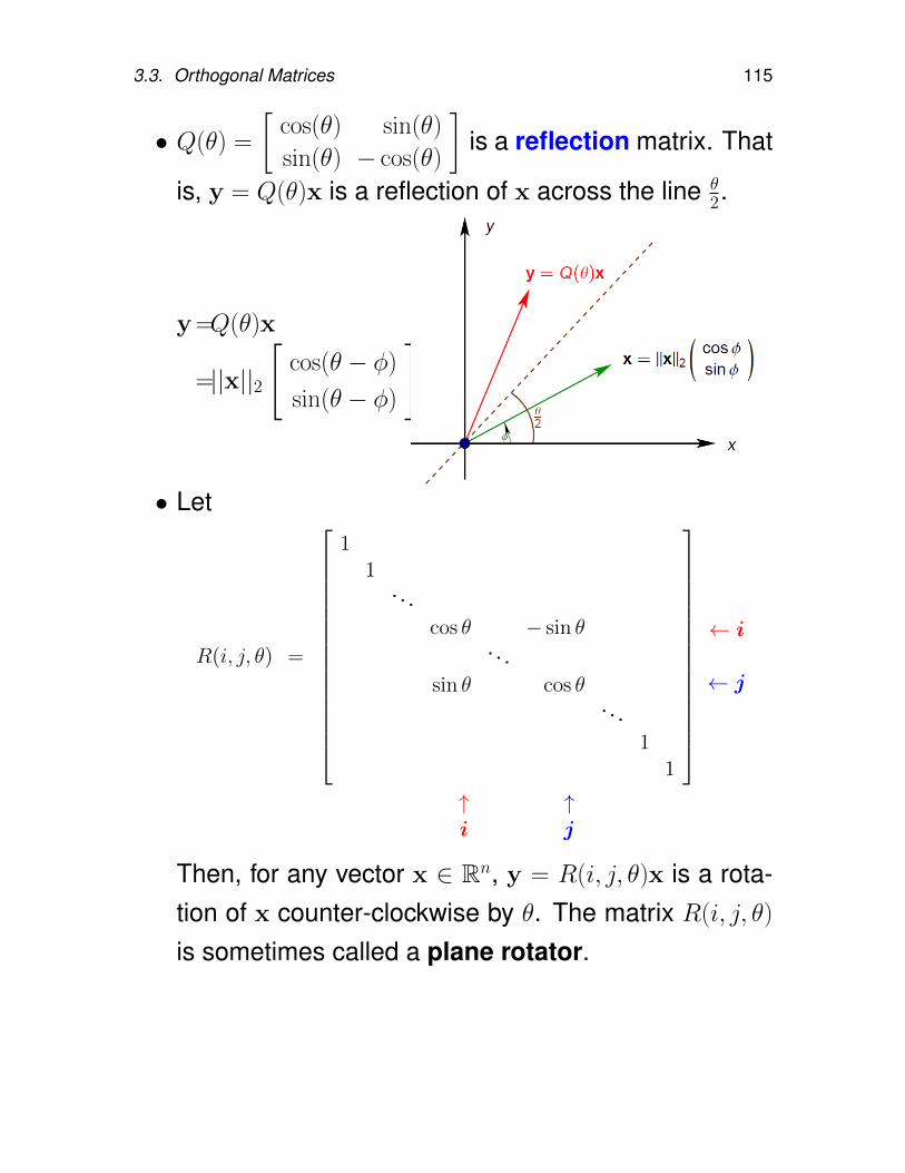
3.3. Orthogonal Matrices 115
• Q(θ) =
[cos(θ) sin(θ)
sin(θ) − cos(θ)
]is a reflection matrix. That
is, y = Q(θ)x is a reflection of x across the line θ2.
y =Q(θ)x
=||x||2
[cos(θ − φ)
sin(θ − φ)
]
• Let
R(i, j, θ) =
11
. . .cos θ − sin θ
. . .sin θ cos θ
. . .1
1
← i
← j
↑ ↑i j
Then, for any vector x ∈ Rn, y = R(i, j, θ)x is a rota-tion of x counter-clockwise by θ. The matrix R(i, j, θ)
is sometimes called a plane rotator.
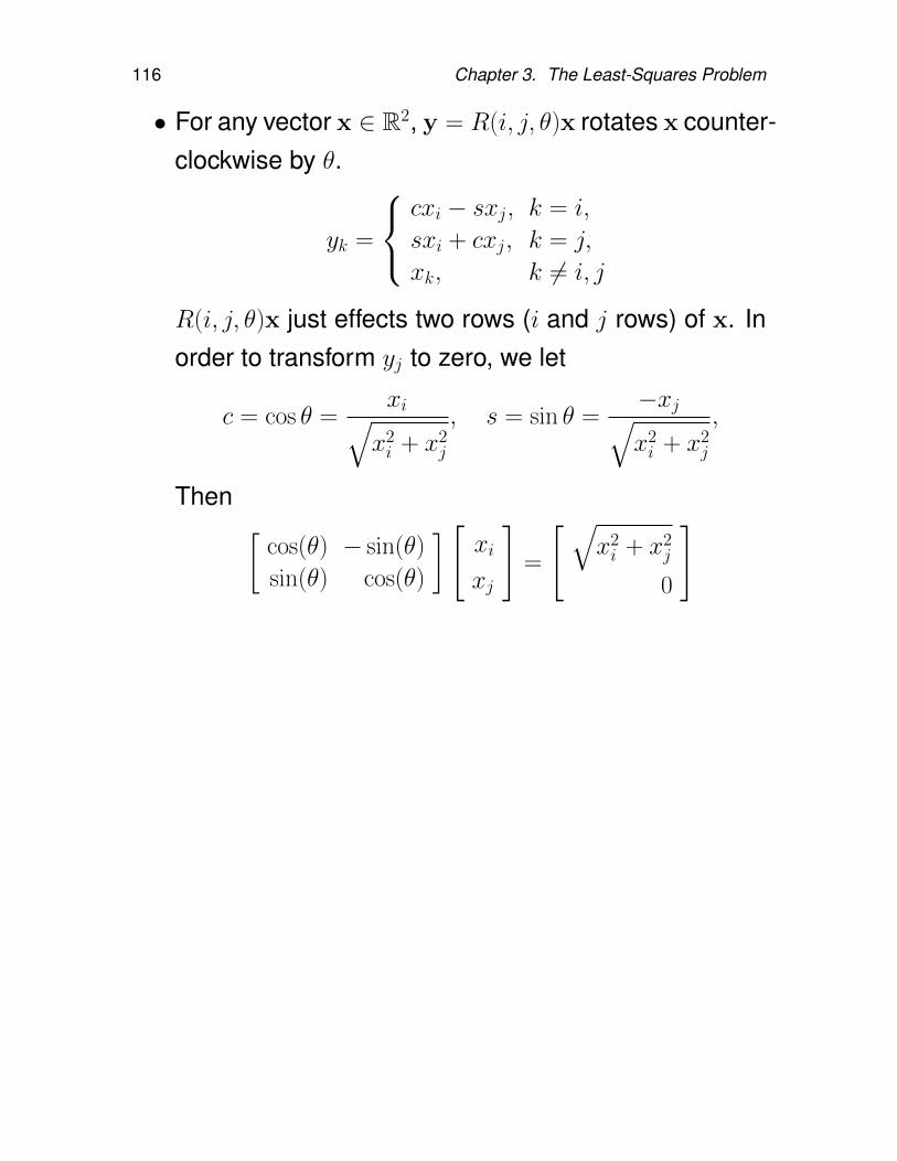
116 Chapter 3. The Least-Squares Problem
• For any vector x ∈ R2, y = R(i, j, θ)x rotates x counter-clockwise by θ.
yk =
cxi − sxj, k = i,
sxi + cxj, k = j,
xk, k 6= i, j
R(i, j, θ)x just effects two rows (i and j rows) of x. Inorder to transform yj to zero, we let
c = cos θ =xi√x2i + x2
j
, s = sin θ =−xj√x2i + x2
j
,
Then [cos(θ) − sin(θ)
sin(θ) cos(θ)
][xi
xj
]=
[ √x2i + x2
j
0
]

3.3. Orthogonal Matrices 117
Algorithm 3.33. (Givens Rotation Algorithm) Givenscalars a and b, the following function computes c = cos θ
and s = sin θ. [c −ss c
][a
b
]=
[r
0
]where r =
√a2 + b2.
function [c, s] = givens(a, b)
if b = 0
c = 1; s = 0;
else
if |b| > |a|
τ = −ab
; s =1√
1 + τ 2; c = sτ ;
else
τ = −ba
; c =1√
1 + τ 2; s = cτ ;
end
end
Note: It does not compute θ and it does not involve in-verse trig. functions. Total cost: 5 flops and a singlesquare root.
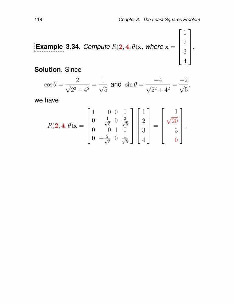
118 Chapter 3. The Least-Squares Problem
Example 3.34. Compute R(2,4, θ)x, where x =
1
2
3
4
.
Solution. Since
cos θ =2√
22 + 42=
1√5
and sin θ =−4√
22 + 42=−2√
5,
we have
R(2,4, θ)x =
1 0 0 0
0 1√5
0 2√5
0 0 1 0
0 − 2√5
0 1√5
1
2
3
4
=
1√
20
3
0
.
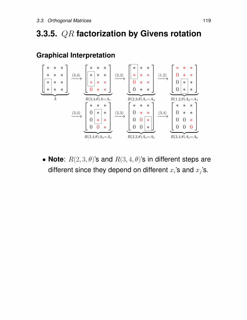
3.3. Orthogonal Matrices 119
3.3.5. QR factorization by Givens rotation
Graphical Interpretation∗ ∗ ∗∗ ∗ ∗∗ ∗ ∗∗ ∗ ∗
︸ ︷︷ ︸
A
(3,4)−−→
∗ ∗ ∗∗ ∗ ∗∗ ∗ ∗0 ∗ ∗
︸ ︷︷ ︸R(3,4,θ)A=A1
(2,3)−−→
∗ ∗ ∗∗ ∗ ∗0 ∗ ∗0 ∗ ∗
︸ ︷︷ ︸R(2,3,θ)A1=A2
(1,2)−−→
∗ ∗ ∗0 ∗ ∗0 ∗ ∗0 ∗ ∗
︸ ︷︷ ︸R(1,2,θ)A2=A3
(3,4)−−→
∗ ∗ ∗0 ∗ ∗0 ∗ ∗0 0 ∗
︸ ︷︷ ︸R(3,4,θ)A3=A4
(2,3)−−→
∗ ∗ ∗0 ∗ ∗0 0 ∗0 0 ∗
︸ ︷︷ ︸R(2,3,θ)A4=A5
(3,4)−−→
∗ ∗ ∗0 ∗ ∗0 0 ∗0 0 0
︸ ︷︷ ︸R(3,4,θ)A5=A6
• Note: R(2, 3, θ)’s and R(3, 4, θ)’s in different steps aredifferent since they depend on different xi’s and xj ’s.
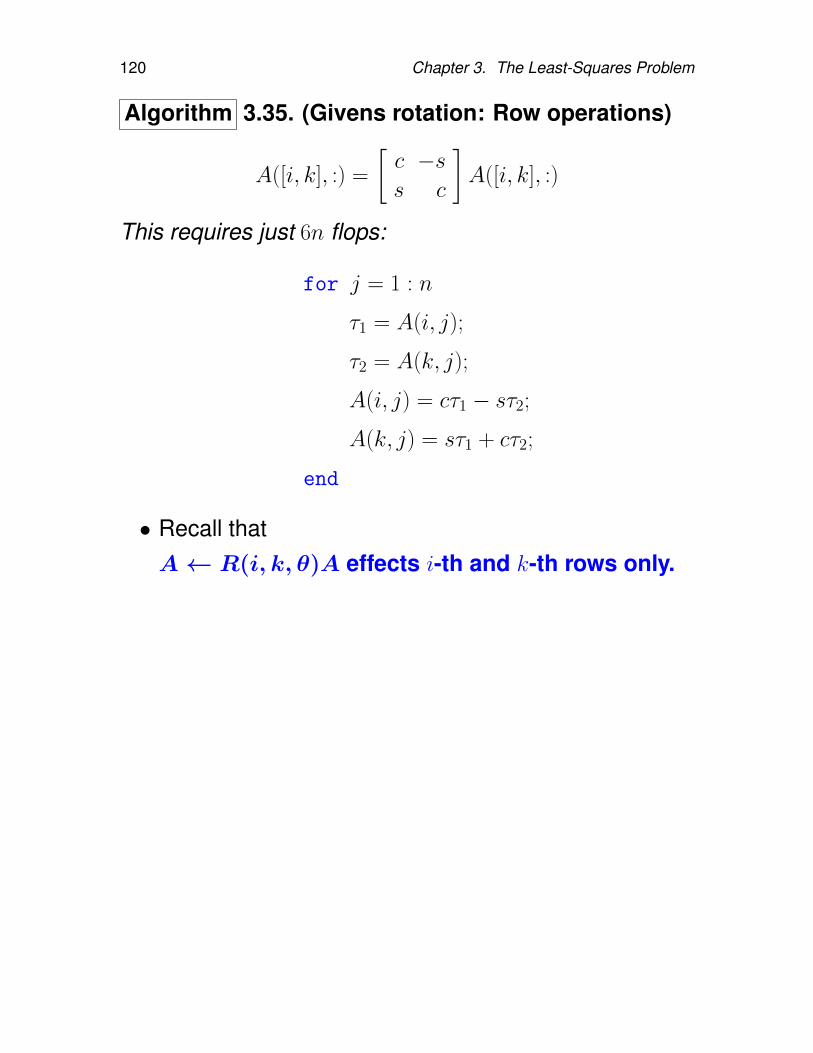
120 Chapter 3. The Least-Squares Problem
Algorithm 3.35. (Givens rotation: Row operations)
A([i, k], :) =
[c −ss c
]A([i, k], :)
This requires just 6n flops:
for j = 1 : n
τ1 = A(i, j);
τ2 = A(k, j);
A(i, j) = cτ1 − sτ2;
A(k, j) = sτ1 + cτ2;
end
• Recall thatA← R(i, k, θ)A effects i-th and k-th rows only.
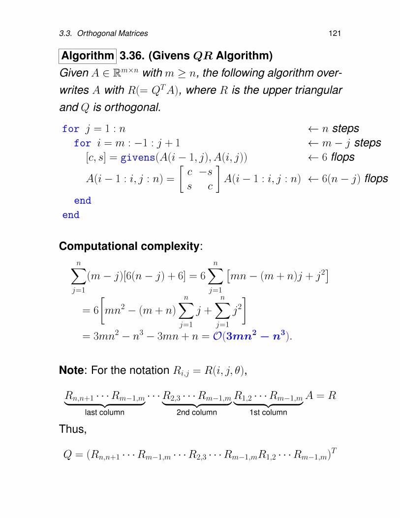
3.3. Orthogonal Matrices 121
Algorithm 3.36. (Givens QR Algorithm)Given A ∈ Rm×n with m ≥ n, the following algorithm over-writes A with R(= QTA), where R is the upper triangularand Q is orthogonal.
for j = 1 : n ← n stepsfor i = m : −1 : j + 1 ← m− j steps
[c, s] = givens(A(i− 1, j), A(i, j)) ← 6 flops
A(i− 1 : i, j : n) =
[c −ss c
]A(i− 1 : i, j : n) ← 6(n− j) flops
end
end
Computational complexity:n∑j=1
(m− j)[6(n− j) + 6] = 6
n∑j=1
[mn− (m + n)j + j2
]= 6
[mn2 − (m + n)
n∑j=1
j +
n∑j=1
j2
]= 3mn2 − n3 − 3mn + n = O(3mn2 − n3).
Note: For the notation Ri,j = R(i, j, θ),
Rn,n+1 · · ·Rm−1,m︸ ︷︷ ︸last column
· · ·R2,3 · · ·Rm−1,m︸ ︷︷ ︸2nd column
R1,2 · · ·Rm−1,m︸ ︷︷ ︸1st column
A = R
Thus,
Q = (Rn,n+1 · · ·Rm−1,m · · ·R2,3 · · ·Rm−1,mR1,2 · · ·Rm−1,m)T
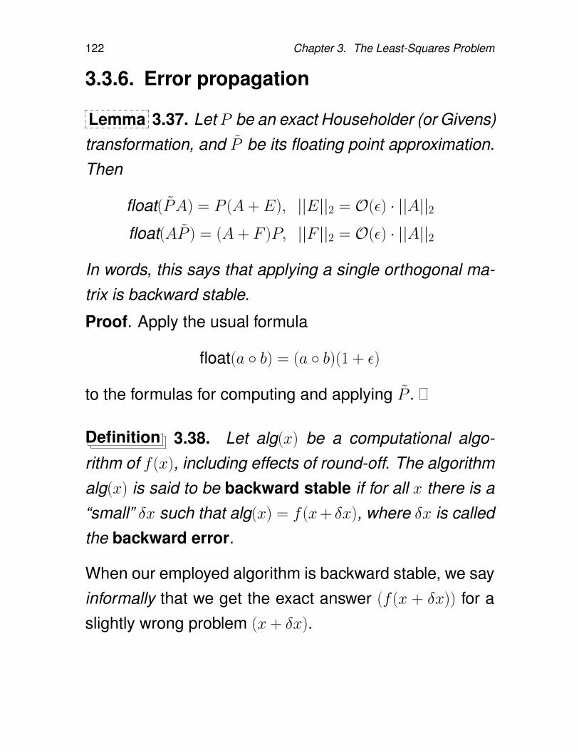
122 Chapter 3. The Least-Squares Problem
3.3.6. Error propagation
Lemma 3.37. Let P be an exact Householder (or Givens)transformation, and P be its floating point approximation.Then
float(PA) = P (A + E), ||E||2 = O(ε) · ||A||2float(AP ) = (A + F )P, ||F ||2 = O(ε) · ||A||2
In words, this says that applying a single orthogonal ma-trix is backward stable.
Proof. Apply the usual formula
float(a b) = (a b)(1 + ε)
to the formulas for computing and applying P .
Definition 3.38. Let alg(x) be a computational algo-rithm of f (x), including effects of round-off. The algorithmalg(x) is said to be backward stable if for all x there is a“small” δx such that alg(x) = f (x+ δx), where δx is calledthe backward error.
When our employed algorithm is backward stable, we sayinformally that we get the exact answer (f (x + δx)) for aslightly wrong problem (x + δx).
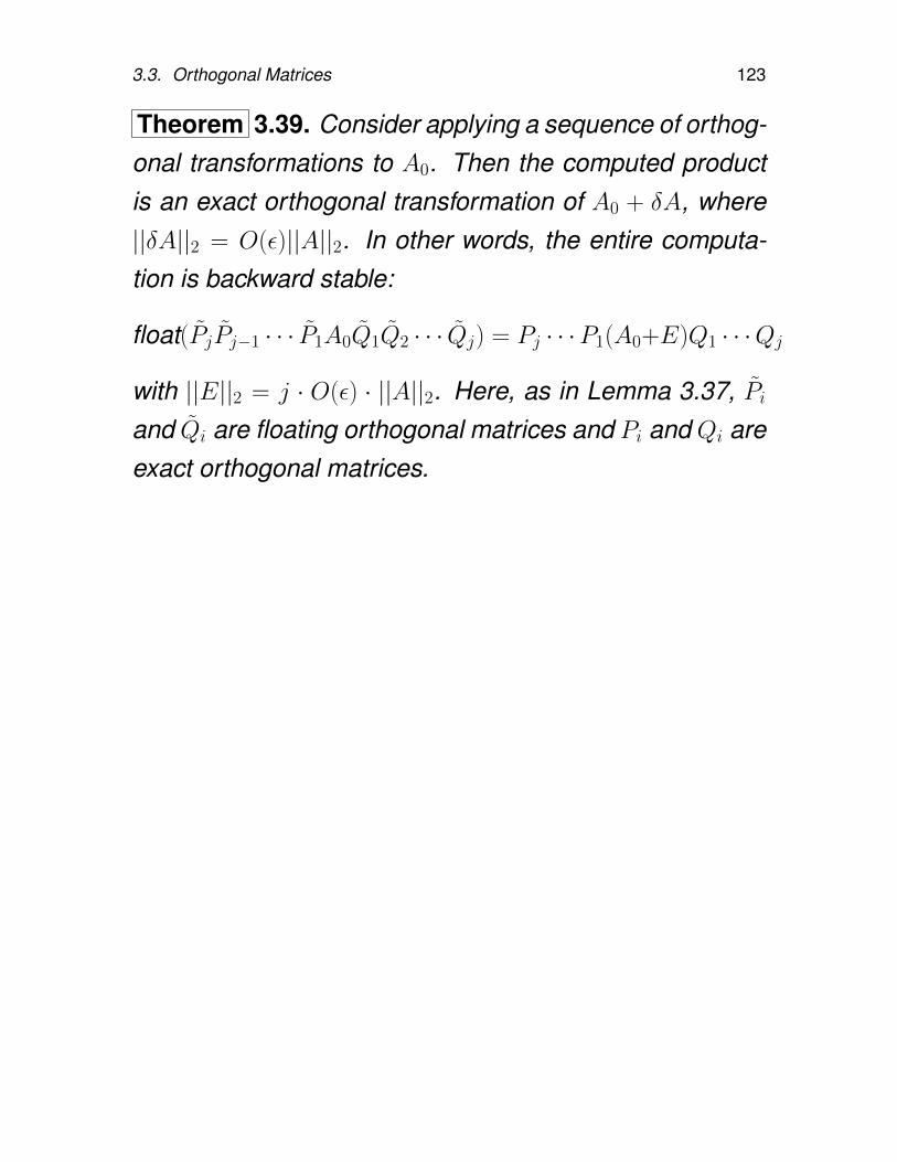
3.3. Orthogonal Matrices 123
Theorem 3.39. Consider applying a sequence of orthog-onal transformations to A0. Then the computed productis an exact orthogonal transformation of A0 + δA, where||δA||2 = O(ε)||A||2. In other words, the entire computa-tion is backward stable:
float(PjPj−1 · · · P1A0Q1Q2 · · · Qj) = Pj · · ·P1(A0+E)Q1 · · ·Qj
with ||E||2 = j · O(ε) · ||A||2. Here, as in Lemma 3.37, Piand Qi are floating orthogonal matrices and Pi and Qi areexact orthogonal matrices.
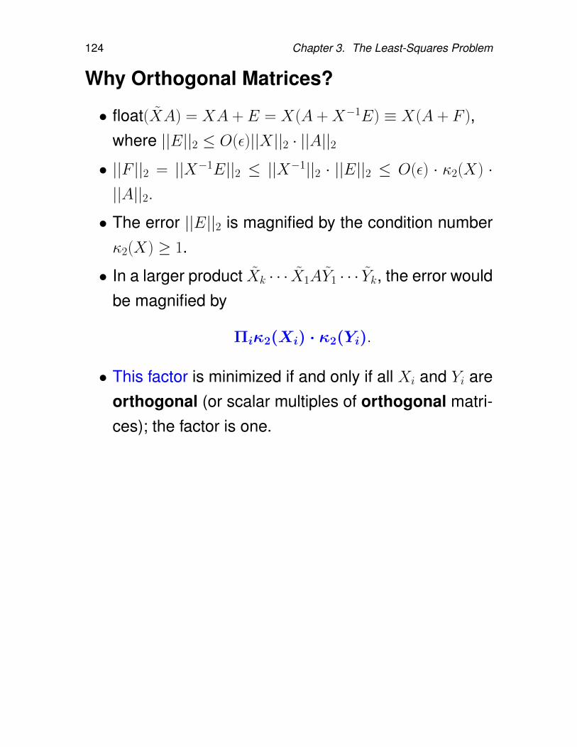
124 Chapter 3. The Least-Squares Problem
Why Orthogonal Matrices?
• float(XA) = XA + E = X(A + X−1E) ≡ X(A + F ),where ||E||2 ≤ O(ε)||X||2 · ||A||2• ||F ||2 = ||X−1E||2 ≤ ||X−1||2 · ||E||2 ≤ O(ε) · κ2(X) ·||A||2.
• The error ||E||2 is magnified by the condition numberκ2(X) ≥ 1.
• In a larger product Xk · · · X1AY1 · · · Yk, the error wouldbe magnified by
Πiκ2(Xi) · κ2(Yi).
• This factor is minimized if and only if all Xi and Yi areorthogonal (or scalar multiples of orthogonal matri-ces); the factor is one.
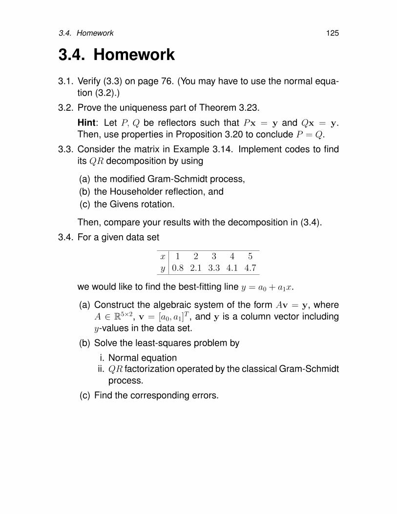
3.4. Homework 125
3.4. Homework3.1. Verify (3.3) on page 76. (You may have to use the normal equa-
tion (3.2).)
3.2. Prove the uniqueness part of Theorem 3.23.
Hint: Let P, Q be reflectors such that Px = y and Qx = y.Then, use properties in Proposition 3.20 to conclude P = Q.
3.3. Consider the matrix in Example 3.14. Implement codes to findits QR decomposition by using
(a) the modified Gram-Schmidt process,(b) the Householder reflection, and(c) the Givens rotation.
Then, compare your results with the decomposition in (3.4).
3.4. For a given data set
x 1 2 3 4 5y 0.8 2.1 3.3 4.1 4.7
we would like to find the best-fitting line y = a0 + a1x.
(a) Construct the algebraic system of the form Av = y, whereA ∈ R5×2, v = [a0, a1]
T , and y is a column vector includingy-values in the data set.
(b) Solve the least-squares problem by
i. Normal equationii. QR factorization operated by the classical Gram-Schmidt
process.
(c) Find the corresponding errors.
126 Chapter 3. The Least-Squares Problem
Chapter 4
Singular Value Decomposition (SVD)
The QR decomposition is a fine tool for the solution ofleast-squares problems when the matrix is known to havefull rank. However, if the matrix does not have full rank, orif the rank is not known, a more powerful tool is required.Such more powerful tools (for rank-deficient cases) are
• The QR decomposition with column pivoting
• Singular value decomposition (SVD)
SVD may be the most important matrix decomposition ofall, for both theoretical and computational purposes.
127
128 Chapter 4. Singular Value Decomposition (SVD)
4.1. Introduction to the SVD
Rank-deficient case: We begin with a discussion onrank-deficient algebraic problems.
Definition 4.1. Let A ∈ Rm×n, m ≥ n. The matrix A iscalled rank-deficient if rank(A) = k < n.
Theorem 4.2. Let A ∈ Rm×n, m ≥ n, with rank(A) = k > 0.Then there exist matrices A, Q, and R such that
A = QR, (4.1)
where A is obtained from A by permuting its columns,Q ∈ Rm×m is orthogonal, and
R =
[R11 R12
0 0
]∈ Rm×n,
R11 ∈ Rk×k is nonsingular and upper triangular.
Proposition 4.3. (Rank-deficient LS problems) LetA ∈ Rm×n, m ≥ n, with rank(A) = k < n. Then thereexists an (n − k)-dimensional set of vectors x that mini-mize
||Ax− b||2.
Proof. Let Az = 0. Then if x minimize ||Ax−b||2, so doesx + z. dim(Null(A)) = n − rank(A) = n − k by the RankTheorem.
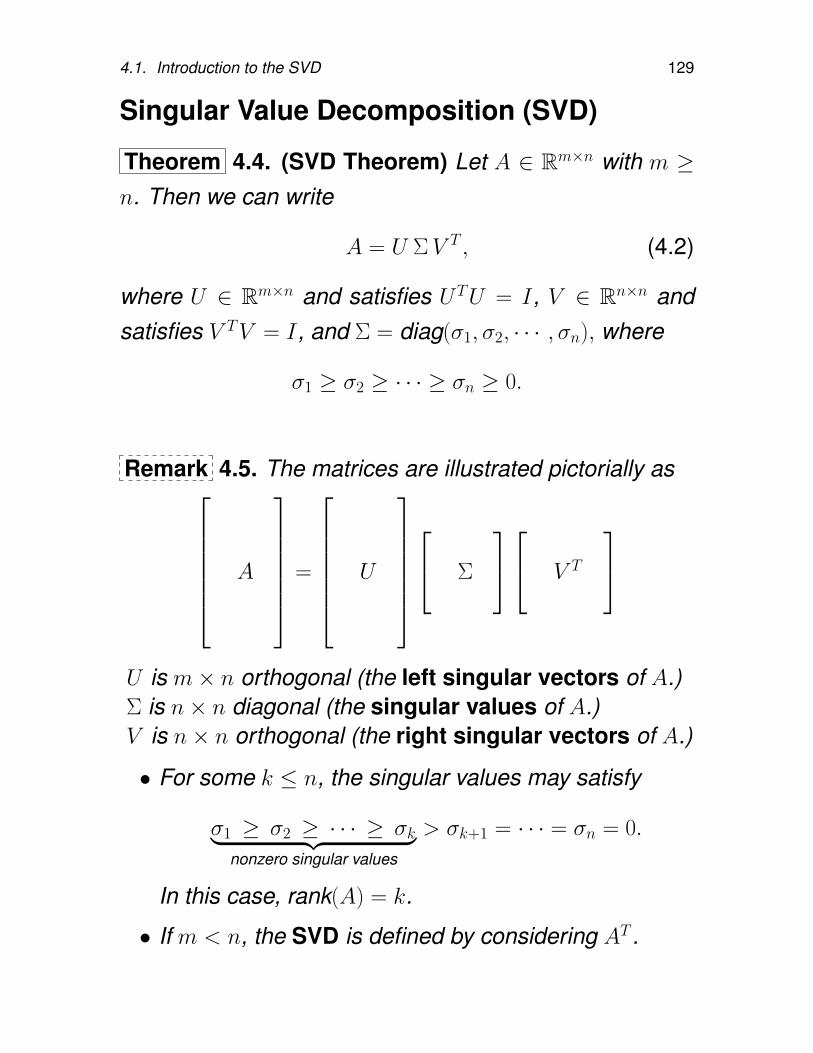
4.1. Introduction to the SVD 129
Singular Value Decomposition (SVD)
Theorem 4.4. (SVD Theorem) Let A ∈ Rm×n with m ≥n. Then we can write
A = U ΣV T , (4.2)
where U ∈ Rm×n and satisfies UTU = I, V ∈ Rn×n andsatisfies V TV = I, and Σ = diag(σ1, σ2, · · · , σn), where
σ1 ≥ σ2 ≥ · · · ≥ σn ≥ 0.
Remark 4.5. The matrices are illustrated pictorially as A
=
U
Σ
V T
U is m× n orthogonal (the left singular vectors of A.)Σ is n× n diagonal (the singular values of A.)V is n× n orthogonal (the right singular vectors of A.)
• For some k ≤ n, the singular values may satisfy
σ1 ≥ σ2 ≥ · · · ≥ σk︸ ︷︷ ︸nonzero singular values
> σk+1 = · · · = σn = 0.
In this case, rank(A) = k.
• If m < n, the SVD is defined by considering AT .
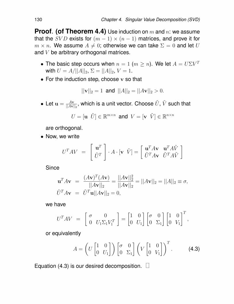
130 Chapter 4. Singular Value Decomposition (SVD)
Proof. (of Theorem 4.4) Use induction on m and n: we assumethat the SV D exists for (m − 1) × (n − 1) matrices, and prove it form × n. We assume A 6= 0; otherwise we can take Σ = 0 and let Uand V be arbitrary orthogonal matrices.
• The basic step occurs when n = 1 (m ≥ n). We let A = UΣV T
with U = A/||A||2, Σ = ||A||2, V = 1.• For the induction step, choose v so that
||v||2 = 1 and ||A||2 = ||Av||2 > 0.
• Let u = Av||Av||2 , which is a unit vector. Choose U , V such that
U = [u U ] ∈ Rm×n and V = [v V ] ∈ Rn×n
are orthogonal.• Now, we write
UTAV =
[uT
UT
]· A · [v V ] =
[uTAv uTAV
UTAv UTAV
]Since
uTAv =(Av)T (Av)
||Av||2=||Av||22||Av||2
= ||Av||2 = ||A||2 ≡ σ,
UTAv = UTu||Av||2 = 0,
we have
UTAV =
[σ 00 U1Σ1V
T1
]=
[1 00 U1
] [σ 00 Σ1
] [1 00 V1
]T,
or equivalently
A =
(U
[1 00 U1
])[σ 00 Σ1
](V
[1 00 V1
])T. (4.3)
Equation (4.3) is our desired decomposition.
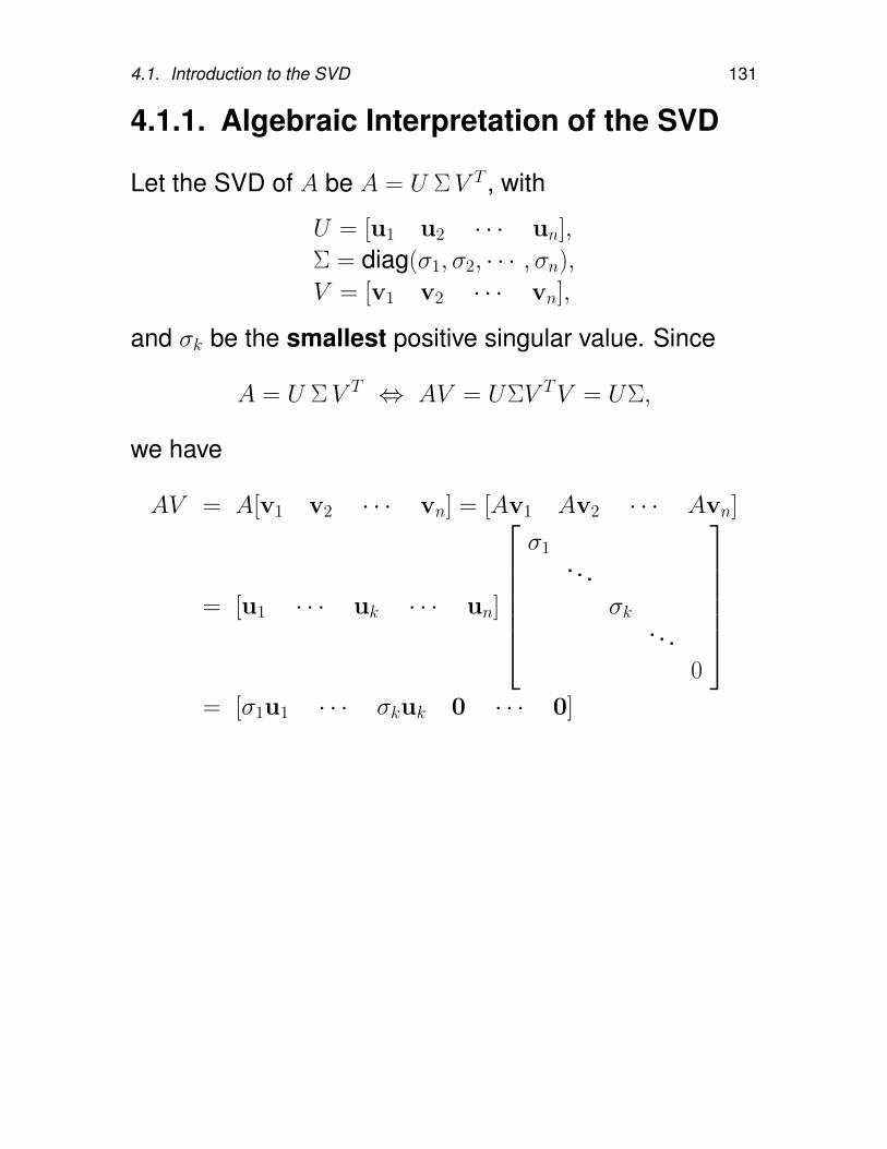
4.1. Introduction to the SVD 131
4.1.1. Algebraic Interpretation of the SVD
Let the SVD of A be A = U ΣV T , with
U = [u1 u2 · · · un],
Σ = diag(σ1, σ2, · · · , σn),
V = [v1 v2 · · · vn],
and σk be the smallest positive singular value. Since
A = U ΣV T ⇔ AV = UΣV TV = UΣ,
we have
AV = A[v1 v2 · · · vn] = [Av1 Av2 · · · Avn]
= [u1 · · · uk · · · un]
σ1
. . .σk
. . .0
= [σ1u1 · · · σkuk 0 · · · 0]
132 Chapter 4. Singular Value Decomposition (SVD)
Therefore,
A = U ΣV T ⇔Avj = σjuj, j = 1, 2, · · · , kAvj = 0, j = k + 1, · · · , n (4.4)
Similarly, starting from AT = V ΣUT ,
AT = V ΣUT ⇔ATuj = σjvj, j = 1, 2, · · · , kATuj = 0, j = k + 1, · · · , n
(4.5)
Summary 4.6. It follows from (4.4) and (4.5) that
• σ2j, j = 1, 2, · · · , k, are positive eigenvalues of ATA.
ATAvj = AT (σjuj) = σ2jvj, j = 1, 2, · · · , k. (4.6)
So, the singular values play the role of eigenvalues.
• Equation (4.6) gives how to find the singular valuesand the right singular vectors, while (4.4) shows a wayto compute the left singular vectors.
• (Dyadic decomposition) The matrix A ∈ Rm×n, withrank(A) = k ≤ n, can be expressed as
A =
k∑j=1
σjujvTj . (4.7)
This property has been utilized for various approxi-mations and applications, e.g., by dropping singularvectors corresponding to small singular values.
4.1. Introduction to the SVD 133
4.1.2. Geometric Interpretation of the SVD
The matrix A maps an orthonormal basis
B1 = v1,v2, · · · ,vn
of Rn onto a new “scaled” orthogonal basis
B2 = σ1u1, σ2u2, · · · , σkuk
for a subspace of Rm.
B1 = v1,v2, · · · ,vnA−→ B2 = σ1u1, σ2u2, · · · , σkuk
(4.8)Consider a unit sphere Sn−1 in Rn:
Sn−1 =
x∣∣∣ n∑j=1
x2j = 1
.
Then, ∀x ∈ Sn−1,
x = x1v1 + x2v2 + · · · + xnvn
Ax = σ1x1u1 + σ2x2u2 + · · · + σkxkuk
= y1u1 + y2u2 + · · · + ykuk, (yj = σjxj)
(4.9)
So, we have
yj = σjxj ⇐⇒ xj =yjσj
n∑j=1
x2j = 1 (sphere) ⇐⇒
k∑j=1
y2j
σ2j
= α ≤ 1 (ellipsoid)
(4.10)
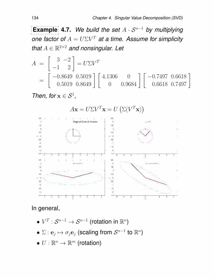
134 Chapter 4. Singular Value Decomposition (SVD)
Example 4.7. We build the set A · Sn−1 by multiplyingone factor of A = UΣV T at a time. Assume for simplicitythat A ∈ R2×2 and nonsingular. Let
A =
[3 −2
−1 2
]= UΣV T
=
[−0.8649 0.5019
0.5019 0.8649
] [4.1306 0
0 0.9684
] [−0.7497 0.6618
0.6618 0.7497
]Then, for x ∈ S1,
Ax = UΣV Tx = U(Σ(V Tx)
)
In general,
• V T : Sn−1 → Sn−1 (rotation in Rn)
• Σ : ej 7→ σjej (scaling from Sn−1 to Rn)
• U : Rn → Rm (rotation)
4.1. Introduction to the SVD 135
4.1.3. Properties of the SVD
Theorem 4.8. Let A ∈ Rm×n and p = min(m,n). LetA = UΣV T be the SVD of A, with
σ1 ≥ · · · ≥ σk > σk+1 = · · · = σp = 0.
Then,
1.
rank(A) = k
Null(A) = Spanvk+1, · · · ,vnRange(A) = Spanu1, · · · ,uk
A =
k∑i=1
σiuivTi
2.
||A||2 = σ1 (See HW 4.1.)||A||2F = σ2
1 + · · · + σ2k (See HW 4.2.)
minx6=0
||Ax||2||x||2
= σn (m ≥ n)
κ2(A) = ||A||2 · ||A−1||2 =σ1
σn( when m = n,& ∃A−1)
136 Chapter 4. Singular Value Decomposition (SVD)
Theorem 4.9. Let A ∈ Rm×n with m ≥ n. Then,
||ATA||2 = ||A||22κ2(ATA) = κ2(A)2. (when A−1 exists)
(4.11)
Proof. Use the SVD of A to deduce the SVD of ATA.
Theorem 4.10. Let A ∈ Rm×n, m ≥ n, rank(A) = n, withsingular values
σ1 ≥ σ2 ≥ · · ·σn > 0.
Then||(ATA)−1||2 = σ−2
n ,
||(ATA)−1AT ||2 = σ−1n ,
||A(ATA)−1||2 = σ−1n ,
||A(ATA)−1AT ||2 = 1.
(4.12)
Definition 4.11. (ATA)−1AT is called the pseudoinverseof A, while A(ATA)−1 is called the pseudoinverse of AT .Let A = UΣV T be the SVD of A. Then
(ATA)−1AT = V Σ−1UT ≡ A+. (4.13)
4.1. Introduction to the SVD 137
Theorem 4.12. Let A ∈ Rm×n with rank(A) = r > 0. LetA = UΣV T be the SVD of A, with singular values
σ1 ≥ · · · ≥ σr > 0.
Define, for k = 1, · · · , r − 1,
Ak =
k∑j=1
σjujvTj (sum of rank-1 matrices).
Then, rank(Ak) = k and
||A− Ak||2 = min||A−B||2∣∣ rank(B) ≤ k
= σk+1,
||A− Ak||2F = min||A−B||2F∣∣ rank(B) ≤ k
= σ2k+1 + · · · + σ2
r .
(4.14)
That is, of all matrices of rank ≤ k, Ak is closest to A.
Note: The matrix Ak can be written as
Ak = UΣkVT ,
where Σk = diag(σ1, · · · , σk, 0, · · · , 0).
Corollary 4.13. Suppose A ∈ Rm×n has full rank. Thusrank(A) = p, where p = min(m,n). Let σ1 ≥ · · · ≥ σp bethe singular values of A. Let B ∈ Rm×n satisfy
||A−B||2 < σp.
Then B also has full rank.
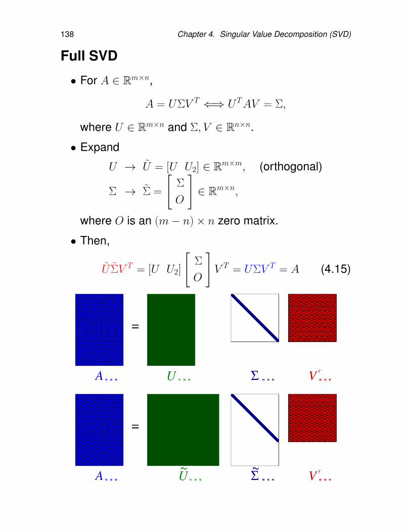
138 Chapter 4. Singular Value Decomposition (SVD)
Full SVD
• For A ∈ Rm×n,
A = UΣV T ⇐⇒ UTAV = Σ,
where U ∈ Rm×n and Σ, V ∈ Rn×n.
• Expand
U → U = [U U2] ∈ Rm×m, (orthogonal)
Σ → Σ =
[Σ
O
]∈ Rm×n,
where O is an (m− n)× n zero matrix.
• Then,
U ΣV T = [U U2]
[Σ
O
]V T = UΣV T = A (4.15)
4.1. Introduction to the SVD 139
Proposition 4.14. There are important relation betweenthe SVD of a matrix A and the Schur decompositionsof the symmetric matrices
ATA, AAT , and[O AT
A O
].
Let A ∈ Rm×n, m ≥ n. If UTAV = diag(σ1, · · · , σn) is theSV D of A, then
V T (ATA)V = diag(σ21, · · · , σ2
n) ∈ Rn×n
UT (AAT )U = diag(σ21, · · · , σ2
n, 0 · · · , 0︸ ︷︷ ︸m−n
) ∈ Rm×m
Separate U as
U = [ U1︸︷︷︸n
U2︸︷︷︸m−n
],
and define
Q ≡ 1√2
[V V O
U1 −U1
√2U2
]∈ R(m+n)×(m+n).
Then,
QT
[O AT
A O
]Q = diag(σ1, · · · , σn,−σ1, · · · ,−σn, 0 · · · , 0︸ ︷︷ ︸
m−n
) (4.16)
140 Chapter 4. Singular Value Decomposition (SVD)
Theorem 4.15. Let A = UΣV T be the SV D of A ∈ Rm×n
(m ≥ n).
1. (m = n) Suppose that A is symmetric, with eigen-values λi and orthonormal e-vectors ui. In other words,
A = UΛUT
is an eigendecomposition, with Λ = diag(λ1, · · · , λn).Then an SVD of A is A = UΣV T , where
σi = |λi| and vi = sign(λi)ui, where sign(0) = 1.
2. The eigenvalues of the symmetric matrix ATA areσ2i . The right singular vectors vi are corresponding
orthonormal eigenvectors.
3. The eigenvalues of the symmetric matrix AAT are σ2i
and m− n zeros. The left singular vectors ui are cor-responding orthonormal eigenvectors for the e-valuesσ2i . One can take any m− n other orthogonal vectors
as eigenvectors for the eigenvalue 0.
4. Let H =
[0 AT
A 0
]. A is square and A = UΣV T is the
SV D of A. Σ = diag(σ1, · · · , σn), U = [u1 u2 · · · un],and V = [v1 v2 · · · vn]. Then the 2n e-values of H
are ±σi, with e-vectors 1√2
[vi
±ui
].
5. If A has full rank, the solution of minx ||Ax − b||2 isx = V Σ−1UTb.
4.1. Introduction to the SVD 141
4.1.4. Computation of the SVD
For A ∈ Rm×n, the procedure is as follows.
1. Form ATA (ATA – covariance matrix of A).
2. Find the eigendecomposition of ATA by orthogonal-ization process, i.e., Λ = diag(λ1, · · · , λn),
ATA = V ΛV T ,
where V = [v1 · · · vn] is orthogonal, i.e., V TV = I.
3. Sort the eigenvalues according to their magnitude andlet
σj =√λj, j = 1, 2, · · · , n.
4. Form the U matrix as follows,
uj =1
σjAvj, j = 1, 2, · · · , r.
If necessary, pick up the remaining columns of U so itis orthogonal. (These additional columns must be inNull(AAT ).)
5. A = UΣV T = [u1 · · · ur · · · un] diag(σ1, · · · , σr, 0, · · · , 0)
vT1...
vTn
Lemma 4.16. Let A ∈ Rn×n be symmetric. Then (a) allthe eigenvalues of A are real and (b) eigenvectors corre-sponding to distinct eigenvalues are orthogonal.
Proof. See Homework 4.3.
142 Chapter 4. Singular Value Decomposition (SVD)
Example 4.17. Find the SV D for A =
1 2
−2 1
3 2
.
Solution.
1. ATA =
[14 6
6 9
].
2. Solving det(ATA − λI) = 0 gives the eigenvalues ofATA
λ1 = 18 and λ2 = 5,
of which corresponding eigenvectors are
v1 =
[3
2
], v2 =
[−2
3
]. =⇒ V =
[3√13− 2√
132√13
3√13
]
3. σ1 =√λ1 =
√18 = 3
√2, σ2 =
√λ2 =
√5. So
Σ =
[√18 0
0√
5
]
4. u1 = 1σ1Av1 = 1√
18A
[3√132√13
]= 1√
181√13
7
−4
13
=
7√234
− 4√23413√234
u2 = 1
σ2Av2 = 1√
5A
[−2√
133√13
]= 1√
51√13
4
7
0
=
4√657√65
0
.
5. A = UΣV T =
7√234
4√65
− 4√234
7√65
13√234
0
[√18 0
0√
5
] [ 3√13
2√13
− 2√13
3√13
]
4.1. Introduction to the SVD 143
Example 4.18. Find the pseudoinverse of A,
A+ = (ATA)−1AT = V Σ−1UT ,
when A =
1 2
−2 1
3 2
.
Solution. From Example 4.17, we have
A = UΣV T =
7√234
4√65
− 4√234
7√65
13√234
0
[√18 0
0√
5
][ 3√13
2√13
− 2√13
3√13
]
Thus,
A+ = V Σ−1UT =
[3√13− 2√
132√13
3√13
][1√18
0
0 1√5
][7√234− 4√
23413√234
4√65
7√65
0
]
=
[− 1
30 −415
16
1145
1345
19
]
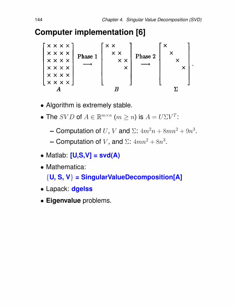
144 Chapter 4. Singular Value Decomposition (SVD)
Computer implementation [6]
• Algorithm is extremely stable.
• The SV D of A ∈ Rm×n (m ≥ n) is A = UΣV T :
– Computation of U , V and Σ: 4m2n + 8mn2 + 9n3.
– Computation of V , and Σ: 4mn2 + 8n3.
• Matlab: [U,S,V] = svd(A)
• Mathematica:U, S, V = SingularValueDecomposition[A]
• Lapack: dgelss
• Eigenvalue problems.
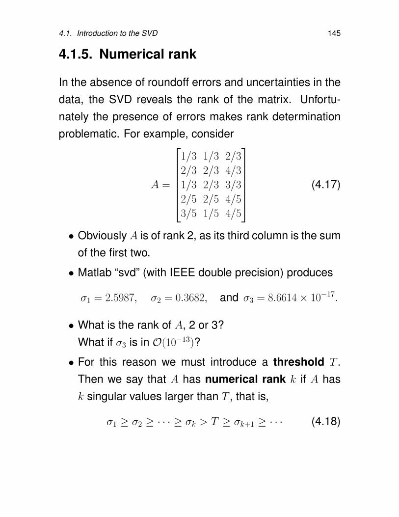
4.1. Introduction to the SVD 145
4.1.5. Numerical rank
In the absence of roundoff errors and uncertainties in thedata, the SVD reveals the rank of the matrix. Unfortu-nately the presence of errors makes rank determinationproblematic. For example, consider
A =
1/3 1/3 2/3
2/3 2/3 4/3
1/3 2/3 3/3
2/5 2/5 4/5
3/5 1/5 4/5
(4.17)
• Obviously A is of rank 2, as its third column is the sumof the first two.
• Matlab “svd” (with IEEE double precision) produces
σ1 = 2.5987, σ2 = 0.3682, and σ3 = 8.6614× 10⁻¹⁷.
• What is the rank of A, 2 or 3?What if σ3 is in O(10−13)?
• For this reason we must introduce a threshold T .Then we say that A has numerical rank k if A hask singular values larger than T , that is,
σ1 ≥ σ2 ≥ · · · ≥ σk > T ≥ σk+1 ≥ · · · (4.18)
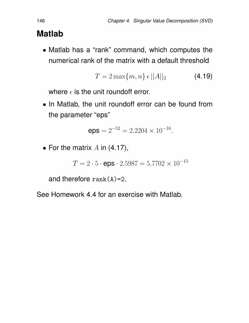
146 Chapter 4. Singular Value Decomposition (SVD)
Matlab
• Matlab has a “rank” command, which computes thenumerical rank of the matrix with a default threshold
T = 2 maxm,n ε ||A||2 (4.19)
where ε is the unit roundoff error.
• In Matlab, the unit roundoff error can be found fromthe parameter “eps”
eps = 2−52 = 2.2204× 10⁻¹⁶.
• For the matrix A in (4.17),
T = 2 · 5 · eps · 2.5987 = 5.7702× 10⁻¹⁵
and therefore rank(A)=2.
See Homework 4.4 for an exercise with Matlab.
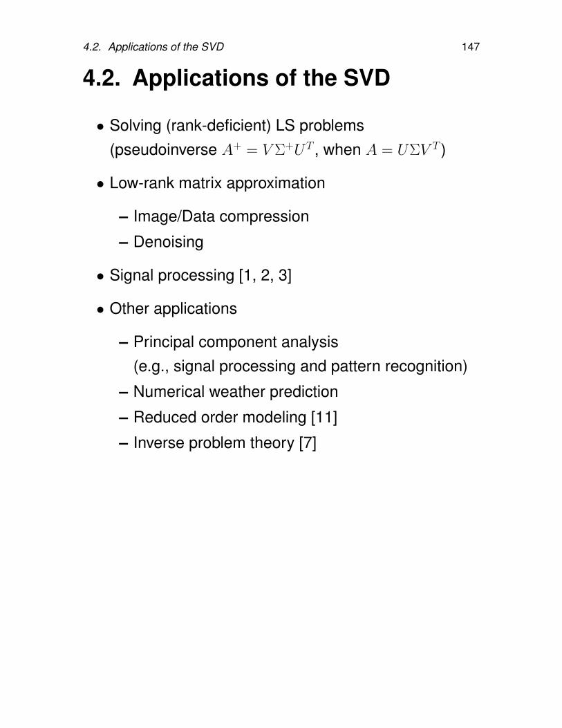
4.2. Applications of the SVD 147
4.2. Applications of the SVD
• Solving (rank-deficient) LS problems(pseudoinverse A+ = V Σ+UT , when A = UΣV T )
• Low-rank matrix approximation
– Image/Data compression
– Denoising
• Signal processing [1, 2, 3]
• Other applications
– Principal component analysis(e.g., signal processing and pattern recognition)
– Numerical weather prediction
– Reduced order modeling [11]
– Inverse problem theory [7]
148 Chapter 4. Singular Value Decomposition (SVD)
4.2.1. Image compression
• A ∈ Rm×n is a sum of rank-1 matrices:
V = [v1, · · · ,vn], U = [u1, · · · ,un],
A = UΣV T =
n∑i=1
σiuivTi .
• The approximation
Ak = UΣkVT =
k∑i=1
σiuivTi
is closest to A among matrices of rank≤ k, and
||A− Ak||2 = σk+1.
• It only takes m · k + n · k = (m + n) · k words to storeu1 through uk, and σ1v1 through σkvk, from which wecan reconstruct Ak.
• We use Ak as our compressed images, stored using(m + n) · k words.
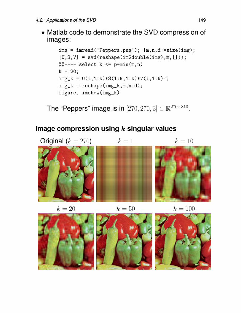
4.2. Applications of the SVD 149
• Matlab code to demonstrate the SVD compression ofimages:
img = imread(’Peppers.png’); [m,n,d]=size(img);
[U,S,V] = svd(reshape(im2double(img),m,[]));
%%---- select k <= p=min(m,n)
k = 20;
img_k = U(:,1:k)*S(1:k,1:k)*V(:,1:k)’;
img_k = reshape(img_k,m,n,d);
figure, imshow(img_k)
The “Peppers” image is in [270, 270, 3] ∈ R270×810.
Image compression using k singular values
Original (k = 270) k = 1 k = 10
k = 20 k = 50 k = 100
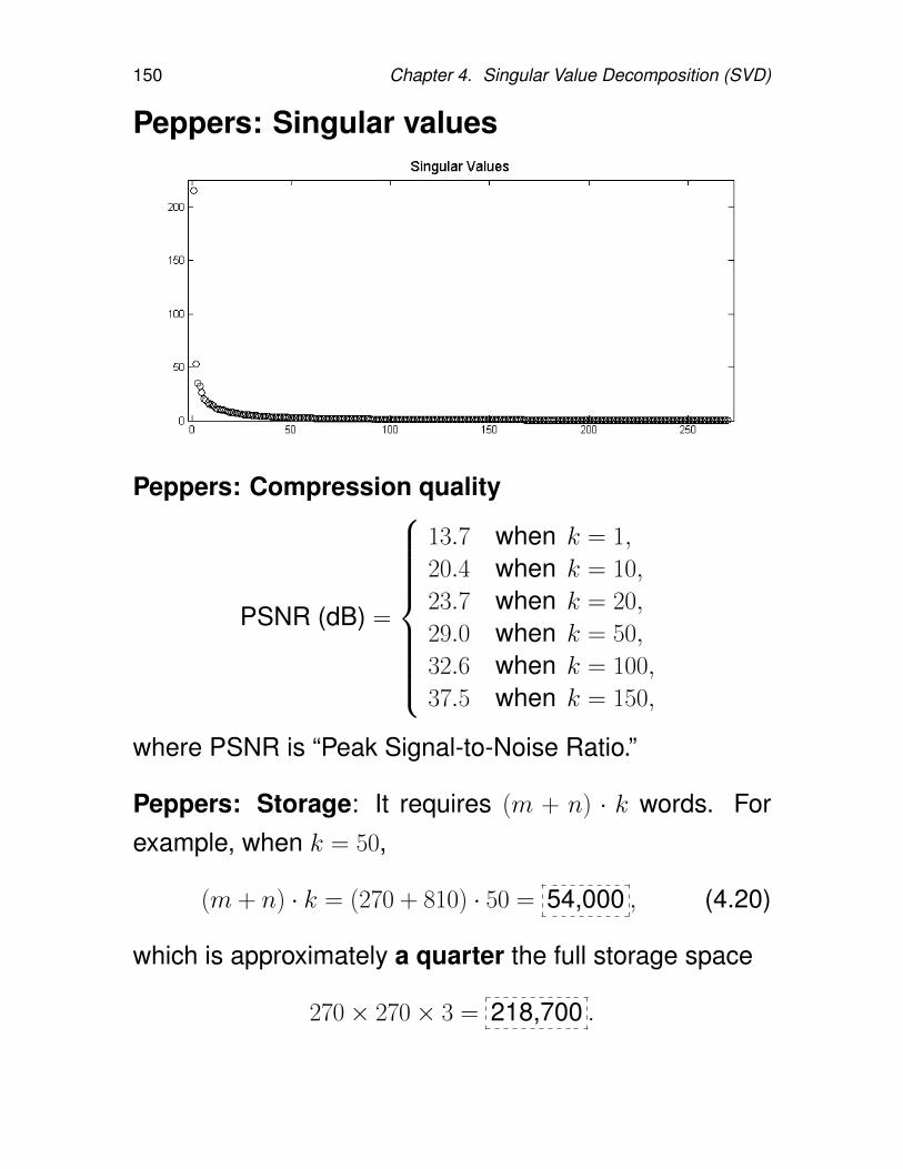
150 Chapter 4. Singular Value Decomposition (SVD)
Peppers: Singular values
Peppers: Compression quality
PSNR (dB) =
13.7 when k = 1,
20.4 when k = 10,
23.7 when k = 20,
29.0 when k = 50,
32.6 when k = 100,
37.5 when k = 150,
where PSNR is “Peak Signal-to-Noise Ratio.”
Peppers: Storage: It requires (m + n) · k words. Forexample, when k = 50,
(m + n) · k = (270 + 810) · 50 = 54,000 , (4.20)
which is approximately a quarter the full storage space
270× 270× 3 = 218,700 .
4.2. Applications of the SVD 151
4.2.2. Rank-deficient least-squares problems
The LS problem: For the system of equations
Ax = b, (4.21)
where A ∈ Rm×n and b ∈ Rm, find the best-fitting solu-tion x as a solution of
minx∈Rn||Ax− b||2. (4.22)
• If m > n, then the system (4.21) is overdetermined,and we cannot expect to find an exact solution. Thesolution can be obtained through the LS problem (4.22).
• The solution of the LS problem is sometimes not unique,for example, when
rank(A) = r < minm,n.
In this case, we may consider the following additionalproblem:
Of all the x ∈ Rn that minimizes ||Ax−b||2, findthe one for which ||x||2 is minimized.
This problem always has a unique solution, the minimum-norm solution.
152 Chapter 4. Singular Value Decomposition (SVD)
Proposition 4.19. (Rank-deficient LS problems, Propo-sition 4.3 on page 128). Let A ∈ Rm×n, m ≥ n, withrank(A) = k < n. Then there exists an (n−k)-dimensionalset of vectors x that minimize
||Ax− b||2.
Proposition 4.20. Let σmin = σmin(A), the smallest sin-gular value of A. Assume σmin > 0. Then
1. If x minimize ||Ax − b||2, then ||x||2 ≥ |uTnb|/σmin,where un is the last column of U in A = UΣV T .
2. Changing b to b + δb can change x to x + δx, where||δx||2 is as large as ||δb||2/σmin.
In other words, if A is nearly rank deficient (σmin is small),then the solution x is ill-conditioned and possibly verylarge.
Proof. Part 1:
x = A+b = V Σ−1UTb.
So
||x||2 = ||Σ−1UTb||2 ≥ |(Σ−1UTb
)n| = |uTnb|/σmin.
Part 2: choose δb parallel to un.
4.2. Applications of the SVD 153
Proposition 4.21. When A ∈ Rm×n is exactly singular,then
x = arg minx∈Rn||Ax− b||2
can be characterized as follows.
Let A = UΣV T have rank r < n, and write the SVD ofA as
A = [U1 U2]
[Σ1 0
0 0
][V1 V2] = U1Σ1V
T1 , (4.23)
where Σ1 is r × r and nonsingular and U1 and V1 have r
columns. Let σ = σmin(Σ1), the smallest nonzero singularvalue of A. Then
1. All solutions x can be written
x = V1Σ−11 UT
1 b + V2z (= A+b), (4.24)
where z is an arbitrary vector.
2. The solution x has a minimal norm ||x||2 preciselywhen z = 0, in which case
x = V1Σ−11 UT
1 b and ||x||2 ≤ ||b||2/σ. (4.25)
3. Changing b to b + δb can change the minimal normsolution x by at most ||δb||2/σ.
In other words, the norm and condition number of theunique minimal norm solution x depend on the smallestnonzero singular value of A.
154 Chapter 4. Singular Value Decomposition (SVD)
Solving LS problems by the SVD:Let A ∈ Rm×n, m ≥ n, have rank r ≤ n. Let A = UΣV T bethe SVD of A.
• Because U is orthogonal,
||Ax− b||2 = ||UT (Ax− b)||2 = ||Σ(V Tx)− UTb||2.
• Letting c = UTb and y = V Tx, we have
||Ax− b||22 = ||Σy − c||22 =
r∑j=1
|σjyj − cj|2 +
m∑j=r+1
|cj|2
(4.26)It is clear that (4.26) is minimized when and onlywhen
yj =cjσj, j = 1, · · · , r. (4.27)
• (When r < n): It is clear to see that ||y||2 is mini-mized when and only when
yr+1 = · · · = yn = 0.
• Since x = V y, we have ||x||2 = ||y||2. Thus ||x||2 isminimized when and only when ||y||2 is. This provesthat the LS problem has exactly one minimum-normsolution.
4.2. Applications of the SVD 155
Solving LS problems by the SVD:It is useful to repeat the development using partitionedmatrices. Let A ∈ Rm×n, m ≥ n, have rank r ≤ n. LetA = UΣV T be the SVD of A given as in (4.23):
A = [U1 U2]
[Σ1 0
0 0
][V1 V2] = U1Σ1V
T1 , (4.28)
where Σ1 is r × r and nonsingular and U1 and V1 have r
columns.
• Let, with the corresponding partitioning,
c = UTb =
[c1
c2
]and y = V Tx =
[y1
y2
].
• Then,
Σy − c =
[Σ1 0
0 0
][y1
y2
]−
[c1
c2
]=
[Σ1y1 − c1
−c2
].
• So
||Ax− b||22 = ||Σy − c||22 = ||Σ1y1 − c1||22 + ||c2||22.(4.29)
• Equation (4.29) is minimized when and only when
y1 = Σ−11 c1. (4.30)
• For the minimum-norm solution, take y2 = 0.
156 Chapter 4. Singular Value Decomposition (SVD)
Summary 4.22. (Solving LS problems by the SVD).For solving the LS problem
minx∈Rn||Ax− b||2, A ∈ Rm×n,
we summarize the above SVD procedure as follows.
1. Find the SVD of A: A = UΣV T and rank(A) = r.
2. Calculate
[c1
c2
]= c = UTb, where c1 ∈ Rr.
3. Let y1 = Σ−11 c1, where Σ1 = Σ(1 : r, 1 : r).
4. If r < n, choose y2 ∈ Rn−r arbitrarily.(For minimum-norm solution, take y2 = 0.)
5. Let y =
[y1
y2
]∈ Rn.
6. Let x = V y ∈ Rn.
Note:
• The above procedure is equivalent to solve the LSproblem by the pseudoinverse of A, particular whenA has full rank.
• The minimum-norm solution reads: x = V1 y1.
4.2. Applications of the SVD 157
Example 4.23. Use the pseudoinverse to solve the LSproblem min ||Ax− b||2, where
A =
1 2−1 1
1 2
and b =
1
2
3
.Solution. The eigenvalues of ATA are
λ1 = 3(2 +√
2), λ2 = 3(2−√
2).
If v1 and v2 are the corresponding eigenvectors of ATA,then
uj =1
σjAvj =
1√λjAvj, j = 1, 2.
The SVD of A reads
A = UΣV T =
1+√
22√
31−√
22√
3√2−1√
6
√2+1√
6
1+√
22√
31−√
22√
3
[√
λ1 00√λ2
] √2−1√
4−2√
2−
√2+1√
4+2√
21√
4−2√
2
1√4+2√
2
Thus
A+ = V Σ−1UT =
[16 −
23
16
16
13
16
]and therefore
x = A+b =
[16 −
23
16
16
13
16
] 1
2
3
=
[−2
343
]
The corresponding least L2-error is√
2, that is,
||Ax− b||2 = miny||Ay − b||2 =
√2.
158 Chapter 4. Singular Value Decomposition (SVD)
4.2.3. Principal component analysis (PCA)
Definition 4.24. Principal component analysis is astatistical procedure for data (a set of observations) that
(a) uses an orthogonal transformation and
(b) converts data of possibly correlated variables intoa set of values of linearly uncorrelated variablescalled principal components.
PCA
• #principal components < #original variables.
• The transformation is defined in such a way that
– the first principal component has the largest pos-sible variance,
– and each succeeding component has the highestvariance possible under the constraint that it is or-thogonal to (i.e., uncorrelated with) the precedingcomponents.
• Principal components are guaranteed to be indepen-dent if the data set is jointly normally distributed.
4.2. Applications of the SVD 159
In other words:
• PCA is a mathematical algorithm that reduces thedimensionality of the data while retaining most ofthe variation in the data set.
• It accomplishes this reduction by identifying direc-tions, called principal components, along which thevariation in the data is maximal.
• By using a few components, each sample can be rep-resented by relatively few numbers instead of by val-ues for thousands of variables.
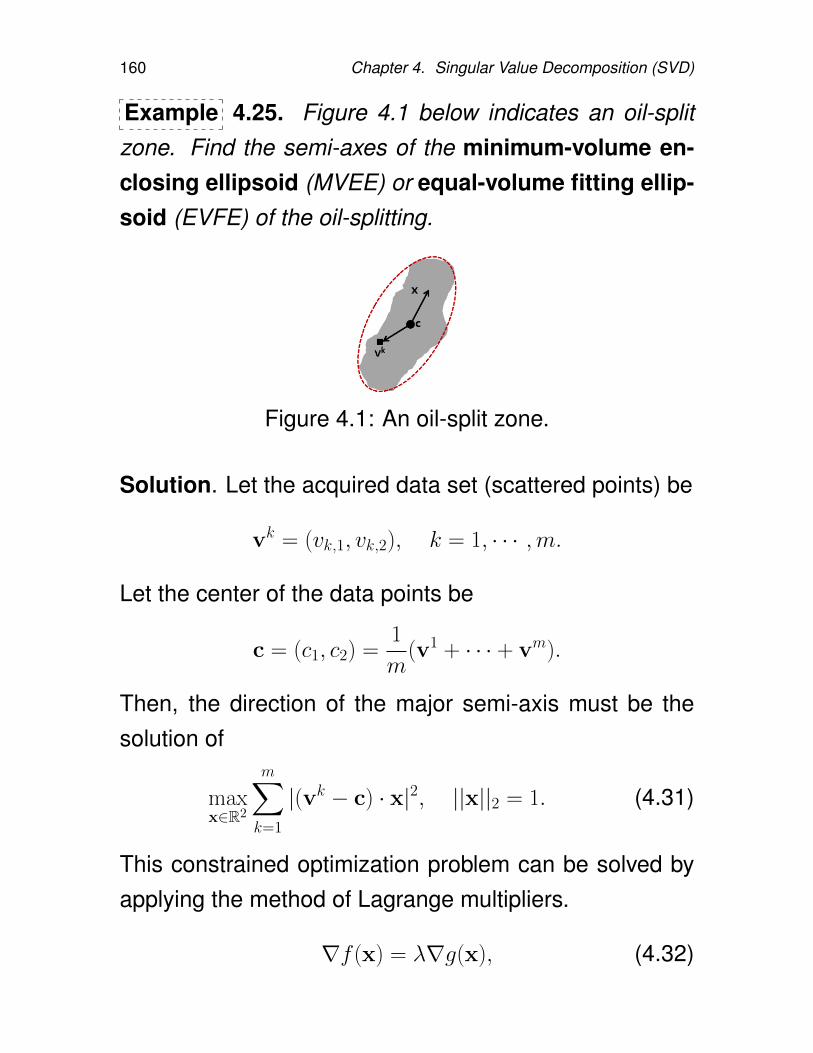
160 Chapter 4. Singular Value Decomposition (SVD)
Example 4.25. Figure 4.1 below indicates an oil-splitzone. Find the semi-axes of the minimum-volume en-closing ellipsoid (MVEE) or equal-volume fitting ellip-soid (EVFE) of the oil-splitting.
Figure 4.1: An oil-split zone.
Solution. Let the acquired data set (scattered points) be
vk = (vk,1, vk,2), k = 1, · · · ,m.
Let the center of the data points be
c = (c1, c2) =1
m(v1 + · · · + vm).
Then, the direction of the major semi-axis must be thesolution of
maxx∈R2
m∑k=1
|(vk − c) · x|2, ||x||2 = 1. (4.31)
This constrained optimization problem can be solved byapplying the method of Lagrange multipliers.
∇f (x) = λ∇g(x), (4.32)
4.2. Applications of the SVD 161
where
f (x) =
m∑k=1
|(vk − c) · x|2, g(x) = ||x||22.
Note that
f (x) =
m∑k=1
((vk,1 − c1)x1 + (vk,2 − c2)x2
)2, (4.33)
where x = (x1, x2). Thus it follows from (4.32) that
Ax = λx, (4.34)
where A = (aij) ∈ R2×2 with
aij =
m∑k=1
(vk,i − ci)(vk,j − cj), i, j = 1, 2.
The direction of the major semi-axis of the ellipsoid canbe found from the eigenvector of the matrixA correspond-ing to the larger eigenvalue.
Definition 4.26. Let us collect x- and y-components sep-arately from the data:
X = (v1,1, v2,1, · · · , vm,1),
Y = (v1,2, v2,2, · · · , vm,2).
Then, the matrix A in (4.34) can be rewritten as
A =
[Var(X) Cov(X, Y )
Cov(X, Y ) Var(Y )
], (4.35)
called the covariance matrix of the data points (X, Y ).
162 Chapter 4. Singular Value Decomposition (SVD)
Semi-axes of the ellipsoid:
In order to find the minor semi-axis, the maximizationproblem (4.31) can be replaced with the correspondingminimization problem. This would be reduced to the sameeigenvalue problem given in (4.34). Thus, both major andminor semi-axes of the ellipsoid can be found from theeigenvalue problem.
Theorem 4.27. Let A be the covariance matrix with
Ax` = λ`x`, ||x`||2 = 1.
Then the semi-axes of the MVEE in Rn are found as
η√λ` x`, ` = 1, · · · , n, (4.36)
where η > 0 is a scaling constant given by
η2 = maxk
(vk − c)TA−1(vk − c),
provided that c is the real center.
4.2. Applications of the SVD 163
Example 4.28. A data set of scattered points can beproduced and analyzed by
close all; %clear all;
n = 100; h=10/n; P = 1:n;
X = h*P+randn(1,n); Y = h*P+randn(1,n);
%%-------------------------------------------
plot(X,Y,’ko’);
title(’Scattered Points & Their Principal Components’,...
’fontsize’,13)
%%-------------------------------------------
A = zeros(n,2);
A(:,1) = X;
A(:,2) = Y;
[U,S,V]= svd(A);
k=1; PC1 = U(:,k)*S(k,k)*V(:,k)’;
k=2; PC2 = U(:,k)*S(k,k)*V(:,k)’;
hold
plot(PC1(:,1),PC1(:,2),’b*’);
plot(PC2(:,1),PC2(:,2),’rs’);
legend(’Scattered Points’,’PC-1’,’PC-2’,’fontsize’,12);
%%-------------------------------------------
C = cov(X,Y);
[V2,D] = eig(C);
[D,order] = sort(diag(D),’descend’);
V2 = V2(:,order); L2 = sqrt(D);
hold
Cntr = [mean(X) mean(Y)];
arrow(Cntr,Cntr+1.5*L2(1)*V2(:,1)’,’width’,3);
arrow(Cntr,Cntr+1.5*L2(2)*V2(:,2)’,’width’,3);
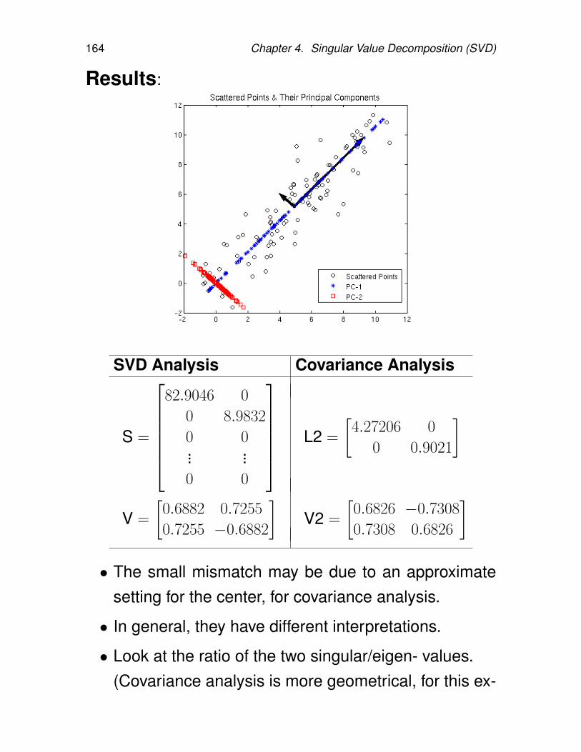
164 Chapter 4. Singular Value Decomposition (SVD)
Results:
SVD Analysis Covariance Analysis
S =
82.9046 0
0 8.9832
0 0... ...0 0
L2 =
[4.27206 0
0 0.9021
]
V =
[0.6882 0.7255
0.7255 −0.6882
]V2 =
[0.6826 −0.7308
0.7308 0.6826
]• The small mismatch may be due to an approximate
setting for the center, for covariance analysis.
• In general, they have different interpretations.
• Look at the ratio of the two singular/eigen- values.(Covariance analysis is more geometrical, for this ex-
4.2. Applications of the SVD 165
ample.)
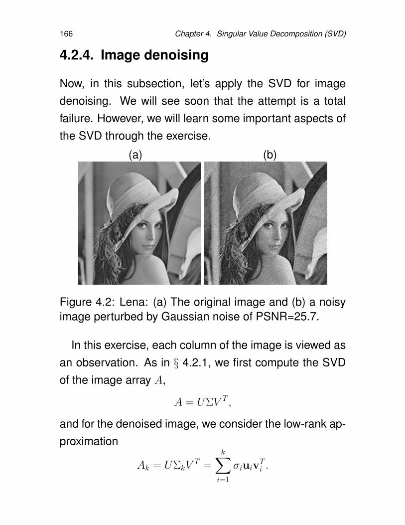
166 Chapter 4. Singular Value Decomposition (SVD)
4.2.4. Image denoising
Now, in this subsection, let’s apply the SVD for imagedenoising. We will see soon that the attempt is a totalfailure. However, we will learn some important aspects ofthe SVD through the exercise.
(a) (b)
Figure 4.2: Lena: (a) The original image and (b) a noisyimage perturbed by Gaussian noise of PSNR=25.7.
In this exercise, each column of the image is viewed asan observation. As in § 4.2.1, we first compute the SVDof the image array A,
A = UΣV T ,
and for the denoised image, we consider the low-rank ap-proximation
Ak = UΣkVT =
k∑i=1
σiuivTi .
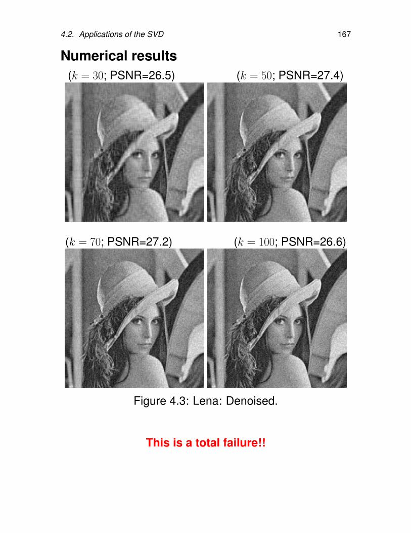
4.2. Applications of the SVD 167
Numerical results(k = 30; PSNR=26.5) (k = 50; PSNR=27.4)
(k = 70; PSNR=27.2) (k = 100; PSNR=26.6)
Figure 4.3: Lena: Denoised.
This is a total failure!!
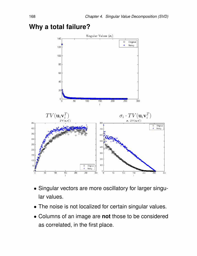
168 Chapter 4. Singular Value Decomposition (SVD)
Why a total failure?
TV (uivTi ) σi · TV (uiv
Ti )
• Singular vectors are more oscillatory for larger singu-lar values.
• The noise is not localized for certain singular values.
• Columns of an image are not those to be consideredas correlated, in the first place.
4.3. Homework 169
4.3. Homework4.1. Let A ∈ Rm×n. Prove that ||A||2 = σ1, the largest singular value
of A.
Hint: Use the following
||Av1||2||v1||2
=σ1||u1||2||v1||2
= σ1 =⇒ ||A||2 ≥ σ1
and arguments around Equations (4.9) and (4.10) for the oppo-site directional inequality.
4.2. Recall that the Frobenius matrix norm is defined by
||A||F =( m∑
i=1
n∑j=1
|aij|2)1/2
, A ∈ Rm×n.
Show that ||A||F = (σ21 + · · · + σ2
k)1/2, where σj are nonzero sin-
gular values of A.
Hint: First show that if B = UC, where U is orthogonal, then||B||F = ||C||F .
4.3. Prove Lemma 4.16.
Hint: For (b), let Avi = λivi, i = 1, 2, and λ1 6= λ2. Then
(λ1v1) · v2 = (Av1) · v2 = v1 · (Av2)︸ ︷︷ ︸∵ A is symmetric
= v1 · (λ2v2).
For (a), you may use a similar argument, but with the dot productbeing defined for complex values, i.e.,
u · v = uT v,
where v is the complex conjugate of v.
4.4. Use Matlab to generate a random matrix A ∈ R8×6 with rank 4.For example,
A = randn(8,4);
A(:,5:6) = A(:,1:2)+A(:,3:4);
[Q,R] = qr(randn(6));
A = A*Q;
170 Chapter 4. Singular Value Decomposition (SVD)
(a) Print out A on your computer screen. Can you tell by lookingif it has (numerical) rank 4?
(b) Use Matlab’s “svd” command to obtain the singular values ofA. How many are “large?” How many are “tiny?” (You mayuse the command “format short e” to get a more accurateview of the singular values.)
(c) Use Matlab’s “rank” command to confirm that the numericalrank is 4.
(d) Use the “rank” command with a small enough threshold thatit returns the value 6. (Type “help rank” for information abouthow to do this.)
4.5. Let A ∈ R2×2 with singular values σ1 ≥ σ2 > 0. Show the setAx | ||x||2 = 1 (the image of the unit circle) is an ellipse inR2 whose major and minor semiaxes have lengths σ1 and σ2
respectively.
4.6. Work this homework problem using pencil and paper (and exactarithmetic). Let
A =
1 22 43 6
, b =
1
1
1
.(a) Find the SVD of A. You may use the condensed form given
in (4.28).
(b) Calculate the pseudoinverse of A, A+.
(c) Calculate the minimum-norm solution of the least-squaresproblem for the overdetermined system Ax = b.
(d) Find a basis for Null(A).
(e) Find all solutions of the least-squares problem.
Chapter 5
Eigenvalue Problems
For eigenvalue problems, we will begin with basic defini-tions in matrix algebra, including Jordan/Schur canonicalforms and diagonalization. Then, we will study pertur-bation theory in order to understand effects of errors inboth data acquisition and computation. After consideringGershgorins theorem and its applicability, we will work onnonsymmetric eigenvalue problems and finally symmetriceigenvalue problems.
171
172 Chapter 5. Eigenvalue Problems
5.1. Definitions and Canonical Forms
• For an n × n matrix A, if a scalar λ and a nonzerovector x satisfies
Ax = λx,
we call λ is a eigenvalue and x a eigenvector of A.(λ, x) is called an eigenpair of A.
• λ is an eigenvalue of A⇐⇒ There ∃x 6= 0 s.t. Ax = λx
⇐⇒ (A− λI)x = 0 has nontrivial solutions⇐⇒ p(λ) = det(A− λI) = 0.
p(λ) is called characteristic polynomial of A.
• If A has n linearly independent eigenvectors
x1, x2, · · · ,xn,
then A ∼ Λ (similar) and has an EigenValue Decom-position (EVD):
A = XΛX−1 ≡ [x1 x2 · · · xn]
λ1
λ2. . .
λn
[x1 x2 · · · xn]−1
5.1. Definitions and Canonical Forms 173
When A is Diagonalizable
• An n × n matrix A is called diagonalizable if A ∼ Λ,a diagonal matrix. Otherwise it is called defective.
• The algebraic multiplicity of λj:the multiplicity of the root λj in the characteristic equa-tion det(A− λI) = 0.
• The geometric multiplicity of λj:the dimension of the eigenspace for λj= dim(Null(A− λjI)).
* algebraic multiplicity ≥ geometric multiplicity
• Let A is an n× n matrix. Λ = diag(λ1, · · ·λn).
A is diagonalizable⇐⇒ A has n lin. indep. e-vectors⇐⇒ ∀λj, algebraic multiplicity = geometric multiplicity⇐⇒ S−1AS = Λ (⇐⇒ A = S ΛS−1)⇐⇒ AS = SΛ; col. of S are the right e-vectors of A⇐⇒ S−1A = ΛS−1; col. of (S−1)∗ are left e-vectors ofA
• Let S = [x1 · · · xn], the matrix of right e-vectors of A.Then S−1 = [y∗1/y
∗1x1 y∗2/y
∗2x2 · · · y∗n/y
∗nxn]T .
174 Chapter 5. Eigenvalue Problems
Jordan Canonical Forms
• The eigenvector x is also called right eigenvector. Anonzero vector y satisfying y∗A = λy∗ is called lefteigenvector of A. (Recall that y∗ = yH = (y)T is theconjugate transpose of y.)
• Jordan Canonical Forms Given a square matrix A,there exists a nonsingular S such that
S−1AS = J, (5.1)
where J is in Jordan canonical form. This meansthat J is block diagonal, with
J = diag(Jn1(λ1), Jn2(λ2), · · · , Jnk(λk))
and
Jnj(λj) =
λj 1
λj 1. . . . . .
. . . 1
λj
nj×nj
(Jordan block for λj)nj=algebraic multiplicity
J is unique, up to permutations of its diagonal blocks.
5.1. Definitions and Canonical Forms 175
Schur Canonical Forms
• For an n×n matrix A, there exists a unitary matrix Qand an upper triangular matrix T such that
Q∗AQ = T. (5.2)
The eigenvalues of A are the diagonal entries ofT .
• Real Schur Canonical Forms. If A is real, there ex-ists a real orthogonal matrix V such that
V TAV = T is quasi-upper triangular.
This means that T is block upper triangular with 1× 1
and 2× 2 blocks on the diagonal.
Its eigenvalues are the eigenvalues of its diagonalblocks. The 1× 1 blocks correspond to real eigenval-ues, and the 2 × 2 blocks to complex conjugate pairsof eigenvalues.
Theorem 5.1. (Fundamental Theorem of Algebra).Every nonconstant polynomial has at least one root (pos-sibly, in the complex field).
Polynomial Factorization: If P is a nonconstant polyno-mial of real coefficients, then it can be factorized as a mul-tiple of linear and quadratic factors of which coefficientsare all real.
176 Chapter 5. Eigenvalue Problems
Computing E-vectors from Schur Form
• Let Q∗AQ = T be the Schur form of A. Then if λ is aneigenvalue of T , Tx = λx.
AQx = QTx = Q(λx) = λQx
So Qx is an eigenvector of A.
• To find eigenvectors ofA, it suffices to find eigen-vectors of T .
5.2. Perturbation Theory: Bauer-Fike Theorem 177
5.2. Perturbation Theory: Bauer-FikeTheorem
Theorem 5.2. Let λ be a simple eigenvalue of A withright eigenvector x and left eigenvector y, normalized sothat ||x||2 = ||y||2 = 1. Let λ + δλ be the correspondingeigenvalue of A + δA. Then
δλ =y∗δAx
y∗x+O(||δA||2), or
|δλ| ≤ ||δA|||y∗x|
+O(||δA||2) = sec Θ(y,x)||δA|| +O(||δA||2)
(5.3)where Θ(y,x) is the acute angle between y and x.
Note that sec Θ(y,x) = 1/|y∗x| ≡ c(λ) is the conditionnumber of the eigenvalue λ. [s(λ) = |y∗x| in other texts.]
Note: The perturbation on the eigenvalue (due to a matrixperturbation) is proportional to the condition number ofthe eigenvalue.
Corollary 5.3. Let A be be symmetric (or, more gener-ally, normal: AA∗ = A∗A). Then
|δλ| ≤ ||δA|| +O(||δA||2). (5.4)
178 Chapter 5. Eigenvalue Problems
Note: Theorem 5.2 is useful only for sufficiently small||δA||. We can remove the O(||δA||2) term and get a sim-ple theorem true for any size perturbation ||δA||, at thecost of increasing the condition number of the eigenvalueby a factor of n.
Theorem 5.4. (Bauer-Fike Theorem). Let A have allsimple eigenvalues (i.e., be diagonalizable). Call themλi, with right and left e-vectors xi and yi, normalized so||xi||2 = ||yi||2 = 1. Then the e-values of A+δA lie in disksBi, where Bi has center λi and radius n ||δA|||y∗i xi|
.
Theorem 5.5. (Bauer-Fike Theorem). If µ is an eigen-value of A + E ∈ Cn×n and
X−1AX = D = diag(λ1, · · · , λn),
then
minλ∈σ(A)
|λ−µ| ≤ ||X||p · ||X−1||p · ||E||p = κp(X) ||E||p (5.5)
where || · ||p denotes any of the p-norms. [6, Theorem7.2.2].
5.2. Perturbation Theory: Bauer-Fike Theorem 179
Theorem 5.6. Let λ be a simple e-value of A, with unitright and left e-vectors x and y and condition numberc = 1/|y∗x|. Then ∃ δA such that A + δA has a multiplee-value at λ, and
||δA||2||A||2
≤ 1√c2 − 1
.
If c 1, i.e., the e-value is ill-conditioned, then the upperbound on the distance is 1√
c2−1≈ 1
c , the reciprocal of thecondition number.
Note: Multiple eigenvalues have infinite condition num-bers; see Homework 5.1. Being “close to singular” im-plies ill-conditioning.
180 Chapter 5. Eigenvalue Problems
Example 5.7. LetA =
1 2 3
0 4 5
0 0 4.001
, E =
0 0 0
0 0 0
.001 0 0
.Then
σ(A) = 1, 4, 4.001,σ(A + E) ≈ 1.0001, 4.0582, 3.9427.
The reciprocals of the condition numbers are
s(1) ≈ .8,
s(4) ≈ .2e− 3,
s(4.001) ≈ .2e− 3,
and||E||2||A||2
=0.001
8.0762≈ 0.00012 < .2e− 3
See Theorem 5.6.
5.2. Perturbation Theory: Bauer-Fike Theorem 181
Note: If any eigenvalue has a large condition number,then the matrix of eigenvectors has to have an approxi-mately equally large condition number.
Theorem 5.8. Let A be diagonalizable with e-values λiand right and left e-vectors xi, yi, respectively, normalizedso ||xi|| = ||yi|| = 1. Suppose that S satisfies
S−1AS = Λ = diag(λ1, · · · , λn).
Thenκ2(S) ≡ ||S||2 · ||S−1||2 ≥ max
i
1
|y∗ixi|. (5.6)
If we choose S = [x1, · · · ,xn], then
κ2(S) ≤ n ·maxi
1
|y∗ixi|. (5.7)
That is, the condition number of S, κ2(S), is within a factorof n of its smallest value.
182 Chapter 5. Eigenvalue Problems
5.3. Gerschgorin’s Theorem
Theorem 5.9. (Gerschgorin’s Theorem [5]). Let B bean arbitrary matrix. Then the eigenvalues λ of B are lo-cated in the union of the n disks defined by
|λ− bii| ≤ ri ≡∑j 6=i
|bij|, for i = 1, · · · , n. (5.8)
Proof. Let Bx = λx, x 6= 0. By scaling x if necessary, wemay assume that
||x||∞ = xk = 1, for some k.
Thenn∑j=1
bkjxj = λxk = λ
and therefore
|λ− bkk| =∣∣∣∑j 6=k
bkjxj
∣∣∣ ≤∑j 6=k
|bkjxj| ≤∑j 6=k
|bkj|. (5.9)
For other eigenvalues, one can derive a similar inequalityas in (5.9).
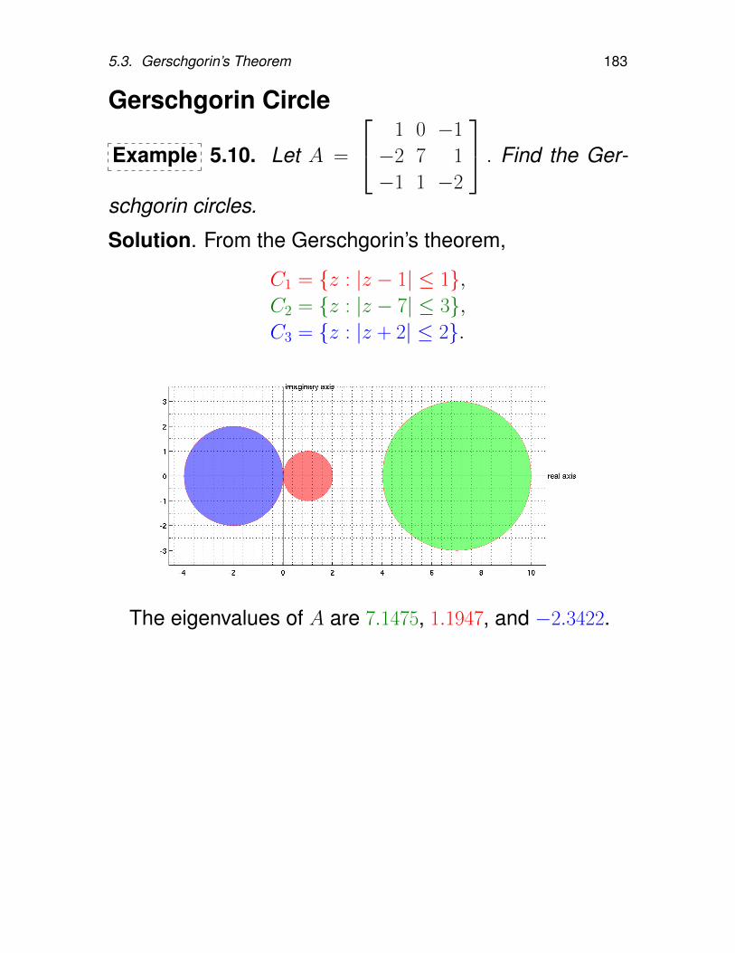
5.3. Gerschgorin’s Theorem 183
Gerschgorin Circle
Example 5.10. Let A =
1 0 −1
−2 7 1
−1 1 −2
. Find the Ger-
schgorin circles.
Solution. From the Gerschgorin’s theorem,
C1 = z : |z − 1| ≤ 1,C2 = z : |z − 7| ≤ 3,C3 = z : |z + 2| ≤ 2.
The eigenvalues of A are 7.1475, 1.1947, and −2.3422.
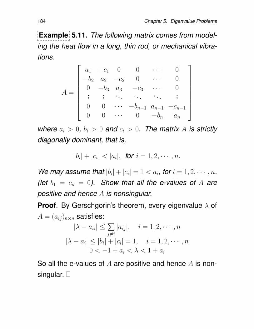
184 Chapter 5. Eigenvalue Problems
Example 5.11. The following matrix comes from model-ing the heat flow in a long, thin rod, or mechanical vibra-tions.
A =
a1 −c1 0 0 · · · 0
−b2 a2 −c2 0 · · · 0
0 −b3 a3 −c3 · · · 0... ... . . . . . . . . . ...0 0 · · · −bn−1 an−1 −cn−1
0 0 · · · 0 −bn an
where ai > 0, bi > 0 and ci > 0. The matrix A is strictlydiagonally dominant, that is,
|bi| + |ci| < |ai|, for i = 1, 2, · · · , n.
We may assume that |bi|+ |ci| = 1 < ai, for i = 1, 2, · · · , n.(let b1 = cn = 0). Show that all the e-values of A arepositive and hence A is nonsingular.
Proof. By Gerschgorin’s theorem, every eigenvalue λ ofA = (aij)n×n satisfies:
|λ− aii| ≤∑j 6=i|aij|, i = 1, 2, · · · , n
|λ− ai| ≤ |bi| + |ci| = 1, i = 1, 2, · · · , n0 < −1 + ai < λ < 1 + ai
So all the e-values of A are positive and hence A is non-singular.
5.4. Taussky’s Theorem and Irreducibility 185
5.4. Taussky’s Theorem and Irreducibil-ity
Theorem 5.12. (Taussky [8, 1948]) Let B = [bij] bean irreducible n × n complex matrix. Assume that λ, aneigenvalue of B, is a boundary point of the union of thedisks |z−bii| ≤ ri. Then, all the n circles |z−bii| = ri mustpass through the point λ, i.e.,
|λ− bii| = ri for all 1 ≤ i ≤ n.
Definition 5.13. A permutation matrix is a square ma-trix in which each row and each column has one entry ofunity, all others zero.
Definition 5.14. For n ≥ 2, an n × n complex-valuedmatrix A is reducible if there is a permutation matrix Psuch that
PAP T =
[A11 A12
0 A22
],
whereA11 andA22 are respectively r×r and (n−r)×(n−r)submatrices, 0 < r < n. If no such permutation matrixexists, then A is irreducible.
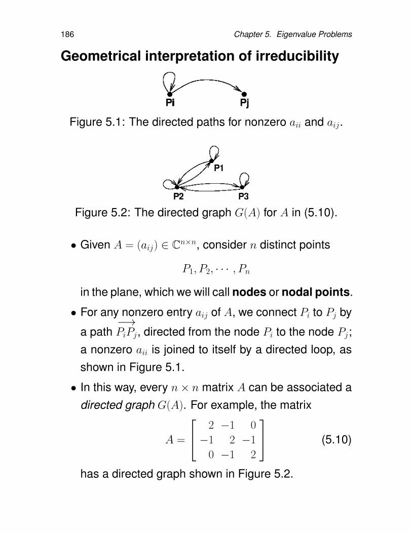
186 Chapter 5. Eigenvalue Problems
Geometrical interpretation of irreducibility
Figure 5.1: The directed paths for nonzero aii and aij.
Figure 5.2: The directed graph G(A) for A in (5.10).
• Given A = (aij) ∈ Cn×n, consider n distinct points
P1, P2, · · · , Pn
in the plane, which we will call nodes or nodal points.
• For any nonzero entry aij of A, we connect Pi to Pj by
a path−→PiPj, directed from the node Pi to the node Pj;
a nonzero aii is joined to itself by a directed loop, asshown in Figure 5.1.
• In this way, every n× n matrix A can be associated adirected graph G(A). For example, the matrix
A =
2 −1 0
−1 2 −1
0 −1 2
(5.10)
has a directed graph shown in Figure 5.2.
5.4. Taussky’s Theorem and Irreducibility 187
Definition 5.15. A directed graph is strongly connectedif, for any ordered pair of nodes (Pi, Pj), there is a directedpath of a finite length
−→PiPk1,
−→Pk1Pk2, · · · ,
−→Pkr−1Pkr=j,
connecting from Pi to Pj.
The theorems to be presented in this subsection canbe found in [10] along with their proofs.
Theorem 5.16. An n × n complex-valued matrix A isirreducible if and only if its directed graph G(A) is stronglyconnected.
It is obvious that the matrices obtained from FD/FEmethods of the Poisson equation are strongly connected.Therefore the matrices are irreducible.
188 Chapter 5. Eigenvalue Problems
Example 5.17. Find the eigenvalue loci for the matrix
A =
2 −1 0
−1 2 −1
0 −1 2
.Solution. The matrix A is irreducible, first of all, and
r1 = 1, r2 = 2, and r3 = 1.
Since aii = 2, for i = 1, 2, 3, the union of the three disksreads
z : |z − 2| ≤ 2 ≡ Ω.
Note r1 = r3 = 1 and their corresponding disks do nottouch the boundary of Ω. So, using the Taussky theorem,we have
|λ− 2| < 2 (5.11)
for all eigenvalues λ of A. Furthermore, since A is sym-metric, its eigenvalues must be real. Thus we conclude
0 < λ < 4. (5.12)
5.5. Nonsymmetric Eigenvalue Problems 189
5.5. Nonsymmetric Eigenvalue Prob-lems
Residual and Rayleigh Quotient
• Let (λ,x) be an approximation to an eigenpair of A.Then, the residual is defined as
r = Ax− λx.
• If x is an approximation to an e-vector of A, thenthe Rayleigh quotient
λ =x∗Ax
x∗x
is an approximation to the corresponding e-value.
• Rayleigh quotient minimizes ||r|| = ||Ax− λx||.
190 Chapter 5. Eigenvalue Problems
5.5.1. Power method
Given A ∈ Cn×n, let
X−1AX = diag(λ1, · · · , λn),
where
X = [x1, · · · ,xn], and |λ1|>|λ2| ≥ · · · ≥ |λn|.
The power method produces a sequence of vectors q(k)as follows,
choose q(0) ∈ Cn such that ||q(0)||2 = 1
for k = 1, 2, · · ·z = Aq(k−1) apply A
q(k) = z/||z||2 normalize → q
λ(k) =[q(k)]∗Aq(k) Rayleigh quotient → λ1
end
(5.13)
Note: q(k) → q = ±x1/||x1|| as k → ∞, where x1 is theeigenvector corresponding to λ1.
5.5. Nonsymmetric Eigenvalue Problems 191
Convergence of power method
Note Akxj = λkjxj. Let
q(0) = α1x1 + α2xn + · · · + αnxn, α1 6= 0.
Then
Akq(0) =
n∑j=1
αjAkxj = α1λ
k1
(x1 +
n∑j=2
αjα1
(λjλ1
)kxj
)Since q(k) ∈ Span
Akq(0)
,
dist(
Spanq(k),Spanx1)
= O( ∣∣∣∣λ2
λ1
∣∣∣∣k ).Thus, we obtain ∣∣∣λ1 − λ(k)
∣∣∣ = O( ∣∣∣∣λ2
λ1
∣∣∣∣k ). (5.14)
192 Chapter 5. Eigenvalue Problems
Error estimates for the power method
• The estimate of the error |λ(k)−λ1| can be obtained byapplying Bauer-Fike theorem, more specifically, The-orem 5.2 on p. 177.
Let r(k) = Aq(k) − λ(k)q(k). Observe that
(A + E(k))q(k) = λ(k)q(k), for E(k) = −r(k)(q(k))∗.
(5.15)Thus λ(k) is an e-value of A + E(k), and∣∣∣λ(k) − λ1
∣∣∣ ≈ ||E(k)||2s(λ1)
=||r(k)||2s(λ1)
where s(λ1) is the reciprocal of the condition numberof λ1.
• If we use the power method to generate approximateright/left dominant e-vectors, then it is possible to ob-tain an estimate of s(λ1). In particular, if w(k) is a unit2-norm in the direction of (A∗)kw(0), then
s(λ1) ≈ |(w(k))∗q(k)|. (5.16)
5.5. Nonsymmetric Eigenvalue Problems 193
Example 5.18. Let A =
−31 −35 16
−10 −8 4
−100 −104 49
, then σ(A) =
9, 3,−2. Applying the power method with q(0) = [1, 0, 0]T .
Solution. We have
k λ(k)
1 7.6900
2 9.6377
3 8.9687
4 9.0410
5 9.0023
6 9.0033
7 9.0005
8 9.0003
9 9.0001
10 9.0000
Power method converges at k = 10
(correct to 4 decimal places).
Computed result:
eigenvalue: λ(10) = 9.000,
eigenvector: x = q(10) =
−0.3714
−0.0000
−0.9285
residual: ||r(10)|| = 9.1365e− 06.
194 Chapter 5. Eigenvalue Problems
Remark 5.19. Power iteration is of limited use due toseveral reasons.
• It converges to the eigenpair only for the eigenvaluewith largest absolute magnitude.
• The usefulness of the power method depends uponthe ratio |λ2|/|λ1|. The smaller the ratio, the faster theconvergence. But if there are two largest eigenvalueare close in magnitude, the convergence will be veryslow.
• For example, if A is real and the largest eigenvalue iscomplex, then there will be two complex conjugatee-values with the same largest absolute magnitude|λ1| = |λ2|. In this case, the power method will notconverge. And it won’t work in the extreme case of anorthogonal matrix with all the eigenvalues the sameabsolute value.
• Overall, the method is useful when A is large andsparse, and when there is a big gap between |λ1|and |λ2|.
5.5. Nonsymmetric Eigenvalue Problems 195
5.5.2. Inverse power method
To overcome the drawbacks of power method, we mayapply it to (A − σI)−1 instead of A, where σ is called ashift. Then it will converge to the e-value closest to σ,rather than just λ1.
It is called inverse iteration or inverse power itera-tion.
Algorithm 5.20. (Inverse Power Iteration).
input x0; initial guessi = 0;
do repeatsolve (A− σI)yi+1 = xixi+1 = yi+1/||yi+1||2; approx. e-vectorηi+1 = xTi+1Axi+1; approx. e-valuei = i + 1;
until convergence
(5.17)
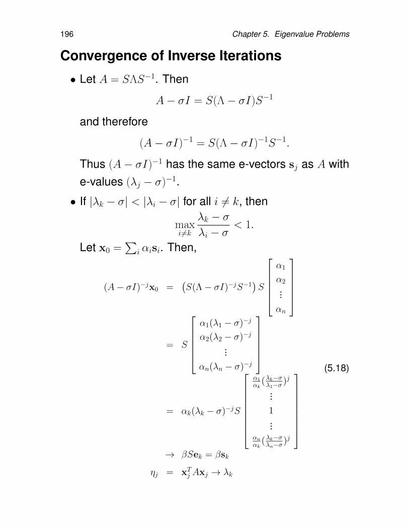
196 Chapter 5. Eigenvalue Problems
Convergence of Inverse Iterations
• Let A = SΛS−1. Then
A− σI = S(Λ− σI)S−1
and therefore
(A− σI)−1 = S(Λ− σI)−1S−1.
Thus (A− σI)−1 has the same e-vectors sj as A withe-values (λj − σ)−1.
• If |λk − σ| < |λi − σ| for all i 6= k, then
maxi 6=k
λk − σλi − σ
< 1.
Let x0 =∑
i αisi. Then,
(A− σI)−jx0 =(S(Λ− σI)−jS−1
)S
α1
α2
...αn
= S
α1(λ1 − σ)−j
α2(λ2 − σ)−j
...αn(λn − σ)−j
= αk(λk − σ)−jS
α1
αk(λk−σλ1−σ )j
...1...
αn
αk(λk−σλn−σ)j
→ βSek = βsk
ηj = xTj Axj → λk
(5.18)
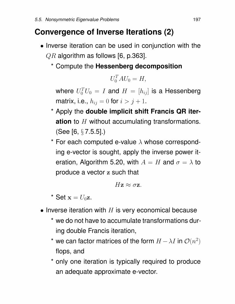
5.5. Nonsymmetric Eigenvalue Problems 197
Convergence of Inverse Iterations (2)
• Inverse iteration can be used in conjunction with theQR algorithm as follows [6, p.363].
* Compute the Hessenberg decomposition
UT0 AU0 = H,
where UT0 U0 = I and H = [hij] is a Hessenberg
matrix, i.e., hij = 0 for i > j + 1.
* Apply the double implicit shift Francis QR iter-ation to H without accumulating transformations.(See [6, §7.5.5].)
* For each computed e-value λ whose correspond-ing e-vector is sought, apply the inverse power it-eration, Algorithm 5.20, with A = H and σ = λ toproduce a vector z such that
Hz ≈ σz.
* Set x = U0z.
• Inverse iteration with H is very economical because
* we do not have to accumulate transformations dur-ing double Francis iteration,
* we can factor matrices of the form H−λI in O(n2)
flops, and
* only one iteration is typically required to producean adequate approximate e-vector.
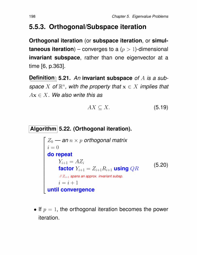
198 Chapter 5. Eigenvalue Problems
5.5.3. Orthogonal/Subspace iteration
Orthogonal iteration (or subspace iteration, or simul-taneous iteration) – converges to a (p > 1)-dimensionalinvariant subspace, rather than one eigenvector at atime [6, p.363].
Definition 5.21. An invariant subspace of A is a sub-space X of Rn, with the property that x ∈ X implies thatAx ∈ X. We also write this as
AX ⊆ X. (5.19)
Algorithm 5.22. (Orthogonal iteration).
Z0 — an n× p orthogonal matrixi = 0
do repeatYi+1 = AZifactor Yi+1 = Zi+1Ri+1 using QR
// Zi+1 spans an approx. invariant subsp.
i = i + 1
until convergence
(5.20)
• If p = 1, the orthogonal iteration becomes the poweriteration.
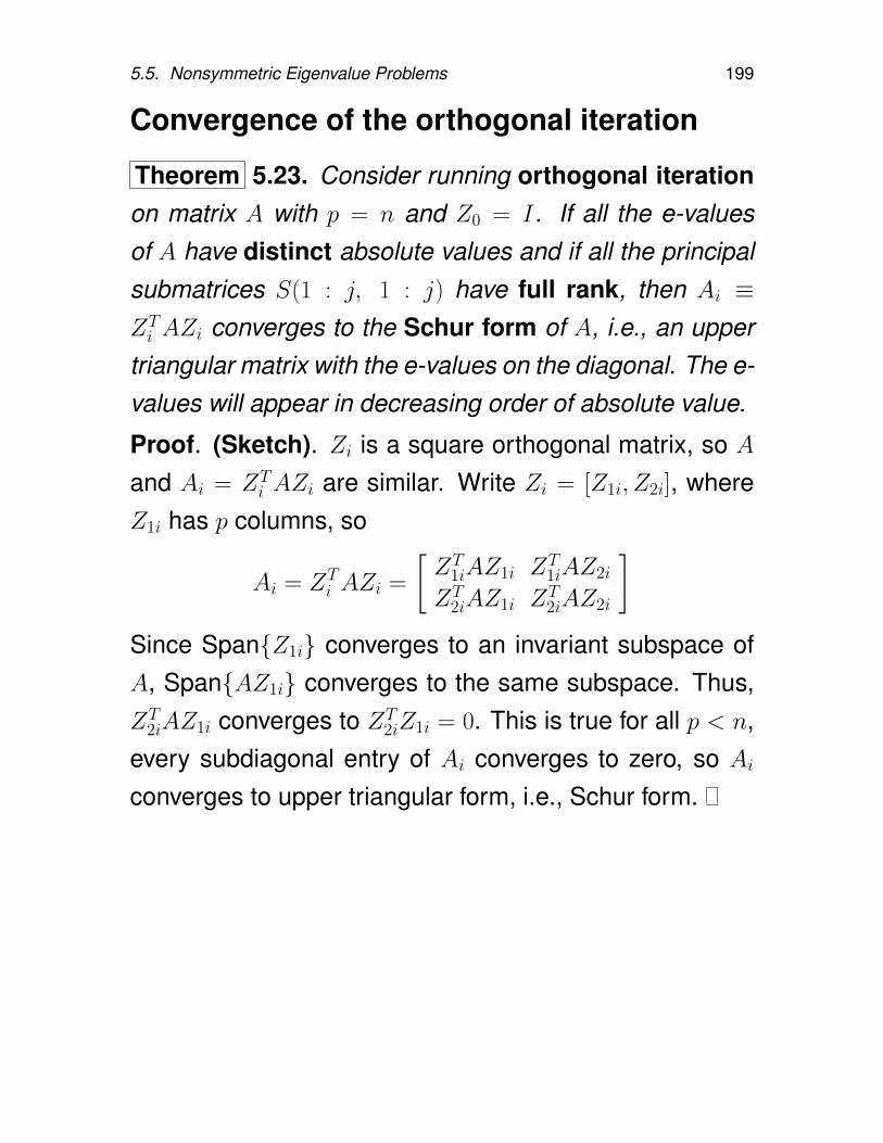
5.5. Nonsymmetric Eigenvalue Problems 199
Convergence of the orthogonal iteration
Theorem 5.23. Consider running orthogonal iterationon matrix A with p = n and Z0 = I. If all the e-valuesof A have distinct absolute values and if all the principalsubmatrices S(1 : j, 1 : j) have full rank, then Ai ≡ZTi AZi converges to the Schur form of A, i.e., an upper
triangular matrix with the e-values on the diagonal. The e-values will appear in decreasing order of absolute value.
Proof. (Sketch). Zi is a square orthogonal matrix, so A
and Ai = ZTi AZi are similar. Write Zi = [Z1i, Z2i], where
Z1i has p columns, so
Ai = ZTi AZi =
[ZT
1iAZ1i ZT1iAZ2i
ZT2iAZ1i Z
T2iAZ2i
]Since SpanZ1i converges to an invariant subspace ofA, SpanAZ1i converges to the same subspace. Thus,ZT
2iAZ1i converges to ZT2iZ1i = 0. This is true for all p < n,
every subdiagonal entry of Ai converges to zero, so Ai
converges to upper triangular form, i.e., Schur form.
200 Chapter 5. Eigenvalue Problems
Remarks:
• In Theorem 5.23, S(1 : j, 1 : j) must be nonsingu-lar. Suppose that A is diagonal with the eigenvaluesnot in decreasing order. Then orthogonal iterationyields Zi = diag(±1) and Ai = A for all i, so the eigen-values do not move into decreasing order.
• Theorem 5.23 also requires that the e-values of Amust be distinct in absolute values. If A is orthogonaland all its e-values have absolute value 1, then the al-gorithm leaves Ai essentially unchanged. (The rowsand columns may be multiplied by −1.)
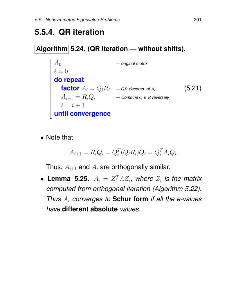
5.5. Nonsymmetric Eigenvalue Problems 201
5.5.4. QR iteration
Algorithm 5.24. (QR iteration — without shifts).
A0 — original matrix
i = 0
do repeatfactor Ai = QiRi — QR decomp. of Ai
Ai+1 = RiQi — Combine Q & R reversely
i = i + 1
until convergence
(5.21)
• Note that
Ai+1 = RiQi = QTi (QiRi)Qi = QT
i AiQi.
Thus, Ai+1 and Ai are orthogonally similar.
• Lemma 5.25. Ai = ZTi AZi, where Zi is the matrix
computed from orthogonal iteration (Algorithm 5.22).Thus Ai converges to Schur form if all the e-valueshave different absolute values.
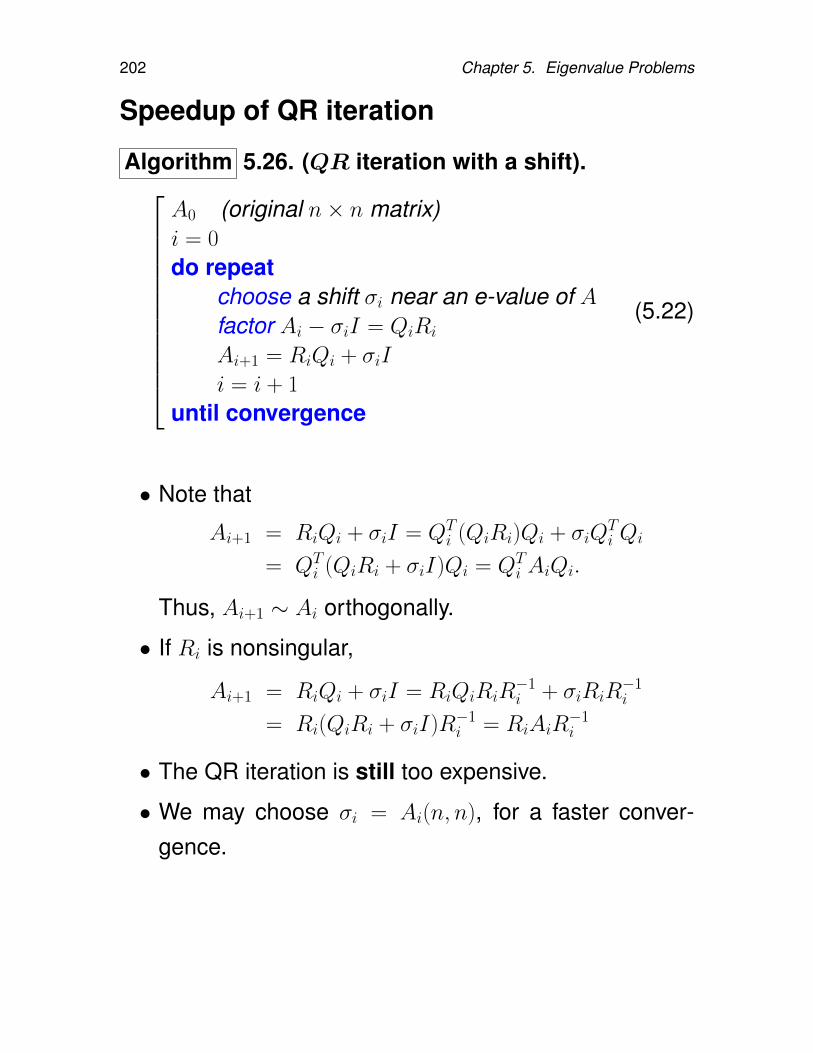
202 Chapter 5. Eigenvalue Problems
Speedup of QR iteration
Algorithm 5.26. (QR iteration with a shift).
A0 (original n× n matrix)i = 0
do repeatchoose a shift σi near an e-value of Afactor Ai − σiI = QiRi
Ai+1 = RiQi + σiI
i = i + 1
until convergence
(5.22)
• Note that
Ai+1 = RiQi + σiI = QTi (QiRi)Qi + σiQ
Ti Qi
= QTi (QiRi + σiI)Qi = QT
i AiQi.
Thus, Ai+1 ∼ Ai orthogonally.
• If Ri is nonsingular,
Ai+1 = RiQi + σiI = RiQiRiR−1i + σiRiR
−1i
= Ri(QiRi + σiI)R−1i = RiAiR
−1i
• The QR iteration is still too expensive.
• We may choose σi = Ai(n, n), for a faster conver-gence.
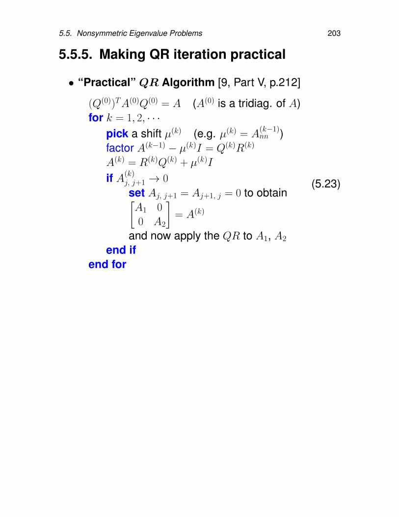
5.5. Nonsymmetric Eigenvalue Problems 203
5.5.5. Making QR iteration practical
• “Practical” QR Algorithm [9, Part V, p.212]
(Q(0))TA(0)Q(0) = A (A(0) is a tridiag. of A)for k = 1, 2, · · ·
pick a shift µ(k) (e.g. µ(k) = A(k−1)nn )
factor A(k−1) − µ(k)I = Q(k)R(k)
A(k) = R(k)Q(k) + µ(k)I
if A(k)j, j+1 → 0
set Aj, j+1 = Aj+1, j = 0 to obtain[A1 0
0 A2
]= A(k)
and now apply the QR to A1, A2
end ifend for
(5.23)
204 Chapter 5. Eigenvalue Problems
Making QR iteration more practical
• Issues:
– The convergence of the algorithm is slow.
– The the iteration is very expensive. At each step,the QR decomposition costs O(n3) flops. To find neigenvalues, we need to have O(n4) flops.
• Improvement:
– Reduce the matrix to upper Hessenberg form.Apply QR implicitly. Cost is reduced from O(n4)
to O(n3).
– Simultaneous shifts for complex e-values.
– Convergence occurs when subdiagonal entries ofAi are “small enough”.
Details will be described in later subsections.
5.5. Nonsymmetric Eigenvalue Problems 205
5.5.6. Hessenberg reduction
Similarity transforms:
Definition 5.27. Two matrices A, B ∈ Cn×n are similarif there is a nonsingular matrix S ∈ Cn×n such that
B = S−1AS. (5.24)
Equation (5.24) is called a similarity transformation andS is called the transforming matrix.
Theorem 5.28. Similar matrices have the same eigen-values.
Proof. See Homework 5.2.
Theorem 5.29. Suppose B = S−1AS. Then v is aneigenvector of A with eigenvalue λ if and only if S−1v isan eigenvector of B with associated eigenvalue λ.
Hessenberg reduction: Find an orthogonal matrixQ such that
Q∗AQ = H, (5.25)
where H = [hij] is an upper Hessenberg matrix, i.e.,hij = 0 whenever i > j + 1.
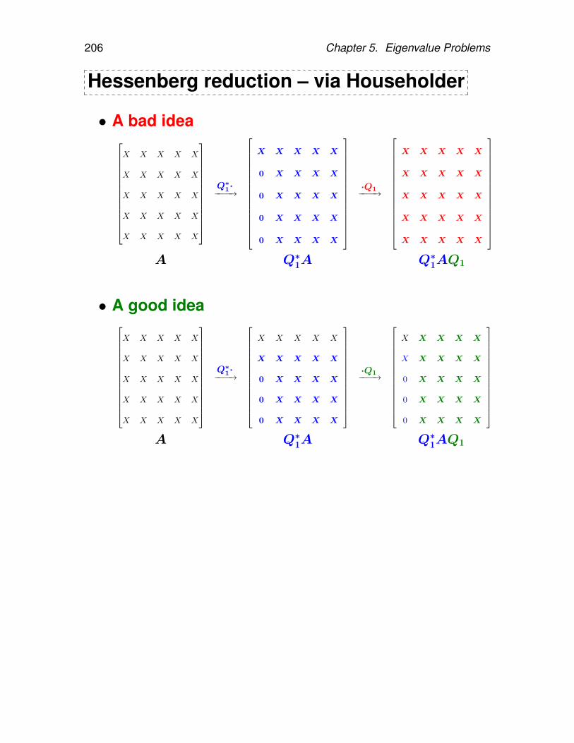
206 Chapter 5. Eigenvalue Problems
Hessenberg reduction – via Householder
• A bad idea
X X X X X
X X X X X
X X X X X
X X X X X
X X X X X
Q∗1·−−−−→
X X X X X
0 X X X X
0 X X X X
0 X X X X
0 X X X X
·Q1−−−−→
X X X X X
X X X X X
X X X X X
X X X X X
X X X X X
A Q∗1A Q∗1AQ1
• A good idea
X X X X X
X X X X X
X X X X X
X X X X X
X X X X X
Q∗1·−−−−→
X X X X X
X X X X X
0 X X X X
0 X X X X
0 X X X X
·Q1−−−−→
X X X X X
X X X X X
0 X X X X
0 X X X X
0 X X X X
A Q∗1A Q∗1AQ1
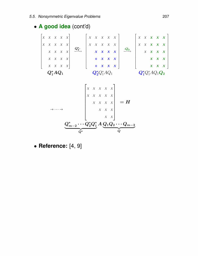
5.5. Nonsymmetric Eigenvalue Problems 207
• A good idea (cont’d)
X X X X X
X X X X X
X X X X
X X X X
X X X X
Q∗2·−−−−→
X X X X X
X X X X X
X X X X
0 X X X
0 X X X
·Q2−−−−→
X X X X X
X X X X X
X X X X
X X X
X X X
Q∗1AQ1 Q∗2Q
∗1AQ1 Q∗1Q
∗1AQ1Q2
→ · · · →
X X X X X
X X X X X
X X X X
X X X
X X
= H
Q∗m−2 · · ·Q∗2Q∗1︸ ︷︷ ︸
Q∗
AQ1Q2 · · ·Qm−2︸ ︷︷ ︸Q
• Reference: [4, 9]
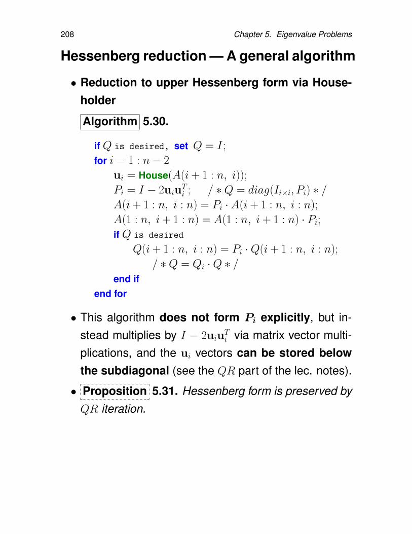
208 Chapter 5. Eigenvalue Problems
Hessenberg reduction — A general algorithm
• Reduction to upper Hessenberg form via House-holder
Algorithm 5.30.
if Q is desired, set Q = I ;
for i = 1 : n− 2
ui = House(A(i + 1 : n, i));
Pi = I − 2uiuTi ; / ∗Q = diag(Ii×i, Pi) ∗ /
A(i + 1 : n, i : n) = Pi · A(i + 1 : n, i : n);
A(1 : n, i + 1 : n) = A(1 : n, i + 1 : n) · Pi;if Q is desired
Q(i + 1 : n, i : n) = Pi ·Q(i + 1 : n, i : n);
/ ∗Q = Qi ·Q ∗ /end if
end for
• This algorithm does not form Pi explicitly, but in-stead multiplies by I − 2uiu
Ti via matrix vector multi-
plications, and the ui vectors can be stored belowthe subdiagonal (see the QR part of the lec. notes).
• Proposition 5.31. Hessenberg form is preserved byQR iteration.
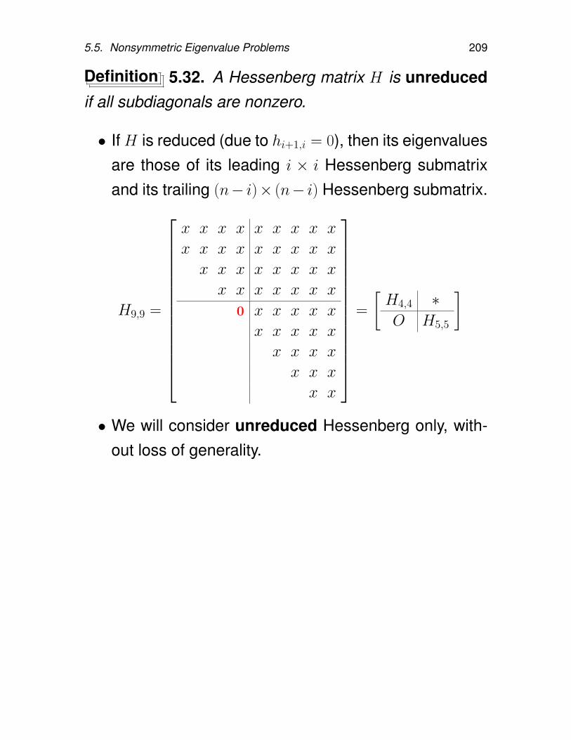
5.5. Nonsymmetric Eigenvalue Problems 209
Definition 5.32. A Hessenberg matrix H is unreducedif all subdiagonals are nonzero.
• If H is reduced (due to hi+1,i = 0), then its eigenvaluesare those of its leading i × i Hessenberg submatrixand its trailing (n− i)× (n− i) Hessenberg submatrix.
H9,9 =
x x x x x x x x x
x x x x x x x x x
x x x x x x x x
x x x x x x x
0 x x x x x
x x x x x
x x x x
x x x
x x
=
[H4,4 ∗O H5,5
]
• We will consider unreduced Hessenberg only, with-out loss of generality.
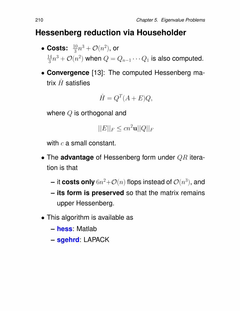
210 Chapter 5. Eigenvalue Problems
Hessenberg reduction via Householder
• Costs: 103 n
3 +O(n2), or143 n
3 +O(n2) when Q = Qn−1 · · ·Q1 is also computed.
• Convergence [13]: The computed Hessenberg ma-trix H satisfies
H = QT (A + E)Q,
where Q is orthogonal and
||E||F ≤ cn2u||Q||F
with c a small constant.
• The advantage of Hessenberg form under QR itera-tion is that
– it costs only 6n2+O(n) flops instead ofO(n3), and
– its form is preserved so that the matrix remainsupper Hessenberg.
• This algorithm is available as
– hess: Matlab
– sgehrd: LAPACK
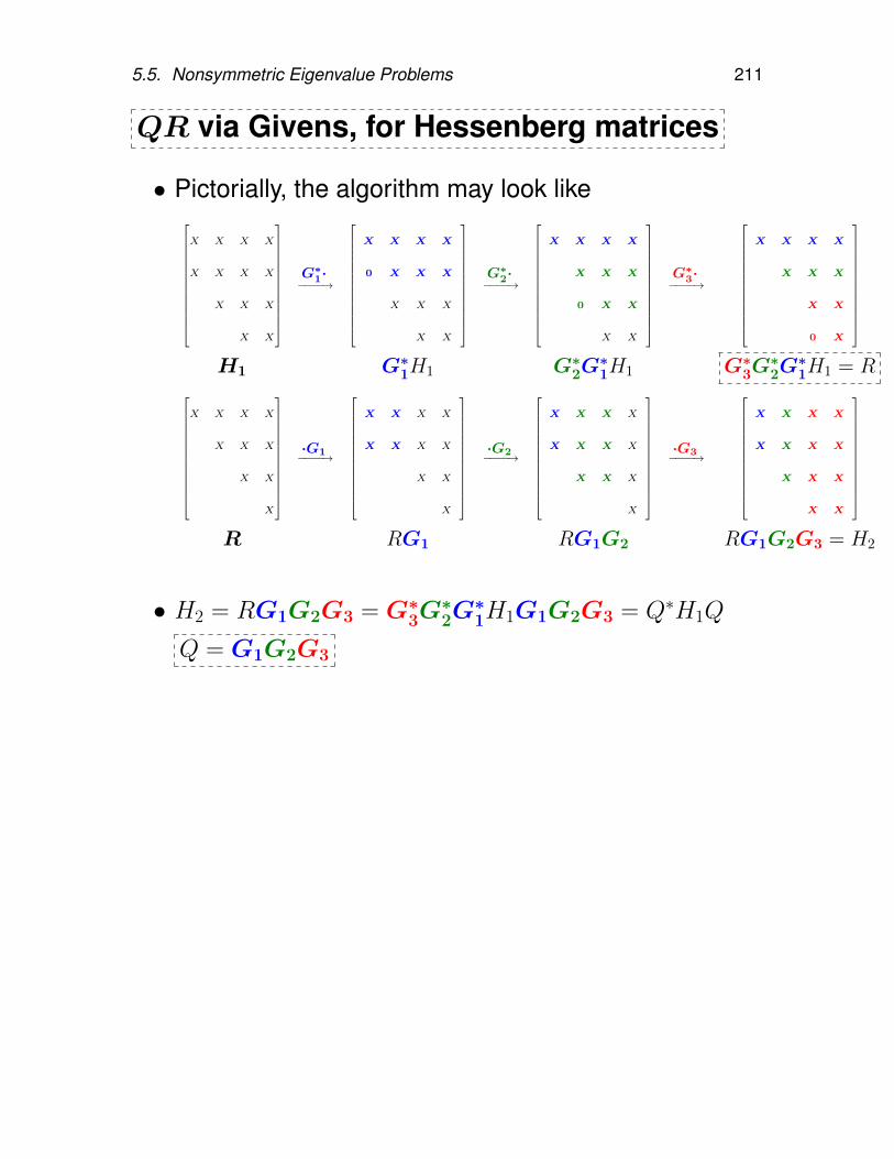
5.5. Nonsymmetric Eigenvalue Problems 211
QR via Givens, for Hessenberg matrices
• Pictorially, the algorithm may look like
X X X X
X X X X
X X X
X X
G∗1·−−−−→
X X X X
0 X X X
X X X
X X
G∗2·−−−−→
X X X X
X X X
0 X X
X X
G∗3·−−−−→
X X X X
X X X
X X
0 X
H1 G∗1H1 G∗2G
∗1H1 G∗3G
∗2G∗1H1 = R
X X X X
X X X
X X
X
·G1−−−−→
X X X X
X X X X
X X
X
·G2−−−−→
X X X X
X X X X
X X X
X
·G3−−−−→
X X X X
X X X X
X X X
X X
R RG1 RG1G2 RG1G2G3 = H2
• H2 = RG1G2G3 = G∗3G∗2G∗1H1G1G2G3 = Q∗H1Q
Q = G1G2G3
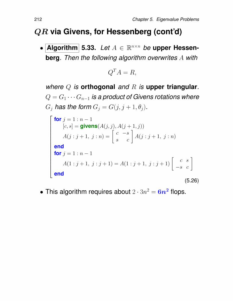
212 Chapter 5. Eigenvalue Problems
QR via Givens, for Hessenberg (cont’d)
• Algorithm 5.33. Let A ∈ Rn×n be upper Hessen-berg. Then the following algorithm overwrites A with
QTA = R,
where Q is orthogonal and R is upper triangular.Q = G1 · · ·Gn−1 is a product of Givens rotations whereGj has the form Gj = G(j, j + 1, θj).
for j = 1 : n− 1[c, s] = givens(A(j, j), A(j + 1, j))
A(j : j + 1, j : n) =
[c −ss c
]A(j : j + 1, j : n)
endfor j = 1 : n− 1
A(1 : j + 1, j : j + 1) = A(1 : j + 1, j : j + 1)
[c s
−s c
]end
(5.26)
• This algorithm requires about 2 · 3n2 = 6n2 flops.
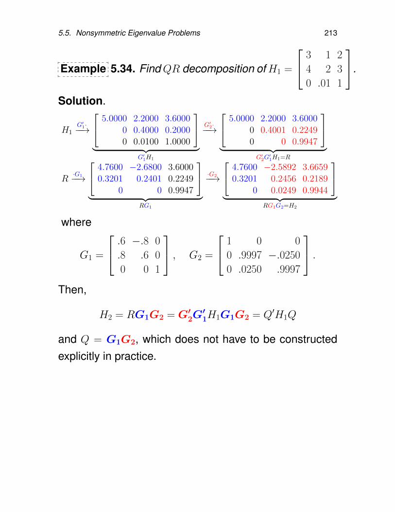
5.5. Nonsymmetric Eigenvalue Problems 213
Example 5.34. FindQR decomposition ofH1 =
3 1 2
4 2 3
0 .01 1
.
Solution.
H1G′1·−−→
5.0000 2.2000 3.60000 0.4000 0.20000 0.0100 1.0000
︸ ︷︷ ︸
G′1H1
G′2·−−→
5.0000 2.2000 3.60000 0.4001 0.22490 0 0.9947
︸ ︷︷ ︸
G′2G′1H1=R
R·G1−−→
4.7600 −2.6800 3.60000.3201 0.2401 0.2249
0 0 0.9947
︸ ︷︷ ︸
RG1
·G2−−→
4.7600 −2.5892 3.66590.3201 0.2456 0.2189
0 0.0249 0.9944
︸ ︷︷ ︸
RG1G2=H2
where
G1 =
.6 −.8 0
.8 .6 0
0 0 1
, G2 =
1 0 0
0 .9997 −.0250
0 .0250 .9997
.Then,
H2 = RG1G2 = G′2G′1H1G1G2 = Q′H1Q
and Q = G1G2, which does not have to be constructedexplicitly in practice.
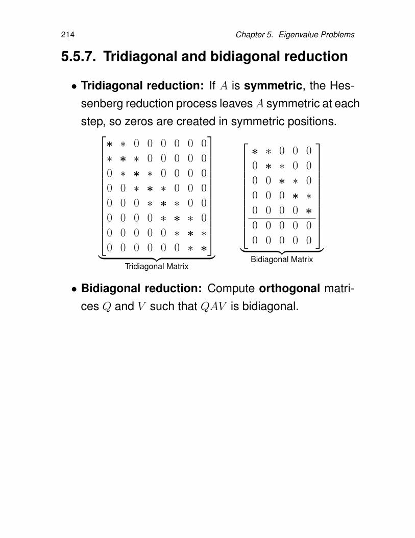
214 Chapter 5. Eigenvalue Problems
5.5.7. Tridiagonal and bidiagonal reduction
• Tridiagonal reduction: If A is symmetric, the Hes-senberg reduction process leavesA symmetric at eachstep, so zeros are created in symmetric positions.
∗ ∗ 0 0 0 0 0 0
∗ ∗ ∗ 0 0 0 0 0
0 ∗ ∗ ∗ 0 0 0 0
0 0 ∗ ∗ ∗ 0 0 0
0 0 0 ∗ ∗ ∗ 0 0
0 0 0 0 ∗ ∗ ∗ 0
0 0 0 0 0 ∗ ∗ ∗0 0 0 0 0 0 ∗ ∗
︸ ︷︷ ︸
Tridiagonal Matrix
∗ ∗ 0 0 0
0 ∗ ∗ 0 0
0 0 ∗ ∗ 0
0 0 0 ∗ ∗0 0 0 0 ∗0 0 0 0 0
0 0 0 0 0
︸ ︷︷ ︸
Bidiagonal Matrix
• Bidiagonal reduction: Compute orthogonal matri-ces Q and V such that QAV is bidiagonal.
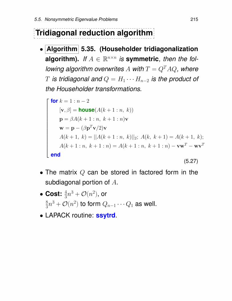
5.5. Nonsymmetric Eigenvalue Problems 215
Tridiagonal reduction algorithm
• Algorithm 5.35. (Householder tridiagonalizationalgorithm). If A ∈ Rn×n is symmetric, then the fol-lowing algorithm overwrites A with T = QTAQ, whereT is tridiagonal and Q = H1 · · ·Hn−2 is the product ofthe Householder transformations.
for k = 1 : n− 2
[v, β] = house(A(k + 1 : n, k))
p = βA(k + 1 : n, k + 1 : n)v
w = p− (βpTv/2)v
A(k + 1, k) = ||A(k + 1 : n, k)||2; A(k, k + 1) = A(k + 1, k);
A(k + 1 : n, k + 1 : n) = A(k + 1 : n, k + 1 : n)− vwT −wvT
end(5.27)
• The matrix Q can be stored in factored form in thesubdiagonal portion of A.
• Cost: 43n
3 +O(n2), or83n
3 +O(n2) to form Qn−1 · · ·Q1 as well.
• LAPACK routine: ssytrd.
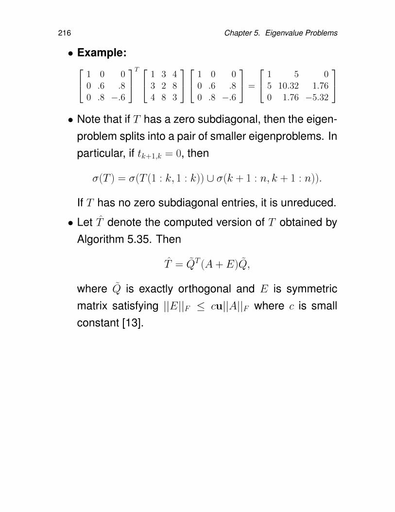
216 Chapter 5. Eigenvalue Problems
• Example: 1 0 00 .6 .80 .8 −.6
T 1 3 43 2 84 8 3
1 0 00 .6 .80 .8 −.6
=
1 5 05 10.32 1.760 1.76 −5.32
• Note that if T has a zero subdiagonal, then the eigen-
problem splits into a pair of smaller eigenproblems. Inparticular, if tk+1,k = 0, then
σ(T ) = σ(T (1 : k, 1 : k)) ∪ σ(k + 1 : n, k + 1 : n)).
If T has no zero subdiagonal entries, it is unreduced.
• Let T denote the computed version of T obtained byAlgorithm 5.35. Then
T = QT (A + E)Q,
where Q is exactly orthogonal and E is symmetricmatrix satisfying ||E||F ≤ cu||A||F where c is smallconstant [13].
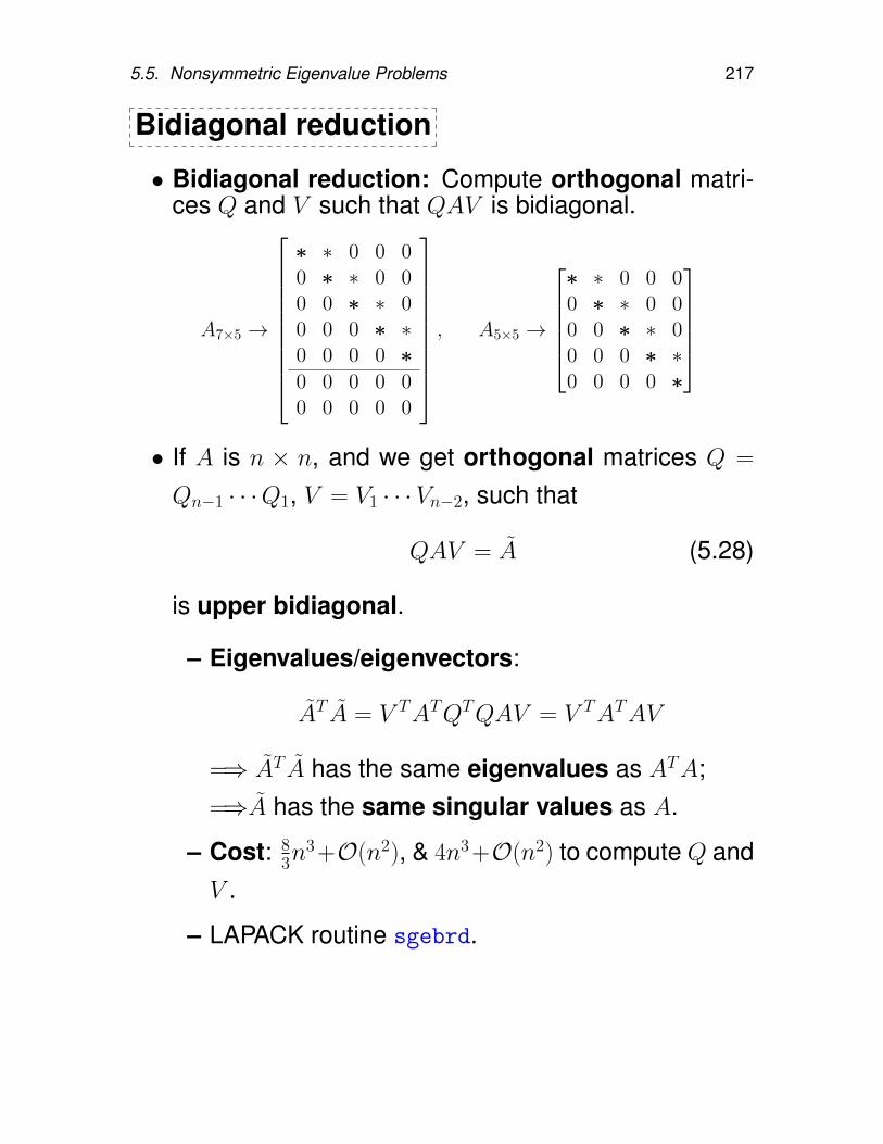
5.5. Nonsymmetric Eigenvalue Problems 217
Bidiagonal reduction
• Bidiagonal reduction: Compute orthogonal matri-ces Q and V such that QAV is bidiagonal.
A7×5 →
∗ ∗ 0 0 00 ∗ ∗ 0 00 0 ∗ ∗ 00 0 0 ∗ ∗0 0 0 0 ∗0 0 0 0 00 0 0 0 0
, A5×5 →
∗ ∗ 0 0 00 ∗ ∗ 0 00 0 ∗ ∗ 00 0 0 ∗ ∗0 0 0 0 ∗
• If A is n × n, and we get orthogonal matrices Q =
Qn−1 · · ·Q1, V = V1 · · ·Vn−2, such that
QAV = A (5.28)
is upper bidiagonal.
– Eigenvalues/eigenvectors:
AT A = V TATQTQAV = V TATAV
=⇒ AT A has the same eigenvalues as ATA;=⇒A has the same singular values as A.
– Cost: 83n
3 +O(n2), & 4n3 +O(n2) to compute Q andV .
– LAPACK routine sgebrd.
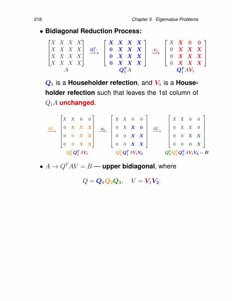
218 Chapter 5. Eigenvalue Problems
• Bidiagonal Reduction Process:X X X XX X X XX X X XX X X X
QT1 ·−−→
X X X X0 X X X0 X X X0 X X X
·V1−−→
X X 0 00 X X X0 X X X0 X X X
A QT
1A QT1AV1
Q1 is a Householder refection, and V1 is a House-holder refection such that leaves the 1st column ofQ1A unchanged.
QT2 ·−−→
X X 0 0
0 X X X
0 0 X X
0 0 X X
·V2−−→
X X 0 0
0 X X 0
0 0 X X
0 0 X X
QT
3 ·−−→
X X 0 0
0 X X 0
0 0 X X
0 0 0 X
QT
2QT1AV1 QT
2QT1AV1V2 QT
3QT2Q
T1AV1V2 = B
• A→ QTAV = B — upper bidiagonal, where
Q = Q1Q2Q3, V = V1V2.
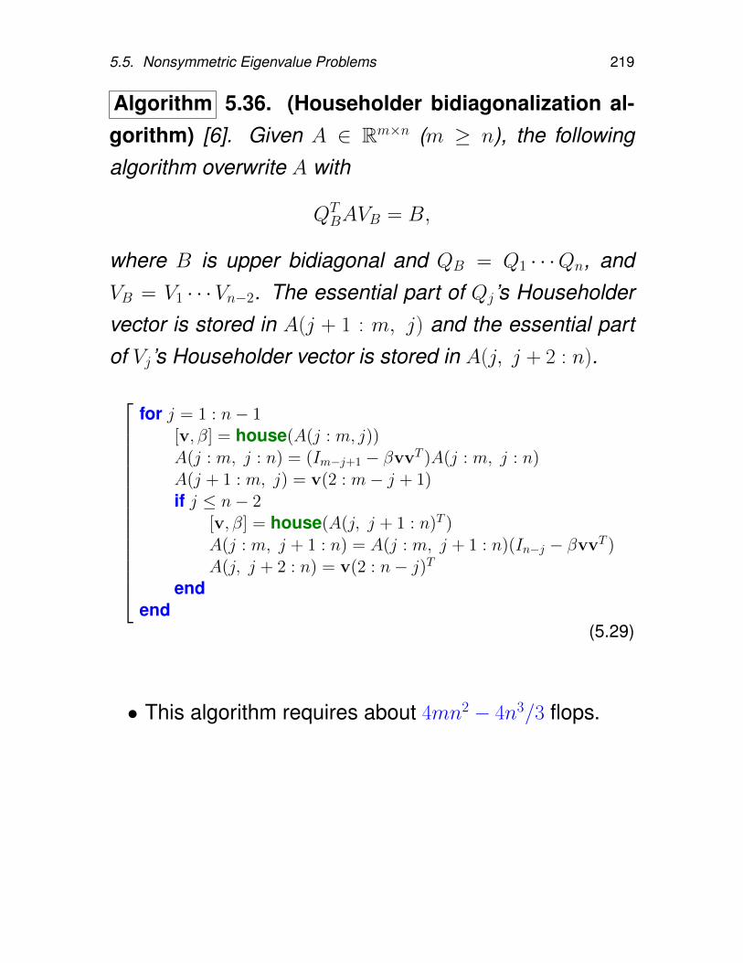
5.5. Nonsymmetric Eigenvalue Problems 219
Algorithm 5.36. (Householder bidiagonalization al-gorithm) [6]. Given A ∈ Rm×n (m ≥ n), the followingalgorithm overwrite A with
QTBAVB = B,
where B is upper bidiagonal and QB = Q1 · · ·Qn, andVB = V1 · · ·Vn−2. The essential part of Qj ’s Householdervector is stored in A(j + 1 : m, j) and the essential partof Vj ’s Householder vector is stored in A(j, j + 2 : n).
for j = 1 : n− 1[v, β] = house(A(j : m, j))A(j : m, j : n) = (Im−j+1 − βvvT )A(j : m, j : n)A(j + 1 : m, j) = v(2 : m− j + 1)if j ≤ n− 2
[v, β] = house(A(j, j + 1 : n)T )A(j : m, j + 1 : n) = A(j : m, j + 1 : n)(In−j − βvvT )A(j, j + 2 : n) = v(2 : n− j)T
endend
(5.29)
• This algorithm requires about 4mn2 − 4n3/3 flops.
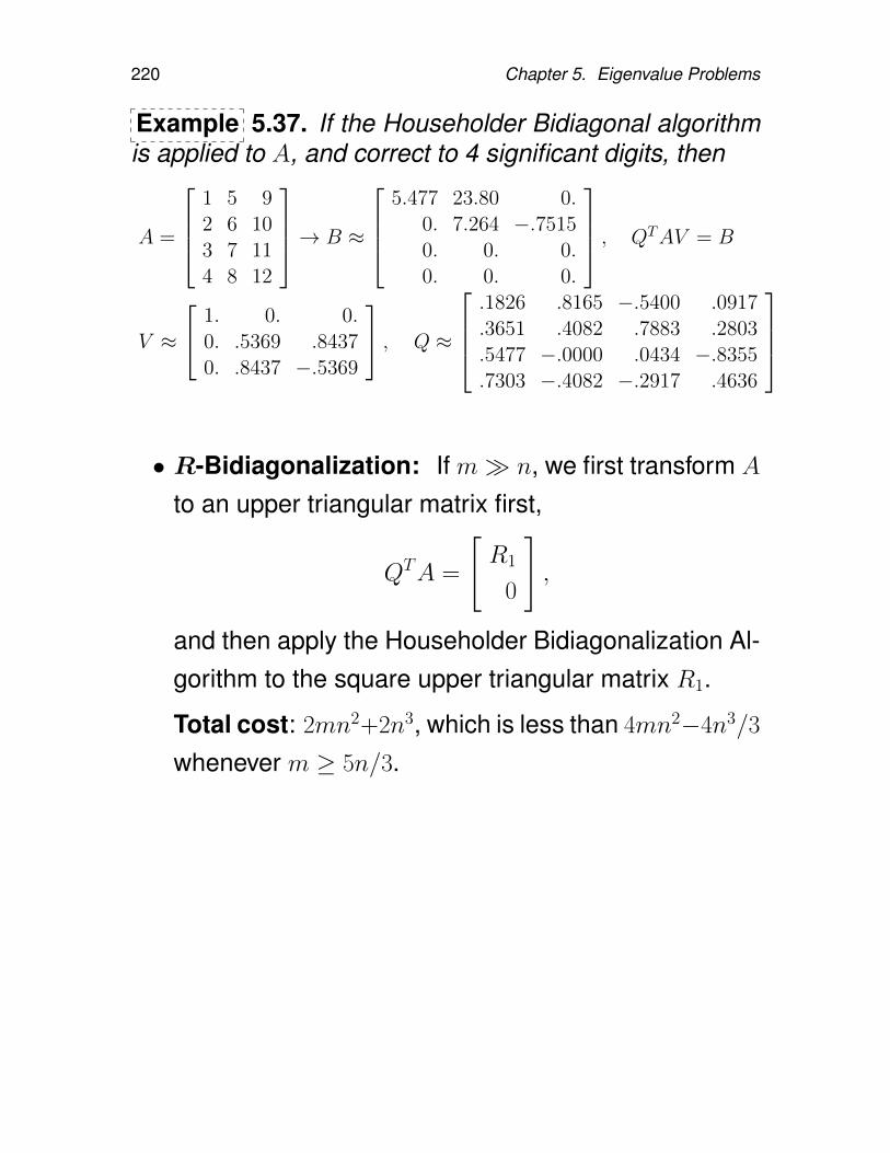
220 Chapter 5. Eigenvalue Problems
Example 5.37. If the Householder Bidiagonal algorithmis applied to A, and correct to 4 significant digits, then
A =
1 5 92 6 103 7 114 8 12
→ B ≈
5.477 23.80 0.
0. 7.264 −.75150. 0. 0.0. 0. 0.
, QTAV = B
V ≈
1. 0. 0.0. .5369 .84370. .8437 −.5369
, Q ≈
.1826 .8165 −.5400 .0917.3651 .4082 .7883 .2803.5477 −.0000 .0434 −.8355.7303 −.4082 −.2917 .4636
• R-Bidiagonalization: If m n, we first transform A
to an upper triangular matrix first,
QTA =
[R1
0
],
and then apply the Householder Bidiagonalization Al-gorithm to the square upper triangular matrix R1.
Total cost: 2mn2+2n3, which is less than 4mn2−4n3/3
whenever m ≥ 5n/3.
5.5. Nonsymmetric Eigenvalue Problems 221
5.5.8. QR iteration with implicit shifts – Im-plicit Q theorem
In this subsection, we show how to implement QR itera-tion effectively for an upper Hessenberg matrix H.
• The implementation is implicit in the sense that we donot explicitly compute the QR factorization of H, butrather construct Q as a product of Givens rotationsand simple orthogonal matrices.
• the implicit Q theorem shows that this implicitly con-structed Q is the Q we want.
Theorem 5.38. (Implicit Q theorem). Suppose thatQTAQ = H is unreduced upper Hessenberg. Thencolumns 2 through n of Q are determined uniquely (upto signs) by the first column of Q.
Implication of the theorem: To compute Ai+1 = QTi AiQi
from Ai (in the QR iteration), we will need only to
• compute the 1st column of Qi (which is parallel to the1st column of Ai − σiI and so can be gotten just bynormalizing this column vector).
• choose other columns ofQi such thatQi is orthogonaland Ai+1 is unreduced Hessenberg.
222 Chapter 5. Eigenvalue Problems
Proof. (Sketch of the Proof of ImplicitQ theorem). Let
QTAQ = H, V TAV = G
be unreduced upper Hessenberg, Q and V be orthogo-nal, and the 1st columns of Q and V are equal. Define
W = V TQ = [w1, · · · ,wn].
Then W is orthogonal and GW = WH and therefore wehave
hi+1,iwi+1 = Gwi −i∑
j=1
hjiwj, i = 1, 2, · · · , n− 1
Since w1 = e1 and G is upper Hessenberg, W is uppertriangular. Since W is also orthogonal, W is diagonal andW = diag(±1, · · · ,±1).
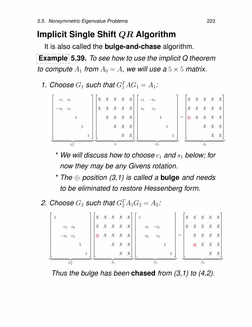
5.5. Nonsymmetric Eigenvalue Problems 223
Implicit Single Shift QR AlgorithmIt is also called the bulge-and-chase algorithm.
Example 5.39. To see how to use the implicit Q theoremto compute A1 from A0 = A, we will use a 5× 5 matrix.
1. Choose G1 such that GT1AG1 = A1:
c1 s1
−s1 c1
1
1
1
︸ ︷︷ ︸
GT1
X X X X X
X X X X X
X X X X
X X X
X X
︸ ︷︷ ︸
A
c1 −s1
s1 c1
1
1
1
︸ ︷︷ ︸
G1
=
X X X X X
X X X X X
⊕ X X X X
X X X
X X
︸ ︷︷ ︸
A1
* We will discuss how to choose c1 and s1 below; fornow they may be any Givens rotation.
* The ⊕ position (3,1) is called a bulge and needsto be eliminated to restore Hessenberg form.
2. Choose G2 such that GT2A1G2 = A2:
1
c2 s2
−s2 c2
1
1
︸ ︷︷ ︸
GT2
X X X X X
X X X X X
⊕ X X X X
X X X
X X
︸ ︷︷ ︸
A1
1
c2 −s2
s2 c2
1
1
︸ ︷︷ ︸
G2
=
X X X X X
X X X X X
X X X X
⊕ X X X
X X
︸ ︷︷ ︸
A2
Thus the bulge has been chased from (3,1) to (4,2).
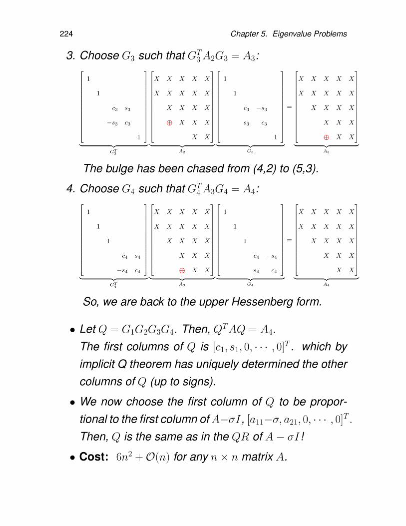
224 Chapter 5. Eigenvalue Problems
3. Choose G3 such that GT3A2G3 = A3:
1
1
c3 s3
−s3 c3
1
︸ ︷︷ ︸
GT3
X X X X X
X X X X X
X X X X
⊕ X X X
X X
︸ ︷︷ ︸
A2
1
1
c3 −s3
s3 c3
1
︸ ︷︷ ︸
G3
=
X X X X X
X X X X X
X X X X
X X X
⊕ X X
︸ ︷︷ ︸
A3
The bulge has been chased from (4,2) to (5,3).
4. Choose G4 such that GT4A3G4 = A4:
1
1
1
c4 s4
−s4 c4
︸ ︷︷ ︸
GT4
X X X X X
X X X X X
X X X X
X X X
⊕ X X
︸ ︷︷ ︸
A3
1
1
1
c4 −s4
s4 c4
︸ ︷︷ ︸
G4
=
X X X X X
X X X X X
X X X X
X X X
X X
︸ ︷︷ ︸
A4
So, we are back to the upper Hessenberg form.
• Let Q = G1G2G3G4. Then, QTAQ = A4.The first columns of Q is [c1, s1, 0, · · · , 0]T . which byimplicit Q theorem has uniquely determined the othercolumns of Q (up to signs).
• We now choose the first column of Q to be propor-tional to the first column ofA−σI, [a11−σ, a21, 0, · · · , 0]T .
Then, Q is the same as in the QR of A− σI!
• Cost: 6n2 +O(n) for any n× n matrix A.
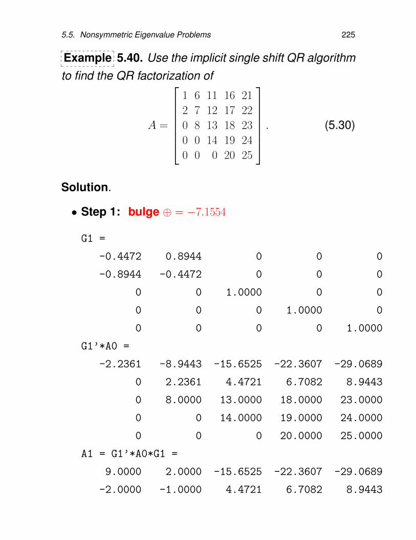
5.5. Nonsymmetric Eigenvalue Problems 225
Example 5.40. Use the implicit single shift QR algorithmto find the QR factorization of
A =
1 6 11 16 21
2 7 12 17 22
0 8 13 18 23
0 0 14 19 24
0 0 0 20 25
. (5.30)
Solution.
• Step 1: bulge ⊕ = −7.1554
G1 =
-0.4472 0.8944 0 0 0
-0.8944 -0.4472 0 0 0
0 0 1.0000 0 0
0 0 0 1.0000 0
0 0 0 0 1.0000
G1’*A0 =
-2.2361 -8.9443 -15.6525 -22.3607 -29.0689
0 2.2361 4.4721 6.7082 8.9443
0 8.0000 13.0000 18.0000 23.0000
0 0 14.0000 19.0000 24.0000
0 0 0 20.0000 25.0000
A1 = G1’*A0*G1 =
9.0000 2.0000 -15.6525 -22.3607 -29.0689
-2.0000 -1.0000 4.4721 6.7082 8.9443
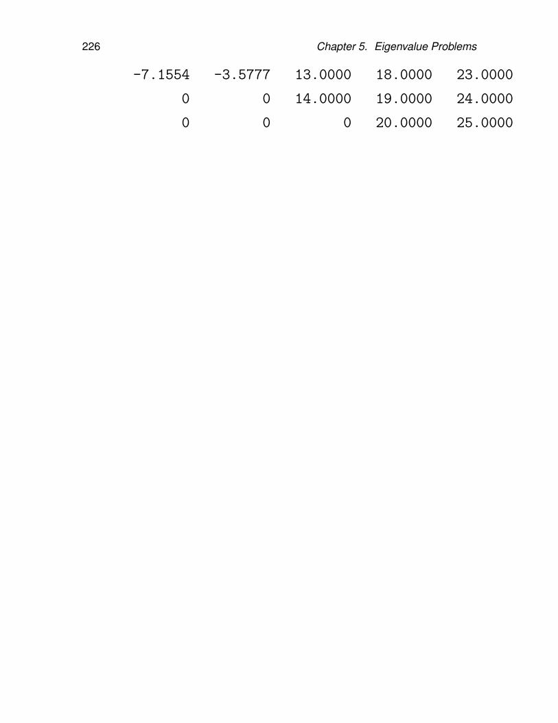
226 Chapter 5. Eigenvalue Problems
-7.1554 -3.5777 13.0000 18.0000 23.0000
0 0 14.0000 19.0000 24.0000
0 0 0 20.0000 25.0000
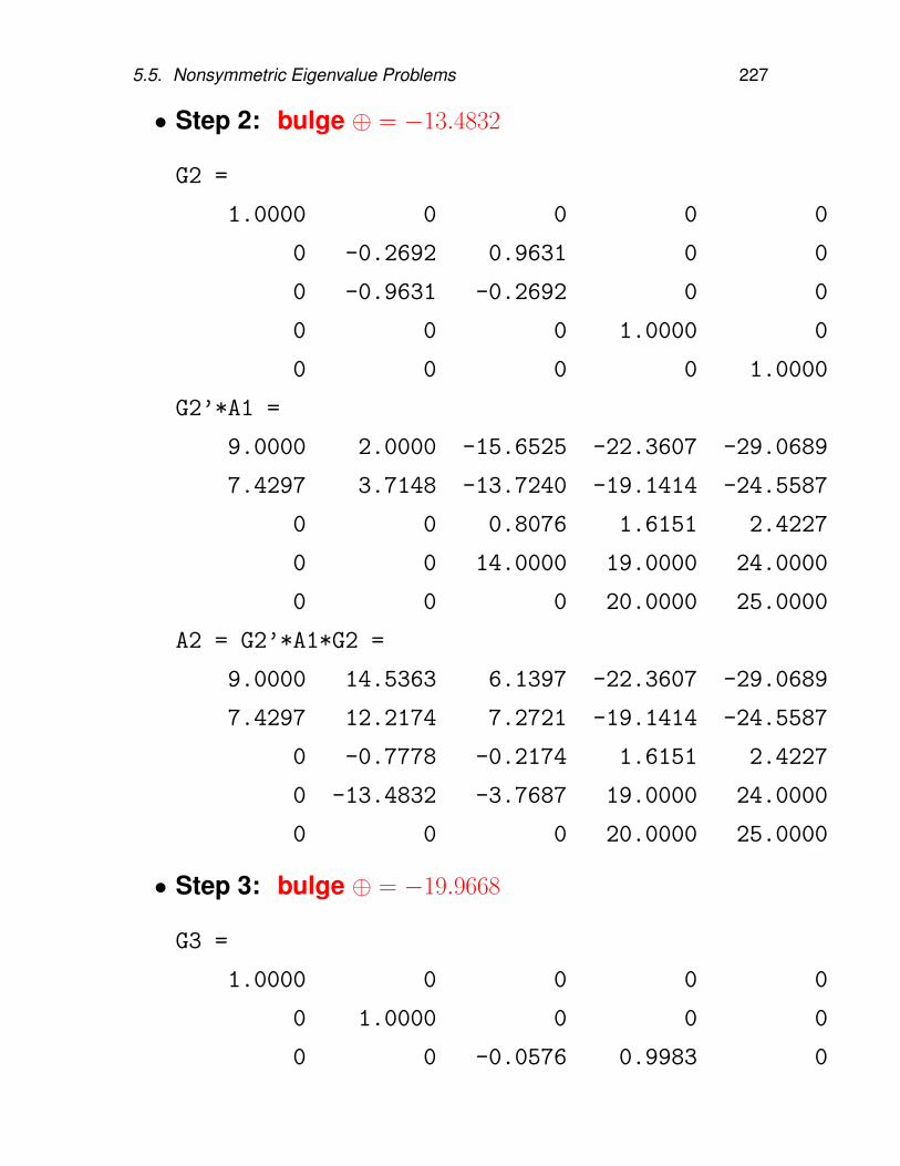
5.5. Nonsymmetric Eigenvalue Problems 227
• Step 2: bulge ⊕ = −13.4832
G2 =
1.0000 0 0 0 0
0 -0.2692 0.9631 0 0
0 -0.9631 -0.2692 0 0
0 0 0 1.0000 0
0 0 0 0 1.0000
G2’*A1 =
9.0000 2.0000 -15.6525 -22.3607 -29.0689
7.4297 3.7148 -13.7240 -19.1414 -24.5587
0 0 0.8076 1.6151 2.4227
0 0 14.0000 19.0000 24.0000
0 0 0 20.0000 25.0000
A2 = G2’*A1*G2 =
9.0000 14.5363 6.1397 -22.3607 -29.0689
7.4297 12.2174 7.2721 -19.1414 -24.5587
0 -0.7778 -0.2174 1.6151 2.4227
0 -13.4832 -3.7687 19.0000 24.0000
0 0 0 20.0000 25.0000
• Step 3: bulge ⊕ = −19.9668
G3 =
1.0000 0 0 0 0
0 1.0000 0 0 0
0 0 -0.0576 0.9983 0
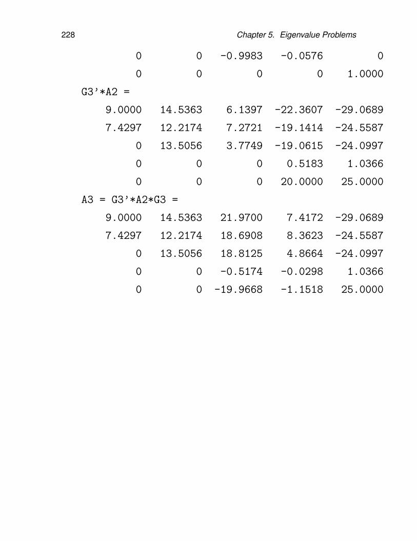
228 Chapter 5. Eigenvalue Problems
0 0 -0.9983 -0.0576 0
0 0 0 0 1.0000
G3’*A2 =
9.0000 14.5363 6.1397 -22.3607 -29.0689
7.4297 12.2174 7.2721 -19.1414 -24.5587
0 13.5056 3.7749 -19.0615 -24.0997
0 0 0 0.5183 1.0366
0 0 0 20.0000 25.0000
A3 = G3’*A2*G3 =
9.0000 14.5363 21.9700 7.4172 -29.0689
7.4297 12.2174 18.6908 8.3623 -24.5587
0 13.5056 18.8125 4.8664 -24.0997
0 0 -0.5174 -0.0298 1.0366
0 0 -19.9668 -1.1518 25.0000
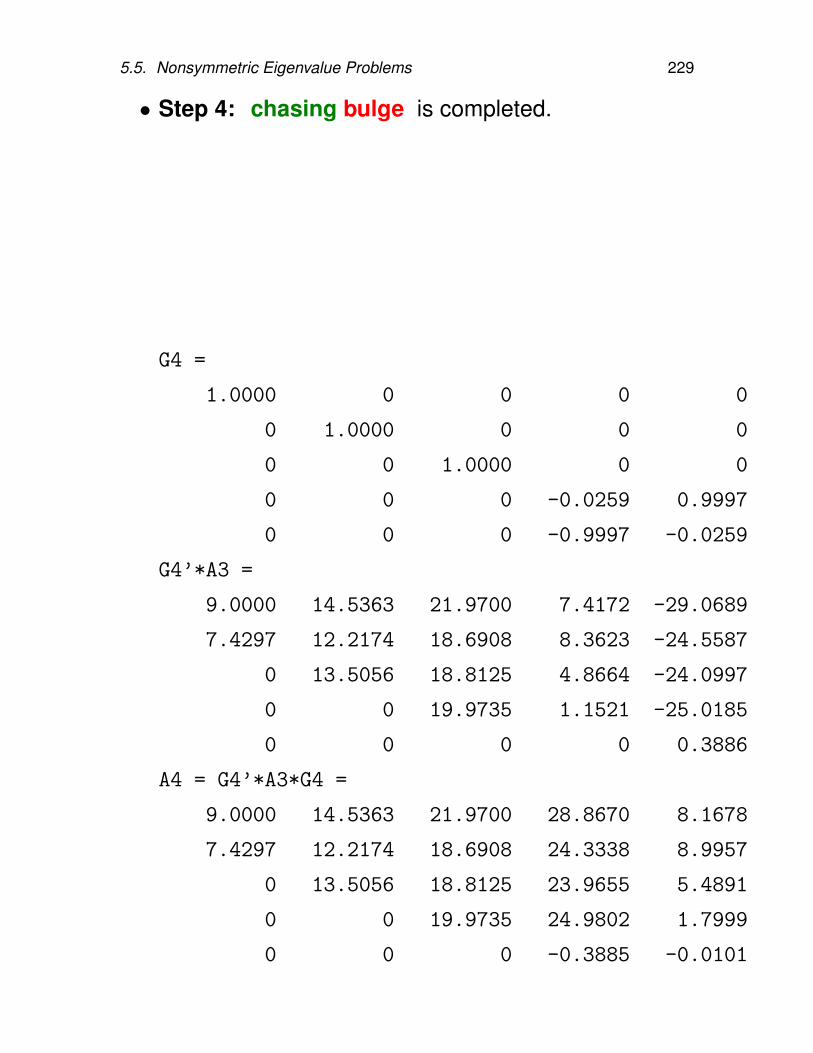
5.5. Nonsymmetric Eigenvalue Problems 229
• Step 4: chasing bulge is completed.
G4 =
1.0000 0 0 0 0
0 1.0000 0 0 0
0 0 1.0000 0 0
0 0 0 -0.0259 0.9997
0 0 0 -0.9997 -0.0259
G4’*A3 =
9.0000 14.5363 21.9700 7.4172 -29.0689
7.4297 12.2174 18.6908 8.3623 -24.5587
0 13.5056 18.8125 4.8664 -24.0997
0 0 19.9735 1.1521 -25.0185
0 0 0 0 0.3886
A4 = G4’*A3*G4 =
9.0000 14.5363 21.9700 28.8670 8.1678
7.4297 12.2174 18.6908 24.3338 8.9957
0 13.5056 18.8125 23.9655 5.4891
0 0 19.9735 24.9802 1.7999
0 0 0 -0.3885 -0.0101
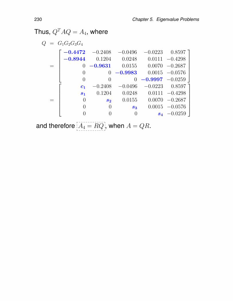
230 Chapter 5. Eigenvalue Problems
Thus, QTAQ = A4, where
Q = G1G2G3G4
=
−0.4472 −0.2408 −0.0496 −0.0223 0.8597−0.8944 0.1204 0.0248 0.0111 −0.4298
0 −0.9631 0.0155 0.0070 −0.26870 0 −0.9983 0.0015 −0.05760 0 0 −0.9997 −0.0259
=
c1 −0.2408 −0.0496 −0.0223 0.8597s1 0.1204 0.0248 0.0111 −0.42980 s2 0.0155 0.0070 −0.26870 0 s3 0.0015 −0.05760 0 0 s4 −0.0259
and therefore A4 = RQ , when A = QR.
5.5. Nonsymmetric Eigenvalue Problems 231
Implicit Double Shift QR AlgorithmDouble shifting has been considered to maintain real
arithmetic, for computing the eigenvalues of companionand fellow matrices.
• Companion and fellow matrices are Hessenberg ma-trices, that can be decomposed into the sum of a uni-tary and a rank-1 matrix.
• The Hessenberg, the unitary as well as the rank-1structures are preserved under a step of the QR-method.This makes these matrices suitable for the design ofa fast QR-method.
• Several techniques already exist for performing a QR-step. The implementation of these methods is highlydependent on the representation used.
232 Chapter 5. Eigenvalue Problems
Definition 5.41. Given an nth-orer monic polynomial
a(x) = a0 + a1x + · · · + an−1xn−1 + xn, (5.31)
its companion matrix is defined as
A =
0 0 · · · 0 −a0
1 0 · · · 0 −a1
0 1 · · · 0 −a2... ... . . . ... ...0 0 · · · 1 −an−1
. (5.32)
The eigenvalues of A are the roots of the polynomial a(x).
Definition 5.42. Fellow matrices are rank-1 perturba-tions of unitary Hessenberg matrices. That is, a fellowmatrix F is expressed as
F = H + uvT , (5.33)
where H is a unitary Hessenberg matrix and u and v arevectors.
5.6. Symmetric Eigenvalue Problems 233
5.6. Symmetric Eigenvalue Problems
5.6.1. Algorithms for the symmetric eigen-problem – Direct methods
1. Tridiagonal QR iteration: This algorithm finds all theeigenvalues, and optionally all the eigenvectors, of asymmetric tridiagonal matrix.
– Implemented efficiently, it is currently the fastestpractical method to find all the eigenvalues of asymmetric tridiagonal matrix, taking O(n2) flops.
– But for finding all the eigenvectors as well, QR it-eration takes a little over 6n3 flops on average andis only the fastest algorithm for small matrices, upto about n = 25.
Matlab command: eigLAPACK routines:
ssyev (for dense matrices),sstev (for tridiagonal matrices).
234 Chapter 5. Eigenvalue Problems
2. Rayleigh quotient iteration: This algorithm under-lies the QR iteration. But it can be used separately(without assuming that the matrix has first been re-duced to tridiagonal form).
3. Divide-and-conquer method: This is currently thefastest method to find all the eigenvalues and eigen-vectors of symmetric tridiagonal matrices larger thann = 25.
LAPACK routines:sstevd, defaults to QR iteration for smaller ma-
trices.
In the worst case, divide-and-conquer requires O(n3)
flops, but in practice the constant is quite small. Overa large set of random test cases, it appears to takeonly O(n2.3) flops in average, and as low as O(n2) forsome eigenvalue distributions.
In theory, divide-and-conquer could be implementedto run in O(n · logp n).
5.6. Symmetric Eigenvalue Problems 235
4. Bisection and inverse iteration: Bisection may beused to find just a subset of the eigenvalues of a sym-metric tridiagonal matrix, say, those in an interval [a, b]
or [αi, αi−j].
It needs only O(nk) flops, where k is the number ofeigenvalues desired. Thus Bisection can be muchfaster than QR iteration when k n, since QR it-eration requires O(n2) flops.
Inverse iteration can then be used to find the corre-sponding eigenvectors. In the best case, when theeigenvalues are “well separated” inverse iteration alsocosts only O(nk) flops.
But in the worst case, when many eigenvalues areclustered close together, inverse iteration takesO(nk2)
flops and does not even guarantee the accuracy.
5. Jacobi’s method: This method is historically the old-est method for the eigenproblem, dating to 1846. Itis usually much slower than any of the above meth-ods, taking O(n3) flops with a large constant. Butit is sometimes much more accurate than the abovemethods. It does not require tridiagonalization of thematrix.
236 Chapter 5. Eigenvalue Problems
5.6.2. Tridiagonal QR iteration
• Tridiagonal QR iteration:
1. Given A = AT , use a variant of the Householdertridiagonalization algorithm (Algorithm 5.35 on p. 215)to find orthogonal Q so that
QAQT = T
is tridiagonal.
2. Apply QR iteration to T to get a sequence
T = T0, T1, T2, · · ·
of tridiagonal matrices converging to diagonal form.
• The QR iteration keeps all the Ti tridiagonal. Indeed,since QAQT is symmetric and upper Hessenberg, itmust also be lower Hessenberg, i.e., tridiagonal. Thiskeeps each the QR iteration very inexpensive.
5.6. Symmetric Eigenvalue Problems 237
• Tridiagonal QR iteration – Operation count:
– Reducing A to symmetric tridiagonal form T costs43n
3 +O(n2) flops, or 83n
3 +O(n2) flops if eigenvec-tors are also desired.
– One tridiagonalQR iteration with a single shift (“bulgechasing”) costs 6n flops.
– Finding all eigenvalues of T takes only 2 QR stepsper eigenvalue on average, for a total of 6n2 flops.
– Finding all eigenvalues and eigenvectors of T costs6n3 +O(n2) flops.
– The total cost to find just eigenvalues of A is4
3n3 +O(n2) flops.
– The total cost to find all the eigenvalues and
eigenvectors of A is 82
3n3 +O(n2) flops.
238 Chapter 5. Eigenvalue Problems
• Tridiagonal QR iteration – How to chose the shifts:
Denote the ith iterate by Ti =
a1 b1
b1. . . . . .. . . . . . bn−1
bn−1 an
.– The simplest choice of shift would be σi = an; this
is the single shift QR iteration (see § 5.5.8). It iscubically convergent for almost all matrices.
– Wilkinson’s shift: Let the shift σi be the eigen-
value of[an−1 bn−1
bn−1 an
]that is closest to an.
– Wilkinson Theorem: QR iteration with Wilkinson’sshift is globally, and at least linearly, convergent. Itis asymptotically cubically convergent for almostall matrices.
5.6. Symmetric Eigenvalue Problems 239
Tridiagonal QR iteration with Wilkinson’s shift
• Matlab Program: T ∈ Rn×n — symmetric tridiago-nal, m — number of iterations
% Dr. James Demmel’s matlab code tridiQR.m % (slightly modified)
%
% Store last subdiagonal and last diagonal entries of QR iterates in NN
NN = [ T(n,n-1), T(n,n) ];
% Perform QR iteration with Wilkinson’s shift
for i = 1:m
% Compute the shift
lc = T(n-1:n, n-1:n); elc = eig(lc); %calculate the e-values of lc
if ( abs(T(n,n)-elc(1)) < abs(T(n,n)-elc(2)) )
shift = elc(1);
else
shift = elc(2);
end
% Perform QR iteration; enforce symmetry explicitly
[q,r] = qr(T - shift*eye(n)); T = r*q + shift*eye(n);
T = tril(triu(T,-1),1); T = (T + T’)/2;
% Update NN
NN = [NN;[T(n,n-1),T(n,n)]]; %append T(n,n-1),T(n,n) to NN
end
NN = [NN,NN(:,2)-NN(m+1,2)];
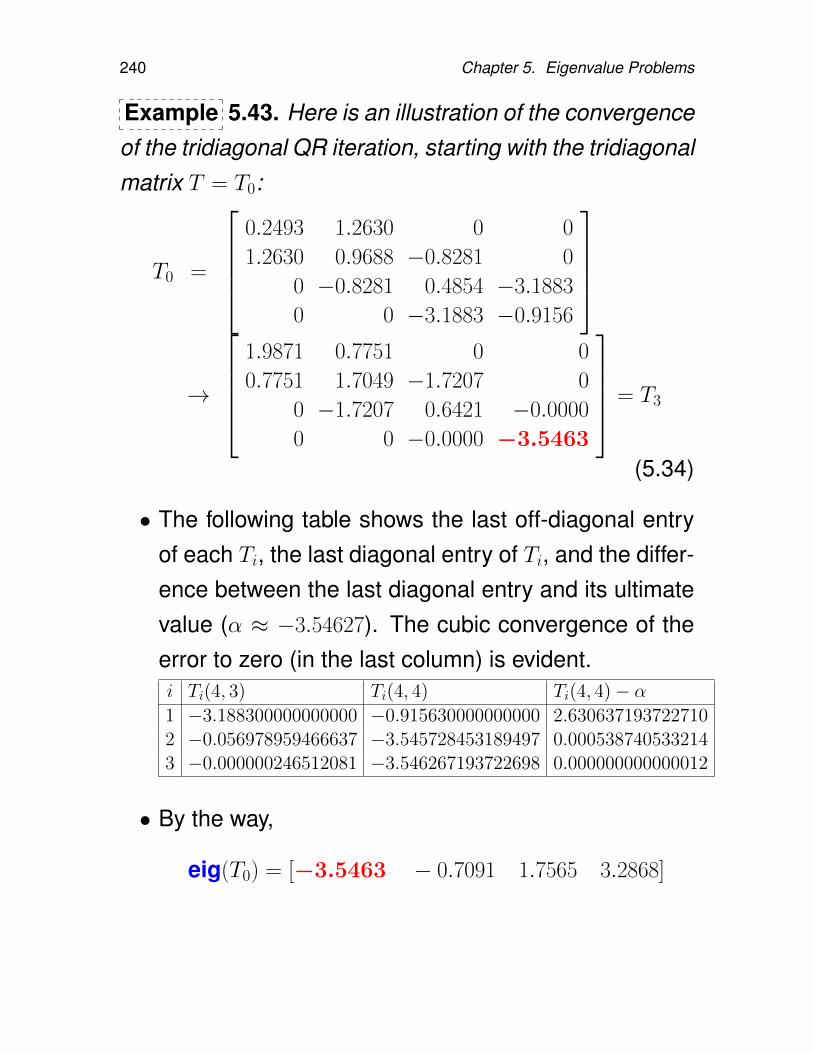
240 Chapter 5. Eigenvalue Problems
Example 5.43. Here is an illustration of the convergenceof the tridiagonal QR iteration, starting with the tridiagonalmatrix T = T0:
T0 =
0.2493 1.2630 0 0
1.2630 0.9688 −0.8281 0
0 −0.8281 0.4854 −3.1883
0 0 −3.1883 −0.9156
→
1.9871 0.7751 0 0
0.7751 1.7049 −1.7207 0
0 −1.7207 0.6421 −0.0000
0 0 −0.0000 −3.5463
= T3
(5.34)
• The following table shows the last off-diagonal entryof each Ti, the last diagonal entry of Ti, and the differ-ence between the last diagonal entry and its ultimatevalue (α ≈ −3.54627). The cubic convergence of theerror to zero (in the last column) is evident.i Ti(4, 3) Ti(4, 4) Ti(4, 4)− α1 −3.188300000000000 −0.915630000000000 2.6306371937227102 −0.056978959466637 −3.545728453189497 0.0005387405332143 −0.000000246512081 −3.546267193722698 0.000000000000012
• By the way,
eig(T0) = [−3.5463 − 0.7091 1.7565 3.2868]
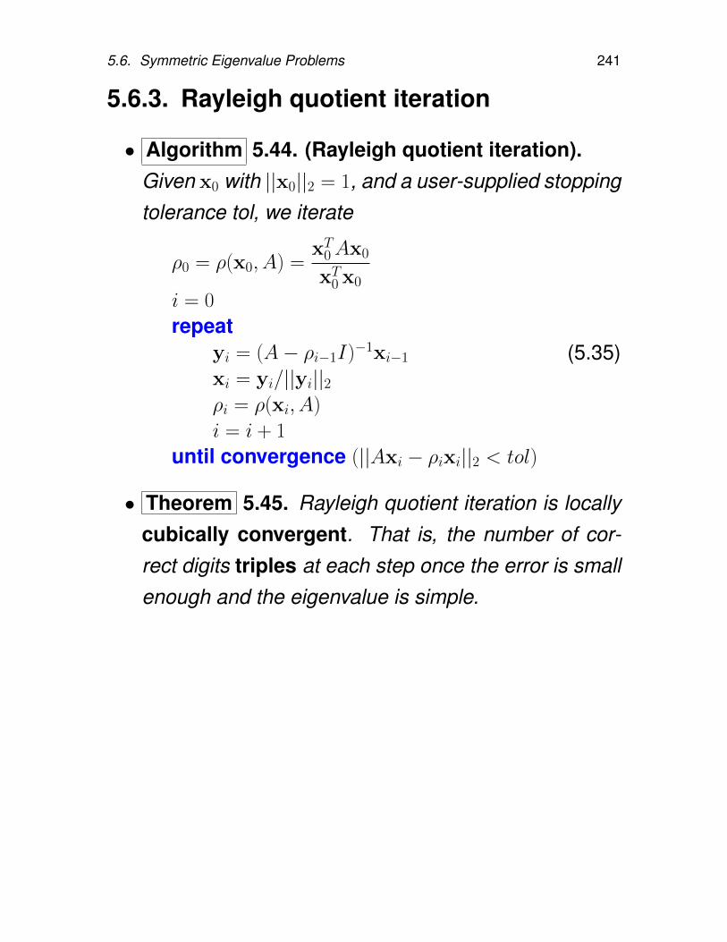
5.6. Symmetric Eigenvalue Problems 241
5.6.3. Rayleigh quotient iteration
• Algorithm 5.44. (Rayleigh quotient iteration).Given x0 with ||x0||2 = 1, and a user-supplied stoppingtolerance tol, we iterate
ρ0 = ρ(x0, A) =xT0Ax0
xT0 x0
i = 0
repeatyi = (A− ρi−1I)−1xi−1
xi = yi/||yi||2ρi = ρ(xi, A)
i = i + 1
until convergence (||Axi − ρixi||2 < tol)
(5.35)
• Theorem 5.45. Rayleigh quotient iteration is locallycubically convergent. That is, the number of cor-rect digits triples at each step once the error is smallenough and the eigenvalue is simple.
242 Chapter 5. Eigenvalue Problems
5.6.4. Divide-and-conquer
• Divide-and-conquer is the fastest algorithm so far tofind all e-values and e-vectors of a tridiagonal matrix(dim ≥ 25).
• The idea is to compute the Schur decomposition
QTTQ = Λ = diag(λ1, · · · , λn), QTQ = I, (5.36)
for tridiagonal T by
* “tearing” T in half;
* computing the Schur decompositions of the 2 parts;
* combining the 2 half-sized Schur decompositionsinto the required full size Schur decomposition.
The overall procedure is suitable for parallel compu-tation.
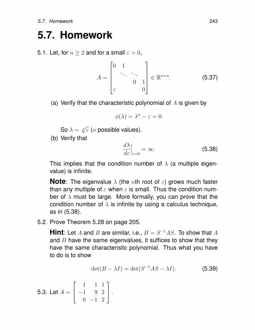
5.7. Homework 243
5.7. Homework5.1. Let, for n ≥ 2 and for a small ε > 0,
A =
0 1
. . . . . .0 1
ε 0
∈ Rn×n. (5.37)
(a) Verify that the characteristic polynomial of A is given by
φ(λ) = λn − ε = 0.
So λ = n√ε (n possible values).
(b) Verify thatdλ
dε
∣∣∣ε=0
=∞. (5.38)
This implies that the condition number of λ (a multiple eigen-value) is infinite.
Note: The eigenvalue λ (the nth root of ε) grows much fasterthan any multiple of ε when ε is small. Thus the condition num-ber of λ must be large. More formally, you can prove that thecondition number of λ is infinite by using a calculus technique,as in (5.38).
5.2. Prove Theorem 5.28 on page 205.
Hint: Let A and B are similar, i.e., B = S−1AS. To show that Aand B have the same eigenvalues, it suffices to show that theyhave the same characteristic polynomial. Thus what you haveto do is to show
det(B − λI) = det(S−1AS − λI). (5.39)
5.3. Let A =
1 1 1−1 9 2
0 −1 2
.
244 Chapter 5. Eigenvalue Problems
(a) Using Matlab, apply the inverse power iteration with the shiftσ = 9, starting with x0 = [1 1 1]T . For simplicity, just form
B = (A− 9I)−1 (B=inv(A-9*eye(3));)
and then iterate at least 10 iterations with B.(b) Use [V,D]=eig(A) to get the true dominant eigenvector v.
Calculate the errors and ratios
||xj − v||2,||xj+1 − v||2||xj − v||2
; j = 1, 2, · · · .
Compute the theoretical convergence rate (from the knowneigenvalues) and compare it with these errors/ratios.
5.4. Let
A =
−31 −35 16−10 −8 4−100 −104 49
. (5.40)
Then, we have its spectrum σ(A) = 9, 3,−2. Applying theorthogonal iteration, Algorithm 5.22, with Z0 = [e1 e2].
5.5. This problem is concerned with the QR iteration for the samematrix A in Homework 5.4.
(a) Apply Algorithm 5.24 to find eigenvalues of A.(b) Apply Algorithm 5.26, with the shift σi = Ai(3, 3), to find
eigenvalues of A.(c) Compare their convergence speeds.
5.6. Consider the matrix in Example 5.40
A =
1 6 11 16 212 7 12 17 220 8 13 18 230 0 14 19 240 0 0 20 1
.(a) Use [V,D]=eig(A) to get the true eigenvalues and eigen-
vectors of A.(b) Use the implicit single shift QR iteration to find eigenvalues
of A. Compare the results with the true eigenvalues.
Chapter 6
Iterative Methods for Linear Systems
To be filled, to be covered during Fall 2016.
245

246 Chapter 6. Iterative Methods for Linear Systems
6.1. A Model Problem

6.2. Relaxation Methods 247
6.2. Relaxation Methods

248 Chapter 6. Iterative Methods for Linear Systems
6.3. Krylov Subspace Methods
6.4. Domain Decomposition Methods 249
6.4. Domain Decomposition Methods
250 Chapter 6. Iterative Methods for Linear Systems
6.5. Multigrid Methods

6.6. Homework 251
6.6. Homework6.1.

252 Chapter 6. Iterative Methods for Linear Systems
Bibliography
1. O. ALTER, P. O. BROWN, AND D. BOTSTEIN, Singular value de-composition for genome-wide expression data processing andmodeling, PNAS, 97 (2000), pp. 10101–10106.
2. O. ALTER AND G. H. GOLUB, Integrative analysis of genome-scale data by using pseudoinverse projection predicts novel cor-relation between DNA replication and RNA transcription, PNAS,101 (2004), pp. 16577–16582.
3. N. M. BERTAGNOLLI, J. A. DRAKE, J. M. TENNESSEN, AND
O. ALTER, SVD identifies transcript length distribution functionsfrom DNA microarray data and reveals evolutionary forces glob-ally affecting GBM metabolism, PLoS One, 8 (2013), p. e78913.
4. J. W. DEMMEL, Applied Numerical Linear Algebra, SIAM,Philadelphia, 1997.
5. S. GERSCHGORIN, Uber die abgrenzung der eigenwerte einermatrix, Izv. Akad. Nauk SSSR Ser. Mat., 7 (1931), pp. 746–754.
6. F. GOLUB AND C. V. LOAN, Matrix Computations, 3rd Ed., TheJohns Hopkins University Press, Baltimore, 1996.
7. M. G. SHIRANGI, History matching production data and uncer-tainty assessment with an efficient TSVD parameterization al-gorithm, Journal of Petroleum Science and Engineering, 113(2014), pp. 54–71.
8. O. TAUSSKY, Bounds for characteristic roots of matrices, DukeMath. J., 15 (1948), pp. 1043–1044.
9. L. N. TREFETHEN AND D. BAU, Numerical Linear Algebra,SIAM: Society for Industrial and Applied Mathematics, 1997.
253
254 Bibliography
10. R. VARGA, Matrix Iterative Analysis, 2nd Ed., Springer-Verlag,Berlin, Heidelberg, 2000.
11. S. WALTON, O. HASSAN, AND K. MORGAN, Reduced ordermodelling for unsteady fluid flow using proper orthogonal de-composition and radial basis functions, Applied MathematicalModelling, 37 (2013), pp. 8930–8945.
12. D. WATKINS, Foundations of Matrix Computations, 3rd Ed., JohnWiley and Sons, New York, Chichester, Brisbane, Toronto, Sin-gapore, 2010.
13. J. H. WILKINSON, The Algebraic Eigenvalue Problem, OxfordUniversity Press, 1965. (reprint 1988).
Index
A-norm, 8algebraic multiplicity, 173
back substitution, 33backward error, 122backward stable, 122Bauer-Fike theorem, 178bidiagonal reduction, 214, 217bisection and inverse iteration,
235bulge-and-chase, 223
Cauchy-Schwarz inequality, 8characteristic polynomial, 172Cholesky factorization, 58, 63,
76classical Gram-Schmidt process,
84colon notation, 5companion matrix, 232condition number, 12, 177covariance matrix, 141, 161
defective, 173diagonalizable, 173direct algebraic solver, 23directed graph, 186Dirichlet boundary condition, 29discrete least-squares, 72Divide-and-conquer, 242Divide-and-conquer method, 234
domain decomposition method,249
dot product, 4double implicit shift, 197dyadic decomposition, 132
eigendecomposition, 140eigenpair, 172eigenvalue decomposition, 172elementary matrix, 35elementary row operations, 34equal-volume fitting ellipsoid, 160Euclidean norm, 7
fellow matrix, 232finite difference scheme, 26floating point operation, 6flop, 6forward substitution, 32Francis QR iteration, 197Frobenius norm, 9fundamental theorem of algebra,
175
Gauss elimination, 34Gaussian elimination with par-
tial pivoting, 52gaxpy, 4geometric multiplicity, 173Gerschgorin’s theorem, 182ghost grid value, 27Givens rotation, 113, 211
255
256 Index
Gram-Schmidt process, 78
Hadamard product, 4Hessenberg decomposition, 197Hessenberg matrix, 197, 205Hessenberg reduction, 206Hessenberg, unreduced, 209Hessian matrix, 75House, 101Householder bidiagonalization al-
gorithm, 219Householder matrix, 97Householder reflection, 95, 96Householder tridiagonalization al-
gorithm, 215
ill-conditioned, 16image compression, 148Implicit double shift QR algorithm,
231implicit Q theorem, 221induced norm, 9infinity-norm, 7inner product, 4invariant subspace, 198inverse matrix, 24inverse power iteration, 195inverse power method, 195invertible matrix, 24invertible matrix theorem, 24irreducible matrix, 185iterative algebraic solver, 23
Jacobi’s method, 235Jordan canonical form, 174
Krylov subspace method, 248
Lagrange multiplier, 160
LDLT factorization, 63leading principal submatrix, 38least-squares problem, 72left eigenvector, 174left singular vectors, 129linear least-squares problem, 72lower-triangular matrix, 30LU decomposition theorem, 38
M-matrix, 67matrix norms, 9matrix operations, 2matrix-vector multiplication, 4maximum-norm, 7minimum-norm solution, 151minimum-volume enclosing el-
lipsoid, 160modified Gram-Schmidt process,
85multigrid method, 250mutually consistent, 9
nodal point, 186nonsingular matrix, 24normal equation, 74normal matrix, 10numerical rank, 145
operator norm, 9orthogonal basis, 78orthogonal decomposition, 95orthogonal iteration, 198orthogonal matrix, 10, 94, 114orthonormal basis, 80outer bordering, 28
p-norms, 7parallel computation, 242
Index 257
Peppers image, 149permutation matrix, 49, 185plane rotator, 115polynomial factorization, 175positive definite, 75power method, 190principal component analysis, 158principal components, 158projection, 95pseudoinverse, 136PSNR, 150
QR decomposition, 81QR iteration, 201QR iteration, with a shift, 202QR iteration, without shifts, 201quasi-upper triangular, 175
rank, 19rank-deficient least-squares prob-
lem, 128, 151rank-deficient matrix, 128Rayleigh quotient, 189Rayleigh quotient iteration, 234,
241reducible matrix, 185reflection matrix, 115reflector, 95, 97relaxation method, 247residual, 189right eigenvector, 174right singular vectors, 129
saxpy, 4Schur canonical form, 175Schur decomposition, 139, 242semi-axis of an ellipsoid, 160shift, 195
similar, 205similarity, 172similarity transformation, 205simultaneous iteration, 198single shift QR algorithm, 223singular value decomposition, 129singular values, 129sstevd, 234stability, 18Stieltjes matrix, 67strictly diagonally dominant, 184strictly upper triangular, 20strong stability, 18strongly connected directed graph,
187subordinate norm, 9subspace iteration, 198SVD theorem, 129symmetric positive definite, 58symmetric positive semidefinite,
62
transforming matrix, 205triangular systems, 30tridiagonal QR iteration, 233tridiagonal reduction, 214
unit roundoff error, 146upper bidiagonal, 217upper-triangular matrix, 30
vector multiply, 4vector norm, 7vector operations, 4
well-conditioned, 16Wilkinson theorem, 238Wilkinson’s shift, 238