future demand analysis introduction

April 9, 2021

Santa Clara Valley Water District of 30 Technical Memorandum 4 Future Demand Analysis

April 9, 2021

To: Samantha Greene, Ph.D.

From: Luke Wang Jack Kiefer Kinsey Hoffman Leah Bensching

cc: Jing Wu, Metra Richert, Jessica Lovering

Technical Memorandum 4 Future Demand Analysis

Introduction

Santa Clara Valley Water District (Valley Water) has developed a new model to forecast total water demand in Santa Clara County. Demand projections from the model will be used to support several planning initiatives and documents including:

• The 2021 Urban Water Management Plan (UWMP); • Monitoring of and updates to the Water Supply Master Plan; • Inputs to Valley Water’s water supply planning model; and • Evaluation of conservation programs and other water supply investments.

Valley Water manages a diverse portfolio of water supplies to provide water to Santa Clara County’s independent well owners and thirteen water supply retailers. The majority of water users in Santa Clara County are direct customers of the water supply retailers. As a result, each retailer develops their own water demand forecasts. These forecasts are useful and have been used to inform Valley Water’s prior UWMPs. However, since Valley Water is the wholesale water provider to the County retailers and other independent well owners throughout the County, Valley Water needs to ensure the agency invests in sufficient water supplies to meet future needs without overinvesting. Therefore, Valley Water had a demand model developed for the County that uses a consistent modeling approach and planning assumptions across the service area.

The purpose of this Technical Memorandum (TM 4) is to document the future demand analysis, including data collection, data processing, and assumptions for baseline demand projections. The models establish demand projections from 2020 to 2045 at a monthly timestep. Demand projections presented in this TM do not consider additional water conservation. Projections of future conservation savings are generated separately by Valley Water and then deducted from the baseline projections. Data sources documented in this TM are limited to projected future datasets. Review of historical datasets are documented in TM2: Data Collection and Review, and review of the modeling approach is documented in TM3: Modeling Approach and Development.

April 9, 2021


Table of Contents 1. Baseline Scenario Assumptions................................................................................... 3

1.1 Evaluation of ABAG Projections ............................................................................................. 4

1.2 Model Calibration ................................................................................................................... 4

2. Development of Forecast Inputs .................................................................................. 5

2.1 Retailer Driver Units ............................................................................................................... 5

2.2 Weather and Climate ............................................................................................................. 8

2.3 Water Prices .......................................................................................................................... 9

2.4 Detrended Economic Factor ................................................................................................. 11

2.5 Median Income .................................................................................................................... 11

2.6 Housing Density ................................................................................................................... 11

2.7 Persons Per Household ....................................................................................................... 12

2.8 Relative Sectoral Employment.............................................................................................. 13

2.9 Drought Rebound ................................................................................................................. 14

2.10 Seasonality .......................................................................................................................... 15

3. Baseline Sectoral Forecasts....................................................................................... 16

3.1 Single Family ....................................................................................................................... 16

3.2 Multifamily ............................................................................................................................ 17

3.3 CII ........................................................................................................................................ 17

3.4 Non-Retail Pumpers ............................................................................................................. 18

3.5 “Other” Consumption ............................................................................................................ 21

3.6 Nonrevenue Water ............................................................................................................... 22

3.7 Raw Water ........................................................................................................................... 23

3.8 County-Wide Totals.............................................................................................................. 24

4. Forecast Impact Factor Analysis ................................................................................ 24

5. Future Considerations ................................................................................................ 30

6. Summary ..................................................................................................................... 30

April 9, 2021


1. Baseline Scenario Assumptions

This section reviews the future conditions and assumptions that define Valley Water’s baseline demand scenario. Future conditions and assumptions were defined for each element of the water demand model, including sectoral driver units and explanatory variables. Growth in driver units was tied to the Association of Bay Area Governments (ABAG) projections for relevant metrics through 2040, as published in 2017. Conditions for all other explanatory variables were selected to represent expected changes or to remain constant. A summary of the baseline demand scenario assumptions for driver units and explanatory variables are summarized in Table 1-1. Development of future datasets used to define the inputs are further detailed in Section 2.

Table 1-1: Summary of Baseline Scenario Data Sources and Assumptions

Input Source Assumptions

Driver Units ABAG • Initialized with historical 2018 value and grown using the rate of

change in ABAG projected single family housing units, multifamily housing units, non-agricultural jobs, and population (a)

Monthly Maximum temperature and Total Precipitation

PRISM • 30-year historical normal weather (b)

Water Rates Retailers • Price grows in time based on the 2020 PAWS report rates from

2020-2030, then increase each year by 5% after that (c) • Prices are adjusted for inflation assuming 3% each year

Detrended Economic Factor

Economic Cycles Research Institute

(ECRI) Coincident Index

• Assume long-term trend economy based on the detrended ECRI coincident index

Median Income US Census • Assume constant income at 2018 value (real dollars)

Housing Density ABAG

• North County retailers assume housing density derived from ABAG projected housing units divided by constant (2018) residential acres

• South County retailers assume constant density at 2018 value Persons Per Household (PPH)

ABAG • Initialized with historical 2018 value and grown using rate of change in ABAG total PPH projections

Relative Sectoral Employment ABAG • Calculated based on ABAG projections of non-agricultural jobs

Drought Rebound N/A (d) • Assumes a 50% rebound by 2025 in water use following the last

drought period

Seasonality - • Sine/cosine functions to capture monthly pattern

(a) Stanford University is the only retail agency utilizing population as a driver unit. (b) Climate change scenarios use General Circulation Model (GCM) projections of temperature and precipitation were also developed, but not applied to the baseline scenario. Climate change projections are further discussed in Section 2.2. (c) A constant water rate scenario was also considered, which assumed 2018 deflated price value. (d) Representation of drought rebound is further discussed in Section 0.

April 9, 2021


1.1 Evaluation of ABAG Projections

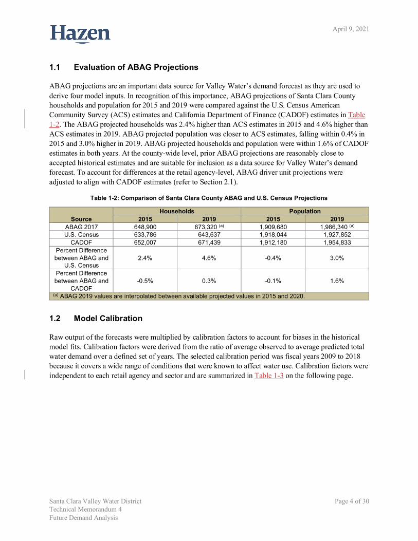
ABAG projections are an important data source for Valley Water’s demand forecast as they are used to derive four model inputs. In recognition of this importance, ABAG projections of Santa Clara County households and population for 2015 and 2019 were compared against the U.S. Census American Community Survey (ACS) estimates and California Department of Finance (CADOF) estimates in Table 1-2. The ABAG projected households was 2.4% higher than ACS estimates in 2015 and 4.6% higher than ACS estimates in 2019. ABAG projected population was closer to ACS estimates, falling within 0.4% in 2015 and 3.0% higher in 2019. ABAG projected households and population were within 1.6% of CADOF estimates in both years. At the county-wide level, prior ABAG projections are reasonably close to accepted historical estimates and are suitable for inclusion as a data source for Valley Water’s demand forecast. To account for differences at the retail agency-level, ABAG driver unit projections were adjusted to align with CADOF estimates (refer to Section 2.1).

Table 1-2: Comparison of Santa Clara County ABAG and U.S. Census Projections

Source Households Population

2015 2019 2015 2019 ABAG 2017 648,900 673,320 (a) 1,909,680 1,986,340 (a) U.S. Census 633,786 643,637 1,918,044 1,927,852

CADOF 652,007 671,439 1,912,180 1,954,833 Percent Difference between ABAG and

U.S. Census 2.4% 4.6% -0.4% 3.0%

Percent Difference between ABAG and

CADOF -0.5% 0.3% -0.1% 1.6%

(a) ABAG 2019 values are interpolated between available projected values in 2015 and 2020.

1.2 Model Calibration

Raw output of the forecasts were multiplied by calibration factors to account for biases in the historical model fits. Calibration factors were derived from the ratio of average observed to average predicted total water demand over a defined set of years. The selected calibration period was fiscal years 2009 to 2018 because it covers a wide range of conditions that were known to affect water use. Calibration factors were independent to each retail agency and sector and are summarized in Table 1-3 on the following page.

April 9, 2021


Table 1-3: Calibration Factors by Sector and Retailer

Retail Agency

Single Family

Residential Multifamily Residential CII

Agricultural Water Use

M&I Water Use

California Water Service 1.134 0.995 0.972 - - City of Gilroy 0.996 1.005 0.998 - - City of Milpitas 1.005 1.024 1.003 - - City of Morgan Hill 0.911 0.963 1.004 - - City of Mountain View 0.932 0.984 0.988 - - City of Palo Alto 0.995 0.995 1.089 - - City of Santa Clara 1.012 1.050 1.002 - - City of Sunnyvale 0.997 0.971 0.999 - - Great Oaks Water Company 1.006 1.014 0.999 - - Purissima Hills Water District 1.001 - 0.956 - - San Jose Municipal Water 0.982 1.047 1.003 - - San Jose Water Company 1.004 1.011 1.009 - - Stanford University - - 1.003 - - Independent Pumpers, W2 - - - 1.000 1.000 Independent Pumpers. W5 - - - 1.000 0.998

2. Development of Forecast Inputs

This section reviews the data sources and methodology applied to develop future values of variables contained in the demand model.

2.1 Retailer Driver Units

Driver units reflect the size or scale of a water use sector and allow for differentiation of rate of use from total consumption. The selected driver units for each model sector are shown in Table 2-1. All driver units were derived from the ABAG 2017 Plan Bay Area Projections 20401, which estimate single family residential housing units, multifamily residential housing units, jobs by sector, and total population at five-year intervals from 2015 through 2040. Driver units of jobs for the CII model sector were calculated as the total number of non-agricultural jobs from the ABAG jobs categories, which included: Health, Education and Recreational Service; Financial and Professional Services; Informational, Government and Construction; Manufacturing, Wholesale and Transportation; and Retail.

Table 2-1: Driver Units by Model Sector

Model Sector Driver Unit Single Family Housing Units Multifamily Housing Units CII Jobs, Population (for Stanford only) Other N/A(a)

(a) Other water use was projected as a percentage of total single family, multifamily, and CII consumption. See Section 3.5.

1 Association of Bay Area Governments (ABAG), 2017. Plan Bay Area Projections 2040. Accessed from http://projections.planbayarea.org/.

http://projections.planbayarea.org/

April 9, 2021


ABAG projections were available at census tract level geographies, which required geoprocessing to retailer service area boundaries. Geoprocessing was performed using GIS overlays of census tract boundaries and retail agency service area boundaries to aggregate ABAG projections by retail agency; this geoprocessing is described further in TM2: Data Collection and Review.

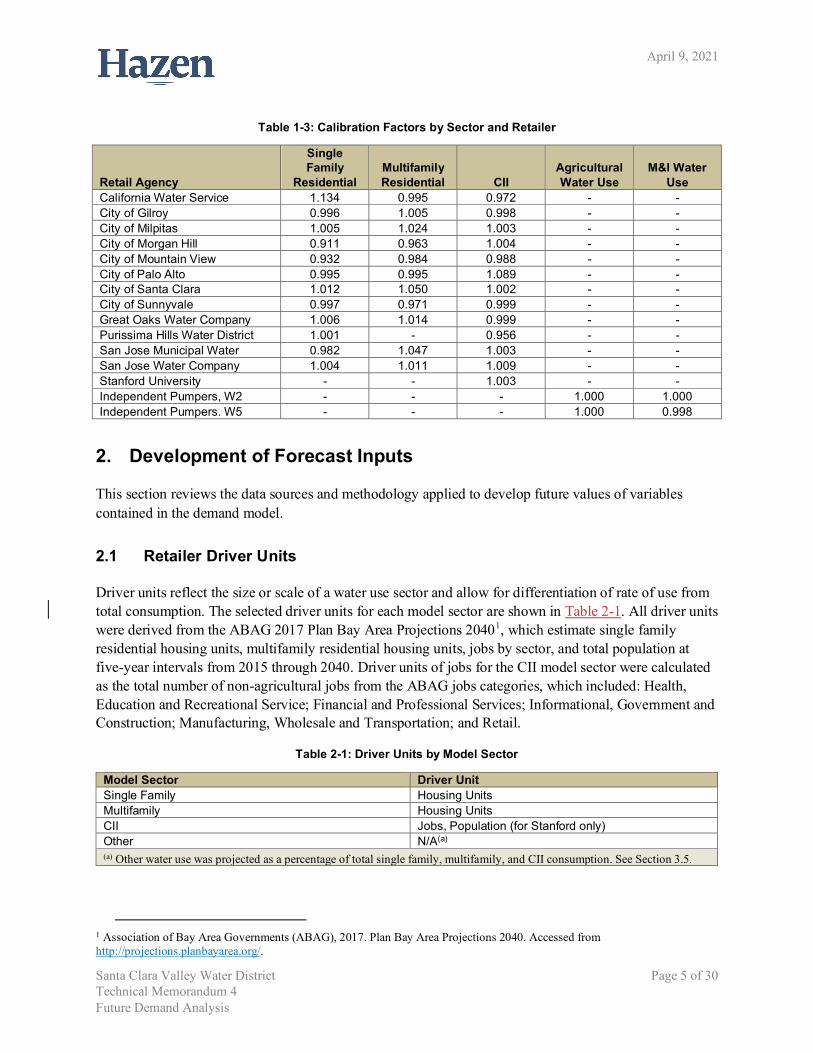
ABAG projections at the retailer level did not always align in magnitude with the historical driver units. To ensure consistency from historical to future datasets, the future time series for driver units were developed by calculating the rate of change in the ABAG projections and modifying the last historical value (CADOF estimate) of the driver units by the corresponding ABAG rate of change. Further, the future driver units needed to be extended to 2045, the end year of the demand projections. The rate of change in ABAG projections from 2035 to 2040 was repeated for the period from 2040 to 2045 in order to extrapolate the projected driver unit values to 2045. An illustration of the difference between ABAG projections, historical driver units, and projected driver units for a sample retail agency is shown in Figure 2-1. The resulting county-wide projected driver units are shown in Figure 2-2 (housing units) and Figure 2-3 (total non-agricultural jobs). Time series plots of processed future driver units by retailer are included in the appendices associated with sectoral demand forecasts described in Section 3.

Figure 2-1: Example of ABAG Projections and Driver Units

April 9, 2021


Figure 2-2: County Wide ABAG-Derived Housing Unit Projections

Figure 2-3: County Wide ABAG-Derived Total Non-Agricultural Job Projections

April 9, 2021


2.2 Weather and Climate

For the water demand model baseline scenario, future precipitation and temperature values were assumed to be equal to historical normal values. Historical normal values were calculated as the average values by month based on all values from 1981 to 2010. As defined in TM3: Model Approach and Development, the demand model uses departures from historical normal precipitation and temperature for the retailer forecasts and unadjusted historical normal precipitation and temperature for non-retail pumper forecasts. Given this, future weather inputs in the retailer forecasts are reflected by a projected departure values of 0 for the precipitation and temperature variables.

Additional demand scenarios can be developed that consider the potential effects of climate change on precipitation and temperature using data from 16 downscaled global circulation models (GCMs) recommended by Professor Ed Maurer of Santa Clara University.2 These GCMs include the 10 GCMs recommended for California by the California Department of Water Resources Climate Change Technical Advisory Group.3 Historical precipitation and temperature time series were developed using a different dataset: PRISM (refer to TM2: Data Collection and Review for further detail). To correct for this difference in source data and to generate future values, the PRISM historical normal values were multiplied by the ratio of GCM projected values to GCM historical values calculated over the same time period as the PRISM historical normal (1981 to 2010). This adjustment is shown in the Equation 1 below.

𝑃𝑃𝑃𝑃𝑃𝑃𝑃𝑃𝑃𝑃𝑓𝑓𝑓𝑓𝑓𝑓𝑓𝑓𝑓𝑓𝑓𝑓 = 𝑃𝑃𝑃𝑃𝑃𝑃𝑃𝑃𝑃𝑃ℎ𝑖𝑖𝑖𝑖𝑓𝑓𝑖𝑖𝑓𝑓𝑖𝑖𝑖𝑖𝑖𝑖𝑖𝑖 𝑛𝑛𝑖𝑖𝑓𝑓𝑛𝑛𝑖𝑖𝑖𝑖 ∗𝐺𝐺𝐺𝐺𝑃𝑃𝑓𝑓𝑓𝑓𝑓𝑓𝑓𝑓𝑓𝑓𝑓𝑓

𝐺𝐺𝐺𝐺𝑃𝑃ℎ𝑖𝑖𝑖𝑖𝑓𝑓𝑖𝑖𝑓𝑓𝑖𝑖𝑖𝑖𝑖𝑖𝑖𝑖 𝑛𝑛𝑖𝑖𝑓𝑓𝑛𝑛𝑖𝑖𝑖𝑖 (1)

Table 2-2 on the following page presents the average forecasted percentage change in precipitation and temperature between the PRISM historical normal and projected 2040 values. This percent change was applied to the historical normal values for each retailer.

2 Santa Clara University - Santa Clara Valley Water District Collaboration on Estimating Local Climate Change Projections: Update for 2018. Draft Final Report. October 31, 2018. 3 California Department of Water Resources (DWR) Climate Change Technical Advisory Group (CCTAG). 2015. Perspectives and Guidance for Climate Change Analysis. 142 pages.

April 9, 2021


Table 2-2: Average Percent Change in Precipitation and Temperature between Historical Normal and Projected 2040 Values

GCM Precipitation Temperature access1-0 -14% 4.4% canesm2 36% 5.4% ccsm4 0.3% 3.2% cesm1-bgc 42% 3.2% cmcc-cms 12% 3.9% cnrm-cm5 57% 2.8% csiro-mk3-6-0 32% 4.3% gfdl-cm3 16% 5.2% gfdl-esm2g 28% 3.5% hadgem2-cc 29% 4.6% hadgem2-es -6.6% 6.0% inmcm4 4.1% 2.6% miroc5 -11% 4.1% mpi-esm-lr 91% 3.8% mri-cgcm3 32% 2.0% noresm1-m 32% 3.9%

2.3 Water Prices

Projections of future water rates were included as an explanatory variable in the water demand model. Two future paths for water prices were considered: a constant rate scenario that assumes constant inflation-adjusted water rates from 2018 and a variable price scenario based on Valley Water’s proposed water charges from the 2020-21 Protection and Augmentation of Water Supplies (PAWS) 2020 Report. The variable prices were derived by modifying the last historical water rate value (from 2018) by the rate of change in price per year from the PAWS 2020 Report values available from 2020 to 2030 and a 5% increase each subsequent year from 2035-2045. These nominal prices were adjusted for inflation assuming 3% each year. The inflation-adjusted water rates in dollars per hundred cubic feet (2015$/ccf) for each retailer are shown in Table 2-3 on the following page.

For Stanford, the projected water rates were similarly derived from the rate of change in the PAWS 2020 report. Historical water rates were based on the Water Utility Enterprise (WUE) rate (see TM2: Data Collection and Review for more detail) in dollars per acre-foot ($/AF). Projected water rates used the last historical WUE rate value and were updated over time following the inflation-adjusted rate of change from the PAWS 2020 report. Stanford projected water rates are also shown in Table 2-3. Water rates for non-retail pumpers were held constant at 2018 historical values.

April 9, 2021


Table 2-3: Water Rates (2015$/ccf) by Retailer

Year California

Water Service

City of

Gilroy

City of Milpitas

City of Morgan

Hill

City of Mountain

View

City of Palo Alto

City of Santa Clara

City of Sunny-

vale

Great Oaks Water

Company

Purissima Hills

Water District

San Jose Muni-cipal

Water

San Jose Water

Company Stanford (a)

2019 $5.04 $3.90 $0.98 $2.26 $6.21 $8.54 $5.41 $4.85 $3.17 $6.13 $3.62 $3.42 $2.56 2020 $5.22 $4.05 $1.01 $2.35 $6.44 $8.85 $5.60 $5.02 $3.28 $6.35 $3.75 $3.55 $2.65 2021 $5.51 $4.31 $1.07 $2.50 $6.80 $9.34 $5.92 $5.30 $3.47 $6.71 $3.96 $3.74 $2.80 2022 $5.82 $4.58 $1.13 $2.66 $7.18 $9.86 $6.25 $5.60 $3.66 $7.08 $4.18 $3.95 $2.95 2023 $6.15 $4.87 $1.19 $2.83 $7.58 $10.42 $6.60 $5.91 $3.87 $7.48 $4.41 $4.18 $3.12 2024 $6.49 $5.18 $1.26 $3.01 $8.00 $11.00 $6.97 $6.24 $4.08 $7.90 $4.66 $4.41 $3.29 2025 $6.85 $5.51 $1.33 $3.20 $8.45 $11.61 $7.36 $6.59 $4.31 $8.34 $4.92 $4.66 $3.48 2026 $7.24 $5.86 $1.40 $3.40 $8.93 $12.27 $7.77 $6.96 $4.55 $8.81 $5.20 $4.92 $3.67 2027 $7.65 $6.24 $1.48 $3.62 $9.43 $12.95 $8.21 $7.35 $4.81 $9.30 $5.49 $5.19 $3.88 2028 $8.07 $6.63 $1.56 $3.85 $9.95 $13.68 $8.66 $7.76 $5.08 $9.82 $5.79 $5.48 $4.10 2029 $8.53 $7.05 $1.65 $4.09 $10.51 $14.44 $9.15 $8.20 $5.36 $10.37 $6.12 $5.79 $4.33 2030 $9.00 $7.50 $1.74 $4.35 $11.10 $15.25 $9.66 $8.66 $5.66 $10.95 $6.46 $6.11 $4.57 2031 $9.18 $7.65 $1.78 $4.44 $11.32 $15.56 $9.85 $8.83 $5.77 $11.17 $6.59 $6.24 $4.66 2032 $9.37 $7.81 $1.82 $4.53 $11.55 $15.87 $10.05 $9.01 $5.89 $11.40 $6.72 $6.36 $4.75 2033 $9.55 $7.96 $1.85 $4.62 $11.78 $16.18 $10.25 $9.19 $6.01 $11.62 $6.86 $6.49 $4.85 2034 $9.75 $8.12 $1.89 $4.71 $12.01 $16.51 $10.46 $9.37 $6.13 $11.86 $6.99 $6.62 $4.94 2035 $9.94 $8.28 $1.93 $4.81 $12.25 $16.84 $10.67 $9.56 $6.25 $12.09 $7.13 $6.75 $5.04 2036 $10.14 $8.45 $1.96 $4.90 $12.50 $17.18 $10.88 $9.75 $6.38 $12.34 $7.28 $6.89 $5.14 2037 $10.34 $8.62 $2.00 $5.00 $12.75 $17.52 $11.10 $9.95 $6.50 $12.58 $7.42 $7.02 $5.25 2038 $10.55 $8.79 $2.04 $5.10 $13.00 $17.87 $11.32 $10.15 $6.63 $12.83 $7.57 $7.16 $5.35 2039 $10.76 $8.97 $2.09 $5.20 $13.26 $18.23 $11.55 $10.35 $6.77 $13.09 $7.72 $7.31 $5.46 2040 $10.97 $9.15 $2.13 $5.31 $13.53 $18.59 $11.78 $10.56 $6.90 $13.35 $7.88 $7.45 $5.57 2041 $11.19 $9.33 $2.17 $5.41 $13.80 $18.96 $12.01 $10.77 $7.04 $13.62 $8.04 $7.60 $5.68 2042 $11.42 $9.52 $2.21 $5.52 $14.08 $19.34 $12.25 $10.98 $7.18 $13.89 $8.20 $7.75 $5.79 2043 $11.65 $9.71 $2.26 $5.63 $14.36 $19.73 $12.50 $11.20 $7.32 $14.17 $8.36 $7.91 $5.91 2044 $11.88 $9.90 $2.30 $5.74 $14.64 $20.12 $12.75 $11.43 $7.47 $14.45 $8.53 $8.07 $6.03 2045 $12.12 $10.10 $2.35 $5.86 $14.94 $20.53 $13.00 $11.65 $7.62 $14.74 $8.70 $8.23 $6.15 (a) Stanford water rates are presented in this table in dollars per ccf but were included in the demand model in dollars per acre-ft ($/AF).

April 9, 2021


2.4 Detrended Economic Factor

For the baseline water demand forecast, the future economy was assumed to be at long term trend. The Economic Cycles Research Institute (ECRI) coincident index is a measure of the macro-economy that captures cycles in economic activity based on tracking indicators of production, employment, income, and sales. Historically, the ECRI index is characterized by long-term positive growth with shorter-term fluctuations of higher or lower than average growth related to business cycles. The detrended ECRI index provides focus on potentially meaningful periods of more acute economic fluctuations to capture the effects of the business cycle on unit rates of water consumption. The assumption of long term trend economy for the baseline forecast scenario assumed the ECRI index followed the long-term historical trend, represented by a projected value of 0 for the detrended ECRI coincident index.

2.5 Median Income

Median income was included as an explanatory variable in the water demand model. Median income by retailer was held constant at the historical 2018 level denominated in inflation-adjusted 2015 dollar values, as shown in Table 2-4.

Table 2-4: Median Household Income

Agency Median Income California Water Service $156,235 City of Gilroy $91,643 City of Milpitas $108,352 City of Morgan Hill $109,752 City of Mountain View $138,060 City of Palo Alto $144,307 City of Santa Clara $107,272 City of Sunnyvale $125,285 Great Oaks Water Company $108,184 Purissima Hills Water District $206,783 San Jose Municipal Water $116,052 San Jose Water Company $106,368

2.6 Housing Density

Housing density was included as an explanatory variable in the single family and multifamily residential model sectors. Separate variables were created for single family housing density and multifamily housing density. Two scenario options for density were considered based on discussions with Valley Water staff: a constant density condition and a variable density condition. The constant density condition assumed a “build out” scenario where development of additional housing units would occur in new land area at prevailing historical densities, while the variable density condition assumed a “build up” scenario where housing units could vary within a constant land area thereby affecting average density. Retail agencies in the South County (Gilroy and Morgan Hill) were assumed to have constant housing density and all other retail agencies were assumed to have variable housing density. Constant density was held at the last historical value. Variable density was derived from the projected number of single family or multifamily

April 9, 2021


housing units (see Section 2.1) divided by the land area classified as residential land use within the retail service area boundary.

Table 2-5 shows the housing density values for each retailer in 2045 (representing the variable density option) compared to the last historical value (representing the constant density option). Time series graphs of variable density for each retailer are in Appendix A.

Table 2-5: Single Family and Multifamily Residential Housing Density (Units/Acre)

Agency 2019 2045

Single Family Housing Density

Multifamily Housing Density

Single Family Housing Density

Multifamily Housing Density

California Water Service 3.14 16.08 3.17 18.90 City of Gilroy 5.92 5.26 5.92 5.26 City of Milpitas 6.74 22.92 7.25 38.10 City of Morgan Hill 2.78 8.87 2.78 8.87 City of Mountain View 10.89 21.16 11.51 33.39 City of Palo Alto 4.74 35.61 4.75 41.23 City of Santa Clara 6.83 31.42 6.88 40.86 City of Sunnyvale 8.47 20.02 8.62 41.13 Great Oaks Water Company 7.22 22.43 8.13 27.98 Purissima Hills Water District 0.74 -- 0.75 -- San Jose Municipal Water 5.45 23.21 5.62 73.55 San Jose Water Company 5.54 21.35 5.66 37.18

2.7 Persons Per Household

Persons per household was used as an explanatory variable in the single family and multifamily residential model sectors. Separate variables were created for single family persons per household and multifamily persons per household. The ABAG 2017 projections provide future estimates of total persons per household. Future conditions for persons per household were derived by modifying the last historical single family and multifamily persons per household values by the rate of change in the ABAG overall persons per household projections. 2045 projected persons per household by retailer are shown in Table 2-6. Time series values of persons per household for each retailer are in Appendix B.

Table 2-6: Projected Persons Per Household in 2045

Retail Agency Single Family Persons per Household Multifamily Persons per Household California Water Service 3.00 2.52 City of Gilroy 3.90 3.82 City of Milpitas 3.77 2.84 City of Morgan Hill 3.38 3.19 City of Mountain View 2.89 2.29 City of Palo Alto 2.95 2.01 City of Santa Clara 3.09 2.42 City of Sunnyvale 3.03 2.46 Great Oaks Water Company 3.54 3.05 Purissima Hills Water District 2.98 2.99 San Jose Municipal Water 3.49 2.36 San Jose Water Company 3.38 2.64

April 9, 2021


2.8 Relative Sectoral Employment

Ratios of sectoral employment were included as an explanatory variable in the CII model sector. These ratios of sectoral employment represent the estimated mix of CII activity within each retail service area. The projected number of jobs by sector were obtained from the ABAG 2017 projections, as described in Section 2.1. The projected ratios of sectoral employment were then calculated as the number of jobs in each sector divided by the total non-agricultural jobs. A summary of projected ratios of sectoral employment in 2045 is shown in Table 2-7. Time series values of sectoral employment ratios for each retailer are in Appendix C.

Table 2-7: Projected Ratio of Sectoral Employment by ABAG Sector and Retailer in 2045

Retail Agency

Health, Educational, and

Recreational Service

Financial and

Professional Services

Informational, Government

and Construction

Manufacturing, Wholesale and Transportation

Retail

California Water Service 39% 16% 3% 35% 8% City of Gilroy 41% 5% 10% 15% 29% City of Milpitas 27% 26% 13% 23% 12% City of Morgan Hill 32% 11% 12% 30% 15% City of Mountain View 28% 25% 34% 5% 8% City of Palo Alto 38% 28% 19% 8% 7% City of Santa Clara 28% 39% 9% 18% 6% City of Sunnyvale 29% 35% 11% 17% 8% Great Oaks Water Company 51% 11% 6% 22% 12% Purissima Hills Water District 55% 11% 8% 10% 16% San Jose Municipal Water 24% 26% 17% 27% 5% San Jose Water Company 41% 20% 12% 13% 13% Stanford 42% 38% 10% 8% 2%

April 9, 2021


2.9 Drought Rebound

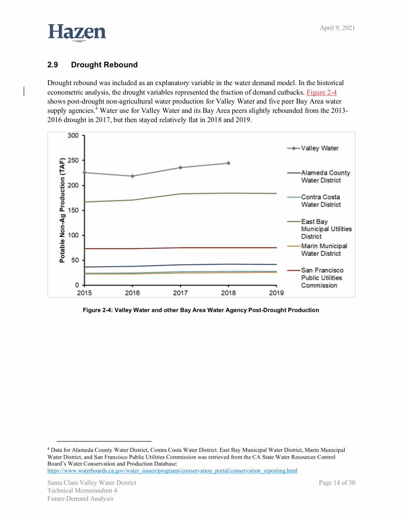
Drought rebound was included as an explanatory variable in the water demand model. In the historical econometric analysis, the drought variables represented the fraction of demand cutbacks. Figure 2-4 shows post-drought non-agricultural water production for Valley Water and five peer Bay Area water supply agencies.4 Water use for Valley Water and its Bay Area peers slightly rebounded from the 2013-2016 drought in 2017, but then stayed relatively flat in 2018 and 2019.

Figure 2-4: Valley Water and other Bay Area Water Agency Post-Drought Production

4 Data for Alameda County Water District, Contra Costa Water District. East Bay Municipal Water District, Marin Municipal Water District, and San Francisco Public Utilities Commission was retrieved from the CA State Water Resources Control Board’s Water Conservation and Production Database: https://www.waterboards.ca.gov/water_issues/programs/conservation_portal/conservation_reporting.html

https://nam12.safelinks.protection.outlook.com/?url=https%3A%2F%2Fwww.waterboards.ca.gov%2Fwater_issues%2Fprograms%2Fconservation_portal%2Fconservation_reporting.html&data=02%7C01%7CLwang%40hazenandsawyer.com%7C027380df5224439ca55508d83ef24b32%7C083fc4d272ad412bae7d6b81b83916dd%7C0%7C0%7C637328558652982433&sdata=YfTw3bdj6gyvmkdv2M74I2byO70%2BnRn8UreIrdtTJY8%3D&reserved=0

April 9, 2021


It is expected that there are some behavioral changes adopted during the last drought that will dissipate in the future, but there are also possible permanent changes that could preclude a full drought rebound, such as reduced water use due to increased rates or removal or replacement of landscape materials. To approximate this drought rebound and potential persistence of consumer behavior, the projected drought effect variable was represented by a surrogate demand cutback decreasing from 20% to 10% over the first five years of the demand forecast and remaining at 10% through 2045. A time series of the implied persistence of demand reductions associated with the drought effect variable is shown in Figure 2-5.

Figure 2-5: Projected Persistence of Demand Reductions from Drought Variable

For the non-retail pumper demand forecast, the drought effect variable was held at zero to indicate no prolonged drought effect (i.e., assumes that non-retail pumper demand has already rebounded).

2.10 Seasonality

Seasonal indices were included as explanatory variables in the water demand model. These seasonal indices are represented in the model as a sine/cosine pair of variables to capture the cyclical monthly pattern in water use where demands are generally higher in the summer and lower in the winter. Most sectors had a single sine/cosine pair representing the seasonal cycle, except for Stanford. Stanford had two sine/cosine pairs to more effectively capture seasonal effects associated with the academic calendar.

April 9, 2021


3. Baseline Sectoral Forecasts

This section provides a summary of the baseline demand forecasts by each model sector. Note that the model output summarized in the following sections reflects the baseline scenario and does not include projected water conservation.

3.1 Single Family

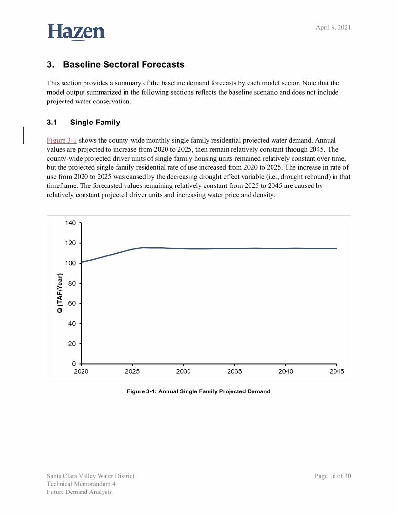
Figure 3-1 shows the county-wide monthly single family residential projected water demand. Annual values are projected to increase from 2020 to 2025, then remain relatively constant through 2045. The county-wide projected driver units of single family housing units remained relatively constant over time, but the projected single family residential rate of use increased from 2020 to 2025. The increase in rate of use from 2020 to 2025 was caused by the decreasing drought effect variable (i.e., drought rebound) in that timeframe. The forecasted values remaining relatively constant from 2025 to 2045 are caused by relatively constant projected driver units and increasing water price and density.

Figure 3-1: Annual Single Family Projected Demand

April 9, 2021


3.2 Multifamily

Figure 3-2 shows the county-wide monthly multifamily residential projected water demand. Annual values are projected to steadily increase from 2020 through 2045. This increase is largely driven by an increase in multifamily housing units over time.

Figure 3-2: Annual Multifamily Projected Demand

3.3 CII

Figure 3-3 shows the county-wide monthly CII projected water demand. Demands are projected to steadily increase from 2020 through 2045. This increase is largely driven by an increase in the driver units of total non-agricultural jobs. A steeper increase in CII demand occurs from 2020 to 2025, which is caused by the drought rebound over the same time frame.

Projected demand from 2025 to 2030 has a slightly flatter rate of increase than other periods. The variable water rate from 2020 to 2030 followed the 2020 PAWS report rate changes, which were typically larger increases per year than the 5% assumed increase in price from 2030 to 2045. The effect on projected CII demand from 2025 to 2030 suggests that drought rebound had a larger impact on projected rate of use than price.

April 9, 2021


Figure 3-3: Annual CII Projected Demand

3.4 Non-Retail Pumpers

Figure 3-4 shows the annual non-retail pumpers projected groundwater demand for M&I groundwater use. Agricultural groundwater use was held constant at a rate of 24.7 thousand acre-ft (TAF) per year, based on the average historical value from 2009 to 2018 (refer to TM3: Modeling Approach and Development for more details). For the non-retail pumpers M&I water use, the baseline scenario assumed no drought effect and constant price. These conditions resulted in a constant annual projected demand.

April 9, 2021


Figure 3-4: Annual Non-Retail Pumpers Projected M&I Demand

Since non-retail pumpers groundwater demand was projected on an annual basis, a set of monthly factors was used to provide a monthly estimate of demand. The monthly factors are shown in Table 3-1. Monthly non-retail pumper M&I projected demands developed with these factors are presented in Figure 3-5 on the following page.

Table 3-1: Monthly Factors for Non-Retail Pumpers Demand

Month Percent of Annual Demand January 3.1% February 3.8%

March 6.7% April 9.3% May 11.7% June 13.1% July 14.0%

August 12.6% September 10.5%

October 7.7% November 4.5% December 3.0%

The demand model estimates projected demand for the W2 and W5 charge zones. Starting in 2020, Valley Water split W5 into three charge zone: W5, W7, and W8. The projected demand for the W5 charge zone was split into two zones which overlay the Llagas sub-basin (W5 and W8) and the Coyote Valley (W7). W5/W8 represented a constant 75% of the original W5 charge zone (Llagas sub-basin) and W7 represented a constant 25% of the original W5 charge zone (Coyote Valley).

April 9, 2021


Figure 3-5: Monthly Non-Retail Pumpers Projected M&I Demand

April 9, 2021


3.5 “Other” Consumption

Some – predominantly low volume – water use categories do not fit neatly into Single Family, Multifamily or CII sectors such as “fireline”, “Other Water Utilities”, and “Other”. To account for these “other” water uses, a relative ratio for other uses to total use was used to generate forecast values. The ratio was assumed to be constant into the future based on the historical average from 2009 to 2018. Table 3-2 shows the ratios of “other” water uses to total use for each retailer. Figure 3-6 shows the projected annual “other” water use. Note that applying the constant ratio to an increasing total demand results in increasing volume of “other” water use over time.

Table 3-2: Percent Other Water Consumption by Agency

Agency Other Retail Factor California Water Service 0.24% City of Gilroy 14.71%(a) City of Milpitas 0.10% City of Morgan Hill 0% City of Mountain View 0.14% City of Palo Alto 0.03% City of Santa Clara 0% City of Sunnyvale 0.05% Great Oaks Water Company 0.58% Purissima Hills Water District 0.65% San Jose Municipal Water 0.23% San Jose Water Company 0.70% Stanford University 0% (a) Landscape water use was included in the “other” water use category at the instruction of City of Gilroy. Refer to TM2: Data Collection and Review.

April 9, 2021


Figure 3-6: Annual "Other" Projected Demand

San Jose Municipal Water and Gilroy did not include recycled water in the consumption data; thus it was explicitly excluded from retail forecast development. The long-term averages of recycled water production were assumed to be constant into the future and were added back to the total demand forecast along with the retail sector demands to correct for the recycled water being excluded from the model forecast. Forecasted annual recycled water uses for San Jose Municipal Water and Gilroy are shown in Table 3-3.

Table 3-3: Recycled Water Quantities

Agency Recycled Water (TAF/year)

City of Gilroy 2.01 San Jose Municipal Water 3.83

3.6 Nonrevenue Water

Nonrevenue water represents the difference between the amount of water produced and the amount of water sold through the retailers’ systems so that altogether the forecasts represent total production demand. Estimates of nonrevenue water were determined based on the ratio difference between production and consumption for each retailer in 2018. The ratio was calculated from 2018 values because it was the most recent year with complete data. Nonrevenue percentages by agency is shown in Table 3-4. The annual nonrevenue water demand is shown in Figure 3-7. Note that applying the constant ratio to an increasing total demand results in increasing volume of nonrevenue water over time.

April 9, 2021


Table 3-4: Percent Nonrevenue Water by Retailer

Agency Percent Nonrevenue

California Water Service 6.19% City of Gilroy 10.95% City of Milpitas 6.06% City of Morgan Hill 10.85% City of Mountain View 4.16% City of Palo Alto 4.52% City of Santa Clara 6.82% City of Sunnyvale 4.30% Great Oaks Water Company 5.99% Purissima Hills Water District 4.53% San Jose Municipal Water 6.01% San Jose Water Company 5.21% Stanford University 12.14%

Figure 3-7: Annual Projected Nonrevenue Water

3.7 Raw Water

Raw water represents a small amount of untreated imported and local surface water used primarily for landscape and agricultural irrigation. Due to planned changes in Valley Water’s Untreated Water Program rules and some customers switching to recycled water, the future raw water demands were estimated by assuming the average of historical use for customers that are anticipated to remain in the program and holding that demand at a constant rate into the future, as described in Valley Water’s 2015 UWMP (Valley Water, 2016). The assumed raw water demand was 1.7 TAF/year.

April 9, 2021


3.8 County-Wide Totals

The total county-wide projected production demand is shown in Figure 3-8 and includes the sum of projections for the single family, multifamily, and CII sectors; total non-retail pumper demand (M&I plus agricultural); other retailer consumption, and nonrevenue water. Future conservation is not included.

Figure 3-8: Annual Total Projected Demand

Projected total production demands given the baseline scenario are expected to increase over the next 35 years to approximately 374 TAF in 2045. The rate of change in the forecast is not constant over time. The most rapid period of growth (300 TAF to 340 TAF) occurs in 2020-2025 during the assumed drought rebound. Following this period, projected demand remains relatively flat until approximately 2030, where it begins to steadily increase to 2045. This pattern is mostly attributable to driver unit growth dampened by the effect of increasing water rates and increasing housing density.

4. Forecast Impact Factor Analysis

The derivation of “impact factors” is helpful for evaluating the relative effect of each explanatory variable on forecasted water use. Impact factors are calculated by comparing the ratio change in forecasted volumetric water use with the ratio change in each forecasted explanatory variable to identify the explanatory variables that had the largest impact. For this analysis ratio changes are the forecasted water use and forecasted driver units, where the ratio change is calculated as the end value (2045) divided by the start value (2020). The multiplicative nature of the demand model makes calculation of the impact factors straightforward, where ratio changes between end (2045) to start (2020) values are simply raised

April 9, 2021


to the power of the calibrated model coefficient.5 Equation (2) shows how impact factors were calculated for each explanatory variable and driver units.

𝑃𝑃𝐼𝐼𝐼𝐼𝐼𝐼𝐼𝐼𝐼𝐼 𝐹𝐹𝐼𝐼𝐼𝐼𝐼𝐼𝐹𝐹𝐹𝐹𝑋𝑋 = � 𝑋𝑋𝑒𝑒𝑒𝑒𝑒𝑒𝑋𝑋𝑠𝑠𝑠𝑠𝑠𝑠𝑠𝑠𝑠𝑠

�𝐶𝐶𝑖𝑖𝑓𝑓𝑓𝑓𝑓𝑓𝑖𝑖𝑖𝑖𝑖𝑖𝑓𝑓𝑛𝑛𝑓𝑓𝑋𝑋 (2)

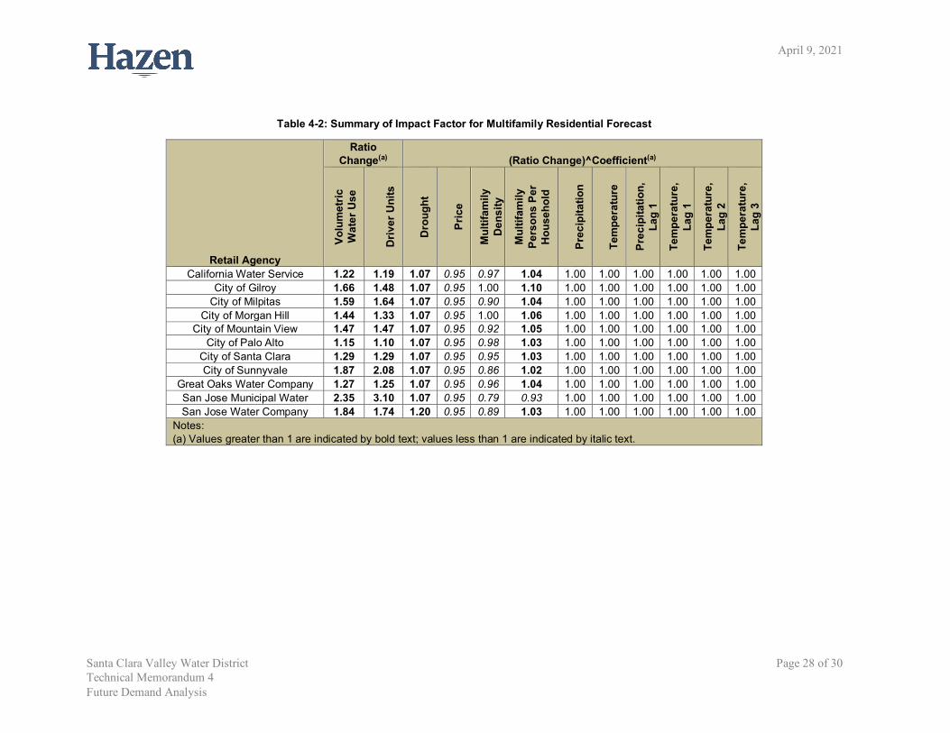
The impact factors for each retail model sector and retail agency are shown in Table 4-1 (single family residential), Table 4-2 (multifamily residential), and Table 4-3 (CII). Impact ratios greater than 1 indicate that forecasted changes in the values of any given variable increase the forecast, whereas ratios less than 1 indicate a decreasing effect. Since the factors are independent by design, the product of factors provides the overall collective impact of baseline assumptions. All retail agencies had a forecasted increase in water use and driver units for single family and multifamily residential water use. For CII, most agencies had a forecasted increase in water use and driver units, with the exceptions of City of Gilroy, City of Morgan Hill, and Stanford. However, it is important to note that the projected proportional change in water use does not have to equate to the proportional change in driver units because of the influence of other demand model factors. For example, the impact factors associated with single family residential water use indicated that the effect of the drought variable and its coefficient caused forecasted rate of use to increase (impact factor value of 1.16), while the effect of the price variable and its coefficient caused forecasted rate of use to decrease (impact factor value of 0.93). Further, single family housing density and its coefficient had varying effects by retailer (impact factor varying between 0.95 to 1.0).

Aside from projected growth in housing units in the single family residential sector, the largest impact on increasing forecasted water use was generally in order of magnitude the drought rebound assumption, followed by single family residential PPH, as evidenced by impact factor values greater than 1 for all retail agencies. The impact of price and single family residential density dampened that increase, as evidenced by impact factor values less than 1 for all or most retail agencies. Since climate variables in the baseline forecast scenario were assumed to be equal to historical normal values (i.e., no change), the impact factor was equal to 1, indicating no impact on forecasted water use.

Multifamily residential impact factors were similar to those for single family residential. Drought and multifamily residential PPH had impact factors that caused forecasted water use to increase, while price and multifamily residential density had impact factors that caused forecasted water use to decrease. The impact factor for drought was smaller in magnitude for multifamily residential water use than single family residential water use due to relatively lower estimated effects from drought restrictions. For CII, the change in forecasted water use (excluding Stanford) was driven by drought, price, and the sectoral employment ratios. Drought had a similar impact factor for CII as for single family residential water use. Price had a similar impact factor for CII as for both single family and multifamily residential water use, due to the relatively small differences in estimated price elasticities.

The impact of sectoral employment ratios varied by retail agency. For most retail agencies, the effect of a projected increase in the proportion of Health, Educational and Recreational Service jobs had an increasing impact on the forecasted water use, while the projected change in the proportion of Industrial jobs and Professional Services jobs had a decreasing impact on the forecasted water use. The impact

5 This exponential transformation was required because the demand model used variables in natural log-space. Driver units implicitly have an exponent of 1.

April 9, 2021


factor associated with Information, Government, and Construction jobs and Retail jobs were generally small and centered around 1, indicating a smaller effect on forecasted water use than other sectoral employment categories given the baseline scenario values.

The net impact factor of all five sectoral employment ratios is shown in Table 4-3 under the column for “Net Impact Factor, Sectoral Employment.” This net impact factor was calculated as the product of all five sectoral employment impact factors. Looking at the net effect, changes in sectoral employment ratios had an increasing effect for half of the retail agencies and a decreasing effect for the other half of the retail agencies. The retail agencies where CII forecasted water use was most affected by changes in sectoral employment were California Water Service (net increasing effect) and City of Gilroy (net decreasing effect).

Stanford CII water use was modeled separately from the other retail agencies. For Stanford, the change in forecasted water use was driven by drought and price. The effect of price was large enough to overcome the effect of drought rebound assumptions and increasing driver units, resulting in decreasing forecasted water use for Stanford.

April 9, 2021


Table 4-1: Summary of Impact Factor for Single Family Residential Forecast

Retail Agency

Ratio Change(a) (Ratio Change)^Coefficient(a)

Volu

met

ric W

ater

Use

Driv

er U

nits

Dro

ught

Med

ian

Inco

me

Pric

e

Sing

le F

amily

Den

sity

Sing

le F

amily

Per

sons

Pe

r Hou

seho

ld

Prec

ipita

tion

Tem

pera

ture

Prec

ipita

tion,

Lag

1

Tem

pera

ture

, Lag

1

Prec

ipita

tion,

Lag

2

Tem

pera

ture

, Lag

2

Tem

pera

ture

, Lag

3

California Water Service 1.11 1.01 1.16 1.00 0.93 1.00 1.02 1.00 1.00 1.00 1.00 1.00 1.00 1.00 City of Gilroy 1.41 1.25 1.16 1.00 0.93 1.00 1.05 1.00 1.00 1.00 1.00 1.00 1.00 1.00

City of Milpitas 1.16 1.08 1.16 1.00 0.93 0.97 1.02 1.00 1.00 1.00 1.00 1.00 1.00 1.00 City of Morgan Hill 1.31 1.18 1.16 1.00 0.93 1.00 1.03 1.00 1.00 1.00 1.00 1.00 1.00 1.00

City of Mountain View 1.15 1.06 1.16 1.00 0.93 0.98 1.03 1.00 1.00 1.00 1.00 1.00 1.00 1.00 City of Palo Alto 1.10 1.00 1.16 1.00 0.93 1.00 1.02 1.00 1.00 1.00 1.00 1.00 1.00 1.00

City of Santa Clara 1.10 1.01 1.16 1.00 0.93 1.00 1.01 1.00 1.00 1.00 1.00 1.00 1.00 1.00 City of Sunnyvale 1.10 1.02 1.16 1.00 0.93 0.99 1.01 1.00 1.00 1.00 1.00 1.00 1.00 1.00

Great Oaks Water Company 1.18 1.13 1.16 1.00 0.93 0.95 1.02 1.00 1.00 1.00 1.00 1.00 1.00 1.00 Purissima Hills Water District 1.11 1.01 1.16 1.00 0.93 0.99 1.02 1.00 1.00 1.00 1.00 1.00 1.00 1.00

San Jose Municipal Water 1.06 1.03 1.16 1.00 0.93 0.99 0.96 1.00 1.00 1.00 1.00 1.00 1.00 1.00 San Jose Water Company 1.12 1.02 1.16 1.00 0.93 0.99 1.02 1.00 1.00 1.00 1.00 1.00 1.00 1.00

Notes: (a) Values greater than 1 are indicated by bold text; values less than 1 are indicated by italic text.

April 9, 2021


Table 4-2: Summary of Impact Factor for Multifamily Residential Forecast

Retail Agency


Volu

met

ric

Wat

er U

se

Driv

er U

nits

Dro

ught

Pric

e

Mul

tifam

ily

Den

sity

Mul

tifam

ily

Pers

ons

Per

Hou

seho

ld

Prec

ipita

tion

Tem

pera

ture

Prec

ipita

tion,

La

g 1

Tem

pera

ture

, La

g 1

Tem

pera

ture

, La

g 2

Tem

pera

ture

, La

g 3

California Water Service 1.22 1.19 1.07 0.95 0.97 1.04 1.00 1.00 1.00 1.00 1.00 1.00 City of Gilroy 1.66 1.48 1.07 0.95 1.00 1.10 1.00 1.00 1.00 1.00 1.00 1.00

City of Milpitas 1.59 1.64 1.07 0.95 0.90 1.04 1.00 1.00 1.00 1.00 1.00 1.00 City of Morgan Hill 1.44 1.33 1.07 0.95 1.00 1.06 1.00 1.00 1.00 1.00 1.00 1.00

City of Mountain View 1.47 1.47 1.07 0.95 0.92 1.05 1.00 1.00 1.00 1.00 1.00 1.00 City of Palo Alto 1.15 1.10 1.07 0.95 0.98 1.03 1.00 1.00 1.00 1.00 1.00 1.00

City of Santa Clara 1.29 1.29 1.07 0.95 0.95 1.03 1.00 1.00 1.00 1.00 1.00 1.00 City of Sunnyvale 1.87 2.08 1.07 0.95 0.86 1.02 1.00 1.00 1.00 1.00 1.00 1.00

Great Oaks Water Company 1.27 1.25 1.07 0.95 0.96 1.04 1.00 1.00 1.00 1.00 1.00 1.00 San Jose Municipal Water 2.35 3.10 1.07 0.95 0.79 0.93 1.00 1.00 1.00 1.00 1.00 1.00 San Jose Water Company 1.84 1.74 1.20 0.95 0.89 1.03 1.00 1.00 1.00 1.00 1.00 1.00

Notes: (a) Values greater than 1 are indicated by bold text; values less than 1 are indicated by italic text.

April 9, 2021


Table 4-3: Summary of Impact Factor for CII Forecast

Retail Agency


Volu

met

ric W

ater

Use

Driv

er U

nits

Dro

ught

Pric

e

Pric

e (b

ased

on

WU

E R

ate)

Prec

ipita

tion

Tem

pera

ture

Prec

ipita

tion,

Lag

1

Tem

pera

ture

, Lag

1

Prec

ipita

tion,

Lag

2

Tem

pera

ture

, Lag

2

Rat

io o

f Hea

lth, E

duca

tion

and

Rec

reat

iona

l Ser

vice

s Jo

bs

Rat

io o

f Ind

ustr

ial J

obs

Rat

io o

f Inf

orm

atio

n,

Gov

ernm

ent,

and

Con

stru

ctio

n

Rat

io o

f Pro

fess

iona

l Ser

vice

s Jo

bs

Rat

io o

f Ret

ail J

obs

Net

Impa

ct, S

ecto

ral

Empl

oym

ent R

atio

s

California Water Service 1.46 1.19 1.15 0.95 - 1.00 1.00 1.00 1.00 1.00 1.00 1.13 0.91 1.00 1.10 0.99 1.12 City of Gilroy 1.00 1.19 1.15 0.95 - 1.00 1.00 1.00 1.00 1.00 1.00 0.97 1.06 1.00 0.73 1.03 0.77

City of Milpitas 1.44 1.27 1.15 0.95 - 1.00 1.00 1.00 1.00 1.00 1.00 1.08 0.93 1.00 1.05 0.98 1.04 City of Morgan Hill 0.99 1.01 1.15 0.95 - 1.00 1.00 1.00 1.00 1.00 1.00 1.08 0.97 1.01 0.84 1.02 0.90

City of Mountain View 1.41 1.21 1.15 0.95 - 1.00 1.00 1.00 1.00 1.00 1.00 1.23 0.92 0.98 0.94 1.02 1.06 City of Palo Alto 1.11 1.02 1.15 0.95 - 1.00 1.00 1.00 1.00 1.00 1.00 0.95 0.97 1.01 1.06 1.01 0.99

City of Santa Clara 1.63 1.42 1.15 0.95 - 1.00 1.00 1.00 1.00 1.00 1.00 1.19 0.83 0.99 1.09 0.98 1.05 City of Sunnyvale 1.44 1.28 1.15 0.95 - 1.00 1.00 1.00 1.00 1.00 1.00 1.20 0.90 1.01 0.96 0.99 1.03

Great Oaks Water Company 1.08 1.19 1.15 0.95 - 1.00 1.00 1.00 1.00 1.00 1.00 1.08 0.93 1.01 0.77 1.05 0.83 Purissima Hills Water District 1.17 1.09 1.15 0.95 - 1.00 1.00 1.00 1.00 1.00 1.00 0.96 1.15 1.01 0.81 1.07 0.98

San Jose Municipal Water 1.58 1.34 1.15 0.95 - 1.00 1.00 1.00 1.00 1.00 1.00 1.20 0.88 1.02 1.03 0.97 1.08 San Jose Water Company 1.27 1.22 1.15 0.95 - 1.00 1.00 1.00 1.00 1.00 1.00 1.09 0.96 0.99 0.92 0.99 0.95

Stanford University 0.80 1.33 1.09 - 0.56 1.00 - 1.00 1.00 1.00 - - - - - - - Notes: (a) Values greater than 1 are indicated by bold text; values less than 1 are indicated by italic text.

April 9, 2021


5. Future Considerations

The baseline scenario may be considered to be somewhat conservative (i.e., relatively low risk of under-predicting demand) given the assumptions around drought rebound. The drought rebound assumptions are reasonable given prior drought rebounds for Valley Water and other California water suppliers. Still, it is prudent to monitor trends over the next few years and adjust the rebound assumptions accordingly.

The impacts of climate change should be monitored and considered in future scenarios. All climate models analyzed in the development of this TM identified increases in average temperature by 2040 (see Table 2-2). Changes in precipitation were more varied, as the ensemble of climate models identified both increases and decreases in average precipitation. The exact impact of these changes on demand is uncertain, as water demand is expected to increase with temperature but decrease with increased precipitation.

In addition to monitoring the drought rebound and considering climate change, recent conditions stemming from the COVID-19 pandemic should be monitored for impacts on water demand. In particular, the baseline assumptions around trend economy and certain demographic variables, such as persons per household, may need to be adjusted as more information becomes available. Demand share between the residential and CII sectors may also require adjustment depending on the length of regional stay-at-home orders and long-term trends in remote work.6 Lastly, anecdotal trends in regional employment, such as major tech companies leaving the Bay Area or switching to a more permanent work-from-home model should be monitored for potential adjustments to the number of projected jobs within the county and/or the geographical distribution of employment across the retailers.

6. Summary

The baseline scenario results represent a projection of future water demand for Valley Water without additional conservation. The scenario assumptions outlined in Section 1 reflect a reasonable “best guess” for future conditions of parameters that are known to influence water demand derived from multiple available sources. The forecast uses ABAG data to depict local / regional trends in demographics and development in the demand model. Consistent with regional trends, demands in the single family sector are forecasted to remain relatively flat over the next 35 years as there is not expected to be substantial growth in single family housing units. Growth in residential demand is largely forecasted to occur within the multifamily sector, which is consistent with expectations about higher growth in multifamily housing. Demands in the CII sector are also expected to increase, which is consistent with ABAG forecasts of total jobs in the county. Increasing water rates and housing density are expected to have some modulating effect on demand (as housing density and water rates increase, water demand decreases) however, under the baseline scenario projected changes in the values of these variables do not generally counteract the effect of growth in overall driver units.

6 Systematic shifts in demand shares between residential and CII sectors may require refitting of the econometric models defined in TM3: Modeling Approach and Development.

April 9, 2021

Santa Clara Valley Water District A-1 Technical Memorandum 4 Future Demand Analysis

Appendix A: Projected Residential Housing Density by Retailer

Table A-1: California Water Service Residential Housing Density

April 9, 2021


Figure A-2: City of Gilroy Residential Housing Density

Figure A-3: City of Milpitas Residential Housing Density

April 9, 2021


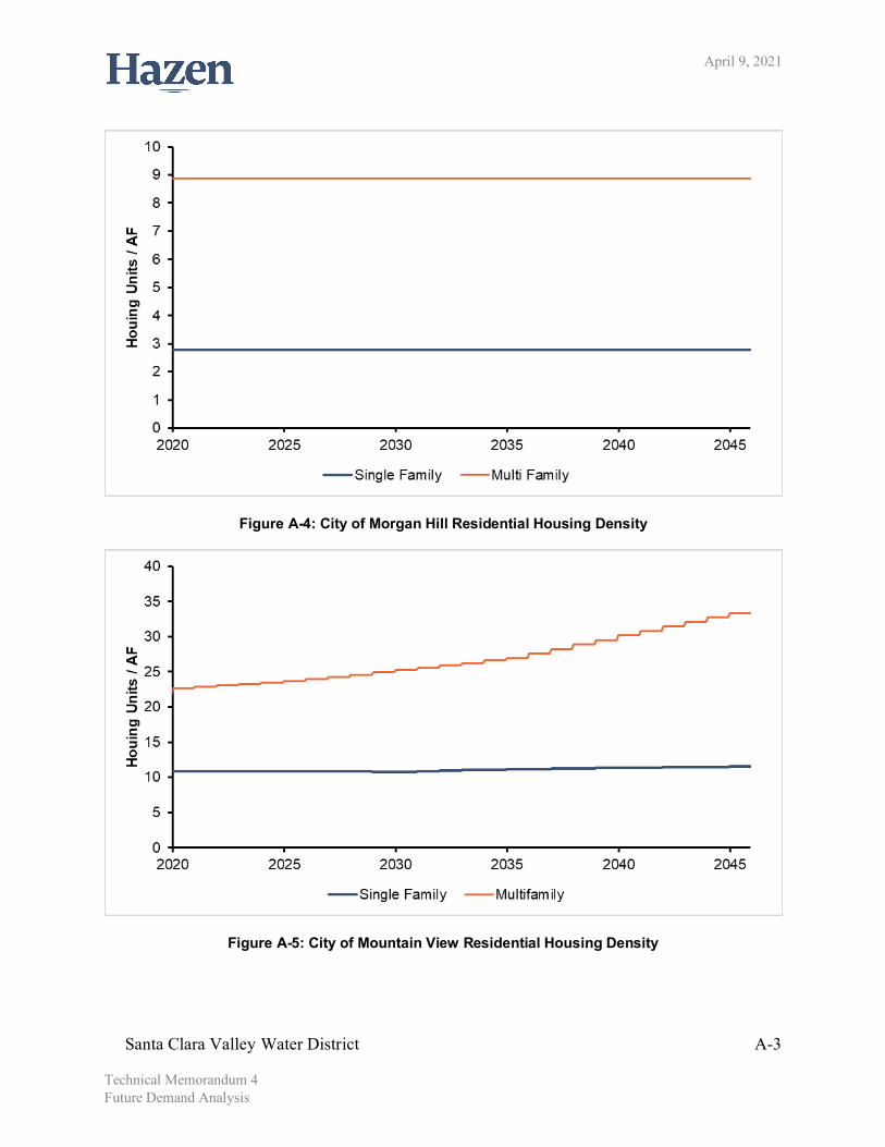
Figure A-4: City of Morgan Hill Residential Housing Density

Figure A-5: City of Mountain View Residential Housing Density

April 9, 2021


Figure A-6: City of Palo Alto Residential Housing Density

Figure A-7: City of Santa Clara Residential Housing Density

April 9, 2021


Figure A-8: City of Sunnyvale Residential Housing Density

Figure A-9: Great Oaks Water Company Residential Housing Density

April 9, 2021


Figure A-10: Purissima Hills Water District Residential Housing Density

Figure A-11: San Jose Municipal Water Residential Housing Density

April 9, 2021


Figure A-12: San Jose Water Company Residential Housing Density

April 9, 2021

Santa Clara Valley Water District B-1 Technical Memorandum 4 Future Demand Analysis

Appendix B: Projected Persons per Household by Retailer

Table B-1: California Water Service Residential Persons Per Household

April 9, 2021


Figure B-2: City of Gilroy Residential Persons Per Household

Figure B-3: City of Milpitas Residential Persons Per Household

April 9, 2021


Figure B-4: City of Morgan Hill Residential Persons Per Household

Figure B-5: City of Mountain View Residential Persons Per Household

April 9, 2021


Figure B-6: City of Palo Alto Residential Persons Per Household

Figure B-7: City of Santa Clara Residential Persons Per Household

April 9, 2021


Figure B-8: City of Sunnyvale Residential Persons Per Household

Figure B-9: Great Oaks Water Company Residential Persons Per Household

April 9, 2021


Figure B-10: Purissima Hills Water District Residential Persons Per Household

Figure B-11: San Jose Municipal Water Residential Persons Per Household

April 9, 2021


Figure B-12: San Jose Water Company Residential Persons Per Household

April 9, 2021

Santa Clara Valley Water District C-1 Technical Memorandum 4 Future Demand Analysis

Appendix C: Projected Employment Ratios by Retailer

Figure C-1: California Water Service Projected Sectoral Employment Ratios

April 9, 2021


Figure C-2: City of Gilroy Projected Sectoral Employment Ratios

Figure C-3: City of Milpitas Projected Sectoral Employment Ratios

April 9, 2021


Figure C-4: City of Morgan Hill Projected Sectoral Employment Ratios

Figure C-5: City of Mountain View Projected Sectoral Employment Ratios

April 9, 2021


Figure C-6: City of Palo Alto Projected Sectoral Employment Ratios

Figure C-7: City of Santa Clara Projected Sectoral Employment Ratios

April 9, 2021


Figure C-8: City of Sunnyvale Projected Sectoral Employment Ratios

Figure C-9: Great Oaks Water Company Projected Sectoral Employment Ratios

April 9, 2021


Figure C-10: Purissima Hills Water District Projected Sectoral Employment Ratios

Figure C-11: San Jose Municipal Water Projected Sectoral Employment Ratios

April 9, 2021


Figure C-12: San Jose Water Company Projected Sectoral Employment Ratios

Figure C-13: Stanford Projected Sectoral Employment Ratio

April 9, 2021

Santa Clara Valley Water District J-1 Technical Memorandum 4 Future Demand Analysis

future demand analysis introduction

Documents