future mobile communications: lte optimization and mobile ... · future mobile communications: lte...
TRANSCRIPT

Future Mobile Communications: LTE Optimizationand Mobile Network Virtualization
submitted to theFaculty of Physics and Electrical Engineering,
University of Bremen
for obtainment of the academic degree
Doktor-Ingenieur (Dr.-Ing.)Dissertation
by
Yasir Zaki, M.Sc. B.Sc.from Baghdad, Iraq
First assessor: Prof. Dr. rer. nat. habil. Carmelita GörgSecond assessor: Prof. Dr. Samir R. DasSubmission date: 7th of May 2012Colloquium date: 6th of July 2012


I assure, that this work has been done solely by me without any further help fromothers except for the official support of the Communication Networks group of theUniversity of Bremen. The literature used is listed completely in the bibliography.
Bremen, 7th of May 2012
(Yasir Zaki)


Dedication
I would like to dedicate this Doctoral dissertation to my beloved wife TamaraHamed, for her unconditional support and great patience at all times. I will fo-rever owe her a debt of gratitude, for always believing in me, even in the timeswhen I didn’t. I would also like to thank my parents, who have given me their un-equivalent support throughout, as always, for which my mere expression of thankslikewise does not suffice. Special dedication to my beloved kids Tanya and Yezin.


Acknowledgments
It would not have been possible to finish this work, and write the thesis withoutthe help and support of all the kind people around me, to only some of whom it ispossible to give particular mention here.
This thesis would not have seen the light without the help, support and patienceof my supervisor, Prof. Dr. Carmelita Görg. Her wide knowledge, encouragementand personal guidance have been of great value to me. I would also like to expressmy gratitude to Prof. Dr.-Ing. Andreas Timm-Giel, for all his support and valuableinput.
The good advice, support and friendship of my colleague, Dr. Thushara Weera-wardane, has been invaluable on both academic and personal level, for which I amextremely grateful. During this work I have collaborated with many colleagues forwhom I have great respect, in particular I wish to extend my warmest thanks toDr. Koojana Kuladinithi and Asanga Udugama, for providing all the great familyoriented activities. I would also like to express my gratitude to Dr. Hadeer Hamedand Mr. Khalis Mahmoud Khalis, for their great support in revising the thesis.
I would like to acknowledge all of my friends and colleagues within the Com-Nets department, of the University of Bremen, for their support and help that keptme stay sane, through these difficult years. Dr. Xi Li, for her help in proof rea-ding of the thesis, Liang Zhao, for being a great work partner throughout all theprojects we worked together. I would also like to thank Dr. Andreas Könsgen andMarkus Becker, for offering their Linux expertise. Lots of gratitude to Umar To-seef, Muhammed Mutakin Siddique, Aman Singh, Dr. Bernd-Ludwig Wenning,Martina Kamman and Karl-Heinz Volk, for their support. In addition, I would alsolike to thank my students Nikola Zahariev and Safdar Nawaz Khan Marwat fortheir support and good work.
Finally, a special acknowledgment, for the DAAD (German Academic ExchangeService), for giving me the chance to come to Germany, to do my Master studies,which lead eventually, to the finishing of my doctoral studies.
Yasir Zaki


Abstract
Providing QoS while optimizing the LTE network in a cost efficient manner isvery challenging. Thus, radio scheduling is one of the most important functionsin mobile broadband networks. The design of a mobile network radio schedulerholds several objectives that need to be satisfied, for example: the scheduler needsto maximize the radio performance by efficiently distributing the limited radio re-sources, since the operator’s revenue depends on it. In addition, the scheduler hasto guarantee the user’s demands in terms of their Quality of Service (QoS). Thus,the design of an effective scheduler is rather a complex task. In this thesis, the au-thor proposes the design of a radio scheduler that is optimized towards QoS guar-antees and system performance optimization. The proposed scheduler is called“Optimized Service Aware Scheduler” (OSA). The OSA scheduler is tested andanalyzed in several scenarios, and is compared against other well-known sched-ulers.
A novel wireless network virtualization framework is also proposed in this the-sis. The framework targets the concepts of wireless virtualization applied withinthe 3GPP Long Term Evolution (LTE) system. LTE represents one of the new mo-bile communication systems that is just entering the market. Therefore, LTE waschosen as a case study to demonstrate the proposed wireless virtualization frame-work. The framework is implemented in the LTE network simulator and analyzed,highlighting the many advantages and potential gain that the virtualization processcan achieve. Two potential gain scenarios that can result from using network virtu-alization in LTE systems are analyzed: Multiplexing gain coming from spectrumsharing, and multi-user diversity gain.
Several LTE radio analytical models, based on Continuous Time Markov Chains(CTMC) are designed and developed in this thesis. These models target the model-ing of three different time domain radio schedulers: Maximum Throughput (MaxT),Blind Equal Throughput (BET), and Optimized Service Aware Scheduler (OSA).The models are used to obtain faster results (i.e., in a very short time period in theorder of seconds to minutes), compared to the simulation results that can take con-siderably longer periods, such as hours or sometimes even days. The model resultsare also compared against the simulation results, and it is shown that it provides a
X Abstract
good match. Thus, it can be used for fast radio dimensioning purposes.Overall, the concepts, investigations, and the analytical models presented in this
thesis can help mobile network operators to optimize their radio network and pro-vide the necessary means to support services QoS differentiations and guarantees.In addition, the network virtualization concepts provides an excellent tool that canenable the operators to share their resources and reduce their cost, as well as pro-vides good chances for smaller operators to enter the market.
Kurzfassung
Die Bereitstellung von Dienstgüte (Quality of Service, QoS) bei der Optimie-rung von LTE-Netzen ist eine große Herausforderung. Daher ist das Schedulingauf der Funkschnittstelle eine der wichtigsten Funktionen in mobilen Breitband-netzen. Der Entwurf eines Schedulers für mobile Funknetze beinhaltet verschiede-ne Kriterien, die erfüllt werden müssen, beispielsweise soll der Scheduler das Leis-tungsverhalten auf der Funkschnittstelle durch effiziente Verteilung der begrenz-ten Funkressourcen maximieren, da hiervon der Ertrag des Betreibers abhängt.Zusätzlich muss der Scheduler die Nutzeranforderungen bgzl. ihrer Dienstgütegarantieren. Aus diesem Grund ist der Entwurf eines effektiven Schedulers eindurchaus komplexer Prozess. In dieser Arbeit schlägt der Autor einen Schedulerfür die Funkschnittstelle vor, der für Dienstgütegarantien und die Optimierung desSystemleistungsverhaltens ausgelegt ist. Der vorgestellte Scheduler trägt die Be-zeichnung “Optimierter dienstgütesensitiver Scheduler, Optimized Service AwareScheduler (OSA)”. Der OSA-Scheduler wird in verschiedenen Szenarien getestetund analysiert sowie mit anderen gut bekannten Schedulern verglichen.
Ein neuartiges Framework zur Virtualisierung drahtloser Netze wird in dieserArbeit ebenfalls vorgeschlagen. Das Framework zielt auf die Konzepte der draht-losen Virtualisierung ab, die innerhalb des 3GPP Long Term Evolution-Systemsangewendet werden. LTE repräsentiert eines der neuen mobilen Kommunikations-systeme, die gegenwärtig in den Markt eintreten. Daher wurde LTE als Fallstudieausgewählt, um das vorgeschlagene drahtlose Virtualisierungs-Framework zu de-monstrieren. Das Framework wird im LTE-Netzsimulator implementiert und ana-lysiert, wobei die zahlreichen Vorteile und der mögliche Zugewinn herausgestelltwird, den der Virtualsierungsprozess erzielen kann. Zwei mögliche Szenarien,die sich aus der Nutzung der Netzvirtualisierung ergeben und Zugewinn erzielenkönnen, werden analysiert: Multiplexing-Gewinn, der sich aus der Aufteilung desSpektrums ergibt, und Diversitätsgewinn zwischen mehreren Benutzern.
Verschiedene analytische Modelle für LTE-Funknetze, basierend auf zeitkon-tinuierlichen Markov-Ketten (Continuous Time Markov Chains, CMTC), werdenin dieser Arbeit entworfen und entwickelt. Diese Modelle zielen auf die Untersu-chung drei verschiedener Scheduler für die Funkschnittstelle ab, die in der zeit-
XII Kurzfassung
lichen Domäne arbeiten: maximaler Durchsatz (Maximum Throughput, MaxT),blinder Scheduler mit gleichverteiltem Durchsatz (Blind Equal Throughput, BET)und optimierter dienstgütesensitiver Scheduler (Optimised Service Aware Sche-duler, OSA). Die Modelle werden verwendet, um schneller Ergebnisse zu erzielen(d.h. in einer sehr kurzen zeitlichen Periode in der Größenordnung Sekunden bisMinuten), verglichen mit Simulationen, die deutlich längere zeitliche Perioden be-anspruchen, wie Stunden oder manchmal sogar Tage. Die Ergebnisse des Modellswerden auch mit den Simulationsergebnissen verglichen, und es wird gezeigt, dasssie gut übereinstimmen. Daher können sie zum Zweck einer schnellen Dimensio-nierung der Funkschnittstelle eingesetzt werden.
Insgesamt können die Konzepte, Untersuchungen und die analytischen Model-le, die in dieser Arbeit vorgestellt werden, den Betreibern mobiler Netze helfen,ihr Funknetz zu optimieren und die notwendigen Mittel für die Unterstützung vonDienstgütedifferenzierung und -garantien bereitzustellen. Zusätzlich bilden dieKonzepte der Netzvirtualisierung ein hervorragendes Werkzeug, das es den Be-treibern ermöglicht, Ressourcen zu teilen und Kosten zu reduzieren, was auchkleineren Providern den Markteintritt ermöglicht.

Contents
Abstract IX
Kurzfassung XI
List of Figures XVII
List of Tables XXI
List of Abbreviations XXIII
List of Symbols XXVII
1 Introduction 1
2 Mobile Communication Systems 52.1 Global System for Mobile Communication (GSM) . . . . . . . . 62.2 Universal Mobile Telecommunication System (UMTS) . . . . . . 9
3 Long Term Evolution (LTE) 133.1 Motivation and Targets . . . . . . . . . . . . . . . . . . . . . . . 133.2 LTE Multiple Access Schemes . . . . . . . . . . . . . . . . . . . 14
3.2.1 OFDM . . . . . . . . . . . . . . . . . . . . . . . . . . . 143.2.2 OFDMA . . . . . . . . . . . . . . . . . . . . . . . . . . 153.2.3 SC-FDMA . . . . . . . . . . . . . . . . . . . . . . . . . 16
3.3 LTE Network Architecture . . . . . . . . . . . . . . . . . . . . . 173.3.1 User Equipment (UE) . . . . . . . . . . . . . . . . . . . 183.3.2 Evolved UTRAN (E-UTRAN) . . . . . . . . . . . . . . . 183.3.3 Evolved Packet Core (EPC) . . . . . . . . . . . . . . . . 19
3.4 E-UTRAN Protocol Architecture . . . . . . . . . . . . . . . . . . 203.4.1 Radio Link Control (RLC) . . . . . . . . . . . . . . . . . 233.4.2 Medium Access Control (MAC) . . . . . . . . . . . . . . 24
3.4.2.1 Logical and Transport Channels . . . . . . . . . 24
XIV Contents
3.4.2.2 HARQ . . . . . . . . . . . . . . . . . . . . . . 253.4.2.3 Scheduling . . . . . . . . . . . . . . . . . . . . 26
3.4.3 LTE Frame and Physical Resource Structure . . . . . . . 273.5 LTE Quality of Service Bearers . . . . . . . . . . . . . . . . . . . 283.6 Beyond LTE . . . . . . . . . . . . . . . . . . . . . . . . . . . . . 30
3.6.1 Wider Bandwidth for Transmission . . . . . . . . . . . . 313.6.2 Advanced MIMO Solutions . . . . . . . . . . . . . . . . 313.6.3 CoMP . . . . . . . . . . . . . . . . . . . . . . . . . . . . 323.6.4 Relays and Repeaters . . . . . . . . . . . . . . . . . . . . 32
4 LTE Network Simulator 354.1 Simulation Environment . . . . . . . . . . . . . . . . . . . . . . 354.2 Simulation Framework . . . . . . . . . . . . . . . . . . . . . . . 364.3 Simulation Model . . . . . . . . . . . . . . . . . . . . . . . . . . 37
4.3.1 UE Node Model . . . . . . . . . . . . . . . . . . . . . . 384.3.2 eNodeB Node Model . . . . . . . . . . . . . . . . . . . . 394.3.3 Access Gateway Node Model . . . . . . . . . . . . . . . 404.3.4 Packet Data Network Gateway Node Model . . . . . . . . 404.3.5 Mobility and Channel Node . . . . . . . . . . . . . . . . 414.3.6 Global User Database . . . . . . . . . . . . . . . . . . . 444.3.7 Application Configuration . . . . . . . . . . . . . . . . . 444.3.8 Profile Configuration . . . . . . . . . . . . . . . . . . . . 44
4.4 Traffic Models . . . . . . . . . . . . . . . . . . . . . . . . . . . . 454.4.1 Voice over IP Model (VoIP) . . . . . . . . . . . . . . . . 464.4.2 Web Browsing Model . . . . . . . . . . . . . . . . . . . 474.4.3 Video Streaming Model . . . . . . . . . . . . . . . . . . 484.4.4 File Transfer Model . . . . . . . . . . . . . . . . . . . . 49
4.5 Statistical Evaluation . . . . . . . . . . . . . . . . . . . . . . . . 494.5.1 Confidence Interval Estimation . . . . . . . . . . . . . . . 494.5.2 Independent Replications Method . . . . . . . . . . . . . 50
5 LTE Virtualization 535.1 Virtualization . . . . . . . . . . . . . . . . . . . . . . . . . . . . 53
5.1.1 Server Virtualization . . . . . . . . . . . . . . . . . . . . 545.1.2 Network Virtualization . . . . . . . . . . . . . . . . . . . 56
5.2 4WARD Project . . . . . . . . . . . . . . . . . . . . . . . . . . . 575.2.1 4WARD Virtualization Paradigm . . . . . . . . . . . . . . 57
5.3 Wireless Virtualization in Mobile Communication . . . . . . . . . 595.3.1 Motivation behind Mobile Network Virtualization . . . . . 61
Contents XV
5.3.2 LTE Virtualization Framework . . . . . . . . . . . . . . . 615.3.2.1 Framework Architecture . . . . . . . . . . . . . 625.3.2.2 LTE Hypervisor Algorithm . . . . . . . . . . . 635.3.2.3 Operator Bandwidth Estimation . . . . . . . . . 645.3.2.4 Contract based Framework . . . . . . . . . . . 65
5.4 LTE Virtualization Evaluation . . . . . . . . . . . . . . . . . . . 685.4.1 Multiplexing Gain based Analysis . . . . . . . . . . . . . 695.4.2 Multi-User Diversity Gain based Analysis . . . . . . . . . 735.4.3 Contract Based Framework based Analysis . . . . . . . . 76
5.5 Conclusion . . . . . . . . . . . . . . . . . . . . . . . . . . . . . 83
6 LTE Radio Scheduler 856.1 LTE Dynamic Packet Scheduling . . . . . . . . . . . . . . . . . . 866.2 LTE MAC Schedulers State of the Art . . . . . . . . . . . . . . . 87
6.2.1 Classical Scheduling Algorithms . . . . . . . . . . . . . . 876.3 Downlink MAC Scheduler Design . . . . . . . . . . . . . . . . . 89
6.3.1 QCI Classification . . . . . . . . . . . . . . . . . . . . . 906.3.2 Time Domain Scheduler (TDS) . . . . . . . . . . . . . . 916.3.3 Frequency Domain Scheduler (FDS) . . . . . . . . . . . . 946.3.4 Link-to-System Mapping (L2S) . . . . . . . . . . . . . . 966.3.5 HARQ Modeling . . . . . . . . . . . . . . . . . . . . . . 98
6.4 Downlink MAC Scheduler Analysis . . . . . . . . . . . . . . . . 996.4.1 OSA vs. Classical Schedulers . . . . . . . . . . . . . . . 99
6.4.1.1 FTP only scenario . . . . . . . . . . . . . . . . 1006.4.1.2 Mixed traffic scenario . . . . . . . . . . . . . . 104
6.4.2 GBR delay Exploitation . . . . . . . . . . . . . . . . . . 1086.5 Conclusion . . . . . . . . . . . . . . . . . . . . . . . . . . . . . 112
7 Analytical Modeling of the LTE Radio Scheduler 1137.1 General Analytical Model . . . . . . . . . . . . . . . . . . . . . . 114
7.1.1 Performance Evaluation . . . . . . . . . . . . . . . . . . 1157.1.2 Generic Departure Rate . . . . . . . . . . . . . . . . . . . 117
7.2 LTE Downlink Scheduler Modeling . . . . . . . . . . . . . . . . 1207.2.1 Single Class Model . . . . . . . . . . . . . . . . . . . . . 1207.2.2 Single Class Model Results . . . . . . . . . . . . . . . . 124
7.2.2.1 Analysis 1 - MaxT . . . . . . . . . . . . . . . . 1257.2.2.2 Analysis 2 - BET . . . . . . . . . . . . . . . . 1297.2.2.3 Analysis 3 - Sensitivity Analysis . . . . . . . . 1327.2.2.4 Analysis 4 - OSA . . . . . . . . . . . . . . . . 133

XVI Contents
7.2.2.5 Analysis 5 - BET with Random Direction (RD) 1347.2.3 Two Dimensional Model . . . . . . . . . . . . . . . . . . 136
7.2.3.1 2D TDS Modeling . . . . . . . . . . . . . . . . 1387.2.3.2 2D Performance Analysis . . . . . . . . . . . . 139
7.2.4 Two Dimensional Model Results . . . . . . . . . . . . . . 1417.2.4.1 Analysis - w-MaxT . . . . . . . . . . . . . . . 1427.2.4.2 Analysis - w-BET . . . . . . . . . . . . . . . . 1467.2.4.3 Analysis - OSA . . . . . . . . . . . . . . . . . 150
7.3 Conclusion . . . . . . . . . . . . . . . . . . . . . . . . . . . . . 151
8 Conclusions and Outlook 153
A Appendix 159A.1 Mobility Models . . . . . . . . . . . . . . . . . . . . . . . . . . 159A.2 3GPP Transport Block Size . . . . . . . . . . . . . . . . . . . . . 161A.3 Simulation Results Confidence Interval . . . . . . . . . . . . . . 162
Bibliography 165

List of Figures
2.1 3GPP releases overview [HT09] [Zah11] . . . . . . . . . . . . . . 62.2 GSM network Architecture 1 . . . . . . . . . . . . . . . . . . . . 72.3 GSM system evolution . . . . . . . . . . . . . . . . . . . . . . . 92.4 UMTS network Architecture 1 . . . . . . . . . . . . . . . . . . . 10
3.1 LTE EPS network architecture . . . . . . . . . . . . . . . . . . . 133.2 OFDM signal in frequency and time domain [Hoa05] . . . . . . . 153.3 An example of channel dependent scheduling between two users
[ADF+09] . . . . . . . . . . . . . . . . . . . . . . . . . . . . . . 163.4 An example comparing SC-FDMA to OFDMA [Agi09] . . . . . . 173.5 LTE E-UTRAN architecture . . . . . . . . . . . . . . . . . . . . 193.6 LTE E-UTRAN user plane protocol stack . . . . . . . . . . . . . 203.7 Detailed LTE downlink protocol architecture [Dah07] . . . . . . . 223.8 Multiple parallel HARQ processes example [Dah07] . . . . . . . 263.9 LTE FDD frame structure [Anr09] . . . . . . . . . . . . . . . . . 273.10 Relationship between slot, symbol and Resource Blocks [Anr09] . 283.11 SAE bearer model [HT09] . . . . . . . . . . . . . . . . . . . . . 293.12 LTE-advanced CoMP . . . . . . . . . . . . . . . . . . . . . . . . 323.13 LTE-advanced in-band relay and backhaul [Agi11] . . . . . . . . 33
4.1 OPNET Modeler© hierarchical editors . . . . . . . . . . . . . . . 354.2 LTE reference model . . . . . . . . . . . . . . . . . . . . . . . . 364.3 LTE OPNET simulation model . . . . . . . . . . . . . . . . . . . 374.4 UE Node Model . . . . . . . . . . . . . . . . . . . . . . . . . . . 384.5 eNodeB Node Model . . . . . . . . . . . . . . . . . . . . . . . . 394.6 aGW Node Model . . . . . . . . . . . . . . . . . . . . . . . . . . 404.7 PDN-GW Node Model . . . . . . . . . . . . . . . . . . . . . . . 414.8 An example result of the fast fading model . . . . . . . . . . . . . 434.9 Sample OPNET application configuration . . . . . . . . . . . . . 454.10 Sample OPNET profile configuration . . . . . . . . . . . . . . . . 454.11 VoIP traffic model . . . . . . . . . . . . . . . . . . . . . . . . . . 46

XVIII List of Figures
4.12 VoIP MOS values [IT09] . . . . . . . . . . . . . . . . . . . . . . 474.13 Web traffic model . . . . . . . . . . . . . . . . . . . . . . . . . . 47
5.1 Full virtualization environment [Cha09] . . . . . . . . . . . . . . 555.2 Para virtualization environment [Cha09] . . . . . . . . . . . . . . 555.3 OS-virtualization environment [Cha09] . . . . . . . . . . . . . . 565.4 Network Virtualization Proposed Business Model . . . . . . . . . 585.5 Multiple Access Schemes . . . . . . . . . . . . . . . . . . . . . . 605.6 LTE virtualization framework architecture . . . . . . . . . . . . . 635.7 The general hypervisor algorithm framework . . . . . . . . . . . 675.8 LTE virtualization simulation model in OPNET . . . . . . . . . . 695.9 Virtual operators allocated bandwidth over simulation time . . . . 715.10 Virtual Operator 1 VoIP air interface throughput . . . . . . . . . . 725.11 Virtual Operator 1 VoIP application end-to-end delay . . . . . . . 725.12 Virtual Operator 1 VoIP application end-to-end delay . . . . . . . 735.13 Virtual Operator 1 cell throughput with and without virtualization 755.14 Virtual Operator 1 cell throughput gain due to virtualization . . . . 765.15 Virtual Operator allocated bandwidth/PRBs) . . . . . . . . . . . . 785.16 Virtual Operator 1 Video downlink application end-to-end delay . 795.17 Virtual Operator 2 Video downlink application end-to-end delay . 805.18 Virtual Operator 2 downlink allocated bandwidth . . . . . . . . . 805.19 Virtual Operator 3 Video downlink application end-to-end delay . 815.20 Virtual Operator 3 average FTP download time . . . . . . . . . . 825.21 Virtual Operator 3 average number of FTP Files downloaded . . . 825.22 Virtual Operator 4 VoIP downlink application end-to-end delay . . 83
6.1 General packet scheduling framework [HT09] . . . . . . . . . . . 866.2 OSA general scheduler framework . . . . . . . . . . . . . . . . . 906.3 FDS general flow chart . . . . . . . . . . . . . . . . . . . . . . . 956.4 Reference BLER versus SINR AWGN curves . . . . . . . . . . . 966.5 Average user FTP download time . . . . . . . . . . . . . . . . . . 1016.6 Unfairness between users FTP download time . . . . . . . . . . . 1026.7 Average cell throughput comparison . . . . . . . . . . . . . . . . 1036.8 40 UE scenario - scheduler comparison . . . . . . . . . . . . . . 1046.9 Application delay performance comparison between schedulers . . 1066.10 Fairness and cell throughput comparison between schedulers . . . 1076.11 Average cell throughput . . . . . . . . . . . . . . . . . . . . . . . 1096.12 Average VoIP application end-to-end delay . . . . . . . . . . . . 1106.13 Average VoIP MOS value . . . . . . . . . . . . . . . . . . . . . . 110

List of Figures XIX
6.14 non-GBR services performance comparison spider chart . . . . . 111
7.1 General Continuous Time Markov Chain . . . . . . . . . . . . . . 1147.2 MaxT scheduling of users (example with 7 MCSs) . . . . . . . . 1227.3 BET scheduling of users (example with 7 MCSs) . . . . . . . . . 1227.4 MCSs static probability obtained from simulations . . . . . . . . 1237.5 OSA scheduling of users (example with 7 MCSs) . . . . . . . . . 1247.6 MaxT 10UEs scenario - average FTP download time . . . . . . . 1267.7 MaxT 20UEs scenario - average FTP download time . . . . . . . 1277.8 MaxT Markov chain state probability . . . . . . . . . . . . . . . 1287.9 BET 10UEs scenario - average FTP download time . . . . . . . . 1297.10 BET 20UEs scenario - average FTP download time . . . . . . . . 1307.11 BET Markov chain state probability . . . . . . . . . . . . . . . . 1317.12 MaxT sensitivity analysis results . . . . . . . . . . . . . . . . . . 1327.13 OSA 10UEs scenario - average FTP download time . . . . . . . . 1337.14 OSA Markov chain state probability . . . . . . . . . . . . . . . . 1347.15 BET RD 10UEs scenario - average FTP download time . . . . . . 1357.16 Two dimensional Markov chain . . . . . . . . . . . . . . . . . . . 1367.17 2D Markov chain represented in a single chain . . . . . . . . . . . 1397.18 Example Q mapping with N1=2 and N2=4 . . . . . . . . . . . . . 1397.19 Analysis1 w-MaxT average FTP download time . . . . . . . . . . 1427.20 Analysis2 w-MaxT average FTP download time . . . . . . . . . . 1437.21 Analysis1 w-MaxT Markov chain state probability . . . . . . . . 1447.22 Analysis2 w-MaxT Markov chain state probability . . . . . . . . 1457.23 Analysis3 w-BET average FTP download time . . . . . . . . . . . 1467.24 Analysis3 w-BET Markov chain state probability . . . . . . . . . 1477.25 Analysis4 w-BET average FTP download time . . . . . . . . . . . 1487.26 Analysis4 w-BET Markov chain state probability . . . . . . . . . 1497.27 Analysis5 OSA average FTP download time . . . . . . . . . . . . 150
A.1 Random Way Point (RWP) mobility model . . . . . . . . . . . . 159A.2 Random Direction (RD) mobility model . . . . . . . . . . . . . . 160


List of Tables
3.1 LTE MAC logical channels [36.11b] . . . . . . . . . . . . . . . . 253.2 LTE MAC transport channels [36.11b] . . . . . . . . . . . . . . . 253.3 LTE standardized QCIs and their parameters [SBT09] . . . . . . . 303.4 System performance comparison [Nak09] . . . . . . . . . . . . . 31
4.1 VoIP traffic model parameters [Li10] . . . . . . . . . . . . . . . . 464.2 Web browsing traffic model parameters [Wee11] . . . . . . . . . . 48
5.1 Scenario I simulation configurations . . . . . . . . . . . . . . . . 705.2 Scenario II simulation configurations . . . . . . . . . . . . . . . . 745.3 Scenario III simulation configurations . . . . . . . . . . . . . . . 77
6.1 DSCP/QCI to MAC-QoS-Class mapping example . . . . . . . . . 916.2 An example of QoS weight values for different non-GBR services 936.3 β values for each MCS [KSW+08][LV08a][Val06] . . . . . . . . 986.4 BLER and HARQ transmissions . . . . . . . . . . . . . . . . . . 996.5 Simulation configurations . . . . . . . . . . . . . . . . . . . . . . 1006.6 Simulation configurations . . . . . . . . . . . . . . . . . . . . . . 1056.7 Simulation configurations . . . . . . . . . . . . . . . . . . . . . . 108
7.1 n=2, K=2 combinations example . . . . . . . . . . . . . . . . . . 1197.2 Single class validation general parameters . . . . . . . . . . . . . 1247.3 Single class validation scenarios . . . . . . . . . . . . . . . . . . 1257.4 2-D model validation general parameters . . . . . . . . . . . . . . 1417.5 2-D model validation scenarios . . . . . . . . . . . . . . . . . . . 141
A.1 3GPP transport block size table (subset) . . . . . . . . . . . . . . 161A.2 Analysis 1 - MaxT 10 UEs simulation results confidence interval . 162A.3 Analysis 1 - MaxT 20 UEs simulation results confidence interval . 162A.4 Analysis 2 - BET 10 UEs simulation results confidence interval . . 162A.5 Analysis 2 - BET 20 UEs simulation results confidence interval . . 162

XXII List of Tables
A.6 Analysis 3 - BET sensitivity analysis simulation results confidenceinterval . . . . . . . . . . . . . . . . . . . . . . . . . . . . . . . 162
A.7 Analysis 4 - OSA simulation results confidence interval . . . . . . 163A.8 Analysis 5 - BET RD simulation results confidence interval . . . . 163A.9 Analysis 1 - w-MaxT simulation results confidence interval . . . . 163A.10 Analysis 2 - w-MaxT simulation results confidence interval . . . . 163A.11 Analysis 3 - w-BET simulation results confidence interval . . . . 163A.12 Analysis 4 - w-BET simulation results confidence interval . . . . 163
List of Abbreviations
���� 3rd Generation PartnershipProject
��� Adaptive Modulation andCoding
��� Ad-hoc On-demand DistanceVector
�� Allocation and RetentionPriority
�� Automatic Repeat Request
��� Authentication Center
� �� Additive White GaussianNoise
��� Blind Equal Throughput
��� Block Error Rate
��� Base Station Controller
��� Base Station Subsystem
��� Base Transceiver Station
�� Carrier Aggregation
���� Code Division MultipleAccess
�� Core Network
���� Coordinated Multi-Point
��� Channel Quality Indicator
���� Continuous Time MarkovChain
���� Donor eNodeB
�� Downlink
���� Differentiated Services CodePoint
�� Digital Video Broadcasting
������ enhanced NodeB
������ Evolved Universal TerrestrialRadio Access Network
���� Enhanced Data for GSMEvolution
���� Exponential Effective SINRMapping
�� Enhanced Full Rate
��� Exponential Moving Average
��� Evolved Packet Core
��� Evolved Packet System
��� Frequency Division Duplex
��� Frequency DomainMultiplexing
���� Frequency Division MultipleAccess
��� Frequency Domain Scheduler
��� File Transfer Protocol
�� Guaranteed Bit Rate
���� Gaussian Minimum ShiftKeying
��� General Packet Radio Service
��� Global System for MobileCommunication
��� Gateway Tunneling Protocol

XXIV List of Abbreviations
���� Hybrid Automatic RepeatRequest
��� Home Location Registry
����� High Speed Downlink PacketAccess
���� High Speed Packet Access
��� Home Subscriber Server
���� High Speed Uplink PacketAccess
�� Hypertext Transfer Protocol
�� International MobileTelecommunication
�� Internet Protocol
��� Internet Service Provider
� Information Technology
� InternationalTelecommunication Union
� Long Term Evolution
��� Medium Access Channel
��� Maximum Throughput
��� Modulation and CodingScheme
�� �� Mutual Information EffectiveSINR Mapping
���� Multi Input Multi Output
�� Mobility Management Entity
��� Mean Opinion Score
�� Mobile Station
��� Mobile Switching Center
������� non-Guaranteed Bit Rate
����� Orthogonal FrequencyDomain Multiple Access
�� Operating System
��� Optimized Service Aware
���� Policy and Charging RulesFunction
��� Personal Digital Assistant
���� Packet Data ConvergenceProtocol
��� Packet Data Network
������ Packet Data Network Gateway
�� Protocol Data Unit
��� Physical Layer
��� Physical Resource Block
���� Physical Resource Blocks
��� Phase Shift Keying
��� Public Switched TelephoneNetwork
��� QoS Class Identifier
��� Quality of Service
�� Random Direction
��� Radio Link Control
�� Relay Node
��� Radio Network Controller
��� Radio Resource Control
��� Random Way Point
���� Serving Gateway
�� System Architecture Evolution
��� Storage Area Network
������� Single Carrier FrequencyDomain Multiple Access
���� Space Division MultipleAccess
��� Software Defined Radio
��� Subscriber Identity Module
���� Signal to Interference NoiseRatio
�� Transport Block Size
�� Time Domain Scheduler
List of Abbreviations XXV
���� Time Division MultipleAccess
�� Terminal Equipment
��� Transmission Time Interval
�� User Equipment
�� Uplink
��� User Mode Linux
��� Universal MobileTelecommunication System
��� User Service Identity Module
���� UMTS Terrestrial RadioAccess Network
�� Visitor Location Registry
�� Virtual Machine
��� Virtual Machine Monitor
�� � Virtual Network
���� Virtual Network Operators
���� Voice over Internet Protocol
����� Wideband Code DivisionMultiple Access
���� Wireless Local Area Network


List of Symbols
������ ����
α smoothing factorβ MCS scaling factor
γk[t] normalized average channel condition of bearer kδ 2 varianceη actual number of users served per TTI
θmax maximum achieved throughput if all PRBs are used underperfect channel conditions
θk[t] instantaneous achieved throughput for bearer kθk[t] normalized average throughout of bearer k
λ arrival rate (file inter-arrival time)μ(n) generic departure rate of state nπ(n) state n steady state probability
πππ Markov chain steady state probability vectorτ smoothing factorψ maximum number of users served per TTI
BLEP([γk]) instantaneous Block Error Probability for channel state γk
BLEP([γe f f ]) instantaneous Block Error Probability for channel state γe f f
D mean number of departures by unit timeEtotal total BE PRB estimate over all BE operatorsE(N) average required PRBs at the Nth TTI
Fi operator i fairness factorHOLdelayk head-of-line packet delay for bearer k
K Number of MCSsMCSk kth modulation and coding scheme
n Number of active users per TTInk number of users in MCSk
N Number of users in the systemN0 thermal noise (dB)NF noise floor (dBm)

XXVIII List of Symbols
������ ����
Pk MCSk static probabilityPL path loss (dB)Ptx eNodeB transmission power per PRB (dBm)
PBETk (t) BET scheduler time domain priority factor for bearer k
PGBRk (t) time domain GBR priority metric of bearer k
PMaxTk (t) MaxT scheduler time domain priority factor for user k
PnonGBRk (t) time domain non-GBR priority metric of bearer k
Pw−BETk (t) weighted BET scheduler time domain priority factor for user k
Pw−MaxTk (t) weighted MaxT scheduler time domain priority factor for user k
PRBsAlloci operator i allocated number of PRBsPRBsT T I(N) instantaneous PRB count at the Nth TTI
Q Markov chain infinitesimal generator matrixQ mean number of usersR distance between UE and eNodeB (km)
S(nδ ) slow fading at point nδ (dB)SINRe f f effective SINR mappingSINRk[t] instantaneous SINR value of bearer kSINRi, j Signal to Interference Noise Ratio on PRBi) for user j (dB)
SINRmax scaling factor (maximum achieved SINR)t(α/2,N−1) upper critical value of the t-distribution with N-1 degrees of freedom
to f f traffic model average OFF durationton average ON duration (file download time)
Tavg average download time of all usersTi per-user average download time
T BSk(η) number of bits that can be transmitted by a served UE using MCSk
T BS(n) state n average number of bits transmitted within a TTIT BS(n0, ...,nk) total bits transmitted for all served users under combination (n0, ...,nk)
UF% Unfairness factor (%)Vi i.i.d. normal random variable
WQoSj QoS weight of the jth MAC QoS classx sample mean
Xc de-correlation distance (m)Xk,i scheduler decision whether a UE is served or not (1 or 0)Xon traffic model average file size
Zα/2 upper α/2 critical value of the standard normal distribution

1 Introduction
Long Term Evolution (LTE) is one of the latest releases of the Third Mobile Gener-ation Partnership Project (3GPP). The idea behind standardizing LTE was to createa system that can surpass the older mobile standards (e.g., UMTS and HSPA), andstay competitive at least for the next 10 years. One of the main features of LTEis that it has a flat and IP packet based architecture. In addition, LTE standardsdefine a new air interface that is based on the concept of Orthogonal FrequencyDomain Multiple Access (OFDMA). Several QoS classes are supported in LTE,where services QoS requirements are guaranteed by defining the so called “bearer”concept. A bearer (EPS bearer) is an IP packet flow between the user side and theLTE core network with predefined QoS characteristics.
The LTE MAC scheduler is an important and crucial entity of the LTE system.It is responsible for efficiently allocating the radio resources among the differentmobile users, who might have different QoS requirements. The scheduler designneeds to take different considerations into account, for example, user throughput,QoS and fairness, in order to properly allocate the scarce radio resources. As men-tioned earlier, LTE is a packet based system that adds several challenges in guaran-teeing the QoS. In addition, LTE has a number of services each with their own QoSrequirements. The scheduler has to be aware of the different service requirementsand should try to satisfy all of them. Within this thesis a novel Optimized ServiceAware scheduler (OSA) is proposed, implemented and investigated to address allof the aforementioned challenges. The OSA scheduler differentiates between thedifferent QoS classes mainly by defining several MAC QoS bearer types, such as,Guaranteed (GBR) and non-Guaranteed (nonGBR) Bit Rate. At the same time,it gains from the multi-users-diversity by exploiting the different users’ channelconditions in order to maximize the cell throughput. The OSA scheduler createsa balance between QoS guarantees and system performance maximization in aproportionally fair manner.
Another interesting research topic, which is discussed in this thesis, that is re-ceiving immense attention in the research community is “Network Virtualization”.Virtualization is a well known technique that has been used for years, especiallyin computing systems, e.g., use of virtual memory and virtual operating systems.

2 1 Introduction
Nevertheless, the idea of using virtualization to create complete virtual networksis new. Looking at the Future Internet research one emerging trend is to havemultiple coexisting architectures, in which each is designed and customized to fitone type of network with specific requirements. Network Virtualization will playa vital role in diversifying the Future Internet into, e.g., separate virtual networksthat are isolated from each other, and can run different architectures within. In thisthesis work a general framework for virtualizing the wireless medium is proposedand investigated. This framework focuses on virtualizing mobile communicationsystems so that multiple operators can share the same physical resources, whilebeing able to stay isolated from each other. Although, the framework is appliedto LTE, it can be generalized to fit other similar wireless system, e.g., WiMax.Several scenarios have been investigated to highlight the advantages that can beobtained from virtualizing the LTE system, more specifically virtualizing the airinterface (i.e. spectrum sharing).
Simulations often take considerable time to run and produce results. In order tovalidate the simulation model, and to be able to produce results at a much fasterpace, several analytical models have been proposed and developed by the author.The analytical models differentiate between three types of time domain sched-ulers: Maximum Throughput scheduler (MaxT), Blind Equal Throughput sched-uler (BET), and Optimized Service Aware scheduler (OSA). The models are alsosplit into two categories: One with no QoS differentiation, and another with QoSdifferentiation that can support two traffic classes.
The thesis work is organized as follows: Chapter 2 gives an introduction ofthe mobile communication history, with special focus on the Third GenerationPartnership Project (3GPP) standards. It introduces first the second mobile gen-eration, that is Global System for Mobile Communication (GSM), explaining themain features of GSM, as well as its network architecture and its main entities.Then, the third mobile generation, the Universal Mobile Telecommunication Sys-tem (UMTS) is introduced, highlighting the main differences between UMTS andGSM. In addition, a short overview of the UMTS extensions (i.e. High SpeedDownlink Packet Access (HSDPA), and High Speed Uplink Packet Access (HSUPA))is also given.
Chapter 3 introduces the Long Term Evolution (LTE), which is the main focusof this thesis. The main motivation and targets of LTE are explained, as well as theLTE radio related topics: e.g., the multiple access schemes used. Then, the LTEnetwork architecture with each of the LTE entities and the protocols used in eachare described in detail. In addition, the LTE quality of service bearer concepts arediscussed. Finally, the chapter gives a short introduction on what is beyond LTE,i.e., LTE-advanced, explaining some of its main new features.
3
Chapter 4 describes the design and development of the detailed LTE networksimulator developed in this thesis work. The LTE simulator is implemented us-ing the OPNET simulation tool. This chapter describes the implemented nodesand their functionalities, as well as the developed channel model. Furthermore,this chapter explains the different traffic models used in this work with their cor-responding parameters. Finally, the statistical evaluation methods used to performthe evaluations are explained.
Chapter 5 presents the network virtualization concept. The main focus of thischapter is the wireless virtualization of the LTE mobile system. A novel wire-less virtualization framework, that is proposed by the author, is introduced andexplained in detail. The work done in this chapter is part of the European project4WARD [4WAf]. The objective of this chapter is to provide the concept of usingwireless virtualization in LTE, and to highlight the potential gain in sharing thespectrum between several network operators, as well as the gain coming from themulti-user diversity exploitation. Several performance analyses are shown in thischapter highlighting the aforementioned gains.
Chapter 6 targets the design of an efficient and novel LTE radio scheduler. Theproposed Optimized Service Aware scheduler (OSA) is explained in this chapter.The motivation of the OSA scheduler is to design a scheduler that can provideservice differentiation, and guarantee the user Quality of Service (QoS), while atthe same time provide good overall system performance. Several performanceevaluations are discussed, comparing the OSA scheduler against other well knownschedulers.
Chapter 7 presents the different novel LTE radio analytical models. Those mod-els are based on the Continuous Time Markov Chain, and are extensions of thegeneral analytical model presented in [DBMC10]. First, the general model of[DBMC10] is described, then the model adaptations and extensions to the LTEsystem are discussed. Two categories of analytical models are developed: onewith no QoS differentiation, and the other with QoS differentiations. The resultsof these analytical models are compared against the simulation results.
Chapter 8 gives the overall conclusion of the thesis, highlighting all the mainpoints and achievements. Finally, an outlook concerning future work is given.

2 Mobile Communication Systems
The first real wireless radio communication was used in the late of 1890s whenGuglielmo Marconi demonstrated the first wireless telegraphy to the English teleg-raphy office. Then in the early 1900s he managed to successfully transmit radiosignals across the Atlantic Ocean from Cornwall to Newfoundland [She00]. Thefirst mobile communication systems started appearing later in the US during the40s, and within Europe during the 60s.
In 1982 the Global System for Mobile Communication (GSM) specificationsstarted with an objective of achieving a European mobile radio network that isdigital and capable of handling roaming. This work on the specification continueduntil 1990, where the first phase of the GSM specification was frozen. The firstofficial GSM network was deployed in Germany in 1992, and at the end of 1997almost 98% of the population was reachable. GSM was a big success and spreadvery rapidly not only within Europe but all over the globe. GSM is also known asthe 2nd generation cellular wireless system (2G).
In the 1980s the International Telecommunication Union (ITU) started specify-ing the next generation mobile communication system. The specifications werefinalized by the end of the 1990s and this system was called International MobileTelecommunication-2000 (IMT-2000). Then the 3GPP finalized the first versionof their mobile communication system following GSM which was known as Uni-versal Mobile Telecommunication System (UMTS).
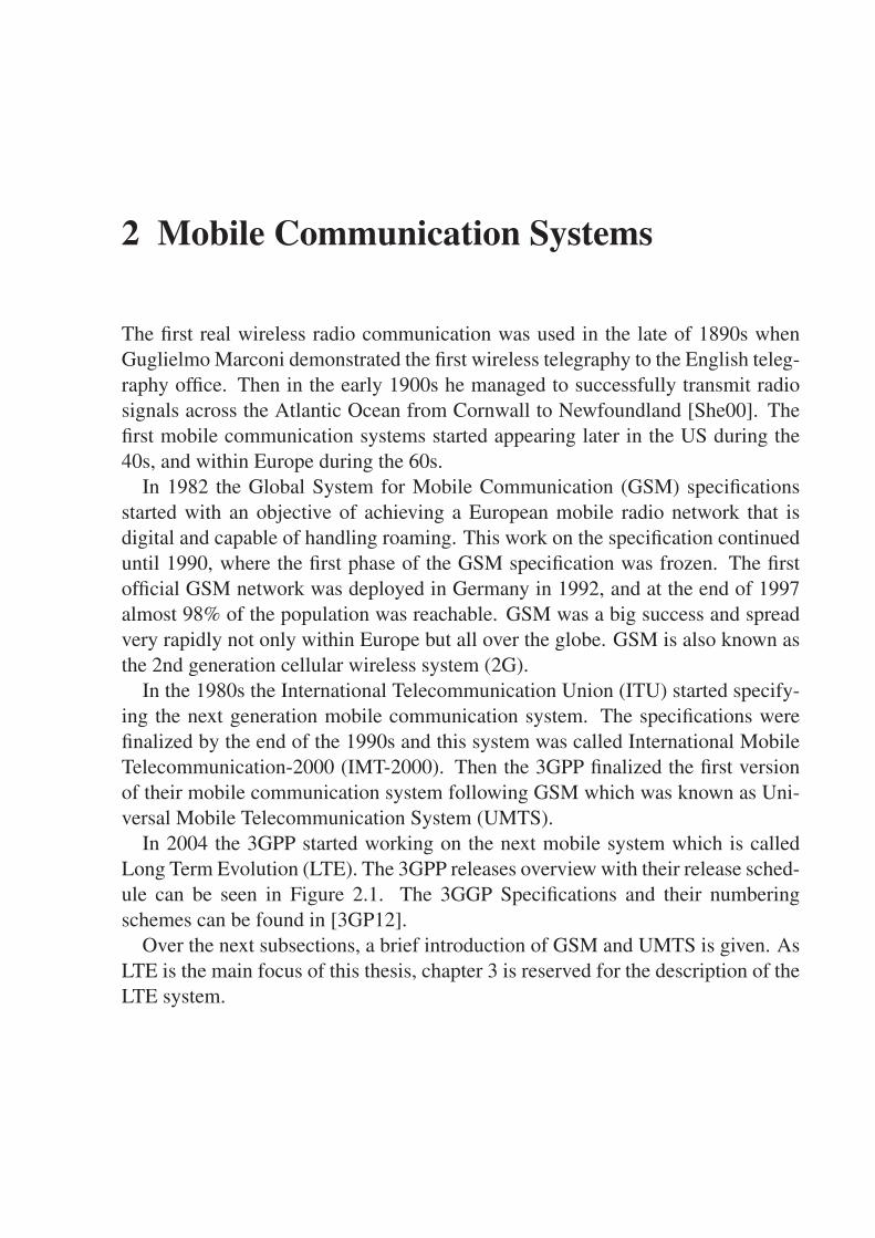
In 2004 the 3GPP started working on the next mobile system which is calledLong Term Evolution (LTE). The 3GPP releases overview with their release sched-ule can be seen in Figure 2.1. The 3GGP Specifications and their numberingschemes can be found in [3GP12].
Over the next subsections, a brief introduction of GSM and UMTS is given. AsLTE is the main focus of this thesis, chapter 3 is reserved for the description of theLTE system.
6 2 Mobile Communication Systems
2000 2001 2002 2003 2004 2005
2006 2007 2008 2009 2010 2011
Release 99 Release 4 Release 5 Release 6
Release 7 Release 8 Release 9 Release 10
Release 99: 1st UMTS (3G) specificationsRelease 4: Originally called Release 2000, new low chip rate TDD version for the TDD UTRANRelease 5: HSDPA and IP Multimedia Subsystem (IMS)Release 6: HSUPA, WLAN-UMTS interworking, Multimedia Broadcast Multicast Service (MBMS)Release 7: Future FDD HSPA evolution, latency reductions and radio interface improvementsRelease 8: First LTE release and all IP network (that is System Architecture Evolution SAE)Release 9: Personal Area Networks supportRelease 10: LTE advanced fulfilling IMT advanced 4G requirementsRelease 11: Advanced IP interconnection of services and non voice emergency services
Figure 2.1: 3GPP releases overview [HT09] [Zah11]
2.1 Global System for Mobile Communication (GSM)
A mobile radio communication system by definition consists of telecommunica-tion infrastructure serving users that are on the move (i.e., mobile). The communi-cation between the users and the infrastructure is done over a wireless mediumknown as a radio channel. Telecommunication systems have several physicalcomponents such as: user terminal/equipment, transmission and switching/routingequipment, etc.
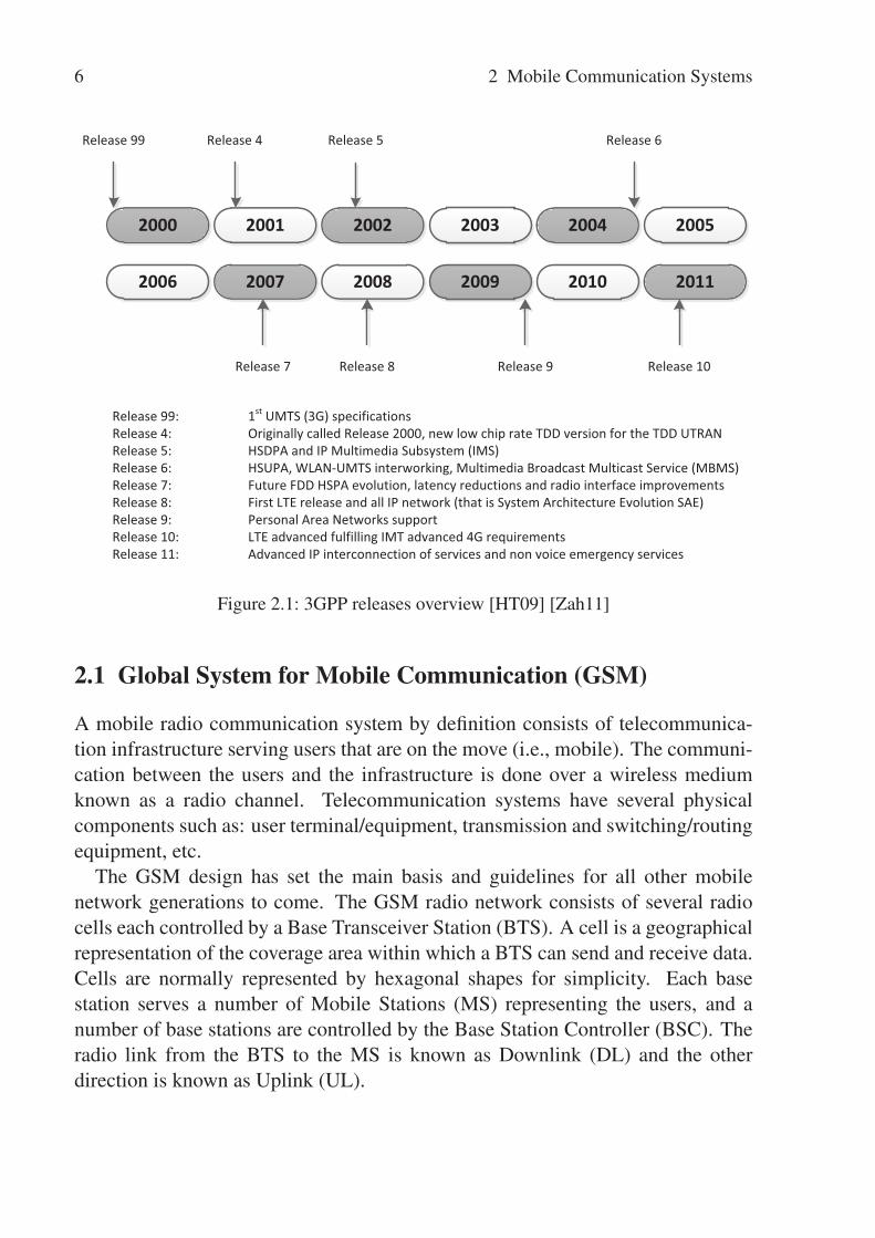
The GSM design has set the main basis and guidelines for all other mobilenetwork generations to come. The GSM radio network consists of several radiocells each controlled by a Base Transceiver Station (BTS). A cell is a geographicalrepresentation of the coverage area within which a BTS can send and receive data.Cells are normally represented by hexagonal shapes for simplicity. Each basestation serves a number of Mobile Stations (MS) representing the users, and anumber of base stations are controlled by the Base Station Controller (BSC). Theradio link from the BTS to the MS is known as Downlink (DL) and the otherdirection is known as Uplink (UL).

2.1 Global System for Mobile Communication (GSM) 7
Figure 2.2 shows the general GSM network architecture. The GSM networkarchitecture is divided into four main functional groups, these are:
• Mobile Station (MS): is also known as User Equipment (UE), this entityconsists of the terminal equipment and the Subscriber Identity Module (SIM).
• Base Station Subsystem (BSS): this entity handles the radio access func-tions, like radio resource management. It connects the UEs with the corenetwork.
• Core Network (CN): includes the transport functions, mobility management,user/subscriber databases with their information, service controlling func-tions, billing, etc.
• External Network: these are the external networks that the UEs can commu-nicate with and that the mobile network has to be connected to. It can be forexample the public telephone network or any other GSM network.
BTS
BSC
BTS
1 2 3
4 5 6
7 8 9
# 0 *
MSC/VLR
PSTN
GSM Core Network
Base Station Subsystem (BSS) External NetworkMobile Station (MS)
MT/TE
SIM
TE
Uplink (UL)
Downlink (DL)
@HLR/AUC
SS7 network
MT: Mobile TerminalTE: Terminal EquipmentBTS: Base Transceiver Station
BSC: Base Station ControllerMSC: Mobile Switching CenterVLR: Visitors Location Registry
HLR: Home Location RegistryAUC: Authentication CenterPSTN: Public Switched Telephone Network
Figure 2.2: GSM network Architecture 1
1Picture is redrawn from
8 2 Mobile Communication Systems
One of the important features of a mobile communication system is the radiointerface. A radio interface is the interface between the mobile stations and thebase station. This interface enables the users of the mobile networks to be mobilewith wireless access. The radio spectrum is the term used to describe the amountof resources (i.e., frequency bandwidth/spectrum) that the air interface uses. Inmobile communication the radio spectrum is one of the most important parts dueto its high incurring cost. In addition, the radio spectrum is often limited and istreated as a scarce resource that the users of the mobile communication systemneed to share. The sharing of the spectrum is done using the so-called multipleaccess scheme.
In GSM, a mixture of Time Division Multiple Access (TDMA) and FrequencyDivision Multiple Access (FDMA) is used as the multiple access scheme. FDMAis used to divide the GSM spectrum into several carrier frequencies. Each carrierfrequency is then divided using TDMA into 8 time slots that are then used by themobile stations for their transmissions. The maximum spectrum/frequency bandof GSM is 25 MHz, that is 124 carrier frequencies that are separated from eachother by 200 kHz. In GSM, Frequency Division Duplex (FDD) is also used toseparate the downlink frequency range from the uplink.
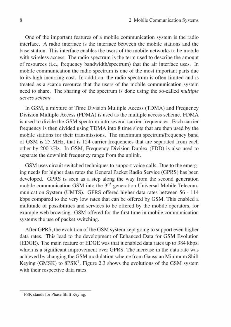
GSM uses circuit switched techniques to support voice calls. Due to the emerg-ing needs for higher data rates the General Packet Radio Service (GPRS) has beendeveloped. GPRS is seen as a step along the way from the second generationmobile communication GSM into the 3rd generation Universal Mobile Telecom-munication System (UMTS). GPRS offered higher data rates between 56 - 114kbps compared to the very low rates that can be offered by GSM. This enabled amultitude of possibilities and services to be offered by the mobile operators, forexample web browsing. GSM offered for the first time in mobile communicationsystems the use of packet switching.
After GPRS, the evolution of the GSM system kept going to support even higherdata rates. This lead to the development of Enhanced Data for GSM Evolution(EDGE). The main feature of EDGE was that it enabled data rates up to 384 kbps,which is a significant improvement over GPRS. The increase in the data rate wasachieved by changing the GSM modulation scheme from Gaussian Minimum ShiftKeying (GMSK) to 8PSK1. Figure 2.3 shows the evolutions of the GSM systemwith their respective data rates.
1PSK stands for Phase Shift Keying.
2.2 Universal Mobile Telecommunication System (UMTS) 9
2G
GSM 9.4 Kbps
1998
2.5G
GPRS 114 Kbps
2000
2.75G
EDGE 384 Kbps
2001
3G
UMTS 2 Mbps
2002
Figure 2.3: GSM system evolution
2.2 Universal Mobile Telecommunication System (UMTS)
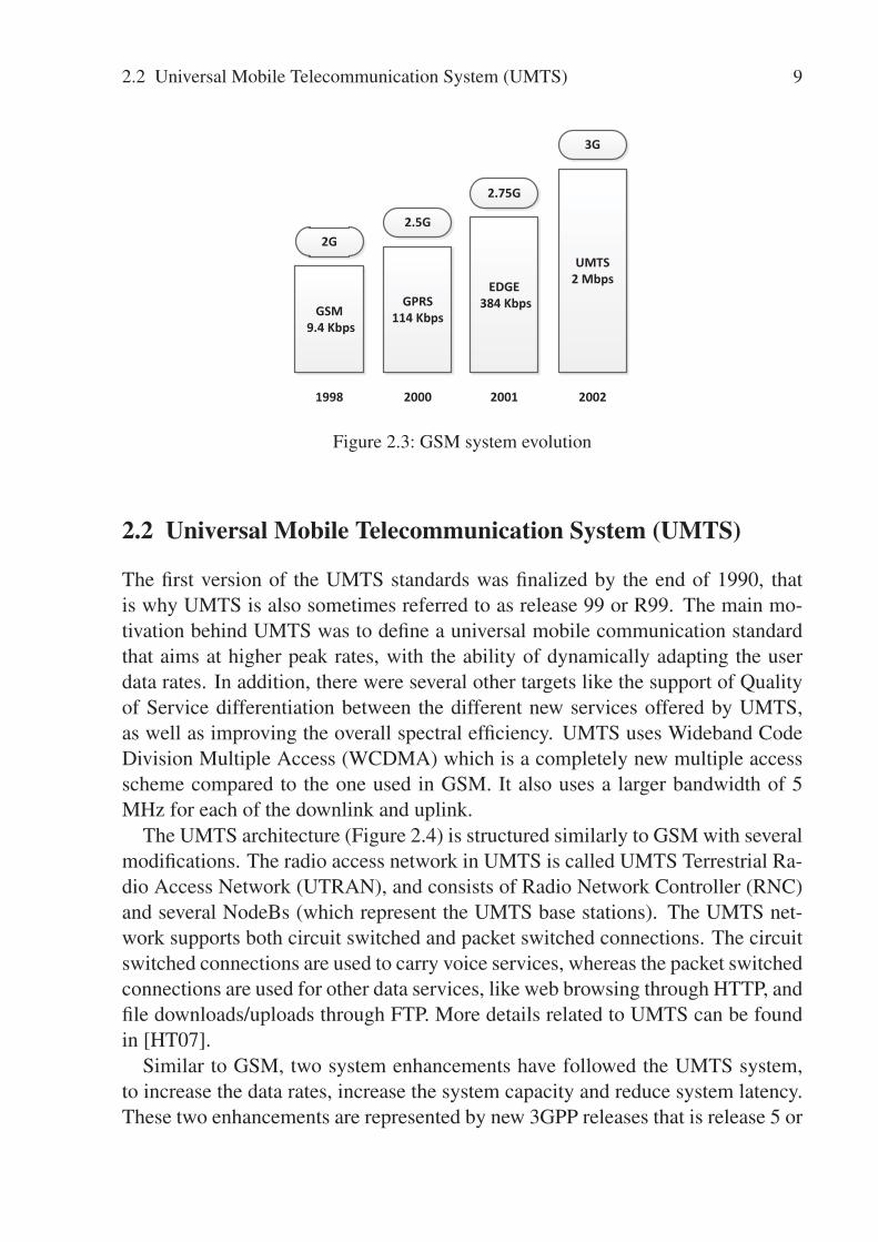
The first version of the UMTS standards was finalized by the end of 1990, thatis why UMTS is also sometimes referred to as release 99 or R99. The main mo-tivation behind UMTS was to define a universal mobile communication standardthat aims at higher peak rates, with the ability of dynamically adapting the userdata rates. In addition, there were several other targets like the support of Qualityof Service differentiation between the different new services offered by UMTS,as well as improving the overall spectral efficiency. UMTS uses Wideband CodeDivision Multiple Access (WCDMA) which is a completely new multiple accessscheme compared to the one used in GSM. It also uses a larger bandwidth of 5MHz for each of the downlink and uplink.
The UMTS architecture (Figure 2.4) is structured similarly to GSM with severalmodifications. The radio access network in UMTS is called UMTS Terrestrial Ra-dio Access Network (UTRAN), and consists of Radio Network Controller (RNC)and several NodeBs (which represent the UMTS base stations). The UMTS net-work supports both circuit switched and packet switched connections. The circuitswitched connections are used to carry voice services, whereas the packet switchedconnections are used for other data services, like web browsing through HTTP, andfile downloads/uploads through FTP. More details related to UMTS can be foundin [HT07].
Similar to GSM, two system enhancements have followed the UMTS system,to increase the data rates, increase the system capacity and reduce system latency.These two enhancements are represented by new 3GPP releases that is release 5 or

10 2 Mobile Communication Systems
NodeB
RNCNodeB
1 2 3
4 5 6
7 8 9
# 0 *
PSTN
Core Network (CN)Access Network (AN)Mobile Station (MS)
MT/TE
USIM
User Equipment (UE)
MT: Mobile TerminalTE: Terminal EquipmentRNC: Radio Network ControllerGMSC: Gateway Mobile Switching Center
EIR: Equipment Identity RegisterHLR: Home Location RegistryVLR: Visitors Location RegistryAUC: Authentication Center
@HLR/AUC
1 2 3
4 5 6
7 8 9
# 0 *
1 2 3
4 5 6
7 8 9
# 0 *
1 2 3
4 5 6
7 8 9
# 0 *
@VLR
@EIR
CS-MGW MSC server
GMSC
Circuit switched
Internet
Packet switched
SGSN
GGSN
Universal Terrestrial Radio Access
Network (UTRAN)
Uu
Figure 2.4: UMTS network Architecture 1
High Speed Downlink Packet Access (HSDPA), and release 6 High Speed UplinkPacket Access (HSUPA).
HSDPA is already mentioned before the 5th release of the UMTS specification.The goal of this release was to enhance the downlink data rates of the UMTSstandard up to 14 Mbps, increase the spectral efficiency, as well as reduce thesystem latency. This is achieved by the introduction of several new functions:
• Adaptive Modulation and Coding (AMC): the modulation and coding schemesof each user transmission is adaptively changed depending on the user chan-nel conditions, for example, a user with very good channel conditions isassigned a higher modulation and coding scheme.
• Fast NodeB Scheduling: the scheduling function is moved from the RNCto the NodeB compared to GSM. Which means the NodeB can track theinstantaneous channel changes of the users and schedule the resources in amore efficient way thus gaining from the multi-user diversity principle.
• Shorter Transmission Time Interval (TTI): the TTI length is reduced in HS-DPA to 2ms, instead of 10ms in UMTS R99. TTI is the duration of a trans-
1Picture is redrawn from

2.2 Universal Mobile Telecommunication System (UMTS) 11
mission over the radio link, it is also the rate of the radio scheduler at whichit takes decisions on which UEs transmit over the next TTI.
• Use of Hybrid Automatic Repeat Request (HARQ): performing retransmis-sions of the erroneous packets between the NodeB and the UE instead ofwaiting for higher layer retransmissions. This of course will result in la-tency reduction. In addition, chase combining and incremental redundancyare also used to combine the two unsuccessfully decoded packets with thenew retransmission to improve the decoding probability.
Similar to HSDPA, HSUPA aims at enhancing the performance of the UMTSR99 uplink in terms of improving the user data rates up to 5.76 Mbps and re-ducing the latency. HSUPA also uses concepts similar to HSDPA: shorter 2msTTI (optional), HARQ and fast scheduling. However, the AMC is not used inHSUPA since it does not support any high order modulation schemes and it onlyuses QPSK. This is because higher modulation schemes require more energy perbit resulting in faster battery discharge. In HSUPA, both soft and softer handoverare allowed, unlike HSDPA, because the UE is the entity performing the transmis-sion and the neighboring NodeBs can also listen to the UE transmission withoutany extra effort.
The use of both enhancements (i.e., HSDPA and HSUPA) is often referred to asHSPA. Network operators deploy HSPA in coexistence with R99 UMTS networks.The instantaneous radio performance may vary overtime, sometimes achievingvery high cell throughputs. However, the network operators dimension their back-haul by considering the average performance so as to reduce cost [LZW+08],which will cause short term congestions in the network backhaul. In order to mit-igate the influence of this, congestion control schemes as well as traffic separationtechniques are used to overcome the aforementioned issues and provide QoS dif-ferentiation between HSPA and R99 traffic [WZTG+09] [LZW+10] [LWZ+11].


3 Long Term Evolution (LTE)
LTE is one of the newest releases of the 3rd Generation Partnership Project (3GPP)specifications. It is also referred to as 3.9G or Release 8. The 3GPP started work-ing on LTE in November 2004 with the Radio Access Network (RAN) Evolutionworkshop in Toronto - Canada. The main task was to standardize a system withnew design goals that can exceed older mobile standards (like UMTS and HSPA),as well as being able to stay competitive at least for the next 10 years.
3.1 Motivation and Targets
In March 2005, a feasibility study on LTE was launched. The main focus of thisstudy was to decide what architecture the new system should have and what multi-ple access techniques were to be used. The LTE network architecture can be seenin Figure 3.1. The main conclusions drawn from the feasibility study [25.05] canbe summarized in terms of requirements and targets as follows:
UE
eNodeB
MME
S-GW
HSS
PDNGW
PCRF
UuS1-U
S1-MME
S6a
S11 Gx
Rx
S5/S8
eNodeB
UE E-UTRAN EPC Services
IP connectivity Layers, The EPS
Service connectivity Layer
User plane
Control plane
SGi
Operator’s IP services
(e.g. IMS, PSS)
Figure 3.1: LTE EPS network architecture

14 3 Long Term Evolution (LTE)
• Simplified flat packet oriented network architecture
• High data rates up to 100 Mbps in the downlink and 50 Mbps in the uplink(even higher with Multi Input Multi Output (MIMO))
• Reduced latency
• Scalable usage of frequency spectrum from 1.25 MHz to 20 MHz
• OFDMA and SC-FDMA as the multiple access techniques for downlink anduplink respectively
3.2 LTE Multiple Access Schemes
In LTE the multiple access transmission scheme is based on the Frequency DomainMultiplexing (FDM). Two different versions are used: Orthogonal Frequency Do-main Multiple Access (OFDMA) for the downlink, and Single Carrier FrequencyDomain Multiple Access (SC-FDMA) for the uplink. OFDMA is a very efficienttransmission scheme which is widely employed in many digital communicationsystems, e.g., Digital Video Broadcasting (DVB), WiMax, Wireless Local AreaNetwork (WLAN). The reason behind the popularity of OFDMA comes fromthe fact that it has very robust characteristics against frequency selective channels.Frequency selectivity is one of the transmission problems that can be overcomethrough equalization, but the complexity of the equalization technique is very high.Another reason for choosing OFDMA as the downlink transmission scheme is thebandwidth flexibility it offers, since changing the number of sub-carriers used canincrease or decrease the used frequency bandwidth.
SC-FDMA is the transmission scheme in the LTE uplink. It provides a low peak-to-average ratio between the transmitted signal; it is a very desirable characteristicfor the uplink to have an efficient usage of the power amplifier. This provides ahigh battery life time for mobile devices.
3.2.1 OFDM
The basic principle of multi-carrier systems is the splitting of the total bandwidthinto a large number of smaller and narrower bandwidth units, which are knownas sub-channels. Due to the narrow bandwidth sub-channels frequency selectivitydoes not exist. As a result, only the gains of the sub-channels has to be compen-sated and no complex equalization techniques is required.
In OFDM the sub-channels are orthogonal to each other. This nice property doesnot require the addition of guard intervals between the sub-channels and hence

3.2 LTE Multiple Access Schemes 15
it increases the system spectral efficiency. Figure 3.2 shows the orthogonalityprinciple of OFDM; the frequency representation of one OFDM sub-channel is aSinc1 function, where if the sampling is done at the exact spacing the result willonly be at the sub-carrier of that sub-channel and zeros at every other sub-carrierfrequency. This means that the sub-channels are orthogonal to each other.
Frequency
Time
Sub-Carriers
Spectrum (Bandwidth)
Figure 3.2: OFDM signal in frequency and time domain [Hoa05]
3.2.2 OFDMA
Orthogonal Frequency Division Multiple Access (OFDMA) is an access schemethat uses the OFDM principle to orchestrate the distribution of the scarce radioresources among several users enabling multi user communications. This is doneby using the Time Domain Multiple Access (TDMA), where users dynamicallyget some resources at the different time instances of the scheduling.
The LTE MAC Scheduler (explained in chapter 6) makes use of the differ-ent user channel conditions to distribute the frequency resources (sub-carriers) towhere it best fits. This can mean giving them to the users, for example with the bestinstantaneous channel conditions (Max-CI scheduling). This distribution processis determined by the used scheduler discipline.
1The sinc function, sometimes also known as the sampling function, is a function that is widely usedin signal processing and Fourier transforms. It is commonly defined as Sinc(x)= Sin(x)/x.
16 3 Long Term Evolution (LTE)
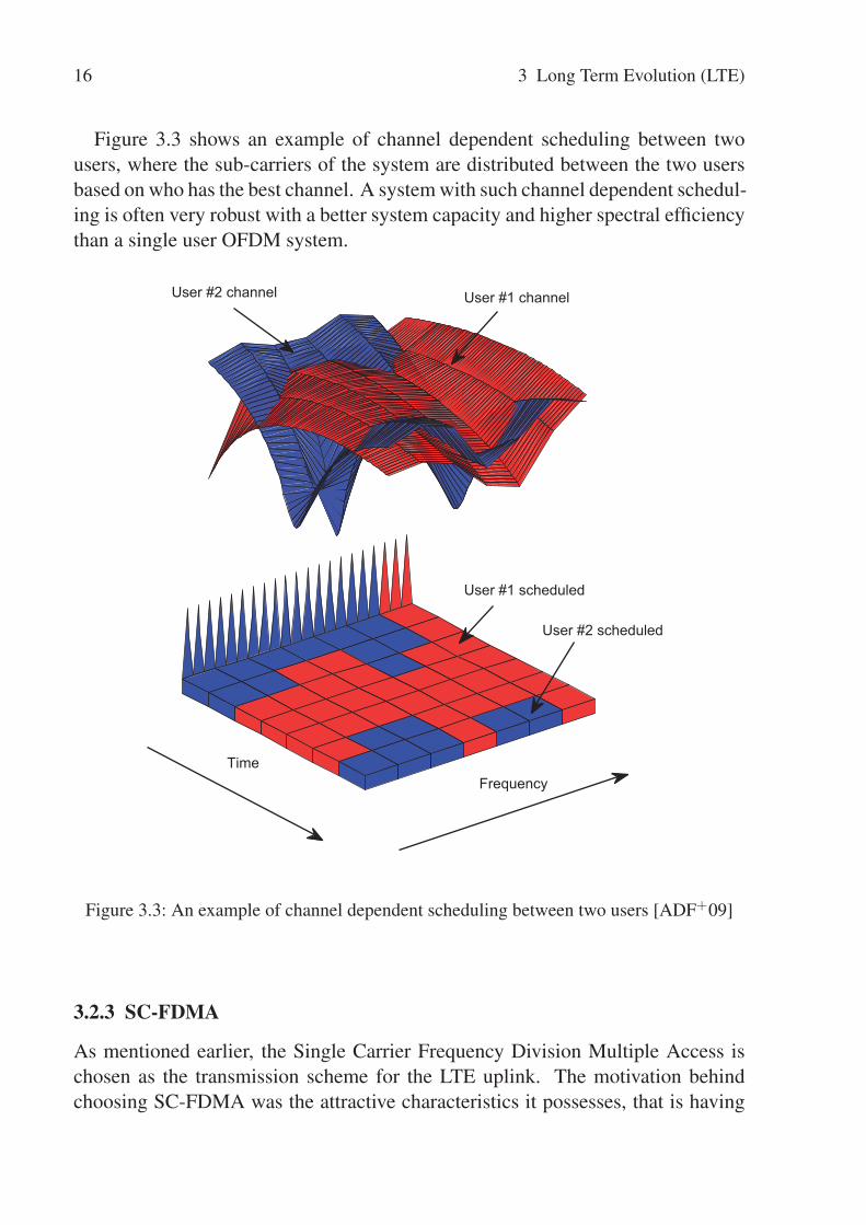
Figure 3.3 shows an example of channel dependent scheduling between twousers, where the sub-carriers of the system are distributed between the two usersbased on who has the best channel. A system with such channel dependent schedul-ing is often very robust with a better system capacity and higher spectral efficiencythan a single user OFDM system.
User #2 scheduled
Frequency
User #1 channel
User #1 scheduled
Time
User #2 channel
Figure 3.3: An example of channel dependent scheduling between two users [ADF+09]
3.2.3 SC-FDMA
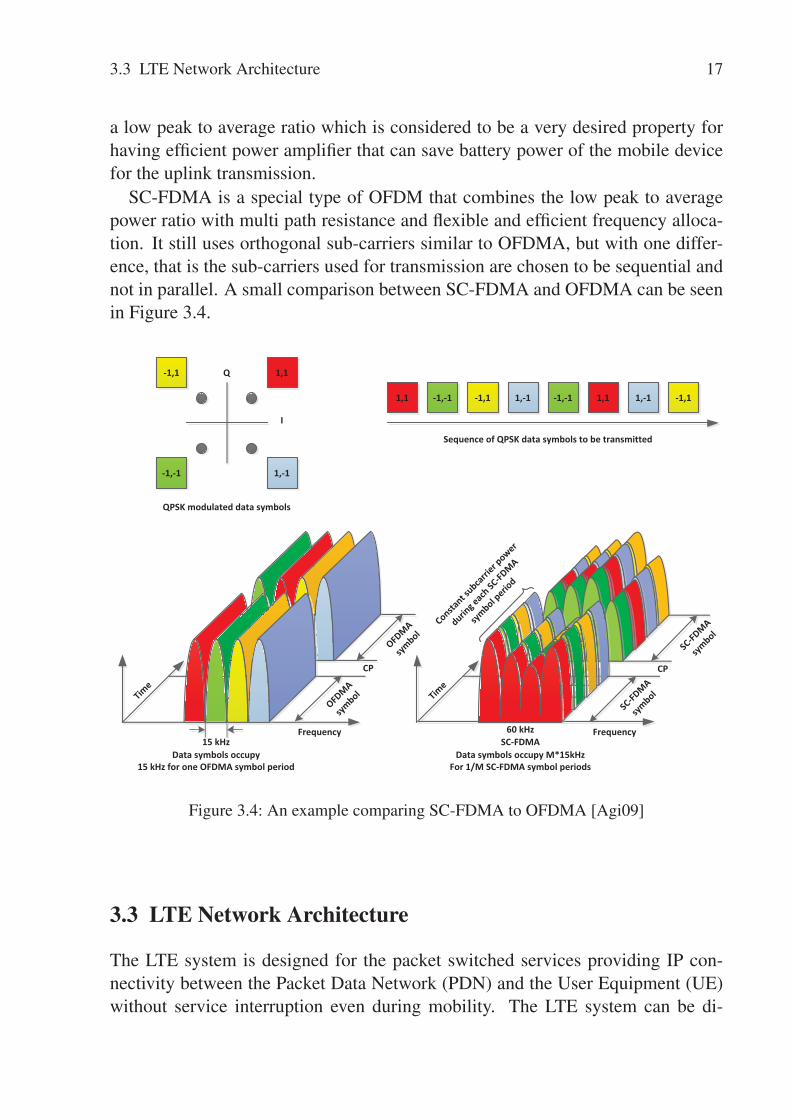
As mentioned earlier, the Single Carrier Frequency Division Multiple Access ischosen as the transmission scheme for the LTE uplink. The motivation behindchoosing SC-FDMA was the attractive characteristics it possesses, that is having
3.3 LTE Network Architecture 17
a low peak to average ratio which is considered to be a very desired property forhaving efficient power amplifier that can save battery power of the mobile devicefor the uplink transmission.
SC-FDMA is a special type of OFDM that combines the low peak to averagepower ratio with multi path resistance and flexible and efficient frequency alloca-tion. It still uses orthogonal sub-carriers similar to OFDMA, but with one differ-ence, that is the sub-carriers used for transmission are chosen to be sequential andnot in parallel. A small comparison between SC-FDMA and OFDMA can be seenin Figure 3.4.
15 kHzFrequency
Data symbols occupy 15 kHz for one OFDMA symbol period
Time
Frequency
Time
SC-FDMAData symbols occupy M*15kHz
For 1/M SC-FDMA symbol periods
60 kHz
CP CP
Constant s
ubcarri
er power
during e
ach SC
-FDMA
symbol p
eriod
1,1-1,1
-1,-1 1,-1
Q
I
QPSK modulated data symbols
1,1 -1,-1 -1,1 1,-1 -1,-1 1,1 1,-1 -1,1
Sequence of QPSK data symbols to be transmitted
OFDMA
symbol
OFDMA
symbol
SC-FD
MA
symbol
SC-FD
MA
symbol
Figure 3.4: An example comparing SC-FDMA to OFDMA [Agi09]
3.3 LTE Network Architecture
The LTE system is designed for the packet switched services providing IP con-nectivity between the Packet Data Network (PDN) and the User Equipment (UE)without service interruption even during mobility. The LTE system can be di-
18 3 Long Term Evolution (LTE)
vided into two main branches: Evolved Universal Terrestrial Radio Access Net-work (E-UTRAN) and System Architecture Evolution (SAE). The E-UTRANevolved from the UMTS radio access network; it is sometimes also referred toas LTE. The SAE supports the evolution of the packet core network, also knownas Evolved Packet Core (EPC). The combination of both the E-UTRAN and theSAE compose the Evolved Packet System (EPS). Figure 3.1 shows the generalLTE network architecture.
According to [SBT09], an EPS bearer is defined to be an IP packet flow betweenthe PDN-GW and the UE with predefined Quality of Service (QoS) characteristics.Both the EPC and the E-UTRAN are responsible for setting and releasing such abearer depending on the application QoS requirements. In LTE multiple bearerscan be established for users with multiple services, e.g., a user can have a voice callusing the Voice over Internet Protocol (VoIP) and at the same time be downloadinga file using File Transfer Protocol (FTP), or browse the web using the HypertextTransfer Protocol (HTTP). Each of these services can be mapped to a differentbearer. More detailed explanations on the quality of service and the bearers inLTE are given in section 3.5. In the next subsection a brief description of theimportant LTE nodes will be presented.
3.3.1 User Equipment (UE)
As the name suggests, a UE is the actual device that the LTE customers useto connect to the LTE network and establish their connectivity. The UE maytake several forms; it can be a mobile phone, a tablet, or a data card used by acomputer/notebook. Similar to all other 3GPP systems, the UE consists of twomain entities: a SIM-card or what is also known as User Service Identity Mod-ule (USIM), and the actual equipment known as Terminal Equipment (TE). TheSIM-card carries the necessary information provided by the operator for user iden-tification and authentication procedures. The terminal equipment on the other handprovides the users with the necessary hardware (e.g., processing, storage, operat-ing system) to run their applications and utilize the LTE system services.
3.3.2 Evolved UTRAN (E-UTRAN)
The E-UTRAN in LTE consists of directly interconnected eNodeBs which areconnected to each other through the X2 interface and to the core network throughthe S1 interface. This eliminates one of the biggest drawbacks of the former 3GPPsystems (UMTS/HSPA): the need to connect and control the NodeBs through the
3.3 LTE Network Architecture 19
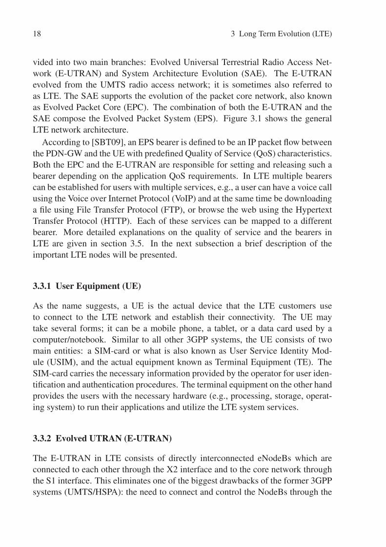
Radio Network Controller (RNC), which make the system vulnerable against RNCfailures. The LTE E-UTRAN architecture can be seen in Figure 3.5.
MME/aGW
MME/aGW
eNodeBeNodeB
eNodeB
X2X2
X2
S1
S1 S1
S1
EPC
E-U
TRA
NFigure 3.5: LTE E-UTRAN architecture
The enhanced NodeB (eNodeB) entity works as a bridge between the UE andthe EPC. It provides the necessary radio protocols to the user equipment, so asto be able to send and receive data and it tunnels the users data securely over theLTE transport to the PDN-GW and vice versa. The GTP tunneling protocol isused, which works on top of the UDP/IP protocols. The eNodeB is also respon-sible for the scheduling which is one of the most important radio functions. TheeNodeB schedules the frequency spectrum resources among the different users byexploiting both the time and frequency, while guaranteeing different quality ofservice for the end users. In addition, the eNodeB also has some mobility man-agement functionalities, e.g., radio link measurements and handover signaling forother eNodeBs.
3.3.3 Evolved Packet Core (EPC)
As shown in Figure 3.1, the EPC (also known as the LTE core network) consistsof three main entities: Mobility Management Entity (MME), Serving Gateway(S-GW) and the Packet Data Network Gateway (PDN-GW). In addition, there aresome other logical entities like the Home Subscriber Server (HSS) and Policy andCharging Rules Function (PCRF). The main purpose of the EPC is to provide the
20 3 Long Term Evolution (LTE)
necessary functionalities to support the users and establish their bearers [SBT09].Each of the EPC main entities and their functionalities is described briefly in thenext paragraphs. A more detailed description can be found in [36.11a].
The MME entity provides control functions as well as signaling for the EPC.The MME is only involved in the control plane. Some of the MME supportedfunctions include: authentication, security, roaming, default/dedicated bearer es-tablishment, tracking user mobility and handover. The S-GW is the main gatewayfor the user traffic, where all the users IP traffic goes through. It is the local mobil-ity anchor point for inter-eNodeB handover, as well as the mobility anchoring forinter-3GPP mobility [36.11a]. In addition the S-GW provides several other func-tions like: routing, forwarding, charging/accounting information gathering. Thepacket data network gateway PDN-GW acts as the user connectivity point for theuser traffic, it is responsible for assigning the users IP addresses as well as clas-sifying the user traffic into different QoS classes. In addition, the PDN-GW actsas the mobility anchor point for inter-working with non 3GPP technologies, likeWireless LAN and WiMax.
3.4 E-UTRAN Protocol Architecture
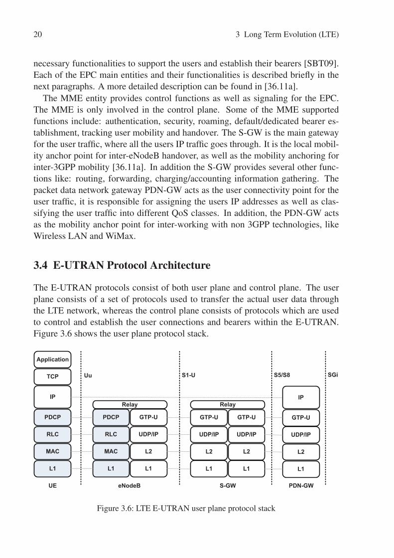
The E-UTRAN protocols consist of both user plane and control plane. The userplane consists of a set of protocols used to transfer the actual user data throughthe LTE network, whereas the control plane consists of protocols which are usedto control and establish the user connections and bearers within the E-UTRAN.Figure 3.6 shows the user plane protocol stack.
L1
MAC
RLC
PDCP
IP
TCP
Application
L1
MAC
RLC
PDCP
L1
L2
UDP/IP
GTP-U
Relay
L1
L2
UDP/IP
GTP-U
L1
L2
UDP/IP
GTP-U
Relay
L1
L2
UDP/IP
GTP-U
IP
UE eNodeB S-GW PDN-GW
Uu S1-U S5/S8 SGi
Figure 3.6: LTE E-UTRAN user plane protocol stack

3.4 E-UTRAN Protocol Architecture 21
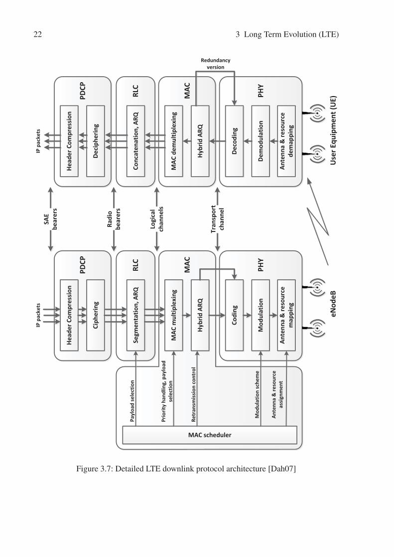
The LTE radio access architecture is mainly the eNodeB which is an enhancedversion of the original NodeB of the UMTS system. Since the RNC was removedfrom the LTE architecture some of its functions have been moved to the eNodeB.Figure 3.7 shows the detailed eNodeB and UE protocol architecture for the down-link [Dah07]. The main LTE radio interface protocols are [HT09]:
• Radio Resource Control (RRC): is responsible for the handover functions,like handover decisions, transfer of UE context from serving eNodeB totarget eNodeB during handover. In addition, it controls the periodicity ofthe Channel Quality Indicator (CQI) and is also responsible for the setupand maintenance of the radio bearers [Mot].
• Packet Data Convergence Protocol (PDCP): is responsible for compressingthe IP header, i.e., reduces the overall overhead which in turn improves theefficiency over the radio interface. This layer also performs additional func-tionalities, e.g., ciphering and integrity protection. A detailed description ofthe PDCP functionality can be found in [36.11c].
• Radio Link Control (RLC): is responsible for the segmentation and con-catenation of the PDCP packets. It also performs retransmissions and guar-antees in-sequence delivery of the packets to the higher layers. The RLCalso performs error corrections using the well-known Automatic Repeat Re-quest (ARQ) methods. A detailed description of the PDCP functionality canbe found in [36.10b].
• Medium Access Channel (MAC): is responsible for scheduling air interfaceresources in both uplink and downlink. It is also responsible for satisfy-ing the users’ QoS over the air interface. In addition, the MAC layer alsoperforms the Hybrid Automatic Repeat Request (HARQ).
• Physical Layer (PHY): is responsible for the radio related issues: e.g., mod-ulation/demodulation, coding/decoding, Multi Input Multi Output (MIMO)techniques.
22 3 Long Term Evolution (LTE)
Head
er C
ompr
essi
on
Ciph
erin
g
PDCP
Segm
enta
tion,
ARQ
RLC
MAC
mul
tiple
Hybr
id A
RQ
MAC scheduler
MAC
Payl
oad
sele
ctio
n
Prio
rity
hand
ling,
pay
load
se
lect
ion
Retr
ansm
issi
on c
ontr
ol
Codi
ng
Mod
ulat
ion
PHY
Ante
nna
& re
sour
ce
map
ping
Mod
ulat
ion
sche
me
Ante
nna
& re
sour
ce
assi
gnm
ent
IP p
acke
ts
eNod
eB
Head
er C
ompr
essi
on
Deci
pher
ing
PDCP
Conc
aten
atio
n, A
RQRL
C
MAC
dem
ultip
lexi
ng
Hybr
id A
RQ
MAC
Deco
ding
Dem
odul
atio
nPH
Y
Ante
nna
& re
sour
ce
dem
appi
ng
IP p
acke
ts
Use
r Equ
ipm
ent (
UE)
Redundancy version
Tran
spor
t ch
anne
l
Logi
cal
chan
nels
Radi
o be
arer
s
SAE
bear
ers
Figure 3.7: Detailed LTE downlink protocol architecture [Dah07]
3.4 E-UTRAN Protocol Architecture 23
3.4.1 Radio Link Control (RLC)
The radio link control protocol is responsible for the concatenation and segmenta-tion process. It segments the packets that come from the PDCP layer (i.e., the IPpackets after compressing the header) into smaller RLC packets, and concatenatesthe RLC packets on the receiver side into the PDCP packets. In addition to theabove functionality, the RLC protocol provides reliable communication betweenthe eNodeB and the UE by the aid of packet retransmissions. The RLC uses se-quence numbers to detect lost packets at the receiver side and inform the senderwhich packets to retransmit by using some selective repeat retransmissions. Thisis also known as Automatic Repeat Request (ARQ). The RLC protocol can operatein three different operational modes, these are:
• Acknowledged Mode (AM): which is used to provide error-free transmis-sion between sender and receiver. This mode is suitable for services that usethe TCP transport protocol, like FTP and HTTP, where reliability and errorfree delivery is of the utmost importance.
• Unacknowledged Mode (UM): in this mode no retransmissions are per-formed and RLC only provides segmentation and concatenation function-alities. This mode is suitable for applications that does not require error-freetransmission and can tolerate some losses, like VoIP and video conferencing.
• Transparent Mode (TM): this operation mode of RLC does not add any pro-tocol overhead to the higher layer data. It can be used for example for ran-dom access.
The RLC segmentation and concatenation is done based on the MAC schedulerdecision, where the scheduler informs the RLC layer on what Transport BlockSize (TBS) to be used by a certain user/bearer. This tells the RLC the amount ofbits to be sent down to the lower layer. In contrast to the RLC version used inUMTS/HSPA [ZWL+08] [ZWL+10], in LTE the RLC Packet Data Unit (PDU)size is not fixed and is dynamically changed based on the scheduler decision. Inaddition to the retransmission and segmentation/concatenation functionalities ofRLC there are a number of other functionalities supported by RLC [HT07]:
• Padding
• In-Sequence delivery of higher layer PDUs
• Duplicate detection
• Flow control

24 3 Long Term Evolution (LTE)
• SN check (unacknowledged data transfer mode)
• Protocol error detection and recovery
• Ciphering
• Suspend/resume function for data transfer
3.4.2 Medium Access Control (MAC)
The MAC layer is responsible for one of the most important functionalities thatis scheduling for both downlink and uplink. In addition, the MAC layer provides:Hybrid Automatic Repeat Request (HARQ), logical channel multiplexing/de-multiplexing,mapping between logical and transport channels, scheduling information report-ing, priority handling between the UEs, priority handling between the logical chan-nels on one UE, logical channel prioritization and transport format selection.
3.4.2.1 Logical and Transport Channels
As stated earlier, since the MAC layer is located below the RLC layer it providesservices to the RLC by offering logical channels. Two different types of logi-cal channels exist, these are traffic and control channels. This classification isdone depending on the type of data the channel is transmitting. According to the3GPP standards [36.11b], the logical channel types defined for the different kindsof services are listed in Table 3.1. The MAC layer uses the services offered bythe physical layer in terms of using the Transport Channels. The LTE transportchannels are listed in Table 3.2. A detailed description of the LTE logical andtransport channels as well as how the mapping between them is done can be foundin [Dah07].
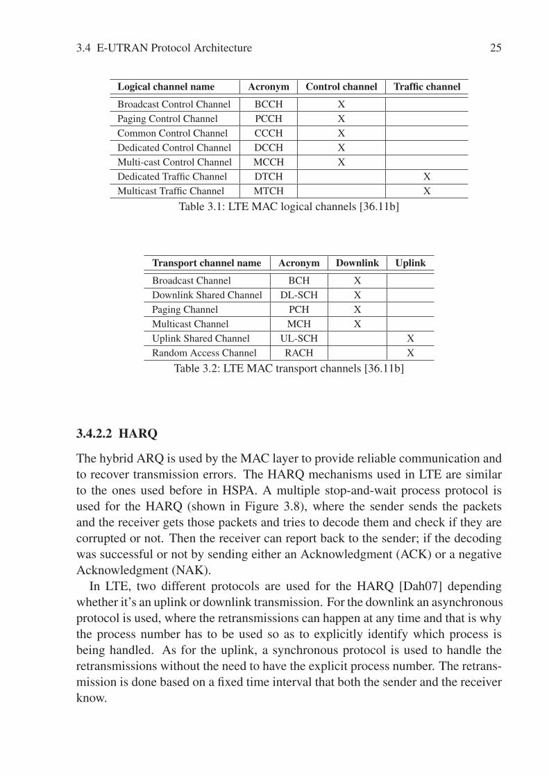
3.4 E-UTRAN Protocol Architecture 25
Logical channel name Acronym Control channel Traffic channel
Broadcast Control Channel BCCH XPaging Control Channel PCCH XCommon Control Channel CCCH XDedicated Control Channel DCCH XMulti-cast Control Channel MCCH XDedicated Traffic Channel DTCH XMulticast Traffic Channel MTCH X
Table 3.1: LTE MAC logical channels [36.11b]
Transport channel name Acronym Downlink Uplink
Broadcast Channel BCH XDownlink Shared Channel DL-SCH XPaging Channel PCH XMulticast Channel MCH XUplink Shared Channel UL-SCH XRandom Access Channel RACH X
Table 3.2: LTE MAC transport channels [36.11b]
3.4.2.2 HARQ
The hybrid ARQ is used by the MAC layer to provide reliable communication andto recover transmission errors. The HARQ mechanisms used in LTE are similarto the ones used before in HSPA. A multiple stop-and-wait process protocol isused for the HARQ (shown in Figure 3.8), where the sender sends the packetsand the receiver gets those packets and tries to decode them and check if they arecorrupted or not. Then the receiver can report back to the sender; if the decodingwas successful or not by sending either an Acknowledgment (ACK) or a negativeAcknowledgment (NAK).
In LTE, two different protocols are used for the HARQ [Dah07] dependingwhether it’s an uplink or downlink transmission. For the downlink an asynchronousprotocol is used, where the retransmissions can happen at any time and that is whythe process number has to be used so as to explicitly identify which process isbeing handled. As for the uplink, a synchronous protocol is used to handle theretransmissions without the need to have the explicit process number. The retrans-mission is done based on a fixed time interval that both the sender and the receiverknow.

26 3 Long Term Evolution (LTE)
Receiver processingooReceiver processingooReceiver processing
TTI #0 1 2 3 4 5 6 7 8 9
TrBlk 0 TrBlk 1 TrBlk 2 TrBlk 3 TrBlk 0 TrBlk 4 TrBlk 5 TrBlk 3 TrBlk 0 TrBlk 4
1ms TTI Fixed timing relation
ooReceiver processingReceiver processingReceiver processingooReceiver processingooReceiver processing
NAK
ACK
ACK
NAK
NAK
NAK
ACK
ACK
oo oo
TrBlk 1 TrBlk 2 TrBlk 5 TrBlk 3
De-multiplexed into logical channels and forwarded to RLC for reordering
Figure 3.8: Multiple parallel HARQ processes example [Dah07]
Looking back at the RLC functionalities described earlier, it can be noticed thata retransmission scheme similar to the MAC HARQ one is also used. Althoughthis might look like using redundant mechanisms, nevertheless, it is important tohave both operating on top of each other. The reason is that although the MACHARQ handles the errors due to the erroneous channel it still fails in some cases,for example, when a NAK is mistakenly assumed to be a positive acknowledgmentdue to some channel errors. This would lead to the RLC layer receiving packetswith gaps between the in-sequence packets and if there is no ARQ functionalitywithin the RLC layer to recover these missing packets then TCP will have to handlethe missing packets. TCP treats all missing packets as an indication of congestion,which will lead to the activation of the TCP congestion avoidance functionality,and thus causes an unnecessary reduction of the overall throughput.
3.4.2.3 Scheduling
Scheduling in LTE is one of the integral functionalities of the MAC layer. Themain purpose of the scheduling is how to orchestrate the user access to the sharedtransport data channels, that is the DL-SCH and UL-SCH.
LTE uses OFDMA as the basic access transmission scheme over the air in-terface. This means that there are two dimensions to the resources that are to bescheduled: time and frequency dimension. The task of the scheduler is to distributethese resources dynamically between the different users and their services depend-ing on a number of criteria: e.g., Channel conditions, Quality of Service (QoS)and fairness.
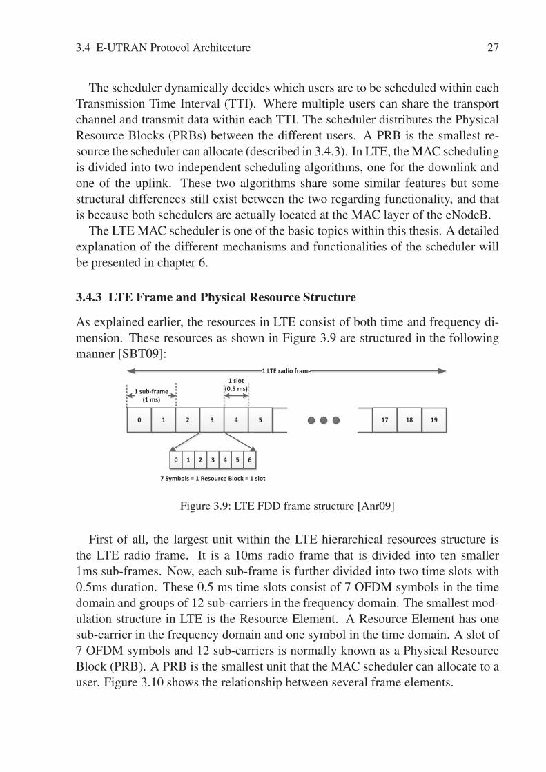
3.4 E-UTRAN Protocol Architecture 27
The scheduler dynamically decides which users are to be scheduled within eachTransmission Time Interval (TTI). Where multiple users can share the transportchannel and transmit data within each TTI. The scheduler distributes the PhysicalResource Blocks (PRBs) between the different users. A PRB is the smallest re-source the scheduler can allocate (described in 3.4.3). In LTE, the MAC schedulingis divided into two independent scheduling algorithms, one for the downlink andone of the uplink. These two algorithms share some similar features but somestructural differences still exist between the two regarding functionality, and thatis because both schedulers are actually located at the MAC layer of the eNodeB.
The LTE MAC scheduler is one of the basic topics within this thesis. A detailedexplanation of the different mechanisms and functionalities of the scheduler willbe presented in chapter 6.
3.4.3 LTE Frame and Physical Resource Structure
As explained earlier, the resources in LTE consist of both time and frequency di-mension. These resources as shown in Figure 3.9 are structured in the followingmanner [SBT09]:
0 1 2 3 4 5 17 18 19
1 LTE radio frame
1 sub-frame (1 ms)
1 slot(0.5 ms)
0 1 2 3 4 5 6
7 Symbols = 1 Resource Block = 1 slot
Figure 3.9: LTE FDD frame structure [Anr09]
First of all, the largest unit within the LTE hierarchical resources structure isthe LTE radio frame. It is a 10ms radio frame that is divided into ten smaller1ms sub-frames. Now, each sub-frame is further divided into two time slots with0.5ms duration. These 0.5 ms time slots consist of 7 OFDM symbols in the timedomain and groups of 12 sub-carriers in the frequency domain. The smallest mod-ulation structure in LTE is the Resource Element. A Resource Element has onesub-carrier in the frequency domain and one symbol in the time domain. A slot of7 OFDM symbols and 12 sub-carriers is normally known as a Physical ResourceBlock (PRB). A PRB is the smallest unit that the MAC scheduler can allocate to auser. Figure 3.10 shows the relationship between several frame elements.
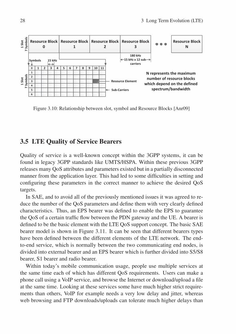
28 3 Long Term Evolution (LTE)
0123456
1 Sl
ot7
Sym
bols
1 2 3 4 5 6 7 8 9 10 11
Resource Block 0
Resource Block 1
Resource Block 2
Resource Block N1
Slot
7 Sy
mbo
ls
Resource Block 3
180 kHz 15 kHz x 12 sub-
carriers15 kHzSymbols
Resource Element
Sub-Carriers
N represents the maximum number of resource blocks
which depend on the defined spectrum/bandwidth
Figure 3.10: Relationship between slot, symbol and Resource Blocks [Anr09]
3.5 LTE Quality of Service Bearers
Quality of service is a well-known concept within the 3GPP systems, it can befound in legacy 3GPP standards like UMTS/HSPA. Within these previous 3GPPreleases many QoS attributes and parameters existed but in a partially disconnectedmanner from the application layer. This had led to some difficulties in setting andconfiguring these parameters in the correct manner to achieve the desired QoStargets.
In SAE, and to avoid all of the previously mentioned issues it was agreed to re-duce the number of the QoS parameters and define them with very clearly definedcharacteristics. Thus, an EPS bearer was defined to enable the EPS to guaranteethe QoS of a certain traffic flow between the PDN gateway and the UE. A bearer isdefined to be the basic element with the LTE QoS support concept. The basic SAEbearer model is shown in Figure 3.11. It can be seen that different bearers typeshave been defined between the different elements of the LTE network. The end-to-end service, which is normally between the two communicating end nodes, isdivided into external bearer and an EPS bearer which is further divided into S5/S8bearer, S1 bearer and radio bearer.
Within today’s mobile communication usage, people use multiple services atthe same time each of which has different QoS requirements. Users can make aphone call using a VoIP service, and browse the Internet or download/upload a fileat the same time. Looking at these services some have much higher strict require-ments than others, VoIP for example needs a very low delay and jitter, whereasweb browsing and FTP downloads/uploads can tolerate much higher delays than

3.5 LTE Quality of Service Bearers 29
UE eNodeB S-GW P-GW Peer Entity
E-UTRAN EPC Internet
End-to-End Service
External BearerEPS Bearer
S5/S8 BearerS1 BearerRadio Bearer
LTE-Uu S1 S5/S8 SGi
Figure 3.11: SAE bearer model [HT09]
VoIP. In order to distinguish between these services and guarantee their QoS re-quirements different bearers are set up by the EPS each with a different QoS asso-ciation.
From the literature, two main general categories are defined in classifying thebearers, depending on the type of QoS they need to satisfy and these are:
• Guaranteed Bit Rate bearers (GBR): these bearers, as the name suggests,guarantee a minimum bit rate for their services. These bearers carry anassociated value that allow other units to reserve/allocate resources for them.Such bearers can be used for applications, like VoIP or video conferencing.
• Non-Guaranteed Bit Rate bearers (non-GBR): these bearers do not guaran-tee any bit rate and are a kind of best effort service. No resources are pre-allocated or reserved for these bearers and they are served only if there areresources/bandwidth left for them. Such bearers can be used for applicationslike HTTP (web browsing) or file transfers like FTP downloads/uploads.
The eNodeB is the entity responsible for guaranteeing the QoS requirements ofthe bearers over the radio part. Each bearer is associated with two QoS parameters[SBT09], and these are:
• QoS Class Identifier (QCI): this is an index that identifies predefined valuesfor priority, delay budget and packet loss rate. Each bearer carries this value
30 3 Long Term Evolution (LTE)
and the eNodeB reads this value and determines how to handle this bearer.A number of QCIs are standardized and are listed in Table 3.3.
• Allocation and Retention Priority (ARP): this parameter defines the impor-tance of bearer request establishment. It is used to determine whether toaccept or reject a bearer establishment in case of radio congestion. Thisparameter is only used during bearer setup and doesn’t influence other deci-sions once the bearer has been established, i.e., it does not affect schedulingor rate control.
QCI Bearer type Priority Packet delay Packet error Example servicesbudget (ms) loss rate
1 GBR 2 100 10−2 Conversational voice2 GBR 4 150 10−3 Conversational video
(live streaming)3 GBR 5 300 10−6 Non-conversational
video (buffered streaming)4 GBR 3 50 10−3 Real time gaming5 non-GBR 1 100 10−6 IMS signaling6 non-GBR 7 100 10−3 Voice,
video (live streaming),interactive gaming
7 non-GBR 6 300 10−6 Video (buffered streaming)8 non-GBR 8 300 10−6 TCP based (e.g., www,
e-mail, chat, FTP, p2p)9 non-GBR 9 300 10−6
Table 3.3: LTE standardized QCIs and their parameters [SBT09]
3.6 Beyond LTE
Up to now, this chapter has presented and discussed the 3GPP Long Term Evolu-tion (LTE). However, according to [PDF+08] the focus now is gradually shiftingfrom LTE (as the work on the first release of the LTE standard is coming to anend) towards the LTE-advanced. LTE-advanced is the evolution of the LTE sys-tem that targets the enhancements of the LTE system so as to meet and exceed theIMT-Advanced requirements within the ITU-R time plan [Nak09]. LTE-advancedtargets much higher data rates compared to LTE, as well as enhancing the spec-trum efficiency. Table 3.4 shows a comparison between LTE, LTE-advanced and

3.6 Beyond LTE 31
the IMT-advanced systems. For the IMT-advanced system the 1 Gbps peak datarate shown in the table is only for low mobility cases, whereas it will support 100Mbps for the high mobility cases.
LTE LTE-advanced IMT-advancedPeak data rate DL 300 Mbps 1 Gbps 1 Gbps
UL 75 Mbps 500 MbpsPeak spectrum DL 15 30 15
efficiency (bps/Hz) UL 3.75 15 6.75Table 3.4: System performance comparison [Nak09]
Some of the main requirements considered in LTE-advanced include [Nak09]:wider bandwidth for transmission and spectrum sharing, advanced multi-antenna(MIMO) solutions, coordinated multi-point transmission and reception (CoMP)and the use of Relays and Repeaters. Over the next subsections each of theserequirements is explained briefly.
3.6.1 Wider Bandwidth for Transmission
LTE-advanced is designed to operate in different spectrum allocations, that can bewider than the 20 MHz spectrum in which LTE operates. Although it is very fa-vorable to have the wider spectrum, it is very difficult within today’s free spectrumto find this. That is why, the IMT-advanced specifications have enabled the use ofbandwidth aggregation to meet the current demands of higher spectrum.
In LTE-advanced, a technique called Carrier Aggregation (CA) is used to pro-vide the necessary means to combine bandwidths to provide the wider operat-ing spectrum. According to [Agi11], three main carrier aggregation scenarios aresupported: intra-band contiguous, intra-band non-contiguous, and inter-band non-contiguous aggregation.
3.6.2 Advanced MIMO Solutions
In LTE, the use of multiple antennas has been defined and used for both downlinkand uplink transmissions. In the downlink transmission it is allowed to use a max-imum of 4 spatial layers of transmission, whereas, in the uplink only one layer oftransmission is allowed.
In LTE-advanced, the number of spatial layers has been increased in comparisonto LTE. It is permitted to use up to eight layers in the downlink and four layers in

32 3 Long Term Evolution (LTE)
the uplink [Agi11]. Increasing the number of transmission layers improves theuser peak data rates because of the enhanced spatial multiplexing.
3.6.3 CoMP
Coordinated multi-point is an advanced MIMO technique used to improve the sys-tem coverage, cell-edge throughput and system efficiency. The concept behindCoMP is simple, when the user is in the cell edge, in the downlink, the user canreceive the signals coming from multiple eNodeBs, whereas in the uplink the mul-tiple eNodeBs can receive the user’s transmission. Now, if the downlink trans-mission of the multiple eNodeBs are coordinated, a significant improvement inthe overall performance can be achieved. In LTE-advanced, the CoMP transmis-sion is used in the downlink, whereas, the CoMP reception is used in the uplink.Figure 3.12, shows the LTE-advanced CoMP concept.
UEeNodeB
Cell3
Cell2
Cell1
eNodeB
eNodeB
Figure 3.12: LTE-advanced CoMP
3.6.4 Relays and Repeaters
Relaying is used in order to deploy cells in areas where no (or very expensive)wired backhaul exists. It is often used to improve the coverage and throughput,for example, in urban, and rural scenarios. Figure 3.13 shows a typical scenariowhere a Relay Node (RN) is connected to an eNodeB wirelessly. The eNodeB thatthe RN is connected to is called in that case, a Donor eNodeB (DeNB). Accordingto [Agi11], there are two main proposals for 3GPP release 10 (LTE-advanced) onhow the RN connects to the DeNB, and these are:

3.6 Beyond LTE 33
• In-band: where the link between the RN and the UE uses the same carrierfrequency of the link between the RN and the DeNB.
• Out-band: where the two links (RN<->UE and RN<->DeNB) do not use thesame carrier frequency.
UEs
DeNB
eNodeB
RN
RN
RN
Over the air backhaul
Cell edge
Multi-hop relaying
Figure 3.13: LTE-advanced in-band relay and backhaul [Agi11]


4 LTE Network Simulator
4.1 Simulation Environment
The LTE simulation model developed in this work is implemented using the OP-NET software environment [mod11]. OPNET is a commercial simulation tool thatprovides several network and application performance management solutions. Thesimulation modeling tool of OPNET Modeler© is used to design and implementthe LTE simulation model. It is a hierarchical modeling environment that is basedon a C/C++ programming tool, and has an advanced Graphical User Interface usedfor analysis and debugging. Some of its key features include [mod11]: a modellibrary involving many protocols and vendor nodes implementations, object ori-ented programming, a 32-bit and 64-bit fully parallel simulation kernel. As statedearlier, it consists of several hierarchical editors as shown in Figure 4.1 mainly:project editor, node editor, process editor and open model source code.
Project Editor Process Editor
Node Editor
Source code Editor
Figure 4.1: OPNET Modeler© hierarchical editors

36 4 LTE Network Simulator
4.2 Simulation Framework
The main objective behind the development of the LTE simulation model is to an-alyze, evaluate and study several aspects of the LTE network such as: end userperformance, LTE radio performance (Uu interface) and the LTE transport perfor-mance (S1/X2 interface). To be able to achieve the above targets the simulationmodel is designed to model both the E-UTRAN and EPC. The modeling is donewith particular focus on the important features and functionalities of the nodesand protocols. These are modeled with great depth in order to be able to conductthe intended study. Mobile communication systems are very complex and includea huge amount of functionalities; this is also the case with LTE. To simplify themodeling of such a system, a reference architecture is required that representsthe desired compromise between the complexity and the intended simulation per-formance targets. The reference LTE network architecture used for this thesis isshown in Figure 4.2 [Wee11]. It consists of a number of eNodeBs each control-ling three cells. The number of eNodeBs, intermediate routers and users shown inthe figure are merely an example and can be changed depending on the requiredscenario.
Remote Server
PDN-GWaGW
R1
R2R3
eNodeB1eNodeB2eNodeB3eNodeB4
UEUEUEUE
Figure 4.2: LTE reference model
By comparing the reference architecture to the general LTE network architectureshown on Figure 3.1, it can be seen that most of the entities have been modeled
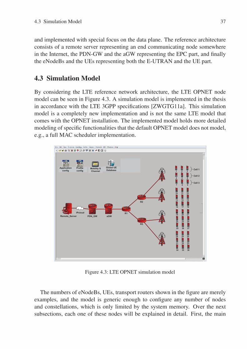
4.3 Simulation Model 37
and implemented with special focus on the data plane. The reference architectureconsists of a remote server representing an end communicating node somewherein the Internet, the PDN-GW and the aGW representing the EPC part, and finallythe eNodeBs and the UEs representing both the E-UTRAN and the UE part.
4.3 Simulation Model
By considering the LTE reference network architecture, the LTE OPNET nodemodel can be seen in Figure 4.3. A simulation model is implemented in the thesisin accordance with the LTE 3GPP specifications [ZWGTG11a]. This simulationmodel is a completely new implementation and is not the same LTE model thatcomes with the OPNET installation. The implemented model holds more detailedmodeling of specific functionalities that the default OPNET model does not model,e.g., a full MAC scheduler implementation.
Applicationconfig
Profileconfig
Mobility &Channel
Global UEDatabase
Remote_ServerIPcloud
PDN_GW aGWR1
R2eNB1
eNB2
UE1 UE2 UE3 UE4 UE5
UE6 UE7 UE8 UE9 UE10
UE11 UE12 UE13 UE14 UE15
UE16 UE17 UE18 UE19 UE20
UE21 UE22 UE23 UE24 UE25
UE26 UE27 UE28 UE29 UE30
Remote_ServerIPcloud
PDN_GW aGWR1
R2
1 2 3
4 5 6
7 8 9
10 11 12
13 14 15
16 17 18
19 20 21
22 23 24
25 26 27
28 29 30
31 32 33
34 35 36
R3
Cell 1
Cell 2
Cell 3
Figure 4.3: LTE OPNET simulation model
The numbers of eNodeBs, UEs, transport routers shown in the figure are merelyexamples, and the model is generic enough to configure any number of nodesand constellations, which is only limited by the system memory. Over the nextsubsections, each one of these nodes will be explained in detail. First, the main

38 4 LTE Network Simulator
implemented LTE nodes, that is the UE, eNodeB, aGW, and PDN gateway areexplained in sections 4.3.1 to 4.3.4. Then, the supporting nodes represented by themobility and channel model node, and the global user database are explained insections 4.3.5 and 4.3.6. Finally, in sections 4.3.7 and 4.3.8 the standard OPNETconfigurations nodes are explained.
4.3.1 UE Node Model
The UE node model can be seen in Figure 4.4. This node represents the userequipment with its predefined protocols, according to the 3GPP standard. Theseprotocols include: application layer, (TCP, UDP)/IP, PDCP, RLC, MAC, and PHY.
application
tpal
tcp
ip_encap
ip
pdcp
rlc
mac
phy
rip
cpu
rt_0r_0
udp
ApplicationProtocols
LTE Uu Protocols
Figure 4.4: UE Node Model
This UE node also holds the individual user attributes, for example, the userspeed, the serving eNodeB, the serving cell and the user applications. The emula-tion of the physical layer and the wireless medium is handled by the MAC layer
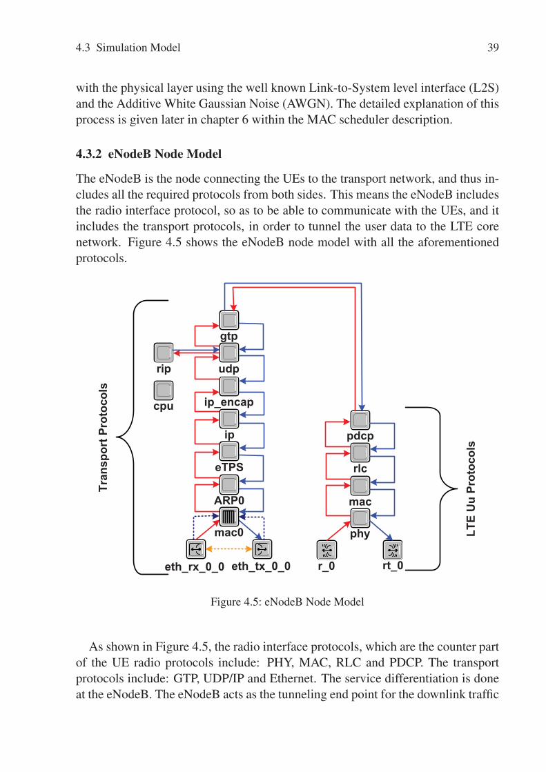
4.3 Simulation Model 39
with the physical layer using the well known Link-to-System level interface (L2S)and the Additive White Gaussian Noise (AWGN). The detailed explanation of thisprocess is given later in chapter 6 within the MAC scheduler description.
4.3.2 eNodeB Node Model
The eNodeB is the node connecting the UEs to the transport network, and thus in-cludes all the required protocols from both sides. This means the eNodeB includesthe radio interface protocol, so as to be able to communicate with the UEs, and itincludes the transport protocols, in order to tunnel the user data to the LTE corenetwork. Figure 4.5 shows the eNodeB node model with all the aforementionedprotocols.
Tran
spor
t Pro
toco
ls
LTE
Uu
Prot
ocol
s
gtp
udp
ip_encap
ip
cpu
rip
pdcp
rlc
mac
phy
rt_0r_0
eTPS
ARP0
mac0
eth_tx_0_0eth_rx_0_0
Figure 4.5: eNodeB Node Model
As shown in Figure 4.5, the radio interface protocols, which are the counter partof the UE radio protocols include: PHY, MAC, RLC and PDCP. The transportprotocols include: GTP, UDP/IP and Ethernet. The service differentiation is doneat the eNodeB. The eNodeB acts as the tunneling end point for the downlink traffic
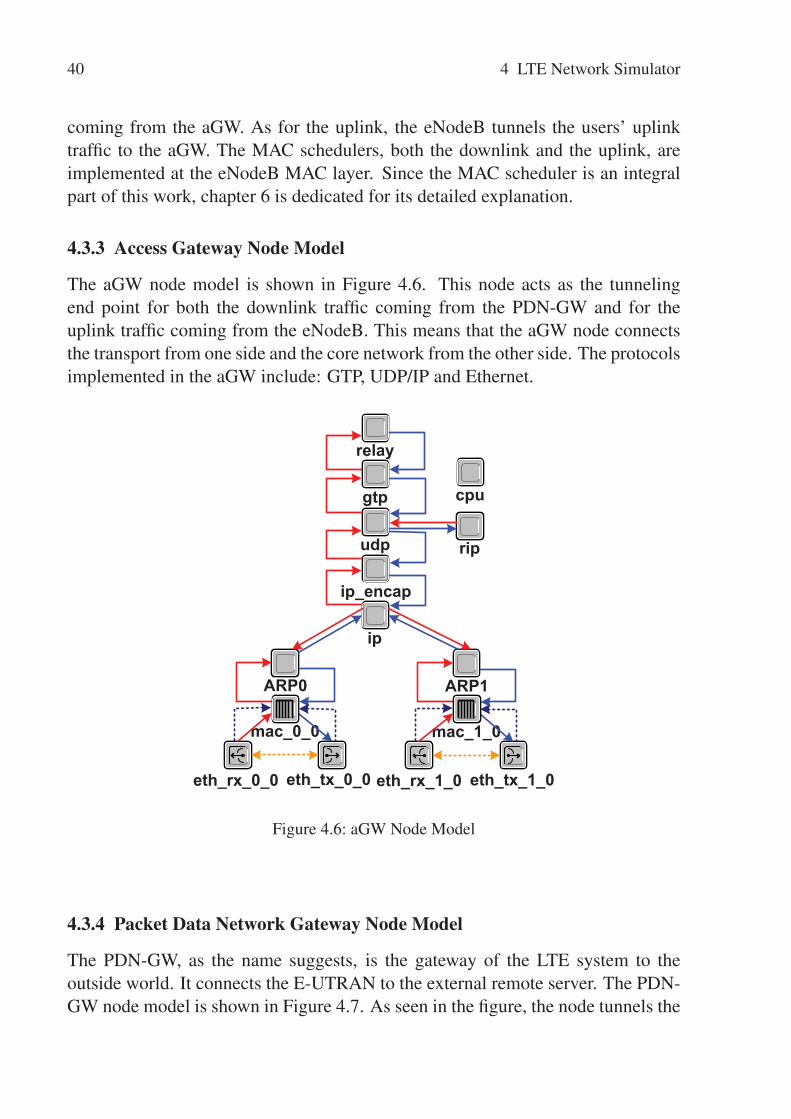
40 4 LTE Network Simulator
coming from the aGW. As for the uplink, the eNodeB tunnels the users’ uplinktraffic to the aGW. The MAC schedulers, both the downlink and the uplink, areimplemented at the eNodeB MAC layer. Since the MAC scheduler is an integralpart of this work, chapter 6 is dedicated for its detailed explanation.
4.3.3 Access Gateway Node Model
The aGW node model is shown in Figure 4.6. This node acts as the tunnelingend point for both the downlink traffic coming from the PDN-GW and for theuplink traffic coming from the eNodeB. This means that the aGW node connectsthe transport from one side and the core network from the other side. The protocolsimplemented in the aGW include: GTP, UDP/IP and Ethernet.
relay
gtp
udp
ip_encap
rip
cpu
ip
ARP0
mac_0_0
eth_tx_0_0eth_rx_0_0
ARP1
mac_1_0
eth_tx_1_0eth_rx_1_0
Figure 4.6: aGW Node Model
4.3.4 Packet Data Network Gateway Node Model
The PDN-GW, as the name suggests, is the gateway of the LTE system to theoutside world. It connects the E-UTRAN to the external remote server. The PDN-GW node model is shown in Figure 4.7. As seen in the figure, the node tunnels the
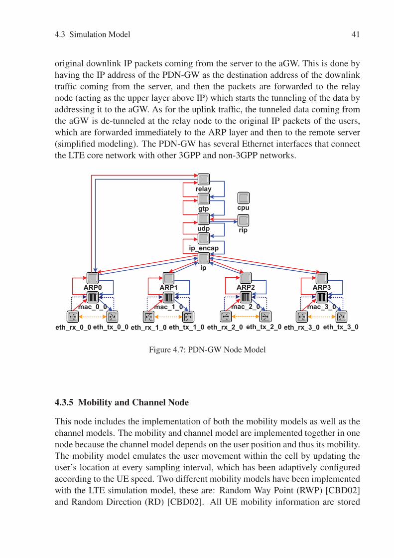
4.3 Simulation Model 41
original downlink IP packets coming from the server to the aGW. This is done byhaving the IP address of the PDN-GW as the destination address of the downlinktraffic coming from the server, and then the packets are forwarded to the relaynode (acting as the upper layer above IP) which starts the tunneling of the data byaddressing it to the aGW. As for the uplink traffic, the tunneled data coming fromthe aGW is de-tunneled at the relay node to the original IP packets of the users,which are forwarded immediately to the ARP layer and then to the remote server(simplified modeling). The PDN-GW has several Ethernet interfaces that connectthe LTE core network with other 3GPP and non-3GPP networks.
relay
gtp
udp
ip_encap
rip
cpu
ip
ARP0
mac_0_0
eth_tx_0_0eth_rx_0_0
ARP1
mac_1_0
eth_tx_1_0eth_rx_1_0
ARP2
mac_2_0
eth_tx_2_0eth_rx_2_0
ARP3
mac_3_0
eth_tx_3_0eth_rx_3_0
Figure 4.7: PDN-GW Node Model
4.3.5 Mobility and Channel Node
This node includes the implementation of both the mobility models as well as thechannel models. The mobility and channel model are implemented together in onenode because the channel model depends on the user position and thus its mobility.The mobility model emulates the user movement within the cell by updating theuser’s location at every sampling interval, which has been adaptively configuredaccording to the UE speed. Two different mobility models have been implementedwith the LTE simulation model, these are: Random Way Point (RWP) [CBD02]and Random Direction (RD) [CBD02]. All UE mobility information are stored
42 4 LTE Network Simulator
and updated regularly in the global user database, where it can be accessed at anytime by any node in the system. Details of these mobility models can be found inAppendix A.1.
The users channel conditions are updated in regular time intervals. The channelconditions consist of the three well known effects, these are: path loss, slow fadingand fast fading. The sum of all the three factors results in the overall losses (in dB)between the user and the eNodeB. LTE operates in a scalable range of spectrumstarting from 1.4 MHz all the way up to 20 MHz, and the spectrum itself is di-vided into Physical Resource Blocks (PRB). A PRB is the smallest unit the MACscheduler can allocate to a specific user. The path loss, slow fading and fast fadingare calculated for each user over each PRB. By using the link budget the Signal toInterference plus Noise Ratio (SINR) of each PRB maybe calculated for each user.The PRBs of each user have different values mainly due to the frequency and timeselectivity.
Path Loss: The path loss is modeled by following the distance dependent pathloss model given by the 3GPP [25.06] as follows:
PL = 128.1+37.6× log10 (R) (4.1)
where PL is the path loss factor in dB. R represents the distance between the userand the eNodeB measured in kilometers.
Slow Fading: The slow fading is typically modeled using a log normal distribu-tion with zero mean and a constant variance, but the time correlation between theslow fading values needs to be considered. For such a model, a moving mobile userstarting at an initial point P, where the slow fading value is to be randomly gen-erated using the log-normal distribution equal to S (0). The shadowing at pointswhich are at distance δ , 2δ , 3δ away from P can be determined according to[CYG95] as follows:
S (nδ ) = S ((n−1)δ )× e−δ/Xc +Vi (4.2)
where S (nδ ) represents the slow fading value at a distance nδ away from point P,Xc is the de-correlation distance, and Vi are independent and identically distributednormal random variables with zero mean, and a variance equal to:
δ 22 = δ 2
[1− e−2δ/Xc
](4.3)
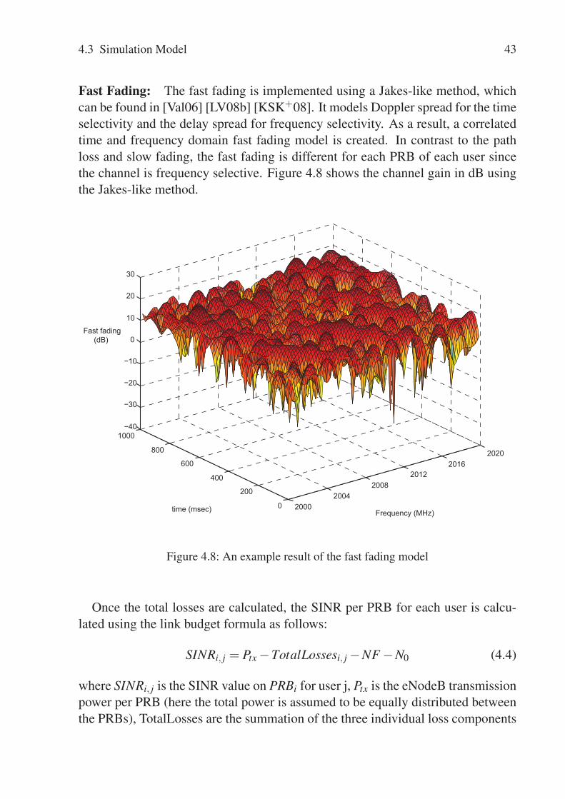
4.3 Simulation Model 43
Fast Fading: The fast fading is implemented using a Jakes-like method, whichcan be found in [Val06] [LV08b] [KSK+08]. It models Doppler spread for the timeselectivity and the delay spread for frequency selectivity. As a result, a correlatedtime and frequency domain fast fading model is created. In contrast to the pathloss and slow fading, the fast fading is different for each PRB of each user sincethe channel is frequency selective. Figure 4.8 shows the channel gain in dB usingthe Jakes-like method.
20002004
20082012
20162020
0
200
400
600
800
1000−40
−30
−20
−10
0
10
20
30
Frequency (MHz)time (msec)
Fast fading (dB)
Figure 4.8: An example result of the fast fading model
Once the total losses are calculated, the SINR per PRB for each user is calcu-lated using the link budget formula as follows:
SINRi, j = Ptx −TotalLossesi, j −NF −N0 (4.4)
where SINRi, j is the SINR value on PRBi for user j, Ptx is the eNodeB transmissionpower per PRB (here the total power is assumed to be equally distributed betweenthe PRBs), TotalLosses are the summation of the three individual loss components

44 4 LTE Network Simulator
(path loss, slow fading and fast fading), NF is the noise floor and N0 is the thermalnoise. The eNodeB transmit power is chosen in such a way that even the cell-edge users (with the lowest Modulation and Coding Scheme (MCS)) are able totransmit. For example, if we assume a transmit power of 20dBm for a system with20MHz bandwidth and 100 PRBs then the transmit power per PRB under the equalpower distribution assumption is:
20dBm−10log10 (100PRBs)dBm = 0dBm ≡ 1mW (4.5)
4.3.6 Global User Database
The global user database is implemented to collect and update the global informa-tion of all the nodes of the system (including the UEs) upon their changes. Forexample, if users change their position during the mobility then this informationis updated in the global database. In addition, all other related information e.g.,channel conditions are updated accordingly. This information within this node isaccessible for all the other nodes in the system.
4.3.7 Application Configuration
This is a standard OPNET node that is used to configure the different applicationparameters. It includes several supported applications, e.g., Email, FTP, HTTP,Video Conferencing, Voice, as well as other custom applications. Each one ofthese supported applications contains several parameters that can be configuredwith different supported distributions, e.g., exponential, Pareto, constant, normaletc. This application configuration is used later by the profile configuration toconfigure a certain user application profile.
Figure 4.9 shows a sample OPNET configuration window for an FTP applica-tion, it can be seen that the file size is constant (15Mbyte), and the inter-arrivaltime between the files is also constant (1 sec).
4.3.8 Profile Configuration
The OPNET profile configuration, is used to define a certain user application pro-file. It is always used in combination with the application configuration. A profileis a collection of one or several applications that a certain user can be configuredto run. Within the profile configuration each application start and finish time canbe set, as well as its repeatability. A profile configuration example can be seen inFigure 4.10.

4.4 Traffic Models 45
Figure 4.9: Sample OPNET application configuration
Figure 4.10: Sample OPNET profile configuration
4.4 Traffic Models
One of the key issues in simulating a communication network is knowing the traf-fic types and services that the network is carrying. Therefore, finding the correcttraffic models to implement in the network simulator is a crucial part in the mod-eling, so as to have a meaningful evaluation. In this section, several traffic modelsincluding Voice over Internet Protocol (VoIP), Web traffic, Video traffic and FileTransfer Protocol (FTP) are discussed.

46 4 LTE Network Simulator
4.4.1 Voice over IP Model (VoIP)
As discussed earlier, LTE is a packet based network. This means circuit switchedvoice traffic is not used anymore, and all voice data has to be sent over a packetnetwork. Thus, the QoS should be guaranteed. The VoIP traffic is modeled us-ing an ON/OFF model [Li10] that models the active and silent periods as seen inFigure 4.11.
Band
wid
th (k
bps)
Time
Call Start Time
Silent Period
Active Period
Figure 4.11: VoIP traffic model
The encoder used for the VoIP traffic model is one of the most widely used voicecodecs that deploys the GSM Enhanced Full Rate (EFR). The GSM EFR belongsto the family of Adaptive Multi-Rate (AMR) codecs with an application data rateof 12.2 kbps. The main parameters of the VoIP model are summarized in Table 4.1.
Parameter Value
Voice Codec GSM EFR with 12.2 kbps data rateSilence period Exponential distribution with mean 3 secondsTalk period Exponential distribution with mean 3 seconds
Table 4.1: VoIP traffic model parameters [Li10]
In order to properly evaluate the performance of the VoIP traffic, the Mean Opin-ion Score (MOS) is used [IT09]. MOS measures the subjective quality of a voicecall and returns a scalar one digit score to express the status of the call quality.The MOS score ranges from 1 (unacceptable call quality) up to 5 (excellent callquality) as shown in Figure 4.12. MOS values that are larger than 4 correspond tousers being satisfied with their VoIP quality [Vi10].
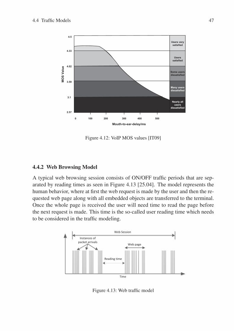
4.4 Traffic Models 47
2.57
3.1
3.59
4.02
4.33
4.5
100 200 300 400 5000
Nearly allusers
dissatisfied
Many usersdissatisfied
Some usersdissatisfied
Userssatisfied
Users verysatisfied
Mouth-to-ear-delay/ms
MO
SVa
lue
Figure 4.12: VoIP MOS values [IT09]
4.4.2 Web Browsing Model
A typical web browsing session consists of ON/OFF traffic periods that are sep-arated by reading times as seen in Figure 4.13 [25.04]. The model represents thehuman behavior, where at first the web request is made by the user and then the re-quested web page along with all embedded objects are transferred to the terminal.Once the whole page is received the user will need time to read the page beforethe next request is made. This time is the so-called user reading time which needsto be considered in the traffic modeling.
Time
Instances of packet arrivals
Reading time
Web page
Web Session
Figure 4.13: Web traffic model

48 4 LTE Network Simulator
According to [25.04], several random variables are required to model web brows-ing traffic and these are:
• Main object size
• Embedded object size
• Number of embedded objects in a page
• Page reading time
• Main page parsing time
The basic web browsing model parameters used in this thesis are:
Parameter Value
Number of pages per session constant 5 pagesAverage page size constant 100 kbyteNumber of objects in a page 2 objects: 1 kbyte and 100 kbyteReading time constant 12 secondsProtocol HTTP with each page using a separate TCP connection
Table 4.2: Web browsing traffic model parameters [Wee11]
4.4.3 Video Streaming Model
The video traffic model used in this thesis represents a buffered video streamingservice. The basic model is simplified in such a way that the application layergenerates video frames with inter-arrival time between the frames and then theseframes are carried over the LTE transport network using the UDP transport proto-col. The two main random variables that can be configured for the video sourceare:
• Frame size: this is the actual frame size in bytes
• Frame inter arrival time: the time between two consecutive video frames.This time is between the start of the last video frame and the start of the nextone

4.5 Statistical Evaluation 49
4.4.4 File Transfer Model
The File Transfer Protocol application consists of a sequence of file transfers. Itis similar to the web browsing application with the difference that it only transfersone large file compared to several smaller objects (in case of HTTP). FTP, likethe HTTP web browsing, relies on TCP as the underlying protocol for the datatransmission. An FTP session can be configured using only two random variables[25.04]:
• FTP File Size: that is the actual application file size that needs to be trans-mitted
• Reading time: the time between two consecutive FTP file transfers. Thistime starts after the finish of the previous FTP file
4.5 Statistical Evaluation
So far, this chapter has discussed the methodology and implementation assump-tions used for building the LTE simulation model. However, the main reason whya simulation model is developed in the first place is to study and analyze the end-to-end system performance. This is done by collecting several statistical data andanalyzing them. The results mainly focus on the steady state analysis, in whichthe average value is presented along with the “Confidence Interval”, which is thewidely used statistical method to indicate the sample mean error.
4.5.1 Confidence Interval Estimation
According to [Per09], having N consecutive endogenously obtained observationsof a random variable, i.e. x1,x2,x3,x4, ...xN , the sample mean of that random vari-able x can be calculated as:
x =1N
n
∑i=1
xi (4.6)
In order to estimate the confidence interval of that sample mean the variancehas to be fist calculated. If the observations are independent of each other then thevariance is calculated as follows:
δ 2 =1
N −1
N
∑i=1
(xi − x)2 (4.7)
Now, the confidence interval at a confidence level of 100(1-α)% is:

50 4 LTE Network Simulator
(x−Zα/2 · δ√N
, x+Zα/2 · δ√N
)
where, x is the sample mean, Zα/2 is the upper α/2 critical value of the standardnormal distribution (can be obtained from the standard distribution table [Sta12]),δ 2 is the variance and N is the number of samples.
The confidence (i.e., 100(1-α)%) can take several values e.g., 99%, 95% and90%. If the number of samples taken for calculating the confidence interval issmaller than 30 then the student-t distribution table is used as follows:
(x− t(α/2,N−1) · δ√N
, x+ t(α/2,N−1) · δ√N
)
where, t(α/2,N−1) is the upper critical value of the t-distribution with N-1 degreesof freedom. This can be obtained from the t-distribution table [Sta12].
4.5.2 Independent Replications Method
Normally in simulations the data gathered for the statistical evaluation are corre-lated with each other. Thus, the confidence interval calculation method explainedearlier cannot be used directly. In literature, a number of solutions exist to solvethe correlated data problem: e.g., replications method, estimation of autocorrela-tion function, batch means and regenerative method. Within this subsection, theindependent replications method is explained which is also used to evaluate theconfidence interval for this thesis.
The independent replication method [Per09], as the name suggests, relies onreplicating several independent simulation runs. For example, N number of repli-cations are done each with M number of data elements:
Replication 1: x11,x12,x13...x1M
Replication 2: x21,x22,x23...x2M
Replication 3: x31,x32,x33...x3M
.
.
.Replication n: xN1,xN2,xN3...xNM
The sample mean of each replication i can be evaluated as:
xi =1M
M
∑j=1
xi j (4.8)

4.5 Statistical Evaluation 51
This will lead to having N approximately independent sample means [x1,x2, ...xN ],the sample mean and variance of them will be:
x =1N
N
∑i=1
xi (4.9)
δ 2 =1
N −1
N
∑i=1
(xi − x
)2 (4.10)
Now, using this variance the confidence interval can be calculated as explainedbefore. Although the independent replications method is easy and simple twoissues still need to be determined: first, how long each independent replicationshould be run (i.e., choosing M which should be a large number), and the seedused for each independent run must be chosen very carefully in order to havethe replications independent. The independence between the replications can bechecked by calculating the autocorrelation between them.

5 LTE Virtualization
This chapter presents the concepts of network virtualization, focusing specificallyon wireless virtualization of the LTE mobile communication system. A novelwireless virtualization framework is proposed and developed by this thesis, whichallows mobile network operators to share the wireless spectrum as well as the in-frastructure (i.e., hardware equipments). The work presented in this chapter targetsproving the concept of using virtualization in wireless systems and highlighting itspotential gain. The chapter is structured in the following manner: in section 5.1the virtualization history and concepts are discussed. Section 5.2.1 describes the4WARD European project and its virtualization architecture, the work was done bythe author as part of the 4WARD project. In section 5.3 the novel LTE virtualiza-tion framework is proposed, explaining the technical details behind the framework.Proof of concept evaluations are discussed in section 5.4, where three different sce-narios are presented each showing a different potential gain area within the LTEvirtualization. Finally section 5.5 summarizes and concludes this chapter. Theproposed LTE virtualization framework, results/achievements and other relatedvirtualization work are published in [ZZGTG10a], [ZZGTG10b], [ZZGTG11],[ZKZG11], [KZ11], [ZLZ+11], [LZZ+12] and [UZZ+10].
5.1 Virtualization
Virtualization is the process of creating virtual versions of physical resources thatemulate the same physical characteristics. It is often used in the Information Tech-nology (IT) context to partition a physical resource into several virtual ones, forexample, virtual memory, hard disk partition and virtual machine. The virtual-ization concept [Sin04] was first introduced at the beginning of the 1960s, whenChristopher Strachey published a paper entitled “Time Sharing in Large Fast Com-puters” that focused on multi-programming. Then came the IBM M44/44X Projectin the mid 1960s, where the term Virtual Machine (VM) was introduced for the firsttime. The creation and maintenance of such virtual machines is what is known to-day as “Server Virtualization”. The idea at that time was to create several virtualmachines out of one mainframe computer to enable multi-tasking, i.e., running

54 5 LTE Virtualization
simultaneous applications and processes in one computer, since such computerswere very expensive at the time. The virtualization concept can be applied in dif-ferent areas. But from what can be seen in today’s IT interest three main areasemerge that adopt the use of virtualization, and these are:
• Storage Virtualization: according to IBM [IBM03], “it is considered as anintelligent “layer” or abstraction that pools storage from multiple storagedevices into a common storage pool. Often part of a Storage Area Network(SAN) virtualized storage appears as one device to the server-operating sys-tems and can be centrally managed and provisioned from a single view”.
• Server Virtualization: is the process of hiding the resources of the physicalserver and dividing the server into a number of virtual servers that share thephysical resources and appear to the operating system running on top as anactual hardware. Server virtualization is used to minimize the IT cost inenterprises, as well as utilizing the full potentials of the physical servers.
• Network Virtualization: is the process of aggregating the created virtual re-sources into forming a Virtual Network (VNet). It enables multiple virtualnetworks to coexist on a common infrastructure in an isolated way. Eachvirtual network is operating similar to a normal network and does not nec-essarily have the awareness of the underlying virtualization process.
5.1.1 Server Virtualization
Within this section, the server virtualization area is discussed in detail since it isclosely related to the main work of this chapter. It is the virtualization of serversby hiding the underlying physical resources and dividing them between severalnewly created virtual instances. For the server users it appears like several phys-ical servers each with its own operating system, and they are not aware of thevirtualization process. The server administrator uses special software to createthese isolated virtual instances. There are three different ways used to virtualizea server: full virtualization, para virtualization and operating system virtualization(OS virtualization).
Full virtualization: It uses the guest/host approach. It requires a special soft-ware layer that sits on top of the physical hardware and interacts with the machinephysical resources. This layer is often called “Hypervisor”, or sometimes it is alsoknown as “Virtual Machine Monitor (VMM)”. The hypervisor provides the nec-essary platform for the guest VMs to operate on top. Figure 5.1 shows the full
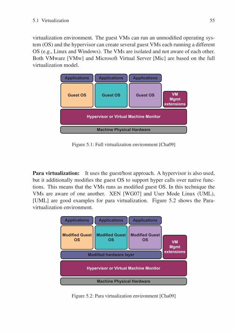
5.1 Virtualization 55
virtualization environment. The guest VMs can run an unmodified operating sys-tem (OS) and the hypervisor can create several guest VMs each running a differentOS (e.g., Linux and Windows). The VMs are isolated and not aware of each other.Both VMware [VMw] and Microsoft Virtual Server [Mic] are based on the fullvirtualization model.
Applications
Machine Physical Hardware
Hypervisor or Virtual Machine Monitor
Guest OS Guest OS Guest OS VMMgmt
extensions
Applications Applications
Figure 5.1: Full virtualization environment [Cha09]
Para virtualization: It uses the guest/host approach. A hypervisor is also used,but it additionally modifies the guest OS to support hyper calls over native func-tions. This means that the VMs runs as modified guest OS. In this technique theVMs are aware of one another. XEN [WG07] and User Mode Linux (UML),[UML] are good examples for para virtualization. Figure 5.2 shows the Para-virtualization environment.
Applications
Machine Physical Hardware
Hypervisor or Virtual Machine Monitor
Modified Guest OS
Modified Guest OS
Modified Guest OS VM
Mgmtextensions
Applications Applications
Modified hardware layer
Figure 5.2: Para virtualization environment [Cha09]
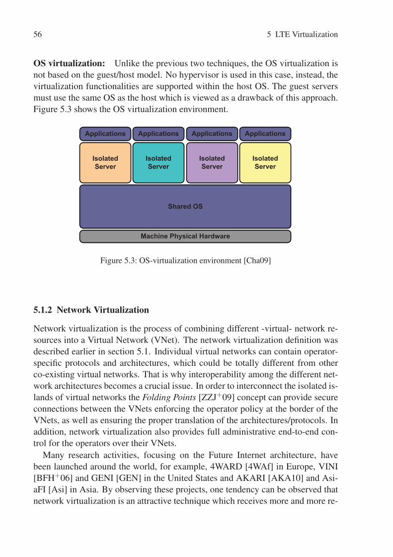
56 5 LTE Virtualization
OS virtualization: Unlike the previous two techniques, the OS virtualization isnot based on the guest/host model. No hypervisor is used in this case, instead, thevirtualization functionalities are supported within the host OS. The guest serversmust use the same OS as the host which is viewed as a drawback of this approach.Figure 5.3 shows the OS virtualization environment.
Shared OS
Applications
Machine Physical Hardware
IsolatedServer
Applications
IsolatedServer
Applications
IsolatedServer
Applications
IsolatedServer
Figure 5.3: OS-virtualization environment [Cha09]
5.1.2 Network Virtualization
Network virtualization is the process of combining different -virtual- network re-sources into a Virtual Network (VNet). The network virtualization definition wasdescribed earlier in section 5.1. Individual virtual networks can contain operator-specific protocols and architectures, which could be totally different from otherco-existing virtual networks. That is why interoperability among the different net-work architectures becomes a crucial issue. In order to interconnect the isolated is-lands of virtual networks the Folding Points [ZZJ+09] concept can provide secureconnections between the VNets enforcing the operator policy at the border of theVNets, as well as ensuring the proper translation of the architectures/protocols. Inaddition, network virtualization also provides full administrative end-to-end con-trol for the operators over their VNets.
Many research activities, focusing on the Future Internet architecture, havebeen launched around the world, for example, 4WARD [4WAf] in Europe, VINI[BFH+06] and GENI [GEN] in the United States and AKARI [AKA10] and Asi-aFI [Asi] in Asia. By observing these projects, one tendency can be observed thatnetwork virtualization is an attractive technique which receives more and more re-

5.2 4WARD Project 57
search attention, and it will be a key area in the future network development forboth testbed developments and operational networks.
VINI is a virtual network infrastructure based on PlanetLab [PMRK06], onwhich researchers can deploy, run and test their own protocols and services ona large scale. GENI (Global Environment for Network Innovations) is a novelsuite of architectures which support a range of experimental protocols, and virtu-alization is one of the most important features. The AKARI Architecture DesignProject aims at implementing the basic technology of a new generation networkfrom a clean slate, and network virtualization has been seen as one of its principlesapplications. The Asia Future Internet Forum (AsiaFI) was founded to coordinateresearch and development on Future Internet, where network virtualization is onits main list of research topics. In spite of all the major research projects that haspreviously been mentioned, one very important piece of the puzzle is still missing,that is “Wireless” Virtualization. Wireless virtualization, according to the best ofthe author’s knowledge, has not yet received the appropriate attention entitled toand only little work has been done in this field.
5.2 4WARD Project
4WARD is a large European project that started at the beginning of 2008, with 36partners including telecommunication operators, manufacturers and research insti-tutions. The main goal of the project is to make the development of networks andnetworked applications faster and easier, leading to both more advanced and moreaffordable communication services. The project is structured into six differentparadigms: three of which focus on innovative solutions of single network archi-tectures [4WAc] [4WAd] [4WAe], one focuses on network virtualization [4WAb]and one focuses on the architectural paradigm [4WAa] that looks into designing aframework for the Future Internet Architecture. In addition, there is one paradigm[CW08] that looks into how the paradigms fit together, as well as taking care ofsome non-technical issues that are of high significance, e.g., governance and reg-ulations. Since one of the main foci in this thesis is network virtualization, the4WARD virtualization work package is explained in more detail in the next sub-section. The virtualization work explained in this thesis was done as part of the4WARD project (mainly the virtualization work package).
5.2.1 4WARD Virtualization Paradigm
The 4WARD network virtualization technique aims at utilizing virtual networks asmeans to achieve the following objectives [4WAb]:
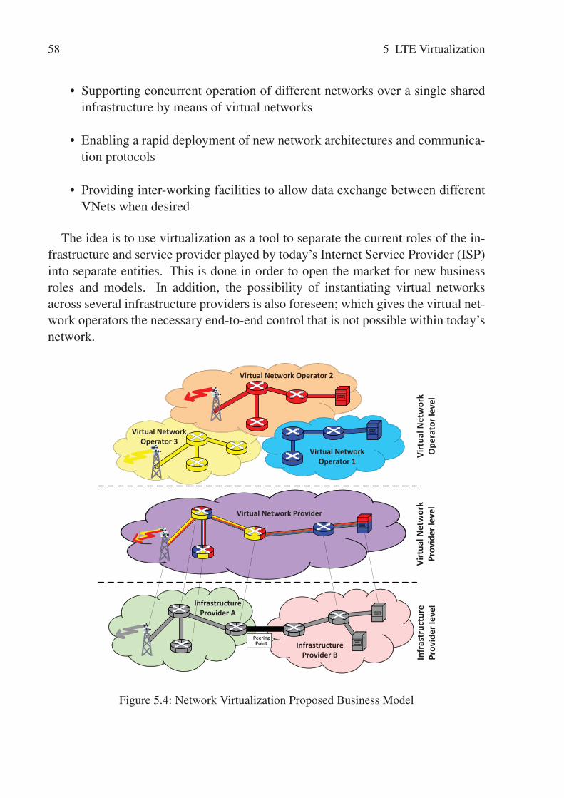
58 5 LTE Virtualization
• Supporting concurrent operation of different networks over a single sharedinfrastructure by means of virtual networks
• Enabling a rapid deployment of new network architectures and communica-tion protocols
• Providing inter-working facilities to allow data exchange between differentVNets when desired
The idea is to use virtualization as a tool to separate the current roles of the in-frastructure and service provider played by today’s Internet Service Provider (ISP)into separate entities. This is done in order to open the market for new businessroles and models. In addition, the possibility of instantiating virtual networksacross several infrastructure providers is also foreseen; which gives the virtual net-work operators the necessary end-to-end control that is not possible within today’snetwork.
Infrastructure Provider A
Infrastructure Provider B
PeeringPoint
Virtual Network Operator 1
Virtual Network Operator 2
Virtual Network Operator 3
Infr
astr
uctu
re
Prov
ider
leve
lVi
rtua
l Net
wor
kPr
ovid
er le
vel
Virt
ual N
etw
ork
Ope
rato
rlev
el
Virtual Network Provider
Figure 5.4: Network Virtualization Proposed Business Model
5.3 Wireless Virtualization in Mobile Communication 59
Figure 5.4 shows the different new players and business entities that are pro-posed by the 4WARD network virtualization paradigm. Basically the paradigmsuggests three different business models:
• Infrastructure Providers: own and maintain the physical network devices.They need to virtualize their physical resources in order to offer them to thevirtual network providers to form VNets, e.g., creating a number of virtuallinks from a physical link, or creating virtual nodes from a physical one.
• Virtual Network Providers: are brokers between the other two businessroles; their main role is to receive requests from the VNet operators, negoti-ate and find the best suitable candidate of the virtual resources from differentinfrastructure providers and finally setting up the VNet.
• Virtual Network Operators: are responsible for running the VNet to pro-vide services to the end users.
5.3 Wireless Virtualization in Mobile Communication
This thesis focuses on wireless network virtualization, more specifically the vir-tualization of mobile communication systems. Within today’s daily life, mobilecommunications are evidently playing a big role in the way people communicateand access information. In the future, mobile communications will require largeamounts of valuable wireless resources, especially when dealing with heteroge-neous wireless networks, and when looking at the extremely high data rates thatare set as targets for future systems. Within the scope of this thesis, the focusis on virtualization of the Long Term Evolution (LTE) network as an importantuse case of mobile network virtualization. Nevertheless, the proposed approachfor LTE virtualization in this thesis is as well applicable for any other wirelesscommunication systems.
Network virtualization allows operators to share the same physical infrastruc-ture and have networks coexisting in a flexible, dynamic manner. Thus utilizingthe available resources much more efficiently. This implies that the physical in-frastructure needs to be virtualized into a number of virtual resources being of-fered to the different virtual networks. In consequence, resource virtualizationrequires all entities to be virtualized: routers, servers, links (wired or wireless) andhost/end systems. The virtualization of servers, routers and wired links has beenextensively studied in the literature [Cis] [VMw] [VRO] [KMC+00] [BMM+08]and [WG07]. However, the wireless part has not yet received major considera-tion within today’s research community. Some early studies have already started,

60 5 LTE Virtualization
for example, in [SB08] a generic framework of wireless virtualization is proposed,and in [MBH+08] a space versus time separation for IEEE 802.11 WLAN wirelessvirtualization is studied.
Virtualization of wireless resources on the air interface is basically a schedul-ing problem of Transmitter/Receiver power, frequency, time and code or spaceallocation. It is very similar to the well known wireless multiple access schemes:FDMA, TDMA, CDMA and SDMA (Figure 5.5), in which the transmission ofthe different virtual networks can be allocated on the different dimensions of thewireless resources.
TimeTime
Time Time
Cod
e
Cod
eC
ode
Cod
e
Frequen
cy
Frequen
cy
Frequen
cy
Frequen
cy
CDMA
OFDMA
FDMATDMA
Figure 5.5: Multiple Access Schemes
Virtualization of wireless resources for mobile communication is a complexchallenge. First, the wireless resources have to be shared and assigned (e.g., at theBase Station) to different Virtual Network Operators (VNOs). The sharing needsto be fair. Fairness in wireless systems can be defined differently: fairness in termsof spectrum used, or power used, or a product of these two, or even fairness ofQoS delivered to the end users. Furthermore, it is not sufficient to look only atthe resources that are being shared, assigned or scheduled at one base station, butalso the interference caused by sharing these resources need to be considered. Thisis even more complex as neighboring base stations of different (virtual) networkoperators could use completely different transmission technologies.

5.3 Wireless Virtualization in Mobile Communication 61
5.3.1 Motivation behind Mobile Network Virtualization
Mobile networks are one of the fastest growing technologies that are influencingmajor aspects of the way we communicate and access information. The virtual-ization of mobile networks is a subset of the wireless virtualization. Virtualizingmobile networks and sharing their resources will bring a more efficient utilizationof the scarce wireless resources. Furthermore, network virtualization can reducethe amount necessary base station equipment and thus reduce the required energyto run wireless networks, as well as reducing the overall investment capital re-quired by mobile operators to setup their own infrastructure.
Network virtualization also enables completely new value chains. Small play-ers can come into the market and provide new services to their customers using avirtual network [ZKZG11] [KZ11]. This also allows completely new future net-works, e.g., isolating one virtual network (like a banking network) from a best ef-fort Internet access network. Sharing the physical resources will enable these newsmall players to enter the market and provide their services wherever required.Furthermore, the idea of being able to share the frequency resources among mul-tiple operators is very appealing. This gives operators the flexibility to expand orshrink their networks and the air interface resources they use. This will lead tomore efficient overall resource utilization and reduced energy consumption.
5.3.2 LTE Virtualization Framework
The future of mobile communication is all about heterogeneous networks and be-ing able to share the different wireless resources so that users can move betweendifferent networks seamlessly without any interruptions. Virtualization of the mo-bile communication system is seen as a fundamental step to achieve this goal. Thisof course means that the mobile communication system has to be virtualized, sothat the operators will obtain the required flexibility in order to achieve their in-dividual desired targets. LTE is the next generation of mobile communication. Inthis thesis, it is chosen as a case study to demonstrate how network virtualizationis applied in mobile networks and what benefits can be achieved.
Virtualizing the LTE network means that the infrastructure of the LTE system(including eNodeBs, routers, Ethernet links ...) has to be virtualized. This is doneso that multiple mobile network operators can create their own virtual networksdepending on their individual requirements and goals, while using a common in-frastructure. The main technical challenges faced are how to virtualize the physicalinfrastructure to support such scenarios and what kind of architectural changes are

62 5 LTE Virtualization
required in the current LTE system. Two different categories of the virtualizationprocesses are mainly foreseen, these are:
1. Physical infrastructure virtualization: the infrastructure of the LTE network(i.e., nodes and links) has to be virtualized so that different virtual mobileoperators can create their own network.
2. Air interface virtualization: being able to virtualize the LTE spectrum, i.e.,the physical spectrum resources can be shared by different virtual mobileoperators.
The latter case is the focus of this work, because the first part can be brokendown into node (routers and servers) as well as link virtualization, which havebeen extensively studied in the literature as mentioned before; while virtualizingthe air interface of the LTE system is a completely new concept. There has beensome similar work done in terms of spectrum sharing especially when consideringSoftware Defined Radio (SDR) [DMA03], but this was only done for the unli-censed bands, and not for whole systems using licensed bands such as LTE.
5.3.2.1 Framework Architecture
Virtualizing the LTE air interface also implies that the eNodeB has to be virtual-ized, since it is the entity that is responsible for accessing the radio channel andscheduling the air interface resources. Virtualizing the eNodeB is similar to nodevirtualization. In node virtualization, there are a number of solutions where thephysical resources of the virtual machine (like the CPU cycles, memory, I/O de-vices etc.) are being shared between multiple virtual instances of virtual operatingsystems. XEN [WG07] for example is a well known PC virtualization solutionthat calls the entity which is responsible for scheduling the physical resources a“Hypervisor”.
Within this thesis, an LTE virtualization framework is proposed [ZZGTG11]following a similar principle to the XEN virtualization. A hypervisor layer is addedon top of the physical resources of the LTE eNodeB, which is responsible forvirtualizing the eNodeB node, as well as the spectrum. The framework architecturecan be seen in Figure 5.6.
The architecture shows that the physical LTE eNodeB has been virtualized intoa number of virtual eNodeBs, assuming that each will be used by a different op-erator. The physical resources are being scheduled among the different virtualinstances via the hypervisor (similar to XEN). In addition, the LTE hypervisor isalso responsible for scheduling the air interface resources (that is the OFDMA
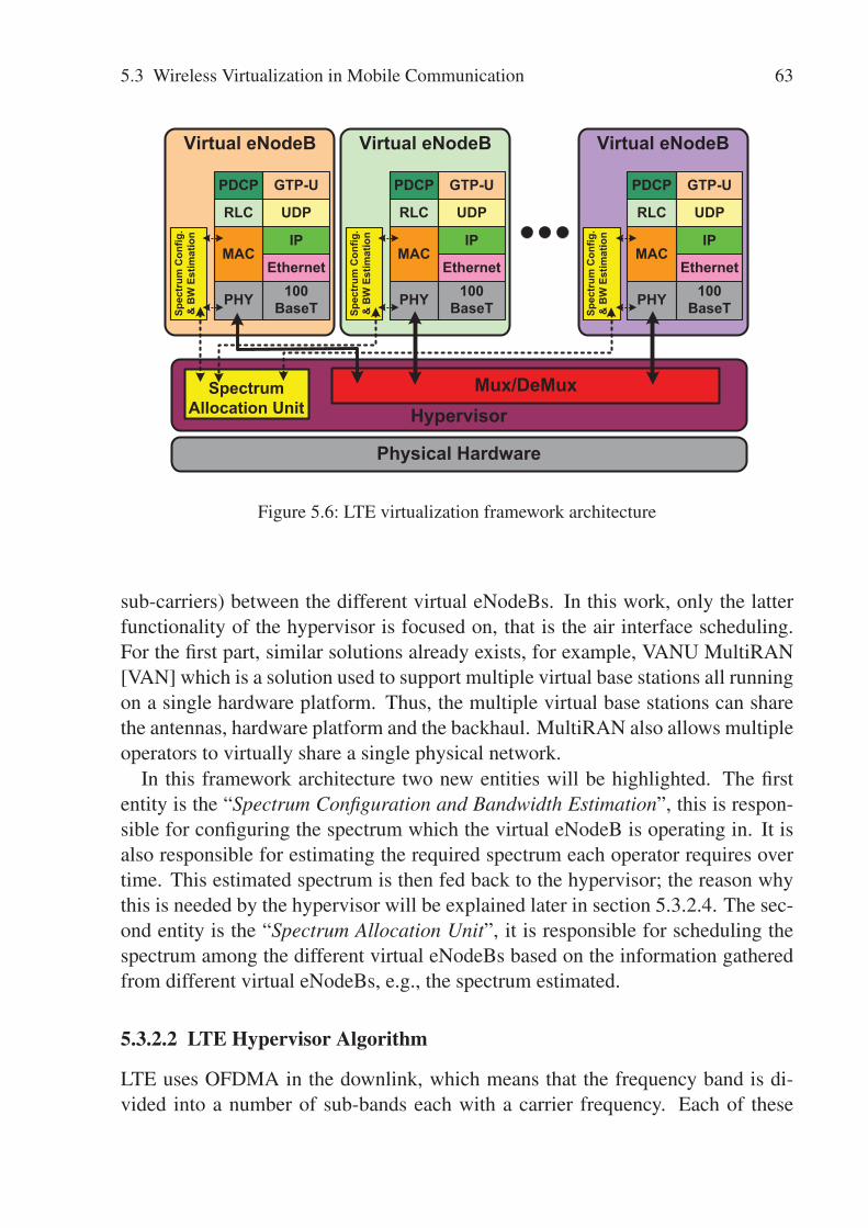
5.3 Wireless Virtualization in Mobile Communication 63
Physical Hardware
Hypervisor
Virtual eNodeB
PDCP
RLC
PHY
GTP-U
UDP
100BaseT
IP
EthernetMAC
Virtual eNodeB
PDCP
RLC
PHY
GTP-U
UDP
100BaseT
IP
EthernetMAC
Virtual eNodeB
PDCP
RLC
PHY
GTP-U
UDP
100BaseT
IP
EthernetMAC
Spec
trum
Con
fig.
&B
WEs
timat
ion
Mux/DeMux
Spec
trum
Con
fig.
&B
WEs
timat
ion
Spec
trum
Con
fig.
&B
WEs
timat
ion
SpectrumAllocation Unit
Figure 5.6: LTE virtualization framework architecture
sub-carriers) between the different virtual eNodeBs. In this work, only the latterfunctionality of the hypervisor is focused on, that is the air interface scheduling.For the first part, similar solutions already exists, for example, VANU MultiRAN[VAN] which is a solution used to support multiple virtual base stations all runningon a single hardware platform. Thus, the multiple virtual base stations can sharethe antennas, hardware platform and the backhaul. MultiRAN also allows multipleoperators to virtually share a single physical network.
In this framework architecture two new entities will be highlighted. The firstentity is the “Spectrum Configuration and Bandwidth Estimation”, this is respon-sible for configuring the spectrum which the virtual eNodeB is operating in. It isalso responsible for estimating the required spectrum each operator requires overtime. This estimated spectrum is then fed back to the hypervisor; the reason whythis is needed by the hypervisor will be explained later in section 5.3.2.4. The sec-ond entity is the “Spectrum Allocation Unit”, it is responsible for scheduling thespectrum among the different virtual eNodeBs based on the information gatheredfrom different virtual eNodeBs, e.g., the spectrum estimated.
5.3.2.2 LTE Hypervisor Algorithm
LTE uses OFDMA in the downlink, which means that the frequency band is di-vided into a number of sub-bands each with a carrier frequency. Each of these
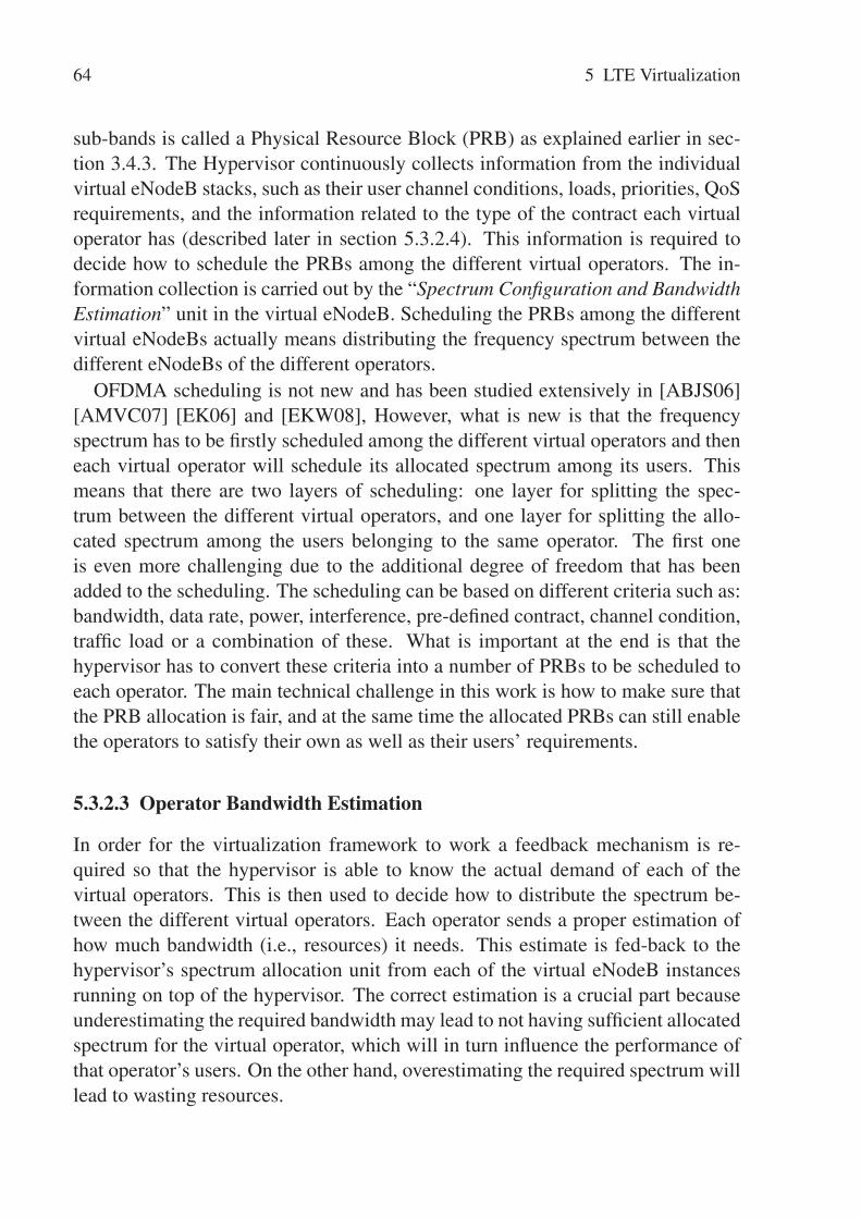
64 5 LTE Virtualization
sub-bands is called a Physical Resource Block (PRB) as explained earlier in sec-tion 3.4.3. The Hypervisor continuously collects information from the individualvirtual eNodeB stacks, such as their user channel conditions, loads, priorities, QoSrequirements, and the information related to the type of the contract each virtualoperator has (described later in section 5.3.2.4). This information is required todecide how to schedule the PRBs among the different virtual operators. The in-formation collection is carried out by the “Spectrum Configuration and BandwidthEstimation” unit in the virtual eNodeB. Scheduling the PRBs among the differentvirtual eNodeBs actually means distributing the frequency spectrum between thedifferent eNodeBs of the different operators.
OFDMA scheduling is not new and has been studied extensively in [ABJS06][AMVC07] [EK06] and [EKW08], However, what is new is that the frequencyspectrum has to be firstly scheduled among the different virtual operators and theneach virtual operator will schedule its allocated spectrum among its users. Thismeans that there are two layers of scheduling: one layer for splitting the spec-trum between the different virtual operators, and one layer for splitting the allo-cated spectrum among the users belonging to the same operator. The first oneis even more challenging due to the additional degree of freedom that has beenadded to the scheduling. The scheduling can be based on different criteria such as:bandwidth, data rate, power, interference, pre-defined contract, channel condition,traffic load or a combination of these. What is important at the end is that thehypervisor has to convert these criteria into a number of PRBs to be scheduled toeach operator. The main technical challenge in this work is how to make sure thatthe PRB allocation is fair, and at the same time the allocated PRBs can still enablethe operators to satisfy their own as well as their users’ requirements.
5.3.2.3 Operator Bandwidth Estimation
In order for the virtualization framework to work a feedback mechanism is re-quired so that the hypervisor is able to know the actual demand of each of thevirtual operators. This is then used to decide how to distribute the spectrum be-tween the different virtual operators. Each operator sends a proper estimation ofhow much bandwidth (i.e., resources) it needs. This estimate is fed-back to thehypervisor’s spectrum allocation unit from each of the virtual eNodeB instancesrunning on top of the hypervisor. The correct estimation is a crucial part becauseunderestimating the required bandwidth may lead to not having sufficient allocatedspectrum for the virtual operator, which will in turn influence the performance ofthat operator’s users. On the other hand, overestimating the required spectrum willlead to wasting resources.

5.3 Wireless Virtualization in Mobile Communication 65
The bandwidth estimation is calculated for each operator, and since it is an esti-mation of the operator’s required spectrum it has to be calculated over some periodof time. The instantaneous bandwidth required by each operator can be calculatedeach TTI, thus the estimation entity will collect a number of instantaneous band-width values over the defined estimation time interval. These values need to beconverted into a single one that can be sent back to the allocation unit as an in-dication of the required bandwidth over that time interval. The most straightfor-ward approach is to take the simple average value of the instantaneous bandwidth.However, simple average values may not be relied on as they may give wrong in-dications especially if it has some spikes (that is onetime events with high values)within the data. In order to avoid these single time events, and filter those out, itis proposed to use the Exponential Moving Average (EMA) [HUN86]. The EMAgives more weight to recent values while not discarding older values. This makes ita perfect solution for the bandwidth estimation, because the most recent values arethe up-to-date values of the operator bandwidth requirement. Thus, the bandwidthestimation is calculated as follows:
E (N) = α ×E (N −1)+(1−α)×PRBsT T I (N) (5.1)
Here, E(N) represents the moving average of the required PRBs (estimate of therequired bandwidth), N is a TTI instance within the hypervisor decision intervaland α is the smoothing factor indicating the weighting between 0 and 1. PRB-sTTI(N) is the instantaneous PRB count at the Nth TTI, calculated by summingthe PRBs that were additionally needed to schedule the un-served users within thisTTI minus the number of left PRBs that were not used. E(N) can take both positiveand negative values, as the operator would either need more PRBs or would like togive some PRBs back that are not required.
5.3.2.4 Contract based Framework
In this section, a practical framework for LTE virtualization and spectrum sharingis proposed to share the LTE spectrum among different virtual operators (each withdifferent goals and requirements). The framework is based on offering differentcontracts that each operator can chose from the infrastructure provider [ZZGTG10b].Based on the requirements of each virtual operator a suitable contract can be madeto express these requirements and satisfy them. In this framework, four differentcontract types are defined and offered by the infrastructure provider to the virtualoperators and these are:

66 5 LTE Virtualization
a. Fixed guarantees: the operator requests a fixed bandwidth that will be allocatedto it at all times whether it is used or not.
b. Dynamic guarantees: the operator gets the bandwidth (in terms of number ofPRBs) according to its actual need. The bandwidth is upper bounded by a max-imum value that is specified by the contract. If the operator requires the max-imum bandwidth, the infrastructure provider will allocate it to him; otherwiseonly the required bandwidth is allocated, which can be less than the maximumvalue. The operator only pays for the actual used bandwidth and thus can savecost.
c. Best effort (BE) with minimum guarantees: the operator specifies a minimumguaranteed bandwidth which will be allocated at all times 1. The minimumbandwidth is always guaranteed and the additional part is added in a BE man-ner.
d. Best effort with no guarantees: the operator does not specify any guarantees forits traffic and the operator is assigned any bandwidth that is remaining, i.e., ina pure BE manner.
The hypervisor uses the estimation value (calculated according to equation 5.1)to allocate each virtual operator’s spectrum. This is used specifically for contracttypes b, c and d. For contract type b, this would serve as the actual allocatedbandwidth for that operator, upper bounded by the contract maximum value. Forthe BE contracts (contract c and d) the hypervisor will first allocate the operatorsof contract c with their minimum guaranteed value and whatever PRBs left at theend would be distributed between the BE operators. The split is based on a fairnessfactor that is calculated as follows:
Fi = Ei (N)/Etotal (5.2)
where Fi is the fairness factor of operator i, Ei (N) is the PRB estimate of operatori, and the Etotal is the total best effort PRB estimate over all best effort operators(e.g., K number of BE operators), and is calculated as follows:
Etotal =K
∑i=1
Ei (N) (5.3)
The number of PRBs allocated for each BE virtual operator is calculated asfollows:
1Conceptually a maximum value may also be configured for that contract acting as an upper boundfor the operator allocated bandwidth.

5.3 Wireless Virtualization in Mobile Communication 67
PRBsAlloci = int (Fi ×Le f tPRBs) (5.4)
where int is the integer function, and the LeftPRBs is the number of PRBs left forthe BE operators after allocating the guaranteed operators.
The proposed framework for the contract-based algorithm in the hypervisor isshown in Figure 5.7.
Star
t
Allo
cate
Ope
rato
rsof
con
trac
t typ
e “a
”
PRB
sAllo
c i=
Ni
LeftP
RB
s=
LeftP
RB
s-
PRB
sAllo
c i
Allo
cate
Ope
rato
rsof
con
trac
t typ
e “b
”
PRB
sAllo
c i=
E i(N
)(U
pper
boun
ded
byN
max
_i)
LeftP
RB
s=
LeftP
RB
s-
PRB
sAllo
c i
Allo
cate
Ope
rato
rsof
con
trac
t typ
e “c
”
PRB
sAllo
c i=
Nm
in_i
(initi
alal
loca
tion
fort
hem
inim
umgu
aran
tees
)
LeftP
RB
s=
LeftP
RB
s-
PRB
sAllo
c i
Allo
cate
BE
Ope
rato
rsof
cont
ract
type
“c
&d”
Cal
cula
teF i
PRB
sAllo
c i=
int(F
i*L
eftP
RB
s)
end
Tota
lPR
Bs
left?
LeftP
RB
s=
Tota
lPR
Bs
Figure 5.7: The general hypervisor algorithm framework

68 5 LTE Virtualization
The framework starts by allocating spectrum to the operators with guaranteedcontracts. First of all, operators with contract type a, or the fixed contract opera-tors, are allocated their spectrum (in terms of number of PRBs, i.e., PRBsAlloci)based on the amount specified by their contract (Ni). The TotalPRBs representsthe total amount of PRBs that an infrastructure provider owns which is the totalowned spectrum/bandwidth. After allocating all the operators of contract type a,the hypervisor starts allocating operators with contract type b. These operators areallocated their spectrum based on their bandwidth estimation upper bounded bythe contract maximum value. After that the hypervisor starts allocating the BEoperators by first allocating operators with contract type c with their minimumguaranteed spectrum and then splitting the rest of the left spectrum between themand the operators with contract type d based on the mechanism explained earlierin equation 5.2. In addition, the hypervisor needs to provide admission controlin accepting new virtual operators, this is necessary as the infrastructure providerhas to guarantee the spectrum for certain operators. This means that the infras-tructure provider will not accept any new virtual operator request if the sum of theguaranteed spectrum exceeds its owned spectrum.
5.4 LTE Virtualization Evaluation
In this work, the LTE virtualization simulation model is built based on the devel-oped OPNET LTE model with certain modifications to include the virtualizationprocess. As mentioned earlier, the focus of this work is not on the node/link virtu-alization but rather on the air interface virtualization (i.e., spectrum sharing). Dueto this reason, node/link virtualization is not modeled, instead a perfect node/linkvirtualization process is assumed in the simulator. Figure 5.8 shows the LTE vir-tualization simulation model.
It can be seen that three virtual operators share the same infrastructure, eachwith its own virtual eNodeB, router and aGW. A hypervisor entity can also be no-ticed, which has the responsibility of scheduling the air interface resources amongthe different virtual eNodeBs. The hypervisor has direct access to the MAC layersof each of the LTE virtual eNodeBs so as to collect all the required relevant infor-mation to be used for the scheduling decisions. This information can consist of,e.g., user channel conditions, operator’s traffic load and operator’s contracts whichis used by the hypervisor to base the spectrum distribution decision on.
In order to find the advantages and potential gains of the LTE virtualization,three different scenarios are investigated in this chapter. The scenarios exploitthe multiplexing gain as well as the multi-user diversity gain, which are com-

5.4 LTE Virtualization Evaluation 69
VO1R1
VO2R1
VO3R1
VO1eNB1
VO2eNB1
VO3eNB1
Hypervisor
VO1aGW1
VO2aGW1
VO3aGW1
VO1Server
VO2Server
VO3Server
VO1_1 VO1_2
VO2_1 VO2_2
VO3_1 VO3_2
Application Profile Mobility Global UE List
Physical eNBPhysicalRouter
PhysicalaGW
PhysicalServer
Figure 5.8: LTE virtualization simulation model in OPNET
pared against a non-virtualized LTE system with the same configuration. Thenon-virtualized LTE system represents the current setup of the LTE system. Thescenarios and their respective results are presented in the next subsections.
5.4.1 Multiplexing Gain based Analysis
This scenario exploits the multiplexing gain that can be achieved through the LTEvirtualization and the spectrum sharing [ZZGTG10a]. Normally, the radio accessnetwork is dimensioned with an overbooked frequency band in order to handle theworst case scenarios when the operators experience their peak traffic loads (e.g.,in busy hours). If the different mobile operators experience their peak loads atdifferent times, or if the instantaneous peaks within each virtual operator busy houroccurs at slightly shifted times (i.e., not exactly at the same time) then a potentialmultiplexing gain can be achieved through spectrum sharing among the differentmobile operators. This will lead to a better resource utilization. This simulationscenario compares two different setups:
• Legacy setup: which is today’s mobile network setup, where each operatorowns a frequency band and is not sharing this band with any other operators.

70 5 LTE Virtualization
• Virtualized setup: where operators are sharing the same infrastructure throughvirtualization and the total combined respective spectrum is shared betweenthe different operators.
In the virtualized setup, the spectrum is scheduled between the different vir-tual operators based on their traffic load. The scenario is configured so that thevirtual operators are assigned the required spectrum to serve their users, and areconfigured as in Table 5.1. In order to investigate the impact and benefits of theair interface resource sharing a sudden increase in the operator traffic load is intro-duced. This increase is emulated, by making some users start a video conferencingapplication at a certain time interval, as can be seen in Table 5.1. The video trafficis used for only 300 seconds, to emulate the sudden peak, and is configured to beat different time intervals for each virtual operator.
Parameter Assumption
Number of virtual operators 3 virtual operators with circular cells of 375 meters radiusTotal Number of PRBs (Spectrum) 75 PRBs (15 MHz), each operator has 25 PRBsMobility model Random Way Point (RWP) with vehicular speed (120 km/h)Number of users per VO 20 VoIP users and 20 Video usersMAC priority mapping VoIP traffic is mapped to MAC-QoS-Class 1
Video traffic is mapped to MAC-QoS-Class 5Channel model described in section 4.3.5VoIP traffic model Silence/Talk Spurt length = negative exponential
distribution with 3 seconds meanEncoder Scheme: GSM EFRContinuous call throughout the whole simulation time
Video traffic model 24 Frames per second with frame size: 1562 bytesDuration: 300 secondsStarting time: VO1 = 100s, VO2 = 400s, VO3 = 700s
Hypervisor resolution 1 second (for the virtualized setup)Simulation run time 1000 secondsNumber of Simulation seeds 20 seeds; simulations with 95% confidence interval
Table 5.1: Scenario I simulation configurations
Figure 5.9 shows the bandwidth in MHz representing the total number of PRBsassigned by the hypervisor to each virtual operator. It can be noticed that theallocated bandwidth changes with time corresponding to the variation of the trafficload of each operator. In the time interval between 100 - 400 seconds, it can beseen that operator 1 has been allocated a much higher bandwidth compared to theother two operators. This is due to the scenario configuration, where operator 1

5.4 LTE Virtualization Evaluation 71
has 20 additional video users that are active during this time period and thus causean increase in the traffic load. Similarly, there is a traffic load increase in the timeinterval between 400 - 700 seconds for VO2 and between 700 - 1000 seconds forVO3. The result also shows that during the peak traffic situation the operator canget more than 5 MHz (25 PRBs) by sharing the free spectrum of the other twooperators, and this would not be possible in without the virtualization process.
0 100 200 300 400 500 600 700 800 900 1000 11000
1
2
3
4
5
6
7
8
9
10
Time (s)
Ban
dwid
th (M
Hz)
Virtual Operators Allocated Bandwidth
VO1VO2VO3
Figure 5.9: Virtual operators allocated bandwidth over simulation time
Figure 5.10 and Figure 5.11 show the VoIP user air interface throughput in kbps(i.e., throughput between the eNodeB and UE physical layers) and the applicationend-to-end delay in ms respectively. It can be seen that the VoIP users have similarperformance in both setups (virtualized and legacy) since the VoIP traffic is puton a higher MAC priority class. The MAC scheduler first serves the VoIP usersbefore serving the video users. In general, the VoIP users require a smaller amountof resources due to their low traffic demand, and the 25 PRBs configured for thelegacy setup are far more than enough to serve the 20 VoIP users in this example.
Figure 5.11 shows that the virtualization setup suffers from a slightly higherdelay values because in some cases when the channel conditions experienced bycertain users are bad the scheduler assigns more PRBs to those users in order toovercome the bad channel conditions. For the legacy setup, enough free resourcesexist that can be allocated, whereas in the virtualized setup there are no free re-
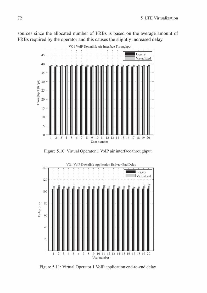
72 5 LTE Virtualization
sources since the allocated number of PRBs is based on the average amount ofPRBs required by the operator and this causes the slightly increased delay.
1 2 3 4 5 6 7 8 9 10 11 12 13 14 15 16 17 18 19 200
5
10
15
20
25
30
35
40
45
User number
Thro
ughp
ut (K
bps)
VO1 VoIP Downlink Air Interface Throughput
LegacyVirtualized
Figure 5.10: Virtual Operator 1 VoIP air interface throughput
1 2 3 4 5 6 7 8 9 10 11 12 13 14 15 16 17 18 19 200
20
40
60
80
100
120
140
User number
Del
ay (m
s)
VO1 VoIP Downlink Application End−to−End Delay
LegacyVirtualized
Figure 5.11: Virtual Operator 1 VoIP application end-to-end delay

5.4 LTE Virtualization Evaluation 73
Figure 5.12 shows the video users’ application end-to-end delay. The resultsshow that the video users have much better performance in the virtualized setupcompared to the legacy setup. This is because in the legacy setup the 25 configuredPRBs are not enough to serve all 20 video users in each TTI. As a result, only afew number of the video users are served in each TTI. Since the MAC schedulerhas a proportional fair characteristic all of the video users can be served at the end.But the video user traffic needs to be buffered longer, hence, increasing the videoend-to-end delay. However, for the virtualized setup the virtual operator is ableto use the free resources from the other virtual operators. This means that the airinterface resources can be higher than the 25 PRBs when required and this willbe enough to serve all of the video users without causing any additional bufferingdelays. The results of the other two virtual operators are similar to VO1 resultsand thus are not shown.
21 22 23 24 25 26 27 28 29 30 31 32 33 34 35 36 37 38 39 400
100
200
300
400
500
600
700
800
User number
Del
ay (m
s)
VO1 Video Downlink Application End−to−End Delay
LegacyVirtualized
Figure 5.12: Virtual Operator 1 VoIP application end-to-end delay
5.4.2 Multi-User Diversity Gain based Analysis
This scenario investigates the multi-user diversity gain that can be obtained by ap-plying LTE air interface virtualization and spectrum sharing. Since OFDMA isused the user channels are normally frequency selective, which means that eachuser will be experiencing different channel conditions on different PRBs. There-

74 5 LTE Virtualization
fore the multi-user diversity can be exploited where the channel-aware schedulerassigns the PRBS to the users experiencing better channel conditions. Virtualiza-tion enables the VOs to share their individual spectrum, which also means that thescheduler of each virtual operator has a bigger set of PRBs to exploit the multi-userdiversity, which can bring additional multi-user diversity gain to the system.
This scenario shows that even in the case where no multiplexing is allowedbetween the different virtual operators, and each operator still has a fixed amountof spectrum, a gain can still be achieved if the spectrum is dynamically chosenbased on the user channel conditions [ZZGTG11]. In this scenario two differentsetups are compared against each other as follows:
• Legacy setup: which is similar to today’s mobile network setup where eachoperator owns a fixed amount of spectrum that is pre-allocated throughoutthe whole simulation.
• Virtualized setup: which aims at showing how the multi-user diversity gaincan be achieved by sharing the spectrum among the operators, with the totalamount of spectrum each operator gets is fixed and not changing (no multi-plexing).
The rest of the simulation configurations is given in Table 5.2.
Parameter Assumption
Number of virtual operators 3 virtual operators with circular cells of 375 meters radiusTotal Number of PRBs - 75 PRBs or 15 MHz (5MHz for each operator)
- 150 PRBs or 30 MHz (10MHz for each operator)- 300 PRBs or 60 MHz (20MHz for each operator)
Mobility model Random Way Point (RWP) with vehicular speed (120 km/h)Number of users VO1: 1, 2, 3, 4, 5, 10, 15 FTP users
VO2: 1, 2, 3, 4, 5, 10, 15 FTP usersVO3: 1, 2, 3, 4, 5, 10, 15 FTP users
Channel model described in section 4.3.5MAC layer scheduler Max-C/I 2
DL traffic model FTP traffic with full buffer occupancyFile size = 5 MByte, next file is loaded immediatelywhen previous file finishes
Hypervisor resolution 1 second (for the virtualized setup)Simulation run time 1000 seconds
Table 5.2: Scenario II simulation configurations
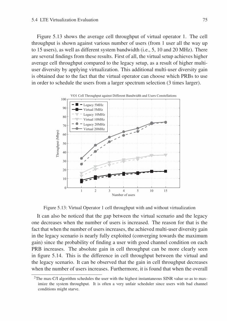
5.4 LTE Virtualization Evaluation 75
Figure 5.13 shows the average cell throughput of virtual operator 1. The cellthroughput is shown against various number of users (from 1 user all the way upto 15 users), as well as different system bandwidth (i.e., 5, 10 and 20 MHz). Thereare several findings from these results. First of all, the virtual setup achieves higheraverage cell throughput compared to the legacy setup, as a result of higher multi-user diversity by applying virtualization. This additional multi-user diversity gainis obtained due to the fact that the virtual operator can choose which PRBs to usein order to schedule the users from a larger spectrum selection (3 times larger).
1 2 3 4 5 10 150
10
20
30
40
50
60
70
80
90
100
Number of users
Thro
ughp
ut (M
bps)
VO1 Cell Throughput against Different Bandwidth and Users Constellations
Legacy 5MHzVirtual 5MHzLegacy 10MHzVirtual 10MHzLegacy 20MHzVirtual 20MHz
Figure 5.13: Virtual Operator 1 cell throughput with and without virtualization
It can also be noticed that the gap between the virtual scenario and the legacyone decreases when the number of users is increased. The reason for that is thefact that when the number of users increases, the achieved multi-user diversity gainin the legacy scenario is nearly fully exploited (converging towards the maximumgain) since the probability of finding a user with good channel condition on eachPRB increases. The absolute gain in cell throughput can be more clearly seenin figure 5.14. This is the difference in cell throughput between the virtual andthe legacy scenario. It can be observed that the gain in cell throughput decreaseswhen the number of users increases. Furthermore, it is found that when the overall
2The max-C/I algorithm schedules the user with the highest instantaneous SINR value so as to max-imize the system throughput. It is often a very unfair scheduler since users with bad channelconditions might starve.
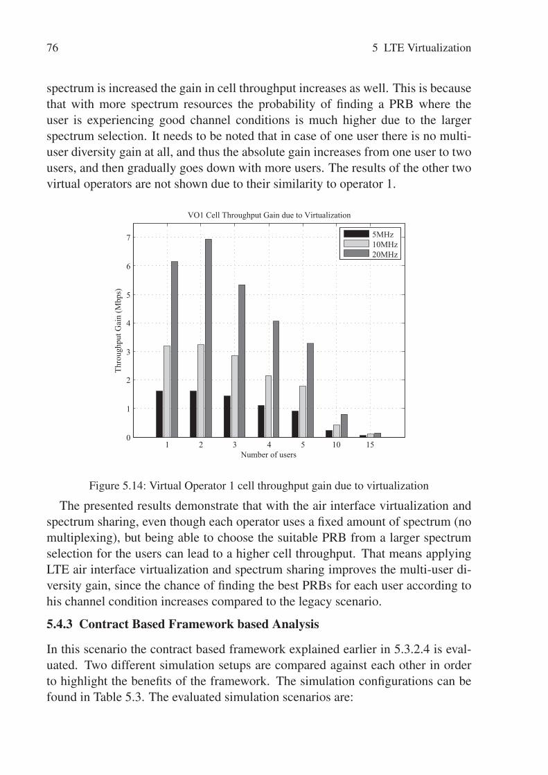
76 5 LTE Virtualization
spectrum is increased the gain in cell throughput increases as well. This is becausethat with more spectrum resources the probability of finding a PRB where theuser is experiencing good channel conditions is much higher due to the largerspectrum selection. It needs to be noted that in case of one user there is no multi-user diversity gain at all, and thus the absolute gain increases from one user to twousers, and then gradually goes down with more users. The results of the other twovirtual operators are not shown due to their similarity to operator 1.
1 2 3 4 5 10 150
1
2
3
4
5
6
7
Number of users
Thro
ughp
ut G
ain
(Mbp
s)
VO1 Cell Throughput Gain due to Virtualization
5MHz10MHz20MHz
Figure 5.14: Virtual Operator 1 cell throughput gain due to virtualization
The presented results demonstrate that with the air interface virtualization andspectrum sharing, even though each operator uses a fixed amount of spectrum (nomultiplexing), but being able to choose the suitable PRB from a larger spectrumselection for the users can lead to a higher cell throughput. That means applyingLTE air interface virtualization and spectrum sharing improves the multi-user di-versity gain, since the chance of finding the best PRBs for each user according tohis channel condition increases compared to the legacy scenario.
5.4.3 Contract Based Framework based Analysis
In this scenario the contract based framework explained earlier in 5.3.2.4 is eval-uated. Two different simulation setups are compared against each other in orderto highlight the benefits of the framework. The simulation configurations can befound in Table 5.3. The evaluated simulation scenarios are:
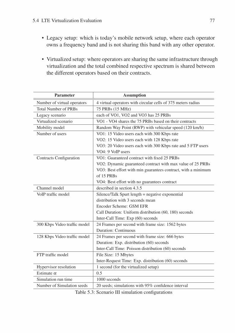
5.4 LTE Virtualization Evaluation 77
• Legacy setup: which is today’s mobile network setup, where each operatorowns a frequency band and is not sharing this band with any other operator.
• Virtualized setup: where operators are sharing the same infrastructure throughvirtualization and the total combined respective spectrum is shared betweenthe different operators based on their contracts.
Parameter Assumption
Number of virtual operators 4 virtual operators with circular cells of 375 meters radiusTotal Number of PRBs 75 PRBs (15 MHz)Legacy scenario each of VO1, VO2 and VO3 has 25 PRBsVirtualized scenario VO1 - VO4 shares the 75 PRBs based on their contractsMobility model Random Way Point (RWP) with vehicular speed (120 km/h)Number of users VO1: 15 Video users each with 300 Kbps rate
VO2: 15 Video users each with 128 Kbps rateVO3: 20 Video users each with 300 Kbps rate and 5 FTP usersVO4: 9 VoIP users
Contracts Configuration VO1: Guaranteed contract with fixed 25 PRBsVO2: Dynamic guaranteed contract with max value of 25 PRBsVO3: Best effort with min guarantees contract, with a minimumof 15 PRBsVO4: Best effort with no guarantees contract
Channel model described in section 4.3.5VoIP traffic model Silence/Talk Spurt length = negative exponential
distribution with 3 seconds meanEncoder Scheme: GSM EFRCall Duration: Uniform distribution (60, 180) secondsInter-Call Time: Exp (60) seconds
300 Kbps Video traffic model 24 Frames per second with frame size: 1562 bytesDuration: Continuous
128 Kbps Video traffic model 24 Frames per second with frame size: 666 bytesDuration: Exp. distribution (60) secondsInter-Call Time: Poisson distribution (60) seconds
FTP traffic model File Size: 15 MbytesInter-Request Time: Exp. distribution (60) seconds
Hypervisor resolution 1 second (for the virtualized setup)Estimate α 0.5Simulation run time 1000 secondsNumber of Simulation seeds 20 seeds; simulations with 95% confidence interval
Table 5.3: Scenario III simulation configurations

78 5 LTE Virtualization
Figure 5.15 shows the bandwidth and the number of PRBs that each virtualoperator is allocated over time.
0 200 400 600 800 10000
1
2
3
4
5
6
7
8
Time (seconds)
Allo
cate
d B
andw
idth
Allocated Bandwidth per Virtual Operator
VO1VO2VO3VO4
0 200 400 600 800 10000
10
20
30
40
50
60
70
80
Time (seconds)
Allo
cate
d PR
Bs
Allocated PRBs per Virtual Operator
VO1VO3VO2VO4
Figure 5.15: Virtual Operator allocated bandwidth/PRBs)
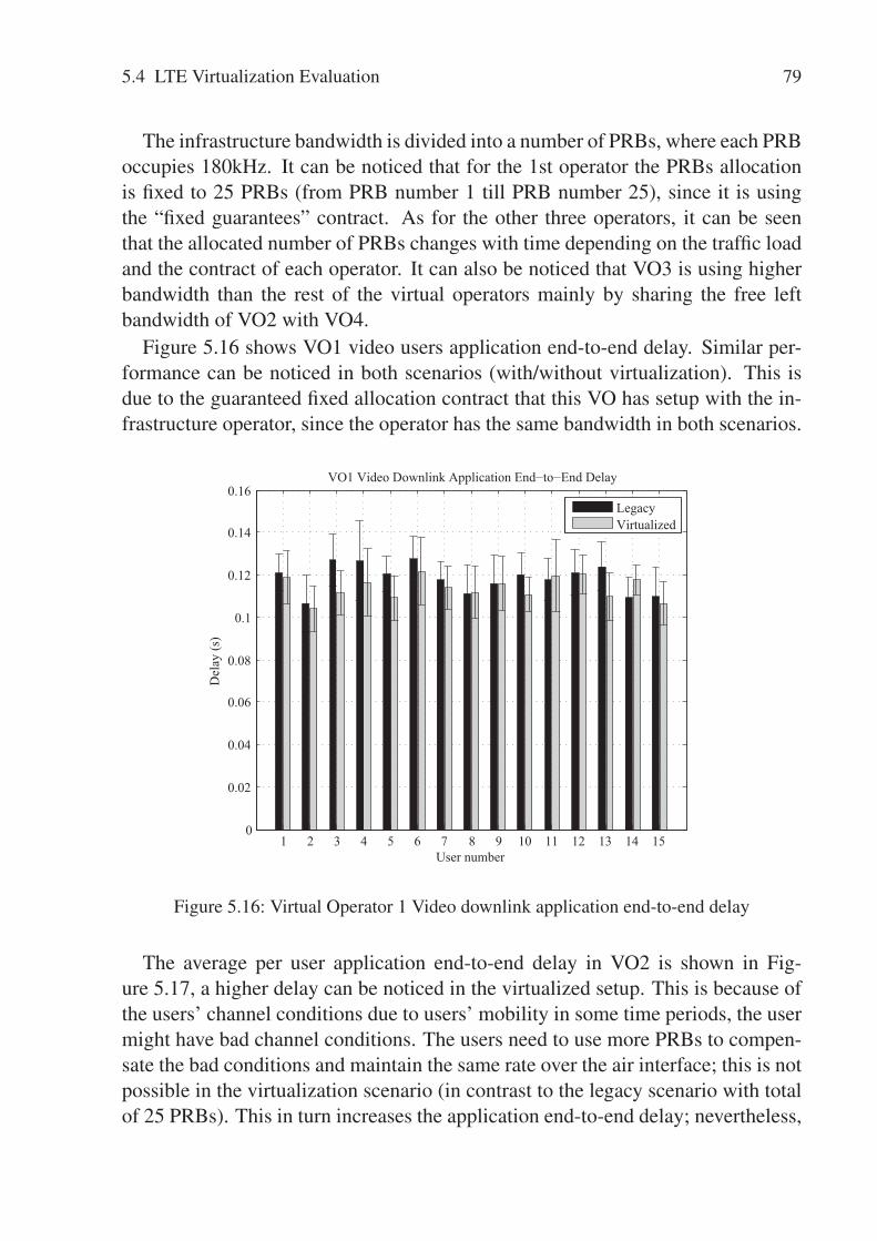
5.4 LTE Virtualization Evaluation 79
The infrastructure bandwidth is divided into a number of PRBs, where each PRBoccupies 180kHz. It can be noticed that for the 1st operator the PRBs allocationis fixed to 25 PRBs (from PRB number 1 till PRB number 25), since it is usingthe “fixed guarantees” contract. As for the other three operators, it can be seenthat the allocated number of PRBs changes with time depending on the traffic loadand the contract of each operator. It can also be noticed that VO3 is using higherbandwidth than the rest of the virtual operators mainly by sharing the free leftbandwidth of VO2 with VO4.
Figure 5.16 shows VO1 video users application end-to-end delay. Similar per-formance can be noticed in both scenarios (with/without virtualization). This isdue to the guaranteed fixed allocation contract that this VO has setup with the in-frastructure operator, since the operator has the same bandwidth in both scenarios.
1 2 3 4 5 6 7 8 9 10 11 12 13 14 150
0.02
0.04
0.06
0.08
0.1
0.12
0.14
0.16
User number
Del
ay (s
)
VO1 Video Downlink Application End−to−End Delay
LegacyVirtualized
Figure 5.16: Virtual Operator 1 Video downlink application end-to-end delay
The average per user application end-to-end delay in VO2 is shown in Fig-ure 5.17, a higher delay can be noticed in the virtualized setup. This is because ofthe users’ channel conditions due to users’ mobility in some time periods, the usermight have bad channel conditions. The users need to use more PRBs to compen-sate the bad conditions and maintain the same rate over the air interface; this is notpossible in the virtualization scenario (in contrast to the legacy scenario with totalof 25 PRBs). This in turn increases the application end-to-end delay; nevertheless,

80 5 LTE Virtualization
the delay in the virtualization scenario is still within acceptable range.
1 2 3 4 5 6 7 8 9 10 11 12 13 14 150
0.02
0.04
0.06
0.08
0.1
0.12
User number
Del
ay (s
)
VO2 Video Downlink Application End−to−End Delay
LegacyVirtualized
Figure 5.17: Virtual Operator 2 Video downlink application end-to-end delay
0 100 200 300 400 500 600 700 800 900 10000
1
2
3
4
5
6
7
Time (seconds)
Allo
cate
d B
andw
idth
VO2 Allocated Bandwidth
LegacyVirtualized
Figure 5.18: Virtual Operator 2 downlink allocated bandwidth
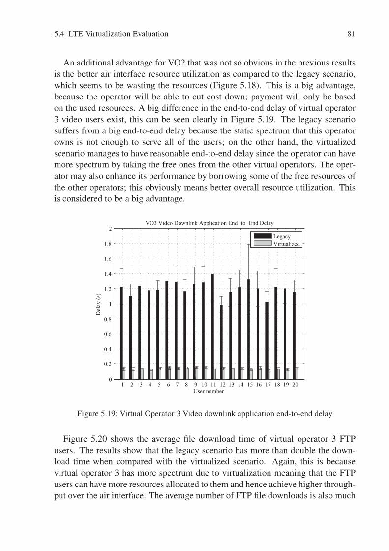
5.4 LTE Virtualization Evaluation 81
An additional advantage for VO2 that was not so obvious in the previous resultsis the better air interface resource utilization as compared to the legacy scenario,which seems to be wasting the resources (Figure 5.18). This is a big advantage,because the operator will be able to cut cost down; payment will only be basedon the used resources. A big difference in the end-to-end delay of virtual operator3 video users exist, this can be seen clearly in Figure 5.19. The legacy scenariosuffers from a big end-to-end delay because the static spectrum that this operatorowns is not enough to serve all of the users; on the other hand, the virtualizedscenario manages to have reasonable end-to-end delay since the operator can havemore spectrum by taking the free ones from the other virtual operators. The oper-ator may also enhance its performance by borrowing some of the free resources ofthe other operators; this obviously means better overall resource utilization. Thisis considered to be a big advantage.
1 2 3 4 5 6 7 8 9 10 11 12 13 14 15 16 17 18 19 200
0.2
0.4
0.6
0.8
1
1.2
1.4
1.6
1.8
2
User number
Del
ay (s
)
VO3 Video Downlink Application End−to−End Delay
LegacyVirtualized
Figure 5.19: Virtual Operator 3 Video downlink application end-to-end delay
Figure 5.20 shows the average file download time of virtual operator 3 FTPusers. The results show that the legacy scenario has more than double the down-load time when compared with the virtualized scenario. Again, this is becausevirtual operator 3 has more spectrum due to virtualization meaning that the FTPusers can have more resources allocated to them and hence achieve higher through-put over the air interface. The average number of FTP file downloads is also much
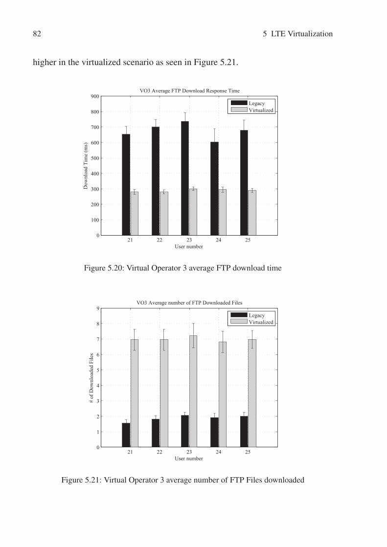
82 5 LTE Virtualization
higher in the virtualized scenario as seen in Figure 5.21.
�� �� �� �� ���
���
���
���
���
���
���
��
��
���
� ���������
���������������� �
� ��!"���#��$�%����������&� '�� ������
(�#�)*���+����,��
Figure 5.20: Virtual Operator 3 average FTP download time
21 22 23 24 250
1
2
3
4
5
6
7
8
9
User number
# of
Dow
nloa
ded
File
s
VO3 Average number of FTP Downloaded Files
LegacyVirtualized
Figure 5.21: Virtual Operator 3 average number of FTP Files downloaded
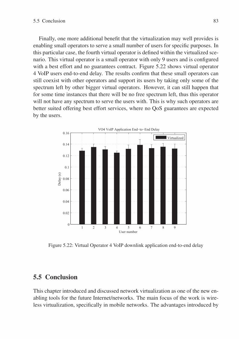
5.5 Conclusion 83
Finally, one more additional benefit that the virtualization may well provides isenabling small operators to serve a small number of users for specific purposes. Inthis particular case, the fourth virtual operator is defined within the virtualized sce-nario. This virtual operator is a small operator with only 9 users and is configuredwith a best effort and no guarantees contract. Figure 5.22 shows virtual operator4 VoIP users end-to-end delay. The results confirm that these small operators canstill coexist with other operators and support its users by taking only some of thespectrum left by other bigger virtual operators. However, it can still happen thatfor some time instances that there will be no free spectrum left, thus this operatorwill not have any spectrum to serve the users with. This is why such operators arebetter suited offering best effort services, where no QoS guarantees are expectedby the users.
1 2 3 4 5 6 7 8 90
0.02
0.04
0.06
0.08
0.1
0.12
0.14
0.16
User number
Del
ay (s
)
VO4 VoIP Application End−to−End Delay
Virtualized
Figure 5.22: Virtual Operator 4 VoIP downlink application end-to-end delay
5.5 Conclusion
This chapter introduced and discussed network virtualization as one of the new en-abling tools for the future Internet/networks. The main focus of the work is wire-less virtualization, specifically in mobile networks. The advantages introduced by

84 5 LTE Virtualization
the LTE virtualization based on spectrum sharing between different operators isstudied and highlighted. An innovative wireless virtualization framework is pro-posed for the virtualization of LTE. However, the framework is not restricted toonly LTE and is open to other similar infrastructure based wireless communicationsystems, e.g., WiMax. The framework was evaluated in several proof of conceptscenarios aiming at showing the benefits of virtualization in the wireless domain:mainly in having better multiplexing gain due to spectrum sharing, as well as bet-ter overall system utilization due to the full exploitation of the multi-user diversitygain. In addition to the above achievements, further advantages of LTE virtualiza-tion can also be seen: for example, sharing the infrastructure of the LTE system is aconsiderably large gain because it leads to having less equipment and thus reducesthe power consumption. It also reduces the capital investment since the operatordoes not need to buy the equipment but only lease virtual resources, which opensthe market for small operators. Another advantage of LTE virtualization is theflexibility the virtualization brings into the operator’s networks, the operator canshrink/expand and change his virtual network on the fly very easily which is oneof the major advantages of network virtualization.

6 LTE Radio Scheduler
Scheduling in LTE is one of the main functions of the eNodeB. The eNodeB aimsat achieving several goals regarding its scheduling functionality. First of all, theeNodeB targets cell throughput maximization, as well as being able to serve asmany active users as possible. This is one of the important features that mobilenetwork operators try to achieve, as it is related to their revenue. The second im-portant objective is to satisfy the user by guaranteeing the QoS of their individualservices. Looking at the scheduling problem within LTE, it is very easy to findthat it is a complex multi-dimensional problem with conflicting targets and there-fore a proper optimization and trade-off is required which can be achieved by thescheduler design.
As explained earlier, LTE uses OFDMA and SC-FDMA as the multiple ac-cess schemes, for both the downlink and uplink respectively. This means that theresources that the scheduler needs to distribute have both a time and a frequencycomponent. The LTE radio scheduler is responsible for distributing a fixed numberof PRBs (obtained from dividing the total system bandwidth) over a varying num-ber of users/bearers in a fixed time interval, so-called for LTE, the TransmissionTime Interval (TTI) which is set to 1ms. This scheduling has to be done for boththe downlink and uplink direction, where the downlink is mainly constrained bythe total transmission power of the eNodeB; while in contrast, the main constrainton the uplink arises from the multi-cell view of inter-cell interference [SBT09]. InLTE, a user can have in general several bearers, one for each service. For example,a user can have a phone call while browsing the web and downloading a file at thesame time, which means for this example the user will have three different bearers.However, within this thesis work, the focus is only on a single bearer users, i.e., allthe investigations done within this thesis are performed with only one bearer peruser. That is why the terms user and bearer are used interchangingly within thethesis.
In this chapter, the LTE radio scheduler is described in detail. First of all, thegeneral scheduling framework is introduced, followed by a state of the art surveyon LTE schedulers. Then the LTE radio scheduler proposed and developed in thisthesis is presented and explained in detail. The proposed scheduler is called “Op-

86 6 LTE Radio Scheduler
timized Service Aware Scheduler” (OSA) which is a proportional fair downlinkscheduler with the motivation of providing service differentiation and guarantee-ing quality of service (QoS). Finally, a detailed simulation analysis is presented,highlighting the achievements and performance gain of the proposed scheduler.
The proposed LTE downlink radio scheduler design, achievements and resultsare published in [ZZW+11] [ZWGTG11b] [ZZW+12].
6.1 LTE Dynamic Packet Scheduling
Two of the main functions of the LTE radio scheduling are the Dynamic PacketScheduling and Link Adaptation. In the dynamic packet scheduling, the time-frequency resources (i.e., Physical Resource Block (PRB) see section 3.4.3) aredistributed between the different active users and their corresponding packets arescheduled at the MAC Layer, the number of packets being scheduled depends onthe Modulation and Coding Scheme (MCS) that the scheduler determines. Thegeneral packet scheduling framework is shown in Figure 6.1.
Time Domain Scheduling (TD)
Frequency Domain Scheduling (FD)
Packet Scheduling
Outer Loop Link Adaptation
Link Adaptation
Inner Loop Link Adaptation
MIMO Link Adaptation
HARQ
QoS attributes
Buffer information
Rank CQI (N)ACK
Figure 6.1: General packet scheduling framework [HT09]
As can be seen, there are a number of interactions and input parameters be-tween the different entities. Both the HARQ manager and the link adaptation areconnected to the packet scheduler, since the scheduler needs to know whether toschedule a new transmission for a certain bearer/user within this TTI, or a pending

6.2 LTE MAC Schedulers State of the Art 87
retransmission is required (as a user cannot do both at the same time). It can beseen that a number of input parameters are also required, such as: QoS attributes,buffer information and some link parameters that are fed back from the users inthe uplink in the form of Channel Quality Indicator (CQI).
The packet scheduling is divided into two different stages: the first stage isthe Time Domain Scheduler (TDS) and the second stage is the Frequency DomainScheduler (FDS). The driver behind such a split is mainly simplicity. The designedscheduler has to work in real life equipment at the end of the day, where resourcesare limited and decisions have to be made within the one millisecond time interval.Thus, the scheduler design and implementation have to be as simple and efficientas possible. In the LTE literature such a split is recommended and is normallycalled decoupled time and frequency domain scheduler [KPK+08a].
6.2 LTE MAC Schedulers State of the Art
In the literature, there are many papers that deal with the problem of LTE schedul-ing. Many of them propose the split of the LTE scheduler into two domains: TimeDomain (TD) and Frequency Domain (FD). The main reason behind the split isto reduce complexity. For example, the authors in [KPK+08a] study the effectsof dynamic packet scheduling in the LTE downlink scheduler and propose the de-coupled time and frequency domain packet scheduling, and use a combination ofknown schedulers. However, the authors also state at the end that several issues arestill missing, for example, QoS differentiation between the services. In [KLZ09],it was demonstrated that the use of a proportional fair multi-user scheduler pro-vides a superior fairness performance when the users average SINR values arefairly uniform. However, service differentiation is also not addressed.
Many publications that deal with the LTE scheduling problem combine severalstandard scheduling techniques for the TD and FD schedulers: e.g., Round Robin(RR), Blind Equal throughput (BET), Proportional Fair (PF), Dynamic Allocation(DA), Equal Resources (ER), Maximum Throughput (MaxT) and many others.They investigate the achievements of using the different scheduling disciplinesin terms of fairness, latency reduction, spectral efficiency and system utilization.Some of these publications are [BAD08] [KPK+08b] [PMP+07] [GL08].
6.2.1 Classical Scheduling Algorithms
Scheduling in principle is a process that tries to create a trade-off, between thedifferent system requirements mainly: fairness between users and performancemaximization (e.g., cell throughput maximization). When designing a scheduling
88 6 LTE Radio Scheduler
algorithm, it all depends on the balance and ratio between these requirements andwhat the respective operator would like to have. Two of the most famous schedul-ing disciplines that are on the opposite edges of the requirements metric are: BlindEqual Throughput (BET) scheduler and Maximum Throughput (MaxT) scheduler.
The BET scheduler represents the fairest algorithm, it tends to gives equalchances for every party involved (i.e., users), as well as a fair chance of the re-sources in order to achieve similar throughput/data rates. It also gives the userswith lower accumulated throughput a higher priority than the ones with higher ac-cumulated throughput. The priority factor calculation for the BET scheduler is asfollows:
PBETk (t) = argmaxk
[1
θk [t]
](6.1)
Where PBETk (t) is the time domain priority factor using the BET scheduler, t is the
tth TTI representing the time instance when the decision is being taken, k is thebearer number and θk [t] is the normalized average throughput of bearer k rangingbetween 0 and 1, it is calculated as follows:
θk [t] =
⎧⎪⎪⎪⎨⎪⎪⎪⎩
(1−1/τ)×θk [t −1]+1/τ × θk[t]θmax
if bearer k is servedin time slot t
(1−1/τ)×θk [t −1] otherwise
(6.2)
where τ is the smoothing factor and is set to 1000 TTIs (1 second) in this work,θk [t] is the instantaneous achieved throughput at the tth TTI and θmax as a normal-ization factor, which is defined to be the maximum throughput that can be achievedif all PRBs are used under perfect channel conditions.
The priority metric shown in equation (6.1) is calculated for all active usersevery TTI, and then a scheduling candidate list is created with all active userssorted based on their priorities, from the highest priorities to the lowest ones.
The BET is often viewed as the least efficient of the overall resource utiliza-tion, or the performance maximization. The explanation is rather simple, if onelooks at a user with relatively bad channel conditions, such a user cannot in factachieve a high transmission rate because of the bad conditions, now even thoughthe accumulated throughput for that user will be small (due to the low transmissionrates) the priority metric for that user will still be high. This means that althoughthe user is in bad channel conditions the scheduler still allocates resources for thatuser, thus wasting valuable air interface resources.
6.3 Downlink MAC Scheduler Design 89
The MaxT scheduler on the other hand tries to maximize the cell throughput andthe system performance. It gives the highest priority to the users that can utilize theradio resources in the most efficient way, which means users with the best channelconditions can transmit higher data rates. The priority factor calculation for theMaxT scheduler is as follows:
PMaxTk (t) = argmaxk [SINRk [t]] (6.3)
where PMaxTk (t) is the time domain priority factor using the MaxT scheduler, k is
the bearer number and SINRk [t] is the instantaneous SINR value of bearer k.MaxT maximizes the cell throughput and the system performance. However, it
fails to provide any fairness among the users. It often has the problem of usersstarvation because users that experience bad channel conditions will rarely get thechance to transmit as other users receive preference for scheduling. The MaxT alsofails in guaranteeing the QoS requirements for the same reason mentioned above.
6.3 Downlink MAC Scheduler Design
The LTE MAC scheduler has a very challenging job of managing the balance be-tween several requirements and targets. On the one hand, the radio scheduler hasto differentiate and guarantee the QoS requirements (e.g., delay budget or loss ra-tio) of the different LTE bearer types corresponding to different services and trafficclasses. On the other hand, it can aim to provide fairness among all users as wellas maximize the cell throughput [ZWGTG11b].
It was discussed earlier within this chapter that the radio scheduler is dividedinto two stages: a Time Domain Scheduler (TDS), and a Frequency DomainScheduler (FDS). Each of these schedulers has different target criteria. The TDSnormally deals with issues related to the QoS requirements and user/bearer pri-oritization; whereas the FDS deals with issues related to spectrum allocation andmulti-user diversity exploitation. The TDS creates a prioritized candidate list ofthe active users/bearers ready to transmit within the TTI, and then passes this can-didate list to the FDS. Then the FDS picks up the users from the list, starting fromthe highest priority ones, and allocates them with the frequency resources (i.e.,PRBs) in a way that exploits the different channel conditions of the different users.
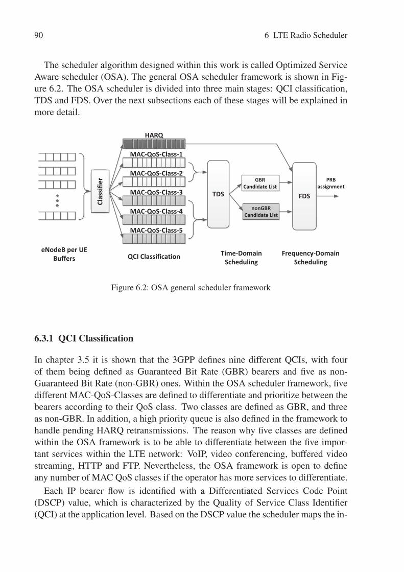
90 6 LTE Radio Scheduler
The scheduler algorithm designed within this work is called Optimized ServiceAware scheduler (OSA). The general OSA scheduler framework is shown in Fig-ure 6.2. The OSA scheduler is divided into three main stages: QCI classification,TDS and FDS. Over the next subsections each of these stages will be explained inmore detail.
eNodeB per UE Buffers
MAC-QoS-Class-1
HARQ
MAC-QoS-Class-2
MAC-QoS-Class-3
MAC-QoS-Class-4
MAC-QoS-Class-5
TDS FDS
QCI Classification Time-Domain Scheduling
Frequency-Domain Scheduling
Clas
sifie
r PRB assignment
GBR Candidate List
nonGBR Candidate List
Figure 6.2: OSA general scheduler framework
6.3.1 QCI Classification
In chapter 3.5 it is shown that the 3GPP defines nine different QCIs, with fourof them being defined as Guaranteed Bit Rate (GBR) bearers and five as non-Guaranteed Bit Rate (non-GBR) ones. Within the OSA scheduler framework, fivedifferent MAC-QoS-Classes are defined to differentiate and prioritize between thebearers according to their QoS class. Two classes are defined as GBR, and threeas non-GBR. In addition, a high priority queue is also defined in the framework tohandle pending HARQ retransmissions. The reason why five classes are definedwithin the OSA framework is to be able to differentiate between the five impor-tant services within the LTE network: VoIP, video conferencing, buffered videostreaming, HTTP and FTP. Nevertheless, the OSA framework is open to defineany number of MAC QoS classes if the operator has more services to differentiate.
Each IP bearer flow is identified with a Differentiated Services Code Point(DSCP) value, which is characterized by the Quality of Service Class Identifier(QCI) at the application level. Based on the DSCP value the scheduler maps the in-
6.3 Downlink MAC Scheduler Design 91
coming IP packets into different MAC QoS classes. A mapping example is shownin Table 6.1.
Bearer type Traffic example QCI DSCP MAC-QoS-Class
GBR VoIP QCI-1 AF43 - EF MAC-QoS-Class-1GBR Video Conferencing QCI-2/4 AF42 - AF33 MAC-QoS-Class-2non-GBR Video Streaming QCI-7 AF32 - AF23 MAC-QoS-Class-3non-GBR HTTP QCI-8 AF22 - AF13 MAC-QoS-Class-4non-GBR FTP QCI-9 AF12 and below MAC-QoS-Class-5
Table 6.1: DSCP/QCI to MAC-QoS-Class mapping example
In each TTI, the QCI classifier identifies the active bearers, i.e., the ones thathave data to transmit and then maps them to the corresponding MAC-QoS-Class.This means at the end of this process, the scheduler will have populated classeswith active bearers that will be considered for this TTI transmission. One thingto notice here is the HARQ handling. Each bearer is checked first against havinga pending HARQ retransmission, if that is the case, the QCI classifier will allowthese bearers to perform their retransmission taking into account the amount ofPRBs required for their transmission. These bearers are no longer considered for anew transmission within this TTI cycle. The retransmissions use the same amountof PRBs as the previous unsuccessful transmission as specified by the 3GPP stan-dardization.
6.3.2 Time Domain Scheduler (TDS)
The time domain scheduler is responsible for prioritizing the bearers based ontheir QoS requirements. This unit is the first stage of a two-stage scheduling pro-cess. Within the first phase, no actual resources are scheduled to the users, theTDS checks the active bearers of the different MAC-QoS-Classes (that are alreadypopulated by the QCI classifier) and prioritizes them based on their urgency andrequirements.
The TDS separates the bearers’ prioritization process into two categories: GBRand non-GBR bearers’ prioritization. In each TTI, the TDS creates two separatebearer candidate lists that are passed later to the FDS, so as to start the spectrum al-location process for that respective TTI. The candidate lists, as the name indicates,are merely suggestions for the FDS. It expresses which bearer has a higher priorityto be served. The prioritization criterion within each list is different depending onthe bearer type.

92 6 LTE Radio Scheduler
GBR bearer prioritization: the GBR bearers have a guaranteed rate that has tobe satisfied, and normally the GBR bearers are used for real time applications sen-sitive to delays. This means that these bearers should be served without any extradelays otherwise they will lose their real time characteristics. VoIP is a typical ex-ample of such a GBR service, in which an application end-to-end delay of higherthan 150ms is already noticeable in terms of bad call quality. The OSA schedulerprioritizes the GBR bearers based on their buffering delays at the eNodB and theirQoS class weight as follows [ZZW+11]:
PGBRk (t) = argmaxk
[WQoS_ j ×HOLdelay_k
](6.4)
Here, PGBRk (t) is the time domain GBR priority metric, k is the bearer number,
WQoS_ j is the QoS weight of the jth MAC QoS class, which is used to enforcepriorities and differentiate between QoS classes, and HOLdelay_k is bearer k’s head-of-line packet delay in the PDCP buffer (i.e., PDCP buffering delay).
The priority metric aims at differentiating the GBR bearers based on their QoSclass, as well as their delay. For example, a bearer of MAC-QoS-Class-1 canbe given higher priority over MAC-QoS-Class-2. Based on PGBR
k (t), the GBRcandidate list is generated by sorting the bearers with the highest values first. Insome cases it can be designed that the GBR bearers are not added to the GBRcandidate list, i.e., not scheduled with these TTIs, if their delays have not exceededa certain pre-defined threshold. Some real time services, like VoIP, can toleratecertain delays (up to 150 ms) and thus it is not crucial to serve them immediately.In addition, these real time services usually have small packet sizes, thus bufferingsome packets together and then multiplexing them can increase the overall spectralefficiency. Delaying the transmission of the GBR packets will increase the overallend-to-end delay for the GBR bearers but will help in serving other non-GBRbearers, as well as increasing the overall spectral efficiency. This will be shownlater in section 6.4.2.
non-GBR bearer prioritization: the non-GBR bearers normally carry best ef-fort type of services such as, buffered video streaming, web browsing (i.e., HTTP),file downloads and uploads (i.e., FTP). Such services do not have strict delayrequirements compared to the real time ones. The OSA scheduler supports upto three different MAC-QoS-Classes to differentiate between the non-GBR ser-vices, and also provides cell throughput maximization while still maintaining fair-ness among the different non-GBR bearers. Again, the three defined MAC-QoS-Classes are not a restriction and the OSA scheduler can define more MAC QoS

6.3 Downlink MAC Scheduler Design 93
classes if required. The active bearers within the non-GBR MAC-QoS-Classes areprioritized by the TDS based on several criteria. The prioritization is done throughcalculating the non-GBR priority factor, this factor follows a similar trend like theweighted proportional fair scheduling but with some minor modifications. Themain difference is the idea of exploiting the average channel conditions of the userwithin the priority factor calculation as follows [ZZW+11]:
PnonGBRk (t) = argmaxk
[WQoS_ j × γk [t]
θk [t]
](6.5)
where PnonGBRk (t) is the time domain priority factor of the non-GBR bearers, k
is the bearer number, WQoS_ j is the QoS weight of the jth QoS class, γk [t] is thenormalized average channel condition (i.e., SINR) of bearer k and θk [t] is thenormalized average throughput of bearer k.
The normalized average channel condition γk [t] is a unit less measure that isnormalized in the range between 0 and 1, it is calculated using the exponentialmoving average formula as follows:
γk [t] = (1−1/τ)× γk [t −1]+1/τ × SINRk [t]SINRmax
(6.6)
τ is the smoothing factor of the exponential moving average window, it is set tobe 1000 TTIs (i.e., 1 second), this means that the averaging function averages theSINR values from 1 second moving window from the past. SINRk is the instanta-neous channel condition of the kth bearer and SINRmax is a scaling factor used tonormalize the channel condition, in order to have a unit less measure between 0and 1.
The average throughput estimate θk [t] is calculated also using the exponentialmoving average formula as in equation (6.2).
The QoS weight factor WQoS_ j is used to ensure the priority differentiation be-tween the different non-GBR services. Table 6.2 shows the weight factor valuesused in this thesis.
Traffic type MAC-QoS-Class WQoS
Video streaming MAC-QoS-Class-3 5HTTP MAC-QoS-Class-4 2FTP MAC-QoS-Class-5 1
Table 6.2: An example of QoS weight values for different non-GBR services

94 6 LTE Radio Scheduler
The reason why these values are chosen was to differentiate between the threenonGBR services by giving HTTP twice higher priority than FTP, since the HTTPhas normally smaller size compared to FTP. As for the video service a weight of 5has been chosen in order to put it on a much higher priority than HTTP and FTP.However, LTE network operators are open to chose any QoS weight values thatmap their internal services differentiation policy.
6.3.3 Frequency Domain Scheduler (FDS)
The FDS is responsible for distributing the radio interface resources (PRBs) amongthe different bearers. Figure 6.3 shows the basic FDS flow chart. The FDS usesthe candidate lists provided by the TDS to choose which bearers should be servedwithin the specific TTIs. The candidate lists contain prioritized bearers based ontheir QoS requirements. The FDS starts first with the GBR candidate list, i.e., theGBR bearers are served first with strict priority over the non-GBR bearers. TheFDS uses an algorithm similar to the well known round robin for the allocationprocess: one PRB at a time, with some channel conditions optimization. OnePRB is allocated first to the highest priority GBR bearer and then another PRB isallocated to the 2nd highest bearer and so on until all PRBs are distributed. Thedistribution is done by assigning the bearers their best PRBs out of the spectrum;the best PRB is measured in terms of their SINR value (the higher the better). Thisis continued in iterations until all GBR bearers have been served within this TTI.For a certain GBR bearer to be scheduled one of two conditions must be satisfied:
1. When a new PRB is assigned for a bearer, the newly achieved data rate ischecked against this bearer PDCP buffer whether or not it can empty thebuffer, or in other words if the new Transport Block Size (TBS) is higherthan that bearer PDCP buffer.
2. If the new iteration PRB leads to a lower TBS than the previous iterationTBS, this is possible in the case that the newly assigned PRB has a very badSINR value that reduces the overall combined SINR into a lower value, andthus achieves a lower TBS/rate.
The first condition, evaluates whether the assigned PRBs are sufficient to emptythe bearer’s buffer. If that is the case there is no need of assigning any further newPRBs for that specific bearer. The second condition, checks if the newly given PRBwill cause a reduction of the new TBS due to the selection of a lower MCS. Sincethe bearer always gets the best PRB, there is no use of keeping this bearer anymore
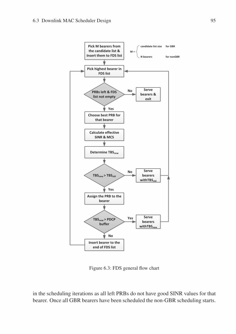
6.3 Downlink MAC Scheduler Design 95
Pick M bearers from the candidate list &
Insert them to FDS list
PRBs left & FDS list not empty
Serve bearers &
exit
Pick highest bearer in FDS list
No
Choose best PRB for that bearer
Calculate effective SINR & MCS
Determine TBSnew
TBSnew > TBSold
Serve bearers
withTBSold
No
Assign the PRB to the bearer
TBSnew > PDCP buffer
Serve bearers
withTBSnew
Yes
Insert bearer to the end of FDS list
Yes
Yes
No
M =
candidate list size for GBR
N bearers for nonGBR
Figure 6.3: FDS general flow chart
in the scheduling iterations as all left PRBs do not have good SINR values for thatbearer. Once all GBR bearers have been scheduled the non-GBR scheduling starts.

96 6 LTE Radio Scheduler
Scheduling the non-GBR bearers is very similar to the GBR procedure with onlyone difference: only a subset of non-GBR bearers are chosen out of the non-GBRcandidate list for the PRBs iterative allocation procedure, instead of the completecandidate list, as in the GBR case. This subset is normally chosen to be the highestnumber of non-GBR bearers ψ in the non-GBR candidate list. ψ is an integervalue and is related to the fairness among the bearers differentiation.
6.3.4 Link-to-System Mapping (L2S)
In wireless network simulation, it is normally not feasible to simulate in detailsboth physical layer aspects, as well as network level aspects at the same time dueto the huge complexity involved. Hence, simulations are normally divided intotwo different levels: link level simulations and system level simulations. The linklevel simulations focus on the wireless medium (channel) and physical layer as-pects, like modulation, channel coding, equalization, MIMO, etc. The system levelsimulations, on the other hand, focus on the performance evaluations of the upperlayer protocols and network performance.
In order to have accurate network performance results within the system levelsimulations, some link level emulation is required. This is normally done usingmapping techniques between the two levels, known as link-to-system mapping.With the help of this mapping technique a statistical emulation of the Block ErrorRate (BLER) can be modeled.
QPSK 1/3QPSK 1/2QPSK 2/316QAM 1/216QAM 2/316QAM 4/564QAM 1/264QAM 2/364QAM 4/5
100
10-1
10-2
-20 -15 -10 -5 0 5 10 15 20
Pre-detection SINR in dB
BLER
in %
QPSK
16QAM
64QAM
Figure 6.4: Reference BLER versus SINR AWGN curves

6.3 Downlink MAC Scheduler Design 97
Within the literature, two methods are mainly used to achieve the mapping:Average Value Interface and the Actual Value Interface (AVI) [HSH+97]. The AVImethod is used to map the SINR value emulated by the system level simulation onthe Additive White Gaussian Noise (AWGN) curves to check what modulation andcoding scheme can be used to obtain a transmission with a certain target BLER.Figure 6.4 shows reference AWGN BLER versus SINR curves for different MCS.For example, when the instantaneous SINR value is 5 dB, then using MCS ofQPSK 2/3, can achieve a transmission with a BLER lower than 10%, whereasusing MCS of 16QAM 1/2 it will not be possible to achieve a transmission withthe target 10% BLER. If there is only one target BLER within the simulation thenhaving only a reference table will be enough, where for each MCS a target SINRvalue is given.
In LTE, the legacy AVI method cannot be applied directly and some mod-ifications are required to make it applicable. As highlighted before, LTE usesOFDMA as the transmission scheme for the downlink, and this means that a UEcan get several frequency resources (i.e., PRBs) for a single transmission. Eachof these PRBs might have a different SINR value, depending on the channel con-ditions that each experiences, and all of these SINR values must be combinedtogether to form a single SINR value that can be mapped to the AWGN curves.Several methods in literature are used to combine the multi-carrier SINR values,and two of the most widely used ones that have been proven to be accurate are:Exponential Effective SINR Mapping (EESM) and Mutual Information EffectiveSINR Mapping (MIESM). The difference between the two methods can be foundin [BAS+05]. For this thesis work, the EESM method is chosen due to its simplerimplementation and less complex computational cost.
For the mapping of the several SINR values into a single effective SINR valueto work properly, it is very important that the following approximation is valid forevery instantaneous channel realization and not “on average” for a given channelmodel [Zah11]:
BLEP({γk})≈ BLEPAWGN
(γeff
)(6.7)
where BLEP({γk}) is the instantaneous BLock Error Probability for the channelstate {γk} and BLEPAWGN
(γeff
)is the AWGN BLock Error Probability.
That is why a scaling factor β is defined for each MCS in order to fulfill equation(6.7). The Effective SINR mapping is calculated as follows:
SINReff = I−1
(1N
N
∑n=1
I (SINRn)
)(6.8)
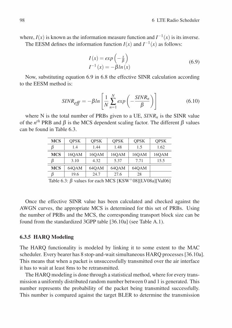
98 6 LTE Radio Scheduler
where, I(x) is known as the information measure function and I−1(x) is its inverse.The EESM defines the information function I(x) and I−1(x) as follows:
I (x) = exp(− x
β
)I−1 (x) =−β ln(x)
(6.9)
Now, substituting equation 6.9 in 6.8 the effective SINR calculation accordingto the EESM method is:
SINReff =−β ln
[1N
N
∑n=1
exp(−SINRn
β
)](6.10)
where N is the total number of PRBs given to a UE, SINRn is the SINR valueof the nth PRB and β is the MCS dependent scaling factor. The different β valuescan be found in Table 6.3.
MCS QPSK QPSK QPSK QPSK QPSKβ 1.4 1.44 1.48 1.5 1.62
MCS 16QAM 16QAM 16QAM 16QAM 16QAMβ 3.10 4.32 5.37 7.71 15.5
MCS 64QAM 64QAM 64QAM 64QAMβ 19.6 24.7 27.6 28
Table 6.3: β values for each MCS [KSW+08][LV08a][Val06]
Once the effective SINR value has been calculated and checked against theAWGN curves, the appropriate MCS is determined for this set of PRBs. Usingthe number of PRBs and the MCS, the corresponding transport block size can befound from the standardized 3GPP table [36.10a] (see Table A.1).
6.3.5 HARQ Modeling
The HARQ functionality is modeled by linking it to some extent to the MACscheduler. Every bearer has 8 stop-and-wait simultaneous HARQ processes [36.10a].This means that when a packet is unsuccessfully transmitted over the air interfaceit has to wait at least 8ms to be retransmitted.
The HARQ modeling is done through a statistical method, where for every trans-mission a uniformly distributed random number between 0 and 1 is generated. Thisnumber represents the probability of the packet being transmitted successfully.This number is compared against the target BLER to determine the transmission

6.4 Downlink MAC Scheduler Analysis 99
probability of the packet. Three different HARQ BLERs are defined: One for the1st transmission, one for the 1st retransmission and one for the 2nd retransmissionas shown in Table 6.4.
It can be seen that the BLER numbers decrease with the retransmissions, un-til it reaches 0% (successful transmission) for the 2nd retransmission. The reasonfor this simplified modeling is the fact that in LTE chase combining with incre-mental redundancy is used to decode the received packets, this means that eachnew retransmission is combined with the older unsuccessful transmission and theprobability of decoding successfully increases.
1st transmission 1st retransmission 2nd retransmissionBLER 10% 1% 0%
Table 6.4: BLER and HARQ transmissions
6.4 Downlink MAC Scheduler Analysis
The purpose of this section is to study and analyze performance of the OptimizedService Aware scheduler (OSA), which is proposed by this thesis. In order toinvestigate the benefits of the OSA scheduler and to see where it lies in the trade-off metric. First, a comparison between the OSA and the most classical sched-ulers (BET and MaxT) is studied. Next, some of the key aspects of the OSA arepresented with a detailed analysis of the scheduler performance in terms of fair-ness, QoS guarantees and the exploitation of the different channel conditions (i.e.,multi-user diversity). In the last analysis, the benefits of the real time GBR delaysensitivity exploitation is discussed, highlighting the additional gains that can beachieved by delaying the GBR services to some extent without harming their QoSor their performance.
6.4.1 OSA vs. Classical Schedulers
In this section, the OSA scheduler is compared against two of the classical sched-ulers: Blind Equal Throughput (BET) and Maximum Throughput (MaxT). Thereason why these two schedulers are chosen for the comparison is that each rep-resents the upper limit of some scheduling characteristics. The BET focuses onfairness and tries to allocate resources in such a way that the overall throughput ofeach user is the same. But the MaxT focuses on maximizing the cell throughputand allocates as many resources as possible to users in best channel conditions
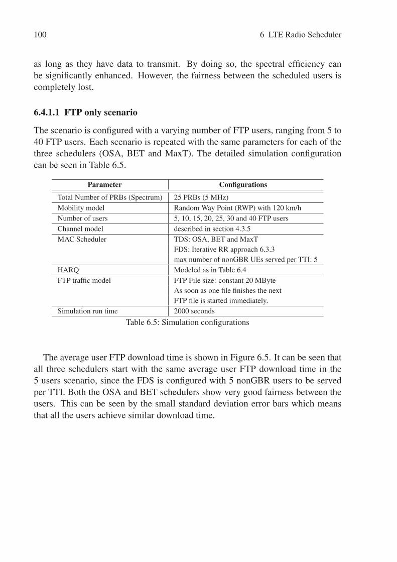
100 6 LTE Radio Scheduler
as long as they have data to transmit. By doing so, the spectral efficiency canbe significantly enhanced. However, the fairness between the scheduled users iscompletely lost.
6.4.1.1 FTP only scenario
The scenario is configured with a varying number of FTP users, ranging from 5 to40 FTP users. Each scenario is repeated with the same parameters for each of thethree schedulers (OSA, BET and MaxT). The detailed simulation configurationcan be seen in Table 6.5.
Parameter Configurations
Total Number of PRBs (Spectrum) 25 PRBs (5 MHz)Mobility model Random Way Point (RWP) with 120 km/hNumber of users 5, 10, 15, 20, 25, 30 and 40 FTP usersChannel model described in section 4.3.5MAC Scheduler TDS: OSA, BET and MaxT
FDS: Iterative RR approach 6.3.3max number of nonGBR UEs served per TTI: 5
HARQ Modeled as in Table 6.4FTP traffic model FTP File size: constant 20 MByte
As soon as one file finishes the nextFTP file is started immediately.
Simulation run time 2000 seconds
Table 6.5: Simulation configurations
The average user FTP download time is shown in Figure 6.5. It can be seen thatall three schedulers start with the same average user FTP download time in the5 users scenario, since the FDS is configured with 5 nonGBR users to be servedper TTI. Both the OSA and BET schedulers show very good fairness between theusers. This can be seen by the small standard deviation error bars which meansthat all the users achieve similar download time.
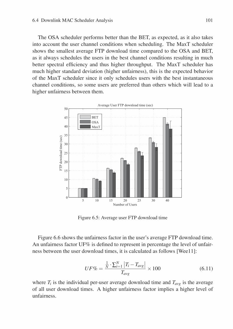
6.4 Downlink MAC Scheduler Analysis 101
The OSA scheduler performs better than the BET, as expected, as it also takesinto account the user channel conditions when scheduling. The MaxT schedulershows the smallest average FTP download time compared to the OSA and BET,as it always schedules the users in the best channel conditions resulting in muchbetter spectral efficiency and thus higher throughput. The MaxT scheduler hasmuch higher standard deviation (higher unfairness), this is the expected behaviorof the MaxT scheduler since it only schedules users with the best instantaneouschannel conditions, so some users are preferred than others which will lead to ahigher unfairness between them.
5 10 15 20 25 30 400
5
10
15
20
25
30
35
40
45
50
Number of Users
FTP
dow
nloa
d tim
e (s
ec)
Average User FTP download time (sec)
BETOSAMaxT
Figure 6.5: Average user FTP download time
Figure 6.6 shows the unfairness factor in the user’s average FTP download time.An unfairness factor UF% is defined to represent in percentage the level of unfair-ness between the user download times, it is calculated as follows [Wee11]:
UF% =1N ·∑N
i=1
∣∣Ti −Tavg∣∣
Tavg×100 (6.11)
where Ti is the individual per-user average download time and Tavg is the averageof all user download times. A higher unfairness factor implies a higher level ofunfairness.
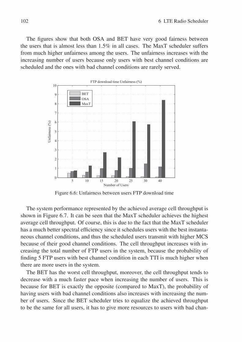
102 6 LTE Radio Scheduler
The figures show that both OSA and BET have very good fairness betweenthe users that is almost less than 1.5% in all cases. The MaxT scheduler suffersfrom much higher unfairness among the users. The unfairness increases with theincreasing number of users because only users with best channel conditions arescheduled and the ones with bad channel conditions are rarely served.
5 10 15 20 25 30 400
1
2
3
4
5
6
7
8
9
10
Number of Users
Unf
airn
ess (
%)
FTP download time Unfairness (%)
BETOSAMaxT
Figure 6.6: Unfairness between users FTP download time
The system performance represented by the achieved average cell throughput isshown in Figure 6.7. It can be seen that the MaxT scheduler achieves the highestaverage cell throughput. Of course, this is due to the fact that the MaxT schedulerhas a much better spectral efficiency since it schedules users with the best instanta-neous channel conditions, and thus the scheduled users transmit with higher MCSbecause of their good channel conditions. The cell throughput increases with in-creasing the total number of FTP users in the system, because the probability offinding 5 FTP users with best channel condition in each TTI is much higher whenthere are more users in the system.
The BET has the worst cell throughput, moreover, the cell throughput tends todecrease with a much faster pace when increasing the number of users. This isbecause for BET is exactly the opposite (compared to MaxT), the probability ofhaving users with bad channel conditions also increases with increasing the num-ber of users. Since the BET scheduler tries to equalize the achieved throughputto be the same for all users, it has to give more resources to users with bad chan-
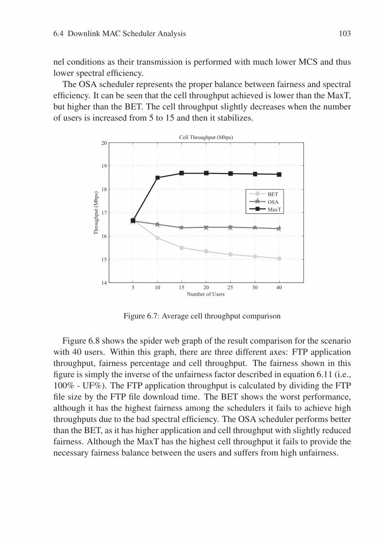
6.4 Downlink MAC Scheduler Analysis 103
nel conditions as their transmission is performed with much lower MCS and thuslower spectral efficiency.
The OSA scheduler represents the proper balance between fairness and spectralefficiency. It can be seen that the cell throughput achieved is lower than the MaxT,but higher than the BET. The cell throughput slightly decreases when the numberof users is increased from 5 to 15 and then it stabilizes.
5 10 15 20 25 30 4014
15
16
17
18
19
20
Number of Users
Thro
ughp
ut (M
bps)
Cell Throughput (Mbps)
BETOSAMaxT
Figure 6.7: Average cell throughput comparison
Figure 6.8 shows the spider web graph of the result comparison for the scenariowith 40 users. Within this graph, there are three different axes: FTP applicationthroughput, fairness percentage and cell throughput. The fairness shown in thisfigure is simply the inverse of the unfairness factor described in equation 6.11 (i.e.,100% - UF%). The FTP application throughput is calculated by dividing the FTPfile size by the FTP file download time. The BET shows the worst performance,although it has the highest fairness among the schedulers it fails to achieve highthroughputs due to the bad spectral efficiency. The OSA scheduler performs betterthan the BET, as it has higher application and cell throughput with slightly reducedfairness. Although the MaxT has the highest cell throughput it fails to provide thenecessary fairness balance between the users and suffers from high unfairness.

104 6 LTE Radio Scheduler
91 94 97 100Fairness %
360
390
420
450FTP App. throughput (kbps)
14
16
18
20
Cell throughput (Mbps)
BETOSAMaxT
Figure 6.8: 40 UE scenario - scheduler comparison
The results shown in the figure above can be interpreted in the following man-ner, the larger the shape of each scheduler is (in this case the graph is the trian-gular shape) the better that scheduler performs. This is because the higher thevalue recorded on each axis is the better is the performance. For example, the cellthroughput axis shows the achieved cell throughput for each of the three schedulersand the MaxT has the highest cell throughput, whereas the BET has the lowest one.The results show that OSA achieves the best relative performance. Although it hasa relatively lower FTP and cell throughput compared to the MaxT, it succeeds inproviding the necessary fairness between the scheduled users.
6.4.1.2 Mixed traffic scenario
This scenario is configured with users of mixed traffic types: VoIP, Video, HTTPand FTP. The performance of the three schedulers (OSA, w-BET and w-MaxT)are compared against each other using the mixed traffic scenario. The weightedBET/MaxT are modified versions of the classical schedulers (see section 6.2.1) sothat a fair comparison to the OSA scheduler is possible. The priority metrics ofthese two modified schedulers are defined as follows:

6.4 Downlink MAC Scheduler Analysis 105
Pw−BETk (t) = argmaxk
[WQoS_ j
θk[t]
]Pw−MaxT
k (t) = argmaxk[WQoS_ j × [SINRk [t]
] (6.12)
where Pk (t) is the time domain priority factor, k is the bearer number, θk [t] is thenormalized average throughput of bearer k, which is calculated in the same way asin equation (6.2), SINRk [t] is the instantaneous SINR value of bearer k and WQoS_ jis the weight factor of the jth QoS class.
The simulation configurations can be seen in Table 6.6. As can be noticed fromthe name, the two classical schedulers are slightly modified by adding the QoSweight to provide the QoS differentiation in order to have a fair comparison.
Parameter Configurations
Total Number of PRBs (Spectrum) 25 PRBs (5 MHz)Mobility model Random Way Point (RWP) with vehicular speedNumber of users 40 VoIP, 20 Video, 20 HTTP and 20 FTP usersChannel model described in section 4.3.5MAC Scheduler TDS: OSA, w-BET and w-MaxT
QoS weights as defined in Table 6.2FDS: Iterative RR approach 6.3.3max number of nonGBR UEs served per TTI: 5
Traffic QoS mapping VoIP is mapped to MAC-QoS-Class 1Video is mapped to MAC-QoS-Class 3HTTP is mapped to MAC-QoS-Class 4FTP is mapped to MAC-QoS-Class 5
HARQ Modeled as in Table 6.4VoIP traffic model Silence/Talk Spurt length = negative exponential
distribution with 3 seconds meanEncoder Scheme: GSM EFR with rate 12.2 kbpsContinuous call throughout the whole simulation time
Video traffic model 24 Frames per second with frame size: 1333 bytesData rate: 256 kbps
HTTP traffic model Number of pages per session: 1 pageNumber of objects in a page: 1 objectObject size: constant 100 KBytesReading time: constant 12 seconds
FTP traffic model FTP File size: constant 5 MByteAs soon as one file finishes the next FTP file is started.
Simulation run time 2000 seconds
Table 6.6: Simulation configurations

106 6 LTE Radio Scheduler
Figure 6.9 shows the spider web graph for the comparison of the different ap-plication delays for each of the different schedulers. The graph has four differentaxes, each representing a specific application delay performance: VoIP applicationend-to-end delay, Video application end-to-end delay, HTTP page response timeand FTP file download time. Since all of the axes represent delays, then the smallerthe spider web shape the better the performance is.
62 64 66 68VoIP E2E delay (ms)
30
50
70
90
Video E2E delay (ms)
36912HTTP response
time (s)100
120
140
160
FTP download time (s)
w−BETOSAw−MaxT
Figure 6.9: Application delay performance comparison between schedulers
The VoIP end-to-end delay is the same for all the three different schedulers, be-cause the VoIP is mapped to the highest GBR MAC-QoS-Class. This means, VoIPusers are served with strict priority before serving any other users for all sched-ulers. Although the w-MaxT scheduler shows the best FTP file download time, ithas the highest end-to-end delay for the video application, as well as the highestHTTP page response time. The w-MaxT scheduler fails in providing the necessaryQoS differentiation, even though a QoS dependent weight is added to the originalMaxT criteria. It still focuses on serving the users with the best instantaneouschannel conditions, leading to a better FTP performance. Both OSA and w-BET,provide good results for the video and HTTP users, however, the OSA scheduleroutperforms the w-BET scheduler when looking at the FTP download time due to

6.4 Downlink MAC Scheduler Analysis 107
the better spectral efficiency and being more aware of the user channel diversity.In summary, the spider web graph shows that the OSA scheduler provides the rightbalance between performance and QoS differentiation.
13 14 15 16Cell throughput (Mbps)
85
90
95
100
Video fairness %
93949596HTTP fairness %
94
96
98
100
FTP fairness %
w−BETOSAw−MaxT
Figure 6.10: Fairness and cell throughput comparison between schedulers
Figure 6.10 shows the scheduler comparison in terms of fairness and cell through-put. The fairness is measured in terms of how similar the user performance of eachclass is, i.e., if the fairness is 100%, it means that all the users achieve the sameend-to-end results. It is calculated as 100% - UF% (for UF% see equation (6.11).As expected, the w-MaxT shows the worst fairness between the users in all threedifferent nonGBR traffic classes (i.e., video, HTTP and FTP). The OSA schedulerprovides very good fairness among the users for each traffic class. Looking at thecell throughput, it can be seen that the w-MaxT achieves the highest cell through-put since it focuses only on exploiting the best instantaneous channel conditions,leading to a better spectral efficiency and thus a better cell throughput. The OSAhas lower cell throughput than the w-MaxT, but still higher than the w-BET. Thisis to be expected, as it is always a trade-off between cell throughput and the userfairness. In this case, a relatively lower cell throughput is the penalty that the OSAscheduler has to pay, to achieve better QoS differentiation between the services.

108 6 LTE Radio Scheduler
6.4.2 GBR delay Exploitation
This analysis studies what happens if the GBR services are intentionally delayedup to their QoS requirements. The aim of the study is to see if any benefit canbe gained while still having acceptable GBR service performance. The intendedGBR service to be delayed is the VoIP service. The reason why the VoIP serviceis chosen is because it is normally served with strict priority, which might lead toworse spectral efficiency due to the small VoIP data volume that is sent over theair interface. In other words, delaying the VoIP packets for some time will leadto a better spectral efficiency (higher cell throughput) due to packet multiplexing.The scenarios are configured based on the additional delay of the VoIP packets.The LTE MAC scheduler checks in each TTI the PDCP buffer head-of-line packetdelay for every VoIP user (i.e., the buffering delay of the first packet in the buffer).If the delay exceeds the pre-defined buffering delay then this VoIP user is servedwithin this TTI. If the VoIP user is chosen to be served, the scheduler will try toallocate enough resources to finish this user’s buffer. The simulation parametersfor this analysis is shown in Table 6.7.
Parameter Assumption
Total Number of PRBs 25 PRBs (5 MHz)(Spectrum)Mobility model Random Way Point (RWP) with vehicular speedNumber of users 40 VoIP, 20 Video, 20 HTTP and 20 FTP usersChannel model described in section 4.3.5MAC Scheduler TDS: OSA; FDS: Iterative RR approach 6.3.3
# nonGBR users served per TTI: 5 usersTraffic QoS mapping Similar to Table 6.6HARQ and Traffic modelsScenarios sc1 (0ms): the VoIP service is served strictly without any delays
sc2 (20ms): the VoIP service is delayed up to 20mssc3 (50ms): the VoIP service is delayed up to 50mssc4 (75ms): the VoIP service is delayed up to 75mssc5 (100ms): the VoIP service is delayed up to 100mssc6 (150ms): the VoIP service is delayed up to 150mssc7 (200ms): the VoIP service is delayed up to 200ms
Simulation run time 2000 seconds
Table 6.7: Simulation configurations
Figure 6.11 shows the system cell throughput of all scenarios. It can be seen thatby increasing the buffering delay of the VoIP service the cell throughput increases.
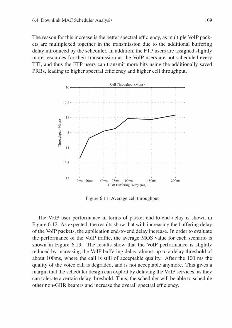
6.4 Downlink MAC Scheduler Analysis 109
The reason for this increase is the better spectral efficiency, as multiple VoIP pack-ets are multiplexed together in the transmission due to the additional bufferingdelay introduced by the scheduler. In addition, the FTP users are assigned slightlymore resources for their transmission as the VoIP users are not scheduled everyTTI, and thus the FTP users can transmit more bits using the additionally savedPRBs, leading to higher spectral efficiency and higher cell throughput.
0ms 20ms 50ms 75ms 100ms 150ms 200ms13
13.5
14
14.5
15
15.5
16Cell Throughput (Mbps)
GBR Buffering Delay (ms)
Thro
ughp
ut (M
bps)
Figure 6.11: Average cell throughput
The VoIP user performance in terms of packet end-to-end delay is shown inFigure 6.12. As expected, the results show that with increasing the buffering delayof the VoIP packets, the application end-to-end delay increase. In order to evaluatethe performance of the VoIP traffic, the average MOS value for each scenario isshown in Figure 6.13. The results show that the VoIP performance is slightlyreduced by increasing the VoIP buffering delay, almost up to a delay threshold ofabout 100ms, where the call is still of acceptable quality. After the 100 ms thequality of the voice call is degraded, and is not acceptable anymore. This gives amargin that the scheduler design can exploit by delaying the VoIP services, as theycan tolerate a certain delay threshold. Thus, the scheduler will be able to scheduleother non-GBR bearers and increase the overall spectral efficiency.

110 6 LTE Radio Scheduler
0ms 20ms 50ms 75ms 100ms 150ms 200ms0
50
100
150
200
250Average VoIP Application end−to−end delay (ms)
GBR Buffering Delay (ms)
Del
ay (m
s)
Figure 6.12: Average VoIP application end-to-end delay
0ms 20ms 50ms 75ms 100ms 150ms 200ms0
0.5
1
1.5
2
2.5
3
3.5
4
4.5
5Average VoIP MOS value
GBR Buffering Delay (ms)
MO
S va
lue
Figure 6.13: Average VoIP MOS value

6.4 Downlink MAC Scheduler Analysis 111
The performance of the other three QoS classes (Video, HTTP and FTP) areshown in Figure 6.14. In this figure only five of the scenarios are shown, exclud-ing the 150ms and 200ms scenario. These two scenarios are excluded as theyshowed unacceptable performance results for the VoIP services. The spiderwebchart shows the performance of the Video, HTTP and FTP in terms of end-to-enddelay, response time, and download time respectively. Of course, the lower thesevalues are the better the performance is, or in other words, the smaller the spi-derweb shape is, the better the performance. As expected, the results show thatby increasing the VoIP buffering delay, the non-GBR service performance is en-hanced.
non−GBR services performance comparison
26 27 28 29
Video E2E delay (ms)
2.3
2.6
2.9
3.2
HTTP response time (s)
120
130
140
150
FTP download time (s)
Strict20ms50ms75ms100ms
Figure 6.14: non-GBR services performance comparison spider chart
In summary, the scheduler is able to exploit some of the GBR service (VoIP inthis case) characteristics and their tolerance to certain delay margins, by delayingtheir scheduling and additionally buffering their packets. By doing so the sched-uler is able to enhance the overall system throughput due to the enhanced spectralefficiency. In addition, the non-GBR service performance is also enhanced.

112 6 LTE Radio Scheduler
6.5 Conclusion
This chapter focused on the design and implementation of an Optimized ServiceAware (OSA) LTE downlink radio scheduler. The OSA scheduler is designed withde-coupled Time and Frequency Domain schedulers (TDS and FDS), the maindesign target behind the scheduler is to provide QoS differentiations to the differ-ent LTE services while at the same time ensuring relative fairness and optimumspectral efficiency.
The OSA scheduler is investigated in several simulation analyses, in order tostudy its behavior in different situations, and to highlight its performance gains. Atfirst the OSA scheduler is compared against other classical schedulers, e.g. Max-imum Throughput (MaxT), and Blind Equal Throughput (BET), with two kind oftraffic scenarios: one without service differentiations by having FTP only users,and one with a traffic mix of several services (VoIP, video, HTTP and FTP). Theresults showed that the OSA scheduler outperforms the other two schedulers inproviding the correct balance between fairness and spectral efficiency, which issomething that both other schedulers fail to provide.
Another investigation, that was analyzed in this chapter, showed the potentialgain that can be achieved by delaying the scheduling of the GBR services (mainlyVoIP services) up to a certain threshold. The simulation scenarios were configuredwith different VoIP delay thresholds. The idea behind these scenarios was to studythe effects of the buffering delay on the VoIP service and see to what extent doesthe VoIP service can tolerate these delays without any degradation on their QoS. Inaddition, the benefits that can arise from delaying the VoIP services were also stud-ied. The results showed that all other nonGBR bearers have gained from delayingthe VoIP bearers, where the average delays values were reduced with increasingthe delay of the VoIP packets. This is due to the fact that when the VoIP servicesare delayed, their additional resources (i.e., PRBs) are free to be used by the otherservices. In addition, a significant gain in the overall cell throughput was achieveddue to the better resource utilizations and the better spectral efficiency.

7 Analytical Modeling of the LTE RadioScheduler
The main motivation behind developing an analytical model is to evaluate the sys-tem performance. Normally, the modeled system is of complex nature, and isevaluated using either simulations or real life experiments that are too exhaustiveand consumes large computation power and time. In addition, real life experimentsare not always possible to perform. That is why, the target behind modeling a sys-tem analytically is to approximate the system behavior mathematically and to doperformance evaluations with much smaller processing effort and time.
In this chapter, several analytical LTE radio scheduler models are proposed. Themodels represent different LTE time domain schedulers, mainly: MaxT, BET andOSA. In addition to the Time Domain Scheduler (TDS) type, two different modelcategories are presented: a single class model and a two classes model. In thesingle class model as the name suggests, only a single traffic class is consideredwith no QoS differentiation. Whereas, the two classes model supports QoS differ-entiation between the two classes.
The analytical models developed in this thesis are based on the general WiMaxanalytical model proposed by [DBMC10]. However, several extensions and mod-ifications have been applied to the [DBMC10] model by this thesis work in orderto: reflect the LTE context, be able to model different LTE TDS schedulers andmost importantly provide QoS differentiations between the traffic classes. Thischapter is organized as follows. In section 7.1, the general analytical model aswell as the performance analysis of the model are explained. Then in section 7.2the LTE downlink scheduler analytical models are introduced, in which the singleclass model is described and analyzed firstly in section 7.2.1 followed by the twodimensional model in section 7.2.3. Finally, section 7.3 concludes the chapter withthe outlook highlighted at the end.

114 7 Analytical Modeling of the LTE Radio Scheduler
7.1 General Analytical Model
The LTE radio scheduler distributes the frequency resources, i.e., PRBs amongthe active users in every TTI (1 ms). There are a number of input parametersthat are used by the scheduler to base the distribution decision upon, e.g., channelconditions, accumulated data rates and QoS. The scheduler uses these input pa-rameters differently based on the scheduler type. Most schedulers consider userchannel conditions as one of the main input parameters in the decision process.The channel conditions change based on the user mobility and location. The chan-nel conditions change stochastically and the scheduler does not have control overthem.
In LTE, a user can transmit data using different modulation and coding schemes(MSC). The choice of the transmission scheme depends on the channel conditionor the received power, i.e. SINR value. The 3GPP standards define several MCSsthat a user can transmit with. Assuming that an operator chooses to support Kdifferent MCSs, then each user can be in any of these MCSs at a given time intervalof the system. In other words, a user can use MCSk, 0 ≤ k ≤ K, where MCS0 isthe outage MCS (user cannot transmit anything) and MCSK is the maximum MCSdefined by the system.
In order to model the LTE radio scheduler analytically, a multidimensionalContinuous Time Markov Chain (CTMC) with state vector (n0, ...,nK) is the moststraight forward solution [DBMC10]. The state describes for each MCS, the num-ber of users nk that can support a certain MCSk. The derivation of the modeltransitions is easy, however, the number of states (model resolution complexity)becomes very large for any realistic value of K.
Following [DBMC10], a work around for the complexity problem can be ap-plied by aggregating the state description into a single dimension, where the Markovchain state n represents the number of active users in the system regardless of theirMCS. The Continuous Time Markov Chain (CTMC) is composed of N+1 states asshown in Figure 7.1, with N being the total number of users in the system.
10 2
Nλ (N-1)λ λ
μ(1) μ(2) μ(N)
nn-1 n+1
(N-n+1)λ (N-n)λ
μ(n) μ(n+1)
N
Figure 7.1: General Continuous Time Markov Chain

7.1 General Analytical Model 115
The figure shows a finite Markov chain limited by the total number of usersin the system N. Each state (apart from state 0 and N) has two transitions, eithergoing to the next state or to the previous state. Since the state itself represents thenumber of active users n, which is normally a subset of the total number of usersN, then a transition from state n to n+1 would mean that one of the inactive users(N-n represents the number of inactive users in state n) has finished its OFF periodand is now ready to transmit. On the other hand, a transition from state n to n-1would mean that one of the active users has finished its transmission and is nowswitching to the inactive state.
These transitions depend on the traffic model. Within the analytical model, aninfinite length ON/OFF elastic traffic model is used [DBMC10]. Such a trafficmodel is used to model best effort traffic, e.g., web browsing or file download.The ON part of the model represents the downloading of a file, where the dura-tion depends on the system parameters, e.g., load, bandwidth, number of users andchannel quality. The OFF period represents the reading time of the downloadedfile, for example, the time the user takes to read a web page before requestingthe next page. This OFF period is independent of the system parameters. TheON period is represented by the file size (Xon), whereas the OFF period is repre-sented by the OFF duration (to f f ), both are assumed to be exponentially distributed[DBMC10].
With the infinite ON/OFF traffic model, a transition from state n to n+1 is per-formed with the rate (N − n)λ , with λ being the inverse of the average readingtime or the file inter-arrival time:
λ =1
to f f(7.1)
The transition from state n to n-1 is performed with the generic rate μ(n) (i.e.,departure rate), since the ON period depends on the system state (as explainedearlier) which in this case depends on the state with n active users.
The work around provides a reduction in the number of states (model resolutioncomplexity) to a small number that depends only on the total number of users inthe system. Nevertheless, the complexity is now moved from the Markov chainstates into the departure rate μ(n) which depends on the scheduling discipline.
7.1.1 Performance Evaluation
The general analytical model explained earlier depends upon two input parameters:arrival transition rate λ and the generic departure transition rate μ(n) as shown inFigure 7.1. Assuming that the generic μ(n) can be estimated, the Markov chain

116 7 Analytical Modeling of the LTE Radio Scheduler
steady state probability π(n) can be evaluated as follows [Kle76]:
πππ ·Q = 0 (7.2)
where πππ is a vector representing the steady state probability of the Markov chain,i.e., πππ=[π0,π1, ...πN] and ∑i πi = 1; Q is the infinitesimal generator, which is amatrix of the transition rates as follows:
Q=
⎡⎢⎢⎢⎢⎢⎢⎢⎣
−Nλ Nλ 0 0 0μ(1) −((N −1)λ +μ(1)) (N −1)λ 0 0
0 μ(2) −((N −2)λ +μ(2)) (N −2)λ 0 ...
.
.
.
⎤⎥⎥⎥⎥⎥⎥⎥⎦
It can be seen in the infinitesimal matrix Q that the diagonal values are set to thenegative value of the sum of the row. This is because the sum of each row in Qshould be zero [Kle76], i.e., ∑ j qi j = 0 for all i. where the diagonal values (i.e., qii)represents the state self transition rate.
Equation 7.2 can be solved using the replace-one-equation method [Ste94]. Analternative to solving equation 7.2 is to use the closed loop solution for the steadystate probability π(n), which is derived from the birth-and-death structure of theMarkov chain [DBMC10], and is as follows:
π(n) =
(n
∏i=1
(N − i+1)λμ(i)
)π(0) (7.3)
where π(0) is obtained by normalization.Once the steady state probabilities have been calculated, the performance eval-
uation of the system can be evaluated. First of all, the average number of activeusers in the system Q is calculated. As Q is the mean number of users and π(n) isthe probability of every state, i.e. probability of having n active users, then Q willbe:
Q =N
∑n=1
nπ(n) (7.4)
Next, the mean number of departures by unit time D is calculated as follows:
D =N
∑n=1
μ(n)π(n) (7.5)
7.1 General Analytical Model 117
And finally, according to Little’s law [Ste11], the average ON duration, i.e. theaverage file download time can be expressed as:
ton =QD
(7.6)
Another possible way to calculate the average ON duration ton would be to di-vide the mean number of users Q by the mean number of arrivals per unit time λ ,which can be expressed as:
λ =N
∑n=1
(N −n+1)λ ·π(n) (7.7)
Thus, the average file download time will be:
ton =Q
λ(7.8)
7.1.2 Generic Departure Rate
μ(n) represents the average departure rate out of state n, thus it depends on thenumber of active users, the system bandwidth, scheduler discipline, file size andthe system transmission interval. In the context of LTE, the transmission intervalis 1ms. A departure from state n to n-1 happens when one of the n active users inthat state finishes its file, and thus μ(n) is estimated as follows [DBMC10]:
μ(n) =T BS(n)
Xon ·T T I(7.9)
where T BS(n) is the average number of bits transmitted within a TTI, when n usersare active. T BS(n) represents the average amount of bits sent for all users servedwithin a TTI. Xon is the average file size of the ON period.
T BS(n) depends on several system parameters. It depends on the MCS usedby the system, the number of active users n and the scheduling discipline. Withinthis general analytical model, each MCS has a stationary probability Pk that rep-resents the probability of a user to be able to use a certain MCSk. This stationaryprobability is estimated through simulations using a predefined scenario for a cer-tain environment, with a certain mobility model and a certain transmission power.T BS(n) can be expressed as follows:
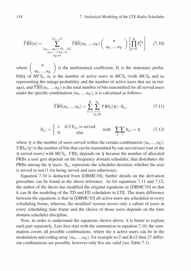
118 7 Analytical Modeling of the LTE Radio Scheduler
T BS(n) =(n,...,n)
∑(n0,...,nK)=(0,...,0)|
n0+...+nK=nn0 �=n
T BS(n0, ...,nK)
(n
n0, ...,nK
)[K
∏k=0
Pnkk
](7.10)
where(
nn0, ...,nK
)is the multinomial coefficient, Pk is the stationary proba-
bility of MCSk, nk is the number of active users in MCSk (with MCS0 and n0representing the outage probability and the number of active users that are in out-age), and T BS(n0, ...,nK) is the total number of bits transmitted for all served usersunder the specific combination (n0, ...,nK), it is calculated as follows:
T BS(n0, ...,nK) =K
∑k=1
nk
∑i=1
nk �=0
T BSk(η) ·Xk,i (7.11)
Xk,i =
{1 if UEk,i is served0 else
with ∑k
∑i
Xk,i = η (7.12)
where η is the number of users served within the certain combination (n0, ...,nK),T BSk(η) is the number of bits that can be transmitted by one served user (out of theη served users) with MCSk. T BSk depends on η because the number of allocatedPRBs a user gets depends on the frequency domain scheduler, that distributes thePRBs among the η users. Xk,i represents the scheduler decision, whether the useris served or not (1 for being served and zero otherwise).
Equation 7.10 is deducted from [DBMC10], further details on the derivationprocedure can be found in the above reference. As for equations 7.11 and 7.12,the author of the thesis has modified the original equations in [DBMC10] so thatit can fit the modeling of the TD and FD schedulers in LTE. The main differencebetween the equations is that in [DBMC10] all active users are scheduled in everyscheduling frame, whereas, the modified version serves only a subset of users inevery scheduling time frame and the choice of those users depends on the timedomain scheduler discipline.
Now, in order to understand the equations shown above, it is better to explaineach part separately. Lets first start with the summation in equation 7.10, the sum-mation covers all possible combinations, where the n active users can be in themodulation and coding array (n0, ...,nK), for example n=2 and K=2 then 27 differ-ent combinations are possible, however only five are valid (see Table 7.1).

7.1 General Analytical Model 119
possibility: (n0 n1 n2) valid(1) 0 0 0(2) 0 0 1(3) 0 0 2 X(4) 0 1 0(5) 0 1 1 X(6) 0 1 2(7) 0 2 0 X(8) 0 2 1(9) 0 2 2
(10) 1 0 0(11) 1 0 1 X(12) 1 0 2(13) 1 1 0 X(14) 1 1 1(15) 1 1 2(16) 1 2 0(17) 1 2 1(18) 1 2 2(19) 2 0 0(20) 2 0 1(21) 2 0 2(22) 2 1 0(23) 2 1 1(24) 2 1 2(25) 2 2 0(26) 2 2 1(27) 2 2 2
Table 7.1: n=2, K=2 combinations example
This is because the summation has two additional requirements: the summa-tions of nk should be equal to n, i.e., all n active users should be present in thecombination, and n0 shall never hold all n active users because otherwise therewill be no transmission.
T BS(n0, ...,nK) is the total number of bits sent for the specific combination(n0, ...,nK), this is calculated using equation 7.11 where only a subset of the usersout of the n total active users are chosen for the scheduling, the chosen η users de-pend on the time domain scheduling. For example, if the TD scheduler is a MaxTscheduler then the η users will be the ones with the highest MCS (i.e., highestSINR). The η number depends upon the frequency domain scheduler which isa round robin scheduler that distributes the PRBs equally among the scheduled
120 7 Analytical Modeling of the LTE Radio Scheduler
users. It can be seen that T BSk depends on η , this is because the number of bitsthat a user can transmit, depends on the MCS, as well as the number of PRBs allo-cated to that users. For example, if the system spectrum is 5MHz (i.e., 25 PRBs)and η is equal to 5 users then on average each of the scheduled η users will beallocated 5 PRBs (that is 25/5).
The multiplication term in equation 7.10 represents the probability of the com-bination (n0, ...,nK), and the multinomial coefficient represents the number of dis-tinct permutations within that combination. For example, if a system is definedwith 2 MCSs (K=2) and the two active users (UE1 and UE2) are present in thesystem, i.e., n=2, then one of the possible combinations is (n0,n1,n2) = (0,1,1),now the multiplication term will give the probability of that combination, butthere are distinct possibilities where UE1 and UE2 might be within that combi-nation, mainly (n0,n1,n2) = (0,UE1,UE2) or (n0,n1,n2) = (0,UE2,UE1) andthat’s what the multinomial coefficient represents.
Now looking at the whole equation after explaining all the individual parts, itcan be seen that it is a weighted average formula. Since each combination numberof transmitted bits T BS(n0, ...,nK) is multiplied with its probability and all thecombinations are summed together. The final results are the average number oftransmitted bits of state n.
7.2 LTE Downlink Scheduler Modeling
This section discusses the analytical modeling of the LTE downlink scheduler us-ing the general analytical model explained earlier in section 7.1. The modeling isdone in two stages: the first stage models the LTE scheduler with a single class,where no QoS differentiation is present. The second stage models the schedulerwith QoS differentiation and using two nonGBR QoS classes. The downlink LTEscheduler as described earlier consists of two schedulers: a Time Domain Sched-uler (TDS) and a Frequency Domain Scheduler (FDS). The FDS scheduler withinthis thesis work is a Round Robin scheduler that distributes the frequency re-sources (i.e., PRBs) equally over the highest η TD priority metric nonGBR users.
7.2.1 Single Class Model
With this model all users use the same traffic model, hence no QoS differentiationis present. The users generate infinite elastic ON/OFF traffic represented by anON period file size Xon and an OFF period of waiting time represented by To f f .Assuming that N users are present in the system then the model is the same CTMC

7.2 LTE Downlink Scheduler Modeling 121
model explained earlier in section 7.1 with arrival rate λ (see equation 7.1) and adeparture rate of μ(n) (see equation 7.9).
μ(n) depends on the TD scheduling discipline since it is inherently dependenton T BS(n). Looking back at equation 7.12, it can be seen that the TDS is reflectedin Xk,i. Where Xk,i is chosen to be 0 or 1 depending on the time domain scheduler.Three different TDS schedulers are modeled in this thesis: BET, OSA and MaxT.
As a generalization, equation 7.11 can be rewritten in a more generic form thatcan incorporate all of the three TD schedulers as:
T BS(n0, ...,nK) = ∑i=[i1,...,iη ]
T BSi(η) (7.13)
with
η = min[n−n0,ψ] (7.14)
where [i1, ..., iη ] represents the index of the chosen η users out of the n active usersconsidered for scheduling within a TTI, and ψ is the number of scheduled usersby the FDS scheduler. Obviously the choice of the η users is determined by theTD scheduler.
Now, substituting equation 7.13 in equation 7.9, the generic departure rate μ(n)will be expressed as:
μ(n) =1
Xon ·T T I
(n,...,n)
∑(n0,...,nK)=(0,...,0)|
n0+...+nK=0n0 �=n
n!
⎡⎣ ∑
i=[i1,...,iη ]T BSi(η)
⎤⎦(
K
∏k=0
Pnkk
nk!
)(7.15)
Once all departure rates have been calculated for every state then the Markovchain steady state probability can be calculated as well as the average file downloadtime using the techniques explained earlier (by using equation 7.6 and 7.3).
In order to model the different TD schedulers, the procedure (scheduler depen-dent) on how to choose η users out of the n active users has to be explained. Forsimplicity, the MaxT scheduler procedure is explained first. According to the def-inition of the MaxT scheduler (section 6.2.1) only the users with the best channelconditions are served, i.e., in every TTI the n active users are prioritized based ontheir channel conditions and then only the highest η users are scheduled. Nowrelating this to the analytical model the η users in the highest MCS are consideredin the scheduling and represent the i user indices ([i1, ..., iη ]). This can be seen inFigure 7.2.

122 7 Analytical Modeling of the LTE Radio Scheduler
MCS0 MCS1 MCS2 MCS3
n0 n1 n2 n3
Find η UEs
MCS4 MCS5 MCS6 MCS7
n4 n5 n6 n7
M
Figure 7.2: MaxT scheduling of users (example with 7 MCSs)
The reason why the MaxT is explained first is the fact that it only depends onthe instantaneous channel conditions (i.e., MCSs). This makes the choice of the ηusers rather straight forward by only choosing the ones with the highest MCSs. Incontrast to other scheduler disciplines like BET or OSA, where the choice of the ηusers does not only depend on the channel conditions but also on the accumulatedsent throughput in the past. This makes the choice rather difficult, as there is amemory aspect in the decision which contradicts one of the basic principles of theMarkov chain, that is the memoryless property.
In order to overcome the above mentioned problem, i.e., memory dependency,some work around is required in the analytical model. This can be done by ap-proximating and emulating the behavior of the schedulers without actually dealingwith the memory aspect. For example, the BET scheduler prioritizes the usersbased on their accumulated throughput from the past as described in equation 6.1.The main target of the BET scheduler is to equalize the users’ throughputs, i.e., allusers will get the same average throughput at the end. This can be approximatedby choosing the η users from the MCSs that correspond to the average throughput.This can be seen in Figure 7.3.
MCS0 MCS1 MCS2 MCS3
n0 n1 n2 n3
Find (η-1) UEs
MCS4 MCS5 MCS6 MCS7
n4 n5 n6 n7
MM
Find 1 UE
Figure 7.3: BET scheduling of users (example with 7 MCSs)
Figure 7.4 shows the MCSs static probability. This can be obtained for eachspecific scenario using simulations (with specific cell coverage, channel model andmobility model). The example figure was created using an eNodeB cell coverage

7.2 LTE Downlink Scheduler Modeling 123
of 375 km, with the channel model explained earlier in section 4.3.5 and bothmobility models (RandomWay Point (RWP), and Random Direction (RD)).
Now, since the BET scheduler tries to let the users achieve the same averagethroughput, the analytical BET model chooses the η users from the MCS thatachieves the average throughput. In the case of the RWP, it is MCS5, whereas forthe RD mobility model it is MCS4. However, since the MCSs static probability(seen in Figure 7.4) shows that with a large probability a user can be in MCS7(50% for RWP, and above 30% for RD mobility model), one user out of the ηchosen users is always chosen from MCS7. The average MCS is chosen by roughlyestimating the average throughput for each mobility model as follows:
AverageT hroughput =K
∑k=1
T BSk ·Pk
where K represents the number of MCSs, TBSk is the transport block size that canbe transmitted when using MCSk, and Pk is the static probability of MCSk.
0 1 2 3 4 5 6 70
0.05
0.1
0.15
0.2
0.25
0.3
0.35
0.4
0.45
0.5
Modulation and Coding Scheme (MCS)
Prob
abili
ty o
f MC
S (P
k)
Random WayPointRandom Direction
Figure 7.4: MCSs static probability obtained from simulations
The OSA scheduler has the same memory dependency problem similar to theBET scheduler. Thus, a similar approximation is required in order to overcomethis problem, so as to emulate the OSA behavior. The OSA scheduler gives higherprobability to users with better channel conditions. This can be seen in equation6.5, where a normalized average channel condition factor in considered in thedenominator of the time domain priority factor of the OSA scheduler.
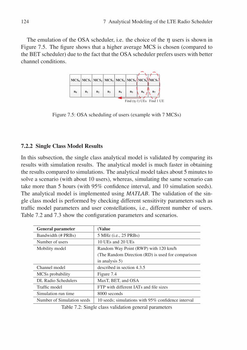
124 7 Analytical Modeling of the LTE Radio Scheduler
The emulation of the OSA scheduler, i.e. the choice of the η users is shown inFigure 7.5. The figure shows that a higher average MCS is chosen (compared tothe BET scheduler) due to the fact that the OSA scheduler prefers users with betterchannel conditions.
MCS0 MCS1 MCS2 MCS3
n0 n1 n2 n3
Find (η-1) UEs
MCS4 MCS5 MCS6 MCS7
n4 n5 n6 n7
M
Find 1 UE
Figure 7.5: OSA scheduling of users (example with 7 MCSs)
7.2.2 Single Class Model Results
In this subsection, the single class analytical model is validated by comparing itsresults with simulation results. The analytical model is much faster in obtainingthe results compared to simulations. The analytical model takes about 5 minutes tosolve a scenario (with about 10 users), whereas, simulating the same scenario cantake more than 5 hours (with 95% confidence interval, and 10 simulation seeds).The analytical model is implemented using MATLAB. The validation of the sin-gle class model is performed by checking different sensitivity parameters such astraffic model parameters and user constellations, i.e., different number of users.Table 7.2 and 7.3 show the configuration parameters and scenarios.
General parameter (ValueBandwidth (# PRBs) 5 MHz (i.e., 25 PRBs)Number of users 10 UEs and 20 UEsMobility model Random Way Point (RWP) with 120 km/h
(The Random Direction (RD) is used for comparisonin analysis 5)
Channel model described in section 4.3.5MCSs probability Figure 7.4DL Radio Schedulers MaxT, BET, and OSATraffic model FTP with different IATs and file sizesSimulation run time 8000 secondsNumber of Simulation seeds 10 seeds; simulations with 95% confidence interval
Table 7.2: Single class validation general parameters

7.2 LTE Downlink Scheduler Modeling 125
Analysis TDS (# of UEs) FTP file size FTP IAT
Analysis1 MaxT 10 UEs and constant uniform (0, 30) seconds,20 UEs 5 MByte, uniform (15, 45) seconds,
10 MByte, and uniform (30, 60) seconds, and20 MByte uniform (45, 75) seconds
Analysis2 BET 10 UEs and constant uniform (0, 30) seconds,20 UEs 5 MByte, uniform (15, 45) seconds,
10 MByte, and uniform (30, 60) seconds, and20 MByte uniform (45, 75) seconds
Analysis3 MaxT 10 UEs negative neg. exp. (15) seconds,exponential neg. exp. (30) seconds,5 MByte neg. exp. (45) seconds, and
neg. exp. (60) secondsAnalysis4 OSA 10 UEs constant uniform (0, 30) seconds,
5 MByte, uniform (15, 45) seconds,10 MByte, and uniform (30, 60) seconds, and20 MByte uniform (45, 75) seconds
Analysis5 BET 10 UEs constant uniform (0, 30) seconds,(RD) 5 MByte, uniform (15, 45) seconds,
10 MByte, and uniform (30, 60) seconds, and20 MByte uniform (45, 75) seconds
Table 7.3: Single class validation scenarios
7.2.2.1 Analysis 1 - MaxT
In this section, the MaxT scheduler analytical model results are compared againstthe simulation ones. The analytical model is investigated under different sensi-tivity analyses. First of all, the MaxT model is validated against changing thetotal number of users, mainly two cases: 10 and 20 users. Then within each ofthese two cases, different FTP traffic model parameters are used. At the begin-ning the FTP file size is changed from a small file size (5MByte), over a mediumfile size (10MByte) to a larger file size (20 MByte). Each of these FTP file sizesare combined with different file inter-arrival times that are uniformly distributedwith mean: 15, 30, 45, and 60 seconds. The is done to check the analytical modelsensitivity against different traffic loads, where a mean of 15 seconds inter-arrivaltime represents a highly loaded situation when compared to a scenario with a 60seconds mean file inter-arrival time.
Figure 7.6 shows the average file download time results comparison betweenthe analytical model and simulations for the 10 UEs scenarios. The solid lines

126 7 Analytical Modeling of the LTE Radio Scheduler
represents the analytical results and the dotted line represents the simulation results(Table A.2 shows the confidence interval of the simulation results). The resultsshow three different curves representing the three different FTP file sizes (5MB,10MB, and 15MB). The x-axis represents the different traffic loads, or in otherwords the different FTP file inter-arrival rates (15, 30, 45, and 60 seconds).
�� �� �� ���
��
��
��
�
���
���
-�+��.����"��.+����-!��� �)�
���������+����� �)�
/�0��!"���#��$�%����������+��������1 � )�������
�/2� �����+����/2�����*+�)����/2� �����+�����/2�����*+�)����/2� �����+�����/2�����*+�)��
Figure 7.6: MaxT 10UEs scenario - average FTP download time
The results show that the analytical model results match the simulation results.The results prove that the MaxT analytical model is not sensitive against differ-ent traffic loads, i.e., different combinations of file sizes and IATs. Figure 7.7shows the result comparison with the 20 users scenario. The analytical model stillachieves accurate results compared to the simulation (Table A.3 shows the confi-dence interval of the simulation results) following the same results trend. However,it can be seen that when the traffic model goes to a larger FTP file sizes, a small gapbetween the analytical and simulation results starts appearing. The reason behindthis gap is the fact that the system is highly loaded in these scenarios due to thehigh number of users (20UEs) and the large file size (15MByte), and as a result thenumber of samples in the FTP average file download time becomes smaller (fixed8000 seconds simulation duration) because it takes much larger download time tofinish a 15MByte file than the 5MByte case.
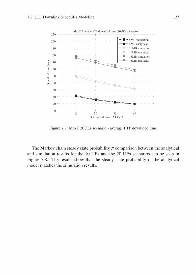
7.2 LTE Downlink Scheduler Modeling 127
�� �� �� ���
��
��
��
�
���
���
���
���
��
���
���
-�+��.����"��.+����-!��� �)�
���������+����� �)�
/�0��!"���#��$�%����������+��������1 � )�������
�/2� �����+����/2�����*+�)����/2� �����+�����/2�����*+�)����/2� �����+�����/2�����*+�)��
Figure 7.7: MaxT 20UEs scenario - average FTP download time
The Markov chain steady state probability π comparison between the analyticaland simulation results for the 10 UEs and the 20 UEs scenarios can be seen inFigure 7.8. The results show that the steady state probability of the analyticalmodel matches the simulation results.

128 7 Analytical Modeling of the LTE Radio Scheduler
0 1 2 3 4 5 6 7 8 9 10 110
0.1
0.2
0.3
0.4
0.5
Number of active users per TTI
Prob
abili
ty
MaxT Markov Chain State Probability (10UEs 5MB scenario)
IAT 15sec simulationIAT 15sec analyticalIAT 30sec simulationIAT 30sec analyticalIAT 45sec simulationIAT 45sec analyticalIAT 60sec simulationIAT 60sec analytical
0 1 2 3 4 5 6 7 8 9 10 110
0.1
0.2
0.3
0.4
0.5
Number of active users per TTIPr
obab
ility
MaxT Markov Chain State Probability (10UEs 10MB scenario)
IAT 15sec simulationIAT 15sec analyticalIAT 30sec simulationIAT 30sec analyticalIAT 45sec simulationIAT 45sec analyticalIAT 60sec simulationIAT 60sec analytical
0 1 2 3 4 5 6 7 8 9 10 110
0.1
0.2
0.3
0.4
0.5
Number of active users per TTI
Prob
abili
ty
MaxT Markov Chain State Probability (10UEs 15MB scenario)
IAT 15sec simulationIAT 15sec analyticalIAT 30sec simulationIAT 30sec analyticalIAT 45sec simulationIAT 45sec analyticalIAT 60sec simulationIAT 60sec analytical
0 1 2 3 4 5 6 7 8 9 1011121314151617181920210
0.05
0.1
0.15
0.2
0.25
0.3
0.35
0.4
Number of active users per TTI
Prob
abili
ty
MaxT Markov Chain State Probability (20UEs 5MB scenario)
IAT 15sec simulationIAT 15sec analyticalIAT 30sec simulationIAT 30sec analyticalIAT 45sec simulationIAT 45sec analyticalIAT 60sec simulationIAT 60sec analytical
0 1 2 3 4 5 6 7 8 9 1011121314151617181920210
0.1
0.2
0.3
0.4
0.5
Number of active users per TTI
Prob
abili
ty
MaxT Markov Chain State Probability (20UEs 10MB scenario)
IAT 15sec simulationIAT 15sec analyticalIAT 30sec simulationIAT 30sec analyticalIAT 45sec simulationIAT 45sec analyticalIAT 60sec simulationIAT 60sec analytical
0 1 2 3 4 5 6 7 8 9 1011121314151617181920210
0.05
0.1
0.15
0.2
0.25
0.3
0.35
0.4
Number of active users per TTI
Prob
abili
ty
MaxT Markov Chain State Probability (20UEs 15MB scenario)
IAT 15sec simulationIAT 15sec analyticalIAT 30sec simulationIAT 30sec analyticalIAT 45sec simulationIAT 45sec analyticalIAT 60sec simulationIAT 60sec analytical
Figure 7.8: MaxT Markov chain state probability
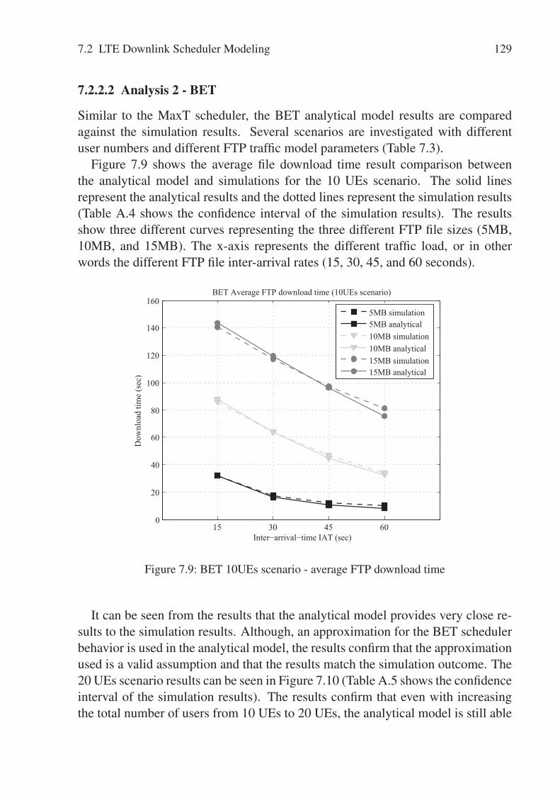
7.2 LTE Downlink Scheduler Modeling 129
7.2.2.2 Analysis 2 - BET
Similar to the MaxT scheduler, the BET analytical model results are comparedagainst the simulation results. Several scenarios are investigated with differentuser numbers and different FTP traffic model parameters (Table 7.3).
Figure 7.9 shows the average file download time result comparison betweenthe analytical model and simulations for the 10 UEs scenario. The solid linesrepresent the analytical results and the dotted lines represent the simulation results(Table A.4 shows the confidence interval of the simulation results). The resultsshow three different curves representing the three different FTP file sizes (5MB,10MB, and 15MB). The x-axis represents the different traffic load, or in otherwords the different FTP file inter-arrival rates (15, 30, 45, and 60 seconds).
�� �� �� ���
��
��
��
�
���
���
���
���
-�+��.����"��.+����-!��� �)�
���������+����� �)�
21��!"���#��$�%����������+��������1 � )�������
�/2� �����+����/2�����*+�)����/2� �����+�����/2�����*+�)����/2� �����+�����/2�����*+�)��
Figure 7.9: BET 10UEs scenario - average FTP download time
It can be seen from the results that the analytical model provides very close re-sults to the simulation results. Although, an approximation for the BET schedulerbehavior is used in the analytical model, the results confirm that the approximationused is a valid assumption and that the results match the simulation outcome. The20 UEs scenario results can be seen in Figure 7.10 (Table A.5 shows the confidenceinterval of the simulation results). The results confirm that even with increasingthe total number of users from 10 UEs to 20 UEs, the analytical model is still able
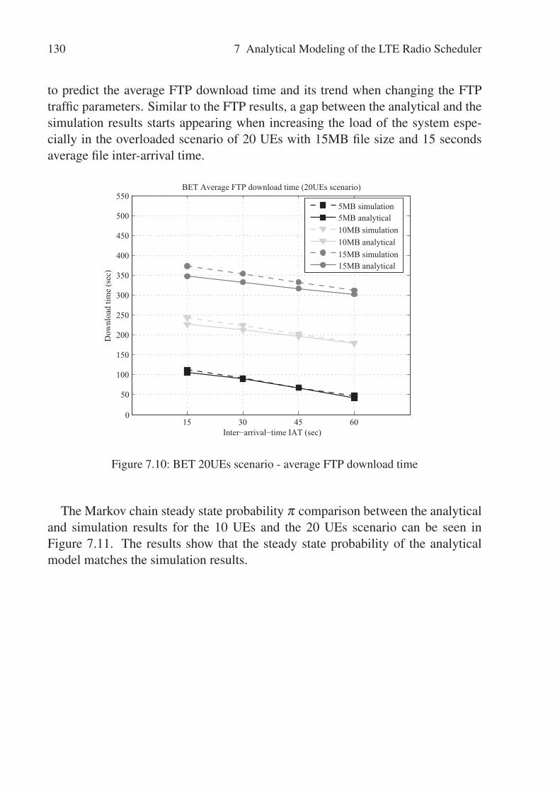
130 7 Analytical Modeling of the LTE Radio Scheduler
to predict the average FTP download time and its trend when changing the FTPtraffic parameters. Similar to the FTP results, a gap between the analytical and thesimulation results starts appearing when increasing the load of the system espe-cially in the overloaded scenario of 20 UEs with 15MB file size and 15 secondsaverage file inter-arrival time.
�� �� �� ���
��
���
���
���
���
���
���
���
���
���
���
-�+��.����"��.+����-!��� �)�
���������+����� �)�
21��!"���#��$�%����������+��������1 � )�������
�/2� �����+����/2�����*+�)����/2� �����+�����/2�����*+�)����/2� �����+�����/2�����*+�)��
Figure 7.10: BET 20UEs scenario - average FTP download time
The Markov chain steady state probability π comparison between the analyticaland simulation results for the 10 UEs and the 20 UEs scenario can be seen inFigure 7.11. The results show that the steady state probability of the analyticalmodel matches the simulation results.

7.2 LTE Downlink Scheduler Modeling 131
0 1 2 3 4 5 6 7 8 9 10 110
0.1
0.2
0.3
0.4
0.5
Number of active users per TTI
Prob
abili
ty
BET Markov Chain State Probability (10UEs 5MB scenario)
IAT 15sec simulationIAT 15sec analyticalIAT 30sec simulationIAT 30sec analyticalIAT 45sec simulationIAT 45sec analyticalIAT 60sec simulationIAT 60sec analytical
0 1 2 3 4 5 6 7 8 9 10 110
0.1
0.2
0.3
0.4
0.5
Number of active users per TTI
Prob
abili
ty
BET Markov Chain State Probability (10UEs 10MB scenario)
IAT 15sec simulationIAT 15sec analyticalIAT 30sec simulationIAT 30sec analyticalIAT 45sec simulationIAT 45sec analyticalIAT 60sec simulationIAT 60sec analytical
0 1 2 3 4 5 6 7 8 9 10 110
0.1
0.2
0.3
0.4
0.5
Number of active users per TTI
Prob
abili
ty
BET Markov Chain State Probability (10UEs 15MB scenario)
IAT 15sec simulationIAT 15sec analyticalIAT 30sec simulationIAT 30sec analyticalIAT 45sec simulationIAT 45sec analyticalIAT 60sec simulationIAT 60sec analytical
0 1 2 3 4 5 6 7 8 9 1011121314151617181920210
0.05
0.1
0.15
0.2
0.25
Number of active users per TTI
Prob
abili
tyBET Markov Chain State Probability (20UEs 5MB scenario)
IAT 15sec simulationIAT 15sec analyticalIAT 30sec simulationIAT 30sec analyticalIAT 45sec simulationIAT 45sec analyticalIAT 60sec simulationIAT 60sec analytical
0 1 2 3 4 5 6 7 8 9 1011121314151617181920210
0.1
0.2
0.3
0.4
0.5
Number of active users per TTI
Prob
abili
ty
BET Markov Chain State Probability (20UEs 10MB scenario)
IAT 15sec simulationIAT 15sec analyticalIAT 30sec simulationIAT 30sec analyticalIAT 45sec simulationIAT 45sec analyticalIAT 60sec simulationIAT 60sec analytical
0 1 2 3 4 5 6 7 8 9 1011121314151617181920210
0.1
0.2
0.3
0.4
0.5
0.6
Number of active users per TTI
Prob
abili
ty
BET Markov Chain State Probability (20UEs 15MB scenario)
IAT 15sec simulationIAT 15sec analyticalIAT 30sec simulationIAT 30sec analyticalIAT 45sec simulationIAT 45sec analyticalIAT 60sec simulationIAT 60sec analytical
Figure 7.11: BET Markov chain state probability

132 7 Analytical Modeling of the LTE Radio Scheduler
7.2.2.3 Analysis 3 - Sensitivity Analysis
The intention of this scenario is to investigate the model sensitivity against usingother distributions for the traffic model parameters. Instead of using a constantfile size as in the previous two analyses, in this analysis, a negative exponentialdistribution is used for generating the file size, which is combined with severalnegative exponentially distributed inter-arrival times. Figure 7.12 shows the resultsof analysis 3 (Table A.6 shows the confidence interval of the simulation results).The left side figure, shows the average file download time. It can be seen, thatalthough negative exponential distributions were used to generate the file size andthe inter-arrival time, the model is quite insensitive to the change, and the resultsstill match the results obtained from simulations.
�� �� �� ��
��
��
��
��
�
��
��
-�+��.����"��.+����-!��� �)�
���������+����� �)�
!"���#��$�%����������+����� �� �+�"�+*�����* � � )�������
�/2� �����+����/2�����*+�)��
0 1 2 3 4 5 6 7 8 9 10 110
0.1
0.2
0.3
0.4
0.5
0.6
Number of active users per TTI
Prob
abili
ty
MaxT Markov Chain State Probability (sensitivity analysis scenario)
IAT 15sec simulationIAT 15sec analyticalIAT 30sec simulationIAT 30sec analyticalIAT 45sec simulationIAT 45sec analyticalIAT 60sec simulationIAT 60sec analytical
Figure 7.12: MaxT sensitivity analysis results
The Markov chain steady state probability π results can be seen in right side ofFigure 7.12. The results show, that the steady state probability of the analyticalmodel matches the simulations results. Similar conclusions regarding the modelinsensitivity were also described in [DBMC10]. There, it was shown that: theaverage performance parameters are insensitive to the distribution of ON and OFFperiods.

7.2 LTE Downlink Scheduler Modeling 133
7.2.2.4 Analysis 4 - OSA
The OSA analytical model results are compared against the simulation results.Several scenarios are investigated with different total number of users and differentFTP traffic model parameters (Table 7.3).
Figure 7.13 shows the average file download time results comparison betweenthe analytical model and simulations for the 10 UEs scenario. The solid linesrepresent the analytical results and the dotted lines represent the simulation results(Table A.7 shows the confidence interval of the simulation results). The resultsshow three different curves representing the three different FTP file sizes (5MB,10MB, and 15MB). The x-axis represents the different traffic load, or in otherwords the different FTP file inter-arrival rates (15, 30, 45, and 60 seconds).
�� �� �� ���
��
��
��
�
���
���
���
-�+��.����"��.+����-!��� �)�
���������+����� �)�
3!�!"���#��$�%����������+��������1 � )�������
�/2� �����+����/2�����*+�)����/2� �����+�����/2�����*+�)����/2� �����+�����/2�����*+�)��
Figure 7.13: OSA 10UEs scenario - average FTP download time
It can be seen from the results that the analytical model provides very close re-sults to the simulation results. Although, an approximation for the OSA schedulerbehavior is used in the analytical model, the results confirm that the approximationused is a valid assumption and that the results match the simulation outcome.
The Markov chain steady state probability π comparison between the analyticaland simulation results for the 10 UEs scenario can be seen in Figure 7.14. The
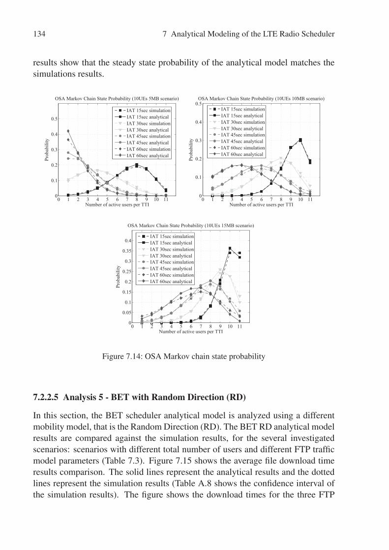
134 7 Analytical Modeling of the LTE Radio Scheduler
results show that the steady state probability of the analytical model matches thesimulations results.
0 1 2 3 4 5 6 7 8 9 10 110
0.1
0.2
0.3
0.4
0.5
Number of active users per TTI
Prob
abili
ty
OSA Markov Chain State Probability (10UEs 5MB scenario)
IAT 15sec simulationIAT 15sec analyticalIAT 30sec simulationIAT 30sec analyticalIAT 45sec simulationIAT 45sec analyticalIAT 60sec simulationIAT 60sec analytical
0 1 2 3 4 5 6 7 8 9 10 110
0.1
0.2
0.3
0.4
0.5
Number of active users per TTI
Prob
abili
ty
OSA Markov Chain State Probability (10UEs 10MB scenario)
IAT 15sec simulationIAT 15sec analyticalIAT 30sec simulationIAT 30sec analyticalIAT 45sec simulationIAT 45sec analyticalIAT 60sec simulationIAT 60sec analytical
0 1 2 3 4 5 6 7 8 9 10 110
0.05
0.1
0.15
0.2
0.25
0.3
0.35
0.4
Number of active users per TTI
Prob
abili
ty
OSA Markov Chain State Probability (10UEs 15MB scenario)
IAT 15sec simulationIAT 15sec analyticalIAT 30sec simulationIAT 30sec analyticalIAT 45sec simulationIAT 45sec analyticalIAT 60sec simulationIAT 60sec analytical
Figure 7.14: OSA Markov chain state probability
7.2.2.5 Analysis 5 - BET with Random Direction (RD)
In this section, the BET scheduler analytical model is analyzed using a differentmobility model, that is the Random Direction (RD). The BET RD analytical modelresults are compared against the simulation results, for the several investigatedscenarios: scenarios with different total number of users and different FTP trafficmodel parameters (Table 7.3). Figure 7.15 shows the average file download timeresults comparison. The solid lines represent the analytical results and the dottedlines represent the simulation results (Table A.8 shows the confidence interval ofthe simulation results). The figure shows the download times for the three FTP

7.2 LTE Downlink Scheduler Modeling 135
file sizes (5MB, 10MB, and 15MB) in combination with the different FTP fileinter-arrival rates (15, 30, 45, and 60 seconds).
�� �� �� ���
��
��
��
�
���
���
���
���
��
���
���
-�+��.����"��.+����-!��� �)�
���������+����� �)�
21��!"���#��$�%����������+��������1 �&�� )�������
�/2� �����+����/2�����*+�)����/2� �����+�����/2�����*+�)����/2� �����+�����/2�����*+�)��
Figure 7.15: BET RD 10UEs scenario - average FTP download time
The results show that the FTP download times are increased compared to anal-ysis 2 (Figure 7.9), this is because in analysis 2 the RWP mobility model is used,which tends to distribute the users density around the center of the eNodeB, whichincreases the probability of having a good channel condition. Thus, the users willhave better channel conditions and a higher spectral efficiency which explains thefaster FTP file downloads. In analysis 5, the RD mobility model uniformly dis-tributes the users density within the cell, which increases the probability of beingin a bad channel condition (see Figure 7.4), thus the spectral efficiency is reducedwhich will lead to slower FTP file downloads.
Nevertheless, the results show that the BET analytical model provides closeresults to the simulation results, in spite of changing the mobility model in thisanalysis.
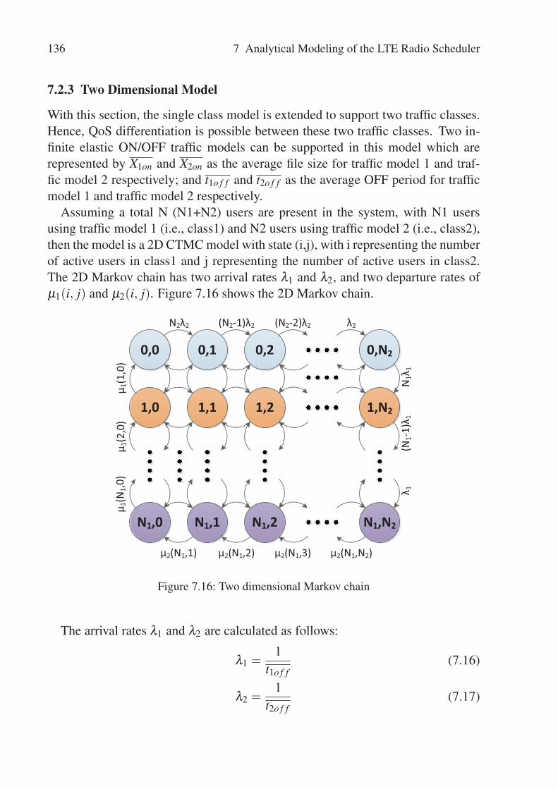
136 7 Analytical Modeling of the LTE Radio Scheduler
7.2.3 Two Dimensional Model
With this section, the single class model is extended to support two traffic classes.Hence, QoS differentiation is possible between these two traffic classes. Two in-finite elastic ON/OFF traffic models can be supported in this model which arerepresented by X1on and X2on as the average file size for traffic model 1 and traf-fic model 2 respectively; and t1o f f and t2o f f as the average OFF period for trafficmodel 1 and traffic model 2 respectively.
Assuming a total N (N1+N2) users are present in the system, with N1 usersusing traffic model 1 (i.e., class1) and N2 users using traffic model 2 (i.e., class2),then the model is a 2D CTMC model with state (i,j), with i representing the numberof active users in class1 and j representing the number of active users in class2.The 2D Markov chain has two arrival rates λ1 and λ2, and two departure rates ofμ1(i, j) and μ2(i, j). Figure 7.16 shows the 2D Markov chain.
0,1
1,1
0,0
1,0
0,2
1,2
0,N2
1,N2
N1,1N1,0 N1,2 N1,N2
N2λ2 (N2-1)λ2 (N2-2)λ2 λ2
μ2(N1,1) μ2(N1,2) μ2(N1,3) μ2(N1,N2)
N1λ
1λ 1
(N1-
1)λ 1
μ 1(1
,0)
μ 1(2
,0)
μ 1(N
1,0)
Figure 7.16: Two dimensional Markov chain
The arrival rates λ1 and λ2 are calculated as follows:
λ1 =1
t1o f f(7.16)
λ2 =1
t2o f f(7.17)

7.2 LTE Downlink Scheduler Modeling 137
The 2D Markov chain departure rates (μ1(i, j) and μ2(i, j)) depend on the TDscheduler type, and are calculated as follows:
μ1(i, j) =T BS1(i, j)X1on ·T T I
(7.18)
μ2(i, j) =T BS2(i, j)X2on ·T T I
(7.19)
where, T BS1(i, j) represents the average data sent for all served users in class1under the Markov chain (i,j), i.e., when the number of users of class1 are i and jin class2. T BS2(i, j) is the average data sent for all served users in class2 in state(i,j). T BS1(i, j) and T BS2(i, j) are calculated as follows:
T BS1(i, j) =(i,...,i, j,..., j)
∑(i0,...,iK , j0,..., jK)=(0,...,0)|
i0+...+iK=ij0+...+ jK= j
i0 �=i with j0 �= j
i! j!T BS1(i0, ..., iK , j0, ..., jK)
[K
∏k=0
Pikk P jk
kik! jk!
]
(7.20)
T BS2(i, j) =(i,...,i, j,..., j)
∑(i0,...,iK , j0,..., jK)=(0,...,0)|
i0+...+iK=ij0+...+ jK= j
i0 �=i with j0 �= j
i! j!T BS2(i0, ..., iK , j0, ..., jK)
[K
∏k=0
Pikk P jk
kik! jk!
]
(7.21)
where, T BS1(i0, ..., iK , j0, ..., jK) is the total data sent of the served class1 usersunder the specific combination (i0, ..., iK , j0, ..., jK). Where, K is the total numberof MCSs used. Equation 7.20, shows that the combinations space is now doubled((i0, ..., iK , j0, ..., jK)) compared to the single class model. This is because, all thepossible combinations, where the users of class1 can be in the MCSs vector incombination with the second class, have to be covered. T BS1(i0, ..., iK , j0, ..., jK)is calculated as follows:
T BS1(i0, ..., iK , j0, ..., jK) = ∑r=[r1,...,rδ1]
T BSr(η) (7.22)
where, r is a vector representing the indices of the served users in class1 withrδ1 being the number of users served in class1. T BS2(i0, ..., iK , j0, ..., jK) can becalculated similarly to T BS1(i0, ..., iK , j0, ..., jK). The total number of served usersper TTI (i.e., η) is the sum of the served users in the two classes: η = rδ1 + rδ2.
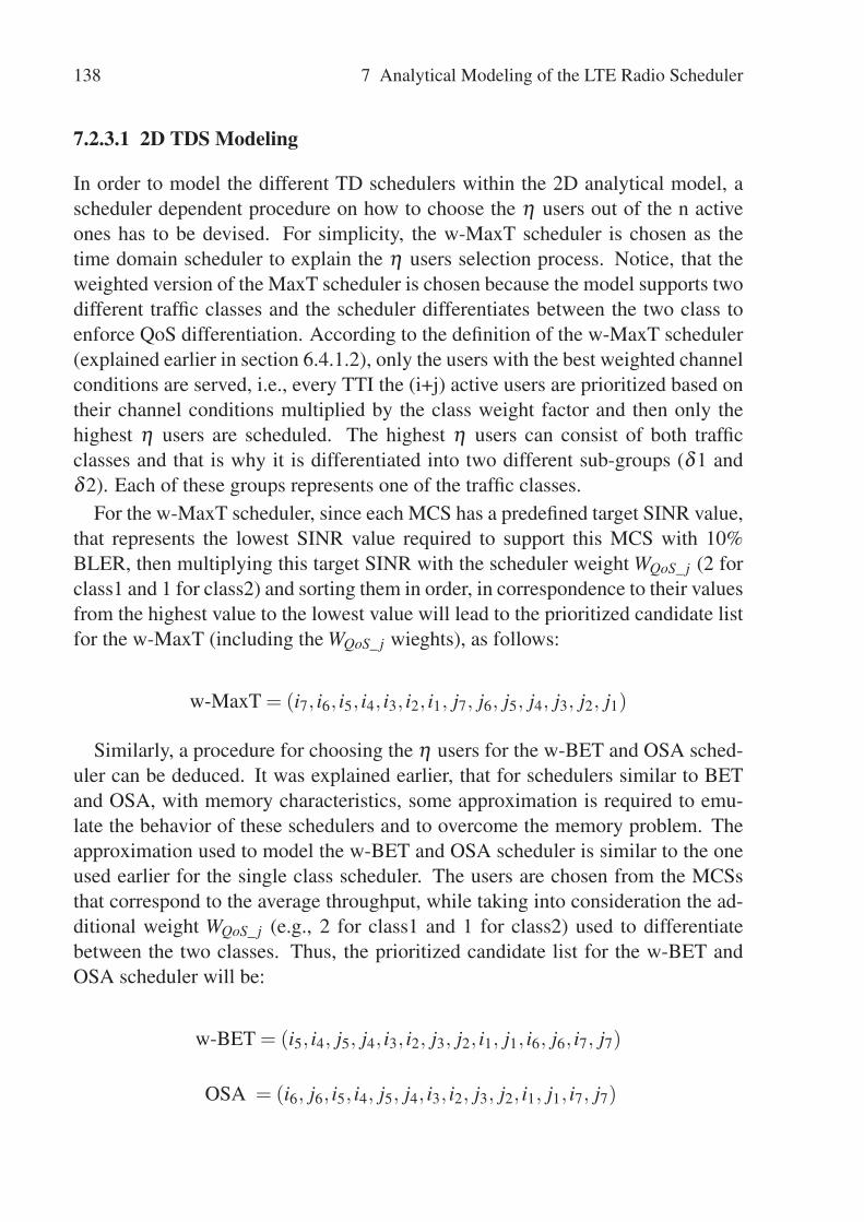
138 7 Analytical Modeling of the LTE Radio Scheduler
7.2.3.1 2D TDS Modeling
In order to model the different TD schedulers within the 2D analytical model, ascheduler dependent procedure on how to choose the η users out of the n activeones has to be devised. For simplicity, the w-MaxT scheduler is chosen as thetime domain scheduler to explain the η users selection process. Notice, that theweighted version of the MaxT scheduler is chosen because the model supports twodifferent traffic classes and the scheduler differentiates between the two class toenforce QoS differentiation. According to the definition of the w-MaxT scheduler(explained earlier in section 6.4.1.2), only the users with the best weighted channelconditions are served, i.e., every TTI the (i+j) active users are prioritized based ontheir channel conditions multiplied by the class weight factor and then only thehighest η users are scheduled. The highest η users can consist of both trafficclasses and that is why it is differentiated into two different sub-groups (δ1 andδ2). Each of these groups represents one of the traffic classes.
For the w-MaxT scheduler, since each MCS has a predefined target SINR value,that represents the lowest SINR value required to support this MCS with 10%BLER, then multiplying this target SINR with the scheduler weight WQoS_ j (2 forclass1 and 1 for class2) and sorting them in order, in correspondence to their valuesfrom the highest value to the lowest value will lead to the prioritized candidate listfor the w-MaxT (including the WQoS_ j wieghts), as follows:
w-MaxT = (i7, i6, i5, i4, i3, i2, i1, j7, j6, j5, j4, j3, j2, j1)
Similarly, a procedure for choosing the η users for the w-BET and OSA sched-uler can be deduced. It was explained earlier, that for schedulers similar to BETand OSA, with memory characteristics, some approximation is required to emu-late the behavior of these schedulers and to overcome the memory problem. Theapproximation used to model the w-BET and OSA scheduler is similar to the oneused earlier for the single class scheduler. The users are chosen from the MCSsthat correspond to the average throughput, while taking into consideration the ad-ditional weight WQoS_ j (e.g., 2 for class1 and 1 for class2) used to differentiatebetween the two classes. Thus, the prioritized candidate list for the w-BET andOSA scheduler will be:
w-BET = (i5, i4, j5, j4, i3, i2, j3, j2, i1, j1, i6, j6, i7, j7)
OSA = (i6, j6, i5, i4, j5, j4, i3, i2, j3, j2, i1, j1, i7, j7)
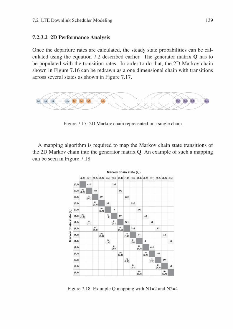
7.2 LTE Downlink Scheduler Modeling 139
7.2.3.2 2D Performance Analysis
Once the departure rates are calculated, the steady state probabilities can be cal-culated using the equation 7.2 described earlier. The generator matrix Q has tobe populated with the transition rates. In order to do that, the 2D Markov chainshown in Figure 7.16 can be redrawn as a one dimensional chain with transitionsacross several states as shown in Figure 7.17.
N1,1N1,0 N1,2 N1,N20,1 1,10,0 1,00,2 1,20,N2 1,N2
Figure 7.17: 2D Markov chain represented in a single chain
A mapping algorithm is required to map the Markov chain state transitions ofthe 2D Markov chain into the generator matrix Q. An example of such a mappingcan be seen in Figure 7.18.
(0,0) (0,1) (0,2) (0,3) (0,4)
(0,0)
(1,0) (1,1) (1,2) (1,3) (1,4) (2,0) (2,1) (2,2) (2,3) (2,4)
(0,1)
(0,2)
(0,3)
(0,4)
(1,0)
(1,1)
(1,2)
(1,3)
(1,4)
(2,0)
(2,1)
(2,2)
(2,3)
(2,4)
4λ1 2λ2
μ1(0,1) 3λ1 2λ2
μ1(0,2) 2λ1 2λ2
μ1(0,3) λ1 2λ2
μ1(0,4) 0 2λ2
μ2(1,0)
μ1(1,0) 4λ1 λ2
μ2(1,1)
μ1(1,1) 3λ1 λ2
μ2(1,2)
μ1(1,2) 2λ1 λ2
μ2(1,3)
μ1(1,3) λ1 λ2
μ2(1,4)
μ1(1,4) 0 λ2
μ2(2,0)
μ1(2,0) 4λ1
μ2(2,1)
μ1(2,1) 3λ1
μ2(2,2)
μ1(2,2) 2λ1
μ2(2,3)
μ1(2,3) λ1
μ2(2,4)
μ1(2,4)
Markov chain state (i,j)
Mar
kov
chai
nst
ate
(i,j)
Figure 7.18: Example Q mapping with N1=2 and N2=4

140 7 Analytical Modeling of the LTE Radio Scheduler
The diagonal cells in the Q matrix (highlighted with gray in Figure 7.18) is thestate self transition. According to [Kle76], the sum of the transition rates of eachstate should equal to zero, so as to create equilibrium. Thus, the value of the darkboxes is equal to:
Q(i, i) =− ∑all j |j �=i
Q(i, j) (7.23)
Once the Markov chain steady state probabilities have been calculated, the 2Dmodel performance analysis can be evaluated. This is done in a way similar to thesingle class model (see section 7.1.1). First of all, the average number of activeusers in the system for each class Q1 and Q2 is calculated. As Q1 and Q2 are themean number of users and π(i, j) is the probability of every state, i.e. probabilityof having i active users in class1 and j active users in class2, then the averagenumber of active users per class is:
Q1 =N1
∑i=0
N2
∑j=0
iπ(i, j) (7.24)
Q2 =N1
∑i=0
N2
∑j=0
jπ(i, j) (7.25)
Next, the mean number of departures by unit time D1 and D2 are calculated asfollows:
D1 =N1
∑i=0
N2
∑j=0
μ1(i, j)π(i, j) (7.26)
D2 =N1
∑i=0
N2
∑j=0
μ2(i, j)π(i, j) (7.27)
And finally, according to Little’s law [Ste11], the average ON duration, i.e. theaverage file download time per class is:
t1on =Q1D1
(7.28)
t2on =Q2D2
(7.29)
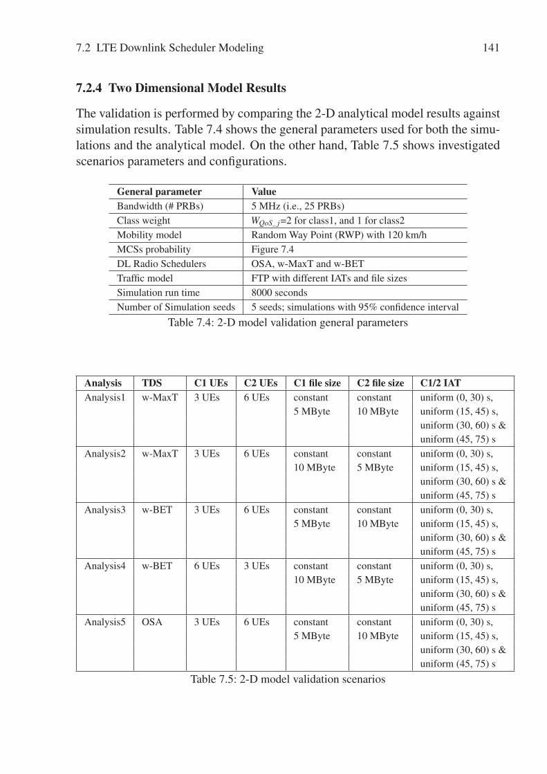
7.2 LTE Downlink Scheduler Modeling 141
7.2.4 Two Dimensional Model Results
The validation is performed by comparing the 2-D analytical model results againstsimulation results. Table 7.4 shows the general parameters used for both the simu-lations and the analytical model. On the other hand, Table 7.5 shows investigatedscenarios parameters and configurations.
General parameter ValueBandwidth (# PRBs) 5 MHz (i.e., 25 PRBs)Class weight WQoS_ j=2 for class1, and 1 for class2Mobility model Random Way Point (RWP) with 120 km/hMCSs probability Figure 7.4DL Radio Schedulers OSA, w-MaxT and w-BETTraffic model FTP with different IATs and file sizesSimulation run time 8000 secondsNumber of Simulation seeds 5 seeds; simulations with 95% confidence interval
Table 7.4: 2-D model validation general parameters
Analysis TDS C1 UEs C2 UEs C1 file size C2 file size C1/2 IATAnalysis1 w-MaxT 3 UEs 6 UEs constant constant uniform (0, 30) s,
5 MByte 10 MByte uniform (15, 45) s,uniform (30, 60) s &uniform (45, 75) s
Analysis2 w-MaxT 3 UEs 6 UEs constant constant uniform (0, 30) s,10 MByte 5 MByte uniform (15, 45) s,
uniform (30, 60) s &uniform (45, 75) s
Analysis3 w-BET 3 UEs 6 UEs constant constant uniform (0, 30) s,5 MByte 10 MByte uniform (15, 45) s,
uniform (30, 60) s &uniform (45, 75) s
Analysis4 w-BET 6 UEs 3 UEs constant constant uniform (0, 30) s,10 MByte 5 MByte uniform (15, 45) s,
uniform (30, 60) s &uniform (45, 75) s
Analysis5 OSA 3 UEs 6 UEs constant constant uniform (0, 30) s,5 MByte 10 MByte uniform (15, 45) s,
uniform (30, 60) s &uniform (45, 75) s
Table 7.5: 2-D model validation scenarios

142 7 Analytical Modeling of the LTE Radio Scheduler
7.2.4.1 Analysis - w-MaxT
The two dimensional w-MaxT model is validated within this section. The w-MaxTmodel is tested with two different analysis scenarios, each with different traffic pa-rameters. In analysis1, the FTP file size of class1 users is chosen to be a constant 5MByte, whereas, the size of the class2 FTP traffic model is chosen to be a constant10 MByte. Each of these file sizes is paired with several uniformly distributed fileinter-arrival times, so as to emulate different traffic loads. In analysis2, the FTPfile sizes are switched between the traffic classes, where class1 users are config-ured to generate constant 10 MByte FTP files, and class2 users generate constant5 MByte FTP files. The average FTP file download times for both analysis1 andanalysis2 are shown in Figure 7.19 and Figure 7.20 respectively.
�� �� �� ���
��
��
��
��
��
��
-�+��.����"��.+����-!��� �)�
���������+����� �)�
�./�0��!"���#��$�%����������+���
)�� �� �����+���)�� ������*+�)��)�� �� �����+���)�� ������*+�)��
Figure 7.19: Analysis1 w-MaxT average FTP download time
The figures show that the w-MaxT model results match the simulation results(Table A.9 and Table A.10 show the confidence interval of the simulation resultsfor analysis1 and analysis2 respectively). The results also prove that the w-MaxTanalytical model is not sensitive against different traffic parameters, i.e., differentcombinations of file sizes and IATs.
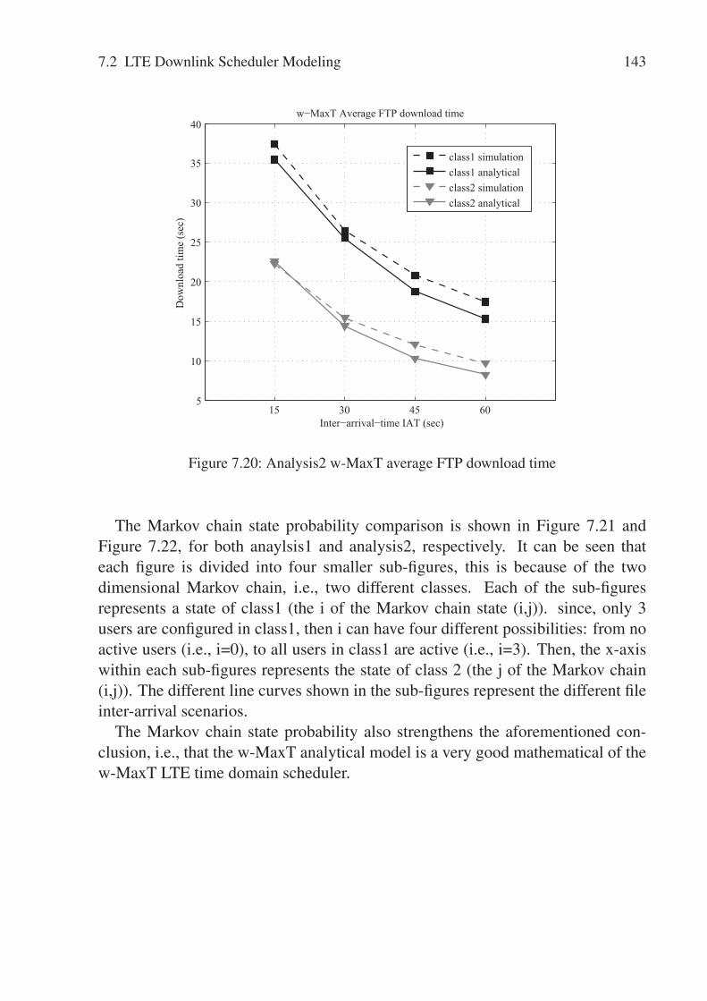
7.2 LTE Downlink Scheduler Modeling 143
�� �� �� ���
��
��
��
��
��
��
��
-�+��.����"��.+����-!��� �)�
���������+����� �)�
�./�0��!"���#��$�%����������+���
)�� �� �����+���)�� ������*+�)��)�� �� �����+���)�� ������*+�)��
Figure 7.20: Analysis2 w-MaxT average FTP download time
The Markov chain state probability comparison is shown in Figure 7.21 andFigure 7.22, for both anaylsis1 and analysis2, respectively. It can be seen thateach figure is divided into four smaller sub-figures, this is because of the twodimensional Markov chain, i.e., two different classes. Each of the sub-figuresrepresents a state of class1 (the i of the Markov chain state (i,j)). since, only 3users are configured in class1, then i can have four different possibilities: from noactive users (i.e., i=0), to all users in class1 are active (i.e., i=3). Then, the x-axiswithin each sub-figures represents the state of class 2 (the j of the Markov chain(i,j)). The different line curves shown in the sub-figures represent the different fileinter-arrival scenarios.
The Markov chain state probability also strengthens the aforementioned con-clusion, i.e., that the w-MaxT analytical model is a very good mathematical of thew-MaxT LTE time domain scheduler.
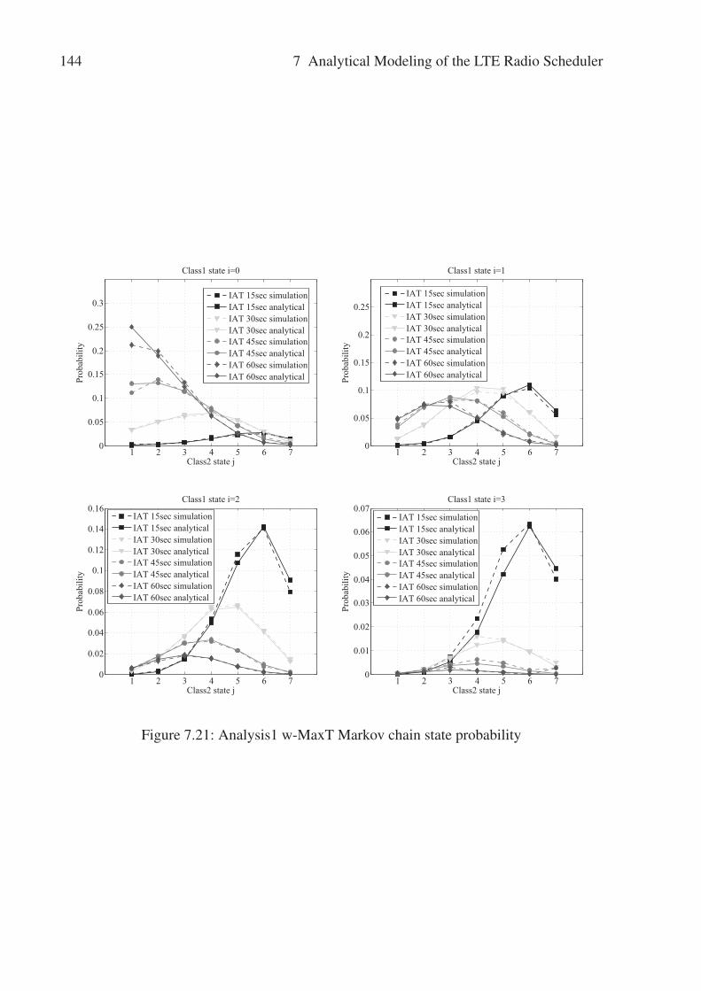
144 7 Analytical Modeling of the LTE Radio Scheduler
1 2 3 4 5 6 70
0.05
0.1
0.15
0.2
0.25
0.3
Class1 state i=0
Class2 state j
Prob
abili
ty
IAT 15sec simulationIAT 15sec analyticalIAT 30sec simulationIAT 30sec analyticalIAT 45sec simulationIAT 45sec analyticalIAT 60sec simulationIAT 60sec analytical
1 2 3 4 5 6 70
0.05
0.1
0.15
0.2
0.25
Class1 state i=1
Class2 state j
Prob
abili
ty
IAT 15sec simulationIAT 15sec analyticalIAT 30sec simulationIAT 30sec analyticalIAT 45sec simulationIAT 45sec analyticalIAT 60sec simulationIAT 60sec analytical
1 2 3 4 5 6 70
0.02
0.04
0.06
0.08
0.1
0.12
0.14
0.16Class1 state i=2
Class2 state j
Prob
abili
ty
IAT 15sec simulationIAT 15sec analyticalIAT 30sec simulationIAT 30sec analyticalIAT 45sec simulationIAT 45sec analyticalIAT 60sec simulationIAT 60sec analytical
1 2 3 4 5 6 70
0.01
0.02
0.03
0.04
0.05
0.06
0.07Class1 state i=3
Class2 state j
Prob
abili
ty
IAT 15sec simulationIAT 15sec analyticalIAT 30sec simulationIAT 30sec analyticalIAT 45sec simulationIAT 45sec analyticalIAT 60sec simulationIAT 60sec analytical
Figure 7.21: Analysis1 w-MaxT Markov chain state probability
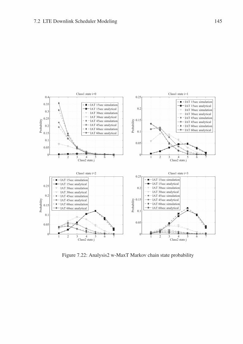
7.2 LTE Downlink Scheduler Modeling 145
1 2 3 4 5 6 70
0.05
0.1
0.15
0.2
0.25
0.3
0.35
0.4Class1 state i=0
Class2 state j
Prob
abili
ty
IAT 15sec simulationIAT 15sec analyticalIAT 30sec simulationIAT 30sec analyticalIAT 45sec simulationIAT 45sec analyticalIAT 60sec simulationIAT 60sec analytical
1 2 3 4 5 6 70
0.05
0.1
0.15
0.2
0.25Class1 state i=1
Class2 state j
Prob
abili
ty
IAT 15sec simulationIAT 15sec analyticalIAT 30sec simulationIAT 30sec analyticalIAT 45sec simulationIAT 45sec analyticalIAT 60sec simulationIAT 60sec analytical
1 2 3 4 5 6 70
0.05
0.1
0.15
0.2
0.25
Class1 state i=2
Class2 state j
Prob
abili
ty
IAT 15sec simulationIAT 15sec analyticalIAT 30sec simulationIAT 30sec analyticalIAT 45sec simulationIAT 45sec analyticalIAT 60sec simulationIAT 60sec analytical
1 2 3 4 5 6 70
0.05
0.1
0.15
0.2
0.25Class1 state i=3
Class2 state j
Prob
abili
ty
IAT 15sec simulationIAT 15sec analyticalIAT 30sec simulationIAT 30sec analyticalIAT 45sec simulationIAT 45sec analyticalIAT 60sec simulationIAT 60sec analytical
Figure 7.22: Analysis2 w-MaxT Markov chain state probability

146 7 Analytical Modeling of the LTE Radio Scheduler
7.2.4.2 Analysis - w-BET
The w-BET analytical model is validated against the simulation results in this sec-tion. The validation includes several scenarios with a sensitivity analysis of themodel parameters: against different traffic model parameters, e.g. FTP file size andFTP file inter-arrival time, and against different users constellations. The analysesare divided into two main categories as seen in Table 7.5: in analysis3, the numberof users in class1 and class2 is set to 3 and 6 respectively, whereas in analysis4,the number of users in each class are exchanged to be 6 users in class1 and 3 usersin class2. Each of these analysis categories contains several sub-scenarios, to testagainst several traffic loads.
Figure 7.23 shows the average FTP download time per class for both the ana-lytical model and the simulation model results (Table A.11 shows the confidenceinterval of the simulation results for analysis3).
�� �� �� ���
��
��
��
��
��
��
�
-�+��.����"��.+����-!��� �)�
���������+����� �)�
�.21��!"���#��$�%����������+���
)�� �� �����+���)�� ������*+�)��)�� �� �����+���)�� ������*+�)��
Figure 7.23: Analysis3 w-BET average FTP download time
The results show, that the analytical model results matches the simulation re-sults. When the inter-arrival time of the FTP traffic model is increased, a gapbetween the analytical and the simulations starts appearing. The reason behind thegap is that when the inter-arrival time between the files increases, the system willhave a lower traffic load and the overall number of FTP downloads decreases since
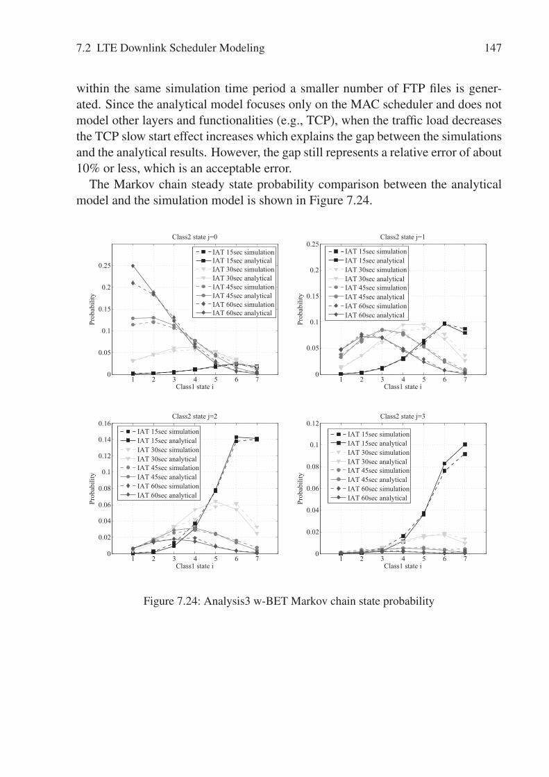
7.2 LTE Downlink Scheduler Modeling 147
within the same simulation time period a smaller number of FTP files is gener-ated. Since the analytical model focuses only on the MAC scheduler and does notmodel other layers and functionalities (e.g., TCP), when the traffic load decreasesthe TCP slow start effect increases which explains the gap between the simulationsand the analytical results. However, the gap still represents a relative error of about10% or less, which is an acceptable error.
The Markov chain steady state probability comparison between the analyticalmodel and the simulation model is shown in Figure 7.24.
1 2 3 4 5 6 70
0.05
0.1
0.15
0.2
0.25
Class2 state j=0
Class1 state i
Prob
abili
ty
IAT 15sec simulationIAT 15sec analyticalIAT 30sec simulationIAT 30sec analyticalIAT 45sec simulationIAT 45sec analyticalIAT 60sec simulationIAT 60sec analytical
1 2 3 4 5 6 70
0.05
0.1
0.15
0.2
0.25Class2 state j=1
Class1 state i
Prob
abili
ty
IAT 15sec simulationIAT 15sec analyticalIAT 30sec simulationIAT 30sec analyticalIAT 45sec simulationIAT 45sec analyticalIAT 60sec simulationIAT 60sec analytical
1 2 3 4 5 6 70
0.02
0.04
0.06
0.08
0.1
0.12
0.14
0.16Class2 state j=2
Class1 state i
Prob
abili
ty
IAT 15sec simulationIAT 15sec analyticalIAT 30sec simulationIAT 30sec analyticalIAT 45sec simulationIAT 45sec analyticalIAT 60sec simulationIAT 60sec analytical
1 2 3 4 5 6 70
0.02
0.04
0.06
0.08
0.1
0.12Class2 state j=3
Class1 state i
Prob
abili
ty
IAT 15sec simulationIAT 15sec analyticalIAT 30sec simulationIAT 30sec analyticalIAT 45sec simulationIAT 45sec analyticalIAT 60sec simulationIAT 60sec analytical
Figure 7.24: Analysis3 w-BET Markov chain state probability
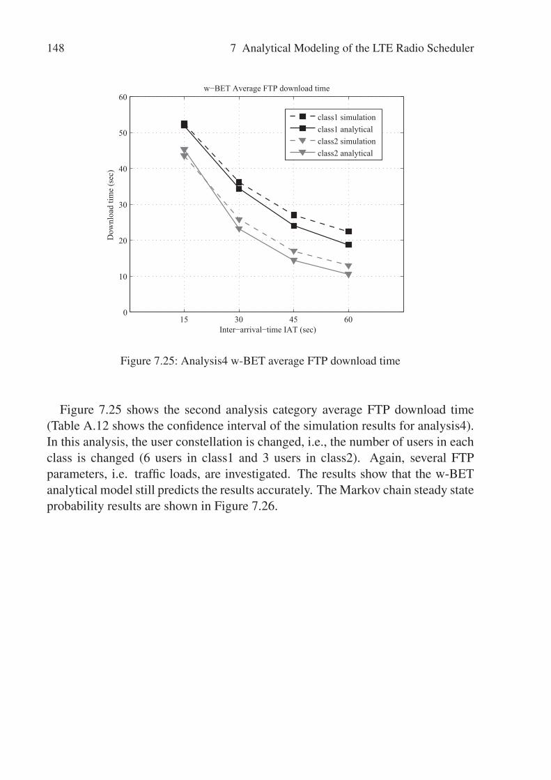
148 7 Analytical Modeling of the LTE Radio Scheduler
�� �� �� ���
��
��
��
��
��
��
-�+��.����"��.+����-!��� �)�
���������+����� �)�
�.21��!"���#��$�%����������+���
)�� �� �����+���)�� ������*+�)��)�� �� �����+���)�� ������*+�)��
Figure 7.25: Analysis4 w-BET average FTP download time
Figure 7.25 shows the second analysis category average FTP download time(Table A.12 shows the confidence interval of the simulation results for analysis4).In this analysis, the user constellation is changed, i.e., the number of users in eachclass is changed (6 users in class1 and 3 users in class2). Again, several FTPparameters, i.e. traffic loads, are investigated. The results show that the w-BETanalytical model still predicts the results accurately. The Markov chain steady stateprobability results are shown in Figure 7.26.

7.2 LTE Downlink Scheduler Modeling 149
1 2 3 4 5 6 70
0.1
0.2
0.3
0.4
0.5
Class2 state j=0
Class1 state i
Prob
abili
ty
IAT 15sec simulationIAT 15sec analyticalIAT 30sec simulationIAT 30sec analyticalIAT 45sec simulationIAT 45sec analyticalIAT 60sec simulationIAT 60sec analytical
1 2 3 4 5 6 70
0.05
0.1
0.15
0.2
0.25Class2 state j=1
Class1 state i
Prob
abili
ty
IAT 15sec simulationIAT 15sec analyticalIAT 30sec simulationIAT 30sec analyticalIAT 45sec simulationIAT 45sec analyticalIAT 60sec simulationIAT 60sec analytical
1 2 3 4 5 6 70
0.05
0.1
0.15
0.2
0.25
Class2 state j=2
Class1 state i
Prob
abili
ty
IAT 15sec simulationIAT 15sec analyticalIAT 30sec simulationIAT 30sec analyticalIAT 45sec simulationIAT 45sec analyticalIAT 60sec simulationIAT 60sec analytical
1 2 3 4 5 6 70
0.1
0.2
0.3
0.4
0.5Class2 state j=3
Class1 state i
Prob
abili
ty
IAT 15sec simulationIAT 15sec analyticalIAT 30sec simulationIAT 30sec analyticalIAT 45sec simulationIAT 45sec analyticalIAT 60sec simulationIAT 60sec analytical
Figure 7.26: Analysis4 w-BET Markov chain state probability

150 7 Analytical Modeling of the LTE Radio Scheduler
7.2.4.3 Analysis - OSA
The OSA analytical model is validated against the simulation results in this sec-tion. The validation is done against simulations with different FTP file inter-arrivaltimes. The scenario is configured with three users in class1 and six users in class2.Each of these categories contains several sub-scenarios to test against several traf-fic loads. Figure 7.27 shows the average FTP download time per class for both theanalytical model and the simulation model results.
15 30 45 600
10
20
30
40
50
60
70
Inter−arrival−time IAT (sec)
Dow
nloa
d tim
e (s
ec)
OSA Average FTP download time
class1 simulationclass1 analyticalclass2 simulationclass2 analytical
Figure 7.27: Analysis5 OSA average FTP download time
The results show that the analytical model results match the simulation results.Similar to the w-BET results, it can be observed that when the inter-arrival time ofthe FTP traffic model is increased a gap between the analytical and the simulationsstarts appearing. This reason behind the gap is again the effect of the TCP slowstart, where it’s effect will become more visible when the traffic load decreases.However, as stated earlier, the gap still represents a relative error of about 10% orless, which is an acceptable error margin.
7.3 Conclusion 151
7.3 Conclusion
The analytical modeling of the LTE radio scheduler is discussed and developedin this chapter. The analytical models are based on the Continuous Time MarkovChain model. Three different LTE time domain schedulers have been modeled inthis chapter: Maximum Throughput (MaxT), Blind Equal Throughput (BET) andOptimized Service Aware (OSA). The analytical model is developed in two stages:in the first stage, no QoS differentiation was considered and only one traffic classis modeled; whereas in the next stage, a two dimensional model is developed so asto model the QoS differentiations between two traffic classes.
The developed analytical models are compared against the simulation modeland the result comparison proves that the analytical model results matches thesimulation ones. The results comparison showed that in most cases the simulationresults, i.e. the file download times, are often slightly higher than the analyticalresults. The reason behind this is the fact that the analytical model only models theradio scheduler, whereas, the simulation model includes the full protocol stack ofall the nodes. In addition, the TCP slow start effect is not reflected in the analyticalmodel, which is another reason why the simulation results are slightly higher thanthe analytical results. Nevertheless, the analytical models proposed in this thesisshowed accurate results and thus they can be used as reliable tools to perform radiodimensioning and generate results in a very short time period.

8 Conclusions and Outlook
The work presented in this thesis focused on the optimization of the 3GPP LongTerm Evolution (LTE) standard, with special focus on the LTE radio part. In ad-dition, the work also introduced a futuristic look of wireless mobile networks byusing network virtualization techniques to virtualize the infrastructure and let op-erators share the infrastructure and the spectrum. As a result a novel LTE wire-less virtualization framework has been proposed, that achieves better spectral effi-ciency, flexibility and end-user performance.
The work involved the implementation and validation of a comprehensive LTEsimulation model based on the OPNET simulator, according to the 3GPP specifica-tions. The corresponding LTE E-UTRAN nodes (UEs, eNodeBs and aGWs) withtheir respective protocols have been modeled and implemented with full details.Furthermore, an LTE downlink radio scheduler has been designed and developed.A realistic channel model is also implemented in the simulator so as to be able toperform detailed analysis and evaluations. In addition, several LTE radio scheduleranalytical models have been developed and implemented in MATLAB. The simu-lation results of the OPNET simulation model are validated against the developedMATLAB analytical models.
The developed LTE simulation models have been used by several other indus-trial and European research projects, for example, it is used by Nokia SiemensNetworks to study, investigate and analyze the LTE E-UTRAN performance. Ithas been used by the 4WARD European project as a proof of concept use casefor applying network virtualization in mobile networks. Furthermore, the modelis also being used to study the benefits of multi-path transmission of 3GPP LTEsystems inter-connected with WLAN [ZZU+11]. Finally, the model is also usedfor scientific research and development by students for their master thesis (e.g.,[Zah11], [Mar11], [Mei12]). On the other hand, the developed LTE scheduler an-alytical models can be used for fast radio dimensioning purposes. It provides agood tool to generate accurate results in a very short time (in the order of minutesfor small scenarios).
The performance of different LTE radio schedulers on the end user performanceand fairness were investigated and analyzed using both simulations and analytical
154 8 Conclusions and Outlook
tools. The simulation results showed that the Optimized Service Aware Scheduler(OSA) outperforms other schedulers and provides the right balance between spec-tral efficiency, as well as performance and fairness among the scheduled users.Another aspect of scheduling was investigated, that is the exploitation of the Guar-anteed Bit Rate (GBR) services tolerance against static delays up to their QoSlimit thresholds. It was shown that by doing so, for example delaying the VoIPuser traffic intentionally up to a certain delay threshold, the overall system spectralefficiency was increased due to the better multiplexing gain, as well as the betterspectral efficiency. In addition, the performance of other nonGBR services (likeHTTP and FTP) were improved.
The advantages introduced by the LTE virtualization, based on spectrum sharingbetween different operators were studied and investigated within this work. Aninnovative wireless virtualization framework was proposed to virtualize the LTEsystem. The investigations showed that a better multiplexing gain due to spectrumsharing, as well as enhanced overall system utilization due to the full exploitationof the multi-user diversity gain can be achieved.
Furthermore, sharing the infrastructure of the LTE system leads to less equip-ment and thus reduces the power consumption, reducing the operators capital in-vestment and providing flexibility into the operator’s networks, where operatorscan shrink/expand and do changes to their virtual network on the fly very easily.
The developed OSA scheduler is proven to be a very attractive downlink sched-uler, that provides good QoS guarantees for the different traffic services. In addi-tion, the OSA scheduler is very simple, easy to implement and only requires smallcomputations; all of these make the scheduler a very practical solution for realproduct deployments.
The analytical models developed in this thesis can serve as a basis for furtherextensions. Mainly, extending the models into more than two traffic classes, inorder to provide a wider variety of service differentiation. The principle of GBRservices can also be easily integrated into the analytical models, since they requirea fixed amount of resources which can be modeled by subtracting them from thetotal resources and using the left resources for the nonGBR services. Additionalmodels for other Time Domain Schedulers (TDS) flavors can also be derived fromthe models presented in this thesis work.
As for the LTE virtualization, this work sets a good starting point for future re-search. For example, cooperative spectrum sharing in a multi-cell scenario, wherethe interference management is considered or investigating an enhanced load es-timation mechanism that can determine each virtual operators required bandwidth(i.e. PRBs) in a more accurate and dynamic way. In addition, investigations on thejoint use of LTE load balancing and network virtualization can also be studied.

155
The OSA scheduler sets a good basis for the development of an uplink LTEradio scheduler that can provide QoS guarantees between services and efficientlyuse the uplink spectrum. Although this is not discussed in this thesis some workhas already began in the designing and investigation of the LTE uplink scheduler,further details can be found in [MWZ+12a] [MWZ+12b] and [MWZ+12c]. Ex-tensions of the analytical models towards the uplink scheduler are also the targetedsubjects of the author’s future work.


Appendix


A Appendix
A.1 Mobility Models
In this section the mobility models used in the simulator are explained. Two general mo-bility models are implemented: RandomWay Point (RWP) and Random Direction (RD)[AB08]. Both of these models relies on random processes to emulate the user movementsand position within the cell.
The RWP first distributes the users within the cell, the initial positions of the users arechosen randomly within the cell. The user initial position P1=(x1,y1) is chosen uniformlyby choosing an x-position between the cell minimum and maximum x position, and simi-larly by choosing a y-position. Then each user will pick up randomly a destination pointP2=(x2,y2) and then starts moving with its velocity towards P2. Once the user reaches P2, itpauses for some time and then picks a new random position with the cell to move towards.This can be seen in Figure A.1(a).
−400 −200 0 200 400−400
−300
−200
−100
0
100
200
300
400
x−axis
y−ax
is
P2
P1
eNodeB
(a) user movement example
−400 −200 0 200 400−400
−300
−200
−100
0
100
200
300
400
x−axis
y−ax
is
(b) user density distribution within the cell
Figure A.1: Random Way Point (RWP) mobility model
The RWP is a very simple and easy to implement mobility model. However, it suffersfrom a number of drawbacks, the most well known issue is the user density distributionwithin the cell, where after long simulation run is becomes non-uniform. The RWP tendsto concentrate the users around the center of the region [AB08]. This can be seen in Fig-ure A.1(b).
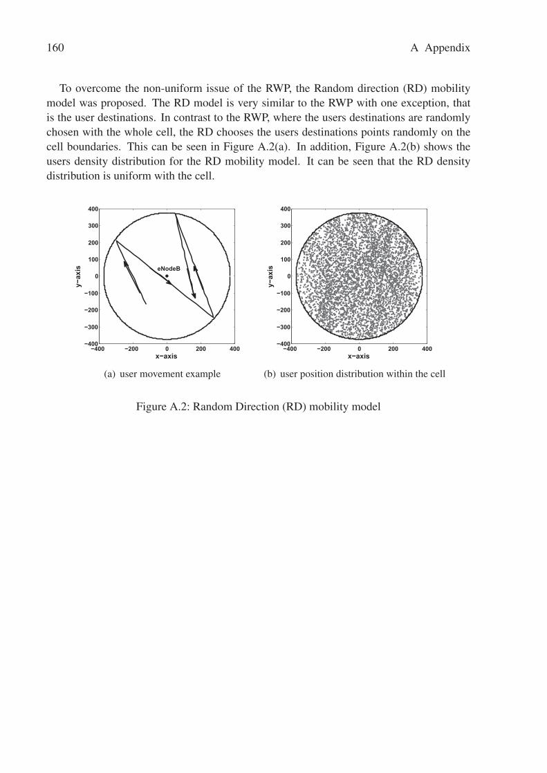
160 A Appendix
To overcome the non-uniform issue of the RWP, the Random direction (RD) mobilitymodel was proposed. The RD model is very similar to the RWP with one exception, thatis the user destinations. In contrast to the RWP, where the users destinations are randomlychosen with the whole cell, the RD chooses the users destinations points randomly on thecell boundaries. This can be seen in Figure A.2(a). In addition, Figure A.2(b) shows theusers density distribution for the RD mobility model. It can be seen that the RD densitydistribution is uniform with the cell.
−400 −200 0 200 400−400
−300
−200
−100
0
100
200
300
400
x−axis
y−ax
is eNodeB
(a) user movement example
−400 −200 0 200 400−400
−300
−200
−100
0
100
200
300
400
x−axis
y−ax
is
(b) user position distribution within the cell
Figure A.2: Random Direction (RD) mobility model
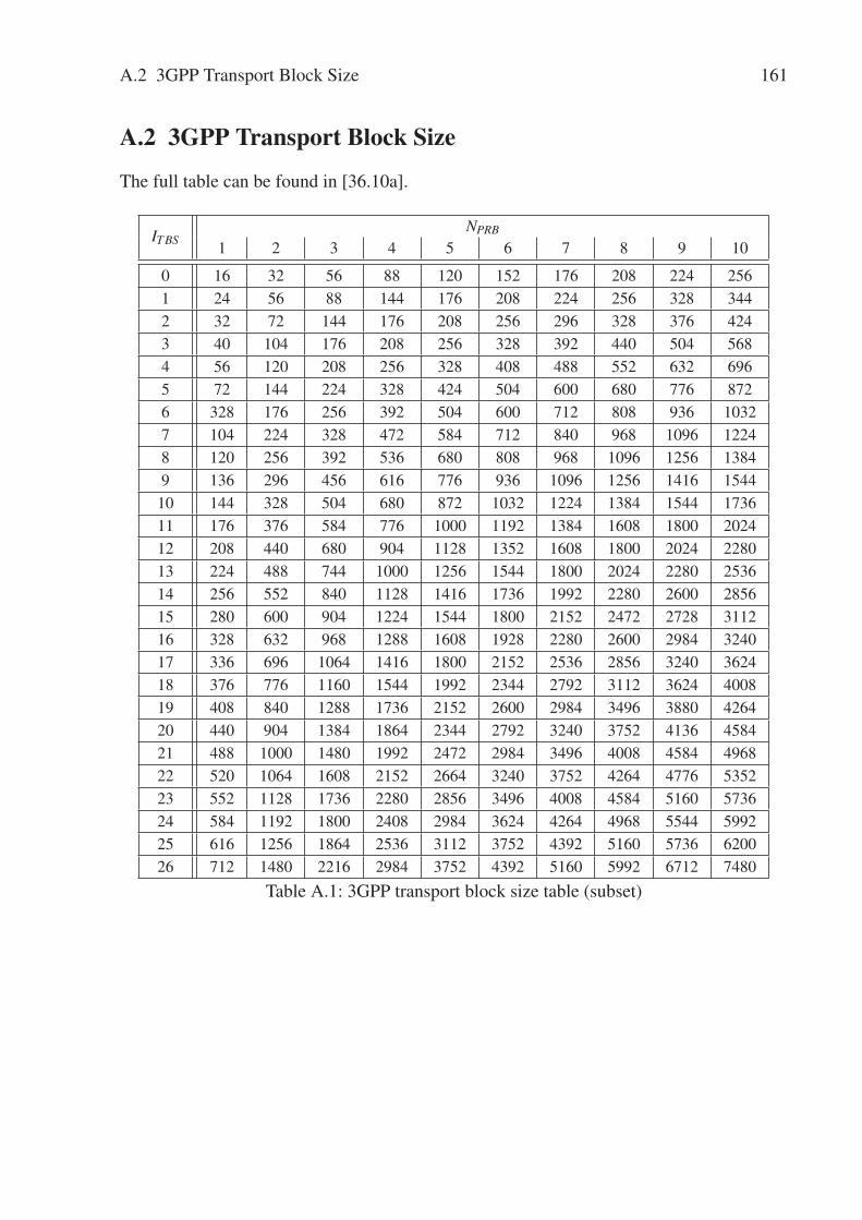
A.2 3GPP Transport Block Size 161
A.2 3GPP Transport Block Size
The full table can be found in [36.10a].
IT BSNPRB
1 2 3 4 5 6 7 8 9 10
0 16 32 56 88 120 152 176 208 224 2561 24 56 88 144 176 208 224 256 328 3442 32 72 144 176 208 256 296 328 376 4243 40 104 176 208 256 328 392 440 504 5684 56 120 208 256 328 408 488 552 632 6965 72 144 224 328 424 504 600 680 776 8726 328 176 256 392 504 600 712 808 936 10327 104 224 328 472 584 712 840 968 1096 12248 120 256 392 536 680 808 968 1096 1256 13849 136 296 456 616 776 936 1096 1256 1416 1544
10 144 328 504 680 872 1032 1224 1384 1544 173611 176 376 584 776 1000 1192 1384 1608 1800 202412 208 440 680 904 1128 1352 1608 1800 2024 228013 224 488 744 1000 1256 1544 1800 2024 2280 253614 256 552 840 1128 1416 1736 1992 2280 2600 285615 280 600 904 1224 1544 1800 2152 2472 2728 311216 328 632 968 1288 1608 1928 2280 2600 2984 324017 336 696 1064 1416 1800 2152 2536 2856 3240 362418 376 776 1160 1544 1992 2344 2792 3112 3624 400819 408 840 1288 1736 2152 2600 2984 3496 3880 426420 440 904 1384 1864 2344 2792 3240 3752 4136 458421 488 1000 1480 1992 2472 2984 3496 4008 4584 496822 520 1064 1608 2152 2664 3240 3752 4264 4776 535223 552 1128 1736 2280 2856 3496 4008 4584 5160 573624 584 1192 1800 2408 2984 3624 4264 4968 5544 599225 616 1256 1864 2536 3112 3752 4392 5160 5736 620026 712 1480 2216 2984 3752 4392 5160 5992 6712 7480
Table A.1: 3GPP transport block size table (subset)
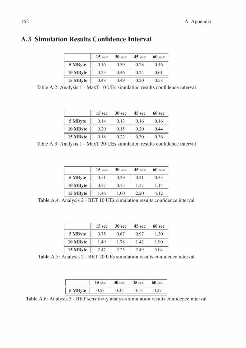
162 A Appendix
A.3 Simulation Results Confidence Interval
15 sec 30 sec 45 sec 60 sec
5 MByte 0.16 0.39 0.28 0.46
10 MByte 0.23 0.46 0.24 0.61
15 MByte 0.48 0.49 0.20 0.58
Table A.2: Analysis 1 - MaxT 10 UEs simulation results confidence interval
15 sec 30 sec 45 sec 60 sec
5 MByte 0.14 0.13 0.16 0.16
10 MByte 0.20 0.15 0.20 0.44
15 MByte 0.18 0.22 0.30 0.36
Table A.3: Analysis 1 - MaxT 20 UEs simulation results confidence interval
15 sec 30 sec 45 sec 60 sec
5 MByte 0.51 0.39 0.31 0.33
10 MByte 0.77 0.73 1.37 1.14
15 MByte 1.46 1.00 2.20 4.12
Table A.4: Analysis 2 - BET 10 UEs simulation results confidence interval
15 sec 30 sec 45 sec 60 sec
5 MByte 0.75 0.67 0.97 1.30
10 MByte 1.49 1.78 1.42 1.90
15 MByte 2.47 2.25 2.49 3.04
Table A.5: Analysis 2 - BET 20 UEs simulation results confidence interval
15 sec 30 sec 45 sec 60 sec
5 MByte 0.53 0.35 0.13 0.27
Table A.6: Analysis 3 - BET sensitivity analysis simulation results confidence interval
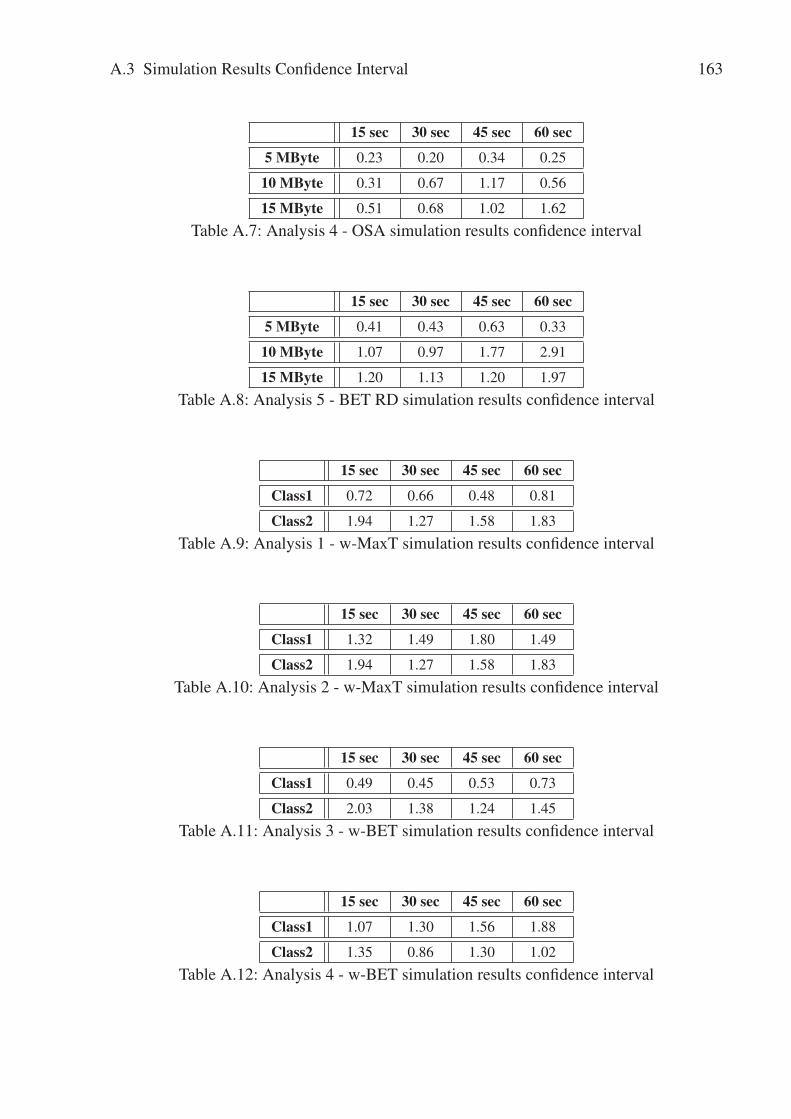
A.3 Simulation Results Confidence Interval 163
15 sec 30 sec 45 sec 60 sec
5 MByte 0.23 0.20 0.34 0.25
10 MByte 0.31 0.67 1.17 0.56
15 MByte 0.51 0.68 1.02 1.62
Table A.7: Analysis 4 - OSA simulation results confidence interval
15 sec 30 sec 45 sec 60 sec
5 MByte 0.41 0.43 0.63 0.33
10 MByte 1.07 0.97 1.77 2.91
15 MByte 1.20 1.13 1.20 1.97
Table A.8: Analysis 5 - BET RD simulation results confidence interval
15 sec 30 sec 45 sec 60 sec
Class1 0.72 0.66 0.48 0.81
Class2 1.94 1.27 1.58 1.83
Table A.9: Analysis 1 - w-MaxT simulation results confidence interval
15 sec 30 sec 45 sec 60 sec
Class1 1.32 1.49 1.80 1.49
Class2 1.94 1.27 1.58 1.83
Table A.10: Analysis 2 - w-MaxT simulation results confidence interval
15 sec 30 sec 45 sec 60 sec
Class1 0.49 0.45 0.53 0.73
Class2 2.03 1.38 1.24 1.45
Table A.11: Analysis 3 - w-BET simulation results confidence interval
15 sec 30 sec 45 sec 60 sec
Class1 1.07 1.30 1.56 1.88
Class2 1.35 0.86 1.30 1.02
Table A.12: Analysis 4 - w-BET simulation results confidence interval

Bibliography
[25.04] 3GPP Technical Report TR 25.892. Feasibility Study for Orthogonal Fre-quency Division Multiplexing (OFDM) for UTRAN enhancement. Techni-cal Report version 6.0.0, 3rd Generation Partnership Project, June 2004.
[25.05] 3GPP Technical Report TR 25.913. Requirements for Evolved UTRAand UTRAN. Technical Report version 2.1.0., 3rd Generation PartnershipProject, June 2005.
[25.06] 3GPP Technical Report TS 25.814. Physical layer aspects for E-UTRA. Technical Report version 7.1.0, 3rd Generation Partnership Project,September 2006.
[36.10a] 3GPP Technical Report TS 36.213. E-UTRA - Physical layer proce-dures. Technical Report version 9.3.0, 3rd Generation Partnership Project,September 2010.
[36.10b] 3GPP Technical Specification TS 36.322. Evolved Universal TerrestrialRadio Access (E-UTRA); Radio Link Control (RLC) protocol specifica-tion. Technical Report Version 10.0.0, 3rd Generation Partnership Project,December 2010.
[36.11a] 3GPP Technical Specification TS 36.300. Evolved Universal TerrestrialRadio Access (E-UTRA) and Evolved Universal Terrestrial Radio AccessNetwork (E-UTRAN); Overall description; Stage 2. Technical Report Ver-sion 10.3.0, 3rd Generation Partnership Project, March 2011.
[36.11b] 3GPP Technical Specification TS 36.321. Evolved Universal Terrestrial Ra-dio Access (E-UTRA); Medium Access Control (MAC) protocol specifica-tion. Technical Report Version 10.2.0, 3rd Generation Partnership Project,June 2011.
[36.11c] 3GPP Technical Specification TS 36.323. Evolved Universal TerrestrialRadio Access (E-UTRA); Packet Data Convergence Protocol (PDCP) spec-ification. Technical Report Version 10.1.0, 3rd Generation PartnershipProject, March 2011.
[3GP12] 3GPP. 3rd generation partnership project specification numbering.������������������� �������������� ���,last accessed on May 2012.

166 Bibliography
[4WAa] 4WARD. D-2.2 draft architectural framework.���������������� ������������������������������.last accessed on April 2012.
[4WAb] 4WARD. D-3.1.1 virtualization approach: Concept.���������������� ������������������������������.last accessed on April 2012.
[4WAc] 4WARD. D-4.2 in-network management concept.���������������� ������������������������������.last accessed on April 2012.
[4WAd] 4WARD. D-5.2.0 description of generic path mechanism.���������������� ������������������������������.last accessed on April 2012.
[4WAe] 4WARD. D-6.1 first netinf architecture description.���������������� ���������������������������� ��.last accessed on April 2012.
[4WAf] 4WARD. Fp7 european project. ���������������� ��������.last accessed on April 2012.
[AB08] A. Alshanyour and U. Baroudi. Random and realistic mobility models im-pact on the performance of bypass-aodv routing protocol. In Wireless Days,2008. WD ’08. 1st IFIP, pages 1 –5, nov. 2008.
[ABJS06] R. Agrawal, R. Berry, Huang Jianwei, and V. Subramanian. Optimalscheduling for ofdma systems. signals, systems and computers. In ACSSC’06, Fortieth Asilomar Conference, 2006.
[ADF+09] D. Astely, E. Dahlman, A. Furuskar, Y. Jading, M. Lindstrom, and S. Park-vall. Lte: the evolution of mobile broadband. Communications Magazine,IEEE, 47(4):44 –51, april 2009.
[Agi09] Agilent. 3gpp long term evolution: System overview, product development,and test challenges. Application Note, June 2009.
[Agi11] Agilent. Introducing lte-advanced. Application Note, March 2011.
[AKA10] AKARI. New generation network architecture akari conceptual design (ver2.0). ����������� ����������� ��������� �������������
��� !"#�������"�"����$��%"��&���#, May 2010.
[AMVC07] R. Agarwal, V. Majjigi, R. Vannithamby, and J. Cioffi. Efficient schedulingfor heterogeneous services in ofdma downlink. In IEEE Globecom, Wash-ington D.C., 2007.
[Anr09] Anritsu. Lte resource guide. Anritsu Testing the FUTURE, 2009.
[Asi] AsiaFI. Asia future internet forum. �������������#������.

Bibliography 167
[BAD08] K. C. Beh, S. Armour, and A. Doufexi. Joint time-frequency domain pro-portional fair scheduler with harq for 3gpp lte systems. In Vehicular Tech-nology Conference, 2008. VTC 2008-Fall. IEEE 68th, pages 1 –5, sept.2008.
[BAS+05] K. Brueninghaus, D. Astely, T. Salzer, S. Visuri, A. Alexiou, S. Karger,and G.-A. Seraji. Link performance models for system level simulationsof broadband radio access systems. In Personal, Indoor and Mobile RadioCommunications, 2005. PIMRC 2005. IEEE 16th International Symposiumon, volume 4, pages 2306 –2311 Vol. 4, sept. 2005.
[BFH+06] A. Bavier, N. Feamster, M. Huang, L. Peterson, and J. Rexford. In viniveritas: realistic and controlled network experimentation. In Proceedingsof the 2006 conference on Applications, technologies, architectures, andprotocols for computer communications, SIGCOMM ’06, pages 3–14, NewYork, NY, USA, 2006. ACM.
[BMM+08] S. Bhatia, M. Motiwala, W. Muhlbauer, V. Valancius, A. Bavier, N. Feam-ster, L. Peterson, and J. Rexford. Hosting virtual networks on commodityhardware. In Tech. Rep. GT-CS-07-10, Georgia Tech University, January2008.
[CBD02] T. Camp, J. Boleng, and V. Davies. A survey of mobility models for adhoc network research. Wireless Communications and Mobile Computing,2(5):483–502, 2002.
[Cha09] D. Chantry. Mapping applications to the cloud. MSDN li-brary, ����� �� ��� ��� ����� ���� ����� ��� � �� ������������ , January 2009.
[Cis] Cisco. Vn-link.������������������� ������������������ ���������
����������������������� ���� �������������������
��!����"�� � �� ������.
[CW08] L. M. Correia and K. Wuenstel. WP1 BIRD: Business Innovation, Regula-tion and Dissemination. In ICT Mobile Summit (presentation), Stockholm,June 2008.
[CYG95] C. N. Chuah, R. D. Yates, and D. J. Goodman. Integrated dynamic ra-dio resource management. In IEEE 45th Vehicular Technology Conference,volume 2, pages 584–588, Chicago, IL, USA, July 1995.
[Dah07] E. Dahlman. 3G evolution: HSPA and LTE for mobile broadband. Elec-tronics & Electrical. Elsevier Academic Press, 2007.
[DBMC10] S. Doirieux, B. Baynat, M. Maqbool, and M. Coupechoux. An efficientanalytical model for the dimensioning of wimax networks supporting multi-profile best effort traffic. Computer Communications, 33(10):1162 – 1179,2010.

168 Bibliography
[DMA03] M. Dillinger, K. Madani, and N. Alonistioti. Software defined radio: ar-chitectures, systems, and functions. Wiley series in software radio. Wiley,2003.
[EK06] M. Einhaus and O. Klein. Performance evaluation of a basic ofdma schedul-ing algorithm for packet data transmissions. In ISCC, Cagliary, Italy, 2006.
[EKW08] M. Einhaus, O. Klein, and B. Walke. Comparison of ofdma resourcescheduling strategies with fair allocation of capacity. In 5th IEEE Con-sumer Communications and Networking Conference (CCNC 2008), Las Ve-gas, NV, January 2008.
[GEN] GENI. Global Environment for Network Innovations.����������������.
[GL08] M. Gidlund and J.-C. Laneri. Scheduling algorithms for 3gpp long-termevolution systems: From a quality of service perspective. In Spread Spec-trum Techniques and Applications, 2008. ISSSTA ’08. IEEE 10th Interna-tional Symposium on, pages 114 –117, aug. 2008.
[Hoa05] J. Hoadley. Building future networks with mimo and ofdm.����� �� �������������� �� ���� � ����� ����������
� ��� ���� ������� , September 2005.
[HSH+97] S. Hämäläinen, P. Slanina, M. Hartman, A. Lappeteläinen, H. Holma, andO. Salonaho. A novel interface between link and system level simulations.In Proc. of ACTS Mobile Communications Summit ’97, volume 2, pages559–604. Aalborg, Denmark, October 1997.
[HT07] H. Holma and A. Toskala. WCDMA for UMTS: HSPA evolution and LTE.Wiley, 2007.
[HT09] H. Holma and A. Toskala. LTE for UMTS: OFDMA and SC-FDMA basedradio access. Wiley, 2009.
[HUN86] J.S. HUNTER. The exponentially weighted moving average. In Jal QualityTechnology, volume 18, pages 203–210, 1986.
[IBM03] IBM. Storage virtualization tutorial.����������� ���������������������������������������
������������������������������������������, 2003.
[IT09] ITU-T. Recommendation g.114 (05/03). One-way transmission time, 2009.
[Kle76] L. Kleinrock. Queueing Systems: Theory. Number Bd. 1 in A Wiley-Interscience publication. Wiley, 1976.
[KLZ09] R. Kwan, C. Leung, and J. Zhang. Proportional fair multiuser scheduling inlte. Signal Processing Letters, IEEE, 16(6):461 –464, june 2009.
[KMC+00] E. Kohler, R. Morris, B. Chen, J. Jahnotti, and M. F. Kasshoek. The clickmodular router. In ACM Transaction on Computer Systems, vol. 18, no- 3,2000.

Bibliography 169
[KPK+08a] P. Kela, J. Puttonen, N. Kolehmainen, T. Ristaniemi, T. Henttonen, andM. Moisio. Dynamic packet scheduling performance in utra long term evo-lution downlink. In Wireless Pervasive Computing, 2008. ISWPC 2008. 3rdInternational Symposium on, pages 308 –313, may 2008.
[KPK+08b] P. Kela, J. Puttonen, N. Kolehmainen, T. Ristaniemi, T. Henttonen, andM. Moisio. Dynamic packet scheduling performance in utra long term evo-lution downlink. In Wireless Pervasive Computing, 2008. ISWPC 2008. 3rdInternational Symposium on, pages 308 –313, may 2008.
[KSK+08] A. Kopke, M. Swigulski, K.Wessel, D. Willkomm, P.T. K. Haneveld,T. Parker, O. Visser, H. S. Lichte, and S. Valentin. Simulating wireless andmobile networks in omnet++: The mixim vision. In Proc. Int. Workshop onOMNeT++ collocated with SIMUTools, March 2008.
[KSW+08] A. Köpke, M. Swigulski, K. Wessel, D. Willkomm, P. T. K. Haneveld,T. E. V. Parker, O. W. Visser, H. S. Lichte, and S. Valentin. Simulatingwireless and mobile networks in omnet++ the mixim vision. In Proceed-ings of the 1st international conference on Simulation tools and techniquesfor communications, networks and systems & workshops, Simutools ’08,pages 71:1–71:8, ICST, Brussels, Belgium, Belgium, 2008. ICST (Institutefor Computer Sciences, Social-Informatics and Telecommunications Engi-neering).
[KZ11] M. Khan and Y. Zaki. Dynamic spectrum trade and game-theory basednetwork selection in lte virtualization using uniform auctioning. In XavierMasip-Bruin, Dominique Verchere, Vassilis Tsaoussidis, and Marcelo Yan-nuzzi, editors, Wired/Wireless Internet Communications, volume 6649 ofLecture Notes in Computer Science, pages 39–55. Springer Berlin / Heidel-berg, 2011. 10.1007/978-3-642-21560-5_4.
[Li10] X. Li. Radio Access Network Dimensioning for 3G UMTS.Vieweg+Teubner Verlag, 2010.
[LV08a] H. S. Lichte and S. Valentin. Implementing mac protocols for coopera-tive relaying: a compiler-assisted approach. In Proceedings of the 1st in-ternational conference on Simulation tools and techniques for communi-cations, networks and systems & workshops, Simutools ’08, pages 32:1–32:10, ICST, Brussels, Belgium, Belgium, 2008. ICST (Institute for Com-puter Sciences, Social-Informatics and Telecommunications Engineering).
[LV08b] H. S. Lichte and S. Valentin. Implementing mac protocols for cooperativerelaying: A compiler-assisted approach. In Proc. Int. Conf. on SimulationTools and Techniques for Communications, Networks and Systems (SIMU-Tools), March 2008.
[LWZ+11] X. Li, T. Weerawardane, Y. Zaki, C. Görg, and A. Timm-Giel. Shared trans-port for different radio broadband mobile technologies. In Recent Advances

170 Bibliography
in Broadband Integrated Network Operations and Services Management,pages 135–159. IGI Global, June 2011.
[LZW+08] X. Li, Y. Zaki, T. Weerawardane, A. Timm-Giel, and C. Görg. Hsupa back-haul bandwidth dimensioning. In Personal, Indoor and Mobile Radio Com-munications, 2008. PIMRC 2008. IEEE 19th International Symposium on,pages 1 –6, sept. 2008.
[LZW+10] X. Li, Y. Zaki, T. Weerawardane, A. Timm-Giel, C. Görg, and G.C.Malafronte. Use of traffic separation techniques for the transport of hspaand r99 traffic in the radio access network with differentiated quality of ser-vice. In Networking and Telecommunications: Concepts, Methodologies,Tools, and Applications, pages 863–878. IGI Global, 2010.
[LZZ+12] M. Li, L. Zhao, Y. Zaki, A. Timm-Giel, and C. Görg. Investigationof network virtualization and load balancing techniques in lte networks.In 2012 IEEE 75th Vehicular Technology Conference: VTC2012-Spring,Yokohama, Japan, May. 2012.
[Mar11] S. N. K. Marwat. Bandwidth and qos aware lte uplink scheduler. In Masterthesis. ComNets - University of Bremen, October 2011.
[MBH+08] R. Mahindra, G. Bhanage, G. Hadjicristofi, I. Seskar, D. Raychaudhuri,and Y.Y. Zhang. Space versus time separation for wireless virtualizationon an indoor grid. In Proceedings of the IEEE Next Generation InternetConference (NGI 2008), 2008.
[Mei12] S. Meier. congestion aware ho in lte systems. In Diplomaarebit. ComNets- University of Bremen, February 2012.
[Mic] Microsoft. Virtual server.�������������� ������������ ����� � ����
������ ������.
[mod11] OPNET modeler. ��������������������, last accessed on August2011.
[Mot] Motorola. Long term evolution (lte): A technical overview.����������������������������� �� �������� ����� ����
��������� ���������������� ������ ��� ������� �!"#�
$%��������������&�� �'()*$+��%�$,������.
[MWZ+12a] S. N. K. Marwat, T. Weerawardane, Y. Zaki, C. Görg, and A. Timm-Giel. Design and performance analysis of bandwidth and qos aware lteuplink scheduler in heterogeneous traffic environment. In 8th InternationalWireless Communications and Mobile Computing Conference, Limassol,Cyprus, August 2012.
[MWZ+12b] S. N. K. Marwat, T. Weerawardane, Y. Zaki, C. Görg, and A. Timm-Giel.Performance evaluation of bandwidth and qos aware lte uplink scheduler. In

Bibliography 171
10th International Conference on Wired/Wireless Internet Communications,WWIC 2012, Santorini, Greece, June 2012.
[MWZ+12c] S. N. K. Marwat, T. Weerawardane, Y. Zaki, C. Görg, and A. Timm-Giel.Performance of bandwidth and qos aware lte uplink scheduler towards delaysensitive traffic. In 17. ITG Fachtagung Mobilkommunikation, Osnabrueck,Germany, May 2012.
[Nak09] T. Nakamura. Proposal for candidate radio interface technologies for imt-advanced based on lte release 10 and beyond (lte-advanced). In ITU-R WP5D 3rd Workshop on IMT-Advanced, October 2009.
[PDF+08] S. Parkvall, E. Dahlman, A. Furuskar, Y. Jading, M. Olsson, S. Wanstedt,and K. Zangi. Lte-advanced - evolving lte towards imt-advanced. In Vehic-ular Technology Conference, 2008. VTC 2008-Fall. IEEE 68th, pages 1 –5,sept. 2008.
[Per09] H. Perros. Computer simulation techniques: The definitive introduction!����� �� ����� ��� ��� ���� ����������� ��� , December 2009.
[PMP+07] A. Pokhariyal, G. Monghal, K.I. Pedersen, P.E. Mogensen, I.Z. Kovacs,C. Rosa, and T.E. Kolding. Frequency domain packet scheduling underfractional load for the utran lte downlink. In Vehicular Technology Confer-ence, 2007. VTC2007-Spring. IEEE 65th, pages 699 –703, april 2007.
[PMRK06] L. Peterson, S. Muir, T. Roscoe, and A. Klingaman. Planetlab architecture:An overview. Technical Report PDN–06–031, PlanetLab Consortium, May2006.
[SB08] J. Sachs and S. Baucke. Virtual radio-a framework for configurable radionetworks. In WICON’08, Hawaii, USA, Nov. 2008.
[SBT09] S. Sesia, M.P.J. Baker, and I. Toufik. LTE, the UMTS long term evolution:from theory to practice. Wiley, 2009.
[She00] J. M. Shea. History of wireless communication. ����� �� ��� � ���
� ���� ��� ��� �� ������������ � ������������� ���� ,December 2000.
[Sin04] A. Singh. An introduction to virtualization. ���������������� ������������ ���������� ��� �����, January 2004.
[Sta12] StatSoft.������������� ������������������������������� ����, lastaccessed on January 2012.
[Ste94] W.J. Stewart. Introduction to the numerical solution of Markov chains.Princeton University Press, 1994.
[Ste11] W.J. Stewart. Probability, Markov Chains, Queues, and Simulation: TheMathematical Basis of Performance Modeling. Princeton University Press,2011.

172 Bibliography
[UML] User Mode Linux UML. ��������������� ��������������.
[UZZ+10] A. Udugama, L. Zhao, Y. Zaki, C. Görg, and A. Timm-Giel. End-to-endperformance evaluation of virtual networks using prototype. In Second In-ternational ICST Conference on Mobile Networks And Management (Mon-ami), Santander, Spain, September 22-24 2010.
[Val06] S. Valentin. Chsim - a wireless channel simulator for om-net++, in tkn tu berlin simulation workshop. ������������
������������������ �������������������� �� ����!�����
������"�#�������������������$%�&$$'���, September 2006.
[VAN] VANU. Multiran.�������������������� ��������� �������� .
[Vi10] VoIP-info.org. Call quality metrics.����� �� ���� ���� � ��� ��� ���� ����� �������
������ , 2010.
[VMw] VMware. ��������������������.
[VRO] VROUT. �������������� �����������.
[Wee11] T. Weerawardane. Optimization and Performance Analysis of High SpeedMobile Access Network. Vieweg & Teubner, 2011.
[WG07] D. E. Williams and J. Garcia. Virtualization with xen: Including xenenter-prise, xenserver, and xenexpress. In Syngress Publishing, Inc., ISBN-13:9781597491679, May 2007.
[WZTG+09] T. Weerawardane, Y. Zaki, A. Timm-Giel, G.C. Malafronte, S. Hauth, andC. Görg. Impact of the transport network congestion control on the hsupaperformance. In Vehicular Technology Conference, 2009. VTC Spring 2009.IEEE 69th, pages 1 –6, april 2009.
[Zah11] N. Zahariev. Optimized service aware radio resource scheduler in lte. InDiplomaarbeit. ComNets - University of Bremen, April 2011.
[ZKZG11] Y. Zaki, M. Khan, L. Zhao, and C. Görg. Realizing the broker based dy-namic spectrum allocation through lte virtualization and uniform auction-ing. In Performance Evaluation of Cognitive Radio Networks. Workshop(PE-CRN), Networking 2011, Valencia, Spain, May 2011.
[ZLZ+11] L. Zhao, M. Li, Y. Zaki, A. Timm-Giel, and C. Görg. Lte virtualization:From theoretical gain to practical solution. In Teletraffic Congress (ITC),2011 23rd International, pages 71 –78, San Francisco, USA, sept. 2011.
[ZWGTG11a] Y. Zaki, T. Weerawardane, C. Görg, and A. Timm-Giel. Long term evo-lution (lte) model development within opnet simulation environment. InOPNET workshop 2011, Washington D.C., USA, August 29-September 12011.

Bibliography 173
[ZWGTG11b] Y. Zaki, T. Weerawardane, C. Görg, and A. Timm-Giel. Multi-qos-awarefair scheduling for lte. In Vehicular Technology Conference (VTC Spring),2011 IEEE 73rd, pages 1 –5, may 2011.
[ZWL+08] Y. Zaki, T. Weerawardane, X. Li, A. Timm-Giel, G.C. Malafronte, andC. Görg. Effect of the rlc and tnl congestion control on the hsupa networkperformance. In Communications, Computers and Applications, 2008.MIC-CCA 2008. Mosharaka International Conference on, pages 1 –7, aug.2008.
[ZWL+10] Y. Zaki, T. Weerawardane, X. Li, A. Timm-Giel, G.C. Malafronte, andC. Görg. Performance enhancement due to the tnl congestion control on thesimultaneous deployment of both hsdpa and hsupa. In Recent Advances inCommunications and Networking Technologies, Journal of Networks, vol-ume 7, 2010.
[ZZGTG10a] Y. Zaki, L. Zhao, C. Görg, and A. Timm-Giel. A Novel LTE Wireless Virtu-alization Framework. In Second International ICST Conference on MobileNetworks And Management (Monami)., Santander, Spain, September 2010.
[ZZGTG10b] Y. Zaki, L. Zhao, C. Görg, and A. Timm-Giel. LTE wireless virtualizationand spectrum management. In Wireless and Mobile Networking Conference(WMNC), 2010 Third Joint IFIP, pages 1 –6, oct. 2010.
[ZZGTG11] Y. Zaki, L. Zhao, C. Görg, and A. Timm-Giel. Lte mobile network virtual-ization. Mobile Networks and Applications (MONET), ACM Journal, pages1–9, 2011. 10.1007/s11036-011-0321-7.
[ZZJ+09] Y. Zaki, L. Zhao, J. Jimenez, K. Mengal, A. Timm-Giel, and C. Görg. To-wards interoperability among virtual networks in the future internet. InICT-MobileSummit 2009, Santander Spain, June 2009.
[ZZU+11] L. Zhao, Y. Zaki, A. Udugama, U. Toseef, C. Görg, and A. Timm-Giel.Open connectivity services for future networks. In Emerging Technologiesfor a Smarter World (CEWIT), 2011 8th International Conference Expo on,pages 1–4, nov. 2011.
[ZZW+11] Y. Zaki, N. Zahariev, T. Weerawardane, C. Görg, and A. Timm-Giel. Op-timized service aware lte mac scheduler: Design, implementation and per-formance evaluation. In OPNET workshop 2011, Washington D.C., USA,August 29-September 1 2011.
[ZZW+12] N. Zahariev, Y. Zaki, T. Weerawardane, X. Li, C. Görg, and A. Timm-Giel.Optimized service aware lte mac scheduler with comparison against otherwell known schedulers. In 10th International Conference on Wired/WirelessInternet Communications, WWIC 2012, Santorini, Greece, June 2012.