futures hedge ratios: a review -...

The Quarterly Review of Economics and Finance43 (2003) 433–465

Futures hedge ratios: a review

Sheng-Syan Chena,∗, Cheng-few Leeb,c, Keshab Shresthad,e

a Department of Finance, College of Management, Yuan Ze University,135 Yuan-Tung Road, Chung-Li, Taoyuan, Taiwan, ROC

b Department of Finance, Rutgers University, New Brunswick, NJ, USAc Graduate Institute of Finance, National Chiao Tung University, Taiwan, ROC

d Nanyang Business School, Nanyang Technological University, Singaporee Faculty of Administration, University of Regina, Regina, Sask., Canada

Received 18 May 2001; received in revised form 22 February 2002; accepted 7 June 2002

Abstract

This paper presents a review of different theoretical approaches to the optimal futures hedge ratios.These approaches are based on minimum variance, mean-variance, expected utility, mean extended-Ginicoefficient, as well as semivariance. Various ways of estimating these hedge ratios are also discussed,ranging from simple ordinary least squares to complicated heteroscedastic cointegration methods. Undermartingale and joint-normality conditions, different hedge ratios are the same as the minimum variancehedge ratio. Otherwise, the optimal hedge ratios based on the different approaches are different and thereis no single optimal hedge ratio that is distinctly superior to the remaining ones.© 2002 Board of Trustees of the University of Illinois. All rights reserved.

JEL classification: C130

Keywords: Hedge ratio; Semivariance; Cointegration; Minimum variance; Gini coefficient

1. Introduction

One of the best uses of derivative securities such as futures contracts is in hedging. In thepast, both academicians and practitioners have shown great interest in the issue of hedging withfutures. This is quite evident from the large number of articles written in this area.

∗ Corresponding author. Tel.:+886-3-4638800x667; fax:+886-3-4354624.E-mail address: [email protected] (S.-S. Chen).

1062-9769/02/$ – see front matter © 2002 Board of Trustees of the University of Illinois. All rights reserved.PII: S1062-9769(02)00191-6

434 S.-S. Chen et al. / The Quarterly Review of Economics and Finance 43 (2003) 433–465

One of the main theoretical issues in hedging involves the determination of the optimalhedge ratio. However, the optimal hedge ratio depends on the particular objective function tobe optimized. Many different objective functions are currently being used. For example, oneof the most widely-used hedging strategies is based on the minimization of the variance of thehedged portfolio (e.g., seeEderington, 1979; Johnson, 1960; Myers & Thompson, 1989). Thisso-called minimum variance (MV) hedge ratio is simple to understand and estimate. However,the MV hedge ratio completely ignores the expected return of the hedged portfolio. Therefore,this strategy is in general inconsistent with the mean-variance framework unless the individualsare infinitely risk averse or the futures price follows a pure martingale process (i.e., expectedfutures price change is zero).

Other strategies that incorporate both the expected return and risk (variance) of the hedgedportfolio have been recently proposed (e.g., seeCecchetti, Cumby, & Figlewski, 1988; Howard& D’Antonio, 1984; Hsin, Kuo, & Lee, 1994). These strategies are consistent with the mean-variance framework. However, it can be shown that if the futures price follows a pure martin-gale process, then the optimal mean-variance hedge ratio will be the same as the MV hedgeratio.

Another aspect of the mean-variance-based strategies is that even though they are an improve-ment over the MV strategy, for them to be consistent with the expected utility maximizationprinciple, either the utility function needs to be quadratic or the returns should be jointly normal.If neither of these assumptions is valid, then the hedge ratio may not be optimal with respectto the expected utility maximization principle. Some researchers have solved this problem byderiving the optimal hedge ratio based on the maximization of the expected utility (e.g., seeCecchetti et al., 1988; Lence, 1995, 1996). However, this approach requires the use of specificutility function and specific return distribution.

Attempts have been made to eliminate these specific assumptions regarding the utility func-tion and return distributions. Some of them involve the minimization of the mean extended-Gini(MEG) coefficient, which is consistent with the concept of stochastic dominance (e.g., seeCheung, Kwan, & Yip, 1990; Kolb & Okunev, 1992, 1993; Lien & Luo, 1993a; Lien & Shaffer,1999; Shalit, 1995). Shalit (1995)shows that if the prices are normally distributed, then theMEG-based hedge ratio will be the same as the MV hedge ratio.

Recently, hedge ratios based on the generalized semivariance (GSV) or lower partial momentshave been proposed (e.g., seeChen, Lee, & Shrestha, 2001; De Jong, De Roon, & Veld, 1997;Lien & Tse, 1998, 2000). These hedge ratios are also consistent with the concept of stochasticdominance. Furthermore, these GSV-based hedge ratios have another attractive feature wherebythey measure portfolio risk by the GSV, which is consistent with the risk perceived by managers,because of its emphasis on the returns below the target return (seeCrum, Laughhunn, & Payne,1981; Lien & Tse, 2000). Lien and Tse (1998)show that if the futures and spot returns arejointly normally distributed and if the futures price follows a pure martingale process, then theminimum-GSV hedge ratio will be equal to the MV hedge ratio.

Most of the studies mentioned above (exceptLence, 1995, 1996) ignore transaction costsas well as investments in other securities.Lence (1995, 1996)derives the optimal hedge ratiowhere transaction costs and investments in other securities are incorporated in the model. Usinga CARA utility function, Lence finds that under certain circumstances, the optimal hedge ratiois zero; i.e., the optimal hedging strategy is not to hedge at all.

S.-S. Chen et al. / The Quarterly Review of Economics and Finance 43 (2003) 433–465 435

In addition to the use of different objective functions in the derivation of the optimal hedgeratio, previous studies also differ in terms of the dynamic nature of the hedge ratio. For example,some studies assume that the hedge ratio is constant over time. Consequently, these statichedge ratios are estimated using unconditional probability distributions (e.g., seeBenet, 1992;Ederington, 1979; Ghosh, 1993; Howard & D’Antonio, 1984; Kolb & Okunev, 1992, 1993). Onthe other hand, several studies allow the hedge ratio to change over time. In some cases, thesedynamic hedge ratios are estimated using conditional distributions associated with models suchas ARCH and GARCH (e.g., seeBaillie & Myers, 1991; Cecchetti et al., 1988; Kroner & Sultan,1993; Sephton, 1993a). Alternatively, the hedge ratios can be made dynamic by considering amulti-period model where the hedge ratios are allowed to vary for different periods. This is themethod used byLien and Luo (1993b).

When it comes to estimating the hedge ratios, many different techniques are currently beingemployed, ranging from simple to complex ones. For example, some of them use such a sim-ple method as the ordinary least squares (OLS) technique (e.g., seeBenet, 1992; Ederington,1979; Malliaris & Urrutia, 1991). However, others use more complex methods such as theconditional heteroscedastic (ARCH or GARCH) method (e.g., seeBaillie & Myers, 1991;Cecchetti et al., 1988; Sephton, 1993a), the random coefficient method (e.g., seeGrammatikos& Saunders, 1983), the cointegration method (e.g., seeChou, Fan, & Lee, 1996; Ghosh,1993; Lien & Luo, 1993b), or the cointegration-heteroscedastic method (e.g., seeKroner &Sultan, 1993).

It is quite clear that there are several different ways of deriving and estimating hedge ratios.In the paper we review these different techniques and approaches and examine their relations.

The paper is divided into five sections. InSection 2alternative theories for deriving theoptimal hedge ratios are reviewed. Various estimation methods are discussed inSection 3.Section 4presents a discussion on the relationship among lengths of hedging horizon, maturityof futures contract, data frequency, and hedging effectiveness. Finally, inSection 5we providea summary and conclusion.

2. Alternative theories for deriving the optimal hedge ratio

The basic concept of hedging is to combine investments in the spot market and futuresmarket to form a portfolio that will eliminate (or reduce) fluctuations in its value. Specifi-cally, consider a portfolio consisting ofCs units of a long spot position andCf units of ashort futures position.1 Let St andFt denote the spot and futures prices at timet, respectively.Since the futures contracts are used to reduce the fluctuations in spot positions, the result-ing portfolio is known as the hedged portfolio. The return on the hedged portfolio,Rh, isgiven by:

Rh = CsStRs − CfFtRfCsSt

= Rs − hRf , (1a)

whereh = CfFt/CsSt is the so-called hedge ratio, andRs = (St+1 − St)/St andRf =(Ft+1 − Ft)/Ft are so-called one-period returns on the spot and futures positions, respectively.Sometimes, the hedge ratio is discussed in terms of price changes (profits) instead of returns.


In this case the profit on the hedged portfolio, VH , and the hedge ratio,H, are respectivelygiven by:

VH = Cs St − Cf Ft and H = Cf

Cs, (1b)

where St = St+1 − St and Ft = Ft+1 − Ft.The main objective of hedging is to choose the optimal hedge ratio (eitherh or H). As

mentioned above, the optimal hedge ratio will depend on a particular objective function to beoptimized. Furthermore, the hedge ratio can be static or dynamic. InSections 2.1 and 2.2, wewill discuss the static hedge ratio and then the dynamic hedge ratio.

It is important to note that in the above setup, the cash position is assumed to be fixed and weonly look for the optimum futures position. Most of the hedging literature assumes that the cashposition is fixed, a setup that is suitable for financial futures. However, when we are dealingwith commodity futures, the initial cash position becomes an important decision variable thatis tied to the production decision. One such setup considered byLence (1995, 1996)will bediscussed inSection 2.3.

2.1. Static case

We consider here that the hedge ratio is static if it remains the same over time. The statichedge ratios reviewed in this paper can be divided into eight categories, as shown inTable 1.We will discuss each of them in the paper.

2.1.1. Minimum variance hedge ratioThe most widely-used static hedge ratio is the MV hedge ratio.Johnson (1960)derives this

hedge ratio by minimizing the portfolio risk, where the risk is given by the variance of changes

Table 1A list of different static hedge ratios

Hedge ratio Objective function

MV hedge ratio Minimize variance ofRhOptimum mean-variance hedge ratio MaximizeE(Rh)− 1

2AVar(Rh)

Sharpe hedge ratio MaximizeE(Rh)− RF√

Var(Rh)Maximum expected utility hedge ratio MaximizeE[U(W1)]Minimum MEG coefficient hedge ratio MinimizeΓv(Rhv)Optimum mean-MEG hedge ratio MaximizeE[Rh] − Γv(Rhv)Minimum GSV hedge ratio MinimizeVδ,α(Rh)Maximum mean-GSV hedge ratio MaximizeE[Rh] − Vδ,α(Rh)

Notes: (1)Rh: return on the hedged portfolio;E(Rh): expected return on the hedged portfolio; Var(Rh): variance ofreturn on the hedged portfolio;A: risk aversion parameter;RF : return on the risk-free security;E(U(W1)): expectedutility of end-of-period wealth;Γv(Rhv): mean extended-Gini coefficient ofRh; Vδ,α(Rh): generalized semivarianceof Rh. (2) With W1 given byEq. (15), the maximum expected utility hedge ratio includes the hedge ratio consideredby Lence (1995, 1996).


in the value of the hedged portfolio as follows:

Var( VH) = C2s Var( S)+ C2

f Var( F )− 2CsCf Cov( S, F ).

The MV hedge ratio, in this case, is given by:

H∗J = Cf

Cs= Cov( S, F )

Var( F ). (2a)

Alternatively, if we use definition (1a) and use Var(Rh) to represent the portfolio risk, thenthe MV hedge ratio is obtained by minimizing Var(Rh) which is given by:

Var(Rh) = Var(Rs)+ h2 Var(Rf )− 2hCov(Rs, Rf ).

In this case, the MV hedge ratio is given by:

h∗J = Cov(Rs, Rf )

Var(Rf )= ρ σs

σf, (2b)

whereρ is the correlation coefficient betweenRs andRf , andσs andσf are standard deviationsof Rs andRf , respectively.

The attractive features of the MV hedge ratio are that it is easy to understand and simpleto compute. However, in general the MV hedge ratio is not consistent with the mean-varianceframework since it ignores the expected return on the hedged portfolio. For the MV hedge ratioto be consistent with the mean-variance framework, either the investors need to be infinitelyrisk averse or the expected return on the futures contract needs to be zero.

2.1.2. Optimum mean-variance hedge ratioVarious studies have incorporated both risk and return in the derivation of the hedge ratio.

For example,Hsin et al. (1994)derive the optimal hedge ratio that maximizes the followingutility function:

maxCfV(E(Rh), σ;A) = E(Rh)− 0.5Aσ2

h, (3)

whereA represents the risk aversion parameter. It is clear that this utility function incorporatesboth risk and return. Therefore, the hedge ratio based on this utility function would be consistentwith the mean-variance framework. The optimal number of futures contract and the optimalhedge ratio are respectively given by:

h2 = −C∗fF

CsS= −

[E(Rf )

Aσ2f

− ρ σsσf

]. (4)

One problem associated with this type of hedge ratio is that in order to derive the optimumhedge ratio, we need to know the individual’s risk aversion parameter. Furthermore, differentindividuals will choose different optimal hedge ratios, depending on the values of their riskaversion parameter.

Since the MV hedge ratio is easy to understand and simple to compute, it will be interestingand useful to know under what condition the above hedge ratio would be the same as the


MV hedge ratio. It can be seen fromEqs. (2b) and (4)that if A → ∞ or E(Rf ) = 0,thenh2 would be equal to the MV hedge ratioh∗

J . The first condition is simply a restatementof the infinitely risk-averse individuals. However, the second condition does not impose anycondition on the risk averseness, and this is important. It implies that even if the individuals arenot infinitely risk averse, the MV hedge ratio would be the same as the optimal mean-variancehedge ratio if the expected return on the futures contract is zero (i.e., futures prices follow asimple martingale process). Therefore, if futures prices follow a simple martingale process,then we do not need to know the risk aversion parameter of the investor to find the optimalhedge ratio.

2.1.3. Sharpe hedge ratioAnother way of incorporating the portfolio return in the hedging strategy is to use the

risk-return tradeoff (Sharpe measure) criteria.Howard and D’Antonio (1984)consider theoptimal level of futures contracts by maximizing the ratio of the portfolio’s excess return to itsvolatility:

maxCfθ = E(Rh)− RF

σh, (5)

whereσ2h = Var(Rh) and RF represents the risk-free interest rate. In this case the optimal

number of futures positions,C∗f , is given by:

C∗f = −Cs (S/F )(σs/σf )[(σs/σf )(E(Rf )/(E(Rs)− RF))− ρ]

[1 − (σs/σf )(E(Rf )ρ/(E(Rs)− RF))] . (6)

From the optimal futures position, we can obtain the following optimal hedge ratio:

h3 = −(σs/σf )[(σs/σf )(E(Rf )/(E(Rs)− RF))− ρ]

[1 − (σs/σf )(E(Rf )ρ/(E(Rs)− RF))] . (7)

Again, if E(Rf ) = 0, thenh3 reduces to:

h3 = σs

σfρ, (8)

which is the same as the MV hedge ratioh∗J .

As pointed out byChen et al. (2001), the Sharpe ratio is a highly non-linear function ofthe hedge ratio. Therefore, it is possible thatEq. (7), which is derived by equating the firstderivative to zero, may lead to the hedge ratio that would minimize, instead of maximizing, theSharpe ratio. This would be true if the second derivative of the Sharpe ratio with respect to thehedge ratio is positive instead of negative. Furthermore, it is possible that the optimal hedgeratio may be undefined as in the case encountered byChen et al. (2001), where the Sharpe ratiomonotonically increases with the hedge ratio.

2.1.4. Maximum expected utility hedge ratioSo far we have discussed the hedge ratios that incorporate only risk as well as the ones

that incorporate both risk and return. The methods, which incorporate both the expected returnand risk in the derivation of the optimal hedge ratio, are consistent with the mean-variance


framework. However, these methods may not be consistent with the expected utility maximiza-tion principle unless either the utility function is quadratic or the returns are jointly normallydistributed. Therefore, in order to make the hedge ratio consistent with the expected utilitymaximization principle, we need to derive the hedge ratio that maximizes the expected utility.However, in order to maximize the expected utility we need to assume a specific utility function.For example,Cecchetti et al. (1988)derive the hedge ratio that maximizes the expected utilitywhere the utility function is assumed to be the logarithm of terminal wealth. Specifically, theyderive the optimal hedge ratio that maximizes the following expected utility function:∫

Rs

∫Rf

log[1 + Rs − hRf ]f(Rs, Rf )dRs dRf ,

where the density functionf(Rs, Rf ) is assumed to be bivariate normal. A third-order linearbivariate ARCH model is used to get the conditional variance and covariance matrix, and anumerical procedure is used to maximize the objective function with respect to the hedge ratio.2

2.1.5. Minimum mean extended-Gini coefficient hedge ratioThis approach of deriving the optimal hedge ratio is consistent with the concept of stochastic

dominance and involves the use of the MEG coefficient.Cheung et al. (1990), Kolb and Okunev(1992), Lien and Luo (1993a), Shalit (1995), andLien and Shaffer (1999)all consider thisapproach. It minimizes the MEG coefficientΓv(Rh) defined as follows:

Γv(Rh) = −vCov(Rh, (1 −G(Rh))v−1), (9)

whereG is the cumulative probability distribution andv is the risk aversion parameter. Notethat 0≤ v < 1 implies risk seekers,v = 1 implies risk-neutral investors, andv > 1 impliesrisk-averse investors.Shalit (1995)has shown that if the futures and spot returns are jointlynormally distributed, then the minimum-MEG hedge ratio would be the same as the MV hedgeratio.

2.1.6. Optimum mean-MEG hedge ratioInstead of minimizing the MEG coefficient,Kolb and Okunev (1993)alternatively consider

maximizing the utility function defined as follows:

U(Rh) = E(Rh)− Γv(Rh). (10)

The hedge ratio based on the utility function defined byEq. (10)is denoted as the M-MEGhedge ratio. The difference between the MEG and M-MEG hedge ratios is that the MEG hedgeratio ignores the expected return on the hedged portfolio. Again, if the futures price followsa martingale process (i.e.,E(Rf ) = 0), then the MEG hedge ratio would be the same as theM-MEG hedge ratio.

2.1.7. Minimum generalized semivariance hedge ratioIn recent years a new approach for determining the hedge ratio has been suggested (seeChen

et al., 2001; De Jong et al., 1997; Lien & Tse, 1998, 2000). This new approach is based onthe relationship between the GSV and expected utility as discussed byFishburn (1977)and


Bawa (1978). In this case the optimal hedge ratio is obtained by minimizing the GSV givenbelow:

Vδ,α(Rh) =∫ δ

−∞(δ− Rh)α dG(Rh), α > 0, (11)

whereG(Rh) is the probability distribution function of the return on the hedged portfolioRh.The parametersδ andα (which are both real numbers) represent the target return and riskaversion, respectively. The risk is defined in such a way that the investors consider only thereturns below the target return (δ) to be risky. It can be shown (seeFishburn, 1977) thatα < 1represents a risk-seeking investor andα > 1 represents a risk-averse investor.

The GSV, due to its emphasis on the returns below the target return, is consistent with therisk perceived by managers (seeCrum et al., 1981; Lien & Tse, 2000). Furthermore, as shownbyFishburn (1977)andBawa (1978), the GSV is consistent with the concept of stochastic dom-inance.Lien and Tse (1998)show that the GSV hedge ratio, which is obtained by minimizingthe GSV, would be the same as the MV hedge ratio if the futures and spot returns are jointlynormally distributed and if the futures price follows a pure martingale process.

2.1.8. Optimum mean-generalized semivariance hedge ratioChen et al. (2001)extend the GSV hedge ratio to a mean-GSV (M-GSV) hedge ratio by

incorporating the mean return in the derivation of the optimal hedge ratio. The M-GSV hedgeratio is obtained by maximizing the following mean-risk utility function, which is similar tothe conventional mean-variance-based utility function (seeEq. (3)):

U(Rh) = E[Rh] − Vδ,α(Rh). (12)

This approach to the hedge ratio does not use the risk aversion parameter to multiply the GSVas done in conventional mean-risk models (seeHsin et al., 1994andEq. (3)). This is because therisk aversion parameter is already included in the definition of the GSV,Vδ,α(Rh). As before,the M-GSV hedge ratio would be the same as the GSV hedge ratio if the futures price followsa pure martingale process.

2.2. Dynamic case

We have up to now examined the situations in which the hedge ratio is fixed at the optimumlevel and is not revised during the hedging period. However, it could be beneficial to changethe hedge ratio over time. One way to allow the hedge ratio to change is by recalculatingthe hedge ratio based on the current (or conditional) information on the covariance (σsf) andvariance (σ2

f ). This involves calculating the hedge ratio based on conditional information (i.e.,σsf|Ωt−1 andσ2

f |Ωt−1) instead of unconditional information. In this case, the MV hedge ratio isgiven by:

h1

∣∣∣∣∣Ωt−1 = σsf|Ωt−1

σ2f |Ωt−1

.

The adjustment to the hedge ratio based on new information can be implemented using suchconditional models as ARCH and GARCH (to be discussed later) or using the moving window


estimation method. Alternatively, we can allow the hedge ratio to change during the hedgingperiod by considering multi-period models, which is the approach used byLien and Luo (1993b).

Lien and Luo (1993b)consider hedging withT periods’ planning horizon and minimize thevariance of the wealth at the end of the planning horizon,WT . Consider the situation whereCs,tis the spot position at the beginning of periodt and the corresponding futures position is givenbyCf,t = −btCs,t. The wealth at the end of the planning horizon,WT , is then given by:

WT =W0 +T−1∑t=0

Cs,t[St+1 − St − bt(Ft+1 − Ft)],

=W0 +T−1∑t=0

Cs,t[ St+1 − bt Ft+1]. (13)

The optimalbt ’s are given by the following recursive formula:

bt = −Cov( St+1, Ft+1)

Var( Ft+1)−

T−1∑i=t+1

(Cs,i

Cs,t

)Cov( Ft+1, Si+1 + bi Fi+1)

Var( Ft+1). (14)

It is clear fromEq. (14)that the optimal hedge ratiobt will change over time. The multi-periodhedge ratio will differ from the single-period hedge ratio due to the second term on the right-handside ofEq. (14). However, it is interesting to note that the multi-period hedge ratio would bedifferent from the single-period one if the changes in current futures prices are correlated withthe changes in future futures prices or with the changes in future spot prices.

2.3. Case with production and alternative investment opportunities

All the models considered inSections 2.1 and 2.2assume that the spot position is fixed orpredetermined, and thus production is ignored. As mentioned earlier, such an assumption maybe appropriate for financial futures. However, when we consider commodity futures, productionshould be considered in which case the spot position becomes one of the decision variables.In an important paper,Lence (1995)extends the model with a fixed or predetermined spotposition to a model where production is included. In his model,Lence (1995)also incorporatesthe possibility of investing in a risk-free asset and other risky assets, borrowing, as well astransaction costs. We will briefly discuss the model considered byLence (1995)below.

Lence (1995)considers a decision maker whose utility is a function of terminal wealthU(W1),such thatU ′ > 0 andU ′′ < 0. At the decision date (t = 0), the decision maker will engagein the production ofQ commodity units for sale at terminal date (t = 1) at the random cashprice P1. At the decision date, the decision maker can lendL dollars at the risk-free lendingrate (RL− 1) and borrowB dollars at the borrowing rate (RB− 1), investI dollars in a differentactivity that yields a random rate of return (RI − 1) and sellX futures at futures priceF0. Thetransaction cost for the futures trade isf dollars per unit of the commodity traded to be paid atthe terminal date. The terminal wealth (W1) is therefore given by:

W1 = W0R = P1Q+ (F0 − F1)X− f |X| − RBB + RLL+ RII, (15)


whereR is the return on the diversified portfolio. The decision maker will maximize the expectedutility subject to the following restrictions:

W0 + B ≥ v(Q)Q+ L+ I, 0 ≤ B ≤ kBv(Q)Q, kB ≥ 0,

L ≥ kLF0|X|, kL ≥ 0, I ≥ 0,

wherev(Q) is the average cost function,kB is the maximum amount (expressed as a proportionof his initial wealth) that the agent can borrow, andkL is the safety margin for the futurescontract.

Using this framework,Lence (1995)introduces two opportunity costs: opportunity cost ofalternative (sub-optimal) investment (calt) and opportunity cost of estimation risk (eBayes).3 LetRopt be the return of the expected-utility maximizing strategy and letRalt be the return ona particular alternative (sub-optimal) investment strategy. The opportunity cost of alternativeinvestment strategycalt is then given by:

E U(W0Ropt) = E[U(W0Ralt + calt)]. (16)

In other words,calt is the minimum certain net return required by the agent to invest in the al-ternative (sub-optimal hedging) strategy rather than in the optimum strategy. Using the CARAutility function and some simulation results,Lence (1995)finds that the expected-utility maxi-mizing hedge ratios are substantially different from the minimum variance hedge ratios. He alsoshows that under certain conditions, the optimal hedge ratio is zero; i.e., the optimal strategy isnot to hedge at all.

Similarly, the opportunity cost of the estimation risk (eBayes) is defined as follows:

Eρ E(UW0[Ropt(ρ)− eBayesρ ]) = Eρ E(U(W0R

Bayesopt )), (17)

whereRopt(ρ) is the expected-utility maximizing return where the agent knows with certaintythe value of the correlation between the futures and spot prices (ρ),RBayes

opt is the expected-utilitymaximizing return where the agent only knows the distribution of the correlationρ, andEρ[·]is the expectation with respect toρ. Using simulation results,Lence (1995)finds that theopportunity cost of the estimation risk is negligible and thus the value of the use of sophisticatedestimation methods is negligible.

3. Alternative methods for estimating the optimal hedge ratio

In Section 2we discussed different approaches to deriving the optimum hedge ratios. How-ever, in order to apply these optimum hedge ratios in practice, we need to estimate these hedgeratios. There are various ways of estimating them. In this section we briefly discuss theseestimation methods.

3.1. Estimation of the MV hedge ratio

3.1.1. OLS methodThe conventional approach to estimating the MV hedge ratio involves the regression of the

changes in spot prices on the changes in futures price using the OLS technique (e.g., seeJunkus


& Lee, 1985). Specifically, the regression equation can be written as:

St = a0 + a1 Ft + et, (18)

where the estimate of the MV hedge ratio,HJ , is given bya1. The OLS technique is quiterobust and simple to use. However, for the OLS technique to be valid and efficient, assumptionsassociated with the OLS regression must be satisfied. One case where the assumptions are notcompletely satisfied is that the error term in the regression is heteroscedastic. This situationwill be discussed later.

Another problem with the OLS method, as pointed out byMyers and Thompson (1989),is the fact that it uses unconditional sample moments instead of conditional sample moments,which use currently available information. They suggest the use of the conditional covarianceand conditional variance inEq. (2a). In this case, the conditional version of the optimal hedgeratio (Eq. (2a)) will take the following form:

H∗J = Cf

Cs= Cov( S, F )|Ωt−1

Var( F )|Ωt−1. (2a*)

Suppose that the current information (Ωt−1) includes a vector of variables (Xt−1) and the spotand futures price changes are generated by the following equilibrium model:

St = Xt−1α+ ut, Ft = Xt−1β + vt.In this case the maximum likelihood estimator of the MV hedge ratio is given by (seeMyers& Thompson, 1989):

h|Xt−1 = σuv

σ2v

, (19)

whereσuv is the sample covariance between the residualsut andvt, andσ2v is the sample variance

of the residualvt. In general, the OLS estimator obtained fromEq. (18)would be different fromthe one given byEq. (19). For the two estimators to be the same, the spot and futures pricesmust be generated by the following model:

St = α0 + ut, Ft = β0 + vt.In other words, if the spot and futures prices follow a random walk with or without drift, then thetwo estimators will be the same. Otherwise, the hedge ratio estimated from the OLS regression(18) will not be optimal.

3.1.2. ARCH and GARCH methodsEver since the development of ARCH and GARCH models, the OLS method of estimating

the hedge ratio has been generalized to take into account the heteroscedastic nature of theerror term inEq. (18). In this case, rather than using the unconditional sample variance andcovariance, the conditional variance and covariance from the GARCH model are used in theestimation of the hedge ratio. As mentioned above, such a technique allows an update of thehedge ratio over the hedging period.


Consider the following bivariate GARCH model (seeBaillie & Myers, 1991; Cecchetti et al.,1988):[

St

Ft

]=

[µ1

µ2

]+

[e1t

e2t

]⇔ Yt = µ+ et,

et|Ωt−1 ∼ N(0, Ht), Ht =[H11,t H12,t

H12,t H22,t

],

vec(Ht) = C + A vec(et−1e′t−1)+ B vec(Ht−1).

The conditional MV hedge ratio at timet is given byht−1 = H12,t/H22,t. This model allows thehedge ratio to change over time, resulting in a series of hedge ratios instead of a single hedgeratio for the entire hedging horizon.

The model can be extended to include more than one type of cash and futures contracts (seeSephton, 1993a). For example, consider a portfolio that consists of spot wheat (S1t), spot canola(S2t), wheat futures (F1t) and canola futures (F2t). We then have the following multi-variateGARCH model:

S1t

S2t

F1t

F2t

=

µ1

µ2

µ3

µ4

+

e1t

e2t

e3t

e4t

⇔ Yt = µ+ et, et|Ωt−1| ∼ N(0, Ht).

The MV hedge ratio can be estimated using a similar technique as described above. For example,the conditional MV hedge ratio is given by the conditional covariance between the spot andfutures price changes divided by the conditional variance of the futures price change.

3.1.3. Random coefficient methodThere is another way to deal with heteroscedasticity. This involves use of the random co-

efficient model as suggested byGrammatikos and Saunders (1983). This model employs thefollowing variation ofEq. (18):

St = β0 + βt Ft + et, (20)

where the hedge ratioβt = β+vt is assumed to be random. This random coefficient model can,in some cases, improve the effectiveness of hedging strategy. However, this technique does notallow for the update of the hedge ratio over time even though the correction for the randomnesscan be made in the estimation of the hedge ratio.

3.1.4. Cointegration and error correction methodThe techniques described so far do not take into consideration the possibility that spot price

and futures price series could be non-stationary. If these series have unit roots, then this willraise a different issue. If the two series are cointegrated as defined byEngle and Granger (1987),then the regressionEq. (18)will be mis-specified and an error-correction term must be includedin the equation. Since the arbitrage condition ties the spot and futures prices, they cannot driftfar apart in the long run. Therefore, if both series follow a random walk, then we expect thetwo series to be cointegrated in which case we need to estimate the error correction model. Thiscalls for the use of the cointegration analysis.


The cointegration analysis involves two steps. First, each series must be tested for a unit root(e.g., seeDickey & Fuller, 1981; Phillips & Perron, 1988). Second, if both series are found tohave a single unit root, then the cointegration test must be performed (e.g., seeEngle & Granger,1987; Johansen & Juselius, 1990; Osterwald-Lenum, 1992).

If the spot price and futures price series are found to be cointegrated, then the hedge ratiocan be estimated in two steps (seeChou et al., 1996; Ghosh, 1993). The first step involves theestimation of the following cointegrating regression:

St = a+ bFt + ut. (21)

The second step involves the estimation of the following error correction model:

St = ρut−1 + β Ft +m∑i=1

δi Ft−i +n∑j=1

θi St−j + ej, (22)

whereut is the residual series from the cointegrating regression. The estimate of the hedgeratio is given by the estimate ofβ. Some researchers (e.g., seeLien & Luo, 1993b) assume thatthe long-run cointegrating relationship is (St −Ft), and estimate the following error correctionmodel:

St = ρ(St−1 − Ft−1)+ β Ft +m∑i=1

δi Ft−i +n∑j=1

θi St−j + ej. (23)

Alternatively,Chou et al. (1996)suggest the estimation of the error correction model as follows:

St = αut−1 + β Ft +m∑i=1

δi Ft−i +n∑j=1

θi St−j + ej, (24)

whereut−1 = St−1−(a+bFt−1); i.e., the seriesut is the estimated residual series fromEq. (21).The hedge ratio is given byβ in Eq. (24).

Kroner and Sultan (1993)combine the error-correction model with the GARCH modelconsidered byCecchetti et al. (1988)andBaillie and Myers (1991)in order to estimate theoptimum hedge ratio. Specifically, they use the following model:[

loge(St)

loge(Ft)

]=

[µ1

µ2

]+

[αs(loge(St−1)− loge(Ft−1))

αf (loge(St−1)− loge(Ft−1))

]+

[e1t

e2t

], (25)

where the error processes follow a GARCH process. As before, the hedge ratio at time (t − 1)is given byht−1 = H12,t/H22,t.

3.2. Estimation of the optimum mean-variance and Sharpe hedge ratios

The optimum mean-variance and Sharpe hedge ratios are given byEqs. (4) and (7), respec-tively. These hedge ratios can be estimated simply by replacing the theoretical moments by theirsample moments. For example, the expected returns can be replaced by sample average returns,the standard deviations can be replaced by the sample standard deviations, and the correlationcan be replaced by sample correlation.


3.3. Estimation of the maximum expected utility hedge ratio

The maximum expected utility hedge ratio involves the maximization of the expected utility.This requires the estimation of distributions of the changes in spot and futures prices. Once thedistributions are estimated, one needs to use a numerical technique to get the optimum hedgeratio. One such method is described inCecchetti et al. (1988)where an ARCH model is usedto estimate the required distributions.

3.4. Estimation of MEG coefficient based hedge ratios

The MEG hedge ratio involves the minimization of the following MEG coefficient:

Γv(Rh) = −vCov[Rh, (1 −G(Rh))v−1].

In order to estimate the MEG coefficient, we need to estimate the cumulative probability densityfunctionG(Rh). The cumulative probability density function is usually estimated by rankingthe observed return on the hedged portfolio. A detailed description of the process can be foundin Kolb and Okunev (1992), and we briefly describe the process here.

The cumulative probability distribution is estimated by using the rank as follows:

G(Rh,i) = Rank(Rh,i)

N,

whereN is the sample size. Once we have the series for the probability distribution function, theMEG is estimated by replacing the theoretical covariance by the sample covariance as follows:

Γ samplev (Rh) = − v

N

N∑i=1

(Rh,i − Rh)((1 −G(Rh,i))v−1 −Θ), (26)

where

Rh = 1

N

N∑i=1

Rh,i and Θ = 1

N

N∑i=1

(1 −G(Rh,i))v−1.

The optimal hedge ratio is now given by the hedge ratio that minimizes the estimated MEG.Since there is no analytical solution, the numerical method needs to be applied in order to get theoptimal hedge ratio. This method is sometimes referred to as the empirical distribution method.

Alternatively, the instrumental variable (IV) method suggested byShalit (1995)can be usedto find the MEG hedge ratio. Shalit’s method provides the following analytical solution for theMEG hedge ratio:

hIV = Cov(St+1, [1 −G(Ft+1)]υ−1)

Cov(Ft+1, [1 −G(Ft+1)]υ−1).

It is important to note that for the IV method to be valid, the cumulative distribution function ofthe terminal wealth (Wt+1) should be similar to the cumulative distribution of the futures price(Ft+1); i.e.,G(Wt+1) = G(Ft+1). Lien and Shaffer (1999)find that the IV-based hedge ratio(hIV ) is significantly different from the minimum MEG hedge ratio.


Lien and Luo (1993a)suggest an alternative method of estimating the MEG hedge ratio. Thismethod involves the estimation of the cumulative distribution function using a non-parametrickernel function instead of using a rank function as suggested above.

Regarding the estimation of the M-MEG hedge ratio, one can follow either the empiricaldistribution method or the non-parametric kernel method to estimate the MEG coefficient. Anumerical method can then be used to estimate the hedge ratio that maximizes the objectivefunction given byEq. (10).

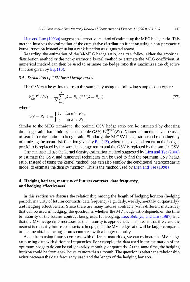
3.5. Estimation of GSV-based hedge ratios

The GSV can be estimated from the sample by using the following sample counterpart:

Vsampleδ,α (Rh) = 1

N

N∑i=1

(δ− Rh,i)αU(δ− Rh,i), (27)

where

U(δ− Rh,i) =

1, for δ ≥ Rh,i,0, for δ < Rh,i.

Similar to the MEG technique, the optimal GSV hedge ratio can be estimated by choosingthe hedge ratio that minimizes the sample GSV,V

sampleδ,α (Rh). Numerical methods can be used

to search for the optimum hedge ratio. Similarly, the M-GSV hedge ratio can be obtained byminimizing the mean-risk function given byEq. (12), where the expected return on the hedgedportfolio is replaced by the sample average return and the GSV is replaced by the sample GSV.

One can instead use the kernel density estimation method suggested byLien and Tse (2000)to estimate the GSV, and numerical techniques can be used to find the optimum GSV hedgeratio. Instead of using the kernel method, one can also employ the conditional heteroscedasticmodel to estimate the density function. This is the method used byLien and Tse (1998).

4. Hedging horizon, maturity of futures contract, data frequency,and hedging effectiveness

In this section we discuss the relationship among the length of hedging horizon (hedgingperiod), maturity of futures contracts, data frequency (e.g., daily, weekly, monthly, or quarterly),and hedging effectiveness. Since there are many futures contracts (with different maturities)that can be used in hedging, the question is whether the MV hedge ratio depends on the timeto maturity of the futures contract being used for hedging.Lee, Bubnys, and Lin (1987)findthat the MV hedge ratio increases as the maturity is approached. This means that if we use thenearest to maturity futures contracts to hedge, then the MV hedge ratio will be larger comparedto the one obtained using futures contracts with a longer maturity.

Aside from using futures contracts with different maturities, we can estimate the MV hedgeratio using data with different frequencies. For example, the data used in the estimation of theoptimum hedge ratio can be daily, weekly, monthly, or quarterly. At the same time, the hedginghorizon could be from a few hours to more than a month. The question is whether a relationshipexists between the data frequency used and the length of the hedging horizon.


Malliaris and Urrutia (1991)andBenet (1992)utilize Eq. (18)and weekly data to estimatethe optimal hedge ratio. According toMalliaris and Urrutia (1991), theex ante hedging is moreeffective when the hedging horizon is 1 week compared to a hedging horizon of 4 weeks.Benet(1992)finds that a shorter hedging horizon (4 weeks) is more effective (inex ante test) comparedto a longer hedging horizon (8 and 12 weeks). These empirical results seem to be consistentwith the argument that when estimating the MV hedge ratio, the hedging horizon’s length mustmatch the data frequency being used.

There is a potential problem associated with matching the length of the hedging horizonand the data frequency. For example, consider the case where the hedging horizon is 3 months(one-quarter). In this case we need to use quarterly data to match the length of the hedginghorizon. In other words, when estimatingEq. (18)we must employ quarterly changes in spot andfutures prices. Therefore, if we have 5 years’ worth of data, then we will have 19 non-overlappingprice changes, resulting in a sample size of 19. However, if the hedging horizon is 1 week, insteadof 3 months, then we will end up with approximately 260 non-overlapping price changes (samplesize of 260) for the same 5 years’ worth of data. Therefore, the matching method is associatedwith a reduction in sample size for a longer hedging horizon.

One way to get around this problem is to use overlapping price changes. For example,Geppert (1995)utilizesk-period differencing for ak-period hedging horizon in estimating theregression-based MV hedge ratio. SinceGeppert (1995)uses approximately 13 months ofdata for estimating the hedge ratio, he employs overlapping differencing in order to eliminatethe reduction in sample size caused by differencing. However, this will lead to correlatedobservations instead of independent observations and will require the use of a regression withautocorrelated errors in the estimation of the hedge ratio.

In order to eliminate the autocorrelated errors problem,Geppert (1995)suggests a methodbased on cointegration and unit-root processes. We will briefly describe his method. Supposethat the spot and futures prices, which are both unit-root processes, are cointegrated. In thiscase the futures and spot prices can be described by the following processes (seeHylleberg &Mizon, 1989; Stock & Watson, 1988):

St = A1Pt + A2τt, (28a)

Ft = B1Pt + B2τt, (28b)

Pt = Pt−1 + wt, (28c)

τt = α1τt−1 + vt, 0 ≤ |α1| < 1, (28d)

wherePt andτt are permanent and transitory factors that drive the spot and futures prices andwt andvt are white noise processes. Note thatPt follows a pure random walk process andτtfollows a stationary process. The MV hedge ratio for ak-period hedging horizon is then givenby (seeGeppert, 1995):

H∗J = A1B1kσ

2w + 2A2B2((1 − αk)/(1 − α2))σ2

v

B21kσ

2w + 2B2

2((1 − αk)/(1 − α2))σ2v

. (29)

One advantage of usingEq. (29)instead of a regression with non-overlapping price changesis that it avoids the problem of a reduction in sample size associated with non-overlappingdifferencing.


5. Summary and conclusions

In this paper we have reviewed various approaches to deriving the optimal hedge ratio, assummarized inAppendix A. These approaches can be divided into the mean-variance-basedapproach, the expected utility maximizing approach, the mean extended-Gini coefficient-basedapproach, and the generalized semivariance-based approach. All these approaches will leadto the same hedge ratio as the conventional MV hedge ratio if the futures price follows apure martingale process and if the futures and spot prices are jointly normal. However, ifthese conditions do not hold, then the hedge ratios based on the various approaches will bedifferent.

The MV hedge ratio is the most understood and most widely-used hedge ratio. Since thestatistical properties of the MV hedge ratio are well known, statistical hypothesis testing can beperformed with the MV hedge ratio. For example, we can test whether the optimal MV hedgeratio is the same as the naıve hedge ratio. Since the MV hedge ratio ignores the expected return,it will not be consistent with the mean-variance analysis unless the futures price follows a puremartingale process. Furthermore, if the martingale and normality condition do not hold, thenthe MV hedge ratio will not be consistent with the expected utility maximization principle.Following the MV hedge ratio is the mean-variance hedge ratio. Even if this hedge ratio incor-porates the expected return in the derivation of the optimal hedge ratio, it will not be consistentwith the expected maximization principle unless either the normality condition holds or theutility function is quadratic.

In order to make the hedge ratio consistent with the expected utility maximization principle,we can derive the optimal hedge ratio by maximizing the expected utility. However, to implementsuch approach, we need to assume a specific utility function and we need to make an assumptionregarding the return distribution. Therefore, different utility functions will lead to differentoptimal hedge ratios. Furthermore, analytic solutions for such hedge ratios are not known andnumerical methods need to be applied.

New approaches have recently been suggested in deriving optimal hedge ratios. These in-clude the mean-Gini coefficient-based hedge ratio as well as semivariance-based hedge ratios.These hedge ratios are consistent with the second-order stochastic dominance principle. There-fore, such hedge ratios are very general in the sense that they are consistent with the expectedutility maximization principle and make very few assumptions on the utility function. The onlyrequirement is that the marginal utility be positive and the second derivative of the utility func-tion be negative. However, both of these hedge ratios do not lead to a unique hedge ratio. Forexample, the mean-Gini coefficient-based hedge ratio depends on the risk aversion parameter(v) and the semivariance-based hedge ratio depends on the risk aversion parameter (α) andtarget return (δ). It is important to note, however, that the semivariance-based hedge ratio hassome appeal in the sense that the semivariance as a measure of risk is consistent with the riskperceived by individuals.

So far as the derivation of the optimal hedge ratio is concerned, almost all of the derivationsdo not incorporate transaction costs. Furthermore, these derivations do not allow investments insecurities other than the spot and corresponding futures contracts. As shown byLence (1995),once we relax these conventional assumptions, the resulting optimal hedge ratio can be quitedifferent from the ones obtained under the conventional assumptions.Lence’s (1995)results are


based on a specific utility function and some other assumption regarding the return distributions.It remains to be seen if such results hold for the mean extended-Gini coefficient-based as wellas semivariance-based hedge ratios.

In this paper we have also reviewed various ways of estimating the optimum hedge ratio,as summarized inAppendix B. As far as the estimation of the conventional MV hedge ratiois concerned, there are a large number of methods that have been proposed in the literature.These methods range from a simple regression method to complex cointegrated heteroscedasticmethods, and some of the estimation methods include a kernel density function method as wellas an empirical distribution method. Except for many of mean-variance-based hedge ratios, theestimation involves the use of a numerical technique. This has to do with the fact that most ofthe optimal hedge ratio formulae do not have a closed-form analytic expression. Again, it isimportant to mention that based on his specific model,Lence (1995)finds that the value of com-plicated and sophisticated estimation methods is negligible. It remains to be seen if such a resultholds for the mean extended-Gini coefficient-based as well as semivariance-based hedge ratios.

In this paper we have also discussed about the relationship between the optimal MV hedgeratio and the hedging horizon. We feel that this relationship has not been fully explored and canbe further developed in the future. For example, we would like to know if the optimal hedgeratio approaches the naıve hedge ratio when the hedging horizon becomes longer.

The main thing we learn from this review is that if the futures price follows a pure martingaleprocess and if the returns are jointly normally distributed, then all different hedge ratios are thesame as the conventional MV hedge ratio, which is simple to compute and easy to understand.However, if these two conditions do not hold, then there are many optimal hedge ratios (de-pending on which objective function one is trying to optimize) and there is no single optimalhedge ratio that is distinctly superior to the remaining ones. Therefore, further research needsto be done to unify these different approaches to the hedge ratio.

For those who are interested in research in this area, we would like to finally point out thatone requires a good understanding of financial economic theories and econometric methodolo-gies. In addition, a good background in data analysis and computer programming would alsobe helpful.

Notes

1. Without loss of generality, we assume that the size of the futures contract is one.2. Lence (1995)also derives the hedge ratio based on the expected utility. We will discuss

it later inSection 2.3.3. Our discussion of the opportunity costs is very brief. We would like to refer interested

readers toLence (1995)for a detailed discussion. We would also like to point to the factthat production can be allowed to be random as is done inLence (1996).

Acknowledgments

We would like to thank an anonymous referee for helpful comments. Any remaining errorsare the authors’.

S.-S.Chen

etal./The

Quarterly

Review

ofEconom

icsand

Finance

43(2003)

433–465451

Appendix A. Theoretical models

References Return definition andobjective function

Summary

Johnson (1960) Ret1, O1 The paper derives the minimum variance hedge ratio. The hedgingeffectiveness is defined asE1, but no empirical analysis is done

Hsin et al. (1994) Ret2, O2 The paper derives the utility function-based hedge ratio. A new measureof hedging effectivenessE2 based on a certainty equivalent is proposed.The new measure of hedging effectiveness is used to compare theeffectiveness of futures and options as hedging instruments

Howard and D’Antonio(1984)

Ret2, O3 The paper derives the optimal hedge ratio based on maximizing theSharpe ratio. The proposed hedging effectivenessE3 is based on theSharpe ratio

Cecchetti et al. (1988) Ret2, O4 The paper derives the optimal hedge ratio that maximizes the expectedutility function:

∫Rs

∫Rf

log[1 + Rs(t)− h(t)Rf (t)]ft(Rs, Rf )dRs dRf ,where the density function is assumed to be bivariate normal. Athird-order linear bivariate ARCH model is used to get the conditionalvariance and covariance matrix. A numerical procedure is used tomaximize the objective function with respect to hedge ratio. Due toARCH, the hedge ratio changes over time. The paper uses certaintyequivalent (E2) to measure the hedging effectiveness

Cheung et al. (1990) Ret2, O5 The paper uses mean-Gini (v = 2, not mean extended-Gini coefficient)and mean-variance approaches to analyze the effectiveness of optionsand futures as hedging instruments

Kolb and Okunev (1992) Ret2, O5 The paper uses mean extended-Gini coefficient in the derivation of theoptimal hedge ratio. Therefore, it can be considered as a generalizationof the mean-Gini coefficient method used byCheung et al. (1990)

452S.-S.C

henetal./T

heQ

uarterlyR

eviewofE

conomics

andF

inance43

(2003)433–465

Appendix A. (Continued )

References Return definition andobjective function

Summary

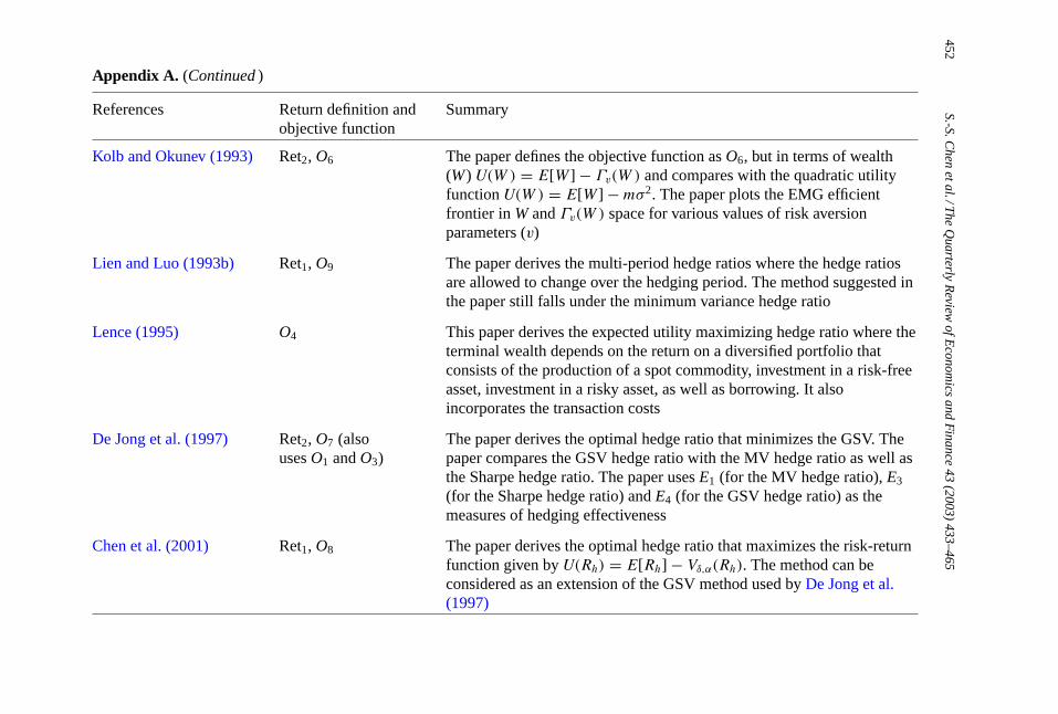
Kolb and Okunev (1993) Ret2, O6 The paper defines the objective function asO6, but in terms of wealth(W) U(W ) = E[W ] − Γv(W ) and compares with the quadratic utilityfunctionU(W ) = E[W ] −mσ2. The paper plots the EMG efficientfrontier in W andΓv(W ) space for various values of risk aversionparameters (v)

Lien and Luo (1993b) Ret1, O9 The paper derives the multi-period hedge ratios where the hedge ratiosare allowed to change over the hedging period. The method suggested inthe paper still falls under the minimum variance hedge ratio

Lence (1995) O4 This paper derives the expected utility maximizing hedge ratio where theterminal wealth depends on the return on a diversified portfolio thatconsists of the production of a spot commodity, investment in a risk-freeasset, investment in a risky asset, as well as borrowing. It alsoincorporates the transaction costs

De Jong et al. (1997) Ret2, O7 (alsousesO1 andO3)

The paper derives the optimal hedge ratio that minimizes the GSV. Thepaper compares the GSV hedge ratio with the MV hedge ratio as well asthe Sharpe hedge ratio. The paper usesE1 (for the MV hedge ratio),E3

(for the Sharpe hedge ratio) andE4 (for the GSV hedge ratio) as themeasures of hedging effectiveness

Chen et al. (2001) Ret1, O8 The paper derives the optimal hedge ratio that maximizes the risk-returnfunction given byU(Rh) = E[Rh] − Vδ,α(Rh). The method can beconsidered as an extension of the GSV method used byDe Jong et al.(1997)

S.-S.Chen

etal./The

Quarterly

Review

ofEconom

icsand

Finance

43(2003)

433–465453

Notes:

A. Return model

(Ret1) VH = Cs Ps + Cf Pf ⇒ hedge ratio= H = Cf

Cs, Cs = units of spot commodity and

Cf = units of futures contract

(Ret2) Rh = Rs + hRf , Rs = St − St−1

St−1, (a)Rf = Ft − Ft−1

Ft−1⇒ hedge ratio :h = CfFt−1

CsSt−1,

(b) Rf = Ft − Ft−1

St−1⇒ hedge ratio :h = Cf

Cs.

B. Objective function(O1) Minimize Var(Rh) = C2

s σ2s + C2

f σ2f + 2CsCfσsf or Var(Rh) = σ2

s + h2σ2f + 2hσsf

(O2) Maximize E(Rh)− A12 Var(Rh)

(O3) MaximizeE(Rh)− RF

Var(Rh)(Sharpe ratio),RF = risk-free interest rate

(O4) Maximize E[U(W )], U(·) = utility function,W = terminal wealth(O5) Minimize Γv(Rh), Γv(Rh) = −vCov(Rh, (1 − F(Rh))v−1)

(O6) Maximize E[Rh] − Γv(Rhv)(O7) Minimize Vδ,α(Rh) = ∫ δ

−∞(δ− Rh)α dG(Rh), α > 0(O8) Maximize U(Rh) = E[Rh] − Vδ,α(Rh)(O9) Minimize Var(Wt) = Var

(∑Tt=1Cs,t St + Cf,t F

).

C. Hedging effectiveness

(E1) e = 1 − Var(Rh)

Var(Rs)

(E2) e = Rceh − Rce

ss , Rceh (R

ces ) = certainty equivalent return of hedged (unhedged) portfolio

(E3) e = (E[Rh] − RF)/Var(Rh)

(E[Rs] − RF)/Var(Rs)or e = E[Rh] − RF

Var(Rh)− E[Rs] − RF

Var(Rs)

(E4) e = 1 − Vδ,α(Rh)Vδ,α(Rs)

.

454S.-S.C

henetal./T

heQ

uarterlyR

eviewofE

conomics

andF

inance43

(2003)433–465

Appendix B. Empirical models

References Commodity Summary

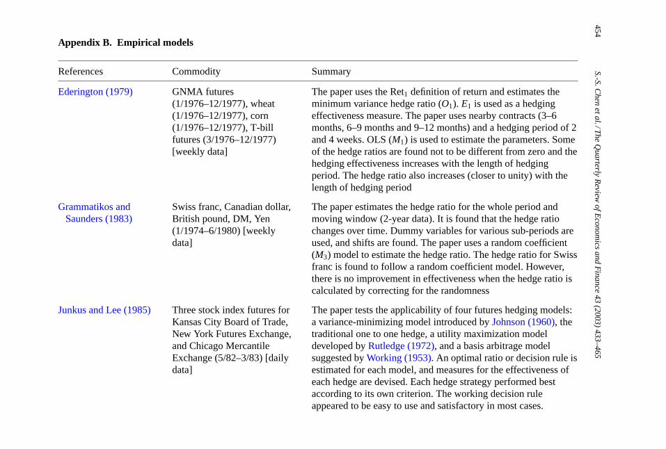
Ederington (1979) GNMA futures(1/1976–12/1977), wheat(1/1976–12/1977), corn(1/1976–12/1977), T-billfutures (3/1976–12/1977)[weekly data]

The paper uses the Ret1 definition of return and estimates theminimum variance hedge ratio (O1). E1 is used as a hedgingeffectiveness measure. The paper uses nearby contracts (3–6months, 6–9 months and 9–12 months) and a hedging period of 2and 4 weeks. OLS (M1) is used to estimate the parameters. Someof the hedge ratios are found not to be different from zero and thehedging effectiveness increases with the length of hedgingperiod. The hedge ratio also increases (closer to unity) with thelength of hedging period

Grammatikos andSaunders (1983)

Swiss franc, Canadian dollar,British pound, DM, Yen(1/1974–6/1980) [weeklydata]

The paper estimates the hedge ratio for the whole period andmoving window (2-year data). It is found that the hedge ratiochanges over time. Dummy variables for various sub-periods areused, and shifts are found. The paper uses a random coefficient(M3) model to estimate the hedge ratio. The hedge ratio for Swissfranc is found to follow a random coefficient model. However,there is no improvement in effectiveness when the hedge ratio iscalculated by correcting for the randomness

Junkus and Lee (1985) Three stock index futures forKansas City Board of Trade,New York Futures Exchange,and Chicago MercantileExchange (5/82–3/83) [dailydata]

The paper tests the applicability of four futures hedging models:a variance-minimizing model introduced byJohnson (1960), thetraditional one to one hedge, a utility maximization modeldeveloped byRutledge (1972), and a basis arbitrage modelsuggested byWorking (1953). An optimal ratio or decision rule isestimated for each model, and measures for the effectiveness ofeach hedge are devised. Each hedge strategy performed bestaccording to its own criterion. The working decision ruleappeared to be easy to use and satisfactory in most cases.

S.-S.Chen

etal./The

Quarterly

Review

ofEconom

icsand

Finance

43(2003)

433–465455

Although the maturity of the futures contract used affected the sizeof the optimal hedge ratio, there was no consistent maturity effect onperformance. Use of a particular ratio depends on how closely theassumptions underlying the model approach a hedger’s real situation

Lee et al. (1987) S&P 500, NYSE, Value Line(1983) [daily data]

The paper tests for the temporal stability of the minimum variancehedge ratio. It is found that the hedge ratio increases as maturity ofthe futures contract nears. The paper also performs a functionalform test and finds support for the regression of rate of change fordiscrete as well as continuous rates of change in prices

Cecchetti et al. (1988) Treasury bond, Treasury bondfutures (1/1978–5/1986)[monthly data]

The paper derives the hedge ratio by maximizing the expectedutility. A third-order linear bivariate ARCH model is used to get theconditional variance and covariance matrix. A numerical procedureis used to maximize the objective function with respect to the hedgeratio. Due to ARCH, the hedge ratio changes over time. It is foundthat the hedge ratio changes over time and is significantly less (inabsolute value) than the MV hedge ratio (which also changes overtime).E2 (certainty equivalent) is used to measure the performanceeffectiveness. The proposed utility-maximizing hedge ratioperforms better than the MV hedge ratio

Cheung et al. (1990) Swiss franc, Canadian dollar,British pound, German mark,Japanese yen(9/1983–12/1984) [daily data]

The paper uses mean-Gini coefficient (v = 2) and mean-varianceapproaches to analyze the effectiveness of options and futures ashedging instruments. It considers both mean-variance andexpected-return mean-Gini coefficient frontiers. It also considers theMV and minimum mean-Gini coefficient hedge ratios. The MV andminimum mean-Gini approaches indicate that futures is a betterhedging instrument. However, the mean-variance frontier indicatesfutures to be a better hedging instrument whereas the mean-Ginifrontier indicates options to be a better hedging instrument

456S.-S.C

henetal./T

heQ

uarterlyR

eviewofE

conomics

andF

inance43

(2003)433–465

Appendix B. (Continued )


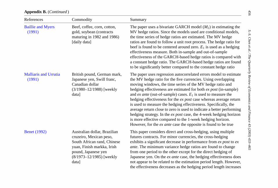
Baillie and Myers(1991)

Beef, coffee, corn, cotton,gold, soybean (contractsmaturing in 1982 and 1986)[daily data]

The paper uses a bivariate GARCH model (M2) in estimating theMV hedge ratios. Since the models used are conditional models,the time series of hedge ratios are estimated. The MV hedgeratios are found to follow a unit root process. The hedge ratio forbeef is found to be centered around zero.E1 is used as a hedgingeffectiveness measure. Both in-sample and out-of-sampleeffectiveness of the GARCH-based hedge ratios is compared witha constant hedge ratio. The GARCH-based hedge ratios are foundto be significantly better compared to the constant hedge ratio

Malliaris and Urrutia(1991)

British pound, German mark,Japanese yen, Swill franc,Canadian dollar(3/1980–12/1988) [weeklydata]

The paper uses regression autocorrelated errors model to estimatethe MV hedge ratio for the five currencies. Using overlappingmoving windows, the time series of the MV hedge ratio andhedging effectiveness are estimated for bothex post (in-sample)andex ante (out-of-sample) cases.E1 is used to measure thehedging effectiveness for theex post case whereas average returnis used to measure the hedging effectiveness. Specifically, theaverage return close to zero is used to indicate a better performinghedging strategy. In theex post case, the 4-week hedging horizonis more effective compared to the 1-week hedging horizon.However, for theex ante case the opposite is found to be true

Benet (1992) Australian dollar, Braziliancruzeiro, Mexican peso,South African rand, Chineseyuan, Finish markka, Irishpound, Japanese yen(8/1973–12/1985) [weeklydata]

This paper considers direct and cross-hedging, using multiplefutures contracts. For minor currencies, the cross-hedgingexhibits a significant decrease in performance fromex post to exante. The minimum variance hedge ratios are found to changefrom one period to the other except for the direct hedging ofJapanese yen. On theex ante case, the hedging effectiveness doesnot appear to be related to the estimation period length. However,the effectiveness decreases as the hedging period length increases

S.-S.Chen

etal./The

Quarterly

Review

ofEconom

icsand

Finance

43(2003)

433–465457

Kolb and Okunev(1992)

Corn, copper, gold, Germanmark, S&P 500 (1989) [dailydata]

The paper estimates the MEG hedge ratio (M9) with v rangingfrom 2 to 200. The MEG hedge ratios are found to be close to theminimum variance hedge ratios for a lower level of riskparameterv (for v from 2 to 5). For higher values ofv, the twohedge ratios are found to be quite different. The hedge ratios arefound to increase with the risk aversion parameter for S&P 500,corn, and gold. However, for copper and German mark, the hedgeratios are found to decrease with the risk aversion parameter. Thehedge ratio tends to be more stable for higher levels of risk

Kolb and Okunev(1993)

Cocoa (3/1952 to 1976) forfour cocoa-producingcountries (Ghana, Nigeria,Ivory Coast, and Brazil)[March and September data]

The paper estimates the M-MEG hedge ratio (M12). The papercompares the M-MEG hedge ratio, minimum variance hedgeratio, and optimum mean-variance hedge ratio for various valuesof risk aversion parameters. The paper finds that the M-MEGhedge ratio leads to reverse hedging (buy futures instead ofselling) forv less than 1.24 (Ghana case). For high-risk aversionparameter values (highv) all hedge ratios are found to convergeto the same value

Lien and Luo (1993a) S&P 500 (1/1984–12/1988)[weekly data]

The paper points out that the MEG hedge ratio can be calculatedeither by numerically optimizing the MEG coefficient or bynumerically solving the first-order condition. Forv = 9 the hedgeratio of−0.8182 is close to the MV hedge ratio of−0.8171.Using the first-order condition, the paper shows that for a largev

the MEG hedge ratio converges to a constant. The empiricalresult shows that the hedge ratio decreases with the risk aversionparameterv. The paper finds that the MV and MEG hedge ratio(for low v) series (obtained by using a moving window) are morestable compared to the MEG hedge ratio for a largev. The paperalso uses a non-parametric Kernel estimator to estimate thecumulative density function. However, the kernel estimator doesnot change the result significantly

458S.-S.C

henetal./T

heQ

uarterlyR

eviewofE

conomics

andF

inance43

(2003)433–465



Lien and Luo (1993b) British pound, Canadiandollar, German mark,Japanese yen, Swiss franc(3/1980–12/1988), MMI,NYSE, S&P(1/1984–12/1988) [weeklydata]

This paper proposes a multi-period model to estimate the optimalhedge ratio. The hedge ratios are estimated using anerror-correction model. The spot and futures prices are found tobe cointegrated. The optimal multi-period hedge ratios are foundto exhibit a cyclical pattern with a tendency for the amplitude ofthe cycles to decrease. Finally, the possibility of spreading amongdifferent market contracts is analyzed. It is shown that hedging ina single market may be much less effective than the optimalspreading strategy

Ghosh (1993) S&P futures, S&P index,Dow Jones industrial average,NYSE composite index(1/1990–12/1991) [daily data]

All the variables are found to have a unit root. For all threeindices the same S&P 500 futures contracts are used(cross-hedging). Using the Engle–Granger two-step test, the S&P500 futures price is found to be cointegrated with each of thethree spot prices: S&P 500, DJIA, and NYSE. The hedge ratio isestimated using the error-correction model (ECM) (M4).Out-of-sample performance is better for the hedge ratio from theECM compared to the Ederington model

Sephton (1993a) Feed wheat, canola futures(1981–1982 crop year) [dailydata]

The paper finds unit roots on each of the cash and futures (log)prices, but no cointegration between futures and spot (log) prices.The hedge ratios are computed using a four-variableGARCH(1,1) model. The time series of hedge ratios are found tobe stationary. Reduction in portfolio variance is used as ameasure of hedging effectiveness. It is found that theGARCH-based hedge ratio performs better compared to theconventional minimum variance hedge ratio

Sephton (1993b) Feed wheat, feed barley,canola futures (1988/1989)[daily data]

The paper finds unit roots on each of the cash and futures (log)prices, but no cointegration between futures and spot (log) prices.A univariate GARCH model shows that the mean returns on the

S.-S.Chen

etal./The

Quarterly

Review

ofEconom

icsand

Finance

43(2003)

433–465459

futures are not significantly different from zero. However, fromthe bivariate GARCH canola is found to have a significant meanreturn. For canola the mean-variance utility function is used tofind the optimal hedge ratio for various values of the risk aversionparameter. The time series of the hedge ratio (based on bivariateGARCH model) is found to be stationary. The benefit in terms ofutility gained from using a multi-variate GARCH decreases asthe degree of risk aversion increases

Kroner and Sultan(1993)

British pound, Canadiandollar, German mark,Japanese yen, Swiss franc(2/1985–2/1990) [weeklydata]

The paper uses the error-correction model with a GARCH error(M5) to estimate the MV hedge ratio for the five currencies. Dueto the use of conditional models, the time series of the MV hedgeratios are estimated. Both within-sample and out-of-sampleevidence shows that the hedging strategy proposed in the paper ispotentially superior to the conventional strategies

Hsin et al. (1994) British pound, German mark,Yen, Swiss franc(1/1986–12/1989) [daily data]

The paper derives the optimum mean-variance hedge ratio bymaximizing the objective functionO2. The hedging horizons of14, 30, 60, 90, and 120 calendar days are considered to comparethe hedging effectiveness of options and futures contracts. It isfound that the futures contracts perform better than the optionscontracts

Shalit (1995) Gold, silver, copper,aluminum (1/1977–12/1990)[daily data]

The paper shows that if the prices are jointly normallydistributed, the MEG hedge ratio will be same as the MV hedgeratio. The MEG hedge ratio is estimated using the instrumentalvariable method. The paper performs normality tests as well asthe tests to see if the MEG hedge ratios are different from the MVhedge ratios. The paper finds that for a significant number offutures contracts the normality does not hold and the MEG hedgeratios are different from the MV hedge ratios

460S.-S.C

henetal./T

heQ

uarterlyR

eviewofE

conomics

andF

inance43

(2003)433–465



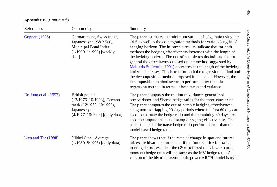
Geppert (1995) German mark, Swiss franc,Japanese yen, S&P 500,Municipal Bond Index(1/1990–1/1993) [weeklydata]

The paper estimates the minimum variance hedge ratio using theOLS as well as the cointegration methods for various lengths ofhedging horizon. The in-sample results indicate that for bothmethods the hedging effectiveness increases with the length ofthe hedging horizon. The out-of-sample results indicate that ingeneral the effectiveness (based on the method suggested byMalliaris & Urrutia, 1991) decreases as the length of the hedginghorizon decreases. This is true for both the regression method andthe decomposition method proposed in the paper. However, thedecomposition method seems to perform better than theregression method in terms of both mean and variance

De Jong et al. (1997) British pound(12/1976–10/1993), Germanmark (12/1976–10/1993),Japanese yen(4/1977–10/1993) [daily data]

The paper compares the minimum variance, generalizedsemivariance and Sharpe hedge ratios for the three currencies.The paper computes the out-of-sample hedging effectivenessusing non-overlapping 90-day periods where the first 60 days areused to estimate the hedge ratio and the remaining 30 days areused to compute the out-of-sample hedging effectiveness. Thepaper finds that the naıve hedge ratio performs better than themodel based hedge ratios

Lien and Tse (1998) Nikkei Stock Average(1/1989–8/1996) [daily data]

The paper shows that if the rates of change in spot and futuresprices are bivariate normal and if the futures price follows amartingale process, then the GSV (referred to as lower partialmoment) hedge ratio will be same as the MV hedge ratio. Aversion of the bivariate asymmetric power ARCH model is used

S.-S.Chen

etal./The

Quarterly

Review

ofEconom

icsand

Finance

43(2003)

433–465461

to estimate the conditional joint distribution, which is then usedto estimate the time varying GSV hedge ratios. The paper findsthat the GSV hedge ratio significantly varies over time and isdifferent from the MV hedge ratio

Lien and Shaffer(1999)

Nikkei (9/86–9/89), S&P(4/82–4/85), TOPIX(4/90–12/93), KOSPI(5/96–12/96), Hang Seng(1/87–12189), IBEX(4/93–3/95) [daily data]

This paper empirically tests the ranking assumption used byShalit (1995). The ranking assumption assumes that the rankingof futures prices is the same as the ranking of the wealth. Thepaper estimates the MEG hedge ratio based on the instrumentalvariable (IV) method used byShalit (1995)and the true MEGhedge ratio. The true MEG hedge ratio is computed using thecumulative probability distribution estimated employing thekernel method instead of the rank method. The paper finds thatthe MEG hedge ratio obtained from the IV method to be differentfrom the true MEG hedge ratio. Furthermore, the true MEGhedge ratio leads to a significantly smaller MEG coefficientcompared to the IV-based MEG hedge ratio

Lien and Tse (2000) Nikkei Stock Average(1/1988–8/996) [daily data]

The paper estimates the GSV hedge ratios for different values ofparameters using a non-parametric kernel estimation method.The kernel method is compared with the empirical distributionmethod. It is found that the hedge ratio from one method is notdifferent from the hedge ratio from another. TheJarque–Bera(1987)test indicates that the changes in spot and futures prices donot follow normal distribution

Chen et al. (2001) S&P 500 (4/982–12/1991)[weekly data]

The paper proposes the use of the M-GSV hedge ratio. The paperestimates the MV, optimum mean-variance, Sharpe, MEG, GSV,M-MEG, and M-GSV hedge ratios. TheJarque–Bera (1987)testandD’Agostino (1971)D Statistic indicate that the price changes

462S.-S.C

henetal./T

heQ

uarterlyR

eviewofE

conomics

andF

inance43

(2003)433–465



are not normally distributed. Furthermore, the expected value ofthe futures price change is found to be significantly different fromzero. It is also found that for a high level of risk aversion, theM-MEG hedge ratio converges to the MV hedge ratio whereasthe M-GSV hedge ratio converges to a lower value

Notes:

A. Minimum variance hedge ratioA.1. OLS

(M1): St = a0 + a1 Ft + et : hedge ratio= a1

Rs = a0 + a1Rf + et : hedge ratio= a1

A.2. ARCH/GARCH

(M2):

[ St

Ft

]=

[µ1

µ2

]+

[e1,t

e2,t

], et|Ωt−1 ∼ N(0, Ht), Ht =

[H11,t H12,t

H12,t H22,t

], hedge ratio= H12,t

H22,t

A.3. Random coefficient(M3): St = β0 + βt Ft + et

βt = β + vt, hedge ratio= βA.4. Cointegration and error-correction

(M4): St = a+ bFt + ut St = ρut−1 + β Ft +

∑mi=1δi Ft−i +

∑nj=1θi St−j + ej, hedge ratio= β

A.5. Error-correction with GARCH

(M5):

[ loge(St)

loge(Ft)

]=

[µ1

µ2

]+

[αs(loge(St−1)− loge(Ft−1))

αf (loge(St−1)− loge(Ft−1))

]+

[e1t

e2t

], et|Ωt−1 ∼ N(0, Ht),

Ht =[H11,t H12,t

H12,t H22,t

], hedge ratio= ht−1 = H12,t

H22,t

S.-S.Chen

etal./The

Quarterly

Review

ofEconom

icsand

Finance

43(2003)

433–465463

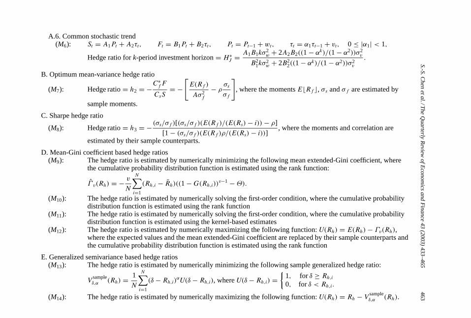
A.6. Common stochastic trend(M6): St = A1Pt + A2τt, Ft = B1Pt + B2τt, Pt = Pt−1 + wt, τt = α1τt−1 + vt, 0 ≤ |α1| < 1,

Hedge ratio fork-period investment horizon= H∗J = A1B1kσ

2w + 2A2B2((1 − αk)/(1 − α2))σ2

v

B21kσ

2w + 2B2

2((1 − αk)/(1 − α2))σ2v

.

B. Optimum mean-variance hedge ratio

(M7): Hedge ratio= h2 = −C∗fF

CsS= −

[E(Rf )

Aσ2f

− ρ σsσf

], where the momentsE Rf , σs andσf are estimated by

sample moments.

C. Sharpe hedge ratio

(M8): Hedge ratio= h3 = −(σs/σf )[(σs/σf )(E(Rf )/(E(Rs)− i))− ρ]

[1 − (σs/σf )(E(Rf )ρ/(E(Rs)− i))] , where the moments and correlation are

estimated by their sample counterparts.

D. Mean-Gini coefficient based hedge ratios(M9): The hedge ratio is estimated by numerically minimizing the following mean extended-Gini coefficient, where

the cumulative probability distribution function is estimated using the rank function:

Γ v(Rh) = − vN

N∑i=1

(Rh,i − Rh)((1 −G(Rh,i))v−1 −Θ).(M10): The hedge ratio is estimated by numerically solving the first-order condition, where the cumulative probability

distribution function is estimated using the rank function(M11): The hedge ratio is estimated by numerically solving the first-order condition, where the cumulative probability

distribution function is estimated using the kernel-based estimates(M12): The hedge ratio is estimated by numerically maximizing the following function:U(Rh) = E(Rh)− Γv(Rh),

where the expected values and the mean extended-Gini coefficient are replaced by their sample counterparts andthe cumulative probability distribution function is estimated using the rank function

E. Generalized semivariance based hedge ratios(M13): The hedge ratio is estimated by numerically minimizing the following sample generalized hedge ratio:

Vsampleδ,α (Rh) = 1

N

N∑i=1

(δ− Rh,i)αU(δ− Rh,i), whereU(δ− Rh,i) =

1, for δ ≥ Rh,i0, for δ < Rh,i.

(M14): The hedge ratio is estimated by numerically maximizing the following function:U(Rh) = Rh − V sampleδ,α (Rh).


References

Baillie, R. T., & Myers, R. J. (1991). Bivariate Garch estimation of the optimal commodity futures hedge.Journalof Applied Econometrics, 6, 109–124.

Bawa, V. S. (1978). Safety-first, stochastic dominance, and optimal portfolio choice.Journal of Financial andQuantitative Analysis, 13, 255–271.

Benet, B. A. (1992). Hedge period length andex ante futures hedging effectiveness: The case of foreign-exchangerisk cross hedges.Journal of Futures Markets, 12, 163–175.

Cecchetti, S. G., Cumby, R. E., & Figlewski, S. (1988). Estimation of the optimal futures hedge.Review of Economicsand Statistics, 70, 623–630.

Chen, S. S., Lee, C. F., & Shrestha, K. (2001). On a mean-generalized semivariance approach to determining thehedge ratio.Journal of Futures Markets, 21, 581–598.

Cheung, C. S., Kwan, C. C. Y., & Yip, P. C. Y. (1990). The hedging effectiveness of options and futures: A mean-Giniapproach.Journal of Futures Markets, 10, 61–74.

Chou, W. L., Fan, K. K., & Lee, C. F. (1996). Hedging with the Nikkei index futures: The conventional model versusthe error correction model.Quarterly Review of Economics and Finance, 36, 495–505.

Crum, R. L., Laughhunn, D. L., & Payne, J. W. (1981). Risk-seeking behavior and its implications for financialmodels.Financial Management, 10, 20–27.

D’Agostino, R. B. (1971). An omnibus test of normality for moderate and large size samples.Biometrika, 58,341–348.

De Jong, A., De Roon, F., & Veld, C. (1997). Out-of-sample hedging effectiveness of currency futures for alternativemodels and hedging strategies.Journal of Futures Markets, 17, 817–837.

Dickey, D. A., & Fuller, W. A. (1981). Likelihood ratio statistics for autoregressive time series with a unit root.Econometrica, 49, 1057–1072.

Ederington, L. H. (1979). The hedging performance of the new futures markets.Journal of Finance, 34, 157–170.Engle, R. F., & Granger, C. W. (1987). Co-integration and error correction: Representation, estimation and testing.

Econometrica, 55, 251–276.Fishburn, P. C. (1977). Mean-risk analysis with risk associated with below-target returns.American Economic

Review, 67, 116–126.Geppert, J. M. (1995). A statistical model for the relationship between futures contract hedging effectiveness and

investment horizon length.Journal of Futures Markets, 15, 507–536.Ghosh, A. (1993). Hedging with stock index futures: Estimation and forecasting with error correction model.Journal

of Futures Markets, 13, 743–752.Grammatikos, T., & Saunders, A. (1983). Stability and the hedging performance of foreign currency futures.Journal

of Futures Markets, 3, 295–305.Howard, C. T., & D’Antonio, L. J. (1984). A risk-return measure of hedging effectiveness.Journal of Financial and

Quantitative Analysis, 19, 101–112.Hsin, C. W., Kuo, J., & Lee, C. F. (1994). A new measure to compare the hedging effectiveness of foreign currency

futures versus options.Journal of Futures Markets, 14, 685–707.Hylleberg, S., & Mizon, G. E. (1989). Cointegration and error correction mechanisms.Economic Journal, 99,

113–125.Jarque, C. M., & Bera, A. K. (1987). A test for normality of observations and regression residuals.International

Statistical Review, 55, 163–172.Johansen, S., & Juselius, K. (1990). Maximum likelihood estimation and inference on cointegration—with

applications to the demand for money.Oxford Bulletin of Economics and Statistics, 52, 169–210.Johnson, L. L. (1960). The theory of hedging and speculation in commodity futures.Review of Economic Studies,

27, 139–151.Junkus, J. C., & Lee, C. F. (1985). Use of three index futures in hedging decisions.Journal of Futures Markets, 5,

201–222.Kolb, R. W., & Okunev, J. (1992). An empirical evaluation of the extended mean-Gini coefficient for futures hedging.

Journal of Futures Markets, 12, 177–186.


Kolb, R. W., & Okunev, J. (1993). Utility maximizing hedge ratios in the extended mean Gini framework.Journalof Futures Markets, 13, 597–609.

Kroner, K. F., & Sultan, J. (1993). Time-varying distributions and dynamic hedging with foreign currency futures.Journal of Financial and Quantitative Analysis, 28, 535–551.

Lee, C. F., Bubnys, E. L., & Lin, Y. (1987). Stock index futures hedge ratios: Test on horizon effects and functionalform. Advances in Futures and Options Research, 2, 291–311.

Lence, S. H. (1995). The economic value of minimum variance hedges.American Journal of Agricultural Economics,77, 353–364.

Lence, S. H. (1996). Relaxing the assumptions of minimum variance hedging.Journal of Agricultural and ResourceEconomics, 21, 39–55.

Lien, D., & Luo, X. (1993a). Estimating the extended mean-Gini coefficient for futures hedging.Journal of FuturesMarkets, 13, 665–676.

Lien, D., & Luo, X. (1993b). Estimating multiperiod hedge ratios in cointegrated markets.Journal of FuturesMarkets, 13, 909–920.

Lien, D., & Shaffer, D. R. (1999). Note on estimating the minimum extended Gini hedge ratio.Journal of FuturesMarkets, 19, 101–113.

Lien, D., & Tse, Y. K. (1998). Hedging time-varying downside risk.Journal of Futures Markets, 18, 705–722.Lien, D., & Tse, Y. K. (2000). Hedging downside risk with futures contracts.Applied Financial Economics, 10,

163–170.Malliaris, A. G., & Urrutia, J. L. (1991). The impact of the lengths of estimation periods and hedging horizons on

the effectiveness of a hedge: Evidence from foreign currency futures.Journal of Futures Markets, 3, 271–289.Myers, R. J., & Thompson, S. R. (1989). Generalized optimal hedge ratio estimation.American Journal of

Agricultural Economics, 71, 858–868.Osterwald-Lenum, M. (1992). A note with quantiles of the asymptotic distribution of the maximum likelihood

cointegration rank test statistics.Oxford Bulletin of Economics and Statistics, 54, 461–471.Phillips, P. C. B., & Perron, P. (1988). Testing unit roots in time series regression.Biometrika, 75, 335–346.Rutledge, D. J. S. (1972). Hedgers’ demand for futures contracts: A theoretical framework with applications to the

United States soybean complex.Food Research Institute Studies, 11, 237–256.Sephton, P. S. (1993a). Hedging wheat and canola at the Winnipeg commodity exchange.Applied Financial

Economics, 3, 67–72.Sephton, P. S. (1993b). Optimal hedge ratios at the Winnipeg commodity exchange.Canadian Journal of Economics,

26, 175–193.Shalit, H. (1995). Mean-Gini hedging in futures markets.Journal of Futures Markets, 15, 617–635.Stock, J. H., & Watson, M. W. (1988). Testing for common trends.Journal of the American Statistical Association,

83, 1097–1107.Working, H. (1953). Hedging reconsidered.Journal of Farm Economics, 35, 544–561.

futures hedge ratios: a review -...

Documents