fuzzy-based condition assessment model for offshore … · fuzzy-based condition assessment model...
TRANSCRIPT

FUZZY-BASED CONDITION ASSESSMENT MODEL FOR OFFSHORE GAS
PIPELINES IN QATAR
by
Fadi Mosleh
A Thesis
in
The Department
of
Building, Civil and Environmental Engineering
Presented in Partial Fulfillment of the Requirements
for the Degree of Master of Applied Science (Building Engineering) at
CONCORDIA UNIVERSITY
Montreal, Quebec, Canada
September, 2014
© Fadi Mosleh

II
CONCORDIA UNIVERSITY
School of Graduate Studies
This is to certify that the thesis prepared
By: Fadi Mosleh
Entitled: Fuzzy-based Condition Assessment Model
for Offshore Gas Pipelines in Qatar
and submitted in partial fulfillment of the requirements for the degree of
Master of Applied Science (Building Engineering)
complies with the regulations of the University and meets the accepted standards with respect
to originality and quality.
Signed by the final examining committee:
______________________________________ Chair
Dr. O Moselhi
______________________________________ Examiner
Dr. A. Hammad
______________________________________ Examiner
Dr. Z. Zhu
______________________________________ Supervisor
Dr. T. Zayed
Approved by ________________________________________________
Chair of Department or Graduate Program Director
Sep. 15th 2014 ________________________________________________
Dean of Faculty

III
ABSTRACT
Fuzzy-based Condition Assessment Model for Offshore Gas Pipelines in Qatar
Fadi Mosleh
Condition assessment of offshore gas pipelines is a key player in pipeline operations and
maintenance. They are used to ensure better decisions for repair and/or replacement and
reduce failure possibilities. Information obtained from pipelines assessments are regularly
used for scheduling upcoming maintenance and inspection activities. Therefore, it is valuable
to have effective condition assessment of pipelines because failure incidents could lead to
catastrophic economical and environmental consequences. Furthermore, current practices of
assessing gas pipelines condition are considered too primitive and simplified. They mainly
depend on experts' opinions in interpreting inspection data where the process is influenced by
the human subjectivity and reasoning uncertainty. In another way, they need the detailed
knowledge on translation of raw inspection data into valuable information. This will surely
lead to decisions lacking thorough and extensive review of the most influential aspects on
pipelines condition.
To redress the weaknesses of the current practices and promote the performance of assessing
offshore gas pipelines condition, this research proposes a new fuzzy-based methodology that
utilizes hierarchical evidential reasoning (HER) for meticulous condition evaluation under
subjectivity and uncertainty. The principle behind the posed structure is to establish an
enhanced mechanism for the aggregation of different evidence bodies at multiple hierarchical
levels in order to attain a reliable and exhaustive pipeline condition assessment. The essential
characteristics of the proposed methodology are recapped in the following points. Firstly, the
IV
new approach suggests a more comprehensive hierarchy of the most influential factors
affecting pipeline condition under three categories: physical, external, and operational.
Secondly, this methodology is designed to consider the relative importance weights of all
assessment factors in the hierarchy and to account for interdependencies among compared
attributes. Thirdly, a hierarchical belief structure that utilizes evidential reasoning and fuzzy
set theory is applied to grasp the uncertainty in pipeline evaluation. A model that utilizes
HER can help combine different bodies of evidence at different hierarchical levels using
Dempster-Shafer (D-S) rule of combination to obtain a detailed pipeline assessment.
Fourthly, a condition assessment scale associated with rehabilitation actions is introduced as
a framework for professionals to plan for future inspection and rehabilitation works. Finally,
an automated, user-friendly, tool is developed for the propounded model to assess pipeline
condition. Multiple sources of data were reached to provide a reliable assessment of pipe
condition through the use of a structured questionnaire distributed among professionals in oil
and gas industry in the studied region. This proposed model is compared and validated with
historical inspection reports that were obtained from a local pipeline operator in Qatar. It is
found that this model delivers satisfactory outcomes and forecasts offshore gas pipeline
condition with an Average Validity Percent (AVP) of 97.6%.
The developed fuzzy-based methodology is believed to offer a reliable condition assessment
that optimizes data interpretation and usage of structured algorithms. Additionally, the
introduced model and tool are compatible to researchers and practitioners such as pipeline
engineers and consultants in order to prioritize inspection and rehabilitation for existing
offshore gas pipelines. This immensely pictures the essence of infrastructure management to
ameliorate cost and time optimization.

V
ACKNOWLEDGEMENTS
At first, I want to thank Almighty God for giving me the health and energy along with the
needed guidance and persistence for carrying out my Master program.
I wish to express my sincere gratitude and appreciation to my mentor and supervisor, Dr.
Tarek Zayed, for his continuous support, patience, motivation, enthusiasm and guidance
throughout the course of this study. His valuable advice and commitment exceeded my
expectations and extended far beyond formalities. Since I became his student and up to now,
I have gained vast knowledge in many aspects of life academically and professionally.
Besides my advisor, I have to acknowledge all my colleagues for their support throughout my
studies. Special thanks are given for all the Staff and Faculty members at the Department of
Building, Civil and Environmental Engineering at Concordia University
My deepest gratitude is for my wonderful parents who supported me spiritually throughout
my life and without their love and encouragement, I would not reach what I achieved so far.
Never ending thanks to Dr. Ahmed Senouci from Qatar University for giving me this
opportunity to achieve my academic goals. I thank you all for your guidance, support and
encouragement materially and morally.
Also, I owe more than thanks to Eng. Mohammed El-Abbasy for his valuable assistance,
support and encouragement. His friendship is another achievement of the past two years in
this program.
Last but not the least, I would like also to extend my gratitude to Qatar University and its
faculty members in the Architecture and Civil Engineering Department for providing me with
the necessary technical knowledge to complete this Master program.

VI
Table of Contents
LIST OF FIGURES ............................................................................................................. IX
LIST OF TABLES ............................................................................................................... XI
LIST OF ABBREVIATIONS .......................................................................................... XIII
CHAPTER ONE: INTRODUCTION ................................................................................... 1
1.1 Overview .......................................................................................................................... 1
1.2 Current Practices .............................................................................................................. 2
1.2.1 Pipeline Condition Assessment in Qatar .................................................................... 3
1.2.2 Condition Rating Procedure in Qatar ......................................................................... 4
1.3 Problem Statement ........................................................................................................... 7
1.4 Research Objectives ......................................................................................................... 8
1.5 Research Methodology ..................................................................................................... 9
1.5.1 Literature Review ....................................................................................................... 9
1.5.2 Data Collection ........................................................................................................... 9
1.5.3 Model Development and Analysis ............................................................................ 10
1.6 Thesis Layout ................................................................................................................. 10
CHAPTER TWO: LITERATURE REVIEW ................................................................... 12
2.1 Introduction .................................................................................................................... 12
2.2 Oil and Gas Pipelines Network in Qatar ........................................................................ 15
2.3 Oil and Gas Pipeline Design and Material ..................................................................... 20
2.4 Analytic Network Process (ANP) .................................................................................. 21
2.4.1 ANP Application ...................................................................................................... 22
2.4.2 ANP Technique ........................................................................................................ 23
2.4.3 ANP Software ........................................................................................................... 26
2.5 Fuzzy Set Theory ........................................................................................................... 26
2.5.1 Fuzzy Sets Shapes ..................................................................................................... 28
2.5.2 Fuzzification and Defuzzification ............................................................................. 29
2.6 Evidential Reasoning (ER) Approach ............................................................................ 33
2.6.1 Theory of Evidence ................................................................................................... 33
2.6.2 ER Application ......................................................................................................... 34
2.6.3 ER Technique ........................................................................................................... 35
2.7 Factors Affecting Offshore Gas Pipelines ...................................................................... 41
2.8 Infrastructure Condition Assessment Models ................................................................ 44
VII
2.8.1 Oil & Gas Pipelines .................................................................................................. 44
2.8.2 Water Pipelines ......................................................................................................... 45
2.8.3 Sewer Pipelines ......................................................................................................... 46
2.9 Summary ........................................................................................................................ 46
CHAPTER THREE: RESEARCH METHODOLOGY ................................................... 48
3.1 Introduction .................................................................................................................... 48
3.2 Literature Review ........................................................................................................... 48
3.3 Data Collection ............................................................................................................... 49
3.4 Condition Assessment Scale .......................................................................................... 51
3.5 Model Development ....................................................................................................... 51
3.5.1 Factors Relative Weights Using ANP ...................................................................... 51
3.5.2 Threshold Determination Using Fuzzy Set Theory .................................................. 53
3.5.3 Degree of Belief Determination Using ER ............................................................... 55
3.5.4 Integrated Condition Assessment Model .................................................................. 56
3.5.5 Defuzzification and Model Validation ..................................................................... 57
3.5.6 Sensitivity Analysis .................................................................................................. 58
3.5.7 Deterioration Curve .................................................................................................. 58
3.6 Condition Assessment Automated Tool ......................................................................... 58
3.7 Summary ........................................................................................................................ 59
CHAPTER FOUR: DATA COLLECTION ...................................................................... 61
4.1 Introduction .................................................................................................................... 61
4.2 Structured Questionnaire ................................................................................................ 63
4.3 Historical Inspection Data .............................................................................................. 66
CHAPTER FIVE: MODEL DEVELOPMENT ................................................................ 69
5.1 Introduction .................................................................................................................... 69
5.2 Relative Weight Determination ...................................................................................... 71
5.3 Fuzzy-based Threshold Model Implementation ............................................................. 78
5.3.1 Developing Membership Functions .......................................................................... 78
5.4 Degree of Belief ER-Based Model Implementation ...................................................... 88
5.5 Defuzzification and Model Validation ........................................................................... 90
5.5.1 Results of Defuzzification Process ........................................................................... 90
5.5.2 Model Validation ...................................................................................................... 91
5.5.3 Results Discussion .................................................................................................... 94
5.6 Sensitivity Analysis ........................................................................................................ 97
VIII
5.7 Development of Pipeline Deterioration Curve ............................................................. 106
5.8 Condition Assessment Scale ........................................................................................ 107
5.8.1 Proposed Condition Rating Scale ........................................................................... 107
5.9 Summary ...................................................................................................................... 109
CHAPTER SIX: CONDITION ASSESSMENT AUTOMATED TOOL...................... 112
6.1 Introduction .................................................................................................................. 112
6.2 Automated Fuzzy-based Tool Framework ................................................................... 112
6.3 Fuzzy-based Condition Evaluator Process ................................................................... 113
6.4 Summary ...................................................................................................................... 122
CHAPTER SEVEN: SUMMARY, CONCLUSIONS AND RECOMMENDATIONS 124
7.1 Summary and Conclusion ............................................................................................ 124
7.2 Research Contributions ................................................................................................ 126
7.3 Research Limitations .................................................................................................... 127
7.4 Future Recommendations ............................................................................................. 127
REFERENCES ................................................................................................................... 130
APPENDIX (A) ................................................................................................................... 137
APPENDIX (B) ................................................................................................................... 145

IX
LIST OF FIGURES
Figure 2 - 1: Variations in Yield Strength and Toughness of Older Linepipes Steels in the
USA.......................................................................................................................................... 15
Figure 2 - 2: Total Energy Consumption in Qatar 2010 .......................................................... 16
Figure 2 - 3: OPEC Crude Oil Production in 2011 .................................................................. 17
Figure 2 - 4: Natural Gas Proven Reserves by Country in 2012. ............................................ 18
Figure 2 - 5: Interdependencies in ANP. ................................................................................. 25
Figure 2 - 6: Fuzzy Sets Representation. ................................................................................. 29
Figure 2 - 7: Typical fuzzy process output: (a) first part of fuzzy output; (b) second part of
fuzzy output; and (c) union of both parts. ................................................................................ 30
Figure 2 - 8: Centroid Defuzzification Method. ...................................................................... 31
Figure 2 - 9: Weighted-Average Defuzzification Method. ...................................................... 31
Figure 2 - 10: Mean-Max membership Defuzzification Method. ............................................ 32
Figure 2 - 11: Center of sums method: (a) First Membership Function; (b) Second
Membership Function; and (c) Defuzzification Step. .............................................................. 33
Figure 2 - 12: Hierarchy of Factors Affecting Offshore Gas Pipelines Condition. ................. 42
Figure 3 - 1: Research Methodology. ...................................................................................... 50
Figure 3 - 2: ANP Technique Methodology ............................................................................ 53
Figure 3 - 3: Fuzzy Set Theory Methodology. ......................................................................... 54
Figure 3 - 4: Evidential Reasoning (ER) Methodology. .......................................................... 55
Figure 4 - 1: Distributed Questionnaires. ................................................................................. 62
Figure 4 - 2: ANP Framework in Distributed Questionnaires. ................................................ 64
Figure 4 - 3: Example of Pair-Wise Comparison in Distributed Questionnaires. ................... 64
Figure 4 - 4: Example of Determining the Score of Factors in Distributed Questionnaires. ... 65
Figure 4 - 5: Example of Gas Pipeline Condition Index. ......................................................... 66
Figure 5 - 1: ANP Network for Offshore Gas Pipelines. ......................................................... 72
Figure 5 - 2: Fuzzy Input Variable (Age). ............................................................................... 82
Figure 5 - 3: Fuzzy Input Variable (Diameter). ....................................................................... 82
Figure 5 - 4: Fuzzy Input Variable (Metal Loss). .................................................................... 83
Figure 5 - 5: Fuzzy Input Variable (Coating Condition). ........................................................ 83
X
Figure 5 - 6: Fuzzy Input Variable (Crossing). ........................................................................ 84
Figure 5 - 7: Fuzzy Input Variable (Cathodic Protection Effectiveness). ................................ 84
Figure 5 - 8: Fuzzy Input Variable (Marine Route Existence). ............................................... 85
Figure 5 - 9: Fuzzy Input Variable (Water Depth). ................................................................. 85
Figure 5 - 10: Fuzzy Input Variable (Corrosive Impurities). ................................................... 86
Figure 5 - 11: Fuzzy Input Variable (Operating Pressure). ..................................................... 86
Figure 5 - 12: Fuzzy Input Variable (Flow Rate). ................................................................... 87
Figure 5 - 13: Fuzzy Output Variable (Overall Condition). .................................................... 88
Figure 5 - 14: Centroid Defuzzification (Plausibility). ............................................................ 96
Figure 5 - 15: Sensitivity Analysis for Physical Factors.......................................................... 98
Figure 5 - 16: Sensitivity Analysis for External Factors .......................................................... 99
Figure 5 - 17: Sensitivity Analysis for Operational Factors. ................................................... 99
Figure 5 - 18: Directly Proportional Factors. ......................................................................... 100
Figure 5 - 19: Inversely Proportional Factors. ....................................................................... 101
Figure 5 - 20: Irregularly Proportional Factors. ..................................................................... 102
Figure 5 - 21: Predicted Deterioration Curve for Offshore Gas Pipeline. ............................. 106
Figure 6 - 1: Flowchart of the Condition Assessment Automated Tool System. .................. 114
Figure 6 - 2: Welcome Page and Contributing Factors.......................................................... 115
Figure 6 - 3: Contributing Factors Description. ..................................................................... 116
Figure 6 - 4: ANP Weights Selection (Default Vs Customized). .......................................... 116
Figure 6 - 5: Generate Customized Weights - SuperDecisions File. ..................................... 117
Figure 6 - 6: Generate Customized Weights - Priorities Table Explanation. ........................ 118
Figure 6 - 7: Generate Customized Weights - Final ANP Weights (1). ................................ 119
Figure 6 - 8: Generate Customized Weights - Final ANP Weights (2) ................................. 119
Figure 6 - 9: Generate Customized Weights - Final Report. ................................................. 121
Figure 6 - 10: Use Default Weights - Final Report. ............................................................... 122

XI
LIST OF TABLES
Table 1 - 1: External Corrosion Growth. ................................................................................... 5
Table 2 - 1: Profile of Oil and Gas Industry in Qatar .............................................................. 18
Table 2 - 2: Dolphin Pipeline Specification. ............................................................................ 20
Table 2 - 3: Inspection Interval for Dolphin Pipeline .............................................................. 20
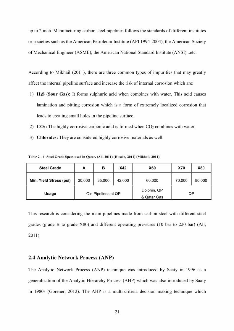
Table 2 - 4: Steel Grade Specs used in Qatar........................................................................... 21
Table 2 - 5: Acceptable CR Values.......................................................................................... 24
Table 2 - 6: ER Algorithm Process as described in (Yang & Xu, 2002). ................................ 39
Table 2 - 7: Explanation of Factors Affecting Offshore Gas Pipelines. .................................. 43
Table 4 - 1: Distributed Questionnaires. .................................................................................. 62
Table 4 - 2: Details of Questionnaire Respondents. ................................................................ 62
Table 4 - 3: Details of Received Inspection Reports. .............................................................. 67
Table 5 - 1: Developed Unweighted Super-Matrix for Response (1) of Received
Questionnaires.......................................................................................................................... 74
Table 5 - 2: Developed Weighted Super-Matrix for Response (1) of Received Questionnaires.
.................................................................................................................................................. 75
Table 5 - 3: Developed Limit Super-Matrix for Response (1) of Received Questionnaires. .. 76
Table 5 - 4: Preliminary and Final Local Weights developed from the Limit Super-matrix for
Response (1)............................................................................................................................. 77
Table 5 - 5: Final Local and Global Weights for Main Categories and factors affecting
Offshore Gas Pipeline Condition. ............................................................................................ 78
Table 5 - 6: Physical Factors Thresholds. ................................................................................ 80
Table 5 - 7: External Factors Thresholds. ................................................................................ 81
Table 5 - 8: Operational Factors Thresholds............................................................................ 81
Table 5 - 9: Proposed Condition Rating Scale. ........................................................................ 87
Table 5 - 10: Adjusted Global Weights for factors affecting Offshore Gas Pipeline Condition
for Model Validation................................................................................................................ 92
Table 5 - 11: Validation Results. ............................................................................................. 94
Table 5 - 12: Factors' Normalization. ...................................................................................... 98
Table 5 - 13: Sensitivity Analysis (ANP Global Weights Vs Condition Difference). .......... 105

XII
Table 5 - 14: Proposed Condition Rating Scale. .................................................................... 108
Table 5 - 15: Numeric and Linguistic Scale for Condition Rating of Offshore Gas Pipelines.
................................................................................................................................................ 110

XIII
LIST OF ABBREVIATIONS
AHP Analytic Hierarchy Process
AIP Average Invalidity Percent
ANP Analytic Network Process
ANSI American National Standard Institute
API American Petroleum Institute
ASME American Society of Mechanical Engineers
ASTM American Society of Testing Materials
AVP Average Validity Percent
Ci Actual Value
CR Consistency Ratio
DOT Department of Transportation, USA
DS Dempster-Shafer Theory of Belief-Function
ei Basic Attribute
Ei Estimated Value
ER Evidential Reasoning
fi Fit Index
FRP Fiber-Reinforced Polymer
FTA Fault Tree Analysis
GE General Electric
H Distinctive Evaluation Grade
ILI Inline Inspection
Kl(i+1) Normalizing Factor
XIV
LNG Liquefied Natural Gas
MAE Mean Absolute Error
MAOP Maximum Allowable Operating Pressure
MCDM Multi-Criteria Decision Making
MFL Magnetic Flux Inspection
mn, i Basic Probability Mass
OPEC Organization of Petroleum Exporting Countries
QatarGas Operating Company Limited
QP Qatar Petroleum
RasGas Ras Laffan Company Limited
RBIM Risk Based Inspection and Maintenance
RMSE Root Mean Squared Error
ROV Remote Operated Vehicle Inspection
S(ei) Assessment
Tcf Trillion Cubic Feet
X Universe of Discourse
y General Attribute
yA (x) Degree of Membership
z* Defuzzified Value
βn Degree of Belief
ωi Weight
1
CHAPTER ONE: INTRODUCTION
1.1 Overview
Pipelines are considered the basic transportation tool of oil and gas worldwide. They
transport various types of products that are worth billions of dollars either offshore or
onshore. The first pipeline network was constructed in the late 19th century in Pennsylvania in
the US. It was used to transport crude oil from an oil field in Pennsylvania to a railroad
station in Oil Creek and it was 109 miles long and had a diameter of 6 inches. Nowadays,
more than 60 countries worldwide operate pipelines networks of around 2000 km long where
the longest pipeline network is operated by the US, Russia and Canada (Goodland, 2005). Oil
and natural gas is being transported between continents by large diameter pipelines. For
example, the Russian system has diameters up to 1422mm, and can be over 1000km in length
(Hopkins, 2007). Pipelines are the most economical way to transport crude oil, natural gas
and refined oil products. They are much safer than usual methods of transporting such as
railroad or ships. On the other hand, a pipeline accident can cause environmental disasters
and economical losses.
The worldwide demand for energy is causing the oil and gas industry to increase and get even
bigger with time. This is due to certain facts such as the prediction of World Energy of the
US Energy Information which states that the fossil fuels will remain the primary sources of
energy, meeting more than 90% of the increase in future energy demand. Also, estimates
showed that global oil demand will rise by about 1.6% per year, from 75 millions of barrels
of oil per day (mb/d) in 2000, to 120 mb/d in 2030 and the demand for natural gas will rise
more strongly than any other fossil fuel (Hopkins, 2007).

2
The fact that the oil and gas pipelines carry hazardous products and operate in various
environments leads to the importance of constructing a safe and sound pipelines network.
Also, regular inspections and maintenance must be provided to ensure the pipelines structural
safety and prevent any future failures. The oil and gas pipelines are designed, constructed and
operated according to recognized standards that mainly focus on safety. In addition, to ensure
these pipelines are safe and secure, they have to satisfy the high standards and safety
regulations in the place where they are being constructed since the surrounding environment
changes from a country to another around the globe (Hopkins, 2007). In order to maintain the
safety of operated pipelines, several inspection practices were developed in the recent years
such as Magnetic Flux Leakage (MFL) and Ultrasound (UT). These inspection techniques
could provide accurate and effective tools to detect any defects in the pipelines that could
cause any failure in the future. Another inspection is the In Line Inspection (ILI) which could
clearly detect oil pipeline anomalies. The problem is that regular inspections are time
consuming and cost millions of dollars every year.
1.2 Current Practices
Condition assessment is very necessary for operating pipelines to evaluate their performance
along their age. Also, they need to be monitored continuously by inspections. The type and
frequency of these inspections are determined by the condition of the pipelines. This is
performed to address the integrity for aging pipeline both economically and environmentally.
Several methods have been used to predict the condition of oil and gas pipelines over the last
years. Researchers introduced many techniques such as Analytic Hierarchy Process (AHP),
Analytic Network Process (ANP), Fuzzy Sets Theory and Evidential Reasoning (ER) plus
other various techniques. All these techniques were used somehow in the development of
models that predict condition assessment of oil and gas pipelines. However, these models

3
used one or two criteria to evaluate a pipeline condition. For example, Kale et al. (2004)
developed a probabilistic model that is based on internal corrosion direct assessment (ICDA)
to predict the most probable corrosion damage location along the gas pipelines. This model
focused on evaluating pipelines from corrosion point of view. Another example is when
Bersani et al. (2010) used historical data from Department of Transportation (DOT) in the US
to develop a risk assessment model that predicts the failure caused by third party activities.
Many other models followed the same pattern where only one or two influential factors were
considered.
1.2.1 Pipeline Condition Assessment in Qatar
Researchers have developed some software programs that are used to assess the condition of
oil and gas pipelines such as ORBIT+ developed by Det Norske Veritas (DNV) and
PIPEVIEWER developed by General Electric (GE). According to the pipeline condition,
these programs suggest inspection frequency in order to know the possibility of service life
extension of the considered pipeline. These software programs use risk analysis which is
mainly based on experts’ opinion (Mikhail, 2011). Unfortunately, all the developed software
programs used in pipeline condition assessment depend greatly on experience and
professionals' feedback.
Pipeline operators around the world face many challenges when it comes to condition
assessment of oil and gas pipelines. According to Ali (2011), the main challenges that face
Qatar regarding condition assessment of pipelines are:
1) Almost 20% of Qatar's pipelines are not suitable for inline inspection (Unpiggable).
2) Lack of data and the absence of data management, especially for pipelines constructed
before 1990.
4
1.2.2 Condition Rating Procedure in Qatar
According to Hashiha (2011), General Electric (GE) services are used by most pipelines
operators in Qatar to perform pipeline inspections and post-inspection programs. GE is
considered one of the leading companies in the field of oil and gas pipeline inspection. It also
suggests post-inspection programs which are based on risk analysis. These post-inspection
programs contain many features such as future inspections frequency, corrosion growth and
remaining strength as discussed in the following points.
1) Pipeline Remaining Strength
Inline Inspection (ILI) results on the discovery of multiple and various types of defects and
threats to operating pipelines. So, pipeline operators require a cost-effective and safe solution
to process the many information received from these inspection reports (General Electric,
2013). That is why, the most threatening metal loss areas are compared with the maximum
allowable rate. These rates are determined by pipeline codes and design criteria. ASME 31.G
and DNV RP 101 are the most used codes to calculate the remaining strength of operating
pipelines (Hopkins, 2002). Newly installed pipelines have maximum allowable operation
pressure (MAOP) but after performing the remaining strength calculations, a new MAOP is
determined according to the results of these calculations. According to two experts in oil and
gas industry, two examples are given below to respond to remaining strength calculations
with respect to pipeline operating pressure:
a) No maintenance will be needed in case that the pipeline operating pressure is below
the calculated maximum allowable pressure after considering the safety factor. Future
inspections are scheduled according to corrosion growth calculations and risk analysis
(Mikhail, 2011).
5
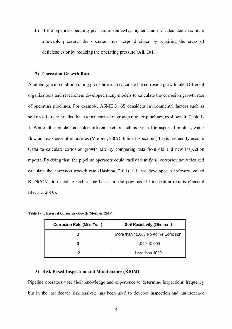
b) If the pipeline operating pressure is somewhat higher than the calculated maximum
allowable pressure, the operator must respond either by repairing the areas of
deficiencies or by reducing the operating pressure (Ali, 2011).
2) Corrosion Growth Rate
Another type of condition rating procedure is to calculate the corrosion growth rate. Different
organizations and researchers developed many models to calculate the corrosion growth rate
of operating pipelines. For example, ASME 31.8S considers environmental factors such as
soil resistivity to predict the external corrosion growth rate for pipelines, as shown in Table 1-
1. While other models consider different factors such as type of transported product, water
flow and existence of impurities (Morbier, 2009). Inline Inspection (ILI) is frequently used in
Qatar to calculate corrosion growth rate by comparing data from old and new inspection
reports. By doing that, the pipeline operators could easily identify all corrosion activities and
calculate the corrosion growth rate (Hashiha, 2011). GE has developed a software, called
RUNCOM, to calculate such a rate based on the previous ILI inspection reports (General
Electric, 2010).
Table 1 - 1: External Corrosion Growth (Morbier, 2009).
Corrosion Rate (Mils/Year) Soil Resistivity (Ohm-cm)
3 More than 15,000 No Active Corrosion
6 1,000-15,000
12 Less than 1000
3) Risk Based Inspection and Maintenance (RBIM)
Pipeline operators used their knowledge and experience to determine inspections frequency
but in the last decade risk analysis has been used to develop inspection and maintenance

6
schedules based on priority (Mikhail, 2011). American Society of Mechanical Engineers
(ASME), American Petrol Institute (API) and many other regulatory bodies approved the risk
based inspection for pipeline and stated guidelines and procedures to perform it (Ali, 2011).
Usually, risk analysis in Qatar is performed by consultants such as GE or DNV but recently
Qatar Petroleum (QP), a leading pipeline operator in Qatar, established a research department
for risk analysis research (Salah, 2011).
GE implements Post-Inspection Program that is performed according to the following steps
(Hashiha, 2011):
a) Collect ILI data.
b) Identify spots with high metal loss.
c) Identify corrosion growth using RUNCOM software.
d) Define new maximum allowable pressure (MAOP).
e) Identify defects causes such as soil type, cathodic protection and coating condition.
Other causes are checked according to the type of defect detected.
f) Identify risk of failure and its consequences using the experience-based
PIPEVIEWER software.
g) Suggest post-inspection program which include maintenance schedule and future
inspection frequency.
Finally, based on the previous section, there is a need to develop a more comprehensive
model that evaluates the pipeline based on several influential factors. Hence, a model to
assess offshore gas pipelines condition is developed and tested in this research. This model
will help pipeline operators to assess the condition of offshore gas pipelines in Qatar and can
be used as a framework for predicting future condition assessments.

7
The current research combined several contributing factors in order to accurately predict the
condition of offshore pipelines. It provided an overall picture of the offshore gas pipeline
condition based on various contributing factors. Also, uncertainty in the respondents'
feedback and the interdependency among influential factors were taken into account, which
can affect the pipeline condition. To discuss these issues, the most influential factors that
affect the offshore gas pipelines were identified. This was performed through literature
review and experts’ feedback from the oil and gas industry. To address the interdependency
among factors, the Analytic Network Process (ANP) technique was utilized as well as
Evidential Reasoning (ER) technique which was used to address the uncertainty in the
experts’ feedback. The ER technique was developed in the mid 1990s to account and quantify
the uncertainty inherited in respondents’ evaluation of factors while the ANP strength
measures the interdependency between the criteria.
1.3 Problem Statement
Pipelines are considered the main part of the oil and gas industry. These pipelines transport
(offshore and onshore) a wide variety of products that may worth millions of dollars such as
liquid gas and crude oil. The condition of these pipelines is ambiguous and interconnected on
various time-dependent attributes. Henceforth, pipeline operators are constantly confronted
with the challenge of determining the most appropriate rehabilitation or replacement plans for
existing pipelines and under which circumstances. Many research works were conducted to
develop condition assessments and failure prediction models in order to predict the pipeline
condition based on available pipeline data. However, these models focused on one type of
failure only such as corrosion or third party failures. Hence, there is a need to develop a more
comprehensive condition assessment model for oil and gas pipelines.
8
In addition, no standard condition rating system for offshore gas pipelines is developed
specifically for Qatar region. This condition rating system may include the rating scale used
to rank the assessed pipelines along with its associated inspection and/or rehabilitation
actions. Experience-based decisions and approximations are currently used to predict the
condition, life expectancy and future actions to be considered for existing offshore gas
pipelines. Also, there is no standard automated tool that could analyze inspection reports and
data in order to predict existing pipe condition. Furthermore, no condition prediction is being
implemented in Qatar and the recently practiced Risk Analysis is very simplified.
1.4 Research Objectives
The objective of this research is not only to provide pipeline operators and consultants in
infrastructure management with a competent and functional tool to evaluate existing offshore
pipelines but also to address the application of ANP and fuzzy logic along with ER algorithm
to predict the condition of offshore gas pipelines in Qatar. This objective was set to be
achieved by first studying the previous research trials in this field and the most contributing
factors. Then, analyze the three mentioned techniques and come up with an integration
procedure to combine them. So, a new methodology was set.
To perform this research, several sub-objectives were considered as follows:
1) Identify and study the critical factors affecting the condition of offshore gas pipelines in
Qatar.
2) Design a new condition assessment methodology to predict the condition of offshore gas
pipelines in Qatar and validate its prediction.
3) Develop deterioration curves and propose a new condition assessment scale for offshore
gas pipelines in Qatar based on the developed methodology.
4) Automate the developed methodology and models.

9
1.5 Research Methodology
The current research purpose is to develop a new methodology and automated tool to assess
existing offshore gas pipelines condition in order to assist professionals and pipeline
operators. Henceforth, the previously mentioned objectives can be achieved through the
following procedure.
1.5.1 Literature Review
A detailed and exhaustive literature review is conducted in various fields using different
resources such as books, scientific journals, internet, and interviews with specialists. The
literature contains a review on pipeline design and manufacturing material. Also, it reveals
few important facts about the oil and gas industry in Qatar and its pipeline network.
Information about the pipelines characteristics, inspection intervals, types of manufacturing
materials used in Qatar's pipelines network and the standards followed for their design are
also included. In addition, a comprehensive literature review on the techniques used to
conduct the current research; Analytic Network Process (ANP), Fuzzy Set Theory and
Evidential Reasoning (ER). Finally, the literature review presents the time-dependent factors
considered in this research which contribute in the deterioration of offshore gas pipelines in
Qatar.
1.5.2 Data Collection
Data were collected from different sources. A local pipeline operator in Qatar was reached in
order to obtain historical inspection reports. Also, a structured questionnaire was distributed
among professionals, engineers and managers, in the oil and gas industry in Qatar and similar
regions such as Saudi Arabia. This method was used to gather the feedback of practitioners
and specialists in regards to the most influential factors affecting the condition of offshore gas

10
pipelines in Qatar, their main categories, and the condition assessment scale. These
questionnaires included pair-wise comparisons between the factors and their main categories.
1.5.3 Model Development and Analysis
The steps of the performed research may include but not limited to the following:
1) Design an integrated model that utilizes three techniques; Fuzzy Set Theory, Analytic
Network Process (ANP), and Hierarchical Evidential Reasoning (HER).
2) Propose a condition assessment scale.
3) Validate the designed model against available data.
4) Develop a deterioration curve based on the developed model.
5) Automate the newly developed methodology.
1.6 Thesis Layout
An extensive literature review on pipelines systems, types, material and protection is
provided in chapter 2 along with information about the oil and gas pipelines networks in
Qatar. Details about condition assessment of pipelines in Qatar are also presented. This
chapter lists some of the previous researches in the field of oil and gas pipelines condition
assessment. Also, the ANP technique, Fuzzy Logic principles and ER algorithm are detailed
before describing the factors taken into consideration, which affects the condition of offshore
gas pipelines in Qatar. Chapter 3 presents the research methodology that will summarize the
development of the new model which will integrate the Analytic Network Process (ANP),
Fuzzy Logic and Evidential Reasoning (ER) to develop the condition assessment model for
offshore gas pipelines in Qatar. Chapter 4 demonstrates the process of collecting data in order
to perform this research either by a structured questionnaire or historical data. The application
of the previously mentioned techniques and how they are integrated to develop the
11
considered condition assessment model are detailed in chapter 5. The developed model is put
through validation tests and sensitivity analysis to confirm its prediction power and discuss
its sensitivity to changes in the factors' values, respectively. As shown in the same chapter, a
deterioration curve is built as a result of the relation between the pipe condition and Age. In
addition, this chapter includes the suggested condition assessment scale. Chapter 6 presents
the proposed automated tool for the developed model. Finally, Chapter 7 contains the thesis
conclusions, contributions, limitations and recommendations for future research.

12
CHAPTER TWO: LITERATURE REVIEW
2.1 Introduction
Pipelines are considered the main part of the oil and gas industry. These pipelines transport
(offshore and onshore) a wide variety of products that may worth millions of dollars such as
liquid gas and crude oil. The first pipeline network was constructed in the late 19th century in
Pennsylvania in the US. It was constructed to transport crude oil from an oil field in
Pennsylvania to a railroad station in Oil Creek and it was 109 miles long and had a diameter
of 6 inches. Currently, over 60 countries in the world operate pipelines networks of over 2000
km long and the longest ones are owned by the US, Russia and Canada (Goodland, 2005).
Pipelines are generally the most economical way to transport crude oil, natural gas and
refined oil product in comparison to the usual methods of transporting such as railroad or by
ships. Also, they are safer than railroads and highway in case of transporting petroleum
products since they have lower rate of accidents. However, a pipeline accident can cause
disastrous damage environmentally and economically in case of oil spillages.
The Oil and Gas Industry is huge and getting even bigger with time. Hopkins (2007) listed
number of facts to show the importance of Oil and Gas Industry in the coming future.
The US Energy Information Administration’s World Energy Outlook has predicted fossil
fuels will remain the primary sources of energy, meeting more than 90% of the increase
in future energy demand;
Global oil demand will rise by about 1.6% per year, from 75 millions of barrels of oil per
day (mb/d) in 2000, to 120 mb/d in 2030;
Demand for natural gas will rise more strongly than for any other fossil fuel: primary gas
consumption will double between now and 2030.

13
The expanding and large demand of energy around the globe secures the Oil and Gas
Industry. In addition, it is highly profitable. Exxon Mobil, the world’s largest oil company,
announced in January 2006 profits of $US36 billion which is the largest profit ever declared
by a listed company. Also, Shell announced a record profit for a British company of $US23
billion in February 2006. This can be taken as a sign of how the profits of Oil and Gas
Industry could increase in the near future as the price of a barrel of oil continues to increase
more and more. To support this continuously increasing demand for energy, the pipeline
infrastructure has grown by a factor of 100 in approximately 50 years. There are more than
32,000km of new pipelines constructed internationally each year and 50% of these new
builds are expected to be in North and South America. Also, 8,000km of offshore pipelines
are being built per year with 60% in North West Europe, Asia Pacific, and the Gulf of
Mexico. These large pipelines systems serve the Oil and Gas Industry in the world as follows:
~64% carry natural gas;
~19% carry petroleum products;
~17% carry crude oil.
Types of Oil and Gas Pipelines
The increasing use of natural gas in the State of Qatar will require the installment and
development of additional pipeline systems and increased use of the existing pipeline
infrastructure. Operating and maintaining a safe and environmentally-sound natural gas
pipeline network is considered a huge challenge in the pipeline industry when facing this
growing utilization (Group, 2011). There are four different types of pipelines that are
designed and operated to accomplish the mission of the overall pipeline network which
collects and transports the gas. These types are stated according to their usage as the
following:

14
1- Production or Flow Lines which used to transport the natural gas near the wellhead and
within the production facility.
2- Gathering Lines that transport natural gas from a production facility to a gas processing
plant.
3- Transmission Lines which transport oil and gas from a processing plant to a distribution
line. They are very long carbon steel pipelines and their maximum diameter is 56 inch.
The largest transmission line in Qatar and the Middle East is the Dolphin pipeline with a
diameter of 48 inch of carbon steel X60 (Husein, 2011).
4- Distribution Lines which transport natural gas from a transmission pipeline and
distribute it to commercial and residential end-users. This type of pipelines has smaller
diameter, up to 6 inch, and operates at lower pressure compared to transmission lines.
(Group, 2011)
The Transmission Lines are the main player in the oil and gas industry. They work 24 hours
per day, seven days a week and continuously supplying our energy needs. Large transmission
pipelines are used to transport oil and gas from extracting facilities to refineries and power
stations. The refineries and power station process the delivered oil and gas and convert them
to other energy forms such as gasoline for vehicle, electricity for buildings, etc. Despite the
existence of other sources of energy in the world, oil and gas provide most of that energy.
Pipeline Design and Materials
The most important point in the pipelines is safety. Because of that, most of the transmission
pipelines are designed according to strict standards such as the American Society of
Mechanical Engineers (ASME) standards (ASME B31.8 for gas lines and ASME B31.4 for
oil lines) or standards based on these. Designing and operating a pipelines network is mostly

15
regulated and subjected to the local laws and regulations of the country where the network
under consideration lies. For example, in the UK, the pipelines are covered by the Pipelines
Safety Regulations 1996, which contains the detailed design, construction, operation and
maintenance requirements for pipelines. The pipelines are usually made by welding various
lengths of steel pipes following the American Petroleum Institute standard API 5L.
The pipeline, which is welded either longitudinally or spirally, is known by its physical
characteristics. These characteristics may include the diameter and wall thickness of the pipe,
welding type (longitudinal, spiral or seamless), and grade. By grade we mean the grade of the
steel used as the pipeline material in the manufacturing process. Mostly grade X60 is used
which has a minimum specified yield strength of 60,000 lbf/in2 (414N/mm2). For example,
Fig. 2-1 shows the typical yield strengths in operating pipelines in the USA. The highest
grade in use today is X80.
Figure 2 - 1: Variations in Yield Strength and Toughness of Older Linepipes Steels in the USA (Hopkins, 2002)
2.2 Oil and Gas Pipelines Network in Qatar
Qatar is a member of the Organization of Petroleum Exporting Countries (OPEC) and holds
the world's third largest natural gas reserve. Recently, Qatar has dedicated more resources for
the development of natural gas industry, especially for its export as Liquefied Natural Gas

16
(LNG). Now, Qatar is the world’s largest supplier for LNG. Energy consumption in Qatar
such as electricity and transportation depends mainly on oil and natural gas. Fig. 2-2 shows
the total energy consumption in Qatar in 2010. The state owned company Qatar Petroleum
(QP) holds the dominant share in all oil and gas projects (US Energy Information
Administration, 2013)
Figure 2 - 2: Total Energy Consumption in Qatar 2010 (US Energy Information Administration, 2013)
Oil
On January 2013, the Oil and Gas Journal stated that Qatar has an approximate of 25.4
billion barrels of proven oil reserve. Qatar is the third smallest crude oil producer in OPEC,
with production exceeding only that of Libya and Ecuador as shown in Fig. 2-3. Estimates
show that Qatar liquid production in 2011 reached almost a total 1.6 million barrels per day
(bbl/d): 850,000 bbl/d of crude oil. Dukhan and Al-Shaheen fields produce half on the
country's crude oil. The dominant company for producing Oil is Qatar Petroleum (QP) (US
Energy Information Administration, 2013).

17
Figure 2 - 3: OPEC Crude Oil Production in 2011 (US Energy Information Administration, 2013)
Natural Gas
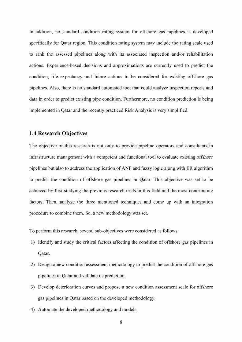
According to Oil and Gas Journal in January 1st, 2013, Qatar holds 13% of the world natural
gas reserve and the third world rank of natural gas reserves after Russia and Iran with
approximately 890 trillion cubic feet (Tcf) as shown in Fig. 2-4. The offshore North Field in
Qatar contains majority of natural gas reserves. The dominant companies for producing LNG
are Operating Company Limited (QatarGas) and Ras Laffan Company Limited (RasGas) (US
Energy Information Administration, 2013). Table 2-1 shows the general profile of oil and gas
industry in Qatar provided by (US Energy Information Administration, 2013).
18
Figure 2 - 4: Natural Gas Proven Reserves by Country in 2012. (US Energy Information Administration, 2013)
Table 2 - 1: Profile of Oil and Gas Industry in Qatar (US Energy Information Administration, 2013)
Resource Capacity/fields
Proven Oil Reserves (2013) 25.4 billion barrels
Oil production (2011) 1,600,000 barrels per day
Proven Natural Gas Reserves (2013) 890 trillion cubic feet
Natural Gas Production (2011) 5,200 billion cubic feet
Major Oil Fields Dukhan, Al-Shaheen
Major Refineries Umm Said (200,000 bbl/d), Ras Laffan (138,700 bbl/d)
Major Natural Gas Field North Field
Major Oil and Gas Ports Umm Said, Ras Laffan

19
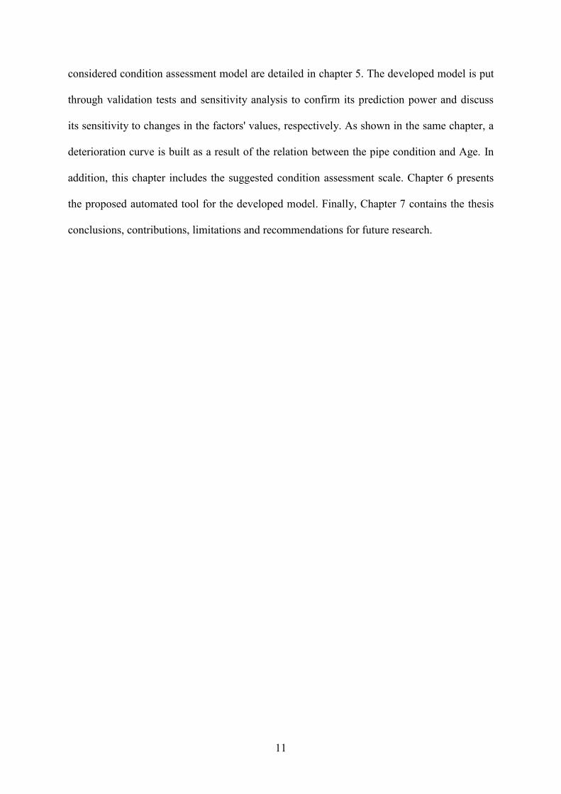
Pipelines
Oil pipelines are the main method that Qatar depends on to transport oil from offshore fields
to refineries then to ports for exporting. Submarine pipelines are also used to transport Gas
from offshore fields to Ras Laffan port to export. Natural Gas is transported from Ras Laffan
port to UAE via Dolphin pipeline. These pipelines were constructed in 2006 to export natural
gas to Oman and UAE. Dolphin Pipelines contain two main submarine lines and according to
Husein (2011), they are the longest submerged pipeline in the Middle East with 364 Km
length and a diameter of 48 inch. Two types of pipelines are being operated by Dolphin with
the following specification:
1) Sea Line: It transports gas from a refinery in Ras Laffan Port at pressure of 120 Bar
through two pipelines with diameter of 36 inch and length of 80 Km (160 Km total). The
transported product is highly corrosive because of the existence of H2S and H2O (Wet
Sour Gas) causing the important need of frequent inspections since these pipelines are
not coated internally.
2) Export Line: This internally coated pipeline with diameter of 48 inch and length of 364
Km transports refined gas (Dry and Sweet Gas) from Ras Laffan Port in Qatar to
Taweela at UAE. The line is coated internally to reduce the friction between the
transported gas and pipeline internal surface hence increasing the pipeline flow rate.
According to Husein (2011), all Export pipelines are coated externally with 2 types of coating
where the outer coating is light reinforced concrete layer, width of 90 to 140 mm, to stabilize
the pipelines and protect them from any external damage. The inner coating consists of three
layers of polypropylene, width 12mm, to prevent external corrosion.
20
All the pipelines are placed above the sea bed except in marine traffic areas where a pipeline
length of 4 km is buried in shallow water, depth less than 4 meters, to protect pipeline from
any damage caused by third party. A summary of Dolphin pipelines specifications is shown
in Table 2-2.
Table 2 - 2: Dolphin Pipeline Specification (Husein, 2011).
Name of
Pipeline/specs
# of
Pipes Dia. Length
Product
Transported
Steel
Grade Coating
Sea line 2 36” 80 km Wet sour gas X60 External
Export line 1 48” 364 km Dry sweet gas X60 External and Internal
As per Dolphin company standards, the constructed pipelines in 2006 need to be inspected
externally using Remote Operated Vehicle (ROV) annually in the first 5 years following
installation and internally using Magnetic Flux after the first year of installation and every
three years after that. Table 2-3 summarizes the previous lines.
Table 2 - 3: Inspection Interval for Dolphin Pipeline (Husein, 2011)
Inspection Method /Years First 5 Years After 5 Years of Installation
Remote Operated Vehicle (ROV) Every Year According to condition
Magnetic Flux (MFL) After 1 year, then every 3 years Every 3 years
2.3 Oil and Gas Pipeline Design and Material
Different types of pipelines are made to transport different products like crude oil, natural gas
and refined products. The carbon steel is mainly used to manufacture pipelines with diameter
from 8 to 48 inch. Smaller distribution pipelines are usually made from plastic with diameter
21
up to 2 inch. Manufacturing carbon steel pipelines follows the standards of different institutes
or societies such as the American Petroleum Institute (API 1994-2004), the American Society
of Mechanical Engineer (ASME), the American National Standard Institute (ANSI)...etc.
According to Mikhail (2011), there are three common types of impurities that may greatly
affect the internal pipeline surface and increase the risk of internal corrosion which are:
1) H2S (Sour Gas): It forms sulphuric acid when combines with water. This acid causes
lamination and pitting corrosion which is a form of extremely localized corrosion that
leads to creating small holes in the pipeline surface.
2) CO2: The highly corrosive carbonic acid is formed when CO2 combines with water.
3) Chlorides: They are considered highly corrosive materials as well.
Table 2 - 4: Steel Grade Specs used in Qatar. (Ali, 2011) (Husein, 2011) (Mikhail, 2011)
Steel Grade A B X42 X60 X70 X80
Min. Yield Stress (psi) 30,000 35,000 42,000 60,000 70,000 80,000
Usage Old Pipelines at QP Dolphin, QP
& Qatar Gas QP
This research is considering the main pipelines made from carbon steel with different steel
grades (grade B to grade X80) and different operating pressures (10 bar to 220 bar) (Ali,
2011).
2.4 Analytic Network Process (ANP)
The Analytic Network Process (ANP) technique was introduced by Saaty in 1996 as a
generalization of the Analytic Hierarchy Process (AHP) which was also introduced by Saaty
in 1980s (Gorener, 2012). The AHP is a multi-criteria decision making technique which

22
provides a hierarchical representation of complicated decision making problems. This
hierarchy is a multilevel structure that contains the decomposed set of clusters, sub-clusters
and so on that were abstracted of the overall objective. Clusters or sub-cluster can have
different names such as factors, forces, attributes, activities... etc. (Cheng & Li, 2001). The
methodology of AHP performs a pair-wise comparison to calculate the relative importance of
each cluster or attribute in the hierarchical structure to finally reach the best decision between
alternatives (Gorener, 2012).
AHP and ANP are methods used to evaluate adjacent factors through judgments that follow
pair-wise comparisons. These judgments represent the dominance of one factor over the other
with respect to a property that is shared between them (Chung, et al., 2005). The Analytic
Network Process is a generalization of the Analytic Hierarchy Process. The purpose of
developing the ANP technique was to overcome the limitations of AHP in regards with the
independence assumptions between compared attributes.
2.4.1 ANP Application
Recently, a number of applications were performed using AHP and ANP in many fields. For
example, Ayag (2011) used ANP to evaluate simulation software alternatives. A combination
between AHP and SWOT Analysis was performed by Wickramasinghe & Takano (2010) to
develop a model that revises the tourism revival strategic marketing planning which was
applied on Sri Lanka tourism as a case study. Greda (2009) applied both AHP and ANP in
the field of food quality management. In addition, Dawotola, et al. (2009) combined AHP
with Fault Tree Analysis (AHP-FTA) to assess the risk of petroleum pipelines. AHP/ANP
was used again by Yang et al. (2009) to propose a system for manufacturing evaluation in the
wafer fabricating industry. Nekhay et al. (2009) used ANP combined with GIS to evaluate the

23
soil erosion risk on Spanish mountain olive plantations. Also, an integrated AHP/ANN model
was developed by Al-Barqawi & Zayed (2008) to evaluate the municipal water mains
performance. Using ANP, Cheng & Li (2004) developed a model for contractor selection in
construction projects. Tran et al. (2004) used ANP for environmental assessment of the Mid-
Atlantic region. Finally, AHP and ANP proved themselves as a powerful decision making
tools and that was represented by the large number of researches conducted using them.
2.4.2 ANP Technique
The AHP builds decision making models by decomposing a decision problem from a general
goal to a set of manageable clusters, sub-clusters and so on. The decomposing process
continues until the final level of the hierarchy is reached. AHP adopts pair wise comparisons
to assign weights to elements that exist at the clusters and sub-clusters levels. The pair wise
comparison is a process of comparing two objects or elements at a time to measure the
relative importance or strength of an elements over another within the same level using a
ratio scale. Then, AHP calculates the final global weights of the assessment at the final level
of the hierarchy through eliminating all the middle criteria.
The Consistency Ratio (CR) is calculated by AHP to measure the consistency of the
judgments given by experts. This is because some experts are often inconsistent or not
serious in answering the pair-wise comparison questions. In general, if the CR value exceeds
0.1, then the results are unacceptable and not trust worthy since they are very close to the
randomness zone and the comparison must be repeated as advised by Saaty (1996) .The
Acceptable CR values has been set by Saaty (1994) for different matrices' sizes developed
from the pair wise comparisons as shown in Table 2-5.

24
Table 2 - 5: Acceptable CR Values (Saaty, 1980).
Matrix Size Average CR Value
1 0.00
2 0.00
3 0.58
4 0.90
5 1.12
6 1.24
7 1.32
8 1.41
9 1.45
10 1.49
The interested reader may refer to Al-Barqawi & Zayed (2008) for a more detailed example
about the main characteristics of AHP technique. In the AHP technique, the relationships
between the elements of the same levels or different levels are assumed to be unidirectional.
That means AHP technique is considered not appropriate for models that involve
interdependent relationships. So, ANP was developed to overcome this disadvantage and
enhance the analytical power of AHP (Cheng & Li, 2004). It is considered a more generic
form of the AHP technique which allows the tool to deal with more complex interdependent
relationships among elements of the same level or different levels. As shown Fig. 2-5 adapted
from Cheng & Li (2004), the interdependence can occur is several ways:
1) Uncorrelated elements are connected.
2) Uncorrelated levels are connected.
3) Dependence of two levels is two-way (i.e., bi-directional).

25
Figure 2 - 5: Interdependencies in ANP (Cheng & Li, 2004).
The working methodology of ANP is deriving relative priority scale of absolute numbers
from a group of judgments or feedbacks provided by expert professionals. These judgments
represent the relative influence of one cluster over the other in a pair wise comparison form
with respect to control criteria. As reported by Garuti & Sandoval (2005), the ANP provides a
clarification of all the relations among the compared criteria and thus decreasing the gap
between the developed model and reality.
A super-matrix can be developed by incorporating interdependencies of the elements in the
hierarchy. This is done by adding feedback loops in the model. The developed super-matrix
adjusts the relative importance weights in individual matrices to form a new matrix called
"overall" matrix with the eigenvectors of the adjusted relative importance weights (Meade &
Sarkis, 1998). Sarkis (1999) mentioned four main step that form the core of ANP which are
the following:
1) Conduct pair-wise comparisons on the elements at the cluster and sub-cluster levels.
Decision Problem
Decomposed Clusters
Decomposed Sub-clusters
Alternatives
(2)
(3)
(1)
26
2) Place the resulting relative importance weights (eigenvectors) in sub matrices within the
super-matrix.
3) Adjust the values in the super-matrix so it can achieve column stochastic.
4) Raise the super matrix to limiting powers until weights have converged and remained
stable.
The previous steps are explained later in details in the ANP implementation section.
2.4.3 ANP Software
For easier ANP implementation, researchers developed a software called "SuperDecisions". It
is a decision making software that is based on the Analytical Hierarchy Process (AHP) and
the Analytical Network Process. An ANP model can be easily developed through
SuperDecisions software due to the friendly interface of the program. The interested reader
may refer to the software website "www.superdecisions.com" for more details. Many
tutorials are available in the website including tutorials for developing AHP or ANP models.
Also, the website provides a variety of detailed examples from different study fields. The
SuperDecisions software can be easily downloaded and installed. A temporary serial key is
given for registered members.
2.5 Fuzzy Set Theory
The fuzzy set concept was first introduced by Zadeh (1965) as a mathematical representation
to deal with uncertainties that are not of statistical nature. Since its development, fuzzy
decision making has been applied in numerous areas such as civil engineering application and
many others (Salah, 2012). According to Zadeh (1965), a fuzzy set is characterized by its
membership function. This means that elements are described in way to permit a gradual
transition from being a member of a set to a nonmember. Each element has a membership

27
degree that ranges from Zero to One, where zero indicates non-membership and one signifies
full membership. The case is different in the conventional crisp sets where elements are not
considered members unless their membership is full (i.e. membership degree of one).
Years after Zadeh (1965) introduced the fuzzy set theory, researchers were paying
considerable attention to this theory in various types of industries that are experiencing rapid
development. The use of fuzzy numbers became so common in many research fields since it
provides the user with a linguistic representation which cannot be provided by other theories
(e.g. probabilistic theory). For example, Ayyub & Halder (1984) and Lorterapong & Moselhi
(1996) used fuzzy logic in project scheduling and project-network analysis. Also, Chao &
Skibniewski (1998) and Wong & Albert (1995) used it in evaluating alternative construction
technology and contract selection strategy & decision making. Raoot & Rakshit (1991) and
Dweiri & Meier (1996) applied fuzzy approach in facilitating lay-out planning. Fuzzy Sets
theory was used in many civil engineering application by Wong (1986) and Furuta (1994).
The advantage of using a fuzzy set instead of the conventional set is that the fuzzy sets
provide a representation of the degree of which an element belong to a certain set of
elements.
Fuzzy subset "A" can be defined as a set of ordered pairs,[𝑥, 𝑦𝐴(𝑥)], where x is an element in
the universe of discourse X, and 𝑦𝐴(𝑥) is the degree of membership associated with the
element x which range from Zero to One. The membership value of x is 𝑦𝐴(𝑥), which
represents “if x belongs to fuzzy number “A” or not”: 𝑦𝐴(𝑥) = 1 means x fully belongs to
fuzzy number “a”, 𝑦𝐴(𝑥) = 0 means x does not belong to “a”. (Salah, 2012)

28
2.5.1 Fuzzy Sets Shapes
There are different shapes to represent the membership function in the fuzzy, however, the
most commonly used shapes are linear approximations such as the trapezoidal and triangular
shapes (Dubois & Prade, 1988; Cheng & Hwang, 1992).
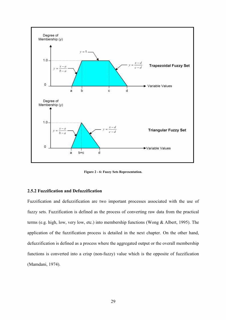
Fig. 2-6 shows two types of fuzzy sets representations which are:
1) Trapezoidal Fuzzy Set: It can be represented by four points (a, b, c, d), where a and d
are the lower and upper bounds, b and c are the lower and upper middle values.
2) Triangular Fuzzy Set: It is considered as a special case of the trapezoidal fuzzy set with
b = c.
The membership function can be formulated as:
𝑦𝐴(𝑥) =
{
𝑥 − 𝑎
𝑏 − 𝑎 𝑎 < 𝑥 < 𝑏
1 𝑎 ≤ 𝑥 ≤ 𝑏
𝑥 − 𝑑
𝑐 − 𝑑 𝑐 < 𝑥 < 𝑑
0 𝑜𝑡ℎ𝑒𝑟𝑤𝑖𝑠𝑒
(2-1)
A membership can be represented graphically by many shapes such as triangles, or
trapezoidal, but it is usually convex. For a given value yA(x) = 0 means that x has a null
membership in fuzzy set A, and yA(x) = 1 means that x has full membership. These
membership functions can be determined subjectively; the closer an element to satisfy the
requirements of a set, the closer its grade of membership is to 1, and the opposite is true
(Raoot & Rakshit, 1991).
29
Figure 2 - 6: Fuzzy Sets Representation.
2.5.2 Fuzzification and Defuzzification
Fuzzification and defuzzification are two important processes associated with the use of
fuzzy sets. Fuzzification is defined as the process of converting raw data from the practical
terms (e.g. high, low, very low, etc.) into membership functions (Wong & Albert, 1995). The
application of the fuzzification process is detailed in the next chapter. On the other hand,
defuzzification is defined as a process where the aggregated output or the overall membership
functions is converted into a crisp (non-fuzzy) value which is the opposite of fuzzification
(Mamdani, 1974).

30
The output of a fuzzy process is the union if two or more fuzzy memberships. For example,
suppose a fuzzy output comprises of two parts: (1)𝐶1, a trapezoidal membership shape and
(2) 𝐶2, a triangular membership shape as shown in Fig. 2-7. The union of these two
membership functions is 𝐶 = 𝐶1 ∪ 𝐶2. This union uses the max. operator which graphically is
the outer envelope of the two shapes. Also, the output fuzzy membership can be the union of
more than two membership functions with different shapes other than triangular and
trapezoidal but the union procedure is the same (Ross, 2010). After defuzzification, a fuzzy
number can be represented by a crisp value. Many defuzzification methods can be used to
defuzzify the overall membership function such as (Ross, 2010):
Figure 2 - 7: Typical fuzzy process output: (a) first part of fuzzy output; (b) second part of fuzzy output; and (c)
union of both parts (Ross, 2010).
1) Centroid Method: Also called "Centre of Area" or "Centre of Gravity". It is the most
prevalent defuzzification method and can be calculated using Eq. (2-2).
31
𝓏∗ =∫𝜇с(𝓏). 𝓏 𝑑𝓏
∫𝜇с(𝓏) 𝑑𝓏
for all 𝓏 ∊ Z, (2-2)
where 𝑧∗ is the defuzzified value and ∫ denotes an algebraic integration.
Figure 2 - 8: Centroid Defuzzification Figure 2 - 9: Weighted-Average
Method (Ross, 2010). Defuzzification Method (Ross, 2010).
2) Weighted-Average Method: It is used most frequently because of its computational
efficiency. Its main disadvantage is that it works only on symmetrical output
membership functions. The algebraic formula is expressed in Eq. (2-3).
𝓏∗ =∑𝜇с(�̅�). �̅�
∑ 𝜇с(�̅�)
(2-3)
where ∑ donates the algebraic sum and 𝑧̅ is the centroid of each symmetrical membership
function. Fig. 2-9 shows a brief example on how Weighted-Average method works.
𝓏∗ =𝑎(0.5) + 𝑏(0.9)
0.5 + 0.9
(2-4)
where a and b are the centroids of the two symmetrical membership functions in Fig. 2-9.

32
3) Mean-Max Membership (middle of maxima): This method can be used when the
peaked output membership function is a plateau rather than a single point. This method
is given by the following expression which is shown in Fig. 2-10.
𝓏∗ =𝑎 + 𝑏
2
(2-5)
Figure 2 - 10: Mean-Max membership Defuzzification Method (Ross, 2010).
4) Center of Sums: It is considered one of the fastest defuzzification methods and it is not
restricted to symmetrical membership functions. Fig. 2-11 shows an example of its use.
The defuzzified value 𝓏∗ is given as follows:
𝓏∗ =∑ 𝜇с𝑘(𝓏)𝑛𝑘=1 ∫ 𝓏 ̅𝑑𝓏
𝓏
∑ 𝜇с𝑘(𝓏)𝑛𝑘=1 ∫ 𝑑𝓏
𝓏
(2-6)
where the symbol 𝓏 ̅ is the distance to the centroid of each of the respective membership
functions.

33
Figure 2 - 11: Center of sums method: (a) First Membership Function; (b) Second Membership Function; and (c)
Defuzzification Step (Ross, 2010).
𝐶1 and 𝐶2 are two individual output fuzzy sets that need to be summed algebraically. There
are two disadvantages for this method which are:
a) The intersecting areas are added twice.
b) It involves finding the centroids of the individual membership functions.
It is important to note that the previously mentioned defuzzification methods are the most
commonly used and there are many other defuzzification methods.
2.6 Evidential Reasoning (ER) Approach
2.6.1 Theory of Evidence
"Evidential Reasoning basically means reasoning with evidence" as stated by Srivastava
(2010). These are common situations in the real world in all domains such as legal, medical
or even business domain. ER Approach uses two frameworks to mange uncertainties:
34
Bayesian Theory and Dempster-Shafer (DS) Theory of Belief-Functions which is considered
a powerful technique to address the ignorance and uncertainty. The basics of Bayesian and
DS theories are introduced by Srivastava (2010). DS theory has been used relatively for data
fusion as a generalization of the Bayesian theory. It was first introduced to the academic
society by Dempster in 1967 and extended later by Shafer in 1976. (Hua, et al., 2007)
The main purpose of developing the Evidential Reasoning as a research methodology is to
address Multi-Criteria Decision Making (MCDM) problems under uncertainity. It is different
from other conventional MCDM methods because it represents any assessment as a
distribution using belief structures. Another difference is that ER aggregates the degrees of
belief using an algorithm developed basically on decision theory and combination rule of DS
theory of evidence instead of aggregating average scores as conventional MCDM methods.
2.6.2 ER Application
Since the development of Evidential Reasoning (ER) Theory and throughout the years, many
researchers used it to develop assessment models in various fields. Starting from 1992 till
2010 , ER has been applied by Srivastava and his colleagues in information systems domains
to assess risks such as audit risks, information security risks, fraud risks and so on (Srivastava
& Shafer, 1992 and Srivastava & Mock, 2000 & 2010). A model was developed by Wang &
Elhag (2008) used the Evidence Theory of Dempster and Shafer to deal with condition
assessment of structural bridges. Hua et al. (2007) translated pipe inspection results to assess
the condition of buried pipelines using theory of evidence. Also, DS theory of evidence was
applied by Sadiq et al. (2006) to estimate the risk of contaminant intrusion in distribution
networks. Wang et al. (2006) used the evidential reasoning approach to perform
environmental impact assessments.

35
Sonmez et al. (2002) developed a model using basic concept of DS theory in Evidential
Reasoning to perform a typical MCDM problem in construction projects. This is the process
of contractors prequalification that takes into consideration multiple criteria both, quantitative
and qualitative. Similarly to the contractors’ pre-qualification ER model performed by
Sonmez et al. (2002), Teng (2002) developed a model for suppliers pre-qualification for a UK
company using evidential reasoning. Also, Morcous et al. (2002) proposed a case-based
reasoning system for infrastructure deterioration. Yang & Sen (1994) proposed a hierarchical
analysis for design selection of ship retro-fit options using evidential reasoning based
methodology.
2.6.3 ER Technique
This section provides a summarized explanation for the ER Technique as discussed in Yang
& Xu (2002). The evidential reasoning is a technique that combines many pieces of evidence.
It aggregates two factors at a time (i.e. ER is a one-by-one based technique) which keeps the
concept of the ER approach clear. Then, the resulting combined of the first two pieces of
evidence is aggregated with the third piece of evidence and so on.
The ER algorithm provides more flexibility to the ER technique when combining large
number of factors affecting the condition of a structure. This results in an easier way to
conduct sensitivity analysis for the parameters of the ER approach such as degrees of belief
and weights.
To explain the procedure of the ER approach, suppose we have a two-level hierarchy of
attributes with a general attribute at the top level and a number of basic attributes at the

36
bottom level. Suppose there are basic attributes 𝑒𝑖(𝑖 = 1,… 𝐿) associated with a general
attribute 𝑦. Define a set of L basic attributes as follows:
𝐸 = {𝑒1 , 𝑒2 … 𝑒𝑖 … 𝑒𝐿 } (2-7)
Each of the given attributes has its own weight (Calculated by ANP technique for the
developed model). The weights of the attributes are given by
𝜔 = {𝜔1 , 𝜔2… 𝜔𝑖… 𝜔𝐿} (2-8)
where 𝜔𝑖 is the relative weight of the 𝑖th basic attribute (𝑒𝑖) with 0 ≤ 𝜔𝑖 ≤ 1 and ∑ 𝜔𝑖 = 1𝐿𝑖=1 .
These weights of the attributes play a major role in the assessment process. There are
different ways to estimate the relative weights of the given attributes. It could be done by
simple rating methods or more advanced methods based on the pair-wise comparisons of
attributes such as ANP as illustrated in the later sections.
N distinctive evaluation grades are supposedly defined which provide a complete set of
standards for assessing an attribute. It is represented by
𝐻 = {𝐻1 , 𝐻2… 𝐻𝑛…𝐻𝑁} (2-9)
where 𝐻𝑛 is the nth evaluation grade. Without loss of generality, it is assumed that 𝐻𝑛+1 is
preferred to 𝐻𝑛.
37
A given assessment for 𝑒𝑖(𝑖 = 1, …, 𝐿) of an alternative may be mathematically represented
as the following distribution:
𝑆(𝑒𝑖) = {(𝐻𝑛, 𝛽𝑛,𝑖), 𝑛 = 1,… ,𝑁} (2-10)
where 𝛽𝑛,𝑖 ≥ 0 , ∑ 𝛽𝑛,𝑖𝑁𝑛=1 ≤1, and 𝛽𝑛,𝑖 be a degree of belief to which the general attribute y
is assessed to the grade 𝐻𝑛 .
The given distributed assessment can be read as that the attribute 𝑒𝑖 is assessed to the grade
𝐻𝑛 with the degree of belief of 𝛽𝑛,𝑖, 𝑛 = 1,… ,𝑁 .
An assessment 𝑆(𝑒𝑖) is considered a complete assessment if the summation of all degrees of
belief is one (i.e. ∑ 𝛽𝑛,𝑖𝑁𝑛=1 = 1). Similarly, the assessment 𝑆(𝑒𝑖) is incomplete when the
summation is less than one (i.e. ∑ 𝛽𝑛,𝑖𝑁𝑛=1 < 1). A special case is ∑ 𝛽𝑛,𝑖
𝑁𝑛=1 = 0 (or 𝛽𝑛,𝑖 = 0
for all 𝑛 = 1,… ,𝑁), which denotes a complete lack of information on 𝑒𝑖.
Note: All the assessments in the developed model are complete assessments since the degrees
of belief are extracted from the fuzzified thresholds’ charts that consider a degree of fuzziness
of 0.5 (i.e. ∑ 𝛽𝑛,𝑖𝑁𝑛=1 = 1 for any given assessment).
The purpose of the aggregation is to generate 𝛽𝑛 (𝑛 = 1,… ,𝑁) by aggregating the
assessments for all the associated basic attributes 𝑒𝑖 (𝑖 = 1,… , 𝐿) as given in Eq. (2-10). The
following evidential reasoning algorithm can be used for this purpose.
38
ER Algorithm
The ER algorithm is explained in details in Yang & Xu (2002), Yang et al. (2006) and Wang
& Elhag (2008). The first step in the ER algorithm is to transform the degrees of belief into
basic probability masses 𝑚𝑛,𝑖. This is performed by combining the relative weights and the
degrees of belief as shown in Eq. (2-11). And 𝜔𝑖 need be normalized.
𝑚𝑛,𝑖 = 𝑚𝑖 (𝐻𝑛) = 𝜔𝑖 𝛽𝑛,𝑖 𝑛 = 1,… ,𝑁; 𝑖 = 1,… , 𝐿 (2-11)
The basic probability mass 𝑚𝑛,𝑖 represents the degree to which the 𝑖th basic attribute 𝑒𝑖
supports the hypothesis that the attribute 𝑦 is assessed to the 𝑛th grade 𝐻𝑛.
Let 𝑚𝐻,𝑖 be a remaining probability mass unassigned to any individual grade after all the 𝑁
grades have been considered for assessing the general attribute as far as 𝑒𝑖 is concerned. 𝑚𝐻,𝑖
is calculated as follows:
𝑚𝐻,𝑖 = 𝑚𝑖 (𝐻) = 1 − ∑ 𝑚𝑛,𝑖𝑁𝑛=1 = 1 − 𝜔𝑖 ∑ 𝛽𝑛,𝑖
𝑁𝑛=1 , 𝑖 = 1,… , 𝐿 (2-12)
�̅�𝐻,𝑖 = �̅�𝑖(𝐻) = 1 − 𝜔𝑖, 𝑖 = 1, … , 𝐿 (2-13)
�̃�𝐻,𝑖 = �̃�𝑖(𝐻) = 𝜔𝑖(1 − ∑ 𝛽𝑖)𝑁𝑛=1 , 𝑖 = 1,… , 𝐿 (2-14)
with
𝑚𝐻,𝑖 = �̅�𝐻,𝑖 + �̃�𝐻,𝑖 and ∑ 𝜔𝑖 = 1𝐿𝑖=1 ,
where, �̅�𝑯,𝒊 is the remaining probability mass that is not yet assigned to individual grades
caused by the relative importance of the attribute 𝑖 (denoted by 𝑒𝑖). �̅�𝐻,𝑖 is a linear decreasing

39
function of 𝜔𝑖. �̅�𝐻,𝑖 will be one if the weight of 𝑒𝑖 is zero or 𝜔𝑖 = 0 ; �̅�𝐻,𝑖 will be zero if 𝑒𝑖
dominates the assessment or 𝜔𝑖 = 1. And �̃�𝑯,𝒊 is the remaining probability mass unassigned
to individual grades caused by the incompleteness of the assessment 𝑆(𝑒𝑖). �̃�𝐻,𝑖 will be zero
if 𝑆(𝑒𝑖) is complete, or ∑ 𝛽𝑛,𝑖𝑁𝑛=1 = 1; otherwise, �̃�𝐻,𝑖 will be positive. �̃�𝐻,𝑖 is proportional
to 𝜔𝑖 and will cause the subsequent assessments to be incomplete.
𝑚𝑛,𝐼(𝑖) and 𝑚𝐻,𝐼(𝑖) can be generated by combining the basic probability masses 𝑚𝑛,𝑗 and 𝑚𝐻,𝑗
for all 𝑛 = 1,… ,𝑁, 𝑗 = 1,… , 𝑖.
Table 2-6 illustrates the process of ER algorithm used in the model developed in this thesis.
Table 2 - 6: ER Algorithm Process as described in (Yang & Xu, 2002).
𝑆(𝑒𝑖) ⊕ 𝑆(𝑒𝑗)
𝑆(𝑒𝑖)
(𝑚1,𝑖)
{𝐻1}
(𝑚2,𝑖)
{𝐻2} ...
(𝑚𝑛,𝑖)
{𝐻𝑛} ...
(𝑚𝑁,𝑖)
{𝐻𝑁}
(�̃�𝐻,𝑖)
{𝐻}
(�̅�𝐻,𝑖)
{𝐻}
𝑆(𝑒𝑗)
(𝑚1,𝑗)
{𝐻1}
(𝑚1,𝑖 𝑚1,𝑗)
{𝐻1}
(𝑚2,𝑖 𝑚1,𝑗)
{ɸ} ...
(𝑚𝑛,𝑖 𝑚1,𝑗)
{ɸ} ...
(𝑚𝑁,𝑖 𝑚1,𝑗)
{ɸ}
(�̃�𝐻,𝑖 𝑚1,𝑗)
{𝐻1}
(�̅�𝐻,𝑖 𝑚1,𝑗)
{𝐻1}
(𝑚2,𝑗)
{𝐻2}
(𝑚1,𝑖 𝑚2,𝑗)
{ɸ}
(𝑚2,𝑖 𝑚2,𝑗)
{𝐻2} ...
(𝑚𝑛,𝑖 𝑚2,𝑗)
{ɸ} ...
(𝑚𝑁,𝑖 𝑚2,𝑗)
{ɸ}
(�̃�𝐻,𝑖 𝑚2,𝑗)
{𝐻2}
(�̅�𝐻,𝑖 𝑚2,𝑗)
{𝐻2}
...
...
...
...
...
...
...
(𝑚𝑛,𝑗)
{𝐻𝑛}
(𝑚1,𝑖 𝑚𝑛,𝑗)
{ɸ}
(𝑚2,𝑖 𝑚𝑛,𝑗)
{ɸ} ...
(𝑚𝑛,𝑖 𝑚𝑛,𝑗)
{𝐻𝑛} ...
(𝑚𝑁,𝑖 𝑚𝑛,𝑗)
{ɸ}
(�̃�𝐻,𝑖 𝑚𝑛,𝑗)
{𝐻𝑛}
(�̅�𝐻,𝑖 𝑚𝑛,𝑗)
{𝐻𝑛}
...
...
...
...
...
...
...
(𝑚𝑁,𝑗)
{𝐻𝑁}
(𝑚1,𝑖 𝑚𝑁,𝑗)
{ɸ}
(𝑚2,𝑖 𝑚𝑁,𝑗)
{ɸ} ...
(𝑚𝑛,𝑖 𝑚𝑁,𝑗)
{ɸ} ...
(𝑚𝑁,𝑖 𝑚𝑁,𝑗)
{𝐻𝑁}
(�̃�𝐻,𝑖 𝑚𝑁,𝑗)
{𝐻𝑁}
(�̅�𝐻,𝑖 𝑚𝑁,𝑗)
{𝐻𝑁}
(�̃�𝐻,𝑗)
{𝐻}
(𝑚1,𝑖 �̃�𝐻,𝑗)
{𝐻1}
(𝑚2,𝑖 �̃�𝐻,𝑗)
{𝐻2} ...
(𝑚𝑛,𝑖 �̃�𝐻,𝑗)
{𝐻𝑛} ...
(𝑚𝑁,𝑖 �̃�𝐻,𝑗)
{𝐻𝑁}
(�̃�𝐻,𝑖 �̃�𝐻,𝑗)
{𝐻}
(�̅�𝐻,𝑖 �̃�𝐻,𝑗)
{𝐻}
(�̅�𝐻,𝑗)
{𝐻}
(𝑚1,𝑖 �̅�𝐻,𝑗)
{𝐻1}
(𝑚2,𝑖 �̅�𝐻,𝑗)
{𝐻2} ...
(𝑚𝑛,𝑖 �̅�𝐻,𝑗)
{𝐻𝑛} ...
(𝑚𝑁,𝑖 �̅�𝐻,𝑗)
{𝐻𝑁}
(�̃�𝐻,𝑖 �̅�𝐻,𝑗)
{𝐻}
(�̅�𝐻,𝑖 �̅�𝐻,𝑗)
{𝐻}
40
Given the previous definitions and discussions, the evidential reasoning algorithm can be
summarized as follows
𝑚𝑛,𝐼(𝑖+1) = 𝐾𝐼(𝑖+1)(𝑚𝑛,𝐼(𝑖)𝑚𝑛,𝑖+1 +𝑚𝑛,𝐼(𝑖)𝑚𝐻,𝑖+1 +𝑚𝐻,𝐼(𝑖)𝑚𝑛,𝑖+1) 𝑛 = 1, . . . , 𝑁 (2-15)
where 𝑚𝐻,𝐼(𝑖) = �̅�𝐻,𝐼(𝑖) + �̃�𝐻,𝐼(𝑖)
�̃�𝐻,𝐼(𝑖+1) = 𝐾𝐼(𝑖+1)[�̃�𝐻,𝐼(𝑖)�̃�𝐻,𝑖+1 + �̅�𝐻,𝐼(𝑖)�̃�𝐻,𝑖+1 + �̃�𝐻,𝐼(𝑖)�̅�𝐻,𝑖+1] (2-16)
�̅�𝐻,𝐼(𝑖+1) = 𝐾𝐼(𝑖+1)[�̅�𝐻,𝐼(𝑖)�̅�𝐻,𝑖+1] (2-17)
𝐾𝐼(𝑖+1) = [1 − ∑ ∑ 𝑚𝑡,𝐼(𝑖)𝑚𝑗,𝑖+1𝑁𝑗=1𝑗≠𝑡
𝑁𝑡=1 ]
−1
𝑖 = 1, . . . , 𝐿 − 1 (2-18)
where 𝐾𝐼(𝑖+1) is a normalizing factor so that ∑ 𝑚𝑛,𝐼(𝑖+1)+𝑚𝐻,𝐼(𝑖+1) = 1𝑁𝑛=1 .
After aggregating all the assessments L, �̅�𝐻,𝐼(𝐿) is assigned back to all individual grades
proportionally to generate the combined degrees of belief as shown in the following
equations:
𝛽𝑛 =𝑚𝑛
1 − �̅�𝐻,𝐼(𝐿), 𝑛 = 1,… ,𝑁
(2-19)
𝛽𝐻 =�̃�𝐻,𝐼(𝐿)
1 − �̅�𝐻,𝐼(𝐿)
(2-20)

41
where 𝛽𝑛 represents the degrees of belief for the aggregated assessment where the final
assessment is assessed to the grades 𝐻𝑛. 𝛽𝐻 represents the incompleteness of the overall
assessment assigned to 𝐻.
2.7 Factors Affecting Offshore Gas Pipelines
In previous researches that handled condition assessment of oil and gas pipelines, the focus
was mainly directed to factors that are related to corrosion or third party characteristics
(Ahammed 1998; Sinha and Pandey 2002; Li et al. 2009; Hallen et al. 2003; Bersani et al.
2010 and Noor et al. 2011) which are insufficient to successfully develop an efficient
condition assessment model. Therefore, other factors are needed to be identified in order to
build an accurate model. For example, Senouci et al. (2014a and 2014b) implemented
Regression Analysis and Artificial Neural Network (ANN) to develop models that predict the
possible failure types other than corrosion. Also, El-Abbasy et al. (2014a, 2014b & 2014c)
proposed three condition assessment models for oil and gas pipelines using integrated
simulation & ANP, regression analysis, and ANN. These models considered various factors
categorized into physical, external and operational factors.
As discussed in the previous section, the factors identification process started with
performing literature review on the previous studies related to pipeline condition assessment.
At the same time, several interviews were conducted with professional experts in the oil and
gas industry in Qatar to identify the factors that may affect the pipeline condition according
to their experience. Later on, the two factors' list, from literature and from interviews, were
compared to each other to come up with a comprehensive list of the most important factors
affecting pipeline condition. Then, the factors were divided into three categories: physical,
external and operational as shown in Fig. 2-12. The physical factors deal with the pipeline

42
general characteristics such as Age, Diameter, Metal Loss and Coating Condition. The
external factors group deals with the pipeline surrounding environment and included factors
like number of crossings of other pipelines, the applied cathodic protection, existence of
marine routes and the water depth. The final group, which is the operational factors group,
deals with operational condition on the pipeline. It included three factors: existence of
corrosive impurities, the operating pressure and the flow rate. Deterioration of offshore gas
pipelines systems can be caused by numerous factors. Table 2-7 summarizes these physical,
external and operational factors.
Figure 2 - 12: Hierarchy of Factors Affecting Offshore Gas Pipelines Condition (El-Abbasy et al., 2014a).
A: Physical
Factors
C: Operational
Factors
A1: Age
B: External
Factors
Factors Affecting Offshore Gas Pipelines Condition
A2: Diameter
A3: Metal Loss
A4: Coating Condition
B1: Crossings
B2: Cathodic Protection
B3: Marine Route Exist.
B4: Water Depth
C1: Corrosive Impurities
C2: Operating Pressure
C3: Flow Rate

43
Table 2 - 7: Explanation of Factors Affecting Offshore Gas Pipelines (El Chanati et al. 2013).
Factor Explanation
Physic
al
Age Pipeline usually degrades as it ages, resulting in a pipeline
condition decrease.
Diameter
Smaller pipeline diameter has a higher probability of failure than
larger ones possibly because smaller standard dimension ratio
(SDR) affects the structural performance of a pipeline and makes it
more vulnerable to external impact or third party damage.
Metal Loss The pipeline condition decreases when the metal loss as a
percentage of the wall thickness increases.
Coating Condition Well maintained applied coating enhances the pipeline condition.
Exte
rna
l
Crossings
As the number of pipelines crossing over or under the considered
pipeline increases, the pipeline becomes less stable and its
condition eventually decreases.
Cathodic Protection
Cathodic protection is essential to protect a pipeline against
corrosion. As the protection potential decreases, the pipeline
condition decreases due to the absence of corrosion resistance.
Marine Route Existence Existence of marine routes near the considered pipeline may lead
to third party damage.
Water Depth
Pipeline depth under the water greatly affects the pipeline condition.
Shallow pipelines are easily exposed to third party damage while
deep pipelines are subjected to high water pressure.
Opera
tiona
l
Corrosive Impurities
The existence of high level of corrosive impurities in the transported
product severely affect the inner pipe wall resulting in internal
corrosion.
Operating Pressure
The maximum allowable operating pressure decreases the pipeline
condition when it gets close to the design pressure because it can
induce more stresses on the pipeline.
Flow Rate
Low flow rates could increase the chances of liquid or solid dropout
and accumulation in low places of the pipeline, whereas high flow
rates may lead to pipeline erosion.
44
2.8 Infrastructure Condition Assessment Models
In the recent years, serious efforts have been carried out to assess infrastructure systems
including oil & gas, water, and sewer pipelines. This is due to the significant environmental
and economical importance of these systems. As a result, different condition assessment
models have been developed to predict the condition rating and possibilities of future failure.
This section provides a brief summary about some of these developed models.
2.8.1 Oil & Gas Pipelines
Oil and gas pipelines hold an important place in any nation’s economy since they transport
millions of dollars’ worth of oil and gas various products. So, condition assessment is very
necessary for operating pipelines to evaluate their performance along their age and prevent
any future disasters caused by pipeline failures. Different models have been promoted for this
purpose. For example, Ahammed (1998) developed a new methodology to assess the
remaining service life of a pressurized pipeline containing active corrosion defects. Following
that, Analytical Hierarchy Process (AHP) was utilized by Dey (2001) to propose a decision
model to help decision makers and pipeline operators select a suitable type of inspection or
monitoring technique for pipelines. Sinha & Pandey (2002) developed a simulation-based
probabilistic fuzzy neural network model to estimate failure probability of aging oil and gas
pipelines that have corrosion vulnerability. Hallen et al. (2003) presented a probabilistic
analysis framework to assess corroding pipelines and its failure probability in the future.
Kumar & Taheri (2004) were concerned about pipeline material effect on oil and gas
pipelines. So, they developed an automated data interpretation system using neural networks
for fiber-reinforced polymer composites (FRP) oil and gas pipelines, which is applicable to
metallic pipes as well.
45
In 2006, historical failure data were adapted using statistical analysis classification and
regression tree to develop a tool that predicts a spillage class in oil pipes (Bertolini &
Bevilacqua, 2006). After three years, Peng et al. (2009) used fuzzy neural network to suggest
a model that is based on failure tree and fuzzy computing to predict the rate of failure for
long-distance oil and gas pipelines. In the same year of 2009, Dawotola et al. combined
Analytic Hierarchy Process (AHP) and Fault Tree Analysis to present an optimal selection
strategy, based on the probability and consequences of failure, in order to support the design,
the construction, and the inspection and maintenance of oil and gas pipelines. In addition,
Noor et al. (2010) and (2011) used a semi-probabilistic and deterministic methodology to
predict the remaining strength of offshore pipelines subjected to internal corrosion. Also,
Bersani et al. (2010) used historical data from Department of Transportation (DOT) in the US
to develop a risk assessment model that predicts the failure caused by third party activities.
Recently, El-Abbasy et al. (2014a, 2014b & 2014c) proposed three condition assessment
models for oil and gas pipelines using integrated simulation & ANP, regression analysis, and
ANN. Similarly, Senouci et al. (2014a and 2014b) implemented Regression Analysis and
Artificial Neural Network (ANN) to develop models that predict the possible failure types
other than corrosion.
2.8.2 Water Pipelines
Water pipelines condition assessment was and still the focus of many researchers in order to
predict the performance and condition rating of these pipelines. For example, Yan and
Vairavamoorthy (2003) assessed the condition of water mains using fuzzy multi-criteria
decision-making (MCDM) techniques. In the same year, Geem (2003) employed the
Artificial Neural Networks (ANN) to develop a decision support system for water pipeline
condition assessment. Two other models were prepared by Al-Barqawi and Zayed (2006a &
46
2006b) in which AHP and ANN were utilized to predict the condition rating of water
pipelines based on physical, operational, and environmental deterioration factors. In 2008,
Al-Barqawi and Zayed prepared an integrated model using AHP and ANP concurrently to
evaluate the sustainability of water pipelines.
2.8.3 Sewer Pipelines
Similarly to water pipelines, many models have been developed to assess the condition of
sewer pipelines. In 2000, Moselhi and Shehab-Eldeen presented a Back-Propagation Neural
Network for the purpose of analysis and classification of defects in sewer pipelines. At the
same time, a sewer management system for prioritizing sewer pipelines inspection based on
the Bayesian belief networks was proposed by Hahn et al. (2000). One year later, Chae &
Abraham (2001) developed a neuro-fuzzy approach for more accurate analysis and data
interpretation of sewer pipelines condition. Also, Najafi and Kulandaivel (2005) proposed a
model that predicts the condition of sewer pipelines based on historical condition assessment
data. In the same year of 2005, Stein et al. developed a model which analyzes the defect-
caused environmental impacts on sewer pipelines using Monte Carlo simulation.
2.9 Summary
To conclude this chapter, we can say that fuzzy set theory is considered a powerful tool when
it comes to modeling complex systems. It is very useful in problems that involve vagueness
and uncertainty. Fuzzy sets theory is a tool that converts linguistic terms into mathematical
data that can be easily managed and interpreted (Mamdani, 1974). The decision maker can
use the fuzzy approach to produce simple evaluation systems according to their own values
and judgments while maintaining tractability. Fuzzy sets theory was successfully used in

47
many applications in different fields. The interested reader may refer to the book "Fuzzy
Logic with Engineering Applications" third edition by Timothy J. Ross published in 2010.
The previous sections introduced the Evidential Reasoning Technique which uses two
frameworks: Bayesian frameworks and the Dempster-Shafer (DS) Theory of Evidence. Also,
the ER algorithm used to develop the model of this research was stated in details to illustrate
the methodology used to aggregate the degrees of belief of Multiple-Criteria Decision-
Making (MCDM) problems. In addition, some of the previous research works were
introduced since the development of ER technique till the current time. Many efforts were put
to develop the previously discussed ER algorithm so it satisfies many theorems, such as the
basic, consensus, complete, and incomplete synthesis theorems. These theorems are discussed
in details in Yang & Xu (2002) for interested readers.
48
CHAPTER THREE: RESEARCH METHODOLOGY
3.1 Introduction
The current research aims to develop a condition assessment tool to evaluate offshore gas
pipelines in Qatar. The presented research methodology consists of different steps as shown
in Fig. 3-1: Literature Review, Data Collection, Model Development, Condition Assessment
Scale, Sensitivity Analysis, Deterioration Curve, Condition Assessment Automated Tool, and
Conclusion and Recommendation. The following sections provide a brief description of the
planned methodology.
3.2 Literature Review
This part summarizes the literature related to the scope of current research. Section 2.1
includes a shortened introduction about pipelines importance nowadays along with some
associated statistics. This section also contains a review about pipeline design and
manufacturing material. Section 2.2 reveals few important facts about the oil and gas industry
in Qatar and its pipeline network. Information about the pipelines characteristics and
inspection interval are also included. These information were collected from extensive
research and interviews with professionals in the oil and gas industry in Qatar. Section 2.3
illustrates the types of manufacturing materials used in Qatar's pipelines network and the
standards followed for their design. Sections 2.4, 2.5 and 2.6, contains a detailed and
comprehensive literature review of the techniques used to conduct the current research;
Analytic Network Process (ANP), Fuzzy Set Theory (FST) and Evidential Reasoning (ER)
respectively. Finally, Section 2.7 presents the time-dependent factors considered in this
research which contribute in the deterioration of offshore gas pipelines in Qatar. These
factors provide the main structure to develop the condition prediction model. They are
classified into three categories; physical, external, and operational. The hierarchy of the

49
factors affecting offshore gas pipelines was made through extensive literature review and
interviews with professionals in oil and gas industry in Qatar.
3.3 Data Collection
Data needed to conduct this research were collected from different sources. First, a structured
questionnaire was distributed among professionals, engineers and managers, in the oil and
gas industry in Qatar and similar regions such as Saudi Arabia. This method was used to
gather the feedback of practitioners and specialists in regards to the most influential factors
affecting the condition of offshore gas pipelines in Qatar, their main categories, and the
condition assessment scale. These questionnaires included pair-wise comparisons between
the factors and their main categories; added to the proposed condition assessment scale. Only
28 were received back from the 55 distributed questionnaires and 25 of them were considered
in this research which represents 45.5% of the distributed sample.
Also, a local pipeline operator in Qatar was reached in order to obtain historical inspection
reports. Three data sets were received which include pipeline age, diameter, wall thickness,
metal loss, coating condition, cathodic protection, metallic debris, operating pressure,
manufacturing material, crossings, ..., etc. The received data was prepared and 20% sample
was randomly selected for validation. The remaining 80% was used as further verification as
discussed in the validation section later on.

50
Figure 3 - 1: Research Methodology.
LITERATURE REVIEW
START
Pipeline Types
Pipeline Material
ANP Technique
Qatar Pipelines
Contributing
Factors
ER Technique
Physical
External
Operational Fuzzy Set Theory
Historical
Inspection Reports
Structured
Questionnaire DATA
COLLECTION
CONDITION RATING
SCALE
DETERIORATION CURVE
FINISH
AUTOMATED TOOL FOR
FUZZY-BASED MODEL
SENSITIVITY ANALYSIS
YES
MODEL VALIDATION
Model
Valid?
NO
ANP Module FST Module
ER Module
CONDITION ASSESSMENT MODEL DEVELOPMENT
51
3.4 Condition Assessment Scale
A new condition assessment scale is proposed in this research based on experts' feedback
from the distributed questionnaires. In this condition assessment scale, five evaluation grades
were suggested; Excellent, Very Good, Good, Fair and Critical where the fuzzy set theory is
applied. The condition numerical scale value ranges from 0 to 10 where 0 indicates pipeline’s
worst condition and 10 indicates the best. Each of the suggested evaluation grades is
described linguistically and numerically along with its associated required action which
includes inspection, rehabilitation or both. This scale could be of great benefit to engineers
and pipeline operators to prioritize future inspection and rehabilitation works for existing
offshore gas pipelines.
3.5 Model Development
Analytic Network Process (ANP) and Evidential Reasoning (ER) are both integrated to
develop the model in hand with the help of Fuzzy sets theory. However, ER technique is the
backbone of the developed model. The steps of the integration process will be discussed in
this section as follows.
3.5.1 Factors Relative Weights Using ANP
Fig. 3-2 describes the methodoly used to calcaulate the factors' relative weights from the
colleced questionnaires using ANP technique. The procedure to implement the ANP
technique can be summarized in the following steps:
1) Collect received questionnaires' responses from experts and professionals.
52
2) Conduct pair-wise comparisons between factors and their main categories to form pair-
wise comparison matrices. Saaty's scale of measurement (1 to 9) is used to measure the
importance of compared elements.
3) Estimate the relative weights of the factors and main categories by calculating vectors of
priorities and normalizing each one to a sum of 1.00 or 100%.
4) Determine the consistencay ratio (CR) to validate the questionnaires' responses. This step
can be performed by comparing the calculated CR with acceptable values.
5) Develop the unweighted super-matrix which is translation of the pair-wise comparisons
into a two-dimentional super-matrix under the influence of interdependency.
6) The weighted super-matrix is derived from the unweighted super-matrix by dividing
each entry in each row in the unweighted super-matrix by the total summation of its
relative intersecting column.
7) The next step is to develop the limit super-matrix which is the result of raising the
weighted super-matrix to sufficient large power until convergence occurs. This is done
until the numbers in all the columns of the limit super-matrix are identical.
8) Finally, the final global weights of the factors and their main categories are obtained by
proportioning the elements of each cluster to themselves so the summation of the final
global weights for all the factors is 1.00.

53
Figure 3 - 2: ANP Technique Methodology.
3.5.2 Threshold Determination Using Fuzzy Set Theory
The collected responses are used to develop the factors' thresholds and their membership
functions which were later used as input in the proposed condition assessment model. Fig. 3-
3 illustrates the methodology of implementing the fuzzy set theory. The methodology of the
fuzzy set theory can be described in the following steps:
1) The fuzzy inputs and outputs of the developed model are identifed after literature review
and interviews with experts.
2) The experts’ feedback on the destributed questionnaires are used to develop the
thresholds of the factors considered in this research.
START
FINISH
Estimate
Relative Weights
Determine
Consistency Ratio
Develop
Weighted Supermatrix
Develop
Limit Supermatrix
Results
Consistent?
NO
YES
Employ
Pairwise Comparisons
Develop
Unweighted Supermatrix
Calculate
Final Global Weights

54
Figure 3 - 3: Fuzzy Set Theory Methodology.
3) After various trials, the suitable membership function is chosen to represent the inputs
and outputs of the developed model. This representation adapted trapizoidal shape for
both membership function ends and triangular shape for the middle ones.
4) Then, the factors' thresholds are fuzzified and converted into the membership functions
used to represent the input and output variables.
5) The output of the developed model is in the form of a membership function. So, a
defuzzification method is chosen to convert these fuzzy membership funcntions into a
START
Define Membership
Functions Representation
Select Defuzzification
Method and Defuzzify
(Weighted-Average Method)
Define Fuzzy Inputs' and Outputs'
Linguistic Variables & their Thresholds
FINISH
Apply ER Module to
Determine the Final Degrees of Belief
Develop Input & Output
Membership Functions Charts

55
crisp value. A comparison between two defuzzification methods, Centroid and
Weighted-Average, is conducted in the validation process to choose the most suitable
method.
3.5.3 Degree of Belief Determination Using ER
The application of the ER technique is performed in the background of the automated tool.
The purpose of using the ER technique is to address uncertainty in Multi-Criteria Decisoin
Making (MCDM) problems. It represnets any assessment as a distribution using belief
structures. The ER aggreagtes the degrees of belief using an algorithm developed basically on
decision theory and combination rule of DS theory of evidence instead of aggragating
average scores as conventional MCDM methods. Fig. 3-4 illustrates the mian steps required
to employ the ER technique in the developed condition assessment model.
Figure 3 - 4: Evidential Reasoning (ER) Methodology.
START
Apply (ANP) Module
to Determine Final
Global Weights (𝜔𝑖)
Apply FST Module to
Determine the Crisp Overall
Condition by Defuzzification
FINISH
Calculate Basic Probability
Masses (𝑚𝑛,𝑖)
Apply FST Module to
Fuzzify the Inputs' and
Outputs' Thresholds
Define Distinctive Evaluation
Grades (𝐻)
Define Normalizing Factors
(𝐾𝐼(𝑖+1)) Aggregate All Assessment
Calculate Final Degrees of
Belief (𝛽𝑛)

56
The procedure to employ the ER technique in the current research is summarized as follows:
1) To start, the distinctive evaluation grades (H) must be identified. This is performed in the
fuzzy set theory stage. These evaluation grades are Excellent, Very Good, Good, Fair,
and Critical.
2) Define each input's relative weight (𝜔𝑖) which is performed by the ANP module.
3) The fuzzy set theory, FST module, is used here to fuzzify the factors' thresholds in order
to obtain a distributed assessment of any given input or output. It can be represented by
Eq. (2-10).
4) All the belief structures are then transformed into basic probability masses (𝑚𝑛,𝑖) using
Eq. (2-11).
5) The normalizing factor (𝐾𝐼(𝑖+1)) is calculated with Eq. (2-18) which is used to combine
two probability masses.
6) The previous steps are repeated for the rest of the factors until all the probability masses
are combined together.
7) Using Eq. (2-19) and (2-20), the final combined probability masses are then converted
into the final degrees of belief (𝛽𝑛) which is defuzzified later into a crisp value.
8) Finally, FST module is applied again to determine the crisp overall condition through
defuzzification.
3.5.4 Integrated Condition Assessment Model
The model developed in this research proposed the idea to integrate the abovementioned
three modules, i.e. relative weights, thresholds, and degrees of belief, to assess the condition
of offshore gas pipelines in Qatar. These modules are developed utilizing three techniques:

57
Analytic Network Process (ANP), Fuzzy Set Theory (FST) and Evidential Reasoning (ER).
The ER module requires two main inputs to operate, relative weights of criteria and belief
structures. First, ANP is used to calculate the relative weights of the factors and their main
categories resulted from the experts’ feedback on the distributed structured questionnaires.
For this purpose, the ANP procedure explained in Literature Review is followed. Second,
Fuzzy Set Theory is applied to build membership functions for all the factors identified in the
current research. The objective is to fuzzify the factors' thresholds developed from
questionnaire responses in order to systemize the generation of their belief structures.
The outputs obtained from implementing ANP and Fuzzy Set Theory are used as inputs for
ER module. Then, ER algorithm is utilized to combine all factors' belief structures. The ER
output is one belief structure that represents the condition of the studied offshore gas pipeline
based on the identified factors' values. It must be noted that the ER technique were not used
to this extent as a condition assessment tool, especially with the integration of both, ANP and
Fuzzy Set Theory. The integration of these three techniques proved its efficiency in
predicting the offshore gas pipelines condition as demonstrated later in the model validation
section.
3.5.5 Defuzzification and Model Validation
After calculating the final degrees of belief, defuzzification is needed to convert the final
degrees of belief into a score out of ten. Two commonly used defuzzification methods,
Centroid and Weighted-Average, were used for this purpose. Any used defuzzification
method should be evaluated in terms of the validity of the final output value in the context of
available data. Two validation studies are performed to compare between the results of the
chosen defuzzification methods, Centroid and Weighted-Average.

58
3.5.6 Sensitivity Analysis
A Sensitivity Analysis is conducted to test the robustness of the developed fuzzy-based
model under uncertainty. In other words, it is performed to examine how the uncertainty in
inputs could affect the model’s results and to increase the understanding of the relationship
between input and output variables. Also, unexpected relationships between inputs and
outputs can be encountered which is another advantage of performing a sensitivity analysis.
This analysis was based on changing a factor's value (input) from lowest to highest while
keeping other factors constant at average condition to check the individual effect on the
overall pipe condition.
3.5.7 Deterioration Curve
Deterioration of pipelines is a natural phenomenon. Forecasting this occurrence is considered
an indispensable component that directs pipeline operators to successfully schedule future
pipeline rehabilitation and replacement. Consequently, researchers devoted a considerable
amount of their efforts in the last years to focus on infrastructure deterioration modeling. In
this research, a deterioration curve is created based on the developed fuzzy-based condition
assessment model by building a relationship between final pipeline condition and the Age
factor. In return, this curve can help the decision makers in scheduling for maintenance and
rehabilitation.
3.6 Condition Assessment Automated Tool
After building the fuzzy-based condition assessment model and verifying its prediction
powers against historical inspection data, the automated fuzzy-based condition evaluator is
developed. Third party software, MS Excel, is used for this purpose. The automated tool will
help professionals and pipeline operators in the oil and gas industry to predict the condition
of existing offshore gas pipelines.
59
This tool displays the hierarchy of factors contributing in the condition assessment of
offshore gas pipelines which are considered in the development of this model after
performing extensive literature review and interviews with experts. These factors are
classified into three categories; physical, external, and operational. Physical factors includes
pipe age, diameter, metal loss and coating condition while number of crossings, cathodic
protection effectiveness, existence of marine routes and water depth are categorized under
external factors. The operational factors category contains corrosive impurities, operating
pressure and flow rate.
Later, the user has the choice whether to use the default ANP weights, generated previously
in the data collection phase, or to generate their own customized weights. In case the user
chose to generate new ANP weights, he/she will be guided through the process, detailed later
in this research, which leads to using a pre-arranged SuperDecisions software file. Then, the
user will be asked to enter the factors' values such as pipeline age, diameter and so on, under
the condition that entered factor's value do not exceed the pre-determined thresholds limits.
The output of this tool is the final evaluation of the considered pipeline as a crisp value
ranging between "0" and "10" where "0" indicates the worst condition and "10" the best. Also
included in the outputs, a mathematical and graphical comparison between Centroid and
Weighted-Average as defuzzification methods where the membership function cut of the
Centroid method is represented graphically.
3.7 Summary
This chapter presents the methodology of the current research. This methodology includes
literature review, data collection, model development steps and validation, proposing a new
60
condition assessment scale, and the automation of the fuzzy-based condition assessment
model. In this research, three techniques are employed to propose a new methodology to
assess the condition of offshore gas pipelines in Qatar. First, ANP is utilized to calculate the
relative weights of the identified factors and to account for interdependency between factors
where one factor’s category is compared to another with respect to the third one and so on.
For example, the physical factors category is compared to the external factors category with
respect to operational factors category. Then, Fuzzy Set theory is applied to generate
membership functions of these factors in order to acquire distributed belief structures.
Finally, the Hierarchical Evidential Reasoning (HER) is used to combine all belief structures
leading to the final assessment distribution of the studied gas pipeline. This final assessment
is then translated into a crisp value, "0" to "10", using a defuzzification method. A
comparison is performed between two defuzzification methods, Centroid and Weighted-
Average, to investigate the most appropriate. The FST and ER were used in order to account
for uncertainty in respondent’s feedback. For example, a professional is not certain that a
specific age value falls under which evaluation grade. After that, a sensitivity analysis is
conducted on the results of current research. Also, a deterioration curve is generated in the
process. In addition, a new adapted condition scale is proposed. Finally, an automated tool is
developed for the model in hand to facilitate this model's application. It is worth mentioning
that the model developed in this research is based on two models presented previously be El-
Abbasy et al. (2014a, 2014b & 2014c) in which integrated simulation & ANP, regression
analysis, and ANN techniques were used to predict and assess the condition of oil and gas
pipelines.
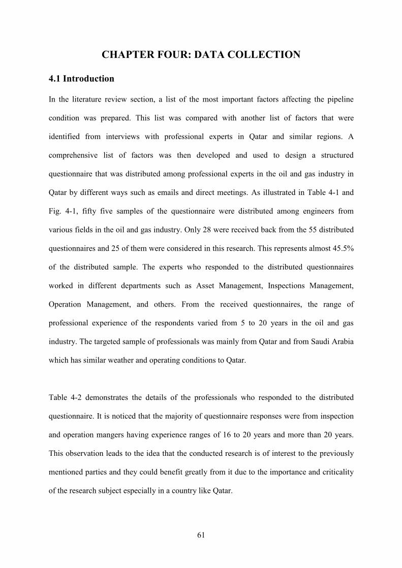
61
CHAPTER FOUR: DATA COLLECTION
4.1 Introduction
In the literature review section, a list of the most important factors affecting the pipeline
condition was prepared. This list was compared with another list of factors that were
identified from interviews with professional experts in Qatar and similar regions. A
comprehensive list of factors was then developed and used to design a structured
questionnaire that was distributed among professional experts in the oil and gas industry in
Qatar by different ways such as emails and direct meetings. As illustrated in Table 4-1 and
Fig. 4-1, fifty five samples of the questionnaire were distributed among engineers from
various fields in the oil and gas industry. Only 28 were received back from the 55 distributed
questionnaires and 25 of them were considered in this research. This represents almost 45.5%
of the distributed sample. The experts who responded to the distributed questionnaires
worked in different departments such as Asset Management, Inspections Management,
Operation Management, and others. From the received questionnaires, the range of
professional experience of the respondents varied from 5 to 20 years in the oil and gas
industry. The targeted sample of professionals was mainly from Qatar and from Saudi Arabia
which has similar weather and operating conditions to Qatar.
Table 4-2 demonstrates the details of the professionals who responded to the distributed
questionnaire. It is noticed that the majority of questionnaire responses were from inspection
and operation mangers having experience ranges of 16 to 20 years and more than 20 years.
This observation leads to the idea that the conducted research is of interest to the previously
mentioned parties and they could benefit greatly from it due to the importance and criticality
of the research subject especially in a country like Qatar.
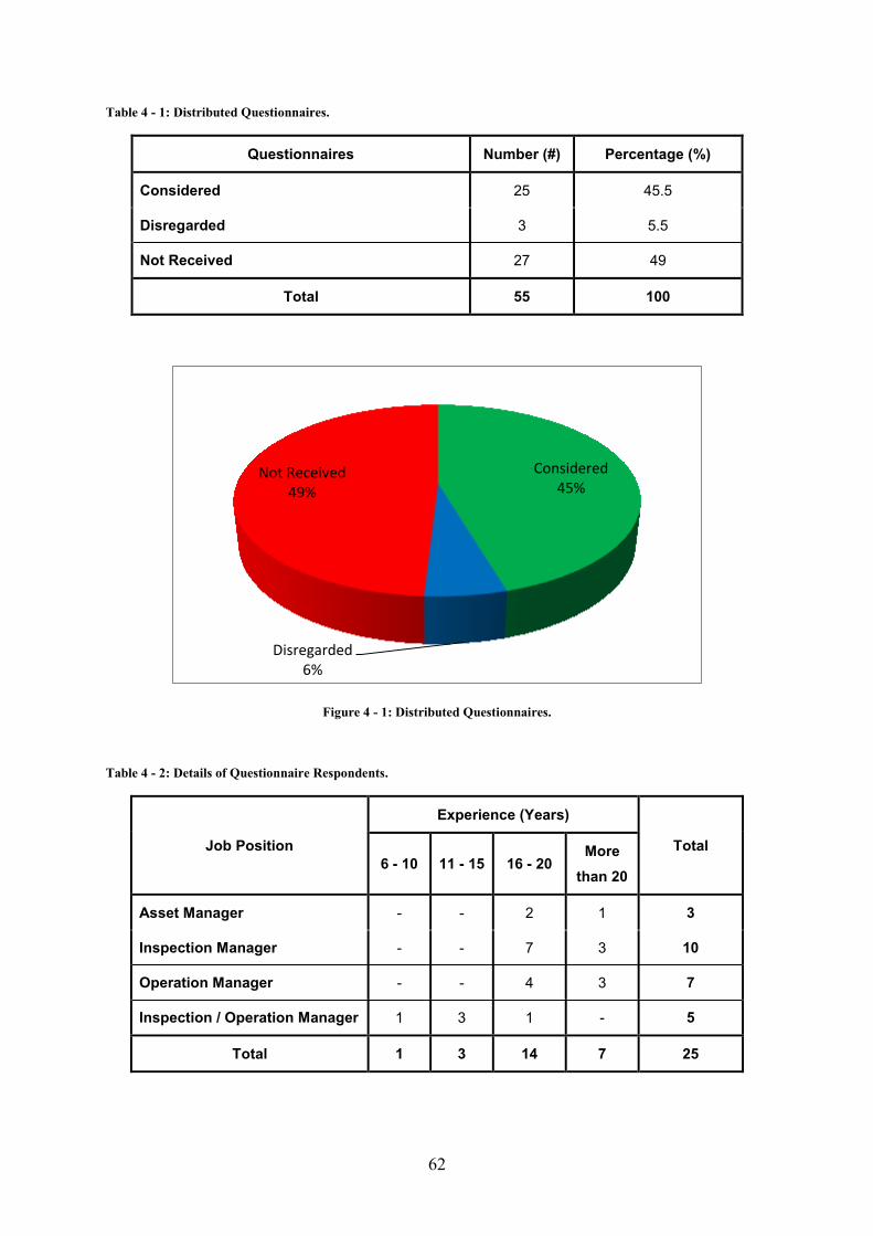
62
Table 4 - 1: Distributed Questionnaires.
Questionnaires Number (#) Percentage (%)
Considered 25 45.5
Disregarded 3 5.5
Not Received 27 49
Total 55 100
Figure 4 - 1: Distributed Questionnaires.
Table 4 - 2: Details of Questionnaire Respondents.
Job Position
Experience (Years)
Total
6 - 10 11 - 15 16 - 20 More
than 20
Asset Manager - - 2 1 3
Inspection Manager - - 7 3 10
Operation Manager - - 4 3 7
Inspection / Operation Manager 1 3 1 - 5
Total 1 3 14 7 25
Considered45%
Disregarded6%
Not Received49%
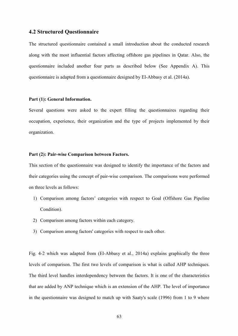
63
4.2 Structured Questionnaire
The structured questionnaire contained a small introduction about the conducted research
along with the most influential factors affecting offshore gas pipelines in Qatar. Also, the
questionnaire included another four parts as described below (See Appendix A). This
questionnaire is adapted from a questionnaire designed by El-Abbasy et al. (2014a).
Part (1): General Information.
Several questions were asked to the expert filling the questionnaires regarding their
occupation, experience, their organization and the type of projects implemented by their
organization.
Part (2): Pair-wise Comparison between Factors.
This section of the questionnaire was designed to identify the importance of the factors and
their categories using the concept of pair-wise comparison. The comparisons were performed
on three levels as follows:
1) Comparison among factors’ categories with respect to Goal (Offshore Gas Pipeline
Condition).
2) Comparison among factors within each category.
3) Comparison among factors' categories with respect to each other.
Fig. 4-2 which was adapted from (El-Abbasy et al., 2014a) explains graphically the three
levels of comparison. The first two levels of comparison is what is called AHP techniques.
The third level handles interdependency between the factors. It is one of the characteristics
that are added by ANP technique which is an extension of the AHP. The level of importance
in the questionnaire was designed to match up with Saaty's scale (1996) from 1 to 9 where
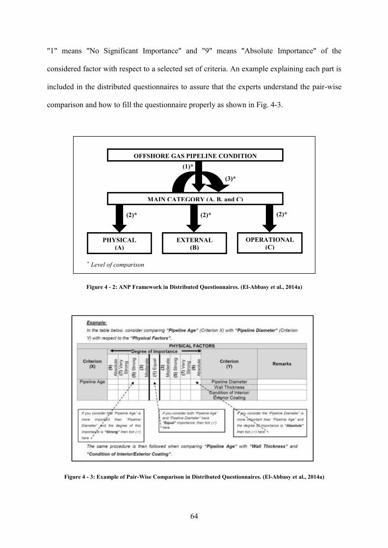
64
"1" means "No Significant Importance" and "9" means "Absolute Importance" of the
considered factor with respect to a selected set of criteria. An example explaining each part is
included in the distributed questionnaires to assure that the experts understand the pair-wise
comparison and how to fill the questionnaire properly as shown in Fig. 4-3.
Figure 4 - 2: ANP Framework in Distributed Questionnaires. (El-Abbasy et al., 2014a)
Figure 4 - 3: Example of Pair-Wise Comparison in Distributed Questionnaires. (El-Abbasy et al., 2014a)
(2)* (2)* (2)*
(3)*
(1)*
MAIN CATEGORY (A, B, and C)
OFFSHORE GAS PIPELINE CONDITION
ASSESSMENT
PHYSICAL
(A)
EXTERNAL
(B)
OPERATIONAL
(C)
* Level of comparison

65
Part (3): Determining the Score of Factors.
Since the factors are not similar in their effect on the gas pipeline condition and have
different attributes, the experts were asked to assign a score value for each of the different
factors' attributes. The scale used for the scores is from "0" to "10" where "0" indicates the
worst or lowest score and "10" indicates the best or highest score. A simple example was
included also in the distributed questionnaires as shown in Fig. 4-4.
Figure 4 - 4: Example of Determining the Score of Factors in Distributed Questionnaires. (El-Abbasy et al., 2014a)
Part (4): Gas Pipelines Condition Index.
The purpose of this part of the questionnaire is to propose a condition rating scale for the
offshore gas pipelines. The same scale used in Part (3), from "0" to "10", was used is this part
where "0" indicates the worst condition and "10" indicates the best. Also, the experts were
requested to assign a suitable qualitative description for the pipeline condition along with
suggested required action to be performed.

66
Figure 4 - 51: Example of Gas Pipeline Condition Index. (El-Abbasy et al., 2014a)
4.3 Historical Inspection Data
In order to validate the developed model, inspection data for three major pipelines was
collected from a famous state-owned pipeline operator in Qatar. The collected data included
inspection reports from four types of inspections: Inline Inspection (ILI), Remotely Operated
Vehicle Inspection (ROV), Cathodic Protection Monitoring System, and Direct Current
Voltage Gradient (DCVG) inspection. These inspections were executed in 1996, 2001, 2004,
2008 and 2009. The oldest pipeline (20 inch.) was constructed in 1972 with a length of 45 km
offshore. The second one (24 inch.) was installed in 1979 with a total length of 121 km (89
offshore and 32 km onshore). The most recent pipeline (12 inch.) was commissioned in 1990
consisting of 80 km of offshore pipeline and 131 km onshore leading to 211 km in total.
However, the inspections were not performed for the total length of pipelines except the
oldest one, constructed in 1972, which was fully inspected. A length of 85 km was inspected
from the second pipeline and 77 km from the most recent one which had a total length of 211
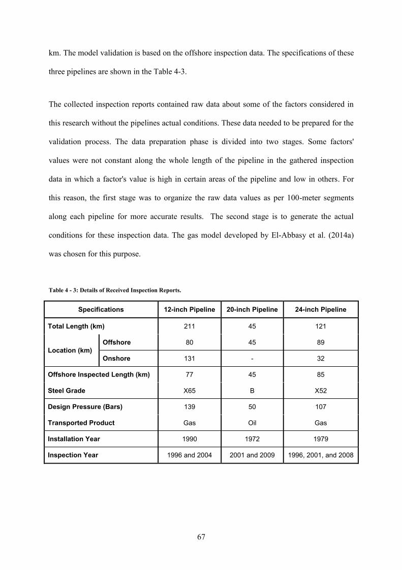
67
km. The model validation is based on the offshore inspection data. The specifications of these
three pipelines are shown in the Table 4-3.
The collected inspection reports contained raw data about some of the factors considered in
this research without the pipelines actual conditions. These data needed to be prepared for the
validation process. The data preparation phase is divided into two stages. Some factors'
values were not constant along the whole length of the pipeline in the gathered inspection
data in which a factor's value is high in certain areas of the pipeline and low in others. For
this reason, the first stage was to organize the raw data values as per 100-meter segments
along each pipeline for more accurate results. The second stage is to generate the actual
conditions for these inspection data. The gas model developed by El-Abbasy et al. (2014a)
was chosen for this purpose.
Table 4 - 3: Details of Received Inspection Reports.
Specifications 12-inch Pipeline 20-inch Pipeline 24-inch Pipeline
Total Length (km) 211 45 121
Location (km)
Offshore 80 45 89
Onshore 131 - 32
Offshore Inspected Length (km) 77 45 85
Steel Grade X65 B X52
Design Pressure (Bars) 139 50 107
Transported Product Gas Oil Gas
Installation Year 1990 1972 1979
Inspection Year 1996 and 2004 2001 and 2009 1996, 2001, and 2008
68
A point to be taken into consideration is that the 20-inch pipeline transports oil products but
is treated as a gas pipeline where the actual pipeline conditions were calculated using the
same gas model applied on the other two pipelines. This is to provide a wide variety of
pipeline diameters and ages. Furthermore, the received inspection data sets contained
information about seven out of the eleven factors considered in this research; Age, Diameter,
Metal Loss, Coating Condition, Crossings, Cathodic Protection and Operating Pressure.
Thus, adjustments were required for the relative weights of these factors as shown later in the
model validation section.
69
CHAPTER FIVE: MODEL DEVELOPMENT
5.1 Introduction
The goal of this research is to develop a condition assessment model of offshore gas pipelines
in Qatar using Evidential Reasoning (ER), Analytic Network Process (ANP) and Fuzzy Set
Theory (FST). The following chapter describes the methodology of the current research. This
methodology started by performing a short literature review to investigate the previous
research trials in the field of condition assessment of oil and gas pipelines. It was also
necessary to study the different methods and techniques used for pipeline condition
assessment. In the literate review, a list of factors was determined which mostly affect the
condition of offshore gas pipelines. That was carried out in three steps. First, a number of
professional experts in the oil and gas industry were asked to give a list of the most
influential factors that affect the pipeline condition. At the same time, another list was being
prepared from literature and previous studies. Then, the two lists were compared to each
other to select the similar factors agreed upon by both, academics and professionals. Thus,
the most important factors that needed to be considered in the pipeline condition assessment
process was identified. Then, a questionnaire was structured, based on the selected factors,
and distributed among professionals in the oil and gas industry in Middle-East but with a
strong focus on Qatar and Saudi Arabia.
The distributed questionnaire served as a ranking tool for the factors that affect the condition
assessment process of offshore gas pipelines. In addition, a condition rating scale was
developed from the responses of the distributed questionnaires. Also, the professionals were
asked to assign an attribute effect value for each factor affecting the pipeline condition. These
70
effect values were later used to develop the factors thresholds and their fuzzy membership
functions as explained later in this chapter.
The structured questionnaire was designed on an open-ended basis where the respondents had
the option to add any other missing factors, that weren't listed in the questionnaire, which
may affect the pipeline condition assessment process. This step was performed to assure that
the distributed questionnaire included the most influential factors on the pipeline condition.
The respondents agreed that the questionnaire listed the most important factors needed to be
considered for the condition assessment. The ANP technique was then applied on the
collected data, Experts Feedback, to calculate the relative weight of each of the listed factors.
The factors' relative weights along with the developed thresholds' membership functions are
used as an input for the proposed Evidential Reasoning (ER) module for the offshore gas
pipelines condition assessment. Then, the developed model was tested using actual inspection
data for existing gas pipelines. These data was obtained from Qatar. After that, a deterioration
curve was developed using the proposed ER module for different ages of the gas pipeline.
Later, a sensitivity study was executed to study the effect of changing the factors' values on
the model's output. Finally, a condition rating scale was proposed based on the outputs of the
previous steps.
It is important to note that Evidential Reasoning algorithm was previously applied on pipeline
condition assessment but not as deep as this research. Also, this research applied ANP
technique, fuzzy membership functions and ER algorithm to perform a comprehensive
condition assessment analysis. It integrated Evidential Reasoning Algorithm with ANP which
dealt with interdependencies and multi-criteria decision analysis under various uncertainties.
This integration considered factors' interdependency using ANP, made decisions under
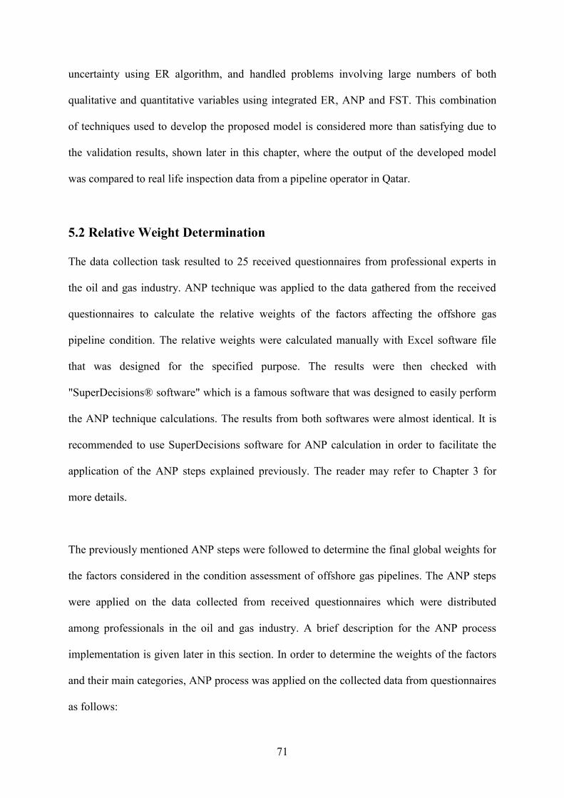
71
uncertainty using ER algorithm, and handled problems involving large numbers of both
qualitative and quantitative variables using integrated ER, ANP and FST. This combination
of techniques used to develop the proposed model is considered more than satisfying due to
the validation results, shown later in this chapter, where the output of the developed model
was compared to real life inspection data from a pipeline operator in Qatar.
5.2 Relative Weight Determination
The data collection task resulted to 25 received questionnaires from professional experts in
the oil and gas industry. ANP technique was applied to the data gathered from the received
questionnaires to calculate the relative weights of the factors affecting the offshore gas
pipeline condition. The relative weights were calculated manually with Excel software file
that was designed for the specified purpose. The results were then checked with
"SuperDecisions® software" which is a famous software that was designed to easily perform
the ANP technique calculations. The results from both softwares were almost identical. It is
recommended to use SuperDecisions software for ANP calculation in order to facilitate the
application of the ANP steps explained previously. The reader may refer to Chapter 3 for
more details.
The previously mentioned ANP steps were followed to determine the final global weights for
the factors considered in the condition assessment of offshore gas pipelines. The ANP steps
were applied on the data collected from received questionnaires which were distributed
among professionals in the oil and gas industry. A brief description for the ANP process
implementation is given later in this section. In order to determine the weights of the factors
and their main categories, ANP process was applied on the collected data from questionnaires
as follows:
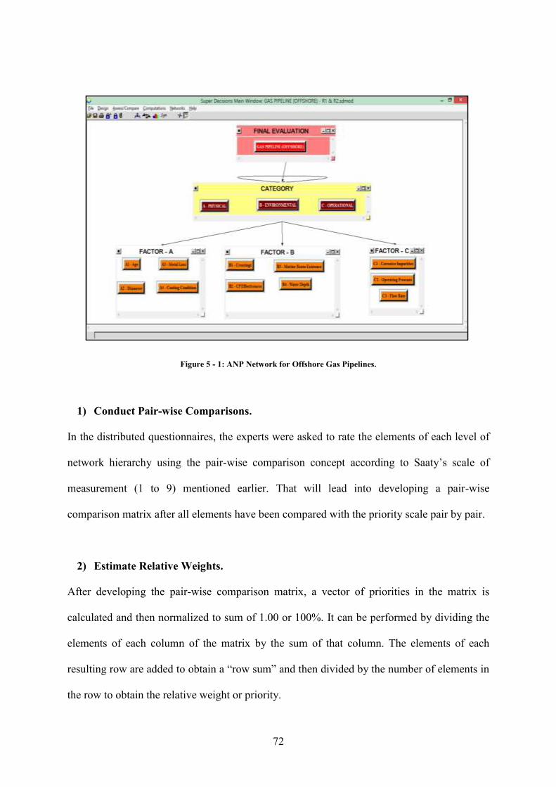
72
Figure 5 - 1: ANP Network for Offshore Gas Pipelines.
1) Conduct Pair-wise Comparisons.
In the distributed questionnaires, the experts were asked to rate the elements of each level of
network hierarchy using the pair-wise comparison concept according to Saaty’s scale of
measurement (1 to 9) mentioned earlier. That will lead into developing a pair-wise
comparison matrix after all elements have been compared with the priority scale pair by pair.
2) Estimate Relative Weights.
After developing the pair-wise comparison matrix, a vector of priorities in the matrix is
calculated and then normalized to sum of 1.00 or 100%. It can be performed by dividing the
elements of each column of the matrix by the sum of that column. The elements of each
resulting row are added to obtain a “row sum” and then divided by the number of elements in
the row to obtain the relative weight or priority.

73
3) Determine Consistency Ratio (CR).
The term "Consistency Ratio" was developed because humans are sometimes inconsistent or
not serious in answering questions in the distributed questionnaires. To overcome this issue,
CR is used to validate the results and measure the consistency in the pair-wise comparison
process. Saaty (1994) presented a set of acceptable CR values for different sizes of matrices.
In the earlier sections, a table of acceptable CR values was introduced. The CR values were
calculated for all matrices in this research and the results showed that all of them were
consistent and within acceptable limits.
4) Develop the Unweighted Super-matrix.
After checking the consistency, the pair-wise comparisons between the main categories and
factors are translated into a two-dimensional super-matrix under the influence of
interdependency. The unweighted super-matrix, shown in Table 5-1, for one of the
questionnaire responses, is constructed from the priorities (i.e. relative weights) derived from
the different pair-wise comparisons that were carried out in the previous steps. The nodes,
grouped by the clusters they belong to, are the labels of rows and columns of the super-
matrix. The following tables does not show the entire matrices sizes due to their large sizes.
For this reason, only the main categories are shown in the column side against the factors in
the row side of the presented matrices.
5) Develop the Weighted Super-matrix.
The weighted super-matrix is derived from the unweighted super-matrix. It is developed by
dividing each entry in each row in the unweighted super-matrix by the total summation of its
relative intersecting column. For example, the summation of column A in Table 5-1
(unweighted super-matrix) is equal to 2.00 and the corresponding entry in row B is 0.875;

74
therefore, dividing 0.875 by 2.00 results in the weighted value of this entry, which is 0.438.
This value is entered into the intersecting cell of row B and column A in Table 5-2 (weighted
super-matrix). This step is repeated for the rest of the values in the unweighted super-matrix.
In Table 5-2 (weighted super-matrix), it can be seen that the summation of each column is
equal to 1.00.
Table 5 - 1: Developed Unweighted Super-Matrix for Response (1) of Received Questionnaires.
GOAL A:
PHYSICAL FACTORS
B: EXTERNAL FACTORS
C: OPERATIONAL
FACTORS
GOAL 0 0 0 0
A: PHYSICAL FACTORS 0.778 0 0.750 0.125
B: EXTERNAL FACTORS 0.111 0.875 0 0.875
C: OPERATIONAL FACTORS 0.111 0.125 0.250 0
A1: Age 0 0.066 0 0
A2: Diameter 0 0.009 0 0
A3: Metal Loss 0 0.462 0 0
A4: Coating Condition 0 0.462 0 0
B1: Crossing 0 0 0.071 0
B2: CP Effectiveness 0 0 0.643 0
B3: Marine Route Existence 0 0 0.214 0
B4: Water Depth 0 0 0.071 0
C1: Corrosive Impurities 0 0 0 0.122
C2: Operating Pressure 0 0 0 0.854
C3: Flow Rate 0 0 0 0.024
Total 1 2 2 2
6) Develop the Limit Super-matrix.
Tables 5-1 and 5-2 showed only the unweighted and weighted super-matrices for the main
categories (column side) only due to size limitations. The rest of the sub-matrices were
entered into the super-matrix and the weighted super-matrix was completed. The next step is
to obtain the limit super-matrix by raising the weighted super-matrix to a sufficient large
power until convergence occurs. This is repeated until the numbers in all columns of limit
super-matrix are identical. Table 5-3 shows the limit-super matrix for Response (1) of the
collected questionnaires. The previous steps were applied to all questionnaire responses until
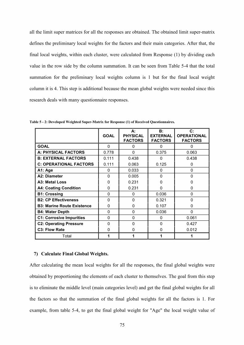
75
all the limit super matrices for all the responses are obtained. The obtained limit super-matrix
defines the preliminary local weights for the factors and their main categories. After that, the
final local weights, within each cluster, were calculated from Response (1) by dividing each
value in the row side by the column summation. It can be seen from Table 5-4 that the total
summation for the preliminary local weights column is 1 but for the final local weight
column it is 4. This step is additional because the mean global weights were needed since this
research deals with many questionnaire responses.
Table 5 - 2: Developed Weighted Super-Matrix for Response (1) of Received Questionnaires.
GOAL A:
PHYSICAL FACTORS
B: EXTERNAL FACTORS
C: OPERATIONAL
FACTORS
GOAL 0 0 0 0
A: PHYSICAL FACTORS 0.778 0 0.375 0.063
B: EXTERNAL FACTORS 0.111 0.438 0 0.438
C: OPERATIONAL FACTORS 0.111 0.063 0.125 0
A1: Age 0 0.033 0 0
A2: Diameter 0 0.005 0 0
A3: Metal Loss 0 0.231 0 0
A4: Coating Condition 0 0.231 0 0
B1: Crossing 0 0 0.036 0
B2: CP Effectiveness 0 0 0.321 0
B3: Marine Route Existence 0 0 0.107 0
B4: Water Depth 0 0 0.036 0
C1: Corrosive Impurities 0 0 0 0.061
C2: Operating Pressure 0 0 0 0.427
C3: Flow Rate 0 0 0 0.012
Total 1 1 1 1
7) Calculate Final Global Weights.
After calculating the mean local weights for all the responses, the final global weights were
obtained by proportioning the elements of each cluster to themselves. The goal from this step
is to eliminate the middle level (main categories level) and get the final global weights for all
the factors so that the summation of the final global weights for all the factors is 1. For
example, from table 5-4, to get the final global weight for "Age" the local weight value of

76
"0.019" was multiplied by the global weight value of the "Physical" which is 0.370 for all the
factors under this category. This will result to 0.039 as global weight for "Age". This step was
repeated for the rest of the factors and for all questionnaire responses. Then, the mean values
of the global weights for all the factors were calculated.
Table 5 - 3: Developed Limit Super-Matrix for Response (1) of Received Questionnaires.
GOAL A:
PHYSICAL FACTORS
B: EXTERNAL FACTORS
C: OPERATIONAL
FACTORS
GOAL 0 0 0 0
A: PHYSICAL FACTORS 0.185 0.185 0.185 0.185
B: EXTERNAL FACTORS 0.233 0.233 0.233 0.233
C: OPERATIONAL FACTORS 0.081 0.081 0.081 0.081
A1: Age 0.019 0.019 0.019 0.019
A2: Diameter 0.006 0.006 0.006 0.006
A3: Metal Loss 0.080 0.080 0.080 0.080
A4: Coating Condition 0.080 0.080 0.080 0.080
B1: Crossing 0.017 0.017 0.017 0.017
B2: CP Effectiveness 0.150 0.150 0.150 0.150
B3: Marine Route Existence 0.050 0.050 0.050 0.050
B4: Water Depth 0.017 0.017 0.017 0.017
C1: Corrosive Impurities 0.014 0.014 0.014 0.014
C2: Operating Pressure 0.063 0.063 0.063 0.063
C3: Flow Rate 0.005 0.005 0.005 0.005
Total 1 1 1 1
Table 5-5 lists the final local and global weights for the factors and their main categories for
all questionnaire responses. It can be noted from the final global weights of the first two main
categories, Physical with 0.400 and External with 0.447, that these two categories affect the
offshore gas pipeline condition almost equally. The late factors' category which is the
Operational factors has a final global weight of 0.153. This makes it the least affecting
category. Also, the final global weight for each of the factors was calculated.
The factors "Metal Loss" and "Cathodic Protection", with mean global weight values of 0.211
and 0.180 respectively, were the most important criteria affecting the offshore gas pipeline
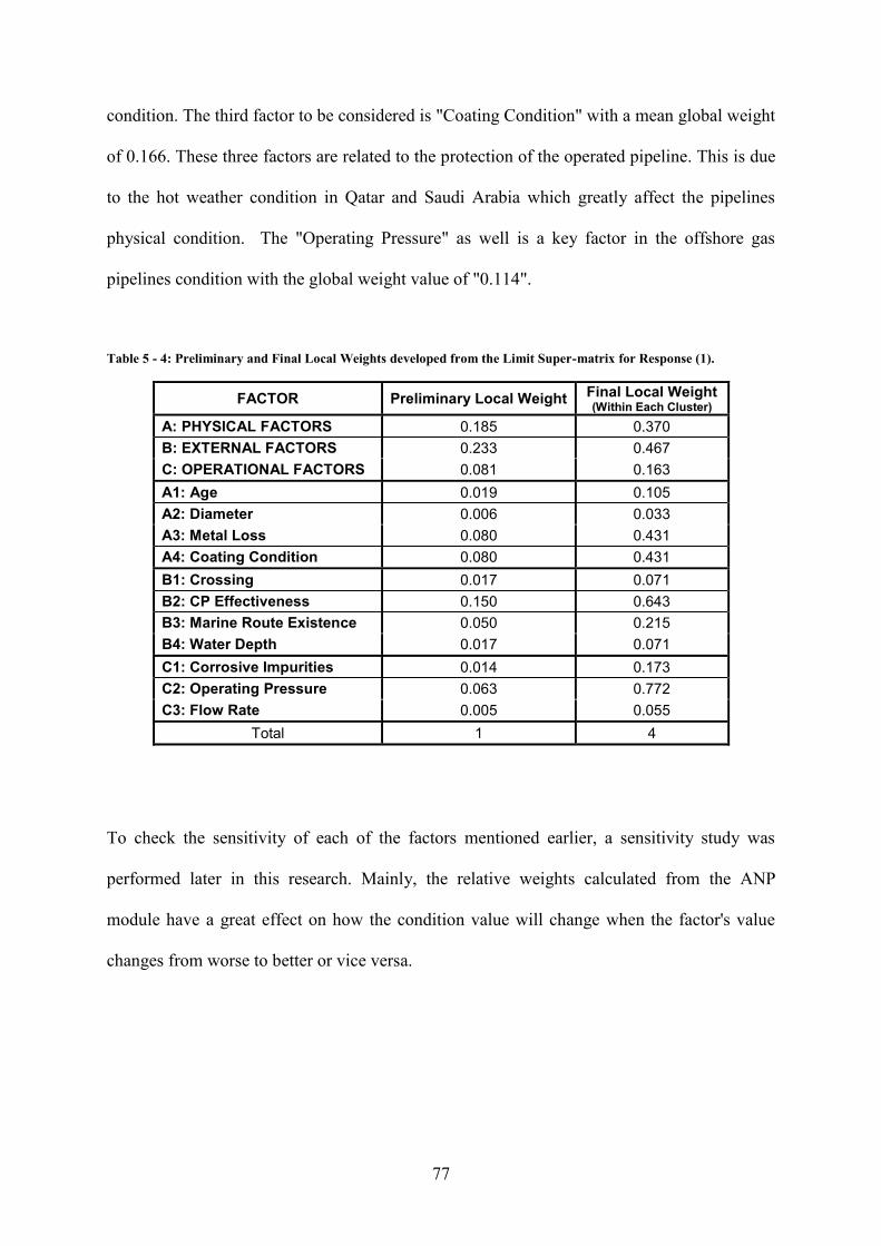
77
condition. The third factor to be considered is "Coating Condition" with a mean global weight
of 0.166. These three factors are related to the protection of the operated pipeline. This is due
to the hot weather condition in Qatar and Saudi Arabia which greatly affect the pipelines
physical condition. The "Operating Pressure" as well is a key factor in the offshore gas
pipelines condition with the global weight value of "0.114".
Table 5 - 4: Preliminary and Final Local Weights developed from the Limit Super-matrix for Response (1).
FACTOR Preliminary Local Weight Final Local Weight (Within Each Cluster)
A: PHYSICAL FACTORS 0.185 0.370
B: EXTERNAL FACTORS 0.233 0.467
C: OPERATIONAL FACTORS 0.081 0.163
A1: Age 0.019 0.105
A2: Diameter 0.006 0.033
A3: Metal Loss 0.080 0.431
A4: Coating Condition 0.080 0.431
B1: Crossing 0.017 0.071
B2: CP Effectiveness 0.150 0.643
B3: Marine Route Existence 0.050 0.215
B4: Water Depth 0.017 0.071
C1: Corrosive Impurities 0.014 0.173
C2: Operating Pressure 0.063 0.772
C3: Flow Rate 0.005 0.055
Total 1 4
To check the sensitivity of each of the factors mentioned earlier, a sensitivity study was
performed later in this research. Mainly, the relative weights calculated from the ANP
module have a great effect on how the condition value will change when the factor's value
changes from worse to better or vice versa.

78
Table 5 - 5: Final Local and Global Weights for Main Categories and factors affecting Offshore Gas Pipeline
Condition.
Category Global
Weight Factor
Local
Weight
Global
Weight
Physical
Factors 0.400
A1 Age 0.100 0.040
A2 Diameter 0.034 0.014
A3 Metal Loss 0.450 0.180
A4 Coating Condition 0.416 0.166
External
Factors 0.447
B1 Crossings 0.064 0.029
B2 Cathodic Protection 0.472 0.211
B3 Marine Route Existence 0.213 0.095
B4 Water Depth 0.251 0.112
Operational
Factors 0.153
C1 Corrosive Impurities 0.199 0.031
C2 Operating Pressure 0.746 0.114
C3 Flow Rate 0.055 0.008
Total 1.000
3.000 1.000
5.3 Fuzzy-based Threshold Model Implementation
5.3.1 Developing Membership Functions
As mentioned in the previous sections, eleven factors were considered in developing the
model in hand. These factors are divided into three categories: Physical, External and
Operational. Tables 5-6, 5-7 and 5-8 show the thresholds for the eleven factors which were
developed from the feedbacks on the distributed questionnaires among professionals in the oil
and gas industry. The factors' thresholds were developed carefully to adapt the experts’
responses from the gathered questionnaires. It can be seen that the thresholds have
overlapping intervals due to uncertainty of the exact limits of the five intervals for each of the
conditions in each factor. For example, an expert cannot define exactly the limits or range of

79
years of the condition "Good" in the "Age" factor. The next tables provide the developed
thresholds for all eleven factors.
5.3.1.1 Fuzzy Input Variables
As discussed in the previous sections, eleven input variables were identified as the most
influential factors that affect the condition of offshore gas pipelines. These factors are Age,
Diameter, Metal Loss, Coating Condition, Number of Crossings, Cathodic Protection
Effectiveness, Marine Route Existence, Water Depth, Corrosive Impurities, Operating
Pressure and Flow Rate. Fuzzy sets theory was applied in this step and a group of fuzzy sets
were identified so that each input variable is expressed by five membership functions:
Excellent, Very Good, Good, Fair and Poor as shown in Fig. 5-2 to Fig. 5-12.
The thresholds developed in the previous section were later used as a basis to determine the
range and shape of the developed membership functions. The maximum and minimum limits
from the thresholds represent the Excellent and Poor membership functions, respectively,
which adapt trapezoidal shapes. The three remaining membership functions in the middle
which adapt triangular shapes were placed to overlap the Excellent and Poor membership
functions and to overlap each other taking into consideration the limits in the developed
thresholds. Water Depth and Flow Rate are exceptions since they do not follow the regular
order of conditions, Excellent to critical or the opposite, as shown later. The overlap between
the five membership functions was placed to achieve a degree of fuzziness of 0.5. This is
performed so that:
1) The total summation of membership functions of any input value will be "1.0",
2) And to eliminate the ignorance in the developed ER module.

80
It is reasonable for the decision maker to be confused between two adjacent evaluation grades
for any given factor's value but they are sure that the given value falls totally between these
two evaluations. Also, a membership degree cannot be expressed by more than two adjacent
evaluation grades since it violates the membership design properties which states that "Each
membership function overlaps only with the closest neighboring membership functions"
(Zhang & Liu, 2006).
Table 5 - 6: Physical Factors Thresholds.
Factor Unit Linguistic Variable Threshold Interval
Age Years
Excellent 0 -- 10
V. Good 6 -- 20
Good 16 -- 30
Fair 26 -- 41
Critical 36 -- 55 & more
Diameter inches
Excellent 38 -- >48
V. Good 23 -- 48
Good 16 -- 26
Fair 9 -- 18
Critical 0 -- 12
Metal Loss %
Excellent 0 -- 17
V. Good 9 -- 35
Good 26 -- 55
Fair 46 -- 74
Critical 66 -- 100
Coating Condition
%
Excellent 84 -- 100
V. Good 66 -- 94
Good 46 -- 75
Fair 27 -- 55
Critical 0 -- 35

81
Table 5 - 7: External Factors Thresholds.
Factor Unit Linguistic Variable Threshold Interval
Crossing number
Excellent 0 -- 1
V. Good 1 -- 3
Good 3 -- 5
Fair 5 -- 7
Critical 7 -- >9
Cathodic Protection
Effectiveness mV
Excellent 951 -- 1300
V. Good 851 -- 1000
Good 751 -- 900
Fair 676 -- 800
Critical <600 -- 700
Marine Route Existence
%
Excellent 0 -- 17
V. Good 9 -- 35
Good 27 -- 55
Fair 46 -- 75
Critical 66 -- 100
Water Depth meters
Excellent 26 -- 40
V. Good 9 -- 33
Good 34 -- 60
Fair 51 -- >60
Critical 0 -- 10
Table 5 - 8: Operational Factors Thresholds.
Factor Unit Linguistic Variable Threshold Interval
Corrosive Impurities
%
Excellent 0 -- 17
V. Good 9 -- 34
Good 26 -- 52
Fair 44 -- 70
Critical 61 -- 100
Operation Pressure
% of Design
Excellent 0 -- 27
V. Good 14 -- 49
Good 41 -- 67
Fair 59 -- 81
Critical 76 -- 100
Flow Rate % of
Design
Excellent 42 -- 63
V. Good 56 -- 85
Good 14 -- 55
Fair 0 -- 27
Critical 81 -- 100

82
Figures 5-2 to 5-12 show the membership functions for the input values of the eleven
considered factors that form the core of the developed model. They are extracted from the
thresholds tables illustrated previously.
Figure 5 - 2: Fuzzy Input Variable (Age).
Figure 5 - 3: Fuzzy Input Variable (Diameter).
0.0
0.5
1.0
0 10 20 30 40 50
EXCELLENT V. GOOD GOOD FAIR CRITICAL
Age (Years)
Mem
ber
ship
Fu
nct
ion
0.0
0.5
1.0
0 10 20 30 40
EXCELLENTV. GOODGOODFAIRCRITICAL
Mem
ber
ship
Fu
nct
ion
Diameter (Inches)

83
Figure 5 - 4: Fuzzy Input Variable (Metal Loss).
Figure 5 - 5: Fuzzy Input Variable (Coating Condition).
0.0
0.5
1.0
0 20 40 60 80 100
EXCELLENT V. GOOD GOOD FAIR CRITICAL
Mem
ber
ship
Fu
nct
ion
Metal Loss (%)
0.0
0.5
1.0
0 20 40 60 80 100
EXCELLENTV. GOODGOODFAIRCRITICAL
Mem
ber
ship
Fu
nct
ion
Coating Condition (%)

84
Figure 5 - 6: Fuzzy Input Variable (Crossing).
Figure 5 - 7: Fuzzy Input Variable (Cathodic Protection Effectiveness).
0.0
0.5
1.0
0 1 2 3 4 5 6 7 8 9
EXCELLENT V. GOOD GOOD FAIR CRITICAL
Mem
ber
ship
Fu
nct
ion
Crossings (#)
0.0
0.5
1.0
600 800 1000 1200
CRITICAL FAIR GOOD V. GOOD EXCELLENT
Mem
ber
ship
Fu
nct
ion
Cathodic Protection Effectiveness (mV)

85
Figure 5 - 8: Fuzzy Input Variable (Marine Route Existence).
Figure 5 - 9: Fuzzy Input Variable (Water Depth).
0.0
0.5
1.0
0 20 40 60 80 100
EXCELLENT V. GOOD GOOD FAIR CRITICAL
Mem
ber
ship
Fu
nct
ion
Marine Route Existance (%)
0.0
0.5
1.0
0 10 20 30 40 50 60
CRITICAL V. GOOD EXCELLENT GOOD FAIR
Mem
ber
ship
Fu
nct
ion
Water Depth (m)
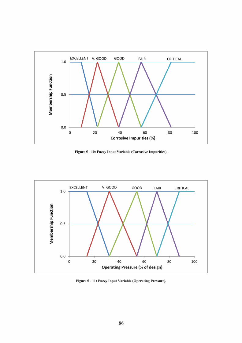
86
Figure 5 - 10: Fuzzy Input Variable (Corrosive Impurities).
Figure 5 - 11: Fuzzy Input Variable (Operating Pressure).
0.0
0.5
1.0
0 20 40 60 80 100
EXCELLENT V. GOOD GOOD FAIR CRITICAL
Mem
ber
ship
Fu
nct
ion
Corrosive Impurities (%)
0.0
0.5
1.0
0 20 40 60 80 100
EXCELLENT V. GOOD GOOD FAIR CRITICAL
Mem
ber
ship
Fu
nct
ion
Operating Pressure (% of design)
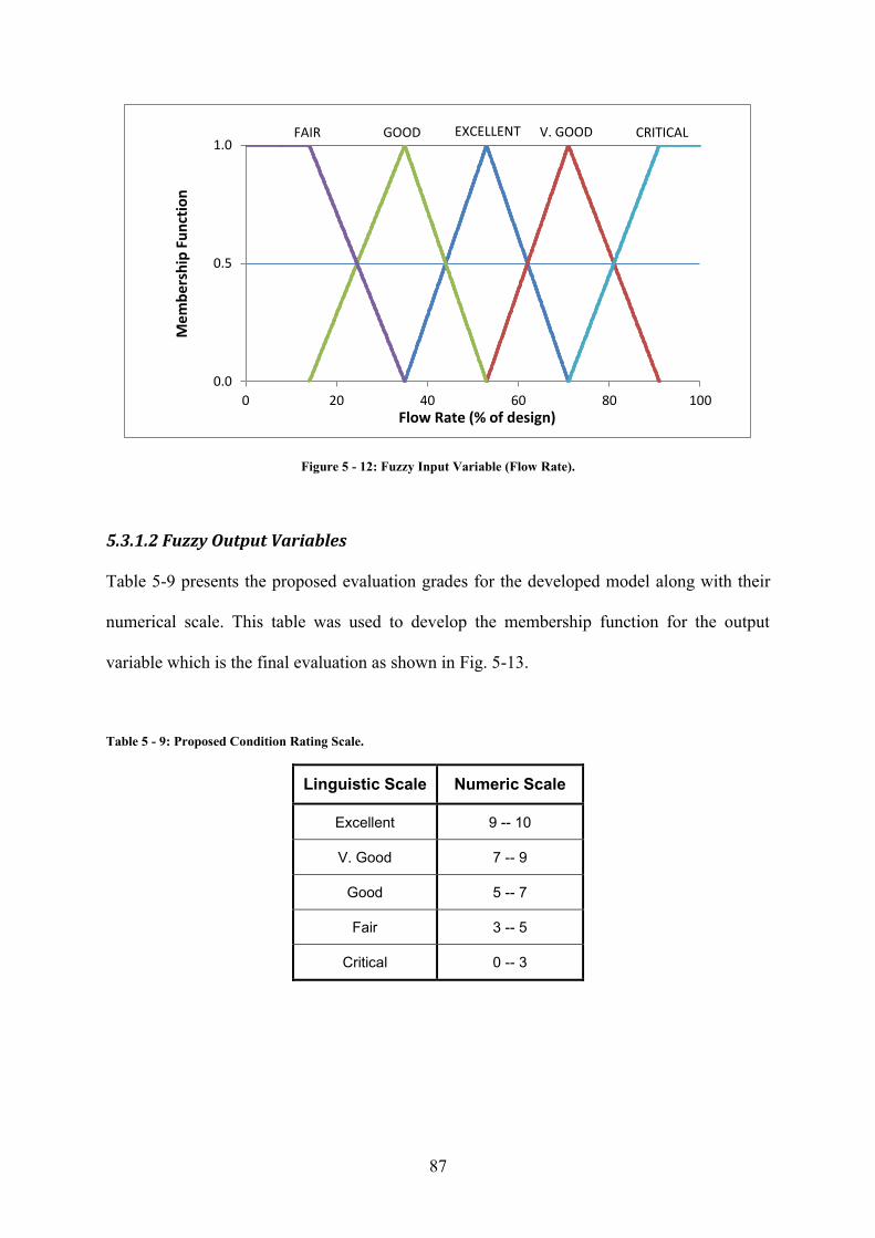
87
Figure 5 - 12: Fuzzy Input Variable (Flow Rate).
5.3.1.2 Fuzzy Output Variables
Table 5-9 presents the proposed evaluation grades for the developed model along with their
numerical scale. This table was used to develop the membership function for the output
variable which is the final evaluation as shown in Fig. 5-13.
Table 5 - 9: Proposed Condition Rating Scale.
Linguistic Scale Numeric Scale
Excellent 9 -- 10
V. Good 7 -- 9
Good 5 -- 7
Fair 3 -- 5
Critical 0 -- 3
0.0
0.5
1.0
0 20 40 60 80 100
EXCELLENT V. GOODGOODFAIR CRITICAL
Mem
ber
ship
Fu
nct
ion
Flow Rate (% of design)
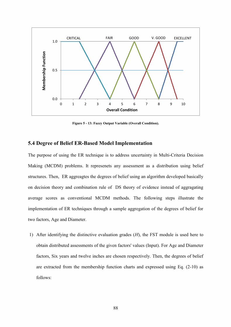
88
Figure 5 - 13: Fuzzy Output Variable (Overall Condition).
5.4 Degree of Belief ER-Based Model Implementation
The purpose of using the ER technique is to address uncertainty in Multi-Criteria Decision
Making (MCDM) problems. It represenets any assessment as a distribution using belief
structures. Then, ER aggreagtes the degrees of belief using an algorithm developed basically
on decision theory and combination rule of DS theory of evidence instead of aggragating
average scores as conventional MCDM methods. The following steps illustrate the
implementation of ER techniques through a sample aggregation of the degrees of belief for
two factors, Age and Diameter.
1) After identifying the distinctive evaluation grades (H), the FST module is used here to
obtain distributed assessments of the given factors' values (Input). For Age and Diameter
factors, Six years and twelve inches are chosen respectively. Then, the degrees of belief
are extracted from the membership function charts and expressed using Eq. (2-10) as
follows:
0.0
0.5
1.0
0 1 2 3 4 5 6 7 8 9 10
CRITICAL FAIR GOOD V. GOOD EXCELLENT
Overall Condition
Mem
ber
ship
Fu
nct
ion

89
𝑆(𝐴𝑔𝑒) = {(𝐸𝑥, 0.88), (𝑉𝐺, 0.13), (𝐺, 0), (𝐹, 0), (𝐶, 0), (𝐻, 0)}
𝑆(𝐷𝑖𝑎. ) = {(𝐸𝑥, 0), (𝑉𝐺, 0), (𝐺, 0), (𝐹, 0.75), (𝐶, 0.25), (𝐻, 0)}
Where,
Ex = Excellent, VG = Very Good, G = Good, F = Fair, C = Critical and H = Ignorance.
2) The factors relative weights (𝜔𝑖) which are calculated by the ANP module:
𝜔𝐴𝑔𝑒 = 0.040
𝜔𝐷𝑖𝑎. = 0.014
3) Later, the belief structures are then transformed into basic probability masses (𝑚𝑛,𝑖)
using Eq. (2-11) where the relative weight is multiplied with each grades' belief value.
𝑚𝐻,𝑖 is the remaining probability mass unassigned to any individual grade after all the 𝑁
grades have been considered for assessing the general attribute and is calculated using
Eq. (2-12), (2-13) & (2-14).
𝑚(𝐴𝑔𝑒) = 0.040 𝑥 {(𝐸𝑥, 0.88), (𝑉𝐺, 0.13), (𝐺, 0), (𝐹, 0), (𝐶, 0), (𝐻, 0)}
= {(𝐸𝑥, 0.04), (𝑉𝐺, 0.01), (𝐺, 0), (𝐹, 0), (𝐶, 0), (𝐻, 0.96)}
𝑚(𝐷𝑖𝑎. ) = 0.014 𝑥 {(𝐸𝑥, 0), (𝑉𝐺, 0), (𝐺, 0), (𝐹, 0.75), (𝐶, 0.25), (𝐻, 0)}
= {(𝐸𝑥, 0), (𝑉𝐺, 0), (𝐺, 0), (𝐹, 0.01), (𝐶, 0), (𝐻, 0.99)}
4) The normalizing factor (𝐾𝐼(𝑖+1)) is calculated with Eq. (2-18). After that, Eq. (2-15), (2-
16) & (2-17) are used to combine the two probability masses which results into an
individual probability mass distribution that represents both Age and Diameter factors.
𝐾𝐼(𝐴𝑔𝑒+𝐷𝑖𝑎.) = 1.001
𝑚(𝐴𝑔𝑒 + 𝐷𝑖𝑎. ) = {(𝐸𝑥, 0.04), (𝑉𝐺, 0), (𝐺, 0), (𝐹, 0.01), (𝐶, 0), (𝐻, 0.95)}
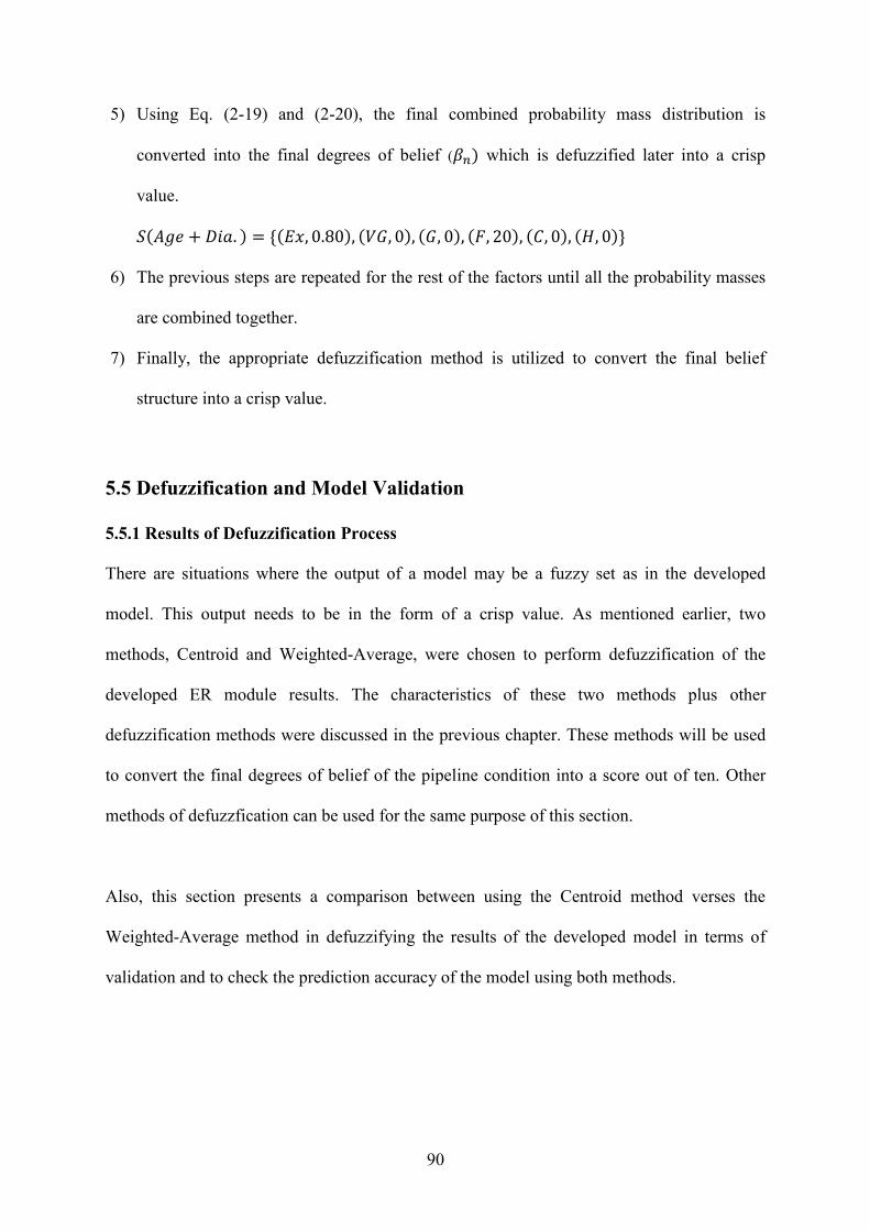
90
5) Using Eq. (2-19) and (2-20), the final combined probability mass distribution is
converted into the final degrees of belief (𝛽𝑛) which is defuzzified later into a crisp
value.
𝑆(𝐴𝑔𝑒 + 𝐷𝑖𝑎. ) = {(𝐸𝑥, 0.80), (𝑉𝐺, 0), (𝐺, 0), (𝐹, 20), (𝐶, 0), (𝐻, 0)}
6) The previous steps are repeated for the rest of the factors until all the probability masses
are combined together.
7) Finally, the appropriate defuzzification method is utilized to convert the final belief
structure into a crisp value.
5.5 Defuzzification and Model Validation
5.5.1 Results of Defuzzification Process
There are situations where the output of a model may be a fuzzy set as in the developed
model. This output needs to be in the form of a crisp value. As mentioned earlier, two
methods, Centroid and Weighted-Average, were chosen to perform defuzzification of the
developed ER module results. The characteristics of these two methods plus other
defuzzification methods were discussed in the previous chapter. These methods will be used
to convert the final degrees of belief of the pipeline condition into a score out of ten. Other
methods of defuzzfication can be used for the same purpose of this section.
Also, this section presents a comparison between using the Centroid method verses the
Weighted-Average method in defuzzifying the results of the developed model in terms of
validation and to check the prediction accuracy of the model using both methods.

91
5.5.2 Model Validation
In order to validate the model, a full inspection data for an existing gas pipeline in Qatar was
collected as described later in the model testing section. After examining the collected data, it
was observed that some of the factors considered when developing this model were not
constant along the whole length of the inspected pipeline. As an example, the metal loss
depth was low in a certain location of the pipeline where it was high in another. Coating
Condition, Cathodic Protection Effectiveness and Crossings underwent this change as well.
To overcome this problem and produce accurate and acceptable evaluation, the pipeline was
divided into similar segment each has 100 m length. The condition of each pipeline segment
is assessed and the overall condition of the whole length of the pipeline can be obtained by
calculating the average condition of the total number of segments. After analyzing the data, a
total number of 4090 data points were summarized to perform the model validation.
Also, the collected inspection data contained information about only 7 out of the 11 factors
considered when developing this model. These factors are Age, Diameter, Metal Loss,
Coating Condition, Crossings, Cathodic Protection and Operating Pressure. So, another
model was developed based on these 7 factors. Therefore, the final global weights of the new
updated factor list was adjusted to keep the summation of weights equal to 100%. Table 5-10
lists the adjusted global weight for the considered 7 factors in the new model.
This section's main purpose is to test the efficiency of the prediction power of the developed
model through mathematical validation. Equations (5-1) and (5-2) show the average validity
and invalidity percentages (AVP & AIP) in order to measure how accurate can the developed
model predict the pipeline condition. If AIP value is closer to 0.0, the model is sound and a
value closer to 100 shows that the model is not appropriate (Zayed & Halpin, 2005).
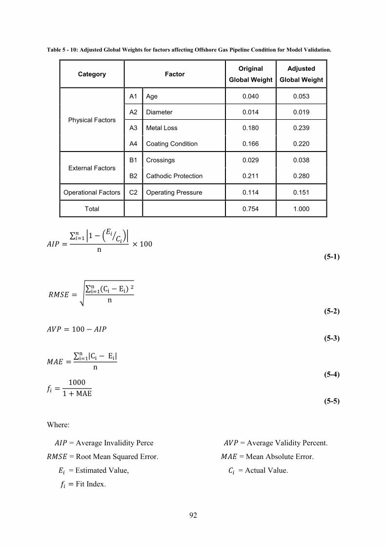
92
Table 5 - 10: Adjusted Global Weights for factors affecting Offshore Gas Pipeline Condition for Model Validation.
Category Factor Original
Global Weight
Adjusted
Global Weight
Physical Factors
A1 Age 0.040 0.053
A2 Diameter 0.014 0.019
A3 Metal Loss 0.180 0.239
A4 Coating Condition 0.166 0.220
External Factors
B1 Crossings 0.029 0.038
B2 Cathodic Protection 0.211 0.280
Operational Factors C2 Operating Pressure 0.114 0.151
Total
0.754 1.000
𝐴𝐼𝑃 =∑ |1 − (
𝐸𝑖𝐶𝑖⁄ )|𝑛
𝑖=1
n × 100
(5-1)
𝑅𝑀𝑆𝐸 = √∑ (Ci − Ei) 2ni=1
n
(5-2)
𝐴𝑉𝑃 = 100 − 𝐴𝐼𝑃 (5-3)
𝑀𝐴𝐸 =∑ |Ci − Ei|ni=1
n
(5-4)
𝑓𝑖 =1000
1 + MAE
(5-5)
Where:
𝐴𝐼𝑃 = Average Invalidity Perce 𝐴𝑉𝑃 = Average Validity Percent.
𝑅𝑀𝑆𝐸 = Root Mean Squared Error. 𝑀𝐴𝐸 = Mean Absolute Error.
𝐸𝑖 = Estimated Value, 𝐶𝑖 = Actual Value.
𝑓𝑖 = Fit Index.

93
Similarly, the Root Mean Square Error (RMSE) and the Mean Absolute Error (MAE) are
estimated. Both RMSE and MAE values varies from 0 to infinity. If their values are close to
0, the model is sound and vice versa (Dikmen, et al., 2005). MAE can be used to calculate the
fitness function 𝑓𝑖 as defined by Eq. 5-5. The equation of the fitness function illustrates that
if the value of 𝑓𝑖 is closer to 1000, the developed model is fit for the validation data and the
opposite is ture. If 𝑓𝑖 is closer to 0, then the model is inappropriate for the representation of
the validation data.
The inspection data had 4090 points in which 20% of them, 818 points, were randomly
chosen to perform the first stage of validation. To ensure randomness and elimination of the
human factor, the selection process was performed through the MATLAB computer software.
For the first stage of validation, two methods of defuzzification, Centroid and Weighted-
Average, are used in order to check the difference between them. The validation results for
the developed model are summarized in Table 5-11.
The use of the Centroid method resulted into an AVP of 90.7% and RSME of 0.758. This
may be considered acceptable but an additional measure was used which is the fit index 𝒇𝒊. It
was calculated for the Centroid method and found to be equal to 571.73 which is not
acceptable since it is far from 1000. On the other hand, using the Weighted-Average method
produced better results. The AVP increased to 97.5%, and RMSE decreased to 0.250 but fit
index 𝒇𝒊 increased dramatically to 836.32 which is very close to 1000. The reason of this
change in results is discussed in the next section.
After testing the two chosen defuzzification methods on 20% of the data chosen randomly,
the Weighted-Average was selected for defuzzification for the final degrees of belief of the
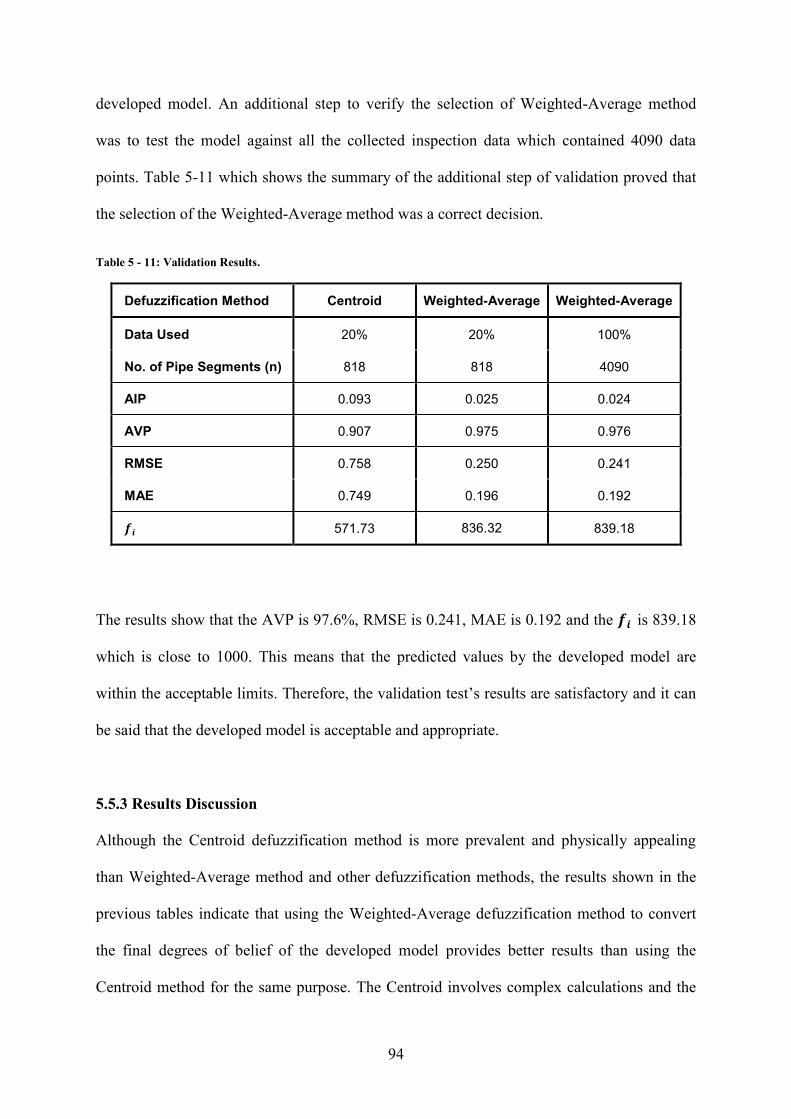
94
developed model. An additional step to verify the selection of Weighted-Average method
was to test the model against all the collected inspection data which contained 4090 data
points. Table 5-11 which shows the summary of the additional step of validation proved that
the selection of the Weighted-Average method was a correct decision.
Table 5 - 11: Validation Results.
Defuzzification Method Centroid Weighted-Average Weighted-Average
Data Used 20% 20% 100%
No. of Pipe Segments (n) 818 818 4090
AIP 0.093 0.025 0.024
AVP 0.907 0.975 0.976
RMSE 0.758 0.250 0.241
MAE 0.749 0.196 0.192
𝒇𝒊 571.73 836.32 839.18
The results show that the AVP is 97.6%, RMSE is 0.241, MAE is 0.192 and the 𝒇𝒊 is 839.18
which is close to 1000. This means that the predicted values by the developed model are
within the acceptable limits. Therefore, the validation test’s results are satisfactory and it can
be said that the developed model is acceptable and appropriate.
5.5.3 Results Discussion
Although the Centroid defuzzification method is more prevalent and physically appealing
than Weighted-Average method and other defuzzification methods, the results shown in the
previous tables indicate that using the Weighted-Average defuzzification method to convert
the final degrees of belief of the developed model provides better results than using the
Centroid method for the same purpose. The Centroid involves complex calculations and the

95
more complex the output membership shape, the more complex the calculations. On the other
hand, Weighted-Average is used most frequently in fuzzy applications because of its
computational efficiency (Ross, 2010).
It is noted that the Weighted-Average defuzzification always gives higher crisp values than
the Centroid for the same degrees of belief which gives better validation results as
demonstrated in this section. This means that the Weighted-Average defuzzification gives
more accurate results for the pipeline condition in this case. In the future, the model user can
choose to use the Centroid defuzzification which gives lower crisp values, i.e. lower pipeline
condition, than the weighted-Average to be more cautious and plan for early maintenance.
Many other methods are mentioned in the literature review that can be used for
defuzzification in this model. In addition, other defuzzification methods are not presented in
this report. The question is "What is the best defuzzification method to use?". Ross (2010)
gave an answer to this question by stating that it is "context or problem dependent". As an
answer to this question Hellendoorn & Thomas (1993) put five criteria to specify the best
defuzzification method to use, as follows:
1) Continuity: A fuzzy output should not change dramatically when the input slightly
changes.
2) Disambiguity: The result of defuzzification should always be a unique value of 𝓏*. For
example, when using Centre of Largest Area method, there is ambiguity in selecting 𝓏*
in case if having equal membership functions.
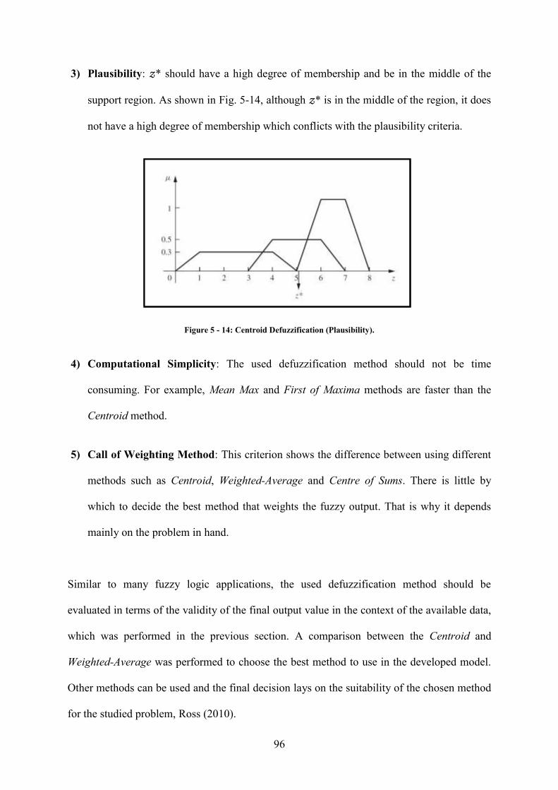
96
3) Plausibility: 𝓏* should have a high degree of membership and be in the middle of the
support region. As shown in Fig. 5-14, although 𝓏* is in the middle of the region, it does
not have a high degree of membership which conflicts with the plausibility criteria.
Figure 5 - 14: Centroid Defuzzification (Plausibility).
4) Computational Simplicity: The used defuzzification method should not be time
consuming. For example, Mean Max and First of Maxima methods are faster than the
Centroid method.
5) Call of Weighting Method: This criterion shows the difference between using different
methods such as Centroid, Weighted-Average and Centre of Sums. There is little by
which to decide the best method that weights the fuzzy output. That is why it depends
mainly on the problem in hand.
Similar to many fuzzy logic applications, the used defuzzification method should be
evaluated in terms of the validity of the final output value in the context of the available data,
which was performed in the previous section. A comparison between the Centroid and
Weighted-Average was performed to choose the best method to use in the developed model.
Other methods can be used and the final decision lays on the suitability of the chosen method
for the studied problem, Ross (2010).

97
5.6 Sensitivity Analysis
A Sensitivity Analysis is conducted to test the robustness of the developed fuzzy-based
model. In other words, it is performed to examine how the uncertainty in inputs could affect
the model’s results and to increase the understanding of the relationship between input and
output variables. Also, unexpected relationships between inputs and outputs can be
encountered which is another advantage of performing a sensitivity analysis.
A sensitivity analysis is carried out for the developed model in order to examine the effect of
changing the factors’ values entered in the model on the pipeline condition. The sensitivity
was based on changing a factor's value (input) from lowest to highest while keeping other
factors constant at average condition to check the individual effect on the overall pipe
condition. In other words, each factor's value was changed within the range of its scale or
thresholds presented earlier to study the effect of this factor on the pipeline condition. The
changing procedure of the factor’s value took place on a 10% intervals of their thresholds
shown earlier. Accordingly, the overall pipeline condition was calculated against each change
and plotted as shown in the below figures. This process was repeated individually for all the
factors considered in the developed model as shown in Figures 5-15, 5-16 and 5-17. The
charts in Figures 5-15, 5-16 and 5-17 can be re-categorized according to their proportionality
to the overall pipe condition as follows; (1) Directly Proportional Factors, (2) Inversely
Proportional Factors, and (3) Irregularly Proportional Factors.
Figures 5-18, 5-19 and 5-20 display the three new classifications of the contributing factors.
These factors use different units of measure. Therefore, factor's normalization is required to
combine them in one figure as shown in Table 5-12.

98
Table 5 - 12: Factors' Normalization.
Category Factor Unit Used Method
A:
PHYSICAL
A1 Age Years A1 / 60
A2 Diameter Inches (A2 – 2) / (52 – 2)
A3 Metal Loss % A3 / 100
A4 Coating Condition % A4 x 100
B:
EXTERNAL
B1 Crossings Number B1 / 10
B2 Cathodic Protection Effectiveness mV (B2 – 600) / (1300 – 600)
B3 Marine Route Existence % B3 / 100
B4 Water Depth meters B4 / 60
C:
OPERATIONAL
C1 Corrosive Impurities % C1 / 100
C2 Operating Pressure % of Design C2 / 100
C3 Flow Rate % of Design C3 / 100
Figure 5 - 15: Sensitivity Analysis for Physical Factors.
7.5
8.0
0 10 20 30 40 50 60
Pip
eC
on
dit
ion
Age (Years)
7.5
8.0
0 10 20 30 40 50 60
Pip
eC
on
dit
ion
Diameter (Inch.)
6.0
7.0
8.0
9.0
0 20 40 60 80 100
Pip
eC
on
dit
ion
Metal Loss (%)
6.0
7.0
8.0
0 20 40 60 80 100
Pip
eC
on
dit
ion
Coating Condition (%)

99
Figure 5 - 16: Sensitivity Analysis for External Factors
Figure 5 - 17: Sensitivity Analysis for Operational Factors.
7.5
8.0
0 10
Pip
eC
on
dit
ion
Crossing(#)
5.0
6.0
7.0
8.0
9.0
600 800 1000 1200
Pip
eC
on
dit
ion
Cathodic Protection (mV)
7.0
8.0
0 20 40 60 80 100
Pip
eC
on
dit
ion
Marine Route Existance (%)
7.0
8.0
9.0
0 20 40 60
Pip
eC
on
dit
ion
Water Depth (m)
7.0
8.0
0 20 40 60 80 100
Pip
e
Corrosie Impurities (%)
7.0
8.0
9.0
0 20 40 60 80 100
Pip
e
Operating Pressure (% of Design)
7.0
8.0
0 20 40 60 80 100
Pip
e
Flow Rate (% of Design)

100
Figure 5 - 18: Directly Proportional Factors.

101
Figure 5 - 19: Inversely Proportional Factors.
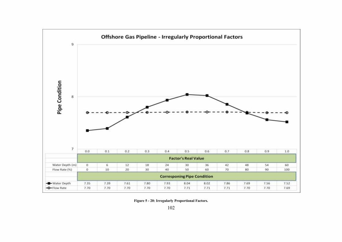
102
Figure 5 - 20: Irregularly Proportional Factors.

103
The results show that all the factors are sensitive to value change but with different degrees of
sensitivity according to their ANP weights as shown in figures 5-18, 5-19 and 5-20. The
factors Age, Metal Loss, Crossings, Marine Route Existence, and Operating Pressure all
show the same trend, in which increasing their values would decrease the pipeline condition.
While on the other hand, the factors Diameter, Coating Condition and Cathodic Protection
Effectiveness show an opposite trend, that is increasing their values increase the pipeline
condition. The reason behind that is that the pipeline coating condition and cathodic
protection are protective measures for the pipeline where improving them prolong the
pipeline life and protects it from degradation for longer periods. Whereas the diameter, i.e.
size, which also increases the pipeline condition due to the possible larger SDR (Standard
Dimension Ratio). This affects the structural performance of the pipeline and decreases its
vulnerability to external impact. Therefore, increasing the values of Diameter, Coating
Condition and Cathodic Protection Effectiveness would definitely increase the overall
pipeline condition.
In regards with irregularly proportional factors which include Water Depth and Flow Rate as
shown in Fig. 5-20, the pipeline condition demonstrated an increasing and decreasing trends
with variability of change percentages for Water Depth. It is because the offshore pipelines
experience high external loading of water pressure in deep waters. This leads to increased
chances of collapse from external force buckle. On the other hand, shallow water pipelines
are easily affected by external parties and weather conditions which may create sea currents.
These currents may impose buckling forces on offshore pipelines as well. According to the
current research, the offshore gas pipelines need to be placed 24 to 36 meters below water
surface in order for these pipeline to be away from shallow water currents and in the same
time not to be exposed to deep water pressure (Muhlbauer, 2004). Furthermore, the Flow
104
Rate factor displayed a stable trend which may be due to having the lowest relative weight,
0.008, of all factors. Nevertheless, it is a necessity to point out that flow rates influence the
pipeline health integrity since low flow rates could increase the chances of liquid or solid
dropout and accumulation in low places of the pipeline, whereas high flow rates may lead to
pipeline erosion (Muhlbauer, 2004). Hence, determining the suitable flow rate is significant.
Table 5-13 demonstrates the ANP weights verses the difference in condition resulting for the
changing the factors’ values from lowest to highest. It can be seen that Cathodic Protection
Effectiveness has the highest change in condition (𝛥 Condition = 2.24) which responds to the
highest global weight (0.211) among all factors. The second highest condition difference (𝛥
Condition = 1.59) happened with Metal Loss which has a global weight of 0.180. Follows
that is Coating Condition which has a condition difference of 1.28 and a global weight of
0.166.
According to the developed sensitivity analysis charts and Table 5-13, it can be observed that
Cathodic Protection and Coating Condition have the highest positive effect on the pipe
condition. They compose together 37.7% of contributing strength. Similarly, Diameter has a
positive effect on the pipe condition but it is the lowest among the factors affecting the pipe
condition positively. On the other hand, Metal Loss and Operating pressure have the highest
negative effect on the pipe condition while Crossings have the lowest negative effect. The
Water Depth and Flow Rate have a changing effect as shown in the sensitivity analysis charts
and thresholds presented earlier.
It is noticed that the factors related to corrosion, Metal Loss, Coating Condition and Cathodic
Protection, have the greatest effect of the pipe condition either positively or negatively.
However, other factors including Age, Diameter, Crossings, Marine Route Existence, Water

105
Depth, Corrosive Impurities, Operating Pressure and Flow Rate, are still essential for pipe
condition prediction as they form together around 44.3% in their condition contributing
strength.
Table 5 - 13: Sensitivity Analysis (ANP Global Weights Vs Condition Difference).
Factor Global
Weight
Max.
Condition
Min.
Condition
𝛥 Condition
A1 Age 0.040 7.84 7.62 0.22
A2 Diameter 0.014 7.75 7.68 0.07
A3 Metal Loss 0.180 8.13 6.54 1.59
A4 Coating Condition 0.166 7.71 6.43 1.28
B1 Crossings - 0.029 7.71 7.55 0.16
B2 Cathodic Protection 0.211 8.04 5.80 2.24
B3 Marine Route Existence 0.095 7.92 7.24 0.68
B4 Water Depth 0.112 8.04 7.35 0.69
C1 Corrosive Impurities 0.031 7.73 7.66 0.07
C2 Operating Pressure 0.114 8.24 7.48 0.76
C3 Flow Rate 0.008 7.71 7.69 0.02
Total 1.000
Finally, the ANP global weights mentioned in Table 5-13 were developed from the feedback
of professionals in the oil and gas industry in Qatar and Saudi Arabia. These weights have a
great effect on the final output of the model when changing the entered factors’ values. Also,
these weights can be updated in the developed model to reflect different conditions but still
affect the model output. The larger ANP weight of the factor, the larger its effect on the final
output (i.e. the bigger the difference in condition) when changing the factor’s value.

106
5.7 Development of Pipeline Deterioration Curve
A relation between the condition rating and Age factor was built based on the developed
model. The purpose of building this relation is to predict the pipe condition based on different
physical, external and operational factors. It is important to express graphically the combined
effect of all the factors on the pipeline condition. As a result, a deterioration curves was built
for the developed model as shown in following figure. This deterioration curve gives a
clearer knowledge of the interrelationships between the pipeline future conditions and the
studied factors. Fig. 5-21 shows a polynomial relation of fifth degree between the overall pipe
condition and Age. The vertical axis represents the predicted pipe condition while the
horizontal axis represents the Age factor.
Figure 5 - 21: Predicted Deterioration Curve for Offshore Gas Pipeline.
y = -2E-08x5 + 3E-06x4 - 5E-05x3 - 0.0034x2 - 0.0595x + 9.6049R² = 0.9992
0
1
2
3
4
5
6
7
8
9
10
0 10 20 30 40 50 60 70
Ove
rall
Pip
e C
on
dit
ion
Age (Years)
107
It is noticed that the previous figure shows an inverse relation between the pipe condition and
Age. Commonly, the effect of aging on the pipe condition is of negative nature. The pipe
condition decreases as age increases. Also, this deterioration curve is built to study the effect
of time on the pipe condition taking into consideration other factors’ degradation. For
example, the Metal Loss would definitely increase over time which in return decreases the
pipe condition. The same thing is applied to the rest of the factors where their values is
changing simultaneously from their best possible effect on the pipe condition to their worst.
On the other hand, the Diameter and Number of Crossings are kept constant at average
condition values which are 20 inches and 3 crossings, respectively.
5.8 Condition Assessment Scale
According to literature, there is no standard condition assessment scale (condition rating scale
and its associated rehabilitation works). Pipeline operators use approximations and experts’
opinions to determine the condition and required rehabilitation or inspection for an existing
pipeline. It is recommended for pipeline operators to build their own condition rating scale
which suits the environmental and operational status that accompanies a functional pipeline.
Additionally, converting all condition rating into a numerical scale such as "0" to "10" scale,
which was used in the proposed condition rating scale, is also recommended. The condition
assessment scale proposed in this section is adapted from El-Abbasy et al. (2014a) who
suggested an assessment scale for oil and gas pipelines using a scale from "0" to "10", where
"0" indicates that the pipeline is at its worst condition and "10" at its best condition.
5.8.1 Proposed Condition Rating Scale
Since there is no standard condition scale was found for offshore gas pipelines, this research
propose its own condition rating scale. This scale was developed from the data collected from

108
the received questionnaires where experts were asked to assign gas pipeline condition index
in the last part. Table 5-14 illustrates the linguistic terms and the numeric values for the
proposed condition rating scale for offshore gas pipelines.
Table 5 - 14: Proposed Condition Rating Scale.
Linguistic Scale Numeric Scale
Excellent 9 -- 10
V. Good 7 -- 9
Good 5 -- 7
Fair 3 -- 5
Critical 0 -- 3
The developed condition rating scale will provide a framework for gas pipeline operators to
decide and perform the required action to maintain their pipelines. For example, if the
reported corrosion resulted in 26 to 55% of metal loss of the original wall thickness and the
loss of coating condition ranged from 35 to 50% of the original. Then, the condition of the
gas pipeline is considered "Good" and the suggested action to be taken is to schedule for re-
coating and cathodic protection rehabilitation in the next 3 to 5 years. Also, the pipeline will
be re-assessed after 5 years. Along with the previous, the pipeline operator may suggest
regular annual maintenance for the considered pipeline to be observed continuously. That
may come in handy if the operator noticed signs of any type of pipeline failure.
It is important to note that this proposed condition rating scale is a preliminary suggestion
and many researches may suggest other alternatives. The choice of a suitable condition rating
scale relays on the pipeline operators and depends whether this scale is designed for their
working environment or not. For example, pipeline operators in Qatar cannot use a condition
109
rating scale that was proposed for rating pipelines in UK. Table 5-15 demonstrates the
suggested required actions to be taken associated with each offshore gas pipeline condition.
A condition rating scale is proposed in this chapter to provide a framework for professional in
the oil and gas industry in Qatar to plan for the required inspection and rehabilitation works
for offshore gas pipelines. The developed scale is of interest to oil and gas pipelines operators
in order to prioritize future inspection and rehabilitation planning for existing offshore gas
pipelines.
5.9 Summary
The current research designed a condition assessment model using the integration of Fuzzy
Logic, Analytical Network Process (ANP) and Evidential Reasoning (ER). Eleven factors
within three main categories (physical, external and operational) were studies to check their
effect on offshore gas pipelines condition in Qatar. A detailed literature review was
performed about oil and gas pipelines and previous condition assessment attempts. In the
literature review section, a detailed explanation was presented for the techniques used in
developing the current model. A structured questionnaire was distributed among
professionals in the oil and gas industry in Qatar to collect their feedback on the chosen
factors. From the received questionnaires, the factors thresholds were developed and fuzzy
logic was applied. The ANP global weights of the studied factors were calculated and a new
condition assessment scale was proposed, as shown in the next chapter, to prioritize pipe
inspection and rehabilitation planning. The Evidential Reasoning algorithm was used to
develop the model by integrating the fuzzified factors' thresholds and the global ANP weights
on these factors. A set of historical inspection data received from a pipeline operator in Qatar
was used to validate the model prediction power.

110
Table 5 - 15: Numeric and Linguistic Scale for Condition Rating of Offshore Gas Pipelines.
Numerical
Scale
Linguistic
Scale Criteria Description Action Required
9 – 10 Excellent
Corrosion: Almost no signs (0 – 17 %
Metal Loss).
Cathodic Protection: Very good (> 951
mV).
Coating Condition: Almost new (< 15 %
coat loss).
Re-assess in 15 years.
Regular annual
maintenance.
7 – 9 V. Good
Corrosion: Few signs (9 – 35 % Metal
Loss).
Cathodic Protection: Good & within
acceptable limits (850 – 1000 mV).
Coating Condition: Few signs of
damage (15 – 35 % coat loss).
Re-assess in 10 years.
Regular annual
maintenance.
Schedule for CP
rehabilitation within the next
5-10 years.
5 – 7 Good
Corrosion: Average signs (26 – 55 %
Metal Loss).
Cathodic Protection: Adequate (751 –
900 mV).
Coating Condition: Small damage but
still intact (35 – 50% coat loss).
Re-assess in 5 years.
Regular annual
maintenance.
Schedule for CP
rehabilitation & Re-coating
within the next 3-5 years.
3 – 5 Fair
Corrosion: Significant signs (46 – 74 %
Metal Loss).
Cathodic Protection: Inadequate but
acceptable (676 – 800 mV).
Coating Condition: Partial damage (45 –
75 % Coat Loss).
Re-assess in 2 years.
Regular annual
maintenance.
Schedule for rehabilitation
and/or replacement within
the next 1-3 year.
0 – 3 Critical
Corrosion: Severe signs, close to failure
(66 – 100 % Metal Loss).
Cathodic Protection: Critical (< 700
mV).
Coating Condition: Significant damage
(> 60 % Coat Loss).
Schedule for immediate
rehabilitation &/or
replacement.

111
After building the model, a sensitivity analysis was performed to check the effect of changing
the factors' values individually. Then, a deterioration curve was plotted in order to check the
aging effect on the pipe condition as well as degradation of other factors.
112
CHAPTER SIX: CONDITION ASSESSMENT AUTOMATED
TOOL
6.1 Introduction
Technology and software advancements promote the existence of automation tools to
overcome time obstacles and facilitate the application of the various methodologies that are
being developed nowadays. These methodologies, which may be time consuming if not
automated, can and will assist practitioners in multiple fields of industry in predicting and
ranking the condition of existing offshore gas pipelines in Qatar and similar regions in less
time and reduced cost.
This chapter illustrates the implementation of the developed fuzzy-based condition
assessment methodology for offshore gas pipelines in Qatar described in the previous
chapters. The methodology is automated via third party software, Microsoft Excel, which
provided the necessary functions to perform such a task. The automated tool sets on four
main pillars: 1) Inputs, 2) Fuzzification, 3) Defuzzification & Outputs and 4) Graphical
Representation.
6.2 Automated Fuzzy-based Tool Framework
The proposed automation of the developed methodology is called Automated Fuzzy-based
Condition Evaluator. It employs the fundamentals of three techniques; Analytic Network
Process (ANP), Evidential Reasoning (ER) and Fuzzy Set Theory (FST). The automated tool
will assist professionals in oil and gas industry to predict the condition rating of existing
offshore gas pipelines based on the data which the model will request from the user as
follows.

113
The Fuzzy-based Condition Evaluator provides two options for the users in regards of the
factors' priorities. The user may decide whether to use the default ANP weights generated
during the course of this thesis or generate their own customized weights. The automated tool
then will require the information related to priorities and the data related to factors which will
be counted for in the pipeline condition prediction. The results will include a condition rating
value that ranges from "0" to "10" where 0 indicates that the considered pipeline is in
"Critical" condition, and 10 expresses "Excellent" condition.
The flowchart shown in Fig. 6-1 epitomizes the functions of the proposed automated tool
model where the procedure is detailed in the next section. This automation employs MS
Excel in order to facilitate the application of the developed fuzzy-based methodology. Also,
another type of software is used in the process, SuperDecisions, which is used as an extra
option for the users to re-calculate their own ANP priorities or weights.
6.3 Fuzzy-based Condition Evaluator Process
The first page the user will face when starting the automated tool file is the welcome page,
Fig. 6-2, which displays the most influential factors, classified into three main categories;
physical, external and operational. These factors contribute in the condition prediction
performed by the developed fuzzy-based model. In case of facing any difficulty in
understanding any of the factors, the user can press the question mark button which will lead
them to another page containing a brief description about all contributing factors as shown in
Fig. 6-3. The automated tool contains "Next" and "Back" buttons which will enable the user
to navigate through the automated tool file and proceed from one stage to another.
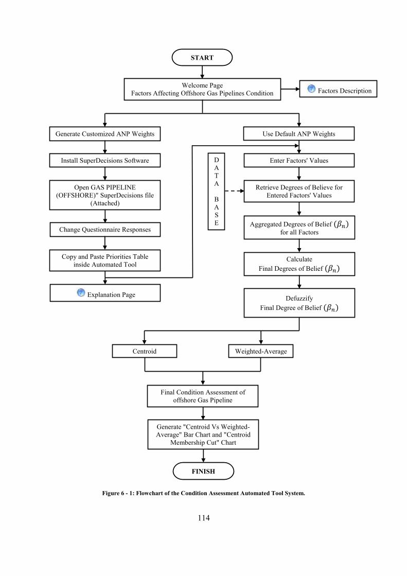
114
Figure 6 - 1: Flowchart of the Condition Assessment Automated Tool System.
START
Generate Customized ANP Weights
FINISH
Welcome Page
Factors Affecting Offshore Gas Pipelines Condition Factors Description
Use Default ANP Weights
Enter Factors' Values
Retrieve Degrees of Believe for
Entered Factors' Values
D
A
T
A
B
A
S
E Aggregated Degrees of Belief (𝛽𝑛) for all Factors
Calculate
Final Degrees of Belief (𝛽𝑛)
Defuzzify
Final Degree of Belief (𝛽𝑛)
Centroid Weighted-Average
Generate "Centroid Vs Weighted-
Average" Bar Chart and "Centroid
Membership Cut" Chart
Install SuperDecisions Software
Open GAS PIPELINE
(OFFSHORE)" SuperDecisions file
(Attached)
Change Questionnaire Responses
Copy and Paste Priorities Table
inside Automated Tool
Explanation Page
Final Condition Assessment of
offshore Gas Pipeline

115
As mentioned earlier, this automated tool was designed using MS Excel software and
includes the functions and information required to automate the developed methodology.
Many excel sheets were programmed to quickly retrieve the necessary information as
response to the data entered by the user.
The user then is forced back to the welcome page where they will press the Next button
which leads the user to the Weights selection page, Fig. 6-4. This page will inquire them to
decide whether to advance using the shown default ANP weights or to generate their own
customized weights. The default ANP weights were generated in the data collection phase by
distributing a structured questionnaire among professionals in the oil and gas industry in
Qatar and similar regions such as Saudi Arabia. The interested reader may refer to Data
Collection chapter for more details.
Figure 6 - 2: Welcome Page and Contributing Factors.

116
Figure 6 - 3: Contributing Factors Description.
Figure 6 - 4: ANP Weights Selection (Default Vs Customized).

117
In case the user chose to generate their own weights, the automated tool will display the page
shown in Fig. 6-5 where the user will be asked to install the SuperDecisions software. After
that, the user will open the pre-arranged SuperDecisions file attached with the automated
tool. It will guide the user through the process of generating the customized ANP weights as
shown in figures 6-5 through 6-8. During this process, the user will be asked to change the
questionnaire responses in the pre-arranged SuperDecisions file as shown in the figure below.
Figure 6 - 5: Generate Customized Weights - SuperDecisions File.
If no previous knowledge of SuperDecisions software existed, instructions are presented to
direct the user. After changing the questionnaire responses, the SuperDecisions will calculate
the re-distributed priorities for the contributing factors and their main categories as shown is
Fig. 6-6.
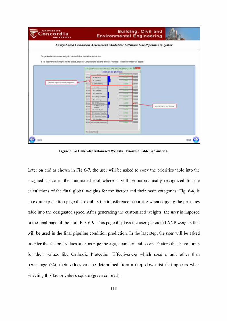
118
Figure 6 - 6: Generate Customized Weights - Priorities Table Explanation.
Later on and as shown in Fig 6-7, the user will be asked to copy the priorities table into the
assigned space in the automated tool where it will be automatically recognized for the
calculations of the final global weights for the factors and their main categories. Fig. 6-8, is
an extra explanation page that exhibits the transference occurring when copying the priorities
table into the designated space. After generating the customized weights, the user is imposed
to the final page of the tool, Fig. 6-9. This page displays the user-generated ANP weights that
will be used in the final pipeline condition prediction. In the last step, the user will be asked
to enter the factors’ values such as pipeline age, diameter and so on. Factors that have limits
for their values like Cathodic Protection Effectiveness which uses a unit other than
percentage (%), their values can be determined from a drop down list that appears when
selecting this factor value's square (green colored).

119
Figure 6 - 7: Generate Customized Weights - Final ANP Weights (1).
Figure 6 - 8: Generate Customized Weights - Final ANP Weights (2)
120
It is important to note that the fuzzified membership functions developed earlier for the
contributing factors (inputs) and final evaluation (output) are inserted into the automation file
as a Data Base along with the programmed sheets to calculate the Centroid and Weighted-
Average of the final evaluation of the model. Therefore, the automated tool will detect the
associated degrees of belief as soon as the factor's value is determined. This process is
repeated for the rest of the contributing factors. After assigning the degrees of belief for all
the factors, the tool will combine them using the newly generated ANP weights and the ER
algorithm discussed earlier. The aggregation of all belief degrees is executed in the tool's
background and does not appear for the user.
Finally, the products of the automated tool can be outlined in two points as follows:
1) The final pipeline evaluation as crisp value using two defuzzification methods; Centroid
and Weighted-Average (blue colored squares).
2) Graphical representation of the final evaluation which includes:
a) Centroid's Membership cut and defuzzified value of the final degrees of belief.
b) Bar chart displays the comparison between Centroid and Weighted-Average
defuzzification results.
Fig. 6-10 shows the page displayed when choosing to use the default ANP weights (red
colored squares) generated in this research. Is this case, the user will only be obliged to enter
the factors' values in the green colored squares. The results will be the same as in Fig. 6-9
which are the final evaluation defuzzified values, their graphical representation and
comparison.

121
Figure 6 - 9: Generate Customized Weights - Final Report.

122
Figure 6 - 10: Use Default Weights - Final Report.
6.4 Summary
An automation tool used for condition rating prediction is proposed. This tool is based on the
developed condition assessment methodology which utilizes FST, ANP and HER to evaluate

123
an existing offshore gas pipeline. It could be beneficial for professionals in oil and gas
industry to predict pipelines condition and assist in planning for future inspection and
rehabilitation works. This automated tool could be enhanced further to be more user friendly
and accommodate new functions to provide an augmented solid platform for future extension
of this research.
124
CHAPTER SEVEN: SUMMARY, CONCLUSIONS AND
RECOMMENDATIONS
7.1 Summary and Conclusion
The current research resulted in the development of a new numerical and linguistic
assessment scale for offshore gas pipelines. This scale comprises five grades, Excellent, Very
Good, Good, Fair and Critical. The details and characteristics of each grade were described
earlier in details. The new condition assessment scale could serve as a framework for pipeline
operators to plan future rehabilitation works for existing pipelines. The developed model in
this research is based on expert's feedback and historical inspection reports gathered mainly
from Qatar. Hence, this model can be described to be best suited for Qatar and similar
regions. On the other hand, the proposed methodology can be updated to apply for different
regions.
This research presented a condition assessment model for offshore gas pipelines in Qatar
using the integration of three techniques which are Analytic Network Process (ANP), Fuzzy
Sets Theory (FST) and Evidential Reasoning (ER). First, a comprehensive literature review
was conducted on the three techniques implemented in this study. This literature review also
contained the types, design and material of oil and gas pipelines used in Qatar. Based on
literature review, eleven factors were identified as the most influential criteria that affect
offshore gas pipelines in the studied region. The data needed to perform this research was
collected from two sources, experts' feedback through a structured questionnaire and
historical data from previous inspections in Qatar.
125
The proposed methodology focused on obtaining a comprehensive evaluation of the offshore
gas pipelines based on multi-criteria and not just the corrosion related ones. Also, the
interdependency between these criteria along with uncertainty of the respondent's view were
addressed through using ANP and HER, respectively. The use of fuzzy logic came in handy
to quantify the respondents' feedback. Many defuzzification methods were introduced and a
comparison was made between two common methods, Centroid and Weighted-Average, to
convert the final degrees of belief into a crisp value.
The developed model was tested with historical inspection data to demonstrate the accuracy
and usefulness of the new methodology in predicting of offshore gas pipeline condition. The
received inspection reports data were prepared and organized to validate the model. The
average validity percent (AVP) of this model was 97.6% and the root mean squared error
(RMSE) ranged between 0.241 and 0.250 which clearly demonstrates the accuracy in
predicting the condition of offshore gas pipelines in Qatar. An extra criteria used to validate
the model is the Fit Index which ranged between 836.32 and 839.18. Since the fit index
values are very close to 1000, the model was considered fit for the predetermined objectives.
A sensitivity analysis was conducted to examine the impact of each factor individually on the
overall pipeline condition. It was found that Cathodic Protection and Metal Loss were the
most positively and negatively influencing factors, respectively. However, the factors of
diameter and crossings had the lowest positive and negative effect on offshore gas pipeline
condition.
Additionally, a relation between the Age factor and the pipe condition was built to predict the
deterioration of the pipe along its age based on the presented methodology. In addition, a new
condition assessment scale was proposed as a guideline for pipeline operators to help in

126
planning for future inspections and rehabilitation works. The last step of this research was to
automate the designed model. This automated tool will assist professionals in oil and gas
industry to predict the condition rating of existing offshore gas pipelines based on the data
requested from the user.
Finally, the model is expected to provide the engineers in oil and gas industry and pipeline
operators with a platform designed solely to predict and assess the condition of offshore gas
pipelines in Qatar and similar environments. Also, this model can assist in planning and
prioritizing their future inspections and rehabilitation works.
7.2 Research Contributions
The current research contributions included a comprehensive evaluation methodology to
assess offshore gas pipelines that are affected by various factors. The following developments
resulted from the proposed methodology:
1) Develop a hierarchy of various factors that affect offshore gas pipeline condition in
Qatar.
2) Develop a condition assessment model for offshore gas pipelines in Qatar considering
uncertainty and subjectivity using the integration of three main techniques, Fuzzy Set
Theory (FST), Analytic Network Process (ANP), and Hierarchical Evidential Reasoning
(HER).
3) Design a condition assessment scale.
4) Build a deterioration curve to predict future conditions of the considered pipeline.
5) Design an automated tool for the developed condition assessment model.
127
7.3 Research Limitations
The presented research work introduced a new methodology to help pipeline operators in
evaluating and predicting the condition of offshore gas pipelines in Qatar. In order to deploy
the developed model in a pipeline operating company, the following should be considered:
1) Only eleven factors within three categories were considered in developing this model
while other factors could be used to provide a more comprehensive picture about the
offshore gas pipeline condition such as Sea Water Current. In order to perform this, a
reliable information system concerning physical, external and operational factors should
be included in the developed model.
2) The data collected from experts' feedback was based on a random sample of 25
professionals which can be considered a small number. Also, experts with more diverse
backgrounds could be reached.
3) The developed model eliminated ignorance in order to a full degree of membership,
equal to 1, for each entered factor’s value.
7.4 Future Recommendations
Recommended future work of the current research can be divided into two section which are
described as follows:
Potential Enhancements of current research:
a) Historical inspection data with various pipe conditions, to cover all possibilities, could
be used to further evaluate the model's prediction power. Other pipeline operators could
be reached in Qatar and similar regions such as UAE and Saudi Arabia. This is because
the data used to validate the developed model was limited to a certain pipe condition

128
that circles around Good and Very Good. So, data for pipelines that have worse
conditions could be gathered and added to the validation process.
b) The factor's hierarchy included 11 factors under three main categories. So, more factors
could be incorporated to enhance the developed model such as structural related factors
like Joint Type or Free Span and external factors like Surrounding Soil Type. These
factors could be chosen based on the availability of gathered data in order to better
validate the developed model.
c) More experts can be encouraged to participate in the data collection part by answering
the structured questionnaire. This could cover a wide variety of feedbacks and
experiences. As mentioned in the Data Collection chapter, the developed model was
based on 25 feedbacks of experienced professionals in the oil and gas industry in Qatar
and Saudi Arabia. Also, they were gathered mainly from inspection and operation
professionals. So, more professionals from different sectors in the industry and from
different countries, that have an environment similar to that of Qatar's and Saudi
Arabia, could be encouraged to participate.
d) The developed model was designed to have zero ignorance. It can be enhanced and
updated to account for ignorance in responses where a professional is not 100% sure
that a pipeline is assessed under a certain pipe condition. Based on that, the new model
will predict the pipeline condition with a degree of confidence and ignorance.
Hypothetical extension areas of current research:
a) Consolidate the developed model with web-GIS system so that the condition rating of
offshore gas pipeline segments in an existing network can be assessed separately and
automatically. A central database will be built to incorporate the existing pipeline
network where each pipeline or segment would have a unique ID. Each pipeline history

129
such as inspection records, annual planned maintenance cost ... etc. will be shared in
real time basis with authorized professionals across the organization or worldwide. This
work history will be used for continuous condition assessing using the developed
model. Then, these assessments are compared with the most recent ones to investigate
each pipeline segment deterioration in any place of the network.
b) Based on the combination of the developed model and web-GIS system, the pipeline
network could be under continuous monitoring. As a result, a new methodology could
be proposed to prioritize future inspection schedules of pipeline segments based on
their condition. This methodology would process inspection reports data and assess the
condition of all offshore gas pipelines in a network in order to generate an inspection
schedule for the whole network on priority basis.
c) The developed model can be the basis of a condition assessment software concerning
not only offshore gas pipelines but exceeding that to oil pipelines either offshore or
onshore (buried or above soil). This software will have options to assess oil or gas
pipelines either offshore or onshore.
d) Design condition prediction software in which historical inspection reports are
imported and analyzed automatically. This requires a thorough literature review about
the software and inspection types used in oil and gas industry in Qatar. The new
software will be designed to automatically accommodate the inspection data without
the need to refine it for the condition assessment model. As a result, time and money
wasted on initial preparing of this data could be saved.
130
REFERENCES
Ahammed, M. (1998). Probabilistic Estimation of Remaining Life of a Pipeline in the
Presence of Active Corrosion Defects. International Journal of Pressure Vessels and Piping ,
75 (4), 321-329.
Al Barqawi, H., & Zayed, T. (2006a). Assessment Model for Water Main Conditions. In A.
Atalah, & A. Tremblay (Ed.), Pipeline Division Specialty Conference 30 July - 2 August,
2006 (pp. 1-8). Chicago, Illinois, United States: American Society of Civil Engineers.
Al Barqawi, H., & Zayed, T. (2006b). Condition Rating Model for Underground
Infrastructure Sustainable Water Mains. Journal of Performance of Constructed Facilities ,
20 (2), 126-135.
Al-Barqawi, H., & Zayed, T. (2008). Infrastructure Management: Integrated AHP/ANN
Model to Evaluate Municipal Water Mains Performance. Journal of Infrastructure Systems ,
14 (4), 305-318.
Ali, A. F. (2011, May 9th). Qatar Petroleum, Sr. Sub-sea Pipeline Engineer. (B. Abdrabou,
Interviewer) Doha, Qatar.
Ayag, Z. (2011). Evaluating Simulation Software Alternatives through ANP. Proceedings of
the 2011 International Conference on Industrial Engineering and Operations Management,
January 22 – 24, (pp. 532-537). Kuala Lumpur, Malaysia.
Ayyub, B. M., & Halder, A. (1984). Project Scheduling Using Fuzzy Set Concepts. Journal
of Construction Engineering and Management, ASCE , 110 (2), 189-204.
Bai, H., Sadiq, R., Najjaran, H., & Rajani, B. (2008). Condition Assessment of Buried Pipes
Using Hierarchical Evidential Reasoning Model. ASCE , 22 (2), 114-122.
Bersani, C., Citro, L., Gagliardi, R., Sacile, R., & Tomasoni, A. (2010). Accident Occurence
Evaluation In The Pipeline Transport Dangerous Goods. Chemical Engineering Transactions
, 19, 249-254.
Bertolini, M., & Bevilacqua, N. (2006). Methodology and Theory Oil Pipeline Cause
Analysis a Classification Tree Approach. Journal of Quality in Maintenance Engineering , 12
(2), 186-198.
Chae, M. J., & Abraham, D. (2001). Neuro-Fuzzy Approaches for Sanitary Sewer Pipeline
Condition Assessment. ASCE Journal of Computing in Civil Engineering , 15 (1), 4-14.
Chao, L., & Skibniewski, M. J. (1998). Fuzzy Logic for Evaluating Alternative Construction
Technology. Journal of Construction Engineering and Management, ASCE , 124 (4), 297-
304.
Cheng, E. W., & Li, H. (2001). Analytic Hierarchy Process: An Approach to Determince
Measures for Business Performance. Measuring Business Excellence , 5 (3), 30-36.

131
Cheng, E., & Li, H. (2004). Contractor Selection using the Analytic Network Process.
Construction Management and Economics , 22 (10), 1021-1032.
Cheng, S. J., & Hwang, C. L. (1992). Fuzzy Multiple Attribute Decision Making: Methods
and Applications. Springer-Verlag. New York: (Lecture Notes in Economics and
Mathematical Systems Series 375).
Chung, S., Lee, A., & Pearn, W. (2005). Analytic Network Process (ANP) Approach for
Product Mix Planning in Semiconductor Fabricator. International Journal of Production
Economics , 96 (1), 15-36.
Crestwood Tubulars, I. (2013). Manufacturing Stainless Steel Piping. Retrieved from
http://www.crestwoodtubulars.com/stainless-steel-piping.html (Oct. 3, 2013)
Davis, P., Dubois, J., Gambardella, F., & Uhlig, F. (2010). Performance of European Cross-
country Oil Pipelines: Statistical Summary of Reported Spillages in 2008 and Since 1971.
Special Task Force. Brussels: CONCAWE Oil Pipelines Management Group (OPMG).
Dawotola, A., Van Gelder, R., & Vrijling, J. (2009). Risk Assessment of Petroleum Pipelines
using a combined Analytical Hierarchy Process - Fault Tree Analysis (AHP-FTA).
Proceedings of the 7th International Probabilistic Workshop, 25-26 November 2009, (pp.
491-501). Delft, Netherlands.
Dey, P. K. (2001). A Risk based Model For Inspection and Maintenance of Cross Country
Petroleum Pipelines. Journal of Quality in Maintenance Engineering , 7 (1), 25-43.
Dey, P. K., Ogunlana, S. O., & Naksuksakul, S. (2004). Risk-based Maintenance Model for
Offshore Oil and Gas Pipelines : A Case Study. Journal of Quality in Maintenance
Engineering , 10 (3), 169-183.
Dikmen, I., Birgonul, M., & Kiziltas, S. (2005). Prediction of Organizational Effectiveness in
Construction Companies. ASCE, Journal of Construction Engineering and Management , 131
(2), 252-261.
Dubois, D., & Prade, H. (1988). Possibility Theory: An Approach to Computerized
Processing of Uncertainty. New York: Plenum Press.
Dweiri, F., & Meier, F. A. (1996). Application of Fuzzy Decision-Making in Facilities
Layout Planning. International Journal of Production Research , 34 (11), 3207-3225.
El Chanati, H., Senouci, A., Mosleh, F., Abouhamad, M., Gkountis, I., & Zayed, T. (2013).
Performance Assessment Model for Water Pipelines in Qatar. Journal of Structure and
Infrastructure Engineering - Taylor & Francis Group , Submitted For Review.
El-Abbasy, M. S. (2014c). Artificial Neural Network Models for Predicting Condition of
Offshore Oil and Gas Pipelines. Automation in Construction , 45, 50-65.
El-Abbasy, M. S., Senouci, A., Zayed, T., & and Mosleh, F. (2014a). A Condition
Assessment Model for Oil And Gas Pipelines using Integrated Simulation and Analytic

132
Network Process. Journal of Structure and Infrastructure Engineering, Taylor and Francis
Group , Published Online.
El-Abbasy, M. S., Senouci, A., Zayed, T., Mirahadi, F., & Parvizsedghy, L. (2014b).
Condition Prediction Models for Oil and Gas Pipelines using Regression Analysis. ASCE
Journal of Construction Engineering and Management , 140 (6).
Furuta, H. (1994). Applications of Fuzzy Logic in Civil Engineering in Japan. Proceedings of
1st Congress on Computing in Civil Engineering, ASCE, 20-22 June 1994, (pp. 1900-1907).
Washington.
Garuti, C., & Sandoval, M. (2005). Comparing AHP and ANP Shiftwork Models: Hierarchy
Simplicity v/s Network Connectivity. 8th International Symposium of the AHP July 2005.
Hawaii, USA.
Geem, Z. (2003). Window-Based Decision Support System for the Water Pipe Condition
Assessment Using Artificial Neural Network. World Water & Environmental Resources
Congress, 23-26 June 2003 (pp. 1-6). Philadelphia, Pennsylvania, United States: American
Society of Civil Engineers.
General Electric. (2004). Pipeline Post-Inspection Evaluation. Retrieved from http://site.ge-
energy.com/prod_serv/serv/pipeline/en/downloads/GEOG_Int_PIE_A4_PROOF.pdf (Nov.
30, 2013)
Goodland, R. (2005). Oil and Gas Pipelines Social and Enviornmentql Impact Assessment:
State of the Art. Virginia USA: International Association of Impact Assessment (IAIA)
Conference 2005.
Gorener, A. (2012). Comparing AHP and ANP: An Application of Strategic Decisions
Making in a Manufacturing Company. International Journal of Business and Social Science ,
3 (11), 194-208.
Greda, A. (2009). Application of the AHP/ANP in Food Quality Management. Proceedings
of International Symposium on the Analytic Hierarchy Process (ISAHP) 29 July - 1 August,
2009, (pp. 1-17). Pittsburgh, Pennsylvania, USA.
Hahn, M., Palmer, R., Merrill, M., & Lukas, A. (2000). Knowledge Acquisition and
Validation of an Expert System for Prioritizing the Inspection of Sewers. Proceedings of
Joint Conference on Water Resource Engineering and Water Resources Planning and
Management, 30 July - 2 August, 2000. Minneapolis, USA: American Society of Civil
Engineers.
Hallen, J., Caleyo, F., Gonzalez, J., & Lagod, F. F. (2003). Probabilistic Condition
Assessment of Corroding Pipelines in Mexico. Proceedings of 3rd Pan American Conference
for Nondestructive Testing (PANNDT), 2-6 June, 2003. Rio de Janeiro, Brazil.
Hashiha, I. (2011, March 13th). General Electric, Doha - Oil Pipeline Integrity Manager. (B.
Abdrabou, Interviewer) Doha, Qatar.
133
Hellendoorn, H., & Thomas, C. (1993). Defuzzification in Fuzzy Controllers. Journal of
Intelligent and Fuzzy Systems , 1, 109-123.
Hopkins, P. (2007). OIL AND GAS PIPELINES: Yesterday and Today. International
Petroleum Technology Institute, Pipeline Systems Division (PSD). UK and USA: Pensen Ltd.
UK and Willbros Inc. USA.
Hopkins, P. (2002). The Structural Integrity Of Oil And Gas Transmission Pipelines. Pensen
Ltd. . UK: Elsevier Publishers.
Hua, B., Sadiq, R., Najjaran, H., & Rajani, B. (2007). Translation of Pipe Inspection Results
into Condition Rating Using Theory of Evidence. Proceedings of Water Management
Challenges in Global Change CCWI2007 and SUWM2007 Conference, (pp. 69-74).
Leicester, UK.
Husein, H. (2011, October 3rd). Dolphin Energy - Senior Subsea Inspection Engineer. (B.
Abdrabou, Interviewer) Doha, Qatar.
Kale, A., Thacker, B. H., Sridhar, N., & Waldhart, C. J. (2004). A Probabilistic Model for
Internal Corrosion of Gas Pipelines. Proceedings of International Pipeline Conference, 4-8
October 2004. Calgary, Alberta, Canada.
Kumar, S., & Taheri, F. (2004). Neuro-Fuzzy Approaches for FRP Oil and Gas Pipeine
Condition Assessment. Proceedings of ASME/JSME Pressure Vessels & Piping Conference,
25-29 July 2004, (pp. 271-275). San Diego, California USA.
Li, S., Yu, S., Zeng, H., Li, J., & Liang, R. (2009). Predicting Corrosion Remaining Life of
Underground Pipelines With a Mechanically-Based Probabilistic Model. Journal of
Petroleum Science and Engineering , 65 (3-4), 162-166.
Lorterapong, P., & Moselhi, O. (1996). Project-Network Analysis Using Fuzzy Sets Theory.
Journal of Construction Engineering and Management, ASCE , 122 (4), 308-318.
Makar, J. M., & Kleiner, Y. (2000). Maintaining Water Pipeline Integrety. Proceedings
AWWA Infrastructure Conference and Exhibition, 12-15 March 2000. Baltimore, Maryland.
Mamdani, E. H. (1974). Application of Fuzzy Algorithms for Simple Dynamic Plant. Proc.
Inst. Elect. Eng. , 121 (12), 1585-1588.
Meade, L., & Sarkis, J. (1998). Analyzing Organizational Project Alternatives for Agile
Manufacturing Processes:An Analytic Network Approach. International Journal of
Production Research , 37 (2), 241-61.
Mikhail, N. (2011, October 5th). Qatar Gas - Head of Insection. (B. Abdrabou, Interviewer)
Doha, Qatar.
Morbier, N. J. (2009). Comentary on Soil Corrosion and Estimate of Pites Growth Rates
(California Public Utilities Commission). Retrieved from
http://www.cpuc.ca.gov/NR/rdonlyres/AB17E3FC-F581-499D-9B62-
37E6201C31C0/0/03AttachmentAItem12CorrosionRate.pdf (Nov. 30, 2013)
134
Morcous, G., Rivard, H., & Hanna, A. (2002). Case-Based Reasoning System for Modeling
Inftrastructure Deterioration. ASCE Journal of Computing in Civil Engineering , 16 (2), 104-
114.
Muhlbauer, W. K. (2004). Pipeline Risk Management Manual: Ideas, Techniques, and
Resources (3rd Edition). Oxford, UK: Gulf Professional Publishing.
Najafi, M., & Kulandaivel, G. (2005). Pipeline Condition Prediction Using Neural Network
Models. Pipeline Division Specialty Conference, 21-24 August 2005 (pp. 767-781). Houston,
Texas, United States: American Society of Civil Engineers.
Nekhay, O., Arriaza, M., & Boerboom, L. (2009). Evaluation of Soil Erosion Risk using
Analytic Network Process and GIS: A Case Study from Spanish Mountain Olive Plantations.
Journal of Environmental Management , 90 (2009) 10, 3091-3104.
Noor, N. M., Ozman, N. A., & Yahaya, N. (2011). Deterministic Prediction of Corroding
Pipeline Remaining Strength in Marine Environment Using DNV RP-F101 (Part A). Journal
of Sustainability Science and Management , 6 (1), 69-78.
Noor, N., Yahaya, N., Ozman, N., & Othman, S. (2010). The Forecasting Residual Life of
Corroding Pipeline Based on Semi-Probabilistic Method. UNIMAS e-Journal of Civil
Engineering , 1 (2), 246-263.
Ozger, S. (2003). A Semi-pressure-driven Approach to Reliability Assessment of Water
Distribution Networks. Arizona State University, PhD Dissertation, Department of Civil and
Environmental Engineering, Arizona, USA.
Peng, X., Zhang, P., & Chen, L. (2009). Long-Distance Oil/Gas Pipeline Failure Rate
Prediction Based On Fuzzy Neural Network Model. Proceedings of CSIE 2009 World
Congress on Computer Science and Information Engineering, 31 March - 2 April 2009, (pp.
651-655). Los Angeles, California, USA.
Raoot, A. D., & Rakshit, A. (1991). A Fuzzy Approach to Facilities Lay-Out Planning .
International Journal of Production Research , 29 (4), 835-857.
Ross, T. J. (2010). Fuzzy Logic with Engineering Applications (3rd Edition). New Mexico,
USA: John Wiley & Sons, Ltd.
Saaty, T. (1996). Decision Making with Dependence and Feedback: The Analytic Netwrok
Process. Pittsburgh, PA: RWS Publications.
Saaty, T. (1994). How to Make a Decision: The Analytic Hierarchy Process. Interfaces , 24
(6), 19-43.
Saaty, T. (1980). The Analytic Hierarchy Process, Planning, Piority Setting, Resource
Allocation. New York, United States: McGraw-Hill.
Sadiq, R., Kleiner, Y., & Rajani, B. (2006). Estimating Risk of Contaminant Intrusion in
Distribution Networks Using Dempster-Shafer Theory of Evidence. Civil Engineering and
Environmental Systems , 23 (3), 129-141.

135
Salah, A. (2012). "Fuzzy Set-based Contingency Estimating and Management". Concordia
University, MSc Dissertation, Department of Building, Civil and Environmental Engineering,
Montreal, QC Canada.
Salah, A. A. (2011, May 4th). Integrity and Operator Advisor ADMA. (B. Abdrabou,
Interviewer) Doha, Qatar.
Sarkis, J. (1999). A Methodological Framework for Evaluating Environmentally Conscious
Manufacturing Programs. Computers and Industrial Engineering , 36 (4), 793-810.
Senouci, A., El-Abbasy, M., & Zayed, T. (2014b). A Fuzzy-Based Model for Predicting
Failure of Oil Pipelines. ASCE, Journal of Infrastructure Systems , Published Online.
Senouci, A., El-Abbasy, M., Elwakil, E., Abdrabou, B., & Zayed, T. (2014a). A Model for
Predicting Failure of Oil Pipelines. Journal of Structure and Infrastructure Engineering,
Taylor and Francis Group , 10 (3), 375-387.
Sinha, S., & Pandey, M. (2002). Probabilistic Neural Network for Reliability Assessment of
Oil and Gas Pipelines. Computer-Aided Civil and Infrastructure Engineering , 17 (5), 320-
329.
Sonmez, M., Holt, G., Yang, J., & Graham, G. (2002). Applying Evidential Reasoning to
Prequalifying Construction Contractors. Journal of Management in Engineering , 18 (3), 111-
119.
Srivastava, R. P. (2010). An Introduction to Evidential Reasoning for Decision Making under
Uncertainty: Bayesian and Belief Functions Perspectives. International Journal of
Accounting Information Systems , 12 (2), 126-135.
Srivastava, R., & Mock, T. (2010). Audit Risk Formula with Mixed Evidence. Proceedings of
the Conference on The Theory of Belief Functions, 1-2 April 2010. Brest, France.
Srivastava, R., & Mock, T. (2000). Evidential Reasoning for WebTrust Assurance Services.
Journal of Managemet Information Systems , 16 (3), 11-32.
Srivastava, R., & Shafer, G. (1992). Belief-Function Formulas for Audit Risks. The
Accounting Review: Journal of the American Accounting Association , 249-283.
Stein, I., & Partner, G. (2005). European Study of the Performance of Various Pipe Systems.
Bochum, Germany: European Expert Panel Report 6-44801.
Teng, J. (2002). "Development of a Supplier Pre-qualification Model for a UK Company".
University of Manchester Institute of Science and Technology, MSc Dissertation, Manchester
School of Management, Manchester.
The Technology Subgroup of The Operations & Environment Task Group. (2011).
NATURAL GAS PIPELINES CHALLENGES. Washington, D.C, USA: The National
Petroleum Council (NPC): North American Resource Development.
136
Tran, L., Knight, C., & O'Neill, R. (2004). Integrated Environmental Assessment of the Mid-
Atlantic Region with Analytical Network Process. Environmental Monitoring and
Assessment , 94 (1), 263-277.
US Energy Information Administration. (2013). Qatar Energy Data, Statistics and Analysis -
Oil, Gas, Electricity, Coal. Retrieved from www.eia.doe.gov (Sep. 29, 2013)
Wang, Y.-M., & Elhag, T. M. (2008). Evidential Reasoning Approach for Bridge Condition
Assessment. Expert Systems with Applications , 34 (1), 689-699.
Wang, Y.-M., Yang, J.-B., & Xu, D.-L. (2006). Environmental Impact Assessment Using
Evidential Reasoning. European Journal of Operational Research , 174 (3), 1885-1913.
Wickramasinghe, V., & Takano, S. (2010). Application of Combined SWOT and Analytic
Hierarchy Process (AHP) for Tourism Revival Strategic Marketing Planning: A Case of Sri
Lanka tourism,. Journal of the Eastern Asia Society for Transportation Studies , 8, 954-969.
Wong, F. S. (1986). Fuzzy Sets Bring Ideas Into Focus. Civil Engineering, ASCE , 56 (9), 78-
79.
Wong, K. C., & Albert, T. P. (1995). A Fuzzy Expert System for Contract Decision Making.
Construction Management and Economics , 13 (2), 95-103.
Yan, J., & Vairavamoorthy, K. (2003). Fuzzy Approach for Pipe Condition Assessment.
Pipeline Engineering and Construction International Conference, 13-16 July 2003 (pp. 466-
476). Baltimore, Maryland, United States: American Society of Civil Engineers.
Yang, C., Chuang, S., & Huang, R. (2009). Manufacturing Evaluation System Based on
AHP/ANP Approach for Wafer Fabricating Industry. Expert Systems with Applications , 36
(8), 11369-11377.
Yang, J., & Sen, P. (1994). "Evidential Reasoning based Hierarchical Analysis for Design
Selection of Ship Retro-fit Options". The Netherlands: Kluwer Academic Publishers, 327-
344.
Yang, J., Wang, Y., Xu, D., & Chin, K. (2004). The Evidential Reasoning Approach for
MADA under Both Probabilistic and Fuzzy Uncertainties. European Journal of Operational
Research , 171 (1), 309-343.
Yang, J.-B., & Xu, D.-L. (2002). On the Evidential Reasoning Algorithm for Multiple
Attribute Decision Analysis Under Uncertainty. IEEE Transaction on Systems, Man, and
Cybernetics - Part A: Systems and Humans , 32, 289-304.
Zadeh, L. (1965). Fuzzy Sets. Information and Control , 8 (3), 338-353.
Zayed, T., & Halpin, D. (2005). Deterministic Models For Assessing Productivity And Cost
Of Bored Piles. Journal of Construction Management and Economics , 23 (5), 531-543.
Zhang, H., & Liu, D. (2006). Fuzzy Modeling and Fuzzy Control. New York: Birkhauser
Boston.

137
APPENDIX (A)

138
APPENDIX (A)
SAMPLE PROFESSIONAL EXPERT QUESTIONNAIRE

139

140
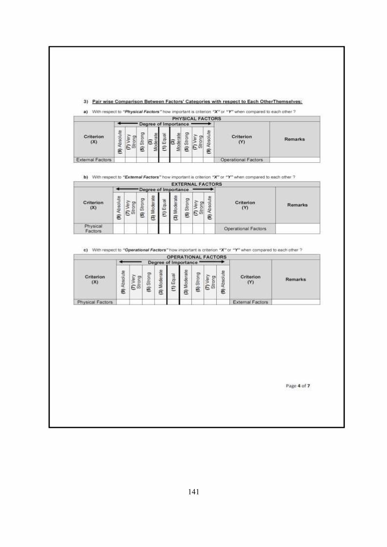
141

142
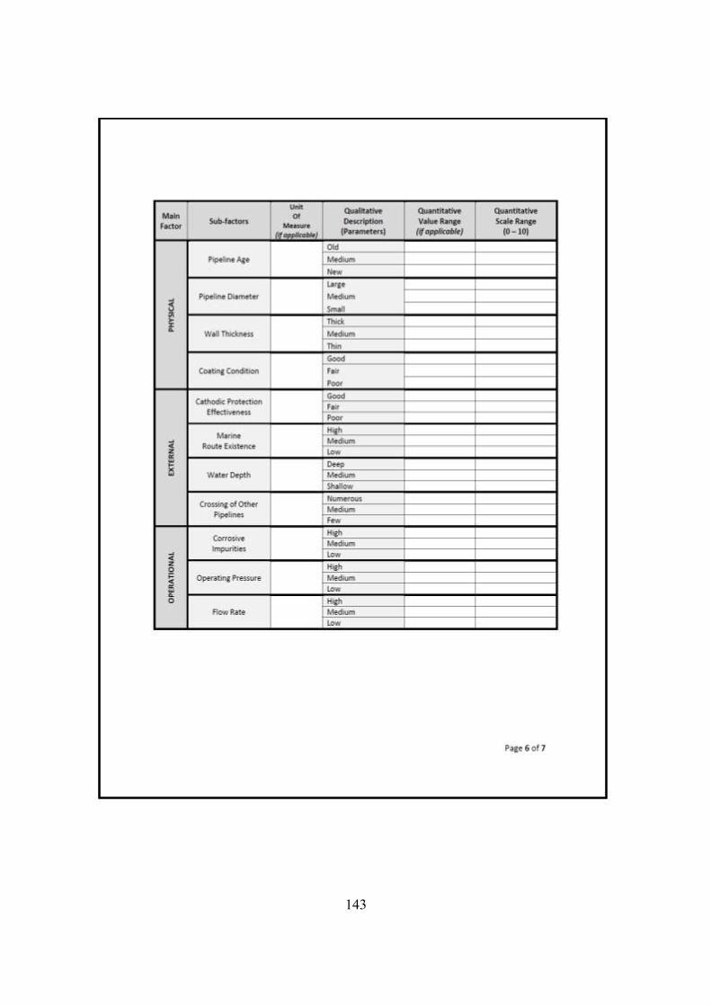
143

144
.

145
APPENDIX (B)
146
APPENDIX (B)
PIPELINE PROTECTION, LEAK DETECTION AND
MANUFACTURING
Pipelines Protection
Hopkins (2002) says that the pipelines are designed to be protected from the surrounding
environment for the following reasons:
1) External Corrosion: In order to protect a steel pipe for the external corrosion, the pipe
must be separated from humid environment like soil or water. There is no standard limit
for the corrosion in the design books to allow for a maximum percentage of external
corrosion in the pipe like increasing the wall thickness. This is called “corrosion
allowance”. So, the external side pipeline is coated with special material like coat tar as a
primary protection and a corrosion protection system is the secondary protection.
2) Internal Corrosion: Unlike the external corrosion, a corrosion allowance is considered
to accommodate in service, predictable, corrosion which can be introduced at the design
stage. On the other hand, it is more convenient to prevent the internal corrosion for
happening in the first place. That is why the pipeline is treated before put to service. That
is done by checking the pipeline quality, cleaning the line and mixing chemicals to
accommodate any corrosion.
3) External Damage: Many precautions can be done to protect the pipeline for any damage
that is caused by external reasons or third parties. These precautions may include
147
increasing the wall thickness of the pipeline, using a deeper cover, installing the
pipelines away from possible interferences and conducting good communications with
third parties including the general public and protective measures such as concrete
casings.
Pipeline Operation and Leak Detection
With the advancement to technology in all fields, the newly installed pipelines existing in
remote areas are operated automatically by computers at the headquarters of the pipeline
company. The pipeline pressure, flow rate and many other parameters at various locations are
monitored by these computers which also performs large numbers of computations and send
the suitable commands along the pipelines network to control the valves and pumps
operation. In some cases, manual operating is needed. These cases may include modifying the
automatic operation when different batches of fuels are directed to different temporary
storage tanks, or when the system must be shut down or restarted. Since the oil spill can
cause big damage environmentally and economically, leak detection systems would be
installed in the pipelines network to prevent leakage and to allow for a rapid response in case
of a pipeline failure. (Hopkins, The Structural Integrity Of Oil And Gas Transmission, 2002)
There are various types of leak detection systems but the most used are the following:
1- Simple Systems: As the names suggests, this system involves a member of the staff
working near the pipelines to regularly survey the pipelines and looking for any evidence
of leakage such as smell, of different in coloration around the pipe. In addition, people
living near the pipelines or just passing by can perform this task.
148
2- Flow Balance: This method is done by measuring the inputs and outputs of a pipeline. If
the outputs are less than the inputs, the supervising staff will conclude a leakage incident.
3- Acoustic Methods: This method uses the noise as an indication of leakage incidents.
The associated noise causes vibrations which have frequencies more than 20 kHz.
Transducers can be attached a pipeline to locate the leak accurately by noting signal
strength.
4- Pipeline Modeling: This method propose pipeline modeling to simulate the operating
conditions of the pipeline and comparing the actual with the expected conditions all the
time. The model which is a mathematical representation of the real life condition. This
model is used to calculate the expected pressure; flows etc., and compare them with the
actual values. If there is any discrepancy that may imply a leak, a leak alarms goes on.
(Hopkins, The Structural Integrity Of Oil And Gas Transmission, 2002)

149
Pipelines Manufacturing
Pipelines manufacturing can be done using either seamless manufacturing or welded
pipelines. Seamless pipelines are formed by drawing a heated solid bar of steel over a
piercing rod while welded pipelines are created by rolling a flat steel plate and welding the
seam longitudinally. Seamless pipeline are stronger than welded ones because they withstand
more pressure since they don't have any seams that can create weak spots but welded
pipelines are cheaper to manufacture. (Crestwood Tubulars, 2013). Qatar's pipelines
operators use both types of pipelines, seamless and welded with different steel grades starting
from grade A to X80. The following table shows the different steel grades and their yield
strength. Pipelines with high steel grades are used for offshore pipelines because they have
higher yield strength and can withstand more pressure. The problem is that they require
special type of welding and they are easily affected by impurities such as H2S (Mikhail,
2011).