fuzzy based power control system using anfis and mimo …830006/fulltext01.pdf · fuzzy based power...
TRANSCRIPT
1 | P a g e
Fuzzy Based power control system Using ANFIS and
MIMO-OFDM Techniques in Cognitive Radio Networks
Mahesh Aleti
Syed Rahamatulla
Rajendra Chennupati
This thesis is presented as part of Degree of
Master of Science in Electrical Engineering
Blekinge Institute of Technology
October 2013
Blekinge Institute of Technology
School of Engineering
Department of Radio communications
Supervisor: Yong Yao
Examiner: Dr. Sven johansson

2 | P a g e
Abstract
Cognitive Radio technology is used for efficient utilization of the spectrum. There are two types of users,
one is the Primary user (PU), and the second one is the Secondary user (SU). In those users, PU is having
the license to use the spectrum. The SU does not have the license to use the spectrum.
Cognitive Radio comprises of Spectrum sensing, Spectrum Management and Spectrum Mobility. In
cognitive radio, optimal power control in spectrum sharing is main research issues.
In the spectrum, sharing both PU and SU can access the spectrum simultaneously as long as there is no
interference to PU‘s of Quality of service (QOS).
So we have to handle this interference to the PU and we have to improve the performance of the SU. For
that power control is the main consternate to improve the performance of SU.
In our thesis, we are divided into two parts, the first one is we used ANFIS (Adaptive Neuro Fuzzy
Inference System) for optimizing power control in cognitive radio network Users (SU) by optimization of
SNR & SINR at Primary User (PU) to maintain QOS of PU and improve the performance of SU and
Channel capacity computation for various ISR tolerance levels at PU.
In second part, we used implementation of MIMO (Multiple Input Multiple output)-OFDM (Orthogonal
Frequency Division Multiplexing) transmission technique in CRN (Cognitive Radio networks) for it is
use in emergency conditions where transmission requires reliability and high data rate. Then it is tested
BER (Bit error rate) performance on MATLAB.
Key words: Cognitive Radio, Power Control, the Fuzzy Interference System (FIS), ANFIS, ―MIMO‖
(―Multiple Input Multiple Output‖), ―OFDM‖ (―Orthogonal Frequency Division Multiplexing‖), AWGN,
BER, SNR, Eb/N0

3 | P a g e
Acknowledgements
We would like to show our gratitude to our supervisor Dr. Sven Johansson for giving us an
opportunity to do our thesis under his supervision. He has given wonderful support and guidance
throughout my thesis work.
We must thank all professors who gave me all the support throughout our master‘s program and
we would like to thank to our friends who gave moral support and building the confidence and
making these two years as unforgettable. Finally we are most thankful to our parents for their
love and support to throughout our life.

4 | P a g e
Table of Contents
Abstract ......................................................................................................................................................... 2
Acknowledgements ....................................................................................................................................... 3
Table of Contents .......................................................................................................................................... 4
Figures list ..................................................................................................................................................... 6
Formula List .................................................................................................................................................. 7
Chapter 1 ....................................................................................................................................................... 8
1. Introduction ....................................................................................................................................... 8
1.1. The Neural Network and the Fuzzy Logic ................................................................................ 8
1.2. ANFIS Systems – ―Adaptive Neuro-Fuzzy Inference Systems‖ .............................................. 8
1.3. Alignment of the project report ................................................................................................. 9
Chapter 2 ..................................................................................................................................................... 10
2 Aim and Objectives of the Thesis and Related work ...................................................................... 10
2.1 Aspiration of the Project ......................................................................................................... 10
2.2 Objectives of Project ............................................................................................................... 10
2.3 Scope of the project................................................................................................................. 10
2.4 Survey of Related Work .......................................................................................................... 10
Chapter 3 ..................................................................................................................................................... 13
3 Research Questions and Main Contribution ................................................................................... 13
3.1 Research Questions ................................................................................................................. 13
3.2 Main Contribution ................................................................................................................... 13
Chapter 4 ..................................................................................................................................................... 14
4 About the FIS System and MIMO-OFDM ..................................................................................... 14
4.1 FIS Technique ......................................................................................................................... 14
4.1.1 Fuzzification ................................................................................................................... 15
4.1.2 Fuzzy Inferencing ........................................................................................................... 15
4.1.3 Aggregation of all outputs ............................................................................................... 16
4.1.4 Defuzzification ................................................................................................................ 16
4.1.5 Generic Method............................................................................................................... 16
4.1.6 Rules for Tipping ............................................................................................................ 17
4.2 ANFIS Systems (―Adaptive Neuro Based Fuzzy Inference Systems‖) .................................. 20
4.2.1 The Forward Pass ............................................................................................................ 22
4.2.2 Backward Pass ................................................................................................................ 23
4.3 . MIMO-OFDM ...................................................................................................................... 23

5 | P a g e
4.4 . MIMO-OFDM System Model .............................................................................................. 23
4.5 Components of MIMO-OFDM System .................................................................................. 26
Chapter 5 ..................................................................................................................................................... 27
5 Implementation of ANFIS .............................................................................................................. 27
5.1 ANFIS System ........................................................................................................................ 27
5.1.1 ANFIS Architecture: Layer 1 .......................................................................................... 27
5.1.2 ANFIS Architecture: Layer 2 .......................................................................................... 28
5.1.3 ANFIS Architecture: Layer 3 .......................................................................................... 29
5.1.4 ANFIS Architecture: Layer 4 .......................................................................................... 29
5.1.5 ANFIS Architecture: Layer 5 .......................................................................................... 30
5.1.6 Alternate ANFIS Architecture ........................................................................................ 30
5.1.7 Tsukamoto model ANFIS Architecture .......................................................................... 31
5.1.8 2 input Sugeno with 9 rules ANFIS Architecture ........................................................... 31
5.2 Flowchart ................................................................................................................................ 32
5. 3 Description of the algorithms used .................................................................................................. 33
5.4 System Model ................................................................................................................................... 33
5.4.1. Propagation environment without path loss .............................................................................. 33
5.4.3. Propagation environment with path loss ................................................................................... 34
Chapter 6 ..................................................................................................................................................... 36
6 Results ............................................................................................................................................. 36
6.1 Case 1: Without Path loss ....................................................................................................... 36
6.2 Case 2: With the path loss ....................................................................................................... 41
Chapter 7 ..................................................................................................................................................... 47
7 Implementation MIMO-OFDM ...................................................................................................... 47
7.1 MIMO-OFDM System ............................................................................................................ 47
7.1. Testing and Results with Snapshots ............................................................................................. 47
Chapter 8 ..................................................................................................................................................... 53
7 Conclusion and Future Work .......................................................................................................... 53
Chapter 9 ..................................................................................................................................................... 54
References ............................................................................................................................................... 54
6 | P a g e
Figures list Figure 1: ANFIS System……………………………………………………………………………………………………………………8 Figure 2: Structure of a Fuzzy Expert System………………………………………………………………………………….15 Figure 3: Antecedent for each rule…………………………………………………………………………………………………17 Figure 4: Rule's Conclusion…………………………………………………………………………………………………………….18 Figure 5: Aggregate Conclusions…………………………………………………………………………………………………….18 Figure 6: Defuzzification…………………………………………………………………………………………………………………19 Figure 7: All Steps of FIS System……………………………………………………………………………………………………..19 Figure 8: An ANFIS architecture for a two rule Sugeno system………………………………………………………20 Figure 9: MIMO-OFDM Model……………………………………………………………………………………………………….24 Figure 10: A two-input first-Order Sugeno Fuzzy Model with two rules…………………………………………27 Figure 11: ANFIS Architecture: Layer 1……………………………………………………………………………………………27 Figure 12: ANFIS Architecture: Layer 2……………………………………………………………………………………………28 Figure 13: ANFIS Architecture: Layer 3……………………………………………………………………………………………29 Figure 14: ANFIS Architecture: Layer 4……………………………………………………………………………………………29 Figure 15: ANFIS Architecture: Layer 5……………………………………………………………………………………………30 Figure16: Alternate ANFIS Architecture………………………………………………………………………………………….30 Figure 17: Tsukamoto model ANFIS Architecture……………………………………………………………………………31 Figure 18: 2 Input Sugeno with 9 rules ANFIS Architecture……………………………………………………………..31 Figure 19: Flow chart………………………………………………………………………………………………………………………32 Figure 20: System model for Propagation environment without path loss……………………………………..33 Figure 21: System Model for Propagation environment with path loss…………………………………………..34 For without path loss Figure 22: Input membership functions of two antecedents (fuzzy inference system)……………………35 Figure 23: ANFIS data of power control parameter for no path loss case……………………………………….36 Figure 24: BER v/s Eb/No raw and ANFIS data for BPSK………………………………………………………………….37 Figure 25: BER v/s Eb/No raw and ANFIS data for QPSK………………………………………………………………….38 Figure 26: BER v/s Eb/No raw and ANFIS data for 16PSK………………………………………………………………..39 Figure 27: Channel Capacity as a function of ISR tolerance…………………………………………………………….39 For with path loss Figure 28: Input membership functions of two antecedents (fuzzy inference system)……………………40 Figure 29: ANFIS data of power control parameter for path loss case……………………………………………41 Figure 30: BER v/s Eb/No raw and ANFIS data for BPSK………………………………………………………………….42 Figure 31: BER v/s Eb/No raw and ANFIS data for QPSK………………………………………………………………….43 Figure 32: BER v/s Eb/No raw and ANFIS data for 16PSK………………………………………………………………..44 Figure 33: Channel Capacity as a function of ISR tolerance…………………………………………………………….45 MIMO-OFDM Figure 34: Plot of BER vs. EbN0 for QPSK………………………………………………………………………………………..47 Figure 35: Plot of BER vs. EbN0 for 8PSK………………………………………………………………………………………..48 Figure 36: Plot of BER vs. EbN0 for 16PSK……………………………………………………………………………………….49 Figure 37: Plot of BER vs. EbN0 for 16QAM…………………………………………………………………………………….50 Figure 38: Plot of BER vs. EbN0 for 64 QQAM…………………………………………………………………………………51

7 | P a g e
Formula List 4.1 The Two Rule Sugeno ANFIS has rules of the form……………………………………………….21
4.2 The output of each node in Layer 1………………………………………………………………....22
4.3 The output of each node in Layer 2………………………………………………………………....22
4.4 The output of each node in Layer 3………………………………………………………………....22
4.5 The output of each node in Layer 4………………………………………………………………....22
4.6 The output of each node in Layer 5………………………………………………………………....23
5.1 An adaptive node with a node function in Layer 1………………………………………………….29
5.2 An adaptive node with a node function in Layer 2………………………………………………….29
5.3 An adaptive node with a node function in Layer 3………………………………………………….30
5.4 An adaptive node with a node function in Layer 4………………………………………………….30
5.5 An adaptive node with a node function in Layer 5………………………………………………….31
5.6 The input 1 for the power control parameter with no path loss case………………………………...33
5.7 The input 2 for the power control parameter with no path loss case………………………………...33
5.8 The primary user‘s Signal to Noise ratio without cognitive user is given by………………………..34
5.9 The primary user‘s Signal to interference noise ratio with the presence of cognitive user is given by
…………………………………………………………………………………………………………….34
5.10 The input 1 for the power control parameter with path loss case………………………….………...34
5.11 The input 2 for the power control parameter with path loss case………….………………………...34
8 | P a g e
Chapter 1
1. Introduction
1.1. The Neural Network and the Fuzzy Logic
Neural networks and fuzzy logic are two integral technologies [1]. Neural networks can understand from
information and reviews. It is challenging to create an understanding of the significance associated with
such neuron and each weight. It is viewed as ―black box‖ approach. The Neuro-fuzzy program can be
categorized into three groups [1].
a) The rule basis fuzzy design is build up by a supervised NXN learning technique
b) The fuzzy rule basis design is build up byreinforcement-based learning
c) The rule wise fuzzy design is build up by NXN to construct its fuzzy partition of the input space
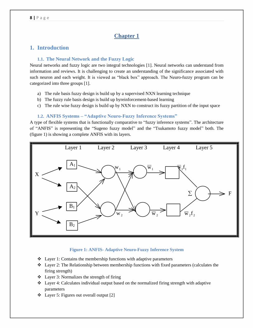
1.2. ANFIS Systems – “Adaptive Neuro-Fuzzy Inference Systems”
A type of flexible systems that is functionally comparative to ―fuzzy inference systems‖. The architecture
of ―ANFIS‖ is representing the ―Sugeno fuzzy model‖ and the ―Tsukamoto fuzzy model‖ both. The
(figure 1) is showing a complete ANFIS with its layers.
Layer 1 Layer 2 Layer 3 Layer 4 Layer 5
1w 1w 11fw
X
F
Y 2w 2w 22fw
A1
A2
B1
B2
Figure 1: ANFIS- Adaptive Neuro-Fuzzy Inference System
Layer 1: Contains the membership functions with adaptive parameters
Layer 2: The Relationship between membership functions with fixed parameters (calculates the
firing strength)
Layer 3: Normalizes the strength of firing
Layer 4: Calculates individual output based on the normalized firing strength with adaptive
parameters
Layer 5: Figures out overall output [2]

9 | P a g e
Layer 4 parameters are estimated with the ―least squares‘ method‖ of forward pass. Here, the equation for
the individual output is considered as the function of input.
Layer 1 parameters estimate the ―back propagation ―and the ―gradient descent‖. The parameters are using
for membership functions.
1.3. Alignment of the project report
The complete report for this proposed system is organizing in nine chapters. In chapter 1, a small
introduction is there to discuss about this proposed system. In chapter 1, we will explain some basic
information about ANFIS data. This chapter will also explain the process of data analysis, using various
techniques. In this chapter, we will also mention the organization of the report.
In Chapter 2, primary goals, objectives and aims that need to be realized in this suggested program. It
will also describe some of the use situations and the opportunity of this venture we will describe the
theoretical qualifications and literary performs evaluation aspect. In this section we will describe some
primary ideas of the proposed system and some of the appropriate works that have already been
completed in this area and that will give us help in the execution of our suggested program and inspiration
of the dissertation.
Chapter 3 will handle the research question and the main contribution of the thesis.
Chapter 4 will handle the technological part of this project about the FIS and the MIMO-OFDM system.
In this chapter we will discuss on the various technologies that are used to complete this project.
Chapter 5 will deal with the implementation of ANFIS. It will describe the way in which we will form
and study this program.
Chapter 6 will explain the major results and the output of our suggested project.
Chapter 7 will explain the Implementation of MIMO-OFDM and results.
Chapter 8 will explain the review and this chapter will end with a proper summary along with the long
run work.
Chapter 9 will describe and discuss regarding all the references and sources that have been taken help for
the efficient performance of our program.

10 | P a g e
Chapter 2
2 Aim and Objectives of the Thesis and Related work
2.1 Aspiration of the Project
The main aim of this project is the implementation of ―ANFIS‖ i.e. ―Adaptive Neuro-Fuzzy Inference
System‖ technique in Cognitive Radio for opportunistic power control of Secondary Users (SU) by
optimization of SNR & SINR at Primary User (PU).
This involves control of the power control factor of SU using ANFIS based control, which uses training
data generated from SNR & SINR of PU, given the channel capacity as a threshold parameter, which is
computed from the ISRtol (ratio of SU Interference to PU Signal) tolerance level. The channels are
assumed to be fading channels for both path loss and without path loss cases.
In second part, we will implement the MIMO-OFDM transmission technique in CRN for its use in
emergency conditions where transmission requires reliability and high data rate using modulation like
BPSK, QPSK & 16-PSK. Then it is BER (Bit Error Rate) versus SNR performance will be estimated
using MATLAB.
2.2 Objectives of Project
Implementation of ANFIS method for maintains good QOS for PU and improves the performance
of SU.
The Power control parameter of raw training data and ANFIS computed data are plotted.
Channel capacity computation for various ISR tolerance levels at PU.
BER vs. Eb/No computation & plots using raw & ANFIS data for various modulations under the
path loss/without pass loss cases
The implementation of the 1x1 MIMO- OFDM and the 2x2 MIMO-OFDM transmission
techniques towards SU in CRN, then validate BER performance on MATLAB
BER vs. SNR computation & plots using raw & ANFIS data for MIMO- OFDM
2.3 Scope of the project
Project scope is limited to standard fading channels like the Raleigh channel [2]. Additive White Gaussian
Noise (AWGN) [2] is also considered for comparisons. It is assumed that the channel model is IID
(independent and identically distributed) and the channel capacity computation is based on this model. In
MIMO-OFDM Project scope is limited to standard MIMO fading channels with Raleigh channel
characteristics. 1x1 and 2x2 MIMO schemes are analyzed.
2.4 Survey of Related Work
In [9] this paper the author used Fuzzy and ANFIS based down link power control schemes.
[10] MahmutBilgehan worked a relative research for the tangible compression durability
assessment using sensory system and the neuro-fuzzy modelling techniques. The research paper
is discussing about the flexible ―neuro-fuzzy inference system‖ (ANFIS) and ―synthetic sensory
system‖ (ANN) model. Those models have been efficiently used for the assessment of
connections between tangible compression durability and ultrasound rhythm speed (UPV)
principles using the trial data obtained from many cores taken from different strengthened
tangible components having different ages and unidentified percentages of tangible mixes. A

11 | P a g e
relative research is made using the sensory netting and neuro-fuzzy (NF) techniques. Evaluating
of the outcomes, it is discovered that the suggested ANFIS structure with Gaussian account
function is discovered to perform better than the multilayer feed-forward ANN learning by ―back-
propagation‖ criteria. The outcomes show that especially the ANFIS acting may represent an
efficient tool for forecast of the tangible compression durability.
In [11] the author improved error rate performance in the Nakagami-m fading channel using
OFDM transmission when DQPSK scheme is used.
In [13] the author explained about the Takagi-Sugeno fuzzy system and compared with the
Mamdani fuzzy system.
In [14] the author applied OFDM technique to CRN for gaining high data rate using different
modulation schemes and they validated BER performance.
In [16] the author explained the probability based method for optimizing the inter-sensing method
in cognitive radios
[17] The author took a pair of primary users and a pair of secondary users in a fading channel; in
this project they improved QOS and causing any interference to the PU.
[19] The authors explained ANFIS method for copper prediction. They also compared to ANN
based system. They concluded that ANFIS method for better results.
In [21] the author proposed the FIS for spectrum sensing in CRN.
In [23] this paper the authors are used optimized Takagi-Sugeno fuzzy inference system (FIS)
based power control strategy for opportunistic spectrum access in CRN and they implemented
OFDM transmission technique for CRN
[26]―M. Abdullahi, H. M. A. Al-Mattarneh, A. H. Hassan, M. H. Abu Hassan and B. S.
Mohammed‖ analysed on An Evaluation on Expert Techniques for Tangible Mix Style. For their
designed expert systems, mix design requirements based on information acquired from the
encounter with concrete components. ―Expert systems‖ designed using expert program seashells
such as EXSYS Expert, stage 5, stage 5 items and kappa-PC.
[27] ―M.C.Nataraja, M.A.Jayaram and C.N.Ravikumar‖ described a ―Fuzzy-Neuro‖ Style for
Normal Tangible Mix Style. This document provides the growth of a novel strategy for the
estimated proportioning of traditional concrete blends. Unique fuzzy inference segments in five
levels have been created to catch the vagueness and estimates in various steps of design as
recommended in IS: 10262-2003 and IS456-2000. A qualified three-part back-reproduction
sensory system is incorporated in the model to remember trial data associated with w/c rate v/s 28
days compression durability connection with three popular manufacturers of concrete. The results
with regards to the amounts of concrete, the fine combination, the course combination and the
water acquired over the existing means for different qualities of traditional concrete blends are in
good contract with those acquired by the frequent traditional strategy.

12 | P a g e
2.1.5. Motivation
Observing from above-related work, so far Takagi Sugeno, Mamdani and FIS methods were implemented
in cognitive radio networks. We proposed ANFIS for the ratio of PU‘s and ratio of SU‘s to maintain QOS
to PU and improving the performance of SU. We also proposed MIMO-OFDM for different modulation
techniques in CRN and calculated BER for different modulation schemes to improve the reliability on
CRN.

13 | P a g e
Chapter 3
3 Research Questions and Main Contribution
3.1 Research Questions
In cognitive radios, the main aim is the utilization of the spectrum in the system. It is sharing and the
power transmission from SU on the PU spectrum. Here the QOS (Quality of service) of PU is degraded.
So, for that we have to maintain the QOS to the PU.
There are a variety of issues that need to be regarded in this suggested program. An appropriate response
should be available for these issues with the help of this suggested program. Some of the essential issues
that need to be resolved in this program are as follows:
How the ANFIS methods improve QOS to the PU‘s and Improve performance of SU‘s?
How will we improve BER performance?
How do the MIMO-OFDM techniques improve the reliability towards SU on CRN?
3.2 Main Contribution
First we are implementing ANFIS for optimizing power control of CRN, and then validate the results
on MATLAB.
We implemented channel capacity theorem for various ISR tolerance levels at PU.
Then we plotted BER V/s Eb/No graphs for different modulation techniques.
The implementation of 1x1 and 2x2 MIMO-OFDM transmission techniques towards SU in CRN,
then validate BER performance on MATLAB.

14 | P a g e
Chapter 4
4 About the FIS System and MIMO-OFDM
4.1 FIS Technique
The procedure of developing the leveling from a given feedback to an outcome using the fuzzy logic is
known as FIS technique [3]. The leveling then provides a support from which choices can be made, or
styles discovered. The procedure of the fuzzy inference system includes all parts that are described in the
If-Then Rules Logical Operations, and Membership Functions.
● The Fuzzy Inference System (FIS) is a way of applying a feedback area to an outcome area using
fuzzy logic
● FIS uses a compilation of fuzzy account features and guidelines, instead of Boolean reasoning, to
consider the data value.
● The rules in FIS are called ―fuzzy expert system‖. These systems are the rules of ―fuzzy
production‖. The form of the rules is:
− If p, then q, where p and q are fuzzy statements.
● For example, in a fuzzy rule
− If x is low and y is high then z is the medium.
− Here x is low; y is high; z is the medium. Those are fuzzy statements. The value of x and
y are input variables. The value of z is an output variable.
● The antecedent explains to what level the concept is applicable, while the summary designates a
fuzzy operator to produce the outcome factors.
● Most resources for dealing with fuzzy expert systems consider more than one summary per
concept.
● The set of rules in a fuzzy expert system is known as the knowledge base.
● The functional operations in the ―fuzzy expert system‖ proceed in the following steps, in this 1,2
and 4 are shows in below (figure 2), Point 3 shows in (figure 3).
− 1. Fuzzification
− 2. Fuzzy Inferencing (It applies implication method)
− 3. Aggregation of all output
− 4. Defuzzification [4]

15 | P a g e
Figure 2: The Basic Architecture of a Fuzzy Expert System
4.1.1 Fuzzification
In Above (figure 2) the process of this method, membership functions explained on feedback factors are
enforced to their definite values so that the level of fact for each concept assumption can be driven.
In the antecedent part, the statements of fuzzy logic resolve to a level of account or membership
between the value of ―0 and 1‖.
o If antecedent method has only one part, then this is the degree of approval for the rule.
o If the antecedent method has several parts, use the operators of ―fuzzy logic‖ and
determine the ―antecedent‖ to a single value. The value should be between 0 and 1.
Antecedent may be joined by OR; AND operators.
o For OR -- max
o For AND -- min
4.1.2 Fuzzy Inferencing
In the process of the inference
o Fact value for the assumption of each concept is calculated and used to the summary
aspect of each concept.
o The results in the fuzzy sets are to be allocated to each outcome varying for each concept.
The use of the degree of support for the integrated guideline is to configure the ―fuzzy set‖
outcome.
The consequent of a fuzzy rule assigns an entire fuzzy set to the output.
If the antecedent is only partially true, (i.e., is assigned a value less than 1), then the resultant
fuzzy set is truncated according to the implication method [5]

16 | P a g e
If the consequent of a rule has multiple parts, then all values are impacted similarly by the output
of the antecedent.
The consequent specifies a fuzzy set to be assigned to the output.
The implication function then modifies that fuzzy set to the degree specified by the antecedent.
The following functions are used in inference rules.
The min and prod are commonly used as the rules of interference.
o Min: abbreviates the membership function of the consequent.
o Prod: scales it.
4.1.3 Aggregation of all outputs
It is the process where the outcome of each concept is mixed with only one the ―fuzzy set‖.
The input of the aggregation process is for listing the features of the outcome. It came back with
the implication procedure for every concept.
The outcome of the process of ―aggregation‖ is a ―fuzzy set‖ for each outcome volatile.
Here, all fuzzy sets allocated to each outcome varying are mixed together to type a single fuzzy
set for each outcome varying using a fuzzy aggregation operator.
Some of the most commonly used aggregation operators are
o The maximum : an overall point basis maximization of the fuzzy sets
o The sum : an overall point basis summation of the fuzzy sets
o The probabilistic sum.
4.1.4 Defuzzification
Defuzzification method shown in (figure 6).
In ―Defuzzification‖,(in figure 6) the output set of ―fuzzy logic‖ is converted to a fresh number.
The centroid method and the maximum method are two commonly used techniques.
o The centroid method is for searching the varying value of the centre of severity of the
membership function for the fuzzy value. It also calculates the fresh value of the
outcome.
o The maximum method is one of the varying principles at which the fuzzy set has its
highest possible fact value. It selects the fresh value for the outcome value.
Some other method for ―defuzzification‖ is:
o Bisector, which is the centre of the maximum value (the average of the maximum value
of the output set), the largest of the maximum value, and smallest of the maximum value,
and etc.
4.1.5 Generic Method
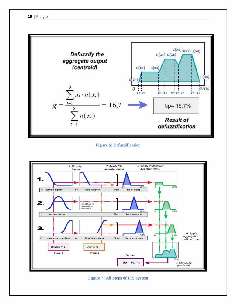
Main steps are
o Asses the antecedent for each guideline
o Access closure for each rule
o Accumulate the completion
o Defuzzification
We will explain these steps using an example of Tipping Problem
Two inputs : The Quality of food and Service at a restaurant rated at scale from 0-10
One output: Amount of tip to be given
Tip should reflect the quality of food and service.
The tip might be in the range 5-15% of the total bill paid. [5]
17 | P a g e
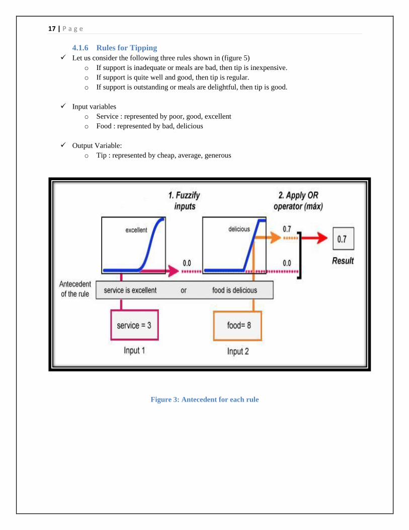
4.1.6 Rules for Tipping
Let us consider the following three rules shown in (figure 5)
o If support is inadequate or meals are bad, then tip is inexpensive.
o If support is quite well and good, then tip is regular.
o If support is outstanding or meals are delightful, then tip is good.
Input variables
o Service : represented by poor, good, excellent
o Food : represented by bad, delicious
Output Variable:
o Tip : represented by cheap, average, generous
Figure 3: Antecedent for each rule
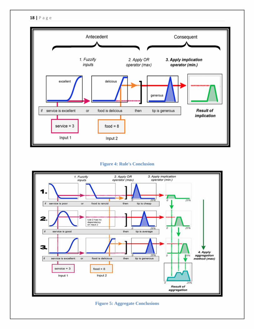
18 | P a g e
Figure 4: Rule's Conclusion
Figure 5: Aggregate Conclusions
19 | P a g e
Figure 6: Defuzzification
Figure 7: All Steps of FIS System
20 | P a g e
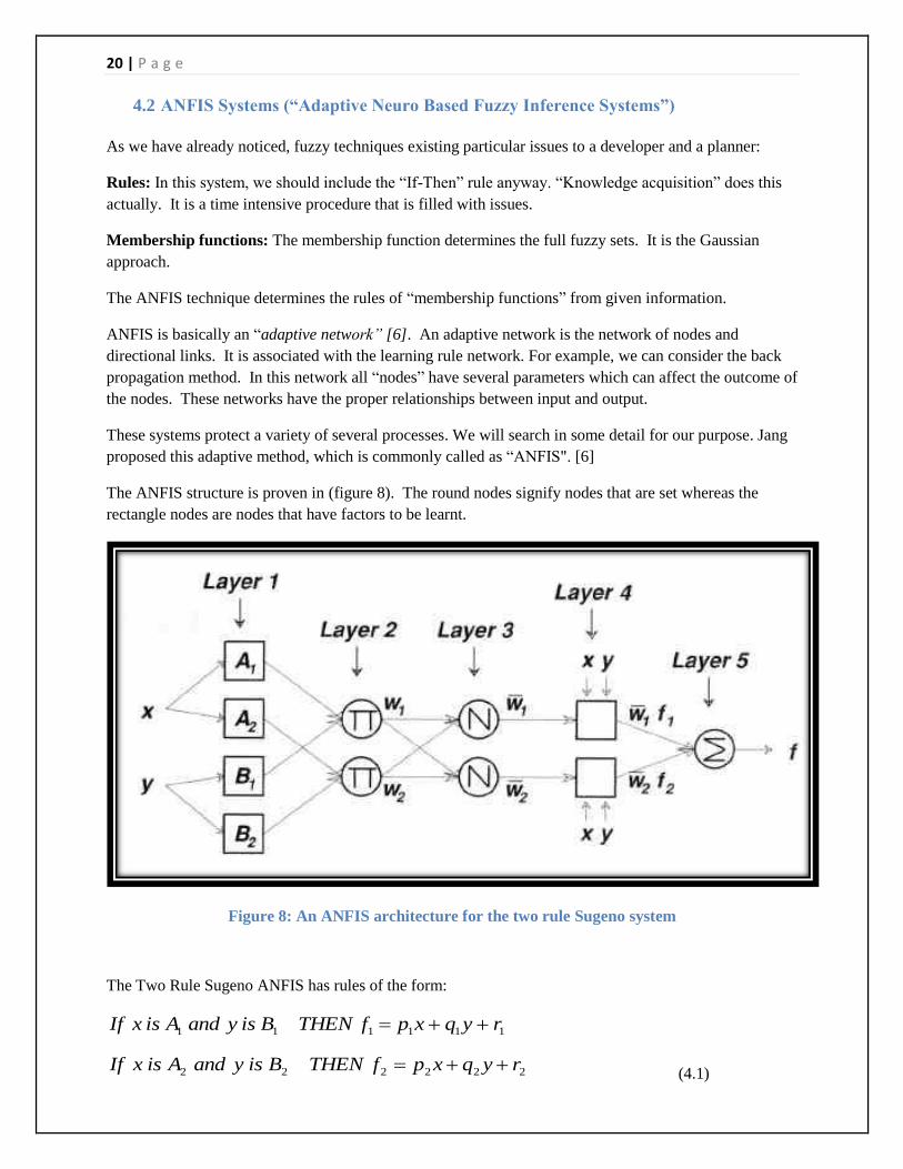
4.2 ANFIS Systems (“Adaptive Neuro Based Fuzzy Inference Systems”)
As we have already noticed, fuzzy techniques existing particular issues to a developer and a planner:
Rules: In this system, we should include the ―If-Then‖ rule anyway. ―Knowledge acquisition‖ does this
actually. It is a time intensive procedure that is filled with issues.
Membership functions: The membership function determines the full fuzzy sets. It is the Gaussian
approach.
The ANFIS technique determines the rules of ―membership functions‖ from given information.
ANFIS is basically an ―adaptive network” [6]. An adaptive network is the network of nodes and
directional links. It is associated with the learning rule network. For example, we can consider the back
propagation method. In this network all ―nodes‖ have several parameters which can affect the outcome of
the nodes. These networks have the proper relationships between input and output.
These systems protect a variety of several processes. We will search in some detail for our purpose. Jang
proposed this adaptive method, which is commonly called as ―ANFIS". [6]
The ANFIS structure is proven in (figure 8). The round nodes signify nodes that are set whereas the
rectangle nodes are nodes that have factors to be learnt.
Figure 8: An ANFIS architecture for the two rule Sugeno system
The Two Rule Sugeno ANFIS has rules of the form:
111111 ryqxpfTHENBisyandAisxIf
222222 ryqxpfTHENBisyandAisxIf (4.1)

21 | P a g e
For the training of the system, there is a forward pass system and a backward pass system. We now
consider each part in turn for the forward pass procedure. The forward pass develops the input vector
through the system, part by part. In the backward pass procedure, the error is sent back again through the
system in a similar way to back again reproduction.
Layer 1
The output of each node is:
2,1)(,1 iforxOiAi
4,3)(2,1
iforyO
iBi (4.2)
So, the )(,1 xO iis essentially the membership grade for x and y .
The membership functions could be anything but for the purpose of representation, we are using the bell-
function given by:
ib
i
i
A
a
cxx
2
1
1)(
Here iii cba ,, are parameters to be learnt. These are the premise parameters.
Layer 2
Every node in this layer is fixed. This is where the t-norm is used to ‗AND‘ the membership grades - for
example the product:
2,1),()(,2 iyxwOii BAii
(4.3)
Layer 3
Layer 3 contains fixed nodes which calculate the ratio of the firing strengths of the rules:
21
,3ww
wwO i
ii
(4.4)
Layer 4
The nodes in this layer are adaptive and perform the consequent of the rules:
)(,4 iiiiiii ryqxpwfwO
(4.5)
The parameters in this layer (iii rqp ,, ) are to be determined and are referred to as the consequent
parameters.

22 | P a g e
Layer 5
There is a single node here that computes the overall output:
i i
i ii
ii
iiw
fwfwO ,5
(4.6)
Generally, the feedback vector is feeding through the system part by part. Now, we discuss about the
premise and consequent parameters which ANFIS learns to achieve the required functions and the needful
rules. [7]
There are a variety of possible techniques, but we will talk about the hybrid learning algorithm proposed
by Jang, Sun and Mizutani (Neuro-Fuzzy and Soft Computing, Prentice Hall, 1997) which uses a
combination of Steepest Descent and Least Squares Estimation (LSE). This is actually a very complex
method. So, here I will offer very advanced stage information of how the criteria functions.
It can be proven that for the system described if the assumption factors are set the outcome is the straight
line in the major factors.
There are three types of parameter sets:
S = Total parameters‘ Set
1S = Premise (nonlinear) parameters‘ Set
2S = Consequent (linear) parameters‘ Set
So, ANFIS uses the two pass learning algorithm:
Forward Pass
Here 1S is unmodified and
2S is computed using a LSE algorithm.
Backward Pass
Here 2S is unmodified and
1S is computed using a gradient descent algorithm such as backing
propagation.
So, the above-mentioned algorithm is typically a combination of steepest-descent and least squares to
accommodate the framework in the adaptive network.
The procedure conclusions are given below:
4.2.1 The Forward Pass
Presentation of the input vector
Calculation of the nodes and presenting output part by part
Repetition of each information N and y build
Identifying of the parameters in Sn using Least Squares Method
Computation of error measurement for each combination of the training value

23 | P a g e
4.2.2 Backward Pass
Use abrupt descent algorithm to upgrade factors in Sm (―back propagation‖)
For given fixed values of Sm , the parameters in Sn discovered in this strategy are assured to be
the global optimum point.
4.3 . MIMO-OFDM The full form of OFDM is ―Orthogonal Frequency Division Multiplexing‖. It is a ―multi-channel
modulation‖ strategy that creates use of FDM (Frequency Division Multiplexing) [8] being regulated by a
low bit amount electronic flow. The primary purpose of using OFDM is because here the icon recognition
is simple and also to improve the sturdiness against frequency particular diminishing and filter group
disturbance. Certain parameter like CFO (carrier frequency offset), I/Q discrepancy (in-phase and
quadrature stage imbalance) discrepancy causes distortions in the obtained indication. Here evaluation is
created for given factors using different programs and a technique is suggested for Multiple Input
Multiple output (MIMO) OFDM program when the icon produced is not an important multiple variety of
transmitters used.
Dominance of MIMO-OFDM techniques are:
Spectral efficiency is very high.
FFT (Fast Fourier Transform) uses for simple execution.
The complexity of the recipient is low.
Very strong and high data-rate transmitting is in this system over the multi-path channel
To connect adaptation, it takes high edibility.
Several accessibility techniques are there for low complexness. As an example, we can consider
―orthogonal regularity division multiple accessibility‖.
Disadvantages of MIMO-OFDM techniques are:
Regularity ―offsets‖ are very sensitive.
It has several moment-mistakes and stage-noise;
Comparatively, it needs more energy rate for the individual service provider program.
It tends to decrease the performance of the RF firm.
4.4 . MIMO-OFDM System Model MIMO (Multiple-input multiple-output) in (figure 9) is a wireless technological innovation along with
OFDM (orthogonal regularity department ―multiplexing‖). ―MIMO-OFDM‖ is the eye-catching online
interface remedy for the upcoming generation. Wireless Local Area Network (WLANs), Wireless
Metropolitan Area Networks (WMANs), and fourth-generation mobile wireless systems are examples of
this MIMO-OFDM.
The key task experienced by next generation wireless interaction techniques is to produce the high-rated
data which can access the Wi-Fi system and top service quality (QoS). Along with the important points
that the variety is a limited source and reproduction circumstances are aggressive due to diminishing. It
causes the dangerous addition of multi path components and disturbance from other customers. This need
demands aids to drastically increase spectral performance and to improve connection stability. Multiple-
input multiple-output (MIMO) Wi-Fi technological innovation seems to fulfill these requirements by
providing improved spectral performance through spatial ―multiplexing‖ obtain, and enhanced connection
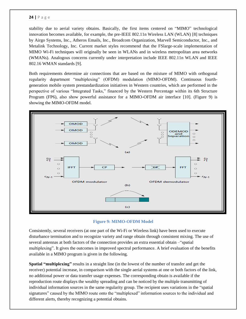
24 | P a g e
stability due to aerial variety obtains. Basically, the first items centered on ―MIMO‖ technological
innovation becomes available, for example, the pre-IEEE 802.11n Wireless LAN (WLAN) [8] techniques
by Airgo Systems, Inc., Atheros Emails, Inc., Broadcom Organization, Marvell Semiconductor, Inc., and
Metalink Technology, Inc. Current market styles recommend that the FSlarge-scale implementation of
MIMO Wi-Fi techniques will originally be seen in WLANs and in wireless metropolitan area networks
(WMANs). Analogous concerns currently under interpretation include IEEE 802.11n WLAN and IEEE
802.16 WMAN standards [9].
Both requirements determine air connections that are based on the mixture of MIMO with orthogonal
regularity department ―multiplexing‖ (OFDM) modulation (MIMO-OFDM). Continuous fourth-
generation mobile system prestandardization initiatives in Western countries, which are performed in the
perspective of various ―Integrated Tasks,‖ financed by the Western Percentage within its 6th Structure
Program (FP6), also show powerful assistance for a MIMO-OFDM air interface [10]. (Figure 9) is
showing the MIMO-OFDM model.
Figure 9: MIMO-OFDM Model
Consistently, several receivers (at one part of the Wi-Fi or Wireless link) have been used to execute
disturbance termination and to recognize variety and range obtain through consistent mixing. The use of
several antennas at both factors of the connection provides an extra essential obtain –―spatial
multiplexing‖. It gives the outcomes in improved spectral performance. A brief evaluation of the benefits
available in a MIMO program is given in the following.
Spatial “multiplexing” results in a straight line (in the lowest of the number of transfer and get the
receiver) potential increase, in comparison with the single aerial systems at one or both factors of the link,
no additional power or data transfer usage expenses. The corresponding obtain is available if the
reproduction route displays the wealthy spreading and can be noticed by the multiple transmitting of
individual information sources in the same regularity group. The recipient uses variations in the ―spatial
signatures‖ caused by the MIMO route onto the ―multiplexed‖ information sources to the individual and
different alerts, thereby recognizing a potential obtains.

25 | P a g e
Diversity results in enhanced link stability by making the route ―less fading‖. It also develops the
sturdiness to co-channel disturbance. The diversity is acquired by transferring the data indication over
several (ideally) individually diminishing measurements soon enough, regularity, and the area. It also can
do proper mixing in the recipient. Spatial (i.e., antenna) diversity is particularly eye-catching in
comparison to an era and regularity variety, because it does not have expenses in transmitting time or data
transfer usage, respectively. Space-time programming understands this approach in schemes and provides
several transfer antennas without demanding route knowledge of the transmitter.
Array gain can be noticed both at the transmitter and the recipient. It needs route information of
consistent mixing and results in a rise in regular get ―signal-to-noise ratio‖ [11] and therefore enhanced
protection. Several antennas at one or both factors of the Wi-Fi or wireless connection can be used to
terminate or decrease co-channel disturbance, and hence enhance mobile system potential. [11]

26 | P a g e
4.5 Components of MIMO-OFDM System In the MIMO-OFDM system, we can find three major components. Those are Transmitter, Receiver and
Fading channel.
The Transmitter: A real-time image produces the information. The transmitter finishes the prevention of
sensibility when ―Forward Error Correction ―(FEC) is used. The dimension the generated data relies on
the size of a block. The intonation patterns used to design the bits to signs is ―64-QAM‖. The produced
information is approved on to the next level, either to the blocks of FEC or straight to the symbol-
mapping, if the FEC is not present.
The Receiver: Depending upon the program for MIMO-OFDM components, there are two aerials for
MISO i.e. multiple input and single output. The OFDM component has one receive aerial. The first
process conducts at the recipient (in reproduction) is elimination of periodic affix. This removes the ISI
also. The information is then approved through the serial to similar ripper of dimension 512.Thenit
approved to the FFT for regularity sector modification.
The Fading Channel: It is one type of mathematical design which inseminates the surroundings of stereo
indication. According to the scale of an indication, which passes the interaction route and alters
arbitrarily, is known as the fading channel. It performs as an affordable design which spreads the stereo
signal before coming at the recipient. When there is no circulation prominent during the range of vision
between transmitter and recipient, the Fading Channel is the best and appropriate approach.
27 | P a g e
Chapter 5
5 Implementation of ANFIS
5.1 ANFIS System
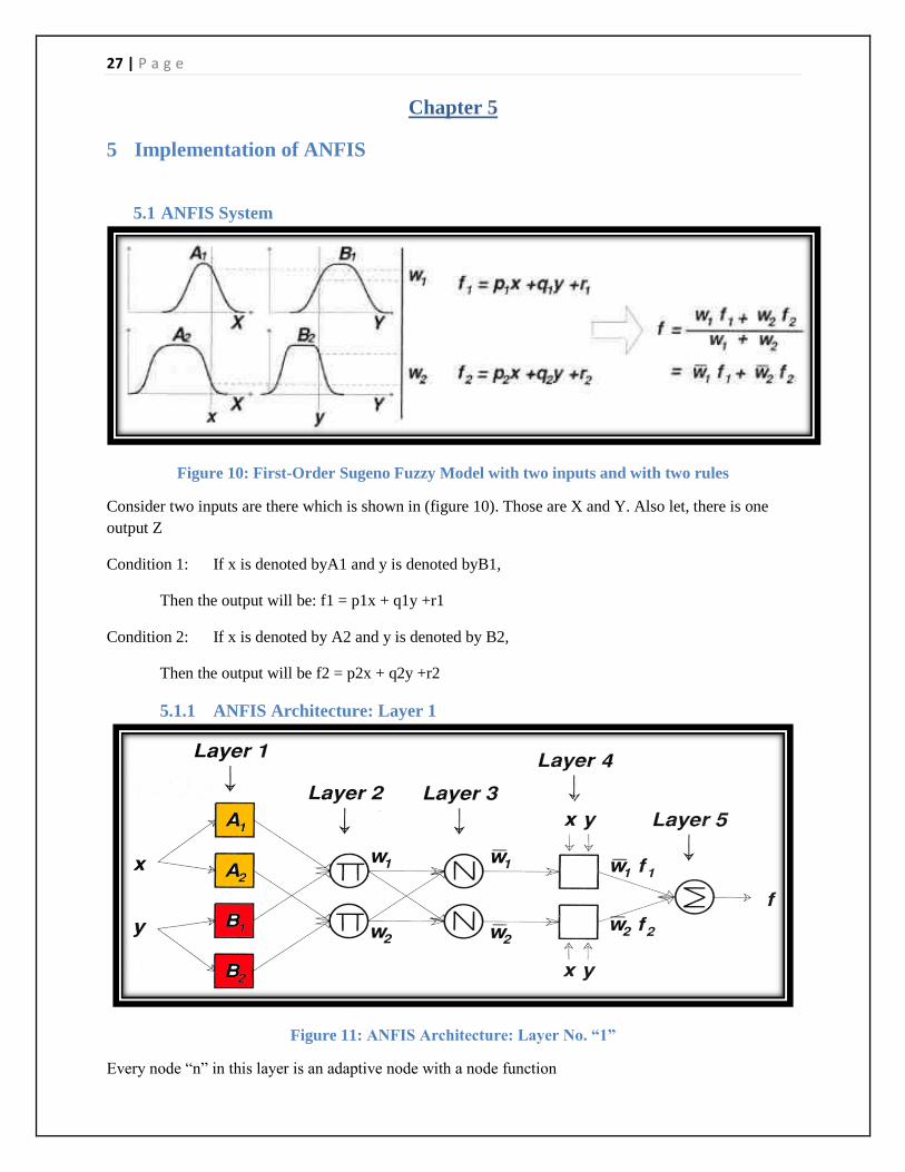
Figure 10: First-Order Sugeno Fuzzy Model with two inputs and with two rules
Consider two inputs are there which is shown in (figure 10). Those are X and Y. Also let, there is one
output Z
Condition 1: If x is denoted byA1 and y is denoted byB1,
Then the output will be: f1 = p1x + q1y +r1
Condition 2: If x is denoted by A2 and y is denoted by B2,
Then the output will be f2 = p2x + q2y +r2
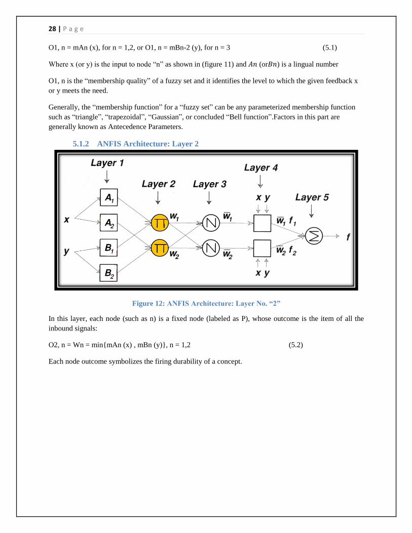
5.1.1 ANFIS Architecture: Layer 1
Figure 11: ANFIS Architecture: Layer No. “1”
Every node ―n‖ in this layer is an adaptive node with a node function
28 | P a g e
O1, n = mAn (x), for n = 1,2, or O1, n = mBn-2 (y), for n = 3 (5.1)
Where x (or y) is the input to node ―n‖ as shown in (figure 11) and 𝐴𝑛 (or𝐵𝑛) is a lingual number
O1, n is the ―membership quality‖ of a fuzzy set and it identifies the level to which the given feedback x
or y meets the need.
Generally, the ―membership function‖ for a ―fuzzy set‖ can be any parameterized membership function
such as ―triangle‖, ―trapezoidal‖, ―Gaussian‖, or concluded ―Bell function‖.Factors in this part are
generally known as Antecedence Parameters.
5.1.2 ANFIS Architecture: Layer 2
Figure 12: ANFIS Architecture: Layer No. “2”
In this layer, each node (such as n) is a fixed node (labeled as P), whose outcome is the item of all the
inbound signals:
O2, n = Wn = min{mAn (x) , mBn (y)}, n = 1,2 (5.2)
Each node outcome symbolizes the firing durability of a concept.
29 | P a g e
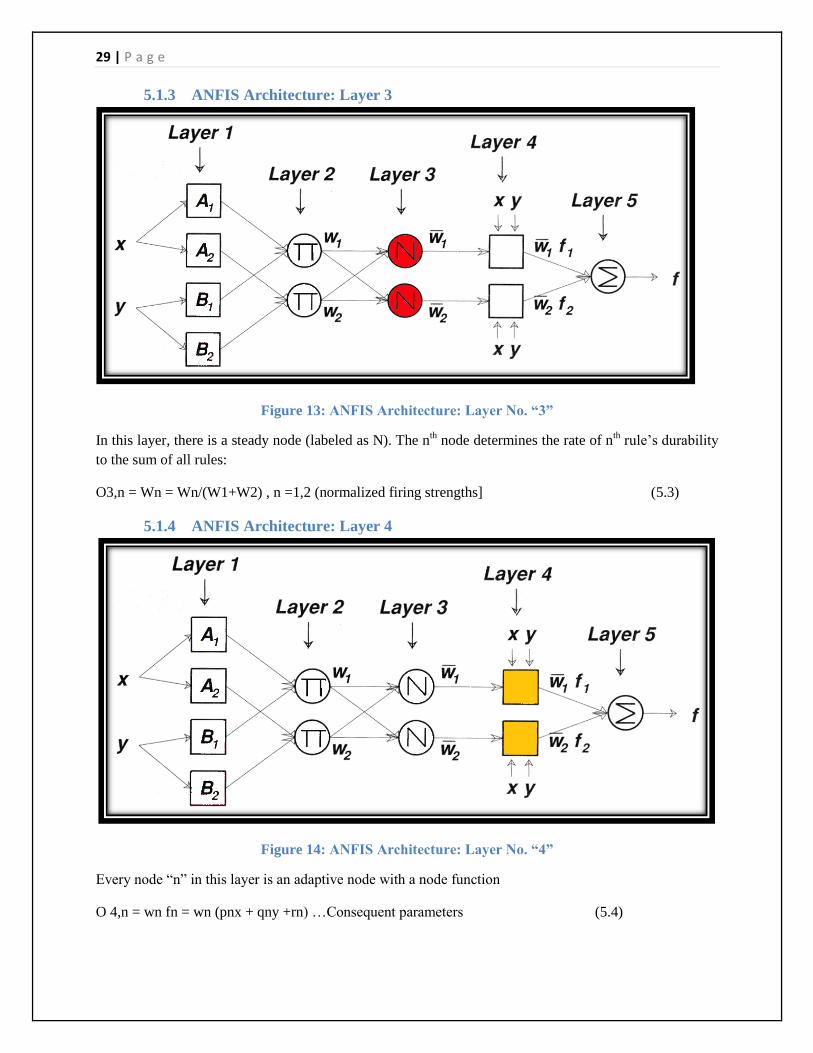
5.1.3 ANFIS Architecture: Layer 3
Figure 13: ANFIS Architecture: Layer No. “3”
In this layer, there is a steady node (labeled as N). The nth node determines the rate of n
th rule‘s durability
to the sum of all rules:
O3,n = Wn = Wn/(W1+W2) , n =1,2 (normalized firing strengths] (5.3)
5.1.4 ANFIS Architecture: Layer 4
Figure 14: ANFIS Architecture: Layer No. “4”
Every node ―n‖ in this layer is an adaptive node with a node function
O 4,n = wn fn = wn (pnx + qny +rn) …Consequent parameters (5.4)

30 | P a g e
5.1.5 ANFIS Architecture: Layer 5
Figure 15: ANFIS Architecture: Layer No. “5”
An individual node in this part is a set node (marked as S), which determines the overall outcome as the
summary of all inbound signals:
O 5,1 = Sn wn fn (5.5)
5.1.6 Alternate ANFIS Architecture
Figure 16: Alternate ANFIS Architecture.
In the Sugeno fuzzy ANFIS architecture model, weight normalization is performed at the very last layer.
31 | P a g e
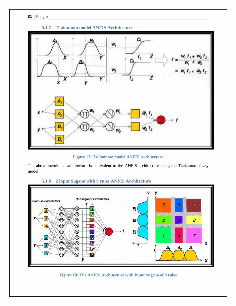
5.1.7 Tsukamoto model ANFIS Architecture
Figure 17: Tsukamoto model ANFIS Architecture
The above-mentioned architecture is equivalent to the ANFIS architecture using the Tsukamoto fuzzy
model.
5.1.8 2 input Sugeno with 9 rules ANFIS Architecture
Figure 18: The ANFIS Architecture with Input Sugeno of 9 rules
32 | P a g e
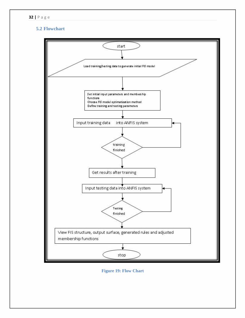
5.2 Flowchart
Figure 19: Flow Chart
33 | P a g e
5. 3 Description of the algorithms used
ANFIS is a main workout algorithm for the Fuzzy Inference System, which is actually a type of Sugeno.
ANFIS uses a multiple learning criteria to classify the factors of FIS, which is a type of Sugeno. It
handles a consolidation of the ―least-squares' technique‖ and the back propagation gradient, the descent
method for preparing FIS membership function factors to replicate a given coaching information set.
ANFIS can also conjure an optionally available discussion for design approval. The kind of design
approval that occurs with this option is a verifying for design over fitting, and the discussion is an
information set called the verifying information set.
5.4 System Model
In Our thesis we have taken two different fading environments
1. Propagation environment without path loss shown in (Figure 20)
2. Propagation environment with path loss shown in (figure 21)
5.4.1. Propagation environment without path loss
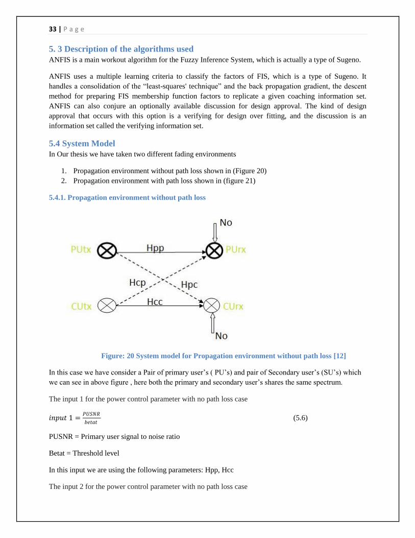
Figure: 20 System model for Propagation environment without path loss [12]
In this case we have consider a Pair of primary user‘s ( PU‘s) and pair of Secondary user‘s (SU‘s) which
we can see in above figure , here both the primary and secondary user‘s shares the same spectrum.
The input 1 for the power control parameter with no path loss case
𝑖𝑛𝑝𝑢𝑡 1 =𝑃𝑈𝑆𝑁𝑅
𝑏𝑒𝑡𝑎𝑡 (5.6)
PUSNR = Primary user signal to noise ratio
Betat = Threshold level
In this input we are using the following parameters: Hpp, Hcc
The input 2 for the power control parameter with no path loss case
34 | P a g e
𝑖𝑛𝑝𝑢𝑡 2 =𝐻𝑐𝑝
𝐻𝑐𝑝𝑚𝑎𝑥 (5.7)
𝐻𝑐𝑝 = 𝑃𝑟𝑖𝑚𝑎𝑟𝑦 𝑢𝑠𝑟𝑒 ′𝑠 𝑖𝑛𝑡𝑒𝑟𝑓𝑒𝑟𝑎𝑛𝑐𝑒 𝑡𝑜 𝑐𝑎𝑛𝑛𝑒𝑙 𝑔𝑎𝑖𝑛
𝐻𝑐𝑝𝑚𝑎𝑥 = 𝑖𝑡′𝑠 𝑚𝑎𝑥𝑖𝑚𝑢𝑚 𝑣𝑎𝑙𝑢𝑒
In this input we are using the following parameters: Hcp, Hpc
The primary user‘s Signal to Noise ratio without cognitive user is given by
𝑆𝑁𝑅 = 𝛼 =𝑃𝑝 𝐺𝑝𝑝
𝑁0 (5.8)
𝑃𝑝- is the power transmitted by the primary transmitter.
𝐺𝑝𝑝 - is the channel gain between the primary transmitter and primary receiver showed by dark link
between them.
The primary user‘s Signal to interference noise ratio with the presence of cognitive user is given by
𝑆𝑁𝐼𝑅 = 𝛽(𝑘) =𝑃𝑝 𝐺𝑝𝑝
𝑘 .𝑃𝑐𝑚𝑎𝑥 𝐺𝑐𝑝 + 𝑁0 (5.9)
𝐺𝑐𝑝 - is the interference channel gain between the primary transmitter and secondary receiver showed by
the dotted link between them.
𝑃𝑐𝑚𝑎𝑥 - is the peak power transmitted by the cognitive user.
𝑘- is the instantaneous power control parameter.
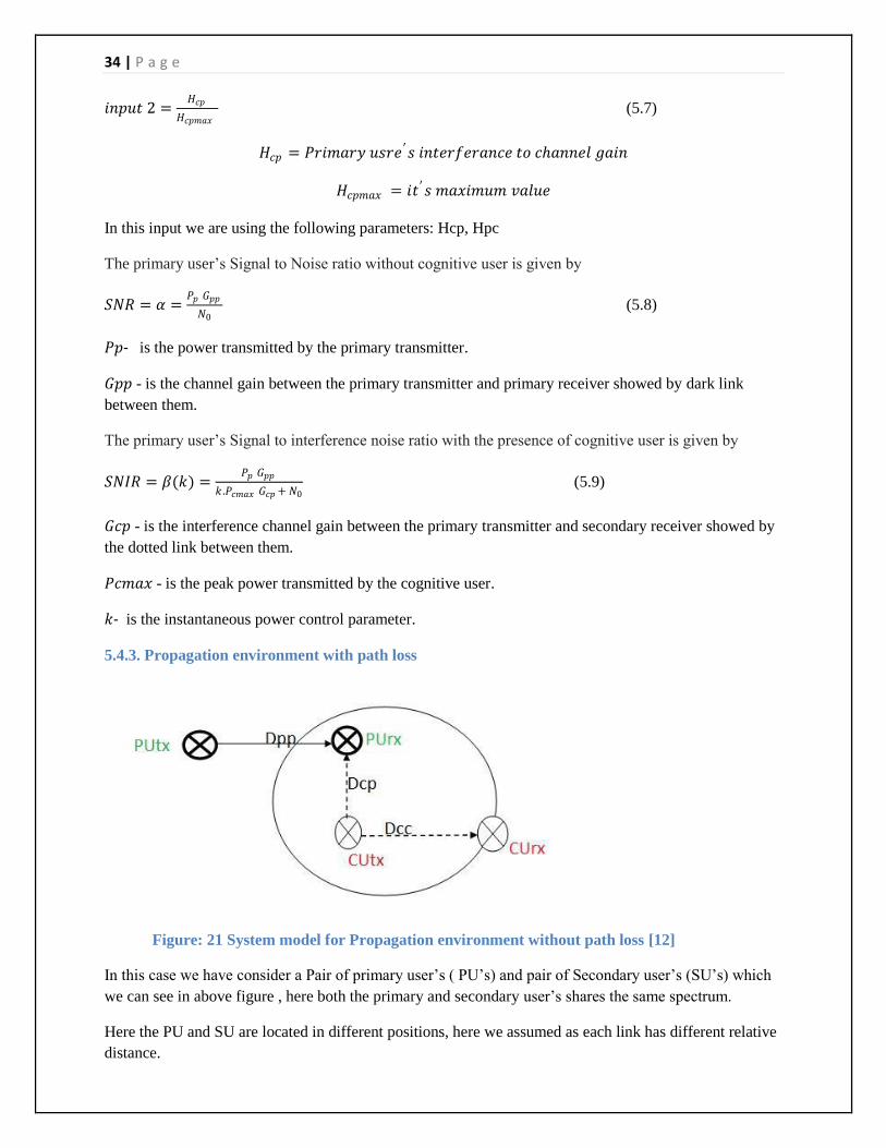
5.4.3. Propagation environment with path loss
Figure: 21 System model for Propagation environment without path loss [12]
In this case we have consider a Pair of primary user‘s ( PU‘s) and pair of Secondary user‘s (SU‘s) which
we can see in above figure , here both the primary and secondary user‘s shares the same spectrum.
Here the PU and SU are located in different positions, here we assumed as each link has different relative
distance.

35 | P a g e
The input 1 for the power control parameter with path loss case
𝑖𝑛𝑝𝑢𝑡 1 =𝑃𝑈𝑆𝑁𝑅
𝑏𝑒𝑡𝑎𝑡 (5.10)
The input 2 for the power control parameter with path loss case
𝑖𝑛𝑝𝑢𝑡 2 =𝑑𝑐𝑝
𝐿𝑐𝑝 (5.11)
𝑑𝑐𝑝 - is the distance between the secondary transmitter and primary receiver.
𝐿c𝑝 is the maximum effective distance.
36 | P a g e
Chapter 6
6 Results
6.1 Case 1: Without Path loss
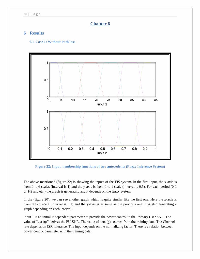
Figure 22: Input membership functions of two antecedents (Fuzzy Inference System)
The above-mentioned (figure 22) is showing the inputs of the FIS system. In the first input, the x-axis is
from 0 to 6 scales (interval is 1) and the y-axis is from 0 to 1 scale (interval is 0.5). For each period (0-1
or 1-2 and etc.) the graph is generating and it depends on the fuzzy system.
In the (figure 20), we can see another graph which is quite similar like the first one. Here the x-axis is
from 0 to 1 scale (interval is 0.1) and the y-axis is as same as the previous one. It is also generating a
graph depending on each interval.
Input 1 is an initial Independent parameter to provide the power control to the Primary User SNR. The
value of ―eta (ŋ)‖ derives the PU-SNR. The value of ―eta (ŋ)‖ comes from the training data. The Channel
rate depends on ISR tolerance. The input depends on the normalizing factor. There is a relation between
power control parameter with the training data.
0 5 10 15 20 25 30 35 40 450
0.5
1
input 1
0 0.1 0.2 0.3 0.4 0.5 0.6 0.7 0.8 0.9 10
0.5
1
input 2
37 | P a g e
Input 2 is used to gain the channel from Primary User. Input 2 decides the consumption of power, which
can be used by the user. Cognitive user will use the power. Input 2 takes the random value, but the value
should between 0 and 1.
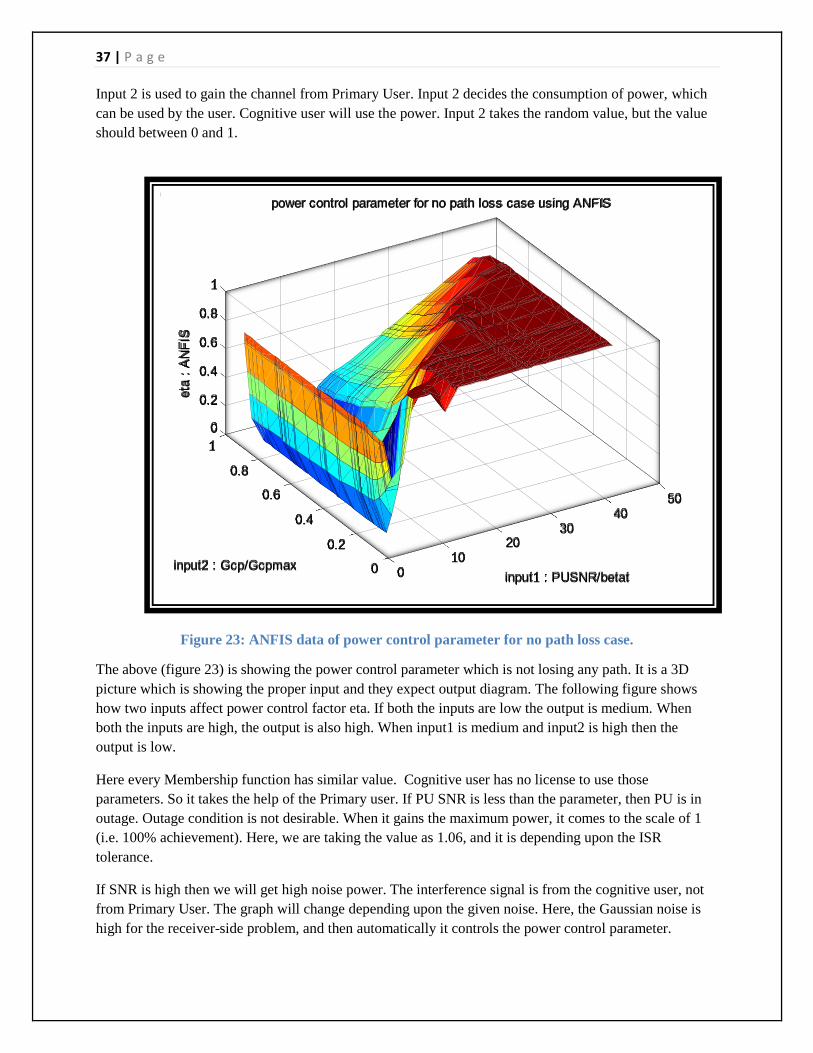
Figure 23: ANFIS data of power control parameter for no path loss case.
The above (figure 23) is showing the power control parameter which is not losing any path. It is a 3D
picture which is showing the proper input and they expect output diagram. The following figure shows
how two inputs affect power control factor eta. If both the inputs are low the output is medium. When
both the inputs are high, the output is also high. When input1 is medium and input2 is high then the
output is low.
Here every Membership function has similar value. Cognitive user has no license to use those
parameters. So it takes the help of the Primary user. If PU SNR is less than the parameter, then PU is in
outage. Outage condition is not desirable. When it gains the maximum power, it comes to the scale of 1
(i.e. 100% achievement). Here, we are taking the value as 1.06, and it is depending upon the ISR
tolerance.
If SNR is high then we will get high noise power. The interference signal is from the cognitive user, not
from Primary User. The graph will change depending upon the given noise. Here, the Gaussian noise is
high for the receiver-side problem, and then automatically it controls the power control parameter.
010
2030
4050
0
0.2
0.4
0.6
0.8
1
0
0.2
0.4
0.6
0.8
1
input1 : PUSNR/betat
power control parameter for no path loss case using ANFIS
input2 : Gcp/Gcpmax
eta
: A
NF
IS
38 | P a g e
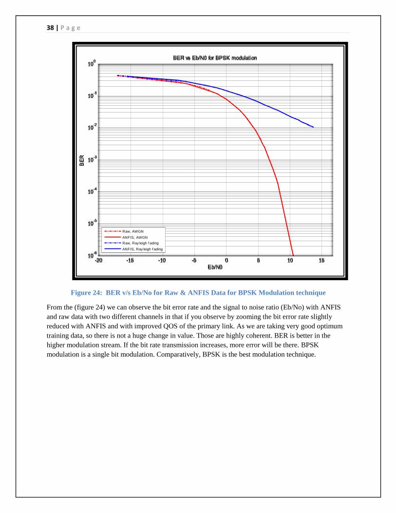
Figure 24: BER v/s Eb/No for Raw & ANFIS Data for BPSK Modulation technique
From the (figure 24) we can observe the bit error rate and the signal to noise ratio (Eb/No) with ANFIS
and raw data with two different channels in that if you observe by zooming the bit error rate slightly
reduced with ANFIS and with improved QOS of the primary link. As we are taking very good optimum
training data, so there is not a huge change in value. Those are highly coherent. BER is better in the
higher modulation stream. If the bit rate transmission increases, more error will be there. BPSK
modulation is a single bit modulation. Comparatively, BPSK is the best modulation technique.
-20 -15 -10 -5 0 5 10 1510
-6
10-5
10-4
10-3
10-2
10-1
100
Eb/N0
BE
R
BER vs Eb/N0 for BPSK modulation
Raw, AWGN
ANFIS, AWGN
Raw, Ray leigh f ading
ANFIS, Ray leigh f ading
39 | P a g e
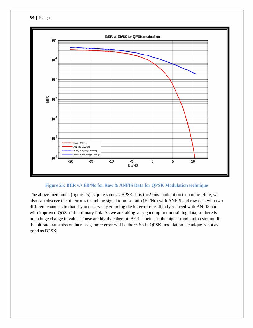
Figure 25: BER v/s EB/No for Raw & ANFIS Data for QPSK Modulation technique
The above-mentioned (figure 25) is quite same as BPSK. It is the2-bits modulation technique. Here, we
also can observe the bit error rate and the signal to noise ratio (Eb/No) with ANFIS and raw data with two
different channels in that if you observe by zooming the bit error rate slightly reduced with ANFIS and
with improved QOS of the primary link. As we are taking very good optimum training data, so there is
not a huge change in value. Those are highly coherent. BER is better in the higher modulation stream. If
the bit rate transmission increases, more error will be there. So in QPSK modulation technique is not as
good as BPSK.
-20 -15 -10 -5 0 5 1010
-6
10-5
10-4
10-3
10-2
10-1
100
Eb/N0
BE
R
BER vs Eb/N0 for QPSK modulation
Raw, AWGN
ANFIS, AWGN
Raw, Ray leigh f ading
ANFIS, Ray leigh f ading

40 | P a g e
Figure 26: BER v/s Eb/No for Raw & ANFIS Data for 16 PSK Modulation Technique.
The above-mentioned (figure 26) is showing the bit error rate and the signal to the noise ratio (Eb/No)
with ANFIS and raw data with two different channels. IN 16-PSK Modulation technique is a less quality
technique. As here bit rate is higher than previous modulations, so it is more error prone.
Figure 27: Channel Capacity as a function of ISR tolerance
-25 -20 -15 -10 -5 0 510
-6
10-5
10-4
10-3
10-2
10-1
100
Eb/N0
BE
R
BER vs Eb/N0 for 16PSK modulation
Raw, AWGN
ANFIS, AWGN
Raw, Ray leigh f ading
ANFIS, Ray leigh f ading
-25 -20 -15 -10 -5 0 50.2
0.4
0.6
0.8
1
1.2
1.4
1.6
1.8
2
ISR tolerance : dB
Cha
nnel
Cap
acity
: b
ps/H
z
IID model Channel Capacity vs ISRtol for Average ISR constraint
41 | P a g e
The above-mentioned (figure 27) is showing the Channel capacity of ISR tolerance. In this graph, the x-
axis shows the ISR tolerance in dB (decibel) and the y-axis shows the Channel capacity in bps/Hz (bit per
second/hertz). For each period it puts a point on the graph and finally it represents a curve graph. This
graph shows the actual tolerance level of ISR over a capacity of a channel.
This graph is implementing from inference theory. It depends on the IID model. The channel is in the
independent-distributed manner. The Channel capacity computes probability functions, and errors. Low
ISR tolerance means lower channel capacity. The higher ISR tolerance will show the higher channel
capacity. The interference signal ratio should increase to meet the better tolerance. If we can meet the
better tolerance, then we can achieve higher channel capacity. It is an Exponential calculation, but there is
a theoretical limit.
6.2 Case 2: With the path loss
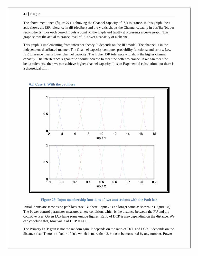
Figure 28: Input membership functions of two antecedents with the Path loss
Initial inputs are same as no path loss case. But here, Input 2 is no longer same as shown in (Figure 28).
The Power control parameter measures a new condition, which is the distance between the PU and the
cognitive user. Given LCP have some unique figures. Ratio of DCP is also depending on the distance. We
can conclude that, Max value of DCP = LCP.
The Primary DCP gain is not the random gain. It depends on the ratio of DCP and LCP. It depends on the
distance also. There is a factor of ―n‖, which is more than 2, but can be measured by any number. Power
2 4 6 8 10 12 14 16 180
0.5
1
input 1
0.1 0.2 0.3 0.4 0.5 0.6 0.7 0.8 0.90
0.5
1
input 2
42 | P a g e
will change the square of the distance. When ―n‖ is high; the power level will fall drastically. So the value
of ―n‖ must be around 2 to 3. DCP gain depends on actual DCP and the distance.
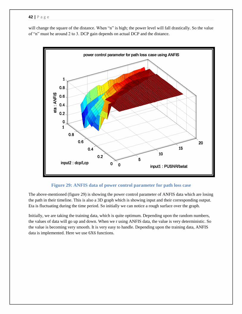
Figure 29: ANFIS data of power control parameter for path loss case
The above-mentioned (figure 29) is showing the power control parameter of ANFIS data which are losing
the path in their timeline. This is also a 3D graph which is showing input and their corresponding output.
Eta is fluctuating during the time period. So initially we can notice a rough surface over the graph.
Initially, we are taking the training data, which is quite optimum. Depending upon the random numbers,
the values of data will go up and down. When we r using ANFIS data, the value is very deterministic. So
the value is becoming very smooth. It is very easy to handle. Depending upon the training data, ANFIS
data is implemented. Here we use 6X6 functions.
0
5
10
15
20
0
0.2
0.4
0.6
0.8
1
0
0.2
0.4
0.6
0.8
1
input1 : PUSNR/betat
power control parameter for path loss case using ANFIS
input2 : dcp/Lcp
eta
: A
NF
IS
43 | P a g e
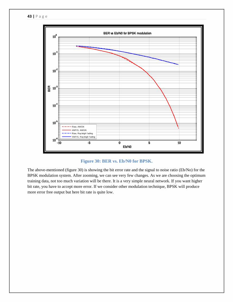
Figure 30: BER vs. Eb/N0 for BPSK.
The above-mentioned (figure 30) is showing the bit error rate and the signal to noise ratio (Eb/No) for the
BPSK modulation system. After zooming, we can see very few changes. As we are choosing the optimum
training data, not too much variation will be there. It is a very simple neural network. If you want higher
bit rate, you have to accept more error. If we consider other modulation technique, BPSK will produce
more error free output but here bit rate is quite low.
-10 -5 0 5 1010
-6
10-5
10-4
10-3
10-2
10-1
100
Eb/N0
BE
R
BER vs Eb/N0 for BPSK modulation
Raw, AWGN
ANFIS, AWGN
Raw, Ray leigh f ading
ANFIS, Ray leigh f ading
44 | P a g e
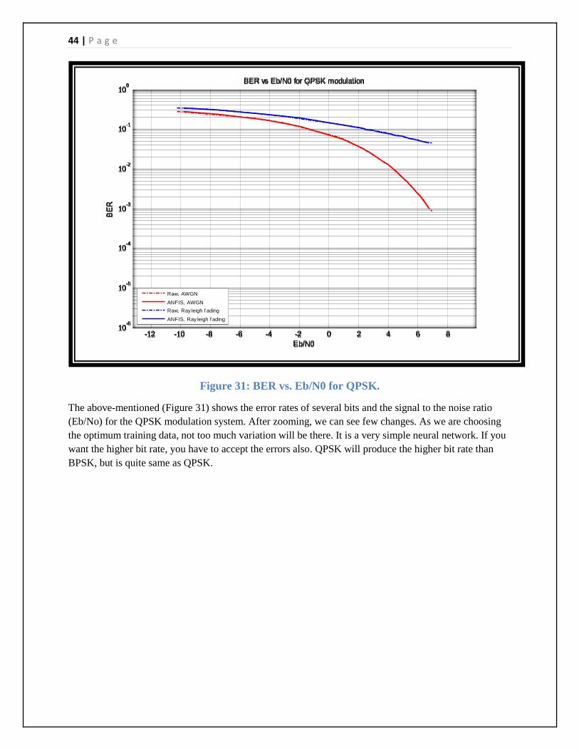
Figure 31: BER vs. Eb/N0 for QPSK.
The above-mentioned (Figure 31) shows the error rates of several bits and the signal to the noise ratio
(Eb/No) for the QPSK modulation system. After zooming, we can see few changes. As we are choosing
the optimum training data, not too much variation will be there. It is a very simple neural network. If you
want the higher bit rate, you have to accept the errors also. QPSK will produce the higher bit rate than
BPSK, but is quite same as QPSK.
-12 -10 -8 -6 -4 -2 0 2 4 6 810
-6
10-5
10-4
10-3
10-2
10-1
100
Eb/N0
BE
R
BER vs Eb/N0 for QPSK modulation
Raw, AWGN
ANFIS, AWGN
Raw, Ray leigh f ading
ANFIS, Ray leigh f ading
45 | P a g e
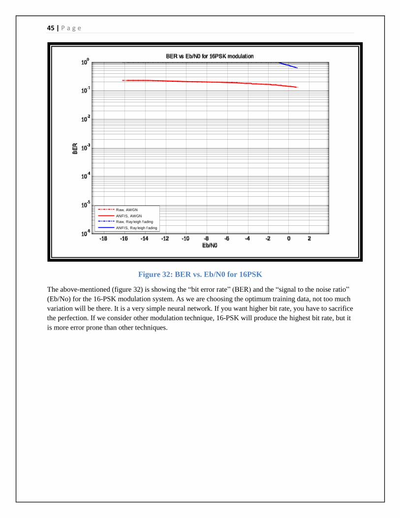
Figure 32: BER vs. Eb/N0 for 16PSK
The above-mentioned (figure 32) is showing the ―bit error rate‖ (BER) and the ―signal to the noise ratio‖
(Eb/No) for the 16-PSK modulation system. As we are choosing the optimum training data, not too much
variation will be there. It is a very simple neural network. If you want higher bit rate, you have to sacrifice
the perfection. If we consider other modulation technique, 16-PSK will produce the highest bit rate, but it
is more error prone than other techniques.
-18 -16 -14 -12 -10 -8 -6 -4 -2 0 210
-6
10-5
10-4
10-3
10-2
10-1
100
Eb/N0
BE
R
BER vs Eb/N0 for 16PSK modulation
Raw, AWGN
ANFIS, AWGN
Raw, Ray leigh f ading
ANFIS, Ray leigh f ading
46 | P a g e
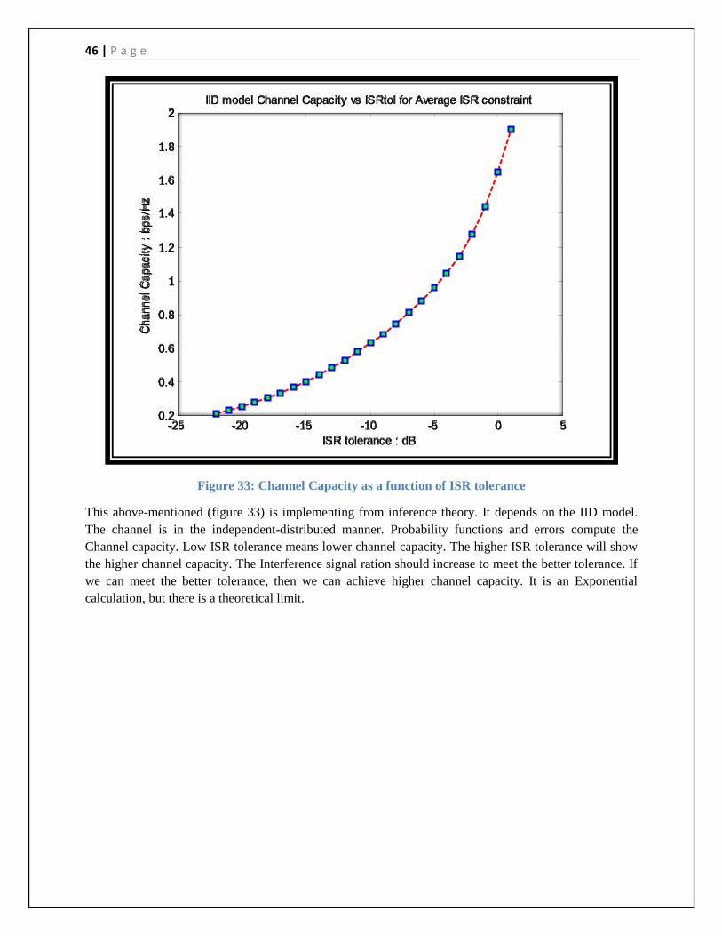
Figure 33: Channel Capacity as a function of ISR tolerance
This above-mentioned (figure 33) is implementing from inference theory. It depends on the IID model.
The channel is in the independent-distributed manner. Probability functions and errors compute the
Channel capacity. Low ISR tolerance means lower channel capacity. The higher ISR tolerance will show
the higher channel capacity. The Interference signal ration should increase to meet the better tolerance. If
we can meet the better tolerance, then we can achieve higher channel capacity. It is an Exponential
calculation, but there is a theoretical limit.
-25 -20 -15 -10 -5 0 50.2
0.4
0.6
0.8
1
1.2
1.4
1.6
1.8
2
ISR tolerance : dB
Channel C
apacity :
bps/H
z
IID model Channel Capacity vs ISRtol for Average ISR constraint

47 | P a g e
Chapter 7
7 Implementation MIMO-OFDM
7.1 MIMO-OFDM System
First, the data is converted to parallel and planned into complicated information prevents by using
several modulation proposals like BPSK, QPSK and 8-PSK. The unused frequency bands are
padded with zeros.
Then IFFT (Inverse Fast Fourier Transform) is implemented to produce the time edition of the
passing signal. The time domain signals are orthogonal to each other, therefore can cause
frequency spectrums to overlap.
The Pilot bits are added to ensure correction of phase noise and frequency offset because the
stage disturbance elements spread the power of an indication to nearby frequencies, which can
cause noise inside bands.
The copy of 25% of transmitter symbol is inserted in the beginning of the transmitted signal. It is
used at receiver to synchronize during demodulation of the received signal. ISI i.e. ―Inter Symbol
Interference‖ and ICI i.e. ―Inter Carrier Interference‖ are two primary concerns for the
transmission therefore cyclic prefix is also used to reduce these obstructions.
A standard MIMO channel is assumed. 1x1 & 2x2 MIMO schemes are analysed.
The full form of OFDM is ―Orthogonal Frequency Division Multiplexing‖. It is a ―multi-channel
intonation technique‖ which creates use of Frequency Division Multiplexing (FDM) being modulated by
a low bit amount electronic flow. The primary purpose of using OFDM is because here the icon
recognition is simple and also to improve the sturdiness against frequency particular diminishing and
filter group disturbance. Certain parameter like CFO (carrier frequency offset), I/Q discrepancy (in-phase
and quadrature stage imbalance) discrepancy causes distortions in the obtained indication. Here
evaluation is created for given factors using different programs and a technique is suggested for Multiple
Input Multiple output (MIMO) OFDM program when the icon produced is not an important multiple of
the variety of transmitters used.
7.1. Testing and Results with Snapshots
In MIMO-OFDM system, we are considering two techniques. One is 1X1 technique and another is 2X2.
We will find the snapshots of several test results which will explain the suggested project. The snapshots
are as follows:
48 | P a g e
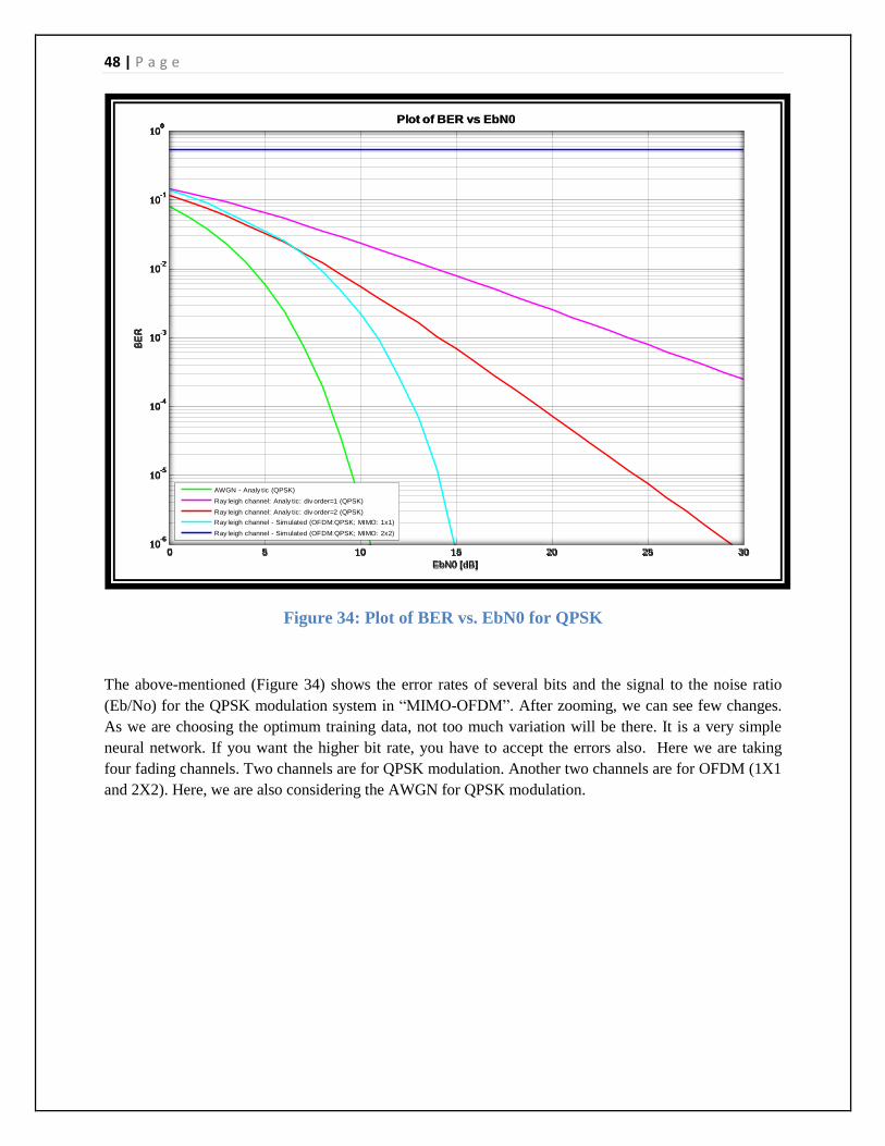
Figure 34: Plot of BER vs. EbN0 for QPSK
The above-mentioned (Figure 34) shows the error rates of several bits and the signal to the noise ratio
(Eb/No) for the QPSK modulation system in ―MIMO-OFDM‖. After zooming, we can see few changes.
As we are choosing the optimum training data, not too much variation will be there. It is a very simple
neural network. If you want the higher bit rate, you have to accept the errors also. Here we are taking
four fading channels. Two channels are for QPSK modulation. Another two channels are for OFDM (1X1
and 2X2). Here, we are also considering the AWGN for QPSK modulation.
0 5 10 15 20 25 3010
-6
10-5
10-4
10-3
10-2
10-1
100
EbN0 [dB]
BE
R
Plot of BER vs EbN0
AWGN - Analy tic (QPSK)
Ray leigh channel: Analy tic: div order=1 (QPSK)
Ray leigh channel: Analy tic: div order=2 (QPSK)
Ray leigh channel - Simulated (OFDM:QPSK; MIMO: 1x1)
Ray leigh channel - Simulated (OFDM:QPSK; MIMO: 2x2)
49 | P a g e
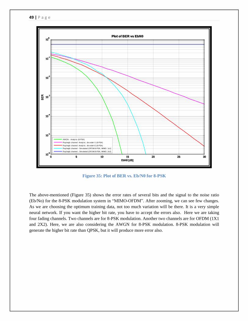
Figure 35: Plot of BER vs. Eb/N0 for 8-PSK
The above-mentioned (Figure 35) shows the error rates of several bits and the signal to the noise ratio
(Eb/No) for the 8-PSK modulation system in ―MIMO-OFDM‖. After zooming, we can see few changes.
As we are choosing the optimum training data, not too much variation will be there. It is a very simple
neural network. If you want the higher bit rate, you have to accept the errors also. Here we are taking
four fading channels. Two channels are for 8-PSK modulation. Another two channels are for OFDM (1X1
and 2X2). Here, we are also considering the AWGN for 8-PSK modulation. 8-PSK modulation will
generate the higher bit rate than QPSK, but it will produce more error also.
0 5 10 15 20 25 3010
-6
10-5
10-4
10-3
10-2
10-1
100
EbN0 [dB]
BE
R
Plot of BER vs EbN0
AWGN - Analy tic (8-PSK)
Ray leigh channel: Analy tic: div order=1 (8-PSK)
Ray leigh channel: Analy tic: div order=2 (8-PSK)
Ray leigh channel - Simulated (OFDM:8-PSK; MIMO: 1x1)
Ray leigh channel - Simulated (OFDM:8-PSK; MIMO: 2x2)
50 | P a g e
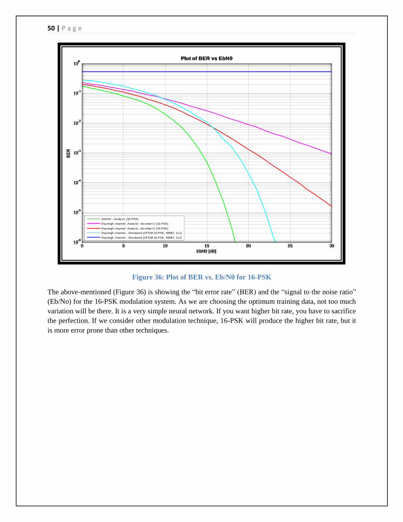
Figure 36: Plot of BER vs. Eb/N0 for 16-PSK
The above-mentioned (Figure 36) is showing the ―bit error rate‖ (BER) and the ―signal to the noise ratio‖
(Eb/No) for the 16-PSK modulation system. As we are choosing the optimum training data, not too much
variation will be there. It is a very simple neural network. If you want higher bit rate, you have to sacrifice
the perfection. If we consider other modulation technique, 16-PSK will produce the higher bit rate, but it
is more error prone than other techniques.
0 5 10 15 20 25 3010
-6
10-5
10-4
10-3
10-2
10-1
100
EbN0 [dB]
BE
R
Plot of BER vs EbN0
AWGN - Analy tic (16-PSK)
Ray leigh channel: Analy tic: div order=1 (16-PSK)
Ray leigh channel: Analy tic: div order=2 (16-PSK)
Ray leigh channel - Simulated (OFDM:16-PSK; MIMO: 1x1)
Ray leigh channel - Simulated (OFDM:16-PSK; MIMO: 2x2)
51 | P a g e
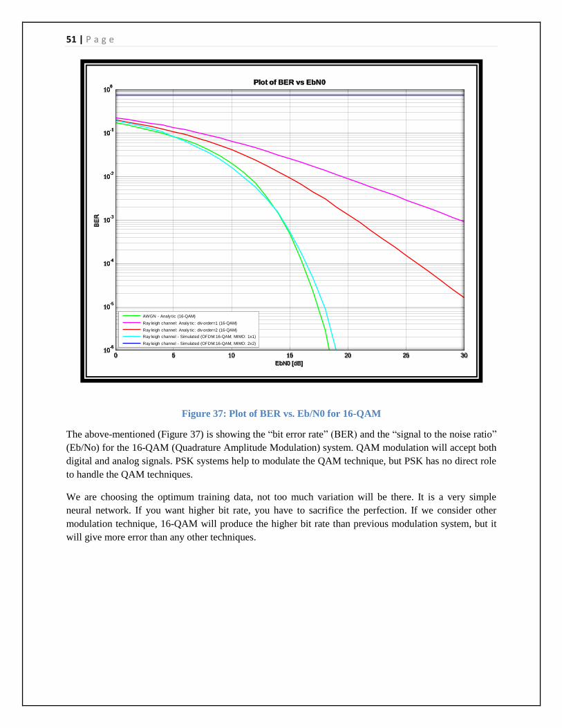
Figure 37: Plot of BER vs. Eb/N0 for 16-QAM
The above-mentioned (Figure 37) is showing the ―bit error rate‖ (BER) and the ―signal to the noise ratio‖
(Eb/No) for the 16-QAM (Quadrature Amplitude Modulation) system. QAM modulation will accept both
digital and analog signals. PSK systems help to modulate the QAM technique, but PSK has no direct role
to handle the QAM techniques.
We are choosing the optimum training data, not too much variation will be there. It is a very simple
neural network. If you want higher bit rate, you have to sacrifice the perfection. If we consider other
modulation technique, 16-QAM will produce the higher bit rate than previous modulation system, but it
will give more error than any other techniques.
0 5 10 15 20 25 3010
-6
10-5
10-4
10-3
10-2
10-1
100
EbN0 [dB]
BE
R
Plot of BER vs EbN0
AWGN - Analy tic (16-QAM)
Ray leigh channel: Analy tic: div order=1 (16-QAM)
Ray leigh channel: Analy tic: div order=2 (16-QAM)
Ray leigh channel - Simulated (OFDM:16-QAM; MIMO: 1x1)
Ray leigh channel - Simulated (OFDM:16-QAM; MIMO: 2x2)
52 | P a g e
Figure 38: Plot of BER vs. Eb/N0 for 64-QAM
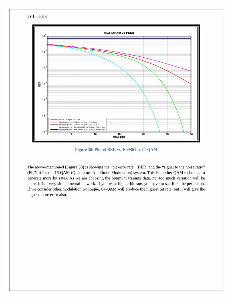
The above-mentioned (Figure 38) is showing the ―bit error rate‖ (BER) and the ―signal to the noise ratio‖
(Eb/No) for the 16-QAM (Quadrature Amplitude Modulation) system. This is another QAM technique to
generate more bit rates. As we are choosing the optimum training data, not too much variation will be
there. It is a very simple neural network. If you want higher bit rate, you have to sacrifice the perfection.
If we consider other modulation technique, 64-QAM will produce the highest bit rate, but it will give the
highest more error also.
0 5 10 15 20 25 3010
-6
10-5
10-4
10-3
10-2
10-1
100
EbN0 [dB]
BE
R
Plot of BER vs EbN0
AWGN - Analy tic (64-QAM)
Ray leigh channel: Analy tic: div order=1 (64-QAM)
Ray leigh channel: Analy tic: div order=2 (64-QAM)
Ray leigh channel - Simulated (OFDM:64-QAM; MIMO: 1x1)
Ray leigh channel - Simulated (OFDM:64-QAM; MIMO: 2x2)

53 | P a g e
Chapter 8
7 Conclusion and Future Work It has been established that implementing ANFIS algorithms can ensure easier control of SU power is
maintaining better BER performance for all scenarios. In second part that implementing MIMO-OFDM
techniques can ensure better BER performance for all scenarios.
In our thesis we have proposed ANFIS based power control strategy in CRN. It is Analyzed and
Validated over different fading environment without and with path loss. We concluded that from results
the proposed ANFIS power control strategy in CRN has better BER performance than without power
control strategy. It has been improved QOS for PU‘s and performance of SU‘s, especially in AWGN
channel environment the BER performance is better than Rayleigh fading channel.
Work can be extended to multiple PU/SU combination and different fading channels using ANFIS.
We also proposed MIMO-OFDM transmission technique in CRN (Cognitive Radio Networks) for its use
in emergency conditions where transmission requires reliability and high data rate. The Results shows
that the BER performance was better than without MIMO-OFDM technique for AWGN Chanel, here
QAM modulation techniques have better results than other modulation techniques.
Work can be extended to 3x3, 4x4, NxN MIMO and with QAM modulation and different MIMO fading
channels
To reduce the complexness for MIMO-OFDM techniques, we will consider the following factors in the
near future:
Less expense loss
Huge variance
Acceleration Appraisal
54 | P a g e
Chapter 9
References
[1] S., B., 2003. ANFIS. s.l.:s.n.
[2] Padinjaremury, J. J., 2013. ANFIS APPLICATION, s.l.: s.n.
[3] Jang, J.-S., 2013. ANFIS: adaptive-network-based fuzzy inference system, California: Dept. of Electr.
Eng. & Comput. Sci., California Univ., Berkeley, CA, USA.
[4] MathWorks, 2013. http://www.mathworks.in. [Online]
Available at: http://www.mathworks.in/help/fuzzy/fuzzy-inference-process.html
[Accessed 6 October 2013].
[5] Koushik, D. S., 2003. Fuzzy Inference (Expert) System. s.l.:s.n.
[6] John, D. B., 2002. Adaptive Network Based Fuzzy Inference Systems (ANFIS), Leicester, UK: De-
Montfort University
[7] Cognitive Radio Technologies, 2012. http://www.crtwireless.com/. [Online]
Available at: http://www.crtwireless.com/
[Accessed 6 September 2013].
[8] BÖLCSKEI, H., 2006. MIMO-OFDM WIRELESS SYSTEMS:BASICS, PERSPECTIVES, AND
CHALLENGES, ZURICH: s.n.
[9] Yang, H., 2005. A road to future broadband wireless access: MIMO-OFDM-Based air interface. IEEE
Communications Magazine, 43(1), pp. 53-60.
[10] Z. S. Lee, ―ANFIS based Power control for Fixed Broadband Wireless access systems,‖ Ph.D.
dissertation, Dept. Comm. Eng., National Central Univ., Taiwan, 2008.
[11]Bilgehan, M., 2010. A comparative study for the concrete compressive strength estimation using
neural network and neuro-fuzzy modeling approaches, s.l.: s.n.
[12] Praneeth Kumar.B, Muneeb.A.G and S.F.Moid. ―Optimized fuzzy based power control strategy in
Cognitive Radio Networks in multi-fading propagation environments, ‖ BTH, Sweden, August 2012.
[13] S.Sirigowri, B. Prabharkara Rao andP. V. Subbaiah, "Performance of DQPSK-OFDM Systems Over
Slowly Nakagami-m Fading Channels," in WCECS, San Francisco, USA, 2007
[14] J. Mitola, ―Cognitive radio—an integrated agent architecture forsoftware-defined radio,‖ Ph.D.
Dissertation, Roy. Inst. Technol., Stockholm, Sweden, May 2000
[15] Jassbi, S.H. J. Alavi, P.J.A. Serra and R.A.Ribeiro,‖ Transformation of a Mamdani FIS to first order
Sugeno FIS‖ in IEEE International Fuzzy Systems Conference, UK, 2007,pp 5-10.
[16] P. Guanming Lin, ―OFDM Simulation in MATLAB,‖ in California Polytechnic State University,
San Luis Obispo, June 2010
[17] S. Haykin, ―Cognitive Radio: Brain-Empowered Wireless Communications,” in IEEE Journa in
Selected Areas in Communications, vol. 23, no. 2, pp. 201-220, Feb., 2005

55 | P a g e
[18]. X. Zhou, J. Ma, Y. Li, Y. H. Kwon, A. C. K, Soong and G. Zhao, ―Probability based transmit power
control for dynamic spectrum access,‖ in 3rd IEEE. Symposium on New Frontiers in Dynamic Spectrum
Access Networks, pp. 1-5, Oct. 2008
[19] H. Cho and J. G. Andrews, ―Upper bound on the Capacity of Cognitive radio without Cooperation,‖
IEEE Trans. on Wireless Commun., vol. 8, no. 9, pp. 4380-4385, Sept. 2009.
[20] H. Ying; Y. Ding, S. Li and S.Shao, ‖ Comparison of necessary conditions for typical Takagi-sugeno
and Mamdani fuzzy systems as universal approximators‖ in IEEE Transactions on systems, Man &
Cybernetics, Part A (systems & Humans), vol. 29, no. 5, pp. 508-14, September .1999.
[21] P. Tahmasebi, A. Hezarkhani. (2010). Application of Adaptive Neuro-Fuzzy Inference system for
Grade Estimation; Case Study, Sarcheshmeh Porphyry Copper Deposit, Kerman, Iran. Aust. J. Basic &
Appl. Sci., [online]. 4(3), pp. 408-420
[22] J. S. R. Jang, C. T. Sun and E. Mizutani, ―Fuzzy inference systems‖ in Neuro fuzzy and soft
computing, New Jersey: Prentice Hall, 1997, ch. 4, pp. 73-92.
[23]. H-S. T. Le and H. D. Ly, ―Opportunistic spectrum access using fuzzy logic for
[24]Cognitive radio networks,‖ IEEE ICCE, June 2008
[25] Dawson & K.R.K, 2013. RESEARCH METHODOLOGY, New Delhi: s.n.
.[26] M. Abdullahi, H. M. A. A.-M. ,. A. H. H. ,. M. H. A. H. ,. B. M., 2008. A Review on Expert
Systems for Concrete Mix Design. ICCBT, A(21), pp. 231-238.
[27] M.C.Nataraja, M. ,., 2006. A FuzzyNeuro Model for Normal Concrete Mix Design, s.l.: s.n.
[28] R. W. Chang, ―Synthesis of band-limited orthogonal signals for multichannel data" BSTJ, pp. 1775-
1797, Dec. 1996.