fuzzy gmm-based confidence measure towards keyword …
TRANSCRIPT
Fuzzy GMM-based Confidence MeasureTowards Keyword Spotting Application
by
Mohamed Kacem Abida
A thesispresented to the University of Waterloo
in fulfilment of thethesis requirement for the degree of
Master of Applied Sciencein
Electrical and Computer Engineering
Waterloo, Ontario, Canada, 2007
c© Mohamed Kacem Abida, 2007

I hereby declare that I am the sole author of this thesis. This is a true copy ofthe thesis, including any required final revisions, as accepted by my examiners.
I understand that my thesis may be made electronically available to the public.
ii

Abstract
The increasing need for more natural human machine interfaces has generated in-tensive research work directed toward designing and implementing natural speechenabled systems. The Spectrum of speech recognition applications ranges from un-derstanding simple commands to getting all the information in the speech signalsuch as words, meaning and emotional state of the user. Because it is very hard toconstrain a speaker when expressing a voice-based request, speech recognition sys-tems have to be able to handle (by filtering out) out of vocabulary words in the usersspeech utterance, and only extract the necessary information (keywords) related tothe application to deal correctly with the user query. In this thesis, we investigatean approach that can be deployed in keyword spotting systems. We propose a con-fidence measure feedback module that provides confidence values to be comparedagainst existing Automatic Speech Recognizer word confidences. The feedbackmodule mainly consists of a soft computing tool-based system using fuzzy Gaus-sian mixture models to identify all English phonemes. Testing has been carried outon the JULIUS system and the preliminary results show that our feedback moduleoutperforms JULIUS confidence measures for both the correct spotted words andthe falsely mapped ones. The results obtained could be refined even further usingother type of confidence measure and the whole system could be used for a NaturalLanguage Understanding based module for speech understanding applications.
iii

Acknowledgments
The author would like to thank his supervisor, Professor Fakhreddine Karray, forhis guidance and support on this research work. The author would also like toacknowledge Dr. Jiping Sun for his advice and assistance. Many thanks are alsodue to my thesis readers Dr. Ramadan El Shatshat and Dr. Kumaraswamy Pon-nambalam for taking the time and assessing my work within a short time frame.Special thanks are due as well for Arash Abgari, Dr. Jin-Myung Won, SameehUllah and Abbas Ahmadi for all the fruitful discussions and feedback. The authoracknowledges Vestec Inc. for providing valuable resources used in this thesis andfor its courtesy to use its labs to carry out some of the reported experiments.
iv

Contents
1 Introduction 1
1.1 Motivation . . . . . . . . . . . . . . . . . . . . . . . . . . . . . . . . 1
1.2 Objectives . . . . . . . . . . . . . . . . . . . . . . . . . . . . . . . . 2
1.3 Contributions . . . . . . . . . . . . . . . . . . . . . . . . . . . . . . 3
1.4 Thesis Organization . . . . . . . . . . . . . . . . . . . . . . . . . . . 3
2 Background And Literature Review 4
2.1 Phoneme Recognition . . . . . . . . . . . . . . . . . . . . . . . . . . 4
2.1.1 Phonetics . . . . . . . . . . . . . . . . . . . . . . . . . . . . 5
2.1.2 Background . . . . . . . . . . . . . . . . . . . . . . . . . . . 7
2.2 Confidence Measures In Speech Recognition . . . . . . . . . . . . . 9
2.2.1 Combination Of Predictor Factors . . . . . . . . . . . . . . . 10
2.2.2 Posterior Probability . . . . . . . . . . . . . . . . . . . . . . 10
2.2.3 Utterance Verification . . . . . . . . . . . . . . . . . . . . . 11
2.3 Keyword Spotting Techniques . . . . . . . . . . . . . . . . . . . . . 12
3 System Architecture And Proposed Techniques 14
3.1 System Architecture . . . . . . . . . . . . . . . . . . . . . . . . . . 14
3.1.1 Specification . . . . . . . . . . . . . . . . . . . . . . . . . . . 14
3.1.2 System Description . . . . . . . . . . . . . . . . . . . . . . . 15
3.2 Phoneme Classification . . . . . . . . . . . . . . . . . . . . . . . . . 16
v

3.2.1 Gaussian Mixture Models Algorithm . . . . . . . . . . . . . 17
3.2.2 Fuzzy Gaussian Mixture Models Algorithm . . . . . . . . . . 19
3.2.3 K-means Clustering Algorithm . . . . . . . . . . . . . . . . . 22
3.2.4 Fuzzy C-means Clustering Algorithm . . . . . . . . . . . . . 23
3.3 Confidence Measure . . . . . . . . . . . . . . . . . . . . . . . . . . . 23
3.3.1 Integration Of The Classifier With Confidence Measure . . . 24
3.4 Conclusion . . . . . . . . . . . . . . . . . . . . . . . . . . . . . . . . 25
4 Experimental Results And Interpretations 26
4.1 Experimental Framework . . . . . . . . . . . . . . . . . . . . . . . . 26
4.1.1 The JULIUS ASR System . . . . . . . . . . . . . . . . . . . 26
4.1.2 ATT Text To Speeh . . . . . . . . . . . . . . . . . . . . . . 27
4.1.3 Hidden Markov Model Toolkit (HTK) . . . . . . . . . . . . 27
4.1.4 TIMIT Speech Corpus . . . . . . . . . . . . . . . . . . . . . 27
4.2 Phone Classification . . . . . . . . . . . . . . . . . . . . . . . . . . 28
4.2.1 Experimental Setup . . . . . . . . . . . . . . . . . . . . . . . 28
4.2.2 Results And Interpretations . . . . . . . . . . . . . . . . . . 29
4.2.3 Preliminary Remarks . . . . . . . . . . . . . . . . . . . . . . 32
4.3 Confidence Measure . . . . . . . . . . . . . . . . . . . . . . . . . . . 32
4.3.1 Experimental Setup . . . . . . . . . . . . . . . . . . . . . . . 32
4.3.2 Results And Interpretations . . . . . . . . . . . . . . . . . . 35
4.3.3 Summary . . . . . . . . . . . . . . . . . . . . . . . . . . . . 39
5 Conclusion And Future Work 41
A Node Synonyms Of the Call Routing Tree 48
B Templates For Natural Language Sentence Generation 50
C List Of Phonemes Based On TIMIT Database 55
D MFCC Features 57
vi

List of Figures
2.1 Spectrogram of the word sees . . . . . . . . . . . . . . . . . . . . . 6
2.2 Relative tongue positions of English vowels[1] . . . . . . . . . . . . 6
3.1 System architecture . . . . . . . . . . . . . . . . . . . . . . . . . . . 16
3.2 Two first dimensions plot for both phone /aa/ and /ae/ . . . . . . . 17
3.3 Confidence measure module . . . . . . . . . . . . . . . . . . . . . . 24
3.4 Classifier and confidence measure integration . . . . . . . . . . . . . 25
4.1 Call routing tree . . . . . . . . . . . . . . . . . . . . . . . . . . . . 33
4.2 Confidence distributions for JULIUS and with our approach . . . . 38
4.3 Confidence distributions for JULIUS and with our approach . . . . 39
4.4 Correct and incorrect word confidences compared to the overall mean 40
vii

List of Tables
4.1 Classification rate for fuzzy GM phone models and GM phone models 30
4.2 Phoneme precisions using the 64 fuzzy mixture models . . . . . . . 31
4.3 Transcript force alignment (word/frame) . . . . . . . . . . . . . . . 34
4.4 Tagging the ASR output . . . . . . . . . . . . . . . . . . . . . . . . 35
4.5 ASR vs GMM phone output . . . . . . . . . . . . . . . . . . . . . . 35
4.6 ASR vs GMM/FGMM confidence comparisons . . . . . . . . . . . . 36
4.7 ASR vs GMM/FGMM average confidences . . . . . . . . . . . . . . 37
A.1 2-level node synonyms for the routing tree in figure 4.1 . . . . . . . 49
C.1 Phone list based on TIMIT database . . . . . . . . . . . . . . . . . 56
viii
Chapter 1
Introduction
The value to our society of being able to communicate with computers in everydaynatural language cannot be overstated. Imagine asking your computer When is thenext televised National League baseball game? Or being able to tell your PC Pleaseformat my homework the way my English professor likes it. Commercial productscan already do some of these things, and AI scientists expect many more in thenext decade. One goal of AI work in natural language is to enable communicationbetween people and computers without resorting to memorization of complex com-mands and procedures.
The increasing need for more natural human-machine interfaces has generated in-tensive research work directed towards designing and implementing natural speechenabled systems. The spectrum of speech recognition applications ranges from un-derstanding simple commands to getting all the information in the speech signalsuch as words, meaning and emotional state of the user. Because it is very hardto constrain a speaker when expressing a voice based request, speech recognitionsystems have to be able to handle (by filtering out) out of vocabulary words inthe users speech utterance and only extract the necessary information (keywords)related to the application to deal correctly with the user query.
1.1 Motivation
The major problem in speech recognition is the inability to predict exactly what auser might say. We can only know the keywords that are needed for a specific speechenabled system. Fortunately, that’s all we need in order to interact adequately with
1
the user. The system that spots these specific terms in the user utterance is calleda keyword spotting system. Most state of the art of the keyword spotting systemsrely on a filler model (garbage model) in order to filter out the out of vocabularyuttered words[2, 3]. Up to now, there is no universal optimal filler model that canbe used with any automatic speech recognizer (ASR) and handle natural language.Several researchers have attempted to build reliable and robust models, but whenusing these kind of garbage models, the search space of the speech recognizer be-comes big and the search process takes considerable time. Our ultimate goal is tobuild a filler model free keyword spotting system. That is, without having to comeup with a model to represent the words outside the speech grammar, we should beable to spot only the necessary information from an utterance that contains a mixof keywords and garbage words.
The approach we are proposing here consists of providing the ASR with only thekeywords and letting it do the recognition of natural sentences and cause false map-ping. That is when the ASR deals with a word that is not in the speech grammar, itwill automatically wrongly map it to an in grammar keyword. By doing this, we arestretching the ASR to the limit and leading it to cause a lot of wrong recognition.As such we have an ASR output that might contain the correct uttered keywordsand also falsely mapped words. Now we have to find a way to filter out and discardall these recognition errors. To do that, we will have to rely on a confidence metricto evaluate the degree of correctness for each recognized word. The easiest wayto do this, is to use the ASR confidence values, but these confidences are usuallynot reliable. In fact, most of the time, the wrongly spotted keywords have a highconfidence score. That is why we cannot rely on the ASR confidence measures.Our solution to this problem is to build a feedback module that will take the ASRoutput and rank it and then we base our decision making process (discarding oraccepting ASR outputs) on this ranking.
1.2 Objectives
Our principal goal in this research work is to find a way for building a filler modelfree keyword spotting system. To achieve this, we need to integrate adequately anumber of steps summarized as follows:
• Build a phoneme classifier based on fuzzy Gaussian mixture modeling, whichis the fuzzy C-means based modification of the Gaussian mixture modeling.
2
• Evaluate the ASR outputs using the phoneme classifier integrated with someconfidence measure techniques.
• Compare the ASR confidence metrics with our confidence scoring method andcheck if they are conclusive enough to adopt this approach.
1.3 Contributions
To achieve the stated goals, we have proposed in this work to integrate in a novelway some classifier technique for phoneme recognition with some standard confi-dence measure approaches. Along the way, we have analyzed the output of eachone of these approaches to find ways on how to improve our proposed technique.This adequate integration will provide us with a new confidence measure for eachrecognizer output, that can be used to better differentiate between the correctlyspotted words and the falsely mapped ones.
1.4 Thesis Organization
The remainder of this thesis is organized as follows. The chapter 2 reviews the stateof the art of phoneme recognition and classification, keyword spotting techniquesand confidence measures techniques used in today’s speech recognizers. Then chap-ter 3 gives an overview of the architecture of the system and describes the varioustechniques used to implement our approach, mainly the Gaussian mixture mod-eling and the fuzzy Gaussian mixture modeling used for phoneme classification.This chapter describes as well the chosen confidence metrics for the ranking ofthe ASR output. Chapter 4 presents the obtained results with interpretations forthe phoneme classification module and then discusses the performance of the fullsystem in terms of the proposed ranking compared to the ASR confidence scores.Finally chapter 5 summarizes the contributions of this thesis and introduces thefocus of future research.
3

Chapter 2
Background And LiteratureReview
This chapter reviews the state of the art of what has been achieved in phoneme clas-sification and recognition. It also highlights some current approach for confidencemeasures in speech recognition and presents some research work in the keywordspotting field.
2.1 Phoneme Recognition
One basic question in speech processing is: what are the primary units that mustbe first recognized to start the recognition process? Should these units be words,syllables, phonemes or acoustic events? Practically speaking a good phonologicalmodel to be used in a speech recognizer must satisfy these conditons[4]:
• Each unit should be mapped to a minimally variant acoustic region, anddistinct units should map into maximally separate acoustic regions.
• The inventory of these units should be small in order to minimize the needfor the training data.
The most promising approach to the problem of large vocabulary automatic speechrecognition is to build a recognizer that works at the phoneme level. Let’s startby a brief introduction to the phonetics and then we will outline the phonemerecognition state of the art.
4

2.1.1 Phonetics
Like fingerprints, every speakers vocal anatomy is unique, and this makes for uniquevocalizations of speech sounds. Yet language communication is based on common-ality of form at the perceptual level. To allow discussion of the commonalities,researchers have identified certain gross characteristics of speech sounds that areadequate for description and classification of words in dictionaries. They have alsoadopted various systems of notation to represent the subset of phonetic phenomenathat are crucial for meaning[1].
In speech science, the term phoneme is used to denote any of the minimal units ofspeech sound in a language that can serve to distinguish one word from another.In this report, we conventionally use the term phone to denote a phonemes acous-tic realization. For example, English phoneme /t/ has two very different acousticrealizations in the words sat and meter. We had better treat them as two differentphones if we want to build a spoken language system. Speech is produced by airpressure waves emanating from the mouth and the nostrils of a speaker. In most ofthe worlds languages, the inventory of phonemes can be split in two basic classes:
• Consonants : articulated in the presence of constrictions in the throat orobstructions in the mouth (tongue, teeth, lips) as we speak.
• Vowels : articulated without major constrictions and obstructions.
Vowels
The tongue shape and positioning in the oral cavity do not form a major constrictionof air flow during vowel articulation. However, variations of tongue placement giveeach vowel its distinct character by changing the resonance, just as different sizesand shapes of bottles give rise to different acoustic effects when struck. The pri-mary energy entering the pharyngeal and oral cavities in vowel production vibratesat the fundamental frequency. The major resonances of the oral and pharyngealcavities for vowels are called F1 and F2 - the first and second formants[1], respec-tively. They are determined by tongue placement and oral tract shape in vowels,and they determine the characteristic timbre or quality of the vowel. The differentvowel qualities are realized in acoustic analysis of vowels by the relative values ofthe formants. The acoustics of vowels can be visualized using spectrograms, whichdisplay the acoustic energy at each frequency, and how this changes with time.Figure 2.1 shows the spectrogram of the word sees. Notice here the difference in
5

Figure 2.1: Spectrogram of the word sees
the characteristics of the energy of the middle vowel. We can obviously concludehere that formants play a major role in the recognition of vowels.
The major articulator for English vowels is the middle to rear portion of the tongue.The position of the tongues surface is manipulated by large and powerful muscles inits root, which move it as a whole within the mouth. The linguistically importantdimensions of movement are generally the ranges [front - back] and [high - low].Figure 2.2 shows a schematic characterization of English vowels in terms of relativetongue positions.
Figure 2.2: Relative tongue positions of English vowels[1]
6

Consonants
The word consonant comes from Latin and means sounding with or sounding to-gether, the idea being that consonants don’t sound on their own, but occur onlywith a nearby vowel, which is the case in Latin. This conception of consonants, how-ever, does not reflect the modern linguistic understanding which defines consonantsin terms of vocal tract constriction. Consonants, as opposed to vowels, are char-acterized by significant constriction or obstruction in the pharyngeal and/or oralcavities. When the vocal folds vibrate during phoneme articulation, the phonemeis considered voiced, otherwise it is unvoiced. Vowels are voiced throughout theirduration. Some consonants are voiced, others are not. Each consonant can bedistinguished by several features:
• The manner of articulation is the method that the consonant is articulated,such as nasal (through the nose), stop (complete obstruction of air), or ap-proximant (vowel like);
• The place of articulation is where in the vocal tract the obstruction of theconsonant occurs, and which speech organs are involved;
• The phonation of a consonant is how the vocal cords vibrate during the ar-ticulation;
• The voice onset time (VOT) indicates the timing of the phonation. Aspirationis a feature of VOT;
• The airstream mechanism is how the air moving through the vocal tract ispowered;
• The length is how long the obstruction of a consonant lasts;
• The articulatory force is how much muscular energy is involved.
2.1.2 Background
The main problem in phoneme recognition is that phoneme pronunciations aredifferent from one word to another, and also depend on the position of the phonemein the same word. Whether this small acoustic unit is at the beginning, in themiddle or at the end of a word matters when it comes to the automatic detection ofthese units. This is besides the variability in the phoneme pronunciation from oneperson to the other. Due to its important role in speech recognition[5], the problem
7

of phoneme recognition has been tackled over the years by many researchers. Inthe literature, there have been two main approaches to deal with this problem:statistical and neural network based approach.
Statistical based approaches
These type of approaches have been widely used to deal with the phoneme recog-nition problem. They can be split into two major categories: pattern-matchingtechniques and stochastic-based methods. In pattern-matching techniques, there isa reference for each class and each test pattern is compared to all of these refer-ences. Dynamic programming is employed to perform pattern-matching[6, 7]. Instochastic-based techniques, the recognition decision is made based on probabilisticrules. The Hidden Markov model is the most important and widely used methodin this approach.
Neural network based approaches
The best phone recognition rate ever reached has been produced by Robinson in1991[8]. He kept improving the system until he reached a rate of 80% and a frame-by-frame accuracy of 70.4% in 1994[9]. His system used a time delayed recurrentneural network. Since TDNNs can capture temporal relationships between acousticevents, they are powerful networks well-suited to performing phoneme recognition.
Chen and Jamieson reported almost the same results based on an extensive setof experiments[10]. They used an almost identical approach to Robinsons RNN,but included a new criterion function that enabled them to directly maximize theframe classification accuracy. Even though their phoneme recognition rate of 79.9%was slightly lower than Robinsons result and their best frame classification resultwas 74.2%.
There is as well new work emerging using a Support Vector Machine (SVM) typeof classifier. Clarkson in [11] created a multi- class SVM system to classify thephonemes. The reported results of 77.6% are good and show the potential of SVMin speech recognition. In [12], the practical issues of training SVMs in the contextof speech recognition were examined. Problems with non-converging training algo-rithms were solved, and two multi-class systems were created and shown to producegood results on a handpicked subset of the TIMIT speech corpus.
8

2.2 Confidence Measures In Speech Recognition
A confidence measure (CM) is a number between 0 and 1 that is applied to speechrecognition output. A CM gives an indication of how confident we are that the unitto which it has been applied (e.g. a phrase, word, phone) is correct. Confidencemeasures are extremely useful in any speech application that involves a dialogue,because they can guide the system towards a more intelligent dialogue that is fasterand less frustrating for the user. In fact, a low degree of confidence should be as-signed to the outputs of a recognizer presented with an out-of-vocabulary(OOV)word or some unclear acoustics, caused by noise or a high level of background mu-sic. Both OOV words and unclear acoustics are a major source of recognizer errorand may be detected by employing a confidence measure as a test statistic in a sta-tistical hypothesis test. Nowadays, to a certain degree, the capability to evaluatereliability of speech recognition results has been regarded as a crucial technique toincrease the usefulness and intelligence of an Automatic Speech Recognition(ASR)system in many practical applications.
Generally speaking, all methods proposed for computing confidence measures inspeech recognition can be roughly classified into three major categories[13]. First,a large portion of works aim to compute confidence measures based on a combi-nation of the so-called predictor features, which are collected during the decodingprocedure and may include acoustic as well as language information about recogni-tion decisions. Then all predictor features are combined in a certain way to generatea single score to indicate the correctness of the recognition decision. Second, it iswell known that the posterior probability in the standard maximum a posteriori(MAP) decision rule is a good candidate for CM in speech recognition since it isan absolute measure of how good the decision is. However, it is very hard to esti-mate the posterior probability in a precise manner due to its normalization termin the denominator. In practice, many different approaches have been proposed toapproximate it, ranging from simple filler-based methods to complex word-graph-based approaches. Third, under the name of utterance verification (UV), lot ofresearch have been conducted to verify the claimed content of a spoken utterance.The content can be hypothesized by a speech recognizer or keyword detector orhuman transcriber. Under the framework of utterance verification (UV), the CMproblem can be formulated as a statistical hypothesis testing[13].
9

2.2.1 Combination Of Predictor Factors
A predictor feature is a feature that is informative enough to distinguish correctlyrecognized words from other recognition errors. So for a given feature, if the prob-ability distribution function (pdf) for correct words is distinct from the wronglyrecognized ones, the feature can be used as a predictor. Usually, the predictorfeatures have to be collected within the recognition process at levels of acoustics,language model, syntax, and semantics. Some of the commonly cited features inliterature include:
• Pure normalized likelihood score related : acoustic score per frame.
• Duration related : HMM state duration, phoneme duration, word duration.
• Language model (LM) related : LM score, LM back-off behavior, etc.
• N-best related : count in the N -best list, N -best homogeneity score (theweighted ratio of all paths passing through the hypothesized word in N -best list), top N recognition scores, top N − 1 difference in adjacently rankedrecognition scores, etc.
• Acoustic stability : a number of alternative hypotheses are generated basedon different language model weights in decoding and the acoustic stability ofany given word is defined as the number of times the word occurs in the listdivided by the number of alternatives in the list.
More features can be found in [13, 14, 15]. According to the literature, it is very hardto find a single ideal feature. That’s why combinations of several predictor featureshave been attempted to improve performance. Many combinational models havebeen reported in the literature such as: single or mixture Gaussian classifier[16],neural networks[14], support vector machine[17] and many others.
2.2.2 Posterior Probability
An automatic speech recognition algorithm is usually formulated as a pattern clas-sification problem using the (maximum a posteriori) (MAP) decision rule to find
the most likely sequence of W which achieves the maximum posterior probabilityp(W |X) given any acoustic observation X.
W = arg maxW∈Σ
p(W |X) = arg maxW∈Σ
p(X|W ).p(W )
p(X)= arg max
W∈Σp(X|W ).p(W ) (2.1)
10
where Σ is the set of all possible sentences, p(W ) is the probability of W evaluatedfrom the language model and p(X|W ) is the probability of observing X given thatW is the underlying word sequence for X. Theoretically, the posterior probabilityp(W |X) is a good confidence measure. But for most recognizers p(X) is discardedas is the case in (2.1) because it is a constant for all the words. This is why the rawASR output scores are not reliable to judge the recognition performance. But ifthese scores get normalized by p(X) they can serve as a good confidence measure.Unless some assumptions or approximations are adopted, the computation of thep(X) is very hard. Most of the work in this approach focuses on the computationof the normalizing factor.
2.2.3 Utterance Verification
Using the confidence measure as utterance verification was mainly motivated bythe speaker verification problem. Under this framework, the confidence measureproblem is formulated as a statistical hypothesis testing problem. For an acousticsequence X, the ASR recognizes the word W which is represented by the HiddenMarkov Model(HMM) λW . The utterance verification examines the reliability ofthe hypothesized recognition result. Let:
H0: X is correctly recognized and comes from λW .H1: X is wrongly classified and is not from λW .
Then, testing H0 against H1 determines whether the recognition result should beaccepted or rejected. The Likelihood Ratio Testing expressed as (LRT) p(X|H0)
p(X|H1)is
compared to a decision threshold. The LRT-based utterance verification providesa good theoretical formulation to address confidence measure problems in ASR.Further details can be found in [13, 15].
It is well known that good confidence measures will largely benefit a variety ofASR applications, to intelligently reject non-speech noises, detect/reject out-of-vocabulary words, and to assist high-level speech understanding and dialogue man-agement. However, confidence measures for ASR are an extremely difficult problem.In fact, even today’s best available measures are not good enough to support mostof the cited applications.
11

2.3 Keyword Spotting Techniques
Most of the techniques are filler model-based. In fact, the idea is to try to find away to model as good as possible the out of vocabulary words so that whenever theuser says something outside the grammar scope, it is directly captured by the fillermodel and discarded.
The work in [2] presents an approach for modeling and recognizing out-of-vocabulary(OOV) words in a one-stage recognizer. The recognizer is word-based and is aug-mented with an extra out-of-vocabulary word model which enables OOV words tobe recognized. The OOV model used is phoneme-based and therefore any OOVword can be realized as an arbitrary sequence of phones.
There are basically three different problems related to OOV words:
• The detection of the OOV word in an utterance;
• The accurate detection of the units constituting the OOV word;
• The probable conversion of these units to actual words.
Most of the keyword spotting systems address the first problem. The most com-mon approach is to use a garbage/filler model in order to absorb all the OOVwords. Usually, the OOV words absorbed by the filler are of poor interest. Thework presented in [2] differs from others in keyword spotting systems. In fact,these absorbed OOV words are of great importance because they will be used forrecovering the actual spoken words. Details on how the recovery of the words isdone are not provided in the paper since the research is still going on. The paperonly presents the ground on which they are building such a system. The systemconsists of coupling a baseline word recognizer with an OOV recognizer (a phonerecognizer in fact since the OOV model is phoneme based). Also, the transitionto the filler model word can be controlled via a penalty (which is related to theprobability of observing an OOV word). The performance of this hybrid recognizerwas evaluated on the weather information domain with one test set containing onlyIn-vocabulary data, and another containing OOV words. On the in vocabularytest set, the recognizer had an OOV insertion rate of only 1.3% and degraded thebaseline word error rate from 10.4% to 10.7%. On the OOV test set, the recognizerwas able to detect nearly half the OOV words (47% detection rate). So with a verysimple generic word model, the system was able to detect half of the OOV wordswith a very small degradation in the word error rate.
12

The work in [3] presents a novel keyword spotting method: a combination of aFinite State Grammar (FSG) and a filler model, the two conventional technologiesof keyword spotting. This mixed grammar model incorporates both a priori knowl-edge (from the FSG) and the capability of covering all possible forms in real speech.This combination has a better performance than a filler model based keyword spot-ting system and is more robust than a simple FSG-based keyword spotting system.In fact, when the size of the keyword set increases to several hundred, FSG-basedsystems still work efficiently for the already defined sentences in the grammar, butthe performance deteriorates drastically for the undefined structures. This is besidethe fact that the recognition speed decreases whenever we increase the scale of thenon-keyword set in the grammar.
Filler model-based keyword spotting systems behave well for a small keyword ta-ble, but severely degrades as the keyword list gets bigger. Moreover, increasingthe number of filler model is not a practical solution to solve this problem. Apriori information must be introduced to help distinguish between keywords andnon keywords. This explains the power of the combination of these two concepts,since their advantages and disadvantages are complementary. With the proposedsystem, only the most frequently used forms need to be described in the grammar.The size of the non keyword-set significantly decreases and filler models can absorbthe non keywords that are not involved in the non-keyword set. As such the searchis easier than simpler for FSG systems: only a few non-keywords are needed andthe filler model will catch all the outbursts in the sentences. The proposed systemhas been tested for English and Chinese. A filler model of 6 Hidden Markov Modelstates with 6 Gaussian mixtures in each state has been used. The system has beencompared to a filler model based keyword spotter, and results showed that for com-plex sentences the proposed system outperforms the filler model-based spotter by25%.
Following this brief overview on the three pertinent areas of research, namely confi-dence measure, phone classification and keyword spotting systems, we present ourapproach in the next chapter.
13

Chapter 3
System Architecture AndProposed Techniques
In this chapter, we present the designed system architecture as well as the differ-ent techniques that have been used to implement the different components of theproposed system. The first section describes the system components. Then thephoneme classifier part is detailed in section 2 and finally the confidence measuretechnique is presented.
3.1 System Architecture
3.1.1 Specification
One of the targeted applications of the system presented in this thesis is keywordspotting. At the end of the day, we would like our system to be able to distinguishclearly between a keyword and a garbage word (out of vocabulary). Robustnessand reliability are key features here. In fact, our module should output the rightdecision as often as possible and it has to produce the same type of output for thesame inputs. In order to be able to judge whether a given ASR output is corrector not, we need to rely on the underlying mechanism and techniques of the speechrecognition by itself. The most widely used parameter for this purpose is the ASRconfidence. The desired output of our system is a high confidence value for correctwords and a lower confidence for incorrect output of the ASR. In this context, theterm correct implies that the word has been definitely spoken by the user, whereas
14
an incorrect token corresponds to a word that has been falsely mapped to an in-vocabulary item. False mapping occurs in one of the following two cases:
• A keyword is falsely mapped to another in vocabulary token;
• A garbage word is falsely mapped to a keyword.
We do not take into account the fact that a keyword gets falsely mapped to agarbage word, because the end system that we are targeting is a one which is afiller model free keyword spotting. That is, we do not provide the ASR with a fillermodel to capture the OOV words from the user utterance. When compared to theASR confidence measures, our module should generate for correct words an equalor higher confidence measure, and a low value for the falsely mapped keywords. Inthis case, we can affirm that our system can distinguish more efficiently the rightfrom the wrong ASR output.
3.1.2 System Description
The system we are proposing is mainly composed of two components:
• Phoneme classification module;
• Confidence measure module.
Feature vectors are extracted from the user speech. These features are then passedto the ASR system for recognition. Among the ASR outputs, we extract word levelconfidences, recognized words and the aligned frame wise phones as described inFigure 3.1. The aligned phones will allow us to pass the corresponding frames to thenext module, the phoneme classifier. We have chosen to build a Gaussian mixturemodel based classifier for the English phonemes. Given a set of frames, this GMM-based classifier outputs the phoneme that best matches the input data. Details ofthe algorithm will be provided later in this chapter. Classifier outputted phones ofa given word are then passed to our confidence measure module in order to deducea confidence value. This newly computed confidence is the outcome of our systemand will be ultimately used to check if a word is either correct or incorrect.
15

M o d e l 1
M o d e l 2
M o d e l 3 8
M o d e l 3 9
S p e e c h A S RW o r d s
C o n f i d e n c e s
A l i g n e d p h o n e s
P h o n e s
C o n f i d e n c em e a s u r e
C o n f i d e n c e s
Phone c lass i f i e rG M M / F G M M p h o n e m o d e l s
.
.
.
N e w l y c o m p u t e d w o r d con f i dences
f r a m e w i s e
A S R o u t p u t s
Figure 3.1: System architecture
3.2 Phoneme Classification
Given a sequence of acoustic observations and the full phoneme set, the phonemeclassifier module is intended to classify these observations to one of the targetphonemes. In this section, we provide the technical details of the phone classifier.A background and the detailed algorithms will be presented.
A Gaussian mixture modeling of the English phonemes has been attempted. Wehave chosen this particular type of technique because its performance has beenproven in several areas such as speaker identification, speaker recognition, emotionrecognition, etc. This technique is known to be reliable and robust enough wherethere is a high degree of overlapping between the different classes. And that isexactly the case here. In fact, several phones present a lot of similarity with eachother, which make their classification a complex problem. To emphasize the diffi-culty of the problem, Figure 3.2 shows for the two first dimensions of frames, thehigh overlapping between two target phones. Also, we have adopted this technique
16

−15 −10 −5 0 5 10 15 20 25−30
−25
−20
−15
−10
−5
0
5
10
15
Dimension 1
Dim
ensi
on 2
Phone /aa/Phone /ae/
Figure 3.2: Two first dimensions plot for both phone /aa/ and /ae/
since it is faster and easier compared to other techniques such as neural networks.In fact, neural networks training tasks take considerable time compared to GMMtraining. GMMs model the probability density function of observed variables usinga multivariate Gaussian mixture density. Given a series of inputs, it refines theweights of each distribution through expectation-maximization algorithms[18]. Weoutline next the GMM and the fuzzy GMM algorithms in details.
3.2.1 Gaussian Mixture Models Algorithm
This algorithm has been used in [19]to deal with the speaker identification problem.We kept the same notations as in [19]. Let X = x1, x2, ..., xT be a set of T featurevectors from the voice data of a person, each of which is a d-dimensional featurevector extracted by digital speech signal processing. The likelihood of the GMM is:
p(X|λ) =T∏
t=1
p(xt|λ) (3.1)
We can approximately model the distribution of theses vectors by a mixture ofGaussian densities:
p(xt|λ) =c∑
i=1
wiN(xt, µi, Σi) (3.2)
17

where λ = {wi, µi, Σi} denotes a set of model parameters, wi and N(xt, µi, Σi),i = 1, ..., c, are the mixture weights and the d-variate Gaussian component densitieswith mean vectors µi and covariance matrices Σi, respectively:
N(xt, µi, Σi) =exp {−1
2(xt − µi)
′Σ−1i (xt − µi)}
(2π)d/2|Σi|1/2(3.3)
where ′ stands for transpose and | | stands for the discriminant of a matrix.In training the GMM, these parameters are estimated such that they best matchthe distribution of the training vectors. The most widely-used training method isthe maximum likelihood(ML) estimation, where a new parameter model λ is foundsuch that p(X|λ) ≥ p(X|λ). An auxiliary function Q is used for this task[20]:
Q(λ, λ) =c∑
i=1
T∑t=1
p(i|xt, λ) log[wiN(xt, µi, Σi)] (3.4)
where p(i|xt, λ) is the a posteriori probability for acoustic class i,i = 1, ..., c andsatisfies:
c∑i=1
p(i|xt, λ) = 1 (3.5)
Setting derivatives of the Q function with respect to λ to zero, the following re-estimation formulas are found:
p(i|xt, λ) =wiN(xt, µi, Σi)
c∑k=1
wkN(xt, µk, Σk)
(3.6)
µi =
T∑t=1
p(i|xt, λ)xt
T∑t=1
p(i|xt, λ)
(3.7)
Σi =
T∑t=1
p(i|xt, λ)(xt − µi)(xt − µi)′
T∑t=1
p(i|xt, λ)
(3.8)
18

wi =1
T
T∑t=1
p(i|xt, λ) (3.9)
The training procedure of the Gaussian mixture modeling is summarized in algo-rithm 1. Details of the k-means algorithms used for initialization can be found in
Algorithm 1 GMM training procedure
1: Given X as the training set of all the phones and M is the number of phones.2: X i contains the data for the phone i, where 1 ≤ i ≤ M .3: For each of the M subsets, train a GMM phone model as follows:4: Generate p(i|xt, λ) at random stratifying (3.5) by running k-means for a few
iterations.5: Calculate phone model λ = {wi, µi, Σi} using equations (3.7), (3.8) and (3.9).6: Update p(i|xt, λ) using (3.6).7: Compute Q8: If the change of Q compared with that in the previous iteration is less than a
preset value then stop else go to step 5.
section 3.2.3. For phoneme classification, let λk, k = 1, ..., N , denote N phonememodels, then a classifier is designed to classify X into N phoneme models by com-puting the log-likelihood of the unknown X given each phoneme model λk andselect phoneme k∗ if
k∗ = arg max1≤k≤N
T∑t=1
log p(xt|λk) (3.10)
3.2.2 Fuzzy Gaussian Mixture Models Algorithm
Fuzzy GMM is the fuzzy c-means-based modification of the GMM. This fuzzyversion of the GMM has been taken from [21]. The FGMM has been used in [21]in order to identify and classify cancer cells in different stages of the disease. Fuzzyc-means algorithm is presented in section 3.2.4. Given X as a set of T featurevectors, we define U = {uit} to be a fuzzy C partition of X, each uit represents thedegree of vector xt to the ith mixture and is called the fuzzy membership function.
19

For 1 ≤ i ≤ C and 1 ≤ t ≤ T , we have:
1 ≤ uit ≤ 1C∑
i=1
uit = 1 (3.11)
0 <
T∑t=1
uit < T
where C is the number of mixtures, m > 1 is a weighting exponent on each fuzzymembership uit and is called degree of fuzziness.The fuzzy objective function was proposed in [22] as follows:
Jm(U, λ) =C∑
i=1
T∑t=1
umit d2
it (3.12)
The generalization of the objective function is done through the use of a fuzzymean vector, a fuzzy covariance matrix and fuzzy mixture weight. To obtain these,since the density of the data in cluster i is proportional to the joint mixture densityfunction P (xt, i|λ), the dissimilarity can be defined by the distance in (3.12) asfollows:
d2it = − log P (xt, i|λ) = − log [wiN(xt, µi, Σi)] (3.13)
From (3.13) and (3.3), we have:
d2it = − log wi +
1
2log (2π)d|Σi| + 1
2(xt − µi)
′Σ−1
i (xt − µi) (3.14)
Substituting (3.13) into (3.12) gives:
Jm(U, µ, Σ, w; X) = −C∑
i=1
T∑t=1
umit log wi −
C∑i=1
T∑t=1
umit log N(xt, µi, Σi) (3.15)
In order to minimize Jm, we need to minimize each term on the right hand side of(3.15).For the first term, after using a Lagrange multiplier and having:
C∑i=1
wi = 1 (3.16)
20

we obtain the fuzzy mixture weight as follows:
wi =
T∑t=1
umit
C∑i=1
T∑t=1
umit
(3.17)
Minimizing the second term of (3.15) is obtained by using (3.3) and (3.14) andsetting the derivative with respect to µi and Σi to zero for every i = 1, ..., C:
T∑t=1
umit Σ
−1
i (xt − µi) = 0 (3.18)
T∑t=1
umit [Σi − (xt − µi)(xt − µi)
′] = 0 (3.19)
From (3.18) and (3.19) we obtain the fuzzy mean vector as well as the fuzzy covari-ance matrix:
µi =
T∑t=1
umit xt
T∑t=1
umit
(3.20)
Σi =
T∑t=1
umit (xt − µi)(xt − µi)
′
T∑t=1
umit
(3.21)
where the uit is computed using (3.12) since it is derived by minimizing Jm with{uit} as variables:
uit =
[C∑
k=1
(dit
dkt
) 2m−1
]−1
(3.22)
The training procedure of the fuzzy Gaussian mixture modeling is summarized inalgorithm 2. For phoneme classification, let λk, k = 1, ..., N ,denote N phonememodels, then a classifier is designed to classify X into N phoneme models by com-puting the fuzzy objective function of the unknown X given each phoneme model
21
Algorithm 2 FGMM training procedure
1: Given X as the training set of all the phones and M is the number of phones.2: X i contains the data for the phone i, where 1 ≤ i ≤ M .3: For each of the M subsets, train a FGMM phone model as follows:4: Generate uit at random stratifying (3.11) by running fuzzy c-means for a few
iterations.5: Calculate phone model λ = {wi, µi, Σi} using equations (3.17),(3.20) and (3.21).6: Update uit using (3.22).7: Compute Jm(U, λ)8: If the change of Jm(U, λ) compared with that in the previous iteration is less
than a preset value then stop else go to step 5.
λk and select phoneme k∗ if
k∗ = arg max1≤k≤N
T∑t=1
[C∑
i=1
[− log p(xt, i|λk)]1
1−m
]1−m
(3.23)
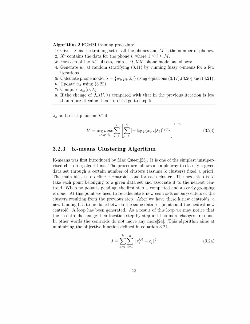
3.2.3 K-means Clustering Algorithm
K-means was first introduced by Mac Queen[23]. It is one of the simplest unsuper-vised clustering algorithms. The procedure follows a simple way to classify a givendata set through a certain number of clusters (assume k clusters) fixed a priori.The main idea is to define k centroids, one for each cluster. The next step is totake each point belonging to a given data set and associate it to the nearest cen-troid. When no point is pending, the first step is completed and an early groupingis done. At this point we need to re-calculate k new centroids as barycenters of theclusters resulting from the previous step. After we have these k new centroids, anew binding has to be done between the same data set points and the nearest newcentroid. A loop has been generated. As a result of this loop we may notice thatthe k centroids change their location step by step until no more changes are done.In other words the centroids do not move any more[24]. This algorithm aims atminimizing the objective function defined in equation 3.24.
J =k∑
j=1
n∑i=1
‖x(j)i − cj‖2 (3.24)
22
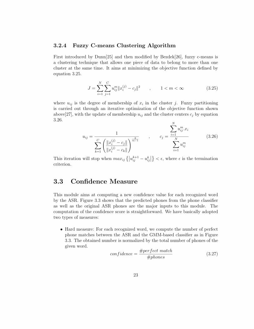
3.2.4 Fuzzy C-means Clustering Algorithm
First introduced by Dunn[25] and then modified by Bezdek[26], fuzzy c-means isa clustering technique that allows one piece of data to belong to more than onecluster at the same time. It aims at minimizing the objective function defined byequation 3.25.
J =N∑
i=1
C∑j=1
umij‖x(j)
i − cj‖2 , 1 < m < ∞ (3.25)
where uij is the degree of membership of xi in the cluster j. Fuzzy partitioningis carried out through an iterative optimization of the objective function shownabove[27], with the update of membership uij and the cluster centers cj by equation3.26.
uij =1
C∑k=1
(‖x(j)
i − cj‖‖x(j)
i − ck‖
) 2m−1
, cj =
N∑i=1
umij .xi
N∑i=1
umij
(3.26)
This iteration will stop when maxij
{∣∣uk+1ij − uk
ij
∣∣} < ε, where ε is the terminationcriterion.
3.3 Confidence Measure
This module aims at computing a new confidence value for each recognized wordby the ASR. Figure 3.3 shows that the predicted phones from the phone classifieras well as the original ASR phones are the major inputs to this module. Thecomputation of the confidence score is straightforward. We have basically adoptedtwo types of measures:
• Hard measure: For each recognized word, we compute the number of perfectphone matches between the ASR and the GMM-based classifier as in Figure3.3. The obtained number is normalized by the total number of phones of thegiven word.
confidence =#perfect match
#phones(3.27)
23

P h o n e m ec lass i f i e r
p h o n e 1
p h o n e n
p h o n e 2
A t t e m p t e d P h o n e s e q u e n c e o f a r e c o g n i z e d W o r d
A S R
p h o n e 1
p h o n e n
p h o n e 2
A S R p h o n e s e q u e n c e o f a r e c o g n i z e d W o r d
.
.
.
.
.
.
= 1
! = 0
Figure 3.3: Confidence measure module
• Weighted measure: Whenever we have a perfect match between the ASR andthe GMM classifier, we sum up the length in terms of number of frames ofthe corresponding matched phone. The obtained value is normalized by thetotal length of the word.
confidence =length of perfect match
word length(3.28)
3.3.1 Integration Of The Classifier With Confidence Mea-sure
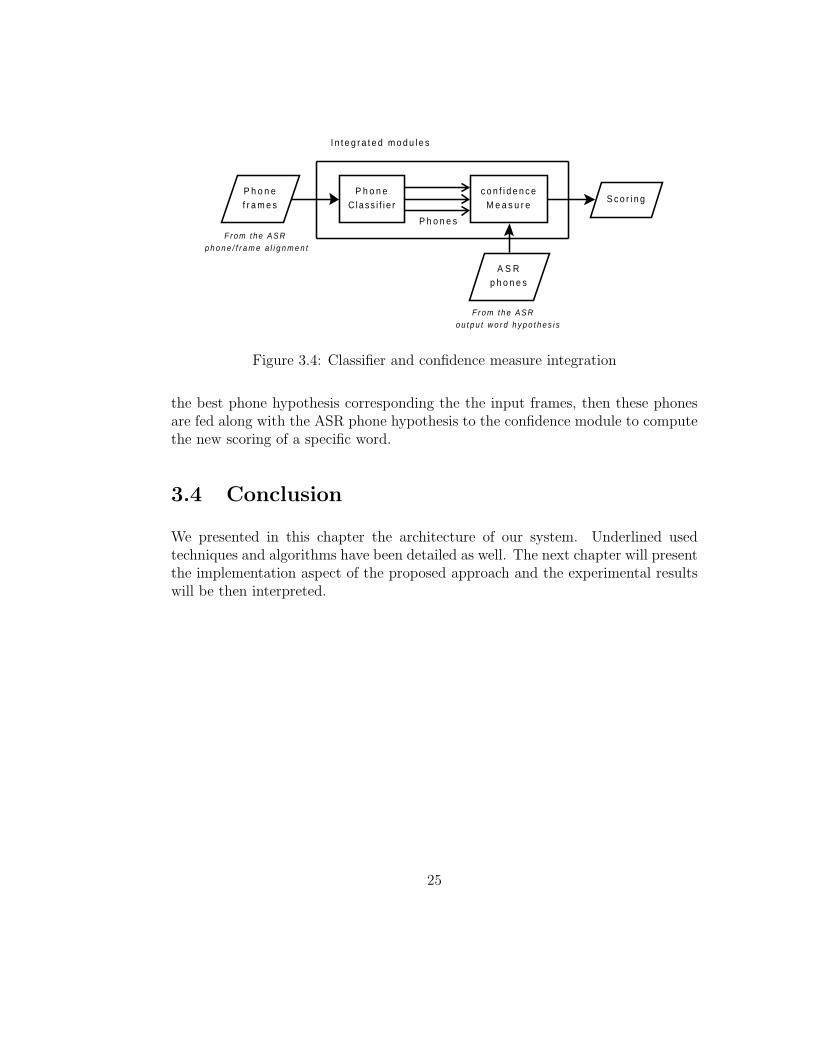
Now that both modules have been presented, we outline their integration. Fig-ure 3.4 describes the integration flow. The input to our system are the alignedphone/frames from the ASR output, which will be fed to the FGMM/GMM basedclassifier, and the actual ASR outputted phones of the corresponding recognizedword which will be used by the confidence measure module. The classifier outputs
24
P h o n eC lass i f i e r
c o n f i d e n c eM e a s u r e
P h o n ef r a m e s
A S Rp h o n e s
I n t e g r a t e d m o d u l e s
P h o n e s
S c o r i n g
F r o m t h e A S R p h o n e / f r a m e a l i g n m e n t
F r o m t h e A S R o u t p u t w o r d h y p o t h e s i s
Figure 3.4: Classifier and confidence measure integration
the best phone hypothesis corresponding the the input frames, then these phonesare fed along with the ASR phone hypothesis to the confidence module to computethe new scoring of a specific word.
3.4 Conclusion
We presented in this chapter the architecture of our system. Underlined usedtechniques and algorithms have been detailed as well. The next chapter will presentthe implementation aspect of the proposed approach and the experimental resultswill be then interpreted.
25
Chapter 4
Experimental Results AndInterpretations
In this chapter, we describe the experimental framework used to implement theproposed approach.
4.1 Experimental Framework
4.1.1 The JULIUS ASR System
Julius[28] is a high performance continuous speech recognition software based onword N-grams. It is able to perform recognition at the sentence level with a vo-cabulary in the tens of thousands. Julius realizes high-speed speech recognitionon a typical desktop PC. It performs at near real time and has a recognition rateof above 90% for a 20, 000-word vocabulary dictation task. The best feature ofthe Julius system is that it is multipurpose. By recombining the pronunciationdictionary, language and acoustic models one is able to build various task specificsystems. The Julius code also is open source so one should be able to recompilethe system for other platforms or to alter the code for one’s specific needs. Inthis thesis, we have used the Julian system[29], a continuous speech recognitionparser based on finite state grammar. It is exactly the same engine as Julius expectthat Julian uses a grammar instead. High precision recognition is achieved using atwo pass hierarchical search. Julian can perform recognition on microphone input,audio files, and feature parameter files. Also, as standard format acoustic modelsand grammar based language models can be used, these models can be changed to
26

perform recognition under various conditions. The maximum vocabulary is 65,535words.
4.1.2 ATT Text To Speeh
In order to generate audio data from the natural language sentences, we have usedATT Natural voices text-to-speech engine (TTS)[30]. The TTS engine providesynthesis services in multiple languages for application builders creating desktopapplications. High-quality male and female voices are included in 8 KHz µlawand CCITT G.711 alaw for telephony applications. Additional voices and higherquality 16 KHz voices are available for non-telephony applications. Further detailson this TTS engine can be found in [30].
4.1.3 Hidden Markov Model Toolkit (HTK)
HTK is a toolkit for building Hidden Markov Models (HMMs). HMMs can be usedto model any time series and the core of HTK is similarly general-purpose [31].However, HTK is primarily designed for building HMM-based speech processingtools, in particular recognizers. The tool kit is open source and is available in [32].We mainly used this toolkit for:
• ASR performance evaluation: for each given sentence, the number of deleted,inserted, substituted and correct words is computed and an overall accuracyand correctness is outputted;
• Transcript force alignment: phoneme/frame alignment is needed for the tran-script testing data. We use the HTK to do recognition of wave files corre-sponding to the testing data and get forced aligned recognition results thatwill be used later for performance evaluation
4.1.4 TIMIT Speech Corpus
The data set used for training and testing the FGMM/GMM models is the TIMITdatabase[33]. It is a corpus of high quality continuous speech from North Americanspeakers, with the entire corpus reliably transcribed at the word and surface pho-netic levels. The TIMIT corpus of read speech has been designed to provide speechdata for the acquisition of acoustic-phonetic knowledge and for the development and
27

evaluation of automatic speech recognition systems. TIMIT has resulted from thejoint efforts of several sites under sponsorship from the Defense Advanced ResearchProjects Agency - Information Science and Technology Office (DARPA-ISTO). Thetext corpus design was a joint effort among the Massachusetts Institute of Technol-ogy (MIT), Stanford Research Institute (SRI), and Texas Instruments (TI). Thespeech was recorded at TI, transcribed at MIT, and has been maintained, verified,and prepared for CD-ROM production by the National Institute of Standards andTechnology (NIST).
The speech is parameterized as 12 Mel-frequency coefficients (MFCC) plus energyfor 25ms frames, with a 10ms frame shift. Note that delta and acceleration coeffi-cients can be derived from these 13 coefficients, resulting in a total of 39 coefficients.The target labels consists of 40 different classes, representing 40 phonemes from theEnglish language. This is a configuration commonly used in speech recognition[34].The corpus is divided into 3648 training utterances and 1344 test utterances. Nospeakers from the training set appear in the test set, making it 100% speaker-independent. TIMIT contains sentences spoken by speakers from 8 major dialectregions of the United States (New England, Northern, North Midland, South Mid-land, Southern, New York city, Western, Army brat where the speakers movedaround a lot during their childhood).
4.2 Phone Classification
In this section, we tackle the training and the evaluation of the Fuzzy GMM andthe GMM models that will serve as the phone classifiers. We start by presentingthe experimental setup, then results will be provided as well as the interpretationsand finally we conclude the section by a summary.
4.2.1 Experimental Setup
For the training part as well as for the classification part of both algorithms GMMand FGMM, we have used the TIMIT database, the de facto speech database forevaluating speech recognition systems. We have used as well the commonly usedfeatures vectors in speech systems, the MFCC features.
Feature extraction As for most of the pattern recognition problems, we needto extract a set of features from the audio raw data that represents all the
28
dynamics and variations of the input. These features will serve as the input setfor training the Gaussian models that will model the phonemes. So the choiceof these features will affect enormously the overall performance of the system.There are plenty of features we can use[1], but we cannot use all of them sincethe training data is limited. Adding new features doesn’t mean that the errorwill decrease systematically. This is not due to the fact that the feature weadded is poor, but rather that our data is insufficient to reliably model all thefeatures. The first feature we use is speech waveform. In general, time-domainfeatures are much less accurate than frequency-domain features such as themel-frequency cepstral coefficients (MFCC). This because many features suchas formants, which are useful in classifying vowels, are better characterized inthe frequency domain with a low dimension feature vector. Temporal changesin the spectra play an important role in the human perception. In order tocapture this information, we use the delta coefficients that measure the changein coefficients over time. For this thesis, we used the typical feature vectorfor speech recognition, the 39 MFCC coefficients :
• 13th order MFCC ck
• 13th order first order delta MFCC computed from ∆ck = ck+1 − ck
• 13th order second order delta MFCC computed from∆∆ck = ∆ck+1 − ∆ck
Further details on these features and how to compute them can be found indetails in [1, 35]. A procedure to extract MFCC coefficients of a given speechis given in appendix D.
Data collection Now that we have extracted the features from the wave files ofthe TIMIT database, we need to collect all the frames (feature vectors) of eachphone in the whole database. This data will serve for training and testingthe FGMM/GMM models. In order to do this data collection, we will usethe alignment provided in the database, alignment in terms of frames (i.e.for every phone, we have the corresponding the first and the last frame). Weused all the 8 dialects in the database to collect the data for each of the 39phones listed in appendix C.
4.2.2 Results And Interpretations
Once we have the data for each phoneme, we can launch the training algorithm tooptimize the models representing each of the phones. According to the theoretical
29

considerations presented in chapter 3, we present now the results of phoneme clas-sification using Gaussian Mixture Modeling and Fuzzy Gaussian Mixture Modeling.
For the GMMs, the initialization of the parameters is done using 5 iterations ofthe k-means algorithm, and the fuzzy c-mean algorithm run for 5 iterations hasalso been used to initialize the model parameters of the fuzzy GMMs. We havechosen the degree of fuzziness m = 1.03. In order to evaluate the performanceof our FGMM/GMM based classifier, we built a confusion matrix. A confusionmatrix[36], contains information about actual and predicted classifications done bya classification system. Performance of such systems is commonly evaluated usingthe data in the matrix. Each column of the matrix represents the instances in apredicted class, while each row represents the instances in an actual class. Onebenefit of a confusion matrix is that it is easy to see if the system is confusingtwo classes (i.e. commonly mislabeling one as another). We have trained modelswith different components. We have chosen to use diagonal covariances. Table 4.1shows the classification rate for both GMMs and FGMMs. The best configuration
Components GMM (%) FGMM (%)8 42 42.5116 47 58.5132 56.39 57.8764 64.21 66128 65.70 67.29
Table 4.1: Classification rate for fuzzy GM phone models and GM phone models
is with 64 components. Although with 128 components we have obtained slightlybetter results, we decided to go with the 64-component GMMs and FGMM. Infact, training time as well as the testing time are multiplied by almost 2.5 timeswhen using 128 components compared to the 64 components configuration. Thefuzzy GMMs yield better performance in all model sizes which are 8, 16, 32 and 64compared to the GMMs.In table 4.2, the precision measure for all the phonemesis presented. The precision measure shows the proportion of correct prediction forevery phone. We notice here that some of the phonemes have low precision. Thisis due in part to the size of the training corpus; for example the phone /zh/ is veryrare and so the training data is small, thus the precision rate is low. Comparedto other techniques, a 66% classification rate is acceptable for the task they areintended to do.
30

Phoneme Precision %/aa/ 68.01/ae/ 78.7/ah/ 70.93/ao/ 65.65/aw/ 27.55/ay/ 61.96/b/ 69.91/ch/ 45.94/d/ 52.72/dh/ 70.29/eh/ 39.86/er/ 52.36/ey/ 50.88/f/ 78.09/g/ 65.81/hh/ 84.13/ih/ 54.19/iy/ 82.34/jh/ 34.09/k/ 83.03/l/ 84.65/m/ 67.13/n/ 74.80/ng/ 40.27/ow/ 40.48/oy/ 45.49/p/ 72.50/r/ 84.33/s/ 83.35/sh/ 82.14/t/ 58.21/th/ 32.37/uh/ 52.08/uw/ 46.66/v/ 56.63/w/ 77.81/y/ 76.59/z/ 63.92/zh/ 26.67
Table 4.2: Phoneme precisions using the 64 fuzzy mixture models
31
4.2.3 Preliminary Remarks
Using the TIMIT database, we have trained GMM and FGMM models for eachof the 39 phone target classes. We have proved that this FGMM technique out-performs the conventional GMM by approximately 2%. The classification rate,however, is still low compared to the other techniques, especially the HMM basedrecognizers that perform a 78% phoneme recognition rate. In order to improve theclassification results, we might need to try more features. In fact, formants are crit-ical in the recognition of vowels, and we didn’t use them for training our models,so it might be worth trying to improve the vowel classification rate. We can as welltry other feature extraction techniques, like the RASTA (Relative Spectra), LPC(Linear Predictive Coding), etc.
4.3 Confidence Measure
In this section, we outline experiments and results preliminary to our second mod-ule, which does the confidence evaluation of the ASR output. We start the sectionby a presentation of the experimental framework, then the obtained results arediscussed and we conclude with a summary.
4.3.1 Experimental Setup
We have used a call routing example in order to evaluate our system. The routingtree is presented in 4.1. The user chooses between one of the 6 products (nodes inthe first level of the tree). Then, for each product, the user might ask for one of the9 services (nodes in the second level of the routing tree). For esthetic purposes, onlyservices for one product have been represented. All the products have the same 9services. This call routing tree can be considered as fairly realistic and complexenough to base our analysis on this application. In fact, most of the routing treesin current use are 1-level trees and the number of nodes is around 10. This numberdecreases drastically when the application deals with a multilevel tree.
Data generation As we already mentioned before, the system will be tested withnatural language sentences; the user will not be constrained. In order to ex-press a request, the speaker can use a natural language sentence that containsone or more keywords. In order to expand the number of possible natural sen-tences, we allowed the speaker to use 4 synonyms to point to a specific second
32

S e r v i c e s
C T V H S I M P S T VW II T
R P I P M F B P C N CS PI M
C T V : c a b l e T VH S I : H i g h s p e e d i n t e r n e tM P : M o b i l e p h o n eIT : I n te rac t i ve te rm ina lW I : W i r e l e s s i n t e r n e tS T V : S a t e l l i t e T V
I : Ins ta l la t ionR P : R e c e p t i o n p r o b l e mS P : S e r v i c e p l a nIP : I ns ta l l a t i on p rob lemM F : M a l f u n c t i o nB P : B i l l p a y m e n tM : M i s p l a c e dC : C a n c e l l a t i o nN C : N e w C l i e n t
Figure 4.1: Call routing tree
level node. The list of synonyms for each node can be found in appendix A.Then we prepared some templates of natural language sentences to generateautomatically natural sentences. In total, we generated 3601 possible natu-ral sentences that a user might utter when calling on the call center. Eachsentences contains two keywords, one from each level. Here are some naturalsentences where the keywords have been emphasized:
There is a reception problem with my cable tv.I want to speak to somebody regarding installation problem of myhigh speed internet.I have been waiting for 15 minutes to talk about my satellite tv poorreception.Is there a way to solve my bill payment problem of my wirelessinternet.
In total we have created 6 different templates because of the different contextof the keywords. All the templates created to generate these sentences canbe found in appendix B.
Tagging and alignment The grammar of the ASR only contains the keywords,no filler model is used here. The grammar is composed of the 6 product names
33
as well as the list of services along with their synonyms. After the ASR doesthe recognition of the 3601 audio files, we should parse each ASR output andtag each word. The tags can be:
• Correct (C) for words that are correctly spotted;
• Incorrect (I) otherwise i.e. false mapping.
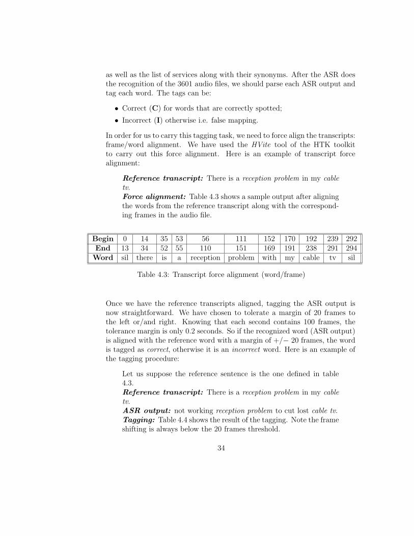
In order for us to carry this tagging task, we need to force align the transcripts:frame/word alignment. We have used the HVite tool of the HTK toolkitto carry out this force alignment. Here is an example of transcript forcealignment:
Reference transcript: There is a reception problem in my cabletv.Force alignment: Table 4.3 shows a sample output after aligningthe words from the reference transcript along with the correspond-ing frames in the audio file.
Begin 0 14 35 53 56 111 152 170 192 239 292End 13 34 52 55 110 151 169 191 238 291 294Word sil there is a reception problem with my cable tv sil
Table 4.3: Transcript force alignment (word/frame)
Once we have the reference transcripts aligned, tagging the ASR output isnow straightforward. We have chosen to tolerate a margin of 20 frames tothe left or/and right. Knowing that each second contains 100 frames, thetolerance margin is only 0.2 seconds. So if the recognized word (ASR output)is aligned with the reference word with a margin of +/− 20 frames, the wordis tagged as correct, otherwise it is an incorrect word. Here is an example ofthe tagging procedure:
Let us suppose the reference sentence is the one defined in table4.3.Reference transcript: There is a reception problem in my cabletv.ASR output: not working reception problem to cut lost cable tv.Tagging: Table 4.4 shows the result of the tagging. Note the frameshifting is always below the 20 frames threshold.
34

Confidence Begin End Word Tag1.000 0 11 sil C0.670 12 29 not I0.000 30 50 working I0.981 51 106 reception C1.000 107 149 problem C0.928 150 159 to I0.486 160 172 cut I0.985 173 192 lost I1.000 193 227 cable C1.000 228 291 tv C1.000 292 293 sil C
Table 4.4: Tagging the ASR output
Now that the data is ready, we can use the trained model and our confidencemeasure approach to evaluate the Julius confidence measure.
4.3.2 Results And Interpretations
The FGMM/GMM models trained previously are now used to evaluate the ASRoutput. We feed the frames corresponding to each phone of each word of the ASRoutput, to the 39 models in order to pick the best phone that matches the inputframe data. Table 4.5 shows the result for the word reception of the same referencesentence discussed in the previous section. In chapter 3, we have defined two types
Begin End ASR GMM51 59 /r/ /r/60 65 /ah/ /aa/66 75 /s/ /s/76 83 /eh/ /ae/84 89 /p/ /p/90 95 /sh/ /sh/96 99 /ah/ /sh/100 106 /n/ /d/
Table 4.5: ASR vs GMM phone output
35

of confidence measures: the hard and the weighted measures. For each of these twomeasures, we computed (for both the correct and incorrect words), the number oftimes where our confidence is below or above the Julius confidences. Table 4.6
Output Hard WeightedC I C I
GMM 4.94% 89.31% 4.025% 89.42%ASR 95.06% 10.69% 95.975% 10.58%
FGMM 5.21% 89.67% 4.2% 90.13%ASR 94.79% 10.33% 95.8% 9.87%
Table 4.6: ASR vs GMM/FGMM confidence comparisons
shows the results obtained for both type of measures. For the incorrect columnslabeled as (I), we computed the number of times where our confidence measure islower than the ASR confidence. And for the correct columns labeled as (C), wecomputed the number of time where our confidence measure is higher than theASR one. With this type of statistics, we can detect if our confidence measureapproach differentiates better between correct and incorrect words.
For the incorrect words spotted by the ASR and when using the GMMs for thephoneme classification, 89.31% of the time the hard measure of the confidence islower than the actual ASR confidence value. This percentage increases slightlywhen using the fuzzy GMM models. It is clear that our system ranks better thefalsely mapped words. But this is not the case for the correctly spotted words.In fact only 4.94% of the times our confidence is larger than the ASR confidence.When using the FGMMs for the phoneme classification, this percentage slightly in-creases to reach 5.21%. There is not much difference for the second type of measure,especially with regards to the correctly spotted words. That is, using our techniquewe are only 4.2% of the times above the ASR confidence values. These results areinconclusive at this early stage of the analysis. Noting that ASR confidences areusually high whether it is for correctly spotted words or falsely mapped ones, weneed to provide a fairer way for carrying out this analysis. This will be done bycomputing the deviations from the average confidences for correct and incorrectwords. We computed the average confidence for correct words and incorrect words.Results are shown in table 4.7. The column C corresponds to the mean confidencefor all the correctly accepted words, whereas the column I corresponds to the meanconfidence of the falsely mapped keywords. Then the overall confidence is the meanof the two columns C and I. The mean values in table 4.7 show clearly the difference
36

Output Hard WeightedCorrect Incorrect Overall Mean Correct Incorrect Overall Mean
GMM 0.3492 0.1197 0.2344 0.1809 0.1121 0.1465FGMM 0.3607 0.11 0.2353 0.186 0.098 0.142ASR 0.9146 0.703 0.8079 0.9146 0.703 0.8079
Table 4.7: ASR vs GMM/FGMM average confidences
in the difference in the confidence values range between the ASR and our approach,which explains the low percentage for the correctly accepted word in table 4.6.
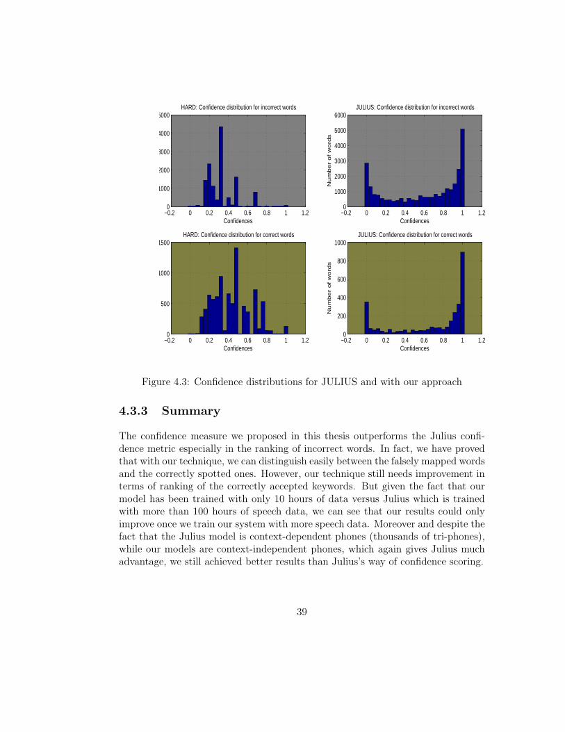
We can notice here as well that the two measurements have different distributions.So in terms of the deviations from the overall mean: Julius is 13% and our approachis 50% (either with GMM or with FGMM), showing a much larger differentiation.This is a very positive indicator for our system. That means that we distinguisheasily and better between the falsely mapped words and the correctly spotted ones.Note that the weighted approach doesn’t seem to perform better than the hardapproach. To emphasize this aspect of different distributions, we have plotted thecorrectly accepted and the falsely mapped word confidence distribution for bothJulius and our system. The histogram distribution graphs are shown in figure 4.2.We notice in figure 4.2 that the ASR’s and our system’s confidence distributions arecompletely different. For incorrect words, our system has asserted lot of zero con-fidences, which makes perfect sense since the words are completely wrong. Juliuson the other hand wrongly ranks incorrect words with high confidence values. Inorder for us to present the distributions more clearly, we have removed in figure4.3 the words with confidence values equal to 1 by the ASR and all the words withconfidences equal to 0 by our system. Features of the distributions are now morevisible in figure 4.3. Obviously, the type of distribution for the ASR is not preferred.In fact, there is lot of overlapping between the correct word confidence distributionand the incorrect one, which shows again the inability of Julius to decide and torank appropriately the correct and the wrongly recognized words. However for oursystem, the distinction is clear and the distributions for correct and incorrect wordsare quite dissociated. But it is not optimal: in fact some overlap exists around the0.2 confidence value. Ideally, the two distributions (for correct and incorrect) haveto avoid any overlapping so that we don’t have correctly accepted word confidencessmaller than wrongly spotted word confidences and falsely mapped word confi-dences bigger than correctly accepted word confidences.
The distribution of the confidences for the correct words with respect to that of the
37

−0.2 0 0.2 0.4 0.6 0.8 1 1.20
0.5
1
1.5
2
2.5x 10
4
Confidences
Nu
mb
er
of
wo
rds
HARD: Confidence distribution for incorrect words
−0.2 0 0.2 0.4 0.6 0.8 1 1.20
500
1000
1500
2000
2500
Confidences
HARD: Confidence distribution for correct words
−0.2 0 0.2 0.4 0.6 0.8 1 1.20
5000
10000
15000
Confidences
Nu
mb
er
of
wo
rds
JULIUS: Confidence distribution for incorrect words
−0.2 0 0.2 0.4 0.6 0.8 1 1.20
2000
4000
6000
8000
10000
Confidences
Nu
mb
er
of
wo
rds
JULIUS: Confidence distribution for correct words
Figure 4.2: Confidence distributions for JULIUS and with our approach
incorrect ones, relative to the overall mean, is also important. Figure 4.4 shows thewords that have confidences less (respectively higher) than the overall confidencevalue for both Julius and our system. For all the plots, the middle red point is theoverall mean confidence value for a specific system and specific status (correct orincorrect). For correct words, ideally most of the words have to be located rightof the overall mean. This is the case for both Julius and our approach. However,Julius behaves quite better than our approach. For the incorrect words, ideallymost of the words have to be located left of the overall mean. For our system, thisis so, but Julius behaves in complete opposition to this. In fact, for Julius, mostof the incorrect words have their confidences above the overall confidence value.This again explains the fact that Julius cannot distinguish clearly and efficientlybetween the correct and falsely mapped words.
38
−0.2 0 0.2 0.4 0.6 0.8 1 1.20
1000
2000
3000
4000
5000
Confidences
HARD: Confidence distribution for incorrect words
−0.2 0 0.2 0.4 0.6 0.8 1 1.20
500
1000
1500
Confidences
HARD: Confidence distribution for correct words
−0.2 0 0.2 0.4 0.6 0.8 1 1.20
1000
2000
3000
4000
5000
6000
Confidences
Nu
mb
er
of
wo
rds
JULIUS: Confidence distribution for incorrect words
−0.2 0 0.2 0.4 0.6 0.8 1 1.20
200
400
600
800
1000
Confidences
Nu
mb
er
of
wo
rds
JULIUS: Confidence distribution for correct words
Figure 4.3: Confidence distributions for JULIUS and with our approach
4.3.3 Summary
The confidence measure we proposed in this thesis outperforms the Julius confi-dence metric especially in the ranking of incorrect words. In fact, we have provedthat with our technique, we can distinguish easily between the falsely mapped wordsand the correctly spotted ones. However, our technique still needs improvement interms of ranking of the correctly accepted keywords. But given the fact that ourmodel has been trained with only 10 hours of data versus Julius which is trainedwith more than 100 hours of speech data, we can see that our results could onlyimprove once we train our system with more speech data. Moreover and despite thefact that the Julius model is context-dependent phones (thousands of tri-phones),while our models are context-independent phones, which again gives Julius muchadvantage, we still achieved better results than Julius’s way of confidence scoring.
39

0.2 0.4 0.6 0.8 1 1.20
2000
4000
6000
8000
10000
Mean confidences
JULIUS: Correct spotted words
0.2 0.4 0.6 0.8 1 1.20
0.5
1
1.5
2
2.5x 10
4
Mean confidencesN
um
be
r o
f w
ord
s
JULIUS: Incorrect spotted words
0 0.1 0.2 0.3 0.4 0.5 0.6 0.70
2000
4000
6000
8000
Mean confidences
HARD: Correct spotted words
−0.1 0 0.1 0.2 0.3 0.4 0.5 0.60
0.5
1
1.5
2
2.5
3x 10
4
Mean confidences
Nu
mb
er
of
wo
rds
HARD: Incorrect spotted words
Figure 4.4: Correct and incorrect word confidences compared to the overall mean
40

Chapter 5
Conclusion And Future Work
The main goal of this thesis was to investigate a new approach to filler model-freekeyword spotting system. The approach consisted of using a phone classifier andsome confidence metrics, different from the existing speech recognizer ones, to geta new ranking for the ASR output. Ultimately, this scoring will be used to discardand filter out all the falsely mapped words returned by the ASR.
We presented in chapter 3 the adopted techniques and methods to implement ourapproach. A fuzzy c-mean based modification of the Gaussian mixture modelingwas attempted. Results showed an improvement of approximately 2% when usingFGMM for phoneme classification that led to a classification rate of 66%.
The analysis in chapter 4 of the scoring mechanism that we introduced provedthat in terms of deviations from total mean, the ASR gives a 13% result comparedto 50% with our proposed approach, showing a much larger differentiation betweencorrect and incorrect spotted words. This shows that our approach is promising,and with further investigation and development it could lead to an efficient way tobuild a filler model-free keyword spotter. The obtained results are encouraging andwe can see lot of potential in this approach toward a robust and reliable scoring ofthe ASR output.
We have already targeted a few areas worthy of further investigation to improvethe performance of the proposed approach in this thesis. Areas of improvements inphoneme classification module include:
• We have to use much more data for training the FGMM/GMM models. Infact, in this thesis, we have only used the TIMIT database to create the mod-
41

els, whereas the Julius acoustic model was trained with at least 100 hoursof speech, and with data coming from a Wall Street Journal database, Re-source Management and other corpus. Using more training data will certainlyimprove the classification rate of our models.
• The phone models used in this thesis are context-independent whereas Juliusis using a context-dependent models, with thousands of tri-phones. So usingcontext-dependent models is another direction to investigate. In fact, this canboost the performance of the phone classifier. We could try using bi-phoneor tri-phone context models. Then instead of having to train only models forthe set of phones, we will train bi-phone models.
• In [19], a robust clustering approach to fuzzy Gaussian mixture modeling isproposed. GMMs and FGMMs both have a common disadvantage in theproblem of sensitivity to outliers. This approach of discarding outliers isquite successful in improving the robustness of a variety of fuzzy clusteringalgorithms. We can use this technique to improve the performance of ourFGMMs.
• Finally, the feature extraction techniques used for converting the acousticevents (speech) to feature vectors. We might need to use other features thatwill help in the classification of similar phones or boost the detection rate forcertain classes of phones, like the formants for the vowels.
Areas of improvements for the confidence metric we have proposed can be summa-rized as follows:
• We need to improve the scoring mechanism. For example we might needto keep the N-Best hypothesis in the phoneme classification, and then checkwhich one of the N-best matches the ASR output.
• We can cluster the phonemes in different classes based on the phone similarityaspect. And when deciding whether a FGMM/GMM phone hypothesis doesor does not match the ASR-output phone, we should accept phones thatbelongs to the same family (class) instead of choosing only the perfect match.
• Another aspect we might need to consider is the output score of the FGMM/GMMmodels. A metric using both the likelihood of the models and the number ofmatches in one word might boost the performance. But this type of approachimplies that our FGMM/GMM have high classification accuracy. So it maybe that other techniques for phone modeling might be worth investigating toincrease the phone classification rate.
42

We strongly believe that further research work in this direction could lead to sub-stantial improvements on the results we have so far obtained during this investiga-tion and could lead to potential commercial adoption.
43
Bibliography
[1] X. Huang, A. Acero, and H. Hon. Spoken language processing: A guide totheory, algorithm and system development. Prentice Hall, 2001.
[2] I. Bazzi and J. Glass. Modeling out-of-vocabulary words for robust speechrecognition. In Proceedings ICSLP, Beijing,China, 2000.
[3] C. Yining, L. Jing, Z. Lin, L. Jia, and L. Runsheng. Keyword spotting based onmixed grammar model. In International Symposium on Intelligent Multimedia,Video and Speech Processing, pages 425–428, Hong Kong, 2001.
[4] M. Sigmund. Searching for phoneme boundaries in speech signal. Technical re-port, Institute of radio electronics,University of Technology, Purkynova, CzechRepublic, 1995.
[5] A. Ahmadi. Modular-based classifer for phoneme recogntion. PhD thesis, Uni-versity of Waterloo, 2005.
[6] J. Deller, J. Hansen, and J. Proakis. Discrete- Time Processing of SpeechSignals. IEEE Press, 2000.
[7] J. Coleman. Introducing speech and language processing. Cambridge universitypress, 2005.
[8] T. Robinson and F. Fallside. A recurrent error propagation network speechrecognition system. Computer Speech and Language, 5:259–274, July 1991.
[9] T. Robinson. An application of recurrent nets to phone probability estimation.IEEE Transactions on Neural Networks, 5(2):298–305, 1994.
[10] R. Chen and L. Jamieson. Experiments on the implementation of recurrentneural networks for speech phone recognition, purdue university, west lafayette,usa, 1998.
44

[11] P. Clarkson and P. Moreno. On the use of support vector machines for phoneticclassification. Acoustics, Speech and Signal Processing, 2:585–588, 2000.
[12] K. K. Chin. Support vector machines applied to speech pattern classification.Master’s thesis, Engineering Department, Cambridge University, 1999.
[13] H. Jiang. Confidence measures for speech recognition: A survey. Speech Com-munication, 45(4):455–470, April 2005.
[14] R. San-Segundo, B. Pellom, K. Hacioglu, and W. Ward. Confidence measuresfor spoken dialogue systems. Proc of International Conference on Acoustics,Speech and Signal Processing, 2001.
[15] S. Cox and R. Rose. Confidence measures for the switchboard database. Proc.of International Conference on Acoustics, Speech and Signal Processing, pages511–514, 1996.
[16] B. Chigier. Rejection and keyword spotting algorithms for a directory assis-tance city name recognition application. Proc. of International Conference onAcoustics, Speech and Signal Processing, pages 93–96, 1992.
[17] R. Zhang and A.I. Rudnicky. Word level confidence annotation using combi-nations of features. Proc. of European Conference on Speech CommunicationTechnology, 2001.
[18] A. Dempster, N. Laird, and D Rubin. Maximum likelihood from incompletedata via the em algorithm. Journal of Royal Statistical Society, 39(1):1–38,1977.
[19] D. Tran and M. Wagner. A robust clustering approach to fuzzy gaussian mix-ture models for speaker identification. In 1999 Third international conferenceon Knowledge-Based Intelligent Information Engineering Systems, pages 337–340, Adelaide, Australia, August 1999.
[20] X. Huang, Y. Ariki, and M. Jack. Hidden markov models for speech recognition.Edinburgh university press, 1990.
[21] D. Tran, T. Pham, and X. Zhou. Cell phase identification using fuzzy gaussianmixture models. In the 2005 International Symposium on Intelligent SignalProcessing and Communications Systems, pages 465–468, Hong Kong, Decem-ber 2005.
45

[22] A. Bleau and L. Leon. Watershed-based segmentation and region merging.Computer Vision and Image Understanding, 77:317–370, 2000.
[23] J. B. MacQueen. Some methods for classification and analysis of multivariateobservations. In Proceedings of 5-th Berkeley Symposium on MathematicalStatistics and Probability, volume 1, pages 281–297. Berkeley, University ofCalifornia Press, 1967.
[24] M. Eucci. K-means clustering. http://www.elet.polimi.it/upload/matteucc/Clustering/tutorialhtml/kmeans.html.
[25] J. C. Dunn. A fuzzy relative of the isodata process and its use in detectingcompact well-separated clusters. Journal of Cybernetics, 3:32–57, 1973.
[26] J. C. Bezdek. Pattern Recognition with Fuzzy Objective Function Algoritms.Plenum Press, New York, 1981.
[27] M. Eucci. C-means clustering. http://www.elet.polimi.it/upload/matteucc/Clustering/tutorialhtml/cmeans.html.
[28] T. Kawahara and A. Lee. Free software toolkit for japanese large vocabularycontinuous speech recognition. International Conference on Spoken LanguageProcessing (ICSLP), 4:476–479, 2000.
[29] I. Lane. Multipurpose large vocabulary continuous speech recognition enginejulius. Technical report, Kyoto University, Kyoto, Japan, March 2001.
[30] ATT Natural Voices. Text-to-speech engines, system developers guide: Server,server-lite, and desktop editions, 2004.
[31] S. Young and al. The HTK Book. Cambridge University Engineering Depart-ment, December 2006.
[32] Cambridge University Engineering Department. HTK speech recognitiontoolkit. http://htk.eng.cam.ac.uk/.
[33] J. Garafolo. Getting started with the DARPA TIMIT CD-ROM: An acousticphonetic speech database, 1988.
[34] L. R. Rabiner and B. H. Juang. Fundamentals of Speech Recognition. PrenticeHall, New Jersey, USA, 1993.
46

[35] Y. Li. Singal processing for speech applications. Language Technology In-stitute, School of Computer Science,Carnegie Mellon University Pittsburgh,2004.
[36] R. Kohavi and F. Provost. Confusion matrix. Machine learning, 30(2-3):271–274, February 1998.
[37] F. Karray and C. de Silva. Soft computing and intelligent systems design:Theory, Tools and Applications. Addison Wesley Publishing, 2004.
[38] M. Seltzer. Sphinx III signal processing front end specification. Technicalreport, CMU Speech Group, 1999.
47
Appendix A
Node Synonyms Of the CallRouting Tree
Each second level node in the call routing tree in figure 4.1 can be referenced by 4synonyms. Table A shows the list of synonyms:
48

Node name Synonymsinstallation
Installation to installto startcommencementreception problem
Reception problem poor receptionno receptionweak signalservice plan
Service plan plan of servicewarrantyrepair planinstallation problem
Installation problem starting problemwon’t startset up problemmalfunction
Malfunction not workingworking incorrectlyoperating problembill payment
Bill payment bill paymentpay billmoney paymentmisplaced
Misplaced loststolendroppedcancellation
Cancelation to cancelto cutto endnew client
New client subscribercustomermember
Table A.1: 2-level node synonyms for the routing tree in figure 4.1
49

Appendix B
Templates For Natural LanguageSentence Generation
The 6 distinct templates prepared to generate natural sentences with the nodesdefined in figure 4.1, are presented in this appendix.
1. The sentences below can be used with the following terminal (ie. final routing)nodes of the routing tree reception problem, installation problem, andmalfunction. Note that [cable tv] will be substituted by all the 6 differentproducts in the tree.
• There is a [reception problem] with my [cable TV]
• Can you help me with [cable tv]’s [reception problem] now
• I want to speak to someone regarding [reception problem] of my [cabletv]
• Is there a way to solve the [reception problem] of my [cable tv]
• I am sick and tired of my [cable tv]’s [reception problem]
• My [cable tv]’s [reception problem] is absolutely terrible
• Why don’t you understand that I need help with [cable tv]’s [receptionproblem]
• Please help fix my [cable tv]’s [reception problem] right now
• Do you have anyone to discuss [reception problem] of [cable tv]
• I can’t wait until Friday for someone to fix my [cable tv]’s [receptionproblem]
50
• Do you understand that I have a serious [reception problem] with my[cable tv]
• Stop arguing with me and have someone fix [cable tv]’s [reception prob-lem]
• I can’t believe that you can’t fix [reception problem] of my [cable tv]
• I have been waiting for twenty minutes to talk about my [cable tv]’s[reception problem]
• So, nobody is available to help me [cable tv]’s [reception problem], huh
2. The sentences below can be used with the following terminal (ie. final rout-ing) nodes of the routing tree misplaced. Note that [mobile phone] will besubstituted by all the 6 different products in the tree.
• I have [misplaced] my [mobile phone] somewhere
• Do you understand that I have [misplaced] my [mobile phone] or not
• Didn’t I just tell you that I [misplaced] my [mobile phone]
• I have been trying to explain for ten minutes that I have [misplaced] my[mobile phone]
• I can’t believe that you don’t understand that my [mobile phone] hasbeen misplaced
• Please help me as I have [misplaced] my [mobile phone]
• I have been waiting to report my [misplaced] [mobile phone]
• Sorry, I forgot to call yesterday to tell you that I [misplaced] my [mobilephone]
• Is there someone who can help regarding my [misplaced] [mobile phone]
• So, you are telling me that I can’t report a [misplaced] [ mobile phone]
• All I want to report is that I [misplaced] my [mobile phone]
• Just listen to me and find someone regarding [misplaced] [mobile phone]
3. The sentences below can be used with the following terminal (ie. final rout-ing) nodes of the routing tree bill payment. Note that [cable tv] will besubstituted by all the 6 different products in the tree.
• Can you help me with [cable tv]’s [bill payment] now
• I want to speak to someone regarding [bill payment] for my [cable tv]
51

• Is there a way to solve the [bill payment] problem of my [cable tv]
• I am sick and tired of your losing my [bill payment] for [cable tv] account
• Why don’t you understand that I need help with [cable tv]’s [bill pay-ment]
• Please report [cable tv]’s [bill payment] right now
• Do you have anyone to discuss [reception problem] of [cable tv] with me
• I can’t wait until Friday for someone to process my [cable tv]’s [billpayment]
• Do you understand that I have a serious [bill payment] issue with my[cable tv]
• Stop arguing with me and just process [cable tv]’s [bill payment] forheaven’s sake
• I can’t believe that you can’t fix my [cable tv] [bill payment] problemuntil next week
• I have been waiting for twenty minutes to talk about last month’s [cabletv] [bill payment]
• So, nobody is available to help me [cable tv]’s [bill payment], huh
• I am telling you you forgot to report last month’s [cable tv]’s [bill pay-ment]
• How can I make a [bill payment] for my [cable tv]
4. The sentences below can be used with the following terminal (ie. final routing)nodes of the routing tree cancelation and installation. Note that [cable tv]will be substituted by all the 6 different products in the tree.
• Can you help me with [cable tv]’s [cancelation] now
• I want to speak to someone regarding [cancelation] of my [cable tv] ser-vice
• Is there a way to solve the [cancelation] problem of my [cable tv]
• I am sick and tired of your losing my [cancelation] notice for [cable tv]service
• Why don’t you understand that I need help with [cable tv]’s [cancelation]
• Please report [cable tv]’s [cancelation] right now
• Do you have anyone to discuss [cancelation] of [cable tv] service with me
52

• I can’t wait until Friday for someone to process my [cable tv]’s [cancela-tion] notice
• Do you understand that I have requested [cancelation] of my [cable tv]service three times
• Stop arguing with me and just process [cable tv]’s [cancelation] order forheaven’s sake
• I can’t believe that you won’t put in [cable tv] [cancelation] order untilnext month
• I have been waiting for twenty minutes to talk about last month’s [cabletv] [cancelation] order
• So, nobody is available to help me [cable tv]’s [cancelation], huh
• I am telling you you forgot to report last month’s [cable tv]’s [cancelation]
• How can I order a [cancelation] for my [cable tv] service
5. The sentences below can be used with the following terminal (ie. final routing)nodes of the routing tree new client. Note that [cable tv] will be substitutedby all the 6 different products in the tree.
• Can you help me become [new client] of [cable tv]
• I want to speak to someone regarding becoming [new client] of [cable tv]
• Don’t you think I deserve as discount as a [new client] of [cable tv]
• I am sick and tired of your losing my [new client] order for [cable tv]
• Why don’t you understand that I need help with become [cable tv]’s[new client]
• Please report my status as [cable tv]’s [new client] right now
• Do you have anyone to explain how I can be [new client] of [cable tv]
• I can’t wait until Friday for someone to process my [cable tv]’s [newclient] request
• Do you understand that I want to become [new client] of your [cable tv]service
• Stop arguing with me and just process [cable tv]’s [new client] requestfor heaven’s sake
• I can’t believe that you won’t process my [cable tv] [new client] requestuntil next week
53

• I have been waiting for twenty minutes to talk about last month’s [cabletv] [new client] order
• So, nobody is available to help me become a [new client] of [cable tv],huh
• I am telling you you forgot to report that I am a [new client] of [cabletv]
• You cannot charge me extra fees as a [new client] of [cable tv]
6. The sentences below can be used with the following terminal (ie. final rout-ing) nodes of the routing tree service plan. Note that [satellite tv] will besubstituted by all the 6 different products in the tree.
• Can you help me with [satellite tv]’s [service plan] now
• I want to speak to someone regarding [service plan] for my [satellite tv]
• Is there a way to change the [service plan] offered for [satellite tv] service
• I am sick and tired of your third-rate [service plan] for [satellite tv]account
• Why don’t you understand that I need help with [satellite tv]’s [serviceplan]
• Please explain [satellite tv]’s [service plan] right now
• Do you have anyone to discuss [service plan] of [satellite tv] with me
• I can’t wait until Friday for someone to process my [satellite tv]’s [serviceplan] request
• Do you understand that I have a serious [service plan] issue with my[satellite tv]
• Stop arguing with me and just process [satellite tv]’s [service plan] changesfor heaven’s sake
• I can’t believe that you can’t modify my [satellite tv] [service plan] untilnext week
• I have been waiting for twenty minutes to talk about last month’s [satel-lite tv] [service plan]
• So, no body is available to help me [satellite tv]’s [service plan], huh
• I am telling you you forgot to send me [satellite tv]’s [service plan] lastmonth
• How can I inquire about the [service plan] for my [satellite tv]
54

Appendix C
List Of Phonemes Based OnTIMIT Database
Table C.1 shows the list of target phones. Note that we removed the silence andthe short pause, only the phones that we have modeled using FGMM/GMM are inthe table.
55

Phonemes Word examples
aa Car
ae At
ah Up
ao Dog
aw How
ay Ice
b Big
ch March
d Dig
dh Father
eh Pet
er Turn
ey Day
f Fork
g Angle
hh Help
ih Hit
iy Feel
jh Joy
k Cut
l Sail
m Mad
n End
ng Sing
ow Go
oy Toy
p Put
r Red
s Sit
sh She
t Talk
th Thin
uh Good
uw Tool
v Over
w With
y Yard
z Lazy
zh Azure
Table C.1: Phone list based on TIMIT database
56

Appendix D
MFCC Features
The steps to construct MFCC features are as follows [38]:
1. Pre-Emphasis:The following FIR pre-emphasis filter is applied to the input waveform:
y[n] = x[n] − αx[n − 1] (D.1)
α is provided by the user or set to the default value. If α = 0 , then this stepis skipped. In addition, the appropriate sample of the input is stored as ahistory value for use during the next round of processing.
2. Windowing: The frame is multiplied by the following Hamming window:
w[n] = 0.54 − 0.46 cos(2πn
N − 1) (D.2)
N is the length of the frame.
3. Power SpectrumThe power spectrum of the frame is computed by performing a DFT of lengthspecified by the user, and then computing its magnitude squared.
S[k] = (real(X[k]))2 + (imag(X[k]))2 (D.3)
4. Mel SpectrumThe mel spectrum of the power spectrum is computed by multiplying the
57

power spectrum by each of the of the triangular mel weighting filters andintegrating the result.
S[l] =
N/2∑k=0
S[k]Ml[k] l = 0, 1, ..., L − 1; (D.4)
N is the length of the DFT, and L is total number of triangular mel weightingfilters.
5. Mel Cepstrum
A DCT is applied to the natural logarithm of the mel spectrum to obtain themel cepstrum:
c[n] =L−1∑i=0
ln(S[i]) cos(πn
2L(2i + 1)) n = 0, 1, ..., C − 1; (D.5)
C is the number of cepstral coefficients.
Delta MFCCAlso, delta MFCC coefficients can be calculated using the following equation [35]:
∆c[n] = c[n + 1] − c[n] (D.6)
Delta delta MFCCMoreover, to obtain delta-delta coefficients, following equation will be applied [35]:
∆∆c[n] = ∆c[n + 1] − ∆c[n] (D.7)
58