fuzzy hierarchical production planning (with a case study)

Fuzzy Sets and Systems 161 (2010) 1511–1529www.elsevier.com/locate/fss

Fuzzy hierarchical production planning (with a case study)

S.A. Torabia,∗, M. Ebadianb, R. Tanhaa

aDepartment of Industrial Engineering, College of Engineering, University of Tehran, Tehran, IranbDepartment of Wood Science, University of British Columbia, 2424 Main Mall, Vancouver, BC V6T-1Z4, Canada

Received 18 February 2009; received in revised form 9 August 2009; accepted 9 November 2009Available online 14 November 2009

Abstract

Hierarchical production planning (HPP) is a well-known approach to cope with the complexity of multi-level production planningand scheduling problems in real-world industrial cases. However, negligence of some issues such as inherent uncertainty in criticalinput data (i.e., market demands, production capacity and unit costs) as well as possible infeasibility of these problems due toimposing the decisions made at a higher level as a hard constraint to the inferior level without allowing any deviation often result inthe inefficiency of HPP approach in practice. In this regard, we incorporate the fuzzy set theory into the HPP structure to handle theuncertainty and infeasibility issues. Inspired by a real industrial case, a fuzzy HPP (FHPP) model is proposed which is composedof two decision making levels. At first, an aggregate production plan is determined by solving a fuzzy linear programming modelat the product family level and then it is disaggregated through another fuzzy linear programming model at the next level to find adisaggregated production plan in final products level. The FHPP model is implemented for the real industrial case and it is comparedwith the previously developed crisp model. The corresponding results are discussed and some important managerial implicationsare provided.© 2009 Elsevier B.V. All rights reserved.

Keywords: Hierarchical production planning; Fuzzy mathematical programming; Make-To-Stock systems

1. Introduction

Production planning and scheduling involves different complicated tasks dealing with a hierarchy of decision makingproblems in the manufacturing environments which require cooperation among multiple functional units (e.g., produc-tion, accounting and marketing) in an organization. Generally speaking, to be competitive in the today’s marketplace,the firms need to cope with these issues at different strategic, tactical and operational levels. The strategic issues dealwith long-term decisions such as facility layout and resource capacity planning. Regarding the tactical decisions, thefirms have to make optimal decisions for example about production, inventory and overtime levels to absorb dynamicdemands in a multiple period mid-term planning horizon. Finally, in a short-term planning horizon, some detaileddecisions for example; scheduling and sequencing of several jobs through the different workstations are made.

To reach consistency between decisions made at different levels of production planning and obtaining feasible andconsistent plans, the upper level decisions should impose constraints on the lower level ones while the latter providerequired feedbacks to revise the higher level decisions. This approach which is one of the important advances in thefield of production planning and scheduling is referred to hierarchical production planning (HPP). HPP partitions

∗ Corresponding author. Tel.: +982188021067; fax: +982188013102.E-mail address: [email protected] (S.A. Torabi).

0165-0114/$ - see front matter © 2009 Elsevier B.V. All rights reserved.doi:10.1016/j.fss.2009.11.006

http://www.elsevier.com/locate/fss

mailto:[email protected]

1512 S.A. Torabi et al. / Fuzzy Sets and Systems 161 (2010) 1511–1529

the production planning and scheduling problem into the different sub-problems at different levels of a hierarchicalframework compatible with the organizational structure of company. In this approach, the outputs of a higher decisionmaking level are considered as the inputs of the lower one. Since the decisions at each level are made with respectto the outputs of the upper one, developed plans will be more feasible while carried out in practice and also morecompatible with the plans of the upper levels which would result in reaching the firm’s final goals. Totally, providingthese compatibility and consistency among various planning activities in the different levels of organization’s hierarchyis the main advantage of the HPP approach.

In spite of this advantage, in most of the proposed HPP structures, the decisions made at the higher level are imposed tothe lower level as hard (crisp) constraints. Moreover, due to internally and externally dynamic production environment,determining the exact value of critical data is relatively impossible. Thus, using the hard constraints as well as crispdata in all levels of the HPP model reduces the flexibility and also compatibility among the solution of different levels.As a result, the final outputs of the HPP model can be infeasible while being implemented in practice. In other words,imposing the decisions made at an upper level as the hard constraints to the lower level without allowing revising them(if necessary) reduces the flexibility and feasibility of HPP structure, and it may lead to inconsistency and infeasibilityissues [1].

An appropriate approach to alleviate this deficiency is to use fuzzy set theory by introducing imprecise/fuzzy dataalong with the soft constraints allowing some minor deviations from the outputs of the upper level while making adecision in the lower level. Incorporating the fuzzy set theory into the HPP framework allows to cope with several issuesinvolving: (1) the inherent ambiguousness existing in some critical parameters, say market demands, unit cost dataand capacity levels, (2) the natural vagueness in soft equations applied for connecting two adjacent decision makinglevels, and also (3) involving the decision makers’ past experiences and judgments more efficiently into the problemformulation [2]. The above characteristics of the fuzzy approach would increase the reality of the corresponding HPPmodels and their attractiveness for both practitioners and researchers.

It should be noted that unlike the previous studies in HPP literature, critical parameters (such as market demandsand capacity levels) are imprecise (fuzzy) in nature due to incompleteness and/or unavailability of the required dataover the mid-term decision horizon. In such situations, for example, the manufacturer knows its demand requirementsalmost certainly, but quotes it in an imprecise manner (e.g., 500±10 units). Therefore, we have to estimate the problemparameters subjectively based on both the current insufficient data and the decision makers’ experiences [3].

The main purpose of this paper is to improve the practicality and performance of the HPP approach when applying inreal cases. In this regard, instead of using the crisp data and imposing hard constraints to provide required consistencybetween decisions of adjacent levels, the imprecise input parameters along with some soft constraints are introducedin the model formulation. In this manner, the resulting production plans through fuzzy HPP would be more feasibleand compatible in practice.

The rest of the paper is organized as follows. The relevant literature is presented in Section 2. A brief description ofcase study is followed by the proposed structure of FHPP model and the corresponding fuzzy mathematical models inSection 3. In Section 4, the FHPP structure is elaborated and by applying appropriate strategies, the associated fuzzylinear programming models are converted into their equivalent auxiliary crisp ones. The proposed FHPP structure isimplemented for the case study and through its comparison with the previously developed crisp model; the obtainedresults as well as some managerial implications are provided in Section 5. Finally, Section 6 is devoted to the concludingremarks and some future research directions.

2. Literature review

The fuzzy set theory has been considerably applied for modeling and solving the different variants of productionplanning and scheduling problems in an uncertain environment. Hsu and Wang [4] developed a possibilistic linear pro-gramming (PLP) model based on Lai and Hwang’s [5] approach to determine appropriate strategies regarding the safetystock levels for assembly materials, regulating dealers’ forecast demands and numbers of key machines in an assemble-to-order environment. Fung et al. [6] presented a fuzzy multi-product aggregate production planning (FMAPP) modelto cater different scenarios under various decision-making preferences by applying integrated parametric program-ming and interactive methods. Wang and Liang [7] developed a fuzzy multi-objective linear programming model withpiecewise linear membership function to solve multi-product APP problems in a fuzzy environment. In another re-search work, the authors [8] presented an interactive possibilistic linear programming model using Lai and Hwang’s [5]

S.A. Torabi et al. / Fuzzy Sets and Systems 161 (2010) 1511–1529 1513

approach for solving the multi-product aggregate production planning problem with imprecise forecast demand, relatedoperating costs and capacity. As a recent study, Mula et al. [9] developed a possibilistic programming model to dealwith the uncertainty in market demand, capacity data and the uncertain costs for backlog for the capacity and materialrequirement planning problem in a multi-product, multi-level and multi-period manufacturing environment.

In mid-term supply chain planning domain, Torabi and Hassini [3] presented a novel multi-objective possibilisticmixed integer linear programming model for a supply chain master planning (SCMP) problem consisting of multi-ple suppliers, one manufacturer and multiple distribution centers which integrates the procurement, production anddistribution aggregate plans considering various conflicting objectives simultaneously as well as the imprecise natureof some critical parameters such as market demands, cost/time coefficients and capacity levels. In another researchwork [10], the authors extended the above model to multi-site production environments and proposed an interactivefuzzy goal programming solution approach for the problem. Some other relevant literature may include Wang and Fang[11], Wang and Fang [12] and Tang et al. [13]. It is noteworthy that there are some other research works applyingstochastic models for solving the production planning problems in uncertain environments. For a recent review ofdifferent approaches dealing with uncertainty in production planning problems, the interested reader is referred toMula et al. [14].

On the other hand, the concept of hierarchical production planning was first presented by seminal work of Haxand Meal [15]. The HPP model primarily consists of recognizing the differences between tactical and operationaldecisions. The tactical decisions are associated with aggregate production planning while the operational decisionsare an outcome of the disaggregation process. There are several extensive reviews of HPP and its applications, amongthem the interested reader is referred to comprehensive reviews provided by Bitran and Tirupati [16] and Okuda[17]. Moreover, HPP approach has been implemented in different applications (for example, see Qiu and Burch [18],Ozdamar and Birbil [19], Omar and Teo [20] and Christou et al. [21] among others).

However, literature review regarding the application of fuzzy approach in production planning and schedulingproblems reveals the lack of using fuzzy sets theory in modeling HPP structures. Therefore, in this paper we developa novel fuzzy HPP model. The novelty of this model is twofold. First, it proposes special aggregate and disaggregatedmodels inspired by the real case study. Second, the fuzzy approach is incorporated into the proposed HPP structure toalleviate the above-mentioned uncertainty and infeasibility issues. The numerical results indicate the superiority of theFHPP structure over the crisp HPP one.

3. The proposed fuzzy hierarchical production planning model

This work develops a novel fuzzy hierarchical production planning (FHPP) model inspired by a real industrial case.The case study is an Iranian T.V. manufacturer. The firm has a license agreement with the three well-known T.V.manufacturers in the world. Because of producing high quality T.V.s, the firm has a high market share among the otherT.V. producers in Iran. The firm produces 17 different kinds of T.V. varying in size between 14 and 29 in. It is also notedthat besides T.V., the firm manufactures five models of monitors. All of these products are manufactured in an MTSenvironment, i.e., based on forecasted demands and available confirmed customer orders. The existing products aregrouped into four product families. These product families are formed considering the three criteria: (a) the similarityin components and assembly parts, (b) having the same supplier’s brand, and (c) the similarity in some operationalcharacteristics such as processing times and manufacturing costs. We call these product families in this paper as F1,F2, F3, and F4. In the first three groups, products belonging to each family are T.V. with different sizes but having thesame suppliers for their main assembly parts, i.e., the electronic kit and lamp. Family F4 is related to monitors.

The production environment includes five assembly lines, four lines for assembling T.V.s and one line for assemblingthe monitors. Moreover, there are two machining work centers named INSERT and SMD before the assembly lines.The INSERT work center is composed of five workstations including Eylet, Sequencers, Jumper, Axial and Radialinsert machines, and the SMD work center consists of two SMD continuous lines. All of the products require the SMDand INSERT work centers to complete their electronic chassis which is the main sub-assembly in all products. Based onpast experiences, the INSERT and SMD work centers act as the system’s bottlenecks while the assembly lines usuallyhave enough capacity for performing the associated assembly operations. Therefore, in the proposed mathematicalmodels, we only consider the capacity constraints of these work centers.

The company currently uses a two-level HPP structure: aggregate production planning (APP) and disaggregateproduction planning (DPP). For each level, a crisp linear programming (LP) is applied. Each LP is an optimization


Lev

el 1

Lev

el2

Fuzzy Aggregate

Production Planning

(FAPP) Model

Fuzzy Disaggregate

Production Planning

(FDPP) Model

Families’ production plan: regular-time and overtime

production, inventory, backorder and

subcontracting quantities

End-items’ production plan: regular-time and overtime

production, inventory, backorder and

subcontracting quantities

Families’ level data

Items’ level data

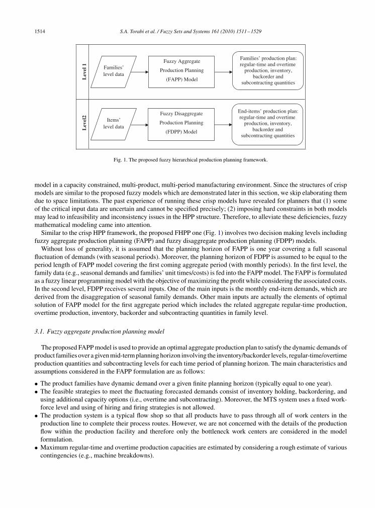
Fig. 1. The proposed fuzzy hierarchical production planning framework.

model in a capacity constrained, multi-product, multi-period manufacturing environment. Since the structures of crispmodels are similar to the proposed fuzzy models which are demonstrated later in this section, we skip elaborating themdue to space limitations. The past experience of running these crisp models have revealed for planners that (1) someof the critical input data are uncertain and cannot be specified precisely; (2) imposing hard constraints in both modelsmay lead to infeasibility and inconsistency issues in the HPP structure. Therefore, to alleviate these deficiencies, fuzzymathematical modeling came into attention.

Similar to the crisp HPP framework, the proposed FHPP one (Fig. 1) involves two decision making levels includingfuzzy aggregate production planning (FAPP) and fuzzy disaggregate production planning (FDPP) models.

Without loss of generality, it is assumed that the planning horizon of FAPP is one year covering a full seasonalfluctuation of demands (with seasonal periods). Moreover, the planning horizon of FDPP is assumed to be equal to theperiod length of FAPP model covering the first coming aggregate period (with monthly periods). In the first level, thefamily data (e.g., seasonal demands and families’ unit times/costs) is fed into the FAPP model. The FAPP is formulatedas a fuzzy linear programming model with the objective of maximizing the profit while considering the associated costs.In the second level, FDPP receives several inputs. One of the main inputs is the monthly end-item demands, which arederived from the disaggregation of seasonal family demands. Other main inputs are actually the elements of optimalsolution of FAPP model for the first aggregate period which includes the related aggregate regular-time production,overtime production, inventory, backorder and subcontracting quantities in family level.

3.1. Fuzzy aggregate production planning model

The proposed FAPP model is used to provide an optimal aggregate production plan to satisfy the dynamic demands ofproduct families over a given mid-term planning horizon involving the inventory/backorder levels, regular-time/overtimeproduction quantities and subcontracting levels for each time period of planning horizon. The main characteristics andassumptions considered in the FAPP formulation are as follows:

• The product families have dynamic demand over a given finite planning horizon (typically equal to one year).• The feasible strategies to meet the fluctuating forecasted demands consist of inventory holding, backordering, and

using additional capacity options (i.e., overtime and subcontracting). Moreover, the MTS system uses a fixed work-force level and using of hiring and firing strategies is not allowed.

• The production system is a typical flow shop so that all products have to pass through all of work centers in theproduction line to complete their process routes. However, we are not concerned with the details of the productionflow within the production facility and therefore only the bottleneck work centers are considered in the modelformulation.

• Maximum regular-time and overtime production capacities are estimated by considering a rough estimate of variouscontingencies (e.g., machine breakdowns).


AoAmAp

1

�A

Fig. 2. The triangular possibility distribution of fuzzy parameter A.

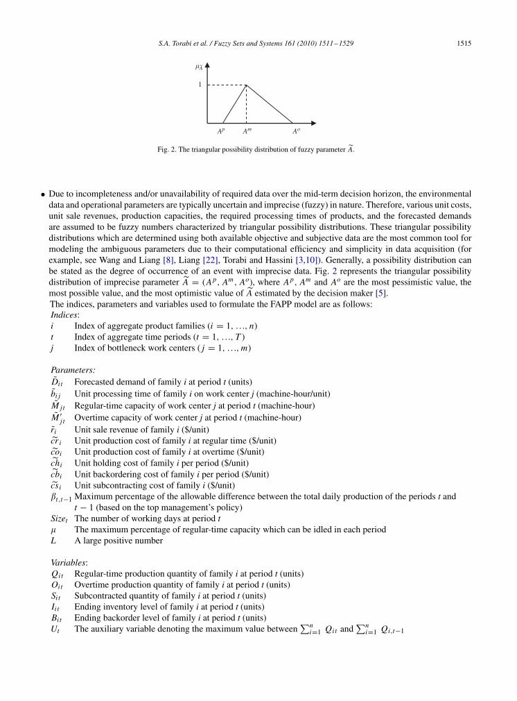
• Due to incompleteness and/or unavailability of required data over the mid-term decision horizon, the environmentaldata and operational parameters are typically uncertain and imprecise (fuzzy) in nature. Therefore, various unit costs,unit sale revenues, production capacities, the required processing times of products, and the forecasted demandsare assumed to be fuzzy numbers characterized by triangular possibility distributions. These triangular possibilitydistributions which are determined using both available objective and subjective data are the most common tool formodeling the ambiguous parameters due to their computational efficiency and simplicity in data acquisition (forexample, see Wang and Liang [8], Liang [22], Torabi and Hassini [3,10]). Generally, a possibility distribution canbe stated as the degree of occurrence of an event with imprecise data. Fig. 2 represents the triangular possibilitydistribution of imprecise parameter A = (Ap, Am, Ao), where Ap, Am and Ao are the most pessimistic value, themost possible value, and the most optimistic value of A estimated by the decision maker [5].The indices, parameters and variables used to formulate the FAPP model are as follows:Indices:i Index of aggregate product families (i = 1, . . ., n)t Index of aggregate time periods (t = 1, . . ., T )j Index of bottleneck work centers ( j = 1, . . ., m)

Parameters:Dit Forecasted demand of family i at period t (units)bi j Unit processing time of family i on work center j (machine-hour/unit)M jt Regular-time capacity of work center j at period t (machine-hour)M ′

j t Overtime capacity of work center j at period t (machine-hour)ri Unit sale revenue of family i ($/unit)cr i Unit production cost of family i at regular time ($/unit)coi Unit production cost of family i at overtime ($/unit)chi Unit holding cost of family i per period ($/unit)cbi Unit backordering cost of family i per period ($/unit)csi Unit subcontracting cost of family i ($/unit)�t,t−1 Maximum percentage of the allowable difference between the total daily production of the periods t and

t − 1 (based on the top management’s policy)Sizet The number of working days at period t� The maximum percentage of regular-time capacity which can be idled in each periodL A large positive number

Variables:Qit Regular-time production quantity of family i at period t (units)Oit Overtime production quantity of family i at period t (units)Sit Subcontracted quantity of family i at period t (units)Ii t Ending inventory level of family i at period t (units)Bit Ending backorder level of family i at period t (units)Ut The auxiliary variable denoting the maximum value between

∑ni=1 Qit and

∑ni=1 Qi,t−1


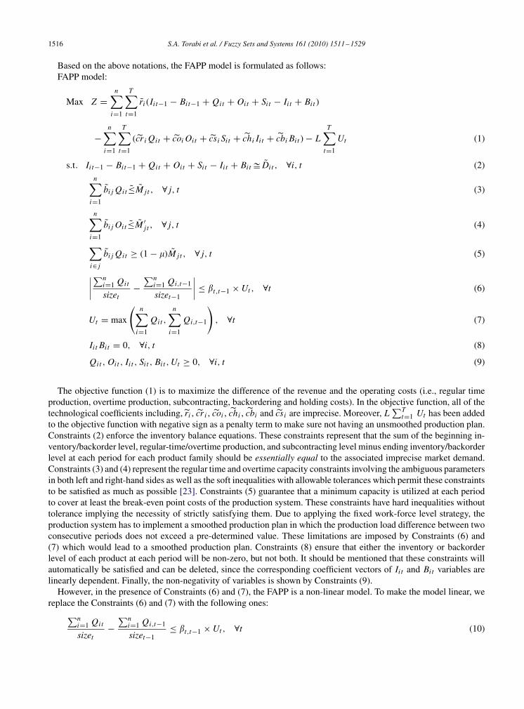
Based on the above notations, the FAPP model is formulated as follows:FAPP model:

Max Z =n∑

i=1

T∑t=1

ri (Ii t−1 − Bit−1 + Qit + Oit + Sit − Ii t + Bit )

−n∑

i=1

T∑t=1

(cr i Qit + coi Oit + csi Sit + chi Ii t + cbi Bit ) − LT∑

t=1

Ut (1)

s.t. Ii t−1 − Bit−1 + Qit + Oit + Sit − Ii t + Bit�Dit , ∀i, t (2)n∑

i=1

bi j Qit ≤M jt , ∀ j, t (3)

n∑i=1

bi j Oit ≤M ′j t , ∀ j, t (4)

∑i∈ j

bi j Qit ≥ (1 − �)M jt , ∀ j, t (5)

∣∣∣∣∑ni=1 Qit

sizet−∑n

i=1 Qi,t−1

sizet−1

∣∣∣∣ ≤ �t,t−1 × Ut , ∀t (6)

Ut = max

(n∑

i=1

Qit ,

n∑i=1

Qi,t−1

), ∀t (7)

Ii t Bit = 0, ∀i, t (8)

Qit , Oit , Ii t , Sit , Bit , Ut ≥ 0, ∀i, t (9)

The objective function (1) is to maximize the difference of the revenue and the operating costs (i.e., regular timeproduction, overtime production, subcontracting, backordering and holding costs). In the objective function, all of thetechnological coefficients including, ri , cr i , coi , chi , cbi and csi are imprecise. Moreover, L

∑Tt=1 Ut has been added

to the objective function with negative sign as a penalty term to make sure not having an unsmoothed production plan.Constraints (2) enforce the inventory balance equations. These constraints represent that the sum of the beginning in-ventory/backorder level, regular-time/overtime production, and subcontracting level minus ending inventory/backorderlevel at each period for each product family should be essentially equal to the associated imprecise market demand.Constraints (3) and (4) represent the regular time and overtime capacity constraints involving the ambiguous parametersin both left and right-hand sides as well as the soft inequalities with allowable tolerances which permit these constraintsto be satisfied as much as possible [23]. Constraints (5) guarantee that a minimum capacity is utilized at each periodto cover at least the break-even point costs of the production system. These constraints have hard inequalities withouttolerance implying the necessity of strictly satisfying them. Due to applying the fixed work-force level strategy, theproduction system has to implement a smoothed production plan in which the production load difference between twoconsecutive periods does not exceed a pre-determined value. These limitations are imposed by Constraints (6) and(7) which would lead to a smoothed production plan. Constraints (8) ensure that either the inventory or backorderlevel of each product at each period will be non-zero, but not both. It should be mentioned that these constraints willautomatically be satisfied and can be deleted, since the corresponding coefficient vectors of Ii t and Bit variables arelinearly dependent. Finally, the non-negativity of variables is shown by Constraints (9).

However, in the presence of Constraints (6) and (7), the FAPP is a non-linear model. To make the model linear, wereplace the Constraints (6) and (7) with the following ones:∑n

i=1 Qit

sizet−∑n

i=1 Qi,t−1

sizet−1≤ �t,t−1 × Ut , ∀t (10)


∑ni=1 Qit

sizet−∑n

i=1 Qi,t−1

sizet−1≥ −(�t,t−1 × Ut ), ∀t (11)

n∑i=1

Qit ≤ Ut , ∀t (12)

n∑i=1

Qi,t−1 ≤ Ut , ∀t (13)

Note that the variable Ut cannot be as large as possible because of its negative sign in objective function. Therefore, byconsidering this fact and recalling the following well-known equivalency, we can easily conclude that the constraints(10)–(13) are equivalent to (6) and (7) ones:

|x | ≤ a ⇔ −a ≤ x ≤ a, ∀a ≥ 0

3.2. Fuzzy disaggregate production planning model

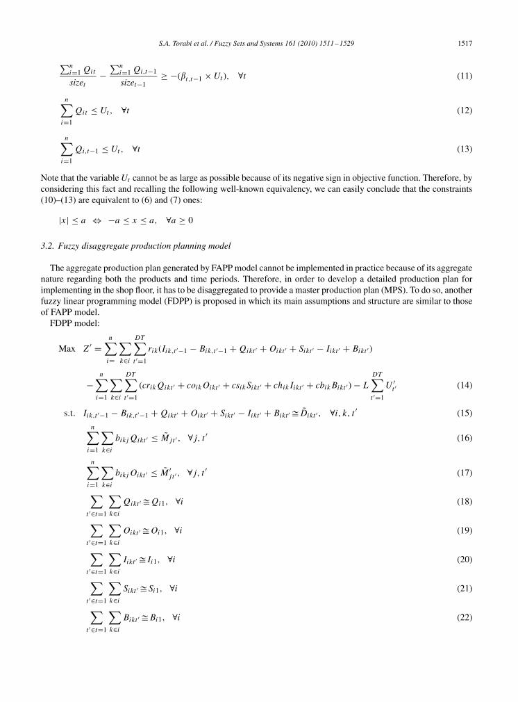
The aggregate production plan generated by FAPP model cannot be implemented in practice because of its aggregatenature regarding both the products and time periods. Therefore, in order to develop a detailed production plan forimplementing in the shop floor, it has to be disaggregated to provide a master production plan (MPS). To do so, anotherfuzzy linear programming model (FDPP) is proposed in which its main assumptions and structure are similar to thoseof FAPP model.

FDPP model:

Max Z ′ =n∑

i=

∑k∈i

DT∑t ′=1

rik(Iik,t ′−1 − Bik,t ′−1 + Qikt ′ + Oikt ′ + Sikt ′ − Iikt ′ + Bikt ′)

−n∑

i=1

∑k∈i

DT∑t ′=1

(crik Qikt ′ + coik Oikt ′ + csik Sikt ′ + chik Iikt ′ + cbik Bikt ′ ) − LDT∑

t ′=1

U ′t ′ (14)

s.t. Iik,t ′−1 − Bik,t ′−1 + Qikt ′ + Oikt ′ + Sikt ′ − Iikt ′ + Bikt ′�Dikt ′ , ∀i, k, t ′ (15)

n∑i=1

∑k∈i

bik j Qikt ′ ≤ M jt ′ , ∀ j, t ′ (16)

n∑i=1

∑k∈i

bik j Oikt ′ ≤ M ′j t ′ , ∀ j, t ′ (17)

∑t ′∈t=1

∑k∈i

Qikt ′�Qi1, ∀i (18)

∑t ′∈t=1

∑k∈i

Oikt ′�Oi1, ∀i (19)

∑t ′∈t=1

∑k∈i

Iikt ′�Ii1, ∀i (20)

∑t ′∈t=1

∑k∈i

Sikt ′�Si1, ∀i (21)

∑t ′∈t=1

∑k∈i

Bikt ′�Bi1, ∀i (22)


∑ni=1

∑k∈i Qikt ′

sizet ′−∑n

i=1∑

k∈i Qikt ′−1

sizet ′−1≤ �t ′,t ′−1 × U ′

t ′ , ∀t ′ (23)

∑ni=1

∑k∈i Qikt ′

sizet ′−∑n

i=1∑

k∈i Qikt ′−1

sizet ′−1≥ −(�t ′,t ′−1 × U ′

t ′ ), ∀t ′ (24)

n∑i=1

∑k∈i

Qikt ′ ≤ U ′t ′ , ∀t ′ (25)

n∑i=1

∑k∈i

Qikt ′−1 ≤ U ′t ′−1, ∀t ′ (26)

n∑i=1

∑k∈i

bik j Qikt ′ ≥ (1 − �)M jt ′ , ∀ j, t ′ (27)

Qikt ′ , Iikt ′ , Oikt ′ , Sikt ′ , Bikt ′ ≥ 0, ∀i, k, t ′ (28)

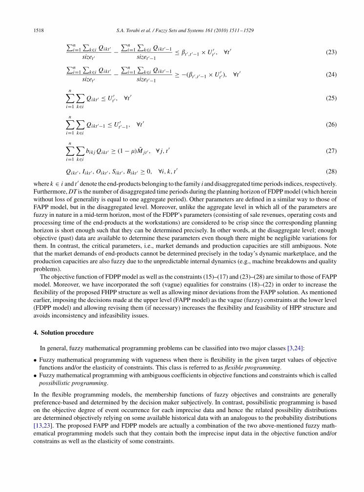
where k ∈ i and t ′ denote the end-products belonging to the family i and disaggregated time periods indices, respectively.Furthermore, DT is the number of disaggregated time periods during the planning horizon of FDPP model (which hereinwithout loss of generality is equal to one aggregate period). Other parameters are defined in a similar way to those ofFAPP model, but in the disaggregated level. Moreover, unlike the aggregate level in which all of the parameters arefuzzy in nature in a mid-term horizon, most of the FDPP’s parameters (consisting of sale revenues, operating costs andprocessing time of the end-products at the workstations) are considered to be crisp since the corresponding planninghorizon is short enough such that they can be determined precisely. In other words, at the disaggregate level; enoughobjective (past) data are available to determine these parameters even though there might be negligible variations forthem. In contrast, the critical parameters, i.e., market demands and production capacities are still ambiguous. Notethat the market demands of end-products cannot be determined precisely in the today’s dynamic marketplace, and theproduction capacities are also fuzzy due to the unpredictable internal dynamics (e.g., machine breakdowns and qualityproblems).

The objective function of FDPP model as well as the constraints (15)–(17) and (23)–(28) are similar to those of FAPPmodel. Moreover, we have incorporated the soft (vague) equalities for constrains (18)–(22) in order to increase theflexibility of the proposed FHPP structure as well as allowing minor deviations from the FAPP solution. As mentionedearlier, imposing the decisions made at the upper level (FAPP model) as the vague (fuzzy) constraints at the lower level(FDPP model) and allowing revising them (if necessary) increases the flexibility and feasibility of HPP structure andavoids inconsistency and infeasibility issues.

4. Solution procedure

In general, fuzzy mathematical programming problems can be classified into two major classes [3,24]:

• Fuzzy mathematical programming with vagueness when there is flexibility in the given target values of objectivefunctions and/or the elasticity of constraints. This class is referred to as flexible programming.

• Fuzzy mathematical programming with ambiguous coefficients in objective functions and constraints which is calledpossibilistic programming.

In the flexible programming models, the membership functions of fuzzy objectives and constraints are generallypreference-based and determined by the decision maker subjectively. In contrast, possibilistic programming is basedon the objective degree of event occurrence for each imprecise data and hence the related possibility distributionsare determined objectively relying on some available historical data with an analogous to the probability distributions[13,23]. The proposed FAPP and FDPP models are actually a combination of the two above-mentioned fuzzy math-ematical programming models such that they contain both the imprecise input data in the objective function and/orconstrains as well as the elasticity of some constraints.


In order to reach a preferred solution for the proposed FHPP structure, the associated mathematical programmingmodels should be converted into the equivalent crisp ones. In this regard, three main stages are considered as thesolution procedure for the proposed FHPP as follows:

(a) Converting the FAPP model into its equivalent auxiliary crisp model.(b) Converting the FDPP model into its equivalent auxiliary crisp model.(c) Applying an interactive fuzzy programming solution algorithm to obtain the final preferred solution.

Hereafter we first apply appropriate strategies to convert the proposed fuzzy models into the crisp ones, and thenpropose an interactive solution algorithm to solve the problem.

4.1. Formulating the FAPP as an auxiliary crisp model

In order to solve the FAPP model, it should be transformed to an auxiliary crisp model. To do so, we present efficientstrategies for converting the fuzzy objective function and soft constraints into the equivalent crisp equations.

4.1.1. Treating the imprecise objective functionThere are several approaches to cope with an objective function with imprecise parameters, among them we apply

the effective method proposed by Lai and Hwang [5] which has been considerably applied in the literature (for examplesee, Hsu and Wang [4], Wang and Liang [8], Torabi and Hassini [3]).

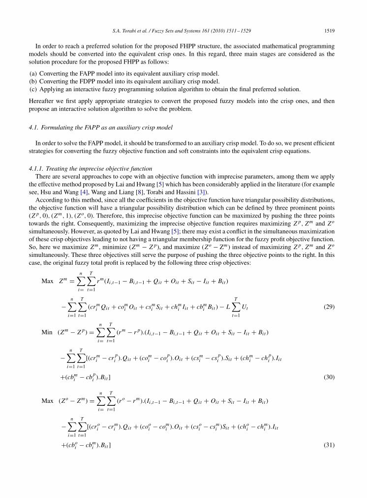
According to this method, since all the coefficients in the objective function have triangular possibility distributions,the objective function will have a triangular possibility distribution which can be defined by three prominent points(Z p, 0), (Zm, 1), (Zo, 0). Therefore, this imprecise objective function can be maximized by pushing the three pointstowards the right. Consequently, maximizing the imprecise objective function requires maximizing Z p, Zm and Zo

simultaneously. However, as quoted by Lai and Hwang [5]; there may exist a conflict in the simultaneous maximizationof these crisp objectives leading to not having a triangular membership function for the fuzzy profit objective function.So, here we maximize Zm , minimize (Zm − Z p), and maximize (Zo − Zm) instead of maximizing Z p, Zm and Zo

simultaneously. These three objectives still serve the purpose of pushing the three objective points to the right. In thiscase, the original fuzzy total profit is replaced by the following three crisp objectives:

Max Zm =n∑

i=

T∑t=1

rm(Ii,t−1 − Bi,t−1 + Qit + Oit + Sit − Ii t + Bit )

−n∑

i=1

T∑t=1

(crmi Qit + com

i Oit + csmi Sit + chm

i Iit + cbmi Bit ) − L

T∑t=1

Ut (29)

Min (Zm − Z p) =n∑

i=

T∑t=1

(rm − r p).(Ii,t−1 − Bi,t−1 + Qit + Oit + Sit − Ii t + Bit )

−n∑

i=1

T∑t=1

[(crmi − cr p

i ).Qit + (comi − cop

i ).Oit + (csmi − cs p

i ).Sit + (chmi − ch p

i ).Ii t

+(cbmi − cbp

i ).Bit ] (30)

Max (Zo − Zm) =n∑

i=

T∑t=1

(ro − rm).(Ii,t−1 − Bi,t−1 + Qit + Oit + Sit − Ii t + Bit )

−n∑

i=1

T∑t=1

[(croi − crm

i ).Qit + (cooi − com

i ).Oit + (csoi − csm

i )Sit + (choi − chm

i ).Ii t

+(cboi − cbm

i ).Bit ] (31)


b+pbb−p

1

a

�c

Fig. 3. A preference-based membership function of soft equation a�b.

4.1.2. Treating the soft constraintsThere are three different variants of the fuzzy constraints in the FAPP model. Regarding the constraints (2) up to (4)

we are dealing with the hybrid cases involving both the imprecise/ambiguous parameters (characterized by possibilitydistributions) and vague equalities/inequalities (characterized by preference-based membership functions). That is, inconstraints (2), there is an imprecise right-hand side along with a soft (vague) equation allowing some minor deviationwith a given tolerance. Moreover, the constraints (3) and (4) involve imprecise coefficients in both sides of the inequalityas well as the vague inequalities. Finally, in constraint (5), the coefficients of both sides are only imprecise. Anyway,to convert these soft constraints to the crisp ones, appropriate methods are applied for each one as follows.

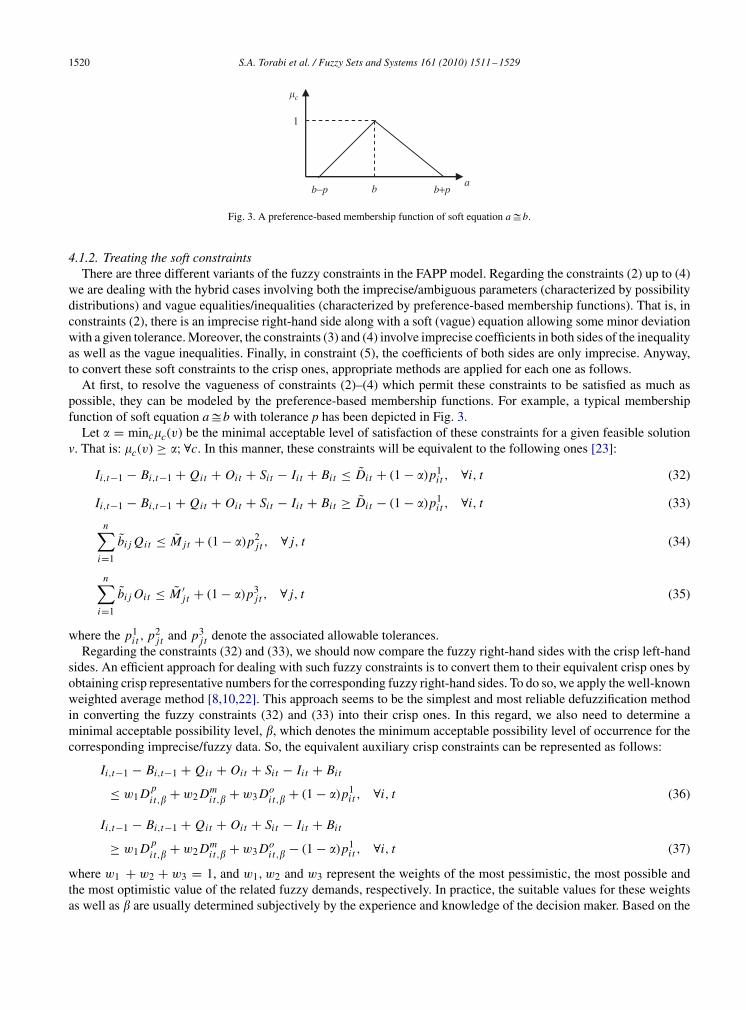
At first, to resolve the vagueness of constraints (2)–(4) which permit these constraints to be satisfied as much aspossible, they can be modeled by the preference-based membership functions. For example, a typical membershipfunction of soft equation a�b with tolerance p has been depicted in Fig. 3.

Let � = minc�c(v) be the minimal acceptable level of satisfaction of these constraints for a given feasible solutionv. That is: �c(v) ≥ �; ∀c. In this manner, these constraints will be equivalent to the following ones [23]:

Ii,t−1 − Bi,t−1 + Qit + Oit + Sit − Ii t + Bit ≤ Dit + (1 − �)p1i t , ∀i, t (32)

Ii,t−1 − Bi,t−1 + Qit + Oit + Sit − Ii t + Bit ≥ Dit − (1 − �)p1i t , ∀i, t (33)

n∑i=1

bi j Qit ≤ M jt + (1 − �)p2j t , ∀ j, t (34)

n∑i=1

bi j Oit ≤ M ′j t + (1 − �)p3

j t , ∀ j, t (35)

where the p1i t , p2

j t and p3j t denote the associated allowable tolerances.

Regarding the constraints (32) and (33), we should now compare the fuzzy right-hand sides with the crisp left-handsides. An efficient approach for dealing with such fuzzy constraints is to convert them to their equivalent crisp ones byobtaining crisp representative numbers for the corresponding fuzzy right-hand sides. To do so, we apply the well-knownweighted average method [8,10,22]. This approach seems to be the simplest and most reliable defuzzification methodin converting the fuzzy constraints (32) and (33) into their crisp ones. In this regard, we also need to determine aminimal acceptable possibility level, �, which denotes the minimum acceptable possibility level of occurrence for thecorresponding imprecise/fuzzy data. So, the equivalent auxiliary crisp constraints can be represented as follows:

Ii,t−1 − Bi,t−1 + Qit + Oit + Sit − Ii t + Bit

≤ w1 D pit,� + w2 Dm

it,� + w3 Doit,� + (1 − �)p1

i t , ∀i, t (36)

Ii,t−1 − Bi,t−1 + Qit + Oit + Sit − Ii t + Bit

≥ w1 D pit,� + w2 Dm

it,� + w3 Doit,� − (1 − �)p1

i t , ∀i, t (37)

where w1 + w2 + w3 = 1, and w1, w2 and w3 represent the weights of the most pessimistic, the most possible andthe most optimistic value of the related fuzzy demands, respectively. In practice, the suitable values for these weightsas well as � are usually determined subjectively by the experience and knowledge of the decision maker. Based on the


most likely value concept proposed by Lai and Hwang [5] and considering several relevant works [9,21,22], we setthese parameters to: w2 = 4

6 , w1 = w3 = 16 and � = 0.5 in our numerical experiments.

It is noteworthy that all the possibility distributions are assumed to be symmetrical here, thus we would haveDm

it,� = Dmit . Further, using �-cut concept of fuzzy set theory D p

it,�, Doit,� are determined as follows, respectively:

D pit,� = (Dm

it − D pit ) × � + D p

it , Doit,� = Do

it − (Doit − Dm

it ) × �.

Regarding the fuzzy constraints (5), (34) and (35), our problem is how to compare the fuzzy right-hand sides andleft-hand sides. In other words, we are dealing with fuzzy numbers ranking problem. An efficient approach for dealingwith such fuzzy constraints is to convert them with the three equivalent auxiliary constraints proposed by Ramik andRimanek [25] and followed by others (e.g., Lai and Hwang [5], Wang and Liang [8], Torabi and Hassini [3]). Forexample, based on this approach, we could replace the fuzzy constraints (5) with the following crisp ones:∑

i∈ j

bpi j,�Qit ≥ (1 − �)M p

jt,�, ∀ j (38)

∑i∈ j

bmi j,�Qit ≥ (1 − �)Mm

jt,�, ∀ j, t (39)

∑i∈ j

boi j,�Qit ≥ (1 − �)Mo

jt,�, ∀ j, t (40)

The same approach can be applied for constraints (34) and (35). In this manner, the original FAPP model is convertedinto an auxiliary crisp multi-objective linear programming (MOLP) one.

4.2. Formulating the FDPP as an auxiliary crisp model

Recalling the FDPP model, since the objective function (14) along with the constraints (23)–(26) is crisp; they donot need any changes. In contrast, for the soft constraints (15) up to (22) and (27), we can apply the same approachesas used in the FAPP model.

4.3. Applying an interactive solution algorithm

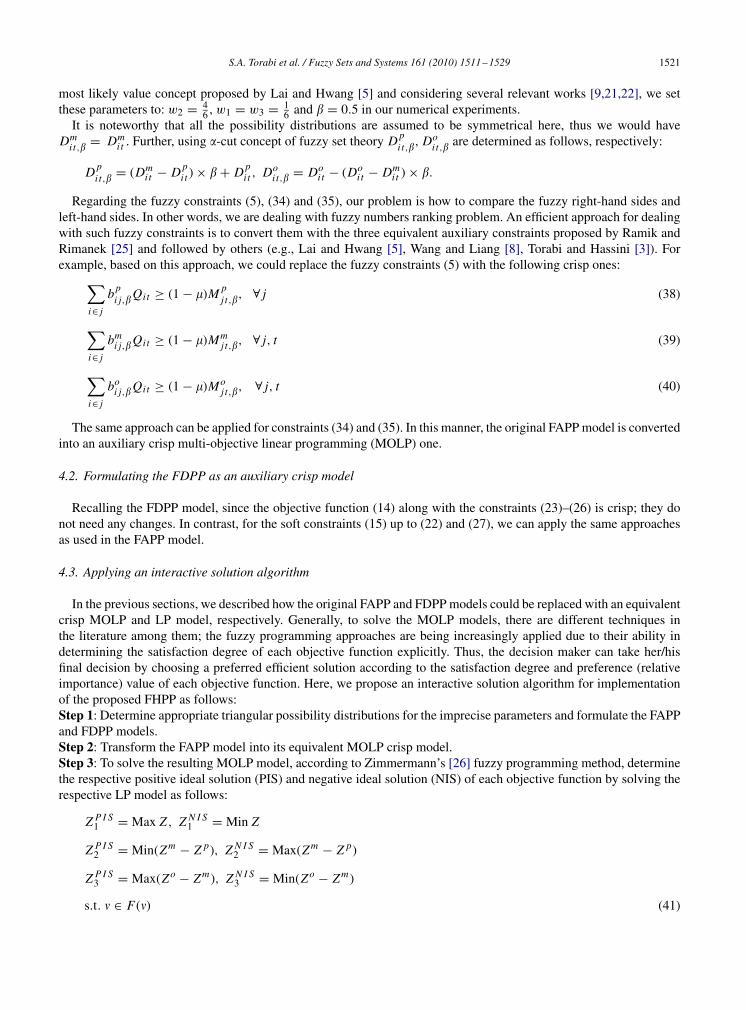
In the previous sections, we described how the original FAPP and FDPP models could be replaced with an equivalentcrisp MOLP and LP model, respectively. Generally, to solve the MOLP models, there are different techniques inthe literature among them; the fuzzy programming approaches are being increasingly applied due to their ability indetermining the satisfaction degree of each objective function explicitly. Thus, the decision maker can take her/hisfinal decision by choosing a preferred efficient solution according to the satisfaction degree and preference (relativeimportance) value of each objective function. Here, we propose an interactive solution algorithm for implementationof the proposed FHPP as follows:Step 1: Determine appropriate triangular possibility distributions for the imprecise parameters and formulate the FAPPand FDPP models.Step 2: Transform the FAPP model into its equivalent MOLP crisp model.Step 3: To solve the resulting MOLP model, according to Zimmermann’s [26] fuzzy programming method, determinethe respective positive ideal solution (PIS) and negative ideal solution (NIS) of each objective function by solving therespective LP model as follows:

Z P I S1 = Max Z , Z N I S

1 = Min Z

Z P I S2 = Min(Zm − Z p), Z N I S

2 = Max(Zm − Z p)

Z P I S3 = Max(Zo − Zm), Z N I S

3 = Min(Zo − Zm)

s.t. � ∈ F(�) (41)


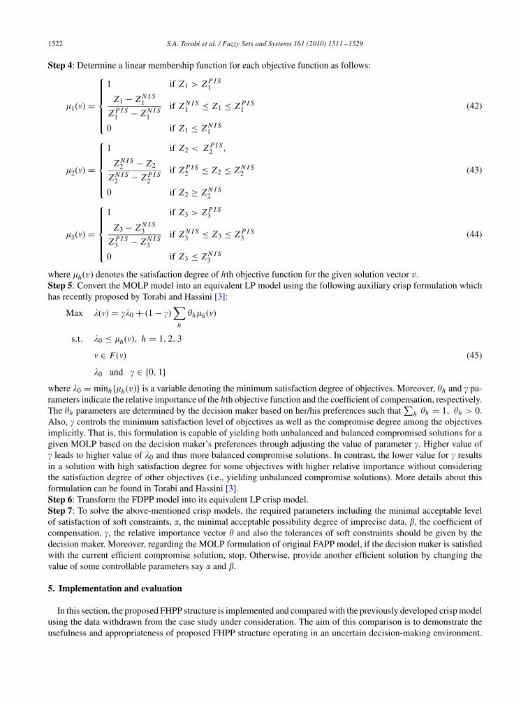
Step 4: Determine a linear membership function for each objective function as follows:

�1(�) =

⎧⎪⎪⎪⎪⎨⎪⎪⎪⎪⎩1 if Z1 > Z P I S

1

Z1 − Z N I S1

Z P I S1 − Z N I S

1

if Z N I S1 ≤ Z1 ≤ Z P I S

1

0 if Z1 ≤ Z N I S1

(42)

�2(�) =

⎧⎪⎪⎪⎪⎨⎪⎪⎪⎪⎩1 if Z2 < Z P I S

2 ,

Z N I S2 − Z2

Z N I S2 − Z P I S

2

if Z P I S2 ≤ Z2 ≤ Z N I S

2

0 if Z2 ≥ Z N I S2

(43)

�3(�) =

⎧⎪⎪⎪⎪⎨⎪⎪⎪⎪⎩1 if Z3 > Z P I S

3

Z3 − Z N I S3

Z P I S3 − Z N I S

3

if Z N I S3 ≤ Z3 ≤ Z P I S

3

0 if Z3 ≤ Z N I S3

(44)

where �h(v) denotes the satisfaction degree of hth objective function for the given solution vector v.Step 5: Convert the MOLP model into an equivalent LP model using the following auxiliary crisp formulation whichhas recently proposed by Torabi and Hassini [3]:

Max �(�) = ��0 + (1 − �)∑

h

�h�h(�)

s.t. �0 ≤ �h(�), h = 1, 2, 3

� ∈ F(�) (45)

�0 and � ∈ {0, 1}where �0 = minh{�h(v)} is a variable denoting the minimum satisfaction degree of objectives. Moreover, �h and � pa-rameters indicate the relative importance of the hth objective function and the coefficient of compensation, respectively.The �h parameters are determined by the decision maker based on her/his preferences such that

∑h �h = 1, �h > 0.

Also, � controls the minimum satisfaction level of objectives as well as the compromise degree among the objectivesimplicitly. That is, this formulation is capable of yielding both unbalanced and balanced compromised solutions for agiven MOLP based on the decision maker’s preferences through adjusting the value of parameter �. Higher value of� leads to higher value of �0 and thus more balanced compromise solutions. In contrast, the lower value for � resultsin a solution with high satisfaction degree for some objectives with higher relative importance without consideringthe satisfaction degree of other objectives (i.e., yielding unbalanced compromise solutions). More details about thisformulation can be found in Torabi and Hassini [3].Step 6: Transform the FDPP model into its equivalent LP crisp model.Step 7: To solve the above-mentioned crisp models, the required parameters including the minimal acceptable levelof satisfaction of soft constraints, �, the minimal acceptable possibility degree of imprecise data, �, the coefficient ofcompensation, �, the relative importance vector � and also the tolerances of soft constraints should be given by thedecision maker. Moreover, regarding the MOLP formulation of original FAPP model, if the decision maker is satisfiedwith the current efficient compromise solution, stop. Otherwise, provide another efficient solution by changing thevalue of some controllable parameters say � and �.

5. Implementation and evaluation

In this section, the proposed FHPP structure is implemented and compared with the previously developed crisp modelusing the data withdrawn from the case study under consideration. The aim of this comparison is to demonstrate theusefulness and appropriateness of proposed FHPP structure operating in an uncertain decision-making environment.


Table 1Aggregate demand data (Dit ) in product units.

F1 F2 F3 F4

Spring (16 000,20 000,24 000) (4800,6000,7400) (11 800,15 000,17 600) (14 000,17 250,20 600)Summer (18 400,23 100,27 700) (28 800,36 000,43 000) (44 000,52 000,66 400) (15 000,18 500,22 300)Autumn (18 300,23 600,28 000) (41 200,51 500,61 800) (44 000,55 000,66 000) (14 100,17 800,21 800)Winter (19 200,24 000,28 800) (33 200,41 500,54 000) (36 000, 45 000,54 000) (13 040,16 300,19 560)

Table 2Aggregate processing times (bi j ) in minutes.

F1 F2 F3 F4

INSERTEylet (0.37,0.46,0.55) (0.3,0.38,0.46) (0.54,0.65,0.74) (0.56,0.7,0.84)Seq. (1.26,1.58,1.9) (1.36,1.7,2.04) (1.12,1.4,1.68) (0.3,0.38,0.46)Axial (1.12,1.4,1.68) (1.13,1.4,165) (0.8,1.02,1.22) (0.26,0.33,0.4)Radial (1.08,1.35,1.62) (1.16,1.45,1.74) (1.2,1.5,1.8) (0.28,0.35,0.42)Jumper (0.27,0.34,0.41) 0 (0.42,0.5,0.61) 0

SMD 0 (1.44,1.8,2.16) 0 0

To do so, the corresponding results of both models are discussed and some managerial implications and characteristicsof the proposed FHPP approach are provided.

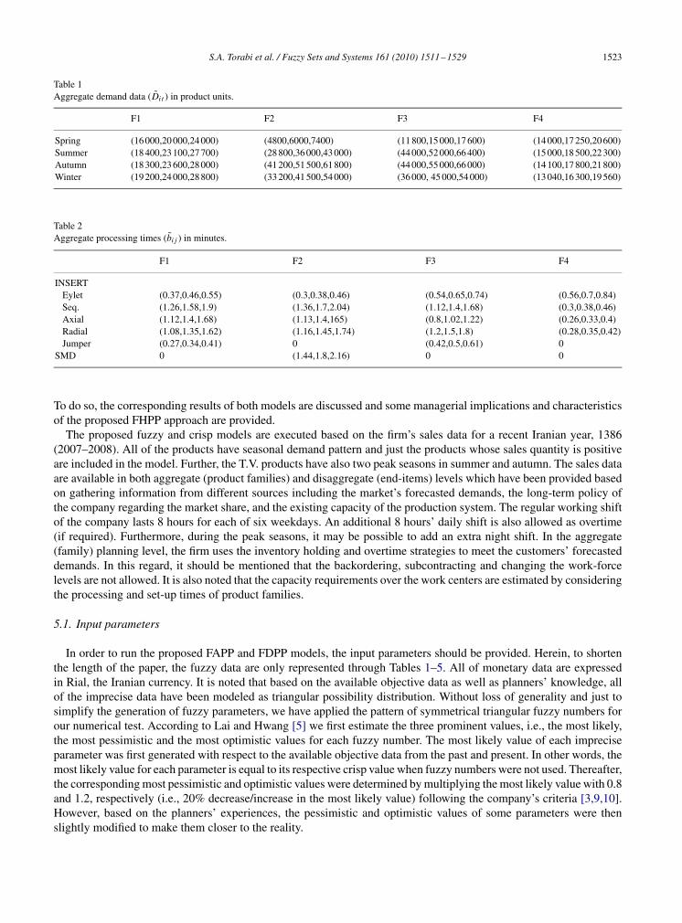
The proposed fuzzy and crisp models are executed based on the firm’s sales data for a recent Iranian year, 1386(2007–2008). All of the products have seasonal demand pattern and just the products whose sales quantity is positiveare included in the model. Further, the T.V. products have also two peak seasons in summer and autumn. The sales dataare available in both aggregate (product families) and disaggregate (end-items) levels which have been provided basedon gathering information from different sources including the market’s forecasted demands, the long-term policy ofthe company regarding the market share, and the existing capacity of the production system. The regular working shiftof the company lasts 8 hours for each of six weekdays. An additional 8 hours’ daily shift is also allowed as overtime(if required). Furthermore, during the peak seasons, it may be possible to add an extra night shift. In the aggregate(family) planning level, the firm uses the inventory holding and overtime strategies to meet the customers’ forecasteddemands. In this regard, it should be mentioned that the backordering, subcontracting and changing the work-forcelevels are not allowed. It is also noted that the capacity requirements over the work centers are estimated by consideringthe processing and set-up times of product families.

5.1. Input parameters

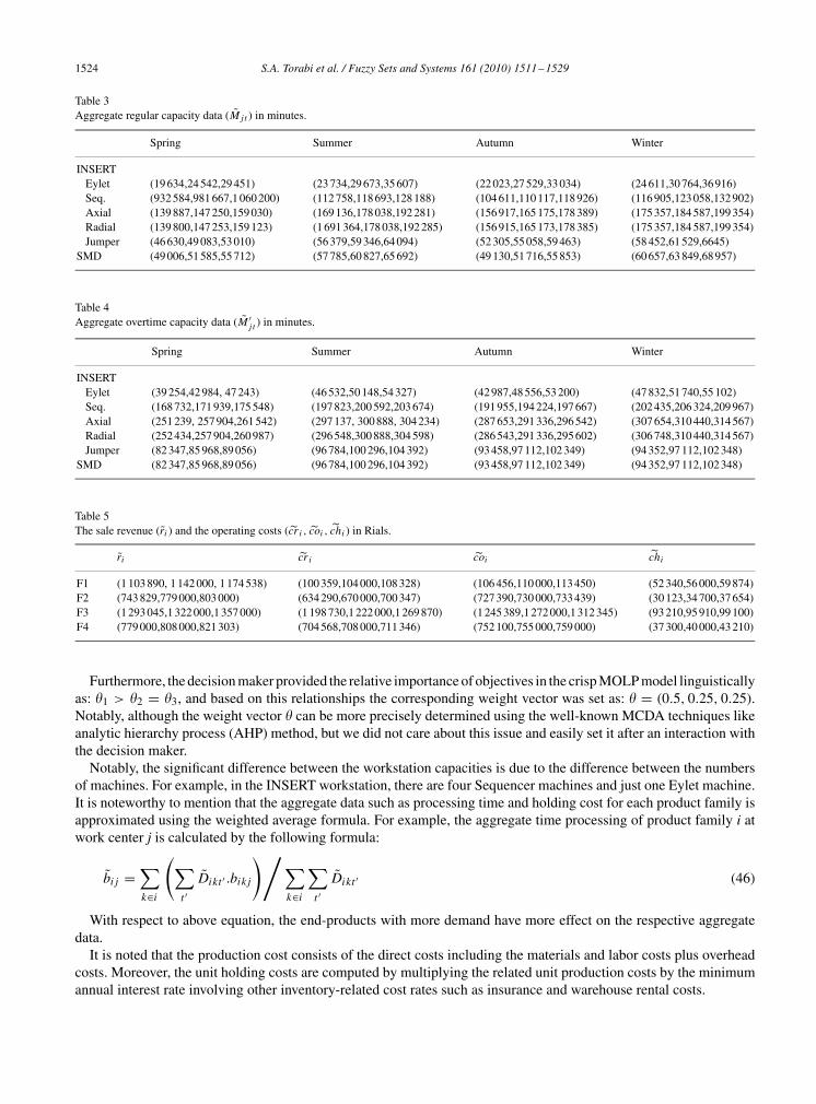
In order to run the proposed FAPP and FDPP models, the input parameters should be provided. Herein, to shortenthe length of the paper, the fuzzy data are only represented through Tables 1–5. All of monetary data are expressedin Rial, the Iranian currency. It is noted that based on the available objective data as well as planners’ knowledge, allof the imprecise data have been modeled as triangular possibility distribution. Without loss of generality and just tosimplify the generation of fuzzy parameters, we have applied the pattern of symmetrical triangular fuzzy numbers forour numerical test. According to Lai and Hwang [5] we first estimate the three prominent values, i.e., the most likely,the most pessimistic and the most optimistic values for each fuzzy number. The most likely value of each impreciseparameter was first generated with respect to the available objective data from the past and present. In other words, themost likely value for each parameter is equal to its respective crisp value when fuzzy numbers were not used. Thereafter,the corresponding most pessimistic and optimistic values were determined by multiplying the most likely value with 0.8and 1.2, respectively (i.e., 20% decrease/increase in the most likely value) following the company’s criteria [3,9,10].However, based on the planners’ experiences, the pessimistic and optimistic values of some parameters were thenslightly modified to make them closer to the reality.


Table 3Aggregate regular capacity data (M jt ) in minutes.

Spring Summer Autumn Winter

INSERTEylet (19 634,24 542,29 451) (23 734,29 673,35 607) (22 023,27 529,33 034) (24 611,30 764,36 916)Seq. (932 584,981 667,1 060 200) (112 758,118 693,128 188) (104 611,110 117,118 926) (116 905,123 058,132 902)Axial (139 887,147 250,159 030) (169 136,178 038,192 281) (156 917,165 175,178 389) (175 357,184 587,199 354)Radial (139 800,147 253,159 123) (1 691 364,178 038,192 285) (156 915,165 173,178 385) (175 357,184 587,199 354)Jumper (46 630,49 083,53 010) (56 379,59 346,64 094) (52 305,55 058,59 463) (58 452,61 529,6645)

SMD (49 006,51 585,55 712) (57 785,60 827,65 692) (49 130,51 716,55 853) (60 657,63 849,68 957)

Table 4Aggregate overtime capacity data (M ′

j t ) in minutes.


INSERTEylet (39 254,42 984, 47 243) (46 532,50 148,54 327) (42 987,48 556,53 200) (47 832,51 740,55 102)Seq. (168 732,171 939,175 548) (197 823,200 592,203 674) (191 955,194 224,197 667) (202 435,206 324,209 967)Axial (251 239, 257 904,261 542) (297 137, 300 888, 304 234) (287 653,291 336,296 542) (307 654,310 440,314 567)Radial (252 434,257 904,260 987) (296 548,300 888,304 598) (286 543,291 336,295 602) (306 748,310 440,314 567)Jumper (82 347,85 968,89 056) (96 784,100 296,104 392) (93 458,97 112,102 349) (94 352,97 112,102 348)

SMD (82 347,85 968,89 056) (96 784,100 296,104 392) (93 458,97 112,102 349) (94 352,97 112,102 348)

Table 5The sale revenue (ri ) and the operating costs (cr i , coi , chi ) in Rials.

ri cr i coi chi

F1 (1 103 890, 1 142 000, 1 174 538) (100 359,104 000,108 328) (106 456,110 000,113 450) (52 340,56 000,59 874)F2 (743 829,779 000,803 000) (634 290,670 000,700 347) (727 390,730 000,733 439) (30 123,34 700,37 654)F3 (1 293 045,1 322 000,1 357 000) (1 198 730,1 222 000,1 269 870) (1 245 389,1 272 000,1 312 345) (93 210,95 910,99 100)F4 (779 000,808 000,821 303) (704 568,708 000,711 346) (752 100,755 000,759 000) (37 300,40 000,43 210)

Furthermore, the decision maker provided the relative importance of objectives in the crisp MOLP model linguisticallyas: �1 > �2 = �3, and based on this relationships the corresponding weight vector was set as: � = (0.5, 0.25, 0.25).Notably, although the weight vector � can be more precisely determined using the well-known MCDA techniques likeanalytic hierarchy process (AHP) method, but we did not care about this issue and easily set it after an interaction withthe decision maker.

Notably, the significant difference between the workstation capacities is due to the difference between the numbersof machines. For example, in the INSERT workstation, there are four Sequencer machines and just one Eylet machine.It is noteworthy to mention that the aggregate data such as processing time and holding cost for each product family isapproximated using the weighted average formula. For example, the aggregate time processing of product family i atwork center j is calculated by the following formula:

bi j =∑k∈i

(∑t ′

Dikt ′ .bik j

)/∑k∈i

∑t ′

Dikt ′ (46)

With respect to above equation, the end-products with more demand have more effect on the respective aggregatedata.

It is noted that the production cost consists of the direct costs including the materials and labor costs plus overheadcosts. Moreover, the unit holding costs are computed by multiplying the related unit production costs by the minimumannual interest rate involving other inventory-related cost rates such as insurance and warehouse rental costs.


Table 6The aggregate plan developed by the proposed FHPP.


A B C A B C A B C A B C

F1 23 715 4000 0 6238 0 0 5741 0 1659 0 0 9200F2 23 909 4000 6504 3729 0 17 271 3645 0 29 045 10 518 0 0F3 7310 9000 26 261 0 17 095 41 296 0 8548 24 452 0 4273 826F4 0 5000 30 318 6272 2500 20 927 5230 1250 25 821 5721 625 3434

A: Production, B: Inventory, C: Overtime.

Table 7The disaggregate plan developed by the proposed FHPP.

March April May

Total production 17 950 18 400 18 200Total inventory 4000 8800 9120Overtime 18 200 23 450 21 300Production cost 1.7E+10 1.6E+10 1.5E+10Inventory cost 2.7E+09 4.9E+09 6.2E+09Overtime cost 1.3E+10 1.7E+10 1.5E+10Total cost 3.3E+10 3.8E+10 3.6E+10

5.2. Implementation

To validate the effectiveness of the proposed FHPP model, it has been implemented in the company under consider-ation. The respective outputs involve an annual aggregate production plan for product families with seasonal periodsstarting with spring based on Iranian calendar, and a disaggregated production plan (MPS) for end items with monthlyperiods of coming season. Aggregate production plan is periodically updated based on the rolling horizon concept con-sidering the most recent data especially regarding the demand data at the beginning of each season. Also, the companyshould stock some inventory as safety stock for each end-product at the beginning of planning horizon based on themanagement’s policy to be able to meet the unpredicted demands. Consequently, the safety stock for each end-productis equal to 100 units.

All of the mathematical models were developed by Lingo 8.0 modeling language. To solve the FAPP, the valueof � was set to 0.4. Recalling the preference relationship �1 > �2 = �3 quoted by the decision maker, the reasonfor selecting � = 0.4 was that the Z1 was the most important objective, and therefore getting somewhat unbalancedcompromise solutions with higher satisfaction degree for Z1 was of particular interest. In this respect, after some initialexperiments, it was concluded that any value for � between 0.3 and 0.6 could be appropriate in most of the probleminstances to get a compromise solution with �1 > �2 ≈ �3 property, among them, � = 0.4 was selected.

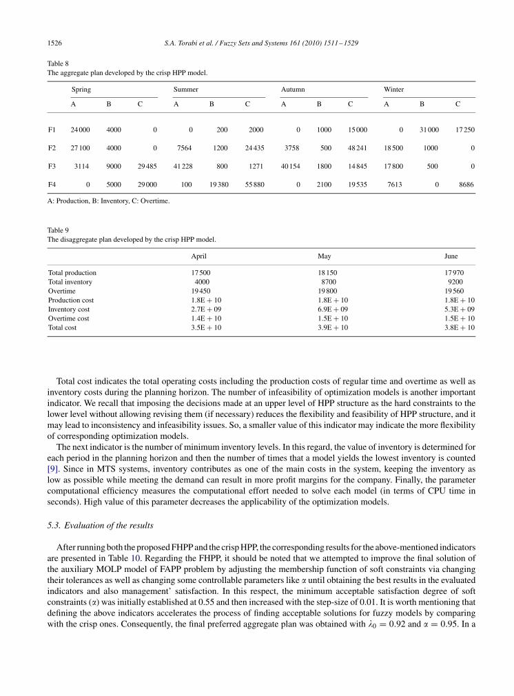
After obtaining the annual aggregate plan, the production plan of only first period (season) is disaggregated viaFDPP model to obtain a monthly production plan for end-items. The resulting aggregate and disaggregate plans of theproposed FHPP at the beginning of the planning horizon have been provided in Tables 6 and 7, respectively. In orderto evaluate the proposed FHPP model, we compare the outputs of the proposed FAPP and FDPP models with thoseof previously used crisp version of these models in which all of the data are assumed to be crisp considering the mostlikely value of each imprecise parameter. Tables 8 and 9 show the results obtained from these crisp models.

To compare the fuzzy HPP model with the currently used crisp HPP one, the following indicators are defined:

(i) Total cost.(ii) Number of infeasibility.

(iii) Number of minimum inventory levels.(iv) Computational efficiency.


Table 8The aggregate plan developed by the crisp HPP model.


A B C A B C A B C A B C

F1 24 000 4000 0 0 200 2000 0 1000 15 000 0 31 000 17 250

F2 27 100 4000 0 7564 1200 24 435 3758 500 48 241 18 500 1000 0

F3 3114 9000 29 485 41 228 800 1271 40 154 1800 14 845 17 800 500 0

F4 0 5000 29 000 100 19 380 55 880 0 2100 19 535 7613 0 8686

A: Production, B: Inventory, C: Overtime.

Table 9The disaggregate plan developed by the crisp HPP model.

April May June

Total production 17 500 18 150 17 970Total inventory 4000 8700 9200Overtime 19 450 19 800 19 560Production cost 1.8E + 10 1.8E + 10 1.8E + 10Inventory cost 2.7E + 09 6.9E + 09 5.3E + 09Overtime cost 1.4E + 10 1.5E + 10 1.5E + 10Total cost 3.5E + 10 3.9E + 10 3.8E + 10

Total cost indicates the total operating costs including the production costs of regular time and overtime as well asinventory costs during the planning horizon. The number of infeasibility of optimization models is another importantindicator. We recall that imposing the decisions made at an upper level of HPP structure as the hard constraints to thelower level without allowing revising them (if necessary) reduces the flexibility and feasibility of HPP structure, and itmay lead to inconsistency and infeasibility issues. So, a smaller value of this indicator may indicate the more flexibilityof corresponding optimization models.

The next indicator is the number of minimum inventory levels. In this regard, the value of inventory is determined foreach period in the planning horizon and then the number of times that a model yields the lowest inventory is counted[9]. Since in MTS systems, inventory contributes as one of the main costs in the system, keeping the inventory aslow as possible while meeting the demand can result in more profit margins for the company. Finally, the parametercomputational efficiency measures the computational effort needed to solve each model (in terms of CPU time inseconds). High value of this parameter decreases the applicability of the optimization models.

5.3. Evaluation of the results

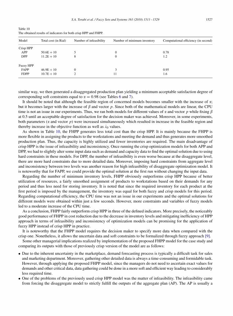
After running both the proposed FHPP and the crisp HPP, the corresponding results for the above-mentioned indicatorsare presented in Table 10. Regarding the FHPP, it should be noted that we attempted to improve the final solution ofthe auxiliary MOLP model of FAPP problem by adjusting the membership function of soft constraints via changingtheir tolerances as well as changing some controllable parameters like � until obtaining the best results in the evaluatedindicators and also management’ satisfaction. In this respect, the minimum acceptable satisfaction degree of softconstraints (�) was initially established at 0.55 and then increased with the step-size of 0.01. It is worth mentioning thatdefining the above indicators accelerates the process of finding acceptable solutions for fuzzy models by comparingwith the crisp ones. Consequently, the final preferred aggregate plan was obtained with �0 = 0.92 and � = 0.95. In a


Table 10The obtained results of indicators for both crisp HPP and FHPP.

Model Total cost (in Rial) Number of infeasibility Number of minimum inventory Computational efficiency (in second)

Crisp HPPAPP 50.6E + 10 5 0 0.78DPP 11.2E + 10 8 0 1.2

Fuzzy HPPFAPP 46.9E + 10 0 3 0.95FDPP 10.7E + 10 2 11 1.6

similar way, we then generated a disaggregated production plan yielding a minimum acceptable satisfaction degree ofcorresponding soft constraints equal to � = 0.98 (see Tables 6 and 7).

It should be noted that although the feasible region of concerned models becomes smaller with the increase of �;but it becomes larger with the increase of � and vector p. Since both of the mathematical models are linear, the CPUtime is not an issue in our experiments. Thus, we ran both models for different values of � and vector p while fixing �at 0.5 until an acceptable degree of satisfaction for the decision maker was achieved. Moreover, in some experiments,both parameters (� and vector p) were increased simultaneously which resulted in increase in the feasible region andthereby increase in the objective function as well as �0 values.

As shown in Table 10, the FHPP generates less total cost than the crisp HPP. It is mainly because the FHPP ismore flexible in assigning the products to the workstations and meeting the demand and thus generates more smoothedproduction plan. Thus, the capacity is highly utilized and fewer inventories are required. The main disadvantage ofcrisp HPP is the issue of infeasibility and inconsistency. Once running the crisp optimization models for both APP andDPP, we had to slightly alter some input data such as demand and capacity data to find the optimal solution due to usinghard constraints in these models. For DPP, the number of infeasibility is even worse because at the disaggregate level,there are more hard constraints due to more detailed data. Moreover, imposing hard constraints from aggregate leveland inconsistency between two levels was another reason for high infeasibility of disaggregate optimization model. Itis noteworthy that for FAPP, we could provide the optimal solution at the first run without changing the input data.

Regarding the number of minimum inventory levels, FHPP obviously outperforms crisp HPP because of betterutilization of resources, a fairly smoothed assignment of products to workstations based on their demands for anyperiod and thus less need for storing inventory. It is noted that since the required inventory for each product at thefirst period is imposed by the management, the inventory was equal for both fuzzy and crisp models for this period.Regarding computational efficiency, the CPU time was not an issue in our experiments and the optimal solutions fordifferent models were obtained within just a few seconds. However, more constraints and variables of fuzzy modelsled to a moderate increase of the CPU time.

As a conclusion, FHPP fairly outperform crisp HPP in three of the defined indicators. More precisely, the noticeablygood performance of FHPP in cost reduction due to the decrease in inventory levels and mitigating inefficiency of HPPapproach in terms of infeasibility and inconsistency of optimization models can be promising for the application offuzzy HPP instead of crisp HPP in practice.

It is noteworthy that the FHPP model requires the decision maker to specify more data when compared with thecrisp one. Nonetheless, it allows the uncertain data and soft constraints to be formalized through fuzzy approach [9].

Some other managerial implications realized by implementation of the proposed FHPP model for the case study andcomparing its outputs with those of previously crisp version of the model are as follows:

• Due to the inherent uncertainty in the marketplace, demand forecasting process is typically a difficult task for salesand marketing department. Moreover, gathering other detailed data is always a time-consuming and formidable task.However, through applying the proposed FHPP model, since the managers do not need to ascertain exact values fordemands and other critical data, data gathering could be done in a more soft and efficient way leading to considerablyless required time.

• One of the problems of the previously used crisp HPP model was the matter of infeasibility. The infeasibility camefrom forcing the disaggregate model to strictly fulfill the outputs of the aggregate plan (AP). The AP is usually a


rough plan while in the lower level, both the data and resulting MPS are more detailed and therefore more accurate.So, it seems reasonable to let the disaggregate model to fulfill the outcomes of the AP to some degree allowing someminor deviations. Doing so is now possible through the proposed FHPP model by applying a soft approach.

• Because of offering flexibility in the model formulation and making possible to generate various production plansin an interactive way, the proposed FHPP model leads to a more preferred and reliable solution. That is, the finalpreferred production plan can be found by using the proposed interactive algorithm until an acceptable degree ofsatisfaction for the decision maker is achieved with respect to the defined indicators.

In summary, we can conclude that based on the results of the case study, the proposed FHPP model can be consideredas an appropriate framework to generate preferred production plans in uncertain environments involving imprecise/fuzzyinput parameters as well as vague consistency constraints through an interactive solution procedure.

6. Concluding remarks

Production planning is a formidable task due to its hierarchical nature and existing highly dynamic and uncertainenvironment both internally and externally. Usually, in order to tackle these complexity features of the productionplanning problems, the hierarchical production planning framework is applied as an efficient approach. However,inherent uncertainty in the critical input parameters such as forecasted market demands and production capacity levelsas well as imposing hard (crisp) constraints from the high level as the inputs of inferior level can lead to the infeasibilityand inconsistency in the HPP structure. In this paper, we propose a novel FHPP model to incorporate the imprecise dataas well as soft constraints into the problem formulation. An interactive solution algorithm is also presented to solve theunderlying FHPP models hierarchically. The results obtained from a real industrial case study shows the superiority ofthe proposed FHPP over the crisp HPP one in which the unfeasibility issue while solving the disaggregate productionplanning model is removed and also the consistency between APP and DPP outputs is increased.

In brief, the merits of the proposed FHPP model can be summarized as: (1) improving the practicality of the HPPapproach by making it possible to consider inherent ambiguousness in the critical data and allowing minor deviationswhen transforming the aggregate plan into the disaggregated (master) plan through introducing soft (vague) constraintsin the DPP model, and (2) removing the infeasibility and inconsistency issues of HPP approach by offering requiredflexibility in the model formulation and making it possible to generate a more preferred and reliable production planin an interaction way with the decision maker. It should be noted that the underlying concepts and methods used forthe proposed FHPP model can easily be applied to similar production planning problems in practice.

There are some directions for further research in this area. One of the main directions is regard to develop a three-levelFHPP model adding the scheduling level for the shop floor where the rate of uncertainty is relatively high. Moreover,a similar approach can be developed for improving the HPP structure in make-to-order (MTO) systems. Since thenumber of MTO orders cannot be predicted in advance, using the fuzzy approach for planning the MTO products willbe definitely an efficient approach.

Acknowledgments

This study was supported by the University of Tehran under the research Grant no. 8109920/1/04. The authors aregrateful for this financial support. We are also grateful to the anonymous reviewers for their valuable comments andconstructive criticism.

References

[1] M. Ebadian, M. Rabbani, S.A. Torabi, F. Jolai, Hierarchical production planning and scheduling in make-to-order environments: reachingshort and reliable delivery dates. International Journal of Production Research, International Journal of Production Research 47 (20) (2009)5761–5789.

[2] A.L. Guiffrida, R. Nagi, Fuzzy set theory applications in production management research: a literature survey, Journal of IntelligentManufacturing 9 (1998) 39–56.

[3] S.A. Torabi, E. Hassini, An interactive possibilistic programming approach for multiple objective supply chain master planning, Fuzzy Setsand Systems 159 (2008) 193–214.

[4] H.M. Hsu, W.P. Wang, Possibilistic programming in production planning of assemble-to-order environments, Fuzzy Sets and Systems 119(2001) 59–70.


[5] Y.J. Lai, C.L. Hwang, A new approach to some possibilistic linear programming problems, Fuzzy Sets and Systems 49 (1992) 121–133.[6] R.Y.K. Fung, J. Tang, D. Wang, Multiproduct aggregate production planning with fuzzy demands and fuzzy capacities, IEEE Transactions on

Systems, Man, and Cybernetics—Part A: Systems and Humans 33 (3) (2003) 302–313.[7] R.C. Wang, T.F. Liang, Application of fuzzy multiobjective linear programming to aggregate production planning, Computers and Industrial

Engineering 46 (1) (2004) 17–41.[8] R.C. Wang, T.F. Liang, Applying possibilistic linear programming to aggregate production planning, International Journal of Production

Economics 98 (2005) 328–341.[9] J. Mula, R. Poler, J.P. Garcia-Sabater, Capacity and material requirement planning modelling by comparing deterministic and fuzzy models,

International Journal of Production Research 46 (20) (2008) 5589–5606.[10] S.A. Torabi, E. Hassini, Multi-site production planning integrating procurement and distribution plans in multi-echelon supply chains: an

interactive fuzzy goal programming approach, International Journal of Production Research 47 (19) (2009) 5475–5499.[11] D. Wang, S.C. Fang, A genetics-based approach for aggregate production planning in a fuzzy environment, IEEE Transactions on Systems,

Man, and Cybernetics—Part A: Systems and Humans 27 (5) (1997) 636–645.[12] R.C. Wang, H.H. Fang, Aggregate production planning with multiple objectives in a fuzzy environment, European Journal of Operational

Research 133 (2001) 521–536.[13] J. Tang, D. Wang, R.Y.K. Fung, Formulation of general possibilistic linear programming problems for complex systems, Fuzzy Sets and System

119 (2001) 41–48.[14] J. Mula, R. Poler, J.P. Garcia-Sabater, F.C. Lario, Models for production planning under uncertainty: a review, International Journal of Production

Economic 103 (2006) 271–285.[15] A.C. Hax, H.C. Meal, Hierarchical integration of production planning and scheduling, in: M. Geisler (Ed.), TIMS Studies in Management

Science, Logistics, Vol. 1, North-Holland, American Elsevier, New York, 1975.[16] G.R. Bitran, D. Tirupati, Hierarchical production planning, in: S.C. Graves, A.H.G. Rinnooy Kan, P.H. Zipkin (Eds.), Logistics of

Production and Inventory, Handbooks in Operations Research and Management Science, Vol.4, North-Holland Publishing, Amsterdam, 1993,pp. 523–567.

[17] K. Okuda, Hierarchical structure in manufacturing systems: a literature survey, International Journal of Manufacturing Technology andManagement 3 (2001) 210–224.

[18] M.M. Qiu, E.E. Burch, Hierarchical production planning and scheduling in a multi-product, multi-machine environment, International Journalof Production Research 35 ) (1997) 3023–3042.

[19] L. Ozdamar, S.I. Birbil, A hierarchical planning system for energy intensive production environment, International Journal of ProductionEconomics 58 (1999) 115–129.

[20] M.K. Omar, S.C. Teo, Hierarchical production planning and scheduling in a multi-product, batch process environment, International Journalof Production Research 45 (5) (2007) 1029–1047.

[21] I.T. Christou, A.G. Lagodimos, D. Lycopoulou, Hierarchical production planning for multi-product lines in the beverage industry, ProductionPlanning & Control 18 (5) (2007) 367–376.

[22] T.F. Liang, Integrating production–transportation planning decision with fuzzy multiple goals in supply chains, International Journal ofProduction Research 46 (6) (2006) 1477–1494.

[23] Y.J. Lai, C.L. Hwang, Fuzzy Multiple Objective Decision Making, Methods and Applications, Springer, Berlin, 1994.[24] M. Inuiguchi, J. Ramik, Possibilistic linear programming: a brief review of fuzzy mathematical programming and a comparison with stochastic

programming in portfolio selection problem, Fuzzy Sets and Systems 111 (2000) 3–28.[25] J. Ramik, J. Rimanek, Inequality between fuzzy numbers and its use in fuzzy optimization, Fuzzy Sets and System 16 (1985) 123–138.[26] H.J. Zimmermann, Fuzzy programming and linear programming with several objective functions, Fuzzy Sets and Systems 1 (1978) 45–55.

fuzzy hierarchical production planning (with a case study)

Documents