Fuzzy Signature Neural Networks for Rule Discovery

Pranav Chandra COMP3006 Project Report October, 2010

Abstract Classification is one of the most frequently encountered decision making tasks of human activity and thus, is an important subject for a variety of fields. Hence, there is a need for developing tools which solve classification problems efficiently and correctly. In this paper we introduce the concept of Fuzzy Signature Neural Networks. A fuzzy signature neural network is an artificial neural network that uses fuzzy signatures as activation functions. We discuss the theory and methodology behind creating such a neural network. A Severe Acute Respiratory Syndrome (SARS) pre-clinical diagnosis system using fuzzy signatures is constructed as an example to show the use of the fuzzy signature neural network. The paper ends with a short discussion on the advantages and disadvantages of such a neural network and future research work possible in connection with fuzzy signature neural networks.

Introduction Classification is one of the most frequently encountered decision making tasks of human activity. A classification problem occurs when an object needs to be assigned into a predefined group or class based on a number of observed attributes related to that object. Many problems in business, science, industry, and medicine can be treated as classification problems. Examples include bankruptcy prediction, credit scoring, medical diagnosis, quality control, handwritten character recognition, and speech recognition, artificial intelligence, pattern recognition, vision analysis, and direct marketing. Since classification is such an important subject for a variety of fields, there is need for developing algorithms and tools which not only solve classification problems correctly, but do so efficiently, and with justifiable and interpretable results. Traditional statistical classification procedures such as discriminant analysis are built on the Bayesian decision theory [1]. In these procedures, an underlying probability model must be assumed in order to calculate the probability upon which the classification decision is made. One major limitation of the statistical models is that they work well only when the underlying assumptions are satisfied. The effectiveness of these methods depends to a large extent on the various assumptions or conditions under which the models are developed. Users must have a good knowledge of both data properties and model capabilities before the models can be successfully applied. More novel techniques like neural networks and fuzzy systems can be used for solving such problems like pattern recognition, regression, classification or density estimation even if there does not exist any mathematical model of the given problem. However, they both have certain advantages and disadvantages specific to themselves. Neural networks can only be used if the problem is expressed by a sufficient amount of observed examples. These observations are used to train a black box. No prior knowledge about the problem needs to be given, but in most cases it is not straightforward to extract comprehensible rules from the neural network's structure. On the contrary, a fuzzy system allows linguistic rules instead of learning examples as prior knowledge. If the knowledge is incomplete, wrong or contradictory, then the fuzzy system must be tuned. Hence, combining both neural networks and fuzzy logic negates most of the disadvantages of both the systems. However, there still remains a problem of extracting easily understandable rules from the neural network’s structure. Moreover, inclusion of fuzzy logic causes an exponential growth in the number of fuzzy sets which model the values each variable can take. It has been shown earlier by Strumillo, Kaminski, 2002 [2] that RBF neural networks are functionally equivalent to fuzzy systems, and by Mendis, Gedeon, and others [3-6], about the applications and advantages of fuzzy signatures in avoiding the exponential growth problem, we try to remedy the problems of fuzzy neural networks by introducing the concept of Fuzzy Signature Neural Networks. A fuzzy signature neural network is an artificial neural network that uses fuzzy signatures as activation functions, in principle replacing each neuron in an Radial Basis Function (RBF) neural network with a fuzzy signature. In this paper, we develop techniques and methodologies to implement such a fuzzy signature neural network, testing it to classify the dataset used by Mendis to create the fuzzy signatures in [5], thereby arguing about the success and feasibility of such a neural network.

Background

Clustering Clustering is a division of data into groups of similar objects. Each group (or cluster) consists of objects that are similar between themselves and dissimilar to objects of other groups. It is the most common form of unsupervised learning, which means that there is no human expert who has assigned documents to classes. In clustering, it is the distribution and makeup of the data that determine cluster membership. The most important step in most clustering algorithms is to select a distance measure, which will determine how the similarity of two elements is calculated. This influences the shape of the clusters, as some elements may be close to one another according to one distance and farther away according to another. Common distance functions include the Euclidean distance, Manhattan distance (aka taxicab norm or 1-norm), etc. All clustering methods, in general, can be divided into two categories based on the cluster structure which they produce, Flat clustering and Hierarchical clustering. Flat clustering creates a flat set of clusters without any explicit structure that would relate clusters to each other, for example k-means and fuzzy c-means clustering techniques. In hierarchical clustering the data is not partitioned into a particular cluster in a single step. Instead, a series of partitions takes place, which may run from a single cluster containing all objects to n clusters each containing a single object (divisive method) or vice-versa (agglomerative method).

Fuzzy Logic In a broad sense, Fuzzy logic can be defined as a way to represent variation or imprecision in data using a multi-valued approach to logic which deals with approximate reasoning rather than crisp or definite reasoning. In Binary (Crisp, Aristotelian, Propositional) Logic, variables can only take two values, that is they are either classified as true or false. For example, the sentence “Does a patient have fever” can only be either true or false depending on whether the temperature measure reads higher than the average. It does not take into account how high the fever is, but just denotes whether the patient has fever or not. In Fuzzy logic however variables may have a truth value that ranges between 0 and 1 and is not constrained to the two truth values of classic propositional logic. This comes from the basics of fuzzy sets theory where elements may belong to more than one set (also referred as linguistic variables). The sentence “does a patient have fever” may represent the degree to which the fever exists. For instance, if the patient has a fever of 39C (with the average temperature being 36.8C), the patient can definitely be said to have high fever and possibly hyperthermia, but can definitely said to not have an average temperature reading. Hence, the patient may belong to the set of hyperthermia with degree 0.3 and set of high fever with degree 0.6 and belong to the set of average temperature with degree 0.

Fuzzy Signatures A fuzzy signature is mainly an extension of the basic concept of data mining, which is to automate the detection of relevant patterns in a large database and to then apply these patterns for data organisation, retrieval and data mining, to include fuzzy set theory. [4] Fuzzy signatures can be considered as special multidimensional fuzzy data that structures data into vectors of fuzzy values, each of which can be a further vector. Hence, each signature corresponds to a nested vector structures or, equivalently, to a tree graph. The relationship between such higher and lower level vectors is governed by fuzzy aggregations [3, 4]. With weighted aggregated functions, fuzzy signatures can assist experts to make decision by removing redundant information. Many benefits of using such an approach to structure the data into fuzzy signatures have been demonstrated by Wong, Gedeon and others in [3]. Some such benefits include, the underlying fuzzy signatures can be extracted directly from data, since fuzzy signatures have lower level vectors aggregated to form the higher level vectors, different aggregation functions provide different features to handle missing or noisy data, and lastly that once the structures have been created, any old or redundant data can be removed at any time without the need to redesign the structure of the whole signature.

Neural Networks An Artificial Neural Network (ANN) is an information processing paradigm that is inspired by the way biological nervous systems, such as the brain, process information. The key element of this paradigm is that it is composed of a large number of highly interconnected processing elements (neurones) working in unison to solve specific problems. Thereby take a different approach to problem solving than that of conventional computers. While conventional computers use an algorithmic approach i.e. the computer follows a set of instructions in order to solve a problem, neural networks process information in a similar way to the way the human brain does. The network is composed of a large number of highly interconnected processing elements (neurones) working in parallel to solve a specific problem. The problem solving capability of conventional computers is limited to problems that we already understand and know how to solve, because until and unless the specific steps that the computer needs to follow are known the computer cannot solve the problem. Neural networks on the other hand learn by example. They are given a training set, from which they extract different patterns of information without any prior knowledge about the dataset, and then apply the patterns in the real problem set. Some of the other advantages of neural nets are that even when an element of the neural network fails, it can continue without any problem by their parallel nature. This cannot be said to be true for the conventional computers. Since neural networks learn by example, they can be implemented in any application since no prior knowledge about the data is required. However, neural nets also have some disadvantages which are specific to themselves. Since neural nets require training to operate, the training set must be selected very carefully otherwise useful time is wasted or even worse the network might be functioning incorrectly. Large neural networks require high processing time. However, the disadvantage can be said that since the network finds out how to solve the problem by itself, its operation can often be unpredictable and the non-linear patterns extracted by the network are usually very difficult to understand.

Experiment The basic experiment outline is described in Figure 1.

Figure1. – Basic outline of all the major steps involved in implementing a Fuzzy Signature Neural Network

Dataset Used The data comes from a study by Wong, Gedeon, Koczy for use in their paper “Construction of Fuzzy Signature from Data: An Example of SARS Pre-clinical Diagnosis System”, 2004 *9+. This data was used by the authors to illustrate the technique and methodology of creating fuzzy signatures and the advantages of using such signatures. This data set includes a total of 4000 instances of patient records. 1000 instances each of SARS patients, healthy patients, Pneumonia patients and patients suffering from High Blood Pressure. The instances are described by 8 attributes, none of which have been scaled or modified from their original readings. The descriptions of the attributes are:

Attribute 1 – fever (taken at 8am)

Attribute 2 – fever (taken at 12pm)

Attribute 3 – fever (taken at 4pm)

Attribute 4 – fever (taken at 8pm)

Attribute 5 – blood pressure (systolic)

Attribute 6 – blood pressure (diastolic)

Attribute 7 – nausea

Attribute 8 – abdominal pain All the data is complete and there are no missing values for any attribute throughout the dataset.

Clustering The difference between clustering and classification may not seem great at first. After all, in both cases we have a partition of a set of items into groups. But as we will see the two problems are fundamentally different. Classification is a form of supervised learning: our goal is to replicate a categorical distinction that a human supervisor imposes on the data. In unsupervised learning, of which clustering is the most common example, we have no such teacher to guide us. As mentioned before, clustering of the data can be done in various ways. Let us first look in depth at a few clustering algorithms so as to make a better guess about which clustering scheme suits us better.

Obtain Raw Data

Cluster the data

Extract Fuzzy

Signatures

Create Neural

Network using Fuzzy

Signatures

Test and train the

NN

Obtain Results

Comparison of clustering techniques Flat clustering (k-means or fuzzy c-means) methods are efficient and conceptually simple, but have a number of drawbacks. The biggest disadvantage of using such methods is that they require a pre-specified number of clusters as input. This number is often nothing more than a good guess based on experience or domain knowledge. On the other hand, hierarchical clustering outputs a hierarchy of clusters, i.e., a structure that is more informative than the unstructured set of clusters returned by flat clustering.

Hierarchical clustering does not require us to prespecify the number of clusters.

Another point of difference is that the flat clustering methods are nondeterministic. This means that successive runs of the same algorithm on the same dataset do not guarantee the same results every time. Whereas hierarchical algorithms are deterministic and will always give the same results no matter when and where they are run. The main advantage of hierarchical clustering can be said to be that clusters generated in early stages are nested in those generated in later stages. Hence, an ordering of the objects is generated, which not only helps in informative data display, but also helps to extract different sub-structures from within any particular cluster structure. Hence, lack of efficiency notwithstanding, hierarchical clustering is most suited towards our need of clustering and extracting various structures and sub-structures of the data.

Agglomerative Hierarchical Clustering Agglomerative Hierarchical Clustering is a bottom-up clustering technique which builds up a hierarchy of clusters, i.e. given N data points to cluster, it starts with N clusters and then builds step-by-step into a single cluster. The algorithm is described as follows.

1. Start with N clusters. 2. Join the two closest clusters 3. Go back to 2 unless no other clusters to merge.

There are different ways of evaluating how close two clusters are.

Single linkage, also called nearest neighbour, defines the distance between two clusters as the distance between the two closest objects in the two clusters.

Complete linkage, also called furthest neighbour, defines the distance between two clusters as the distance between the two farthest objects in the two clusters.

Average linkage defines the distance between two clusters as the average distance between objects from the first cluster and objects from the second cluster.

Ward's linkage uses the incremental sum of squares; that is, the increase in the total within-cluster sum of squares as a result of joining two clusters. The within-cluster sum of squares is defined as the sum of the squares of the distances between all objects in the cluster and the centroid of the cluster.

The sum of squares measure is defined as:

( ) √

( ) || ||

where

|| ||2 is Euclidean distance

s and r are the centroids of clusters r and s

𝑛s and 𝑛r are the number of elements in clusters r and s

In the project, we use agglomerative hierarchical clustering with Ward linkaging. This is done because only Euclidean distances are taken into account throughout the experiment. Moreover, MATLAB has readymade benchmarked programs for hierarchical clustering and creating the various graphs and dendrograms involved. Hence, the results of the clustering can safely assumed to be correct and need not be verified after every step.

Extraction of Fuzzy signatures Choosing the right cluster size Once hierarchical clustering is done on the dataset, we obtain a hierarchy of clusters, where each node is initially a cluster of its own, and then it gets included in other clusters until only one cluster encompassing the entire dataset is obtained. But the question still remains on how to choose the number of clusters and the size of each cluster from such a hierarchy of clusters? We do not want to choose clusters of huge sizes to create fuzzy signatures because then we run the risk of underfitting the data. This essentially means that the fuzzy vectors composing fuzzy signatures will have a very high dimensionality. This might lead the network to ignore some of the more useful patterns which are only possible for detection at a much finer dimensional level. We also do not want to use clusters of very small sizes for the creation of fuzzy signatures because the signatures created thus might overfit the data, which means that fuzzy vectors which compose the fuzzy signature will have a very low dimensionality since they only map a few dataset entries. This might lead the network to discover, rather than ignore, the redundancies and noisiness of the data. Therefore, in our project, we collect the results for 2 sets of data. The first set of data is when the sizes of the clusters from which the signatures are to be extracted are set to a minimum size of 15% (at least 600 dataset entries each). The other set is where the minimum size of the clusters is set to 5% (at least 200 dataset entries each).

Extracting the fuzzy signatures Once the clusters have been selected, the problem of actually extracting the fuzzy signature becomes fairly straightforward. The process can be broken down into the following steps: Data Fuzzification The current dataset has entries which have values taken from the real world. The problem with using such real world values are that they are all scaled differently. One parameter of the input value might range from 0 to 10 while another parameter might range from 10 to 1000.

In order to make sure that both the parameters have the same effect on any further calculations, and that both the parameters are treated exactly the same in all calculations, we employ a method called Fuzzification in order to scale the values from 0 to 1. Another advantage of fuzzifying the data has been stated by Kendal and Last [7], which is that the number of rules extracted from a neural network may be quite large when using discrete real world data. Although such rules are important for the predictive accuracy of the network, the user may find it difficult to understand the entire set of rules and to interpret it in a natural and actionable language. The fuzzification of the data provides an efficient way of reducing the dimensionality of the rule set, without losing its actionable meaning. A more practical reason of using data fuzzification was showed by Shenoi, 1993 [8] where the author used it for information clouding. This essentially means that if sensitive information is being researched upon, for example medical records or business details, the results of the research can still be published by hiding the actual data and only presenting the fuzzified data values. Define linguistic values and setting their numerical values As a first step, we assign linguistic values to the fuzzified data. Whether this assigning is done before the actual fuzzification of the data or after the fuzzification does not matter because fuzzification essentially scales down the dataset into values ranging from 0 to 1 without any loss of precision or functionality. For example, if we are concerned with the patient’s fever, the linguistic variables will match up to the ranges –

Linguistic variable Fuzzified Range Actual Range (Celsius)

Low 0.0 – 0.2 36.0 – 36.8

Normal 0.2 – 0.4 36.8 – 37.6

Slightly high 0.4 – 0.6 37.6 – 38.4

High 0.6 – 0.8 38.4 – 39.2

Very high 0.8 – 1.0 39.2 – 40.0

Table 1. – Matching of linguistic variables to the input argument “fever”.

For the case of abdominal pain, where the normal value for any healthy person is 0, the following classification of values is applied-

Linguistic variable Fuzzified Range Actual Range

Normal (or no) pain 0.0 – 0.2 0 – 20

Slight pain 0.2 – 0.4 20 – 40

Moderate pain 0.4 – 0.6 40 – 60

High pain 0.6 – 0.8 60 – 80

Very high pain 0.8 – 1.0 80 – 100

Table 2. – Matching of linguistic variables to the input argument “abdominal pain”.

Criterion of choosing clusters As discussed previously, the size of the clusters from which the fuzzy signatures have to be extracted has to be chosen very carefully. However, ensuring that all the data entries have been considered once is also essential to creating good fuzzy signatures. The algorithm we use can be described by the following psuedocode- ClusterList = {} Choose(ClusterA){ If (size.clusterA>threshold){ If (size.clusterA.child1 > threshold or size.clusterA.child2 > threshold){ Choose(clusterA.child1) Choose(clusterA.child2) } Else ClusterList.append(clusterA) } Else if (clusterA.parent not in ClusterList) ClusterList.append(clusterA) This code starts at the top of the hierarchical clustering data and looks for any cluster which has a size greater than the threshold value. If any such cluster is found, it looks at the children of that cluster to check whether the size of the children exceeds the threshold or not. If the size of neither of the children exceeds the limit, then this means that this is the biggest cluster which can be found and is thus included in the list. However, if the size of the cluster is below the threshold limit, then it checks whether the parent of the cluster has been included. If the parent has not been included, then that means that one of the sibling clusters had size greater than the limit and has thus been included in the list, and therefore, the current cluster in consideration should also be included so that all the data entries appear once in the clusterlist. For example, if we have a cluster of 100 entries which breaks into 60 and 40, which further break into 30+30 and 20+20 respectively. The threshold limit is 50, then the algorithm will start at 100, see that either of the children exceeds the limit, and thus looks at the children, when it sees that 60 doesn’t have any children greater than the limit specified, so it includes the 60. When it looks at the cluster with 40, it sees that neither children is above the threshold limit, nor is the cluster itself. So it looks at the parent, sees that 100 is not included, infers that there must be some other child of 100 which has been included, and thus includes 40 as well. Thus, the clusterlist contains clusters which cover all the data entries just once. Creation of Fuzzy Signatures Each cluster comprises of a number of dataset entries whose values range from a certain limit to some other limit. In order to create the fuzzy signatures for a cluster, we just look at the range of values to create the multidimensional fuzzy vectors accordingly. For example, if the dataset has only 2 variables, fever and pain, and the range of values which the clusters can take and their corresponding fuzzy signatures will be as shown in figure 2.

Fever - 36.00 to 37.20 Pain - 0.05 to 17.00 Fever - 38.30 to 40.00 Pain - 40.01 to 99.93

Figure 2. – Example of Fuzzy Signatures created using linguistic variables from Tables 1 and 2.

The fuzzy signatures thus created can also help us check whether the threshold limit for the size of the clusters has been chosen properly or not. If a lot of signatures with the same structure or with a large overlap in their structures are obtained, then that means that the data has been overfitted, which means that clusters chosen are very close together and have very similar values. Hence, we need to increase the size of the clusters so as to merge such similar clusters together. Very few signatures with a much lower overlap means that the data has been underfitted and that the clusters chosen are very far apart and thus, we might lose the opportunity to detect some useful patterns. Thus, the fuzzy signatures created should have a good balance of overlap with each other.

Creating the Neural Network Before we introduce fuzzy signatures to neural nets, let us first understand, in a bit more detail, about how neural nets work.

Basic neuron

Figure 3. – Example of a basic neuron showing inputs, connection weights, activation function and output.

The basic functional unit of a neural network is called a Neuron or a Threshold Logical Unit (TLU). Each neuron performs a relatively simple function; it receives a number of inputs either from original data,

or from the output of other neurons in the neural network. The strength of the connection between an input and a neuron is noted by the value of the weight. Negative weight values reflect inhibitory connections, while positive values designate excitatory connections, as explained by Haykin, 1994[10]. The weighted sum of the inputs is formed, and is passed through an activation function (also known as a transfer function) to produce the output of the neuron. The activation function usually controls the amplitude of the output of the neuron to be either between 0 and 1 or between -1 and 1. The output, thus produced, is sent either to the other neurons or processed by the output neurons to create the output values. From this model the interval activity of the neuron can be shown to be:

(∑

)

Within neural systems it is useful to distinguish three types of units:

1. input units (indicated by an index i) which receive raw data from outside the neural network, 2. output units (indicated by an index o) which send data out of the neural network, and 3. hidden units (indicated by an index h) whose input and output signals remain within the

neural network.

Feedforward Backpropagating Neural Network

Figure 4. – Example of a basic feedforward, back propagating neural network.

Feedforward Neural Network Simply put, a Feedforward Neural Network is a network where the flow of information is only in one direction, from the input neurons towards the output neurons and there are no feedback connections in the network. Backpropagating Neural Network The training of a Neural Network is usually accomplished by using a Backpropagation (BP) algorithm that involves two phases (Werbos 1974; Rumelhart et al. 1986): • Forward Phase. During this phase the free parameters of the network are fixed, and the input signal is propagated through the network layer by layer. The forward phase finishes with the computation of an error signal

ei = di - yi where di is the desired response and yi is the actual output produced by the network in response to the input xi. • Backward Phase. During this second phase, the error signal ei is propagated through the network in the backward direction, hence the name of the algorithm. It is during this phase that adjustments are applied to the free parameters of the network so as to minimize the error ei in a statistical sense. The back-propagation learning algorithm is simple to implement and computationally efficient in that its complexity is linear in the synaptic weights of the network. However, a major limitation of the algorithm is that it does not always converge and can be excruciatingly slow, particularly when we have to deal with a difficult learning task that requires the use of a large network. Radial Basis Function Neural Network Another popular layered feedforward network is the radial-basis function (RBF) network which has important universal approximation properties (Park and Sandberg 1993). RBF networks use memory-based learning for their design. Specifically, learning is viewed as a curve-fitting problem in high-dimensional space (Broomhead and Lowe 1989; Poggio and Girosi 1990): 1. Learning is equivalent to finding a surface in a multidimensional space that provides a best fit to the training data. 2. Generalization (i.e., response of the network to input data not seen before) is equivalent to the use of this multidimensional surface to interpolate the test data. RBF networks differ from multilayer perceptrons in many different ways. They are local approximators, whereas multilayer perceptrons are global approximators (though still using local search). RBF networks have a single hidden layer and a linear output layer, whereas multilayer perceptrons can have any number of hidden layers with either a linear or a nonlinear output layer. The activation function of the hidden layer in an RBF network computes the Euclidean distance between the input signal vector and parameter vector of the network, whereas the activation function of a multilayer perceptron computes the inner product between the input signal vector and the pertinent weight vector. Hence, in other words, only when the input vector is similar to the weight vector by a certain amount does any hidden neuron produce an output.

Learning in Neural Networks All learning methods used for adaptive neural networks can be classified into two major categories: Supervised learning which incorporates an external teacher, so that each output unit is told what its desired response to input signals ought to be. During the learning process global information may be required.

An important issue concerning supervised learning is the problem of error convergence, i.e. the minimisation of error between the desired and computed unit values. The aim is to determine a set of weights which minimises the error Unsupervised learning uses no external teacher and is based upon only local information. It is also referred to as self-organisation, in the sense that it self-organises data presented to the network and detects their emergent collective properties. In our project, we will consider only supervised learning in feedforward back propagating neural networks.

Inclusion of Fuzzy signatures into neural network

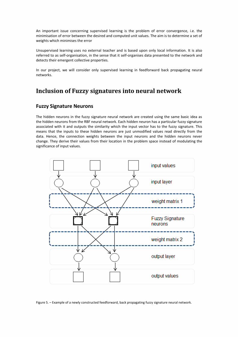
Fuzzy Signature Neurons The hidden neurons in the fuzzy signature neural network are created using the same basic idea as the hidden neurons from the RBF neural network. Each hidden neuron has a particular fuzzy signature associated with it and outputs the similarity which the input vector has to the fuzzy signature. This means that the inputs to these hidden neurons are just unmodified values read directly from the data. Hence, the connection weights between the input neurons and the hidden neurons never change. They derive their values from their location in the problem space instead of modulating the significance of input values.

Figure 5. – Example of a newly constructed feedforward, back propagating fuzzy signature neural network.

The hidden neurons in our fuzzy signature neural network output the degree to which the input value is similar to the associated fuzzy signature. If all the input parameters match perfectly with the corresponding fuzzy signature sub-vectors, then a high value is output. However if the input value arguments match to very few of the corresponding fuzzy signature values, then the output has a very low value. Since the values of the weight matrix between the input layer and the hidden layer are constant throughout, all the learning that is done by the neural network is done via the connection weights between the hidden layer and the output layer. Although a lot of training rules exist for neural networks, we limit ourselves to the most basic training rule called the Delta Rule in this project, which is most commonly used on hidden to output training.

Delta Rule Let us say that the target output is a vector of the form (t1, t2,…, tn) and the current output produced is (o1, o2,…, on), then the delta rule states that during weight modification, the neural net should always seek a weight distribution matrix which minimizes the maximum “average error”.

Where, average error = ∑ ( )

The delta rule is defined in terms of this definition of error. Because error is explained in terms of all the training vectors, the delta rule is an algorithm for taking a particular set of weights and a particular vector, and yielding weight changes that would take the neural net on the path to minimal error. The calculus behind the rule has been shown by Gurney in [11]. Widrow and Stearns [12] showed that when alpha is sufficiently small, the weight vector approaches a vector that minimizes error. In our creation and testing of the fuzzy signature neural network, the learning rate is set to be 1%. The activation function for the hidden neurons is just a simple linear map, which means that the activation function passes all outputs, no matter how small they are. The output neurons have a simple activation function of rounding up the values. Hence, if the net input is equal to or more than 0.5, then the output will activate and give an output, in all the other cases no output will be produced. Hence, we have created a feedforward, back propagation neural net which uses fuzzy signatures to determine which hidden neuron activates and produces the output. Although this is functionally very similar to the Radial Basis Functions, there are a few differences between RBF neural networks and Fuzzy Signature neural networks on the whole. In RBF neural networks all the following are determined during the training phase: the number of neurons in the hidden layer, the coordinates of the center of each hidden-layer RBF function and the radius (spread) of each RBF function in each dimension. However, in Fuzzy signatures, we do not use the concept of center of each function or radius; we use the concept of membership to any particular fuzzy signature. Once the neural network was set up we trained the neural network using an n-fold cross validation scheme. For example, if we use n=2, we have 50% at random from each class (of SARS, pneumonia, healthy and high BP) is the training set, the other half is the test set and then we swap them and average the result. In 10-fold cross validation we split into 10 sets each with 10% at random from each class. Then train 10 times each time training with all but one of these sets and use the leftover one for the test set. The results are then averaged.

Results

Clustering Result Agglomerative Hierarchical clustering on the SARS Dataset with Euclidean distance measure and Ward linkaging gives the following results.

Figure 6. – Dendrogram showing the results of hierarchical clustering using Ward linkaging.

In the research project, 2 sets of fuzzy signatures were created. One were created using clusters whose threshold limit was 15% of the data, in other words, clusters with a minimum of 600 entries each were considered for the signature creation. As can be seen from Figure 6, which is the resultant dendrogram from the agglomerative hierarchical clustering using Ward linkaging, 5 clusters were obtained using this 15% threshold value. The other set were created using clusters with a threshold limit of 5%, i.e. clusters with a minimum of 200 entries each were considered. We obtained 17 such clusters with a 5 threshold value. These results will not be discussed in this report, but are available for inspection in the appendix. The size and the details of the 5 clusters are: Details for cluster 1 with number of elements 1000 are: Percentage of member is class 1 are 1000 100.0 % Percentage of member is class 2 are 0 0.0 % Percentage of member is class 3 are 0 0.0 % Percentage of member is class 4 are 0 0.0 % Cluster centroid - 39.146 39.144 39.157 39.149 169.66 107.97 74.573 70.074 Minimum values of each argument 38.300 38.300 38.303 38.301 150.02 95.017 50.056 40.008 Maximum values of each argument 39.998 39.998 40.000 39.999 189.98 119.98 99.981 99.933

Details for cluster 2 with number of elements 880 are: Percentage of member is class 1 are 0 0.0 % Percentage of member is class 2 are 411 46.7 % Percentage of member is class 3 are 469 53.3 % Percentage of member is class 4 are 0 0.0 % Cluster centroid - 37.978 37.951 37.953 37.974 96.97 75.00 13.010 11.662 Minimum values of each argument 36.002 36.004 36.001 36.001 90.02 65.01 0.058 0.007 Maximum values of each argument 39.998 39.987 39.999 40.000 113.14 83.99 23.950 23.995 Details for cluster 3 with number of elements 433 are: Percentage of member is class 1 are 0 0.0 % Percentage of member is class 2 are 232 53.6 % Percentage of member is class 3 are 201 46.4 % Percentage of member is class 4 are 0 0.0 % Cluster centroid - 37.785 37.747 37.772 37.750 112.56 74.13 18.575 12.628 Minimum values of each argument 36.008 36.006 36.006 36.001 99.23 65.03 9.156 0.018 Maximum values of each argument 39.967 39.992 39.994 39.997 119.97 83.97 23.905 23.985 Details for cluster 4 with number of elements 687 are: Percentage of member is class 1 are 0 0.0 % Percentage of member is class 2 are 357 52.0 % Percentage of member is class 3 are 330 48.0 % Percentage of member is class 4 are 0 0.0 % Cluster centroid - 37.870 37.832 37.823 37.828 110.16 74.02 6.524 11.945 Minimum values of each argument 36.001 36.003 36.004 36.000 95.36 65.01 0.003 0.000 Maximum values of each argument 39.989 39.997 39.996 39.998 119.93 83.90 19.970 23.989 Details for cluster 5 with number of elements 1000 are: Percentage of member is class 1 are 0 0.0 % Percentage of member is class 2 are 0 0.0 % Percentage of member is class 3 are 0 0.0 % Percentage of member is class 4 are 1000 100.0 % Cluster centroid - 36.597 36.605 36.584 36.601 170.50 107.84 12.053 12.048 Minimum values of each argument 36.004 36.005 36.001 36.000 150.04 95.01 0.051 0.000 Maximum values of each argument 37.200 37.199 37.197 37.200 189.88 120.00 23.994 23.998

Results of the Fuzzy Signatures Fuzzy signature values for cluster 1 with 1000 values are- 38.295 39.998 [slight, very high] 38.291 39.998 [slight, very high] 38.303 40.011 [slight, very high] 38.299 39.999 [slight, very high] 149.339 189.980 [high, very high] 95.017 120.925 [high, very high] 40.008 100.140 [moderate, very high] 49.165 99.981 [moderate, very high] Fuzzy signature values for cluster 2 with 880 values are- 35.959 39.998 [low, very high] 35.915 39.987 [low, very high] 35.906 39.999 [low, very high] 35.948 40.000 [low, very high] 80.793 113.140 [low] 65.015 84.987 [low, normal] 0.671 23.995 [normal, slight] 0.058 25.962 [normal, slight] Fuzzy signature values for cluster 3 with 433 values are- 35.603 39.967 [low, very high] 35.503 39.992 [low, very high] 35.550 39.994 [low, very high] 35.502 39.997 [low, very high] 99.233 125.879 [low, normal] 64.283 83.972 [low, normal] 0.018 25.237 [normal, slight] 9.156 27.994 [normal, slight] Fuzzy signature values for cluster 4 with 687 values are- 35.752 39.989 [low, very high] 35.666 39.997 [low, very high] 35.650 39.996 [low, very high] 35.657 39.998 [low, very high] 95.363 124.958 [low, normal] 64.141 83.900 [low, normal] 0.099 23.989 [normal, slight] 6.921 19.970 [normal]

Fuzzy signature values for cluster 5 with 1000 values are- 35.995 37.200 [low, normal] 36.005 37.206 [low, normal] 35.970 37.197 [low, normal] 36.000 37.202 [low, normal] 150.040 190.968 [high, very high] 95.011 120.665 [high, very high] 0.000 24.095 [normal, slight] 0.051 24.055 [normal, slight]

Results of the Neural Network Once the fuzzy signatures have been created, we test the neural network to see how well it performs the classification of the 4 diseases. Success is counted only when the outputs for all the 4 neurons match the classification exactly. False positives count as a failed result. An indecisive result (all outputs are 0, which means network could not infer which class the input belongs to) is also counted as a failed result.

Weight Matrix 1 i1 i2 i3 i4 i5 i6 i7 i8

f1 1 1 1 1 1 1 1 1 f2 1 1 1 1 1 1 1 1 f3 1 1 1 1 1 1 1 1 f4 1 1 1 1 1 1 1 1 f5 1 1 1 1 1 1 1 1 Weight Matrix 2 Between Fuzzy Signature neurons and output neurons Averaged over 100 runs with 2 fold training f1 f2 f3 f4 f5

o1 -0.10969 -0.06757 -0.14614 0.128058 0.982605 o2 0.212376 0.20307 0.185205 0.018741 -0.51764 o3 0.334183 0.275401 0.384087 -0.87397 -0.07432 o4 -0.19081 -0.17407 -0.16035 1.071004 0.120337 Average success rate= 97.78% Standard deviation = 2.59 % Minimum success rate = 86.48 % Maximum success rate = 100 % Averaged over 100 runs with 10 fold training f1 f2 f3 f4 f5

o1 -0.1056 -0.02215 -0.2964 0.214244 1.097582 o2 0.281275 0.297851 0.10684 -0.02554 -0.58537 o3 0.341111 0.193815 0.670696 -1.08944 -0.13537 o4 -0.26908 -0.26516 -0.16933 1.312113 0.195653 Average success rate = 98.74 % Standard deviation = 1.02 % Minimum success rate = 95.65 % Maximum success rate = 100 %

Discussion

Clustering results From the clustering results, we can see that the classes for SARS and high blood pressure were clustered perfectly into 2 separate clusters, whereas the classes for pneumonia and healthy people were clustered together in a very haphazard way. This is expected to be, since the high blood pressure and SARS patients have huge values for their systolic and diastolic, which sets them far apart from the pneumonia and healthy patients group with respect to Euclidean distances. Also, SARS patients have high fevers, whereas high blood pressure patients do not. Hence, SARS and high blood pressure are clustered into perfect classes. However, with the case of pneumonia and healthy people, the main difference came from the fever values, pain and nausea values. However, since the fever values ranged from only 36.00 to 40.00, even the biggest of differences between the values for these classes only resulted in a net small Euclidean distance when coupled with the pain and nausea values. Hence, the driving factors in the pneumonia – healthy cluster are the pain and nausea values.

Fuzzy Signature results From the minimum and maximum values of each cluster, we can further see that the fuzzy signatures created for the high blood pressure is unique in the sense that it has average values for all other symptoms except for the systolic and diastolic. Fuzzy signature for SARS also has a high index for the systolic and diastolic, but in addition, the fever sub-vector also has high values. Hence, there is an overlap of the blood pressure readings while the fever readings remain unique for the other 2. In the case of healthy and pneumonia patients, as has already been said, the driving parameters are the pain and nausea values. Hence, because the pain and nausea values are mixed quite well in the two classes, the clustering gives imperfect clusters. Hence, the fuzzy signatures thus created have an overlap in the pain and nausea values. Hence, the fuzzy signatures created are both unique and have a good mix of overlap arguments. Hence, we can safely argue that such a clustering is good for pattern detection by the neural network.

Neural Network Results MATLAB has a neural network Toolbox and there also exists a free neural network toolbox called Netlab for the MATLAB. Although they both allow the user to set various parameters of the neural network like training rule, number of layers, size of each layer, etc. We could not find a way to implement a way in which individual hidden neurons have specific functions attached to them to map the membership of fuzzy signatures. Hence, we coded the whole neural network from scratch in C, creating and implementing all details of the neural network. From the weights matrix thus obtained, we can see that the weight for the connection of fuzzy signature 4 to output 4 is 1.07, while all the other fuzzy signatures to output 4 have comparatively

very few weights. This leads us to believe that if an input belongs to fuzzy signature 4, it is most probable that the output is class 4. This is the expected result as well, because we can see that fuzzy signature 4 belongs to the cluster which was the high blood pressure class. Since, this cluster was perfect, it was expected that this fuzzy signature will have a very high connection weight to one of the output nodes. Same is the case with the other perfect cluster of SARS. The fuzzy signature 5, which corresponds to this cluster has a connection weight of 0.98 with output 1, while all other fuzzy signatures have low weights for output 1. When we consider the case for the other 3 fuzzy signatures, we can see from the clustering results that they contain an almost homogenous mixture of pneumonia and normal entries. Hence, only in the case of these 3 fuzzy signatures does the neural network have the opportunity to demonstrate learning of the patterns via the connection weights. The success percentage results of the 2 fold and the 10 fold show phenomenal learning capacity of the neural network. As shown by Mendis, Gedeon, et al [13], [14] that MSE and CLE training algorithms give 96.67 % accuracy of results, we have improved the results using our fuzzy neural networks to a 97.78% with 2-fold cross validation, and 98.74% with 10-fold cross validation. This latter 2.07% increase is a great result as the improvement is more than half of the error which remained in the best result in the literature on this data set. The percentage success values also show us that with the increase in the number of training data, the neural network behaves more and more consistently. With a 2000 entry training data, the standard deviation is 2.59% whereas with a 3600 entry training data, the standard deviation drops to 1.02%. Another interesting result is that the neural network for our particular dataset never gives false positives. The only failure which it shows is when it is unable to decide on a particular class. This is a very interesting property to have obtained because in fields like medicine, a false positive can mean that the patient is treated for the wrong disease. However, if there are no false positives and the only failed results are when the network fails to classify it as either of the classes, that just means that some human expert in the field should take over and diagnose the patient for a particular disease.

Catastrophic forgetfulness When the neural network was being trained, another interesting pattern that emerged was that if the training set was fed to the neural network in a class-by-class sorted fashion, then the neural network performed very badly with success rates of close to 50%. This kind of behaviour has been explained by Seipone, Bullinaria [15] and French [16] as catastrophic forgetfulness, where the neural network forgets the old information and connection weights as it acquires new information about the patterns. Hence, in our dataset, when the neural net was being trained for the pneumonia class, it learned the weights, but because of both the pneumonia and normal classes having the same fuzzy signatures, as soon as the training data for the normal class was input, the neural network started forgetting about the pneumonia classification weights. This was solved by randomising the order of presentation of training patterns.

Conclusion In this report I have laid down the basic theory on how to integrate fuzzy signatures and neural networks together to create a new class of fuzzy signature neural networks. I have also shown the improvement in the performance when using such a neural network to classify any given dataset, and achieved a great result, better than the best published result on this data set. The work presented in this paper has some direction for further work. At present we have used a dataset that was complete, meaning there were no missing fields at all. More research can be done in the area of creating fuzzy signatures in a dataset where there are missing values. More can be researched about how the sub vectors in a fuzzy signature can be split apart or joined together to account for the missing values. The clustering of the dataset gave perfect results for SARS and high blood pressure and a mixed result for pneumonia and normal classes. This served to show that the fuzzy signature neural network works well for both good clustering and bad clustering. But more tests and research can be done on how the network works when all the fuzzy signatures include entries of mixed classes. More research can also go into testing and developing other training rules, and also on the structure of the neural network itself. Instead of a feedforward back propagation network, and testing how does a feedbackward neural network with a fuzzy signature perform, how can one implement fuzzy signature neural networks using self-organising maps and all the other various permutations of the neural network family.

References [1] P. O. Duda and P. E. Hart, Pattern Classification and Scene Analysis. New York: Wiley, 1973. [2] Pawel Strumillo, Wladyslaw Kaminski, “Radial Basis Function Neural Networks: Theory and Applications”, proceedings of the Sixth International Conference on Neural Network and Soft Computing, Zakopane, Poland, 2002, pp. 107 [3] K.W. Wong, T.D. Gedeon, L.T. Kóczy, “Construction of Fuzzy Signature from Data: An Example of SARs Pre-clinical Diagnosis System,” Proceedings of IEEE International Conference on Fuzzy Systems – FUZZ-IEEE 2004, Budapest, Hungary, paper 1353, 2004. [4] T. Vamos, L.T. Koczy, and G. Biro, “Fuzzy Signatures in Data Mining,” Proceedings of the joint 9‘‘ IFSA World Congress, 2001, pp. 2842-2846. *5+ B.S.U Mendis, T.D. Gedeon, L.T. Kóczy, “On the issue of learning weights from observations for fuzzy signatures,” Proceedings WAC06, Budapest, pp. 1-6, 2007. *6+ B.S.U. Mendis, T.D. Gedeon, J. Botzheim, L.T. Kóczy, “Generalised weighted relevance aggregation operators for hierarchical fuzzy signatures,” Proceedings International Conference on Intelligent Agents, Web Technologies and Internet Commerce, 2007. *7+ A. Kendal and M. Last, “Fuzzification and Reduction of Information-Theoretic Rule Sets”, Data Mining and Computational Intelligence, pp 63-93 *8+ S Shenoi, “Multilevel Database Security Using Information Clouding”, Proc. Of IEEE International Conference on Fuzzy Systems, pages 483-488. IEEE Press, 1993 *9+ K.W. Wong, T.D. Gedeon, L.T. Kóczy, “Construction of Fuzzy Signature from Data: An Example of SARs Pre-clinical Diagnosis System,” Proceedings of IEEE International Conference on Fuzzy Systems – FUZZ-IEEE 2004, Budapest, Hungary, paper 1353, 2004. [10] Haykin, S. (1994). Neural Networks: A Comprehensive Foundation. New York: Macmillan Publishing. [11] K. Gurney, “An Introduction to Neural Networks”, 1997, London: Routledge.

[12] B. Widrow and S.D. Stearns, “Adaptive Signal Processing”, 1985, New Jersey: Prentice-Hall.

[13] Mendis, B.S.U.; Gedeon, T.D.; Botzheim, J.; Koczy, L.T.; “Generalised Weighted Relevance Aggregation Operators for Hierarchical Fuzzy Signatures”, 2006

[14] Mendis, B S U , " Fuzzy Signatures: Hierarchical Fuzzy Systems and Applications"

*15+ Seipone T., Bullinaria J.A., “EVOLVING NEURAL NETWORKS THAT SUFFER MINIMAL CATASTROPHIC FORGETTING”

*16+ French R.M., “Catastrophic forgetting in connectionist networks”

Appendix Results for the clustering with a threshold limit of 5%, or 200 entries each. Details for cluster number 7986 with number of elements 249 are: Percentage of member is class 1 are 249 100.000000 Percentage of member is class 2 are 0 0.000000 Percentage of member is class 3 are 0 0.000000 Percentage of member is class 4 are 0 0.000000 Cluster centroid - 39.131 39.182 39.124 39.140 167.15 107.83 63.027 58.292 Minimum values of each argument 38.301 38.305 38.303 38.308 150.04 95.04 50.060 40.008 Maximum values of each argument 39.992 39.998 39.989 39.996 189.87 119.95 81.992 79.963 Details for cluster number 7990 with number of elements 276 are: Percentage of member is class 1 are 276 100.000000 Percentage of member is class 2 are 0 0.000000 Percentage of member is class 3 are 0 0.000000 Percentage of member is class 4 are 0 0.000000 Cluster centroid - 39.145 39.126 39.152 39.131 167.49 108.07 86.820 56.086 Minimum values of each argument 38.310 38.301 38.308 38.301 150.02 95.02 62.995 40.230 Maximum values of each argument 39.992 39.997 39.987 39.999 189.82 119.98 99.957 83.784 Details for cluster number 7987 with number of elements 228 are: Percentage of member is class 1 are 228 100.000000 Percentage of member is class 2 are 0 0.000000 Percentage of member is class 3 are 0 0.000000 Percentage of member is class 4 are 0 0.000000 Cluster centroid - 39.132 39.117 39.151 39.157 171.38 106.68 86.575 85.933 Minimum values of each argument 38.314 38.300 38.307 38.306 150.66 95.19 65.181 63.425 Maximum values of each argument 39.998 39.991 39.991 39.992 189.91 119.88 99.981 99.933 Details for cluster number 7991 with number of elements 247 are: Percentage of member is class 1 are 247 100.000000 Percentage of member is class 2 are 0 0.000000 Percentage of member is class 3 are 0 0.000000 Percentage of member is class 4 are 0 0.000000

Cluster centroid - 39.175 39.152 39.201 39.171 173.03 109.20 61.448 82.943 Minimum values of each argument 38.300 38.300 38.305 38.302 151.42 95.06 50.056 55.025 Maximum values of each argument 39.976 39.993 40.000 39.997 189.98 119.93 81.974 99.828 Details for cluster number 7969 with number of elements 215 are: Percentage of member is class 1 are 0 0.000000 Percentage of member is class 2 are 0 0.000000 Percentage of member is class 3 are 0 0.000000 Percentage of member is class 4 are 215 100.000000 Cluster centroid - 36.632 36.612 36.576 36.621 161.49 112.89 13.492 7.263 Minimum values of each argument 36.004 36.010 36.001 36.010 150.16 98.58 0.206 0.026 Maximum values of each argument 37.196 37.196 37.196 37.193 176.62 119.98 23.994 21.408 Details for cluster number 7971 with number of elements 205 are: Percentage of member is class 1 are 0 0.000000 Percentage of member is class 2 are 0 0.000000 Percentage of member is class 3 are 0 0.000000 Percentage of member is class 4 are 205 100.000000 Cluster centroid - 36.593 36.628 36.566 36.597 156.42 105.87 11.006 15.245 Minimum values of each argument 36.004 36.017 36.003 36.012 150.04 95.11 0.374 0.044 Maximum values of each argument 37.198 37.197 37.197 37.200 167.22 119.95 23.982 23.972 Details for cluster number 7937 with number of elements 80 are: Percentage of member is class 1 are 0 0.000000 Percentage of member is class 2 are 0 0.000000 Percentage of member is class 3 are 0 0.000000 Percentage of member is class 4 are 80 100.000000 Cluster centroid - 36.649 36.615 36.576 36.578 178.11 113.11 5.363 19.234 Minimum values of each argument 36.016 36.009 36.030 36.000 162.42 105.16 0.051 12.830 Maximum values of each argument 37.180 37.184 37.180 37.200 189.70 119.97 17.065 23.938 Details for cluster number 7974 with number of elements 219 are: Percentage of member is class 1 are 0 0.000000 Percentage of member is class 2 are 0 0.000000 Percentage of member is class 3 are 0 0.000000 Percentage of member is class 4 are 219 100.000000 Cluster centroid - 36.571 36.591 36.587 36.578 182.73 110.70 14.989 10.425 Minimum values of each argument 36.006 36.009 36.002 36.007 171.02 95.17 0.747 0.000 Maximum values of each argument 37.189 37.199 37.191 37.197 189.86 120.00 23.993 23.964 Details for cluster number 7982 with number of elements 281 are: Percentage of member is class 1 are 0 0.000000 Percentage of member is class 2 are 0 0.000000 Percentage of member is class 3 are 0 0.000000 Percentage of member is class 4 are 281 100.000000

Cluster centroid - 36.580 36.592 36.601 36.613 175.99 101.67 11.332 12.595 Minimum values of each argument 36.010 36.005 36.004 36.015 160.45 95.01 0.119 0.106 Maximum values of each argument 37.200 37.198 37.197 37.199 189.88 119.16 23.893 23.998 Details for cluster number 7980 with number of elements 334 are: Percentage of member is class 1 are 0 0.000000 Percentage of member is class 2 are 160 47.904192 Percentage of member is class 3 are 174 52.095808 Percentage of member is class 4 are 0 0.000000 Cluster centroid - 37.950 37.923 37.978 37.909 95.45 73.67 12.280 4.942 Minimum values of each argument 36.039 36.004 36.003 36.002 90.02 65.03 0.179 0.007 Maximum values of each argument 39.998 39.977 39.999 39.987 104.20 83.82 23.940 15.863 Details for cluster number 7967 with number of elements 213 are: Percentage of member is class 1 are 0 0.000000 Percentage of member is class 2 are 115 53.990610 Percentage of member is class 3 are 98 46.009390 Percentage of member is class 4 are 0 0.000000 Cluster centroid - 37.803 37.797 37.703 37.813 95.05 72.55 8.610 17.520 Minimum values of each argument 36.012 36.019 36.001 36.001 90.04 65.01 0.058 7.232 Maximum values of each argument 39.917 39.969 39.979 39.997 102.25 83.99 21.902 23.995 Details for cluster number 7973 with number of elements 333 are: Percentage of member is class 1 are 0 0.000000 Percentage of member is class 2 are 136 40.840841 Percentage of member is class 3 are 197 59.159159 Percentage of member is class 4 are 0 0.000000 Cluster centroid - 38.119 38.078 38.087 38.141 99.71 77.90 16.557 14.656 Minimum values of each argument 36.002 36.006 36.011 36.005 90.05 66.80 4.606 0.144 Maximum values of each argument 39.997 39.987 39.992 40.000 113.14 83.94 23.950 23.968 Details for cluster number 7959 with number of elements 230 are: Percentage of member is class 1 are 0 0.000000 Percentage of member is class 2 are 112 48.695652 Percentage of member is class 3 are 118 51.304348 Percentage of member is class 4 are 0 0.000000 Cluster centroid - 37.899 37.869 37.875 37.865 112.87 73.49 19.207 7.251 Minimum values of each argument 36.008 36.006 36.008 36.001 100.44 65.03 9.156 0.018 Maximum values of each argument 39.965 39.992 39.994 39.990 119.97 83.97 23.902 15.557 Details for cluster number 7961 with number of elements 203 are: Percentage of member is class 1 are 0 0.000000 Percentage of member is class 2 are 120 59.113300 Percentage of member is class 3 are 83 40.886700 Percentage of member is class 4 are 0 0.000000

Cluster centroid - 37.657 37.609 37.654 37.619 112.20 74.85 17.858 18.719 Minimum values of each argument 36.008 36.016 36.006 36.001 99.23 65.17 10.203 9.854 Maximum values of each argument 39.967 39.981 39.983 39.997 119.95 83.92 23.905 23.985 Details for cluster number 7964 with number of elements 267 are: Percentage of member is class 1 are 0 0.000000 Percentage of member is class 2 are 139 52.059925 Percentage of member is class 3 are 128 47.940075 Percentage of member is class 4 are 0 0.000000 Cluster centroid - 37.915 37.818 37.844 37.833 110.88 74.29 7.330 4.551 Minimum values of each argument 36.001 36.051 36.004 36.001 99.85 65.05 0.073 0.000 Maximum values of each argument 39.987 39.973 39.991 39.998 119.76 83.85 19.970 11.930 Details for cluster number 7944 with number of elements 182 are: Percentage of member is class 1 are 0 0.000000 Percentage of member is class 2 are 93 51.098901 Percentage of member is class 3 are 89 48.901099 Percentage of member is class 4 are 0 0.000000 Cluster centroid - 37.855 37.875 37.827 37.863 115.51 74.41 5.676 16.872 Minimum values of each argument 36.014 36.003 36.014 36.007 107.78 65.06 0.003 8.936 Maximum values of each argument 39.983 39.997 39.996 39.993 119.93 83.89 14.808 23.750 Details for cluster number 7958 with number of elements 238 are: Percentage of member is class 1 are 0 0.000000 Percentage of member is class 2 are 125 52.521008 Percentage of member is class 3 are 113 47.478992 Percentage of member is class 4 are 0 0.000000 Cluster centroid - 37.832 37.814 37.796 37.795 105.27 73.42 6.269 16.472 Minimum values of each argument 36.007 36.007 36.027 36.000 95.36 65.01 0.033 6.196 Maximum values of each argument 39.989 39.982 39.920 39.994 113.69 83.90 18.385 23.989

Weight Matrix 2 Averaged over 100 runs with 2-fold cross validation Average success rate = 96.38 % Standard deviation = 4.68 % Minimum success rate = 75.775 % Maximum success rate = 100 %

o1 o2 o3 o4

f1 0.253466 -0.18683 -0.03734 0.103601 f2 0.287267 -0.1681 -0.06456 0.089991 f3 0.271746 -0.18123 -0.04586 0.097013 f4 0.267285 -0.17181 -0.0463 0.088911 f5 0.04952 -0.0088 -0.22657 0.272726 f6 0.033008 -0.00531 -0.21943 0.281664 f7 0.10202 0.06453 -0.2751 0.179246 f8 0.021535 -0.03769 -0.19734 0.297305 f9 0.036878 -0.04369 -0.2141 0.310036 f10 -0.07406 0.081128 0.178975 -0.08207 f11 -0.05979 0.078025 0.158673 -0.08409 f12 -0.10489 0.050218 0.221211 -0.07241 f13 -0.03439 0.118101 0.120592 -0.10833 f14 -0.02614 0.1258 0.118268 -0.12637 f15 -0.05432 0.10096 0.15874 -0.10977 f16 -0.03435 0.100358 0.134249 -0.10846 f17 -0.07253 0.082004 0.171792 -0.10341

Averaged over 100 runs with 10-fold cross validation Average success rate = 97.80 % Standard deviation = 2.08 % Minimum success rate = 86.975 % Maximum success rate = 100 % o1 o2 o3 o4

f1 0.276148 -0.167642 -0.059499 0.091463 f2 0.307979 -0.128865 -0.095117 0.064831 f3 0.278916 -0.155716 -0.063047 0.081898 f4 0.298334 -0.134839 -0.080281 0.063199 f5 0.048973 -0.023745 -0.226619 0.287644 f6 0.03524 -0.021672 -0.227822 0.308511 f7 0.128149 0.113468 -0.30324 0.127876 f8 0.008912 -0.054858 -0.186664 0.315409 f9 0.027805 -0.065802 -0.204412 0.328813 f10 -0.101018 0.047799 0.219385 -0.058749 f11 -0.080354 0.050696 0.188814 -0.069353 f12 -0.126356 0.025034 0.255628 -0.05635 f13 -0.017822 0.13878 0.094357 -0.119234 f14 -0.001852 0.159174 0.082694 -0.148529 f15 -0.041144 0.1322 0.13493 -0.129604 f16 -0.038206 0.103359 0.146938 -0.122263 f17 -0.062517 0.083478 0.15985 -0.109505