ga east leap modelling technical report · 2. 8.3 household sector 60 8.4 municipal sector 61 8.5...

GA EAST LEAP MODELLING TECHNICAL REPORT

Bryce McCall, Louise Tait and Adrian Stone

CONTENTS

1. INTRODUCTION 3

2. GENERAL BACKGROUND 8

2.1 Households and population 8

2.2 Economy 9

3. MUNICIPAL SECTOR 9

3.1 Data 9

3.2 Methodology 11

4. HOUSEHOLD SECTOR 12

4.1 Data 12

4.2 Methodology 15

5. INDUSTRY 21

5.1 Data 21

5.2 Methodology 23

6. COMMERCIAL SECTOR 24

6.1 Data 24

6.2 Methodology 28

6.2.1 Estimating energy intensities by end-use and fuel 28

6.2.2 Formal sector calculations 29

6.2.3 Informal sector 30

6.2.4 Own-generation 31

7. TRANSPORT SECTOR 36

7.1 Data 36

7.2 Methodology 38

7.2.1 Scope 1 methodology 44

7.2.2 Scope 3 Methodology 49

7.2.3 Discussion on fuel sold in GEM 52

8. BUSINESS AS USUAL (BAU) 53

8.1 Main drivers and assumptions 53

8.2 Transport 57

2

8.3 Household sector 60

8.4 Municipal sector 61

8.5 Commercial sector 61

8.6 Industry 61

9. BAU LEAP RESULTS 61

9.1 GEM scope 1 and 3 methodologies compared for BAU 62

9.2 Transport sector energy consumption 66

9.3 BAU general results 68

9.4 Sensitivity scenario tests 69

10. EFFICIENT CHARCOAL STOVES SCENARIO 71

11. HOUSEHOLD ACCESS TO MODERN FUELS FOR COOKING 75

12. CONCLUSIONS 80

13. DATA ISSUES 82

14. EFFICIENT FRIDGES SCENARIO (EFR) 85

REFERENCES 91

APPENDIX A. OWN-GENERATION EFFICIENCY MODEL 92

APPENDIX B. COMMERCIAL SECTOR ENERGY INTENSITY BY ACTIVITY TYPE 95

APPENDIX C. DISTRIBUTION OF COMMERCIAL OWN GENERATION ELECTRICITY SHARE IN THE GEM AND

ASEM SURVEYS 96

3

1. INTRODUCTION This is the technical documentation for the development, data, and methodology of the Ga East Municipality

(GEM) energy systems model which forms part of the Supporting Sub Saharan African Municipalities with

Sustainable Energy Transitions (SAMSET) project. The project is a collaboration between the Universities of

Uganda Martyrs, Ghana, Cape Town, Durham and University College London, the non-profit organisation

Sustainable Energy Africa and Gamos Consulting. It is co-funded by UK aid from the UK Department for

International Development, the Engineering and Physical Science Research Council and the Department for

Energy and Climate Change.

The model is developed on the Long range Energy Alternatives Planning System (LEAP) platform of the

Stockholm Environment Agency (SEI). LEAP is essentially an accounting-type simulation model although

other uses and features have emerged as the product has developed. The rationale for the selection of LEAP

as a tool for the SAMSET project has been documented in another project output (Tait, McCall, & Stone,

2014) and the LEAP software tool itself is well documented by SEI (http://www.energycommunity.org). For

the SAMSET project, LEAP is used to create a bottom-up data-driven picture of Ga East’s energy system on

the supply and demand side, projecting a reference case into the future. Scenarios are then developed which

project how municipal driven interventions may alter the path of this reference case, reducing energy

consumption and mitigating CO2 emissions.

The dataset for the model was collected by the University of Ghana by means of surveys and stakeholder

workshops with GEM officials and local experts and is documented in another SAMSET output, the Ga East

State of Energy Report (Bawakyillenuo & Agbelie, 2014). In certain instances this dataset was augmented by

data from the literature and online sources. The scope of energy systems models, even of a bounded

municipal area, covers a very broad range of activities and so it was also necessary to make assumptions in a

few instances discussed below but it is hoped that if the model is kept live, as is the goal of the project, these

will be refined as time goes on.

The general form of a LEAP model involves the division of the energy demand side into typical economic

sectors:

• transport;

• municipal services;

• households/residential;

• industry;

http://www.energycommunity.org/

4

• commercial; and

• agriculture;

and of supply sectors under the node ‘Transformation’, typically but not exclusively as follows:

• transmission and distribution;

• electricity production;

• oil refining; and

• charcoal production.

In order to build a model, data must be collected for the demand-side sectors that captures the levels of

output and energy intensity of producing that output categorised by technology and/or energy carrier for

each of the typical services required in that sector, for instance lighting, heating, passenger transport or

production of steel. An example is given in the figure below.

5

Figure 1: Example of the tree structure in LEAP which aids in categorising the sectors and subsectors of a model down to individual technologies. Here the level goes down to the share of private cars which

are diesel or petrol and so on.

It’s important to understand clearly that an energy service, heating for instance, may be supplied by many

technologies which may use different energy carriers (fuels) such as coal, diesel or electricity. A combination

of a technology and energy carrier will have distinct energy efficiency and emissions which has important

implications for sustainability. An important feature of a useful energy systems model is therefore that,

while we want to capture the actual technologies and energy carriers used to supply services today, which

we define as the base year, we want to be able to simulate switching to other technologies and energy

carriers in the future to evaluate the impact on sustainability.

The general mathematical form by which the energy consumption of the services in a sector is calculated is a

simple accounting formula outlined in a general, but not overly mathematically formal way below, for the

6

sake of communicating across disciplines. For simplicity’s sake we will assume that a technology may be

either a different means of doing the same thing for example travelling by bus or by car but also using a

different energy carrier / fuel for example travelling using a petrol fuelled car or electric car.

For a given year in the time horizon of the model:

Energy consumption of a sector = The sum of all the energy consumptions of services required by the sector

Where

ES = ∑ (θi X ηi X OS) Equation 1

if:

ES = the energy consumed by a service in a given year

θi = share of service supplied by technology i

ηi = The energy intensity (equivalent to efficiency) of technology I in units of energy required per units

output for example MJ/[passenger km] or GJ/[ton steel]

OS = The output of a service required in a given year in physical units, for example passenger km of passenger

transport, tons of steel or GJ of heating

This simple structure offers considerable advantages in developing scenarios of shifts to new technologies

because the modeller can easily change the relative shares θI of technologies that supply a service at a given

future output OS and the impact on emissions and energy consumption can be quickly assessed.

Technologies that have no share of service provision in the base year, say electric cars, can be readily

assigned a growing share in a scenario of the future. The given future output is readily projected in LEAP

which provides a spreadsheet-like formula builder for generating time series of parameters such that an

output OS, for instance residential heating or tons of steel, can be linked to a driver such as population or

gross domestic product (GDP). GDP itself can be set up as a global assumption accessible to all sectors in the

tree structure of the model and defined as a geometric progression relative to time such that it grows at a

fixed percentage of, say, 2% per annum for the time horizon of the model. More elaborate representations,

including step changes and linear interpolation between defined points are equally possible using the

formula builder, giving the modeller considerable flexibility in implementing the views of stakeholders or

7

other forms of data. An example of this flexibility is demonstrated below where the shares of individual

technologies is set easily by the user and LEAP instantly shows the graphic representation of this change.

Figure 2: A screen shot of the LEAP interface showing the change in water heating technologies for low-income households through to 2030

LEAP has a financial framework and, if the costs of technologies are known, the impact on net present value

of supplying that service can be quickly assessed. The disadvantage of this simplistic representation is that

the share of a technology may be changed faster than is practical in the real world given the technical life

and age distribution of exiting devices. LEAP does allow for devices to be vintaged and technical change to

be managed by a stock model, but this is much more data-intensive and not suitable for most cases where

sectors have been represented in the SAMSET project given the scope of the surveys. Some attention needs

to be paid, therefore, to keeping rates of change within a conservatively realistic window.

For a bottom-up model to be reliable, the assumed activity levels and energy intensities used in services

need to be calibrated so that the total energy consumed in the model in the base year, which we define as

an historical year, say 2010, agrees with the total energy known to have been supplied to the system in that

year. This total energy data typically comes from recorded total electricity sales and petroleum fuel sales

obtained from the major utilities. Acquiring this data and validating it is therefore an important first step in

the modelling process.

8

In the model developed for Ga East all fuels sold within the municipality, with the exception of transport

fuels, are assumed to be consumed within the boundary and thus count toward the city’s emissions levels.

The representation of transport in a spatially bounded scope such as a municipality is inherently

problematic. Given commuting behaviour to Accra and traffic passing through, it is reasonable to assume

that a significant portion of petrol and diesel that is sold within Ga East transits the boundary while fuel from

elsewhere enters the municipality daily. In this framework we attempt to represent intra-boundary trips,

inter-boundary trips either generated in or attracted to Ga East and corridor trips, of which Ga East is neither

the origin nor destination but which refuel there. LEAP’s tree structure allows the user to include or discard

these sub-nodes in reporting results depending on the scope of interest.

The LEAP model was created to represent all major sectors of Ga East as a bottom-up simulation model, and

this was calibrated with known fuel sales (mainly liquid fuels and electricity) within the municipal boundary.

The main drivers for this model are population and economic growth (one local, and one regional).

2. GENERAL BACKGROUND Data collection was primarily based on surveys and interviews undertaken by the University of Ghana as part

of the SAMSET project. This included the following:

• surveys of 590 households, 310 commercial businesses and 50 industrial businesses in the municipal

area;

• focus groups;

• interviews with municipal staff; and

• municipal records.

Much of the detail of these surveys is presented in the State of Energy report by the Ghanaian team

members of the SAMSET project – see Bawakyillenuo and Agbelie (2014).

The Base year for this model is 2013 since the survey was carried out in 2013.

Ga East is located in the Greater Accra region, and is an outlying part of Accra.

2.1 HOUSEHOLDS AND POPULATION The household population of Ga East in 2010 was estimated, through the 2010 national census to be 33 949

households, and 75% of households were electrified (Bawakyillenuo & Agbelie, 2014). Household

9

classifications are based on standard Ghanaian land-use classifications, which are based on degree of access

to service delivery and other factors1.

Table 1: Household estimate, 2010

Household classification Number Percentage

Household 1 28 743 85

Household 2 1 870 5

Household 3 3 336 9

Total 33 949 100

The population of Ga East was estimated to be 147 742 in 2010 according to the Ghana National Statistics

(Ghana Statistical Service, 2014b). Extrapolating this estimate to 2013 with an annual 3% growth rate,

equates to 161 441 people living in 37 096 households (assuming household density does not change).

2.2 ECONOMY The gross value added (GVA) – the ‘GDP’ for GEM is inferred based on the average GDP per capita for the

country. Due to the proximity of GEM to the economic hub of Ghana, Accra, this value could be an

underestimate.

The population for Ghana in 2013 was 26.4 million (Ghana Statistical Service, 2012) and the national non-oil

GDP for 2013 was GHC71 627 million (Ghana Statistical Service, 2014a).

Thus, with the population of GEM and the GDP per capita, the inferred GDP for the municipality would be

437.5 Million GHC in 2013.

3. MUNICIPAL SECTOR This section describes the energy consumption of the municipality for its operations and services including

energy consumption of municipal buildings and vehicle fleet.

3.1 DATA The SAMSET partners in Ghana provided data on the municipality’s own energy consumption and how the

energy is used within the municipal buildings and for municipal services. Much of this data is taken from the

State of Energy report by Bawakyillenuo and Agbelie (2014). The total floorspace of all municipal buildings in

1 See Bawakyillenuo et. al (2014) for more details on household classification.

10

2013 was estimated to be 8860m2. The energy consumption for the municipality buildings and their vehicle

fleet is presented in the tables below.

Table 2: The GEM own energy consumption by end use for 2013

Unit Lighting Ventilation and air-conditioning

Refrigeration

Transport

Office machines

Electricity kWh 174 468 1 239 840 606 216 0 527 316

Diesel Litres 360 600 240 56 250 303

Table 3: The electricity consumption of GEM’s water system

2010 2011 2012 2013

51 667 kWh

51 667 kWh 23 333 kWh 12 963 kWh

Table 4: The GEM municipality’s data on own generators use in 2013

Diesel generator 120 kW 1 503 L/year

The municipality had eight vehicles in operation in 2013 consuming about 56 250L of diesel a year.

Table 5: Municipality vehicle fleet details and fuel consumption

Vehicle count 8

Average use 520 km/month

km/year 6 240 km

Total diesel 56 250 L/year

The electricity consumption share by end use for the municipality is presented below and highlights

ventilation and air-conditioning as the main energy consumer in municipal buildings.

11

Figure 3: Electricity consumption in municipal buildings

3.2 METHODOLOGY Municipal buildings

Using the electricity consumption data and the total floor space data the energy intensity values for each

end use for the municipality is given below.

Table 6: GEM building end use energy intensity values for 2013

Lighting VAC Refrigeration Office

Machines

kWh/m2 19.7 139.9 68.4 59.5

Transportation

Using the data for the GEM vehicle fleet, the following vehicle km and fuel economy were used for model

input:

Lighting7%

VAC48%

Refrigeration24%

Transport0%

Office Machine21%

12

Table 7: GEM vehicle fleet activity and energy consumption

Total all vehicles 4 160 km/month

Annual km 49 920 All vehicles

Fuel consumption 7 031 L/veh per year

Fuel economy: 113 L/100km* * This fuel efficiency is rather poor, but large garbage trucks are known to have very poor fuel efficiency on the order of 100’s of L/100km (See www.cert.ucr.edu/events/pems2014/liveagenda/25sandhu.pdf).

4. HOUSEHOLD SECTOR 4.1 DATA The data for the household sector is based on survey data of a statistically representative sample of

households undertaken in the municipality. This data was augmented by bottom-up calculations of energy

consumption based on appliance ratings and consumption patterns from the literature. The survey data

collected data for households was disaggregated in three categories based on Ghanaian land-use

classifications. These classifications have been used as a loose proxy for income, in the absence of any other

data. The electrification rate for the municipality was assumed constant across household categories which

yields a breakdown of six household categories as follows (due to the small sample sizes of Household 2

electrified and Household 3 electrified these households values were grouped together and the average

value is used).

Table 8: Number of households in 2013 survey

Household classification Sample size

Total Households

Household 1 – electrified 390 21 534

Household 1 – unelectrified

134 7 209



7 469



13 837

Total 614 33 949

13

The sample survey (adjusted where necessary based on typical appliance ratings and hours of use) shows the

following average annual consumption per energy carrier.

Table 9: Annual average consumption per household

Wood (kg)

Electricity (kWh)

Kerosene (L)

Charcoal (kg)

LPG (kg)

Dry cell batteries (no.

of singles)

Electrified

Household 1 527 2 083 20 265 131 83

Household 2 989* 1 374 67 264 97 72

Household 3 989* 1 595 9 265 126 97

Unelectrified

Household 1 721 - 37 424 113 146

Household 2 1200 - 6 273 72 6

Household 3 1200 - 6 273 72 117 * Survey data revised for wood consumption

The household survey data for wood consumption varied quite significantly, with Household 3 Electrified

reportedly using almost 370% of the amount that Household 2 Electrified households reported using. A

degree of information error in survey data is likely due to issues like memory bias as well as the fact that

people are unlikely to consistently weigh their wood. To resolve this inconsistency and provide a more

reasonable estimate, an average of the two sample estimates was used for both categories of 989 kg per

annum.

14

Table 10: The proportion (%) of the household sample using end-uses (bold) and energy carriers (italic)

Electrified Unelectrified

Household 1

Household 2

Household 3

Household 1

Household 2

Household 3

Lighting 100 100 100 76 90 66

Electricity 100 100 100 - - - Solar 2 8 4 1 0 0 Batteries 41 48 22 75 86 62 Kerosene 1 6 6 1 4 4

Cooking and water heating

100 100 100 100 100 100

Electricity 50 40 22 - - - Wood 8 16 13 24 35 35 Charcoal 81 92 100 94 96 96

LPG 82 76 64 40 15 15 Kerosene 3 4 4 2 1 1

Refrigeration 80 80 67 - - - Electricity 100 100 100 - - -

Entertainment 100 100 100 37 41 41 Electricity 100 100 100 - - - Dry cell batteries

5 0 4 37 41 4154

Space cooling 86 96 82 - - - Electricity 100 100 100 - - -

Other energy services

80 92 62 - - -

Electricity 100 100 100 - - - Source: Household survey Note: A household may use more than one energy carrier for an energy service, for instance electricity and wood for cooking so the sum of household shares for an end-use does not necessarily add up to 100%. In LEAP these are termed ‘saturation’ shares

The household surveys investigated the extent of ownership and usage of efficient appliances. All electrified

households use CFL light bulbs. The Ghanaian government instituted a wide-scale National Efficiency Lighting

Project in 2006/07 aimed at conserving electricity in response to an electricity supply crises. In 2008, the

government legislated against the manufacture and sale of incandescent lamps. The Ghanaian Energy

Commission has also instituted minimum energy-efficiency standards for refrigeration appliances as well as a

refrigeration rebate scheme whereby households can swap old inefficient appliances for newer efficient

15

ones. However, none of the households surveyed reported making use of the Energy Commission’s scheme.

The table below indicates that ownership of efficient refrigeration appliances is higher in the higher-income

category. Despite the widespread usage of charcoal and wood, efficient products have not reached

significant market penetration rates. None of the sampled households recorded using efficient woodstoves.

There was some usage of efficient charcoal stoves, such as the ‘Gyapa’.

Table 11: Efficient appliance usage – share of households in the sample

Electrified Unelectrified

Household 1

Household 2

Household 3

Household 1

Household 2

Household 3

CFL light bulbs 100% 100% 100% - - -

Refrigeration 30% 9% 9% - - -

Charcoal stoves 4% 9% 8% 9% 0% 0%

Wood stoves 0% 0% 0% 0% 0% 0%

4.2 METHODOLOGY The consumption profiles of households in terms of appliance ownership and the total amount of final

energy of energy carriers consumed by households for the various income groups are based on the survey

data collected by the University of Ghana described above. The energy intensities of end-uses input to the

model were estimated based on the typical observed energy profiles of households in the sample, assuming

typical appliance ratings and hours of usage. These were further adjusted where necessary to calibrate

against the total energy consumption of households in the sample, as shown in Table 9 above.

Total consumption for each fuel by energy service is calculated as:

Number of households in sub-category (e.g. Household 1 electrified) X

Percentage of households that use energy service (based on survey data) X

Percentage of households that use fuel (e.g. electricity) for energy service (e.g. cooking) (based on

survey data) X

Energy intensity per energy service (based on bottom up calculations of appliance ratings and hours

of usage, and calibrated to meet total sample consumption estimate from survey data).

Equation 2

16

Table 12: Electricity consumption estimates for ‘Household 1 electrified’

Energy service

Share of household

s using energy service

Share of household

s using electricity for energy

service

Average daily

consumption (kWh)

Days per year used

Average household

energy intensity kWh/yr

Total consumption estimate for population

(annual kWh)


100% 50% 1.512 320 484 5 182 752

Lighting 100% 100% 0.432 365 158 3 395 456

Fridge 80% 100% 2.835 365 1035 17 883 282

Entertainment

100% 100% 0.516 320 165 3 555 668

Space cooling 86% 100% 1.210 350 424 7 833 488

Other 80% 100% 1.148 350 402 6 921 839

Total 44 772 485


Energy service

Share of household


Share of household


service

Average daily

consumption

Days per year used

Average household



(annual kWh)


100% 40% 1.416 320 453 253 924

Lighting 100% 100% 0.432 365 158 220 906

Fridge 80% 100% 2.100 365 767 859 079

Entertainment

100% 100% 0.387 320 124 173 497

Space cooling 96% 100% 0.615 350 215 289 498

Other 92% 100% 0.628 350 220 283 300

Total 2 080 205

17


Energy service

Share of household


Share of household


service

Average daily

consumption

Days per year used

Average household



(annual kWh)


100% 22% 2.162 320 692 384 245

Lighting 100% 100% 0.432 365 158 394 087

Fridge 67% 100% 2.100 365 767 1 277 134

Entertainment

100% 100% 0.486 320 156 388 689

Space cooling 82% 100% 0.615 350 215 442 332

Other 62% 100% 1.518 350 531 826 230

Total 3 712 716

18

Table 15: Household wood consumption estimates

Household category

Share of households using wood for cooking

Appliance type Percentage that use

appliance type

Average estimated

annual consumption

(kg/household )

Total estimated

consumption for population

(kg)

Electrified

Household 1 8% 907 867

Efficient stove 0% - Inefficient stove 100% 527 907 867

Household 2 16% 221 691


Household 3 13% 321 333


Unelectrified

Household 1 24% 1 247 472

Efficient stove 0% - Inefficient stove 100% 721 1 247 472

Household 2 35% 196 990


Household 3 35% 351 421

Efficient stove 0% -

Inefficient stove 100% 1200 351 421

19

Table 16: Charcoal consumption estimates

Household category

Households that use

charcoal for cooking

Appliance type Percentage that use

appliance type

Average esti-mated annual kg/household

Total estimated consumption for all households

(Kg)

Electrified

Household 1 81% 4 632 356

Efficient stove 4% 136 94 538 Inefficient stove 96% 271 4 537 818

Household 2 92% 340 269

Efficient stove 9% 138.0 15 467 Inefficient stove 91% 276.0 324 803

Household 3 100% 661 250

Efficient stove 8% 138 27 552 Inefficient stove 92% 276 633 698

Unelectrified

Household 1 94% 2 866 945

Efficient stove 9% 222 135 092 Inefficient stove 91% 443 2 731 854

Household 2 96% 122 921

Efficient stove 0% - - Inefficient stove 100% 234 122 921

Household 3 96% 219 287

Efficient stove 0% - - Inefficient stove 100% 325 219 287

Table 17: LPG consumption estimates

Household category

Households that use LPG for cooking

Average estimated

annual kg/household

Total estimated consumption for all households

(kg)

Electrified

Household 1

82% 131 2 307 744

Household 2

76% 97 102 753

Household 3

64% 97 155 436

Unelectrified

20

Household 1

40% 113 327 188

Household 2

14% 72 4 824

Household 3

15% 72 9 268

The aggregated survey data for household generator usage in GEM is presented below, along with the

estimate for the entire household population usage of generators. Equations 8 and 11 discussed below in

Section 6.2.4 were used to convert annual fuel use and generator rating into electricity generated, assuming

an average load factor of 0.75. There were 19 households using generators in the survey, all in the

Household 1 category, of which one was un-electrified. The aggregated data below is scaled up to be

representative of the population and compared to the scaled-up electricity demand estimate for the entire

household population.

Table 18: GEM Household (class 1) generator use survey data and estimated population usage

Group Grid status Own generated electricity

(kWh)

Grid electricity

(kWh)

Total electricity

(kWh)

Share of own

gen. elec. (%)

Petrol used

(litres)

Diesel used

(litres)

Estimated average

utilisation (hours/day

)

Sample (with gensets)

Electrified 28 737 111 807 140 544 20% 10 557 3 638 0.5

Unelectrified

285 285 100% 221 0.7

Population (estimate)

Electrified 1 586 729* 44 849 577# 46 436 307 3% 582 926 200 863

Unelectrified

15 336 15 336 100% 11 905

* Scaled from genset-owning sample only # Scaled from entire sample

The data indicate that while not many people own generators, such that they only account for about 3% of

total electricity supply to Household 1 households in the sample, those households that own them make

quite significant use of them, particularly considering that the price of petrol and diesel is likely to discourage

regular use. This may be indicative of substantial suppressed demand of the order of 20% or greater.

21

5. INDUSTRY This section describes the industry sector of GEM and the model data which were derived from the data

provided by the SAMSET team and the survey conducted.

5.1 DATA Based on the classification of the industries in the survey, the industry sector is comprised of the following

subsectors as given in the SoE report (Bawakyillenuo & Agbelie, 2014): construction, manufacturing, and

water and sewerage. The survey conducted by the SAMSET team covered 50 of the approximately 70

industry entities that were identified in the survey preliminary analysis. Their electricity consumption and

their total productivity in tonnes output are given in in the table below.

Table 19: Industry data from the survey for GEM in 2013

Sub-sector Output

(tonnes) Electricity consumed

(kWh)

Construction 524 360* 104 145

Manufacturing 816 089 89 777

Water and sewerage 1 938 855 284 444 * From the SoE report it is unclear as to what the output for the construction subsector entails.

Proportionally scaling up the construction and manufacturing activities to the full 70 industries of GEM, the

following industrial activity is assumed to represent GEM industry.

Table 20: GEM industry activity sample data extrapolated to represent the full sector

Sub-sector Production Tonnes output

Electricity consumed

kWh

Construction 734 105 145 803

Manufacturing 1 142 525 125 688

Water & Sewerage 2 714 396 284 444

Presumably the larger local industrial concerns are in the sample and industry consumption per firm is

typically skewed towards a few large consumers, so this may overstate total consumption but, given the

large sample size, this source of error was assumed to be limited.

Table 21: The electricity consumption in industry by end use for GEM 2013 after extrapolation

22

Sub-sector kWh consumption

Machinery Lighting Cooling systems Other machine

drive Other

Construction 98 966 37 849 5 037 4 145 2 024

Manufacturing 64 690 37 642 13 852 4 518 749

Water and sewerage

309 524 110 098 1 008 465 0

As shown below, the majority of energy consumed in the industry sector is in machinery and in lighting.

Figure 4: The end use shares of electricity consumption industry for GEM, 2013

The consumption of liquid fuels in industry as indicated by the survey and extrapolated to represent the full

population size is estimated to be as follows.

Table 22: The consumption of diesel in various end uses for industry in GEM, 2013

Sub-sector Diesel (litres) Petrol (litres)

Machinery* Machinery Other machine

drive Other

Construction 34 499 840 84

Manufacturing - 1 428 13 415

Water and sewerage 123 618 - - * Typically this would include machinery like bulldozers and earth movers.

0%10%20%30%40%50%60%70%80%90%

100%

Other

Other machine drive

Cooling systems

Lighting

Machinery

23

The data for diesel and petrol generators used in GEM for the year 2013 is given below, after extrapolating

to represent the whole industry sector.

Table 23: Industry diesel and petrol generators sample data scaled to full sector for GEM 2013

Sub-sector Litres consumed kWh output Installed

capacity (kW) Capacity factor

Diesel Petrol Diesel Petrol Diesel Petrol Diesel Petrol

Manufacturing 758 3 271 2 374 6 958 2 57 12.9% 1.6%

Construction 33600 1 210 105 263 2 486 21 19 57.2% 1.5%

Water and sewerage 128383 0 402 203 0 162 0 28.2%

The prevalence of generator ownership and the share of electricity consumed by generator owners in the

sample is shown below.

Table 24: Rates of generator ownership and use for GEM, 2013

Sub-sector Share of sample operating generators

Electricity share of own generation of generator owners

Manufacturing 38% 21%

Construction 11% 93%

Water and sewerage 71% 86%

5.2 METHODOLOGY Using the data provided by the survey and after extrapolating to represent the full industrial sector of GEM,

the energy intensities for each end use in industry was calculated (Table 25). This was done for liquid fuel

consumption as well (Table 26).

Table 25: Final energy intensities of electricity use in industry for GEM 2013 (kWh/tonne)

Machinery Process heating Lighting

Cooling systems

Other machine

drive Other

Construction 0.1348 - 0.0516 0.0069 0.0056 0.0028

Manufacturing 0.0566 - 0.0329 0.0121 0.0040 0.0007

Water and sewerage 0.1140 - 0.0406 0.0004 0.0002 -

24

Table 26: Liquid fuel energy intensities for industry in GEM 2013 (L/tonne)

Diesel Petrol

Machinery Machinery Process heating

Other machine drive Other

0.0470 0.0011 - - 0.0001

- 0.0012 - - 0.0117

0.0455 - - - -

It is most likely that the diesel consumption for ‘machinery’ is earth-moving equipment or other

industry=specific special vehicles or stand-alone internal combustion engines, but this should be more

clearly defined in future iterations of the model to avoid confusion with diesel-fuelled generators.

The following end uses were implemented into the LEAP model with their associated electricity kWh/tonne

and liquid fuel L/tonne intensities as tabulated above:

• lighting;

• cooling;

• machinery;

• other machine drive; and

• other.

Future energy demand for energy could therefore be projected by projecting tons of production. Scenarios

of energy efficiency can be implemented by assuming reductions in the currently observed energy intensities

based on the relative efficiencies of new technologies.

6. COMMERCIAL SECTOR This section describes the representation of commercial activities in GEM, including formal and informal

businesses.

6.1 DATA The University of Ghana surveys collected data on energy carriers used, end-uses, and own generation with

petrol and diesel generators, the floorspace of premises and the costs of energy consumption. A total of 313

businesses were surveyed, including 61 formal businesses and 252 informal businesses. It is thought that this

25

constitutes the whole of the commercial sector for GEM (from communications during SAMSET network

meetings). The types of businesses classified as commercial (based on University of Ghana classifications

include the following:

Formal:

• hotels and guest houses;

• schools;

• non-banks financial services;

• hospitals;

• banks.

Informal:

• aluminium fabricator;

• carpentry/welding shops;

• cold store;

• corn mill;

• drinking bar, restaurant, catering services;

• electronic repair shops;

• fitting/mechanic;

• laundry;

• other;

• petty trading;

• retail;

• tailoring/seamstress.

Energy consumption is driven by floorspace in the model. The total floorspace of the sample was dominated

by the formal sector as shown below even though these only accounted for about 20% of the premises

surveyed.

Table 27: Floorspace of sample

Number of businesses sampled

Floorspace of sample (m2)

Formal 61 94,285

Informal 252 14,966

26

Total 313 109,251

Schools. and to a lesser degree hotels and guest houses, however, account for a disproportionate share of

floorspace area in the formal sub-sector and the sample as a whole, as shown below. The informal sub-

sector shows a more even spread of area by activity. This raises a few issues as regards the use of the data as

follows:

• The entire commercial sector was sampled, so the energy baseline of the sample was not scaled up

and therefore a risk of the contribution of schools becoming more disproportionate was not

incurred.

• The methodology of determining floorspace area and the need for clear metadata in this regard for

this data set is discussed in the data issues section. While possible inconsistencies here may mean

the average energy intensity per unit area is relatively very low, the model itself. which projects area

geometrically into the future. is still internally consistent. The area of more energy-intensive sub-

sectors like banks, for example, still grows at the assumed growth rate independently, thus growing

their absolute energy demand at the assumed rate. The data set, particularly when averaged,

should, however, be compared to other data and to energy efficiency benchmarks with great

caution.

Figure 5: Share of formal commercial floorspace by activity type

27

Figure 6: Share of informal commercial floorspace by activity type

The survey data shows the following estimated consumption of fuel by energy services for formal and

informal sectors.

Table 28: Formal sector: Survey results of annual consumption by fuel and end-use for sample

HVAC Cooking/water heating

Lighting

Refrigeratio

n

Machine

operation

Entertainment

Other

Total

Electricity (kWh)

259 245 32 172 360 554

51 565

196 091 61 855 6 869

968 352

LPG (kg) - 8 904 - - - - 214 9 117

Charcoal (kg) - 13 050 - - - - - 13 050

Wood (kg) - 1 250 - - - - - 1 250

Kerosene (L) - 1 - - - - - 1

Table 29: Informal sector - Survey results of annual consumption by fuel and end-use for sample


Lighting Refrigeratio

n

Machine operatio

n

Entertainment

Other Total

28

Electricity (kWh)

33 779 11 422 108 248

38 197

177 685 53 463 6 903 429 697

LPG (kg) - 7 532 - - 229 - 360 8 121

Charcoal (kg) - 18 648 - - - - 88 18 736

Wood (kg) - 18 300 - - - - - 18 300

Kerosene (L) - 7 - - - - 2 9

The survey also included a questionnaire on own-generator use, although it is thought that the 61 formal

businesses constitutes the entire formal sector most of them have gensets (a total of 39), while the informal

sector has just 47 (out of 252 informal businesses). This data is tabulated below.

Table 30: Generator survey sample data for commercial sector of GEM

Com subsector

Capacity (kW)

Litres used

Electricity generated

(kWh) Capacity

factor Sample count

Petrol Formal 161 18 282 37 827 2.7% 16

Informal 141 24 483 44 002 3.6% 46

Diesel Formal 498 49 726 155 782 3.6% 23

Informal 25 234 734 0.3% 1

6.2 METHODOLOGY

6.2.1 ESTIMATING ENERGY INTENSITIES BY END-USE AND FUEL The consumption of energy for a fuel =

The floor area occupied by sub-sector k X

The share of floor area of businesses in a sub/sector that need an energy service like heating of the

floor area of all business in a sub/sector X

The share of floor area of businesses that use this fuel/technology for this energy service of the floor

area of businesses that use this energy service X

29

The energy intensity (GJ/m2; kg charcoal/m2; litres diesel/m2 etc..) of this energy service for these

businesses using this fuel / technology (we calibrate this from an initial estimate)

Equation 3

6.2.2 FORMAL SECTOR CALCULATIONS Table 31 shows the relevant results of the survey.

Table 31: Percentage of floorspace with end-uses

% of total floor space with end

uses


Lighting Refrigeration

Machine operatio

n

Entertainment

Other

Formal 98% 62% 99% 56% 87% 65% 19%

Table 32: Total floorspace of fuel used for end-use/total floorspace with end-use

HVAC

Cooking/ water

heating


Machine operatio

n

Entertainment

Other

Electricity 99% 53% 99% 99% 98% 98% 100%

LPG - 69% - - - - 4%

Charcoal - 45% - - - - -

Wood - 7% - - - - -

Kerosene - 1% - - - - -

Calibrated:

30

Table 33: Formal sector: Average annual energy intensity by fuel and end-use

HVAC Cooking/ water

heating

Lighting

Refrigeration

Machine

operation

Entertainment

Other

Electricity (kWh/m2)

2.83 1.03 3.93 0.99 2.43 1.04 0.38

LPG (kg/m2) 0.22 0.33

Charcoal (kg/m2) 0.50

Wood (kg/m2) 0.31

Kerosene (L/m2) 0.001

6.2.3 INFORMAL SECTOR Based on survey results, the informal sector utilises lighting and ‘machine operations’ mostly with a mix of

other uses.

Table 34: Percentage of floorspace with end-uses

% of total floor space with end

uses



Machine operatio

n

Entertainment

Other

Formal 26% 20% 95% 29% 70% 58% 7%

Table 35: Total floorspace of fuel used for end-use/total floorspace with end-use

HVAC Cooking/ water

heating

Lighting

Refrigeration

Machine operatio

n

Entertainment

Other

Electricity 99% 94% 100% 100% 95% 100% 30%

LPG - 61% - - 2% - 1%

Charcoal - 82% - - - - 2%

Wood - 23% - - - - -

Kerosene - 1% - - - - -

Calibrated:

31

Table 36: Formal sector: Average annual energy intensity by fuel and end-use

HVAC Cooking/ water

heating

Lighting

Refrigeration

Machine

operation

Entertainment

Other

Electricity (kWh/m2)

8.65 4.11 7.60 8.84 17.89 6.12 21.27

LPG (kg/m2) 4.22 1.22 31.25

Charcoal (kg/m2) 7.72 3.78

Wood (kg/m2) 27.37

Kerosene (L/m2) 0.17 0.69

6.2.4 OWN-GENERATION The following methodology was followed in cleaning the own generator data and converting the corrected

volumes of fuel consumed to an estimate of kWh generated. The Ga East and Awutu Senya East survey

generator data was processed together and this methodology refers to both samples and models. Both

monthly and annual volumes of diesel and petrol consumed were recorded and the agreement between

these was checked. Only ID 742 had a monthly volume that, when scaled up to an annual volume, deviated

by more than 20% from the recorded annual volume. In this case the monthly and annual fuel costs agreed

well so these were assumed a better indication. The monthly and annual expenditure on petrol and diesel

were also recorded. In a few cases there was expenditure data but no volume data and vice versa. Volumes

were divided into Expenditure to yield an implied price which was the same for most observations but with a

distribution of errors either side of this as shown for petrol below

32

Figure 7: Histogram of implied prices obtained by dividing petrol volume data into petrol expenditure data

A ‘corrected’ volume of petrol and diesel was estimated as follows: It was assumed that expenditure data

was likely to be more accurate than volume data on average. Therefore in cases where expenditure was

available this was converted to volume using the median implied price of the respective petrol and diesel

samples otherwise the indicated annual volumes were used. Two observations (ID 128 and 320) had neither

volume nor cost data although an onsite generator was indicated and these data were discarded.

The survey queried whether premises had a petrol or diesel generator on site and its capacity presumed to

be in most cases the kVA rating. A corrected generator capacity was obtained as follows: The generator

capacities were listed in order of magnitude and compared to standard sizes of generator from online

industry catalogues. In the case of petrol generators we would in general expect these to be small (< 10 kVa).

A common size in the sample was 6.5 kVa. It was therefore assumed that values such as 650,000 (ID 302)

and 6500 (IDs 304, 305, 310 and 313) were 6.5 kVa generators. Listed petrol generator sizes of 2700 (ID 423)

and 1500 (ID 309) were assumed to be 2.7 kVA and 1.5 kVA respectively.

The formal sector had four large petrol generators listed between 64 and 94. These correlated with quite

large volumes and were therefore assumed to be correct kVA ratings and are perhaps older machines. Two

other large values for petrol generator ratings of 250 (ID 425) and 240 (ID 724) were however replaced with

the informal sample average (3 kVA) and formal sample average (11 kVA) respectively.

33

In the case of diesel generators we would generally expect larger capacities (> 10 KVa) although smaller

machines are commercially available. Exactly half the diesel generator sample had capacities between 10

and 90 kVA and 42% of the sample were indicated as being small machines (1.2–10 kVA). In cases where the

annual volume consumed was less than 1000 litres these were left unchanged but for cases with high annual

consumption (IDs 43, 741 and 743) the indicated capacity was assumed to be an error and the diesel total

sample average (25 kVA) was assumed.

Any instances where generator consumption volumes were indicated but capacity ratings were not recorded

were replaced either with the petrol informal sample average (3 kVA), petrol formal sample average (11

kVA) or diesel total sample average (25 kVA).

The corrected capacities and volumes were then converted into kWh of electricity produced by assuming a

fixed linear relationship between volumetric consumption and electrical output from a brief survey of online

industrial sources as follows:

FCP = 0.398 RP + 0.566 Equation 42

FCD = 0.3192 RD Equation 53

EP = VP / (FCP/RP) Equation 6

ED = VD / (FCD/RD) Equation 7

Where:

FC = Volumetric consumption (litres/hour)

R = Generator rating (kW)

V = Annual fuel consumed

E = Annual electrical energy produced (kWh)

P denotes petrol and D denotes diesel

By combining Equations 5 and 7 we can derive a constant thermal efficiency assumption of 31.4% for diesel

machines. The more partial the load on a generator relative to its rated load, the lower its thermal efficiency.

There is, however, no way of knowing from the sample data what average load the generators are being run 2 Linear regression by authors of online data for various manufacturers. 3 http://www.hardydiesel.com/generator-fuel-consumption-calculator.html.

34

at. While relatively high, this assumed efficiency for diesel machines is more conservative than some other

sources and was thus assumed reasonable given other sources of error. For petrol machines, the intercept in

Equation 4 results in a diminishing efficiency as the capacity of petrol machines drops which, while true in

reality for both petrol and diesel machines, is poorly captured by this model for very small machines, on

further reflection. For the sample, however, the error is limited by the low volume consumed by small

machines such that the weighted average thermal efficiency assumed is 21%. For future work the author’s

propose the following equations based on a more rigorous analysis of fuel consumption published by various

manufacturers (see Appendix A)

For petrol-fuelled generators of capacity < 20 kVA where a Load Factor has been assumed:

ηP = 1.03X10-1 Load factor + 4.04X10-3 RP + 6.18X10-2 Equation 8

FCP = RP / (CVp X ηP) Equation 9

For petrol-fuelled generators of capacity > 20 kVA or where load factor is not assumed:

FCP = 5.33 X10-1 RP + 5.00 X10-2 Equation 10

For diesel-fuelled generators of all capacities where a load factor has been assumed:

ηD = 1.26E-01* Load factor + 5.13E-04* RD + 1.69E-01 Equation 11

FCD = RD / (CVD X ηD) Equation 12

Where:

FC = Volumetric consumption (litres/hour)

R = Generator rating (kW)

P denotes petrol and D denotes diesel

η denotes the thermal efficiency of the generator

Load factor is the ratio of average load to rated load in operation and is between 25% and 100%

CV denotes the calorific value of the fuel assumed to be 8.94 kWh/litre for petrol and 9.93 kWh/litre for

diesel in this study

For this iteration of the model, the data processed by the first method was assumed to be a satisfactory

estimate, given other sources of error. By assuming a fuel consumption rate for each generator in the

35

sample we can estimate the average time of use of the generators per day which is distributed as shown in

Figure 8.

Figure 8: Distribution of calculated daily generator use for informal and formal businesses in both Ga East and Awutu Senya East

On average, formal businesses use generators for 1.2 hours a day and informal businesses 0.85 hours per

day.

A summary of the data obtained from the survey for own generator use is presented below.

Table 37: Commercial sector own-generator data summary

Total sector

kW Litres used

Electricity generated

(kWh) Capacity

factor Sample count

Share of commercial

sector

Petrol Formal 161 18 282 37 827 2.7% 16 26.2%

Informal 141 24 483 44 002 3.6% 46 18.3% Diesel Formal 498 49 726 155 782 3.6% 23 37.7%

36

Informal 25 234 734 0.3% 1 0.4%

7. TRANSPORT SECTOR This section describes the data and methodologies used for representing the transportation energy demand

in GEM and projecting it into the future. In this methodology, transport is split into passenger and freight

demands, each with its own driver (of demand).

7.1 DATA The data for the transport sector of GEM comes largely from the State of Energy report by Bawakyillenuo

and Agbelie (2014). The data for this was obtained from the focus group discussions with fuel service

stakeholders and representatives from the municipality and the municipal assembly that were part of the

SAMSET survey in GEM. While part of the exercise including the direct surveys undertaken in the residential,

commercial and industrial sectors, the data collection for the transport model did not derive from direct

survey as was the case for other sectors.

The data obtained from the SAMSET data collection process indicated a large population of vehicles in the

municipality (Bawakyillenuo & Agbelie, 2014). A total of 23 315 vehicles from trucks to minibuses were

estimated to be active within the GEM area from the data obtained from the SAMSET project partners. With

a population of 161 441 in 2013, this implies a motorisation of 144 vehicles/1000 people, substantially

higher than the apparent national value and around the same as the average for Turkey and Jordan, both

countries with significantly higher income levels (World Bank n.d.). GEM would therefore be a relatively

prosperous area as reflected in the levels of motorisation presented in Table 38.

Table 38: The vehicle count for GEM in 2013

Vehicle type Passenger Freight % share by fuel

Public Private

Petrol Diesel LPG

Heavy passenger vehicle >12 3

100

Light passenger vehicle <12

18 672

71 29

Mini buses (trotrolikes) 2 759 120

100

Taxi 1 491

43 14 43

Motorbikes 108 12

100

Light trucks

60 100

Medium and heavy trucks

90 100

37

The total fuel sold in the GEM municipality as obtained from the focus group discussions was as follows:

Table 39: Fuel data for GEM in 2013 as reported by focus groups

Description Data Unit

Fuel station 32 Count

LPG stations 8 Count

Average volume petrol sold per station 75 000 L/station

Average volume diesel sold per station 87 500 L/station

Average volume LPG sold per station 12 246 370 kg/station

The focus group discussions indicated that demand for fuels fluctuated in the period 2010 and 2013 with

petrol and diesel demand increasing steadily but LPG demand levelling off.

Table 40: Estimated total fuel sold in GEM 2010 - 2013

2010 2011 2012 2013

Diesel (L) 2 700 000 2 700 000 2 750 000 2 800 000

Petrol (L) 2 200 000 2 200 000 2 400 000 2 400 000

LPG (kg) 83 330 133 111 363 640 110 931 120 97 970 960

Collating all the data on diesel, petrol and LPG use within the other model sectors – commerce, residential,

industry, and the local municipality, the following liquid fuel energy balance was obtained for GEM:

38

Table 41: The GEM liquid fuel energy balance for 2013 from the data obtained for the SAMSET project

Diesel (L) Petrol (L) LPG (kg)

Supply From petrol stations in GEM: 2 800 000 2 400 000 97 970 960

Demand

Sector Use

Industry

Machinery 122 798

Process heating

2 268

Other

13 499

Generators 116 244 3 200

Residential Cooking

2 907 455

Generators 200 079 678 623

Commercial

Cooking

7 532 Machine operations

229

Other

360 Generators 49 960 42 765

Local government*

Vehicles 56 250

Generators 1 503

Demand subtotal 546 833 740 356 2 915 576 Remaining balance to transport model 2 253 167 1 659 644 95 055 384 Implied transport use % share of supply 80.4% 69.1% 97.0% * It is assumed that the local authority obtains fuel from the petrol stations within the municipality.

The balance indicates that the diesel demand from transport dominates as expected while private electricity

generators account for a substantial share of petrol demand, exceeding 30%. The direct survey of industrial,

residential and commercial LPG use accounts for only a small fraction of total demand however this large

volume could not be allocated to transport given that the focus groups reported a relatively low conversion

rate of vehicles, mostly sedan taxis, to LPG as shown in Table 38 above.

7.2 METHODOLOGY GEM is located on the boundary of the Accra municipality, and this would presumably greatly influence the

characteristics of transportation demand from households in GEM, and thus the fuel consumed within GEM

as well. Due to this proximity, it is likely that the vehicles which travel outside the boundary of GEM, and

presumably into Accra, would obtain a significant portion of their fuel there. Having said that, the number of

fuel stations (32) is smaller than, but close to, that of Awutu Senya (36) the other municipality studied, which

39

has a similar sized population. The reported quantity of fuel sold per station is, however, substantially less,

as is discussed in more detail below.

The general approach to the LEAP model of Ga East for other sectors was to employ a calibrated supply and

demand modelling methodology – the consumption of fuels in the model was calibrated so as to sum to the

total supply of fuel to the municipality. This is a common energy modelling methodology and hinges on the

premise that the municipality can usually only influence planning decisions within the municipality

boundary. Clearly, a bounded area like a municipality is a generator and attractor of trips in the case of the

transport sector, and therefore the municipality may be able to exert policy influence on the mode and

other characteristics of these trips. Against this, an unbounded model of a bounded area cannot be

calibrated against supply statistics and may be highly uncertain without a great deal of detailed

measurements. Furthermore, such a model may not be consistent with that of another area, given

overlapping trips and this can make reconciling models of different spatial scopes difficult. The Global

Protocol for Community-Scale Greenhouse Gas Emission Inventories (GPC Protocol), a collaborative effort to

develop practical methodologies for local-scale GHG emission inventories, has developed a standardised

approach to deal with these issues (WRI 2014). This protocol recommends that data and models be

organised in different scopes which tackle the spatial problem in different ways as follows:

Scope 1: Only trips that originate and end within the boundary are included. Upstream emissions embedded

in energy carriers like petrol diesel and electricity are excluded.

Scope 2; Upstream emissions from electricity supply are added.

Scope 3: Transboundary trips originating and ending within the bounded area are included in Scope 3. A few

methods may be considered but ideally the method of induced activity is preferred whereby 50% of the total

trip length that occurs outside the boundary is accounted for as shown below in Figure 9. Trips that pass

through the bounded area are excluded completely in this methodology. It is however recognised that in

general, sophisticated traffic models for a city are required to track transboundary trips to this level of detail.

40

Figure 9: Induced activity method for accounting for transboundary trips in GHG Inventories WRI (2014)

The GPC protocol (WRI 2014) advocates the following methodologies that can be used in a GHG inventory of

a city:

• Fuel sales approach: GHG emissions are based only on the fuel sold within the boundary

• Induced activity approach: GHG emissions from intraboundary trips 50% of trans-boundary trips are

estimated from traffic models and surveys

• Geographic or territorial approach: Only GHG emissions from activity within the city’s boundaries is

included. Only some European traffic models, usually used for local air pollutant models, make these

estimates (WRI, 2014).

• Resident activity approach: Only GHG emissions from activity by city residents is included. This

requires survey of resident behaviour and vehicle registration records but is limited by excluding the

possibly substantial contribution of non-residents.

It was decided, given the data to hand and because the transboundary component of travel was of interest

to stakeholders, to follow a hybrid methodology of the fuel sales and induced activity approaches. Currently

the level of detail in the available data is not sufficient for a rigorous implementation of the induced activity

approach, so it was important to ground the approach in the fuel sales approach which was used to define

‘Scope 1’ energy demand and emissions but taking the following stipulation of the GPC Protocol into

account:

All fuel sales from in-boundary fuel dispensaries should be accounted for in scope 1, even though fuel

purchases may be for transboundary trips. Maintaining all fuel sales emissions in scope 1 also enables more

41

effective multi-city aggregation. However, cities may conduct surveys or use other methods to allocate total

fuel sales into scope 1 and scope 3 emissions.

For this model, given the absence of surveys, Scope 1 balanced fuel sales in the area but included some

portion of transboundary trips.

In the case of Ga East, there is some activity data from focus groups but no direct measurement can be

confirmed, so to completely meet the stipulations of all three scopes of GPC would not be possible. We can

make certain assumptions, however, based on this initial data and furthermore assume, as a starting point,

that work commuting trips are dominated by journeys to Central Accra of a similar distance. On review,

therefore, the following principles were adopted:

• Unless service stations are not permitted within a municipal area the quantity of fuel sold/supplied

therein is likely to be broadly indicative of transport activity consisting of trips confined within the

municipal area (intraboundary trips – Scope 1) and trips both originating and ending within the boundary

of the municipal area (interboundary trips – Scope 2).

• The further away the strong attractors and generators of trips are from the municipal area, the greater

will be the portion of fuel not accounted for by local sales

• Counter to this, the proximity of a major arterial on which filling stations within the municipal area have

been built for the clear purpose of servicing this traffic, as indicated by large volumes, implies that

internal sales of fuel may over-represent in scope transport activity.

• It is important to calibrate energy models where possible, so it was decided to develop a framework that

allows a ‘partial’ calibration whereby the modeller can adjust the assumed or observed ratio of fuel fill-

ups within the municipality relative to those without. While this ratio may be conjectural without direct

measurement, it has the effect of keeping the total fuel used by vehicles registered or used for public

transport in the municipality within reasonable bounds. In the case of Ga East, if we assume a large

proportion of trips are made to central Accra, we can adjust this refuelling ratio and the trip length till a

reasonable compromise is reached between the supply and demand side data from the focus groups,

spatial considerations and typical norms like vehicle fuel economies and trip frequencies.

• If calculated transport energy demand, given reasonable, representative or observed activity levels for

the vehicle population assumed to operate within the municipal boundary, is less than the supply-side

total in the petroleum fuels energy balance (see Table 41) then the remainder can be assigned to

‘corridor’ traffic refuelling in the municipality, which is modelled as a separate demand to transport

42

service demand within the municipality. This is to be considered in the case where the municipality is

located on a major route such as a highway and the fuel stations are reasonably proximate to that route

such that commuters passing through might refuel there. If results were to be reported according to

Scope 3 of the GPC, then the energy demand and emissions from these trips would be excluded but it is

included in the model as a demand node to be included or excluded as required.

• Clearly, in so-called ‘dormitory’ municipalities an important energy and emissions scenario may be to

reduce the travel demand of commuting to a neighbouring big city by developing public transport

options. It is proposed, however, that, in the case that this is of interest, this travel demand is also

modelled as a separate transport demand in the model and furthermore that data be collected on the

frequency, distance and vehicle occupancy of this type of commuting to make a reasonably

representative model possible. This demand node, consisting of transboundary trips, would be

equivalent to Scope 3 of the GPC methodology discussed above. For formal GPC-compliant reporting

purposes this demand can be halved to be consistent with the 50% transboundary trip requirement

given the current simple activity assumptions of a fixed mileage per vehicle at an assumed

representative fuel economy. For the purpose of assessing the energy system of the municipality in

isolation, however, it is more useful to report the estimated entire trip energy demand arising from the

focus group’s assessment of general vehicle behaviour in GEM.

For the GEM model, assumptions were developed for local and commuting passenger demand, applying the

data collected where possible. These are explained in more detail below. Essentially this results in petrol

supply being more or less balanced by local travel demand and commuting to outside the municipality by

residents with little allocation to corridor while diesel allocation to corridor is far greater to balance supply It

must be stressed that these assumptions should ideally be improved by future data collection on both

commuting behaviour and rates of refuelling of vehicles passing through the municipality.

Model set up

The overall approach to handling the data and setting up the transport energy model was to first set up the

model with the given data and review the results against known common indicators/data such as annual km

travelled by each vehicle as well as total fuel supplied to the transport sector.

The model is set up with the following elements:

• Vehicle count (from data)

• For each vehicle type (minibus, bus, cars etc)

• Vehicle split by fuel type (from data)

43

• Diesel, petrol, or LPG (only in taxis)

• Vehicle occupancy per trip (from data)

• Fuel economy (L/100km) (assumptions taking into account indicative values from focus groups)

• Vehicle trips per week (from data)

• Trip split for each vehicle between ‘local’ and ‘Accra’ (an assumption)

• Assumption on frequency of fill-ups for each vehicle that occurs in GEM (assumption)

Model detail

The vehicle count for passenger vehicles is adjusted slightly to account for vehicles registered in GEM but not

operating there.

Table 42: Vehicle count adjustment assumption

Vehicle count

adjustment

New vehicle count

Comment

Bus None 3

Car 90% 16 805 Assuming 10% are registered in GEM but do not operate here or are out of

service

Minibus 90% 2 591 As above

Taxi 90% 1 342 As above

Motorbikes 90% 108 As above

As discussed above, the model needs to take into account the fuel consumed by GEM vehicles but sourced

from outside of GEM. Thus, the total pass-km demand for this model is set up to account for local and

‘Accra’ trips that the average vehicle may make during the year with the proportion that is fuelled within

GEM being based on data provided and various assumptions where necessary. The Calculation of the total

passenger-km that is fuelled from within GEM is outlined in the equations below, showing how the

assumptions made on Local and Accra trips affect the total passenger-demand:

The total effective passenger-km demand as seen by GEM fuelling stations:

𝑇𝑇𝑇𝑇𝑇𝑇𝑇𝑇𝑇𝑇 𝑝𝑝𝑇𝑇𝑝𝑝𝑝𝑝. 𝑘𝑘𝑘𝑘 𝑑𝑑𝑑𝑑𝑘𝑘𝑇𝑇𝑑𝑑𝑑𝑑 = ∑ 𝐸𝐸𝐸𝐸𝐸𝐸𝑣𝑣 × 𝑉𝑉𝑑𝑑ℎ 𝑐𝑐𝑇𝑇𝑐𝑐𝑑𝑑𝑇𝑇𝑣𝑣 × 𝐸𝐸𝐴𝐴𝐴𝐴.𝑂𝑂𝑐𝑐𝑐𝑐𝑐𝑐𝑝𝑝𝑇𝑇𝑑𝑑𝑐𝑐𝑂𝑂𝑣𝑣𝑣𝑣 Equation 13

44

Where EAM is the Effective Annual Mileage4 (in km per year) of each vehicle type (v):

𝐸𝐸𝐸𝐸𝐸𝐸𝑣𝑣 = ∑ 𝑅𝑅𝑡𝑡,𝑣𝑣 ×𝑡𝑡 (% 𝑇𝑇𝑇𝑇𝑇𝑇𝑝𝑝𝑝𝑝 𝑆𝑆𝑑𝑑𝑇𝑇𝐴𝐴𝑇𝑇𝑐𝑐𝑑𝑑𝑑𝑑 𝑏𝑏𝑂𝑂 𝐺𝐺𝐸𝐸𝐸𝐸)𝑡𝑡,𝑣𝑣 Equation 14

Where, Rt,v is the total return trip km for each trip type (t is either ‘Accra’ or ‘Local’) and for each vehicle type

(v) for a year:

𝑅𝑅𝑡𝑡,𝑣𝑣 = 2 × (1𝑤𝑤𝑇𝑇𝑂𝑂 𝑇𝑇𝑇𝑇𝑇𝑇𝑝𝑝 𝑑𝑑𝑇𝑇𝑝𝑝𝑇𝑇𝑇𝑇𝑘𝑘𝑐𝑐𝑑𝑑)𝑡𝑡,𝑣𝑣 × (𝑇𝑇𝑇𝑇𝑇𝑇𝑇𝑇𝑇𝑇 𝑅𝑅𝑑𝑑𝑇𝑇𝑐𝑐𝑇𝑇𝑑𝑑 𝑇𝑇𝑇𝑇𝑇𝑇𝑝𝑝𝑝𝑝 𝑝𝑝𝑑𝑑𝑇𝑇 𝑂𝑂𝑑𝑑𝑇𝑇𝑇𝑇)𝑡𝑡,𝑣𝑣 × (% 𝑇𝑇𝑇𝑇𝑇𝑇𝑝𝑝 𝑝𝑝𝑝𝑝𝑇𝑇𝑇𝑇𝑇𝑇)𝑡𝑡,𝑣𝑣

Equation 15

These equations are used in conjunction with assumptions on trips splits based on two different scopes

adopted for study here. The first scope (scope 1) is a calibrated (to the total fuel sold within GEM) transport

model, and the second (scope 3) is one where transboundary travel (mainly to Accra) is accounted for as well

as the fuel associated with the transboundary trips that may be sourced outside of GEM

7.2.1 SCOPE 1 METHODOLOGY In this scope, the portion of transboundary trips occurring within municipal boundaries as shown in Figure 9

are estimated and combined with local trips presumed to be serviced by GEM such that the energy demand

from the total is calibrated to the total fuel sold in GEM. The assumptions and data to populate the

equations above and thus determine the total passenger-km demand that GEM supports is given in the

following tables. Table 43 shows assumptions for the trip distances (in order to derive vehicle activity).

Table 43: Transport model passenger trips assumptions

Trips split* Km/1way trip* Days of travel** Total trips

Accra Local Accra Local Days/year Return trips/yr

Bus 75% 25% 12 8 312 1 248

Light 50% 50% 12 8 312 312

Minibus 50% 50% 12 8 312 1 248

Taxi 30% 70% 12 8 312 1 872

Motorbikes 0% 100% 12 8 312 780 * These are assumptions ** Communication with Ghanaian SAMSET partners

4 The EAM is the effective veh-km that GEM would be servicing with fuel. A portion of the transport in

and around GEM is thought to be corridor transit – mainly to and from Accra, and thus GEM would not be supply 100% of all the fuel a vehicle consumes, and so only ‘sees’ the vehicle doing less than or equal to the vehicle’s true mileage.

45

Table 44 shows the total vehicle-km travelled by each vehicle using these assumptions (from Table 43) and

shows the assumptions on the share of return trips that GEM would be servicing.

Table 44: GEM passenger transport model fuel servicing assumptions and effective vehicle mileages for scope 1 methodology

Total km of return trips

True mileage

(km/year)

% return trips/day

serviced by GEM

(assumptions)

Veh-km serviced by

GEM

Effective annual

mileage EAM (km/year)

Accra Local

Accra local Accra Local Total

Bus 22 464 4 992 27 456 25 100 5 616 4 992 10 608

Car 3 744 2 496 6 240 10 10 374 250 624

Mini buses

14 976 9 984 24 960 25 0 3 744 0 3 744

Taxi 13 478 20 966 34 445 25 50 3 370 10 483 13 853

Motorbike

0 12 480 12 480 0 100 0 12 480 12 480

The mileage on the light passenger vehicles is very low. This is a result of the assumptions used for all

vehicles in this setup to be consistent with the assumptions across all vehicle types and fuel consumption.

These assumptions will need to be revised in future using a transport use survey.

Using the EAM and occupancy as well as the vehicle population (Table 42) the total passenger-km demand is

calculated.

Table 45: Vehicle occupancies and final passenger-km demand

Vehicle type Occupancy (people/veh per trip)

EAM (veh-km/year)

Total all vehicles Pass-km per year

Bus 60 10 608 1 909 440

Car 2 624 20 972 390

Mini buses 20 3 744 194 021 568

Taxi 3 13 853 55 767 217

Motorbike 1 12 480 1 347 840

46

The fuel economy for the vehicles and their overall fuel consumption using the detail from above (vehicle

mileages and vehicle count) is given in Table 46.

Table 46: Fuel economy assumed for the passenger vehicles in GEM and the total fuel consumed for 2013 in this model

Fuel economy (L/100 km) Consumption (L)

Petrol Diesel LPG Petrol Diesel LPG

Bus 35 30

- 9 547 -

Light 10 8

747 818 240 641 -

Minibus 18 15

- 1 455 162 -

Taxi 10 8 6.5 806 152 206 098 516 836

Motorbikes 3.5

47 174 - -

Total 1 601 145 1 911 448 516 836

Freight

Freight transport modelling is represented using tonne-km demand which is estimated based on data

provided and assumptions made where there is no data available. The freight transport model data used for

the model is given in the tables below.

Table 47: Freight model data input

Vehicle

count Load (assumed)

(Tonnes/trip)

Fuel split Mileage

(assumed)

(km/year)

Served by GEM

(%)

Effective

mileage (km/yea

r) Truck:

Petrol Diesel

Light 60 0.5 0% 100% 20 000 70% 14 000

Medium & heavy 90 20 0% 100% 35 000 10% 3 500

Table 48: Freight model data input continued

Fuel economy

(L/100 km) Total

(tonne-km) Fuel consumption

(L)

Truck Petrol Diesel Petrol Diesel Petrol Diesel

Light 20 18 0 420 000 - 151 200

Medium & heavy 44 38 0 6 300 000 - 119 700

47

The above data for demand of tonne-km and passenger-km were used as inputs into the LEAP model along

with the associated fuel consumption per unit of demand, despite the total fuel consumption being larger

than the data for fuel sales estimates. The final fuel balance for the transport sector is given below:

Table 49: GEM transport model fuel consumption (litres) and errors

Petrol Diesel LPG

Fuel to transport 1 659 644 2 253 167 176 028 488

Fuel consumed 1 601 145 2 182 348 516 836

Error -3.52% -3.14% -99.71%

The remaining fuel is assigned to the corridor component to balance out the fuel sold in GEM, using the

assumptions given below.

Table 50: Remaining fuel to ‘other corridor’ component assumptions

Fuel left over

Split between transport demands (assumptions)

Litres

Diesel Petrol

Diesel 70 819 Passenger 20% 100%

Petrol 58 500 Freight 80% 0%

Combining the corridor balancing with the freight and passenger model set up, the final transport model set

up for Scope 1 methodology is given in Table 51.

48

Table 51: Passenger transport sector of GEM model input for Scope 1 methodology

Locally refuelled Pass-km % share MJ/pass-km

Passenger 272 887 635

Transboundary 214 889 164

Public 208 597 447

Bus 1 010 880 0.5% 0.179

Minibus D 194 021 568 93.0% 0.241

Taxi D 1 879 951 0.9% 0.955

Taxi P 5 882 731 2.8% 1.070

Taxi LPG 5 802 317 2.8% 0.505

Prvt. 6 291 717

Car D 1 804 809 28.7% 2.864

Car P 4 486 908 71.3% 3.210

Local 48 643 096

Public 43 100 778

Bus 898 560 2.1% 0.179

Minibus D - 0.0% 0.241

Taxi P 18 301 831 42.5% 0.955

Taxi D 5 848 735 13.6% 1.070

Taxi LPG 18 051 652 41.9% 0.505

Prvt. 5 542 318

Car D 1 203 206 21.7% 2.864

Car P 2 991 272 54.0% 3.210

Motorbike 1 347 840 24.3% 1.124

Other Corridor 9 355 375

Public 9 355 375

Mini bus D 2 106 172 22.5% 0.241

Mini Bus P 7 249 203 77.5% 0.2889

tonne-km % share MJ/tonne-km

Freight 9 701 834

Local 420 000

Light 420 000 100.0% 12.888

Corridor 9 281 834

MCV-HCV 9 281 834 100.0% 0.680

49

7.2.2 SCOPE 3 METHODOLOGY In this section we present the assumptions used to set up the transport model in the scope 3 methodology

where all trips are accounted for – all of local and all of transboundary trips. We use the same data and

assumptions as Scope 1 for the trip splits and trips per year as given in Table 43, but new assumptions for

the quantity of fuel serviced by GEM.

Table 52: GEM passenger transport model fuel servicing assumptions and effective vehicle mileages for scope 3 methodology

Total km of return trips

True mileage

% return trips/day serviced by GEM

(Assumptions)

Veh-km serviced by

GEM

EAM (km/yea

r)

Accra Local Km/year Accra Local Accra Local Total

Bus 22 464 4 992 27 456 100 100 22 464

4 992 27 456

Car 3 744 2 496 6 240 100 100 3 744 2 496 6 240

Mini buses 14 976 9 984 24 960 100 100 14 976

9 984 24 960

Taxi 13 478 20 966 34 445 100 100 13 478

20 966 34 445

Motorbike 0 12 480 12 480 100 100 - 12 480 12 480

Using occupancy and the total vehicle count as well as the EAM, the total passenger-km demand for this

methodology is given in the table below.

Table 53: The total passenger-km demand for scope 3 methodology

Occupancy People/veh

EAM Veh km/year

Total all vehicles Pass-km

Bus 60 27 456 4 942 080

Light 2 6 240 146 806 733

Minibus 20 24 960 1 293 477 120

Taxi 3 34 445 138 664 431

Motorbikes 1 12 480 1 347 840

50

Using fuel economies of each vehicle type and their total mileages (EAM in scope 3), the total fuel consumed

in Scope 3 is given below.

Table 54: Fuel consumption of passenger transport model for Scope 3 methodology

Fuel Economy (litres/100 km) Consumption - Litres

Petrol Diesel LPG Petrol Diesel LPG

Bus 35 30

- 24 710

Light 10 8

7 478 181 2 406 412

Minibus 18 15

- 9 701 078

Taxi 10 8 7 2 004 486 512 461 1 285 106 Motorbikes 4

47 174 -

Total

9 529 841 12 644 661 1 285 106

Freight

Using the same approach for freight as in Scope 1, GEM services all freight trips for all freight vehicles in the

municipality, given in Table 55.

Table 55: Freight data and assumptions for Scope 3 methodology

Truck

Vehicle count

(numbe)r

Load (assumed)

(tonnes/trip)

Fuel split Mileage (assumed

) (km/year)

Served by GEM (%)

Effective mileage

(km/year) Petro

l Diesel

Light 60 0.5 0% 100% 20 000 100 20 000

Medium & heavy 90 20 0% 100% 35 000 100 35 000

Using fuel economies, the fuel consumed by freight in this methodology is given below.

Table 56: Freight fuel consumption for scope 3 methodology

Truck

Fuel Economy (litres/100 km) Tonne-km Fuel consumption

Petrol Diesel Petrol Diesel Petrol Diesel

Light trucks 20 18 0 600 000 - 216 000

Light 44 38 0 63 000 000 - 1 197 000

51

Combining the freight and passenger model set up, the final transport model set up for scope 1

methodology is given in Table 57.

Table 57: The passenger transport sector of GEM model input for scope 3 methodology

Locally refuelled Pass-km % share MJ/pass-km

Passenger 1 168 043 311 Transboundary 480 112 065 Public 417 194 893 Bus 2 021 760 0.5% 0.179 Minibus D 388 043 136 93.0% 0.241 Taxi D 3 759 901 0.9% 0.955 Taxi P 11 765 463 2.8% 1.070 Taxi LPG 11 604 633 2.8% 0.505 Prvt. 62 917 171 Car D 18 048 088 28.7% 1.432 Car P 44 869 083 71.3% 1.605 Local 687 931 246 Public 602 693 844 Bus 898 560 0.1% 0.179 Minibus D 517 390 848 85.8% 0.241 Taxi P 36 603 662 6.1% 0.955 Taxi D 11 697 471 1.9% 1.070 Taxi LPG 36 103 304 6.0% 0.505 Prvt. 85 237 402 Car D 24 064 117 28.2% 1.432 Car P 59 825 445 70.2% 1.605 Motorbike 1 347 840 1.6% 1.124 Other corridor - Public - Mini bus D - 0.0% 0.241 Mini Bus P - 0.0% 0.2889

tonne-km % share MJ/tonne-km

Freight 63 600 000 Local 600 000 Light 600 000 100 % 12.888

Corridor 63 000 000

MCV-HCV 63 000 000 100 % 0.680

52

The total for passenger and freight transport in the scope 3 methodology approach for transport in GEM is

given below, and shows that the fuel consumed is on the order of 315% to 357% of fuel supply (when

excluding LPG).

Table 58: Total transport fuel consumption for scope 3 methodology

Petrol Diesel LPG

Fuel available 1 659 644 2 253 167 176 028 488

Fuel consumed 9 529 841 14 057 661 1 285 106

Error 574.21% 623.91% 0.73%

7.2.3 DISCUSSION ON FUEL SOLD IN GEM On the model calibration

Reliable local fuel sales data is essential for transport energy representation because of the complexity of

transport systems and the difficulty in collecting data from the diversity of modes that are by definition

mobile and difficult to observe. A calibration of activity or part of activity against the supply-side data, which

is generally easier to determine reliably, gives the modeller some assurance that their assumptions are

reasonable. This methodology was developed with this in mind, adapting this aspect of the GPC protocol,

but as discussed the fuel supply statistics for GEM seem questionable and this needs to be cleared up as

recommended before the outputs can be considered finalised.

The quantities of petrol and diesel sold within GEM are particularly low when compared to the data from the

Awutu Senya East municipality (ASEM) model (McCall et al, 2016) and an estimate for the Greater Accra

region as shown below in Table 59. The numbers for Greater Accra are based on a population of 4.38 million

people (this is 4.01 million people in 2010 extrapolated to 2013 at a 3% pa growth rate) and using data on

fuel sales to the Greater Accra region taken from the website for the National Petroleum Authority of Ghana

(NPA, 2016).

53

Table 59: Comparison of data for per capita fuel sales in GEM and ASEM compared to Greater Accra (L/person)

GEM ASEM Greater Accra

Diesel 14.0 140.7 120.3

Petrol 10.3 136.4 129.8

LPG 1090.4 576.5 17.8

A further source of concern is raised by converting the data on fuel sold per station for GEM, presented in

Table 39, to average annual income for the fuel station. Assuming GHC 2.56/L and GHC 2.44/L for petrol and

diesel respectively with a 10% mark-up this would equate to a turnover of GHC 40 550/year or USD

10 227/year at current exchange rates, before salary and site maintenance expenses for an average fuelling

station. This does not, therefore, seem viable unless quite heavily subsidised by other commercial activity on

the site. This and the low per capita fuel consumption suggest that the supply-side fuel data for GEM

requires review and clarification before the datasets are finalised.

8. BUSINESS AS USUAL (BAU) This section describes the assumptions and methodologies used for projections of energy demand into the

future that will serve as a baseline against which scenarios and interventions can be measured.

8.1 MAIN DRIVERS AND ASSUMPTIONS With accounting multi-sectorial models such as this one, population and economic growth are the main

elements which are assumed to drive the overall levels of activity (and hence energy consumption) of the

municipality.

GDP and economy

The figure below shows national annual GDP growth rates. Although the country has sustained high national

growth rates for the last 15 years, the last couple of years have seen much lower growth rates as the country

has experienced energy shortages, currency depreciation and rising inflation. Ghana’s economic growth has

largely been driven by the services sector, which accounts for approximately half of the national economy,

followed by industry and agriculture sectors.

54

Figure 10: Ghana GDP growth rates www.databank.worldbank.org

The economy of Ghana grew between 4% and 9.6% annually between 2009 and 2013 when excluding the oil

related econometrics; this is as given in the table below. Ghana currently enjoys a relatively high economic

growth rate (even when excluding oil). The average non-oil GDP growth rate between 2009 and 2013 for

Ghana was 7.2%.

Table 60: The growth rates for Ghana (%) Ghana Statistical Services (2014a)

Growth rates (%) 2009 2010 2011 2012 2013

GDP at current market prices 21.3 25.8 29.9 25.3 24.7

GDP at constant 2006 prices 4 8 15 8.8 7.1

Non-oil GDP at constant 2006 prices 4 7.7 9.6 8.1 6.5

Change in GDP deflator 16.6 12.3 16.8 15.2 16.4

It is assumed that since GEM is in close proximity to Accra, which is a major centre for Ghana’s economy, the

local economy of GEM would closely track that of the country. ‘TradingEconomics’ website5 which compiles

many indicators and statistics for countries, indicates that the growth trend for Ghana will likely remain

relatively high through to 2020 of around 6.6%.

The following assumptions were made for this scenario on the economic growth:

5 Website was accessed mid 2015 and projections were based on the data for Ghana at that time. See

http://www.tradingeconomics.com/ghana/gdp-growth-annual for more information on GDP forecasts

http://www.databank.worldbank.org/

http://www.tradingeconomics.com/ghana/gdp-growth-annual

55

• Up to 2020, the economy will grow at national rates of 7.2% on average – this is the average of non-

oil GDP over the last five years.

• Between 2020 and 2030, the economy will ‘slow’ somewhat to 6.5% on average.

Population

The Ghana population census data released in the “Population and housing census 2010” indicated that

Accra and the greater Accra region had a population growth rate of about 3.1% between the last two

censuses. In this scenario, 3.1% is used as the growth rate for the population in GEM.

Fuel costs

The prices of liquid fuels for GEM was obtained from the SoE report as indicated in the table below

(Bawakyillenuo & Agbelie, 2014):

Table 61: The average cost in GHC of fuel in GEM

Fuel type Unit 2010 2011 2012 2013

Petrol L 1.44 1.78 2.00 2.56

Diesel L 1.33 1.67 2.00 2.44

LPG Kg 2.12 2.37 2.57 2.72

It is assumed that the prices of petrol, diesel and LPG will follow the trend of international crude oil prices.

The projection of crude oil prices by the World Bank is given below (the 2030 value is interpolated based on

World Economic Outlook and the 2025 World Bank figure).

Table 62: The expected cost of crude oil, as projected by the World Bank to 2025

2013 2014 2015 2016 2017 2018 2019 2020 2025 2030

Real 2010 USD 98.1 90.9 54.4 56.8 58.2 59.7 61.2 62.7 70.8 75.8

The cost of charcoal as reported by the SAMSET survey was 0.63 GHC per kg in 2013. It is assumed that the

price of charcoal will remain constant in real terms (i.e. - it will fluctuate only with inflation).

Table 63: Charcoal cost (GHC per kg) in GEM

2011 2012 2013

SAMSET survey 0.35 0.44 0.63

56

The cost of fuel sold per unit in 2013 using the data provided and converted to USD (using 2.3 Cedi to a

dollar) is given below.

Table 64: GEM fuel costs in USD in the model

Per unit 2013

Petrol litre 1.11

Diesel litre 1.06

LPG Kg 1.18

Charcoal Kg 0.27

Electricity costs are adapted from the public utilities regulatory commission notice on electricity tariffs

changes for 2013

Table 65: Electricity prices approved by Ghana Public Utilities Regulatory Commission in 2013

Using these prices, the prices given below are assumed for households and for non-residential customers. It

is assumed the electricity price will remain constant at 2013 values from the year 2015 onwards.

Table 66: Electricity prices for GEM in 2013 and 2014

GEM users Grouping Cedi

Pesewas USD

kWh 2013 2013 2014

Household 3 0-150 13.54 0.06 0.11

Household 2 151-300 20.19 0.09 0.16

Household 1 Avg. 301-600 and

601+ 24.08 0.10 0.19

IND Avg. 301 – 600 and

600+ 36.76 0.16 0.29

Commercial formal 600+ 42.43 0.18 0.33

Commercial 0-300 25.27 0.11 0.20

57

informal

8.2 TRANSPORT Freight transportation

The operation of light-to-heavy trucks is assumed to continue with similar characteristics to the base year –

in terms of fuel efficiency. Light-truck freight demand growth into the future is assumed to follow the overall

activity (tonnes output) from the local industry of GEM excluding water and sewerage. Heavy freight

(medium-to-heavy trucks) is driven more by the regional economic activity – this would be heavily

influenced by Accra. So it is assumed that heavy freight demand (in tonne-km) grows proportional to local

GDP (which is the same as the regional activity – see the General section).

Tracking future passenger-km demand

Simulation transport models have generally employed a simple tracking of GDP per capita to estimate future

passenger-km demand as this follows the general wealth of citizens which would lead to higher mobility

demand. However, a simple GDP over population formulation would mean that a scenario exploring

increased population growth would result in a decrease in transport demand. Thus we derived an alternative

formulation of the GDP per capita driver for passenger transport demand – one which keeps the GDP per

capita (or general wealth of the populace) as the key component to transport demand but does not allow for

a net drop in transport demand with increased population (something which would not be observed in

reality). This is outlined below.

Private passenger demand is assumed to be directly proportional to motorisation (vehicles per thousand

people), and motorisation is assumed proportional to GDP per capita6 and can be written as some linear

function of GDP per capita:

𝐸𝐸 ≈ 𝑘𝑘 �𝐺𝐺𝐺𝐺𝐺𝐺𝐺𝐺𝑃𝑃𝑃𝑃

� Equation 16

Where k is a constant to calibrate the base year values (in the year 2011 of the model).

The number of cars (private 4 wheel cars) is then:

6 This relationship is typically represented using a Weibull or Gompertz relation which is a logisitic ‘S-

shaped curve’, however, without reliable registration data on vehicles, this Weibull relation cannot be tested or the parameters for a distribution empirically derived. With this in consideration, a linear relation is deemed sufficient.

58

𝑐𝑐𝑇𝑇𝑇𝑇𝑝𝑝 = 𝐸𝐸 × 𝑝𝑝𝑇𝑇𝑝𝑝𝑐𝑐𝑇𝑇𝑇𝑇𝑇𝑇𝑇𝑇𝑇𝑇𝑑𝑑 × 1000 Equation 17

Again this is calibrated to the base year value for Ga East (this is 16 805 active 4-wheel private vehicles).

Then the population that is motorised (privately) is:

𝑘𝑘𝑝𝑝𝑇𝑇𝑝𝑝 = 𝑂𝑂𝑐𝑐𝑐𝑐𝑐𝑐𝑝𝑝𝑇𝑇𝑑𝑑𝑐𝑐𝑂𝑂 × 𝑐𝑐𝑇𝑇𝑇𝑇𝑝𝑝 Equation 18

Where occupancy is the assumed base year value of 2 people per vehicle.

And thus:

𝑃𝑃𝑇𝑇𝑇𝑇𝐴𝐴𝑇𝑇𝑇𝑇𝑑𝑑 𝑝𝑝𝑇𝑇𝑝𝑝𝑝𝑝.𝑘𝑘𝑘𝑘 𝑑𝑑𝑑𝑑𝑘𝑘𝑇𝑇𝑑𝑑𝑑𝑑 = 𝑂𝑂𝑐𝑐𝑐𝑐𝑐𝑐𝑝𝑝𝑇𝑇𝑑𝑑𝑐𝑐𝑂𝑂 × 𝐸𝐸𝐴𝐴𝐴𝐴 𝐸𝐸𝑇𝑇𝑇𝑇𝑑𝑑𝑇𝑇𝐴𝐴𝑑𝑑 × 𝑐𝑐𝑇𝑇𝑇𝑇𝑝𝑝 Equation 19

Where Avg Mileage is the weighted average of 4-wheel private vehicles (private cars and the LCV’s

assumptions) from the analysis in the transport section of this report.

The population using motorised public transport mostly is then:

𝑁𝑁𝑁𝑁𝐸𝐸𝑃𝑃 = 𝑃𝑃𝑇𝑇𝑝𝑝𝑐𝑐𝑇𝑇𝑇𝑇𝑇𝑇𝑇𝑇𝑇𝑇𝑑𝑑 −𝑘𝑘𝑝𝑝𝑇𝑇𝑝𝑝 Equation 20

Then the passenger-km demand for public transport is assumed to be linearly linked to the non-private car

populace:

𝑝𝑝𝑇𝑇𝑝𝑝𝑝𝑝.𝑘𝑘𝑘𝑘 𝑝𝑝𝑐𝑐𝑏𝑏𝑇𝑇𝑇𝑇𝑐𝑐 = 𝑥𝑥 × 𝑁𝑁𝑁𝑁𝐸𝐸𝑃𝑃 Equation 21

Where x, the total annual public transport distance travelled per person, is used to calibrate to the base year

values in the transport model.

With this formulation, therefore, the demand for private transport is driven by population and income

growth while the demand for public transport is driven by the growth in the population without access to a

car.

Bus rapid transport (BRT) system

BRT is planned to be implemented in Accra by the end of 2015, with only a few buses starting in the initial

phase from Amasaman and Achimota areas as part of a trial phase. The BRT system will be extended in time,

based on the success of the initial phase to include Kasoa (Awutu Senya) and Adenta (not indicated on map –

see Appiah 2015) which is on the border with GEM (Appiah, 2015; Okoye et al., 2010). The second phase of

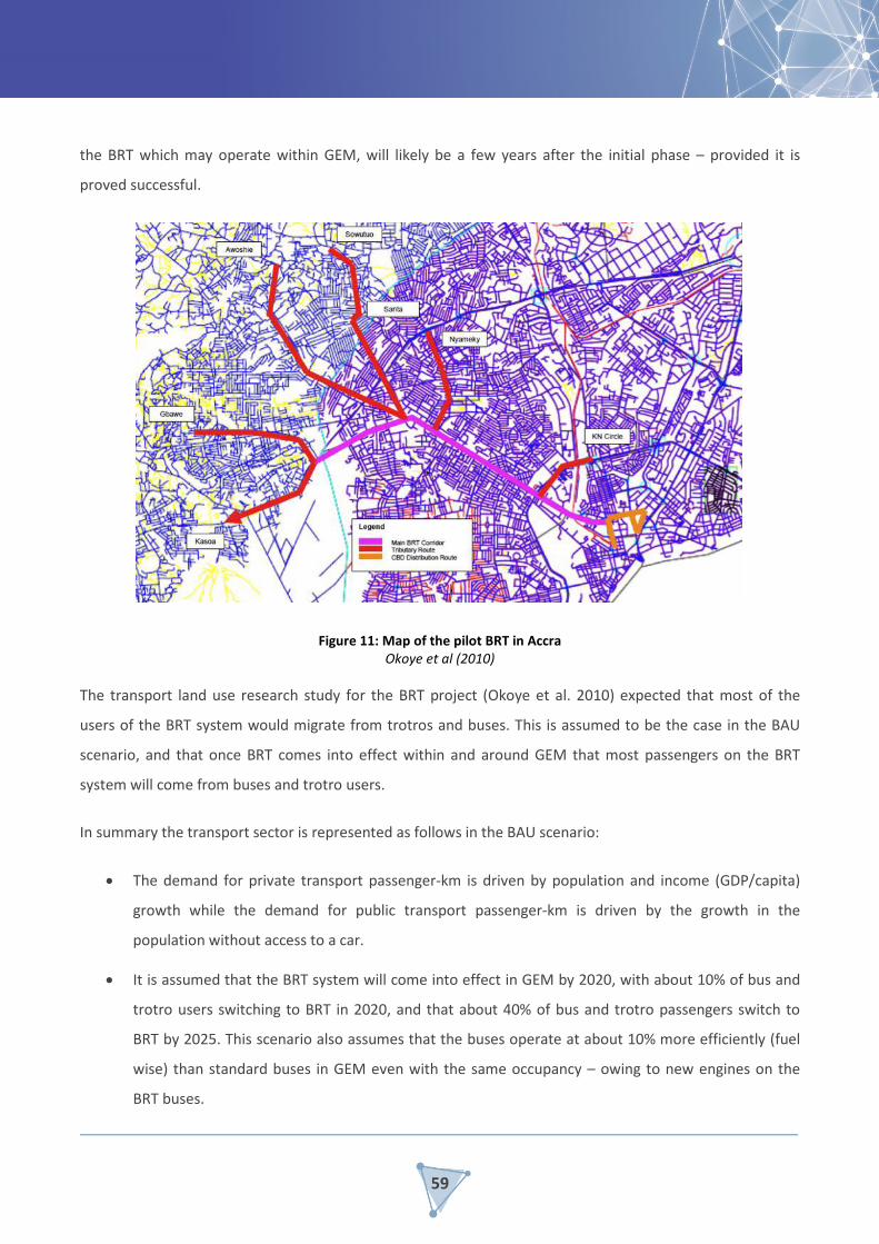
59

the BRT which may operate within GEM, will likely be a few years after the initial phase – provided it is

proved successful.

Figure 11: Map of the pilot BRT in Accra Okoye et al (2010)

The transport land use research study for the BRT project (Okoye et al. 2010) expected that most of the

users of the BRT system would migrate from trotros and buses. This is assumed to be the case in the BAU

scenario, and that once BRT comes into effect within and around GEM that most passengers on the BRT

system will come from buses and trotro users.

In summary the transport sector is represented as follows in the BAU scenario:

• The demand for private transport passenger-km is driven by population and income (GDP/capita)

growth while the demand for public transport passenger-km is driven by the growth in the

population without access to a car.

• It is assumed that the BRT system will come into effect in GEM by 2020, with about 10% of bus and

trotro users switching to BRT in 2020, and that about 40% of bus and trotro passengers switch to

BRT by 2025. This scenario also assumes that the buses operate at about 10% more efficiently (fuel

wise) than standard buses in GEM even with the same occupancy – owing to new engines on the

BRT buses.

60

• Private transportation: light vehicles and motorbikes are assumed to retain the operating

characteristics of the base year – no change in occupancy rates, and similar fuel efficiencies.

• The passenger corridor component is assumed to follow GDP per capita, which itself is an

approximation to national economic growth figures.

• Freight tonne-km for light trucks is driven by local industry growth.

• Freight tonne-km for medium and heavy trucks are assumed to grow with GDP (which is directly

proportional to national and regional economic growth rates).

8.3 HOUSEHOLD SECTOR Ghana’s population growth rate has previously been very high, attributable to declining mortality rates and

high fertility rates (NPC, 2011). The country is, however, experiencing a demographic transition as fertility

rates decline, attributed to higher school enrolment and changing economic opportunities leading to major

declines in under-19 fertility (Saleh, 2012).

Urbanisation is a significant factor influencing household growth. Ga East, lying on the outer periphery of

Greater Accra, receives a lot of inward migration of households seeking access to opportunities afforded by

the city. Geographically, the Greater Accra region is experiencing one of the highest rates of urban growth in

Ghana (Owusu, 2011). Annual household growth to 2030 is assumed to be an average of 2.5% per annum

until 2030. Based on a focus group with municipal officials, the composition of household categories is

projected to change as shown in the table below. It is assumed that there will be no change in the shares of

2nd and 3rd class households and the greatest change will come from increased service delivery within the 1st

class household category.

Table 67: Changes in household composition by category

Share in 2014

Projected share in 2030

Household 1 electrified

63% 75%

Household 1 unelectrified

21% 11%

Household 2 electrified

4% 4%


1% 1%

Household 3 7% 7%

61

electrified


2% 2%

100% 100%

8.4 MUNICIPAL SECTOR Municipal sector floorspace is projected to grow at 10% of the household growth rate, while the diesel

consumption from municipal vehicles is assumed to follow household growth rates (with an elasticity of 1) as

they serve more households through time. The water treatment system operated by the municipality is

assumed to consume more energy in line with the growth of the city population – treating more water as the

population grows. Embedded generation by diesel and petrol generators is assumed to follow the overall

floorspace growth rate for the municipality.

8.5 COMMERCIAL SECTOR The formal sector commercial floorspace is assumed to grow at 90% of the economic growth rate for the

formal sector. The informal commercial sector, however, which makes up a significant part of the economy,

is assumed to follow population growth rates, since the informal sector by nature is driven largely by the

formal economy being unable to create new jobs – pushing people into the informal sector (Ose-Boateng

and Ampratwum, 2011). Embedded generation capacity for the commercial sector is assumed to follow the

overall floor space growth rate above.

8.6 INDUSTRY The following growth rates for the various industry categories in Ga East are assumed:

• Construction – follows GDP growth with 0.8 elasticity.

• Manufacturing – follows GDP growth with 0.8 elasticity.

• Water and sanitation – assumed to grow in line with the population growth rate.

Furthermore, the overall capacity of embedded diesel and petrol generators is assumed to follow the

sector’s output through the years.

9. BAU LEAP RESULTS A model has been developed using the data collected by the University of Ghana in an energy systems

modelling platform called LEAP. The model has a node-based structure that allows the user to disaggregate

the energy system into sectors, subsectors and individual plants. The results in this report reflect an initial

62

assessment of which of these to include as energy demands but other users may wish to deselect some of

them if they are deemed to be outside municipal boundaries, outside the realm of policy influence of the city

or outside the scope of reporting conventions. One of the advantages of the modelling platform selected is

that the in-country teams can elect to select and de-select items in reporting results to suit their purpose.

The in-country teams can also review and change the key assumptions discussed above very easily through

LEAP’s user-friendly interface and quickly generate a new BAU case.

This section will present the results of the LEAP model projections. Given the large difference in the

contribution of transport for the different assumptions around spatial scope of the model, separate sets of

results assuming scope 1 and 3 methodologies for transport in the BAU scenario will be presented in the

next section below, while the other non-BAU scenarios are presented later.

9.1 GEM SCOPE 1 AND 3 METHODOLOGIES COMPARED FOR BAU The energy consumption of GEM in the BAU scenario, where very limited transboundary transport trips are

accounted for so as to calibrate the fuel consumed to the fuel supplied strictly within the municipal area, is

presented below. While the household sector is the dominant player in energy consumption for these scope

1 results, the transport fuel supply-side data for Ga East in particular are, however, in question, as discussed

in Section 7.2.3

63

Figure 12: Ga East Municipality BAU scenario energy demand by sector (above) and fuel (below) for

scope 1 methodology The following figures present the results for the scope 3 methodology, where all estimated transboundary

trips are included and all local (intraboundary) trips are included. A strictly GPC compliant GHG inventory

would report 50% of transboundary trips, but for a view of energy consumption by sector it was thought that

100% of transboundary trips was more useful. The share of trips to include in reporting is quickly adjusted in

the LEAP interface. Comparatively, the transport sector consumes about half the total energy of the

municipality in the base year becoming increasingly dominant with time, considerably more than in the

scope 1 methodology.

64

Figure 13 Ga East Municipality BAU scenario energy demand by sector (above) and fuel (below) for scope 3 methodology

The majority of fuel consumed by GEM in scope 1 methodology is in charcoal, with electricity the next single

largest fuel source, followed by LPG.

65

Figure 14: GEM fuel consumption shares for the base year and for 2030 in scope 1 methodology

Liquid fuels in scope 3 make up the majority of fuel consumed in the base year, and in the BAU scenario this

share of fuel consumption increases from just under half, to two thirds of fuel consumed in 2030.

66

Figure 15: GEM fuel consumption shares for the base year and for 2030 in scope 3 methodology

The underlying assumptions on transport distances in the model will play a bigger role in the scope 3

methodology than in the scope 1 methodology, as without calibrating to a total fuel supply the fuel

consumed will be directly proportional to the average trip distances assumed. In this work we have kept

those assumptions (on trip distances and frequencies) the same for scope 1 and scope 3.

9.2 TRANSPORT SECTOR ENERGY CONSUMPTION Scope 3 transport energy demand is mainly in the transboundary trips with private vehicles accounting for

the majority share:

67

Figure 16: GEM transport sector energy demand by subsector for scope 3 methodology

The major growth in the transport subsectors is in the transboundary private vehicles and is a result of the

increase in GDP per capita assumptions. This trend is similar (but not on the same scale) for the scope 1

methodology (note that the GDP per capita assumptions are identical in each scope, but accounting for

transboundary demand in scope 1 is much less than in scope 3):

Figure 17: GEM transport sector energy demand by subsector for scope 1 methodology

68

9.3 BAU GENERAL RESULTS In this section we present some results where the scope 1 or 3 methodologies do not impact the model – i.e.

the other sectors. Looking at the household sector, most of the energy consumption is in charcoal and

electricity consumption, with LPG also playing a significant role.

Figure 18: Household energy consumption by fuel for Ga East in the BAU scenario

Most of the energy consumed in households comes from class 1 households, while demand from the non-

electrified households are flat to 2030 (see Figure 19). This is a result of an expected increase in the number

of electrified households and a decreasing share of non-electrified households for GEM in the BAU

assumptions.

69

Figure 19: Energy consumption of the household subsectors of GEM in the BAU scenario

9.4 SENSITIVITY SCENARIO TESTS In this section we explore the impact of altered economic growth or population growth has on the energy

consumption of GEM.

Population increase (sPOP)

In this scenario, there is a sudden increase in population from 2016 onward and the city grows at 4% pa

instead of 3.1% as in the BAU.

Economic growth increase (sGDP)

In this scenario, from 2018 the general economy of GEM does not decrease in growth by 2020 as in the BAU

scenario (7.4% until 2020, 6.5% thereafter) and continues to grow at 7.4% pa.

Comparing the sensitivity scenarios to the reference scenario, we see that the energy consumption of GEM

is more sensitive to population than to economic growth.

70

Figure 20: Energy consumption of GEM in the sensitivity scenarios for population and economic growth rates increases (scope 1)

The largest energy-consuming sector in GEM, households, does not respond to the economic growth rates in

the model, but obviously responds greatly to the population increase as indicated in the figure below.

Figure 21: GEM household sector energy consumption for the sensitivity scenarios

71

The second-largest energy-consuming sector in GEM, transport, responds to both population and economic

growth.

Figure 22: Transport sector energy consumption in GEM for the sensitivity scenarios tests (scope 1)

All subsectors of the passenger transport sector respond to population more than the economic growth

rates. This is due to the majority of demand arising from public transport rather than the private, and an

increase in population (without an increase in GDP) leads to more public transport, while the same increase

in GDP will have a comparably smaller impact on the use of private transportation.

10. EFFICIENT CHARCOAL STOVES SCENARIO The household survey undertaken by the Ghanaian SAMSET team, included a question on the use of efficient

charcoal cook stoves. About 20–40% of the households that are electrified use these Gyapa cook stoves.

72

A: Electrified households

B: Non-electrified households

Figure 23: Household questionnaire on the use of efficient charcoal cookstoves from the SAMSET survey

In this scenario it is assumed that:

• A five-year roll-out program of Gyapas to the household sector of GEM begins in 2016, and by 2021

all households that indicated in the survey that they wished to have a Gyapa, get one.

• By 2030, it is assumed that everyone that used charcoal wanted to obtain a Gyapa, and so 90% of all

households that use charcoal cook on a Gyapa.

73

• It is assumed that the Gyapa cookstoves are 50% more efficient, as indicated by the Gyapa

webpage.7

• Gyapa stoves cost USD 10 in 2013, and have a three-year lifespan.8

Figure 24: Household sector energy consumption in the reference scenario by fuel

7 www.gyapa.com. 8 Lifespan information from www.climatecare.org.

74

Figure 25: Household energy consumption for the efficient stove scenario

Figure 26: Total Ga East Municipality energy consumption for the efficient stove scenario

The total monetary savings for this charcoal stove scenario is GHC 38.4 million (constant 2013) as presented

in the table below.

75

Table 68: Cumulative energy and cost savings for the efficient charcoal stoves scenario, relative to the reference scenario (Ghanaian cedi)

2016 2020 2025 2030

Charcoal tonnes saved 582 9 296 31 487 61 051

Cost impact* (incl. capital cost)

142 973 2 282 536 7 719 548 14 943 191

11. HOUSEHOLD ACCESS TO MODERN FUELS FOR COOKING

In this scenario, we explore the impact on fuel consumption in the household sector of an increase in access

and utilisation of modern energy fuels for cooking – mainly LPG and electricity. The number of households

utilising clean fuels increases in this scenario (ACC) starting in 2020 through to 2030. We assume that most

households would prefer to cook on gas (LPG) than electricity as there are a number of them already using

LPG for cooking, while the use of electricity for cooking is virtually non-existent. The uptake in the number of

households using these fuels is presented in the table below.

76

Table 69: The share of households using fuels change for cooking for the ACC scenario

Household class End use

Shares* in % for 2030 (2013) Electricity LPG Charcoal

Electrified

Household 1 Cooking 30 (0) 100 (82) 20 (81)

Other appliance use 85 (50)





Non-electrified

Household 1 Cooking 100 (41) 50 (94)

Other appliance use


Other appliance use


Other appliance use

* Note that shares in this case do not need to sum to 100% as most households use more than one fuel at a time.

While households start the uptake of more frequent use of clean fuels, the use of charcoal is assumed to

decrease – so the average intensity for the clean fuels increases while the average intensity for charcoal (the

majority of non-clean fuel use) will decrease. The numbers for electricity and LPG intensities come from the

study by Cowan (2008), while the charcoal intensities change is an assumption that the average intensity

usage will drop by 75% as most cooking is done on LPG (and electricity for some households) while some still

use charcoal for traditional cooking.

77

Table 70: Intensity change in fuel usage for the ACC scenario

Household class End use Intensity value GJ/Household for 2030

(2013) Electricity LPG Charcoal

Electrified

Household 1 Cooking 3.5 (1.5) 6.5 (5.1) 1 (7.7)

Other appliance use 1.7 (1.7)

Household 2 Cooking 3 (1.5) 5.5 (3.5) 0.75 (7.6)


Household 3 Cooking 3 (1.5) 5 (2.9) 0.75 (7.6)


Non-electrified

Household 1 Cooking 4 (2.1) 2.25 (12.2)

Other appliance use

Household 2 Cooking 3.5 (0.5) 1 (7.9)

Other appliance use

Household 3 Cooking 3.5 (0.5) 1 (7.9)

Other appliance use

The results for this scenario are presented below.

78

Figure 27: Household energy consumption of GEM in the reference scenario (above) and for the ACC scenario (below)

79

The results show that the total energy consumption difference between the two scenarios is very small by

2030, but there is a deviation in total energy consumption between 2020 and 2030.

Figure 28 Total fuel consumption for the household sectors for GEM for the access to clean fuels scenario compared to the reference scenario

The change in fuel consumption for this scenario is presented in the table below, showing a very large

increase in electricity consumption and LPG.

Table 71: Scenario cumulative impact results for access to clean fuels for cooking (ACC) in GEM

2021 2025 2030

Electricity (MWh) 1135 21 500 103 904

LPG (Tonnes) 328 5 819 25 794

Charcoal (Tonnes) -1193 -22 604 -79 589 Note: Positive numbers indicate increase in consumption, negative a decrease.

Using the costs for fuel as presented in Section 8.1, the total cost associated with the fuel consumption in

this scenario is GHC16.4 million cumulative by 2030 with the majority of the cost associated with the use of

LPG mainly due to the fact that this scenario has all households using LPG as their main fuel for cooking.

80

Table 72: Fuel cost impact results for the ACC scenario for GEM (in constant 2013 cedi)

2021 2025 2030

Electricity 262 762 1 852 003 5 458 407 LPG 891 790 15 827 372 70 158 859 Charcoal -632 165 -11 975 609 -42 166 473 Sum of fuel costs 522 386 5 703 765 33 450 793

12. CONCLUSIONS The University of Ghana have developed a unique and detailed energy dataset for the municipality of Ga

East (GEM) near Central Accra in Ghana using detailed surveys and focus groups with stakeholders and

municipal officials. This includes rich detail on household, commercial and industrial energy service demand

and fuel preference and an emerging picture of the transport sector. This dataset has been used to develop

an energy systems model that projects long term scenarios of energy use and the impact of interventions to

make energy use more sustainable.

The results show that the household and transport sectors dominate energy use in Ga East with biomass

(mostly charcoal) still accounting for just under half of household sector consumption. The fuel shares of the

household sector observed in the Ga East (GEM) survey were very similar to those observed in the Awutu

Senya (ASEM) survey as shown below. Per Capita energy consumption was however reported as 34% lower

in GEM.

Table 73: Comparison of energy carrier shares and per capita energy consumption for the household sectors in Awutu Senya and Ga East municipalities

Energy carrier GEM ASEM

Electricity 29% 30%

Kerosene 0.1% 0.4%

LPG 22% 20%

Wood 8% 5%

Charcoal 41% 44%

Per capita (GJ/pp.a) 4.2 6.4

The transport sector’s share of energy demand depends strongly on whether trips that originate inside or

outside the municipality but include a portion of the trip outside its boundaries (transboundary trips) are

81

included or excluded. The results have been presented in two scopes based on the Global Protocol for

Community-Scale Greenhouse Gas Emission Inventories (GPC) to accommodate this. Scope 1 is calibrated to

local fuel sales and includes only a portion of these transboundary trips and the alternative view, scope 3,

includes the estimated energy demand of commuting trips to Accra by private and public transport.

The inclusion of transboundary trips increases transport’s share of demand from less than 20% to just under

half and this share increases with time in the BAU case. Fuel sales in Ga East are, however, very low on a per

capita basis compared to Greater Accra and the other municipality in the survey, Awutu Senya. The implied

financial turnover per service station, furthermore, seems very low, and this data should be confirmed

before the data sets and models are finalised and released into the public domain.

Some other data issues were identified which should be dealt with before publishing the dataset, particularly

the very large discrepancy observed between LPG supply and demand, which was an issue in both surveys.

In general, the inclusion of more detailed metadata would make this interesting dataset more useful to the

research community.

Significant suppressed demand for electricity was indicated by the industry, commercial and household data.

While a minority of enterprises and households owned generators, they accounted for, on average, around

20% of electricity consumption for generator owners in the higher income household group (Household 1),

the manufacturing sub-sector, and the formal commercial sector as a whole in spite of the high price of

petrol and diesel. The Water and sewerage subsector of Industry appears very reliant on diesel-fuelled own-

generation, with five of the seven observations owning generators, which supplied nearly 90% of their

electricity consumption. The distribution of own-generation share (Appendix C) shows that a significant

minority of the commercial sector generator-owning sample use generators for up to half of their electricity

needs. Furthermore, there was a very large span in commercial sector specific electricity consumption

(kWh/m2) within activity types – for instance offices, banks or catering. The issue of consistency in footprint

area definition aside, this suggests that many commercial buildings may not enjoy the same complement of

services that others do, particularly HVAC, and that increasing incomes and reduced constraints on supply

could see significant increases in commercial building energy intensity. While informal commercial activity

appears highly electricity-efficient (or electricity poor), total energy intensity for these buildings was twice

that of the formal sector due to biomass use (see Appendix B).

Generator use in the formal commercial sector was widespread, as well as for certain activities in the

informal commercial sector. The own-generated share of electricity consumption varied widely but averaged

around 20% for the formal sector and 11% for the informal sector (see Appendix B). While this is a minority

82

share, it increases the final energy intensity of floorspace by an order of magnitude for both formal and

informal sectors, due to the relative inefficiency of home generators, particularly the small petrol generators

common in the informal sector. Assuming energy costs of GHC 0.29/kWh for petrol, GHC 0.25/kWh for diesel

and GHC 0.2–0.4/kWh for electricity, depending on consumption band, this means that commerce bears a

very high burden of cost, roughly a tenfold premium, to supplement their electricity supply.

A limited number of scenarios were investigated to illustrate the likely impacts of possible energy saving

interventions in the municipality, including an efficient fridges programme, an efficient charcoal stoves

programme, and access to modern energy (households switching to electricity and LPG). All indicated

significant savings, but access to modern energy showed by far the largest impact.

The validated, reviewed and finalised datasets and models would be very useful to researchers and planners

and should be published into the public domain in an easily accessible way as part of the SAMSET project.

13. DATA ISSUES The University of Ghana undertook extensive survey work and investigation using facilitated workshops with

stakeholders at a level of detail that brings new clarity to the understanding of energy use in the region. In

the process of using this data for model development, validation of the data has raised some questions on

aspects of the data as can be expected. These are dealt with below and it is hoped that this contributes to an

ongoing process of refinement and improvement of that dataset and methodologies.

Population

The total number of households was given as 33 949. However, the Ga East Municipality 2010 Population

and Housing census district analytical report indicated that there were 23 424 households in Ga East in 2010.

Using 3% growth rate, the 2013 household count would then be 25 596. Given that future researchers

accessing this work will likely contrast these numbers and be in doubt which is the better estimate, the

discrepancy should be clarified and documented.

Transport and fuel

With the original data provided by the municipality, the total vehicle count was 18 672 light passenger

vehicles, which was estimated by the local stakeholders in GEM based on the assumption that about 55% of

the households in GEM own a passenger car.

83

A passenger transport survey is needed to get hard data on transport by mode (car, mini bus, walking, etc)

and trip distances or annual mileages (or how long in hours). This will greatly add to the model and

understanding of the largest energy consuming sector in the municipality.

Total fuel sold in GEM for petrol and diesel is considerably lower per person than for ASEM and estimates for

the Greater Accra region – see the end of the Transport methodology section. While this could be explained

by a lack of service stations in the area, the volumes sold per service station seem too low to cover the costs

of such a business.

The consumption of LPG from the bottom-up analysis from all sectors does not calibrate to the total sold

with the municipality. There is more than 90% shortfall in LPG usage for this model calibration owing to the

very large fuel supply that was indicated in the data. The LPG numbers need to be revised.

Commercial sector energy intensities

The energy intensities calculated from the survey data for a number of observations, particularly in the

formal commercial sub-sector categories of hotels and schools, are very low relative to other values in their

categories. This suggests that this may be a result of total footprint of the premises being assumed as

floorspace in these instances, and not just the total area enclosed by the walls of buildings. As can be seen

from Figure 5, the share of area of these activities is very large and, furthermore, as indicated by Table 74

below, the spread of intensities within activity types is very large, which may either indicate a great diversity

in construction and building services practices and suppressed demand or the need to validate some of the

area data as discussed further below.

Table 74: Spread of electricity intensity for selected commercial activities in Ga East

Indicator Schools Hotels Banks Non-bank financial services

Drinking bar, restaurant,

catering services

Observations 26 18 10 4 34 Specific electricity consumption (kWh/m2yr) (including own generation)

Minimum 0.0 3.8 18.0 8.1 0.0

Median 3.8 10.6 121.2 92.0 48.8

Average 1.4 9.5 94.9 18.6 25.2

Maximum 164.8 79.1 783.0 448.1 452.2

84

The discrepancies are such that the average electricity intensity of the formal sector is reduced considerably

by the outliers, resulting in a lower average electricity intensity than the informal sector, even excluding

schools, as shown in Appendix B. This raises questions about the aggregate data and some clarification is

warranted before the datasets are finalised. This data is a particularly interesting subset of the results and,

while it does not affect the internal consistency of this model in that absolute energy demand is likely

correct, it would be useful for the purposes of benchmarking and informing other studies to review the

survey results and assess outliers such that a set of energy intensities can be published.

As shown below in plots of specific electricity consumption per unit area floorspace versus floorspace area,

outliers in the dataset tend to cluster along both axes, with observations having large areas tending to have

very low electricity intensity and vice versa. This may indicate the necessity of data checks for both

extremes. To some extent, as alluded to in the conclusions, the spread of data may indicate significant

suppressed demand in the commercial sector in that many sites lack services currently, particularly HVAC.

Figure 29: Ga East formal commercial sector – specific electricity consumption vs floorspace (Data labels indicate activity and survey ID)

85

Figure 30: Ga East informal commercial sector – specific electricity consumption vs floorspace (Data labels indicate activity and survey ID)

Metadata

In general, the inclusion of more detailed metadata would make this interesting dataset more useful to the

research community at large, for example:

The methodology adopted for determining floor space area – Did respondents disclose the enclosed area of

buildings on the site or sometimes the site area?

The method of determining the energy service share of electricity.

The method by which focus groups determined petroleum fuels supply data. Was this expert judgement or

based directly or indirectly on industry statistics of volume or turnover?

14. EFFICIENT FRIDGES SCENARIO (EFR) The Energy Commission of Ghana initiated a programme in 2011 to introduce efficient fridges, in an attempt

to reduce energy consumption by refrigerators by half. The new fridges were expected to consume 250 kWh

a year as compared to the old inefficient ones, which consumed about 1200 kWh a year on average.

Moreover, importers and retailers of appliances such as light bulbs, air conditioners and fridges are required

86

by Ghanaian standards to meet a minimum energy consumption requirement (SOE, 2013), but it was also

shown from the survey that many households still buy second-hand and inefficient appliances. The survey

showed that there is almost a 50/50 divide between new9 fridges (which are not part of the fridge

replacement programme – see survey results in Figure 31) and second-hand fridges. The results of the

SAMSET GEM survey of household refrigerators bought new or second-hand, compared with proportion of

households with efficient fridges, are shown below.

Table 75: Survey of GEM refrigeration ownership and efficient fridge penetration

Survey of GEM fridge

ownership Fridges with EE label '1'

New Second hand

Household 1 50% 48% 30% Household 2 52% 48% 20% Household 3 29% 68% 17%

Figure 31: Efficient fridge programme participation and awareness results for GEM SAMSET survey

The cost of efficient fridges is assumed to be, on average, GHC 1400, or USD 444 in 2013, and are assumed

have a 15 year lifespan.

9 New fridges are assumed meet minimum energy efficiency standards as part of newly established

legislation on imported appliances into the country (UNDP, nd).

87

Table 76: Cost of new fridges (www.jumia.com.gh/frdges-freezers/)

Cedi 2013 USD Fridge type

1 800 572 280L fridge/freezer

994 316 150L fridge

1 397 444 Average of above In this scenario:

• It is assumed that a new programme which makes it affordable to participants to buy or replace

their old fridges with efficient new ones (specifically marked with efficiency label 1) begins in 2016

and is completed by 2021,

• This replacement programme affects all those that wish to have benefited from the program as

indicated in the survey results presented above.

• The remainder of households who do not participate in this programme buy or replace their fridges

between 2021 and 2030.

• New fridges are assumed to be 80% more efficient than second-hand fridges.

• New fridges on average are 444 USD in 2013 and have a 15 year lifespan.

• Second hand fridges are assumed to be 173 USD and have a 7.5 year lifespan.

88

Figure 32: Household sector fuel consumption in the efficient fridges scenario

Figure 33: Total Ga East Municipality energy consumption comparing reference scenario and efficient fridges scenario (scope 1)

Table 77: Cumulative energy and cost savings of the efficient fridges scenario

2016 2020 2025 2030

kWh saved 928 377 15 459 651 58 840 041 131 394 800

GHC saved 178 805 2 977 529 11 332 592 25 306 638

89

The total energy saved in the stoves scenario has a larger impact than the fridges scenario, as shown below.

Figure 34: Energy consumption for Ga East Municipality comparing household scenarios

This large difference in impact of the two scenarios is mainly due to the limited number of fridges in use

compared to those households which use charcoal. However, the monetary savings are comparable

between the two scenarios, mainly due to the increase in electricity costs in the BAU case.

90

Figure 35: Total cost to GEM comparing the household scenarios

Table 78: Comparison of cumulative cost impacts (2013 GHC) for household scenarios

2016 2020 2025 2030

Efficient fridges 178 805 2 977 529 11 332 592 25 306 638

Efficient stoves 365 483 5 840 364 19 781 486 38 354 876

91

REFERENCES Appiah, S. 2015. Bus rapid transit system to begin in Accra in November, Graphic online, June 2015, available at:

http://graphic.com.gh/news/general-news/44697-bus-rapid-transit-system-to-begin-in-accra-in-november.html Bawakyillenuo, S and Agbelie, I. 2014. Ga East State of Energy Report, ISSER, University of Ghana. Bessey, B. 2014. First phase of bus rapid transport to commence in July, AllAfrica, 2014 available at

http://allafrica.com/stories/201401300987.html Cowan, B., 2008. Alleviation of poverty through the provision of local energy services (APPLES). Project no. EIE-04-168. Cape Town,

South Africa Currency historical exchange rates available at: www.xe.com Ghana Statistical Service. 2014a. Gross domestic product. Accra, Ghana Ghana Statistical Service. 2014b. 2010 population and housing census district analytical report – Awutu Senya East Municipality.

Accra, Ghana Ghana Statistical Service. 2012. Population and housing census 2010. Summary report of final results. Accra, Ghana International Monetary Fund (IMF) 2013. World Economic Outlook. McCall, B, Tait, L and Stone, A. 2016. Awutu Senya East LEAP model technical report. SAMSET project. National Petroleum Authority (NPA). 2016. Regional consumption 2010 to 2014 statistics. Accessed January 2016. Available at

http://npa.gov.gh/npa_new/Downloads.php. National Population Council (NPC). 2011. Ghana Stabilisation report 2011. Available at:

http://www.npc.gov.gh/web/images/ICPD/Ghana_Population_and_Stablisation_Report.pdf. Okoye, V, Sands, J and Debrah C. 2010. The Accra pilot bus-rapid transit project – transport land use research study. Millennium

Cities Initiative. Osei-Boateng, C and Ampratwum, E. 2011. The informal sector in Ghana. Friedrich Ebert Stiftung Owusu, G. 2011. Spatial patterns and trends of Ghana’s contemporary urbanization: Polarization reversal or urban primacy? Institute

of Statistical, Social and Economic Research. Public Utilities Regulatory Commission. 2013. Press release October 2013. Available at:

https://www.giz.de/fachexpertise/downloads/2013-en-ghana-approved-electricity-and-water-tariffs-2013.pdf, Simons, A and Nunoo, S. 2009. Liquefied petroleum gas as an alternative vehicle fuel in Ghana. Petroleum Science and Technology,

27:18: 2223-2233, DOI: 10.1080/10916460802686624. Tait, L, McCall, B and Stone, A. 2014. Energy futures modelling for African cities – selecting a modelling tool for the SAMSET project.

Energy Research Centre, University of Cape Town, United Nations Development Programme (UNDP). n.d. Promoting of appliance of energy efficiency and transformation of the

refrigerating appliances market in Ghana. Available at; http://www.gh.undp.org/content/ghana/en/home/operations/projects/environment_and_energy/Susdevclusterprojects.html.

World Bank. n.d. The world development indicators database. Available at data.worldbank.org. Accessed 18th December 2013. World Bank projections from http://knoema.com/yxptpab/crude-oil-price-forecast-long-term-2015-to-2025-data-and-charts World Resources Institute (WRI). 2014. Global protocol for community-scale greenhouse gas emission inventories: An accounting

and reporting standard for cities/ World Resources Institute, C40 Cities Climate Leadership Group and ICLEI - Local Governments for Sustainability. Available from URL: http://ghgprotocol.org/files/ghgp/GHGP_GPC.pdf.

http://graphic.com.gh/news/general-news/44697-bus-rapid-transit-system-to-begin-in-accra-in-november.html

http://www.xe.com/

http://npa.gov.gh/npa_new/Downloads.php

https://www.giz.de/fachexpertise/downloads/2013-en-ghana-approved-electricity-and-water-tariffs-2013.pdf

http://www.gh.undp.org/content/ghana/en/home/operations/projects/environment_and_energy/Susdevclusterprojects.html

http://knoema.com/yxptpab/crude-oil-price-forecast-long-term-2015-to-2025-data-and-charts

92

Appendix A. Own-generation efficiency model In order to convert the own-generation data from the survey, which consisted of generator ratings an annual

fuel consumption, into electricity consumption, models for gasoline (petrol) and diesel were developed

based on published data as follows. Equation 8 was determined from linear regression of the following data.

The square of the Pearson correlation co-efficient of the correlation (R2) was 62%.

Table 79: Gasoline generator data used to derive a model of generator fuel consumption and efficiency as a function of rating and load factor

Model Rating (kVA/kW)

Load Factor

Consumption (L/hour)

Efficiency (%)

AlphaGen™ ACX2000i 1.9 1 1.77 12%

AlphaGen™ ACX2000i 1.9 0.25 0.71 8%

Champion 80 cc 1.2 0.5 0.55 12%

GEN154 1.2 0.5 0.62 11%

Generac 15,000 15 0.5 6.06 14%

Generac 6500E 6.5 0.5 2.37 15%

Generac GP15000E 15 0.5 6.06 14%

Generac GP17500E 17.5 0.5 6.06 16%

Generac iQ2000 1.6 0.25 0.52 9%

Generac XD 5000 5 0.5 1.40 20%

Honda GX 390 7 1 3.37 23%

Honda GX 390 7 0.75 2.73 22%

Honda GX 390 7 0.5 2.37 17%

Honda GX 630 11.7 1 6.44 20%

Honda GX 630 11.7 0.75 5.30 19%

Honda GX 630 11.7 0.5 4.16 16%

Honda GX 630 14 1 6.44 24%

Honda GX 630 14 0.75 5.30 22%

Honda GX 630 14 0.5 4.16 19%

Honda GXH50 OHV 0.9 1 0.60 17%

Honda GXH50 OHV 0.9 0.25 0.27 9%

NorthStar 15,000 13.5 0.5 5.20 14%

Robin R650 0.55 1 0.47 13%

Unknown 2.7 1 1.71 18%

Unknown 5.5 1 3.52 17%

Unknown 6.8 0.5 2.52 15% Sources:

93

http://www.centralmainediesel.com; http://www.globalspec.com; http://www.buffalotools.com; http://gens.lccdn.com

http://powerequipment.honda.com; http://www.homedepot.com; http://www.northerntool.com

Equation 11 was determined from linear regression of the following data. The square of the Pearson

correlation co-efficient of the correlation (R2) was 66%.

Table 80: Diesel generator data used to derive a model of generator fuel consumption and efficiency as a function of rating and load factor

Model Rating Load factor


Efficiency (%)

Unknown 20 0.25 2.3 22% Unknown 30 0.25 4.9 15% Unknown 40 0.25 6.1 17% Unknown 60 0.25 6.8 22% Unknown 75 0.25 9.1 21% Unknown 100 0.25 9.8 26% Unknown 20 1 6.1 33% Unknown 30 1 11.0 28% Unknown 40 1 15.1 27% Unknown 60 1 18.2 33% Unknown 75 1 23.1 33% Unknown 100 1 28.0 36% Unknown 20 0.75 4.9 31% Unknown 30 0.75 9.1 25% Unknown 40 0.75 12.1 25% Unknown 60 0.75 14.4 31% Unknown 75 0.75 17.4 33% Unknown 100 0.75 22.0 34% Kohler Diesel 6,500 Watt Diesel Generator 6.5 0.5 1.3 25%

Kohler Diesel 6,500 Watt Diesel Generator 6.5 0.75 1.7 29%

Kohler Diesel 6,500 Watt Diesel Generator 6.5 1 2.2 30%

Kohler 35REOZT4 30 1 10.5 29% Kohler 35REOZT4 30 0.75 7.8 29% Kohler 35REOZT4 30 0.5 5.4 28% Kohler 35REOZT4 30 0.25 3.1 24% Kohler 35REOZT4 28 1 9.8 29% Kohler 35REOZT4 28 0.75 7.3 29% Kohler 35REOZT4 28 0.5 5.0 28% Kohler 35REOZT4 28 0.25 2.9 24% Cummins DSKAB 15 0.25 1.3 29% Cummins DSKAB 15 0.5 2.6 29% Cummins DSKAB 15 0.75 3.9 29% Cummins DSKAB 15 1 5.2 29% Cummins DSKAB 13.6 0.25 1.2 29%

94

Model Rating Load factor


Efficiency (%)

Cummins DSKAB 13.6 0.5 2.3 29% Cummins DSKAB 13.6 0.75 3.5 29% Cummins DSKAB 13.6 1 4.7 29%

Sources: http://www.centralmainediesel.com; http://www.dieselserviceandsupply.com/Diesel_Fuel_Consumption.aspx; http://www.kohlerpower.com/onlinecatalog/pdf/g5412.pdf; https://powersuite.cummins.com/PS5/PS5Content/SiteContent/en/Binary_Asset/pdf/Commercial/Diesel/d-3372.pd

http://www.centralmainediesel.com/

http://www.dieselserviceandsupply.com/Diesel_Fuel_Consumption.aspx

http://www.kohlerpower.com/onlinecatalog/pdf/g5412.pdf

95

Appendix B. Commercial sector energy intensity by activity type Table 81: Average breakdown of electricity and energy intensity by type of use in the Ga East

commercial sector

Type and Activity of Use

Floor-space (m2)

Average specific

electricity consumptio

n (kWh/m2.yr

)*

Average specific

electricity consumption (inc. gen

fuel) (kWh/m2.yr)

#

Average specific energy

consumption

(kWh/m2.yr)+

Average share of

own generation (kWh/m2.yr

)x

Formal 94 285 10 104 137 21%

Formal (less Schools) 32 562 26 291 301 23% Hotels & guest houses 22 228 9 82 97 17%

Schools 61 722 1 5 51 6%

Non-banks financial services 1 640 19 330 330 31%

Hospitals 3 253 39 619 619 29%

Banks 5 441 86 932 932 23%

Informal 14 966 28 229 600 11%

Aluminium fabricator 90 100 872 872 9%

Carpentry/welding shops 4 680 22 133 133 7%

Cold store 25 142 142 142 0%

Corn mill 49 118 118 118 0%

Drinking bar, restaurant, catering services 3 301 25 307 1934 18%

Electronic repair shops 188 82 590 636 7%

Fitting/mechanic 2 635 9 9 21 0%

Laundry 36 299 3 259 3 259 16%

Other 1 646 40 716 716 25%

Petty trading 240 22 22 569 0%

Retail 1 320 43 126 129 3%

Tailoring/seamstress 756 49 130 143 2% *: Includes own generated electricity #: Grid electricity and petrol and diesel energy consumed by own generated electricity +: Includes all fuels used on site including charcoal and wood x: Share of own generation of all electricity consumed

96

Appendix C. Distribution of commercial own generation electricity share in the GEM and ASEM surveys

The distribution of own-generation shares in the commercial sectors of both the GEM and ASEM surveys

compared favourably, as shown below, and indicate that, while a minority of formal and informal enterprises

own generators (18% in ASEM and 28% in GEM), those that do own them use them extensively, with a

significant minority generating half their own electricity consumption.

Figure 36: Comparison of share of own-generation distributions for ASEM and GEM commercial sector generator owners

The outliers in the sample are instances where there was a discrepancy in the data between expenditure

recorded as spent on generator fuel and volumes used as generator fuel. The methodology adopted

assumed expenditure to be more reliable however on review in these instances it is likely volumes were

more accurate.

Informal enterprises that owned generators showed a similar distribution to the formal sector for the Ga

East sample with a significant share showing high generator usage rates as shown below. The more ragged

distribution may however indicate less accurate reporting for informal enterprises.

97

Figure 37: Comparison of share of own-generation distributions for formal and informal commercial sector generator owners in Ga East Municipality Sample

This document is an output from a project co-funded by UK aid from the UK Department for International Development (DFID), the Engineering & Physical Science Research Council (EPSRC) and the Department for Energy & Climate Change (DECC), for the benefit of developing countries. The views expressed

are not necessarily those of DFID, EPSRC or DECC, or any institution partner of h j

ga east leap modelling technical report · 2. 8.3 household sector 60 8.4 municipal sector 61 8.5...

Documents