gabriele spenger cryptographic primitives in rfid systems
TRANSCRIPT

deposit_hagenPublikationsserver der Universitätsbibliothek
Mathematik und Informatik
Dissertation
Gabriele Spenger
Cryptographic Primitives in RFID Systems

Cryptographic Primitives
in RFID Systems
Dissertation
for the Degree of
Doctor of Natural Sciences
(Dr. rer. nat.)
Gabriele Spenger
FernUniversität in Hagen
Faculty of Mathematics and Computer Science
Parallelism and VLSI Group
June 2017

Erster Gutachter Herr Prof. Dr. Jörg Keller
FernUniversität in Hagen
Zweiter Gutachter Herr Prof. Dr.-Ing. Damian Weber
Hochschule für Technik und Wirtschaft des
Saarlandes
Vorsitzender der Herr Prof. Dr. Friedrich Steimann
Promotionskommission FernUniversität in Hagen
Protokollantin Frau Dr. Daniela Keller
FernUniversität in Hagen
Tag der mündlichen Prüfung October 05, 2017
i
Abstract
The growth of electronic communication over the last decades and the developmentof technologies like Radio Frequency Identi�cation RFID (or more general the In-ternet of Things) has led to a large interest in data security in all kinds of devices.Sending sensitive information over communication channels that are accessible byattackers, e.g. the Internet, or the air in case of radio transmission, requires measuresto secure the con�dentiality as well as the integrity of the transmitted data. In orderto achieve this, cryptographic protocols have been developed and standardized thatmake use of cryptographic base functions like symmetric or asymmetric encryption,hashing and pseudo-random number generators (PRNGs). Because of the limita-tions in cost, energy consumption and computational performance for devices likeRFID transponders, low-complexity cryptographic functions are of high interest forapplications running on these devices.
The security of cryptographic functions such as pseudo-random number genera-tors (PRNGs) can usually not be mathematically proven. Instead, statistical prop-erties of the algorithms are commonly evaluated using standardized test batterieson a limited number of output values. Additionally, susceptibility against knownattacks can be investigated. This thesis demonstrates that valuable additional in-formation about the properties of the algorithm can be gathered by analyzing thestate space structure. Analysis results for di�erent cryptographic primitives includ-ing commonly used algorithms as well as recent proposals and chaotic functions arepresented.
Furthermore, several novel low-complexity approaches are introduced that im-prove the state space structure of such algorithms signi�cantly. The improvementis demonstrated by applying the approaches to di�erent algorithms and presentingthe analysis results. Further evaluation of the modi�ed algorithms is performed bystatistical analysis using the commonly used standardized test batteries.
Keywords: Low-Cost RFID, Lightweight Security, Chaotic Function, Pseudo-Ran-dom Number Generator
ii
Kurzfassung
Die zunehmende Verbreitung elektronischer Kommunikation in den letzten Jahrzehn-ten und die Entwicklung von Technologien wie z.B. der Radiofrequenz-Identi�kationRFID (oder allgemeiner des Internets der Dinge) hat zu einem erheblichen Interessean Datensicherheit in allen Bereichen geführt. Das Übertragen sensibler Informa-tionen über Kommunikationskanäle, die Angri�en ausgesetzt sein können, wie z.B.dem Internet oder der Luft im Falle von Funkübertragung, erfordert Maÿnahmen,um die Vertraulichkeit und Integrität der übertragenen Daten zu gewährleisten. Umdies zu erreichen, wurden kryptographische Protokolle entwickelt und standardisiert,die auf kryptographischen Basisfunktionen wie z.B. symmetrischer und asymmetri-scher Verschlüsselung, Hashing und Pseudozufallszahlengeneratoren basieren. DieEinschränkungen der Geräte wie z.B. RFID Transpondern bzgl. Preis, Stromver-brauch und Rechenleistung führen in Anwendungen auf diesen Geräten zu einemstarken Interesse an kryptographischen Funktionen mit geringer Komplexität.
Die Sicherheit kryptographischer Funktionen wie beispielsweise Pseudozufalls-zahlengeneratoren kann im Allgemeinen nicht mathematisch bewiesen werden. Statt-dessen werden üblicherweise die statistischen Eigenschaften der Algorithmen mittelsstandardisierter Testsuiten auf Basis einer beschränkten Anzahl von Ausgangswertenuntersucht. Auÿerdem kann die Anfälligkeit gegen bekannte Angri�e geprüft werden.Die vorliegende Arbeit demonstriert, dass wertvolle zusätzliche Informationen überdie Eigenschaften eines Algorithmus' durch die Analyse der Zustandsraumstrukturgewonnen werden können. Es werden Analyseergebnisse verschiedener kryptographi-scher Primitive, einschlieÿlich verbreiteter Algorithmen sowie neuer Verfahren undchaotischer Funktionen präsentiert.
Des Weiteren werden mehrere neuartige Ansätze vorgestellt, die die Zustands-raumstruktur solcher Algorithmen signi�kant verbessern. Diese Verbesserungen wer-den durch ihre Anwendung auf verschiedene Algorithmen sowie einer entsprechendenZustandsraumanalyse demonstriert. Ergänzt wird dies durch weitere Untersuchun-gen auf Basis einer statistischen Auswertung durch die verbreiteten standardisiertenTestsuiten.
Schlüsselworte: Radiofrequenzidenti�kation, geringe Komplexität, kryptographi-sche Funktionen, Chaotische Funktion, Pseudozufallszahlengenerator

iii
Acknowledgements
The inspiration for this thesis and the motivation to work on the topic of low-complexity PRNGs was born out of the growing concerns in the general publicaround privacy in the context of RFID systems. With RFID tags getting ubiquitousand being part of the daily life of everyone, the traceability becomes a problem, asuser pro�les can be created without people being aware. This poses new challengesto cryptographic methods and algorithms that I felt are important to tackle.
The topic of RFID brought me in contact with many knowledgeable people onconferences and symposiums that were in�uential to my work and opened my mindfor new ideas.
I would like to thank my supervisor Prof. Dr. Jörg Keller for his great guidance,the inspirational discussions and his never-ending patience. I am also grateful forthe guidance of Prof. Dr.-Ing. Damian Weber and his helpful input. Furthermore,I want to thank my friends for their fantastic support and for bearing with theamount of time that I spent creating this work. Finally, I want to thank my familyfor their support and their understanding for the many evenings and weekends I wasabsorbed in thoughts about random numbers.
Nürnberg, June 2017

iv
v
Publications and Previous Work
A number of publications have already been published in the context of this disser-tation. In the following, contributions by other authors that have been incorporatedare listed.
• G. Spenger, Sicherheit des Pseudozufallszahlengenerators LAMED, in Proc. ofthe Eight GI SIG SIDAR Graduate Workshop on Reactive Security (SPRING).Technical Report SR-2013-01, page 18, GI FG SIDAR, München, Feb. 2013.
In this publication, di�erent approaches to analyze the state transition graphfor functions with large state spaces were presented. An analysis of the LAMEDalgorithm was shown as a practical application of these methods.
• G. Spenger, J. Keller, Analysis of PRNGs with Large State Spaces and Struc-tural Improvements, in International Journal of RFID Security and Cryptog-raphy, Volume 3, Issue 2, Dec. 2014/2015.
This article demonstrates the break-out approach by parameter modi�cation.The paper was written by Spenger after valuable input on the break-out idea byKeller.
• G. Spenger, J. Keller, Security Aspects of PRNGs with Large State Spaces,in Proc. 10th International Conference for Internet Technology and SecuredTransactions (ICITST-2015), London, Dec. 2015.
In this paper, it was shown how the state space analysis of a reduced state lengthversion of AKARI-1 can provide valuable information about the unmodi�edalgorithm. Furthermore, we presented the result of a sampled analysis of A5/1,clearly demonstrating the known weaknesses of this algorithm. The paper waswritten by Spenger and edited by Keller.
• G. Spenger, J. Keller, Structural Improvements of Chaotic PRNG Implemen-tations, in Proc. 11th International Conference for Internet Technology andSecured Transactions (ICITST-2016), Barcelona, Spain, Dec. 2016.
In this work, the idea of breaking out by parameter modi�cation was applied tochaotic transition functions. Analysis results for the Logistic and Trigonomet-ric chaotic functions have been shown. The paper was written by Spenger andedited by Keller.

vi
• J. Keller, G. Spenger, Tweaking Cryptographic Primitives with Moderate StateSpace by Direct Manipulation, in Proc. IEEE International Conference onCommunications (ICC'17), Paris, France, May 2017.
The idea of breaking out is extended in this work by a white box approach thatemploys a greedy algorithm to identify local optima for the break-out start andtarget nodes. The idea for this approach comes from Keller, the analysis resultsfrom Spenger.
• G. Spenger, J. Keller, Improving the Cycle Lengths of Chaotic PRNGs, inInternational Journal of Chaotic Computing (IJCC), Volume 4, Issue 1, 2017,ISSN 2046-3332 (Online), http://infonomics-society.org/ijcc/.
The idea of breaking out by parameter modi�cation on chaotic transition func-tions was statistically evaluated using the NIST test battery. The paper waswritten by Spenger and reviewed by Keller.
• J. Keller, G. Spenger, S. Wendzel, Ant Colony-inspired Parallel Algorithm toImprove Cryptographic Pseudo Random Number Generators, in IEEE Journalof Cyber Security and Mobility, 2nd Workshop on Bio-inspired Security, Trust,Assurance and Resilience (BioSTAR 2017), May 2017.
In this publication, it was shown that the application of an ant colony algorithmon the state space analysis results in a signi�cant run time reduction for parallelsystems which are necessary for state spaces too large for sequential processing,thus extending the range of the white box approach. The idea comes fromKeller, the analysis results from Spenger, Wendzel reviewed and presented thepaper.
vii
Contents
1 Introduction 11.1 Motivation . . . . . . . . . . . . . . . . . . . . . . . . . . . . . . . . . 11.2 Main Contributions . . . . . . . . . . . . . . . . . . . . . . . . . . . . 21.3 Thesis Overview . . . . . . . . . . . . . . . . . . . . . . . . . . . . . . 4
2 Background and Related Works 52.1 RFID Systems . . . . . . . . . . . . . . . . . . . . . . . . . . . . . . . 5
2.1.1 Overview of RFID Systems . . . . . . . . . . . . . . . . . . . 52.1.2 Security Aspects of RFID Systems . . . . . . . . . . . . . . . 92.1.3 Measures to Protect Privacy in RFID . . . . . . . . . . . . . . 15
2.2 Graph Theory . . . . . . . . . . . . . . . . . . . . . . . . . . . . . . . 172.3 Cryptographic Pseudo-Random Number Generators . . . . . . . . . . 20
2.3.1 Overview of Random Number Generators . . . . . . . . . . . . 202.3.2 Metrics for a "Good" PRNG . . . . . . . . . . . . . . . . . . . 22
3 Analysis Methods 293.1 Depth-First Search . . . . . . . . . . . . . . . . . . . . . . . . . . . . 293.2 Sampling the State Space . . . . . . . . . . . . . . . . . . . . . . . . 303.3 Reducing the State Space . . . . . . . . . . . . . . . . . . . . . . . . 333.4 Candidate Analysis . . . . . . . . . . . . . . . . . . . . . . . . . . . . 33
4 Analysis Results 354.1 AKARI . . . . . . . . . . . . . . . . . . . . . . . . . . . . . . . . . . 35
4.1.1 Sampled Analysis . . . . . . . . . . . . . . . . . . . . . . . . . 364.1.2 Reduced Word Length Analysis . . . . . . . . . . . . . . . . . 364.1.3 Interpretation of Test Results . . . . . . . . . . . . . . . . . . 37
4.2 A5/1 . . . . . . . . . . . . . . . . . . . . . . . . . . . . . . . . . . . . 384.2.1 Sampled Analysis . . . . . . . . . . . . . . . . . . . . . . . . . 394.2.2 Reduced Variant . . . . . . . . . . . . . . . . . . . . . . . . . 404.2.3 Interpretation of Test Results . . . . . . . . . . . . . . . . . . 42
4.3 LAMED . . . . . . . . . . . . . . . . . . . . . . . . . . . . . . . . . . 434.3.1 Sampled Analysis . . . . . . . . . . . . . . . . . . . . . . . . . 444.3.2 Reduced Variant . . . . . . . . . . . . . . . . . . . . . . . . . 454.3.3 Interpretation of Test Results . . . . . . . . . . . . . . . . . . 45
viii CONTENTS
4.4 Chaotic Functions . . . . . . . . . . . . . . . . . . . . . . . . . . . . . 454.4.1 Logistic Map . . . . . . . . . . . . . . . . . . . . . . . . . . . 464.4.2 Trigonometric Function . . . . . . . . . . . . . . . . . . . . . . 47
4.5 Enocoro . . . . . . . . . . . . . . . . . . . . . . . . . . . . . . . . . . 484.5.1 Sampled Analysis . . . . . . . . . . . . . . . . . . . . . . . . . 494.5.2 Reduced Variants . . . . . . . . . . . . . . . . . . . . . . . . . 504.5.3 Interpretation of Test Results . . . . . . . . . . . . . . . . . . 53
4.6 Trivium . . . . . . . . . . . . . . . . . . . . . . . . . . . . . . . . . . 534.6.1 Sampled Analysis . . . . . . . . . . . . . . . . . . . . . . . . . 544.6.2 Reduced Variant . . . . . . . . . . . . . . . . . . . . . . . . . 544.6.3 Interpretation of Test Results . . . . . . . . . . . . . . . . . . 57
4.7 MD5 . . . . . . . . . . . . . . . . . . . . . . . . . . . . . . . . . . . . 574.7.1 Sampled Analysis . . . . . . . . . . . . . . . . . . . . . . . . . 604.7.2 Interpretation of Test Results . . . . . . . . . . . . . . . . . . 60
4.8 Spritz . . . . . . . . . . . . . . . . . . . . . . . . . . . . . . . . . . . 604.8.1 Sampled Analysis . . . . . . . . . . . . . . . . . . . . . . . . . 614.8.2 Interpretation of Test Results . . . . . . . . . . . . . . . . . . 62
4.9 SHA-3 . . . . . . . . . . . . . . . . . . . . . . . . . . . . . . . . . . . 634.9.1 Sampled Analysis . . . . . . . . . . . . . . . . . . . . . . . . . 644.9.2 Interpretation of Test Results . . . . . . . . . . . . . . . . . . 64
5 Improvements 67
5.1 Breaking out of the Cycle . . . . . . . . . . . . . . . . . . . . . . . . 675.2 Counter-Based Random Break-out . . . . . . . . . . . . . . . . . . . 685.3 Parameter Modi�cation . . . . . . . . . . . . . . . . . . . . . . . . . . 69
5.3.1 Analysis for Logistic Map . . . . . . . . . . . . . . . . . . . . 705.3.2 Analysis for Trigonometric Function . . . . . . . . . . . . . . . 72
5.4 Hash Based Parameter Modi�cation . . . . . . . . . . . . . . . . . . . 735.5 Combining Multiple Algorithms . . . . . . . . . . . . . . . . . . . . . 745.6 Direct State Graph Manipulation . . . . . . . . . . . . . . . . . . . . 74
5.6.1 Greedy Algorithm . . . . . . . . . . . . . . . . . . . . . . . . . 775.6.2 Action A . . . . . . . . . . . . . . . . . . . . . . . . . . . . . . 775.6.3 Action B . . . . . . . . . . . . . . . . . . . . . . . . . . . . . . 785.6.4 Implementation . . . . . . . . . . . . . . . . . . . . . . . . . . 795.6.5 Evaluation of Logistic Map . . . . . . . . . . . . . . . . . . . . 825.6.6 Evaluation of MD5 . . . . . . . . . . . . . . . . . . . . . . . . 835.6.7 Evaluation of Trigonometric Function . . . . . . . . . . . . . . 875.6.8 Evaluation of SHA-3 . . . . . . . . . . . . . . . . . . . . . . . 885.6.9 Performance Evaluation . . . . . . . . . . . . . . . . . . . . . 895.6.10 Further Optimization Criteria . . . . . . . . . . . . . . . . . . 91

CONTENTS ix
6 Statistical Evaluation 936.1 Motivation . . . . . . . . . . . . . . . . . . . . . . . . . . . . . . . . . 936.2 DIEHARD . . . . . . . . . . . . . . . . . . . . . . . . . . . . . . . . . 936.3 NIST . . . . . . . . . . . . . . . . . . . . . . . . . . . . . . . . . . . . 986.4 DIEHARDER . . . . . . . . . . . . . . . . . . . . . . . . . . . . . . . 1006.5 Analysis Results . . . . . . . . . . . . . . . . . . . . . . . . . . . . . . 102
6.5.1 Statistic Evaluation of Logistic Map . . . . . . . . . . . . . . . 1026.5.2 Statistic Evaluation of Trigonometric Function . . . . . . . . . 1036.5.3 Statistic Evaluation of MD5 . . . . . . . . . . . . . . . . . . . 1056.5.4 Statistic Evaluation of SHA-3 . . . . . . . . . . . . . . . . . . 105
6.6 Conclusion of Statistic Evaluations . . . . . . . . . . . . . . . . . . . 106
7 Conclusion and Future Work 107
References 109
List of Figures 119
List of Tables 121
A Statistical Data 123A.1 DIEHARDER Output . . . . . . . . . . . . . . . . . . . . . . . . . . 123
A.1.1 DIEHARDER Output for Logistic Map . . . . . . . . . . . . . 123A.1.2 DIEHARDEROutput for Logistic Map with Parameter Change
for k=1024 . . . . . . . . . . . . . . . . . . . . . . . . . . . . 125A.1.3 DIEHARDER Output for Logistic Map with Action A and B 128A.1.4 DIEHARDER Output for Trigonometric Function . . . . . . . 130A.1.5 DIEHARDER Output for Trigonometric Function with Pa-
rameter Change for k=1024 . . . . . . . . . . . . . . . . . . . 133A.1.6 DIEHARDER Output for Trigonometric Function with Action
A and B . . . . . . . . . . . . . . . . . . . . . . . . . . . . . . 135A.1.7 DIEHARDER Output for MD5 Truncated to 64 Bit . . . . . . 138A.1.8 DIEHARDER Output for MD5 Truncated to 64 Bit with Ac-
tion A and B . . . . . . . . . . . . . . . . . . . . . . . . . . . 140A.2 NIST Output . . . . . . . . . . . . . . . . . . . . . . . . . . . . . . . 142
A.2.1 NIST Output for Logistic Map . . . . . . . . . . . . . . . . . 142A.2.2 NIST Output for Logistic Map with Parameter Change for
k=1024 . . . . . . . . . . . . . . . . . . . . . . . . . . . . . . 146A.2.3 NIST Output for Logistic Map with Action A and B . . . . . 149A.2.4 NIST Output for Trigonometric Function . . . . . . . . . . . . 152A.2.5 NIST Output for Trigonometric Function with Parameter Change
for k=1024 . . . . . . . . . . . . . . . . . . . . . . . . . . . . 155A.2.6 NIST Output for Trigonometric Function with Action A and B 158A.2.7 NIST Output for MD5 Truncated to 64 Bit . . . . . . . . . . 161

x CONTENTS
A.2.8 NIST Output for MD5 Truncated to 64 Bit with Action A and B164A.2.9 NIST Output for SHA-3 Truncated to 64 Bit . . . . . . . . . . 167A.2.10 NIST Output for SHA-3 Truncated to 64 Bit with Action A
and B . . . . . . . . . . . . . . . . . . . . . . . . . . . . . . . 170
1
Chapter 1
Introduction
This thesis covers aspects of cryptographic primitives speci�c for RFID applicationsand related low-complexity implementations, with a focus on pseudo-random num-ber generators. This chapter describes the motivation for the investigations and therespective results that are presented, followed by a summary of the main contribu-tions of this work.
1.1 Motivation
The demand for automated identi�cation systems is present in many areas, e.g. trade,production, supply chain management as well as services [Fin15]. The registration ofproduct speci�c data allows e.g. automated inventory lists of warehouses or trackingof the location of a shipment on its dispatch route. There is a whole range of technicalsolutions that deal with this task. The most commonly used method today is thebar code. These printed labels are used for determining the price of goods in shops,but also e.g. for the identi�cation of parcels, and are scanned with an optical readingdevice. The object provides the information that is needed for its identi�cation itself,which is why the method is called auto identi�cation (auto-ID).
A di�erent approach to auto-ID is the use of RFID (Radio Frequency IDenti�ca-tion [Wal83]). In RFID systems, the information is stored on an electronic storagedevice and transmitted via radio waves. RFID systems and applications are morewidespread than evident. There are many areas in which identi�cation processes canbe automated and rationalized. RFID systems extend and enhance the functionalityand possible applications of traditional auto-ID systems and o�er high potential fore�ciency increase. It is imaginable that RFID will completely replace the opticalscan of bar codes in logistics at some point.
Management of stock and inventories in shops and warehouses is a prime domainfor low-cost tags. In 2003, the American mass marketing giant Walmart has begunrequiring its main suppliers to put electronic tags in the pallets and packing casesthat they deliver to it [Avo05]. Although the project was abandoned in 2009, similarprojects have been successful, e.g. by the American Department of Defense and in

2 1. Introduction
2012 in the distribution center of Migros, Switzerland's largest retail company.With the increasing usage of RFID systems that allow contactless digital auto-
mated transmission of information, data security and protection gets more into thefocus. Cryptographic methods allow the encryption and authentication of data andthereby the protection against access or modi�cation by unauthorized parties. Tomake use of the advantages of RFID while protecting the privacy of individuals, thefundamentals of contemporary data privacy laws must be taken into account alreadyearly in the design process [OWH+04].
The potential application areas for RFID systems are manifold and have variousrequirements regarding cost, hardware speci�cations, and data security. The MITpublications [SWE02] and [WSRE04] already mention the challenge of encryption oncost e�cient RFID systems, coming to the conclusion that the price of RFID tagsshould not exceed 5 Cents to allow mass market penetration and replace currentproduct identi�cation systems [Sar01]. Such a low unit price increases the challengeto achieve the required data security: as the price is related to the chip area, thenumber of gates on the RFID tag and thereby the complexity of the executed oper-ations is limited. Furthermore, such a price is not achievable with battery poweredtags and the limitation to passively powered tags puts additional constraints tothe computational power. When product items carry an electronic ID and can bescanned without intervisibility, the security requirements must be reviewed carefullyfor each speci�c application. The ful�llment of these requirements on the other handimpacts the hardware speci�cations and the related unit price.
While the motivation of this work is mainly based on RFID applications, the topicof lightweight cryptography is not limited to this technology. With the emergingInternet of Things, low-power devices that communicate over the Internet e.g. usingWi-Fi connections are becoming ubiquitous. These devices have similar requirementsregarding data security and privacy and the investigations presented in this work areapplicable to them as well. In fact, RFID is believed to be an enabling technology forthe Internet of Things [Pos09], which shows how closely related these applicationsare.
1.2 Main Contributions
The main novel contributions of this work can be summarized under three maintopics:
Analysis of Cryptographic PrimitivesCryptographic primitives are well-established, low-level cryptographic algo-rithms that are frequently used to build cryptographic protocols for computersecurity systems. One of the most common primitives in secure protocols is thePseudo-Random Number Generator (PRNG). Others include stream ciphersand hash chains. While all of these functions target di�erent applications,they can be treated very similarly from an analysis perspective: they generate

1.2. Main Contributions 3
a sequence of values (either from a given input or only based on their internalstate), that ideally does not allow to draw any conclusion on the input and theinternal state. For this reason, these primitives are treated as exchangeablein this work, and examples of each of these categories are used as basis foranalysis and improvement.
There are di�erent potential approaches to evaluate if the security mechanismsof a cryptographic primitive meet the requirements. One approach is analyti-cal, involving cryptographic experts searching for vulnerabilities against knownattacks. This approach is referred to as cryptanalysis. A di�erent approachis experimental, by performing a statistical analysis of a limited set of databeing produced by the analyzed algorithm. In an ideal case, this data is notdistinguishable from a random set of data. Furthermore, every cryptographicfunction can be interpreted as a deterministic state transition function. Theaccording state space can be can be analyzed to deduct information about thesecurity. An example of this approach being applied to A5/1 can be found in[BFKM12].
In the �rst part of this work, the state of the art in the analysis and eval-uation of the graph structure of cryptographic primitives is presented. Thisis followed by practical applications of di�erent analysis methods on severalstate transition functions ranging from known weak algorithms (e.g. A5/1) tolow-complexity algorithms speci�cally targeting RFID applications (LAMED,AKARI) to recent developments (Enocoro and Trivium). Several approachesare presented to extract useful information from the state graph, including in-vestigations around the shortening of the state and sampling of the state space.The results are put into perspective by comparing them to the expected sta-tistical properties of the state graph of a random transition function.
Structural ImprovementsDi�erent novel approaches to improve the state graph structure are presentedand evaluated. Starting with black box approaches that rely on expectancyvalues, di�erent methods are introduced that build up on each other and takeproperties of the speci�c state graph into consideration, crossing the borderto a more white box like approach. The di�erent approaches are applied toseveral cryptographic functions, including functions with known weaknesses aswell as chaotic functions that are known to be of particularly low computationalcomplexity, but have issues when implemented with limited number precision.The same analysis methods as in Part 1 of this work are applied to the resultingalgorithms and the state properties are compared to the unmodi�ed algorithmsfrom the �rst part of this work. Again, the results are put into perspectiveby comparing to the properties of a random transition function, showing theimprovements that can be achieved by the modi�cations.
Statistical Evaluation of the Improved AlgorithmsAfter the presentation of the improved state graph properties in Part 2, the
4 1. Introduction
impact of the modi�cations on the statistical properties of the output of thealgorithms is investigated. While the state graph characteristics represent animportant part of the security relevant properties of cryptographic primitives,the more common approach to evaluate security is the analysis of p-values,distributions and other numerical values that can be calculated from longseries of output data. Di�erent standardized cryptographic suites are appliedand the results are compared to the recommendations by the providers of thesuites and to the values of widespread cryptographic algorithms.
1.3 Thesis Overview
Chapter 2 outlines the background and related works of RFID, graph theory andcryptographic primitives e. g. pseudo-random generators, stream ciphers or hashchains required for understanding the following chapters. A criterion for a "good"PRNG is established from the expected state space properties for a random mapping,that is used as threshold in the course of the remaining work.
In Chapter 3, di�erent analysis methods for state spaces are described in detail,that take the problem into account that the state space for cryptographic primitivesusing a large state cannot easily be analyzed completely. The results of practicalapplications of these methods on di�erent cryptographic algorithms including variousprimitives like PRNGs, symmetric stream ciphers and hash functions are presentedin Chapter 4. It is shown that some of the algorithms have weaknesses, as expectedfrom former work and the literature. In particular, simple chaotic functions areinvestigated and it is proven that they are not suited for security applications.
Chapter 5 introduces several approaches for the improvement of the state spacestructure. The break-out mechanism is presented, that can improve the properties ofthe state space of any transition function based on either a black box or a white boxapproach signi�cantly. The methods are applied to various functions that have beenanalyzed in Chapter 4. The results demonstrate that notable increases of periodlength can be achieved. In particular, it can be shown that the simple chaoticfunctions, that need a very low computational complexity, are improved in a waythat they pass the threshold for "good" PRNGs easily. This might make themusable for certain security applications, where computational complexity is a keyissue. Furthermore, it is demonstrated that the improvement approaches also workfor algorithms that already have very good state space properties, which proves thatthe method works for an arbitrary transition function.
In Chapter 6, these improvement approaches are analyzed from a statistical pointof view. The commonly applied statistical test suites NIST and DIEHARDER areused to evaluate sequences that are generated by the algorithms that have beenimproved. The results are put in perspective to the results for the unmodi�edfunctions and it can be shown that the statistical properties of the algorithms arenot impacted by the modi�cation. Chapter 7 provides a summary of the results andgives an outlook on potential future work.
5
Chapter 2
Background and Related Works
In this chapter, foundations are laid that are required for the understanding ofthe contributions of this work. First, a general introduction to RFID systems isgiven, followed by a discussion of the respective security aspects. After that, a briefintroduction to graph theory is presented. The chapter closes with the basics ofpseudo-random generators.
2.1 RFID Systems
After providing an overview about RFID technology, this section introduces the secu-rity aspects of RFID systems, followed by a brief description of measures protectingprivacy in RFID.
2.1.1 Overview of RFID Systems
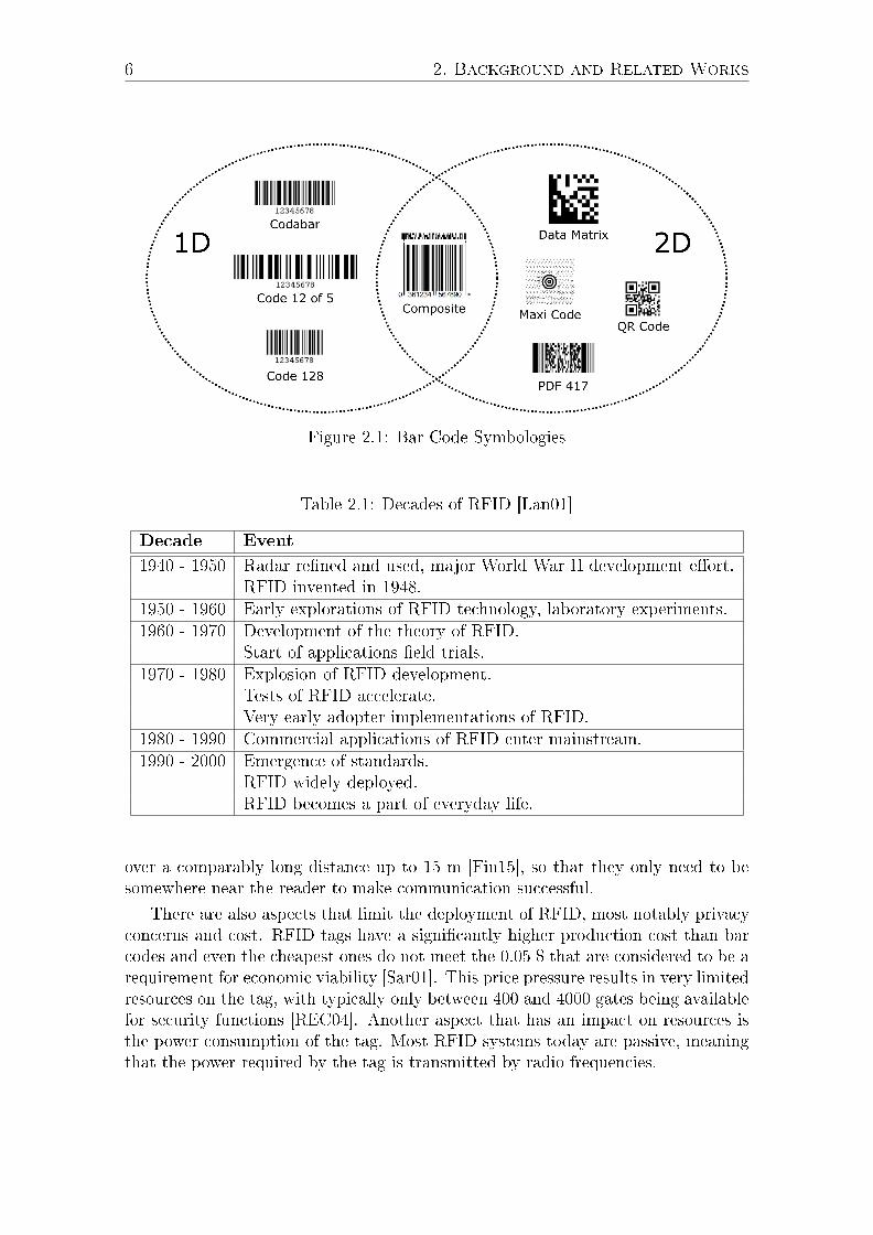
As of today, the most widespread system for the automated identi�cation of itemsis the bar code. Originating from two di�erent region standards, the United StatesUniversal Product Code (UPC) and the European Article Number (EAN), it hasbeen adopted across the world, cumulating in the common world-wide standardGS1 [Int16]. Di�erent �avors of bar codes have been standardized, roughly beingcategorized in one dimensional (1D) and two dimensional (2D) codes in Figure 2.1.
With the ongoing deployment of RFID systems, a successor technology hasstarted taking over, replacing bar codes for a steadily growing number of use cases.RFID technology has been developed already since 1940. Table 2.1 shows the ad-vancements in RFID over the past decades.
RFID systems consist of transponders (or tags), readers and typically a back-end database. Information is exchanged between the tag and the reader via radiofrequency signals. RFID systems have a number of advantages to bar codes: theycan in theory store and transmit an arbitrary amount of data, which allows identi-fying not only product groups, but individual items of a product group. They cantransmit information without line of sight, and they can potentially transmit data
6 2. Background and Related Works
Figure 2.1: Bar Code Symbologies
Table 2.1: Decades of RFID [Lan01]
Decade Event
1940 - 1950 Radar re�ned and used, major World War II development e�ort.RFID invented in 1948.
1950 - 1960 Early explorations of RFID technology, laboratory experiments.1960 - 1970 Development of the theory of RFID.
Start of applications �eld trials.1970 - 1980 Explosion of RFID development.
Tests of RFID accelerate.Very early adopter implementations of RFID.
1980 - 1990 Commercial applications of RFID enter mainstream.1990 - 2000 Emergence of standards.
RFID widely deployed.RFID becomes a part of everyday life.
over a comparably long distance up to 15 m [Fin15], so that they only need to besomewhere near the reader to make communication successful.
There are also aspects that limit the deployment of RFID, most notably privacyconcerns and cost. RFID tags have a signi�cantly higher production cost than barcodes and even the cheapest ones do not meet the 0.05 $ that are considered to be arequirement for economic viability [Sar01]. This price pressure results in very limitedresources on the tag, with typically only between 400 and 4000 gates being availablefor security functions [REC04]. Another aspect that has an impact on resources isthe power consumption of the tag. Most RFID systems today are passive, meaningthat the power required by the tag is transmitted by radio frequencies.
2.1. RFID Systems 7
System Components
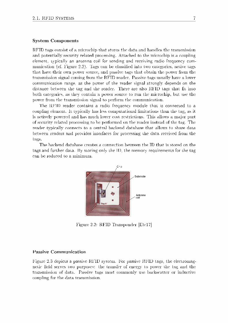
RFID tags consist of a microchip that stores the data and handles the transmissionand potentially security related processing. Attached to the microchip is a couplingelement, typically an antenna coil for sending and receiving radio frequency com-munication (cf. Figure 2.2). Tags can be classi�ed into two categories, active tagsthat have their own power source, and passive tags that obtain the power from thetransmission signal coming from the RFID reader. Passive tags usually have a lowercommunication range, as the power of the reader signal strongly depends on thedistance between the tag and the reader. There are also RFID tags that �t intoboth categories, as they contain a power source to run the microchip, but use thepower from the transmission signal to perform the communication.
The RFID reader contains a radio frequency module that is connected to acoupling element. It typically has less computational limitations than the tag, as itis actively powered and has much lower cost restrictions. This allows a major partof security related processing to be performed on the reader instead of the tag. Thereader typically connects to a central backend database that allows to share databetween readers and provides interfaces for processing the data received from thetags.
The backend database creates a connection between the ID that is stored on thetags and further data. By storing only the ID, the memory requirements for the tagcan be reduced to a minimum.
Figure 2.2: RFID Transponder [Etc17]
Passive Communication
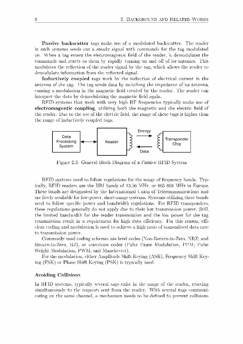
Figure 2.3 depicts a passive RFID system. For passive RFID tags, the electromag-netic �eld serves two purposes: the transfer of energy to power the tag and thetransmission of data. Passive tags most commonly use backscatter or inductivecoupling for the data transmission.
8 2. Background and Related Works
Passive backscatter tags make use of a modulated backscatter. The readerin such systems sends out a steady signal with commands for the tag modulatedon. When a tag enters the electromagnetic �eld of the reader, it demodulates thecommands and reacts to them by rapidly turning on and o� of its antenna. Thismodulates the re�ection of the reader signal by the tag, which allows the reader todemodulate information from the re�ected signal.
Inductively coupled tags work by the induction of electrical current in theantenna of the tag. The tag sends data by switching the impedance of its antenna,causing a modulation in the magnetic �eld created by the reader. The reader caninterpret the data by demodulating the magnetic �eld again.
RFID systems that work with very high RF frequencies typically make use ofelectromagnetic coupling, utilizing both the magnetic and the electric �eld ofthe reader. Due to the use of the electric �eld, the range of these tags is higher thanthe range of inductively coupled tags.
Figure 2.3: General Block Diagram of a Passive RFID System
RFID systems need to follow regulations for the usage of frequency bands. Typ-ically, RFID readers use the ISM bands of 13.56 MHz, or 865-868 MHz in Europe.These bands are designated by the International Union of Telecommunications andare freely available for low-power, short-range systems. Systems utilizing these bandsneed to follow speci�c power and bandwidth regulations. For RFID transponders,these regulations generally do not apply due to their low transmission power. Still,the limited bandwidth for the reader transmission and the low power for the tagtransmission result in a requirement for high data e�ciency. For this reason, e�-cient coding and modulation is used to achieve a high ratio of transmitted data rateto transmission power.
Commonly used coding schemes are level codes (Non-Return-to-Zero, NRZ; andReturn-to-Zero, RZ), or transition codes (Pulse Pause Modulation, PPM; PulseWeight Modulation, PWM; and Manchester).
For the modulation, either Amplitude Shift Keying (ASK), Frequency Shift Key-ing (FSK) or Phase Shift Keying (PSK) is typically used.
Avoiding Collisions
In RFID systems, typically several tags exist in the range of the reader, reactingsimultaneously to the requests sent from the reader. With several tags communi-cating on the same channel, a mechanism needs to be de�ned to prevent collisions
2.1. RFID Systems 9
and thereby avoid information loss. Due to the limited computational power of thetags and the fact that tags cannot communicate to each other, most of the requiredwork needs to be done by the reader. The usual approach is to query the tags untilall singulation identi�ers are obtained. When all tags have been singulated, thereader can send requests to a single selected tag. Two classes of collision avoidanceprotocols have been standardized, deterministic and probabilistic protocols. Deter-ministic protocols are based on singulating tags by single bits of their unique ID.Probabilistic protocols use e.g. a time slot approach, exploiting the probability ofseveral tags responding in the same randomly chosen slot. Usually, probabilisticprotocols are used for the 13.56 MHz frequency band, and deterministic protocolsfor the range of 860-960 MHz.
2.1.2 Security Aspects of RFID Systems
The hardware and cost restrictions in typical low-cost RFID applications presentparticular challenges for securing the related data transmission. Figure 2.4 showsthe relationship between security, performance and computational complexity, whichis mostly directly related to cost. Low-cost means limited storage, limited chip areafor computations, and low power consumption resulting in even more limited com-putational power. Therefore, the known and tested algorithms for general securityapplications are typically not applicable for these systems, because they are not ableto perform even basic cryptographic operations. For this reason, ultra-lightweightalgorithms have been designed speci�cally with RFID applications in mind, e.g.[Pos09].
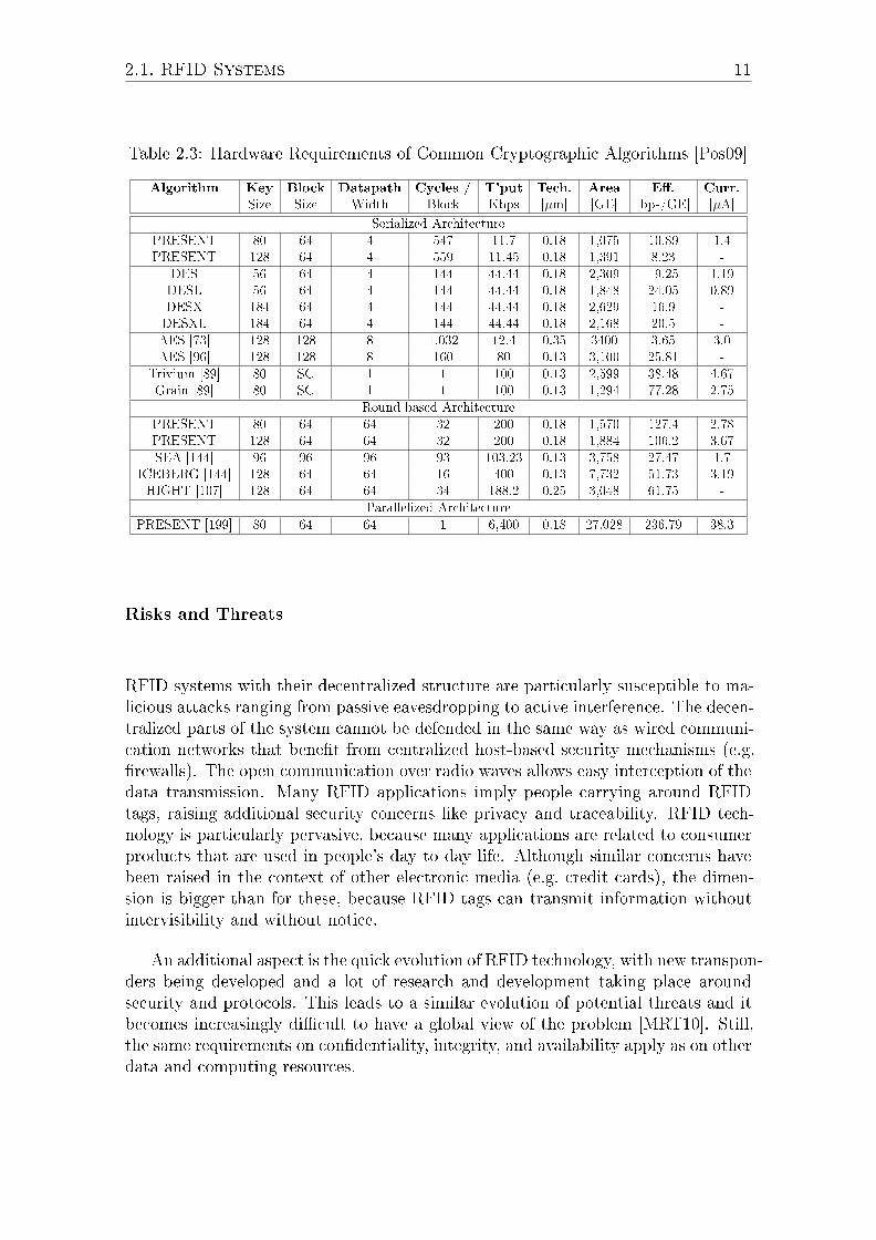
RFID tags can be classi�ed according to their security related capabilities. In[Chi07], tags are divided into four categories, which can be roughly split into high-cost and low-cost classes. In [PL08] the properties have been summed-up, as shownin Table 2.2. The high-cost category is split into the categories full-�edged, provid-ing complex cryptographic functions like symmetric or even asymmetric encryption,and simple, which is limited to pseudo-random number generation and one-wayhash functions. The low-cost category is split into the categories lightweight, againsupporting PRNG and simple checksums, and ultra-lightweight, which is limited tosimple bitwise operations. As many RFID applications target the lightweight (oreven ultra-lightweight) category of tags for cost reasons, there is a strong desire toresearch for cryptographic primitives that allow secure communication using the low-est possible complexity. This is an ongoing challenge, because these tags typicallyhave an order of 250-4000 gates [REC04]. To put this into perspective, a SHA-256implementation requires about 11000 gates to perform a hash calculation on a 512-bitdata block [FR06]. Table 2.3 shows further hardware requirements of several crypto-graphic functions. The required chip area is measured in Gate Equivalents (GE), aunit of measure which allows to specify manufacturing-technology-independent com-plexity of digital electronic circuits. On modern CMOS chips, one GE constitutesthe chip area required for a NAND gate.

10 2. Background and Related Works
Figure 2.4: Security Triangle [Pos09]
Table 2.2: Classes of RFID Tags [PL08]
Low-Cost High-Cost
Standards EPC Class-1 Generation-2 ISO/IEC 14443 A/BISO/IEC 18006-C
Power Source Passively powered Passively poweredStorage 32 - 1K Bits 32 KB - 70 KBCircuitry 250 - 4K Gates Microprocessor
(Security processing) Standard Cryptographic Primitives Implement 3DES, SHA-1, RSAcannot be supported RSA
Reading Distance Up to 3 m About 10 cm(Commercial Devices)
Price 0.05 - 0.1 Euro Several EurosPhysical Attacks Not resistant Tamper Resistance
EAL 5+ Security LevelResistance to Passive Attacks Yes YesResistance to Active Attacks No Yes
Attacking RFID Systems
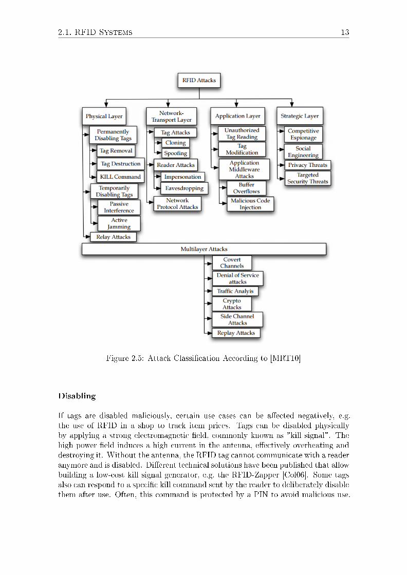
This section examines the risks and threats of RFID technology, followed by a descrip-tion of potential attacks against RFID systems mostly following the classi�cationsgiven in [BDM07] and [MRT10], visualized in Figure 2.5.
2.1. RFID Systems 11
Table 2.3: Hardware Requirements of Common Cryptographic Algorithms [Pos09]
Algorithm Key Block Datapath Cycles / T'put Tech. Area E�. Curr.Size Size Width Block [Kbps] [µm] [GE] [bps/GE] [µA]
Serialized ArchitecturePRESENT 80 64 4 547 11.7 0.18 1,075 10.89 1.4PRESENT 128 64 4 559 11.45 0.18 1,391 8.23 -
DES 56 64 4 144 44.44 0.18 2,309 19.25 1.19DESL 56 64 4 144 44.44 0.18 1,848 24.05 0.89DESX 184 64 4 144 44.44 0.18 2,629 16.9 -DESXL 184 64 4 144 44.44 0.18 2,168 20.5 -AES [73] 128 128 8 1,032 12.4 0.35 3400 3.65 3.0AES [96] 128 128 8 160 80 0.13 3,100 25.81 -
Trivium [89] 80 SC 1 1 100 0.13 2,599 38.48 4.67Grain [89] 80 SC 1 1 100 0.13 1,294 77.28 2.75
Round-based ArchitecturePRESENT 80 64 64 32 200 0.18 1,570 127.4 2.78PRESENT 128 64 64 32 200 0.18 1,884 106.2 3.67SEA [144] 96 96 96 93 103.23 0.13 3,758 27.47 1.7
ICEBERG [144] 128 64 64 16 400 0.13 7,732 51.73 3.19HIGHT [107] 128 64 64 34 188.2 0.25 3,048 61.75 -
Parallelized ArchitecturePRESENT [199] 80 64 64 1 6,400 0.18 27,028 236.79 38.3
Risks and Threats
RFID systems with their decentralized structure are particularly susceptible to ma-licious attacks ranging from passive eavesdropping to active interference. The decen-tralized parts of the system cannot be defended in the same way as wired communi-cation networks that bene�t from centralized host-based security mechanisms (e.g.�rewalls). The open communication over radio waves allows easy interception of thedata transmission. Many RFID applications imply people carrying around RFIDtags, raising additional security concerns like privacy and traceability. RFID tech-nology is particularly pervasive, because many applications are related to consumerproducts that are used in people's day to day life. Although similar concerns havebeen raised in the context of other electronic media (e.g. credit cards), the dimen-sion is bigger than for these, because RFID tags can transmit information withoutintervisibility and without notice.
An additional aspect is the quick evolution of RFID technology, with new transpon-ders being developed and a lot of research and development taking place aroundsecurity and protocols. This leads to a similar evolution of potential threats and itbecomes increasingly di�cult to have a global view of the problem [MRT10]. Still,the same requirements on con�dentiality, integrity, and availability apply as on otherdata and computing resources.
12 2. Background and Related Works
Security Concerns
The two main security concerns related to the use of RFID technology are privacyand traceability. There is no common de�nition of privacy and its meaning variesfor di�erent people, often depending on cultural and other backgrounds. In generalterms, it is the ability of an individual or group to keep their lives and personala�airs out of public view, or to control the �ow of information about themselves[PL08].
Every individual has the right to be protected of interference or attacks on theirprivacy by the law [Ass48]. This is supported by further regulations, e.g. the EU Di-rective 95/46/EC [Dir95] on the protection of individuals with regard to the process-ing of personal data and the free movement, or Article 8 of the European Conventionof Human Rights, identifying the right to have private and family life respected.
RFID technology with its pervasive nature is part of ubiquitous computing, whichwas predicted to be problematic in the context of privacy already by Weiser in 1991[Wei91]. A scenario where the loss of privacy in the context of RFID is a threat toan individual can e.g. be given for medical products, which are often tagged withRFID labels as proof of authenticity. If an attacker reads this information in front ofthe door of a medical store after someone bought an AIDS treatment, he got accessto information that the individual might not want to have shared with everyone.
Traceability describes the possibility to track the location of an individual. Lo-cation information can be seen as a subset of privacy information and therefore fallsunder the same regulations as any other privacy data.
A number of technologies exist that allow location tracking of a person, e.g.mobile phones (where the location can be retrieved by collecting data about the basestation that is in use by the phone), video surveillance, and obviously GPS, whichis nowadays part of most smart phones. RFID adds to these technologies, althoughthe information provided by the tags is typically only meaningful to readers thathave access to the related backend database.
Often, RFID tags will transmit a static ID, which can be used to identify themfrom any reader, even if it cannot interpret the actual information behind this ID.As of today, IDs are most often related to product codes and not to unique items.Still, it was shown e.g. in [WSRE04] that constellations of tags (meaning a speci�ccombination of products that an individual might carry around at the same time)allow to uniquely identify the owner.
Furthermore, it can be expected that IDs will be used to uniquely identify certainproducts in the future, making an association between the tag and its owner eveneasier. An example for such a use of RFID is the E-Passport, which contains acollision avoidance mechanism speci�ed in ISO/IEC 14443 A/B that is based ona unique identi�er. This allows to uniquely identify a passport and to use it forlocation tracking.
2.1. RFID Systems 13
Figure 2.5: Attack Classi�cation According to [MRT10]
Disabling
If tags are disabled maliciously, certain use cases can be a�ected negatively, e.g.the use of RFID in a shop to track item prices. Tags can be disabled physicallyby applying a strong electromagnetic �eld, commonly known as "kill signal". Thehigh power �eld induces a high current in the antenna, e�ectively overheating anddestroying it. Without the antenna, the RFID tag cannot communicate with a readeranymore and is disabled. Di�erent technical solutions have been published that allowbuilding a low-cost kill signal generator, e.g. the RFID-Zapper [Col06]. Some tagsalso can respond to a speci�c kill command sent by the reader to deliberately disablethem after use. Often, this command is protected by a PIN to avoid malicious use.
14 2. Background and Related Works
In some systems, this disabled state is only a sleeping state and tags can be activatedagain if required.
Hiding
Hiding means that the presence of a tag is concealed from the reader. A potentialscenario for such an attack is an automated cashier system in a shop that calculatesthe receipt sum from the items that it detects in the vicinity of the exit. If an itemcannot be detected, the attacker will be able to leave the shop without paying for it.Such attacks can be performed by insulating the tag from any kind of electromagneticradiation, e.g. making use of a Faraday cage, or by disabling the tag by other means.
Cloning
Cloning is the process of duplicating a tag so that the reader cannot detect a di�er-ence. The goal of this attack is to pretend a fake identity of the entity the tag isattached to. The prevention of cloning is well covered by current cryptographic pro-tocols, typically involving hash calculations or asymmetric encryption. For low-costRFID tags, these methods are not applicable due to the high required computationalcomplexity. Their use is restricted to higher cost RFID chips, like those embeddedinto the electronic passport.
Tracking
Tracking of a tag can be used to create "movement pro�les" of individuals, violatingtheir rights on privacy. To perform the tracking, tags need to be identi�ed by non-authorized RFID readers. Di�erently to cloning, there is no need to be able to accessall data on the tag. Instead, it is su�cient to access any kind of data that is uniqueto the tag. Tracking can be prevented by similar measures as cloning.
Replay and Relay Attacks
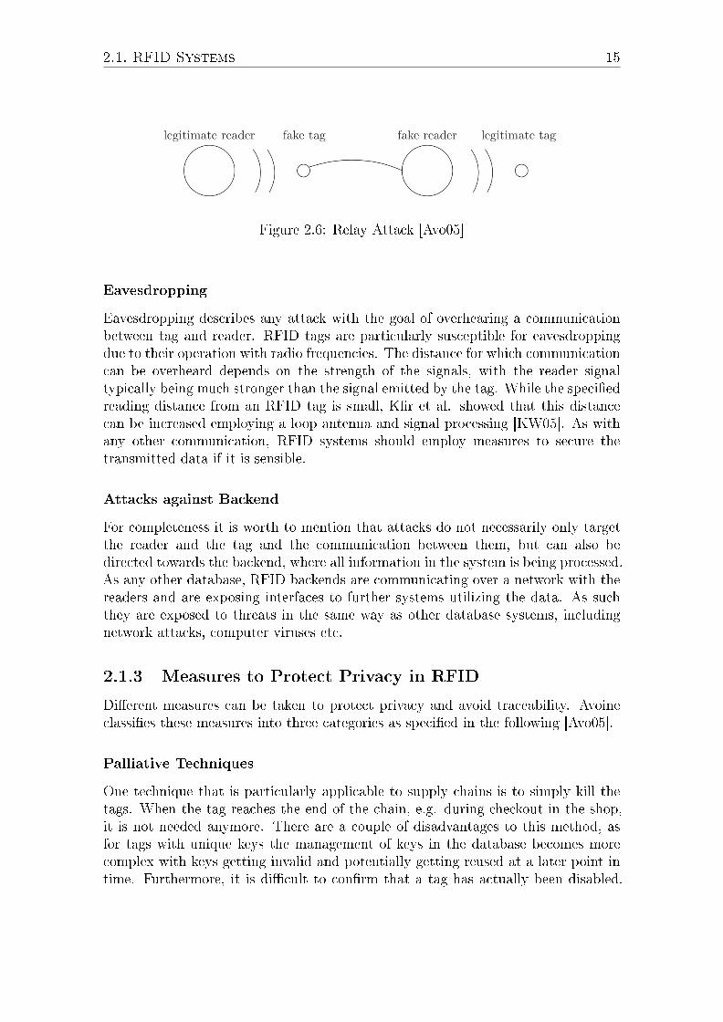
Replay attacks work by storing transmitted messages from a valid communicationand resending it in a di�erent context later on, thereby pretending knowledge that isprivate to the original sender. This allows the attacker to gain access to data or itemsit is not authorized to. Prevention against replay attacks is possible by using noncesthat are randomly created for every communication. The communication data de-pends on this nonce, so a replay attack is not successful. Relay attacks are similar,but instead of storing the data from a valid communication, the communication isrelayed between the two communication parties by the attacker. This is e�ectivelycarrying out the authorization process over an arbitrary distance and without knowl-edge of one of the participants (see Figure 2.6). A practical implementation of arelay attack on an RFID system is presented in [Han06].
2.1. RFID Systems 15
Figure 2.6: Relay Attack [Avo05]
Eavesdropping
Eavesdropping describes any attack with the goal of overhearing a communicationbetween tag and reader. RFID tags are particularly susceptible for eavesdroppingdue to their operation with radio frequencies. The distance for which communicationcan be overheard depends on the strength of the signals, with the reader signaltypically being much stronger than the signal emitted by the tag. While the speci�edreading distance from an RFID tag is small, K�r et al. showed that this distancecan be increased employing a loop antenna and signal processing [KW05]. As withany other communication, RFID systems should employ measures to secure thetransmitted data if it is sensible.
Attacks against Backend
For completeness it is worth to mention that attacks do not necessarily only targetthe reader and the tag and the communication between them, but can also bedirected towards the backend, where all information in the system is being processed.As any other database, RFID backends are communicating over a network with thereaders and are exposing interfaces to further systems utilizing the data. As suchthey are exposed to threats in the same way as other database systems, includingnetwork attacks, computer viruses etc.
2.1.3 Measures to Protect Privacy in RFID
Di�erent measures can be taken to protect privacy and avoid traceability. Avoineclassi�es these measures into three categories as speci�ed in the following [Avo05].
Palliative Techniques
One technique that is particularly applicable to supply chains is to simply kill thetags. When the tag reaches the end of the chain, e.g. during checkout in the shop,it is not needed anymore. There are a couple of disadvantages to this method, asfor tags with unique keys the management of keys in the database becomes morecomplex with keys getting invalid and potentially getting reused at a later point intime. Furthermore, it is di�cult to con�rm that a tag has actually been disabled.
16 2. Background and Related Works
Di�erent methods are applicable to disable a tag. Besides the ones described inSubsection 2.1.2, tags can be constructed such that the antenna can easily be man-ually separated from the chip. This allows the tag to be activated again, but onlyintentionally [KM05].
Other techniques interrupt the communication between the tag and a reader byshielding the signal with a Faraday cage and thereby also only allowing communica-tion by user action. Similarly, communication can be based on a secret informationthat is only accessible by an optical reader. Again, a user can avoid unintendedcommunication by not exposing the tag to view. Independent on the actual tech-nique to stop a tag from communication, Gar�nkel elaborated the so-called "RFIDBill of Rights" [Gar02], which outlines the fundamental rights of the tag's bearers.Gar�nkel claims:
• The right to know whether products contain RFID tags.
• The right to have RFID tags removed or deactivated when they purchaseproducts.
• The right to use RFID-enabled services without RFID tags.
• The right to access an RFID tag's stored data.
• The right to know when, where and why the tags are being read.
These methods are e�cient, but the requirement for user action and the other dis-advantages do not make them applicable for many use cases. For many applications,the use of security protocols is much more appropriate [Avo13].
Protocols Resistant to Traceability
A tag that sends its information unencrypted is easy to trace. Encrypting the in-formation with a key it shares with the reader avoids this, but has a number ofdisadvantages. If the same key is used by all tags in the RFID system, security canbe easily corrupted by an adversary that is able to access the content of a single tag.If a di�erent key is used by each tag, there are two cases: either the encryption isdeterministic, resulting in an identical ciphertext being sent every time. This obvi-ously does not solve the traceability issue, as the tag can be easily identi�ed withciphertext it transmits. Or, the encryption is randomized, choosing from a selectionof encryption keys. This creates a complexity problem on the reader side, as thereader needs to test all keys in the database to �nd the one that matches the cipher-text sent by the tag. This method is in fact a challenge-response protocol wherethe reader does not know the tag's identity. Such scenarios are exactly what public-key encryption schemes have been developed for. Unfortunately, the complexity ofpublic-key encryption prevents it from being used in low-complexity RFID systems.The overall goal for these protocols is to make sure that the information transmittedis changed for every transmission instance. There are two categories in which these
2.2. Graph Theory 17
protocols can be classi�ed, those where the necessary refresh of the information istriggered by the reader, and those where the refresh is performed by the tag itselfwithout help by the reader.
Protocols Based on Reader-Aided ID-Refreshment
Reader-aided refresh is usually a 3-moves protocol. First, the reader sends a requestto the tag, followed by the tag replay that allows its identi�cation. As a �nal step,the reader sends data to the tag that allows it to refresh the information that it willsend for the next identi�cation. If an adversary is able to send a successful requestto the tag followed by a fake refresh information, the tag and the database behindthe reader will get out of sync, rendering the tag unusable by the RFID system.This means, that this class of protocols is only useful for a weak adversary model.
Protocols Based on Self-Refreshment
Usually, protocols that are based on a self-refresh of the tag identi�er without readerinteraction are 2-moves or 3-moves protocols when mutual authentication betweenreader and tag is required. These protocols usually require cryptographic primi-tives to be implemented on the tag, typically involving a PRNG (e.g. [WSRE04],[MW04]), a hash function [RKKW05] or an encryption function [FDW04]. Theseprotocols are not limited in general to a weak adversary model and therefore arethe best approach to avoid traceability. For this reason, this work concentrates onthe respective low-complexity functions for such cryptographic primitives, with aparticular focus on PRNGs.
2.2 Graph Theory
This section provides the basics of graph theory that are required for understand-ing the analyses performed later in this work. After de�ning di�erent propertiesof mathematical functions according to [Tur09], [Die00], [CLGM+95], [FO90] and[SF13], the di�erent elements of a function graph are explained.
De�nition: Injective, Surjective and Bijective Function
Let A and B be sets. A function or a mapping from A to B, denoted by f : A→ Bis a relation from A to B in which every element from A appears exactly once asthe �rst component of an ordered pair in the relation. If A is �nite as well and ifa ∈ A is interpreted as a discrete state, f is also called a state transition function.
• The function f : A→ B is injective, if for two di�erent elements a1 6= a2 of Ait follows that f(a1) 6= f(a2).
• The function f : A → B is surjective, if for every element b ∈ B an elementa ∈ A exists, with f(a) = b.
18 2. Background and Related Works
• The function f : A → B is bijective, if it is both injective and surjective. IfA = B, f is called self mapping.
De�nition: Directed Graph
A directed graph G = (V,E) (digraph) is a tuple of the sets V (the set of nodes)and E (the set of edges) with E ⊆ V × V . For �nite V it follows that E and thusG are also �nite. In the following, any mention of graph in this work is referring toa directed graph, unless explicitly speci�ed otherwise.
De�nition: State Transition Graph
A state transition graph G = (V,E) is a graph induced by a function f : V → Vwith E = {(x, f(x)) : x ∈ V }. The function f(x) denotes the transition from a statex0 = x to another state x1 = f(x).
De�nition: Subgraph
Let G = (V,E) be a graph and U ⊆ V , then the subgraph G(U) that is induced byU is the graph G(U) := (U,E ′) with E ′ = E ∩ U × U and the nodes incident to eare in U .
De�nition: Degrees of Vertices
Let G = (V,E) be a graph, then the in-degree of a node v, meaning the total numberof all ingoing edges of v, is E(v). Correspondingly, A(v) is the outdegree, meaningthe total number of all outgoing edges of v. If E(v) = 0, v is called a leaf.
De�nition: Paths and Ways
A path p = (v0, v1, ..., vm−1, vm) in a graph G is a �nite sequence of nodes, with(vi, vi+1) ∈ E for i = 0, ...,m− 1.
The length of the path is m. The node v0 is called the start node or head of thepath p, the node vm is called the end node or tail. The remaining nodes of p arecalled inner nodes.
A path p is called simple path or way, if no node is passed multiple times, thatis if all nodes vi and all vj with i 6= j and i, j ∈ {0, ...,m} are pairwise distinct, withthe possible exception v0 = vm.
De�nition: Cycle or Circle
A way W = v0, v1, ...vl with l ≥ 1 in a graph G is called cycle or circle, if v0 = vl. lis called the length of the cycle.

2.2. Graph Theory 19
De�nition: Connected Component
A graph G = (V,E) is called weakly connected if and only if for all nodes u, v ∈ Vwith u 6= v a way exists between u and v or between v and u.
A subgraph G(U) of G is called connected component or simply component ofG if and only if G(U) is connected and G(U ∪ {v})∀v ∈ V \ U is not connected.This means G(U) is maximal connected. Figure 2.7 shows a typical example for aconnected component of a transition graph.
The total number of nodes in a connected component is called the size of thecomponent.
Figure 2.7: A Typical Connected Component of a State Transition Graph [BFKM12]
De�nition: Tree
In undirected graphs, a connected graph B that does not contain a cycle is calledtree and has m = n − 1 edges. For two nodes u, v ∈ V , exactly one path u → v inB exists.
A polytree (also known as oriented tree or singly connected network) is a directedacyclic graph whose underlying undirected graph is a tree. As the remains of thiswork refers to directed graphs only, tree is used synonym to polytree in the followingunless noted otherwise. It is furthermore notable, that in the course of this workonly directed graphs with indegree E(v) ≤ 1 are considered.
As further convention, in this work the root of a tree is de�ned to be the nodeu (u ∈ V ) where the tree connects to a cycle. The length of the way from u tov (u, v ∈ V ) is called depth of v in B or tail length λ(u). The longest way is themaximum tree size. The direction of a tree is assumed to be given by the direction
20 2. Background and Related Works
of the graph, meaning that in the course of this work a tree shall be de�ned to bedirected towards its root.
De�nition: Rho Length
The rho length ρ(u) is de�ned as the sum of the tail length λ(u) and the length l ofthe cycle that the path starting from u connects to.
De�nition: Predecessors Size
The predecessors size of a node u is de�ned as the size of the tree rooted at u.
2.3 Cryptographic Pseudo-Random Number Gener-
ators
Random numbers are needed and used in many security related applications. Theyare an essential component for the generation of passwords, session keys and forauthentication protocols. The security of such applications depends substantially onthe quality of the involved random number generator. Predictable random numbersallow unauthorized parties to eavesdrop communication, counterfeit a false identityor manipulate the transmitted information. In the following, the basics of RandomNumber Generators are explained, with a subsequent discussion of the quality ofpseudo-random number generators.
2.3.1 Overview of Random Number Generators
Random Number Generators can be classi�ed into True Random Number Genera-tors and Pseudo-Random Number Generators. A true random number generator(TRNG) requires a naturally occurring source of randomness. Designing a hardwaredevice or software program to exploit this randomness and produce a bit sequencethat is free of biases and correlations is a di�cult task. Additionally, for mostcryptographic applications, the generator must not be subject to observation ormanipulation by an adversary.
Random bit generators based on natural sources of randomness are subject toin�uence by external factors, and also to malfunction [MvOV96]. It is imperativethat such devices be tested periodically, for example by using statistical tests. Pass-ing these statistical tests is a necessary but not su�cient condition for a generatorto be secure. In [Neu04], a list of constraints is given which could be tested.
A simple example for a statistical test of a Random Number Generators is tocount the number of zeros in the generated random sequence. Common statisticaltests are the frequency, serial, poker, autocorrelation, run and long run test whichare described in [Knu98], [BP82], [FO10]. In Chapter 5 of Menezes et al. [MvOV96],

2.3. Cryptographic Pseudo-Random Number Generators 21
it is shown that it is impossible to give a mathematical proof whether a RandomNumber Generator creates real random numbers or not.
De�nition: Pseudo-Random Number Generator
Pseudo-Random Number Generators (PRNGs) are generally deterministic statetransition functions f : M → M mapping a �nite state space to itself as longas they do not receive new seed or entropy bits. Every output of the PRNG resultsin a state transition. This means that the generated sequences of pseudo-randomnumbers are periodic. Figure 2.8 depicts the general structure of a PRNG. Theoutput is deterministic and dependent on the state. Therefore, only the state isconsidered in the following. Usually the output is compressed, meaning that therelationship between output and internal state of the PRNG is not unique and thePRNG constitutes a one-way-function.
If a single state is interpreted as a node and the transition between a stateand its unique successor state is interpreted as an edge, the result is a directedgraph Gf = (V ;E) with V := M and E := {(x; f(x))|x ∈ M} where M is theset of states. The structure of the generated graph provides information about thebehavior of the pseudo-random generator. Due to the �nite state space of a realworld implementation of a PRNG, every path in the state space will end up in acycle, resulting in a periodic output sequence. For non-bijective transition functionsthe graph typically consists of several weakly connected components. Each of thesecomponents consists of one cycle and generally several trees with roots located onthe cycle (see e.g. Figure 2.7).
Figure 2.8: Pseudo-Random Number Generator
Attacks on Pseudo-Random Number Generators
Attacks on Pseudo-Random Number Generators can be classi�ed as follows [KSWH98]:
1. Direct Cryptanalytic Attack
The capability of an attacker to distinguish between the output of a PRNGand real random outputs is covered by the term direct cryptanalytic attack.

22 2. Background and Related Works
This attack is applicable to most applications of PRNGs, although there aresome applications, where the PRNG output cannot be accessed directly (e.g.when the PRNG is used to generate triple-DES keys).
2. Input-Based Attacks
The access or control of the input of the PRNG enables an attacker to cryptana-lyze the PRNG and perform an input attack. Input attacks can be categorizedinto known-input, replayed-input, and chosen-input attacks. Known-input at-tacks can be performed, when a source that is used as input for the PRNGis observable by the attacker. Replayed-input attacks are applicable, if theinput can not only be observed, but the data can be fed into the PRNG again.Chosen-input attacks require maximum control by the attacker, as it involvesfeeding arbitrary data into the PRNG, e.g. while analysing a smart card witha cryptanalytic attack.
3. State Compromise Extension Attacks
When the state S of the PRNG has been recovered successfully at some point intime, an attacker might extend this knowledge to other points in time using astate compromise extension attack. This kind of attack is particularly likely tobe successful, when the PRNG is started with insu�cient entropy and thereforethe start state is easily guessable.
(a) Backtracking Attacks: A backtracking attack uses the compromise ofthe PRNG state S at time t to learn previous PRNG outputs.
(b) Permanent Compromise Attacks: A permanent compromise attackoccurs if, once an attacker compromises S at time t, all future and pastS values are vulnerable to attack.
(c) Iterative Guessing Attacks: An iterative guessing attack uses knowl-edge of S at time t, and the intervening PRNG outputs, to learn S attime t+ε, when the inputs collected during this span of time are guessable(but not known) by the attacker.
(d) Meet-in-the-Middle Attacks: A meet-in-the-middle attack is essen-tially a combination of an iterative guessing attack with a backtrackingattack. Knowledge of S at times t and t+2ε allow the attacker to recoverS at time t+ ε.
Several examples for attacks on speci�c widespread PRNG implementations arepresented in [KSWH98].
2.3.2 Metrics for a "Good" PRNG
To be able to compare the quality of PRNGs, it is required that metrics are de�nedthat allow to associate a measurable quality with a certain PRNG implementation.
2.3. Cryptographic Pseudo-Random Number Generators 23
The selected properties to compare depend heavily on the application, but for secu-rity related applications the following criteria are reasonable and can be extractedfrom the state space structure of the PRNG function:
• Number of Components
• Cycle Lengths of the Components
• Size of the Components
A further candidate for a criterion is the ratio of branches (nodes with more thanone predecessor), as these increase the backwards secrecy. This con�icts with thecycle length criterion to a certain extent.
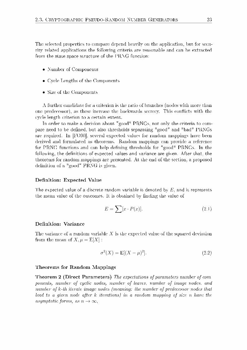
In order to make a decision about "good" PRNGs, not only the criteria to com-pare need to be de�ned, but also thresholds separating "good" and "bad" PRNGsare required. In [FO90], several expected values for random mappings have beenderived and formulated as theorems. Random mappings can provide a referencefor PRNG functions and can help de�ning thresholds for "good" PRNGs. In thefollowing, the de�nitions of expected values and variance are given. After that, thetheorems for random mappings are presented. At the end of the section, a proposedde�nition of a "good" PRNG is given.
De�nition: Expected Value
The expected value of a discrete random variable is denoted by E, and it representsthe mean value of the outcomes. It is obtained by �nding the value of
E =∑
[x · P (x)]. (2.1)
De�nition: Variance
The variance of a random variable X is the expected value of the squared deviationfrom the mean of X,µ = E[X] :
σ2(X) = E[(X − µ)2]. (2.2)
Theorems for Random Mappings
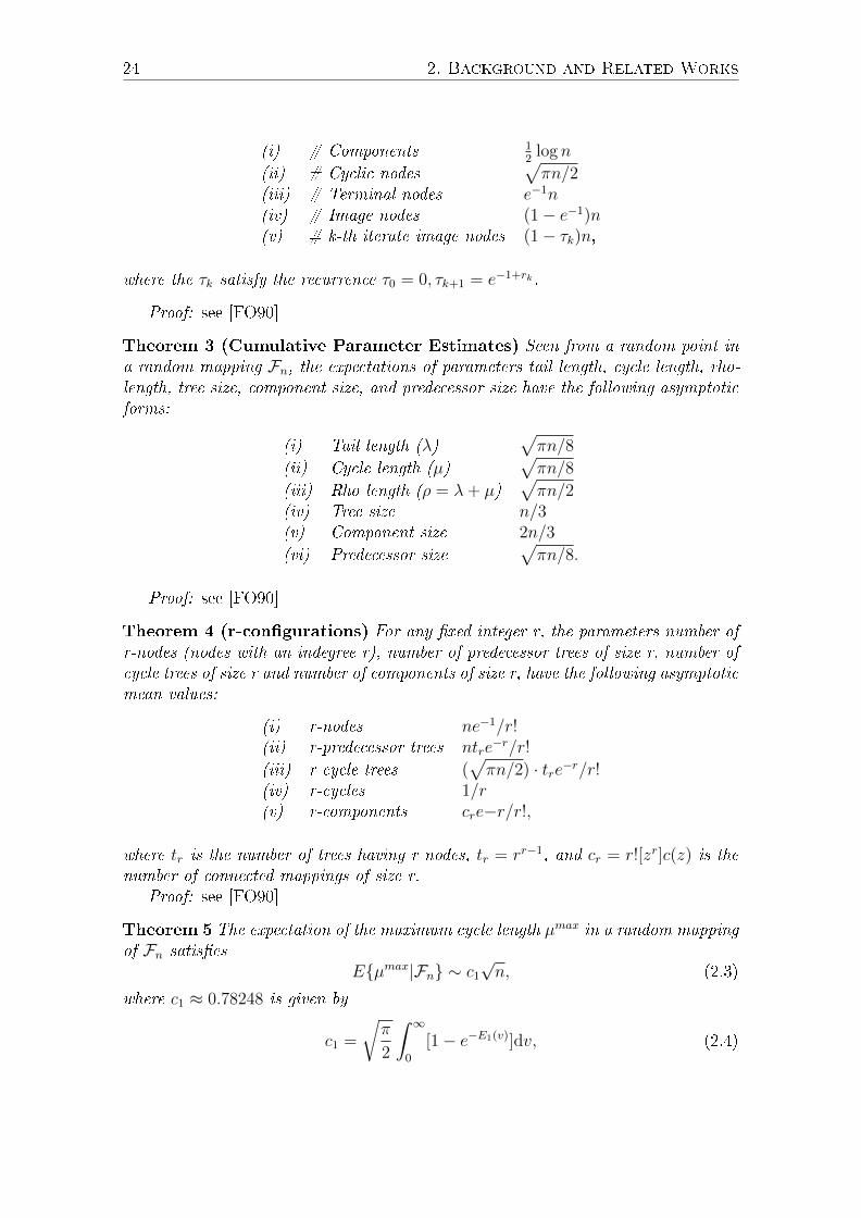
Theorem 2 (Direct Parameters) The expectations of parameters number of com-ponents, number of cyclic nodes, number of leaves, number of image nodes, andnumber of k-th iterate image nodes (meaning: the number of predecessor nodes thatlead to a given node after k iterations) in a random mapping of size n have theasymptotic forms, as n→∞,
24 2. Background and Related Works
(i) # Components 12
log n
(ii) # Cyclic nodes√πn/2
(iii) # Terminal nodes e−1n(iv) # Image nodes (1− e−1)n(v) # k-th iterate image nodes (1− τk)n,
where the τk satisfy the recurrence τ0 = 0, τk+1 = e−1+rk .
Proof: see [FO90]
Theorem 3 (Cumulative Parameter Estimates) Seen from a random point ina random mapping Fn, the expectations of parameters tail length, cycle length, rho-length, tree size, component size, and predecessor size have the following asymptoticforms:
(i) Tail length (λ)√πn/8
(ii) Cycle length (µ)√πn/8
(iii) Rho length (ρ = λ+ µ)√πn/2
(iv) Tree size n/3(v) Component size 2n/3
(vi) Predecessor size√πn/8.
Proof: see [FO90]
Theorem 4 (r-con�gurations) For any �xed integer r, the parameters number ofr-nodes (nodes with an indegree r), number of predecessor trees of size r, number ofcycle trees of size r and number of components of size r, have the following asymptoticmean values:
(i) r-nodes ne−1/r!(ii) r-predecessor trees ntre
−r/r!
(iii) r-cycle trees (√πn/2) · tre−r/r!
(iv) r-cycles 1/r(v) r-components cre−r/r!,
where tr is the number of trees having r nodes, tr = rr−1, and cr = r![zr]c(z) is thenumber of connected mappings of size r.
Proof: see [FO90]
Theorem 5 The expectation of the maximum cycle length µmax in a random mappingof Fn satis�es
E{µmax|Fn} ∼ c1√n, (2.3)
where c1 ≈ 0.78248 is given by
c1 =
√π
2
∫ ∞0
[1− e−E1(v)]dv, (2.4)

2.3. Cryptographic Pseudo-Random Number Generators 25
and E1(v) denotes the exponential integral
E1(v) =
∫ ∞v
e−udu
u. (2.5)
Proof: see [FO90]
Theorem 6 The expectation of the maximum tail length (λmax) in a random mappingof Fn satis�es
E{λmax|Fn} ∼ c2√n, (2.6)
where c2 ≈ 1.73746 is given by
c2 =√
2π log 2. (2.7)
Proof: see [FO90]
Theorem 7 The expectation of the maximum rho length (ρmax) in a random mappingof Fn satis�es
E{ρmax|Fn} ∼ c3√n, (2.8)
where c3 ≈ 2.4149 is given by
c3 =
√π
2
∫ ∞0
[1− e−E1(v)−I(v)]dv, (2.9)
with E1(v) denoting the exponential integral and
I(v) =
∫ v
0
e−u[1− exp( −2u
ev−u − 1)]
du
u. (2.10)
Proof: see [FO90]
Theorem 8 Assuming the smoothness condition, the expected value of the size ofthe largest tree and the size of the largest connected component in a random mappingof Fn are asymptotically
(i) Largest tree: d1n(ii) Largest component : d2n,
where d1 ≈ 0.48 and d2 ≈ 0.75782 are given by
d1 = 2
∫ ∞0
[1− 1
1 + 12√π
∫∞xe−vv−3/2dv
]dx (2.11)
d2 = 2
∫ ∞0
[1− exp(1
2
∫ ∞x
e−vv−1dv)]dx. (2.12)
26 2. Background and Related Works
Proof: see [FO90]
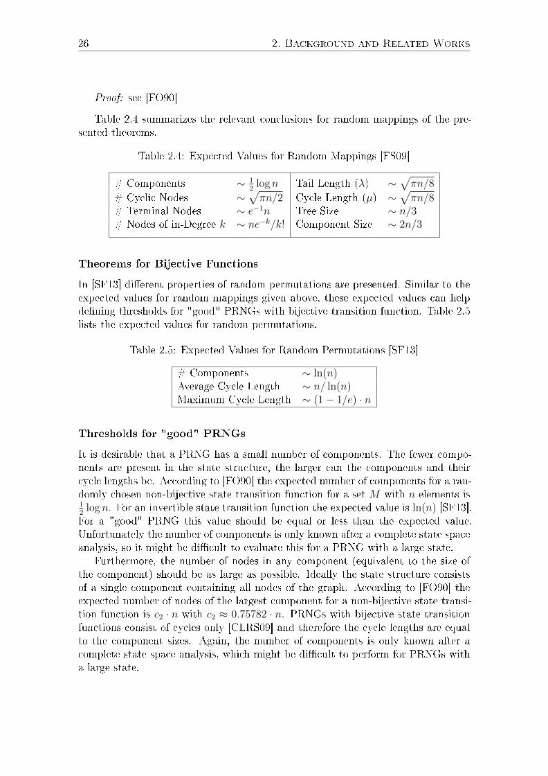
Table 2.4 summarizes the relevant conclusions for random mappings of the pre-sented theorems.
Table 2.4: Expected Values for Random Mappings [FS09]
# Components ∼ 12
log n Tail Length (λ) ∼√πn/8
# Cyclic Nodes ∼√πn/2 Cycle Length (µ) ∼
√πn/8
# Terminal Nodes ∼ e−1n Tree Size ∼ n/3# Nodes of in-Degree k ∼ ne−k/k! Component Size ∼ 2n/3
Theorems for Bijective Functions
In [SF13] di�erent properties of random permutations are presented. Similar to theexpected values for random mappings given above, these expected values can helpde�ning thresholds for "good" PRNGs with bijective transition function. Table 2.5lists the expected values for random permutations.
Table 2.5: Expected Values for Random Permutations [SF13]
# Components ∼ ln(n)Average Cycle Length ∼ n/ ln(n)Maximum Cycle Length ∼ (1− 1/e) · n
Thresholds for "good" PRNGs
It is desirable that a PRNG has a small number of components. The fewer compo-nents are present in the state structure, the larger can the components and theircycle lengths be. According to [FO90] the expected number of components for a ran-domly chosen non-bijective state transition function for a set M with n elements is12
log n. For an invertible state transition function the expected value is ln(n) [SF13].For a "good" PRNG this value should be equal or less than the expected value.Unfortunately the number of components is only known after a complete state spaceanalysis, so it might be di�cult to evaluate this for a PRNG with a large state.
Furthermore, the number of nodes in any component (equivalent to the size ofthe component) should be as large as possible. Ideally the state structure consistsof a single component containing all nodes of the graph. According to [FO90] theexpected number of nodes of the largest component for a non-bijective state transi-tion function is c2 · n with c2 ≈ 0.75782 · n. PRNGs with bijective state transitionfunctions consist of cycles only [CLRS09] and therefore the cycle lengths are equalto the component sizes. Again, the number of components is only known after acomplete state space analysis, which might be di�cult to perform for PRNGs witha large state.

2.3. Cryptographic Pseudo-Random Number Generators 27
Finally, it is desirable that the number of nodes on a cycle (which is equivalent tothe cycle length) is as large as possible. This results in a high number of steps untilthe states and the produced pseudo-random numbers are repeated. According to[FO90] the expected cycle length for non-bijective state transition functions is
√πn2.
The largest cycle length should be about c1 ·√n with c1 ≈ 0.78248. The average
cycle length can be identi�ed for an existing PRNG even when no analysis of thecomplete state space has been performed, because a sampled analysis can alreadyprovide a reasonably high con�dence, if enough samples have been taken.
Therefore, it seems reasonable to de�ne that a "good" non-bijective PRNGshould have an average cycle length that is in the order of magnitude of the cy-cle length for a random mapping.
For a "good" PRNG it is assumed that the average cycle length is:
µ ∼√πn/8 (2.13)
For bijective state transition functions the expected length of the largest cycle is(1− 1
e) · n = 0.632 · n.
Other Security Models
In addition to the criteria to evaluate the security of PRNGs as given above, othersecurity models have been proposed. Commonly used security notions are
• Resilience: an adversary must not be able to predict future PRNG outputseven if he can in�uence the entropy source used to initialize or refresh theinternal state of the PRNG.
• Forward security: an adversary must not be able to predict future outputseven if he can compromise the internal state of the PRNG.
• Backward security: an adversary must not be able to deduce past outputs evenif he can compromise the internal state of the PRNG.
In [DPR+13], these security notions have been extended by a property that captureshow a PRNG with input should accumulate the entropy of the input data into theinternal state.

28 2. Background and Related Works

29
Chapter 3
Analysis Methods
Modern cryptographic primitives are a great challenge for structural analysis, be-cause their state space is typically huge. This is an integral part of their security, asthe time required for brute force attacks directly depends on the state space size. Ifthe time needed for such an attack is so long that the protected information has be-come useless before the attack is �nished, such an attack is not attractive anymore.As of today, state lengths of 128 bits (resulting in a state space size of 2128) arecommonly used as a minimum, with a tendency towards 256, 512 or even 1024 bitsfor applications without signi�cant restrictions regarding computational complexity.The higher numbers are used mostly as a safety guard against potential weaknessesof the algorithm that are yet unknown today, but might be found in the future.This robustness against brute force attacks also makes a full analysis of the statespace impossible in a reasonable amount of time. Unfortunately, the full state spacewould need to be examined to fully assess the security of a cryptographic primitive.In the following, di�erent analysis approaches are described, that try to reduce therequired analysis time, while still providing useful information.
3.1 Depth-First Search
The most straight-forward method to analyze the state space of a PRNG is to runa depth-�rst search in the directed graph as described in [Tur09]. The methodpresented in [Hoc08] is based on labeling every single entry of the state space witha component number. Every entry is used as a start state for the algorithm andall succeeding values are marked with the same component number. As soon as anentry is reached that is already labeled with a component number, there are twopossibilities: either it has the same component number which means that the cycleof a newly detected component has been reached, or it has a di�erent number, whichmeans that the current component is a tree of this other component. This methodin theory allows the creation of the complete directed graph of the algorithm.
In order to achieve this, a component number for every existing state must bestored. Due to the large number of states, the memory requirement for this needs
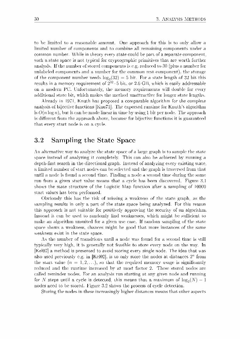
30 3. Analysis Methods
to be limited to a reasonable amount. One approach for this is to only allow alimited number of components and to combine all remaining components under acommon number. While in theory every state could be part of a separate component,such a state space is not typical for cryptographic primitives that are worth furtheranalysis. If the number of stored components is e.g. reduced to 30 (plus a number forunlabeled components and a number for the common rest component), the storageof the component number needs log2(32) = 5 bit. For a state length of 32 bit thisresults in a memory requirement of 232 · 5 bit, or 2.6 GB, which is easily addressableon a modern PC. Unfortunately, the memory requirements will double for everyadditional state bit, which makes the method unattractive for longer state lengths.
Already in 1971, Knuth has proposed a comparable algorithm for the completeanalysis of bijective functions [Knu71]. The expected runtime for Knuth's algorithmis O(n log n), but it can be made linear in time by using 1 bit per node. The approachis di�erent from the approach above, because for bijective functions it is guaranteedthat every start node is on a cycle.
3.2 Sampling the State Space
An alternative way to analyze the state space of a large graph is to sample the statespace instead of analyzing it completely. This can also be achieved by running adepth-�rst search in the directional graph. Instead of analyzing every existing state,a limited number of start nodes can be selected and the graph is traversed from thatuntil a node is found a second time. Finding a node a second time during the samerun from a given start value means that a cycle has been discovered. Figure 3.1shows the state structure of the Logistic Map function after a sampling of 10000start values has been performed.
Obviously this has the risk of missing a weakness of the state graph, as thesampling results in only a part of the state space being analyzed. For this reasonthis approach is not suitable for positively approving the security of an algorithm.Instead it can be used to randomly �nd weaknesses, which might be su�cient tomake an algorithm unsuited for a given use case. If random sampling of the statespace shows a weakness, chances might be good that more instances of the sameweakness exist in the state space.
As the number of transitions until a node was found for a second time is stilltypically very high, it is generally not feasible to store every node on the way. In[Kel07] a method is presented to avoid storing every single node. The idea that wasalso used previously e.g. in [Kel02], is to only store the nodes at distances 2n fromthe start value (n = 1, 2, . . .), so that the required memory usage is signi�cantlyreduced and the runtime increased by at most factor 2. These stored nodes arecalled reminder nodes. For an analysis run starting at any given node and runningfor N steps until a cycle is detected, this means that a maximum of log2(N) − 1nodes need to be stored. Figure 3.2 shows the process of cycle detection.
Storing the nodes in these increasingly higher distances means that other aspects
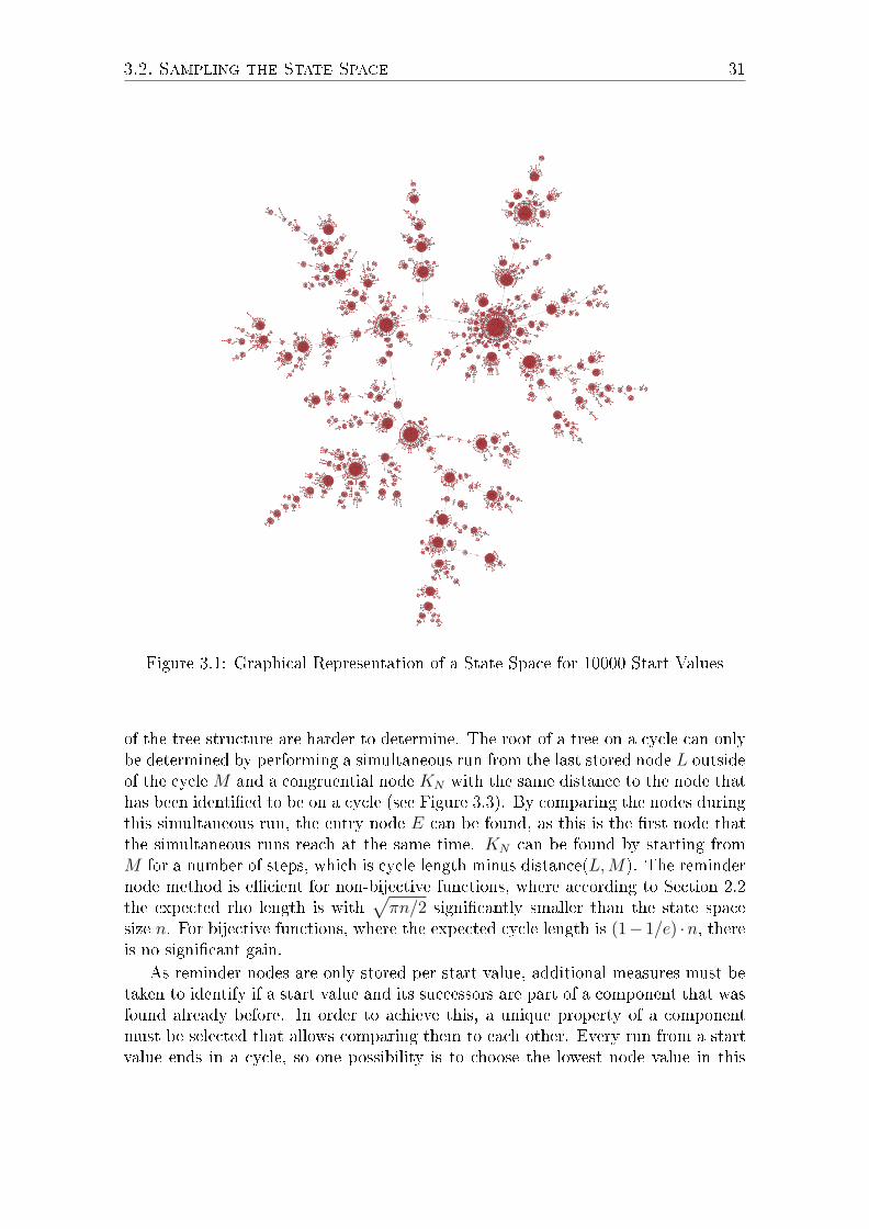
3.2. Sampling the State Space 31
Figure 3.1: Graphical Representation of a State Space for 10000 Start Values
of the tree structure are harder to determine. The root of a tree on a cycle can onlybe determined by performing a simultaneous run from the last stored node L outsideof the cycle M and a congruential node KN with the same distance to the node thathas been identi�ed to be on a cycle (see Figure 3.3). By comparing the nodes duringthis simultaneous run, the entry node E can be found, as this is the �rst node thatthe simultaneous runs reach at the same time. KN can be found by starting fromM for a number of steps, which is cycle length minus distance(L,M). The remindernode method is e�cient for non-bijective functions, where according to Section 2.2the expected rho length is with
√πn/2 signi�cantly smaller than the state space
size n. For bijective functions, where the expected cycle length is (1− 1/e) ·n, thereis no signi�cant gain.
As reminder nodes are only stored per start value, additional measures must betaken to identify if a start value and its successors are part of a component that wasfound already before. In order to achieve this, a unique property of a componentmust be selected that allows comparing them to each other. Every run from a startvalue ends in a cycle, so one possibility is to choose the lowest node value in this
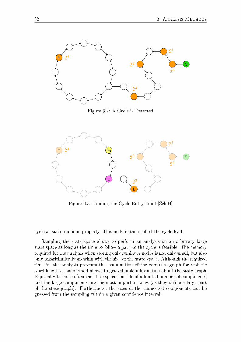
32 3. Analysis Methods
Figure 3.2: A Cycle is Detected
Figure 3.3: Finding the Cycle Entry Point [Sch04]
cycle as such a unique property. This node is then called the cycle lead.
Sampling the state space allows to perform an analysis on an arbitrary largestate space as long as the time to follow a path to the cycle is feasible. The memoryrequired for the analysis when storing only reminder nodes is not only small, but alsoonly logarithmically growing with the size of the state space. Although the requiredtime for the analysis prevents the examination of the complete graph for realisticword lengths, this method allows to get valuable information about the state graph.Especially because often the state space consists of a limited number of components,and the large components are the most important ones (as they de�ne a large partof the state graph). Furthermore, the sizes of the connected components can beguessed from the sampling within a given con�dence interval.

3.4. Candidate Analysis 33
3.3 Reducing the State Space
Another possibility to reduce the required time for analysis is to reduce the wordlength of the algorithm under the assumption that the basic properties do not changetoo much. Obviously there are cases, in which an algorithm will behave completelydi�erently when the size of the state is modi�ed, e.g. for rotating bit shifts that de-generate to no operations if the shift length is equal to the word length. Neverthelessthere might be algorithms that behave similar even when applied on a shorter state.In Chapter 4, the results of several investigations on this are presented.
3.4 Candidate Analysis
Instead of choosing reminder nodes based on the distance to the start node of ananalysis run, the nodes to be stored can also be selected by a property of the state.Assuming that the complete state is represented by a given number of bits, such aproperty could for example be that a certain range of bits is zero. Nodes that ful�llthis criterion are called candidates [BK07]. Similar approaches have been presentedas distinguished points method e.g. in [KY10], [VOW99], [GLV00].
The advantage of this method compared to the reminder node method is that itcan be immediately identi�ed when a candidate node has been encountered during ananalysis run. If a database of previously identi�ed candidates is maintained, it is veryeasy to detect, when a known component is met. Furthermore, the candidate nodescreate a graph with very similar properties to the graph of the original transitionfunction. As this candidate graph has a smaller number of nodes than the originalgraph, any additional analysis on this graph can be performed much more e�cientlythan on the original graph. Figure 3.4 shows a state space graph with candidatesbeing colored in red. The candidate graph is displayed in red over the originalgraph. A further advantage is that the identi�cation of candidates is based on aglobal property of the state and not based on a property of an analysis instance (thenumber of steps since the start value) as is the case for the reminder node. Thisallows for parallelization of analysis runs on di�erent start nodes, as the databaseof known candidates can be shared between analysis instances.
There are also two drawbacks of this method: As the property of a node thatmakes it a candidate is the same for all nodes, the number of candidates is lin-early growing with the length of the analyzed path, which results in higher memoryrequirements for graphs with long paths compared to the reminder node method.Furthermore, it is not ensured that every cycle in the graph contains at least onecandidate. This can lead to an in�nite analysis run, as the path will continue runningaround a cycle without ever hitting a candidate and therefore without being ableto detect the cycle. Therefore, the candidate criterion is ideally chosen such, thatstatistically every cycle will contain at least one candidate. This can be achieved byeither using existing knowledge about the state tree, or by using the properties of arandom mapping as guidance: Theorem 3 in Subsection 2.3.2 assumes an expected

34 3. Analysis Methods
Figure 3.4: Candidate Graph
cycle length of√πn/8 for a random mapping, so the criterion for a candidate node
should be chosen such, that at least one candidate node per√πn/8 nodes is selected.
Furthermore, the candidate method can be enhanced by storing reminder nodesin addition, which will always detect cycles. This will avoid such in�nite loops.

35
Chapter 4
Analysis Results
In this chapter, the analysis methods from Chapter 3 are applied on a selectionof cryptographic primitives and the results are presented. As mentioned in 2.1.3,PRNGs, hash functions and stream ciphers are particularly interesting in the con-text of RFID privacy, therefore candidates of all of these classes of cryptographicprimitives have been examined. Besides AKARI and LAMED, that have been tai-lored towards low-complexity RFID-Systems, A5/1 and MD5 are examined as exam-ples for widely used implementations. Furthermore, Enocoro, Trivium, SHA-3 andSpritz have been included as recent developments. In addition, the Logistic Mapand the Trigonometric Function are taken into account as representatives for chaoticalgorithms.
4.1 AKARI
AKARI in its variants AKARI-1 and AKARI-2 is a lightweight PRNG that has beendesigned by Pedro Peris-López et al. speci�cally with a use on RFID transponders inmind [MME+11]. The design criteria were good statistical properties and suitabilityfor security applications with the hardware limitations of RFID transponders takeninto consideration. Further requirements were a tiny footprint, high throughputand a low power consumption. The approach taken was to combine a T-functionas proposed in [KS03] with a non-linear �lter function based on a composition ofextremely light operands. The state consists of two state variables with a lengthof 32 bits resulting in a state length of 64 bits. In the course of this work, onlyAKARI-1 was analyzed. Figure 4.1 shows the pseudo code of the algorithm. Theanalysis results presented by the authors for the ENT, DIEHARD and NIST testbatteries show promising results, leading to the conclusion that the algorithm is wellsuited for its intended use in security applications.

36 4. Analysis Results
/* Initialize x0 and x1 of m-bits */
x0 = x0 + ((x0 · x0) ∨ 5)x1 = x1 + ((x1 · x1) ∨ 13)z = x0
for r from 0 to 63z = (z >> 1) + (z << 1) + z + x1
end for
/* Output m/2 bits, lower half of z */
Figure 4.1: AKARI-1 Algorithm in Pseudo Code [MME+11]
4.1.1 Sampled Analysis
The state length of AKARI is with 64 bits too long to perform a complete analysis ofthe state space, therefore the approach of a sampled analysis with a reduced numberof starting points was chosen.
Component Cycle Length Size Relative Size
1 4294967296 4294967296 0.000000023%2 4294967296 4294967296 0.000000023%3 4294967296 4294967296 0.000000023%4 4294967296 4294967296 0.000000023%5 4294967296 4294967296 0.000000023%... ... ... ...
Table 4.1: Results of Sampled Analysis of AKARI
The results in Table 4.1 show that the cycle lengths and component sizes of allsampled components for AKARI-1 are identically 232 = 4294967296. This meansthat all start points are on cycles, which indicates that the transition function islikely bijective.
4.1.2 Reduced Word Length Analysis
In addition, the state space of AKARI-1 was analyzed completely for a variant usinga reduced word length. The algorithm itself was unmodi�ed, only the state variablesx1 and x2 have been reduced in length by masking out the highest bits after everyoperation. The C source code example in Figure 4.2 illustrates the procedure.
Table 4.2 shows the result of the analysis for a word length of 14 bits respectivelya state length of 28 bits: 30 components have been identi�ed, all of them with thesame size being identical to the cycle length. This indicates similar to the sampled

4.1. AKARI 37
#define BITSMASK 0 x 3 f f f
x0 = ( x0 + ( ( x0 ∗ x0 ) | 5 ) ) & BITSMASK;x1 = ( x1 + ( ( x1 ∗ x1 ) | 13) ) & BITSMASK;
for ( r = 0 ; r <= 63 ; r++) {z = ( r o t r ( z , 1) + r o t l ( z , 1) + z + x1 ) & BITSMASK;
}
Figure 4.2: Reduced AKARI-1 Algorithm in Pseudo Code, based on [PLHCETR09]
analysis approach the bijectivity of the algorithm. It can be concluded, that for thisparticular case the behavior of the reduced and the original variant of the algorithmshare certain properties.
Component Cycle Length Size Relative Size
1 16384 16384 0.0061%2 16384 16384 0.0061%3 16384 16384 0.0061%4 16384 16384 0.0061%5 16384 16384 0.0061%... ... ... ...27 16384 16384 0.0061%28 16384 16384 0.0061%29 16384 16384 0.0061%30 16384 16384 0.0061%Rest n/a 267943936 99.8169%
Table 4.2: Analysis Results of AKARI for 14 Bit Word Length
4.1.3 Interpretation of Test Results
Due to the bijectivity of AKARI, an inverse of the transition function might bederivable and thus backward security can be compromised if an internal state isleaked. As a side note, the cycle lengths are far worse than what is proposed fora "good" PRNG in Subsection 2.3.2. Still, AKARI appears to be a good choicefor cryptographic RFID use cases, as it easily passes the test batteries and showsreasonable cycle lengths.
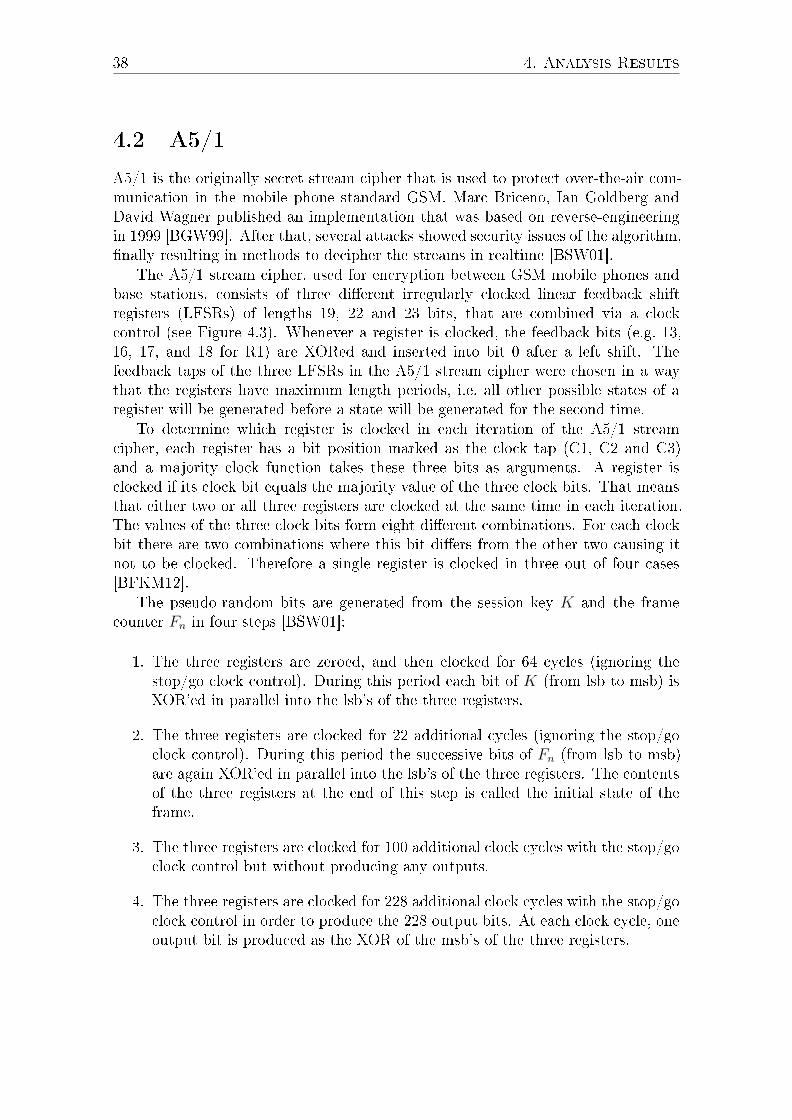
38 4. Analysis Results
4.2 A5/1
A5/1 is the originally secret stream cipher that is used to protect over-the-air com-munication in the mobile phone standard GSM. Marc Briceno, Ian Goldberg andDavid Wagner published an implementation that was based on reverse-engineeringin 1999 [BGW99]. After that, several attacks showed security issues of the algorithm,�nally resulting in methods to decipher the streams in realtime [BSW01].
The A5/1 stream cipher, used for encryption between GSM mobile phones andbase stations, consists of three di�erent irregularly clocked linear feedback shiftregisters (LFSRs) of lengths 19, 22 and 23 bits, that are combined via a clockcontrol (see Figure 4.3). Whenever a register is clocked, the feedback bits (e.g. 13,16, 17, and 18 for R1) are XORed and inserted into bit 0 after a left shift. Thefeedback taps of the three LFSRs in the A5/1 stream cipher were chosen in a waythat the registers have maximum length periods, i.e. all other possible states of aregister will be generated before a state will be generated for the second time.
To determine which register is clocked in each iteration of the A5/1 streamcipher, each register has a bit position marked as the clock tap (C1, C2 and C3)and a majority clock function takes these three bits as arguments. A register isclocked if its clock bit equals the majority value of the three clock bits. That meansthat either two or all three registers are clocked at the same time in each iteration.The values of the three clock bits form eight di�erent combinations. For each clockbit there are two combinations where this bit di�ers from the other two causing itnot to be clocked. Therefore a single register is clocked in three out of four cases[BFKM12].
The pseudo-random bits are generated from the session key K and the framecounter Fn in four steps [BSW01]:
1. The three registers are zeroed, and then clocked for 64 cycles (ignoring thestop/go clock control). During this period each bit of K (from lsb to msb) isXOR'ed in parallel into the lsb's of the three registers.
2. The three registers are clocked for 22 additional cycles (ignoring the stop/goclock control). During this period the successive bits of Fn (from lsb to msb)are again XOR'ed in parallel into the lsb's of the three registers. The contentsof the three registers at the end of this step is called the initial state of theframe.
3. The three registers are clocked for 100 additional clock cycles with the stop/goclock control but without producing any outputs.
4. The three registers are clocked for 228 additional clock cycles with the stop/goclock control in order to produce the 228 output bits. At each clock cycle, oneoutput bit is produced as the XOR of the msb's of the three registers.
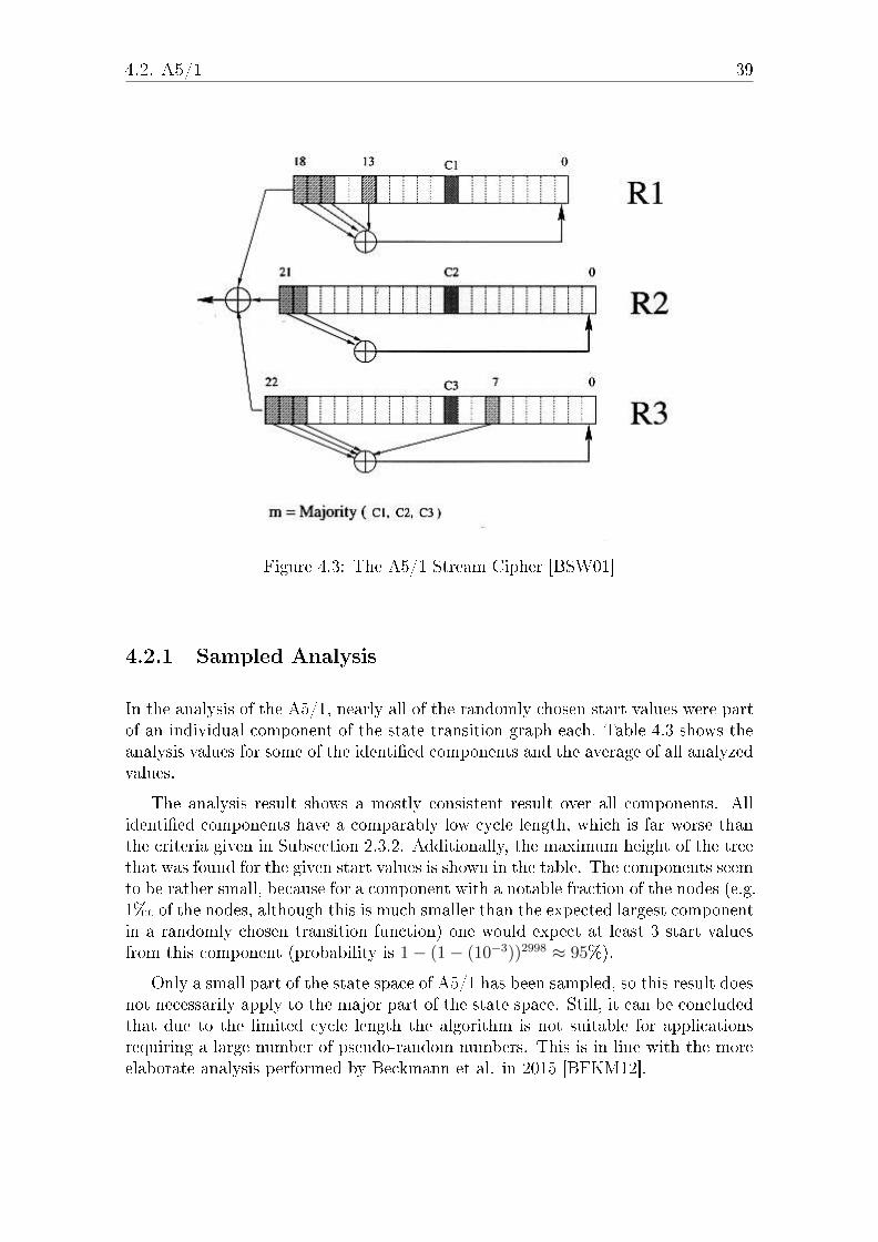
4.2. A5/1 39
Figure 4.3: The A5/1 Stream Cipher [BSW01]
4.2.1 Sampled Analysis
In the analysis of the A5/1, nearly all of the randomly chosen start values were partof an individual component of the state transition graph each. Table 4.3 shows theanalysis values for some of the identi�ed components and the average of all analyzedvalues.
The analysis result shows a mostly consistent result over all components. Allidenti�ed components have a comparably low cycle length, which is far worse thanthe criteria given in Subsection 2.3.2. Additionally, the maximum height of the treethat was found for the given start values is shown in the table. The components seemto be rather small, because for a component with a notable fraction of the nodes (e.g.1%� of the nodes, although this is much smaller than the expected largest componentin a randomly chosen transition function) one would expect at least 3 start valuesfrom this component (probability is 1− (1− (10−3))2998 ≈ 95%).
Only a small part of the state space of A5/1 has been sampled, so this result doesnot necessarily apply to the major part of the state space. Still, it can be concludedthat due to the limited cycle length the algorithm is not suitable for applicationsrequiring a large number of pseudo-random numbers. This is in line with the moreelaborate analysis performed by Beckmann et al. in 2015 [BFKM12].
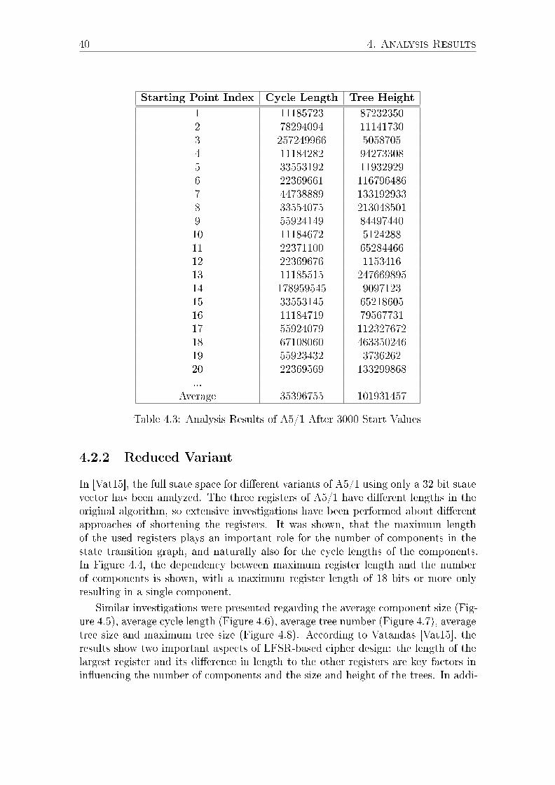
40 4. Analysis Results
Starting Point Index Cycle Length Tree Height
1 11185723 872323502 78294094 111417303 257249966 50587054 11184282 942733085 33553192 119329296 22369661 1167964867 44738889 1331929338 33554075 2130485019 55924149 8449744010 11184672 512428811 22371100 6528446612 22369676 115341613 11185515 24766989514 178959545 909712315 33553145 6521860516 11184719 7956773117 55924079 11232767218 67108060 46335024619 55923432 373626220 22369569 133299868...
Average 35396755 101931457
Table 4.3: Analysis Results of A5/1 After 3000 Start Values
4.2.2 Reduced Variant
In [Vat15], the full state space for di�erent variants of A5/1 using only a 32 bit statevector has been analyzed. The three registers of A5/1 have di�erent lengths in theoriginal algorithm, so extensive investigations have been performed about di�erentapproaches of shortening the registers. It was shown, that the maximum lengthof the used registers plays an important role for the number of components in thestate transition graph, and naturally also for the cycle lengths of the components.In Figure 4.4, the dependency between maximum register length and the numberof components is shown, with a maximum register length of 18 bits or more onlyresulting in a single component.
Similar investigations were presented regarding the average component size (Fig-ure 4.5), average cycle length (Figure 4.6), average tree number (Figure 4.7), averagetree size and maximum tree size (Figure 4.8). According to Vatandas [Vat15], theresults show two important aspects of LFSR-based cipher design: the length of thelargest register and its di�erence in length to the other registers are key factors inin�uencing the number of components and the size and height of the trees. In addi-
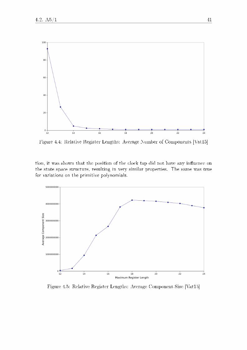
4.2. A5/1 41
Figure 4.4: Relative Register Lengths: Average Number of Components [Vat15]
tion, it was shown that the position of the clock tap did not have any in�uence onthe state space structure, resulting in very similar properties. The same was truefor variations on the primitive polynomials.
Figure 4.5: Relative Register Lengths: Average Component Size [Vat15]

42 4. Analysis Results
Figure 4.6: Relative Register Lengths: Average Cycle Size [Vat15]
Figure 4.7: Relative Register Lengths: Average Trees per Component [Vat15]
4.2.3 Interpretation of Test Results
The results of the sampled analysis performed in this work indicates a structuralweakness of A5/1. This supports the result of other works, that showed signi�cantweaknesses of the algorithm. The di�erent reduced variants that have been analyzed
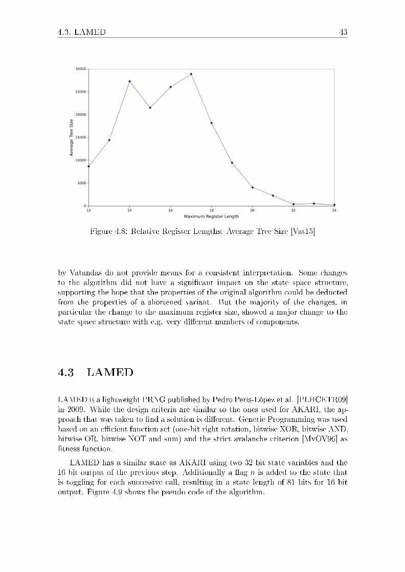
4.3. LAMED 43
Figure 4.8: Relative Register Lengths: Average Tree Size [Vat15]
by Vatandas do not provide means for a consistent interpretation. Some changesto the algorithm did not have a signi�cant impact on the state space structure,supporting the hope that the properties of the original algorithm could be deductedfrom the properties of a shortened variant. But the majority of the changes, inparticular the change to the maximum register size, showed a major change to thestate space structure with e.g. very di�erent numbers of components.
4.3 LAMED
LAMED is a lightweight PRNG published by Pedro Peris-López et al. [PLHCETR09]in 2009. While the design criteria are similar to the ones used for AKARI, the ap-proach that was taken to �nd a solution is di�erent. Genetic Programming was usedbased on an e�cient function set (one-bit right rotation, bitwise XOR, bitwise AND,bitwise OR, bitwise NOT and sum) and the strict avalanche criterion [MvOV96] as�tness function.
LAMED has a similar state as AKARI using two 32 bit state variables and the16 bit output of the previous step. Additionally a �ag n is added to the state thatis toggling for each successive call, resulting in a state length of 81 bits for 16 bitoutput. Figure 4.9 shows the pseudo code of the algorithm.

44 4. Analysis Results
lamed()
If n is odd
a0=a1 + iv
a1=out ^ s
If n is even
a0=a1 ^ iv
a1=out + s
aux1=a0 + a1;
aux2=a0 ^ a1;
aux3=vrotdk(aux1,5);
aux3=aux3 + aux2;
aux3=vrotdk(aux3,3);
aux3=aux3 ^ aux1;
aux3=vrotdk(aux3,4);
aux3=a1 + aux3;
aux3=vrotdk(aux3,2);
aux3=aux3 + aux1;
aux3=vrotdk(aux3,2);
aux3=aux3 ^ aux1;
aux3=vrotdk(aux3,3);
aux33=aux3 + a1;
aux3=vrotdk(aux3,2);
aux3=aux3 + aux1;
aux3=vrotdk(aux3,4);
aux3=aux3 ^ a1;
aux3=vrotd(aux3);
aux3=aux3 + aux2;
aux3=vrotdk(aux3,2);
out=aux1 ^ aux3;
}
Figure 4.9: LAMED Algorithm in Pseudo Code [PLHCETR09]
4.3.1 Sampled Analysis
A sampled approach was attempted to analyze the original algorithm. Although anextensive search was performed using many days of CPU time, no cycle could beidenti�ed. This might be evidence of a bijective transition function. Further analysiscould be performed using the candidate analysis on a highly parallel architecture,e.g. a powerful GPU system.

4.4. Chaotic Functions 45
4.3.2 Reduced Variant
As the result of the full variant did not lead to any result, the state was reduced toa length of 31 bits by using a word length of 12 bits. Table 4.4 shows the analysisresults.
Component Cycle Length Size Relative Size
1 64 2147483648 100%Rest n/a 0 0%
Table 4.4: Analysis Results of LAMED for 12 Bit Word Length
It can be seen from the results, that only a single component could be identi�ed,with a cycle length that is signi�cantly lower than the component size. This means,that this extremely reduced variant of LAMED is not bijective. If this result isapplicable to the original algorithm under these extreme modi�cation conditionscannot be answered though.
4.3.3 Interpretation of Test Results
The results of both the sampled and the reduced analysis indicate that there appearsto be a comparably small number of components with a large size. Overall, theresults appear too unspeci�c to make an informed statement though.
4.4 Chaotic Functions
Chaotic functions have been announced as particularly promising for implementinglow-complexity pseudo-random number generators (PRNGs) required e.g. for RFIDsecurity applications. They combine good theoretical statistical properties witha computationally simple algorithm. Unfortunately, actual implementations with�nite number precision show a disappointing behavior compared to the mathematicaltheory [KW07], [Mih07]. This results for example in comparably short cycles in thestate space graph, which lead to a repetition of the generated pseudo-random valuesafter a small number of iterations.
De�nition: Chaotic Functions
The de�nitions of a chaotic function f : R → R, where R is a an interval in thereals, vary widely. Most de�nitions agree on the following properties of a sequenceof points x, f(x), f(f(x)), ... ([KW07]):
• f reacts sensibly to changes in x, i.e. even small changes to the value of xresult in large changes of the sequence.

46 4. Analysis Results
• f is topologically transitive, i.e. almost every element of R can be connectedto almost every other element of R by a �nite sequence.
• f is topologically dense, i.e. even small intervals of R contain periodic pointsof f .
In the scope of this work, chaotic functions are assumed to be functions f :[0, 1] → [0, 1] that exhibit chaotic behavior. Practical implementations of PRNGsbased on such chaotic functions have therefore a state s which is a real in theinterval [0, 1]. The PRNG output is computed as a function of the state. Due tothe chaotic behavior it is assumed that chaotic PRNGs have desirable statisticalproperties. Unfortunately, the restriction to a �nite state because of �nite numberrepresentation can cause problems because the Lyapunov exponent is not greaterthan zero anymore.
To achieve a reasonably good behavior of the chaotic function, IEEE754 doubleprecision was chosen as numeric representation for the following investigations. Only62 bits of this 64 bit number representation are used for the interval [0, 1], becausethe sign bit is always positive and the uppermost exponent bit is always 0. A 62-bitstate is far too large to allow a complete analysis of the state space, so the statespace was sampled in order to be able to run an analysis in a reasonable amount oftime.
4.4.1 Logistic Map
A common and simple chaotic function is the Logistic Map function (cf. [KW07]and the references therein):
f1 : [0, 1]→ [0, 1] with f1(x) = a · x · (1− x), a ≈ 4 (4.1)
Sampled Analysis
Table 4.5 shows the analysis of the state space for 100 randomly chosen start values.
Table 4.5: Analysis Results of Logistic Map Algorithm for 100 Start Values
Component Cycle Maximum PercentLength Tree Height of Start Values
1 6623920 68244008 100
The table shows that a single component was identi�ed with a comparably lowcycle length.
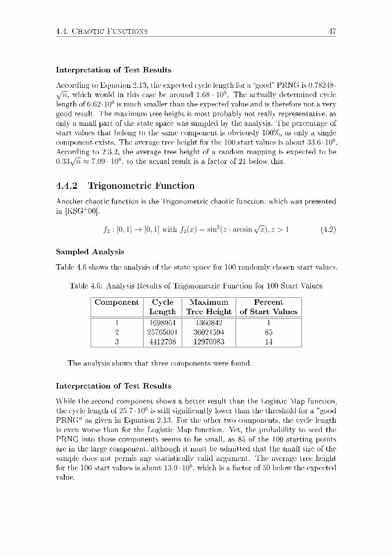
4.4. Chaotic Functions 47
Interpretation of Test Results
According to Equation 2.13, the expected cycle length for a �good� PRNG is 0.78248·√n, which would in this case be around 1.68 · 109. The actually determined cycle
length of 6.62·106 is much smaller than the expected value and is therefore not a verygood result. The maximum tree height is most probably not really representative, asonly a small part of the state space was sampled by the analysis. The percentage ofstart values that belong to the same component is obviously 100%, as only a singlecomponent exists. The average tree height for the 100 start values is about 33.6 ·106.According to 2.3.2, the average tree height of a random mapping is expected to be0.33√n ≈ 7.09 · 108, so the actual result is a factor of 21 below this.
4.4.2 Trigonometric Function
Another chaotic function is the Trigonometric chaotic function, which was presentedin [KSG+00].
f2 : [0, 1]→ [0, 1] with f2(x) = sin2(z · arcsin√x), z > 1 (4.2)
Sampled Analysis
Table 4.6 shows the analysis of the state space for 100 randomly chosen start values.
Table 4.6: Analysis Results of Trigonometric Function for 100 Start Values
Component Cycle Maximum PercentLength Tree Height of Start Values
1 1698951 1360842 12 25765001 36021594 853 4412798 12976983 14
The analysis shows that three components were found.
Interpretation of Test Results
While the second component shows a better result than the Logistic Map function,the cycle length of 25.7 ·106 is still signi�cantly lower than the threshold for a "goodPRNG" as given in Equation 2.13. For the other two components, the cycle lengthis even worse than for the Logistic Map function. Yet, the probability to seed thePRNG into those components seems to be small, as 85 of the 100 starting pointsare in the large component, although it must be admitted that the small size of thesample does not permit any statistically valid argument. The average tree heightfor the 100 start values is about 13.9 ·106, which is a factor of 50 below the expectedvalue.
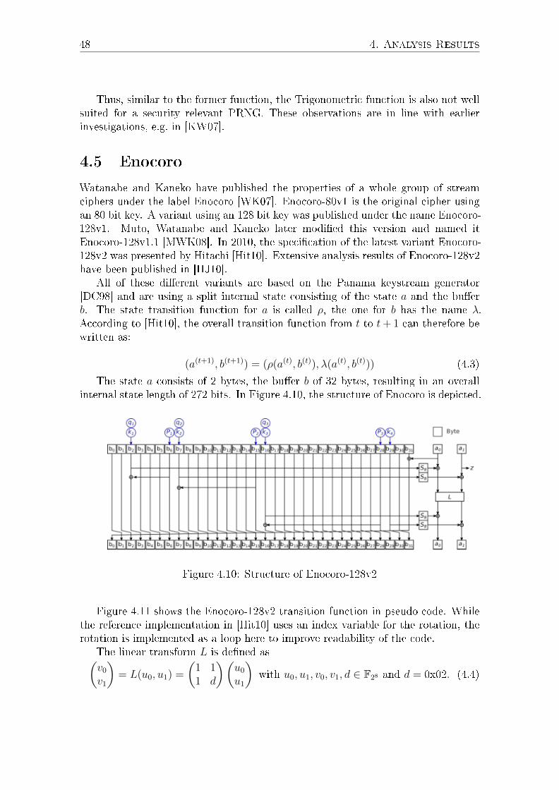
48 4. Analysis Results
Thus, similar to the former function, the Trigonometric function is also not wellsuited for a security relevant PRNG. These observations are in line with earlierinvestigations, e.g. in [KW07].
4.5 Enocoro
Watanabe and Kaneko have published the properties of a whole group of streamciphers under the label Enocoro [WK07]. Enocoro-80v1 is the original cipher usingan 80 bit key. A variant using an 128 bit key was published under the name Enocoro-128v1. Muto, Watanabe and Kaneko later modi�ed this version and named itEnocoro-128v1.1 [MWK08]. In 2010, the speci�cation of the latest variant Enocoro-128v2 was presented by Hitachi [Hit10]. Extensive analysis results of Enocoro-128v2have been published in [HJ10].
All of these di�erent variants are based on the Panama keystream generator[DC98] and are using a split internal state consisting of the state a and the bu�erb. The state transition function for a is called ρ, the one for b has the name λ.According to [Hit10], the overall transition function from t to t+ 1 can therefore bewritten as:
(a(t+1), b(t+1)) = (ρ(a(t), b(t)), λ(a(t), b(t))) (4.3)
The state a consists of 2 bytes, the bu�er b of 32 bytes, resulting in an overallinternal state length of 272 bits. In Figure 4.10, the structure of Enocoro is depicted.
Figure 4.10: Structure of Enocoro-128v2
Figure 4.11 shows the Enocoro-128v2 transition function in pseudo code. Whilethe reference implementation in [Hit10] uses an index variable for the rotation, therotation is implemented as a loop here to improve readability of the code.
The linear transform L is de�ned as(v0v1
)= L(u0, u1) =
(1 11 d
)(u0u1
)with u0, u1, v0, v1, d ∈ F28 and d = 0x02. (4.4)

4.5. Enocoro 49
function enocoro()tmp_a0 ← a0tmp_b31 ← b31/ ∗ ρ ∗ /u0 ← a0 ⊕ s8[bk1]u1 ← a1 ⊕ s8[bk2]v0 ← u0 ⊕ u1v1 ← u0 ⊕ 0x02 · u1a0 ← v0 ⊕ s8[bk3]a1 ← v1 ⊕ s8[bk4]/ ∗ λ ∗ /bq1 ← bq1 ⊕ bp1bq2 ← bq2 ⊕ bp2bq3 ← bq3 ⊕ bp3for i← 31 to 1 step −1 do
bi ← bi−1
end forb0 ← tmp_b31 ⊕ tmp_a0
end enocoro/* S8 Box */s8[256] = {
99,82,26,223,138,246,174,85,137,231,208,45,189,1,36,120,
27,217,227,84,200,164,236,126,171,0,156,46,145,103,55,83,
78,107,108,17,178,192,130,253,57,69,254,155,52,215,167,8,
184,154,51,198,76,29,105,161,110,62,197,10,87,244,241,131,
245,71,31,122,165,41,60,66,214,115,141,240,142,24,170,193,
32,191,230,147,81,14,247,152,221,186,106,5,72,35,109,212,
30,96,117,67,151,42,49,219,132,25,175,188,204,243,232,70,
136,172,139,228,123,213,88,54,2,177,7,114,225,220,95,47,
93,229,209,12,38,153,181,111,224,74,59,222,162,104,146,23,
202,238,169,182,3,94,211,37,251,157,97,89,6,144,116,44,
39,149,160,185,124,237,4,210,80,226,73,119,203,58,15,158,
112,22,92,239,33,179,159,13,166,201,34,148,250,75,216,101,
133,61,150,40,20,91,102,234,127,206,249,64,19,173,195,176,
242,194,56,128,207,113,11,135,77,53,86,233,100,190,28,187,
183,48,196,43,255,98,65,168,21,140,18,199,121,143,90,252,
205,9,79,125,248,134,218,16,50,118,180,163,63,68,129,235
}
Figure 4.11: Enocoro Algorithm in Pseudo Code [Huf16]
4.5.1 Sampled Analysis
An attempt to �nd a cycle in the state space graph of the original Enocoro implemen-tation did not succeed even after many days of CPU time. Due to the comparablylarge state length of 272 bits this is not surprising. It might hint to the fact thatEnocoro-128v2 is bijective, although it is not as strong evidence as for LAMED,where a similar e�ect was observed. For a random mapping of this state space size,

50 4. Analysis Results
the expected cycle length is µ =√πn/8 = 5.46 · 1040, so even for a non-bijective
function a cycle might not be detectable in reasonable time.
4.5.2 Reduced Variants
In [Huf16], two di�erent variants of Enocoro using a reduced state length have beeninvestigated. In Figure 4.10, the bits that are used in the algorithm beyond therotation of the bu�er are marked in blue. In order to keep the general structure ofEnocoro intact, both of the variants adhere to the following rules:
1. The split into the state a and the bu�er b is kept.
2. The order of the marked bits in 4.10 is kept the same.
3. The usage of the marked bits is kept the same.
4. The position of the marked bits relatively to the length of the bu�er stayssimilar.
5. The overall state including a and b is not longer than 32 bits.
Enocoro32_1
The �rst analyzed variant Enocoro32_1 is based on a 2 bit state a and a 30 bitbu�er b. This variant uses the obvious approach to shorten a and b while keepingthe relationship of their lengths nearly identical. Table 4.7 shows the positions ofthe used bits compared to the original algorithm.
Table 4.7: Bit Positions for Enocoro32_1 Compared to Bit Positions in Enocoro-128v2 [Huf16]
Pos. Enocoro-128v2 Enocoro32_132 Bytes 30 Bits
k1 2 2k2 7 7k3 16 15k4 29 28p1 6 6p2 15 14p3 28 27q1 2 2q2 7 7q3 16 15
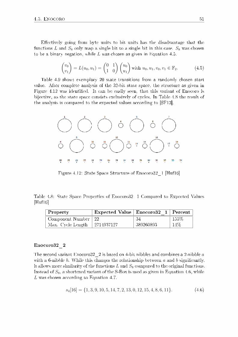
4.5. Enocoro 51
E�ectively going from byte units to bit units has the disadvantage that thefunctions L and S8 only map a single bit to a single bit in this case. S8 was chosento be a binary negation, while L was chosen as given in Equation 4.5.(
v0v1
)= L(u0, u1) =
(0 11 0
)(u0u1
)with u0, u1, v0, v1 ∈ F2. (4.5)
Table 4.9 shows exemplary 20 state transitions from a randomly chosen startvalue. After complete analysis of the 32-bit state space, the structure as given inFigure 4.12 was identi�ed. It can be easily seen, that this variant of Enocoro isbijective, as the state space consists exclusively of cycles. In Table 4.8 the result ofthe analysis is compared to the expected values according to [SF13].
Figure 4.12: State Space Structure of Enocoro32_1 [Huf16]
Table 4.8: State Space Properties of Enocoro32_1 Compared to Expected Values[Huf16]
Property Expected Value Enocoro32_1 Percent
Component Number 22 34 155%Max. Cycle Length 2714937127 389260893 14%
Enocoro32_2
The second variant Enocoro32_2 is based on 4-bit nibbles and combines a 2-nibble awith a 6-nibble b. While this changes the relationship between a and b signi�cantly,it allows more similarity of the functions L and S8 compared to the original functions.Instead of S8, a shortened variant of the S-Box is used as given in Equation 4.6, whileL was chosen according to Equation 4.7.
s4[16] = {1, 3, 9, 10, 5, 14, 7, 2, 13, 0, 12, 15, 4, 8, 6, 11}. (4.6)

52 4. Analysis Results
Table
4.9:Enocoro32_
1State
Transitions
(Shortened)[Huf16]
Enocoro32_1
TEST
Algorith
m(N
ominalValue)
TInterm
ediate
Value
InputPASS
Hex
Bin
27
1528
614
2720
aBu�
era
Bu�
erbk1
bk2
bk3
bp1
bp2
bp3
bk1
a0
a1
bq1
bq2
bq3
a0
a1
a:1b:381daca9
START
1381D
ACA9
0100111000000111011010110010101001
01
11
00
10
10
10
11
a:3b:303a5953
PASS
3303A
595311
001100000011101001011001010100110
00
11
10
11
11
01
0a:2
b:2074b3aePASS
22074B
3AE
1000100000011101001011001110101110
11
10
00
01
01
11
00
a:0b:00e9675c
PASS
000E
9675C00
000000001110100101100111010111001
00
01
10
00
01
00
1a:1
b:01d2cfb0PASS
101D
2CFB0
0100000001110100101100111110110000
01
10
01
00
10
01
10
a:2b:03a59e60
PASS
203A
59E60
1000000011101001011001111001100000
00
10
10
01
01
01
11
a:3b:074b3cc9
PASS
3074B
3CC9
1100000111010010110011110011001001
01
00
10
01
11
10
01
a:1b:0e96799b
PASS
10E
96799B01
000011101001011001111001100110110
10
00
11
01
00
10
0a:0
b:1d2df236PASS
01D
2DF236
0000011101001011011111001000110110
10
11
01
10
01
10
10
a:2b:3a5ae56c
PASS
23A
5AE56C
1000111010010110101110010101101100
10
11
11
11
00
10
11
a:3b:34b4cb
d0PASS
334B
4CBD0
1100110100101101001100101111010000
01
11
11
01
11
01
10
a:2b:296996a8
PASS
2296996A
810
001010010110100110010110101010000
11
00
01
10
01
00
1a:1
b:12d22d50PASS
112D
22D50
0100010010110100100010110101010000
00
01
10
00
11
00
11
a:3b:25a45aa8
PASS
325A
45AA8
1100100101101001000101101010101000
01
00
01
01
10
00
01
a:1b:0b48b450
PASS
10B
48B450
0100001011010010001011010001010000
00
10
10
10
11
00
00
a:0b:169068a8
PASS
0169068A
800
000101101001000001101000101010000
10
10
10
00
00
01
1a:3
b:2d20d050PASS
32D
20D050
1100101101001000001101000001010000
00
10
11
11
11
10
01
a:1b:1a40a1a8
PASS
11A
40A1A
801
000110100100000010100001101010000
11
10
01
01
01
01
1a:3
b:34804350PASS
334804350
1100110100100000000100001101010000
00
01
11
01
11
10
10
a:2b:290087a8
PASS
2290087A
810
001010010000000010000111101010000
11
00
01
10
01
00
1a:1
b:12000f50PASS
112000F
5001
000100100000000000001111010100000
00
11
00
01
10
01
1
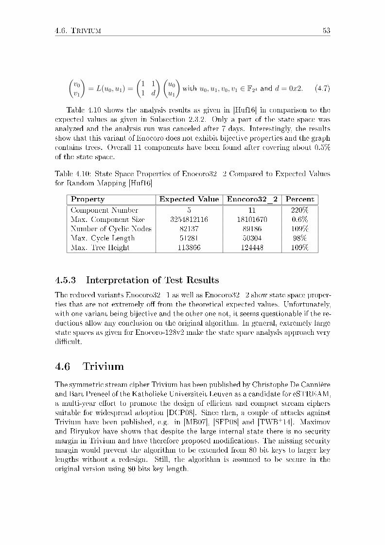
4.6. Trivium 53
(v0v1
)= L(u0, u1) =
(1 11 d
)(u0u1
)with u0, u1, v0, v1 ∈ F24 and d = 0x2. (4.7)
Table 4.10 shows the analysis results as given in [Huf16] in comparison to theexpected values as given in Subsection 2.3.2. Only a part of the state space wasanalyzed and the analysis run was canceled after 7 days. Interestingly, the resultsshow that this variant of Enocoro does not exhibit bijective properties and the graphcontains trees. Overall 11 components have been found after covering about 0.5%of the state space.
Table 4.10: State Space Properties of Enocoro32_2 Compared to Expected Valuesfor Random Mapping [Huf16]
Property Expected Value Enocoro32_2 Percent
Component Number 5 11 220%Max. Component Size 3254812116 18101670 0.6%Number of Cyclic Nodes 82137 89186 109%Max. Cycle Length 51281 50304 98%Max. Tree Height 113866 124448 109%
4.5.3 Interpretation of Test Results
The reduced variants Enocoro32_1 as well as Enocoro32_2 show state space proper-ties that are not extremely o� from the theoretical expected values. Unfortunately,with one variant being bijective and the other one not, it seems questionable if the re-ductions allow any conclusion on the original algorithm. In general, extremely largestate spaces as given for Enocoro-128v2 make the state space analysis approach verydi�cult.
4.6 Trivium
The symmetric stream cipher Trivium has been published by Christophe De Cannièreand Bart Preneel of the Katholieke Universiteit Leuven as a candidate for eSTREAM,a multi-year e�ort to promote the design of e�cient and compact stream cipherssuitable for widespread adoption [DCP08]. Since then, a couple of attacks againstTrivium have been published, e.g. in [MB07], [SFP08] and [TWB+14]. Maximovand Biryukov have shown that despite the large internal state there is no securitymargin in Trivium and have therefore proposed modi�cations. The missing securitymargin would prevent the algorithm to be extended from 80 bit keys to larger keylengths without a redesign. Still, the algorithm is assumed to be secure in theoriginal version using 80 bits key length.
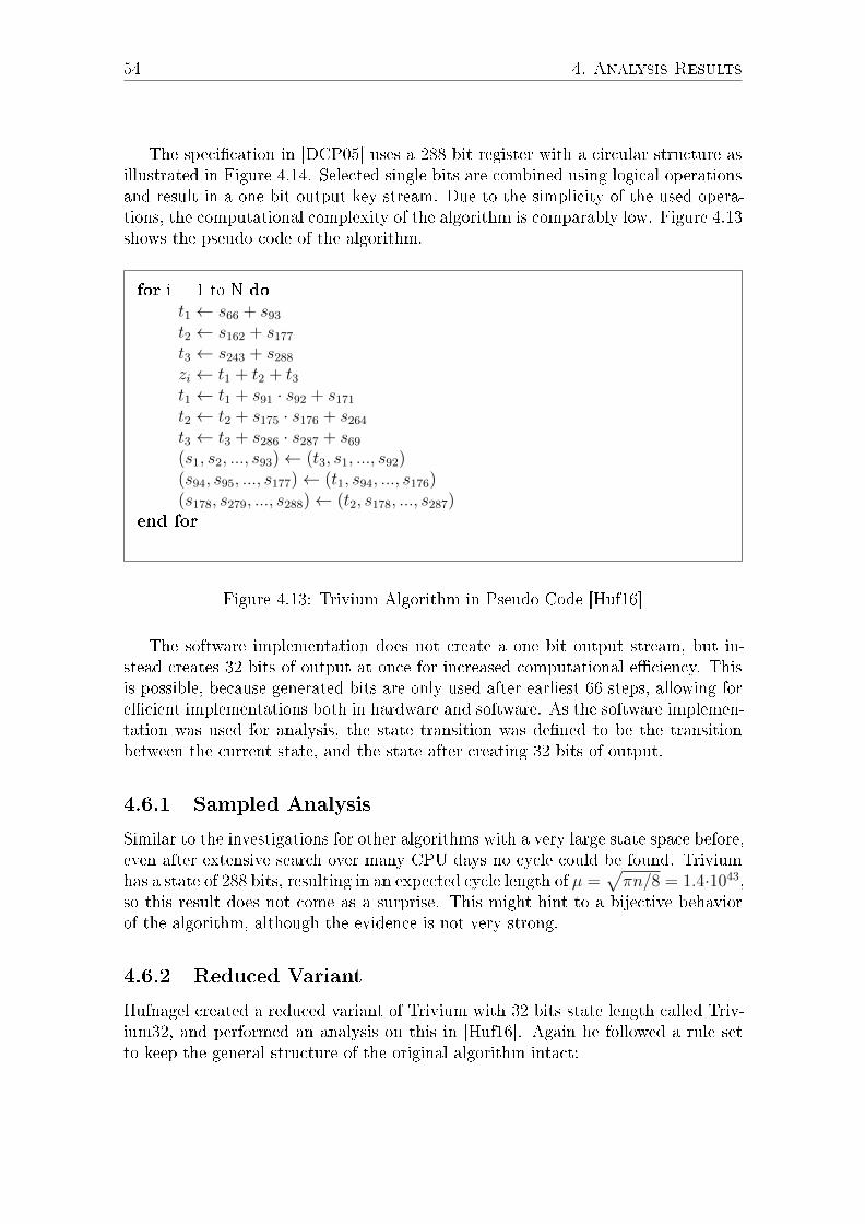
54 4. Analysis Results
The speci�cation in [DCP05] uses a 288 bit register with a circular structure asillustrated in Figure 4.14. Selected single bits are combined using logical operationsand result in a one bit output key stream. Due to the simplicity of the used opera-tions, the computational complexity of the algorithm is comparably low. Figure 4.13shows the pseudo code of the algorithm.
for i = 1 to N dot1 ← s66 + s93t2 ← s162 + s177t3 ← s243 + s288zi ← t1 + t2 + t3t1 ← t1 + s91 · s92 + s171t2 ← t2 + s175 · s176 + s264t3 ← t3 + s286 · s287 + s69(s1, s2, ..., s93)← (t3, s1, ..., s92)(s94, s95, ..., s177)← (t1, s94, ..., s176)(s178, s279, ..., s288)← (t2, s178, ..., s287)
end for
Figure 4.13: Trivium Algorithm in Pseudo Code [Huf16]
The software implementation does not create a one bit output stream, but in-stead creates 32 bits of output at once for increased computational e�ciency. Thisis possible, because generated bits are only used after earliest 66 steps, allowing fore�cient implementations both in hardware and software. As the software implemen-tation was used for analysis, the state transition was de�ned to be the transitionbetween the current state, and the state after creating 32 bits of output.
4.6.1 Sampled Analysis
Similar to the investigations for other algorithms with a very large state space before,even after extensive search over many CPU days no cycle could be found. Triviumhas a state of 288 bits, resulting in an expected cycle length of µ =
√πn/8 = 1.4·1043,
so this result does not come as a surprise. This might hint to a bijective behaviorof the algorithm, although the evidence is not very strong.
4.6.2 Reduced Variant
Hufnagel created a reduced variant of Trivium with 32 bits state length called Triv-ium32, and performed an analysis on this in [Huf16]. Again he followed a rule setto keep the general structure of the original algorithm intact:

4.6. Trivium 55
Figure 4.14: Structure of Trivium [Huf16]
1. The cyclic structure of the algorithm stays the same.
2. The separation into three segments stays the same.
3. The order of the marked bits stays the same.
4. The operations on the marked bits stay the same.
5. A marked bit position is not used more than once.
6. The position of the marked bits relatively to the length of the bu�er stayssimilar.
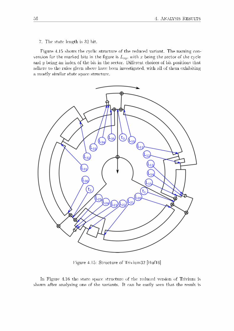
56 4. Analysis Results
7. The state length is 32 bit.
Figure 4.15 shows the cyclic structure of the reduced variant. The naming con-vention for the marked bits in the �gure is Lxy, with x being the sector of the cycleand y being an index of the bit in the sector. Di�erent choices of bit positions thatadhere to the rules given above have been investigated, with all of them exhibitinga mostly similar state space structure.
Figure 4.15: Structure of Trivium32 [Huf16]
In Figure 4.16 the state space structure of the reduced version of Trivium isshown after analysing one of the variants. It can be easily seen that the result is

4.7. MD5 57
a bijective state space graph, which is consistent for all reduced variants that havebeen analyzed in [Huf16]. Table 4.11 lists the properties of the components.
Figure 4.16: State Space Structure of Trivium32 [Huf16]
Table 4.11: State Space Properties of Trivium32 [Huf16]
Component Size Cycle Length
1 2647713485 26477134852 1274867434 12748674343 126176124 1261761244 133880466 1338804665 96773525 967735256 12951347 129513477 2536239 2536239
4.6.3 Interpretation of Test Results
In Subsection 2.3.2 the expected state space properties for bijective functions havebeen introduced. The expected maximum cycle length for a state length of 32 bit is2.7 · 109 accordingly. This is very close to the actual result for Trivium32, so this isa very good result.
4.7 MD5
MD5 was designed by Ronald Rivest in 1991 to replace an earlier hash functionMD4 [Riv92]. It was the state of the art hashing algorithm until weaknesses werediscovered in 2004 and it was not recommended for security relevant applicationsanymore [WFLY04], [Ste06], [BCH06], [SNKO05].
The algorithm takes as input a message of arbitrary length and produces asoutput a 128-bit "�ngerprint" or "message digest" of the input. It is conjectured thatit is computationally infeasible to produce two messages having the same message
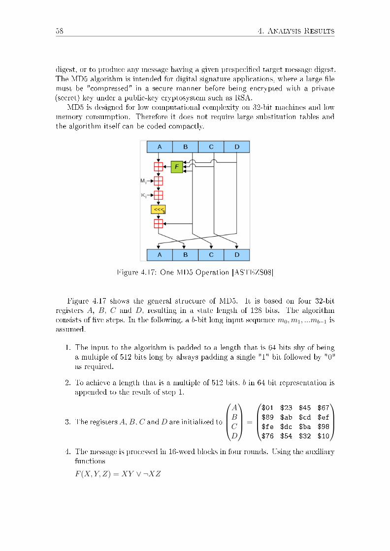
58 4. Analysis Results
digest, or to produce any message having a given prespeci�ed target message digest.The MD5 algorithm is intended for digital signature applications, where a large �lemust be "compressed" in a secure manner before being encrypted with a private(secret) key under a public-key cryptosystem such as RSA.
MD5 is designed for low computational complexity on 32-bit machines and lowmemory consumption. Therefore it does not require large substitution tables andthe algorithm itself can be coded compactly.
Figure 4.17: One MD5 Operation [ASTEZS08]
Figure 4.17 shows the general structure of MD5. It is based on four 32-bitregisters A, B, C and D, resulting in a state length of 128 bits. The algorithmconsists of �ve steps. In the following, a b-bit long input sequence m0,m1, ...mb−1 isassumed.
1. The input to the algorithm is padded to a length that is 64 bits shy of beinga multiple of 512 bits long by always padding a single "1" bit followed by "0"as required.
2. To achieve a length that is a multiple of 512 bits, b in 64 bit representation isappended to the result of step 1.
3. The registersA, B, C andD are initialized to
ABCD
=
$01 $23 $45 $67
$89 $ab $cd $ef
$fe $dc $ba $98
$76 $54 $32 $10
4. The message is processed in 16-word blocks in four rounds. Using the auxiliary
functions
F (X, Y, Z) = XY ∨ ¬XZ

4.7. MD5 59
G(X, Y, Z) = XZ ∨ Y ¬ZH(X, Y, Z) = X ⊕ Y ⊕ ZI(X, Y, Z) = Y ⊕ (X ∨ ¬Z),
the pseudo code as given below is executed.
5. A, B, C, D is provided as output of MD5, beginning with the low-order byteof A, and ending with the high-order byte of D.
The pseudo code that is executed in step 4 consists of the following:
/∗ Process each 16−word b l o c k . ∗/For i = 0 to N/16−1 do
/∗ Copy b l o c k i in to X. ∗/For j = 0 to 15 do
Set X[ j ] to M[ i ∗16+ j ] .end /∗ o f loop on j ∗/
/∗ Save A as AA, B as BB, C as CC, and D as DD. ∗/AA = ABB = BCC = CDD = D
/∗ Round 1. ∗//∗ Let [ abcd k s i ] denote the operat ion
a = b + (( a + F(b , c , d ) + X[ k ] + T[ i ] ) <<< s ) . ∗//∗ Do the f o l l ow i n g 16 opera t ions . ∗/[ABCD 0 7 1 ] [DABC 1 12 2 ] [CDAB 2 17 3 ] [BCDA 3 22 4 ][ABCD 4 7 5 ] [DABC 5 12 6 ] [CDAB 6 17 7 ] [BCDA 7 22 8 ][ABCD 8 7 9 ] [DABC 9 12 10 ] [CDAB 10 17 11 ] [BCDA 11 22 12 ][ABCD 12 7 13 ] [DABC 13 12 14 ] [CDAB 14 17 15 ] [BCDA 15 22 16 ]
/∗ Round 2. ∗//∗ Let [ abcd k s i ] denote the operat ion
a = b + (( a + G(b , c , d ) + X[ k ] + T[ i ] ) <<< s ) . ∗//∗ Do the f o l l ow i n g 16 opera t ions . ∗/[ABCD 1 5 17 ] [DABC 6 9 18 ] [CDAB 11 14 19 ] [BCDA 0 20 20 ][ABCD 5 5 21 ] [DABC 10 9 22 ] [CDAB 15 14 23 ] [BCDA 4 20 24 ][ABCD 9 5 25 ] [DABC 14 9 26 ] [CDAB 3 14 27 ] [BCDA 8 20 28 ][ABCD 13 5 29 ] [DABC 2 9 30 ] [CDAB 7 14 31 ] [BCDA 12 20 32 ]
/∗ Round 3. ∗//∗ Let [ abcd k s t ] denote the opera t ion
a = b + (( a + H(b , c , d ) + X[ k ] + T[ i ] ) <<< s ) . ∗//∗ Do the f o l l ow i n g 16 opera t ions . ∗/[ABCD 5 4 33 ] [DABC 8 11 34 ] [CDAB 11 16 35 ] [BCDA 14 23 36 ][ABCD 1 4 37 ] [DABC 4 11 38 ] [CDAB 7 16 39 ] [BCDA 10 23 40 ][ABCD 13 4 41 ] [DABC 0 11 42 ] [CDAB 3 16 43 ] [BCDA 6 23 44 ][ABCD 9 4 45 ] [DABC 12 11 46 ] [CDAB 15 16 47 ] [BCDA 2 23 48 ]
/∗ Round 4. ∗//∗ Let [ abcd k s t ] denote the opera t ion
a = b + (( a + I (b , c , d ) + X[ k ] + T[ i ] ) <<< s ) . ∗//∗ Do the f o l l ow i n g 16 opera t ions . ∗/[ABCD 0 6 49 ] [DABC 7 10 50 ] [CDAB 14 15 51 ] [BCDA 5 21 52 ][ABCD 12 6 53 ] [DABC 3 10 54 ] [CDAB 10 15 55 ] [BCDA 1 21 56 ][ABCD 8 6 57 ] [DABC 15 10 58 ] [CDAB 6 15 59 ] [BCDA 13 21 60 ]

60 4. Analysis Results
[ABCD 4 6 61 ] [DABC 11 10 62 ] [CDAB 2 15 63 ] [BCDA 9 21 64 ]
/∗ Then perform the f o l l ow i n g add i t i on s . (That i s increment eacho f the four r e g i s t e r s by the va lue i t had be fo r e t h i s b l o c kwas s t a r t e d . ) ∗/
A = A + AAB = B + BBC = C + CCD = D + DD
end /∗ o f loop on i ∗/
4.7.1 Sampled Analysis
A sampled analysis of MD5 using 1000 randomly chosen start values was performed.Table 4.12 shows the analysis results.
Table 4.12: Analysis Results of MD5 for 1000 Start Values
Component Cycle Maximum PercentLength Tree Height of Start Values
1 2029334271 4383236584 562 3385752161 4824490137 423 475894939 838987207 14 234279338 1352543 0.15 9767600 5755432 0.1
4.7.2 Interpretation of Test Results
One of the identi�ed components has a very short cycle length of about 107, whichsupports the common security concerns about MD5. According to Equation 2.13,the expected cycle length for a "good" PRNG or stream cipher with 128 bit state is14.4 · 1018, so also the other components have a cycle length that is far lower thanexpected.
4.8 Spritz
In 2014, Rivest and Schuldt published a successor for RC4, a proprietary streamcipher from 1987, that was reverse-engineered and published in 1994. Over time,several weaknesses of RC4 were identi�ed, which lead to an e�ort by Rivest tocreate an algorithm that serves as a drop-in replacement for RC4 and answers thequestion "What should the original RC4 have looked like?" [RS16]. It improvesseveral aspects of RC4, but keeps the desirable properties of its predecessor: a large
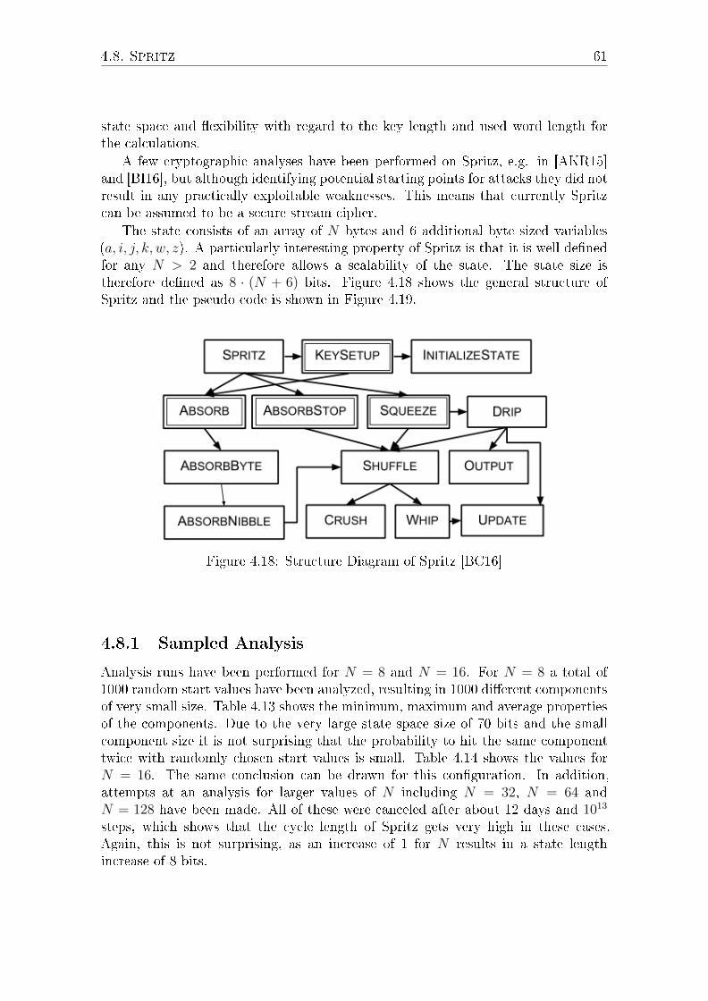
4.8. Spritz 61
state space and �exibility with regard to the key length and used word length forthe calculations.
A few cryptographic analyses have been performed on Spritz, e.g. in [AKR15]and [BI16], but although identifying potential starting points for attacks they did notresult in any practically exploitable weaknesses. This means that currently Spritzcan be assumed to be a secure stream cipher.
The state consists of an array of N bytes and 6 additional byte sized variables(a, i, j, k, w, z). A particularly interesting property of Spritz is that it is well de�nedfor any N > 2 and therefore allows a scalability of the state. The state size istherefore de�ned as 8 · (N + 6) bits. Figure 4.18 shows the general structure ofSpritz and the pseudo code is shown in Figure 4.19.
Figure 4.18: Structure Diagram of Spritz [BC16]
4.8.1 Sampled Analysis
Analysis runs have been performed for N = 8 and N = 16. For N = 8 a total of1000 random start values have been analyzed, resulting in 1000 di�erent componentsof very small size. Table 4.13 shows the minimum, maximum and average propertiesof the components. Due to the very large state space size of 70 bits and the smallcomponent size it is not surprising that the probability to hit the same componenttwice with randomly chosen start values is small. Table 4.14 shows the values forN = 16. The same conclusion can be drawn for this con�guration. In addition,attempts at an analysis for larger values of N including N = 32, N = 64 andN = 128 have been made. All of these were canceled after about 12 days and 1013
steps, which shows that the cycle length of Spritz gets very high in these cases.Again, this is not surprising, as an increase of 1 for N results in a state lengthincrease of 8 bits.

62 4. Analysis Results
InitializeState(N)i = j = k = z = a = 0w = 1for v = 0 to N − 1S[v] = v
Absorb(I)for v = 0 to I.length− 1AbsorbByte(I[v])
AbsorbByte(b)AbsorbNibble(low(b))AbsorbNibble(high(b))
AbsorbNibble(x)if a = bN/2cShuffle()
Swap(S[a], S[bN/2c+ x])a = a+ 1
AbsorbStop()if a = bN/2cShuffle()
a = a+ 1
Shuffle()Whip(2N)Crush()Whip(2N)Crush()Whip(2N)a = 0
Whip(r)for v = 0 to r − 1Update()
do w = w + 1until gcd(w,N) = 1
Crush()for v = 0 to bN/2c − 1if S[v] > S[N − 1− v]Swap(S[v], s[N − 1− v])
Squeeze(r)if a > 0Shuffle()
P = Array.New(r)for v = 0 to r − 1P [v] = Drip()
return P
Drip()if a > 0Shuffle()
Update()return Output()
Update()i = i+ wj = k + S[j + S[i]]k = i+ k + S[j]Swap(S[i], S[j])
Output()z = S[j + S[i+ S[z + k]]]return z
Figure 4.19: Spritz Algorithm in Pseudo Code [RS16]
4.8.2 Interpretation of Test Results
The state length of Spritz gets quickly very large with increasing N . Comparing theresults for N = 8 to the expected cycle length of a random mapping with the samestate size shows that the cycle lengths are much smaller: the expected cycle length
is 0.78248 ·√n = 0.78248 ·
√28(N+6) = 56 · 1015, while the results are less than order
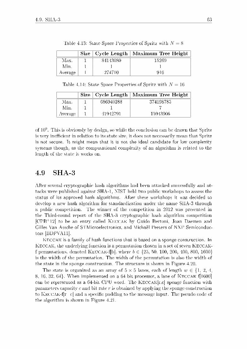
4.9. SHA-3 63
Table 4.13: State Space Properties of Spritz with N = 8
Size Cycle Length Maximum Tree Height
Max. 1 84143080 15269Min. 1 1 1
Average 1 274710 916
Table 4.14: State Space Properties of Spritz with N = 16
Size Cycle Length Maximum Tree Height
Max. 1 686940288 374198785Min. 1 1 7
Average 1 41942791 15943906
of 109. This is obviously by design, so while the conclusion can be drawn that Spritzis very ine�cient in relation to its state size, it does not necessarily mean that Spritzis not secure. It might mean that it is not the ideal candidate for low-complexitysystems though, as the computational complexity of an algorithm is related to thelength of the state it works on.
4.9 SHA-3
After several cryptographic hash algorithms had been attacked successfully and at-tacks were published against SHA-1, NIST held two public workshops to assess thestatus of its approved hash algorithms. After these workshops it was decided todevelop a new hash algorithm for standardization under the name SHA-3 througha public competition. The winner of the competition in 2012 was presented inthe Third-round report of the SHA-3 cryptographic hash algorithm competition[CPB+12] to be an entry called Keccak by Guido Bertoni, Joan Daemen andGilles Van Assche of STMicroelectronics, and Michaël Peeters of NXP Semiconduc-tors [BDPVA11].
Keccak is a family of hash functions that is based on a sponge construction. InKeccak, the underlying function is a permutation chosen in a set of seven Keccak-f permutations, denoted Keccak-f[b], where b ∈ {25, 50, 100, 200, 400, 800, 1600}is the width of the permutation. The width of the permutation is also the width ofthe state in the sponge construction. The structure is shown in Figure 4.20.
The state is organized as an array of 5 × 5 lanes, each of length w ∈ {1, 2, 4,8, 16, 32, 64}. When implemented on a 64-bit processor, a lane of Keccak-f[1600]can be represented as a 64-bit CPU word. The Keccak[r,c] sponge function withparameters capacity c and bit rate r is obtained by applying the sponge constructionto Keccak-f[r+c] and a speci�c padding to the message input. The pseudo code ofthe algorithm is shown in Figure 4.21.

64 4. Analysis Results
Figure 4.20: Structure of SHA-3 [Kel13]
4.9.1 Sampled Analysis
A sampled analysis based on 1000 start values was performed on SHA-3. Only thelower 64 bit of the SHA-3 state were taken into account to create the graph, so theresults are not representative of the original algorithm with its huge state. Table 4.15shows the results.
Table 4.15: Analysis Results of SHA-3 for 1000 Start Values
Component Cycle Maximum PercentLength Tree Height of Start Values
1 6787219743 5430785306 962 495476314 596842881 1.33 1171336976 550504209 24 48314220 858572136 0.5
4.9.2 Interpretation of Test Results
In relation to the expected cycle length of 0.78248 ·√n according to Equation 2.13,
which would in this case be around 3.36 · 109, the results look promising. Two of thefour identi�ed components are a factor of 2 away in either direction of this value.The other two components are further o� (in particular component 4), but as the sizeof these components is very small compared to the largest component, the impacton the result is comparably low. As the investigations are based on a state that wasshortened to 64 bit, these results are not necessarily representative for the originalSHA-3 algorithm.
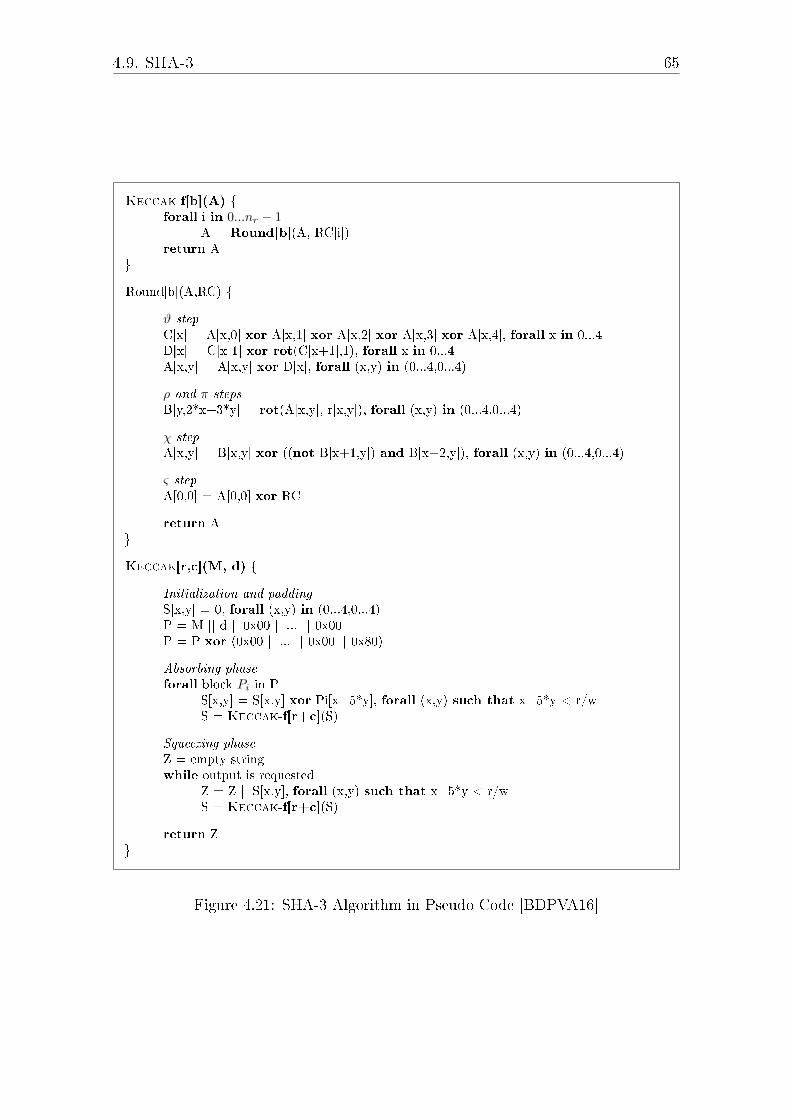
4.9. SHA-3 65
Keccak-f[b](A) {forall i in 0...nr − 1
A = Round[b](A, RC[i])return A
}
Round[b](A,RC) {
ϑ step
C[x] = A[x,0] xor A[x,1] xor A[x,2] xor A[x,3] xor A[x,4], forall x in 0...4D[x] = C[x-1] xor rot(C[x+1],1), forall x in 0...4A[x,y] = A[x,y] xor D[x], forall (x,y) in (0...4,0...4)
ρ and π steps
B[y,2*x+3*y] = rot(A[x,y], r[x,y]), forall (x,y) in (0...4,0...4)
χ step
A[x,y] = B[x,y] xor ((not B[x+1,y]) and B[x+2,y]), forall (x,y) in (0...4,0...4)
ς step
A[0,0] = A[0,0] xor RC
return A}
Keccak[r,c](M, d) {
Initialization and padding
S[x,y] = 0, forall (x,y) in (0...4,0...4)P = M || d || 0x00 || ... || 0x00P = P xor (0x00 || ... || 0x00 || 0x80)
Absorbing phase
forall block Pi in PS[x,y] = S[x,y] xor Pi[x+5*y], forall (x,y) such that x+5*y < r/wS = Keccak-f[r+c](S)
Squeezing phase
Z = empty stringwhile output is requested
Z = Z || S[x,y], forall (x,y) such that x+5*y < r/wS = Keccak-f[r+c](S)
return Z}
Figure 4.21: SHA-3 Algorithm in Pseudo Code [BDPVA16]

66 4. Analysis Results
67
Chapter 5
Improvements
The results for the di�erent low-complexity cryptographic primitives given in Sec-tion 4 show that a majority of them are of limited usability for security applications.The state space structure analysis shows e.g. comparably short cycles and smallcomponents. Cryptographic functions with known good properties on the otherhand typically have a much higher computational complexity, rendering them inap-propriate for low-cost RFID applications. This section presents a novel approachto improve the state space properties of practically arbitrary transition functions.After approaching the concept systematically, di�erent re�nements are investigatedthat reduce the required complexity for real-world implementations or improve theresult step by step.
5.1 Breaking out of the Cycle
One of the main issues of the analyzed cryptographic primitives is the comparablyshort cycle length. A simple way to avoid short cycles is to modify the cryptographicprimitive transition function for certain iterations, so that the follow up state isaltered compared to the original function. If this happens when a short cycle hasalready been entered, and if the follow-up state is not part of a similarly sized cycle,the cycle length of this modi�ed transition function is larger than the cycle length ofthe original function. This mechanism can be seen as a "break-out" from the cycle.Figure 5.1 illustrates what is happening in the break-out case.
In Subsection 2.3.2, the properties of a random mapping have been presentedas benchmark for a good transition state space structure. For this reason, it seemsworthwhile to try to make use of these properties for the break-out mechanism. Ifthe target node for the break-out is chosen randomly, there is a high probabilitythat the new state is located in a tree and not a cycle. The cycle has successfullybeen broken out of in this case. The high probability of a successful break-out comesfrom the fact, that for a non-bijective transition function the number of cycle nodesis typically small compared to the overall number of nodes. As shown before, for arandom mapping the number if cyclic nodes is
√πn/2.

68 5. Improvements
Figure 5.1: Breaking Out of the Cycle
5.2 Counter-Based Random Break-out
A single break-out would only improve the cycle length of a single component, so inorder to improve the overall state space structure, the break-out can be performedrepeatedly, e.g. in average for every kth transition. As a special case of breakingout every k steps on average, the following analysis results are based on a counterto select the random transition points and therefore break-out exactly after every ksteps. Di�erent values of k have been investigated to evaluate the in�uence of thebreak-out frequency. Experiments have been performed with values of k rangingfrom 2 to 1024. In Table 5.1 the results of the analysis are shown.
Figure 5.2 shows the analysis results for a break-out to a random node in thestate graph for the Logistic Map transition function. The x-axis shows the values ofk, while on the y-axis the maximum cycle length that was found for a run with 100di�erent start values is displayed. Unfortunately, using a real random transition forthe break-out is not very practical. For this reason, AES as a stream cipher withknown very good statistical and cryptographic properties was chosen as a pseudo-random function. In order to use the stream cipher as pseudo-random generator,the algorithm was used in Cipher Feedback (CFB) mode, meaning that the outputof the encryption algorithm was used as input for the next iteration. With AESbeing such a highly regarded cryptographic algorithm, this creates a pseudo-randomgenerator of exceptional quality, but even more importantly without any expectedstatistical dependency on the Logistic Map function.
The result given in Figure 5.2 shows a very mixed behavior: for some values ofk, the maximum cycle length is increased compared to the values in Table 4.5. Bute.g. for k = 64, the maximum cycle length is even lower than without the break-out mechanism. The conclusion that can be drawn is, that a blind break-out to arandom target node will not generally improve the state space structure, but might
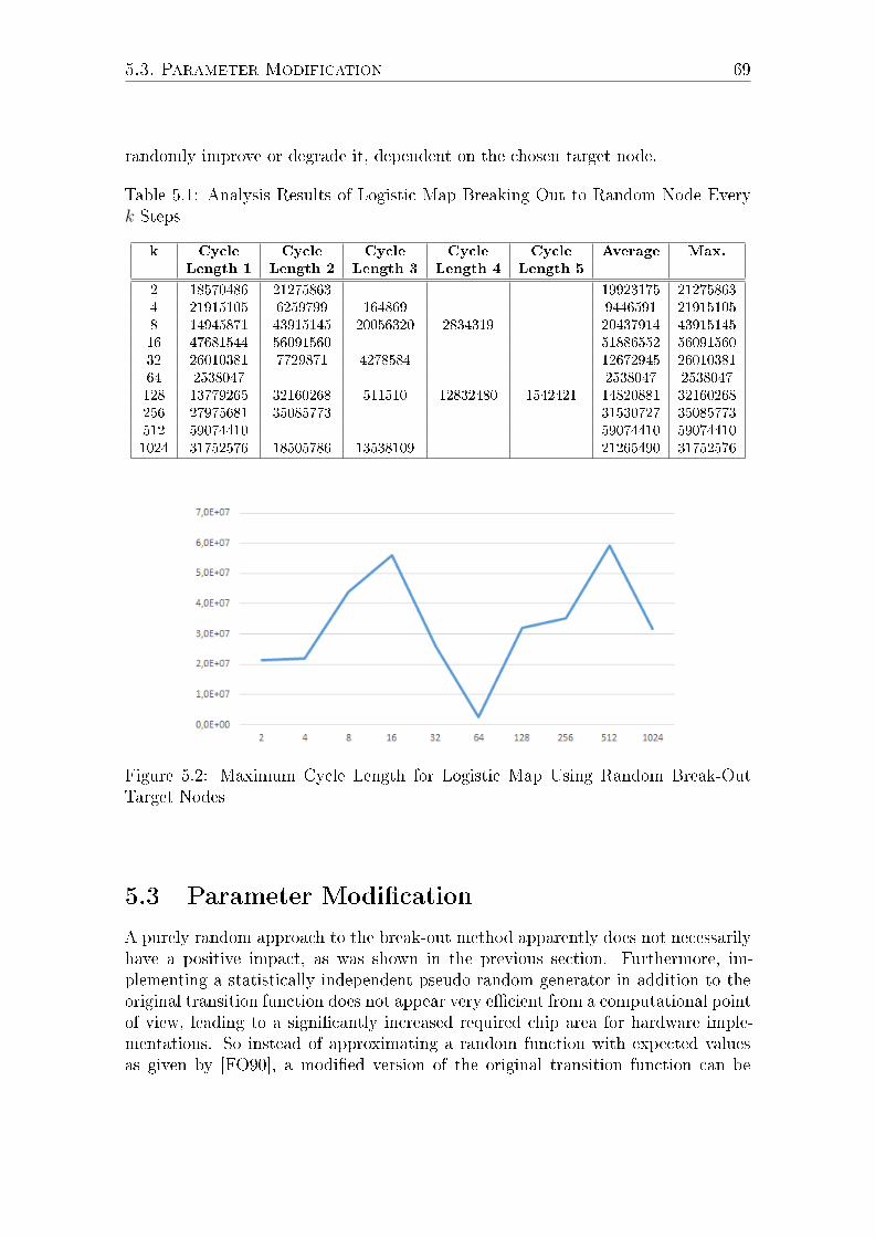
5.3. Parameter Modification 69
randomly improve or degrade it, dependent on the chosen target node.
Table 5.1: Analysis Results of Logistic Map Breaking Out to Random Node Everyk Steps
k Cycle Cycle Cycle Cycle Cycle Average Max.Length 1 Length 2 Length 3 Length 4 Length 5
2 18570486 21275863 19923175 212758634 21915105 6259799 164869 9446591 219151058 14945871 43915145 20056320 2834319 20437914 4391514516 47681544 56091560 51886552 5609156032 26010381 7729871 4278584 12672945 2601038164 2538047 2538047 2538047128 13779265 32160268 511510 12832480 1542421 14820881 32160268256 27975681 35085773 31530727 35085773512 59074410 59074410 590744101024 31752576 18505786 13538109 21265490 31752576
Figure 5.2: Maximum Cycle Length for Logistic Map Using Random Break-OutTarget Nodes
5.3 Parameter Modi�cation
A purely random approach to the break-out method apparently does not necessarilyhave a positive impact, as was shown in the previous section. Furthermore, im-plementing a statistically independent pseudo-random generator in addition to theoriginal transition function does not appear very e�cient from a computational pointof view, leading to a signi�cantly increased required chip area for hardware imple-mentations. So instead of approximating a random function with expected valuesas given by [FO90], a modi�ed version of the original transition function can be

70 5. Improvements
used. This allows to share the same implementation, saving chip area for hardwareimplementations or program memory for software implementations. The modi�ca-tion of the algorithm needs to result in a behavior that is su�ciently statisticallyindependent from the original function to be treated similarly to the random targetfrom Section 5.2.
Investigations have been performed for chaotic functions, as these react per de�-nition sensitively to a changed parametrization. Even a small change to the functionparameters leads to strongly di�erent output.
5.3.1 Analysis for Logistic Map
Looking at the Logistic Map function f1(x) = a · x · (1 − x), there are not manypossibilities for parametrization: the only candidate to modify is parameter a. Theanalyzed approach was to insert after k − 1 steps with an a-value of 3.99 a singletransition with an a value of 3.98. The value k was chosen out of a range from2 to 1024. Table 5.2 shows the result of the state space analysis. It can be seenthat breaking out of the cycles increases the maximum cycle length signi�cantly bya minimum factor of 2 for k = 2 up to a factor of 227 for k = 1024. It can alsoclearly be seen that the maximum cycle length increases with k. Figure 5.3 showsthis relationship. The graph is not completely consistent with k-values of 32 and256 showing a decline compared to the previous values. This can most probably beexplained by the very low number of 10 start values for measuring the cycle lengths.
Figure 5.3: Maximum Cycle Length Over k for Logistic Map
As a special variant, a strategy was chosen to switch between 32 di�erent a-valuesin each iteration. The overhead for this strategy is comparably low, as the countercan be used as index into an a-value table. Still, the overhead is larger than for theprevious strategies, because the 32 a-values would need to be stored in a table. Theresults are displayed in Table 5.3.

5.3. Parameter Modification 71
Table 5.2: Analysis Results of Logistic Map Switching to Alternative a-ParameterEvery k Steps
k Cycle Length Maximum Tree Height Percent of Start Values
2 14258373 169347594 1004 81839355 219447222 1008 92330073 116649348 508 158592654 153814118 208 23977917 39516082 208 5583933 29542408 1016 166687958 347193629 9016 18456033 66490210 1032 16463304 509498228 5032 106561026 184708805 5064 285351755 247720291 7064 27448135 163920805 2064 186333745 138538519 10128 365089092 459489459 90128 490073193 568127512 10256 122507017 1011052679 50256 61896137 766210246 50512 918541890 913649910 70512 505315773 506390293 301024 1517222425 2056217674 601024 997359850 1168909136 40
Table 5.3: Analysis Results of Logistic Map Switched Between 32 Alternative a-Values (3.98...3.99) Every Step
Component Cycle Maximum PercentLength Tree Height of Start Values
1 78866912 211723507 942 9936544 11642151 23 18963552 37204563 4
The results show, that the additional variations in a-values do not improve thecycle length of the identi�ed components. Compared to the previous switchingstrategies, cycle lengths of 78.9 · 106 are still an improvement to the unmodi�edalgorithm, but not to the other switched algorithms. The average tree height of17.7 · 106 is by a factor of 2 worse than the original value.
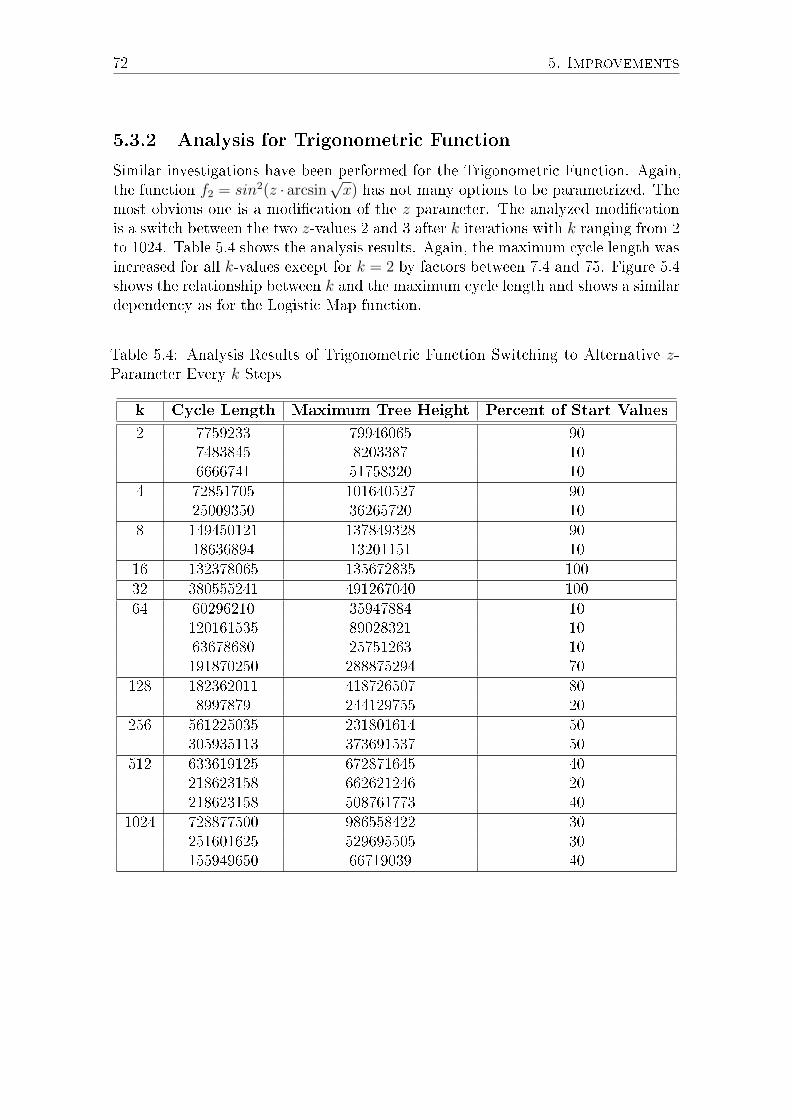
72 5. Improvements
5.3.2 Analysis for Trigonometric Function
Similar investigations have been performed for the Trigonometric Function. Again,the function f2 = sin2(z · arcsin
√x) has not many options to be parametrized. The
most obvious one is a modi�cation of the z parameter. The analyzed modi�cationis a switch between the two z-values 2 and 3 after k iterations with k ranging from 2to 1024. Table 5.4 shows the analysis results. Again, the maximum cycle length wasincreased for all k-values except for k = 2 by factors between 7.4 and 75. Figure 5.4shows the relationship between k and the maximum cycle length and shows a similardependency as for the Logistic Map function.
Table 5.4: Analysis Results of Trigonometric Function Switching to Alternative z-Parameter Every k Steps
k Cycle Length Maximum Tree Height Percent of Start Values
2 7759233 79946065 907483845 8203387 106666741 51758320 10
4 72851705 101640527 9025009350 36265720 10
8 149450121 137849328 9018636894 13201151 10
16 132378065 135672835 10032 380555241 491267040 10064 60296210 35947884 10
120161535 89028321 1063678680 25751263 10191870250 288875294 70
128 182362011 418726507 808997879 244129755 20
256 561225035 231801614 50305935113 373691537 50
512 633619125 672871645 40218623158 662621246 20218623158 508761773 40
1024 728877500 986558422 30251601625 529695505 30155949650 66719039 40

5.4. Hash Based Parameter Modification 73
Figure 5.4: Maximum Cycle Length Over k for Trigonometric Function
5.4 Hash Based Parameter Modi�cation
Instead of using a counter to select the nodes for a modi�ed transition function, thenodes can also be selected solely based on the state vector of the node itself. As thestate vector is typically much larger than log2(k) bits, which is required to result ina certain value to compare to after k steps, a hash function is needed that calculatesa log2(k)-bit value from the state vector. For a transition function that exhibitsa reasonable amount of di�usion (meaning that each state is signi�cantly di�erentfrom the predecessor state), this hash function can be very simple. In the following,a simple bit mask that extracts a number of bits from the state is chosen as hashfunction, which should be su�cient for the analyzed algorithms.
There are two advantages of this approach compared to the counter-based method.First of all, the complexity of the additional counter is not needed. This might savesome chip area, although the impact compared to an implementation of a PRNG ora stream cipher is probably negligible. Much more interesting in the scope of thiswork is that it allows to perform a parallel analysis on the state space. The counterneeds to be included in the state vector, because the selection of the transition func-tion modi�cation is based on the counter value. For the counter-based approach itcannot be ensured that the behavior of the algorithm is identical for di�erent startvalues, as if two analysis runs reach the same node, one of them might choose thenormal transition function, while the other one chooses the modi�ed parametriza-tion. If this decision is based only on the state, the algorithm will behave the sameindependently of the start value. If an analysis run reaches a node that was part of aformer analysis run, the analysis run can be stopped immediately as the propertiesof the remaining path are already known. For su�ciently random changes to thestate for each transition, it is not expected that the behavior is di�erent from thecounter-based method, which is why no dedicated experiments have been performed.

74 5. Improvements
5.5 Combining Multiple Algorithms
A di�erent approach to avoid the overhead of running a high quality PRNG forthe break-out mechanism is to use very simple algorithms for breaking out. Thisraises the general question, if the break-out mechanism can improve the propertiesof simple algorithms by combining them with other comparably simple algorithms.Such an approach has been analyzed e.g. in [Bre06], e.g. by XOR-ing or mixing theoutput of several independently running PRNGs.
In [Rei16], investigations on the combination of simple PRNGs have been pre-sented, under the condition that the state space size stays the same as for thenon-combined PRNG (32 bits). In particular, the state space properties of di�erentcombinations of bijective and non-bijective algorithms were in the focus of the work.Similar to the results presented in Section 5.2 and 5.4, the switch between the twoPRNGs was done dependent on certain properties of the state vector to avoid theincrease of the state length by adding a counter. For some PRNGs, this propertycould be chosen such, that a dedicated improvement of the state space structurecould be expected due to known weaknesses of the PRNG. For "better" PRNGsthat do not exhibit a recognizable pattern for their state this was not easily possibleand the state property for the switch was chosen arbitrarily.
Overall, Reich could show that combining di�erent PRNGs typically resultedin state space properties that are better than the properties of the worse of thecombined algorithms. In some cases, the properties could be improved signi�cantlyover the original PRNGs. For the combination of the PRNGs given as:
xn+1 = (69069 · xn) mod 232 (5.1)
xn+1 = xn⊕ (xn << 5)⊕ (xn >> 4)⊕ (xn << 10)⊕ (xn >> 16)+1090584833 (5.2)
a pattern could be identi�ed that applies to all state vectors on the cycles of the �rstPRNG. All of these states have the common property that only a maximum numberof bits is set. This allows a dedicated break-out from these cycles by counting thenumber of set bits in the state to this maximum and using the second algorithm.The state space analysis of the single algorithms is shown in Table 5.5 and 5.6. Theresult of the combined PRNGs is shown in Table 5.7: only a single component existswith a cycle length that is with 0x081ea19e = 136225182 signi�cantly higher thanthe expected cycle length for non-bijective transition functions of 0.78248 ·
√232 =
51281.
5.6 Direct State Graph Manipulation
The previous approaches for a break-out from a cycle in the state transition graphhave been purely statistical. The actual state transition graph was assumed to beunknown, and a general rule was applied to decide in which nodes the alternativetransition function is used. This black box approach did lead to signi�cant improve-ments to the state graph properties in some cases, but such an improvement cannot
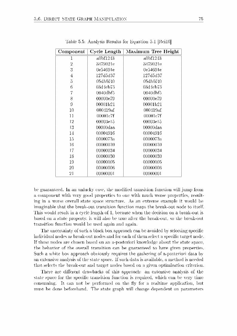
5.6. Direct State Graph Manipulation 75
Table 5.5: Analysis Results for Equation 5.1 [Rei16]
Component Cycle Length Maximum Tree Height
1 a0bf1243 a0bf12432 3479021e 3479021e3 0e54691e 0e54691e4 127d5d37 127d5d375 05db5f40 05db5f406 03d4eb75 03d4eb757 0040dbf5 0040dbf58 00000e79 00000e799 00001b21 00001b2110 000419af 000419af11 00001e7f 00001e7f12 00003e15 00003e1513 00000daa 00000daa14 00004916 0000491615 0000073a 0000073a16 00000059 0000005917 00000034 0000003418 00000030 0000003019 00000005 0000000520 00000006 0000000621 00000001 00000001
be guaranteed. In an unlucky case, the modi�ed transition function will jump froma component with very good properties to one with much worse properties, result-ing in a worse overall state space structure. As an extreme example it would beimaginable that the break-out transition function maps the break-out node to itself.This would result in a cycle length of 1, because when the decision on a break-out isbased on a state property, it will also be true after the break-out, so the break-outtransition function would be used again and again.
The uncertainty of such a black box approach can be avoided by selecting speci�cindividual nodes as break-out nodes and for each of them select a speci�c target node.If these nodes are chosen based on an a-posteriori knowledge about the state space,the behavior of the overall transition can be guaranteed to have given properties.Such a white box approach obviously requires the gathering of a-posteriori data byan extensive analysis of the state space. If such data is available, a method is neededthat selects the break-out and target nodes based on a given optimization criterion.
There are di�erent drawbacks of this approach: an extensive analysis of thestate space for the speci�c transition function is required, which can be very timeconsuming. It can not be performed on the �y for a realtime application, butmust be done beforehand. The state graph will change dependent on parameters
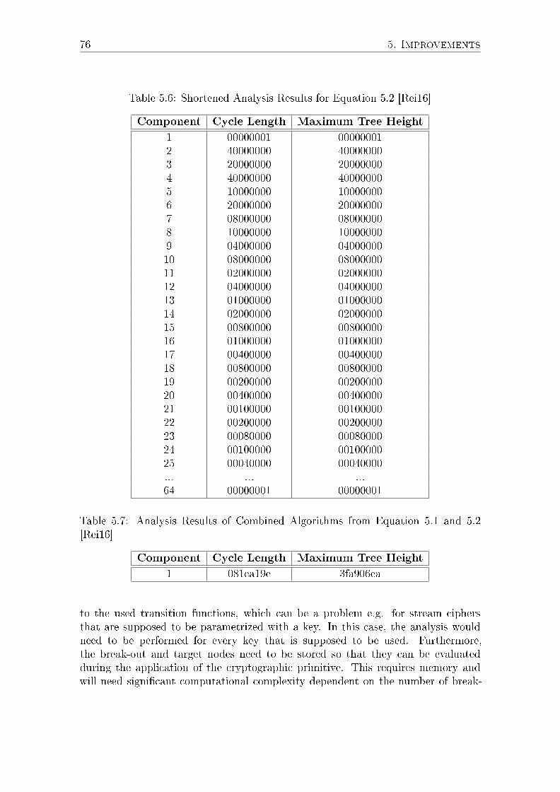
76 5. Improvements
Table 5.6: Shortened Analysis Results for Equation 5.2 [Rei16]
Component Cycle Length Maximum Tree Height
1 00000001 000000012 40000000 400000003 20000000 200000004 40000000 400000005 10000000 100000006 20000000 200000007 08000000 080000008 10000000 100000009 04000000 0400000010 08000000 0800000011 02000000 0200000012 04000000 0400000013 01000000 0100000014 02000000 0200000015 00800000 0080000016 01000000 0100000017 00400000 0040000018 00800000 0080000019 00200000 0020000020 00400000 0040000021 00100000 0010000022 00200000 0020000023 00080000 0008000024 00100000 0010000025 00040000 00040000... ... ...64 00000001 00000001
Table 5.7: Analysis Results of Combined Algorithms from Equation 5.1 and 5.2[Rei16]
Component Cycle Length Maximum Tree Height
1 081ea19e 3fa906ea
to the used transition functions, which can be a problem e.g. for stream ciphersthat are supposed to be parametrized with a key. In this case, the analysis wouldneed to be performed for every key that is supposed to be used. Furthermore,the break-out and target nodes need to be stored so that they can be evaluatedduring the application of the cryptographic primitive. This requires memory andwill need signi�cant computational complexity dependent on the number of break-

5.6. Direct State Graph Manipulation 77
out nodes. But if the system allows for the additional complexity, the improvementsmight outweigh this. The following sections present an approach for an optimizationmethod that is a good compromise between e�ciency and computational complexity.
5.6.1 Greedy Algorithm
Finding an optimum in a complex system can be a di�cult task. An importantclass of algorithms to solve such optimization problems are the so-called "greedy"algorithms (described e.g. in [Tur09]). Instead of trying to �nd the global optimum,they iteratively optimize towards local optima in several steps. After a decision hasbeen made for an iteration, it will not be revisited at a later stage. The fact thatthese algorithms only care for the maximum gain in the current iteration and do notlook further into the future is �guratively re�ected by the term "greedy".
The advantage of greedy algorithms is that they are easy to design and e�cientto implement. In particular for very complex problems like the optimization of ahuge state space, greedy algorithms can sometimes be the only approach to performthe optimization in a reasonable amount of time. The disadvantage is that greedyalgorithms might not �nd the global optimum, although there are problems for whichthis is the case. In the following, a greedy algorithm to improve the average cyclelength of a state graph is developed.
An important decision for any optimization is the criterion which shall be opti-mized. In the following, the average cycle length of the known components is chosenas optimization criterion. The majority of the algorithms that have been analyzedin Chapter 4 have su�ered from a less than optimal cycle length and the cycle lengthcan be comparably easily determined, so it seems a reasonable goal to try to improvethis state space property.
5.6.2 Action A
Suppose that a small number of special �states� si can be identi�ed where the succes-sor state f(si) determined by the original transition function is changed to a �xedvalue s′i, such that the average cycle length is increased. Then the implementationof the transition function could be modi�ed as follows:
state_t newt ran s i t i on func t i on ( state_t s) {i f (s=si for some i=1 . . .k ) {
return s′i ;} else {
return t r a n s i t i o n f u n c t i o n (s ) ;}
}
The check if s is a special state can be realized as a map implementation. Forexample, the special states could be stored together with their successor states inan array in sorted order, and the check implemented as a binary search.
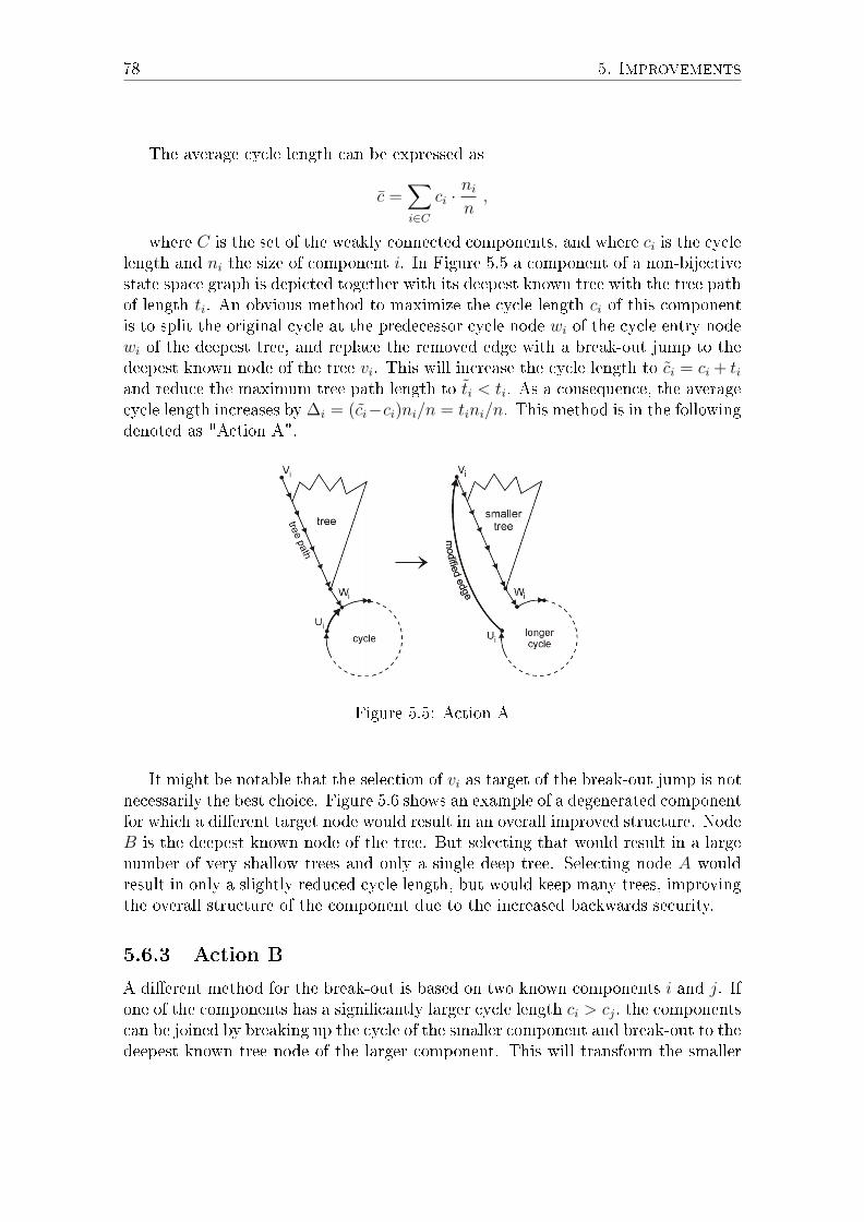
78 5. Improvements
The average cycle length can be expressed as
c =∑i∈C
ci ·nin,
where C is the set of the weakly connected components, and where ci is the cyclelength and ni the size of component i. In Figure 5.5 a component of a non-bijectivestate space graph is depicted together with its deepest known tree with the tree pathof length ti. An obvious method to maximize the cycle length ci of this componentis to split the original cycle at the predecessor cycle node wi of the cycle entry nodewi of the deepest tree, and replace the removed edge with a break-out jump to thedeepest known node of the tree vi. This will increase the cycle length to ci = ci + tiand reduce the maximum tree path length to ti < ti. As a consequence, the averagecycle length increases by ∆i = (ci−ci)ni/n = tini/n. This method is in the followingdenoted as "Action A".
Figure 5.5: Action A
It might be notable that the selection of vi as target of the break-out jump is notnecessarily the best choice. Figure 5.6 shows an example of a degenerated componentfor which a di�erent target node would result in an overall improved structure. NodeB is the deepest known node of the tree. But selecting that would result in a largenumber of very shallow trees and only a single deep tree. Selecting node A wouldresult in only a slightly reduced cycle length, but would keep many trees, improvingthe overall structure of the component due to the increased backwards security.
5.6.3 Action B
A di�erent method for the break-out is based on two known components i and j. Ifone of the components has a signi�cantly larger cycle length ci > cj, the componentscan be joined by breaking up the cycle of the smaller component and break-out to thedeepest known tree node of the larger component. This will transform the smaller
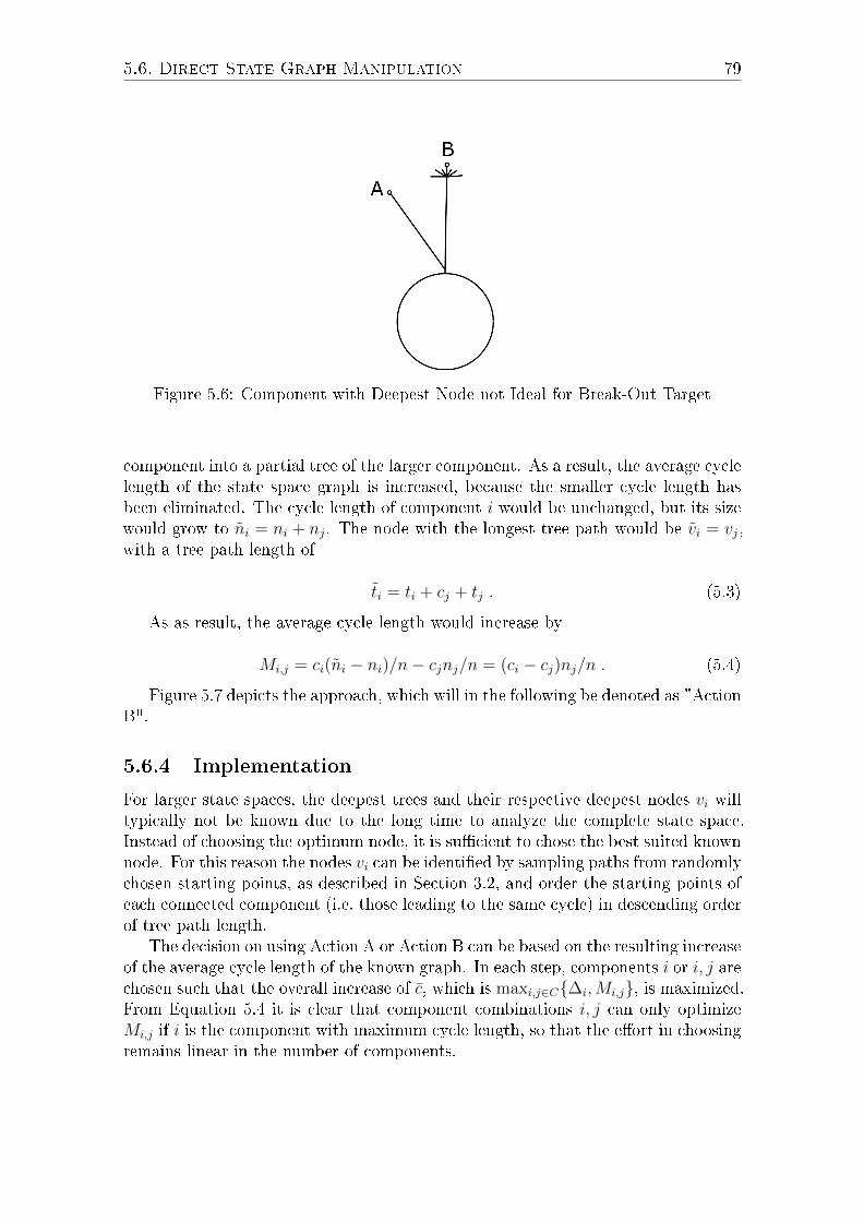
5.6. Direct State Graph Manipulation 79
Figure 5.6: Component with Deepest Node not Ideal for Break-Out Target
component into a partial tree of the larger component. As a result, the average cyclelength of the state space graph is increased, because the smaller cycle length hasbeen eliminated. The cycle length of component i would be unchanged, but its sizewould grow to ni = ni + nj. The node with the longest tree path would be vi = vj,with a tree path length of
ti = ti + cj + tj . (5.3)
As as result, the average cycle length would increase by
Mi,j = ci(ni − ni)/n− cjnj/n = (ci − cj)nj/n . (5.4)
Figure 5.7 depicts the approach, which will in the following be denoted as "ActionB".
5.6.4 Implementation
For larger state spaces, the deepest trees and their respective deepest nodes vi willtypically not be known due to the long time to analyze the complete state space.Instead of choosing the optimum node, it is su�cient to chose the best suited knownnode. For this reason the nodes vi can be identi�ed by sampling paths from randomlychosen starting points, as described in Section 3.2, and order the starting points ofeach connected component (i.e. those leading to the same cycle) in descending orderof tree path length.
The decision on using Action A or Action B can be based on the resulting increaseof the average cycle length of the known graph. In each step, components i or i, j arechosen such that the overall increase of c, which is maxi,j∈C{∆i,Mi,j}, is maximized.From Equation 5.4 it is clear that component combinations i, j can only optimizeMi,j if i is the component with maximum cycle length, so that the e�ort in choosingremains linear in the number of components.

80 5. Improvements
Figure 5.7: Action B
It is important to note that after Action A, the node vi with the new maximumtree path length ti has to be identi�ed, because the formerly deepest node is nowpart of the component cycle. The node ti is not necessarily the node with the secondlongest tree path prior to Action A, but the node with the longest disjunct tree path,as the point where its tree path merges with the tree path from vi is the new entrypoint wi into the new cycle. Therefore, ti might be notably smaller than ti.
The modi�ed transition function for the white box approach has the disadvantageof slowing down execution of the transition function by adding O(log k) work to everytransition because of the check for a special state, as both binary search and otherimplementations like B-tree require a logarithmic number of steps. Even though kis small, this slows down execution of the transition function, which is not desiredin an implementation. To reduce the complexity, the candidate approach presentedin Section 3.4 was chosen, described by the pseudo code as listed in the following.
state_t newt ran s i t i on func t i on ( state_t s) {i f (s i s candidate ) {
i f (s=si for some i=1 . . .k ) {return s′i ;
} else {return t r a n s i t i o n f u n c t i o n (s ) ;
}}
}
The computational complexity is reduced signi�cantly due to the fact that the�rst if-statement, that is executed with every step, is a very simple operation, while
5.6. Direct State Graph Manipulation 81
the second if-statement that contains the search through the set of break-out nodesis executed only infrequently. If the candidate criterion is chosen to be having c �xedbits of the binary state representation at value 1, only every 2cth node on averagealong a path in the graph is a candidate.
When sampling paths, only candidates are chosen as start nodes. When followinga path, every candidate that is reached is stored, together with the distance to andthe index of the previous candidate. Thus, by checking if a candidate is reached asecond time, a cycle can be detected, and all candidates reached in-between can bemarked as candidates on a cycle.
There is no guarantee that every cycle contains a candidate. Thus, the methodof storing an anchor node after 2i steps, where i = 0, 1, 2, . . ., and comparing if thelast anchor has been reached again (cf. Section 3.2), can be used in addition to avoidin�nite loops around a cycle in the state graph. It might be worth mentioning thatfor some state transitions it is possible to de�ne a candidate criterion such, that it isguaranteed that there is at least one candidate on every cycle, e.g. for A5/1 [BK07].
The fact that the candidate method allows to identify candidate nodes based on aglobal criterion independently of the start node of the analysis runs leads to anotheradvantage: if, while sampling a path, a candidate is reached that was already visitedand stored while sampling an earlier path, the analysis run can stop following thepath immediately, and set the tree path length of all candidates in the path, given thetree path length of the candidate that is already stored. Without candidates, eachpath would need to be followed to the cycle, to see to which connected componentthe path and thus the starting point belongs.
Let c be the number of state bits that are taken into account for the candidatecriterion. If the candidates are stored in a map structure like a B-tree or skiplist,then inserting a candidate or checking if a candidate is already present can be donein time O(log(n/2c)) = O(log n − c), as there are n/2c candidates. Thus, if c ischosen as c ≥ log log n, then on average, at most once every log n steps a candidateis reached and thus the amortized e�ort per step is O(1). In practice, one wouldchoose c as large as possible, so that following chains of candidates (see below) canbe performed quickly, and that on the other hand at least the larger cycles of lengthabout
√n contain at minimum one candidate. Choosing 2c ≤ 0.5
√n results in
c ≤ 0.5 log n − 1 as an upper bound for c, which would result in only a very smallnumber of candidates on a tree path (see below). A good choice for c depends on theexact structure on the graph and will be somewhere in-between the above bounds.
If Action A is performed, then starting node vi, which is a candidate, becomesa cycle node, and thus all candidates on its tree path become cycle candidates aswell and will be marked. Thus, updating the tree path length for any other startingnode zi in this component can be done by following the list of candidates reachedfrom zi and adding up the distances until a cycle candidate is reached. Note thatthis computation is not exact, as the path from zi may merge with the path fromvi at any node between the last tree candidate and the �rst cycle candidate. Forsimplicity, half of their distance is counted. If the number of candidates on the path
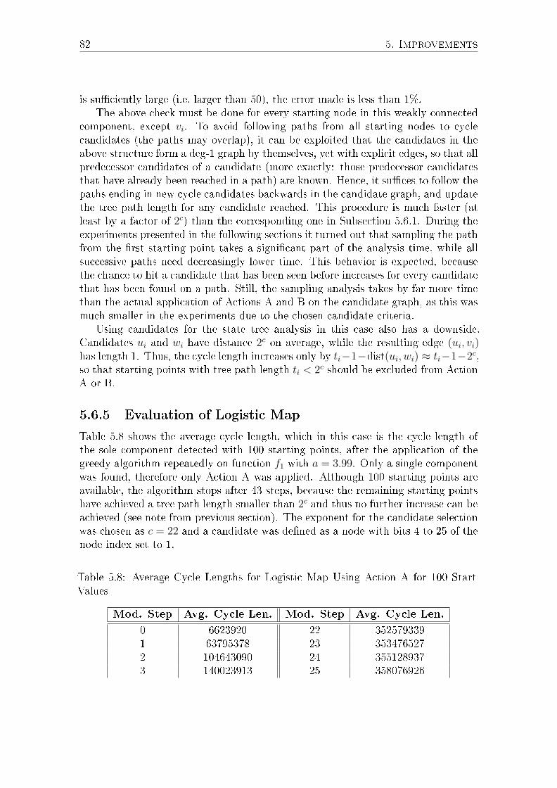
82 5. Improvements
is su�ciently large (i.e. larger than 50), the error made is less than 1%.The above check must be done for every starting node in this weakly connected
component, except vi. To avoid following paths from all starting nodes to cyclecandidates (the paths may overlap), it can be exploited that the candidates in theabove structure form a deg-1 graph by themselves, yet with explicit edges, so that allpredecessor candidates of a candidate (more exactly: those predecessor candidatesthat have already been reached in a path) are known. Hence, it su�ces to follow thepaths ending in new cycle candidates backwards in the candidate graph, and updatethe tree path length for any candidate reached. This procedure is much faster (atleast by a factor of 2c) than the corresponding one in Subsection 5.6.1. During theexperiments presented in the following sections it turned out that sampling the pathfrom the �rst starting point takes a signi�cant part of the analysis time, while allsuccessive paths need decreasingly lower time. This behavior is expected, becausethe chance to hit a candidate that has been seen before increases for every candidatethat has been found on a path. Still, the sampling analysis takes by far more timethan the actual application of Actions A and B on the candidate graph, as this wasmuch smaller in the experiments due to the chosen candidate criteria.
Using candidates for the state tree analysis in this case also has a downside.Candidates ui and wi have distance 2c on average, while the resulting edge (ui, vi)has length 1. Thus, the cycle length increases only by ti−1−dist(ui, wi) ≈ ti−1−2c,so that starting points with tree path length ti < 2c should be excluded from ActionA or B.
5.6.5 Evaluation of Logistic Map
Table 5.8 shows the average cycle length, which in this case is the cycle length ofthe sole component detected with 100 starting points, after the application of thegreedy algorithm repeatedly on function f1 with a = 3.99. Only a single componentwas found, therefore only Action A was applied. Although 100 starting points areavailable, the algorithm stops after 43 steps, because the remaining starting pointshave achieved a tree path length smaller than 2c and thus no further increase can beachieved (see note from previous section). The exponent for the candidate selectionwas chosen as c = 22 and a candidate was de�ned as a node with bits 4 to 25 of thenode index set to 1.
Table 5.8: Average Cycle Lengths for Logistic Map Using Action A for 100 StartValues
Mod. Step Avg. Cycle Len. Mod. Step Avg. Cycle Len.
0 6623920 22 3525793391 63795378 23 3534765272 104643090 24 3551289373 140023913 25 358076926
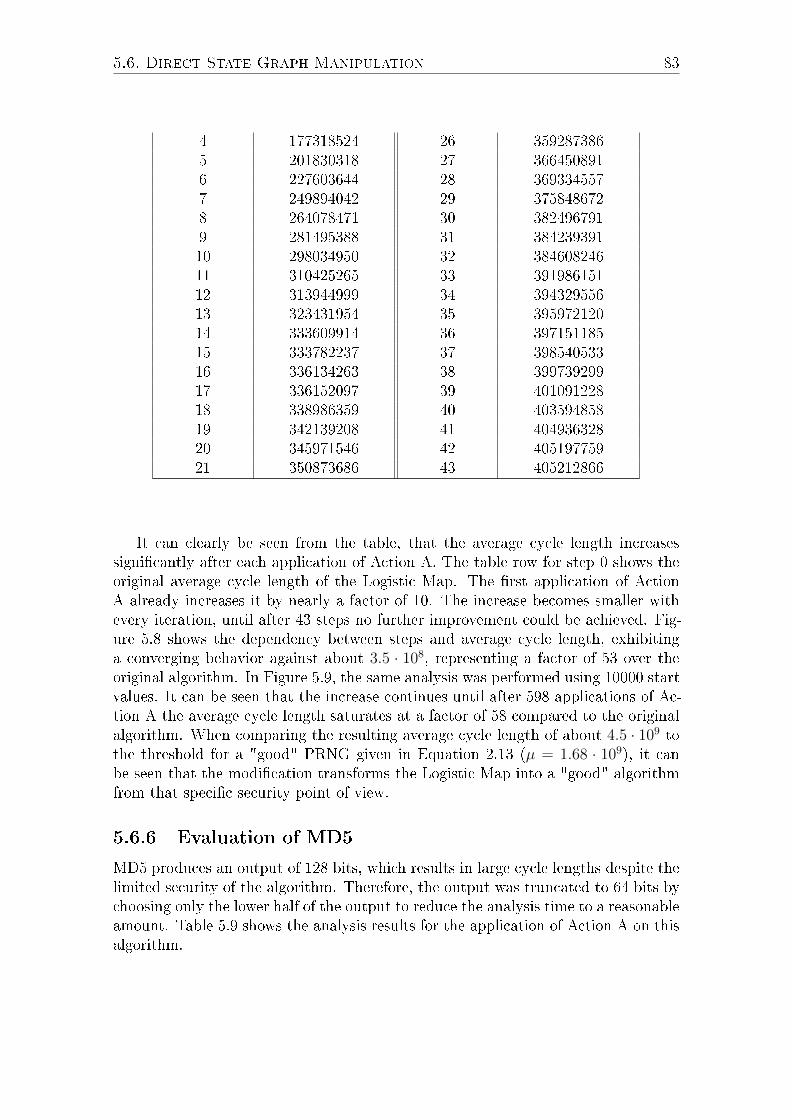
5.6. Direct State Graph Manipulation 83
4 177318524 26 3592873865 201830318 27 3664508916 227603644 28 3693345577 249894042 29 3758486728 264078471 30 3824967919 281495388 31 38423939110 298034950 32 38460824611 310425265 33 39198615112 313944999 34 39432955613 323431954 35 39597212014 333609914 36 39715118515 333782237 37 39854053316 336134263 38 39973929917 336152097 39 40109122818 338986359 40 40359485819 342139208 41 40493632820 345971546 42 40519775921 350873686 43 405212866
It can clearly be seen from the table, that the average cycle length increasessigni�cantly after each application of Action A. The table row for step 0 shows theoriginal average cycle length of the Logistic Map. The �rst application of ActionA already increases it by nearly a factor of 10. The increase becomes smaller withevery iteration, until after 43 steps no further improvement could be achieved. Fig-ure 5.8 shows the dependency between steps and average cycle length, exhibitinga converging behavior against about 3.5 · 108, representing a factor of 53 over theoriginal algorithm. In Figure 5.9, the same analysis was performed using 10000 startvalues. It can be seen that the increase continues until after 598 applications of Ac-tion A the average cycle length saturates at a factor of 58 compared to the originalalgorithm. When comparing the resulting average cycle length of about 4.5 · 109 tothe threshold for a "good" PRNG given in Equation 2.13 (µ = 1.68 · 109), it canbe seen that the modi�cation transforms the Logistic Map into a "good" algorithmfrom that speci�c security point of view.
5.6.6 Evaluation of MD5
MD5 produces an output of 128 bits, which results in large cycle lengths despite thelimited security of the algorithm. Therefore, the output was truncated to 64 bits bychoosing only the lower half of the output to reduce the analysis time to a reasonableamount. Table 5.9 shows the analysis results for the application of Action A on thisalgorithm.

84 5. Improvements
Figure 5.8: Cycle Length Depending on Repeated Application of Action A on Lo-gistic Map for 100 Start Values
Figure 5.9: Cycle Length Depending on Repeated Application of Action A on Lo-gistic Map for 10000 Start Values
Table 5.9: Average Cycle Lengths for MD5 Truncated to 64 Bits Using Action A
Mod. Step Avg. Cycle Len. Mod. Step Avg. Cycle Len.
0 2523941143 50 292429537501 4940337098 51 293822238352 7147957837 52 295196061273 9123901127 53 296378180054 10913252938 54 297715110055 12578202534 55 298920993086 14007350888 56 300169246107 14800071523 57 30140889555

5.6. Direct State Graph Manipulation 85
8 15529553395 58 302614206229 16235569316 59 3038207289510 16926427475 60 3049596167111 17607318149 61 3059632074512 18253656834 62 3070057566513 18855856619 63 3079546508114 19409468718 64 3088330900615 19948262461 65 3096962356816 20480295312 66 3104974893217 20926920080 67 3112291528718 21349309637 68 3119707228919 21756843603 69 3126720681520 22150000855 70 3133616543821 22531788529 71 3139653240522 22912820781 72 3145710047023 23271039711 73 3151714098324 23621206634 74 3157288598525 23965602247 75 3162981220626 24306564115 76 3167729278427 24611277183 77 3172592006328 24916308545 78 3177070525229 25195817121 79 3181192407230 25465404940 80 3185865705131 25733835796 81 3188839773032 25999776369 82 3192386299833 26269108344 83 3195829953034 26514134753 84 3198879062235 26745380918 85 3201948585136 26960101947 86 3204277559937 27174884339 87 3206987768338 27366497041 88 3208994622439 27550997715 89 3211092054540 27736883149 90 3213271626541 27912545755 91 3215071263242 28079357411 92 3216636623843 28239070025 93 3217716597244 28388658920 94 3218221810645 28539008702 95 3218751021646 28685108991 96 3219530111347 28826316110 97 3220117441148 28964276715 98 3220128071449 29105682143

86 5. Improvements
Also for this reduced version of MD5, a signi�cant increase in average cycle lengthcould be achieved. Figure 5.10 shows the average cycle length over the numberof iterations for either Action A only or the combination of Action A and B. InFigure 5.11 the same combination is shown for 100 start values. The start value ofthe graphs (before any action is taken), shows that the average cycle length for 100starting points is slightly lower than for 10 starting points. The reason is that for100 starting points, a third, small (2 of 100 starting points hit) connected componentwith short cycle (about 0.48 ·109) is detected. After one Action A, the average cyclelength for 100 starting points is already higher, because with more starting points,chances are increased to �nd one with a high tree path length: the maximum treepath length of the largest component is 4.02 · 109 (100 starting points) vs. 3.18 · 109
(10 starting points).
Figure 5.10: Average Cycle Length Depending on Application of Action A and A+Bon MD5 for 10 Start Values
Action B is applied as often as possible, i.e. once for 10 and twice for 100 startingpoints, as it merges two components. It can be seen that the increase in averagecycle length by Action B is not very large, however the following Action A produces anotable increase, because a much deeper tree is available. This is expected, becauseif component i is increased in size in one step by Action B, the maximum tree pathlength is increased signi�cantly at the same time (cf. Equation 5.3), so that i willbe a good candidate for Action A in the next step.
After 99 iterations and an increase by a factor of 25.4, no further improvementcould be achieved, as all candidates except one are on one cycle, and the last has atree path length so small that it is excluded from further action. The use of ActionB is important, as it allows twice the total increase compared to Action A alone:25.4 vs. 12.7. The expected cycle length of about 3 · 109 is superseded already afterone iteration.
It is notable that while the two large connected components have 61 and 37starting points respectively, the larger component initially has a shorter cycle length

5.6. Direct State Graph Manipulation 87
Figure 5.11: Average Cycle Length Depending on Application of Action A and A+Bon MD5 for 100 Start Values
than the smaller one: 2.03 ·109 versus 3.39 ·109. Also, the maximum tree path lengthis larger in the smaller component: 4.68 · 109 vs. 4.02 · 109.
5.6.7 Evaluation of Trigonometric Function
The same analysis has been performed on the Trigonometric Function. Table 5.10shows the average cycle length of the four components that have been detected with100 starting points, after the application of the greedy algorithm and Actions A andB repeatedly on function f1 with z = 2. Coincidently, the algorithm stops also after43 steps, the same number as for the Logistic Map, before no further increase canbe achieved. Again, c was chosen as 22 with bits 4 to 25 of the node index set to 1as candidate criterion.
Table 5.10: Average Cycle Lengths for Trigonometric Function Using Action A andB for 100 Start Values
Mod. Step Avg. Cycle Len. Mod. Step Avg. Cycle Len.
0 20872939 22 4579051731 51837161 23 4690026452 72511052 24 4800857163 97178017 25 4877142774 124748450 26 4932148305 179057085 27 5024012826 204500434 28 5112277327 234438535 29 5161209838 259961673 30 5220080149 281034258 31 525297366
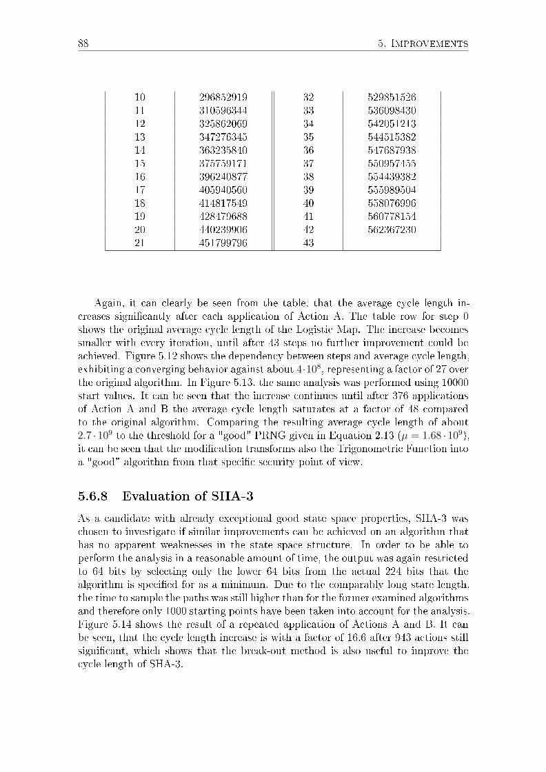
88 5. Improvements
10 296852919 32 52985152611 310596344 33 53609843012 325862069 34 54205121313 347276345 35 54451538214 363235840 36 54768793815 375759171 37 55095745516 396240877 38 55443938217 405940560 39 55598950418 414817549 40 55807699619 428479688 41 56077815420 440239906 42 56236723021 451799796 43
Again, it can clearly be seen from the table, that the average cycle length in-creases signi�cantly after each application of Action A. The table row for step 0shows the original average cycle length of the Logistic Map. The increase becomessmaller with every iteration, until after 43 steps no further improvement could beachieved. Figure 5.12 shows the dependency between steps and average cycle length,exhibiting a converging behavior against about 4·108, representing a factor of 27 overthe original algorithm. In Figure 5.13, the same analysis was performed using 10000start values. It can be seen that the increase continues until after 376 applicationsof Action A and B the average cycle length saturates at a factor of 48 comparedto the original algorithm. Comparing the resulting average cycle length of about2.7 ·109 to the threshold for a "good" PRNG given in Equation 2.13 (µ = 1.68 ·109),it can be seen that the modi�cation transforms also the Trigonometric Function intoa "good" algorithm from that speci�c security point of view.
5.6.8 Evaluation of SHA-3
As a candidate with already exceptional good state space properties, SHA-3 waschosen to investigate if similar improvements can be achieved on an algorithm thathas no apparent weaknesses in the state space structure. In order to be able toperform the analysis in a reasonable amount of time, the output was again restrictedto 64 bits by selecting only the lower 64 bits from the actual 224 bits that thealgorithm is speci�ed for as a minimum. Due to the comparably long state length,the time to sample the paths was still higher than for the former examined algorithmsand therefore only 1000 starting points have been taken into account for the analysis.Figure 5.14 shows the result of a repeated application of Actions A and B. It canbe seen, that the cycle length increase is with a factor of 16.6 after 943 actions stillsigni�cant, which shows that the break-out method is also useful to improve thecycle length of SHA-3.

5.6. Direct State Graph Manipulation 89
Figure 5.12: Cycle Length Depending on Repeated Application of Action A and Bon Trigonometric Function for 100 Start Values
Figure 5.13: Cycle Length Depending on Repeated Application of Action A and Bon Trigonometric Function for 10000 Start Values
5.6.9 Performance Evaluation
In order to assess the performance of the algorithms, three experiments have beenperformed. First, the time has been measured to process 1, 10, 100 and 1000 startingpoints if the number of candidates is increased by reducing c to 20 and 18 bits, andthus increasing the number of candidates by factors of 4 and 16, respectively. Theseexperiments have been done on a Dell notebook with Intel i5-6300 CPU at 2.4 GHz,8 GByte of main memory, Windows 7 operating system and Watcom C compiler.In all cases, the same starting points are used and thus the same paths are followedachieving comparable results. The increase in the number of candidates means that
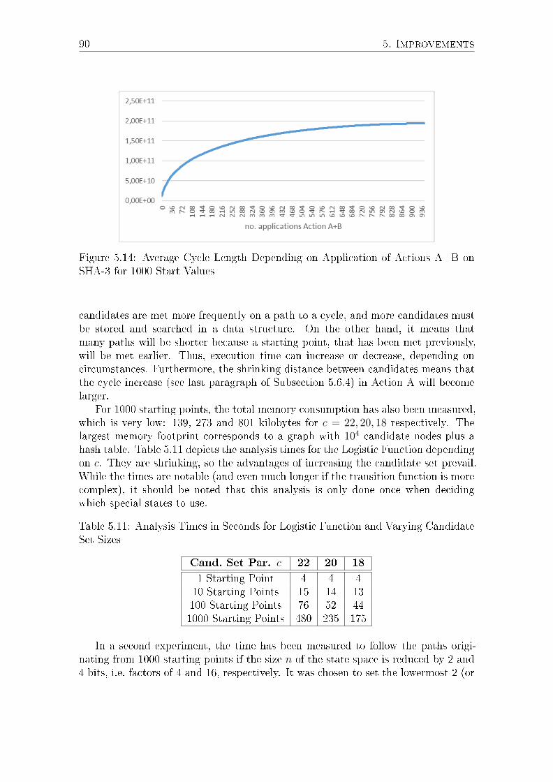
90 5. Improvements
Figure 5.14: Average Cycle Length Depending on Application of Actions A+B onSHA-3 for 1000 Start Values
candidates are met more frequently on a path to a cycle, and more candidates mustbe stored and searched in a data structure. On the other hand, it means thatmany paths will be shorter because a starting point, that has been met previously,will be met earlier. Thus, execution time can increase or decrease, depending oncircumstances. Furthermore, the shrinking distance between candidates means thatthe cycle increase (see last paragraph of Subsection 5.6.4) in Action A will becomelarger.
For 1000 starting points, the total memory consumption has also been measured,which is very low: 139, 273 and 801 kilobytes for c = 22, 20, 18 respectively. Thelargest memory footprint corresponds to a graph with 104 candidate nodes plus ahash table. Table 5.11 depicts the analysis times for the Logistic Function dependingon c. They are shrinking, so the advantages of increasing the candidate set prevail.While the times are notable (and even much longer if the transition function is morecomplex), it should be noted that this analysis is only done once when decidingwhich special states to use.
Table 5.11: Analysis Times in Seconds for Logistic Function and Varying CandidateSet Sizes
Cand. Set Par. c 22 20 18
1 Starting Point 4 4 410 Starting Points 15 14 13100 Starting Points 76 52 441000 Starting Points 480 235 175
In a second experiment, the time has been measured to follow the paths origi-nating from 1000 starting points if the size n of the state space is reduced by 2 and4 bits, i.e. factors of 4 and 16, respectively. It was chosen to set the lowermost 2 (or
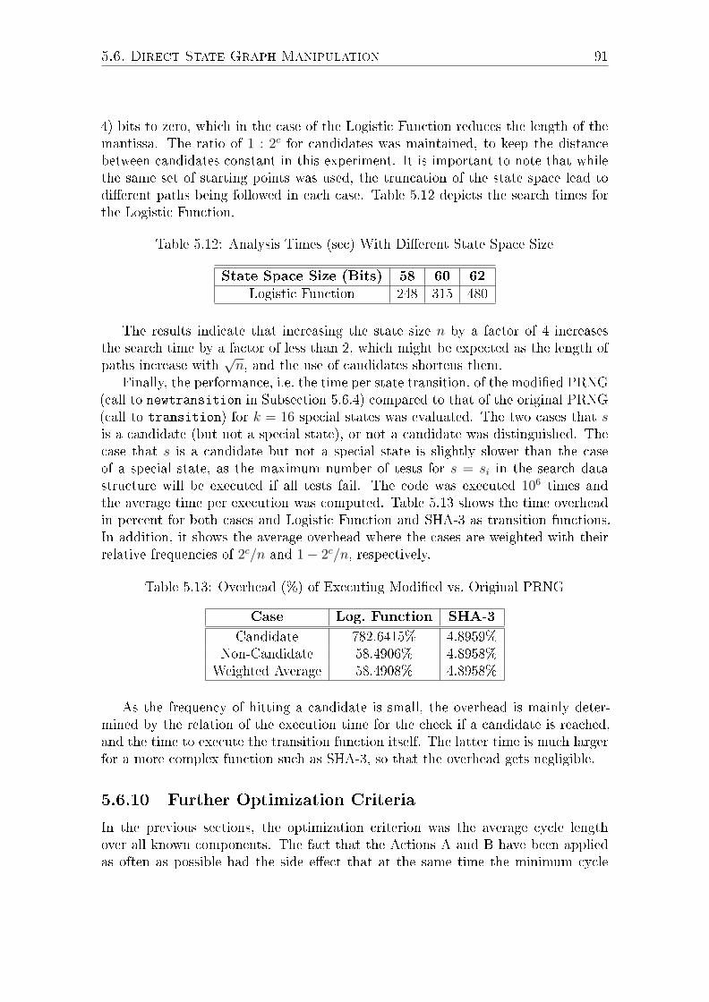
5.6. Direct State Graph Manipulation 91
4) bits to zero, which in the case of the Logistic Function reduces the length of themantissa. The ratio of 1 : 2c for candidates was maintained, to keep the distancebetween candidates constant in this experiment. It is important to note that whilethe same set of starting points was used, the truncation of the state space lead todi�erent paths being followed in each case. Table 5.12 depicts the search times forthe Logistic Function.
Table 5.12: Analysis Times (sec) With Di�erent State Space Size
State Space Size (Bits) 58 60 62Logistic Function 248 315 480
The results indicate that increasing the state size n by a factor of 4 increasesthe search time by a factor of less than 2, which might be expected as the length ofpaths increase with
√n, and the use of candidates shortens them.
Finally, the performance, i.e. the time per state transition, of the modi�ed PRNG(call to newtransition in Subsection 5.6.4) compared to that of the original PRNG(call to transition) for k = 16 special states was evaluated. The two cases that sis a candidate (but not a special state), or not a candidate was distinguished. Thecase that s is a candidate but not a special state is slightly slower than the caseof a special state, as the maximum number of tests for s = si in the search datastructure will be executed if all tests fail. The code was executed 106 times andthe average time per execution was computed. Table 5.13 shows the time overheadin percent for both cases and Logistic Function and SHA-3 as transition functions.In addition, it shows the average overhead where the cases are weighted with theirrelative frequencies of 2c/n and 1− 2c/n, respectively.
Table 5.13: Overhead (%) of Executing Modi�ed vs. Original PRNG
Case Log. Function SHA-3
Candidate 782.6415% 4.8959%Non-Candidate 58.4906% 4.8958%
Weighted Average 58.4908% 4.8958%
As the frequency of hitting a candidate is small, the overhead is mainly deter-mined by the relation of the execution time for the check if a candidate is reached,and the time to execute the transition function itself. The latter time is much largerfor a more complex function such as SHA-3, so that the overhead gets negligible.
5.6.10 Further Optimization Criteria
In the previous sections, the optimization criterion was the average cycle lengthover all known components. The fact that the Actions A and B have been appliedas often as possible had the side e�ect that at the same time the minimum cycle

92 5. Improvements
length was increased. Although this criterion addresses one of the weak spots thathave been identi�ed during the analyzes of the original algorithms, other criteriaare imaginable. The presence of trees in the state graph improves the backwardssecurity, so a potential criterion might be the number of nodes that have more thanone predecessor. Another option would be the average length from an arbitrary startnode to the �rst repeated node in a path, i.e. the sum of the tree size and the cyclelength. Dependent on the requirements on the resulting algorithm, more criteriamight be good candidates.
93
Chapter 6
Statistical Evaluation
6.1 Motivation
The previous sections of this work have concentrated on the state space propertiesof the analyzed cryptographic primitives. While these properties are importantaspects of the security of such algorithms, they are not the only property to beconsidered. In Subsection 2.3.1, it was motivated that the output of e.g. PRNGsneed to be statistically analyzed to ensure that they are su�ciently hard to predict.The same is true for all other cryptographic algorithms mentioned in this work. Thetypical approach to evaluate them is to use standardized statistical test suites. Inthe following, the most common of these test suites are described in detail and theresults of their application on both the original algorithms as well as their modi�edversions using the break-out mechanism from Chapter 5 are compared.
6.2 DIEHARD
In 1995, Marsaglia published a collection of tests for pseudo-random numbers underthe name DIEHARD. The tests contained in the DIEHARD suite are described inthe source code as in the following [Mar95].
The Birthday Spacings Test
Choose m birthdays in a year of n days. List the spacings between the birthdays. Ifj is the number of values that occur more than once in that list, then j is asymptot-ically Poisson distributed with mean m3/(4n). Experience shows n must be quitelarge, say n = 218, for comparing the results to the Poisson distribution with thatmean. This test uses n = 224 and m = 210, so that the underlying distribution forj is taken to be Poisson with λ = 227/226 ≈ 2. A sample of 500 js is taken, anda chi-square goodness of �t test provides a p-value. The �rst test uses bits 1-24(counting from the left) from integers in the speci�ed �le. Then the �le is closed andreopened. Next, bits 2-25 are used to provide birthdays, then 3-26 and so on to bits
94 6. Statistical Evaluation
9-32. Each set of bits provides a p-value, and the nine p-values provide a sample fora KSTEST.
The Overlapping 5-Permutation Test
This is the OPERM5 test. It looks at a sequence of one million 32-bit randomintegers. Each set of �ve consecutive integers can be in one of 120 states, for the 5!possible orderings of �ve numbers. Thus the 5th, 6th, 7th, ... numbers each providea state. As many thousands of state transitions are observed, cumulative countsare made of the number of occurrences of each state. Then the quadratic form inthe weak inverse of the 120 × 120 covariance matrix yields a test equivalent to thelikelihood ratio test that the 120 cell counts came from the speci�ed (asymptotically)normal distribution with the speci�ed 120 × 120 covariance matrix (with rank 99).This version uses 1000000 integers, twice.
The Binary Rank Test for 31× 31 Matrices
The leftmost 31 bits of 31 random integers from the test sequence are used to forma 31 × 31 binary matrix over the �eld {0, 1}. The rank is determined. That rankcan be from 0 to 31, but ranks < 28 are rare, and their counts are pooled with thosefor rank 28. Ranks are found for 40000 such random matrices and a chi-square testis performed on counts for ranks 31, 30, 29 and ≤ 28.
The Binary Rank Test for 32× 32 Matrices
A random 32× 32 binary matrix is formed, each row a 32-bit random integer. Therank is determined. That rank can be from 0 to 32, ranks less than 29 are rare,and their counts are pooled with those for rank 29. Ranks are found for 40000 suchrandom matrices and a chi-square test is performed on counts for ranks 32, 31, 30and ≤ 29.
The Binary Rank Test for 6× 8 Matrices
From each of six random 32-bit integers from the generator under test, a speci�edbyte is chosen, and the resulting six bytes form a 6× 8 binary matrix whose rank isdetermined. That rank can be from 0 to 6, but ranks 0, 1, 2, 3 are rare; their countsare pooled with those for rank 4. Ranks are found for 100000 random matrices, anda chi-square test is performed on counts for ranks 6, 5 and ≤ 4.
The Bitstream Test
The �le under test is viewed as a stream of bits. Call them b1, b2, ... . Consider analphabet with two "letters", 0 and 1 and think of the stream of bits as a successionof 20-letter "words", overlapping. Thus the �rst word is b1b2...b20, the second isb2b3...b21, and so on. The bitstream test counts the number of missing 20-letter
6.2. DIEHARD 95
(20-bit) words in a string of 221 overlapping 20-letter words. There are 220 possible20-letter words. For a truly random string of 221 + 19 bits, the number of missingwords j should be (very close to) normally distributed with mean 141909 and sigma428. Thus (j−141909)/428 should be a standard normal variate (z score) that leadsto a uniform [0, 1) p-value. The test is repeated twenty times.
The Tests OPSO, OQSO and DNA
OPSO means overlapping-pairs-sparse-occupancy. The OPSO test considers 2-letterwords from an alphabet of 1024 letters. Each letter is determined by a speci�edten bits from a 32-bit integer in the sequence to be tested. OPSO generates 221(overlapping) 2-letter words (from 221 + 1 "keystrokes") and counts the number ofmissing words - that is 2-letter words which do not appear in the entire sequence.That count should be very close to normally distributed with mean 141909, sigma290. Thus (missing words−141909)/290 should be a standard normal variable. TheOPSO test takes 32 bits at a time from the test �le and uses a designated set often consecutive bits. It then restarts the �le for the next designated 10 bits, andso on. OQSO means overlapping-quadruples-sparse-occupancy. The test OQSOis similar, except that it considers 4-letter words from an alphabet of 32 letters,each letter determined by a designated string of 5 consecutive bits from the test�le, elements of which are assumed 32-bit random integers. The mean number ofmissing words in a sequence of 221 four-letter words, (221 + 3 "keystrokes"), isagain 141909, with sigma = 295. The mean is based on theory; sigma comes fromextensive simulation. The DNA test considers an alphabet of 4 letters C, G, A, T,determined by two designated bits in the sequence of random integers being tested.It considers 10-letter words, so that as in OPSO and OQSO, there are 220 possiblewords, and the mean number of missing words from a string of 221 (overlapping)10-letter words (221 + 9 "keystrokes") is 141909. The standard deviation sigma =339 was determined as for OQSO by simulation. Sigma for OPSO, 290, is the truevalue (to three places), not determined by simulation.
The count-the-1's Test on a Stream of Bytes
Consider the �le under test as a stream of bytes (four per 32-bit integer). Each bytecan contain from none to eight 1s, with probabilities 1, 8, 28, 56, 70, 56, 28, 8, 1 over256. Now let the stream of bytes provide a string of overlapping 5-letter words, each"letter" taking values A, B, C, D, E. The letters are determined by the number of1s in a byte 0, 1, or 2 yield A, 3 yields B, 4 yields C, 5 yields D and 6, 7 or 8 yield E.Thus we have a monkey at a typewriter hitting �ve keys with various probabilities(37, 56, 70, 56, 37 over 256). There are 55 possible 5-letter words, and from a stringof 256000 (overlapping) 5-letter words, counts are made on the frequencies for eachword. The quadratic form in the weak inverse of the covariance matrix of the cellcounts provides a chi-square test Q5-Q4, the di�erence of the naive Pearson sumsof (OBS− EXP)2/EXP on counts for 5- and 4-letter cell counts.

96 6. Statistical Evaluation
The count-the-1's Test for Speci�c Bytes
Consider the �le under test as a stream of 32-bit integers. From each integer, aspeci�c byte is chosen, say the leftmost bits 1 to 8. Each byte can contain from 0 to8 1s, with probabilities 1, 8, 28, 56, 70, 56, 28, 8, 1 over 256. Now let the speci�edbytes from successive integers provide a string of (overlapping) 5-letter words, each"letter" taking values A, B, C, D, E. The letters are determined by the number of1s, in that byte 0, 1, or 2 → A, 3 → B, 4 → C, 5 → D, and 6, 7 or 8 → E.Thus we have a monkey at a typewriter hitting �ve keys with various probabilities37, 56, 70, 56, 37 over 256. There are 55 possible 5-letter words, and from a stringof 256000 (overlapping) 5-letter words, counts are made on the frequencies for eachword. The quadratic form in the weak inverse of the covariance matrix of the cellcounts provides a chi-square test Q5-Q4, the di�erence of the naive Pearson sumsof (OBS− EXP)2/EXP on counts for 5- and 4-letter cell counts.
The Parking Lot Test
In a square of side 100, randomly "park" a car - a circle of radius 1. Then try to parka 2nd, a 3rd, and so on, each time parking "by ear". That is, if an attempt to park acar causes a crash with one already parked, try again at a new random location. (Toavoid path problems, consider parking helicopters rather than cars.) Each attemptleads to either a crash or a success, the latter followed by an increment to the listof cars already parked. If we plot the number of attempts n versus the number ksuccessfully parked, we get a curve that should be similar to those provided by aperfect random number generator. Theory for the behavior of such a random curveseems beyond reach, and as graphics displays are not available for this battery oftests, a simple characterization of the random experiment is used: k, the numberof cars successfully parked after n = 12000 attempts. Simulation shows that kshould average 3523 with sigma 21.9 and is very close to normally distributed. Thus(k−3523)/21.9 should be a standard normal variable, which, converted to a uniformvariable, provides input to a KSTEST based on a sample of 10.
The Minimum Distance Test
It does this 100 times: choose n = 8000 random points in a square of side 10000.Find d, the minimum distance between the (n2−n)/2 pairs of points. If the points aretruly independent uniform, then d2, the square of the minimum distance should be(very close to) exponentially distributed with mean 0.995. Thus 1− exp(−d2/0.995)should be uniform on [0, 1) and a KSTEST on the resulting 100 values serves as atest of uniformity for random points in the square. Test numbers = 0 mod 5 areprinted but the KSTEST is based on the full set of 100 random choices of 8000points in the 10000× 10000 square.
6.2. DIEHARD 97
The 3D Spheres Test
Choose 4000 random points in a cube of edge 1000. At each point, center a spherelarge enough to reach the next closest point. Then the volume of the smallest suchsphere is (very close to) exponentially distributed with mean 120π/3. Thus theradius cubed is exponential with mean 30. (The mean is obtained by extensivesimulation.) The 3D spheres test generates 4000 such spheres 20 times. Each minradius cubed leads to a uniform variable by means of 1 − exp(−r3/30), then aKSTEST is done on the 20 p-values.
The Squeeze Test
Random integers are �oated to get uniforms on [0, 1). Starting with k = 231 =2147483648, the test �nds j, the number of iterations necessary to reduce k to 1,using the reduction k = ceiling(k ·U), with U provided by �oating integers from the�le being tested. Such js are found 100000 times, then counts for the number of timesj was ≤ 6, 7, ..., 47,≥ 48 are used to provide a chi-square test for cell frequencies.
The Overlapping Sums Test
Integers are �oated to get a sequence U(1), U(2), ... of uniform [0, 1) variables. Thenoverlapping sums, S(1) = U(1) + ... + U(100), S(2) = U(2) + ... + U(101), ... areformed. The Ss are virtually normal with a certain covariance matrix. A lineartransformation of the Ss converts them to a sequence of independent standard nor-mals, which are converted to uniform variables for a KSTEST. The p-values fromten KSTESTs are given still another KSTEST.
The Runs Test
It counts runs up, and runs down, in a sequence of uniform [0, 1) variables, obtainedby �oating the 32-bit integers in the speci�ed �le. This example shows how runsare counted: 0.123, 0.357, 0.789, 0.425, 0.224, 0.416, 0.95 contains an up-run oflength 3, a down-run of length 2 and an up-run of (at least) 2, depending on thenext values. The covariance matrices for the runs-up and runs-down are well known,leading to chi-square tests for quadratic forms in the weak inverses of the covariancematrices. Runs are counted for sequences of length 10000. This is done ten times,then repeated.
The Craps Test
It plays 200000 games of craps, �nds the number of wins and the number of throwsnecessary to end each game. The number of wins should be (very close to) a normalwith mean 200000p and variance 200000p(1−p), with p = 244/495. Throws necessaryto complete the game can vary from 1 to in�nity, but counts for all > 21 are lumpedwith 21. A chi-square test is made on the no.-of-throws cell counts. Each 32-bit
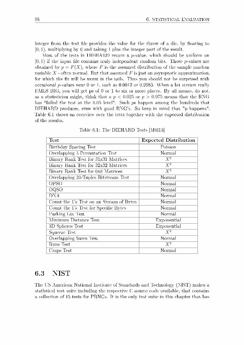
98 6. Statistical Evaluation
integer from the test �le provides the value for the throw of a die, by �oating to[0, 1), multiplying by 6 and taking 1 plus the integer part of the result.
Most of the tests in DIEHARD return a p-value, which should be uniform on[0, 1) if the input �le contains truly independent random bits. Those p-values areobtained by p = F (X), where F is the assumed distribution of the sample randomvariable X - often normal. But that assumed F is just an asymptotic approximation,for which the �t will be worst in the tails. Thus you should not be surprised withoccasional p-values near 0 or 1, such as 0.0012 or 0.9983. When a bit stream reallyFAILS BIG, you will get ps of 0 or 1 to six or more places. By all means, do not,as a statistician might, think that a p < 0.025 or p > 0.975 means that the RNGhas "failed the test at the 0.05 level". Such ps happen among the hundreds thatDIEHARD produces, even with good RNG's. So keep in mind that "p happens".Table 6.1 shows an overview over the tests together with the expected distributionof the results.
Table 6.1: The DIEHARD Tests [Mül13]
Test Expected Distribution
Birthday Spacing Test PoissonOverlapping 5 Permutation Test NormalBinary Rank Test for 31x31 Matrices X2
Binary Rank Test for 32x32 Matrices X2
Binary Rank Test for 6x8 Matrices X2
Overlapping 20-Tuples Bitstream Test NormalOPSO NormalOQSO NormalDNA NormalCount the 1's Test on an Stream of Bytes NormalCount the 1's Test for Speci�c Bytes NormalParking Lot Test NormalMinimum Distance Test Exponential3D Spheres Test ExponentialSqueeze Test X2
Overlapping Sums Test NormalRuns Test X2
Craps Test Normal
6.3 NIST
The US American National Institute of Standards and Technology (NIST) makes astatistical test suite including the respective C source code available, that containsa collection of 15 tests for PRNGs. It is the only test suite in this chapter that has

6.3. NIST 99
been published by governmental authorities and that is explicitly mentioned to besuited for cryptographic use [Sch13]: "The focus [...] is on those applications whererandomness is required for cryptographic purposes. A set of statistical tests forrandomness is described [...]. The National Institute of Standards and Technology(NIST) believes that these procedures are useful in detecting deviations of a binarysequence from randomness". The source code for nine PRNGs that are intended asreference for the test cases is part of the suite.
Regarding the size of the input data, it is mentioned that "For many of the testsin this test suite, the assumption has been made that the size of the sequence length,n, is large (of the order 103 to 107). For such large sample sizes of n, asymptoticreference distributions have been derived and applied to carry out the tests. Mostof the tests are applicable for smaller values of n. However, if used for smallervalues of n, the asymptotic reference distributions would be inappropriate and wouldneed to be replaced by exact distributions that would commonly be di�cult tocompute." The authors furthermore specify recommendations for each test case, fromwhich input size meaningful results can be expected. This information is includedin Table 6.2, but the numbers provided might depend on further parameters inaddition.
Table 6.2: The NIST Statistical Test Suite [Sch13]
Test Recommended ExpectedInput Distribution
Frequency (Monobit) Test ≥ 100 Bit Half-NormalFrequency Test within a Block ≥ 100 Bit X2
Runs Test ≥ 100 Bit X2
Longest Run of Ones in a Block Variable X2
Binary Matrix Rank Test ≥ 38912 Bit X2
Discrete Fourier Transform (Spectral) Test ≥ 1 000 Bit NormalNon Overlapping Template Matching Test ≥ 100 Bit X2
Overlapping Template Matching Test ≥ 100 000 Bit X2
Maurer's Universal Statistical Test ≥ 387 840 Bit Half-NormalLinear Complexity Test ≥ 100 000 Bit X2
Serial Test Variable X2
Approximate Entropy Test Variable X2
Cumulative Sums (Cusums) Test ≥ 100 Bit NormalRandom Excursions Test ≥ 100 000 Bit X2
Random Excursions Variant Test ≥ 1 000 000 Bit Half-Normal
Some of the test cases have equivalents in the DIEHARD suite, e.g. the RunsTest or the Binary Matrix Rank Test. Others are di�erent: the Frequency Monobittest examines e.g. the number of ones in a bit sequence that are expected to approach50% for a su�ciently high number of input bits. The Discrete Fourier Transform(Spectral) Test examines bit sequences for repeating patterns.
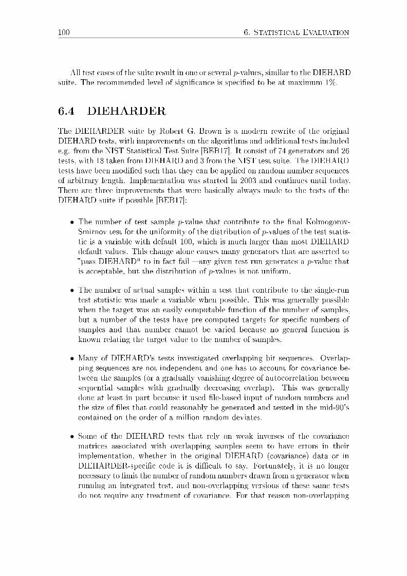
100 6. Statistical Evaluation
All test cases of the suite result in one or several p-values, similar to the DIEHARDsuite. The recommended level of signi�cance is speci�ed to be at maximum 1%.
6.4 DIEHARDER
The DIEHARDER suite by Robert G. Brown is a modern rewrite of the originalDIEHARD tests, with improvements on the algorithms and additional tests includede.g. from the NIST Statistical Test Suite [BEB17]. It consist of 74 generators and 26tests, with 18 taken from DIEHARD and 3 from the NIST test suite. The DIEHARDtests have been modi�ed such that they can be applied on random number sequencesof arbitrary length. Implementation was started in 2003 and continues until today.There are three improvements that were basically always made to the tests of theDIEHARD suite if possible [BEB17]:
• The number of test sample p-value that contribute to the �nal Kolmogorov-Smirnov test for the uniformity of the distribution of p-values of the test statis-tic is a variable with default 100, which is much larger than most DIEHARDdefault values. This change alone causes many generators that are asserted to"pass DIEHARD" to in fact fail � any given test run generates a p-value thatis acceptable, but the distribution of p-values is not uniform.
• The number of actual samples within a test that contribute to the single-runtest statistic was made a variable when possible. This was generally possiblewhen the target was an easily computable function of the number of samples,but a number of the tests have pre-computed targets for speci�c numbers ofsamples and that number cannot be varied because no general function isknown relating the target value to the number of samples.
• Many of DIEHARD's tests investigated overlapping bit sequences. Overlap-ping sequences are not independent and one has to account for covariance be-tween the samples (or a gradually vanishing degree of autocorrelation betweensequential samples with gradually decreasing overlap). This was generallydone at least in part because it used �le-based input of random numbers andthe size of �les that could reasonably be generated and tested in the mid-90'scontained on the order of a million random deviates.
• Some of the DIEHARD tests that rely on weak inverses of the covariancematrices associated with overlapping samples seem to have errors in theirimplementation, whether in the original DIEHARD (covariance) data or inDIEHARDER-speci�c code it is di�cult to say. Fortunately, it is no longernecessary to limit the number of random numbers drawn from a generator whenrunning an integrated test, and non-overlapping versions of these same testsdo not require any treatment of covariance. For that reason non-overlapping

6.4. DIEHARDER 101
versions of the questionable tests have been provided where possible (in par-ticular testing permutations and sums) and the overlapping versions of thosetests are deprecated pending a resolution of the apparent errors.
The advantage of the suite compared to the original DIEHARD suite is thatit is easier to modify and build and it already contains pass/fail criteria for everytest. This makes the evaluation for random sequences much more convenient. Thefollowing tests have been added in addition to the NIST and DIEHARD based tests[BEB17]:
• RGB Bit Distribution Test: Accumulates the frequencies of all n-tuples ofbits in a list of random integers and compares the distribution thus generatedwith the theoretical (binomial) histogram, forming chi-square test and theassociated p-value.
• Generalized Minimum Distance Test: This test utilizes correction terms thatare essential in order for the test not to fail for large numbers of trials. It re-places the minimum distance test and the 3d spheres test from the DIEHARDsuite.
• RGB Permutations Test: This is a non-overlapping test that simply countsorder permutations of random numbers, pulled out n at a time. There aren! permutations and all are equally likely. The samples are independent, soone can do a simple chi-square test on the count vector with n!− 1 degrees offreedom. This is a poor-man's version of the overlapping permutations tests,which are much more di�cult because of the covariance of the overlappingsamples.
• RGB Lagged Sums Test: This test adds up uniform deviates sampled from theRNG, skipping lag samples in between each rand used. The mean of tsamplessamples thus summed should be 0.5 · tsamples. The standard deviation shouldbe sqrt(tsamples/12).
• The Kolmogorov-Smirnov Test: This test generates a vector of tsamples uni-form deviates from the selected RNG, then applies an Anderson-Darling orKuiper KS test to it to directly test for uniformity.
• DAB Byte Distribution Test: Extract n independent bytes from each of kconsecutive words. Increment indexed counters in each of n tables (total of256 · n counters).
• DCT (Frequency Analysis) Test: This test performs a Discrete Cosine Trans-form (DCT) on the output of the RNG. More speci�cally, it performs tsamplestransforms, each over an independent block of ntuple words. If tsamples is largeenough, the positions of the maximum (absolute) value in each transform arerecorded and subjected to a chi-square test for uniformity/independence.

102 6. Statistical Evaluation
• DAB Fill Tree Test: This test �lls small binary trees of �xed depth with wordsfrom the RNG. When a word cannot be inserted into the tree, the currentcount of words in the tree is recorded, along with the position at which theword would have been inserted.
• DAB Fill Tree 2 Test: Bit version of Fill Tree test. This test �lls small binarytrees of �xed depth with "visited" markers. When a marker cannot be placed,the current count of markers in the tree and the position that the marker wouldhave been inserted, if it had not already been marked.
• DAB Monobit 2 Test: Block-monobit test, trying multiple block sizes. Inparticular, tries all block sizes of 2k words, where k = {0..n}. The value of nis calculated from the word size of the generator and the sample size used, andis shown as ntuple.
6.5 Analysis Results
In order to evaluate the potential positive or negative impact of the break-outmethod to the statistical properties of the analysed cryptographic primitives, dif-ferent original and modi�ed versions of the algorithms have been analyzed with thestatistical test suites as presented in the sections before. DIEHARDER and theNIST suite have been chosen, because they cover a wide range of di�erent tests andare easily applicable on a larger number of input values. The handling of the in-put data for these two test suites is slightly di�erent: while DIEHARDER treats thePRNG as a stream of numbers that is used to feed one test after the other, the NISTsuite uses a sequence of a given length (in this case 1000000 bits was chosen) andapplies all tests one after the other on this sequence. This can be repeated severaltimes and the passed respectively failing p-values are reported for each sequence.
The results are interpreted in the next subsections, while the complete test resultsof DIEHARDER and NIST are listed in the appendix for further reference.
6.5.1 Statistic Evaluation of Logistic Map
One issue with the state of the chaotic functions is that it represents a 64 bit doublenumber in the range between 0.0 and 1.0. While the sequence of double numbersthat is generated by the function is distributed comparably equally across this range,this is not true for the binary representation of the double number in memory. Infact, there are bits which always have the same value (due to maximum of 1.0), whileothers are highly unevenly distributed (e.g. the bits of the exponent). In order toconvert the fractional numbers xf into a reasonable representation of random integernumbers xi as they are required for the statistic analysis, the range of 0.0 to 1.0 wasmapped to the range of an unsigned 32 bit integer number by multiplying it withthe maximum integer value:

6.5. Analysis Results 103
xi = round(xf ∗ (232 − 1))
The DIEHARDER test results for the original Logistic Map in Subsection A.1.1show that the majority of tests are failing, which is not surprising due to the knownweaknesses of chaotic functions with respect to cryptographic applications. Onlythree tests pass, diehard_birthdays, diehard_rank_32x32 and diehard_rank_6x8.
In Subsection A.1.2, the same test results for the parameter based break-outmethod according to Subsection 5.3.1 using k = 1024 are shown. There is oneadditional test case that passes: marsaglia_tsang_gc. This is not a signi�cantimprovement, but it has to be taken into account that the sequence is only modi-�ed every 1024 values. If the result of the unmodi�ed algorithm is assumed to berepresentative for the major part of the state space, it is not surprising that thecomparably low number of changed transitions does not have a big impact.
Subsection A.1.3 shows the results for the application of Action A and Action Bas shown in Subsection 5.6.5. The resulting passed tests are identical to the resultfor the parameter based break-out method. Again, it is not surprising that there isno huge impact, because a comparably low number of transitions is modi�ed. Thecriterion for the selection of candidates only selects every 222 ≈ 4 millionth nodeand of those, only a fraction is chosen for one of the Actions.
Figure 6.1 depicts the percentage of passed NIST tests for the 100 sequencesof the Logarithmic Map that have been analyzed. The results are simply orderedby percentage to allow an easy overview. The red solid line is the result for theunmodi�ed function, the blue dashed line for the parameter based break-out andthe grey dotted line for the break-out using Actions A and B. It can clearly beseen that similar to the results of the DIEHARDER suite there is only a negligibledi�erence between all versions. Interestingly, the NIST tests have a by far higherpass rate than the DIEHARDER tests. The detailed results for the NIST suite areshown in Subsection A.2.1 to A.2.3.
6.5.2 Statistic Evaluation of Trigonometric Function
The DIEHARDER results for the Trigonometric Function are displayed in Subsec-tion A.1.4 show a slightly better result than for the Logistic Map: overall 32 testspass, of which 20 tests pass weakly. This is still far from the results that are expectedfor cryptographic secure primitives.
The number of fully passed tests increases signi�cantly for the parameter basedbreak-out method, with a total of 39 passing tests and only 3 weak passes (seeSubsection A.1.5).
For the break-out based on Actions A and B, the result becomes actually worsewith 32 passing tests and 20 of them only passing weakly. The test results areslightly di�erent from the results for the original function, which means that thesuspicion that no break-out was triggered during the analysis run is unfounded (seeSubsection A.1.6).
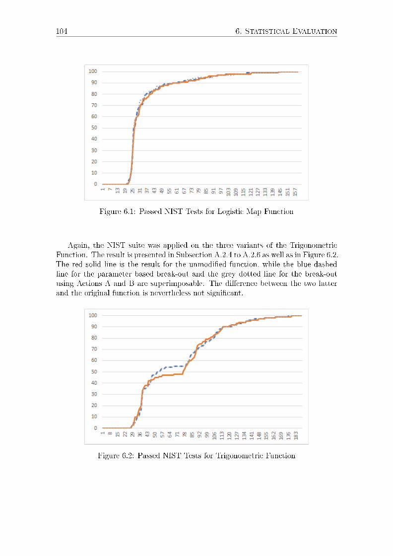
104 6. Statistical Evaluation
Figure 6.1: Passed NIST Tests for Logistic Map Function
Again, the NIST suite was applied on the three variants of the TrigonometricFunction. The result is presented in Subsection A.2.4 to A.2.6 as well as in Figure 6.2.The red solid line is the result for the unmodi�ed function, while the blue dashedline for the parameter based break-out and the grey dotted line for the break-outusing Actions A and B are superimposable. The di�erence between the two latterand the original function is nevertheless not signi�cant.
Figure 6.2: Passed NIST Tests for Trigonometric Function
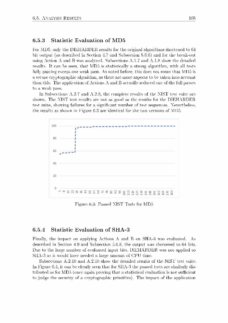
6.5. Analysis Results 105
6.5.3 Statistic Evaluation of MD5
For MD5, only the DIEHARDER results for the original algorithms shortened to 64bit output (as described in Section 4.7 and Subsection 5.6.6) and for the break-outusing Action A and B was analyzed. Subsections A.1.7 and A.1.8 show the detailedresults. It can be seen, that MD5 is statistically a strong algorithm, with all testsfully passing except one weak pass. As noted before, this does not mean that MD5 isa secure cryptographic algorithm, as there are more aspects to be taken into accountthan this. The application of Actions A and B actually reduced one of the full passesto a weak pass.
In Subsections A.2.7 and A.2.8, the complete results of the NIST test suite areshown. The NIST test results are not as good as the results for the DIEHARDERtest suite, showing failures for a signi�cant number of test sequences. Nevertheless,the results as shown in Figure 6.3 are identical for the two versions of MD5.
Figure 6.3: Passed NIST Tests for MD5
6.5.4 Statistic Evaluation of SHA-3
Finally, the impact on applying Actions A and B on SHA-3 was evaluated. Asdescribed in Section 4.9 and Subsection 5.6.8, the output was shortened to 64 bits.Due to the large number of evaluated input bits, DIEHARDER was not applied toSHA-3 as it would have needed a large amount of CPU time.
Subsections A.2.10 and A.2.10 show the detailed results of the NIST test suite.In Figure 6.4, it can be clearly seen that for SHA-3 the passed tests are similarly dis-tributed as for MD5 (once again proving that a statistical evaluation is not su�cientto judge the security of a cryptographic primitive). The impact of the application

106 6. Statistical Evaluation
of Action A and B is low, which can be seen on the similarity of the dashed and thegrey dotted line in the graph.
Figure 6.4: Passed NIST Tests for SHA-3
6.6 Conclusion of Statistic Evaluations
It could overall be seen that the application of the break-out mechanism (be itparameter based or by applying Action A and B) does only have a negligible impacton the results of the DIEHARDER and NIST test suites. Most probably this comesfrom the fact that the evaluated number of input values is not larger than the typicalcycle length of the state space graphs of the algorithms. Still, the conclusion canbe drawn that the break-out mechanism does not negatively impact the statisticproperties of a transition function for the examined cases.

107
Chapter 7
Conclusion and Future Work
In the context of the ubiquity of RFID applications, low-complexity cryptographicprimitives have become of increasingly high importance in the last decades. Thecommonly used cryptographic algorithms that are applied for general security relatedapplications are well tested, but require typically a computational complexity thatmakes them inappropriate for low-cost passive RFID transponders.
In order to address this issue, di�erent primitives have been analyzed in thecourse of this work with respect to their suitability for security related applications.As it is typically not possible to prove the security mathematically, the commonapproach for such analyses is the application of standardized statistical test suites.Unfortunately, the successful attacks on widespread algorithms like A5/1 or MD5have shown that there are more aspects to consider. A particularly weak spot of low-complexity functions is the presence of short cycles that the algorithms enter aftera while, the size of the connected components in the state graph or the depth of thetrees. Graph theory provides the means to describe and investigate the state spaceand thereby allows to get insights about such properties of a transition function.
Due to the fact that the state space of these algorithms is very large, it is normallynot possible to perform a full analysis. Drawing conclusions about the security ofcryptographic functions from the limited analysis data is di�cult. The availabledata can only be used to give hints on a usability of the algorithm for a certainuse case. A single type of analysis is usually not su�cient, instead several typesof analysis should be performed to increase the con�dence in the properties of analgorithm.
In the �rst part of this work, di�erent methods for the analysis of the state spacehave been described, including the sampling of the state space as well as approachesto reduce the state space size by modifying the analyzed algorithm. The methodshave been applied on di�erent chaotic functions and algorithms from the literatureand the respective results have been presented. The results show, that these methodscan extract useful information about security related properties of the cryptographicprimitives. It could be demonstrated with high probability that the AKARI pseudo-random generator is a bijective function, which might make it unsuited for certainuse cases due to the missing backward security. Furthermore, weaknesses in the
108 7. Conclusion and Future Work
state space of the A5/1 algorithm could be found, that are in line with the �ndingsabout the vulnerabilities in literature. Chaotic functions that are often the subjectof investigation in the context of low-complexity functions could be demonstrated tohave very limited security in their basic variant due to their particularly low cyclelengths and component sizes.
In the second part of the work, a simple way to improve the state space prop-erties of any transition function has been developed with the break-out method.After di�erent black box approaches, a greedy algorithm comprising two e�cientmethods to improve the state graph properties of cryptographic primitives by directmanipulation has been presented. It could be demonstrated that by only modifyinga small number of state transitions using Action A and B, the cycle length of thedi�erent cryptographic primitives could be increased by factors in the order of tens.For simple chaotic functions, this modi�cation results in average cycle lengths thatare in the order of the expected cycle length for a random mapping, which is a greatimprovement. Generally, this might make even very low-complexity cryptographicprimitives usable for an extended range of security applications where increasing thesize of the state or choosing more complex algorithms is not an option because ofhardware or computational restrictions. A statistical analysis of the resulting transi-tion functions has been performed using the commonly used test suites. The resultsshow that there is no negative impact on the statistical behavior of these functions.
As future work it might be worthwhile to investigate, how further propertiesof the state space graph can be improved using the break-out method by using adi�erent target function. One example is to optimize the number of nodes withmore than one incoming edge, as this has an in�uence on the backwards security ofa transition function. Another example is the sum of the cycle length and the treeheight, which has a similar impact on backwards security.
Furthermore, instead of a greedy approach it could be evaluated if a method canbe found that performs a global optimization of the target function instead of a localoptimization.
Finally, it might be interesting to investigate �x-point implementations of thechaotic functions that have been subject to analysis in this work. It has been shownin previous work that these can behave better than the �oating point implementa-tions investigated in this work [Lub14], and it would be interesting to investigate ifthe resulting modi�ed transition functions are even better than the results presentedhere.

109
References
[AKR15] Ralph Ankele, Stefan Kölbl, and Christian Rechberger. State-recovery analysis of Spritz. In International Conference on Cryp-tology and Information Security in Latin America, pages 204�221.Springer, 2015.
[Ass48] UN General Assembly. Universal declaration of human rights. UNGeneral Assembly, 1948.
[ASTEZS08] Khalid Abu Al-Saud, Hatim Mohd Tahir, Adel A El-Zoghabi, andMohammad Saleh. Performance Evaluation of Secured versus Non-Secured EIGRP Routing Protocol. In Security and Management,pages 292�297, 2008.
[Avo05] Gildas Avoine. Cryptography in Radio Frequency Identi�cation andFair Exchange Protocols. PhD thesis, Institut de Systemes de Com-munication École Polytechnique Fédérale de Lausanne, Universitéde Caen Basse-Normandie, France, 2005.
[Avo13] Gildas Avoine. RFID Security & Privacy Lounge. http://www.
avoine.net/rfid/index.php, 2013. Accessed: 15.04.2017.
[BC16] Debjyoti Bhattacharjee and Anupam Chattopadhyay. Hardware Ac-celerator for Stream Cipher Spritz. In Proceedings of the 13th Inter-national Joint Conference on e-Business and Telecommunications -Volume 4: SECRYPT, (ICETE 2016), pages 215�222, 2016.
[BCH06] John Black, Martin Cochran, and Trevor Highland. A study of theMD5 attacks: insights and improvements. In International Work-shop on Fast Software Encryption, pages 262�277. Springer, 2006.
[BDM07] Mike Burmester and Breno De Medeiros. RFID security: attacks,countermeasures and challenges. In The 5th RFID Academic Con-vocation, The RFID Journal Conference, 2007.
[BDPVA11] Guido Bertoni, Joan Daemen, Michaël Peeters, and Gilles Van Ass-che. The Keccak SHA-3 submission. Submission to NIST (Round3), 6(7):16, 2011.

110 REFERENCES
[BDPVA16] Guido Bertoni, Joan Daemen, Michaël Peeters, and Gilles Van Ass-che. The Keccak sponge function family. http://keccak.noekeon.org/specs_summary.html, 2016. Accessed: 15.04.2017.
[BEB17] Robert G. Brown, Dirk Eddelbuettel, and David Bauer. Dieharder:A Random Number Test Suite. https://www.phy.duke.edu/~rgb/General/dieharder.php, 2017. Accessed: 07.05.2017.
[BFKM12] Andreas Beckmann, Jaroslaw Fedorowicz, Jörg Keller, and UlrichMeyer. A structural analysis of the A5/1 state transition graph.In First Workshop on GRAPH Inspection and Traversal Engineer-ing, volume 99 of Electronic Proceedings in Theoretical ComputerScience, pages 5�19. Open Publishing Association, 2012.
[BGW99] Marc Briceno, Ian Goldberg, and David Wagner. A pedagogicalimplementation of A5/1. http://www.scard.org/gsm/a51.html,1999. Accessed: 17.04.2017.
[BI16] Subhadeep Banik and Takanori Isobe. Cryptanalysis of the fullSpritz stream cipher. In International Conference on Fast SoftwareEncryption, pages 63�77. Springer, 2016.
[BK07] Andreas Beckmann and Jörg Keller. Parallel-External Computationof the Cycle Structure of Invertible Cryptographic Functions. InParallel, Distributed and Network-Based Processing, 2007. PDP'07.15th EUROMICRO International Conference on, pages 526�533.IEEE, 2007.
[BP82] Henry Beker and Fred Piper. Cipher systems: the protection ofcommunications. Northwood Books, 1982.
[Bre06] Richard Brent. Fast and reliable random number generators forscienti�c computing. Applied Parallel Computing. State of the Artin Scienti�c Computing, pages 1�10, 2006.
[BSW01] Alex Biryukov, Adi Shamir, and David Wagner. Real Time Crypt-analysis of A5/1 on a PC. In Fast Software Encryption, pages 37�44.Springer, 2001.
[Chi07] Hung-Yu Chien. SASI: A new ultralightweight RFID authenticationprotocol providing strong authentication and strong integrity. IEEETransactions on Dependable and Secure Computing, 4(4):337�340,2007.
[CLGM+95] Frank Celler, Charles R. Leedham-Green, Scott H. Murray, Alice C.Niemeyer, and Eamonn A. O'Brien. Generating Random Elementsof a Finite Group. Communications in algebra, 23(13):4931�4948,1995.
REFERENCES 111
[CLRS09] Thomas H. Cormen, Charles E. Leiserson, Ronald L. Rivest, andCli�ord Stein. Introduction to Algorithms (3rd ed.). MIT Press,2009.
[Col06] Jonathan Collins. RFID-Zapper shoots to kill. RFID Journal, 2006.
[CPB+12] Shu-jen Chang, Ray Perlner, William E. Burr, Meltem Sönmez Tu-ran, John M. Kelsey, Souradyuti Paul, and Lawrence E. Bassham.Third-round report of the SHA-3 cryptographic hash algorithm com-petition. NIST Interagency Report, 7896, 2012.
[DC98] Joan Daemen and Craig Clapp. Fast hashing and stream Encryp-tion with PANAMA. In International Workshop on Fast SoftwareEncryption, pages 60�74. Springer, 1998.
[DCP05] Christophe De Canniere and Bart Preneel. Trivium speci�cations.eSTREAM. ECRYPT Stream Cipher Project, Report, 30(2005):266,2005.
[DCP08] Christophe De Canniere and Bart Preneel. Trivium. In New StreamCipher Designs, pages 244�266. Springer, 2008.
[Die00] Reinhard Diestel. Graph Theory. Springer Verlag Berlin and Heidel-berg GmbH, 2000.
[Dir95] EU Directive. 95/46/EC-The Data Protection Directive. O�cialJournal of the European Communities, 1995.
[DPR+13] Yevgeniy Dodis, David Pointcheval, Sylvain Ruhault, Damien Verg-niaud, and Daniel Wichs. Security analysis of pseudo-random num-ber generators with input:/dev/random is not robust. In Proceedingsof the 2013 ACM SIGSAC conference on Computer & communica-tions security, pages 647�658. ACM, 2013.
[Etc17] Chips Etc. RFID Chips in Inventory Tags, Badges & CreditCards. http://www.chipsetc.com/rfid-chips.html, 2017. Ac-cessed: 03.03.2017.
[FDW04] Martin Feldhofer, Sandra Dominikus, and Johannes Wolkerstorfer.Strong authentication for RFID systems using the AES algorithm. InInternational Workshop on Cryptographic Hardware and EmbeddedSystems, pages 357�370. Springer, 2004.
[Fin15] Klaus Finkenzeller. RFID-Handbuch: Grundlagen und praktischeAnwendungen von Transpondern, kontaktlosen Chipkarten und NFC.Carl Hanser Verlag, 2015.
112 REFERENCES
[FO90] Philippe Flajolet and Andrew M. Odlyzko. Random Mapping Statis-tics. In Advances in Cryptology, pages 329�354. Springer Verlag,1990.
[FO10] Bernhard Fechner and Andre Osterloh. A meta-level true ran-dom number generator. International Journal of Critical Computer-Based Systems, 1(1-3):267�279, 2010.
[FR06] Martin Feldhofer and Christian Rechberger. A case against currentlyused hash functions in RFID protocols. In OTM Confederated In-ternational Conferences" On the Move to Meaningful Internet Sys-tems", pages 372�381. Springer, 2006.
[FS09] Philippe Flajolet and Robert Sedgewick. Analytic combinatorics.Cambridge University Press, 2009.
[Gar02] Simson Gar�nkel. Adopting fair information practices to low costRFID systems. In Privacy in Ubiquitous Computing Workshop, 2002.
[GLV00] Robert Gallant, Robert Lambert, and Scott Vanstone. Improvingthe parallelized Pollard lambda search on anomalous binary curves.Mathematics of Computation of the American Mathematical Society,69(232):1699�1705, 2000.
[Han06] Gerhard P. Hancke. Practical attacks on proximity identi�cation sys-tems. In 2006 IEEE Symposium on Security and Privacy (S&P'06).IEEE, 2006.
[Hit10] Ltd. Hitachi. Stream cipher Enocoro, Speci�cation Ver. 2.0.http://www.hitachi.com/rd/yrl/crypto/enocoro/enocoro_
spec_20100222.zip, 2010. Accessed: 03.03.2017.
[HJ10] Martin Hell and Thomas Johansson. Security evaluation of streamcipher Enocoro-128v2. Technical report, CRYPTREC (Cryptogra-phy Research and Evaluation Committee), 2010.
[Hoc08] Katrin Hockemeyer. Analyse von rekursiven Pseudozufallszahlen-generatoren. Bachelorarbeit, FernUniversität in Hagen, 2008.
[Huf16] Thomas Hufnagel. Zustandsraumstruktur bitreduzierter Variantenvon Stromchi�ren. Bachelorarbeit, FernUniversität in Hagen, 2016.
[Int16] EAN International. GS1. http://www.ean-int.org, 2016. Ac-cessed: 17.04.2017.
[Kel02] Jörg Keller. Parallel exploration of the structure of random func-tions. In Proceedings of the 6th Workshop on Parallel Systems and
REFERENCES 113
Algorithms (PASA) in conjunction with the International Confer-ence on Architecture of Computing Systems, ARCS, pages 233�236.VDE Verlag, April 2002.
[Kel07] Jörg Keller. E�cient Sampling of the Structure of Crypto Gen-erators State Transition Graphs. In 2nd European Conference onComputer Network Defence (EC2ND) 2006, pages 3�12. SpringerLondon, 2007.
[Kel13] John Kelsey. SHA3: Past, present, and future. Invited Talk Givenat CHES, 2013.
[KM05] Günter Karjoth and Paul A. Moskowitz. Disabling RFID tags withvisible con�rmation: clipped tags are silenced. In Proceedings ofthe 2005 ACM workshop on Privacy in the electronic society, pages27�30. ACM, 2005.
[Knu71] Donald E. Knuth. Mathematical analysis of algorithms. Technicalreport, DTIC Document, 1971.
[Knu98] Donald E. Knuth. The Art of Computer Programming, Seminumer-ical Algorithms, Vol. 2, Addison-Wesley. Reading, Massachusetts,1998.
[KS03] Alexander Klimov and Adi Shamir. A New class of invertible Map-pings. In Proceedings Cryptographic Hardware and Embedded Sys-tems, pages 470�483. Springer Verlag, 2003.
[KSG+00] Zbigniew Kotulski, Janusz Szczepanski, Karol Górski, Anna Górska,and Andrzej Paszkiewicz. On constructive approach to chaotic pseu-dorandom number generators. In Annual Regional Conferences onMilitary Command, Control, Communications and Information Sys-tems 2000, Zegrze, pages 191�203, 2000.
[KSWH98] John Kelsey, Bruce Schneier, David Wagner, and Chris Hall. Crypt-analytic attacks on pseudorandom number generators. In Inter-national Workshop on Fast Software Encryption, pages 168�188.Springer, 1998.
[KW05] Ziv K�r and Avishai Wool. Picking virtual pockets using relay at-tacks on contactless smartcard. In First International Conferenceon Security and Privacy for Emerging Areas in CommunicationsNetworks (SECURECOMM'05), pages 47�58. IEEE, 2005.
[KW07] Jörg Keller and Hanno Wiese. Period Lengths of Chaotic Pseudo-random Number Generators. In 4th IASTED International Confer-ence on Communication, Network and Information Security, CNIS'07, pages 7�11, Anaheim, CA, USA, 2007. ACTA Press.
114 REFERENCES
[KY10] Ju-Sung Kang and Ok-Yeon Yi. On Distinguished Points Method toImplement a Parallel Collision Search Attack on ECDLP. In SecurityTechnology, Disaster Recovery and Business Continuity, pages 39�46. Springer, 2010.
[Lan01] Jeremy Landt. Shrouds of Time: The history of RFID. AIM Publi-cation, 2001.
[Lub14] Gerald Luber. Statistische Analyse der Ausgaben von chaotischenPseudozufallszahlengeneratoren mit Festkommadarstellung. Master-arbeit, FernUniversität in Hagen, 2014.
[Mar95] George Marsaglia. The Marsaglia Random Number CDROM includ-ing the Diehard Battery of Tests of Randomness. http://www.stat.fsu.edu/pub/diehard/, 1995. Accessed: 17.04.2017.
[MB07] Alexander Maximov and Alex Biryukov. Two trivial attacks on Triv-ium. In International Workshop on Selected Areas in Cryptography,pages 36�55. Springer, 2007.
[Mih07] Daniel Mihajlov. Statistische Analyse chaotischer PRNGs. Bachelo-rarbeit, FernUniversität in Hagen, 2007.
[MME+11] Honorio Martin, Enrique San Millan, Luis Entrena, Pedro Peris-Lopez, and Julio Cesar Hernandez Castro. AKARI-X: A pseudoran-dom number generator for secure lightweight systems. 11th IEEEInternational On-Line Testing Symposium, 0:228�233, 2011.
[MRT10] Aikaterini Mitrokotsa, Melanie R. Rieback, and Andrew S. Tanen-baum. Classi�cation of RFID attacks. Gen, 15693:14443, 2010.
[Mül13] Christoph Müller. Statistische Analysen von Pseudozufallszahlen-generatoren auf Basis mod�zierter Hashketten. Masterarbeit, Fer-nUniversität in Hagen, 2013.
[MvOV96] Alfred J. Menezes, Paul C. van Oorschot, and Scott A. Vanstone.Handbook of Applied Cryptography. CRC Press, 1996.
[MW04] David Molnar and David Wagner. Privacy and security in libraryRFID: Issues, practices, and architectures. In Proceedings of the 11thACM conference on Computer and communications security, pages210�219. ACM, 2004.
[MWK08] K. Muto, D. Watanabe, and T. Kaneko. Strength evaluation ofEnocoro-128 against LDA and its Improvement. In Symposium onCryptography and Information Security, 2008.

REFERENCES 115
[Neu04] Daniel Neuenschwander. Probabilistic and statistical methods incryptology: an introduction by selected topics. Springer Science &Business Media, 2004.
[OWH+04] Britta Oertel, Michaela Wölk, Lorenz Hilty, Andreas Köhler, Har-ald Kelter, Markus Ullmann, and Stefan Wittmann. Risiken undChancen des Einsatzes von RFID-Systemen. Trends und Entwick-lungen in Technologien, Anwendungen und Sicherheit. Bundesamtfür Sicherheit in der Informationstechnik, Bonn, 2004.
[PL08] Pedro Peris-Lopez. Lightweight Cryptography in Radio FrequencyIdenti�cation (RFID) Systems. PhD thesis, Charles III Universityof Madrid, 2008.
[PLHCETR09] Pedro Peris-Lopez, Julio Cesar Hernandez-Castro, Juan M. Estevez-Tapiador, and Arturo Ribagorda. LAMED � a PRNG for EPCclass-1 generation-2 RFID speci�cation. Computer Standards & In-terfaces, 31(1):88�97, 2009.
[Pos09] Axel York Poschmann. Lightweight Cryptography: CryptographyEngineering for a Pervasive World. Dissertation, Ruhr-Universität,Bochum, 2009.
[REC04] Damith Ranasinghe, Daniel Engels, and Peter Cole. Low-cost RFIDsystems: Confronting security and privacy. In Auto-ID labs researchworkshop, pages 54�77, 2004.
[Rei16] Paul Reich. Zustandsraumanalyse von kombiniertenPseudozufallszahlen-Algorithmen. Bachelorarbeit, FernUniver-sität in Hagen, 2016.
[Riv92] Ronald Rivest. The MD5 message-digest algorithm. Technical Re-port 1321, RFC Editor, 1992.
[RKKW05] Keunwoo Rhee, Jin Kwak, Seungjoo Kim, and Dongho Won.Challenge-response based RFID authentication protocol for dis-tributed database environment. In International Conference on Se-curity in Pervasive Computing, pages 70�84. Springer, 2005.
[RS16] Ronald L. Rivest and Jacob C. N. Schuldt. Spritz�a spongy RC4-like stream cipher and hash function. Technical report, CryptologyePrint Archive, Report 2016/856, 2016.
[Sar01] Sanja E. Sarma. Towards the 5 Cent Tag. Auto-ID Center, 2001.
[Sch04] Jörg Schwerdtfeger. Parallele Strukturbestimmung nicht-bijektiverZustandsübergangsfunktionen. Diplomarbeit, FernUniversität in Ha-gen, 2004.

116 REFERENCES
[Sch13] Tom Scheele. Entwicklung einer Testumgebung zur Untersuchungvon Pseudozufallszahlengeneratoren mit Testsuiten. Diplomarbeit,FernUniversität in Hagen, 2013.
[SF13] Robert Sedgewick and Philippe Flajolet. An introduction to theanalysis of algorithms. Addison-Wesley, Reading, Mass., 2013.
[SFP08] Ilaria Simonetti, Jean-Charles Faugere, and Ludovic Perret. Alge-braic attack against Trivium. In First International Conference onSymbolic Computation and Cryptography, SCC, volume 8, pages 95�102, 2008.
[SNKO05] Yu Sasaki, Yusuke Naito, Noboru Kunihiro, and Kazuo Ohta. Im-proved Collision Attack on MD5. IACR Cryptology EPrint Archive,2005:400, 2005.
[Ste06] Marc Stevens. Fast Collision Attack on MD5. IACR CryptologyePrint Archive, 2006:104, 2006.
[SWE02] Sanjay E. Sarma, Stephen A. Weis, and Daniel W. Engels. RFIDSystems and Security and Privacy Implications. In InternationalWorkshop on Cryptographic Hardware and Embedded Systems, pages454�469. Springer, 2002.
[Tur09] Volker Turau. Algorithmische Graphentheorie. Oldenbourg Wis-senschaftsverlag, 2009.
[TWB+14] Sui-Guan Teo, Kenneth Koon-Ho Wong, Harry Bartlett, LeonieSimpson, and Ed Dawson. Algebraic analysis of Trivium-like ciphers(Poster). In Proceedings of the Twelfth Australasian Information Se-curity Conference-Volume 149, pages 77�81. Australian ComputerSociety, Inc., 2014.
[Vat15] Adnan Vatandas. Analysis of Reduced Variants of A5/1 StreamCipher. Bachelorarbeit, FernUniversität in Hagen, 2015.
[VOW99] Paul C. Van Oorschot and Michael J. Wiener. Parallel CollisionSearch with Cryptanalytic Applications. J. Cryptol., 12(1):1�28,January 1999.
[Wal83] C.A. Walton. Portable radio frequency emitting identi�er. https:
//www.google.com/patents/US4384288, 17 1983. US Patent4,384,288.
[Wei91] Mark Weiser. The computer for the 21st century. Scienti�c Ameri-can, 265(3):94�104, 1991.

REFERENCES 117
[WFLY04] Xiaoyun Wang, Dengguo Feng, Xuejia Lai, and Hongbo Yu. Col-lisions for Hash Functions MD4, MD5, HAVAL-128 and RIPEMD.IACR Cryptology ePrint Archive, 2004:199, 2004.
[WK07] Dai Watanabe and Toshinobu Kaneko. A construction of lightweight PANAMA-like keystream generator. IEICE Technical Re-port, ISEC 2007, 2007.
[WSRE04] Stephen A. Weis, Sanjay E. Sarma, Ronald L. Rivest, and Daniel W.Engels. Security and privacy aspects of low-cost radio frequencyidenti�cation systems. In Security in pervasive computing, pages201�212. Springer, 2004.

118 REFERENCES

119
List of Figures
2.1 Bar Code Symbologies . . . . . . . . . . . . . . . . . . . . . . . . . . 62.2 RFID Transponder [Etc17] . . . . . . . . . . . . . . . . . . . . . . . . 72.3 General Block Diagram of a Passive RFID System . . . . . . . . . . . 82.4 Security Triangle [Pos09] . . . . . . . . . . . . . . . . . . . . . . . . . 102.5 Attack Classi�cation According to [MRT10] . . . . . . . . . . . . . . 132.6 Relay Attack [Avo05] . . . . . . . . . . . . . . . . . . . . . . . . . . . 152.7 A Typical Connected Component of a State Transition Graph [BFKM12] 192.8 Pseudo-Random Number Generator . . . . . . . . . . . . . . . . . . . 21
3.1 Graphical Representation of a State Space for 10000 Start Values . . 313.2 A Cycle is Detected . . . . . . . . . . . . . . . . . . . . . . . . . . . . 323.3 Finding the Cycle Entry Point [Sch04] . . . . . . . . . . . . . . . . . 323.4 Candidate Graph . . . . . . . . . . . . . . . . . . . . . . . . . . . . . 34
4.1 AKARI-1 Algorithm in Pseudo Code [MME+11] . . . . . . . . . . . . 364.2 Reduced AKARI-1 Algorithm in Pseudo Code, based on [PLHCETR09] 374.3 The A5/1 Stream Cipher [BSW01] . . . . . . . . . . . . . . . . . . . 394.4 Relative Register Lengths: Average Number of Components [Vat15] . 414.5 Relative Register Lengths: Average Component Size [Vat15] . . . . . 414.6 Relative Register Lengths: Average Cycle Size [Vat15] . . . . . . . . . 424.7 Relative Register Lengths: Average Trees per Component [Vat15] . . 424.8 Relative Register Lengths: Average Tree Size [Vat15] . . . . . . . . . 434.9 LAMED Algorithm in Pseudo Code [PLHCETR09] . . . . . . . . . . 444.10 Structure of Enocoro-128v2 . . . . . . . . . . . . . . . . . . . . . . . 484.11 Enocoro Algorithm in Pseudo Code [Huf16] . . . . . . . . . . . . . . 494.12 State Space Structure of Enocoro32_1 [Huf16] . . . . . . . . . . . . . 514.13 Trivium Algorithm in Pseudo Code [Huf16] . . . . . . . . . . . . . . . 544.14 Structure of Trivium [Huf16] . . . . . . . . . . . . . . . . . . . . . . . 554.15 Structure of Trivium32 [Huf16] . . . . . . . . . . . . . . . . . . . . . 564.16 State Space Structure of Trivium32 [Huf16] . . . . . . . . . . . . . . . 574.17 One MD5 Operation [ASTEZS08] . . . . . . . . . . . . . . . . . . . . 584.18 Structure Diagram of Spritz [BC16] . . . . . . . . . . . . . . . . . . . 614.19 Spritz Algorithm in Pseudo Code [RS16] . . . . . . . . . . . . . . . . 624.20 Structure of SHA-3 [Kel13] . . . . . . . . . . . . . . . . . . . . . . . . 64
120 LIST OF FIGURES
4.21 SHA-3 Algorithm in Pseudo Code [BDPVA16] . . . . . . . . . . . . . 65
5.1 Breaking Out of the Cycle . . . . . . . . . . . . . . . . . . . . . . . . 685.2 Maximum Cycle Length for Logistic Map Using Random Break-Out
Target Nodes . . . . . . . . . . . . . . . . . . . . . . . . . . . . . . . 695.3 Maximum Cycle Length Over k for Logistic Map . . . . . . . . . . . 705.4 Maximum Cycle Length Over k for Trigonometric Function . . . . . . 735.5 Action A . . . . . . . . . . . . . . . . . . . . . . . . . . . . . . . . . . 785.6 Component with Deepest Node not Ideal for Break-Out Target . . . . 795.7 Action B . . . . . . . . . . . . . . . . . . . . . . . . . . . . . . . . . . 805.8 Cycle Length Depending on Repeated Application of Action A on
Logistic Map for 100 Start Values . . . . . . . . . . . . . . . . . . . . 845.9 Cycle Length Depending on Repeated Application of Action A on
Logistic Map for 10000 Start Values . . . . . . . . . . . . . . . . . . . 845.10 Average Cycle Length Depending on Application of Action A and
A+B on MD5 for 10 Start Values . . . . . . . . . . . . . . . . . . . . 865.11 Average Cycle Length Depending on Application of Action A and
A+B on MD5 for 100 Start Values . . . . . . . . . . . . . . . . . . . 875.12 Cycle Length Depending on Repeated Application of Action A and
B on Trigonometric Function for 100 Start Values . . . . . . . . . . . 895.13 Cycle Length Depending on Repeated Application of Action A and
B on Trigonometric Function for 10000 Start Values . . . . . . . . . . 895.14 Average Cycle Length Depending on Application of Actions A+B on
SHA-3 for 1000 Start Values . . . . . . . . . . . . . . . . . . . . . . . 90
6.1 Passed NIST Tests for Logistic Map Function . . . . . . . . . . . . . 1046.2 Passed NIST Tests for Trigonometric Function . . . . . . . . . . . . . 1046.3 Passed NIST Tests for MD5 . . . . . . . . . . . . . . . . . . . . . . . 1056.4 Passed NIST Tests for SHA-3 . . . . . . . . . . . . . . . . . . . . . . 106

121
List of Tables
2.1 Decades of RFID [Lan01] . . . . . . . . . . . . . . . . . . . . . . . . . 62.2 Classes of RFID Tags [PL08] . . . . . . . . . . . . . . . . . . . . . . . 102.3 Hardware Requirements of Common Cryptographic Algorithms [Pos09] 112.4 Expected Values for Random Mappings [FS09] . . . . . . . . . . . . . 262.5 Expected Values for Random Permutations [SF13] . . . . . . . . . . . 26
4.1 Results of Sampled Analysis of AKARI . . . . . . . . . . . . . . . . . 364.2 Analysis Results of AKARI for 14 Bit Word Length . . . . . . . . . . 374.3 Analysis Results of A5/1 After 3000 Start Values . . . . . . . . . . . 404.4 Analysis Results of LAMED for 12 Bit Word Length . . . . . . . . . 454.5 Analysis Results of Logistic Map Algorithm for 100 Start Values . . . 464.6 Analysis Results of Trigonometric Function for 100 Start Values . . . 474.7 Bit Positions for Enocoro32_1 Compared to Bit Positions in Enocoro-
128v2 [Huf16] . . . . . . . . . . . . . . . . . . . . . . . . . . . . . . . 504.8 State Space Properties of Enocoro32_1 Compared to Expected Values
[Huf16] . . . . . . . . . . . . . . . . . . . . . . . . . . . . . . . . . . . 514.9 Enocoro32_1 State Transitions (Shortened) [Huf16] . . . . . . . . . . 524.10 State Space Properties of Enocoro32_2 Compared to Expected Values
for Random Mapping [Huf16] . . . . . . . . . . . . . . . . . . . . . . 534.11 State Space Properties of Trivium32 [Huf16] . . . . . . . . . . . . . . 574.12 Analysis Results of MD5 for 1000 Start Values . . . . . . . . . . . . . 604.13 State Space Properties of Spritz with N = 8 . . . . . . . . . . . . . . 634.14 State Space Properties of Spritz with N = 16 . . . . . . . . . . . . . 634.15 Analysis Results of SHA-3 for 1000 Start Values . . . . . . . . . . . . 64
5.1 Analysis Results of Logistic Map Breaking Out to Random Node Ev-ery k Steps . . . . . . . . . . . . . . . . . . . . . . . . . . . . . . . . 69
5.2 Analysis Results of Logistic Map Switching to Alternative a-ParameterEvery k Steps . . . . . . . . . . . . . . . . . . . . . . . . . . . . . . . 71
5.3 Analysis Results of Logistic Map Switched Between 32 Alternativea-Values (3.98...3.99) Every Step . . . . . . . . . . . . . . . . . . . . 71
5.4 Analysis Results of Trigonometric Function Switching to Alternativez-Parameter Every k Steps . . . . . . . . . . . . . . . . . . . . . . . . 72
5.5 Analysis Results for Equation 5.1 [Rei16] . . . . . . . . . . . . . . . . 75

122 LIST OF TABLES
5.6 Shortened Analysis Results for Equation 5.2 [Rei16] . . . . . . . . . . 765.7 Analysis Results of Combined Algorithms from Equation 5.1 and 5.2
[Rei16] . . . . . . . . . . . . . . . . . . . . . . . . . . . . . . . . . . . 765.8 Average Cycle Lengths for Logistic Map Using Action A for 100 Start
Values . . . . . . . . . . . . . . . . . . . . . . . . . . . . . . . . . . . 825.9 Average Cycle Lengths for MD5 Truncated to 64 Bits Using Action A 845.10 Average Cycle Lengths for Trigonometric Function Using Action A
and B for 100 Start Values . . . . . . . . . . . . . . . . . . . . . . . . 875.11 Analysis Times in Seconds for Logistic Function and Varying Candi-
date Set Sizes . . . . . . . . . . . . . . . . . . . . . . . . . . . . . . . 905.12 Analysis Times (sec) With Di�erent State Space Size . . . . . . . . . 915.13 Overhead (%) of Executing Modi�ed vs. Original PRNG . . . . . . . 91
6.1 The DIEHARD Tests [Mül13] . . . . . . . . . . . . . . . . . . . . . . 986.2 The NIST Statistical Test Suite [Sch13] . . . . . . . . . . . . . . . . . 99
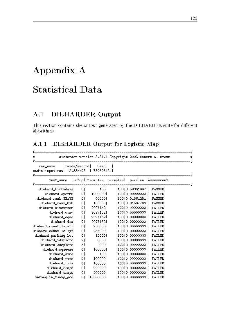
123
Appendix A
Statistical Data
A.1 DIEHARDER Output
This section contains the output generated by the DIEHARDER suite for di�erentalgorithms.
A.1.1 DIEHARDER Output for Logistic Map
#=============================================================================#
# dieharder version 3.31.1 Copyright 2003 Robert G. Brown #
#=============================================================================#
rng_name |rands/second| Seed |
stdin_input_raw| 2.33e+07 | 759696131|
#=============================================================================#
test_name |ntup| tsamples |psamples| p-value |Assessment
#=============================================================================#
diehard_birthdays| 0| 100| 100|0.59301997| PASSED
diehard_operm5| 0| 1000000| 100|0.00000000| FAILED
diehard_rank_32x32| 0| 40000| 100|0.01361251| PASSED
diehard_rank_6x8| 0| 100000| 100|0.04507703| PASSED
diehard_bitstream| 0| 2097152| 100|0.00000000| FAILED
diehard_opso| 0| 2097152| 100|0.00000000| FAILED
diehard_oqso| 0| 2097152| 100|0.00000000| FAILED
diehard_dna| 0| 2097152| 100|0.00000000| FAILED
diehard_count_1s_str| 0| 256000| 100|0.00000000| FAILED
diehard_count_1s_byt| 0| 256000| 100|0.00000000| FAILED
diehard_parking_lot| 0| 12000| 100|0.00000000| FAILED
diehard_2dsphere| 2| 8000| 100|0.00000000| FAILED
diehard_3dsphere| 3| 4000| 100|0.00000000| FAILED
diehard_squeeze| 0| 100000| 100|0.00000000| FAILED
diehard_sums| 0| 100| 100|0.00000000| FAILED
diehard_runs| 0| 100000| 100|0.00000000| FAILED
diehard_runs| 0| 100000| 100|0.00000000| FAILED
diehard_craps| 0| 200000| 100|0.00000000| FAILED
diehard_craps| 0| 200000| 100|0.00000000| FAILED
marsaglia_tsang_gcd| 0| 10000000| 100|0.00000000| FAILED
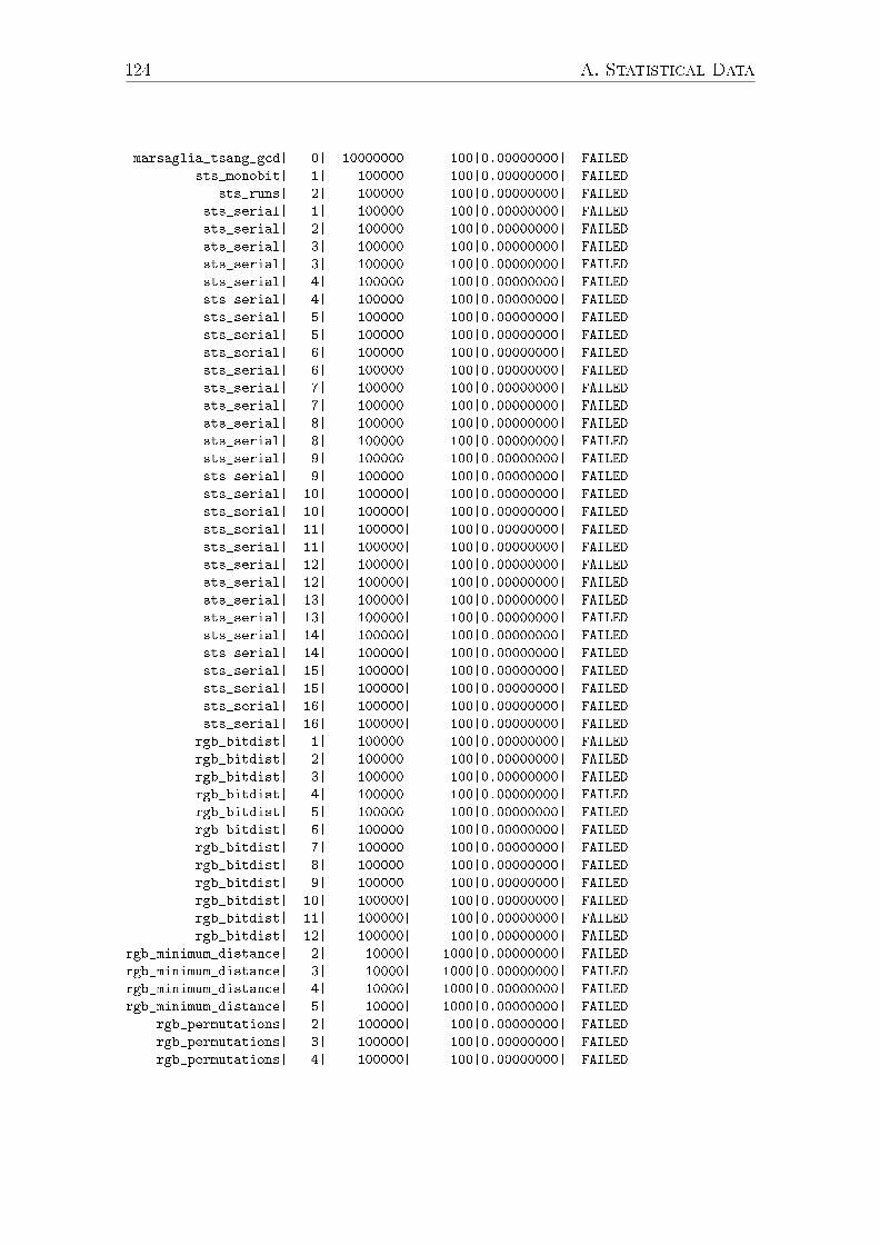
124 A. Statistical Data
marsaglia_tsang_gcd| 0| 10000000| 100|0.00000000| FAILED
sts_monobit| 1| 100000| 100|0.00000000| FAILED
sts_runs| 2| 100000| 100|0.00000000| FAILED
sts_serial| 1| 100000| 100|0.00000000| FAILED
sts_serial| 2| 100000| 100|0.00000000| FAILED
sts_serial| 3| 100000| 100|0.00000000| FAILED
sts_serial| 3| 100000| 100|0.00000000| FAILED
sts_serial| 4| 100000| 100|0.00000000| FAILED
sts_serial| 4| 100000| 100|0.00000000| FAILED
sts_serial| 5| 100000| 100|0.00000000| FAILED
sts_serial| 5| 100000| 100|0.00000000| FAILED
sts_serial| 6| 100000| 100|0.00000000| FAILED
sts_serial| 6| 100000| 100|0.00000000| FAILED
sts_serial| 7| 100000| 100|0.00000000| FAILED
sts_serial| 7| 100000| 100|0.00000000| FAILED
sts_serial| 8| 100000| 100|0.00000000| FAILED
sts_serial| 8| 100000| 100|0.00000000| FAILED
sts_serial| 9| 100000| 100|0.00000000| FAILED
sts_serial| 9| 100000| 100|0.00000000| FAILED
sts_serial| 10| 100000| 100|0.00000000| FAILED
sts_serial| 10| 100000| 100|0.00000000| FAILED
sts_serial| 11| 100000| 100|0.00000000| FAILED
sts_serial| 11| 100000| 100|0.00000000| FAILED
sts_serial| 12| 100000| 100|0.00000000| FAILED
sts_serial| 12| 100000| 100|0.00000000| FAILED
sts_serial| 13| 100000| 100|0.00000000| FAILED
sts_serial| 13| 100000| 100|0.00000000| FAILED
sts_serial| 14| 100000| 100|0.00000000| FAILED
sts_serial| 14| 100000| 100|0.00000000| FAILED
sts_serial| 15| 100000| 100|0.00000000| FAILED
sts_serial| 15| 100000| 100|0.00000000| FAILED
sts_serial| 16| 100000| 100|0.00000000| FAILED
sts_serial| 16| 100000| 100|0.00000000| FAILED
rgb_bitdist| 1| 100000| 100|0.00000000| FAILED
rgb_bitdist| 2| 100000| 100|0.00000000| FAILED
rgb_bitdist| 3| 100000| 100|0.00000000| FAILED
rgb_bitdist| 4| 100000| 100|0.00000000| FAILED
rgb_bitdist| 5| 100000| 100|0.00000000| FAILED
rgb_bitdist| 6| 100000| 100|0.00000000| FAILED
rgb_bitdist| 7| 100000| 100|0.00000000| FAILED
rgb_bitdist| 8| 100000| 100|0.00000000| FAILED
rgb_bitdist| 9| 100000| 100|0.00000000| FAILED
rgb_bitdist| 10| 100000| 100|0.00000000| FAILED
rgb_bitdist| 11| 100000| 100|0.00000000| FAILED
rgb_bitdist| 12| 100000| 100|0.00000000| FAILED
rgb_minimum_distance| 2| 10000| 1000|0.00000000| FAILED
rgb_minimum_distance| 3| 10000| 1000|0.00000000| FAILED
rgb_minimum_distance| 4| 10000| 1000|0.00000000| FAILED
rgb_minimum_distance| 5| 10000| 1000|0.00000000| FAILED
rgb_permutations| 2| 100000| 100|0.00000000| FAILED
rgb_permutations| 3| 100000| 100|0.00000000| FAILED
rgb_permutations| 4| 100000| 100|0.00000000| FAILED
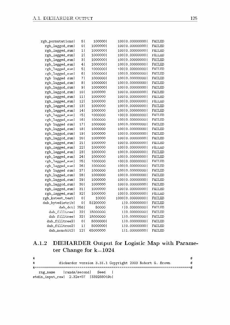
A.1. DIEHARDER Output 125
rgb_permutations| 5| 100000| 100|0.00000000| FAILED
rgb_lagged_sum| 0| 1000000| 100|0.00000000| FAILED
rgb_lagged_sum| 1| 1000000| 100|0.00000000| FAILED
rgb_lagged_sum| 2| 1000000| 100|0.00000000| FAILED
rgb_lagged_sum| 3| 1000000| 100|0.00000000| FAILED
rgb_lagged_sum| 4| 1000000| 100|0.00000000| FAILED
rgb_lagged_sum| 5| 1000000| 100|0.00000000| FAILED
rgb_lagged_sum| 6| 1000000| 100|0.00000000| FAILED
rgb_lagged_sum| 7| 1000000| 100|0.00000000| FAILED
rgb_lagged_sum| 8| 1000000| 100|0.00000000| FAILED
rgb_lagged_sum| 9| 1000000| 100|0.00000000| FAILED
rgb_lagged_sum| 10| 1000000| 100|0.00000000| FAILED
rgb_lagged_sum| 11| 1000000| 100|0.00000000| FAILED
rgb_lagged_sum| 12| 1000000| 100|0.00000000| FAILED
rgb_lagged_sum| 13| 1000000| 100|0.00000000| FAILED
rgb_lagged_sum| 14| 1000000| 100|0.00000000| FAILED
rgb_lagged_sum| 15| 1000000| 100|0.00000000| FAILED
rgb_lagged_sum| 16| 1000000| 100|0.00000000| FAILED
rgb_lagged_sum| 17| 1000000| 100|0.00000000| FAILED
rgb_lagged_sum| 18| 1000000| 100|0.00000000| FAILED
rgb_lagged_sum| 19| 1000000| 100|0.00000000| FAILED
rgb_lagged_sum| 20| 1000000| 100|0.00000000| FAILED
rgb_lagged_sum| 21| 1000000| 100|0.00000000| FAILED
rgb_lagged_sum| 22| 1000000| 100|0.00000000| FAILED
rgb_lagged_sum| 23| 1000000| 100|0.00000000| FAILED
rgb_lagged_sum| 24| 1000000| 100|0.00000000| FAILED
rgb_lagged_sum| 25| 1000000| 100|0.00000000| FAILED
rgb_lagged_sum| 26| 1000000| 100|0.00000000| FAILED
rgb_lagged_sum| 27| 1000000| 100|0.00000000| FAILED
rgb_lagged_sum| 28| 1000000| 100|0.00000000| FAILED
rgb_lagged_sum| 29| 1000000| 100|0.00000000| FAILED
rgb_lagged_sum| 30| 1000000| 100|0.00000000| FAILED
rgb_lagged_sum| 31| 1000000| 100|0.00000000| FAILED
rgb_lagged_sum| 32| 1000000| 100|0.00000000| FAILED
rgb_kstest_test| 0| 10000| 1000|0.00000000| FAILED
dab_bytedistrib| 0| 51200000| 1|0.00000000| FAILED
dab_dct| 256| 50000| 1|0.00000000| FAILED
dab_filltree| 32| 15000000| 1|0.00000000| FAILED
dab_filltree| 32| 15000000| 1|0.00000000| FAILED
dab_filltree2| 0| 5000000| 1|0.00000000| FAILED
dab_filltree2| 1| 5000000| 1|0.00000000| FAILED
dab_monobit2| 12| 65000000| 1|1.00000000| FAILED
A.1.2 DIEHARDER Output for Logistic Map with Parame-
ter Change for k=1024
#=============================================================================#
# dieharder version 3.31.1 Copyright 2003 Robert G. Brown #
#=============================================================================#
rng_name |rands/second| Seed |
stdin_input_raw| 2.32e+07 |3392880495|

126 A. Statistical Data
#=============================================================================#
test_name |ntup| tsamples |psamples| p-value |Assessment
#=============================================================================#
diehard_birthdays| 0| 100| 100|0.15528079| PASSED
diehard_operm5| 0| 1000000| 100|0.00000000| FAILED
diehard_rank_32x32| 0| 40000| 100|0.52336628| PASSED
diehard_rank_6x8| 0| 100000| 100|0.40828182| PASSED
diehard_bitstream| 0| 2097152| 100|0.00000000| FAILED
diehard_opso| 0| 2097152| 100|0.00000000| FAILED
diehard_oqso| 0| 2097152| 100|0.00000000| FAILED
diehard_dna| 0| 2097152| 100|0.00000000| FAILED
diehard_count_1s_str| 0| 256000| 100|0.00000000| FAILED
diehard_count_1s_byt| 0| 256000| 100|0.00000000| FAILED
diehard_parking_lot| 0| 12000| 100|0.00000000| FAILED
diehard_2dsphere| 2| 8000| 100|0.00000000| FAILED
diehard_3dsphere| 3| 4000| 100|0.00000000| FAILED
diehard_squeeze| 0| 100000| 100|0.00000000| FAILED
diehard_sums| 0| 100| 100|0.00000000| FAILED
diehard_runs| 0| 100000| 100|0.00000000| FAILED
diehard_runs| 0| 100000| 100|0.00000000| FAILED
diehard_craps| 0| 200000| 100|0.00000000| FAILED
diehard_craps| 0| 200000| 100|0.00000000| FAILED
marsaglia_tsang_gcd| 0| 10000000| 100|0.00000000| FAILED
marsaglia_tsang_gcd| 0| 10000000| 100|0.78189464| PASSED
sts_monobit| 1| 100000| 100|0.00000000| FAILED
sts_runs| 2| 100000| 100|0.00000000| FAILED
sts_serial| 1| 100000| 100|0.00000000| FAILED
sts_serial| 2| 100000| 100|0.00000000| FAILED
sts_serial| 3| 100000| 100|0.00000000| FAILED
sts_serial| 3| 100000| 100|0.00000000| FAILED
sts_serial| 4| 100000| 100|0.00000000| FAILED
sts_serial| 4| 100000| 100|0.00000000| FAILED
sts_serial| 5| 100000| 100|0.00000000| FAILED
sts_serial| 5| 100000| 100|0.00000000| FAILED
sts_serial| 6| 100000| 100|0.00000000| FAILED
sts_serial| 6| 100000| 100|0.00000000| FAILED
sts_serial| 7| 100000| 100|0.00000000| FAILED
sts_serial| 7| 100000| 100|0.00000000| FAILED
sts_serial| 8| 100000| 100|0.00000000| FAILED
sts_serial| 8| 100000| 100|0.00000000| FAILED
sts_serial| 9| 100000| 100|0.00000000| FAILED
sts_serial| 9| 100000| 100|0.00000000| FAILED
sts_serial| 10| 100000| 100|0.00000000| FAILED
sts_serial| 10| 100000| 100|0.00000000| FAILED
sts_serial| 11| 100000| 100|0.00000000| FAILED
sts_serial| 11| 100000| 100|0.00000000| FAILED
sts_serial| 12| 100000| 100|0.00000000| FAILED
sts_serial| 12| 100000| 100|0.00000000| FAILED
sts_serial| 13| 100000| 100|0.00000000| FAILED
sts_serial| 13| 100000| 100|0.00000000| FAILED
sts_serial| 14| 100000| 100|0.00000000| FAILED
sts_serial| 14| 100000| 100|0.00000000| FAILED
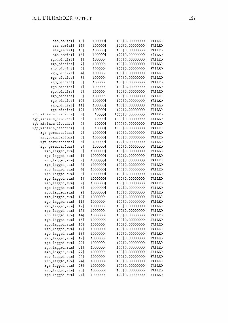
A.1. DIEHARDER Output 127
sts_serial| 15| 100000| 100|0.00000000| FAILED
sts_serial| 15| 100000| 100|0.00000000| FAILED
sts_serial| 16| 100000| 100|0.00000000| FAILED
sts_serial| 16| 100000| 100|0.00000000| FAILED
rgb_bitdist| 1| 100000| 100|0.00000000| FAILED
rgb_bitdist| 2| 100000| 100|0.00000000| FAILED
rgb_bitdist| 3| 100000| 100|0.00000000| FAILED
rgb_bitdist| 4| 100000| 100|0.00000000| FAILED
rgb_bitdist| 5| 100000| 100|0.00000000| FAILED
rgb_bitdist| 6| 100000| 100|0.00000000| FAILED
rgb_bitdist| 7| 100000| 100|0.00000000| FAILED
rgb_bitdist| 8| 100000| 100|0.00000000| FAILED
rgb_bitdist| 9| 100000| 100|0.00000000| FAILED
rgb_bitdist| 10| 100000| 100|0.00000000| FAILED
rgb_bitdist| 11| 100000| 100|0.00000000| FAILED
rgb_bitdist| 12| 100000| 100|0.00000000| FAILED
rgb_minimum_distance| 2| 10000| 1000|0.00000000| FAILED
rgb_minimum_distance| 3| 10000| 1000|0.00000000| FAILED
rgb_minimum_distance| 4| 10000| 1000|0.00000000| FAILED
rgb_minimum_distance| 5| 10000| 1000|0.00000000| FAILED
rgb_permutations| 2| 100000| 100|0.00000000| FAILED
rgb_permutations| 3| 100000| 100|0.00000000| FAILED
rgb_permutations| 4| 100000| 100|0.00000000| FAILED
rgb_permutations| 5| 100000| 100|0.00000000| FAILED
rgb_lagged_sum| 0| 1000000| 100|0.00000000| FAILED
rgb_lagged_sum| 1| 1000000| 100|0.00000000| FAILED
rgb_lagged_sum| 2| 1000000| 100|0.00000000| FAILED
rgb_lagged_sum| 3| 1000000| 100|0.00000000| FAILED
rgb_lagged_sum| 4| 1000000| 100|0.00000000| FAILED
rgb_lagged_sum| 5| 1000000| 100|0.00000000| FAILED
rgb_lagged_sum| 6| 1000000| 100|0.00000000| FAILED
rgb_lagged_sum| 7| 1000000| 100|0.00000000| FAILED
rgb_lagged_sum| 8| 1000000| 100|0.00000000| FAILED
rgb_lagged_sum| 9| 1000000| 100|0.00000000| FAILED
rgb_lagged_sum| 10| 1000000| 100|0.00000000| FAILED
rgb_lagged_sum| 11| 1000000| 100|0.00000000| FAILED
rgb_lagged_sum| 12| 1000000| 100|0.00000000| FAILED
rgb_lagged_sum| 13| 1000000| 100|0.00000000| FAILED
rgb_lagged_sum| 14| 1000000| 100|0.00000000| FAILED
rgb_lagged_sum| 15| 1000000| 100|0.00000000| FAILED
rgb_lagged_sum| 16| 1000000| 100|0.00000000| FAILED
rgb_lagged_sum| 17| 1000000| 100|0.00000000| FAILED
rgb_lagged_sum| 18| 1000000| 100|0.00000000| FAILED
rgb_lagged_sum| 19| 1000000| 100|0.00000000| FAILED
rgb_lagged_sum| 20| 1000000| 100|0.00000000| FAILED
rgb_lagged_sum| 21| 1000000| 100|0.00000000| FAILED
rgb_lagged_sum| 22| 1000000| 100|0.00000000| FAILED
rgb_lagged_sum| 23| 1000000| 100|0.00000000| FAILED
rgb_lagged_sum| 24| 1000000| 100|0.00000000| FAILED
rgb_lagged_sum| 25| 1000000| 100|0.00000000| FAILED
rgb_lagged_sum| 26| 1000000| 100|0.00000000| FAILED
rgb_lagged_sum| 27| 1000000| 100|0.00000000| FAILED
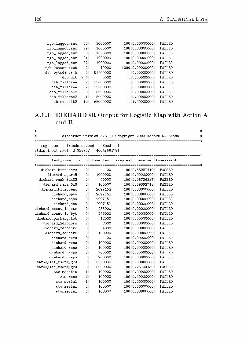
128 A. Statistical Data
rgb_lagged_sum| 28| 1000000| 100|0.00000000| FAILED
rgb_lagged_sum| 29| 1000000| 100|0.00000000| FAILED
rgb_lagged_sum| 30| 1000000| 100|0.00000000| FAILED
rgb_lagged_sum| 31| 1000000| 100|0.00000000| FAILED
rgb_lagged_sum| 32| 1000000| 100|0.00000000| FAILED
rgb_kstest_test| 0| 10000| 1000|0.00000000| FAILED
dab_bytedistrib| 0| 51200000| 1|0.00000000| FAILED
dab_dct| 256| 50000| 1|0.00000000| FAILED
dab_filltree| 32| 15000000| 1|0.00000000| FAILED
dab_filltree| 32| 15000000| 1|0.00000000| FAILED
dab_filltree2| 0| 5000000| 1|0.00000000| FAILED
dab_filltree2| 1| 5000000| 1|0.00000000| FAILED
dab_monobit2| 12| 65000000| 1|1.00000000| FAILED
A.1.3 DIEHARDER Output for Logistic Map with Action A
and B
#=============================================================================#
# dieharder version 3.31.1 Copyright 2003 Robert G. Brown #
#=============================================================================#
rng_name |rands/second| Seed |
stdin_input_raw| 2.32e+07 |4004756178|
#=============================================================================#
test_name |ntup| tsamples |psamples| p-value |Assessment
#=============================================================================#
diehard_birthdays| 0| 100| 100|0.66987419| PASSED
diehard_operm5| 0| 1000000| 100|0.00000000| FAILED
diehard_rank_32x32| 0| 40000| 100|0.05736387| PASSED
diehard_rank_6x8| 0| 100000| 100|0.59392713| PASSED
diehard_bitstream| 0| 2097152| 100|0.00000000| FAILED
diehard_opso| 0| 2097152| 100|0.00000000| FAILED
diehard_oqso| 0| 2097152| 100|0.00000000| FAILED
diehard_dna| 0| 2097152| 100|0.00000000| FAILED
diehard_count_1s_str| 0| 256000| 100|0.00000000| FAILED
diehard_count_1s_byt| 0| 256000| 100|0.00000000| FAILED
diehard_parking_lot| 0| 12000| 100|0.00000000| FAILED
diehard_2dsphere| 2| 8000| 100|0.00000000| FAILED
diehard_3dsphere| 3| 4000| 100|0.00000000| FAILED
diehard_squeeze| 0| 100000| 100|0.00000000| FAILED
diehard_sums| 0| 100| 100|0.00000000| FAILED
diehard_runs| 0| 100000| 100|0.00000000| FAILED
diehard_runs| 0| 100000| 100|0.00000000| FAILED
diehard_craps| 0| 200000| 100|0.00000000| FAILED
diehard_craps| 0| 200000| 100|0.00000000| FAILED
marsaglia_tsang_gcd| 0| 10000000| 100|0.00000000| FAILED
marsaglia_tsang_gcd| 0| 10000000| 100|0.25194189| PASSED
sts_monobit| 1| 100000| 100|0.00000000| FAILED
sts_runs| 2| 100000| 100|0.00000000| FAILED
sts_serial| 1| 100000| 100|0.00000000| FAILED
sts_serial| 2| 100000| 100|0.00000000| FAILED
sts_serial| 3| 100000| 100|0.00000000| FAILED
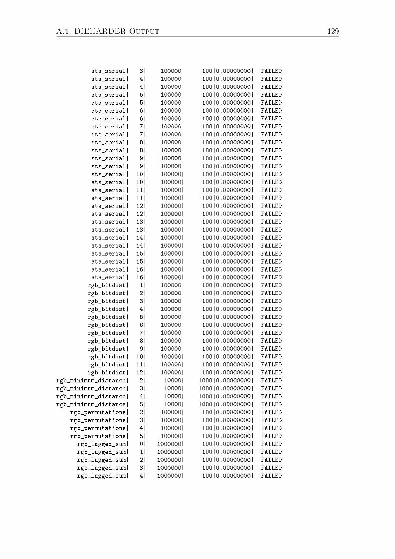
A.1. DIEHARDER Output 129
sts_serial| 3| 100000| 100|0.00000000| FAILED
sts_serial| 4| 100000| 100|0.00000000| FAILED
sts_serial| 4| 100000| 100|0.00000000| FAILED
sts_serial| 5| 100000| 100|0.00000000| FAILED
sts_serial| 5| 100000| 100|0.00000000| FAILED
sts_serial| 6| 100000| 100|0.00000000| FAILED
sts_serial| 6| 100000| 100|0.00000000| FAILED
sts_serial| 7| 100000| 100|0.00000000| FAILED
sts_serial| 7| 100000| 100|0.00000000| FAILED
sts_serial| 8| 100000| 100|0.00000000| FAILED
sts_serial| 8| 100000| 100|0.00000000| FAILED
sts_serial| 9| 100000| 100|0.00000000| FAILED
sts_serial| 9| 100000| 100|0.00000000| FAILED
sts_serial| 10| 100000| 100|0.00000000| FAILED
sts_serial| 10| 100000| 100|0.00000000| FAILED
sts_serial| 11| 100000| 100|0.00000000| FAILED
sts_serial| 11| 100000| 100|0.00000000| FAILED
sts_serial| 12| 100000| 100|0.00000000| FAILED
sts_serial| 12| 100000| 100|0.00000000| FAILED
sts_serial| 13| 100000| 100|0.00000000| FAILED
sts_serial| 13| 100000| 100|0.00000000| FAILED
sts_serial| 14| 100000| 100|0.00000000| FAILED
sts_serial| 14| 100000| 100|0.00000000| FAILED
sts_serial| 15| 100000| 100|0.00000000| FAILED
sts_serial| 15| 100000| 100|0.00000000| FAILED
sts_serial| 16| 100000| 100|0.00000000| FAILED
sts_serial| 16| 100000| 100|0.00000000| FAILED
rgb_bitdist| 1| 100000| 100|0.00000000| FAILED
rgb_bitdist| 2| 100000| 100|0.00000000| FAILED
rgb_bitdist| 3| 100000| 100|0.00000000| FAILED
rgb_bitdist| 4| 100000| 100|0.00000000| FAILED
rgb_bitdist| 5| 100000| 100|0.00000000| FAILED
rgb_bitdist| 6| 100000| 100|0.00000000| FAILED
rgb_bitdist| 7| 100000| 100|0.00000000| FAILED
rgb_bitdist| 8| 100000| 100|0.00000000| FAILED
rgb_bitdist| 9| 100000| 100|0.00000000| FAILED
rgb_bitdist| 10| 100000| 100|0.00000000| FAILED
rgb_bitdist| 11| 100000| 100|0.00000000| FAILED
rgb_bitdist| 12| 100000| 100|0.00000000| FAILED
rgb_minimum_distance| 2| 10000| 1000|0.00000000| FAILED
rgb_minimum_distance| 3| 10000| 1000|0.00000000| FAILED
rgb_minimum_distance| 4| 10000| 1000|0.00000000| FAILED
rgb_minimum_distance| 5| 10000| 1000|0.00000000| FAILED
rgb_permutations| 2| 100000| 100|0.00000000| FAILED
rgb_permutations| 3| 100000| 100|0.00000000| FAILED
rgb_permutations| 4| 100000| 100|0.00000000| FAILED
rgb_permutations| 5| 100000| 100|0.00000000| FAILED
rgb_lagged_sum| 0| 1000000| 100|0.00000000| FAILED
rgb_lagged_sum| 1| 1000000| 100|0.00000000| FAILED
rgb_lagged_sum| 2| 1000000| 100|0.00000000| FAILED
rgb_lagged_sum| 3| 1000000| 100|0.00000000| FAILED
rgb_lagged_sum| 4| 1000000| 100|0.00000000| FAILED

130 A. Statistical Data
rgb_lagged_sum| 5| 1000000| 100|0.00000000| FAILED
rgb_lagged_sum| 6| 1000000| 100|0.00000000| FAILED
rgb_lagged_sum| 7| 1000000| 100|0.00000000| FAILED
rgb_lagged_sum| 8| 1000000| 100|0.00000000| FAILED
rgb_lagged_sum| 9| 1000000| 100|0.00000000| FAILED
rgb_lagged_sum| 10| 1000000| 100|0.00000000| FAILED
rgb_lagged_sum| 11| 1000000| 100|0.00000000| FAILED
rgb_lagged_sum| 12| 1000000| 100|0.00000000| FAILED
rgb_lagged_sum| 13| 1000000| 100|0.00000000| FAILED
rgb_lagged_sum| 14| 1000000| 100|0.00000000| FAILED
rgb_lagged_sum| 15| 1000000| 100|0.00000000| FAILED
rgb_lagged_sum| 16| 1000000| 100|0.00000000| FAILED
rgb_lagged_sum| 17| 1000000| 100|0.00000000| FAILED
rgb_lagged_sum| 18| 1000000| 100|0.00000000| FAILED
rgb_lagged_sum| 19| 1000000| 100|0.00000000| FAILED
rgb_lagged_sum| 20| 1000000| 100|0.00000000| FAILED
rgb_lagged_sum| 21| 1000000| 100|0.00000000| FAILED
rgb_lagged_sum| 22| 1000000| 100|0.00000000| FAILED
rgb_lagged_sum| 23| 1000000| 100|0.00000000| FAILED
rgb_lagged_sum| 24| 1000000| 100|0.00000000| FAILED
rgb_lagged_sum| 25| 1000000| 100|0.00000000| FAILED
rgb_lagged_sum| 26| 1000000| 100|0.00000000| FAILED
rgb_lagged_sum| 27| 1000000| 100|0.00000000| FAILED
rgb_lagged_sum| 28| 1000000| 100|0.00000000| FAILED
rgb_lagged_sum| 29| 1000000| 100|0.00000000| FAILED
rgb_lagged_sum| 30| 1000000| 100|0.00000000| FAILED
rgb_lagged_sum| 31| 1000000| 100|0.00000000| FAILED
rgb_lagged_sum| 32| 1000000| 100|0.00000000| FAILED
rgb_kstest_test| 0| 10000| 1000|0.00000000| FAILED
dab_bytedistrib| 0| 51200000| 1|0.00000000| FAILED
dab_dct| 256| 50000| 1|0.00000000| FAILED
dab_filltree| 32| 15000000| 1|0.00000000| FAILED
dab_filltree| 32| 15000000| 1|0.00000000| FAILED
dab_filltree2| 0| 5000000| 1|0.00000000| FAILED
dab_filltree2| 1| 5000000| 1|0.00000000| FAILED
dab_monobit2| 12| 65000000| 1|1.00000000| FAILED
A.1.4 DIEHARDER Output for Trigonometric Function
#=============================================================================#
# dieharder version 3.31.1 Copyright 2003 Robert G. Brown #
#=============================================================================#
rng_name |rands/second| Seed |
stdin_input_raw| 8.31e+06 | 724784823|
#=============================================================================#
test_name |ntup| tsamples |psamples| p-value |Assessment
#=============================================================================#
diehard_birthdays| 0| 100| 100|0.32930902| PASSED
diehard_operm5| 0| 1000000| 100|0.00000000| FAILED
diehard_rank_32x32| 0| 40000| 100|0.29246055| PASSED
diehard_rank_6x8| 0| 100000| 100|0.77601374| PASSED
diehard_bitstream| 0| 2097152| 100|0.00000000| FAILED
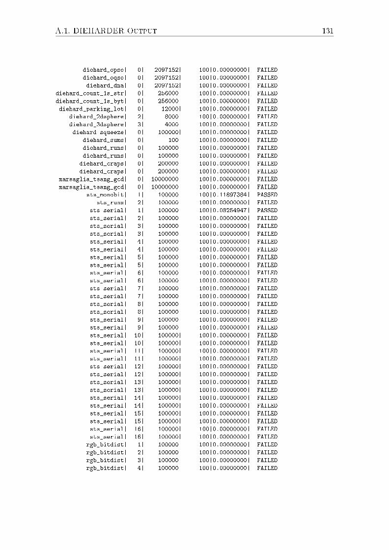
A.1. DIEHARDER Output 131
diehard_opso| 0| 2097152| 100|0.00000000| FAILED
diehard_oqso| 0| 2097152| 100|0.00000000| FAILED
diehard_dna| 0| 2097152| 100|0.00000000| FAILED
diehard_count_1s_str| 0| 256000| 100|0.00000000| FAILED
diehard_count_1s_byt| 0| 256000| 100|0.00000000| FAILED
diehard_parking_lot| 0| 12000| 100|0.00000000| FAILED
diehard_2dsphere| 2| 8000| 100|0.00000000| FAILED
diehard_3dsphere| 3| 4000| 100|0.00000000| FAILED
diehard_squeeze| 0| 100000| 100|0.00000000| FAILED
diehard_sums| 0| 100| 100|0.00000000| FAILED
diehard_runs| 0| 100000| 100|0.00000000| FAILED
diehard_runs| 0| 100000| 100|0.00000000| FAILED
diehard_craps| 0| 200000| 100|0.00000000| FAILED
diehard_craps| 0| 200000| 100|0.00000000| FAILED
marsaglia_tsang_gcd| 0| 10000000| 100|0.00000000| FAILED
marsaglia_tsang_gcd| 0| 10000000| 100|0.00000000| FAILED
sts_monobit| 1| 100000| 100|0.11897384| PASSED
sts_runs| 2| 100000| 100|0.00000000| FAILED
sts_serial| 1| 100000| 100|0.08254947| PASSED
sts_serial| 2| 100000| 100|0.00000000| FAILED
sts_serial| 3| 100000| 100|0.00000000| FAILED
sts_serial| 3| 100000| 100|0.00000000| FAILED
sts_serial| 4| 100000| 100|0.00000000| FAILED
sts_serial| 4| 100000| 100|0.00000000| FAILED
sts_serial| 5| 100000| 100|0.00000000| FAILED
sts_serial| 5| 100000| 100|0.00000000| FAILED
sts_serial| 6| 100000| 100|0.00000000| FAILED
sts_serial| 6| 100000| 100|0.00000000| FAILED
sts_serial| 7| 100000| 100|0.00000000| FAILED
sts_serial| 7| 100000| 100|0.00000000| FAILED
sts_serial| 8| 100000| 100|0.00000000| FAILED
sts_serial| 8| 100000| 100|0.00000000| FAILED
sts_serial| 9| 100000| 100|0.00000000| FAILED
sts_serial| 9| 100000| 100|0.00000000| FAILED
sts_serial| 10| 100000| 100|0.00000000| FAILED
sts_serial| 10| 100000| 100|0.00000000| FAILED
sts_serial| 11| 100000| 100|0.00000000| FAILED
sts_serial| 11| 100000| 100|0.00000000| FAILED
sts_serial| 12| 100000| 100|0.00000000| FAILED
sts_serial| 12| 100000| 100|0.00000000| FAILED
sts_serial| 13| 100000| 100|0.00000000| FAILED
sts_serial| 13| 100000| 100|0.00000000| FAILED
sts_serial| 14| 100000| 100|0.00000000| FAILED
sts_serial| 14| 100000| 100|0.00000000| FAILED
sts_serial| 15| 100000| 100|0.00000000| FAILED
sts_serial| 15| 100000| 100|0.00000000| FAILED
sts_serial| 16| 100000| 100|0.00000000| FAILED
sts_serial| 16| 100000| 100|0.00000000| FAILED
rgb_bitdist| 1| 100000| 100|0.00000000| FAILED
rgb_bitdist| 2| 100000| 100|0.00000000| FAILED
rgb_bitdist| 3| 100000| 100|0.00000000| FAILED
rgb_bitdist| 4| 100000| 100|0.00000000| FAILED

132 A. Statistical Data
rgb_bitdist| 5| 100000| 100|0.00000000| FAILED
rgb_bitdist| 6| 100000| 100|0.00000000| FAILED
rgb_bitdist| 7| 100000| 100|0.00000000| FAILED
rgb_bitdist| 8| 100000| 100|0.00000000| FAILED
rgb_bitdist| 9| 100000| 100|0.00000000| FAILED
rgb_bitdist| 10| 100000| 100|0.00000000| FAILED
rgb_bitdist| 11| 100000| 100|0.00000000| FAILED
rgb_bitdist| 12| 100000| 100|0.00000000| FAILED
rgb_minimum_distance| 2| 10000| 1000|0.00000000| FAILED
rgb_minimum_distance| 3| 10000| 1000|0.00000000| FAILED
rgb_minimum_distance| 4| 10000| 1000|0.00000000| FAILED
rgb_minimum_distance| 5| 10000| 1000|0.00000000| FAILED
rgb_permutations| 2| 100000| 100|0.00000000| FAILED
rgb_permutations| 3| 100000| 100|0.00000000| FAILED
rgb_permutations| 4| 100000| 100|0.00000000| FAILED
rgb_permutations| 5| 100000| 100|0.00000000| FAILED
rgb_lagged_sum| 0| 1000000| 100|0.00316891| WEAK
rgb_lagged_sum| 1| 1000000| 100|0.00213611| WEAK
rgb_lagged_sum| 2| 1000000| 100|0.00000459| WEAK
rgb_lagged_sum| 3| 1000000| 100|0.52946223| PASSED
rgb_lagged_sum| 4| 1000000| 100|0.00050888| WEAK
rgb_lagged_sum| 5| 1000000| 100|0.00000000| FAILED
rgb_lagged_sum| 6| 1000000| 100|0.00000161| WEAK
rgb_lagged_sum| 7| 1000000| 100|0.00257619| WEAK
rgb_lagged_sum| 8| 1000000| 100|0.00001824| WEAK
rgb_lagged_sum| 9| 1000000| 100|0.00000090| FAILED
rgb_lagged_sum| 10| 1000000| 100|0.00040992| WEAK
rgb_lagged_sum| 11| 1000000| 100|0.00000001| FAILED
rgb_lagged_sum| 12| 1000000| 100|0.00004175| WEAK
rgb_lagged_sum| 13| 1000000| 100|0.00001414| WEAK
rgb_lagged_sum| 14| 1000000| 100|0.00000110| WEAK
rgb_lagged_sum| 15| 1000000| 100|0.04516800| PASSED
rgb_lagged_sum| 16| 1000000| 100|0.00001023| WEAK
rgb_lagged_sum| 17| 1000000| 100|0.00000000| FAILED
rgb_lagged_sum| 18| 1000000| 100|0.00099514| WEAK
rgb_lagged_sum| 19| 1000000| 100|0.32036246| PASSED
rgb_lagged_sum| 20| 1000000| 100|0.00037429| WEAK
rgb_lagged_sum| 21| 1000000| 100|0.00667597| PASSED
rgb_lagged_sum| 22| 1000000| 100|0.00195068| WEAK
rgb_lagged_sum| 23| 1000000| 100|0.00000000| FAILED
rgb_lagged_sum| 24| 1000000| 100|0.01335125| PASSED
rgb_lagged_sum| 25| 1000000| 100|0.00043678| WEAK
rgb_lagged_sum| 26| 1000000| 100|0.00000000| FAILED
rgb_lagged_sum| 27| 1000000| 100|0.00093370| WEAK
rgb_lagged_sum| 28| 1000000| 100|0.00149525| WEAK
rgb_lagged_sum| 29| 1000000| 100|0.00000000| FAILED
rgb_lagged_sum| 30| 1000000| 100|0.00009189| WEAK
rgb_lagged_sum| 31| 1000000| 100|0.35273532| PASSED
rgb_lagged_sum| 32| 1000000| 100|0.00007282| WEAK
rgb_kstest_test| 0| 10000| 1000|0.00000000| FAILED
dab_bytedistrib| 0| 51200000| 1|0.00000000| FAILED
dab_dct| 256| 50000| 1|0.68051330| PASSED
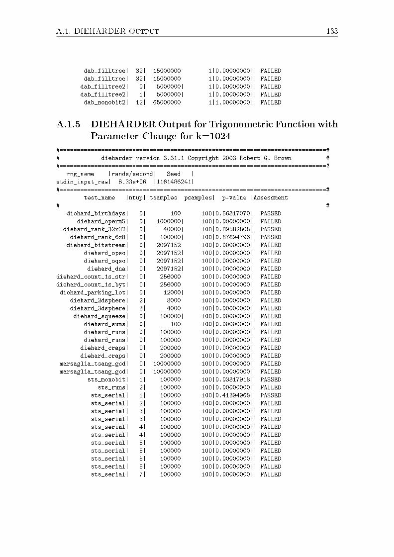
A.1. DIEHARDER Output 133
dab_filltree| 32| 15000000| 1|0.00000000| FAILED
dab_filltree| 32| 15000000| 1|0.00000000| FAILED
dab_filltree2| 0| 5000000| 1|0.00000000| FAILED
dab_filltree2| 1| 5000000| 1|0.00000000| FAILED
dab_monobit2| 12| 65000000| 1|1.00000000| FAILED
A.1.5 DIEHARDER Output for Trigonometric Function with
Parameter Change for k=1024
#=============================================================================#
# dieharder version 3.31.1 Copyright 2003 Robert G. Brown #
#=============================================================================#
rng_name |rands/second| Seed |
stdin_input_raw| 8.33e+06 |1161486241|
#=============================================================================#
test_name |ntup| tsamples |psamples| p-value |Assessment
#=============================================================================#
diehard_birthdays| 0| 100| 100|0.56317070| PASSED
diehard_operm5| 0| 1000000| 100|0.00000000| FAILED
diehard_rank_32x32| 0| 40000| 100|0.89582808| PASSED
diehard_rank_6x8| 0| 100000| 100|0.67694796| PASSED
diehard_bitstream| 0| 2097152| 100|0.00000000| FAILED
diehard_opso| 0| 2097152| 100|0.00000000| FAILED
diehard_oqso| 0| 2097152| 100|0.00000000| FAILED
diehard_dna| 0| 2097152| 100|0.00000000| FAILED
diehard_count_1s_str| 0| 256000| 100|0.00000000| FAILED
diehard_count_1s_byt| 0| 256000| 100|0.00000000| FAILED
diehard_parking_lot| 0| 12000| 100|0.00000000| FAILED
diehard_2dsphere| 2| 8000| 100|0.00000000| FAILED
diehard_3dsphere| 3| 4000| 100|0.00000000| FAILED
diehard_squeeze| 0| 100000| 100|0.00000000| FAILED
diehard_sums| 0| 100| 100|0.00000000| FAILED
diehard_runs| 0| 100000| 100|0.00000000| FAILED
diehard_runs| 0| 100000| 100|0.00000000| FAILED
diehard_craps| 0| 200000| 100|0.00000000| FAILED
diehard_craps| 0| 200000| 100|0.00000000| FAILED
marsaglia_tsang_gcd| 0| 10000000| 100|0.00000000| FAILED
marsaglia_tsang_gcd| 0| 10000000| 100|0.00000000| FAILED
sts_monobit| 1| 100000| 100|0.03317918| PASSED
sts_runs| 2| 100000| 100|0.00000000| FAILED
sts_serial| 1| 100000| 100|0.41394968| PASSED
sts_serial| 2| 100000| 100|0.00000000| FAILED
sts_serial| 3| 100000| 100|0.00000000| FAILED
sts_serial| 3| 100000| 100|0.00000000| FAILED
sts_serial| 4| 100000| 100|0.00000000| FAILED
sts_serial| 4| 100000| 100|0.00000000| FAILED
sts_serial| 5| 100000| 100|0.00000000| FAILED
sts_serial| 5| 100000| 100|0.00000000| FAILED
sts_serial| 6| 100000| 100|0.00000000| FAILED
sts_serial| 6| 100000| 100|0.00000000| FAILED
sts_serial| 7| 100000| 100|0.00000000| FAILED

134 A. Statistical Data
sts_serial| 7| 100000| 100|0.00000000| FAILED
sts_serial| 8| 100000| 100|0.00000000| FAILED
sts_serial| 8| 100000| 100|0.00000000| FAILED
sts_serial| 9| 100000| 100|0.00000000| FAILED
sts_serial| 9| 100000| 100|0.00000000| FAILED
sts_serial| 10| 100000| 100|0.00000000| FAILED
sts_serial| 10| 100000| 100|0.00000000| FAILED
sts_serial| 11| 100000| 100|0.00000000| FAILED
sts_serial| 11| 100000| 100|0.00000000| FAILED
sts_serial| 12| 100000| 100|0.00000000| FAILED
sts_serial| 12| 100000| 100|0.00000000| FAILED
sts_serial| 13| 100000| 100|0.00000000| FAILED
sts_serial| 13| 100000| 100|0.00000000| FAILED
sts_serial| 14| 100000| 100|0.00000000| FAILED
sts_serial| 14| 100000| 100|0.00000000| FAILED
sts_serial| 15| 100000| 100|0.00000000| FAILED
sts_serial| 15| 100000| 100|0.00000000| FAILED
sts_serial| 16| 100000| 100|0.00000000| FAILED
sts_serial| 16| 100000| 100|0.00000000| FAILED
rgb_bitdist| 1| 100000| 100|0.00000000| FAILED
rgb_bitdist| 2| 100000| 100|0.00000000| FAILED
rgb_bitdist| 3| 100000| 100|0.00000000| FAILED
rgb_bitdist| 4| 100000| 100|0.00000000| FAILED
rgb_bitdist| 5| 100000| 100|0.00000000| FAILED
rgb_bitdist| 6| 100000| 100|0.00000000| FAILED
rgb_bitdist| 7| 100000| 100|0.00000000| FAILED
rgb_bitdist| 8| 100000| 100|0.00000000| FAILED
rgb_bitdist| 9| 100000| 100|0.00000000| FAILED
rgb_bitdist| 10| 100000| 100|0.00000000| FAILED
rgb_bitdist| 11| 100000| 100|0.00000000| FAILED
rgb_bitdist| 12| 100000| 100|0.00000000| FAILED
rgb_minimum_distance| 2| 10000| 1000|0.00000000| FAILED
rgb_minimum_distance| 3| 10000| 1000|0.00000000| FAILED
rgb_minimum_distance| 4| 10000| 1000|0.00000000| FAILED
rgb_minimum_distance| 5| 10000| 1000|0.00000000| FAILED
rgb_permutations| 2| 100000| 100|0.00000000| FAILED
rgb_permutations| 3| 100000| 100|0.00000000| FAILED
rgb_permutations| 4| 100000| 100|0.00000000| FAILED
rgb_permutations| 5| 100000| 100|0.00000000| FAILED
rgb_lagged_sum| 0| 1000000| 100|0.34983953| PASSED
rgb_lagged_sum| 1| 1000000| 100|0.04009790| PASSED
rgb_lagged_sum| 2| 1000000| 100|0.07096895| PASSED
rgb_lagged_sum| 3| 1000000| 100|0.41564894| PASSED
rgb_lagged_sum| 4| 1000000| 100|0.48058083| PASSED
rgb_lagged_sum| 5| 1000000| 100|0.34487360| PASSED
rgb_lagged_sum| 6| 1000000| 100|0.40012125| PASSED
rgb_lagged_sum| 7| 1000000| 100|0.57029117| PASSED
rgb_lagged_sum| 8| 1000000| 100|0.59879580| PASSED
rgb_lagged_sum| 9| 1000000| 100|0.71776235| PASSED
rgb_lagged_sum| 10| 1000000| 100|0.44381973| PASSED
rgb_lagged_sum| 11| 1000000| 100|0.03842493| PASSED
rgb_lagged_sum| 12| 1000000| 100|0.46796016| PASSED
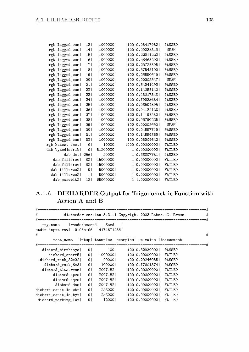
A.1. DIEHARDER Output 135
rgb_lagged_sum| 13| 1000000| 100|0.03417952| PASSED
rgb_lagged_sum| 14| 1000000| 100|0.00238513| WEAK
rgb_lagged_sum| 15| 1000000| 100|0.22311220| PASSED
rgb_lagged_sum| 16| 1000000| 100|0.58463200| PASSED
rgb_lagged_sum| 17| 1000000| 100|0.25728895| PASSED
rgb_lagged_sum| 18| 1000000| 100|0.57543103| PASSED
rgb_lagged_sum| 19| 1000000| 100|0.25550619| PASSED
rgb_lagged_sum| 20| 1000000| 100|0.00308547| WEAK
rgb_lagged_sum| 21| 1000000| 100|0.64341493| PASSED
rgb_lagged_sum| 22| 1000000| 100|0.14058140| PASSED
rgb_lagged_sum| 23| 1000000| 100|0.48017548| PASSED
rgb_lagged_sum| 24| 1000000| 100|0.79333684| PASSED
rgb_lagged_sum| 25| 1000000| 100|0.06594895| PASSED
rgb_lagged_sum| 26| 1000000| 100|0.04182128| PASSED
rgb_lagged_sum| 27| 1000000| 100|0.11198530| PASSED
rgb_lagged_sum| 28| 1000000| 100|0.96790225| PASSED
rgb_lagged_sum| 29| 1000000| 100|0.00003650| WEAK
rgb_lagged_sum| 30| 1000000| 100|0.04557719| PASSED
rgb_lagged_sum| 31| 1000000| 100|0.14554869| PASSED
rgb_lagged_sum| 32| 1000000| 100|0.03309642| PASSED
rgb_kstest_test| 0| 10000| 1000|0.00000000| FAILED
dab_bytedistrib| 0| 51200000| 1|0.00000000| FAILED
dab_dct| 256| 50000| 1|0.66807781| PASSED
dab_filltree| 32| 15000000| 1|0.00000000| FAILED
dab_filltree| 32| 15000000| 1|0.00000000| FAILED
dab_filltree2| 0| 5000000| 1|0.00000000| FAILED
dab_filltree2| 1| 5000000| 1|0.00000000| FAILED
dab_monobit2| 12| 65000000| 1|1.00000000| FAILED
A.1.6 DIEHARDER Output for Trigonometric Function with
Action A and B
#=============================================================================#
# dieharder version 3.31.1 Copyright 2003 Robert G. Brown #
#=============================================================================#
rng_name |rands/second| Seed |
stdin_input_raw| 9.03e+06 |4174671456|
#=============================================================================#
test_name |ntup| tsamples |psamples| p-value |Assessment
#=============================================================================#
diehard_birthdays| 0| 100| 100|0.32930902| PASSED
diehard_operm5| 0| 1000000| 100|0.00000000| FAILED
diehard_rank_32x32| 0| 40000| 100|0.29246055| PASSED
diehard_rank_6x8| 0| 100000| 100|0.77601374| PASSED
diehard_bitstream| 0| 2097152| 100|0.00000000| FAILED
diehard_opso| 0| 2097152| 100|0.00000000| FAILED
diehard_oqso| 0| 2097152| 100|0.00000000| FAILED
diehard_dna| 0| 2097152| 100|0.00000000| FAILED
diehard_count_1s_str| 0| 256000| 100|0.00000000| FAILED
diehard_count_1s_byt| 0| 256000| 100|0.00000000| FAILED
diehard_parking_lot| 0| 12000| 100|0.00000000| FAILED
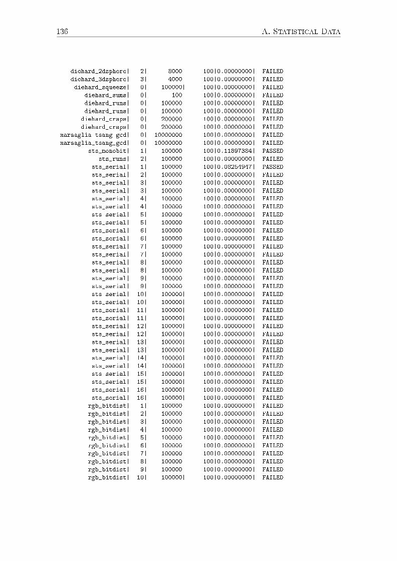
136 A. Statistical Data
diehard_2dsphere| 2| 8000| 100|0.00000000| FAILED
diehard_3dsphere| 3| 4000| 100|0.00000000| FAILED
diehard_squeeze| 0| 100000| 100|0.00000000| FAILED
diehard_sums| 0| 100| 100|0.00000000| FAILED
diehard_runs| 0| 100000| 100|0.00000000| FAILED
diehard_runs| 0| 100000| 100|0.00000000| FAILED
diehard_craps| 0| 200000| 100|0.00000000| FAILED
diehard_craps| 0| 200000| 100|0.00000000| FAILED
marsaglia_tsang_gcd| 0| 10000000| 100|0.00000000| FAILED
marsaglia_tsang_gcd| 0| 10000000| 100|0.00000000| FAILED
sts_monobit| 1| 100000| 100|0.11897384| PASSED
sts_runs| 2| 100000| 100|0.00000000| FAILED
sts_serial| 1| 100000| 100|0.08254947| PASSED
sts_serial| 2| 100000| 100|0.00000000| FAILED
sts_serial| 3| 100000| 100|0.00000000| FAILED
sts_serial| 3| 100000| 100|0.00000000| FAILED
sts_serial| 4| 100000| 100|0.00000000| FAILED
sts_serial| 4| 100000| 100|0.00000000| FAILED
sts_serial| 5| 100000| 100|0.00000000| FAILED
sts_serial| 5| 100000| 100|0.00000000| FAILED
sts_serial| 6| 100000| 100|0.00000000| FAILED
sts_serial| 6| 100000| 100|0.00000000| FAILED
sts_serial| 7| 100000| 100|0.00000000| FAILED
sts_serial| 7| 100000| 100|0.00000000| FAILED
sts_serial| 8| 100000| 100|0.00000000| FAILED
sts_serial| 8| 100000| 100|0.00000000| FAILED
sts_serial| 9| 100000| 100|0.00000000| FAILED
sts_serial| 9| 100000| 100|0.00000000| FAILED
sts_serial| 10| 100000| 100|0.00000000| FAILED
sts_serial| 10| 100000| 100|0.00000000| FAILED
sts_serial| 11| 100000| 100|0.00000000| FAILED
sts_serial| 11| 100000| 100|0.00000000| FAILED
sts_serial| 12| 100000| 100|0.00000000| FAILED
sts_serial| 12| 100000| 100|0.00000000| FAILED
sts_serial| 13| 100000| 100|0.00000000| FAILED
sts_serial| 13| 100000| 100|0.00000000| FAILED
sts_serial| 14| 100000| 100|0.00000000| FAILED
sts_serial| 14| 100000| 100|0.00000000| FAILED
sts_serial| 15| 100000| 100|0.00000000| FAILED
sts_serial| 15| 100000| 100|0.00000000| FAILED
sts_serial| 16| 100000| 100|0.00000000| FAILED
sts_serial| 16| 100000| 100|0.00000000| FAILED
rgb_bitdist| 1| 100000| 100|0.00000000| FAILED
rgb_bitdist| 2| 100000| 100|0.00000000| FAILED
rgb_bitdist| 3| 100000| 100|0.00000000| FAILED
rgb_bitdist| 4| 100000| 100|0.00000000| FAILED
rgb_bitdist| 5| 100000| 100|0.00000000| FAILED
rgb_bitdist| 6| 100000| 100|0.00000000| FAILED
rgb_bitdist| 7| 100000| 100|0.00000000| FAILED
rgb_bitdist| 8| 100000| 100|0.00000000| FAILED
rgb_bitdist| 9| 100000| 100|0.00000000| FAILED
rgb_bitdist| 10| 100000| 100|0.00000000| FAILED
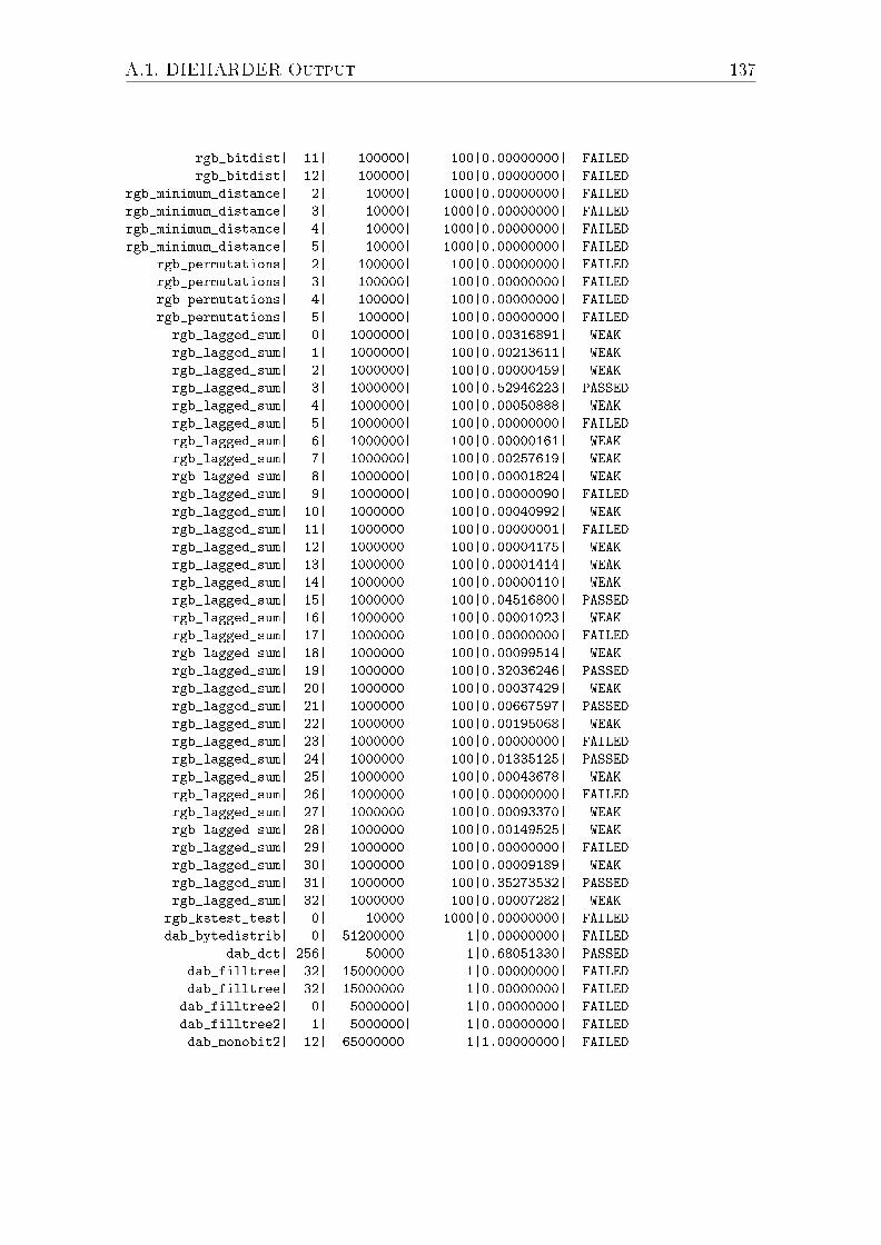
A.1. DIEHARDER Output 137
rgb_bitdist| 11| 100000| 100|0.00000000| FAILED
rgb_bitdist| 12| 100000| 100|0.00000000| FAILED
rgb_minimum_distance| 2| 10000| 1000|0.00000000| FAILED
rgb_minimum_distance| 3| 10000| 1000|0.00000000| FAILED
rgb_minimum_distance| 4| 10000| 1000|0.00000000| FAILED
rgb_minimum_distance| 5| 10000| 1000|0.00000000| FAILED
rgb_permutations| 2| 100000| 100|0.00000000| FAILED
rgb_permutations| 3| 100000| 100|0.00000000| FAILED
rgb_permutations| 4| 100000| 100|0.00000000| FAILED
rgb_permutations| 5| 100000| 100|0.00000000| FAILED
rgb_lagged_sum| 0| 1000000| 100|0.00316891| WEAK
rgb_lagged_sum| 1| 1000000| 100|0.00213611| WEAK
rgb_lagged_sum| 2| 1000000| 100|0.00000459| WEAK
rgb_lagged_sum| 3| 1000000| 100|0.52946223| PASSED
rgb_lagged_sum| 4| 1000000| 100|0.00050888| WEAK
rgb_lagged_sum| 5| 1000000| 100|0.00000000| FAILED
rgb_lagged_sum| 6| 1000000| 100|0.00000161| WEAK
rgb_lagged_sum| 7| 1000000| 100|0.00257619| WEAK
rgb_lagged_sum| 8| 1000000| 100|0.00001824| WEAK
rgb_lagged_sum| 9| 1000000| 100|0.00000090| FAILED
rgb_lagged_sum| 10| 1000000| 100|0.00040992| WEAK
rgb_lagged_sum| 11| 1000000| 100|0.00000001| FAILED
rgb_lagged_sum| 12| 1000000| 100|0.00004175| WEAK
rgb_lagged_sum| 13| 1000000| 100|0.00001414| WEAK
rgb_lagged_sum| 14| 1000000| 100|0.00000110| WEAK
rgb_lagged_sum| 15| 1000000| 100|0.04516800| PASSED
rgb_lagged_sum| 16| 1000000| 100|0.00001023| WEAK
rgb_lagged_sum| 17| 1000000| 100|0.00000000| FAILED
rgb_lagged_sum| 18| 1000000| 100|0.00099514| WEAK
rgb_lagged_sum| 19| 1000000| 100|0.32036246| PASSED
rgb_lagged_sum| 20| 1000000| 100|0.00037429| WEAK
rgb_lagged_sum| 21| 1000000| 100|0.00667597| PASSED
rgb_lagged_sum| 22| 1000000| 100|0.00195068| WEAK
rgb_lagged_sum| 23| 1000000| 100|0.00000000| FAILED
rgb_lagged_sum| 24| 1000000| 100|0.01335125| PASSED
rgb_lagged_sum| 25| 1000000| 100|0.00043678| WEAK
rgb_lagged_sum| 26| 1000000| 100|0.00000000| FAILED
rgb_lagged_sum| 27| 1000000| 100|0.00093370| WEAK
rgb_lagged_sum| 28| 1000000| 100|0.00149525| WEAK
rgb_lagged_sum| 29| 1000000| 100|0.00000000| FAILED
rgb_lagged_sum| 30| 1000000| 100|0.00009189| WEAK
rgb_lagged_sum| 31| 1000000| 100|0.35273532| PASSED
rgb_lagged_sum| 32| 1000000| 100|0.00007282| WEAK
rgb_kstest_test| 0| 10000| 1000|0.00000000| FAILED
dab_bytedistrib| 0| 51200000| 1|0.00000000| FAILED
dab_dct| 256| 50000| 1|0.68051330| PASSED
dab_filltree| 32| 15000000| 1|0.00000000| FAILED
dab_filltree| 32| 15000000| 1|0.00000000| FAILED
dab_filltree2| 0| 5000000| 1|0.00000000| FAILED
dab_filltree2| 1| 5000000| 1|0.00000000| FAILED
dab_monobit2| 12| 65000000| 1|1.00000000| FAILED
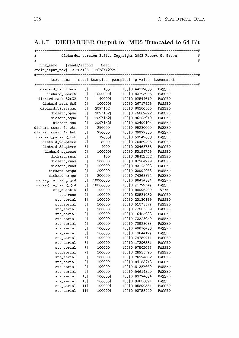
138 A. Statistical Data
A.1.7 DIEHARDER Output for MD5 Truncated to 64 Bit
#=============================================================================#
# dieharder version 3.31.1 Copyright 2003 Robert G. Brown #
#=============================================================================#
rng_name |rands/second| Seed |
stdin_input_raw| 3.28e+06 |2678772924|
#=============================================================================#
test_name |ntup| tsamples |psamples| p-value |Assessment
#=============================================================================#
diehard_birthdays| 0| 100| 100|0.44912855| PASSED
diehard_operm5| 0| 1000000| 100|0.83725906| PASSED
diehard_rank_32x32| 0| 40000| 100|0.92544610| PASSED
diehard_rank_6x8| 0| 100000| 100|0.26717925| PASSED
diehard_bitstream| 0| 2097152| 100|0.60306305| PASSED
diehard_opso| 0| 2097152| 100|0.75082422| PASSED
diehard_oqso| 0| 2097152| 100|0.96205970| PASSED
diehard_dna| 0| 2097152| 100|0.52499105| PASSED
diehard_count_1s_str| 0| 256000| 100|0.99230600| PASSED
diehard_count_1s_byt| 0| 256000| 100|0.29922350| PASSED
diehard_parking_lot| 0| 12000| 100|0.59549008| PASSED
diehard_2dsphere| 2| 8000| 100|0.76469496| PASSED
diehard_3dsphere| 3| 4000| 100|0.28468783| PASSED
diehard_squeeze| 0| 100000| 100|0.53159725| PASSED
diehard_sums| 0| 100| 100|0.38452322| PASSED
diehard_runs| 0| 100000| 100|0.87984279| PASSED
diehard_runs| 0| 100000| 100|0.93725498| PASSED
diehard_craps| 0| 200000| 100|0.20992963| PASSED
diehard_craps| 0| 200000| 100|0.74863874| PASSED
marsaglia_tsang_gcd| 0| 10000000| 100|0.98434381| PASSED
marsaglia_tsang_gcd| 0| 10000000| 100|0.71729747| PASSED
sts_monobit| 1| 100000| 100|0.99996400| WEAK
sts_runs| 2| 100000| 100|0.58581932| PASSED
sts_serial| 1| 100000| 100|0.23130199| PASSED
sts_serial| 2| 100000| 100|0.51073577| PASSED
sts_serial| 3| 100000| 100|0.77803539| PASSED
sts_serial| 3| 100000| 100|0.16455088| PASSED
sts_serial| 4| 100000| 100|0.72328050| PASSED
sts_serial| 4| 100000| 100|0.78923688| PASSED
sts_serial| 5| 100000| 100|0.49616436| PASSED
sts_serial| 5| 100000| 100|0.19644127| PASSED
sts_serial| 6| 100000| 100|0.74750271| PASSED
sts_serial| 6| 100000| 100|0.17896531| PASSED
sts_serial| 7| 100000| 100|0.97502083| PASSED
sts_serial| 7| 100000| 100|0.28935795| PASSED
sts_serial| 8| 100000| 100|0.26224662| PASSED
sts_serial| 8| 100000| 100|0.84188273| PASSED
sts_serial| 9| 100000| 100|0.81387669| PASSED
sts_serial| 9| 100000| 100|0.54614320| PASSED
sts_serial| 10| 100000| 100|0.63724084| PASSED
sts_serial| 10| 100000| 100|0.93055891| PASSED
sts_serial| 11| 100000| 100|0.95690534| PASSED
sts_serial| 11| 100000| 100|0.98758440| PASSED

A.1. DIEHARDER Output 139
sts_serial| 12| 100000| 100|0.76287820| PASSED
sts_serial| 12| 100000| 100|0.54176905| PASSED
sts_serial| 13| 100000| 100|0.42122860| PASSED
sts_serial| 13| 100000| 100|0.17711053| PASSED
sts_serial| 14| 100000| 100|0.03732113| PASSED
sts_serial| 14| 100000| 100|0.07870234| PASSED
sts_serial| 15| 100000| 100|0.02455619| PASSED
sts_serial| 15| 100000| 100|0.01298811| PASSED
sts_serial| 16| 100000| 100|0.14844165| PASSED
sts_serial| 16| 100000| 100|0.20049474| PASSED
rgb_bitdist| 1| 100000| 100|0.74382259| PASSED
rgb_bitdist| 2| 100000| 100|0.79862603| PASSED
rgb_bitdist| 3| 100000| 100|0.80668525| PASSED
rgb_bitdist| 4| 100000| 100|0.04552024| PASSED
rgb_bitdist| 5| 100000| 100|0.30982398| PASSED
rgb_bitdist| 6| 100000| 100|0.62117810| PASSED
rgb_bitdist| 7| 100000| 100|0.42432399| PASSED
rgb_bitdist| 8| 100000| 100|0.12593233| PASSED
rgb_bitdist| 9| 100000| 100|0.07588392| PASSED
rgb_bitdist| 10| 100000| 100|0.50607176| PASSED
rgb_bitdist| 11| 100000| 100|0.39927131| PASSED
rgb_bitdist| 12| 100000| 100|0.82771587| PASSED
rgb_minimum_distance| 2| 10000| 1000|0.61872702| PASSED
rgb_minimum_distance| 3| 10000| 1000|0.00637705| PASSED
rgb_minimum_distance| 4| 10000| 1000|0.12400325| PASSED
rgb_minimum_distance| 5| 10000| 1000|0.21929089| PASSED
rgb_permutations| 2| 100000| 100|0.55001628| PASSED
rgb_permutations| 3| 100000| 100|0.02492065| PASSED
rgb_permutations| 4| 100000| 100|0.49687610| PASSED
rgb_permutations| 5| 100000| 100|0.48455807| PASSED
rgb_lagged_sum| 0| 1000000| 100|0.05002232| PASSED
rgb_lagged_sum| 1| 1000000| 100|0.44775723| PASSED
rgb_lagged_sum| 2| 1000000| 100|0.71149059| PASSED
rgb_lagged_sum| 3| 1000000| 100|0.12323450| PASSED
rgb_lagged_sum| 4| 1000000| 100|0.24694159| PASSED
rgb_lagged_sum| 5| 1000000| 100|0.99150233| PASSED
rgb_lagged_sum| 6| 1000000| 100|0.93835911| PASSED
rgb_lagged_sum| 7| 1000000| 100|0.86811477| PASSED
rgb_lagged_sum| 8| 1000000| 100|0.52161209| PASSED
rgb_lagged_sum| 9| 1000000| 100|0.80650078| PASSED
rgb_lagged_sum| 10| 1000000| 100|0.41589189| PASSED
rgb_lagged_sum| 11| 1000000| 100|0.94962055| PASSED
rgb_lagged_sum| 12| 1000000| 100|0.32061325| PASSED
rgb_lagged_sum| 13| 1000000| 100|0.71595169| PASSED
rgb_lagged_sum| 14| 1000000| 100|0.08763251| PASSED
rgb_lagged_sum| 15| 1000000| 100|0.08109480| PASSED
rgb_lagged_sum| 16| 1000000| 100|0.69309760| PASSED
rgb_lagged_sum| 17| 1000000| 100|0.97880922| PASSED
rgb_lagged_sum| 18| 1000000| 100|0.28975520| PASSED
rgb_lagged_sum| 19| 1000000| 100|0.79183397| PASSED
rgb_lagged_sum| 20| 1000000| 100|0.09928306| PASSED
rgb_lagged_sum| 21| 1000000| 100|0.86761499| PASSED
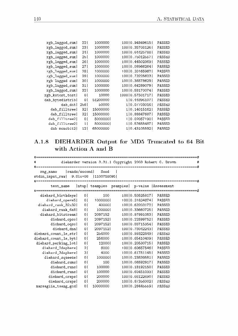
140 A. Statistical Data
rgb_lagged_sum| 22| 1000000| 100|0.94849615| PASSED
rgb_lagged_sum| 23| 1000000| 100|0.35708126| PASSED
rgb_lagged_sum| 24| 1000000| 100|0.64425788| PASSED
rgb_lagged_sum| 25| 1000000| 100|0.75012557| PASSED
rgb_lagged_sum| 26| 1000000| 100|0.44502369| PASSED
rgb_lagged_sum| 27| 1000000| 100|0.08966264| PASSED
rgb_lagged_sum| 28| 1000000| 100|0.30165962| PASSED
rgb_lagged_sum| 29| 1000000| 100|0.73225623| PASSED
rgb_lagged_sum| 30| 1000000| 100|0.36578629| PASSED
rgb_lagged_sum| 31| 1000000| 100|0.64289079| PASSED
rgb_lagged_sum| 32| 1000000| 100|0.58170074| PASSED
rgb_kstest_test| 0| 10000| 1000|0.57501717| PASSED
dab_bytedistrib| 0| 51200000| 1|0.44896107| PASSED
dab_dct| 256| 50000| 1|0.07703016| PASSED
dab_filltree| 32| 15000000| 1|0.14015162| PASSED
dab_filltree| 32| 15000000| 1|0.88847687| PASSED
dab_filltree2| 0| 5000000| 1|0.02057190| PASSED
dab_filltree2| 1| 5000000| 1|0.57655487| PASSED
dab_monobit2| 12| 65000000| 1|0.43105592| PASSED
A.1.8 DIEHARDER Output for MD5 Truncated to 64 Bit
with Action A and B
#=============================================================================#
# dieharder version 3.31.1 Copyright 2003 Robert G. Brown #
#=============================================================================#
rng_name |rands/second| Seed |
stdin_input_raw| 9.81e+06 |1100758095|
#=============================================================================#
test_name |ntup| tsamples |psamples| p-value |Assessment
#=============================================================================#
diehard_birthdays| 0| 100| 100|0.50525817| PASSED
diehard_operm5| 0| 1000000| 100|0.31834874| PASSED
diehard_rank_32x32| 0| 40000| 100|0.63203172| PASSED
diehard_rank_6x8| 0| 100000| 100|0.33660725| PASSED
diehard_bitstream| 0| 2097152| 100|0.97991083| PASSED
diehard_opso| 0| 2097152| 100|0.22599752| PASSED
diehard_oqso| 0| 2097152| 100|0.88715354| PASSED
diehard_dna| 0| 2097152| 100|0.78042243| PASSED
diehard_count_1s_str| 0| 256000| 100|0.99322849| PASSED
diehard_count_1s_byt| 0| 256000| 100|0.65410409| PASSED
diehard_parking_lot| 0| 12000| 100|0.20530715| PASSED
diehard_2dsphere| 2| 8000| 100|0.60657546| PASSED
diehard_3dsphere| 3| 4000| 100|0.61751145| PASSED
diehard_squeeze| 0| 100000| 100|0.23839581| PASSED
diehard_sums| 0| 100| 100|0.06592917| PASSED
diehard_runs| 0| 100000| 100|0.18192150| PASSED
diehard_runs| 0| 100000| 100|0.60451033| PASSED
diehard_craps| 0| 200000| 100|0.66122690| PASSED
diehard_craps| 0| 200000| 100|0.87356002| PASSED
marsaglia_tsang_gcd| 0| 10000000| 100|0.28445559| PASSED

A.1. DIEHARDER Output 141
marsaglia_tsang_gcd| 0| 10000000| 100|0.13637311| PASSED
sts_monobit| 1| 100000| 100|0.10694987| PASSED
sts_runs| 2| 100000| 100|0.80382398| PASSED
sts_serial| 1| 100000| 100|0.53670356| PASSED
sts_serial| 2| 100000| 100|0.19929105| PASSED
sts_serial| 3| 100000| 100|0.26204591| PASSED
sts_serial| 3| 100000| 100|0.47276350| PASSED
sts_serial| 4| 100000| 100|0.83527478| PASSED
sts_serial| 4| 100000| 100|0.28013217| PASSED
sts_serial| 5| 100000| 100|0.59674050| PASSED
sts_serial| 5| 100000| 100|0.76935389| PASSED
sts_serial| 6| 100000| 100|0.71519961| PASSED
sts_serial| 6| 100000| 100|0.67967410| PASSED
sts_serial| 7| 100000| 100|0.21044002| PASSED
sts_serial| 7| 100000| 100|0.23688774| PASSED
sts_serial| 8| 100000| 100|0.47761663| PASSED
sts_serial| 8| 100000| 100|0.79109088| PASSED
sts_serial| 9| 100000| 100|0.68481343| PASSED
sts_serial| 9| 100000| 100|0.83773620| PASSED
sts_serial| 10| 100000| 100|0.40829625| PASSED
sts_serial| 10| 100000| 100|0.16588511| PASSED
sts_serial| 11| 100000| 100|0.97752076| PASSED
sts_serial| 11| 100000| 100|0.73442543| PASSED
sts_serial| 12| 100000| 100|0.45139492| PASSED
sts_serial| 12| 100000| 100|0.54604718| PASSED
sts_serial| 13| 100000| 100|0.26724082| PASSED
sts_serial| 13| 100000| 100|0.18171841| PASSED
sts_serial| 14| 100000| 100|0.70894536| PASSED
sts_serial| 14| 100000| 100|0.87861382| PASSED
sts_serial| 15| 100000| 100|0.97191493| PASSED
sts_serial| 15| 100000| 100|0.99036030| PASSED
sts_serial| 16| 100000| 100|0.61777807| PASSED
sts_serial| 16| 100000| 100|0.92436906| PASSED
rgb_bitdist| 1| 100000| 100|0.89819260| PASSED
rgb_bitdist| 2| 100000| 100|0.79562213| PASSED
rgb_bitdist| 3| 100000| 100|0.65061975| PASSED
rgb_bitdist| 4| 100000| 100|0.12144714| PASSED
rgb_bitdist| 5| 100000| 100|0.75521426| PASSED
rgb_bitdist| 6| 100000| 100|0.21282015| PASSED
rgb_bitdist| 7| 100000| 100|0.24422904| PASSED
rgb_bitdist| 8| 100000| 100|0.26093073| PASSED
rgb_bitdist| 9| 100000| 100|0.40602057| PASSED
rgb_bitdist| 10| 100000| 100|0.88127755| PASSED
rgb_bitdist| 11| 100000| 100|0.41179660| PASSED
rgb_bitdist| 12| 100000| 100|0.90913111| PASSED
rgb_minimum_distance| 2| 10000| 1000|0.71493468| PASSED
rgb_minimum_distance| 3| 10000| 1000|0.75861673| PASSED
rgb_minimum_distance| 4| 10000| 1000|0.44246111| PASSED
rgb_minimum_distance| 5| 10000| 1000|0.93352135| PASSED
rgb_permutations| 2| 100000| 100|0.53497849| PASSED
rgb_permutations| 3| 100000| 100|0.36004649| PASSED
rgb_permutations| 4| 100000| 100|0.44924201| PASSED

142 A. Statistical Data
rgb_permutations| 5| 100000| 100|0.63047813| PASSED
rgb_lagged_sum| 0| 1000000| 100|0.06283839| PASSED
rgb_lagged_sum| 1| 1000000| 100|0.06016684| PASSED
rgb_lagged_sum| 2| 1000000| 100|0.53019004| PASSED
rgb_lagged_sum| 3| 1000000| 100|0.69448577| PASSED
rgb_lagged_sum| 4| 1000000| 100|0.12267992| PASSED
rgb_lagged_sum| 5| 1000000| 100|0.08147523| PASSED
rgb_lagged_sum| 6| 1000000| 100|0.61014718| PASSED
rgb_lagged_sum| 7| 1000000| 100|0.87378890| PASSED
rgb_lagged_sum| 8| 1000000| 100|0.51600498| PASSED
rgb_lagged_sum| 9| 1000000| 100|0.77141927| PASSED
rgb_lagged_sum| 10| 1000000| 100|0.99892808| WEAK
rgb_lagged_sum| 11| 1000000| 100|0.04425701| PASSED
rgb_lagged_sum| 12| 1000000| 100|0.57362538| PASSED
rgb_lagged_sum| 13| 1000000| 100|0.77055070| PASSED
rgb_lagged_sum| 14| 1000000| 100|0.25549185| PASSED
rgb_lagged_sum| 15| 1000000| 100|0.52835953| PASSED
rgb_lagged_sum| 16| 1000000| 100|0.39657587| PASSED
rgb_lagged_sum| 17| 1000000| 100|0.58960271| PASSED
rgb_lagged_sum| 18| 1000000| 100|0.48729656| PASSED
rgb_lagged_sum| 19| 1000000| 100|0.34145344| PASSED
rgb_lagged_sum| 20| 1000000| 100|0.08335533| PASSED
rgb_lagged_sum| 21| 1000000| 100|0.89207197| PASSED
rgb_lagged_sum| 22| 1000000| 100|0.04287002| PASSED
rgb_lagged_sum| 23| 1000000| 100|0.99996424| WEAK
rgb_lagged_sum| 24| 1000000| 100|0.64987237| PASSED
rgb_lagged_sum| 25| 1000000| 100|0.81568520| PASSED
rgb_lagged_sum| 26| 1000000| 100|0.38017519| PASSED
rgb_lagged_sum| 27| 1000000| 100|0.56906644| PASSED
rgb_lagged_sum| 28| 1000000| 100|0.50668373| PASSED
rgb_lagged_sum| 29| 1000000| 100|0.28199698| PASSED
rgb_lagged_sum| 30| 1000000| 100|0.96273702| PASSED
rgb_lagged_sum| 31| 1000000| 100|0.74696166| PASSED
rgb_lagged_sum| 32| 1000000| 100|0.62287764| PASSED
rgb_kstest_test| 0| 10000| 1000|0.53216782| PASSED
dab_bytedistrib| 0| 51200000| 1|0.74750108| PASSED
dab_dct| 256| 50000| 1|0.37585312| PASSED
dab_filltree| 32| 15000000| 1|0.52752830| PASSED
dab_filltree| 32| 15000000| 1|0.52302115| PASSED
dab_filltree2| 0| 5000000| 1|0.31245008| PASSED
dab_filltree2| 1| 5000000| 1|0.36479034| PASSED
dab_monobit2| 12| 65000000| 1|0.20151182| PASSED
A.2 NIST Output
This section contains the output generated by the NIST suite for di�erent algorithms.
A.2.1 NIST Output for Logistic Map
------------------------------------------------------------------------------
RESULTS FOR THE UNIFORMITY OF P-VALUES AND THE PROPORTION OF PASSING SEQUENCES
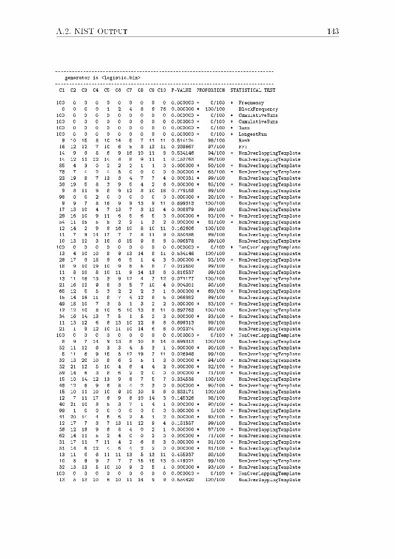
A.2. NIST Output 143
------------------------------------------------------------------------------
generator is <logistic.bin>
------------------------------------------------------------------------------
C1 C2 C3 C4 C5 C6 C7 C8 C9 C10 P-VALUE PROPORTION STATISTICAL TEST
------------------------------------------------------------------------------
100 0 0 0 0 0 0 0 0 0 0.000000 * 0/100 * Frequency
0 0 0 0 1 2 4 8 9 76 0.000000 * 100/100 BlockFrequency
100 0 0 0 0 0 0 0 0 0 0.000000 * 0/100 * CumulativeSums
100 0 0 0 0 0 0 0 0 0 0.000000 * 0/100 * CumulativeSums
100 0 0 0 0 0 0 0 0 0 0.000000 * 0/100 * Runs
100 0 0 0 0 0 0 0 0 0 0.000000 * 0/100 * LongestRun
9 10 15 8 10 14 5 7 11 11 0.514124 98/100 Rank
16 12 12 7 10 6 5 8 13 11 0.289667 97/100 FFT
14 9 9 8 6 9 16 10 11 8 0.534146 94/100 * NonOverlappingTemplate
14 12 11 12 14 8 8 9 11 1 0.153763 98/100 NonOverlappingTemplate
85 4 3 0 2 2 2 1 1 0 0.000000 * 50/100 * NonOverlappingTemplate
78 7 4 2 4 5 0 0 0 0 0.000000 * 65/100 * NonOverlappingTemplate
23 19 8 7 13 8 4 7 7 4 0.000031 * 99/100 NonOverlappingTemplate
39 19 5 8 3 9 5 4 2 6 0.000000 * 85/100 * NonOverlappingTemplate
9 8 11 9 8 9 12 8 10 16 0.779188 99/100 NonOverlappingTemplate
98 0 0 2 0 0 0 0 0 0 0.000000 * 20/100 * NonOverlappingTemplate
9 9 7 8 16 9 9 13 9 11 0.699313 100/100 NonOverlappingTemplate
17 18 10 4 7 13 7 8 12 4 0.008879 99/100 NonOverlappingTemplate
29 16 10 9 11 6 5 6 5 3 0.000000 * 93/100 * NonOverlappingTemplate
54 11 15 5 5 2 2 1 3 2 0.000000 * 81/100 * NonOverlappingTemplate
12 14 2 9 8 16 10 8 10 11 0.162606 100/100 NonOverlappingTemplate
11 7 9 14 17 7 7 8 11 9 0.350485 99/100 NonOverlappingTemplate
10 13 12 3 16 6 15 9 8 8 0.096578 99/100 NonOverlappingTemplate
100 0 0 0 0 0 0 0 0 0 0.000000 * 0/100 * NonOverlappingTemplate
13 4 10 10 8 9 13 14 8 11 0.534146 100/100 NonOverlappingTemplate
28 17 9 18 9 6 5 1 4 3 0.000000 * 93/100 * NonOverlappingTemplate
18 9 10 19 10 9 5 5 8 7 0.012650 99/100 NonOverlappingTemplate
11 8 10 8 10 11 9 14 13 6 0.816537 99/100 NonOverlappingTemplate
13 11 16 13 3 9 12 4 7 12 0.071177 100/100 NonOverlappingTemplate
21 16 12 9 8 8 5 7 10 4 0.004301 98/100 NonOverlappingTemplate
65 12 5 5 3 2 2 2 3 1 0.000000 * 69/100 * NonOverlappingTemplate
15 14 16 11 8 7 4 12 8 5 0.066882 99/100 NonOverlappingTemplate
49 18 10 7 3 5 1 3 2 2 0.000000 * 83/100 * NonOverlappingTemplate
12 12 10 8 10 6 10 13 8 11 0.897763 100/100 NonOverlappingTemplate
34 16 14 13 7 5 1 5 2 3 0.000000 * 93/100 * NonOverlappingTemplate
11 13 12 6 8 13 10 12 9 6 0.699313 99/100 NonOverlappingTemplate
21 1 9 12 10 11 10 14 6 6 0.002374 98/100 NonOverlappingTemplate
100 0 0 0 0 0 0 0 0 0 0.000000 * 0/100 * NonOverlappingTemplate
8 9 7 14 9 13 8 10 8 14 0.699313 100/100 NonOverlappingTemplate
52 11 12 6 3 3 4 5 3 1 0.000000 * 90/100 * NonOverlappingTemplate
5 11 6 9 15 5 12 19 7 11 0.026948 99/100 NonOverlappingTemplate
32 13 20 10 8 6 2 5 1 3 0.000000 * 94/100 * NonOverlappingTemplate
32 21 12 5 10 4 6 4 4 2 0.000000 * 92/100 * NonOverlappingTemplate
59 14 6 3 8 6 2 2 0 0 0.000000 * 71/100 * NonOverlappingTemplate
15 10 14 12 13 9 8 7 5 7 0.334538 100/100 NonOverlappingTemplate
48 12 6 9 8 8 4 2 3 0 0.000000 * 90/100 * NonOverlappingTemplate
15 10 11 10 10 9 10 10 9 6 0.883171 100/100 NonOverlappingTemplate
12 7 11 17 9 9 8 10 14 3 0.145326 98/100 NonOverlappingTemplate
40 21 10 8 5 3 7 1 4 1 0.000000 * 90/100 * NonOverlappingTemplate
99 1 0 0 0 0 0 0 0 0 0.000000 * 5/100 * NonOverlappingTemplate
41 20 14 4 5 6 2 5 1 2 0.000000 * 93/100 * NonOverlappingTemplate
12 17 7 8 7 13 11 12 9 4 0.181557 99/100 NonOverlappingTemplate
38 12 18 9 8 8 4 0 2 1 0.000000 * 87/100 * NonOverlappingTemplate
62 14 11 5 2 4 0 0 2 0 0.000000 * 71/100 * NonOverlappingTemplate
31 17 11 7 11 4 2 6 8 3 0.000000 * 91/100 * NonOverlappingTemplate
51 14 5 12 4 6 4 2 2 0 0.000000 * 81/100 * NonOverlappingTemplate
13 11 6 6 11 11 13 5 13 11 0.455937 98/100 NonOverlappingTemplate
10 8 9 9 7 7 7 15 15 13 0.419021 99/100 NonOverlappingTemplate
32 13 13 5 10 10 9 2 5 1 0.000000 * 93/100 * NonOverlappingTemplate
100 0 0 0 0 0 0 0 0 0 0.000000 * 0/100 * NonOverlappingTemplate
13 5 13 10 6 10 11 14 9 9 0.554420 100/100 NonOverlappingTemplate
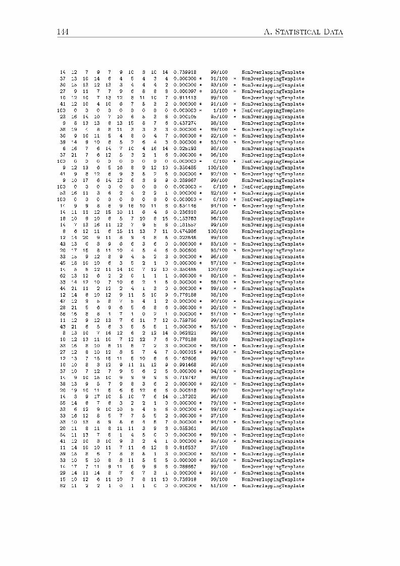
144 A. Statistical Data
14 12 7 9 7 9 10 8 10 14 0.739918 99/100 NonOverlappingTemplate
37 13 10 14 6 4 5 4 3 4 0.000000 * 91/100 * NonOverlappingTemplate
30 15 13 12 13 3 4 4 4 2 0.000000 * 93/100 * NonOverlappingTemplate
27 9 11 7 7 9 6 8 8 8 0.000097 * 93/100 * NonOverlappingTemplate
10 12 10 7 13 12 8 11 10 7 0.911413 99/100 NonOverlappingTemplate
41 12 10 4 10 6 7 5 3 2 0.000000 * 91/100 * NonOverlappingTemplate
100 0 0 0 0 0 0 0 0 0 0.000000 * 1/100 * NonOverlappingTemplate
23 16 14 10 7 10 6 5 3 6 0.000105 95/100 * NonOverlappingTemplate
9 8 13 13 8 13 15 8 7 6 0.437274 98/100 NonOverlappingTemplate
38 19 4 8 8 11 3 3 3 3 0.000000 * 89/100 * NonOverlappingTemplate
36 9 16 11 5 4 8 0 4 7 0.000000 * 92/100 * NonOverlappingTemplate
39 14 9 10 8 5 2 6 4 3 0.000000 * 83/100 * NonOverlappingTemplate
6 16 7 6 14 7 10 4 16 14 0.025193 98/100 NonOverlappingTemplate
37 21 7 6 12 5 3 2 1 6 0.000000 * 96/100 NonOverlappingTemplate
100 0 0 0 0 0 0 0 0 0 0.000000 * 0/100 * NonOverlappingTemplate
9 12 13 6 5 16 8 9 12 10 0.350485 100/100 NonOverlappingTemplate
41 9 8 12 6 9 3 5 2 5 0.000000 * 92/100 * NonOverlappingTemplate
9 10 17 6 14 12 6 8 9 9 0.289667 99/100 NonOverlappingTemplate
100 0 0 0 0 0 0 0 0 0 0.000000 * 0/100 * NonOverlappingTemplate
53 16 11 3 6 2 4 2 2 1 0.000000 * 82/100 * NonOverlappingTemplate
100 0 0 0 0 0 0 0 0 0 0.000000 * 0/100 * NonOverlappingTemplate
14 9 9 8 6 9 16 10 11 8 0.534146 94/100 * NonOverlappingTemplate
14 11 11 12 15 10 11 6 4 6 0.236810 98/100 NonOverlappingTemplate
18 10 9 10 8 5 7 10 8 15 0.153763 96/100 NonOverlappingTemplate
14 7 13 16 11 12 7 9 5 6 0.181557 99/100 NonOverlappingTemplate
8 6 12 11 6 15 11 13 7 11 0.474986 100/100 NonOverlappingTemplate
12 14 20 9 11 8 9 4 8 5 0.023545 99/100 NonOverlappingTemplate
43 13 6 8 9 6 6 3 6 0 0.000000 * 83/100 * NonOverlappingTemplate
20 17 15 8 11 10 4 5 4 6 0.000600 95/100 * NonOverlappingTemplate
33 15 9 12 8 9 4 5 2 3 0.000000 * 96/100 NonOverlappingTemplate
45 18 10 10 6 3 5 2 1 0 0.000000 * 87/100 * NonOverlappingTemplate
14 5 5 12 11 14 10 7 12 10 0.350485 100/100 NonOverlappingTemplate
62 13 12 6 2 2 0 1 1 1 0.000000 * 80/100 * NonOverlappingTemplate
33 14 12 10 7 10 6 2 1 5 0.000000 * 88/100 * NonOverlappingTemplate
44 21 11 2 12 2 4 1 3 0 0.000000 * 89/100 * NonOverlappingTemplate
12 14 8 10 12 9 11 5 10 9 0.779188 98/100 NonOverlappingTemplate
47 12 9 5 8 7 5 4 1 2 0.000000 * 90/100 * NonOverlappingTemplate
28 21 5 6 9 6 5 6 8 6 0.000000 * 90/100 * NonOverlappingTemplate
56 16 8 8 1 7 1 0 2 1 0.000000 * 81/100 * NonOverlappingTemplate
11 12 9 12 13 7 6 11 7 12 0.759756 99/100 NonOverlappingTemplate
43 21 6 5 6 3 5 5 5 1 0.000000 * 85/100 * NonOverlappingTemplate
8 13 10 7 16 12 6 2 12 14 0.062821 99/100 NonOverlappingTemplate
10 12 13 11 10 7 12 12 7 6 0.779188 98/100 NonOverlappingTemplate
33 16 8 10 5 11 5 7 2 3 0.000000 * 88/100 * NonOverlappingTemplate
27 12 8 10 12 8 5 7 4 7 0.000015 * 94/100 * NonOverlappingTemplate
12 13 7 15 15 11 5 10 6 6 0.162606 99/100 NonOverlappingTemplate
10 10 8 8 12 9 11 11 12 9 0.991468 98/100 NonOverlappingTemplate
37 10 7 12 7 9 5 6 2 5 0.000000 * 94/100 * NonOverlappingTemplate
14 9 10 15 10 9 9 9 9 6 0.719747 98/100 NonOverlappingTemplate
38 13 9 5 7 9 8 3 6 2 0.000000 * 92/100 * NonOverlappingTemplate
20 19 10 11 5 6 5 12 6 6 0.000818 99/100 NonOverlappingTemplate
14 8 9 17 10 5 10 7 6 14 0.137282 96/100 NonOverlappingTemplate
55 14 8 7 8 3 2 2 1 0 0.000000 * 79/100 * NonOverlappingTemplate
33 6 12 9 10 10 5 4 5 6 0.000000 * 89/100 * NonOverlappingTemplate
33 16 12 8 5 7 7 5 5 2 0.000000 * 97/100 NonOverlappingTemplate
33 10 13 8 9 5 6 4 5 7 0.000000 * 94/100 * NonOverlappingTemplate
20 11 8 11 8 11 11 3 9 8 0.055361 96/100 NonOverlappingTemplate
54 11 13 7 5 1 4 5 0 0 0.000000 * 89/100 * NonOverlappingTemplate
41 12 10 8 10 9 3 2 4 1 0.000000 * 95/100 * NonOverlappingTemplate
11 14 10 10 11 7 11 6 12 8 0.816537 97/100 NonOverlappingTemplate
39 15 8 6 7 8 8 5 1 3 0.000000 * 85/100 * NonOverlappingTemplate
33 10 5 10 8 8 11 5 5 5 0.000000 * 95/100 * NonOverlappingTemplate
14 17 7 11 9 11 5 9 9 8 0.289667 99/100 NonOverlappingTemplate
29 14 11 14 8 7 6 7 3 1 0.000000 * 91/100 * NonOverlappingTemplate
15 10 12 6 11 10 7 8 11 10 0.739918 99/100 NonOverlappingTemplate
82 11 2 2 1 0 1 1 0 0 0.000000 * 51/100 * NonOverlappingTemplate
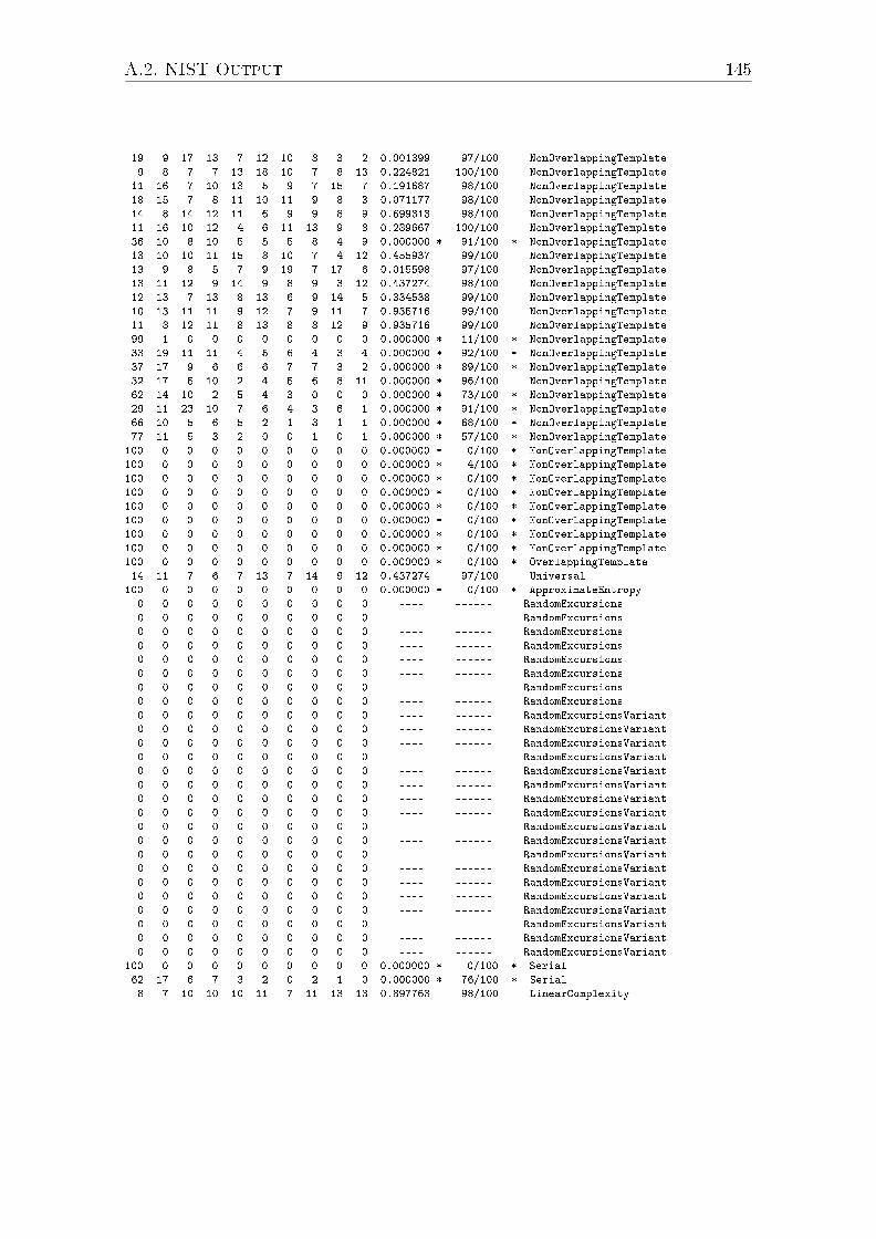
A.2. NIST Output 145
19 9 17 13 7 12 10 8 3 2 0.001399 97/100 NonOverlappingTemplate
9 8 7 7 13 18 10 7 8 13 0.224821 100/100 NonOverlappingTemplate
11 16 7 10 13 5 9 7 15 7 0.191687 98/100 NonOverlappingTemplate
18 15 7 8 11 10 11 9 8 3 0.071177 98/100 NonOverlappingTemplate
14 8 14 12 11 6 9 9 8 9 0.699313 98/100 NonOverlappingTemplate
11 16 10 12 4 6 11 13 9 8 0.289667 100/100 NonOverlappingTemplate
36 10 8 10 5 5 5 8 4 9 0.000000 * 91/100 * NonOverlappingTemplate
13 10 10 11 15 8 10 7 4 12 0.455937 99/100 NonOverlappingTemplate
13 9 8 5 7 9 19 7 17 6 0.015598 97/100 NonOverlappingTemplate
13 11 12 9 14 9 8 9 3 12 0.437274 98/100 NonOverlappingTemplate
12 13 7 13 8 13 6 9 14 5 0.334538 99/100 NonOverlappingTemplate
10 13 11 11 9 12 7 9 11 7 0.935716 99/100 NonOverlappingTemplate
11 8 12 11 8 13 8 8 12 9 0.935716 99/100 NonOverlappingTemplate
99 1 0 0 0 0 0 0 0 0 0.000000 * 11/100 * NonOverlappingTemplate
33 19 11 11 4 5 6 4 3 4 0.000000 * 92/100 * NonOverlappingTemplate
37 17 9 6 6 6 7 7 3 2 0.000000 * 89/100 * NonOverlappingTemplate
32 17 5 10 2 4 5 6 8 11 0.000000 * 96/100 NonOverlappingTemplate
62 14 10 2 5 4 3 0 0 0 0.000000 * 73/100 * NonOverlappingTemplate
29 11 23 10 7 6 4 3 6 1 0.000000 * 91/100 * NonOverlappingTemplate
66 10 5 6 5 2 1 3 1 1 0.000000 * 68/100 * NonOverlappingTemplate
77 11 5 3 2 0 0 1 0 1 0.000000 * 57/100 * NonOverlappingTemplate
100 0 0 0 0 0 0 0 0 0 0.000000 * 0/100 * NonOverlappingTemplate
100 0 0 0 0 0 0 0 0 0 0.000000 * 4/100 * NonOverlappingTemplate
100 0 0 0 0 0 0 0 0 0 0.000000 * 0/100 * NonOverlappingTemplate
100 0 0 0 0 0 0 0 0 0 0.000000 * 0/100 * NonOverlappingTemplate
100 0 0 0 0 0 0 0 0 0 0.000000 * 0/100 * NonOverlappingTemplate
100 0 0 0 0 0 0 0 0 0 0.000000 * 0/100 * NonOverlappingTemplate
100 0 0 0 0 0 0 0 0 0 0.000000 * 0/100 * NonOverlappingTemplate
100 0 0 0 0 0 0 0 0 0 0.000000 * 0/100 * NonOverlappingTemplate
100 0 0 0 0 0 0 0 0 0 0.000000 * 0/100 * OverlappingTemplate
14 11 7 6 7 13 7 14 9 12 0.437274 97/100 Universal
100 0 0 0 0 0 0 0 0 0 0.000000 * 0/100 * ApproximateEntropy
0 0 0 0 0 0 0 0 0 0 ---- ------ RandomExcursions
0 0 0 0 0 0 0 0 0 0 ---- ------ RandomExcursions
0 0 0 0 0 0 0 0 0 0 ---- ------ RandomExcursions
0 0 0 0 0 0 0 0 0 0 ---- ------ RandomExcursions
0 0 0 0 0 0 0 0 0 0 ---- ------ RandomExcursions
0 0 0 0 0 0 0 0 0 0 ---- ------ RandomExcursions
0 0 0 0 0 0 0 0 0 0 ---- ------ RandomExcursions
0 0 0 0 0 0 0 0 0 0 ---- ------ RandomExcursions
0 0 0 0 0 0 0 0 0 0 ---- ------ RandomExcursionsVariant
0 0 0 0 0 0 0 0 0 0 ---- ------ RandomExcursionsVariant
0 0 0 0 0 0 0 0 0 0 ---- ------ RandomExcursionsVariant
0 0 0 0 0 0 0 0 0 0 ---- ------ RandomExcursionsVariant
0 0 0 0 0 0 0 0 0 0 ---- ------ RandomExcursionsVariant
0 0 0 0 0 0 0 0 0 0 ---- ------ RandomExcursionsVariant
0 0 0 0 0 0 0 0 0 0 ---- ------ RandomExcursionsVariant
0 0 0 0 0 0 0 0 0 0 ---- ------ RandomExcursionsVariant
0 0 0 0 0 0 0 0 0 0 ---- ------ RandomExcursionsVariant
0 0 0 0 0 0 0 0 0 0 ---- ------ RandomExcursionsVariant
0 0 0 0 0 0 0 0 0 0 ---- ------ RandomExcursionsVariant
0 0 0 0 0 0 0 0 0 0 ---- ------ RandomExcursionsVariant
0 0 0 0 0 0 0 0 0 0 ---- ------ RandomExcursionsVariant
0 0 0 0 0 0 0 0 0 0 ---- ------ RandomExcursionsVariant
0 0 0 0 0 0 0 0 0 0 ---- ------ RandomExcursionsVariant
0 0 0 0 0 0 0 0 0 0 ---- ------ RandomExcursionsVariant
0 0 0 0 0 0 0 0 0 0 ---- ------ RandomExcursionsVariant
0 0 0 0 0 0 0 0 0 0 ---- ------ RandomExcursionsVariant
100 0 0 0 0 0 0 0 0 0 0.000000 * 0/100 * Serial
62 17 6 7 3 2 0 2 1 0 0.000000 * 76/100 * Serial
8 7 10 10 10 11 7 11 13 13 0.897763 98/100 LinearComplexity
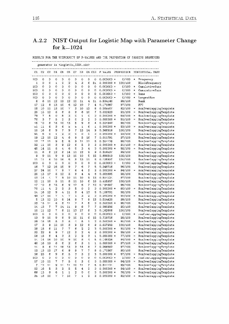
146 A. Statistical Data
A.2.2 NIST Output for Logistic Map with Parameter Change
for k=1024------------------------------------------------------------------------------
RESULTS FOR THE UNIFORMITY OF P-VALUES AND THE PROPORTION OF PASSING SEQUENCES
------------------------------------------------------------------------------
generator is <logistic_1024.bin>
------------------------------------------------------------------------------
C1 C2 C3 C4 C5 C6 C7 C8 C9 C10 P-VALUE PROPORTION STATISTICAL TEST
------------------------------------------------------------------------------
100 0 0 0 0 0 0 0 0 0 0.000000 * 0/100 * Frequency
1 0 0 1 2 2 4 3 6 81 0.000000 * 100/100 BlockFrequency
100 0 0 0 0 0 0 0 0 0 0.000000 * 0/100 * CumulativeSums
100 0 0 0 0 0 0 0 0 0 0.000000 * 0/100 * CumulativeSums
100 0 0 0 0 0 0 0 0 0 0.000000 * 0/100 * Runs
100 0 0 0 0 0 0 0 0 0 0.000000 * 0/100 * LongestRun
8 6 11 12 13 12 12 11 4 11 0.534146 99/100 Rank
17 12 9 13 10 6 12 10 7 4 0.171867 97/100 FFT
18 10 11 13 10 7 3 10 12 6 0.085587 92/100 * NonOverlappingTemplate
20 15 12 8 6 8 8 6 10 7 0.032923 93/100 * NonOverlappingTemplate
79 7 5 0 5 3 0 1 0 0 0.000000 * 59/100 * NonOverlappingTemplate
76 3 7 5 2 3 0 2 2 0 0.000000 * 55/100 * NonOverlappingTemplate
15 10 8 18 10 13 5 9 8 4 0.051942 98/100 NonOverlappingTemplate
51 11 6 8 6 5 5 1 6 1 0.000000 * 83/100 * NonOverlappingTemplate
10 16 6 9 7 9 7 13 14 9 0.366918 100/100 NonOverlappingTemplate
91 6 0 1 2 0 0 0 0 0 0.000000 * 23/100 * NonOverlappingTemplate
19 12 10 12 4 6 9 5 16 7 0.011791 97/100 NonOverlappingTemplate
12 17 11 9 5 6 9 11 12 8 0.304126 98/100 NonOverlappingTemplate
33 11 10 8 9 12 6 5 3 3 0.000000 * 91/100 * NonOverlappingTemplate
45 14 11 8 4 6 5 3 4 0 0.000000 * 88/100 * NonOverlappingTemplate
11 6 8 12 8 14 11 12 9 9 0.816537 99/100 NonOverlappingTemplate
9 9 11 9 9 13 10 10 5 15 0.699313 100/100 NonOverlappingTemplate
11 11 6 10 16 6 8 13 11 8 0.455937 100/100 NonOverlappingTemplate
100 0 0 0 0 0 0 0 0 0 0.000000 * 0/100 * NonOverlappingTemplate
16 7 12 16 15 9 7 6 7 5 0.048716 96/100 NonOverlappingTemplate
27 24 10 7 9 7 6 4 3 3 0.000000 * 94/100 * NonOverlappingTemplate
20 13 17 8 12 8 8 4 4 6 0.001895 98/100 NonOverlappingTemplate
13 14 4 7 9 10 11 10 9 13 0.514124 97/100 NonOverlappingTemplate
12 11 10 5 11 8 11 10 6 16 0.455937 100/100 NonOverlappingTemplate
17 10 8 15 6 9 12 6 7 10 0.191687 96/100 NonOverlappingTemplate
70 11 4 2 3 3 5 0 2 0 0.000000 * 68/100 * NonOverlappingTemplate
14 16 12 9 4 11 9 4 13 8 0.108791 98/100 NonOverlappingTemplate
49 17 10 7 4 7 1 3 2 0 0.000000 * 80/100 * NonOverlappingTemplate
5 13 12 10 8 14 9 7 9 13 0.554420 99/100 NonOverlappingTemplate
33 15 14 8 8 11 2 4 5 0 0.000000 * 96/100 NonOverlappingTemplate
14 18 7 7 14 11 9 6 7 7 0.090936 98/100 NonOverlappingTemplate
10 11 12 7 8 11 13 17 8 3 0.162606 100/100 NonOverlappingTemplate
100 0 0 0 0 0 0 0 0 0 0.000000 * 0/100 * NonOverlappingTemplate
13 9 10 9 8 9 10 11 6 15 0.759756 98/100 NonOverlappingTemplate
39 18 15 5 3 8 4 5 1 2 0.000000 * 90/100 * NonOverlappingTemplate
17 8 9 10 10 8 9 12 8 9 0.657933 100/100 NonOverlappingTemplate
38 18 6 11 7 7 6 2 2 3 0.000000 * 95/100 * NonOverlappingTemplate
32 22 6 9 7 12 3 2 4 3 0.000000 * 89/100 * NonOverlappingTemplate
58 18 6 4 3 3 2 2 3 1 0.000000 * 77/100 * NonOverlappingTemplate
14 14 16 10 10 9 10 8 4 5 0.145326 94/100 * NonOverlappingTemplate
46 16 13 6 6 2 6 3 1 1 0.000000 * 87/100 * NonOverlappingTemplate
14 8 6 11 16 13 3 14 8 7 0.066882 97/100 NonOverlappingTemplate
13 13 13 17 6 9 9 7 7 6 0.171867 98/100 NonOverlappingTemplate
38 23 6 9 8 5 3 3 2 3 0.000000 * 87/100 * NonOverlappingTemplate
100 0 0 0 0 0 0 0 0 0 0.000000 * 2/100 * NonOverlappingTemplate
57 10 11 7 7 5 0 3 0 0 0.000000 * 84/100 * NonOverlappingTemplate
7 12 14 9 14 11 10 11 7 5 0.514124 99/100 NonOverlappingTemplate
52 16 5 8 3 5 5 4 2 0 0.000000 * 84/100 * NonOverlappingTemplate
68 13 9 6 1 1 2 0 0 0 0.000000 * 76/100 * NonOverlappingTemplate
35 18 10 7 7 10 7 1 2 3 0.000000 * 92/100 * NonOverlappingTemplate

A.2. NIST Output 147
58 10 8 11 2 6 2 0 1 2 0.000000 * 80/100 * NonOverlappingTemplate
13 7 8 12 7 15 17 6 9 6 0.115387 98/100 NonOverlappingTemplate
13 12 11 8 13 10 6 12 7 8 0.739918 100/100 NonOverlappingTemplate
25 14 12 17 5 7 4 7 5 4 0.000002 * 97/100 NonOverlappingTemplate
100 0 0 0 0 0 0 0 0 0 0.000000 * 0/100 * NonOverlappingTemplate
11 5 13 10 7 10 9 12 10 13 0.759756 99/100 NonOverlappingTemplate
8 12 15 11 13 6 14 10 5 6 0.236810 98/100 NonOverlappingTemplate
23 16 15 13 6 5 12 4 3 3 0.000004 * 98/100 NonOverlappingTemplate
38 14 12 9 4 6 6 6 4 1 0.000000 * 91/100 * NonOverlappingTemplate
25 11 18 9 8 11 3 7 7 1 0.000001 * 99/100 NonOverlappingTemplate
8 14 9 10 10 22 8 5 3 11 0.003712 99/100 NonOverlappingTemplate
38 14 15 5 8 4 6 5 5 0 0.000000 * 90/100 * NonOverlappingTemplate
100 0 0 0 0 0 0 0 0 0 0.000000 * 0/100 * NonOverlappingTemplate
28 16 15 9 4 3 6 5 8 6 0.000000 * 96/100 NonOverlappingTemplate
8 11 14 8 6 7 10 13 13 10 0.657933 99/100 NonOverlappingTemplate
47 14 10 7 4 3 6 5 4 0 0.000000 * 88/100 * NonOverlappingTemplate
35 13 15 10 5 6 7 1 4 4 0.000000 * 92/100 * NonOverlappingTemplate
48 15 12 6 7 4 2 3 3 0 0.000000 * 81/100 * NonOverlappingTemplate
11 12 6 5 16 7 12 9 10 12 0.350485 98/100 NonOverlappingTemplate
37 11 11 9 8 6 5 3 8 2 0.000000 * 88/100 * NonOverlappingTemplate
100 0 0 0 0 0 0 0 0 0 0.000000 * 0/100 * NonOverlappingTemplate
10 12 8 7 7 12 10 12 10 12 0.924076 99/100 NonOverlappingTemplate
40 20 8 8 6 4 5 1 4 4 0.000000 * 89/100 * NonOverlappingTemplate
9 12 12 10 5 11 7 13 11 10 0.798139 99/100 NonOverlappingTemplate
100 0 0 0 0 0 0 0 0 0 0.000000 * 0/100 * NonOverlappingTemplate
59 12 12 5 2 2 4 2 1 1 0.000000 * 83/100 * NonOverlappingTemplate
100 0 0 0 0 0 0 0 0 0 0.000000 * 0/100 * NonOverlappingTemplate
18 10 11 13 10 7 3 10 12 6 0.085587 92/100 * NonOverlappingTemplate
16 11 10 7 11 7 12 8 9 9 0.678686 99/100 NonOverlappingTemplate
12 18 7 9 6 7 11 11 7 12 0.224821 97/100 NonOverlappingTemplate
9 18 12 14 11 8 15 5 4 4 0.011791 100/100 NonOverlappingTemplate
9 9 6 14 11 15 9 10 4 13 0.304126 100/100 NonOverlappingTemplate
16 18 12 10 16 5 6 6 7 4 0.003996 100/100 NonOverlappingTemplate
40 15 13 8 8 9 3 3 0 1 0.000000 * 88/100 * NonOverlappingTemplate
28 17 11 7 6 10 7 7 4 3 0.000000 * 91/100 * NonOverlappingTemplate
24 18 9 9 5 9 8 10 4 4 0.000034 * 99/100 NonOverlappingTemplate
50 17 7 8 7 5 2 3 0 1 0.000000 * 84/100 * NonOverlappingTemplate
7 12 7 7 11 9 17 14 11 5 0.191687 99/100 NonOverlappingTemplate
64 13 6 2 6 2 5 1 1 0 0.000000 * 76/100 * NonOverlappingTemplate
24 12 11 15 11 6 10 1 8 2 0.000011 * 96/100 NonOverlappingTemplate
32 19 14 9 8 5 6 5 2 0 0.000000 * 90/100 * NonOverlappingTemplate
16 11 9 15 6 7 6 9 14 7 0.162606 99/100 NonOverlappingTemplate
44 18 11 8 5 4 4 4 2 0 0.000000 * 85/100 * NonOverlappingTemplate
27 10 9 11 10 9 6 8 4 6 0.000034 * 94/100 * NonOverlappingTemplate
65 14 3 6 4 2 2 2 1 1 0.000000 * 78/100 * NonOverlappingTemplate
5 10 4 14 12 9 14 7 17 8 0.066882 99/100 NonOverlappingTemplate
44 21 8 9 4 3 4 5 2 0 0.000000 * 92/100 * NonOverlappingTemplate
6 7 10 13 9 15 8 13 12 7 0.474986 99/100 NonOverlappingTemplate
20 11 4 16 12 6 6 9 9 7 0.008879 98/100 NonOverlappingTemplate
36 19 12 9 9 4 3 2 3 3 0.000000 * 89/100 * NonOverlappingTemplate
36 16 15 7 7 7 4 3 3 2 0.000000 * 90/100 * NonOverlappingTemplate
17 9 11 12 9 7 11 9 11 4 0.319084 98/100 NonOverlappingTemplate
8 11 12 15 7 4 11 9 10 13 0.437274 100/100 NonOverlappingTemplate
38 18 5 12 6 7 7 1 4 2 0.000000 * 87/100 * NonOverlappingTemplate
8 12 15 9 4 11 11 10 11 9 0.595549 100/100 NonOverlappingTemplate
35 15 7 11 6 10 6 6 4 0 0.000000 * 91/100 * NonOverlappingTemplate
16 19 11 9 12 10 12 1 7 3 0.001628 96/100 NonOverlappingTemplate
13 14 13 7 9 12 15 4 8 5 0.129620 98/100 NonOverlappingTemplate
60 5 17 4 8 3 1 1 1 0 0.000000 * 76/100 * NonOverlappingTemplate
35 16 11 9 6 7 6 4 3 3 0.000000 * 92/100 * NonOverlappingTemplate
28 14 8 11 12 8 7 5 4 3 0.000000 * 90/100 * NonOverlappingTemplate
28 18 11 10 7 7 8 5 5 1 0.000000 * 94/100 * NonOverlappingTemplate
15 7 17 14 6 12 7 9 10 3 0.037566 95/100 * NonOverlappingTemplate
57 14 9 6 3 3 6 0 1 1 0.000000 * 72/100 * NonOverlappingTemplate
36 14 12 7 5 7 8 1 6 4 0.000000 * 90/100 * NonOverlappingTemplate
10 7 10 9 11 11 11 8 14 9 0.946308 97/100 NonOverlappingTemplate

148 A. Statistical Data
36 10 13 9 8 4 4 5 9 2 0.000000 * 91/100 * NonOverlappingTemplate
22 20 13 9 9 11 5 4 3 4 0.000007 * 97/100 NonOverlappingTemplate
16 17 8 12 8 5 5 9 14 6 0.035174 98/100 NonOverlappingTemplate
29 19 10 11 7 5 6 7 2 4 0.000000 * 93/100 * NonOverlappingTemplate
6 16 13 7 7 8 12 6 11 14 0.213309 99/100 NonOverlappingTemplate
86 4 4 5 1 0 0 0 0 0 0.000000 * 42/100 * NonOverlappingTemplate
23 10 16 11 9 9 7 9 2 4 0.000216 96/100 NonOverlappingTemplate
6 8 4 15 8 15 14 8 12 10 0.145326 100/100 NonOverlappingTemplate
13 10 10 12 10 10 9 7 8 11 0.971699 98/100 NonOverlappingTemplate
11 7 14 18 4 10 8 12 8 8 0.115387 99/100 NonOverlappingTemplate
6 15 11 13 8 9 10 14 10 4 0.289667 99/100 NonOverlappingTemplate
10 12 8 11 5 11 10 14 12 7 0.699313 98/100 NonOverlappingTemplate
28 16 11 11 8 5 7 6 5 3 0.000000 * 93/100 * NonOverlappingTemplate
13 10 10 10 6 8 13 12 11 7 0.816537 99/100 NonOverlappingTemplate
13 8 10 9 13 7 12 15 8 5 0.437274 99/100 NonOverlappingTemplate
12 8 16 10 11 4 10 7 12 10 0.401199 98/100 NonOverlappingTemplate
21 10 11 6 8 7 10 11 10 6 0.051942 99/100 NonOverlappingTemplate
6 13 11 8 7 12 13 10 12 8 0.739918 100/100 NonOverlappingTemplate
9 9 11 12 11 9 11 8 11 9 0.996335 100/100 NonOverlappingTemplate
98 1 1 0 0 0 0 0 0 0 0.000000 * 12/100 * NonOverlappingTemplate
31 18 9 5 6 5 12 8 1 5 0.000000 * 91/100 * NonOverlappingTemplate
36 21 10 9 6 6 3 4 3 2 0.000000 * 91/100 * NonOverlappingTemplate
28 10 11 10 7 5 9 11 4 5 0.000003 * 98/100 NonOverlappingTemplate
72 9 9 4 1 0 3 1 0 1 0.000000 * 60/100 * NonOverlappingTemplate
32 15 9 8 10 3 6 10 2 5 0.000000 * 95/100 * NonOverlappingTemplate
62 14 7 2 4 7 3 0 0 1 0.000000 * 71/100 * NonOverlappingTemplate
69 14 5 5 2 2 2 1 0 0 0.000000 * 62/100 * NonOverlappingTemplate
100 0 0 0 0 0 0 0 0 0 0.000000 * 0/100 * NonOverlappingTemplate
100 0 0 0 0 0 0 0 0 0 0.000000 * 4/100 * NonOverlappingTemplate
100 0 0 0 0 0 0 0 0 0 0.000000 * 0/100 * NonOverlappingTemplate
100 0 0 0 0 0 0 0 0 0 0.000000 * 0/100 * NonOverlappingTemplate
100 0 0 0 0 0 0 0 0 0 0.000000 * 0/100 * NonOverlappingTemplate
100 0 0 0 0 0 0 0 0 0 0.000000 * 0/100 * NonOverlappingTemplate
100 0 0 0 0 0 0 0 0 0 0.000000 * 0/100 * NonOverlappingTemplate
100 0 0 0 0 0 0 0 0 0 0.000000 * 0/100 * NonOverlappingTemplate
100 0 0 0 0 0 0 0 0 0 0.000000 * 0/100 * OverlappingTemplate
13 8 12 16 7 9 11 9 8 7 0.554420 98/100 Universal
100 0 0 0 0 0 0 0 0 0 0.000000 * 0/100 * ApproximateEntropy
0 0 0 0 0 0 0 0 0 0 ---- ------ RandomExcursions
0 0 0 0 0 0 0 0 0 0 ---- ------ RandomExcursions
0 0 0 0 0 0 0 0 0 0 ---- ------ RandomExcursions
0 0 0 0 0 0 0 0 0 0 ---- ------ RandomExcursions
0 0 0 0 0 0 0 0 0 0 ---- ------ RandomExcursions
0 0 0 0 0 0 0 0 0 0 ---- ------ RandomExcursions
0 0 0 0 0 0 0 0 0 0 ---- ------ RandomExcursions
0 0 0 0 0 0 0 0 0 0 ---- ------ RandomExcursions
0 0 0 0 0 0 0 0 0 0 ---- ------ RandomExcursionsVariant
0 0 0 0 0 0 0 0 0 0 ---- ------ RandomExcursionsVariant
0 0 0 0 0 0 0 0 0 0 ---- ------ RandomExcursionsVariant
0 0 0 0 0 0 0 0 0 0 ---- ------ RandomExcursionsVariant
0 0 0 0 0 0 0 0 0 0 ---- ------ RandomExcursionsVariant
0 0 0 0 0 0 0 0 0 0 ---- ------ RandomExcursionsVariant
0 0 0 0 0 0 0 0 0 0 ---- ------ RandomExcursionsVariant
0 0 0 0 0 0 0 0 0 0 ---- ------ RandomExcursionsVariant
0 0 0 0 0 0 0 0 0 0 ---- ------ RandomExcursionsVariant
0 0 0 0 0 0 0 0 0 0 ---- ------ RandomExcursionsVariant
0 0 0 0 0 0 0 0 0 0 ---- ------ RandomExcursionsVariant
0 0 0 0 0 0 0 0 0 0 ---- ------ RandomExcursionsVariant
0 0 0 0 0 0 0 0 0 0 ---- ------ RandomExcursionsVariant
0 0 0 0 0 0 0 0 0 0 ---- ------ RandomExcursionsVariant
0 0 0 0 0 0 0 0 0 0 ---- ------ RandomExcursionsVariant
0 0 0 0 0 0 0 0 0 0 ---- ------ RandomExcursionsVariant
0 0 0 0 0 0 0 0 0 0 ---- ------ RandomExcursionsVariant
0 0 0 0 0 0 0 0 0 0 ---- ------ RandomExcursionsVariant
100 0 0 0 0 0 0 0 0 0 0.000000 * 0/100 * Serial
68 14 6 7 1 3 1 0 0 0 0.000000 * 71/100 * Serial
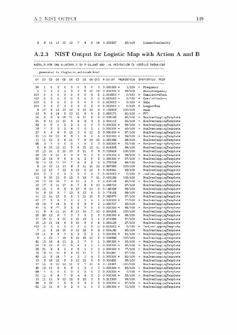
A.2. NIST Output 149
9 9 14 13 10 12 7 4 8 14 0.383827 98/100 LinearComplexity
A.2.3 NIST Output for Logistic Map with Action A and B------------------------------------------------------------------------------
RESULTS FOR THE UNIFORMITY OF P-VALUES AND THE PROPORTION OF PASSING SEQUENCES
------------------------------------------------------------------------------
generator is <logistic_actionab.bin>
------------------------------------------------------------------------------
C1 C2 C3 C4 C5 C6 C7 C8 C9 C10 P-VALUE PROPORTION STATISTICAL TEST
------------------------------------------------------------------------------
99 1 0 0 0 0 0 0 0 0 0.000000 * 1/100 * Frequency
1 0 2 0 2 2 3 6 10 74 0.000000 * 99/100 BlockFrequency
100 0 0 0 0 0 0 0 0 0 0.000000 * 0/100 * CumulativeSums
100 0 0 0 0 0 0 0 0 0 0.000000 * 0/100 * CumulativeSums
100 0 0 0 0 0 0 0 0 0 0.000000 * 0/100 * Runs
100 0 0 0 0 0 0 0 0 0 0.000000 * 0/100 * LongestRun
6 10 6 13 13 12 9 10 12 9 0.739918 100/100 Rank
13 9 9 14 8 10 12 8 8 9 0.883171 95/100 * FFT
20 6 8 9 15 11 9 11 5 6 0.025193 95/100 * NonOverlappingTemplate
24 6 11 11 12 8 9 9 4 6 0.001112 95/100 * NonOverlappingTemplate
82 5 5 1 2 2 2 1 0 0 0.000000 * 59/100 * NonOverlappingTemplate
79 7 3 2 2 4 0 0 2 1 0.000000 * 58/100 * NonOverlappingTemplate
27 8 9 9 9 13 3 8 12 2 0.000003 * 97/100 NonOverlappingTemplate
41 13 10 12 5 6 1 6 2 4 0.000000 * 89/100 * NonOverlappingTemplate
11 11 14 2 9 11 7 9 13 13 0.262249 99/100 NonOverlappingTemplate
95 3 1 0 0 0 1 0 0 0 0.000000 * 25/100 * NonOverlappingTemplate
6 9 12 12 12 5 8 12 13 11 0.616305 99/100 NonOverlappingTemplate
15 13 10 8 10 10 8 11 9 6 0.739918 100/100 NonOverlappingTemplate
28 14 9 11 8 8 6 6 4 6 0.000002 * 94/100 * NonOverlappingTemplate
35 18 13 9 6 5 4 2 5 3 0.000000 * 87/100 * NonOverlappingTemplate
15 14 13 11 12 7 9 8 5 6 0.275709 98/100 NonOverlappingTemplate
5 10 12 11 11 9 8 11 10 13 0.867692 100/100 NonOverlappingTemplate
14 12 13 7 12 8 12 5 12 5 0.319084 99/100 NonOverlappingTemplate
100 0 0 0 0 0 0 0 0 0 0.000000 * 0/100 * NonOverlappingTemplate
12 9 15 10 6 12 5 13 7 11 0.401199 100/100 NonOverlappingTemplate
22 12 12 16 7 9 12 3 3 4 0.000105 95/100 * NonOverlappingTemplate
12 17 6 11 17 6 7 9 5 10 0.048716 97/100 NonOverlappingTemplate
18 12 4 9 9 9 13 6 11 9 0.145326 99/100 NonOverlappingTemplate
14 9 13 8 7 12 9 12 8 8 0.779188 99/100 NonOverlappingTemplate
14 15 14 13 8 8 1 11 10 6 0.045675 97/100 NonOverlappingTemplate
57 17 8 5 3 4 2 1 2 1 0.000000 * 77/100 * NonOverlappingTemplate
19 19 7 14 8 9 5 9 8 2 0.000757 98/100 NonOverlappingTemplate
41 15 9 17 3 5 5 2 0 3 0.000000 * 88/100 * NonOverlappingTemplate
11 9 9 11 14 6 11 10 7 12 0.834308 100/100 NonOverlappingTemplate
35 26 12 6 7 3 3 3 2 3 0.000000 * 96/100 NonOverlappingTemplate
17 19 14 4 10 5 10 12 4 5 0.001296 97/100 NonOverlappingTemplate
15 13 11 14 9 9 10 6 9 4 0.304126 97/100 NonOverlappingTemplate
100 0 0 0 0 0 0 0 0 0 0.000000 * 0/100 * NonOverlappingTemplate
7 11 8 14 10 8 12 15 6 9 0.534146 98/100 NonOverlappingTemplate
53 11 8 9 7 2 2 5 2 1 0.000000 * 81/100 * NonOverlappingTemplate
9 5 12 7 16 4 15 16 10 6 0.026948 100/100 NonOverlappingTemplate
41 13 19 4 11 2 2 7 0 1 0.000000 * 93/100 * NonOverlappingTemplate
33 18 12 8 11 6 6 3 2 1 0.000000 * 95/100 * NonOverlappingTemplate
55 21 9 4 2 3 5 1 0 0 0.000000 * 77/100 * NonOverlappingTemplate
15 19 14 10 8 4 10 11 7 2 0.004981 97/100 NonOverlappingTemplate
43 13 8 14 7 5 3 1 4 2 0.000000 * 92/100 * NonOverlappingTemplate
13 9 16 12 8 5 12 10 9 6 0.350485 99/100 NonOverlappingTemplate
17 15 5 10 12 11 8 7 10 5 0.115387 100/100 NonOverlappingTemplate
45 12 11 9 8 9 2 3 1 0 0.000000 * 88/100 * NonOverlappingTemplate
99 1 0 0 0 0 0 0 0 0 0.000000 * 2/100 * NonOverlappingTemplate
51 11 8 4 7 6 4 4 3 2 0.000000 * 83/100 * NonOverlappingTemplate
13 11 11 9 12 12 9 15 3 5 0.213309 99/100 NonOverlappingTemplate
46 8 18 7 6 6 3 2 2 2 0.000000 * 87/100 * NonOverlappingTemplate
62 15 11 6 3 2 0 1 0 0 0.000000 * 75/100 * NonOverlappingTemplate
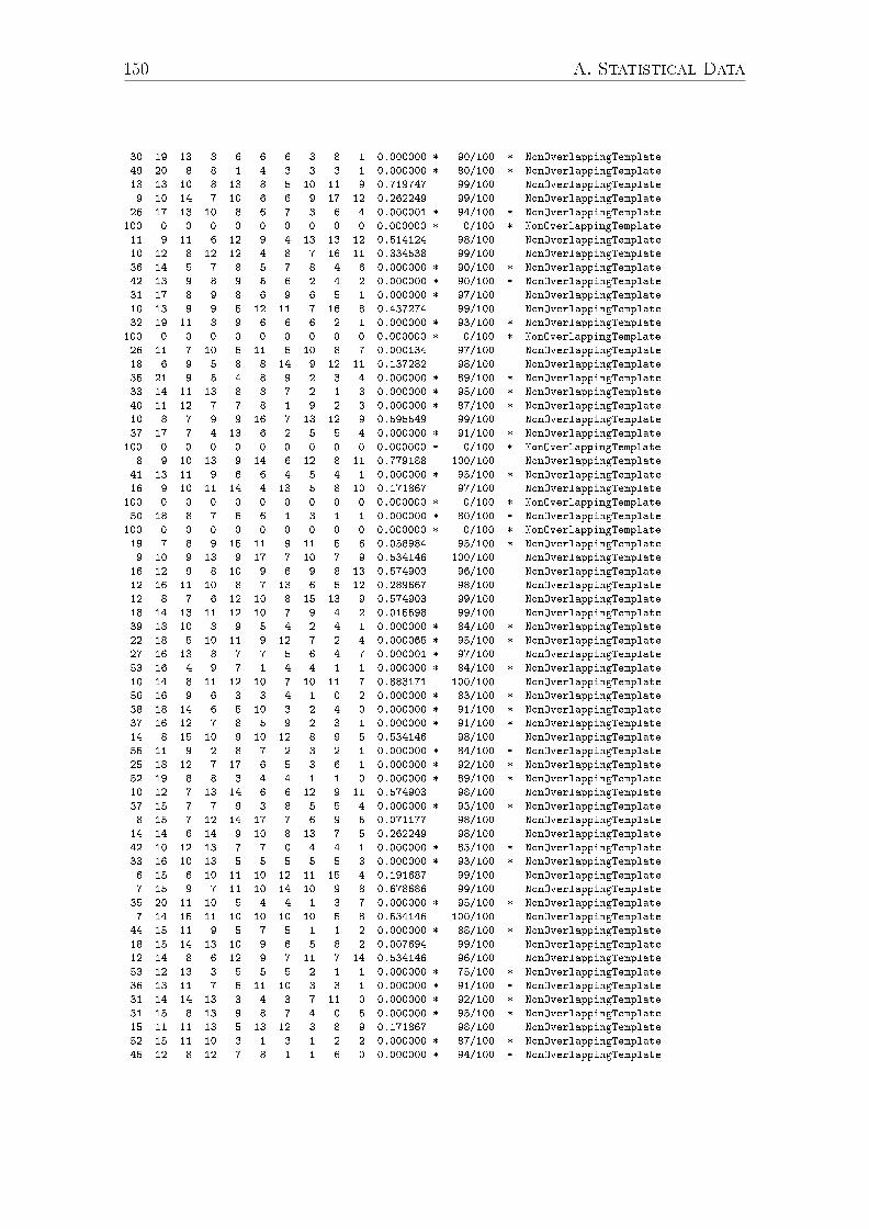
150 A. Statistical Data
30 19 13 8 6 6 6 3 8 1 0.000000 * 90/100 * NonOverlappingTemplate
49 20 8 8 1 4 3 3 3 1 0.000000 * 80/100 * NonOverlappingTemplate
13 13 10 8 13 8 5 10 11 9 0.719747 99/100 NonOverlappingTemplate
9 10 14 7 10 6 6 9 17 12 0.262249 99/100 NonOverlappingTemplate
26 17 13 10 8 6 7 3 6 4 0.000001 * 94/100 * NonOverlappingTemplate
100 0 0 0 0 0 0 0 0 0 0.000000 * 0/100 * NonOverlappingTemplate
11 9 11 6 12 9 4 13 13 12 0.514124 98/100 NonOverlappingTemplate
10 12 8 12 12 4 8 7 16 11 0.334538 99/100 NonOverlappingTemplate
36 14 5 7 8 5 7 8 4 6 0.000000 * 90/100 * NonOverlappingTemplate
42 13 9 8 9 5 6 2 4 2 0.000000 * 90/100 * NonOverlappingTemplate
31 17 8 9 8 6 9 6 5 1 0.000000 * 97/100 NonOverlappingTemplate
10 13 9 9 5 12 11 7 16 8 0.437274 99/100 NonOverlappingTemplate
32 19 11 8 9 6 6 6 2 1 0.000000 * 93/100 * NonOverlappingTemplate
100 0 0 0 0 0 0 0 0 0 0.000000 * 0/100 * NonOverlappingTemplate
26 11 7 10 5 11 5 10 8 7 0.000134 97/100 NonOverlappingTemplate
18 6 9 5 8 8 14 9 12 11 0.137282 98/100 NonOverlappingTemplate
35 21 9 5 4 8 9 2 3 4 0.000000 * 89/100 * NonOverlappingTemplate
33 14 11 13 8 8 7 2 1 3 0.000000 * 95/100 * NonOverlappingTemplate
40 11 12 7 7 8 1 9 2 3 0.000000 * 87/100 * NonOverlappingTemplate
10 8 7 9 9 16 7 13 12 9 0.595549 99/100 NonOverlappingTemplate
37 17 7 4 13 6 2 5 5 4 0.000000 * 91/100 * NonOverlappingTemplate
100 0 0 0 0 0 0 0 0 0 0.000000 * 0/100 * NonOverlappingTemplate
8 9 10 13 9 14 6 12 8 11 0.779188 100/100 NonOverlappingTemplate
41 13 11 9 6 6 4 5 4 1 0.000000 * 95/100 * NonOverlappingTemplate
16 9 10 11 14 4 13 5 8 10 0.171867 97/100 NonOverlappingTemplate
100 0 0 0 0 0 0 0 0 0 0.000000 * 0/100 * NonOverlappingTemplate
50 18 8 7 5 6 1 3 1 1 0.000000 * 80/100 * NonOverlappingTemplate
100 0 0 0 0 0 0 0 0 0 0.000000 * 0/100 * NonOverlappingTemplate
19 7 8 9 15 11 9 11 5 6 0.058984 95/100 * NonOverlappingTemplate
9 10 9 13 9 17 7 10 7 9 0.534146 100/100 NonOverlappingTemplate
16 12 9 8 10 9 6 9 8 13 0.574903 96/100 NonOverlappingTemplate
12 16 11 10 8 7 13 6 5 12 0.289667 98/100 NonOverlappingTemplate
12 8 7 6 12 10 8 15 13 9 0.574903 99/100 NonOverlappingTemplate
18 14 13 11 12 10 7 9 4 2 0.015598 99/100 NonOverlappingTemplate
39 18 10 8 9 5 4 2 4 1 0.000000 * 84/100 * NonOverlappingTemplate
22 18 5 10 11 9 12 7 2 4 0.000065 * 95/100 * NonOverlappingTemplate
27 16 13 8 7 7 5 6 4 7 0.000001 * 97/100 NonOverlappingTemplate
53 16 4 9 7 1 4 4 1 1 0.000000 * 84/100 * NonOverlappingTemplate
10 14 8 11 12 10 7 10 11 7 0.883171 100/100 NonOverlappingTemplate
56 16 9 6 3 3 4 1 0 2 0.000000 * 83/100 * NonOverlappingTemplate
38 18 14 6 5 10 3 2 4 0 0.000000 * 91/100 * NonOverlappingTemplate
37 16 12 7 8 5 9 2 3 1 0.000000 * 91/100 * NonOverlappingTemplate
14 8 15 10 9 10 12 8 9 5 0.534146 98/100 NonOverlappingTemplate
55 11 9 2 8 7 2 3 2 1 0.000000 * 84/100 * NonOverlappingTemplate
25 18 12 7 17 6 5 3 6 1 0.000000 * 92/100 * NonOverlappingTemplate
52 19 8 8 3 4 4 1 1 0 0.000000 * 89/100 * NonOverlappingTemplate
10 12 7 13 14 6 6 12 9 11 0.574903 98/100 NonOverlappingTemplate
37 15 7 7 9 3 8 5 5 4 0.000000 * 93/100 * NonOverlappingTemplate
8 15 7 12 14 17 7 6 9 5 0.071177 98/100 NonOverlappingTemplate
14 14 6 14 9 10 8 13 7 5 0.262249 98/100 NonOverlappingTemplate
42 10 12 13 7 7 0 4 4 1 0.000000 * 83/100 * NonOverlappingTemplate
33 16 10 13 5 5 5 5 5 3 0.000000 * 93/100 * NonOverlappingTemplate
6 15 6 10 11 10 12 11 15 4 0.191687 99/100 NonOverlappingTemplate
7 15 9 7 11 10 14 10 9 8 0.678686 99/100 NonOverlappingTemplate
35 20 11 10 5 4 4 1 3 7 0.000000 * 95/100 * NonOverlappingTemplate
7 14 15 11 10 10 10 10 5 8 0.534146 100/100 NonOverlappingTemplate
44 15 11 9 5 7 5 1 1 2 0.000000 * 88/100 * NonOverlappingTemplate
18 15 14 13 10 9 6 5 8 2 0.007694 99/100 NonOverlappingTemplate
12 14 8 6 12 9 7 11 7 14 0.534146 96/100 NonOverlappingTemplate
53 12 13 3 5 5 5 2 1 1 0.000000 * 75/100 * NonOverlappingTemplate
36 13 11 7 5 11 10 3 3 1 0.000000 * 91/100 * NonOverlappingTemplate
31 14 14 13 3 4 3 7 11 0 0.000000 * 92/100 * NonOverlappingTemplate
31 15 8 13 9 8 7 4 0 5 0.000000 * 95/100 * NonOverlappingTemplate
15 11 11 13 5 13 12 3 8 9 0.171867 98/100 NonOverlappingTemplate
52 15 11 10 3 1 3 1 2 2 0.000000 * 87/100 * NonOverlappingTemplate
45 12 8 12 7 8 1 1 6 0 0.000000 * 94/100 * NonOverlappingTemplate
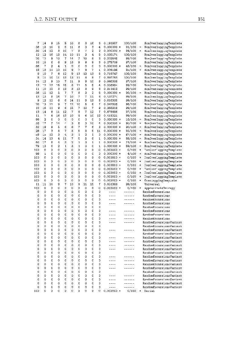
A.2. NIST Output 151
7 14 9 15 5 10 8 8 16 8 0.191687 100/100 NonOverlappingTemplate
36 18 10 2 5 11 8 3 3 4 0.000000 * 91/100 * NonOverlappingTemplate
30 14 12 8 10 7 8 7 2 2 0.000000 * 94/100 * NonOverlappingTemplate
12 12 16 13 14 10 11 3 4 5 0.035174 100/100 NonOverlappingTemplate
20 12 9 10 7 14 7 10 8 3 0.023545 98/100 NonOverlappingTemplate
16 15 6 6 9 13 9 9 9 8 0.275709 97/100 NonOverlappingTemplate
86 7 2 4 1 0 0 0 0 0 0.000000 * 48/100 * NonOverlappingTemplate
18 18 11 10 10 9 7 9 7 1 0.006196 95/100 * NonOverlappingTemplate
9 10 7 6 12 9 13 13 13 8 0.719747 100/100 NonOverlappingTemplate
8 11 10 11 13 13 11 8 8 7 0.897763 100/100 NonOverlappingTemplate
14 12 9 10 7 11 9 9 10 9 0.946308 97/100 NonOverlappingTemplate
12 12 12 16 15 8 11 5 5 4 0.058984 99/100 NonOverlappingTemplate
11 10 12 8 13 8 13 8 9 8 0.911413 99/100 NonOverlappingTemplate
36 15 12 5 7 7 8 3 2 5 0.000000 * 90/100 * NonOverlappingTemplate
13 13 8 16 7 10 7 7 11 8 0.437274 99/100 NonOverlappingTemplate
9 12 12 6 6 14 11 9 13 8 0.616305 99/100 NonOverlappingTemplate
20 13 11 9 7 12 10 5 6 7 0.042808 96/100 NonOverlappingTemplate
10 16 11 9 6 15 7 10 7 9 0.366918 99/100 NonOverlappingTemplate
13 14 8 11 12 7 9 7 12 7 0.678686 97/100 NonOverlappingTemplate
11 7 6 16 13 10 9 6 10 12 0.419021 99/100 NonOverlappingTemplate
98 2 0 0 0 0 0 0 0 0 0.000000 * 10/100 * NonOverlappingTemplate
33 17 7 14 4 3 5 3 10 4 0.000000 * 90/100 * NonOverlappingTemplate
32 19 9 5 6 6 7 7 6 3 0.000000 * 90/100 * NonOverlappingTemplate
28 17 3 8 7 8 5 8 5 11 0.000000 * 95/100 * NonOverlappingTemplate
59 15 12 3 4 3 1 2 1 0 0.000000 * 67/100 * NonOverlappingTemplate
34 14 13 4 11 7 5 5 6 1 0.000000 * 88/100 * NonOverlappingTemplate
60 17 8 4 3 2 1 3 1 1 0.000000 * 74/100 * NonOverlappingTemplate
79 13 0 2 1 3 1 0 0 1 0.000000 * 59/100 * NonOverlappingTemplate
100 0 0 0 0 0 0 0 0 0 0.000000 * 0/100 * NonOverlappingTemplate
99 1 0 0 0 0 0 0 0 0 0.000000 * 4/100 * NonOverlappingTemplate
100 0 0 0 0 0 0 0 0 0 0.000000 * 0/100 * NonOverlappingTemplate
100 0 0 0 0 0 0 0 0 0 0.000000 * 0/100 * NonOverlappingTemplate
100 0 0 0 0 0 0 0 0 0 0.000000 * 0/100 * NonOverlappingTemplate
100 0 0 0 0 0 0 0 0 0 0.000000 * 0/100 * NonOverlappingTemplate
100 0 0 0 0 0 0 0 0 0 0.000000 * 0/100 * NonOverlappingTemplate
100 0 0 0 0 0 0 0 0 0 0.000000 * 0/100 * NonOverlappingTemplate
100 0 0 0 0 0 0 0 0 0 0.000000 * 0/100 * OverlappingTemplate
11 11 10 9 7 10 9 11 15 7 0.851383 99/100 Universal
100 0 0 0 0 0 0 0 0 0 0.000000 * 0/100 * ApproximateEntropy
0 0 0 0 0 0 0 0 0 0 ---- ------ RandomExcursions
0 0 0 0 0 0 0 0 0 0 ---- ------ RandomExcursions
0 0 0 0 0 0 0 0 0 0 ---- ------ RandomExcursions
0 0 0 0 0 0 0 0 0 0 ---- ------ RandomExcursions
0 0 0 0 0 0 0 0 0 0 ---- ------ RandomExcursions
0 0 0 0 0 0 0 0 0 0 ---- ------ RandomExcursions
0 0 0 0 0 0 0 0 0 0 ---- ------ RandomExcursions
0 0 0 0 0 0 0 0 0 0 ---- ------ RandomExcursions
0 0 0 0 0 0 0 0 0 0 ---- ------ RandomExcursionsVariant
0 0 0 0 0 0 0 0 0 0 ---- ------ RandomExcursionsVariant
0 0 0 0 0 0 0 0 0 0 ---- ------ RandomExcursionsVariant
0 0 0 0 0 0 0 0 0 0 ---- ------ RandomExcursionsVariant
0 0 0 0 0 0 0 0 0 0 ---- ------ RandomExcursionsVariant
0 0 0 0 0 0 0 0 0 0 ---- ------ RandomExcursionsVariant
0 0 0 0 0 0 0 0 0 0 ---- ------ RandomExcursionsVariant
0 0 0 0 0 0 0 0 0 0 ---- ------ RandomExcursionsVariant
0 0 0 0 0 0 0 0 0 0 ---- ------ RandomExcursionsVariant
0 0 0 0 0 0 0 0 0 0 ---- ------ RandomExcursionsVariant
0 0 0 0 0 0 0 0 0 0 ---- ------ RandomExcursionsVariant
0 0 0 0 0 0 0 0 0 0 ---- ------ RandomExcursionsVariant
0 0 0 0 0 0 0 0 0 0 ---- ------ RandomExcursionsVariant
0 0 0 0 0 0 0 0 0 0 ---- ------ RandomExcursionsVariant
0 0 0 0 0 0 0 0 0 0 ---- ------ RandomExcursionsVariant
0 0 0 0 0 0 0 0 0 0 ---- ------ RandomExcursionsVariant
0 0 0 0 0 0 0 0 0 0 ---- ------ RandomExcursionsVariant
0 0 0 0 0 0 0 0 0 0 ---- ------ RandomExcursionsVariant
100 0 0 0 0 0 0 0 0 0 0.000000 * 0/100 * Serial
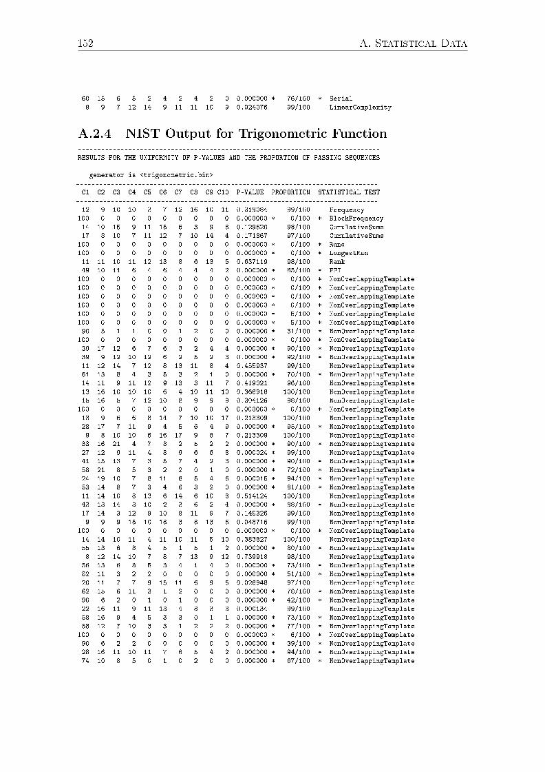
152 A. Statistical Data
60 15 6 5 2 4 2 4 2 0 0.000000 * 76/100 * Serial
8 9 7 12 14 9 11 11 10 9 0.924076 99/100 LinearComplexity
A.2.4 NIST Output for Trigonometric Function------------------------------------------------------------------------------
RESULTS FOR THE UNIFORMITY OF P-VALUES AND THE PROPORTION OF PASSING SEQUENCES
------------------------------------------------------------------------------
generator is <trigonometric.bin>
------------------------------------------------------------------------------
C1 C2 C3 C4 C5 C6 C7 C8 C9 C10 P-VALUE PROPORTION STATISTICAL TEST
------------------------------------------------------------------------------
12 9 10 10 3 7 12 16 10 11 0.319084 99/100 Frequency
100 0 0 0 0 0 0 0 0 0 0.000000 * 0/100 * BlockFrequency
14 10 15 9 11 15 6 3 9 8 0.129620 98/100 CumulativeSums
17 8 10 7 11 12 7 10 14 4 0.171867 97/100 CumulativeSums
100 0 0 0 0 0 0 0 0 0 0.000000 * 0/100 * Runs
100 0 0 0 0 0 0 0 0 0 0.000000 * 0/100 * LongestRun
11 11 10 11 12 13 8 6 13 5 0.637119 98/100 Rank
49 10 11 6 4 6 4 4 4 2 0.000000 * 85/100 * FFT
100 0 0 0 0 0 0 0 0 0 0.000000 * 0/100 * NonOverlappingTemplate
100 0 0 0 0 0 0 0 0 0 0.000000 * 0/100 * NonOverlappingTemplate
100 0 0 0 0 0 0 0 0 0 0.000000 * 0/100 * NonOverlappingTemplate
100 0 0 0 0 0 0 0 0 0 0.000000 * 0/100 * NonOverlappingTemplate
100 0 0 0 0 0 0 0 0 0 0.000000 * 5/100 * NonOverlappingTemplate
100 0 0 0 0 0 0 0 0 0 0.000000 * 5/100 * NonOverlappingTemplate
90 5 1 1 0 0 1 2 0 0 0.000000 * 31/100 * NonOverlappingTemplate
100 0 0 0 0 0 0 0 0 0 0.000000 * 0/100 * NonOverlappingTemplate
39 17 12 6 7 6 3 2 4 4 0.000000 * 90/100 * NonOverlappingTemplate
39 9 12 10 12 6 2 5 2 3 0.000000 * 92/100 * NonOverlappingTemplate
11 12 14 7 12 8 13 11 8 4 0.455937 99/100 NonOverlappingTemplate
61 13 8 4 3 5 3 2 1 0 0.000000 * 70/100 * NonOverlappingTemplate
14 11 9 11 12 9 13 3 11 7 0.419021 96/100 NonOverlappingTemplate
13 16 10 10 10 6 4 10 11 10 0.366918 100/100 NonOverlappingTemplate
15 16 5 7 12 10 8 9 9 9 0.304126 98/100 NonOverlappingTemplate
100 0 0 0 0 0 0 0 0 0 0.000000 * 0/100 * NonOverlappingTemplate
13 9 6 6 8 14 7 10 10 17 0.213309 100/100 NonOverlappingTemplate
28 17 7 11 9 4 5 6 4 9 0.000000 * 95/100 * NonOverlappingTemplate
9 8 10 10 6 16 17 9 8 7 0.213309 100/100 NonOverlappingTemplate
33 16 21 4 7 8 2 5 2 2 0.000000 * 90/100 * NonOverlappingTemplate
27 12 9 11 4 8 9 6 6 8 0.000024 * 99/100 NonOverlappingTemplate
41 15 13 7 3 5 7 4 2 3 0.000000 * 90/100 * NonOverlappingTemplate
58 21 8 5 3 2 2 0 1 0 0.000000 * 72/100 * NonOverlappingTemplate
24 19 10 7 8 11 6 5 4 6 0.000015 * 94/100 * NonOverlappingTemplate
53 14 8 7 3 4 6 3 2 0 0.000000 * 81/100 * NonOverlappingTemplate
11 14 10 8 13 6 14 6 10 8 0.514124 100/100 NonOverlappingTemplate
43 13 14 3 10 2 3 6 2 4 0.000000 * 88/100 * NonOverlappingTemplate
17 14 3 12 9 10 8 11 9 7 0.145326 99/100 NonOverlappingTemplate
9 9 9 15 10 18 3 8 13 6 0.048716 99/100 NonOverlappingTemplate
100 0 0 0 0 0 0 0 0 0 0.000000 * 0/100 * NonOverlappingTemplate
14 14 10 11 4 11 10 11 5 10 0.383827 100/100 NonOverlappingTemplate
55 13 6 8 4 5 1 5 1 2 0.000000 * 80/100 * NonOverlappingTemplate
8 12 14 10 7 8 7 13 9 12 0.739918 98/100 NonOverlappingTemplate
56 13 6 8 5 3 4 1 4 0 0.000000 * 73/100 * NonOverlappingTemplate
82 11 3 2 2 0 0 0 0 0 0.000000 * 51/100 * NonOverlappingTemplate
20 11 7 7 9 15 11 6 9 5 0.026948 97/100 NonOverlappingTemplate
62 15 6 11 3 1 2 0 0 0 0.000000 * 78/100 * NonOverlappingTemplate
90 6 2 0 1 0 1 0 0 0 0.000000 * 42/100 * NonOverlappingTemplate
22 16 11 9 11 13 4 8 3 3 0.000134 99/100 NonOverlappingTemplate
58 16 9 4 5 3 3 0 1 1 0.000000 * 73/100 * NonOverlappingTemplate
58 12 7 10 3 3 1 2 2 2 0.000000 * 77/100 * NonOverlappingTemplate
100 0 0 0 0 0 0 0 0 0 0.000000 * 6/100 * NonOverlappingTemplate
90 6 2 2 0 0 0 0 0 0 0.000000 * 39/100 * NonOverlappingTemplate
28 16 11 10 11 7 6 5 4 2 0.000000 * 94/100 * NonOverlappingTemplate
74 10 8 5 0 1 0 2 0 0 0.000000 * 67/100 * NonOverlappingTemplate
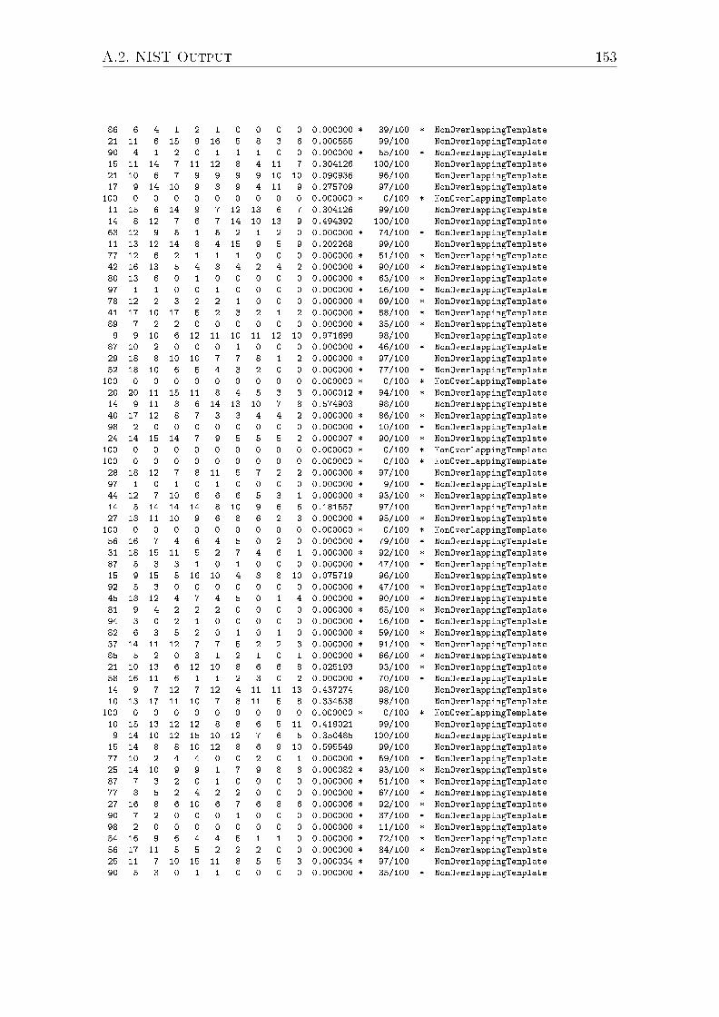
A.2. NIST Output 153
86 6 4 1 2 1 0 0 0 0 0.000000 * 39/100 * NonOverlappingTemplate
21 11 6 15 9 16 5 8 3 6 0.000555 99/100 NonOverlappingTemplate
90 4 1 2 0 1 1 1 0 0 0.000000 * 55/100 * NonOverlappingTemplate
15 11 14 7 11 12 8 4 11 7 0.304126 100/100 NonOverlappingTemplate
21 10 6 7 9 9 9 9 10 10 0.090936 96/100 NonOverlappingTemplate
17 9 14 10 9 8 9 4 11 9 0.275709 97/100 NonOverlappingTemplate
100 0 0 0 0 0 0 0 0 0 0.000000 * 0/100 * NonOverlappingTemplate
11 15 6 14 9 7 12 13 6 7 0.304126 99/100 NonOverlappingTemplate
14 8 12 7 6 7 14 10 13 9 0.494392 100/100 NonOverlappingTemplate
63 12 9 5 1 5 2 1 2 0 0.000000 * 74/100 * NonOverlappingTemplate
11 13 12 14 8 4 15 9 5 9 0.202268 99/100 NonOverlappingTemplate
77 12 6 2 1 1 1 0 0 0 0.000000 * 51/100 * NonOverlappingTemplate
42 16 13 5 4 8 4 2 4 2 0.000000 * 90/100 * NonOverlappingTemplate
80 13 6 0 1 0 0 0 0 0 0.000000 * 63/100 * NonOverlappingTemplate
97 1 1 0 0 1 0 0 0 0 0.000000 * 16/100 * NonOverlappingTemplate
78 12 2 3 2 2 1 0 0 0 0.000000 * 69/100 * NonOverlappingTemplate
41 17 10 17 5 2 3 2 1 2 0.000000 * 88/100 * NonOverlappingTemplate
89 7 2 2 0 0 0 0 0 0 0.000000 * 35/100 * NonOverlappingTemplate
9 9 10 6 12 11 10 11 12 10 0.971699 98/100 NonOverlappingTemplate
87 10 2 0 0 0 1 0 0 0 0.000000 * 46/100 * NonOverlappingTemplate
29 18 8 10 10 7 7 8 1 2 0.000000 * 97/100 NonOverlappingTemplate
52 18 10 6 5 4 3 2 0 0 0.000000 * 77/100 * NonOverlappingTemplate
100 0 0 0 0 0 0 0 0 0 0.000000 * 0/100 * NonOverlappingTemplate
20 20 11 15 11 8 4 5 3 3 0.000012 * 94/100 * NonOverlappingTemplate
14 9 11 8 6 14 13 10 7 8 0.574903 98/100 NonOverlappingTemplate
40 17 12 8 7 3 3 4 4 2 0.000000 * 86/100 * NonOverlappingTemplate
98 2 0 0 0 0 0 0 0 0 0.000000 * 10/100 * NonOverlappingTemplate
24 14 15 14 7 9 5 5 5 2 0.000007 * 90/100 * NonOverlappingTemplate
100 0 0 0 0 0 0 0 0 0 0.000000 * 0/100 * NonOverlappingTemplate
100 0 0 0 0 0 0 0 0 0 0.000000 * 0/100 * NonOverlappingTemplate
28 18 12 7 8 11 5 7 2 2 0.000000 * 97/100 NonOverlappingTemplate
97 1 0 1 0 1 0 0 0 0 0.000000 * 9/100 * NonOverlappingTemplate
44 12 7 10 6 6 6 5 3 1 0.000000 * 93/100 * NonOverlappingTemplate
14 5 14 14 14 8 10 9 6 6 0.181557 97/100 NonOverlappingTemplate
27 18 11 10 9 6 8 6 2 3 0.000000 * 95/100 * NonOverlappingTemplate
100 0 0 0 0 0 0 0 0 0 0.000000 * 0/100 * NonOverlappingTemplate
56 16 7 4 6 4 5 0 2 0 0.000000 * 79/100 * NonOverlappingTemplate
31 18 15 11 5 2 7 4 6 1 0.000000 * 92/100 * NonOverlappingTemplate
87 5 3 3 1 0 1 0 0 0 0.000000 * 47/100 * NonOverlappingTemplate
15 9 15 5 16 10 4 8 8 10 0.075719 96/100 NonOverlappingTemplate
92 5 3 0 0 0 0 0 0 0 0.000000 * 47/100 * NonOverlappingTemplate
45 18 12 4 7 4 5 0 1 4 0.000000 * 90/100 * NonOverlappingTemplate
81 9 4 2 2 2 0 0 0 0 0.000000 * 65/100 * NonOverlappingTemplate
94 3 0 2 1 0 0 0 0 0 0.000000 * 16/100 * NonOverlappingTemplate
82 6 3 5 2 0 1 0 1 0 0.000000 * 59/100 * NonOverlappingTemplate
37 14 11 12 7 7 5 2 2 3 0.000000 * 91/100 * NonOverlappingTemplate
85 5 2 0 3 1 2 1 0 1 0.000000 * 66/100 * NonOverlappingTemplate
21 10 13 6 12 10 8 6 6 8 0.025193 93/100 * NonOverlappingTemplate
58 16 11 6 1 1 2 3 0 2 0.000000 * 70/100 * NonOverlappingTemplate
14 9 7 12 7 12 4 11 11 13 0.437274 98/100 NonOverlappingTemplate
10 13 17 11 10 7 8 11 5 8 0.334538 98/100 NonOverlappingTemplate
100 0 0 0 0 0 0 0 0 0 0.000000 * 0/100 * NonOverlappingTemplate
10 15 13 12 12 8 8 6 5 11 0.419021 99/100 NonOverlappingTemplate
9 14 10 12 15 10 12 7 6 5 0.350485 100/100 NonOverlappingTemplate
15 14 8 8 10 12 8 6 9 10 0.595549 99/100 NonOverlappingTemplate
77 10 2 4 4 0 0 2 0 1 0.000000 * 59/100 * NonOverlappingTemplate
25 14 10 9 9 1 7 9 8 8 0.000082 * 93/100 * NonOverlappingTemplate
87 7 3 2 0 1 0 0 0 0 0.000000 * 51/100 * NonOverlappingTemplate
77 8 5 2 4 2 2 0 0 0 0.000000 * 67/100 * NonOverlappingTemplate
27 16 8 6 10 6 7 6 8 6 0.000006 * 92/100 * NonOverlappingTemplate
90 7 2 0 0 0 1 0 0 0 0.000000 * 37/100 * NonOverlappingTemplate
98 2 0 0 0 0 0 0 0 0 0.000000 * 11/100 * NonOverlappingTemplate
54 16 9 6 4 4 5 1 1 0 0.000000 * 72/100 * NonOverlappingTemplate
56 17 11 5 5 2 2 2 0 0 0.000000 * 84/100 * NonOverlappingTemplate
25 11 7 10 15 11 8 5 5 3 0.000034 * 97/100 NonOverlappingTemplate
90 5 3 0 1 1 0 0 0 0 0.000000 * 35/100 * NonOverlappingTemplate
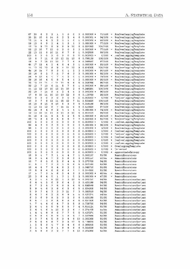
154 A. Statistical Data
67 20 6 2 3 1 1 0 0 0 0.000000 * 71/100 * NonOverlappingTemplate
20 21 15 8 14 8 2 2 4 6 0.000001 * 94/100 * NonOverlappingTemplate
73 11 5 4 2 2 1 1 0 1 0.000000 * 58/100 * NonOverlappingTemplate
59 13 8 9 2 4 1 3 1 0 0.000000 * 77/100 * NonOverlappingTemplate
12 15 9 12 8 9 8 9 10 8 0.851383 100/100 NonOverlappingTemplate
53 12 10 7 12 0 3 0 3 0 0.000000 * 77/100 * NonOverlappingTemplate
22 13 11 8 10 11 8 7 9 1 0.002559 99/100 NonOverlappingTemplate
100 0 0 0 0 0 0 0 0 0 0.000000 * 0/100 * NonOverlappingTemplate
13 8 7 11 9 10 12 11 13 6 0.798139 100/100 NonOverlappingTemplate
19 9 7 15 11 10 7 7 6 9 0.085587 97/100 NonOverlappingTemplate
44 17 13 4 2 4 8 4 3 1 0.000000 * 93/100 * NonOverlappingTemplate
14 12 10 10 8 9 4 11 13 9 0.616305 100/100 NonOverlappingTemplate
45 16 15 7 9 3 0 1 2 2 0.000000 * 90/100 * NonOverlappingTemplate
39 16 9 5 7 5 7 6 3 3 0.000000 * 88/100 * NonOverlappingTemplate
56 9 13 4 4 7 4 2 0 1 0.000000 * 79/100 * NonOverlappingTemplate
39 16 16 4 5 8 5 4 1 2 0.000000 * 90/100 * NonOverlappingTemplate
20 15 11 11 4 11 11 6 6 5 0.008266 96/100 NonOverlappingTemplate
33 12 7 10 6 11 5 7 8 1 0.000000 * 89/100 * NonOverlappingTemplate
14 12 12 10 10 13 11 10 2 6 0.249284 100/100 NonOverlappingTemplate
32 19 7 15 8 5 2 4 5 3 0.000000 * 96/100 NonOverlappingTemplate
17 6 10 11 10 10 13 12 3 8 0.153763 98/100 NonOverlappingTemplate
100 0 0 0 0 0 0 0 0 0 0.000000 * 0/100 * NonOverlappingTemplate
10 8 7 6 13 11 15 12 7 11 0.554420 100/100 NonOverlappingTemplate
15 18 9 15 9 10 5 8 3 8 0.019188 96/100 NonOverlappingTemplate
11 12 11 12 8 7 15 11 5 8 0.554420 97/100 NonOverlappingTemplate
62 14 8 4 6 2 1 1 1 1 0.000000 * 74/100 * NonOverlappingTemplate
12 13 10 11 11 8 11 8 10 6 0.911413 99/100 NonOverlappingTemplate
34 16 9 11 8 5 5 2 5 5 0.000000 * 90/100 * NonOverlappingTemplate
43 15 8 8 6 5 5 6 2 2 0.000000 * 85/100 * NonOverlappingTemplate
100 0 0 0 0 0 0 0 0 0 0.000000 * 0/100 * NonOverlappingTemplate
90 4 3 0 3 0 0 0 0 0 0.000000 * 36/100 * NonOverlappingTemplate
99 1 0 0 0 0 0 0 0 0 0.000000 * 2/100 * NonOverlappingTemplate
100 0 0 0 0 0 0 0 0 0 0.000000 * 2/100 * NonOverlappingTemplate
100 0 0 0 0 0 0 0 0 0 0.000000 * 0/100 * NonOverlappingTemplate
100 0 0 0 0 0 0 0 0 0 0.000000 * 0/100 * NonOverlappingTemplate
100 0 0 0 0 0 0 0 0 0 0.000000 * 0/100 * NonOverlappingTemplate
100 0 0 0 0 0 0 0 0 0 0.000000 * 0/100 * NonOverlappingTemplate
100 0 0 0 0 0 0 0 0 0 0.000000 * 0/100 * OverlappingTemplate
100 0 0 0 0 0 0 0 0 0 0.000000 * 0/100 * Universal
100 0 0 0 0 0 0 0 0 0 0.000000 * 0/100 * ApproximateEntropy
15 9 4 7 3 1 4 4 7 1 0.000157 53/55 RandomExcursions
16 8 4 4 7 2 2 6 3 3 0.000157 50/55 * RandomExcursions
10 7 8 5 6 2 6 4 4 3 0.275709 54/55 RandomExcursions
14 6 4 7 3 3 1 6 6 5 0.007160 53/55 RandomExcursions
10 4 8 7 8 4 8 2 2 2 0.048716 55/55 RandomExcursions
12 6 9 4 6 6 6 4 1 1 0.014550 53/55 RandomExcursions
17 5 7 3 5 6 2 4 3 3 0.000082 * 48/55 * RandomExcursions
23 3 8 4 5 1 3 1 5 2 0.000000 * 47/55 * RandomExcursions
5 2 4 5 5 12 1 3 13 5 0.000757 54/55 RandomExcursionsVariant
6 4 4 5 6 9 6 4 2 9 0.401199 54/55 RandomExcursionsVariant
8 7 3 5 2 6 8 5 6 5 0.595549 54/55 RandomExcursionsVariant
5 9 4 6 3 6 6 5 6 5 0.834308 54/55 RandomExcursionsVariant
5 9 7 4 3 3 3 11 7 3 0.080519 54/55 RandomExcursionsVariant
8 4 7 6 2 3 6 9 5 5 0.437274 54/55 RandomExcursionsVariant
6 3 6 9 9 5 3 5 3 6 0.401199 55/55 RandomExcursionsVariant
5 6 4 3 8 5 5 8 6 5 0.834308 53/55 RandomExcursionsVariant
4 7 4 4 6 4 7 5 5 9 0.759756 54/55 RandomExcursionsVariant
2 6 4 8 5 9 5 5 7 4 0.514124 55/55 RandomExcursionsVariant
2 4 4 6 5 10 8 3 6 7 0.275709 55/55 RandomExcursionsVariant
1 4 4 6 8 8 7 7 5 5 0.437274 55/55 RandomExcursionsVariant
0 6 6 4 5 9 1 8 9 7 0.037566 55/55 RandomExcursionsVariant
3 3 7 4 5 8 3 4 8 10 0.202268 55/55 RandomExcursionsVariant
2 6 5 4 6 7 3 5 12 5 0.129620 55/55 RandomExcursionsVariant
1 5 5 8 4 7 9 4 6 6 0.366918 55/55 RandomExcursionsVariant
3 5 4 6 8 1 8 6 8 6 0.334538 55/55 RandomExcursionsVariant
3 4 6 8 3 2 7 7 5 10 0.202268 55/55 RandomExcursionsVariant

A.2. NIST Output 155
100 0 0 0 0 0 0 0 0 0 0.000000 * 0/100 * Serial
87 5 3 0 3 0 0 2 0 0 0.000000 * 35/100 * Serial
11 7 16 7 9 11 11 10 13 5 0.419021 99/100 LinearComplexity
A.2.5 NIST Output for Trigonometric Function with Param-
eter Change for k=1024------------------------------------------------------------------------------
RESULTS FOR THE UNIFORMITY OF P-VALUES AND THE PROPORTION OF PASSING SEQUENCES
------------------------------------------------------------------------------
generator is <trigonometric_1024.bin>
------------------------------------------------------------------------------
C1 C2 C3 C4 C5 C6 C7 C8 C9 C10 P-VALUE PROPORTION STATISTICAL TEST
------------------------------------------------------------------------------
27 12 9 7 5 7 6 7 13 7 0.000017 * 98/100 Frequency
100 0 0 0 0 0 0 0 0 0 0.000000 * 0/100 * BlockFrequency
19 18 10 11 8 8 8 6 6 6 0.014550 96/100 CumulativeSums
25 12 13 8 14 5 10 2 7 4 0.000011 * 98/100 CumulativeSums
100 0 0 0 0 0 0 0 0 0 0.000000 * 0/100 * Runs
100 0 0 0 0 0 0 0 0 0 0.000000 * 0/100 * LongestRun
12 10 13 8 5 10 10 13 11 8 0.779188 99/100 Rank
57 9 9 7 7 2 5 2 1 1 0.000000 * 79/100 * FFT
100 0 0 0 0 0 0 0 0 0 0.000000 * 0/100 * NonOverlappingTemplate
100 0 0 0 0 0 0 0 0 0 0.000000 * 0/100 * NonOverlappingTemplate
100 0 0 0 0 0 0 0 0 0 0.000000 * 0/100 * NonOverlappingTemplate
100 0 0 0 0 0 0 0 0 0 0.000000 * 0/100 * NonOverlappingTemplate
99 0 0 0 0 0 1 0 0 0 0.000000 * 3/100 * NonOverlappingTemplate
98 2 0 0 0 0 0 0 0 0 0.000000 * 10/100 * NonOverlappingTemplate
90 6 2 0 2 0 0 0 0 0 0.000000 * 43/100 * NonOverlappingTemplate
100 0 0 0 0 0 0 0 0 0 0.000000 * 0/100 * NonOverlappingTemplate
48 14 12 5 3 4 5 7 2 0 0.000000 * 83/100 * NonOverlappingTemplate
39 14 8 8 8 6 5 6 5 1 0.000000 * 89/100 * NonOverlappingTemplate
9 14 11 10 15 10 6 5 9 11 0.474986 100/100 NonOverlappingTemplate
52 16 12 8 4 4 1 1 1 1 0.000000 * 77/100 * NonOverlappingTemplate
5 8 9 14 8 8 10 15 15 8 0.289667 99/100 NonOverlappingTemplate
23 14 12 6 9 4 8 13 8 3 0.000320 95/100 * NonOverlappingTemplate
16 13 12 14 9 8 6 9 8 5 0.236810 95/100 * NonOverlappingTemplate
100 0 0 0 0 0 0 0 0 0 0.000000 * 0/100 * NonOverlappingTemplate
15 8 10 7 16 9 7 9 11 8 0.437274 100/100 NonOverlappingTemplate
25 19 11 10 8 8 9 1 3 6 0.000001 * 98/100 NonOverlappingTemplate
13 10 9 13 15 7 5 9 10 9 0.534146 99/100 NonOverlappingTemplate
40 12 13 5 9 4 5 7 4 1 0.000000 * 92/100 * NonOverlappingTemplate
17 14 18 9 7 9 15 6 2 3 0.000555 99/100 NonOverlappingTemplate
39 15 8 13 5 4 4 5 2 5 0.000000 * 90/100 * NonOverlappingTemplate
50 11 9 4 7 6 5 1 5 2 0.000000 * 75/100 * NonOverlappingTemplate
20 10 15 19 6 7 8 12 1 2 0.000015 * 94/100 * NonOverlappingTemplate
50 18 10 3 7 0 5 2 4 1 0.000000 * 83/100 * NonOverlappingTemplate
13 11 10 8 6 9 13 11 11 8 0.867692 99/100 NonOverlappingTemplate
51 11 12 8 5 3 4 1 2 3 0.000000 * 86/100 * NonOverlappingTemplate
16 13 7 11 12 11 11 7 6 6 0.334538 96/100 NonOverlappingTemplate
14 12 11 9 13 12 12 4 10 3 0.191687 100/100 NonOverlappingTemplate
100 0 0 0 0 0 0 0 0 0 0.000000 * 0/100 * NonOverlappingTemplate
10 11 13 12 11 7 10 9 10 7 0.946308 98/100 NonOverlappingTemplate
60 14 6 5 6 3 3 0 3 0 0.000000 * 90/100 * NonOverlappingTemplate
17 5 6 9 12 8 16 11 7 9 0.102526 98/100 NonOverlappingTemplate
66 11 8 10 1 3 0 1 0 0 0.000000 * 75/100 * NonOverlappingTemplate
77 7 9 4 1 1 0 1 0 0 0.000000 * 60/100 * NonOverlappingTemplate
24 20 11 10 11 6 6 2 4 6 0.000001 * 96/100 NonOverlappingTemplate
66 8 13 2 5 3 2 1 0 0 0.000000 * 75/100 * NonOverlappingTemplate
90 8 1 1 0 0 0 0 0 0 0.000000 * 42/100 * NonOverlappingTemplate
25 17 13 7 5 7 7 8 5 6 0.000017 * 94/100 * NonOverlappingTemplate
62 16 5 5 4 3 1 2 2 0 0.000000 * 80/100 * NonOverlappingTemplate
65 17 3 6 2 5 1 1 0 0 0.000000 * 74/100 * NonOverlappingTemplate
100 0 0 0 0 0 0 0 0 0 0.000000 * 10/100 * NonOverlappingTemplate
92 6 0 1 0 1 0 0 0 0 0.000000 * 33/100 * NonOverlappingTemplate

156 A. Statistical Data
21 12 13 9 9 10 9 10 6 1 0.005358 98/100 NonOverlappingTemplate
69 10 7 5 4 2 3 0 0 0 0.000000 * 63/100 * NonOverlappingTemplate
85 9 2 2 0 0 1 1 0 0 0.000000 * 47/100 * NonOverlappingTemplate
18 8 18 7 9 9 11 10 6 4 0.020548 97/100 NonOverlappingTemplate
77 13 4 2 1 1 1 1 0 0 0.000000 * 60/100 * NonOverlappingTemplate
9 9 14 9 7 9 9 11 10 13 0.911413 99/100 NonOverlappingTemplate
14 14 11 12 10 7 7 7 10 8 0.657933 99/100 NonOverlappingTemplate
7 12 13 9 13 9 10 4 8 15 0.366918 99/100 NonOverlappingTemplate
100 0 0 0 0 0 0 0 0 0 0.000000 * 0/100 * NonOverlappingTemplate
8 17 7 6 8 7 13 10 6 18 0.035174 100/100 NonOverlappingTemplate
10 10 11 8 11 12 8 12 10 8 0.987896 100/100 NonOverlappingTemplate
65 14 9 5 2 3 0 0 1 1 0.000000 * 84/100 * NonOverlappingTemplate
15 13 15 8 14 8 9 8 3 7 0.102526 98/100 NonOverlappingTemplate
84 6 5 4 1 0 0 0 0 0 0.000000 * 55/100 * NonOverlappingTemplate
31 19 12 10 12 4 3 6 3 0 0.000000 * 90/100 * NonOverlappingTemplate
81 8 1 4 4 1 1 0 0 0 0.000000 * 60/100 * NonOverlappingTemplate
96 1 2 0 1 0 0 0 0 0 0.000000 * 17/100 * NonOverlappingTemplate
72 12 4 4 2 2 1 2 1 0 0.000000 * 62/100 * NonOverlappingTemplate
39 18 14 11 5 2 5 2 2 2 0.000000 * 90/100 * NonOverlappingTemplate
93 3 1 1 0 2 0 0 0 0 0.000000 * 37/100 * NonOverlappingTemplate
19 10 4 16 8 7 12 6 8 10 0.025193 99/100 NonOverlappingTemplate
90 6 0 1 2 1 0 0 0 0 0.000000 * 38/100 * NonOverlappingTemplate
43 9 19 7 7 2 6 1 2 4 0.000000 * 87/100 * NonOverlappingTemplate
59 15 3 8 4 5 4 0 0 2 0.000000 * 81/100 * NonOverlappingTemplate
100 0 0 0 0 0 0 0 0 0 0.000000 * 0/100 * NonOverlappingTemplate
23 18 15 6 9 12 7 5 4 1 0.000002 * 99/100 NonOverlappingTemplate
14 14 10 9 9 10 11 5 10 8 0.699313 100/100 NonOverlappingTemplate
33 16 18 16 3 3 3 2 4 2 0.000000 * 91/100 * NonOverlappingTemplate
96 3 0 0 0 1 0 0 0 0 0.000000 * 12/100 * NonOverlappingTemplate
26 13 10 13 7 3 8 8 4 8 0.000017 * 93/100 * NonOverlappingTemplate
100 0 0 0 0 0 0 0 0 0 0.000000 * 0/100 * NonOverlappingTemplate
100 0 0 0 0 0 0 0 0 0 0.000000 * 0/100 * NonOverlappingTemplate
29 13 10 7 6 8 7 5 10 5 0.000001 * 91/100 * NonOverlappingTemplate
99 1 0 0 0 0 0 0 0 0 0.000000 * 18/100 * NonOverlappingTemplate
44 14 12 9 7 4 0 5 2 3 0.000000 * 93/100 * NonOverlappingTemplate
15 11 9 8 10 10 9 11 5 12 0.719747 96/100 NonOverlappingTemplate
28 21 7 18 5 6 6 5 2 2 0.000000 * 92/100 * NonOverlappingTemplate
100 0 0 0 0 0 0 0 0 0 0.000000 * 0/100 * NonOverlappingTemplate
61 16 9 7 2 1 1 1 1 1 0.000000 * 79/100 * NonOverlappingTemplate
28 10 14 4 10 12 6 4 8 4 0.000000 * 90/100 * NonOverlappingTemplate
81 12 4 1 2 0 0 0 0 0 0.000000 * 51/100 * NonOverlappingTemplate
20 11 9 12 8 7 13 6 8 6 0.058984 94/100 * NonOverlappingTemplate
85 10 4 0 1 0 0 0 0 0 0.000000 * 45/100 * NonOverlappingTemplate
46 12 8 10 4 2 4 9 2 3 0.000000 * 92/100 * NonOverlappingTemplate
75 10 6 3 1 0 2 0 0 3 0.000000 * 58/100 * NonOverlappingTemplate
94 5 1 0 0 0 0 0 0 0 0.000000 * 20/100 * NonOverlappingTemplate
85 5 5 2 2 0 0 1 0 0 0.000000 * 46/100 * NonOverlappingTemplate
42 11 8 8 3 5 6 9 5 3 0.000000 * 92/100 * NonOverlappingTemplate
84 6 3 3 2 0 1 1 0 0 0.000000 * 53/100 * NonOverlappingTemplate
19 16 14 9 12 4 8 4 12 2 0.000883 96/100 NonOverlappingTemplate
61 13 6 13 2 2 1 1 1 0 0.000000 * 73/100 * NonOverlappingTemplate
12 14 13 9 10 10 9 8 9 6 0.816537 100/100 NonOverlappingTemplate
9 14 12 11 13 8 6 11 9 7 0.719747 99/100 NonOverlappingTemplate
100 0 0 0 0 0 0 0 0 0 0.000000 * 0/100 * NonOverlappingTemplate
19 8 6 8 7 7 8 10 9 18 0.023545 97/100 NonOverlappingTemplate
18 8 11 7 13 5 7 11 9 11 0.191687 99/100 NonOverlappingTemplate
15 10 6 6 12 8 10 13 12 8 0.514124 97/100 NonOverlappingTemplate
80 8 5 1 3 1 2 0 0 0 0.000000 * 56/100 * NonOverlappingTemplate
21 17 11 6 9 7 5 13 5 6 0.001296 96/100 NonOverlappingTemplate
80 12 2 2 1 1 2 0 0 0 0.000000 * 46/100 * NonOverlappingTemplate
69 10 5 7 5 2 1 1 0 0 0.000000 * 66/100 * NonOverlappingTemplate
27 15 8 10 11 8 6 9 2 4 0.000001 * 94/100 * NonOverlappingTemplate
83 9 6 0 1 0 1 0 0 0 0.000000 * 47/100 * NonOverlappingTemplate
98 1 0 1 0 0 0 0 0 0 0.000000 * 10/100 * NonOverlappingTemplate
56 22 10 4 1 3 1 1 1 1 0.000000 * 77/100 * NonOverlappingTemplate
55 11 10 11 4 4 3 2 0 0 0.000000 * 85/100 * NonOverlappingTemplate
A.2. NIST Output 157
26 15 9 8 14 9 5 5 6 3 0.000004 * 94/100 * NonOverlappingTemplate
83 7 3 4 1 1 0 1 0 0 0.000000 * 42/100 * NonOverlappingTemplate
64 14 4 8 3 5 0 0 2 0 0.000000 * 70/100 * NonOverlappingTemplate
26 7 14 9 10 6 9 7 6 6 0.000089 * 95/100 * NonOverlappingTemplate
75 15 3 4 0 2 1 0 0 0 0.000000 * 61/100 * NonOverlappingTemplate
48 18 7 12 6 2 2 1 3 1 0.000000 * 81/100 * NonOverlappingTemplate
17 14 11 7 10 8 11 9 7 6 0.304126 98/100 NonOverlappingTemplate
63 14 8 5 3 2 1 3 1 0 0.000000 * 82/100 * NonOverlappingTemplate
15 11 9 13 12 11 9 6 7 7 0.574903 99/100 NonOverlappingTemplate
100 0 0 0 0 0 0 0 0 0 0.000000 * 0/100 * NonOverlappingTemplate
9 12 12 13 7 11 9 15 4 8 0.401199 99/100 NonOverlappingTemplate
27 15 8 10 10 10 5 7 4 4 0.000003 * 97/100 NonOverlappingTemplate
30 17 15 14 6 8 5 2 1 2 0.000000 * 94/100 * NonOverlappingTemplate
14 19 9 7 11 12 7 2 5 14 0.007160 100/100 NonOverlappingTemplate
48 19 8 6 6 0 6 2 3 2 0.000000 * 79/100 * NonOverlappingTemplate
32 13 13 5 7 11 4 6 4 5 0.000000 * 92/100 * NonOverlappingTemplate
58 16 8 7 3 5 2 1 0 0 0.000000 * 80/100 * NonOverlappingTemplate
25 18 18 10 6 10 8 5 0 0 0.000000 * 95/100 * NonOverlappingTemplate
22 13 13 6 6 12 8 8 8 4 0.003447 97/100 NonOverlappingTemplate
34 13 15 12 6 8 5 0 6 1 0.000000 * 94/100 * NonOverlappingTemplate
17 11 9 10 8 6 10 10 8 11 0.574903 96/100 NonOverlappingTemplate
22 14 14 8 14 7 8 7 5 1 0.000170 97/100 NonOverlappingTemplate
6 8 7 12 17 9 16 11 4 10 0.075719 100/100 NonOverlappingTemplate
100 0 0 0 0 0 0 0 0 0 0.000000 * 0/100 * NonOverlappingTemplate
11 14 6 10 13 8 11 10 8 9 0.816537 98/100 NonOverlappingTemplate
16 14 12 7 6 15 5 5 9 11 0.071177 95/100 * NonOverlappingTemplate
9 12 12 13 9 11 8 11 9 6 0.897763 100/100 NonOverlappingTemplate
58 14 7 4 4 4 1 4 1 3 0.000000 * 77/100 * NonOverlappingTemplate
14 8 8 13 14 8 5 12 11 7 0.419021 99/100 NonOverlappingTemplate
26 17 7 21 9 9 4 3 3 1 0.000000 * 90/100 * NonOverlappingTemplate
44 11 8 6 5 9 5 7 2 3 0.000000 * 84/100 * NonOverlappingTemplate
100 0 0 0 0 0 0 0 0 0 0.000000 * 0/100 * NonOverlappingTemplate
87 9 3 0 0 0 0 1 0 0 0.000000 * 45/100 * NonOverlappingTemplate
100 0 0 0 0 0 0 0 0 0 0.000000 * 2/100 * NonOverlappingTemplate
100 0 0 0 0 0 0 0 0 0 0.000000 * 3/100 * NonOverlappingTemplate
100 0 0 0 0 0 0 0 0 0 0.000000 * 0/100 * NonOverlappingTemplate
100 0 0 0 0 0 0 0 0 0 0.000000 * 0/100 * NonOverlappingTemplate
100 0 0 0 0 0 0 0 0 0 0.000000 * 0/100 * NonOverlappingTemplate
100 0 0 0 0 0 0 0 0 0 0.000000 * 0/100 * NonOverlappingTemplate
100 0 0 0 0 0 0 0 0 0 0.000000 * 0/100 * OverlappingTemplate
100 0 0 0 0 0 0 0 0 0 0.000000 * 0/100 * Universal
100 0 0 0 0 0 0 0 0 0 0.000000 * 0/100 * ApproximateEntropy
19 7 6 4 3 1 2 3 2 1 0.000000 * 44/48 * RandomExcursions
18 6 5 5 5 4 1 0 0 4 0.000000 * 42/48 * RandomExcursions
13 8 8 3 5 1 2 4 3 1 0.000073 * 46/48 RandomExcursions
9 7 8 4 6 3 2 3 4 2 0.066882 45/48 RandomExcursions
17 8 6 4 2 1 5 2 3 0 0.000000 * 43/48 * RandomExcursions
12 8 5 3 1 4 1 6 2 6 0.000954 45/48 RandomExcursions
15 7 3 6 3 3 1 3 3 4 0.000026 * 38/48 * RandomExcursions
25 5 3 2 3 4 3 0 2 1 0.000000 * 38/48 * RandomExcursions
4 5 5 8 8 3 1 3 8 3 0.078086 48/48 RandomExcursionsVariant
2 8 6 8 7 2 0 4 4 7 0.021262 48/48 RandomExcursionsVariant
2 8 7 6 5 6 1 3 7 3 0.105618 48/48 RandomExcursionsVariant
3 2 7 10 7 3 1 5 7 3 0.017912 48/48 RandomExcursionsVariant
4 2 1 5 10 8 6 7 3 2 0.012650 48/48 RandomExcursionsVariant
4 2 2 5 7 8 8 4 3 5 0.162606 48/48 RandomExcursionsVariant
2 3 3 3 4 8 6 7 9 3 0.078086 48/48 RandomExcursionsVariant
1 6 2 4 9 7 4 4 7 4 0.090936 48/48 RandomExcursionsVariant
2 6 6 6 2 4 6 6 6 4 0.534146 48/48 RandomExcursionsVariant
3 3 6 8 3 3 9 3 4 6 0.141256 47/48 RandomExcursionsVariant
5 3 4 3 6 7 5 3 6 6 0.689019 47/48 RandomExcursionsVariant
4 7 4 2 9 1 4 6 6 5 0.122325 47/48 RandomExcursionsVariant
4 6 7 6 4 6 3 3 5 4 0.739918 47/48 RandomExcursionsVariant
8 6 4 3 6 4 3 0 6 8 0.078086 47/48 RandomExcursionsVariant
8 5 6 2 6 1 8 5 1 6 0.048716 47/48 RandomExcursionsVariant
7 5 2 4 7 5 3 8 3 4 0.311542 47/48 RandomExcursionsVariant

158 A. Statistical Data
7 2 6 5 5 2 7 3 5 6 0.392456 47/48 RandomExcursionsVariant
4 9 4 4 3 3 5 5 2 9 0.105618 47/48 RandomExcursionsVariant
100 0 0 0 0 0 0 0 0 0 0.000000 * 0/100 * Serial
82 9 3 5 0 1 0 0 0 0 0.000000 * 35/100 * Serial
15 6 7 8 11 10 6 13 11 13 0.437274 98/100 LinearComplexity
A.2.6 NIST Output for Trigonometric Function with Action
A and B------------------------------------------------------------------------------
RESULTS FOR THE UNIFORMITY OF P-VALUES AND THE PROPORTION OF PASSING SEQUENCES
------------------------------------------------------------------------------
generator is <trigonometric_actionab.bin>
------------------------------------------------------------------------------
C1 C2 C3 C4 C5 C6 C7 C8 C9 C10 P-VALUE PROPORTION STATISTICAL TEST
------------------------------------------------------------------------------
12 9 10 10 3 7 12 16 10 11 0.319084 99/100 Frequency
100 0 0 0 0 0 0 0 0 0 0.000000 * 0/100 * BlockFrequency
14 10 15 9 11 15 6 3 9 8 0.129620 98/100 CumulativeSums
17 8 10 7 11 12 7 10 14 4 0.171867 97/100 CumulativeSums
100 0 0 0 0 0 0 0 0 0 0.000000 * 0/100 * Runs
100 0 0 0 0 0 0 0 0 0 0.000000 * 0/100 * LongestRun
11 11 10 11 12 13 8 6 13 5 0.637119 98/100 Rank
49 10 11 6 4 6 4 4 4 2 0.000000 * 85/100 * FFT
100 0 0 0 0 0 0 0 0 0 0.000000 * 0/100 * NonOverlappingTemplate
100 0 0 0 0 0 0 0 0 0 0.000000 * 0/100 * NonOverlappingTemplate
100 0 0 0 0 0 0 0 0 0 0.000000 * 0/100 * NonOverlappingTemplate
100 0 0 0 0 0 0 0 0 0 0.000000 * 0/100 * NonOverlappingTemplate
100 0 0 0 0 0 0 0 0 0 0.000000 * 5/100 * NonOverlappingTemplate
100 0 0 0 0 0 0 0 0 0 0.000000 * 5/100 * NonOverlappingTemplate
90 5 1 1 0 0 1 2 0 0 0.000000 * 31/100 * NonOverlappingTemplate
100 0 0 0 0 0 0 0 0 0 0.000000 * 0/100 * NonOverlappingTemplate
39 17 12 6 7 6 3 2 4 4 0.000000 * 90/100 * NonOverlappingTemplate
39 9 12 10 12 6 2 5 2 3 0.000000 * 92/100 * NonOverlappingTemplate
11 12 14 7 12 8 13 11 8 4 0.455937 99/100 NonOverlappingTemplate
61 13 8 4 3 5 3 2 1 0 0.000000 * 70/100 * NonOverlappingTemplate
14 11 9 11 12 9 13 3 11 7 0.419021 96/100 NonOverlappingTemplate
13 16 10 10 10 6 4 10 11 10 0.366918 100/100 NonOverlappingTemplate
15 16 5 7 12 10 8 9 9 9 0.304126 98/100 NonOverlappingTemplate
100 0 0 0 0 0 0 0 0 0 0.000000 * 0/100 * NonOverlappingTemplate
13 9 6 6 8 14 7 10 10 17 0.213309 100/100 NonOverlappingTemplate
28 17 7 11 9 4 5 6 4 9 0.000000 * 95/100 * NonOverlappingTemplate
9 8 10 10 6 16 17 9 8 7 0.213309 100/100 NonOverlappingTemplate
33 16 21 4 7 8 2 5 2 2 0.000000 * 90/100 * NonOverlappingTemplate
27 12 9 11 4 8 9 6 6 8 0.000024 * 99/100 NonOverlappingTemplate
41 15 13 7 3 5 7 4 2 3 0.000000 * 90/100 * NonOverlappingTemplate
58 21 8 5 3 2 2 0 1 0 0.000000 * 72/100 * NonOverlappingTemplate
24 19 10 7 8 11 6 5 4 6 0.000015 * 94/100 * NonOverlappingTemplate
53 14 8 7 3 4 6 3 2 0 0.000000 * 81/100 * NonOverlappingTemplate
11 14 10 8 13 6 14 6 10 8 0.514124 100/100 NonOverlappingTemplate
43 13 14 3 10 2 3 6 2 4 0.000000 * 88/100 * NonOverlappingTemplate
17 14 3 12 9 10 8 11 9 7 0.145326 99/100 NonOverlappingTemplate
9 9 9 15 10 18 3 8 13 6 0.048716 99/100 NonOverlappingTemplate
100 0 0 0 0 0 0 0 0 0 0.000000 * 0/100 * NonOverlappingTemplate
14 14 10 11 4 11 10 11 5 10 0.383827 100/100 NonOverlappingTemplate
55 13 6 8 4 5 1 5 1 2 0.000000 * 80/100 * NonOverlappingTemplate
8 12 14 10 7 8 7 13 9 12 0.739918 98/100 NonOverlappingTemplate
56 13 6 8 5 3 4 1 4 0 0.000000 * 73/100 * NonOverlappingTemplate
82 11 3 2 2 0 0 0 0 0 0.000000 * 51/100 * NonOverlappingTemplate
20 11 7 7 9 15 11 6 9 5 0.026948 97/100 NonOverlappingTemplate
62 15 6 11 3 1 2 0 0 0 0.000000 * 78/100 * NonOverlappingTemplate
90 6 2 0 1 0 1 0 0 0 0.000000 * 42/100 * NonOverlappingTemplate
22 16 11 9 11 13 4 8 3 3 0.000134 99/100 NonOverlappingTemplate
58 16 9 4 5 3 3 0 1 1 0.000000 * 73/100 * NonOverlappingTemplate
58 12 7 10 3 3 1 2 2 2 0.000000 * 77/100 * NonOverlappingTemplate
A.2. NIST Output 159
100 0 0 0 0 0 0 0 0 0 0.000000 * 6/100 * NonOverlappingTemplate
90 6 2 2 0 0 0 0 0 0 0.000000 * 39/100 * NonOverlappingTemplate
28 16 11 10 11 7 6 5 4 2 0.000000 * 94/100 * NonOverlappingTemplate
74 10 8 5 0 1 0 2 0 0 0.000000 * 67/100 * NonOverlappingTemplate
86 6 4 1 2 1 0 0 0 0 0.000000 * 39/100 * NonOverlappingTemplate
21 11 6 15 9 16 5 8 3 6 0.000555 99/100 NonOverlappingTemplate
90 4 1 2 0 1 1 1 0 0 0.000000 * 55/100 * NonOverlappingTemplate
15 11 14 7 11 12 8 4 11 7 0.304126 100/100 NonOverlappingTemplate
21 10 6 7 9 9 9 9 10 10 0.090936 96/100 NonOverlappingTemplate
17 9 14 10 9 8 9 4 11 9 0.275709 97/100 NonOverlappingTemplate
100 0 0 0 0 0 0 0 0 0 0.000000 * 0/100 * NonOverlappingTemplate
11 15 6 14 9 7 12 13 6 7 0.304126 99/100 NonOverlappingTemplate
14 8 12 7 6 7 14 10 13 9 0.494392 100/100 NonOverlappingTemplate
63 12 9 5 1 5 2 1 2 0 0.000000 * 74/100 * NonOverlappingTemplate
11 13 12 14 8 4 15 9 5 9 0.202268 99/100 NonOverlappingTemplate
77 12 6 2 1 1 1 0 0 0 0.000000 * 51/100 * NonOverlappingTemplate
42 16 13 5 4 8 4 2 4 2 0.000000 * 90/100 * NonOverlappingTemplate
80 13 6 0 1 0 0 0 0 0 0.000000 * 63/100 * NonOverlappingTemplate
97 1 1 0 0 1 0 0 0 0 0.000000 * 16/100 * NonOverlappingTemplate
78 12 2 3 2 2 1 0 0 0 0.000000 * 69/100 * NonOverlappingTemplate
41 17 10 17 5 2 3 2 1 2 0.000000 * 88/100 * NonOverlappingTemplate
89 7 2 2 0 0 0 0 0 0 0.000000 * 35/100 * NonOverlappingTemplate
9 9 10 6 12 11 10 11 12 10 0.971699 98/100 NonOverlappingTemplate
87 10 2 0 0 0 1 0 0 0 0.000000 * 46/100 * NonOverlappingTemplate
29 18 8 10 10 7 7 8 1 2 0.000000 * 97/100 NonOverlappingTemplate
52 18 10 6 5 4 3 2 0 0 0.000000 * 77/100 * NonOverlappingTemplate
100 0 0 0 0 0 0 0 0 0 0.000000 * 0/100 * NonOverlappingTemplate
20 20 11 15 11 8 4 5 3 3 0.000012 * 94/100 * NonOverlappingTemplate
14 9 11 8 6 14 13 10 7 8 0.574903 98/100 NonOverlappingTemplate
40 17 12 8 7 3 3 4 4 2 0.000000 * 86/100 * NonOverlappingTemplate
98 2 0 0 0 0 0 0 0 0 0.000000 * 10/100 * NonOverlappingTemplate
24 14 15 14 7 9 5 5 5 2 0.000007 * 90/100 * NonOverlappingTemplate
100 0 0 0 0 0 0 0 0 0 0.000000 * 0/100 * NonOverlappingTemplate
100 0 0 0 0 0 0 0 0 0 0.000000 * 0/100 * NonOverlappingTemplate
28 18 12 7 8 11 5 7 2 2 0.000000 * 97/100 NonOverlappingTemplate
97 1 0 1 0 1 0 0 0 0 0.000000 * 9/100 * NonOverlappingTemplate
44 12 7 10 6 6 6 5 3 1 0.000000 * 93/100 * NonOverlappingTemplate
14 5 14 14 14 8 10 9 6 6 0.181557 97/100 NonOverlappingTemplate
27 18 11 10 9 6 8 6 2 3 0.000000 * 95/100 * NonOverlappingTemplate
100 0 0 0 0 0 0 0 0 0 0.000000 * 0/100 * NonOverlappingTemplate
56 16 7 4 6 4 5 0 2 0 0.000000 * 79/100 * NonOverlappingTemplate
31 18 15 11 5 2 7 4 6 1 0.000000 * 92/100 * NonOverlappingTemplate
87 5 3 3 1 0 1 0 0 0 0.000000 * 47/100 * NonOverlappingTemplate
15 9 15 5 16 10 4 8 8 10 0.075719 96/100 NonOverlappingTemplate
92 5 3 0 0 0 0 0 0 0 0.000000 * 47/100 * NonOverlappingTemplate
45 18 12 4 7 4 5 0 1 4 0.000000 * 90/100 * NonOverlappingTemplate
81 9 4 2 2 2 0 0 0 0 0.000000 * 65/100 * NonOverlappingTemplate
94 3 0 2 1 0 0 0 0 0 0.000000 * 16/100 * NonOverlappingTemplate
82 6 3 5 2 0 1 0 1 0 0.000000 * 59/100 * NonOverlappingTemplate
37 14 11 12 7 7 5 2 2 3 0.000000 * 91/100 * NonOverlappingTemplate
85 5 2 0 3 1 2 1 0 1 0.000000 * 66/100 * NonOverlappingTemplate
21 10 13 6 12 10 8 6 6 8 0.025193 93/100 * NonOverlappingTemplate
58 16 11 6 1 1 2 3 0 2 0.000000 * 70/100 * NonOverlappingTemplate
14 9 7 12 7 12 4 11 11 13 0.437274 98/100 NonOverlappingTemplate
10 13 17 11 10 7 8 11 5 8 0.334538 98/100 NonOverlappingTemplate
100 0 0 0 0 0 0 0 0 0 0.000000 * 0/100 * NonOverlappingTemplate
10 15 13 12 12 8 8 6 5 11 0.419021 99/100 NonOverlappingTemplate
9 14 10 12 15 10 12 7 6 5 0.350485 100/100 NonOverlappingTemplate
15 14 8 8 10 12 8 6 9 10 0.595549 99/100 NonOverlappingTemplate
77 10 2 4 4 0 0 2 0 1 0.000000 * 59/100 * NonOverlappingTemplate
25 14 10 9 9 1 7 9 8 8 0.000082 * 93/100 * NonOverlappingTemplate
87 7 3 2 0 1 0 0 0 0 0.000000 * 51/100 * NonOverlappingTemplate
77 8 5 2 4 2 2 0 0 0 0.000000 * 67/100 * NonOverlappingTemplate
27 16 8 6 10 6 7 6 8 6 0.000006 * 92/100 * NonOverlappingTemplate
90 7 2 0 0 0 1 0 0 0 0.000000 * 37/100 * NonOverlappingTemplate
98 2 0 0 0 0 0 0 0 0 0.000000 * 11/100 * NonOverlappingTemplate
160 A. Statistical Data
54 16 9 6 4 4 5 1 1 0 0.000000 * 72/100 * NonOverlappingTemplate
56 17 11 5 5 2 2 2 0 0 0.000000 * 84/100 * NonOverlappingTemplate
25 11 7 10 15 11 8 5 5 3 0.000034 * 97/100 NonOverlappingTemplate
90 5 3 0 1 1 0 0 0 0 0.000000 * 35/100 * NonOverlappingTemplate
67 20 6 2 3 1 1 0 0 0 0.000000 * 71/100 * NonOverlappingTemplate
20 21 15 8 14 8 2 2 4 6 0.000001 * 94/100 * NonOverlappingTemplate
73 11 5 4 2 2 1 1 0 1 0.000000 * 58/100 * NonOverlappingTemplate
59 13 8 9 2 4 1 3 1 0 0.000000 * 77/100 * NonOverlappingTemplate
12 15 9 12 8 9 8 9 10 8 0.851383 100/100 NonOverlappingTemplate
53 12 10 7 12 0 3 0 3 0 0.000000 * 77/100 * NonOverlappingTemplate
22 13 11 8 10 11 8 7 9 1 0.002559 99/100 NonOverlappingTemplate
100 0 0 0 0 0 0 0 0 0 0.000000 * 0/100 * NonOverlappingTemplate
13 8 7 11 9 10 12 11 13 6 0.798139 100/100 NonOverlappingTemplate
19 9 7 15 11 10 7 7 6 9 0.085587 97/100 NonOverlappingTemplate
44 17 13 4 2 4 8 4 3 1 0.000000 * 93/100 * NonOverlappingTemplate
14 12 10 10 8 9 4 11 13 9 0.616305 100/100 NonOverlappingTemplate
45 16 15 7 9 3 0 1 2 2 0.000000 * 90/100 * NonOverlappingTemplate
39 16 9 5 7 5 7 6 3 3 0.000000 * 88/100 * NonOverlappingTemplate
56 9 13 4 4 7 4 2 0 1 0.000000 * 79/100 * NonOverlappingTemplate
39 16 16 4 5 8 5 4 1 2 0.000000 * 90/100 * NonOverlappingTemplate
20 15 11 11 4 11 11 6 6 5 0.008266 96/100 NonOverlappingTemplate
33 12 7 10 6 11 5 7 8 1 0.000000 * 89/100 * NonOverlappingTemplate
14 12 12 10 10 13 11 10 2 6 0.249284 100/100 NonOverlappingTemplate
32 19 7 15 8 5 2 4 5 3 0.000000 * 96/100 NonOverlappingTemplate
17 6 10 11 10 10 13 12 3 8 0.153763 98/100 NonOverlappingTemplate
100 0 0 0 0 0 0 0 0 0 0.000000 * 0/100 * NonOverlappingTemplate
10 8 7 6 13 11 15 12 7 11 0.554420 100/100 NonOverlappingTemplate
15 18 9 15 9 10 5 8 3 8 0.019188 96/100 NonOverlappingTemplate
11 12 11 12 8 7 15 11 5 8 0.554420 97/100 NonOverlappingTemplate
62 14 8 4 6 2 1 1 1 1 0.000000 * 74/100 * NonOverlappingTemplate
12 13 10 11 11 8 11 8 10 6 0.911413 99/100 NonOverlappingTemplate
34 16 9 11 8 5 5 2 5 5 0.000000 * 90/100 * NonOverlappingTemplate
43 15 8 8 6 5 5 6 2 2 0.000000 * 85/100 * NonOverlappingTemplate
100 0 0 0 0 0 0 0 0 0 0.000000 * 0/100 * NonOverlappingTemplate
90 4 3 0 3 0 0 0 0 0 0.000000 * 36/100 * NonOverlappingTemplate
99 1 0 0 0 0 0 0 0 0 0.000000 * 2/100 * NonOverlappingTemplate
100 0 0 0 0 0 0 0 0 0 0.000000 * 2/100 * NonOverlappingTemplate
100 0 0 0 0 0 0 0 0 0 0.000000 * 0/100 * NonOverlappingTemplate
100 0 0 0 0 0 0 0 0 0 0.000000 * 0/100 * NonOverlappingTemplate
100 0 0 0 0 0 0 0 0 0 0.000000 * 0/100 * NonOverlappingTemplate
100 0 0 0 0 0 0 0 0 0 0.000000 * 0/100 * NonOverlappingTemplate
100 0 0 0 0 0 0 0 0 0 0.000000 * 0/100 * OverlappingTemplate
100 0 0 0 0 0 0 0 0 0 0.000000 * 0/100 * Universal
100 0 0 0 0 0 0 0 0 0 0.000000 * 0/100 * ApproximateEntropy
15 9 4 7 3 1 4 4 7 1 0.000157 53/55 RandomExcursions
16 8 4 4 7 2 2 6 3 3 0.000157 50/55 * RandomExcursions
10 7 8 5 6 2 6 4 4 3 0.275709 54/55 RandomExcursions
14 6 4 7 3 3 1 6 6 5 0.007160 53/55 RandomExcursions
10 4 8 7 8 4 8 2 2 2 0.048716 55/55 RandomExcursions
12 6 9 4 6 6 6 4 1 1 0.014550 53/55 RandomExcursions
17 5 7 3 5 6 2 4 3 3 0.000082 * 48/55 * RandomExcursions
23 3 8 4 5 1 3 1 5 2 0.000000 * 47/55 * RandomExcursions
5 2 4 5 5 12 1 3 13 5 0.000757 54/55 RandomExcursionsVariant
6 4 4 5 6 9 6 4 2 9 0.401199 54/55 RandomExcursionsVariant
8 7 3 5 2 6 8 5 6 5 0.595549 54/55 RandomExcursionsVariant
5 9 4 6 3 6 6 5 6 5 0.834308 54/55 RandomExcursionsVariant
5 9 7 4 3 3 3 11 7 3 0.080519 54/55 RandomExcursionsVariant
8 4 7 6 2 3 6 9 5 5 0.437274 54/55 RandomExcursionsVariant
6 3 6 9 9 5 3 5 3 6 0.401199 55/55 RandomExcursionsVariant
5 6 4 3 8 5 5 8 6 5 0.834308 53/55 RandomExcursionsVariant
4 7 4 4 6 4 7 5 5 9 0.759756 54/55 RandomExcursionsVariant
2 6 4 8 5 9 5 5 7 4 0.514124 55/55 RandomExcursionsVariant
2 4 4 6 5 10 8 3 6 7 0.275709 55/55 RandomExcursionsVariant
1 4 4 6 8 8 7 7 5 5 0.437274 55/55 RandomExcursionsVariant
0 6 6 4 5 9 1 8 9 7 0.037566 55/55 RandomExcursionsVariant
3 3 7 4 5 8 3 4 8 10 0.202268 55/55 RandomExcursionsVariant

A.2. NIST Output 161
2 6 5 4 6 7 3 5 12 5 0.129620 55/55 RandomExcursionsVariant
1 5 5 8 4 7 9 4 6 6 0.366918 55/55 RandomExcursionsVariant
3 5 4 6 8 1 8 6 8 6 0.334538 55/55 RandomExcursionsVariant
3 4 6 8 3 2 7 7 5 10 0.202268 55/55 RandomExcursionsVariant
100 0 0 0 0 0 0 0 0 0 0.000000 * 0/100 * Serial
87 5 3 0 3 0 0 2 0 0 0.000000 * 35/100 * Serial
11 7 16 7 9 11 11 10 13 5 0.419021 99/100 LinearComplexity
A.2.7 NIST Output for MD5 Truncated to 64 Bit------------------------------------------------------------------------------
RESULTS FOR THE UNIFORMITY OF P-VALUES AND THE PROPORTION OF PASSING SEQUENCES
------------------------------------------------------------------------------
generator is <md5.bin>
------------------------------------------------------------------------------
C1 C2 C3 C4 C5 C6 C7 C8 C9 C10 P-VALUE PROPORTION STATISTICAL TEST
------------------------------------------------------------------------------
13 4 13 13 9 14 13 4 9 8 0.162606 100/100 Frequency
13 3 12 10 14 5 9 14 6 14 0.085587 99/100 BlockFrequency
11 5 10 11 16 12 10 8 9 8 0.574903 99/100 CumulativeSums
13 10 6 6 14 16 10 12 8 5 0.181557 100/100 CumulativeSums
7 15 11 7 13 8 10 7 10 12 0.637119 100/100 Runs
20 8 12 8 8 15 6 4 12 7 0.014550 98/100 LongestRun
10 11 10 13 4 8 8 9 15 12 0.494392 100/100 Rank
13 7 10 9 6 15 10 13 9 8 0.595549 98/100 FFT
14 13 11 10 7 10 7 8 12 8 0.779188 99/100 NonOverlappingTemplate
11 9 10 9 9 8 19 9 9 7 0.350485 100/100 NonOverlappingTemplate
13 9 14 9 14 10 8 10 6 7 0.616305 100/100 NonOverlappingTemplate
6 21 13 12 2 8 13 7 10 8 0.004301 100/100 NonOverlappingTemplate
12 5 9 8 7 16 14 12 10 7 0.289667 99/100 NonOverlappingTemplate
15 10 6 9 9 7 7 18 10 9 0.181557 100/100 NonOverlappingTemplate
9 12 14 11 6 7 13 15 6 7 0.304126 98/100 NonOverlappingTemplate
16 13 9 8 7 9 8 11 8 11 0.637119 98/100 NonOverlappingTemplate
6 8 11 15 15 13 8 7 6 11 0.275709 100/100 NonOverlappingTemplate
12 10 5 10 16 5 15 11 8 8 0.191687 97/100 NonOverlappingTemplate
8 11 10 8 4 10 8 12 18 11 0.224821 98/100 NonOverlappingTemplate
12 10 11 8 8 5 16 10 9 11 0.574903 97/100 NonOverlappingTemplate
12 7 8 13 10 10 7 12 13 8 0.816537 99/100 NonOverlappingTemplate
9 7 9 10 10 11 12 10 10 12 0.991468 100/100 NonOverlappingTemplate
5 10 9 10 14 13 8 11 11 9 0.759756 100/100 NonOverlappingTemplate
15 11 6 12 11 12 11 7 6 9 0.554420 100/100 NonOverlappingTemplate
10 7 8 15 5 12 16 11 7 9 0.249284 100/100 NonOverlappingTemplate
9 12 14 6 8 9 14 11 10 7 0.657933 99/100 NonOverlappingTemplate
15 10 12 12 6 6 10 10 7 12 0.554420 99/100 NonOverlappingTemplate
6 19 11 12 5 12 12 10 6 7 0.066882 100/100 NonOverlappingTemplate
11 11 6 12 14 9 10 11 6 10 0.779188 100/100 NonOverlappingTemplate
10 6 6 17 5 12 18 11 10 5 0.017912 99/100 NonOverlappingTemplate
9 11 9 13 9 10 11 9 9 10 0.996335 98/100 NonOverlappingTemplate
12 2 16 12 14 8 11 10 5 10 0.080519 98/100 NonOverlappingTemplate
7 14 6 3 12 12 12 17 10 7 0.066882 100/100 NonOverlappingTemplate
9 8 10 11 11 10 7 15 9 10 0.897763 98/100 NonOverlappingTemplate
13 11 10 11 7 4 11 12 7 14 0.474986 99/100 NonOverlappingTemplate
11 7 9 15 9 7 13 12 4 13 0.319084 100/100 NonOverlappingTemplate
7 6 13 14 11 12 4 12 7 14 0.213309 100/100 NonOverlappingTemplate
12 6 7 13 15 14 11 6 7 9 0.304126 99/100 NonOverlappingTemplate
7 10 12 7 11 9 14 11 9 10 0.897763 100/100 NonOverlappingTemplate
14 7 11 14 12 10 6 9 11 6 0.534146 99/100 NonOverlappingTemplate
9 8 13 9 10 7 15 11 9 9 0.816537 100/100 NonOverlappingTemplate
8 11 7 12 12 5 10 12 10 13 0.739918 99/100 NonOverlappingTemplate
6 6 14 8 9 19 14 8 4 12 0.021999 100/100 NonOverlappingTemplate
8 9 9 8 13 11 9 10 9 14 0.924076 99/100 NonOverlappingTemplate
7 9 9 9 11 11 13 10 12 9 0.971699 100/100 NonOverlappingTemplate
7 10 13 11 11 14 9 7 9 9 0.851383 99/100 NonOverlappingTemplate
8 10 12 6 9 11 13 6 13 12 0.699313 100/100 NonOverlappingTemplate
7 10 9 14 11 13 7 13 7 9 0.699313 98/100 NonOverlappingTemplate
162 A. Statistical Data
13 12 10 12 9 5 11 9 6 13 0.637119 99/100 NonOverlappingTemplate
10 9 12 11 11 19 7 10 4 7 0.115387 100/100 NonOverlappingTemplate
13 6 12 7 7 6 9 12 16 12 0.289667 99/100 NonOverlappingTemplate
14 14 8 10 10 8 10 11 8 7 0.798139 100/100 NonOverlappingTemplate
10 5 9 14 14 8 8 5 19 8 0.040108 100/100 NonOverlappingTemplate
10 7 10 8 13 8 16 8 6 14 0.366918 97/100 NonOverlappingTemplate
7 14 8 12 7 12 8 9 8 15 0.534146 100/100 NonOverlappingTemplate
6 13 10 9 10 7 10 14 14 7 0.574903 99/100 NonOverlappingTemplate
10 13 8 15 9 7 15 7 10 6 0.366918 100/100 NonOverlappingTemplate
9 15 6 9 9 13 14 5 12 8 0.334538 98/100 NonOverlappingTemplate
8 9 7 18 10 9 7 11 10 11 0.437274 100/100 NonOverlappingTemplate
10 15 12 6 6 13 9 8 9 12 0.534146 100/100 NonOverlappingTemplate
11 8 8 6 12 15 10 9 9 12 0.739918 100/100 NonOverlappingTemplate
9 11 10 10 8 16 10 6 6 14 0.437274 99/100 NonOverlappingTemplate
14 8 11 14 11 9 5 9 9 10 0.678686 98/100 NonOverlappingTemplate
8 8 10 10 11 14 16 6 5 12 0.304126 100/100 NonOverlappingTemplate
7 10 9 10 10 12 10 12 10 10 0.994250 99/100 NonOverlappingTemplate
6 11 12 17 10 14 9 7 7 7 0.249284 100/100 NonOverlappingTemplate
8 9 8 14 8 11 7 9 13 13 0.759756 98/100 NonOverlappingTemplate
6 12 8 8 10 13 12 11 6 14 0.595549 99/100 NonOverlappingTemplate
9 13 10 10 9 9 10 9 12 9 0.994250 99/100 NonOverlappingTemplate
11 12 7 12 6 13 11 10 7 11 0.798139 100/100 NonOverlappingTemplate
11 11 11 10 10 10 11 9 13 4 0.834308 100/100 NonOverlappingTemplate
10 8 12 10 10 10 7 5 15 13 0.574903 100/100 NonOverlappingTemplate
7 3 9 9 12 12 17 8 15 8 0.090936 100/100 NonOverlappingTemplate
7 15 16 10 6 8 14 9 7 8 0.213309 100/100 NonOverlappingTemplate
13 12 8 11 9 9 10 5 14 9 0.719747 100/100 NonOverlappingTemplate
11 7 18 7 11 7 10 11 7 11 0.319084 99/100 NonOverlappingTemplate
8 12 4 11 12 15 10 6 8 14 0.275709 99/100 NonOverlappingTemplate
10 6 10 13 8 8 7 12 12 14 0.678686 99/100 NonOverlappingTemplate
9 11 9 13 8 11 12 8 12 7 0.924076 98/100 NonOverlappingTemplate
9 7 13 10 16 12 13 6 9 5 0.275709 99/100 NonOverlappingTemplate
11 14 6 4 10 7 11 15 8 14 0.191687 100/100 NonOverlappingTemplate
12 9 14 13 7 9 11 10 9 6 0.759756 99/100 NonOverlappingTemplate
14 13 11 10 7 10 7 8 12 8 0.779188 99/100 NonOverlappingTemplate
7 5 6 12 12 10 18 12 7 11 0.137282 100/100 NonOverlappingTemplate
10 14 10 12 10 10 8 5 10 11 0.834308 100/100 NonOverlappingTemplate
12 13 8 8 10 5 9 11 11 13 0.759756 98/100 NonOverlappingTemplate
16 11 13 16 6 5 6 7 11 9 0.090936 100/100 NonOverlappingTemplate
4 12 13 9 8 12 10 12 10 10 0.719747 100/100 NonOverlappingTemplate
13 4 18 12 14 7 11 6 7 8 0.051942 100/100 NonOverlappingTemplate
11 10 6 10 12 11 7 17 8 8 0.455937 100/100 NonOverlappingTemplate
9 12 13 9 6 16 9 5 6 15 0.145326 99/100 NonOverlappingTemplate
14 9 11 8 10 4 10 8 10 16 0.366918 99/100 NonOverlappingTemplate
8 9 11 6 9 11 8 13 11 14 0.798139 100/100 NonOverlappingTemplate
6 4 15 11 15 10 8 16 4 11 0.035174 99/100 NonOverlappingTemplate
7 11 15 11 7 10 14 13 7 5 0.319084 99/100 NonOverlappingTemplate
9 17 9 10 7 7 8 10 14 9 0.437274 100/100 NonOverlappingTemplate
15 12 6 13 8 12 7 7 9 11 0.514124 99/100 NonOverlappingTemplate
6 14 11 9 6 10 13 10 8 13 0.616305 99/100 NonOverlappingTemplate
12 12 11 8 9 13 12 10 4 9 0.699313 100/100 NonOverlappingTemplate
12 12 9 14 11 15 3 7 7 10 0.224821 100/100 NonOverlappingTemplate
11 8 8 12 8 11 8 13 13 8 0.883171 99/100 NonOverlappingTemplate
8 11 18 13 8 6 11 5 12 8 0.153763 99/100 NonOverlappingTemplate
11 9 6 16 11 15 8 10 3 11 0.145326 99/100 NonOverlappingTemplate
7 7 12 11 11 11 12 11 8 10 0.946308 98/100 NonOverlappingTemplate
10 8 9 12 13 10 16 5 7 10 0.455937 100/100 NonOverlappingTemplate
8 5 16 12 9 8 9 8 9 16 0.236810 98/100 NonOverlappingTemplate
10 11 10 9 11 10 12 10 10 7 0.996335 100/100 NonOverlappingTemplate
8 6 12 10 11 8 8 16 10 11 0.637119 99/100 NonOverlappingTemplate
8 10 12 12 11 10 10 8 9 10 0.994250 99/100 NonOverlappingTemplate
9 12 10 10 7 13 9 12 11 7 0.924076 100/100 NonOverlappingTemplate
13 16 8 5 10 7 14 12 9 6 0.213309 99/100 NonOverlappingTemplate
10 12 9 7 8 19 9 5 12 9 0.162606 100/100 NonOverlappingTemplate
6 5 15 10 10 14 8 10 10 12 0.437274 99/100 NonOverlappingTemplate
9 11 10 10 7 9 5 11 15 13 0.616305 100/100 NonOverlappingTemplate
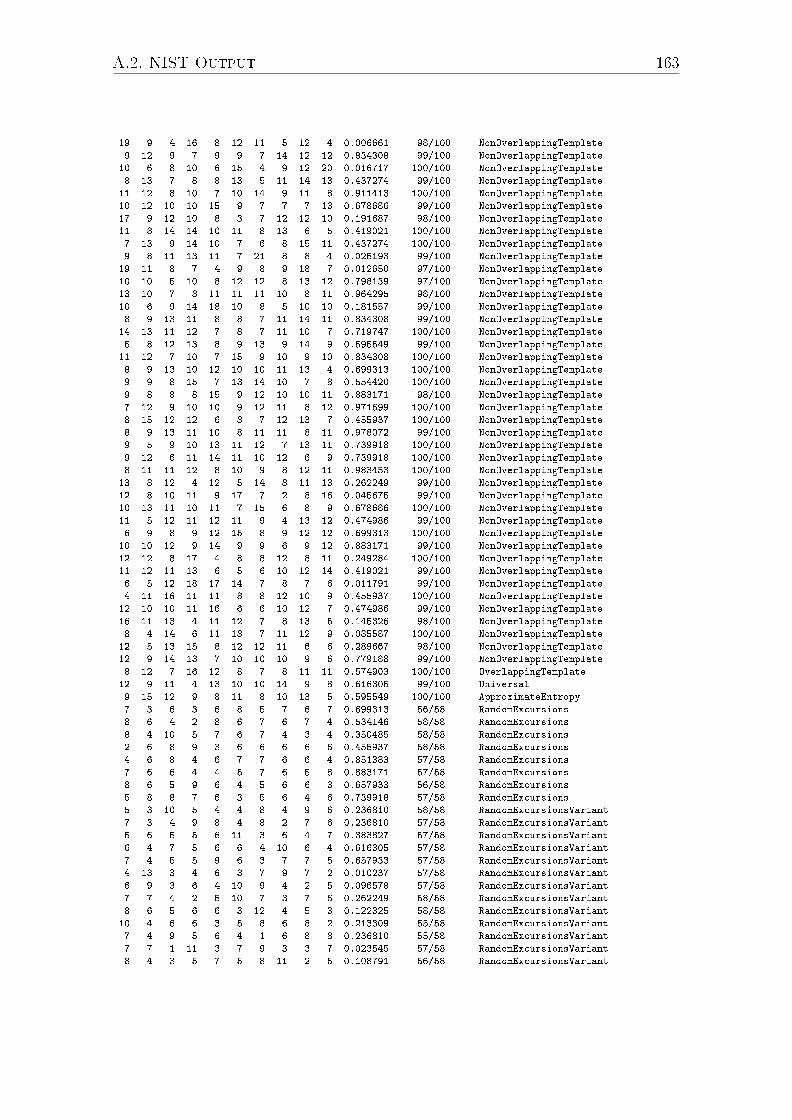
A.2. NIST Output 163
19 9 4 16 8 12 11 5 12 4 0.006661 98/100 NonOverlappingTemplate
9 12 9 7 9 9 7 14 12 12 0.834308 99/100 NonOverlappingTemplate
10 6 8 10 6 15 4 9 12 20 0.016717 100/100 NonOverlappingTemplate
8 13 7 8 8 13 5 11 14 13 0.437274 99/100 NonOverlappingTemplate
11 12 8 10 7 10 14 9 11 8 0.911413 100/100 NonOverlappingTemplate
10 12 10 10 15 9 7 7 7 13 0.678686 99/100 NonOverlappingTemplate
17 9 12 10 8 3 7 12 12 10 0.191687 98/100 NonOverlappingTemplate
11 8 14 14 10 11 8 13 6 5 0.419021 100/100 NonOverlappingTemplate
7 13 9 14 10 7 6 8 15 11 0.437274 100/100 NonOverlappingTemplate
9 8 11 13 11 7 21 8 8 4 0.025193 99/100 NonOverlappingTemplate
19 11 8 7 4 9 8 9 18 7 0.012650 97/100 NonOverlappingTemplate
10 10 5 10 8 12 12 8 13 12 0.798139 97/100 NonOverlappingTemplate
13 10 7 8 11 11 11 10 8 11 0.964295 98/100 NonOverlappingTemplate
10 6 9 14 18 10 8 5 10 10 0.181557 99/100 NonOverlappingTemplate
8 9 13 11 8 8 7 11 14 11 0.834308 99/100 NonOverlappingTemplate
14 13 11 12 7 8 7 11 10 7 0.719747 100/100 NonOverlappingTemplate
5 8 12 13 8 9 13 9 14 9 0.595549 99/100 NonOverlappingTemplate
11 12 7 10 7 15 9 10 9 10 0.834308 100/100 NonOverlappingTemplate
8 9 13 10 12 10 10 11 13 4 0.699313 100/100 NonOverlappingTemplate
9 9 8 15 7 13 14 10 7 8 0.554420 100/100 NonOverlappingTemplate
9 8 8 8 15 9 12 10 10 11 0.883171 98/100 NonOverlappingTemplate
7 12 9 10 10 9 12 11 8 12 0.971699 100/100 NonOverlappingTemplate
8 15 12 12 6 8 7 12 13 7 0.455937 100/100 NonOverlappingTemplate
8 9 13 11 10 8 11 11 8 11 0.978072 99/100 NonOverlappingTemplate
9 5 9 10 13 11 12 7 13 11 0.739918 100/100 NonOverlappingTemplate
9 12 6 11 14 11 10 12 6 9 0.739918 100/100 NonOverlappingTemplate
8 11 11 12 8 10 9 8 12 11 0.983453 100/100 NonOverlappingTemplate
13 8 12 4 12 5 14 8 11 13 0.262249 99/100 NonOverlappingTemplate
12 8 10 11 9 17 7 2 8 16 0.045675 99/100 NonOverlappingTemplate
10 13 11 10 11 7 15 6 8 9 0.678686 100/100 NonOverlappingTemplate
11 5 12 11 12 11 9 4 13 12 0.474986 99/100 NonOverlappingTemplate
6 9 8 9 12 15 8 9 12 12 0.699313 100/100 NonOverlappingTemplate
10 10 12 9 14 9 9 6 9 12 0.883171 99/100 NonOverlappingTemplate
12 12 8 17 4 8 8 12 8 11 0.249284 100/100 NonOverlappingTemplate
11 12 11 13 6 5 6 10 12 14 0.419021 99/100 NonOverlappingTemplate
6 5 12 18 17 14 7 8 7 6 0.011791 99/100 NonOverlappingTemplate
4 11 16 11 11 8 8 12 10 9 0.455937 100/100 NonOverlappingTemplate
12 10 10 11 16 6 6 10 12 7 0.474986 99/100 NonOverlappingTemplate
16 11 13 4 11 12 7 8 13 5 0.145326 98/100 NonOverlappingTemplate
8 4 14 6 11 18 7 11 12 9 0.085587 100/100 NonOverlappingTemplate
12 5 13 15 8 12 12 11 6 6 0.289667 98/100 NonOverlappingTemplate
12 9 14 13 7 10 10 10 9 6 0.779188 99/100 NonOverlappingTemplate
8 12 7 16 12 8 7 8 11 11 0.574903 100/100 OverlappingTemplate
12 9 11 4 13 10 10 14 9 8 0.616305 99/100 Universal
9 15 12 9 8 11 8 10 13 5 0.595549 100/100 ApproximateEntropy
7 3 6 3 6 8 5 7 6 7 0.699313 56/58 RandomExcursions
8 6 4 2 8 6 7 6 7 4 0.534146 58/58 RandomExcursions
8 4 10 5 7 6 7 4 3 4 0.350485 58/58 RandomExcursions
2 6 8 9 3 6 6 6 6 6 0.455937 58/58 RandomExcursions
4 6 8 4 6 7 7 6 6 4 0.851383 57/58 RandomExcursions
7 6 6 4 4 5 7 6 5 8 0.883171 57/58 RandomExcursions
8 6 5 9 6 4 5 6 6 3 0.657933 56/58 RandomExcursions
5 8 8 7 6 3 5 6 4 6 0.739918 57/58 RandomExcursions
5 3 10 5 4 4 8 4 9 6 0.236810 58/58 RandomExcursionsVariant
7 3 4 9 8 4 8 2 7 6 0.236810 57/58 RandomExcursionsVariant
5 6 5 5 6 11 3 6 4 7 0.383827 57/58 RandomExcursionsVariant
6 4 7 5 6 6 4 10 6 4 0.616305 57/58 RandomExcursionsVariant
7 4 5 5 9 6 3 7 7 5 0.657933 57/58 RandomExcursionsVariant
4 13 3 4 6 3 7 9 7 2 0.010237 57/58 RandomExcursionsVariant
6 9 3 6 4 10 9 4 2 5 0.096578 57/58 RandomExcursionsVariant
7 7 4 2 5 10 7 3 7 6 0.262249 58/58 RandomExcursionsVariant
8 6 5 6 6 3 12 4 5 3 0.122325 58/58 RandomExcursionsVariant
10 4 6 6 3 5 8 6 8 2 0.213309 55/58 RandomExcursionsVariant
7 4 9 5 6 4 1 6 8 8 0.236810 55/58 RandomExcursionsVariant
7 7 1 11 3 7 9 3 3 7 0.023545 57/58 RandomExcursionsVariant
8 4 3 5 7 5 8 11 2 5 0.108791 56/58 RandomExcursionsVariant

164 A. Statistical Data
8 3 5 7 7 1 8 5 7 7 0.289667 58/58 RandomExcursionsVariant
8 6 6 2 6 3 10 7 6 4 0.262249 58/58 RandomExcursionsVariant
8 9 4 4 3 5 3 11 4 7 0.085587 58/58 RandomExcursionsVariant
8 7 4 4 5 4 6 5 6 9 0.657933 57/58 RandomExcursionsVariant
6 6 4 3 6 2 8 9 7 7 0.350485 58/58 RandomExcursionsVariant
13 6 8 15 10 9 11 9 9 10 0.759756 98/100 Serial
14 10 8 5 10 14 9 7 17 6 0.137282 99/100 Serial
5 10 11 10 7 13 17 8 8 11 0.334538 100/100 LinearComplexity
A.2.8 NIST Output for MD5 Truncated to 64 Bit with Action
A and B------------------------------------------------------------------------------
RESULTS FOR THE UNIFORMITY OF P-VALUES AND THE PROPORTION OF PASSING SEQUENCES
------------------------------------------------------------------------------
generator is <md5_actionab.bin>
------------------------------------------------------------------------------
C1 C2 C3 C4 C5 C6 C7 C8 C9 C10 P-VALUE PROPORTION STATISTICAL TEST
------------------------------------------------------------------------------
13 4 13 13 9 14 13 4 9 8 0.162606 100/100 Frequency
13 3 12 10 14 5 9 14 6 14 0.085587 99/100 BlockFrequency
11 5 10 11 16 12 10 8 9 8 0.574903 99/100 CumulativeSums
13 10 6 6 14 16 10 12 8 5 0.181557 100/100 CumulativeSums
7 15 11 7 13 8 10 7 10 12 0.637119 100/100 Runs
20 8 12 8 8 15 6 4 12 7 0.014550 98/100 LongestRun
10 11 10 13 4 8 8 9 15 12 0.494392 100/100 Rank
13 7 10 9 6 15 10 13 9 8 0.595549 98/100 FFT
14 13 11 10 7 10 7 8 12 8 0.779188 99/100 NonOverlappingTemplate
11 9 10 9 9 8 19 9 9 7 0.350485 100/100 NonOverlappingTemplate
13 9 14 9 14 10 8 10 6 7 0.616305 100/100 NonOverlappingTemplate
6 21 13 12 2 8 13 7 10 8 0.004301 100/100 NonOverlappingTemplate
12 5 9 8 7 16 14 12 10 7 0.289667 99/100 NonOverlappingTemplate
15 10 6 9 9 7 7 18 10 9 0.181557 100/100 NonOverlappingTemplate
9 12 14 11 6 7 13 15 6 7 0.304126 98/100 NonOverlappingTemplate
16 13 9 8 7 9 8 11 8 11 0.637119 98/100 NonOverlappingTemplate
6 8 11 15 15 13 8 7 6 11 0.275709 100/100 NonOverlappingTemplate
12 10 5 10 16 5 15 11 8 8 0.191687 97/100 NonOverlappingTemplate
8 11 10 8 4 10 8 12 18 11 0.224821 98/100 NonOverlappingTemplate
12 10 11 8 8 5 16 10 9 11 0.574903 97/100 NonOverlappingTemplate
12 7 8 13 10 10 7 12 13 8 0.816537 99/100 NonOverlappingTemplate
9 7 9 10 10 11 12 10 10 12 0.991468 100/100 NonOverlappingTemplate
5 10 9 10 14 13 8 11 11 9 0.759756 100/100 NonOverlappingTemplate
15 11 6 12 11 12 11 7 6 9 0.554420 100/100 NonOverlappingTemplate
10 7 8 15 5 12 16 11 7 9 0.249284 100/100 NonOverlappingTemplate
9 12 14 6 8 9 14 11 10 7 0.657933 99/100 NonOverlappingTemplate
15 10 12 12 6 6 10 10 7 12 0.554420 99/100 NonOverlappingTemplate
6 19 11 12 5 12 12 10 6 7 0.066882 100/100 NonOverlappingTemplate
11 11 6 12 14 9 10 11 6 10 0.779188 100/100 NonOverlappingTemplate
10 6 6 17 5 12 18 11 10 5 0.017912 99/100 NonOverlappingTemplate
9 11 9 13 9 10 11 9 9 10 0.996335 98/100 NonOverlappingTemplate
12 2 16 12 14 8 11 10 5 10 0.080519 98/100 NonOverlappingTemplate
7 14 6 3 12 12 12 17 10 7 0.066882 100/100 NonOverlappingTemplate
9 8 10 11 11 10 7 15 9 10 0.897763 98/100 NonOverlappingTemplate
13 11 10 11 7 4 11 12 7 14 0.474986 99/100 NonOverlappingTemplate
11 7 9 15 9 7 13 12 4 13 0.319084 100/100 NonOverlappingTemplate
7 6 13 14 11 12 4 12 7 14 0.213309 100/100 NonOverlappingTemplate
12 6 7 13 15 14 11 6 7 9 0.304126 99/100 NonOverlappingTemplate
7 10 12 7 11 9 14 11 9 10 0.897763 100/100 NonOverlappingTemplate
14 7 11 14 12 10 6 9 11 6 0.534146 99/100 NonOverlappingTemplate
9 8 13 9 10 7 15 11 9 9 0.816537 100/100 NonOverlappingTemplate
8 11 7 12 12 5 10 12 10 13 0.739918 99/100 NonOverlappingTemplate
6 6 14 8 9 19 14 8 4 12 0.021999 100/100 NonOverlappingTemplate
8 9 9 8 13 11 9 10 9 14 0.924076 99/100 NonOverlappingTemplate
7 9 9 9 11 11 13 10 12 9 0.971699 100/100 NonOverlappingTemplate
7 10 13 11 11 14 9 7 9 9 0.851383 99/100 NonOverlappingTemplate

A.2. NIST Output 165
8 10 12 6 9 11 13 6 13 12 0.699313 100/100 NonOverlappingTemplate
7 10 9 14 11 13 7 13 7 9 0.699313 98/100 NonOverlappingTemplate
13 12 10 12 9 5 11 9 6 13 0.637119 99/100 NonOverlappingTemplate
10 9 12 11 11 19 7 10 4 7 0.115387 100/100 NonOverlappingTemplate
13 6 12 7 7 6 9 12 16 12 0.289667 99/100 NonOverlappingTemplate
14 14 8 10 10 8 10 11 8 7 0.798139 100/100 NonOverlappingTemplate
10 5 9 14 14 8 8 5 19 8 0.040108 100/100 NonOverlappingTemplate
10 7 10 8 13 8 16 8 6 14 0.366918 97/100 NonOverlappingTemplate
7 14 8 12 7 12 8 9 8 15 0.534146 100/100 NonOverlappingTemplate
6 13 10 9 10 7 10 14 14 7 0.574903 99/100 NonOverlappingTemplate
10 13 8 15 9 7 15 7 10 6 0.366918 100/100 NonOverlappingTemplate
9 15 6 9 9 13 14 5 12 8 0.334538 98/100 NonOverlappingTemplate
8 9 7 18 10 9 7 11 10 11 0.437274 100/100 NonOverlappingTemplate
10 15 12 6 6 13 9 8 9 12 0.534146 100/100 NonOverlappingTemplate
11 8 8 6 12 15 10 9 9 12 0.739918 100/100 NonOverlappingTemplate
9 11 10 10 8 16 10 6 6 14 0.437274 99/100 NonOverlappingTemplate
14 8 11 14 11 9 5 9 9 10 0.678686 98/100 NonOverlappingTemplate
8 8 10 10 11 14 16 6 5 12 0.304126 100/100 NonOverlappingTemplate
7 10 9 10 10 12 10 12 10 10 0.994250 99/100 NonOverlappingTemplate
6 11 12 17 10 14 9 7 7 7 0.249284 100/100 NonOverlappingTemplate
8 9 8 14 8 11 7 9 13 13 0.759756 98/100 NonOverlappingTemplate
6 12 8 8 10 13 12 11 6 14 0.595549 99/100 NonOverlappingTemplate
9 13 10 10 9 9 10 9 12 9 0.994250 99/100 NonOverlappingTemplate
11 12 7 12 6 13 11 10 7 11 0.798139 100/100 NonOverlappingTemplate
11 11 11 10 10 10 11 9 13 4 0.834308 100/100 NonOverlappingTemplate
10 8 12 10 10 10 7 5 15 13 0.574903 100/100 NonOverlappingTemplate
7 3 9 9 12 12 17 8 15 8 0.090936 100/100 NonOverlappingTemplate
7 15 16 10 6 8 14 9 7 8 0.213309 100/100 NonOverlappingTemplate
13 12 8 11 9 9 10 5 14 9 0.719747 100/100 NonOverlappingTemplate
11 7 18 7 11 7 10 11 7 11 0.319084 99/100 NonOverlappingTemplate
8 12 4 11 12 15 10 6 8 14 0.275709 99/100 NonOverlappingTemplate
10 6 10 13 8 8 7 12 12 14 0.678686 99/100 NonOverlappingTemplate
9 11 9 13 8 11 12 8 12 7 0.924076 98/100 NonOverlappingTemplate
9 7 13 10 16 12 13 6 9 5 0.275709 99/100 NonOverlappingTemplate
11 14 6 4 10 7 11 15 8 14 0.191687 100/100 NonOverlappingTemplate
12 9 14 13 7 9 11 10 9 6 0.759756 99/100 NonOverlappingTemplate
14 13 11 10 7 10 7 8 12 8 0.779188 99/100 NonOverlappingTemplate
7 5 6 12 12 10 18 12 7 11 0.137282 100/100 NonOverlappingTemplate
10 14 10 12 10 10 8 5 10 11 0.834308 100/100 NonOverlappingTemplate
12 13 8 8 10 5 9 11 11 13 0.759756 98/100 NonOverlappingTemplate
16 11 13 16 6 5 6 7 11 9 0.090936 100/100 NonOverlappingTemplate
4 12 13 9 8 12 10 12 10 10 0.719747 100/100 NonOverlappingTemplate
13 4 18 12 14 7 11 6 7 8 0.051942 100/100 NonOverlappingTemplate
11 10 6 10 12 11 7 17 8 8 0.455937 100/100 NonOverlappingTemplate
9 12 13 9 6 16 9 5 6 15 0.145326 99/100 NonOverlappingTemplate
14 9 11 8 10 4 10 8 10 16 0.366918 99/100 NonOverlappingTemplate
8 9 11 6 9 11 8 13 11 14 0.798139 100/100 NonOverlappingTemplate
6 4 15 11 15 10 8 16 4 11 0.035174 99/100 NonOverlappingTemplate
7 11 15 11 7 10 14 13 7 5 0.319084 99/100 NonOverlappingTemplate
9 17 9 10 7 7 8 10 14 9 0.437274 100/100 NonOverlappingTemplate
15 12 6 13 8 12 7 7 9 11 0.514124 99/100 NonOverlappingTemplate
6 14 11 9 6 10 13 10 8 13 0.616305 99/100 NonOverlappingTemplate
12 12 11 8 9 13 12 10 4 9 0.699313 100/100 NonOverlappingTemplate
12 12 9 14 11 15 3 7 7 10 0.224821 100/100 NonOverlappingTemplate
11 8 8 12 8 11 8 13 13 8 0.883171 99/100 NonOverlappingTemplate
8 11 18 13 8 6 11 5 12 8 0.153763 99/100 NonOverlappingTemplate
11 9 6 16 11 15 8 10 3 11 0.145326 99/100 NonOverlappingTemplate
7 7 12 11 11 11 12 11 8 10 0.946308 98/100 NonOverlappingTemplate
10 8 9 12 13 10 16 5 7 10 0.455937 100/100 NonOverlappingTemplate
8 5 16 12 9 8 9 8 9 16 0.236810 98/100 NonOverlappingTemplate
10 11 10 9 11 10 12 10 10 7 0.996335 100/100 NonOverlappingTemplate
8 6 12 10 11 8 8 16 10 11 0.637119 99/100 NonOverlappingTemplate
8 10 12 12 11 10 10 8 9 10 0.994250 99/100 NonOverlappingTemplate
9 12 10 10 7 13 9 12 11 7 0.924076 100/100 NonOverlappingTemplate
13 16 8 5 10 7 14 12 9 6 0.213309 99/100 NonOverlappingTemplate
10 12 9 7 8 19 9 5 12 9 0.162606 100/100 NonOverlappingTemplate

166 A. Statistical Data
6 5 15 10 10 14 8 10 10 12 0.437274 99/100 NonOverlappingTemplate
9 11 10 10 7 9 5 11 15 13 0.616305 100/100 NonOverlappingTemplate
19 9 4 16 8 12 11 5 12 4 0.006661 98/100 NonOverlappingTemplate
9 12 9 7 9 9 7 14 12 12 0.834308 99/100 NonOverlappingTemplate
10 6 8 10 6 15 4 9 12 20 0.016717 100/100 NonOverlappingTemplate
8 13 7 8 8 13 5 11 14 13 0.437274 99/100 NonOverlappingTemplate
11 12 8 10 7 10 14 9 11 8 0.911413 100/100 NonOverlappingTemplate
10 12 10 10 15 9 7 7 7 13 0.678686 99/100 NonOverlappingTemplate
17 9 12 10 8 3 7 12 12 10 0.191687 98/100 NonOverlappingTemplate
11 8 14 14 10 11 8 13 6 5 0.419021 100/100 NonOverlappingTemplate
7 13 9 14 10 7 6 8 15 11 0.437274 100/100 NonOverlappingTemplate
9 8 11 13 11 7 21 8 8 4 0.025193 99/100 NonOverlappingTemplate
19 11 8 7 4 9 8 9 18 7 0.012650 97/100 NonOverlappingTemplate
10 10 5 10 8 12 12 8 13 12 0.798139 97/100 NonOverlappingTemplate
13 10 7 8 11 11 11 10 8 11 0.964295 98/100 NonOverlappingTemplate
10 6 9 14 18 10 8 5 10 10 0.181557 99/100 NonOverlappingTemplate
8 9 13 11 8 8 7 11 14 11 0.834308 99/100 NonOverlappingTemplate
14 13 11 12 7 8 7 11 10 7 0.719747 100/100 NonOverlappingTemplate
5 8 12 13 8 9 13 9 14 9 0.595549 99/100 NonOverlappingTemplate
11 12 7 10 7 15 9 10 9 10 0.834308 100/100 NonOverlappingTemplate
8 9 13 10 12 10 10 11 13 4 0.699313 100/100 NonOverlappingTemplate
9 9 8 15 7 13 14 10 7 8 0.554420 100/100 NonOverlappingTemplate
9 8 8 8 15 9 12 10 10 11 0.883171 98/100 NonOverlappingTemplate
7 12 9 10 10 9 12 11 8 12 0.971699 100/100 NonOverlappingTemplate
8 15 12 12 6 8 7 12 13 7 0.455937 100/100 NonOverlappingTemplate
8 9 13 11 10 8 11 11 8 11 0.978072 99/100 NonOverlappingTemplate
9 5 9 10 13 11 12 7 13 11 0.739918 100/100 NonOverlappingTemplate
9 12 6 11 14 11 10 12 6 9 0.739918 100/100 NonOverlappingTemplate
8 11 11 12 8 10 9 8 12 11 0.983453 100/100 NonOverlappingTemplate
13 8 12 4 12 5 14 8 11 13 0.262249 99/100 NonOverlappingTemplate
12 8 10 11 9 17 7 2 8 16 0.045675 99/100 NonOverlappingTemplate
10 13 11 10 11 7 15 6 8 9 0.678686 100/100 NonOverlappingTemplate
11 5 12 11 12 11 9 4 13 12 0.474986 99/100 NonOverlappingTemplate
6 9 8 9 12 15 8 9 12 12 0.699313 100/100 NonOverlappingTemplate
10 10 12 9 14 9 9 6 9 12 0.883171 99/100 NonOverlappingTemplate
12 12 8 17 4 8 8 12 8 11 0.249284 100/100 NonOverlappingTemplate
11 12 11 13 6 5 6 10 12 14 0.419021 99/100 NonOverlappingTemplate
6 5 12 18 17 14 7 8 7 6 0.011791 99/100 NonOverlappingTemplate
4 11 16 11 11 8 8 12 10 9 0.455937 100/100 NonOverlappingTemplate
12 10 10 11 16 6 6 10 12 7 0.474986 99/100 NonOverlappingTemplate
16 11 13 4 11 12 7 8 13 5 0.145326 98/100 NonOverlappingTemplate
8 4 14 6 11 18 7 11 12 9 0.085587 100/100 NonOverlappingTemplate
12 5 13 15 8 12 12 11 6 6 0.289667 98/100 NonOverlappingTemplate
12 9 14 13 7 10 10 10 9 6 0.779188 99/100 NonOverlappingTemplate
8 12 7 16 12 8 7 8 11 11 0.574903 100/100 OverlappingTemplate
12 9 11 4 13 10 10 14 9 8 0.616305 99/100 Universal
9 15 12 9 8 11 8 10 13 5 0.595549 100/100 ApproximateEntropy
7 3 6 3 6 8 5 7 6 7 0.699313 56/58 RandomExcursions
8 6 4 2 8 6 7 6 7 4 0.534146 58/58 RandomExcursions
8 4 10 5 7 6 7 4 3 4 0.350485 58/58 RandomExcursions
2 6 8 9 3 6 6 6 6 6 0.455937 58/58 RandomExcursions
4 6 8 4 6 7 7 6 6 4 0.851383 57/58 RandomExcursions
7 6 6 4 4 5 7 6 5 8 0.883171 57/58 RandomExcursions
8 6 5 9 6 4 5 6 6 3 0.657933 56/58 RandomExcursions
5 8 8 7 6 3 5 6 4 6 0.739918 57/58 RandomExcursions
5 3 10 5 4 4 8 4 9 6 0.236810 58/58 RandomExcursionsVariant
7 3 4 9 8 4 8 2 7 6 0.236810 57/58 RandomExcursionsVariant
5 6 5 5 6 11 3 6 4 7 0.383827 57/58 RandomExcursionsVariant
6 4 7 5 6 6 4 10 6 4 0.616305 57/58 RandomExcursionsVariant
7 4 5 5 9 6 3 7 7 5 0.657933 57/58 RandomExcursionsVariant
4 13 3 4 6 3 7 9 7 2 0.010237 57/58 RandomExcursionsVariant
6 9 3 6 4 10 9 4 2 5 0.096578 57/58 RandomExcursionsVariant
7 7 4 2 5 10 7 3 7 6 0.262249 58/58 RandomExcursionsVariant
8 6 5 6 6 3 12 4 5 3 0.122325 58/58 RandomExcursionsVariant
10 4 6 6 3 5 8 6 8 2 0.213309 55/58 RandomExcursionsVariant
7 4 9 5 6 4 1 6 8 8 0.236810 55/58 RandomExcursionsVariant
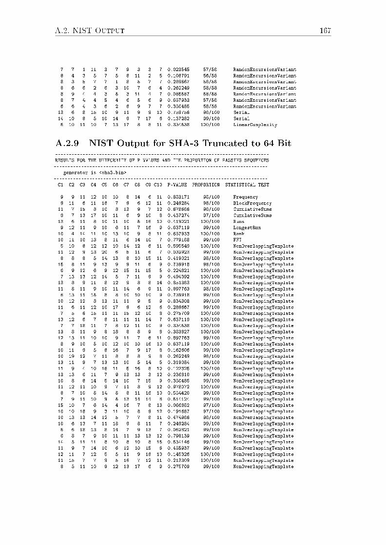
A.2. NIST Output 167
7 7 1 11 3 7 9 3 3 7 0.023545 57/58 RandomExcursionsVariant
8 4 3 5 7 5 8 11 2 5 0.108791 56/58 RandomExcursionsVariant
8 3 5 7 7 1 8 5 7 7 0.289667 58/58 RandomExcursionsVariant
8 6 6 2 6 3 10 7 6 4 0.262249 58/58 RandomExcursionsVariant
8 9 4 4 3 5 3 11 4 7 0.085587 58/58 RandomExcursionsVariant
8 7 4 4 5 4 6 5 6 9 0.657933 57/58 RandomExcursionsVariant
6 6 4 3 6 2 8 9 7 7 0.350485 58/58 RandomExcursionsVariant
13 6 8 15 10 9 11 9 9 10 0.759756 98/100 Serial
14 10 8 5 10 14 9 7 17 6 0.137282 99/100 Serial
5 10 11 10 7 13 17 8 8 11 0.334538 100/100 LinearComplexity
A.2.9 NIST Output for SHA-3 Truncated to 64 Bit------------------------------------------------------------------------------
RESULTS FOR THE UNIFORMITY OF P-VALUES AND THE PROPORTION OF PASSING SEQUENCES
------------------------------------------------------------------------------
generator is <sha3.bin>
------------------------------------------------------------------------------
C1 C2 C3 C4 C5 C6 C7 C8 C9 C10 P-VALUE PROPORTION STATISTICAL TEST
------------------------------------------------------------------------------
9 9 11 12 10 10 8 14 6 11 0.883171 98/100 Frequency
9 11 6 11 18 7 9 6 12 11 0.249284 98/100 BlockFrequency
11 7 15 8 10 8 13 9 7 12 0.678686 98/100 CumulativeSums
9 7 13 17 10 11 6 9 10 8 0.437274 97/100 CumulativeSums
13 6 11 8 10 11 10 5 16 10 0.419021 100/100 Runs
9 12 11 9 10 6 11 7 16 9 0.637119 99/100 LongestRun
10 4 14 11 10 13 10 9 8 11 0.657933 100/100 Rank
10 11 10 13 8 11 6 14 10 7 0.779188 99/100 FFT
5 10 8 12 12 10 14 12 6 11 0.595549 100/100 NonOverlappingTemplate
11 12 9 13 20 6 5 11 6 7 0.032923 99/100 NonOverlappingTemplate
8 8 8 5 14 13 8 10 15 11 0.419021 98/100 NonOverlappingTemplate
15 8 11 9 13 9 9 11 6 9 0.739918 98/100 NonOverlappingTemplate
6 9 12 6 9 12 15 11 15 5 0.224821 100/100 NonOverlappingTemplate
7 13 13 12 14 5 7 11 9 9 0.494392 100/100 NonOverlappingTemplate
13 8 9 11 8 12 9 8 8 14 0.851383 100/100 NonOverlappingTemplate
11 8 11 9 10 11 14 6 9 11 0.897763 98/100 NonOverlappingTemplate
6 13 11 15 8 8 10 10 10 9 0.739918 99/100 NonOverlappingTemplate
10 12 12 8 13 11 11 9 5 9 0.834308 99/100 NonOverlappingTemplate
11 6 11 12 10 17 9 6 12 6 0.289667 99/100 NonOverlappingTemplate
7 5 6 15 11 11 15 12 10 8 0.275709 100/100 NonOverlappingTemplate
13 12 6 7 8 11 11 11 14 7 0.637119 100/100 NonOverlappingTemplate
7 7 18 11 7 8 12 11 10 9 0.334538 100/100 NonOverlappingTemplate
13 8 11 9 8 18 8 8 9 8 0.383827 100/100 NonOverlappingTemplate
12 13 11 10 10 9 11 7 6 11 0.897763 99/100 NonOverlappingTemplate
8 9 10 5 10 12 10 10 16 10 0.637119 100/100 NonOverlappingTemplate
10 11 9 5 8 16 7 9 17 8 0.162606 99/100 NonOverlappingTemplate
10 19 12 7 11 8 8 8 9 8 0.262249 98/100 NonOverlappingTemplate
13 11 9 7 13 13 10 5 14 5 0.319084 99/100 NonOverlappingTemplate
11 9 4 10 16 11 5 16 8 10 0.122325 100/100 NonOverlappingTemplate
13 13 6 11 7 9 13 13 3 12 0.236810 99/100 NonOverlappingTemplate
10 8 8 14 5 14 10 7 15 9 0.350485 99/100 NonOverlappingTemplate
11 12 11 10 9 7 11 8 9 12 0.978072 100/100 NonOverlappingTemplate
8 7 10 8 14 8 8 11 16 10 0.554420 99/100 NonOverlappingTemplate
7 9 11 10 9 5 13 14 14 8 0.514124 99/100 NonOverlappingTemplate
15 10 7 6 14 4 16 7 8 13 0.066882 97/100 NonOverlappingTemplate
10 10 18 9 3 11 10 8 9 12 0.191687 97/100 NonOverlappingTemplate
10 13 13 14 12 5 7 7 8 11 0.474986 98/100 NonOverlappingTemplate
10 6 13 7 11 18 9 8 11 7 0.249284 99/100 NonOverlappingTemplate
5 6 18 13 8 14 7 9 13 7 0.062821 99/100 NonOverlappingTemplate
6 8 7 9 10 11 11 13 13 12 0.798139 99/100 NonOverlappingTemplate
14 5 11 11 8 10 8 10 8 15 0.534146 99/100 NonOverlappingTemplate
11 9 7 14 10 6 12 10 15 6 0.455937 99/100 NonOverlappingTemplate
12 11 7 12 5 5 11 9 18 10 0.145326 100/100 NonOverlappingTemplate
11 15 7 7 9 5 16 7 12 11 0.213309 100/100 NonOverlappingTemplate
8 5 11 10 9 12 13 17 6 9 0.275709 99/100 NonOverlappingTemplate

168 A. Statistical Data
14 9 9 4 12 13 3 14 14 8 0.085587 98/100 NonOverlappingTemplate
11 14 10 13 10 3 10 11 8 10 0.534146 100/100 NonOverlappingTemplate
13 9 10 13 6 11 5 10 11 12 0.678686 99/100 NonOverlappingTemplate
9 22 9 10 8 8 9 10 8 7 0.051942 99/100 NonOverlappingTemplate
10 11 11 12 9 11 11 11 6 8 0.964295 100/100 NonOverlappingTemplate
12 7 12 7 8 9 12 12 8 13 0.816537 99/100 NonOverlappingTemplate
7 12 15 10 7 5 10 7 14 13 0.304126 100/100 NonOverlappingTemplate
11 8 12 12 9 6 7 10 14 11 0.779188 99/100 NonOverlappingTemplate
10 13 10 13 4 9 12 8 13 8 0.574903 99/100 NonOverlappingTemplate
6 10 13 10 7 15 9 11 11 8 0.678686 99/100 NonOverlappingTemplate
9 9 13 10 7 5 13 14 13 7 0.455937 100/100 NonOverlappingTemplate
9 10 9 14 13 11 12 7 11 4 0.554420 99/100 NonOverlappingTemplate
11 11 8 14 6 13 12 9 5 11 0.554420 98/100 NonOverlappingTemplate
21 12 7 12 7 9 12 5 7 8 0.025193 98/100 NonOverlappingTemplate
10 15 10 9 10 8 11 14 10 3 0.383827 100/100 NonOverlappingTemplate
13 9 12 10 6 14 10 11 8 7 0.739918 99/100 NonOverlappingTemplate
10 13 6 11 8 11 12 14 9 6 0.657933 99/100 NonOverlappingTemplate
11 6 13 8 8 9 10 10 6 19 0.153763 99/100 NonOverlappingTemplate
6 12 8 10 11 7 12 9 14 11 0.779188 100/100 NonOverlappingTemplate
12 10 10 11 9 14 8 6 10 10 0.897763 98/100 NonOverlappingTemplate
8 16 11 8 15 6 9 8 13 6 0.236810 100/100 NonOverlappingTemplate
7 11 11 7 7 16 7 9 12 13 0.455937 100/100 NonOverlappingTemplate
8 9 8 17 17 11 5 6 9 10 0.090936 99/100 NonOverlappingTemplate
10 18 4 7 10 15 11 9 6 10 0.085587 100/100 NonOverlappingTemplate
6 7 11 6 12 13 11 14 12 8 0.534146 100/100 NonOverlappingTemplate
10 12 12 17 8 6 8 8 11 8 0.437274 99/100 NonOverlappingTemplate
10 14 13 7 6 13 12 6 11 8 0.494392 100/100 NonOverlappingTemplate
10 11 12 7 9 10 13 12 9 7 0.924076 100/100 NonOverlappingTemplate
6 9 7 7 8 12 18 16 6 11 0.066882 99/100 NonOverlappingTemplate
7 7 10 6 12 9 11 12 12 14 0.699313 100/100 NonOverlappingTemplate
8 11 16 5 10 8 10 9 10 13 0.534146 99/100 NonOverlappingTemplate
9 11 12 14 10 8 9 11 7 9 0.924076 100/100 NonOverlappingTemplate
7 12 11 7 13 15 11 5 12 7 0.383827 100/100 NonOverlappingTemplate
11 11 8 11 18 6 10 9 5 11 0.249284 100/100 NonOverlappingTemplate
8 9 9 10 5 17 7 17 10 8 0.115387 99/100 NonOverlappingTemplate
8 10 6 14 13 8 8 11 15 7 0.455937 100/100 NonOverlappingTemplate
15 12 10 10 11 12 5 16 5 4 0.075719 99/100 NonOverlappingTemplate
5 10 8 12 12 10 14 12 6 11 0.595549 100/100 NonOverlappingTemplate
8 12 11 11 8 14 13 7 10 6 0.699313 98/100 NonOverlappingTemplate
12 5 7 12 18 12 7 9 9 9 0.202268 98/100 NonOverlappingTemplate
5 7 10 9 7 20 14 7 12 9 0.042808 98/100 NonOverlappingTemplate
7 14 15 10 11 12 9 9 5 8 0.474986 100/100 NonOverlappingTemplate
14 10 8 14 8 10 11 6 13 6 0.514124 98/100 NonOverlappingTemplate
15 8 9 11 6 13 5 12 12 9 0.437274 100/100 NonOverlappingTemplate
8 10 10 7 7 12 14 8 10 14 0.719747 98/100 NonOverlappingTemplate
8 8 6 17 7 7 10 14 15 8 0.137282 98/100 NonOverlappingTemplate
13 11 10 11 7 10 11 4 13 10 0.678686 100/100 NonOverlappingTemplate
6 11 14 7 13 8 8 9 13 11 0.637119 99/100 NonOverlappingTemplate
12 13 6 14 10 8 14 6 11 6 0.366918 99/100 NonOverlappingTemplate
15 11 13 16 3 14 5 5 5 13 0.008879 100/100 NonOverlappingTemplate
9 13 9 9 9 8 14 10 9 10 0.946308 100/100 NonOverlappingTemplate
10 9 8 12 16 10 10 8 11 6 0.678686 100/100 NonOverlappingTemplate
9 6 12 12 7 13 9 9 10 13 0.798139 100/100 NonOverlappingTemplate
7 12 13 7 17 13 4 6 8 13 0.080519 99/100 NonOverlappingTemplate
9 11 6 15 5 10 14 9 14 7 0.275709 98/100 NonOverlappingTemplate
15 8 13 17 10 13 4 7 4 9 0.037566 100/100 NonOverlappingTemplate
7 8 15 8 8 13 11 12 8 10 0.699313 99/100 NonOverlappingTemplate
4 13 7 13 10 17 10 9 10 7 0.202268 100/100 NonOverlappingTemplate
7 6 6 11 14 11 10 8 12 15 0.419021 100/100 NonOverlappingTemplate
5 11 10 13 18 4 10 9 13 7 0.080519 100/100 NonOverlappingTemplate
12 8 6 12 11 13 12 7 8 11 0.779188 100/100 NonOverlappingTemplate
3 16 7 13 14 8 12 8 7 12 0.108791 100/100 NonOverlappingTemplate
7 12 12 7 15 14 14 7 6 6 0.191687 99/100 NonOverlappingTemplate
11 7 11 11 8 14 14 8 7 9 0.719747 100/100 NonOverlappingTemplate
10 10 10 12 8 12 6 6 13 13 0.719747 97/100 NonOverlappingTemplate
9 9 8 12 18 9 7 10 10 8 0.455937 99/100 NonOverlappingTemplate

A.2. NIST Output 169
6 12 10 9 10 9 8 12 12 12 0.924076 100/100 NonOverlappingTemplate
9 7 7 8 10 12 13 13 11 10 0.867692 100/100 NonOverlappingTemplate
11 9 11 14 9 9 6 9 6 16 0.437274 100/100 NonOverlappingTemplate
8 4 13 8 11 15 13 11 7 10 0.366918 98/100 NonOverlappingTemplate
8 10 9 7 14 7 7 11 14 13 0.595549 100/100 NonOverlappingTemplate
12 13 10 10 11 7 6 8 12 11 0.851383 99/100 NonOverlappingTemplate
9 13 9 10 12 12 9 14 7 5 0.637119 99/100 NonOverlappingTemplate
9 11 11 11 5 11 17 9 5 11 0.304126 97/100 NonOverlappingTemplate
14 14 8 10 10 7 7 12 10 8 0.719747 99/100 NonOverlappingTemplate
8 10 12 5 8 7 12 8 19 11 0.137282 100/100 NonOverlappingTemplate
9 11 8 9 11 13 11 11 9 8 0.983453 97/100 NonOverlappingTemplate
12 11 7 12 8 9 16 4 9 12 0.350485 99/100 NonOverlappingTemplate
8 14 15 9 11 8 7 8 13 7 0.514124 100/100 NonOverlappingTemplate
5 11 11 7 8 13 11 10 13 11 0.739918 99/100 NonOverlappingTemplate
7 7 12 3 11 10 13 11 8 18 0.090936 98/100 NonOverlappingTemplate
8 13 14 8 7 7 14 13 9 7 0.474986 99/100 NonOverlappingTemplate
10 9 13 9 12 8 7 16 7 9 0.595549 100/100 NonOverlappingTemplate
11 14 9 8 7 8 9 10 9 15 0.719747 99/100 NonOverlappingTemplate
10 6 6 10 11 10 10 12 10 15 0.719747 100/100 NonOverlappingTemplate
13 9 7 7 8 11 14 12 12 7 0.678686 99/100 NonOverlappingTemplate
10 10 8 16 5 7 11 12 11 10 0.534146 100/100 NonOverlappingTemplate
4 3 12 13 11 14 16 9 10 8 0.075719 99/100 NonOverlappingTemplate
9 9 7 6 15 12 11 10 9 12 0.719747 99/100 NonOverlappingTemplate
11 8 5 12 13 12 11 8 6 14 0.494392 99/100 NonOverlappingTemplate
12 10 9 9 13 10 10 10 4 13 0.739918 99/100 NonOverlappingTemplate
7 8 10 9 8 10 13 14 11 10 0.883171 99/100 NonOverlappingTemplate
17 12 11 7 5 14 9 9 13 3 0.058984 100/100 NonOverlappingTemplate
7 11 14 10 8 12 14 6 11 7 0.574903 99/100 NonOverlappingTemplate
14 10 11 10 10 10 9 10 6 10 0.946308 98/100 NonOverlappingTemplate
13 12 5 12 9 8 12 10 11 8 0.779188 99/100 NonOverlappingTemplate
8 8 9 10 14 14 15 5 4 13 0.137282 98/100 NonOverlappingTemplate
10 10 12 9 9 12 8 12 6 12 0.924076 98/100 NonOverlappingTemplate
9 13 11 10 12 9 6 10 11 9 0.946308 99/100 NonOverlappingTemplate
11 13 11 4 8 12 12 7 12 10 0.616305 98/100 NonOverlappingTemplate
8 11 12 12 8 8 8 14 9 10 0.897763 99/100 NonOverlappingTemplate
12 10 13 11 6 9 8 4 17 10 0.213309 100/100 NonOverlappingTemplate
10 8 8 10 7 12 14 15 8 8 0.637119 99/100 NonOverlappingTemplate
11 9 8 12 8 11 7 14 7 13 0.759756 100/100 NonOverlappingTemplate
5 11 9 10 16 13 7 15 8 6 0.181557 99/100 NonOverlappingTemplate
9 14 8 9 12 11 13 5 11 8 0.678686 99/100 NonOverlappingTemplate
14 7 6 10 10 12 13 7 12 9 0.657933 99/100 NonOverlappingTemplate
7 6 9 16 6 12 10 15 8 11 0.262249 100/100 NonOverlappingTemplate
14 6 11 8 12 8 10 8 12 11 0.798139 100/100 NonOverlappingTemplate
8 13 6 10 9 9 14 10 9 12 0.816537 99/100 NonOverlappingTemplate
15 12 10 10 12 11 5 16 5 4 0.075719 99/100 NonOverlappingTemplate
12 11 15 8 11 11 8 4 12 8 0.494392 97/100 OverlappingTemplate
9 12 13 12 7 8 14 10 8 7 0.739918 99/100 Universal
11 13 11 11 8 8 7 12 12 7 0.867692 99/100 ApproximateEntropy
6 4 2 13 8 4 10 6 4 5 0.060239 61/62 RandomExcursions
8 3 5 3 9 8 7 4 8 7 0.568055 62/62 RandomExcursions
13 5 6 3 9 8 7 3 5 3 0.082177 61/62 RandomExcursions
8 7 7 8 6 7 6 4 6 3 0.911413 61/62 RandomExcursions
5 8 7 3 8 12 6 7 3 3 0.195163 62/62 RandomExcursions
10 7 9 8 2 7 5 5 6 3 0.378138 59/62 RandomExcursions
7 9 7 5 5 8 2 4 9 6 0.568055 62/62 RandomExcursions
2 8 9 6 6 5 8 6 7 5 0.739918 62/62 RandomExcursions
13 5 5 6 10 4 6 4 4 5 0.148094 62/62 RandomExcursionsVariant
12 12 4 2 5 5 7 6 4 5 0.054199 62/62 RandomExcursionsVariant
8 15 5 5 3 5 3 8 6 4 0.025193 61/62 RandomExcursionsVariant
7 8 6 8 10 5 6 3 6 3 0.602458 59/62 RandomExcursionsVariant
7 7 2 6 8 6 11 4 4 7 0.407091 59/62 RandomExcursionsVariant
9 8 5 6 0 4 11 5 4 10 0.054199 59/62 RandomExcursionsVariant
12 4 8 5 4 4 7 7 2 9 0.148094 60/62 RandomExcursionsVariant
9 13 4 4 5 5 9 5 5 3 0.100508 61/62 RandomExcursionsVariant
6 12 7 8 2 2 10 5 5 5 0.082177 61/62 RandomExcursionsVariant
8 9 10 4 5 4 8 3 5 6 0.468595 62/62 RandomExcursionsVariant

170 A. Statistical Data
8 7 8 6 4 5 7 4 8 5 0.911413 61/62 RandomExcursionsVariant
8 8 6 4 12 5 3 4 5 7 0.299251 61/62 RandomExcursionsVariant
7 7 4 3 5 11 7 5 9 4 0.407091 62/62 RandomExcursionsVariant
7 5 5 4 4 11 9 5 5 7 0.534146 61/62 RandomExcursionsVariant
8 4 6 8 5 9 7 8 5 2 0.602458 62/62 RandomExcursionsVariant
6 3 6 5 12 10 9 4 3 4 0.100508 62/62 RandomExcursionsVariant
6 6 4 7 7 3 12 6 5 6 0.468595 62/62 RandomExcursionsVariant
5 6 8 5 5 7 3 6 10 7 0.772760 62/62 RandomExcursionsVariant
17 12 10 10 7 7 9 6 12 10 0.419021 97/100 Serial
14 9 10 13 6 12 10 6 11 9 0.699313 97/100 Serial
8 10 8 11 7 11 8 12 18 7 0.350485 99/100 LinearComplexity
A.2.10 NIST Output for SHA-3 Truncated to 64 Bit with
Action A and B------------------------------------------------------------------------------
RESULTS FOR THE UNIFORMITY OF P-VALUES AND THE PROPORTION OF PASSING SEQUENCES
------------------------------------------------------------------------------
generator is <sha3_actionab.bin>
------------------------------------------------------------------------------
C1 C2 C3 C4 C5 C6 C7 C8 C9 C10 P-VALUE PROPORTION STATISTICAL TEST
------------------------------------------------------------------------------
9 9 11 12 10 10 8 14 6 11 0.883171 98/100 Frequency
9 11 6 11 18 7 9 6 12 11 0.249284 98/100 BlockFrequency
11 7 15 8 10 8 13 9 7 12 0.678686 98/100 CumulativeSums
9 7 13 17 10 11 6 9 10 8 0.437274 97/100 CumulativeSums
13 6 11 8 10 11 10 5 16 10 0.419021 100/100 Runs
9 12 11 9 10 6 11 7 16 9 0.637119 99/100 LongestRun
10 4 14 11 10 13 10 9 8 11 0.657933 100/100 Rank
10 11 10 13 8 11 6 14 10 7 0.779188 99/100 FFT
5 10 8 12 12 10 14 12 6 11 0.595549 100/100 NonOverlappingTemplate
11 12 9 13 20 6 5 11 6 7 0.032923 99/100 NonOverlappingTemplate
8 8 8 5 14 13 8 10 15 11 0.419021 98/100 NonOverlappingTemplate
15 8 11 9 13 9 9 11 6 9 0.739918 98/100 NonOverlappingTemplate
6 9 12 6 9 12 15 11 15 5 0.224821 100/100 NonOverlappingTemplate
7 13 13 12 14 5 7 11 9 9 0.494392 100/100 NonOverlappingTemplate
13 8 9 11 8 12 9 8 8 14 0.851383 100/100 NonOverlappingTemplate
11 8 11 9 10 11 14 6 9 11 0.897763 98/100 NonOverlappingTemplate
6 13 11 15 8 8 10 10 10 9 0.739918 99/100 NonOverlappingTemplate
10 12 12 8 13 11 11 9 5 9 0.834308 99/100 NonOverlappingTemplate
11 6 11 12 10 17 9 6 12 6 0.289667 99/100 NonOverlappingTemplate
7 5 6 15 11 11 15 12 10 8 0.275709 100/100 NonOverlappingTemplate
13 12 6 7 8 11 11 11 14 7 0.637119 100/100 NonOverlappingTemplate
7 7 18 11 7 8 12 11 10 9 0.334538 100/100 NonOverlappingTemplate
13 8 11 9 8 18 8 8 9 8 0.383827 100/100 NonOverlappingTemplate
12 13 11 10 10 9 11 7 6 11 0.897763 99/100 NonOverlappingTemplate
8 9 10 5 10 12 10 10 16 10 0.637119 100/100 NonOverlappingTemplate
10 11 9 5 8 16 7 9 17 8 0.162606 99/100 NonOverlappingTemplate
10 19 12 7 11 8 8 8 9 8 0.262249 98/100 NonOverlappingTemplate
13 11 9 7 13 13 10 5 14 5 0.319084 99/100 NonOverlappingTemplate
11 9 4 10 16 11 5 16 8 10 0.122325 100/100 NonOverlappingTemplate
13 13 6 11 7 9 13 13 3 12 0.236810 99/100 NonOverlappingTemplate
10 8 8 14 5 14 10 7 15 9 0.350485 99/100 NonOverlappingTemplate
11 12 11 10 9 7 11 8 9 12 0.978072 100/100 NonOverlappingTemplate
8 7 10 8 14 8 8 11 16 10 0.554420 99/100 NonOverlappingTemplate
7 9 11 10 9 5 13 14 14 8 0.514124 99/100 NonOverlappingTemplate
15 10 7 6 14 4 16 7 8 13 0.066882 97/100 NonOverlappingTemplate
10 10 18 9 3 11 10 8 9 12 0.191687 97/100 NonOverlappingTemplate
10 13 13 14 12 5 7 7 8 11 0.474986 98/100 NonOverlappingTemplate
10 6 13 7 11 18 9 8 11 7 0.249284 99/100 NonOverlappingTemplate
5 6 18 13 8 14 7 9 13 7 0.062821 99/100 NonOverlappingTemplate
6 8 7 9 10 11 11 13 13 12 0.798139 99/100 NonOverlappingTemplate
14 5 11 11 8 10 8 10 8 15 0.534146 99/100 NonOverlappingTemplate
11 9 7 14 10 6 12 10 15 6 0.455937 99/100 NonOverlappingTemplate
12 11 7 12 5 5 11 9 18 10 0.145326 100/100 NonOverlappingTemplate
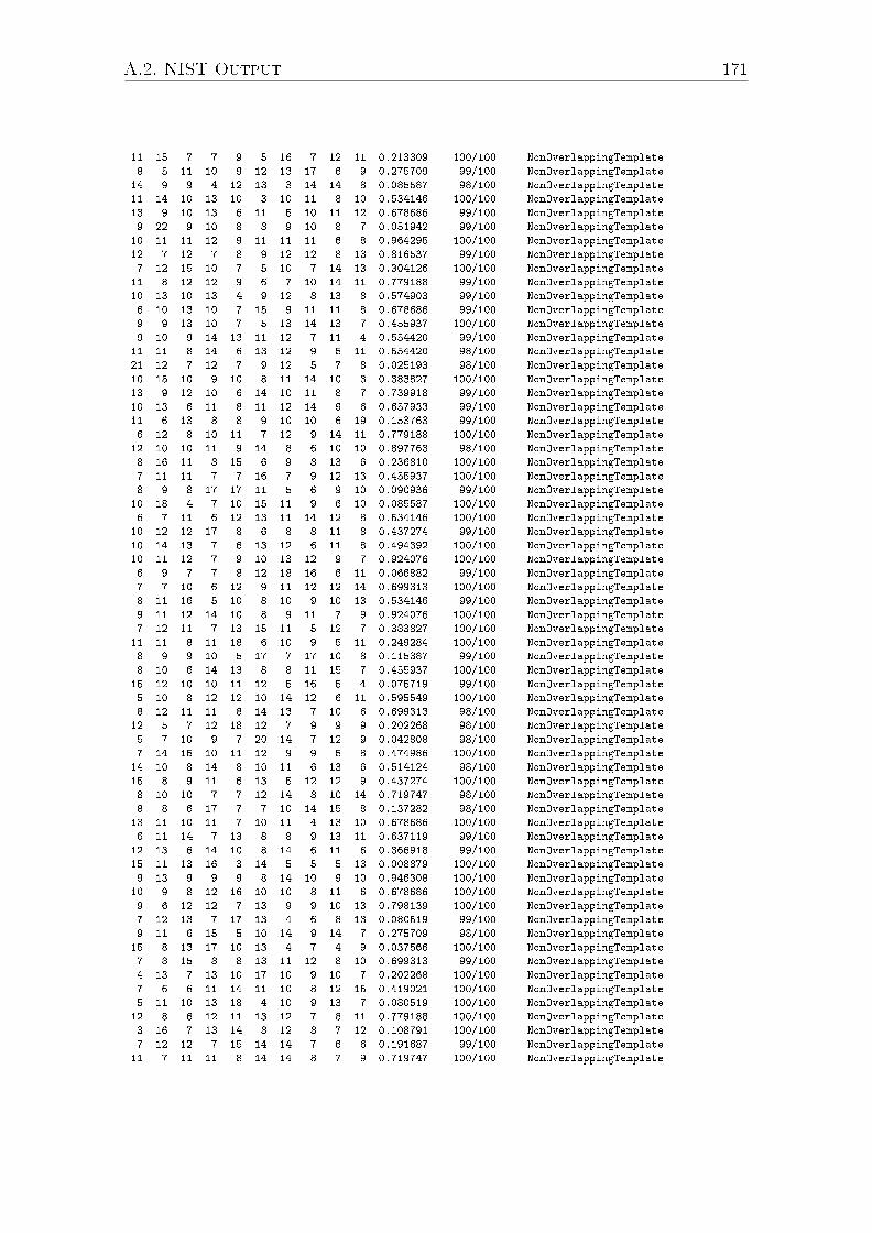
A.2. NIST Output 171
11 15 7 7 9 5 16 7 12 11 0.213309 100/100 NonOverlappingTemplate
8 5 11 10 9 12 13 17 6 9 0.275709 99/100 NonOverlappingTemplate
14 9 9 4 12 13 3 14 14 8 0.085587 98/100 NonOverlappingTemplate
11 14 10 13 10 3 10 11 8 10 0.534146 100/100 NonOverlappingTemplate
13 9 10 13 6 11 5 10 11 12 0.678686 99/100 NonOverlappingTemplate
9 22 9 10 8 8 9 10 8 7 0.051942 99/100 NonOverlappingTemplate
10 11 11 12 9 11 11 11 6 8 0.964295 100/100 NonOverlappingTemplate
12 7 12 7 8 9 12 12 8 13 0.816537 99/100 NonOverlappingTemplate
7 12 15 10 7 5 10 7 14 13 0.304126 100/100 NonOverlappingTemplate
11 8 12 12 9 6 7 10 14 11 0.779188 99/100 NonOverlappingTemplate
10 13 10 13 4 9 12 8 13 8 0.574903 99/100 NonOverlappingTemplate
6 10 13 10 7 15 9 11 11 8 0.678686 99/100 NonOverlappingTemplate
9 9 13 10 7 5 13 14 13 7 0.455937 100/100 NonOverlappingTemplate
9 10 9 14 13 11 12 7 11 4 0.554420 99/100 NonOverlappingTemplate
11 11 8 14 6 13 12 9 5 11 0.554420 98/100 NonOverlappingTemplate
21 12 7 12 7 9 12 5 7 8 0.025193 98/100 NonOverlappingTemplate
10 15 10 9 10 8 11 14 10 3 0.383827 100/100 NonOverlappingTemplate
13 9 12 10 6 14 10 11 8 7 0.739918 99/100 NonOverlappingTemplate
10 13 6 11 8 11 12 14 9 6 0.657933 99/100 NonOverlappingTemplate
11 6 13 8 8 9 10 10 6 19 0.153763 99/100 NonOverlappingTemplate
6 12 8 10 11 7 12 9 14 11 0.779188 100/100 NonOverlappingTemplate
12 10 10 11 9 14 8 6 10 10 0.897763 98/100 NonOverlappingTemplate
8 16 11 8 15 6 9 8 13 6 0.236810 100/100 NonOverlappingTemplate
7 11 11 7 7 16 7 9 12 13 0.455937 100/100 NonOverlappingTemplate
8 9 8 17 17 11 5 6 9 10 0.090936 99/100 NonOverlappingTemplate
10 18 4 7 10 15 11 9 6 10 0.085587 100/100 NonOverlappingTemplate
6 7 11 6 12 13 11 14 12 8 0.534146 100/100 NonOverlappingTemplate
10 12 12 17 8 6 8 8 11 8 0.437274 99/100 NonOverlappingTemplate
10 14 13 7 6 13 12 6 11 8 0.494392 100/100 NonOverlappingTemplate
10 11 12 7 9 10 13 12 9 7 0.924076 100/100 NonOverlappingTemplate
6 9 7 7 8 12 18 16 6 11 0.066882 99/100 NonOverlappingTemplate
7 7 10 6 12 9 11 12 12 14 0.699313 100/100 NonOverlappingTemplate
8 11 16 5 10 8 10 9 10 13 0.534146 99/100 NonOverlappingTemplate
9 11 12 14 10 8 9 11 7 9 0.924076 100/100 NonOverlappingTemplate
7 12 11 7 13 15 11 5 12 7 0.383827 100/100 NonOverlappingTemplate
11 11 8 11 18 6 10 9 5 11 0.249284 100/100 NonOverlappingTemplate
8 9 9 10 5 17 7 17 10 8 0.115387 99/100 NonOverlappingTemplate
8 10 6 14 13 8 8 11 15 7 0.455937 100/100 NonOverlappingTemplate
15 12 10 10 11 12 5 16 5 4 0.075719 99/100 NonOverlappingTemplate
5 10 8 12 12 10 14 12 6 11 0.595549 100/100 NonOverlappingTemplate
8 12 11 11 8 14 13 7 10 6 0.699313 98/100 NonOverlappingTemplate
12 5 7 12 18 12 7 9 9 9 0.202268 98/100 NonOverlappingTemplate
5 7 10 9 7 20 14 7 12 9 0.042808 98/100 NonOverlappingTemplate
7 14 15 10 11 12 9 9 5 8 0.474986 100/100 NonOverlappingTemplate
14 10 8 14 8 10 11 6 13 6 0.514124 98/100 NonOverlappingTemplate
15 8 9 11 6 13 5 12 12 9 0.437274 100/100 NonOverlappingTemplate
8 10 10 7 7 12 14 8 10 14 0.719747 98/100 NonOverlappingTemplate
8 8 6 17 7 7 10 14 15 8 0.137282 98/100 NonOverlappingTemplate
13 11 10 11 7 10 11 4 13 10 0.678686 100/100 NonOverlappingTemplate
6 11 14 7 13 8 8 9 13 11 0.637119 99/100 NonOverlappingTemplate
12 13 6 14 10 8 14 6 11 6 0.366918 99/100 NonOverlappingTemplate
15 11 13 16 3 14 5 5 5 13 0.008879 100/100 NonOverlappingTemplate
9 13 9 9 9 8 14 10 9 10 0.946308 100/100 NonOverlappingTemplate
10 9 8 12 16 10 10 8 11 6 0.678686 100/100 NonOverlappingTemplate
9 6 12 12 7 13 9 9 10 13 0.798139 100/100 NonOverlappingTemplate
7 12 13 7 17 13 4 6 8 13 0.080519 99/100 NonOverlappingTemplate
9 11 6 15 5 10 14 9 14 7 0.275709 98/100 NonOverlappingTemplate
15 8 13 17 10 13 4 7 4 9 0.037566 100/100 NonOverlappingTemplate
7 8 15 8 8 13 11 12 8 10 0.699313 99/100 NonOverlappingTemplate
4 13 7 13 10 17 10 9 10 7 0.202268 100/100 NonOverlappingTemplate
7 6 6 11 14 11 10 8 12 15 0.419021 100/100 NonOverlappingTemplate
5 11 10 13 18 4 10 9 13 7 0.080519 100/100 NonOverlappingTemplate
12 8 6 12 11 13 12 7 8 11 0.779188 100/100 NonOverlappingTemplate
3 16 7 13 14 8 12 8 7 12 0.108791 100/100 NonOverlappingTemplate
7 12 12 7 15 14 14 7 6 6 0.191687 99/100 NonOverlappingTemplate
11 7 11 11 8 14 14 8 7 9 0.719747 100/100 NonOverlappingTemplate
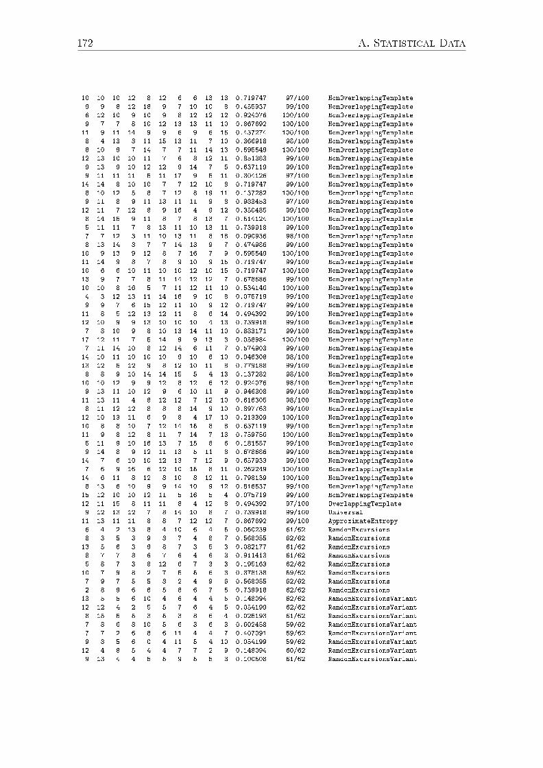
172 A. Statistical Data
10 10 10 12 8 12 6 6 13 13 0.719747 97/100 NonOverlappingTemplate
9 9 8 12 18 9 7 10 10 8 0.455937 99/100 NonOverlappingTemplate
6 12 10 9 10 9 8 12 12 12 0.924076 100/100 NonOverlappingTemplate
9 7 7 8 10 12 13 13 11 10 0.867692 100/100 NonOverlappingTemplate
11 9 11 14 9 9 6 9 6 16 0.437274 100/100 NonOverlappingTemplate
8 4 13 8 11 15 13 11 7 10 0.366918 98/100 NonOverlappingTemplate
8 10 9 7 14 7 7 11 14 13 0.595549 100/100 NonOverlappingTemplate
12 13 10 10 11 7 6 8 12 11 0.851383 99/100 NonOverlappingTemplate
9 13 9 10 12 12 9 14 7 5 0.637119 99/100 NonOverlappingTemplate
9 11 11 11 5 11 17 9 5 11 0.304126 97/100 NonOverlappingTemplate
14 14 8 10 10 7 7 12 10 8 0.719747 99/100 NonOverlappingTemplate
8 10 12 5 8 7 12 8 19 11 0.137282 100/100 NonOverlappingTemplate
9 11 8 9 11 13 11 11 9 8 0.983453 97/100 NonOverlappingTemplate
12 11 7 12 8 9 16 4 9 12 0.350485 99/100 NonOverlappingTemplate
8 14 15 9 11 8 7 8 13 7 0.514124 100/100 NonOverlappingTemplate
5 11 11 7 8 13 11 10 13 11 0.739918 99/100 NonOverlappingTemplate
7 7 12 3 11 10 13 11 8 18 0.090936 98/100 NonOverlappingTemplate
8 13 14 8 7 7 14 13 9 7 0.474986 99/100 NonOverlappingTemplate
10 9 13 9 12 8 7 16 7 9 0.595549 100/100 NonOverlappingTemplate
11 14 9 8 7 8 9 10 9 15 0.719747 99/100 NonOverlappingTemplate
10 6 6 10 11 10 10 12 10 15 0.719747 100/100 NonOverlappingTemplate
13 9 7 7 8 11 14 12 12 7 0.678686 99/100 NonOverlappingTemplate
10 10 8 16 5 7 11 12 11 10 0.534146 100/100 NonOverlappingTemplate
4 3 12 13 11 14 16 9 10 8 0.075719 99/100 NonOverlappingTemplate
9 9 7 6 15 12 11 10 9 12 0.719747 99/100 NonOverlappingTemplate
11 8 5 12 13 12 11 8 6 14 0.494392 99/100 NonOverlappingTemplate
12 10 9 9 13 10 10 10 4 13 0.739918 99/100 NonOverlappingTemplate
7 8 10 9 8 10 13 14 11 10 0.883171 99/100 NonOverlappingTemplate
17 12 11 7 5 14 9 9 13 3 0.058984 100/100 NonOverlappingTemplate
7 11 14 10 8 12 14 6 11 7 0.574903 99/100 NonOverlappingTemplate
14 10 11 10 10 10 9 10 6 10 0.946308 98/100 NonOverlappingTemplate
13 12 5 12 9 8 12 10 11 8 0.779188 99/100 NonOverlappingTemplate
8 8 9 10 14 14 15 5 4 13 0.137282 98/100 NonOverlappingTemplate
10 10 12 9 9 12 8 12 6 12 0.924076 98/100 NonOverlappingTemplate
9 13 11 10 12 9 6 10 11 9 0.946308 99/100 NonOverlappingTemplate
11 13 11 4 8 12 12 7 12 10 0.616305 98/100 NonOverlappingTemplate
8 11 12 12 8 8 8 14 9 10 0.897763 99/100 NonOverlappingTemplate
12 10 13 11 6 9 8 4 17 10 0.213309 100/100 NonOverlappingTemplate
10 8 8 10 7 12 14 15 8 8 0.637119 99/100 NonOverlappingTemplate
11 9 8 12 8 11 7 14 7 13 0.759756 100/100 NonOverlappingTemplate
5 11 9 10 16 13 7 15 8 6 0.181557 99/100 NonOverlappingTemplate
9 14 8 9 12 11 13 5 11 8 0.678686 99/100 NonOverlappingTemplate
14 7 6 10 10 12 13 7 12 9 0.657933 99/100 NonOverlappingTemplate
7 6 9 16 6 12 10 15 8 11 0.262249 100/100 NonOverlappingTemplate
14 6 11 8 12 8 10 8 12 11 0.798139 100/100 NonOverlappingTemplate
8 13 6 10 9 9 14 10 9 12 0.816537 99/100 NonOverlappingTemplate
15 12 10 10 12 11 5 16 5 4 0.075719 99/100 NonOverlappingTemplate
12 11 15 8 11 11 8 4 12 8 0.494392 97/100 OverlappingTemplate
9 12 13 12 7 8 14 10 8 7 0.739918 99/100 Universal
11 13 11 11 8 8 7 12 12 7 0.867692 99/100 ApproximateEntropy
6 4 2 13 8 4 10 6 4 5 0.060239 61/62 RandomExcursions
8 3 5 3 9 8 7 4 8 7 0.568055 62/62 RandomExcursions
13 5 6 3 9 8 7 3 5 3 0.082177 61/62 RandomExcursions
8 7 7 8 6 7 6 4 6 3 0.911413 61/62 RandomExcursions
5 8 7 3 8 12 6 7 3 3 0.195163 62/62 RandomExcursions
10 7 9 8 2 7 5 5 6 3 0.378138 59/62 RandomExcursions
7 9 7 5 5 8 2 4 9 6 0.568055 62/62 RandomExcursions
2 8 9 6 6 5 8 6 7 5 0.739918 62/62 RandomExcursions
13 5 5 6 10 4 6 4 4 5 0.148094 62/62 RandomExcursionsVariant
12 12 4 2 5 5 7 6 4 5 0.054199 62/62 RandomExcursionsVariant
8 15 5 5 3 5 3 8 6 4 0.025193 61/62 RandomExcursionsVariant
7 8 6 8 10 5 6 3 6 3 0.602458 59/62 RandomExcursionsVariant
7 7 2 6 8 6 11 4 4 7 0.407091 59/62 RandomExcursionsVariant
9 8 5 6 0 4 11 5 4 10 0.054199 59/62 RandomExcursionsVariant
12 4 8 5 4 4 7 7 2 9 0.148094 60/62 RandomExcursionsVariant
9 13 4 4 5 5 9 5 5 3 0.100508 61/62 RandomExcursionsVariant

A.2. NIST Output 173
6 12 7 8 2 2 10 5 5 5 0.082177 61/62 RandomExcursionsVariant
8 9 10 4 5 4 8 3 5 6 0.468595 62/62 RandomExcursionsVariant
8 7 8 6 4 5 7 4 8 5 0.911413 61/62 RandomExcursionsVariant
8 8 6 4 12 5 3 4 5 7 0.299251 61/62 RandomExcursionsVariant
7 7 4 3 5 11 7 5 9 4 0.407091 62/62 RandomExcursionsVariant
7 5 5 4 4 11 9 5 5 7 0.534146 61/62 RandomExcursionsVariant
8 4 6 8 5 9 7 8 5 2 0.602458 62/62 RandomExcursionsVariant
6 3 6 5 12 10 9 4 3 4 0.100508 62/62 RandomExcursionsVariant
6 6 4 7 7 3 12 6 5 6 0.468595 62/62 RandomExcursionsVariant
5 6 8 5 5 7 3 6 10 7 0.772760 62/62 RandomExcursionsVariant
17 12 10 10 7 7 9 6 12 10 0.419021 97/100 Serial
14 9 10 13 6 12 10 6 11 9 0.699313 97/100 Serial
8 10 8 11 7 11 8 12 18 7 0.350485 99/100 LinearComplexity