gain scheduled active power control for wind turbines€¦ · gain scheduled active power control...

Gain Scheduled Active Power Control

for Wind Turbines

Shu Wang∗ and Peter Seiler†

Department of Aerospace Engineering & Mechanics

University of Minnesota, Minneapolis, MN, 55455, USA

Traditional wind turbine control algorithms attempt to maximize power capture at lowspeeds and maintain rated power at high wind speeds. Active power control refers to amode of operation where the turbine tracks a desired power reference command. Activepower control enables wind farms to perform frequency regulation and to provide ancillaryservices in the energy markets. This paper presents a multiple input, multiple outputstrategy for active power control. An H∞ controller is designed at several operating pointsto coordinate the blade pitch angle and generator torque. The objective is to track a givenpower reference command while also minimizing the structural loads. The controller isgain-scheduled based on the wind speed and the power output in order to compensate forthe nonlinear turbine dynamics. This allows the turbine to be operated smoothly anywherewithin the power / wind speed envelope. The performance of this gain-scheduled design isevaluated using high fidelity simulations.

Nomenclature

ρ Air density, kg/m2

v Wind speed, m/sAr Rotor area, m2

β Blade pitch angle, degτg Generator torque, N ·mλ Tip speed ratio (TSR), unitlessω Rotor speed, rad/sR Radius of rotor area, mP Generator power, WCp Power coefficient, unitlessN Gearbox ratio, unitlessAPC Active power controlAGC Automatic generation control

I. Introduction

As a promising renewable energy, wind power is increasing fast in energy markets all over the world.Though it only accounts for 3 % of the electricity produced globally in 2011, the penetration of wind energyis very high in some European countries.1 In the United States, the amount of wind energy is expected toincrease to about 30 % by 2020 to 2030.2 The power output of wind turbines is variable due to time-varyingwind speeds and this may cause unreliable operation of the power grid. This is not a significant issue whenwind power is only a small portion of the total electricity generated on the grid. However, to integrate higherlevels of variable wind power into the grid it is important for wind turbines to provide active power control(APC).3 APC can be used for the turbine to respond to fluctuations in grid frequency, termed primary

∗Graduate Student, [email protected]†Assistant Professor, [email protected]

1 of 15

American Institute of Aeronautics and Astronautics

response, and to the power curtailment command from transmission system operator, termed secondaryresponse or automatic generation control (AGC).4

Traditional wind turbine control systems5 do not provide active power control. The power electronicsused in variable speed wind turbines decouple the mechanical/inertial turbine dynamics from the power grid.Thus a wind turbine with a traditional control law does not have the inertial response to a grid frequencyevent like a conventional coal power generator.6 As a result the wind turbine does not participate in theprimary response. Moreover, the power output from the turbine fluctuates with variations in wind speed.As a result, new control strategies are being considered to enable wind turbines to track power commandsand possible provide ancillary services.7–12 Some of these designs provide primary response by using inertiaresponse emulation.7,8 Another approach is to operate the wind turbine above the optimal tip speed ratiothus reserving kinetic energy.9,10 This approach enables the wind turbine to track the power commands andhence this can be used to realize AGC. The use of blade pitch control with or without combined generatortorque control has also been explored.11,12

This paper proposes a gain-scheduled H∞ controller to provide APC. The architecture is a 2-input, 2-output controller where collective blade pitch and generator torque are coordinated in order to track powerand rotor speed reference commands. The controller is scheduled on the wind speed and power output. Thisenables the gain-scheduled controller to have a uniform structure and operate smoothly anywhere within thepower/wind speed envelope of the turbine. Compared with a standard LPV controller13,14 which is solvedfrom linear matrix inequalities, the gain scheduling in this paper is realized by linear interpolation of theLTI controllers designed at grid points in the envelope. This simplifies the design process and allows forsmooth transitions of the closed-loop system between low and high wind speed operation. The remainderof the paper is organized as follows. Section II briefly reviews traditional turbine control and describesthe proposed gain-scheduling approach for APC. Section III gives the detailed design process for the gainscheduled H∞ controller. Simulation results are presented and discussed in Section IV. Finally, conclusionsand future work are summarized in Section V.

II. Control Strategy Development for APC

The proposed strategy for active power control of an individual turbine is developed in this section.Section II.A briefly reviews the traditional operation and control for a utility-scale wind turbine. The newactive power control strategy is described in Section II.B.

A. Traditional Wind Turbine Control

The captured power is given by Pc = 12ρArv

3Cp(β, λ) where ρ is the air density [kg/m3], Ar is the sweptarea of the rotor blades perpendicular to the wind flow [m2], and v is the wind speed [m/s].5,15 The non-dimensional power coefficient Cp is the fraction of the available wind power captured by the turbine. Thepower coefficient is a function of the (collective) blade pitch angle β [deg] and the tip speed ratio λ [unitless].The tip speed ratio is defined as the ratio λ := Rω

v where ω is the rotor speed [rad/s] (low speed side ofthe drive train) and R is the radius of the rotor area [m]. In words, λ is defined as the blade tip tangentialvelocity divided by the wind speed. Figure 1 shows a contour plot of the power coefficient Cp as a functionof the blade pitch β and tip speed ratio λ. The contours are shown for the WindPACT 1.5 MW turbinemodel provided with the NREL FAST turbine simulation package.16 The main control inputs to operate theturbine are the blade pitch angle β and generator torque τg [N ·m].

The trade-off between power capture and load reduction is typically achieved using a mode-dependentcontroller with objectives that depend on the wind speed.5,17,18 There are essentially four operating regionsas shown in the power versus wind speed curve in Figure 2. Below the cut-in speed (Region 1), there isinsufficient wind and the turbine is kept in a parked, non-rotating state. Above the cut-out speed (Region4), the turbine is shut down to prevent structural damage.

Between the cut-in and rated wind speeds (Region 2), the objective is to maximize the captured power.As shown in Figure 1, the power coefficient attains its optimal value of Cp∗ = .5075 when λ∗ = 7.2 andβ∗ = 1.4 deg. Thus power capture is maximized by holding blade pitch constant at β∗ and commanding thegenerator torque such that the turbine operates at λ∗. It can be shown that the standard control law18,19

2 of 15


Figure 1. Power coefficient contours for WindPACT 1.5MW Model.

Figure 2. Turbine operating regions.

τg = Kgω2 achieves this goal in steady winds if the gain is chosen as

Kg =Cp∗ρAR

3

2λ3∗N(1)

where N [unitless] is the gearbox ratio.Between the rated and cut-out wind speeds (Region 3), the objective is to maintain the rated power

while minimizing the structural loads on the turbine. In Region 3, the generator torque can be held constantand the blade pitch angles are actively controlled to maintain rotor speed at its rated value. Classical PI orPID controllers18,19 are widely used for the blade pitch control. Many methods have also been developedto improve the load reduction performance in this region, e.g. individual pitch control,20,21 LIDAR feed-forward,22,23 and advanced modern control methods.24–26 Blending is used as the wind speed approachesthe rated wind speed to ensure smooth transition between the Region 2 and Region 3 control objectives.The transition between Regions 2 and 3 is sometimes referred to as Region 2.5. Region 2.5 is introducedbecause the rated rotor speed is usually reached before the Region 2 control law reaches the rated torque.A linear torque vs. rotor speed relation is typically used to ramp from the standard τg = Kgω

2 to the ratedtorque.5

B. Architecture for APC

The traditional turbine control system reviewed in Section II.A does not provide active power control. Thissection describes the proposed approach to provide the capability to track power reference commands. It is

3 of 15


important to note that the wind conditions limit the power that can be generated (in steady-state) by theturbine. Specifically, the turbine must operate within the power vs. wind speed envelope shown in Figure 2.Thus active power control is constrained to power reference commands that are within this envelope. Methodsto reserve power and operate within this envelope include de-rating, relative spinning reserve, and absolutespinning reserve.10,12,27 Each of these methods corresponds to operation along a specific power vs. windspeed curve that lies within the available power envelope.

Our proposed approach is to use gain scheduling to operate anywhere within the power envelope. Thiswould enable de-rating, relative spinning reserve, and absolute spinning reserve as special cases. The basicoperational concept is shown in Figure 3. Trim points, denoted by red x’s, are chosen at many points ona grid within the power curve. At each trim point, the turbine dynamics are linearized and a control lawis designed using linear design techniques. Linear interpolation is used to calculate the controller gains foroperation between trim points, i.e. the controller is gain scheduled based on trim power and wind condition.Details on this design and implementation are provided in the next section. The gain scheduling approachdescribed here is less rigorous than modern linear parameter varying (LPV) techniques.28,29 The LPV designtechniques account for time variations in the scheduling variables. The gain scheduling proposed here shouldbe sufficient for slow variations in the scheduling parameters although there are no formal performanceguarantees. The benefit of gain-scheduling, as compared to more formal LPV techniques, is the ease ofdesign and implementation.

Figure 3. Operation envelope for gain scheduling.

The control design at a single trim point is now briefly described. To operate at one of the (v, P ) trimconditions within the envelope, the turbine must reduce the power coefficient to a new value Cp < Cp∗ bychanging the blade pitch angle and/or the tip speed ratio. As shown in Figure 1, there is a contour of possiblevalues of (λ, β) that achieve any value of Cp < Cp∗. For a given (v, P ) trim condition, the controller can bedesigned to operate at any point on the new Cp contour. For example, in low wind speeds the controllerproposed in10 shifts from (λ∗, β∗) to a larger tip speed ratio λ > λ∗ while holding blade pitch fixed at β∗.The benefit of this approach is that the turbine operates at a higher rotor speed and hence retains kineticenergy that can be extracted at a later point in time. To summarize, each (v, P ) trim condition correspondsto a desired power coefficient. The selection of (λ, β) along the contour of this desired Cp enables a secondaryperformance objective to be achieved, e.g. stored kinetic energy, reduced structural loads, etc.

The controller proposed in this paper tracks the desired power as follows. In low wind speeds, thecontroller shifts from (λ∗, β∗) to the desired Cp by increasing to a larger blade pitch β > β∗ while holdingtip speed ratio fixed at λ∗. The red arrow in Figure 1 indicates the proposed shift to the desired Cp in lowwind speeds. In constant wind conditions, this approach holds desired rotor speed constant (to maintainλ∗) while blade pitch angle is increased to shed extra power according to the desired power command. Thebenefit is that the constant loads on the blade, tower, and gearbox should be reduced by this method ofshedding power. However, this approach has the drawback that it will increase the pitch actuator usage.Another drawback of this approach is that less kinetic energy is retained in the rotor than if the turbinewere to shift to a larger tip speed ratio.

The APC strategy proposed in this paper can be implemented as the control system structure shown in

4 of 15


Figure 4. A 2-input, 2-output control system is used to coordinate the blade pitch and generator torque. Themain objective is to track the power reference command Pcmd. The rotor speed command ωcmd specifies thedesired point on the power coefficient contour. In particular the rotor speed command is defined as follows:

ωcmd = min

{vtrimλ∗R

,wrated

}(2)

where wrated is the rated rotor speed and vtrim is an estimate of the effective wind speed. As describedabove, this rotor speed command attempts to keep the λ at the optimal value λ∗ at lower wind speeds. Thiswill cause an increasing rotor speed demand as wind speed increases. At higher wind speeds, the rotor speedcommand saturates and attempts to maintain the rated rotor speed. It is assumed that an accurate and realtime measurement of the wind speed is available. As shown in Figure 4, an estimate of the wind speed couldbe obtained from a LIDAR.30 Alternatively, an estimate of the effective wind speed could be constructed.31

In either case, the actual wind speed fluctuates and hence low-pass filtering, denoted LPF1 in the figure, isused to smooth out these fluctuations.

The use of gain-scheduling with this MIMO architecture allows for uniform performance of the turbineacross all wind conditions. In other words, controllers of the same structure can be integrated using thetechnique of gain scheduling to meet the requirements in different wind conditions. The performance ofthe control system should be uniform and easy to design. The problem of transferring between regions ofoperations will also be a natural procedure in the design. However, it should be noted that this combinedMIMO control structure is more complicated than the SISO loops used in traditional wind turbine control.This may limit the ease of transitioning the proposed method to industrial turbines. A variety of simplercontrol architectures for APC were proposed and compared by Jeong, et. al.12

Figure 4. Proposed control strategy for APC.

III. Gain Scheduled H∞ Control Synthesis

This section provides details on the gain-scheduled approach introduced in Section II. The controlleris designed for the WindPACT 1.5 MW wind turbine whose model is contained in the FAST simulationpackage.16 First, the one-state rotor dynamic model is linearized at an arbitrary trim condition. Next,H∞ control design is described for one trim condition. Finally, details are provided for the gain-schedulingapproach.

A. Linearized Model For Control Design

The FAST simulation package developed by NREL16 is a nonlinear simulation package that is widely usedfor wind turbine control and analysis. This model includes up to 24 degrees of freedom, including differenttower and blade bending modes. FAST models can be linearized at a steady wind speed to obtain aperiodic, linear time-varying model. The multi-blade coordinate transformation can then be applied toobtain an approximate linear time-invariant model. The resulting linear time invariant models are suitablefor advanced control design. However, to simplify the synthesis of the gain scheduled controller this paperuses the one-state rotor model (described below) for design. The nonlinear one-state rotor model capturesthe essential aerodynamics and rotor dynamics of a wind turbine.19 This model does not contain structuraldynamics but it simplifies the design and it is useful for understanding the effectiveness of the proposed

5 of 15


active power control strategy. Moreover, the one-state model is only used for design but the controller isevaluated using higher fidelity simulations within FAST.

The one-state rotor model is given by:

Jω = τa −Nτg (3)

where τa and τg [N · m] are the aerodynamic and generator torques on the drive train. J [kg · m2] is theinertia of all rotating parts, including the blades, hub and drive train. ω [rad/s] is the rotor speed on thelow speed side of the drive train. The aerodynamic torque can be expressed in terms of the captured poweras

τa =Paω

=CpρAv

3

2ω(4)

The generator power output is given byP = ENτgω (5)

where E is the generator efficiency.The model used here also includes the standard control law in Equation 1 as an inner loop of the turbine

dynamics and part of the system to be controlled. This inner loop is helpful to maintain stability of theturbine. The analysis will be provided later. Moreover, retaining this inner loop feedback enables thepotential to shift smoothly between APC and the traditional torque control. Therefore, τg is given by:

τg = τ +Kgω2 (6)

where τ [N ·m] is the torque commanded by the outer loop for APC.The model used for control design is obtained by linearizing this nonlinear system at a trim condition.

Since the objective is to control the power output, a specific power P0 and wind speed v0 are selected fortrim condition. The trim rotor speed ω0 can then be calculated from v0 based on the rotor speed commandin Equation 2. The trim generator torque is calculated from τg0 = P0

ENω0. Cp0 is derived from the ratio of

trim generator power P0 to the power available from the wind. Finally, the trim collective blade pitch β0 isfound from the Cp0 contour data. Table 1 shows a single trim condition used for linearizing the WindPACTmodel.

Table 1. WindPACT Trim Condition

Parameter Value

v0 (m/s) 8

P0 (kW ) 400

ω0 (RPM) 15.715

τg0 (N ·m) 2909.3

Cp0 0.34896

β0 (deg) 8.9289

Let ∆ be used to denote the deviation of a variable from its trim condition, e.g. ∆ω := ω − ω0 denotesthe deviation of the rotor speed from the trim operating condition. The linearization of the nonlinear rotormodel is given by a state space model of the form

x = Ax+[Bβ Bτ

]u+Bv∆v (7)

y =

[EN(τg0 + 2Kgω

20)

1

]x+

[0 ENω0

0 0

]u+

[0

0

]∆v (8)

x := ∆ω is the state, u :=

[∆β

∆τ

]is the vector of control inputs, and y :=

[∆P

∆ω

]is the vector of system

6 of 15


outputs. The state matrices are given by:

A =

(−Cp0 + λ0

∂Cp∂λ

)ρArv

30

2Jω20

− Cp∗ρArR3

Jλ3∗ω0 (9)

Bβ =∂Cp∂β

ρArv30

2Jω0(10)

Bτ = −NJ

(11)

Bv =

(3Cp0 − λ0

∂Cp∂λ

)ρArv

20

2Jω0(12)

For the trim condition in Table 1, the partials derivatives appearing in this linearization are∂Cp

∂λ = 0.0017

and∂Cp

∂β = −2.1486. Some parameters of the system are listed here: A = −0.1104, Bβ = −0.4624, Bτ =

−2.5816× 10−5 and Bv = 0.0278. The second term of the state matrix A is −Cp∗ρArR3

Jλ3∗

ω0. This term arises

from the inner-loop standard law feedback and it is helpful to ensure the stability of the turbine dynamics.

B. H∞ Synthesis at One Trim Condition

This section describes the APC design at a single operating condition using the linearized one-state modelpresented in the previous subsection. The proposed control architecture in Figure 4 uses collective blade pitchand generator torque in order to track power and rotor speed commands. In principle, the controller couldbe implemented using the decoupled system shown in Figure 5. In this diagram G(s) denotes the linearizedone-state rotor dynamics and Aβ(s) denotes the dynamics of the blade pitch actuator. The dynamics of theblade pitch actuator are modeled as a low pass filter Aβ(s) = 1

s+1 . In this decoupled structure, the bladepitch is used to track power reference commands. The blade pitch actuation shifts the power coefficientbased on the power tracking error and this causes a change in the aerodynamic torque τa. The generatortorque is used to track the rotor speed commands. The decoupled controllers in this architecture, Kβ(s) andKτ (s), could be simple classical controllers, e.g. PI controllers, designed to achieve the tracking objectives.

Figure 5. Decoupled Controller Architecture

This decoupled structure is simple and easy to understand. However, it complicates the control designbecause the turbine dynamics couple together the power and rotor speed. This dynamic coupling makes itdifficult to properly tune the independent controllers Kβ(s) and Kτ (s). Moreover, the gain scheduling designdescribed in Section II.B requires controllers to be designed at many different trim points. Thus, manualtuning of the controllers in this decoupled architecture would be time consuming and it would be difficult toachieve uniform performance across the entire operational envelope.

For these reasons H∞ synthesis32,33 is applied in this paper to design coupled MIMO controllers. Thismethodology should enhance the performance by properly coordinating the two control inputs. Moreover,performance weights can be specified to enable tuning of the controller at many trim conditions. Theaugmented system for H∞ synthesis is shown in Figure 6. Here, seven different weight functions are chosento specify the performance requirements. The choice for each of these weights is described in detail below.

W1(s) and W2(s) are two performance weights that specify the objectives for power and rotor speedtracking. These weights are chosen to limit the low frequency error with less emphasis on high frequencytracking. The bandwidth of the power tracking weight is selected to be 0.08 rad/s. This is a conservativebandwidth but it is sufficiently fast for many power tracking objectives, e.g. AGC. The low frequency gainis 5000 which corresponds to a desired steady-state error in power tracking of 0.2 kW . This enforces a verytight power tracking requirement in steady state. Finally, the performance weight on the power tracking

7 of 15


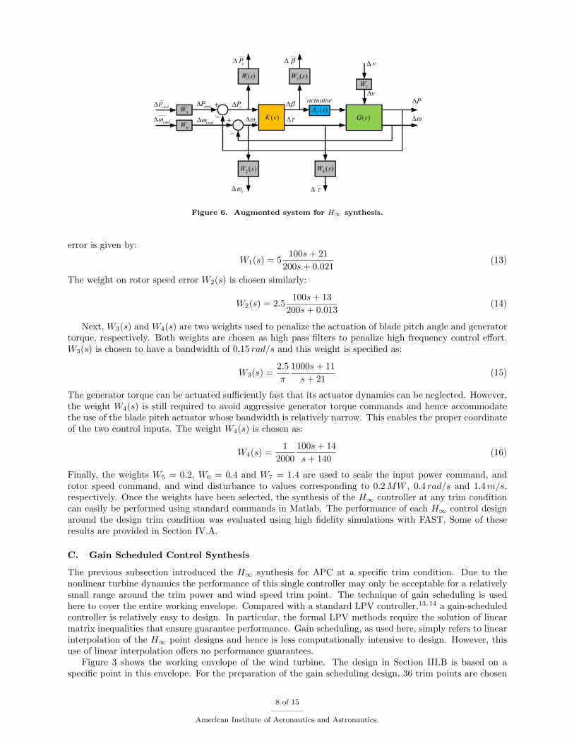
Figure 6. Augmented system for H∞ synthesis.

error is given by:

W1(s) = 5100s+ 21

200s+ 0.021(13)

The weight on rotor speed error W2(s) is chosen similarly:

W2(s) = 2.5100s+ 13

200s+ 0.013(14)

Next, W3(s) and W4(s) are two weights used to penalize the actuation of blade pitch angle and generatortorque, respectively. Both weights are chosen as high pass filters to penalize high frequency control effort.W3(s) is chosen to have a bandwidth of 0.15 rad/s and this weight is specified as:

W3(s) =2.5

π

1000s+ 11

s+ 21(15)

The generator torque can be actuated sufficiently fast that its actuator dynamics can be neglected. However,the weight W4(s) is still required to avoid aggressive generator torque commands and hence accommodatethe use of the blade pitch actuator whose bandwidth is relatively narrow. This enables the proper coordinateof the two control inputs. The weight W4(s) is chosen as:

W4(s) =1

2000

100s+ 14

s+ 140(16)

Finally, the weights W5 = 0.2, W6 = 0.4 and W7 = 1.4 are used to scale the input power command, androtor speed command, and wind disturbance to values corresponding to 0.2MW , 0.4 rad/s and 1.4m/s,respectively. Once the weights have been selected, the synthesis of the H∞ controller at any trim conditioncan easily be performed using standard commands in Matlab. The performance of each H∞ control designaround the design trim condition was evaluated using high fidelity simulations with FAST. Some of theseresults are provided in Section IV.A.

C. Gain Scheduled Control Synthesis

The previous subsection introduced the H∞ synthesis for APC at a specific trim condition. Due to thenonlinear turbine dynamics the performance of this single controller may only be acceptable for a relativelysmall range around the trim power and wind speed trim point. The technique of gain scheduling is usedhere to cover the entire working envelope. Compared with a standard LPV controller,13,14 a gain-scheduledcontroller is relatively easy to design. In particular, the formal LPV methods require the solution of linearmatrix inequalities that ensure guarantee performance. Gain scheduling, as used here, simply refers to linearinterpolation of the H∞ point designs and hence is less computationally intensive to design. However, thisuse of linear interpolation offers no performance guarantees.

Figure 3 shows the working envelope of the wind turbine. The design in Section III.B is based on aspecific point in this envelope. For the preparation of the gain scheduling design, 36 trim points are chosen

8 of 15


uniformly in increments of 200 kW in power and 2m/s in wind speed. These 36 trim points are denoted byx’s in Figure 3. H∞ controllers are designed at each trim condition using the same weights given in SectionIII.B.

Gain scheduling is used to interpolate the point control designs and their corresponding trim conditions.The detailed gain-scheduled structure is shown in Figure 7. Wind speed and power output signals are lowpass filtered and sent to the controller as trim conditions vtrim and Ptrim. The wind speed signal is the sameas that used to calculate the rotor speed reference command. The two low pass filters are chosen after sometrial and error to have corner frequencies of 0.1 rad/s (LPF 1) and 0.04 rad/s (LPF 2).

Figure 7. Structure of the gain scheduled controller.

The trim values of blade pitch angle βtrim and generator torque τtrim are calculated by linear interpola-tion. Specifically, the four nearest “grid” trim points {vi, Pi}4i=1 of the current (vtrim, Ptrim) are determined

as shown in Figure 3. The fractional distance along each coordinate axis is computed as k1 =P2 − PtrimP2 − P1

and k2 =v3 − vtrimv3 − P1

. Finally, the trim blade pitch and generator torque is given by

[βtrim

τtrim

]= k2

(k1

[β1

τ1

]+ (1− k1)

[β2

τ2

])+ (1− k2)

(k1

[β3

τ3

]+ (1− k1)

[β4

τ4

])(17)

Some trim conditions near the boundary of the operating area have less than four neighboring “grid” trimpoints. For conditions with only two neighbors, the interpolation is along a single dimension. For conditionswith only three neighbors, the fourth missing interpolant is filled using the grid condition that occurs at the

same trim wind speed. The state-space matrices for the controller,

[Ak Bk

Ck Dk

]are interpolated in a similar

fashion as that given in Equation 17. As shown in Figure 7, the trim inputs βtrim and τtrim are added tothe control inputs ∆β and ∆τ generated by the scheduled controller K. The standard torque feedback isused as an additional inner loop feedback for stabilizing the system as described in Section III.A.

IV. Simulation Results

A. Simulation for A Single LTI Controller

The first group of simulations were performed on both the linearized one state model of Wind PACT 1.5 MWwind turbine and the corresponding nonlinear model in FAST. The structural modes in the FAST modelinclude the first flap-wise blade mode for each blade and the first fore-after tower bending mode. Includingthe rotor position, the model has five degrees of freedom. This is a general setting for all the simulations inFAST. Both simulations only use an H∞ controller designed at one trim condition as described in SectionIII.B. The controller was designed at the steady wind speed of 8m/s and trim power of 400 kW . Themaximum captured power at this wind speed is 581 kW .

Two simulation results are shown in Figure 8. The left subplots show the results for a power commandsignal that steps from 400 kW to 450 kW at t = 50 s and then back to 400 kW at t = 150 s. The wind

9 of 15


speed was held constant at the trim condition. The left subplots show, from top to bottom, the rotor speedresponse, power output, blade pitch angle, and generator torque. Results are shown for both the linear(dashed) and nonlinear (solid) simulations. These simulation results show good agreement between thenonlinear FAST and linear simulations. The generator power output reached the new level by 90 % in lessthan 10 s without overshoot. The rotor speed fluctuation was also well regulated.

The right subplots in Figure 8 shown the simulation results for a power step command from 400 kW to550 kW and then back. The wind speed was again held constant at the trim condition. The linear and non-linear simulations show similar power tracking performance. However, the nonlinear simulations show somediscrepancies in the rotor speed and blade pitch angle responses. These discrepancies are due to the nonlin-ear turbine dynamics which become more significant for larger deviations from the trim operating condition.In general a single H∞ controller can perform well near its corresponding equilibrium point. However, thedifference between linear and nonlinear model will increase as the power command signal increases. Thisverifies the importance of implementing a gain-scheduled controller to deal with the nonlinearity of the windturbine.

Figure 8. Simulations for a single H∞ controller.

B. Simulation for Gain Scheduled Controller

The second group of simulations were performed with the gain-scheduled controller designed in Section III.C.The gain-scheduled controller was simulated using the nonlinear FAST model in turbulent wind conditions.

In the first simulation, the wind profile contains 5 % turbulence at a mean wind speed of 8m/s. Thiscorresponds to a typical Region 2 wind profile. The results are shown in Figure 9 for the gain-scheduledcontroller (solid line). For comparison, the figure also shows the turbine response for the the standard Kω2

torque feedback which attempts to maximize power capture (dashed line). The subplots are, from top tobottom, the rotor speed, power capture, blade pitch, and generator torque. The power capture command forthe gain-scheduled controller (dash-dot line in second subplot) steps from 400 kW to 500 kW at t = 150 s,

10 of 15


then drops to 300 kW at t = 300 s and finally steps back to 400 kW at t = 450 s. The gain-scheduledcontroller has a 90 % settling time response to the step commands of less than 10 s. In addition, the powertracking resists the fluctuations introduced by wind turbulence. Since the wind speed remains within theregion 2, the rotor speed command specified in Equation 2 is proportional to the low-pass filtered windspeed estimate. This rotor speed command is shown as the dash-dot line in the top subplot. The rotor speedregulation for the gain-scheduled controller has smaller fluctuations than those observed for the standardtorque feedback. To evaluate these fluctuations, define the root mean square (RMS) of the rotor speedtracking error ωRMS as:

ωRMS =

(1

T

∫ T

0

|ω − ωcmd|2dt

) 12

(18)

T is the simulation time. ω and ωcmd are the rotor speed and its reference. Since both standard control lawand APC try to track the optimal TSR λ∗ in low wind speed, their tracking errors as defined above can becalculated. Similarly, the RMS of the pitch rate can be defined to indicate the pitch actuation. The damageequivalent loads (DEL) are also calculated to evaluate the performance of the gain-scheduled controller. Allthese results are shown in the first part of Table 2 which is labeled by ‘under Rated Wind’. Compared tothe standard control law, there is a significant decrease in the RMS of the rotor speed tracking error for thegain-scheduled controller. At the same time, the DEL of the blade root flapwise bending moment and thetower fore-after bending moment decrease over 20 % (the exact ratio is shown in the parentheses after thevalue for each item). The DEL of the low speed shaft torque for the gain-scheduled controller is very closeto the value for the standard control law. However, the simulation for APC in Figure 9 contains severalstep power command signals that lead to abrupt changes in generator torque. In order to certify the effectof these changes to the DEL, a supplementary simulation using the gain-scheduled controller is done withconstant power command signal at 500 kW . The results are shown in the last column of Table 2. The DELof the low speed shaft torque decreases about 30 %. These results indicate that large loads occur on theshaft during step changes in power command. These loads would be alleviated in practice by using smooth(rather than step) power command transitions. The gain-scheduled controller uses (third subplot of Figure9) blade pitch actuation in these region 2 conditions to obtain the improved performance mentioned above.It is also shown in the rows of the ‘RMS Pitch Rate’ and the ‘Max Pitch Rate’ of Table 2. This additionalpitch actuation is the extra price the gain-scheduled controller paid for APC at under rated wind speed.Finally, the maximum available power is 581 kW for a steady 8m/s wind speed and the power commandremains within this limit. However, there were two periods during t = 200 s to t = 300 s where the windspeed dropped sufficiently that the available power was lower than the command power. The time intervalswere short enough that the impact on power tracking was negligible. The transient performance in turbulentwind conditions needs further consideration.

Table 2. Controller Performance Comparison for Simulations in FAST

Description Standard Control Gain-Scheduled G-S Supplementary

(under Rated Wind)

Blade Root Flapwise DEL 308.1 242.4 (−21.33%) 252.4 (−18.07%)

Tower Fore-after DEL 4602 3550 (−22.86%) 3525 (−23.4%)

Low Speed Shaft DEL 56.45 55.87 (−1.03%) 39.69 (−29.69%)

RMS Rotor Speed Error(RPM) 0.1951 0.1027 (−47.36%) 0.1026 (−47.41%)

RMS Pitch Rate (rad/s) 0 0.0022 (N/A) 0.0023 (N/A)

Max Pitch Rate (rad/s) 0 0.0132 (N/A) 0.0082 (N/A)

(above Rated Wind)

Blade Root Flapwise DEL 433.4 351.5 (−18.9%) 302.3 (−30.26%)

Tower Fore-after DEL 7027 5919 (−15.77%) 5088 (−27.59%)

Low Speed Shaft DEL 49.6 146.7 (+195.8%) 56.41 (+13.73%)

RMS Rotor Speed Error(RPM) 0.4064 0.3707 (−8.78%) 0.4003 (−1.5%)

RMS Pitch Rate (rad/s) 0.0061 0.0025 (−59.02%) 0.0025 (−59.02%)

Max Pitch Rate (rad/s) 0.0201 0.0191 (−4.98%) 0.0074 (−63.18%)

11 of 15


Figure 9. Simulation in below rated turbulent wind.

The second simulation was performed at an average wind speed of 13m/s with 5 % turbulence. The meanwind speed corresponds to above-rated, i.e. Region 3, wind conditions. The results are shown in Figure 10for the gain-scheduled controller (solid line) and a traditional PI blade pitch control law (dashed line). Thesubplots again are, from top to bottom, the rotor speed, power capture, blade pitch, and generator torque.The power capture command for the gain-scheduled controller (dash-dot line in second subplot) steps from500 kW to 900 kW at t = 150 s, then drops to 100 kW at t = 300 s and finally steps back to 500 kW att = 450 s. The rotor speed command for the gain-scheduled controller (Equation 2) is held fixed at the ratedrotor speed (shown as dashed dot line in top subplot). Compared to the traditional PI blade pitch controller,the gain-scheduled design shows better rotor speed regulation except for the transients after step changesin power command. Since both the traditional PI controller and the gain scheduled controller try to trackthe rated rotor speed in high wind speed, the RMS of the tracking errors can be calculated as defined inEquation 19. The second part of Table 2 which is labeled by ‘above Rated Wind’ verifies this observation.The power tracking and disturbance rejection performance of the gain-scheduled design was also reasonable.The blade pitch actuation was smoother for the gain-scheduled design than the traditional PI controller. Thisis also shown in Table 2. However, the high frequency blade pitch actuation obtained with the traditionalPI controller could be removed with further tuning. Finally, the generator torque for the gain-scheduled

12 of 15


design required additional activity to track the power commands and that leads to a significant increase(about 200 %) of the low speed shaft DEL when step signal adds in. Again, a supplementary simulationusing the gain-scheduled controller is done with constant power command at 900 kW . The low speed shaftDEL is about 14 % over the value for the standard control law in this situation. These results again indicatethat discontinuous step changes in the power command lead to a significant increase in shaft DELs. Hencesmooth power commands would be required in practice to avoid large shaft loads. Finally, the DEL of theblades and the tower are much lower for the gain-scheduled controller than the standard law, especially whenthe power command is constant.

Figure 10. Simulation in above rated turbulent wind.

V. Conclusion

This paper proposes a gain-scheduled H∞ control design for active power control. The blade pitch andgenerator torque are coordinated in order to track a power command and a specific tip speed ratio. Con-trollers are synthesized on a grid of trim operating conditions and the gain scheduling is used to interpolatefor operating between these trim points. The proposed structure enables a uniform design and operationanywhere within the power envelope of the turbine. Simulation results were provided for the feasibilityassessments of this control architecture. The power tracking performance is reasonable. Simulations studies

13 of 15


indicate that the proposed control design shows better rotor speed tracking and lower tower/blade dam-age equivalent loads as compared to the standard control law. Shaft damage equivalent loads are higherfor the proposed control design but still remain within acceptable limits. However, several aspects of thegain-scheduled control design need further consideration. These include the maximum power tracking band-width, additional outer loop controls for different ancillary services, upper bounds on the command powerin turbulent wind conditions, actuator saturation, and more rigorous LPV designs.

Acknowledgments

This work was supported by the National Science Foundation under Grant No. NSF-CMMI-1254129 en-titled ”CAREER: Probabilistic Tools for High Reliability Monitoring and Control of Wind Farms.” The workwas also supported by IREE Project RL001113, Innovating for Sustainable Electricity Systems: IntegratingVariable Renewable, Regional Grids, and Distributed Resources. Any opinions, findings, and conclusions orrecommendations expressed in this material are those of the authors and do not necessarily reflect the viewsof the National Science Foundation.

References

1“World Wind Energy Report 2011,” Proceedings of the 11 th World Energy Conference, World Wind Energy Associtation,Bonn, Germany, 2012.

2Crabtree, G., Misewich, J., Ambrosio, R., Clay, K., DeMartini, P., James, R., Lauby, M., Mohta, V., Moura, J., Sauer,P., et al., “Integrating Renewable Electricity on the Grid,” AIP Conference Proceedings-American Institute of Physics, Vol.1401, 2011, p. 387.

3Aho, J., Buckspan, A., Laks, J., Fleming, P., Jeong, Y., Dunne, F., Churchfield, M., Pao, L., and Johnson, K., “ATutorial of Wind Turbine Control for Supporting Grid Frequency through Active Power Control,” Proceedings of AmericanControl Conference, IEEE, 2012, pp. 3120–3131.

4Rebours, Y., Kirschen, D., Trotignon, M., and Rossignol, S., “A Survey of Freqency and Voltage Control AncillaryServices-Part I: Technical Features,” IEEE Transactions on Power Systems, Vol. 22, No. 1, 2007, pp. 350–357.

5Burton, T., Sharpe, D., Jenkins, N., and Bossanyi, E., Wind Energy Handbook , John Wiley & Sons, 1st ed., 2001.6Greedy, L., “Review of electrical drive-train topologies,” Project UpWind, Mekelweg, the Netherlands and Aalborg East,

Denmark, Tech. Rep, 2007.7Nelson, R. J., “Frequency-Responsive Wind Turbine Output Control,” 2011, U.S. Patent 0 001 318.8Keung, P.-K., Li, P., Banakar, H., and Ooi, B. T., “Kinetic Energy of Wind Turbine Generators for System Frequency

Support,” IEEE Transactions on Power Systems, Vol. 24, No. 1, 2009, pp. 279–287.9Juankorena, X., Esandi, I., Lopez, J., and Marroyo, L., “Method to Enable Variable Speed Wind Turbine Primary

Regulation,” International Conference on Power Engineering, Energy and Electrical Drives, 2009 , IEEE, 2009, pp. 495–500.10Aho, J., Buckspan, A., Pao, L., and Fleming, P., “An Active Power Control System for Wind Turbines Capable of

Primary and Secondary Frequency Control for Supporting Grid Reliability,” 51st AIAA Aerospace Sciences Meeting includingthe New Horizons Forum and Aerospace Exposition, 2013, pp. AIAA 2013–0456.

11Acedo Sanchez, J., Carcar, M., Lusarreta, M., Perez Barbachano, J., Simon Segura, S., Sole Lopez, D., Zabaleta Maeztu,M., Marroyo Palomo, L., Lopez Taberna, J., et al., “Method of Operation of A Wind Turbine to Guarantee Primary orSecondary Regulation in An Electric Grid,” 2011, U.S. Patent 0 057 445.

12Jeong, Y., Johnson, K., and Fleming, P., “Comparison and testing of power reserve control strategies for grid-connectedwind turbines,” Wind Energy, 2013.

13Apkarian, P., Gahinet, P., and Becker, G., “Self-scheduled H∞ Control of Linear Parameter-varying Systems: a DesignExamples,” Automatica, Vol. 31, No. 9, 1995, pp. 1251–1261.

14Bobanac, V., Jelavic, M., and Peric, N., “Linear Parameter Varying Approach to Wind Turbine Control,” 14th Interna-tional Power Electronics and Motion Control Conference, 2010, pp. T12–60–T12–67.

15Manwell, J., McGowan, J., and Rogers, A., Wind Energy Explained: Theory, Design, and Application, Wiley, 2010.16Jonkman, J. and Buhl, M., FAST User’s Guide, National Renewable Energy Laboratory, Golden, Colorado, 2005.17Bossanyi, E., “The design of closed loop controllers for wind turbines,” Wind Energy, Vol. 3, 2000, pp. 149–163.18Laks, J., Pao, L., and Wright, A., “Control of Wind Turbines: Past, Present, and Future,” Proceedings of American

Control Conference, 2009, pp. 2096–2103.19Johnson, K., Pao, L., Balas, M., and Fingersh, L., “Control of variable-speed wind turbines: standard and adaptive

techniques for maximizing energy capture,” IEEE Control System Magazine, Vol. 26, No. 3, 2006, pp. 70–81.20Bossanyi, E. A., “Individual Blade Pitch Control for Load Reduction,” Wind Energy, Vol. 6, No. 2, 2003, pp. 119–128.21Stol, K., Zhao, W., and Wright, A., “Individual blade pitch control for the controls advanced research turbine (CART),”

Journal of Solar Energy Engineering, Vol. 128, 2006, pp. 498.22Laks, J., Pao, L., Wright, A., Kelley, N., and Jonkman, B., “Blade pitch control with preview wind measurements,” 48th

AIAA Aerospace Sciences Meeting and Exhibit , 2010, pp. AIAA–2010–251.23Laks, J., Pao, L., and Wright, A., “Combined Feed-forward/Feedback Control of Wind Turbines to Reduce Blade Flap

Bending Moments,” 47th AIAA Aerospace Sciences Meeting, 2009, pp. AIAA–2009–687.

14 of 15


24Stol, K. and Balas, M., “Full-State Feedback Control of a Variable-Speed Wind Turbine: A Comparison of Periodic andConstant Gains,” Journal of Solar Energy Engineering, Vol. 123, No. 4, 2001, pp. 319–326.

25Stol, K. and Balas, M., “Periodic Disturbance Accommodating Control for Blade Load Mitigation in Wind Turbines,”Journal of Solar Energy Engineering, Vol. 125, No. 4, 2003, pp. 379–385.

26Wright, A. and Balas, M., “Design of Controls to Attenuate Loads in the Controls Advanced Research Turbine,” Journalof Solar Energy Engineering, Vol. 126, No. 4, 2004, pp. 1083–1091.

27Tarnowski, G., Kjær, P., Dalsgaard, S., and Nyborg, A., “Regulation and Frequency Response Service Capability ofModern Wind Power Plants,” Proceedings of IEEE Power and Energy Society General Meeting, 2010, pp. 1–8.

28Packard, A., “Gain Scheduling via Linear Fractional Transformations,” Systems and Control Letters, Vol. 22, 1994,pp. 79–92.

29Apkarian, P. and Gahinet, P., “A Convex Characterization of Gain-scheduled H∞ Controllers,” IEEE Transactions onAutomatic Control , Vol. 40, No. 5, 1995, pp. 853–864.

30Mikkelsen, T., Hansen, K., Angelou, N., Sjoholm, M., Harris, M., Hadley, P., Scullion, R., Ellis, G., and Vives, G., “Lidarwind speed measurements from a rotating spinner,” Proc. European Wind Energy Conference, Warsaw, Poland , 2010.

31Knudsen, T., Bak, T., and Soltani, M., “Prediction models for wind speed at turbine locations in a wind farm,” WindEnergy, Vol. 14, No. 7, 2011, pp. 877–894.

32Zhou, K., Doyle, J. C., and Glover, K., Robust and Optimal Control, 1st Edition, Prentice Hall, 1996.33Skogestad, S. and Postlethwaite, I., Multivariable Feedback Control , John Wiley and Sons Ltd., 2007.

15 of 15


gain scheduled active power control for wind turbines€¦ · gain scheduled active power control...

Documents