Munich Personal RePEc Archive

Gains from Free Trade Agreements: A

Theoretical Analysis

Huria, Sugandha

Jawaharlal Nehru University, New Delhi-India, Indian Institute of

Foreign Trade, New Delhi-India

28 October 2020

Online at https://mpra.ub.uni-muenchen.de/109815/

MPRA Paper No. 109815, posted 20 Sep 2021 20:27 UTC

1

Gains from Free Trade Agreements: A Theoretical Analysis

Sugandha Huria1

ABSTRACT

Empirical estimates from various studies on impact assessment of free trade agreements show that

there are limited economic gains from concluding such arrangements. It has been argued by trade

negotiators of many countries that while some partners gain more from an agreement, others gain less

or, even suffer from a rise in their current account deficits and overall economic losses. Even the Indian

scenario is not an outlier in such a case. This question about unequal gains from an FTA has raised

various policy concerns. We attempt to provide an answer to this debate by incorporating the role of

the type of commodities that countries trade with each other. In an imperfectly competitive setup with

three countries and two types of commodities viz. a final good and an intermediate input, our findings

reveal that bilateral free trade in final goods is more welfare-enhancing for the member countries vis-

à-vis bilateral free trade in intermediates. However, the former possibility is feasible only for a very

small range of parametric values given the pre-requisites for ensuring the formation of an effective

FTA. More specifically, we find that a horizontal FTA covering final goods becomes feasible only

when the degree of market size asymmetry between the two partners is very less. On the contrary,

when we emphasise on the role of vertical trade, i.e., where one of the FTA members exports

intermediate inputs to the other, and imports the final good in return, we find that FTA is feasible only

when the larger partner is an exporter of final goods and an importer of intermediate inputs, vis-à-vis

the smaller partner. In such a case, the larger partner accrues higher gains from such a bilateral

engagement. While capturing the role of tradable intermediates, we also show that in the presence of

well-connected GVCs, RTAs actually become a less attractive option for enhancing trade and welfare

of an economy.

JEL Classification: F12, F15

Key Words: Free Trade Agreements, Global Value Chains, Vertical Industry Structure

1 Jawaharlal Nehru University, New Delhi-IN; Indian Institute of Foreign Trade, New Delhi-IN. Email ID:

<sugandhahuria@hotmail.com>.

2

1. Introduction

Globally, the anti-trade sentiment has been on the rise, with various big economies like the United

States, China, among others, engaged in multiple escalations in a quest to protect their domestic

economies. The Covid-19 pandemic has further aggravated the situation, where many countries have

started adopting protectionist measures to preserve their democracies. This has raised scepticism about

free(r) trade, making it incumbent for the policymakers and the trade negotiators to explore and explain

the benefits of such policies. One such policy instrument is the ability of the countries to form

preferential trade pacts, or what in WTO terminology, are referred to as regional trade agreements. At

the time when these were allowed as an exception to GATT’s (General Agreement of Tariff and Trade,

1948) Most Favoured Nation (MFN) principle (Article I, GATT2), it was believed that regional

engagements would at least pave a towards global trade expansion by allowing the economies to take

advantage of preferential market access being offered by their intra-RTA countries (Pant and

Sadhukhan 2009, Pant and Paul 2018). It was also assumed that these arrangements would provide risk

cover during periods of global trade turmoil. However, recently, not only the ongoing global trade and

investment scenario has raised questions regarding their welfare effects, but various countries such as

India, members of the European Union (EU), amongst others, are also raising doubts regarding their

usefulness based on the premise that these pacts lead to unequal distribution of gains among the partner

economies (Dhar 2014, Hartwell and Movchan 2018, Kwatra and Kundu 2018). Even the former US

president, Mr. Trump, had raised this inequality concern while announcing the withdrawal of his

country’s partnership from the 12-nation Trans-Pacific Partnership (TPP) agreement in the year 2017

(Subramaniam 2016, Garrett 2017).

In this entire discourse on the distribution of (economic) gains from RTAs by some of the dominant

players and policy planners in the world market, the Indian industries seem to have been particularly

vocal about these arrangements. They have complained that their gains are being hampered by the

country’s commitments with its member nations. In an interaction with Business Line on June 12th,

2019, for instance, a Ministry of Commerce’ official said, “Many sectors such as steel, electronics,

chemicals, textiles and agricultural items like spices and Vanaspati have been hit due to the existing

FTAs, and the overall trade deficit with partner countries has also gone up.”3 The pharmaceutical sector

also criticised the country’s trade agreements with ASEAN, Japan, and South Korea on similar grounds

and reported only limited gains for their segment (FE Bureau, 2019). In fact, this issue has been at the

forefront of the country’s policy debates since 2017 when similar concerns were voiced by Indian

farmers and spokespersons of various industries, and the country’s government decided to review its

2 The MFN principle states that no member country should follow any discriminatory practice against the other signatories

of the agreement. 3 Sen (2019a)

3

free trade pacts for the first time (PTI 2017). India’s recent decision to opt-out of the RCEP deal after

more than 28 rounds of negotiations, is a perfect signal to its growing apprehensions about the welfare

effects from these mega trade blocs.4

A very specific cause has been pointed out by the North Indian Textile Mills’ Association (NITMA),

which is one of the biggest textile bodies of the country. In an interaction with the Secretary Textiles,

Government of India, the association explained that the India-ASEAN FTA had led to a surge in

imports of finished products of spinning mills, mainly from Vietnam and Indonesia, thereby forcing

many Indian MSMEs to close their spinning mills (Mathew 2019, TNN 2020). A similar complaint

was registered by Indian non-ferrous metal producers and the corresponding metal recycling units of

the country (Jha 2019). However, at the same time, it has also been reported by the Hindu Business

Line that several Indian industries are not entirely opposed to such deals. For instance, the textile

sector, while being against the India-ASEAN FTA or the RCEP talks, wants that the country should

negotiate an FTA with the EU (Sen 2019b) even though the Indian automobile industry is completely

against it (PTI 2015, PTI 2019). In particular, it has been identified that the cotton textile exporters

have been urging the country’s government to expedite the FTAs with EU, Australia, and Canada since

2015 (Jha 2015). Further, the findings of the Economic Survey 2019-20 also suggested that at least

some of the free trade agreements (signed between 1993 and 2018) have actually benefitted the country

by exerting a positive impact on its merchandise exports (Government of India 2020). Thus, it seems

that a balanced view needs to be taken by the government on the matter. Besides, although the literature

abounds with numerous studies on the welfare assessment of RTAs, with some of them being highly

critical of gains from these arrangements, it is not very clear why such complaints have been raised in

the past few years only.

Given this backdrop, the first question to ask is – When and why did this problem emerge? – The

review of the literature suggests that the evolution of preferential trade can actually be traced back to

the rise of international trade between different countries around the globe. Even before the

formulation of the GATT, RTAs existed between Belgium, the Netherlands, and Luxembourg

(popularly known as Benelux) and amongst some of the members of the current European Union

(former European Economic Committee). However, it is only in the past two - two and a half decades

that the world market experienced an exponential rise in the number of such deals being negotiated by

the WTO members – ranging only about 36 in number in the year 1975 and about 100 in 1995, there

4 Regional Comprehensive Economic Partnership (or RCEP) is a multilateral trade agreement between the ten-country

ASEAN bloc and its five FTA partners viz. China, Japan, South Korea, Australia, and New Zealand. Sources: Economic

Times (2019a, 2019b), Business Today (2019), Business Line (2019), among others.

4

are in total 302 physical RTAs5 in force today (WTO RTA Database). More so, as of September 2019,

no less than 695 notifications were received by the WTO, of which 481 were for those that are currently

in force. Clearly, then, these arrangements have gained a lot of popularity over time. However, are

these economically advantageous too? – From Viner’s static theory (1950) based on the concepts of

trade creation and trade diversion, the following long-lasted debate initiated by Lipsey and Lancaster

(1956), Lipsey (1957), Bhagwati (1971), Kirman (1973), and the like, to the more recent assessments

done by Baccini (2019), Nguyen (2019), Mon and Kakinana (2020), Takarada et al. (2020), etc., the

literature on RTAs is now flooded with both theoretical and empirical studies. Primarily, three different

yet interrelated questions have been addressed in these works – Are RTAs welfare enhancing for the

member countries? If yes, does the rise in welfare increase with the conclusion of deeper agreements?6

What is the impact on the welfare of non-member nations? And lastly, does regionalism hinder the

growth of multilateral free trade?

Surprisingly, the answer to none of these questions is unambiguous. Some of these studies have

stressed RTAs as a ‘bad idea’, that reduce welfare for both intra- and extra-RTA partners and detract

efforts towards the expansion of multilateral liberalisation (Bhagwati 1991, Grossman and Helpman

1994, Krishna 1998). On the contrary, others have argued that these agreements represent a positive

path to multilateralism and, thus, provide evidence that small countries want to participate in a global

system, which usually remains dominated by the industrialised economies (Freund 2000, Robinson

and Thierfelder 2002).

But, how do these gains or losses associated with the conclusion of an RTA vary from agreement to

agreement, and how are they divided among the member countries? – The literature seems to give little

guidance on the answer to these questions. To date, only a small literature, including studies by Carrère

(2006), Kohl (2014), Berlingieri, Breinlich and Dhingra (2018), and Baier et al. (2019), among others,

has discussed the asymmetric gains from FTAs. While the former two have analysed across-agreement

heterogeneity, Baier et al. (2019) have also empirically studied the underlying determinants of within-

agreement heterogeneity in FTA effects based on country-specific institutions, factor endowments,

already existing FTAs, monopoly power, pre-FTA trade barriers, etc. Berlingieri, Breinlich and

Dhingra (2018), on the other hand, have assessed the impact of EU common external trade policy on

consumer welfare (in various EU countries) in terms of changes in variety, access to better quality

products, and lower prices. Similarly, entering into deeper agreements leads to greater coordination,

5 As per the WTO’ terminology, the number of physical RTAs are counted by considering goods, services, and accession to an RTA together.

6 Depth, here, refers to the coverage/content of RTAs. As put forward by Hoffman, Osnago and Ruta (2017), RTAs now

do not only allow tariff concessions but, they also cover, in addition, an expanding set of policy areas such as services,

investment, and competition policy.

5

but that also comes at the expense of greater loss of autonomy. This, in turn, raises the question of

whether countries should continue to negotiate RTAs, and if so, with whom?

When the theory of economic integration started developing, most of the trade was in final goods –

goods were being produced in one country, and competition used to take place between domestic and

foreign goods with their own national characteristics. This type of trade was actually guided by the so-

called free trade doctrine as propounded by conventional theorists of the 18th century and early 20th

century (Smith 1776, Ricardo 1921 or Heckscher 1919 and Ohlin 1933 among others). As a

consequence, the countries from the North (and lately from the South as well) started negotiating RTAs

based on this premise. However, this popular doctrine is governed by the assumptions of the perfectly

competitive product as well factor markets, small open economies, inter-industry trade, and the theory

of first best7 – none of which prevail in reality. More importantly, another shortcoming of these theories

was their assumption that all the production stages are undertaken domestically within each economy.

In other words, these theories inherently assumed the absence of tradable intermediates.

However, the past few decades have experienced a fundamental transformation in the composition and

structure of trade being conducted between various economies. Today, more than half of world trade

is in intermediate products,8 and the so-called two-way/intra-industry trade contributes a significant

share in this new variety. Rapid advancements in technologies, reduction in transportation and

communication costs, and the gradual reduction of political as well as economic barriers to trade are

among some of the crucial factors that have accentuated this process of international slicing of

production activities, guided by the global value chains (GVCs). This is why what we observe today

is not only trade in final goods but of components and parts as well, thereby raising the scope and

coverage of trade agreements.

In this light, and with the development of the New Trade theory post-1975, the theory of RTAs

developed further. The implications of these considerations have been well discussed in some of the

earlier studies by Smith and Venables (1988), Wonnacott and Lutz (1989), Krugman (1991), Summers

(1991), Mukonoki (2004), etc. They have examined the welfare effects of RTAs in the presence of

monopolistic competition. Relatively fewer studies such as those by Krishna (2005), Ishikawa et al.

(2007), Kawabata, Yanase and Kurata (2010), Kawabata (2014, 2015), on the other hand, have

incorporated the features of vertically related markets as well. Across these vertical networks, some

countries are engaged in upstream stages of production depending upon their specialisation. In

contrast, others are involved in downstream stages where firms transform the imported and indigenous

inputs into final products using specific production techniques and, finally, export them into the

7 For details, refer to any textbook on trade theories such as Batra (1973) or Bhagwati, Panagariya and Srinivasan (1998)). 8 WTO (2019), Basco, S., & Mestieri (2019)

6

international market. While the rise of these internationally fragmented value chains has been

ubiquitous across the world, their expansion has raised concerns regarding the distribution of gains

among various participating economies – depending upon where a country is positioned on the so-

called smile curve (OECD–WTO-World Bank Group report (2014), Meng et al. (2020)). For instance,

it has often been argued that economies that perform high value-added tasks have seen higher mark-

ups, while the gains for producers to whom they outsource the manufacturing of parts/low value-added

tasks have been declining (World Development Report 2020). Likewise, even the benefits from RTAs

could vary depending upon the type of good (whether final or intermediate) that a country trades with

the partner country. If the composition of the trade basket differs on each side, then, ceteris paribus,

one member may gain more than the other, which is what has been experienced in the recent past.

While the studies mentioned above assess the effects of cross-regional RTAs on tariffs, welfare, and

incentives for global free trade in a vertical industry set up, the distinction between welfare gains or

losses, arising from engaging with partners based on different commodity baskets, has not been

explicitly studied in any of them.

Thus, in this essay, we build on these models and aim to theoretically examine whether the welfare

effects of free trade agreements (FTAs) are conditional on what type of products (final or

intermediates) are traded (imported/exported) by the member countries. In other words, the research

question would help us to address the debate regarding the uneven benefits of engagements in different

RTAs by focussing on the role of (tradable) commodity baskets.9 In doing so, unlike the studies by

Kawabata, Yanase and Kurata (2010), Kawabata (2015, 2016), we put special emphasis on the role of

preferential rules of origin (or ROOs) in determining the effective formation of an FTA, specifically

between asymmetric countries in terms of their market sizes. These rules now represent an essential

component of a trade agreement, and prevent non-member countries from exploiting differences in

tariffs they face while exporting to FTA members. Hence, they act as a means to prevent trade

deflection. While these agreements have become more of an empirical concern now, the significance

of a theoretical model arises from the fact that in reality, each RTA includes all kinds of trade, and

hence may falsely predict a weak or no empirical relationship between the type of products traded by

each country and the welfare gains from such arrangements. Developing a theory structure, therefore,

allows us to decide the commodity basket for each country, and also entails enough flexibility to ensure

that only a specific type of product is allowed to be traded via an RTA route at a time, while others

become a part of the exclusion list.

9 In fact, it seems plausible to assert that the analysis in our study could also be utilised to assess whether the imposition of

higher tariffs on imports of intermediate goods or final commodities are more harmful to a country’s welfare – something

that is extremely relevant for the impact on a country’s growth in the post Covid-19 scenario.

7

We also assess the welfare gains/losses of the non-member country, in the presence of each type of

agreement and determine the conditions under which RTAs hinder the progress towards

multilateralism. Besides, our theoretical framework also makes it possible to examine whether well-

connected global value chains affect the benefits that an intra-RTA bloc or the non-member countries

leverage from the RTA. As explained by Bruhn (2014) and Chains (2014), in GVC-led trade, goods

cross international borders several times in different forms (raw materials, processed/intermediate

inputs, final goods), incurring some amount of tariff at each stage of value-addition. As a consequence,

the structure of GVCs may actually multiply the effects of even low-level rates of duties, thus making

multilateral liberalisation more preferable vis-à-vis preferential liberalisation. In this context, our

second question is an attempt to illustrate whether GVCs make a strong case for bilateral trade

agreements or not.

Subsequent sections of this paper are structured as follows. Section 2 outlines the theoretical

framework that we have employed to answer our research questions, followed by sections 3 and 4,

which entail detailed information on different (trade) scenarios assumed and the corresponding results

as well. In particular, section 3 attempts to focus on horizontal FTAs in final goods or intermediate

inputs. On the contrary, the case of vertical FTAs, i.e., where the partner countries are involved in

exports of products belonging to different production stages, has been discussed in section 4. Finally,

the last section summarises some of the important results and concludes the essay.

2. The Analytical Framework

2.1 A simple three-country, 2-industry set up

The usual approach to document intra-industry trade is to assume that products produced or services

offered in different countries are (at least) slightly different from each other. Hence, their trade raises

the welfare of the economies by satisfying consumers’ tastes for variety – an insight (first) documented

by Krugman in his 1979 study. However, as argued by Brander (1981) and further examined by

Venables (1985) and many others, there are equally good reasons to expect a two-way trade in identical

products as well – which is popularly referred to as cross-hauling. Such type of trade occurs due to

strategic interactions among domestic and foreign firms.

We base our analysis along these lines and consider a simple world economy with three countries

denoted by 𝑖, where 𝑖 = 𝐴, 𝐵, 𝑅. Countries A (the home economy) and B (the partner country) are

assumed to be located in the same region, while R represents the rest of the world. In each country,

there are two imperfectly competitive industries viz. an upstream industry producing an intermediate

input (𝐼), and a downstream industry that utilises (𝐼) for producing the final output (𝐹). For analytical

simplicity, we assume that only one unit of intermediate input is required to produce a unit of final

8

good (and no other inputs are needed). Production of a unit of intermediate input, on the other hand,

requires services of a non-tradable factor of production (𝑉). As in Kawabata (2015), the factor market

in each country is perfectly competitive, and the average, marginal costs of producing the intermediate

input (anywhere in the world market) are assumed to be constant. We normalise this cost to zero.

Further, in each industry, all the three countries have a single firm, and produce a homogenous good.

We assume away any relocation (i.e., foreign direct investment) of these firms because of prohibitive

transaction costs. This completes the description of the supply side of our framework

On the demand side, we assume that consumer preferences in each country 𝑖 are characterised by an

aggregate quasi-linear utility function given by: 𝑈𝑖 = 𝑢𝑖(𝐹𝑖) + 𝑋𝑖 (1)

Here, 𝐹𝑖 represents the consumption of final good (𝐹) in country 𝑖, and 𝑢𝑖(𝐹𝑖) is assumed to take a

quadratic form. 𝑋𝑖 is the consumption of a competitively produced numeraire good. This type of setting

allows us to assume that the income effects are negligible and therefore, in the three countries, the

demand function for final good is represented by 𝐹𝑖 = 𝛼𝑖 − 𝑝𝑖 (2)

where 𝑝𝑖 is the market price of the final good in country 𝑖, and 𝛼𝑖 > 0 represents its market size.10

The asymmetry between the three countries is captured by their different market sizes. For expositional

simplicity and to focus our analysis on the assessment of different RTAs in the presence of ROOs, we

specifically assume that countries 𝐵 and 𝑅 are of similar sizes so that 𝛼𝐵 = 𝛼𝑅 = 𝛼. On the other hand, 𝛼𝐴 = 𝜃𝛼, where 𝜃 > 0 represents the degree of market size asymmetry between countries 𝐴 and 𝐵, 𝑅.

Such a setting is useful to examine the effects of FTAs when the participating economies are of

different sizes (which, in turn, also determines the potential market access opportunities that an FTA

entails, provided that the good, in question, is demanded in the partner country as well), and also allows

to compare and contrasts the benefits from an FTA when the countries involved are of similar sizes,

vis-à-vis the rest of the world.

2.2 Game structure and trade costs under alternative regimes

To answer our questions of interest, we formulate different cases, each of which represents a different

scenario in our 3 country-2 industry set up.

We begin with Case 1, where we assume that the three economies only trade in final goods. Therefore,

in addition to the domestic cost of production, each downstream firm incurs an additional cost in terms

10 The linearity of demand may not be essential for our main results, but simplifies their derivation and presentation.

9

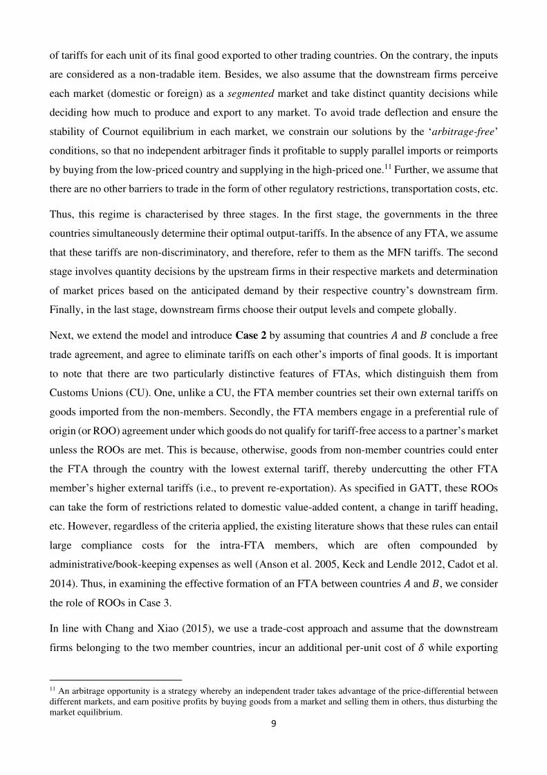
of tariffs for each unit of its final good exported to other trading countries. On the contrary, the inputs

are considered as a non-tradable item. Besides, we also assume that the downstream firms perceive

each market (domestic or foreign) as a segmented market and take distinct quantity decisions while

deciding how much to produce and export to any market. To avoid trade deflection and ensure the

stability of Cournot equilibrium in each market, we constrain our solutions by the ‘arbitrage-free’

conditions, so that no independent arbitrager finds it profitable to supply parallel imports or reimports

by buying from the low-priced country and supplying in the high-priced one.11 Further, we assume that

there are no other barriers to trade in the form of other regulatory restrictions, transportation costs, etc.

Thus, this regime is characterised by three stages. In the first stage, the governments in the three

countries simultaneously determine their optimal output-tariffs. In the absence of any FTA, we assume

that these tariffs are non-discriminatory, and therefore, refer to them as the MFN tariffs. The second

stage involves quantity decisions by the upstream firms in their respective markets and determination

of market prices based on the anticipated demand by their respective country’s downstream firm.

Finally, in the last stage, downstream firms choose their output levels and compete globally.

Next, we extend the model and introduce Case 2 by assuming that countries 𝐴 and 𝐵 conclude a free

trade agreement, and agree to eliminate tariffs on each other’s imports of final goods. It is important

to note that there are two particularly distinctive features of FTAs, which distinguish them from

Customs Unions (CU). One, unlike a CU, the FTA member countries set their own external tariffs on

goods imported from the non-members. Secondly, the FTA members engage in a preferential rule of

origin (or ROO) agreement under which goods do not qualify for tariff-free access to a partner’s market

unless the ROOs are met. This is because, otherwise, goods from non-member countries could enter

the FTA through the country with the lowest external tariff, thereby undercutting the other FTA

member’s higher external tariffs (i.e., to prevent re-exportation). As specified in GATT, these ROOs

can take the form of restrictions related to domestic value-added content, a change in tariff heading,

etc. However, regardless of the criteria applied, the existing literature shows that these rules can entail

large compliance costs for the intra-FTA members, which are often compounded by

administrative/book-keeping expenses as well (Anson et al. 2005, Keck and Lendle 2012, Cadot et al.

2014). Thus, in examining the effective formation of an FTA between countries 𝐴 and 𝐵, we consider

the role of ROOs in Case 3.

In line with Chang and Xiao (2015), we use a trade-cost approach and assume that the downstream

firms belonging to the two member countries, incur an additional per-unit cost of 𝛿 while exporting

11 An arbitrage opportunity is a strategy whereby an independent trader takes advantage of the price-differential between

different markets, and earn positive profits by buying goods from a market and selling them in others, thus disturbing the

market equilibrium.

10

their product within the FTA bloc via the FTA route. Further, to induce them to comply with ROO,

we specifically put a restriction that 𝛿 always falls short of the external tariff rates that the two

governments announce to maximise their respective welfare levels.12 While there have been several

studies on assessing the welfare effects of these ROOs, it is essential to mention that they assume the

role of tariffs in ensuring that the intra-FTA markets remain segmented even after the conclusion of a

free trade agreement.13

The significance of introducing Cases 1 and 2 is that they allow us to assess the welfare implications

of free trade arrangements, where we assume that the downstream firms are vertically unified entities,

i.e., they are dependent only on their own imperfectly competitive domestic markets for fulfilling their

input requirements. Though there exist several such studies in the literature (for instance, Chen and

Joshi 2010, Chang and Xiao 2015, among others), however, unlike our study, they assume perfectly

competitive input markets.

Considering Case 1 as the baseline scenario, we next incorporate the role of trade in intermediate goods

in Case 3, and assume that now the upstream firms also supply their products to the foreign

downstream players. This modifies stages 1 and 2 of our game – now, the governments in stage 1

simultaneously decide about the welfare maximising input and output tariffs. In stage 2, the three

upstream firms play in quantities and simultaneously decide about their production and export

decisions. Once again, we assume that the markets remain segmented (both downstream and upstream

markets), and there does not exist any profitable arbitrage opportunities.

Case 4, as an extension of Case 2, assumes that the governments of countries 𝐴 and 𝐵 decide to form

an FTA, whereby they agree to eliminate output-tariffs imposed on each other’s imports while

continuing to impose a positive MFN tariff rate on their imports of intermediate inputs. Thus, the

tradable inputs are considered as a part of the exclusion list in this case. However, their tradability now

makes it all the more imperative for the FTA partners to lay down the ROO conditions so as to avoid

tariff shopping. The objectives of this exercise are twin fold. In particular, we want to assess as to (a).

when does an FTA guarantee a higher level of welfare – in the absence or in the presence of globally

linked production structures? And, (b). when does an FTA guarantee a larger increase in the level of

welfare – in the absence/presence of these global chains?14 To put it differently, we want to analyse

12 This is because if the per-unit ROO cost exceeds the member country’s MFN tariff rate, then no firm would want to trade via the FTA route. 13 At times, the rules of origin are also required to incentivise them to move towards bilateral (if not, global) free trade by

limiting the benefits that the non-members get by member countries’ FTA. Hence, these also help in ensuring the stability of market equilibrium. 14 Our notion of vertical trade contrasts with the definition of Hummels, Rapoport, and Yi (1998), according to whom three

conditions must hold to for vertical specialisation to occur – a). production of a good must involve multiple sequential

stages, b). more than one country must specialise in some, but not all, production stages, c). at least one stage must cross

border more than once. However, in our present framework, we assume that each of the three countries produce as well as

11

whether the dramatic rise in the trade of intermediates in the past few decades has raised or reduced

the welfare-improving effects of free trade agreements? Hereafter, we refer to Case 4 as the case of

FTA in final goods in the presence of globally linked production chains.

In the next case, i.e., Case 5, we consider a possibility, when instead of bilateral free trade in final

goods, the governments in the two partner countries, 𝐴 and 𝐵, agree to eliminate tariffs imposed on

each other’s imports of intermediate inputs – referred to as the FTA in intermediates. Thus, in this case,

we assume that final goods become a part of their FTA’s exclusion list. The game structure remains

the same as in the previous case, except that in the second stage, the upstream firms in the two member

countries incur an additional per-unit cost of 𝛾 as ROO-induced trade cost while exporting their inputs

within the FTA bloc via the FTA route. The rest of the trade, however, takes place at the optimal MFN

rates between 𝐴, 𝐵 and 𝐶.

After assessing the welfare-improving effects of this FTA, we compare and contrast them with the

results obtained in Case 4, and analyse whether the benefits from reciprocity are larger in the case of

free trade in final goods or when FTAs are signed to eliminate barriers to trade in intermediates. In

other words, our simple model provides us a tractable framework to examine as to when larger gains

could be expected – when a country signs an FTA with a member with whom it trades mostly in final

goods or with the one, with whom the majority of its trade is in intermediate goods. This type of

analysis is specific to those set of countries where trade is mainly intra-industry trade. Besides, we also

assess the impact on changes in the individual components of the welfare of countries 𝐴 and 𝐵 vis-à-

vis the rest of the world. As argued by Copeland and Mattoo (2008),15 the consumer-lobbies for free

trade are often weaker than the producer-lobbies for protection. The latter represents a well-organised

interest group, and the government of any country, in general, faces considerable pressure from the

producers while deciding about trade-related policy instruments. Thus, such an exercise is useful to

assess the likely reasons for producers to support/show resistance for a particular FTA. Lastly, we also

utilise a rudimentary method to comment on the terms of trade effect of the two FTAs, the details of

which are documented in section 3 of this study. We also verify our results by theorising a situation

when A and B trade only in final goods with each other, followed by the case when they trade only in

intermediate inputs.

Next, we introduce Cases 6 and 7, and examine the possibility where the FTA partners are mostly

engaged in vertical trade, i.e., where one is engaged in the production and export of intermediate inputs,

while the other utilises that input in its final good’s industry and export it back to the FTA partner (like

trade in both intermediate input and final good, and therefore, are linked to each other. Since every downstream firm not

only employs the local intermediate inputs, but imported inputs as well, and finally exports its product to the rest of the

world, it is clear that inputs cross border more than once – one, in their original form, and two, as a part of the final good. 15 Chapter 3 in Handbook of International Trade in Services, Editors: Mattoo, Stern and Zanini.

12

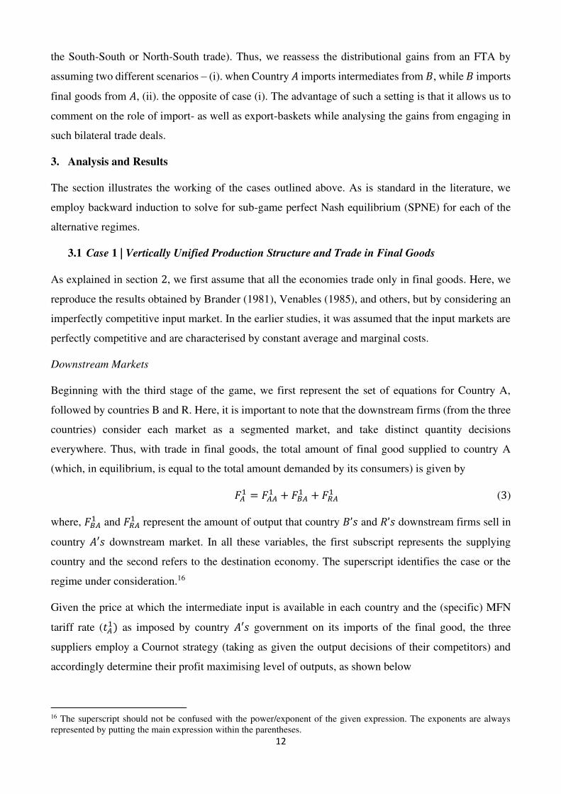
the South-South or North-South trade). Thus, we reassess the distributional gains from an FTA by

assuming two different scenarios – (i). when Country 𝐴 imports intermediates from 𝐵, while 𝐵 imports

final goods from 𝐴, (ii). the opposite of case (i). The advantage of such a setting is that it allows us to

comment on the role of import- as well as export-baskets while analysing the gains from engaging in

such bilateral trade deals.

3. Analysis and Results

The section illustrates the working of the cases outlined above. As is standard in the literature, we

employ backward induction to solve for sub-game perfect Nash equilibrium (SPNE) for each of the

alternative regimes.

3.1 Case 1 | Vertically Unified Production Structure and Trade in Final Goods

As explained in section 2, we first assume that all the economies trade only in final goods. Here, we

reproduce the results obtained by Brander (1981), Venables (1985), and others, but by considering an

imperfectly competitive input market. In the earlier studies, it was assumed that the input markets are

perfectly competitive and are characterised by constant average and marginal costs.

Downstream Markets

Beginning with the third stage of the game, we first represent the set of equations for Country A,

followed by countries B and R. Here, it is important to note that the downstream firms (from the three

countries) consider each market as a segmented market, and take distinct quantity decisions

everywhere. Thus, with trade in final goods, the total amount of final good supplied to country A

(which, in equilibrium, is equal to the total amount demanded by its consumers) is given by 𝐹𝐴1 = 𝐹𝐴𝐴1 + 𝐹𝐵𝐴1 + 𝐹𝑅𝐴1 (3)

where, 𝐹𝐵𝐴1 and 𝐹𝑅𝐴1 represent the amount of output that country 𝐵’𝑠 and 𝑅’𝑠 downstream firms sell in

country 𝐴′𝑠 downstream market. In all these variables, the first subscript represents the supplying

country and the second refers to the destination economy. The superscript identifies the case or the

regime under consideration.16

Given the price at which the intermediate input is available in each country and the (specific) MFN

tariff rate (𝑡𝐴1) as imposed by country 𝐴′𝑠 government on its imports of the final good, the three

suppliers employ a Cournot strategy (taking as given the output decisions of their competitors) and

accordingly determine their profit maximising level of outputs, as shown below

16 The superscript should not be confused with the power/exponent of the given expression. The exponents are always

represented by putting the main expression within the parentheses.

13

𝐹𝐴𝐴1 = αA − 3𝑑𝐴1 + 𝑑𝐵1 +𝑑𝑅1 + 2𝑡𝐴1 4 (4)

𝐹𝐵𝐴1 = αA + 𝑑𝐴1 − 3𝑑𝐵1 + 𝑑𝑅1 − 2𝑡𝑅1 4 (5)

𝐹𝑅𝐴1 = αA + 𝑑𝐴1 + 𝑑𝐵1 − 3𝑑𝑅1 − 2𝑡𝐴1 4 (6)

From the quantity equations, it is clear that each firm’s supply depends negatively on its own cost, and

positively on rival firms’ costs. We add the three quantities to determine the total output supplied to

country 𝐴′𝑠 consumers and use Equation (2) to compute the equilibrium price of final output in this

market. Thus,

𝐹𝐴1 = 3αA − 𝑑𝐴1 − 𝑑𝐵1 −𝑑𝑅1 − 2𝑡𝐴1 4 (7)

And,

𝑃𝐴1 = 3αA + 𝑑𝐴1+ 𝑑𝐵1 +𝑑𝑅1 + 2𝑡𝐴1 4 (8)

Following the same procedure, we next solve for the third stage’s solutions sets in countries B and R,

and find similar solutions for the two countries. Thus, once again, we observe standard results in terms

of Equations (7) and (8). However, as discussed in sub-section 2.2, two conditions constrain the

activities of downstream players and the resulting equilibrium solutions in the three markets (𝐴, 𝐵, 𝑅).

The first assumes that, in any country 𝑖 (𝑖 ∈ {𝐴, 𝐵, 𝑅}), the downstream firms supply positive

quantities, i.e., 𝐹𝑗𝑖1 > 0 ∀ 𝑖, 𝑗 ∈ {𝐴, 𝐵, 𝑅}. This condition requires that 𝛼𝑖 > 0 should be large enough

to ensure that the second-order condition for profit maximisation is satisfied for every downstream

firm. We also assume that the final goods market in each of the three countries are segmented, and the

three equilibrium prices satisfy the following ‘arbitrage-free’ conditions. 𝑃𝐴1 + 𝑡𝐵1 ≥ 𝑃𝐵1 ≥ 𝑃𝐴1 − 𝑡𝐴1 (9) 𝑃𝐴1 + 𝑡𝑅1 ≥ 𝑃𝑅1 ≥ 𝑃𝐴1 − 𝑡𝑅1 (10) 𝑃𝐵2 + 𝑡𝑅2 ≥ 𝑃𝑅2 ≥ 𝑃𝐵2 − 𝑡𝐵2 (11)

Intuitively, these imply that the price differential between any two markets should not exceed the trade

costs, and therefore, the two constraints together ensure a unique and stable Cournot equilibrium in

each country.

Upstream Markets

14

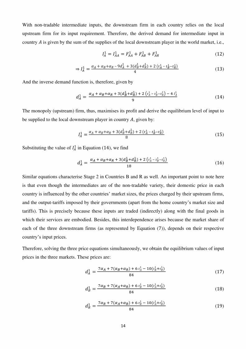
With non-tradable intermediate inputs, the downstream firm in each country relies on the local

upstream firm for its input requirement. Therefore, the derived demand for intermediate input in

country 𝐴 is given by the sum of the supplies of the local downstream player in the world market, i.e., 𝐼𝐴1 = 𝐼𝐴𝐴1 = 𝐹𝐴𝐴1 + 𝐹𝐴𝐵1 + 𝐹𝐴𝑅1 (12)

⇒ 𝐼𝐴1 = 𝛼𝐴 + 𝛼𝐵+𝛼𝑅 – 9𝑑𝐴1 + 3(𝑑𝐵1 +𝑑𝑅1 ) + 2 (𝑡𝐴1 – 𝑡𝐵1 −𝑡𝑅1) 4 (13)

And the inverse demand function is, therefore, given by

𝑑𝐴1 = 𝛼𝐴 + 𝛼𝐵+𝛼𝑅 + 3(𝑑𝐵1 +𝑑𝑅1 ) + 2 (𝑡𝐴1 – 𝑡𝐵1 −𝑡𝑅1 ) − 4 𝐼𝐴19 (14)

The monopoly (upstream) firm, thus, maximises its profit and derive the equilibrium level of input to

be supplied to the local downstream player in country 𝐴, given by:

𝐼𝐴1 = 𝛼𝐴 + 𝛼𝐵+𝛼𝑅 + 3(𝑑𝐵1 +𝑑𝑅1 ) + 2 (𝑡𝐴1 – 𝑡𝐵1 −𝑡𝑅1) 8 (15)

Substituting the value of 𝐼𝐴1 in Equation (14), we find

𝑑𝐴1 = 𝛼𝐴 + 𝛼𝐵+𝛼𝑅 + 3(𝑑𝐵1 +𝑑𝑅1 ) + 2 (𝑡𝐴1 – 𝑡𝐵1 −𝑡𝑅1 ) 18 (16)

Similar equations characterise Stage 2 in Countries B and R as well. An important point to note here

is that even though the intermediates are of the non-tradable variety, their domestic price in each

country is influenced by the other countries’ market sizes, the prices charged by their upstream firms,

and the output-tariffs imposed by their governments (apart from the home country’s market size and

tariffs). This is precisely because these inputs are traded (indirectly) along with the final goods in

which their services are embodied. Besides, this interdependence arises because the market share of

each of the three downstream firms (as represented by Equation (7)), depends on their respective

country’s input prices.

Therefore, solving the three price equations simultaneously, we obtain the equilibrium values of input

prices in the three markets. These prices are:

𝑑𝐴1 = 7𝛼𝐴 + 7(𝛼𝐵+𝛼𝑅) + 6 𝑡𝐴1 − 10(𝑡𝐵1 +𝑡𝑅1 ) 84 (17)

𝑑𝐵1 = 7𝛼𝐵 + 7(𝛼𝐴+𝛼𝑅) + 6 𝑡𝐵1 − 10(𝑡𝐴1 +𝑡𝑅1 ) 84 (18)

𝑑𝑅1 = 7𝛼𝑅 + 7(𝛼𝐴+𝛼𝐵) + 6 𝑡𝑅1 − 10(𝑡𝐴1 +𝑡𝐵1 ) 84 (19)

15

Here, in each of the three equations, a positive coefficient on the three countries’ market sizes indicates

a higher demand for final goods (which are traded in the world market), and therefore, a higher derived

demand for the intermediate input as well. Likewise, a higher import tariff imposed by any country’s

government (in contrast to a higher tariff imposed by its trading partners) discourages imports while

encouraging domestic production and hence, domestic requirement of inputs rises. Higher demand for

inputs, in turn, leads to a higher market price in each of the three countries.

Tariffs and Welfare

Finally, we solve for the equilibrium in stage 1 of this game, where the governments simultaneously

decide about their respective country’s optimal level of output-tariffs (considering the other countries’

tariffs as given). With the involvement of this fourth agent, the welfare in each country is equal to the

sum of consumer surplus, producer surplus, and tariff revenue. Therefore, using the first-order

condition, i.e., 𝜕𝑊𝑖1𝜕𝑡𝑖1 = 0 (𝑖 ∈ {𝐴, 𝐵, 𝑅}), we derive the optimal output-tariff rate in 𝐴, 𝐵, and 𝑅 as

𝑡𝐴1 = 0.322𝛼𝐴 − 0.045(𝛼𝐵 + 𝛼𝑅) + 0.041(𝑡𝐵1 + 𝑡𝑅1) (20) 𝑡𝐵1 = 0.322𝛼𝐵 − 0.045(𝛼𝐴 + 𝛼𝑅) + 0.041(𝑡𝐴1 + 𝑡𝑅1) (21) 𝑡𝑅1 = 0.322𝛼𝑅 − 0.045(𝛼𝐴 + 𝛼𝐵) + 0.041(𝑡𝐴1 + 𝑡𝐵1) (22)

By solving these equations simultaneously, we obtain the Nash equilibrium tariffs under regime 1: 𝑡𝐴1 = 0.320𝛼𝐴 − 0.033(𝛼𝐵 + 𝛼𝑅) (23) 𝑡𝐵1 = 0.320𝛼𝐵 − 0.033(𝛼𝐴 + 𝛼𝑅) (24) 𝑡𝑅1 = 0.320𝛼𝑅 − 0.033(𝛼𝐴 + 𝛼𝐵) (25)

Two observations are particularly noteworthy here – one, ceteris paribus, from Equations (20) − (22),

it is clear that unlike those studies that assume the absence of an intermediary stage of production,

tariff in each country now depends on the other countries’ tariff rates as well. This is happening even

when we assume that the intermediate inputs are non-tradable, and the countries only engage in

horizontal trade in final goods. Further solving for the optimal rates, Equations (23) − (25) indicate

that it is beneficial for a country to charge a lower tariff – the smaller is its size, and the larger is the

size of its trading partners. These observations can be re-interpreted in terms of the free-trade

optimality for the small open economies when both the product and factor markets are perfectly

competitive. Even in the presence of imperfection in the product market (if not in the factor markets),

our results indicate that it is welfare-improving for a comparatively smaller country to impose a lower

level of tariff vis-à-vis its larger trading partners.

16

Therefore, based on our assumption about market sizes, we can write the three countries’ welfare

function as: 𝑊𝐴1 = (𝛼)2(0.053  − 0.055𝜃 + 0.360𝜃2) (26) 𝑊𝐵1 = (𝛼)2(0.348  − 0.006𝜃 + 0.016𝜃2) (27) 𝑊𝑅1 = (𝛼)2(0.348  − 0.006𝜃 + 0.016𝜃2) (28) ⇒ 𝐺𝑊1 = (𝛼)2(0.750  − 0.068𝜃 + 0.392𝜃2) > 0 𝑖𝑓 (𝛼, 𝜃) > 0 (29)

Once again, this final solution set is constrained by two conditions – one, the positive output and input

conditions require that: 0.251 < 𝜃 < 2.565 (30)

while for the arbitrage-free conditions to hold, 0.355 < 𝜃 < 3.375 (31)

With 𝜃 > 0, Equations (30) and (31) imply 0.355 < 𝜃 < 2.565 (32)

This implies that beyond some limit, there will exist a possibility for profitable arbitrage to occur.

However, if we do not impose these conditions, then the optimal range for 𝜃 is given by (0.251, 2.565).

What this implies is that, unlike a perfectly competitive scenario, a shift from autarky to trade

(restricted trade, in this case), doesn’t necessarily guarantee higher welfare for the participating

economies. Nonetheless, the welfare-maximising tariffs are also positive, and not zero as shown in

Equations (20)-(22).17

3.2 Case 2 | Vertically Unified Production Structure and Free Trade in Final Goods between A

and B

We now consider the possibility of the formation of a free trade agreement between countries 𝐴 and 𝐵

while retaining our assumption regarding autarkic intermediate input markets.

Akin to the previous case 1, there are three stages of decision making. However, the only difference is

that the FTA member countries now do not impose any positive tariff on each other’s imports of final

goods. But to avoid tariff shopping and trade deflection, they agree to abide by the preferential ROO

requirements to obtain tariff-free access to partner country’s downstream market. After solving all the

17 This is a well-established result, and has been demonstrated in studies such as Brander and Spencer (1984), Ishikawa

(2000), Furusawa, Higashida and Ishikawa (2004), etc.

17

stages of the game, we find the range of feasible values of 𝛼, 𝛿 (ROO-induced trade cost), and 𝜃, while

ensuring that the following conditions hold:

a. A positive level of quantities for final goods produced by each downstream firm, which, in turn, will

ensure positive intermediate input quantities as well. The purpose is to ensure that no single firm

(upstream or downstream) ends up serving the entire world market.

b. No possibility of ‘profitable arbitrage’ in the case of downstream markets, i.e. 𝑃𝐴2 + 𝛿 ≥ 𝑃𝐵2 ≥ 𝑃𝐴2 − 𝛿 (33) 𝑃𝐴2 + 𝑡𝑅2 ≥ 𝑃𝑅2 ≥ 𝑃𝐴2 − 𝑡𝑅2 (34) 𝑃𝐵2 + 𝑡𝑅2 ≥ 𝑃𝑅2 ≥ 𝑃𝐵2 − 𝑡𝐵2 (35)

These conditions assume a crucial role in determining which RTAs improve welfare, and under what

conditions.

c. Post-FTA external tariff rates imposed by the two member countries do not exceed their pre-FTA MFN

rates, i.e., 𝑡𝐴3 ≤ 𝑡𝐴2 and 𝑡𝐵3 ≤ 𝑡𝐵2. It is important to ensure this constraint since it is explicitly mentioned

in GATT’s Article XXIV that the formation of any FTA should not raise trade barriers for the non-

FTA members. Henceforth, this condition is referred to as the GATT’s condition.

d. Post-FTA external tariff rates imposed by the two member countries are more than the ROO-induced

trade cost, i.e., 𝑡𝐴3 > 𝛿 and 𝑡𝐵3 > 𝛿. As discussed by Ju and Krishna (2005) and Chang and Xiao (2015),

this condition on the ROO-cost ensures that the FTA members' external tariffs effectively induce their

exporting firms to comply with the ROOs. Let’s call this as the ROO condition.

e. Since any country would be willing to conclude an FTA as long as doing so enhances its overall

welfare, we finally assume that 𝑊𝐴2 > 𝑊𝐴1 and 𝑊𝐵2 > 𝑊𝐵1

i.e., we subject the final set of solutions to the constraint that the post-FTA welfare level of member

countries should not be less than or equal to their pre-FTA welfare level. This is referred to as the

welfare-improving condition for the conclusion of an effective FTA.

Downstream Markets

Profit maximisation in each of the three countries’ final goods market yields the following set of

solutions. In country A, the total amount of final good supplied is now given by: 𝐹𝐴2 = 3αA − 𝑑𝐴2 − 𝑑𝐵2 − 𝑑𝑅2 − 𝛿 − 𝑡𝐴2 4 (36)

And, from (2),

𝑃𝐴2 = 3αA + 𝑑𝐴2 + 𝑑𝐵2 + 𝑑𝑅2 + 𝛿 + 𝑡𝐴2 4 (37)

18

Similarly, in country B, 𝐹𝐵2 = 3αB − 𝑑𝐴2 − 𝑑𝐵2 − 𝑑𝑅2 − 𝛿 − 𝑡𝐵2 4 𝑃𝐵2 = 3αB + 𝑑𝐴2 + 𝑑𝐵2 + 𝑑𝑅2 + 𝛿 + 𝑡𝐵2 4 (38)

In country R, the equilibrium can be represented by the same set of equations as in Case 1, and further,

we ensure that conditions (a) and (b) hold in this stage.

Upstream Markets

With no change in the second stage of this regime vis-à-vis the no-FTA case (1), the internally-

consistent equilibrium prices of the three suppliers are given by: 𝑑𝐴2 = 7(𝛼𝐴 + 𝛼𝐵 + 𝛼𝑅) + 3( 𝑡𝐴2 + 𝑡𝐵2 ) − 10(𝛿 + 𝑡𝑅2) 84 (39)

𝑑𝐵2 = 7(𝛼𝐴 + 𝛼𝐵 + 𝛼𝑅) + 3( 𝑡𝐴2 + 𝑡𝐵2 ) − 10(𝛿 + 𝑡𝑅2) 84 (40)

𝑑𝑅2 = 7(𝛼𝐴 + 𝛼𝐵 + 𝛼𝑅)− 13( 𝑡𝐴2 + 𝑡𝐵2 ) + 6(𝛿 + 𝑡𝑅2) 84 (41)

Equations (39)-(41) show that the optimal input prices for the FTA members are decreasing in the

ROO-induced cost, while that of the non-member country R, is increasing in 𝛿 . The intuition is that,

ceteris paribus, higher ROO cost implies higher exporting cost for the firms operating in the member

countries. Hence, they will export less within the FTA bloc compared to when 𝛿 is low. This, in turn,

will reduce their production, and hence, their demand for inputs, while at the same time, raising the

demand for inputs in country R. The latter happens because of a comparatively higher rise in the

exports of R with a higher ROO cost.

Tariffs and Welfare

We now turn to the determination of welfare-maximising output-tariffs in each of the three countries.

The only difference from Case 1 (i.e., the pre-FTA case) is that now the two FTA members do not

earn any tariff revenue on their imports from each other. Solving for the three optimal output-tariff

rates simultaneously, we obtain 𝑡𝐴2 = 0.361𝛿 + 0.166𝛼𝐴 − 0.005𝛼𝐵 − 0.048𝛼𝑅 (42) 𝑡𝐵2 = 0.361𝛿 − 0.005𝛼𝐴 + 0.166𝛼𝐵 − 0.048𝛼𝑅 (43) 𝑡𝑅2 = 0.034𝛿 − 0.039(𝛼𝐴 + 𝛼𝐵) + 0.319𝛼𝑅 (44)

From Equations (42)-(44), it is clear that higher ROO-induced cost is not only associated with a higher

level of output-tariffs in both the FTA members (due to the ROO condition) but in the non-member

country as well (because of the complementarity between different tariff rates as observed in Equations

19

(20)-(22)), meaning thereby it makes exports more costly in comparison to when 𝛿 = 0. In fact, for

countries 𝐴 and 𝐵, the responsiveness of tariffs to a unit change in 𝛿 is more than the responsiveness

to a unit change in their own or trading partner’s market size (as represented by the parameter 𝛼).

Therefore, with 𝛼𝐵 = 𝛼𝑅 = 𝛼 and 𝛼𝐴 = 𝜃𝛼 (where 𝜃 > 0), we find 𝑊𝐴2 = 0.576(𝛿)2 + 𝛼𝛿(−0.380 + 0.055𝜃) + (𝛼)2(0.122 − 0.057𝜃 + 0.319(𝜃)2) (45) 𝑊𝐵2 = 0.576(𝛿)2 + 𝛼𝛿(0.043 − 0.368𝜃) + (𝛼)2(0.312 − 0.017𝜃 + 0.090(𝜃)2) (46) 𝑊𝑅2 = 0.009(𝛿)2 + 𝛼𝛿(0.0006 − 0.025𝜃) + (𝛼)2(0.358 − 0.004𝜃 + 0.026(𝜃)2) (47) ⇒ 𝐺𝑊2 = 1.161(𝛿)2 − 𝛼𝛿(0.336 + 0.339𝜃) + (𝛼)2(0.792 − 0.079𝜃 + 0.435(𝜃)2) (48)

Thus, the ROO-cost, while ensuring the absence of profitable arbitrage opportunities (thereby

eliminating the possibility of trade deflection), raises the cost of exporting for the downstream firm in

each of the two member countries, viz. 𝐴 and 𝐵, and hence, negatively affects their welfare. Figure 1

illustrates this point graphically. Assuming that 𝛼 takes a value equal to 100 and 𝜃 equals 0.9, it plots

each country's welfare on the vertical axis against the ROO cost on the horizontal axis.

Figure 1: ROO cost and Welfare in each country, Case 2 (α=100, θ=0.9)

Source: Author’s representation

Thus, the welfare of both the member and non-member countries decreases in 𝛿, given that other

parameters remain unchanged. Moreover, the same result holds when country 𝐴 becomes large vis-à-

vis countries 𝐵 and 𝑅 (i.e., when 𝜃 > 1), or when 𝜃 equals 1. This implies that the two FTA members

will fix the lowest level of the ROO-induced trade cost (that prevents trade deflection), given that they

have the option to choose it freely.

With these results, we next determine the feasible values of the market size asymmetry, and ROO cost

that satisfy conditions (𝑎)-(𝑒) stated above. These conditions are a pre-requisite to ensure the formation

of an effective FTA between countries 𝐴 and 𝐵. For expositional simplicity, and to make our results

20

more intuitive, we specifically consider three different subsets of values that the parameter 𝜃 can take

viz. {𝜃: 𝜃 ∈ (0, 1) ∪ {1} ∪ (1, ∞)}. The distinctive feature of each of these subsets are as follows:

• 𝜃 ∈ (0, 1): This implies that Country 𝐴 is small vis-à-vis countries 𝐵 and 𝑅, of which the latter

represents the ROW.

• 𝜃 = {1}: This case assumes the absence of any market size asymmetry, and therefore, focusses

on FTAs between similar countries. In other words, the significance of this case is that it

controls for the differences in market sizes of the three trading partners, allowing us to focus

only on the RTA effects.18

• 𝜃 ∈ (1, ∞): In this subset, country A becomes the large country vis-à-vis the ROW.

Henceforth, we referred to these subsets as subcases. Since there are three parameters in our model

viz. 𝛼, 𝜃, and 𝛿, we use three-dimensional region plots to represent our results graphically. In each of

the plots, we restrict the values of 𝛼 in the range (0, 100], and assume that 𝛿 ∈ [0, 1], though such is

not the case when we mention the feasible bounds in equation form. This has been done to intuitively

interpret our results via graphical demonstration since the expressions (so derived) are quite

complicated.

Subcase 2.1: 𝜃 ∈ (0, 1)

From the previous Case 1, we know that the feasible bound for 𝜃 is given by: 0.355 ≤ 𝜃 < 2.565

Therefore, along with this constraint, and assuming that conditions (a), i.e., the quantity constraint, (c)

or the GATT condition, and the welfare-improving condition as in point (e), hold, we find the optimal

values that the three parameters can take. (𝛿 = 0 & 0.781 < 𝜃 < 1 & 𝛼 > 0), or (𝛿 > 0 & 0.781 < 𝜃 < 1 & 𝛼 > 𝛽2.1(𝜃, 𝛿)) (49)

where 𝛽2.1 = 567.(−2.251×1013𝛿+1.929×1014𝛿𝜃)−2.154×1016−6.591×1015𝜃+4.377×1016𝜃2 + 0.5√3.012×1034𝛿2−2.153×1033𝛿2𝜃−1.201×1034𝛿2𝜃2(−2.154×1016−6.591×1015𝜃+4.377×1016𝜃2)2

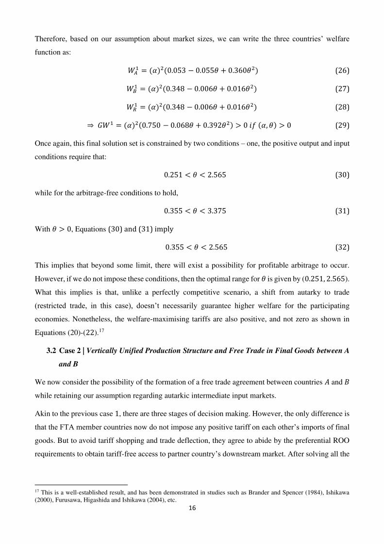
The region covered by these values is plotted in the leftmost panel (yellow-area) in Figure 2.

Regardless of whether 𝛿 takes a value greater than or equal to zero, the feasible range indicates that

only when the market size asymmetry is very less, i.e., when 𝜃 takes a value closer to 1, then the FTA

18 In the presence of homogenous final goods and intermediate inputs, we can also interpret this Subcase (i.e., when 𝜃 = 1)

as representing the formation of a customs union between symmetric countries, but in the absence of market integration

(characterised by 𝛿 = 0).

21

becomes welfare improving for both the partner countries. This signifies that the formation of a free

trade agreement may not necessarily be Pareto-improving. In fact, a similar range binds the values of

the parameters when we combine the constraints (a), (c), and (e) along with the constraint imposed by

the ROO-cost that is constraint (d), as shown by the green region in the second panel of Figure 2. This

implies that in this specific case, the ROO constraint is not binding. On the other hand, with a decrease

in the value of 𝜃 (i.e., when 𝜃 ∈ [0.355, 0.781]), we find that the FTA becomes welfare-deteriorating

for the big country, i.e., country 𝐵.

Figure 2: Feasible Regions, Subcase 2.1

Further, it is worth noting that in equation (49), for a given value of 𝛼, 𝛽2.1 represents a positive

association between the values of 𝜃 and 𝛿. In other words, it shows that when the market size

asymmetry falls (in which case, the price differential will be low), the ROO cost increases. This is

shown by the blue line (labelled as LHS(𝛽)) in Figure 3. A similar result was also observed by Chang

and Xiao (2015). This is because, if 𝜃 takes a value close to 1, then the welfare-improving condition

will hold for both the members even at higher values of 𝛿.

22

Figure 3: Relationship between Market Size Asymmetry and the ROO cost, Subcase 3.1

However, when we ensure that the arbitrage-free bounds also hold (as represented algebraically by the

set of inequalities (33)-(35)), then we find that there exists an upper bound on the values that 𝛼 can

take,19 and it shows a negative link between 𝜃 and 𝛿 (Pink line labelled as RHS in Figure 3).20 The

entire feasible region in this case (in comparison to Equation (49)), is given by: 𝛿 > 0 & (0.869 < 𝜃 ≤ 1 & 𝛽2.1 ≤ 𝛼 ≤ − 1591.𝛿−466.+466.𝜃) (50)

This region has been plotted in black in the rightmost panel in Figure 2, which is smaller in volume

vis-à-vis the yellow or the green regions in the other two panels of the same figure. Thus, imposing

the arbitrage-free bounds restricts the solution set and shows that only a small range of parametric

values supports the formation of an effective FTA with ROO. This is because when the countries are

dissimilar, then the likelihood of a tariff shopping increases. Hence, the arbitrage-free bounds impose

a higher penalty in terms of the ROO cost to ensure that the markets remain segmented. On the

contrary, when we do not assume the 'arbitrage-free' bounds, the possibility of welfare improvement

from FTAs increases as represented by Figure 4 that plots the feasible region with (black coloured

region) and without (yellow and black coloured region) the arbitrage-free constraints.21

Figure 4: Area bounded by the (effective) welfare-improving A-B FTA, Subcase 2.1

19 Such an upper bound is usually missing from studies that assume the absence of arbitrage-free bounds. 20 Here, the LHS and RHS correspond to the lower and upper bounds of 𝛼 in equation (50). 21 Even though a standard comparison is not possible because we don’t have free trade, and ours is a qualification vis-à-vis

the perfect competition framework, yet here also the general equilibrium results regarding free trade optimality holds.

23

Assessment of gains from the 𝐴 − 𝐵 FTA, and its effect on MFN tariffs

In the feasible region represented by equation (50), we find that even though the welfare of country 𝐴

falls short of the welfare of country 𝐵 as in the previous two cases when 𝜃 < 1, but the change in

welfare for the former is (unambiguously) more than the increase in welfare for country 𝐵 with the

formation of the FTA. This implies, like in the case of perfectly competitive markets, a smaller partner

gains more from integration vis-à-vis the large partner as freer trade does not enlarge the latter’s market

by as much as it does the smaller partner’s market access (Schiff 1996, Soo 2011). An important

observation is that the 𝐴 − 𝐵 FTA necessarily worsens the trade balance of country 𝐵 vis-à-vis the

smaller partner, yet it gains in terms of welfare within the feasible region. Further, decomposition of

welfare gains shows that while the FTA ensures higher consumer surplus as well as higher profits for

the upstream firm in each of the two members, it reduces surplus for the downstream firms. This is

because, with FTA, their exports increase to the member country and to the rest of the world, and so

do their export earnings, but their revenue from domestic sales fall. As a consequence, their total profits

(i.e., earnings from both domestic and export sales) decline vis-à-vis the pre-FTA scenario. Thus, even

though free trade expands the market coverage for the downstream firms within the FTA, but it does

so at the expense of their sales in their own domestic markets. This is the reason why domestic

producers or producer lobby often urge the government to deviate from liberal trade policy.22 This

means that in order to leverage The gains to consumers, on the other hand, can be explained via the

so-called pro-competitive effects of trade due to a fall in price of final goods (Impullitti and Licandro

2018), while the upstream firms profit with an increase in overall demand for final goods in the two

markets. Moreover, our findings also suggest that the FTA necessarily improves the participating

22 To some extent, these findings relate to the complaints registered by the local Television manufacturing units in India

regarding the adverse effects of zero duty imports of TVs (from the ASEAN countries, specifically Vietnam) on their

domestic production as well as sales (Rathee 2019).

24

countries’ terms of trade vis-à-vis the rest of the world.23 This is despite the fact that the FTA members

reduce their external tariff imposed on imports from country R, unlike what we observe in the case of

a perfectly competitive framework, where lower tariffs are associated with lower terms of trade (Batra

1973).

It is worth pointing out here that in the pre-FTA case (1), 𝑑𝐴1 < 𝑑𝐵1 = 𝑑𝑅1 . What this implies is that the

free trade area leads to some degree of trade diversion in the case of country 𝐴 by shifting some of the

production of final goods to countries 𝐵 and 𝑅, while it leads to only trade creation in the case of 𝐵.

Thus, the arguments by Lipsey (1957) and Bhagwati (1971) regarding welfare-enhancing effects of a

trade diverting FTA, also hold in the present case with imperfectly competitive output and input

markets, and intra-industry trade. A similar outcome was also observed by Krishna (1998).

Further, we find that even if we do not put impose the tariff condition (𝑐), then also, under the feasible

bounds, Bagwell-Staiger’s tariff complementarity effect holds24 – i.e., the bilateral FTA induces each

of the member countries to reduce the external tariff rate imposed on imports from the non-member

country, R. In fact, in response to this, within the feasible bounds, the MFN tariff imposed by the non-

member country also reduces in comparison to case 1. Equation (51) indicates the link between the

output-tariffs set by the FTA members and the non-member, 𝑅. 𝑡𝑅2 = 0.008𝛿 − 0.045(𝛼𝐴 + 𝛼𝐵) + 0.322𝛼𝑅 − 0.036(𝑡𝐴3 + 𝑡𝐵3)) (51)

What about country 𝑅’s welfare, and how does it compare with the welfare gains to the FTA partners?

– In the region bounded by inequality (50), the welfare of 𝑅 is higher than the pre-FTA case, and it is

also higher than the welfare of the similar-sized country 𝐵. This implies that the non-member is able

to accrue substantial gains when the member countries integrate with each other. This is because the

external tariffs imposed by all the countries reduce, and hence, country R’s trade with the two FTA

members also increases, and so does its total welfare. However, while comparing the gains with

country A, we find that for the majority of the combinations of parametric values (approx. 75 per cent),

gains are higher for the small FTA member than the rest of the world. We also find that while the 𝐴 −𝐵 FTA unambiguously benefits the producers in country R, the consumers suffer from welfare loss

due to an increase in the price of final good in the post FTA scenario. This is because of a higher rise

in the price of intermediate inputs in country R (with an increase in its demand by the downstream

firm), vis-à-vis the FTA members.

23 The terms of trade, for any country, represent the ratio of export-price to import price. For instance, for country 𝐴’s trade with country R, export price is given by 𝑝𝑅3, i.e., the price at which 𝐴’s goods are sold in 𝑅’s downstream market, and accordingly, the import price is given 𝑝𝐴3. 24 Bagwell and Staiger (1999).

25

These findings can be summarised in the following proposition.

Proposition 1. In a 3-country, 2 (imperfectly-competitive) sector framework with non-tradable

intermediate inputs, forming a free trade agreement between a small and a large trading partner (when

the rest of the world is also large) with rules of origin is welfare improving only when the degree of

market size asymmetry is very less, and the ROO-induced trade cost is not very high. The critical value

of this preferential cost varies positively or negatively with the degree of market size asymmetry

depending upon whether or not the arbitrage-free bounds (ensuring the absence of trade deflection)

hold. Nonetheless, the rest of the world unambiguously benefits from the welfare-improving FTA

between the two participating economies.

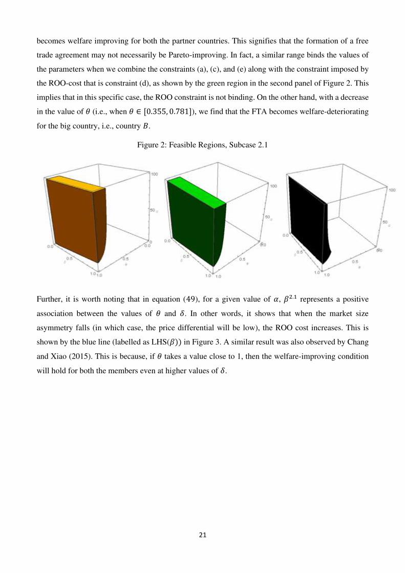
Subcase 2.2: 𝜃 ∈ {1}

In the absence of any market size asymmetry, we find that the feasible region is given by: 𝛿 = 0 & 𝛼 > 0, or 0 ≤ δ ≤ 0.098α (52)

Figure 5 plots the range of values that ensure the formation of an effective FTA between countries A

and B.

Figure 5: Region bounded by the (effective) welfare-improving A-B FTA, Subcase 2.2

Rest all the results remain the same as in the case when 𝜃 < 1. In fact, for all three countries, we find

higher welfare is positively associated with the size of their economies and negatively associated with

the ROO-induced trade cost. More so, any change in 𝛿 impacts the FTA members more than it impacts

the non-FTA country. This implies that the welfare-enhancing effects of FTAs depend not so much

(only) on the three countries’ market sizes but on the preferential rules of origin, which should be

strategically designed in order to ensure that FTAs lead to economic gains for the member economies.

26

On comparing the rise in welfare from the pre- to the post-FTA scenarios for the member and the non-

member countries, we find:25 𝑊𝐴𝑜𝑟𝐵2 − 𝑊𝐴𝑜𝑟𝐵2 > 𝑊𝑅2 − 𝑊𝑅1 if 0 ≤ 𝛿 < 0.015𝑎 𝑊𝐴𝑜𝑟𝐵2 − 𝑊𝐴𝑜𝑟𝐵1 ≤ 𝑊𝑅2 − 𝑊𝑅1 if 0.015 ≤ 𝛿 < 0.098𝑎

Thus, the lower the value of 𝛿, the higher are the chances that the rise in welfare level will be more for

the members than for the non-member country. Figure 6 also highlights this point, where the change

in welfare is higher for the partner countries in the purple region, while the grey area represents the

opposite case. The figure plots 𝑎 on the vertical axis whilst 𝛿 on the horizontal axis.

Figure 6: Gains from FTA (Members V/s Non-Member), Subcase 2.2

Subcase 2.3: 𝜃 ∈ (1, ∞)

This case considers country A as a large country, and countries B and R as small. Once again, we find

that the arbitrage-free bounds restrict the parameter space by a large amount, and only the black region

in Figure 7 represents the feasible set of values for α, 𝜃, and 𝛿 to ensure an effective FTA. On the

contrary, the entire coloured region (yellow plus black) represents the feasible bounds when we do not

put the arbitrage-free constraints to ensure a stable equilibrium. Algebraically, the region is defined by

the following: 𝛿 > 0 & 1 < 𝜃 < 1.151 & 𝛽2.3 < α ≤ − 3.414𝛿1. −1.𝜃 (53)

where, 𝛽2.3 = 𝛿(−4.514×1017+6.495×1016𝜃)−1.629×1017+3.774×1015𝜃+9.656×1016𝜃2 + √𝛿2(−1.900×1034−5.348×1034𝜃+1.363×1035𝜃2)(1.629×1017−3.774×1015𝜃−9.656×1016𝜃2)2

25 From symmetry, A’s welfare is same as B’s welfare.

27

Figure 7: Region bounded by the (effective) welfare-improving A-B FTA, Subcase 2.3

Regardless of whether country R is small or large, we find that, in the free trade area, a large country’s

welfare is more than the small country’s welfare. However, the rise in welfare (from pre- to post-FTA

scenario) is more for the smaller partner (i.e., partner B in the present subcase) in the entire feasible

region. This is despite the fact that the larger country’s trade balance worsens post the conclusion of

the FTA. The welfare of country R also increases, and therefore, the world welfare (or the global

welfare) as well. But, in contrast to Subcase 2.1, we find that for most of the feasible parametric values,

country B now gains more from engaging into the 𝐴 − 𝐵 FTA vis-à-vis country 𝑅. Therefore, we

establish the following proposition.

Proposition 2. In our 3-country, 2 (imperfectly-competitive) sector framework with non-tradable

intermediate inputs, the formation of a welfare-improving FTA between two asymmetric countries

(where asymmetry is measured in terms of their market sizes) always benefits the smaller partner more

vis-à-vis the large partner, irrespective of whether the non-member country is small or large. When

the non-member country is small and is similar in market size as one of the FTA members, then, at all

optimal equilibria, we find that the welfare gains for the non-member unambiguously exceed the gains

to the smaller FTA member (due to the formation of the FTA). However, when the non-member country

is large, then the similar-sized partner gains more for the majority of the combinations of the feasible

parametric values.

This means that if one small country partners with a large country, then it may also incentivise the

other small country to join the agreement to appropriate higher gains from free trade – something that

has also been observed empirically as well. This also relates to the domino theory of regionalism, as

28

explained by Baldwin (1993), and demonstrates the so-called ‘contagion effect’ in the proliferation of

FTAs in the past few decades (Baldwin and Jaimovich 2012).26

Not only 𝐵 gains more, but the terms of trade of both the FTA partners improve vis-à-vis the rest of

the world with the conclusion of the 𝐴 − 𝐵 FTA. However, R’s welfare gains are more than the larger

partner’s gains. Further, our results suggest that the MFN tariff of 𝑅 necessarily reduces in comparison

to Case 2. Thus, within the context of our framework, when 𝜃 > 1, it seems plausible to conclude that

regionalism acts as a building block towards multilateral free trade.

3.3 Case 3 | Vertically-linked production structures and Trade in Final and Intermediate Goods

So far, we have addressed the possibility of only horizontal trade between countries. However, vertical

trade, i.e., a trade where trading partners transact in different stages of production, has gained

significant importance in the past few decades. In fact, these types of transactions lead to the formation

of what are popularly referred to as the global value chains or GVCs.

In reality, a GVC may consist of ‘n’ different stages of production being carried out at ‘n’ different

places in the world market (𝑛𝜖ℕ), however, in our present setup, we are considering only a 2-stage

value chain where the first stage involves production of an intermediate input and the final stage

involves transformation of this input into a final good for consumption. Further, we assume that all

three countries now start trading in both intermediate inputs and final goods. Like in the case of final

goods, each upstream supplier also employs a Cournot strategy while deciding how much to sell in a

particular market, taking as given the quantity of inputs produced and sold by the other two firms. The

role of arbitrage-free bounds cannot be neglected in determining the final equilibrium in the

intermediate input market as well.

Downstream Markets

As in the Case 1, with trade in only final goods, a similar set of equations will characterise the

equilibrium in the three downstream markets in this case as well.

Upstream Markets

In stage 2, however, the three upstream firms (one from each country) compete in quantities in each

of the three countries, and decide about the optimal level of inputs to be supplied to their own

downstream market, and the downstream firms in other countries. Once again, due to market

segmentation, it is sufficient to focus on only one country’s equilibrium level of input (and hence,

26 Even though we do not explicitly model the behaviour of the non-member on formation of FTAs between the member

countries, our finding suggests a purely economic motive that might have induced the non-members to join some of the

free trade agreements.

29

market prices). Thus, based on the (stage-1) market-clearing conditions in the three countries, we can

derive the inverse demand for the intermediate input by the downstream firm in country 𝐴 as follows

𝐼𝐴3 = ∑ 𝐹𝐴𝑖3𝑖 where 𝑖 = {𝐴, 𝐵, 𝑅}

⇒ 𝐼𝐴3 = 𝑎𝐴 + 𝑎𝐵 + 𝑎𝑅 − 9 𝑑𝐴3 + 3 (𝑑𝐵3 + 𝑑𝑅3 ) + 2 (𝑡𝐴3 − 𝑡𝐵3 − 𝑡𝑅3) 4 (54)

⇒ 𝑑𝐴3 = 𝑎𝐴 + 𝑎𝐵 + 𝑎𝑅 − 9 𝑑𝐴3 + 3 (𝑑𝐵3 + 𝑑𝑅3 ) + 2 (𝑡𝐴3 − 𝑡𝐵3 − 𝑡𝑅3)−4𝐼𝐴39 (55)

Now, based on our technological assumption, the derived demand by country 𝐴’s final output producer

can be obtained by summing up the supplies of the intermediate inputs from its own country’s supplier,

and producers in other foreign countries, viz. countries 𝐵 and 𝑅. Algebraically, 𝐼𝐴3 = ∑ 𝐼𝑖𝐴3𝑖 where 𝑖 = {𝐴, 𝐵, 𝑅} (56)

The profit functions of the three suppliers are given by: 𝜏𝐴𝐴3 = (𝑑𝐴3) 𝐼𝐴𝐴3 (57) 𝜏𝐵𝐴3 = (𝑑𝐴3 − 𝑠𝐴3) 𝐼𝐵𝐴3 (58) 𝜏𝑅𝐴3 = (𝑑𝐴3 − 𝑠𝐴3) 𝐼𝑅𝐴3 (59)

where 𝑠𝐴3 represents the (MFN) input-tariff imposed by country 𝐴’s government. By assumption, (akin

to final good’s case) no country imposes any tax on the local upstream firm. Considering 𝑑𝐵3 and 𝑑𝑅3

as exogenous, the marginal first-order conditions (FOCs) for the two exporters along with the FOC for

the local player determine the optimal level of inputs to be supplied to country 𝐴’s downstream firm.

These quantities are given by:

𝐼𝐴𝐴3 = 𝑎𝐴 + 𝑎𝐵 + 𝑎𝑅 − 9 𝑑𝐴3 + 3 (𝑑𝐵3 + 𝑑𝑅3 ) + 18𝑠𝐴3 + 2 (𝑡𝐴3 − 𝑡𝐵3 − 𝑡𝑅3) 16 (60)

𝐼𝐵𝐴3 = 𝑎𝐴 + 𝑎𝐵 + 𝑎𝑅 − 9 𝑑𝐴3 + 3 (𝑑𝐵3 + 𝑑𝑅3 )− 18𝑠𝐴3 + 2 (𝑡𝐴3 − 𝑡𝐵3 − 𝑡𝑅3) 16 (61)

𝐼𝑅𝐴3 = 𝑎𝐴 + 𝑎𝐵 + 𝑎𝑅 − 9 𝑑𝐴3 + 3 (𝑑𝐵3 + 𝑑𝑅3 )− 18𝑠𝐴3 + 2 (𝑡𝐴3 − 𝑡𝐵3 − 𝑡𝑅3) 16 (62)

⇒ 𝑑𝐴3 = 𝑎𝐴 + 𝑎𝐵 + 𝑎𝑅 − 9 𝑑𝐴3 + 3 (𝑑𝐵3 + 𝑑𝑅3 )+ 18𝑠𝐴3 + 2 (𝑡𝐴3 − 𝑡𝐵3 − 𝑡𝑅3) 36 (63)

Similarly, solving stage 2 in upstream markets of 𝐵 and 𝑅, we find

𝑑𝐵3 = 𝑎𝐴 + 𝑎𝐵 + 𝑎𝑅 − 9 𝑑𝐴3 + 3 (𝑑𝐴3 + 𝑑𝑅3 )+ 18𝑠𝐵3 + 2 (− 𝑡𝐴3 + 𝑡𝐵3 − 𝑡𝑅3) 36 (64)

𝑑𝑅3 = 𝑎𝐴 + 𝑎𝐵 + 𝑎𝑅 − 9 𝑑𝐴3 + 3 (𝑑𝐴3 + 𝑑𝐵3 )+ 18𝑠𝑅3 + 2 (− 𝑡𝐴3 − 𝑡𝐵3 + 𝑡𝑅3) 36 (65)

30

As stated earlier, it is important to note that with quantity competition, there is no strategic

interdependence between the three country’s input prices. This interdependence arises only because of

the interaction of the three downstream players in the third stage in each of the three countries. This is

because, the value of the final goods produced by each firm, in turn, depends upon the cost of

intermediate inputs in each market. The three equations (63), (64), and (65) are thus solved

simultaneously to obtain: 𝑑𝐴3 = 0.033(𝑎𝐴 + 𝑎𝐵 + 𝑎𝑅) + 0.508𝑠𝐴3 + 0.046(𝑠𝐵3 + 𝑠𝑅3 + 𝑡𝐴3) − (𝑡𝐵3 + 𝑡𝑅3) (66)

A similar equation characterises the equilibrium input prices in countries 𝐵 and 𝑅 as well. Thus, what

we observe from here is that a country’s intermediate input price varies positively with input tariffs

imposed by its own government and so does with input tariffs imposed by others. The former could be

because tariffs lead to an increase in domestic prices of the importable good (at least in the absence of

a (Metzler) paradoxical kind of situation). The positive association could also be due to each producer's

market power that allows him to shift some burden of tariffs on to the final consumers (i.e., downstream

firms in our case). Further, with an increase in input-tariff imposed by foreign countries, the price of

their inputs increases, thereby raising the cost of producing the final output by their respective

downstream firm. Consequently, the demand for their final output falls in the world market, of which

country 𝐴 is a part. As a result, the demand for country 𝐴’s final output may rise. This leads to an

increase in its derived demand of input and hence, an increase in input price too.

Further, it is necessary to ensure that the opening up of upstream markets does not lead to profitable

arbitrage opportunities. Therefore, we assume that the following set of inequalities hold: 𝑑𝐴3 + 𝑠𝐵3 ≥ 𝑑𝐵3 ≥ 𝑑𝐴3 − 𝑠𝐴3 (67) 𝑑𝐴3 + 𝑠𝑅3 ≥ 𝑑𝑅3 ≥ 𝑑𝐴3 − 𝑠𝐴3 (68) 𝑑𝐵3 + 𝑠𝑅3 ≥ 𝑑𝑅3 ≥ 𝑑𝐵3 − 𝑠𝐵3 (69)

Tariffs and Welfare

Akin to the previous cases, the welfare of country 𝑖 (where 𝑖 = {𝐴, 𝐵, 𝑅}) is equal to the sum of

domestic surplus and export profits. However, domestic surplus now also includes revenues earned

from the imposition of input-tariffs. Thus, with no FTA, each country chooses its non-discriminatory

input as well as output tariff to maximize its own welfare. From the FOCs, and given the rate of input

and output tariffs imposed by the other two countries’ governments, we find that for country 𝐴, 𝑡𝐴3 = 0.296𝛼𝐴 − 0.035(𝛼𝐵 + 𝛼𝑅) + 0.008(𝑠𝐵3 + 𝑠𝑅3) + 0.028(𝑡𝐵3 + 𝑡𝑅3) (70) 𝑠𝐴3 = 0.030𝛼𝐴 + 0.029(𝛼𝐵 + 𝛼𝑅) + 0.009(𝑠𝐵3 + 𝑠𝑅3) − 0.043(𝑡𝐵3 + 𝑡𝑅3) (71)

31

Thus, unlike the results observed by Freund (2000) and Saggi (2006), country A’s tariffs depend on

the other countries’ tariff rates even in the presence of segmented markets and constant marginal costs

of producing the intermediate inputs. This feature is specific to models that assume different stages of

production. The problem confronting the other countries is exactly analogous to that confronting in

country 𝐴, and therefore solving the three countries’ tariff equations simultaneously, we obtain 𝑡𝐴3 = 0.295𝛼𝐴 − 0.027(𝛼𝐵 + 𝛼𝑅) 𝑠𝐴3 = 0.032𝛼𝐴 − 0.018(𝛼𝐵 + 𝛼𝑅) (72) 𝑡𝐵3 = 0.295𝛼𝐵 − 0.027(𝛼𝐴 + 𝛼𝑅) 𝑠𝐵3 = 0.032𝛼𝐵 − 0.018(𝛼𝐴 + 𝛼𝑅) (73) 𝑡𝑅3 = 0.295𝛼𝑅 − 0.027(𝛼𝐴 + 𝛼𝐵) 𝑠𝑅3 = 0.032𝛼𝑅 − 0.018(𝛼𝐴 + 𝛼𝐵) (74)

These results are similar to what we observed in equations (20) – (22), and with 𝛼𝐵 = 𝛼𝑅 = 𝛼 and 𝛼𝐴 = 𝜃𝛼, we find 𝑊𝐴3 = (𝛼)2(0.052  − 0.032𝜃 + 0.373𝜃2) (75) 𝑊𝐵3 = (𝛼)2(0.374  − 0.001𝜃 + 0.018𝜃2) (76) 𝑊𝑅3 = (𝛼)2(0.374  − 0.001𝜃 + 0.018𝜃2) (77) ⇒ 𝐺𝑊3 = (𝛼)2(0.800  − 0.030𝜃 + 0.408𝜃2) (78)

Further, assuming that all the quantities are positive, and the arbitrage-free conditions bind the final

set of solutions, we determine the (feasible) degree of market size asymmetry, as represented by

equation (79): 𝛼 > 0 & 0.375 ≤ 𝜃 ≤ 3.062 (79)

Before switching to the next case, i.e., Case 4, to assess the welfare-improving effects of an FTA (with

an emphasis on trade in final goods) in the presence of vertically integrated markets, we compare the

outcomes from Case 3 vis-à-vis Case 1 with vertically unified product markets. Table 1 briefly

encapsulates our findings from this analysis, which can be summarised in the following proposition:

Proposition 3. In our 3-country, 2 (imperfectly-competitive) sector framework, the opening up of

intermediate input markets incentivises the three economies to reduce their nominal output tariffs (in

almost all the optimal equilibria) and expand their overall trade volumes, regardless of whether the

degree of market size asymmetry is greater than or equal to or less than one. In doing so, the welfare

of each country rises, and so does the global welfare.

Table 1: Comparison of Outcomes, Case 3 Vs. Case 1

S. No. Basis for Comparison Observations (Case 3 V/s Case 1)

32

1 Feasible Region

In comparison to Case 3, the feasible values of 𝜃 in Case 1,

belong to the range [0.355, 2.565). This implies that

introducing vertically integrated production structures

allows for a greater degree of market size asymmetry when 𝜃 > 1, while allowing for a little less asymmetry when 𝜃 <1 (ensuring the absence of any profitable arbitrage

opportunities). However, the overall feasible range for 𝜃,

unambiguously increases. What this could imply is that the

introduction of tradable intermediates allows a wider range

of (welfare-improving) trade participation even between

those set of countries who do not (otherwise) trade with each

other.27

2 Output-tariffs

𝑡𝐴3 ≥ 𝑡𝐴1 𝑖𝑓 0.375 ≤ 𝜃 ≤ 0.456 𝑡𝐴3 < 𝑡𝐴1 𝑖𝑓 0.456 < 𝜃 < 2.565

However, tariff rates for countries 𝐵 and 𝑅 unambiguously

fall in the entire feasible range. This implies that fragmented

production structures or the so-called international

production chains assume a crucial role in guiding a

country’s trade policy. Blanchard, Bown and Johnson (2017) also reached a similar conclusion in an empirical study on

GVCs and trade policy for a total of 14 major economies

during the period 1995-2009.

3 Trade With a fall in output-tariffs, we find that all three countries

trade more in final goods in Case 3 than in Case 1.

4 Welfare of each country

In each of the three countries, consumer surplus, profits for

the final good producers, and tariff revenues are higher in

Case 4 than in Case 2. However, the surplus for the upstream

firms is lower than before. This mainly happens because of

the inelastic nature of the input demand in our set up.

Nonetheless, the total welfare increases with the opening up

of the input markets.

5 Global Welfare Global welfare is also higher in Case 3, than in Case 1.

27 In our model set-up, value added of final good exceeds the value added of intermediate inputs. Thus, our findings imply

that these global production/supply chains enable the trade and exchange of even low value-added tasks, and hence allow

the hitherto less open economies to expand their trade volumes and raise their overall welfare, while benefitting other large

open economies too as the latter get access to relatively cheaper inputs.

33

Thus, becoming a part of a global value chain or opening up of intermediate input markets, not only

ensures higher welfare for the participating economies but also incentivises them to adopt liberalised

trade policies, hence, benefitting the world as a whole.

3.4 Case 4 | Trade in Final and Intermediate Goods, FTA in Final Goods

In this case, we assume that countries 𝐴 and 𝐵 enter into a free trade agreement whereby they agree to

eliminate tariffs on each other’s exports of the final good. However, intermediate inputs become a part

of the negative list on which tariffs are not eliminated.

Apart from analysing the welfare effects of this FTA, we will also assess its benefits vis-à-vis case 2

in which intermediates were assumed to be non-tradable in nature. Further, in the next sub-section, we

will also compare and contrast the welfare with respect to the FTA that allows free trade in

intermediates (i.e., with Case 5).

Downstream Markets

Stage 3 solutions are similar to those observed in case 2. These solutions are constrained by positive

quantity conditions, and the arbitrage-free bounds as represented by Equations (33)- (35).

Upstream Markets

With no change in Stage 2 of this game, we follow the same procedure as in the previous case 3 (the

pre-FTA scenario but with trade in intermediates) and find the consistent equilibrium values of

intermediate input prices in the three countries. These prices are: 𝑑𝐴4 = 0.033(𝑎𝐴 + 𝑎𝐵 + 𝑎𝑅) + 0.508𝑠𝐴4 + 0.046(𝑠𝐵4 + 𝑠𝑅4) + 0.023(𝑡𝐴4 + 𝑡𝐵4) − 0.056(𝛿 + 𝑡𝑅4) (80) 𝑑𝐵4 = 0.033(𝑎𝐴 + 𝑎𝐵 + 𝑎𝑅) + 0.508𝑠𝐵4 + 0.046(𝑠𝐴4 + 𝑠𝑅4) + 0.023(𝑡𝐴4 + 𝑡𝐵4) − 0.056(𝛿 + 𝑡𝑅4) (81) 𝑑𝑅4 = 0.033(𝑎𝐴 + 𝑎𝐵 + 𝑎𝑅) + 0.508𝑠𝐴4 + 0.046(𝑠𝐵4 + 𝑠𝑅4) − 0.079(𝑡𝐴4 + 𝑡𝐵4) + 0.046(𝛿 − 𝑡𝑅4) (82)

Thus, once again, we find that the optimal input prices vary negatively with the ROO cost in the case

of the two FTA members, while it is directly related to 𝛿 in the case of country R. Nonetheless, we

impose the arbitrage-free bounds in the three upstream markets to ensure the stability of Cournot

equilibrium in each of them.

Tariffs and Welfare

The welfare maximising governments in countries A and B implement a positive input-tariff on intra-

FTA imports, as on the imports from country R. However, a positive output-tariff is imposed only on

imports of final goods from country R. Besides, the latter continues to impose the non-preferential

34

tariffs on its imports of intermediate inputs and final goods. The following equations (83)-(88)

represent the consistent Nash equilibrium tariffs rates in the three countries: 𝑡𝐴4 = 0.147𝑎𝐴 − 0.007𝑎𝐵 − 0.036𝑎𝑅 + 0.351𝛿 (83) 𝑡𝐵4 = −0.007𝑎𝐴 + 0.147𝑎𝐵 − 0.036𝑎𝑅 + 0.351𝛿 (84) 𝑡𝑅4 = −0.032(𝑎𝐴 + 𝑎𝐵) + 0.295𝑎𝑅 + 0.029𝛿 (85) 𝑠𝐴4 = 0.0001𝑎𝐴 + 0.037𝑎𝐵 + 0.017𝑎𝑅 − 0.003𝛿 (86) 𝑠𝐵4 = 0.037𝑎𝐴 + 0.0001𝑎𝐵 + 0.017𝑎𝑅 − 0.003𝛿 (87) 𝑠𝑅4 = 0.021(𝑎𝐴 + 𝑎𝐵) + 0.034𝑎𝑅 − 0.012𝛿 (88)

So, a higher ROO cost, while being positively associated with the output-tariffs (due to the so-called

ROO condition), negatively impacts the optimal rate of input-tariffs. This could be because a higher

output-tariff implies a higher cost of importing, which, in turn, negatively affects the imports of any

country while positively impacting its local production of the final good. Since a higher production of

final goods requires more intermediate inputs as well (some of which are also imported from abroad),

a lower 𝑠𝑖4 (𝑖 ∈ {𝐴, 𝐵, 𝑅}) reduces the cost of imports, and hence, the cost of producing final good.

Substituting Equations (83)-(88) in the second and third stage solutions, and therefore, in the welfare-

functions of the three countries, where 𝛼𝐵 = 𝛼𝑅 = 𝛼 and 𝛼𝐴 = 𝜃𝛼 (where 𝜃 > 0), we find 𝑊𝐴4 = 0.590(𝛿)2 + 𝛼𝛿(−0.375 + 0.032𝜃) + (𝛼)2(0.113 − 0.031𝜃 + 0.335(𝜃)2) (89) 𝑊𝐵4 = 0.590(𝛿)2 + 𝛼𝛿(0.027 − 0.371𝜃) + (𝛼)2(0.341 − 0.009𝜃 + 0.085(𝜃)2) (90) 𝑊𝑅4 = 0.010(𝛿)2 − 𝛼𝛿(0.014 + 0.022𝜃) + (𝛼)2(0.387 + 0.005𝜃 + 0.028(𝜃)2) (91) ⇒ 𝐺𝑊4 = 1.190(𝛿)2 − 𝛼𝛿(0.336 + 0.339𝜃) + (𝛼)2(0.841 − 0.035𝜃 + 0.448(𝜃)2) (92)

Although the ROO-cost helps in ensuring the absence of parallel imports or trade deflection even after

the formation of an FTA, yet higher the ROO cost, ceteris paribus, lower is the welfare of any country

(member or non-member, i.e., country R). This result is analogous to what we observed in case 2.

Next, we determine the feasible range of values for 𝛼, market size asymmetry, and the ROO-induced

cost. Akin to case 2, for ease of interpretation, we consider three subcases viz. {𝜃: 𝜃 ∈ (0, 1) ∪ {1} ∪ (1, ∞)} and subject the optimal solutions so obtained to the five pre-requisites for ensuring the

formation of an effective FTA (with ROO). The only difference from case 2 is that now we have to

ensure that the arbitrage-free bounds hold in upstream markets as well. Further, we also assess whether

FTAs lead to higher welfare gains in the presence or the absence of tradable intermediates. In so doing,

we obtain the following proposition:

35

Proposition 4. In our 3-country, 2 (imperfectly-competitive) sector framework with tradable

intermediate inputs, even though a greater degree of market size asymmetry supports welfare-

enhancing trade between the three trading partners compared to when the inputs are non-tradable,

such is not the case when a pair of two asymmetric countries bilaterally eliminate output-tariffs on

each other’s imports. In the case of the latter, an even smaller range of the degree of market size

asymmetry supports the formation of a free trade zone (when intermediate inputs become a part of the

exclusion list) between the two partners, regardless of whether their (bilateral) trade balance improves

or worsens after the conclusion of the FTA.

Proof of this proposition is discussed in the three subcases below.

Subcase 4.1: 𝜃 ∈ (0, 1)

In Case 3, given 𝛼 > 0, the feasible bound for 𝜃 was given by: 0.375 ≤ 𝜃 ≤ 3.062

Combining this constraint with the ones ensuring positive quantities, lower external tariffs (vis-à-vis

the pre-FTA scenario), and the welfare-improving conditions, while assuming 𝜃 < 1, we find 𝛿 ≥ 0 & 0.779 < 𝜃 < 1 & 𝛼 > 𝛽4.1 (93)

Where

𝛽4.1 = 2.339 × 10−9√𝛿2(1.544×1066+6.272×1064𝜃−4.207×1065𝜃2)(6.858×1023+2.052×1023𝜃−1.392×1024𝜃2)2 + 𝛿(−2.820×1023+3.832×1024𝜃)−6.858×1023−2.052×1023𝜃+1.392×1024𝜃2

This region is shown in the leftmost panel of Figure 8. This is the same as the region when we also

include the ROO constraint, i.e. when we assume that the ROO cost is strictly less than the FTA

partners’ external output-tariffs (the green coloured region in the middle panel of Figure 8).

Figure 8: Region bounded by the (effective) welfare-improving A-B FTA, Subcase 4.1

36

However, imposing the arbitrage-free bounds limits the parametric space, and only a small subset of

values supports the formation of an effective FTA. The black coloured region shows this in the

rightmost panel of Figure 8. Equation (94) algebraically represents this range.28

𝛿 > 0 & 0.876 < 𝜃 < 1 & 𝛽4.1 < 𝛼 ≤ 1.133×1016𝛿3.270×1015−3.270×1015𝜃 (94)

In this range, 𝜃 takes values that are close to one. This implies that in an imperfectly competitive setup

like ours, even with vertical trade, an effective FTA could be formed only between countries that are

not very different from each other in terms of their market sizes, provided that the arbitrage-free bounds

hold. In the absence of these bounds, however, the range of 𝜃 increases, as shown by the yellow or

green regions in the leftmost and middle-panel of Figure 8. Further, it is imperative to note that the

parametric values are constrained by the welfare-improving condition for country B, i.e., the larger

FTA partner (whose deficit with the FTA partner rises in the feasible range, even though intra-FTA

trade volumes expand).29

Assessment of gains from the 𝐴 − 𝐵 FTA, and its effect on MFN tariffs

Similar to case 3, we find that the smaller partner (i.e., country 𝐴) gains more by concluding the 𝐴 − 𝐵

FTA vis-à-vis the larger partner. The FTA unambiguously benefits the consumers of the two countries.

In fact, the surplus for upstream firms also rises, however, it necessarily falls for the downstream firm

28 Had we not introduced the arbitrage-free bounds to ensure the stability of market equilibrium in all the cases, there would

not have been any restriction on the country size as well. 29 From our observations in Cases 2 and 4 so far, it seems plausible to conclude that FTAs of a country should not be

evaluated only in terms of their impact on a country’s trade balance. A similar argument has also been put forward in

India’s recent Economic Survey 2019-20, in which the authors have called the trade-balance approach as the mercantilist

way of weighing the gains from trade. We further verify our assertion in the rest of the trade scenarios that we assume for

answering our research questions.

37

in country 𝐵 with a fall in the price of the final good post the formation of the 𝐴 − 𝐵 FTA. In the case

of country 𝐴, the downstream firm gains when 𝜃 is towards the lowest end within the feasible region,

i.e., when country 𝐴 is comparatively smaller vis-à-vis country 𝐵 and the rest of the world. This is

because, in such a range, its downstream firm gains in terms of a higher increase in market access than

when 𝜃 approaches 1. This result contrasts with our findings in Subcase 3.1. We show these findings

graphically in Figure 9. The leftmost panel shows the area where the producer surplus rises for the

downstream firm in country 𝐴, while the middle-panel graphs the area where it falls. On the extreme

right, the Figure shows the back-view of the two regions in the same 3-D plot.

Figure 9: Change in country A’s downstream firm’s surplus, Subcase 4.130

Further, we find that the optimal input tariffs also fall in the member countries vis-à-vis case 4, and

their tariff revenue unambiguously decreases post the formation of the FTA. The intuition is that with

the FTA, the demand for the member countries’ exports increases, and therefore, their domestic

production also rises (even though domestic sales as well as revenue fall). Since both domestic and

imported inputs are utilised in their production, it is beneficial for the country to reduce their input-

tariff and make its final goods more cost-competitive in the world market.31 On the contrary, in country 𝑅, all the components of welfare rise. This finding also contrasts with Subcase 2.1, in which we found

that the consumer surplus falls due to an increase in the price of the final good and highlights the

critical role played by tradable intermediate inputs. In fact, in the present subcase, although 𝑅’s optimal

rate of MFN output-tariffs fall with a fall in country A’s and B’s external output-tariff, its optimal

input-tariff rate rises. Equations (70) and (71) show these links between output and input tariffs

30 Here also, we restrict the values of 𝛼 in the range (0, 100], and 𝛿 in the range [0, 1]. Since the two parameters are

positively associated with each other, that’s why we observe that the possibility of the effective formation of a welfare-

increasing FTA is more when 𝛿 is high. 31 This is similar to what we observed in Equations (86)-(88).

38

explicitly. The former result, along with the tariff complementarity effect, signifies that in this specific

case, regionalism does act as a building bloc towards multilateralism to some extent.

On comparing the changes in the welfare of country 𝑅 pre- and post-FTA formation, vis-à-vis the gains

accrued by the member countries, we find that the FTA is most welfare-improving for country 𝑅,

followed by country 𝐴 and 𝐵. However, the non-member’s terms of trade necessarily deteriorate vis-

à-vis the member countries. Hence, it seems plausible to conclude that the rise in terms of trade

incentivises the large partner to sign such an FTA despite the fact that it is able to appropriate lesser

gains by concluding that, vis-a-vis the similar-sized non-partner country. Nevertheless, there would

have been no such gains (less or more) in the absence of any free trade agreement.

Comparison of gains vis-à-vis Subcase 2.1

We first find out the intersection of the feasible regions obtained in Subcases 2.1 and 4.1, and then

compare the welfare gains for partners and the non-partner economy. The range of values of 𝛼, 𝛿, and 𝜃 that support the effective formation of an FTA (in final goods) in the absence as well as the presence

of tradable intermediates, is given by: 𝛿 > 0 & 0.877 < 𝜃 < 1 & (95)

3.371 × 108√𝛿2(6.602 × 1016 + 2.682 × 1015𝜃 − 1.799 × 1016𝜃2)(2.044 × 1016 + 6.117 × 1015𝜃 − 4.148 × 1016𝜃2)2 + 𝛿(−8.405 × 1015 + 1.142 × 1017𝜃)−2.044 × 1016 − 6.117 × 1015𝜃 + 4.148 × 1016𝜃2 < 𝛼≤ 3.414𝛿1  − 𝜃

Here, the upper limit of 𝛼 is the same as what we observed in Case 2, while the feasible values of 𝜃

are constrained by the bounds in Case 4. Figure 10 graphs the region bounded by these inequalities:

(Figure 10 here)

In this region, we find that in comparison to Subcase 2.1,

1. 𝑊𝑖4 > 𝑊𝑖2 ∀ 𝑖 = {𝐴, 𝐵, 𝑅}, i.e., the welfare of both the member and non-member countries

increases, and so does the global welfare as well. Considering specific components of total

welfare for each country, we find that except for upstream firms, surplus for others is more in

Subcase 5.1 than in Subcase 2.1.

2. The optimal MFN (output) tariff rates (imposed by both the member and non-member

countries) reduce. This is because, unlike the scenario where intermediates are non-tradable,

output tariffs now also affect the demand (both local and foreign) of the intermediate inputs,

and hence, the earnings of the input suppliers and the revenues earned by the governments.

39

Figure 10: Feasible Region, Subcases 2.1 and 4.1

However, when we compare the change in welfare levels, both pre- and post-FTAs in the absence and

presence of trade in intermediates, we observe:

1. [(𝑊𝐴 𝑜𝑟 𝐵4 − 𝑊𝐴 𝑜𝑟 𝐵3 ) − (𝑊𝐴 𝑜𝑟 𝐵2 − 𝑊𝐴 𝑜𝑟 𝐵1 )] < 0

2. [(𝑊𝑅4 − 𝑊𝑅3) − (𝑊𝑅2 − 𝑊𝑅1)] > 0

This implies that as far as the intra-FTA members are concerned, the rise in post-FTA welfare is more

in the absence of tradable intermediates. There could be two plausible reasons for this – one that relates

to what we can call as the ‘base-effect’ and the second relates to how the GVCs are designed/structured.

We know that any change in welfare, in itself, depends upon the endpoint and the point of comparison.

As a consequence, when an economy starts from a no-GVC scenario, its welfare was comparatively

low (Case 1), and any movement towards freer trade or higher integration with the world market (Case 2) raises its welfare by a higher amount. On the contrary, the opening up of intermediate input markets

(Case 3), in itself, represents a step towards higher economic integration and is also associated with

higher welfare levels (both at the individual and the global level). Thus, any further movement towards

liberalised regime, say in the form of an FTA in final goods (Case 4), while being welfare improving,

may not lead to an equivalent rise in welfare that we observe when a country switches from pre-FTA

to a post-FTA scenario in the absence of GVCs.

Moreover, in our present set up, the structure of GVCs are such that tariffs imposed by the rest of the

world, upstream or downstream, matter as much as barriers put in place by the FTA partner. This is

because the goods (both final and intermediate) are homogenous in nature, and country 𝑅’s optimal

input tariffs rise post the formation of the 𝐴 − 𝐵 FTA. In such a case, it may be possible that

multilateral market opening is preferred over preferential arrangements, as a result of which we

40

observe that the welfare-enhancing effect of an FTA falls in the presence of global value chains.

Nevertheless, this also implies that the role of GVCs or trade in intermediates is important to

incorporate while assessing the impact of regional trade agreements. On the contrary, with lower input-

and output-tariffs in case 4 vis-à-vis case 2, country 𝑅 is able to accrue higher gains with FTA

formation in the presence of tradable intermediate inputs.

Subcase 4.2: 𝜃 ∈ {1}

In the absence of any market size asymmetry, the feasible bounds on 𝛿 and 𝑎 are given by: 0 ≤ 𝛿 ≤ 0.082𝑎 (96)

In this subcase, apart from the ROO-constraint, the arbitrage-free conditions also become non-binding.

This is because in the presence of exactly similar (segmented) markets, the possibility of trade

deflection (due to divergence of prices) does not arise. This is why studies on FTAs that focus on

symmetric markets do not specifically restrict their solution sets by assuming the arbitrage-free bounds

to prevent trade deflection. We plot the region bounded by the inequality (96) in Figure 11.

Figure 11: Region bounded by the (effective) welfare-improving A-B FTA, Subcase 4.2

Akin to Subcase 2.2, we observe that country 𝐴 and 𝐵’s optimal input-tariff rates fall with the

formation of the FTA, while the optimal rate for country 𝑅 rises, and so does its tariff revenue.

However, unlike the previous subcase, with 𝜃 = 1, the downstream firm in country A, as in country

B, unambiguously losses some of its profits compared to the pre-FTA case (3), though the consumers

and the upstream firm necessarily gain. Another related point worth mentioning here is that not just

the downstream firm gains in country R (or, the non-member country), the increase in its overall

welfare also exceeds the rise in welfare of the two FTA partners. This contrasts our finding from Case 2, where we showed that at lower values of 𝛿, the FTA partners gain more than country 𝑅.

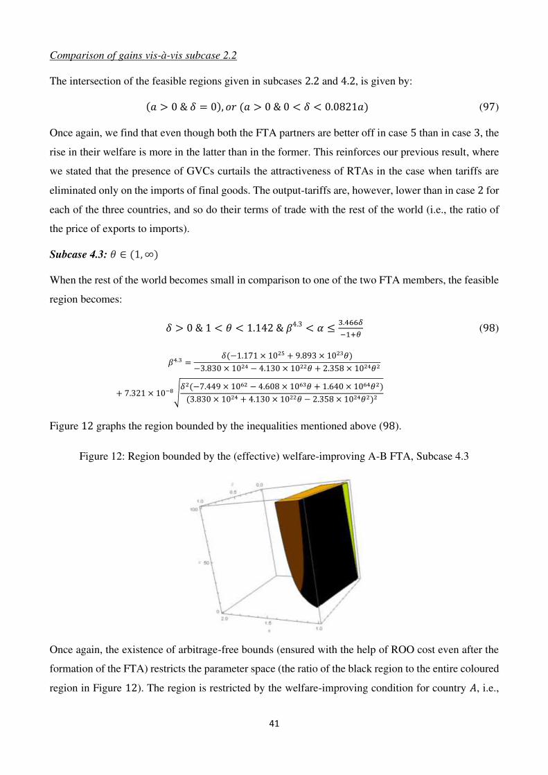
41

Comparison of gains vis-à-vis subcase 2.2

The intersection of the feasible regions given in subcases 2.2 and 4.2, is given by: (𝑎 > 0 & 𝛿 = 0), 𝑜𝑟 (𝑎 > 0 & 0 < 𝛿 < 0.0821𝑎) (97)

Once again, we find that even though both the FTA partners are better off in case 5 than in case 3, the

rise in their welfare is more in the latter than in the former. This reinforces our previous result, where

we stated that the presence of GVCs curtails the attractiveness of RTAs in the case when tariffs are

eliminated only on the imports of final goods. The output-tariffs are, however, lower than in case 2 for

each of the three countries, and so do their terms of trade with the rest of the world (i.e., the ratio of

the price of exports to imports).

Subcase 4.3: 𝜃 ∈ (1, ∞)

When the rest of the world becomes small in comparison to one of the two FTA members, the feasible

region becomes: 𝛿 > 0 & 1 < 𝜃 < 1.142 & 𝛽4.3 < 𝛼 ≤ 3.466𝛿−1+𝜃 (98)

𝛽4.3 = 𝛿(−1.171 × 1025 + 9.893 × 1023𝜃)−3.830 × 1024 − 4.130 × 1022𝜃 + 2.358 × 1024𝜃2+ 7.321 × 10−8√𝛿2(−7.449 × 1062 − 4.608 × 1063𝜃 + 1.640 × 1064𝜃2)(3.830 × 1024 + 4.130 × 1022𝜃 − 2.358 × 1024𝜃2)2

Figure 12 graphs the region bounded by the inequalities mentioned above (98).

Figure 12: Region bounded by the (effective) welfare-improving A-B FTA, Subcase 4.3

Once again, the existence of arbitrage-free bounds (ensured with the help of ROO cost even after the

formation of the FTA) restricts the parameter space (the ratio of the black region to the entire coloured

region in Figure 12). The region is restricted by the welfare-improving condition for country 𝐴, i.e.,

42

the larger FTA partner in subcase 4.3. Even though 𝑊𝐴 4 > 𝑊𝐵4, yet welfare gains (from pre- to post-

FTA) are higher in the case of 𝐵 than in 𝐴.

On comparing the gains accrued by the non-member country (which is now smaller than country A),

we find that both 𝐴 and 𝐵 (unambiguously) gain less vis-à-vis country 𝑅. However, the terms of trade

effect is favourable towards the FTA members. In fact, analogous to Subcase 4. 1, we find that while

the downstream firm’s profit falls in country 𝐴 post the FTA formation, it may rise in the case of the

smaller partner, 𝐵 when 𝜃 takes a comparatively large value within the feasible bounds. Out of the

other three agents, consumers and the upstream firm in each FTA member benefit (due to the so-called

pro-competitive effects of FTAs triggered via the fall in both output- as well input-tariffs), while the

government revenue necessarily fall. The country 𝑅’s government, however, earns higher revenue with

lower output-tariffs and higher input-tariffs vis-à-vis Case 3.

Comparison of gains vis-à-vis subcase 2.3

The feasible region under consideration is represented by the following Figure 13.

Figure 13: Region bounded by the (effective) welfare-improving A-B FTA, Subcase 4.3

The same results, as in the previous two subcases, 4.1 and 4.2, are observed here too. Therefore, the

following proposition is noteworthy.

Proposition 5. In our vertical industry set-up, FTAs (in Final Goods) lead to a higher level of welfare

in the presence than in the absence of tradable intermediates. However, the welfare gains vis-à-vis the

pre-FTA scenario are more in the case of latter than the former.

We know that the link between global value chains and free trade agreements runs in both the directions

– on the one hand, the issue is how much FTAs can enhance GVC participation (Ignatenko, Raei and

Mircheva 2019), while the other policy question concerns whether these international production

43

chains alter the merits of engaging in free trade agreements, and deeper trade agreements as well (Ruta

2017). While we do not model the depth of FTAs, our framework allows us to analyse this two-way

association between two forms of economic integration. In line with the empirical study by Hoffman,

Osnago, and Ruta (2017), we measure GVC participation as imports of intermediate inputs, and find

that in each of the three Subcases discussed above, with FTA, each partner’s intra-FTA exports of

inputs, as well as its exports to country R, rise, and so do their imports. In fact, the exports and imports

of final goods also expand, vis-à-vis the pre-FTA case in all the three countries. This implies that trade

policy plays an important role in determining the benefits from GVC integration. Further, in

comparison to Case 2, where the production of final goods was entirely national in each of them, we

find that with the introduction of trade in intermediates, the level of economic integration among all

the countries rises (as demonstrated in case 2), but the attractiveness of FTAs as a welfare-enhancing

economic instrument falls. Thus, while GVCs do support the effective formation of welfare-enhancing

FTAs, but the rise in welfare is lower than in Case 2. This shows the feedback effect of the increase in

GVC trade on the trade policy of any country. In fact, our three subcases (4.1 − 4.3) suggest that this

result holds regardless of the market sizes of the FTA partners and the rest of the world.

It is equally imperative to point to the issue of Inverted Duty Structure (IDS) here. IDS refers to the

situation when customs duties on imports of final goods exceed the rate of duties imposed on

intermediate inputs that are required for their production. Several Indian industrialists have complained

that with the rise in FTAs signed by the country (specifically with its East Asian partners viz. the

ASEAN bloc, South Korea, or Japan), the issue of duty of inversion has arisen, which has adversely

affected their competitiveness, and hence, profitability in the market of India’s FTA partners. This is

because, in certain cases (especially when inputs are imported from the non-FTA partners), they have

to pay a higher cost for their imported inputs (due to higher import duties), while at the same time,

FTAs expose their final products to intense foreign competition (Jha 2019, Chandrashekhar 2019).

With free trade in final goods, the present case 4 thus represents a specific scenario where the

possibility of IDS occurs as far as the 𝐴 − 𝐵 FTA is concerned. This is because not only countries 𝐴

and 𝐵 import inputs from Country 𝑅, but inputs are also excluded from the FTA’s exemption list.

Thus, akin to the complaints that have been raised by the Indian manufacturers, we also observe that

in each of the three subcases, the downstream firm’s surplus does fall (except for the smaller FTA

partner in subcases 4.1 and 4.3 for some feasible values of 𝛼, 𝜃, and 𝛿). However, all these subcases

only indicate the possibility of welfare-improving FTAs. This implies that even if the downstream

firm’s profits decline post the formation of the FTA, yet the government could ensure that every agent

gains by devising a mechanism to make some transfers from the beneficiaries of the FTA in 𝐴 and 𝐵

(viz. consumers and upstream firm) to those who lose from such an arrangement (maybe in the form

44

of some subsidies or taxes). Nonetheless, it is also important to note that IDS does not necessarily

imply negative effective protection, as argued by Pathania and Bhattacharjea (2020), and hence, may

not necessarily affect the competitiveness of a country’s exports. The effective rate of protection

becomes negative when value added under free trade exceeds value added under restricted trade, or

when value added under free trade becomes negative, as defined by Corden (1971). Although we do

not specifically compute ERP in our study, it is worth mentioning here that with zero tariffs being

imposed by FTA members on each other’s imports of final goods, and a fall in external output-tariff

as well, input-tariffs fall too. In fact, in our set up, we find that while the 𝐴 − 𝐵 FTA unambiguously

raises the export sales and revenue for the downstream firm post the formation of the agreement, their

domestic sales contract, due to which their overall profits fall short of the pre-FTA case.

3.5 Case 5 | Trade in Final and Intermediate Goods, FTA in Intermediate Goods

We now consider the possibility of the conclusion of an FTA between countries 𝐴 and 𝐵, whereby

they agree to eliminate tariffs on imports of intermediate inputs while continuing to impose positive

MFN tariffs on imports of final goods from each other. The objective of this exercise is to ascertain

whether the composition of tradable commodity baskets matters while determining the (potential)

welfare-enhancing effects of an FTA.

Like in the case of bilateral free trade in final goods, we assume that the intra-FTA members maintain

their independence in setting differential external input-tariffs on their respective imports from the rest

of the world. However, to prevent imports of grey products, we assume that the upstream firm in each

of the two FTA countries has to incur an additional per-unit cost of 𝛾 in order to claim the tariff-free

treatment for their exports within the free trade area. The three-stage solutions obtained via the process

of backward induction are detailed below.

Downstream Markets

The stage-3 equilibrium solutions are similar to what we obtained in case 3 since there is no change

as far as the downstream markets are concerned. The equilibrium level of outputs and market prices

are, therefore, given by Equation (7) with each 𝐹𝑖5 > 0 ∀ 𝑖 ∈ {𝐴, 𝐵, 𝑅}. Further, the arbitrage-free

bounds as in Equations (9)-(11) stabilise the equilibrium prices in the three segmented markets.

Upstream Markets

As in case 3, each upstream firm maximises its profits and determine the level of input to be supplied

to its own country’s downstream firm, and foreign downstream firms as well, taking the inputs

provided by rival upstream firms and the ROO-cost/ input-tariffs as given. The Cournot Nash

Equilibrium prices in three markets are given by:

45

𝑑𝐴5 = 0.033(𝑎𝐴 + 𝑎𝐵 + 𝑎𝑅) + 0.254𝑠𝐴5 + 0.023(𝑠𝐵5 + 2𝑠𝑅5 + 2𝑡𝐴5) − 0.056(𝑡𝐵5 + 𝑡𝑅5) + 0.277γ (99) 𝑑𝐵5 = 0.033(𝑎𝐴 + 𝑎𝐵 + 𝑎𝑅) + 0.254𝑠𝐵5 + 0.023(𝑠𝐴5 + 2𝑠𝑅5 + 2𝑡𝐵5) − 0.056(𝑡𝐴5 + 𝑡𝑅5) + 0.277γ(100) 𝑑𝑅5 = 0.033(𝑎𝐴 + 𝑎𝐵 + 𝑎𝑅) + 0.508𝑠𝑅5 + 0.023(𝑠𝐴5 + 𝑠𝐵5 + 2𝑡𝑅5) − 0.056(𝑡𝐴5 + 𝑡𝐵5) + 0.046γ (101)

From Equations (99)-(101), we observe that the link between γ and optimal input-prices corresponds

to the link that we found between 𝛿 and the optimal output-prices in cases 2 and 4. The positive

association is intuitive because a). a higher ROO-cost makes the imported input more expensive, as in

the case of higher input-tariffs, and b). With an increase in γ, ceteris paribus, the cost of producing

final goods in FTA partners also increases, which, in turn, negatively affects the demand for their final

good, while positively affecting the demand for country R’s final goods and intermediate inputs. Thus,

there exists an indirect but positive association between γ and 𝑑𝑅6 .

The arbitrage free-bounds are now given by: 𝑑𝐴5 + γ ≥ 𝑑𝐵5 ≥ 𝑑𝐴5 − γ (102) 𝑑𝐴5 + 𝑠𝑅5 ≥ 𝑑𝑅5 ≥ 𝑑𝐴5 − 𝑠𝐴5 (103) 𝑑𝐵5 + 𝑠𝑅5 ≥ 𝑑𝑅5 ≥ 𝑑𝐵5 − 𝑠𝐵5 (104)

Tariffs and Welfare

Substituting the values of 𝑎𝐴, 𝑎𝐵, and 𝑎𝑅, we find the welfare maximising input- and output tariffs in

each of the three countries as given below: 𝑡𝐴5 = −0.066𝑎 + 0.286𝑎𝜃 + 0.190γ (105) 𝑡𝐵5 = 0.253𝑎 − 0.033𝑎𝜃 + 0.190γ (106) 𝑡𝑅5 = 0.270𝑎 − 0.026𝑎𝜃 − 0.104γ (107) 𝑠𝐴5 = 0.015𝑎 + 0.013𝑎𝜃 + 0.372γ (108) 𝑠𝐵5 = 0.021𝑎 + 0.007𝑎𝜃 + 0.372γ (109) 𝑠𝑅5 = 0.049𝑎 + 0.017𝑎𝜃 + 0.032γ (110)

The comparative statics results for the effect of the ROO-cost on input- and output-tariffs in the three

countries show that, ceteris paribus, any increase in γ unambiguously raises the output-tariffs in the

FTA members, but reduces the optimal rate in Country 𝑅. This is because a higher γ is associated with

a higher cost of imported inputs in countries 𝐴 and 𝐵, which, in turn, makes their final outputs more

costly. As a consequence, their respective governments raise the optimal rate of output-tariff to protect

their downstream firm while balancing its negative effects on its consumers (due to an increase in the

46

price of the final good). On the other hand, the final output becomes relatively less costly in country 𝑅, and therefore, we observe a fall in 𝑡𝑅6. As regards the input-tariffs, a positive association with γ is

clear from equations (99)-( 101). A higher 𝛾 leads to higher 𝑑𝑖5 (∀ 𝑖 ∈ {𝐴, 𝐵, 𝑅}), and thus, a rise in

input-tariffs in all the three countries. Further, in the FTA members, we already know that 𝑠𝐴5 > 𝛾 and 𝑠𝐵5 > 𝛾.

Utilising equations (105)-(110) and substituting their values in solutions obtained from stage 3 and 2,

we compute the level of total welfare in all the three countries under consideration. 𝑊𝐴5 = 1.299(γ)2 − 𝛼γ(0.192 + 0.172𝜃) + (𝛼)2(0.057 − 0.027𝜃 + 0.373(𝜃)2) (111) 𝑊𝐵5 = 1.299(γ)2 − 𝛼γ(0.207 + 0.157𝜃) + (𝛼)2(0.375 + 0.006𝜃 + 0.021(𝜃)2) (112) 𝑊𝑅5 = 0.065(γ)2 + 𝛼γ(−0.062 + 0.032𝜃) + (𝛼)2(0.380 + 0.003𝜃 + 0.018(𝜃)2) (113) ⇒ 𝐺𝑊5 = 2.663(𝛾)2 − 𝛼γ(0.462 + 0.298𝜃) + (𝛼)2(0.812 − 0.017𝜃 + 0.412(𝜃)2) (114)

Once again, we find that regardless of the value of 𝜃, the welfare of each country (FTA member or

non-member), and hence, the global welfare, falls with a rise in the ROO-induced trade cost. This

finding is similar to cases 2 and 4, where we assumed bilateral free trade in final, and not in

intermediate goods, between 𝐴 and 𝐵.

Now, we have to determine the feasible regions for 𝑎, 𝜃, and 𝛾 that ensure the effective formation of

an FTA. Thus, we constraint our solutions obtained from the three stages by imposing the five pre-

requisites as detailed in case 2,32 and accordingly compare the welfare-enhancing effects of this FTA

vis-à-vis FTA in final goods, i.e., case 4, to answer our second research question. In doing so, we

establish the following proposition:

Proposition 6. In our vertically integrated set up, a (horizontal) free trade agreement is not always

Pareto-improving for the FTA members, vis-à-vis the no-FTA case. When these engagements

potentially raise the welfare of the two members, their downstream/upstream lose some of their

surpluses, depending on whether the (bilateral) output- or input-tariffs get eliminated within the free

trade zone. However, this doesn’t happen because of a loss in their export competitiveness; rather,

their exports to the FTA partners rise but at the expense of their domestic sales and revenue.

While we have already proved this proposition (partially) in Cases 2 and 4 when countries A and B

negotiate an FTA in final goods, the following discussion in Subcases 5.1-5.3 justify our assertion

when the two countries agree to eliminate tariffs on each other’s imports of intermediate inputs.

32 Condition (b) laid down in case 3, also entails the arbitrage-free bounds in upstream markets, as represented in Equations

(102)- (104).

47

Subcase 5.1: 𝜃 ∈ (0, 1)

Considering the feasible region obtained in case 3 (i.e., the pre-FTA case), and the five pre-requisites

for the formation of the 𝐴 − 𝐵 FTA, we find the optimal range of values for the three parameters: 𝛾 > 0 & 0.475 < 𝜃 < 1 & 𝛽5.1 < 𝑎 ≤ − 29.28𝛾−1+𝜃 (115)

where,

𝛽5.1 = 𝛾(3.754 × 1026 + 2.847 × 1026𝜃)4.213 × 1024 + 2.074 × 1025𝜃 + 1.213 × 1025𝜃2+ 2.627 × 10−8√𝛾2(1.755 × 1068 + 1.685 × 1068𝜃 + 3.486 × 1067𝜃2)(4.213 × 1024 + 2.074 × 1025𝜃 + 1.213 × 1025𝜃2)2

The black coloured region in the middle panel of Figure 14 graphs these inequalities and the rightmost

panel of the figure shows its side view. The left-panel (yellow coloured region), on the other hand,

shows the full set of values for the three parameters in the absence of the arbitrage-free bounds, and

the red coloured region (out of the yellow region) shows the feasible set of value when arbitrage free-

bounds are imposed only in the case of downstream markets.

Figure 14: Region bounded by the (effective) welfare-improving A-B FTA, Subcase 5.1

From figures (4), (8), and (14), it seems plausible to conclude that the possibility of a rise in parallel

imports or profitable arbitrage opportunities in downstream markets is very low in Case 5 with free

trade in intermediates than in Cases 2 or 4. While that in the upstream markets, is relatively high, and

hence, imposing the three inequalities (102)-(104) squeezes our solution set from red to the black

coloured region in the above figures. This signifies why it is imperative to consider the arbitrage-free

bounds while analysing the benefits of FTAs in order to control for trade deflection or any kind of

tariff-shopping that could disturb the Cournot equilibrium. However, most of the existing studies on

RTAs (in which the model structure is quite similar to ours) such as Kawabata, Yanase and Kurata

48

(2010) or Chang and Xiao (2015), etc., do not explicitly model these possibilities. This could mean

that the likelihood of concluding a welfare-improving FTA (whether with partners with whom a

country mostly trades in final or intermediate inputs, or both of them) that has already been established

in such studies is overestimated. The recent study by Conconi et al. (2018) also showed that in the case

of the North American Free Trade Agreement (NAFTA), these rules led to a significant fall in imports

of intermediate goods from the extra-FTA trading partners vis-à-vis the NAFTA countries.

Further, from the right panel of Figure (14), it is observed that as the value of 𝛾 increases, the likelihood

of the formation of a welfare-improving FTA between asymmetric countries also increases. This is

because, with our assumptions of linear demand and constant (and same) marginal cost of producing

intermediate inputs, higher 𝛾 is required to eliminate the arbitrage opportunities when countries are

dissimilar in terms of their market sizes. This contrasts with our findings in cases 2 and 4, which show

that a final-goods FTA (in the presence of arbitrage-free bounds) is (potentially) welfare-enhancing

only between relatively similar countries. Thus, with the introduction of tradable intermediates, the

scope of the formation of an effective FTA between different relatively dissimilar countries expands –

something that could be related to the fact that the period when RTAs were negotiated in large numbers

also coincides with the period when even GVCs started expanding on a much wider scale (i.e., in the

past two-two and a half decades).

Assessment of gains from the 𝐴 − 𝐵 FTA, and its effect on MFN tariffs

Akin to the FTA in final goods, in the feasible region as represented by Equation (115), we find that

the welfare of the smaller partner, 𝐴, falls short of the welfare of country 𝐵, but the increase in welfare

due to FTA formation is more in the former than the latter. Downstream firms in the two countries

unambiguously gain due to the fall in their production cost with a fall in the price of intermediate

inputs. This is because, not only the FTA partners eliminate input-tariffs on imports within the FTA,

but their external tariff rate also falls, and hence, the cost of imports from R also goes down. This, in

turn, reduces the price of final goods and benefits the consumers unambiguously. However, the surplus

earned by upstream firms reduce post the formation of the FTA,33 and so does the tariff revenue of the

governments of the two countries. The reason is that even though the FTA allows the two countries’

upstream firms to export more to each other by incurring the per-unit ROO cost, however, their

domestic sales as well as exports to the rest of the world fall unambiguously. The latter happens

because of an increase in output tariff by country 𝑅’s government post the conclusion of the 𝐴 − 𝐵

33 In the case of the smaller partner (𝐴), surplus increases for its upstream firm for a very small subset of values of 𝛼, 𝜃,

and 𝛾.

49

FTA.34 Thus, from our findings in Cases 2, 4, and 5, it seems plausible to conclude that (in our specific

framework), FTAs hurt the producers of goods on which tariffs are eliminated. However, this doesn’t

happen because of a loss in their export competitiveness; rather, their exports to the FTA partners rise

but at the expense of their domestic sales and revenue.

Regarding country 𝑅, we find that its overall welfare rises in the feasible region, but the profit earned

by its downstream firm falls. This is despite the fact that its optimal input-tariff as well as input price

also decline post the formation of the 𝐴 − 𝐵 FTA.35 Further, unlike cases 2 and 4, we find that for

some combination of the feasible values of the three parameters, the rise in welfare is more for both

the FTA partners vis-à-vis country 𝑅, and therefore, in the new equilibrium, 𝑊𝐵5 > 𝑊𝑅5. This is shown

in the left panel of Figure 15, in which the rise in the welfare of country 𝐴 is also more than the change

in the welfare of 𝑅. From the region plot, it is clear that such a possibility arises when 𝜃 takes a value

close to one, and 𝛾 also takes a small value (within our chosen range for 𝛼). This could be because the

loss for country R’s downstream firm is more, the lower is the degree of market size asymmetry (or,

higher the value of 𝜃) between the two FTA partners. Besides, country 𝐴 will be better off due to the

larger size of country 𝐵’s market.

Figure 15: Comparison of welfare gains from the A-B FTA, Subcase 5.1

The right panel of Figure 15 shows the blue and yellow regions, where country 𝑅 gains more than

countries 𝐴 and 𝐵, along with the purple area, where the opposite happens. Nevertheless, even in this

subcase, we find that the terms of trade of the FTA partners improve, vis-à-vis country 𝑅.

34 This could be because with free trade in intermediates, input prices decline in both A and B, as a consequence of which

the prices of their final goods fall too. This implies that the relative price of final output produced in country R rises, and

therefore, to protect its domestic downstream firm, the government raises the optimal output tariff. Nonetheless, this result

contrasts with our previous findings, where we showed that three countries’ output-tariffs are complementary to each other. 35 The rise in input tariff of country 𝑅 (when 𝐴 and 𝐵 forms an FTA in intermediates), implies that Bagwell-Staiger’s tariff complementarity condition does not hold in this case.

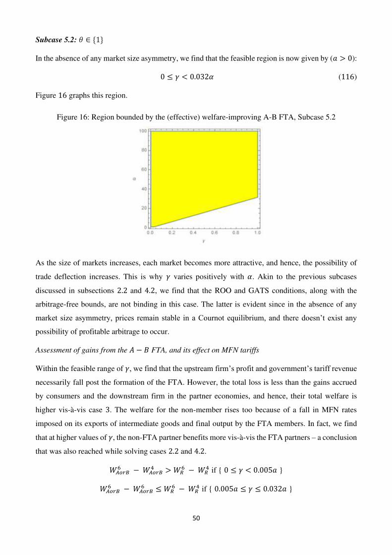
50

Subcase 5.2: 𝜃 ∈ {1}

In the absence of any market size asymmetry, we find that the feasible region is now given by (𝑎 > 0): 0 ≤ 𝛾 < 0.032𝛼 (116)

Figure 16 graphs this region.

Figure 16: Region bounded by the (effective) welfare-improving A-B FTA, Subcase 5.2

As the size of markets increases, each market becomes more attractive, and hence, the possibility of

trade deflection increases. This is why 𝛾 varies positively with 𝛼. Akin to the previous subcases

discussed in subsections 2.2 and 4.2, we find that the ROO and GATS conditions, along with the

arbitrage-free bounds, are not binding in this case. The latter is evident since in the absence of any

market size asymmetry, prices remain stable in a Cournot equilibrium, and there doesn’t exist any

possibility of profitable arbitrage to occur.

Assessment of gains from the 𝐴 − 𝐵 FTA, and its effect on MFN tariffs

Within the feasible range of 𝛾, we find that the upstream firm’s profit and government’s tariff revenue

necessarily fall post the formation of the FTA. However, the total loss is less than the gains accrued

by consumers and the downstream firm in the partner economies, and hence, their total welfare is

higher vis-à-vis case 3. The welfare for the non-member rises too because of a fall in MFN rates

imposed on its exports of intermediate goods and final output by the FTA members. In fact, we find

that at higher values of 𝛾, the non-FTA partner benefits more vis-à-vis the FTA partners – a conclusion

that was also reached while solving cases 2.2 and 4.2. 𝑊𝐴𝑜𝑟𝐵6 − 𝑊𝐴𝑜𝑟𝐵4 > 𝑊𝑅6 − 𝑊𝑅4 if { 0 ≤ 𝛾 < 0.005𝑎 } 𝑊𝐴𝑜𝑟𝐵6 − 𝑊𝐴𝑜𝑟𝐵6 ≤ 𝑊𝑅6 − 𝑊𝑅4 if { 0.005𝑎 ≤ 𝛾 ≤ 0.032𝑎 }

51

Figure 17 plots the above-mentioned inequalities. In the purple region, the partners gain more than the

non-partner, while the gray-coloured region highlights the opposite scenario.

Figure 17: Comparison of welfare gains from the A-B FTA, Subcase 6.2

The rest of the results are similar to what we observed in subcase 5.1. The terms of trade improve for

countries 𝐴 and 𝐵. While the optimal output tariff of R necessarily rises (and the profit of its

downstream firm fall with the FTA), its input-tariff declines for most of the feasible parametric values

as represented by the following inequalities (117), (118). 𝑠𝑅5 < 𝑠𝑅3 if 𝛾 < 0.028𝑎 (117) 𝑠𝑅5 ≥ 𝑠𝑅3 if 0.028𝑎 < 𝛾 ≤ 0.032𝑎 (118)

Thus, unlike a horizontal FTA in final goods, the one in intermediate goods doesn’t necessarily prove

to be a building block towards multilateral free trade in our model set up. Put differently, input-tariffs

imposed by the three trading partners are not necessarily complementary to each other (specifically

when 𝛾 takes a very high value within the feasible range). This could be because when 𝛾 takes a

comparatively high value, then due to the ROO condition, even the external input tariffs imposed by

the two FTA members, are comparatively high compared to when 𝛾 is zero or very small. As a

consequence, country 𝑅’s government imposes a higher 𝑠𝑅6 to protect its upstream firm, which

otherwise also earns (relatively) less in terms of its export revenue due to the formation of the 𝐴 − 𝐵

FTA.

52

Subcase 5.3: 𝜃 ∈ (1, ∞)

When country 𝐴 becomes larger vis-à-vis country 𝐵, and the rest of the world (i.e., country 𝑅), then,

we observe that a larger range for 𝜃 supports the five pre-requisites for ensuring the formation of an

effective (horizontal) FTA in intermediate goods (compared to Subcase 4.3). The feasible region is

algebraically represented in Equation (119), and demonstrated graphically in Figure (18). 𝛾 > 0 & (1 < 𝜃 < 1 + 𝜀 & 𝛽5.31 < 𝐴 ≤ 732.𝛾−25.+25.𝜃) 𝑜𝑟 (1 < 𝜃 < 2.017 & 𝛽5.32 < 𝐴 ≤ 732.𝛾−25.+25.𝜃)

(119)

where, 𝜀 is a very small number, and

𝛽5.31 = 𝛾(3.754 × 1026 + 2.847 × 1026𝜃)4.213 × 1024 + 2.074 × 1025𝜃 + 1.213 × 1025𝜃2+ 2.627 × 10−8√𝛾2(1.755 × 1068 + 1.685 × 1068𝜃 + 3.486 × 1067𝜃2)(4.213 × 1024 + 2.074 × 1025𝜃 + 1.213 × 1025𝜃2)2

and 𝛽5.32 = 1.580×109(3.309×1017𝛾+2.964×1017𝛾𝜃)2.605×1025+2.591×1025𝜃+3.721×1024𝜃2 + 2.472 × 10−8√1.464×1068𝛾2+5.021×1068𝛾2𝜃+3.159×1068𝛾2𝜃2(2.605×1025+2.591×1025𝜃+3.721×1024𝜃2)2

Figure 18: Region bounded by the (effective) welfare-improving A-B FTA, Subcase 5.3

Here, in both the panels, the black coloured region represents a combination of those parametric values

which support the effective formation of the 𝐴 − 𝐵 FTA. In contrast, the yellow plus black region

excludes the constraints imposed by the arbitrage-free bounds. The right panel shows the back view of

the left panel to highlight all the feasible values of the three parameters within our chosen range. Thus,

even though the FTA is welfare-enhancing even when country 𝐴 is three times the size of country B,

or R, but our feasible bounds suggest that to exclude the possibility of profitable arbitrage

opportunities, the value of 𝜃 should not exceed 2.017.

53

Assessment of gains from the 𝐴 − 𝐵 FTA, and its effect on MFN tariffs

Within the feasible region, we find that even this type of horizontal FTA is more beneficial for the

smaller partner, vis-à-vis the larger partner as overall welfare increases more (post the conclusion of

the FTA) in the case of the former than the latter. In each of the two countries, we find that consumers

benefit due to an increase in the total supply of the final good, and so does the downstream firm as its

domestic and foreign sales increase. However, the upstream profits in country A necessarily falls due

to a fall in the domestic sales and revenue of the upstream firm (even though its export sales rise). On

the contrary, for the one in country B, profits increase for a small range of feasible values of the three

parameters. This range is shown in Figure 19:

Figure 19: Feasible region for an increase in profit of upstream firm in country B, Subcase 5.3

From the figure, it is clear that only when 𝜃 takes a value closer to its upper-limit, surplus for country

B’s upstream firms rise (under certain restrictions on the values of 𝛼 and 𝛾). Besides, the two FTA

partners also lose some of their tariff revenue due to the elimination of input tariffs on each other’s

exports. Also, because their optimal external tariffs rates on imports of inputs as well outputs fall post

the formation of the free trade agreement. However, the FTA raises their terms of trade, vis-à-vis the

rest of the world.

As regards country R, we find that the FTA improves its welfare within the feasible region represented

by Equation (119). In fact, the rise in its welfare exceeds the welfare gain for the FTA partners in the

greyish region shown in the rightmost panel of Figure 20. The leftmost panel displays the region where

the benefits are more for the larger FTA partner (𝐴) vis-à-vis 𝑅, and in the middle panel with the blue

coloured region, country 𝐵 benefits more than country 𝑅.

54

Figure 20: Comparison of welfare gains, Subcase 5.3

Thus, for all higher (feasible) values of the degree of market size asymmetry, we observe that the non-

member benefits more because the rise in its consumer surplus, upstream profits, and tariff revenue

dominates the fall in its downstream profits (due to a decline in its domestic as well as export sales, as

we also observed in subcase 5.1). On the contrary, the overall sales of the downstream seller in

countries 𝐴 and 𝐵 unambiguously rise. This implies that the forward-linkage effect induced by free

trade in intermediates raises the efficiency of firms in the FTA members by lowering their production

cost, and hence, benefits them unambiguously vis-à-vis the non-member country. As a consequence,

country R raises its optimal output-tariff to protect its downstream firm. The optimal input-tariff also

rises, but for a very small region (as shown in Figure 21); otherwise, it declines, thus, following

Bagwell-Staiger’s tariff complementarity condition.

Figure 21: Feasible region (Decline in country R’s optimal input-tariff), Subcase 5.3

This completes the description of the welfare-gains from the two FTAs in the presence of tradable

intermediate inputs.

55

Subcase 5.4: Comparison of Gains – Case 4 and 5

We now compare the gains across the two types of Horizontal FTAs – one that allows free trade in

final goods, and two, whereby the FTA members eliminate tariffs on each other’s imports of

intermediate goods (Cases 4 and 5, respectively). Since, for each of the two cases, case 3 represents

the pre-FTA scenario, we directly compare their outcomes to analyse their welfare-enhancing effects.

Put differently, this analysis is also useful to understand whether higher gains accrue to a free trade

area involving more trade in final or intermediate goods. Nevertheless, both of these are GVC-related

trade.36

It is important to note that while comparing the gains across the two FTAs, our analysis is guided by

four different parameters viz. 𝜃, 𝛿, 𝛾, and 𝛼 since we need to ensure that all of them lie within their

feasible ranges as shown in Cases 4 and 5 above. The restriction on the size parameter, 𝛼, arises

because of the manner in which we introduce the two ROO-induced trade costs. As a result, our

expressions become even more complicated relative to those represented in subsections 3.2, 3.4 and, 3.5, and we can’t easily represent them graphically. Hence, we compute the quadruple integrals of our

functions and evaluate the hypervolumes (which is equal to the product of the four dimensions) of the

4-D regions to compare different outcomes across the two FTAs. Table 2 details our findings from this

assessment. Besides, for subcases 4.2 and 5.2 (that assume the absence of any market size asymmetry,

i.e., when 𝜃 = 1), we use 3-D region plots to demonstrate our results graphically.

(Table 2 here)

Therefore, we establish the following proposition.

Proposition 7. An FTA in final goods or intermediate inputs improves the welfare of both member

countries and the non-member as well, under certain conditions. However, the increase in welfare for

the FTA members is more when bilateral tariffs are eliminated on imports of final goods than on

intermediate inputs. In other words, considering a set of countries where trade is predominantly intra-

industry trade, then it is beneficial to conclude an FTA with a partner with whom a country trades

mostly in final goods than with whom the majority of the trade is in intermediate inputs.

This has already been shown in Table 2. Thus, a priori, even though it may seem plausible to think

that a country may accrue higher welfare gains by signing an FTA with a nation from which it is mostly

importing intermediate products since the reduction (or even elimination) of input-tariffs will not only

36 As defined in Ignatenko, Raei and Mircheva (2019), this type of trade incorporates those imports and exports that either

embody imported value added (i.e., trade in final goods in our case), or are exports of domestic value added that are re-

exported in other countries’ exports (trade in intermediates). GVC-non-related trade, on the other hand, is defined as the

import/export that gets directly absorbed in other countries.

56

Table 2: Comparison of Gains, Case 4 V/s. Case 5

S. No. Basis for Comparison Case 4 V/s 5 Remarks

1 Feasible range for ‘𝜃’ • Case 4: 0.876 < 𝜃 < 1.142

• Case 5: 0.475 < 𝜃 < 2.017

The formation of an FTA in final goods is feasible only within a small range of the

degree of market size asymmetry (i.e., when the smaller FTA partner is not too small

in comparison to the larger partner and the rest of the world, or when it is larger, then

it should not be very large in comparison to the other partner, and the ROW). On the

contrary, bilateral free trade in intermediates is advantageous even when the degree of

market size asymmetry is relatively high. This implies that if the two countries (who

are willing to conclude an FTA) trade mostly in final goods, then the FTA will be

beneficial to both only if they are not too different from each other in terms of their

market sizes. If they are very different from each other, i.e., if 𝜃 goes beyond the range

(0.876, 1.142), then the larger partner will not gain, and the FTA will not be inherently

stable within the context of our framework. However, suppose they trade mostly in

intermediate inputs. In that case, the FTA will be advantageous to both even if one of

them is exactly half in size vis-à-vis the other (given the restrictions on the other

parameters of the system).

‘Common’ Feasible Range for 𝜽: 0.876 < 𝜃 < 1.142

(This represents the common region bounded by the feasible parametric values computed in Cases 4 and 5)

2 Domestic Sales

𝐹𝑖𝑖5 > 𝐹𝑖𝑖4 and 𝐼𝑖𝑖5 < 𝐼𝑖𝑖4

But, 𝐹𝐴5 < 𝐹𝐴4, 𝐹𝐵5 < 𝐹𝐵4, and 𝐹𝑅5 > 𝐹𝑅4

An FTA in final goods not only raises the intra-FTA exports of final goods but also

leads to an increase in their exports of intermediate inputs to country 𝑅, vis-à-vis Case 6. This is because of the so-called backward-linkage effect – a reduction in the cost of

their exports of final goods not only benefits the end customers since 𝐹𝐴5 < 𝐹𝐴4, and 3 Export Sales

𝐹𝐴𝐵4 , 𝐹𝐵𝐴4 , 𝐹𝑅𝐴4 , 𝐹𝑅𝐵4 , 𝐼𝐴𝑅4 , 𝐼𝐵𝑅4 , 𝐼𝑅𝐴4 , 𝐼𝑅𝐵4 , are greater than in Case 5.

57

𝐼𝐴𝐵5 , 𝐼𝐵𝐴5 are higher than in Case 4.

𝐹𝐵5 < 𝐹𝐵4, but also the upstream firm in the two FTA partners, by raising their overall

production, and exports.37 However, the rise in the latter is more in Case 5.

Analogously, an FTA in intermediates positively affects the exports as well as

domestic sales of final goods of the downstream firm in countries A and B. This can

be termed as the forward-linkage effect. But, the rise in their overall production and

exports is more in Case 5.

Besides, domestic sales of the goods under consideration fall in each of the two cases.

As a consequence, domestic supplies of the downstream firms in FTA partners are

higher in Case 6, while those of the upstream firms are higher in Case 5.

4 Price of Final Goods 𝑃𝑖5 > 𝑃𝑖4 ∀ 𝑖 ∈ {𝐴, 𝐵, 𝑅} The elimination of output-tariffs within the FTA (Case 4), as well as the subsequent

reduction of external MFN tariffs by both the FTA members and the non-member,

unambiguously lead to a decrease in the price of final goods in all the three markets.

In fact, the output prices fall in Case 5 as well, though its magnitude is less in

comparison to Case 4. Similarly, input-prices fall in case 5, and not just in case 6 due

to the FTA in intermediates.

The important point to note is that this result does not only hold for the FTA partners,

but also for country 𝑅.

5 Output-tariff 𝑡𝑖5 > 𝑡𝑖4 ∀ 𝑖 ∈ {𝐴, 𝐵, 𝑅}

6 Price of Intermediate

Inputs 𝑑𝑖5 < 𝑑𝑖4 ∀ 𝑖 ∈ {𝐴, 𝐵, 𝑅}

7 Input-tariff 𝑠𝑖5 < 𝑠𝑖4 ∀ 𝑖 ∈ {𝐴, 𝐵, 𝑅}

8 Consumer Surplus 𝐶𝑆𝐴5 < 𝐶𝑆𝐴4, 𝐶𝑆𝐵5 < 𝐶𝑆𝐵4, but 𝐶𝑆𝑅5 > 𝐶𝑆𝑅4

A higher increase in the total supply of final goods to A and B in case 4 leads to a more

significant increase in their consumer surplus. Conversely, in country 𝑅, consumers

gain more in Case 5 than in 4. This happens due to a rise in the downstream exports

of the FTA partners to country 𝑅 because of a fall in their input cost post the conclusion

of the 𝐴 − 𝐵 FTA in intermediate goods.

37 The exports of inputs by the upstream firm in the large country increases in 99.88 percentage of the total volume bounded by the feasible range.

58

9 Downstream Firm’s Surplus

𝑃𝑆𝐴5 > 𝑃𝑆𝐴4, 𝑃𝑆𝐵5 > 𝑃𝑆𝐵4, but 𝑃𝑆𝑅5 > 𝑃𝑆𝑅4

In each of the two FTAs (Cases 4 and 5), we find that the producers of the goods on

which import tariffs are eliminated, gain in terms of market access for their exports

within the FTA bloc, but suffer from a loss in their sales and earnings from the

domestic market. On the contrary, the producers in the preceding/subsequent stage of

production gain due to the so-called backward/forward-linkage effect. 10

Upstream Firm’s Surplus

𝑃𝑆𝐴5 < 𝑃𝑆𝐴4, 𝑃𝑆𝐵5 < 𝑃𝑆𝐵4, but 𝑃𝑆𝑅5 < 𝑃𝑆𝑅4

11 Government Revenue 𝐺𝑅𝐴5 > 𝐺𝑅𝐴4, 𝐺𝑅𝐵5 > 𝐺𝑅𝐵4 , but 𝐺𝑅𝑅5 ≷ 𝐺𝑅𝑅4

Even though the tariff revenue falls in both the cases for the FTA partners, yet, we

observe that the fall is more in Case 4 than in Case 5 This is despite the fact that both

input- and output-tariffs decrease in the two cases.

12 Welfare

In more than 97% of the feasible

region, we find that 𝑊𝐴5 < 𝑊𝐴4, 𝑊𝐵5 < 𝑊𝐵4. For country R, 𝑊𝑅5 <𝑊𝑅4 in the entire feasible region.

This implies that within the common feasible bounds, bilateral free trade in final goods

is more welfare-enhancing for the member countries vis-à-vis bilateral free trade in

intermediate inputs. In this region, for only 11% of the region, 𝛿 < 𝛾. For the non-

member, benefits are necessarily higher in case 4 than in case 5.

Further, we find the favourable terms of trade effect is also stronger in Case 4 than in 5 for the two FTA members.38 13 Terms of Trade 𝑇𝑜𝑇𝐴5 < 𝑇𝑜𝑇𝐴4, 𝑇𝑜𝑇𝐵5 < 𝑇𝑜𝑇𝐵4

14 Global Welfare

𝐺𝑊 5 < 𝐺𝑊 4 (in 99.99% of the

region covered by the feasible set

of values).

The overall welfare increases more in case 4, not only when 𝑊𝐴5 < 𝑊𝐴4, 𝑊𝐵5 < 𝑊𝐵4,

but otherwise, too.

38 We also verify our results by assuming 𝛿 < 𝛾.

59

benefit the producers who will be able to source these inputs at a lesser cost, but also the consumers

who would then be able to purchase the final goods at a lower price. Further, this will also increase

the effectiveness of their products in the world market by reducing the cost of exports (Dhir 2020).

However, our analysis shows that this may not necessarily be the case. In fact, for the majority of the

feasible values of the four parameters, we find that bilateral free trade in final goods leads to a higher

increase in welfare of the two members than the elimination of only input-tariffs on each other’s

imports. We can also demonstrate this result for a special case when 𝜃 takes a value equal to one, or

put differently, when we correct for the differences in the three countries’ market sizes.

Given the five pre-requisites to ensure the formation of an effective FTA, from cases 4 and 5, we find 0 < 𝛿 ≤ 0.082𝛼 & 0 < 𝛾 ≤ 0.032𝛼, where 𝛼 > 0 (120)

This range is shown by the coloured region in the leftmost panel of Figure 22.

Figure 22: Comparison of welfare gains within the feasible region, Subcase 5.4

In fact, except for the small black-coloured area in the middle panel of Figure 22, in the entire feasible

region on the left, the welfare of both the partners and the non-partner country is higher in case 5 than

in Case 5. In particular, we find that FTAs in intermediates are likely to be more welfare-improving

in comparison to FTAs in final goods when 𝛾 takes a very small value and 𝛿 takes a comparatively

large value. This is because higher 𝛾 is associated with lower welfare gains in case of the former,

while higher 𝛿 is associated with lower gains from FTAs in final goods.

A similar conclusion also holds when we compare global welfare in the two cases. The rightmost

panel of Figure 22 shows the blue region where global welfare in Case 4 falls short of the overall

welfare in Case 5. Here, an even smaller range of feasible values of 𝛾 and 𝛿 now support the

possibility of FTA in intermediates being more welfare-improving than FTA in final goods.

60

As a specific case, we compare and contrasts the welfare effects of an FTA between 𝐴 and 𝐵 when

(i). they trade only in final goods, and (ii). where they trade only in intermediate inputs with each

other. Our findings reinforce our results that we observe in Cases 4 and 5 (regardless of the value of 𝜃). In addition, we also find that the absolute level of welfare of the two partners is more in (i) than

in (ii) post the formation of the FTA.

4. Alternative Trade Regimes and the case of Vertical FTAs

So far, we focussed only on horizontal FTAs, where we assumed that trade between the prospective

FTA partners is predominately horizontal trade in either final goods or intermediate inputs. Now, we

consider the possibility of forming an FTA between a pair of countries, where vertical trade (i.e.,

when countries are engaged in exports and imports of different products belonging to a particular

value chain) is dominant. More specifically, we assume that country 𝐵 now exports only intermediate

inputs to country 𝐴, while the latter exports only final goods to 𝐵 (which also embed imported

intermediates from 𝐵). Such kind of trade dominates the exchanges between developing and

developed markets. We call this Case 6. The rest of the trade engagements remain the same as in

Case 3. Therefore, we continue to assume that 𝐴 and 𝐵 trade in both the commodities with the rest of

the world and accordingly solve the three stages of the game to compute the sub-game perfect

In the absence of FTA, we find 𝑊𝐴6 = (𝛼)2(0.059 − 0.035𝜃 + 0.358(𝜃)2) (121) 𝑊𝐵6 = (𝛼)2(0.354 − 0.001𝜃 + 0.006(𝜃)2) (122) 𝑊𝑅6 = (𝛼)2(0.371 − 0.002𝜃 + 0.021(𝜃)2) (123)

And, given the two constraints viz. positive quantities, and the arbitrage-free bounds, the possible

values of 𝜃 belong to the range [0.397, 2.758]. These conditions ensure that all the producers

(upstream or downstream) are engaged in production activity, and no independent agent can

destabilise the Cournot equilibrium by exploiting the arbitrage opportunities (if any). However, when 𝐴 and 𝐵 conclude the FTA, wherein the governments of the two countries impose an ROO-induced

cost of 𝛿 on the intra-FTA imports so as to avoid trade deflection, we find that the feasible values of

the three parameters viz. 𝛼, 𝜃, and 𝛿 are restricted by the following set of conditions: 𝛿 ≥ 0, and (𝟏. 𝟐𝟎𝟒 < 𝜽 ≤ 𝟏. 𝟒𝟑𝟕 & 𝛼 > 𝛽6.1) (124)

where, 𝛽6.1 = 1.2874×10−19(3.694×1035𝛿+2.504×1035𝛿𝜃)−1.130×1016+7.597×1015𝜃+1.486×1015𝜃2 + 6.776 × 10−21 √1.864×1074𝛿2−2.545×1073𝛿2𝜃+4.593×1072𝛿2𝜃2(−1.130×1016+7.597×1015𝜃+1.486×1015𝜃2)2

61

or, (𝟏. 𝟒𝟑𝟕 < 𝜽 ≤ 𝟐. 𝟎𝟒𝟒 & 𝛽6.1 < 𝛼 ≤ 𝛽6.2)

where, 𝛽6.2 = 4.312×1018𝛿−2.981×1017+2.074×1017𝜃

or, (𝟐. 𝟎𝟒𝟒 < 𝜽 < 𝟐. 𝟐𝟓𝟕 & 𝛽6.3 < 𝛼 ≤ 𝛽6.2)

where, 𝛽6.3 = 𝛿(6.260×1019+2.318×1018𝜃)2.006×1019−6.723×1018𝜃+4.682×1015𝜃2 + 1.388 × 10−17√−8.875×1072𝛿2+1.130×1073𝛿2𝜃+2.109×1070𝛿2𝜃2(2.006×1019−6.723×1018𝜃+4.682×1015𝜃2)2

Since this range is quite complicated, therefore, to intuitively interpret our results, we again use 3-D

region plots.

Figure 23: Region bounded by the (effective) welfare-improving A-B FTA, Case 6

In the left-panel of Figure 23, the entire coloured region (yellow, red, and black) shows the feasible

range when only the welfare-improving conditions and the positive quantity constraints are assumed.

This gets reduced to the red and black region, when we impose the arbitrage-free bounds in the

downstream markets. Further, out of the two, only the black region represents the set of feasible

values where all the pre-requisites for the effective formation of the 𝐴 − 𝐵 FTA hold. Thus, once

again, we find that the FTAs act as a viable instrument for trade creation and welfare enhancement

only within a small range of parametric values. What’s more crucial to note is that now 𝜃 belongs to

the range (1.204, 2.257) irrespective of whether or not we assume the arbitrage-free bounds. This

finding, which is specific to the present case, implies that if 𝐴 is small vis-à-vis 𝐵 and 𝑅, or if the two

FTA partners are of similar sizes but engage in exports of different products (i.e., when one supplies

only the inputs to the other, and imports the final good in return from the FTA partner), then such an

FTA is not necessarily welfare-enhancing for the two partners in the context of our model framework.

In each of the two cases, we find that country 𝐵 necessarily loses in terms of lower welfare in the

post-FTA scenario vis-à-vis the pre-FTA case. Put differently, even when we control for the so-called

size-effect by assuming 𝜃 = 1, we find that the FTA is detrimental to country B’s overall welfare,

62

which is the exporter of intermediate input within the FTA region. We demonstrate these results using

Figure 24.

Figure 24: Welfare-improving effects of the A-B FTA, Case 6

Here, the left-panel (pink-coloured region) shows all the feasible parametric values where 𝐴

necessarily gains post the conclusion of the 𝐴 − 𝐵 FTA, whereas the right panel plots such a region

for country 𝐵. The two panels of Figure 24, thus, show that regardless of whether country A is small

or large, or even similar in size vis-à-vis country 𝐵, it gains from the 𝐴 − 𝐵 FTA, given the restrictions

on the values of 𝛼 and 𝛿. However, such is not the case for country 𝐵. As shown in the right panel of

the Figure, only when 𝜃 takes a value greater than 1, country 𝐵 gains from it (under certain

conditions), otherwise not. This shows the importance of commodity baskets while measuring gains

from an FTA. Furthermore, we also find that, for the majority of the feasible combinations of the

values of the three parameters (as in Equation (124)), the change in welfare for country 𝐴 is more

than the rise in the welfare of country 𝐵. This has been shown by the pink-coloured region in the left

panel of Figure 25.

Figure 25: Comparison of gains from the A-B FTA, Case 6

63

In the purple region (left panel of Figure 25), however, the welfare increase is more for 𝐵 than for 𝐴.

This happens only at very high values of 𝜃 (within the feasible range), specifically, when it takes a

value greater than 1.985, and very low values of 𝛼. This implies that higher FTA gains could be

accrued if a country signs an FTA with a partner from whom it mostly imports intermediates, and, in

return, exports its final goods. To intuitively interpret these findings, we compare and contrast the

gains and losses for the two partners in terms of the four components of their total welfare function

in Table 3. Nevertheless, it is worth pointing out that this result contrasts with the findings in

subsections 2.3 and 4.3, in which case, we found that the smaller partner (mostly) profits more within

a free trade area due to higher market access for its products, vis-à-vis the pre-FTA scenario.39

Table 3: Comparison of Outcomes, Country A Vs. Country B (Case 6)

S. No. Basis for

Comparison Observations (Country A Vs. Country B)

1 Consumer

Surplus

Both the countries’ consumers gain after the formation of the 𝐴 − 𝐵 FTA,

however, the gain is higher in 𝐵 than in country 𝐴. This could be because the price

of final good decreases in country 𝐵 due to duty-free imports from country 𝐴. As

a result, the direct effect is stronger than the indirect gains to 𝐴’s consumers due to a fall in input cost for its downstream firm.

2

Producer

Surplus

(Final +

Intermediates)

Gains: We find that the downstream firm in country 𝐴 and the upstream firm in

country 𝐵 profit from the 𝐴 − 𝐵 FTA, however, the gains are higher for the former

vis-à-vis the latter. This is because, with lower input cost (due to the elimination

of input tariffs on imports from 𝐵, and an overall reduction of external tariffs on

imports of inputs from 𝑅), the cost of production decreases for the downstream

firm in country 𝐴. Further, its exports also become more cost-competitive with a

fall in trade cost imposed by country 𝐵 as well as 𝑅 (in the case of country 𝐵, the

tariffs are eliminated). This could be referred to as the positive ‘forward-linkage’ effect. On the contrary, country B’s upstream firm gains only because of zero

tariffs imposed on its exports to country 𝐴 as well as higher demand by the latter’s downstream firm (or, the ‘backward-linkage’ effect). In the present case, thus, the

forward-linkage effect is stronger vis-à-vis the backward-linkage effect (unlike

Cases 4 and 5).

3

Losses: The other two producers within the FTA, viz. the upstream firm in country 𝐴, and the downstream firm in country 𝐵, necessarily lose from the 𝐴 − 𝐵 FTA.

Further, the losses are more for the latter than the former. Intuitively, this happens

because country 𝐵’s downstream firm now faces a higher competition from

relatively cheaper imports from country 𝐴 (and more efficient too due to a fall in 𝐴’s downstream firm’s input cost). On the other hand, higher imports of inputs

39 This finding also highlights the crucial role played by the composition of commodity baskets while determining the

heterogenous effects of FTAs across the participating economies.

64

from 𝐵 (due to duty free access within the FTA) affects the upstream firm in

country 𝐴 negatively (some effect of which gets nullified to an overall rise in the

production of final good by its downstream firm, as explained in point 2 above).

Therefore, on the whole, we find that the total gain in producer surplus is more in

country 𝐴 than 𝐵.

These results, along with the previous one, imply that in the case of vertical FTAs,

the partner countries’ exporters gain while the importers of goods (final or intermediate) lose from the FTA. This is important to note because in the previous

sub-sections, where we were considering the dominance of (horizontal) intra-

industry trade, in the case of final goods’ FTA (Cases 2 and 4), downstream firms’ surplus declined compared to the pre-FTA scenario, while in the other Case (5),

the upstream firms suffered due to lower surplus.

4 Tariff Revenue

Not only the external input tariff of country 𝐴, and the external output-tariff of

country 𝐵 fall post the FTA, in fact, the external output-tariff of 𝐴 along with the

optimal input-tariff of 𝐵 also decline. What this implies is that the 𝐴 -B FTA does

act a building block for multilateral free trade, at least as far as the partner

countries are concerned. As a consequence, the tariff revenue in country 𝐴 and B

necessarily fall in both countries. Once again, we find that for most of the feasible

parametric values, the loss to 𝐵 exceeds the loss to 𝐴. This is shown by the green

coloured region in Figure 26, while in the brown coloured region (which is almost

similar to the region where the welfare gains from FTA are higher for 𝐵 than for 𝐴), the loss of tariff revenue is higher in country 𝐴 and lower in 𝐵.

Thus, with lower value-addition in stage 2 vis-à-vis stage 3 of the game, we find that (within the

feasible region), most of the combinations of the values of the three parameters show higher gains for

the larger country 𝐴 (i.e., the exporter of final goods), vis-à-vis the smaller partner 𝐵 (who exports

intermediates to and imports final good from the FTA partner).40 However, the terms of trade for the

latter (with the rest of the world or country 𝑅), necessarily improve, while that of country 𝐴 deteriorate

in comparison to the pre-FTA case. This is despite the fact that after the conclusion of the FTA, gains

to country 𝐵 are less than for country 𝑅.

Figure 26: Loss in Tariff Revenue, Country A Vs. Country B

40 Our findings also highlight the crucial role of market sizes in the determination of gains from an FTA. In fact, in a

recent article in the Hindu Business Line, Srivastav (2019) also argued that it is easier to harmonise trade deals between

countries that are at similar level of development.

65

Further, we find that 𝑅 necessarily gains within the feasible region due to an increase in its consumer

surplus, surplus for the upstream firm, and the government revenue, the total of which exceeds the

loss to its downstream firm with the formation of the 𝐴 − 𝐵 FTA. As with country 𝐵, this could be

because of the rise in competition from 𝐴’s downstream firm, specifically when 𝑅 also reduces its

external output-tariff in response to the reduction of nominal duties by 𝐴 and 𝐵. However, its optimal

input tariff unambiguously rises. Nonetheless, an important observation is that, for a comparatively

higher value of 𝜃, i.e., when it takes a value greater than 1.5, then the welfare gains for 𝐴 are less

than the FTA’s welfare gains for country 𝑅. This is shown by the blue-coloured region in the right

panel of Figure 25. On the contrary, the pink coloured region bounds those feasible parametric values,

which support higher welfare gains for 𝐴 than for 𝑅. This is because, given the values of 𝛿 and 𝛼, the

welfare gains for 𝐴 reduces as the degree of market size asymmetry increases, and it becomes larger

vis-à-vis 𝐵 or 𝑅.

We also cross-verify our results by considering that the governments of the two FTA members impose

different ROO requirements on each other’s imports of final goods/intermediate inputs. In particular,

we assume that country 𝐴’s government imposes a per-unit trade cost of 𝛾 on imports of intermediate

inputs from country 𝐵, while the latter imposes a cost worth 𝛿 per-unit of its imports of final goods

from 𝐴. Even in such a case, we find that (i). when we do not impose any restriction on the two costs,

i.e., when 𝛿 ≷ 𝛾, then, in most of the region covered by the feasible parametric values, welfare gains

for 𝐴 are more than for 𝐵 (due to the 𝐴 − 𝐵 FTA), (ii). similar result holds when we assume 𝛿 > 𝛾,

and (iii). when 𝛿 ≤ 𝛾, then, 𝐵’s welfare gains are always lower than 𝐴’s gains from the FTA.

Therefore, the following two propositions are noteworthy.

Proposition 8. In our 3-country, 2 (imperfectly-competitive) industry model, a (vertical) FTA between

two trading partners mostly leads to a higher welfare gain for the larger partner exporting final good,

vis-à-vis the smaller partner, who exports intermediate inputs to the larger partner.

66

Proposition 9. In our 3-country, 2 (imperfectly-competitive) industry model, a (vertical) FTA between

two partners is feasible only when the larger partner is an exporter of final goods and an importer of

intermediate inputs, vis-à-vis the smaller partner. In other cases, when the two partners are of similar

sizes vis-à-vis the rest of the world, or if the larger partner exports intermediate inputs to, and imports

final good from the smaller partner, then the FTA is not welfare-improving for both the partners

within the feasible range.

While we have already proved Proposition 8, we now consider an alternative trade regime to verify

our assertion in Proposition 9. Since our model specifically assumes that countries 𝐵 and 𝑅 are of

similar sizes, and the size of 𝐴 differs from the two whenever 𝜃 ≷ 1, we re-assess the welfare effects

of the 𝐴 − 𝐵 FTA by assuming that now 𝐴 exports intermediate inputs to 𝐵, while 𝐵 becomes the

final good exporter. We refer to this trade regime as Case 7. Figure 27 demonstrates our results in

this case. Here, we assume that 𝛿 = 𝛾, i.e., the two partners impose the same ROO-cost on each

other’s imports, while continuing to maintain their independence in setting up of the external tariff

rates imposed on imports from country 𝑅.41

Figure 27: Region bounded by the (effective) welfare-improving A-B FTA, Case 7

In Figure 27, the leftmost panel shows the feasible region (in yellow), where we do not consider the

welfare-improving condition for the two FTA partners. The crucial point to note is that, in this region, 𝜃 lies in the range (0.409, 1.547). However, when we use the welfare-improving constraint for

country 𝐴, then the feasible range for 𝜃 becomes (0.413, 0.865). This is shown in the middle panel

(pink-coloured region) of Figure 27, and while considering the same constraint for B, feasible values

of 𝜃 ∈ (0.454, 1.547). This implies that, akin to the previous subcase, the effective formation of the 𝐴 − 𝐵 FTA is possible only if the larger partner (i.e., country 𝐵) exports the final good whereas the

smaller partner is an exporter of intermediate input within the FTA. For any value of 𝜃 ≥ 1, such an

41 We have also verified our results by re-solving the model and assuming that 𝛿 ≷ 𝛾

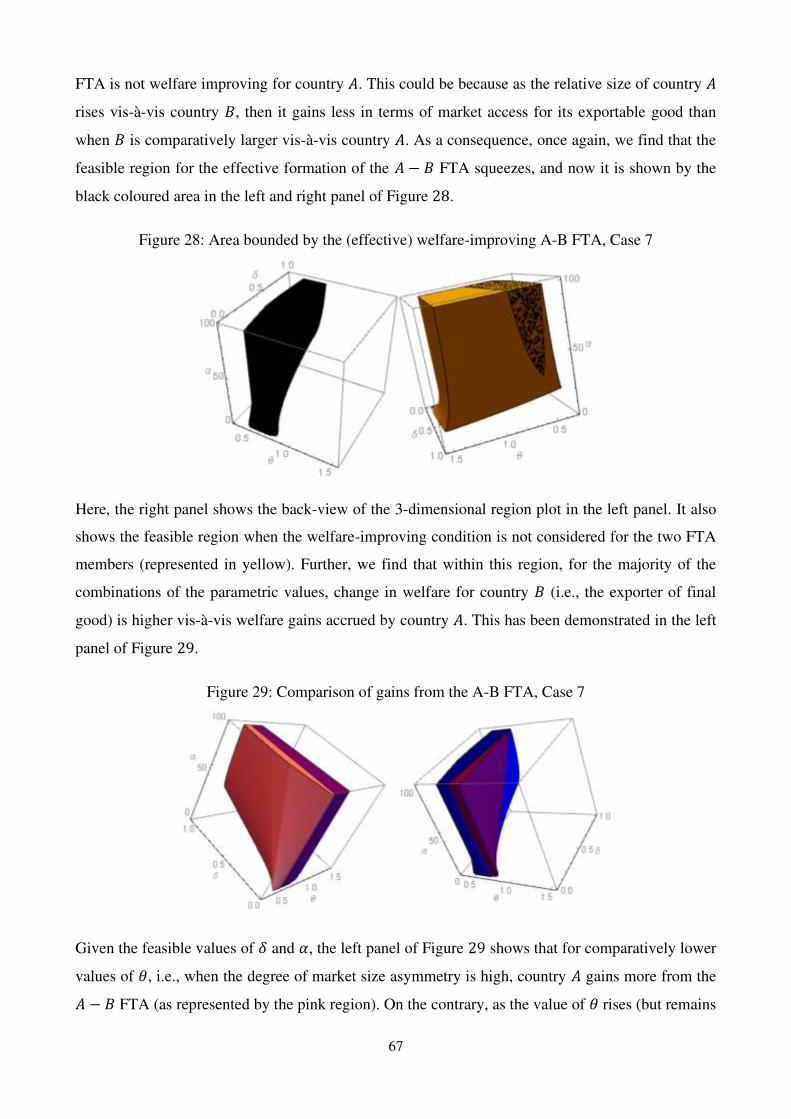
67

FTA is not welfare improving for country 𝐴. This could be because as the relative size of country 𝐴

rises vis-à-vis country 𝐵, then it gains less in terms of market access for its exportable good than

when 𝐵 is comparatively larger vis-à-vis country 𝐴. As a consequence, once again, we find that the

feasible region for the effective formation of the 𝐴 − 𝐵 FTA squeezes, and now it is shown by the

black coloured area in the left and right panel of Figure 28.

Figure 28: Area bounded by the (effective) welfare-improving A-B FTA, Case 7

Here, the right panel shows the back-view of the 3-dimensional region plot in the left panel. It also

shows the feasible region when the welfare-improving condition is not considered for the two FTA

members (represented in yellow). Further, we find that within this region, for the majority of the

combinations of the parametric values, change in welfare for country 𝐵 (i.e., the exporter of final

good) is higher vis-à-vis welfare gains accrued by country 𝐴. This has been demonstrated in the left

panel of Figure 29.

Figure 29: Comparison of gains from the A-B FTA, Case 7

Given the feasible values of 𝛿 and 𝛼, the left panel of Figure 29 shows that for comparatively lower

values of 𝜃, i.e., when the degree of market size asymmetry is high, country 𝐴 gains more from the 𝐴 − 𝐵 FTA (as represented by the pink region). On the contrary, as the value of 𝜃 rises (but remains

68

less than 1), the welfare-gains for the final good exporter become more than the exporter of

intermediate inputs. Although this result is quite similar to the one we observed in Case 6, there does

exist some difference. As we can see from Figures 25 and 29, the region supporting higher welfare-

gain for the input exporter is more in the case of the latter than the former. This difference arises

because of the size of country 𝑅, which is similar to country 𝐵, and also because of its response to

the changes in 𝐴’s and 𝐵’s optimal tariff rates. In particular, we find that in the present case, country 𝑅’s input tariff necessarily increases (as in the previous Case 6), but its output-tariff also rises under

certain conditions. This, in turn, reduces the potential gains for country 𝐵’s downstream firm, whose

input cost reduces with the formation of the 𝐴 − 𝐵 FTA.

Nonetheless, it is crucial to point out that in the absence of any market size asymmetry (between 𝐴

and 𝐵, or 𝐴 and 𝑅), the 𝐴 − 𝐵 FTA necessarily reduces the welfare of the intermediate input exporter

within the FTA region, while benefitting both the final goods exporter as well as the rest of the world.

In fact, the latter (i.e., country 𝑅) profits in the entire yellow region shown in the leftmost panel of

Figure 27 or in the right panel of figure 28. While this FTA turns out to be more beneficial for R than

for 𝐴, the former gains less than 𝐵 in the purple region shown in the right panel of Figure 29. The

blue coloured region in the same figure, however, shows all those combinations of the feasible values

of 𝛼, 𝜃, and 𝛿 where 𝑅 gains the most. One reason for such a result could be that with lower market-

size asymmetry, country 𝐵’s tariff (and, hence, tariff revenue) reduces by a smaller amount post the

conclusion of the 𝐴 − 𝐵 FTA than when 𝐵 is much larger than 𝐴. This is because as observed from

Case 1, a country’s tariff rate is directly proportional to its market size. On the contrary, country 𝑅

gains in terms of tariff revenue with higher input as well output tariff under certain conditions.

Proposition 10 summarises the findings for country 𝑅.

Proposition 10. Regardless of the feasible range of the parametric values and the composition of

trade baskets of the FTA partners, in our 3-country vertical industry set up, country R, i.e., the rest

of the world unambiguously gains from the formation of the A-B FTA. In fact, in some of the cases,

welfare gains are higher for country R, vis-à-vis the two FTA partners, though its terms of trade

deteriorate in comparison to the pre-FTA scenario.

This has already been proved in Cases 2, 4, 5, 6, and 7 of our analysis. It is also important to note

that this result is independent of whether or not 𝑅 raises its input/output tariffs after the formation of

the 𝐴 − 𝐵 FTA. In fact, in each of the five cases, 𝑅’s trade balance improved vis-à-vis country 𝐴 and 𝐵. However, wherever the gains from FTA are more for 𝐵 than for 𝑅, it seems plausible to conclude

that under certain conditions, the trade-creation and diversion effects of free trade agreements can

induce non-members (that were previously against the membership) to join the block.

69

5. Summary and Concluding Remarks

One of the fundamental principles of the international trade theory is that lowering trade barriers leads

to increased welfare. Regional trade agreements represent one such policy mechanism, via which the

participating economies offer preferential market access to each other’s goods and services, and hence

aim to enhance their welfares via increased trade volumes. The existing literature abounds with

various theoretical studies that anticipate and advocate the benefits of such arrangements. But, the

question regarding their heterogeneous effects on member countries has not been explicitly studied

in any of them. In fact, barring a few, most of the empirical studies, to date, have also estimated a

common average effect across all the RTAs or assume that the impact of a trade agreement is the

same for all the participating economies (Baier, Yotov and Zylkin 2019). However, recently, it has

been argued by trade negotiators of many countries that while some partners gain more from an RTA,

others gain less or, at times, suffer from a rise in their current account deficits and overall economic

losses as well. Even the Indian scenario is not an outlier in such a case. In this backdrop, the objective

of this essay has been to address this ongoing debate regarding the uneven benefits from RTAs by

specifically focussing on the type of commodities (intermediate inputs or final goods) that countries

trade with each other, and show how the composition of their trade baskets leads to asymmetric effects

on their imports and exports (and hence, overall social welfare).

We have built on a simple 3-country and 2-vertically related (imperfectly-competitive) industry

framework to study the effects of free trade agreements (in particular) and analyse the conditions

under which they result in higher welfare for the participating economies in the presence of

preferential rules of origin. To incorporate the role of commodity profiles, we have focussed on

alternative trade regimes. In particular, we have assumed two different scenarios – a). where FTAs

cover horizontal trade between the participating economies, either in final or intermediate goods, and

b). where vertical trade dominates, i.e., where one of the FTA members exports intermediate inputs

to the other, and imports the final good in return (like the South-South or North-South trade).

First of all, our findings suggest that not all FTAs are Pareto-improving (regardless of the trade profile

of the two members), and they lead to higher welfare only under certain conditions. This essentially

implies that any country, while designing its trade agreements, should very carefully consider looking

at the economic gains from an FTA, and not the political aspect of signing those agreements. These

conditions depend on the size of the participating economies, the degree of market size asymmetry

between the two, and the ROO-induced trade cost. Here, the arbitrage-free bounds play an

indispensable role in determining the effective formation of an FTA and excluding the possibility of

trade deflection. In fact, when we considered the role of vertical FTAs, even the trade baskets of the

two members assumed significant importance in establishing whether the free trade agreement will

70

be beneficial to them or not. This is an important observation as it highlights why most RTAs since

1990s have been of the S-S variety.

This is so far as the welfare-improving FTAs are concerned. We also examined the heterogeneity in

FTAs effects on the two trading partners. We first focussed on what we referred to as ‘horizontal

FTAs’, and compared and contrasted the benefits when such an agreement leads to bilateral free trade

in final goods between the member countries, vis-à-vis the scenario where final goods become a part

of the exclusion list, and the members agree to eliminate tariffs on each other’s imports of

intermediate inputs. Our findings suggest that contrary to the widely held view that a country’s

primary focus should always be on bringing down its input-tariffs so as to improve the

competitiveness of its downstream products, bilateral free trade in final goods (when the countries

also trade in intermediates) leads to higher welfare for both the member countries.42 This result could

be interpreted in terms of what is referred to as the ‘backward-linkage’ effect in the GVC literature –

zero tariffs on imports of final goods improve their tradability within the FTA, which not only benefits

the consumers due to lower prices, but also raise the demand for intermediate inputs. In fact, in our

model, we found that the optimal response of the two governments to the elimination of their

(bilateral) output-tariffs has been to reduce their input-tariffs too, which not only reduces the cost of

producing their final goods (and induce (positive) forward-linkage effect onto the downstream firms),

but also positively affects the downstream firm in the rest of the world, and raise the overall welfare

of the world economy. As a consequence, even the non-member country profits more in this case.

Nevertheless, it is equally imperative to note that a comparatively larger range of feasible values of

our model parameters (including market size asymmetry) supports the effective formation of the FTA

in intermediate goods than in final goods. On the contrary, the conclusion of an FTA in final goods

is most likely to emerge between countries that are not very different from each other in terms of their

market sizes. Another important finding is that in each of the two cases, the exporters of the respective

goods under consideration suffered from a loss in their profits due to the formation of the FTA. This

did not happen because of a loss in their export sales or revenue, but because of a fall in their domestic

sales due to intense competition from foreign goods. What this implies is that a country should

simultaneously accelerate domestic market reforms (to improve the competitiveness of its local firms)

while negotiating different FTAs to sufficiently leverage these arrangements to increase their

presence in the world market.

Most of these findings, however, drastically changed when we considered the role of vertical FTAs.

In particular, we found that if the final good exporter within the FTA is small vis-à-vis the input

42 This result is independent of whether the two members’ trade deficit with each other rises or falls after the establishment of the free trade agreement.

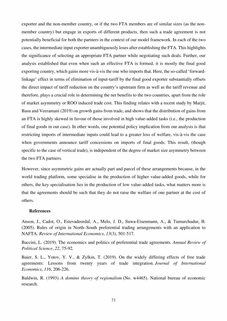
71

exporter and the non-member country, or if the two FTA members are of similar sizes (as the non-

member country) but engage in exports of different products, then such a trade agreement is not

potentially beneficial for both the partners in the context of our model framework. In each of the two

cases, the intermediate input exporter unambiguously loses after establishing the FTA. This highlights

the significance of selecting an appropriate FTA partner while negotiating such deals. Further, our

analysis established that even when such an effective FTA is formed, it is mostly the final good

exporting country, which gains more vis-à-vis the one who imports that. Here, the so-called ‘forward-

linkage’ effect in terms of elimination of input-tariff by the final good exporter substantially offsets

the direct impact of tariff reduction on the country’s upstream firm as well as the tariff revenue and

therefore, plays a crucial role in determining the net benefits to the two countries, apart from the role

of market asymmetry or ROO induced trade cost. This finding relates with a recent study by Marjit,

Basu and Veeramani (2019) on growth gains from trade, and shows that the distribution of gains from

an FTA is highly skewed in favour of those involved in high value-added tasks (i.e., the production

of final goods in our case). In other words, one potential policy implication from our analysis is that

restricting imports of intermediate inputs could lead to a greater loss of welfare, vis-à-vis the case

when governments announce tariff concessions on imports of final goods. This result, (though

specific to the case of vertical trade), is independent of the degree of market size asymmetry between

the two FTA partners.

However, since asymmetric gains are actually part and parcel of these arrangements because, in the

world trading platform, some specialise in the production of higher value-added goods, while for

others, the key specialisation lies in the production of low value-added tasks, what matters more is

that the agreements should be such that they do not raise the welfare of one partner at the cost of

others.

References

Anson, J., Cadot, O., Estevadeordal, A., Melo, J. D., Suwa‐Eisenmann, A., & Tumurchudur, B. (2005). Rules of origin in North–South preferential trading arrangements with an application to

NAFTA. Review of International Economics, 13(3), 501-517.

Baccini, L. (2019). The economics and politics of preferential trade agreements. Annual Review of

Political Science, 22, 75-92.

Baier, S. L., Yotov, Y. V., & Zylkin, T. (2019). On the widely differing effects of free trade

agreements: Lessons from twenty years of trade integration. Journal of International

Economics, 116, 206-226.

Baldwin, R. (1993). A domino theory of regionalism (No. w4465). National bureau of economic

research.

72

Baldwin, R., & Jaimovich, D. (2012). Are free trade agreements contagious?. Journal of international

Economics, 88(1), 1-16.

Basco, S., & Mestieri, M. (2019). The world income distribution: the effects of international

unbundling of production. Journal of Economic Growth, 24(2), 189-221.

Batra, R. N. (1973). Studies in the pure theory of international trade. Springer.

Berlingieri, G. (2013) Outsourcing and the rise in services. CEP Discussion Papers (CEPDP1199).

Centre for Economic Performance, London School of Economics and Political Science, London, UK.

Accessed on September 30, 2020.

Berlingieri, G., Breinlich, H., & Dhingra, S. (2018). The impact of trade agreements on consumer

welfare—evidence from the eu common external trade policy. Journal of the European Economic

Association, 16(6), 1881-1928. Doi: https://doi.org/10.1093/jeea/jvx053

Bhagwati, J. (1971). Trade-diverting customs unions and welfare-improvement: A clarification. The

Economic Journal, 81(323), 580-587.

Bhagwati, J. N. (1991). The world trading system at risk. Princeton University Press.

Bhagwati, J. N., Panagariya, A., & Srinivasan, T. N. (1998). Lectures on international trade. MIT

press.

Blanchard, E. J., Bown, C. P., & Johnson, R. C. (2017). Global value chains and trade

policy. Dartmouth College and Peterson Institute for International Economics, 2. Retrieved from

<http://faculty.tuck.dartmouth.edu/images/uploads/faculty/emily-blanchard/BBJ-August2017.pdf>

Brander, J. A. (1981). Intra-industry trade in identical commodities. Journal of international

Economics, 11(1), 1-14.

Brander, J. A., & Spencer, B. J. (1984). Trade warfare: tariffs and cartels. Journal of international

Economics, 16(3-4), 227-242.

Bruhn, D. (2014). Global value chains and deep preferential trade agreements: promoting trade at the

cost of domestic policy autonomy?. Available at SSRN 2464136.

Cadot, O., Graziano, A., Harris, J., & Volpe, C. (2014). Do Rules of Origin Constrain Export

Growth?. IDB Integration and Trade Sector No. IDB-DP-350.

Carrère, C (2006), “Revisiting the effects of regional trade agreements on trade flows with proper specification of the gravity model”, European Economic Review 50(2): 223–247.

Chains, G. V. (2014). Challenges, Opportunities, and Implications for Policy. In Report prepared for

submission to the G20 Trade Ministers Meeting Sydney, Australia (Vol. 19).

Chandrashekhar, G. (2019, December 30). Inverted duty structure hurts soaps industry. The Hindu

Business Line. Retrieved from

<https://www.thehindubusinessline.com/markets/commodities/inverted-duty-structure-hurts-soaps-

industry/article30431722.ece>

Chang, Y. M., & Xiao, R. (2015). Preferential trade agreements between asymmetric countries: Free

trade areas (with rules of origin) vs. customs unions. Japan and the World Economy, 33, 28-43.

73

Chen, M. X., & Joshi, S. (2010). Third-country effects on the formation of free trade

agreements. Journal of International Economics, 82(2), 238-248.

Bagwell, K., & Staiger, R. W. (1999). Regionalism and multilateral tariff co-operation.

In International trade policy and the pacific rim (pp. 157-190). Palgrave Macmillan, London.

Copeland, B., & Mattoo, A. (2008). The basic economics of services trade. A handbook of

international trade in services, 84-129.

Corden, W. M. (1971). The effects of trade on the rate of growth. Trade, Balance of payment And

Growth. Amsterdam: North Holland, 117-43.

Dhar, B., (2014, October 10). Are free trade agreements a dead end for India? East Asia Forum, New

Delhi. Retrieved from <https://www.eastasiaforum.org/2014/10/10/are-free-trade-agreements-a-

dead-end-for-india/>

Dhir, G. (2020, September 19). COVID-19 and Opportunities for India in World Trade. Medium.

Retrieved from <https://medium.com/@garimadhir2/covid-19-and-opportunities-for-india-in-world-

trade-1a0caa3ba46f>

FE Bureau. (2019, September 11). India, Asean to set up joint panel to review free

trade agreement. Financial Express. Retrieved from

<https://www.financialexpress.com/economy/joint-panel-to-be-formed-india-asean-to-review-free-

trade-agreement/1702529/>

Freund, C. (2000). Different paths to free trade: The gains from regionalism. The Quarterly Journal

of Economics, 115(4), 1317-1341.

Furusawa, T., Higashida, K., & Ishikawa, J. (2004). Tariffs versus quotas in the presence of imperfect

competition and cross‐border externalities. Canadian Journal of Economics/Revue canadienne

d'économique, 37(2), 445-458.

Garrett, G. (2017, February 1). Do Trade Agreements Lead to Income Inequality? Knowledge @

Wharton. Wharton University of Pennsylvania. Retrieved from <

https://knowledge.wharton.upenn.edu/article/do-trade-agreements-lead-to-income-inequality/>

Government of India. (2020). Economic Survey 2019-20 (Volume 1). Economics Division,

Department of Economic Affairs, Ministry of Finance. Retrieved from

<https://www.indiabudget.gov.in/economicsurvey/doc/echapter.pdf>

Grossman, G., & Helpman, E. (1994). Protection for Sale. The American Economic Review, 84(4),

833-850. <http://www.jstor.org/stable/2118033>

Ignatenko, A., Raei, F., & Mircheva, B. (2019). Global Value Chains: What are the Benefits and Why

Do Countries Participate?. IMF Working Papers, WP/19/18.

Hartwell, C. & Movchan, V. (2018). Finding the right balance across EU FTAs: benefits and risks

for EU economic sectors. European Parliament Think Tank

Heckscher, E. F. (1919). The effect of foreign trade on the distribution of income. [in Swedish].

Ekonomisk Tidskrift, 21(2), pp. 1-32; reprinted in Readings in the theory of international trade.

Homewood, IL: Irwin, 1950, pp. 272-300.

74

Hoffman, C., Osnago, A., & Ruta, M. (2017). Horizontal Depth A New Database on the Content of

Preferential Trade Agreements. Policy Research Working Paper, 7981, accessed on November 9th,

2017

Hummels, D. L., Rapoport, D., & Yi, K. M. (1998). Vertical specialization and the changing nature

of world trade. Economic Policy Review, 4(2).

Impullitti, G. and Licandro, O. (2018). “Quantifying the gains from trade”, VoxEU.org, 29 April.

Retrieved from <https://voxeu.org/article/quantifying-gains-trade>

Ishikawa, J. (2000). Foreign monopoly and trade policy under segmented and integrated

markets. Economic Review, 51(4), 321-336.

Ishikawa, J., & Spencer, B. J. (1999). Rent-shifting export subsidies with an imported intermediate

product. Journal of International Economics, 48(2), 199-232.

Ishikawa, J., Mukunoki, H., & Mizoguchi, Y. (2007). Economic integration and rules of origin under

international oligopoly. International Economic Review, 48(1), 185-210.

Jha, D. K. (2019, June 20). Secondary metals producers fear inverted duty structure could hurt.

Business Standard. Retrieved from < https://www.business-

standard.com/article/companies/secondary-metals-producers-fear-inverted-duty-structure-could-

hurt-119061900301_1.html>

Jha, D. K. (2015, September 17). FTA with EU to increase cotton textile exports. Business Standard.

Retrieved from < https://www.business-standard.com/article/markets/fta-with-eu-to-increase-cotton-

textile-exports-115091700433_1.html>

Ju, J., & Krishna, K. (2005). Firm behaviour and market access in a free trade area with rules of

origin. Canadian Journal of Economics/Revue canadienne d'économique, 38(1), 290-308.

Kawabata, Y. (2014). The effects of cross-regional free trade agreements under a vertical industry

structure. The Journal of International Trade & Economic Development, 23(6), 906-922.

Kawabata, Y. (2015). Endogenous formation of free trade agreements in vertically related

markets. Research in Economics, 69(2), 214-223.

Kawabata, Y. (2016). Cost Asymmetries and Import Tariff Policy in a Vertically Related Industry.

In Regional Free Trade Areas and Strategic Trade Policies (pp. 151-163). Springer, Tokyo.

Kawabata, Y., Yanase, A., & Kurata, H. (2010). Vertical trade and free trade agreements. Journal of

the Japanese and International Economies, 24(4), 569-585.

Keck, A., & Lendle, A. (2012). New evidence on preference utilization. World Trade Organization

Staff Working Paper No. ERSD-2012-12.

Kirman, A. P. (1973). Trade diverting customs unions and welfare improvement: a comment. The

Economic Journal, 83(331), 890-894.

Kohl, T. (2014). Do we really know that trade agreements increase trade?. Review of World

Economics, 150(3), 443-469.

Krishna, K. (2005). Understanding rules of origin (No. w11150). National Bureau of Economic

Research.

75

Krishna, P. (1998). Regionalism and multilateralism: A political economy approach. The Quarterly

Journal of Economics, 113(1), 227-251.

Krugman, P. (1991). Increasing returns and economic geography. Journal of political

economy, 99(3), 483-499.

Krugman, P. R. (1979). Increasing returns, monopolistic competition, and international trade. Journal

of international Economics, 9(4), 469-479.

Kwatra, N., & Kundu, T. (2018, August 14). Can regional trade agreements boost India’s exports?. Mint. Retrieved from <https://www.livemint.com/Industry/srfvvWL76rtMLaeQzOtbJM/Can-

regional-trade-agreements-boost-Indias-exports.html>

Lipsey, R. G. (1957). The theory of customs unions: trade diversion and welfare. Economica, 24(93),

40-46.

Lipsey, R. G., & Lancaster, K. (1956). The general theory of second best. The review of economic

studies, 24(1), 11-32.

Marjit, S., Basu, A, & Veeramani, C. (2019). Growth Gains from Trade. CESifo Working Paper No.

7905, Available at SSRN: <https://ssrn.com/abstract=3477718>. Accessed on April 13, 2020.

Mathew, J.C. (2019, September 27). Are free trade agreements beneficial for India? Business Today.

Retrieved from <https://www.businesstoday.in/current/economy-politics/are-free-trade-agreements-

beneficial-for-india/story/381624.html>

Meng, B., Ye, M., & Wei, S. J. (2020). Measuring Smile Curves in global value chains. Oxford

Bulletin of Economics and Statistics, 82(5), 988-1016. Doi: <https://doi.org/10.1111/obes.12364>

Mon, Y. Y., & Kakinaka, M. (2020). Regional trade agreements and income inequality: Are there

any differences between bilateral and plurilateral agreements?. Economic Analysis and Policy, 67,

136-153.

Mukunoki, H. (2004). On the optimal external tariff of a free trade area with internal market

integration. Japan and the World Economy, 16(4), 431-448.

Nguyen, D. B. (2019). A new examination of the impacts of regional trade agreements on

international trade patterns. Journal of Economic Integration, 34(2), 236-279.

OECD, WTO, & World Bank Group. (2014). Global Value Chains: Challenges, Opportunities, and

Implications for Policy. In Report prepared for the G20 Trade Ministers Meeting Sydney. Australia.

(Vol. 19). <http://www.oecd.org/tad/gvc_report_g20_july_2014.pdf >

Ohlin, B. (1933). International and interregional trade. Harvard Economic Studies, Cambridge, MA.

Panagariya, A., & Krishna, P. (2002). On necessarily welfare-enhancing free trade areas. Journal of

International Economics, 57(2), 353-367.

Pant, M., & Paul, A. (2018). The role of regional trade agreements: In the case of India. Journal of

Economic Integration, 33(3), 538-571.

Pant, M., & Sadhukhan, A. (2009). Does Regionalism Hinder Multilateralism: a Case Study of

India. Journal of Economic Integration, 222-247.

76

Pathania, K., & Bhattacharjea, A. (2020). Inverted Duty Structures and the Paradox of Negative

Effective Protection in India, 2000–2014. Foreign Trade Review, 55(2), 139-167.

PTI (2015, April 13). Auto sector inclusion in India-EU FTA against 'Make in India'. Economic

Times. Retrieved from <https://auto.economictimes.indiatimes.com/news/industry/auto-sector-

inclusion-in-india-eu-fta-against-make-in-india/46906251>

PTI (2017, July 30). India, South Korea reviewing FTA to boost trade. Economic Times. Retrieved

from <https://economictimes.indiatimes.com/news/economy/foreign-trade/india-south-korea-

reviewing-fta-to-boost-trade/articleshow/59830991.cms>

PTI (2019, June 21). FTAs are against Make in India, need to approach EU pact with caution:

SIAM. The Economic Times. Retrieved from

<https://economictimes.indiatimes.com/news/economy/policy/ftas-are-against-make-in-india-need-

to-approach-eu-pact-with-caution-siam/articleshow/69890551.cms?from=mdr>

Rathee, K. (2019, July 23). FTAs with Asean nations hurt domestic TV production. Financial

Express. Retrieved from <https://www.financialexpress.com/industry/ftas-with-asean-nations-hurt-

domestic-tv-production/1653061/>

Ricardo, D. (1921). The first six chapters of the principles of political economy and taxation of David

Ricardo, 1817. Macmillan.

Robinson, S., & Thierfelder, K. (2002). Trade liberalisation and regional integration: the search for

large numbers. Australian Journal of Agricultural and Resource Economics, 46(4), 585-604.

Ruta, M. (2017). Preferential trade agreements and global value chains: Theory, evidence, and open

questions. The World Bank. https://doi.org/10.1596/1813-9450-8190 (Accessed on September 7th,

2020).

Saggi, K., & Yildiz, H. M. (2006). On the international linkages between trade and merger

policies. Review of International Economics, 14(2), 212-225.

Schiff, M. (1996). Small is beautiful: Preferential trade agreements and the impact of country size,

market share, efficiency, and trade policy. World Bank Policy Research Working Paper, (1668).

Accessed on August 15, 2020.

Sen, A. (2019a, June 12). Commerce Minister reviews free trade pacts. The Hindu Business Line.

Retrieved from <https://www.thehindubusinessline.com/economy/commerce-minister-reviews-free-

trade-pacts/article27891028.ece?homepage=true>

Sen, A. (2019b, December 15). EU FTA talks: India looking at ways to end stalemate, re-start

negotiations. The Hindu Business Line. Retrieved from

<https://www.thehindubusinessline.com/economy/eu-fta-talks-india-looking-at-ways-to-end-

stalemate-re-start-negotiations/article30313313.ece>

Smith, A. (1776). An inquiry into the wealth of nations. Strahan and Cadell, London, 1-11.

Smith, A., & Venables, A. J. (1988). Completing the internal market in the European Community:

Some industry simulations. European economic review, 32(7), 1501-1525.

77

Srivastav, A. (2019, January 4). How to enter into an FTA that delivers. The Hindu Business Line.

Retrieved from <https://www.thehindubusinessline.com/opinion/columns/ajay-srivastav/how-to-

enter-into-an-fta-that-delivers/article25912371.ece>

Subramaniam, V. (2016, November 26). Here's why Trump hates the Trans-Pacific Partnership so

much. Business Insider. Retrieved from <https://www.businessinsider.com/heres-why-trump-hates-

the-trans-pacific-partnership-so-much-2016-11?IR=T>

Summers, L. (1991). Regionalism and the world trading system. Policy implications of trade and

currency zones, 295-301.

Takarada, Y., Kawabata, Y., Yanase, A., & Kurata, H. (2020). Standards policy and international

trade: Multilateralism versus regionalism. Journal of Public Economic Theory.

TNN. (2020, February 29). Textile industry demands level playing field with Asean. Times of India.

Retrieved from <https://timesofindia.indiatimes.com/city/ludhiana/textile-industry-demands-level-

playing-field-with-asean/articleshow/74409390.cms>

Venables, A. J. (1985). Trade and trade policy with imperfect competition: The case of identical

products and free entry. Journal of International Economics, 19(1-2), 1-19.

Viner, J. (1950). The Customs Union Issue. Carnegie Endowment for International Peace. New York.

Soo, K. T. (2011). The gains from specialisation and comparative advantage. Lancaster University.

Retrieved from < https://www.etsg.org/ETSG2011/Papers/Soo.pdf>

Wonnacott, P., & Lutz, M. (1989). Is there a case for free trade areas? Free trade areas and US trade

policy, 59, 84.

World Bank (2020). World Development Report 2020: Trading for Development in the Age of Global

Value Chains. World Bank, Washington, DC.

World Trade Organisation (2019). World trade statistical review 2019. WTO, Geneva.

[Data] WTO RTA Database: https://rtais.wto.org/UI/charts.aspx#