galactic potential constraints from clustering in action
TRANSCRIPT

University of Groningen
Galactic potential constraints from clustering in action space of combined stellar stream dataReino, Stella; Rossi, Elena M.; Sanderson, Robyn E.; Sellentin, Elena; Helmi, Amina;Koppelman, Helmer H.; Sharma, SanjibPublished in:Monthly Notices of the Royal Astronomical Society
DOI:10.1093/mnras/stab304
IMPORTANT NOTE: You are advised to consult the publisher's version (publisher's PDF) if you wish to cite fromit. Please check the document version below.
Document VersionPublisher's PDF, also known as Version of record
Publication date:2021
Link to publication in University of Groningen/UMCG research database
Citation for published version (APA):Reino, S., Rossi, E. M., Sanderson, R. E., Sellentin, E., Helmi, A., Koppelman, H. H., & Sharma, S. (2021).Galactic potential constraints from clustering in action space of combined stellar stream data. MonthlyNotices of the Royal Astronomical Society, 502(3), 4170-4193. https://doi.org/10.1093/mnras/stab304
CopyrightOther than for strictly personal use, it is not permitted to download or to forward/distribute the text or part of it without the consent of theauthor(s) and/or copyright holder(s), unless the work is under an open content license (like Creative Commons).
The publication may also be distributed here under the terms of Article 25fa of the Dutch Copyright Act, indicated by the “Taverne” license.More information can be found on the University of Groningen website: https://www.rug.nl/library/open-access/self-archiving-pure/taverne-amendment.
Take-down policyIf you believe that this document breaches copyright please contact us providing details, and we will remove access to the work immediatelyand investigate your claim.
Downloaded from the University of Groningen/UMCG research database (Pure): http://www.rug.nl/research/portal. For technical reasons thenumber of authors shown on this cover page is limited to 10 maximum.
Download date: 06-01-2022
MNRAS 502, 4170–4193 (2021) doi:10.1093/mnras/stab304Advance Access publication 2021 February 4
Galactic potential constraints from clustering in action space of combinedstellar stream data
Stella Reino ,1‹ Elena M. Rossi,1 Robyn E. Sanderson ,2,3 Elena Sellentin,1 Amina Helmi,4
Helmer H. Koppelman4 and Sanjib Sharma 5
1Leiden Observatory, Leiden University, Niels Bohrweg 2, NL-2333 CA Leiden, the Netherlands2Department of Physics and Astronomy, University of Pennsylvania, 209 S 33rd St, Philadelphia, PA 19104, USA3Center for Computational Astrophysics, Flatiron Institute, 162 5th Ave., New York, NY 10010, USA4Kapteyn Astronomical Institute, University of Groningen, PO Box 800, NL-9700 AV Groningen, the Netherlands5Sydney Institute for Astronomy, School of Physics, The University of Sydney, Sydney, NSW 2006, Australia
Accepted 2021 January 29. Received 2021 January 29; in original form 2020 June 29
ABSTRACTStream stars removed by tides from their progenitor satellite galaxy or globular cluster act as a group of test particles onneighbouring orbits, probing the gravitational field of the Milky Way. While constraints from individual streams have beenshown to be susceptible to biases, combining several streams from orbits with various distances reduces these biases. We fit acommon gravitational potential to multiple stellar streams simultaneously by maximizing the clustering of the stream stars inaction space. We apply this technique to members of the GD-1, Palomar 5 (Pal 5), Orphan, and Helmi streams, exploiting boththe individual and combined data sets. We describe the Galactic potential with a Stackel model, and vary up to five parameterssimultaneously. We find that we can only constrain the enclosed mass, and that the strongest constraints come from the GD-1,Pal 5, and Orphan streams whose combined data set yields M(< 20 kpc) = 2.96+0.25
−0.26 × 10¹¹ M�. When including the Helmistream in the data set, the mass uncertainty increases to M(< 20 kpc) = 3.12+3.21
−0.46 × 10¹¹ M�.
Key words: methods: numerical – Galaxy: fundamental parameters – Galaxy: kinematics and dynamics – Galaxy: structure –dark matter.
1 IN T RO D U C T I O N
The outer reaches of the Milky Way, known as the ‘halo’, aredominated by dark matter. Knowledge of the mass and shape ofthe halo is required for placing strong constraints on the formationhistory of the Milky Way, testing the nature of dark matter, andmodified gravity models (e.g. Mao, Williamson & Wechsler 2015;Thomas et al. 2018). Some of the most promising dynamical tracersof the Galactic potential in the halo region are stellar steams. Stellarstreams form when stars are torn from globular clusters or dwarfgalaxies due to Galactic tidal forces. The stars in the ensuingdebris gradually stretch out in a series of neighbouring orbits. Thisproperty makes stellar streams superb probes of the underlyinggravitational potential, allowing us to constrain the mass distributionwithin the extent of their orbits (Johnston et al. 1999). In addition,density variations and gaps within a stream can potentially provideinformation about past encounters with small-scale substructureand therefore an opportunity to detect the presence of dark mattersubhaloes (Carlberg, Grillmair & Hetherington 2012; Sanders, Bovy& Erkal 2016; Erkal, Koposov & Belokurov 2017; Banik & Bovy2019; Bonaca et al. 2019, 2020).
The first detections of streams included the discovery of thetidally distorted Sagittarius dwarf galaxy by Ibata, Gilmore & Irwin
� E-mail: [email protected]
(1994), the tidal tails around multiple globular clusters by Grillmairet al. (1995), and the Helmi streams by Helmi et al. (1999). Sincethen, the number of known streams has grown rapidly owing tothe high-quality data from wide-field surveys. The first surge indiscoveries came with the arrival of the Sloan Digital Sky Survey(SDSS), where among others, the GD-1 (Grillmair & Dionatos2006b), Orphan (Belokurov et al. 2006; Grillmair 2006), Palomar 5(Pal 5; Odenkirchen et al. 2001), and NGC 5466 streams (Grillmair& Johnson 2006) were found. More discoveries from other surveys,such as the Pan-Andromeda Archaeological Survey (PAndAS), thePanoramic Survey Telescope and Rapid Response System 1 (Pan-STARRS1), and the Dark Energy Survey, followed (Bernard et al.2014, 2016; Koposov et al. 2014; Martin et al. 2014; Shipp et al.2018).
Despite the abundance of known streams (see e.g. Newberg &Carlin 2016; Mateu, Read & Kawata 2018), full six-dimensional (6D)phase-space maps of stream members, crucial for obtaining accurateconstraints on the Galactic potential, have only been made for a fewcases. Recently, the second data release of Gaia (Gaia DR2; GaiaCollaboration et al. 2018) expanded our ability to make such maps byseveral orders of magnitude, by measuring proper motions for morethan a billion Milky Way stars. This phenomenal wealth of datahas already facilitated the discovery of many new streams (Malhan,Ibata & Martin 2018; Ibata, Malhan & Martin 2019; Meingast,Alves & Furnkranz 2019) and prompted further investigations ofthe previously known ones (Price-Whelan & Bonaca 2018; Koposov
C© 2021 The Author(s)Published by Oxford University Press on behalf of Royal Astronomical Society
Dow
nloaded from https://academ
ic.oup.com/m
nras/article/502/3/4170/6128656 by University of G
roningen user on 12 May 2021

Galactic potential constraints from streams 4171
et al. 2019; Koppelman et al. 2019; Price-Whelan et al. 2019). Togain a full 6D view of more distant streams, Gaia data must becombined with radial velocity measurements for faint stars fromcurrent or future wide-field spectroscopic surveys such as the RadialVelocity Experiment (RAVE; Kunder et al. 2017), Southern StellarStream Spectroscopic Survey (S5; Li et al. 2019), WHT EnhancedArea Velocity Explorer (WEAVE; Dalton et al. 2012), 4-metre Multi-Object Spectroscopic Telescope (4MOST; de Jong et al. 2019), fifthgeneration of the Sloan Digital Sky Survey (SDSS-V; Kollmeier et al.2017), etc.
Perhaps the most intuitive approach for constraining the Galacticpotential with stellar streams is the orbit-fitting technique, whereorbits integrated in different potentials are compared with the tracksof observed streams (e.g. Koposov, Rix & Hogg 2010; Newberg et al.2010). However, the oversimplification that streams perfectly followthe original progenitor’s orbit has been shown to lead to systematicbiases when used to constrain the Galactic potential (Sanders &Binney 2013a). More realistic stream modelling involves creatingeither full N-body simulations of disruptions of stellar clusters (themost accurate but also most computationally expensive option) orparticle-spray models, where the stream is created by ejecting starsfrom the Lagrange points of an analytical model of the progenitor atspecific times (Bonaca et al. 2014; Kupper et al. 2015; Erkal et al.2019).
All these methods compare models to observed streams in 6Dphase space, or some subset of measured positions and velocities.It is, however, possible to simplify the behaviour of streams con-siderably by switching to action-angle coordinates (McMillan &Binney 2008; Sanders & Binney 2013b; Bovy et al. 2016). In thiswork, we follow the action-space clustering method of Sanderson,Helmi & Hogg (2015). Actions are integrals of motion that, savefor orbital phase, completely define the orbit of a star bound in astatic or adiabatically time-evolving potential. Converting the 6Dphase-space position of a star to action space essentially compressesthe entire orbit of a star to just three numbers. Stream stars movealong similar orbits and thus should cluster tightly in action space.However, since action calculation requires knowledge of the Galacticpotential, clustering occurs only if the actions are calculated withsomething close to the true potential (Penarrubia, Koposov & Walker2012; Magorrian 2014; Yang, Boruah & Afshordi 2020). Therefore,our strategy to find the true Galactic potential is to identify thepotential that produces the most clumpy distribution of stars in actionspace.
The method outlined in Sanderson et al. (2015) quantifies the de-gree of action-space clustering with the Kullback–Leibler divergence(KLD), which is used to determine both the best-fitting potentialand its associated uncertainties. In that work, we demonstratedthe effectiveness of this procedure by successfully recovering theinput parameters of a potential using mock streams evolved in thatpotential. Here, we apply the same technique to real stellar streams.
Stellar streams can possess a variety of morphologies: someappear as long narrow arcs, others shells, while still others are fullyphase mixed and no longer easily distinguishable as single structures(Hendel & Johnston 2015; Amorisco 2015). However, even if phasemixing has induced a lack of apparent spatial features, the fact thatthese stars still follow similar orbits causes them to condense intoa single cluster in action space. Our method is thus applicable tostreams in any evolutionary stage.
Another important advantage of this technique is that it can beapplied to multiple streams simultaneously. Combining multiplestreams is crucial since it helps counteract the biases to whichsingle-stream fits have been shown to be susceptible (Bonaca et al.
2014). Single-stream fits that account for only statistical uncertaintiesare severely limited by systematics, both in the insufficiency of thepotential model (compare e.g. the Law & Majewski 2010 and Vera-Ciro & Helmi 2013 fits to the Sagittarius stream in the era beforeGaia) and in the limited range of orbits explored. Only simultaneousfitting of multiple streams can begin to probe the extent and nature ofthese systematic uncertainties by consolidating several independentmeasurements of the mass profile over a range of Galactic distances.
This paper is organized as follows. In Section 2, we explain thetheoretical background and the details of our procedure. In particular,the Stackel potential used to model the Milky Way is introduced inSection 2.1, the calculation of actions from the observed phase spaceis described in Section 2.2, and Sections 2.3 and 2.4 discuss howwe determine the best-fitting potential (see also Appendix B) andconfidence intervals, respectively. In Section 3, we introduce the fourstreams in our sample, giving a brief overview of their properties andan outline of our data sets (for more detail see Appendix A). Ourresults, for both individual and combined streams, are presented inSection 4 for the one-component model and in Section 5 for the two-component model. Section 6 is dedicated to validating our resultsand presenting the predicted orbits. In Section 7, we compare ourresults with other potential models of the Milky Way and discuss theimplications, and in Section 8, we summarize our main conclusions.
2 M E T H O D
To constrain the Milky Way’s gravitational potential, we exploit theidea that stream stars’ action-space distributions bear the memoryof their progenitor’s orbit. We describe the Galactic potential witha one- or two-component Stackel model (Section 2.1), convertingthe observed phase-space coordinates of each star in our sample intoaction-space coordinates (Section 2.2) for a wide, astrophysicallymotivated range of Stackel potential parameters. The model for thepotential that produces the most clumped configuration of actionsis selected as the best-fitting potential (Section 2.3). Once the best-fitting potential is identified, its confidence intervals are determinedby quantifying the relative difference between the action distributionin the best-fitting potential and those of all other considered potentials(Section 2.4).
2.1 Stackel potential
While there exist algorithms to estimate approximate actions forany gravitational potential (see review by Sanders & Binney 2016),analytical transformation from phase-space coordinates to action-angle coordinates is possible only for a small set of potentials. Thebest suited of these to describe a real galaxy is the axisymmetricStackel model (de Zeeuw 1985; Batsleer & Dejonghe 1994). Thiswork exploits potentials of the Stackel form, enabling us to explorethe relevant parameter space efficiently. In addition, using a potentialwith analytic actions avoids introducing additional numerical errorsfrom action estimation, which are a function of the actions them-selves, and are several orders of magnitude higher for radial thancircular orbits (Vasiliev 2019a).
The Hamilton–Jacobi equation is a formalization of classicalmechanics used for solving the equations of motion of mechanicalsystems (see e.g. Goldstein 1950). The Stackel potential, whenexpressed in ellipsoidal coordinates, allows the Hamilton–Jacobiequation to be solved by the separation of variables and thereforethe actions to be calculated analytically. Here, we describe theStackel potential using spheroidal coordinates: the limiting case
MNRAS 502, 4170–4193 (2021)
Dow
nloaded from https://academ
ic.oup.com/m
nras/article/502/3/4170/6128656 by University of G
roningen user on 12 May 2021

4172 S. Reino et al.
of ellipsoidal coordinates that is used to describe an axisymmetricdensity distribution.
The transformation from cylindrical coordinates R, z, φ tospheroidal coordinates λ, ν, φ is achieved using the equation
R2
τ − a2+ z2
τ − c2= 1, (1)
where τ = λ, ν. Hence, this is a quadratic equation for τ with rootsλ and ν. Parameters a and c, which can be interpreted as the scalelengths on the equatorial and meridional planes, respectively, definethe location of the foci � = √
a2 − c2 and therefore the shape of thecoordinate system. We also define the axial ratio of the coordinatesurfaces, e ≡ a
c.
An oblate density distribution has a > c, while a prolate densitydistribution has a < c. Further details about this coordinate systemcan be found in de Zeeuw (1985) and Dejonghe & de Zeeuw (1988).The Stackel potential, �, in spheroidal coordinates has the form
�(λ, ν) = −f (λ) − f (ν)
λ − ν,
f (τ ) = (τ − c2)G(τ ), (2)
where G(τ ) is the potential in the z = 0 plane, defined as
G(τ ) = GMtot√τ + c
, (3)
with Mtot the total mass and G the gravitational constant. Puttingthese elements together, we get
�(λ, ν) = − GMtot√λ + √
ν. (4)
It is possible to combine two Stackel potentials for a more realisticmodel of the Galaxy (Batsleer & Dejonghe 1994). In this case,we have two components in the full potential, �outer and �inner,each following equation (2). In Batsleer & Dejonghe (1994), theinner component is intended to represent the disc, while the outercomponent is associated with the halo. However, for our workthe individual components are not intended to represent specificstructures of the Milky Way; their purpose is simply to add moreflexibility to our model.
The two components have different axis ratios and scale radii,defined by parameters aouter, couter and ainner, cinner. For the overallpotential to retain the Stackel form (as defined by equation 2), andhence the separability of the Hamilton–Jacobi equation, the twocomponents must share the same foci and therefore the coordinatesmust be related by
λouter − λinner = νouter − νinner = q, (5)
and the parameters of the two components’ coordinate systems haveto be linked by
a2outer − a2
inner = c2outer − c2
inner = q, (6)
where q is a constant. The total potential is then
�(λouter, νouter, q) = −GMtot
[1 − k√
λouter + √νouter
+ k√λouter − q + √
νouter − q
], (7)
where k is the ratio of the inner component mass to the outercomponent mass, and Mtot is the sum of the two component masses.
We set q > 0, so that the scale of the outer component is larger thanthe scale of the inner component. We restrict our model to potentials
where the inner component has an oblate shape, i.e. einner > 1, suitablefor the inner regions of the Milky Way. In addition, we require theinner component to be flatter than the outer component by restrictingeinner > eouter. These choices force the outer component also to haveeouter > 1, meaning the overall model is limited to quasi-spherical andoblate shapes. The cause for this final restriction becomes evidentwhen we write down q in the following from:
q = c2inner
(e2
inner − e2outer
)e2
outer − 1. (8)
Ultimately, the cause for this final restriction comes from therequirement that both the disc potential and the halo potentialshare the same foci, which means they have to be oriented inthe same way. We first consider a model that consists of a singlecomponent represented by a Stackel potential. The set of threeparameters that defines a particular potential is ζ = (Mtot, a, e).We select trial potentials by drawing 40 points from a uniformdistribution in log space for each parameter over its prior range: [0.7,1.8] in log10(a/kpc), [11.5, 12.5] in log10(M/M�), and [log10(0.5),log10(2.0)] in log10(e). Consequently, there are 403 trial potentialsfor this model.
Next, we consider two-component Stackel potential, defined by aset of five parameters ζ = (Mtot, aouter, eouter, ainner, k). In this casethe parameters are not all independent, but are constrained by equa-tions (6). Thus, we select the trial potentials by drawing 50 points forthe shape parameters, again from uniform distributions in log space,over the following ranges: [0.7, 1.8] in log10(aouter/kpc), [log10(1.0),log10(2.0)] in log10(eouter), and [log10(0), log10(0.7)] in log10(ainner).Of these, we only use the (∼8000) parameter combinations that allowus to construct a mathematically valid potential, i.e. one where botheinner and eouter are larger than 1. In addition, we draw 20 pointsfor the mass parameters in these parameter ranges: [11.5, 12.5] inlog10(M/M�) and [log10(0.01), log10(0.3)] in log10(k). For each ofthese potentials we find the mass enclosed within r = R2 + z2 bycalculating
M(< r) = 2π∫ r
0
∫ √r2−R2
−√
r2−R2ρ(R, z) R dz dR, (9)
where the density ρ(R, z) is found through the Poisson equation.Therefore, rather than determining the mass enclosed within anisodensity contour, we integrate the density profile out to a sphericalr in order to compare with previous work.
2.2 Actions
In this work, we analyse stellar data in action-angle coordinates. Theactions are integrals of motion that uniquely define a bound stellarorbit and the angles are periodic coordinates that define the phase ofthe orbit. For a bound, regular orbit,1 the actions Ji are related to thecoordinates qi and their conjugate momenta pi by
Ji = 1
2π
∮pi dqi, (10)
where the integration is over one full oscillation in qi. In thespheroidal coordinate system defined in Section 2.1, q1 = λ, q2 = ν,and q3 = φ. The expressions for the actions in the Stackel potentialare found by solving the Hamilton–Jacobi equation via separationof variables (see e.g. Binney & Tremaine 2008). This leads to the
1An orbit for which the angle-action variables exist (Binney & Tremaine2008).
MNRAS 502, 4170–4193 (2021)
Dow
nloaded from https://academ
ic.oup.com/m
nras/article/502/3/4170/6128656 by University of G
roningen user on 12 May 2021

Galactic potential constraints from streams 4173
definition of three integrals of motion: the total energy E, and theactions I2 and I3; and to the equations for the momenta. The integralof motion I2 is related to the angular momentum in the z-direction,
I2 = L2z
2, (11)
while I3 can be seen as a generalization of L − Lz (Dejonghe & deZeeuw 1988),
I3 = 1
2
(L2
x + L2y
) + (a2 − c2)
[1
2v2
z − z2 G(λ) − G(ν)
λ − ν
]. (12)
The momenta, pτ , are then expressed as a function of the τ coordinateand the three integrals of motion:
p2τ = 1
2(τ − a2)
[G(τ ) − I2
τ − a2− I3
τ − c2+ E
], (13)
from which the first two actions can be calculated as
Jτ = 1
2π
∮pτ dτ, (14)
where the integral is over the full oscillation of the orbit in τ , i.e. thelimits are the roots of p2
τ . As pτ is only a function of τ and the threeintegrals of motion, it follows that Jτ is also an integral of motion.The third action, Jφ , is equal to Lz and therefore independent of theparticular axisymmetric potential.
We calculate the actions for all stars in our sample for eachtrial potential. From the observed sky positions and proper motionsin Gaia DR2, cross-matched with distance and radial velocityestimators from the various sources discussed in Section 3, wederive the Galactocentric phase-space coordinates ω = (x, v), wherex is the three-dimensional position vector and v is the three-dimensional velocity vector. Details of this transformation are givenin Appendix A. The phase-space coordinates are then used tocalculate (τ , pτ ) and E, I2, and I3 for each star in each trial potential.As mentioned before, Jφ = Lz and does not vary from potentialto potential. The other two actions, Jλ and Jν , are found fromequation (14) by numerical integration. We discuss the influenceof measurement errors in Section 6.
Some combinations of observed phase-space coordinates and trialpotential can result in the star being unbound from the Galaxy, inwhich case its actions are undefined. In our analysis, we throw outany potential that produces unbound stars, a reasonable assumptiongiven that the stars in our data set are all well within the Galaxy’sexpected virial radius and have velocities much less than estimatesof the escape velocity. We comment on the impact of this choice onour results in Section 6.
2.3 Determination of the best-fitting potential
In the previous section, we transformed the phase-space coordinatesof stream stars to action-space coordinates for particular trial poten-tials. Now, we analyse the resulting action distributions to measuretheir degree of clustering. We quantify the degree of clustering withthe use of the KLD following Sanderson et al. (2015). The KLDmeasures the difference between two probability distributions p(x)and q(x) and is defined by
KLD(p||q) =∫
p(x) logp(x)
q(x)dnx. (15)
The larger the difference between the two probability distributions,the larger the value of the associated KLD. If the two distributionsare identical, the KLD value is 0.
For a discrete sample [xi] with i = 1, . . . , N drawn from adistribution p(x), the KLD can be calculated via Monte Carlointegration as
KLD(p||q) ≈ 1
N
N∑i
logp(xi)
q(xi), if q(xi) �= 0 ∀i. (16)
We now specify the distribution q(x) to be a uniform distributionu( J), in the actions. This uniform distribution corresponds to afully unclustered action space. To test whether a trial potentialparametrized by ζ maps the observed phase-space data ω to amore clustered distribution than u( J), we set p(x) to p( J | ζ , ω).p( J | ζ , ω) is the probability distribution p of actions J , givenparameter values ζ , and the phase-space coordinates ω.
The KLD is then
KLD1(ζ ) = 1
N
N∑i
logp( J | ζ , ω)
u( J)
∣∣∣∣J=J i
ζ
, (17)
where N is the total number of stars in our sample. p is evaluatedat J i
ζ = J(ζ , ωi), where ωi are the phase-space coordinates of stari. The potential closest to the true potential gives rise to the mostclumped probability distribution; i.e. the distribution that is the mostpeaked and therefore most dissimilar to a uniform distribution. Wetherefore select as our best-fitting potential parameters, ζ 0, the pa-rameters that maximize the KLD across all our trial potentials. This isequivalent to selecting the model that produces the most similar orbitsfor all stars in a given stream, by exploring all possible star orbitsover a range of models given their current phase-space coordinates.We label equation (17) as KLD1 because the identification of thebest-fitting model is the first step in our procedure. Practically, wecalculate KLD1 using equation (17) for all potentials that are notdiscarded for producing unbound stars. We obtain the numeratorin equation (17) by constructing a three-dimensional probabilitydensity function p( J | ζ ,ω) using the EnLink algorithm developedby Sharma & Johnston (2009). This algorithm computes a locallyadaptive metric by making use of a binary space-partitioning treescheme, where the partitioning criterion is determined by comparingthe Shannon entropy or information along different dimensions.The density is then computed using the Epanechnikov kernel withthe smoothing length determined by the given number of nearestneighbours identified by the tree. We use the code’s default 10 nearestneighbours as recommended in Sharma & Johnston (2009).
The denominator in equation (17), u( J), is a uniform distributionnormalized over the maximum possible range of J :
u = [(J max
λ − J minλ
) (J max
ν − J minν
) (J max
φ − J minφ
)]−1, (18)
where Jmax and Jmin are the extrema amongst all J calculated forour five-parameter search. This means u( J) is constant for all J andall ζ and as such does not have an impact on maximizing KLD1(ζ ).
The standard KLD1(ζ ), calculated using equation (17), givesequal weight to each of the stars in the sample, and it is suited to caseswhere our data sample includes either a single stream or multiplestreams with unknown stellar membership. However when combinedstellar stream data are analysed and star membership is known, asit is in our case, we can exploit this extra information and modifyequation (17) accordingly. Equation (17) has the implicit propertythat streams with more stars exert a larger influence on the resultscompared to streams with fewer stars, since each star contributesequally to the KLD. While this is reasonable when membership isnot known a priori, it is not the ideal use of the data since then thelargest and hottest streams, which give the least sensitive constraints,dominate over thinner and colder streams with far fewer members.
MNRAS 502, 4170–4193 (2021)
Dow
nloaded from https://academ
ic.oup.com/m
nras/article/502/3/4170/6128656 by University of G
roningen user on 12 May 2021

4174 S. Reino et al.
When membership information is available, we can instead introducea scheme that gives equal weight to all streams, by weighting thecontribution of each star with
wj = 1
Ns× 1
Nj
, (19)
where Ns is the number of streams in our sample and Nj is the numberof stars in stream ‘j’ (and therefore N = ∑Ns
j Nj ). This weightedKLD1(ζ ) is thus calculated as follows:
wKLD1(ζ ) =Ns∑j
Nj∑i
wj logp( J | ζ , ω)
u( J)
∣∣∣∣J=J ij
ζ
, (20)
where J ijζ = J(ζ , ωij ), where ωij are the phase-space coordinates
for star i in stream j.The KLD works best if there is little overlap between the different
streams in action space. We showed in previous work (Sandersonet al. 2015) that the clustering-maximization algorithm will stillfind a good model potential if the streams overlap, and does notcrucially depend on knowing stream membership. However, in ourcase, stream membership is known, and the performance of thealgorithm can be further improved by incorporating this informationin the weighted KLD1 approach. The most straightforward way ofdoing this is simply to shift each stream by a constant in actionspace so that they are well separated, since it is the clustering, notthe location in action space, that drives the fit.2 This tactic alsohelps avoid the spurious solution achieved by increasing the massand decreasing the scale radius until all stars are clustered near theorigin in action space, which sometimes can dominate over the trueconsensus fit for severely overlapping streams or in cases with a highfraction of interlopers from the thick disc. For this work, we displacethe streams from one another in Lz, since this action is independentof the potential for our axisymmetric model. On the other hand, whenperforming our analysis with the standard KLD1 (equation 17) thisshift in action space will not be applied.
2.4 Determination of confidence intervals
One interpretation of the KLD is that of an average log-likelihoodratio of a data set. The likelihood ratio,
� =N∏i
p(xi | ζ )
q(xi | ζ ), (21)
indicates how much more likely x is to occur under p(x | ζ ) thanunder q(x | ζ ), where we recall that p(x | ζ ) and q(x | ζ ) areprobability density functions. Therefore, the average log-likelihoodratio for xi is
〈log �〉 = 1
N
N∑i
logp(xi | ζ )
q(xi | ζ ), (22)
which is equivalent to calculating the KLD. The interpretation ofKLD as an average log-likelihood ratio allows us to draw confidenceintervals on the best-fitting parameters through Bayes’ theorem,which states that the posterior probability of a model defined by
2In fact, in previous papers we used the product of the marginal distributionsof p instead of the uniform distribution as the comparison distribution q;this form of the KLD is known as the mutual information (MI), and fora multivariate Gaussian it can be shown that the MI depends only on theoff-diagonal elements of the covariance matrix – or in other words, on thecorrelation between actions.
its parameters ζ , given data x, is equal to the likelihood of the datagiven the model times the prior probability of the model:
p(ζ | x) ∝ p(x | ζ )p(ζ ). (23)
This indicates that the ratio of likelihoods is directly linked to theratio of posterior probabilities:
KLD(p || q) = 1
N
N∑i
logp(xi | ζ )
q(xi | ζ )
= 1
N
N∑i
logp(ζ | xi)
q(ζ | xi)− log
p(ζ )
q(ζ ). (24)
Assuming that the prior distributions are flat or equal, the KLD isthus equal to the expectation value of the log of the ratio of posteriorprobabilities (for more information, see Kullback 1959).
This leads us to the second step in our procedure, where we com-pare the action distribution of the best-fitting potential, p( J | ζ 0, ω),to the action distributions of the other trial potentials, p( J | ζ trial, ω),by computing
KLD2(ζ ) = 1
N
N∑i
logp( J | ζ 0,ω)
p( J | ζ trial,ω)
∣∣∣∣J=J i
0
, (25)
where both functions are evaluated at J0 = J(ζ 0, ω), i.e. at theactions computed with the best-fitting potential parameters ζ0 andphase space ω. In our procedure, we use equation (25) to calculatethe KLD2(ζ ) for each trial potential. In contrast to the calculation ofthe KLD1(ζ ), two different sets of actions are used to obtain the prob-ability density functions in the numerator and the denominator: bothsets of actions are calculated using the same observed phase-spacecoordinates ω but two different potentials (the best-fitting potentialwith parameters ζ 0 and another trial potential with parameters ζ trial).We use EnLink to estimate the probability densities for the two setsof actions J(ζ 0, ω) and J(ζ trial, ω).
Analogous to KLD1(ζ ), we introduce an alternative version ofKLD2(ζ ) that incorporates weights. The weighted KLD2(ζ ) isdefined as follows:
wKLD2(ζ ) =N∑i
wi logp( J | ζ 0,ω)
p( J | ζ trial,ω)
∣∣∣∣J=J i
0
, (26)
where the weights are calculated using equation (19).As discussed above, the KLD2(ζ ) values can be interpreted as the
relative probability of parameters ζ 0 and ζ trial, given the data. Theconfidence intervals on the best-fitting potential are then derived byestimating the value of KLD2(ζ ) at which the posterior distributionsbecome significantly different, i.e. KLD2(ζ ) becomes significantlydifferent from KLD2(ζ 0) = 0.
We begin by assuming that the posterior probability distributionsare approximately D-dimensional Gaussians with a covariance ma-trix � that is equal to a D × D identity matrix, where D is the numberof free parameters in our model. We calculate KLD2(ζ ) between twoof these identical Gaussian distributions placed at different positions:one centred at ζ 0 representing the probability distribution of our best-fitting model and the other centred at ζ trial representing the probabilitydistribution of a trial model. Since we are interested in determiningwhich of our trial models are within 1σ of our best-fitting model, weuse here the limiting case for ζ trial where the Gaussian function forthe trial model is centred exactly at 1σ away from ζ 0. The 1σ contourin this situation is a D-dimensional sphere, centred at ζ 0 with radius1σ . The second Gaussian is then centred on a point on this sphere,i.e. centred anywhere on ‖ζ 0‖ + 1.
MNRAS 502, 4170–4193 (2021)
Dow
nloaded from https://academ
ic.oup.com/m
nras/article/502/3/4170/6128656 by University of G
roningen user on 12 May 2021

Galactic potential constraints from streams 4175
Calculation of the KLD2(ζ ) between these two distributionsresults in
KLD2(ζ ) = 1
N
N∑i
loge−(ri−‖ζ 0‖)2/2
e−(ri−(‖ζ 0‖+1))2/2= 0.5, (27)
where r are points drawn from the Gaussian centred on ζ 0. Thiscorresponds to a 1σ confidence interval. Similarly, the KLD2(ζ )value that signifies the limiting edge of 2σ confidence can becalculated using a trial model that is centred at exactly 2σ awayfrom ζ 0, etc.
The single parameter 1σ confidence intervals are drawn as the fullrange of parameter values in the subset of potentials that are within1σ from the best-fitting potential, i.e. from the subset of potentialsthat have KLD2(ζ ) ≤ 0.5 (or wKLD2(ζ ) ≤ 0.5 when the weightedcase is used).
3 ST R E A M C ATA L O G U E
The goal of this work is to use the action-space clustering method onreal data of known stream stars. For this purpose we compiled datafrom seven different literature sources (Willett et al. 2009; Koposovet al. 2010, 2019; Ibata et al. 2017; Li et al. 2017; Koppelman et al.2019; Price-Whelan et al. 2019) to obtain a data set containingfull 6D phase-space information for stars in the GD-1, Helmi,Orphan, and Pal 5 streams. When complete 6D information forindividual stars was not available, we made use of the stream’strack: the measurements of the stream’s mean phase-space positionas a function of a coordinate aligned with the stream. We fit thetracks with a simple polynomial function in order to find the stars’missing 6D phase-space components, based on their location alongthe stream. We do not assign membership probabilities to the starsin each stream, but rather treat all of them as certain members. Aperfectly clean selection of stream stars is not crucial for our method,which can operate without any membership information at all sinceit relies on finding the most clustered total action distribution. Theaddition of stars incorrectly classified as stream members – as longas such stars are in the minority – will simply result in slightlyless clustered action space for each of the trial potentials. We donot expect interlopers to bias the result: since stream membershipis usually determined by making selections in some combination ofpositions, velocities, colours, and magnitudes rather than in actions,it is unlikely that interlopers will cluster with the rest of the streamin action space near the best-fitting potential.
Nevertheless, to focus on the most informative stars, we performcuts on some of the streams after visually inspecting them in μα–μδ or Lz–L⊥ space (we discuss the possible impact of this cut inSection 6). Our full data set is available in electronic format online.In the following, we briefly review each stream’s properties andcompiled data set. For more details on our data assembly process werefer to Appendices A1–A3.
3.1 The GD-1 stream
GD-1 is a long and remarkably narrow stream first discoveredby Grillmair & Dionatos (2006b) in the SDSS data. It lies at adistance of ∼15 kpc from the Galactic Centre and ∼8 kpc abovethe plane of the disc. Because of its thinness and location highabove the Galactic disc, it is thought to have formed from a tidallydisrupted globular cluster, but no progenitor has yet been found.Orbits fitted to the available data have shown that GD-1 is movingretrograde with respect to the rotation of the Galactic disc, and
is currently near pericentre (around 14 kpc), with apocentre 26–28 kpc from the Galactic Centre (Willett et al. 2009; Koposov et al.2010).
The GD-1 stream has seen considerable use in studies aiming toconstrain the inner Galactic potential. For example, using a single-component potential Koposov et al. (2010) find that the orbit thatbest fits the GD-1 data corresponds to a potential with the circularvelocity at the solar radius Vc(R�) = 221+16
−20 km s−1 and the flatten-ing q = 0.87+0.12
−0.03. A more recent work by Malhan & Ibata (2019),which uses a combination of Gaia DR2, Sloan Extension for GalacticUnderstanding and Exploration (SEGUE), and Large Sky AreaMulti-Object Fibre Spectroscopic Telescope (LAMOST) data, findsa circular velocity at the solar radius of Vc(R�) = 244 ± 4 km s−1,the flattening of the halo q = 0.82+0.25
−0.13, and the mass enclosed within20 kpc M(<20 kpc) = 2.5 ± 0.2 × 10¹¹ M�.
We compiled a list of GD-1 members with measured radialvelocities from Koposov et al. (2010), Li et al. (2017), and Willettet al. (2009). These stars’ measurements are then supplementedwith positions and proper motions from Gaia DR2. Finally, we fit apolynomial to the stream track distance information from Koposovet al. (2010) and Li et al. (2018) and use the resulting functionto predict distances to each of our stream members based on theirlocation along the stream. In total our GD-1 data set consists of82 member stars with full 6D phase-space information. We furtherclean this sample by discarding 13 stars that are not part of thecentral clump in either μα–μδ or Lz–L⊥ space, leaving 69 stars (seeAppendix A1).
3.2 Orphan stream
The Orphan stream was discovered by Grillmair (2006) and Be-lokurov et al. (2006) as a broad stream of stars extending ∼60◦ in theNorthern Galactic hemisphere. Although thought to be the remnantof a small dwarf galaxy (Grillmair 2006), no suitable progenitor forthe stream has so far been found. Using SDSS DR7 data, Newberget al. (2010) obtained a well-defined orbit to the stream and showedthat the stars are on a prograde orbit with respect to disc rotation witha pericentre of 16 kpc and an apocentre of 90 kpc. At the time, thedetected portion of the stream ranged from ∼20 to ∼50 kpc in theGalactic frame.
Recently, several discoveries regarding the Orphan stream weremade by Koposov et al. (2019) who traced the track of the Orphanstream using RR Lyrae in the Gaia DR2 catalogue. They foundthat the stream is much longer than previously thought and showedthat it also extends to the Southern Galactic hemisphere: the streamwas found to extend from ∼50 kpc in the north to ∼50 kpc inthe south, going through its closest approach at ∼15 kpc fromthe Galactic Centre. They noticed, however, that the stream trackbehaviour changes between the two hemispheres. First, a twist in thestream track emerges soon after the stream crosses the Galactic planefrom south to north. Second, the motion of the stars in the Southernhemisphere is not aligned with the stream track. Erkal et al. (2019)show that these effects can be reproduced by adding the contributionof the Large Magellanic Cloud (LMC) into the Milky Way potential.These results demonstrate that the assumption that the Orphanstream stars orbit in a static Milky Way potential would lead to abias.
Using the Orphan stream RR Lyrae from Koposov et al. (2019) andincluding the perturbation from the LMC, Erkal et al. (2019) find thatthe best fit Milky Way potential has a mass enclosed within 50 kpc of3.80+0.14
−0.11 × 10¹¹ M� and scale radius of the Navarro–Frenk–White(NFW) halo of 17.5+2.2
−1.8 kpc. As a comparison, when using only the
MNRAS 502, 4170–4193 (2021)
Dow
nloaded from https://academ
ic.oup.com/m
nras/article/502/3/4170/6128656 by University of G
roningen user on 12 May 2021

4176 S. Reino et al.
northern portion of the stream Newberg et al. (2010) find that theorbit is best fit to a Milky Way potential that has a mass enclosedwithin 60 kpc of about 2.6 × 10¹¹ M�.
We assemble our Orphan stream data in two parts. In both casesthe positions and proper motions are from Gaia DR2, but accurateindividual distances and radial velocities have been measured fordisparate sets of stars.
To compile the first subsample, we begin with a list of streammembers that have accurate distance measurements: the Orphanstream RR Lyrae from Koposov et al. (2019). We fit a polynomial tothe radial velocity track information from Koposov et al. (2019) anduse it to predict radial velocities to our stream members based ontheir location along the stream. Although the RR Lyrae stars stretchfrom φ1 ∼ −78◦ to ∼123◦, we discard those that have φ1 < 0◦, i.e.those in the Southern Galactic hemisphere. We do this because thereare no radial velocity measurements in the negative φ1 section ofthe stream (see the bottom right-hand panel of Fig. 1), leading ourestimates to depend too heavily on the selection of the degree of thepolynomial and its fit to the positive φ1 section of the stream. As anadded advantage, this cut-off eliminates the part of the stream thatappears to be most strongly affected by the LMC, which is not in ourpotential model.
To compile the second subsample, we begin with a list of streammembers that instead have individual radial velocity measurements:the stream members from Li et al. (2017) with radial velocitiesfrom SDSS or LAMOST. Next, we fit a polynomial to the distancetrack data from Koposov et al. (2019) to find distances for thestars.
After combining the two data sets, we make an additional cut inLz–L⊥ and μα–μδ space, selecting after visual inspection the 129stars that form a clump in velocity space. More details can be foundin Appendix A2.
3.3 The Palomar 5 stream
The tidal streams around the Palomar 5 (Pal 5) globular clusterwere first found by Odenkirchen et al. (2001). They detected twosymmetrical tails on either side of the cluster, extending in totalabout 2.◦6 on the sky. Subsequent data have allowed the stream tobe traced further out and revealed that the two tidal tails are farfrom symmetric, the tails having distinctly different lengths andstar counts. The current known length of the trailing trail is 23◦
(Carlberg et al. 2012) while that of the leading tail is only 3.◦5(Odenkirchen et al. 2003). The reason for the asymmetry is notclear but possible options include perturbations from spiral arms,rotating bar, molecular clouds, and dark matter subhaloes (Amoriscoet al. 2016; Erkal et al. 2017; Pearson, Price-Whelan & Johnston2017). Pal 5 is currently near the apocentre of its prograde orbit,which ranges from pericentre at 7–8 kpc to apocentre at around19 kpc from the Galactic Centre (Odenkirchen et al. 2003; Grillmair& Dionatos 2006a; Kupper et al. 2015). The stream has previouslybeen used to constrain the Milky Way potential by Kupper et al.(2015) who found the mass enclosed within Pal 5 apocentre distanceto be M(<19) kpc = (2.1 ± 0.4) × 1011 M� and the halo flatteningin the z-direction to be qz = 0.95+0.16
−0.12.As before, we use a combination of sources to get full 6D phase-
space information for stars in the Pal 5 stream. We use a list of27 RR Lyrae member stars with distance estimates from Price-Whelan et al. (2019) and another 154 members with radial velocitymeasurements from Ibata et al. (2017). To find the distances for themembers from Ibata et al. (2017) and radial velocities for membersfrom Price-Whelan et al. (2019), we use the measurements of the
individual members in the other set, using the same track-fittingstrategy as for the other streams. In other words, we fit a polynomialto the distances from Price-Whelan et al. (2019) to find distanceestimates for the Ibata et al. (2017) members and, similarly, fit apolynomial to the radial velocity data from Ibata et al. (2017) tofind radial velocity estimates for the Price-Whelan et al. (2019)members. As always, the positions and proper motions are fromGaia DR2.
After the two data sets are then joined, a cut in Lz–L⊥ and μα–μδ
space is performed, resulting in the sample of 136 stars. More detailscan be found in Appendix A3.
Note that since we have adopted the distances from Price-Whelanet al. (2019), our Pal 5 stars are closer than previously reported. Price-Whelan et al. (2019) find a mean cluster heliocentric distance of20.6 ± 0.2 kpc, while previous distance measurements are ∼23 kpc(e.g. Odenkirchen et al. 2001; Carlberg et al. 2012; Erkal et al.2017). The main cause for this distinction is that the previouslyreported distances were computed from distance moduli (Harris1996; Dotter, Sarajedini & Anderson 2011) that were not correctedfor dust extinction.
3.4 The Helmi stream
The Helmi stream was first detected by Helmi et al. (1999) as acluster of 12 stars in the angular momentum space of the localhalo, based on Hipparcos measurements. The orbit of the streamwas found to be confined within 7 and 16 kpc from the GalacticCentre. While forming a single clump in Lz–L⊥ diagram, in velocityspace the structure separates into two distinct groups: one withpositive vz and the other with negative vz. Helmi et al. (1999)postulated that the two clumps originate from a common dwarfgalaxy that has since its disruption reached a highly phase-mixedstate. This view explains the observed bimodality of vz as a featurethat arises due to the existence of several wraps of the streamnear the solar neighbourhood (as shown in fig. 5 of Helmi 2008;see also McMillan & Binney 2008 for further discussion of thisphenomenon).
Using Gaia DR2 data complemented by radial velocities fromthe APO Galactic Evolution Experiment (APOGEE), RAVE, andLAMOST surveys, Koppelman et al. (2019) found 523 new membersof the Helmi stream within 5 kpc of the Sun selected in Lz–L⊥space. In this work, we include 401 high confidence members thatare within 1 standard deviation of the mean radial velocity fromthe Koppelman et al. (2019) sample with their full 6D phase-spaceinformation.
4 R ESULTS FOR A SI NGLE-COMPONENTPOTENTIAL
In this section, we present our results for a single-componentStackel potential with both individual and combined stream datasets (Sections 4.1 and 4.2, respectively). The best-fitting parametervalues (those that maximize KLD1) and uncertainties (derived fromKLD2) are summarized in Table 1. Here, we focus on the KLD2distributions, while those for KLD1 can be found in Appendix B.The KLD1 values associated with the best-fitting parameters aregiven in Table B1.
4.1 Results for the individual stream data sets
Fig. 2 shows the individual results for GD-1, Helmi, Or-phan, and Pal 5 on the enclosed mass–scale length plane. The
MNRAS 502, 4170–4193 (2021)
Dow
nloaded from https://academ
ic.oup.com/m
nras/article/502/3/4170/6128656 by University of G
roningen user on 12 May 2021

Galactic potential constraints from streams 4177
Figure 1. Phase-space projections of our uncleaned stream data and fits used to interpolate missing distance and radial velocity (RV) data for stream stars. Thecoordinate φ1 on the x-axis is the stream-aligned coordinate for the stream portrayed on each particular panel. Measurements used for the polynomial fits areshown in black (>0.5 membership probability) or grey points (<0.5 membership probability); measurements for individual stars shown as green points are forcomparison only. Polynomial fits are shown in yellow; estimated values we adopt for individual stars are shown as small blue points. Data sources are discussedin detail in Appendix A. Top left-hand panel: fit to distance estimates along the track of GD-1 from Koposov et al. (2010) (circles) and Li, Yanny & Wu (2018)(triangles). Second row left-hand panel: RV measurements from Koposov et al. (2010), Li et al. (2017), and Willett et al. (2009). Top centre panel: fit to distancesof individual Pal 5 members from Price-Whelan et al. (2019). Second row centre panel: fit to RVs of individual Pal 5 members from Ibata et al. (2017). Topright-hand panel: fit to distance estimates along the track of the Orphan stream from Koposov et al. (2019). Individual measurements from Koposov et al. (2019)(green points) are shown for comparison. Second row right-hand panel: fit to RV estimates along the track of the Orphan stream from Koposov et al. (2019).Note that the RV estimates in this panel are in the Galactic standard of rest frame. Individual measurements from Li et al. (2017) (green points) are shown forcomparison. Bottom two rows: proper motion measurements from Gaia DR2.
parameter space is colour coded by their KLD2 values. Thesmaller the KLD2 value, the more similar the action distributionof that potential is to the action distribution of the best-fittingpotential. The potentials with values of KLD2 ≤ 0.5 – marked
in Fig. 2 with orange – are the 1σ region, as explained in Sec-tion 2.4. The grey points stand for discarded potentials, where atleast one star is on a dynamically unbound orbit as discussed inSection 2.2.
MNRAS 502, 4170–4193 (2021)
Dow
nloaded from https://academ
ic.oup.com/m
nras/article/502/3/4170/6128656 by University of G
roningen user on 12 May 2021

4178 S. Reino et al.
Table 1. The individual and combined stream results for a single-component potential. Best-fitting parameters are given with their 1σ
confidence intervals. We remind the reader that e > 1 corresponds to an oblate potential, while e < 1 corresponds to a prolate potential.
Streams N∗ M(<20 kpc) × 1011 (M�) a (kpc) e Mtot × 1012 (M�)
GD-1 69 4.73+0.33−1.05 15.12+2.10
−10.11 0.88+0.07−0.38 2.65+0.51
−1.88
Helmi 401 9.06+3.20−6.36 10.24+10.68
−5.23 0.95+0.79−0.31 2.81+0.35
−2.39
Pal 5 136 2.73+0.60−0.74 20.92+4.50
−5.80 1.40+0.60−0.19 1.86+1.30
−1.14
Orphan 117 1.89+1.05−0.60 27.12+8.05
−12.00 1.26+0.74−0.17 2.35+0.81
−1.32
GD-1/Orphan/Pal 5 standard 322 2.60+0.39−0.28 18.37+5.45
−2.24 1.45+0.35−0.24 1.38+1.43
−0.35
GD-1/Orphan/Pal 5 weighted 322 3.08+0.39−0.35 20.92+4.50
−4.79 1.40+0.46−0.19 2.09+1.07
−1.00
GD-1/Helmi/Orphan/Pal 5 standard 723 5.01+2.37−1.18 11.66+5.56
−3.23 1.86+0.14−0.60 1.30+1.86
−0.44
GD-1/Helmi/Orphan/Pal 5 weighted 723 4.18+1.63−0.70 15.12+5.80
−3.46 1.86+0.14−0.60 1.47+1.69
−0.55
Figure 2. Individual stream results for the single-component potential in the enclosed mass–scale length space. The best-fitting point is marked with a pinkcross, the grey points represent potentials that resulted in unbound stars and were therefore discarded, and other points are colour coded according to their KLD2value. The orange region shows 1σ contours (defined as described in Section 2.4).
Fig. 2 indicates that the GD-1, Pal 5, and Orphan streams deliverconstraints that are much more precise than those from the Helmistream.
The best-fitting values for M(<20 kpc) range from 1.89 × 10¹¹
to ∼9 × 10¹¹ M� between individual streams, with the Orphanstream returning the lowest and Helmi stream the highest estimates.Although their best-fitting values differ by an order of magnitude,their derived confidence intervals are compatible. However, the
confidence intervals from the GD-1 stream are in tension with thosefrom Pal 5 and Orphan streams. This is likely a manifestation of thesystematic biases affecting single-stream fits.
With the exception of Pal 5 and, to some extent, the Orphanstream, the individual streams cannot place strong constraints on thescale length of the potential: the best-fitting values range from 10.24to 27.12 kpc between individual streams, with the Helmi streamyielding the lowest and the Orphan stream the highest values. All
MNRAS 502, 4170–4193 (2021)
Dow
nloaded from https://academ
ic.oup.com/m
nras/article/502/3/4170/6128656 by University of G
roningen user on 12 May 2021

Galactic potential constraints from streams 4179
Figure 3. As in Fig. 2, but showing the weighted combined data results forthe single-component potential. Top: results when combining all four streams.Bottom: results for the combination of GD-1, Orphan, and Pal 5.
four streams accept a values between ∼15 and ∼17 kpc within a 1σ
uncertainty level.The best-fitting values for flattening range from 0.88 to 1.40, with
the lowest estimate belonging to the GD-1 and the highest to thePal 5 stream. We remind the reader that in the Stackel conventionflattening is defined as a
c, so e > 1 corresponds to an oblate potential
while e < 1 corresponds to a prolate potential.The GD-1 stream provides a strong upper limit to the flattening –
only accepting prolate shapes (e ≤ 0.95) – but it is unable to determinethe lower limit. The Helmi stream accepts almost all flattening valuesexcept the ones corresponding to the most prolate (e < 0.64) and mostoblate (e > 1.74) shapes. The Pal 5 and Orphan streams, on the otherhand, provide a lower limit to flattening, both only allowing oblateshapes (e ≥ 1.09 for Orphan and e ≥ 1.21 for Pal 5).
4.2 Results for the combined data set
The weighted combined data results are shown in Fig. 3: thecombination of all four streams on the top panel and the combinationof GD-1, Orphan, and Pal 5 on the bottom panel. As a reminder, theweighted results incorporate the knowledge of stream membershipby (a) calculating the stream-weighted versions of KLD1 and KLD2(the latter is marked on the relevant figures as wKLD2), and (b)by artificially separating streams in action space during the densityestimation. This is in contrast to the standard results that assume no
knowledge of the stream membership. In this section, we discuss theweighted results only. The standards results will be discussed in thesubsequent section.
Constraints from analysing combined data sets are tighter thanthose yielded by individual stream data sets. The 1σ constraint onthe enclosed mass for the combination of GD-1, Orphan, and Pal 5data sets is much tighter than that obtained by combining all fourstreams’ data sets. The possible reasons are discussed in more detailin Section 7.1.
The two different analyses also give results that are somewhatinconsistent with each other: we find 4.18+1.63
−0.70 × 10¹¹ M� whenanalysing the combination of four streams’ data and 3.08+0.39
−0.35 ×10¹¹ M� for the GD-1, Orphan, and Pal 5 data sets, i.e. the inclusionof Helmi stream data pulls the consensus result to a higher enclosedmass.
In contrast, the scale lengths of the two sets of combined dataare in good agreement within the errors: we find 15.12+5.80
−3.46 and20.92+4.50
−4.79 kpc for the combination of four- and three-stream datasets, respectively.
Although the flattening parameters of the two combinations areconsistent with one another within their 1σ intervals, their best-fittingvalues vary from 1.86 for the combination of four streams to 1.40for the combination of GD-1, Orphan, and Pal 5. These high best-fitting values, which correspond to oblate potentials, are likely drivenby the Pal 5 and Orphan streams, which individually disfavour thelower values of e. Both Pal 5 and Orphan individually accept values offlattening above 1.2, and the 1σ confidence intervals of the combinedsets clearly reflect this, as both find a lower limit of ∼1.2.
The combined stream results therefore show virtually no improve-ment over the individual results. We therefore conclude that we canonly weakly constrain the flattening parameter with our data and thisone-component potential.
We do not expect the single-component potential to be a goodrepresentation of the Milky Way’s actual gravitational field forstreams whose orbits intersect the disc, such as the Helmi and Pal 5streams. Although we give results for these streams and use them insome combined fits with this model, we caution that the best-fittingparameters should not be interpreted as representing a particularcomponent of the Milky Way’s structure. The best-fitting models tendto respond to the need for a more concentrated central component(i.e. the disc) than the model will allow by increasing the total mass,leading to larger circular velocities at large radii.
Fig. 4 shows the total distributions of wKLD2 for the enclosedmass and flattening parameters that result from the analysis of thecombined data sets (upper panel: four-stream data set; lower panel:three-stream data set). The black horizontal lines are at wKLD2 =0.5, the value that corresponds to the 1σ confidence interval fora single-component potential. The quoted 1σ confidence intervalscorrespond to the parameter range on the x-axis in each panel wherewKLD2 ≤ 0.5 (shown with a grey shaded region). It is clear, inboth cases, that the confidence interval of the enclosed mass (acombination of the scale radius and total mass parameters) is welldefined. In contrast, the flattening is only weakly constrained.
Fig. 5 summarizes the enclosed mass, scale length, and flatteningresults with their 1σ confidence limits as presented in Table 1.For comparison, the results from both the standard and weightedKLD analysis for combinations of streams are shown. We findthat the difference between the best-fitting values of the standardand weighted methods is not significant: the results are consistentwithin their 1σ confidence limits. Nevertheless, the use of the stellarmembership knowledge clearly affects the results. In the case of thefour combined streams, this has the expected effect of lowering the
MNRAS 502, 4170–4193 (2021)
Dow
nloaded from https://academ
ic.oup.com/m
nras/article/502/3/4170/6128656 by University of G
roningen user on 12 May 2021

4180 S. Reino et al.
Figure 4. The weighted combined data results for a single-componentpotential: marginalized single parameter distributions. The top panel showsthe results from the combination of all four streams, and the bottom panelshows the results of the combination of GD-1, Orphan, and Pal 5 streams. Thegreen points show the parameter values against the wKLD2 of the potentialthey belong to. The values of the parameters in the best-fitting potentials aremarked with a pink cross. The black lines are drawn at wKLD2 = 0.5 thatsignifies the 1σ confidence interval. The light grey bars show the range ofvalues that are accepted with 1σ confidence.
best-fitting enclosed mass value: the influence of the Helmi stream,which contains the largest number of stars in our sample, has nowbeen off-set. The opposite happens for the combination of GD-1, Orphan, and Pal 5 combination, where the best-fitting enclosedmass increases, because we counteract the fact that the Orphan andPal 5 members outnumber those of GD-1 in our sample. In addition,no appreciable shift is found for the best-fitting scale length andflattening between the two approaches.
5 R E SULTS FOR A TWO-COMPONENTPOTENTIAL
In this section, we present the results of fitting the streams with thetwo-component Stackel potential. The best-fitting parameter valuesare summarized in Table 2. As for the single-component potential(Section 4.1), we focus on the KLD2 results for the confidenceintervals and summarize KLD1 values associated with the best-fitting parameters in Appendix B and Table B1 and Figs 10 andB1 give examples of a KLD1 distribution, alongside the actiondistributions produced by two different potentials. The analysis ofthe single-component model results for stream combinations showedthat the difference between the best-fitting values of the standard andweighted methods is not significant, so we will only discuss theweighted results from this point onward.
5.1 Results for individual stream data sets
Fig. 6 presents the results of the individual streams on the enclosedmass–aouter plane. The 1σ confidence intervals, again marked inorange. GD-1’s 1σ interval for the enclosed mass forms a relativenarrow stripe well within the allowed parameter space of potentials
producing bound orbits for all stars. In contrast, while the Orphanand Pal 5 streams also produce clear confidence intervals for theenclosed mass, their uncertainty regions in the direction of low aouter
are limited by the edge of the allowed parameter space of potentialsproducing bound orbits for all stars (see the discussion in Section 6).Finally, the Helmi stream includes within its 1σ confidence contoura significant subset of all explored enclosed mass values.
Compared to the single-component case, the best-fittingM(<20 kpc) values are now in better agreement between individualstreams, ranging from 1.91 × 10¹¹ to 7.93 × 10¹¹ M�. As with thesingle-component potential, the Orphan stream returns the lowestand the Helmi stream the highest estimates of enclosed mass. Asbefore, the 1σ ranges of Pal 5 and GD-1 are in tension, but this is nolonger true for the GD-1 and Orphan pair.
The mass estimates of individual streams are in good agreementwith the measurements obtained with a single-component potential.
The variation in the best-fitting values is the smallest in the case ofthe Orphan stream, whose best-fitting values differ only by 1 per centbetween the two models. It is also notable that the best-fitting valuesof the Helmi stream differ only by 12 per cent between the models, inspite of their large error bars. The best-fitting values of the GD-1 andPal 5 streams change by 19 per cent and 26 per cent, respectively,between the two models.
Pal 5 is therefore the most sensitive to the change of model: thismight be because Pal 5 has the smallest pericentre distance relativeto the Galactic Centre, where the mass in the new inner componentis concentrated. In addition, Pearson et al. (2017) have shown thatPal 5 was likely affected by the Galactic bar on its pericentre passagethat might add to its sensitivity to the centrally concentrated massprofile. While the Helmi stream also has a small pericentre distance,it is not as sensitive to the change in potential model. The possiblereasons for this are discussed in Section 7.1.
Although all four streams have a best-fitting flattening of the outercomponent of ∼1, Pal 5 and Orphan data are the only ones that canactually constrain the flattening of the outer component, limiting itto be lower than 1.04 in both cases. The GD-1 and Helmi streamsinclude the entire allowed range of values within their 1σ confidencecontours. We remind the reader that in the two-component potentialwe have limited our exploration of the halo to near-spherical andoblate shapes, which corresponds to e > 1.
The flattening of the single-component model cannot be directlycompared to the flattening of the outer (or the inner) component of thetwo-component model. In the single-component case the flatteningparameter reflects the combined axis ratios of the Galactic disc, bulge,and halo. Therefore, we expect the flattening not to be spherical.In the two-component case, the two different axis ratios add moreflexibility to our model, but neither of them corresponds fully to theflattening of the single-component model. We can, however, makea qualitative comparison in the case of Pal 5: the single-componentmodel best-fitting flattening is ∼1.40, which may be interpreted asa synthesis of the two-component results, where the outer flatteningis ∼1, while the inner flattening is 2.55 (as expected if the latterdescribes a component that incorporates a disc-like structure).
Although in most cases we cannot constrain the flattening param-eter, the fact that all streams prefer a nearly spherical halo couldbe explained by the limitation of the Stackel potential. Batsleer &Dejonghe (1994) found that to produce flat rotation curves theyneeded an almost spherical halo. Both the halo and disc potentialsare described in the same spheroidal coordinate system (i.e. theymust have the same foci) but have independent length scales ainner
and aouter. The halo component has the larger scale compared towhich the foci are relatively close together, and the halo thus appears
MNRAS 502, 4170–4193 (2021)
Dow
nloaded from https://academ
ic.oup.com/m
nras/article/502/3/4170/6128656 by University of G
roningen user on 12 May 2021

Galactic potential constraints from streams 4181
Figure 5. Comparison of best-fitting parameter values for the single-component potential with their 1σ confidence intervals for enclosed mass (left), scalelength (middle), and flattening (right). Results for individual streams are labelled with the stream name. Combined results are labelled with ‘GD-1/Orphan/Pal 5’for the three-stream combination and ‘All’ for the four-stream combination. In addition, the combined stream labels end with an ‘s’ or a ‘w’ for the standard andweighted analyses, respectively. We remind the reader that e > 1 corresponds to an oblate potential, while e < 1 corresponds to a prolate potential.
Table 2. The individual and combined stream results for a two-component potential. Best-fitting parameters are given with their 1σ confidence intervals. Notethat e > 1 corresponds to an oblate potential in our convention.
Streams N∗ M(<20 kpc) × 1011 (M�) aouter (kpc) eouter ainner (kpc) Mtot × 1012 (M�) k
GD-1 69 5.64+0.25−2.56 16.46+46.64
−11.44 1.00+0.94−0.00 4.69+0.32
−3.69 3.16+0.00−2.65 0.01+0.29
−0.00
Helmi 401 7.93+3.51−6.14 12.07+51.03
−7.06 1.00+0.86−0.00 3.49+1.52
−2.49 2.80+0.36−2.49 0.02+0.28
−0.01
Pal 5 136 2.01+0.23−0.63 27.59+1.46
−11.97 1.01+0.03−0.01 5.01+0.00
−3.08 2.80+0.36−1.97 0.01+0.09
−0.00
Orphan 117 1.91+1.26−0.84 39.62+23.47
−24.00 1.00+0.04−0.00 1.53+3.48
−0.53 3.16+0.00−1.97 0.04+0.21
−0.03
GD-1/Orphan/Pal 5 weighted 322 2.96+0.25−0.26 18.25+10.81
−5.54 1.01+0.06−0.01 3.27+1.74
−2.27 1.95+1.21−0.89 0.01+0.11
−0.00
GD-1/Helmi/Orphan/Pal 5 weighted 723 3.12+3.21−0.46 59.92+3.18
−53.75 1.00+0.10−0.00 2.87+2.15
−1.87 3.16+0.00−2.33 0.12+0.18
−0.11
almost spherical. On the other hand, the foci are far apart relativeto the smaller scale of the disc potential, giving it a more oblateshape.
None of the other parameters can be strongly constrained byany of the streams. As the enclosed mass is a function of all fivepotential parameters, we conclude that only combinations of thesefive parameters, but not their individual values, can be constrained.
5.2 Results for the combined data set
The results of our analysis of combined stream data sets are shownin Fig. 7 in the enclosed mass–aouter plane. The top panel shows theresults of combining all four streams, while the bottom panel showsthe results of combining GD-1, Orphan, and Pal 5.
The enclosed mass estimates of the two sets of combined resultsare consistent with each other within 1σ . We find M(< 20 kpc) =3.12+3.21
−0.46 × 10¹¹ M� for the combination of four streams and M(<20 kpc) = 2.96+0.25
−0.26 × 10¹¹ M� for the combination of GD-1, Or-phan, and Pal 5. As for the single-component potential, the three-stream combination returns confidence limits that are smaller than thelimits for the four-stream combination. Notably, the mass estimatesfrom combined data sets appear robust against the adopted model forthe potential: they are consistent with those obtained with a single-component potential (∼4.18+1.63
−0.70 × 10¹¹ and ∼3.08+0.39−0.35 × 10¹¹ M�,
respectively). The change in the best-fitting estimates is 25 per centin the case of the four-stream combination and 4 per cent in the caseof the three-stream combination.
The analysis of the combined data sets again shows no significantimprovement over the individual results of Pal 5 and Orphan: thefour-stream combination places an upper limit of eouter ≤ 1.1, while
the combination of GD-1, Orphan, and Pal 5 limits it to ≤1.07, bothwith a best-fitting value of ∼1.
The other parameters cannot reliably be constrained with thecurrent data. As seen in Fig. 7, the limits on the scale length ofthe outer component extend almost the entire prior range when thedata of all four streams is used. The same applies for the scalelength of the inner component, the total mass, and the mass ratioparameters. In contrast, with the combination of GD-1, Orphan, andPal 5 data, we see a smaller uncertainty region for aouter. However,the lower limit of this region is defined by the edge of the allowedparameter space of potentials producing bound orbits for all stars.Relaxing this strict constraint would likely increase this region, alsoallowing lower aouter (see discussion in Section 6.1). We concludethat it is the combinations of the five model parameters that give afixed enclosed mass, rather than individual parameter values, that areconstrained.
Fig. 8 summarizes the results of the two-component model asgiven in Table 2.
6 VALI DATI ON
Several types of different tests of this method with mock data havepreviously been performed. In Sanderson et al. (2015), the authorsdemonstrated that this method works for mock streams integratedin an isochrone potential when also fitting an isochrone potential.In Sanderson, Hartke & Helmi (2017), the authors showed that theycould recover a good approximation to a simulated cosmologicalhalo potential when fitting a simple, spherical NFW potential. Thiswas a simpler model than the ones we fit in this work, and had alarger mismatch to the shape of the simulated halo that was being
MNRAS 502, 4170–4193 (2021)
Dow
nloaded from https://academ
ic.oup.com/m
nras/article/502/3/4170/6128656 by University of G
roningen user on 12 May 2021

4182 S. Reino et al.
Figure 6. As in Fig. 2, but showing individual stream results for the two-component potential.
fitted (which was more triaxial than is expected for real haloes)and to its radial profile (which was pronouncedly not NFW) thanwe expect to be the case for the Stackel models that we fit here,which have already been shown to accommodate a Milky Way-likerotation curve and allow for a variation in the degree of flattening withradius.
Sanderson et al. (2015, 2017) also studied the effect of observa-tional errors on the performance of this method extensively. Theyfound that including the Gaia errors serves to expand the uncertaintyregions slightly, compared to the error-free case, but that otherwisethe results are not significantly affected. This is supported by ourfindings, as we will show in this section.
These works also found that the total number of stars used is lessimportant than the number of different streams represented. Althoughit is perhaps a little surprising at first glance that we get good resultswith so few streams (for comparison, Sanderson et al. 2017 used15 streams and Sanderson et al. 2015 showed that about 20–25streams are needed for the error bar sizes to converge), Sandersonet al. (2015) also showed that already with five they started to geta relatively unbiased answer in those tests (see discussion in theirsection 7). Moreover, these tests were performed only with satellitestreams that are thicker than the globular cluster streams that wemake use of in this work.
In this section, we further validate our results by discussing theeffect of measurement errors, considering the consequences of clean-ing our sample to restrict the analysis to the more informative stars,
reviewing our decision to discard potentials that produce unboundstars, exploring the orbits that our results would produce for theindividual streams, and analysing stream orbital phase information.
6.1 Tests of fitting assumptions
To evaluate the impact that measurement errors would have on ourresults, we run a test with the GD-1 sample where the input positionsand velocities are modified in the following manner. We draw thenew sky positions, proper motions, and radial velocities for eachGD-1 star from a normal distribution centred at the their measuredvalues with a width determined by the measurement uncertainties.These new values are assigned as the stars’ current observables. Theestimated distances do not have formal measurement errors, but weevaluate an uncertainty of 0.5 kpc based on the spread of the trackmeasurements as shown in the top left-hand panel of Fig. 1. Weagain draw the new distances from a normal distribution centred atour estimated distances with the width of 0.5 kpc. We transformthe modified observables to Galactocentric (x, v) and repeat ouranalysis for the two-component potential model. The new result isconsistent with the original one. The 1σ region for the enclosed massparameter shifts only slightly compared to the original result: whilepreviously the 1σ region encompassed values from 3.08 × 10¹¹ to5.89 × 1011 M�, with the perturbed observables it shifts to includea region from 3.33 × 10¹¹ to 6.07 × 10¹¹ M�. The best-fitting valueitself differs by ∼8 per cent from the result quoted in Table 2.
MNRAS 502, 4170–4193 (2021)
Dow
nloaded from https://academ
ic.oup.com/m
nras/article/502/3/4170/6128656 by University of G
roningen user on 12 May 2021

Galactic potential constraints from streams 4183
Figure 7. As in Fig. 2, but showing the weighted combined data resultsfor the two-component potential. Top: results for our four-stream data set.Bottom: results for the combination of GD-1, Orphan, and Pal 5.
To see how our results would change when relaxing the strictcondition that no stars must be unbound in accepted potentials, werepeat our analysis for the GD-1 sample allowing for a maximum of10 per cent of the stars to be unbound. We find that our results forall parameters are unaffected: enforcing the strict no-unbound-starsrule does not have any impact on the GD-1 results.
When we repeat this analysis for other streams, we find thefollowing.
(i) The enclosed mass parameter is similarly unaffected in thecase of the Orphan and Helmi streams. Pal 5 enclosed massregion however does shift somewhat. While the original 1σ regionencompasses values from 1.38 × 10¹¹ to 2.24 × 10¹¹ M�, the regionthat also allows 10 per cent of the stars to be unbound containsvalues from 1.59 × 10¹¹ to 2.83 × 10¹¹ M�. The best-fitting valueitself differs by ∼7 per cent from the result quoted in Table 2.
(ii) The uncertainty regions of Pal 5 and Orphan now reach lowerin aouter as they are no longer limited by the edge of the allowedparameter space (the grey points in Fig. 7). This confirms once againthat we are unable to meaningfully constrain any parameters besidesthe enclosed mass.
To estimate the effect of cleaning up our stream sample by makingselections in angular momentum, we reanalyse the GD-1 stream inthe two-component potential without making any cuts to the originalsample of 82 stars. The most significant change in the results is that
the 1σ region for the enclosed mass has now been slightly extended.While the previous 1σ region encompasses values from 3.08 × 10¹¹
to 5.89 × 10¹¹ M�, the region resulting from the uncleaned samplecontains values from 3.05 × 10¹¹ to 6.14 × 10¹¹ M�. The best-fitting value itself differs by ∼6 per cent from the result quotedin Table 2 that is well within the 1σ region for both fits. This isconsistent with our expectation that minor selections in constants-of-motion space to clean up outliers slightly improve the constraintsbut does not significantly bias the fit. When repeating our analysiswith the uncleaned samples of Pal 5 and Orphan streams, we findthat each stream has at least one star that is unbound across all thetrial potentials. We therefore additionally relaxed the no-unbound-stars restriction, allowing for a maximum of 10 per cent of thestars to be unbound as in the previous paragraph. The combinedeffect further extends the uncertainty regions while having only aminor effect on the best-fitting value. For Pal 5 the uncertaintyregion now extends from 1.54 × 10¹¹ to 2.96 × 10¹¹ M�, only asmall increase from when we considered the cleaned sample with10 per cent unbound stars in the previous paragraph. The best-fittingvalue experiences ∼0.5 per cent change compared to the previouscase, and a total of ∼8 per cent change compared to the original resultquoted in Table 2. For Orphan, we see the 1σ region increase from1.07 × 1011 to 3.17 × 10¹¹ M� in the original case to 0.97 × 10¹¹ to3.42 × 1011 M�. The best-fitting value has changed by ∼7 per centfrom the result quoted in Table 2.
In conclusion, none of the above mentioned choices affect ourmain result, the enclosed mass estimates, by more than 8 per cent;all changes are far below 1σ .
6.2 Predicted orbits
Fig. 9 shows the results of orbit integration using the results of thecombined GD-1, Orphan, and Pal 5 analysis. We track four starsin each of the GD-1, Pal 5, and Orphan streams. We do not showthe orbits for the Helmi stream because the Helmi stream’s starsare phase mixed and do not exhibit coherent stream-like structurein position space. Each shaded region corresponds to the star whosecurrent position has been marked with a dot of the same colour. Theedges of the shaded regions are defined by the potentials that producethe highest and the lowest M(<20 kpc) among those that are within1σ of the best-fitting potential. The figure confirms that the orbitspredicted by our analysis from GD-1 and Pal 5 are locally alignedwith the tracks of these streams.
Even though we see plausible orbits also for Orphan stream’s stars,we do not expect perfect alignment here for two reasons. First, theOrphan stream is a remnant of a dwarf galaxy and as such has alarger energy spread than the GD-1 and Pal 5 streams. Second, theOrphan stream has been shown to be perturbed by the LMC and anypotential that neglects the influence of the LMC is therefore unlikelyto find a perfect fit to the Orphan stream track.
6.3 Action space and stream orbital phase
In this section, we discuss the action-space characteristics of ourstreams and validate the fit with orbital phase information that is notutilized in our fitting method.
In the left-hand panel of Fig. 10, we show an example of theKLD1 contours as a function of enclosed mass and scale lengthof the outer component, for the GD-1, Pal 5, and Orphan streamsin the two-component model. For each data set, there is a clearsingle peak in parameter space; the best-fitting model is markedwith the black cross. To give an idea of the difference in clustering
MNRAS 502, 4170–4193 (2021)
Dow
nloaded from https://academ
ic.oup.com/m
nras/article/502/3/4170/6128656 by University of G
roningen user on 12 May 2021

4184 S. Reino et al.
Figure 8. Comparison of the best-fitting parameter values for the two-component potential with their 1σ confidence intervals for enclosed mass (left), scalelength (middle), and flattening (right). Results for individual streams are labelled with the stream name. Combined results are labelled with ‘GD-1/Orphan/Pal 5’for the three-stream combination and ‘All’ for the four-stream combination. We remind the reader that e > 1 corresponds to an oblate potential in our convention.
associated with a given difference in KLD1, we also mark anotherlocation in parameter space that has KLD1 lower than the best fit(purple cross) for comparison. In the central panel, we show theaction distribution corresponding to the best-fitting models (blackcross), which should be the most clustered. For comparison, in theright-hand panels, we show the action distribution corresponding tothe potential with lower KLD1 (purple cross), which shows a visiblyless clustered action distribution. The centroid of the cluster has alsomoved, which is expected since the stream will be on different orbitsin the two different potentials.
The middle panel of Fig. 10 should also be compared with themiddle panels of Fig. B1 that shows individual stream best-fittingaction spaces.
Our fit only makes use of the action coordinates, while theinformation about the orbital phase of each star is not used. Fig. 11shows the histograms of the current λ for stars in GD-1 and Pal 5streams in different potentials. The current λ positions of the starshave been normalized to lie between the λmin and λmax positions ofeach star’s orbit in the considered potential. Since λ correspondsroughly to the radial direction in our spheroidal coordinate system,the λmin and λmax can be viewed as the pericentre and apocentrepositions of these stars’ orbits. Fig. 11 then shows the approximateorbital phase of each star in the given potential. Most of the GD-1stars are near their apocentre in the best-fitting potential obtainedusing GD-1 alone, in tension with other studies that have found GD-1 to be near its pericentre (see Section 3). We also see that there isconsiderable variation in the phases of the stars in the best-fitting GD-1 potential. These issues disappear when we consider the GD-1 starsin the potential that was best fit to the combination of GD-1, Orphan,and Pal 5 data. All stars are now near their pericentre, as expected,and there is a very clear agreement between the phases of the stars.
A similar, although less striking, behaviour is evident when weconsider Pal 5 stars. If we assume the best-fitting Pal 5 potential,most of the stars are near the apocentre, as expected, but there arestill quite a few stars near pericentre as well. When switching to thepotential that is best fit for the combination of GD-1 and Pal 5 data,we once again see a better agreement in the orbital phases of thePal 5 stars. The peak at apocentre is much better defined and thereare fewer outliers at all other phases.
These instances are illustrative of the biases to which fits ofindividual streams are susceptible. For individual streams, maximalclustering can occur with the wrong potential exactly because we arenot including any information about the current phase of the stars.Stars are sorted along the stream based on their energies and this
sorting of energies should also be present in action space: stars thathave higher energies are on slightly larger orbits, and this should bereflected in action space. However, since we are neglecting the phaseinformation (i.e. we do not know how far apart the stars are), wecan inadvertently lose this expected sorting of energy and allow theformation of clusters that are smaller than the ones produced by thetrue potential. However, the potential at which such a biased solutionoccurs will be different for each different stream. Fitting multiplestreams simultaneously prevents these individual biases from beingconfused with the true potential, since no individually biased solutionis preferred by more than one stream.
An example of this can be seen in Fig. B1, where we show acomparison of the action space corresponding to individual-streamand three-stream best-fitting potentials and the energy gradientpresent in the formed clusters.
The most prominent example is given by the GD-1 stream, forwhich maximal clustering is reached when all its stars are compressednear Jλ ∼ 0 (first row middle panel of Fig. B1). As discussed above,this is caused by a high enclosed mass that forces the stars to bepositioned at the apocentres of their orbits. However, we also seethat there is no clear energy gradient in the action-space cluster,leading us to suspect that what we are selecting is not actually thetrue potential. Turning to the action distribution of GD-1 in the best-fitting three-stream potential (first row right-hand panel of Fig. B1),we see a clear improvement: first of all, the stream is no longerconfined to near Jλ ∼ 0 (which is unreasonable as we expect theorbit of GD-1 to have some radial variation) and, second, the energygradient along the action-space cluster is now evident. The sameeffect can be observed in the case of the Orphan stream (third rowin Fig. B1). It is, however, not as obvious in the case of Pal 5 stream(second row in Fig. B1). The latter is in line with expectation, asthe action space of the Pal 5 stream changes the least between thetwo potentials and the KLD1 value also changes the least betweenthese potentials. That is to say, the KLD1 value of the best-fittingthree-stream potential (purple cross in Fig. B1) also has a fairly highvalue in the Pal 5-only analysis, while the difference is greater forboth Orphan and GD-1.
7 C OMPA RI SON AND DI SCUSSI ON
In this section, we put our results into a broader context. We firstcompare our enclosed mass estimates to those obtained previouslywith different techniques, applied to the same stellar streams (Section7.1). Next, we compare our results with other, more general mass
MNRAS 502, 4170–4193 (2021)
Dow
nloaded from https://academ
ic.oup.com/m
nras/article/502/3/4170/6128656 by University of G
roningen user on 12 May 2021

Galactic potential constraints from streams 4185
Figure 9. The orbits for the GD-1 (top), Pal 5 (middle), and Orphan (bottom) streams. These shaded regions correspond to the allowed orbits of the stars whosecurrent position has been marked with a dot of the same colour. The edges of the shaded regions are defined by the potentials that produce the highest and thelowest enclosed mass within 20 kpc among those that are within 1σ of the best-fitting results of the combined analysis of GD-1, Orphan, and Pal 5 streams.Other stars in the stream are shown with purple dots. Axes are in the Galactocentric frame.
estimates (see Fig. 12). Then we comment on the overall potentialshape by qualitatively comparing our inferred Galactic rotation curvewith recent data (Eilers et al. 2019), and with the curve obtained fromthe widely used potential from Bovy (2015) (Section 7.2).
7.1 Enclosed mass estimates
Our most precisely constrained parameter is the enclosed massat 20 kpc from the GD-1 stream 5.64+0.25
−2.56 (4.73+0.33−1.05) × 1011 M�,
the Pal 5 stream 2.01+0.23−0.63 (2.73+0.60
−0.74) × 1011 M�, the Orphanstream 1.91+1.26
−0.84 (1.89+1.05−0.60) × 1011 M�, and their combined data sets
2.96+0.25−0.26 (3.08+0.39
−0.35) × 1011 M�. Here we quote our best-fitting val-ues with 1σ uncertainties for the two-component (single-component)model. The single-component accepted ranges are smaller and almostentirely contained within the two-component model accepted ranges.The relative change in best-fitting values between the two models is19 per cent, 26 per cent, 1 per cent, and 4 per cent, respectively.
Our two-component model enclosed mass estimates shouldbe compared with recent mass measurements performed on thesame streams with independent techniques. With the orbit-fittingmethod, Malhan & Ibata (2019) find a mass of M(<20 kpc) =2.5 ± 0.2 × 10¹¹ M� with GD-1 data. Our best-fitting GD-1
MNRAS 502, 4170–4193 (2021)
Dow
nloaded from https://academ
ic.oup.com/m
nras/article/502/3/4170/6128656 by University of G
roningen user on 12 May 2021

4186 S. Reino et al.
Figure 10. Comparison of actions of GD-1 (orange points), Pal 5 (teal points), and Orphan (yellow points) produced by two different two-component potentials:the best-fitting potential of the three-stream combination and another potential. Left: KLD1 values of the three-stream combination as a function of enclosedmass and scale length of the outer component. The higher the KLD1 value, the more clustered the action space. Centre: action distribution of the best-fittingpotential (black cross in left-hand panel). Right: action distribution of a different potential with KLD1 0.46 lower than the corresponding best fit (purple crossin left-hand panel). All Orphan stars have been shifted up by 2500 kpc km s−1 in Jν for clarity on both panels.
Figure 11. Histograms of the current λ for stars in GD-1 and Pal 5in different two-component potentials, normalized by the pericentre andapocentre positions of each star’s orbit to serve as a proxy for the orbital phase,with pericentre at 0 and apocentre at 1. Top left-hand panel: the approximateorbital phase of GD-1 stars assuming the best-fitting GD-1 potential. Topright-hand panel: the position of GD-1 stars assuming the potential best fitto the combined GD-1, Orphan, and Pal 5 data. Bottom left-hand panel: theposition of Pal 5 stars assuming the best-fitting Pal 5 potential. Bottom right-hand panel: the position of Pal 5 stars assuming the potential best fit to thecombined GD-1, Orphan, and Pal 5 data.
measurement is more than twice as high as this. However, asexplained in Section 6.3, the measurement we yield with GD-1 datausing our method is a biased one that places all GD-1 stars incorrectlyat apocentre. A more meaningful comparison would be with ourresults from the three-stream combined data. This is in agreementwith the Malhan & Ibata (2019) measurement on the low-mass end.
With their streakline modelling Kupper et al. (2015) obtainM(<19 kpc) = (2.1 ± 0.4) × 1011 M� using Pal 5 data. This shouldbe compared with our M(< 19 kpc) = 1.81+0.21
−0.53 × 10¹¹ M� whenonly Pal 5 data are used or with M(< 19 kpc) = 2.71+0.20
−0.20 × 10¹¹ M�from the combined three-stream result. The latter is in agreement withresults obtained by Kupper et al. (2015) on low-mass end, while thePal 5-only result shows much greater agreement.
Erkal et al. (2019) fit the Orphan stream data using realisticstream models generated by the modified Lagrange Cloud Strippingtechnique and also include the influence of LMC in their MilkyWay potential. Their result of M(< 50 kpc) = 3.80+0.14
−0.11 × 10¹¹ M�should be compared with our Orphan-only measurement of M(<50 kpc) = 6.78+2.00
−2.23 × 10¹¹ M�. Our measurement is considerablyhigher than that of Erkal et al. (2019). We speculate that the causefor this could at least partly be the fact that we neglect the effect ofthe LMC.
In contrast to the other streams, the Helmi stream stars fail tofind a preferentially high clustered configuration in action space forour potential models, resulting in very poor parameter determina-tion. There are several reasons for the strikingly weak parameterconstraints provided by the Helmi stream. First, all stars in ourHelmi stream sample are within the 6D Gaia volume, which islikely only a small segment of the whole, phase-mixed stream. Aspatially limited ‘local sample’ like this produces a subtly biasedsubset in action space (McMillan & Binney 2008) that could beinterfering with the fit for this stream. Given its confinement to the6D Gaia volume, the Helmi stream also has the most limited rangeof Galactocentric distances of any of the streams we include in ourdata set. This makes it most susceptible to degeneracies betweentotal mass and scale radius, as discussed in Bonaca et al. (2014) andSanderson (2016). Second, the progenitor of the Helmi stream is adwarf galaxy, which are generally hotter (in terms of their velocitydispersion) than streams from globular clusters. This means that theHelmi stream stars naturally occupy a larger volume in action spaceat lower density, compared to streams from globular cluster originsuch as GD-1 or Pal 5, and thus have a lower maximum value ofthe KLD. This in turn places weaker constraints on the potentialparameters. Finally, as discussed in Section 3, of the four streams weconsider in this work, three are selected by standard observationalcuts, where interlopers will likely have quite different actions (for anillustration, see Donlon et al. 2019). The Helmi stream is however
MNRAS 502, 4170–4193 (2021)
Dow
nloaded from https://academ
ic.oup.com/m
nras/article/502/3/4170/6128656 by University of G
roningen user on 12 May 2021

Galactic potential constraints from streams 4187
Figure 12. Comparison of our two-component potential results with previous measurements of the enclosed mass at different radii. The light blue shaded arearepresents the combined results for all four streams (left-hand panel) and for GD-1, Orphan, and Pal 5 (right-hand panel). The darker shaded regions show thesubset of the potentials that are compatible with the current measurements of the local standard of rest velocity. The black markers signify individual streamresults at their respective average radii. The coloured markers show measurements of the enclosed mass by other authors. The markers showing the results ofKoposov et al. (2010) and Newberg et al. (2010) are slightly offset from 20 and 50 kpc, respectively, for clarity.
identified and selected as a cluster in angular momentum space soany interlopers remaining are likely to overlap with the true streammembers in action space, also increasing the minimum size of theaction-space cluster.
A visual comparison of our results with previous enclosed massmeasurements is shown in Fig. 12. Our mass estimates agree withsome of the recent measurements, while generally allowing formasses that are higher than those from other measurements. Wespeculate that these systematics are likely due to insufficiencies inour Stackel model of the potential and to the limited phase spaceexplored by the data set of four streams.
7.2 The Galactic rotation curve
To check the global performance of our results, we calculate theresulting rotation curves for our two-component potentials (shadedareas in Fig. 13) and benchmark them against the rotation curves ofGALPY’s MWPOTENTIAL2014 (Bovy 2015) (black dashed line) andMcMillan (2017) (cyan dashed line) and the data from Eilers et al.(2019) (grey points). The average Galactocentric distance of thestars of each stream is marked with a dot at the rotational velocitycurve of their respective best-fitting potential. At those locations,we plot ‘error bars’ given by the rotation curve values produced bypotentials with KLD2 values below 0.5. This is also how the shadeduncertainty regions have been computed for all Galactocentricdistances. The darker shaded regions represent the subset of thesepotentials that also go through the local standard of rest. We havetaken the rotational velocity at the Sun’s location to be 232 km s−1
(Koppelman, Helmi & Veljanoski 2018, and references therein) withan uncertainty of 10 per cent.
The single-component potentials (not shown here) do not providea good match to the shape of the Galactic rotation curve: their innerrising slope is too shallow and their peaks are too far out. The two-component potentials have much more flexibility and are able toproduce a realistic rotation curve. However, our uncertainties arelarge and we note that the overall normalization remains somewhat
high with respect to the data points from Eilers et al. (2019), whichbeyond ≥10 kpc are barely included in the lower rim of the shadedregion. When taking into account the additional constraint of the localstandard of rest velocity (marked by the red cross), we are able to fur-ther resolve the velocity curves by discarding the surplus potentials.
Finally, a related method to the one used here was proposed byYang et al. (2020), who utilize the two-point correlation function as ameasure of clustering in the action space. They model the Milky Waypotential as a combination of the disc, bulge, and halo componentsand calculate the actions using the Stackel fudge approximation. Asopposed to this work, only the parameters of the halo componentare explored while others are held fixed. They apply their methodto ∼77 000 halo stars between 9 and 15 kpc with the full 6D phase-space information from Gaia DR2. So, although using a similarapproach, they apply it to the halo stars rather than individual stellarstreams as we do here. In contrast to our work, they find the best-fitting circular velocity curve to be 5–10 per cent lower than previousmeasurements. We think this discrepancy could be due to two factors.First, they fix the mass of the disc and bulge and fit only the halocomponent, but with a small range of distances the scale radius isvery difficult to constrain, leading back to the total mass–scale radiusdegeneracy. Thus if the data prefer a slightly less massive disc/bulge,their fit would naturally lead to a lower circular velocity at higherradius, since the halo component will be less massive at the radii of thefit. Second, Yang et al. (2020) use a cut-off for the two-point functionthat effectively limits the action-space size, and therefore the mass, ofclusters in the distribution to structures comparable to or more mas-sive than Gaia-Enceladus, so their clustering analysis uses essentiallya completely different set of stars from ours. Therefore we do notconsider it too surprising that their result differs somewhat from ours.
8 C O N C L U S I O N S
In this paper, we apply the action-space clustering method to knownstellar stream data for the first time, and obtain constraints onthe Galactic potential. Specifically, we consider members of the
MNRAS 502, 4170–4193 (2021)
Dow
nloaded from https://academ
ic.oup.com/m
nras/article/502/3/4170/6128656 by University of G
roningen user on 12 May 2021

4188 S. Reino et al.
Figure 13. Rotation curves corresponding to the results of the two-component potential model. The lighter shaded region shows the rotation curves for potentialswithin 1σ of the best fit for each data set. The purple, orange, teal, and yellow data points correspond to the results of the Helmi, GD-1, Pal 5, and Orphanstreams, respectively: they show the rotation velocity of the best-fitting potential at the mean Galactocentric distance of the stars in that stream. The darkershaded region shows the subset of the rotation curves that are compatible with the current measurements of the local standard of rest velocity. For comparison,the dashed black and cyan lines are the rotation curves from the GALPY MWPOTENTIAL2014 (Bovy 2015) and McMillan (2017), respectively, and the grey dotsrepresent the data from Eilers et al. (2019).
MNRAS 502, 4170–4193 (2021)
Dow
nloaded from https://academ
ic.oup.com/m
nras/article/502/3/4170/6128656 by University of G
roningen user on 12 May 2021

Galactic potential constraints from streams 4189
GD-1, Pal 5, Orphan, and Helmi streams, both individually andin combination. The motivation for a simultaneous fit for multiplestreams lies in obtaining more stringent, and above all robust,constraints on the mass profile over a range of Galactic distances.
Our conclusions are as follows.
(i) The most precise constraints on the parameters are obtainedwith the GD-1, Orphan, and Pal 5 streams. In contrast, the Helmistream allows a much wider range of models. We speculate why thisis in Section 7.1.
(ii) Even when combining the streams that yield the most preciseconstraints, the only parameter we can robustly constrain is the en-closed mass, which we calculate at 20 kpc (corresponding to the meandistance for stars in our sample) for comparison across all our fits.For a two-component potential model we find for the GD-1 streamM(< 20 kpc) = 5.64+0.25
−2.56, for the Orphan stream M(< 20 kpc) =1.91+1.26
−0.84, for the Pal 5 stream M(< 20 kpc) = 2.01+0.23−0.63, and for
their combination M(< 20 kpc) = 2.96+0.25−0.26. The combination of all
four streams in our sample yields M(< 20 kpc) = 3.12+3.21−0.46. Our
best enclosed mass results are consistent with recent measurements,obtained with the same streams.
(iii) We have shown that fits from individual streams can lead tobiases when using the action-clustering method and discussed thecauses for this in Section 6.3. We have also shown that these biasesare cancelled by the simultaneous analysis of multiple streams.
(iv) Some additional bias in the fits to individual streams andpossible tension in their combinations could be introduced by theinsufficiencies in the Stackel model. However, Sanderson et al.(2015) showed in tests with mock streams that even if the modelis identical to the form of the true potential, different streams stillshow different biases and parameter estimations generally do notoverlap until a sufficient number of streams are included in thesample. Therefore, these inconsistencies cannot be solely tracedback to the use of the Stackel potential. What additional biasthe use of the two-component Stackel potential introduces whenmodelling a Milky Way-like galaxy will be investigated in futurework. In particular, we intend to test the method on streams foundin cosmological hydrodynamical simulations from the Feedback inRealistic Environments (FIRE) suite.
Future developments of this work should incorporate more datafrom known streams, spread over a large range of Galactocentricdistances and with reliable 6D information for stellar members.Moreover, our procedure, as tested here, can more broadly be appliedto a large ensemble of halo stars with 6D information withoutknowing stream membership, as originally intended by Sandersonet al. (2015). Data to do this over a sufficiently broad distance rangeare within reach in the near future, thanks to upcoming spectroscopicsurveys, such as WEAVE (Dalton et al. 2012), 4MOST (de Jonget al. 2019), Dark Energy Spectroscopic Instrument (DESI; Levi et al.2019), SDSS-V (Kollmeier et al. 2017), and H3 (Conroy et al. 2019),that will complement the increasingly precise next data releases ofthe ESA Gaia mission.
AC K N OW L E D G E M E N T S
We thank the referee for thorough and thought-provoking commentsthat led to substantial improvements in the paper. We also thankTim de Zeeuw for helpful comments and discussion. This workhas made use of data from the European Space Agency (ESA)mission Gaia (https://www.cosmos.esa.int/gaia), processed by theGaia Data Processing and Analysis Consortium (DPAC, https://www.cosmos.esa.int/web/gaia/dpac/consortium). Funding for the
DPAC has been provided by national institutions, in particular theinstitutions participating in the Gaia Multilateral Agreement. Thisproject was developed in part at the 2019 Santa Barbara Gaia Sprint,hosted by the Kavli Institute for Theoretical Physics, University ofCalifornia, Santa Barbara. This research was supported in part atKITP by the Heising-Simons Foundation and the National ScienceFoundation under grant no. NSF PHY-1748958.
DATA AVAI LABI LI TY
The data underlying this paper are available in the paper and in itsonline supplementary material.
REFERENCES
Akaike H., 1974, IEEE Trans. Automatic Control, 19, 716Amorisco N. C., 2015, MNRAS, 450, 575Amorisco N. C., Gomez F. A., Vegetti S., White S. D. M., 2016, MNRAS,
463, L17Anguiano B. et al., 2018, A&A, 620, A76Banik N., Bovy J., 2019, MNRAS, 484, 2009Batsleer P., Dejonghe H., 1994, A&A, 287, 43Belokurov V. et al., 2006, ApJ, 642, L137Bernard E. J. et al., 2014, MNRAS, 443, L84Bernard E. J. et al., 2016, MNRAS, 463, 1759Binney J., Tremaine S., 2008, Galactic Dynamics, 2nd edn. Princeton Univ.
Press, Princeton, NJBonaca A., Geha M., Kupper A. H. W., Diemand J., Johnston K. V., Hogg D.
W., 2014, ApJ, 795, 94Bonaca A., Hogg D. W., Price-Whelan A. M., Conroy C., 2019, ApJ, 880,
38Bonaca A. et al., 2020, ApJ, 892, L37Bovy J., 2015, ApJS, 216, 29Bovy J., Bahmanyar A., Fritz T. K., Kallivayalil N., 2016, ApJ, 833, 31Carlberg R. G., Grillmair C. J., Hetherington N., 2012, ApJ, 760, 75Chen B. et al., 2001, ApJ, 553, 184Conroy C. et al., 2019, ApJ, 883, 107Dalton G. et al., 2012, in McLean I. S., Ramsay S. K., Takami H., eds,
Proc. SPIE Vol. 8446, Ground-Based and Airborne Instrumentation forAstronomy IV. SPIE, Bellingham, p. 84460P
Dejonghe H., de Zeeuw T., 1988, ApJ, 333, 90de Jong R. S. et al., 2019, The Messenger, 175, 3de Zeeuw T., 1985, MNRAS, 216, 273Donlon, Thomas I., Newberg H. J., Weiss J., Amy P., Thompson J., 2019,
ApJ, 886, 76Dotter A., Sarajedini A., Anderson J., 2011, ApJ, 738, 74Eilers A.-C., Hogg D. W., Rix H.-W., Ness M. K., 2019, ApJ, 871, 120Erkal D., Koposov S. E., Belokurov V., 2017, MNRAS, 470, 60Erkal D. et al., 2019, MNRAS, 487, 2685Gaia Collaboration et al., 2018, A&A, 616, A1Gibbons S. L. J., Belokurov V., Evans N. W., 2014, MNRAS, 445,
3788Goldstein H., 1950, Classical Mechanics. Addison-Wesley, Reading, MAGrillmair C. J., 2006, ApJ, 645, L37Grillmair C. J., Dionatos O., 2006a, ApJ, 641, L37Grillmair C. J., Dionatos O., 2006b, ApJ, 643, L17Grillmair C. J., Freeman K. C., Irwin M., Quinn P. J., 1995, AJ, 109,
2553Grillmair C. J., Johnson R., 2006, ApJ, 639, L17Harris W. E., 1996, AJ, 112, 1487Helmi A., 2008, A&AR, 15, 145Helmi A., White S. D. M., de Zeeuw P. T., Zhao H., 1999, Nature, 402,
53Hendel D., Johnston K. V., 2015, MNRAS, 454, 2472Holl B. et al., 2018, A&A, 618, A30Ibata R. A., Gilmore G., Irwin M. J., 1994, Nature, 370, 194
MNRAS 502, 4170–4193 (2021)
Dow
nloaded from https://academ
ic.oup.com/m
nras/article/502/3/4170/6128656 by University of G
roningen user on 12 May 2021

4190 S. Reino et al.
Ibata R. A., Lewis G. F., Thomas G., Martin N. F., Chapman S., 2017, ApJ,842, 120
Ibata R. A., Malhan K., Martin N. F., 2019, ApJ, 872, 152Johnston K. V., Zhao H., Spergel D. N., Hernquist L., 1999, ApJ, 512,
L109Kollmeier J. A. et al., 2017, preprint (arXiv:1711.03234)Koposov S. E., Irwin M., Belokurov V., Gonzalez-Solares E., Yoldas A. K.,
Lewis J., Metcalfe N., Shanks T., 2014, MNRAS, 442, L85Koposov S. E., Rix H.-W., Hogg D. W., 2010, ApJ, 712, 260Koposov S. E. et al., 2019, MNRAS, 485, 4726Koppelman H., Helmi A., Veljanoski J., 2018, ApJ, 860, L11Koppelman H. H., Helmi A., Massari D., Roelenga S., Bastian U., 2019,
A&A, 625, A5Kullback S., 1959, Information Theory and Statistics. Wiley, New YorkKunder A. et al., 2017, AJ, 153, 75Kupper A. H. W., Balbinot E., Bonaca A., Johnston K. V., Hogg D. W.,
Kroupa P., Santiago B. X., 2015, ApJ, 803, 80Law D. R., Majewski S. R., 2010, ApJ, 714, 229Levi M. et al., 2019, BAAS, 51, 57Li G.-W., Yanny B., Wu Y., 2018, ApJ, 869, 122Li G.-W. et al., 2017, Res. Astron. Astrophys., 17, 062Li T. S. et al., 2019, MNRAS, 490, 3508Magorrian J., 2014, MNRAS, 437, 2230Malhan K., Ibata R. A., 2019, MNRAS, 486, 2995Malhan K., Ibata R. A., Martin N. F., 2018, MNRAS, 481, 3442Mao Y.-Y., Williamson M., Wechsler R. H., 2015, ApJ, 810, 21Martin N. F. et al., 2014, ApJ, 787, 19Mateu C., Read J. I., Kawata D., 2018, MNRAS, 474, 4112McMillan P. J., 2017, MNRAS, 465, 76McMillan P. J., Binney J. J., 2008, MNRAS, 390, 429Meingast S., Alves J., Furnkranz V., 2019, A&A, 622, L13Newberg H. J., Carlin J. L., eds, 2016, ASSL Vol. 420, Tidal Streams in
the Local Group and Beyond: Observations and Implications. Springer,Cham, Switzerland
Newberg H. J., Willett B. A., Yanny B., Xu Y., 2010, ApJ, 711, 32Odenkirchen M. et al., 2001, ApJ, 548, L165Odenkirchen M. et al., 2003, AJ, 126, 2385Pearson S., Price-Whelan A. M., Johnston K. V., 2017, Nat. Astron., 1,
633Penarrubia J., Koposov S. E., Walker M. G., 2012, ApJ, 760, 2Posti L., Helmi A., 2019, A&A, 621, A56Price-Whelan A., 2017, Journal of Open Source Software, 2, 388Price-Whelan A. M., Bonaca A., 2018, ApJ, 863, L20Price-Whelan A. M., Mateu C., Iorio G., Pearson S., Bonaca A., Belokurov
V., 2019, AJ, 158, 223Sanders J. L., Binney J., 2013a, MNRAS, 433, 1813Sanders J. L., Binney J., 2013b, MNRAS, 433, 1826Sanders J. L., Binney J., 2016, MNRAS, 457, 2107Sanders J. L., Bovy J., Erkal D., 2016, MNRAS, 457, 3817Sanderson R. E., 2016, ApJ, 818, 41Sanderson R. E., Hartke J., Helmi A., 2017, ApJ, 836, 234Sanderson R. E., Helmi A., Hogg D. W., 2015, ApJ, 801, 98Schonrich R., Binney J., Dehnen W., 2010, MNRAS, 403, 1829Sesar B. et al., 2017, AJ, 153, 204Sharma S., Johnston K. V., 2009, ApJ, 703, 1061Shipp N. et al., 2018, ApJ, 862, 114Sohn S. T., Watkins L. L., Fardal M. A., van der Marel R. P., Deason A. J.,
Besla G., Bellini A., 2018, ApJ, 862, 52Taylor M. B., 2005, ASP Conf. Ser., 347, 29Thomas G. F., Famaey B., Ibata R., Renaud F., Martin N. F., Kroupa P., 2018,
A&A, 609, A44Vasiliev E., 2019a, MNRAS, 482, 1525Vasiliev E., 2019b, MNRAS, 484, 2832Vera-Ciro C., Helmi A., 2013, ApJ, 773, L4Watkins L. L., van der Marel R. P., Sohn S. T., Evans N. W., 2019, ApJ, 873,
118Wenger M., Ochsenbein F., Egret D., Dubois P., Bonnarel F., Borde S.,
Genova F., et al., 2000, A&AS, 143, 9–22
Willett B. A., Newberg H. J., Zhang H., Yanny B., Beers T. C., 2009, ApJ,697, 207
Yang T., Boruah S. S., Afshordi N., 2020, MNRAS, 493, 3061
SUPPORTI NG INFORMATI ON
Supplementary data are available at MNRAS online.
streams table.txt
Please note: Oxford University Press is not responsible for the contentor functionality of any supporting materials supplied by the authors.Any queries (other than missing material) should be directed to thecorresponding author for the article.
APPENDI X A : DATA C OLLECTI ON
We compile the 6D phase-space data for three of the four streamsused in this work (GD-1, Orphan, and Pal 5) from various lit-erature sources. In this appendix, we describe in detail the dataassembly process for each individual stream (Sections A1–A3).To convert from the assembled 6D heliocentric observables toGalactocentric Cartesian coordinates, we further make the followingassumptions.
(i) The Sun is located at a distance of 8.2 kpc from the GalacticCentre in the direction of the negative X-axis and 27 pc above theGalactic plane in the direction of the positive Z-axis (Chen et al.2001).
(ii) The Sun’s peculiar velocity is (11.1, 12.24, 7.25) km s−1
(Schonrich, Binney & Dehnen 2010).(iii) The velocity of the local standard of rest is 232 km s−1
(Koppelman et al. 2018, and references therein).
A1 GD-1 data
We combine data from four literature sources to create a list ofidentified GD-1 members with full 6D phase-space information.Koposov et al. (2010) performed spectroscopic measurements for23 GD-1 members at the Calar Alto Observatory. They also providestream track distances, i.e. estimates of constant distance for certainintervals of the stream’s track. They divide the GD-1 stream into sixsections based on the stream-aligned longitude coordinate φ1 andderive a distance to each by isochrone fitting using SDSS photometry.Willett et al. (2009) list a further 48 high-confidence GD-1 membersin their table 2. The table includes individual radial velocities asmeasured by the SEGUE survey, but no individual distances. Table 1in Li et al. (2017) contains another 20 GD-1 stars with radial velocityinformation from LAMOST. We select only the 11 stars that wereflagged by the authors as high-confidence members, i.e. candidateswith confidence level 1. In addition, we use the stream track distancesfrom Li et al. (2018) table 1, determined by fitting isochrones (i.e.using the same strategy as Koposov et al. 2010) to 18 differentregions along the GD-1 stream. In total, this makes 82 candidateGD-1 members with measured radial velocities. For these stars weassemble the full phase-space information in the following way.
(i) The SDSS identifiers given in Koposov et al. (2010) table 1and Willett et al. (2009) table 2 are matched with the correspondingGaia DR2 identifiers using SIMBAD (Wenger et al. 2000).
(ii) The Gaia DR2 identifiers for these two data sets are used toacquire Gaia DR2 position and proper motion coordinates for eachstar.
MNRAS 502, 4170–4193 (2021)
Dow
nloaded from https://academ
ic.oup.com/m
nras/article/502/3/4170/6128656 by University of G
roningen user on 12 May 2021

Galactic potential constraints from streams 4191
Figure A1. Cuts performed to reach the final cleaned sample for GD-1,Pal 5, and Orphan streams: discarded stars are shown in yellow and the finalsample is shown in purple. Left-hand panels: stars in μα–μδ space. Right-hand panels: stars in Lz–L⊥ space.
(iii) The candidate members in the third data set, stars withconfidence level 1 in Li et al. (2017) table 1, are cross-matchedwith the Gaia DR2 catalogue in TOPCAT (Taylor, 2005) using theLAMOST right ascension and declination with a 1 arcsec searchradius to find their Gaia DR2 positions and proper motions.
(iv) LAMOST radial velocities have been shown to be underesti-mated by 4.5 km s−1 (Anguiano et al. 2018). We correct for this byadding 4.5 km s−1 to the quoted LAMOST radial velocities.
(v) Using the transformation matrix in the appendix of Koposovet al. (2010) the stream-aligned longitude coordinate φ1 is cal-culated using Gaia DR2 right ascension and declination for allstars.
(vi) A polynomial of degree 2 is fitted to the combined stream trackdistance data from Li et al. (2018) table 1 and Koposov et al. (2010)table 3 using the inverted measurement uncertainties as weights.
(vii) The polynomial fit is then used to find distances to each starbased on their φ1 values (see the top left-hand panel of Fig. 1).
Finally, we make a further cut by discarding the 13 stars that are notpart of the central clump in Lz–L⊥ and μα–μδ space (see Fig. A1).
A2 Orphan stream data
We draw from two literature sources to build our Orphan streammembers list.
Koposov et al. (2019) identify 109 likely Orphan stream membersamongst the RR Lyrae stars in Gaia DR2, which are listed alongsidetheir heliocentric distances in their table 5. The stream track distancesdefined according to the distribution of the RR Lyrae members aregiven in their table C2. In addition, the stream radial velocity track(given in the Galactic standard of rest) derived using likely Orphanstream members found in the SDSS data is presented in their table 3.We collect the 6D phase-space information for these 109 membersin the following way.
(i) We use TOPCAT to cross-match the stars in table 5 of Koposovet al. (2019) with the Gaia DR2 catalogue, using a 1 arcsec searchradius.
(ii) We fit a polynomial of degree 2 to the radial velocity trackinformation from table 3 in Koposov et al. (2019) using the invertedmeasurement uncertainties as weights.
(iii) The transformation matrix in appendix B of Koposov et al.(2019) is used to find φ1 for all stars.
(iv) There are no radial velocity track measurements in thenegative φ1 part of the stream, leading the fit in that region to beunreliable. Therefore, we neglect the 52 stars with φ1 < 0.
(v) The polynomial function is used to find a radial velocityestimate for the remaining 57 stars based on their φ1 values (seethe bottom right-hand panel of Fig. 1).
(vi) Finally, since the fit to the radial velocities is done in theGalactic standard of rest frame, we transform the vgsr assigned to thestream members back to the heliocentric rest frame using the solarreflex motion that Koposov et al. (2019) adopted for their transfor-mation. This is necessary to maintain a uniform transformation ofall stars from heliocentric to Galactocentric Cartesian coordinatesacross all samples, using consistent values for the solar position andvelocity.
Li et al. (2017) present 139 Orphan stream members with eitherLAMOST or SDSS radial velocities. In this work, we use only the 82highest confidence members, i.e. candidates with confidence level 1.We find the full phase-space map for these stars using the followingsteps.
(i) We use TOPCAT to cross-match the SDSS or LAMOST rightascension and declination provided for the stars in Li et al. (2017)with the Gaia DR2 catalogue, again using a 1 arcsec search radius.
(ii) As for GD-1, LAMOST radial velocities are corrected byadding 4.5 km s−1 to the quoted values.
(iii) A polynomial of degree 4 is fitted to the points defining theheliocentric distance track in table C2 of Koposov et al. (2019). Weassume the measurement errors of the RR Lyrae distances from GaiaDR2 to be of order 5 per cent and use the inverted errors as weightsin the fit.
(iv) The transformation matrix in appendix B of Koposov et al.(2019) is used to find φ1 for all stars.
(v) The polynomial function is used to find a distance estimate foreach star based on their φ1 values (see the top right-hand panel ofFig. 1).
A cross-match between the two data sets using Gaia DR2 sourceidentifiers reveals two common stars: for these two stars we usedistances from Koposov et al. (2019) and radial velocities from Liet al. (2017).
In summary, our data set consists of two stars with both radialvelocity and distance measurements, 80 stars with radial velocitymeasurements and fitted distances, and 55 stars with distancemeasurements and fitted radial velocities. The fitted estimates areconsistent with the spread of the measurements both in the case of
MNRAS 502, 4170–4193 (2021)
Dow
nloaded from https://academ
ic.oup.com/m
nras/article/502/3/4170/6128656 by University of G
roningen user on 12 May 2021

4192 S. Reino et al.
distances and radial velocities, as can be seen in Fig. 1. Lastly,a cut in in Lz–L⊥ and μα–μδ space is performed to discardoutliers. Our final Orphan sample thus consists of 117 stars (seeFig. A1).
A3 Palomar 5 stream data
We use two literature sources to create a list of Palomar 5 (Pal 5)stream members with a full 6D phase-space map.
Price-Whelan et al. (2019) find 27 Pal 5 stream members in thesample of stars that appear both in the Pan-STARRS1 catalogue ofRR Lyrae stars (Sesar et al. 2017) and the RR Lyrae catalogues ofGaia DR2 (Holl et al. 2018), presented with derived heliocentricdistances in table 2 of Price-Whelan et al. (2019). We build a full 6Dphase-space map for these 27 members using the following steps.
(i) We use the Gaia DR2 source identifiers in table 2 of Price-Whelan et al. (2019) to determine Gaia DR2 positions and propermotions for all stars.
(ii) We calculate the stream-aligned longitude coordinate φ1 usingthe transformation matrix provided in Price-Whelan et al. (2017),applied to the Gaia DR2 right ascension and declination, for allstars.
(iii) The radial velocity track is created from measurements ofindividual Pal 5 stream members in table 2 of Ibata et al. (2017).We begin by cross-matching the table with the Gaia DR2 cataloguein TOPCAT, using the right ascension and declination with a 1 arcsecsearch radius. We then transform to stream-aligned coordinates usingthe rotation matrices provided in Price-Whelan et al. (2017), andselect only the 115 stars that within ±15 km s−1 of −55.30 km s−1,guided by the fit performed by Ibata et al. (2017).
(iv) A line is fitted to the radial velocities of the retained stars.We add the uncertainties of the measurements and the membershipprobability in quadrature and use the inverted values as weights inthe fit.
(v) The polynomial function is used to find a radial velocityestimate for each star based on its φ1 value (see the bottom middlepanel of Fig. 1).
Ibata et al. (2017) present a sample of 154 members of the Pal 5stream alongside their radial velocity measurements in their table 2.We find the full 6D phase space for these stars in the following way.
(i) A cross-match between the stars in table 2 of Ibata et al. (2017)and the Gaia DR2 catalogue is performed in TOPCAT using the rightascension and declination with a 1 arcsec search radius. We find thatnot all Ibata et al. (2017) stars cross-match to a unique Gaia star:some Gaia stars are the best match for two (or in one case eventhree) Ibata et al. (2017) stars. If possible, in each pair we selectthe star that has a smaller angular distance to their Gaia match, anddiscard the other star. In the cases where both stars in the pair havethe same angular distance to the Gaia star, we select one or the other,randomly.
(ii) Using the transformation matrix provided in Price-Whelanet al. (2017), we calculate the stream-aligned longitude coordinateφ1 using Gaia DR2 right ascension and declination for all stars.
(iii) The distance track is created from table 2 in Price-Whelanet al. (2019) by cross-matching the table with the Gaia DR2 catalogueusing Gaia DR2 source identifiers and transforming to stream-aligned coordinates using the rotation matrices provided in Price-Whelan et al. (2017).
(iv) A polynomial of degree 2 is fitted to these distances. The mea-surement errors on the distances are of order 3 per cent (Sesar et al.
2017). We add these uncertainties and the membership probabilitiesin quadrature and use the inverted values as weights in the fit.
(v) The polynomial function is used to find a distance estimate foreach star based on their φ1 values (Fig. 1, top middle panel).
After this procedure, the two data sets are joined (there are nocommon stars in the two samples). Finally, we discard outliers inLz–L⊥ and μα–μδ space. This cut reduces our final Pal 5 sample to136 stars (see Fig. A1).
This set of 136 stars contains 10 Ibata et al. (2017) stars thatoriginally had a duplicate with the same angular distance to theirmatched Gaia star, as explained above. Although we use only oneset of these duplicates in our work, we find that if we use the alternateset of 10 stars instead, our results for Pal 5 would remain virtuallyunchanged: for the single-component model the best-fitting valuechanges 6 per cent while for the two-component model there is nochange to the best-fitting value. In both cases the range of values thatthe 1σ region encompasses remains unchanged.
APPENDI X B: K LD1 EXAMPLE
Here, we briefly discuss the determination of the best-fitting valuesusing the KLD1 (equations 17 and 20). Fig. B1 shows a comparisonof the action space of individual-stream best-fitting potential and thethree-stream best-fitting potential. In the left-hand panels, we showthe KLD1 contours as a function of enclosed mass and scale lengthof the outer component, for the GD-1, Pal 5, and Orphan streams inthe two-component model. The best-fitting model is marked withthe black cross and the location of the three-stream best-fittingpotential is marked with a purple cross for comparison. In the centralpanels, we show the action distribution corresponding to the blackcross potential, and in the right-hand panels, we show the actiondistribution corresponding to the purple cross potential. Finally, thestars in action space are coloured based on their energies.
Table B1 summarizes the KLD1 values of the best-fitting resultsfor all streams and stream combinations. Since these values are perstar, they also serve as a measure of how intrinsically clustered eachstream’s stars are (in the individual fits) and how clustered the totaldistribution is (for the consensus fits). We remind the reader that thehigher the KLD1 value, the greater the clustering in action space.
For the individual fits, GD-1 and Pal 5 can achieve the tightestclustering across all models, while the Helmi and Orphan streamsare less clustered. GD-1 and Pal 5 are thought to originate fromglobular clusters (in Pal 5’s case the progenitor is known), whileOrphan and Helmi are more likely disrupted satellite galaxies. Thetighter clustering of the globular cluster streams compared to thesatellite streams is consistent with the smaller total phase-spacevolume of globular clusters compared with satellite galaxies. TheOrphan stream is substantially less clustered than Helmi accordingto this measure, but this may be partially due to the localized natureof the sample of Helmi stream stars, which likely do not fully samplethe phase-space volume occupied by its progenitor.
Differences between the KLD1 of consensus fits and the KLD1for each individual stream provide some indication of the degree oftension between the best-fitting potentials preferred by each streamindividually. This is another way of understanding the trade-offbetween the precision of the individual stream fits and the improvedaccuracy of the combined fits.
When combining GD-1, Orphan, and Pal 5, this tension reduces theinformation content per star compared to the maximum clustering ofboth Pal 5 and GD-1, but increases it compared to Orphan. However,for the combined fit from all streams, there is more tension: the
MNRAS 502, 4170–4193 (2021)
Dow
nloaded from https://academ
ic.oup.com/m
nras/article/502/3/4170/6128656 by University of G
roningen user on 12 May 2021
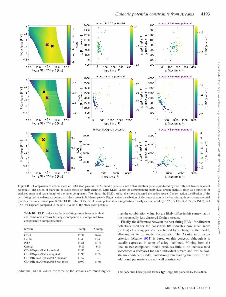
Galactic potential constraints from streams 4193
Figure B1. Comparison of action space of GD-1 (top panels), Pal 5 (middle panels), and Orphan (bottom panels) produced by two different two-componentpotentials. The action of stars are coloured based on their energies. Left: KLD1 values of corresponding individual stream analysis given as a function ofenclosed mass and scale length of the outer component. The higher the KLD1 value, the more clustered the action space. Centre: action distribution of thebest-fitting individual-stream potentials (black cross in left-hand panel). Right: action distribution of the same stream in the best-fitting three-stream potential(purple cross in left-hand panel). The KLD1 value of the purple cross potential in a single-stream analysis is reduced by 0.57 (for GD-1), 0.35 (for Pal 5), and0.52 (for Orphan) compared to the KLD1 value of the black cross potential.
Table B1. KLD1 values for the best-fitting results from individualand combined streams for single-component (1-comp) and two-component (2-comp) potentials.
Stream 1-comp 2-comp
GD-1 17.37 16.64Helmi 13.43 13.43Pal 5 14.81 13.71Orphan 9.85 9.84GD-1/Orphan/Pal 5 standard 11.83 –GD-1/Orphan/Pal 5 weighted 11.95 11.72GD-1/Helmi/Orphan/Pal 5 standard 11.57 –GD-1/Helmi/Orphan/Pal 5 weighted 10.99 11.06
individual KLD1 values for three of the streams are much higher
than the combination value, but are likely offset in this somewhat bythe intrinsically less clustered Orphan stream.
Finally, the difference between the best-fitting KLD1 for differentpotentials used for the consensus fits indicates how much more(or less) clustering per star is achieved by a change to the model,allowing us to do model comparison. The Akaike informationcriterion (Akaike 1974) is based on this concept, although it isusually expressed in terms of a log-likelihood. Moving from theone- to two-component model produces little to no increase (andsometimes a decrease) for each individual stream and for the two-stream combined model, underlining our finding that most of theadditional parameters are not well constrained.
This paper has been typeset from a TEX/LATEX file prepared by the author.
MNRAS 502, 4170–4193 (2021)
Dow
nloaded from https://academ
ic.oup.com/m
nras/article/502/3/4170/6128656 by University of G
roningen user on 12 May 2021