game theoretic analysis of a three-stage interconnected
TRANSCRIPT

Game theoretic analysis of a three-stageinterconnected forward and reverse supply chainManojit Das
IIEST Shibpur: Indian Institute of Engineering Science and TechnologyDipak Kumar Jana ( [email protected] )
Haldia Institute of Technology, Haldia https://orcid.org/0000-0003-2297-6576Shariful Alam
IIEST Shibpur: Indian Institute of Engineering Science and Technology
Research Article
Keywords: Supply chain management, Green supply chain, Green sensitive, Remanufacturing, Gametheory
Posted Date: May 4th, 2021
DOI: https://doi.org/10.21203/rs.3.rs-299551/v1
License: This work is licensed under a Creative Commons Attribution 4.0 International License. Read Full License
Game theoretic analysis of a three-stage interconnected forward
and reverse supply chain
Manojit Dasa, Dipak Kumar Janab∗, Shariful Alama
aIndian Institute of Engineering Science and Technology, Shibpur,
Howrah - 711103, West Bengal, India
Email: [email protected], [email protected] of Applied Science & Humanities, Haldia Institute of Technology, Haldia,
Purba Midnapur-721657, West Bengal, India, Email: [email protected]
Abstract: The dynamic economic scenario of today ensures that industrial and environmental
policies that contribute to greener supply chain are incorporated. This paper considers an inter-
connected three-stage forward and reverse supply chain, which provides green products to a green
conscious market. The procurement of raw materials is responsible for the first stage of the supply
chain; The second manufacturing/remanufacturing process; And the third stage of marketing the
products to the consumer. There is one supplier, one manufacturer, and one retailer in the forward
supply chain. New raw materials are used in this supply chain, and new products are manufactured
and sold. There is also a market for remanufactured products and in this market, the same retailer
also sells. There is one collector, one remanufacturer, and one retailer in the reverse supply chain.
From consumers the collector collects used products; processes and sells the remanufacturable ones
to the remanufacturer. If the raw materials supplied by the collector are not adequate to satisfy
the demand, the remanufacturer purchases the remainder from the seller. Both the manufacturer
and the remanufacturer use green manufacturing processes. Two models namely centralized model
and decentralized model are formulated. A numerical example is taken to illustrate the two model
and perform sensitivity analysis.
Keywords: Supply chain management; Green supply chain; Green sensitive; Remanufacturing;
Game theory.
1 Introduction
Now-a-day humanity is under a wonderful danger due to speedy environmental deterioration, global
warming, population density, rapid urbanization and additionally usage of environmental resources.
So, many industries are giving a great deal significance to sustainability for the sake of existing and
∗Corresponding author Email:[email protected]
1

even for future generations. There are a number of approaches reachable for sustainable improve-
ment in exercise such as green purchasing, reusing, remanufacturing, recycling, etc. [1], [2]. In
order to save resources and reduce the environmental impact, remanufacturing has become highly
essential. [3]. The Cisco company is trying to increase their remanufacturing process; In 2019 total
revenue increased by 5% compared with fiscal 2018 and they assured that the Cisco Energy Man-
agement Suite can reduce energy costs by about 35% (www.cisco.com). Therefore, the integration
of environmental and industrial strategies is now becoming extremely relevant. Although staying
competitive in the business, companies also have to implement such plans to minimize negative
impacts on the environment. However, if environmental conservation precautions are not taken
nowadays, the cost of atmospheric emissions would, throughout the near future, rise even more,
even contributing to an unlivable climate. In order to raise demand for green goods and services,
this recognition has also impacted customers. As a result, companies are focusing hard to overcome
the possible impacts of their products or services. There are many companies that introduce green-
ing practices in their supply chains, Walmart, Dell, Toyota, Honda, Nestle, Coca-Cola, etc., for
example. [4]. The above examples demonstrate that in both real life and literature, green supply
chain management (GSCM) is gaining more prominence. In multiple phases of forward and reverse
supply chain management, GSCM combines environmental consideration, such as product design,
supplier selection and partnership[5], manufacturing and remanufacturing processes, forward and
reverse logistics [6] and management of end-of-life products[7]. Even with that environmental point
of view, economic and social dimensions are often taken into account; and at various levels of supply
chain management, it seeks to combine all three aspects.[8].
The research problem throughout this paper is inspired by the examples set out already and is
derived on green procurement management, forward and reverse. This study analyzes an intercon-
nected three-stage supply chain forward as well as reverse, which delivers green products to the
market of green awareness. The procurement of raw materials is liable for the first stage of the
supply chain; The second stage of manufacturing/remanufacturing; As well as the third stage of the
marketing of products to the consumer. There is one supplier, one manufacturer, and one retailer
in the forward supply chain. New raw materials are used in this supply chain, and new goods
are manufactured and sold. There has also been a demand for remanufactured products and even
the same retailer also sells remanufactured products on this market. There is one collector, one
remanufacturer, and one retailer in the reverse supply chain. From consumers the collector stores
the products used; processes and delivers to the remanufacturer the re-manufacturable items. Even
when the raw materials provided by the collector are not adequate to satisfy the requirement, the
remanufacturer purchases the remainder from the seller. Green manufacturing techniques are used
by both the manufacturer and the remanufacturer. This paper is organized as follows
1. An interconnected green forward as well as reverse three-stage supply chain is considered.
2. The consumer demand is considered as linearly decreasing in retail price and increasing in green-
2
ing level.
3. Two models namely centralized model and decentralized model are formulated.
4. The centralized and decentralized models and their solutions are compared.
5. The response functions for the optimal solution in the both centralized and decentralized models
are plotted.
6. A numerical example is taken to illustrate the two model and perform sensitivity analysis.
2 Literature review
In this segment, we are going to review the various literature in consideration of three distinct
sources of research paper: reverse supply chain, Stackelberg game and sustainable development in
supply chain.
2.1 The literature on reverse supply chain:
Throughout the last three decades, Supply Chain Management(SCM) has gained considerable in-
terest from both corporate and academic research. Almost all of the SCM paper focuses upon on
forward movement and conversion of products from manufacturers to end users. However, there
has not been much interest in the reverse transport of resources from customers to upstream manu-
facturers. Reverse flow management is an extension to conventional supply chains of reused goods
or services that either return to or being discarded by reprocessing companies. Management of the
Reverse Supply Chain(RSCM) is identified as the proper management of the sequence of processes
needed to acquire and distribute goods from a customer or to regain value. Prahinski et al.[9] have
shown managers can enhance productivity improvements, customer support, negotiation of con-
tracts, product development, post market sales volume with after service through proper planning
of the RSC. In recent decades, significant attention has been given to product take-back, product
recycling and the re-distribution of end-of-life goods due to growing environmental concern. Re-
verse Logistics (RL), relating to the distribution operations regarding product returns have gained
significant attention and many industries use it to support their customers as a marketing weapon;
and therefore, can deliver significant revenues. Sasikumar et al.[10] have analysed the RL studies
and recommended a classification primarily based on reverse distribution issues. The outcome of
this study offers a deeper idea of RL and identifies several new approaches for advanced visualiza-
tion research. De la Fuente et al.[11] have investigated supply chain management as incorporated
in organizations that operate with forward and reverse logistics simultaneously. They have inves-
tigated the processes involved, indicating that the IMSCM (Integrated Model for Supply Chain
Management) integrated model requires new reverse logistics processes. Mokhtar et al.[12] have
analysed the role of Supply Chain Management styles in the outcome measures of suppliers rele-
vant to reverse processes. In addition, the mediating position in this relationship is explored by two
3
governance structures (i.e., trust and legal-legitimate power). This research uses structural equa-
tion modelling to interpret the result from 190 Malaysian manufacturing companies. The article
demonstrated that change and transactional leadership are relevant and constructive contributors
to the reverse higher level of performance of suppliers; trust and power initiate these interactions
dramatically. Doan et al.[13] have shown that in developing countries, product flow amounts to
reverse supply chain (RSC) facilities, and also other parameters, are uncertain and vague. In this
research a fuzzy approach to address all ambiguous parameters to help electronics enterprises set
up more powerful RSCs. In order, to make it more systematic, risk factors are implemented into
the model. Gorji et al.[14] have considered a supply chain including an end-of-life vehicles (ELV)
take-back centre, an inspection centre, and a repair centre. Three decision variables seem to be the
purchase price of the ELVs, the sales price of the repaired vehicle and the level of the reconstruction
of the vehicle. The influence of government subsidies on stability values of its choice variables of the
centres in the supply chain of the ELV was evaluated in different scenarios using the game theory
technique. Taleizadeh et al.[15] they have considered two accumulating reverse supply chains which
contains one retailer and one manufacturer. One of these chains aims to accelerate the collection
process and achieve greater market share through the use of direct and conventional networks. One
of the others only uses the conventional channel. To obtain the optimal channels rewards they
have applied three game theory structures and using numerical analysis, the outcomes of the deci-
sion variables as well as the profit function of its participants are compared throughout all three
structures.
2.2 The literature on Stackelberg game:
Dastidar et al.[16] put together all the traditional results of Stackelberg quantity games in a homo-
geneous product party system with concave demand and purely convex costs. They include some
new results with Stackelberg price games and compare the equilibrium structure of the quantity
games with the price games. Yang et al.[17] have considered the price and quantity preferences of a
two-stage system with a manufacturer who provides two successful retailers with a single commod-
ity. They have assumed a Stackelberg structure wherein the manufacturer functioning as a leader
specifies its wholesale price to every retailers and retailers operating like followers individually set
their selling prices and corresponding inventory levels under the price structure of the manufac-
turer. Almehdawe et al.[18] have constructed a model in which the inventory system is controlled
by the Stackelberg game under two scenarios. In this system the supply chain is composed of a
single manufacturer and many retailers. They implement the conventional approach in which the
manufacturer is the leader and the retailers operate as the supply chain’s dominant player. In-
clude a game-theoretical model consists of three stages Sheu et al.[19] have analysed the impact
of governmental financial interference on rivalry in sustainable development. For government and
chain member decisions, they formulated Nash equilibrium solutions. Huang et al.[20] discuss op-
4

timal closed-loop supply chain (CLSC) strategies for dual recycling streams. In the forward supply
chain, the manufacturer sells products via the retailer and in the reverse supply chain the retailer
and the third party competitively collect used products. With the approach of game theory, they
interpret the efficiency of the supply chain function of pricing decisions and recycling methods for
both decentralized and centralized channel cases. Li et al.[21] have considered a retailer’s Stack-
elberg supply chain and developed a model with the approach of game theory. By introducing a
comparatively overall market demand feature, Chaab et al.[22] analyse supply chain management
through cooperative advertising and pricing. They have discussed four potential game structures,
including the Nash, retailer Stackelberg, manufacturer Stackelberg and cooperation games.
2.3 The literature on Sustainable development:
Green supply chain management has been recognized as an important management style for re-
ducing environmental problems. Using an Interpretive Structural Modelling (ISM) system, Diabat
et al.[23] have considered a model of the drivers influencing the effectiveness of green supply chain
management. Focused on literature and consultations from the GSM with industry leaders, the
numerous generators of green supply chain management (GSCM) are described. Li et al.[24] have
considered a dual-channel supply chain in which the manufacturer produces green goods that be-
come eco-friendly. Both for centralized and decentralized scenarios, while using Stackelberg control
strategy, they have investigated the pricing and greening strategies for the chain members. In the
development of effective supply chain networks, Nagurney et al.[25] have constructed a compre-
hensive analysis and research model. They have considered a company involved in evaluating the
capacities of its various supply chain operations, i.e., the manufacturing, storage and transport of
the commodity to the locations of demand. The company is considered to have been a decision-
maker with multiple requirements who not only seeks to minimize the overall costs associated
with design/construction and service, but also to minimize the generated emissions. The reduction
of carbon emissions is a hot issue for environmental protection and the implementation of limits
is considered an appropriate way to improve the environment. Sustainable products indicate, as
per practical world standards, that the manufacturing processes encourage the impact on carbon
emissions and actually respond to consumer demand. Dong et al.[26] have studied sustainable in-
vestment in sustainable goods with awareness of pollution control for decentralized and centralized
supply chains. Within this dual supply chain with three echelons comprising one collector, one
recycler, and one manufacturer, Jafari et al.[27] have considered the waste recycling process. The
game-theoretical models are developed among the members under its different power structures.
Then, the solutions of equilibrium are derived and different leadership perspectives are identified.
They have shown that the manufacturer gets a larger advantage when the collector and recycler
have similar decision-making powers than when they make decisions with individuals who have
different powers. Making the supply chain of a greener product, Ghosh et al.[28] have formulated
5

an organized structure on the advanced payment policy of the manufacturer and the retailer’s trade
credit facility. They have proposed a model that enhances the sales effort of the retailer, the whole-
sale price required by the manufacturer, the green procurement level, and also the retailers’ selling
price.
3 Model Formulation
In this paper, We consider three-stage interconnected forward and reverse supply chain, in which
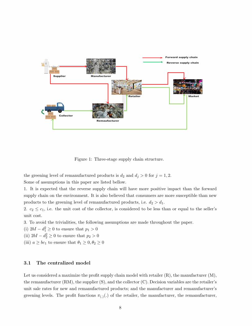
new as well as remanufactured green products are shipped to the green market. Fig. 1 represent
the three-stage interconnected forward and reverse supply chain. We have used some notation
throughout the paper which are given in the Table 1. The forward supply chain comprises one
raw material supplier, one manufacturer and one retailer. At a unit price of c1, the supplier buys
and processes new raw materials and Sells those at such unit price of s1 to the manufacturer. The
manufacturer produces new product using green manufacturing process with a greening level of θ1,
where θ1 ≥ 0. The manufacturer takes an increasing quadratic function Iθ21 as the green investment
cost, Where the green investment parameter is I and I > 0. Compared with green investment costs,
all other production costs are ignored. At such wholesale price per unit of w1, the manufacturer
sells new products to the retailer; and the retailer sells the new products to the market at a unit
price of p1.
In the reverse supply chain the retailer also sells remanufactured products to the same market. The
reverse supply chain comprises one collector, one remanufacturer and one retailer. Used products
are collected from customers by the collector and process it at a unit cost c2 and it is sold at
such a price per unit s2 to the remanufacturer. The probability to meet the demand of the raw
materials of the remanufacturer supplied by the collector is β,where 0 < β ≤ 1. If the collector is
unable to satisfy the remanufacturer’s requirement, the remanufacturer purchases the remainder
from the seller at such price per unit of s1. Then the probability of buying raw materials from seller
by the remanufacturer is 1− β. The remanufacturer produces product using green manufacturing
process with a greening level of θ2, where θ2 ≥ 0. The remanufacturer takes an increasing quadratic
function Iθ22 as the green investment cost, where I is the green investment parameter and I > 0 .
Compared with green investment costs, all other remanufacturing expenditures are ignored. At a
unit wholesale price of w2, the remanufacturer sells products to the retailer; and the retailer sells
the remanufactured products to the consumer at a unit price of p2.
The functional form of market demand is
Dj = a− bpj + djθj , j = 1, 2. (1)
where, a(> 0) is the total market potential, b(> 0) is the price sensitivity of consumer demand,The
consumer sensitivity to the greening level of new products is d1, and the consumer sensitivity to
6
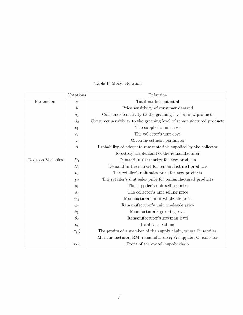
Table 1: Model Notation
Notations Definition
Parameters a Total market potential
b Price sensitivity of consumer demand
d1 Consumer sensitivity to the greening level of new products
d2 Consumer sensitivity to the greening level of remanufactured products
c1 The supplier’s unit cost
c2 The collector’s unit cost.
I Green investment parameter
β Probability of adequate raw materials supplied by the collector
to satisfy the demand of the remanufacturer
Decision Variables D1 Demand in the market for new products
D2 Demand in the market for remanufactured products
p1 The retailer’s unit sales price for new products
p2 The retailer’s unit sales price for remanufactured products
s1 The supplier’s unit selling price
s2 The collector’s unit selling price
w1 Manufacturer’s unit wholesale price
w2 Remanufacturer’s unit wholesale price
θ1 Manufacturer’s greening level
θ2 Remanufacturer’s greening level
Q Total sales volume
π(.) The profits of a member of the supply chain, where R: retailer;
M: manufacturer; RM: remanufacturer; S: supplier; C: collector
πSC Profit of the overall supply chain
7
Supplier Manufacturer
Retailer
Remaufacturer
Market
Collector
Forward supply chain
Reverse supply chain
Figure 1: Three-stage supply chain structure.
the greening level of remanufactured products is d2 and dj > 0 for j = 1, 2.
Some of assumptions in this paper are listed bellow.
1. It is expected that the reverse supply chain will have more positive impact than the forward
supply chain on the environment. It is also believed that consumers are more susceptible than new
products to the greening level of remanufactured products, i.e. d2 > d1.
2. c2 ≤ c1, i.e. the unit cost of the collector, is considered to be less than or equal to the seller’s
unit cost.
3. To avoid the trivialities, the following assumptions are made throughout the paper.
(i) 2bI − d21 ≥ 0 to ensure that p1 > 0
(ii) 2bI − d22 ≥ 0 to ensure that p2 > 0
(iii) a ≥ bc1 to ensure that θ1 ≥ 0, θ2 ≥ 0
3.1 The centralized model
Let us considered a maximize the profit supply chain model with retailer (R), the manufacturer (M),
the remanufacturer (RM), the supplier (S), and the collector (C). Decision variables are the retailer’s
unit sale rates for new and remanufactured products; and the manufacturer and remanufacturer’s
greening levels. The profit functions π(.)(.) of the retailer, the manufacturer, the remanufacturer,
8

the supplier and the collector are as follows.
πR(p1, p2) = (p1 − w1)D1 + (p2 − w2)D2 (2)
πM (θ1, w1) = (w1 − s1)D1 − Iθ21 (3)
πRM (θ2, w2) = (w2 − βs2 − (1− β)s1)D2 − Iθ22 (4)
πS(s1) = (s1 − c1)(D1 + (1− β)D2) (5)
πC(s2) = (s2 − c2)βD2 (6)
Therefore, the profit function of the overall supply chain(SC) is
πSC(p1, p2, ) = (p1 − c1)D1 + (p2 − βc2 − (1− β)c1)D2 − I(θ21 − θ22) (7)
For maximizing the profit function of the overall supply chain given in Eq.(7), the unique global
optimal solution is are as follows.
p∗1 =2aI + c1(2bI − d21)
4bI − d21(8)
p∗2 =2aI + (βc2 + (1− β)c1)(2bI − d22)
4bI − d22(9)
θ∗1 =d1(a− bc1)
4bI − d21(10)
θ∗2 =d2(a− βbc2 − (1− β)bc1)
4bI − d22(11)
The optimal values of demands for the new products and remanufactured products are as follows.
D∗1 =
2bI(a− bc1)
4bI − d21(12)
D∗2 =
2bI(a− βbc2 − (1− β)bc1)
4bI − d22(13)
The Optimal profit of the overall supply chain is given by,
π∗SC = I
[
(a− bc1)2
4bI − d21+
(a− βbc2 − (1− β)bc1)2
4bI − d22
]
(14)
Proof. See 5 Appendix A
It is easy to understand from the solution that the manufacturer’s(remanufacturer’s) greening level
and the retailer’s unit selling price for new(remanufactured) products increases, whereas customer
sensitivity to the greening level of new(remanufactured) products increases. Moreover, the demand
for new(remanufactured) products increases and the overall supply chain obtains more profit as con-
sumers become more receptive to the greening level of new(remanufactured) products. Contrarily,
if the price sensitivity of consumer demand and the green investment parameter increase, then the
9

retailer’s unit selling price for new(remanufactured) products, the demands of both products, the
manufacturer’s(remanufacturer’s) greening level and the overall supply chain profit decrease. It
turns out that the remanufacturer decides a higher greening level as the sufficiency of the collector
to satisfy the demand of the remanufacturer rises, and the retailer sells the remanufactured goods
at a lower price. Thus, the demands of the remanufactured products increases and the overall
supply chain obtains more profit.
3.2 The decentralized model
Each supply chain member tries to maximize their own profit in the decentralized model. Eqs. (2)
- (6) are the profit functions of the retailer, the manufacturer, the remanufacturer, the supplier and
the collector respectively. Considering game theoretical approach, In the first stage, the supplier
and the collector determine at the same time on the selling prices of their unit to the manufacturer
and the remanufacturer, i.e., with the expectation of manufacturer’s and remanufacturer’s actions
the supplier determine s1 and collector determine s2. In the second step, with the expectation of
retailer’s actions the manufacturer and the remanufacturer determine their unit wholesale prices
and greening levels simultaneously. The manufacturer and the remanufacturer decide their greening
levels and unit wholesale prices θ1,θ2 and w1,w2 respectively. The retailer determines its unit sale
prices for new products and remanufactured products p1 and p2 respectively in the final step.
Using backward induction method we have solved this model.After computing hessian matrix we
get, retailer profit function as specified in Eq.(2) is strictly concave. We get the best retailer
response functions by using first order conditions with respect to p1 and p2 simultaneously.
pd1(θ1, w1) =a+ d1θ1 + bw1
2b(15)
pd2(θ2, w2) =a+ d2θ2 + bw2
2b(16)
where superscript stands for the decentralised case.
Then we substitute this values into the manufacturer’s and the remanufacturer’s profit functions
given in Eqs. (3) and (4), respectively.
By computing hessian matrix we get, manufacturer’s profit function is strictly concave. Using first
order conditions with respect to θ1 and w1 simultaneously we get the best response functions of
the manufacturer as follows
θd1(s1) =d1(a− bs1)
8bI − d21(17)
wd1(s1) =4aI + s1(4bI − d21)
8bI − d21(18)
Similarly, remanufacturer’s profit function is strictly concave. Using first order conditions with
respect to θ2 and w2 simultaneously we get the best response functions of the remanufacturer as
10

follows
θd2(s1, s2) =d2(a− βbs2 − (1− β)bs1)
8bI − d22(19)
wd2(s1, s2) =4aI + (βs2 + (1− β)s1)(4bI − d22)
8bI − d22(20)
In the final step we put the Eqs.(15) - (20) into the seller’s profit function given in Eq.(5) and
Eqs.(16),(19),(20) into the collector’s profit function given in Eq.(6).
Similarly, we get seller’s and collector’s profit functions are concave. Using first order condition
with respect to s1 of Eq.(5) and first order condition with respect to s2 of Eq.(6) simultaneously
we get.
sd1 =2(8bI − d22)(a+ bc1) + (8bI − d21)(1− β)(a− βbc2 + 2(1− β)bc1)
b(4(8bI − d22) + 3(8bI − d21)(1− β)2)(21)
sd2 =
a+ βbc2 − (1− β)
[
2(8bI−d22)(a+bc1)+(8bI−d21)(1−β)(a−βbc2+2(1−β)bc1)
4(8bI−d22)+3(8bI−d21)(1−β)2
]
2βb(22)
For the retailer, the manufacturer, the remanufacturer, the seller and the collector, the unique
global optimal solutions for decentralized models are as follows. The supplier and collector decide
sd1 and sd2 according Eqs.(20) and (21). After that the manufacturer determines θd1(s1) and wd1(s1)
and the remanufacturer determines θd2(s1, s2) and wd2(s1, s2) according to Eqs.(17) - (20). In the
end retailer decides pd1(θ1, w1) and pd2(θ2, w2) according to Eqs.(15) and (16). The optimal values
of demands for the new products and remanufactured products as follows.
Dd1 =
2bI(a− bsd1)
8bI − d21(23)
Dd2 =
2bI(a− b(βsd2 + (1− β)sd1))
8bI − d22(24)
The optimal profit of the overall supply chain is
πdSC = I
[
(a− bs1)ψ1
(8bI − d21)2+
(a− βbs2 − (1− β)bs1)ψ2
(8bI − d22)2
]
(25)
where,
ψ1 = a(12bI − d21)− 2bc1(8bI − d21) + b(4bI − d21)s1
ψ2 = a(12bI − d22)− 2bc1(8bI − d22)(1− β) + b((4bI − d22)(s1(1− β)− (2c2 − s2)β))− 8b2Iβc2
Proof. See 5Appendix B
In the forward supply chain it can be noticed that c1 ≤ sd1 ≤ wd1 ≤ pd1. In a similar way in the
reverse supply chain cd2 ≤ sd2 and βsd2+(1−β)sd1 ≤ wd2 ≤ pd2,Where βsd2+(1−β)sd1 is the purchasing
price of the remanufacturer.
11
3.3 Comparison between the solutions of the centralized model and decentral-
ized model
After obtaining centralized and decentralized solutions, comparing it gives the following observa-
tions:
1. The manufacturer’s greening level in the centralized solution is greater than or
equal to the greening level in the decentralized solution, i.e. θ∗1≥ θd
1
Proof: c1 ≤ sd1 =⇒ a− bc1 ≥ a− bsd1 (Since b > 0)
Since, 4bI − d21 < 8bI − d21 and d1 > 0
Therefore, d1(a−bc1)4bI−d21
≥d1(a−bsd1)
8bI−d21i.e. θ∗1 ≥ θd1
2. The remanufacturer’s greening level in the centralized solution is greater than or
equal to the greening level in the decentralized solution, i.e. θ∗2≥ θd
2
Proof: c1 ≤ sd1 and c2 ≤ sd2 =⇒ a− βbc2 − (1− β)bc1 ≥ a− βbsd2 − (1− β)bsd1(Since b > 0)
Since, 4bI − d22 < 8bI − d22 and d2 > 0
Therefore, d2{a−bc1(1−β)−bc2β}4bI−d22
≥d2{a−bsd1(1−β)−bs
d2β}
8bI−d22i.e. θ∗2 ≥ θd2
3. The unit selling price in the decentralized solution for the retailer’s new products is
greater than or equal to the unit selling price in the centralized solution, i.e. pd1≥ p∗
1
Proof: p∗1 =2aI+c1(2bI−d21)
4bI−d21
pd1 =a+d1θd1+bw
d1
2b where, θd1 =d1(a−bsd1)
8bI−d21and wd1 =
4aI+sd1(4bI−d21)
8bI−d21
Therefore, pd1 =a+d1
d1(a−bsd1)
8bI−d21+b
4aI+sd1(4bI−d21)
8bI−d212b =
6aI+sd1(2bI−d21)
8bI−d21
Now, pd1 − p∗1 =6aI+sd1(2bI−d
21)
8bI−d21−
2aI+c1(2bI−d21)
4bI−d21=
(2bI−d21)[4I(a−bc1)+(sd1−c1)(4bI−d21)]
(8bI−d21)(4bI−d21)
As 2bI − d21 ≥ 0, a ≥ bc1 and sd1 ≥ c1
Therefore,pd1 − p∗1 ≥ 0, i.e. pd1 ≥ p∗1
4. The unit selling price in the decentralized solution for the retailer’s remanufactured
products is greater than or equal to the unit selling price in the centralized solution,
i.e. pd2≥ p∗
2
Proof: p∗2 =2aI+(βc2+(1−β)c1)(2bI−d22)
4bI−d22
pd2 = a+d2θ2+bw22b where, θd2 =
d2(a−βbsd2−(1−β)bsd1)
8bI−d22and wd2 =
4aI+(βsd2+(1−β)sd1)(4bI−d22)
8bI−d22
Therefore, pd2 =a+d2
d2(a−βbsd2−(1−β)bsd1)
8bI−d22+b
4aI+(βsd2+(1−β)sd1)(4bI−d22)
8bI−d222b =
6aI+(βsd2+(1−β)sd1)(2bI−d22)
8bI−d22
Now,pd2 − p∗2 =6aI+(βsd2+(1−β)sd1)(2bI−d
22)
8bI−d22−
2aI+(βc2+(1−β)c1)(2bI−d22)
4bI−d22
=(2bI−d22)[4I((a−bc1)+bβ(c1−c2))+(β(sd2−c2)+(1−β)(sd1−c1))(4bI−d
22)]
(8bI−d22)(4bI−d22)
As 2bI − d22 ≥ 0, a ≥ bc1, c≥c2, sd2 ≥ c2 and sd1 ≥ c1
Therefore, pd2 − p∗2 ≥ 0 i.e. pd2 ≥ p∗2
5. In the centralized solution, the demand for new products is greater than or equal
to the demand for a decentralized solution, i.e.D∗1≥ Dd
1
12

Proof: c1 ≤ sd1 =⇒ a− bc1 ≥ a− bsd1 (Since b > 0)
Since 4bI − d21 < 8bI − d21 , b > 0, I > 0
Therefore,2bI(a−bc1)4bI−d21
≥2bI(a−bsd1)
8bI−d21, i.e.D∗
1 ≥ Dd1
6. In the centralized solution, the demand for remanufactured products is greater than
or equal to the demand for a decentralized solution, i.e.D∗2≥ Dd
2
Proof:D∗2 = 2bI(a−βbc2−(1−β)bc1)
4bI−d22and Dd
2 =2bI(a−βbsd2−(1−β)bsd1))
8bI−d22
Now, D∗2 −Dd
2 = 2bI(a−βbc2−(1−β)bc1)4bI−d22
−2bI(a−βbsd2−(1−β)bsd1))
8bI−d22
=2b2I[4I((a−bc1)+bβ(c1−c2))+(β(sd2−c2)+(1−β)(sd1−c1))(4bI−d
22)]
(8bI−d22)(4bI−d22)
As 2bI − d22 ≥ 0, a ≥ bc1, c≥c2, sd2 ≥ c2 and sd1 ≥ c1
Therefore, D∗2 −Dd
2 ≥ 0, i.e. D∗2 ≥ Dd
2
7. In the centralized solution, the profit of the overall supply chain is greater than or
equal to the profit in the decentralized solution, i.e. π∗SC
≥ πdSC
Proof:π∗SC = I
[
(a−bc1)2
4bI−d21+ (a−βbc2−(1−β)bc1)2
4bI−d22
]
πdSC = I
[
(a−bs1)ψ1
(8bI−d21)2 + (a−βbs2−(1−β)bs1)ψ2
(8bI−d22)2
]
Where, ψ1 = a(12bI − d21)− 2bc1(8bI − d21) + b(4bI − d21)s1
ψ2 = a(12bI − d22)− 2bc1(8bI − d22)(1− β) + b((4bI − d22)(s1(1− β)− (2c2 − s2)β))− 8b2Iβc2
Now, π∗SC − πdSC = I
[
(a−bc1)2
4bI−d21+ (a−βbc2−(1−β)bc1)2
4bI−d22
]
−
I
[
(a−bs1)(a(12bI−d21)−2bc1(8bI−d21)+b(4bI−d21)s1)
(8bI−d21)2 +
(a−βbs2−(1−β)bs1)(a(12bI−d22)−2bc1(8bI−d22)(1−β)+b((4bI−d22)(s1(1−β)−(2c2−s2)β))−8b2Iβc2)
(8bI−d22)2
]
=−(a−bc1)2d21I
(4bI−d21)2 +
2b(a−bc1)I
(
−c1+c1d
21−2aI−2bc1I
d21−4bI
)
4bI−d21+d21I(a−bs1)
2
(d21−8bI)2−
2bI(a−bs1)
(
−c1+(a−
d12(a−bs1)
d12−8bi+
b(4ai−d12s1+4bis1)
−d12+8bi2b
)
8bI−d21−
I(ad2−bc1d2+bc1d2β−bc2d2β)2
(−d22+4bI)2+d22I(a−bs1+bs1β−bs2β)
2
(d22−8bI)2+
2bI(a+bc1(−1+β)−bc2β)
(
−c1(1−β)−c2β+−2aI−c1(d
22−2bI)(−1+β)+c2(d22−2bI)β
d22−4bI
)
(4bI−d22)
−
2bI(a−b(s1(1−β)+s2β))
(
−c1(1−β)−c2β+
a−d22(a−bs1+bs1β−bs2β)
d22−8bI+
b(4aI−d22s1+4bIs1+d22s1β−4bIs1β−d22s2β+4bIs2β)
8bI−d222b
)
8bI−d22
= I
[
−(a−bc1)2d21(d21−4bI)2
+4b(a−bc1)2I)(d21−4bI)2
+d21(a−bs1)
2
(d21−8bI)2+
2b(−a+bs1)(6aI+c1(d21−8bI)−d21s1+2bIs1)
(d21−8bI)2−d22(a+bc1(−1+β)−bc2β)2
(d22−4bI)2+
4bI(a+bc1(−1+β)−bc2β)2
(d22−4bI)2+
d22(a+bs1(−1+β)−bs2β)2
(d22−8bI)2+
2b(a+bs1(−1+β)−bs2β)(−6aI+d22s1−2bIs1+c1(d22−8bI)(−1+β)−c2d22β+8bc2Iβ−d22s1β+2bIs1β+d22s2β−2bIs2β))
(d22−8bI)2
]
= I
[
{−(a−bc1)2d21(d21−4bI)2
+4b(a−bc1)2I)(d21−4bI)2
}+{d21(a−bs1)
2
(d21−8bI)2+
(2b(−a+bs1)(6aI+c1(d21−8bI)−d21s1+2bIs1))
(d21−8bI)2}+{−
d22(a+bc1(−1+β)−bc2β)2
(d22−4bI)2+
4bI(a+bc1(−1+β)−bc2β)2
(d22−4bI)2}+ {
d22(a+bs1(−1+β)−bs2β)2
(d22−8bI)2+
13

(2b(a+bs1(−1+β)−bs2β)(−6aI+d22s1−2bIs1+c1(d22−8bI)(−1+β)−c2d22β+8bc2Iβ−d22s1β+2bIs1β+d22s2β−2bIs2β))
(d22−8bI)2}
]
= I
[
(a−bc1)2
4bI−d21+
(a−bs1){a(d21−12bI)−2bc1(d21−8bI)+b(d21−4bI)s1}
(d21−8bI)2− (a+bc1(−1+β)−bc2β)2
d22−4bI−
{a+bs1(−1+β)−bs2β}[−a(d22−12bI)+b{−2c1(d22−8bI)(−1+β)+d22(−s1+2c2β+s1β−s2β)+4bI(s1−4c2β−s1β+s2β)}]
(d22−8bI)2
]
= I
[
b2{4aI+c1(d21−8bI)−d21s1+4bIs1}2
(8bI−d21)2(4bI−d21)
+b2{−4aI+d22s1−4bIs1+c1(d22−8bI)(−1+β)−c2d22β+8bc2Iβ−d22s1β+4bIs1β+d22s2β−4bIs2β}2
(8bI−d22)2(4bI−d22)
]
Since, 4bI − d21 > 0 and 4bI − d22 > 0
Threfore, π∗SC − πdSC ≥ 0, i.e. π∗SC ≥ πdSC
Figure 2: Profit of the overall supply chain(SC)
in the centralized model and decentralized model.
Figure 3: Profit of the overall supply chain(SC)
in the centralized model and decentralized model.
Figure 4: Profit of the overall supply chain(SC)
in the centralized model and decentralized model.
Figure 5: Profit of the overall supply chain(SC)
in the centralized model and decentralized model.
14

Figure 6: Greening level of the manufacturer and
remanufacturer in the centralized and decentral-
ized model.
Figure 7: Greening level of the manufacturer in
the centralized and decentralized model.
Figure 8: Greening level of the remanufacturer in
the centralized and decentralized model.
Figure 9: Greening level of the manufacturer and
remanufacturer in the decentralized model.
4 Results and discussion
In order to understand the outcomes, this section provides a numerical analysis. Sensitivity analysis
is carried out for the profit functions of the members of the green supply chain, greening level of
the product, unit selling price and market demand. The initial parameters are adjusted as follows:
a = 200, b = 2.5, c1 = 10, c2 = 8, I = 40, β = 0.90, d1 = 2 and d2 = 3. The values of the initial
parameters are changed for sensitivity analysis in such a way that all the assumptions are fulfilled
in the paper. Table 2 represents the change in the level of greening and retailer selling prices
w.r.t. % change of a, b, c1, c2, I and β. Table 3 represents the change of greening levels and retailer
selling prices w.r.t. % change of d1 and d2. The change of unit selling prices of manufacturer,
remanufacturer, seller, collector and market demand for both new and remanufactured products
w.r.t. % change of a, b, c1, c2, I and β are presented in Table 4. In Table 5, the change of unit
15

Figure 10: Greening level of remanufacturer in
the centralized and decentralized model.
Figure 11: Unit selling price of the retailer for
new products in the centralized and decentralized
model.
Figure 12: Unit selling price of the retailer for
remanufactured products in the centralized and
decentralized model.
Figure 13: Unit selling price of the retailer for
remanufactured products in the centralized and
decentralized model.
selling prices of manufacturer, remanufacturer, seller, collector and market demand for both new
and remanufactured products w.r.t. % change of d1 and d2 are presented. The change of different
profit functions w.r.t. % change of a, b, c1, c2, I and β are presented in Table 6. In Table 7, the
change of different profit functions w.r.t. % change of d1 and d2 are presented. It’s in Fig. 2,3,4,5;
we investigate the influence of consumer sensitivity on the level of greening of new(remanufactured)
products, the green investment parameter and the probability that the collector meets the demand
of the remanufacturer for the profit of the overall supply chain. The findings indicate that, in cen-
tralized as well as decentralized models, overall profit increases as customers become more sensitive
to greening levels, Overall profit increases as the probability that the collector will meet the demand
of the remanufacturer increases, overall profit decreases as green investment wages increase. The
importance of increasing profits for the centralized system seem to be effective and the supply chain
16
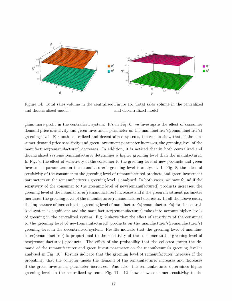
Figure 14: Total sales volume in the centralized
and decentralized model.
Figure 15: Total sales volume in the centralized
and decentralized model.
gains more profit in the centralized system. It’s in Fig. 6, we investigate the effect of consumer
demand price sensitivity and green investment parameter on the manufacturer’s(remanufacturer’s)
greening level. For both centralized and decentralized systems, the results show that, if the con-
sumer demand price sensitivity and green investment parameter increases, the greening level of the
manufacturer(remanufacturer) decreases. In addition, it is noticed that in both centralized and
decentralized systems remanufacturer determines a higher greening level than the manufacturer.
In Fig. 7, the effect of sensitivity of the consumer to the greening level of new products and green
investment parameters on the manufacturer’s greening level is analysed. In Fig. 8, the effect of
sensitivity of the consumer to the greening level of remanufactured products and green investment
parameters on the remanufacturer’s greening level is analysed. In both cases, we have found if the
sensitivity of the consumer to the greening level of new(remanufactured) products increases, the
greening level of the manufacturer(remanufacturer) increases and if the green investment parameter
increases, the greening level of the manufacturer(remanufacturer) decreases. In all the above cases,
the importance of increasing the greening level of manufacturer’s(remanufacturer’s) for the central-
ized system is significant and the manufacturer(remanufacturer) takes into account higher levels
of greening in the centralized system. Fig. 9 shows that the effect of sensitivity of the consumer
to the greening level of new(remanufactured) products on the manufacturer’s(remanufacturer’s)
greening level in the decentralised system. Results indicate that the greening level of manufac-
turer(remanufacturer) is proportional to the sensitivity of the consumer to the greening level of
new(remanufactured) products. The effect of the probability that the collector meets the de-
mand of the remanufacturer and green invest parameter on the manufacturer’s greening level is
analysed in Fig. 10. Results indicate that the greening level of remanufacturer increases if the
probability that the collector meets the demand of the remanufacturer increases and decreases
if the green investment parameter increases. And also, the remanufacturer determines higher
greening levels in the centralized system. Fig. 11 - 12 shows how consumer sensitivity to the
17
greening of new(remanufactured) products and green investment parameters impact the retailer’s
unit selling price for new(remanufactured) products. It seems that when customers are much
more sensitive to the greening of new(remanufactured) products, the retailer’s unit selling price
for new(remanufactured) products rises. And as a result of rising green investment parameter the
retailer’s unit selling price for new(remanufactured) products increases. Fig. 13 shows how the
probability that the collector meets the demand of the remanufacturer and green investment pa-
rameter impact the retailer’s unit selling price for new(remanufactured) products. The analysis
showed that if the probability of the collector meeting the demand of the remanufacturer increases,
the retailer can set a lower unit selling price for remanufactured products. In all the above cases,
the retailer’s unit selling price for new(remanufactured) products is relatively low in the centralized
system. In Fig. 14 we investigate the influence of consumer sensitivity on the level of greening of
new(remanufactured) products to the total sales volume of the supply chain. Results indicate that
the total sales volume of the supply chain is proportional to the sensitivity of the consumer to the
greening level of new(remanufactured) products. Fig. 15 shows how the probability of the collector
meeting the demand of the remanufacturer and green investment parameter impact the total sales
volume of the supply chain. The analysis revealed that if the possibility of the collector to fulfill
the needs of the remanufacturer increases, then the total supply chain sales volume increases, and
if the green investment parameter increases, the total supply chain sales volume decreases. In both
cases, the sales volume is relatively high in the centralized system.
5 Conclusions
We consider three-stage interconnected forward and reverse supply chains, in which new as well as
remanufactured green products are shipped to the green market. The manufacturer and the re-
manufacturer both invest and decide their greening levels in green manufacturing processes. Each
supply chain member tries to maximize their own profit in the decentralized model and lower green-
ing levels are decided by both the manufacturer and the remanufacturer than the optimum solution,
i.e., the centralized solution. Therefore, the demands for the both products are lower than that of
the optimal demands, and less profit is obtained by the supply chain than the optimum. The pro-
duction of eco-friendly products or services is becoming ever more relevant because of deteriorating
environmental conditions. The customer is also being impacted by such a consciousness. On the
other hand, for eco-friendly products, green-conscious customers have to pay higher. Therefore,
governments should offer certain incentives to green companies to lower selling prices to increase
demand for green products and for a sustainable environment. From this viewpoint, when the
results in this study are evaluated, it can be shown that as customers become more sensitive to
the greening levels of new and remanufactured products, their greening levels are increased by the
manufacturer and the remanufacturer; the demands for both kinds of green products are therefore
going to increase; and the overall supply chain receives more gain. As demand rises, more green
18

Table 2: Change of greening levels and retailer selling prices w.r.t. % change of a, b, · · ·
Para. % θ1 θ2 p1 p2
C D C D C D C D
-20 1.13043 0.255732 1.75318 0.377122 39.1304 58.3739 38.8544 58.591
-10 1.30435 0.295334 2.00726 0.431436 43.3043 65.5026 43.2102 65.812
a 0 1.47826 0.334937 2.26134 0.485749 47.4783 72.6314 47.5659 73.033
10 1.65217 0.37454 2.51543 0.540062 51.6522 79.7601 51.9216 80.254
20 1.82609 0.414143 2.76951 0.594376 55.8261 86.8889 56.2773 87.475
-20 2.51811 0.563935 3.8849 0.810599 72.4345 113.228 75.3982 114.65
-10 2.19165 0.492712 3.36585 0.708655 64.5595 100.655 66.5003 101.719
b 0 1.47826 0.334937 2.26134 0.485749 47.4783 72.6314 47.5659 73.033
10 1.31496 0.298403 2.01408 0.434697 43.5591 66.1082 43.327 66.3818
20 1.17986 0.268057 1.81103 0.392453 40.3165 60.6801 39.8462 60.8546
-20 1.53043 0.34783 2.27659 0.487592 46.3304 72.3478 47.3472 73.0065
-10 1.50435 0.341383 2.26897 0.48667 46.9043 72.4896 47.4566 73.0198
c1 0 1.47826 0.334937 2.26134 0.485749 47.4783 72.6314 47.5659 73.033
10 1.45217 0.328491 2.25372 0.484828 48.0522 72.7732 47.6752 73.0462
20 1.42609 0.322045 2.2461 0.483906 48.6261 72.915 47.7845 73.0594
-20 1.47826 0.334263 2.302 0.495383 47.4783 72.6462 46.9828 72.8948
-10 1.47826 0.3346 2.28167 0.490566 47.4783 72.6388 47.2743 72.9639
c2 0 1.47826 0.334937 2.26134 0.485749 47.4783 72.6314 47.5659 73.033
10 1.47826 0.335274 2.24102 0.480932 47.4783 72.624 47.8574 73.1021
20 1.47826 0.335612 2.22069 0.476115 47.4783 72.6165 48.149 73.1712
-20 1.86813 0.420735 2.89095 0.613693 47.8681 72.7634 48.4473 73.302
-10 1.65049 0.372965 2.53768 0.542276 47.6505 72.6899 47.9527 73.1518
I 0 1.47826 0.334937 2.26134 0.485749 47.4783 72.6314 47.5659 73.033
10 1.33858 0.303946 2.03928 0.439894 47.3386 72.5837 47.255 72.9366
20 1.22302 0.278204 1.85693 0.40195 47.223 72.5441 46.9997 72.8568
-20 1.47826 0.331612 2.24102 0.435613 47.4783 72.7045 47.8574 73.7521
-10 1.47826 0.331352 2.25118 0.460391 47.4783 72.7103 47.7117 73.3967
β 0 1.47826 0.334937 2.26134 0.485749 47.4783 72.6314 47.5659 73.033
10 1.47826 0.342599 2.27151 0.511047 47.4783 72.4628 47.4201 72.6701
20 1.47826 0.354352 2.28167 0.535585 47.4783 72.2042 47.2743 72.3182
19

Table 3: Change of greening levels and retailer selling prices w.r.t. % change of d1, d2Para. % θ1 θ2 p1 p2
C D C D C D C D
-20 1.16438 0.265755 2.26134 0.485721 46.9315 72.4526 47.5659 73.0334
-10 1.31953 0.300136 2.26134 0.485734 47.1876 72.5366 47.5659 73.0332
d1 0 1.47826 0.334937 2.26134 0.485749 47.4783 72.6314 47.5659 73.033
10 1.64107 0.370213 2.26134 0.485766 47.8052 72.7371 47.5659 73.0327
20 1.80851 0.406017 2.26134 0.485784 48.1702 72.8541 47.5659 73.0325
-20 1.47826 0.335329 1.75295 0.382778 47.4783 72.6228 46.3633 72.655
-10 1.47826 0.335146 2.00139 0.433693 47.4783 72.6268 46.9218 72.8321
d2 0 1.47826 0.334937 2.26134 0.485749 47.4783 72.6314 47.5659 73.033
10 1.47826 0.334703 2.53482 0.539107 47.4783 72.6365 48.3036 73.2588
20 1.47826 0.334442 2.82412 0.593939 47.4783 72.6423 49.1445 73.5108
products are sold, which already enhances the collector’s ability to purchase used products from
the market. The remanufacturer decides a higher greening standard while the collector’s sufficiency
increases. The demand for remanufactured products and the overall profit of the supply chain are
therefore going to increase. As a result, the sustainable green approach throughout the supply
chain provokes others to and it also contributes to a greener and more sustainable and therefore
more financial gains. As a result, the supply chain has been both economically and ecologically able
to succeed. Within different game systems, such as Stackelberg games with various representatives,
this supply chain can be analysed. Some of the important future research recommendations in this
field also will be to consider stochastic demand functions.
20

Table 4: Change of unit selling prices and market demand w.r.t. % change of a, b, · · ·
Para. % w1 w2 s1 s2 D1 D2
C D C D C D C D C D C D
-20 52.2363 52.126 39.9612 39.0048 67.8261 15.3439 75.1361 16.1624
-10 58.4146 58.4159 44.2386 43.4702 78.26.9 17.7201 86.0254 18.4901
a 0 64.5929 64.7058 48.5159 47.9355 88.6957 20.0962 96.9147 20.8178
10 70.7712 70.9958 52.7933 52.4008 99.1304 22.4724 107.804 23.1455
20 76.9494 77.2857 57.0706 56.8662 109.565 24.8486 118.693 25.4732
-20 99.6934 100.754 72.6245 73.0469 96.6953 21.6551 106.557 22.2336
-10 88.8296 89.5702 65.1794 65.297 94.6791 21.2852 103.86 21.8671
b 0 64.5929 64.7058 48.5159 47.9355 88.6957 20.0962 96.9147 20.8178
10 58.9465 58.9299 44.6232 43.8766 86.7874 19.6946 94.9493 20.4929
20 54.2467 54.1269 41.38 40.4942 84.9496 19.3001 93.1386 20.1833
-20 63.9998 64.6478 47.304 48.087 91.8261 20.8698 97.5681 20.8968
-10 64.2964 64.6768 47.91 48.0113 90.2609 20.483 97.2414 20.8573
c1 0 64.5929 64.7058 48.5159 47.9355 88.6957 20.0962 96.9147 20.8178
10 64.8894 64.7349 49.1219 47.8598 87.1304 19.7095 96.588 20.7783
20 65.1859 64.7639 49.7278 47.784 85.5652 19.3227 96.2613 20.7388
-20 64.6239 64.4025 48.5793 47.1276 88.6957 20.0558 98.657 21.2307
-10 64.6084 64.5542 48.5476 47.5315 88.6957 20.076 97.7858 21.0243
c2 0 64.5929 64.7058 48.5159 47.9355 88.6957 20.0962 96.9147 20.8178
10 64.5774 64.8575 48.4842 48.3395 88.6957 20.1165 96.0436 20.6114
20 64.5619 65.0092 48.4525 48.7434 88.6957 20.1367 95.1724 20.4049
-20 64.6853 64.8856 48.529 47.9339 89.6703 20.1953 99.1183 21.0409
-10 64.6338 64.7853 48.5217 47.9348 89.1262 20.1401 97.8819 20.9164
I 0 64.5929 64.7058 48.5159 47.9355 88.6957 20.0962 96.9147 20.8178
10 64.5595 64.6414 48.5112 47.9361 88.3465 20.0604 96.1375 20.7379
20 64.5319 64.5881 48.5073 47.9366 88.0576 20.0307 95.4993 20.6717
-20 64.7458 66.2844 48.8284 52.767 88.6957 19.8967 96.0436 18.6691
-10 64.7578 65.5043 48.8529 50.0564 88.6957 19.8811 96.4791 19.7311
β 0 64.5929 64.7058 48.5159 47.9355 88.6957 20.0962 96.9147 20.8178
10 64.2404 63.9093 47.7957 46.1957 88.6957 20.5559 97.3503 21.902
20 63.6998 63.1367 46.6909 44.6939 88.6957 21.2611 97.7858 22.9536
21

Table 5: Change of unit selling prices and market demand w.r.t. % change of d1, d2Para. % w1 w2 s1 s2 D1 D2
C D C D C D C D C D C D
-20 64.4799 64.7067 48.5346 47.9332 87.3288 19.9316 96.9147 20.8166
-10 64.533 64.7063 48.5258 47.9343 87.969 20.009 96.9147 20.8172
d1 0 64.5929 64.7058 48.5159 47.9355 88.6957 20.0962 96.9147 20.8178
10 64.6597 64.7053 48.505 47.9369 89.5129 20.1934 96.9147 20.8185
20 64.7337 64.7047 48.4931 47.9384 90.42555 20.3009 96.9147 20.8193
-20 64.5749 64.4527 48.479 47.9401 88.6957 20.1198 93.9083 20.5059
-10 64.5833 64.5713 48.4963 47.938 88.6957 20.1087 95.3044 20.652
d2 0 64.5929 64.7058 48.5159 47.9355 88.6957 20.0962 96.9147 20.8178
10 64.6037 64.8571 48.5379 47.9328 88.6957 20.0822 98.759 21.0042
20 64.6157 65.0259 48.5625 47.9297 88.6957 20.0665 100.861 21.2121
Appendix A:
The Hessian matrix of the objective function πSC(p1, p2, θ1, θ2) of the centralized model given in
Eq.(7) is calculated as
H(p1, p2, θ1, θ2) =
∂2πSC
∂p21
∂2πSC
∂p1∂p2
∂2πSC
∂p1∂θ1
∂2πSC
∂p1∂θ2∂2πSC
∂p2∂p1
∂2πSC
∂p22
∂2πSC
∂p2∂θ1
∂2πSC
∂p2∂θ2∂2πSC
∂θ1∂p1
∂2πSC
∂θ1∂p2
∂2πSC
∂θ21
∂2πSC
∂θ1∂θ2∂2πSC
∂θ2∂p1
∂2πSC
∂θ2∂p2
∂2πSC
∂θ2∂θ1
∂2πSC
∂θ22
=
−2b 0 d1 0
0 −2b 0 d2
d1 0 −2I 0
0 d2 0 −2I
The leading principal minors ∆k of H(p1, p2, θ1, θ2) of order k are given by
∆1 = −2b,∆2 = 4b2,∆3 = −2b(4bI − d21),∆4 = (4bI − d21)(4bI − d22)
From Assumptions 3(i) and 3(ii) we get , 4bI − d21 > 0 and 4bI − d22 > 0. Therefore, (−1)k∆k > 0
for all leading principle minors of H(p1, p2, θ1, θ2). Thus, H(p1, p2, θ1, θ2) is negative definite and
πSC(p1, p2, θ1, θ2) is strictly concave. Using the first order conditions of Eq.(7) simultaneously, we
get the unique global optimal solution to the centralized model as given in Eqs.(8) - (11). Putting
the Eqs.(7) - (10) into Eq.(1), we get the optimal values of demands for the new and remanufac-
tured products as given in Eqs.(12) - (13). Finally. putting the Eqs.(8) - (10) into Eq.(7) we get
the optimal profit of the overall supply chain as given in Eq.(14).
Appendix B:
In decentralized model, first we consider retailer’s profit function. The Hessian matrix of the ob-
jective function πR(p1, p2) given in Eq.(2) is calculated as
22

Table 6: Change of different profit functions w.r.t. % change of a, b, · · ·
Para. % πSC πR πM πRM πS πC
C D C D C D C D C D C D
-20 3837.24 1503.84 198.663 184.424 200.445 519.418 400.89
-10 5066.23 1985.83 262.354 245.967 262.339 690.488 524.678
a 0 6465.82 2534.76 334.896 316.356 332.548 885.868 665.096
10 8035.99 3150.65 416.29 395.59 411.072 1105.56 822.145
20 9776.77 3833.5 506.535 483.67 497.912 1349.56 995.824
-20 11654.3 4487.03 602.047 567.099 578.49 1582.41 1156.98
-10 10004.9 3874.19 517.348 488.832 501.167 1364.51 1002.33
b 0 6465.82 2534.76 334.896 316.356 332.548 885.868 665.096
10 5670.1 2228.97 293.758 276.749 294.086 776.208 588.173
20 5016.77 1976.61 259.953 244.018 262.336 685.633 524.671
-20 6729.12 2639.75 348.889 341.179 335.076 944.453 670.151
-10 6596.49 2586.84 341.832 328.65 333.811 914.926 667.621
c1 0 6465.82 2534.76 334.896 316.356 332.548 885.868 665.096
10 6337.1 2483.52 328.081 304.296 331.288 857.279 662.576
20 6210.34 2433.11 321.386 292.47 330.03 829.159 660.06
-20 6590.98 2582.83 341.191 315.083 345.87 888.947 691.741
-10 6528.12 2558.68 338.026 315.719 339.176 887.407 678.353
c2 0 6465.82 2534.76 334.896 316.356 332.548 885.868 665.096
10 6404.07 2511.08 331.8 316.993 325.985 884.331 651.97
20 6342.88 2487.63 328.739 317.631 319.487 882.795 638.975
-20 6577.4 2557.74 340.227 317.782 336.098 891.435 672.196
-10 6514.89 2544.92 337.248 316.988 334.116 888.333 668.233
I 0 6465.82 2534.76 334.896 316.356 332.548 885.868 665.096
10 6426.27 2526.52 332.992 315.839 331.276 883.863 662.552
20 6393.73 2519.7 331.419 315.41 330.223 882.2 660.446
-20 6404.07 2390.49 297.766 310.106 267.443 980.286 534.887
-10 6434.87 2455.93 313.829 309.619 298.734 936.278 597.468
β 0 6465.82 2534.76 334.896 316.356 332.548 885.868 665.096
10 6496.9 2626.05 360.898 330.995 368.088 829.894 736.175
20 6528.12 2727.93 391.562 354.095 404.285 769.419 808.569
23
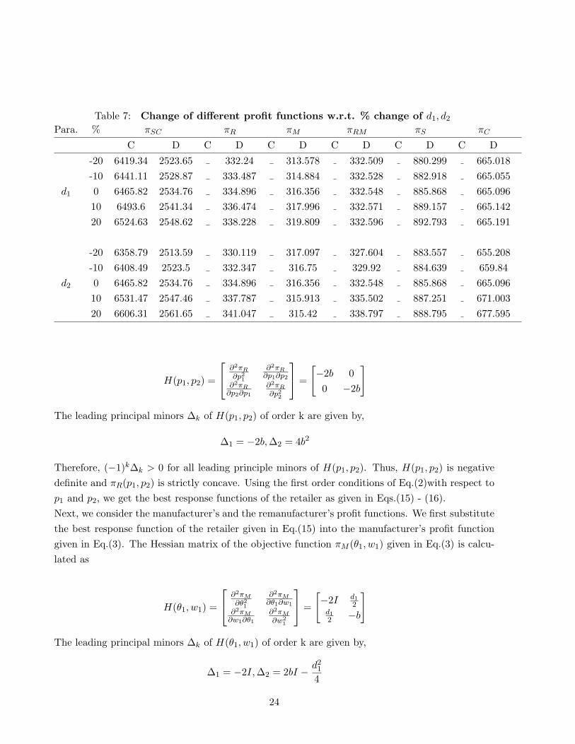
Table 7: Change of different profit functions w.r.t. % change of d1, d2Para. % πSC πR πM πRM πS πC
C D C D C D C D C D C D
-20 6419.34 2523.65 332.24 313.578 332.509 880.299 665.018
-10 6441.11 2528.87 333.487 314.884 332.528 882.918 665.055
d1 0 6465.82 2534.76 334.896 316.356 332.548 885.868 665.096
10 6493.6 2541.34 336.474 317.996 332.571 889.157 665.142
20 6524.63 2548.62 338.228 319.809 332.596 892.793 665.191
-20 6358.79 2513.59 330.119 317.097 327.604 883.557 655.208
-10 6408.49 2523.5 332.347 316.75 329.92 884.639 659.84
d2 0 6465.82 2534.76 334.896 316.356 332.548 885.868 665.096
10 6531.47 2547.46 337.787 315.913 335.502 887.251 671.003
20 6606.31 2561.65 341.047 315.42 338.797 888.795 677.595
H(p1, p2) =
∂2πR∂p21
∂2πR∂p1∂p2
∂2πR∂p2∂p1
∂2πR∂p22
=
[
−2b 0
0 −2b
]
The leading principal minors ∆k of H(p1, p2) of order k are given by,
∆1 = −2b,∆2 = 4b2
Therefore, (−1)k∆k > 0 for all leading principle minors of H(p1, p2). Thus, H(p1, p2) is negative
definite and πR(p1, p2) is strictly concave. Using the first order conditions of Eq.(2)with respect to
p1 and p2, we get the best response functions of the retailer as given in Eqs.(15) - (16).
Next, we consider the manufacturer’s and the remanufacturer’s profit functions. We first substitute
the best response function of the retailer given in Eq.(15) into the manufacturer’s profit function
given in Eq.(3). The Hessian matrix of the objective function πM (θ1, w1) given in Eq.(3) is calcu-
lated as
H(θ1, w1) =
∂2πM∂θ21
∂2πM∂θ1∂w1
∂2πM∂w1∂θ1
∂2πM∂w2
1
=
[
−2I d12
d12 −b
]
The leading principal minors ∆k of H(θ1, w1) of order k are given by,
∆1 = −2I,∆2 = 2bI −d214
24

From Assumptions 3(i) we get 2bI−d214 > 0. Therefore, (−1)k∆k > 0 for all leading principle minors
of H(θ1, w1). Thus, H(θ1, w1) is negative definite and πM (θ1, w1)) is strictly concave. Using the
first order conditions of Eq.(3) with respect to θ1 and w1, we get the best response functions of the
manufacturer as given in Eqs.(17) - (18).
In a similar way, We substitute the best response function of the retailer given in Eq.(16) into
the remanufacturer’s profit function given in Eq.(4). The Hessian matrix of the objective function
πRM (θ2, w2) given in Eq.(4) is calculated as
H(θ2, w2) =
∂2πRM
∂θ22
∂2πRM
∂θ2∂w2
∂2πRM
∂w2∂θ2
∂2πRM
∂w22
=
[
−2I d22
d22 −b
]
The leading principal minors ∆k of H(θ2, w2) of order k are given by,
∆1 = −2I,∆2 = 2bI −d224
From Assumptions 3(ii) we get 2bI −d224 > 0. Therefore, (−1)k∆k > 0 for all leading principle
minors of H(θ2, w2). Thus, H(θ2, w2) is negative definite and πRM (θ2, w2)) is strictly concave.
Using the first order conditions of Eq.(4) with respect to θ2 and w2, we get the best response
functions of the manufacturer as given in Eqs.(19) - (20).
In the last step, we consider the supplier’s and the collector’s profit functions. We first substitute
the best response function of the retailer, manufacturer, remanufacturer given in Eqs.(15) - (20)
into the supplier’s profit function given in Eq.(5). Then, the second order derivative of the supplier’s
objective function πS(s1) given in Eq.(5) with respective to s1 is calculated as
∂2πS
∂s21= −
4b2I
8bI − d21−
4b2I(1− β)2
8bI − d22
From Assumptions 3(i) and 3(ii) we get , 8bI−d21 > 0 and 8bI−d22 > 0. And since I > 0, it can be
seen that − 4b2I8bI−d21
− 4b2I(1−β)2
8bI−d22< 0. Therefore, ∂
2πS∂s21
< 0, i.e. πS(s1) is a strictly concave function.
In a similar way, We first substitute the best response function of the retailer, remanufacturer
given in Eqs.(16), (19) and (20) into the collector’s profit function given in Eq.(6). Then, the second
order derivative of the collector’s objective function πC(s2) given in Eq.(5) with respective to s2 is
calculated as
∂2πC
∂s22= −
4b2Iβ2
8bI − d22
From Assumptions 3(ii) we get, 8bI − d22 > 0. And since I > 0, it can be seen that − 4b2Iβ2
8bI−d22< 0.
Therefore, ∂2πC∂s22
< 0, i.e. πC(s2) is a strictly concave function.
Finally, simultaneously solving the first order condition of Eq.(5) with respect to s1 and first order
condition of Eq.(6) with respect to s2 gives the optimal unit selling prices of the supplier and the
25

collector as given in Eqs.(21) and (22). Putting the Eqs.(15) - (22) into Eq.(1), we get the optimal
values of demands for the new and remanufactured products as given in Eqs.(23) - (24). Finally.
putting the Eqs.(15) - (22) into Eq.(7) we get the optimal profit of the overall supply chain as given
in Eq.(25).
Compliance with ethical standards
Conflict of interest: The authors declare that they have no conflict of interest.
Ethical approval: This article does not contain any studies with human participants or animals
performed by any of the authors.
Funding: This study was not funded by any agency or Government. None of the authors received
any kind of financial grant or support for this study.
Informed consent: Informed consent was obtained from all individual participants included in
the study.
Authorship contributions
Dr. Dipak Jana has formulated the models. Mr. Manojit has solved the models and compared
the solutions of the models and drawn the figure. Dr. Shariful Alam has done the Numerical part.
This paper is written by Mr. Manojit Das.
References
[1] M. Grimmer and T. Bingham, “Company environmental performance and consumer purchase
intentions,” Journal of business research, vol. 66, no. 10, pp. 1945–1953, 2013.
[2] K. Salimifard and R. Raeesi, “A green routing problem: optimising co2 emissions and costs
from a bi-fuel vehicle fleet,” International Journal of Advanced Operations Management, vol. 6,
no. 1, pp. 27–57, 2014.
[3] S. Yang, H. Ngiam, S. Ong, and A. Nee, “The impact of automotive product remanufacturing
on environmental performance,” Procedia Cirp, vol. 29, pp. 774–779, 2015.
[4] S. Bag, N. Anand, and K. K. Pandey, “Green supply chain management model for sustainable
manufacturing practices,” in Green supply chain management for sustainable business practice,
pp. 153–189, IGI Global, 2017.
[5] B. Van Hoof and M. Thiell, “Collaboration capacity for sustainable supply chain manage-
ment: small and medium-sized enterprises in mexico,” Journal of Cleaner Production, vol. 67,
pp. 239–248, 2014.
[6] H. Liu, H. Long, and X. Li, “Identification of critical factors in construction and demolition
waste recycling by the grey-dematel approach: A chinese perspective,” Environmental Science
and Pollution Research, vol. 27, no. 8, pp. 8507–8525, 2020.
26

[7] S. K. Srivastava, “Green supply-chain management: a state-of-the-art literature review,” In-
ternational journal of management reviews, vol. 9, no. 1, pp. 53–80, 2007.
[8] S. L. Hart, “Beyond greening: strategies for a sustainable world,” Harvard business review,
vol. 75, no. 1, pp. 66–77, 1997.
[9] C. Prahinski and C. Kocabasoglu, “Empirical research opportunities in reverse supply chains,”
Omega, vol. 34, no. 6, pp. 519–532, 2006.
[10] P. Sasikumar and G. Kannan, “Issues in reverse supply chains, part ii: reverse distribution
issues–an overview,” International Journal of Sustainable Engineering, vol. 1, no. 4, pp. 234–
249, 2008.
[11] M. V. de la Fuente, L. Ros, and M. Cardos, “Integrating forward and reverse supply chains:
application to a metal-mechanic company,” International Journal of Production Economics,
vol. 111, no. 2, pp. 782–792, 2008.
[12] A. R. M. Mokhtar, A. Genovese, A. Brint, and N. Kumar, “Improving reverse supply chain
performance: The role of supply chain leadership and governance mechanisms,” Journal of
Cleaner Production, vol. 216, pp. 42–55, 2019.
[13] L. T. T. Doan, Y. Amer, S.-H. Lee, P. N. K. Phuc, and L. Q. Dat, “A comprehensive re-
verse supply chain model using an interactive fuzzy approach–a case study on the vietnamese
electronics industry,” Applied Mathematical Modelling, vol. 76, pp. 87–108, 2019.
[14] M.-A. Gorji, M.-B. Jamali, and M. Iranpoor, “A game-theoretic approach for decision analysis
in end-of-life vehicle reverse supply chain regarding government subsidy,” Waste Management,
2020.
[15] A. A. Taleizadeh and R. Sadeghi, “Pricing strategies in the competitive reverse supply chains
with traditional and e-channels: A game theoretic approach,” International Journal of Pro-
duction Economics, vol. 215, pp. 48–60, 2019.
[16] K. G. Dastidar, “On stackelberg games in a homogeneous product market,” European Eco-
nomic Review, vol. 48, no. 3, pp. 549–562, 2004.
[17] S.-L. Yang and Y.-W. Zhou, “Two-echelon supply chain models: Considering duopolistic retail-
ers’ different competitive behaviors,” International Journal of Production Economics, vol. 103,
no. 1, pp. 104–116, 2006.
[18] E. Almehdawe and B. Mantin, “Vendor managed inventory with a capacitated manufacturer
and multiple retailers: Retailer versus manufacturer leadership,” International Journal of Pro-
duction Economics, vol. 128, no. 1, pp. 292–302, 2010.
27

[19] J.-B. Sheu and Y. J. Chen, “Impact of government financial intervention on competition among
green supply chains,” International Journal of Production Economics, vol. 138, no. 1, pp. 201–
213, 2012.
[20] M. Huang, M. Song, L. H. Lee, and W. K. Ching, “Analysis for strategy of closed-loop supply
chain with dual recycling channel,” International Journal of Production Economics, vol. 144,
no. 2, pp. 510–520, 2013.
[21] W. Li and J. Chen, “Backward integration strategy in a retailer stackelberg supply chain,”
Omega, vol. 75, pp. 118–130, 2018.
[22] J. Chaab and M. Rasti-Barzoki, “Cooperative advertising and pricing in a manufacturer-
retailer supply chain with a general demand function; a game-theoretic approach,” Computers
& Industrial Engineering, vol. 99, pp. 112–123, 2016.
[23] A. Diabat and K. Govindan, “An analysis of the drivers affecting the implementation of green
supply chain management,” Resources, conservation and recycling, vol. 55, no. 6, pp. 659–667,
2011.
[24] B. Li, M. Zhu, Y. Jiang, and Z. Li, “Pricing policies of a competitive dual-channel green supply
chain,” Journal of Cleaner Production, vol. 112, pp. 2029–2042, 2016.
[25] A. Nagurney and L. S. Nagurney, “Sustainable supply chain network design: a multicriteria
perspective,” International Journal of Sustainable Engineering, vol. 3, no. 3, pp. 189–197,
2010.
[26] C. Dong, B. Shen, P.-S. Chow, L. Yang, and C. T. Ng, “Sustainability investment under
cap-and-trade regulation,” Annals of Operations Research, vol. 240, no. 2, pp. 509–531, 2016.
[27] H. Jafari, S. R. Hejazi, and M. Rasti-Barzoki, “Sustainable development by waste recycling un-
der a three-echelon supply chain: A game-theoretic approach,” Journal of cleaner production,
vol. 142, pp. 2252–2261, 2017.
[28] P. K. Ghosh, A. K. Manna, J. K. Dey, and S. Kar, “Supply chain coordination model for green
product with different payment strategies: a game theoretic approach,” Journal of Cleaner
Production, p. 125734.
28

Figures
Figure 1
Three-stage supply chain structure.
Figure 2
Pro� t of the overall supply chain(SC) in the centralized model and decentralized model.
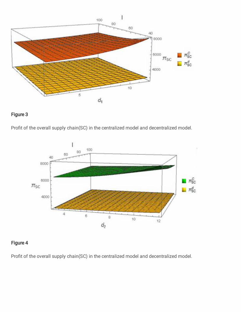
Figure 3
Pro� t of the overall supply chain(SC) in the centralized model and decentralized model.
Figure 4
Pro �t of the overall supply chain(SC) in the centralized model and decentralized model.

Figure 5
Pro� t of the overall supply chain(SC) in the centralized model and decentralized model.
Figure 6
Greening level of the manufacturer and remanufacturer in the centralized and decentralized model.

Figure 7
Greening level of the manufacturer in the centralized and decentralized model.
Figure 8
Greening level of the remanufacturer in the centralized and decentralized model.

Figure 9
Greening level of the manufacturer and remanufacturer in the decentralized model.
Figure 10
Greening level of remanufacturer in the centralized and decentralized model.
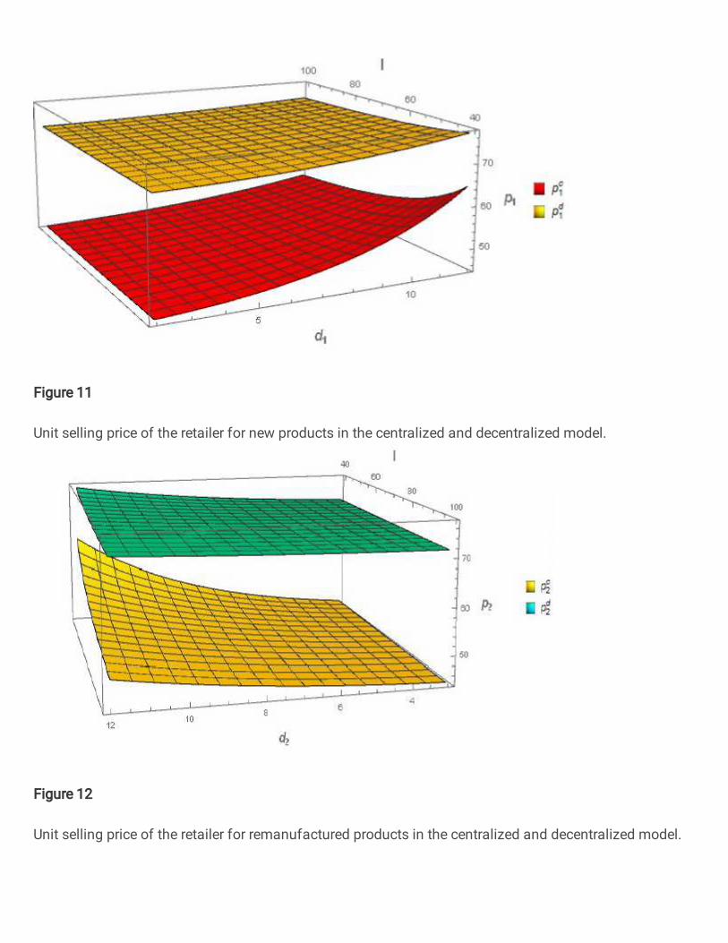
Figure 11
Unit selling price of the retailer for new products in the centralized and decentralized model.
Figure 12
Unit selling price of the retailer for remanufactured products in the centralized and decentralized model.

Figure 13
Unit selling price of the retailer for remanufactured products in the centralized and decentralized model.
Figure 14
Total sales volume in the centralized and decentralized model.

Figure 15
Total sales volume in the centralized and decentralized model.