game theoretic optimization of production planning
TRANSCRIPT

GAME THEORETIC OPTIMIZATION OF PRODUCTION PLANNING


GAME THEORETIC APPROACHES TO PETROLEUM REFINERY PRODUCTION
PLANNING – A JUSTIFICATION FOR THE ENTERPRISE LEVEL OPTIMIZATION
OF PRODUCTION PLANNING
by
PHILIP A. TOMINAC
M.Eng.D., B.Eng.Biosciences (Chemical Engineering & Biosciences)
A Thesis
Submitted to the School of Graduate Studies
In Partial Fulfillment of the Requirements for the Degree
Doctor of Philosophy
McMaster University
© Copyright by Philip A. Tominac, Sept. 2017

ii
DOCTOR OF PHILOSOPHY (2017) McMaster University
(Chemical Engineering) Hamilton, Ontario
TITLE: Game theoretic approaches to petroleum refinery production
planning – a justification for the enterprise level optimization
of production planning
AUTHOR: Philip A. Tominac, M.Eng.D., B.Eng.Biosciences
(Chemical Engineering & Biosciences)
(McMaster University, Canada)
SUPERVISOR: Dr. V. Mahalec
NUMBER OF PAGES: xiv,158
iii
LAY ABSTRACT
This thesis presents a mathematical framework in which refinery production
planning problems are solved to optimal solutions in competing scenarios. Concepts from
game theory are used to formulate these competitive problems into mathematical
programs under single objective functions which coordinate the interests of the competing
refiners. Several different cases are considered presenting refinery planning problems as
static and dynamic programs in which decisions are time independent or dependent,
respectively. A theoretical development is also presented in the concept of the mixed
integer game, a game theoretic problem containing both continuous and discrete valued
variables and which must satisfy both continuous and discrete definitions of Nash
equilibrium. This latter development is used to examine refinery problems in which
individual refiners have access to numerous unit upgrades which can potentially improve
performance. The results are used to justify a game theoretic approach to enterprise
optimization.

iv
ABSTRACT
This thesis presents frameworks for the optimal strategic production planning of
petroleum refineries operating in competition in multiple markets. The game theoretic
concept of the Cournot oligopoly is used as the basic competitive model, and the Nash
equilibrium as the solution concept for the formulated problems, which are reformulated
into potential games. Nonlinear programming potential game frameworks are developed
for static and dynamic production planning problems, as well for mixed integer nonlinear
expansion planning problems in which refiners have access to potential upgrades
increasing their competitiveness. This latter model represents a novel problem in game
theory as it contains both integer and continuous variables and thus must satisfy both
discrete and continuous mathematical definitions of the Nash equilibrium. The concept of
the mixed-integer game is introduced to explore this problem and the theoretical
properties of the new class of games, for which conditions are identified defining when a
class of two-player games will possess Nash equilibria in pure strategies, and conjectures
offered regarding the properties of larger problems and the class as a whole. In all
examples, petroleum refinery problems are solved to optimality (equilibrium) to illustrate
the competitive utility of the mathematical frameworks. The primary benefit of such
frameworks is the incorporation of the influence of market supply and demand on
refinery profits, resulting in rational driving forces in the underlying production planning
problems. These results are used to justify the development of frameworks for enterprise
optimization as a means of decision making in competitive industries.

v
ACKNOWLEDGEMENTS
I would like to thank my supervisor Dr. Vladimir Mahalec, whose knowledge and
experience inspired this thesis, and without whose guidance I would not have been able to
accomplish all that I have. Thank you.
I would like to thank my committee members Drs. Thomas Adams II and Elkafi
Hassini, both of whom have provided invaluable input to my work over the last four
years.
Special thanks are due to the professors of the Department of Chemical
Engineering, and in the wider McMaster community, who have contributed to ten years
of university education. I shall put it all to good use.
Perhaps most of all I would like to thank my mother, who has been encouraging my
education for as long as I can remember, and without whose influence I would not have
come so far. I would also like to thank my grandmother, who did not get to see me
complete this thesis, but who would have been very proud.
Finally, I would like to thank my colleagues, past and present, in the McMaster
Advanced Control Consortium. It was certainly fun.

vi
Table of Contents
LAY ABSTRACT .................................................................................................... iii
ABSTRACT .............................................................................................................. iv
ACKNOWLEDGEMENTS ....................................................................................... v
List of figures ........................................................................................................... xii
List of tables ............................................................................................................ xiii
Declaration of academic achievement .................................................................... xiv
Chapter 1 Introduction ....................................................................................................... 1
Motivation .................................................................................................................. 2
Background and literature review .............................................................................. 3
Supply chain production planning ..................................................................... 3
Game theory ....................................................................................................... 4
Contributions ........................................................................................................... 11
Static and dynamic game theoretic planning frameworks ............................... 11
Mixed integer games and expansion planning ................................................. 12
Thesis overview ....................................................................................................... 12
Author’s statement of contribution .......................................................................... 15
References ................................................................................................................ 16
Chapter 2 A game theoretic framework for petroleum refinery strategic production
planning ............................................................................................................................. 19
Introduction .............................................................................................................. 21
Background .............................................................................................................. 23
Nash equilibrium .............................................................................................. 23
Potential games and the potential function ...................................................... 25
vii
Problem statement .................................................................................................... 26
Scenario 1 (S1) - Competition for market share ............................................... 29
Scenario 2 (S2) - Elimination of inefficient competitors ................................. 29
Models and Formulation ........................................................................................... 31
Production planning model ............................................................................... 31
A demand-based Cournot oligopoly ................................................................. 34
Potential function formulation .......................................................................... 34
Fixed-price analysis .......................................................................................... 35
Model alterations for Scenario 2 ...................................................................... 36
Results and Discussion ............................................................................................. 39
Scenario basis and data ..................................................................................... 39
Scenario 1 results .............................................................................................. 41
Scenario 2 results .............................................................................................. 44
Existence of multiple equilibria ........................................................................ 48
Model solution statistics ................................................................................... 48
Conclusions .............................................................................................................. 49
Notation .................................................................................................................... 50
Sets ................................................................................................................... 50
Parameters ........................................................................................................ 52
Continuous variables ........................................................................................ 53
Binary variables ................................................................................................ 54
Literature Cited ......................................................................................................... 55
Acknowledgements .................................................................................................. 59

viii
Chapter 3 A dynamic game theoretic framework for process plant competitive upgrade
and production planning .................................................................................................... 60
Introduction .............................................................................................................. 62
Background .............................................................................................................. 65
Dynamic Nash equilibrium .............................................................................. 65
Problem statement .................................................................................................... 66
Models and Formulation .......................................................................................... 69
Deriving a dynamic potential function ............................................................ 69
Verification of the dynamic potential function ................................................ 71
A potential function for the elimination game ................................................. 72
Solution Procedure ........................................................................................... 74
Refinery Models .............................................................................................. 74
Results and Discussion ............................................................................................ 75
On avoiding elimination .................................................................................. 75
Influence of time discretization ....................................................................... 78
Existence of multiple equilibria ....................................................................... 79
Model solution statistics .................................................................................. 80
Conclusions .............................................................................................................. 82
Notation ................................................................................................................... 82
Sets ................................................................................................................... 82
Parameters ........................................................................................................ 83
Continuous Variables ....................................................................................... 83
Binary Variables .............................................................................................. 84
Literature Cited ........................................................................................................ 84

ix
Acknowledgements .................................................................................................. 87
Chapter 4 Conjectures regarding the existence and properties of mixed integer potential
games ................................................................................................................................. 88
Introduction .............................................................................................................. 90
Background ............................................................................................................... 92
Nash Equilibrium .............................................................................................. 92
Pure and mixed strategy Nash equilibria in finite games ................................. 92
Nash equilibria in continuous potential games ................................................. 93
Nash equilibria in finite potential games .......................................................... 93
Problem statement .................................................................................................... 95
Models and formulation ........................................................................................... 96
PSNE existence conditions ....................................................................................... 97
Ordinal mixed integer games of cost .............................................................. 101
Ordinal Mixed Integer Games of Capacity..................................................... 103
Numerical Examples............................................................................................... 106
Illustrative example – MIPG of cost............................................................... 106
Application example – competitive refinery expansion planning .................. 108
Conjectures ............................................................................................................. 111
Conclusions ............................................................................................................ 112
Notation .................................................................................................................. 113
Sets ................................................................................................................. 113
Parameters ...................................................................................................... 113
Continuous Variables ..................................................................................... 113
Binary Variables ............................................................................................. 114

x
References ...................................................................................................... 114
Acknowledgements ................................................................................................ 115
Chapter 5 Conclusions and recommendations ............................................................... 116
Conclusions ............................................................................................................ 117
Enterprise optimization .................................................................................. 117
Mixed integer games ...................................................................................... 118
Concluding thoughts ...................................................................................... 118
Recommendations for further work ....................................................................... 118
Market entry and denial ................................................................................. 119
Uncertainty and Bayesian games ................................................................... 119
Extensions to mixed integer games ............................................................... 120
Additional Considerations ............................................................................. 120
Appendix Supplementary materials ............................................................................... 122
Supplementary material to: A game theoretic framework for petroleum refinery
strategic production planning ........................................................................................ 123
A. The Cournot oligopoly in brief ................................................................. 124
B. Refinery production planning model ........................................................ 125
C. Table of set elements and indices .............................................................. 131
D. Tables of parameter values ....................................................................... 133
Supplementary material to: Conjectures regarding the existence and properties of
mixed integer potential games ...................................................................................... 142
A. Refinery expansion and production planning model ................................ 143
B. Table of set elements and indices .............................................................. 147
C. Tables of parameter values ........................................................................ 150

xi
Relationships with existing market structures ........................................................ 160

xii
List of figures
Chapter 2
Figure 1. Sample arrangement of domestic and global markets. ............................... (28)
Figure 2. Refinery model schematic. .......................................................................... (32)
Figure 3. S1 production volume breakdown and totals by refiner and scenario variant.
............................................................................................................................... (42)
Figure 4. S2 production volume breakdown and totals by refiner and scenario variant.
............................................................................................................................... (45)
Figure 5. Inclusion region boundary characterization for S2; boundaries define paired
domestic and global demand levels (as scaled values) below which low-cost refiners
shut down the high-cost refiner with the indicated price increase. ........................ (47)
Chapter 3
Figure 1. Market scenario layout ................................................................................ (69)
Figure 2. Nash equilibrium price trajectories with normal high-cost refiner 𝑨𝒑𝒘𝑯𝑪 value.
REG and DE2 are used to denote regular gasoline and diesel prices; D and G are
used to denote domestic and global markets. The line labelled HCR indicates
whether and when the high-cost refiner has been eliminated. The dashed FX lines
indicate price trajectories in the case no elimination occurs. ................................ (76)
Figure 3. Domestic market supply of regular gasoline including (A) and excluding (B)
imports of finished product. ................................................................................... (77)
Figure 4. Nash equilibrium price trajectories with large high-cost refiner 𝑨𝒑𝒘𝑯𝑪 value.
REG and DE2 are used to denote regular gasoline and diesel prices; D and G are
used to denote domestic and global markets. The line labelled HCR indicates
whether and when the high-cost refiner has been eliminated. ............................... (77)
Figure 5. Nash equilibrium price trajectories obtained for discretizations of four (A)
eight (B) and ten (C) periods of an eight month planning horizon. ....................... (79)
Chapter 4
Figure 1. Potential and profit values in a refining MIG ........................................... (110)

xiii
Appendix
Figure A1. Map of refineries and pipelines in western Canada…………..(160)
List of tables
Chapter 2
Table 1. Scenario nomenclature and corresponding equations. ................................. (41)
Table 2. Profit values by scenario (106 CAD). (43)
Table 3. Scenario prices (CAD/m3). S1-F and S2-F show fixed price values and the
equivalent game theoretic Cournot prices corresponding to the production levels in
those scenarios. (44)
Table 4. Solution data. (49)
Chapter 3
Table 1. Solution statistics ......................................................................................... (80)

xiv
Declaration of academic achievement
I, Philip A. Tominac, declare this thesis to be my own work. I am the sole author of
this document with exception to those chapters included as works published, submitted,
or accepted for publication in research journals in which case authorship, credit, and
copyright are duly noted with respect to each such included item.
As this thesis contains materials published, submitted, or accepted for publication in
journals, all steps have been taken to ensure that the necessary copyright limitations and
rights have been respected.
My supervisor, Dr. Vladimir Mahalec, and supervisory committee members Drs.
Thomas Adams II and Elkafi Hassini have provided guidance to me throughout my
Ph.D.; I completed all the research work included within this thesis.

Ph.D. Thesis – Philip A. Tominac, McMaster University – Chemical Engineering
1
Chapter 1
Introduction

Ph.D. Thesis – Philip A. Tominac, McMaster University – Chemical Engineering
2
Motivation
The work presented in this thesis is defined by the common goal of investigating
supply chain production planning problems common to the field of chemical engineering
in competitive contexts. A competitive supply chain production planning problem is
interpreted to be one in which two or more parties are involved, and where there exists
some interaction between the parties resulting in a dependency of each individual
participant’s outcome on the decisions made not only by itself but also by all other
parties. In particular, this thesis focuses upon the case in which this interaction is
antagonistic as opposed to cooperative, i.e., where each participant possesses its own
objective unique from those of its opposition, and fulfillment of that objective conflicts
with the fulfillment of opposing parties’ objectives. Concepts from game theory are
employed to model and quantify competitive behaviour in supply chain planning
problems. In particular, the Cournot oligopoly model of competitive market behaviour is
used as the basic competitive framework for competing suppliers, and the concept of the
Nash equilibrium to define the solutions to such problems. These two conceptual entities
are used throughout this thesis and form the basis upon which qualitative interpretations
are drawn from results. Petroleum refining is used consistently in this thesis as an
example supply chain planning problem; the phrasing refinery production planning is
used with regard to these examples. The results presented in this thesis form a
groundwork for the use of game theoretic planning as a means of achieving optimization
across an entire enterprise, incorporating both large scale strategic objectives, decisions
concerning production and associated operational constraints, the presence of
competitors, and market distribution channels. By combining all of these decision levels
within a single planning framework in which optimization is conducted at the enterprise
level, suboptimal decisions resulting from optimization at multiple discrete planning
levels can be avoided. The mechanism and primary benefit of the game theoretic
enterprise planning framework is the unification of all objectives under a single economic
objective function.

Ph.D. Thesis – Philip A. Tominac, McMaster University – Chemical Engineering
3
In this chapter the background material necessary for the thesis is introduced,
providing a unified conceptual framework for various elements of theory. Later chapters
consist of work published in or submitted for publication in peer-reviewed journals, and
the theory discussed in those chapters may contain discrepancies in notation where the
same concept emerges in multiple chapters. In part, the purpose of a reintroduction of the
background material here unifies the notation for comparative purposes, and allows for
some elaboration which is not feasible in articles intended for publication, even while
keeping the background discussion brief.
Background and literature review
This section contains a general overview of the topics addressed in subsequent
thesis chapters and is intended to unify certain nomenclature. There is thus some overlap
between the review in this section and those in each of the following chapters. It is
attempted not to reproduce in detail that which is addressed in other chapters, but to
provide a unified overview of the theoretical background drawn upon throughout this
work. With this objective in mind, overviews of supply chain production planning and
game theoretic concepts are included here. The specifics of refinery operations and
modelling which form the basis for the example scenarios in this thesis are presented in
Chapter 2, with little need for reproduction in this section. Detailed refinery models and
parameter data are attached as appendices.
Supply chain production planning
Production planning is a relevant problem within multiple disciplines, with varying
interpretations. Stadtler reviews and outlines the general structure of supply chain
management literature, in which production planning is a foundational element to overall
competitiveness1. This thesis is primarily concerned with the interpretation of production
planning in the field of process systems engineering, sometimes termed optimal
production planning or simply optimal planning. Production planning is one of the
primary elements of supply chain management and optimization; it is concerned with the

Ph.D. Thesis – Philip A. Tominac, McMaster University – Chemical Engineering
4
determination of material and product inventories and production activities required to
ensure that a process is capable of meeting demands placed upon it by future operations,
and provides objectives to process scheduling and control initiatives which take into
account process operational characteristics2.
The body of literature in optimal planning is large. For the interested reader,
Shapiro3, Shah
4, Papageorgiou
5, and Sahebi, Nickel, and Ashayeri
6 provide reviews of
relevant problems in and the state of the art of optimal planning problems, the latter with
a particular focus on crude oil supply chains. The common theme among these reviews is
the interpretation and modelling of supply chain planning problems as mathematical
programs, and relationship between developments in the field of computational
optimization and supply chain planning. Grossmann7 and Trespalacios and Grossmann
8
provide reviews of MINLP methods used in process systems engineering. Floudas and
Lin review MILP algorithms with a focus on process scheduling9. This thesis is
concerned primarily with optimal planning problem structures employed in refinery
planning. Joly10
defines the role of production planning in the context of the Brazilian
refining sector, in particular defining the relevant planning problems addressed in terms
of strategic planning for future expansions, annual (long term) planning of production and
maintenance, monthly (mid term) planning of operational targets, and short term planning
of operations. Neiro and Pinto11
provide a framework for the modelling and optimization
of a wider petroleum supply chain including multiple refineries and the associated supply
and distribution channels.
Game theory
The Nash equilibrium
Competitive game theoretic problems inherently quantify the conflicting interests of
multiple parties. The Nash equilibrium provides a solution concept for these problems. A
game theoretic problem is denoted 𝐺, with a set of competing, rational players 𝑅.
Rationality in the game theoretic sense is understood to mean that players are assumed to
behave in a prescribed manner; i.e., following some mathematical description. Each

Ph.D. Thesis – Philip A. Tominac, McMaster University – Chemical Engineering
5
player 𝑟 possesses a set of available options in the game, referred to as strategies. The set
of strategies available to player 𝑟 is Ξ𝑟, and an individual strategy in that set is denoted
𝜉𝑟. The outcome of a game is quantified in terms of payoffs to individual players resulting
from their chosen strategies, as well as the strategies chosen by their competitors. The
payoff to player 𝑟 is defined as 𝐽𝑟(𝜉𝑟 , 𝜉−𝑟) where 𝜉−𝑟 is used to indicate all other players
except 𝑟. We assume without loss of generality that players in the game 𝐺 seek to
maximize their payoffs. A player’s Nash equilibrium strategy is 𝜉𝑟∗ and is defined
according to Eq. (1).
𝐽𝑟(𝜉𝑟∗, 𝜉−𝑟
∗ ) ≥ 𝐽𝑟(𝜉𝑟, 𝜉−𝑟∗ ) ∀𝜉𝑟 ∈ Ξ𝑟 , 𝑟 ∈ 𝑅 (1)
The interpretation of this definition is that player 𝑟 has no better payoff than that
which can be achieved than by playing its Nash equilibrium strategy when every other
player is also playing its Nash equilibrium strategy. This does not preclude the existence
of a better payoff resulting to a player from a combination of strategies in which two or
more players avoid the Nash strategy, but it relates how strategies are chosen by
individual players such that certain combinations of strategies are not rational and not
realizable.
Nash proved the existence of at least one equilibrium solution in games with finitely
valued strategy sets Ξ𝑟; this solution may exist as a probability-weighted combination of
strategies referred to as a mixed strategy Nash equilibrium (MSNE)12
. A special case
arises in which each player in such a game selects a single strategy with probability one,
and is referred to as a pure strategy Nash equilibrium (PSNE). In games in which player
strategy sets are infinitely valued (i.e., are continuous variables) there will exist at least
one Nash equilibrium, analogously in pure strategies. The existence of a Nash equilibrium
in infinitely-valued games is due independently to Debreu13
, Glicksberg14
, and Fan15
.
Static games
The defining characteristic of a static game is that all strategies in the game are
executed at once, and without any player able to observe other players’ strategic decisions
prior to making their own16
. Typical static games involve a single decision from multiple
players, but this is not the limit of the form. Consider a game defined over multiple time

Ph.D. Thesis – Philip A. Tominac, McMaster University – Chemical Engineering
6
instants; the static realization of this game is that in which all strategic decisions in all
time instants are made prior to the realization of the game. In the context of petroleum
refining this could be thought of as a scenario in which two refiners are forced to commit
to a month-long production plan before either finds out what the other decided, and in
which case each is unable to alter that plan once it is realized. The concept of equilibrium
in static games is exactly as defined in Eq. (1).
Dynamic games
The concept of time becomes relevant in dynamic games; players become capable
of making multiple decisions throughout the game, and have knowledge of their
opposition’s historic strategies as they become available. In this thesis, discussion of
dynamic games is limited to Cournot oligopoly models – a subject for which there exists
a large body of literature notwithstanding – for cohesiveness and consistency. Most of the
theoretical elements discussed with respect to such games will be general in nature, but
discussed with respect to the dynamic Cournot oligopoly model introduced by Simaan
and Takayama17
. There are two important features of this dynamic game which determine
the properties of the game and methods by which it is solved. These are whether the game
is formulated in continuous or discretized time, and whether the time horizon is finite or
infinite in length.
Important developments in dynamic game theory have occurred through study of
continuous time infinite horizon games, which are in some senses the most general form.
Such games are problems of optimal control, where players’ strategies are feedback
control functions of past strategies17
. Fershtman and Kamien made additional
developments to the study of dynamic Cournot oligopolies in the continuous time finite
horizon case, and demonstrated the turnpike properties of Nash equilibrium strategies:
namely that the strategic profile initially approaches the infinite horizon equilibrium as it
evolves through time, but deviates as the end of the time horizon approaches18,19
. The
reasoning behind this difference is a function of the time horizon itself: strategies become
viable in the endgame which are not acceptable in the early game (typically because they

Ph.D. Thesis – Philip A. Tominac, McMaster University – Chemical Engineering
7
would result in unacceptable payouts in future periods) and which are generally not
acceptable in the infinite horizon game.
The variation considered in this thesis is the discrete time finite horizon dynamic
game, which has several desirable properties. The discrete time finite horizon dynamic
Cournot oligopoly problem is a potential game with a readily derived potential function;
see Chapter 3 for additional discussion and a derivation of such a function. As a potential
game, the dynamic Cournot oligopoly can be solved directly using numerical
optimization rather than integration, which is the approach used to solve optimal control
problems17
. Since the model can be posed as an optimization problem, the incorporation
of process constraints for the modelling of realistic systems is trivial. Furthermore,
problems of significant size can be solved using existing numerical optimization tools.
An important difference between static and dynamic games is the interpretation of
the Nash equilibrium. In the discrete time finite horizon game 𝐺 with 𝑅 players and 𝑁
discrete time periods, player strategy sets are denoted Ξ𝑛𝑟 to indicate the additional time
dimension. Player payoff functions become 𝐽𝑟(𝜉𝑟𝑛, 𝜉−𝑟𝑛), and are functions of a strategy
profile which evolves over time as a function of previous time instances. The Nash
equilibrium definition is shown in Eq. (2).
𝐽𝑟(𝜉𝑟𝑛∗ , 𝜉−𝑟𝑛
∗ ) ≥ 𝐽𝑟(𝜉𝑟𝑛, 𝜉−𝑟𝑛∗ ) ∀𝜉𝑟𝑛 ∈ Ξ𝑟𝑛, 𝑟 ∈ 𝑅, 𝑛 ∈ 𝑁 (2)
Equilibria in finite games
The payoffs in a game with finitely valued strategies constitute a payoff matrix. To
distinguish finite payoffs from continuously valued payoff functions in infinite games, the
notation 𝑗𝑟(𝜉𝑟 , 𝜉−𝑟) is introduced and is used to indicate scalar payoff values in finitely
valued games. Pure strategy Nash equilibria in finitely valued games are identified as
instances in which all players simultaneously possess a payoff maximum in the matrix
dimension corresponding to their strategy vector. Instances in which this is not the case
reflect finite games possessing only equilibrium in mixed strategies. Finding all equilibria
in a finite game is NP hard20
.
A PSNE in a finite game is illustrated in Eq. (3) where the players R and C
participate in a prisoners’ dilemma21
. The equilibrium is identified by placing accent

Ph.D. Thesis – Philip A. Tominac, McMaster University – Chemical Engineering
8
marks �̇� on the strategy vector minima (in this particular case) for each player; i.e., R’s
column minima and C’s row minima. Individual payoffs in the matrix are presented as
vectors [𝑗𝑅(𝜉𝑅, 𝜉𝐶), 𝑗𝐶(𝜉𝑅 , 𝜉𝐶)]. The PSNE occurs where the accent marks indicate both
players possess a mutual minimum payoff subject to the opposing player’s decision.
𝐶
𝑅 [1,1 10, 0̇
0̇, 10 3̇, 3̇] (3)
The canonical example of a finite game possessing only a MSNE is the classic
rock-paper-scissors21
. The payoff matrix for this game is shown in Eq. (4), and illustrates
that no PSNE can be identified based on matrix dimension maxima; there is always an
alternative strategy one player can select which improves their own payoff while
simultaneously reducing that of the opponent. As an aside, the equilibrium in mixed
strategies is easily deduced in this game: each strategy should be selected with probability
1/3.
𝐶
𝑅 [0,0 0, 1̇ 1̇, 0
1̇, 0 0,0 0, 1̇
0, 1̇ 1̇, 0 0,0
] (4)
Equilibria in infinite games
In finite games payoff functions are typically functions of continuous strategy
variables. Each participant in a game seeks to maximize its payoff with respect to those
variables over which it has control. The Nash equilibria of a continuous game are defined
as the solutions to the set of payoff function derivatives defined in Eq. (5).
𝜕𝐽𝑟(𝜉𝑟 , 𝜉−𝑟)
𝜕𝜉𝑟= 0 ∀𝜉𝑟 ∈ Ξ𝑟 , 𝑟 ∈ 𝑅 (5)
This set of equations is also referred to as the set of best response functions, as each
player’s payoff is optimized with respect to every opponent’s similarly payoff-
maximizing strategy22
. Nash equilibrium in continuous games is thus also defined as a
maximization problem as in Eq. (6).
𝜉𝑟∗ = 𝑎𝑟𝑔𝑚𝑎𝑥(𝐽𝑟(𝜉𝑟 , 𝜉−𝑟)) ∀𝜉𝑟 , 𝜉−𝑟 ∈ Ξ𝑟 , 𝑟 ∈ 𝑅 (6)

Ph.D. Thesis – Philip A. Tominac, McMaster University – Chemical Engineering
9
Generalized Nash equilibrium
In certain cases players’ strategy spaces will not be independent of each other. Such
strategy sets are generally referred to as having coupling constraints and are written as
Ξ𝑟(𝜉−𝑟). The Nash equilibrium concept in such cases is modified to account for these
coupling constraints, and is referred to as a generalized Nash equilibrium23,24
. Generalized
Nash equilibria are in general not unique. Rosen developed a process known as
normalization based on the weighting of dual variables to define a unique Nash
equilibrium in such games23,25,26
. In this thesis the concept of the generalized Nash
equilibrium is important as an interpretation; in later chapters problems will be solved in
which coupling constraints may or may not be active in a given equilibrium solution,
changing the interpretation of the type of equilibrium obtained.
Potential games
The definitions of Nash equilibrium presented so far have many definitions arising
as optimization arguments. The class of potential games are those in which the set of
players behaves independently in such a way as to maximize a single objective function
whose solution is a Nash equilibrium to the game27,28,29
. The objective to a potential
games is referred to as the potential function 𝑍 and has the property in Eq. (7) that the
potential function derivative with respect to a player’s strategy variable is exactly equal to
the derivative of that player’s payoff function derivative.
𝜕𝑍(𝜉𝑟 , 𝜉−𝑟)
𝜕𝜉𝑟=𝜕𝐽𝑟(𝜉𝑟 , 𝜉−𝑟)
𝜕𝜉𝑟∀𝜉𝑟 ∈ Ξ𝑟 , 𝑟 ∈ 𝑅 (7)
The concept of the potential game also extends to finite games in which the
potential to a game payoff matrix of dimension |Ξ1| × …× |Ξ𝑟| × …× |Ξ𝑅| × |𝑅|
containing the payoff values 𝑗𝑟(𝜉𝑟 , 𝜉−𝑟) is a matrix of dimension |Ξ1| × …× |Ξ𝑟| × …×
|Ξ𝑅| containing the potential values 𝑧(𝜉𝑟 , 𝜉−𝑟) which satisfy the relationship in Eq. (8)29
.
𝑗𝑟(𝜉𝑟 , 𝜉−𝑟) − 𝑗𝑟(𝜉𝑟′ , 𝜉−𝑟) = 𝑧(𝜉𝑟 , 𝜉−𝑟) − 𝑧(𝜉𝑟
′ , 𝜉−𝑟) ∀𝜉𝑟 , 𝜉𝑟′ ∈ Ξ𝑟 , 𝑟 ∈ 𝑅 (8)
This is the definition of an exact potential game in which the change in payoff
resulting from a change in strategy by a player is exactly equal to the change in value in
the potential corresponding to the same strategies, and holds true for all players.
Alternative definitions of finite game potential exist; these are the weighted potential, in
Ph.D. Thesis – Philip A. Tominac, McMaster University – Chemical Engineering
10
which the potential definition in Eq. (8) is satisfied subject to the weighting of the
potential difference as 𝑤𝑟(𝑧(𝜉𝑟 , 𝜉−𝑟) − 𝑧(𝜉𝑟′ , 𝜉−𝑟)), and the ordinal potential in which the
signs of the two differences need to be the same, but the magnitudes do not. More in-
depth discussion of the theoretical background of finite potential games is presented in
Chapter 4.
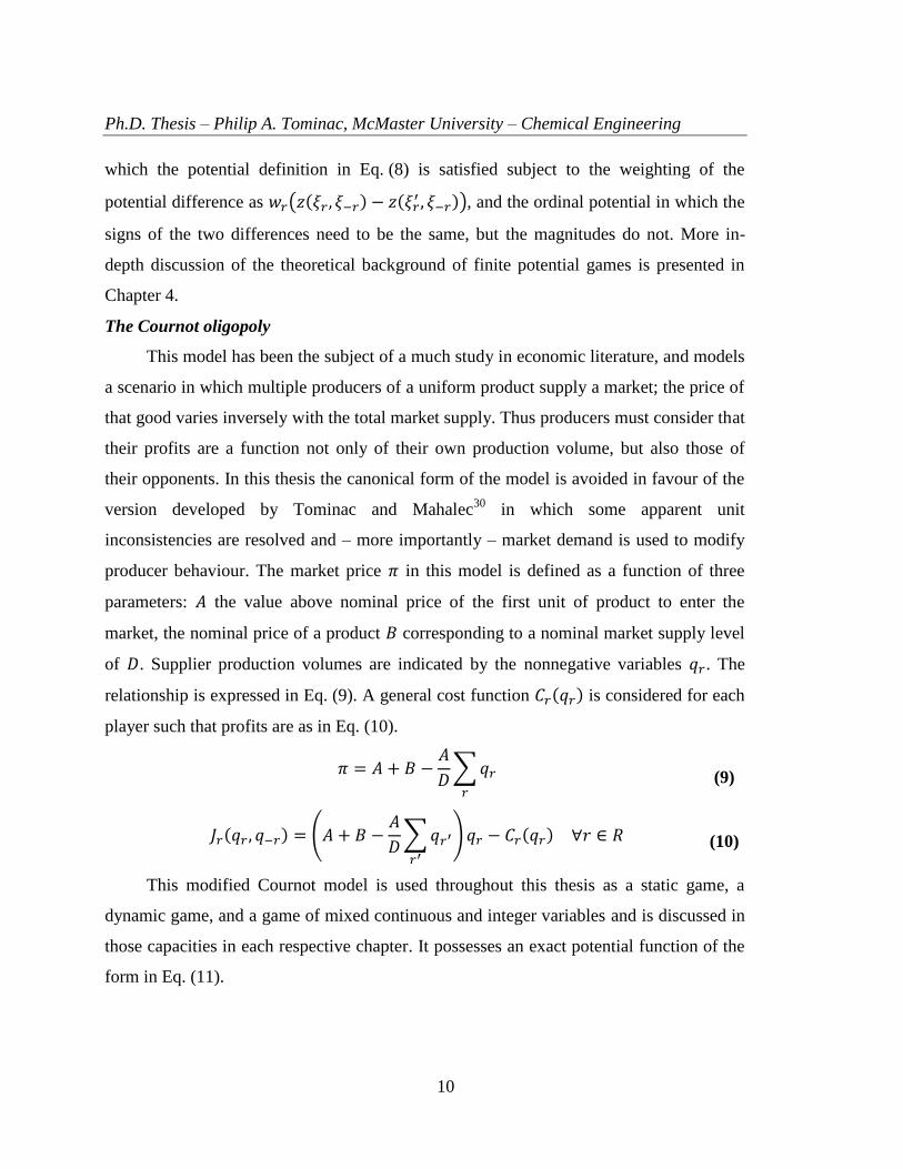
The Cournot oligopoly
This model has been the subject of a much study in economic literature, and models
a scenario in which multiple producers of a uniform product supply a market; the price of
that good varies inversely with the total market supply. Thus producers must consider that
their profits are a function not only of their own production volume, but also those of
their opponents. In this thesis the canonical form of the model is avoided in favour of the
version developed by Tominac and Mahalec30
in which some apparent unit
inconsistencies are resolved and – more importantly – market demand is used to modify
producer behaviour. The market price 𝜋 in this model is defined as a function of three
parameters: 𝐴 the value above nominal price of the first unit of product to enter the
market, the nominal price of a product 𝐵 corresponding to a nominal market supply level
of 𝐷. Supplier production volumes are indicated by the nonnegative variables 𝑞𝑟. The
relationship is expressed in Eq. (9). A general cost function 𝐶𝑟(𝑞𝑟) is considered for each
player such that profits are as in Eq. (10).
𝜋 = 𝐴 + 𝐵 −𝐴
𝐷∑𝑞𝑟𝑟
(9)
𝐽𝑟(𝑞𝑟 , 𝑞−𝑟) = (𝐴 + 𝐵 −𝐴
𝐷∑𝑞𝑟′
𝑟′
)𝑞𝑟 − 𝐶𝑟(𝑞𝑟) ∀𝑟 ∈ 𝑅 (10)
This modified Cournot model is used throughout this thesis as a static game, a
dynamic game, and a game of mixed continuous and integer variables and is discussed in
those capacities in each respective chapter. It possesses an exact potential function of the
form in Eq. (11).

Ph.D. Thesis – Philip A. Tominac, McMaster University – Chemical Engineering
11
𝑍(𝑞𝑟 , 𝑞−𝑟) =∑((𝐴 + 𝐵)𝑞𝑟 −
𝐴
𝐷𝑞𝑟2 − 𝐶𝑟(𝑞𝑟))
𝑟
−𝐴
𝐷∑∑(𝑞𝑟𝑞𝑟′)
𝑟′
𝑟′<𝑟𝑟
(11)
Contributions
This thesis contains arguments for the use of game theoretic analysis in strategic
refinery production planning. The primary argument upon which this thesis is predicated
is that most production planning literature implicitly assumes a monopolistic market
structure in its formulation. This structure yields mathematical results that are not
realizable in their implementation, primarily due to the presence of competitors in real
systems that make certain optimal production planning strategies unviable. This thesis
presents static and dynamic frameworks for competitive refinery production planning
across multiple markets and products, and identifies a new class of games in the mixed
integer game in order to solve refinery expansion problems. These arguments are
assembled within the broader context of this thesis as an argument for game theoretic
optimization at the enterprise level.
Static and dynamic game theoretic planning frameworks
These frameworks are the first contribution that this thesis makes. Potential game
structures are used to capture the presence of competitors in multi-market production
planning problems with the objective of generating rational strategic planning results. The
models used in these frameworks include producer economics using a detailed refining
model, as well as the market economics of supply and demand in what are modelled as
domestic and global markets. By modifying Cournot price variations to include nominal
market demand levels refinery output and profit levels are linked to market supply
volumes. This framework could allow refiners to optimize production with respect to
changing demands and prices in markets, and to avoid costly planning errors. In addition,
these frameworks provide a link between enterprise level decision making procedures as
well as plant operating decisions and constraints. The dynamic game theoretic production
Ph.D. Thesis – Philip A. Tominac, McMaster University – Chemical Engineering
12
planning framework is interesting in this respect as it also provides an indication of future
economic repercussions to decisions made in the present; a feature absent in most
production planning approaches. An example considered throughout this thesis is a
scenario representative of Western Canada in which a small refinery competes with much
larger opponents. The question in this scenario is whether the opposition should simply
force the small refiner into closure. Based on the economic impacts it is found that the
answer is highly dependent on market conditions, and the results tend to mirror the
structure of the refining assets in Western Canada, suggesting that similar market forces
may be at play, and can be accounted for in strategic planning approaches.
Mixed integer games and expansion planning
Expansion planning is a strategic planning problem in which future refinery
upgrades are included as discrete variables such that the optimal future plant
configuration can be determined along with the strategic operating conditions of that
plant. Such problems are typically MINLP models and to date were not solvable by game
theoretic approaches. This thesis provides a basis for the theory of mixed integer games,
starting with the algebraic conditions under which two player, two strategy games are
guaranteed to possess a Nash equilibrium in pure strategies. This contribution has
implications in relevant engineering problems, and also as an academic line of inquiry
into the properties and structure of this new class of game theoretic problems. This thesis
offers as much in the way of developments as have been possible in the identification of
the existence and behaviour of these problems, but does not offer mathematical proof,
which remains as a line of inquiry.
Thesis overview
Chapter 2 of this thesis consists of the submitted text of a paper published in AIChE
Journal. This paper details the static game elements of the potential game theoretic
framework for strategic production planning. It outlines in detail prior works in the field
of engineering supply chain planning that have used elements of game theory, then

Ph.D. Thesis – Philip A. Tominac, McMaster University – Chemical Engineering
13
proceeds to outline how a potential game approach allows relevant production planning
problems to be formulated and solved in a competitive context. This paper and its
associated supplementary material (included as an appendix with this thesis) provide a
detailed refinery production planning model, and an account of all data sources from
which data were obtained with the goal of modelling competitive behaviour in the
petroleum refining industry in a Canadian context. Necessary elements of game theory
are introduced in this paper including a detailed derivation of the potential function used
to link the refinery planning objectives to a market supply objective. Results in this paper
demonstrate the benefits of using a game theoretic approach to production planning in
contrast with typical single refiner fixed price approaches; primarily these are a more
conservative prediction of profits, and a production regime which is robust to changes in
opposing refiners’ strategies. A scenario is also examined in which a small, high-cost
refinery competes with larger, lower cost opponents, and the conditions under which the
opponents seek to force the high-cost refiner to shut down. Game theoretic analysis of
this scenario yields economic curves as functions of domestic and global market demand
indicating the point at which the threat of elimination is realized, and are contrasted with
similar curves obtained when a fixed price approach is used. In general, the fixed price
approach does not capture the game theoretic results, which vindicate the continued
existence of small refineries in Western Canada under certain market conditions. The
citation for this work is presented below.
Tominac P, Mahalec V. A game theoretic framework for petroleum
refinery strategic production planning. AICHE J, 2017; 63(7): 2751-2763.
Chapter 3 of this thesis consists of the text submitted for publication to AIChE
Journal and which is in review at the time of writing. This work extends the static
potential game framework of Chapter 2 to a dynamic potential game framework allowing
refiners to observe the past behaviour of their opponents and to respond to it over the
planning horizon. This manuscript reviews applications of dynamic games in engineering
problems, presents the required background in dynamic Nash equilibria, and based on the
static competitive refining model of Chapter 2, derives and verifies the properties of a

Ph.D. Thesis – Philip A. Tominac, McMaster University – Chemical Engineering
14
dynamic potential function for the modified Cournot oligopoly model. This manuscript
focuses primarily on the problem of the high-cost refiner in dynamic setting. In this work,
the high-cost refiner may attempt to avert the threat of elimination by upgrading its
facilities and becoming competitive with the low-cost refiners. Upgrading takes time, and
changes the properties of the market in which the refiners operate; thus the threat of
elimination also changes, potentially occurring in an earlier time period. The high-cost
refiner must thus be able to complete its upgrades prior to being shut down, else it is
unable to escape the threat. An interesting result emerges from this work in that the threat
of elimination may not be legitimate; the low-cost refiners may decide not to eliminate
the high-cost refiner at all, or at a time in the future which is never realized due to the
rolling horizon nature of the implemented model. In such cases the high-cost refiner is
safe if it does not initiate upgrade procedures, but the threat may become legitimate if it
elects to do so. The submitted title of this manuscript is as below:
Tominac P, Mahalec V. A dynamic game theoretic framework for process
plant competitive upgrade and production planning.
Chapter 4 of this thesis is another manuscript submitted for publication, this one in
the European Journal of Operational Research. The focus of this manuscript is on the
properties of finite games with the objective of solving games possessing both discrete
and continuous variables as mixed integer programs. At time of writing, there is no theory
regarding games of this type, and the manuscript refers to them simply as mixed integer
games, or mixed integer potential games with reference to the type of problem that is
investigated. This work is heavily based on theoretical developments made by Monderer
and Shapley18
in their formalization of finite and infinite potential games. This paper
examines those developments and extends the work to the case of two-player, two-
strategy mixed integer Cournot oligopoly games. The conditions under which such a
game is guaranteed to possess a Nash equilibrium in pure strategies are derived, and are
established as conditions upon which it can be determined whether a given game of the
indicated structure can be solved as an MINLP with the resulting solution being a Nash
equilibrium. An example is presented where these conditions are applied, and the

Ph.D. Thesis – Philip A. Tominac, McMaster University – Chemical Engineering
15
resulting game enumerated to validate the result. A second example consists of a refinery
expansion game in higher dimensions, and thus the conditions derived in the paper cannot
be applied; however, the game presented is enumerated to demonstrate that it also
possesses a PSNE which is correctly obtained from the solution of the MINLP
formulation, and it is noted that it no case was a game found which lacked a PSNE.
Conjectures are then offered regarding the properties of mixed integer games. This work
defines a new class of game theoretic problems and opens up a new line of inquiry for
further research. The working title of the submitted manuscript is as below.
Tominac P, Mahalec V. Conjectures regarding the existence and
properties of mixed integer potential games.
Chapter 5 concludes the thesis and offers remarks on the work enclosed, the overall
theme, and potential avenues for future research. The included appendices are the texts
submitted as supplementary material to the publication in Chapter 2, and the submitted
manuscript in Chapter 4.
Author’s statement of contribution
I am the author of this thesis and the first author of all works submitted or accepted
for publication included in this thesis.

Ph.D. Thesis – Philip A. Tominac, McMaster University – Chemical Engineering
16
References
1. Stadtler H. Supply chain management and advanced planning – basics, overview
and challenges. Eur J Oper Res. 2005; 163: 575-588.
2. Papageorgiou LG. Supply chain optimisation for the process industries: Advances
and opportunities. Comput Chem Eng. 2009; 33: 1931-1938.
3. Shapiro JF. Challenges of supply chain planning and modeling. Comput Chem Eng.
2004; 28: 855-861.
4. Shah N. Process industry supply chains: Advances and challenges. Comput Chem
Eng. 2005; 29: 1225-1235.
5. Papageorgiou LG. Supply chain optimization for the process industries: Advances
and opportunities. Comput Chem Eng. 2009; 33: 1931-1938.
6. Sahebi H, Nickel S, Ashyeri J. Strategic and tactical mathematical programming
models within the crude oil supply chain context – A review. Comput Chem Eng.
2014; 68: 56-77.
7. Grossmann IE. Review of nonlinear mixed-integer and disjunctive programming
techniques. Optim Eng. 2002; 3(3): 227-252.
8. Trespalacios F, Grossmann IE. Review of mixed-integer nonlinear and generalized
disjunctive programming methods. Chem Ing Tech. 2014; 86(7): 991-1012.
9. Foudas CA, Lin X. Mixed integer linear programming in process scheduling:
Modeling, algorithms, and applications. Ann Oper Res. 2005; 139: 131-162.
10. Joly M. Refinery production planning and scheduling: the refining core business.
Braz J Chem Eng. 2012; 29(2): 371-384.
11. Neiro SMS, Pinto JM. A general modeling framework for the operational planning
of petroleum supply chains. Comput Chem Eng. 2004; 28: 871-896.
12. Nash, J. Non-cooperative Games. Ann Math. 1951; 54(2): 286-295.
13. Debreu G. A social equilibrium existence theorem. P Natl Acad Sci USA. 1952;
38(10): 886-893.

Ph.D. Thesis – Philip A. Tominac, McMaster University – Chemical Engineering
17
14. Glicksberg IL. A further generalization of the Kakutani fixed point theorem, with
application to Nash equilibrium points. P Am Math Soc. 1952; 3(1): 170-174.
15. Fan K. Fixed-point and minimax theorems in locally convex topological linear
spaces. P Natl Acad Sci USA. 1952; 38(2): 121-126.
16. Webb JN. Game Theory: Decisions, Interaction and Evolution. London, UK:
Springer London; 2007.
17. Simaan M. Takayama T. Game theory applied to dynamic duopoly problems with
production constraints. Automatica. 1978; 14: 161-166.
18. Fershtman C, Kamien MI. Dynamic duopolistic competition with sticky prices.
Econometrica. 1987; 55(5): 1151-1164.
19. Fershtman C, Kamien MI. Turnpike properties in a finite-horizon differential game:
dynamic duopoly with sticky prices. Int Econ Rev. 1990; 31(1): 49-60.
20. McKelvey RD, McLennan A. Computation of equilibria in finite games. In:
Handbook of computational economics. 1st ed. 1996: 87-142.
21. Peters H. Game theory: a multi-leveled approach. Maastricht, The Netherlands:
Springer; 2008.
22. Wu H, Parlar M. Games with incomplete information: A simplified exposition with
inventory management applications. Int J Prod Econ. 2011; 133: 562-577.
23. Rosen B. Existence and uniqueness of equilibrium points for concave n-person
games. Econometrica. 1965; 520-534.
24. Harker P. Generalized Nash games and quasi-variational inequalities. Eur J Oper
Res. 1991; 54(1): 81-94.
25. Facchinei F, Fischer A, Piccialli V. On generalized Nash games and variational
inequalities. Oper Res Lett. 2007; 35(2): 159-164.
26. Facchinei F, Kanzow C. Generalized Nash equilibrium problems. 4OR-Q J Oper
Res. 2007; 5(3): 173-210.
27. Slade ME. The Fictitious Payoff-Function: Two Applications to Dynamic Games.
Ann Econ Stat. 1989; 15/16: 193-216.
28. Slade ME. What does an oligopoly maximize? J Ind Econ. 1994; 42(1): 45-61.

Ph.D. Thesis – Philip A. Tominac, McMaster University – Chemical Engineering
18
29. Monderer D, Shapley L. Potential Games. Game Econ Behav. 1996; 14(1): 124-
143.
30. Tominac P, Mahalec V. A game theoretic framework for petroleum refinery
strategic production planning. AICHE J, 2017; 63(7): 2751-2763.
Ph.D. Thesis – Philip A. Tominac, McMaster University – Chemical Engineering
19
Chapter 2
A game theoretic framework for petroleum refinery strategic
production planning
The content of this chapter is a revision of the manuscript text accepted for publication
under the following citation:
Tominac P, Mahalec V. A game theoretic framework for petroleum
refinery strategic production planning. AICHE J, 2017; 63(7): 2751-2763.
Ph.D. Thesis – Philip A. Tominac, McMaster University – Chemical Engineering
20
A game theoretic framework for
petroleum refinery strategic production
planning
Philip Tominac and Vladimir Mahalec*
Department of Chemical Engineering, McMaster University, 1280 Main St. W.,
Hamilton, ON, L8S 4L8, Canada
*Corresponding author. Tel.: +1 905 525 9140 ext. 26386. E-mail address:
Topical Heading – Process Systems Engineering
Keywords – refinery planning; strategic planning; game theory; potential game; Nash
equilibrium
Abstract A game theoretic framework for strategic refinery production planning is presented
in which strategic planning problems are formulated as non-cooperative potential games
whose solutions represent Nash equilibria. The potential game model takes the form of a
nonconvex nonlinear program (NLP) and we examine an additional scenario extending
this to a nonconvex mixed integer nonlinear program (MINLP). Tactical planning
decisions are linked to strategic decision processes through a potential game structure
derived from a Cournot oligopoly-type game in which multiple crude oil refineries supply
several markets. Two scenarios are presented which illustrate the utility of the game
theoretic framework in the analysis of production planning problems in competitive
scenarios. Solutions to these problems are interpreted as mutual best responses yielding
maximum profit in the competitive planning game. The resulting production planning
decisions are rational in a game theoretic sense and are robust to deviations in competitor
strategies.

Ph.D. Thesis – Philip A. Tominac, McMaster University – Chemical Engineering
21
Introduction
Strategic production planning plays a vital role in modern organizations as a tool for
strategic and tactical decision making at an organization-wide level1. In a comprehensive
review of refinery supply chain planning models Sahebi, Nickel, and Ashayeri identify
crude oil supply chain planning optimization as an imperative source of competitive
advantage in the refining business2. Few papers exist in which refinery production
planning has been examined in a competitive context where the presence of separate
refiners competing for limited market share is taken into account at the strategic or
tactical planning levels. Game theory provides the tools to investigate competitive
interactions and has seen wide use in process systems engineering in areas where the
interactions between competing entities are of fundamental interest. Of note is the area of
electricity market modelling in deregulated power markets, where the ability of interested
power suppliers to “game” established auction and distribution systems is well known.
Bajpai and Singh review game theoretic methodologies used in modelling strategic
decision making processes in electrical markets3. Also of note is the area of distributed
model predictive control (MPC) in which the control actions of separate but interacting
controllers are managed using game theoretic principles. Scattolini reviews game
theoretic and other distributed MPC architectures4.
Game theoretic principles have seen use in engineering supply chain planning
literature to solve cooperative and competitive problems. Gjerdrum, Shah, and
Papageorgiou have implemented Nash bargaining objective functions to determine fair
profit allocation among members of multi-enterprise supply chains5,6
. Pierru used
Aumann-Shapley cost sharing to allocate carbon dioxide emissions to various products in
an oil refinery7. Bard, Plumer, and Sourie used a bilevel formulation to investigate
interactions between governments and biofuels producers as a Stackelberg game where
the government leads by enacting policy8. Bai, Ouyang, and Pang have used a bilevel
formulation to solve a competitive biofuel refinery location and planning problem as a
Stackelberg game wherein the biofuel refiner takes the role of the leader and farmers

Ph.D. Thesis – Philip A. Tominac, McMaster University – Chemical Engineering
22
follow by adjusting their land use9. Yue and You used KKT conditions to reduce the
bilevel program describing a Stackelberg game into a single nonconvex MINLP whose
global optimum is a Stackelberg equilibrium10
. Zamarripa et al have developed a
framework for solving cooperative and competitive supply chain problems through
enumeration of the payoff matrix in multi-objective scenarios, yielding Nash equilibria in
almost all cases11,12,13
.
With the exception to the works of Zamarripa et al, the applications of game
theoretic principles in engineering supply chain literature do not yield Nash equilibrium
planning results, and rely instead on other game theoretic constructs. In particular, the use
of a Stackelberg game allows the planning decisions of a leader to be optimized such that
the followers are constrained to Nash equilibrium strategies. The Stackelberg framework
is not appropriate if no single competitor can be identified as a leader or does not have the
capacity to implement a strategy before competitors can react14,15
. The framework
proposed by Zamarripa et al yields Nash equilibria in most cases, but does not under
certain conditions, as they observed in their work13
. Since their method is based on
enumeration of a finite strategy matrix, and the framework examines only pure strategy
solutions (as opposed to mixed strategies) a Nash equilibrium is not guaranteed to exist in
all cases16
. There is thus a gap in engineering supply chain literature where supply chain
planning problems in competitive scenarios cannot be effectively solved to Nash
equilibrium strategies. We address this problem with a game theoretic framework for
strategic and tactical production planning which generates production plans representative
of Nash equilibria between competing producers and we illustrate the properties of this
framework using a set of competing oil refiners. Our framework treats production
planning problems as continuous games (also referred to as infinite games) which
guarantees that at least one Nash equilibrium will exist17,18,19
. Problems are formulated as
potential games, and Nash equilibrium solutions are identified as the global maxima of a
potential function objective20
. This potential game framework circumvents many of the
problems which arise in the application of game theoretic models to production planning
as the planning and game theoretic aspects of the problem are defined by a single

Ph.D. Thesis – Philip A. Tominac, McMaster University – Chemical Engineering
23
objective function which can be solved using conventional NLP and MINLP solvers. The
contributions and novel elements of this work are:
A framework under which strategic production planning problems can be
solved in a game theoretic context using a potential game formulation
yielding solutions forming Nash equilibria;
A modification to the Cournot oligopoly model which uses a defined
demand level as a modifier of price behaviour;
Two case studies which illustrate the utility of the game theoretic
framework in relevant planning scenarios which exemplify its potential
applications to strategic and tactical production planning.
Background
Nash equilibrium
The concept of the Nash equilibrium as a solution to a noncooperative game has
been studied extensively and has different interpretations in various types of game
theoretic problems16,21,22
. We present elements of Nash equilibrium theory pertinent to the
development of our potential game framework. Denoting the game as 𝐺 and the strategy
sets of each of 𝑁 players as 𝑆𝑛 with strategies 𝑠𝑛 ∈ 𝑆𝑛 then a Nash equilibrium of 𝐺 is
defined as a set of strategies 𝐺{𝑠1∗, … , 𝑠𝑁
∗ } where 𝑠𝑛∗ represents player 𝑛’s equilibrium
strategy. Each player has an objective function 𝐽𝑛{𝑠𝑛, 𝑠−𝑛}; a Nash equilibrium strategy
has the property in Eq. (1).
𝐽𝑛{𝑠𝑛, 𝑠−𝑛∗ } ≤ 𝐽𝑛{𝑠𝑛
∗ , 𝑠−𝑛∗ } ∀𝑛 ∈ 𝑁, 𝑠𝑛 ∈ 𝑆𝑛 (1)
A non-strict inequality in this definition allows multiple equilibria to exist with the
same value, referred to in such cases as weak Nash equilibria. Where an equilibrium
satisfies the definition to strict inequality, the resulting Nash equilibrium is termed
strict23
. Nash equilibrium strategies are interpreted as a set of mutual best responses
among all players; deviation from equilibrium will not yield an increase in objective

Ph.D. Thesis – Philip A. Tominac, McMaster University – Chemical Engineering
24
value. The Nash equilibrium may also be interpreted as a maximizer of the set of player
objectives in Eq. (2).
𝑠𝑛∗ = 𝑎𝑟𝑔𝑚𝑎𝑥{𝐽𝑛(𝑠𝑛, 𝑠−𝑛
∗ )} ∀𝑛 ∈ 𝑁, 𝑠𝑛 ∈ 𝑆𝑛 (2)
Each player’s objective is maximized with regard to the best responses of all other
players, which are usually not the global maximizers of 𝐽𝑛(𝑠𝑛, 𝑠−𝑛) with respect to both
strategy sets 𝑆𝑛 and 𝑆−𝑛. Where the players’ objectives are continuous and differentiable
functions of strategy variables 𝑠𝑛 ∈ 𝑆𝑛 the Nash equilibrium is defined by solving the set
of equations in Eq. (3) 22
.
𝜕𝐽𝑛(𝑠𝑛, 𝑠−𝑛)
𝜕𝑠𝑛= 0 ∀𝑠𝑛 ∈ 𝑆𝑛, 𝑛 ∈ 𝑁 (3)
Multiple Nash equilibria may exist in a continuous game. Calculation of all Nash
equilibria which exist in a game is an NP-hard problem, although heuristics exist which
allow additional equilibria to be characterized24,25
.
Games can be defined such that participants’ strategy spaces are not independent.
Such games are referred to as generalized Nash equilibrium problems (GNEP) 26,27,28
. In a
GNEP player strategies are defined in terms of a strategy set 𝑠𝑛 ∈ 𝑆𝑛(𝑠−𝑛) which is
dependent on competing players’ chosen strategies. Constraints on player strategies make
analytical solutions more difficult to obtain28
. The solution to a GNEP is referred to as a
generalized Nash equilibrium, and shares many of the same properties of a Nash
equilibrium, with the definition in Eq. (4).
𝑠𝑛∗ = 𝑎𝑟𝑔𝑚𝑎𝑥{𝐽𝑛(𝑠𝑛, 𝑠−𝑛
∗ )} ∀𝑛 ∈ 𝑁, 𝑠𝑛 ∈ 𝑆𝑛(𝑠−𝑛) (4)
The generalized Nash equilibrium is defined by the KKT conditions corresponding
to players’ problems, and multiple generalized Nash equilibria may be defined this way.
Normalization is a process through which a single equilibrium is defined as an
appropriate solution and is accomplished by imposing a set of relative weightings on the
dual variables which, for convex games, guarantees that a unique normalized Nash
equilibrium exists for each unique set of weightings29,30
.

Ph.D. Thesis – Philip A. Tominac, McMaster University – Chemical Engineering
25
Potential games and the potential function
For a subclass of games called potential games, the system of equations defining
Nash equilibria can be used to formulate a potential function whose maxima correspond
to the Nash equilibria of the game. Early work demonstrating existence of the potential
function was formalized by Bergstrom and Varian in 198531
, and Slade in 198932
and
199433
. The class of potential games and the associated nomenclature were characterized
by Monderer and Shapley in 199620
. Potential games can be solved using optimization
tools, and the equilibria defined may be strict, weak, or of the generalized type34,35
.
A potential function is derived from the objective functions 𝐽𝑛(𝑠𝑛, 𝑠−𝑛). All
objective functions must be of the form in Eq. (5).
𝐽𝑛(𝑠𝑛, 𝑠−𝑛) = Ψ(𝑠𝑛, 𝑠−𝑛) + Ω𝑛(𝑠𝑛) + Θ𝑛(𝑠−𝑛) ∀𝑛 ∈ 𝑁 (5)
In this form each player’s objective consists of three parts: Ψ is a term common to
all players and a function of all players’ strategy variables; Ω𝑛 is a term unique to each
player and is a function exclusively of that player’s strategy variables; and Θ𝑛 is a term
unique to each player which contains only the variables associated with the other players.
The potential function is formulated as in Eq. (6).
𝑍(𝑠𝑛, 𝑠−𝑛) = Ψ(𝑠𝑛, 𝑠−𝑛) +∑Ω𝑛(𝑠𝑛)
𝑛
(6)
This yields the same definition of the Nash equilibrium as defined in Eq. (3): the
derivative with respect to any individual player’s strategy variable yields the derivative of
that player’s objective function, as in Eq. (7).
𝜕𝑍(𝑠𝑛, 𝑠−𝑛)
𝜕𝑠𝑛=
𝜕
𝜕𝑠𝑛(Ψ(𝑠𝑛, 𝑠−𝑛) + Ω𝑛(𝑠𝑛)) =
𝜕𝐽𝑛(𝑠𝑛, 𝑠−𝑛)
𝜕𝑠𝑛 (7)
The maxima of the potential function are also solutions to the set of partial
differential equations obtained by equating each player’s derivative to zero, and are
therefore Nash equilibria by definition. These concepts extend to constrained games and
the generalized Nash equilibrium; i.e., the maxima of the potential function subject to
coupling constraints are generalized Nash equilibria29
.

Ph.D. Thesis – Philip A. Tominac, McMaster University – Chemical Engineering
26
Problem statement
We examine strategic refinery production planning in a game theoretic framework
to investigate the effects of competition on strategic planning decisions. In this
framework individual refineries are owned and operated by single, competing refiners
such that each refinery in a given market is considered to be an individual competitor in a
game theoretic sense. Each refiner produces the same set of petroleum products as the
others and has access to the same crude oil stocks. Refineries are identical in
configuration, but vary in capacity.
Refiners are faced with a production planning problem in which multiple target
markets exist and each market is characterized by its own nominal demand levels,
corresponding nominal prices, and status as either a domestic or a global market.
Domestic markets consist of the geographical area in which refiners are physically
located and corresponding points of sale. Refiners are collectively obligated to satisfy
product supply constraints in their domestic market, and refiners outside that market
cannot export product there for sale due to a lack of shipping infrastructure; e.g., we
consider pipelines that carry product from domestic markets to global markets, but not
between domestic markets. In this way, shipping between domestic markets by other
means is prohibitively costly such that domestic market refiners have an oligopoly36
.
Each domestic market’s maximum and minimum demand for each product are
known, and will be satisfied by the refiners operating in that market. Domestic markets
will absorb product levels between their upper and lower demand limits at the
corresponding price and clear the market. Since this assumption of demand obligation can
render the problem infeasible (i.e., if combined production capacity is too low) we
assume that refiners are able to import finished product at a fixed price from other assets
owned by the same entity, located elsewhere, and which are thus not market purchases.
This import option provides the slack necessary to maintain feasibility. The products
imported in this way cannot be exported to global markets.

Ph.D. Thesis – Philip A. Tominac, McMaster University – Chemical Engineering
27
Global markets are considered to be points of sale in geographical regions not
occupied by refineries. Since global markets do not contain refiners, they are reliant upon
imports from refiners in domestic markets. Global markets are connected to domestic
markets by pipelines, and any refiner with access to a pipeline may export product to a
global market without limit, as no shipping constraints are placed on global markets; we
assume that the pipelines have sufficient capacity in this regard.
The refinery market is formulated with Cournot oligopoly pricing. Product prices in
each market are variable functions of the collective market supply of that product;
refiners do not control prices, but do influence them with their production decisions.
Pricing is based on the concept of inverse demand; prices decrease in response to a
market supply in excess of demand, and increase when supply falls short of demand. This
pricing structure assumes that prices adjust to a point where all supplied product is sold
and the market clears. Each refiner has the objective of maximizing its profit
independently of the others. A refiner’s individual problem is thus to:
Determine the amounts of each product which should be sold in its
domestic market in order to satisfy domestic supply constraints in concert
with its competitors, and whether any product should be imported, in order
to maximize its own profit (a strategic decision).
Determine the amounts of each product which should be sold to global
markets accounting for all competitors with market access in order to
maximize its profit (a strategic decision).
Determine how much of each crude oil stock to purchase and how to
process the purchased stocks into the desired products in the most cost
efficient manner (production planning decisions).
Each refiners’ decision variables are:
Crude stock purchase volumes.
Blend volumes and unit operating modes.
Product volumes and shipping destinations, including imports.

Ph.D. Thesis – Philip A. Tominac, McMaster University – Chemical Engineering
28
This game theoretic production planning problem is formulated as a potential game
taking the form of an NLP. Domestic and global maxima of the potential function
objective are defined as Nash equilibrium strategies in terms of refiner production
decisions, and may be generalized Nash equilibria29,33
. Due to the domestic market supply
constraint forcing refiners to satisfy production within specified limits, the solutions
obtained from this model may be characterized as generalized Nash equilibria when the
constraint is enforced. Figure 1 illustrates an arrangement of refiners, consumers, and
markets with three domestic markets and two global markets; one refiner has a domestic
market monopoly because no other refiners have access to its point of sale, the rest
compete in domestic oligopolies, and all compete in either one or two global market
oligopolies.
Two scenarios are presented under this framework in which multiple refiners
compete under different conditions. Each scenario explores different aspects of
production planning problems in a competitive context. The first scenario illustrates the
properties of game theoretic planning solutions to competitive problems; the second
defines a complex scenario in which a competitor may be eliminated from a market, and
illustrates how game theoretic planning can be implemented to make rational solutions to
such problems. The scenarios are described in the following sections.
Figure 1. Sample arrangement of domestic and global markets.

Ph.D. Thesis – Philip A. Tominac, McMaster University – Chemical Engineering
29
Scenario 1 (S1) - Competition for market share
This scenario examines refiners competing in the petroleum market, serves to
illustrate the properties of game theoretic planning solutions, and forms a point of
comparison with other production planning approaches. In this scenario unit capacity
constraints in the production planning model limit the ability of any individual refiner to
process more than a certain total throughput regardless of market driving forces. It will be
shown by removing these unit capacity constraints and allowing refiners to produce
potentially infinite volumes that there exist Nash equilibria as the global maxima of the
unconstrained potential function and that both types of solution share similar properties.
We present this as variant S1-G. The production planning problem is also solved under a
fixed price profit maximization objective for comparison using the sum of refiner profits
as the objective function. With fixed prices the refiners are not in competition; this variant
is intended to present the classical approach to planning (by which we mean profit
maximization under the assumption of fixed prices) and in particular, to illustrate the
motivating forces which define an optimal solution in the context of the defined market
problem for the purpose of comparison with game theoretic results. This variant is
defined as S1-F. Our results show that the classical approach results in non-optimal
solutions to the defined problem. We discuss comparisons between the classic planning
results with the game theoretic results.
Scenario 2 (S2) - Elimination of inefficient competitors
This scenario examines refiners in competition where the market structure may
change. A subset of refineries are considered to be more efficient and competitive than
the remainder and are labeled low-cost refineries, denoted by the subset 𝐿𝐶𝑁 ⊆ 𝑁. The
remaining refineries are, typically by virtue of their size or age, rendered less competitive
than the low-cost refineries and are termed high-cost refineries, denoted as part of the
subset 𝐻𝐶𝑁 ⊆ 𝑁. In addition, high-cost refineries are characterized as being isolated
from other assets. All refiners are in competition regardless of low or high-cost status, and
the low cost refiners need to decide whether to shut down high-cost refineries and obtain

Ph.D. Thesis – Philip A. Tominac, McMaster University – Chemical Engineering
30
additional market share for themselves, or to continue operating in the existing market
structure. Examples of such industry structures exist in western Canada where several
small refiners compete with large capacity refiners, as described by the Government of
Canada National Energy Board in a listing of refining assets and the corresponding
distribution pipeline network in Western Canada37
. We draw attention to the trans-
mountain and plateau pipelines which link five independent refineries in a distribution
channel, three of which have quoted capacities of at least 100 Mb/d, one with a quoted
capacity of 55 Mb/d, and the smallest with a capacity of 12 Mb/d and which is isolated
from other pipelines in the network and other assets owned by the same parent company.
Examination of the existence of this type of scenario has been cited as an industrially
relevant problem at the enterprise planning level in a private communication with V.
Mahalec in 2015. Similar problems examining refinery competitiveness as a function of
scale have been identified by industry experts38
.
Cournot limit theorem states that all else being equal a market with fewer
competitors maintains higher prices39
. Based on this theorem, any option to reduce the
number of competitors is a positive decision for the remaining refiners. We differentiate
our scenario from this theorem by assuming that a high-cost refinery requires higher
market prices than its low-cost competitors to remain profitable. In our model, as long as
high-cost refineries remain active in a domestic market, all refiners gain the benefit of the
higher domestic market prices; if the high-cost refineries shut down, prices drop to reflect
the competitive margins of the low-cost refineries. We do not examine cases of
differentiated products, thus high-cost refiners influence markets only through the
differences in prices that they effect. Low-cost refiners have the option either to drive a
high-cost refiner out of business by aggressively supplying the domestic market, or
allowing the high-cost refiner to continue to operate; this decision occurs by consensus
among the low-cost refiners in order to avoid cartel game mechanics40
. The consensus
decision is modelled as a binary variable such that this scenario is modeled as a
nonconvex MINLP. The question in this game is under what market conditions a high-
cost refiner is allowed to remain in operation. It will be shown that an inclusion region

Ph.D. Thesis – Philip A. Tominac, McMaster University – Chemical Engineering
31
can be characterized based on market demand levels and the price increase associated
with the high-cost refiner. We also defined variants S2-G and S2-F analogous to those
defined for S1. We compare the inclusion regions defined in S2 and S2-F to illustrate how
the decision to shut down a competitor varies under analysis by game theoretic and
classical approaches.
Models and Formulation
Production planning model
The refinery production planning model consists of the set of equations which
describe how crude oil is transformed into intermediates and products. We use a
simplified linear yield-based model similar to that used by Castillo Castillo and
Mahalec41
. A schematic of the refinery is shown in Figure 2 illustrating the pathways that
crude oil, production intermediates, and products take through the process units. Each
refinery consists of a crude distillation unit (CDU) two hydrotreaters (HT1 and HT2) a
hydrocracker (HC) a fluid catalytic cracker (FCC) and a catalytic reformer (CR).
Blending of intermediates into products occurs in a gas blender (GB) and a diesel blender
(DB). The eight intermediates of interest are straight run light naphtha (srln) hydrocracker
light naphtha (hcln) catalytic cracker light naphtha (fccln) heavy naphtha (fcchn) light
cycle oil (fcclco) straight run distillate (srds) hydrocracker distillate (hcds) and reformate
(rft). The six products are regular, mid-grade, and premium gasoline (reg, mid, and pre)
and diesel grades 1, 2, and 4 (de1, de2, and de4). We examine a planning horizon of one
year divided into two six-month periods.
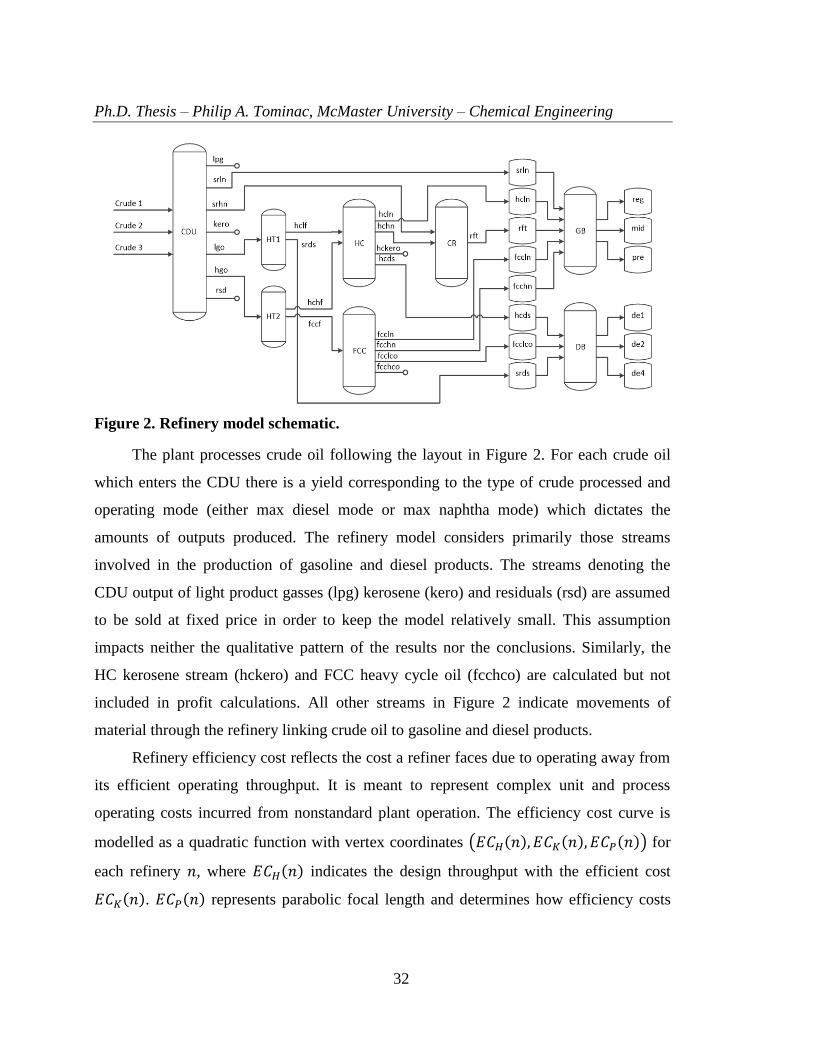
Ph.D. Thesis – Philip A. Tominac, McMaster University – Chemical Engineering
32
Figure 2. Refinery model schematic.
The plant processes crude oil following the layout in Figure 2. For each crude oil
which enters the CDU there is a yield corresponding to the type of crude processed and
operating mode (either max diesel mode or max naphtha mode) which dictates the
amounts of outputs produced. The refinery model considers primarily those streams
involved in the production of gasoline and diesel products. The streams denoting the
CDU output of light product gasses (lpg) kerosene (kero) and residuals (rsd) are assumed
to be sold at fixed price in order to keep the model relatively small. This assumption
impacts neither the qualitative pattern of the results nor the conclusions. Similarly, the
HC kerosene stream (hckero) and FCC heavy cycle oil (fcchco) are calculated but not
included in profit calculations. All other streams in Figure 2 indicate movements of
material through the refinery linking crude oil to gasoline and diesel products.
Refinery efficiency cost reflects the cost a refiner faces due to operating away from
its efficient operating throughput. It is meant to represent complex unit and process
operating costs incurred from nonstandard plant operation. The efficiency cost curve is
modelled as a quadratic function with vertex coordinates (𝐸𝐶𝐻(𝑛), 𝐸𝐶𝐾(𝑛), 𝐸𝐶𝑃(𝑛)) for
each refinery 𝑛, where 𝐸𝐶𝐻(𝑛) indicates the design throughput with the efficient cost
𝐸𝐶𝐾(𝑛). 𝐸𝐶𝑃(𝑛) represents parabolic focal length and determines how efficiency costs

Ph.D. Thesis – Philip A. Tominac, McMaster University – Chemical Engineering
33
increase with deviation from 𝐸𝐶𝐻(𝑛). A quadratic efficiency function is calculated with
the parameters in Eqs. (8), (9), and (10).
𝐸𝐶𝐴(𝑛) =
1
4(𝐸𝐶𝑃(𝑛)) (8)
𝐸𝐶𝐵(𝑛) = −
𝐸𝐶𝐻(𝑛)
2(𝐸𝐶𝑃(𝑛)) (9)
𝐸𝐶𝐶(𝑛) =
(𝐸𝐶𝐻(𝑛))2
4(𝐸𝐶𝑃(𝑛))+ 𝐸𝐶𝐾(𝑛) (10)
The total efficiency cost experienced by a refiner is the quadratic efficiency cost
multiplied by the total output from the refinery cumulatively over all products and
planning periods, and is cubic overall. Total efficiency cost is defined by Eq. (11), where
the variable 𝑃𝑟𝑐(𝑡, 𝑝, 𝑛) indicates the amount of a product produced in a given time
period by a refiner.
𝑇𝐸𝐶(𝑛) = 𝐸𝐶𝐴(𝑛) [∑∑𝑃𝑟𝑐(𝑡, 𝑝, 𝑛)
𝑝𝑡
]
3
+ 𝐸𝐶𝐵(𝑛) [∑∑𝑃𝑟𝑐(𝑡, 𝑝, 𝑛)
𝑝𝑡
]
2
+ 𝐸𝐶𝐶(𝑛)∑∑𝑃𝑟𝑐(𝑡, 𝑝, 𝑛)
𝑝𝑡
, ∀𝑛 ∈ 𝑁
(11)
The use of quadratic functions to represent refinery costs follows the arguments of
economies of scale, which we implement in a simple form as a cost which increases with
deviation from an ideal operating capacity42
. In real refinery unit operations increased
throughput can decrease efficiency because equipment may operate at non-optimal
conditions. Olefin recovery efficiency downstream of FCC units, for example, can
decrease at higher throughputs43
. The production planning model equations are included
as supplementary material. The refinery production planning model consists of Eqs. (B1)
to (B41). Model equation variants specific to a scenario are outlined in the following
subsections.

Ph.D. Thesis – Philip A. Tominac, McMaster University – Chemical Engineering
34
A demand-based Cournot oligopoly
A brief summary of the Cournot oligopoly is presented in the supplementary
material available online. We present here a modified Cournot oligopoly designed for use
with this work which assumes that if the total market production level of a product is
equal to a nominal market demand level, denoted 𝐷(𝑝,𝑤), then the market price of that
product will take a value 𝐵(𝑝,𝑤). As in the classic Cournot model, price varies linearly
with total market supply, where individual producer amounts are denoted 𝑇𝑝𝑑(𝑝, 𝑛, 𝑤)
with a product index 𝑝. The marginal value of the first unit of a product to enter the
market is defined as 𝐴(𝑝, 𝑤) + 𝐵(𝑝,𝑤), thus the price of a product 𝑝 varies according to
Eq. (12).
𝑃𝑟(𝑝, 𝑤) = 𝐴(𝑝,𝑤) + 𝐵(𝑝,𝑤) −
𝐴(𝑝,𝑤)
𝐷(𝑝,𝑤)∑𝑇𝑝𝑑(𝑝, 𝑛, 𝑤)
𝑛
∀𝑝 ∈ 𝑃,𝑤 ∈ 𝑊 (12)
The competitor profit function is defined in Eq. (13) using the definition of market
price in Eq. (12) and cost total 𝑇𝑜𝑡𝐶𝑜𝑠𝑡(𝑛). This demand-based Cournot oligopoly
problem is a potential game and forms the basis of the game theoretic refinery planning
framework.
𝐽(𝑛) =∑∑(Pr(𝑝,𝑤) 𝑇𝑝𝑑(𝑝, 𝑛, 𝑤))
𝑤𝑝
− 𝑇𝑜𝑡𝐶𝑜𝑠𝑡(𝑛) ∀𝑛 ∈ 𝑁 (13)
Potential function formulation
The potential function corresponding to the set of objectives defined in Eq. (13)
consists of the common part Ψ and the unique parts Ω(𝑛) of the objectives 𝐽(𝑛), and is
defined in Eq. (14) with definitions for Ψ and Ω(𝑛) in Eqs. (15) and (16).
max𝑍 = Ψ +∑Ω(𝑛)
𝑛
(14)
Ψ =∑
[
−𝐴(𝑝,𝑤)
𝐷(𝑝,𝑤)∑ ∑ 𝑇𝑝𝑑(𝑝, 𝑛, 𝑤)𝑇𝑝𝑑(𝑝, 𝑛′, 𝑤)
𝑛′
𝑛′<𝑛𝑛
]
𝑝,𝑤
(15)

Ph.D. Thesis – Philip A. Tominac, McMaster University – Chemical Engineering
35
Ω(𝑛) =∑[(𝐴(𝑝,𝑤) + 𝐵(𝑝,𝑤) −
𝐴(𝑝, 𝑤)
𝐷(𝑝, 𝑤)𝑇𝑝𝑑(𝑝, 𝑛, 𝑤))𝑇𝑝𝑑(𝑝, 𝑛, 𝑤)]
𝑝,𝑤
− 𝑇𝑜𝑡𝐶𝑜𝑠𝑡(𝑛) ∀𝑛 ∈ 𝑁
(16)
This form of the potential function serves as the model objective and its maxima are
Nash equilibria of strict, weak, or generalized types depending on the included
constraints. The total product leaving a refinery 𝑇𝑝𝑑(𝑝, 𝑛, 𝑤) is defined in Eq. (17) as the
sum of the product the refinery produces and the amounts which it imports. These
variables link the refinery planning model to the potential function.
𝑇𝑝𝑑(𝑝, 𝑛, 𝑤) =∑𝐷𝑙𝑣(𝑡, 𝑝, 𝑛′, 𝑤)
𝑡
+ 𝐼𝑚𝑝(𝑝, 𝑛, 𝑤) (17)
Fixed-price analysis
Current practices generally use fixed prices in refinery planning models, generally
assuming that prices will become known prior to the planning period2; we compare the
outcomes of such analyses with game theoretic results. Our scenarios are examined under
a fixed-price profit maximization framework using the objective in Eq. (18). This
objective is the total profit of all refiners. Revenues are calculated based on fixed market
prices 𝐹(𝑝,𝑤) and are linear calculations; the only nonlinearity in this variant is the
efficiency cost calculation.
max𝑍 =∑(∑(𝐹(𝑝,𝑤)𝑇𝑝𝑑(𝑝, 𝑛, 𝑤))
𝑝
− 𝑇𝑜𝑡𝐶𝑜𝑠𝑡(𝑛))
𝑛
(18)
The domestic market supply constraints defined by Eqs. (B40) and (B41) enforce
refiner coordination. With exception to these constraints, refiners are independent of one
another in terms of their decision making; their profits are not interdependent under this
objective.

Ph.D. Thesis – Philip A. Tominac, McMaster University – Chemical Engineering
36
Model alterations for Scenario 2
The game theoretic model is modified such that high-cost refiners are linked to a
binary variable that is incorporated into the high-cost refiner model equations in order to
allow all flow rates, inventories, and outputs to be set to zero, effectively shutting down
those refiners. The continued participation of high-cost refiners is dependent on a binary
variable 𝑌𝐻𝐶𝑁(𝑤). High-cost refiners are also limited to a decreased production level
𝐻𝐶𝑁𝑠𝑒𝑡 using Eq. (19), and are prevented from making import purchases in this scenario.
These changes define the characteristics of the high-cost refiner, along with its parameter
values.
∑∑𝑃𝑟𝑐(𝑡, 𝑝, 𝑛) = 𝑌𝐻𝐶𝑁(𝑤)𝐻𝐶𝑁𝑠𝑒𝑡
𝑝𝑡
∀ (𝑛, 𝑤) ∈ 𝑊𝐻𝐶𝑁(𝑛,𝑤) (19)
The participation binary is also used to relax variable bound constraints in
Eqs. (B3), (B4), (B10), (B12), (B13), (B19), (B20), (B27), and (B29)-(B32); each use the
binary variable to reduce a constraint value to zero if the value of 𝑌𝐻𝐶𝑁(𝑤) is zero in
order to deactivate the high-cost refiner model. The potential function term Ω(𝑛) is
altered to include the price increase 𝐴𝐻𝐶(𝑝, 𝑤) corresponding to the presence or absence
of the high-cost refiner defined in Eq. (20).
Ω(𝑛) =∑ ∑
[
(
𝐴(𝑝,𝑤) + 𝐴𝐻𝐶(𝑝, 𝑤) ∑ 𝑌𝐻𝐶𝑁(𝑤
′)
𝑤′
𝑤′∈𝑊𝐿𝑁
𝑤𝑤∈𝑊𝑁(𝑛,𝑤)
𝑝
+ 𝐵(𝑝,𝑤) −𝐴(𝑝, 𝑤)
𝐷(𝑝, 𝑤)𝑇𝑝𝑑(𝑝, 𝑛, 𝑤)
)
𝑇𝑝𝑑(𝑝, 𝑛, 𝑤)
]
− 𝑇𝑜𝑡𝐶𝑜𝑠𝑡(𝑛) ∀𝑛 ∈ 𝑁
(20)
This version of Ω(𝑛) contains a bilinear term of the form 𝑌𝐻𝐶𝑁(𝑤)𝑇𝑝𝑑(𝑝, 𝑛, 𝑤)
which has an exact linearization obtained by introducing two variables and the constraints
in Eqs. (21), (22), and (23). This linearization technique reduces the number of model
nonlinearities and is described in more detail by You and Grossmann44
. The presented

Ph.D. Thesis – Philip A. Tominac, McMaster University – Chemical Engineering
37
formulation allows multiple high-cost refiners to exist in a single domestic market, and
dictates their activity on an all-or-none basis. The upper bound 𝑇𝑝𝑑̅̅ ̅̅ ̅(𝑝, 𝑛, 𝑤) represents
the total combined processing capacity of a refiner plus its product import limit.
𝑇𝑃(𝑝, 𝑛, 𝑤,𝑤′) + 𝑇𝑃1(𝑝, 𝑛, 𝑤,𝑤′) = 𝑇𝑝𝑑(𝑝, 𝑛, 𝑤)
∀𝑝 ∈ 𝑃, 𝑛 ∈ 𝑁, (𝑤,𝑤′) ∈ 𝑊 (21)
𝑇𝑃(𝑝, 𝑛, 𝑤, 𝑤′) ≤ 𝑌𝐻𝐶𝑁(𝑤′)𝑇𝑝𝑑̅̅ ̅̅ ̅(𝑝, 𝑛, 𝑤) ∀𝑝 ∈ 𝑃, 𝑛 ∈ 𝑁, (𝑤,𝑤′) ∈ 𝑊 (22)
𝑇𝑃1(𝑝, 𝑛, 𝑤) ≤ (1 − 𝑌𝐻𝐶𝑁(𝑤′))𝑇𝑝𝑑̅̅ ̅̅ ̅(𝑝, 𝑛, 𝑤) ∀𝑝 ∈ 𝑃, 𝑛 ∈ 𝑁, (𝑤,𝑤′) ∈ 𝑊 (23)
With this linearization Eq. (20) can be rewritten as in Eq. (24), which is the form of
the equation implemented in the elimination scenario and is denoted ΩK(𝑛) in order to
differentiate it from the version used in other scenarios.
ΩK(𝑛) =∑ ∑
[ (𝐴(𝑝, 𝑤) + 𝐵(𝑝,𝑤))𝑇𝑝𝑑(𝑝, 𝑛, 𝑤)
𝑤𝑤∈𝑊𝑁(𝑛,𝑤)
𝑝
+
(
𝐴𝐻𝐶(𝑝,𝑤) ∑ 𝑇𝑃(𝑝, 𝑛, 𝑤,𝑤′)
𝑤′
𝑤′∈𝑊𝐿𝑁 )
−𝐴(𝑝,𝑤)
𝐷(𝑝,𝑤)(𝑇𝑝𝑑(𝑝, 𝑛, 𝑤))
2
] − 𝑇𝑜𝑡𝐶𝑜𝑠𝑡(𝑛) ∀𝑛 ∈ 𝑁
(24)
The elimination scenario is intended to determine whether low-cost refiners in a
domestic market are better off with or without high-cost refiners. High-cost refiners’
production decisions cannot be part of the potential function in this scenario. Exclusion of
the high-cost refiners assures that the comparison made regarding the elimination
decision includes only the interests of the low-cost refiners and their preferences
regarding the market structure. Since the high-cost refiners are not included in the
objective function, their decision variables must be fixed to game theoretically rational
values. A two-stage solution process is used to solve this problem. In the first stage all
refiners are active under a full potential function generating the optimal game theoretic
production decisions for all refiners. This first stage amounts to solving a Scenario 1

Ph.D. Thesis – Philip A. Tominac, McMaster University – Chemical Engineering
38
problem where the high-cost refiner is unable to import product and effects a price
increase in its domestic market. In the second stage of the solution process the potential
function is generated with ΩK(𝑛) for the low-cost refiners which captures their profits and
the price increase effected by the high-cost refiner. The variable Ψ is generated over all
refiners and captures the decrease in market prices caused by their collective production
decisions, including the fixed first stage values assigned to the high-cost refiner. The
second stage thus represents the interests of only the low-cost refiners. Any product
profile could be assigned to the high-cost refiner in order to solve the Scenario 2 problem;
generating the high-cost refiner’s profile using the first stage ensures that the decision is
rational with respect to game theoretic analysis. In this scenario we assume that high-cost
refiners behave as they would in S1 if active; we do not examine cases where high-cost
refiners could modify their behaviour in order to remain active, i.e., limiting their
production to levels that would encourage low-cost refiners to allow them to remain
operational. The potential function used in the second stage is formulated as in Eq. (25).
max𝑍 = Ψ+ ∑ ΩK(𝑛)
𝑛∈𝐿𝐶𝑁
(25)
The fixed price approach to the elimination problem is formulated using the
objective function in Eq. (26).
max𝑍 = ∑
(
∑
(
(
𝐹(𝑝,𝑤)
𝑝𝑛𝑛∈𝐿𝐶𝑁
+ 𝐴𝐻𝐶(𝑝,𝑤) ∑ 𝑌𝐻𝐶𝑁(𝑤′)
𝑤′
𝑤′∈𝑊𝐿𝑁 )
𝑇𝑝𝑑(𝑝, 𝑛, 𝑤)
)
− 𝑇𝑜𝑡𝐶𝑜𝑠𝑡(𝑛)
)
(26)

Ph.D. Thesis – Philip A. Tominac, McMaster University – Chemical Engineering
39
Results and Discussion
Scenario basis and data
The scenarios presented in this work are based as much as possible on the Canadian
national fuel market using data from 2014. Each scenario is based on the same example
involving three refineries acting in a domestic market 𝐿𝑀1 with access to an global
market 𝐸𝑀1. Product demand is scaled down to an appropriate level corresponding to the
total combined production capacity existing among the three refineries. All numerical and
structural problem data are included as supplementary material.
Market demands 𝐷(𝑝,𝑤) for the six products in the scenarios are calculated based
on historical Canadian national consumption using data from Statistics Canada for
gasoline and diesel products. The published net consumer sales of gasoline and diesel
provide the baseline for demand, but the reported net gasoline and diesel sales are not
listed by grade45
. The fraction of demand associated with each product grade is calculated
using the Canadian gasoline and diesel totals assuming that the sales by grade can be
approximated using consumer sales data for the relevant gasoline and diesel product
grades in the USA in 2014 made available by the EIA46,47
. These values are scaled to 18%
and 21% of the real total in order to create domestic and global market demand totals with
values scaling to the same order of magnitude as the combined production capacity of the
three refineries.
The product pricing structure is based on weekly national average price data from
2014 published by Natural Resources Canada. Data are available for regular, mid-grade,
and premium gasoline48,49,50
. Data is also available for diesel fuel, but due to changes in
the sale of diesel fuels the majority of diesel fuel sold for commercial purposes consists of
a single grade51,52
. We take the average price of each corresponding fuel in 2014 as
𝐵(𝑝,𝑤) in both markets. In order to account for the different grades of diesel, the average
diesel price obtained from Natural Resources Canada data is assigned to fuel oil type 2
and the price for fuel oil types 1 and 4 are calculated as one standard deviation above and
below that price based on the available data. The marginal value of the first unit of each

Ph.D. Thesis – Philip A. Tominac, McMaster University – Chemical Engineering
40
product on the market is calculated using a value of 𝐴(𝑝,𝑤) equal to three standard
deviations of price. Thus the price of the first unit of product corresponds roughly to the
highest observed price in the data, and the price resulting from a supply of twice 𝐷(𝑝,𝑤)
to the lowest, fitting the product demand space to the available price data. The values of
𝐴𝐻𝐶(𝑝,𝑤) are taken to be 5% of the value of one standard deviation of the calculated
prices, e.g., 5% of ⅓ of 𝐴(𝑝,𝑤) in the domestic market and zero elsewhere; 𝐶𝐼(𝑝, 𝑤) is
120% of 𝐵(𝑝, 𝑤), and 𝐹(𝑝,𝑤) is calculated as the sum of 𝐴(𝑝, 𝑤) and 𝐵(𝑝,𝑤) meaning
that the fixed price in the corresponding examples is the price of the first unit sold in the
equivalent game theoretic scenario.
The primary operating cost burden to the refiner is the purchase price of crude oil.
In this work crude oil prices are denoted by parameter 𝐶𝑜𝑠𝑡(𝑖) and are considered to be
constant. Three crude oil stocks are available on the market: a light sweet, a medium, and
a heavy sour variety. The prices for these crude oils are chosen from representative
average monthly prices of benchmark crude oils reported by Natural Resources Canada,
using Canadian Light Chicago, Canadian Light Sweet, Canadian Heavy Chicago, and
Canadian Heavy Hardisty prices to generate three representative crude stock prices at
610.20, 577.30, and 535.04 dollars per cubic meter53
. Yield values in the production
planning model are calculated based on assays for three crude oil stocks produced by
ExxonMobil: Hibernia, a light blend, Terra Nova, a medium crude, and Cold Lake, a
heavy sour crude54,55,56
. Yields are computed for max naphtha and max diesel CDU
operating modes using data from Fu, Sanchez, and Mahalec57
.
The two scenarios presented in this work are referred to using the notation S1 and
S2 for convenience. Associated with each of these scenarios are two additional variations.
The first is a version of the game theoretic scenario excluding upper capacity limits on
refinery units such that refiners are capable of processing unlimited amounts of material.
This variant is intended to illustrate the relationship between unit capacity constraints and
Nash equilibria, and is denoted by adding –G to the scenario name. The second variant
solves the scenario problem under fixed prices for contrast with the game theoretic
planning results. The fixed price variants are referred to by appending each model name

Ph.D. Thesis – Philip A. Tominac, McMaster University – Chemical Engineering
41
with –F. Equation listings for each scenario are given in Table 1. All set and parameter
data is included as supplementary material.
Table 1. Scenario nomenclature and corresponding equations.
Scenario Equation list
S1 (11), (14) to (17), and (B1) to (B41)
S1-G (11), (14) to (17), (B1) to (B41), excluding: (B4), (B13), (B20), and (B30)
S1-F (11), (18), and (B1) to (B41)
S2 (11), (17), (19), (21) to (25), and (B1) to (B41)
S2-G (11), (17), (19), (21) to (25), and (B1) to (B41), excluding: (B4), (B13), (B20),
and (B30)
S2-F (11), (19), (26), and (B1) to (B41)
Scenario 1 results
Results are characterized entirely by refiner production decisions interpreted
through the potential function as profits. Market prices and individual refiner profits are
implicitly defined in the potential function and do not appear directly in the model. The
production volumes resulting in S1 are presented in Figure 3 and correspond to the
variables 𝑇𝑝𝑑(𝑝, 𝑛, 𝑤). Domestic and import production volumes satisfy domestic market
demand while production excesses of gasoline products are exported in order to take
advantage of higher global market prices. Refiners have similar optimal production plans
which scale according to refinery capacity. In the case that all three refiners are identical
in size, their production volumes will be symmetric. Import volumes scale inversely with
refinery size; smaller refiners import more than larger ones.
Refiners do not have the capacity to satisfy domestic market diesel demand to the
minimum constraint level and must import to do so. Each refiner produces some portfolio
of diesel products up to its capacity, and then imports the balance volumes of each of
these products in such a way that all refiners supply the same volume of each diesel
product in order to satisfy domestic market demands. Larger refiners are able to produce
more diesel in-house and import less. The cumulative amount produced by the refiners
satisfies precisely the lower supply limit. Similarly, refiners produce identical amounts of
diesel 1 without imports; the cumulative volume satisfies the minimum supply. This
pattern is not observed for gasoline products, in which case refiners produce amounts

Ph.D. Thesis – Philip A. Tominac, McMaster University – Chemical Engineering
42
varying with their capacity for both domestic and global markets. This result suggests that
game theoretic planning drives refiners to compete on marginally more profitable
products and to allocate production equally for less profitable products. We note that the
observed results are strongly dependent on refinery production capacities; e.g., refineries
configured for diesel would have a reversed pattern of production volumes.
Figure 3. S1 production volume breakdown and totals by refiner and scenario
variant.
The results of S1-G are presented in Figure 3 for comparison with S1. The total
amount of diesel product is unchanged from S1 (minimum domestic supply is satisfied)
but the amounts of gasoline product produced are increased. No product is supplied in the
domestic market at an amount large enough to reach the upper constraint level; the
solution in the domestic market is defined by Nash equilibrium prices, not domestic
supply constraints. Import amounts in S1-G are unchanged from S1. This outcome
suggests that with unlimited production capacity it is not profitable to produce any more
diesel products than those required in the domestic market, and that the most cost
effective means of obtaining those products is to produce a fraction and import the
balance, where the decision is driven by prices, not capacity constraints.
Refiners export more gasoline product to the global market in S1-G than S1.
Despite unconstrained capacities the refiners halt production at a price point representing
a Nash equilibrium, contrasting with the different equilibrium obtained in S1 defined by
capacity constraints. Refiners continue to plan production according to their sizes due to
efficiency costs.

Ph.D. Thesis – Philip A. Tominac, McMaster University – Chemical Engineering
43
The production volumes obtained from the solution of S1-F are shown in Figure 3.
Total domestic market supply satisfies the upper and lower demand constraints, but
production volumes associated with each refiner do not follow a competitively optimal
pattern. In S1-F prices are fixed and the objective is total refiner profit. The allocation of
production is that which maximizes total market profit regardless of individual profits.
This result is unobtainable barring a monopoly; an individual refiner will not yield profits
because a competitor has a better marginal gain. This fixed price approach does not
generate competitively optimal behaviour. Refiners only export premium gasoline as
there is no consideration of market demand levels. We present this result to illustrate the
driving forces at play in fixed priced models.
The results of S1, S1-G, and S1-F also serve to illustrate the role of flexibility in the
refinery model. Although capacity to produce diesel is limited, the refinery models
implemented in this work are flexible in the production of gasoline products. The refiners
are capable of much larger throughput than in S1, as seen in S1-G and S1-F where total
product is higher. They are also capable of changing product ratios, as seen by comparing
S1 and S1-F. This flexibility allows refiners to reach a Nash equilibrium defined
primarily by throughput constraints rather than individual product limitations.
The prices and profits associated with these three cases and for all scenarios are
collected in Table 2 and Table 3. In S1-G refiners produce more than in S1; refiners R1
and R2 lose profits in S1-G while R3 gains. This illustrates the rationality of Nash
equilibria: refiners will not be worse off in terms of their own profits if any others behave
differently; they can make gains if competitors deviate from equilibrium strategies. In this
case R1 lost profits in S1-G relative to S1, but could stand to gain if R2 or R3 made a
non-equilibrium plan. The profits reported in S1-F by comparison are much higher, and
are unrealistic in a game-theoretic sense.
Table 2. Profit values by scenario (106 CAD).
R1 R2 R3
S1 97.82 52.81 4.24
S1-G 71.61 50.73 30.18
S1-F 1102.98 971.85 899.27
S2 47.96 0.72 121.11

Ph.D. Thesis – Philip A. Tominac, McMaster University – Chemical Engineering
44
S2-G 132.81 95.60 0.00
S2-F 1112.83 1014.83 646.16
The prices in scenarios S1 and S1-G illustrate the Cournot property: as refiners
supply more of a product, its price drops. In S1-F the prices reported are the highest
possible due to the assumption of fixed prices (under FIXED heading). The equivalent
game theoretic prices (under EQUIV. heading) corresponding to the market supplies in
S1-F are correspondingly lower and, in the case of the price of premium gasoline in the
global market, substantially lower than those observed in the game theoretic version
where consideration of market demand and price limits the total volume of premium
gasoline supplied to a rational level.
Table 3. Scenario prices (CAD/m3). S1-F and S2-F show fixed price values and the
equivalent game theoretic Cournot prices corresponding to the production levels in
those scenarios.
MARKET PRODUCT S1 S1-G S1-F S2 S2-G S2-F
FIXED EQUIV. FIXED EQUIV.
LOCAL REG 912.18 912.18 1130.49 909.72 916.22 912.18 1134.53 909.72
MID 977.00 958.01 1183.36 911.64 980.82 977.00 1187.18 911.64
PRE 1028.12 971.91 1238.94 959.67 1032.02 1021.10 1242.84 959.67
DE1 1089.39 1089.39 1238.58 1042.34 1092.15 1089.39 1241.34 1042.34
DE2 1034.13 1034.13 1183.33 1036.14 1036.90 1034.13 1186.09 1036.14
DE4 978.88 978.88 1128.07 980.89 981.64 978.88 1130.83 980.89
GLOBAL REG 1003.27 924.58 1049.64 1049.64 1008.15 958.00 1049.64 1043.54
MID 1017.59 938.91 1106.93 1106.93 1022.47 977.10 1106.93 1086.84
PRE 1031.07 952.39 1160.86 -367.68 1035.96 995.07 1160.86 70.25
DE1 1183.33 1183.33 1183.33 1183.33 1183.33 1183.33 1183.33 1183.33
DE2 1128.07 1128.07 1128.07 1128.07 1128.07 1128.07 1128.07 1128.07
DE4 1072.81 1072.81 1072.81 1072.81 1072.81 1072.81 1072.81 1072.81
Scenario 2 results
The purpose of this scenario is to examine conditions under which strategic
planning can incorporate large scale decisions affecting the structure of the market.
Results are presented for S2 in Figure 4 in which the high-cost refiner R3 continues to
participate in the market, and are similar to the production plans in S1, but the high-cost
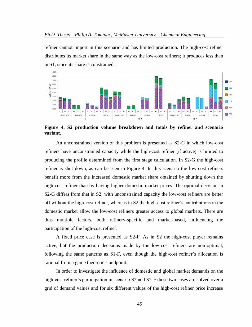
Ph.D. Thesis – Philip A. Tominac, McMaster University – Chemical Engineering
45
refiner cannot import in this scenario and has limited production. The high-cost refiner
distributes its market share in the same way as the low-cost refiners; it produces less than
in S1, since its share is constrained.
Figure 4. S2 production volume breakdown and totals by refiner and scenario
variant.
An unconstrained version of this problem is presented as S2-G in which low-cost
refiners have unconstrained capacity while the high-cost refiner (if active) is limited to
producing the profile determined from the first stage calculation. In S2-G the high-cost
refiner is shut down, as can be seen in Figure 4. In this scenario the low-cost refiners
benefit more from the increased domestic market share obtained by shutting down the
high-cost refiner than by having higher domestic market prices. The optimal decision in
S2-G differs from that in S2; with unconstrained capacity the low-cost refiners are better
off without the high-cost refiner, whereas in S2 the high-cost refiner’s contributions in the
domestic market allow the low-cost refiners greater access to global markets. There are
thus multiple factors, both refinery-specific and market-based, influencing the
participation of the high-cost refiner.
A fixed price case is presented as S2-F. As in S2 the high-cost player remains
active, but the production decisions made by the low-cost refiners are non-optimal,
following the same patterns as S1-F, even though the high-cost refiner’s allocation is
rational from a game theoretic standpoint.
In order to investigate the influence of domestic and global market demands on the
high-cost refiner’s participation in scenario S2 and S2-F these two cases are solved over a
grid of demand values and for six different values of the high-cost refiner price increase

Ph.D. Thesis – Philip A. Tominac, McMaster University – Chemical Engineering
46
𝐴𝐻𝐶(𝑝,𝑤). Demand scaling factors for all products are taken at 19 even intervals ranging
from 6% to 25.3% of the demand values 𝐷(𝑝,𝑤) included as supplementary data. The
test values for the price increase 𝐴𝐻𝐶(𝑝,𝑤) are taken at 10% intervals ranging from 5%
up to 55% of the standard deviation of product price calculated from Statistics Canada
data as described earlier in this work. These values are reported in the supplementary
material available online.
Objective values are calculated for the six values of 𝐴𝐻𝐶(𝑝,𝑤) and are used to
define contours characterizing the inclusion region boundary. These boundary lines are
visualized in Figure 5 as solid lines labeled with the associated price increase percentage.
As the high-cost refiner’s presence brings larger price increases, the minimum domestic
and global demands at which it will be shut down decrease. This result is intuitive; as the
benefit accrued by low-cost refiners increases, they become more tolerant of the high-cost
refiner in smaller markets.

Ph.D. Thesis – Philip A. Tominac, McMaster University – Chemical Engineering
47
Figure 5. Inclusion region boundary characterization for S2; boundaries define
paired domestic and global demand levels (as scaled values) below which low-cost
refiners shut down the high-cost refiner with the indicated price increase.
Results are shown for the inclusion region associated with S2-F as dashed lines.
Boundary lines are shown for values of 𝐴𝐻𝐶(𝑝,𝑤) equal to 5%, 15%, and 25% of
𝐴(𝑝,𝑤) for domestic market prices; no such boundary lines are found for values of 35%
or greater, in which case the high cost refiner is allowed to remain active for all demand
levels tested. Under fixed price analysis, the low-cost refiners will mistakenly allow the

Ph.D. Thesis – Philip A. Tominac, McMaster University – Chemical Engineering
48
high-cost refiner to operate when its impacts will reduce their profits, instead of
increasing them as they would predict.
Existence of multiple equilibria
Multiple Nash equilibria may exist in continuous games; our potential game
formulation is nonconvex and we identify equilibria of the generalized type as globally
optimal solutions. The existence of equilibria with equal objective value is of interest to
determine whether normalization is required. To ascertain whether equal-valued
equilibria exist in this problem, we constrain the potential function to the obtained
optimal value 𝑍∗ and modify the objective function to drive refiners’ individual decision
variables to different values corresponding to the same optimum. Changes in
𝐷𝑙𝑣(𝑡, 𝑝, 𝑛, 𝑤) or 𝐼𝑚𝑝(𝑝, 𝑛, 𝑤) yielding 𝑍∗ constitute equal valued alternative equilibria.
We were unable to find alternative Nash equilibria using this approach, suggesting that
there is a single globally optimal Nash equilibrium under the implemented formulation
and data set. Since the equilibrium is unique, we are not concerned with normalization to
characterize a best equilibrium solution30
.
Model solution statistics
All results are generated on a Dell Optiplex 9010 computer with Intel Core-i7-3770
CPU and a 3.40 GHz processor running the Windows 10 64-bit operating system. Models
are solved using GAMS 24.7.1 with ANTIGONE 1.158
warm starting with
CONOPT 3.17A or DICOPT. Solution data for each scenario are given in Table 4
including preprocessing results.
Solution results consist of the objective function value and optimality gap data
reported by the solver, as well as the model statistics generated by GAMS. The model
status indicates the optimality of the solution achieved; scenarios with a model status of 1
are solved to global optimality; a model status of 2 indicates local optimality. All
scenarios presented are solved to global optimality with a relative gap of 1×10⁻⁹
. The
processed model sizes generated by ANTIGONE are also reported; these indicate the

Ph.D. Thesis – Philip A. Tominac, McMaster University – Chemical Engineering
49
types of equations, variables, and nonlinear terms detected by the solver and provide
additional model information. The relative gap and CPU time reported by ANTIGONE
are also included. The CPU times are essentially the same as those reported by GAMS,
but exclude model generation time.
Table 4. Solution data.
S1 S1-G S1-F S2 S2-G S2-F
Model statistics (GAMS)
Single equations 1833 1713 1753 2121 2009 1825
Single variables 1245 1245 1165 1376 1376 1140
Nonlinear entities 111 111 3 55 55 20
Solve summary (ANTIGONE)
Objective value 871.7855 1182.4504 2974.0996 354.0593 864.1746 2127.6622
Model status 1 1 1 1 1 1
Resource usage 0.364 1.534 0.151 0.583 0.885 0.541
After pre-processing
Variables 531 531 513 498 498 438
Continuous 531 531 513 497 497 437
Binary
1 1 1
Equations 1153 1153 1063 1172 1162 1004
Linear 1077 1077 1060 1132 1122 1000
Convex nonlinear
Nonconvex nonlinear 76 76 3 40 40 4
Nonlinear terms 348 348 6 194 194 80
Bilinear/quadratic 345 345 3 192 192 78
Sigmoidal 3 3 3 2 2 2
Solve statistics
Relative gap 1.00E-09 1.00E-09 1.00E-09 1.00E-09 1.00E-09 1.00E-09
Total time (CPU s) 0.35 1.43 0.15 0.56 0.81 0.44
Conclusions
We have presented a game theoretic strategic production planning framework based
on a modified Cournot oligopoly formulated as a potential game which we use to solve
strategic refinery production planning problems to Nash equilibrium solutions. Two
scenarios have been presented illustrating competitive behaviour in production planning

Ph.D. Thesis – Philip A. Tominac, McMaster University – Chemical Engineering
50
problems. The first scenario illustrates competitive behaviour in the game theoretic sense
and contrasts those results with equivalent fixed price planning results. The second
scenario extends the framework to include a decision to shut down a competitor by
claiming its market share. This scenario illustrates how competitive behaviour manifests
in problems involving market restructuring and that the inclusion of planning decisions
influences the outcome. In both scenarios, the results of production planning in a game
theoretic framework were contrasted with those obtained by solving the same problem
under the assumption of fixed prices. Making production planning decisions in a
competitive context is a non-obvious problem, particularly so when market restructuring
decisions are involved, and using fixed price methods does not yield competitively
optimal solutions in either case. The importance of competitive planning arises from the
reality that most industries operate under competition. The proposed potential game
framework demonstrates that refinery production planning benefits from game theoretic
analysis.
Notation
Sets
𝐵𝐿 (𝑏𝑙) set of blenders
𝐼 (𝑖) set of process streams
𝐼𝐶 (𝑖) set of crude oils streams entering refinery
𝑀 (𝑚) set of unit operating modes
𝑁 (𝑛) set of refineries
𝑃 (𝑝) set of products
𝑄 (𝑞) set of quality properties
𝑊 (𝑤) set of markets
𝑇 (𝑡) set of time periods in which planning takes place
𝑇𝐾 (𝑡𝑘) set of tanks for intermediates
𝑈 (𝑢) set of process units
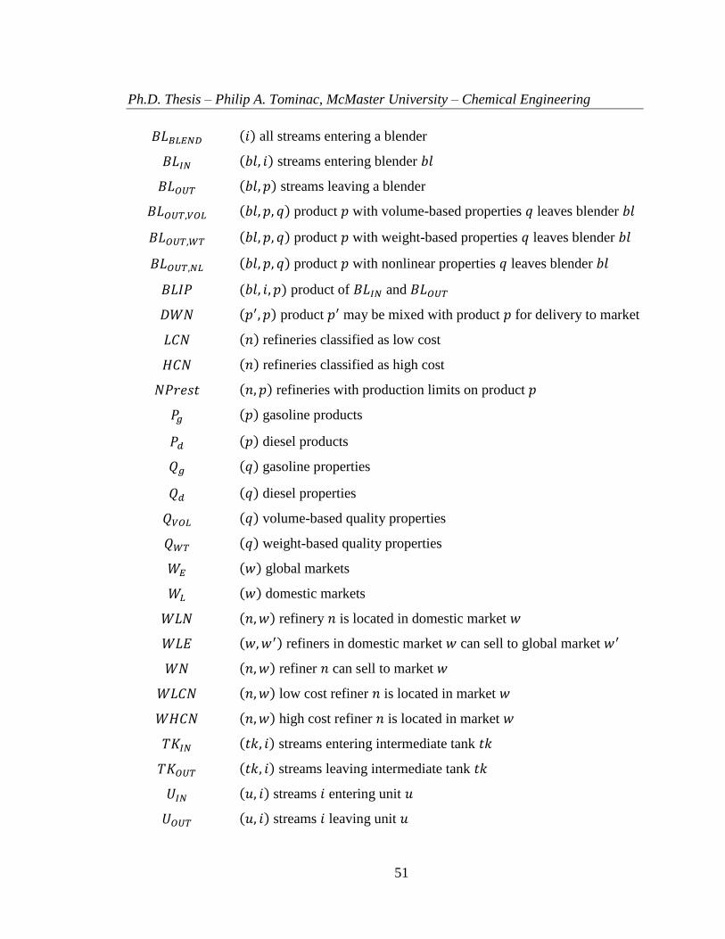
Ph.D. Thesis – Philip A. Tominac, McMaster University – Chemical Engineering
51
𝐵𝐿𝐵𝐿𝐸𝑁𝐷 (𝑖) all streams entering a blender
𝐵𝐿𝐼𝑁 (𝑏𝑙, 𝑖) streams entering blender 𝑏𝑙
𝐵𝐿𝑂𝑈𝑇 (𝑏𝑙, 𝑝) streams leaving a blender
𝐵𝐿𝑂𝑈𝑇,𝑉𝑂𝐿 (𝑏𝑙, 𝑝, 𝑞) product 𝑝 with volume-based properties 𝑞 leaves blender 𝑏𝑙
𝐵𝐿𝑂𝑈𝑇,𝑊𝑇 (𝑏𝑙, 𝑝, 𝑞) product 𝑝 with weight-based properties 𝑞 leaves blender 𝑏𝑙
𝐵𝐿𝑂𝑈𝑇,𝑁𝐿 (𝑏𝑙, 𝑝, 𝑞) product 𝑝 with nonlinear properties 𝑞 leaves blender 𝑏𝑙
𝐵𝐿𝐼𝑃 (𝑏𝑙, 𝑖, 𝑝) product of 𝐵𝐿𝐼𝑁 and 𝐵𝐿𝑂𝑈𝑇
𝐷𝑊𝑁 (𝑝′, 𝑝) product 𝑝′ may be mixed with product 𝑝 for delivery to market
𝐿𝐶𝑁 (𝑛) refineries classified as low cost
𝐻𝐶𝑁 (𝑛) refineries classified as high cost
𝑁𝑃𝑟𝑒𝑠𝑡 (𝑛, 𝑝) refineries with production limits on product 𝑝
𝑃𝑔 (𝑝) gasoline products
𝑃𝑑 (𝑝) diesel products
𝑄𝑔 (𝑞) gasoline properties
𝑄𝑑 (𝑞) diesel properties
𝑄𝑉𝑂𝐿 (𝑞) volume-based quality properties
𝑄𝑊𝑇 (𝑞) weight-based quality properties
𝑊𝐸 (𝑤) global markets
𝑊𝐿 (𝑤) domestic markets
𝑊𝐿𝑁 (𝑛, 𝑤) refinery 𝑛 is located in domestic market 𝑤
𝑊𝐿𝐸 (𝑤,𝑤′) refiners in domestic market 𝑤 can sell to global market 𝑤′
𝑊𝑁 (𝑛, 𝑤) refiner 𝑛 can sell to market 𝑤
𝑊𝐿𝐶𝑁 (𝑛, 𝑤) low cost refiner 𝑛 is located in market 𝑤
𝑊𝐻𝐶𝑁 (𝑛, 𝑤) high cost refiner 𝑛 is located in market 𝑤
𝑇𝐾𝐼𝑁 (𝑡𝑘, 𝑖) streams entering intermediate tank 𝑡𝑘
𝑇𝐾𝑂𝑈𝑇 (𝑡𝑘, 𝑖) streams leaving intermediate tank 𝑡𝑘
𝑈𝐼𝑁 (𝑢, 𝑖) streams 𝑖 entering unit 𝑢
𝑈𝑂𝑈𝑇 (𝑢, 𝑖) streams 𝑖 leaving unit 𝑢
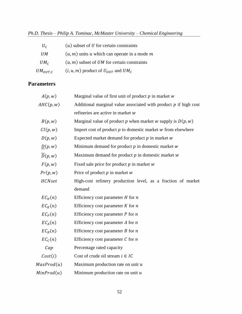
Ph.D. Thesis – Philip A. Tominac, McMaster University – Chemical Engineering
52
𝑈𝐶 (𝑢) subset of 𝑈 for certain constraints
𝑈𝑀 (𝑢,𝑚) units 𝑢 which can operate in a mode 𝑚
𝑈𝑀𝐶 (𝑢,𝑚) subset of 𝑈𝑀 for certain constraints
𝑈𝑀𝑂𝑈𝑇,𝐶 (𝑖, 𝑢, 𝑚) product of 𝑈𝑂𝑈𝑇 and 𝑈𝑀𝐶
Parameters
𝐴(𝑝, 𝑤) Marginal value of first unit of product 𝑝 in market 𝑤
𝐴𝐻𝐶(𝑝, 𝑤) Additional marginal value associated with product 𝑝 if high cost
refineries are active in market 𝑤
𝐵(𝑝, 𝑤) Marginal value of product 𝑝 when market 𝑤 supply is 𝐷(𝑝,𝑤)
𝐶𝐼(𝑝, 𝑤) Import cost of product 𝑝 to domestic market 𝑤 from elsewhere
𝐷(𝑝, 𝑤) Expected market demand for product 𝑝 in market 𝑤
𝐷(𝑝, 𝑤) Minimum demand for product 𝑝 in domestic market 𝑤
𝐷(𝑝, 𝑤) Maximum demand for product 𝑝 in domestic market 𝑤
𝐹(𝑝,𝑤) Fixed sale price for product 𝑝 in market 𝑤
𝑃𝑟(𝑝,𝑤) Price of product 𝑝 in market 𝑤
𝐻𝐶𝑁𝑠𝑒𝑡 High-cost refinery production level, as a fraction of market
demand
𝐸𝐶𝐻(𝑛) Efficiency cost parameter 𝐻 for 𝑛
𝐸𝐶𝐾(𝑛) Efficiency cost parameter 𝐾 for 𝑛
𝐸𝐶𝑃(𝑛) Efficiency cost parameter 𝑃 for 𝑛
𝐸𝐶𝐴(𝑛) Efficiency cost parameter 𝐴 for 𝑛
𝐸𝐶𝐵(𝑛) Efficiency cost parameter 𝐵 for 𝑛
𝐸𝐶𝐶(𝑛) Efficiency cost parameter 𝐶 for 𝑛
𝐶𝑎𝑝 Percentage rated capacity
𝐶𝑜𝑠𝑡(𝑖) Cost of crude oil stream 𝑖 ∈ 𝐼𝐶
𝑀𝑎𝑥𝑃𝑟𝑜𝑑(𝑢) Maximum production rate on unit 𝑢
𝑀𝑖𝑛𝑃𝑟𝑜𝑑(𝑢) Minimum production rate on unit 𝑢

Ph.D. Thesis – Philip A. Tominac, McMaster University – Chemical Engineering
53
𝑉(𝑡𝑘) Maximum holding in intermediate tank 𝑡𝑘
𝑉(𝑡𝑘) Minimum holding in intermediate tank 𝑡𝑘
𝑉𝑖𝑛𝑖(𝑡𝑘) Initial holding in intermediate tank 𝑡𝑘
𝑉𝑃(𝑝) Maximum holding in product tank 𝑝
𝑉𝑃(𝑝) Minimum holding in product tank 𝑝
𝑉𝑃𝑖𝑛𝑖(𝑝) Initial holding in product tank 𝑝
𝐵𝑙𝑒𝑛𝑑𝑀𝑎𝑥(𝑏𝑙) Maximum blending rate for blender 𝑏𝑙
𝐵𝑙𝑒𝑛𝑑𝑀𝑖𝑛(𝑏𝑙) Minimum blending rate for blender 𝑏𝑙
𝐵𝐿𝑐𝑜𝑠𝑡(𝑏𝑙) Cost of operating blender 𝑏𝑙
𝜏(𝑡) Duration of time period 𝑡
𝑂𝑝𝐶𝑜𝑠𝑡(𝑢,𝑚) Operating cost of unit 𝑢 in mode 𝑚
𝑃𝑟𝑜𝑑𝑅𝑒𝑠𝑡(𝑛, 𝑝) Restriction on refinery 𝑛 production level of product 𝑝
𝑞𝑞(𝑖, 𝑞) Quality property 𝑞 of stream 𝑖
𝑄(𝑞, 𝑝) Maximum quality specification of property 𝑞 for product 𝑝
𝑄(𝑞, 𝑝) Minimum quality specification of property 𝑞 for product 𝑝
𝑅(𝑖, 𝑝) Maximum specification of stream 𝑖 for product 𝑝
𝑅(𝑖, 𝑝) Minimum specification of stream 𝑖 for product 𝑝
𝑇𝐶 Time scaling cost factor
𝑇𝑝𝑑(𝑝, 𝑛, 𝑤) Total product variable upper bound
𝑌(𝑖,𝑚, 𝑢) Yield of stream 𝑖 from unit 𝑢 operating in mode 𝑚
𝑋(𝑖,𝑚, 𝑖′) CDU yield of stream 𝑖 from feed of crude oil 𝑖′ ∈ 𝐼𝐶 operating in
mode 𝑚
Continuous variables
𝑍 Objective function value
Ψ Potential function term
Ω𝑛 Potential function term
𝑇𝐸𝐶(𝑛) Total efficiency cost for 𝑛
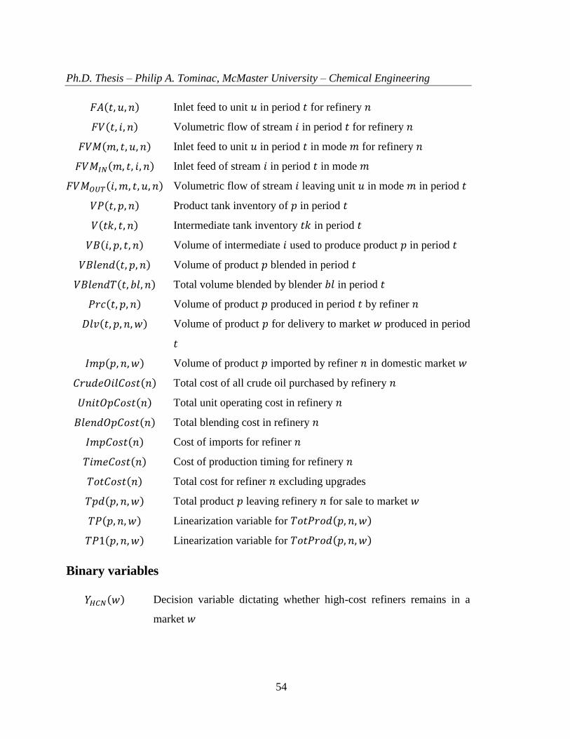
Ph.D. Thesis – Philip A. Tominac, McMaster University – Chemical Engineering
54
𝐹𝐴(𝑡, 𝑢, 𝑛) Inlet feed to unit 𝑢 in period 𝑡 for refinery 𝑛
𝐹𝑉(𝑡, 𝑖, 𝑛) Volumetric flow of stream 𝑖 in period 𝑡 for refinery 𝑛
𝐹𝑉𝑀(𝑚, 𝑡, 𝑢, 𝑛) Inlet feed to unit 𝑢 in period 𝑡 in mode 𝑚 for refinery 𝑛
𝐹𝑉𝑀𝐼𝑁(𝑚, 𝑡, 𝑖, 𝑛) Inlet feed of stream 𝑖 in period 𝑡 in mode 𝑚
𝐹𝑉𝑀𝑂𝑈𝑇(𝑖,𝑚, 𝑡, 𝑢, 𝑛) Volumetric flow of stream 𝑖 leaving unit 𝑢 in mode 𝑚 in period 𝑡
𝑉𝑃(𝑡, 𝑝, 𝑛) Product tank inventory of 𝑝 in period 𝑡
𝑉(𝑡𝑘, 𝑡, 𝑛) Intermediate tank inventory 𝑡𝑘 in period 𝑡
𝑉𝐵(𝑖, 𝑝, 𝑡, 𝑛) Volume of intermediate 𝑖 used to produce product 𝑝 in period 𝑡
𝑉𝐵𝑙𝑒𝑛𝑑(𝑡, 𝑝, 𝑛) Volume of product 𝑝 blended in period 𝑡
𝑉𝐵𝑙𝑒𝑛𝑑𝑇(𝑡, 𝑏𝑙, 𝑛) Total volume blended by blender 𝑏𝑙 in period 𝑡
𝑃𝑟𝑐(𝑡, 𝑝, 𝑛) Volume of product 𝑝 produced in period 𝑡 by refiner 𝑛
𝐷𝑙𝑣(𝑡, 𝑝, 𝑛, 𝑤) Volume of product 𝑝 for delivery to market 𝑤 produced in period
𝑡
𝐼𝑚𝑝(𝑝, 𝑛, 𝑤) Volume of product 𝑝 imported by refiner 𝑛 in domestic market 𝑤
𝐶𝑟𝑢𝑑𝑒𝑂𝑖𝑙𝐶𝑜𝑠𝑡(𝑛) Total cost of all crude oil purchased by refinery 𝑛
𝑈𝑛𝑖𝑡𝑂𝑝𝐶𝑜𝑠𝑡(𝑛) Total unit operating cost in refinery 𝑛
𝐵𝑙𝑒𝑛𝑑𝑂𝑝𝐶𝑜𝑠𝑡(𝑛) Total blending cost in refinery 𝑛
𝐼𝑚𝑝𝐶𝑜𝑠𝑡(𝑛) Cost of imports for refiner 𝑛
𝑇𝑖𝑚𝑒𝐶𝑜𝑠𝑡(𝑛) Cost of production timing for refinery 𝑛
𝑇𝑜𝑡𝐶𝑜𝑠𝑡(𝑛) Total cost for refiner 𝑛 excluding upgrades
𝑇𝑝𝑑(𝑝, 𝑛, 𝑤) Total product 𝑝 leaving refinery 𝑛 for sale to market 𝑤
𝑇𝑃(𝑝, 𝑛, 𝑤) Linearization variable for 𝑇𝑜𝑡𝑃𝑟𝑜𝑑(𝑝, 𝑛, 𝑤)
𝑇𝑃1(𝑝, 𝑛, 𝑤) Linearization variable for 𝑇𝑜𝑡𝑃𝑟𝑜𝑑(𝑝, 𝑛, 𝑤)
Binary variables
𝑌𝐻𝐶𝑁(𝑤) Decision variable dictating whether high-cost refiners remains in a
market 𝑤

Ph.D. Thesis – Philip A. Tominac, McMaster University – Chemical Engineering
55
Literature Cited
1. Guyonnet P, Grant F H, Bagajewicz M J. Integration model for refinery planning,
oil procuring, and product distribution. Ind Eng Chem Res. 2009; 48: 464-482.
2. Sahebi H, Nickel S, Ashayeri J. Strategic and tactical mathematical programming
models within the crude oil supply chain context – a review. Comput Chem Eng.
2014; 68: 56-77.
3. Bajpai P, Singh S N. Bidding and gaming in electricity market: an overview and
key issues. In: Proceedings of national power system conference (NPSC), Chennai;
2004. p. 338-346.
4. Scattolini R. Architectures for distributed and hierarchical model predictive control
– a review. J Process Contr. 2009; 19: 723-731.
5. Gjerdrum J, Shah N, Papageorgiou LG. Transfer prices for multienterprise supply
chain optimization. Ind Eng Chem Res. 2001; 49(7): 1650-1660.
6. Gjerdrum J, Shah N, Papageorgiou LG. Fair transfer price and inventory holding
policies in two-enterprise supply chains. Eur J Oper Res. 2002; 143: 582-599.
7. Pierru A. Allocating the CO2 emissions of an oil refinery with Aumann-Shapley
prices. Energ Econ. 2007; 29: 563-577.
8. Bard JF, Plummer J, Sourie JC. A bilevel programming approach to determining tax
credits for biofuel production. Eur J Oper Res. 2000; 120: 30-46.
9. Bai Y, Ouyang Y, Pang J. Biofuel supply chain design under competitive
agricultural land use and feedstock market equilibrium. Energ Econ. 2012; 34:
1623-1633.
10. Yue D, You F, Game-theoretic modelling and optimization of multi-echelon supply
chain design and operation under Stackelberg game and market equilibrium.
Comput Chem Eng. 2014; 71; 347-361.
11. Zamarripa MA, Aguirre AM, Méndez CA, Espuña A. Improving supply chain
management in a competitive environment. In: Proceedings of 21st European
symposium on computer aided process engineering - ESCAPE 21; 2011. p. 1000-
1005.
12. Zamarripa MA, Aguirre AM, Méndez CA, Espuña A. Integration of mathematical
programming and game theory for supply chain planning optimization in multi-
objective competitive scenarios. In: Proceedings of 22nd
European symposium on
computer aided process engineering - ESCAPE 22; 2012. p. 402-406.
13. Zamarripa MA, Aguirre AM, Méndez CA, Espuña A. Mathematical programming
and game theory optimization-based tool for supply chain planning in

Ph.D. Thesis – Philip A. Tominac, McMaster University – Chemical Engineering
56
cooperative/competitive environments. Chem Eng Res Des. 2013; 91(8): 1588-
1600.
14. Korzhyk D, Yin Z, Kiekintveld C, Conitzer V, Tambe M. Stackelberg vs. Nash in
security games: an extended investigation of interchangeability, equivalence, and
uniqueness. J Artif Intell Res. 2011; 41: 297-327.
15. Simaan M, Cruz JB. Additional aspects of the Stackelberg strategy in nonzero-sum
games. J Optimiz Theory App. 1973; 11(6): 613-626.
16. Nash, J. Non-cooperative Games. Ann Math. 1951; 54(2): 286-295.
17. Debreu G. A social equilibrium existence theorem. P Natl Acad Sci USA. 1952;
38(10): 886-893.
18. Glicksberg IL. A further generalization of the Kakutani fixed point theorem, with
application to Nash equilibrium points. P Am Math Soc. 1952; 3(1): 170-174.
19. Fan K. Fixed-point and minimax theorems in locally convex topological linear
spaces. P Natl Acad Sci USA. 1952; 38(2): 121-126.
20. Monderer D, Shapley L. Potential Games. Game Econ Behav. 1996; 14(1): 124-
143.
21. Peters H. Game theory: a multi-leveled approach. Maastricht, The Netherlands:
Springer; 2008.
22. Parlar M. Game theoretic analysis of the substitutable product inventory problem
with random demands. Nav Res Log. 1988; 35(3): 397-409.
23. Dayanand K, Magesh S. Defence strategy against flooding attacks using Nash
equilibrium game theory. ACS-IJCI. 2013; 4(1): 39-43.
24. Paruchuri P, Pearce JP, Marecki J, Tambe M, Ordonez F, Kraus S. Playing games
for security: An efficient exact algorithm for solving Bayesian Stackelberg games.
Proceedings of the 7th international joint conference on Autonomous agents and
multiagent systems. 2008; 2: 895-902.
25. Sandholm T, Gilpin A, Conitzer V. Mixed-integer programming methods for
finding Nash equilibria. Proceedings of the National Conference on Artificial
Intelligence. Menlo Park, CA. 2005; 20(2); 495.
26. Harker P. Generalized Nash games and quasi-variational inequalities. Eur J Oper
Res. 1991; 54(1): 81-94.
27. Facchinei F, Fischer A, Piccialli V. On generalized Nash games and variational
inequalities. Oper Res Lett. 2007; 35(2): 159-164.
28. Facchinei F, Kanzow C. Generalized Nash equilibrium problems. 4OR-Q J Oper
Res. 2007; 5(3): 173-210.
29. Ghosh A, Cottatellucci L, Altman E. Normalized Nash equilibrium for power
allocation in cognitive radio networks. IEEE Trans. Cogn Commun Netw. 2015;
1(1):86-99.

Ph.D. Thesis – Philip A. Tominac, McMaster University – Chemical Engineering
57
30. Rosen B. Existence and uniqueness of equilibrium points for concave n-person
games. Econometrica. 1965; 520-534.
31. Bergstrom TC, Varian HR. Two remarks on Cournot equilibria. Econ Lett. 1985;
19: 5-8.
32. Slade ME. The Fictitious Payoff-Function: Two Applications to Dynamic Games.
Ann Econ Stat. 1989; 15/16: 193-216.
33. Slade ME. What does an oligopoly maximize? J Ind Econ. 1994; 42(1): 45-61.
34. Morris S, Ui T. Generalized potentials and robust sets of equilibria. J Econ Theory.
2005; 124: 45-78.
35. Monderer D. Multipotential games. IJCAI. 2007; 1422-1427.
36. Redding S, Venables AJ. The economics of isolation and distance. NOPEC. 2002;
28: 93-108.
37. Government of Canada, National Energy Board. Feature article: understanding the
production, transport, and refining of crude oil in Canada. https://www.neb-
one.gc.ca/nrg/ntgrtd/mrkt/prcstrdrtcl/qrtrlprcpdts/ftrrtcl/2016-04-29ndrstndngcrl-
eng.html. Updated May 2, 2016. Accessed August 17, 2016.
38. Johnston D. Refining report complexity index indicates refinery capability, value.
Oil gas J. 1996; 94(12).
39. Green EJ. Noncooperative price taking in large dynamic markets. J Econ Theory.
1980; 22(2): 155-182.
40. Webb JN. Game Theory: Decisions, Interaction and Evolution. London, UK:
Springer London; 2007.
41. Castillo Castillo PA, Mahalec V. Inventory pinch based multi-scale model for
refinery production planning. In: Proceedings of the 24th
European symposium on
computer aided process engineering – ESCAPE 24; 2014. p. 283-288.
42. Shoesmith GL. Economies of scale and scope in petroleum refining. Appl Econ.
1988; 20: 1643-1652.
43. Couch KA, Glavin JP, Wegerer DA, Qafisheh JA. FCC propylene production. PTQ.
2007; Q3: 33-43.
44. You F, Grossmann I. Integrated multi-echelon supply chain design with inventories
under uncertainty: MINLP models, computational strategies. AICHE J. 2010; 56(2):
419-440.
45. Statistics Canada. Table 405-0002 - Gasoline and Other Petroleum Fuels Sold,
annual (litres), CANSIM (database). Accessed July 13, 2015.
46. U.S. EIA. Distillate Fuel Oil and Kerosene Sales by End Use. http://www.eia.gov/.
Accessed July 20, 2015.
47. U.S. EIA. Refiner Motor Gasoline Sales Volumes. http://www.eia.gov/. Accessed
July 20, 2015.

Ph.D. Thesis – Philip A. Tominac, McMaster University – Chemical Engineering
58
48. Natural Resources Canada, Energy Division. Average Retail Prices for Mid-Grade
Gasoline in 2014Canada. In: Fuel Focus.
http://www2.nrcan.gc.ca/eneene/sources/pripri/prices_bycity_e.cfm?PriceYear=201
4&ProductID=2&LocationID=66#PriceGraph. Accessed July 13, 2015.
49. Natural Resources Canada, Energy Division. Average Retail Prices for Premium
Gasoline in 2014Canada. In: Fuel Focus.
http://www2.nrcan.gc.ca/eneene/sources/pripri/prices_bycity_e.cfm?PriceYear=201
4&ProductID=3&LocationID=66#PriceGraph. Accessed July 13, 2015.
50. Natural Resources Canada, Energy Division. Average Retail Prices for Regular
Gasoline in 2014Canada. In: Fuel Focus.
http://www2.nrcan.gc.ca/eneene/sources/pripri/prices_bycity_e.cfm?PriceYear=201
4&ProductID=1&LocationID=66#PriceGraph. Accessed July 13, 2015.
51. Canada. Sulfur in diesel fuel regulations. SOR/2002-254. Minister of Justice
(Online) http://laws-lois.justice.gc.ca/PDF/SOR-2002-254.pdf. Accessed July 13,
2015.
52. Natural Resources Canada, Energy Division. Average Retail Prices for Diesel in
2014Canada. In: Fuel Focus.
http://www2.nrcan.gc.ca/eneene/sources/pripri/prices_bycity_e.cfm?PriceYear=201
4&ProductID=5&LocationID=66#PriceGraph. Accessed July 13, 2015.
53. Natural Resources Canada, Energy Division. Selected Crude Oil Prices Monthly –
2014. In: Fuel Focus. http://www.nrcan.gc.ca/energy/fuel-prices/crude/15085.
Accessed July 13, 2015.
54. ExxonMobil Refining & Supply. About cold lake blend.
http://www.exxonmobil.com/crudeoil/about_crudes_cold.aspx. Accessed Oct. 16,
2015.
55. ExxonMobil Refining & Supply. About hibernia.
http://www.exxonmobil.com/crudeoil/about_crudes_hibernia.aspx. Accessed Oct.
16, 2015.
56. ExxonMobil Refining & Supply. About terra nova.
http://www.exxonmobil.com/crudeoil/about_crudes_terranova.aspx. Accessed Oct.
16, 2015.
57. Fu G, Sanchez Y, Mahalec V. Hybrid model for optimization of crude distillation
units. AICHE J. 2015; 62(4): 1065-1078.
58. Misener R, Floudas CA. ANTIGONE: algorithms for continuous/integer global
optimization of nonlinear equations. J Global Optim. 2014; 59(2-3): 503-526.

Ph.D. Thesis – Philip A. Tominac, McMaster University – Chemical Engineering
59
Acknowledgements
This work has been funded by the Natural Sciences and Engineering Research
Council of Canada, the Government of Ontario, and the McMaster Advanced Control
Consortium whom we thank for their support. We would also like to extend our gratitude
to our reviewers whose commentary is appreciated.

Ph.D. Thesis – Philip A. Tominac, McMaster University – Chemical Engineering
60
Chapter 3
A dynamic game theoretic framework for process plant
competitive upgrade and production planning
The content of this chapter is a revision of the manuscript text submitted for publication
under the following title:
Tominac P, Mahalec V. A dynamic game theoretic framework for process
plant competitive upgrade and production planning.

Ph.D. Thesis – Philip A. Tominac, McMaster University – Chemical Engineering
61
A dynamic game theoretic framework
for process plant competitive upgrade
and production planning
Philip Tominac and Vladimir Mahalec*
Department of Chemical Engineering, McMaster University, 1280 Main St. W.,
Hamilton, ON, L8S 4L8, Canada
*Corresponding author. Tel.: +1 905 525 9140 ext. 26386. E-mail address:
Topical Heading – Process Systems Engineering
Keywords – production planning; strategic planning; dynamic game; potential game;
Nash equilibrium
Abstract A dynamic potential game theoretic production planning framework is presented in
which production plants are treated as individual competing entities and competition
occurs dynamically over a discrete finite time horizon. A modified Cournot oligopoly
with sticky prices provides the basis for dynamic game theoretic competition in a multi-
market nonlinear and nonconvex production planning model wherein market price adapts
to a value that clears cumulative market supply. The framework is used to investigate a
petrochemical refining scenario in which a single inefficient refiner faces elimination by
its competitors; we demonstrate that there exist conditions under which the threatened
refiner may upgrade itself in order to become competitive and escape the threat, or
alternatively in which the threat of elimination will never be carried out and the refiner is
effectively safe in the given market configuration. Globally optimal dynamic Nash
equilibrium production trajectories are presented for each case.
Ph.D. Thesis – Philip A. Tominac, McMaster University – Chemical Engineering
62
Introduction
We develop a dynamic game theoretic framework for competitive production
planning and re-examine the static game theoretic competitor elimination problem
introduced by Tominac and Mahalec1. In this problem a plant can be forced to shut down
through the actions of its competitors and its market share be claimed by them at the
expense of decreased market prices. Extension of optimal game theoretic production
planning to the dynamic domain facilitates the analysis of decision-making processes in
time-varying competitive markets. In particular, we investigate the elimination problem in
a petrochemical refining setting from the perspective of the threatened refiner and the
decisions it faces as it attempts to prolong its survival. Game theory provides a means of
analyzing the complex interactions between competing and cooperating entities. A
number of authors have used game theoretic principals to examine cooperative and
competitive interactions in chemical engineering supply chain literature. Gjerdrum, Shah,
and Papageorgiou examine fair profit allocation among supply chain participants using
transfer prices and Nash bargaining equilibria2,3
. Bai, Ouyang, and Pang incorporate
agricultural decisions into the biorefinery supply chain using a Stackelberg framework to
analyze business interactions between biofuels and food crop producers4. Yue and You
propose a mixed integer nonlinear programming (MINLP) Stackelberg framework for the
optimal design of multi-echelon supply chain systems5. Zamarripa et al solve cooperative
and competitive supply chain planning problems using a framework in which Nash
equilibria are identified through the assembly of a payoff matrix7,8,15
. Game theory has
seen use in engineering design problems as well: Bard, Plummer, and Sourie use a
Stackelberg game framework to determine optimal biofuel tax credit policies9. Pierru uses
Aumann-Shapley cost sharing to allocate refinery carbon dioxide emissions over finished
products10
. Chew et al present a game theoretic model for water integration in industrial
parks11
. Recent reviews of supply chain optimization literature by Papageorgiou12
and
Sahebi, Nickel, and Ashayeri13
identify few papers taking advantage of game theoretic
principles, and of the research identified in those reviews and here, none make use of
Ph.D. Thesis – Philip A. Tominac, McMaster University – Chemical Engineering
63
dynamic game theoretic models. The model used by Tominac and Mahalec1, for example,
is a multiperiod planning problem formulated under a static Cournot game objective,
precluding the ability of competitors to react to temporally changing market conditions.
Dynamic game theoretic problems are problems of optimal control with solutions
that are Nash equilibria, and have seen extensive research and use in the area of process
control14
. Due to the breadth of the field of dynamic (or differential) game theory, we
restrict ourselves to a review of theory regarding Cournot oligopoly models, which emit
exact potential functions. Dynamic Cournot oligopoly models owe their present day form
to developments made by Simaan and Takayama, whose pricing model is based on an
adjustment function relating price at some instant to all historical prices15
. Fershtman and
Kamien presented a variation on this model in which the rate of price adjustment is
allowed to take an arbitrary value; their model is referred to as the Cournot oligopoly with
sticky prices16
. In their subsequent paper, equilibrium price trajectories are analyzed on
finite time horizons, and are shown to exhibit asymptotic steady state (or turnpike)
properties in which the equilibrium trajectory approaches the infinite horizon steady state
price trajectory from the outset of the time horizon, but deviates as the game terminates17
.
Fershtman and Kamien examine primarily closed loop equilibrium trajectories
representative of subgame perfect Nash equilibria; Cellini and Lambertini examine open
loop equilibrium steady state properties18
, and steady state properties of both open and
closed loop strategies in oligopoly games with product differentiation19
.
Wiszniewska-Matyszkiel, Bodnar, and Mirota extend the analysis of the dynamic Cournot
oligopoly to off-steady states20
. These dynamic oligopoly models assume that
competitors’ individual actions result in significant impact on the system.
Wiszniewska-Matyszkiel presents dynamic game models, in both discrete21
and
continuous22
time domains, involving competitor continua of sizes large enough to render
an individual’s influence negligible. Such frameworks are important in the analysis of
renewable resource usage. Zazo et al analyze a number of constrained dynamic game
models as potential games23
.
Ph.D. Thesis – Philip A. Tominac, McMaster University – Chemical Engineering
64
Taking advantage of the potential game emitted by the dynamic Cournot oligopoly
structure, we propose a dynamic closed-loop game theoretic process plant production
planning framework based on a discrete time potential game formulation. To the best of
our knowledge, such a framework has not been proposed within the body of literature of
engineering supply chain planning. The closed loop dynamic game formulation allows
competitors to respond to each other temporally, reacting to competing players’ decisions
at prior time points16
. This dynamic framework synergizes with multiperiod strategic and
tactical production planning models; planning decisions at each period are also
interpreted as competitive best responses to decisions from prior periods. Competitor
decision variables in this framework are infinitely valued, assuring from a theoretical
standpoint that at least one Nash equilibrium strategy exists24,25,26
. A Nash equilibrium
trajectory to a dynamic potential game is defined as the maximum of the dynamic
potential function; thus the proposed framework guarantees an equilibrium solution exists
and is obtainable using numerical optimization27
. The properties of this dynamic potential
game framework are illustrated using a set of competing petrochemical refiners with a
focus on the interpretation of the competitor elimination scenario. The novel elements
presented in this work are:
A dynamic potential game theoretic framework for production planning
problems yielding Nash equilibrium trajectories;
The derivation of the dynamic potential function corresponding to the
modified Cournot oligopoly model of Tominac and Mahalec1 and the
demonstration of the validity of this potential function;
A case study in which a refiner threatened with closure predicts competitor
hostility throughout phases of vulnerable growth and expansion in order to
determine whether the threat of closure is legitimate and if so, whether
closure can be prevented through upgrading of its facilities;
If facilities are to be upgraded, the proposed framework will indicate the
time available in which those upgrades must be completed before a closure
would occur.
Ph.D. Thesis – Philip A. Tominac, McMaster University – Chemical Engineering
65
Background
Dynamic Nash equilibrium
The dynamic Nash equilibrium is defined in the same way as the static Nash
equilibrium: for a set of players 𝑅 playing a competitive game 𝐺 over 𝑁 discrete periods
of time and having available strategies 𝜉𝑛𝑟 ∈ Ξ𝑛𝑟 (where 𝜉 and Ξ are used to denote
unique strategies and strategy sets, respectively) with objective functions 𝐽𝑟(𝜉𝑟𝑛, 𝜉−𝑟𝑛) of
both each player’s own and opposing players’ strategies (denoted −𝑟), then the set of
Nash equilibrium strategy trajectories (denoted as player-indexed vectors 𝜉�̅� =
[𝜉𝑟1, … , 𝜉𝑟𝑁]) to the game, 𝐺{𝜉1̅∗, … , 𝜉�̅�
∗} have the property in Eq. (1)17
.
𝐽𝑟(𝜉�̅� , 𝜉−̅𝑟∗ ) ≤ 𝐽𝑟(𝜉�̅�
∗, 𝜉−̅𝑟∗ ) ∀𝑟 ∈ 𝑅,𝜉�̅� ∈ Ξ̅𝑟 (1)
There exist several important distinctions between dynamic and static Nash
equilibrium, and we restrict ourselves to a discussion of these as they relate to the
Cournot oligopoly with sticky prices. The dynamic closed-loop Nash equilibrium
trajectory steady state value in games of infinite duration is not equivalent to the
corresponding static game Nash equilibrium value16
. Closed-loop dynamic games of
finite duration exhibit a turnpike property prior to termination, but will exhibit an
intermediate steady state value at some point following the beginning of a sufficiently
long time horizon and before its end; this intermediate steady state is not equivalent to the
corresponding static game Nash equilibrium17
. As the number of firms increases to
infinity, the steady state values of these games approach the static Nash equilibrium
values, representing a dynamic perfectly competitive environment18
. Games of finite
duration terminate at the static game Nash equilibrium; players become perfectly
competitive when there is no future time in which to compete18,28
. While the equilibrium
steady state value is unique, the strategy trajectories which yield this value are generally
not unique17
.

Ph.D. Thesis – Philip A. Tominac, McMaster University – Chemical Engineering
66
Problem statement
We examine a dynamic version of the game theoretic refinery production planning
problem presented by Tominac and Mahalec1, in which multiple refineries are considered
in a framework in which each refinery is a private firm seeking to maximize its profits.
Refiners are rational in the game theoretic sense and are competitive. All refiners are
capable of producing identical products and have access to the same set of crude
feedstocks, but refineries vary in size and capacity. Geographic regions of sale are
identified as markets in which each product has a nominal demand level and a price
determined by a modified linear Cournot model1. Markets containing refineries are
identified as domestic markets and receive all products from those refiners, who are in
turn obligated to supply domestic markets with product levels within some predefined
socially acceptable window, and thus also a predefined price window. The potential for
domestic market supply infeasibility (in which refiners cannot produce the minimum
domestic market supply of all products) is avoided by allowing domestic market refiners
to import finished product at a fixed cost from other refiner-owned assets. Markets
lacking any local refiner presence are defined as global markets, and are connected to
domestic markets by pipelines. All refiners in connected domestic markets may export to
global markets without any restrictions on total market supply, or thus price. In all cases,
markets are assumed to clear at the Cournot price corresponding to total market supply in
a given period of time; i.e., the market supply is sold entirely without residual demand.
The dynamic Cournot oligopoly pricing model is such that price in a given period of time
is a function of the initial product price and all prior supply as well as the product
supplied within the current period. Under these conditions refiners are faced with the
following problem:
To determine the product amounts which must be provided and the delivery time of
those products at the domestic market level in order to satisfy supply obligations
together with other competing domestic market refiners, including whether and when
any product imports are required (a strategic decision).

Ph.D. Thesis – Philip A. Tominac, McMaster University – Chemical Engineering
67
To determine the timing and amounts of each product for export to available global
markets in which a refiner is competing with both local domestic refiners and refiners
in other domestic markets (a strategic decision).
To determine the required amounts of available crude stocks and purchase timing, and
the blend plan to be used to produce products in the means yielding the greatest profit
(production planning decisions).
We focus our attention on the scenario in which a high-cost refiner may be
eliminated from a domestic market and examine this problem in the dynamic game
theoretic production planning framework. This scenario is based on the notion that market
prices are higher while the high-cost refiner is active, allowing all refiners to benefit. The
remaining low-cost refiners may unanimously elect to shut down the high-cost refiner, at
which point they gain the high-cost refiner’s market share. The problem is interpreted as a
trade-off between higher prices and a larger market from the low-cost refiners’
perspective; Tominac and Mahalec1 discuss the ramifications of this interpretation of the
problem in depth, which is based on observations of refining assets and pipeline networks
in western Canada29
. From a modelling perspective, this scenario represents a case in
which price parameters are larger when the high-cost refiner is active; since Cournot
prices are a result of production volumes, it is possible to observe lower market prices in
the presence of the high-cost refiner than without.
We consider instead the high-cost refiner’s perspective on the problem, which is
inherently one of survival. In a dynamic game theoretic framework, the high-cost refiner
may be shut down in any period. From the perspective of the low-cost refiners, this will
occur when and if it maximizes their own profits to do so. While the high cost refiner
would rather avoid being shut down, its available strategies are limited in order to
investigate a scenario in which it either transitions into a low-cost refiner or is shut down.
The high-cost refiner is not allowed to lower its production levels in order to prevent
closure; its production levels are fixed to the values which result in the equivalent
dynamic scenario in which no elimination threat exists. We consider the transition of a
high-cost refiner to a low-cost refiner through an implicit upgrade argument: as the high-

Ph.D. Thesis – Philip A. Tominac, McMaster University – Chemical Engineering
68
cost refiner implements upgrades, the higher prices associated with its presence will
diminish. If the high-cost refiner can implement upgrades which reduce its associated
higher prices to zero (i.e., market prices become the unmodified Counrot prices, or
equivalently the high-cost refiner induces a zero-level increase in Cournot price) then it is
considered to have become competitive with the low-cost refiners (it has in effect become
a low-cost refiner) and cannot be eliminated by them any longer. If the high-cost refiner is
unable to complete upgrades in this manner, then it is shut down. The assumptions made
regarding the high-cost refiner’s problem are as follows:
A high-cost refiner may become a low-cost refiner through upgrading.
High-cost refiners are unable to import product from other assets; at some time after
transitioning to low-cost refiner status and not threatened with elimination, a high-cost
refiner will establish an import source.
Low-cost refiners cannot be eliminated from markets.
The elimination decision is made unanimously by the set of low-cost refiners; this is in
part to avoid gaming effects on that decision30
.
A high-cost refiner is vulnerable until it becomes a low-cost refiner; i.e., it is
vulnerable until its upgrades are complete.
The process of upgrading is represented entirely by changes to the high-cost refiner’s
price increase parameter; an upgrade increasing the high-cost refiner’s efficiency
lowers the value of this parameter, and the high-cost refiner has completed transition
to a low-cost refiner if the value of this parameter becomes zero
Multiple upgrade stages may be examined by sequential solution of the dynamic
model using changing values of the price increase and setting the initial price to the
current period price in which an upgrade is completed.
If the high-cost refiner is not eliminated within the finite horizon, it is never
eliminated. The static game Nash equilibrium includes the high-cost refiner.
Under these assumptions, the high-cost refiner’s problem is to determine if an
upgrade plan is available which results in its continued participation in the market as
either a high-cost or low-cost refiner. This is a strategic decision on the high-cost refiner’s
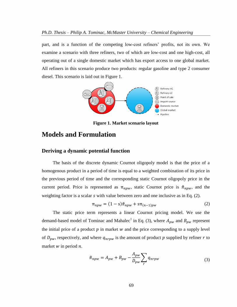
Ph.D. Thesis – Philip A. Tominac, McMaster University – Chemical Engineering
69
part, and is a function of the competing low-cost refiners’ profits, not its own. We
examine a scenario with three refiners, two of which are low-cost and one high-cost, all
operating out of a single domestic market which has export access to one global market.
All refiners in this scenario produce two products: regular gasoline and type 2 consumer
diesel. This scenario is laid out in Figure 1.
Figure 1. Market scenario layout
Models and Formulation
Deriving a dynamic potential function
The basis of the discrete dynamic Cournot oligopoly model is that the price of a
homogenous product in a period of time is equal to a weighted combination of its price in
the previous period of time and the corresponding static Cournot oligopoly price in the
current period. Price is represented as π𝑛𝑝𝑤, static Cournot price is �̃�𝑛𝑝𝑤, and the
weighting factor is a scalar 𝑠 with value between zero and one inclusive as in Eq. (2).
π𝑛𝑝𝑤 = (1 − s)�̃�𝑛𝑝𝑤 + sπ(𝑛−1)𝑝𝑤 (2)
The static price term represents a linear Cournot pricing model. We use the
demand-based model of Tominac and Mahalec1 in Eq. (3), where 𝐴𝑝𝑤 and 𝐵𝑝𝑤 represent
the initial price of a product 𝑝 in market 𝑤 and the price corresponding to a supply level
of 𝐷𝑝𝑤, respectively, and where 𝑞𝑛𝑟𝑝𝑤 is the amount of product 𝑝 supplied by refiner 𝑟 to
market 𝑤 in period 𝑛.
�̃�𝑛𝑝𝑤 = 𝐴𝑝𝑤 + 𝐵𝑝𝑤 −
𝐴𝑝𝑤
𝐷𝑝𝑤∑𝑞𝑛𝑟𝑝𝑤𝑟
(3)

Ph.D. Thesis – Philip A. Tominac, McMaster University – Chemical Engineering
70
Price π𝑛𝑝𝑤 is shown in its general recursive expression in Eq. (4), and with �̃�𝑛𝑝𝑤
expanded in Eq. (5). The dependence of price on the initial price 𝜋0𝑝𝑤 is apparent in the
recursive expression; it is assumed to be 𝜋0𝑝𝑤 = 𝐴𝑝𝑤 + 𝐵𝑝𝑤.
π𝑛𝑝𝑤 = ∑[𝑠𝑛−𝑛
′(1 − 𝑠)�̃�𝑛′𝑝𝑤]
𝑛
𝑛′=1
+ s𝑛𝜋0𝑝𝑤 (4)
𝜋𝑛𝑝𝑤 = ∑ [𝑠𝑛−𝑛
′(1 − 𝑠) (𝐴𝑝𝑤 + 𝐵𝑝𝑤 −
𝐴𝑝𝑤
𝐷𝑝𝑤∑𝑞𝑛′𝑟𝑝𝑤𝑟
)]
𝑛
𝑛′=1
+ s𝑛𝜋0𝑝𝑤 (5)
We assume a general refiner cost function of the form 𝐶𝑛𝑟(𝑞𝑛𝑟𝑝𝑤) such that refiner
profit 𝐽𝑟 may be defined as in Eq. (6), and expressed as in Eq. (7). The parameter 𝑒−𝑖𝑛 is a
discounting factor decreasing the weight of future profits using the parameter 𝑖 to
determine the amount.
𝐽𝑟 =∑𝑒−𝑖𝑛(∑∑[𝜋𝑛𝑝𝑤𝑞𝑛𝑟𝑝𝑤]
𝑤𝑝
− 𝐶𝑛𝑟(𝑞𝑛𝑟𝑝𝑤))
𝑛
(6)
𝐽𝑟 =∑𝑒−𝑖𝑛(∑∑[(∑[𝑠𝑛−𝑛′(1 − 𝑠)�̃�𝑛′𝑝𝑤]
𝑛
𝑛′=1
+ sn𝜋0𝑝𝑤)𝑞𝑛𝑟𝑝𝑤]
𝑤𝑝𝑛
− 𝐶𝑛𝑟(𝑞𝑛𝑟𝑝𝑤))
(7)
The potential function is defined according to the methods defined by Monderer
and Shapley27
and Slade31,32
and is defined by Eq. (8). We separate the usual Ω into
Ω𝑟𝑆 + Ω𝑟
𝐶 to isolate costs from the main part of the term. The definitions of Ψ, Ω𝑟𝑆, and Ω𝑟
𝐶
are provided in Eqs. (9), (10), and (11).
𝑍 = Ψ +∑(Ω𝑟𝑆 + Ω𝑟
𝐶)
𝑟
(8)

Ph.D. Thesis – Philip A. Tominac, McMaster University – Chemical Engineering
71
Ψ =∑∑∑∑
[ 𝑒−𝑖𝑛𝑠𝑛−𝑛
′(1
𝑛
𝑛′=1𝑛𝑤𝑝
− 𝑠) (−𝐴𝑝𝑤
𝐷𝑝𝑤)(∑∑ 𝑞𝑛𝑟𝑝𝑤𝑞𝑛′𝑟′𝑝𝑤
𝑟′
𝑟′≠𝑟𝑟
)
]
(9)
Ω𝑟𝑆 =∑∑∑(∑ [𝑒−𝑖𝑛𝑠𝑛−𝑛
′(1 − 𝑠) ((𝐴𝑝𝑤 + 𝐵𝑝𝑤)𝑞𝑛𝑟𝑝𝑤
𝑛
𝑛′=1𝑛𝑤𝑝
−𝐴𝑝𝑤
𝐷𝑝𝑤𝑞𝑛𝑟𝑝𝑤𝑞𝑛′𝑟𝑝𝑤)] + s
𝑛𝜋0𝑝𝑤𝑞𝑛𝑟𝑝𝑤)
(10)
Ω𝑟𝐶 = −∑𝑒−𝑖𝑛𝐶𝑛𝑟(𝑞𝑛𝑟𝑝𝑤)
𝑛
(11)
Verification of the dynamic potential function
The dynamic potential function defined by Eqs. (8), (9), (10), and (11) is verified as
a potential function for the dynamic game by demonstrating that it simultaneously
maximizes the profits of all competing refiners 𝑟 ∈ 𝑅31,32. The condition that must be
satisfied by the potential function is defined in Eq. (12). The derivative of profit 𝐽𝑟 is
defined in Eq. (13).
𝜕Z
𝜕𝑞𝑛𝑟𝑝𝑤=
𝜕𝐽𝑟𝜕𝑞𝑛𝑟𝑝𝑤
∀𝑛 ∈ 𝑁, 𝑟 ∈ 𝑅, 𝑝 ∈ 𝑃,𝑤 ∈ 𝑊 (12)
𝜕𝐽𝑟𝜕𝑞𝑛𝑟𝑝𝑤
= 𝑒−𝑖𝑛 {∑ [𝑠𝑛−𝑛′(1 − 𝑠) (𝐴𝑝𝑤 + 𝐵𝑝𝑤 −
𝐴𝑝𝑤
𝐷𝑝𝑤∑𝑞𝑛′𝑟′𝑝𝑤𝑟′
)]
𝑛
𝑛′=1
+ (1 − 𝑠) (−𝐴𝑝𝑤
𝐷𝑝𝑤𝑞𝑛𝑟𝑝𝑤) + s
𝑛𝜋0𝑝𝑤 −𝜕𝐶𝑛𝑟(𝑞𝑛𝑟𝑝𝑤)
𝜕𝑞𝑛𝑟𝑝𝑤}
(13)
For the dynamic potential function derivatives for each component are determined
to be as in Eqs. (14), (15), and (16).
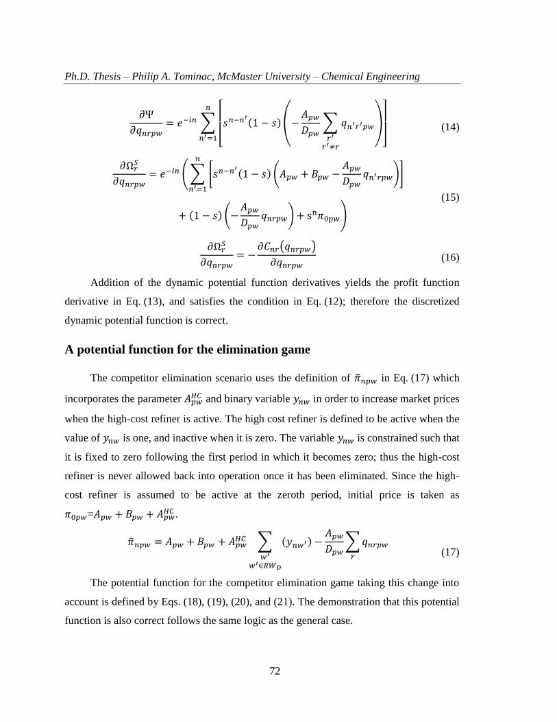
Ph.D. Thesis – Philip A. Tominac, McMaster University – Chemical Engineering
72
𝜕Ψ
𝜕𝑞𝑛𝑟𝑝𝑤= 𝑒−𝑖𝑛 ∑
[ 𝑠𝑛−𝑛
′(1 − 𝑠)(−
𝐴𝑝𝑤
𝐷𝑝𝑤∑ 𝑞𝑛′𝑟′𝑝𝑤𝑟′
𝑟′≠𝑟
)
] 𝑛
𝑛′=1
(14)
𝜕Ω𝑟𝑆
𝜕𝑞𝑛𝑟𝑝𝑤= 𝑒−𝑖𝑛 (∑ [𝑠𝑛−𝑛
′(1 − 𝑠) (𝐴𝑝𝑤 + 𝐵𝑝𝑤 −
𝐴𝑝𝑤
𝐷𝑝𝑤𝑞𝑛′𝑟𝑝𝑤)]
𝑛
𝑛′=1
+ (1 − 𝑠) (−𝐴𝑝𝑤
𝐷𝑝𝑤𝑞𝑛𝑟𝑝𝑤) + s
n𝜋0𝑝𝑤)
(15)
𝜕Ω𝑟𝑆
𝜕𝑞𝑛𝑟𝑝𝑤= −
𝜕𝐶𝑛𝑟(𝑞𝑛𝑟𝑝𝑤)
𝜕𝑞𝑛𝑟𝑝𝑤 (16)
Addition of the dynamic potential function derivatives yields the profit function
derivative in Eq. (13), and satisfies the condition in Eq. (12); therefore the discretized
dynamic potential function is correct.
A potential function for the elimination game
The competitor elimination scenario uses the definition of �̃�𝑛𝑝𝑤 in Eq. (17) which
incorporates the parameter 𝐴𝑝𝑤𝐻𝐶 and binary variable 𝑦𝑛𝑤 in order to increase market prices
when the high-cost refiner is active. The high cost refiner is defined to be active when the
value of 𝑦𝑛𝑤 is one, and inactive when it is zero. The variable 𝑦𝑛𝑤 is constrained such that
it is fixed to zero following the first period in which it becomes zero; thus the high-cost
refiner is never allowed back into operation once it has been eliminated. Since the high-
cost refiner is assumed to be active at the zeroth period, initial price is taken as
𝜋0𝑝𝑤=𝐴𝑝𝑤 + 𝐵𝑝𝑤 + 𝐴𝑝𝑤𝐻𝐶 .
�̃�𝑛𝑝𝑤 = 𝐴𝑝𝑤 + 𝐵𝑝𝑤 + 𝐴𝑝𝑤
𝐻𝐶 ∑ (𝑦𝑛𝑤′)
𝑤′
𝑤′∈𝑅𝑊𝐷
−𝐴𝑝𝑤
𝐷𝑝𝑤∑𝑞𝑛𝑟𝑝𝑤𝑟
(17)
The potential function for the competitor elimination game taking this change into
account is defined by Eqs. (18), (19), (20), and (21). The demonstration that this potential
function is also correct follows the same logic as the general case.

Ph.D. Thesis – Philip A. Tominac, McMaster University – Chemical Engineering
73
𝑍 = Ψ + ∑(Ω𝑟𝑆 + Ω𝑟
𝐶)𝑟
𝑟∈𝑅𝐿
(18)
Ψ =∑∑∑∑
[ 𝑒−𝑖𝑛𝑠𝑛−𝑛
′(1
𝑛
𝑛′=1𝑛𝑤𝑝
− 𝑠) (−𝐴𝑝𝑤
𝐷𝑝𝑤)(∑∑ 𝑞𝑛𝑟𝑝𝑤𝑞𝑛′𝑟′𝑝𝑤
𝑟′
𝑟′≠𝑟𝑟
)
]
(19)
Ω𝑟𝑆 =∑∑∑
(
∑
[
𝑒−𝑖𝑛𝑠𝑛−𝑛′(1
𝑛
𝑛′=1𝑛𝑤𝑝
− 𝑠)
(
(
𝐴𝑝𝑤 + 𝐵𝑝𝑤 + 𝐴𝑝𝑤
𝐻𝐶 ∑ 𝑦𝑛𝑤′
𝑤′
𝑤′∈𝑅𝑊𝐷 )
𝑞𝑛𝑟𝑝𝑤
−𝐴𝑝𝑤
𝐷𝑝𝑤𝑞𝑛𝑟𝑝𝑤𝑞𝑛′𝑟𝑝𝑤
)
]
+ s𝑛𝜋0𝑝𝑤𝑞𝑛𝑟𝑝𝑤
)
(20)
Ω𝑟𝐶 = −∑𝑒−𝑖𝑛𝐶𝑛𝑟(𝑞𝑛𝑟𝑝𝑤)
𝑛
(21)
Introduction of the binary variable 𝑦𝑛𝑤 yields a bilinear term of the form 𝑦𝑛𝑤𝑞𝑛𝑟𝑝𝑤
for which there exists an exact linearization33
. We replace the binary term identified in
Eq. (22) with the equivalent linearization, and add the constraints in Eqs. (23), (24), and
(25) to the model to preserve the original functionality. The parameter �̅�𝑛𝑟𝑝𝑤 is used to
represent the maximum value of 𝑞𝑛𝑟𝑝𝑤.
∑ 𝑦𝑛𝑤′𝑞𝑛𝑟𝑝𝑤𝑤′
𝑤′∈𝑅𝑊𝐷
≡ ∑ 𝛾𝑛𝑟𝑝𝑤𝑤′
𝑤′
𝑤′∈𝑅𝑊𝐷
(22)

Ph.D. Thesis – Philip A. Tominac, McMaster University – Chemical Engineering
74
𝛾𝑛𝑟𝑝𝑤𝑤′ + 𝛾𝑛𝑟𝑝𝑤𝑤′∗ = 𝑞𝑛𝑟𝑝𝑤 ∀𝑛 ∈ 𝑁, 𝑟 ∈ 𝑅, 𝑝 ∈ 𝑃, (𝑤,𝑤′) ∈ 𝑊 (23)
𝛾𝑛𝑟𝑝𝑤𝑤′ ≤ 𝑦𝑛𝑤′�̅�𝑛𝑟𝑝𝑤 ∀𝑛 ∈ 𝑁, 𝑟 ∈ 𝑅, 𝑝 ∈ 𝑃, (𝑤,𝑤′) ∈ 𝑊 (24)
𝛾𝑛𝑟𝑝𝑤𝑤′∗ ≤ (1 − 𝑦𝑛𝑤′)�̅�𝑛𝑟𝑝𝑤 ∀𝑛 ∈ 𝑁, 𝑟 ∈ 𝑅, 𝑝 ∈ 𝑃, (𝑤,𝑤′) ∈ 𝑊 (25)
The potential function in the elimination scenario takes into account the high-cost
refiner only in the Ψ term; it is ignored in the addition of both Ω𝑟 terms. This formulation
presents an interesting interpretation of the scenario: the high-cost refiner examines when
the low-cost refiners prefer to have it active in the petroleum market and when or if they
would prefer to have it inactive. Its own profits do not factor into the decision, which
might be anticipated given the assumed game theoretic definitions of rationality.
Solution Procedure
Since the high-cost refiner’s profits are not factored into the elimination scenario
potential function defined by Eqs. (18) to (21) this potential function cannot be used to
determine the high-cost refiner’s production plan. We thus use a two stage solution
process with the rationale that the high-cost refiner selects as its production plan the game
theoretically optimal scheme as though it is not facing elimination (i.e., its competitive
production scheme from the planning problem in which there is no elimination option)
and then holds to that production scheme in the elimination scenario. Mathematically, this
corresponds to first solving the potential function corresponding to Eqs. (8) to (11) to
calculate the high-cost refiner’s Nash equilibrium profile, and then holding these values
constant for only the high-cost refiner in the solution of the elimination scenario potential
function defined by Eqs. (18) to (21). Thus the low-cost refiners may alter their own
production schemes in response to the high cost refiner’s fixed choice, but ceteris paribus
it is anticipated that any changes in behaviour from the first stage to the second are
attributable only to whether and when the high-cost refiner is eliminated.
Refinery Models
The refinery production planning model implemented in this work is that of
Tominac and Mahalec1 defined in the supplementary material. We make one change to

Ph.D. Thesis – Philip A. Tominac, McMaster University – Chemical Engineering
75
the model in that we do not limit the high-cost refiner’s production throughput to a fixed
value in the elimination scenario. We use only the regular gasoline and type 2 diesel
products in this model for two reasons: Tominac and Mahalec1 observed mainly small
values of the other four products whose production they modelled; and to reduce the
overall model size and complexity in the dynamic framework.
Results and Discussion
On avoiding elimination
Results are interpreted in the context of the high-cost refiner and its objective of
remaining an active market participant. To reiterate, we assume that the high-cost refiner
is not willing to modify its current market share in order to disincentivize its own
elimination. Instead, the high-cost refiner’s survival is dependent on the amount by which
it maintains higher prices than would exist following its elimination and whether those
prices are high enough to incentivize the low-cost refiners to desire the high-cost refiner’s
continued participation in the market; in the alternative, the high-cost refiner is shut down
and its market share seized by the low-cost refiners. As the high-cost refiner attempts to
upgrade its processes and reduce its costs, the amount by which it requires high prices is
reduced, and the market prices fall to match. The interaction between prices and
competitors is complex in real cases; we attempt to isolate price changes in the facet of
upgrades through the notion of the high-cost refiner’s higher price requirement.
Using the standard data set to construct a dynamic game theoretic refinery
production planning model over an eight month time horizon discretized into ten periods,
the Nash equilibrium product price trajectories in Figure 2 are obtained. The standard data
set of Tominac and Mahalec1 assumes a value of 𝐴𝑝𝑤
𝐻𝐶 equal to 5% of 𝐴𝑝𝑤 in domestic
markets, and zero elsewhere. In this example the high-cost refiner is eliminated in the
fourth period; the price trajectories corresponding to the case in which no elimination
occurs are included in the figure for comparison. Domestic market product prices actually
rise following elimination due to an overall decrease in market supply. Figure 3 presents
Ph.D. Thesis – Philip A. Tominac, McMaster University – Chemical Engineering
76
refiner and market supply volume trajectories for domestic regular gasoline sales. Market
supply opens at its upper limit and remains there for three periods; following elimination
of the high-cost refiner market supply drops below its upper limit, causing prices to rise in
subsequent periods, though both low-cost refiners are able to increase their production
rates. Since the high-cost refiner is able to export, this change influences global market
prices as well. Thus while prices are high low-cost refiners prefer the additional marginal
profit obtained by allowing the high-cost refiner to persist. As prices drop, they prefer the
market share that is made available by eliminating the high-cost competitor. In this
example, the high-cost refiner thus has three periods in which to implement upgrades that
would enable it to compete with the low-cost refiners and prevent its elimination in period
four. As this corresponds to less than three months of time, it is unlikely the high-cost
refiner would be able to prevent this outcome.
Figure 2. Nash equilibrium price trajectories with normal high-cost refiner 𝑨𝒑𝒘𝑯𝑪
value. REG and DE2 are used to denote regular gasoline and diesel prices; D and G
are used to denote domestic and global markets. The line labelled HCR indicates
whether and when the high-cost refiner has been eliminated. The dashed FX lines
indicate price trajectories in the case no elimination occurs.

Ph.D. Thesis – Philip A. Tominac, McMaster University – Chemical Engineering
77
Figure 3. Domestic market supply of regular gasoline including (A) and excluding
(B) imports of finished product.
Figure 4. Nash equilibrium price trajectories with large high-cost refiner 𝑨𝒑𝒘𝑯𝑪 value.
REG and DE2 are used to denote regular gasoline and diesel prices; D and G are
used to denote domestic and global markets. The line labelled HCR indicates
whether and when the high-cost refiner has been eliminated.
A second scenario is examined in which the high-cost refiner is extremely
inefficient and requires market prices to be in significant excess of their competitive
values. This scenario is represented using 𝐴𝑝𝑤𝐻𝐶 equal to 𝐴𝑝𝑤 in domestic markets. The
Nash equilibrium price trajectories are presented in Figure 4. In this scenario the high-
cost refiner is never eliminated; even as prices decrease from their initial values. Since the
high-cost refiner is active in the terminal period, we interpret this scenario to represent a
market in which the high-cost refiner is never eliminated; the low-cost refiners desire it to
remain active indefinitely. Despite its inefficiencies there is thus no external incentive to
the high-cost refiner to upgrade its facilities. Optimization of its own internal costs
independent of the greater market context in which it operates may suggest capacity
expansion as a viable and profitable endeavor for the operators of this refinery;

Ph.D. Thesis – Philip A. Tominac, McMaster University – Chemical Engineering
78
nevertheless they run the risk of becoming too competitive. If the high-cost refiner in this
scenario upgrades its facilities (following which we assume that market prices decrease
via 𝐴𝑝𝑤𝐻𝐶 adapt to the new market context) it may find itself in the initial scenario
presented wherein its benefit to its competitors has decreased below the value of its
market share in a market that no longer includes itself, and is subsequently eliminated by
its competitors. The high-cost refiner thus must be able to upgrade its facilities to the
extent that it becomes a competitive low-cost refiner, or upgrade only so far as to improve
its operating costs without risking elimination. Either of these options entails careful
evaluation of the greater market context during and following its upgrade procedures. Of
course, in this case the high-cost refiner may elect to do nothing at all and anticipate its
continued market participation; any risk of elimination emerges only when and if it takes
action to improve its efficiency.
Influence of time discretization
Dynamic games are differential optimal control problems; discretization of the
differential form of the dynamic game facilitates the use of NLP and MINLP solvers in
the solution of games of finite length. The formulation of the dynamic Cournot game is
such that the terminal period of the dynamic game is interpreted as an equivalent static
Cournot game; i.e., the terminal point of the finite dynamic Cournot game Nash
equilibrium trajectory is the Nash equilibrium of a static Cournot game. A fixed length
time horizon of eight months is considered in this work: thus changing the number of
discretization points (or time periods) in the dynamic model changes the duration of each
period, and by the interpretation of discrete dynamic games, the static game solution
corresponding to the terminal period. The terminal point of a Nash equilibrium trajectory
is not expected to remain constant in alternative time discretizations; it is of interest
whether the quantitative pattern observed over the horizon is altered by the selection of a
different time discretization as well.

Ph.D. Thesis – Philip A. Tominac, McMaster University – Chemical Engineering
79
Figure 5. Nash equilibrium price trajectories obtained for discretizations of four (A)
eight (B) and ten (C) periods of an eight month planning horizon.
Maintaining the horizon length of eight months, discretizations of four, eight, and
ten time periods are applied to the dynamic production planning model and the Nash
equilibrium price trajectories obtained are presented in Figure 5. It is observed that the
terminal points of the trajectories vary with time discretization as anticipated. The
qualitative paths of the trajectories are similar in each case, though in the case of the four
point discretization we observe that resolution is lost. Importantly, the elimination trend
does not seem to be adversely impacted by the selection of horizon discretization; it is
interpreted from this that the elimination decision is a function of profit and the total
duration of the time horizon, but not discretization.
Existence of multiple equilibria
While price trajectories represent (generally) unique dynamic Nash equilibrium
solutions to the problems examined, the underlying refiner decision variables yielding
these trajectories are not unique. Refiner in-house production levels (i.e., excluding
imports) of domestic market regular gasoline are presented in Figure 3B. The production
trajectories corresponding to the refiners are linked: even excluding the import volumes,
the collective regular gasoline total is the same at every point on the horizon.
The game constraints limit the refiners’ strategy space and force them to operate in
concert with one another. The resulting solution is a generalized Nash equilibrium34,35,36
.
The existence of non-unique solutions is addressed by Rosen through the process of
normalization37
. We do not attempt to apply normalization procedures to our solutions;
we are interested in the macroscopic behaviour of the refiners: knowing that the

Ph.D. Thesis – Philip A. Tominac, McMaster University – Chemical Engineering
80
underlying planning model is feasible (and that multiple solutions exist) demonstrates the
connections between the physical capabilities of the plants and organization-level
decision making. Since the optimum is identical in these equivalent cases, the qualitative
and quantitative interpretations of the results with regard to strategy are not altered.
Proper application of normalization would presumably yield smooth in-house as well as
import trajectories for individual refiners, which would be desirable from an
implementation perspective.
Model solution statistics
Model size is a particular challenge in the solution of discretized dynamic game
theoretic problems; the growth of bilinear terms in the presented formulation increases
rapidly with each additional time point added to the horizon. Price at any point in time is
a function of all preceding prices and the original price at time zero; the original price is
asymptotically rejected in successive time points, but nevertheless complicates the model
equations. The solution procedure defined for this framework applies CONOPT 3.17A38
,
IPOPT 3.1239
, and ANTIGONE 1.140
in the first stage NLP to determine the high-cost
refiner’s production trajectory, and then DICOPT41
and ANTIGONE 1.1 to solve the
MINLP which determines whether and when the high-cost refiner is eliminated.
CONOPT provides a warm start for IPOPT, which in turn provides a warm start for
ANTIGONE; in this way solution times are significantly reduced. The same warm start
strategy is used with DICOPT and ANTIGONE in the solution of the MINLP. Maximum
solution times of 1000 seconds were applied for the warm start solvers, but were not
realized in the solution procedure. Solution statistics for the models presented in this work
are collected in Table 1, and were generated on a Dell Optiplex 9010 computer with Intel
Core-i7-3770 CPU and a 3.40 GHz processor operating on Windows 10 64-bit system.
Table 1. Solution statistics
Standard 4
period
Standard 8
period
Standard 10
period
Inefficient 10
period
Model statistics (GAMS)
Single equations 2732 5802 7487 7487
Single variables 2042 2534 5972 5972

Ph.D. Thesis – Philip A. Tominac, McMaster University – Chemical Engineering
81
Nonlinear entities 304 1120 1720 1720
Second Stage ANTIGONE Output
Solve summary
Objective value 764.7155 612.1062 549.6476 772.8618
Model status 1 1 1 1
After pre-processing
Variables 579 1263 1653 1653
Continuous 575 1255 1643 1643
Binary 4 8 10 10
Equations 1122 2484 3267 3267
Linear 969 1931 2418 2418
Nonconvex
nonlinear 153 553 849 849
Nonlinear terms 1264 5216 8200 8200
Bilinear/quadratic 1232 5152 8120 8120
Sigmoidal 32 64 80 80
Solve statistics
Relative gap 1.00E-09 1.00E-09 1.00E-09 1.00E-09
Total time (CPU s) 4.25 23.46 57.95 61.69
Total combined first and second stage solve time (CPU s)
1212.10 184.27 1021.48 555.16
Data are presented for the second stage ANTIGONE solve. The numbers of bilinear
terms increase quickly with the number of time periods, and results in large nonconvex
nonlinear problems overall. In all four cases, global optimality is obtained, indicated by
the model status of 1, with a relative optimality gap of 1×10⁻⁹
. The solution times are on
the scale of seconds to minutes for the final second stage solve; more time is spent
obtaining feasible solutions in the first stage problem and in the DICOPT phase of the
second stage. The multistage solution approach is such that the solution at which
ANTIGONE starts its search possesses an optimality gap within stopping tolerance. Once
ANTIGONE initializes the solution and completes its pre-solve operations, only a single
iteration is required before the algorithm concludes optimality has been obtained. Without
the two stage approach, a global solver has yet to be found which closes the gap in
reasonable time.

Ph.D. Thesis – Philip A. Tominac, McMaster University – Chemical Engineering
82
Conclusions
A framework has been presented for dynamic game theoretic refinery production
planning problems in which refiners operate in multiple markets with pricing functions
based on a modified dynamic Cournot oligopoly model with sticky prices. This
framework is used to examine competitor elimination scenarios from the perspective of a
refiner facing potential elimination by its competitors. Our results indicate that there exist
scenarios in which a refiner’s best strategy is to upgrade its facilities in order to avoid
elimination, while in other cases the same refiner would be better off taking no action at
all. Where upgrades are required in order to avoid closure, the available time before
closure is obtained and presents a deadline on upgrade procedures. These decisions are
the result of a complex trade-off between a refiner’s own cost structures and its
interactions with its competitors. Planning scenarios accounting for these types of
interactions have not been examined in prior production planning literature, and can
identify market forces whose impacts are otherwise not possible to quantify in an optimal
planning framework. Process plants in large markets may face these complex types of
decisions wherein internal costs and planning have market-wide impacts and
consequences; the presented game theoretic planning framework aids in exploring these
problems.
Notation
Sets
𝑁 (𝑛) time periods
𝑅 (𝑟) refiners
𝑅𝐿 (𝑟) low-cost refiners
𝑅𝐻 (𝑟) high-cost refiners
𝑃 (𝑝) products
𝑊 (𝑤) markets

Ph.D. Thesis – Philip A. Tominac, McMaster University – Chemical Engineering
83
𝑊𝐷 (𝑤) domestic markets
𝑊𝐺 (𝑤) global markets
𝑅𝑊𝐷 (𝑟, 𝑤) refiner 𝑟 is located in domestic market 𝑤
Ξ (𝜉) strategy set
Parameters
𝑠 Price stickiness factor
𝐴𝑝𝑤 Price decline rate
𝐴𝑝𝑤𝐻𝐶 Price increase due to high-cost refiner activity
𝐵𝑝𝑤 Price of product 𝑝 in market 𝑤 corresponding to supply of exactly 𝐷𝑝𝑤
𝐷𝑝𝑤 Nominal market supply of product 𝑝 in market 𝑤
𝜋0𝑝𝑤 Initial price of product 𝑝 in market 𝑤 corresponding to the zeroth time period
𝑖 Profit discounting factor
�̅�𝑛𝑟𝑝𝑤 Maximum production of product 𝑝 in period 𝑛 to rmarket 𝑤 by refiner 𝑟
including both in-house production and imports
Continuous Variables
𝐽𝑟 Profit for refiner 𝑟
π𝑛𝑝𝑤 Price of product 𝑝 in market 𝑤 in period n
�̃�𝑛𝑝𝑤 Static Cournot price of product 𝑝 in market 𝑤 in period n
𝑞𝑛𝑟𝑝𝑤 Total volume of product 𝑝 delivered to market 𝑤 in period 𝑛 by refiner 𝑟
accounting for in-house production and imports
𝐶𝑛𝑟 General cost function of refiner 𝑟 in period 𝑛
𝑍 Potential function value
Ω𝑟 Potential function individual term
Ω𝑟𝑆 Profit component of Ω𝑟
Ω𝑟𝐶 Cost component of Ω𝑟
Ψ Potential function collective term
Ph.D. Thesis – Philip A. Tominac, McMaster University – Chemical Engineering
84
𝛾𝑛𝑟𝑝𝑤𝑤′ Exact bilinear reformulation variable
Binary Variables
𝑦𝑛𝑤 Determines at which period 𝑛 high-cost refiners are eliminated from market
𝑤
Literature Cited
1. Tominac P, Mahalec V. A game theoretic framework for petroleum refinery strategic
production planning. AICHE J. 2017; DOI 10.1002/aic/15644.
2. Gjerdrum J, Shah N, Papageorgiou LG. Transfer prices for multienterprise supply
chain optimization. Ind Eng Chem Res. 2001; 49(7): 1650-1660.
3. Gjerdrum J, Shah N, Papageorgiou LG. Fair transfer price and inventory holding
policies in two-enterprise supply chains. Eur J Oper Res. 2002; 143: 582-599.
4. Bai Y, Ouyang Y, Pang J. Biofuel supply chain design under competitive agricultural
land use and feedstock market equilibrium. Energ Econ. 2012; 34: 1623-1633.
5. Yue D, You F, Game-theoretic modelling and optimization of multi-echelon supply
chain design and operation under Stackelberg game and market equilibrium. Comput
Chem Eng. 2014; 71: 347-361.
6. Zamarripa MA, Aguirre AM, Méndez CA, Espuña A. Improving supply chain
management in a competitive environment. In: Proceedings of 21st European
symposium on computer aided process engineering - ESCAPE 21; 2011. p. 1000-
1005.
7. Zamarripa MA, Aguirre AM, Méndez CA, Espuña A. Integration of mathematical
programming and game theory for supply chain planning optimization in multi-
objective competitive scenarios. In: Proceedings of 22nd
European symposium on
computer aided process engineering - ESCAPE 22; 2012. p. 402-406.
8. Zamarripa MA, Aguirre AM, Méndez CA, Espuña A. Mathematical programming and
game theory optimization-based tool for supply chain planning in
cooperative/competitive environments. Chem Eng Res Des. 2013; 91(8): 1588-1600.
Ph.D. Thesis – Philip A. Tominac, McMaster University – Chemical Engineering
85
9. Bard JF, Plummer J, Sourie JC. A bilevel programming approach to determining tax
credits for biofuel production. Eur J Oper Res. 2000; 120: 30-46.
10. Pierru A. Allocating the CO2 emissions of an oil refinery with Aumann-Shapley
prices. Energ Econ. 2007; 29: 563-577.
11. Chew IML, Tan RR, Foo DCY, Chiu ASF. Game theory approach to the analysis
of inter-plant water integration in an eco-industrial park. J Clean Prod. 2009; 17:
1611-1619.
12. Papageorgiou LG. Supply chain optimization for the process industries: advances
and opportunities. Comput Chem Eng. 2009; 33: 1931-1938.
13. Sahebi H, Nickel S, Ashayeri J. Strategic and tactical mathematical programming
models within the crude oil supply chain context – a review. Comput Chem Eng. 2014;
68: 56-77.
14. Scattolini R. Architectures for distributed and hierarchical model predictive
control – a review. J Process Contr. 2009; 19: 723-731.
15. Simaan M. Takayama T. Game theory applied to dynamic duopoly problems with
production constraints. Automatica. 1978; 14: 161-166.
16. Fershtman C, Kamien MI. Dynamic duopolistic competition with sticky prices.
Econometrica. 1987; 55(5): 1151-1164.
17. Fershtman C, Kamien MI. Turnpike properties in a finite-horizon differential
game: dynamic duopoly with sticky prices. Int Econ Rev. 1990; 31(1): 49-60.
18. Cellini R, Lambertini L. Dynamic oligopoly with sticky prices: closed-loop,
feedback, and open-loop solutions. Eur J Oper Res. 2004; 10(3): 303-314.
19. Cellini R, Lambertini L. A differential oligopoly game with differentiated goods
and sticky prices. J Dyn Control Syst. 2007; 176: 1131-1144.
20. Wiszniewska-Matyszkiel A, Bodnar M, Mirota F. Dynamic oligopoly with sticky
prices: off-steady state analysis. DGAA. 2015; 5(4): 568-598.
21. Wiszniewska-Matyszkiel A. Discrete time dynamic games with continuum of
players II: semi-decomposable games. Int Game Theor Rev. 2003; 5(1): 27-40.

Ph.D. Thesis – Philip A. Tominac, McMaster University – Chemical Engineering
86
22. Wiszniewska-Matyszkiel A. A dynamic game with continuum of players and its
counterpart with finitely many players. Ann Int Soc Dyn Game. 2005; 7: 455-469.
23. Zazo S, Macua SV, Sánchez-Fernández M, Zazo J. Dynamic potential games with
constraints: fundamentals and applications in communications. IEEE T Signal Process.
2016; 64(14): 3806-3821.
24. Debreu G. A social equilibrium existence theorem. P Natl Acad Sci USA. 1952;
38(10): 886-893.
25. Glicksberg IL. A further generalization of the Kakutani fixed point theorem, with
application to Nash equilibrium points. P Am Math Soc. 1952; 3(1): 170-174.
26. Fan K. Fixed-point and minimax theorems in locally convex topological linear
spaces. P Natl Acad Sci USA. 1952; 38(2): 121-126.
27. Monderer D, Shapley L. Potential Games. Game Econ Behav. 1996; 14(1): 124-
143.
28. Goldbaum D. Equilibrium analysis of conformity and influence on a social
network. SSRN. 2015.
29. Government of Canada, National Energy Board. Feature article: understanding the
production, transport, and refining of crude oil in Canada. https://www.neb-
one.gc.ca/nrg/ntgrtd/mrkt/prcstrdrtcl/qrtrlprcpdts/ftrrtcl/2016-04-29ndrstndngcrl-
eng.html. Updated May 2, 2016. Accessed August 17, 2016.
30. Webb JN. Game Theory: Decisions, Interaction and Evolution. London, UK:
Springer London; 2007.
31. Slade ME. The Fictitious Payoff-Function: Two Applications to Dynamic Games.
Ann Econ Stat. 1989; 15/16: 193-216.
32. Slade ME. What does an oligopoly maximize? J Ind Econ. 1994; 42(1): 45-61.
33. You F, Grossmann I. Integrated multi-echelon supply chain design with
inventories under uncertainty: MINLP models, computational strategies. AICHE J.
2010; 56(2): 419-440.
34. Harker P. Generalized Nash games and quasi-variational inequalities. Eur J Oper
Res. 1991; 54(1): 81-94.

Ph.D. Thesis – Philip A. Tominac, McMaster University – Chemical Engineering
87
35. Facchinei F, Fischer A, Piccialli V. On generalized Nash games and variational
inequalities. Oper Res Lett. 2007; 35(2): 159-164.
36. Facchinei F, Kanzow C. Generalized Nash equilibrium problems. 4OR-Q J Oper
Res. 2007; 5(3): 173-210.
37. Rosen B. Existence and uniqueness of equilibrium points for concave n-person
games. Econometrica. 1965; 520-534.
38. Drud AS. CONOPT – a large scale GRG code. ORSA J Comput. 1994; 6(2): 207-
216.
39. Wächter A, Biegler LT. On the implementation of a primal-dual interior point
filter line search algorithm for large-scale nonlinear programming. Math Program.
2006; 106(1): 25-57.
40. Misener R, Floudas CA. ANTIGONE: algorithms for continuous/integer global
optimization of nonlinear equations. J Global Optim. 2014; 59(2-3): 503-526.
41. Grossman IE, Viswanathan J, Vecchietti A, Raman R, Kalvelagen E.
GAMS/DICOPT: A discrete continuous optimization package. GAMS Corporation Inc.
2002.
Acknowledgements
This work has been funded by the Natural Sciences and Engineering Research
Council of Canada, the Government of Ontario, and the McMaster Advanced Control
Consortium whom we thank for their support. Philip Tominac would like to dedicate this
paper in memory of Anica Vukelic.

Ph.D. Thesis – Philip A. Tominac, McMaster University – Chemical Engineering
88
Chapter 4
Conjectures regarding the existence and properties of mixed
integer potential games
The content of this chapter is revision of the manuscript submitted for publication under
the following title:
Tominac P, Mahalec V. Conjectures regarding the existence and
properties of mixed integer potential games.

Ph.D. Thesis – Philip A. Tominac, McMaster University – Chemical Engineering
89
Conjectures regarding the existence and
properties of mixed integer potential
games
Philip Tominac and Vladimir Mahalec*
Department of Chemical Engineering, McMaster University, 1280 Main St. W.,
Hamilton, ON, L8S 4L8, Canada
*Corresponding author. Tel.: +1 905 525 9140 ext. 26386.
E-mail address: [email protected]
Category: Game theory
Keywords –potential game; mixed-integer programming; expansion planning; strategic
planning
Abstract A novel mixed integer nonlinear programming framework is investigated in which
game theoretic capacity expansion and production planning problems formulated as
potential games yield pure strategy Nash equilibria (PSNE) to finite games implied by the
enumeration of integer solutions. The theoretical properties of and existence criteria for
PSNE are presented for two types of upgrade games. These games represent the first
instances of a class of games that we term mixed integer potential games (MIPG) and
which are solved using mixed integer nonlinear programming (MINLP) methods without
enumeration of the implied finite game payoff matrix. Conjectures are made regarding
MIPG properties, and an industrially relevant example problem is solved to a PSNE
solution in which two refiners compete in multiple markets and products where each has
available for purchase four potential unit upgrades. The problem is formulated and solved
as a MIPG, and the implied finite game payoff matrix is enumerated to verify that the
solution is a PSNE.

Ph.D. Thesis – Philip A. Tominac, McMaster University – Chemical Engineering
90
Introduction
Mixed-integer programming models form the basis for a number of important
problems in chemical engineering, as have been cited by Grossmann (2002), Lin and
Floudas (2005), and Trespalacios and Grossmann (2014). These models are of particular
importance to supply chain planning and scheduling; a subject for which there exists a
wide body of literature and well-researched theoretical background. Tominac and
Mahalec (2017) draw on theoretical aspects of game theory to solve competitive
production planning problems modelled as nonlinear static potential games. As a
framework in which to solve production planning problems, the potential game structure
formalized by Monderer and Shapley (1996) is attractive: the interests (notionally,
profits) of multiple competing entities can be collected under a single objective which is
then optimized to determine the resulting Nash equilibrium occurring as each individual
entity attempts to maximize its profits. Many relevant supply chain optimization problems
can be modelled under this framework as competitive problems with multiple interested
parties.
Certain problems cannot be modelled as potential games due to a gap in the theory
which exists, to the best of our knowledge, between the solution concepts to finite and
infinite games. This gap in the theory has been addressed by other authors outside the
context of the potential game. Morrow, Mineroff, and Whitefoot (2014) solve mixed
integer design problems by simulation. Liu, Du, Jiao, and Xia (2017) use a bilevel
programming formulation for product design problems. Shiau and Michalek (2009) solve
mixed game problems as nonlinear programs with explicit Nash constraints. The concept
of the Nash equilibrium exists similarly for games with only finitely-valued variables and
for games with purely continuous decision variables, but with important differences;
Webb (2007) provides definitions and detailed information regarding Nash equilibria. To
the best of the authors’ knowledge, no theorem exists at the time of writing defining the
corresponding Nash equilibrium for a mixed integer potential game (MIPG) i.e., a game
containing both continuous and integer-valued variables and whose equilibrium solution

Ph.D. Thesis – Philip A. Tominac, McMaster University – Chemical Engineering
91
satisfies both finite and continuous definitions of a Nash equilibrium. A theory of mixed
integer potential games is not required to solve all competitive mixed integer problems,
but where both integer and continuous variables represent game decisions, such problems
form MIPGs and cannot be solved as potential games to a guaranteed Nash equilibrium.
This problem is relevant to a number of engineering supply chain problems, in particular
to the classes of capacity expansion, unit upgrade, and facility location problems such as
those in Neiro and Pinto (2008) and You and Grossmann (2008).
We present theoretical arguments for the existence of mixed integer potential games
possessing PSNE the mathematical conditions under which a PSNE exists, and numerical
experiments demonstrating our arguments. The primary benefit resulting from these
mathematical arguments is that it is unnecessary to obtain the entire game payoff matrix
in order to determine a Nash equilibrium; mixed integer programming algorithms are
capable of obtaining mixed integer game PSNE with significantly reduced computational
burden. Based on our results, we conjecture that it is possible to demonstrate that a class
of mixed integer potential games exists which under reasonable assumptions will possess
PSNE. The novel elements of this work are:
A definition for the class of mixed integer games as ordinal potential games,
Conditions under which two player, two strategy games will be ordinal potential
games and possess PSNE (termed ordinality conditions),
A numerical example of a two-by-two MIPG, and verification of the ordinality
conditions for this example,
A numerical example of refinery planning model as a large scale MIPG with a
PSNE which is solved using the MINLP potential game approach, and the PSNE
verified through enumeration of the implied game payoff matrix,
Conjectures regarding the existence and properties of PSNE in higher dimension
MIPGs.

Ph.D. Thesis – Philip A. Tominac, McMaster University – Chemical Engineering
92
Background
Brief definitions of discrete and continuous Nash equilibria as are necessary for
later arguments are presented here, as well as a brief discussion of the differences
between pure and mixed strategy equilibria which arise in finite games. Relevant theory
regarding Nash equilibria in potential games is also presented.
Nash Equilibrium
As a solution concept the Nash equilibrium is defined similarly for discrete and
continuous games. A game in either form is generally referred to as 𝐺 and played by a
finite set of players 𝑅, each whom has a strategy set which at this point may be finite or
infinitely valued Ξ𝑟, with strategies defined as 𝜉𝑟. Player profits, or more generally,
payoffs, are 𝐽𝑟(𝜉𝑟 , 𝜉−𝑟) and are a function of each player’s individually selected strategy
𝜉𝑟 as well as all the strategies of its competitors 𝜉−𝑟. The Nash equilibrium is the set of
strategies yielding the result in Eq. (1) where 𝜉𝑟∗ is a player’s optimal strategy, and no
deviation from this strategy improves that player’s payoff.
𝐽𝑟(𝜉𝑟∗, 𝜉−𝑟
∗ ) ≥ 𝐽𝑟(𝜉𝑟, 𝜉−𝑟∗ ) ∀𝜉𝑟 ∈ Ξ𝑟 , 𝑟 ∈ 𝑅 (1)
Nash (1951) proved the existence of at least one equilibrium in either pure or mixed
strategies in every finite game. Continuously valued games possess one or more equilibria
in the equivalent of a pure strategy, guaranteed by theorems due to Debreu (1952),
Glicksberg (1952) and Fan (1952). The mixed strategy case applies to games of perfect
information only in the case of finite games.
Pure and mixed strategy Nash equilibria in finite games
In a finite game a player is confined to a choice among limited strategies, and in
certain games no PSNE may result. Nash’s method of reconciling this result is the mixed
strategy in which one or more players selects two or more strategies each with some
probability. The game outcome is thus an expected value in the long run subject to
realization. The mathematical definition of a mixed strategy Nash equilibrium (MSNE) in

Ph.D. Thesis – Philip A. Tominac, McMaster University – Chemical Engineering
93
the general case of a finite game with |𝑅| ≥ 3 players and possessing strategy sets Ξ𝑟 is
NP-hard and not easily solved, although algorithms exist for determining such equilibria
such as those in McKelvey and McLennan (1996). The PSNE is a case of the MSNE in
which each player selects a single strategy with probability one. While every finite game
possesses at least one Nash equilibrium, there is in general no guarantee that said
equilibrium is of the pure strategy type due to Nash (1952).
Nash equilibria in continuous potential games
Formalized by Monderer and Shapley (1996) potential games are a subclass of
games for which a potential exists and defines the Nash equilibria of the game. We
address continuous potential games first, and finite potential games in the section that
follows. The Nash equilibrium of a continuous game is defined as the solution to the set
of differential equations defined by Eq. (2) interpreted to mean that each player
maximizes its profit with respect to the variables it controls.
𝜕𝐽𝑟(𝜉𝑟 , 𝜉−𝑟)
𝜕𝜉𝑟= 0 ∀𝜉𝑟 ∈ Ξ𝑟 , 𝑟 ∈ 𝑅 (2)
A continuous game is a potential game if a function 𝑍(𝜉𝑟 , 𝜉−𝑟) exists with the
property that its derivatives with respect to each player’s strategy variables are exactly the
derivatives of that player’s profit functions, as in Eq. (3). Thus, maximizing the potential
function becomes equivalent to solving the set of differential equations, and the potential
function maximum is defined as a Nash equilibrium. This is true even if the potential
function is maximized subject to constraints, although in the event constraints are active
at equilibrium the equilibrium is referred to as a generalized Nash equilibrium as defined
by Rosen (1965) and discussed by Ghosh, Cottatellucci, and Altman (2015).
𝜕𝑍(𝜉𝑟 , 𝜉−𝑟)
𝜕𝜉𝑟=𝜕𝐽𝑟(𝜉𝑟 , 𝜉−𝑟)
𝜕𝜉𝑟∀𝜉𝑟 ∈ Ξ𝑟 , 𝑟 ∈ 𝑅 (3)
Nash equilibria in finite potential games
A finite potential game is a game for which a potential exists, analogous to the
definition of the continuous game potential function. If the matrix of player rewards for a

Ph.D. Thesis – Philip A. Tominac, McMaster University – Chemical Engineering
94
finite game has dimension |Ξ1| × …× |Ξ𝑟| × …× |Ξ𝑅| × |𝑅|, i.e., matrix dimensions
|Ξ1| … |Ξ𝑅| corresponding to players’ strategies and |𝑅| representing a vector of payoff
values 𝑗𝑟(𝜉𝑟 , 𝜉−𝑟) to each player resulting in each realization, then the game potential is a
matrix of dimension |Ξ1| × …× |Ξ𝑟| × …× |Ξ𝑅| containing scalar values 𝑧(𝜉𝑟, 𝜉−𝑟)
which satisfy the definition of an exact potential as defined by Monderer and Shapley
(1996) in Eq. (4).
𝑗𝑟(𝜉𝑟 , 𝜉−𝑟) − 𝑗𝑟(𝜉𝑟′ , 𝜉−𝑟) = 𝑧(𝜉𝑟 , 𝜉−𝑟) − 𝑧(𝜉𝑟
′ , 𝜉−𝑟) ∀𝜉𝑟 , 𝜉𝑟′ ∈ Ξ𝑟 , 𝑟 ∈ 𝑅 (4)
The interpretation of this definition is that the difference between a player’s rewards
𝑗𝑟(𝜉𝑟 , 𝜉−𝑟) − 𝑗𝑟(𝜉𝑟′ , 𝜉−𝑟) obtained by selection of two strategies 𝜉𝑟 and 𝜉𝑟
′ is exactly the
same as the difference between the potential values corresponding to those strategies
𝑧(𝜉𝑟 , 𝜉−𝑟) − 𝑧(𝜉𝑟′ , 𝜉−𝑟), and holds true for every player. Less stringent potential
definitions include the weighted potential Eq. (5), and the ordinal potential Eq. (6).
𝑗𝑟(𝜉𝑟 , 𝜉−𝑟) − 𝑗𝑟(𝜉𝑟′ , 𝜉−𝑟) = 𝑤𝑟(𝑧(𝜉𝑟 , 𝜉−𝑟) − 𝑧(𝜉𝑟
′ , 𝜉−𝑟)) ∀𝜉𝑟 , 𝜉𝑟′ ∈ Ξ𝑟 , 𝑟 ∈ 𝑅 (5)
𝑗𝑟(𝜉𝑟 , 𝜉−𝑟) − 𝑗𝑟(𝜉𝑟′ , 𝜉−𝑟) > 0 ⟺ 𝑧(𝜉𝑟 , 𝜉−𝑟) − 𝑧(𝜉𝑟
′ , 𝜉−𝑟) > 0 ∀𝜉𝑟 , 𝜉𝑟′ ∈ Ξ𝑟 , 𝑟 ∈ 𝑅 (6)
The weighted potential allows the difference between the player profits to be a
weighting by 𝑤𝑟 of the exact potential difference; the ordinal potential only requires that
the signs of these differences be the same. In addition to these definitions, Monderer and
Shapley (1996) prove the following theorem regarding the definition of a potential game:
𝐺 is a finite game, then 𝐺 has the finite improvement property if and only if 𝐺 has a
generalized ordinal potential6. The finite improvement property, as it relates to a finite
game, states that if players are sequentially allowed to select from among their available
strategies one which improves their payoff, this process terminates following a finite
number of steps. It is axiomatic that this termination point is a Nash equilibrium.
Monderer and Shapley (1996) also prove the following corollary, which will be essential
in this work: let 𝐺 be a finite game possessing the finite improvement property; in
addition, let 𝐺 have the property 𝑗𝑟(𝜉𝑟 , 𝜉−𝑟) ≠ 𝑗𝑟(𝜉𝑟′ , 𝜉−𝑟) ∀𝜉𝑟 , 𝜉𝑟
′ ∈ Ξ𝑟 , 𝑟 ∈ 𝑅, then 𝐺
possesses an ordinal potential. In summary, if a game possessing the finite improvement
property also has the property that each player’s strategic choice results in a unique
payoff, then the game possesses an ordinal potential, or equivalently, if the finite game
Ph.D. Thesis – Philip A. Tominac, McMaster University – Chemical Engineering
95
possesses a pure strategy Nash equilibrium and the payoffs to each player are unique in
every strategic realization, then the game is an ordinal potential game.
Problem statement
We examine the static game theoretic refinery model of Tominac and Mahalec
(2017) in the context of a capacity expansion and unit upgrade problem. The model
includes multiple refiners operating in competitive markets seeking to produce multiple
products in a profile maximizing their individual profits. For a full description of the
original model, refinery schematic, assumptions, equations, and the parameter values and
data sources used in its development, see Tominac and Mahalec (2017) and the associated
supplementary material. In this work, we consider the case where the refiners are looking
for the most competitive means of which to expand their operations, and so we add to the
model a menu of unit upgrades of two types: unit capacity upgrades and cost reduction
upgrades. Refiners select and purchase upgrades from the menu corresponding to various
unit operation upgrades. The modified game theoretic refinery production planning and
upgrade model used in this work is included as supplementary material. Our work is
differentiated from similar capacity expansion and upgrade problems in that the objective
function is a game theoretic one, and the resulting optimal upgrade selections are a Nash
equilibrium of a game theoretic problem of mixed integer and continuous variables, hence
the termed a mixed integer game (MIPG) problem. The resulting upgrade selections made
by each player are representative of a competitive upgrade plan, satisfying the definitions
of a Nash equilibrium in both the continuous and discrete aspects of the game.
In order to verify that the solutions obtained to these MIPG problems are indeed
Nash equilibria, a two-player version of the Cournot game of Tominac and Mahalec
(2017) is analyzed and the conditions under which a discrete potential game is defined
and a PSNE is obtained in the implied matrix game are determined. The resulting
conditions provide a numerical test which can be applied to determine whether the
solution to a given MIPG problem will possess the correct interpretation as a PSNE; if the

Ph.D. Thesis – Philip A. Tominac, McMaster University – Chemical Engineering
96
conditions are satisfied, the MIPG solution will not be a PSNE as none exists in the
implied finite game.
Models and formulation
For the purpose of deriving the necessary existence conditions to first qualify the
MIPG as a proper discrete potential game and to second verify that a PSNE will exist, we
consider (without loss of generality with respect to two-player game theoretic problems) a
simplified two-player Cournot game with the same pricing structure as that of the refinery
production planning game, but with only a single arbitrary product, one market, and no
underlying process constraints which would add significant complexity to the derivation.
The pricing structure is such that the continuous Cournot game problem will be an exact
potential game, satisfying the definitions in Eqs. (2) and (3), and also that in Eq. (4),
which can be easily verified. The pricing structure for the two-player game is defined in
Eq. (7). Player costs functions are taken as quadratic functions of production and are
assumed to be convex such that there exists an efficient production point for each player
wherein cost is minimized, as well as a single unique Nash equilibrium. The cost
functions are included as Eqs. (8) and (9).
𝜋(𝑞1, 𝑞2) = 𝐴 + 𝐵 −
𝐴
𝐷(𝑞1 + 𝑞2) (7)
𝐶1(𝑞1) = 𝑎1𝑞12 + 𝑏1𝑞1 + 𝑐1 (8)
𝐶2(𝑞2) = 𝑎2𝑞22 + 𝑏2𝑞2 + 𝑐2 (9)
Player profits are determined by Eqs. (10) and (11), and are functions of both
players’ production volumes due to the dependence of price upon market supply. The
profit functions yield the potential function in Eq. (12).
𝐽1(𝑞1, 𝑞2) = (𝐴 + 𝐵 −
𝐴
𝐷(𝑞1 + 𝑞2)) 𝑞1 − 𝑎1𝑞1
2 − 𝑏1𝑞1 − 𝑐1 (10)
𝐽2(𝑞1, 𝑞2) = (𝐴 + 𝐵 −
𝐴
𝐷(𝑞1 + 𝑞2)) 𝑞2 − 𝑎2𝑞2
2 − 𝑏2𝑞2 − 𝑐2 (11)

Ph.D. Thesis – Philip A. Tominac, McMaster University – Chemical Engineering
97
𝑍(𝑞1, 𝑞2) = (𝐴 + 𝐵 − 𝑏1)𝑞1 + (𝐴 + 𝐵 − 𝑏2)𝑞2 −
𝐴
𝐷𝑞1𝑞2 − (
𝐴
𝐷+ 𝑎1) 𝑞1
2
− (𝐴
𝐷+ 𝑎2) 𝑞2
2 − 𝑐1 − 𝑐2
(12)
The Nash equilibrium defined by this potential function is determined by the
solution to the set of equations defined by Eqs. (13) and (14), and is equivalent to the
potential function maximum. The solution (𝑞1∗, 𝑞2
∗) is defined by Eqs. (15) and (16), and
represents the production volumes resulting in a Nash equilibrium in the continuous
Cournot game.
𝜕𝐽1(𝑞1, 𝑞2)
𝜕𝑞1=𝜕𝑍(𝑞1, 𝑞2)
𝜕𝑞1= 𝐴 + 𝐵 −
𝐴
𝐷(2𝑞1 + 𝑞2) − 2𝑎1𝑞1 − 𝑏1 = 0 (13)
𝜕𝐽2(𝑞1, 𝑞2)
𝜕𝑞2=𝜕𝑍(𝑞1, 𝑞2)
𝜕𝑞2= 𝐴 + 𝐵 −
𝐴
𝐷(𝑞1 + 2𝑞2) − 2𝑎2𝑞2 − 𝑏2 = 0 (14)
𝑞1∗ =
𝐴𝐷(𝐴 + 𝐵 − 2𝑏1 + 𝑏2) + 2𝑎2(𝐴 + 𝐵 − 𝑏1)
3 (𝐴𝐷)
2
+ 4𝐴𝐷(𝑎1 + 𝑎2) + 4𝑎1𝑎2
(15)
𝑞2∗ =
𝐴𝐷(𝐴 + 𝐵 + 𝑏1 − 2𝑏2) + 2𝑎1(𝐴 + 𝐵 − 𝑏2)
3 (𝐴𝐷)
2
+ 4𝐴𝐷(𝑎1 + 𝑎2) + 4𝑎1𝑎2
(16)
PSNE existence conditions
We are interested in how the Cournot solution behaves as the generator of a finite
potential game when a single parameter is varied; i.e., under what conditions the set of
optimal solutions to Cournot games of the form defined in the previous section results in
a potential game with a pure strategy Nash equilibrium. In this derivation we consider the
case in which each player has a single available upgrade, and thus two strategies: either to
purchase the upgrade, or not. The purchase cost of the upgrade is assumed to be fixed and
thus its magnitude does not impact the qualitative interpretation of the derivation; for this
reason upgrade cost is not included in the derivation. An upgrade is interpreted as a
change in a single parameter resulting in a different game with new equilibrium.

Ph.D. Thesis – Philip A. Tominac, McMaster University – Chemical Engineering
98
Enumeration of all solutions to all possible combinations of upgrade purchase decisions
defines a finite game payoff matrix in which the Nash equilibrium solution to the
underlying continuous game defines the payoffs in the finite game, and to which we argue
that the potential function values associated with the underlying Cournot game are also a
potential to the finite game implicitly defined. To illustrate, consider an upgrade to each
player’s linear cost term 𝑏𝑟 defined as Δ𝑏𝑟 such that each player’s resulting linear cost
term following the upgrade is 𝑏𝑟 + Δ𝑏𝑟. As apparent from Eqs. (15) and (16), the optimal
solution (𝑞1∗, 𝑞2
∗) is dependent on 𝑏𝑟, and thus is expected to change in strategic
realization of the game. The implied finite game payoff matrix defined by the solutions to
the Cournot game in each realization of upgrade purchase is presented as Eq. (17), where
the ‘no upgrade’ strategy is represented as ∅𝑟 and the upgrade strategy as Δ𝑏𝑟. The
corresponding potential function values are shown in Eq. (18).
∅2 Δ𝑏2∅1Δ𝑏1
[𝐽1(𝑞1, 𝑞2), 𝐽2(𝑞1, 𝑞2) 𝐽1(𝑞1
′′, 𝑞2′ ), 𝐽2(𝑞1
′′, 𝑞2′ )
𝐽1(𝑞1′ , 𝑞2
′′), 𝐽2(𝑞1′ , 𝑞2
′′) 𝐽1(𝑞1′′′, 𝑞2
′′′), 𝐽2(𝑞1′′′, 𝑞2
′′′)] (17)
∅2 Δ𝑏2∅1Δ𝑏1
[𝑍(𝑞1, 𝑞2) 𝑍(𝑞1
′′, 𝑞2′ )
𝑍(𝑞1′ , 𝑞2
′′) 𝑍(𝑞1′′′, 𝑞2
′′′)] (18)
Together, these two matrices demonstrate an important feature of the implied finite
game: it cannot be guaranteed to be an exact potential game. This assertion is easily
verified using the definition of an exact potential game from Eq. (4), which is applied to
player 1 in Eq. (19) across player 1’s strategies while player 2 holds to its ∅2 strategy.
Verification arises from comparison of the difference between the Cournot profit values
with the difference between the potential function values, which is not guaranteed to be
equal as required.
𝑗1(∅1, ∅2) − 𝑗1(Δ𝑏1, ∅2) = 𝐽1(𝑞1, 𝑞2) − 𝐽1(𝑞1′ , 𝑞2
′′)
≠ 𝑍(𝑞1, 𝑞2) − 𝑍(𝑞1′ , 𝑞2
′′)
(19)
Player 1’s finite game payoffs under comparison are 𝑗1(∅1, ∅2) and 𝑗1(Δ𝑏1, ∅2),
which are equal to 𝐽1(𝑞1, 𝑞2) and 𝐽1(𝑞1′ , 𝑞2
′′), respectively. The requirement however is
that 𝐽1(𝑞1, 𝑞2) − 𝐽1(𝑞1′ , 𝑞2
′′) = 𝑍(𝑞1, 𝑞2) − 𝑍(𝑞1′ , 𝑞2
′′) in order for the game to be an exact

Ph.D. Thesis – Philip A. Tominac, McMaster University – Chemical Engineering
99
potential, but this is not guaranteed to be true, because 𝑞2 ≠ 𝑞2′′, as is known from the
solution derivation, and therefore 𝐽1(𝑞1, 𝑞2) − 𝐽1(𝑞1′ , 𝑞2
′′) ≠ 𝑍(𝑞1, 𝑞2) − 𝑍(𝑞1′ , 𝑞2
′′). From
the potential function definition, it is guaranteed only that 𝜕𝑍(𝜉𝑟,𝜉−𝑟)
𝜕𝜉𝑟=
𝜕𝐽𝑟(𝜉𝑟,𝜉−𝑟)
𝜕𝜉𝑟 which no
longer holds because both 𝑟 player’s and the −𝑟 player’s strategies have changed
simultaneously. Thus, we cannot guarantee that the finite game arising from the changes
to the underlying Cournot exact potential game will itself be an exact potential game.
While the implied finite game does not possess an exact potential, Monderer and
Shapley’s theorems regarding finite potential games include the definition of an ordinal
potential game. It can be demonstrated that the continuous Cournot potential game will,
under the correct numerical conditions, emit a finite game possessing a PSNE and which
is guaranteed to be an ordinal potential game. These two properties are related, and both
are demonstrated by an examination of the conditions under which the emitted finite
potential game possesses no PSNE and only a MSNE.
The conditions under which a given finite game possesses only a MSNE are related
to the payoffs that each player receives in the realization of a set of strategies; these
conditions must be such that in every realization of the game, at least one player is
incentivized to change their strategy due to the existence of a better payoff. Equivalently,
there can be no realization of the finite game matrix in which players are content with
their payoffs. Functionally, the conditions disallowing a PSNE state that the first player’s
column maximum payoffs do not coincide with the second player’s row maximum
payoffs. The general case of this circumstance is expressed logically in terms of strategies
in Eq. (20).
∀𝑟 ∈ 𝑅, 𝜉𝑟 ∈ Ξ𝑟 , 𝜉−𝑟 ∈ Ξ−𝑟 ∃𝜉𝑟′ ∈ Ξ𝑟
𝑠. 𝑡. 𝑗𝑟(𝜉𝑟′ , 𝜉−𝑟) > 𝑗𝑟(𝜉𝑟 , 𝜉−𝑟) ∧ 𝑗−𝑟(𝜉𝑟
′ , 𝜉−𝑟) < 𝑗−𝑟(𝜉𝑟 , 𝜉−𝑟) (20)
Some notation is introduced in order to make subsequent arguments more compact;
rather than use the Δ𝑏𝑟 , ∅𝑟 notations for upgrade purchasing, we use the more general 0,1
notation in which 0 represents the strategy ‘not upgrading,’ and 1 represents the
‘upgrade’ strategy. These strategy indicators are included as a subscript tuple in player
order in square brackets with the profit variable; thus 𝐽1,[0,1] represents the profit resulting

Ph.D. Thesis – Philip A. Tominac, McMaster University – Chemical Engineering
100
to player 1 in the case where player 1 does not upgrade and player 2 upgrades. The
important factor in the determination of whether a PSNE exists is the relative payoff to a
player, not the absolute value, and thus the notation Δ𝐽𝑟,[𝜉1,𝜉2] is introduced to indicate the
difference is profit obtained by a player relative to the profit that would be obtained in the
𝐽𝑟,[0,0] case; for example, Δ𝐽2,[1,1] = 𝐽2,[1,1] − 𝐽2,[0,0] and of course Δ𝐽𝑟,[0,0] = 0. Under this
notation, the requirements necessary in order for a two-by-two finite game to possess only
a MSNE and to fail to exhibit a PSNE are presented collectively in Eq. (21). Note that
these conditions remain true if all inequalities are reversed; the indicated form will be
used in this work, with the understanding the reverse-sign conditions are equivalent, and
must also be considered in evaluating the existence of a PSNE.
Δ𝐽1,[1,0] < 0
Δ𝐽1,[0,1] < 0
Δ𝐽1,[1,1] > Δ𝐽1,[1,0]Δ𝐽1,[1,1] > Δ𝐽1,[0,1]Δ𝐽2,[1,0] > 0
Δ𝐽2,[0,1] > 0
Δ𝐽2,[1,1] < Δ𝐽2,[1,0]Δ𝐽2,[1,1] < Δ𝐽2,[0,1]}
(21)
With the conditions under which a given two-by-two game will possess only a
MSNE established, we return to the concept of an ordinal potential game and to the
verification that the finite game emitted by the Cournot upgrade game will possess an
ordinal potential. Monderer and Shapley (1996) first note that an ordinal potential game
must possess the finite improvement property; possessing the finite improvement property
implies that the game also possesses a PSNE, thus the conditions in Eq. (21) define all
possible cases in which the resulting game would not have the finite improvement
property. To guarantee that the game possesses an ordinal potential, each strategic
realization of the game must result in a unique payoff for a given player. This additional
requirement is easily added to the MSNE conditions in Eq. (21) by replacing the strict
inequality signs with non-strict signs; the new conditions are presented in Eq. (22), and
define cases in which the game would lack a PSNE and additionally cases in which a
PSNE exists where a given player’s payoffs are not unique. These new conditions are
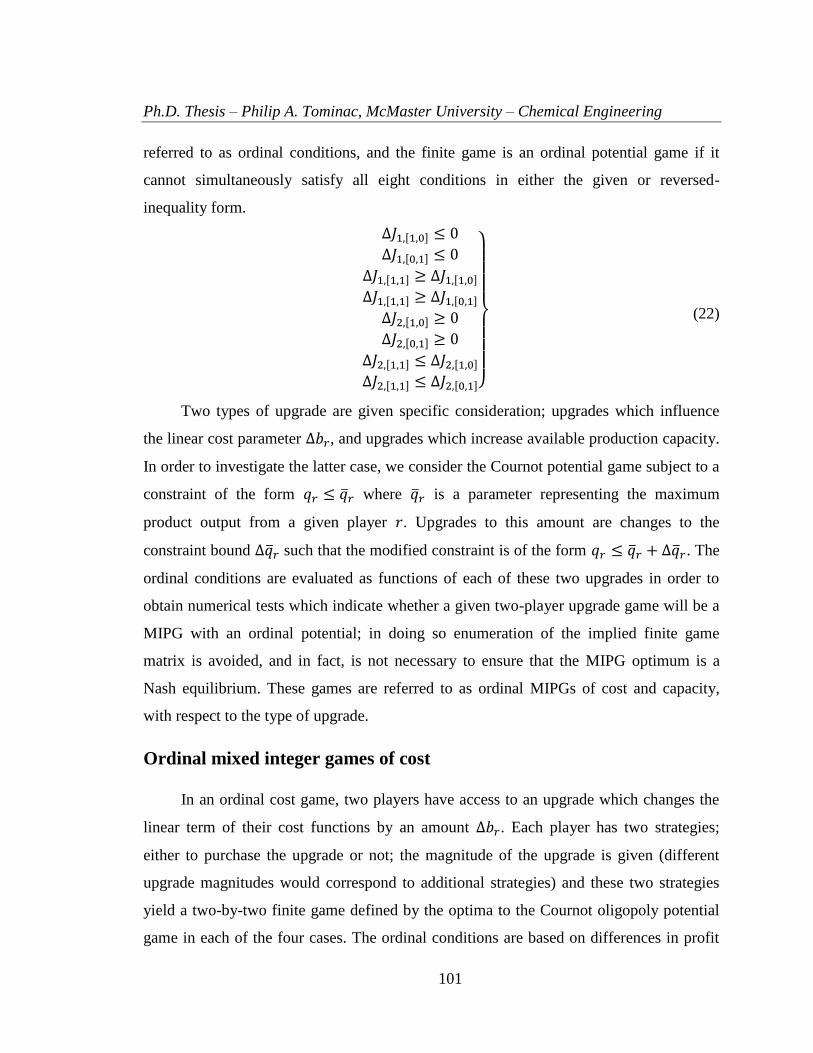
Ph.D. Thesis – Philip A. Tominac, McMaster University – Chemical Engineering
101
referred to as ordinal conditions, and the finite game is an ordinal potential game if it
cannot simultaneously satisfy all eight conditions in either the given or reversed-
inequality form.
Δ𝐽1,[1,0] ≤ 0
Δ𝐽1,[0,1] ≤ 0
Δ𝐽1,[1,1] ≥ Δ𝐽1,[1,0]Δ𝐽1,[1,1] ≥ Δ𝐽1,[0,1]Δ𝐽2,[1,0] ≥ 0
Δ𝐽2,[0,1] ≥ 0
Δ𝐽2,[1,1] ≤ Δ𝐽2,[1,0]Δ𝐽2,[1,1] ≤ Δ𝐽2,[0,1]}
(22)
Two types of upgrade are given specific consideration; upgrades which influence
the linear cost parameter Δ𝑏𝑟, and upgrades which increase available production capacity.
In order to investigate the latter case, we consider the Cournot potential game subject to a
constraint of the form 𝑞𝑟 ≤ �̅�𝑟 where �̅�𝑟 is a parameter representing the maximum
product output from a given player 𝑟. Upgrades to this amount are changes to the
constraint bound Δ�̅�𝑟 such that the modified constraint is of the form 𝑞𝑟 ≤ �̅�𝑟 + Δ�̅�𝑟. The
ordinal conditions are evaluated as functions of each of these two upgrades in order to
obtain numerical tests which indicate whether a given two-player upgrade game will be a
MIPG with an ordinal potential; in doing so enumeration of the implied finite game
matrix is avoided, and in fact, is not necessary to ensure that the MIPG optimum is a
Nash equilibrium. These games are referred to as ordinal MIPGs of cost and capacity,
with respect to the type of upgrade.
Ordinal mixed integer games of cost
In an ordinal cost game, two players have access to an upgrade which changes the
linear term of their cost functions by an amount Δ𝑏𝑟. Each player has two strategies;
either to purchase the upgrade or not; the magnitude of the upgrade is given (different
upgrade magnitudes would correspond to additional strategies) and these two strategies
yield a two-by-two finite game defined by the optima to the Cournot oligopoly potential
game in each of the four cases. The ordinal conditions are based on differences in profit

Ph.D. Thesis – Philip A. Tominac, McMaster University – Chemical Engineering
102
values, which can be determined from changes in the optimal solution (Δ𝑞1∗, Δ𝑞2
∗) relative
to the base case [0,0] corresponding to no upgrades. To simplify the following algebraic
expressions the parameter 𝜃 is defined in Eq. (23).
𝜃 = (3 (
𝐴
𝐷)2
+ 4𝐴
𝐷(𝑎1 + 𝑎2) + 4𝑎1𝑎2)
−1
(23)
The relative changes to the solutions (Δ𝑞1∗, Δ𝑞2
∗) which occur in each case are
defined in Eq. (24); the expressions for Δ𝑞𝑟,[0,0] are both zero.
Δ𝑞1,[1,0] = −2(
𝐴
𝐷+ 𝑎2) 𝜃Δ𝑏1
Δ𝑞1,[0,1] =𝐴
𝐷𝜃Δ𝑏2
Δ𝑞1,[1,1] = −2(𝐴
𝐷+ 𝑎2)𝜃Δ𝑏1 +
𝐴
𝐷𝜃Δ𝑏2
Δ𝑞2,[1,0] =𝐴
𝐷𝜃Δ𝑏1
Δ𝑞2,[0,1] = −2(𝐴
𝐷+ 𝑎1) 𝜃Δ𝑏2
Δ𝑞2,[1,1] = −2(𝐴
𝐷+ 𝑎1)𝜃Δ𝑏2 +
𝐴
𝐷𝜃Δ𝑏1}
(24)
These changes in production as a function of Δ𝑏𝑟 are used to determine the relevant
Δ𝐽𝑟[𝜉1,𝜉2] values, which are presented in Eq. (25).
Δ𝐽1,[1,0] = (𝐴 + 𝐵 +𝐴
𝐷𝜃 (𝐴
𝐷+ 2𝑎2)Δ𝑏1)(−2
𝐴
𝐷− 2𝑎2) 𝜃Δ𝑏1 − 4𝑎1𝜃
2 (𝐴
𝐷+ 𝑎2)
2
Δ𝑏12 + 2𝜃 (
𝐴
𝐷+ 𝑎2)Δ𝑏1
2
Δ𝐽1,[0,1] = (𝐴 + 𝐵 +𝐴
𝐷𝜃 (𝐴
𝐷+ 2𝑎1)Δ𝑏2)(
𝐴
𝐷)𝜃Δ𝑏2 − 𝑎1𝜃
2 (𝐴
𝐷)2
Δ𝑏22 −
𝐴
𝐷𝜃𝑏1Δ𝑏2
Δ𝐽1,[1,1] = (𝐴 + 𝐵 +𝐴
𝐷𝜃 ((
𝐴
𝐷+ 2𝑎2)Δ𝑏1 + (
𝐴
𝐷+ 2𝑎1)Δ𝑏2))(−2(
𝐴
𝐷+ 𝑎2)Δ𝑏1 +
𝐴
𝐷Δ𝑏2)𝜃
−𝑎1𝜃2 (−2 (
𝐴
𝐷+ 𝑎2)Δ𝑏1 +
𝐴
𝐷Δ𝑏2)
2
− Δ𝑏1𝜃 (−2(𝐴
𝐷+ 𝑎2)Δ𝑏1 +
𝐴
𝐷Δ𝑏2)
Δ𝐽2,[1,0] = (𝐴 + 𝐵 +𝐴
𝐷𝜃 (𝐴
𝐷+ 2𝑎2)Δ𝑏1)(
𝐴
𝐷)𝜃Δ𝑏1 − 𝑎2𝜃
2 (𝐴
𝐷)2
Δ𝑏12 −
𝐴
𝐷𝜃𝑏2Δ𝑏1
Δ𝐽2,[0,1] = (𝐴 + 𝐵 +𝐴
𝐷𝜃 (𝐴
𝐷+ 2𝑎1)Δ𝑏2)(−2
𝐴
𝐷− 2𝑎1)𝜃Δ𝑏2 − 4𝑎2𝜃
2 (𝐴
𝐷+ 𝑎1)
2
Δ𝑏22 + 2𝜃 (
𝐴
𝐷+ 𝑎1)Δ𝑏2
2
Δ𝐽2,[1,1] = (𝐴 + 𝐵 +𝐴
𝐷𝜃 ((
𝐴
𝐷+ 2𝑎2)Δ𝑏1 + (
𝐴
𝐷+ 2𝑎1)Δ𝑏2))(−2(
𝐴
𝐷+ 𝑎1)Δ𝑏2 +
𝐴
𝐷Δ𝑏1)𝜃
−𝑎2𝜃2 (−2(
𝐴
𝐷+ 𝑎1)Δ𝑏2 +
𝐴
𝐷Δ𝑏1)
2
− Δ𝑏2𝜃 (−2(𝐴
𝐷+ 𝑎1)Δ𝑏2 +
𝐴
𝐷Δ𝑏1) }
(25)
Applying to these the ordinal conditions in Eq. (22), the algebraic expressions in
Eq. (26) are obtained which define the circumstances in which a given MIPG of cost will
not be an ordinal potential game. Thus as a numerical test, a given MIPG of cost is an
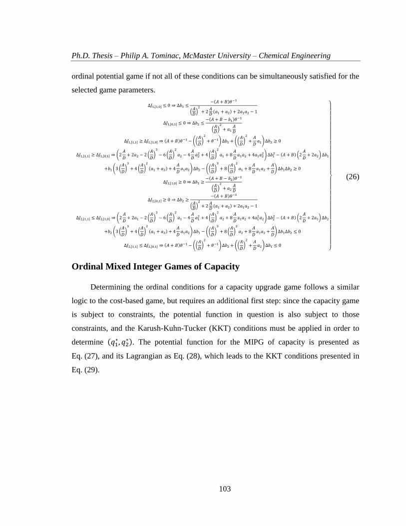
Ph.D. Thesis – Philip A. Tominac, McMaster University – Chemical Engineering
103
ordinal potential game if not all of these conditions can be simultaneously satisfied for the
selected game parameters.
Δ𝐽1,[1,0] ≤ 0 ⇒ Δ𝑏1 ≤−(𝐴 + 𝐵)𝜃−1
(𝐴𝐷)2
+ 2𝐴𝐷(𝑎1 + 𝑎2) + 2𝑎1𝑎2 − 1
Δ𝐽1,[0,1] ≤ 0 ⇒ Δ𝑏2 ≤−(𝐴 + 𝐵 − 𝑏1)𝜃
−1
(𝐴𝐷)2
+ 𝑎1𝐴𝐷
Δ𝐽1,[1,1] ≥ Δ𝐽1,[1,0] ⇒ (𝐴 + 𝐵)𝜃−1 − ((𝐴
𝐷)2
+ 𝜃−1)Δ𝑏1 + ((𝐴
𝐷)2
+𝐴
𝐷𝑎1)Δ𝑏2 ≥ 0
Δ𝐽1,[1,1] ≥ Δ𝐽1,[0,1] ⇒ (2𝐴
𝐷+ 2𝑎2 − 2(
𝐴
𝐷)3
− 6(𝐴
𝐷)2
𝑎2 − 4𝐴
𝐷𝑎22 + 4(
𝐴
𝐷)2
𝑎1 + 8𝐴
𝐷𝑎1𝑎2 + 4𝑎1𝑎2
2)Δ𝑏12 − (𝐴 + 𝐵) (2
𝐴
𝐷+ 2𝑎2)Δ𝑏1
+𝑏1 (3 (𝐴
𝐷)3
+ 4(𝐴
𝐷)2
(𝑎1 + 𝑎2) + 4𝐴
𝐷𝑎1𝑎2)Δ𝑏2 − ((
𝐴
𝐷)3
+ 8(𝐴
𝐷)2
𝑎1 + 8𝐴
𝐷𝑎1𝑎2 +
𝐴
𝐷) Δ𝑏1Δ𝑏2 ≥ 0
Δ𝐽2,[1,0] ≥ 0 ⇒ Δ𝑏1 ≥−(𝐴 + 𝐵 − 𝑏2)𝜃
−1
(𝐴𝐷)2
+ 𝑎2𝐴𝐷
Δ𝐽2,[0,1] ≥ 0 ⇒ Δ𝑏2 ≥−(𝐴 + 𝐵)𝜃−1
(𝐴𝐷)2
+ 2𝐴𝐷(𝑎1 + 𝑎2) + 2𝑎1𝑎2 − 1
Δ𝐽2,[1,1] ≤ Δ𝐽2,[1,0] ⇒ (2𝐴
𝐷+ 2𝑎1 − 2(
𝐴
𝐷)3
− 6(𝐴
𝐷)2
𝑎1 − 4𝐴
𝐷𝑎12 + 4(
𝐴
𝐷)2
𝑎2 + 8𝐴
𝐷a1𝑎2 + 4𝑎1
2𝑎2)Δ𝑏22 − (𝐴 + 𝐵) (2
𝐴
𝐷+ 2𝑎1) Δ𝑏2
+𝑏2 (3 (𝐴
𝐷)3
+ 4(𝐴
𝐷)2
(𝑎1 + 𝑎2) + 4𝐴
𝐷𝑎1𝑎2)Δ𝑏1 − ((
𝐴
𝐷)3
+ 8(𝐴
𝐷)2
𝑎2 + 8𝐴
𝐷𝑎1𝑎2 +
𝐴
𝐷)Δ𝑏1Δ𝑏2 ≤ 0
Δ𝐽2,[1,1] ≤ Δ𝐽2,[0,1] ⇒ (𝐴 + 𝐵)𝜃−1 − ((𝐴
𝐷)2
+ 𝜃−1)Δ𝑏2 + ((𝐴
𝐷)2
+𝐴
𝐷𝑎2)Δ𝑏1 ≤ 0
}
(26)
Ordinal Mixed Integer Games of Capacity
Determining the ordinal conditions for a capacity upgrade game follows a similar
logic to the cost-based game, but requires an additional first step: since the capacity game
is subject to constraints, the potential function in question is also subject to those
constraints, and the Karush-Kuhn-Tucker (KKT) conditions must be applied in order to
determine (𝑞1∗, 𝑞2
∗). The potential function for the MIPG of capacity is presented as
Eq. (27), and its Lagrangian as Eq. (28), which leads to the KKT conditions presented in
Eq. (29).

Ph.D. Thesis – Philip A. Tominac, McMaster University – Chemical Engineering
104
𝑍 = (𝐴 + 𝐵 − 𝑏1)𝑞1 + (𝐴 + 𝐵 − 𝑏2)𝑞2 −𝐴
𝐷𝑞1𝑞2 − (
𝐴
𝐷+ 𝑎1) 𝑞1
2 − (𝐴
𝐷+ 𝑎2) 𝑞2
2 − 𝑐1 − 𝑐2
𝑞1 ≤ �̅�1𝑞2 ≤ �̅�2
} (27)
𝐿 = (𝐴 + 𝐵 − 𝑏1)𝑞1 + (𝐴 + 𝐵 − 𝑏2)𝑞2 −𝐴
𝐷𝑞1𝑞2 − (
𝐴
𝐷+ 𝑎1) 𝑞1
2 − (𝐴
𝐷+ 𝑎2) 𝑞2
2 − 𝑐1 − 𝑐2
+ 𝜇1(𝑞1 − �̅�1) + 𝜇2(𝑞2 − �̅�2) (28)
𝐴 + 𝐵 −𝐴
𝐷(2𝑞1 + 𝑞2) − 2𝑎1𝑞1 − 𝑏1 + 𝜇1 = 0
𝐴 + 𝐵 −𝐴
𝐷(𝑞1 + 2𝑞2) − 2𝑎2𝑞2 − 𝑏2 + 𝜇2 = 0
𝑞1 ≤ �̅�1𝑞2 ≤ �̅�2
𝜇1(𝑞1 − �̅�1) = 0
𝜇2(𝑞2 − �̅�2) = 0𝜇1 ≤ 0𝜇2 ≤ 0 }
(29)
The possible combinations of the complementarity constraints imply that there exist
four individual resolutions to this problem: both capacity constraints inactive, one
player’s constraint active and the other’s inactive, the opposite of the previous, and both
constraints active, all four of which would need to be accounted for in each case of the
two-by-two game. The simplest case which can result in the finite capacity game is that in
which it is assumed that players begin the game operating at capacity, and the capacity
added (we will assume that the upgrade does not result in diminished capacity) leaves
both players operating at an optimum where their capacity constraints are inactive. This
means that in either case that one of, or both players, upgrade their capacity, that
following the upgrade, both will be operating below the level of their capacity constraint.
This includes a player who does not upgrade when its competitor has done so, implying
that such a player reduces its output. That this will result will be made apparent by the
(Δ𝑞1∗, Δ𝑞2
∗) value calculation, from which it will be seen that when one player upgrades
and the other does not, the non-upgrade player reduces its production level from its
constraint bound to a lesser amount. Operating under these assumptions the optimal
solutions 𝑞𝑟,[𝜉1,𝜉2]∗ are defined in Eq. (30).

Ph.D. Thesis – Philip A. Tominac, McMaster University – Chemical Engineering
105
𝑞1,[0,0]∗ = (
𝐴
𝐷(𝐴 + 𝐵 − 2𝑏1 + 𝑏2 + 2𝜇1 − 𝜇2) + 2𝑎2(𝐴 + 𝐵 − 𝑏1 + 𝜇1))𝜃
𝑞2,[0,0]∗ = (
𝐴
𝐷(𝐴 + 𝐵 + 𝑏1 − 2𝑏2 − 𝜇1 + 2𝜇2) + 2𝑎1(𝐴 + 𝐵 − 𝑏2 + 𝜇2))𝜃
𝑞1,[1,0]∗ = (
𝐴
𝐷(𝐴 + 𝐵 − 2𝑏1 + 𝑏2 − 𝜇2) + 2𝑎2(𝐴 + 𝐵 − 𝑏1)) 𝜃
𝑞1,[0,1]∗ = (
𝐴
𝐷(𝐴 + 𝐵 − 2𝑏1 + 𝑏2 + 2𝜇1) + 2𝑎2(𝐴 + 𝐵 − 𝑏1 + 𝜇1)) 𝜃
𝑞1,[1,1]∗ = (
𝐴
𝐷(𝐴 + 𝐵 − 2𝑏1 + 𝑏2) + 2𝑎2(𝐴 + 𝐵 − 𝑏1))𝜃
𝑞2,[1,0]∗ = (
𝐴
𝐷(𝐴 + 𝐵 + 𝑏1 − 2𝑏2 + 2𝜇2) + 2𝑎1(𝐴 + 𝐵 − 𝑏2 + 𝜇2)) 𝜃
𝑞2,[0,1]∗ = (
𝐴
𝐷(𝐴 + 𝐵 + 𝑏1 − 2𝑏2 − 𝜇1) + 2𝑎1(𝐴 + 𝐵 − 𝑏2)) 𝜃
𝑞2,[1,1]∗ = (
𝐴
𝐷(𝐴 + 𝐵 + 𝑏1 − 2𝑏2) + 2𝑎1(𝐴 + 𝐵 − 𝑏2))𝜃
}
(30)
The corresponding (Δ𝑞1, Δ𝑞2) values are collected in Eq. (31). Note that since the
Lagrange multipliers (𝜇1, 𝜇2) are nonpositive in value, a negative Δ𝑞 coefficient indicates
positive change; also note that in the single player upgrade cases, the non-upgrading
player reduces its production in response to the upgrading player’s increased output.
Substitution of the Δ𝑞 values into the profit functions is qualitatively similar to the cost-
based game; the resulting algebraic conditions define circumstances under which a MIPG
of capacity will not be an ordinal potential game, and are presented in Eq. (32).
Δ𝑞1,[1,0] = −2(
𝐴
𝐷+ 𝑎2) 𝜃𝜇1
Δ𝑞1,[0,1] =𝐴
𝐷𝜃𝜇2
Δ𝑞1,[1,1] = −2(𝐴
𝐷+ 𝑎2) 𝜃𝜇1 +
𝐴
𝐷𝜃𝜇2
Δ𝑞2,[1,0] =𝐴
𝐷𝜃𝜇1
Δ𝑞2,[0,1] = −2(𝐴
𝐷+ 𝑎1) 𝜃𝜇2
Δ𝑞2,[1,1] = −2(𝐴
𝐷+ 𝑎1)𝜃𝜇2 +
𝐴
𝐷𝜃𝜇1}
(31)

Ph.D. Thesis – Philip A. Tominac, McMaster University – Chemical Engineering
106
Δ𝐽1,[1,0] ≤ 0 ⇒ 𝜇1 ≥ −(𝐴 + 𝐵 − 𝑏1)𝜃
−1
(𝐴𝐷)
2
+ 2𝐴𝐷(𝑎2 − 𝑎1) + 2𝑎1𝑎2
Δ𝐽1,[0,1] ≤ 0 ⇒ 𝜇2 ≤ −(𝐴 + 𝐵 − 𝑏1)𝜃
−1
(𝐴𝐷)
2
+𝐴𝐷 𝑎1
Δ𝐽1,[1,1] ≥ Δ𝐽1,[1,0] ⇒ (𝐴 + 𝐵 − 𝑏1) − (𝐴
𝐷)2
𝜃𝜇1 + ((𝐴
𝐷)2
+𝐴
𝐷𝑎1)𝜃𝜇2 ≥ 0
Δ𝐽1,[1,1] ≥ Δ𝐽1,[0,1] ⇒ (𝐴 + 𝐵 − 𝑏1) (−2 (𝐴
𝐷+ 𝑎2)) + (−2(
𝐴
𝐷)3
− 4(𝐴
𝐷)2
𝑎1 − 6(𝐴
𝐷)2
𝑎2 − 4𝐴
𝐷𝑎22 − 8
𝐴
𝐷𝑎1𝑎2 − 4𝑎1𝑎2
2)𝜃𝜇1 − (𝐴
𝐷)3
𝜃𝜇2 ≥ 0
Δ𝐽2,[1,0] ≥ 0 ⇒ 𝜇1 ≥ −(𝐴 + 𝐵 − 𝑏2)𝜃
−1
(𝐴𝐷)
2
+𝐴𝐷 𝑎2
Δ𝐽2,[0,1] ≥ 0 ⇒ 𝜇2 ≤ −(𝐴 + 𝐵 − 𝑏2)𝜃
−1
(𝐴𝐷)
2
+ 2𝐴𝐷(𝑎2 − 𝑎1) + 2𝑎1𝑎2
Δ𝐽2,[1,1] ≤ Δ𝐽2,[1,0] ⇒ (𝐴 + 𝐵 − 𝑏2) (−2 (𝐴
𝐷+ 𝑎1)) − (
𝐴
𝐷)3
𝜃𝜇1 + (−2(𝐴
𝐷)3
− 6(𝐴
𝐷)2
𝑎1 − 4𝐴
𝐷𝑎12 − 4(
𝐴
𝐷)2
𝑎2 − 8𝐴
𝐷𝑎1𝑎2 − 4𝑎1
2𝑎2)𝜃𝜇2 ≤ 0
Δ𝐽2,[1,1] ≤ Δ𝐽2,[0,1] ⇒ (𝐴 + 𝐵 − 𝑏2) − (𝐴
𝐷)2
𝜃𝜇2 + ((𝐴
𝐷)2
+𝐴
𝐷𝑎2)𝜃𝜇1 ≤ 0
}
(32)
Numerical Examples
Illustrative example – MIPG of cost
A simple game of the form defined by Eqs. (7)-(9) is presented which is solved as a
MINLP to a Nash equilibrium solution satisfying both continuous game and discrete
game equilibrium definitions. The implied finite game matrix is enumerated and
presented for comparison with the MINLP solution matrix, and the ordinal game
conditions are evaluated in order to verify that the game is indeed an ordinal cost game.
Parameter values for this example problem are as follows: 𝐴 = 2, 𝐵 = 8, 𝐷 = 10, 𝑎1 =
1, 𝑎2 = 2, 𝑏1 = 5, 𝑏2 = 4, 𝑐1 = 3, 𝑐2 = 2, and Δ𝑏1 = Δ𝑏2 = −1. The MINLP
formulation is as in Eq. (33). This problem is indicative of two competing producers of a
single product operating in a single Cournot-type market, with each producer having the
option to implement a single upgrade, the cost of which is irrelevant to the qualitative
interpretation of the result.
max𝑞1,𝑞2≥0
𝑦1,𝑦2∈{0,1}
𝑍(𝑞1, 𝑞2, 𝑦1, 𝑦2)
= (𝐴 + 𝐵 − (𝑏1 + 𝑦1Δ𝑏1))𝑞1
+ (𝐴 + 𝐵 − (𝑏2 + 𝑦2Δ𝑏2))𝑞2 −𝐴
𝐷𝑞1𝑞2 − (
𝐴
𝐷+ 𝑎1) 𝑞1
2
− (𝐴
𝐷+ 𝑎2) 𝑞2
2 − 𝑐1 − 𝑐2
(33)

Ph.D. Thesis – Philip A. Tominac, McMaster University – Chemical Engineering
107
As a pre-solve measure, the ordinal conditions corresponding to the game of cost in
Eq. (26) are checked; it is determined that conditions 4 and 8 are not satisfied by the
chosen parameter values in the given inequality case, and conditions 2, 5, 6, and 7 are all
unsatisfied in the reverse-sign case. It is thus assured that the game is an ordinal potential
game and that the solution to the MINLP formulation of the problem in Eq. (33) will be a
PSNE. Solution of this problem yields an objective value of 9.787, corresponding to
profit values of 5.723 and 3.963 to players 1 and 2 resulting from the PSNE strategy
(𝑦1, 𝑦2) = (1,1) in which both players implement their upgrade.
Enumeration of all strategy sets gives the potential function matrix in Eq. (34), and
the corresponding profit values in Eq. (35). Verification of the existence of a PSNE in
these enumerated matrices is accomplished by finding that the potential maximum of
9.787 coincides with the profit matrix column (player 1) and row (player 2) maxima
corresponding to the strategy (1,1). The matrix of production volumes is presented in
Eq. (36); it is noted that production changes due to an opposing player changing its
strategy are small, and thus that the example presented is close to having an exact
potential.
𝑍 0 101
[5.511 7.1078.192 9.787
] (34)
𝑗 0 101
[3.055,2.383 3.043,3.9805.737,2.369 5.723,3.963
] (35)
𝑞 0 101
[2.437,1.473 2.434,1.7212.927,1.471 2.924,1.718
] (36)
In this example, enumeration is a computationally feasible means of determining
the PSNE, however, increasing cardinality of players’ strategy sets results in the rapidly
increasing size of the game matrix. Assuming a general game with 𝑅 players each
possessing |Ξ𝑟| strategies (which shall be assumed to be of equal number Ξ) then the
number of matrix elements is Ξ𝑅. To complicate this scaling, a strategy set must include
all possible player decisions; thus in a set of players each having a set of potential
upgrades 𝑈𝑟 (where again it is assumed here that all |𝑈𝑟| = 𝑈) each player will possess
Ph.D. Thesis – Philip A. Tominac, McMaster University – Chemical Engineering
108
Ξ = 2𝑈 strategies, corresponding to a matrix with 2𝑈𝑅 entries. Problems of meaningful
size and scale quickly become inconvenient to solve by enumeration; the ability to solve
MIPG problems as MINLPs takes advantage of decades of developments in branching
algorithms to reduce the computational effort required to obtain a PSNE. The solutions to
competitive expansion problems as Nash equilibria are competitively optimal and are
desirable for their potential industrial applications.
Application example – competitive refinery expansion planning
We now turn to an application of MIPG modelling using an industrially motivated
example in which two petroleum refiners compete in the same markets and seek to
expand their facilities in order to establish a competitive advantage. This scenario is
formulated as a static multiproduct multimarket game of the form in Tominac and
Mahalec4 with six products and two markets. Refiners have four upgrades available
which may be purchased and implemented in any combination. These are: a hydrocracker
processing upgrade, a hydrotreater processing upgrade, a CDU capacity upgrade, and a
gasoline blender capacity upgrade. Upgrade costs are estimated based on data in the
Refining Processes Handbook (2008) and Meyers (2004) Handbook of Petroleum
Refining Processes. The complexity of this formulation prohibits the use of the ordinality
conditions derived in this work; in part because the case of multiple products and markets
have not been addressed in those derivations, and in addition because this example
includes strategies in which multiple upgrades are selected, and such cases were not
considered due to the additional algebraic complexity introduced. For these reasons, the
refinery upgrade MINLP is solved using the MIPG potential game approach to find the
PSNE, and the result is verified by enumeration. The patterns in the results lead to several
conjectures regarding the existence of PSNE in MIPGs which will be formalized in the
section that follows. The enumerated potential function values and player profit values
are presented in Figure 1 as matrices in which refiner 1 is the row player and refiner 2 is
the column player, which have been overlaid with heat maps for readability. Rows and
columns are labeled with strategy numbers corresponding to the binary variable values in

Ph.D. Thesis – Philip A. Tominac, McMaster University – Chemical Engineering
109
the legend included in the figure. Both refiners in this example possess that same upgrade
options, and so identical upgrade labels are used for both players. The values in this
figure represent optimal solutions to the enumerated cases, and are obtained using
ANTIGONE 1.1 in GAMS 24.7.1 with the relative gap set to 1×10⁻⁹
, and warm started
with DICOPT on a Dell Optiplex 9010 computer with Intel Core-i7-3770 CPU, a
3.40 GHz processor, and Windows 10 64-bit operating system. The model has 820
continuous and 16 binary variables with 695 equations following ANTIGONE
preprocessing. Of these equations, 39 are nonconvex nonlinear and the remainder are
linear. The model contains 130 nonlinear terms, 128 are bilinear and the remaining two
are the sigmoidal cost functions. All cases are solved to global optimality with model and
solver status both reported as 1 in all cases, indicating optimality and normal completion,
respectively. The results obtained under the specified gap are taken to be sufficiently
close to true global optimality for the purposes of this example. It can be verified that the
profit matrices and potential matrix independently define the same pure strategy
equilibrium. The PSNE occurs in the case that both players purchase all upgrades except
the hydrocracker processing upgrade, corresponding to row and column eight in the
matrices.

Ph.D. Thesis – Philip A. Tominac, McMaster University – Chemical Engineering
110
Figure 1. Potential and profit values in refining example MIPG

Ph.D. Thesis – Philip A. Tominac, McMaster University – Chemical Engineering
111
The value in the MIPG approach to competitive expansion planning problems lies
in computational efficiency; by solving finite game problems as MINLPs branching
algorithms dictate the number of matrix entries which must be calculated, which in the
worst case results in complete enumeration. In addition, the existence of MIPG implies
that the complete reward matrix is not required in order to determine whether the outcome
of a game will be a PSNE; as long as the ordinality conditions are satisfied it is assured
that the outcome will be a PSNE and this solution can be obtained using standard mixed
integer nonlinear optimization approaches. This result is novel at time of writing; no other
game-type problems of mixed integer and continuous decision variables have been solved
satisfying both continuous and discrete definitions of Nash equilibria, and this example
represents the first practical MIPG solved to equilibrium by optimization. While a single
example is presented, no parameter combinations tested – including those with
unreasonably large, small, or negative values – defining a feasible game was observed to
yield a matrix without a pure strategy equilibrium.
Conjectures
We have presented algebraic conditions defining the existence of mixed integer
games of two players possessing two strategies. Analysis of these games is nontrivial
even in the two-by-two case, and the algebraic analysis required scales poorly as the
dimension of the game in question increases both in strategy set cardinality and in the
number of interested players. Based on the analytical and numerical results obtained, and
because we have not been able to conclusively prove the existence of the observed
results, we offer the following conjectures regarding the existence and properties of
mixed integer games based on continuous Cournot potential games:
1) MIPG games exist possessing PSNE,
2) The existence of PSNE in a MIPG is determined by parameters associated with the
continuous game which define the optima to each strategic realization of the implied
finite game which collectively define the implied finite game payoff matrix,

Ph.D. Thesis – Philip A. Tominac, McMaster University – Chemical Engineering
112
3) Conjectures 1 and 2 generalize to games of arbitrary strategic size and number of
players,
4) In the event it exists, a PSNE is obtained as the solution to a mixed integer nonlinear
program; enumeration of the implied finite game payoff matrix is not required to
achieve such equilibria.
MIPG are interesting and relevant problems, and proof of the conjectures made in
this work merits additional research. In particular, the ordinal conditions defining when a
MIPG possesses a PSNE must be generalized for cases of arbitrary numbers of players
and player strategies, including cases in which multiple finite changes are applied in a
single strategy (i.e., the multiple active upgrade case addressed in the refinery problem)
and influence the objective value of the game. In addition, it may be possible to prove that
the ordinality conditions guarantee the existence of PSNE in MIPGs under reasonable
assumptions. The conditions that have been presented in this work are useful as metrics,
but they have not been resolved in such a way as to make generalized guarantees with
respect to game parameters; our conditions are useful only in specific instances of a game
to determine whether a PSNE exists.
Conclusions
We have presented conditions defining parameter instances of two-player two-
strategy Cournot based mixed integer ordinal potential games which guarantee that the
defined game will possess a pure strategy Nash equilibrium for two types of discrete
strategies which have been interpreted as upgrades in a competitive refinery capacity
expansion and production planning problem. Based on results presented in which games
of higher dimension possessed PSNE, in particular a refinery expansion model in which
two refiners each possess sixteen strategies, we conjecture that the properties we have
defined for small MIPGs extend to games of higher dimension. The MIPG as a
framework for industrially motivated competitive problems is useful and provides insight
into organizational level planning; such a framework allows planning problems to be cast
across the height and breadth of an organization, optimizing both high and low-level

Ph.D. Thesis – Philip A. Tominac, McMaster University – Chemical Engineering
113
decisions of both discrete and continuous types. MIPGs merit additional research, in part
to lay out their theoretical properties, and to explore their applications and utility in
difficult industrial problems where competitive interactions interplay with technological
decisions.
Notation
Sets
𝑅 (𝑟) refiners or players
Ξ𝑅 (𝜉𝑟) strategy set for refiner 𝑟
Parameters
𝐴 Price decline rate
𝐵 Price of product 𝑝 in market 𝑤 corresponding to supply of exactly 𝐷𝑝𝑤
𝐷 Nominal market supply of product 𝑝 in market 𝑤
�̅�𝑟 Maximum production rate by refiner 𝑟
𝑎𝑟 Refiner 𝑟 quadratic cost term
𝑏𝑟 Refiner 𝑟 linear cost term
𝑐𝑟 Refiner 𝑟 constant cost term
Continuous Variables
𝐽𝑟 Profit function for refiner 𝑟
𝑗𝑟 A profit value for refiner 𝑟; used to indicate scalar values
π Price
𝑞𝑟 Product volume produced by refiner 𝑟
𝐶𝑟 General cost function of refiner 𝑟
𝑍 Potential function value
𝐿 Lagrangian function value

Ph.D. Thesis – Philip A. Tominac, McMaster University – Chemical Engineering
114
𝜇𝑟 Lagrange multiplier
Binary Variables
𝑦𝑟 Refiner 𝑟 decision to purchase an upgrade
References
Debreu, G. (1952) A social equilibrium existence theorem. P Natl Acad Sci USA,
38(10), 886-893.
Fan, K. (1952) Fixed-point and minimax theorems in locally convex topological
linear spaces. P Natl Acad Sci USA, 38(2), 121-126.
Ghosh, A., Cottatellucci, L., Altman, E. (2015) Normalized Nash equilibrium for
power allocation in cognitive radio networks. IEEE Trans. Cogn Commun Netw, 1(1), 86-
99.
Glicksberg, I. L. (1952) A further generalization of the Kakutani fixed point
theorem, with application to Nash equilibrium points. P Am Math Soc, 3(1), 170-174.
Grossmann, I. E. (2002) Review of nonlinear nixed-integer and disjunctive
programming techniques. Optim Eng, 3, 227-252.
Hydrocarbon Processing. 2008 refining processes handbook. GPC; 2008.
Lin, X., Floudas, C. A. (2005) Mixed integer linear programming in process
scheduling: modeling, algorithms and applications. Ann Oper Res, 139, 131-162.
Liu, X., Du, G., Jiao, R. J., & Xia, Y. (2017). Product Line Design Considering
Competition by Bilevel Optimization of a Stackelberg-Nash Game. IISE Transactions,
(just-accepted)
Meyers, R. (2004) Handbook of petroleum refining processes. 3rd ed. McGraw-
Hill.
McKelvey, R. D., McLennan, A. (1996) Computation of equilibria in finite games.
In: Handbook of computational economics. 1st ed. 87-142.
Monderer, D., Shapley, L. (1996) Potential Games. Game Econ Behav. 14(1), 124-
143.

Ph.D. Thesis – Philip A. Tominac, McMaster University – Chemical Engineering
115
Morrow, W. R., Mineroff, J., & Whitefoot, K. S. (2014). Numerically Stable Design
Optimization With Price Competition. Journal of Mechanical Design, 136(8), 081002.
Nash, J. (1951) Non-cooperative Games. Ann Math, 54(2), 286-295.
Neiro, S. M. S., Pinto, J. M. (2008) A general modeling framework for the
operational planning of petroleum supply chains. Comput Chem Eng, 28, 871-896.
Rosen, B. (1965) Existence and uniqueness of equilibrium points for concave n-
person games. Econometrica, 520-534.
Shiau, C. S. N., & Michalek, J. J. (2009). Optimal product design under price
competition. Journal of Mechanical Design, 131(7), 071003.
Tominac, P., Mahalec, V. (2017) A game theoretic framework for petroleum
refinery strategic production planning. AICHE J, 63(7), 2751-2763.
Trespalacios, F., Grossmann, I. E. (2014) Review of mixed-integer nonlinear and
generalized disjunctive programming methods. 2014; Chem-Ing-Tech, 86(7), 991-1012.
Webb, J. N. (2007) Game Theory: Decisions, Interaction and Evolution. London,
UK: Springer London.
You, F., Grossmann, I. E. (2008) Mixed-integer nonlinear programming models and
algorithms for large-scale supply chain design with stochastic inventory management. Ind
Eng Chem Res, 47, 7802-7817.
Acknowledgements
This work has been funded by the Natural Sciences and Engineering Research
Council of Canada, the Government of Ontario, and the McMaster Advanced Control
Consortium whom we thank for their support.

Ph.D. Thesis – Philip A. Tominac, McMaster University – Chemical Engineering
116
Chapter 5
Conclusions and recommendations

Ph.D. Thesis – Philip A. Tominac, McMaster University – Chemical Engineering
117
Conclusions
This thesis makes significant progress towards the development of frameworks for
the analysis of competitive behaviour in strategic production planning. The game
theoretic concept of the potential function has a natural synergy with mathematical
formulations of process systems, effectively allowing economic models to build directly
onto complex process models and to have the entire program optimized under a single
objective function. The static and dynamic competitive models presented in this thesis
take strides in the direction of creating enterprise optimization models in which both
enterprise level objectives and detailed process constraints can be included in a single
program. In addition, a new class of game theoretic problems has been identified in the
mixed integer game, and progress has been made in characterizing these games.
Enterprise optimization
The competitive production planning frameworks developed in Chapters 2 and 3,
and the expansion planning framework of Chapter 4 represent means by which the
combined goals of profit maximization, cost minimization, and process optimization may
be incorporated into a single mathematical program optimizing an entire enterprise.
Process details from the operational to the strategic can be incorporated with models of
markets and delivery channels, including competitors in those channels, into a single
problem which has as its objective the economic success of the enterprise and a rational,
game theoretic objective by which to achieve it. The Cournot potential game objective
used in this work is based on the fundamental link between the behaviours of market
price and supply. The refinery models allow rigorous engineering models to regulate
production, and offer insight to competitive and mechanical limitations in process
operations. The primary limitation to the achievement of this objective is the size and
scaling of such models, the solutions to which are limited by available computation
power.

Ph.D. Thesis – Philip A. Tominac, McMaster University – Chemical Engineering
118
Mixed integer games
The class of mixed integer games is of interest from an academic perspective,
representing the game theoretic analogue to the mixed integer nonlinear program. Of
primary interest is the result determined in Chapter 4: that enumeration of all payoffs is
not required to determine a Nash equilibrium. A knowledge of the mathematical nature of
the game in question and the parameters which define the form of the solution is
sufficient. Determination of the conditions under which an equilibrium in pure strategies
is guaranteed to exist is a challenging problem becoming significantly more difficult with
increasing problem sizes. Nevertheless, conjectures have been made regarding the form
of these problems and the suspected features of the class of games if it can be defined.
Concluding thoughts
The driving force initiating this thesis was a suspicion that existing production
planning techniques offer suboptimal recommendations since the influence of competitors
on strategic decision making is ignored. The work in this thesis demonstrates that by
accounting for the presence of industrial opponents enterprise strategy is significantly
altered. In many ways the results presented are reflective of a more intuitive planning
solution. Game theoretic production planning avoids some of the common pitfalls of
standard planning approaches without the requirement of additional constraints; product
portfolios are diversified according to the behaviour of market prices and demands, and
take into account the optimal behaviour of competitors, meaning that the resulting plans
are conservative rather than being best case scenarios. The computation results achieved
in these frameworks provide logical reasons for intuitive behaviours, bringing
computational solutions closer to human solutions.
Recommendations for further work
The work in this thesis opens up several avenues for investigation into game
theoretic solutions for process engineering problems. Some of these are based on

Ph.D. Thesis – Philip A. Tominac, McMaster University – Chemical Engineering
119
validating assumptions made in the modelling process, while others represent novel lines
of inquiry that extend the work. In addition, the opportunity to explore the class of mixed
integer games is an interesting one, especially if it is possible to mathematically prove the
existence or properties of either specific mixed integer games or for the class as a whole.
With consideration of these options, three research projects are recommended.
Market entry and denial
A primary assumption in the production planning framework is that refiners outside
a domestic market cannot sell product there; this has been justified in several ways, but
rather than work with this assumption, it can be reformulated into a new research
question, namely: is it viable for a refiner outside a domestic market to attempt to enter
that domestic market by constructing refining resources there? This question should be
posed as a game theoretic market entry problem factoring in rigorous models of refinery
building costs and construction duration, and consider the options possessed by domestic
refiners that might be pursued in order to discourage such entries, such as price
management, or in keeping with the work in Chapter 3 and 4, whether domestic refiners
can initiate counter upgrade procedures to make market entry potentially unprofitable for
the outsider. The problem has industrial significance and further links enterprise
management decisions with operational constraints.
Uncertainty and Bayesian games
A particular problem in the game theoretic framework is the assumption that
competitors possess perfect knowledge of each other and can plan accordingly. The
Bayesian game structure allows uncertainty of opposing players’ strategies to be included
in the framework, and should have a form similar to that of a stochastic program.
Bayesian game structure is such that opponents have beliefs about one another and
formulate their own responses based on the distribution of those beliefs. Thus a scenario-
based formulation of a refinery production planning problem could be cast in which each
refiner has associated with it opponents beliefs as a set of discrete cases; the solution to

Ph.D. Thesis – Philip A. Tominac, McMaster University – Chemical Engineering
120
such a model is a Bayesian Nash equilibrium and will be indicative of the optimal
strategy under uncertainty.
Extensions to mixed integer games
This thesis includes a demonstration of the existence of mixed integer games, but
no proof that the structures behave in the way that they appear to. A mathematical
exercise undertaken to prove conclusively that games of the form in Chapter 4 are either
guaranteed to possess a PSNE in all cases, or else are guaranteed to possess such an
equilibrium under a defined set of conditions would represent a large step towards the
understanding of this new class of games. This project is perhaps the most difficult of the
three, but is of significant academic interest.
Additional Considerations
Other factors which might be addressed in future work could contribute to the
realism of the market models. Tariffs and transportation costs are relatively simple to
implement, and introduce geographical dependencies into the market models. Tariffs and
transportation costs both impact the price realized by refiners in the models. Transport
costs give refiners geographically near their markets an asymmetric advantage. Tariffs
would decrease prices in specific global markets for certain domestic refiners. The
interplay of such factors with the motivation of profit will differentiate refiners based on
geographical location, even if such refiners are identical in capacity and cost structure.
The game theoretic concept of the Stackelberg game has largely been avoided in
this thesis under the assumption that refinery behaviours are visible on the requisite time
scales and are thus adequately modelled using Nash equilibrium concepts; i.e., refiners
can observe and react to changes in competitors’ production, and similarly can observe
and respond to upgrade plans. The Stackelberg game provides a useful solution concept
when this assumption is not true, and could provide insights into elements of refinery
interactions and competition. In the Stackelberg optimization framework, one player
moves first and is able to maximize its objective directly while its competitors are

Ph.D. Thesis – Philip A. Tominac, McMaster University – Chemical Engineering
121
constrained to Nash equilibrium strategies. By analogy, such a game could be solved in
the frameworks proposed in this thesis by maximizing the first-mover’s profit, with all
other players subject to the KKT conditions of a corresponding Nash Cournot potential
game. The development of such KKT conditions presents the primary boundary to such
pursuits.

Ph.D. Thesis – Philip A. Tominac, McMaster University – Chemical Engineering
122
Appendix
Supplementary materials
This section contains the supplementary materials included for online publication
with the manuscripts in Chapters 2 and 4. Lists of figure and tables included in the online
document have been omitted here.

Ph.D. Thesis – Philip A. Tominac, McMaster University – Chemical Engineering
123
Supplementary material to: A game
theoretic framework for petroleum
refinery strategic production planning
Philip Tominac and Vladimir Mahalec*
Department of Chemical Engineering, McMaster University, 1280 Main St. W.,
Hamilton, ON, L8S 4L8, Canada
*Corresponding author. Tel.: +1 905 525 9140 ext. 26386. E-mail address:

Ph.D. Thesis – Philip A. Tominac, McMaster University – Chemical Engineering
124
A. The Cournot oligopoly in brief
The Cournot oligopoly is a classic economic model used to examine market
competition, which we use to structure game theoretic interactions between competitors.
The Cournot oligopoly defines a game in which a set 𝑁 of producers of a good each must
decide how much of that good to sell to a market21,40
. The realized price for the good is a
function of the collective amount the players deliver to the market. This scenario results
in a game in which each player’s only strategic decision is a production volume. We
focus on a static Cournot game assuming complete information and homogeneous
product21
.
Each market participant attempts to maximize its profits according to a function
𝐽𝑛 = 𝑃𝑟 ∙ 𝑞𝑛 − 𝑐𝑛(𝑞𝑛) where 𝑃𝑟 represents market price, 𝑞𝑛 is the amount supplied by
producer 𝑛, each of whom has a production cost 𝑐𝑛(𝑞𝑛) which is some function of its
production level. The solution to this game theoretic model is a Nash equilibrium in terms
of the quantities of product 𝑞𝑛 that each of the 𝑁 producers supply. The market price 𝑃𝑟
is a function of 𝑞𝑛 and the most common interpretation is that in Eq. (A1).
𝑃𝑟 = {𝐴 − ∑ 𝑞𝑛𝑛 ∑ 𝑞𝑛𝑛 < 𝐴
0 ∑ 𝑞𝑛𝑛 ≥ 𝐴 (A1)
𝐴 is a parameter indicative of the marginal value of the first unit sold on the market.
This interpretation is presented in similar form in21,32,40
. Player objective functions can be
rewritten as functions of total production of the form in Eq. (A2).
𝐽𝑛 = (𝐴 − ∑ 𝑞𝑛′𝑛′ )𝑞𝑛 − 𝑐𝑛(𝑞𝑛) (A2)

Ph.D. Thesis – Philip A. Tominac, McMaster University – Chemical Engineering
125
The Nash equilibrium in terms of 𝑞𝑛 for this oligopoly problem is defined by the
solution to the set of best response equations in Eq. (A3).
𝜕𝐽𝑛
𝜕𝑞𝑛= 0 ∀𝑛 ∈ 𝑁 (A3)
The Cournot oligopoly presented here is a potential game33
. The corresponding
potential function has the form in Eq. (A4).
𝑍 = ∑ (𝐴 ∙ 𝑞𝑛 − 𝑞𝑛2 − 𝑐𝑛(𝑞𝑛))𝑛 − ∑ ∑ (𝑞𝑛𝑞𝑛′)𝑛′
𝑛′<𝑛𝑛 (A4)
B. Refinery production planning model
The purpose of the production planning model equations is to determine the
volumes of products that the refinery should produce in order to satisfy the model
objective and what crude oil stocks, intermediate products, and blending strategies must
be used in order to satisfy quality constraints associated with each product. Flow of
material between process units is defined based on inclusion of set elements in equation
definitions. The total volumetric inlet flow to each unit in the refinery is defined by
Eq. (B1). Inlet flow is broken down by mode for those units which have multiple
operating modes in Eq. (B2). The minimum and maximum total inlet flows into a unit are
defined by Eqs. (B3) and (B4).
𝐹𝐴(𝑡, 𝑢, 𝑛) = ∑ 𝐹𝑉𝑀(𝑚, 𝑡, 𝑢, 𝑛)𝑚𝑚∈𝑈𝑀
∀𝑡 ∈ 𝑇, 𝑢 ∈ 𝑈, 𝑛 ∈ 𝑁 (B1)
𝐹𝑉𝑀(𝑚, 𝑡, 𝑢, 𝑛) = ∑ 𝐹𝑉𝑀𝐼𝑁(𝑚, 𝑡, 𝑖, 𝑛)𝑖𝑖∈𝑈𝐼𝑁
∀𝑡 ∈ 𝑇, 𝑛 ∈ 𝑁, (𝑢,𝑚) ∈ 𝑈𝑀 (B2)
𝐹𝐴(𝑡, 𝑢, 𝑛) ≥ 𝑀𝑖𝑛𝑃𝑟𝑜𝑑(𝑢, 𝑛)𝜏(𝑡) ∀𝑡 ∈ 𝑇, 𝑢 ∈ 𝑈𝐶 , 𝑛 ∈ 𝑁 (B3)
𝐹𝐴(𝑡, 𝑢, 𝑛) ≤ 𝑀𝑎𝑥𝑃𝑟𝑜𝑑(𝑢, 𝑛)𝜏(𝑡) ∀𝑡 ∈ 𝑇, 𝑢 ∈ 𝑈𝐶 , 𝑛 ∈ 𝑁 (B4)

Ph.D. Thesis – Philip A. Tominac, McMaster University – Chemical Engineering
126
Volumetric flow rates of streams exiting a unit are defined using a similar set of
equations. Streams entering a unit have a corresponding stream or streams leaving that
unit which are defined by specific yield values. Yield relationships are governed by
Eq. (B5). The total volume leaving each unit is defined by Eq. (B6).
𝐹𝑉𝑀𝑂𝑈𝑇(𝑖,𝑚, 𝑡, 𝑢, 𝑛) = 𝑌(𝑖,𝑚, 𝑢)𝐹𝑉𝑀(𝑚, 𝑡, 𝑢, 𝑛)
∀𝑡 ∈ 𝑇, 𝑛 ∈ 𝑁, (𝑖, 𝑢,𝑚) ∈ 𝑈𝑀𝑂𝑈𝑇,𝐶 (B5)
𝐹𝐴(𝑡, 𝑢, 𝑛) = ∑ 𝐹𝑉(𝑡, 𝑖, 𝑛)𝑖𝑖∈𝑈𝑂𝑈𝑇
∀𝑡 ∈ 𝑇, 𝑢 ∈ 𝑈𝐶 , 𝑛 ∈ 𝑁 (B6)
Unit outlet and inlet volumetric flow rates are calculated on a stream basis using
Eqs. (B7) and (B8).
𝐹𝑉(𝑡, 𝑖, 𝑛) = ∑ 𝐹𝑉𝑀𝑂𝑈𝑇(𝑖,𝑚, 𝑡, 𝑢, 𝑛)𝑚𝑚∈𝑈𝑀
∀𝑡 ∈ 𝑇, 𝑛 ∈ 𝑁, (𝑖, 𝑢) ∈ 𝑈𝑂𝑈𝑇 (B7)
𝐹𝑉(𝑡, 𝑖, 𝑛) = ∑ 𝐹𝑉𝑀𝐼𝑁(𝑚, 𝑡, 𝑖, 𝑛)𝑚𝑚∈𝑈𝑀
∀𝑡 ∈ 𝑇, 𝑛 ∈ 𝑁, (𝑖, 𝑢) ∈ 𝑈𝐼𝑁 (B8)
The CDU uses Eq. (B9) to compute intermediate yields based on the crude streams
entering the unit.
𝐹𝑉𝑀𝑂𝑈𝑇(𝑖,𝑚, 𝑡, 𝑢, 𝑛) = ∑ 𝑋(𝑖,𝑚, 𝑖′)𝐹𝑉𝑀𝐼𝑁(𝑚, 𝑡, 𝑖′, 𝑛)𝑖′
𝑖′∈𝑈𝐼𝑁
∀𝑚 ∈ 𝑀, 𝑖 ∈ 𝐼, 𝑡 ∈ 𝑇, 𝑛 ∈ 𝑁, 𝑢 = 𝐶𝐷𝑈 (B9)
The holdings of refining intermediates are defined by balance equations around the
intermediate tanks and the initial tank content in Eqs. (B10) and (B11), and by constraints
which maintain the tank level between its maximum and minimum values in Eqs. (B12)
and (B13).
∑ 𝐹𝑉(𝑡, 𝑖, 𝑛)𝑖𝑖∈𝑇𝐾𝐼𝑁
− ∑ 𝐹𝑉(𝑡, 𝑖, 𝑛)𝑖𝑖∈𝑇𝐾𝑂𝑈𝑇
+ 𝑉𝑖𝑛𝑖(𝑡𝑘, 𝑛) − 𝑉(𝑡𝑘, 𝑡, 𝑛) = 0
∀𝑡𝑘 ∈ 𝑇𝐾, 𝑡 = 1, 𝑛 ∈ 𝑁 (B10)

Ph.D. Thesis – Philip A. Tominac, McMaster University – Chemical Engineering
127
∑ 𝐹𝑉(𝑡, 𝑖, 𝑛)𝑖𝑖∈𝑇𝐾𝐼𝑁
− ∑ 𝐹𝑉(𝑡, 𝑖, 𝑛)𝑖𝑖∈𝑇𝐾𝑂𝑈𝑇
+ 𝑉(𝑡𝑘, 𝑡 − 1, 𝑛) − 𝑉(𝑡𝑘, 𝑡, 𝑛) = 0
∀𝑡𝑘 ∈ 𝑇𝐾, 𝑡 > 1, 𝑛 ∈ 𝑁(B11)
𝑉(𝑡𝑘, 𝑡, 𝑛) ≥ 𝑉(𝑡𝑘) ∀𝑡𝑘 ∈ 𝑇𝐾, 𝑡 ∈ 𝑇, 𝑛 ∈ 𝑁 (B12)
𝑉(𝑡𝑘, 𝑡, 𝑛) ≤ 𝑉(𝑡𝑘) ∀𝑡𝑘 ∈ 𝑇𝐾, 𝑡 ∈ 𝑇, 𝑛 ∈ 𝑁 (B13)
The process of blending refining intermediates into products is governed by a
number of equations and constraints which dictate blend volumes and quality
specifications. The volume of a stream to be blended into a particular product is defined
by Eq. (B14). The blended volume of a product is defined by Eq. (B15).
∑ 𝑉𝐵(𝑖, 𝑝, 𝑡, 𝑛)𝑝𝑝∈𝐵𝐿𝑂𝑈𝑇
= 𝐹𝑉(𝑡, 𝑖, 𝑛) ∀𝑡 ∈ 𝑇, 𝑛 ∈ 𝑁, (𝑏𝑙, 𝑖) ∈ 𝐵𝐿𝐼𝑁 (B14)
∑ 𝑉𝐵(𝑖, 𝑝, 𝑡, 𝑛)𝑖𝑖∈𝐵𝐿𝐼𝑁
= 𝑉𝐵𝑙𝑒𝑛𝑑(𝑡, 𝑝, 𝑛) ∀𝑡 ∈ 𝑇, 𝑛 ∈ 𝑁, (𝑏𝑙, 𝑝) ∈ 𝐵𝐿𝑂𝑈𝑇 (B15)
The minimum and maximum fractions of an intermediate allowed in the blending of
a product are defined by Eqs. (B16) and (B17).
𝑉𝐵(𝑖, 𝑝, 𝑡, 𝑛) ≥ 𝑅𝑀𝑖𝑛(𝑏𝑙)𝑉𝐵𝑙𝑒𝑛𝑑(𝑡, 𝑝, 𝑛) ∀𝑡 ∈ 𝑇, 𝑛 ∈ 𝑁, (𝑏𝑙, 𝑖, 𝑝) ∈ 𝐵𝐿𝐼𝑃 (B16)
𝑉𝐵(𝑖, 𝑝, 𝑡, 𝑛) ≤ 𝑅𝑀𝑎𝑥(𝑏𝑙)𝑉𝐵𝑙𝑒𝑛𝑑(𝑡, 𝑝, 𝑛) ∀𝑡 ∈ 𝑇, 𝑛 ∈ 𝑁, (𝑏𝑙, 𝑖, 𝑝) ∈ 𝐵𝐿𝐼𝑃 (B17)
The total volume processed in a blender is defined by Eq. (B18). This volume must
be within the lower and upper capacity values for each blender, reflected through the
constraints in Eqs. (B19) and (B20).
∑ 𝑉𝐵(𝑖, 𝑝, 𝑡, 𝑛)𝑖,𝑝(𝑖,𝑝)∈𝐵𝐿𝐼𝑃
= 𝑉𝐵𝑙𝑒𝑛𝑑𝑇(𝑡, 𝑏𝑙, 𝑛) ∀𝑏𝑙 ∈ 𝐵𝐿, 𝑡 ∈ 𝑇, 𝑛 ∈ 𝑁 (B18)
𝑉𝐵𝑙𝑒𝑛𝑑𝑇(𝑡, 𝑏𝑙, 𝑛) ≥ 𝐵𝑙𝑒𝑛𝑑𝑀𝑖𝑛(𝑏𝑙)𝜏(𝑡) ∀𝑏𝑙 ∈ 𝐵𝐿, 𝑡 ∈ 𝑇, 𝑛 ∈ 𝑁 (B19)
𝑉𝐵𝑙𝑒𝑛𝑑𝑇(𝑡, 𝑏𝑙, 𝑛) ≤ 𝐵𝑙𝑒𝑛𝑑𝑀𝑎𝑥(𝑏𝑙)𝜏(𝑡) ∀𝑏𝑙 ∈ 𝐵𝐿𝑡 ∈ 𝑇, 𝑛 ∈ 𝑁 (B20)

Ph.D. Thesis – Philip A. Tominac, McMaster University – Chemical Engineering
128
Quality properties are divided into three groups: properties based on volume, based
on weight, and based on nonlinear relationships. The upper and lower bounds for each
property are defined by Eqs. (B21) to (B26).
∑ 𝑉𝐵(𝑖, 𝑝, 𝑡, 𝑛)𝑞𝑞(𝑖, 𝑞)𝑖𝑖∈𝐵𝐿𝐼𝑁
≥ 𝑄(𝑞, 𝑝)𝑉𝐵𝑙𝑒𝑛𝑑(𝑡, 𝑝, 𝑛)
∀𝑡 ∈ 𝑇, 𝑛 ∈ 𝑁, (𝑏𝑙, 𝑝, 𝑞) ∈ 𝐵𝐿𝑂𝑈𝑇,𝑉𝑂𝐿 (B21)
∑ 𝑉𝐵(𝑖, 𝑝, 𝑡, 𝑛)𝑞𝑞(𝑖, 𝑞)𝑖𝑖∈𝐵𝐿𝐼𝑁
≤ 𝑄(𝑞, 𝑝)𝑉𝐵𝑙𝑒𝑛𝑑(𝑡, 𝑝, 𝑛)
∀𝑡 ∈ 𝑇, 𝑛 ∈ 𝑁, (𝑏𝑙, 𝑝, 𝑞) ∈ 𝐵𝐿𝑂𝑈𝑇,𝑉𝑂𝐿
(B22)
∑ 𝑉𝐵(𝑖, 𝑝, 𝑡, 𝑛)𝑞𝑞(𝑖, 𝑞)𝑞𝑞(𝑖, 𝑞′)𝑖𝑖∈𝐵𝐿𝐼𝑁
≥ 𝑄(𝑞, 𝑝)∑ 𝑉𝐵(𝑖, 𝑝, 𝑡, 𝑛)𝑞𝑞(𝑖, 𝑞′)𝑖𝑖∈𝐵𝐿𝐼𝑁
∀𝑡 ∈ 𝑇, 𝑛 ∈ 𝑁, 𝑞′ = 𝑆𝐺, (𝑏𝑙, 𝑝, 𝑞) ∈ 𝐵𝐿𝑂𝑈𝑇,𝑊𝑇 (B23)
∑ 𝑉𝐵(𝑖, 𝑝, 𝑡, 𝑛)𝑞𝑞(𝑖, 𝑞)𝑞𝑞(𝑖, 𝑞′)𝑖𝑖∈𝐵𝐿𝐼𝑁
≤ 𝑄(𝑞, 𝑝)∑ 𝑉𝐵(𝑖, 𝑝, 𝑡, 𝑛)𝑞𝑞(𝑖, 𝑞′)𝑖𝑖∈𝐵𝐿𝐼𝑁
∀𝑡 ∈ 𝑇, 𝑛 ∈ 𝑁, 𝑞′ = 𝑆𝐺, (𝑏𝑙, 𝑝, 𝑞) ∈ 𝐵𝐿𝑂𝑈𝑇,𝑊𝑇
(B24)
∑ 𝑉𝐵(𝑖, 𝑝, 𝑡, 𝑛)𝑞𝑞(𝑖, 𝑞)1.25𝑖𝑖∈𝐵𝐿𝐼𝑁
≥ 𝑄(𝑞, 𝑝)1.25𝑉𝐵𝑙𝑒𝑛𝑑(𝑡, 𝑝, 𝑛)
∀𝑡 ∈ 𝑇, 𝑛 ∈ 𝑁, (𝑏𝑙, 𝑝, 𝑞) ∈ 𝐵𝐿𝑂𝑈𝑇,𝑁𝐿 (B25)
∑ 𝑉𝐵(𝑖, 𝑝, 𝑡, 𝑛)𝑞𝑞(𝑖, 𝑞)1.25𝑖𝑖∈𝐵𝐿𝐼𝑁
≤ 𝑄(𝑞, 𝑝)1.25𝑉𝐵𝑙𝑒𝑛𝑑(𝑡, 𝑝, 𝑛)
∀𝑡 ∈ 𝑇, 𝑛 ∈ 𝑁, (𝑏𝑙, 𝑝, 𝑞) ∈ 𝐵𝐿𝑂𝑈𝑇,𝑁𝐿
(B26)
The products produced by blending are either stored in product tanks or delivered to
a market for sale. The product tank balances for the initial tank condition and for
subsequent time periods take the form of Eqs. (B27) and(B28). The maximum and
minimum product tank levels are defined by Eqs. (B29) and (B30).
𝑉𝐵𝑙𝑒𝑛𝑑(𝑡, 𝑝, 𝑛) + 𝑉𝑃𝑖𝑛𝑖(𝑝) − 𝑉𝑃(𝑡, 𝑝, 𝑛) − 𝑃𝑟𝑐(𝑡, 𝑝, 𝑛) = 0∀𝑡 = 1, 𝑝 ∈ 𝑃, 𝑛 ∈ 𝑁
(B27)
𝑉𝐵𝑙𝑒𝑛𝑑(𝑡, 𝑝, 𝑛) + 𝑉𝑃(𝑡 − 1, 𝑝, 𝑛) − 𝑉𝑃(𝑡, 𝑝, 𝑛) − 𝑃𝑟𝑐(𝑡, 𝑝, 𝑛) = 0∀𝑡 > 1, 𝑝 ∈ 𝑃, 𝑛 ∈ 𝑁
(B28)

Ph.D. Thesis – Philip A. Tominac, McMaster University – Chemical Engineering
129
𝑉𝑃(𝑡, 𝑝, 𝑛) ≥ 𝑉𝑃(𝑝) ∀𝑡 ∈ 𝑇, 𝑝 ∈ 𝑃, 𝑛 ∈ 𝑁 (B29)
𝑉𝑃(𝑡, 𝑝, 𝑛) ≤ 𝑉𝑃(𝑝) ∀𝑡 ∈ 𝑇, 𝑝 ∈ 𝑃, 𝑛 ∈ 𝑁 (B30)
At the end of the planning horizon all tank levels should return to their minimum
levels. Equations (B31) and (B32) enforce this constraint for the sets of intermediate and
product tanks.
𝑉(𝑡𝑘, 𝑡, 𝑛) = 𝑉(𝑡𝑘) ∀𝑡𝑘 ∈ 𝑇𝐾, 𝑡 = 𝑇, 𝑛 ∈ 𝑁 (B31)
𝑉𝑃(𝑡, 𝑝, 𝑛) = 𝑉𝑃(𝑝) ∀𝑡 = 𝑇, 𝑝 ∈ 𝑃, 𝑛 ∈ 𝑁 (B32)
The total amount of each product produced by a refiner is delivered to a market for
sale. Eq. (B33) defines the balance between the products produced and those delivered to
a market.
𝑃𝑟𝑐(𝑡, 𝑝, 𝑛) − ∑ 𝐷𝑙𝑣(𝑡, 𝑝, 𝑛, 𝑤)𝑤 = 0 ∀𝑡 ∈ 𝑇, 𝑝 ∈ 𝑃, 𝑛 ∈ 𝑁 (B33)
The costs of crude oil, unit operation, and blender operation are defined by
Eqs. (B34), (B35), and (B36), respectively.
𝐶𝑟𝑢𝑑𝑒𝑂𝑖𝑙𝐶𝑜𝑠𝑡(𝑛) = ∑ [(1 + 0.01𝑡) ∑ 𝐶𝑜𝑠𝑡(𝑖)𝐹𝑉(𝑡, 𝑖, 𝑛)𝑖𝑖∈𝐼𝐶
]𝑡 ∀𝑛 ∈ 𝑁 (B34)
𝑈𝑛𝑖𝑡𝑂𝑝𝐶𝑜𝑠𝑡(𝑛) = ∑ 𝑂𝑝𝐶𝑜𝑠𝑡(𝑢,𝑚)𝐹𝑉𝑀(𝑚, 𝑡, 𝑢, 𝑛)𝑚,𝑛,𝑢 ∀𝑛 ∈ 𝑁 (B35)
𝐵𝑙𝑒𝑛𝑑𝑂𝑝𝐶𝑜𝑠𝑡(𝑛) = ∑ 𝐵𝐿𝑐𝑜𝑠𝑡(𝑏𝑙)𝑏𝑙,𝑛 𝑉𝐵𝑙𝑒𝑛𝑑𝑇(𝑡, 𝑏𝑙, 𝑛) ∀𝑛 ∈ 𝑁 (B36)
Refiners are able to import products from another seller located elsewhere whose
prices are fixed at values of 𝐶𝐼(𝑝, 𝑤) for refiners in domestic markets. Buyers in domestic
and global markets do not have access to this purchasing channel; refiners may purchase
imports at a price 𝐶𝐼(𝑝, 𝑤) and sell them in their domestic market at the market price
Pr(𝑝, 𝑤). Imports cannot be sold in global markets and are limited to an amount of

Ph.D. Thesis – Philip A. Tominac, McMaster University – Chemical Engineering
130
1.589×10⁶ m
3 per year of each product by each refiner as a reasonable upper limit. The
cost of imports incurred by a refiner is defined by Eq. (B37).
𝐼𝑚𝑝𝐶𝑜𝑠𝑡(𝑛) = ∑ 𝐶𝐼(𝑝, 𝑤)𝑝,𝑤 𝐼𝑚𝑝(𝑝, 𝑛, 𝑤) ∀𝑛 ∈ 𝑁 (B37)
Refiners also incur time-based costs which are calculated based on the total amount
produced in a given time period and which decrease in each subsequent time period in the
planning horizon. Eq. (B38) defines this cost value which serves, all else being equal, to
make production near the end of the planning horizon more efficient.
𝑇𝑖𝑚𝑒𝐶𝑜𝑠𝑡(𝑛) = 𝑇𝐶 ∑ (1 − 0.01 ∙ 𝑡)𝑃𝑟𝑜𝑑𝑢𝑐𝑒(𝑡, 𝑝, 𝑛)𝑡,𝑝 ∀𝑛 ∈ 𝑁 (B38)
For convenience of equation writing we define the variable 𝑇𝑜𝑡𝐶𝑜𝑠𝑡(𝑛) as in
Eq. (B39).
𝑇𝑜𝑡𝐶𝑜𝑠𝑡(𝑛) = 𝐶𝑟𝑢𝑑𝑒𝑂𝑖𝑙𝐶𝑜𝑠𝑡(𝑛) + 𝑈𝑛𝑖𝑡𝑂𝑝𝐶𝑜𝑠𝑡(𝑛) + 𝐵𝑙𝑒𝑛𝑑𝑂𝑝𝐶𝑜𝑠𝑡(𝑛) +
𝑇𝐸𝐶(𝑛) + 𝐼𝑚𝑝𝐶𝑜𝑠𝑡(𝑛) + 𝑇𝑖𝑚𝑒𝐶𝑜𝑠𝑡(𝑛) ∀𝑛 ∈ 𝑁 (B39)
Deliveries to global markets are unrestricted and are driven purely by competition,
but deliveries to domestic markets by the refiners situated in those markets face contracts
stipulating that neither too low a supply of any one product, nor more than the market can
absorb, be collectively produced. In domestic markets the collective supply from
domestic refiners is constrained to fall within upper and lower bounds. Since the model is
formulated as a deterministic static game refiners are capable of making competitive
plays guaranteed to satisfy these constraints, which take the form in Eqs. (B40) and(B41).
∑ 𝐷𝑙𝑣(𝑡, 𝑝, 𝑛, 𝑤)𝑡,𝑛 ≥ 𝐷(𝑝,𝑤) ∀𝑝 ∈ 𝑃,𝑤 ∈ 𝑊𝐿 (B40)
∑ 𝐷𝑙𝑣(𝑡, 𝑝, 𝑛, 𝑤)𝑡,𝑛 ≤ 𝐷(𝑝,𝑤) ∀𝑝 ∈ 𝑃,𝑤 ∈ 𝑊𝐿 (B41)

Ph.D. Thesis – Philip A. Tominac, McMaster University – Chemical Engineering
131
C. Table of set elements and indices
Set Indices Elements
𝐵𝐿 (𝑏𝑙) GB, DB
𝐼 (𝑖) crude1, crude2, crude3, lpg, srln, srhn, kero, lgo, hgo, rsd,
rft, srds, hclf, hchf, hcln, hckero, hcds, hchn, fccf, fccln,
fcchn, fcclco, fcchco, srln_tk, rft_tk, hcln_tk, fccln_tk,
fcchn_tk, srds_tk, hcds_tk, fcclco_tk
𝐼𝐶 (𝑖) crude1, crude2, crude3
𝑀 (𝑚) 1, 2
𝑁 (𝑛) R1, R2, R3
𝑃 (𝑝) REG, MID, PRE, DE1, DE2, DE4
𝑄 (𝑞) RON, MON, ARO, FLS, CNU, SUL, SG, RVP
𝑊 (𝑤) LM1, EM1
𝑇 (𝑡) 1, 2
𝑇𝐾 (𝑡𝑘) tk1, tk2. Tk3, tk4, tk5, tk6, tk7, tk8
𝑈 (𝑢) CDU, CR, HC, FCC, HT1, HT2
𝑈𝑃𝐺 (𝑢𝑝𝑔) uHCproc, uHTproc, uCDUcap, uCRcap, uHCcap,
uFCCcap, uGBcap, uDBcap
𝐵𝐿𝐵𝐿𝐸𝑁𝐷 (𝑖) (GB).(srln_tk, rft_tk, hcln_tk, fccln_tk, fcchn_tk),
(DB).(srds_tk, hcds_tk, fcclco_tk)
𝐵𝐿𝐼𝑁 (𝑏𝑙, 𝑖) srln_tk, rft_tk, hcln_tk, fccln_tk, fcchn_tk, srds_tk, hcds_tk,
fcclco_tk
𝐵𝐿𝑂𝑈𝑇 (𝑏𝑙, 𝑝) (GB).(REG, MID, PRE), (DB).(DE1, DE2, DE4)
𝐵𝐿𝑂𝑈𝑇,𝑉𝑂𝐿 (𝑏𝑙, 𝑝, 𝑞) (GB).(REG, MID, PRE).(RON, MON, ARO, SG),
(DB).(DE1, DE2, DE4).(FLS, CNU, SG)
𝐵𝐿𝑂𝑈𝑇,𝑊𝑇 (𝑏𝑙, 𝑝, 𝑞) (GB).(REG, MID, PRE).(RVP)
𝐵𝐿𝑂𝑈𝑇,𝑁𝐿 (𝑏𝑙, 𝑝, 𝑞) (DB).(DE1, DE2, DE4).(SUL)
𝐵𝐿𝐼𝑃 (𝑏𝑙, 𝑖, 𝑝) 𝐵𝐿𝐼𝑁 ∙ 𝐵𝐿𝑂𝑈𝑇

Ph.D. Thesis – Philip A. Tominac, McMaster University – Chemical Engineering
132
𝐷𝑊𝑁 (𝑝′, 𝑝) (REG).(REG), (MID).(REG, MID), (PRE).(REG, MID,
PRE), (DE1).(DE1), (DE2).(DE1, DE2), (DE4).(DE1, DE2,
DE4)
𝐿𝐶𝑁 (𝑛) R1, R2
𝐻𝐶𝑁 (𝑛) R3
𝑁𝑃𝑟𝑒𝑠𝑡 (𝑛, 𝑝) (R1, R2, R3).(REG)
𝑃𝑔 (𝑝) REG, MID, PRE
𝑃𝑑 (𝑝) DE1, DE2, DE4
𝑄𝑔 (𝑞) RON, MON, ARO, SG, RVP
𝑄𝑑 (𝑞) FLS, CNU, SUL, SG
𝑄𝑉𝑂𝐿 (𝑞) RON, MON, ARO, FLS, CNU, SG, RVP
𝑄𝑊𝑇 (𝑞) SUL
𝑊𝐸 (𝑤) EM1
𝑊𝐿 (𝑤) LM1
𝑊𝐿𝑁 (𝑛, 𝑤) (R1, R2, R3).(LM1)
𝑊𝐿𝐸 (𝑤,𝑤′) (LM1).(EM1)
𝑊𝑁 (𝑛, 𝑤) (R1, R2, R3).(LM1, EM1)
𝑊𝐿𝐶𝑁 (𝑛, 𝑤) (R1, R2).(LM1)
𝑊𝐻𝐶𝑁 (𝑛, 𝑤) (R3).(LM1)
𝑇𝐾𝐼𝑁 (𝑡𝑘, 𝑖) (tk1).(srln), (tk2).(rft), (tk3).(hcln), (tk4).(fccln),
(tk5).(fcchn), (tk6).(srds), (tk7).(hcds), (tk8).(fcclco)
𝑇𝐾𝑂𝑈𝑇 (𝑡𝑘, 𝑖) (tk1).(srln_tk), (tk2).(rft_tk), (tk3).(hcln_tk),
(tk4).(fccln_tk), (tk5).(fcchn_tk), (tk6).(srds_tk),
(tk7).(hcds_tk), (tk8).(fcclco_tk)
𝑈𝐼𝑁 (𝑢, 𝑖) (CDU).(crude1, crude2, crude3), (CR).(srhn, hchn),
(HC).(hclf, hchf), (FCC).(fccf), (HT1).(lgo), (HT2).(hgo)
𝑈𝑂𝑈𝑇 (𝑢, 𝑖) (CDU).(lpg, srln, srhn, kero, lgo, hgo, rsd), (CR).(rft),
(HC).(hcln, hchn, hckero, hcds), (FCC).(fccln, fcchn,
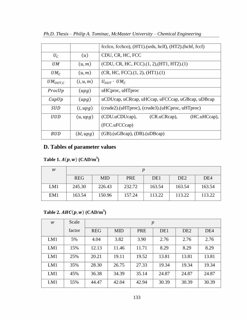
Ph.D. Thesis – Philip A. Tominac, McMaster University – Chemical Engineering
133
fcclco, fcchco), (HT1).(srds, hclf), (HT2).(hchf, fccf)
𝑈𝐶 (𝑢) CDU, CR, HC, FCC
𝑈𝑀 (𝑢,𝑚) (CDU, CR, HC, FCC).(1, 2),(HT1, HT2).(1)
𝑈𝑀𝐶 (𝑢,𝑚) (CR, HC, FCC).(1, 2), (HT1).(1)
𝑈𝑀𝑂𝑈𝑇,𝐶 (𝑖, 𝑢,𝑚) 𝑈𝑂𝑈𝑇 ∙ 𝑈𝑀𝐶
𝑃𝑟𝑜𝑐𝑈𝑝 (𝑢𝑝𝑔) uHCproc, uHTproc
𝐶𝑎𝑝𝑈𝑝 (𝑢𝑝𝑔) uCDUcap, uCRcap, uHCcap, uFCCcap, uGBcap, uDBcap
𝑆𝑈𝐷 (𝑖, 𝑢𝑝𝑔) (crude2).(uHTproc), (crude3).(uHCproc, uHTproc)
𝑈𝑈𝐷 (𝑢, 𝑢𝑝𝑔) (CDU.uCDUcap), (CR.uCRcap), (HC.uHCcap),
(FCC.uFCCcap)
𝐵𝑈𝐷 (𝑏𝑙, 𝑢𝑝𝑔) (GB).(uGBcap), (DB).(uDBcap)
D. Tables of parameter values
Table 1. 𝑨(𝒑,𝒘) (CAD/m3)
𝑤 𝑝
REG MID PRE DE1 DE2 DE4
LM1 245.30 226.43 232.72 163.54 163.54 163.54
EM1 163.54 150.96 157.24 113.22 113.22 113.22
Table 2. 𝑨𝑯𝑪(𝒑,𝒘) (CAD/m3)
𝑤 Scale
factor
𝑝
REG MID PRE DE1 DE2 DE4
LM1 5% 4.04 3.82 3.90 2.76 2.76 2.76
LM1 15% 12.13 11.46 11.71 8.29 8.29 8.29
LM1 25% 20.21 19.11 19.52 13.81 13.81 13.81
LM1 35% 28.30 26.75 27.33 19.34 19.34 19.34
LM1 45% 36.38 34.39 35.14 24.87 24.87 24.87
LM1 55% 44.47 42.04 42.94 30.39 30.39 30.39

Ph.D. Thesis – Philip A. Tominac, McMaster University – Chemical Engineering
134
Table 3. 𝑩(𝒑,𝒘) (CAD/m3)
𝑤 𝑝
REG MID PRE DE1 DE2 DE4
LM1 886.86 956.05 1006.37 1075.56 1018.95 962.34
EM1 886.86 956.05 1006.37 1075.56 1018.95 962.34
Table 4. 𝑪𝑰(𝒑) (CAD/m3)
𝑝
REG MID PRE DE1 DE2 DE4
1065.51 1144.89 1205.63 1287.38 1221.07 1154.76
Table 5. 𝑫(𝒑,𝒘) (106 m
3/year)
𝑤 𝑝
REG MID PRE DE1 DE2 DE4
LM1 6.38 0.48 0.71 0.08 3.19 0.17
EM1 7.45 0.56 0.83 0.10 3.73 0.20
Table 6. 𝑫(𝒑,𝒘) (106 m
3/year)
𝑤 𝑝
REG MID PRE DE1 DE2 DE4
LM1 5.75 0.43 0.64 0.07 2.87 0.16
Table 7. 𝑫(𝒑,𝒘) (106 m
3/year)
𝑤 𝑝
REG MID PRE DE1 DE2 DE4
LM1 7.66 0.57 0.86 0.10 3.83 0.21

Ph.D. Thesis – Philip A. Tominac, McMaster University – Chemical Engineering
135
Table 8. 𝑭(𝒑,𝒘) (CAD/m3)
𝑤 𝑝
REG MID PRE DE1 DE2 DE4
LM1 1132.16 1182.48 1239.09 1239.09 1182.48 1125.87
EM1 1050.40 1107.00 1163.61 1182.48 1125.87 1075.56
Table 9. 𝑯𝑪𝑵𝒔𝒆𝒕 (106 m
3/year)
𝑛
R3 2.86
Table 10. Efficiency cost curve parameters
𝑛
R1 R2 R3
𝐸𝐶𝐻(𝑛) (106 m
3) 5.56 4.79 4.12
𝐸𝐶𝐾(𝑛) (CAD/m3) 6.04 5.98 6.16
𝐸𝐶𝑃(𝑛) ((m3)3/CAD) 2.009×10
11 2.010×10
11 2.011×10
11
𝐸𝐶𝐴(𝑛) (CAD/(m3)3) 1.24×10
-12 1.24×10
-12 1.24×10
-12
𝐸𝐶𝐵(𝑛) (CAD/(m3)2) -1.38×10
-5 -1.19×10
-5 -1.02×10
-5
𝐸𝐶𝐶(𝑛) (CAD/ m3) 44.45 34.49 27.27
Table 11. 𝑪𝒂𝒑
𝐶𝑎𝑝 0.65
Table 12. 𝑪𝒐𝒔𝒕(𝒊) (CAD/m3)
𝑖
crude 1 crude 2 crude 3
610.20 577.30 535.04
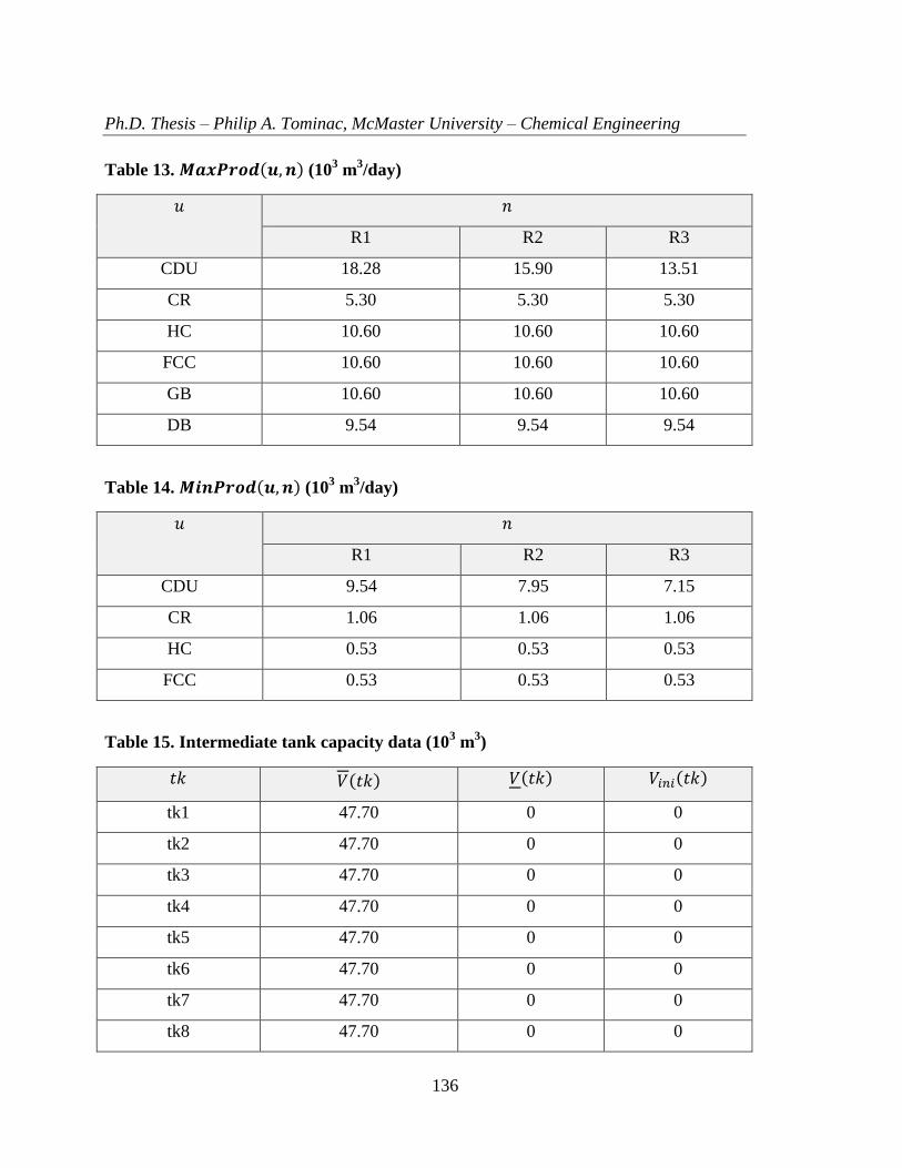
Ph.D. Thesis – Philip A. Tominac, McMaster University – Chemical Engineering
136
Table 13. 𝑴𝒂𝒙𝑷𝒓𝒐𝒅(𝒖,𝒏) (103 m
3/day)
𝑢 𝑛
R1 R2 R3
CDU 18.28 15.90 13.51
CR 5.30 5.30 5.30
HC 10.60 10.60 10.60
FCC 10.60 10.60 10.60
GB 10.60 10.60 10.60
DB 9.54 9.54 9.54
Table 14. 𝑴𝒊𝒏𝑷𝒓𝒐𝒅(𝒖,𝒏) (103 m
3/day)
𝑢 𝑛
R1 R2 R3
CDU 9.54 7.95 7.15
CR 1.06 1.06 1.06
HC 0.53 0.53 0.53
FCC 0.53 0.53 0.53
Table 15. Intermediate tank capacity data (103 m
3)
𝑡𝑘 𝑉(𝑡𝑘) 𝑉(𝑡𝑘) 𝑉𝑖𝑛𝑖(𝑡𝑘)
tk1 47.70 0 0
tk2 47.70 0 0
tk3 47.70 0 0
tk4 47.70 0 0
tk5 47.70 0 0
tk6 47.70 0 0
tk7 47.70 0 0
tk8 47.70 0 0
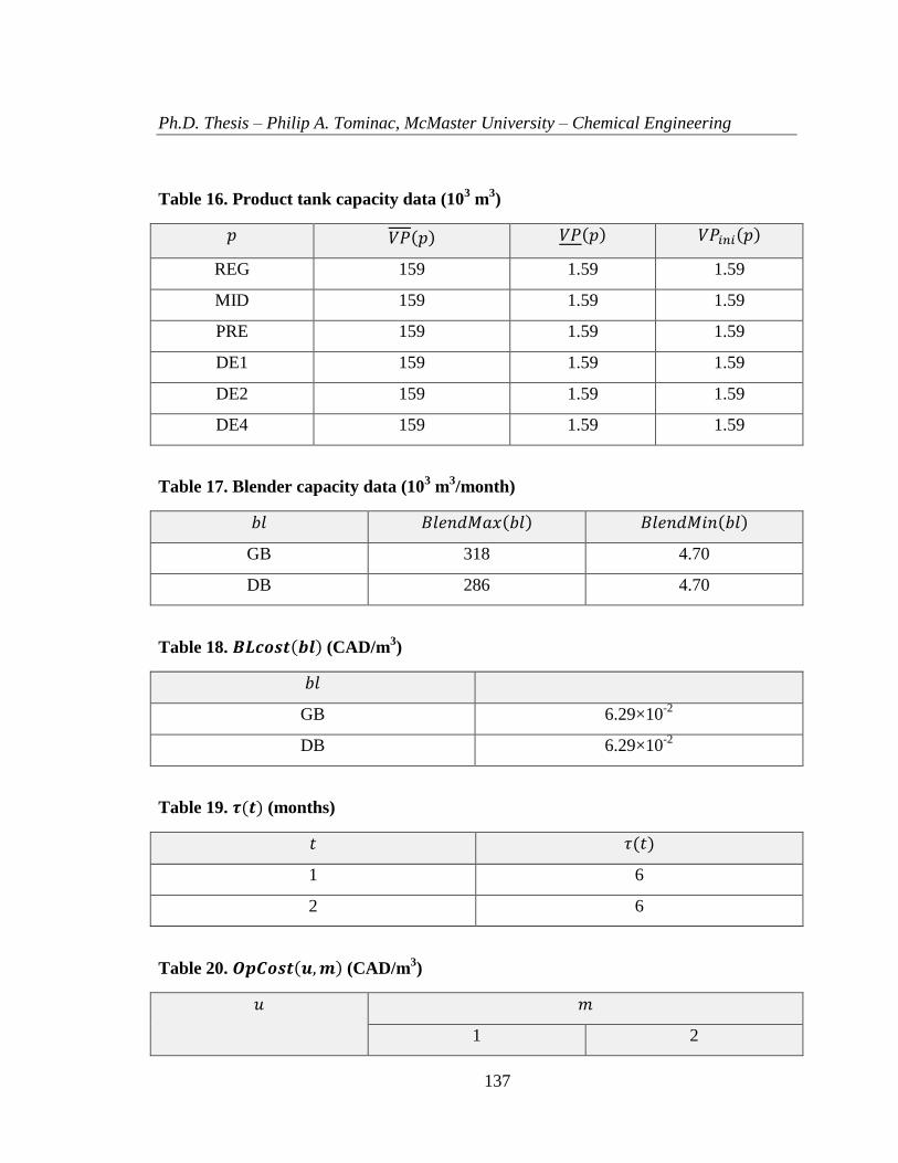
Ph.D. Thesis – Philip A. Tominac, McMaster University – Chemical Engineering
137
Table 16. Product tank capacity data (103 m
3)
𝑝 𝑉𝑃(𝑝) 𝑉𝑃(𝑝) 𝑉𝑃𝑖𝑛𝑖(𝑝)
REG 159 1.59 1.59
MID 159 1.59 1.59
PRE 159 1.59 1.59
DE1 159 1.59 1.59
DE2 159 1.59 1.59
DE4 159 1.59 1.59
Table 17. Blender capacity data (103 m
3/month)
𝑏𝑙 𝐵𝑙𝑒𝑛𝑑𝑀𝑎𝑥(𝑏𝑙) 𝐵𝑙𝑒𝑛𝑑𝑀𝑖𝑛(𝑏𝑙)
GB 318 4.70
DB 286 4.70
Table 18. 𝑩𝑳𝒄𝒐𝒔𝒕(𝒃𝒍) (CAD/m3)
𝑏𝑙
GB 6.29×10⁻²
DB 6.29×10⁻²
Table 19. 𝝉(𝒕) (months)
𝑡 𝜏(𝑡)
1 6
2 6
Table 20. 𝑶𝒑𝑪𝒐𝒔𝒕(𝒖,𝒎) (CAD/m3)
𝑢 𝑚
1 2

Ph.D. Thesis – Philip A. Tominac, McMaster University – Chemical Engineering
138
CDU 1.95 1.41
CR 2.61 5.43
HC 3.37 2.62
FCC 2.12 2.07
GB 0.21 0.21
DB 2.20 2.20
Table 21. 𝒒𝒒(𝒊, 𝒒)
𝑖 𝑞
RON MON ARO FLS CNU SUL SG RVP
srln 69.4 64.2 0 0 0 0 0.694 2.378
rft 103 90.8 74.9 0 0 0 0.818 2.378
hcln 93.2 81.6 18 0 0 0 0.751 12.335
hcds 0 0 0 56 50 0.008 0.832 0
fccln 87.7 75.8 25 0 0 0 0.713 13.876
fcchn 82.3 73.5 20 0 0 0 0.764 19.904
fcclco 0 0 0 53 50 0.009 0.802 0
srds 0 0 0 46 40 0.008 0.852 0
Table 22. 𝑸(𝒒, 𝒑)
𝑞 𝑝
REG MID PRE DE1 DE2 DE4
RON 200 200 200 200 200 200
MON 200 200 200 200 200 200
ARO 60 50 45 200 200 200
FLS 200 200 200 200 200 200
CNU 200 200 200 200 200 200
SUL 0.01 0.01 0.01 0.01 0.01 0.05

Ph.D. Thesis – Philip A. Tominac, McMaster University – Chemical Engineering
139
SG 0.81 0.81 0.81 0.85 0.87 0.9
RVP 15.6 15.6 15.6
Table 23. 𝑸(𝒒, 𝒑)
𝑞 𝑝
REG MID PRE DE1 DE2 DE4
RON 88 91 94 0 0 0
MON 75 78 81 0 0 0
ARO 0 0 0 0 0 0
FLS 0 0 0 40 45 55
CNU 0 0 0 40 40 30
SUL 0 0 0 0 0 0
SG 0.7 0.7 0.7 0.81 0.81 0.81
RVP 0 0 0 0 0 0
Table 24. 𝑹(𝒊, 𝒑)
𝑖 𝑝
REG MID PRE DE1 DE2 DE4
srln 1 1 1 0 0 0
rft 1 1 1 0 0 0
hcln 1 1 1 0 0 0
hcds 1 1 1 0 0 0
fccln 1 1 1 0 0 0
fcchn 0 0 0 1 1 1
fcclco 0 0 0 1 1 1
srds 0 0 0 1 1 1
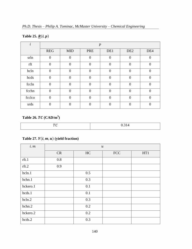
Ph.D. Thesis – Philip A. Tominac, McMaster University – Chemical Engineering
140
Table 25. 𝑹(𝒊, 𝒑)
𝑖 𝑝
REG MID PRE DE1 DE2 DE4
srln 0 0 0 0 0 0
rft 0 0 0 0 0 0
hcln 0 0 0 0 0 0
hcds 0 0 0 0 0 0
fccln 0 0 0 0 0 0
fcchn 0 0 0 0 0 0
fcclco 0 0 0 0 0 0
srds 0 0 0 0 0 0
Table 26. 𝑻𝑪 (CAD/m3)
𝑇𝐶 0.314
Table 27. 𝒀(𝒊,𝒎, 𝒖) (yield fraction)
𝑖.𝑚 𝑢
CR HC FCC HT1
rft.1 0.8
rft.2 0.9
hcln.1
0.5
hchn.1
0.3
hckero.1
0.1
hcds.1
0.1
hcln.2
0.3
hchn.2
0.2
hckero.2
0.2
hcds.2
0.3
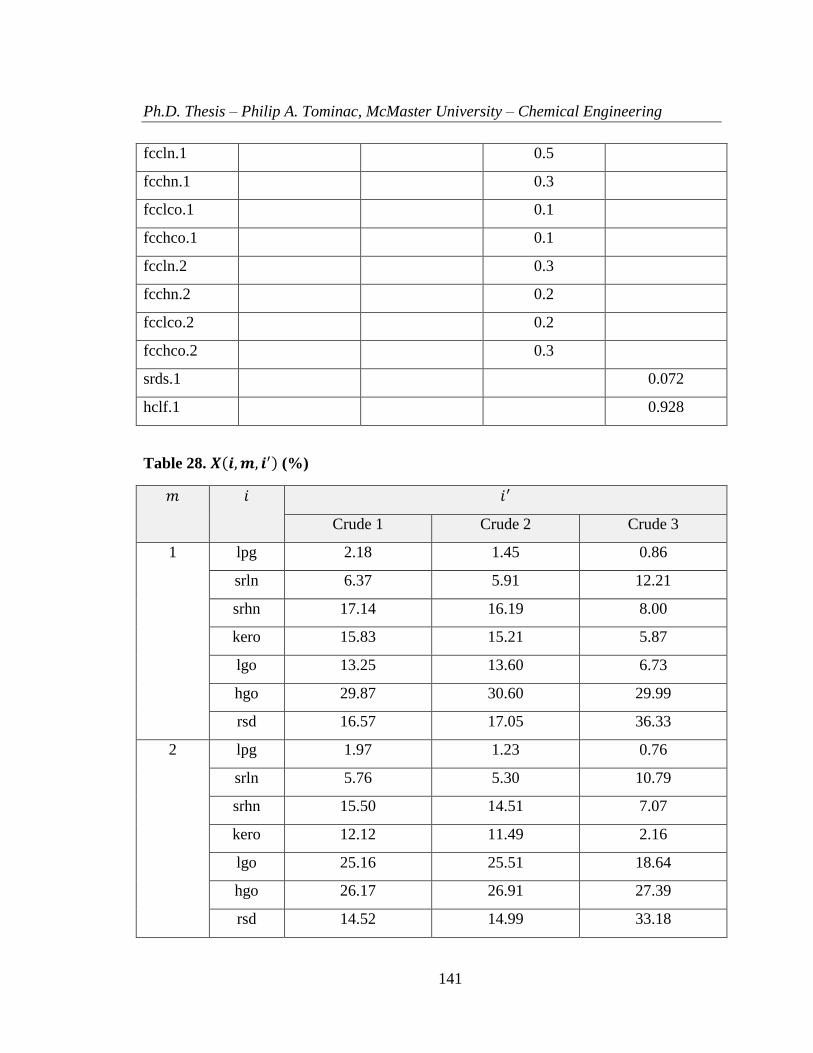
Ph.D. Thesis – Philip A. Tominac, McMaster University – Chemical Engineering
141
fccln.1
0.5
fcchn.1
0.3
fcclco.1
0.1
fcchco.1
0.1
fccln.2
0.3
fcchn.2
0.2
fcclco.2
0.2
fcchco.2
0.3
srds.1
0.072
hclf.1
0.928
Table 28. 𝑿(𝒊,𝒎, 𝒊′) (%)
𝑚 𝑖 𝑖′
Crude 1 Crude 2 Crude 3
1 lpg 2.18 1.45 0.86
srln 6.37 5.91 12.21
srhn 17.14 16.19 8.00
kero 15.83 15.21 5.87
lgo 13.25 13.60 6.73
hgo 29.87 30.60 29.99
rsd 16.57 17.05 36.33
2 lpg 1.97 1.23 0.76
srln 5.76 5.30 10.79
srhn 15.50 14.51 7.07
kero 12.12 11.49 2.16
lgo 25.16 25.51 18.64
hgo 26.17 26.91 27.39
rsd 14.52 14.99 33.18

Ph.D. Thesis – Philip A. Tominac, McMaster University – Chemical Engineering
142
Supplementary material to: Conjectures
regarding the existence and properties of
mixed integer potential games
Philip Tominac and Vladimir Mahalec*
Department of Chemical Engineering, McMaster University, 1280 Main St. W.,
Hamilton, ON, L8S 4L8, Canada
*Corresponding author Tel.: +1 905 525 9140 ext. 26386.
E-mail address: [email protected]

Ph.D. Thesis – Philip A. Tominac, McMaster University – Chemical Engineering
143
A. Refinery expansion and production planning model
The refinery model used for the capacity expansion and production planning model
is a modification of that used by Tominac and Mahalec4 and uses the same notation and
data. Data values have been reproduced here for consistency and convenience. The model
is an MINLP, with integer variables used to represent upgrade purchase decisions within
a competitive nonlinear potential game model. The purpose of each equation is detailed
briefly for the purpose of reproducibility.
Volumetric flows are determined by Eqs. (A1) to (A5); inlet unit flow by Eq. (A1),
flow to units operating in multiple modes by Eq. (A2), Eq. (A3) defines minimum
production rates, and Eqs. (A4) and (A5) define maximum flow rates under available
upgrade schemes.
𝐹𝐴(𝑡, 𝑢, 𝑛) = ∑ 𝐹𝑉𝑀(𝑚, 𝑡, 𝑢, 𝑛)𝑚𝑚∈𝑈𝑀
∀𝑡 ∈ 𝑇, 𝑢 ∈ 𝑈, 𝑛 ∈ 𝑁 (A1)
𝐹𝑉𝑀(𝑚, 𝑡, 𝑢, 𝑛) = ∑ 𝐹𝑉𝑀𝐼𝑁(𝑚, 𝑡, 𝑖, 𝑛)𝑖𝑖∈𝑈𝐼𝑁
∀𝑡 ∈ 𝑇, 𝑛 ∈ 𝑁, (𝑢,𝑚) ∈ 𝑈𝑀 (A2)
𝐹𝐴(𝑡, 𝑢, 𝑛) ≥ 𝑀𝑖𝑛𝑃𝑟𝑜𝑑(𝑢, 𝑛)𝜏(𝑡) ∀𝑡 ∈ 𝑇, 𝑢 ∈ 𝑈𝐶 , 𝑛 ∈ 𝑁 (A3)
𝐹𝑉𝑀𝐼𝑁(𝑚, 𝑡, 𝑖, 𝑛) ≤ 𝑈𝑌(𝑢𝑝𝑔, 𝑛)(𝑀𝑎𝑥𝑃𝑟𝑜𝑑(𝐶𝐷𝑈) + 𝑈𝑃𝐺𝑐𝑎𝑝(𝑢𝐶𝐷𝑈𝑐𝑎𝑝))𝜏(𝑡)
∀𝑚 ∈ 𝑀, 𝑡 ∈ 𝑇, 𝑛 ∈ 𝑁, (𝑖, 𝑢𝑝𝑔) ∈ 𝑆𝑈𝐷 (A4)
𝐹𝐴(𝑡, 𝑢, 𝑛) ≤ [𝑀𝑎𝑥𝑃𝑟𝑜𝑑(𝑢) + ∑ 𝑈𝑌(𝑢𝑝𝑔, 𝑛)𝑈𝑃𝐺𝑐𝑎𝑝(𝑢𝑝𝑔)𝑢𝑝𝑔𝑢𝑝𝑔∈𝑈𝑈𝐷
] 𝜏(𝑡)
∀𝑡 ∈ 𝑇, 𝑢 ∈ 𝑈𝐶 , 𝑛 ∈ 𝑁
(A5)
Eqs. (A6) and (A7) define volumetric flow rates of material leaving process units;
effluent rates are linked to influent rates by fixed yield relationships.
𝐹𝑉𝑀𝑂𝑈𝑇(𝑖,𝑚, 𝑡, 𝑢, 𝑛) = 𝑌(𝑖,𝑚, 𝑢)𝐹𝑉𝑀(𝑚, 𝑡, 𝑢, 𝑛)
∀𝑡 ∈ 𝑇, 𝑛 ∈ 𝑁, (𝑖, 𝑢,𝑚) ∈ 𝑈𝑀𝑂𝑈𝑇,𝐶 (A6)

Ph.D. Thesis – Philip A. Tominac, McMaster University – Chemical Engineering
144
𝐹𝐴(𝑡, 𝑢, 𝑛) = ∑ 𝐹𝑉(𝑡, 𝑖, 𝑛)𝑖𝑖∈𝑈𝑂𝑈𝑇
∀𝑡 ∈ 𝑇, 𝑢 ∈ 𝑈𝐶 , 𝑛 ∈ 𝑁 (A7)
Stream basis flow rates are determined using Eqs. (A8) and (A9).
𝐹𝑉(𝑡, 𝑖, 𝑛) = ∑ 𝐹𝑉𝑀𝑂𝑈𝑇(𝑖,𝑚, 𝑡, 𝑢, 𝑛)𝑚𝑚∈𝑈𝑀
∀𝑡 ∈ 𝑇, 𝑛 ∈ 𝑁, (𝑖, 𝑢) ∈ 𝑈𝑂𝑈𝑇 (A8)
𝐹𝑉(𝑡, 𝑖, 𝑛) = ∑ 𝐹𝑉𝑀𝐼𝑁(𝑚, 𝑡, 𝑖, 𝑛)𝑚𝑚∈𝑈𝑀
∀𝑡 ∈ 𝑇, 𝑛 ∈ 𝑁, (𝑖, 𝑢) ∈ 𝑈𝐼𝑁 (A9)
Effluent rates in the CDU are determined by Eq. (A10) using an independent set of
yield data.
𝐹𝑉𝑀𝑂𝑈𝑇(𝑖,𝑚, 𝑡, 𝑢, 𝑛) = ∑ 𝑋(𝑖,𝑚, 𝑖′)𝐹𝑉𝑀𝐼𝑁(𝑚, 𝑡, 𝑖′, 𝑛)𝑖′
𝑖′∈𝑈𝐼𝑁
∀𝑚 ∈ 𝑀, 𝑖 ∈ 𝐼, 𝑡 ∈ 𝑇, 𝑛 ∈ 𝑁, 𝑢 = 𝐶𝐷𝑈 (A10)
Intermediate product tank levels are defined by Eqs. (A11) and (A12); Eqs. (A13)
and (A14) define the maximum and minimum levels within these tanks.
∑ 𝐹𝑉(𝑡, 𝑖, 𝑛)𝑖𝑖∈𝑇𝐾𝐼𝑁
− ∑ 𝐹𝑉(𝑡, 𝑖, 𝑛)𝑖𝑖∈𝑇𝐾𝑂𝑈𝑇
+ 𝑉𝑖𝑛𝑖(𝑡𝑘, 𝑛) − 𝑉(𝑡𝑘, 𝑡, 𝑛) = 0
∀𝑡𝑘 ∈ 𝑇𝐾, 𝑡 = 1, 𝑛 ∈ 𝑁 (A11)
∑ 𝐹𝑉(𝑡, 𝑖, 𝑛)𝑖𝑖∈𝑇𝐾𝐼𝑁
− ∑ 𝐹𝑉(𝑡, 𝑖, 𝑛)𝑖𝑖∈𝑇𝐾𝑂𝑈𝑇
+ 𝑉(𝑡𝑘, 𝑡 − 1, 𝑛) − 𝑉(𝑡𝑘, 𝑡, 𝑛) = 0
∀𝑡𝑘 ∈ 𝑇𝐾, 𝑡 > 1, 𝑛 ∈ 𝑁(A12)
𝑉(𝑡𝑘, 𝑡, 𝑛) ≥ 𝑉(𝑡𝑘) ∀𝑡𝑘 ∈ 𝑇𝐾, 𝑡 ∈ 𝑇, 𝑛 ∈ 𝑁 (A13)
𝑉(𝑡𝑘, 𝑡, 𝑛) ≤ 𝑉(𝑡𝑘) ∀𝑡𝑘 ∈ 𝑇𝐾, 𝑡 ∈ 𝑇, 𝑛 ∈ 𝑁 (A14)
Stream dedication to product blenders is determined by Eq. (A15); Eq. (A16)
defines total blend volume. Intermediate product fraction allowances in a blend are
defined by Eqs. (A17) and (A18).
∑ 𝑉𝐵(𝑖, 𝑝, 𝑡, 𝑛)𝑝𝑝∈𝐵𝐿𝑂𝑈𝑇
= 𝐹𝑉(𝑡, 𝑖, 𝑛) ∀𝑡 ∈ 𝑇, 𝑛 ∈ 𝑁, (𝑏𝑙, 𝑖) ∈ 𝐵𝐿𝐼𝑁 (A15)
∑ 𝑉𝐵(𝑖, 𝑝, 𝑡, 𝑛)𝑖𝑖∈𝐵𝐿𝐼𝑁
= 𝑉𝐵𝑙𝑒𝑛𝑑(𝑡, 𝑝, 𝑛) ∀𝑡 ∈ 𝑇, 𝑛 ∈ 𝑁, (𝑏𝑙, 𝑝) ∈ 𝐵𝐿𝑂𝑈𝑇 (A16)

Ph.D. Thesis – Philip A. Tominac, McMaster University – Chemical Engineering
145
𝑉𝐵(𝑖, 𝑝, 𝑡, 𝑛) ≥ 𝑅𝑀𝑖𝑛(𝑏𝑙)𝑉𝐵𝑙𝑒𝑛𝑑(𝑡, 𝑝, 𝑛) ∀𝑡 ∈ 𝑇, 𝑛 ∈ 𝑁, (𝑏𝑙, 𝑖, 𝑝) ∈ 𝐵𝐿𝐼𝑃 (A17)
𝑉𝐵(𝑖, 𝑝, 𝑡, 𝑛) ≤ 𝑅𝑀𝑎𝑥(𝑏𝑙)𝑉𝐵𝑙𝑒𝑛𝑑(𝑡, 𝑝, 𝑛) ∀𝑡 ∈ 𝑇, 𝑛 ∈ 𝑁, (𝑏𝑙, 𝑖, 𝑝) ∈ 𝐵𝐿𝐼𝑃 (A18)
The total volume processed in a blender is defined by Eq. (A19), and Eqs. (A20)
and (A21) define the upper and lower bounds on this volume.
∑ 𝑉𝐵(𝑖, 𝑝, 𝑡, 𝑛)𝑖,𝑝(𝑖,𝑝)∈𝐵𝐿𝐼𝑃
= 𝑉𝐵𝑙𝑒𝑛𝑑𝑇(𝑡, 𝑏𝑙, 𝑛) ∀𝑏𝑙 ∈ 𝐵𝐿, 𝑡 ∈ 𝑇, 𝑛 ∈ 𝑁 (A19)
𝑉𝐵𝑙𝑒𝑛𝑑𝑇(𝑡, 𝑏𝑙, 𝑛) ≥ 𝐵𝑙𝑒𝑛𝑑𝑀𝑖𝑛(𝑏𝑙)𝜏(𝑡) ∀𝑏𝑙 ∈ 𝐵𝐿, 𝑡 ∈ 𝑇, 𝑛 ∈ 𝑁 (A20)
𝑉𝐵𝑙𝑒𝑛𝑑𝑇(𝑡, 𝑏𝑙, 𝑛) ≤ [𝐵𝑙𝑒𝑛𝑑𝑀𝑎𝑥(𝑏𝑙) + ∑ 𝑈𝑌(𝑢𝑝𝑔, 𝑛)𝑈𝑃𝐺𝑐𝑎𝑝(𝑢𝑝𝑔)𝑢𝑝𝑔𝑢𝑝𝑔∈𝐵𝑈𝐷
] 𝜏(𝑡)
∀𝑏𝑙 ∈ 𝐵𝐿𝑡 ∈ 𝑇, 𝑛 ∈ 𝑁
(A21)
Eqs. (A22) to (A27) represent product quality bounds for all products.
∑ 𝑉𝐵(𝑖, 𝑝, 𝑡, 𝑛)𝑞𝑞(𝑖, 𝑞)𝑖𝑖∈𝐵𝐿𝐼𝑁
≥ 𝑄(𝑞, 𝑝)𝑉𝐵𝑙𝑒𝑛𝑑(𝑡, 𝑝, 𝑛)
∀𝑡 ∈ 𝑇, 𝑛 ∈ 𝑁, (𝑏𝑙, 𝑝, 𝑞) ∈ 𝐵𝐿𝑂𝑈𝑇,𝑉𝑂𝐿 (A22)
∑ 𝑉𝐵(𝑖, 𝑝, 𝑡, 𝑛)𝑞𝑞(𝑖, 𝑞)𝑖𝑖∈𝐵𝐿𝐼𝑁
≤ 𝑄(𝑞, 𝑝)𝑉𝐵𝑙𝑒𝑛𝑑(𝑡, 𝑝, 𝑛)
∀𝑡 ∈ 𝑇, 𝑛 ∈ 𝑁, (𝑏𝑙, 𝑝, 𝑞) ∈ 𝐵𝐿𝑂𝑈𝑇,𝑉𝑂𝐿
(A23)
∑ 𝑉𝐵(𝑖, 𝑝, 𝑡, 𝑛)𝑞𝑞(𝑖, 𝑞)𝑞𝑞(𝑖, 𝑞′)𝑖𝑖∈𝐵𝐿𝐼𝑁
≥ 𝑄(𝑞, 𝑝)∑ 𝑉𝐵(𝑖, 𝑝, 𝑡, 𝑛)𝑞𝑞(𝑖, 𝑞′)𝑖𝑖∈𝐵𝐿𝐼𝑁
∀𝑡 ∈ 𝑇, 𝑛 ∈ 𝑁, 𝑞′ = 𝑆𝐺, (𝑏𝑙, 𝑝, 𝑞) ∈ 𝐵𝐿𝑂𝑈𝑇,𝑊𝑇 (A24)
∑ 𝑉𝐵(𝑖, 𝑝, 𝑡, 𝑛)𝑞𝑞(𝑖, 𝑞)𝑞𝑞(𝑖, 𝑞′)𝑖𝑖∈𝐵𝐿𝐼𝑁
≤ 𝑄(𝑞, 𝑝)∑ 𝑉𝐵(𝑖, 𝑝, 𝑡, 𝑛)𝑞𝑞(𝑖, 𝑞′)𝑖𝑖∈𝐵𝐿𝐼𝑁
∀𝑡 ∈ 𝑇, 𝑛 ∈ 𝑁, 𝑞′ = 𝑆𝐺, (𝑏𝑙, 𝑝, 𝑞) ∈ 𝐵𝐿𝑂𝑈𝑇,𝑊𝑇
(A25)
∑ 𝑉𝐵(𝑖, 𝑝, 𝑡, 𝑛)𝑞𝑞(𝑖, 𝑞)1.25𝑖𝑖∈𝐵𝐿𝐼𝑁
≥ 𝑄(𝑞, 𝑝)1.25𝑉𝐵𝑙𝑒𝑛𝑑(𝑡, 𝑝, 𝑛)
∀𝑡 ∈ 𝑇, 𝑛 ∈ 𝑁, (𝑏𝑙, 𝑝, 𝑞) ∈ 𝐵𝐿𝑂𝑈𝑇,𝑁𝐿 (A26)
∑ 𝑉𝐵(𝑖, 𝑝, 𝑡, 𝑛)𝑞𝑞(𝑖, 𝑞)1.25𝑖𝑖∈𝐵𝐿𝐼𝑁
≤ 𝑄(𝑞, 𝑝)1.25𝑉𝐵𝑙𝑒𝑛𝑑(𝑡, 𝑝, 𝑛)
∀𝑡 ∈ 𝑇, 𝑛 ∈ 𝑁, (𝑏𝑙, 𝑝, 𝑞) ∈ 𝐵𝐿𝑂𝑈𝑇,𝑁𝐿
(A27)

Ph.D. Thesis – Philip A. Tominac, McMaster University – Chemical Engineering
146
Product balances are defined by Eqs. (A28) and(A29), and Eqs. (A30) and (A31)
define the maximum and minimum product inventories in the balance equations.
𝑉𝐵𝑙𝑒𝑛𝑑(𝑡, 𝑝, 𝑛) + 𝑉𝑃𝑖𝑛𝑖(𝑝) − 𝑉𝑃(𝑡, 𝑝, 𝑛) − 𝑃𝑟𝑐(𝑡, 𝑝, 𝑛) = 0∀𝑡 = 1, 𝑝 ∈ 𝑃, 𝑛 ∈ 𝑁
(A28)
𝑉𝐵𝑙𝑒𝑛𝑑(𝑡, 𝑝, 𝑛) + 𝑉𝑃(𝑡 − 1, 𝑝, 𝑛) − 𝑉𝑃(𝑡, 𝑝, 𝑛) − 𝑃𝑟𝑐(𝑡, 𝑝, 𝑛) = 0∀𝑡 > 1, 𝑝 ∈ 𝑃, 𝑛 ∈ 𝑁
(A29)
𝑉𝑃(𝑡, 𝑝, 𝑛) ≥ 𝑉𝑃(𝑝) ∀𝑡 ∈ 𝑇, 𝑝 ∈ 𝑃, 𝑛 ∈ 𝑁 (A30)
𝑉𝑃(𝑡, 𝑝, 𝑛) ≤ 𝑉𝑃(𝑝) ∀𝑡 ∈ 𝑇, 𝑝 ∈ 𝑃, 𝑛 ∈ 𝑁 (A31)
Product tank levels are constrained such that they return to their minimum (and also
starting) levels at the end of the planning horizon by Eqs. (A32) and (A33).
𝑉(𝑡𝑘, 𝑡, 𝑛) = 𝑉(𝑡𝑘) ∀𝑡𝑘 ∈ 𝑇𝐾, 𝑡 = 𝑇, 𝑛 ∈ 𝑁 (A32)
𝑉𝑃(𝑡, 𝑝, 𝑛) = 𝑉𝑃(𝑝) ∀𝑡 = 𝑇, 𝑝 ∈ 𝑃, 𝑛 ∈ 𝑁 (A33)
Eq. (A34) allocates product volumes to various markets for delivery.
𝑃𝑟𝑐(𝑡, 𝑝, 𝑛) − ∑ 𝐷𝑙𝑣(𝑡, 𝑝, 𝑛, 𝑤)𝑤 = 0 ∀𝑡 ∈ 𝑇, 𝑝 ∈ 𝑃, 𝑛 ∈ 𝑁 (A34)
Eqs. (A35) to (A38) represent costs of crude oil, unit operation, blend operation,
and upgrade purchasing.
𝐶𝑟𝑢𝑑𝑒𝑂𝑖𝑙𝐶𝑜𝑠𝑡(𝑛) = ∑ [(1 + 0.01𝑡) ∑ 𝐶𝑜𝑠𝑡(𝑖)𝐹𝑉(𝑡, 𝑖, 𝑛)𝑖𝑖∈𝐼𝐶
]𝑡 ∀𝑛 ∈ 𝑁 (A35)
𝑈𝑛𝑖𝑡𝑂𝑝𝐶𝑜𝑠𝑡(𝑛) = ∑ 𝑂𝑝𝐶𝑜𝑠𝑡(𝑢,𝑚)𝐹𝑉𝑀(𝑚, 𝑡, 𝑢, 𝑛)𝑚,𝑛,𝑢 ∀𝑛 ∈ 𝑁 (A36)
𝐵𝑙𝑒𝑛𝑑𝑂𝑝𝐶𝑜𝑠𝑡(𝑛) = ∑ 𝐵𝐿𝑐𝑜𝑠𝑡(𝑏𝑙)𝑏𝑙,𝑛 𝑉𝐵𝑙𝑒𝑛𝑑𝑇(𝑡, 𝑏𝑙, 𝑛) ∀𝑛 ∈ 𝑁 (A37)
𝑈𝑝𝑔𝑟𝑎𝑑𝑒𝑠𝐶𝑜𝑠𝑡(𝑛) = ∑ 𝑈𝑌(𝑢𝑝𝑔, 𝑛)𝑈𝑃𝐺𝑐𝑜𝑠𝑡(𝑢𝑝𝑔)𝑢𝑝𝑔 ∀𝑛 ∈ 𝑁 (A38)
Eq. (A39) defines the cost of imports, which serve primarily as a slack variable for
domestic market production.

Ph.D. Thesis – Philip A. Tominac, McMaster University – Chemical Engineering
147
𝐼𝑚𝑝𝐶𝑜𝑠𝑡(𝑛) = ∑ 𝐶𝐼(𝑝, 𝑤)𝑝,𝑤 𝐼𝑚𝑝(𝑝, 𝑛, 𝑤) ∀𝑛 ∈ 𝑁 (A39)
Eq. (A40) defines a time cost which becomes lower in subsequent time periods,
thus making production decisions non-degenerate.
𝑇𝑖𝑚𝑒𝐶𝑜𝑠𝑡(𝑛) = 𝑇𝐶 ∑ (1 − 0.01 ∙ 𝑡)𝑃𝑟𝑜𝑑𝑢𝑐𝑒(𝑡, 𝑝, 𝑛)𝑡,𝑝 ∀𝑛 ∈ 𝑁 (A40)
Eq. (A41) aggregates cost values.
𝑇𝑜𝑡𝐶𝑜𝑠𝑡(𝑛) = 𝐶𝑟𝑢𝑑𝑒𝑂𝑖𝑙𝐶𝑜𝑠𝑡(𝑛) + 𝑈𝑛𝑖𝑡𝑂𝑝𝐶𝑜𝑠𝑡(𝑛) + 𝐵𝑙𝑒𝑛𝑑𝑂𝑝𝐶𝑜𝑠𝑡(𝑛) +
𝑈𝑝𝑔𝑟𝑎𝑑𝑒𝑠𝐶𝑜𝑠𝑡(𝑛) + 𝑇𝐸𝐶(𝑛) + 𝐼𝑚𝑝𝐶𝑜𝑠𝑡(𝑛) + 𝑇𝑖𝑚𝑒𝐶𝑜𝑠𝑡(𝑛) ∀𝑛 ∈ 𝑁 (A41)
Eqs. (A42) and(A43) define domestic market supply limitations.
∑ 𝐷𝑙𝑣(𝑡, 𝑝, 𝑛, 𝑤)𝑡,𝑛 ≥ 𝐷(𝑝,𝑤) ∀𝑝 ∈ 𝑃,𝑤 ∈ 𝑊𝐿 (A42)
∑ 𝐷𝑙𝑣(𝑡, 𝑝, 𝑛, 𝑤)𝑡,𝑛 ≤ 𝐷(𝑝,𝑤) ∀𝑝 ∈ 𝑃,𝑤 ∈ 𝑊𝐿 (A43)
Eqs. (A44) to (A46) define the overall potential function objective.
max𝑍 = Ψ + ∑ Ω(𝑛)𝑛 (A44)
Ψ = ∑ [−𝐴(𝑝)
𝐷𝑒𝑚𝑎𝑛𝑑(𝑝)∑ (∑ 𝐷𝑒𝑙𝑖𝑣𝑒𝑟(𝑡, 𝑝, 𝑛)𝑡 )(∑ 𝐷𝑒𝑙𝑖𝑣𝑒𝑟(𝑡, 𝑝, 𝑛′)𝑡 )𝑛,𝑛′
𝑛<𝑛′]𝑝 (A45)
Ω(𝑛) =
∑ [(𝐴(𝑝) + 𝐵(𝑝) −𝐴(𝑝)
𝐷𝑒𝑚𝑎𝑛𝑑(𝑝)(∑ 𝐷𝑒𝑙𝑖𝑣𝑒𝑟(𝑡, 𝑝, 𝑛)𝑡 )) (∑ 𝐷𝑒𝑙𝑖𝑣𝑒𝑟(𝑡, 𝑝, 𝑛)𝑡 )]𝑝 −
𝑇𝑜𝑡𝐶𝑜𝑠𝑡(𝑛) ∀𝑛 ∈ 𝑁 (A46)
B. Table of set elements and indices
Set Indices Elements
𝐵𝐿 (𝑏𝑙) GB, DB
𝐼 (𝑖) crude1, crude2, crude3, lpg, srln, srhn, kero, lgo, hgo, rsd,
rft, srds, hclf, hchf, hcln, hckero, hcds, hchn, fccf, fccln,

Ph.D. Thesis – Philip A. Tominac, McMaster University – Chemical Engineering
148
fcchn, fcclco, fcchco, srln_tk, rft_tk, hcln_tk, fccln_tk,
fcchn_tk, srds_tk, hcds_tk, fcclco_tk
𝐼𝐶 (𝑖) crude1, crude2, crude3
𝑀 (𝑚) 1, 2
𝑁 (𝑛) R1, R2, R3
𝑃 (𝑝) REG, MID, PRE, DE1, DE2, DE4
𝑄 (𝑞) RON, MON, ARO, FLS, CNU, SUL, SG, RVP
𝑊 (𝑤) LM1, EM1
𝑇 (𝑡) 1, 2
𝑇𝐾 (𝑡𝑘) tk1, tk2. Tk3, tk4, tk5, tk6, tk7, tk8
𝑈 (𝑢) CDU, CR, HC, FCC, HT1, HT2
𝑈𝑃𝐺 (𝑢𝑝𝑔) uHCproc, uHTproc, uCDUcap, uCRcap, uHCcap,
uFCCcap, uGBcap, uDBcap
𝐵𝐿𝐵𝐿𝐸𝑁𝐷 (𝑖) (GB).(srln_tk, rft_tk, hcln_tk, fccln_tk, fcchn_tk),
(DB).(srds_tk, hcds_tk, fcclco_tk)
𝐵𝐿𝐼𝑁 (𝑏𝑙, 𝑖) srln_tk, rft_tk, hcln_tk, fccln_tk, fcchn_tk, srds_tk, hcds_tk,
fcclco_tk
𝐵𝐿𝑂𝑈𝑇 (𝑏𝑙, 𝑝) (GB).(REG, MID, PRE), (DB).(DE1, DE2, DE4)
𝐵𝐿𝑂𝑈𝑇,𝑉𝑂𝐿 (𝑏𝑙, 𝑝, 𝑞) (GB).(REG, MID, PRE).(RON, MON, ARO, SG),
(DB).(DE1, DE2, DE4).(FLS, CNU, SG)
𝐵𝐿𝑂𝑈𝑇,𝑊𝑇 (𝑏𝑙, 𝑝, 𝑞) (GB).(REG, MID, PRE).(RVP)
𝐵𝐿𝑂𝑈𝑇,𝑁𝐿 (𝑏𝑙, 𝑝, 𝑞) (DB).(DE1, DE2, DE4).(SUL)
𝐵𝐿𝐼𝑃 (𝑏𝑙, 𝑖, 𝑝) 𝐵𝐿𝐼𝑁 ∙ 𝐵𝐿𝑂𝑈𝑇
𝐷𝑊𝑁 (𝑝′, 𝑝) (REG).(REG), (MID).(REG, MID), (PRE).(REG, MID,
PRE), (DE1).(DE1), (DE2).(DE1, DE2), (DE4).(DE1, DE2,
DE4)
𝐿𝐶𝑁 (𝑛) R1, R2
𝐻𝐶𝑁 (𝑛) R3
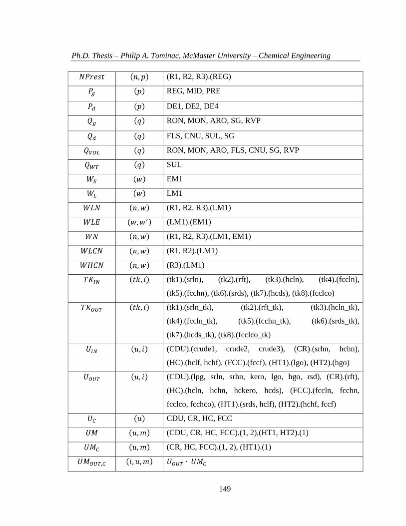
Ph.D. Thesis – Philip A. Tominac, McMaster University – Chemical Engineering
149
𝑁𝑃𝑟𝑒𝑠𝑡 (𝑛, 𝑝) (R1, R2, R3).(REG)
𝑃𝑔 (𝑝) REG, MID, PRE
𝑃𝑑 (𝑝) DE1, DE2, DE4
𝑄𝑔 (𝑞) RON, MON, ARO, SG, RVP
𝑄𝑑 (𝑞) FLS, CNU, SUL, SG
𝑄𝑉𝑂𝐿 (𝑞) RON, MON, ARO, FLS, CNU, SG, RVP
𝑄𝑊𝑇 (𝑞) SUL
𝑊𝐸 (𝑤) EM1
𝑊𝐿 (𝑤) LM1
𝑊𝐿𝑁 (𝑛, 𝑤) (R1, R2, R3).(LM1)
𝑊𝐿𝐸 (𝑤,𝑤′) (LM1).(EM1)
𝑊𝑁 (𝑛, 𝑤) (R1, R2, R3).(LM1, EM1)
𝑊𝐿𝐶𝑁 (𝑛, 𝑤) (R1, R2).(LM1)
𝑊𝐻𝐶𝑁 (𝑛, 𝑤) (R3).(LM1)
𝑇𝐾𝐼𝑁 (𝑡𝑘, 𝑖) (tk1).(srln), (tk2).(rft), (tk3).(hcln), (tk4).(fccln),
(tk5).(fcchn), (tk6).(srds), (tk7).(hcds), (tk8).(fcclco)
𝑇𝐾𝑂𝑈𝑇 (𝑡𝑘, 𝑖) (tk1).(srln_tk), (tk2).(rft_tk), (tk3).(hcln_tk),
(tk4).(fccln_tk), (tk5).(fcchn_tk), (tk6).(srds_tk),
(tk7).(hcds_tk), (tk8).(fcclco_tk)
𝑈𝐼𝑁 (𝑢, 𝑖) (CDU).(crude1, crude2, crude3), (CR).(srhn, hchn),
(HC).(hclf, hchf), (FCC).(fccf), (HT1).(lgo), (HT2).(hgo)
𝑈𝑂𝑈𝑇 (𝑢, 𝑖) (CDU).(lpg, srln, srhn, kero, lgo, hgo, rsd), (CR).(rft),
(HC).(hcln, hchn, hckero, hcds), (FCC).(fccln, fcchn,
fcclco, fcchco), (HT1).(srds, hclf), (HT2).(hchf, fccf)
𝑈𝐶 (𝑢) CDU, CR, HC, FCC
𝑈𝑀 (𝑢,𝑚) (CDU, CR, HC, FCC).(1, 2),(HT1, HT2).(1)
𝑈𝑀𝐶 (𝑢,𝑚) (CR, HC, FCC).(1, 2), (HT1).(1)
𝑈𝑀𝑂𝑈𝑇,𝐶 (𝑖, 𝑢,𝑚) 𝑈𝑂𝑈𝑇 ∙ 𝑈𝑀𝐶

Ph.D. Thesis – Philip A. Tominac, McMaster University – Chemical Engineering
150
𝑃𝑟𝑜𝑐𝑈𝑝 (𝑢𝑝𝑔) uHCproc, uHTproc
𝐶𝑎𝑝𝑈𝑝 (𝑢𝑝𝑔) uCDUcap, uCRcap, uHCcap, uFCCcap, uGBcap, uDBcap
𝑆𝑈𝐷 (𝑖, 𝑢𝑝𝑔) (crude2).(uHTproc), (crude3).(uHCproc, uHTproc)
𝑈𝑈𝐷 (𝑢, 𝑢𝑝𝑔) (CDU.uCDUcap), (CR.uCRcap), (HC.uHCcap),
(FCC.uFCCcap)
𝐵𝑈𝐷 (𝑏𝑙, 𝑢𝑝𝑔) (GB).(uGBcap), (DB).(uDBcap)
C. Tables of parameter values
Table 1. 𝑨(𝒑,𝒘) (CAD/m3)
𝑤 𝑝
REG MID PRE DE1 DE2 DE4
LM1 245.30 226.43 232.72 163.54 163.54 163.54
EM1 163.54 150.96 157.24 113.22 113.22 113.22
Table 2. 𝑨𝑯𝑪(𝒑,𝒘) (CAD/m3)
𝑤 Scale
factor
𝑝
REG MID PRE DE1 DE2 DE4
LM1 5% 4.04 3.82 3.90 2.76 2.76 2.76
LM1 15% 12.13 11.46 11.71 8.29 8.29 8.29
LM1 25% 20.21 19.11 19.52 13.81 13.81 13.81
LM1 35% 28.30 26.75 27.33 19.34 19.34 19.34
LM1 45% 36.38 34.39 35.14 24.87 24.87 24.87
LM1 55% 44.47 42.04 42.94 30.39 30.39 30.39
Table 3. 𝑩(𝒑,𝒘) (CAD/m3)
𝑤 𝑝
REG MID PRE DE1 DE2 DE4
LM1 886.86 956.05 1006.37 1075.56 1018.95 962.34

Ph.D. Thesis – Philip A. Tominac, McMaster University – Chemical Engineering
151
EM1 886.86 956.05 1006.37 1075.56 1018.95 962.34
Table 4. 𝑪𝑰(𝒑) (CAD/m3)
𝑝
REG MID PRE DE1 DE2 DE4
1065.51 1144.89 1205.63 1287.38 1221.07 1154.76
Table 5. 𝑫(𝒑,𝒘) (106 m
3/year)
𝑤 𝑝
REG MID PRE DE1 DE2 DE4
LM1 6.38 0.48 0.71 0.08 3.19 0.17
EM1 7.45 0.56 0.83 0.10 3.73 0.20
Table 6. 𝑫(𝒑,𝒘) (106 m
3/year)
𝑤 𝑝
REG MID PRE DE1 DE2 DE4
LM1 5.75 0.43 0.64 0.07 2.87 0.16
Table 7. 𝑫(𝒑,𝒘) (106 m
3/year)
𝑤 𝑝
REG MID PRE DE1 DE2 DE4
LM1 7.66 0.57 0.86 0.10 3.83 0.21
Table 8. 𝑭(𝒑,𝒘) (CAD/m3)
𝑤 𝑝
REG MID PRE DE1 DE2 DE4
LM1 1132.16 1182.48 1239.09 1239.09 1182.48 1125.87
EM1 1050.40 1107.00 1163.61 1182.48 1125.87 1075.56

Ph.D. Thesis – Philip A. Tominac, McMaster University – Chemical Engineering
152
Table 9. 𝑯𝑪𝑵𝒔𝒆𝒕 (106 m
3/year)
𝑛
R3 2.86
Table 10. Efficiency cost curve parameters
𝑛
R1 R2 R3
𝐸𝐶𝐻(𝑛) (106 m
3) 5.56 4.79 4.12
𝐸𝐶𝐾(𝑛) (CAD/m3) 6.04 5.98 6.16
𝐸𝐶𝑃(𝑛) ((m3)3/CAD) 2.009×10
11 2.010×10
11 2.011×10
11
𝐸𝐶𝐴(𝑛) (CAD/(m3)3) 1.24×10
-12 1.24×10
-12 1.24×10
-12
𝐸𝐶𝐵(𝑛) (CAD/(m3)2) -1.38×10
-5 -1.19×10
-5 -1.02×10
-5
𝐸𝐶𝐶(𝑛) (CAD/ m3) 44.45 34.49 27.27
Table 11. 𝑪𝒂𝒑
𝐶𝑎𝑝 0.65
Table 12. 𝑪𝒐𝒔𝒕(𝒊) (CAD/m3)
𝑖
crude 1 crude 2 crude 3
610.20 577.30 535.04
Table 13. 𝑴𝒂𝒙𝑷𝒓𝒐𝒅(𝒖,𝒏) (103 m
3/day)
𝑢 𝑛
R1 R2 R3
CDU 18.28 15.90 13.51
CR 5.30 5.30 5.30

Ph.D. Thesis – Philip A. Tominac, McMaster University – Chemical Engineering
153
HC 10.60 10.60 10.60
FCC 10.60 10.60 10.60
GB 10.60 10.60 10.60
DB 9.54 9.54 9.54
Table 14. 𝑴𝒊𝒏𝑷𝒓𝒐𝒅(𝒖,𝒏) (103 m
3/day)
𝑢 𝑛
R1 R2 R3
CDU 9.54 7.95 7.15
CR 1.06 1.06 1.06
HC 0.53 0.53 0.53
FCC 0.53 0.53 0.53
Table 15. Intermediate tank capacity data (103 m
3)
𝑡𝑘 𝑉(𝑡𝑘) 𝑉(𝑡𝑘) 𝑉𝑖𝑛𝑖(𝑡𝑘)
tk1 47.70 0 0
tk2 47.70 0 0
tk3 47.70 0 0
tk4 47.70 0 0
tk5 47.70 0 0
tk6 47.70 0 0
tk7 47.70 0 0
tk8 47.70 0 0
Table 16. Product tank capacity data (103 m
3)
𝑝 𝑉𝑃(𝑝) 𝑉𝑃(𝑝) 𝑉𝑃𝑖𝑛𝑖(𝑝)
REG 159 1.59 1.59
MID 159 1.59 1.59

Ph.D. Thesis – Philip A. Tominac, McMaster University – Chemical Engineering
154
PRE 159 1.59 1.59
DE1 159 1.59 1.59
DE2 159 1.59 1.59
DE4 159 1.59 1.59
Table 17. Blender capacity data (103 m
3/month)
𝑏𝑙 𝐵𝑙𝑒𝑛𝑑𝑀𝑎𝑥(𝑏𝑙) 𝐵𝑙𝑒𝑛𝑑𝑀𝑖𝑛(𝑏𝑙)
GB 318 4.70
DB 286 4.70
Table 18. 𝑩𝑳𝒄𝒐𝒔𝒕(𝒃𝒍) (CAD/m3)
𝑏𝑙
GB 6.29×10⁻²
DB 6.29×10⁻²
Table 19. 𝝉(𝒕) (months)
𝑡 𝜏(𝑡)
1 6
2 6
Table 20. 𝑶𝒑𝑪𝒐𝒔𝒕(𝒖,𝒎) (CAD/m3)
𝑢 𝑚
1 2
CDU 1.95 1.41
CR 2.61 5.43
HC 3.37 2.62
FCC 2.12 2.07
GB 0.21 0.21
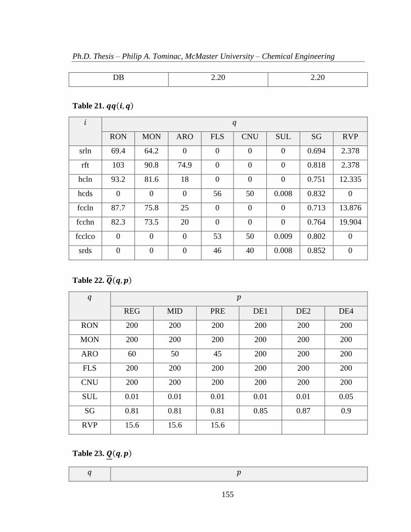
Ph.D. Thesis – Philip A. Tominac, McMaster University – Chemical Engineering
155
DB 2.20 2.20
Table 21. 𝒒𝒒(𝒊, 𝒒)
𝑖 𝑞
RON MON ARO FLS CNU SUL SG RVP
srln 69.4 64.2 0 0 0 0 0.694 2.378
rft 103 90.8 74.9 0 0 0 0.818 2.378
hcln 93.2 81.6 18 0 0 0 0.751 12.335
hcds 0 0 0 56 50 0.008 0.832 0
fccln 87.7 75.8 25 0 0 0 0.713 13.876
fcchn 82.3 73.5 20 0 0 0 0.764 19.904
fcclco 0 0 0 53 50 0.009 0.802 0
srds 0 0 0 46 40 0.008 0.852 0
Table 22. 𝑸(𝒒, 𝒑)
𝑞 𝑝
REG MID PRE DE1 DE2 DE4
RON 200 200 200 200 200 200
MON 200 200 200 200 200 200
ARO 60 50 45 200 200 200
FLS 200 200 200 200 200 200
CNU 200 200 200 200 200 200
SUL 0.01 0.01 0.01 0.01 0.01 0.05
SG 0.81 0.81 0.81 0.85 0.87 0.9
RVP 15.6 15.6 15.6
Table 23. 𝑸(𝒒, 𝒑)
𝑞 𝑝
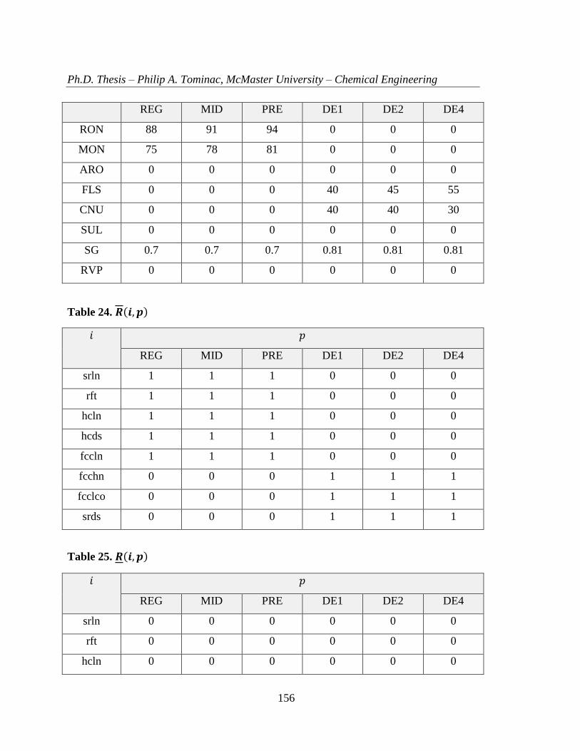
Ph.D. Thesis – Philip A. Tominac, McMaster University – Chemical Engineering
156
REG MID PRE DE1 DE2 DE4
RON 88 91 94 0 0 0
MON 75 78 81 0 0 0
ARO 0 0 0 0 0 0
FLS 0 0 0 40 45 55
CNU 0 0 0 40 40 30
SUL 0 0 0 0 0 0
SG 0.7 0.7 0.7 0.81 0.81 0.81
RVP 0 0 0 0 0 0
Table 24. 𝑹(𝒊, 𝒑)
𝑖 𝑝
REG MID PRE DE1 DE2 DE4
srln 1 1 1 0 0 0
rft 1 1 1 0 0 0
hcln 1 1 1 0 0 0
hcds 1 1 1 0 0 0
fccln 1 1 1 0 0 0
fcchn 0 0 0 1 1 1
fcclco 0 0 0 1 1 1
srds 0 0 0 1 1 1
Table 25. 𝑹(𝒊, 𝒑)
𝑖 𝑝
REG MID PRE DE1 DE2 DE4
srln 0 0 0 0 0 0
rft 0 0 0 0 0 0
hcln 0 0 0 0 0 0

Ph.D. Thesis – Philip A. Tominac, McMaster University – Chemical Engineering
157
hcds 0 0 0 0 0 0
fccln 0 0 0 0 0 0
fcchn 0 0 0 0 0 0
fcclco 0 0 0 0 0 0
srds 0 0 0 0 0 0
Table 26. 𝑻𝑪 (CAD/m3)
𝑇𝐶 0.314
Table 27. 𝑼𝑷𝑮𝒄𝒐𝒔𝒕(𝒖𝒑𝒈) (106 CAD)
𝑢𝑝𝑔
uHCproc 7.00
uHTproc 3.63
uCDUcap 8.40
uCRcap 2.475
uHCcap 6.00
uFCCcap 10.50
uGBcap 1.00
uDBcap 1.00
Table 28. 𝑼𝑷𝑮𝒄𝒐𝒔𝒕(𝒖𝒑𝒈) (103 m
3/day)
𝑢𝑝𝑔
uCDUcap 9.27
uCRcap 2.65
uHCcap 5.30
uFCCcap 5.30
uGBcap 5.30
uDBcap 4.77

Ph.D. Thesis – Philip A. Tominac, McMaster University – Chemical Engineering
158
Table 29. 𝒀(𝒊,𝒎, 𝒖) (yield fraction)
𝑖.𝑚 𝑢
CR HC FCC HT1
rft.1 0.8
rft.2 0.9
hcln.1
0.5
hchn.1
0.3
hckero.1
0.1
hcds.1
0.1
hcln.2
0.3
hchn.2
0.2
hckero.2
0.2
hcds.2
0.3
fccln.1
0.5
fcchn.1
0.3
fcclco.1
0.1
fcchco.1
0.1
fccln.2
0.3
fcchn.2
0.2
fcclco.2
0.2
fcchco.2
0.3
srds.1
0.072
hclf.1
0.928
Table 30. 𝑿(𝒊,𝒎, 𝒊′) (%)
𝑚 𝑖 𝑖′
Crude 1 Crude 2 Crude 3

Ph.D. Thesis – Philip A. Tominac, McMaster University – Chemical Engineering
159
1 lpg 2.18 1.45 0.86
srln 6.37 5.91 12.21
srhn 17.14 16.19 8.00
kero 15.83 15.21 5.87
lgo 13.25 13.60 6.73
hgo 29.87 30.60 29.99
rsd 16.57 17.05 36.33
2 lpg 1.97 1.23 0.76
srln 5.76 5.30 10.79
srhn 15.50 14.51 7.07
kero 12.12 11.49 2.16
lgo 25.16 25.51 18.64
hgo 26.17 26.91 27.39
rsd 14.52 14.99 33.18

Ph.D. Thesis – Philip A. Tominac, McMaster University – Chemical Engineering
160
Relationships with existing market structures
A primary scenario revisited throughout this work consists of a market in which a
high-cost refiner competes with multiple low-cost refiners. The basis for distinguishing
high-cost refiners from low-cost has been discussed, and in summary, may be due to a
variety of economic factors which result in one refiner possessing a disadvantage relative
to the others with which it competes. This scenario is intended to capture elements of the
Canadian refining economy, which are exemplified in a government publication cited as
reference number 37 in the second chapter of this thesis. This publication includes a map
of western Canada showing the locations and capacities of refineries and the pipeline
networks connecting them to domestic and foreign markets, and is included as Figure A1.
Figure A1. Map of refineries and pipelines in western Canada.

Ph.D. Thesis – Philip A. Tominac, McMaster University – Chemical Engineering
161
From the perspective of the frameworks developed in this thesis this map presents
an interesting case study: refineries located in the city of Edmonton (labeled A) have a
combined capacity exceeding 400 Mb/d (thousands of oil barrels per day) and have
access to the trans-mountain pipeline (labeled 3) leading to Canada’s west coast markets
and shipping lanes. The city of Prince George hosts a single refinery with a capacity of 12
Mb/d and feeds into the same west coast markets; in the framework developed in this
thesis it would be considered a high-cost refiner relative to those in Edmonton. Of course,
this analysis does not consider the influence exerted by larger parent corporations on the
sustainability of such market arrangements; the identified case study is based primarily on
arguments of scale. Nevertheless, the question remains as to the factors which contribute
to such asymmetrical competition in the Canadian petrochemical market, and what
considerations motivate the structure of refining assets in this geographical region. Our
work explores this question through a game theoretic production planning interpretation,
which has shaped our answers to these questions.