Game Theory∗

Theodore L. TurocyTexas A&M University

Bernhard von StengelLondon School of Economics

CDAM Research Report LSE-CDAM-2001-09

October 8, 2001

Contents

1 What is game theory? 4

2 Definitions of games 6

3 Dominance 8

4 Nash equilibrium 12

5 Mixed strategies 17

6 Extensive games with perfect information 22

7 Extensive games with imperfect information 29

8 Zero-sum games and computation 33

9 Bidding in auctions 34

10 Further reading 38

∗This is the draft of an introductory survey of game theory, prepared for theEncyclopedia of InformationSystems, Academic Press, to appear in 2002.

1

Glossary

Backward induction

Backward induction is a technique to solve a game of perfect information. It first consid-

ers the moves that are the last in the game, and determines the best move for the player

in each case. Then, taking these as given future actions, it proceeds backwards in time,

again determining the best move for the respective player, until the beginning of the game

is reached.

Common knowledge

A fact is common knowledge if all players know it, and know that they all know it, and

so on. The structure of the game is often assumed to be common knowledge among the

players.

Dominating strategy

A strategy dominates another strategy of a player if it always gives a better payoff to

that player, regardless of what the other players are doing. It weakly dominates the other

strategy if it is always at least as good.

Extensive game

An extensive game (or extensive form game) describes with a tree how a game is played.

It depicts the order in which players make moves, and the information each player has at

each decision point.

Game

A game is a formal description of a strategic situation.

Game theory

Game theory is the formal study of decision-making where several players must make

choices that potentially affect the interests of the other players.

2

Mixed strategy

A mixed strategy is an active randomization, with given probabilities, that determines the

player’s decision. As a special case, a mixed strategy can be the deterministic choice of

one of the given pure strategies.

Nash equilibrium

A Nash equilibrium, also called strategic equilibrium, is a list of strategies, one for each

player, which has the property that no player can unilaterally change his strategy and get

a better payoff.

Payoff

A payoff is a number, also called utility, that reflects the desirability of an outcome to a

player, for whatever reason. When the outcome is random, payoffs are usually weighted

with their probabilities. The expected payoff incorporates the player’s attitude towards

risk.

Perfect information

A game has perfect information when at any point in time only one player makes a move,

and knows all the actions that have been made until then.

Player

A player is an agent who makes decisions in a game.

Rationality

A player is said to be rational if he seeks to play in a manner which maximizes his own

payoff. It is often assumed that the rationality of all players is common knowledge.

Strategic form

A game in strategic form, also called normal form, is a compact representation of a game

in which players simultaneously choose their strategies. The resulting payoffs are pre-

sented in a table with a cell for each strategy combination.

3

Strategy

In a game in strategic form, a strategy is one of the given possible actions of a player. In

an extensive game, a strategy is a complete plan of choices, one for each decision point

of the player.

Zero-sum game

A game is said to be zero-sum if for any outcome, the sum of the payoffs to all players is

zero. In a two-player zero-sum game, one player’s gain is the other player’s loss, so their

interests are diametrically opposed.

1 What is game theory?

Game theory is the formal study of conflict and cooperation. Game theoretic concepts

apply whenever the actions of several agents are interdependent. These agents may be

individuals, groups, firms, or any combination of these. The concepts of game theory

provide a language to formulate, structure, analyze, and understand strategic scenarios.

History and impact of game theory

The earliest example of a formal game-theoretic analysis is the study of a duopoly by

Antoine Cournot in 1838. The mathematician Emile Borel suggested a formal theory of

games in 1921, which was furthered by the mathematician John von Neumann in 1928

in a “theory of parlor games.” Game theory was established as a field in its own right

after the 1944 publication of the monumental volumeTheory of Games and Economic

Behaviorby von Neumann and the economist Oskar Morgenstern. This book provided

much of the basic terminology and problem setup that is still in use today.

In 1950, John Nash demonstrated that finite games have always have an equilibrium

point, at which all players choose actions which are best for them given their opponents’

choices. This central concept of noncooperative game theory has been a focal point of

analysis since then. In the 1950s and 1960s, game theory was broadened theoretically

and applied to problems of war and politics. Since the 1970s, it has driven a revolution

4

in economic theory. Additionally, it has found applications in sociology and psychology,

and established links with evolution and biology. Game theory received special attention

in 1994 with the awarding of the Nobel prize in economics to Nash, John Harsanyi, and

Reinhard Selten.

At the end of the 1990s, a high-profile application of game theory has been the design

of auctions. Prominent game theorists have been involved in the design of auctions for al-

locating rights to the use of bands of the electromagnetic spectrum to the mobile telecom-

munications industry. Most of these auctions were designed with the goal of allocating

these resources more efficiently than traditional governmental practices, and additionally

raised billions of dollars in the United States and Europe.

Game theory and information systems

The internal consistency and mathematical foundations of game theory make it a prime

tool for modeling and designing automated decision-making processes in interactive en-

vironments. For example, one might like to have efficient bidding rules for an auction

website, or tamper-proof automated negotiations for purchasing communication band-

width. Research in these applications of game theory is the topic of recent conference and

journal papers (see, for example, Binmore and Vulkan, “Applying game theory to auto-

mated negotiation,”NetnomicsVol. 1, 1999, pages 1–9) but is still in a nascent stage. The

automation of strategic choices enhances the need for these choices to be made efficiently,

and to be robust against abuse. Game theory addresses these requirements.

As a mathematical tool for the decision-maker the strength of game theory is the

methodology it provides for structuring and analyzing problems of strategic choice. The

process of formally modeling a situation as a game requires the decision-maker to enu-

merate explicitly the players and their strategic options, and to consider their preferences

and reactions. The discipline involved in constructing such a model already has the poten-

tial of providing the decision-maker with a clearer and broader view of the situation. This

is a “prescriptive” application of game theory, with the goal of improved strategic deci-

sion making. With this perspective in mind, this article explains basic principles of game

theory, as an introduction to an interested reader without a background in economics.

5

2 Definitions of games

The object of study in game theory is thegame, which is a formal model of an interactive

situation. It typically involves severalplayers; a game with only one player is usually

called adecision problem. The formal definition lays out the players, their preferences,

their information, the strategic actions available to them, and how these influence the

outcome.

Games can be described formally at various levels of detail. Acoalitional (or cooper-

ative) game is a high-level description, specifying only what payoffs each potential group,

or coalition, can obtain by the cooperation of its members. What is not made explicit is

the process by which the coalition forms. As an example, the players may be several

parties in parliament. Each party has a different strength, based upon the number of seats

occupied by party members. The game describes which coalitions of parties can form a

majority, but does not delineate, for example, the negotiation process through which an

agreement to vote en bloc is achieved.

Cooperative game theoryinvestigates such coalitional games with respect to the rel-

ative amounts of power held by various players, or how a successful coalition should

divide its proceeds. This is most naturally applied to situations arising in political science

or international relations, where concepts like power are most important. For example,

Nash proposed a solution for the division of gains from agreement in a bargaining prob-

lem which depends solely on the relative strengths of the two parties’ bargaining position.

The amount of power a side has is determined by the usually inefficient outcome that

results when negotiations break down. Nash’s model fits within the cooperative frame-

work in that it does not delineate a specific timeline of offers and counteroffers, but rather

focuses solely on the outcome of the bargaining process.

In contrast,noncooperative game theoryis concerned with the analysis of strategic

choices. The paradigm of noncooperative game theory is that the details of the ordering

and timing of players’ choices are crucial to determining the outcome of a game. In

contrast to Nash’s cooperative model, a noncooperative model of bargaining would posit

a specific process in which it is prespecified who gets to make an offer at a given time. The

term “noncooperative” means this branch of game theory explicitly models the process of

6

players making choices out of their own interest. Cooperation can, and often does, arise

in noncooperative models of games, when players find it in their own best interests.

Branches of game theory also differ in their assumptions. A central assumption in

many variants of game theory is that the players arerational. A rational player is one

who always chooses an action which gives the outcome he most prefers, given what he

expects his opponents to do. The goal of game-theoretic analysis in these branches, then,

is to predict how the game will be played by rational players, or, relatedly, to give ad-

vice on how best to play the game against opponents who are rational. This rationality

assumption can be relaxed, and the resulting models have been more recently applied to

the analysis of observed behavior (see Kagel and Roth, eds.,Handbook of Experimental

Economics, Princeton Univ. Press, 1997). This kind of game theory can be viewed as

more “descriptive” than the prescriptive approach taken here.

This article focuses principally on noncooperative game theory with rational play-

ers. In addition to providing an important baseline case in economic theory, this case

is designed so that it gives good advice to the decision-maker, even when – or perhaps

especially when – one’s opponents also employ it.

Strategic and extensive form games

The strategic form(also callednormal form) is the basic type of game studied in non-

cooperative game theory. A game in strategic form lists each player’s strategies, and the

outcomes that result from each possible combination of choices. An outcome is repre-

sented by a separatepayoff for each player, which is a number (also calledutility) that

measures how much the player likes the outcome.

Theextensive form, also called agame tree, is more detailed than the strategic form of

a game. It is a complete description of how the game is played over time. This includes

the order in which players take actions, the information that players have at the time they

must take those actions, and the times at which any uncertainty in the situation is resolved.

A game in extensive form may be analyzed directly, or can be converted into an equivalent

strategic form.

Examples in the following sections will illustrate in detail the interpretation and anal-

ysis of games in strategic and extensive form.

7

3 Dominance

Since all players are assumed to be rational, they make choices which result in the out-

come they prefer most, given what their opponents do. In the extreme case, a player may

have two strategiesA andB so that, given any combination of strategies of the other

players, the outcome resulting fromA is better than the outcome resulting fromB. Then

strategyA is said todominatestrategyB. A rational player will never choose to play a

dominated strategy. In some games, examination of which strategies are dominated re-

sults in the conclusion that rational players could only ever choose one of their strategies.

The following examples illustrate this idea.

Example: Prisoner’s Dilemma

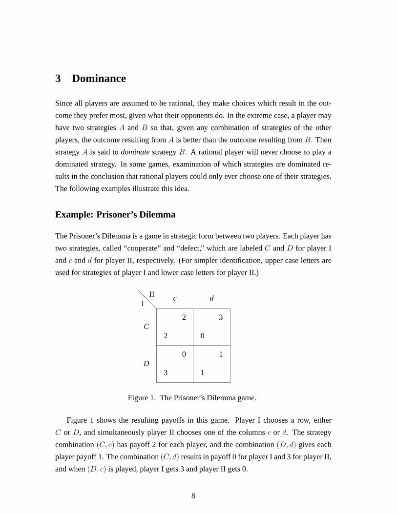
The Prisoner’s Dilemma is a game in strategic form between two players. Each player has

two strategies, called “cooperate” and “defect,” which are labeledC andD for player I

andc andd for player II, respectively. (For simpler identification, upper case letters are

used for strategies of player I and lower case letters for player II.)

@@

@

2

2

3

0

0

3

1

1

III

C

D

c d

Figure 1. The Prisoner’s Dilemma game.

Figure 1 shows the resulting payoffs in this game. Player I chooses a row, either

C or D, and simultaneously player II chooses one of the columnsc or d. The strategy

combination(C, c) has payoff 2 for each player, and the combination(D, d) gives each

player payoff 1. The combination(C, d) results in payoff 0 for player I and 3 for player II,

and when(D, c) is played, player I gets 3 and player II gets 0.

8

Any two-player game in strategic form can be described by a table like the one in

Figure 1, with rows representing the strategies of player I and columns those of player II.

(A player may have more than two strategies.) Each strategy combination defines a payoff

pair, like (3, 0) for (D, c), which is given in the respective table entry. Each cell of the

table shows the payoff to player I at the (lower) left, and the payoff to player II at the

(right) top. These staggered payoffs, due to Thomas Schelling, also make transparent

when, as here, the game is symmetric between the two players. Symmetry means that the

game stays the same when the players are exchanged, corresponding to a reflection along

the diagonal shown as a dotted line in Figure 2. Note that in the strategic form, there is no

order between player I and II since they act simultaneously (that is, without knowing the

other’s action), which makes the symmetry possible.

. . . . . . . . . . . . . . . . . . . . . . . . . . . . . . . . . . . . . . . . . . . . . . . . . .

@@

@

2

2

3

0

0

3

1

1

III

C

D

c d

↓ ↓

→

→

Figure 2. The game of Figure 1 with annotations, implied by the payoff structure. Thedotted line shows the symmetry of the game. The arrows at the left and rightpoint to the preferred strategy of player I when player II plays the left or rightcolumn, respectively. Similarly, the arrows at the top and bottom point to thepreferred strategy of player II when player I plays top or bottom.

In the Prisoner’s Dilemma game, “defect” is a strategy that dominates “cooperate.”

StrategyD of player I dominatesC since if player II choosesc, then player I’s payoff is 3

when choosingD and 2 when choosingC; if player II choosesd, then player I receives 1

for D as opposed to 0 forC. These preferences of player I are indicated by the downward-

pointing arrows in Figure 2. Hence,D is indeed always better and dominatesC. In the

same way, strategyd dominatesc for player II.

9

No rational player will choose a dominated strategy since the player will always be

better off when changing to the strategy that dominates it. The unique outcome in this

game, as recommended to utility-maximizing players, is therefore(D, d) with payoffs

(1, 1). Somewhat paradoxically, this is less than the payoff(2, 2) that would be achieved

when the players chose(C, c).

The story behind the name “Prisoner’s Dilemma” is that of two prisoners held suspect

of a serious crime. There is no judicial evidence for this crime except if one of the prison-

ers testifies against the other. If one of them testifies, he will be rewarded with immunity

from prosecution (payoff 3), whereas the other will serve a long prison sentence (pay-

off 0). If both testify, their punishment will be less severe (payoff 1 for each). However, if

they both “cooperate” with each other by not testifying at all, they will only be imprisoned

briefly, for example for illegal weapons possession (payoff 2 for each). The “defection”

from that mutually beneficial outcome is to testify, which gives a higher payoff no matter

what the other prisoner does, with a resulting lower payoff to both. This constitutes their

“dilemma.”

Prisoner’s Dilemma games arise in various contexts where individual “defections” at

the expense of others lead to overall less desirable outcomes. Examples include arms

races, litigation instead of settlement, environmental pollution, or cut-price marketing,

where the resulting outcome is detrimental for the players. Its game-theoretic justification

on individual grounds is sometimes taken as a case for treaties and laws, which enforce

cooperation.

Game theorists have tried to tackle the obvious “inefficiency” of the outcome of the

Prisoner’s Dilemma game. For example, the game is fundamentally changed by playing

it more than once. In such arepeated game, patterns of cooperation can be established

as rational behavior when players’ fear of punishment in the future outweighs their gain

from defecting today.

Example: Quality choice

The next example of a game illustrates how the principle of elimination of dominated

strategies may be applied iteratively. Suppose player I is an internet service provider and

player II a potential customer. They consider entering into a contract of service provision

for a period of time. The provider can, for himself, decide between two levels of quality

10

of service,High or Low. High-quality service is more costly to provide, and some of the

cost is independent of whether the contract is signed or not. The level of service cannot

be put verifiably into the contract. High-quality service is more valuable than low-quality

service to the customer, in fact so much so that the customer would prefer not to buy the

service if she knew that the quality was low. Her choices are tobuy or not to buythe

service.

@@

@

2

2

3

0

0

1

1

1

III

High

Low

buy don’tbuy

↓ ↓

→

←

Figure 3. High-low quality game between a service provider (player I) and a customer(player II).

Figure 3 gives possible payoffs that describe this situation. The customer prefers to

buy if player I provides high-quality service, and not to buy otherwise. Regardless of

whether the customer chooses to buy or not, the provider always prefers to provide the

low-quality service. Therefore, the strategyLowdominates the strategyHigh for player I.

Now, since player II believes player I is rational, she realizes that player I always

prefersLow, and so she anticipates low quality service as the provider’s choice. Then she

prefersnot to buy(giving her a payoff of 1) tobuy(payoff 0). Therefore, the rationality of

both players leads to the conclusion that the provider will implement low-quality service

and, as a result, the contract will not be signed.

This game is very similar to the Prisoner’s Dilemma in Figure 1. In fact, it differs

only by a single payoff, namely payoff 1 (rather than 3) to player II in the top right cell

in the table. This reverses the top arrow from right to left, and makes the preference of

player II dependent on the action of player I. (The game is also no longer symmetric.)

Player II does not have a dominating strategy. However, player I still does, so that the

11

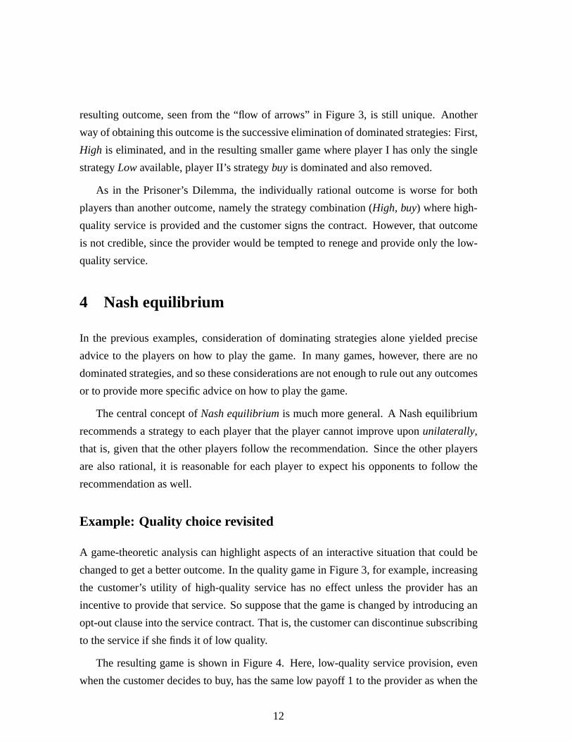
resulting outcome, seen from the “flow of arrows” in Figure 3, is still unique. Another

way of obtaining this outcome is the successive elimination of dominated strategies: First,

High is eliminated, and in the resulting smaller game where player I has only the single

strategyLowavailable, player II’s strategybuy is dominated and also removed.

As in the Prisoner’s Dilemma, the individually rational outcome is worse for both

players than another outcome, namely the strategy combination (High, buy) where high-

quality service is provided and the customer signs the contract. However, that outcome

is not credible, since the provider would be tempted to renege and provide only the low-

quality service.

4 Nash equilibrium

In the previous examples, consideration of dominating strategies alone yielded precise

advice to the players on how to play the game. In many games, however, there are no

dominated strategies, and so these considerations are not enough to rule out any outcomes

or to provide more specific advice on how to play the game.

The central concept ofNash equilibriumis much more general. A Nash equilibrium

recommends a strategy to each player that the player cannot improve uponunilaterally,

that is, given that the other players follow the recommendation. Since the other players

are also rational, it is reasonable for each player to expect his opponents to follow the

recommendation as well.

Example: Quality choice revisited

A game-theoretic analysis can highlight aspects of an interactive situation that could be

changed to get a better outcome. In the quality game in Figure 3, for example, increasing

the customer’s utility of high-quality service has no effect unless the provider has an

incentive to provide that service. So suppose that the game is changed by introducing an

opt-out clause into the service contract. That is, the customer can discontinue subscribing

to the service if she finds it of low quality.

The resulting game is shown in Figure 4. Here, low-quality service provision, even

when the customer decides to buy, has the same low payoff 1 to the provider as when the

12

@@

@

2

2

1

0

0

1

1

1

III

High

Low

buy don’tbuy

↑ ↓

→

←

Figure 4. High-low quality game with opt-out clause for the customer. The left arrowshows that player I prefersHigh when player II choosesbuy.

customer does not sign the contract in the first place, since the customer will opt out later.

However, the customer still prefers not to buy when the service isLow in order to spare

herself the hassle of entering the contract.

The changed payoff to player I means that the left arrow in Figure 4 points upwards.

Note that, compared to Figure 3, only the provider’s payoffs are changed. In a sense,

the opt-out clause in the contract has the purpose of convincing the customer that the

high-quality service provision is in the provider’s own interest.

This game has no dominated strategy for either player. The arrows point in different

directions. The game hastwo Nash equilibria in which each player chooses his strategy

deterministically. One of them is, as before, the strategy combination (Low, don’t buy).

This is an equilibrium sinceLow is the best response(payoff-maximizing strategy) to

don’t buyand vice versa.

The second Nash equilibrium is the strategy combination (High, buy). It is an equilib-

rium since player I prefers to provide high-quality service when the customer buys, and

conversely, player II prefers to buy when the quality is high. This equilibrium has a higher

payoff to both players than the former one, and is a more desirable solution.

Both Nash equilibria are legitimate recommendations to the two players of how to

play the game. Once the players have settled on strategies that form a Nash equilibrium,

neither player has incentive to deviate, so that they will rationally stay with their strategies.

This makes the Nash equilibrium a consistent solution concept for games. In contrast, a

13

strategy combination that isnot a Nash equilibrium is not a credible solution. Such a

strategy combination would not be a reliable recommendation on how to play the game,

since at least one player would rather ignore the advice and instead play another strategy

to make himself better off.

As this example shows, a Nash equilibrium may be not unique. However, the pre-

viously discussed solutions to the Prisoner’s Dilemma and to the quality choice game in

Figure 3 are unique Nash equilibria. A dominated strategy can never be part of an equilib-

rium since a player intending to play a dominated strategy could switch to the dominating

strategy and be better off. Thus, if elimination of dominated strategies leads to a unique

strategy combination, then this is a Nash equilibrium. Larger games may also have unique

equilibria that do not result from dominance considerations.

Equilibrium selection

If a game has more than one Nash equilibrium, a theory of strategic interaction should

guide players towards the “most reasonable” equilibrium upon which they should focus.

Indeed, a large number of papers in game theory have been concerned with “equilibrium

refinements” that attempt to derive conditions that make one equilibrium more plausible

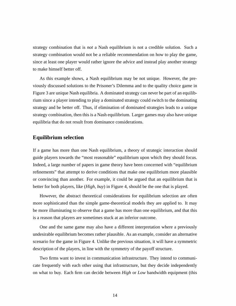
or convincing than another. For example, it could be argued that an equilibrium that is

better for both players, like (High, buy) in Figure 4, should be the one that is played.

However, the abstract theoretical considerations for equilibrium selection are often

more sophisticated than the simple game-theoretical models they are applied to. It may

be more illuminating to observe that a game has more than one equilibrium, and that this

is a reason that players are sometimes stuck at an inferior outcome.

One and the same game may also have a different interpretation where a previously

undesirable equilibrium becomes rather plausible. As an example, consider an alternative

scenario for the game in Figure 4. Unlike the previous situation, it will have a symmetric

description of the players, in line with the symmetry of the payoff structure.

Two firms want to invest in communication infrastructure. They intend to communi-

cate frequently with each other using that infrastructure, but they decide independently

on what to buy. Each firm can decide betweenHigh or Low bandwidth equipment (this

14

time, the same strategy names will be used for both players). For player II,High andLow

replacebuyanddon’t buyin Figure 4. The rest of the game stays as it is.

The (unchanged) payoffs have the following interpretation for player I (which applies

in the same way to player II by symmetry): ALow bandwidth connection works equally

well (payoff 1) regardless of whether the other side has high or low bandwidth. How-

ever, switching fromLow to High is preferable only if the other side has high bandwidth

(payoff 2), otherwise it incurs unnecessary cost (payoff 0).

As in the quality game, the equilibrium (Low, Low) (the bottom right cell) is inferior

to the other equilibrium, although in this interpretation it does not look quite as bad.

Moreover, the strategyLow has obviously the betterworst-casepayoff, as considered for

all possible strategies of the other player, no matter if these strategies are rational choices

or not. The strategyLow is therefore also called amax-minstrategy since it maximizes

the minimum payoff the player can get in each case. In a sense, investing only in low-

bandwidth equipment is a safe choice. Moreover, this strategy is part of an equilibrium,

and entirely justified if the player expects the other player to do the same.

Evolutionary games

The bandwidth choice game can be given a different interpretation where it applies to a

largepopulationof identical players. Equilibrium can then be viewed as the outcome of

adynamic processrather than of conscious rational analysis.

@@

@

5

5

1

0

0

1

1

1

III

High

Low

High Low

↑ ↓

→

←

Figure 5. The bandwidth choice game.

15

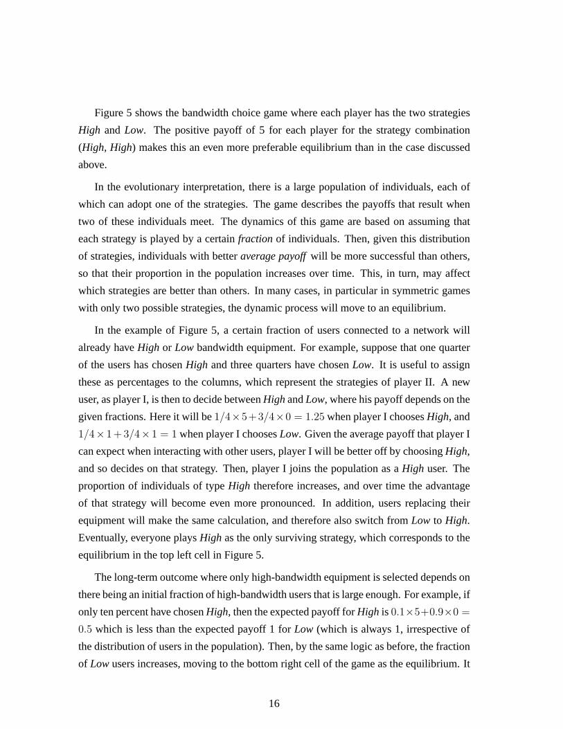
Figure 5 shows the bandwidth choice game where each player has the two strategies

High and Low. The positive payoff of 5 for each player for the strategy combination

(High, High) makes this an even more preferable equilibrium than in the case discussed

above.

In the evolutionary interpretation, there is a large population of individuals, each of

which can adopt one of the strategies. The game describes the payoffs that result when

two of these individuals meet. The dynamics of this game are based on assuming that

each strategy is played by a certainfraction of individuals. Then, given this distribution

of strategies, individuals with betteraverage payoffwill be more successful than others,

so that their proportion in the population increases over time. This, in turn, may affect

which strategies are better than others. In many cases, in particular in symmetric games

with only two possible strategies, the dynamic process will move to an equilibrium.

In the example of Figure 5, a certain fraction of users connected to a network will

already haveHigh or Low bandwidth equipment. For example, suppose that one quarter

of the users has chosenHigh and three quarters have chosenLow. It is useful to assign

these as percentages to the columns, which represent the strategies of player II. A new

user, as player I, is then to decide betweenHigh andLow, where his payoff depends on the

given fractions. Here it will be1/4×5+3/4×0 = 1.25 when player I choosesHigh, and

1/4× 1+3/4× 1 = 1 when player I choosesLow. Given the average payoff that player I

can expect when interacting with other users, player I will be better off by choosingHigh,

and so decides on that strategy. Then, player I joins the population as aHigh user. The

proportion of individuals of typeHigh therefore increases, and over time the advantage

of that strategy will become even more pronounced. In addition, users replacing their

equipment will make the same calculation, and therefore also switch fromLow to High.

Eventually, everyone playsHigh as the only surviving strategy, which corresponds to the

equilibrium in the top left cell in Figure 5.

The long-term outcome where only high-bandwidth equipment is selected depends on

there being an initial fraction of high-bandwidth users that is large enough. For example, if

only ten percent have chosenHigh, then the expected payoff forHigh is 0.1×5+0.9×0 =

0.5 which is less than the expected payoff 1 forLow (which is always 1, irrespective of

the distribution of users in the population). Then, by the same logic as before, the fraction

of Lowusers increases, moving to the bottom right cell of the game as the equilibrium. It

16

is easy to see that the critical fraction ofHigh users so that this will take off as the better

strategy is 1/5. (When new technology makes high-bandwidth equipment cheaper, this

increases the payoff 0 to theHigh user who is meetingLow, which changes the game.)

The evolutionary, population-dynamic view of games is useful because it does not

require the assumption that all players are sophisticated and think the others are also ra-

tional, which is often unrealistic. Instead, the notion of rationality is replaced with the

much weaker concept ofreproductive success: strategies that are successful on average

will be used more frequently and thus prevail in the end. This view originated in the-

oretical biology with Maynard Smith (Evolution and the Theory of Games, Cambridge

University Press, 1982) and has since significantly increased in scope (see Hofbauer and

Sigmund,Evolutionary Games and Population Dynamics, Cambridge University Press,

1998).

5 Mixed strategies

A game in strategic form does not always have a Nash equilibrium in which each player

deterministically chooses one of his strategies. However, players may instead randomly

select from among thesepure strategies with certain probabilities. Randomizing one’s

own choice in this way is called amixedstrategy. Nash showed in 1951 that any finite

strategic-form game has an equilibrium if mixed strategies are allowed. As before, an

equilibrium is defined by a (possibly mixed) strategy for each player where no player

can gainon averageby unilateral deviation. Average (that is,expected) payoffs must be

considered because the outcome of the game may be random.

Example: Compliance inspections

Suppose a consumer purchases a license for a software package, agreeing to certain re-

strictions on its use. The consumer has an incentive to violate these rules. The vendor

would like to verify that the consumer is abiding by the agreement, but doing so requires

inspections which are costly. If the vendor does inspect and catches the consumer cheat-

ing, the vendor can demand a large penalty payment for the noncompliance.

Figure 6 shows possible payoffs for such an inspection game. The standard outcome,

defining the reference payoff zero to both vendor (player I) and consumer (player II),

17

@@

@

0

0

–1

0

–10

10

– 6

– 90

III

Don’tinspect

Inspect

comply cheat

↑ ↓

→

←

Figure 6. Inspection game between a software vendor (player I) and consumer (player II).

is that the vendor choosesDon’t inspectand the consumer chooses tocomply. Without

inspection, the consumer prefers tocheatsince that gives her payoff10, with resulting

negative payoff−10 to the vendor. The vendor may also decide toInspect. If the con-

sumer complies, inspection leaves her payoff0 unchanged, while the vendor incurs a cost

resulting in a negative payoff−1. If the consumer cheats, however, inspection will result

in a heavy penalty (payoff−90 for player II) and still create a certain amount of hassle

for player I (payoff−6).

In all cases, player I would strongly prefer if player II complied, but this is outside of

player I’s control. However, the vendor prefers to inspect if the consumer cheats (since

−6 is better than−10), indicated by the downward arrow on the right in Figure 6. If the

vendor always preferredDon’t inspect, then this would be a dominating strategy and be

part of a (unique) equilibrium where the consumer cheats.

The circular arrow structure in Figure 6 shows that this game has no equilibrium in

pure strategies. If any of the players settles on a deterministic choice (likeDon’t inspect

by player I), the best reponse of the other player would be unique (herecheatby player II),

to which the original choice wouldnot be a best reponse (player I prefersInspectwhen

the other player choosescheat, against which player II in turn prefers tocomply). The

strategies in a Nash equilibrium must be best responses to each other, so in this game this

fails to hold for any pure strategy combination.

18

Mixed equilibrium

What should the players do in the game of Figure 6? One possibility is that they prepare

for the worst, that is, choose amax-minstrategy. As explained before, a max-min strategy

maximizes the player’s worst payoff against all possible choices of the opponent. The

max-min strategy for player I is toInspect(where the vendor guarantees himself payoff

−6), and for player II it is tocomply(which guarantees her payoff0). However, this is

not a Nash equilibrium and hence not a stable recommendation to the two players, since

player I could switch his strategy and improve his payoff.

A mixed strategyof player I in this game is toInspectonly with a certain probability.

In the context of inspections, randomizing is also a practical approach that reduces costs.

Even if an inspection is not certain, a sufficiently high chance of being caught should

deter from cheating, at least to some extent.

The following considerations show how to find the probability of inspection that will

lead to an equilibrium. If the probability of inspection is very low, for example one

percent, then player II receives (irrespective of that probability) payoff0 for comply, and

payoff0.99×10+0.01×(−90) = 9, which is bigger than zero, forcheat. Hence, player II

will still cheat, just as in the absence of inspection.

If the probability of inspection is much higher, for example0.2, then the expected

payoff for cheat is 0.8 × 10 + 0.2 × (−90) = −10, which is less than zero, so that

player II prefers tocomply. If the inspection probability is either too low or too high, then

player II has a unique best response. As shown above, such a pure strategy cannot be part

of an equilibrium.

Hence, the only case where player II herself could possibly randomize between her

strategies is if both strategies give her the same payoff, that is, if she isindifferent. It

is never optimal for a player to assign a positive probability to playing a strategy that

is inferior, given what the other players are doing. It is not hard to see that player II is

indifferent if and only if player I inspects with probability 0.1, since then the expected

payoff for cheatis 0.9× 10 + 0.1× (−90) = 0, which is then the same as the payoff for

comply.

With this mixed strategy of player I (Don’t inspectwith probability 0.9 andInspect

with probability 0.1), player II is indifferent between her strategies. Hence, she canmix

19

them (that is, play them randomly) without losing payoff. The only case where, in turn,

the original mixed strategy of player I is a best response is if player I is indifferent. Ac-

cording to the payoffs in Figure 6, this requires player II to choosecomplywith probability

0.8 andcheatwith probability 0.2. The expected payoffs to player I are then forDon’t

inspect0.8× 0 + 0.2× (−10) = −2, and forInspect0.8× (−1) + 0.2× (−6) = −2, so

that player I is indeed indifferent, and his mixed strategy is a best response to the mixed

strategy of player II.

This defines the only Nash equilibrium of the game. It uses mixed strategies and is

therefore called amixedequilibrium. The resulting expected payoffs are−2 for player I

and0 for player II.

Interpretation of mixed strategy probabilities

The preceding analysis showed that the game in Figure 6 has a mixed equilibrium, where

the players choose their pure strategies according to certain probabilities. These probabil-

ities have several noteworthy features.

The equilibrium probability of 0.1 forInspectmakes player II indifferent between

complyandcheat. This is based on the assumption that anexpected payoffof 0 for cheat,

namely0.9 × 10 + 0.1 × (−90), is the same for player II as when getting the payoff 0

for certain, by choosing tocomply. If the payoffs were monetary amounts (each payoff

unit standing for one thousand dollars, say), one would not necessarily assume such a

risk neutralityon the part of the consumer. In practice, decision-makers are typicallyrisk

averse, meaning they prefer the safe payoff of 0 to the gamble with an expectation of 0.

In a game-theoretic model with random outcomes (as in a mixed equilibrium), how-

ever, the payoff is not necessarily to be interpreted as money. Rather, the player’s attitude

towards risk is incorporated into the payoff figure as well. To take our example, the con-

sumer faces a certain reward or punishment when cheating, depending on whether she

is caught or not. Getting caught may not only involve financial loss but embarassment

and other undesirable consequences. However, there is a certain probability of inspec-

tion (that is, of getting caught) where the consumer becomes indifferent betweencomply

andcheat. If that probability is 1 against 9, then this indifference implies that the cost

(negative payoff) for getting caught is 9 times as high as the reward for cheating success-

fully, as assumed by the payoffs in Figure 6. If the probability of indifference is 1 against

20

20, the payoff−90 in Figure 6 should be changed to−200. The units in which payoffs

are measured are arbitrary. Like degrees on a temperature scale, they can be multiplied

by a positive number and shifted by adding a constant, without altering the underlying

preferences they represent.

In a sense, the payoffs in a game mimic a player’s (consistent) willingness to bet

when facing certain odds. With respect to the payoffs, which may distort the monetary

amounts, players are then risk neutral. Such payoffs are also calledexpected-utilityvalues.

Expected-utility functions are also used in one-player games to model decisions under

uncertainty.

The risk attitude of a player may not be known in practice. A game-theoretic analysis

should be carried out for different choices of the payoff parameters in order to test how

much they influence the results. Typically, these parameters represent the “political” fea-

tures of a game-theoretic model, those most sensitive to subjective judgement, compared

to the more “technical” part of a solution. In more involved inspection games, the tech-

nical part often concerns the optimal usage of limited inspection resources, whereas the

political decision is when to raise an alarm and declare that the inspectee has cheated (see

Avenhaus and Canty,Compliance Quantified, Cambridge University Press, 1996).

Secondly, mixing seems paradoxical when the player is indifferent in equilibrium. If

player II, for example, can equally wellcomplyor cheat, why should she gamble? In

particular, she couldcomplyand get payoff zero for certain, which is simpler and safer.

The answer is that precisely because there is no incentive to choose one strategy over

the other, a player can mix, and only in that case there can be an equilibrium. If player II

wouldcomplyfor certain, then the only optimal choice of player I isDon’t inspect, making

the choice of complying not optimal, so this is not an equilibrium.

The least intuitive aspect of mixed equilibrium is that the probabilities depend on

the opponent’s payoffsand not on the player’s own payoffs (as long as the qualitative

preference structure, represented by the arrows, remains intact). For example, one would

expect that raising the penalty−90 in Figure 6 for being caught lowers the probability

of cheating in equilibrium. In fact, it does not. What does change is the probability of

inspection, which is reduced until the consumer is indifferent.

This dependence of mixed equilibrium probabilities on the opponent’s payoffs can be

explained terms of population dynamics. In that interpretation, Figure 6 represents an evo-

21

lutionary game. Unlike Figure 5, it is a non-symmetric interaction between a vendor who

choosesDon’t InspectandInspectfor certain fractions of a large number of interactions.

Player II’s actionscomplyandcheatare each chosen by a certain fraction of consumers in-

volved in these interactions. If these fractions deviate from the equilibrium probabilities,

then the strategies that do better will increase. For example, if player I choosesInspect

too often (relative to the penalty for a cheater who is caught), the fraction of cheaters will

decrease, which in turn makesDon’t Inspecta better strategy. In this dynamic process,

the long-term averages of the fractions approximate the equilibrium probabilities.

6 Extensive games with perfect information

Games in strategic form have no temporal component. In a game in strategic form, the

players choose their strategies simultaneously, without knowing the choices of the other

players. The more detailed model of agame tree, also called a game inextensive form,

formalizes interactions where the players can over time be informed about the actions

of others. This section treats games ofperfect information. In an extensive game with

perfect information, every player is at any point aware of the previous choices of all other

players. Furthermore, only one player moves at a time, so that there are no simultaneous

moves.

Example: Quality choice with commitment

Figure 7 shows another variant of the quality choice game. This is a game tree with

perfect information. Every branching point, ornode, is associated with a player who

makes a move by choosing the next node. The connecting lines are labeled with the

player’s choices. The game starts at the initial node, theroot of the tree, and ends at a

terminal node, which establishes the outcome and determines the players’ payoffs. In

Figure 7, the tree grows from left to right; game trees may also be drawn top-down or

bottom-up.

The service provider, player I, makes the first move, choosingHigh or Lowquality of

service. Then the customer, player II, is informed about that choice. Player II can then

decide separately betweenbuyanddon’t buyin each case. The resulting payoffs are the

22

•I@@@@@@

������

High

Low

•IIHHHHHHHH

����

����

buy

don’tbuy

•IIHHHHHHHH

����

����

buy

don’tbuy

(2, 2)

(0, 1)

(3, 0)

(1, 1)

�

*

j

��

��

HH

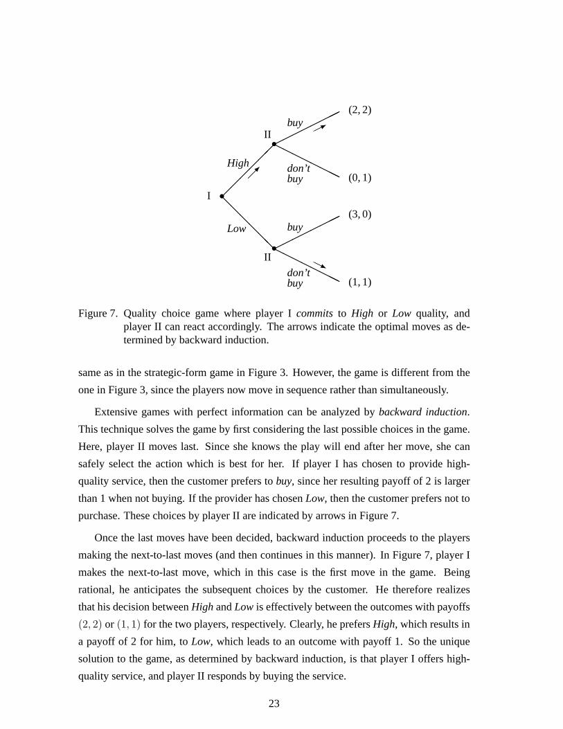
Figure 7. Quality choice game where player Icommitsto High or Low quality, andplayer II can react accordingly. The arrows indicate the optimal moves as de-termined by backward induction.

same as in the strategic-form game in Figure 3. However, the game is different from the

one in Figure 3, since the players now move in sequence rather than simultaneously.

Extensive games with perfect information can be analyzed bybackward induction.

This technique solves the game by first considering the last possible choices in the game.

Here, player II moves last. Since she knows the play will end after her move, she can

safely select the action which is best for her. If player I has chosen to provide high-

quality service, then the customer prefers tobuy, since her resulting payoff of 2 is larger

than 1 when not buying. If the provider has chosenLow, then the customer prefers not to

purchase. These choices by player II are indicated by arrows in Figure 7.

Once the last moves have been decided, backward induction proceeds to the players

making the next-to-last moves (and then continues in this manner). In Figure 7, player I

makes the next-to-last move, which in this case is the first move in the game. Being

rational, he anticipates the subsequent choices by the customer. He therefore realizes

that his decision betweenHigh andLow is effectively between the outcomes with payoffs

(2, 2) or (1, 1) for the two players, respectively. Clearly, he prefersHigh, which results in

a payoff of 2 for him, toLow, which leads to an outcome with payoff 1. So the unique

solution to the game, as determined by backward induction, is that player I offers high-

quality service, and player II responds by buying the service.

23

Strategies in extensive games

In an extensive game with perfect information, backward induction usually prescribes

unique choices at the players’ decision nodes. The only exception is if a player is indif-

ferent between two or more moves at a node. Then, any of these best moves, or even

randomly selecting from among them, could be chosen by the analyst in the backward

induction process. Since the eventual outcome depends on these choices, this may affect

a player who moves earlier, since the anticipated payoffs of that player may depend on

the subsequent moves of other players. In this case, backward induction does not yield

a unique outcome; however, this can only occur when a player is exactly indifferent be-

tween two or more outcomes.

The backward induction solution specifies the way the game will be played. Starting

from the root of the tree, play proceeds along a path to an outcome. Note that the analysis

yields more than the choices along the path. Because backward induction looks at every

node in the tree, it specifies for every player acomplete planof what to do at every point

in the game where the player can make a move, even though that point may never arise in

the course of play. Such a plan is called astrategyof the player. For example, a strategy

of player II in Figure 7 is “buy if offered high-quality service, don’t buy if offered low-

quality service.” This is player II’s strategy obtained by backward induction. Only the

first choice in this strategy comes into effect when the game is played according to the

backward-induction solution.

@@

@

2

2

3

0

2

2

1

1

0

1

3

0

0

1

1

1

III

High

Low

H: buy,L: buy

H: buy,L: don’t

H: don’t,L: buy

H: don’t,L: don’t

Figure 8. Strategic form of the extensive game in Figure 7.

With strategies defined as complete move plans, one can obtain thestrategic formof

the extensive game. As in the strategic form games shown before, this tabulates all strate-

24

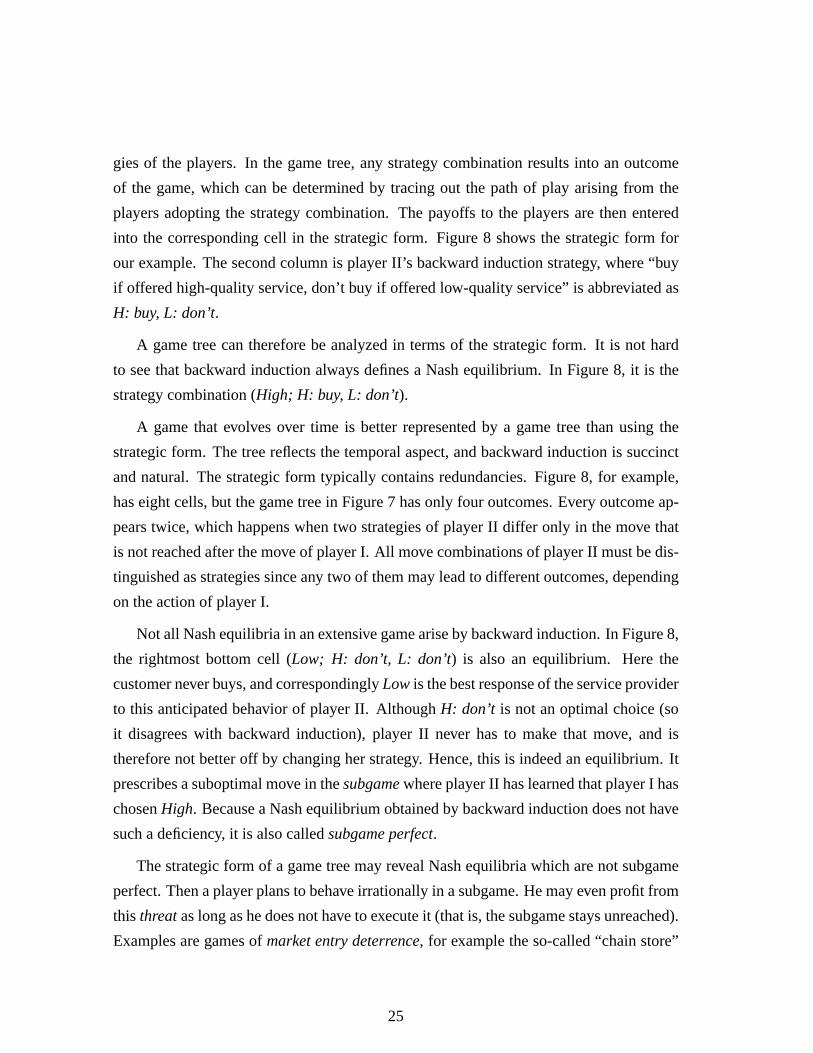
gies of the players. In the game tree, any strategy combination results into an outcome

of the game, which can be determined by tracing out the path of play arising from the

players adopting the strategy combination. The payoffs to the players are then entered

into the corresponding cell in the strategic form. Figure 8 shows the strategic form for

our example. The second column is player II’s backward induction strategy, where “buy

if offered high-quality service, don’t buy if offered low-quality service” is abbreviated as

H: buy, L: don’t.

A game tree can therefore be analyzed in terms of the strategic form. It is not hard

to see that backward induction always defines a Nash equilibrium. In Figure 8, it is the

strategy combination (High; H: buy, L: don’t).

A game that evolves over time is better represented by a game tree than using the

strategic form. The tree reflects the temporal aspect, and backward induction is succinct

and natural. The strategic form typically contains redundancies. Figure 8, for example,

has eight cells, but the game tree in Figure 7 has only four outcomes. Every outcome ap-

pears twice, which happens when two strategies of player II differ only in the move that

is not reached after the move of player I. All move combinations of player II must be dis-

tinguished as strategies since any two of them may lead to different outcomes, depending

on the action of player I.

Not all Nash equilibria in an extensive game arise by backward induction. In Figure 8,

the rightmost bottom cell (Low; H: don’t, L: don’t) is also an equilibrium. Here the

customer never buys, and correspondinglyLow is the best response of the service provider

to this anticipated behavior of player II. AlthoughH: don’t is not an optimal choice (so

it disagrees with backward induction), player II never has to make that move, and is

therefore not better off by changing her strategy. Hence, this is indeed an equilibrium. It

prescribes a suboptimal move in thesubgamewhere player II has learned that player I has

chosenHigh. Because a Nash equilibrium obtained by backward induction does not have

such a deficiency, it is also calledsubgame perfect.

The strategic form of a game tree may reveal Nash equilibria which are not subgame

perfect. Then a player plans to behave irrationally in a subgame. He may even profit from

this threatas long as he does not have to execute it (that is, the subgame stays unreached).

Examples are games ofmarket entry deterrence, for example the so-called “chain store”

25

game. The analysis of dynamic strategic interaction was pioneered by Selten, for which

he earned a share of the 1994 Nobel prize.

First-mover advantage

A practical application of game-theoretic analysis may be to reveal the potential effects

of changing the “rules” of the game. This has been illustrated with three versions of the

quality choice game, with the analysis resulting in three different predictions for how the

game might be played by rational players. Changing the original quality choice game in

Figure 3 to Figure 4 yielded an additional, although not unique, Nash equilibrium (High,

buy). The change from Figure 3 to Figure 7 is more fundamental since there the provider

has the power tocommithimself to high or low quality service, and inform the customer of

that choice. The backward induction equilibrium in that game is unique, and the outcome

is better for both players than the original equilibrium (Low, don’t buy).

Many games in strategic form exhibit what may be called thefirst-mover advantage.

A player in a game becomes a first mover or “leader” when he cancommitto a strategy,

that is, choose a strategy irrevocably and inform the other players about it; this is a change

of the “rules of the game.” The first-mover advantage states that a player who can become

a leader is not worse off than in the original game where the players act simultaneously.

In other words, if one of the players has the power to commit, he or she should do so.

This statement must be interpreted carefully. For example, if more than one player

has the power to commit, then it is not necessarily best to go first. For example, consider

changing the game in Figure 3 so that player II can commit to her strategy, and player I

moves second. Then player I will always respond by choosingLow, since this is his

dominant choice in Figure 3. Backward induction would then amount to player II not

buying and player I offering low service, with the low payoff 1 to both. Then player II

is not worse off than in the simultaneous-choice game, as asserted by the first-mover

advantage, but does not gain anything either. In contrast, making player I the first mover

as in Figure 7 is beneficial to both.

If the game has antagonistic aspects, like the inspection game in Figure 6, then mixed

strategies may be required to find a Nash equilibrium of the simultaneous-choice game.

The first-mover game always has an equilibrium, by backward induction, but having to

commit and inform the other player of a pure strategy may be disadvantageous. The

26

correct comparison is to consider commitment to arandomized choice, like to a certain

inspection probability. In Figure 6, already the commitment to the pure strategyInspect

gives a better payoff to player I than the original mixed equilibrium since player II will

respond by complying, but a commitment to a sufficiently high inspection probability

(anything above 10 percent) is even better for player I.

Example: Duopoly of chip manufacturers

The first-mover advantage is also known asStackelberg leadership, after the economist

Heinrich von Stackelberg who formulated this concept for the structure of markets in

1934. The classic application is to the duopoly model by Cournot, which dates back to

1838.

@@

@

0

0

8

12

12

8

16

16

18

9

20

15

36

0

32

0

9

18

0

36

15

20

0

32

18

18

0

27

27

0

0

0

III

H

M

L

N

h m l n

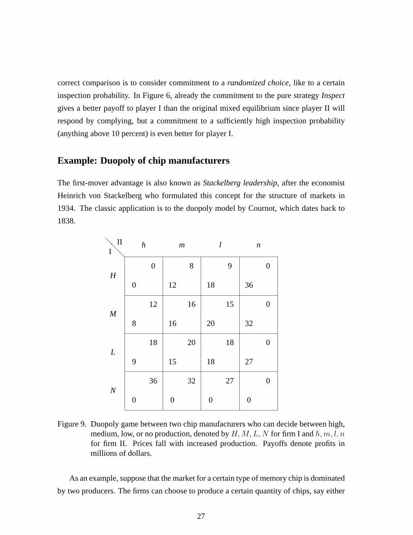
Figure 9. Duopoly game between two chip manufacturers who can decide between high,medium, low, or no production, denoted byH,M, L, N for firm I andh,m, l, nfor firm II. Prices fall with increased production. Payoffs denote profits inmillions of dollars.

As an example, suppose that the market for a certain type of memory chip is dominated

by two producers. The firms can choose to produce a certain quantity of chips, say either

27

high, medium, low, or none at all, denoted byH, M, L,N for firm I and h,m, l, n for

firm II. The market price of the memory chips decreases with increasing total quantity

produced by both companies. In particular, if both choose a high quantity of production,

the price collapses so that profits drop to zero. The firms know how increased production

lowers the chip price and their profits. Figure 9 shows the game in strategic form, where

both firms choose their output level simultaneously. The symmetric payoffs are derived

from Cournot’s model, explained below.

The game can be solved by dominance considerations. Clearly, no production is dom-

inated by low or medium production, so that rowN and columnn in Figure 9 can be

eliminated. Then, high production is dominated by medium production, so that rowH

and columnh can be omitted. At this point, only medium and low production remain.

Then, regardless of whether the opponent produces medium or low, it is always better for

each firm to produce medium. Therefore, the Nash equilibrium of the game is(M, m),

where both firms make a profit of $16 million.

Consider now the commitment version of the game, with a game tree (omitted here)

corresponding to Figure 9 just as Figure 7 is obtained from Figure 3. Suppose that firm I is

able to publicly announce and commit to a level of production, given by a row in Figure 9.

Then firm II, informed of the choice of firm I, will respond toH by l (with maximum

payoff 9 to firm II), toM by m, to L also bym, and toN by h. This determines the

backward induction strategy of firm II. Among these anticipated responses by firm II,

firm I does best by announcingH, a high level of production. The backward induction

outcome is thus that firm I makes a profit $18 million, as opposed to only $16 million in

the simultaneous-choice game. When firm II must play the role of the follower, its profits

fall from $16 million to $9 million.

The first-mover advantage again comes from the ability of firm I to credibly commit

itself. After firm I has chosenH, and firm II replies withl, firm I would like to be able

switch toM , improving profits even further from $18 million to $20 million. However,

once firm I is producingM , firm II would change tom. This logic demonstrates why,

when the firms choose their quantities simultaneously, the strategy combination(H, l) is

not an equilibrium. The commitment power of firm I, and firm II’s appreciation of this

fact, is crucial.

28

The payoffs in Figure 9 are derived from the following simple model due to Cournot.

The high, medium, low, and zero production numbers are 6, 4, 3, and 0 million memory

chips, respectively. The profit per chip is12 − Q dollars, whereQ is the total quantity

(in millions of chips) on the market. The entire production is sold. As an example,

the strategy combination(H, l) yields Q = 6 + 3 = 9, with a profit of $3 per chip.

This yields the payoffs of 18 and 9 million dollars for firms I and II in the(H, l) cell in

Figure 9. Another example is firm I acting as a monopolist (firm II choosingn), with a

high production levelH of 6 million chips sold at a profit of $6 each.

In this model, a monopolist would produce a quantity of 6 million even if other num-

bers than 6, 4, 3, or 0 were allowed, which gives the maximum profit of $36 million. The

two firms could cooperate and split that amount by producing 3 million each, correspond-

ing to the strategy combination(L, l) in Figure 9. The equilibrium quantities, however, are

4 million for each firm, where both firms receive less. The central four cells in Figure 9,

with low and medium production in place of “cooperate” and “defect,” have the structure

of a Prisoner’ Dilemma game (Figure 1), which arises here in a natural economic context.

The optimal commitment of a first mover is to produce a quantity of 6 million, with the

follower choosing 3 million. These numbers, and the equilibrium (“Cournot”) quantity of

4 million, apply even when arbitrary quantities are allowed (see Gibbons, 1992).

7 Extensive games with imperfect information

Typically, players do not always have full access to all the information which is relevant

to their choices. Extensive games withimperfect informationmodel exactly which in-

formation is available to the players when they make a move. Modeling and evaluating

strategic information precisely is one of the strengths of game theory. John Harsanyi’s

pioneering work in this area was recognized in the 1994 Nobel awards.

Consider the situation faced by a large software company after a small startup has

announced deployment of a key new technology. The large company has a large research

and development operation, and it is generally known that they have researchers work-

ing on a wide variety of innovations. However, only the large company knows for sure

whether or not they have made any progress on a product similar to the startup’s new tech-

nology. The startup believes that there is a 50 percent chance that the large company has

29

developed the basis for a strong competing product. For brevity, when the large company

has the ability to produce a strong competing product, the company will be referred to as

having a “strong” position, as opposed to a “weak” one.

The large company, after the announcement, has two choices. It can counter by an-

nouncing that it too will release a competing product. Alternatively, it can choose to cede

the market for this product. The large company will certainly condition its choice upon its

private knowledge, and may choose to act differently when it has a strong position than

when it has a weak one. If the large company has announced a product, the startup is

faced with a choice: it can either negotiate a buyout and sell itself to the large company,

or it can remain independent and launch its product. The startup does not have access to

the large firm’s private information on the status of its research. However, it does observe

whether or not the large company announces its own product, and may attempt to infer

from that choice the likelihood that the large company has made progress of their own.

When the large company does not have a strong product, the startup would prefer to

stay in the market over selling out. When the large company does have a strong product,

the opposite is true, and the startup is better off by selling out instead of staying in.

Figure 10 shows an extensive game that models this situation. From the perspective of

the startup, whether or not the large company has done research in this area is random. To

capture random events such as this formally in game trees,chance movesare introduced.

At a node labelled as a chance move, the next branch of the tree is taken randomly and

non-strategically by chance, or “nature”, according to probabilities which are included in

the specification of the game.

The game in Figure 10 starts with a chance move at the root. With equal probabil-

ity 0.5, the chance move decides if the large software company, player I, is in a strong

position (upward move) or weak position (downward move). When the company is in

a weak position, it can choose toCedethe market to the startup, with payoffs(0, 16) to

the two players (with payoffs given in millions of dollars of profit). It can alsoAnnounce

a competing product, in the hope that the startup company, player II, willsell out, with

payoffs 12 and 4 to players I and II. However, if player II decides instead tostay in, it will

even profit from the increased publicity and gain a payoff of 20, with a loss of−4 to the

large firm.

30

•chance@@@@@@

����������

�����

0.5

0.5

•

•HHHHHHHH

������

���

(Announce)

Announce

Cede

stayin

sellout

stayin

sellout

•HHHHHHHH

����

����

•HHHHHHHH

������

�� (20, – 4)

(12, 4)

(– 4, 20)

(12, 4)

(0, 16)

I��

��

I��

��

II

�

�

�

�

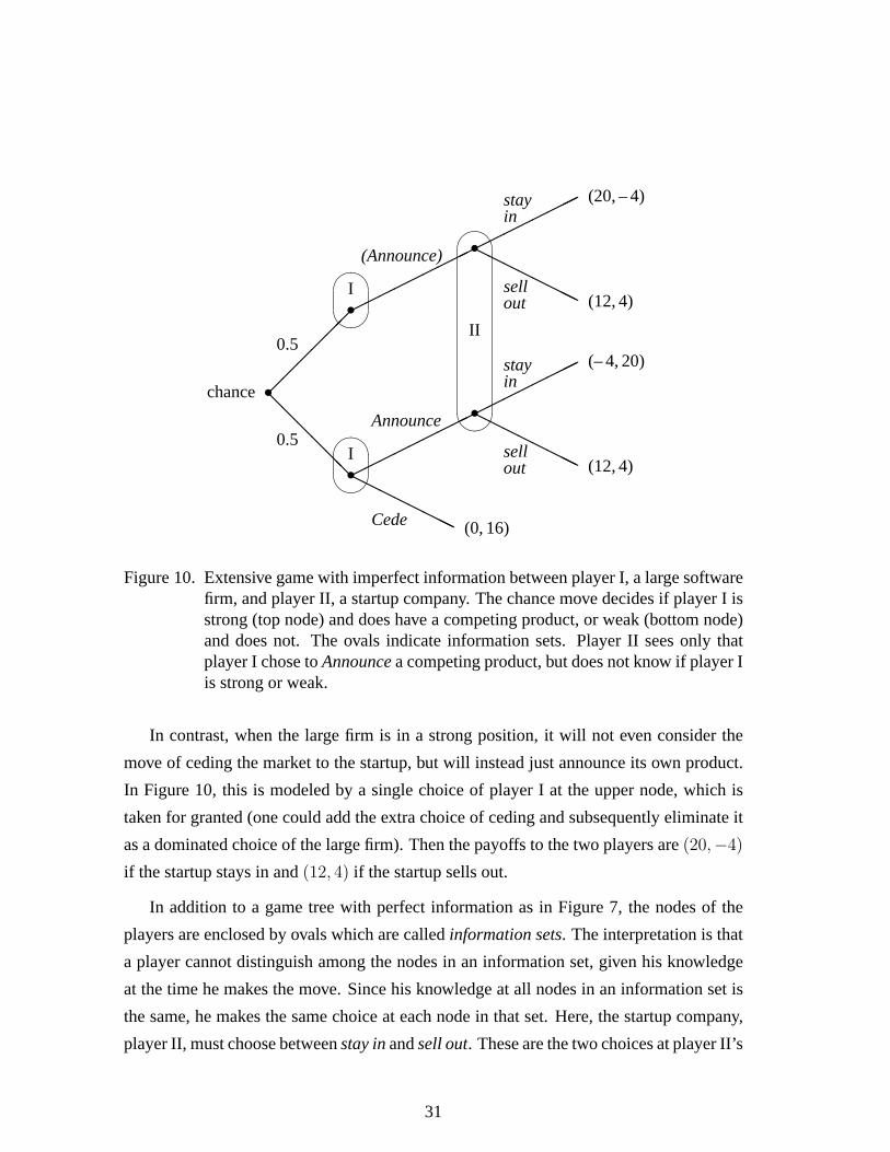
Figure 10. Extensive game with imperfect information between player I, a large softwarefirm, and player II, a startup company. The chance move decides if player I isstrong (top node) and does have a competing product, or weak (bottom node)and does not. The ovals indicate information sets. Player II sees only thatplayer I chose toAnnouncea competing product, but does not know if player Iis strong or weak.

In contrast, when the large firm is in a strong position, it will not even consider the

move of ceding the market to the startup, but will instead just announce its own product.

In Figure 10, this is modeled by a single choice of player I at the upper node, which is

taken for granted (one could add the extra choice of ceding and subsequently eliminate it

as a dominated choice of the large firm). Then the payoffs to the two players are(20,−4)

if the startup stays in and(12, 4) if the startup sells out.

In addition to a game tree with perfect information as in Figure 7, the nodes of the

players are enclosed by ovals which are calledinformation sets. The interpretation is that

a player cannot distinguish among the nodes in an information set, given his knowledge

at the time he makes the move. Since his knowledge at all nodes in an information set is

the same, he makes the same choice at each node in that set. Here, the startup company,

player II, must choose betweenstay inandsell out. These are the two choices at player II’s

31

information set, which has two nodes according to the different histories of play, which

player II cannot distinguish.

Because player II is not informed about its position in the game, backward induction

can no longer be applied. It would be better tosell outat the top node, and tostay in

at the bottom node. Consequently, player I’s choice when being in the weak position is

not clear: if player II stays in, then it is better toCede(since 0 is better than−4), but if

player II sells out, then it is better toAnnounce.

The game does not have an equilibrium in pure strategies: The startup would respond

to Cedeby selling out when seeing an announcement, since then this is only observed

when player I is strong. But then player I would respond by announcing a product even in

the weak position. In turn, the equal chance of facing a strong or weak opponent would

induce the startup to stay in, since then the expected payoff of0.5(−4) + 0.5 × 20 = 8

exceeds 4 when selling out.

@@

@

8

8

10

6

12

4

6

10

III

Announce

Cede

stayin

sellout

↓ ↑

→

←

Figure 11. Strategic form of the extensive game in Figure 10, with expected payoffs re-sulting from the chance move and the player’s choices.

The equilibrium of the game involves both players randomizing. The mixed strategy

probabilities can be determined from the strategic form of the game in Figure 11. When

it is in a weak position, the large firm randomizes with equal probability 1/2 between

AnnounceandCedeso that the expected payoff to player II is then 7 for bothstay inand

sell out.

Since player II is indifferent, randomization is a best response. If the startup chooses

to stay inwith probability 3/4 and tosell outwith probability 1/4, then player I, in turn, is

32

indifferent, receiving an overall expected payoff of 9 in each case. This can also be seen

from the extensive game in Figure 10: when in a weak position, player I is indifferent

between the movesAnnounceandCedewhere the expected payoff is 0 in each case. With

probability 1/2, player I is in the strong position, and stands to gain an expected payoff of

18 when facing the mixed strategy of player II. The overall expected payoff to player I

is 9.

8 Zero-sum games and computation

The extreme case of players with fully opposed interests is embodied in the class of two-

player zero-sum(or constant-sum) games. Familiar examples range from rock-paper-

scissors to many parlor games like chess, go, or checkers.

A classic case of a zero-sum game, which was considered in the early days of game

theory by von Neumann, is the game of poker. The extensive game in Figure 10, and

its strategic form in Figure 11, can be interpreted in terms of poker, where player I is

dealt a strong or weak hand which is unknown to player II. It is aconstant-sumgame

since for any outcome, the two payoffs add up to 16, so that one player’s gain is the other

player’s loss. When player I chooses to announce despite being in a weak position, he

is colloquially said to be “bluffing.” This bluff not only induces player II to possibly sell

out, but similarly allows for the possibility that player II stays in when player I is strong,

increasing the gain to player I.

Mixed strategies are a natural device for constant-sum games with imperfect infor-

mation. Leaving one’s own actions open reduces one’s vulnerability against malicious

responses. In the poker game of Figure 10, it is too costly to bluff all the time, and better

to randomize instead. The use of active randomization will be familiar to anyone who has

played rock-paper-scissors.

Zero-sum games can be used to model strategically the computer science concept of

“demonic” nondeterminism. Demonic nondeterminism is based on the assumption that,

when an ordering of events is not specified, one must assume that the worst possible se-

quence will take place. This can be placed into the framework of zero-sum game theory

by treating nature (or the environment) as an antagonistic opponent. Optimal randomiza-

tion by such an opponent describes a worst-case scenario that can serve as a benchmark.

33

A similar use of randomization is known in the theory of algorithms as Rao’s theorem,

and describes the power of randomized algorithms. An example is the well-knownquick-

sort algorithm, which has one of the best observed running times of sorting algorithms in

practice, but can have bad worst cases. With randomization, these can be made extremely

unlikely.

Randomized algorithms and zero-sum games are used for analyzing problems inon-

line computation. This is, despite its name, not related to the internet, but describes the

situation where an algorithm receives its input one data item at a time, and has to make

decisions, for example in scheduling, without being able to wait until the entirety of the

input is known. The analysis of online algorithms has revealed insights into hard opti-

mization problems, and seems also relevant to the massive data processing that is to be

expected in the future. At present, it constitutes an active research area, although mostly

confined to theoretical computer science (see Borodin and El-Yaniv,Online Computation

and Competitive Analysis, Cambridge University Press, 1998).

9 Bidding in auctions

The design and analysis of auctions is one of the triumphs of game theory. Auction the-

ory was pioneered by the economist William Vickrey in 1961. Its practical use became

apparent in the 1990s, when auctions of radio frequency spectrum for mobile telecommu-

nication raised billions of dollars. Economic theorists advised governments on the design

of these auctions, and companies on how to bid (see McMillan, “Selling spectrum rights,”

Journal of Economic PerspectivesVol. 8, 1994, pages 145–162). The auctions for spec-

trum rights are complex. However, many principles for sound bidding can be illustrated

by applying game-theoretic ideas to simple examples. This section highlights some of

these examples; see Milgrom, “Auctions and bidding: a primer” (Journal of Economic

PerspectivesVol. 3, 1989, pages 3–22) for a broader view of the theory of bidding in

auctions.

Second-price auctions with private values

The most familiar type of auction is the familiaropen ascending-bidauction, which is

also called anEnglishauction. In this auction format, an object is put up for sale. With

34

the potential buyers present, an auctioneer raises the price for the object as long as two

or more bidders are willing to pay that price. The auction stops when there is only one

bidder left, who gets the object at the price at which the last remaining opponent drops

out.

A complete analysis of the English auction as a game is complicated, as the exten-

sive form of the auction is very large. The observation that the winning bidder in the

English auction pays the amount at which the last remaining opponent drops out suggests

a simpler auction format, thesecond-priceauction, for analysis. In a second-price auc-

tion, each potential buyer privately submits, perhaps in a sealed envelope or over a secure

computer connection, his bid for the object to the auctioneer. After receiving all the bids,

the auctioneer then awards the object to the bidder with the highest bid, and charges him

the amount of the second-highest bid. Vickrey’s analysis dealt with auctions with these

rules.

How should one bid in a second-price auction? Suppose that the object being auc-

tioned is one where the bidders each have aprivate valuefor the object. That is, each

bidder’s value derives from his personal tastes for the object, and not from considerations

such as potential resale value. Suppose this valuation is expressed in monetary terms, as

the maximum amount the bidder would be willing to pay to buy the object. Then the

optimal bidding strategy is to submit a bid equal to one’s actual value for the object.

Bidding one’s private value in a second-price auction is aweakly dominantstrategy.

That is, irrespective of what the other bidders are doing, no other strategy can yield a better

outcome. (Recall that a dominant strategy is one that isalwaysbetter than the dominated

strategy; weak dominance allows for other strategies that are sometimes equally good.)

To see this, suppose first that a bidder bids less than the object was worth to him. Then if

he wins the auction, he still pays the second-highest bid, so nothing changes. However, he

now risks that the object is sold to someone else at a lower price than his true valuation,

which makes the bidder worse off. Similarly, if one bids more than one’s value, the only

case where this can make a difference is when there is, below the new bid, another bid

exceeding the own value. The bidder, if he wins, must then pay that price, which he

prefers less than not winning the object. In all other cases, the outcome is the same.

Bidding one’s true valuation is a simple strategy, and, being weakly dominant, does not

require much thought about the actions of others.

35

While second-price sealed-bid auctions like the one described above are not very com-

mon, they provide insight into a Nash equilibrium of the English auction. There is a

strategy in the English auction which is analogous to the weakly dominant strategy in

the second price auction. In this strategy, a bidder remains active in the auction until the

price exceeds the bidder’s value, and then drops out. If all bidders adopt this strategy, no

bidder can make himself better off by switching to a different one. Therefore, it is a Nash

equilibrium when all bidders adopt this strategy.

Most online auction websites employ an auction which has features of both the En-

glish and second-price rules. In these auctions, the current price is generally observable

to all participants. However, a bidder, instead of frequently checking the auction site for

the current price, can instead instruct an agent, usually an automated agent provided by

the auction site, to stay in until the price surpasses a given amount. If the current bid is

by another bidder and below that amount, then the agent only bids up the price enough so

that it has the new high bid. Operationally, this is similar to submitting a sealed bid in a

second-price auction. Since the use of such agents helps to minimize the time investment

needed for bidders, sites providing these agents encourage more bidders to participate,

which improves the price sellers can get for their goods.

Example: Common values and the winner’s curse

A crucial assumption in the previous example of bidding in a second-price auction is that

of private values. In practice, this assumption may be a very poor approximation. An

object of art may be bought as an investment, and a radio spectrum license is acquired

for business reasons, where the value of the license depends on market forces, such as

the demand for mobile telephone usage, which have a common impact on all bidders.

Typically, auctions have both private andcommon valueaspects.

In a purely common value scenario, where the object is worth the same to all bidders,

bidders must decide how to take into account uncertainty about that value. In this case,

each bidder may have, prior to the auction, received some private information or signals

about the value of the object for sale. For example, in the case of radio spectrum licenses,

each participating firm may have undertaken its own market research surveys to estimate

the retail demand for the use of that bandwidth. Each survey will come back with slightly

36

different results, and, ideally, each bidder would like to have access to all the surveys in

formulating its bid. Since the information is proprietary, that is not possible.

Strategic thinking, then, requires the bidders to take into account the additional infor-

mation obtained by winning the auction. Namely, the sheer fact of winning means that

one’s own, private information about the worth of the object was probably overly opti-

mistic, perhaps because the market research surveys came back with estimates for band-

width demand which were too bullish. Even if everybody’s estimate about that worth is

correct on average, the largest (or smallest) of these estimates is not. In a procurement

situation, for example, an experienced bidder should add to his own bid not only a markup

for profit, but also for the likely under-estimation of the cost that results from the compet-

itive selection process. The principle that winning a common-value auction is “bad news”

for the winner concerning the valuation of the object is called thewinner’s curse.

The following final example, whose structure was first proposed by Max Bazerman

and William Samuelson, demonstrates the considerations underlying the winner’s curse

not for an auction, but in a simpler situation where the additional information of “winning”

is crucial for the expected utility of the outcome. Consider a potential buyer who is

preparing a final, “take it or leave it” offer to buy out a dot-com company. Because of

potential synergies, both the buyer and the seller know that the assets of the dot-com are

worth 50 percent more to the buyer than to the current owner of the firm. If the value of the

company were publicly known, the parties could work out a profitable trade, negotiating

a price where both would profit from the transaction.

However, the buyer does not know the exact value of the company. She believes

that it is equally likely to be any value between zero and ten million dollars. The dot-

com’s current owners know exactly the value of retaining the company, because they have

complete information on their company’s operations. In this case, the expected value of

the company to the current owners is five million dollars, and the expected value of the

company to the prospective buyer is seven and a half million dollars. Moreover, no matter

what the value of the company truly is, the company is always worth more to the buyer

than it is to the current owner. With this in mind, what offer should the buyer tender to

the dot-com as her last, best offer, to be accepted or rejected?

To find the equilibrium of this game, note that the current owners of the dot-com will

accept any offer that is greater than the value of the company to them, and reject any

37

offer that is less. So, if the buyer tenders an offer of five million dollars, then the dot-

com owners will accept if their value is between zero and five million. The buyer, being

strategic, then realizes that this implies the value of the company to her is equally likely to

be anywhere between zero and seven and a half million. This means that, if she offers five

million, the average value of the company, conditioning upon the owners of the dot-com

accepting the offer, is only three and three-quarters million – less than the value of the

offer. Therefore, the buyer concludes that offering five million will lead to an expected

loss.

The preceding analysis does not depend on the amount of the offer. The buyer soon

realizes that, no matter what offer she makes, when she takes into account the fact that

the offer will be accepted only when the value of the dot-com turns out to be on the low

end. The expected value of the company to the buyer, conditional on her offer being

accepted, is always less than her offer. It is this updating of the buyer’s beliefs, shifting

her estimation of the dot-com’s value to the low end, which embodies the winner’s curse

in this example. Having her offer accepted is bad news for the buyer, because she realizes

it implies the value of the dot-com is low. The equilibrium in this game involves the buyer

making an offer of zero, and the offer never being accepted.

This example is particularly extreme, in that no transaction is made even though every-

one involved realizes that a transaction would be profitable to both sides. As is generally

the case with noncooperative game theory, the equilibrium does depend on the details of

the rules of the game, in this case, the assumption that one last, best offer is being made,

which will either be accepted or rejected. In general, the winner’s curse will not always

prohibit mutually profitable transactions from occurring. This example demonstrates the

importance of carefully taking into account the information one learns during the course

of play of a game. It also shows how a game-theoretic model that incorporates the infor-

mation and incentives of others helps promote sound decision-making.

10 Further reading

Binmore, Ken (1991),Fun and Games: A Text on Game Theory. D. C. Heath, Lexington,

MA.

Dixit, Avinash K., and Nalebuff, Barry J. (1991),Thinking Strategically: The Competitive

Edge in Business, Politics, and Everyday Life. Norton, New York.

38

Fudenberg, Drew and Tirole, Jean (1991),Game Theory. MIT Press, Cambridge, MA.

Gibbons, Robert (1992),Game Theory for Applied Economists. Princeton University

Press, Princeton, NJ.

Myerson, Roger B. (1991),Game Theory: Analysis of Conflict. Harvard University Press,

Cambridge, MA.

Nasar, Sylvia (1998),A Beautiful Mind: A Biography of John Forbes Nash, Jr., Winner of

the Nobel Prize in Economics, 1994.Simon and Schuster, New York.

Rasmusen, Eric (2001),Games and Information: An Introduction to Game Theory, 3rd

ed. Blackwell, Oxford.

39