gamma-gompertz life expectancy at birth · demographic research: volume 28, article 9 formal...

DEMOGRAPHIC RESEARCH

VOLUME 28, ARTICLE 9, PAGES 259-270

PUBLISHED 12 FEBRUARY 2013 http://www.demographic-research.org/Volumes/Vol28/9/

DOI: 10.4054/DemRes.2013.28.9

Formal Relationship 20

Gamma-Gompertz life expectancy at birth

Trifon I. Missov

© 2013 Trifon I. Missov.

This open-access work is published under the terms of the Creative Commons

Attribution NonCommercial License 2.0 Germany, which permits use, reproduction & distribution in any medium for non-commercial purposes,

provided the original author(s) and source are given credit.

See http:// creativecommons.org/licenses/by-nc/2.0/de/

Table of Contents1 Relationship 262

2 Proof of the Relationship 263

3 History and Related Results 263

4 Applications 267

5 Conclusion 267

6 Acknowledgements 269

References 270

Demographic Research: Volume 28, Article 9

Formal Relationship

Gamma-Gompertz life expectancy at birth

Trifon I. Missov 1

Abstract

BACKGROUNDThe gamma-Gompertz multiplicative frailty model is the most common parametric modelapplied to human mortality data at adult and old ages. The resulting life expectancy hasbeen calculated so far only numerically.

OBJECTIVEProperties of the gamma-Gompertz distribution have not been thoroughly studied. The fo-cus of the paper is to shed light onto its first moment or, demographically speaking, char-acterize life expectancy resulting from a gamma-Gompertz force of mortality. The paperprovides an exact formula for gamma-Gompertz life expectancy at birth and a simplerhigh-accuracy approximation that can be used in practice for computational convenience.In addition, the article compares actual (life-table) to model-based (gamma-Gompertz)life expectancy to assess on aggregate how many years of life expectancy are not captured(or overestimated) by the gamma-Gompertz mortality mechanism.

COMMENTSA closed-form expression for gamma-Gomeprtz life expectancy at birth contains a special(the hypergeometric) function. It aids assessing the impact of gamma-Gompertz parame-ters on life expectancy values. The paper shows that a high-accuracy approximation canbe constructed by assuming an integer value for the shape parameter of the gamma dis-tribution. A historical comparison between model-based and actual life expectancy forSwedish females reveals a gap that is decreasing to around 2 years from 1950 onwards.Looking at remaining life expectancies at ages 30 and 50, we see this gap almost disap-pearing.

1 Max Planck Institute for Demographic Research, Konrad-Zuse-Str. 1, 18057 Rostock, Germany

http://www.demographic-research.org 261

Missov: Gamma-Gompertz life expectancy at birth

1. Relationship

Suppose in a population individuals die according to a force of mortality

µ(x |Z) = Zµ(x),(1)

where Z is a random variable, called frailty (Vaupel, Manton, and Stallard 1979), whichaccounts for unobserved heterogeneity across individuals, and µ(x) is the baseline forceof mortality. Model (1) is called a multiplicative (frailty) model.

Assume µ(x) follows the Gompertz law

µ(x) = aebx , a, b > 0

and frailty is gamma-distributed, i.e. Z ∼ Γ(k, λ) has a probability density function

π(z) =λk

Γ(k)zk−1 e−λx , k, λ > 0 .

Then life expectancy at birth e0 can be expressed as

(2) e0 =1

bk2F1

(k, 1; k + 1; 1− a

bλ

),

where 2F1(α, β; γ; z) is the Gaussian hypergeometric function

(3) 2F1(α, β; γ; z) =

+∞∑j=0

α(α+ 1) . . . (α− j + 1)β(β + 1) . . . (β − j + 1)

γ(γ + 1) . . . (γ − j + 1) j!zj

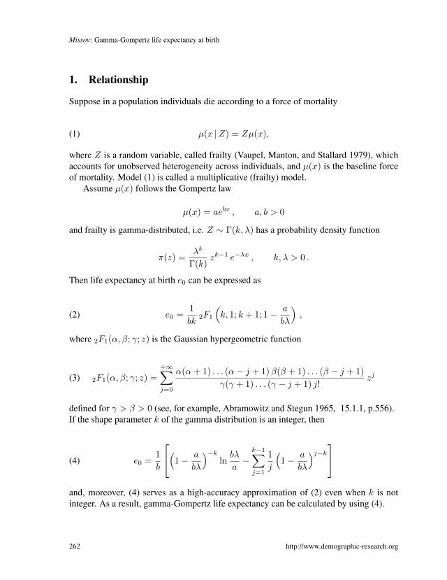
defined for γ > β > 0 (see, for example, Abramowitz and Stegun 1965, 15.1.1, p.556).If the shape parameter k of the gamma distribution is an integer, then

(4) e0 =1

b

(1− a

bλ

)−klnbλ

a−k−1∑j=1

1

j

(1− a

bλ

)j−kand, moreover, (4) serves as a high-accuracy approximation of (2) even when k is notinteger. As a result, gamma-Gompertz life expectancy can be calculated by using (4).

262 http://www.demographic-research.org


2. Proof of the Relationship

Life expectancy is the integrated survivorship of the population across all ages

e0 =

∞∫0

S(x)dx

where

S(x) =

∞∫0

exp

{−∫ x

0

µ(t | z)dt}π(z)dz

In a gamma-Gompertz multiplicative model S(x) =(1 + a

bλ

(ebx − 1

))−kand thus

(5) e0 =

∞∫0

(1 +

a

bλ

(ebx − 1

))−kdx.

A t = 1− e−bx substitution will result in

(6) e0 =1

b

1∫0

(1− t)k−1(

1−(

1− a

bλ

)t)−k

dt

Taking into account

2F1(α, β; γ; z) =Γ(γ)

Γ(β)Γ(γ − β)

1∫0

tβ−1 (1− t)γ−β−1(1− tz)−α dt

(see Abramowitz and Stegun 1965, 15.3.1, p.558), (6) reduces to (2). Relationship (4) isobtained by integrating k times the right-hand side of (5) by parts.

Q.E.D.

3. History and Related Results

The gamma-Gompertz multiplicative frailty model (1) has been introduced in demogra-phy by Vaupel, Manton, and Stallard (1979). While capturing the observed bending of



human mortality rates at older ages (see Beard 1959), it also takes into account unob-served heterogeneity. Relationship (2) describes, on the one hand, the first moment ofthe mixture gamma-Gompertz distribution and, from a demographic point of view, theexpected lifetime duration under the gamma-Gompertz assumption.

The fact that gamma-Gompertz life expectancy is proportional to a hypergeometricfunction with a z-argument close to 1 (for human populations a ∝ 10−6, b ≈ 0.14,and k = λ > 1) sheds light on the dynamics of e0 with respect to model parameters.As γ − α − β = 0 for the hypergeometric function 2F1 in (2), life expectancy is anincreasing function of z for z → 1− and lim

z→12F1(α, β; γ; z) = +∞ (see Abramowitz

and Stegun 1965, p.556, 15.1.1(c)). This implies that e0 increases when a declineskeeping all other parameters fixed, which is intuitively justified as a denotes the startinglevel of mortality. A little counterintutive is the finding that life expectancy increases asthe rate of aging b = d lnµ(x)/dx increases (see Figure 1). The gamma parameters k andλ, often assumed to be equal to one another, so that µ(x) denotes the force of mortalityof the “standard” individual (with frailty Z = 1), have one and the same impact on lifeexpectancy – the higher k, λ, the higher e0.

Figure 1: Life expectancy as a function of b.

Notes: Life expectancy at birth as a function of b for fixed a = 5× 10−7, k = λ = 7.

Note that when baseline mortality µ(x) in (1) is Gompertz-Makeham, i.e.

µ(x) = aebx + c ,

and, consequently,



µ(x |Z) = Z(aebx + c) ,

the corresponding life-expectancy integral

e0 =

∞∫0

(1− a

bλ+c

λx+

a

bλebx)−k

dx

cannot be solved analytically, even for integer values of k.As already pointed out, for human populations we have 1− a/bλ ≈ 1, which leads to

further simplification of (4):

(7) e0 ≈1

b

lnbλ

a−k−1∑j=1

1

j

Note that when k = λ (often assumed, see Vaupel, Manton, and Stallard (1979)), theright-hand side of (7) contains the difference between the partial sum of the harmonicseries and the natural logarithm:

(8) e0 ≈1

b

lnb

a+

1

k−

k∑j=1

1

j− ln k

.The limit of the latter when k → ∞ is the Euler-Mascheroni constant γ∗ ≈ 0.577.Note that k → ∞ corresponds to the case when the Gompertz model for a gamma-heterogeneous population tends to the Gompertz model for a homogeneous population.As a result, life expectancy at birth for a homogeneous population experiencing a Gom-pertz force of mortality could be approximated by

(9) e0 ≈1

b

[lnb

a− γ∗

].

An expression for remaining life expectancy ex at age x in terms of a hypergeometricfunction can also be derived. Consider the indefinite integral in the right-hand side of (5):



I :=

∫ (1 +

a

bλ

(ebx − 1

))−kdx =

∫ (bλ

ae−bx

)k (1−

(1− bλ

a

)e−bx

)−kdx .

A y = e−bx substitution will result in

I = −1

b

(bλ

a

)k ∫yk−1

(1−

(1− bλ

a

)y

)−kdy .

Taking into account (see Lebedev 1965, p.258)

(1−

(1− bλ

a

)y

)−k= 2F1

(k,C;C;

(1− bλ

a

)y

)∀C ≡ const

and 2F1(α, β; γ; z) = 2F1(β, α; γ; z) , we have

(1−

(1− bλ

a

)y

)−k= 2F1

(k, k; k;

(1− bλ

a

)y

).

Using in addition (see MathWorld 2012, http://functions.wolfram.com/07.23.21.0006.01)

∫zγ−1 2F1(α, β; γ; z)dz =

zγ

γ2F1(α, β; γ + 1; z)

and switching back to the original variable x, we reduce (6) to

I = − 1

bk

(bλ

ae−bx

)k2F1

(k, k; k + 1;

(1− bλ

a

)e−bx

).

Taking into account

limx→∞

{− 1

bk

(bλ

ae−bx

)k2F1

(k, k; k + 1;

(1− bλ

a

)e−bx

)}= 0 ,

we finally get

(10) ex =1

bk

(bλ

ae−bx

)k2F1

(k, k; k + 1;

(1− bλ

a

)e−bx

).



4. Applications

Relationship (2) and its approximation (4) can be used to measure the difference betweenactual (calculated by lifetable methods) and model-predicted (based on the estimationof gamma-Gompertz parameters) life expectancy at birth. This difference quantifies thecumulative excess infant and adult mortality. Figure 2 illustrates this gap for Swedishfemales from 1891 to 2010. As infant mortality improves over time, the difference de-creases from 1950 onwards to an almost constant value of about 2 years.

If we use expression (10) or its approximation (for integer k) analogous to (4), we cansee that the gap between actual and fitted gamma-Gompertz remaining life expectancydecreases over age x (see Figure 3). This illustrates on aggregate the phenomenon thatmost deaths which are not captured by the gamma-Gompertz model, occur from infant toyoung adult ages.

Empirically, it does not make a significant difference whether life expectancy is calcu-lated in terms of the hypergeometric function (2) or by approximation (4). I use the datafor Swedish females (HMD 2012) to estimate parameters a, b, and k (assuming k = λ) bymiximizing a Poisson likelihood of the respective death counts. I start at age 70, assumingthe baseline force of mortality onwards to be purely Gompertz, and calculate the initialmortality level by multiplying the estimated a by exp{(initial age− 70)b}, where b is themaximum-likelihood estimate of b. Table 1 shows observed and fitted gamma-Gompertzlife expectancies at birth and at age 30 for Swedish females in several specified years, il-lustrating how close these values are, regardless of the proximity of k to its closest integer[k]. This implies that one can use (4) instead of (2) without losing much precision.

Approximations (7) and (8) are not very accurate as small deviations a/bk (k = λ)from 1 can lead to substantial deviations from (4) and, thus, from (2). They can be used,though, to assess the impact of model parameters on the values of life expectancy at birth.

5. Conclusion

Life expectancy in a gamma-Gompertz multiplicative model can be expressed analyticallyin terms of a special function (the hypergeometric series), which provides insight on lifeexpectancy dynamics with respect to model parameters. In practice, one can use high-accuracy approximation (4) instead of (2) to calculate model-based e0 for fitted parametervalues. The difference between the latter and actual (life-table) life expectancy at birthor any age x could tell how many years of actual life expectancy are potentially due tocauses not captured by the gamma-Gompertz frailty model.



Figure 2: Actual vs gamma-Gompertz life expectancy at birth.

Notes: Actual vs gamma-Gompertz life expectancy (Data source: HMD (2012), Sweden, females; own estimation).

Figure 3: Actual vs gamma-Gompertz life expectancy.

Notes: Actual vs gamma-Gompertz remaining life expectancy at ages 0, 30, and 50 (Data source: HMD (2012),Sweden, females; own estimation).



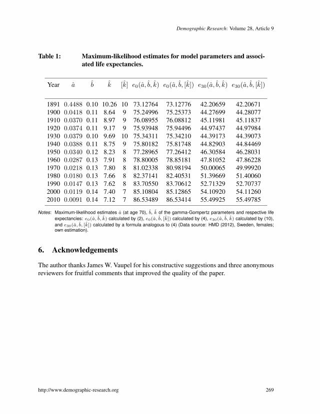
Table 1: Maximum-likelihood estimates for model parameters and associ-ated life expectancies.

Year a b k [k] e0(a, b, k) e0(a, b, [k]) e30(a, b, k) e30(a, b, [k])

1891 0.4488 0.10 10.26 10 73.12764 73.12776 42.20659 42.206711900 0.0418 0.11 8.64 9 75.24996 75.25373 44.27699 44.280771910 0.0370 0.11 8.97 9 76.08955 76.08812 45.11981 45.118371920 0.0374 0.11 9.17 9 75.93948 75.94496 44.97437 44.979841930 0.0379 0.10 9.69 10 75.34311 75.34210 44.39173 44.390731940 0.0388 0.11 8.75 9 75.80182 75.81748 44.82903 44.844691950 0.0340 0.12 8.23 8 77.28965 77.26412 46.30584 46.280311960 0.0287 0.13 7.91 8 78.80005 78.85181 47.81052 47.862281970 0.0218 0.13 7.80 8 81.02338 80.98194 50.00065 49.999201980 0.0180 0.13 7.66 8 82.37141 82.40531 51.39669 51.400601990 0.0147 0.13 7.62 8 83.70550 83.70612 52.71329 52.707372000 0.0119 0.14 7.40 7 85.10804 85.12865 54.10920 54.112602010 0.0091 0.14 7.12 7 86.53489 86.53414 55.49925 55.49785

Notes: Maximum-likelihood estimates a (at age 70), b, k of the gamma-Gompertz parameters and respective lifeexpectancies: e0(a, b, k) calculated by (2), e0(a, b, [k]) calculated by (4), e30(a, b, k) calculated by (10),and e30(a, b, [k]) calculated by a formula analogous to (4) (Data source: HMD (2012), Sweden, females;own estimation).

6. Acknowledgements

The author thanks James W. Vaupel for his constructive suggestions and three anonymousreviewers for fruitful comments that improved the quality of the paper.



References

Abramowitz, M. and Stegun, I. (1965). Handbook of Mathematical Functions. Washing-ton, DC: US Government Printing Office.

Bailey, W.N. (1935). Generalised Hypergeometric Series. Cambridge: University Press.

Beard, R.E. (1959). Note on some mathematical mortality models. In: Woolstenholme,G. and O’Connor, M. (eds.). The Lifespan of Animals. Little, Brown and Company:302–311.

Finkelstein, M.S. and Esaulova, V. (2006). Asymptotic behavior of a generalclass of mixture failure rates. Advances in Applied Probability 38(1): 244–262.doi:10.1239/aap/1143936149.

HMD (2012). The human mortality database. [electronic resource]. URL:http://www.mortality.org.

Keyfitz, N. and Caswell, H. (2005). Applied Mathematical Demography. New York:Springer, 3rd ed.

Lebedev, N.N. (1965). Special Functions and Their Applications. Englewood Cliffs, N.J.:Prentice-Hall.

MathWorld (2012). Wolfram mathworld. [electronic resource]. URL:http://mathworld.wolfram.org.

Vaupel, J.W. (2008). Supercentenarians and the theory of heterogeneity. [unpublishedmanuscript]. Rostock: Max Planck Institute for Demographic Research. JohannSüßmilch Lecture Series in 2008/2009.

Vaupel, J.W., Manton, K.G., and Stallard, E. (1979). The impact of heterogeneityin individual frailty on the dynamics of mortality. Demography 16(3): 439–454.doi:10.2307/2061224.


http://dx.doi.org/10.1239/aap/1143936149

http://dx.doi.org/10.2307/2061224

gamma-gompertz life expectancy at birth · demographic research: volume 28, article 9 formal...

Documents