gao-04-802 federal-aid highways: trends, effect … 2004 federal-aid highways trends, effect on...

GAOUnited States Government Accountability Office

Report to the Ranking Minority Member Subcommittee on Transportation and Infrastructure, Committee on Environment and Public Works, U.S. Senate

August 2004 FEDERAL-AID HIGHWAYS

Trends, Effect on State Spending, and Options for Future Program Design

a
GAO-04-802

www.gao.gov/cgi-bin/getrpt?GAO-04-802. To view the full product, including the scope and methodology, click on the link above. For more information, contact JayEtta Hecker at (202) 512-2834 or [email protected].

Highlights of GAO-04-802, a report to the Ranking Minority Member, Subcommittee on Transportation and Infrastructure, Committee on Environment and Public Works, U.S. Senate

August 2004

FEDERAL-AID HIGHWAYS

Trends, Effect on State Spending, and Options for Future Program Design

In 2004, both houses of Congress approved separate legislation to reauthorize the federal-aid highway program to help meet the Nation’s surface transportation needs, enhance mobility, and promote economic growth. Both bills also recognized that the Nation faces significant transportation challenges in the future, and each established a National Commission to assess future revenue sources for the Highway Trust Fund and to consider the roles of the various levels of government and the private sector in meeting future surface transportation financing needs.

This report (1) updates information on trends in federal, state, and local capital investment in highways; (2) assesses the influence that federal-aid highway grants have had on state and local highway spending; (3) discusses the implications of these trends for the federal-aid highway program; and (4) discusses options for the federal-aid highway program.

Congress may wish to consider expanding the mandate of the proposed National Commission to consider options to redesign the federal-aid highway program in light of these issues. DOT officials commented on a draft of this report and said that the report raised important issues that merit further study.

The Nation’s investment in its highway system has doubled in the last 20 years, as state and local investment outstripped federal investment—both in terms of the amount of and growth in spending. In 2002, states and localities contributed 54 percent of the Nation’s capital investment in highways, while federal funds accounted for 46 percent. However, as state and local governments faced fiscal pressures and an economic downturn, their investment from 1998 through 2002 decreased by 4 percent in real terms, while the federal investment increased by 40 percent in real terms. Evidence suggests that increased federal highway grants influence states andlocalities to substitute federal funds for funds they otherwise would have spent on highways. Our model, which expanded on other recent models, estimated that states used roughly half of the increases in federal highway grants since 1982 to substitute for state and local highway funding, and that the rate of substitution increased during the 1990s. Therefore, while state and local highway spending increased over time, it did not increase as much as it would have had states not withdrawn some of their own highway funds. These results are consistent with our earlier work and with other evidence. For example, the federal-aid highway program creates the opportunity for substitution because states typically spend substantially more than the amount required to meet federal matching requirements—usually 20 percent. Thus, states can reduce their own highway spending and still obtain increased federal funds. These trends imply that substitution may be limiting the effectiveness of strategies Congress has put into place to meet the federal-aid highway program’s goals. For example, one strategy has been to significantly increase the federal investment and ensure that funds collected for highways are used for that purpose. However, federal increases have not translated into commensurate increases in the nation’s overall investment in highways, in part because while Congress can dedicate federal funds for highways, it cannot prevent state highway funds from being used for other purposes. GAO identified several options for the future design and structure of the federal-aid highway program that could be considered in light of these issues. For example, increasing the required state match, rewarding states that increase their spending, or requiring states to maintain levels of investment over time could all help reduce substitution. On the other hand, the ability of states to meet a variety of needs and fiscal pressures might be better accomplished by providing states with funds through a more flexible federal program—this could also reduce administrative expenses associated with the federal-aid highway program. While some of these options are mutually exclusive, others could be enacted in concert with each other. The commission separately approved by both houses of Congress in 2004 may be an appropriate vehicle to examine these options.

http://www.gao.gov/cgi-bin/getrpt?GAO-04-802


Contents

Letter 1Results in Brief 3Background 7States and Localities Invest More in Highways Than the Federal

Government; However, Recent Federal Investment Has Outpaced State and Local Investment 16

Evidence Suggests Federal Highway Grants Have Increasingly Been Used to Substitute for Rather Than Supplement Spending from States’ Own Resources 21

Substitution May Be Limiting the Effectiveness of Strategies to Accomplish the Federal-Aid Highway Program’s Overall Goals 32

We Identified Several Options for the Design and Structure of the Federal-Aid Highway Program 40

Conclusions 46Matter for Congressional Consideration 47Agency Comments and Our Evaluation 47

AppendixesAppendix I: Objectives, Scope, and Methodology 50

Appendix II: Description of Grant Substitution Model, Statistical

Methods, and Results 53Summary of Previous Studies 53Description of GAO’s Statistical Model 62Statistical Results 72

Appendix III: State Characteristics Associated with States’ Level of Effort

to Fund Highways from State Resources 87

Appendix IV: Program Options Designed to Reduce Substitution 89

Appendix V: GAO Contacts and Staff Acknowledgments 94GAO Contacts 94Staff Acknowledgments 94

Tables Table 1: Federal-Aid Highway Program Grant Programs and Formulas 9

Table 2: Range of Estimates of Highway Substitution Rates by Time Period Based on a 95 Percent Confidence Level 24

Table 3: Options to Reduce Substitution 41Table 4: Summary of Fiscal Substitution Studies 56

Page i GAO-04-802 Federal-Aid Highways

Contents

Table 5: Highway Grant Substitution Rates Reported in Fiscal Substitution Studies 60

Table 6: Variables Considered in the Second Stage State Highway Expenditure Equation 63

Table 7: Variables Used to Explain the Distribution of Federal Highway Grants 67

Table 8: Descriptive Statistics 70Table 9: Instrumental Variables Estimator of Federal Grants per

Capita 73Table 10: Instrumental Variables Estimates of State Highway

Spending Model, Without Correcting for Autocorrelation 75

Table 11: Instrumental Variables Estimates of State Highway Spending Model, Correcting for Autocorrelation 77

Table 12: Summary Results of the Statistical Testing of the Variable Coefficients 79

Table 13: State Highway Spending Model with Statistically Insignificant Variables Removed 81

Table 14: State Highway Spending Model with Substitution Rates by Time Period 83

Table 15: Statistical Tests for the Endogeneity of Federal Grants and State Highway Spending 85

Table 16: Stepwise Regression Analysis of the Fixed Effects 86

Figures Figure 1: Illustrative Effects of $1 Increase in Federal Highway Grant 15

Figure 2: Federal and State and Local Highway Capital Expenditures, 1982 through 2002 (2001 dollars) 17

Figure 3: Amount of Yearly Capital Expenditures, 1998 through 2002 (2001 dollars) 19

Figure 4: Federal and State and Local Highway Capital Investment, 1991 through 2002 (2001 dollars) 20

Figure 5: Rates of Fiscal Substitution into Nonhighway Uses by Time Period 23

Figure 6: Summary of Federal Grant Substitution Rates Reported in Various Studies Using Data from Various Time Periods 28

Figure 7: State and Local Highway Spending for Capital Projects as a Percent of Total (Federal Plus State and Local) Capital Spending (1997 through 2000) 31

Figure 8: Federal Obligations by System in Fiscal Year 2001 37

Page ii GAO-04-802 Federal-Aid Highways

Contents

Figure 9: DOT Performance Measures for Condition and System Performance 39

Abbreviations

DOT Department of TransportationBEA Bureau of Economic AnalysisFHWA Federal Highway AdministrationGPRA Government Performance and Results ActISTEA Intermodal Surface Transportation Efficiency Act MOE Maintenance of EffortNHTSA National Highway Traffic Safety AdministrationTEA-21 Transportation Equity Act for the 21st Century

This is a work of the U.S. government and is not subject to copyright protection in the United States. It may be reproduced and distributed in its entirety without further permission from GAO. However, because this work may contain copyrighted images or other material, permission from the copyright holder may be necessary if you wish to reproduce this material separately.

Page iii GAO-04-802 Federal-Aid Highways

United States Government Accountability Office Washington, D.C. 20548

A

August 31, 2004 Letter

The Honorable Harry Reid Ranking Minority Member Subcommittee on Transportation and Infrastructure Committee on Environment and Public Works United States Senate

Dear Senator Reid:

In 2004, both houses of Congress approved separate legislation to reauthorize the federal-aid highway program to help meet the Nation’s surface transportation needs, enhance mobility, and promote economic growth. Each bill also recognized that the Nation faces significant transportation challenges in the future. Many transportation experts have noted that eventually, the introduction of more fuel-efficient vehicles and clean fuels may undermine the sustainability of financing the Nation’s surface transportation program through motor fuel taxes. As such, both bills established a National Commission to assess future revenue sources for the Highway Trust Fund and to consider the roles of the various levels of government and the private sector in meeting future surface transportation financing needs. In the longer term, broader fiscal challenges face the Nation, including federal and state budget deficits and the fiscal crisis looming as the baby boomer generation retires, causing mandatory commitments to Social Security and Medicare to consume a greater share of the Nation’s resources, squeezing funding available for all domestic discretionary programs. These challenges require the Nation to think critically about existing government programs and commitments.

In light of these issues, you asked us to provide information on past trends in the federal, state, and local capital investment in highways, and on how federal-aid highway program grants influence the level of state and local highway spending. We responded to the first part of your request in June 2003.1 This report (1) updates information on trends in federal, state, and local capital investment in highways; (2) assesses the influence that federal-aid highway grants have had on state and local highway spending; (3) discusses the implications of these trends for the federal-aid highway program; and (4) discusses options for the structure and design of the

1GAO, Trends in Federal and State Capital Investment in Highways, GAO-03-744R (Washington, D.C.: June 18, 2003).

Page 1 GAO-04-802 Federal-Aid HighwaysPage 1 GAO-04-802 Federal-Aid Highways

http://www.gao.gov/cgi-bin/getrpt?GAO-03-744R

federal-aid highway program that could be considered in light of these issues. In addition, this report identifies characteristics associated with differences among states’ levels of effort for highway investment (see app. III).

To respond to your request, we reviewed data from the Department of Transportation’s (DOT) Federal Highway Administration (FHWA), the Bureau of the Census, and other sources for the period from 1982 through 2002. We determined that the data were sufficiently reliable for the purposes of our analyses. We also reviewed and synthesized the research literature on the influence that federal highway grants have had on the level of state and local highway spending. Our literature review revealed a number of studies that used statistical models developed by the studies’ authors to estimate the influence of federal funding on state spending choices. These models examined different time periods, employed different statistical methods, and considered different social, demographic, economic, and political factors that may affect state highway spending decisions. None of the models used in the studies we reviewed included the most recent data now available on highway funding, and none examined whether the effect of federal grants on state spending changed over the time period covered in the study. Therefore, based on the models used in the earlier studies, we developed a statistical model of state highway spending outcomes to estimate the fiscal effects of federal highway funding on state highway spending choices. This model included the most recent data available and examined whether the effect of federal grants on state spending changed over the time period covered by our data. The purpose of the statistical model was to isolate the effect that federal grants have on state highway spending by controlling for other factors that also affect state spending decisions. The model therefore takes into account changing state economic conditions, the size and intensity of highway usage, and other factors that may be associated with states’ willingness to support highway spending. This statistical model was reviewed by experts in DOT and peer reviewed by three authors of the earlier studies on the fiscal effects of federal highway grants. These experts and authors generally agreed with our methods, and we made revisions based on their comments as appropriate. A more detailed description of the literature and the statistical model is contained in appendix II. We conducted our work from August 2003 through July 2004 in accordance with generally accepted government auditing standards.

Page 2 GAO-04-802 Federal-Aid Highways

Results in Brief The Nation’s capital investment in its highway system has doubled in the last 20 years, and during that time period as a whole, state and local investment in highways outstripped federal investment in highways—both in terms of the amount of and growth in spending. Between 1982 and 2002, state and local capital investment in highways increased 150 percent, from $14.1 billion to $35.7 billion in real terms, whereas the federal investment increased 98 percent, from $15.5 billion to $30.7 billion in real terms.2 For every year after 1986, states and localities invested more in the Nation’s highways than did the federal government. Most recently, in 2002, states and localities contributed 54 percent of the Nation’s capital investment in highways, spending $35.7 billion, while the federal government contributed 46 percent, or $30.7 billion. However, since the early 1990s, state and local investment in highways has increased at a slower rate than federal investment in highways. From 1991, when the Intermodal Surface Transportation Efficiency Act (ISTEA) was enacted, through 2002, state and local investment increased 23 percent, from $29.0 to $35.7 billion in real terms. During that same time period, federal investment increased 47 percent, from $20.9 to $30.7 billion in real terms. In the period following the enactment of the Transportation Equity Act for the 21st Century (TEA-21), from 1998 through 2002, during which state and local governments faced fiscal pressures and an economic downturn, the trend intensified, with state and local investment decreasing by 4 percent—from $37.0 to $35.7 billion in real terms—and federal investment increasing by 40 percent—from $21.9 to $30.7 billion in real terms.

The preponderance of evidence suggests that federal-aid highway grants have influenced state and local governments to substitute federal funds for state and local funds that otherwise would have been spent on highways. Therefore, according to our model—which refined and expanded on other recent models and controlled for the effects of other factors—and according to other studies, when federal highway grants increased, total highway spending did not increase as much as it would have had states not withdrawn some of their own highway-related funds. Specifically, our model examined how federal highway spending affected state spending, and it estimated that state and local governments have used roughly half of the increases in federal highway grants since 1982 to substitute for funding they would otherwise have spent from their own resources. In addition, our

2Dollar amounts in this report are adjusted to 2001 dollars, matching adjustments made in the earlier related report GAO-03-744R.


http://www.gao.gov/cgi-bin/getrpt?GAO-03-447R.

model estimated that the rate of grant substitution increased significantly over the past two decades, rising from about 18 cents on the dollar during the early 1980s to roughly 60 cents on the dollar during the 1990s, when ISTEA and TEA-21 were in effect.3 Three previous studies of this issue all found that substitution occurred, although their estimates of levels of substitution varied, probably due to differences in time periods studied, definitions of substitution, and statistical methods employed. There are a number of reasons why substitution may occur. Our earlier work found that in general, the federal grant system as a whole does not encourage states to use federal dollars as a supplement rather than a substitute for their own spending.4 Specifically, the structure of the federal-aid highway program creates an opportunity for substitution because states typically spend substantially more in state and local funds than is required to meet current federal matching requirements. As a consequence, when federal funding increases, states are able to reduce their own highway spending and yet obtain the increased federal funds. If states substitute some of the increase in federal funds for their own funds, then total highway spending may increase, but not by as much as it would have had substitution not occurred.

These trends imply that substitution may be limiting the effectiveness of the strategies Congress has put into place to meet the federal-aid highway program’s overall goals. Congress and DOT have at various times enumerated goals for the federal-aid highway program, including, among other things, enhancing safety, promoting economic growth, enhancing mobility, supporting interstate and international commerce, and meeting national security needs. To meet these goals, Congress has put in place strategies that include significantly increasing the federal investment in the highway system—particularly since 1991—and ensuring that funds collected by the federal government for highways are used for that purpose. However, due to probable substitution, the sizable increases in

3While these estimates represent our most likely estimates of the substitution that occurred, they are only estimates. The uncertainty surrounding our estimates can be expressed in terms of a level of confidence that a given range of values encompasses the actual substitution rate. This is discussed later in this report. For example, the estimate of an 18 percent substitution rate for the early 1980s is not statistically different from a finding of no substitution. Regarding our estimate of 60 cents on the dollar during the 1990s, the actual substitution rate, with a 95 percent level of confidence, may be as high as 96 percent or as low as 21 percent.

4GAO, Federal Grants: Design Improvements Could Help Federal Resources Go Further (GAO/AIMD-97-7), December 18, 1996.


http://www.gao.gov/cgi-bin/getrpt?GAO/AIMD-97-7

dedicated federal funding that Congress has provided for highways since 1991 have not translated into commensurate increases in the Nation’s overall investment in its highway system. In part this is because, while Congress can dedicate federal funds for highways, it cannot prevent state highway funds from being used for other purposes. Furthermore, Congress has sought to meet the goals of the program through a strategy of emphasizing states’ priorities and decision-making. Specifically, Congress has incorporated return-to-origin features into the highway program and returned to each state more of the fuel and other taxes collected in that state, and has given states wide latitude in deciding how to use and administer federal grants to best meet their transportation needs. However, substitution may be limiting the effectiveness of this strategy. Although the federal-aid highway program has a considerable regulatory component that requires states to follow and enact certain laws as a condition of receiving federal funds, from a funding standpoint, the program’s return-to-origin features and flexibility, combined with substitution and the use of state and local highway funds for other purposes, means that the federal-aid highway program is to some extent functioning as a cash transfer, general purpose grant program. This raises broader questions about the effectiveness of the federal investment in highways in accomplishing the program’s goals and outcomes. While under the Government Performance and Results Accountability Act (GPRA), DOT has established performance measures and outcomes for the federal-aid highway program to enhance mobility and economic growth, the program’s current structure does not link funding with performance or the accomplishment of these goals and outcomes.

We identified several options for the design and structure of the federal-aid highway program that could be considered in light of these issues. These options include program designs that have been used for other federal programs and which could reduce substitution. For example, increasing the required state match on federal highway projects, rewarding states that increase their highway spending effort, or requiring states to maintain levels of highway investment over time to receive federal funds could all reduce substitution. On the other hand, the ability of states to meet a variety of needs and fiscal pressures might be better accomplished by providing states with funds through a more flexible federal program. Adopting such an option could be seen as recognizing substitution as an appropriate response on the part of states to increasing fiscal challenges and competing demands. It could also reduce the level of administrative involvement needed and thereby reduce administrative expenses associated with the federal-aid highway program. Finally, policy makers may wish to consider the design of the federal-aid highway program in the


broader context of aligning the program with program-related goals, possibly taking into account performance measures and results. While some of these options are mutually exclusive, others could be enacted in concert with each other. For instance, requiring states to maintain levels of highway investment over time or other options to limit substitution could be combined with an effort to align funding with the accomplishment of performance measures. Similarly, aligning funding with the accomplishment of performance measures could also be carried out in conjunction with creating a more flexible federal program.

The proposed National Commission to assess future revenue sources to support the Highway Trust Fund may be an appropriate vehicle through which to examine these options. This commission is to consider how the program is financed and the roles of the federal and state governments and other stakeholders in financing it; the appropriate program structure and mechanisms for delivering that funding are important components of making these decisions. Therefore, in light of the issues raised in this report and the fiscal challenges the Nation faces in the 21st Century, Congress may wish to consider expanding the mandate of the National Commission to assess possible changes to the federal-aid highway program to maximize the effectiveness of federal funding and promote national goals and strategies. Consideration could be given to the program’s design, structure, and funding formulas; the roles of the various levels of government; and the inclusion of greater performance and outcome oriented features.

We provided a draft of this report to DOT for review and obtained comments from departmental officials, including FHWA’s Director of Legislation and Strategic Planning. These officials said that our analysis raised interesting and important issues regarding state funding flexibility and the federal-aid highway program that merit further study. We agree with DOT’s characterization of the importance of the issues raised in this report, and we continue to believe that Congress has the opportunity to maximize the effectiveness of federal funding and promote national goals and strategies by expanding the proposed mandate of the National Commission. DOT also provided some technical comments, which we incorporated where appropriate.


Background Federal funding for highways is provided to the states mostly through a series of formula grant programs collectively known as the federal-aid highway program.5 Periodically Congress enacts multiyear legislation that authorizes the Nation’s surface transportation programs, including highway, transit, highway safety, and motor carrier programs. This legislation authorizes the federal-aid highway program and the individual grant programs that comprise it, and it sets overall funding for it and other surface transportation programs. In 1991, for example, Congress enacted ISTEA, which authorized $121 billion for highways for the 6-year period from fiscal years 1992 through 1997, and in 1998 Congress enacted TEA-21, which authorized $171 billion for the federal-aid highway program from fiscal years 1998 through 2003. In 2004, the House and Senate each approved separate legislation to reauthorize the federal-aid highway program, the House authorizing $226.3 billion and the Senate authorizing $256.4 billion for fiscal years 2004 through 2009. These authorizations provide multiyear “contract authority” that gives the states notice several years in advance of the size of the federal-aid program and the approximate amount of federal funding they may expect to receive.

Funding for the federal-aid highway program is provided through the Highway Trust Fund. Established by the Highway Revenue Act of 1956, the Highway Trust Fund is a dedicated source of revenues generated by highway user fees such as taxes on motor fuels, tires, and trucks. TEA-21 established two additional mechanisms to support the dedication of highway user fees to highways. First, the act established guaranteed funding for certain highway, transit, and highway safety programs, including the federal-aid highway program, by protecting them with “firewalls” from competing for funding with other domestic discretionary programs through the congressional budget process. Second, the act provided that the highway program funding authorizations would be adjusted to reflect changes in estimates of Highway Trust Fund revenue, ensuring that funding available for the federal-aid highway program reflected the revenue taken in by the Highway Trust Fund. Both the Senate and the House have each approved separate legislation to extend the collection of fuel taxes to the Highway Trust Fund, the Senate through 2009 and the House through 2011. Amid concerns that the introduction of more

5The federal-aid highway program also includes discretionary grants and research and development programs. While grants are provided to states, localities may also sponsor federal-aid projects and can receive some federal funds, primarily through their state.


fuel-efficient vehicles and clean fuels may undermine the sustainability of financing the Highway Trust Fund through fuel taxes in the future, both houses also included provisions to create a National Commission to examine future revenue sources to support the Highway Trust Fund and to consider, among other things, the roles of the various levels of government and the private sector in meeting future surface transportation financing needs.

Once Congress authorizes funding, FHWA makes federal funding available to the states annually at the start of each fiscal year through apportionments based on formulas specified in law for each of the several formula grant programs that make up the federal-aid highway program. Ninety-two percent of the funds apportioned to the states in fiscal year 2003 were apportioned by formula. The remaining highway program funds were distributed through allocations to states with qualifying projects. The highway programs with apportionments based on formulas are shown in table 1.


Table 1: Federal-Aid Highway Program Grant Programs and Formulas

Program PurposeFY 2003 funding

(in billions)a Grant formula Minimum apportionment

Interstate Maintenance Program

Resurfacing, restoring, rehabilitating, and reconstructing most routes on the Interstate Highway System.

$4.2 Interstate System lane miles (33 1/3%)

Vehicle miles traveled on the Interstate System (33 1/3%)

Annual contributions to the Highway Account of the Highway Trust Fund attributable to commercial vehicles (33 1/3%)

½ percent of Interstate Maintenance and National Highway System apportionments combined

National Highway System Program

Improvements to rural and urban routes that are part of the National Highway System (including the Interstate System) and designated connections to major intermodal terminals.

$5.1 Lane miles on principal arterial routes, excluding the Interstate System (25%)

Vehicle miles traveled on principal arterial routes, excluding the Interstate System (35%)

Diesel fuel used on highways (30%)

Total lane miles on principal arterial highways divided by the State’s total population (10%)

½ percent of Interstate Maintenance and National Highway System apportionments combined

Surface Transportation Program

Projects on any federal-aid highway, bridge projects on any public road, transit capital projects, intracity and intercity bus terminals and facilities, and other uses.

$5.9 Total lane miles of federal-aid highways (25%)

Total vehicle miles traveled on federal-aid highways (40%)

Estimated tax payments attributable to highway users paid into the Highway Account of the Highway Trust Fund (35%)

½ percent

Highway Bridge Replacement and Rehabilitation Program

Replacing or rehabilitating deficient highway bridges and seismic retrofits for bridges on public roads.

$3.6 Relative share of total cost to repair or replace deficient highway bridges (100%)

¼ percent (10 percent maximum)


Source: FHWA.

aReflects amounts apportioned by formula before the distribution of Minimum Guarantee Program funding among the core programs.bIncludes funds for the Appalachian Development Highway System and Recreational Trails Programs.

As we reported in 1995, the federal funding formula derives from a complicated set of calculations and is a complex process in which the underlying data and factors are ultimately not meaningful because they are overridden by other provisions that yield a predetermined outcome.6 One reason is the presence of “equity provisions” that ensure that states receive set amounts based on historic funding levels and other considerations. These equity provisions were strengthened after our 1995 report. For example, as table 1 shows, TEA-21’s Minimum Guarantee Program ensures that each state’s share of apportionments from nearly all federal-aid highway funds is not less than 90.5 percent of that state’s percentage share

Congestion Mitigation and Air Quality Improvement Program

Projects which reduce transportation related emissions in air quality nonattainment and maintenance areas for ozone, carbon monoxide, and particulate matter.

$1.4 Weighted population in nonattainment and maintenance areas (100%)

½ percent

Minimum Guarantee Program

Funding to states based on equity considerations including specific shares of overall program funds and minimum return on contributions to the highway account of the Highway Trust Fund. A portion of the funds are distributed among core highway programs while remaining funds are eligible under the same rules as the Surface Transportation Program.

$6.4 90.5 percent of the percentage share of contributions to the Highway Account of the Highway Trust Fund from motor fuel and other taxes collected in that state based on latest available data

N/A

Other b $0.5

(Continued From Previous Page)

Program PurposeFY 2003 funding

(in billions)a Grant formula Minimum apportionment

6GAO, Highway Funding: Alternatives for Distributing Federal Funds (GAO/RCED-96-6) Nov. 28, 1995.


http://www.gao.gov/cgi-bin/getrpt?GAO/RCED-96-6

of contributions to the Highway Account of the Highway Trust Fund.7 Funds from this program accounted for nearly a quarter of all highway funding in fiscal year 2003. Under separate legislation approved by both the House and the Senate, each state’s share of apportionments could rise to 95 percent by 2009.8 Furthermore, as table 1 shows, states receive minimum apportionments regardless of the formula for several grant programs.

States have broad flexibility to transfer funds between the various grant programs. For example, states may transfer up to 50 percent of their Interstate Maintenance and National Highway System Program funds to other programs, including the Surface Transportation Program, which, as table 1 shows, has broad eligibility rules. In addition, ISTEA and TEA-21 provided the states broad authority to transfer federal-aid highway funds to transit projects and vice versa. Between fiscal years 1992 and 2002, 47 states and the District of Columbia transferred about $8.8 billion from federal-aid highway funds to transit programs to fund rail line improvements, motor vehicle purchases, new or improved passenger facilities, and other projects. During that same time, about $40 million was transferred from FTA to FHWA for highway projects.

Once FHWA apportions funds to the states, funds are available to be obligated by the states for construction, reconstruction, and improvement of highways and bridges on eligible federal-aid highway routes and for other purposes authorized in law. About 1 million of the Nation’s 4 million miles of roads are eligible for federal aid; however, these roads accounted for 85 percent of the vehicle miles traveled on the Nation’s roadways in 2001. The roads that are generally ineligible are functionally classified as local roads or minor collectors. Around 161,000 miles of federally eligible roadways are on the National Highway System, of which around 47,000 belong to the Interstate Highway System. With few exceptions, federal funds for highways must be matched by funds from other sources—usually state and local governments. The matching requirement on most projects is

7According to FHWA, although never legally described and named as such, the portion of the Highway Trust Fund that is not specifically credited by law to the Mass Transit Account of the Highway Trust Fund has come to be called the “Highway Account” and receives all Trust Fund receipts not specifically designated for the Mass Transit Account.

8The Senate approved the 95 percent amount while the House bill contained a “reopener” provision that would delay fiscal year 2006 funding for most federal-aid highway programs from October 2005 until August 2006 if Congress has not enacted legislation by September 30, 2005, raising each states’ guaranteed rates of return to 95 percent, effective in fiscal year 2009.


80 percent federal and 20 percent state or local funding. In addition to matching federal funds, states and localities spend funds to finance highway capital projects and to maintain existing roadways.

The federal-aid highway program is administered by FHWA, whose responsibilities include reviewing periodic transportation improvement plans prepared by state and local governments, approving projects for federal aid, apportioning grant funding to the states, providing technical support, and overseeing federally funded projects. In fiscal year 2004, FHWA received $334 million to provide these services, with an authorized staff level of 2,931 positions. FHWA personnel are located in Washington, D.C., and in 52 field offices located in each state, the District of Columbia, and Puerto Rico, as well as a regional “resource center” with four offices across the country that provide specialized technical assistance to the field offices and the states.

The federal-aid highway program has a considerable regulatory component. As a condition of receiving federal aid, states agree to apply and enforce certain federal laws on federally aided projects, such as the environmental assessment provisions in the National Environmental Policy Act, the Americans With Disabilities Act, the nondiscrimination protections found in the Civil Rights Act of 1964, and others. In addition, states are required to establish goals and to award a set percentage of contracts (the national goal is 10 percent) on federally aided projects to small businesses owned and controlled by socially and economically disadvantaged individuals, including minority and women-owned businesses. Furthermore, in accepting federal-aid highway funds, states must enact certain laws to improve highway safety or face penalties in the form of either withholdings or transfers in their federal grants.9 In addition to these penalties, states may apply for and receive highway safety incentive grants through programs administered outside the federal-aid highway program by the National Highway Traffic Safety Administration (NHTSA). For example, states in which the use of seat belts exceeds the national average or improves over time are eligible for incentive grants based on NHTSA’s

9Under TEA-21, states are subject to withholdings or transfers in their federal grants if they fail to enact laws that (1) prohibit open alcoholic beverage containers in the passenger area of a motor vehicle, (2) establish minimum penalties for repeat drunk-driving offenders, and (3) establish laws making it illegal for people to drive with the specified level of alcohol in their blood of .08 blood alcohol concentration—the level at which a person’s blood contains 2/25th of 1 percent alcohol.


calculation of the annual savings to the federal government in medical costs that resulted from the increased use.

In general, there are three possible ways that federal grant funding can influence state spending for a program, as illustrated in figure 1. First, increased federal funding may stimulate, or leverage, additional spending from state resources. For example, a state may have to increase its own spending in order to meet federal matching requirements and obtain federal funds, thus increasing the overall level of spending by more than the amount of the federal grant.10 As the federal-aid highway program in most cases requires that states must contribute 20 percent of the total cost of a project in order to receive federal matching funds of 80 percent of the total cost, the suggestion is that every $1.00 increase in federal funds would go towards a total spending increase of $1.25 ($1.00 is 80 percent of $1.25), $0.25 of which would be funded with state and local government funds ($0.25 is 20 percent of $1.25). The result of a stimulative effect of federal grant funding is illustrated in the first panel of figure 1, in which an additional $1.00 of federal aid increases spending from state resources by 25 cents, increasing the overall level of highway spending by $1.25. Alternatively, increased federal funding may supplement state spending by adding to what states would otherwise have spent, increasing the overall level of spending by the amount of the federal grant, as illustrated in the second panel of figure 1. To the extent that states maintain their own spending when they receive additional federal funding, either because federal policy requires that they do so or because they do so voluntarily, then the additional federal aid supplements state spending. Finally, states may use increased federal funding to substitute for, or replace, what they would otherwise have spent from state resources, so that the overall level of spending increases by less than the amount of the federal grant. This substitution of federal funds for state funds is illustrated in the third panel of figure 1, in which an additional $1.00 in federal funding results in only a 50 cent increase to total spending because in response to the influx of

10With matching requirements, states must contribute their own funds in order to receive federal matching funds. Economic theory suggests that grants requiring matching, by lowering the effective price of aided programs relative to other state spending priorities, encourage states to spend more of their own funds. Matching grants typically contain either a single rate (e.g., 50 percent) or a range of rates (e.g., 50 percent to 80 percent) at which the federal government will match state spending on an aided program.


federal funds, the state withdraws 50 cents of its own spending on the program and uses these funds for other purposes.11

11Although the fiscal effect of grants has been described in the text only in terms of an increase in federal grant funding, stimulation and substitution may also occur when federal funding is declining. If in response to a decline in federal aid, for example, states increase spending from state resources to compensate for the loss in federal funding, this too represents grant substitution, the substitution of state funds for federal funding.


Figure 1: Illustrative Effects of $1 Increase in Federal Highway Grant

State highway spending

Stimulative Effect: Total Highway Spending Increases by $1.25

Before Grant After Grant

Before Grant After Grant

After Grant

$5.25

$5.00

$5.00

$0.50

$6.25

$0.25 $1.00

$1.00

$1.00

$6.00

$5.50

Federal grant

Supplemental Effect: Total Highway Spending Increases by $1.00

Substitutive Effect: Total Highway Spending Increases by $0.50

Source: GAO.

Statespending

Statespending

Statespending

Statespending

Federalspending

Statespending

Statespending

Federalspending

Federalspending

$5.00

$4.50

Before Grant

$5.00

Federal grant

Federal grant

Other public services or

state taxpayer

relief







States and Localities Invest More in Highways Than the Federal Government; However, Recent Federal Investment Has Outpaced State and Local Investment

The Nation’s capital investment in its highway system has doubled in the last 20 years, and during that time period as a whole, state and local investment in highways outstripped federal investment in highways—both in terms of the amount of and growth in spending. Between 1982 and 2002, state and local capital investment in highways increased 150 percent, from $14.1 billion to $35.7 billion in real terms, whereas the federal investment increased 98 percent, from $15.5 billion to $30.7 billion in real terms.12 For every year after 1986, states and localities invested more in the Nation’s highways than did the federal government. (See fig. 2.) Most recently, in 2002, states and localities contributed 54 percent of the Nation’s capital investment in highways, spending $35.7 billion, while the federal government contributed 46 percent or $30.7 billion in real terms.

12To determine trends in real terms, we adjusted the data to 2001-year dollars to coincide with the data in our related report, GAO-03-744R, which presented data from 1982 through 2001. We converted these data using the Bureau of Economic Analysis’ (BEA) Price Indexes for Gross Government Fixed Investment—Highways and Streets.



Figure 2: Federal and State and Local Highway Capital Expenditures, 1982 through 2002 (2001 dollars)

In addition to the billions of dollars states and localities invest in capital highway projects to expand highway capacity or rehabilitate existing highways, states and localities spend additional funds maintaining and policing their roadways. For example, in 2001, states and localities spent about 27 percent of their total capital and maintenance funding on maintenance activities, including fixing potholes, sealing cracks in bridge decks, and fixing highway lighting.

Although states and localities still spend more on highway capital investment than the federal government, recently, state and local highway investment has increased at a slower pace than federal highway investment. In addition, state and local investment has decreased in real terms three times since 1996: between 1996 and 1997, between 1999 and 2000, and between 2001 and 2002. Last year, we reported that since TEA-21 was passed, from 1998 through 2001, federal investment increased faster

Dollars in billions (2001)

Source: GAO analysis of FHWA data.

Year

0

5

10

15

20

25

30

35

40

45

State and localFederal

200220012000199919981997199619951994199319921991199019891988198719861985198419831982


than state and local investment.13 In real terms, federal investment increased 29 percent, while state and local investment increased 2 percent.14 This trend of federal investment increasing more quickly than state and local investment continued in 2002. From 2001 through 2002, federal investment increased 8.5 percent, while state and local investment decreased 5 percent in real terms. Thus, from 1998 through 2002, federal investment increased 40 percent, while state and local investment decreased by 4 percent. Figure 3 shows the annual federal and state and local capital expenditures on highways during these years.

13The percent change from 1998 through 2001 is computed by comparing the investment in these 2 years. The calculation does not describe the variations in the intervening years.

14As we reported, federal investment did not follow this pattern from 1997 to 1998, despite the large increase in funding authorized by TEA-21. When comparing the change in funding from 1997 through 2001, federal investment increased 23 percent while state and local investment increased 16 percent. This lower level of increase in federal expenditures was likely due to the midyear passage of TEA-21 in June 1998 and the amount of time it takes states to spend capital project funds.


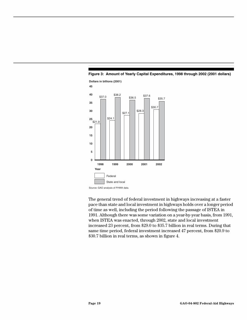
Figure 3: Amount of Yearly Capital Expenditures, 1998 through 2002 (2001 dollars)

The general trend of federal investment in highways increasing at a faster pace than state and local investment in highways holds over a longer period of time as well, including the period following the passage of ISTEA in 1991. Although there was some variation on a year-by-year basis, from 1991, when ISTEA was enacted, through 2002, state and local investment increased 23 percent, from $29.0 to $35.7 billion in real terms. During that same time period, federal investment increased 47 percent, from $20.9 to $30.7 billion in real terms, as shown in figure 4.

0

5

10

15

20

25

30

35

40

45

State and local

Federal

20022001200019991998


Year


$21.9

$37.0$38.2

$24.1

$36.5

$27.1$28.3

$37.6

$30.7

$35.7


Figure 4: Federal and State and Local Highway Capital Investment, 1991 through 2002 (2001 dollars)

Although the reasons for this change in spending patterns by level of government are unclear, tough economic times, with a majority of states needing to reduce spending to avoid budget deficits, along with large increases in federal funds for highways may have influenced these spending patterns. For example, a recent survey of states by the National Conference of State Legislatures found that even after the economy began growing after the March 2001 national recession, 36 states still have budget shortfalls with a cumulative gap of about $25.7 billion.15

15National Conference of State Legislatures, State Budget Update: February 2003.

0

5

10

15

20

25

30

35

40

45

State and localFederal

200220012000199919981997199619951994199319921991


Year



Evidence Suggests Federal Highway Grants Have Increasingly Been Used to Substitute for Rather Than Supplement Spending from States’ Own Resources

The preponderance of evidence suggests that increases in federal-aid highway grants influence state and local governments to substitute federal funds for funding they would have otherwise spent on highway projects from their own resources.16 We built on earlier studies to develop a model that analyzed data from 1982 through 2000 to examine whether and to what extent states have substituted increases in federal highway funds for state highway funds. Our preferred model analyzes data from 1983 through 2000 because of the statistical techniques we used.17 Our analysis suggests that significant substitution has occurred and that the rate of grant substitution increased significantly over the past two decades, rising from 18 percent in the early 1980s to about 60 percent during the 1990s—the periods that ISTEA and TEA-21 were in effect. Three previous studies of this issue also found that substitution existed, although their estimates of levels of substitution varied.18 The structure of the federal grant system as a whole may encourage substitution. Specifically, the structure of the federal-aid highway program creates an opportunity for substitution because states typically spend substantially more in state and local funds than is required to meet current federal matching requirements. As a consequence, when federal funding increases, states are able to reduce their own highway spending and yet obtain the increased federal funds. If states substitute some of the increase in federal funds for their own funds, then total highway spending may increase, but not by as much as it would have had substitution not occurred.

16Alternatively, our results suggest that during periods of declining federal aid, states may replace some of the decline in federal funding with additional funding from state resources.

17See appendix II for a description of the various statistical models we considered and the rationale for our selection of a preferred model.

18Shama Gamkhar, “The Role of Federal Budget and Trust Fund Institutions in Measuring the Effect of Federal Highway Grants on State and Local Government Highway Expenditure,” Public Budgeting and Finance, Spring 2003; Brian Knight, “Endogenous Federal Grants and Crowd-out of State Government Spending: Theory and Evidence from the Federal Highway Aid Program,” The American Economic Review, Vol. 92 No. 1, March 2002, pp. 71-92; and Harry Meyers, “Displacement Effects of Federal Highway Grants,” National Tax Journal, Vol. XL, No. 2, June 1987, pp. 221-235.


Our Statistical Model Suggests Federal Highway Funds Have Increasingly Been Substituted for State Funds That Were Shifted to Nonhighway Uses

Our statistical model, which we developed from previous models, estimates that states have used a significant portion of increases in federal highway funding to substitute for state and local funding for highways, and that the rate of substitution increased during the 1990s. According to our preferred model, for the entire period from 1983 through 2000, state governments used roughly half of the increases in federal highway grants to substitute for funding they would have otherwise spent from their own resources on highways.19 When our model examined four separate time periods from 1983 through 2000 that corresponded to the four authorization periods for the federal-aid highway program, the results suggest that the rate of grant substitution increased in the 1990s, during the periods in which ISTEA and TEA-21 were in effect, in comparison to the early 1980s.20 Specifically, our model suggests that states substituted approximately 18 cents (not statistically significant) of every dollar increase in federal aid from 1983 to 1986 for funds they would have spent on highways from their own resources. Our model suggests that the substitution rate rose to approximately 36 cents of every dollar increase in federal aid for the period from 1987 to 1991, and that the substitution rates then rose again to approximately 60 cents for every dollar increase in federal aid for the two periods examined in the 1990s: 1992 through 1997 and 1998 through 2000. (See fig. 5.)

19Our model and all the studies we examined used grant expenditures recorded by states as the measure of federal grants. Grant expenditures are recorded when the federal government reimburses states for eligible project expenses. One study, described later in the report, also used an alternative measure.

20Because grant allotments remain available for expenditures for up to 4 years, some of the grant expenditures for a given time period includes grant obligations from prior periods.


Figure 5: Rates of Fiscal Substitution into Nonhighway Uses by Time Period

The rates of grant substitution for the time periods reported in figure 5 are derived from our statistical model of state spending choices and are subject to some uncertainty. While these estimates represent our most likely estimates of the rate at which states substituted federal funds for state and local funds, the actual substitution may be larger or smaller than these estimates. The uncertainty surrounding our estimates can be expressed in terms of a level of confidence that a given range of values encompasses the actual substitution rate. The range of values surrounding each of our estimates is shown in table 2 at a 95 percent level of confidence. The size of each interval provides a sense of the uncertainty associated with our estimates. The intervals associated with the two time periods during the 1980s contain possible values of zero, meaning that we cannot be 95 percent confident that substitution occurred during these periods. In contrast, the range of estimates for both time periods in the 1990s does not encompass zero; therefore, they are statistically different from zero, which means that our results imply at least a 95 percent level of confidence that substitution occurred. Our most likely estimates for the two periods we looked at in the 1990s are in both cases just under 60 percent, and we can

0

10

20

30

40

50

60

70

80

90

100

1998

-200

0

1992

-199

7

1987

-199

1

1983

-198

6

Percentage

59 58

18

36

Time period

Source: GAO.


be 95 percent confident that the actual substitution rate was between 21 percent and 97 percent.

Table 2: Range of Estimates of Highway Substitution Rates by Time Period Based on a 95 Percent Confidence Levela

Source: GAO

aPositive values represent grant substitution and negative values indicate grant stimulation.

These results are roughly consistent with previous studies that, when taken together, also seem to suggest increasing substitution rates over time. We made four primary enhancements to the models used in previous studies in developing our model. First, we used more recent data on highway expenditures than were available for previous studies. Second, we used a conservative definition of substitution. Our model defined substitution as occurring only when, in response to increased federal highway funds, state and local funds were moved out of highway-related projects altogether. We did not consider it substitution if in response to increased federal highway funds, state and local funds were moved from highway projects that were eligible for federal aid to highway projects that were not eligible for federal aid. Third, our model is structured to examine substitution rates over time, rather than being limited to one estimate covering all the years included in our study. Finally, compared to previous studies, we employed a more comprehensive collection of factors related to state spending decisions.

Combined, we believe these enhancements increase the ability of our model to provide a conservative and more reliable estimate of the extent to which states substitute federal highway aid for spending that would otherwise have come from state and local resources. However, all estimates that are based on statistical models, particularly of complex processes such as the determination of states’ budget choices, are subject to uncertainty. This uncertainty can derive from both choices about what factors to include in a model and the inherent impreciseness in estimating relationships between one factor—in this case federal highway grants—

Time periodPoint estimate

(percent)Low estimate

(percent)High estimate

(percent)

1983-1986 18 -21 57

1987-1991 36 -2 74

1992-1997 59 22 97

1998-2000 58 21 95


and another, state and local highway spending. While we have attempted to take many factors affecting state spending decisions into account, there may be other factors that are not subject to precise measurement, such as the influence of citizen and interest groups on states’ funding decisions, that could not be included in our analysis. As a result of the uncertainty in both the data and the statistical formulation of our model, the precision of our estimate, or any other estimate, is limited and our estimate should be considered one point in a range within which the actual extent of substitution falls, and one piece of a body of evidence on the existence of substitution. (See app. II for additional details on our statistical model.)

In commenting on a draft of this report, DOT officials said that to the extent substitution occurred and increased during the 1990s, it was likely due to a number of factors, including changes in states’ revenues and priorities. While our analysis specifically took changing economic conditions into account when assessing state spending choices, determining specific causes is beyond the scope of our statistical model. For example, states faced rising demands for health care and education during the 1980s and early 1990s that they may have funded, in part, by reducing their own levels of highway funding effort when federal highway funding increased. Accordingly, our model establishes an association between substitution and increases in federal highway grants; it does not identify the specific causes responsible for these rising rates.

Earlier Studies Found That Federal Grants Reduced States’ Highway Spending, Although Substitution Estimates Varied

Three other studies, including two published in the past 3 years, have reported that states substituted additional federal highway spending for state spending. These studies reported a wide range of estimates for the percentage of federal funds that has been used as a substitute for state and local funds, from zero to nearly 100 percent. The wide range of estimates is the result of different time periods examined, different definitions of substitution, and differences in the statistical methods employed.21

A study by Brian Knight, which, of the three studies, included the most recent data, found that from 1983 through 1997, roughly 90 percent of

21Issues related to the differing statistical methods employed in previous studies are discussed in appendix II.


increased federal aid was substituted for state highway spending.22 Knight used a different definition of substitution than we used in our study. Knight defined substitution as occurring when, in response to increased federal highway funds, state funds were moved out of highway-related projects. He did not take into account local spending on highways, which might possibly have mitigated the reduction in state funds.

Another study, by Shama Gamkhar,23 analyzed data from 1976 through 1990 using two different measures of federal grants. Gamkhar reported an average substitution rate of 63 percent when measuring federal grants through grant expenditures (the same measure of federal grants used by the other studies, including our model) and an average substitution rate of 22 percent when measuring federal grants through grant obligations.24 Gamkhar defined substitution the same way our model did, as when, in response to increased federal highway funds, state and local funds were moved out of highway-related projects altogether.

22Knight, op. cit.

23Gamkhar, op. cit.

24The grant distribution process first allots federal funding to states. States then obligate these funds for eligible highway projects, and, finally, the federal government reimburses states at the time obligated balances are actually spent. Thus, obligations are the second step in the federal grant making process, and grant expenditures are the final step of the process.


A study by Harry G. Meyers examined data from 1976 through 1982, and modeled substitution based on two different definitions of substitution.25 Using a definition of substitution similar to the definition employed in our model, the study found no evidence of substitution during this period. Meyers also modeled the substitution rate based on a different definition of substitution, defining substitution as occurring when state funds were moved out of federal-aid highway projects, even if those funds were used for highway projects that were ineligible for federal aid. Using this definition of substitution, the study found a substitution rate of 63 percent. The findings of these studies and GAO’s results are summarized in figure 6. In this figure, we placed next to our finding the findings of the three models that used the same measure of federal grants and the same or a similar definition of substitution that we did, organizing these chronologically.26

25Meyers, op. cit.

26Gamkhar and Meyers’s findings on the second and third bars of the figure used the same measure of federal grants and similar definitions of substitution. Knight’s study used the same measure of federal grants that we did and a definition of substitution that was closer to our definition than Meyers’s second analysis, and so we placed his finding as the fourth bar on the figure. Gamkhar and Meyers’s alternative ways of modeling (shown in the fifth and sixth bars of the figure) used considerably different measures of federal grants (Gamkhar) and substitution (Meyers) than we did in our model.


Figure 6: Summary of Federal Grant Substitution Rates Reported in Various Studies Using Data from Various Time Periods

Alternative approaches employed to measure grant substitution:aSubstitution defined as the reduction in state and local government spending on all highway-related projects; federal grants measured as grant expenditures.bSubstitution defined as the increase in state and local government nonhighway spending; federal grants measured as grant expenditures.cSubstitution defined as the reduction in state (but not local) government spending on all highway-related projects; federal grants measured as grant expenditures.dSubstitution defined as the reduction in state and local government spending on all highway-related projects; federal grants measured as grant obligations.eSubstitution defined as the reduction in state and local government spending on federal-aid eligible highway projects; federal grants measured as grant expenditures.

As can be seen from this figure, generally, those studies with the same or similar definitions of substitution as our model also suggest that substitution rates may have increased over time. Specifically, Meyers reported no evidence of substitution into nonhighway spending from 1976 through 1982; Gamkhar, based on data through 1990, reported higher rates of substitution; and Knight, based on data through 1997, reported even higher rates of substitution, although using a somewhat different definition of substitution. Our model also found evidence of such a trend.

0

10

20

30

40

50

60

70

80

90

100

Mey

ers

e19

76-1

982

Gam

khar

d19

76-1

990

Kni

ghtc

1983

-199

6

Gam

khar

a19

76-1

990

Mey

ers

b19

76-1

982

GAO

a19

83-2

000

Percentage

50

63

91

22

63

0

Source: GAO, Meyers, op. cit., Gamkhar, op. cit., and Knight, op. cit.


Structure of the Federal Grant System in General May Encourage Substitution

In 1996, we reported that the federal grant system as a whole does not encourage states to use federal dollars to supplement their own spending but rather results in states using federal grants to substitute for their own spending.27 In summarizing research over the past 30 years for a wide variety of federal grant programs, we reported that each additional dollar of federal grant funding substitutes for between 11 and 74 cents of funding states otherwise would have spent. On balance, we found that for every dollar of additional federal aid, states have withdrawn about 60 cents of their own funding.

Our 1996 study found that federal grant programs produced a variety of fiscal effects, in part depending on the grant program’s structure. For example, grants are considered “open-ended” when there is no limit on federal matching, and “closed-ended” when total federal matching funds are capped. The influence of federal matching is essentially the same for both types of grants until a state obtains the maximum federal contribution for a closed-ended grant. After this point, closed-ended grants no longer provide additional matching funds in response to additional state spending. This lack of additional federal matching funds reduces the incentive for states to increase their own spending on aided activities. As a result, we found that open-ended grant programs, for example, Foster Care, Adoption Assistance and Medicaid, generally stimulated additional spending from state resources because the more states spent of their own resources, the more federal resources they would obtain.28 In contrast, closed-ended matching grant programs, such as the federal-aid highway program, which place a limit on the total amount of federal funds that states can receive through meeting matching requirements, as well as programs that do not require states to contribute matching funds to receive federal funds, were associated with higher rates of grant substitution and stimulated less additional spending on the aided activity.

27GAO/AIMD-97-7.

28The median estimate, from the studies reviewed, was that each additional dollar of federal matching aid leverages an additional $0.38 in state spending.



Structure of Federal-Aid Highway Program Creates an Opportunity for Substitution

The federal-aid highway program is particularly susceptible to substitution because in general the current matching requirement for states is not high enough to require states to maintain or increase their spending in order to receive increases in federal funds. In most cases, the federal-aid highway program requires that the federal contribution be no more than 80 percent of the total cost of the project, while the state’s matching contribution be at least 20 percent. If the federal highway program worked to stimulate state spending, this might suggest that every $1.00 increase in federal funds would result in a total spending increase of $1.25 ($1.00 is 80 percent of $1.25), $0.25 of which would be funded with state and local government funds ($0.25 is 20 percent of $1.25). However, because in most cases state funding already exceeds the required state matching contribution, often by large amounts, states are not required to increase or even maintain their level of funding for projects in order to receive increases in federal funds.

Several studies have demonstrated that state highway spending substantially exceeds federal matching requirements. The earliest study we reviewed found that, during the 1960s, 38 percent of aggregate state capital spending for noninterstate federal-aid highways was in excess of federal matching requirements.29 This study found that for the large majority of states, state spending on federal-aid highway system projects exceeded federal matching requirements by more than 10 percent. Another study found that in 1982, state spending on federal-aid highway system projects exceeded the required federal match by more than 19 percent.30 Other studies that have analyzed the fiscal effects of federal highway aid have also reported that state spending typically exceeds federal matching requirements.31

In general, states continue to spend more than their required match on federal-aid highway projects. In 2000, the most recent year for which data are available for federal-aid highways, states accounted for approximately 49 percent of all federal-aid-eligible highway capital spending, which is over twice the required 20 percent match on most federal-aid highway

29Edward Miller, “The Economics of Matching Grants: The ABC Highway Program,” National Tax Journal, Vol. XXVII, No. 2 pp. 221-229, June 1974.

30Meyers, op. cit., considered his estimate of the over match by states conservative due to data limitations.

31Gamkhar, op. cit., and Knight, op. cit.


projects.32 Figure 7 shows the variation among states in their highway capital spending as a percent of total (federal plus state and local) highway capital spending during the period from 1997 through 2000. Although these data include spending on nonfederal-aid-eligible highways and therefore can not be used to determine precisely to what extent states are exceeding federal matching requirements, they show that in the majority of states, state and local spending counts for over half of total capital highway spending.

Figure 7: State and Local Highway Spending for Capital Projects as a Percent of Total (Federal Plus State and Local) Capital Spending (1997 through 2000)

32States and localities invest in capital projects on both their federal-aid-eligible highways and roads where federal aid is not eligible to be used, such as roads functionally classified as local. The amount of funding spent on only federal-aid-eligible roads is periodically estimated by FHWA. This estimate is used for the national number. However, this information is not available for state-by-state analysis. Thus, figure 7 includes state and local spending on roads that are not eligible for federal aid, overstating the amount of state “match” on federal-aid eligible roads.

0

2

4

6

8

10

12

14

16

18

20

81

% a

nd

ab

ove

66-8

0%

51-6

5%

36-5

0%

21-3

5%

20%

or

le

ss

Number of states

1

6

12

19

13

0

Percentage of state and local capital spending



Substitution May Be Limiting the Effectiveness of Strategies to Accomplish the Federal-Aid Highway Program’s Overall Goals

The trends in funding and probable substitution described in this report imply that substitution may be limiting the effectiveness of strategies Congress has put into place to help the federal-aid highway program accomplish its overall goals. Congress and DOT have at various times enumerated goals for the federal-aid highway program, and, to meet these goals, Congress has put in place a number of strategies, including increasing its investment in highways and giving states wide latitude in deciding how to use and administer federal grants to best meet their transportation needs. However, because of substitution, the sizable increases Congress provided in federal funding for highways have not translated into commensurate increases in the Nation’s overall spending in its highway system. In part, this is because, while Congress can dedicate federal funds to highways, it cannot prevent state highway funds from being used for other purposes. Congress has also sought to meet the goals of the program through a strategy of emphasizing states’ priorities and decision-making. However, substitution may be limiting the effectiveness of this strategy. Although the federal-aid highway program has a considerable regulatory component, from a funding standpoint, the program is to some extent functioning as a cash transfer, general purpose grant program. This raises broader questions about the effectiveness of the federal investment in highways in accomplishing the program’s goals and outcomes, for although DOT has created performance measures and outcomes under GPRA, currently there is no link between the achievement of these measures and outcomes and federal funding provided to the states.

Congress and DOT Have Set Out Goals for the Federal-Aid Highway Program

Congress and DOT have at various times enumerated goals for the federal-aid highway program to, among other things, enhance safe and reliable travel, promote economic growth, enhance mobility, support interstate and international commerce, and meet national security needs. According to DOT’s 2003-08 Strategic Plan, the department’s mission is enumerated in 49 U.S.C. 101, which states that “the national objectives of general welfare, economic growth and stability, and the security of the United States require the development of transportation policies and programs that contribute to providing fast, safe, efficient, and convenient transportation…”. In establishing the Interstate Highway System, Congress, in the Federal-Aid Highway Act of 1956, stated that the Interstate system was to serve principal metropolitan areas and industrial centers, support the national defense, and connect with routes of continental importance in Canada and Mexico. Current law defines the primary focus of the federal-aid highway program as completion and expansion of the National Highway System, of


which the Interstate is a part, to provide interconnected routes that serve, among other things, major population centers, international border crossings, commercial ports, airports, and major travel destinations.

Congress continued to set out these goals in reauthorization legislation that the Senate and House each passed in 2004. For example, the legislation approved by the Senate states that:

“…among the foremost needs that the surface transportation system must meet to provide for a strong and vigorous national economy are safe, efficient, and reliable (i) national and interregional personal mobility (including personal mobility in rural and urban areas) and reduced congestion; (ii) flow of interstate and international commerce and freight transportation; and (iii) travel movements essential for national security.”

To meet the program’s goals, Congress has set out a number of strategies, including increasing investment in highways and providing states flexibility to best meet their transportation needs. Furthermore, under Congress’ direction, DOT has established strategic goals and performance measures and outcomes for the federal-aid highway program to enhance mobility and economic growth. Among these goals are to reduce the growth of congestion on the Nation’s highways and improve the condition of the National Highway System.

One Strategy to Meet Goals Has Been to Increase Investment and Ensure Federal Highway Funds Go to Highway Program

Since the Federal-Aid Highway Act was enacted in 1956, every time Congress has reauthorized the highway program it has expanded either the size or scope, or both, of the federal-aid highway program.33 Since 1991, Congress has provided significant increases in federal spending on highways. ISTEA’s authorization of $121 billion for highways for the 6-year period from fiscal years 1992 through 1997 was a 73 percent increase over the $70 billion authorized in the prior 6-year bill, and TEA-21’s authorization of $171 billion for the federal-aid highway program from fiscal years 1998 through 2003 represented an increase of 41 percent over ISTEA’s authorization level. In 2004, the House and Senate each approved separate legislation to reauthorize the federal-aid highway program, increases of 32 percent and 50 percent over TEA-21, respectively.34 Despite these increases, numerous congressional transportation leaders stated that

33See CRS report 98-221: ISTEA Reauthorization: Highway and Transit Legislative

Proposals in the 105th Congress, 2nd Session.

34Increases are shown in nominal dollars.


these increases were not enough, and that further spending was required to meet the country’s needs.

Congress has also included features in the design of the federal-aid highway program to attempt to ensure that funds collected by the federal government for highways are used for that purpose. Prior to 1956, federal fuel and motor vehicle taxes were directed to the General Fund of the U.S. Treasury, and there was no relationship between the receipts from these taxes and federal funding for highways. Amid concerns that federal taxes on motor fuel were being used for nontransportation purposes, Congress established the Highway Trust Fund in 1956 and specifically provided that revenues from most highway user taxes would be used to finance the greatly expanded highway program enacted by the Federal-Aid Highway Act of 1956. Despite having a dedicated source of funding, highways competed for federal funding with other forms of domestic discretionary spending through the appropriations process over the years. As a result, Congress often appropriated less money than was authorized, even though sufficient funds were being collected in the Highway Trust Fund to support the authorized levels. So Congress took further action in TEA-21, establishing guaranteed spending levels for highway programs that protected highway programs from having to compete for funding through the congressional budget and appropriations process. It also established “Revenue Aligned Budget Authority,” directly linking highway revenues collected into the Highway Trust Fund with the apportionments provided annually to the states for their highway programs.

Despite congressional efforts to increase the federal investment in the highway system and to ensure that funds collected by the federal government for highways are used for that purpose, due to probable substitution, the sizable increases in dedicated federal funding that Congress has provided for highways have not translated into commensurate increases in the Nation’s overall investment in its highway system. Moreover, the effectiveness of Congress’ strategy to dedicate federal funds to highways is limited because Congress has no similar ability to prevent state and local highway funds, where most of the investment occurs, from being used for other purposes. Therefore, while Congress can ensure that certain federal moneys are dedicated to highways and given to the states for that purpose, it cannot ensure that state and local highway funds are not used for other purposes. When substitution occurs, some dedicated federal highway funds replace state highway funds, and those state highway funds are then used for other purposes.


Another Strategy Has Been to Emphasize Importance of States’ Priorities and Decision-making

Congress has also sought to meet the goals of the program by emphasizing the importance of states’ priorities and decision-making regarding how to meet their most pressing transportation needs. One way it has done so is by incorporating return-to-origin features into the program--returning to the states more of the money collected in fuel taxes. TEA-21’s Minimum Guarantee provisions ensure that each state receives back from most highway programs 90.5 percent of the total estimated percentage share of contributions to the Highway Account of the Highway Trust Fund from motor fuel and other taxes collected in that state. Under separate legislation passed by both the House and Senate in 2004, this amount could rise to 95 percent by 2009.35

In addition, Congress has given the states broad flexibility in the use of its federal aid grant funds by providing states significant discretion to use these funds flexibly across highway, bridge, transit, and other transportation projects. States have, if they choose, broad flexibility in the use of slightly more than half of their federal-aid highway funds. For example, the Surface Transportation grant program has broad eligibility rules, and states can use those funds for highways, bridges, transit capital projects, bus terminals, and many other uses. States may use some of their Minimum Guarantee Program grant funds under the same rules;36 in fiscal year 2003, the funds apportioned under these two programs accounted for one third of all federal aid highway funds apportioned nationwide. For eight states that receive higher levels of Minimum Guarantee grant funds, these two programs account for more than 40 percent of their funding, and in one of these eight states, for just over 50 percent. While other federal-aid highway grant funds have more limited uses, states have the authority to transfer funds from these limited programs to more flexible programs and uses. For example, states may transfer up to 50 percent of their National Highway System and Interstate Maintenance program funds to the Surface Transportation Program or certain other grant programs, and, in the case of

35Specifically, the Senate bill provides that each state would achieve a 95 percent return on payments to the highway account of the Highway Trust Fund by 2009. While the House bill does not contain this provision, it would delay fiscal year 2006 funding for most federal-aid highway programs from October 2005 until August 2006, if Congress has not enacted legislation by September 30, 2005, raising each state’s guaranteed rate of return to 95 percent, effective in fiscal year 2009.

36Specifically, those funds that are not distributed to the core highway programs. See table 1.


the National Highway System program, 100 percent under certain conditions.

Furthermore, states have broad flexibility in deciding which projects to pick and how to implement them. The projects for which states use federal funding must be for construction, reconstruction, and improvement on eligible federal-aid highway routes. Nevertheless, federal law (23 U.S.C. §145) provides that the authorization or appropriation of federal funds “shall in no way infringe on the sovereign rights of the States to determine which projects shall be federally financed.” Moreover, FHWA’s role in overseeing the design and construction of most projects is limited. Specifically, only high cost construction or reconstruction projects on the Interstate Highway System are always subject to “full” oversight in which FHWA prescribes design and construction standards, approves design plans and estimates, approves contract awards, inspects construction progress, and renders final acceptance when projects are completed. For projects that are not located on the National Highway System, states are required to assume oversight responsibility for the design and construction of projects unless a state determines that it is not appropriate for it to do so.37 As figure 8 shows, in 2002, about $1 out of every $5 obligated for federal-aid projects occurred on the Interstate system, while projects off the National Highway System accounted for about 57 percent, nearly 3 times as much.

37FHWA approves state transportation plans, environmental assessments, and property acquisition for all federally financed highway projects. On projects that are not located on the Interstate system but are part of the National Highway System, states may assume responsibility for overseeing the design and construction of projects unless either the state or FHWA determines that this responsibility is not appropriate. While FHWA and each state enter into an agreement documenting the types of projects for which the state will assume these oversight responsibilities, FHWA does not maintain information centrally on how many states have opted for federal versus state oversight in cases where discretion is permitted.


Figure 8: Federal Obligations by System in Fiscal Year 2001

Substitution may be limiting the effectiveness of Congress’ strategy of emphasizing the role of states’ priorities and decision-making regarding how to meet their most pressing transportation needs. The program does have a substantial regulatory component that requires states to enact and follow certain laws as a condition of receiving federal funds; for example, states are required to enact drunk-driving laws, such as .08 blood alcohol laws, and to contract with disadvantaged business enterprises. However, from a funding standpoint, the federal-aid highway program’s return-to-origin features and flexibility, combined with substitution and the use of state and local highway funds for other purposes, means that the program is, to some extent, functioning as a cash transfer, general purpose grant program. This raises broader questions about the effectiveness of the federal investment in highways in accomplishing the program’s goals and outcomes.

Broader Questions Exist about the Program’s Goals and Outcomes

Our findings on substitution lead to broader questions about whether the federal-aid highway program is effective in meeting its goals. As required by the Government Performance and Results Act (GPRA), DOT has articulated goals for the department’s programs, including the federal-aid highway program, to achieve by establishing measurable performance goals, measures, and outcomes. One of the purposes of GPRA is to provide

57%24%

19%

Projects on the National Highway System(noninterstate)

Interstate projects

Projects off the National Highway SystemSource: GAO analysis of FHWA data.


decisionmakers a means of allocating resources to achieve desired results. Linking resources and results will become even more important than it is today in the years ahead, as the Nation faces a fiscal crisis in which mandatory commitments to Social Security and Medicare will consume a greater share of the Nation’s resources, squeezing the funding available for discretionary programs, potentially including highways. These challenges require the Nation to think critically about all existing government programs and commitments.

Among its performance goals, DOT has articulated goals for mobility and economic growth, including to improve the condition of the transportation system, reduce travel times, and increase access to and reliability of the transportation system. Two major performance measures related to the federal-aid highway program are to (1) improve the percentage of travel on the National Highway System meeting pavement performance standards for acceptable ride and (2) slow the growth of congestion--in particular, to limit the annual growth of urban area travel time under congested conditions to one-fifth of 1 percent below the growth that has been projected. These goals are shown in figure 9.


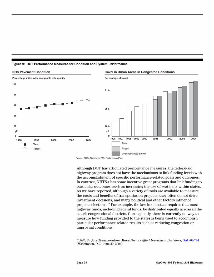
Figure 9: DOT Performance Measures for Condition and System Performance

Although DOT has articulated performance measures, the federal-aid highway program does not have the mechanisms to link funding levels with the accomplishment of specific performance-related goals and outcomes. In contrast, NHTSA has some incentive grant programs that link funding to particular outcomes, such as increasing the use of seat belts within states. As we have reported, although a variety of tools are available to measure the costs and benefits of transportation projects, they often do not drive investment decisions, and many political and other factors influence project selections.38 For example, the law in one state requires that most highway funds, including federal funds, be distributed equally across all the state’s congressional districts. Consequently, there is currently no way to measure how funding provided to the states is being used to accomplish particular performance-related results such as reducing congestion or improving conditions.

100

95

90

85

80

1996 1998 2000 2002 2004

NHS Pavement Condition

Trend

Target

0

Percentage miles with acceptable ride quality

26.0

28.5

31.0

Travel in Urban Areas in Congested Conditions

1996 1997 1998 1999 2000 2001 2002 2003 2004

Trend

Target

Unconstrainted growth

Percentage of travel

0

Source: DOT's Fiscal Year 2004 Performance Plan.

38GAO, Surface Transportation: Many Factors Affect Investment Decisions, GAO-04-744 (Washington, D.C.: June 30, 2004).



We Identified Several Options for the Design and Structure of the Federal-Aid Highway Program

We identified several options for the design and structure of the federal-aid highway program that could be considered in light of the issues raised by our findings. On the one hand, there are options that have been used in other federal programs that could limit substitution. Another option to consider may be to simplify the program towards a more flexible approach. Another option would be to consider whether a different program structure and different financing mechanisms could be used to target funding and more closely align resources with desired results.

Reduce Substitution To increase the extent to which federal-aid highway program funds are used to supplement state highway funds rather than substitute for them, several options exist to re-design the program to limit substitution. These include:

• Revising federal matching requirements to increase the percentage of projects’ costs that must be paid for with state and local funds.

• Instituting the use of funding formulas that reward states that increase state and local highway funding by increasing their federal funding, while reducing the federal funding of those states that do not.

• Adding a requirement that states maintain their own level of highway spending effort over time in order to receive additional federal funds.

All three options are designed to reduce or eliminate substitution. The first two options are designed to stimulate additional state spending on highways, while the third option is designed so that increased federal funding will supplement state spending rather than replace it. These objectives may not be perfectly achieved because models of substitution, like any models, produce estimates that are subject to uncertainty. As such, there is no way to objectively determine with certainty what states would have spent in the absence of increased federal funding. Table 3 summarizes the options, along with possible approaches that could be taken in implementing them.


Table 3: Options to Reduce Substitution

Source: GAO.

Each of these options and approaches would be likely to have somewhat different effects and would require careful consideration of various factors. Some possible effects are summarized below; see appendix IV for additional discussion of these options.

• The likely effect of revising the matching requirement would depend on the magnitude of the change. For example, if the requirement was changed so that states generally had to provide 60 percent of the total funding for eligible projects, states currently spending less than 60 percent of total highway funds for eligible projects would have an incentive to increase their spending in order to obtain the maximum federal match, while those spending more than 60 percent would not have an incentive to increase their spending. A few states with a low state/federal spending ratio might have to more than double their current spending in order to receive additional federal funds. Setting the required match at 40 percent would give fewer states an incentive to increase their spending and would generally require less of an increase in spending from those states with low state/federal spending ratios. An advantage of continuing to set the state match at 20 percent but counting only state spending in excess of what each state spent during a base time period towards the match is that it would stimulate state spending in all states to a similar degree.

Option Approaches

Revise matching requirements

Revise state match to a higher percentage than current 20 percent of total funding for project

Keep state match at 20 percent but count only state spending in excess of base time period for match

Link federal funding to states’ highway funding effort

Provide federal funds to states proportionally, based on their effort compared to average effort of all states

Provide federal funds to states proportionally, based on each state’s own effort relative to an initial base time period

Institute a maintenance of effort provision

Require states to maintain existing levels of state spending in order to receive federal funds


• Using funding formulas that link federal funds to states’ highway funding effort could also be achieved through various approaches.39 For example, providing federal funds to states proportionally based on their effort in comparison to the average effort of all states would put states in competition with each other, rewarding states whose funding effort is already high and penalizing states whose funding effort is currently low. On the other hand, providing federal funds to states proportionally based on each state’s own effort during an initial base time period would put each state in competition with the funding effort it made in the base period, rewarding states whose spending grew more quickly in comparison to their spending during the base period and penalizing states whose spending stayed the same or dropped when compared to their spending during the base period.40 Such provisions could be designed so they could be suspended in a recession or severe economic downturn in order to prevent states from having to make disproportionate reductions in other state services to maintain highway funding.

• Instituting a maintenance of effort provision would require each state to continue to spend what it spent in a defined base period, plus inflation, in order to obtain increased federal funds. Therefore, it would not stimulate state spending, but it would attempt to ensure that states used federal funds to supplement rather than replace state and local funds. In previous work, we concluded that, to be effective, maintenance of effort provisions need to define a minimum level of state spending effort that can be objectively quantified and updated to keep pace with inflation in program costs so that the maintenance of effort provision ensures a continued level of activity when measured in inflation adjusted dollars.41 This could be achieved by defining a state’s base spending level as the

39Defining a state’s highway spending effort would need to avoid unfairly penalizing low-income states, which may not have the resources to compete with the highway spending of wealthier states. Therefore, each state’s highway funding effort could be defined as the state’s highway spending compared to some measure of the state’s taxing capacity. The most comprehensive measure of states’ taxing capacity that is available annually is Total Taxable Resources (TTR), which is produced annually by the Department of the Treasury.

40Defining a state’s spending during a base time period should, to the extent possible, be established by measuring spending levels that are typical rather than unusually high or low.

41GAO, Proposed Changes in Federal Matching and Maintenance of Effort Requirements

for State and Local Governments, GAO/GGD-81-7 (Washington, D.C.: Dec. 23, 1980); and Block Grants: Issues in Designing Accountability Provisions, GAO/AIMD-95-226 (Washington, D.C.: Sept. 1, 1995).



amount spent per year during a recent historical period and then adjusting that base spending level for inflation.42

Increase Flexibility in States’ Use of Funds and Reduce Administrative Expenses

Another potential option would be to build on trends giving states greater flexibilities and discretion with their federal-aid highway program funds. In contrast to changes in program designs that would limit substitution, adopting such an option could be seen as recognizing substitution as an appropriate response on the part of states to increasing fiscal challenges and competing demands. Adopting such an option could also be seen as recognizing that the ability of states to meet a variety of needs and fiscal pressures might be better accomplished by providing states with federal funding for highways through a more flexible federal program.

Such an option would also recognize the changing nature of FHWA’s role and the federal-aid highway program. Currently, FHWA reviews and approves transportation plans and environmental reviews, and—on some projects—designs, plans, specifications, estimates, and contract awards. FHWA also has duties related to the program’s considerable regulatory component. To carry out these responsibilities, FHWA has among the largest field office structure in DOT, and a larger field structure than many other federal agencies. FHWA has personnel in over 50 field offices, including one office in each state, and has had a field office in each state since 1944. However, the federal-aid highway program has changed considerably in 60 years. In 2004, the program’s return-to-origin features and flexibility, combined with substitution and the use of state and local highway funds for other purposes, means that from a funding standpoint, the federal-aid highway program is, to some extent, functioning as a cash transfer, general purpose grant program. Devolving funding responsibilities to the states in a manner consistent with that function would build on the flexibilities already present and obviate much of the need for FHWA’s extensive field organization, allowing it to be greatly reduced in scope. This could produce budgetary savings of some portion of FHWA’s $334 million annual budget.

42One drawback of a maintenance of effort provision is that basing it on a historical spending period could result in a base spending period that represents an unusually high spending level for some states, effectively locking them into continued high spending in future years. This could be ameliorated however by establishing waivers for states that are able to demonstrate that spending in the base period chosen is unusually high, to allow a more “typical” spending level for purposes of the maintenance of effort provision.


Adopting such an option would involve weighing numerous factors, including FHWA’s role and value. But devolving funding responsibilities to the states would not require abandoning the program’s regulatory component. Some federal laws and requirements in place originated outside the transportation program and would doubtless remain in force, such as civil rights compliance. Others that are currently part of the transportation program could also remain in effect. Depending on priorities, these could continue to be overseen by FHWA directly or a process could be established through which states certify their compliance with the requirements, as is done in other programs. In this manner, it would be possible to enforce these laws and requirements without an extensive field structure, as other federal agencies and programs do.

Devolving authority to the states could also take the form of devolving not only the federal programs, but the revenue sources that support it. Considerable federal effort goes into collecting and accounting for motor fuel taxes and other highway user fees. One argument for maintaining a federal fuel tax is that this tax may be a useful public policy to prevent tax competition between states to avoid the disinvestment in the highway system that could potentially result. Such a “turnback” provision was considered in the form of an amendment to TEA-21 in the House of Representatives in 1998, but it did not pass.

Devolving federal responsibilities to the states is not dissimilar to the Surface Transportation System Performance Pilot Program that was proposed in the administration’s reauthorization proposal, but which was not included in either the House or Senate version of the bill. Up to five states could have participated in the program, which would have allowed a state to assume some or all of FHWA’s authorities and responsibilities under most federal law or regulations.43 Once approved to participate, a state would have had to identify annually what goals it wanted to achieve with its federal funds and what performance measures it would use to gauge success. A state would also have had to agree to a maintenance of effort requirement that it maintain its total combined state and federal

43Under the proposed pilot program, the federal government would not have devolved its responsibilities (1) to review states and local governments’ transportation plans, (2) to oversee “major” projects costing over $1 billion, (3) under Title VI of the Civil Rights Act of 1964, or (4) under any laws relating to federally recognized tribes. In addition, the proposal specified that nothing in it would be interpreted to relieve any project from the requirements of the National Environmental Policy Act, nor would it preclude DOT from issuing rulemaking actions as needed.


highway program expenditures at the level of at least the average level of the three previous years. A state’s participation in the pilot program would have been terminated if that state did not achieve the agreed performance for two consecutive years.

Link Federal-Aid Highway Funding with Program Goals

Another option could be to consider whether a different program structure and different financing mechanisms could be used to target funding and more closely align resources with desired results. Restructuring the program in this way could take several forms. For example, the program could be reoriented to function more like a competitive discretionary grant program, in which program sponsors justify projects seeking federal aid based on an assessment of their potential benefits. This is not dissimilar to the program used by DOT to fund large transit capital projects.44 The program could also be revised to include the use of incentive grant programs similar to those that NHTSA has to link funding to particular outcomes, such as increasing the use of seat belts within states.

Adopting such an option would require asking the following questions:

• What policy goals have been established by Congress for the performance of the federal-aid highway program, what outcomes and results have been articulated in DOT’s strategic plans to fulfill those goals, and are they the right goals and outcomes?

• What is the appropriate role of each level of government? Would the roles need to be redefined in order to align federal spending more closely with a greater performance and outcome orientation? In particular, what refocusing of federal involvement (e.g., interstate commerce, homeland security, national defense) would need to occur?

• How could the design of the federal-aid highway program’s grants and funding mechanisms best support accomplishment of agreed-upon

44Under the Federal Transit Administration’s New Starts Program, local transit agencies compete for project funds based on specific financial and project justification criteria. FTA assesses the technical merits of a major transit project proposal and its finance plan and then notifies Congress that it intends to commit, subject to appropriations, New Starts funding to certain projects through full funding grant agreements. The agreement establishes the terms and conditions for federal participation in the project, including the maximum amount of federal funds—which by law must be no more than 80 percent of the estimated net cost of the project, but in practice is often less than that percentage.


performance goals and outcomes? What funding incentives are needed to introduce a greater performance and outcome orientation?

• What type of departmental administrative structure for the federal-aid highway program would best ensure that the performance goals established by Congress and articulated in DOT’s strategic plans and outcomes are measured and accomplished?

• Can a greater performance and outcome orientation to the federal-aid highway program be reconciled with congressional and state legislative policies and preferences toward providing at least some transportation funding in the form of specific project earmarks?

Conclusions Addressing the issues raised in this report would require weighing competing and sometimes conflicting options and strategies. If, for example, reducing the level of grant substitution is an important concern, then design changes in the current program, including adopting features that have been used in other federal programs, may be warranted. If, on the other hand, preserving states’ flexibility, including their ability to meet a variety of needs and fiscal pressures is a higher priority, then design changes in the direction of a different, more flexible program may be warranted. While some options are mutually exclusive, others could be enacted in concert. For instance, an option to limit substitution could be combined with efforts to align resources with desired results, and returning program authorities and resources to the states could be accompanied by adding performance measures.

Beyond these options, our work raises broader and more fundamental issues given the challenges the Nation faces in the 21st Century. The fact that both the federal and state governments face budget deficits totaling hundreds of billions of dollars and a growing fiscal crisis requires policymakers to think critically about existing government programs and commitments and make tough choices in setting priorities and linking resources to results to ensure that every federal dollar is wisely and effectively spent. The opportunity to better align the federal-aid highway program with performance goals and outcomes comes at a time when both houses of Congress have already approved separate legislation to create a National Commission to examine future revenue sources to support the Highway Trust Fund and to consider the roles of the various levels of government and the private sector in meeting future surface transportation financing needs. The proposed commission is to consider how the program


is financed and the roles of the federal and state governments and other stakeholders in financing it; the appropriate program structure and mechanisms for delivering that funding are important components of making these decisions. Thus, this commission may be an appropriate vehicle through which to examine these options for the future structure and design of the federal-aid highway program.

Matter for Congressional Consideration

In light of the issues raised in this report and the fiscal challenges the Nation faces in the 21st Century, Congress may wish to consider expanding the proposed mandate of the National Commission to assess possible changes to the federal-aid highway program to maximize the effectiveness of federal funding and promote national goals and strategies. Consideration could be given to the program’s design, structure, and funding formulas; the roles of the various levels of government; and the inclusion of greater performance and outcome-oriented features.

Agency Comments and Our Evaluation

We provided DOT a draft of this report for review and obtained comments from departmental officials, including FHWA’s Director of Legislation and Strategic Planning. These officials said that our analysis raised interesting and important issues regarding state funding flexibility and the federal-aid highway program that merit further study. DOT officials also stated that while they recognize that federal-aid highway grants can influence state and local governments to substitute federal funds for state and local funds that otherwise might have been spent on highways, they believe that this substitution is likely due to numerous factors. Specifically, the officials said that to the extent substitution occurred and increased during the 1990s, it was also likely due to changes in states’ revenues and priorities. DOT officials also emphasized that regardless of changes in the availability of state funds for highway programs, the overall federal share of capital spending on highways declined during the period we studied, from over 55 percent in the early 1980s to around 45 percent today. DOT officials also emphasized that there is no evidence that the substitution discussed in our report resulted in the diversion of federal-aid highway funds apportioned to the states. They further stated that substitution may reflect appropriate resource allocations by states and that preserving states’ flexibility has been a priority of the federal-aid highway program and is a goal of DOT’s reauthorization proposal. Finally, regarding options for changes in the design of the federal-aid highway program, officials emphasized that FHWA adds considerable value to the federal-aid highway program by providing


program oversight and sharing its expertise with states to ensure states uniformly address key areas of national concern including safety and environmental protection.

We agree with DOT’s characterization of the importance of the issues raised in this report, including the effect that federal-aid highway grants have on state spending decisions and states’ funding flexibility. We also agree with DOT officials that many factors influence state budgetary decisions, including changing state budget priorities and the availability of state revenues. It was for this reason that we used a statistical model that specifically took changing economic conditions and revenues into account in order to better isolate the effect of federal grants on state spending choices. We believe that our model has reasonably distinguished between the effects of changing economic conditions and revenues and the effect of federal grants, and, consistent with earlier models and studies, we found the relationship between federal grants and state spending, indicating substitution, to be statistically significant, particularly during the 1990s. However, determining specific causes of substitution is beyond the scope of our statistical model. For example, while states faced rising demands for health care and education during the 1980s and 1990s that could have resulted in states reducing their highway spending when federal highway funding increased, our model does not identify the specific causes responsible for rising substitution rates. Although DOT officials said that the overall federal share of capital spending on highways declined during the period we studied, these relative shares do not affect our findings on substitution since substitution can occur when the federal share of funding is either rising or falling; if substitution occurs when state funding is rising it simply means that state spending increased less than the increase that might have occurred had there been no substitution. While DOT officials stated that there is no evidence that substitution resulted in the diversion of federal-aid highway funds, there are important differences between diversion and substitution. In the context in which DOT officials raised it, diversion is the transfer of federal funds for purposes other than those authorized by law, while substitution, as we have reported it, is the transfer of state funds that would have otherwise been spent on highways. States can both use federal funds for the purposes authorized by law and at the same time substitute federal funds for state funds. Thus, while we agree that there is no evidence that substitution resulted in the diversion of federal-aid highway funds, we do not believe our report suggests the existence of such evidence.


Finally, we agree with DOT officials that states’ flexibility and FHWA’s role are important factors in the federal-aid highway program; however, we believe that options for changing the design, structure, and funding mechanisms of the federal-aid highway program should be considered in light of substitution and the issues raised in this report, and that a variety of factors, including but not limited to these two, should be weighed when considering such changes. While the department took no position on the matter for congressional consideration to expand the mandate of the proposed National Commission, officials did state that they believe these issues merit further study. We continue to believe that Congress has the opportunity to maximize the effectiveness of federal funding and promote national goals and strategies by expanding the proposed mandate of the National Commission to consider these issues.

We are sending copies of this report to the Honorable Norman Mineta, Secretary of Transportation. We will also make copies available to others upon request. In addition, the report will be available at no charge on the GAO Web site at http://www.gao.gov.

If you have any questions about this report, please contact me at [email protected], or (202) 512-2834, or contact Jerry Fastrup at [email protected] or (202) 512-7211, or Steve Cohen at [email protected] or (202) 512-4864. GAO contacts and acknowledgments are listed in appendix V.

Sincerely yours,

JayEtta Z. Hecker Director, Physical Infrastructure


mailto:[email protected]



http://www.gao.gov

Appendix I

AppendixesObjectives, Scope, and Methodology Appendix I

In light of the increasing federal-aid highway program funding and concerns over future federal revenues for highways, you asked us to provide information on past trends in the federal, state, and local capital investment in highways, and how federal-aid highway program grants influence the level of state and local highway spending. We responded to the first part of your request in June 2003. This report (1) updates information on trends in federal, state, and local capital investment in highways; (2) assesses the influence that federal-aid highway grants have had on state and local highway spending; (3) discusses the implications of these issues on the federal-aid highway program; and (4) discusses options for the federal-aid highway program that could be considered in light of these issues. In addition, this report identifies characteristics associated with differences among states’ levels of effort for highways (see app. III).

To update information on federal, state, and local capital investment in highways, we obtained 2002 (the most recent year available) expenditure data from the Federal Highway Administration. We converted these expenditure data to 2001-year dollars to coincide with the data in our previous report,1 which presented data from 1982 through 2001.

To assess the influence that federal-aid highway grants have had on all state and local highway spending, we reviewed and synthesized the research literature on this issue. Our literature review revealed a number of studies that used statistical models to estimate the influence of federal funding on state spending. These models examined different time periods, employed different statistical methods, and considered different potential social, demographic, economic, and political factors that may affect state highway spending decisions. None of the models used in the studies we reviewed included the most recent data now available on highway funding, and none examined whether the effect of federal grants on state spending changed during the time period covered in the study. Therefore, based on the models used in the earlier studies, we developed our own statistical model of state highway capital and maintenance outcomes to estimate the fiscal effects of federal highway funding on state highway spending. The purpose of our statistical model was to isolate the effect of federal grants on highway spending in states by controlling for other factors that affect state spending decisions. Our model therefore considered a wide range of potential factors such as economic conditions and the size of a state’s highway system, that may affect state spending choices. In addition, our

1GAO, Trends in Federal and State Highway Investment (GAO-03-744R).



Appendix I

Objectives, Scope, and Methodology

model included the most recent data available and examined whether the effect of federal grants on state spending changed during the time period.2 A more detailed description of the literature and our statistical model is contained in appendix II. Finally, our model was reviewed by experts in the Department of Transportation (DOT) and peer reviewed by three authors of the earlier studies on the fiscal effects of federal highway grants. These experts and authors generally agreed with our methods, and we made revisions based on their comments as appropriate.

To address the implications of the effect of federal highway grants on state and local highway spending and options raised by these implications, we reviewed pertinent legislation and congressional actions affecting the federal-aid highway program, including goals, funding trends, program features, and financing mechanisms. We reviewed the Government Performance and Results Act and DOT’s strategic and performance plans and reports for 2003 and 2004. We then evaluated how our model results and other analysis on the existence of substitution affect the design and performance of the federal-aid highway program.

Finally, to identify state characteristics associated with their effort to fund highways from state resources, we defined a state’s level of effort broadly to include both a state’s and its local governments’ spending for highway maintenance and capital construction relative to the personal income of state residents.3 We determined a multivariate analysis is required so that other factors, in addition to the state characteristic under consideration, can be taken into account and held constant. (See app. III for results.)

To perform this multivariate analysis, we utilized the same statistical model of state highway spending used to analyze the fiscal effect of federal highway grants (see app. II). The variables expected to affect state highway spending fall into four broad categories: (1) fiscal capacity, (2) the cost of transportation services to the representative voter/consumer (tax price),

2We adjusted for the changing cost of highway services over time by deflating expenditures using the chain-price deflator for state and local government streets and highways published by the Bureau of Economic Analysis.

3Our previous report defined level of effort more narrowly as highway capital spending as a percentage of gross state product. We have adopted a broader definition for the current analysis that is consistent with the scope of this report’s focus on highway spending broadly defined to include capital as well as maintenance spending. Also consistent with this report, we have used the personal income of state residents rather than gross state product to reflect states’ fiscal capacities.


Appendix I

Objectives, Scope, and Methodology

(3) federal grants, and (4) indicators of state preferences for highway spending. The specific variables we considered are listed in table 6.

We conducted our work from August 2003 through July 2004 in accordance with generally accepted government auditing standards.


Appendix II

Description of Grant Substitution Model, Statistical Methods, and Results Appendix II

This appendix presents a thorough description of the statistical analysis that we conducted to estimate the extent to which states substitute federal highway grants for funds that would have been spent on highways from their own resources. The first section summarizes the literature on this topic because we built upon models from previous studies in developing our model. The next section describes the model that we developed. The final section describes the statistical tests that we used and presents the results of those tests.

Summary of Previous Studies

We reviewed a number of studies on substitution and relied most heavily on the models used in three of them in developing our statistical model.1 The three studies are similar in that each draws upon economic models that explain states’ highway spending in terms of the demand for mobility that flows from the construction and maintenance of a highway network. Within the context of these models, the potential for grant substitution arises in the response of state highway spending to changes in federal grant funding. However, these models differ in key details, such as the statistical methods used to estimate the extent of substitution, the definition of state highway expenditures, and the control variables used in the model. They also differ in their estimation of substitution rates.

Conceptual Framework The models in each of the key studies are built upon the premise that the political process responds to the preferences of voters/consumers for highway transportation services. As a result, the models characterize the demand for and supply of highway spending as depending on four types of factors:

1The three studies that we relied on most heavily were: Harry G. Meyers, op. cit; Brian Knight, op. cit; and Shama Gamkhar, op. cit. Other studies that we reviewed include: Shama Gamkhar, “Is the Response of State and Local Highway Spending Symmetric to Increases and Decreases in Federal Highway Grants?” Public Finance Review, Vol. 28 No. 1, January 2000 pp. 3-25: Janet G. Stotsky, “State Fiscal Responses to Federal Government Grants,” Growth and Change, Summer 1991, pp 17-31; Roger D. Congleton and Randall W. Bennett, “On the Political Economy of State Highway Expenditures: Some Evidence of the Relative Performance of Alternative Choice Models,” Public Choice, 84 (1995), pp. 1-24; Rajeev K. Goel and Michael A. Nelson, “Use or Abuse of Highway Tax Revenues?: An Economic Analysis of Highway Spending,” unpublished draft, April 2001; Edward Miller, “The Economics of Matching Grants: The ABC Highway Program,” National Tax Journal, XXVII, no. 2, pp. 221-229; Herman B. Leonard, By Choice or By Chance: Tracking the Values in

Massachusetts' Public Spending (Pioneer Institute for Public Policy Research, 1992).


Appendix II

Description of Grant Substitution Model,

Statistical Methods, and Results

1. Fiscal capacity (FC), which is the ability of states to fund services using within-state resources;

2. The tax price (TP) faced by the typical voter/consumer of highway services, which can be thought of as the cost of an additional unit of mobility;

3. Intergovernmental grant funding (G), including both grants intended for highways and grants for other public services; and

4. Differences in voter/consumer preferences (P) for highway transportation services.

This relationship can be summarized in the following relationship:

State Highway Expenditure = f(FC,TP, G, P)

In these models, greater tax paying capacity is expected to result in a higher demand for mobility that in turn increases the demand for a larger highway network. Similarly, more grant funding (both for highways as well as for other public services) increases the resources available to states and is expected to increase total highway spending. Differences in political culture are also expected to result in different preferences for transportation services relative to other public services, such as health and education. Finally, if the typical voter/consumer faces a higher unit cost of transportation services, also called the tax price of highway services, the demand for transportation services is likely to be lower.

The tax price of highway services is, in turn, dependent upon several factors:

1. A higher cost of inputs (labor, building materials, supplies, etc.) used to build and maintain highways results in more expensive transportation services. A higher unit cost of mobility is expected to reduce the demand for transportation services, but will increase highway spending as long as the demand for transportation services is price inelastic.

2. Economies and/or diseconomies of scale may also affect the unit cost of mobility. A required minimum facility size may result in more lane miles per resident in smaller states, which may result in a higher unit cost for the typical voter/consumer. Similarly, very low lane miles per


Appendix II



resident may be associated with more intensive usage, which may also result in a higher unit cost as well. Thus, unit cost may be U-shaped.

3. A greater number of voter/consumers with whom the cost of highway services may be shared is expected to reduce unit cost to the typical state voter, increasing the demand for transportation services. This will result in higher total highway spending and lower spending per voter so long as demand is price inelastic.

4. More highway users may lead to greater deterioration in the quality of highways and greater congestion, raising the unit cost of transportation services to the typical voter/consumer, reducing the demand for highway services. The effect on spending is expected to be positive if demand is price inelastic. In addition to cost considerations, more users could also be thought of as reflecting a stronger preference for highway services relative to other goods and services.

5. Matching grants on the marginal dollar of highway spending reduce the unit cost of services to the typical voter/consumer. To the extent that matching requirements apply to additional state spending the typical voter/consumer pays a smaller share of additional spending, lowering the cost of additional spending to the typical voter/consumer and raising the demand for highway services.2

In table 4, we summarize three studies that are representative of the variety of models that have been considered in the literature and upon which we base our analysis.

2Closed-ended matching programs that limit the availability of federal matching funds at the margin of spending do not lower the cost of additional highway spending and hence the tax price faced by the typical voter/consumer.


Appendix II



Table 4: Summary of Fiscal Substitution Studies

Source: GAO analysis.

aTreated as an endogenous variable.

Statistical Methods The three studies employ a variety of statistical methods in estimating the substitution effect of federal highway grants. All use simultaneous equations estimators, but they treat different variables as endogenous. Knight and Gamkhar treat federal grant expenditures and state own-source

StudyTime period

State highway expenditures

Fiscal capacity Tax price variables Grant variables Preferences Other variables

Knight 1983-1997

State (but not local) government spending for highway-related projects (capital and maintenance, real per capita)

Personal Income per capita

1. Population2. Drivers per capita3. Registered

vehicles per capita

Highway grant expenditures per capitaa

1. Governor Democrat

2. Percent Democrats in State House

3. Percent Democrats in State Senate

State fixed effects

Gamkhar 1976-1990

State & local government spending for highway-related projects (capital and maintenance, real per capita)

Personal income per capita

1. Effective nonhighway match rate

2. Registered Vehicles per capita

3. Vehicle miles traveled per capita

4. Percent light vehicles

5. Percent metro population

6. Population density

1. Highway grant expenditures per capitaa

2. Highway grant obligations per capita

3. Other fed grants per capita

1. State fixed effects

2. Time fixed effects

3. Percent unemployed

4. Debt as a percent of income

Meyers 1976-1982

State capital spending on federal-aid highways (net of interstate highways, real per capita)

Personal income per capita

1. Effective highway match ratea

2. Effective nonhighway match rate

3. Registered Vehicles per capita

4. Vehicle miles traveled per capita

5. Lane miles per capita

1. Highway grant expenditures per capita

2. Other federal grants per capita


Appendix II



highway expenditures as jointly determined and therefore use an instrumental variable estimator for their per capita federal grant variable to remove the endogenous component associated with this variable.3 In contrast, Meyers does not treat per capita federal highway grants as an endogenous variable and may have a biased estimate of the substitution rate. He does, however, treat the effective matching rate associated with highway grants (i.e., the ratio of highway grants to total highway spending) as endogenous and uses an instrumental variable procedure to correct for potential bias in that variable.4

Both Gamkhar and Meyers find autocorrelation in their error terms and, therefore, make an adjustment for autocorrelation. The Knight study does not correct for autocorrelation. Finally, both Knight and Gamkhar use a fixed effect estimating procedure to control for unique circumstances across states that are not captured by the other control variables included in their models. Neither study reports the significance of fixed effects in their model. In addition, Gamkhar also includes time dummy variables to capture systematic effects over time that the other control variables do not capture. Knight does not include a time adjustment in his model. Meyers includes neither a fixed effects nor time adjustment.

Differing Definitions of State Highway Expenditures

Each of the three studies define state highway spending differently, which has important implications regarding how grant substitution is measured and influences the interpretation of the studies’ results.5 The earliest study, by Meyers, includes state capital spending only for projects eligible under the federal-aid highway program, excluding spending for interstate highways. Measuring the dependent variable in this way means the

3If state expenditures and federal grants were jointly determined, ordinary least squares (OLS) methods would provide biased estimates of the substitution rate. Gamkhar does, however, use OLS methods in a model in which federal grants are measured using grant obligations, arguing that obligations are known prior to states’ expenditure decisions and therefore treated obligations data as exogenous.

4Neither Knight nor Gamkhar includes a price effect associated with federal highway grant funding arguing that such an effect is not present because states spend substantially more than is required to satisfy the matching requirements associated with federal funding.

5Gamkhar uses the implicit price deflator for government purchases, and Meyers uses the implicit price deflator for state and local government purchases to adjust for changes in the purchasing power of a dollar over time. Knight does not identify the deflator he uses. None of the studies adjusts for cross-state differences in input costs. All three studies express state highway spending and federal grants on a per capita basis.


Appendix II



highway grant coefficient measures only the response of state capital spending on federal-aid highway projects to changes in federal funding. As a consequence, Meyers counts increased state or local spending for maintenance on federal-aid highway projects, or increased state or local capital and maintenance on nonfederal-aid highway spending, as grant substitution in the same way as increased spending for other state services such as education and health or increased state taxpayer relief would be counted as substitution.

In contrast, Knight defines state highway spending more broadly to include all highway spending by state governments, whether for federal-aid highways or for other state highway projects. However, Knight does not include local spending on highways in his definition of state highway spending. As a consequence, increased state maintenance spending on federal-aid highway projects or spending on state government highway projects that are not part of the federal-aid system is not considered grant substitution in his study, even though such spending is not eligible for federal assistance. However, increased highway spending by local governments is considered to be grant substitution in the same way that increased state or local spending for other state services and increased tax relief are considered substitution. Finally, the Gamkhar study defines highway spending to include both capital and maintenance spending by both state and local governments. This study, therefore, counts only increased state or local spending for nonhighway purposes, including increased tax relief, as representing grant substitution.

The Estimated Effect of Federal Highway Grants on State Highway Spending

All three studies use federal grants expenditures to measure federal grants received by states. This variable is statistically significant in all studies. In addition to grant expenditures, Gamkhar also considers grant obligations as an alternative measure. Since obligated funds are available for expenditure for several years, she included this variable with lagged values.6

The reported estimates of substitution rates associated with federal highway grants vary across the three studies. These differences are, in part, due to differences in the time periods studied, the definitions of state

6Gamkhar treats grant obligation data as a predetermined variable and therefore uses OLS methods to estimate the grant coefficient. However, if state spending and federal grants are jointly determined this may yield biased estimates of the substitution rate.


Appendix II



highway spending, and the statistical methods employed. Among the highlights of the studies were the following:

• Knight’s study reports a grant substitution rate of over 90 percent for the period from 1983 to 1997. Knight defines substitution as the reduction in state (but not local) government spending on all highway-related projects.

• Gamkhar reports a substitution rate of 63 percent for the period 1976 through 1990. Gamkhar defines substitution as the reduction in state and local government spending on all highway-related projects; Gamkhar measured federal grants using grant expenditures. When grants were measured using obligations rather than actual grant expenditures, a lower substitution rate of 22 percent is reported.7

• Meyers also reports a 63 percent substitution rate for the period 1976 through 1982. Meyers defines the substitution rate as the reduction in state and local government spending on federal-aid eligible highway projects net of spending on the Interstate Highway Systems; federal grants are measured using grant expenditures. However, when he defined substitution as the increase in state and local government nonhighway spending, he reports no substitution.

7The estimate based on grant obligations data may be downwardly biased if, as argued by Knight, federal grants and state expenditures are jointly determined (see Knight op. cit, p. 77).


Appendix II



Table 5 summarizes the definitions used and findings of these three studies.

Table 5: Highway Grant Substitution Rates Reported in Fiscal Substitution Studies


aMeyers’s formal test for substitution into nonhighway spending is to test whether federal highway grants are systematically related to state nonhighway spending. He finds no statistical evidence of such a relationship.

Controls for Other Factors Associated with State Spending Choices

To isolate the effect of federal highway grants on state highway spending, these studies include additional variables in their models to control for other factors also related to state spending. Some of the control variables are similar across the studies, but others differ.

Fiscal Capacity All three studies use per capita personal income to represent states’ funding capacity, and in each study the variable is found to be statistically significant.

Tax Price All three studies include a wide variety of variables that are intended to capture various components of the tax price faced by the typical voter/consumer.

StudyDefinitions of state highway expenditures Substitution rate

Knight State (but not local) government spending for highway-related projects (capital and maintenance, real per capita dollars)

91 percent

Gamkhar State and local government spending for highway-related projects (capital and maintenance real per capita dollars)

63 percent (grant expenditures)22 percent (grant obligations)

Meyers State capital spending on federal-aid highways (net of interstate highways, real per capita)

State and local government nonhighway spending, (real per capita)a

63 percent

0 percent


Appendix II



Input prices All three studies measure financial variables in real dollars by adjusting for price level differences over time but otherwise do not explicitly include an input cost adjustment as a tax price proxy, except to the extent that the fixed effects procedure employed by Knight and Gamkhar capture these differences.8

Highway System Size Only Meyers uses an indicator of highway system size: lane miles on federal-aid highways. While this variable has the expected positive sign it is statistically insignificant. However, a quadratic term to capture a possible U-shaped functional form was not used.

Highway usage All studies use the number of registered vehicles as a measure of highway usage. In addition, Knight uses the number of drivers, whereas Meyers includes vehicle miles traveled. Gamkhar includes several additional proxies for highway use that are not included in the other studies: the percentage of light motor vehicles, population density, and percentage of population living in metropolitan areas. However, none of these factors was statistically significant. In general, only one of the use variables is statistically significant in each study and no one measure is statistically significant across studies. In several instances the coefficient has a negative sign, although a positive relationship between highway usage and state spending would be expected.

Highway matching rates Although highway grants require state matching, Knight and Gamkhar do not include highway matching rates as part of their models because they found that states’ highway spending exceeds the amounts required for their federal grant allotments and, therefore, have only an income effect but no price effect. Meyers, in contrast, does include the effective matching rate (highway grants as a percentage of highway expenditures) and reports a price elasticity of one.

Nonhighway matching rates Other grants may also have a price effect because programs such as Medicaid, Foster Care, and Adoption Assistance are all open-ended matching grants. Including the effective matching rate associated with other grant spending (i.e., other grants as a percent of

8However, to the extent that cross-state differences in input costs is relatively stable over time, Knight and Gamkhar may have accounted for these differences through the fixed effects estimating procedure.


Appendix II



nonhighway spending) captures the potential price effect of other grants.9 The sign on the effective matching rate is expected to be negative because higher demand for other state services would reduce the demand for highway spending. These variables are statistically significant in both studies. The Knight study does not consider the tax price effect of nonhighway grant funding.

Cost sharing Only Knight, by including population in his model, includes a factor that could be interpreted as reflecting the cost-reducing effect of having more taxpayers sharing the cost of highway services. Neither Gamkhar nor Meyers includes such a factor.

Other Grant Funding In addition to the tax price effect of nonhighway grant funding, the studies may also have income effects. Both Meyers and Gamkhar include other nonhighway grants per capita in their models to capture the income effect of these grants.10 The income effect is expected to have a negative effect on own-source spending as some of these grants may be substituted into highway spending and supplant funding from state resources. The Knight study does not consider either price or income effects associated with nonhighway grant funding.

Political Culture/Preferences Only Knight includes variables that are intended to reflect differences in state preferences for highway spending that may be associated with the political party of the state governor and the partisan representation in the state legislature. He finds the party of the state governor to be statistically significant at the 10 percent level, while the other political variables are not statistically significant.

Description of GAO’s Statistical Model

Consistent with previous studies, we model state spending choices as being conditioned on states’ fiscal capacities, the tax price faced by state voters, federal grant funding for highways and for other state services, and preferences of state voters for highway spending. Because both theory and the results of previous studies suggest that federal grants and state

9The effective matching rate is measured by expressing other grant funding as a percentage of total nonhighway spending.

10As noted above, both studies also include these grants as a share of total nonhighway spending to capture any price effect these grants may have.


Appendix II



spending decisions are jointly determined, we use an instrumental variables (IV) approach to estimate the fiscal effect of federal grants.

To capture other factors that may be systematically associated with differences in state spending choices, we estimate the model using a fixed effects estimating procedure. The fixed effects procedure is intended to capture factors such as topographical differences and weather conditions across states that do not change over time and to capture other unmeasured factors with large cross-state variation that exhibit relatively little change over time.11 In addition, we include a time trend to capture trend changes in state spending that may not be captured by the other variables included in our model.

The specific variables considered for our model are listed in table 6.12

Table 6: Variables Considered in the Second Stage State Highway Expenditure Equation

11Both Knight and Gamkhar adopt this strategy.

12Consistent with previous studies, we expressed state highway spending on a per capita basis and adjusted for the changing cost of highway services over time by deflating expenditures using the chain-price deflator for state and local government streets and highways published by the Bureau of Economic Analysis as part of the National Income Accounts.

Variable name

Dependent variable (per capita)

Real state and local government spending for highway capital and maintenance

Fiscal capacity (per capita)

Real personal income

Real income squared

Tax price

Vehicle miles traveled per capita

Drivers per capita

Registered motor vehicles per capita

Effective match rate of nonhighway grants

Population

Lane miles per capita


Appendix II




aPredicted values of federal highway grants.bWith the exception of some independents, office holders are either Democratic or Republican. Therefore, the choice of using the percentage Democrats or Republicans is arbitrary and has no effect on the statistical results except to change the sign of the regression coefficient.

Testing the Stability of the Substitution Rate

With each time period, various rules and regulations change that may affect the ability of states to substitute federal grants for state spending. Given the range of estimates over different time periods reported in past research, we also want to test whether the rate of grant substitution, if found, systematically differ across the time periods included in our data. To see if the substitution rate differs over time, we introduce dummy variables for each of the time periods covered in our study into our model.13 We then multiply these dummy variables by the grants variables and included these interaction variables in the model. If statistically significant, these variables would provide evidence that substitution has varied from one time period to another.

Squared lane miles per capita

Federal grants (per capita)

Real highway grantsa

Real other federal grants

State preferencesb

Governor democratic

Percentage of state House represented by Democratic party

Percentage of state Senate represented by Democratic party

Other variables

Utah Olympics (=1 for 1997-2000)

Time trend

Time trend squared

Inverse time trend

State fixed effects


Variable name

13Our grant expenditures variable reflects, in part, obligations made in prior years. As a consequence, the substitution rate for a particular time period will, in part, be conditioned on grant obligations made in prior time periods.


Appendix II



Definition of State Highway Spending

The estimated effect of federal highway grants on state highway spending is measured by the regression coefficient associated with federal highway grants. As a consequence, the interpretation of that coefficient is directly affected by how the dependent variable, state expenditures, is defined. If we defined state highway spending narrowly as only capital expenditures on federal-aid highway projects, the federal grants coefficient in our model would be interpreted as the response of state capital spending to changes in federal highway aid. This approach, taken by Meyers,14 represents a definition of state spending that is consistent with the requirements of the federal-aid highway program, which restricts federal grants to authorized uses, such as capital investment on eligible federal-aid highway routes. Under this approach, grant funds that are used for purposes that are not eligible for federal aid, would represent grant substitution in the same way that increased spending for health and education and for state tax relief would represent grant substitution. Some policymakers may not view this as substitution, perhaps arguing that state transportation officials are better positioned to determine the best use of available funding for highway-related projects. Our analysis uses this broader definition of state highway spending. Thus, our measure of grant substitution considers only state grant funds that are effectively used for nonhighway purposes as substitution.15

We adopt this approach for two reasons. First, we want to be conservative in our definition of grant substitution. A broader definition of state highway spending that includes state and local spending on highway projects not eligible for federal funding would yield a lower estimate for the substitution rate because some types of adjustments would not be treated as grant substitution. Second, an estimate of grant substitution that is based only on state (but not local) government spending would be affected by cross-state differences in the extent to which highway spending is centralized at the state level. Since there are large differences across states in the extent to which highway spending is centralized, we include local as well as state government spending so that our measure of highway spending would be comparable across states.

14Meyers, op. cit.

15Knight, op. cit, takes an intermediate approach by using only state government capital and maintenance spending, excluding highway spending by local governments.


Appendix II



Definition of Federal Highway Grants and Specification of the Federal Grants Equation

Because federal highway grants are provided on a reimbursement basis, we obtained from FHWA federal highway grant expenditures that are contemporaneous with states’ reported own-source highway spending. As with state spending, we express federal grants in real per capita dollars, using the BEA chain-price index for state and local government streets and roads. Because federal grant expenditures, by definition, represent formula grant allotments from current and prior years, any lagged response in state spending to federal highway grant funds is already included in our grants variable. We therefore do not include lagged values of federal highway grants in our model.

Knight provides an economic argument explaining that state highway spending and federal grant funding are jointly determined because elected officials reflect the preferences of state voter/consumers both in state legislatures and in Congress. His study tests for and finds confirming evidence for his theoretical argument.16 Based on these findings, we also employ an IV estimator that provides a consistent estimate of the federal grant coefficient to measure the fiscal effect of federal grants. Using this approach, we estimate a first stage instrumental variable equation that models federal highway funding in terms of exogenous variables that are expected to influence the distribution of federal grants. The instrumental variables include the exogenous variables from the state expenditure equation (e.g., fiscal capacity, the individual components of tax price, and preferences) and variables that are highly correlated with federal grants but uncorrelated with state highway spending (e.g., variables included in federal grant formulas and those that may affect the distribution of discretionary grants). Predicted values of federal grants, derived from the instrumental variables (highway grants) equation, are then used in lieu of actual grant values to correct for the bias in ordinary least squares (OLS) estimates of the federal grants coefficient in the state expenditure equation.

The excluded exogenous variables we consider include state contributions to the highway trust fund and variables that are intended to reflect the influence of state representatives on the distribution of federal highway grants: tenure in Congress, state representation on transportation committees, and state representation in the majority party. The exogenous variables we consider are summarized in table 7.

16Knight, op. cit.


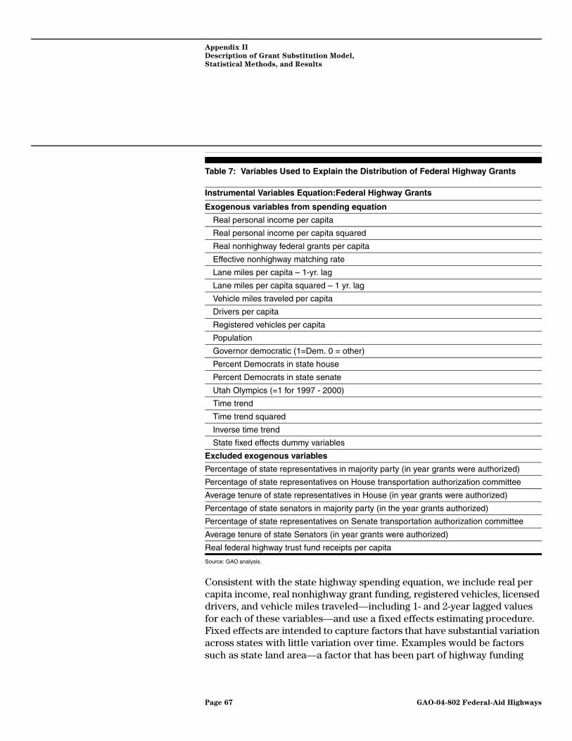
Appendix II



Table 7: Variables Used to Explain the Distribution of Federal Highway Grants


Consistent with the state highway spending equation, we include real per capita income, real nonhighway grant funding, registered vehicles, licensed drivers, and vehicle miles traveled—including 1- and 2-year lagged values for each of these variables—and use a fixed effects estimating procedure. Fixed effects are intended to capture factors that have substantial variation across states with little variation over time. Examples would be factors such as state land area—a factor that has been part of highway funding

Instrumental Variables Equation:Federal Highway Grants

Exogenous variables from spending equation

Real personal income per capita

Real personal income per capita squared

Real nonhighway federal grants per capita

Effective nonhighway matching rate

Lane miles per capita – 1-yr. lag

Lane miles per capita squared – 1 yr. lag

Vehicle miles traveled per capita

Drivers per capita

Registered vehicles per capita

Population

Governor democratic (1=Dem. 0 = other)

Percent Democrats in state house

Percent Democrats in state senate

Utah Olympics (=1 for 1997 - 2000)

Time trend

Time trend squared

Inverse time trend

State fixed effects dummy variables

Excluded exogenous variables

Percentage of state representatives in majority party (in year grants were authorized)

Percentage of state representatives on House transportation authorization committee

Average tenure of state representatives in House (in year grants were authorized)

Percentage of state senators in majority party (in the year grants authorized)

Percentage of state representatives on Senate transportation authorization committee

Average tenure of state Senators (in year grants were authorized)

Real federal highway trust fund receipts per capita


Appendix II



formulas and that does not change over time—and constraints that are applied to funding formulas, such as the ½-of 1 percent minimum state grant that is included in highway funding formulas (see table 1).

State Funding Capacity Consistent with previous studies, we use real per capita personal income to measure states’ taxing capacities. Unlike previous studies, we also include the squared value of per capita income to capture the possibility that demand for highways does not increase in proportion to increases in income, perhaps signifying that as basic transportation needs are met, increases in income are increasingly allocated to other uses such as health and education. Personal income is published by the BEA in the Department of Commerce. We include 1- and 2-year lagged values of real per capita income in the model to allow for lagged responses to changes in income and also to reflect cyclical changes affecting the level of state revenues.

Tax Price The tax price faced by state voters/consumers is reflected in a number of variables included in the model. Highway usage is reflected by vehicle miles traveled on state highways, and by registered vehicles and licensed drivers in the state, as reported by FHWA. We include 1- and 2-year lagged values in each of these variables to allow for lagged responses in spending to changes in highway usage.

Consistent with prior studies, we do not include the matching rate on highway grants because states spend more than the required federal match, and therefore, states pay 100 percent of the cost of funding additional highway projects, and because highway matching rates vary little both over time and across states. However, we do include the effective match rate on other grant funding to capture the price effect of other grant funding. Medicaid, Foster Care, and Adoption Assistance, for example, are open-ended matching programs with price effects that may encourage states to spend less on highways in order to provide matching funds for these and possibly other matching programs. We include 1- and 2-year lagged values to capture these effects. Using data from the Census Bureau, we measure the effective matching rate for nonhighway spending by deducting states’ federal highway grants from their total federal grants and expressing the net amount (nonhighway grants) as a proportion of each state’s nonhighway spending, also calculated by deducting highway spending from total spending.


Appendix II



Although previous studies do not include the size of the highway network to be maintained, we expect the per capita cost of maintaining an existing highway network to be higher in states with more miles of road per capita. Therefore, we include this variable in our model along with its squared value to test for evidence of per capita costs varying with the scale of the road network—that is, economies or diseconomies of scale. We obtained data on total lane miles of state highways from FHWA.

Other Federal Grants In addition to federal highway grants, states receive federal grants for a variety of other purposes, including health, education, and welfare. While it is possible that state highway funds may be substituted into spending for other state services, it is also possible that some state funds that would have otherwise been used for other purposes may be redirected into highways. For this reason, we also include other federal grant funding in our model to capture the income effect of these grants and their potential substitution into highway spending. While some of this aid is provided on a reimbursement basis (Medicaid, for example) other grants can remain eligible for expenditure in subsequent years. For this reason, we include 1- and 2-year lagged values of other federal grants to capture these potential effects. Other federal grants are also expressed in real per capita dollars.

State Preferences The political culture of states may affect both the overall level of spending on public services, as well as spending priorities for different types of services, such as highways, versus education and health care. Differences in political culture and spending priorities may be relatively stable over time, in which case the fixed effects adjustment may adequately control for cross-state differences in these spending preferences. Nonetheless, in addition to including fixed effects, we have also included variables that may be associated with differences in political culture. For this purpose, we have included dummy variables that are equal to one if the state governor is Democratic and zero otherwise, and the percentage of the state Senate and state House that is represented by the Democratic Party. With the exception of some independents, office holders are either Democratic or Republican. Therefore, the choice of using the percentage Democrats or Republicans is arbitrary and has no effect on the statistical results except to change the sign of the regression coefficient. We obtained these data from the Elections section of the Census Bureau’s Statistical Abstract.


Appendix II



Other Variables To capture trend changes in state spending that cannot be captured by the other variables included in our model, while allowing for a possible curvilinear trend, we have also included time, time squared, and the inverse of time. Finally, we include a dummy variable for the state of Utah that was equal to 1 during the years 1997 through 2000 and zero otherwise to account for the unusually large increase in highway spending in that state just prior to the 2002 Winter Olympics.

The means and standard deviations for the variables included in our statistical model are shown in table 8.

Table 8: Descriptive Statistics


Variables Units MeanStandard deviation

Real State Highway Spending Per Capita

Dollars per person$203 $80

Real Federal Highway Grants Per Capita


Real Non-Hwy Federal Grants Per Capita


Federal Nonhighway Grants percent of Nonhighway Expenditures

Ratio

16% 4%

Road Miles Per Person Lane Miles per 1,000 population 53 53

Registered Vehicles per Person

Registered vehicles per 1,000 population 786 117

Vehicle Miles Traveled per Person

1,000 miles per person9 2

Licensed Drivers per Person Licensed drivers per 1,000 population 679 50

Real Per Capita Income Dollars per person 21,272 4,223

Percent Democratic in State House

Percent57% 17%

Percent Democratic in State Senate

Percent58% 18%

Governor Democrat, (1=Democrat; 0=otherwise)

Not applicable52% 50%


Appendix II



Statistical Methods Because we use time series and cross-section data to estimate the model, we expect autocorrelation to bias the estimates of the standard errors associated with variables in our model. To reduce the problem of heteroscedasticity, we normalize variables by expressing them on a per capita basis (except for those already expressed in ratio or percentage terms). We conducted statistical tests to determine if our data are affected by autocorrelation and found statistical evidence of its presence. Therefore, we estimate all our models using a correction for autocorrelation. As noted above, we use a fixed effects procedure that allows for a separate constant term associated with each state to represent differences in state funding that are unique to each state and independent of the other variables included in the model.

Additional Analysis of Fixed Effects

The fixed effects coefficients of our model represent state differences in highway spending, after controlling for the other explanatory variables in our model. They are intended to capture the effect of variables that have comparatively little variation over time but are systematically associated with differences in spending across states. To identify those state characteristics that are systematically related to the fixed effects associated with state highway expenditures, we perform an additional stepwise regression analysis that regresses the following explanatory variables on our estimated fixed effects, using the following:

• Heating degree days,

• State land area,

• Lane miles per capita,

• Population,

• Vehicles per capita,

• Drivers per capita,

• Federal land area,

• Percentage of Democrats in state House,

• Percentage of Democrats in state Senate,


Appendix II



• Governor Democratic,

• Federal nonhighway grants per person, and

• Ratio of federal nonhighway grants per person to state nonhighway spending

We use the mean value of 21 observations from 1980 to 2000 per state to represent each variable in explaining our estimated fixed effects.

Statistical Results We report the statistical results explaining federal highway grants in terms of exogenous instrumental variables in table 9. Based on the R2 statistics, the fixed effects adjustment accounts for 85 percent of the variation in federal grants funding and the additional exogenous variables added to the model increases the R2 by 5 percent to 90 percent. Variables that are statistically significant at the 5 percent level appear in bold in the table. In addition to the fixed effects coefficients, per capita income, highway lane miles of roads, and state contributions to the Highway Trust Fund are strongly associated with the distribution of federal highway funding.


Appendix II



Table 9: Instrumental Variables Estimator of Federal Grants per Capita

Model R2

Constant term only 0.000

State fixed effects only 0.854

X - variables only 0.739

X and group effects 0.895

Variables Coefficients Standard error Probability value

Personal income, real per capita 0.015 0.007 0.035

Personal income, real per capita, (t-1) 0.008 0.009 0.375

Personal income, real per capita, (t-2) -0.021 0.006 0.000

Personal income squared, real per capita -0.3121E-06 0.1500E-06 0.037

Personal income squared, real per capita, (t-1) -0.1150E-06 0.2005E-06 0.566

Personal income squared, real per capita, (t-2) 0.4831E-06 0.1288E-06 0.000

Nonhighway federal grant, real per capita 0.035 0.027 0.187

Nonhighway federal grant, real per capita, (t-1) 0.133 0.032 0.000

Nonhighway federal grant, real per capita, (t-2) -0.051 0.026 0.048

Effective nonhighway match ratea -201.622 129.481 0.119

Effective nonhighway match ratea (t-1) -388.050 148.409 0.009

Effective nonhighway match ratea (t-2) 139.497 118.758 0.240

Vehicle miles traveled per capita -7.331 3.204 0.022

Vehicle miles traveled per capita, (t-1) -0.852 3.721 0.819

Vehicle miles traveled per capita, (t-2) 2.688 2.637 0.308

Registered vehicles per capita 0.048 0.024 0.041

Registered vehicles per capita, (t-1) -0.013 0.028 0.643

Registered vehicles per capita,(t-2) -0.007 0.024 0.785

Drivers per capita -0.022 0.034 0.514

Drivers per capita,(t-1) -0.018 0.038 0.634

Drivers per capita, (t-2) 0.041 0.033 0.221

Population, in 1,000 0.002 0.002 0.138

Road miles per capita, (t-1) 1.231 0.313 0.000

Road miles squared per capita, (t-1) -0.004 0.001 0.002

Governor Democrat, (1=Democrat; 0=otherwise) -3.836 1.737 0.027

Percent Democratic in State House 2.758 14.498 0.849

Percent Democratic in State Senate 32.801 11.695 0.005

Utah Olympics = 1 for Utah in 1997-2000, 0 otherwise -12.757 12.055 0.290

Time trend -3.123 2.627 0.234


Appendix II




aRatio of federal nonhighway grants to state and local nonhighway expenditures.

Displacement Effect of Federal Highway Grants

We report the results for the second stage expenditure equation without a correction for autocorrelation in table 10. Again, regression results for variables that are statistically significant at the 5-percent level appear in bold in the table. The model explains 78 percent of the variation in state own-source highway spending and fixed effects alone account for 69 percent of the variation. The estimated substitution rate associated with federal grants is 84 percent17 and is statistically significant. That is, other things being equal, a dollar increase in federal highway grants is associated with an 84-cent reduction in highway spending from state own-source revenues. Alternatively, the coefficient also implies that states replace 84 cents of each dollar decline in federal funding.18 These results are similar to the findings reported by Knight, who reported a substitution rate of 91 percent, higher than the substitution rates reported by Gamkhar.

Inverse time trend 66.101 33.632 0.049

Time trend squared -0.009 0.089 0.923

Highway trust fund per capita 0.294 0.088 0.001

Highway trust fund per capita, (t-1) 0.330 0.089 0.000

Highway trust fund per capita, (t-2) 0.225 0.088 0.010

Percent of the State's House delegation on the authorizing committee 8.233 5.761 0.153

Percent of the State's Senate delegation on the authorizing committee -14.760 4.515 0.001

Percent of the State's Senate delegation in the majority party 1.649 2.223 0.458

Percent of the State's House delegation in the majority party 5.940 3.863 0.124

Tenure for each State's U.S. House Delegation 0.148 0.283 0.601

Tenure for each State's U.S. Senate Delegation 0.063 0.202 0.756


Variables Coefficients Standard error Probability value

17The substitution rate is the coefficient of the federal grants variable after removing the negative sign.

18In a related paper Gamkhar tests whether the substitution rate is symmetrical during periods of rising and falling federal aid and found no statistically significant difference; see Shama Gamkhar, op. cit.


Appendix II



Table 10: Instrumental Variables Estimates of State Highway Spending Model, Without Correcting for Autocorrelation

Model statistics R2





Variables Coefficients Standard error Probability

Predicted FHWA payments / per capita -0.8412 0.233 0.000

Personal income, real per capita, (t) 0.0160 0.013 0.221



Personal income squared, real per capita, (t) -0.6259E-07 2.860E-07 0.827



Nonhighway federal grants, real per capita, (t) 0.0719 0.051 0.159

Nonhighway federal grants, real per capita, (t-1) 0.0789 0.070 0.261

Nonhighway federal grants, real per capita, (t-2) -0.0483 0.051 0.341

Effective nonhighway grant match ratea, (t) -509.8810 250.807 0.042

Effective nonhighway grant match ratea, (t-1) -394.9280 300.760 0.189

Effective nonhighway grant match ratea, (t-2) -102.9480 230.545 0.655

Vehicle miles traveled per capita, (t) -6.4858 6.106 0.288

Vehicle miles traveled per capita, (t-1) 7.8859 7.135 0.269

Vehicle miles traveled per capita,(t-2) 2.0446 5.113 0.689

Registered vehicles per capita, (t) 0.0444 0.046 0.338

Registered vehicles per capita, (t-1) 0.0210 0.054 0.695

Registered vehicles per capita, (t-2) -0.0683 0.046 0.135

Drivers per capita, (t) -0.1290 0.065 0.046

Drivers per capita, (t-1) -0.0498 0.072 0.491

Drivers per capita, (t-2) 0.0777 0.064 0.227

Governor Democrat, (1=Democrat; 0=otherwise) 1.2802 3.400 0.707

% Democratic in State House -4.5781 27.136 0.866

% Democratic in State Senate 46.8598 23.539 0.047

Utah Olympics = 1 for 1997-2000 in Utah, 0 otherwise 154.8240 22.803 0.000

Time trend -32.6570 4.883 0.000

Inverse time trend -95.4868 54.237 0.078

Time trend squared 1.0301 0.153 0.000


Appendix II





However, the model also indicates the presence of autocorrelation (ρ=0.53, shown in the last row of table 10). As a consequence the standard error for the grants coefficient is biased downward, which raises the prospect that the grants coefficient may not be statistically significant. We therefore re-estimated the model adjusting for autocorrelation using two methods: Cochrane-Orcutt and Newey-West.19 The results are reported in table 11.20 The Cochrane-Orcutt procedure produces a feasible generalized-least squares estimate of the grants coefficient and its standard error. With this procedure, the point estimate of the substitution rate drops from 84 to 39 percent and is statistically insignificant (shown in the second column of tables 10 and 11). The Newey-West correction for autocorrelation does not involve re-estimating the grants coefficient, so the estimated substitution rate remains at 84 percent. The coefficient continues to be statistically significant after correcting for the bias in its standard error.

Population, in 1,000 0.0033 0.003 0.287

Road miles per capita, (t-1) 1.1212 0.677 0.098

Road Miles squared per capita, (t-1) -0.0013 0.003 0.630

Autocorrelation coefficient 0.5298


Variables Coefficients Standard error Probability

19We used two software packages to estimate the model: Limdep version 7 and Stata version 8. Limdep uses the Cochrane-Orcutt method to correct for autocorrelation, which results in a revised generalized-least-squares estimate of the model coefficients and their standard errors, while Stata uses the Newey-West method, which only corrects the estimates of the standard errors. Each method yields a different but equally valid estimate of the substitution rate. Because the Cochrane-Orcutt method does not include the first observation for each state, these estimates are based on observations from 1983 through 2000. In contrast, the Newey-West method includes the first observation.

20We also adjusted for heteroscedasticity using White’s methods. The effect of this adjustment was minor and therefore we did not report it.


Appendix II



Table 11: Instrumental Variables Estimates of State Highway Spending Model, Correcting for Autocorrelation

Model statistics R2 R2




X and group effectsa 0.558 0.783

Variables

Autocorrelation corrected model estimates

Cochrane-Orcutt estimates Newey-West estimates

Coefficients Probability Coefficients Probability

FHWA payments / per capita -0.3859 0.222 -0.841 0.002

Personal income, real per capita, (t) 0.0028 0.824 0.016 0.226

Personal income, real per capita,, (t-1) 0.0177 0.157 0.020 0.211

Personal income, real per capita, (t-2) 0.0058 0.567 0.011 0.309

Personal income squared, real per capita, (t) 1.083E-07 0.683 -0.0626E-07 0.827

Personal income squared, real per capita, (t-1) -3.273E-07 0.231 -4.160E-07 0.237

Personal income squared, real per capita, (t-2) -0.6321E-07 0.785 -0.9140E-07 0.716

Nonhighway federal grants, real per capita, (t) 0.1065 0.012 0.072 0.140

Nonhighway federal grants, real per capita, (t-1) 0.0312 0.595 0.079 0.214

Nonhighway federal grants, real per capita, (t-2) -0.0715 0.118 -0.048 0.330

Effective nonhighway grant match rateb, (t) -624.9567 0.004 -509.881 0.034

Effective nonhighway grant match rateb, (t-1) -311.9012 0.176 -394.928 0.124

Effective nonhighway grant match rateb, (t-2) 119.4099 0.553 -102.948 0.646

Vehicle miles traveled per capita, (t) 2.1109 0.689 -6.486 0.268

Vehicle miles traveled per capita, (t-1) 3.6408 0.461 7.886 0.159

Vehicle miles traveled per capita,(t-2) -0.2714 0.953 2.045 0.657

Registered vehicles per capita, (t) 0.0180 0.640 0.044 0.319

Registered vehicles per capita, (t-1) 0.0336 0.348 0.021 0.633

Registered vehicles per capita, (t-2) -0.0342 0.353 -0.068 0.118

Drivers per capita, (t) -0.0826 0.107 -0.129 0.036

Drivers per capita, (t-1) -0.0555 0.277 -0.050 0.407

Drivers per capita, (t-2) 0.0381 0.470 0.078 0.206

Governor Democrat, (1=Democrat; 0=otherwise) 3.4241 0.387 1.280 0.735

% Democratic in State House -9.4411 0.753 -4.578 0.878

% Democratic in State Senate -13.8934 0.613 46.860 0.073

Utah Olympics, = 1 for 1997-2000 in Utah, 0 otherwise 142.8233 0.000 154.824 0.000

Time trend -17.7499 0.199 -32.657 0.000


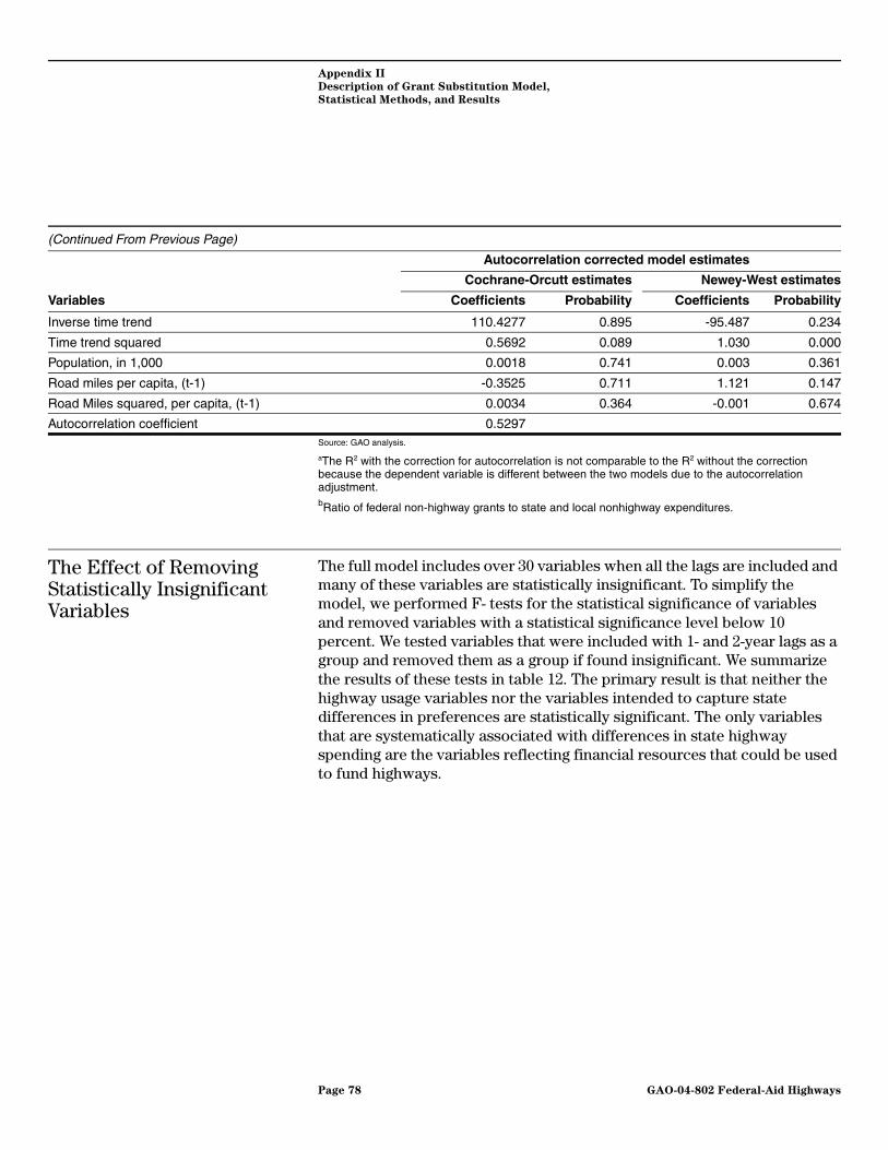
Appendix II




aThe R2 with the correction for autocorrelation is not comparable to the R2 without the correction because the dependent variable is different between the two models due to the autocorrelation adjustment.bRatio of federal non-highway grants to state and local nonhighway expenditures.

The Effect of Removing Statistically Insignificant Variables

The full model includes over 30 variables when all the lags are included and many of these variables are statistically insignificant. To simplify the model, we performed F- tests for the statistical significance of variables and removed variables with a statistical significance level below 10 percent. We tested variables that were included with 1- and 2-year lags as a group and removed them as a group if found insignificant. We summarize the results of these tests in table 12. The primary result is that neither the highway usage variables nor the variables intended to capture state differences in preferences are statistically significant. The only variables that are systematically associated with differences in state highway spending are the variables reflecting financial resources that could be used to fund highways.

Inverse time trend 110.4277 0.895 -95.487 0.234

Time trend squared 0.5692 0.089 1.030 0.000

Population, in 1,000 0.0018 0.741 0.003 0.361

Road miles per capita, (t-1) -0.3525 0.711 1.121 0.147

Road Miles squared, per capita, (t-1) 0.0034 0.364 -0.001 0.674



Variables

Autocorrelation corrected model estimates

Cochrane-Orcutt estimates Newey-West estimates

Coefficients Probability Coefficients Probability


Appendix II



Table 12: Summary Results of the Statistical Testing of the Variable Coefficients


aVehicle miles traveled per capita, registered vehicles per capita, and licensed drivers per capita.

The result of removing statistically insignificant variables is shown in table 13. With the Cochrane-Orcutt method for autocorrelation correction, the grant substitution coefficient is 0.50 and with the Newey-West correction the coefficient is 0.58; both estimates are statistically significant at the 1 percent significance level. Thus, the difference in estimated substitution rates under the two methods narrowed with the simplified model. To be conservative in our findings regarding grant substitution, we are using the lower estimate of 0.50, based on the Cochrane-Orcutt method, as our preferred estimate. The 95 percent confidence interval ranges from 12 to 88 percent, which includes Gamkhar’s estimate of 63 percent but not Knight’s higher estimate of 91 percent. Because the Cochrane-Orcutt method does not include the first observation for each state, these estimates are based on observations from 1983 through 2000.

Analysis of Remaining Explanatory Variables

The full model includes per capita income squared to test for nonlinear effects of income on state spending. However, the squared term is statistically insignificant. We conclude that state spending is proportional to income, which implies that both high- and low-income states respond to changes in income in roughly the same proportion, once other factors affecting state spending choices are taken into account. The lag structure on per capita income indicates that the largest increase occurs in the first

Variables testedStatistical results

F Statistic Probability

Personal income, all 3.6169 0.0000

Linear 2.5524 0.0545

Squared 1.1269 0.3373

Nonhighway grants, all 3.5888 0.0016

Amounts 2.3880 0.0677

Ratio 3.5081 0.0150

Use variablesa 0.8952 0.5447

Political preference 0.3476 0.7909

Time trend 4.3000 0.0050

Lane miles 1.3333 0.2642


Appendix II



year, but prior year changes in income also affect state expenditures (see table 13).

The effect of nonhighway grants enters into the model in two ways: the absolute size of other grant funding, measured in per capita terms, representing the income effect of other-grant funding; and the ratio of the nonhighway grants to state nonhighway spending, representing the tax price effect of other-grant funding. The net income effect of other grants is small but positive. The coefficients on the nonhighway grant variables sum to a small positive effect with a statistically significant positive effect in the current year and a statistically significant negative effect in year 2. This result is contrary to expectations in that the net effect would be expected to result in some of the funding from other federal grants to be used as a substitute for states’ own highway spending.

In contrast, the tax price effect of other grants is strongly negative indicating that matching requirements associated with other federal programs, such as Medicaid, result in states spending less of their own resources on highways. For every dollar spent by a state, the federal government reimburses the state for a percentage of the cost, reducing the tax price of these services to the state. The lower price for other public services raises the demand for those services and reduces the demand for highways, suggesting that highways and other public services are substitute goods.

We enter the time trend variable into the model in linear, quadratic, and inverse form to provide a flexible functional form. The inverse term was statistically insignificant and we dropped it from the model. The coefficients on the linear and quadratic term indicate a negative trend for most of the years in state highway spending when other factors affecting state spending are taken into account.

Varying Substitution Rates Over Time

As we noted in our summary of previous studies, Meyers reports no evidence of substitution into nonhighway spending during the 1976 to 1982 time period. Gamkhar, based on data from 1976 through 1990, reports higher rates of substitution, and Knight’s study, based on data from 1983 through 1997, reports even higher rates of substitution. We therefore tested for evidence of increasing substitution rates using the Cochran-Orcutt method, which, as discussed earlier, uses the estimation period 1983 to 2000. The results are shown in table 14.


Appendix II



Table 13: State Highway Spending Model with Statistically Insignificant Variables Removed


Model statistics R2



X – variables only 0.078


Autocorrelation Adjustment Method

Cochrane-Orcut Newey-West

Variables CoefficientsStandard

errorsProbability

values

95 Percent confidence

interval CoefficientsStandard

errorsProbability

values

FHWA highway grants, real per capita -0.501 0.194 0.010 -0.881 -0.121 -0.580 0.174 0.001

Personal income, real per capita, (t) 0.006 0.002 0.005 0.002 0.010 0.009 0.003 0.000

Personal income, real per capita, (t-1) 0.005 0.002 0.033 0.001 0.009 0.006 0.003 0.041

Personal income, real per capita, (t-2) 0.002 0.002 0.280 -0.002 0.006 0.001 0.002 0.652

Nonhighway federal grants, real per capita, (t) 0.115 0.040 0.004 0.037 0.193 0.064 0.046 0.168

Nonhighway federal grants, real per capita, (t-1) 0.044 0.049 0.370 -0.052 0.140 0.037 0.058 0.522

Nonhighway federal grants, real per capita, (t-2) -0.081 0.041 0.045 -0.161 -0.001 -0.036 0.047 0.445

Effective nonhighway grant match ratea, (t) -630.218 204.465 0.002 -1030.969 -229.467 -475.541 231.228 0.040

Effective nonhighway grant match rate, (t-1) -310.799 208.831 0.137 -720.108 98.510 -238.395 242.269 0.325

Effective nonhighway grant match rate, (t-2) 214.391 186.720 0.251 -151.580 580.362 -172.916 212.623 0.416

Utah Olympics, = 1 for 1997-2000, 0 otherwise 140.309 27.778 0.000 85.864 194.754 165.540 25.423 0.000

Time trend -17.804 5.107 0.000 -27.814 -7.794 -15.166 3.150 0.000

Time trend squared 0.570 0.162 0.000 0.252 0.888 0.461 0.098 0.000



Appendix II



aRatio of federal nonhighway grants to state and local nonhighway expenditures

To test whether the substitution rate has increased over the period of our sample data, we divided our sample into four time estimation periods, corresponding with the authorization periods for the federal-aid highway program.21

• 1983 to 1986,

• 1987 to 1990,

• 1991 to 1997, and

• 1998 to 2000.

Allowing the substitution rate to vary over time improves the explanatory power of the model, increasing the R2 of our preferred model from 48 percent to 57 percent. The first period from 1983 to 1986 shows a substitution rate of 18 percent that is not significantly different from zero. The estimated substitution rate increases to 36 percent in the 1987 to 1990 period and is significant at the 10 percent level. The substitution rate rises to just under 60 percent during the two periods of the 1990s and is statistically significant at the 1 percent level. As shown in Table 14, these results are roughly consistent with previous studies that, when taken together, seem to suggest increasing matching rates over time.

21As stated earlier, grant expenditures represent, in part, obligation authority provided in prior years.


Appendix II



Table 14: State Highway Spending Model with Substitution Rates by Time Period



When the substitution rate is allowed to vary over time, the time trend coefficients become statistically insignificant. This lack of significance suggests that there is no negative time trend in state spending once the increasing substitution rate associated with different time periods is taken into account.

We use an IV estimator because we assume federal grants and state spending are jointly determined. To test the reliability and validity of the IV estimator we ran three additional statistical tests: (1) a weak instruments

Model R2



X – variables only 0.145


Variables CoefficientsStandard

errorsProbability

values95 Percent confidence

interval

FHWA Grant, real per capita for 1983-1986. -0.178 0.198 0.370 -0.566 0.211

FHWA Grant, real per capita for 1987-1990. -0.360 0.195 0.065 -0.742 0.022

FHWA Grant, real per capita for 1991-1997. -0.592 0.190 0.002 -0.965 -0.22

FHWA Grant, real per capita for 1998-2000. -0.581 0.188 0.002 -0.95 -0.213

Personal income, real per capita, (t) 0.007 0.002 0.004 0.002 0.011

Personal income, real per capita, (t-1) 0.000 0.002 0.857 -0.004 0.005

Personal income, real per capita, (t-2) 0.004 0.002 0.067 0 0.007

Non-Hwy federal grants, real per capita, (t) 0.147 0.041 0.000 0.068 0.227

Non-Hwy federal grants real per capita, (t-1) 0.046 0.049 0.346 -0.05 0.142

Non-Hwy federal grants real per capita, (t-2) -0.084 0.041 0.039 -0.163 -0.004

Effective federal nonhighway-grant match ratea, (t) -756.328 204.332 0.000 -1156.819 -355.837

Effective federal nonhighway-grant match ratea, (t-1) -243.191 208.038 0.242 -650.945 164.563

Effective federal nonhighway-grant match ratea, (t-2) 241.691 188.098 0.199 -126.981 610.363

Utah Olympics, = 1 for 1997-2000, 0 otherwise 144.022 26.282 0.000 92.51 195.534

Time Trend -5.423 5.193 0.296 -15.602 4.756

Time Trend Squared 0.187 0.168 0.265 -0.142 0.516



Appendix II



test, (2) a test for exogeneity of excluded exogenous instruments, and (3) a test for endogeneity of federal grants.

The weak instruments test is intended to verify that the excluded exogenous instrumental variables included in the grants equation are correlated with federal grants. If they are not, the IV estimator provides no advantage to a simple (and more efficient) OLS estimator. To test the significance of the excluded exogenous variables, we calculated the partial R2 associated with the excluded exogenous instruments and found the instruments to be statistically significant at the 1 percent level.

To test for the exogeneity of excluded exogenous instruments, we conducted a Hausman over-identifying restrictions test.22 This test compares the estimated federal grant coefficients for each time period using the full set of excluded exogenous variables with coefficients derived from using a subset of instruments composed of predetermined variables that can safely be assumed to be exogenous. A finding that the set of grant coefficients from the two models are not statistically different from one another lends support for the hypothesis that the full set of excluded exogenous instruments are independent of the error term in the second stage expenditure equation. For this test, we used a subset of excluded exogenous variables. Differences between the grant coefficients for each time period using all instruments, and the coefficients using the subset of exogenous instruments, were not statistically significant and are quantitatively very similar to one another. Thus, we found no evidence that our excluded exogenous instruments were correlated with the error term of the expenditure equation.

Finally, we conducted a Hausman test for the endogeneity of the federal grant variable.23 This test consists of comparing the IV estimate of the grant coefficient for each time period with the corresponding grant coefficient based on the OLS estimate. If the differences were not statistically significant there would be little justification for using the IV estimator. This test yielded statistically significant differences between the two sets of estimates, lending support for the assumption that federal grants and state

22Jeffrey M. Woolridge, Econometric analysis of Cross-section and Panel Data, The MIT Press, Cambridge, Massachusetts, 2002.

23William H. Greene, Econometric Analysis, 5th Edition, Prentice Hall, New Jersey, 2003, pp. 80-81.


Appendix II



spending are jointly determined. The results of each of the three tests are summarized in table 15.

Table 15: Statistical Tests for the Endogeneity of Federal Grants and State Highway Spending


Additional Tests for Varying Substitution Rates

We also estimated alternative models that allow the substitution rate to vary according to state size (measured by population), per capita income, and state per capita spending on mass transit to test for a varying substitution rate related to these factors. The results of these models were negative. Overall we found no evidence that substitution rates systematically differ by either population size or the level of mass transit spending. We did obtain higher estimates of substitution rates in states with higher per capita income (56-66 percent in high income states compared to just over 30 percent in lower income states), but these differences were not statistically different from the average substitution rate of 50 percent found for the period from 1983 to 2000.

Weak instrument test Partial R2 Probability value

0.10 0.000

Grant coefficient

Hausman over-identifying restrictions test All instruments

Subset of instruments Probability value

’83-‘86 -0.178 -0.187 0.531

’87-‘90 -0.360 -0.366

’91-‘97 -0.592 -0.590

’98-‘00 -0.581 .581

Grant coefficient

Hausman endogeneity test 2SLS OLS Probability value

’83-‘86 -0.178 -0.047 .0001

’87-‘90 -0.360 -0.160

’91-‘97 -0.592 -0.340

’98-‘00 -0.582 -0.343


Appendix II



State Characteristics Associated with Fixed Effects

In the models reported above, state fixed effects account for most of the variation in state highway spending. Based on our preferred model (the model in table 12 using the Cochrane-Orcutt autocorrelation correction method), differences in state spending associated with these fixed effects can be as much as $400 per capita. However, these fixed effects are difficult to interpret since they represent all factors that are systematically related to cross-sectional differences in state spending not included in the model (e.g., geography, weather, and other variables that have substantial cross-sectional variation).

To determine if the differences in state spending measured by the fixed effects of our model are systematically associated with particular state characteristics, we performed a step-wise regression using the fixed effects from our preferred model as the dependent variable. Of the 12 variables we considered, 3 are statistically significant: per capita highway lane miles, per capita income, and heating degree days (see table 16). In the first step, lane miles account for 51 percent of the cross-state variation in our fixed effects, the second step equation added per capita income, and increases the explained variation to 68 percent. The third step equation adds heating degree-days, raising the variation explained to 77 percent. The remaining variables are statistically insignificant and provide little additional explanatory power.

Table 16: Stepwise Regression Analysis of the Fixed Effects


The positive coefficient on lane miles per capita may reflect a higher per capita cost of maintaining a larger highway network. The negative coefficient on per capita income suggests that, other things being equal, states with high average real incomes per capita spend less for highways than states with low average real incomes per capita. Finally, the positive coefficient on heating-degree days indicates that states in colder climates spend more on highways than states in warmer climates, all other things remaining equal.

Step Variables CoefficientProbability

value R2

1 Average lane miles per capita 0.58322 0.002 51%

2 Average real income per capita -0.01778 0.000 68%

3 Average heating degree days 0.01324 0.004 77%


Appendix III

State Characteristics Associated with States’ Level of Effort to Fund Highways from State Resources Appendix III

Based on our model of state highway spending, we found a number of factors that are systematically related to state highway spending and, in turn, a state’s level of effort to fund highway from state resources.1 Perhaps most importantly, more federal highway aid is associated with less state effort to fund highways from state resources once other factors related to state spending are taken into account. Our conservative estimate of grant substitution suggests that about half the increase in federal highway grants is used to reduce states’ level of highway spending effort.

Increases in federal grant funding for nonhighway purposes, such as health, education, and welfare, are also associated with reduced effort on the part of states to fund highways. Based on our model of state highway spending, we found that states with a higher percentage of their nonhighway spending funded by federal grants reduced their effort to fund highways, presumably, to provide matching funds for programs like Medicaid, which is an open-ended matching program.

In addition to federal grants, we found two cost factors that are systematically related to states’ levels of highway spending effort, other things being equal. States with large highway networks, as measured by the number of highway lane miles, systematically spend more per capita. Presumably, a larger road network is more expensive to maintain and states must therefore devote a larger share of their funding capacity to maintaining their highway network. In addition, we found that colder than average temperatures, as measured by heating degree days, are associated with higher state spending, suggesting that colder weather creates more wear and tear on the highways and hence the need for states to make a greater spending effort to maintain their highway network, other things being equal.

Finally, we found that high per capita income states make less effort than states with lower incomes. This result is, perhaps, not surprising since the same effective tax rate, (level of effort), generates more revenues in high-

1Since level of effort is defined as state spending relative to funding capacity, factors that are shown to be directly related to state spending are also directly related to a state’s level of effort. In an earlier report, GAO, Trends in Federal and State Capital Investment in

Highways, (GAO-03-744R, June 18, 2003), we reported considerable variation among states in the level of highway funding effort that persisted over the entire period of our study from 1982 through 2000. In addition, we reported wide movement in the states’ relative levels of effort over time. That is, some states making a low level of effort in the 1980s ranked above average in the 1990s and vice versa.



Appendix III

State Characteristics Associated with States’

Level of Effort to Fund Highways from State

Resources

income states than in states with lower incomes. Thus, the same level of highway spending can be funded with less effort in high-income states and low-income states compensate by undertaking a greater effort to fund highways from state resources.2

2The relationship between income and level of effort is complex. We found that low-income states make a greater level of effort to fund highway from state resources compared to higher income states. At the same time, there was no evidence of a difference in the spending response of high- and low-income states to a change in income, that is, the squared term from the substitution model was not statistically significant. In our model of state highway spending, we found that the fixed effect coefficients were negatively related to state per capita income, indicating that high-income states make less effort than states with lower income. In addition to the fixed effects, we also included per capita income and per capita income squared in our model to test whether the spending response to changes in income differed between high- and low-income states. As reported in appendix II we found no evidence of a differential response.


Appendix IV

Program Options Designed to Reduce Substitution Appendix IV

One program option that could be designed to reduce substitution would be to modify the matching requirement to leverage additional state highway spending. While the use of matching requirements as an economic tool is designed to leverage additional spending, the federal-aid highway program’s current matching requirements, which typically call for 20 percent state funding and 80 percent federal funding of eligible projects, permit substitution because most states’ highway funding is already higher than 20 percent of their total highway funds. The matching requirement, therefore, does not provide states with an incentive to increase or even maintain their level of funding in order to receive additional federal funds. Instead, states are free to substitute federal funds for funds they would have spent from their own resources and to use their own funds in other ways.

For the matching requirement to leverage additional state spending, the states’ matching portion would have to be set high enough so that states would not receive additional federal funds without spending beyond what they would have otherwise spent without additional federal assistance. This objective cannot be perfectly achieved because models of substitution, like any models, produce estimates that are subject to uncertainty, and there is no way to objectively determine with certainty what states would have spent in the absence of increased federal funding. However, the likelihood that increased federal funding will leverage additional state highway spending can be achieved in several ways.

Increase State Matching Requirements

The most direct approach would be to change the current 80 percent federal/20 percent state match ratio to a matching ratio closer to the 45 percent federal/55 percent state division of funding in fiscal year 2002. This would likely mean that some states (those whose spending is less than 60 percent of combined federal and state spending) would be required to increase their highway spending in order to qualify for any increased federal funding, while other states whose spending is already over 60 percent of combined federal and state spending would not have to increase or maintain their spending in order to receive increased federal funds.

Increasing the required state match from 20 percent to 60 percent might require a few states, whose state highway funding levels are currently a comparatively small proportion of their total highway spending, to more than double their current level of highway spending to avoid losing federal funds. If increases of this magnitude were deemed too extreme, a more moderate increase in the state match could be established. For example,


Appendix IV

Program Options Designed to Reduce

Substitution

raising the state matching share to 40 percent instead of 60 percent would require smaller funding increases in states whose state and local spending is currently a smaller proportion of the total highway spending, but it would also reduce the number of states that would be required to increase their level of funding in response to increased federal funding.

Another drawback of simply increasing state matching requirements is that even substantial increases in the requirements (raising the required state match from 20 percent to 60 percent) would not be likely to leverage additional state spending in all states. An alternative that would increase the likelihood of leveraging additional state spending in all states would be to continue with the 80 percent federal/20 percent state matching ratio but stipulate that only state spending in excess of what the state had spent for highways in an appropriate base time period be counted against its federal matching requirement. This approach has the advantage of maintaining the current 20 percent state matching rate, yet provides a leveraging incentive in all states rather than in only those states with below average spending. However, it might have the effect of making it easier for those states that were not spending much in the base time period to increase their spending and receive increased federal funds than it would be for those states whose spending was already high.

Modify Funding Formulas to Reward State Highway Funding Effort

Another approach that would reduce substitution by creating an incentive for states to increase their own highway spending would be to directly link the level of federal highway aid to each state’s level of highway funding effort. This link could be achieved by setting aside a fixed percentage of formula grant funding to be distributed in accordance with states’ highway funding efforts. As stated in the text, to avoid penalizing low income states, each state’s highway funding effort could be defined as the state’s highway spending compared to some measure of the state’s taxing capacity. There are a variety of indicators that could serve as a measure of states’ funding capacity. The most comprehensive that is available annually is Total Taxable Resources (TTR), which is produced annually by the Department of the Treasury and used to distribute substance and mental health block grants. Less comprehensive measures would include Gross State Product (GSP) and Personal Income (PI), both published annually by the Department of Commerce.

This approach could be implemented in a variety of ways. One approach would be to compare each state’s funding effort to the average effort of all states. If, for example, $100 per capita were set aside and distributed in this


Appendix IV


Substitution

way, states whose highway spending efforts were above the average spending effort would receive funding proportionally above the $100 per capita average and states whose effort was below the average spending effort would receive funding proportionally below the $100 per capita average.

Initially, those states with an above-average highway funding effort would be rewarded with higher per capita funding, and those states with a below-average highway funding effort would be penalized with lower per capita funding. In following years, each state’s highway spending effort would continue to be compared to the average state highway spending effort, so that states whose funding effort rose relative to the national average would automatically be rewarded with higher per capita funding, while states whose effort fell relative to the national average would automatically be penalized. Distributing the set aside in this fashion would, in effect, put all states in competition with one another, automatically rewarding states whose effort rose compared to the national average and penalizing states whose effort fell compared to the national average.

The approach just described would reward those states whose funding effort is currently high and penalize those whose effort is currently low. However, this approach could be modified to avoid rewarding or penalizing states based on their current level of effort. Instead, the linking of federal funds to state effort could be based only on future changes in each state’s level of highway funding effort. In this approach, each state’s highway funding effort would be compared to its own effort during an initial time period, such as the year (or an appropriate average of years) prior to initiation of the set aside. For example, all states could be awarded the same per capita grant amount in the first year of the set-aside program. Then, in future years, each state’s funding effort would be compared to its own funding effort in the first year of the set aside program and adjusted accordingly. Each state whose funding effort increased compared to the initial base year would receive an increase in federal funding proportionate to the increase in its own spending. Such an approach would, in effect, put


Appendix IV


Substitution

each state in competition with the effort it made in the base period.1 If both approaches to rewarding state highway funding effort were deemed desirable, a combination of the two approaches could be employed. The strength of the incentive would depend on the amount of total formula funding distributed through the set aside program; the greater the amount of funding distributed in this manner, the larger the financial consequences to states of changing their level of highway funding effort.

Introduce a State Maintenance of Effort Requirement

If, instead of seeking to stimulate additional state spending on highways, the goal of federal policy makers is for federal grants to supplement state spending on highways, then instituting a maintenance-of-effort (MOE) provision may be a more appropriate approach. MOE provisions require states to maintain existing levels of state spending on an aided program as a condition of receiving federal funds. As a tool, MOE requirements are designed not to stimulate additional state spending but to guard against grant substitution so that increased federal spending will supplement rather than replace states’ own spending.

As with matching requirements, this objective cannot be perfectly achieved because models of substitution, like any models, produce estimates that are subject to uncertainty and there is no way to objectively determine with certainty what states would have spent in the absence of increased federal funding. However, the likelihood that increased federal funding will not be used as a substitute for state spending can be strengthened if MOE requirements are designed appropriately. In previous work, we concluded that, to be effective, MOE provisions should define a minimum level of state spending effort that can be objectively quantified based on reasonably current expenditures on the aided activity. 2 Adjusting the MOE requirement for inflation in program costs would ensure the minimum spending level is maintained when measured in inflation adjusted dollars.

1To work in the way described here, funding for the set-aside program, as described in the text, would have to be adjusted annually to reflect the overall change in states’ funding effort. If states’ overall level of state effort remained unchanged from year-to-year, funding for the set-aside program would not have to change in order to ensure that states whose effort increased were rewarded and states whose effort declined were penalized. If, however, the overall average state effort increased, funding for the set-aside program would have to increase proportionally to ensure that all states with increased effort were rewarded and those with declining effort were penalized.

2GAO, Proposed Changes in Federal Matching and Maintenance of Effort Requirements

for State and Local Governments, GAO/GGD-81-7, December 23, 1980.


http://www.gao.gov/cgi-bin/getrpt?GAO/GGD-81-7

Appendix IV


Substitution

This could be achieved by defining a state’s base spending level as the amount spent per year during a recent historical period and then adjusting that base spending level for inflation.

One drawback of an MOE provision is that basing it on historical spending period could result in a base spending period for the MOE provision that represents an unusually high spending level for some states, effectively locking them into continued high spending in future years. This could be ameliorated however by establishing waivers for states that are able to demonstrate that spending in the base period chosen is unusually high, to allow a more “typical” spending level for purposes of the MOE provision.

Developing an indicator of state highway spending effort to link federal funding to state spending or establishing a state’s base spending level to design an MOE requirement would require careful consideration. Among other issues, in defining these indicators, consideration would have to be given to whether to measure:

• Capital expenditures for highways or capital plus maintenance spending;

• Expenditures on all state roads or for federal-aid roads only;

• State government expenditures only, or spending by state and local governments;

• Total expenditures, or expenditures normalized on a per capita, per lane mile, or other basis.

In addition, an indicator of state funding effort or a state’s base funding level for an MOE provision should, to the extent possible, be established by measuring spending levels that are typical rather than unusually high or low. Highway capital expenditures in a state can increase or decrease dramatically from year to year and may be unusually high or low for variety of reasons (e.g., Utah’s unusually high spending during preparations for the 2002 Winter Olympics, or a state particularly hard hit by recession that drops spending below its usual effort). To some extent, such factors can be taken into account by defining a state’s funding effort or base level of spending for an MOE provision using multi-year averages so that such unique circumstances are averaged out.


Appendix V

GAO Contacts and Staff Acknowledgments Appendix V

GAO Contacts JayEtta Z. Hecker (202) 512-2834 Steve Cohen (202) 512-4864 Jerry Fastrup (202) 512-7211

Staff Acknowledgments

In addition to those named above, Jay Cherlow, Catherine Colwell, Gregory Dybalski, Edda Emmanuelli-Perez, Scott Farrow, Donald Kittler, Alex Lawrence, Sara Ann Moessbauer, Robert Parker, Paul Posner, Teresa Renner, Stacey Thompson, and Alwynne Wilbur made key contributions to this report.

(544074)

GAO’s Mission The Government Accountability Office, the audit, evaluation and investigative arm of Congress, exists to support Congress in meeting its constitutional responsibilities and to help improve the performance and accountability of the federal government for the American people. GAO examines the use of public funds; evaluates federal programs and policies; and provides analyses, recommendations, and other assistance to help Congress make informed oversight, policy, and funding decisions. GAO’s commitment to good government is reflected in its core values of accountability, integrity, and reliability.

Obtaining Copies of GAO Reports and Testimony

The fastest and easiest way to obtain copies of GAO documents at no cost is through GAO’s Web site (www.gao.gov). Each weekday, GAO posts newly released reports, testimony, and correspondence on its Web site. To have GAO e-mail you a list of newly posted products every afternoon, go to www.gao.gov and select “Subscribe to Updates.”

Order by Mail or Phone The first copy of each printed report is free. Additional copies are $2 each. A check or money order should be made out to the Superintendent of Documents. GAO also accepts VISA and Mastercard. Orders for 100 or more copies mailed to a single address are discounted 25 percent. Orders should be sent to:

U.S. Government Accountability Office 441 G Street NW, Room LM Washington, D.C. 20548

To order by Phone: Voice: (202) 512-6000 TDD: (202) 512-2537 Fax: (202) 512-6061

To Report Fraud, Waste, and Abuse in Federal Programs

Contact:

Web site: www.gao.gov/fraudnet/fraudnet.htm E-mail: [email protected] Automated answering system: (800) 424-5454 or (202) 512-7470

Congressional Relations

Gloria Jarmon, Managing Director, [email protected] (202) 512-4400 U.S. Government Accountability Office, 441 G Street NW, Room 7125 Washington, D.C. 20548

Public Affairs Jeff Nelligan, Managing Director, [email protected] (202) 512-4800 U.S. Government Accountability Office, 441 G Street NW, Room 7149 Washington, D.C. 20548

United States Government Accountability Office Washington, D.C. 20548-0001

Official Business Penalty for Private Use $300

Address Service Requested

Presorted StandardPostage & Fees Paid

GAOPermit No. GI00

http://www.gao.gov

http://www.gao.gov

http://www.gao.gov

http://www.gao.gov

http://www.gao.gov