gao, yu (2016) statistical modelling of games. phd thesis
TRANSCRIPT
Statistical modelling of games
by
Yu Gao, MSci.
Thesis submitted to the University of Nottingham
for the degree of Doctor of Philosophy
July 2016

Abstract
This thesis mainly focuses on the statistical modelling of a selection of games,
namely, the minority game, the urn model and the Hawk-Dove game. Chapters
1 and 2 give a brief introduction and survey of the field. In Chapter 3, the key
characteristics of the minority game are reproduced. In addition, the minority
game is extended to include wealth distribution and leverage effect. By assuming
that each player has initial wealth which rises and falls according to profit and
loss, with the potential of borrowing and bankruptcy, we find that modelled wealth
distribution may be power law distributed and leverage increases the instability of
the system. In Chapter 4, to explore the effects of memory, we construct a model
where agents with memories of different lengths compete for finite resources. Using
analytical and numerical approaches, our research demonstrates that an instability
exists at a critical memory length; and players with different memory lengths are
able to compete with each other and achieve a state of co-existence. The analytical
solution is found to be connected to the well-known urn model. Additionally, our
findings reveal that the temperature is related to the agent’s memory. Due to its
general nature, this memory model could potentially be relevant for a variety of
other game models. In Chapter 5, our main finding is extended to the Hawk-Dove
game, by introducing the memory parameter to each agent playing the game. An
assumption is made that agents try to maximise their profits by learning from
past experiences, stored in their finite memories. We show that the analytical
results obtained from these two games are in agreement with the results from
our simulations. It is concluded that the instability occurs when agents’ memory
lengths reach the critical value. Finally, Chapter 6 provides some concluding
remarks and outlines some potential future work.
2

List of publications
Some of the results presented in this thesis are also published in the following
manuscripts:
Chapter 4:
1. James Burridge, Yu Gao, Yong Mao, Forgetfulness Can Help You Win Games,
Physical Review E 92, 032119 (2015).
Chapter 5:
2. James Burridge, Yu Gao, Yong Mao, Memory and Limit Cycles in the Hawk-
Dove Game, in preparation for European Physics Letters.
3

Acknowledgements
I acknowledge my studentship funding from the School of Physics and Astronomy.
I am grateful to my supervisor, Dr Yong Mao, from the School of Physics
and Astronomy and co-supervisor Dr James Burridge from the University of
Portsmouth. I am extremely thankful and indebted to them for their expertise,
guidance and encouragement. I have also benefited from valuable discussions with
Dr John Fry from the University of Sheffield.
I would like to take this opportunity to express gratitude to all faculty mem-
bers for their help and support. In particular, I am thankful for the IT support
from Philip Hawker, and LaTeX help from Siyuan Ji.
I want to offer my special thanks to my parents, grand-parents, and cousins
for their unceasing encouragement, support and attention. I am also grateful to
my wife Shuangqi who supported me throughout this journey. Her love is most
precious to me.
I also place on record, my sense of gratitude to one and all, who directly or
indirectly, have let their hands in this venture.
4
Contents
Abstract 2
List of publications 3
Acknowledgements 4
1 Introduction 13
1.1 Econophysics . . . . . . . . . . . . . . . . . . . . . . . . . . . . . . 13
1.2 Models of games . . . . . . . . . . . . . . . . . . . . . . . . . . . . 15
2 Review of models 17
2.1 The minority game . . . . . . . . . . . . . . . . . . . . . . . . . . . 17
2.2 Urn models . . . . . . . . . . . . . . . . . . . . . . . . . . . . . . . 20
2.2.1 Polya-Eggenberger model . . . . . . . . . . . . . . . . . . . 23
2.2.2 Stagewise linkage model . . . . . . . . . . . . . . . . . . . . 24
2.2.3 Urn transfer model . . . . . . . . . . . . . . . . . . . . . . . 25
2.2.4 Ehrenfest model . . . . . . . . . . . . . . . . . . . . . . . . . 25
2.2.5 Application of the urn model to social science . . . . . . . . 26
2.2.6 Application of the urn model in genetics . . . . . . . . . . . 27
2.3 The Hawk-Dove game . . . . . . . . . . . . . . . . . . . . . . . . . 29
2.3.1 Model definition . . . . . . . . . . . . . . . . . . . . . . . . . 30
2.3.2 Evolutionary stable strategy . . . . . . . . . . . . . . . . . . 31
2.3.3 Retaliator . . . . . . . . . . . . . . . . . . . . . . . . . . . . 32
5

3 The minority game and its extension 34
3.1 Mathematical formulations . . . . . . . . . . . . . . . . . . . . . . . 35
3.2 Results . . . . . . . . . . . . . . . . . . . . . . . . . . . . . . . . . . 38
3.2.1 Time evolution of attendance . . . . . . . . . . . . . . . . . 38
3.2.2 Volatility of the standard MG . . . . . . . . . . . . . . . . . 38
3.2.3 Information and frozen agents . . . . . . . . . . . . . . . . . 41
3.3 Wealth distribution . . . . . . . . . . . . . . . . . . . . . . . . . . . 42
3.3.1 Non-zero-sum case . . . . . . . . . . . . . . . . . . . . . . . 42
3.3.2 Zero-sum case . . . . . . . . . . . . . . . . . . . . . . . . . . 46
3.4 Leverage effect . . . . . . . . . . . . . . . . . . . . . . . . . . . . . 48
3.4.1 The leverage effect . . . . . . . . . . . . . . . . . . . . . . . 48
3.4.2 The bankruptcy rate vs. memory . . . . . . . . . . . . . . . 49
3.4.3 The bankruptcy rate vs. time steps . . . . . . . . . . . . . . 50
3.5 Appendix . . . . . . . . . . . . . . . . . . . . . . . . . . . . . . . . 52
4 New urn model 57
4.1 Model definition . . . . . . . . . . . . . . . . . . . . . . . . . . . . . 58
4.2 Simulation results . . . . . . . . . . . . . . . . . . . . . . . . . . . . 59
4.2.1 Instability . . . . . . . . . . . . . . . . . . . . . . . . . . . . 59
4.2.2 Coexistence . . . . . . . . . . . . . . . . . . . . . . . . . . . 61
4.3 Analysis . . . . . . . . . . . . . . . . . . . . . . . . . . . . . . . . . 63
4.3.1 Equilibrium . . . . . . . . . . . . . . . . . . . . . . . . . . . 63
4.3.2 Instability . . . . . . . . . . . . . . . . . . . . . . . . . . . . 66
4.4 Conclusion . . . . . . . . . . . . . . . . . . . . . . . . . . . . . . . . 69
4.5 Appendix . . . . . . . . . . . . . . . . . . . . . . . . . . . . . . . . 71
4.5.1 Alternative transition probabilities . . . . . . . . . . . . . . 71
4.5.2 Derivation of analytical solutions . . . . . . . . . . . . . . . 75
5 Memory and limit cycles in the Hawk-Dove game 87
5.1 Model definition . . . . . . . . . . . . . . . . . . . . . . . . . . . . . 88
6

5.2 Simulation results . . . . . . . . . . . . . . . . . . . . . . . . . . . . 90
5.3 Theory . . . . . . . . . . . . . . . . . . . . . . . . . . . . . . . . . . 92
5.3.1 Strategy optimization . . . . . . . . . . . . . . . . . . . . . . 92
5.3.2 Delay equation . . . . . . . . . . . . . . . . . . . . . . . . . 93
5.3.3 Linear stability analysis . . . . . . . . . . . . . . . . . . . . 93
5.3.4 Numerical tests of stability . . . . . . . . . . . . . . . . . . . 97
5.4 Conclusion . . . . . . . . . . . . . . . . . . . . . . . . . . . . . . . . 97
5.5 Appendix . . . . . . . . . . . . . . . . . . . . . . . . . . . . . . . . 98
5.5.1 The plots of equations (5.7), (5.8) and (5.9) . . . . . . . . . 98
5.5.2 The derivation of equation (5.16) . . . . . . . . . . . . . . . 100
5.5.3 The derivation of equation (5.25) . . . . . . . . . . . . . . . 102
6 Conclusion 104
7

List of Figures
3.1 Demonstration of the MG [139]. . . . . . . . . . . . . . . . . . . . 36
3.2 Time evolution of attendance for original MG. We assume the func-
tion g(x) = x, N = 301 and s = 2. From top to button, the
memories are set to the values of m = 2, 7 and 15 respectively. . . . 39
3.3 Volatility plot of standard MG. . . . . . . . . . . . . . . . . . . . . 40
3.4 Information H (open symbols) and fraction of frozen agents φ (full
symbols) as a function of the control parameter α = 2m/N for s = 2
and m = 5, 6, 7 (circles, squares and diamonds respectively). . . . . 41
3.5 An example of generated wealth distribution. . . . . . . . . . . . . 43
3.6 An example of generated wealth distribution without negative bins. 44
3.7 Values of calculated parameter b (N = 1001, repeats= 100). . . . . 47
3.8 Bankruptcy rates vs. memory lengths when t = 500. . . . . . . . . 49
3.9 Bankruptcy rates vs. time steps when m = 4. . . . . . . . . . . . . 50
3.10 The generated wealth distribution without negative bins where N =
10001, t = 2000. . . . . . . . . . . . . . . . . . . . . . . . . . . . . 52
3.11 The generated wealth distribution without negative bins where N =
10001, t = 3000. . . . . . . . . . . . . . . . . . . . . . . . . . . . . 52
3.12 Bankruptcy rates vs. memory lengths when t = 1000. . . . . . . . 53
3.13 Bankruptcy rates vs. memory lengths when t = 2000. . . . . . . . 53
3.14 Bankruptcy rates vs. memory lengths when t = 3000. . . . . . . . 54
3.15 Bankruptcy rates vs. memory lengths when t = 5000. . . . . . . . 54
3.16 Bankruptcy rates vs. time steps when m = 5. . . . . . . . . . . . . 55
8

3.17 Bankruptcy rates vs. time steps when m = 6. . . . . . . . . . . . . 55
3.18 Bankruptcy rates vs. time steps when m = 7. . . . . . . . . . . . . 56
3.19 Bankruptcy rates vs. time steps when m = 8. . . . . . . . . . . . . 56
4.1 Evolution of φt when n = 106, ω = 2, β = 5, ε = 10−6, and φ0 = 0.5.
Memory values are τ ∈ {5, 10, 50, 500} (squares, circles, dots, trian-
gles, respectively). Dashed lines are analytical equilibrium values
[see Equation (4.12)]. Critical memory is τc = 1.8× 10⁵. . . . . . . 60
4.2 Evolution of φt when n = 106, ω = 2, β = 5, ε = 10−3, and
φ0 = 0.5. Memory values are τ ∈ {5, 10, 50, 500} (squares, circles,
dots, triangles, respectively). Dashed lines is solution to Equation
(4.16) when τ = 500 and ω, β, ε are as above. Critical memory is
τc ≈ 390. . . . . . . . . . . . . . . . . . . . . . . . . . . . . . . . . . 60
4.3 Scaled populations pτ (t) := pτ1(t) + pτ2(t) for τ = 10 (circles) and
τ = 1000 (triangles) when total initial populations is n = 106, ε =
10−3, β = 5 with γ = 10−4 and δ = 2×10⁻⁴. Also shown (thin black
line) is evolution of variance of φt, over a moving time window of
105 steps, during population dynamics simulation. Straight dashed
line shows variance of homogeneous population with the same ε,
β, ω values at critical memory τc ≈ 390, where τc is calculated
analytically using the theory of Hopf bifurcation. Note: rapid initial
equilibration of population values (bringing birth and death into
balance) is not visible on time scale of plot. . . . . . . . . . . . . . 61
4.4 Estimated variance of φt in steady state, as a function of memory
length τ , from simulations with n = 106, ω = 2, β = 5 and ε = 10−3
(squares), 10−4 (dots), 10−5 (circles). Variance estimates computed
using time average over 106 time steps for ε ∈ {10−3, 10−4} and 107
time steps for ε = 10−5. Vertical black line marks theoretical Hopf
bifurcation point ετc = 0.39, computed from Equation (4.16). . . . . 68
9

4.5 Evolution of φt (fraction of agents in urn 1) using alternative tran-
sition probabilities when n = 106, ε = 10−3, ω = 2, and φ0 = 0.5.
Memory values are τ ∈ {5, 100, 1750} (open circles, dots, squares). . 72
4.6 Scaled populations pτ (t) := pτ1(t) + pτ2(t) for τ = 100 (circles) and
τ = 4000 (triangles) when the initial populations is n = 106 with
memory types in ratio short:long = 10 : 1. Parameters values are
ε = 10−3, γ = 10−4 and δ = 2× 10⁻⁴. Also shown (thin black line)
is evolution of variance of φt, over a moving time window of 105
steps, during population dynamics simulation. Note: rapid initial
equilibration of population values (bringing birth and death into
balance) is not visible on time scale of plot. . . . . . . . . . . . . . 73
4.7 Scaled populations pτ (t) := pτ1(t) + pτ2(t) in the original model with
step rates when inverse temperature β → ∞. Memory lengths are
τ = 10 (circles) and τ = 1000 (triangles) and the initial populations
is n = 106 with memory types in ratio short:long = 10 : 1. Param-
eters values are ε = 10−3, γ = 10−4 and δ = 2 × 10⁻⁴. Also shown
(thin black line) is evolution of variance of φt, over a moving time
window of 105 steps, during population dynamics simulation. Note:
rapid initial equilibration of population values (bringing birth and
death into balance) is not visible on time scale of plot. . . . . . . . 74
4.8 The difference plot when β = 1 and σ = 1. . . . . . . . . . . . . . . 77
4.9 The difference plot when β = 2 and σ = 3. . . . . . . . . . . . . . . 78
5.1 Domains in which either strategy is assessed to be optimal. . . . . . 88
5.2 Probability weights of hawk (circle) and dove (square) agents in
a group of size L = 10000 with V = 1, C = 1. All agents have
memory m = 100 and update rate ε = 6× 10⁻³. Dashed lines show
solutions to delay Equation (5.11) using the same parameter values. 90
10

5.3 Probability weights of hawk (pentagram) and dove (dot) agents in
a group of size L = 10000 with V = 1, C = 1 and t ∈ [1, 40].
All agents have memory m = 100 and update rate ε = 3 × 10⁻³.
Dashed lines show solutions to delay Equation (5.11) using the same
parameter values. . . . . . . . . . . . . . . . . . . . . . . . . . . . 90
5.4 Probability weights of hawk (pentagram) and dove (dot) agents in
a group of size L = 10000 with V = 1, C = 1 and t ∈ [160, 200].
All agents have memory m = 100 and update rate ε = 3 × 10⁻³.
Dashed lines show solutions to delay Equation (5.11) using the same
parameter values. . . . . . . . . . . . . . . . . . . . . . . . . . . . 91
5.5 The derivative ∂p/∂φ evaluated directly from Equation (5.10) at
φm = 1/2. The derivative is plotted using black dot. The blue line
shows corresponding expansion coefficients from Equation (5.16). . 94
5.6 Black line shows φ(t) from the numerical solutions to Equation
(5.11) in the symmetric case when m = 100 and ε = 5× 10⁻³. Blue
dashed line shows corresponding solution when ε = 7× 10⁻³. Open
black circles and open blue squares show corresponding simulation
results in a system of size L = 10000. . . . . . . . . . . . . . . . . 96
5.7 Dependence of the steady state amplitude of φ(t) on ε for m = 51
(light blue), m = 101 (blue) and m = 201 (black). L = 100 in all
cases. . . . . . . . . . . . . . . . . . . . . . . . . . . . . . . . . . . 96
5.8 The plot for f(n, φ) in Equation (5.8) against n and φ. . . . . . . . 98
5.9 The plot for f(h, φ) in Equation (5.8) against time t for an individ-
ual agent where m = 100, L = 10000, V = C = 1, ε = 3× 10⁻³. . . 98
5.10 The plot for p(φm) in Equation (5.9) against φ. . . . . . . . . . . . 99
5.11 The plot for p(φm) in Equation (5.9) against time t for an individual
agent where m = 100, L = 10000, V = C = 1, ε = 3× 10⁻³. . . . . 99
5.12 The plot for φm in Equation (5.7) against time t for an individual
agent where m = 100, L = 10000, V = C = 1, ε = 3× 10⁻³. . . . . 100
11

List of Tables
2.1 Generalised Polya-Eggenberger scheme [89]. . . . . . . . . . . . . . 23
3.1 Example of a strategy for the case of m = 3. . . . . . . . . . . . . . 36
3.2 Example of the value of parameter b with different numbers of time
steps. . . . . . . . . . . . . . . . . . . . . . . . . . . . . . . . . . . . 45
3.3 The average value of parameter b with different numbers of time
steps. . . . . . . . . . . . . . . . . . . . . . . . . . . . . . . . . . . 45
3.4 Example of the value of parameter b with different values of mem-
ories and time steps (zero-sum case). . . . . . . . . . . . . . . . . . 46
3.5 The average value of parameter b with different values of time steps
(zero-sum case). . . . . . . . . . . . . . . . . . . . . . . . . . . . . 47
3.6 Example of the value of parameter b with leverage effect. . . . . . . 48
3.7 The average value of parameter b with leverage effect. . . . . . . . . 48
12

Chapter 1
Introduction
1.1 Econophysics
The term ‘econophysics’ was first coined by Mantegna and Stanley [1] in 1996,
to describe the application of statistical physics to study economic and financial
systems. Specifically, concepts such as stochastic modelling and probability theory
have been fruitfully applied to economics, finance and social science [1, 2, 3, 4]. The
subject of econophysics has received much attention [5, 6, 7, 8], and subsequently
developed to such an extent that some has argued that it can be classified into two
broad categories, namely, the statistical and the phenomenological econophysics
[9]. Today, econophysics is often regarded as a subject in its own right, and
in recognition of its significance, many universities/institutions offer courses and
training programmes on econophysics [10].
A key strength of econophysics is that it offers a rigorous and quantitative
approach to understanding and analysing economic issues [11, 12]. Historically, its
most established contribution is in the area of complex correlations and financial
time series analyses [13, 14]. For example, the fluctuations and volatilities of
individual stocks are shown to be correlated, which can in turn help explain the
financial behaviour of the overall market [15]. As an example, Stanley et al. [16]
used a detrended fluctuation analysis (DFA) to quantify the correlations in their
13

analysis of S&P 500 data.
In econophysics, probabilistic method is a common approach to economics
and finance [17]. For example, Silva et al. [18] applied the Levy distribution to
investigate the multi-scale properties in foreign exchange rates. From the Levy
sections theorem, the relationship between the local volatility in foreign exchange
rates and fat tails in distribution can be explained [19].
The ubiquitous power law distribution in statistical physics also makes frequent
appearance in finance, e.g. in the time series of stock prices and exchange rates
[20, 21]. Econophysics attempts to relate pricing to equilibrium thermodynamics
[22, 23]. The economic system is extremely complex, but the statistics of the
market is often characterised by a power-law distribution [22]. Interestingly, the
two-power law function has been successfully applied to analyses of the distribution
of personal income as well as gross domestic production by using two different
exponents to fit high and low-to-middle regions respectively [24].
In recent years, it has become popular to regard econophysics as an interdis-
ciplinary research. According to the research by Fan et al. [25], econophysics is
interconnected with other fields as part of a network: this approach can explain
the rapid development of the subject of econophysics, and it is believed that the
network will continue to enhance its research and development. For example,
econophysics can be studied in connection with subjects like psychology, probabil-
ity theory and the theory of preference [26], and of course, econophysics can play a
vital role in society through economics and finance. For instance, Fry [27, 28, 29]
developed mathematical models to understand dramatic financial bubbles which
affect us all.
The past few decades saw a meteoric rise in the volumes traded in the financial
derivatives market, involving instruments such as the options. An option provides
its holder(s) with the right to buy or sell an underlying asset in the future, but
it is not compulsory to implement this agreed contract [30]. The Black-Scholes
formula, essentially a diffusion equation, has been hugely successful in pricing
14

options [31], though discrepancies exists, e.g. the option smile [32].
It is well known that the derivatives can lead to a significantly leveraged and
risky market. This leverage effect has been studied in order to explain the financial
crisis of 2008 [33, 34]. Although there is a huge trading volume in existing deriva-
tives, investors sometimes are unlikely to consider the worst possible scenario [35].
When traders employ new financial derivatives, they seem to pay less attention to
risks. The improvement of financial markets regulation is likely to keep the risks
at an acceptable range [36]. Academics and market participants need to analyse
potential risks with suitable methods [37]. Till now, research has largely focussed
on analysing those risks in the financial markets, especially for highly-leveraged
derivatives [38].
A well-constructed option game theory can offer an understanding of the uncer-
tainty in a competitive environment [39]. Option game theory can provide insights
into the financial markets, for example, levered firm’s equity can be regarded as
an option on the firm and priced by option pricing techniques [40, 41].
1.2 Models of games
Econophysics can become more productive and relevant when combined with sta-
tistical models of games, an example of which is the minority game. Whilst simple
in construction, the game captures the complex collective behaviour of a group
of agents competing for finite resources. The minority game has been studied
extensively with tools of statistical physics, and it has been suggested that the
game provides a basis for understanding broader financial markets [42, 43]. For
example, agents may cooperate to create a more resilient market, and develop a
particular wealth distribution [44, 45, 46]. In this thesis, we extend the minority
game by allowing agents to accumulate wealth through play, and borrowing and
bankruptcy are introduced. A key feature of the game model is the propagation
15

of information through time: the game memorises the past via wealth distribution
and strategy choice, but resets via bankruptcy.
The theme of memory is formally explored through two classes of models,
namely the statistical urn model and the Hawk-Dove model. We find that, when
competing in a game for finite resources, a long memory can help players to make
‘wiser’ choices by weeding out irrelevant noises, but too long a memory could lead
to large collective fluctuations resulting in limit cycles and instability. In those
situations, players with shorter memory could gain an advantage by adapting
faster to the changing environment, and thus players of different memories could
coexist in a dynamical equilibrium, characterised by a Hopf bifurcation [47]. Our
main findings with memory are general, and should be applicable to other game
models such as the rock-paper-scissors game [48, 49].
The rest of this thesis is structured as follows: Chapter 2 provides a focussed
review of the three models considered in this thesis: the minority game, the urn
model and the Hawk-Dove game. In Chapter 3, we present the minority game
with extension to the wealth distribution and the leverage effect. Chapter 4 offers
our variation of the urn model to explore the effectiveness of memory. In Chapter
5, we demonstrate how our findings from Chapter 4 are applied to the Hawk-Dove
game. In the final chapter, a conclusion is drawn, along with a description of the
limitations of the study and what further developments could be undertaken.
16

Chapter 2
Review of models
2.1 The minority game
Game theory models offer an alternative approach to finance, especially in areas
such as asset pricing and corporate finance [50, 51, 52]. For instance, models
can be used to understand the arrangement of dividend payments, firms capital
structure, market microstructure, etc [53]. More recently, game theory models
have been employed to study multifractality and turbulence found in financial
markets’ dynamics, e.g. logarithm stock price, absolute returns and transaction
volume [54, 55, 56]. Furthermore, the game theory model has been extended to
seek methods for stabilising the financial markets including the futures market [57].
Interestingly, some researchers have also attempted to predict the stock markets
using game theory models [58, 59]. For example, the minority game is one of the
most popular game models for market behaviour [60]. In contrast, the majority
game is dominated by the majority group. The mixed majority-minority game
can be used to model the market dynamics and traders strategies [61, 62, 63].
The minority game (MG) formulates the El Farol bar problem, in which a
group of people have to decide whether to go to the El Farol bar each night [64].
The capacity of the bar is limited, so that if the number of visitors exceeds its
capacity on a given night, these people will not enjoy their night out, in which
17

case, it would be better for them to stay at home. However, if the capacity is not
reached, all attendees share a positive experience. The minority rule governs this
problem. Everybody attending the bar expects that it will not be overcrowded,
but in reality, they will face one of two outcomes. Based on the knowledge of
previous attendance records and their individual strategies, people try to optimise
their next decision.
The El Farol bar problem was formulated and solved, providing insight into
some complex scenarios [65, 66, 67, 68]. Marsili, Challet and Zecchina’s work [69]
provided significant results in the attendance (price) dependence of each player.
Franke [70] also found a long-run equilibrium frequency distribution in addition
to the Nash equilibrium solutions. Furthermore, the El Farol bar problem with
externally ‘imposed comfort levels’ was explored [71]. In Lustosa and Cajueiro’s
study [72], previous work in this area was extended by offering players unparalleled
information to analyse arbitrage opportunities. The MG has also been utilised
in various fields, such as the financial markets. Therefore, it is instructive to
investigate the relation between the minority game and financial games [68].
In the MG, each of N agents has to make a choice between two strategies,
and the overall minority category wins. However, the agents are free to specialise
in a line of strategies, S [67]. Players can utilise the history of their previous
strategy performances to determine their future outcome. The following condi-
tions govern the game: firstly, the resources are scarce, and participating agents
cannot all win. Secondly, the behaviour of participants is determined by others’
behaviour. Thirdly, there is no classification of bad or good behaviour in the game.
Fourthly, prediction is possible but only through players’ experiences and choices
(strategies).
Traditionally, market and economics models utilise equilibrium ideology, the
assumption being that the players’ decisions in the financial market revolve around
two factors [73, 74, 75]. One factor is that markets are subject to external in-
fluences, such as incoming information relating to regulation change, business,
18

technological advances and political dealings. The quest for equilibrium in the fi-
nancial markets must cope with the fact that balance is often disturbed by external
factors. These models typically assume that markets would remain inherently sta-
ble even after large external shocks. The second factor is that the large number
of market participants (pursuing their individual interests) necessarily create a
fluctuating market, where decisions by key players may result in market prices
moving out of equilibrium. However, market activities such as arbitrage will en-
sure that fundamental values are more or less sustained in the long run. Challet
et al. [76, 77] used the MG to model the real market mechanisms by accounting
for roles of different agents.
The minority game can be interpreted in terms of buying and selling prefer-
ences. In the case of the buyer/seller, it is not possible to determine the day that
most clients would be buying or selling, and, therefore, the day chosen by a client
might turn out to be one when the market is over- or under- sold. In particular,
consider a new product in the market where N players are expected to participate
in either buying or selling of a specific commodity at time t. If the minority de-
cides to buy, then buyers gain an advantage [78]. Similarly, if the minority decides
to sell, they gain by obtaining a better price due to the excess demand.
The market scenario resembles the minority game to a degree. Interaction in
the market is not controlled by one factor or one strategy. The profitable strat-
egy is not independent of other strategies. After all, the winner is determined
by the other strategies in play. In particular, the minority game engages interre-
lated strategies [79]. Although buyer and seller strategies may move the price in
ways that will be an advantage to one or the other (minority or majority), the
market dynamics are also controlled by time t. Players who fall into the majority
category, say selling, may opt to change their strategies with time and join the
minority buyers [69]. Evidently, the market would fluctuate without any exter-
nal influence affecting it. The agents’ evolving strategies ultimately control the
market dynamics.
19

The strategy for optimising two choices can arise from trial-and-error learning.
It may require a player to have played the game for a considerable period to
successfully come up with a personal definitive strategy. If we use 1 and −1 to
represent the two choices available to a player, then a strategy is a particular way
of mapping from a sequence of M outcomes, represented by a string of 1’s and
−1’s, to a single number of 1 or −1 [67]. Each player may have a number of
available strategies to choose from, according to their historical performance. In
theory, each player will have to consider 2M of possible scenarios. We defer the
detailed formulation to Chapter 3.
2.2 Urn models
The statistical urn model consists of a number of urns containing different coloured
balls [80, 81]. Players pick up and add ball(s) from urn(s) each round according
to certain rules of play. The rules vary, leading to different types of urn models.
Following play, the distributions of different coloured balls and other statistics can
be analysed. The distributions can range from the discrete to the continuous, and
ultimately, urns and/or balls represent some real objects of interest, such as atoms
or people.
The basic Polya urn model has been heavily studied [82], and it consists of
only one urn, containing balls of two different colours, say white and black. Each
round, a player randomly selects a ball from the urn and returns it with an extra
ball of the same colour. As play continues, the number of balls increases, and
the number of white or black draws can be shown to settle into the beta-binomial
distribution. More recently, Chen and Kuba’s [83] derived the exact equations to
demonstrate the expected value and variance for the Polya model, together with
a new two-urn generalisation [84]. Mahmoud [85] investigated the relationship
between Polya urn models and random trees.
The Ehrenfest model is another popular type of urn model, first introduced to
20

the second law of thermodynamics. There are only two urns and N balls, which
are labelled from 1 to N . A ball is randomly selected and moved into the other urn.
It can be shown that when the system stabilises, the entropy reaches a maximum
[86]. Metzler et al. [87] studied this class of urn models with deterministic, time-
reversible conditions using different types of distributions, including hierarchical
and power-law ones. Prestipino [88] generalised the Ehrenfest model enabling it
to be used for energy considerations.
Many variations of the urn model exist [89]. For instance, we may insist that
different coloured balls are picked in the two consecutive rounds; it is also pos-
sible to temporarily neglect one or more urns [90, 91]. We can add balls of the
opposite colour to the urn if there are only two coloured balls. Or we do not have
to add back any balls at all. Another example is where the number of replace-
ment balls is a random variable generated by a specific distribution. We can also
increase the number of coloured balls in the urn to more than two. Godreche
and Luck [92] investigated the non-equilibrium dynamics of urn models, especially
the backgammon model and the zeta urn model. Prestipino [88] generalised the
Ehrenfest model to study an ideal gas, reproducing the Boltzmann entropy for-
mula (S = kB lnW ). In ideal gas, S is the entropy, W is number microstates
of system of gas particles, and kB is Boltzmann constant. In urn model, S is
corresponding entropy and W arises from the number of urns. The system can
lead to a stable state by using a stochastic urn model to analyse the probable
evolution of the system. In the paper by Buhot et al. [93], a generalised form
of urn model yielding non-constant number of particles was obtained and both
equilibrium and non-equilibrium dynamics were analysed using mean-field theory
which has the form of a diffusion-annihilation process and is accurate in describing
out-of-equilibrium dynamics in the low temperature regime. Randomness is a key
issue connected with urn models. Laruelle and Page [94] demonstrated its effi-
ciency when applying stochastic approximation to randomised urn models. The
combination of the urn model and the random partitioning model has been used
21

to explore the multiplicities of box occupancies [95].
The urn model, which can be classified into the Ehrenfest class and the Monkey
class, has been applied not only to physics, but also to economics. Different
from Ehrenfest class, which randomly chooses the ball initially, the Monkey class
will randomly choose the urn first. The equilibrium statistical properties of a
disordered urn model, including both classes, were studied by Jun-ichi Inoue and
Jun Ohkubo [96]. Interestingly, they found heavy-tailed power-law behaviour in
the occupation probability distribution. The arbitrary energy function was added
to the formula and a possible linkage to the macro economy was constructed [96].
The application of urn models extends to the social sciences [97, 98, 99, 100,
101, 102]. For example, a one-dimensional urn model can be applied to traffic
models and driven-diffusive systems. A generalised form for one class of zero-
range processes was achieved by Levine, Mukamel and Ziv [98]. As another exam-
ple, the relationship between Italian cities’ economical structure and population
distribution has been analysed in association with economic, historical, demo-
graphic and political considerations at national and regional levels [99]. In Tong
and Mahmoud’s paper [100], an Ehrenfest urn model was generalised to develop
an understanding of migration issues. Lambersona and Page [101] used an urn
model to model feedback from the markets. The urn model can be applied to
inventory distribution, products reproduction, frequency of seeing films, etc [101].
They built new theorem showing the relationship between second-order stochastic
dominance and expected market share [101]. In addition, a new model named
‘immigrated urn’ was proposed by Zhang et al. [102], which can be employed to
analyse the immigration process.
Urn models have also been applied to medical studies. A clinical trial using
an urn model with modification of the reinforcement scheme was constructed by
Aletti et al [103]. Their work presented the convergence theorem numerically.
Their goal was to help patients receive treatments more efficiently and effectively
[103].
22

2.2.1 Polya-Eggenberger model
To illustrate the mathematics involved, we choose the Polya-Eggenberger urn
model [104], which differs from the basic Polya model only in the exact crite-
ria for adding extra balls. We start with the basic Polya model of a single urn
containing balls with two colours (w white balls and b black balls). The replace-
ment rule is modified so that s of the same coloured balls will be added after each
discrete time step (s = 1 redueces to the basic Polya model). After n time steps,
the distribution of the number of black balls drawn is described by the following
equation.
P[k] =
(n
k
)b(b+ s)...{b+ (k − 1)s}w(w + s)...{w + (n− k − 1)s}
(b+ w)(b+ w + s)...{(b+ w) + (n− 1)s}, (2.1)
where k specifies the number of black balls drawn. For the special case s = 0, it
can be simplified to:
P[k] =
(n
k
)wk bn−k
(w + b)n(2.2)
which is the standard binomial distribution.
The generalized Polya-Eggenberger distribution is defined via the following re-
placement scheme in Table 2.1.
Colour of the chosen ball
White BlackNumber of balls White ωw ωbadded to the urn Black βw βb
Table 2.1: Generalised Polya-Eggenberger scheme [89].
According to Table 2.1, if we choose white at a particular time, there are ωw
white balls and βw black balls being added. Otherwise, we will add ωb white balls
and βb black balls. In both cases, the chosen ball will be returned to the urn as
well. Suppose after n rounds we have bn black balls and wn white balls, then the
23

above reasoning can be written as:
bn+1 = bn + Tnβb + (1− Tn)βw, (2.3)
where Tn is a random variable defined as:
P[Tn = 0] =wn
bn + wn, (2.4)
P[Tn = 1] =bn
bn + wn. (2.5)
Therefore, the expected value and variance can be found to be:
E[bn+1|bn, wn] = bn +bnβb + wnβwbn + wn
, (2.6)
var[bn+1|bn, wn] =(βb − βw)2bnwn
(bn + wn)2. (2.7)
Note βw = ωb = 0, βb = ωw corresponds to the Polya-Eggenberger model before
generalisation.
2.2.2 Stagewise linkage model
Another interesting variant of the urn model is the ‘stagewise linkage’ model [105].
Only one urn is used, and it is filled with n > 2 balls, labelled 1 to n. In each
round, a player picks out two balls. For example, in the first round, ball i and ball
j are picked up say, they are then individually labelled with both labels i and j
(so-called ‘linkage’), before being returned to the urn. Now two balls are doubly
labelled with both numbers i and j, and the remaining (n − 2) balls are singly
labelled. The game is played continuously, and all balls gain labels (links) until
they are all labelled 1 to n eventually. What is the minimum number of rounds
required to ensure all the balls have the same label? In other words, how long does
it take to make all balls labelled 1, 2, ..., n? It can be shown that the expected
24

number of drawings C satisfies:
(1− ε)n lnn < E[C] < (2 + ε)n(lnn)2 for all n ≥ N(ε), (2.8)
where ε� 1, denotes any positive constant; and N(ε)� 1, is an integer function
of ε. The linkage model is equivalent to the telephone model [106], where n people
each possessing a unique piece of news, and C random individual calls would be
required before they all know the news.
2.2.3 Urn transfer model
The earliest urn transfer model was introduced by Bernoulli in 1713 [107]. There
are two urns in this model, one of which contains k white balls and the other,
k black balls. In each round, one ball is drawn from urn 1 and returned to urn
2. Then one ball is drawn from urn 2 and returned to urn 1. This is a repeated
process. The general formula for the expected number of white balls in urn 1 is
given by:
Er =1
2k
{(k − 1
k + 1
)r+ 1
}. (2.9)
where k denotes the number of balls in each urn, and r represents the number of
balls have been drawn.
2.2.4 Ehrenfest model
The Ehrenfest urn model involves two urns [108]. Urn 1 contains k′ balls and urn
2 contains k′′ balls. The Ehrenfest urn model is equivalent to a Polya-Eggenberger
urn model if we express the system as a single urn model which contains k′ white
balls and k′′ black balls. We randomly select one ball in each round and replace
it with one in the opposite colour. According to Table 2.1 , this is the case when
ωw = βb = −1, ωb = βw = 1. The probability of having k white balls after n
25

rounds is defined as Pn(k) which can be written as:
k0Pn(k) = (k + 1)Pn−1(k + 1) + (k0 − k + 1)Pn−1(k − 1), (2.10)
where k0 = k′ + k′′ (the total number of balls) with initial conditions P0(k′) = 1,
and P0(k) = 0 for all (k 6= k′). When n → ∞, this distribution becomes a
binomial distribution.
The Ehrenfest urn model can be generalised by adding a probability parameter
p. Probability p describes the probability of changing the chosen ball with an
opposite coloured ball. The remaining probability is (1 − p), which refers to the
probability of returning the ball to the urn without changing its colour. The
distribution of the number of white balls after n rounds becomes:
k0Pn(k) = (k + 1)pPn−1(k + 1) + k0qPn−1(k) + (k0 − k + 1)pPn−1(k − 1), (2.11)
where q = 1− p. Note that the distribution does not depend on the probability p.
2.2.5 Application of the urn model to social science
In social science, issues such as analysing and interpreting social experiments can
be viewed as allocation problems [97], which consist of categories and objects. Urns
and balls can represent categories and objects respectively, thus the urn model has
been used to understand the relationship between lottery winnings and political
attitudes, the effect of voting costs on turnout [97]. Similarly, the urn model has
been applied decision making, reinforcement learning, technology usage, and other
statistics in our society [109].
Human populations can be divided according to geography (country, county,
city, area, street, etc), and similarly to race or social class. When sampling, it
is common to make a selection based on one criterion after another, a multistage
sampling process. Suppose a large urn represents the whole population; it contains
µ smaller urns each of which might contain even smaller urns, etc; eventually,
26

the lowest level urns contain balls representing people [89]. We could sample
the population via simple random sampling, or we could perform a multistage
sampling, but at each stage we have to weigh the probability of choosing an urn
by the number of people it and its subsidiary urns contain, a process known as the
probability proportional to size (PPS) sampling [110]. For simplicity, we consider
only one intermediate stage, so that our µ smaller urns contain ν1, ν2,..., νµ people
respectively. The selection rule is to choose m urns from the pool of µ urns and
select ni individuals from the ith urn if that urn has been chosen. The definition
of a ith urn sampling fraction is ni/νi. Let xi1, xi2, ..., xiνi be the numbers on the
νi balls in the i-th smaller urn, and these numbers represent the characteristics
of interest. We can estimate the characteristics of the entire population via the
following construction:
ξ =
µ∑i=1
νi∑j=1
xij =
µ∑i=1
νixi, (2.12)
where xi = ν−1i
∑νij=1 xij. The statistics of each stage of sampling can also be
formulated following this construction.
2.2.6 Application of the urn model in genetics
In genetics, different generations may be represented by urns and their correspond-
ing genes may be interpreted as balls, thus the urn model has been generalised
to topics ranging from the spread of infectious diseases, population dynamics, to
the biological evolutionary [111]. Limiting behaviour of Polya-like urn process has
been applied to population genetics by Hoppe [112]. In particular, the process of
coalescent, a retrospective trace back of genetic drift, is mapped to the urn model
in reverse time [112]. In Trieb’s work [113], a single urn model containing one
black and various numbers of other coloured balls is used to analyse coalescent.
The drawing of different coloured balls leads to the genetic variations of the next
generation, with the black ball representing a genetic mutation [113]. Another no-
table example in population genetics is the Wright-Fisher model (may be viewed
27

as a variation of the urn model) [111], which analyses how specific allele frequen-
cies in a finite population and their mating behaviour evolve over generations. It
helps geneticists to understand different factors contributing to the evolutionary
process.
In a simplified case, all balls in an urn represent the genes in a population. Each
colour denotes one type of a gene. We pay attention to genetics in the language
of urn models in two areas: the composition of the coloured balls in a sequence of
urns in each time step and the colour compositions of lots of balls drawn from one
urn. Suppose we have m genes in a generation of one population and each gene
has two types, A1 & A2. A single population consists of i type A1 and (m− i) type
A2 genes. Assume the genetic composition from parents is binomially distributed.
The probability of i genes of type A1 in the next generation is:
pij =
(m
j
)(i
m
)j (1− i
m
)m−j, (2.13)
where j is the number of balls in the second urn.
This can be explained in the context of urn models. Suppose we have a se-
quence of urns. The first urn consists of m coloured balls. The colour can be either
red or green. The second urn will be filled by the same coloured balls drawn from
the first urn until it reaches the number of m. We then calculate the probability
of j red balls in the second urn given that there are i red balls in the first urn.
This rule is continuously applicable in the next urn. This can be extended to the
concept of mutation if the next urn has a (1 − u) probability of being filled with
the same coloured ball. And the remaining probability of u fills the next urn with
an entirely new colour, where it indicates the appearance of a new property. In
addition to the applications elaborated in this study, the urn models can also be
applied to many other fields, such as the military, and in physiology and computer
science.
28

2.3 The Hawk-Dove game
We seek to connect the urn model to evolutionary game models [114]. The Hawk-
Dove game is first used to as a toy model to explore the implications. In the
real world, some species behave aggressively and fight for their allocated resource
maximisation. In contrast, the remaining groups possess a conservative attitude
and opt to minimise their potential incurred costs, such as injuries. The Hawk-
Dove game addresses this phenomenon mathematically. It was first introduced by
Smith and Price in 1973 [115, 116]. This game model assumes that there are only
two groups in the system. One group, namely ‘H’, representing ‘hawk’ players,
fights for allocated resources until they win or lose. The other group, called ‘D’,
denoting ‘dove’ players, avoids direct conflicts [117].
This simple game was initially used to explore the evolution of animal contest
behaviour [118, 119]. For example, Pham and Feng, who studied Asian carp in-
vasions, used a varied Hawk-Dove game model to establish simulations, aiming to
provide an efficient and low-cost method to solve the problem [120]. The appli-
cation of the Hawk-Dove game became popular not only in the field of biology,
but also in the measurement of reciprocity and fairness [121]. Additionally, it has
also been applied widely in modern economics and finance [122]. For instance,
the financial crisis of 2008 was analysed by Hanauske et al. using the Hawk-Dove
game in a quantum approach [122]. This study concluded that an evolutionary
stable strategy (ESS) can emerge, which could help mitigate future economic and
financial crises [122].
The basic Hawk-Dove game has been developed in a variety of forms for wider
applications. In 2008, Carlsson and Johansson proposed a development of the
Hawk-Dove game called the iterated Hawk-and-Dove game [123]. They noted
that the evolutionary Hawk-Dove game is a repeated game throughout history.
The iterated Hawk-and-Dove game was created to analyse the ESS [124]. The
two-stage Hawk-Dove game was mathematically written by Cressman [125]. It
emphasises the change of input in additional rounds in the game [125]. In social
29

science, the Hawk-Dove game can play a significant role in managing customer
expectation, in that it helps firms achieve a better financial performance and
create stronger values [126]. Moreover, the game itself can be used in political
science to investigate international relations [127]. Finally, it has been applied to
entrepreneurship in macro- and micro-economics [128].
2.3.1 Model definition
There are three situations in total: 1) hawk vs. hawk, 2) hawk vs. dove, and
3) dove vs. dove. In the first situation, each of the hawk strategy players has a
50% chance of winning the game. We assume there is V resource and the cost of
a flight is C. Therefore, the payoff in this situation is (V − C)/2. In the hawk
vs. dove situation, the payoff for the hawk is V and for the dove, 0. For the last
situation, the payoff for each dove strategy player is V/2. The result is given in
the following payoff matrix.
Hawk (H) Dove (D)H (V − C)/2 VD 0 V/2
where V > 0 and C > 0.
Suppose that we have a group of players with the same initial fitness of W0,
and p denotes the probability of players choosing a hawk strategy. Therefore, the
Hawk-and-Dove strategy players’ fitness can be expressed respectively:
W (H) = W0 + pE(H,H) + (1− p)E(H,D), (2.14)
W (D) = W0 + pE(D,H) + (1− p)E(D,D), (2.15)
where E(H,H) denotes the expected payoff when ’Hawk’ strategy player plays
against ’Hawk’ strategy player, E(H,D) demonstrates the expected payoff when
’Hawk’ strategy player plays against ’Dove’ strategy player, E(D,D) shows the
expected payoff when ’Dove’ strategy player plays against ’Dove’ strategy player.
30

Assume that the players reproduce their kind in proportion to their fitness.
The probability of a hawk player being in the next generation is:
p′ = pW (H)/W , (2.16)
where
W = pW (H) + (1− p)W (D). (2.17)
2.3.2 Evolutionary stable strategy
Now the dynamics of the game can be explored. Suppose we have a two-strategy
(strategies: I and J) game [115], the evolutionary stable strategy I for a two-
strategy game is satisfied by
W (I) = W0 + pE(I, I) + (1− p)E(I, J), (2.18)
W (J) = W0 + pE(J, I) + (1− p)E(J, J). (2.19)
If a population adopt evolutionary stable strategy I, this group cannot be invaded
by any other strategies. In other words, strategy I does better than J in two-
strategy game, i. e. W (I) > W (J). As J 6= I, either
E(I, J) > E(J, I), (2.20)
or
E(I, I) = E(J, I) and E(I, J) > E(J, J). (2.21)
In consideration of these conditions, the Hawk-Dove game’s evolutionary stable
strategy (ESS) can be found [129]. Because the payoff from dove against dove is
less than the payoff from hawk against dove, the dove strategy cannot be ESS.
If V > C, in other words, the cost of two hawks’ flights is relatively small, the
hawk strategy is pure ESS. Finally, the situation when V < C is considered. In
31

this case, the cost of fights is higher than the rewards. Players will use a hawk
strategy with probability p and a dove strategy with the probability (1− p). This
is known as the mixed ESS. The general form of probability p is calculated as:
p =(b− d)
(b+ c− a− d), (2.22)
with a generalised payoff matrix
I JI a bJ c d
2.3.3 Retaliator
When payoff values from the Hawk-Dove game are substituted, the probability of
p is equal to V/C. Then the ‘retaliator’ strategy, R, is introduced to the model
in order to demonstrate system behaviour with more than a two-strategy game.
When the R strategy player meets the hawk strategy player, the R strategy player
will use the hawk strategy. If a R strategy player meets the dove strategy player,
they will behave like a dove. The following payoff matrix illustrates the ideas.
H D RH −1 2 −1D 0 1 0.9R −1 1.1 1
Strategy R is an ESS, since E(R,R) > E(D,R) and E(R,R) > E(H,R). The
following calculations prove that the mixed strategy I = H/2 + D/2 is also an
ESS.
E(H, I) =1
2× (−1) +
1
2× 2 =
1
2, (2.23)
E(D, I) =1
2× 0 +
1
2× 1 =
1
2, (2.24)
32

E(R, I) =1
2× (−1) +
1
2× 1.1 = 0.05. (2.25)
Therefore, the system has two ESSs, I = H/2 +D/2 and R. Smith has concluded
that “a game with only two pure strategies always has at least one ESS; but if
there are three or more strategies, there may be no ESS” [114].
The Hawk-Dove game can be applied to social science such as: negotiation
skills, business strategy, management and cooperate social responsibility (CSR),
etc. [130, 131, 132]. For example, Garcıa et al. provided an analysis based on the
sequential Hawk-Dove game in order to improve the bargaining power [133]. Using
the game, it can provide company throughout ideas to survive in the competition
[134]. Additionally, the Hawk-Dove game is able to model the establishment of
property rights and laws [135, 136]. Furthermore, the Hawk-and-Dove strategy has
already been applied to the United Kingdom’s grocery market, where the sacrifice
of short-term profits can be defined as the ‘hawk’ strategy [137].
33
Chapter 3
The minority game and its
extension
In order to establish a robust and thorough understanding of the MG, we include
derivations and a series of generated graphs. The rules and logic of the MG are
extended to create the new model to be developed in the following sections.
We follow Challet and Zhang’s first formulation of the minority game of 1997
[65]. For simplicity, the number of participants is set to be odd; thus the minority
side can be identified without ambiguity. During the decision-making process,
each player has a finite set of strategies to engage with. Finally, each player’s
payoff is determined by the others’ choices.
The rest of this chapter is structured as follows. In Section 3.1, the mathe-
matical formulations of the MG are defined. In Section 3.2, major results from
the MG are listed. In Section 3.3 and 3.4, the wealth distribution and bankruptcy
rates are presented. The chapter ends with a brief conclusion.
34

3.1 Mathematical formulations
Suppose N players are engaged, where N is an odd number and each player has
S strategies in a game (S is a finite number). These players can only choose one
of two possible outcomes in each game, namely side ‘A’ or side ‘B’. This game
can be interpreted as the El Farol bar problem by setting side ‘A’ as ‘going to the
bar’. MG is played in discrete time, which equals number of times game is played.
ai(t) = 1, (3.1)
where ai(t) represents an individual participant’s decision at time t, i = 1, 2, ..., N .
Meanwhile, side ‘B’ represents ‘staying at home’
ai(t) = −1. (3.2)
Consequently, when we collect the actions of all the players, the overall action can
be expressed as
A(t) =N∑i=1
ai(t). (3.3)
Multiplying by individual decision with A(t), each of them has the payoff in a
mathematical form
Payoffi = −ai(t)g[A(t)], (3.4)
where g(x) is an odd function. Challet and Zhang initially chose g(x) = sign(x)
[65, 138]. However, this does not limit the choices of function g(x), some other
functions can also be applied to g(x) (e.g. g(x) = x/N).
All of the players make their decisions using inductive reasoning [139]. In other
words, players have finite limited memories for the record of past winning sides.
The letter m stands for the value of memory to be taken into consideration, which
means each player employs m historical records to make their decision in the next
game round.
35

According to the information of the last m winning group, there are a total
of P = 2m possible inputs for each strategy, which must predict an output (of 2
possible variations) for each of those inputs. Hence, the total number of possible
strategies is 22m . For example, when the value of memory is set to 3, the total
number of strategies is 256. The following table shows one possible strategy in
the case of m = 3.
Input Output
−1 −1 −1 +1
−1 −1 +1 −1
−1 +1 −1 +1
−1 +1 +1 −1
+1 −1 −1 +1
+1 −1 +1 +1
+1 +1 −1 −1
+1 +1 +1 −1
Table 3.1: Example of a strategy for the case of m = 3.
Figure 3.1: Demonstration of the MG [139].
Figure 3.1 illustrates the entire set-up of the classical minority game. The
36

logical flow starts from the top of the figure displaying a sequence of numbers
with values of 1 or −1. The values represent the record of the full set of the
historical winning group/side. Arrows below the historical data indicate that the
records of previous m winning groups flow into each player’s memory. According
to their strategies, players will then perform their preferred actions. The winning
group is established when all of the players have completed strategy selections,
and the payoffs for each player will be calculated. Finally, the historical winning
group is updated in a current time step.
We introduce the following vector formula
~ria = (−1,−1,+1,−1,−1,+1,−1,+1) (3.5)
to represent the a-th strategy belonging to the i-th player.
Then we use µ(t) to describe the set of possible strategies, where µ(t) ∈
{1, .., 2m}. Thus, each player’s decision within one particular time step comes
from one of its components. Recall that the entire set is expressed as {1, .., 2m}.
The changing of binary expressions of the historical winning group can be more
efficient (i.e. +1 → 1,−1 → 0). Using updated notations, µ(t) can be expressed
clearly. For instance, the original expressions for the historical data are given
by set {+1,−1,−1}. Corresponding to the latest notation, the historical data is
presented as {1, 0, 0}, where µ(t) = 5.
Additionally, the new vector ~I(t) is introduced. This vector has all other zero
components except the µ(t) component, which is 1. The product of ~I(t) and ~ria
provides the prediction of strategies. According to the example above, we obtain
the µ(t) = 5 and ~I(t) = (0, 0, 0, 0, 1, 0, 0). We assume that each player wants
to maximise their payoffs. They track the virtual total payoffs of their available
strategies:
pai (t+ 1) = pai (t)− ~ria~I(t)g[A(t)], (3.6)
where t shows time step and pai denotes the virtual total payoffs of the a-th strategy
37

of the i-th player, if it were used all the time. The minus sign arises from the payoffs
equation (3.4). The virtual payoffs are then used to rank strategies in terms of
their effectiveness, with the top ranking strategy being used for the next round.
If two or more strategies are ranked joint top, then a random choice of those is
made:
ai = ~riβi(t)~I(t), (3.7)
where βi(t) ∈ {1, ..., s} represents the best performing of strategies, and it may
vary with time steps.
In summary, we have described the basic formulation of the MG. In the fol-
lowing section, we reproduce some of the key results.
3.2 Results
3.2.1 Time evolution of attendance
Figure 3.2 shows some typical time evolution sequences of attendance for the
standard MG. This is generated by program MATLAB [140].
The first curve has the property of periodicity, which indicates that the function
has the relationship f(x) = f(x + T ), where T denotes the value of period. A
player with a long memory (compared to T ) could easily predict the outcome if
pitched against a group of such players. Compared to the first curve, the second
and third curves become less ‘predictable’, and the magnitudes of fluctuations also
vary greatly amongst the three scenarios.
3.2.2 Volatility of the standard MG
The analyses of Figure 3.2 in previous section show the importance of the magni-
tude and periodicity of the fluctuations. The volatility/variance plot the minority
game is key to characterising the behaviour of the system. The variance is defined
38

0 50 100 150 200 250 300 350 400 450 500A
(t)
-200
0
200
0 50 100 150 200 250 300 350 400 450 500
A(t
)
-50
0
50
t0 50 100 150 200 250 300 350 400 450 500
A(t
)
-100
0
100
Figure 3.2: Time evolution of attendance for original MG. We assume the functiong(x) = x, N = 301 and s = 2. From top to button, the memories are set to thevalues of m = 2, 7 and 15 respectively.
as:
σ2 = 〈[A(t)− 〈A(t)〉]2〉, (3.8)
where 〈...〉 devotes the time average, · · · presents an average over possible realisa-
tions of ~ria.
Since the magnitude of A(t) arises from the disparity of the winning and losing
groups, the value of σ indicates the size of the winning and losing group. A larger
σ implies that there is a smaller number of winners, and vice versa. Therefore,
it is essential to analyse the behaviour of σ. Different parameters, such as length
of memory of players’ strategy, m, and number of players’ accessible strategies, s,
are used to characterise σ2. Figure 3.3 plots the volatilities of the standard MG,
where N = 1001, t = 100000, s = 2, repeats= 100.
In Figure 3.3, different shapes of symbols represent different numbers of players
taking part in the MG (red circle: 51, green star: 101, blue plus: 201, black star:
301, up triangle: 501). It is interesting that the data generated from different
number of players collapse into a single curve. The values of the memory parameter
39

α=2m/N
10-3 10-2 10-1 100 101 102
σ2/N
10-1
100
101
102
N=51N=101N=201N=301N=501
Figure 3.3: Volatility plot of standard MG.
are set from 1 to 12. Initially, the volatility decreases sharply with an increasing
value of α. Volatility reaches its minimum value around α = 0.5, it begins to
increase and finally tends to 1 at larger values of α.
The random historical data does not affect the performance of variance as a
function of α. The critical value, that is, the minimum value of volatility has
practical implications. In the real world, if the volatility of the financial market
stays at or around the critical value, the whole market would become desirably
stabilised and create an investment environment with less risks. We assume that
the simulated minority game is consistent with the efficient market hypothesis,
which maintains that the resulting winning group (price) shown to each agent
reflects all information [141, 142].
40

3.2.3 Information and frozen agents
Extensive studies on the MG model have shown that the optimal strategy can be
determined [139]. The information is denoted by H, and the fraction of frozen
agents is demonstrated by φ.
Figure 3.4: Information H (open symbols) and fraction of frozen agents φ (fullsymbols) as a function of the control parameter α = 2m/N for s = 2 andm = 5, 6, 7(circles, squares and diamonds respectively).
The figure above displays the information content of the distribution and the
fraction of frozen agents [139]. These characteristics can be utilised to predict
an optimal future strategy. The parameter α facilitates the prediction of future
prices using past price records.
The data above show that a larger α is correlated with an increase in infor-
mation content [143]. However, the agent’s flexibility with strategies determines
the probability of catching on this pattern. Identifying the pattern requires a
large memory capability; therefore, few agents are able to identify these recurring
patterns for exploitation. Furthermore, the market may retain its level of unpre-
dictability if few agents are in play [143, 144, 145]. The recurrence of the pattern
depends on the diversity of the strategies utilised by the agents [146].
On the other hand, a smaller α is likely to change the game. According to
41

Savit et al., the probability of landing into the winning pattern becomes low at
this point [147]. With a large α, the pattern is bound to appear on several agents’
plans, making identification likely. In this case, however, the pattern is likely to
appear in one agent’s range of strategies. However, the prediction of future prices
is likely to be difficult in reality due to transaction costs.
3.3 Wealth distribution
3.3.1 Non-zero-sum case
The linkage between the MG and wealth distribution is explored in this section.
The assumption of odd player numbers is retained. The initial total wealth of par-
ticipants is set to a constant, and it could be any positive finite number (e.g. £100).
This assumption can be relaxed in the later work using a number of methods, for
instance, generating an initial wealth distribution for all players.
At the preliminary stage, the program simulates artificial data for the historical
winning group. The players follow the rules in the standard MG to play the game
in each round. For simplicity, the number of strategies, s, is set to the value of 2,
and can be increased in the future. In the second step, the updated process for
wealth will be added to the standard MG. The decision from each player at each
round will be recorded.
Each participant chooses the most profitable strategy from the available strate-
gies in order to maximise its own profits. We keep track of the change of wealth
for all participants, which is described below. Each winning player gains 1 unit of
wealth, and the rest lose 1 at each time step.
This method fundamentally assumes the equality of all players. This assump-
tion can also be relaxed by adding payoff equations, organising the payoffs to each
player after each round.
Figure 3.5 shows an example of artificial wealth distribution. In this figure,
N = 101, m = 3 and t = 1000. The program generates a series of wealth distri-
42

Wealth Ranges-400 -300 -200 -100 0 100 200 300 400 500
No
. o
f P
laye
rs
0
2
4
6
8
10
12
14
16
18The Generated Wealth Distribution (Std MG)
Figure 3.5: An example of generated wealth distribution.
butions using various values of time steps. However, the distribution generated in
this fashion never truly stabilises. This is caused by the decrease in the sum of
players’ wealth: since only minority wins each time step, the total wealth of the
group is not conserved. The distribution eventually contains increasing number of
negative-value bins, indicating that the system allows players to continue playing
the game even when their wealth is negative.
However, in the real world, investors must attract external resources to con-
tinue participating in the game when they are facing the risk of bankruptcy. Oth-
erwise, they have to leave the market with losses. In order to make the statistical
model more realistic, the study assumes that an equal number of new investors
will come to the market with the same amount of initial wealth if any existing
investors go bankruptcy.
The wealth distribution generated by the updated model no longer contains
negative values, and the total number of players remains the same as the initial
odd number throughout the game because the number of inflow players equals the
number of outflow players. Thus, the system might be in a stable condition. The
following figure shows the newly generated wealth distribution histograms.
Figure 3.6 is an example of non-negative wealth distribution (T = 1000). It
43

Wealth Ranges0 50 100 150 200 250 300 350 400 450 500
No.
of P
laye
rs
0
500
1000
1500
2000
2500The Generated Wealth Distribution (Std MG)
Figure 3.6: An example of generated wealth distribution without negative bins.
evidently contains no negative bins in the histograms, as we replace the bankruptcy
players with fresh ones. However, the distributions from different program runs
do not achieve a stationary state, continuing to evolve slowly with time. Figures
3.10 and 3.11 in the appendix demonstrate the cases that at very large time steps
(T = 2000 and T = 3000 respectively), the distribution broadens with a sharp
peak near the origin representing the fresh injection of players. Leaving aside the
peak near the origin, we have been able to use the following equation to perform
curve fitting on the generated wealth distributions.
f(x) = ax−b, (3.9)
where a, b are both non-zero constants.
The confidence bounds are set to 95% as default. Table 3.2 below shows the results
from different runs.
44

N m T The value of parameter b
10001 3 2000 0.7559 0.7891 0.6694 0.5392 0.5263
10001 3 3000 0.8225 1.0390 0.7848 0.8448 0.8765
10001 3 4000 1.1150 0.9688 0.9983 1.0220 1.0110
Table 3.2: Example of the value of parameter b with different numbers of timesteps.
According to Table 3.2, the value of power parameter, b, increases as the time step
increases. Table 3.3 shows the average value of power from different runs with the
same parameters’ values.
N m T b
10001 3 2000 0.6598± 0.1007
10001 3 3000 0.8543± 0.0870
10001 3 4000 1.0224± 0.0493
Table 3.3: The average value of parameter b with different numbers of time steps.
The standard deviation is relatively small compared to the value of power.
However, the value of power still increases as time steps increase, indicating that
the wealth distribution within the system continues to evolve. The following sec-
tion suggests a method that potentially reduces this effect.
45

3.3.2 Zero-sum case
Recall that the wealth distribution from the standard MG is unstable due to the
system’s decreasing wealth. Increasing the system’s wealth by introducing new
players does not give rise to a stationary distribution either. Next, the system is
adjusted to the zero-sum case.
A new option is added in order to achieve the zero-sum: the payoffs are scaled
so that at each time step the gain made by the winners cancels exactly the loss
made by the losers. In addition, if the wealth of any of the players decreases to zero,
this(these) player(s) can borrow the initial wealth from other players repeatedly.
The contributions from other players are proportional to their existing wealth.
Then the modified model could be understood as a type of ‘self-financing’ system
where there are either no external outflows or cash inflows [148].
As before, curve fitting is performed for the generated wealth distribution.
Repeatedly, the system generates values of parameter b. The results are presented
in Table 3.4.
N m T The Value of Parameter b
10001 3 2000 0.7135 0.8974 0.6696 0.5522 0.7559
10001 3 3000 0.8454 0.8717 0.8163 0.9425 0.9965
10001 3 4000 0.9316 1.0200 1.0610 1.0500 0.9842
10001 4 3000 0.6717 0.6604 0.5906 0.6688 0.6454
10001 4 4000 0.7342 0.7678 0.6851 0.8358 0.5758
10001 4 5000 1.0590 0.7585 0.9906 1.0040 0.8524
Table 3.4: Example of the value of parameter b with different values of memoriesand time steps (zero-sum case).
Table 3.5 lists the average values of power with different memories and time
steps.
46

N m T b
10001 3 2000 0.7177± 0.1260
10001 3 3000 0.8945± 0.0737
10001 3 4000 1.0094± 0.0527
10001 4 3000 0.6474± 0.0333
10001 4 3000 0.7197± 0.0973
10001 4 5000 0.9329± 0.1237
Table 3.5: The average value of parameter b with different values of time steps(zero-sum case).
Time Steps×104
0 1 2 3 4 5 6 7 8 9 10
Va
lue
s o
f P
ow
er
2
2.5
3
3.5
4
4.5
5Values of Power against Time Steps
Figure 3.7: Values of calculated parameter b (N = 1001, repeats= 100).
Figure 3.7 represents the values of power from the fitting curves (red: m = 3,
blue: m = 4, green: m = 5). As the figure illustrates, the appear to asymptote,
but within the time and computational resources available, the system did not
completely stabilise. The results obtained from zero-sum processes appear to
improve on those from non-zero-sum processes, but the results are not deemed
consistent enough for publication. This remains an area of possible future work.
47

3.4 Leverage effect
3.4.1 The leverage effect
Previously, the assumption was made that every player play had the same stake at
each time step. With consideration of leverage products in the financial markets,
we relax this assumption in this section. We introduce the double bet situation
when a player loses the previous game. It offers the chance to potentially double
their payoffs and win back losses. Table 3.6 presents the fitted values of power
after this modification.
N m T The Value of Parameter b
10001 3 2000 1.427 1.252 1.267 1.393 1.606
10001 3 3000 2.103 3.594 2.308 2.148 2.345
10001 4 4000 2.206 1.265 2.033 1.548 2.210
Table 3.6: Example of the value of parameter b with leverage effect.
The values of parameter b range from 1.3 to 2.2. The following table shows the
average value of power for each scenario when the leverage effect is introduced.
N m T b
10001 3 2000 1.3890± 0.1434
10001 3 3000 2.4996± 0.6203
10001 4 4000 1.8522± 0.4250
Table 3.7: The average value of parameter b with leverage effect.
We see that changing the time step from 2000 to 3000 whilst keeping the
memory as a constant, lead to a significant change of power. The leverage effect
generally destabilises the system, which is confirmed by increased bankruptcy rates
presented in the the next section. As risk theory states [149], the higher the risk
is, the more profit one can gain. A leveraged product may create increased profits,
but it may also lead to larger losses for investors.
48
3.4.2 The bankruptcy rate vs. memory
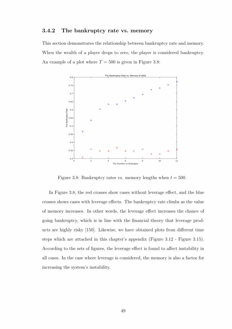
This section demonstrates the relationship between bankruptcy rate and memory.
When the wealth of a player drops to zero, the player is considered bankruptcy.
An example of a plot where T = 500 is given in Figure 3.8:
The Number of Strategies0 2 4 6 8 10 12
The
Ban
krup
tcy
Rat
e
0.3
0.35
0.4
0.45
0.5
0.55
0.6
0.65
0.7
0.75
0.8The Bankruptcy Rate vs. Memory (t=500)
Figure 3.8: Bankruptcy rates vs. memory lengths when t = 500.
In Figure 3.8, the red crosses show cases without leverage effect, and the blue
crosses shows cases with leverage effects. The bankruptcy rate climbs as the value
of memory increases. In other words, the leverage effect increases the chance of
going bankruptcy, which is in line with the financial theory that leverage prod-
ucts are highly risky [150]. Likewise, we have obtained plots from different time
steps which are attached in this chapter’s appendix (Figure 3.12 - Figure 3.15).
According to the sets of figures, the leverage effect is found to affect instability in
all cases. In the case where leverage is considered, the memory is also a factor for
increasing the system’s instability.
49

3.4.3 The bankruptcy rate vs. time steps
This section investigates the relationship between the bankruptcy rate and time
steps. The memory is kept as a constant for each run of the program. An example
is given in the following figure:
Figure 3.9: Bankruptcy rates vs. time steps when m = 4.
Figure 3.9 shows the relationship between bankruptcy rate and time steps
(m = 4). The blue curve indicates cases with a leverage effect and the red curve
indicates cases without a leverage effect. The leverage effect makes the player
go bankruptcy quicker and also leads to more players going bankruptcy. The
bankruptcy rate jumps when time increases, which refers to the ‘cluster effect’
[151]. As a result, one or some players’ losses might affect other players.
Additional curves have been generated with different parameter values indi-
cating similar patterns, which are attached in this chapter’s appendix (Figure
3.16 - Figure 3.19). A proper risk analysis seems appropriate before investing in
leveraged products.
The MG has drawn the attention of many researchers’ attention and has been
a popular research topic in recent years. In our study, we have extended the MG
50

to explore the wealth distribution and the leverage effect. We have found that
leverage could dramatically increase the system’s instability, which implies that
in the real financial market, the risks of trading leveraged products should not be
under-estimated. The statistics of our simulation did not reach the high standard
for publication, but we believe our effort offers a basis for exploring broader issues
of financial stability and market regulations. This area clearly merits further
research work.
51

3.5 Appendix
The following section presents the figures generated from different parameter val-
ues. Firstly, the wealth distribution is generated by using two different time steps,
t = 2000 and t = 3000.
Wealth Ranges0 100 200 300 400 500 600 700
No.
of P
laye
rs
0
5
10
15
20
25
30
35The Generated Wealth Distribution (Non-Negative Bins)
Figure 3.10: The generated wealth distribution without negative bins where N =10001, t = 2000.
Wealth Ranges0 100 200 300 400 500 600 700 800 900 1000
No.
of P
laye
rs
0
5
10
15
20
25
30
35
40
45The Generated Wealth Distribution (Non-Negative Bins)
Figure 3.11: The generated wealth distribution without negative bins where N =10001, t = 3000.
These generated wealth distributions indicate that they may be fitted by power
52

law distribution. Then the plots of bankruptcy rates against memory lengths are
shown.
The Value of Memory0 2 4 6 8 10 12
The
Ban
krup
tcy
Rat
e
0.4
0.45
0.5
0.55
0.6
0.65
0.7
0.75
0.8
0.85
0.9The Bankruptcy Rate vs. Memory (t=1000)
Figure 3.12: Bankruptcy rates vs. memory lengths when t = 1000.
The Value of Memory0 2 4 6 8 10 12
The
Ban
krup
tcy
Rat
e
0.4
0.45
0.5
0.55
0.6
0.65
0.7
0.75
0.8
0.85The Bankruptcy Rate vs. Memory (t=2000)
Figure 3.13: Bankruptcy rates vs. memory lengths when t = 2000.
53

The Value of Memory0 2 4 6 8 10 12
The
Ban
krup
tcy
Rat
e
0.35
0.4
0.45
0.5
0.55
0.6
0.65
0.7
0.75
0.8
0.85The Bankruptcy Rate vs. Memory (t=3000)
Figure 3.14: Bankruptcy rates vs. memory lengths when t = 3000.
The Value of Memory0 2 4 6 8 10 12
The
Ban
krup
tcy
Rat
e
0.3
0.4
0.5
0.6
0.7
0.8
0.9The Bankruptcy Rate vs. Memory (t=5000)
Figure 3.15: Bankruptcy rates vs. memory lengths when t = 5000.
These four generated figures follow similar patterns. It agrees that the leverage
effect increases risk. Finally, we present the plots for bankruptcy rates against time
steps using different agents’ memory lengths.
54

Figure 3.16: Bankruptcy rates vs. time steps when m = 5.
Figure 3.17: Bankruptcy rates vs. time steps when m = 6.
55

Figure 3.18: Bankruptcy rates vs. time steps when m = 7.
Figure 3.19: Bankruptcy rates vs. time steps when m = 8.
56

Chapter 4
New urn model
This chapter demonstrates how a model is built to illustrate the effectiveness of
memory. Agents, in this model, have different memory lengths and compete for
finite resources. Using analytical and numerical approaches, the research demon-
strates that instability exists at a critical memory length; hence, players with
different memory lengths are able to compete with each other and achieve a state
of co-existence. The analytical solution is found to be connected to the urn mod-
els. Additionally, the findings also demonstrate that the temperature introduced
in the urn model is mirrored by the agent’s memory. This simple model could
potentially be applied to a variety of other game models, where an example is
investigated in the next chapter.
The rest of this chapter is structured as follows. In Section 4.1, the model is
defined. In Section 4.2, simulation results are presented followed by theoretical
analysis in Section 4.3. Finally, a conclusion is drawn, along with a brief discussion
on the limitations of the study and potential future work.
57

4.1 Model definition
The case of two urns and a total of n agents is considered. The urns yield U1(t)
and U2(t), where they are random variables uniformly distributed on [0, ωn] and
[0, n], at round t respectively. ω is a parameter we set, ω > 1, so that urn 1
yields more on average than urn 2. This choice of yield distribution is motivated
by simplicity-only one extra model parameter, ω, is required to describe it. The
behaviour of the model is not tied to the particular choice of yield distribution; it
requires only that the yields have finite variance, allowing the central limit theorem
[152] to be applied to sums of payoffs. At time t, agents’ access to the arithmetic
mean of the last τ payoffs is allowed, however other forms of sampling could also
be used. Letting φt be the fraction of agents in urn 1, then the difference in the
average payoffs between urn 1 and urn 2 is
∆t :=1
τ
τ−1∑s=0
[U2(t− s)n(1− φt−s)
− U1(t− s)nφt−s
], (4.1)
where τ is refereed as the “memory length” of the agents. Agent dynamics is
encoded in transition probabilities between urns, which are deterministic functions
of ∆t. At each round, each agent will switch urns using the probabilities
W1→2(∆) =ε
2[1 + tanh(β∆)], (4.2)
W2→1(∆) =ε
2[1− tanh(β∆)]. (4.3)
These transitions are used in evolutionary game models, where changes in
strategy are made based upon perceived increases in payoff, but with some degree
of noise or irrationality in the switching process. The level of this stochasticity
in decision making, which has been experimentally measured in humans [153] is
captured by the parameter β, the “inverse temperature”. For finite β, agents may
decide to switch strategies even though their estimate of the payoff difference is
58

unfavourable. In the limit β → ∞, agents will only move if their estimate of the
payoff difference indicates that the move is favourable. The parameter ε controls
the rate at which strategy switching takes place compared to the rate at which
yield information arrives, or equivalently the inertia in agent’s decision making.
It may also be seen as the frequency with which opportunities to switch strategy
arise. In the limit ε → 1, at most one agent will move at each round. The
effects which we uncover do not require that the transition probabilities take the
particular forms of Equations (4.2) and (4.3). In Section 4.5.1, we show that the
same qualitative behaviour is observed for transition probabilities that increase in
proportion with the perceived payoff difference (±∆), provided the difference is
positive and |∆| < ε−1.
4.2 Simulation results
4.2.1 Instability
The model for a series of values of τ when n = 106 is simulated. Two different
values of ε are used; in Figure 4.1, we have ε−1 = 106 � τ and in Figure 4.2,
ε = 10−3 is set. For ε = 10−6, the expected number of moves at each step
is < 1, and φ appears very stable. For larger ε, φ experiences much larger
fluctuations about the steady-state value, driven by the yield process. For shorter
memory values these fluctuations are random, but as τ approaches ε−1, periodic
oscillations appear and dominate. The appearance of these stable oscillations at
critical memory, τc, calculated analytically in Section 4.3, is known as a Hopf
bifurcation [47]. The bifurcation parameter is memory, which is a combination of
ε and τ , whilst simulations are shown for different ε and same τ , analysis will be
performed assuming varying τ with ε fixed. From Figures 4.1 and 4.2, the number
of rounds taken for the system to evolve to steady state have been observed,
in the probabilistic sense, starting from an equal distribution between the two
urns, is ≈ ε−1. By allowing agents to access only to the mean of their memory,
59

we implicitly assume that changes in the expected payoff over the course of their
memory, brought about by oscillations, are too subtle for them to infer from noise.
Figure 4.1: Evolution of φt when n = 106, ω = 2, β = 5, ε = 10−6, and φ0 = 0.5.Memory values are τ ∈ {5, 10, 50, 500} (squares, circles, dots, triangles, respec-tively). Dashed lines are analytical equilibrium values [see Equation (4.12)]. Crit-ical memory is τc = 1.8× 10⁵.
Figure 4.2: Evolution of φt when n = 106, ω = 2, β = 5, ε = 10−3, and φ0 = 0.5.Memory values are τ ∈ {5, 10, 50, 500} (squares, circles, dots, triangles, respec-tively). Dashed lines is solution to Equation (4.16) when τ = 500 and ω, β, ε areas above. Critical memory is τc ≈ 390.
60

4.2.2 Coexistence
We now investigate how agents switch two different memories, and compete against
one another by interpreting the payoff as reproduction rate. The quantities δ and
γ are defined as rates of death and reproduction per unit payoff, respectively.
Reproduction is assumed to occur before death in each round, but in practice the
probability of any one agent reproducing and dying in the same round is extremely
small for the γ, δ values we choose. Letting pτi (t) be the number of agents with
memory τ in urn i at time t we set the probability of birth for each agent in urn
i to be
P(birth) =γUi(t)∑τ p
τi (t)
. (4.4)
Figure 4.3: Scaled populations pτ (t) := pτ1(t) + pτ2(t) for τ = 10 (circles) and τ =1000 (triangles) when total initial populations is n = 106, ε = 10−3, β = 5 with γ =10−4 and δ = 2× 10⁻⁴. Also shown (thin black line) is evolution of variance of φt,over a moving time window of 105 steps, during population dynamics simulation.Straight dashed line shows variance of homogeneous population with the same ε,β, ω values at critical memory τc ≈ 390, where τc is calculated analytically usingthe theory of Hopf bifurcation. Note: rapid initial equilibration of populationvalues (bringing birth and death into balance) is not visible on time scale of plot.
The denominator in this term is the total population in urn i, reflecting the
fact that the yield Ui(t) is shared between all agents in the urn. When a given
agent reproduces, he produces a copy of himself in his current urn, having the
61

same memory length, τ . The death probability for each agent is set equal to δ.
If populations are fixed in size and the system is not in an oscillatory state, the
longer-memory agents will dominate the high yielding urn is expected. Their long
memory allows them to perceive smaller statistical advantages that are obscured by
noise for the short-memory agents. Using the thermodynamic analogy, the higher-
temperature (shorter-memory) agents are more likely to make moves that leave
them in an urn with a lower expected payoff, corresponding to a higher “energy”
state. Above zero temperature, and in the absence of oscillations, the high yield
urn will be under-exploited, placing long-memory agents at an advantage. This
effect can be observed in Figure 4.3, where a mixed population of two memories
τ ∈ {10, 1000} beginning with a ratio of 10 : 1 short-memory to long-memory
agents has been simulated. We observe that initially the advantage afforded by the
long-memory agents causes their population to grow, whereas the short-memory
agents reduce in number. Were this advantage to be sustained indefinitely then
we would expect the short-memory agents to eventually disappear, but in fact
the populations stabilize. This effect appears because the long-memory agents
cause oscillations to develop once they are in sufficiently high concentration. In
the presence of oscillations the short-memory agents have an advantage because
they can quickly observe opportunities offered by the oscillating payoffs. Therefore
we expect the system to evolve to the point where oscillations are just beginning
to form. We may observe this evolution by making use of the variance of φt as
an order parameter that captures proximity to the Hopf bifurcation point. In
Figure 4.3 we see that at a critical ratio of short- to long-memory agents, the
variance climbs rapidly, stabilizing just below the value seen in a system where all
agents have memory τc but all other parameters are equal. In this way the Hopf
bifurcation may be viewed as a self-organized state.
62

4.3 Analysis
4.3.1 Equilibrium
The behaviour of our model is considered as ε → 0, allowing us to view it as an
urn model in the Ehrenfest class [92], where agents independently make transitions
using state (φt) dependent probabilities. Provided τ � ε−1, the fraction φt may
be approximated by a constant φ during the window over which payoff averaging
takes place. In this case, by the central limit theorem, the marginal distributions
of ∆t for each t are approximately normal N(∆, σ2/τ), (the detailed derivations
are produced in Section 4.5.2). Here we quote the expressions for ∆(φ, ω) and
σ2(φ, ω)/τ as
∆(φ, ω) :=1
2
(1
1− φ− ω
φ
), (4.5)
σ2(φ, ω)
τ:=
1
12τ
[ω2
φ2+
1
(1− φ)2
], (4.6)
respectively. Recall that ∆ is the differential payoff of the 2 urns in an agent’s
memory (Equation (4.1)), and ∆ is its average over the urn payoff (characterised by
ω) at any given φ; correspondingly, σ2/τ is the standard deviation arising from this
average. A intermediate time scale T is introduced which satisfies τ � T � ε−1
and the time average 〈...〉 is defined, over a window of length T ,
〈Wi→j(∆)〉(t) :=1
T
t∑s=t−T+1
Wi→j(∆s). (4.7)
This average is a random variable which, for constant φ, has expected value
E[Wi→j(∆)], where the expectation is taken over the marginal distribution of ∆.
The condition τ � T � ε−1 ensures that φ is approximately constant over the
window and that the variance of 〈Wi→j(∆)〉 is proportional to T−1 (because ∆t1
and ∆t2 are dependent only when |t2−t1| < τ � T ). As ε→ 0, then assuming T is
sufficiently large, the probability that an agent will make a transition i→ j during
63

interval T approaches T 〈Wi→j(∆)〉 ≈ TE[Wi→j(∆)], equivalent to a memoryless
(Ehrenfest class) model, where transition probabilities, Equations (4.2) and (4.3),
are replaced with their expectations E[Wi→j(∆)]. Averaging over the normally
distributed difference ∆ we find that
〈Wi→j(∆)〉 ≈ E[Wi→j(∆)] ≈ ε
2[1 + tanh(α∆)], (4.8)
where
α =
√2τβ2
2τ + πβ2σ2. (4.9)
To obtain this result, the approximation tanh(β∆) ≈ erf(√πβ∆/2) has been
made, when β∆ is small, allowing us to make use of the exact relationship E[erf(√πβ∆/2)].
The constant α acts as an effective inverse temperature and we see that increas-
ing τ “cools” the system closer to the inverse temperature β, and in the limit
β →∞, α ∝√τ . To complete our analogy to a thermal urn model we now write
the probability of finding the agents in a particular arrangement, or microstate, i,
such that a fraction φ are in urn 1, as pi(φ) ∝ e−αE where E is an “energy” func-
tion. Considering two microstates separated by a single transition, and defining
δφ = 1/n, then detailed balance requires that in equilibrium 2α∆ = ∂φ(αE)δφ.
This condition allows E(φ) to be computed, in principle, by integration. A closed
form approximation E(φ) ≈ −n ln[φω(1 − φ)] is obtained by noting that α de-
pends weakly on φ compared to E so that ∂φ(αE) ≈ α∂φE. Summing over
all microstates corresponding to macrostate φ we have a Boltzmann probability
distribution for φ,
P(φ) =n!
(nφ)![n(1− φ)]!
e−α(φ)E(φ)
Z, (4.10)
where Z is the partition function. Taking the thermodynamic limit n → ∞, and
making use of Stirling’s approximation, we find that the most likely fraction, φ,
satisfies (where detailed derivations can be found in Section 4.5.2)
1
2n
∂
∂φln P(φ) = −α∆− 2φ+ 1 = 0. (4.11)
64

As the memory increases and the system cools we expect the agents to arrange
themselves so that yields are shared more fairly. Therefore Equation (4.11) is
linearised about the perfectly fair state, φ = ω/(1 +ω), where agents in both urns
receive the same expected payoff, finding that
φ ≈f(τ) + β(1+ω)2
2
2f(τ) + β(1+ω)3
2ω
, (4.12)
where
f(τ) =√
1 + πβ2(1 + ω)2/(12τ). (4.13)
The accuracy of this approximation is verified in Figure 4.1. For larger values
of ε (Figure 4.2), agents move more quickly so the averaging effect Equation (4.8)
damps fluctuations in transition rates less strongly, creating larger fluctuations in
φt. For finite β the system cannot reach perfect fairness for any memory length,
but in the limit β → ∞ where the transition probabilities, Equations (4.2) and
(4.3), become step functions, we have that
φ ≈ ω
ω + 1
[1−
√π(ω − 1)√
3π(ω + 1)2+ O
(τ−1)]. (4.14)
From this we see that the distance away from the fair state decreases as τ−1/2 as
the memory of the agents becomes large.
We have shown that when the time-scales of switching and agent memory are
sufficiently separated, our model behaves as a memoryless dynamical urn model
[92, 108] with time-averaged transition rates. This averaging is equivalent to a
rescaling of temperature, and we have given an approximate analytic expression
for this new temperature, α, in terms of the underlying “selection temperature”
of agents, β, and their memory length, τ . The study of the dynamics of par-
ticles in urns began with Ehrenfest’s dog-flea model [108], where agents make
random transitions between two urns at a fixed rate without reference to energy
or temperature. Thermal models [92] include an energy, E, and have transition
65

probabilities that respect detailed balance with respect to the Boltzmann distri-
bution. These probabilities are decreasing functions of β∆E, where ∆E is the
energy change associated with the transition, and β is the inverse thermodynamic
temperature, so that reducing temperature makes energy increasing transitions
less likely. In our case, ∆ plays the role of an energy change and α is the inverse
temperature. Increasing memory reduces α, making payoff reducing transitions
less likely. However, if memory is increased to the extent that it becomes compa-
rable to the timescale of switching between urns (≈ ε−1) then the model begins
to behave quite differently to classical thermal urn models [92, 108]. It becomes
important that the average payoff agents use to make decisions is calculated from
the history of the system. This is because the populations in the urns are able
to change significantly during the course of a single agent’s memory, and so using
delayed information for decision making can falsely identify the optimal urn. To
understand mathematically why increasing τ too far, when ε is finite, destabilizes
the system, we must make use of the theory of delay differential equations [47].
4.3.2 Instability
As τ increases, fluctuations in ∆t due to the yield process are reduced but for
finite ε we can no longer treat φt as a constant over the averaging window. It
is instructive, therefore, to study the effect of variations in φt, neglecting the
variations in yield. Promoting t to a continuous variable and replacing the urn
yields with their mean values we have
∆t ≈1
2τ
∫ t
t−τ
[1
1− φs− ω
φs
]ds. (4.15)
Then the evolution of φt is approximated by using the following delay differential
equation:
φt = (1− φt)W2→1(∆t)− φtW1→2(∆t). (4.16)
A numerical solution to this equation is shown in Figure 4.2, along with simu-
66

lation results using the same parameter values. The oscillations in the simulation
are accurately captured by Equation (4.16), but the stochastic yield disrupts their
perfect periodicity. To discover the parameter values at which stable oscillations
develop, Equation (4.15) is linearised by writing φt = φ + ψt, where ψt are small
fluctuations and φ is the constant fixed point, not necessarily stable, of Equation
(4.15). In terms of these new variables,
∆t ≈ ∆(φ, ω) + 6σ2(φ,
√ω)
τ
∫ t
t−τψsds, (4.17)
where the functions ∆ and σ2 are defined in Equations (4.5) and (4.6). After
expanding the tanh functions in the transition rates to first order about ∆(φ, ω),
the following linear delay equation is obtained:
ψt = −ε[ψt +
A
τ
∫ t
t−τψsds
], (4.18)
where
A = 3βsech2[β∆(φ, ω)]σ2(φ,√ω). (4.19)
To determine the stability of this equation, an exponential trial solution ψt =
eλt where λ = x + iy is introduced. Substitution into Equation (4.18) yields a
characteristic equation with real and imaginary parts given by
x2 − y2 + εx+εA
τ(1− e−τx cos τy) = 0, (4.20)
2xy + εy +εA
τe−τx sin τy = 0. (4.21)
For sufficiently small memory, τ , the real part, x, of the solutions to Equations
(4.20) and (4.21) is negative so the fixed point φ is stable. As τ is increased,
λ crosses through the imaginary axis, destabilizing the fixed point and creating
oscillations of exponentially increasing magnitude in the linearised version Equa-
67

tion (4.18) of the full delay Equation (4.16). Although the fixed point of the full
Equation (4.16) shares this transition to instability, we find that the resulting
oscillations are bounded. The appearance of these stable oscillations as τ passes
through a critical value, which we denote τc, constitutes the Hopf Bifurcation [47].
To compute τc we set x = 0 in Equation (4.21) so that sinc(τy) = −A−1, where
sinc(τy) = sin(τy)/τy. Expanding the sinc function to second order about its root
at π/τ and solving the resulting quadratic, we find that
y ≈ π
2τ
(3−√
1− 4A−1)
:=κ
τ, (4.22)
which defines a new constant κ. Substitution of this solution into Equation (4.20)
yields the following expression for the critical memory length:
τc =κ2
εA(1− cosκ). (4.23)
Figure 4.4: Estimated variance of φt in steady state, as a function of memorylength τ , from simulations with n = 106, ω = 2, β = 5 and ε = 10−3 (squares),10−4 (dots), 10−5 (circles). Variance estimates computed using time average over106 time steps for ε ∈ {10−3, 10−4} and 107 time steps for ε = 10−5. Vertical blackline marks theoretical Hopf bifurcation point ετc = 0.39, computed from Equation(4.16).
68

In order to test this analysis, in Figure 4.4 we have plotted estimates of the
variance of φt in equilibrium as a function of memory length for three values
of ε ∈ {10−3, 10−4, 10−5}. The transition from stable fixed point to limit cycles
should, according to Equation (4.23), occur when the product ετ reaches a critical
value, beyond which we expect the oscillations to increase the variance of φt. This
behaviour is clearly observed in the Figure 4.4. For the largest ε value, the variance
is significantly greater than zero for τ < τc because the shorter memory length
has a reduced damping effect on stochastic fluctuations in the yield process.
4.4 Conclusion
We have defined a simple thermal urn model of competition between agents with
memory. Increasing memory allows agents to more accurately determine the
most productive strategy and reduces the temperature of the model. However,
a large number of long-memory agents can give rise to large collective fluctua-
tions in the form of a limit cycle which reduces their competitiveness, whereas
short-memory agents can exploit the fluctuations more effectively. By modelling
payoffs as birthrate, we demonstrated a coexistence of different memories, and a
self-organized Hopf bifurcation driven by population dynamics. The simplicity of
our memory model, its connection to classical urn models, together with the fact
that limit cycles arise naturally, suggest it might be fruitfully generalised and em-
ployed to study different games. For example, our approach may be applied to the
Hawk-Dove game and the Rock-Paper-Scissors game [114], where agents, interact-
ing pairwise, recall their last τ interactions [154]. Other natural extensions include
the introduction of multiple urns to represent different sources of yield or game
strategies, or heterogeneity in switching rates and a more general distribution of
memory lengths. By introducing multiple urns we might expect to observe more
complex patterns of oscillation [155] and regimes of behaviour [156]. Experimental
research into the nature of human and animal memory [157, 158, 159, 160] places
69

emphasis on the “forgetting function”, which describes how memories decay with
time. Such a function, or greater powers of statistical inference, could be naturally
incorporated into our analysis, and their effects on stability explored.
70

4.5 Appendix
4.5.1 Alternative transition probabilities
In this subsection, we address the following question: Is the (smoothed step)
transition probability function essential to the effects we uncover? To motivate
this question, we note that the step form,
W1→2(∆) =ε
2[1 + tanh(β∆)], (4.24)
produces transition rates that remain approximately constant for values of the
payoff difference ∆ � β−1. As β becomes large, agents become progressively
less sensitive to the magnitude of the payoff difference, and in the limit β → ∞
they react only to its sign. As an alternative we consider the following form of
transition probability:
W1→2(∆) =
min(ε∆, 1), if ∆ ≥ 0
0, if ∆ < 0
, (4.25)
with W2→1 = W1→2(−∆). Here we have no concept of irrationality in agent
behaviour, and stochasticity in decision making is driven purely by noise inherent
in the finite memory of agents. This corresponds to taking the limit β → ∞ in
the original rates. In contrast to the original form of Equation (4.24), here the
transition probability is proportional to payoff difference provided that ∆ < ε−1.
For the values of ε we consider, this condition is always met so, in contrast to the
original rates, agents remain sensitive to the magnitude of ∆. With these new
transition rates, the connection to thermal urn models is lost because they do
not satisfy detailed balance with respect to a Boltzmann distribution for which ∆
plays the role of an energy change.
71

Figure 4.5: Evolution of φt (fraction of agents in urn 1) using alternative transitionprobabilities when n = 106, ε = 10−3, ω = 2, and φ0 = 0.5. Memory values areτ ∈ {5, 100, 1750} (open circles, dots, squares).
We first explore the evolution of a system where all agents have identical mem-
ory. In Figure 4.5 we consider the case ε = 10−3 where we see that provided agents’
memory is sufficiently short, the system remains stable. As with the original rates,
increasing memory brings the system closer to the fair state φ = ω/(1+ω), but for
long enough memory, high-amplitude regular oscillations appear. Qualitatively,
therefore, the system behaves in the same way for both choices of rate. However,
the critical memory length at which oscillations appear differs between the two
choices.
We now consider the case of mixed memory with population dynamics. In
Figure 4.6 we have simulated a population of two memory lengths τ ∈ {100, 4000}
in the case ε = 10−3. From Figure 4.5 we see that these memory values lie
below and above the critical length, respectively. We see that the behaviour
of the system matches its behaviour in the case of smoothed step rates Equation
(4.24): initially the population of short-memory agents declines. While the system
possesses a stable fixed point (no oscillations) agents with a longer memory make
more accurate estimates of the true payoff difference between the urns and are less
72

Figure 4.6: Scaled populations pτ (t) := pτ1(t) + pτ2(t) for τ = 100 (circles) andτ = 4000 (triangles) when the initial populations is n = 106 with memory typesin ratio short:long = 10 : 1. Parameters values are ε = 10−3, γ = 10−4 and δ =2×10⁻⁴. Also shown (thin black line) is evolution of variance of φt, over a movingtime window of 105 steps, during population dynamics simulation. Note: rapidinitial equilibration of population values (bringing birth and death into balance)is not visible on time scale of plot.
likely to make detrimental moves. Once oscillations appear, short-memory agents
have an advantage because they respond more quickly to opportunities created by
oscillating payoffs. The onset of oscillations takes place once long-memory agents
are in sufficient concentration and is marked by a dramatic jump in the window
averaged variance φt. This jump coincides with a stabilization of the population
dynamics, indicating that the advantage of long-memory players has disappeared.
Figure 4.6 demonstrates that the phenomenon of a dynamical equilibrium between
competing memory lengths appears both with “smoothed step” probabilities (W )
and “proportional” probabilities (W ).
To complete our analysis we perform a population dynamics simulation using
the original transition probabilities (W ) in the limit β → ∞, obtaining a pure
step functional form
W1→2(∆) =
ε, if ∆ ≥ 0
0, if ∆ < 0
, (4.26)
73

so that individual agents react only to the sign of the perceived payoff difference.
In this way we are able to compare the two types of transition probability when
agents have no intrinsic irrationality of behaviour. The simulation results are
shown in Figure 4.7. We use the same ε value in both simulations, but agents
make fewer moves with proportional rates because the payoff difference is typically
small: ∆ � 1 ⇒ W1→2(∆) � ε. This delays the appearance of payoff differences
between memory lengths that drive the population changes, so these changes take
place on a longer time scale for proportional transition probabilities. This effect
is evident in Figures 4.6 and 4.7.
Figure 4.7: Scaled populations pτ (t) := pτ1(t) + pτ2(t) in the original model withstep rates when inverse temperature β →∞. Memory lengths are τ = 10 (circles)and τ = 1000 (triangles) and the initial populations is n = 106 with memorytypes in ratio short:long = 10 : 1. Parameters values are ε = 10−3, γ = 10−4
and δ = 2 × 10⁻⁴. Also shown (thin black line) is evolution of variance of φt,over a moving time window of 105 steps, during population dynamics simulation.Note: rapid initial equilibration of population values (bringing birth and deathinto balance) is not visible on time scale of plot.
In both Figures 4.6 and 4.7, we see that the population of short-memory agents
initially declines, but eventually stabilises. This stabilisation occurs coincidentally
with a jump in the variance of φt, indicating that Hopf Bifurcation is responsible
for the dynamical equilibrium between memory lengths. It is interesting to note
74

that the jump in variance is more dramatic in the case of proportional probabilities
(Figure 4.6). We suggest that this occurs because the proportional form of tran-
sition probability damps fluctuations more effectively than the step form, so that
when oscillations do appear in φt they have a more significant effect on the be-
haviour of the system, and therefore on the relative competitiveness of agents with
different memory lengths. Variance builds more gradually with step probabilities
because fluctuations are damped less effectively, and prior to the fixed point los-
ing stability, we see decaying oscillations (under damping) that increase variance
when coupled with stochastic fluctuations. The relative equilibrium frequency of
short- to long-memory agents depends, in a non-trivial way, on the functional
form of switching probabilities, memory length, and population dynamics, and
can vary quite considerably (Figures 4.6 and 4.7). A theoretical calculation of
these equilibrium population sizes remains an open challenge.
We conclude by noting that the proportional transition probability we have
considered in this appendix is a representative of a wider class of functional forms
that are zero when ∆ � 0 and increase continuously with ∆ for ∆ > 0. When
∆ is small, the behaviour of such systems will depend on the first derivative of
the transition probability at ∆ = 0+, which in the case we have considered is
equal to ε. We therefore expect to see similar behaviour for all such forms when
fluctuations about the fixed point are small.
4.5.2 Derivation of analytical solutions
The derivation of Equation (4.5) and (4.6)
In this section of appendix we show the derivations in this chapter. Firstly, we
show the derivation of Equations (4.5) and (4.6) from Equation (4.1). Assuming
φt ≈ φ, ∆t becomes
∆t ≈1
τ
τ−1∑s=0
[U2(t− s)n(1− φ)
− U1(t− s)nφ
]. (4.27)
75

Assuming φ to be constant and averaging over payoff, ∆ can be calculated as
∆(φ, ω) ≈ 1
n(1− φ)
∫ n
0
x1
ndx− 1
nφ
∫ ωn
0
y1
ωndy. (4.28)
Simplifying Equation (4.28), ∆ can be expressed as
∆(φ, ω) ≈ 1
2
(1
1− φ− ω
φ
). (4.29)
Similarly, E[∆2] can be calculated as
E[∆2(φ, ω]) ≈ 1
n2(1− φ)2
∫ n
0
x2 1
ndx− 1
n2φ2
∫ ωn
0
y2 1
ωndy. (4.30)
Simplifying Equation (4.30), E[∆2] can be expressed as
E[∆2(φ, ω)] ≈ 1
3
[1
(1− φ)2+ω2
φ2
]. (4.31)
Combining Equations (4.29) and (4.31), we have
σ2(φ, ω)
τ≈ 1
τ
[E[∆2]− ∆2
], (4.32)
Then, Equation (4.32) becomes
σ2(φ, ω)
τ≈ 1
3τ
[1
(1− φ)2+ω2
φ2
]− 1
4τ
[1
(1− φ)2+ω2
φ2
], (4.33)
Finally, the variance, σ2(φ, ω)/τ can be expressed as
σ2(φ, ω)
τ≈ 1
12τ
[ω2
φ2+
1
(1− φ)2
]. (4.34)
76

The verification of approximation of transition probability
The program Mathematica [161] is used to verify the approximation of transition
probability. The equations below are defined in the program.
WErf[x , β ] :=1
2
(1 + Erf
[π1/2
2xβ
]), (4.35)
φ[x , µ , σ ] :=Exp
[−(x−µ)2
2σ2
](2π)1/2σ
, (4.36)
α[β , σ ] :=
√2β√
2 + πβ2σ2, (4.37)
WErfBApx[µ , β , σ ] := WErf[µ, α[β, σ]]. (4.38)
Firstly, we set β = 1 and σ = 1. The plot is generated to show the difference
between error function and the result from Gaussian averaging the error function.
The code is as follows.
Plot[{WErfBApx[µ, 1, 1]−NIntegrate[WErf[x, 1]φ[x, µ, 1], {x,−∞,∞}]}, {µ, 0, 20}].
(4.39)
5 10 15 20
-8.´ 10-11
-6.´ 10-11
-4.´ 10-11
-2.´ 10-11
2.´ 10-11
4.´ 10-11
Figure 4.8: The difference plot when β = 1 and σ = 1.
77

Then, we set β = 2 and σ = 3.
Plot[{WErfBApx[µ, 2, 3]−NIntegrate[WErf[x, 2]φ[x, µ, 3], {x,−∞,∞}]}, {µ, 0, 20}].
(4.40)
5 10 15 20
-6.´ 10-10
-4.´ 10-10
-2.´ 10-10
2.´ 10-10
4.´ 10-10
6.´ 10-10
8.´ 10-10
Figure 4.9: The difference plot when β = 2 and σ = 3.
From the two figures, the difference is in the range between 10−11 and 10−10.
Therefore, we conclude that Gaussian averaging the error function gives another
error function.
The derivation of approximation for energy function
In equilibrium, the condition satisfies the relationship 2α∆ = ∂φ(αE)δφ. Rear-
ranging this condition, we have
α
(1
1− φ− ω
φ
)=d(αE)
dφ. (4.41)
Since α depends weakly on φ compared to E, the right hand side of Equation(4.41)
is approximated to
d(αE)
dφ≈ α
dE
dφ. (4.42)
Substituting Equation (4.42) into Equation (4.41), we have
(1
1− φ− ω
φ
)=dE
dφ. (4.43)
78

Integrating both sides of Equation (4.43), we obtain
∫dE =
∫ (1
1− φ− ω
φ
)dφ. (4.44)
Then Equation (4.44) becomes
∫dE =
∫1
1− φdφ− ω
∫1
φdφ. (4.45)
So that, E is calculated as
E ≈ − ln(1− φ)− ω lnφ = −[ln(1− φ) + lnφω]. (4.46)
Finally, E is approximated as
E ≈ − ln[φω(1− φ)]. (4.47)
The derivation of equation (4.11)
The following part shows the derivation of Equation (4.11). Recall that Boltzmann
probability distribution for φ,
P(φ) =n!
(nφ)![n(1− φ)]!
e−α(φ)E(φ)
Z, (4.48)
Recall that α depends weakly on φ compared to E in Equation (4.10). So that
the partial derivative gives
1
2n
∂
∂φln P(φ) =
1
2n
{∂
∂φ[−αE(φ)]− ∂
∂φln[(nφ)!]− ∂
∂φln ([n(1− φ)]!)
}.
(4.49)
Since we use the Stirling approximation ln[z!] ≈ z ln z−z+ 12
log(2πz), the equation
79

becomes
1
2n
∂
∂φln P(φ) ∝ −α∂E(φ)
∂φ− n ln(nφ) + n ln[n(1− φ)]. (4.50)
Recall that E(φ) ≈ −n ln[φω(1− φ)] in Equation (4.10), we have
E(φ) = −nω lnφ− n ln(1− φ), (4.51)
so that
∂E(φ)
∂φ= n
(1
1− φ− ω
φ
). (4.52)
Therefore,
∂E(φ)
∂φ= 2n∆. (4.53)
The term −n ln(nφ) + n ln[n(1− φ)] is approximated by Taylor series at φ = 1/2
for simplicity, rather than ω/(1 + ω),
−n ln(nφ) + n ln[n(1− φ)] = n ln
(1− φφ
)≈ 2n(1− 2φ). (4.54)
Substituting Equation (4.53) and (4.54) into Equation (4.50), we obtain
1
2n
∂
∂φln P(φ) =
1
2n
[−2nα∆ + 2n(1− 2φ)
], (4.55)
= −α∆− 2φ+ 1. (4.56)
The verification of approximations made in section 4.3.1
The following part demonstrates how the program Mathematica [161] is used to
verify the approximation of φ. The definitions of α and σ are listed in Equations
80

(4.57) and(4.58)
α[β , σ ] :=2β√
4 + 2πβ2σ2, (4.57)
σ[ω , φ , τ ] :=
(1
12τ
(ω2
φ2+
1
(1− φ)2
))1/2
. (4.58)
Substituting Equation (4.58) into Equation (4.57), we obtain
α[β, σ[ω, φ, τ ]] =2β√
4 +πβ2
(1
(1−φ)2+ω2
φ2
)6τ
. (4.59)
Then α becomes a function of β, ω, φ and τ .
α[β , ω , φ , τ ] := α[β, σ[ω, φ, τ ]]. (4.60)
Recall entropy derivative defined in Equation (4.11) and derived in Section 4.5.2
(Equation (4.48) - Equation (4.56)).
g[φ , ω , α ] := −2(−1 + 2φ)− α(− 1
1− φ+ω
φ
). (4.61)
Then, we linearise function g[...] about ω/(1 + ω) using program Mathematica
[161] language as below.
Solve
[Normal
[Series
[g[φ, ω, α[β, ω, φ, τ ]]/.φ→ ω
1 + ω− δ, {δ, 0, 1}
]]== 0, δ
],
(4.62)
The result is displayed as
δ → 2(−1 + ω)
(1 + ω)
4 +2β(3+ 1
ω+3ω+ω2)√
4+πβ2(1+2ω+ω2)
3τ
. (4.63)
81
Then, the definition of φ1 is given as
φBar1[ω , β , τ ] :=ω
1 + ω− 2(−1 + ω)
(1 + ω)
4 +2β(3+ 1
ω+3ω+ω2)√
4+πβ2(1+2ω+ω2)
3τ
. (4.64)
Recall the definitions of function f and φ2 in Equations (4.12) and (4.13).
f [β , ω , τ ] :=
(1 +
πβ2(1 + ω)2
12τ
)1/2
, (4.65)
φBar2[ω , β , τ ] :=
(f [β, ω, τ ] + β (1 + ω)2/ 2
2f [β, ω, τ ] + β (1 + ω)3/ (2ω)
). (4.66)
Comparing the difference between φ1 in Equation (4.64) and φ2 in Equation (4.66),
we have
Simplify[φBar1[ω, β, τ ]− φBar2[ω, β, τ ]] = 0. (4.67)
The results show that there is no difference between φ1 and φ2. Finally, we look
at the simplification of φ when β →∞ by using program Mathematica [161].
Simplify[Series[Limit[φBar2[ω, β, τ ], β →∞], {τ,∞, 1}],Assumptions→ ω > 0].
(4.68)
The program provides us the following result.
ω
1 + ω−
√π3(−1 + ω)ω
√1τ
(1 + ω)3+
2π(−1 + ω)ω2
3(1 + ω)5τ+O
[1
τ
]3/2
. (4.69)
82

The derivation of equations in section 4.3.2
The following part shows the derivation from Equation (4.15) to Equation (4.17).
Writing φt = φ+ ψt, we have
∆t ≈1
2τ
∫ τ
t−τ
[1
1− (φ+ ψs)− ω
φ+ ψs
]ds. (4.70)
The variable φ is being Taylor expanded in Equation (4.15), then the approxima-
tion becomes
∆t ≈1
2τ
∫ τ
t−τ
[1
1− φ+
ψs(1− φ)2
− ω
φ+ωψsφ2
]ds, (4.71)
≈ 1
2τ
∫ τ
t−τ
[1
1− φ− ω
φ
]ds+
1
2τ
∫ τ
t−τ
[(√ω)2
φ2+
1
(1− φ)2
]ψsds. (4.72)
According to the definition of ∆(φ, ω) and σ2(φ,√ω), finally we have
∆t ≈ ∆(φ, ω) + 6σ2(φ,
√ω)
τ
∫ t
t−τψsds. (4.73)
Since φt = φ+ ψt, we have φt = ψt. Thus Equation (4.16) becomes
ψt = (1− φt)ε
2[1− tanh(β∆t)]− φt
ε
2[1 + tanh(β∆t)] . (4.74)
Simplifying Equation (4.60), we obtain
ψt =ε
2− εφ− εψt −
ε
2tanh(β∆t). (4.75)
Expanding tanh function at ∆(φ, ω), we have
tanh(β∆t) ≈ tanh(β∆) + β[1− tanh2(β∆)](∆t − ∆). (4.76)
83

Note the hyperbolic functions relation, 1− tanh2(β∆) = sech2(β∆). Substituting
Equation (4.17) into it, the tanh function becomes,
tanh(β∆t) ≈ tanh(β∆) +6βσ2sech2(β∆)
τ
∫ t
t−τψsds. (4.77)
Substituting Equation (4.77) into Equation (4.75), we obtain
ψt =ε
2− εφ− ε
2tanh(β∆)− εψt −
εA
τ
∫ t
t−τψsds, (4.78)
where A = 3βsech2[β∆(φ, ω)]σ2(φ,√ω).
Since the first three terms give the value of zero, Equation (4.78) becomes
ψt = −ε[ψt +
A
τ
∫ t
t−τψsds
], (4.79)
as required.
The derivation of characteristic equation
The following part demonstrates the derivations of Equations (4.20) and (4.21).
Recall that the Equation (4.18).
ψt = −ε[ψt +
A
τ
∫ t
t−τψsds
], (4.80)
and an exponential trial solution ψt = eλt where λ = x+ iy, we have
ψt = λeλt, (4.81)
and ∫ t
t−τψsds =
∫ t
t−τeλsds, (4.82)
84

=1
λ
[eλt − eλ(t−τ)
], (4.83)
=eλt
λ
(1− e−λτ
). (4.84)
Substituting above equations into Equation (4.18), we obtain
−λeλt
ε= eλt +
A
τ
eλt
λ
(1− e−λτ
). (4.85)
Simplifying equation above, we have
λ2 + ελ+εA
τ
(1− e−λτ
)= 0. (4.86)
Recall that λ = x+ iy, we have
λ2 = x2 − y2 + 2xyi, (4.87)
and
e−λτ = e−τxe−τyi, (4.88)
= e−τx[cos(τy)− i sin(τy)]. (4.89)
Substituting these equations above into Equation (4.86), we have
x2 − y2 + 2xyi+ εx+ εyi+εA
τ[1− e−τx cos(τy)] +
εA
τsin(τy)i = 0. (4.90)
Since both real and imaginary parts equal zero, we obtain Equations (4.20) and
(4.21)
x2 − y2 + εx+εA
τ(1− e−τx cos τy) = 0, (4.91)
85

2xy + εy +εA
τe−τx sin τy = 0. (4.92)
To compute τc we set x = 0 in Equation (4.21):
εy +εA
τsin(τy) = 0. (4.93)
Simplifying it, we have
sinc(τy) = −A−1, (4.94)
as required.
Expanding the sinc function as Taylor series to the second order at π/τ , we have
−τ(y − π/τ)
π+τ 2(y − π/τ)2
π2= −A−1. (4.95)
The solutions of above quadratic function are
y =π
2τ
(3±√
1− 4A−1). (4.96)
The root which satisfies our system is
y =π
2τ
(3−√
1− 4A−1). (4.97)
86

Chapter 5
Memory and limit cycles in the
Hawk-Dove game
The Hawk-Dove game is an example of simple models from game theory. In this
chapter, we extend the memory analysis from the previous chapter to this game, by
introducing a finite but variable memory to each individual player. The analytical
results obtained from this modified games are in agreement with the simulation
results presented in Chapter 4. We draw special attention to the critical memory
length affecting the instability of the system.
The rest of this chapter is structured as follows. In Section 5.1, the model of the
Hawk-Dove game with memory parameter is defined. In Section 5.2, simulation
results are presented followed by theoretical analyses in Section 5.3. Finally, we
offer some concluding remarks.
87

5.1 Model definition
We adopt the standard Hawk-Dove game, with the following payoff matrix.
H DH V/2− C VD 0 V/2
where V > 0 and C > 0.
A group of L ≥ 2 agents play this Hawk-Dove game in discrete time. Inter-
actions take places via random pairing between agents at a rate of L/2 per unit
time, such that each agent has one interaction per unit time on average. When the
interaction happens, each agent adopts either ‘Hawk’ or ‘Dove’, according to its
specific probabilistic strategy, φi(t), defined as the probability of agent i adopting
‘Hawk’ at time t. Each interaction results in a payoff which is memorized by the
pair. Each agent has a memory m of its previous interactions, which is used by
the agent to adapt his/her strategy.
Figure 5.1: Domains in which either strategy is assessed to be optimal.
If h is the number of hawks encountered in an agent’s memory ofm interactions,
then φ = h/m is its estimate of the average strategy of other agents. Given the
payoff matrix, its optimal strategy is to adopt ‘Hawk’ if φ < V/2C and ‘Dove’ if
φ > V/2C, see Figure 5.1. The critical fraction, V/2C, is determined by equating
the expected payoffs of the two strategies:
(V
2− C
)φc + V (1− φc) =
V
2(1− φc), (5.1)
88

which leads to
φc =V
2C. (5.2)
We denote the probability of φ < V/2C as ph, which can be expressed in terms of
the Heaviside function H:
ph(φ) = H(V
2C− φ). (5.3)
In a small time interval δt, an agent has a probability of Lδt interacting, and if
so, it has a probability ph of evolving towards a pure ‘Hawk’ strategy φ = 1, and
a probability of (1− ph) towards φ = 0:
φi(t+ δt) =
φi(t) w.p. (1− Lδt)
φi(t) + ε(1−φi)L
w.p. phLδt
φi(t)− εφiL
w.p. (1− ph)Lδt
, (5.4)
where ε is the ‘update’ or ‘learning’ rate which regulates how fast agents adapt to
change, and so should remain in the range of [0, 1]. The Equation (5.4) simplifies
to
δφiδt
= ε[ph(φ)− φi
], (5.5)
which shows the evolution of agent i’s strategy evolution according to his/her
memory φ.
The overall probability weights associated with ‘Hawk’ is given by the average
over the agents (denoted by i)
φ(t) :=1
L
L∑i=1
φi(t), (5.6)
and the average probability of ‘Dove’ is 1− φ(t).
89

5.2 Simulation results
t0 20 40 60 80 100 120 140 160 180 200
h,d
0.3
0.35
0.4
0.45
0.5
0.55
0.6
0.65
0.7
Figure 5.2: Probability weights of hawk (circle) and dove (square) agents in agroup of size L = 10000 with V = 1, C = 1. All agents have memory m = 100 andupdate rate ε = 6 × 10⁻³. Dashed lines show solutions to delay Equation (5.11)using the same parameter values.
t5 10 15 20 25 30 35 40
h,d
0.2
0.3
0.4
0.5
0.6
0.7
0.8
Figure 5.3: Probability weights of hawk (pentagram) and dove (dot) agents ina group of size L = 10000 with V = 1, C = 1 and t ∈ [1, 40]. All agents havememory m = 100 and update rate ε = 3 × 10⁻³. Dashed lines show solutions todelay Equation (5.11) using the same parameter values.
A population of identical agents is simulated, with the same memory length
90
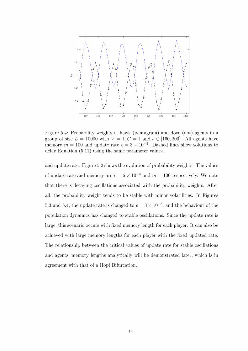
t160 165 170 175 180 185 190 195 200
h,d
0.4
0.45
0.5
0.55
0.6
Figure 5.4: Probability weights of hawk (pentagram) and dove (dot) agents in agroup of size L = 10000 with V = 1, C = 1 and t ∈ [160, 200]. All agents havememory m = 100 and update rate ε = 3 × 10⁻³. Dashed lines show solutions todelay Equation (5.11) using the same parameter values.
and update rate. Figure 5.2 shows the evolution of probability weights. The values
of update rate and memory are ε = 6× 10⁻³ and m = 100 respectively. We note
that there is decaying oscillations associated with the probability weights. After
all, the probability weight tends to be stable with minor volatilities. In Figures
5.3 and 5.4, the update rate is changed to ε = 3× 10⁻³, and the behaviour of the
population dynamics has changed to stable oscillations. Since the update rate is
large, this scenario occurs with fixed memory length for each player. It can also be
achieved with large memory lengths for each player with the fixed updated rate.
The relationship between the critical values of update rate for stable oscillations
and agents’ memory lengths analytically will be demonstrated later, which is in
agreement with that of a Hopf Bifurcation.
91

5.3 Theory
In this section, an analysis of the system dynamics (exact in the limit of large
m and L) is presented, and the mathematical expression for system stability is
derived.
5.3.1 Strategy optimization
For large m and L, an individual agent encounters an average strategy over a
memory of m, defined as:
φm :=1
m
∫ m
0
φ(t− s)ds. (5.7)
Statistically, we expect its memory of m interactions to consist of h ‘Hawk’ strate-
gies according to the binomial distribution associated with probability φm:
f(n, φm) =m! φnm(1− φm)m−n
n! (m− n)!. (5.8)
In reality, this distribution is non-stationary over time and agents. However, we
expect the approximation to be accurate for large memory, m, and agent number
L, provided that the system reaches a steady state. This allows us to average over
agents’ memories, and thus the expectation value of p(φm) can be defined as
p(φm) :=m∑h=0
ph(h
m) f(h, φm), (5.9)
and incorporating Equation (5.3), it simplifies to:
p(φm) =
mV2C∑h=0
f(h, φm), (5.10)
which is the average probability of an agent evolving towards a pure ‘Hawk’ strat-
egy, whilst in interaction with a population with an average strategy φm. The
plots of Equations (5.7), (5.8) and (5.9) are presented in Section 5.5.1.
92

5.3.2 Delay equation
The strategy evolution Equation (5.5) can now be averaged over the population
of agents and their memories. Taking the limit of δt to 0, we have
dφ
dt= ε
[p(φm)− φ
],where p given by (5.9) and φm by (5.7), (5.11)
which is a delay equation for the evolution of φ(t) over time t, since φm contains the
memory m of the previous time. This delay equation can be solved numerically,
and we have included the solutions in Figures 5.2, 5.3 and 5.4 for comparison. The
agreement with the simulation results is excellent.
5.3.3 Linear stability analysis
In order to determine the critical condition for stability, we now seek to linearise
the delay equation around its fixed point. The analysis can be carried out with
general values of V and C. However, for simplicity, V = C = 1 is set, and therefore
the fixed point is φ0 = V/2C = 1/2. Equations are introduced as follows.
ψ(t) := φ(t)− 1
2, (5.12)
and
ψm(t) :=1
m
∫ t
t−mψ(τ)dτ. (5.13)
To evaluate p, as given in Equation (5.10), the summation with a continuous
integral is replaced, and the binomial distribution is approximated with a Gaussian
distribution of the same mean, µ and variance, σ, where
µ(φ) = mφ, (5.14)
σ(φ) =√mφ(1− φ). (5.15)
93

Then Equation (5.10) leads to the following approximate expression, of which
detailed derivations are listed in the appendix:
p(ψm) ≈ 1
2−√
2m√πψm. (5.16)
The approximation is verified by comparing the expansion coefficients to the exact
values of the derivatives of p(φ) evaluated at φ = 1/2, as shown in Figure 5.5.
20 40 60 80 100
-8
-6
-4
-2
Figure 5.5: The derivative ∂p/∂φ evaluated directly from Equation (5.10) at φm =1/2. The derivative is plotted using black dot. The blue line shows correspondingexpansion coefficients from Equation (5.16).
The delay Equation (5.11) is finally linearised to:
1
ε
dψ
dt= −√
2m√πψm(t)− ψ(t). (5.17)
The expression ψ(t) = eλt is substituted as a trial solution to obtain the char-
acteristic equation. Since ψ(t) = eλt, dψ(t)/dt = λeλt is derived. Then the
characteristic equation becomes:
λeλt
ε= −
√2√πm
1
λ
[eλt − eλ(t−m)
]− eλt. (5.18)
By simplifying Equation (5.18), we obtain
λ2 + ελ+ε√
2√πm
(1− e−λm
)= 0. (5.19)
94
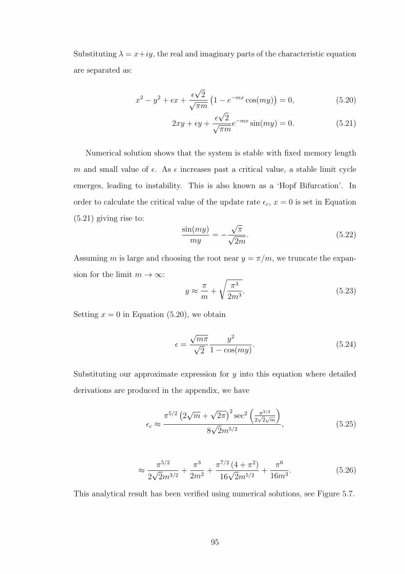
Substituting λ = x+iy, the real and imaginary parts of the characteristic equation
are separated as:
x2 − y2 + εx+ε√
2√πm
(1− e−mx cos(my)
)= 0, (5.20)
2xy + εy +ε√
2√πm
e−mx sin(my) = 0. (5.21)
Numerical solution shows that the system is stable with fixed memory length
m and small value of ε. As ε increases past a critical value, a stable limit cycle
emerges, leading to instability. This is also known as a ‘Hopf Bifurcation’. In
order to calculate the critical value of the update rate εc, x = 0 is set in Equation
(5.21) giving rise to:
sin(my)
my= −
√π√
2m. (5.22)
Assuming m is large and choosing the root near y = π/m, we truncate the expan-
sion for the limit m→∞:
y ≈ π
m+
√π3
2m3. (5.23)
Setting x = 0 in Equation (5.20), we obtain
ε =
√mπ√2
y2
1− cos(my). (5.24)
Substituting our approximate expression for y into this equation where detailed
derivations are produced in the appendix, we have
εc ≈π5/2
(2√m+
√2π)2
sec2(
π3/2
2√
2√m
)8√
2m5/2, (5.25)
≈ π5/2
2√
2m3/2+
π3
2m2+π7/2 (4 + π2)
16√
2m5/2+
π6
16m3. (5.26)
This analytical result has been verified using numerical solutions, see Figure 5.7.
95

t0 20 40 60 80 100 120 140 160 180 200
h(t)
0.2
0.3
0.4
0.5
0.6
0.7
Figure 5.6: Black line shows φ(t) from the numerical solutions to Equation (5.11)in the symmetric case when m = 100 and ε = 5 × 10⁻³. Blue dashed line showscorresponding solution when ε = 7 × 10⁻³. Open black circles and open bluesquares show corresponding simulation results in a system of size L = 10000.
ǫ m3/2
2 4 6 8 10 12 14
Var
ianc
e
0.005
0.01
0.015
0.02
0.025
0.03
0.035
Variance Plot of Hawk Dove Game
m=201
m=101
m=51
Figure 5.7: Dependence of the steady state amplitude of φ(t) on ε for m = 51(light blue), m = 101 (blue) and m = 201 (black). L = 100 in all cases.
96

5.3.4 Numerical tests of stability
The delay Equation (5.11) can be numerically solved. The probability p(φm) is ob-
tained by summing over the binomial distribution. The critical point is calculated
by our stability analysis, where the figure is generated. Plotting the result finally
shows a set of stable oscillations, which is in line with the theoretical analysis.
The verification has numerically carried out to confirm the relationship between
memory and the corresponding critical value of ε. We have obtained variance plot
for three different values of memory. In Figure 5.7, x-axis indicates the increasing
values of ε, and y-axis shows the corresponding values of variance. The results
demonstrate that the simulated outcomes are in agreement of analytical solutions.
5.4 Conclusion
In this chapter, we have extended the traditional Hawk-Dove game to include
memory effects. We have presented both numerical and analytical results which
are in excellent agreements.
The system is found to have a stable fixed point. Initially players with longer
memories are better at selecting an optimal strategy, as they are more accurate
at assessing the true probability characteristics of the system. However, when the
agent memory exceeds a certain value, large collective fluctuations can emerge
in the form of limit cycles, and players with shorter memories can exploit the
fluctuations more effectively than those with longer memories. In essence, for a
population of players with different memories, a better memory does not always
help with games.
97

5.5 Appendix
5.5.1 The plots of equations (5.7), (5.8) and (5.9)
We present the plots of Equations (5.7), (5.8) and (5.9).
0.20.150.1
φ
0.055
10
n
15
0
0.3
0.05
0.1
0.15
0.2
0.35
0.25
0.4
20
f(n,φ
)
Figure 5.8: The plot for f(n, φ) in Equation (5.8) against n and φ.
t0 500 1000 1500 2000 2500 3000 3500 4000 4500 5000
f
0
0.01
0.02
0.03
0.04
0.05
0.06
0.07
0.08
0.09Equation (5.8)
Figure 5.9: The plot for f(h, φ) in Equation (5.8) against time t for an individualagent where m = 100, L = 10000, V = C = 1, ε = 3× 10⁻³.
98
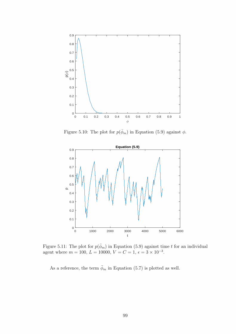
φ
0 0.1 0.2 0.3 0.4 0.5 0.6 0.7 0.8 0.9 1
p(φ
)
0
0.1
0.2
0.3
0.4
0.5
0.6
0.7
0.8
0.9
Figure 5.10: The plot for p(φm) in Equation (5.9) against φ.
t0 1000 2000 3000 4000 5000 6000
p
0
0.1
0.2
0.3
0.4
0.5
0.6
0.7
0.8
0.9Equation (5.9)
Figure 5.11: The plot for p(φm) in Equation (5.9) against time t for an individualagent where m = 100, L = 10000, V = C = 1, ε = 3× 10⁻³.
As a reference, the term φm in Equation (5.7) is plotted as well.
99

t0 500 1000 1500 2000 2500 3000 3500 4000 4500 5000
aver
age
prob
abili
ty
0.35
0.4
0.45
0.5
0.55
0.6Equation (5.7)
Figure 5.12: The plot for φm in Equation (5.7) against time t for an individualagent where m = 100, L = 10000, V = C = 1, ε = 3× 10⁻³.
5.5.2 The derivation of equation (5.16)
We present the derivation for Equation (5.16). Recall Equation (5.10), and V =
C = 1
p(φm) =
m2∑
h=0
f(h, φm
). (5.27)
The summation can be approximated by integration, then Equation (5.27) be-
comes
p(φm) ≈∫ m/2
h=0
f(h, φm
). (5.28)
The binomial distribution f(h, φm
)is approximated with a Gaussian distribution.
p(ψm) ≈ 1
σ√
2π
∫ m/2
0
exp(−(h−
(mψm +m/2
))2
2σ2)dh. (5.29)
Since the integrand is insignificant for (−∞, 0], the lower limit of the integration
has been approximated to −∞:
p(ψm) ≈ 1
σ√
2π
∫ m/2
−∞exp(−
(h−
(mψm +m/2
))2
2σ2)dh. (5.30)
100
By expanding the exponential in Equation (5.30), we obtain
p(ψm) =1
σ√
2π
∫ m/2
−∞exp(−(h−m/2)2
2σ2)exp(
mψm (h−m/2)
σ2)(1 +O
(ψ2))dh.
(5.31)
The term O(ψ2)
is neglected due to its small value. The Equation (5.31) becomes
p(ψm) ≈ 1
σ√
2π
∫ m/2
−∞exp(−(h−m/2)2
2σ2)exp(
mψm (h−m/2)
σ2)dh. (5.32)
By changing of variable h, x = h−m/2, we have
p(ψm) =1
σ√
2π
∫ 0
−∞exp(− x2
2σ2)exp(
mψmx
σ2)dx. (5.33)
The term exp(mψmxσ2 ) has been approximated by Taylor series.
p(ψm) =1
σ√
2π
∫ 0
−∞e−
x2
2σ2
(1 +
mψmx
σ2
)dx. (5.34)
Rearranging the above equation, we have
p(ψm) =1
σ√
2π
∫ 0
−∞e−
x2
2σ2 dx+ψmm
σ3√
2π
∫ 0
−∞xe−
x2
2σ2 dx. (5.35)
The first term of Equation (5.35) is the Gaussian distribution with mean 0 and
standard deviation σ.
1
σ√
2π
∫ 0
−∞e−
x2
2σ2 dx =1
2. (5.36)
The second term of Equation (5.35) can be calculated as
ψmm
σ3√
2π
∫ 0
−∞xe−
x2
2σ2 dx =ψmm
σ√
2π
[−e−
x2
2σ2
]0
−∞, (5.37)
= − mψm
σ√
2π. (5.38)
101

Recall that σ =√m/2. Finally, equation (5.35) becomes
p(ψm) =1
2−√
2m√πψm. (5.39)
5.5.3 The derivation of equation (5.25)
Recall Equation (5.22),
sinc(my) =sin(my)
my= −
√π√
2m. (5.40)
Expanding the sinc function as Taylor series to the second order at π/m, we have
−τ(y − π/m)
π+τ 2(y − π/m)2
π2= −
√π√
2m. (5.41)
The solutions of above quadratic function are
y =π
2m
3±
√1− 4
√π
2m
. (5.42)
The root which satisfies our system is
y =π
2m
3−
√1− 4
√π
2m
. (5.43)
Applying the Taylor expansion for√
1− x ≈ 1− x/2, we have
y =π
2m
(3−
(1− 2
√π
2m
)). (5.44)
102

Finally, we obtain the expression for Equation (5.23).
y ≈ π
m+
√π3
2m3. (5.45)
Substituting Equation (5.23) into Equation (5.24), we obtain
εc =
√mπ√2
(πm
+√
π3
2m3
)2
1− cos
(m
(πm
+√
π3
2m3
)) . (5.46)
The term of cos(.) can be simplified to
cos
(π +
π3/2
√2m
)= − cos
(π3/2
√2m
). (5.47)
Applying double angle formulas from trigonometric identities, cos(2x) = 2(cos x)2−
1, we obtain
cos
(π +
π3/2
√2m
)= 2
(cos
(π3/2
2√
2√m
)). (5.48)
Note that sec2(.) = 1/ cos2(.), then Equation (5.24) becomes
εc ≈π5/2
(2√m+
√2π)2
sec2(
π3/2
2√
2√m
)8√
2m5/2. (5.49)
103

Chapter 6
Conclusion
I conducted research on the statistical modelling of a selection of three games,
namely the minority games, the statistical urn models and the Hawk-Dove games.
In Chapter 3, the key characteristics of the minority game were explored. We
extended the standard MG by allowing players to accumulate profits and losses in
each game round. Bankruptcy and borrowing (leverage) were introduced, and the
resulting game statistics were analysed numerically. Curve fitting was performed
for wealth distributions, showing a weak evidence of power law behaviour. We
explored a number of variations when curve fitting for wealth distributions, for
example a zero-sum rule could be introduced. Due to the time limit of the re-
search and possible variations in the system parameters, we did not obtain fitting
of sufficient quality for publication. It is possible that with larger set of players
simulated for longer time could lead to better statistics and higher quality curve
fitting for wealth distributions. However, our results clearly demonstrated that
leverage increases the instability of the system. This corresponds to the increased
risks of trading leveraged financial products in the real market. Our model pro-
vides a possible testing ground for introducing new measures that might modify
and control the risks arising from the leverage effects.
In Chapter 4, a new simple urn model was developed to investigate the ef-
fectiveness of memory. The model consists of a group of agents with different
104

memories competing against each other for finite resources. Our results showed
that instability exists in the model at a critical memory length, which can be
verified both numerically and analytically. Additionally, we showed that the tem-
perature in the urn model is related by the agent’s memory length, suggesting
that this model may be applied to other game models with links to classical ther-
modynamics. Increasing memory lengths can allow agents to more accurately and
reliably determine the optimal strategy, and in terms of thermodynamics, this is
equivalent to less thermal noise and a lower temperature. However, if a sufficient
number of agents with very long-memory lengths are present, instability in the
form of a limit cycle occurs, resulting in reduced competitiveness, in which case
agents with shorter memories can exploit the fluctuations more effectively. By
modelling payoffs as birthrates, we demonstrated a coexistence of different mem-
ories, leading to a self-organised Hopf bifurcation driven by population dynamics.
The simplicity of our memory model, its connection to classical urn models, to-
gether with the fact that limit cycles arise naturally, suggested that it might be
fruitfully generalised to different games. Indeed Chapter 5 extended this approach
to the Hawk-Dove game. However, other extensions might include using multiple
urns to represent different sources of yield or game strategies, introducing hetero-
geneity in switching rates, and utilising a more general distribution of memory
lengths and behaviour. Multiple urns might give rise to more complex patterns
of oscillation and regimes of behaviour. Experimental research into the nature of
human and animal memory puts an emphasis on the ‘forgetting function’, which
describes how memories decay with time. Such a function, or greater powers of
statistical inference, could be naturally incorporated into our analysis and their
effects on stability explored.
In Chapter 5, the main findings from Chapter 4 were extended to the Hawk-
Dove game. We generalised the standard HD game so that players possess finite
memories and utilise them to optimise their strategies in each round. With each
time step, agents use a form of online learning to amend their strategies. We
105

presented both analytical and numerical results for this generalised HD game,
showing excellent agreement. In particular, we derived an analytical expression
for the critical memory length where instability occurs, and this is confirmed by
simulation. Our analysis is not only limited to HD game, it can also potentially
be applied to, for example, all evolutionary games.
Our work on minority games and the two-urn model has shown a range of
complex behaviours which offer possible future foci. A direct link between the
game models and real financial markets still needs to be fully developed. Stock
price movement may be related to minority game by assuming that one side in the
game are the sellers and the other buyers. The prediction for markets needs to be
verified by comparisons with historical stocks data. Similarly our urn model can be
applied to real markets. It may also be used to analyse the effectiveness of financial
resource allocation, by considering urn 1 to represent the cash holding, and urn
2 to be other financial instruments holdings, i.e. stocks, bonds, derivatives, etc.
We can analyse the transition between these holdings under different investment
environment. Furthermore, this urn model could be extended to multi-urn model,
in order to capture the dynamics of different financial portfolios.
106

Bibliography
[1] Mantegna, R. N. and Stanley, H. E., 2000. Introduction to Econo-
physics Correlations and Complexity in Finance. Cambridge: Cam-
bridge University Press.
[2] Savoiu, G., 2013. Econophysics: Background and Applications in Eco-
nomics, Finance, and Sociophysics. Oxford Waltham, Mass: Aca-
demic Press.
[3] Grimmett, G. and Stirzaker, D., 2001. Probability and random pro-
cesses. Third Edition. Oxford: Oxford University Press.
[4] Fry, J., 2015. Stochastic modelling for financial bubbles and policy.
Cogent Economics & Finance, 3(1), 1002152.
[5] Cockshott, P., Cottrell, A. F., Michaelson, G. J., Wright, I. P. and
Yakovenko, V. M., 2009. Classical Econophysics. London: Routledge.
[6] Slanina, F., 2014. Essentials of Econophysics Modelling. Oxford: Ox-
ford University Press.
[7] Sinha, S., Chatterjee, A., Chakraborti, A., Chakrabarti, B. K., 2011.
Econophysics: An Introduction. Weinheim: Wiley-VCH.
[8] Jovanovic, F. and Schinckus, C., 2013. The history of econophysics
emergence: a new approach in modern financial theory. History of
Political Economy, 45, pp. 443-474.
107

[9] Spanulescu, I. and Gheorghiu, A., 2013. A classification of the econo-
physics directions. Hyperion International Journal of Econophysics
& New Economy, 6(2), pp. 175-198.
[10] Kutner, R. and Grech, D., 2008. Report on foundation and organi-
zation of econophysics graduate courses at faculty of physics of Uni-
versity of Warsaw and department of physics and astronomy of the
Wroclaw University. Acta Physica Polonica Series A, 114(3), pp. 637-
647.
[11] Namatame, A., Kaizouji, T., Aruka, Y., 2006. The Complex Net-
works of Economic Interactions: Essays in Agent-Based Economics
and Econophysics. Berlin: Springer.
[12] Takayasu, H., 2004. The Application of Econophysics proceedings of
the Second Nikkei Econophysics Symposium. Tokyo: Springer Japan.
[13] Roehner, B. M., 2005. Patterns of Speculation: A Study in Observa-
tional Econophysics. Cambridge: Cambridge University Press.
[14] Preis, T., 2011. Econophysics - complex correlations and trend switch-
ings in financial time series. The European Physical Journal Special
Topics, 194(1), pp. 5-86.
[15] Amaral, L. A. N., Cizeau, P., Gopikrishnan, P., Liu, Y., Meyer, M.,
Peng, C.-K. and Stanley, H. E., 1999. Econophysics: can statistical
physics contribute to the science of economics? Computer Physics
Communications, 121-122, pp. 145-152.
[16] Stanley, H. E., Amaral, L. A. N., Canning, D., Gopikrishnan, P.,
Lee, Y. and Liu, Y., 1999. Econophysics: can physicists contribute
to the science of economics? Physica A: Statistical Mechanics and its
Applications, 269, pp. 156-169.
108

[17] Garibaldi, U. and Scalas, E., 2010. Finitary Probabilistic Methods in
Econophysics. Cambridge: Cambridge University Press.
[18] Silva, S. D., Matsushita, R., Gleria, I., Figueiredo, A., Rathie, P.,
2005. International finance, Levy distributions, and the econophysics
of exchange rates. Communications in Nonliner Science and Numer-
ical Simulation, 10(4), pp. 365-393.
[19] Figueiredo, A., Matsushita, R., Silva, S. D., Serva, M., Viswanathan,
G. M., Nascimento, C. and Gleria, I., 2007. The Levy sections
theorem: an application to econophysics. Munich Personal RePEc
Archive Paper, Paper No. 3810.
[20] Abergel, F., 2011. Econophysics of Order-Driven Markets Proceedings
of Econophys-Kolkata V. New York: Springer.
[21] Gabaix, X., 1999. Zipf’s law for cities: An explanation. The Quarterly
Journal of Economics, 144, pp. 739-767.
[22] Sousa, T. and Domingos, T., 2006. Equilibrium econophysics: a uni-
fied formalism for neoclassical economics and equilibrium thermody-
namics. Physica A: Statistical Mechanics and its Applications, 371(2),
pp. 492-512.
[23] Aspromourgos, T., 1986. On the origins of the term ‘neoclassical’.
Cambridge Journal of Economics, 10(3), pp. 265-270.
[24] Scarfone, A. M., 2007. A mechanism to drive multi-power law func-
tions: an application in the econophysics framework. Physica A: Sta-
tistical Mechanics and its Applications, 382 (1), pp. 271-277.
[25] Fan, Y., Li, M., Chen, J., Gao, L., Di, Z. and Wu, J., 2004. Network of
econophysicists: a weighted network to investigate the development
of econophysics. International Journal of Modern Physics B, 18(17-
19), pp. 2505-2511.
109

[26] Bordley, R. F., 2005. Econophysics and individual choice. Physica A:
Statistical Mechanics and its Applications, 354, pp. 479-495.
[27] Fry, J., 2011. Gaussian and non-Gaussian models for financial bubbles
via econophysics. Hyperion International Journal of Econophysics &
New Economy, 4(1), pp. 7-23.
[28] Fry, J., 2010. Bubbles and crashes in finance: a phase transition
from random to deterministic behaviour in prices. Journal of Applied
Research in Finance Bi-Annually, II(2), pp. 131-137.
[29] Fry, J. and Cheah, E-T., 2016. Negative bubbles and shocks in
crytocurrency markets. International Review of Financial Analysis,
(forthcoming).
[30] Hull, J. C., 2012. Options, Futures, & Other Derivatives. Boston:
Prentice Hall.
[31] Etheridge, A., 2002. A Course in Financial Calculus. Cambridge:
Cambridge University Press.
[32] Bodie, Z., Kane, A., Marcus, A. J., 2008. Investments. New York:
McGraw-Hill/Irwin.
[33] Grima, S., 2012. The current financial crisis and derivative misuse.
Online Journal of Social Sciences Research, 1(8), pp. 265-276.
[34] Reinhart, C. and Rogoff, K., 2009. This time it’s different: eight
centuries of financial folly. Princeton: Princeton University Press.
[35] McCauley, J. L., 2009. Dynamics of Markets: The New Financial
Economics. Cambridge: Cambridge University Press.
[36] Huang, J. P., 2014. Experimental Econophysics: Properties and Mech-
anisms of Laboratory Markets. Heidelberg: Springer Verlag.
110

[37] Bouchaud, J. P. and Potters, M., 2003. Theory of Financial Risk
and Derivative Pricing : from statistical physics to risk management.
Cambridge: Cambridge University Press.
[38] Takayasu, H., Watanabe, T., 2010. Econophysics Approaches to
Large-Scale Business Data and Financial Crisis. Tokyo: Springer
Japan.
[39] Chai, H. and Song, D., 2010. Enterprise investment timing based
on options game theory. International Conference on Information
Management, Innovation Management and Industrial Engineering
(ICIII), 4, pp. 155-158.
[40] Ziegler, A. C., 2004. A Game Theory Analysis of Options. Heidelberg:
Springer Verlag.
[41] Angelou, G. N. and Economides, A. A., 2009. A multi-criteria game
theory and real-options model for irreversible ICT investment Deci-
sions. Telecommunications Policy, 33(10-11), pp. 686-705.
[42] Challet, D. and Zhang, Y.-C., 1998. On the minority game: analyt-
ical and numerical studies. Physica A: Statistical Mechanics and its
Applications, 256(3-4), pp. 514-532.
[43] Tanaka-Yamawaki, M., 2005. Minority Game and the wealth distri-
bution in the artificial markets. Knowledge-Based Intelligent Infor-
mation and Engineering Systems, 9th International Conference, KES
2005, Proceedings, Part I, pp. 15-20.
[44] Brzezinski, M., 2014. Do wealth distributions follow power laws? Ev-
idence from ‘rich lists’. Physica A: Statistical Mechanics and its Ap-
plications, 406, pp. 155-162.
[45] Newman, M. E. J., 2005. Power laws, Pareto distributions and Zipf’s
law. Contemporary Physics, 46(5), pp. 323-351.
111

[46] Sinha, S., 2006. Evidence for power-law tail of the wealth distribu-
tion in India. Physica A: Statistical Mechanics and its Applications,
359(1), pp. 555-562.
[47] Erneux, T., 2009. Applied Delay Differential Equations. London:
Springer.
[48] Fisher, L., 2008. Rock, Paper, Scissors: game theory in everyday life.
New York: Basic Books.
[49] Walker, D. and Walker, G., 2004. The Official Rock Paper Scissors
Strategy Guide. London: Simon & Schuster.
[50] Shelton, R. B., 1997. Gaming the Market: Applying Game Theory to
Create Winning Trading Strategies. Oxford: John Wiley & Sons.
[51] Greenwood, G. W. and Tymerski, R., 2008. A game-theoretical ap-
proach for designing market trading strategies. IEEE Symposium on
Computational Intelligence and Games, pp. 316-322.
[52] Li, H., Wu, C. and Yuan, M., 2013. An evolutionary game model
of financial markets with heterogeneous players. Procedia Computer
Science, 17, pp. 958-964.
[53] Allen, F. and Morris, S., 2001. Chapter: Game theory and business
applications, Volume 35 of the series International Series in Opera-
tions Research & Management Science, pp. 17-48.
[54] Zhou, W-X. and Sornette, D., 2007. Self-fulfilling Ising model of fi-
nancial markets, European Physical Journal B, 55(2), pp. 175-181.
[55] Goncalves, C. P. and Goncalves, C., 2007. An evolutionary quan-
tum game model of financial market dynamics - theory and evi-
dence. [Online] available at Social Science Research Network: http:
//ssrn.com/abstract=982086 [Accessed 16 March 2016].
112

[56] Wiszniewska-Matyszkiel, A., 2005. Stock market as a dynamic game
with continuum of players. Control and Cybernetics, 37(3), pp. 617-
647.
[57] Musolino, F., 2012. Game theory for speculative derivatives: a possi-
ble stabilizing regulatory model, Atti della Accademia Peloritana dei
Pericolanti, 90(1), C1.
[58] Chen, F., Gou, C., Guo, X. and Gao, J., 2008. Prediction of
stock markets by the evolutionary mix-game model. Physica A, 387,
pp. 3594-3604.
[59] Chen, Y., Dimitrov, S., Sami, R., Reeves, D. M., Pennock, D. M.,
Hanson, R. D., Fortnow, L. and Gonen, R., 2009. Gaming prediction
markets: equilibrium strategies with a market maker. Algorithmica,
58(4), pp. 930-969.
[60] Challet, D., Marsili, M. and Zhang, Y.-C., 2014. Minority games:
Interacting Agents In Financial Markets. Oxford: Oxford University
Press.
[61] Martino, A. D., Giardina, I. and Mosetti, G., 2003. Statistical me-
chanics of the mixed majority-minority game with random external
information. Journal of Physics A: Mathematical and General, 36,
pp. 8935-8954.
[62] Marsili, M., 2001. Market mechanism and expectations in minority
and majority games. Physica A, 299, pp. 93-103.
[63] Alfi, V., Martino, A. D., Pietronero, L. and Tedeschi, A., 2007. De-
tecting the traders’ strategies in minority-majority games and real
stock-prices. Physica A, 382, pp. 1-8.
113

[64] Arthur, W., 1994. Inductive reasoning and bounded rationality (the
El Farol problem). The American Economic Review: Papers and Pro-
ceedings, 84(2), pp. 406-411.
[65] Challet, D. and Zhang, Y.-C., 1997. Emergence of cooperation and
organization in an evolutionary game. Physica A: Statistical Mechan-
ics and its Applications, 246(3), pp. 407-418.
[66] Challet, D., Marsili, M. and Ottino, G., 2004. Shedding light on
El Farol. Physica A: Statistical Mechanics and its Applications, 332,
pp. 469-482.
[67] Jefferies, P., Hart, M. L., Hui, P. M. and Johnson, N. F., 2001. From
market games to real-world markets. The European Physical Journal
B - Condensed Matter and Complex Systems, 20(4), pp. 493-501.
[68] Challet, D., Marsili, M. and Zhang, Y.-C., 2001. Stylized facts of
financial markets and market crashes in minority games. Physica A:
Statistical Mechanics and its Applications, 294(3-4), pp. 514-524.
[69] Marsili, M., Challet, D. and Zecchina, R., 2000. Exact solution of a
modified El Farol’s bar problem: efficiency and the role of market
impact. Physica A: Statistical Mechanics and its Applications, 280(3-
4), pp. 522-553.
[70] Franke, R., 2003. Reinforcement learning in the El Farol model. Jour-
nal of Economic Behavior & Organization, 51(3), pp. 367-388.
[71] Lus, H., Aydın, C. O., Keten, S., Unsal, H. I. and Atılgan, A. R.,
2005. El Farol revisited. Physica A: Statistical Mechanics and its Ap-
plications, 346(3-4), pp. 651-656.
[72] Lustosa, B. C. and Cajueiro, D. O., 2010. Constrained information
minority game: how was the night at El Farol? Physica A: Statistical
Mechanics and its Applications, 389(6), pp. 1230-1238.
114

[73] Valdez, S. and Molyneux, P., 2010. An Introduction to Global Finan-
cial Markets. Hampshire New York: Palgrave Macmillam.
[74] Benninga, S., 2014. Financial Modelling. Massachusetts: MIT Press.
[75] Boumans, M., 2005. How Economists Model the World into Numbers.
London: Routledge.
[76] Challet, D. , Marsili, M. and Zhang, Y.-C., 2000. Modeling market
mechanism with minority game. Physica A: Statistical Mechanics and
its Applications, 276, pp. 284-315.
[77] D’hulst, R. and Rodgers, G. J., 2000. Strategy selection in the mi-
nority game. Physica A: Statistical Mechanics and its Applications,
278(3-4), pp. 579-587.
[78] Andersen, J. V. and Sornette, D., 2003. The $-game. The European
Physical Journal B, 31, pp. 141-145.
[79] Challet, D. and Marsili, M., 2000. Relevance of memory in minority
games. Physical Review E, 62, pp. 1862-1868.
[80] Huygens, C., 1655. Tome XIV: Calcul des probabilites. Travaux de
mathematiques pures 1655-1666 (1920), (In French). Den Haag: Ni-
jhoff.
[81] Coolidge, J., 1925. An Introduction to Mathematical Probability. Ox-
ford: Oxford University Press.
[82] Mahmoud, H., 2009. Polya Urn Models. Boca Raton, FL: CRC Press.
[83] Chen, M. and Kuba, M., 2013. On generalized Polya urn models.
Journal of Applied Probability, 50(4), pp. 1169-1186.
[84] Chen, M. R., Hsiau, S.-R. and Yang, T.-H., 2014. A new two-urn
model. Journal of Applied Probability, 51, pp. 590-597.
115

[85] Mahmoud, H. M., 2003. Polya urn models and connections to random
trees: a review. Journal of Iranian Statistical Society, 2(1), pp 53-114.
[86] Kac, M., 1976. Probability and Related Topics in Physical Sciences.
Providence, R.I: American Mathematical Society.
[87] Metzler, R., Kinzel, W. and Kanter, I., 2000. On time’s arrow in
Ehrenfest models with reversible deterministic dynamics. Journal of
Physics A: Mathematical and General, 34, pp. 317-326.
[88] Prestipino, S., 2005. The Ideal gas as an urn model: derivation of the
entropy formula. European Journal of Physics, 26(1), pp. 137-153.
[89] Johnson, N. L. and Kotz, S., 1977. Urn Models and Their Application:
an approach to modern discrete probability theory. New York: John
Wiley & Sons Inc.
[90] Lexis, W., 1875. Introduction to the Theory of Population Statistics,
(In German). Strassburg: Trubner.
[91] Lexis, W., 1903. Treatises on Population and Social Statistics, (In
German). Jena: G. Fischer.
[92] Godreche, C. and Luck, J. M., 2002. Nonequilibrium dynamics of urn
models. Journal of Physics: Condensed Matter, 14(7), pp. 1601-1615.
[93] Buhot, A., Garrahan, J. P. and Sherrington, D., 2003. Simple strong
glass forming models: mean-field solution with activation. Journal of
Physics A: Mathematical and General, 36(2), pp. 307-328.
[94] Laruelle, S. and Pages, G., 2013. Randomized urn models revisited
using stochastic approximation. The Annals of Applied Probability,
23(4), pp. 1409-1436.
116

[95] Huillet, T. E., 2011. A Bose-Einstein approach to the random parti-
tioning of an integer. Journal of Statistical Mechanics: Theory and
Experiment, 2011(08), P08021.
[96] Inoue, J. and Ohkubo, J., 2008. Power-law behavior and conden-
sation phenomena in disordered urn models. Journal of Physics A:
Mathematical and Theoretical, 41(32), 324020.
[97] Dunning, T., 2012. Natural Experiments in the Social Sciences - A
Design-Based Approach. Cambridge: Cambridge University Press.
[98] Levine, E., Mukamel, D. and Ziv, G., 2004. The condensation tran-
sition in zero-range processes with diffusion. Journal of Statistical
Mechanics: Theory and Experiment, 2004(05), P05001.
[99] Cerqueti, R. and Ausloos, M., 2015. Cross ranking of cities and re-
gions: population versus income. Journal of Statistical Mechanics:
Theory and Experiment, 2015(7), P07002.
[100] Tong, Z. and Mahmoud, H. M., 2013. An urn model for population
mixing and the phases within. Methodology and Computing in Applied
Probability, 15, pp. 683-706.
[101] Lambersona, P. J. and Page, S. E., 2012. The effect of feedback con-
sistency on success in markets with positive feedbacks. Economics
Letters, 114, pp. 259-261.
[102] Zhang, L. X., Hu, F., Cheung, S. H. and Chan, W. S., 2011. Im-
migrated urn models - theoretical properties and applications. The
Annals of Statistics, 39(1), pp. 643-671.
[103] Aletti, G., Ghiglietti, A. and Paganoni, A. M., 2013. Randomly re-
inforced urn designs with prespecified allocations. Journal of Applied
Probability, 50, pp. 486-498.
117

[104] Eggenberger, F. and Polya, G., 1923. Uber die statistik verket-
teter vorgange. ZAMM - Journal of Applied Mathematics and Me-
chanics/Zeitschrift fur Angewandte Mathematik und Mechanik, 3(4),
pp. 279-289.
[105] Moon, J. W., 1972. Random exchanges of information. Nieuw Archief
voor Wiskunde, 20, pp. 246-249.
[106] Tijdeman, R., 1971. On a telephone problem, Nieuw Arch. Wiskunde,
19(3), pp. 188-192.
[107] Bernoulli, J., 1713. Ars Conjectandi, (In Latin). Basel: Impensis
Thurnisiorum, fratrom.
[108] Ehrenfest, P., 1907. Uber zwei bekannte Einwande gegen das Boltz-
mannsche H-theorem. Physikalishce Zeitschrift, 8, pp. 311-314.
[109] Alfred, B. M., 1987. Elements of Statistics for the Life and Social
Sciences. New York: Springer New York.
[110] Thompson, M., 1997. Theory of Sample Surveys. London: Chapman
and Hall/CRC.
[111] DasGupta, A., 2010. Urn Models in Physics and Genetics. Chap-
ter: Fundamentals of Probability: A First Course, Part of the series
Springer Texts in Statistics, pp. 379-407.
[112] Hoppe, F. M., 1987. The sampling theory of neutral alleles and an
urn model in population genetics. Journal of Mathematical Biology,
25(2), pp. 123-159.
[113] Trieb, G., 1992. A Polya urn model and the coalescent. Journal of
Applied Probability, 29(1), pp. 1-10.
[114] Smith, J. M., 1982. Evolution and the Theory of Games. Cambridge:
Cambridge University Press.
118

[115] Smith, J. M. and Price, G. R., 1973. The logic of animal conflict.
Nature, 246, pp. 15-18.
[116] Smith, J. M., 1976. Evolution and the theory of games: in situations
characterized by conflict of interest, the best strategy to adopt de-
pends on what others are doing. American Scientist, 64(1), pp. 41-45.
[117] Smith, J. M., 1979. Game theory and the evolutionary of behaviour.
Proceedings of the Royal Society of London. Series B, Biological Sci-
ences, 205(1161), The Evolution of Adaptation by Nature Selection,
pp. 475-488.
[118] Bernstein, A., 2014. Monte Carlo simulation of learning in
the Hawk Dove game. Spring 2014, Paper 70. [Online] avail-
able from: https://economics.wustl.edu/files/economics/
imce/alex_bernstein_-_final.pdf [Accessed 16 September 2015].
[119] McNamara, J. M. and Weissing, F. J., 2010. Evolutionary Game
Theory, in: Szekely, T., Moore, A. J., Komdeur, J. (eds), Social
Behaviour: Genes, Ecology and Evolution. Cambridge: Cambridge
University Press.
[120] Pham, K. and Feng, Y., 2013. Using the Hawk-Dove model
and ordinary differential equation systems to study Asian carp
invasion. [Online] available from: http://www.math.uci.edu/
icamp/summer/research/student_research/asian_carp.pdf [Ac-
cessed 16 September 2015].
[121] Neugebnauer, T., Poulsen, A. and Schram, A., 2008. Fairness and
reciprocity in the Hawk-Dove game. Journal of Economic Behavior
& Organization, 66(2), pp. 243-250.
[122] Hanauske, M., Kunz, J., Bernius, S. and Konig, W., 2010. Doves and
hawks in economics revisited: an evolutionary quantum game theory-
119

based analysis of financial crises. Physica A: Statistical Mechanics and
its Applications, 389(21), pp. 5084-5102.
[123] Carlsson, B. and Johansson, S., 2006. An iterated Hawk-and-Dove
game. Chapter: Agents and multi-agent systems formalisms, method-
ologies, and applications, Volume 1441 of the series Lecture Notes in
Computer Science, pp. 179-192.
[124] Taylor, P. D. and Jonker L. B., 1978. Evolutionary stable strategies
and game dynamics. Mathematical Biosciences, 40(1-2), pp. 145-156.
[125] Cressman, R., 1995. Evolutionary stability for two-stage Hawk-Dove
games. Rocky Mountain Journal of Mathematics, 25(1), pp. 145-154.
[126] Hsieh, Y-H., Yuan, S-T. and Liu, H-C., 2014. Service interaction de-
sign: a Hawk-Dove game based approach to managing customer ex-
pectations for oligopoly service providers. Information Systems Fron-
tiers, 16(4), pp. 697-713.
[127] Sartori, A. E., 2001. Hawks, doves, and diplomats; reputa-
tion and communication in a modified Hawk-Dove game. [Online]
available from: http://www.politics.as.nyu.edu/docs/IO/4760/
Sartori4-13.pdf [Accessed 16 September 2015].
[128] Friedman, D., 1998. On economic applications of evolutionary game
theory. Journal of Evolutionary Economics, 8(1), pp. 15-43.
[129] Bishop, D. T. and Cannings, C., 1978. A generalized war of attrition.
Journal of Theoretical Biology, 70, pp. 85-124.
[130] Crane, A., Matten, D., McWilliams, A., Moon, J. and Siegel, D. S.,
2008. The Oxford Handbook of Corporate Social Responsibility. Ox-
ford: Oxford University Press.
120

[131] Douma, S. W. and Schreuder, H., 2008. Economic Approaches to
Organizations. Harlow: Pearson Education.
[132] Hatfield, M., 2012. Game Theory in Management: Modelling Busi-
ness Decisions and their Consequences. Farnham: Gower Publishing
Ltd.
[133] Garcıa, L. A. P., Aguilar, A. C. and Munoz-Herrera, M., 2015. The
bargaining power of commitment: an experiment of the effects of
threats in the sequential Hawk-Dove game. Rationality and Society,
27(3), pp. 283-308.
[134] Erickson, K. H., 2014. Game theory for business: a simple introduc-
tion. CreateSpace.
[135] Ricketts, M., 2003. The Economics of Business Enterprise: An In-
troduction to Economic Organisation and the Theory of the Firm.
Cheltenham: Edward Elgar Publishing.
[136] Polinsky, A. M. and Shavell, S., 2007. Handbook of Law and Eco-
nomics. Amsterdam Boston: Elsevier.
[137] Parkin, M., Matthews, K., Powell, M., 2008. Economics. Harlow:
Addison-Wesley.
[138] Challet, D. and Marsili, M., 1999. Phase transition and symmetry
break in the minority game. Physical Review E, 60, R6271-R6274.
[139] Moro, E., 2004. The minority game: an introductory guide. In:
Korutcheva, E. (ed.) Advances in Condensed Matter and Statistical
Physics. New York: Nova Science Publishers, Inc.
[140] MATLAB and Statistics Toolbox Release 2015a, The MathWorks,
Inc., Natick, Massachusetts, United States.
121

[141] Brenner, M., 1973. The sensitivity of the efficient market hypothesis
to alternative specifications of the market model. New York: Cornell
University.
[142] Malkiel, B. G., 2003. The efficient market hypothesis and its critics.
Journal of Economic Perspectives, 17(1), pp. 5982.
[143] Johnson, N. F., Lamper, D., Jefferies, P., Hart, M. L. and Howison,
S., 2001. Application of multi-agent games to the prediction of finan-
cial time series. [Online] available from: http://arxiv.org/pdf/
cond-mat/0105303.pdf [Accessed 16 September 2015].
[144] Johnson, N. F., Jarvis, S., Jonson, R., Cheung, P., Kwong, Y. R. and
Hui, P. M., 1998. Volatility and agent adaptability in a self organizing
market. Physica A: Statistical Mechanics and its Applications, 258(1-
2), pp. 230-236.
[145] Johnson, N. F., Hart, M., Hui, P. M., Zheng, D., 2000. Trader dy-
namics in a model market. International Journal of Theoretical and
Applied Finance, 03(03), pp. 443-450.
[146] Ferreira, F. F., Francisco, G., Machado, B. S. and Muruganandam, P.,
2003. Time series analysis for minority game simulations of financial
markets. Physica A: Statistical Mechanics and its Applications, 321(3-
4), pp. 619-632.
[147] Savit R., Manuca, R. and Riolo, R., 1999. Adaptive competition,
market efficiency, phase transition. Physical Review Letters, 82(10),
pp. 2203-2206.
[148] Fabozzi, F. and Nahlik, C., 2012. Project Financing. London: Eu-
romoney Institutional Investor PLC.
[149] Vose, D., 2008. Risk Analysis: a quantitative guide. Chichester, Eng-
land Hoboken, NJ: John Wiley & Sons.
122

[150] Maxwell, W. and Shenkman, M., 2010. Leveraged Financial Markets:
A Comprehensive Guide to Loans, Bonds, and Other High-Yield In-
struments. New York: McGraw-Hill Education.
[151] Porter, M. E., 1990. The Competitive Advantage of Nations. New
York: Free Press.
[152] Grimmett, G. and Stirzaker, D., 2001. Probability and Random Pro-
cessses. Oxford: Oxford University Press.
[153] Traulsen, A., Semmann, D., Sommerfeld, R. D., Krambeck, H-J. and
Milinski, M., 2010. Human strategy updating in evolutionary games.
Proceedings of the National Academy of Sciences of the United States
of America, USA 107, 2962.
[154] Burridge, J., 2015. Limit cycles and the benefits of a short memory
in Rock-Paper-Scissors games. Physical Review E, 92(4), 042111.
[155] Manfredi, P. and Fanti, L., 2004. Cycles in dynamics economic mod-
elling. Economic Modelling, 21, pp. 573-594.
[156] Cavagna, A., 1999. Irrelevance of memory in the minority game. Phys-
ical Review E, 59(4), R3783.
[157] Estes, W. K., 1972. Research and theory on the learning of probabil-
ities. Journal of the American Statistical Association, 67(337), 81.
[158] Killeen, P. R., 2001. Writing and overwriting short-term memory.
Psychonomic Bulletin and Review, 8, pp. 18-43.
[159] Cook, R. G. and Blaisdell, A. P., 2006. Short-term item memory in
successive same-different discriminations. Behavioural Processes, 72,
pp. 255-264.
123
[160] Averell, L. and Heathcote, A., 2011. The form of the forgetting curve
and the fate of memories. Journal of Mathematical Psychology, 55,
pp. 25-35.
[161] Wolfram Research, 2012. Mathematica 9.0, Wolfram Research Inc,
Champaign, Illinios.
124