UNIVERSIDAD DE CHILEFACULTAD DE CIENCIAS FÍSICAS Y MATEMÁTICASDEPARTAMENTO DE ASTRONOMÍA

GAP FORMATION AND ITS CONSECUENCE IN THEEVOLUTION OF SMBHS BINARIES IN GALAXY MERGERS

TESIS PARA OPTAR AL GRADO DEDOCTOR EN CIENCIAS CON MENCIÓN EN ASTRONOMÍA

LUCIANO NOE DEL VALLE BERTONI

PROFESOR GUÍA:DR. ANDRÉS ESCALA ASTORQUIZA

MIEMBROS DE LA COMISIÓN:DR. JORGE CUADRA STIPETICHDR. DIEGO MARDONES PÉREZ

DR. PAU AMARO SEOANEDR. CESAR FUENTES GONZÁLEZ

SANTIAGO DE CHILEDICIEMBRE, 2015

RESUMEN

En el contexto del modelo de formacion jerárquico, las galaxias son esculpidas por unasecuencia de colisiones y eventos de acreción. En algunas de estas colisiones los núcleosde cada galaxia migran a la región central del nuevo sistema y se fusionan, forman-do un nuevo núcleo virializado. Dentro de este nuevo núcleo los agujeros negros supermasivos (SMBHs) de cada galaxia migran hacia el centro debido a la fricción dinámi-ca, formando un sistema binario de SMBHs. Entender la evolución de estas binarias escrucial ya que si la separacion de los SMBHs se reduce a un tamaño comparable conaGW ∼ 10−3(MMBHs/106M�) pc, entonces la binaria se convierte en una fuente intensade ondas gravitacionales (GW) lo cual permite la coalescencia de los SMBHs en 1010

años. Por lo tanto, si somos capaces de determinar que le ocurrirá a las binarias deSMBH después de una colisión de galaxias, seremos capaces de determinar la cantidad defuentes intensas de GW en el Universo y comprenderemos mejor la evolución cósmica dela población de SMBHs. Si las galaxias involucradas en una colisión tienen una fracciónde gas de al menos 1%, esperamos que se forme un disco de gas masivo en el kiloparseccentral del remanente de la colisón, con una masa ∼ 1− 10 veces la masa de los SMBHs.Este gas puede extraer eficientemente el momento angular de la binaria, haciendo que suseparación disminuya hasta un valor comparable con aGW, en una escala de tiempo delorden de 107 años. Sin embargo, si el gas no es capaz de redistribuir de manera eficienteel momento angular extraído de la binaria entonces se alejara de esta, generando un vacíode baja densidad (gap) alrededor de la binaria. En este caso la binaria entrara en un ré-gimen de contracción lenta cuya escala de tiempo es comparable con la edad del Universo.

Motivado por este escenario, en esta tesis derivo un criterio analítico para determinarla formación de gap en estos sistemas, es decir, bajo que condiciones una binaria expe-rimentará una contracción rápida o una lenta. Las estimaciones derivadas de mi criterioson concordantes con los resultados de simulaciones numéricas de sistemas binaria/disco.

Realice simulaciones numéricas de colisiones de galaxias para determinar la probabi-lidad de que se cumplan las condiciones para una contracción rapida de la binaria, ensistemas astrofísicos reales. En todas las simulaciones observe que la formación de un gapes poco probable. Estime que la formación de gap sería posible sólo si el gas tiene unavelocidad turbulenta igual o menor a la del centro de galaxias espirales locales (10 kms−1). Otra posibilidad sería que los SMBHs acreten una masa mayor al 2% de la masa delnúcleo de la galaxia remanente, lo que implica que los SMBHs deberían acretar a un ritmomucho mayor que el derivado de observaciones. Además, use simulaciones numéricas paraestudiar el efecto de la formación estrelar en la evolución dinámica de un par de SMBHsen la época pre-binaria y concluí que si la eficiencia de la formación estrelar cambia enun factor ∼ 20, entonces el tiempo de migración de los SMBHs cambia sólo en un factor 2.

De mi resultados concluyo que es probable que las binarias de SMBHs experimentenuna contracción rápida. Esto implica que el número de binarias de SMBHs en el Universodebiera ser muy bajo. Esta restricción es muy importante para la evolución de la poblacióncósmica de SMBHs, el número esperado de binarias de SMBH en el Universo y la cantidadde fuentes de GW que esperamos observar con futuras misiones.

i

ABSTRACT

In the context of hierarchical structure formation galaxies are sculpted by a sequenceof mergers and accretion events. In some of these mergers, the core of each galaxy will sinkto the central region of the new system, until they coalesce forming a new virialized core.Inside this new core the SMBHs of each galaxy will sink by dynamical friction until theyform a SMBH binary. Understand the further evolution of these SMBH binaries is crucialbecause if they are able to shrink their separation down to aGW ∼ 10−3(MMBHs/106M�)pc, then the binary becomes an intensive emitter of gravitational waves (GW) whichallows the binary to coalescence within 1010 years. Therefore, if we are able to determinewhat happens to SMBH binaries after galaxy mergers we will be able to determine theamount of sources of GW in the Universe and understand better the cosmic evolution ofthe population of SMBHs. If the galaxies involved in these mergers have a gas fraction ofat least 1%, we expect that a massive gaseous disk with a mass ∼ 1− 10 times the massof the SMBHs will form in the central kiloparsec of the merger remnant. This gas canefficiently extract angular momentum from the binary making the shrinking timescale,down to a separation comparable with aGW, as short as 107 years. However, if the gasdoes not efficiently redistribute the extracted angular momentum from the binary then itwill be pushed away, generating a gap of low density around the binary. In this case thebinary will shift to a regime of slow shrinking which has a shrinking timescale comparablewith the age of the Universe.

Motivated by this scenario, In this thesis I derive an analytical criterion to determinewhen this gap will form. This criterion will allow me to determine in which conditions abinary will experience a fast or slow shrinking. I successfully test this analytical criterionagainst several numerical simulations of binaries embedded in isothermal gaseous disks.

I perform simulations of galaxy merges to determine how likely is that the conditionsfor a fast shrinking are fulfilled in real astrophysical systems. In all these simulationsI find that the formation of a gap is unlikely. Moreover, I estimate that gap formationwould be possible only if the gas has a turbulent velocity of the order of 10 km s−1, whichis comparable with the turbulent velocity in the inner region of local spiral galaxies. Also,the gap formation would be possible if the SMBHs accrete a mass that is of the order of2% the mass of the bulge of the remnant galaxy before they form a bound binary, thisimplies that the SMBHs have to accrete mass at a rate much greater than the derivedfrom observations.

Also, using numerical simulations I study the effect of star formation in the dynamicalevolution of a pair of SMBHs in the pre-binary epoch and I prove that for a differenceof two order of magnitude in the star formation efficiency the migration timescale of theSMBHs change only in factor of two.

From my result I conclude that is likely that SMBH binaries will experience a fastshrinking. This means that the number of SMBH binaries in the Universe should be verylow, setting important constraints to the evolution of the cosmic population of SMBHs,the expected number of SMBH binaries in the Universe and the amount of GW sourcesthat we expect to observe with future missions.

ii

Tabla de contenido

1. Introduction 11.0.1. Super massive black holes and galaxies . . . . . . . . . . . . . . . 11.0.2. Observational evidence of SMBHs pairs . . . . . . . . . . . . . . . 41.0.3. Evolution of SMBH binaries in galaxy mergers . . . . . . . . . . . 101.0.4. Binary-disk interaction . . . . . . . . . . . . . . . . . . . . . . . . 151.0.5. Thesis outline . . . . . . . . . . . . . . . . . . . . . . . . . . . . . 17

2. Method 192.1. The N-body/SPH code Gadget . . . . . . . . . . . . . . . . . . . . . . . 19

2.1.1. Gas dynamics and the SPH formulation . . . . . . . . . . . . . . 192.1.2. Collisionless dynamics and gravity . . . . . . . . . . . . . . . . . . 21

2.2. Implementation of star formation, cooling and feedback in Gadegt-3 . . . 222.2.1. Cooling . . . . . . . . . . . . . . . . . . . . . . . . . . . . . . . . 222.2.2. Star Formation . . . . . . . . . . . . . . . . . . . . . . . . . . . . 242.2.3. Feedback . . . . . . . . . . . . . . . . . . . . . . . . . . . . . . . . 24

2.3. Recipes test . . . . . . . . . . . . . . . . . . . . . . . . . . . . . . . . . . 252.3.1. Shock expansion . . . . . . . . . . . . . . . . . . . . . . . . . . . 252.3.2. Relation of Kennicutt-Schmidt in an isolated galaxy . . . . . . . . 27

2.4. Resampling . . . . . . . . . . . . . . . . . . . . . . . . . . . . . . . . . . 28

3. Gap-Opening criteria for comparable mass binaries 293.1. Introduction . . . . . . . . . . . . . . . . . . . . . . . . . . . . . . . . . . 293.2. Gap-opening criteria derivation . . . . . . . . . . . . . . . . . . . . . . . 323.3. Initial conditions and numerical method . . . . . . . . . . . . . . . . . . 343.4. How to identify the simulations with gap . . . . . . . . . . . . . . . . . . 373.5. Gap-opening criterion for equal mass binaries . . . . . . . . . . . . . . . 38

3.5.1. Testing the gap-opening criterion . . . . . . . . . . . . . . . . . . 383.5.2. Determining an average value for f(∆φ, α0, β0, αss) . . . . . . . . 403.5.3. Transition from closed regime to opened regime . . . . . . . . . . 40

3.6. Testing the gap-opening criterion for unequal mass binaries . . . . . . . . 413.7. Deviation and their causes . . . . . . . . . . . . . . . . . . . . . . . . . . 433.8. Limits for the final evolution of the binary . . . . . . . . . . . . . . . . . 463.9. Comparison with previous studies . . . . . . . . . . . . . . . . . . . . . . 483.10. Discussion and conclusions . . . . . . . . . . . . . . . . . . . . . . . . . . 49

iii

4. Super massive black holes in star forming gaseous circumnuclear discs 554.1. Introduction . . . . . . . . . . . . . . . . . . . . . . . . . . . . . . . . . . 554.2. Code and simulation setup . . . . . . . . . . . . . . . . . . . . . . . . . . 57

4.2.1. Code . . . . . . . . . . . . . . . . . . . . . . . . . . . . . . . . . . 574.2.2. Simulation Setup . . . . . . . . . . . . . . . . . . . . . . . . . . . 58

4.3. Evolution of the SMBHs separation . . . . . . . . . . . . . . . . . . . . . 614.3.1. The evolution in our simulations . . . . . . . . . . . . . . . . . . . 614.3.2. Effect of the gas distribution on the orbital decay . . . . . . . . . 63

4.4. Gas physics and its effect on orbital decay . . . . . . . . . . . . . . . . . 654.5. Gaseous clumps . . . . . . . . . . . . . . . . . . . . . . . . . . . . . . . 66

4.5.1. Density of the gaseous clumps. . . . . . . . . . . . . . . . . . . . 664.5.2. Force resolution and the SMBH-clump interaction. . . . . . . . . 67

4.6. Conclusions . . . . . . . . . . . . . . . . . . . . . . . . . . . . . . . . . . 71

5. Gap-opening criterion in simulations of galaxy mergers 755.1. Introduction . . . . . . . . . . . . . . . . . . . . . . . . . . . . . . . . . . 755.2. The position on the gap-opening criterion phase space . . . . . . . . . . . 765.3. Initial conditions and numerical method . . . . . . . . . . . . . . . . . . 785.4. The gap-opening criterion in remnants’ CND . . . . . . . . . . . . . . . . 80

5.4.1. Evaluating the gap-opening criterion . . . . . . . . . . . . . . . . 805.4.2. Conditions needed to open a gap and further evolution . . . . . . 83

5.5. Discussion and Conclusions . . . . . . . . . . . . . . . . . . . . . . . . . 85

6. Conclusions 926.1. Main results . . . . . . . . . . . . . . . . . . . . . . . . . . . . . . . . . . 936.2. Open issues . . . . . . . . . . . . . . . . . . . . . . . . . . . . . . . . . . 94

6.2.1. SMBHs in the context of hierarchical structure formation . . . . . 96

7. Bibliography 98

iv

Capítulo 1

Introduction

Black holes are one of the most interesting predictions of the general relativity theoryof Einstein (GR). Their gravitational force is so strong that even light can be captured byit. We find indications of the existence of these objects in the Universe in three differentregimes of mass; the lightest ones have masses between 5-30 M� and they are the relicof massive stars (Ozel et al. 2010), the intermediate ones with masses of the order of102 − 105 M� are suggested to have been formed in the collapse of population III stars(Madau & Rees 2001) and the heaviest ones have masses of the order of 106−109M� andthey are known as super massive black holes (SMBH). These extreme massive objects arefound in the central region of practically every galaxy (Richstone et al. 1998, Magorrianet al. 1998, Gultekin et al. 2009) and they were first proposed in 1960s to explain theenormous luminosities of quasars (Salpeter 1964, ZelDovich & Novikov 1964) which webelieved to be powered by the accretion of gas and stars onto SMBHs. If massive galaxieshost a SMBH at their center, we expect that a pair of bound SMBHs will be form in thecourse of a galaxy merger (Kazanrzidis et al. 2005; Khan et al. 2012; Chapon, Mayer &Teyssier 2012). In this thesis we study the evolution of pairs of SMBHs in the nuclearregion of mergers remnants to estimate how likely is the coalescence of two SMBH afterthe merger of their host galaxies.

1.0.1. Super massive black holes and galaxies

Active galactic nucleus (AGN) are very bright compact sources at the center of somegalaxies. Their luminosities can be as large as 1047 erg s−1 (Hopkins, Richards & Hern-quist 2007) and their spectrum can be very wide, covering a large range of frequenciesfrom radio to x-rays and even up to the gamma range. Also, their spectrum exhibits verybroad emission lines. The width of these lines when interpreted as Doppler broadening,yields values of up to ∆v ∼ 8500 km s−1. The high luminosity of AGNs, the large broade-ning of their spectrum and the fact that the luminosities of some AGNs changes by morethan 50% on time-scale of a day, are all evidences that support the model where theseextreme objects are powered by the accretion of material onto SMBHs (Hoyle & Fowler1963; Salpeter 1964; Zeldovich 1964; Lynden-Bell 1969, 1978; Lynden-Bell & Rees 1971).

There is also dynamical evidence of the existence of SMBHs at the center of practi-cally every galaxy with a significant bulge (Richstone et al. 1998), which comes from themeasurement of the velocity dispersion of stars at the nuclei of galaxies. There is typically

1

found that the velocity dispersion of the host galaxy bulge σ∗ is tightly correlated withthe mass of the SMBH mbh (Ferrarese & Merrit 2000; Marconi & Hunt 2003; Ferrarese& Ford 2005, Kormendy & Ho 2013). Similarly, the bulge (or spheroid) luminosity is co-rrelated with the mass of the SMBH. These correlations indicate that for some galaxiestheir properties are interwined with the growth of their central SMBH.

Observations of the cosmic evolution of the quasars population can give us hints aboutthe coupled evolution of SMBHs and galaxies. We observed that the space density ofquasars increases with redshift, until it reaches a prominent peak at redshift z ∼ 2.5 andthen, for larger redshifts, it drops again (Richards et al. 2006). As the typical estimates ofa quasar lifetime lie in the range of 106−108 yrs (Salpeter 1964; Yu & Tremaine 2002), thecosmic evolution of the luminosity of the quasar population L∗(z) does not indicate thatthe luminosity of every quasar varies in time following the same trend that the evolutionof L∗(z). Therefore, the cosmic evolution of quasars population has to be triggered byan external process. A plausible trigger of this cosmic evolution is the interaction andmergers between galaxies that can feed the central region of the remnant galaxy withlarge amount of stars and gas (Barnes 2002; Mayer et al. 2010; Ueda et al. 2014). Indeed,the cosmic star formation activity (see figure 1.1), that trace predominately interactinggalaxies and mergers, evolve in a similar way than the quasar population with a peak atz ∼ 3 (Boyle et al. 2000).

Figura 1.1: The history of cosmic star formation from FUV (blue, green and magen-ta points) and IR (red, brown and orange points) rest-frame measurements (Madau &Dickinson 2015).

Also, supporting the merger scenario, there is evidence that dusty ultra-luminousinfrared galaxies (ULIRGs, LIR > 1012L�) in the local universe are invariably majormergers of gas-rich disk galaxies (Sanders et al. 1988). Therefore, an interpretation forthe redshift evolution of the quasar space density is that, at early times the merger andinteraction between galaxies were significantly more frequent than today, triggering alarger number of quasars. However, at very large redshift the number of quasars decrease

2

because SMBHs first need to form, which happens in the first 109 years after the BigBang (this is explained deeply below in the text).

In this picture, the evolution of SMBHs is tightly coupled with the evolution of ga-laxies, however, this does not necessarily means that the evolution of galaxies is tightlycoupled with the evolution of their central massive black holes. In fact, observations tellus that MBH masses correlate tightly with classical bulges and ellipticals (see figure 1.2)but they correlate weakly with pseudo-bulges and dark halos. This weak dependence im-plies no relationship closer than the fact that it is easier to grow bigger BHs in biggergalaxies because they contain more fuel (Kormendy & Ho 2013). On the other hand,semi-analytical models and numerical simulations need some form of feedback from AGNto successfully reproduce the properties of massive galaxies (Fabian 2002), however, aprecise description of how this feedback works and how it affects galaxies is still missing(Kormendy & Ho 2013, Heckman & Best 2014).

Figura 1.2: SMBH masses as function of velocity dispersion σ based on the measurementsof 49 galaxies (Gultekin et al. 2009).

Even though we are not sure of how the evolution of galaxies is related to the evolutionof SMBHs and vice-versa, the more accepted picture of the cosmic evolution of SMBHs is:Black holes first appeared at large redshift z > 9 inside low mass (Mhalo < 108M�) darkmatter halos (Volonteri, Haardt & Madau 2003). Then, in concordance with hierarchicalstructure formation (model in which small gravitationally bound objects form first andcontinuously evolve via merging activity, e.g: White & Frenk 1991, Springel et al. 2005),galaxies are sculpted by a sequence of mergers and accretion events (see figure 1.3), andthe black holes inside these galaxies are expected to grow in mass in these events by

3

accretion and/or merging with other black holes (Volonteri, Haardt & Madau 2003; Mer-loni 2004; Merloni & Heinz 2008). Hereafter, MBHs accreting at high rates evolve in apopulation of bright quasars, with a peak at redshift z ∼ 2.5, and then latter in time theypass to a more quiescent state possibly with much less accretion, like the one observed inSMBHs in the nuclei of local galaxies (Soltan 1982, Shaver et al. 1996; Yu & Tremaine2002). In this picture, an important part of the evolution of SMBHs is the coalescence ofMBHs after two galaxies merge, an issue that we discuss in subsection §1.0.3.

Figura 1.3: Example of a galaxy merger tree. Symbols are colour coded as function ofB-V colour and their area scales with the stellar mass. Only progenitors more massivethan 1010 M� are shown with symbols because in this particular case the merger treecorrespond to the merger tree of bright cluster galaxies (Lucia & Blaizot 2007). Fromthis figure is clear how galaxies are form via major and minor mergers as proposed bythe hierarchical structure formation model.

1.0.2. Observational evidence of SMBHs pairs

In the context of hierarchical structure formation, the formation of SMBHs binariesafter a major merger of galaxies should be a common event. Although to date there isnot conclusive evidence of gravitational bound SMBHs binaries, in this subsection wewill review some direct observational evidence of unbound pairs of SMBHs (and maybeone bound pair) and indirect evidence of objects that can be interpreted as unresolvedbound SMBH binaries1.

There are several indirect observations of unbound pairs of SMBHs. An example isthe star-burst galaxy NGC 6240 (see figure 1.4), this galaxy is the result of the merger oftwo galaxies and is considered an ULIRG with a very high star formation rate. We ob-serve two optical nuclei inside NGC 6240. As NGC 6240 is a galaxy with a large amount

1Here I use the following nomenclature. SMBH pair: one pair of two SMBHs that eventually will bevery likely gravitationally bound but are not yet.SMBH binary: are two SMBH which are already bound.

4

of gas in the central region, we need x-rays observations to observe clearly this region.From observations with the space observatory Chandra it is found that, inside the centralkilo parsec of NGC 6240, there are two SMBHs with a projected separation of ∼ 700 pc(Komossa et al. 2003; Max et al. 2007).

Figura 1.4: Hubble optical image and Chandra x-ray image of the galaxy NGC 6240.Credits: Optical: R.P.van der Marel & J.Gerssen(STScI),NASA; X-ray: S.Komossa &G.Hasinger(MPE) et al. ,CXC,NASA

An interesting example is the radio elliptical galaxy 0402+379. Mannes et al. (2004)reported that, using multi-frequency very long baseline array (VLBA) observations, theyfound two compact flat-spectrum components inside 0402+379. After this report, Rodri-guez et al. (2006) observed in more detail the same galaxy with VLBA and concludedthat the two components were two SMBHs of mass ∼ 108 M� with a projected separationof 7.3 pc (see figure 1.5).

Another evidence of the existence of pairs of SMBHs comes from the observation ofthe optical spectre of AGNs. The AGNs optical spectra is typically characterised by acombination of narrow and broad emission lines. The narrow emission lines are generatedby gas around the accreting SMBH that has less kinetic energy (narrow line region) andbroad emission lines are generated by gas around the SMBHs that has greater kineticenergy (broad line region, see figure 1.6).

5

Figura 1.5: VLBA image of the radio elliptical galaxy 0402+379 (Rodriguez et al. 2006).

Figura 1.6: Caricature of an AGN. The accreting SMBHs is located in the center of anaccretion disk and a dusty torus. Further away we identify the broad line region consistentof high velocity clouds and the narrow line region consistent of low velocity clouds.

6

In some peculiar cases these emission lines appear double and some authors studythe possibility that this double emission are caused by the presences of two accretingSMBHs. In this scenario each SMBHs carries his own narrow and broad line region andthe orbit of the two SMBHs around each other cause a blue and red shift in these emis-sion lines, which can be reflected as a double peaked AGN. In recent years several doublepeaked lines candidates have been identified in surveys like SDSS, LAMOST and AGES(double narrow lines: Liu et al. 2010; Comerford et al. 2013; Barrows et al. 2013; Shiet al. 2014, double broad lines: Eracleous et al. 2012; Decarli et al. 2013; Shen et al.2013). However, for double narrow lines emitters it is shown that only a small fraction(2% -10%) harbour an AGN pair (Liu et al. 2011). From these small fraction of systemsone confirmed AGN pair is SDSSJ1502+1115 which, with high-resolution radio imagesfrom the Expanded Very Large Array, is revealed as two steep-spectrum compact radiosources separated by 7.4 kiloparsecs (see figure 1.7, Fu et al. 2011). Also, Liu et al. (2010)using deep near-infrared images and optical slit spectra obtained from the Magellan 6.5m and the Apache point Observatory 3.5 m telescopes, discovered four kiloparsecs scalepair of AGNs in a sample of 43 AGNs selected from the Sloan Digital Sky Survey basedon double-peaked [OIII ] λλ 4959, 5007 emission lines.

Figura 1.7: Keck K band, SDSS i band and EVLA X C L bands of SDSSJ1502+1115 (Fuet al. 2011).

Also interesting is the case of the Seyfert galaxy NGC 4151 for which Bon et al.(2012) present a model of an eccentric subparsec SMBHB with an orbital period of 16years based on the variability observed in the Hα emission line (broad emission region)in many years of spectroscopic monitoring (see figure 1.8).

An indirect evidence of the existence of SMBH binaries comes from the bright quasarOJ 287. This quasar has been observed since the late nineteenth century and shows quasiperiodic pattern of prominent outbursts in its light curve (Valtonen et al. 2008, see figure1.9). Several authors had proposed different scenarios for the variability of OJ 287 thatinvoke the presence of a SMBH binary (Sillanpaa et al. 1988; Lehto & Valtonen 1996;Katz 1997). More recently Valtonen et al. (2008) argue that a plausible scenario is thatthe variability is caused by the impact of the secondary SMBH on the accretion disk of theprimary SMBH. In their model, the mass of the primary is 18×109M� and for the secon-dary is about 107M�. With this model Valtonen et al. 2008 predicts the next outburst ofactivity of OJ 287 and they obtain a good agreement with observations. However OJ 287is a blazar ( i.e. a quasar which relativistic jet is pointing towards the Earth) and therefo-re OJ 287, as all the blazars, has a very large optical variability, which in principle meansthat we can adjust any type of model to the variability of the optical spectrum of OJ 287.

7

Figura 1.8: The Hα emission line of the core of the Seyfert galaxy NGC 4151. Each panelcorrespond to a different epoch. The best fit of Hα line are show as dashed lines (Bon etal. 2012).

8

Figura 1.9: Variability of the quasar OJ 2087 and the model proposed to explain thevariability (Valtonen et al. 2008).

Recently, Graham et al. (2015) reported the indirect observation of a sub-parsec scaleSMBH binary in the quasar PG 1302-102. They found that this quasar has a smoothperiodic signal in the optical variability with a mean period of 1884±88 days (see figure1.10). They argue that even when the interpretation of this phenomenon is still uncertain,the more plausible mechanism to drive this variability is a SMBH binary with a masson the order of 108.5 M� and a projected separation of ∼ 0.01-0.1 parsecs. For this sameobject D’Orazion, Haiman & Schiminovich (2015) show that the sinusoidal like shapeof the variability of PG 1302-102 can be fit by relativistic Doppler boosting of emissionfrom a compact, steadily accreting, unequal-mass binary (see figure 1.11).

Figura 1.10: Optical variability of the quasar PG 1302-102 (Graham et al. 2015).

9

Figura 1.11: Optical variability of the quasar PG 1302-102. The black curve is the fitof D’Orazion, Haiman & Schiminovich (2015) using their model of a steadily accretingunequal-mass binary.

1.0.3. Evolution of SMBH binaries in galaxy mergers

As I discussed previously, the possibility that SMBHs interact between them is clo-sely related to the fact that, in the context of hierarchical structure formation, their hostgalaxies frequently merge between them.

This picture of SMBHs interacting after a merger of galaxies was first considered byBegelman, Blandford & Rees (1980). They argue that in the early evolution of a ga-laxy merger the SMBHs will follow the center of each galactic core until they merge.Afterwards, the new core will experience violent relaxation in a characteristic galacticdynamical time tgal ∼ 108 yr and the SMBHs will end coexisting inside a common sphe-rical bulge. They noticed that the evolution of SMBHs inside this newly formed sphericalstellar system can be divided in three dynamical phases:

Pairing phase: First the SMBHs embedded in the distribution of stars exchangemomentum with every single star that they encounter, deflecting the orbits of thesestars that have a mass much smaller than the mass of the SMBHs. For each oneof these encounters the SMBHs experience a loss of momentum. Summing over allthe single interactions between the massive perturber of mass MBH (in our case aSMBH) and the star of the background, Chandrasekar (1943) show that the massiveperturber will experience a net gravitational drag or dynamical friction given by

Fdf = −4π ln(Λ)G2M2BHρstars

[erf

(V√2σ

)−(√

2

π

V

σ

)exp

(− V

2

2σ2

)]V

V 3,

where V and MBH are the velocity and mass of the massive perturber, ρstars is thedensity of stars, σ is the velocity dispersion of the background of stars, G is the

10

gravitational constant and ln(Λ) ∼ ln(bmax/bmin) is the Coulomb logarithm whichexpress the non-locality of the drag as it comprises the whole range of impact pa-rameters (b) relevant for the exchange of momentum in the interaction of the starswith the SMBH. Since gravity is a long-range force, bmax is close to the size L ofthe collissionless background, while bmin = V 2/GM rmBH is the impact parameterfor a large-scattering angle gravitational interaction.

This process drives the in-spiral of the two SMBHs into the center of the stellarsystem (Binney & Tremaine 1987) leading to the subsequent pairing of the SMBHs.The time that takes to two SMBHs, in an orbit of radius rcirc and velocity Vcirc, loseenough angular momentum to fall towards the center of the distribution of stars isgiven by

tdf = 5× 108

(5

ln(Mstars/MBH)

)(rcir

300 pc

)2(Vcirc√

2× 100 km s−1

)(106M�MBH

)yr

where Mstars is the mass on stars enclosed by the orbit of the SMBHs. Thereforethe SMBHs can sink to the center of the stellar system in a timescale comparablewith 108 years if they begin with a circular orbit of a few hundred parsecs.

Hardening phase:

The SMBHs that sink to the center of the stellar system, due to dynamical friction,will form a binary when their relative orbit enclose a mass on stars equal or smallerthan the mass of the two SMBHs (MMBHs). This happens when the distance betweenthe SMBHs reach a value comparable with

abinary ∼GMMBHs

2σ2∼ 0.2

(MMBHs

106M�

)(100kms−1

σ

)pc,

separation at which the orbital velocity of the SMBHs is comparable with the dis-persion velocity of the background stars (Dotti, Sesana & Decarli 2012).

After reach this separation, the SMBHs will continue to get closer and closer dueto dynamical friction, until their separation is

ahard ∼GµMBHs

3σ2∼ 0.3

q

(1 + q)2

(MMBHs

106M�

)(100kms−1

σ

)pc,

separation at which the binding energy per unit of mass of the binary exceeds(3/2)σ2 (the average kinetic energy of a star in the stellar system).

Then, the SMBH binary will begin to lose angular momentum by single star scat-terings (3-body interaction). With each scattering the binary increase its bindingenergy (Ebinding) and therefore decrease its separation in a rate δEbinding/Ebinding =δa/a ∼ mstar/MMBHs, with mstar the mass of the star involved in the scattering.The total mass of stars that has to be ejected from the system by the binary inorder to reach a separation af is

11

Meject(af) ∼µMBHs

3ln

(ahardaf

)with µMBHs the reduced mass of the SMBH binary. If we set af = aGW, whereaGW is the separation at which gravitational waves can drive the SMBH binaryto coalescence within a Hubble time (a expression of this separation is presentedbelow), then Meject(aGW) ∼ 10µMBHs.

If we assume that there is a constant flux of stars Fstars ∼ nstarsσ and that the binarycross section can be expressed as Abin ∼ πaGMMBHs/(2σ) we can compute the rateat which the separation of the binary decrease as δa/a ∼ (mstar/MMBHs)FstarsAbin δt.Integrating this expression we obtain the hardening timescale

thard = 7× 108( σ

100km s−1

)(104M�pc−3

ρstars

)(10−3pc

af

)yr (1.1)

However, only stars which angular momentum and energy are such that their orbitsare centrophilic, which means that they orbits pass closer enough to the binary inorder to be scattered, can interact with the binary and drive its shrinking. Thephase space that contains these selected stars is called loss-cone and typically has amass much smaller than Meject(aGW), which means that the loss-cone will be deple-ted before the binary reach a separation comparable with aGW (Makino & Funato2004).

The further decay of the binary separation, after loss-cone depletion, will depend oftwo body star-star relaxation that will repopulate the loss-cone in a time ∼ (solidangle loss cone)×(two-body relaxation time), where two-body relaxation time isthe timescale in which, due to the gravitational deflection between stars, the orbitsof the stars lose any memory of their initial configuration.

Gravitational wave emission phase: The general relativity theory of Einsteinpredicts that the motion of masses trough the space-time generate a propagationof waves trough the space-time at the speed of light (c). In this context the SMBHsof a binary system will emit gravitational waves because they are rotating aroundeach other. These waves will carry away mass-energy and angular momentum, anddepending on the spin, also linear momentum. Therefore, the emission of gravita-tional waves will drive the shrinking of the SMBH binary. Peters & Mathew (1963)and Peters (1964) show that the timescale in which this shrinking leads to thecoalescence of the SMBHs is

tG =5

64

c5

G3

(1 + q)2

q F (e)

a4

M3MBHs

(1.2)

where F (e) is a function with a strong dependence on the eccentricity e of thebinary. This expression for the shrinking timescale due to the emission of gravita-tional wave have a strong dependence on the binary separation (∝ a4), meaning

12

that for large binary separations the emission of gravitational waves may not beefficient enough to drive the coalescence of the binary within the age of the Univer-se. Indeed, if we consider a SMBH binary of total mass ∼ 106 M�, initial separation∼ 1 pc and zero eccentricity, then tGW ∼ 1021 years which is much greater than theage of the Universe. Also, the hardening timescale (thard, equation 1.1) is thard ∝ a−1

which explains why for parsec scale and even hundredth parsec scale the scatteringof stars dominates over the emission of gravitational waves as the main angularmomentum extraction mechanism.

From equation 1.2 we can derive an expression to the scale aGW at which gravita-tional waves drives the binary to coalescence on a timescale tGW < 1010 years

aGW = 2× 10−3(q F (e)

(1 + q)2

)1/4(MMBHs

106M�

)3/4

pc, (1.3)

length scale that is comparable to ten thousand Schwarzschild radius of a SMBHof mass ∼ 106 M�.

This path to coalescence of a pair of SMBHs has a bottleneck in the hardening phase,because if the refill of the loss-cone is not efficient enough then the shrinking of the binaryseparation will stall at parsec scale (last parsec problem). The solution of this last parsecproblem is to refill this zone with new stars but, for spherical stellar system, the refillingtime is of the order of the relaxation time which is greater than the age of the universe.

Some authors claim that in triaxial stellar systems the existence of centrophilic orbits(Merrit & Poon 2004; Berczik etal. 2006) can keep the loss-cone full (Khan etal 2011),making possible to the background of stars drive the shrinking of the binary to coales-cence in a timescale of the order of one Gyr (Khan etal 2011) to ten Gyr (Berczik etal.2006). However, recent studies show that the feeding of the loss-cone by cetrophilic orbitshas a significant dependence in the number of particles used to model the distribution ofstars (Vasiliev, Antonini & Merritt 2014) and that the binary hardening rate is alwayssubstantially lower than its maximum possible rate (“full-loss-cone” rate), besides it de-creases with time (Vasiliev, Antonini & Merritt 2015, nevertheless they show that somedegree of triaxiality may permit the binary coalescence on a timescale ∼ 1 Gyr).

Even when the triaxiality is an expected characteristic of the merger remnant (Pretoet al. 2012), the typical time scales that are obtained in this systems for the coalescenceof the MBH binary are comparable or greater than the typical time that takes for agalaxy to be involve in two major mergers (see figure 1.3). This makes the conclusion ofcoalescence of the MBH binary, driven only by the action of the stars, a more delicatestatement because we are not sure how another merger can change the outcome of thebinary evolution, because it will change the environment of the binary.

In this picture of SMBHs inside stellar system, proposed by Begelman, Blandford &Rees 1980 (see figure 1.12), the effect of gas is only considered when it fuels the SMBHs.They propose that if the gas falls into the SMBHs, the increase of their mass will producean orbital contraction, shrinking the binary separation. However, they do not consider

13

Figura 1.12: Diagram of the time scales involved in the approach and eventual coalescenceof a SMBH binary (Begelman, Blandford & Rees 1980). The radius rb, rh, rlc are theseparation of the SMBHs when they form a binary, when they begin the hardening phaseand when the loss-cone is depleted, respectively. The dashed line shows the evolution ofthe binary separation ignoring the depletion of the loss-cone.

any other dynamical effect of the gas on the path to coalescence.

If the galaxies that are involved in the merger are rich in gas, numerical simulationsshow that 60 to 90% of this gas falls to the central kilo parsec of the remnant (Barnes &Hernquist 1996; Mihos & Hernquist 1996; Barnes 2002; Mayer et al. 2007, 2010). This isconsistent with observations of gas-rich interacting galaxies, where it is often found thatthe amount of gas contained in their central regions is comparable with the total gascontent of a large gas-rich galaxy (Sanders & Mirabel 1996; Downes & Solomon 1998;Medling et al. 2014; Ueda et al. 2014). Therefore, even in a relative dry merger, forexample the merger of two Sa galaxies of 1012M� with a gas mass fraction of the orderof 1%∼5% (Young et al. 1995), if the amount of gas that reach the central kilo parsec ofthe remnant is only 60%,then the mass in gas of this central region will be of the orderof 1 - 5 ×1010M�, which is ten to hundred times greater than the mass of the SMBHsthat lives at the center of these galaxies. For this reason, it is natural to expect that notonly the stars but also the nuclear gas that surrounds the SMBH binary after a merger,will have an important influence in its dynamical evolution.

14

Although in principle the stars and the gas are good candidates to extract enoughangular momentum of the MBH binary, in order to decrease its separation down to thescale where the emission of gravitational waves can drive its final coalescence (aGW ∼ 10−3

parsecs for a SMBH binary of mass ∼ 106 M�), the typical time scale in which this isachieved by the stars and the gas are very different.

When it is taken into account the effect of the gas over the evolution of a binarywe found that, for simplified models of the typical environment on the nuclear regionof strongly interacting galaxies, the coalescence of the SMBH binary is achieved on atimescale of the order of 2.5 Myr ( Escala etal 2004, 2005) or 16 Myr (Dotti etal 2006),which is between a hundred to thousand times shorter than the time scales found fortriaxial stellar systems.

But the gas can also have problems to drive the binary to coalescence because theexistence of gas inside the binary orbits is the result of the efficient dissipation of theangular momentum extracted from the binary. If this dissipation is not quick enoughthe tidal torque exerted by the binary will clear a cavity (Artymowicz & Lubow 1996;del Valle & Escala 2012, 2014) with a size of the order of 2 times the binary separation(Artymowicz & Lubow 1996; Farris etal 2014). Thus, to determine how efficiently the gascan shrink the SMBH binary separation we need a better understanding of the interactionbetween a binary and a gaseous background.

1.0.4. Binary-disk interaction

Both, numerical simulations of merging galaxies (Barnes & Hernquist 1996; Mihos &Hernquist 1996; Barnes 2002; Mayer et al. 2007, 2010) and observations of the moleculargas in the central kilo parsec of interacting galaxies (Downes & Solomon 1998; Medlinget al. 2014; Ueda et al. 2014), suggest that the gas that is driven to the central region ofthe remnant of a galaxy merger often settles in a disk-like distribution or circum-nucleardisk (CND). Therefore, as a first approximation to study the effect of gas in the path tocoalescence of a pair of SMBHs, it is crucial to get more insight of the dominant dyna-mical processes in binary-disk systems.

The binary-disk systems are repeatedly found in astrophysical contexts. Some exam-ples are the interaction between planetary rings and satellites (Goldreich & Tremaine1982), the formation of planets in protoplanetary disks and their migration (Goldreich &Tremaine 1980, Ward 1997, Armitage & Rice 2005, Baruteau & Masset 2013 ) and theevolution of stellar binaries (Shu et al. 1987, McKee & Ostriker 2007).

One of the most widely studied case is the one of a planet interacting with proto-planetary disk. In this case, the central star and the planet are the binary system whichtypically has an extreme mass ratio q = Mplanet/M∗ << 1. In these disk-planet systemsit is found that the planet experiences a migration to the center of the disk due to thegravitational torques produced by the disk onto the planet (Kley & Nelson 2012).

Usually, there are two main regimes of migration recognized: For low planet masses

15

(Mplanet ∼MEarth) the disk is not strongly perturbed by the planet and the rate of migra-tion of the planet is controlled by the sum of the torques arising from the inner and outerLindblad resonances (resonances located in the disk where the local epicyclic frequencyof the gas is equal to the orbital frequency of the planet) and corotation resonances (re-sonances located in the disk where the local orbital frequency of the gas is equal to theorbital frequency of the planet), which is generally non-zero (Armitage & Rice 2005).This type of migration is typically known as Type I migration. For more massive planetsthe deposition of angular momentum onto the disk is strong enough to repeal gas froman annular region surrounding the orbit of the planet, driving the formation of a gap inthe disk. The size and location of this gap is controlled by the balance between the torqueproduced by the planet, that tends to open the gap, and the viscous dissipation of thegas, that tends to close the gap (Baruteau & Masset 2012). This process typically leadsto a migration that is coupled with the viscous timescale of the disk and which is muchslower than Type I migration. This type of migration is known as Type II migration (seefigure 1.13 for a comparison of the gaseous disks in Type I and Type II migration).

Figura 1.13: Type I migration regime (left panel) and Type II migration regime (rightpanel). In both cases the binary is a extreme mass binary with q << 1 (Armitage & Rice2005).

Some authors use the same perturbative approach for systems where the mass ratioof the binary is comparable q ∼ 1 (Artymowicz & Lubow 1994, 1996; MacFadyen & Mi-losavljevic 2008), even when for comparable mass binaries the secondary’ gravitationalpotential can not be considered as a perturbation to the gravitational potential of theprimary and therefore resonant torques does not drive the interaction between the binaryand the disk (Shi et al. 2012). The studies that use this perturbative approach to studythe interaction between a comparable mass binary and a gaseous disk typically foundthat the formation of a gap always occurs because they are mainly focused in the regimeof low mass (Mdisk/Mbinary << 1) thin disks (Hdisk/abinary << 1) regime in which thedominant potential of the binary and the slow viscous diffusion of the gas leads inevi-table to the formation of a gap (Artymowicz & Lubow 1994). Extending this result toSMBHs binaries many authors consider that after a major galaxy merger the SMBHs

16

binaries will inevitably excavate a gap on the gaseous disk in which they are embedded,and therefore, they will experience a slow Type II shrinking (Ivanov etal. 1999; Gould &Rix 2000; Roedig etal. 2011; Gold et al. 2013; Hayasaki, Saito & Mineshige 2013).

However, from observation of interacting galaxies such as ULIRGs, we found that thenuclear region of these galaxies often contains massive and highly turbulent gaseous disks,with masses of the order of ∼ 109 M� and turbulent velocities of the order of ∼ 50− 100km s−1 (Downes & Solomon 1998; Medling et al. 2014). This is consistent with numericalsimulations of merging galaxies where it is found that 60% to 90% of the gas of the gala-xies involved in the merger end in the central kilo parsec of the merger remnant, resultingin a gaseous disk with a mass ten to hundred times greater than the mass of the SMBHbinary (Mdisk/Mbinary >> 1). Therefore, we can not assume that the conditions that leadsto gap formation in the study of Artymowicz & Lubow (1994) (Mdisk/Mbinary << 1 andHdisk/abinary << 1) will be fulfilled in the nuclear region of merger remnants.

Therefore, in this thesis I argue that gap formation and the subsequent slow shrin-king of a binary is not an inevitable outcome for SMBH binaries because in a majormerger SMBH binaries will have a comparable mass ratio (for which the perturbativeapproach is not valid) and they will typically end embedded in a massive highly tur-bulent gaseous disk. Moreover, I argue that to determine if a SMBH will experience aslow or fast shrinking we need to derive a gap-opening criterion that allow us to deter-mine which conditions of a SMBH binary/disk systems will lead to the formation of a gap.

1.0.5. Thesis outline

In this thesis I study the evolution of supermassive black holes (SMBH) in the nuclearregion of the remnants of galaxy mergers. I focus my study in determine the differentregimes of evolution of a SMBH binary that is embedded in a gaseous circum-nuclear disk(CND), that is expected to be formed in the central kilo parsec of a merger remnant.My aim is to derive a criterion to distinguish between two regimes of shrinking of thebinary: a fast shrinking regime in which the binary separation shrinks in a time scale ofthe order of 107 yr and a slow shrinking regime in which the binary shrinks slowly in atime scale typically longer than the age of the Universe. Determine which of these regimesis dominant in real galaxies will allow us to put constraints in the rate of SMBHs binarycoalescence in the universe, which is a crucial ingredient to understand the evolutionon mass of the cosmic population of SMBHs and determine the amount of gravitationalwaves sources that we expect to observe with the future European Laser InterferometerSpace Antenna (eLISA, Amaro-Seoane et al. 2012). The organization of this thesis is asfollow:

In Chapter 2 I present a description of the numerical code that I use to test myanalytical predictions. I discuss the basic principles of the smooth particle hydrodynamictechnique (SPH) and of the computation of gravitational forces that is performed witha N-body technique. In these chapter I also show how I implement in the N-body/SPHcode Gadget3 recipes for star formation, cooling and heating due to supernovae explo-sions to study the evolution of SMBHs binaries in more real systems. I also discuss how

17

I re-sample some of our simulations in order to increase their resolution so I will be ableto follow the evolution of a SMBH binary to smaller scales.

In Chapter 3 I present the derivation of a gap-opening criterion for comparable massbinaries (0.1 ≤ M1/M2 ≤ 1.0). This allow us to distinguish in what binary-disk systemsthe binary will experience a fast (systems without gap) or slow (systems with gap) shrin-king. In this chapter I also test my gap-opening criterion against SPH simulations and Ishow that the prediction of my gap-opening criterion are consistent with these simula-tions and simulations of the literature.

In Chapter 4 I use the star formation, cooling and supernova heating recipes that Iimplement in the code Gadget-3 to study the evolution of a pair of SMBHs embedded ina star forming cirum-nuclear disk down to a parsec scale. I show that for a one order ofmagnitude of variation on the star formation rate, the migration times scale of the pairof black holes only change in a factor three. I also show that the migration timescale inthese simulation is only a factor 2 slower than in more idealized simulation where thereis not star formation included.

In Chapter 5 I simulate the merger of galaxy to follow the evolution SMBHs fromgalactic scale down to parsec scales. I evaluate our gap-opening criterion for the binary-disk system that are formed in situs in these simulations and I show that, for the fourmergers that I simulate, the gap-opening criterion predicts that the binary will not beable to open a gap and therefore they will experience a fast shrinking, in concordancewith the simulations. Also I show that in these mergers even if the mass of the SMBHsis of the order of 1010 M� the formation of a gap is difficult.

Finally in Chapter 6 I summarize the more important results of my investigationand I discuss their implications on the evolution of SMBHs.

18

Capítulo 2

Method

In this chapter I present the method used in this thesis to study the evolution ofSMBHs in dense gaseous environments. Although an important part of this thesis areanalytical estimations of the gravitational interaction between SMBHs and circum-binarygaseous disks, I test all our analytical predictions against numerical simulations. All thesimulations that I perform are run using the code Gadget-2 (or Gadget-3; Springel 2005)which follows the evolution of collisionless component (SMBHs, stars in galaxies and darkmatter) and of an ideal gas, both subject to and coupled by gravity.

2.1. The N-body/SPH code Gadget

2.1.1. Gas dynamics and the SPH formulation

In the code Gadget-2 the gaseous medium (collisional component), such as the interstellar medium (ISM) or the inter galactic medium (IGM), is modeled as an ideal, viscidgas which is governed by the continuity equation

dp

dt+ ρ∇ · v = 0, (2.1)

the momentum equationdv

dt= −∇P

ρ+ avisc −∇Φ, (2.2)

and an energy per unit mass (u) equation

du

dt= −P

ρ∇v +

(du

dt

)visc

, (2.3)

where ρ is the density of a fluid element, P the pressure onto the fluid element, aviscthe viscous acceleration,

(dudt

)visc

is the viscous heating and Φ the gravitational potentialonto the fluid element. In these equations is used the Lagrangian time derivative d/dt =∂/∂t + v · ∇. To close the set of equations a simple polytropic equation of state is usedfor the gas

P = (γ − 1)ρu, (2.4)

where γ is the adiabatic exponent, which for mono-atomic ideal gas is γ = 5/3.

19

To solve this set of equations the code Gadget-2 uses a SPH formulation. The SPHformulation uses a set of discrete particles to describe the state of a fluid, where thecontinuous fluid quantities are defined by a kernel interpolation technique (Lucy 1977;Gingold & Monahan 1977; Monahan 1992). Using this approach in Gadget-2 any quantityA in a point r of the fluid can be estimated as

A =N∑j=1

mjAjρjW (|xi − xj|, hi), (2.5)

where xj is the position of the fluid tracer j, ρj is the density associated to the fluidtracer j and W (rij, hi) is the SPH smoothing kernel defined as

W (r, h) =8

πh3

1− 6

(rh

)2+ 6

(rh

)30 ≤ r

h≤ 1

2

2(1− r

h

)3 12< r

h≤ 1

0 rh> 1

, (2.6)

where hi is called the smoothing length of the particle i and is defined such that thekernel volume around the particle i contains a constant mass of neighbour particles.

From this formulation we found that the density estimate of a fluid tracer i is

ρi =N∑j=1

mjW (|xi − xj|, hi). (2.7)

We note that if Nsph is the number of neighbours and m is the average mass per particle,hi follows the implicit equation

mNSPH =4π

3h3i ρi . (2.8)

Therefore, for a constant value of Nsph the smoothing length hi is smaller in regions ofhigh density.

The essential point of the SPH formulation is that allows us to construct a differen-tiable interpolant of a function from its values at the particles (interpolation points) byusing the differentiable kernel. Therefore to obtain derivatives of any quantity of the fluidA there is no need to use finite differences and no need for a grid. For example if we needto compute the derivative of a fluid quantity A we obtain that

∇A =N∑j=1

mjAjρj∇W (|xi − xj|, hi) (2.9)

With the estimation of any quantity for the i particle tracer (Ai) and starting froma discrete version of the fluid Lagrangian, the code Gadget-2 computes the equations ofmotion of the particle tracer and their energy evolution. However, to solve these equationswe also need to know the gravitational force exerted onto the tracer particle by the otherSPH particles and by the collisionless component. In the next subsection we explain howGadget-2 computes these gravitational forces.

20

2.1.2. Collisionless dynamics and gravity

The continuum limit of a self-gravitating collisionless component (such as stars in agalaxy or dark matter) can be described by the collisionless Boltzmann equation

df

dt=∂f

∂t+ v

∂f

∂r− ∂Φ

∂r

∂f

∂v= 0 , (2.10)

where f(r,v, t) dv dr is the phase space density and Φ is the gravitational potential thatsatisfies the Poisson’s equation (Binney & Tremaine 1987). As this set of coupled equa-tions is too difficult to be solved directly, the code Gadget-2 uses a common N-bodyapproach where the phase “fluid” is represented by a finite number of N tracer particles.

The dynamics of these N particles is described by the Hamiltonian

H =∑i

p2i

2mi

+1

2

∑ij

mimjΦ(xi − xj) (2.11)

here H is function of p1,p1,..., pN,x1,x2,...,xN and t, where xi are the coordinate vectorsof the N particles particles with canonical momentum pi = mixi.

To derive the equations of motion of the N particles from this Hamiltonian we needthe gravitational potential produced by each particle j onto each particle i (Φ(xi − xj)).In principle this potential has to be the potential of a point mass Φ(r) = −Gm/r, howe-ver this potential produces problems of integration when two particles get too close (rto small). For this reason, the code Gadget-2 uses a normalised gravitational softeningkernel of scale ε to represent the particle gravitational potential, which is analog to as-sume that the mass of the particle is distributed in a sphere of radius ∼ ε with a densityprofile determined by the kernel. The exact form of the gravitational softening kernel isderived by taking the force from a point mass mi to be the one resulting from a densitydistribution ρi(r) = miW (r; ε). This lead to a potential of the form

φ(r) = −GmεW2(r, ε) (2.12)

where

W2(r, ε) =

−16

3

(rε

)2+ 48

5

(rε

)4 − 325

(rε

)5+ 14

50 ≤ r

ε≤ 1

2

− 115

(rε

)−1 − 323

(rε

)2+ 16

(rε

)3 − 485

(rε

)4+ 32

15

(rε

)5+ 16

512< r

ε≤ 1(

rε

)−1 rε> 1

,

(2.13)

Finally as a complete force computation of the gravitational force between the Nparticles particles (of the collisional and collisionless components) involves a double sum,its computation results in a N2 scaling of the computational cost. This reflects the longrange nature of gravity, where each particle interacts with every other particle, makinghigh accuracy solutions for the gravitational force very expensive for large N. For thisreason the code Gadget-2 uses a tree algorithm to compute the gravitational force bet-ween particles. This algorithm is a hierarchical multipole expansion for which distant

21

particles are grouped into larger cells, allowing their gravity to be accounted for meansof a single multipole force.

With this algorithm the summation of the gravitational potential onto a particle canbe computed with just O(log N) interactions, instead of the N-1 interactions needed tocompute the gravitational force in a direct summation scheme (Springel et al 2001). Itshould be noted that the final result of the tree algorithm will in general only representan approximation to the true force. However, the error of this estimation in the codeGADGET-2 is controlled by setting the size of the cells, for which a multipole expan-sion of the gravitational force will be used, such that the force accuracy is smaller thansome tolerance. We set this tolerance as 0.005 which means that the gravitational forcecomputed from this hierarchical multipole expansion has a maximum perceptual error of0.5%.

2.2. Implementation of star formation, cooling and feed-back in Gadegt-3

In this section I will introduce the recipes for star formation, supernovae heating andcooling that I implement in the code GADGET3. For make easier the comparison of ourrecipes with some other recipes typically used in the literature we include in table 1 asummary of these recipes.

2.2.1. Cooling

The cooling due to radiative emission is typically modeled as a function of the meta-llicity, density, and temperature of the ISM (Λ(ρ, T, zm)) and its action on the ISM canbe described by the relation

du

dt= ρΛ(ρ, T, zm) (2.14)

where u, ρ, T and zm are the internal energy, density, temperature and metalicity ofthe ISM respectively.

For temperatures between 104 K and 108 K I estimate the cooling function Λ in thesame way described by Katz etal (1996), considering the radiative processes that areproduced in an optically thin gas with solar metallicity. The abundance of the differentionized states of the different species are explicitly computed under the supposition of ancollision-less equilibrium state.

As in my simulations I pretend to resolve the multiphase structure of the ISM andthe high density of low temperature where the stars form, I extend the cooling functionsdown to 50 K using the parametrization of Gerritsen & Icke (1997). The extension of thecooling function down to 50 K it is essential to model the star formation without thenecessity of a fine-tune of the controlling parameters of the star formation recipe (Saitohet al. 2008 Gerritsen & Icke 1997, Ceverino & Klypin 2009).

22

Tabla1:

Recipes

ontheliterature

Reference

SFCriteria

Coo

ling

Resolution

Gerritsen

&Icke

1997

MJ<M

c=

10m

sph≈

105M�

10<T<

106(Fun

ction)

Nsp

h=

5000

t criterio1>t c

=fc

√4πGρ

Dalga

rno&

McG

ray1972

hgas≈

0.2[Kpc

]r g

as≈

5[Kpc

]

Wad

a&

Norman

2000

Σgas>

5×

104M�pc−2

10<T<

108(T

able)

∼1

[pc]

Tgas<

50[K

]Sp

aans

&Norman

1997

criteria

1an

d2full-filleddu

ring

5Myr

Stinsonet

al20

06nH>

0.1cm−3yVirializad

o10

4<T<

109

Nsp

h≈

10.0

00−

300.

000

Tgas<

1.5×

104[K

]KW

H30

0−

600

[pc]

∇·v

<0

Tasker

&Bryan

2006

nH>

1000cm−3

300<T<

109

25−

50[pc]

Mgas>M

jeans

Sarazin&

White

1987

∇·v

<0

Rosen

&Bregm

an19

95τ cool<τ dyn

Saitho

etal

2008

nH>

100cm−3

10<T<

108(T

able)

msph∼

102−3M�

Tgas<

5×

103[K

](8

0%

SFat

100[K

])Sp

aans

&Norman

1997

∇·v

<0

Ceverino&

Klypin20

09ρgas>

0.03

5M�pc−3

(nH

=1cm−3)

102<T<

109(T

able)

30−

70[pc]

Tgas<

104K

(50

%at

300[K

])Kravstsov

2003

Ferlan

detal

1998

CLO

UDY

Governa

toet

al20

09nH>

100cm−3

104<T<

108(T

able)

mclumps∼

105M�

Tgas<

104[K

]Sp

aans

&Norman

1997

Hop

kins

etal

2011

nH>

100cm−3

1<T<

109(T

able)

2.5−

3.5

[pc]

Sánchez-Sa

lcedoet

al20

02Fe

rlan

detal

1998

CLO

UDY

23

2.2.2. Star Formation

To define the star formation recipes I rely in the theoretical (Bromm, Coppi & Larson2002) and observational restrictions (Evans 1999) that suggest that the star formingregion have temperatures between 100 to 200 K and densities between 103 to 105 cm−3,and also the expectation that the star forming regions have to be initially under collapse.From this simple restrictions for the star forming regions I consider that gas particles willbe able to form stars only if their temperature are below some limit, their density aregreater than some critical value and the velocity field around them is convergent,

nH ≥ ncrit (2.15)Tgas ≤ Tcrit (2.16)∇ · ~v < 0 . (2.17)

Ideally in any region where these three criteria are fulfilled I expect star formation, butas my simulations do not have the necessary mass resolutions to capture the formationof singles stars I use a stochastic description for the star formation process. For each gasparticle of mass mgas that satisfy these criteria I compute a star formation probability pdefined as

p =mgas

m?

(1− ec?

∆ttg

), (2.18)

where m? is the mass of the star particle, c? is the constant star formation efficiencyfactor and tdyn = (G ρ)−1/2 is the dynamical time. Here following Stinson et al. (2006) Ichoose the star formation timescale as the dynamical timescale without any considerationof the cooling timescale because we introduce the thermal star formation criterion (2.16)that constraints star formation to gas regions that are cool enough to collapse unimpededby gas pressure. Finally for each star formation eligible gas particle I draw a randomnumber r between zero and one, and if r < p a new star particle of mass mstar is spawned.If the mass of the forming stars results to be equal to the mass of the progenitor gasparticle then I transform the gas particle into a star particle.

2.2.3. Feedback

Every newly formed “star” is assumed to be a Single Stellar Population (SSP) with athree piece power law IMF as defined in Miller & Scalo (1979, hereafter MS79). From thisIMF and the same stellar lifetime calculations used by Stinson etal (2006), I compute foreach SSP the number of type II supernovae (SNII) events in function of time (NsnII(t))as.

NsnII(t) =

∫ Mup(t−tform)

Mlow(t−tform)

φ(m)dm

m(2.19)

Where φ(m) is the IMF of the SSP, tform is the time in which the SSP was formed andMlow(t) (Mup(t) ) is the mass of the smaller (bigger) star that explode as a supernova inthe time t. For this number of SNII events per unit time I compute the total energy thatthe SSP deposits in the ISM assuming a nominal energy per explosion EsnII = 1051 ergs.

24

I distribute all this energy in the closest 32 gas particles using the SPH kernel functionof Gadget as weight function (for a region of density ∼ 100 cm−3 these 32 particles arecontained inside a sphere of radius ∼ 1.3× (msph/M�)1/3 pc, with msph the mass of thegas particles). I not include any heating by supernovae type Ia (SNIa) because the typicaltime of integration of our simulations is 30-100 Myr and the SNIa timescale is of the orderof 1 Gyr.

In the same way that Stinson etal (2006), when a gas particle is heated by the super-nova feedback of a closes star particle the cooling of the gas particle is turned off onlyfor a time equal to the expected lifespan of the shock wave produced by the supernova;tmax = 106.85E0.33

51 n0P−0.704 yr where E51 is the energy per explosion in units of 1051 erg,

n0 is the density of hydrogen of the region where the shock wave expand and P is thepressure in this region (Mckee & Ostriker 1977; Stinson et al. 2006).

2.3. Recipes testIn order to test the star formation, feedback and cooling recipes I analyze the in-

fluence of these recipes in two test simulations. The first test is the study of the shockexpansion in the gas after the explosion of a star as supernova. The second test is thestudy of the relation between the density of the star formation rate and the density ofthe gas, to determine if they follow the Kenniccut-Shcmidt relation. I use these tests toensure that I implement in a correct way the recipes. Although these are only two tests,the applicability of these recipes is supported by the large number of simulations that usethese same recipes to study astrophysical systems of different sizes with different resolu-tions (e.g: Stinson et al. 2006; Tasker & Bryan 2006; Mashchenko, Wadsley & Couchman2008; Christensen et al. 2010; Guedes et al. 2011; Van Wassenhove et al. 2012)

2.3.1. Shock expansion

When a stars explode as supernova delivers energy to the interstellar medium, whichgenerates a shock expansion through it. I include this energy input in the stellar feedbackrecipe in our more realistic simulations, therefore we must analyse if the shock expansionis well reproduced in our simulations.

I simulate one SN explosion in an homogeneous and adiabatic gaseous medium, and Istudy the evolution of the shock expansion in the gas. This expansion in these conditionswas analytically studied by L. I. Sedov in 1946 who determined that the time evolutionof the shock radius was RF ∝ t0.4.

In figure 2.1 I show the time evolution of the shock radius in the adiabatic and ho-mogeneous gas. The time evolution of the shock radius observed in my test simulation isconsistent with the relation derived by Seldov 1946 RF ∝ t0.4 during the simulation.

25

0 2 4 6 8 100

0.5

1

1.5

2

t

R(t

)

Figura 2.1: Time evolution of the shock radius generated by the energy injection in theadiabatic and homogeneous gas. The green dashed line shows the analytical solution fromSeldov 1946. The red squares show the time evolution of the test simulation that includesthe SN feedback.

In figure 2.2 I show the time evolution of the shock geometry generated by the SNexplosion. Here we can see that the the shock geometry is spherical during the simulation.This shows that the energy injection delivered to 64 neighbors is good enough to keep alldirections equally important for the SN explosion and the subsequent shock expansion. Ialso check that the energy delivered to the gas is actually the nominal supernova energy1051 erg. This result is in concordance with my model which has no privileged directionat the moment of deliver the energy in the gaseous environment produced by the SNexplosion.

X /

YX

/ Z

t

Figura 2.2: Time evolution of the protected density after the SN explosion. In the upperrow we show the xy protection and in the lower row the xz protection. Here we can seethat the shock geometry is spherical.

26

2.3.2. Relation of Kennicutt-Schmidt in an isolated galaxy

As an additional test for the recipes, I test if in a simulation of an isolated galaxy theKenniccut-Schmidt relation is obeyed (Kennicutt 1998). In figure 2.3.2 I show with thevalues of Σgas and ΣSFR for simulations of an isolated “Milky way” type galaxy using ourrecipes for star formation, cooling and heating. The green squares correspond to a simu-lation where ncrit = 100 cm−3, Tcrit = 103 K, c? = 0.05 and ESN = 1051 erg and the redsquares to a simulation where ncrit = 100 cm−3, Tcrit = 103 K, c? = 0.05 and ESN = 1053

erg. We can see from this figure that for the typical values c? = 0.05 and ESN = 1051

our simulation of an isolated galaxy using our recipes reproduce in a fairly good way theKenniccut-Schmidt relation. Also I study the effect of increasing the energy released bythe supernova explosions. I find that if we increase in two orders of magnitude the energyper supernova the star formation rate decreases from ∼30 M� yr−1 kpc−2 to ∼ 15 M�yr−1 kpc−2, which is only a factor two of difference. Therefore, in simulations runningwith these recipes the values of Σgas vs ΣSFR does not depend strongly on the electionof ESN. This is consistent with the work of Saitoh et al. (2006), where they find that forhigh star formation density thresholds ncrit > 10 cm−3 the star formation rate dependsweakly on the exact values of the other parameters of the recipes of star formation andsupernova feedback.

103 104

Σgas [M� pc−2]

100

101

102

103

ΣSF

R[M�

yr−

1K

pc−

2 ]

K-S lawC005 Esn1e51C005 Esn1e53SDH05 s 1pc

Figura 2.3: Relation of Kenniccut-Shmidt in a isolated galaxy for our recipes (C005) andthe recipes included in the code Gadget-3 (SDH05). Points of the same color representthe value of Σgas v/s ΣSFR in different times of the evolution of the same galaxy. Thecontinuous line corresponds to the best fit of the correlation for 61 normal spiral galaxiesand 36 infrared-selected star-bust galaxies obtained by (Kennicutt 1998). The dashedlines delimit the scatter of the observational relation obtained by (Kennicutt 1998).

27

I also compare the values of Σgas and ΣSFR obtained with these recipes with the onesobtained with the recipes of star formation, cooling and heating included in the codeGadget-3. These recipes are define in such a way that the star formation is self regulatedand it is only parametrized by one parameter; the star formation timescale t∗0. We uset∗0 = 2.1 which is the same value used by Springel, Di Matteo and Hernquist (2005) (Iname the runs using this recipe with a value of t0 = 2.1 as SDH05). In figure 2.3 I plotwith purple triangles the values of Σgas and ΣSFR obtained for the simulation SDH05. Ifind that the values of Σgas and ΣSFR from the isolated galaxy ran with our recipes arein concordance with the values obtained for the simulation SDH05.

2.4. ResamplingWhen we need to improve the resolution of a SPH simulations in some region of in-

terest we can split each one of the particles in this region in many particles as we want inorder to increase the mass resolution of our simulations (Kitsionas 2000;Bromm & Loeb2003). This is particularly useful when we want to resolve the evolution of the separationbetween two SMBHs in a galaxy merger down to parsec scales because is too expensiveto follow all the evolution of the galaxy merger with too many particles. Instead we canbegin the simulation with a moderate number of particles ∼ 100000 and when the SMBHsget closer we can increase the number of particles in the innermost part of the mergerremnant where the SMBH binary is formed, in order to properly follow the evolution ofthe SMBHs binary.

When I split a particle in Nsplit more particles I randomly distribute these Nsplit par-ticles by employing a standard Monte-Carlo comparison-rejection method, in such a waythat the distribution of particles follows the SPH smoothing kernel function W (r;hparent)(where hparent is the smoothing length of the parent particle) centered in the positionof the “parent” particle. I set the velocity of these new particles equal to the velocityof the “parent” particle and the mass of each of these particles as mc = mparent/Nsplit,where mparent is the mass of the parent particle. This procedure conserves linear andangular momentum well. Energy is also conserved well, although there arises a smallartificial contribution to the gravitational potential energy due to the discreteness of theresampling.

28

Capítulo 3

Gap-Opening criteria for comparablemass binaries

Originally published by: del Valle & Escala, 2012, The Astrophysical Journal, 761,33and del Valle & Escala, 2014, The Astrophysical Journal 780,84

We study the interaction between an unequal mass binary with an isothermal circum-binary disk, motivated by the theoretical and observational evidence that after a majormerger of gas-rich galaxies, a massive gaseous disk with a SMBH binary will be formed inthe nuclear region. We focus on the gravitational torques that the binary exerts onto thedisk and how these torques can drive the formation of a gap in the disk. This exchange ofangular momentum between the binary and the disk is mainly driven by the gravitationalinteraction between the binary and a strong non-axisymmetric density perturbation thatis produced in the disk, as response to the presence of the binary. Using SPH numericalsimulations we tested two gap-opening criterion, one that assumes that the geometry ofthe density perturbation is an ellipsoid/thick-spirals and another that assumes a geome-try of flat-spirals for the density perturbation. We find that the flat-spirals gap openingcriterion successfully predicts which simulations will have a gap on the disk and whichsimulations will not have a gap on the disk. We also study the limiting cases predictedby the gap-opening criteria. Since the viscosity in our simulations is considerably smallerthan the expected value in the nuclear regions of gas-rich merging galaxies, we concludethat in such environments the formation of a circumbinary gap is unlikely.

3.1. IntroductionA binary embedded in a gaseous disk is a configuration that is repeatedly found in

astrophysics at a variety of scales. Some examples are the interaction between planetaryrings and satellites (Goldreich & Tremaine 1982), the formation of planets in protopla-netary disks and their migration (Goldreich & Tremaine 1980, Ward 1997, Armitage &Rice 2005, Baruteau & Masset 2013 ), the evolution of stellar binaries (Shu et al. 1987,McKee & Ostriker 2007), the interaction of stars and black holes in AGNs (Goodman &Tan 2004, Miralda-Escude & Kollmeier 2005, Levin 2007), and the expected interactionof massive black holes (MBHs) binaries at the center of merging galaxies. In all thesecases, it is fundamental to have a proper understanding of the main dynamical processes

29

that drives the evolution of a binary-disk system.

The MBH binaries that interact with gaseous disks are expected to form in the contextof hierarchical structure formation (White & Frenk 1991, Springel et al. 2005 ). In thisscenario, the formation and evolution of galaxies is a complex process, where their finalstates will be sculpted by a sequence of mergers and accretion events. If the galaxies thatare involved in this mergers are rich in gas, there is theoretical (Barnes & Hernquist 1992,1996; Mihos & Hernquist 1996; Barnes 2002; Mayer et al. 2007, 2010) and observational(Sanders & Mirabel 1996; Downes & Solomon 1998) evidence that a large amount of thegas on these galaxies will reach the central kilo-parse (Kpc) of the newly formed system.Also, there is observational evidence for the existence of MBH at the center of practicallyall observed galaxies with a significant bulge (Richstone etal 1998, Magorrian etal 1998,Gultekin etal 2009). Therefore, it is expected that the MBH in the center of each galaxyfollow the gas flow and form a MBH binary embedded in a gas environment at the cen-tral parsec of the newly formed galaxy, as is shown by a variety of numerical simulations(Kazantzidis et al. 2005, Mayer et al. 2007, Hopkins & Quataert 2010, Chapon et al. 2011).

Although numerical simulations suggests the formation of MBH binaries, the onlyconclusive evidence of pairs of black holes come from the observation of quasar pairswith separations of ∼ 100 Kpc (Hennawi et al. 2006; Myers et al. 2007, 2008; Foreman etal. 2009; Shen et al. 2011, Liu et al. 2011) and some acreting black holes with separationsof the order or smaller than one Kpc (Komosa et al. 2003, Fabbiano et al. 2011, Comerfordet al. 2012). On the other hand, there is evidence of at least one MBH binary with a sepa-ration of a few parsecs (Rodriguez et al. 2006), but in general, the observational evidenceof bound MBH binaries remains elusive, and most of the candidates have observationalsignatures that can be explained by other configuration and processes different from aMBH binary (Valtonen et al. 2008; Komossa et al. 2008; Boroson & Lauer 2009; Tsalman-tza et al. 2011; Eracleous et al. 2011; Dotti, Sesana & Decarli 2012 and references therein).

Considering the lack of observational evidence, it is crucial to get more insight ofthe dynamical process of the binary-disk interaction to determine in what type of mergerremnants it is more probable to find these binaries and how the binary separation of thesesystems depends on the characteristics of the central parsec of the mergers remnants.

A considerable amount of work and progress on the understanding of the interaction ofa MBH binary with a gas environment has been made since Escala et al. (2004, 2005) sho-wed, with numerical simulations, that “when the binary arrives at separations comparableto the gravitational influence radius of the black hole (Rinf = 2GMBH/(v

2 + c2s ))”, localythe binary stars dominate the total gravitational field and the gas tends to follow thegravitational potential of the binary, forming a non-axisymmetric density perturbationthat interacts gravitationally with the binary and drives a decrease on the binary separa-tion. Due to the self-similar nature of the gravitational potential, in the regime where thegravitational potential is domianted by the MBH binary, the non-axisymmetric densityperturbation is also self-similar in nature. This suggest that, although in the simulationsof Escala et al. (2004, 2005) the shrinking of the binary stops at the gravitational reso-lution, the fast decay will continue down to scales where the gravitational wave emissionis effective enough to bring the binary to coalescence.

30

For systems like the ones explored by Escala et al. (2004, 2005), where the gas massof the disk is much greater than the binary mass, it is expected that the time the binarytakes to merge will be on the order of a few initial orbital times (Escala et al. 2005, Dottiet al. 2006), unless a dramatic change happens in the nearby gas of the binary wherethe strong non-axisymmetric density perturbation forms (such as gap formation or gasejection by the BH accretion luminosity). This contrasts with the results of simulationsof disks with negligible masses, compared to the binary mass, where the coalescence timeis found to be on the order of several thousands of local orbital times (Artymowicz &Lubow 1994; Ivanov, Papaloizou, & Polnarev 1999; Armitage & Natarajan 2002; Milosa-vljevic & Phinney 2005), which for MBH ≥ 107M� is even longer than the Hubble time(Cuadra et al. 2009).

This fast/slow (few orbital times versus several thousand orbital times) migrationduality can also be found in simulations of protoplanetary disks that harbour planets(eg. extreme mass ratios; Ward et al. 1989, Ward 1997, Bate et al. 2003, Armitage &Rice 2005; Baruteau & Masset 2012, Kocsis et al. 2012). In this type of simulations, theplanet/star binary is an extreme mass ratio binary (q � 1) and the fast/slow migrationregime is defined as TypeI/TypeII migration. In the Type I regime, the protoplanetarydisk experiences a perturbation, due to the small gravitational potential of the planet.This allows a fast migration of the planet (in the order of a few torb) with a characteristictime scale that scales as the inverse of the planet mass (tmigration ∝ M−1

p ). The Type IImigration (slow migration) is experienced by a planet when its Hill radius is greater thanthe local pressure scale height of the protoplanetary disk (RHill >> h). In this case theperturbation in the protoplanetary disk due to the presence of the planet becomes impor-tant and the planet begins to excavate a gap on the disk. This leads to a coupled evolutionof the planet and the disk on a viscous time scale, making the migration time much longer.

For the case of a comparable mass binary embedded in a disk, as in the extreme massratio case of a star-planet-disk system, the threshold between the fast and slow migra-tions is also determined by the formation of a gap or cavity in the disk. Therefore, if wecan determine for which systems a gap is opened we can determine in what system a fastor slow migration will occur. For this reason, in this work we will derive a gap-openingcriterion for comparable mass binaries(0.1 ≤ q ≤ 1) which we will test against numericalsimulations to prove its validity.

This work is organized as follows. In Section §3.2 we present the derivation of theanalytic gap-opening criterion derived in the case of moderate mass ratio binaries (0.1 ≤q ≤ 1) assuming that the non-axisymmetric density perturbation produced by the bi-nary has an ellipsoidal geometry. In Section §3.3 we present the setup of the numericalsimulations that we use to test our analytic gap-opening criterion. In Section §3.4 wedescribe how we identified the formation of a gap in our numerical simulations. In §3.5we test the “ellipsoidal” analytic gap-opening criterion for the case of equal mass binariesagainst this numerical simulations. In Section §3.6 we extend our study for unequal, butcomparable, mass ratio binaries and, in §3.7, we study why the formation of a gap insome simulations is not well predicted by the “ellipsoidal” gap-opening criterion and wederived a new gap-opening criterion that is consistent with all our numerical simulations.

31

In Section §3.8 we study the limits for the final evolution of a binary embedded in a gasdisk that are predicted by this successful analytic gap-opening criterion. To improve therobustness of our study in section §3.9 we test our gap-opening criterion against nume-rical simulations from the literature. Finally, in Section §3.10 we discuss the implicationof our results for real astrophysical systems and we present our conclusions.

3.2. Gap-opening criteria derivationThe most widely studied case for binary-disk interaction, is the case of a binary

embedded in a gas disk with much smaller mass than the mass of the primary. Thislimiting case of low-mass disk (Mdisk/Mprimary � 1) is typically found in the late stagesof star/planet formation (Lin & Papaloizou 1979; Goldreich& Tremaine 1982; Takeuchiet al. 1996; Armitage & Rice 2005; Baruteau & Masset 2012). In these studies, whenthe binary has an extreme-mass ratio (q � 1), the gravitational potential produced bythe secondary is treated as a perturbation to the axisymmetric gravitational potential ofthe primary-disk system, allowing a linear approximation for the equations of motion ofthe secondary. From this approximation, studies find that the sum of the torques, arisingfrom the inner and outer Lindblad and co-rotation resonances, drive the interaction bet-ween the secondary and the disk. This approach leads to predictions of the gap structurethat are consistent with simulations within the same regime of validity of it (q � 1 andMdisk/Mprimary � 1) (Ivanov et al. 1999; Armitage & Natarajan 2002; Nelson & Papaloi-zou 2003; Haiman et al. 2009; Baruteau & Masset 2012).

Motivated by the success of this approach in the planetary regime (q � 1), someauthors extrapolate this analysis to other cases where q ∼ 1 (Artymowicz & Lubow 1994,1996; Gunther & Kley 2002; MacFadyen & Milosavljevic 2008) regardless of the strongnonlinear perturbation that is produced by the non-axisymmetric gravitational field ofthe binary, which breaks the validity of the linearization of the equations of motion inthis regime (q ∼ 1) (Shi et al. 2012).

In this paper we study the binary-disk interaction in the regime q ∼ 1 without anyassumption of linearity. For this purpose we explore if it’s possible, due to the tidal na-ture of the binary-disk interaction, that the gap-opening process can be described bythe interaction of the binary with a strong non-axisymmetric perturbation on the diskinstead of a resonant process such as the one used in the linear approximation. This typeof interaction between a strong non-axisymmetric perturbation and a binary was inves-tigated in Escala et al. (2004, 2005). They show that, when the gravitational influencespheres (i.e. Hill spheres) of the two component of the binary overlap, a strong tidalnon-axisymmetric perturbation is produced in the disk with an ellipsoidal geometry foran equal mass binary (q = 1). They also found that the symmetry axis of this strongnon-axisymmetric perturbation is not coincident with the binary axis but lags behind it,producing a gravitational torque on the binary that is responsible for an angular momen-tum transport from the binary to the disk.

Motivated by the result of Escala etal 2005 we study the gravitational interaction bet-

32

ween the binary and an ellipsoid to derive analytically the exchange of angular momentumbetween the disk and the binary and then use this exchange of angular momentum to de-rive a gap-opening criterion. This binary-ellipsoid system can be treated as an equivalentone body problem subject to an external gravitational potential caused by the ellipsoidalperturbation. The gravitational potential of a uniform ellipsoid is given by

Φ(x, y, z) = π Gρ (α0x2 + β0y

2 + γ0z2 + χ0 ) , (3.1)

with α0, β0, γ0 and χ0 constant given in Lamb (1879) which depend on the ratio bet-ween the principal axes of the ellipsoid. For the symmetry of the ellipsoidal perturbationobserved in Escala et al. (2004, 2005) γ0 = β0 and χ0 = 0. Therefore, the Lagrangian ofthe binary-ellipsoid system in cylindrical coordinates has the form

L =1

2µ

[(dr

dt

)2

+ r2(dφ

dt

)2

+

(dz

dt

)2]

+Gµ2

r

−π2Gµρ(α0r

2 cos2(∆φ) + β0r2 sin2(∆φ) + γ0z

2) , (3.2)

with µ = M1M2/Mbin being the reduced mass of the binary and ∆φ the angle betweenthe major axis of the ellipsoid and the binary axis which is approximately constant overthe evolution of the system (Escala et al 2004, 2005). From this Lagrangian we derivethe Euler-Lagrange equation for the coordinate φ,

dlbindt

= µd

dt

(r2dφ

dt

)= −πr2 µ ρG (β0 − α0) cos(∆φ) sin(∆φ) , (3.3)

This equation expresses the decrease of the angular momentum of the binary lbin andtherefore, the injection of angular momentum (torque) from the binary to the disk.

To derive a criterion for the opening of a gap in the disk we compare the gap-openingtime scale (determined by the torque that the binary exchange over the disk) with the gap-closing time scales (Goldreich & Tremaine 1980). The angular momentum ∆L that mustbe added to the gas to open a gap of radius ∆r in a disk with thickness h, is of the order of∆L ≈ ρ (∆r)2 h r v. The torque that the binary exchange over the disk is τ = −dlbin/dt =r2ρ µGπ (β0 − α0) cos(∆φ) sin(∆φ). This torque injects an angular momentum ∆L ona time scale ∆topen = ∆L/τ and therefore, this is the characteristic time scale to opena gap. This tendency is opposed by viscous diffusion, which fills up a gap of with ∆ron a timescale ∆tclose = (∆r)2/ν (Goldreich & Tremaine 1980) where ν is the turbulentviscosity of the gas that can be parametrised assuming the standard α-prescription ν =αsscsh of Shakura & Sunyaev (1973) where αss is the dimensionless viscosity parameterand cs is the sound speed of the gas. Gap formation occurs when ∆topen ≤ ∆tclose,therefore, if we assume that cs/v ≈ h/r, with v the circular velocity of the binary-ellipsoidsystem, and, based on previous numerical results (Escala et al 2004, 2005), we assumethat the binary and the ellipsoid (strong non-axisymmetric perturbation) co-rotate in acircular orbit it is straightforward to find that the binary will open a gap in the disk if

∆topen∆tclose

=1

fq

(csv

)3 ( v

vbin

)2

≤ 1 , (3.4)

33

where we define vbin = (Gµ/(2r))1/2 and where fq = f(∆φ, α0, β0, αss) = 2π(β0 −α0) cos(∆φ) sin(∆φ)α−1ss is a dimensionless function of the geometric parameters of theellipsoid (α0, β0), the offset angle ∆φ and the viscosity parameter αss. The geometricparameters of the ellipsoid are approximately constant due to the self-similar behaviorof the ellipsoid (Escala et al 2004, 2005). This formulation of the gap opening criterioncontains information of the relative weight of the characteristic rotational speed of thebinary-disk system (v), with the characteristic rotational speed of the isolated binary(vbin) and the thermal state of the disk (cs).

We note that regardless of the exact geometry of the strong non-axisymmetric densityperturbation, the gravitational torque from the perturbed background medium onto thebinary will have the form τ = r2ρGµK, where K is a parameter that depends on thegeometry of the density perturbation. Therefore, the dimensionless function fq has ingeneral the form fq = 2K/αss that represents the relative strength between the gravita-tional and viscous torque.

In addition, if we assume that the binary-disk system is in rotational support againstthe overall gravitational potential on a circular orbit, we can also express this samecriterion in terms of the disk structural parameters and the mass of the binary-disksystem:

∆topen∆tclose

=1

fq

(h

r

)3 [1 + 8

M(< r)

Mbin

]≤ 1 , (3.5)

where M(< r) is the total mass enclosed by the orbit of the binary.

3.3. Initial conditions and numerical methodIn this section we present the SPH simulations that we ran to study the binary-disk

interaction and test our gap-opening criterion. All our simulations consist of a unequalmass binary of mass ratio q, initial separation a0, and massMbin embedded on an isother-mal and stable (Q > 1) gas disk of radius Rdisk and mass Mdisk. The orbit of the binaryis coplanar with the gaseous disk. In these simulations we use a natural system of unitswhere [mass] = 1, [distance] = 1, and G = 1. In these units, we set the initial radius ofthe disk as Rdisk = 30 and the mass of the disk as Mdisk = 30 for all the runs.

The density of the disk is given by

ρ(R, z) =Σ0

2hc

R0

Rc

cosh−2(z

hc

)R ≤ Rc (3.6)

=Σ0

2hc

R0Rc

R2cosh−2

(z

hc

Rc

R

)Rc ≤ R ≤ Rdisk , (3.7)

where Rc = 3, and hc are the radius and thickness of the central zone of the disk where thesurface density is constant. With this density we obtain a surface density Σ(r) = constantfor R < Rc and Σ(r) ∝ R−1 if R > Rc. The vertical distribution of the disk changes over

34

the evolution of the system, but the initial vertical distribution chosen at least preventsan initial vertical collapse on the disk.

The parameter space that we explore with our numerical simulations is determined bythe variation of four parameters a0,Mbin, hc and q, in the ranges, a0 ∈ [2, 6],Mbin ∈ [1, 33],hc ∈ [0.8, 3] and q ∈ [0.1, 1]. We run 41 simulations (see table 1) with different combina-tions of these parameters.

In addition to the disk and the binary we include a fixed Plummer potential (Plummer1911) that helps to stabilize the disk and also, when we apply our result on the study ofSMBH binaries in sections §3.8 and §3.10, will mimic the existence of an external stellarcomponent. The total mass of the Plummer potential inside the initial orbit of the bi-nary is Mp = 0.12Mdisk and its scale radius is Rp = 0.638Rdisk. The applicability of thegap-opening criterion derived in §2, remains valid even in the presence of this Plummerpotential because its mass can be included in the total mass enclosed by the orbit of thebinary M(< r).

We model the gaseous disk with a collection of 2× 105 SPH particles of gravitationalsoftening 0.1. We use a stable (Q ≥ 1) isothermal disk to avoid fragmentation, to sim-plify the testing of our analytic criterion derived in the section §2. In table 1 we tabulatethe minimum value of the parameter Q of Toomre of each simulation. Since the totalpotential of the system (Binary-Disk-Plummer) is non-axisymmetric and therefore lacksof a well defined circular velocity, we assume initially a symmetric representation of thebinary potential to compute the circular velocity of the disk (see Appendix A for details).For the binary we use 2 collisionless particles with gravitational softening of 0.1. We runeach simulation for 10-15 binary orbital times using the SPH code called GADGET2(Springel 2005, Springel et al. 2001).

In addition, to test the numerical convergence of the results, we run simulations with1 million SPH particles and find that the conclusions found in §3.10 for our analyticgap-opening criterion do not change (Appendix B).

35

Table 1: Run ParametersRUN q a0/Rdisk M(< r)/Mbin (cs/vbin)

2 Qmin

A1 0.1 0.100 0.0125 3.110 2.62A2 0.1 0.133 0.0222 1.780 2.20A3 0.1 0.133 0.0133 2.220 2.20A4 0.1 0.200 0.0500 4.650 2.19B1 0.3 0.100 0.0125 1.037 2.62B2 0.3 0.133 0.0222 0.593 2.20B3 0.3 0.133 0.0133 0.740 2.20B4 0.3 0.200 0.0500 1.550 2.19C1 0.5 0.100 0.0125 0.622 2.62C2 0.5 0.133 0.0222 0.365 2.20C3 0.5 0.133 0.0133 0.444 2.20C4 0.5 0.200 0.0500 0.930 2.19D1 1.0 0.100 0.0125 0.311 2.62D2 1.0 0.133 0.0222 0.178 2.20D3 1.0 0.133 0.0133 0.222 2.20D4 1.0 0.200 0.0500 0.465 2.19D5 1.0 0.133 0.05 0.088 2.62D6 1.0 0.1 0.06 0.080 2.50D7 1.0 0.1 0.06 0.159 2.50D8 1.0 0.1 0.06 0.199 2.49D9 1.0 0.1 0.06 0.279 2.48D10 1.0 0.067 0.06 0.053 2.50D11 1.0 0.1 0.1 0.133 2.22D13 1.0 0.067 0.1 0.089 2.20D14 1.0 0.1 0.1 0.199 2.20D15 1.0 0.067 0.1 0.178 2.20D16 1.0 0.067 0.1 0.222 2.20D17 1.0 0.1 0.1 0.465 2.19D18 1.0 0.067 0.1 0.311 2.19D19 1.0 0.1 0.12 0.159 2.14D20 1.0 0.05 0.12 0.080 2.15D21 1.0 0.05 0.12 0.199 2.14D21 1.0 0.067 0.2 0.178 2.01D22 1.0 0.033 0.2 0.088 2.01D23 1.0 0.033 0.2 0.219 1.99D24 1.0 0.067 0.2 0.623 1.98D25 1.0 0.017 0.4 0.090 1.85D26 1.0 0.033 0.4 0.175 1.85D27 1.0 0.067 0.4 0.356 1.85D28 1.0 0.017 2.0 0.452 1.70D29 1.0 0.067 2.0 1.779 1.70

36

3.4. How to identify the simulations with gapIn order to test our analytic gap opening criterion against SPH simulations, we first

need a criterion that determines numerically in which of our simulations the binary opensa gap in the disk and in which ones it does not. To determine whether a gap is openedor not, we explore the radial density profile of each simulation and the evolution of thebinary separation.

If the binary opens a gap in the disk, it must have a flow of gas from the central tothe outer regions of the disk. This flow produces a “pile-up” of gas on the perimeter ofthe gap. This type of pile-up is also expected to form on the evolution of a circumbinarydisk that interacts with an unequal mass binary but in this regime (q � 1) is associatedto a drop in the density of the disk and not necessarily to the formation of a gap (Kocsiset al. 2012). The pile-up formed in the evolution of our simulations (q = 1) is representedby a peak in the density profile and its maximum is correlated to the existence of a gap inthe disk. In the figure 3.1 we show that the density plot has a peak or pile-up if the diskhas a gap. For the cases that the disk doesn’t have a gap, this pile-up is less prominentor doesn’t exist.

Figura 3.1: In the top: the density projection in the plane x-y of the simulation D12 (left)and D27 (right). In the bottom: The density profiles of the simulation D12 (left) and D27(right). In this set of graphics is shown the correlation between the simulations with agap (without a gap) and a density profile with a pile up of gas whose maximum value isρpeak > 0.015 (ρpeak < 0.015) (see section §4)

We also explore if the gap can be identified as a drop in the azimuthal mean density.

37

Although in some cases the existence of a gap is correlated with a drop in the meanazimuthal density, in many other cases there are streams of gas or inner disks aroundindividual components of the binary that hide the existence of a gap in an azimuthallyaveraged density plot. Therefore, we decided to use the peak in the density profile as ourfirst indicator for the existence of a gap. In addition to this, we follow the evolution ofthe binary separation. The separation tell us whether the binary is migrating or not tothe inner regions of the disk on a time scale comparable to its orbital time torb, which isonly possible if there is enough gas around the binary to extract efficiently the angularmomentum of the binary in a orbital timescale. Therefore, a binary that is migrating tothe center of the disk on a time scale ∼ torb, is only consistent with a disk that does nothave a gap (Type I migration).

Considering the density profile and the possible migration of the binary to the innerregion of the disk, we called opened to a simulation in a given time t, if it has a peak orpill-up in density with ρpeak ≥ 0.015 (in internal units) and if the binary separation donot decreases by more than 10% in a orbit. If a simulation in a time t have a maximumdensity of the pile up ρpeak ≤ 0.015 and the binary separation decreases more than 10%in a orbit, we called closed. Otherwise we called it indefinite.

We analyze our simulations at the times t in which the binary complete 2, 3, 5,7, 10 and 15 orbits. For all the simulations in each of these time intervals, we define itas opened, closed or indefinite if the gap in the disk is open, close or indefinite respectively.

3.5. Gap-opening criterion for equal mass binaries

3.5.1. Testing the gap-opening criterion

In order to test our analytic gap-opening criterion we plot the velocity parametersof the system ( ( vbin / v )2 , ( cs / v )3 ). These parameters are present in one of the twoequivalents gap-opening criteria (equation 3.4). In a first attempt we try to determinethe values of the parameters ( 1 +M(< r) /Mbin )−1 and (h / r )3 that are present in theother gap-opening criterion (equation 3.5) but were poorly defined because the structuralparameters of the disk (thick, radius and density profile) can vary strongly (variationson the order of 30-70% ) in the vicinity of the binary, in time-scales shorter than theorbital time-scale of the binary, due to the local action of the gravitational potential ofthe components of the binary.

The velocity parameters are derived from the dynamical state of the binary which,unlike the structural parameters of the disk, have variations in times scales greater orat least comparable, to the time scale of the orbit of the binary. Therefore, to com-pute the structural parameters of the system we derive them from the velocity pa-rameters. These structural and velocity parameters are related through the relations8(M(< r)/Mbin) + 1 = (v/vbin)2 and (h/r)3 = (cs/v)3.

In figure 3.2, we plot two groups of simulations; the opened and the closed simulations

38

according to our definition. The opened simulations are represented by red open circlesand the closed simulations are represented by blue filled circles. We find that the openedand closed simulations are distributed in two different regions. The interface that sepa-rates the set of simulations that are opened from the set of simulations that are closedcan be modeled by a straight line (which slope is f as we will show in the next section).The linear nature of the interface indicates that the functional dependence of our gap-opening criterion on the parameters of the disk-binary system works fine, in the range ofparameters that we explore. This encourages us to explore in more detail the significanceof this linear interface.

An important consequence of Figure 2 is that the extension of the standard gap-opening criterion derived for the planetary regime (q � 1) to the regime q ∼ 1 doesn’tpredicts the right shape of the interface line between the opened and closed simulations.For example the standard gap opening criterion in Lin & Papaloizou (1986) (Equation(4)) for the case q = 1 can be expressed as (h/r)3 ≤ (1/40αss)

3/5 which corresponds to anhorizontal line in Figure 2, which clearly cannot explain the distribution of opened andclosed simulations in 3.2.

Figura 3.2: The figure shows the cubic ratio between the sound speed of the gas and therotational velocity of the binary-disk system (cs/v)3 plotted against the quadratic ratiobetween the rotational velocity of the isolated binary and the rotational velocity of thebinary-disk system (vbin/v)2. As (vbin/v)2 = (1 + 8M(< r)/Mbin)−1 and (cs/v)3 = (h/r)3

we also include this axis labels where M(< r)/Mbin is the enclosed to binary mass rationand h/r is the ratio between the disk thickness and half the binary separation (r = a/2).The red circles are simulations where the binary has opened a gap in the disk (openedsimulations) and the blue filled circles are simulations where the disk does not have a gap(closed simulations) (see section §4). The green line is the threshold between the openedsimulations and the closed simulations that is predicted by our analytic gap-openingcriterion. Below the green line are the opened simulations and above the line are theclosed simulations. The slope of the interface is the function f(∆φ, α0, β0, αss).

39

3.5.2. Determining an average value for f(∆φ, α0, β0, αss)

The interface-line that was shown in the previous section separates the parameterspace, between the opened and closed simulations and can be interpreted as the criticalcase in which a simulation have equals opening and closing times (i.e ∆topen = ∆tclose).The slope of the interface-line that separates the set of opened simulations from the setof closed simulations in the velocity variables graph (figure 3.2) is

m =

(v

vbin

)2 (csv

)3=

(h

r

)3 [1 + 8

M(< r)

Mbin

]. (3.8)

We find a value for the slope of the interface-line approximately of m = 0.095.

From equation 3.4 for the case ∆topen = ∆tclose we can estimate that the dimensionlessfunction f that contains the information of the relative strength between the gravitationaland viscous torques , is on average f(∆φ, α0, β0, αss) = m. Replacing this numerical valuefor f in the equations 3.4 and 3.5 we can express the gap-opening criterion for an equalmass binary as

(v

vbin

)2 (csv

)3≤ 0.095 . (3.9)

or

(h

r

)3 [1 + 8

M(< r)

Mbin

]≤ 0.095 (3.10)

As f ∝ α−1ss any changes on the viscosity parameter αss will change the slope of theinterface-line of the figure 3.2. If we increase the value of αss the slope will be less steepand the number of closed simulations will increase. This is consistent with the fact thatwith an increase of the viscosity it will be harder for the binary to open a gap on disk.In our simulations we can estimate αss from the value of the SPH parameter of artificialviscosity αsph (Artymowicz & Lubow 1994, Murray 1996, Lodato & Price 2010, Taylor &Miller 2011). The value that we estimate ranges between αss ≈ 0.008 ∼ 0.016. However,independent to the exact value; the functional dependence of our gap-opening criterionremains unchanged.

3.5.3. Transition from closed regime to opened regime

Only one of our 29 simulations of equal mass binaries (simulation D15 in table 3.3)evolves from a state where the disk has no gap (closed) to a state where the disk has agap (opened). The binary in this simulation initially migrates to the center of the diskdriven by the action of the tidal torque. As the binary migrates to the center, eventuallyreaches a separation where the torque exerted into the disk is enough to open a gap.It is important to emphasize that this is only a particular case that already start nearthe opened region and doesn’t mean that any binary as migrates to the center will be

40

able to open a gap. Moreover, in most cases studied, we have binaries that as migrate tothe center never fulfil the condition to open a gap, because the mass ratio Mbin/M(< r)doesn’t grows fast enough compared to the growth of the thickness h/r.

Figura 3.3: The figure shows the cubic ratio between the sound speed of the gas and therotational velocity of the binary-disk system (cs/v)3 plotted against the quadratic ratiobetween the rotational velocity of the isolated binary and the rotational velocity of thebinary-disk system (vbin/v)2. We plot three groups of points representing three groupsof different regimes for a same simulation in different times (D15). The three regimesare opened (red open circles), closed (blue filled circles) and a transitory indefinite regime(green triangles) according to our definition (see section §4). The green line is the interfacebetween the opened population of parameters (below the line) and the closed populationof parameters (above the line). The slope of the interface is the function f(∆φ, α0, β0, αss).The three regimes are distributed in the plot consistently with the criterion.

It’s interesting to visualize the transition of the simulation D15 between the openedand closed gap regions in the velocity parameters space ((vbin/v)2, (cs/v)3) (figure 3.3).In this plot we find that the three regimes of evolution in this simulation are distributedconsistently with our criterion derived in §2, with the closed points above the thresholdline (f = 0.095), the opened points below the threshold and the indefinite ones, oscillatingaround it.

3.6. Testing the gap-opening criterion for unequal massbinaries

In this section we include in our test of the gap-opening criterion the simulations ofunequal mass binaries. We explore if all our closed and opened simulations of different qcan be well separated by the same gap-opening criterion with the same value of f .

41

In figure 3.4, we plot with open circles the simulations that we called opened si-mulations and with filled circles the closed simulations. In this plot, as in figure 3.2, thehorizontal axis is (vbin/v)2 and the vertical axis is (cs/v)3. In the case of unequal mas bina-ries we use the secondary’s orbital speed as the speed of the binary/density-perturbationsystem (v) because the strong non-axisymmetric density perturbation is formed by thegas that tends to follow the gravitational potential of the binary and therefore corotateswith it.

0 0.1 0.2 0.3 0.4 0.5 0.6 0.70

0.04

0.08

0.12

0.16

(vbin

/v)2

(cs/v

)3

Opened

Closed

f=0.1

Figura 3.4: Cubic ratio between the sound speed of the gas and the rotational velo-city of the binary-disk system (cs/v)3 plotted against the quadratic ratio between therotational velocity of the isolated binary and the rotational velocity of the binary-disksystem (vbin/v)2. The red circles are simulations where the binary has opened a gap in thedisk (opened simulations) and the blue filled circles are simulations where the disk doesnot have a gap (closed simulations) (see section §4).We plot together all the simulationswith different values of the mass ratio q that we explore. The green line is the linearq-independent threshold between the opened simulations and the closed simulations thatis predicted by our analytic gap-opening criterion. Below the green line are the openedsimulations and above the line are the closed simulations. The slope of the interface isthe function f .

We can see, from figure 3.4, that the average distribution of opened simulations andthe average distribution of closed simulations populate two different regions of parameterspace. As we explain in the previous section, the lower region that is populated by theopened simulations is the region, for which the opening time of a gap is shorter than theclosing time (∆topen < ∆tclose) and the upper region, populated by the closed simula-tions, is the region for which the closing time of a gap is shorter than the opening time(∆topen > ∆tclose).

We first explore if the linear threshold can be assumed to be q-independent (i.e.mq = f), even though the geometry of the density perturbation (Kq) is expected to beq-dependent. This assumption implies that in figure 3.4 a line of slope f will be sufficient

42

to model the threshold between the opened and closed simulations. We find that the slo-pe of the line that better separate the closed simulations from the opened simulations ism = f = 0.1 (green line) which is very close to the value of m that we found by onlytaking into account the simulations of equal mass binaries. Although from figure 3.4 weobserve that the average distribution of opened simulations and the average distributionof closed simulation is correctly separated by one linear threshold, we find that are somesimulations that are inconsistent with this threshold line. Indeed, the 17 % of the totalnumber of simulations have positions in parameter space that are inconsistent with thisq-independent threshold line. This discrepancy is even greater for the simulations of massratio q = 0.1 for which 40 % of the total number of them has a position in parameterspace that can not be explained by this q-independent threshold line. This suggest thatthe value of fq can not be assumed as a q-independent one.

As an alternative in figure 3.5 we test if a q-dependent slope for the threshold lineis a better assumption. We separate the simulations with different values of q in fourdifferent plots. In each of this four plots the axis are the same as those in figure 3.4 andwe use a different slope mq = fq for the threshold line. We find that the values of theq-dependent slopes that better separates the closed simulations from the opened simula-tion are: fq=1 = 0.095, fq=0.5 = 0.100, fq=0.3 = 0.110 and fq=0.1 = 0.180. We found thatthe q-dependent threshold lines increases the number of simulations that are consistentwith the gap-opening criterion, in comparison with the q-independent line.

For the case q = 1 (figure 3.5a), as we find in the previous section, all the simulationsare well separated by this q-dependent linear threshold. For the other mass ratios, we findthat the q-dependent linear threshold separates well almost all our simulations. However,there are still some simulations that are not consistent with this q-dependent thresholdlines. These deviations are most important for the simulation with mass ratio q = 0.1(figure 3.5d), but even for this extreme case, the number of simulations that deviatesfrom the prediction of our q-dependent gap-opening criterion are less than 10 %. In thenext section, we explore the possible causes for these deviations.

3.7. Deviation and their causesIn the previous section we test the analytic gap-opening criterion and found that,

regardless of it simplicity, it successfully predict the distribution of opened and closedsimulations in most cases. However, some simulations at certain times, have positions inthe space of parameters (figure 3.5) that are inconsistent with this gap-opening criterion.For example, for q = 0.3 and q = 0.1 (3.5c and 3.5d respectively), it is clear that thelinear shape of the threshold is not the best curve to explain the separation of closedand opened simulations, even if the slope of the linear threshold is not the same for allthe values of q that we explore. In order to explain these deviations, we focus on theapproximations that we use to derive this gap-opening criterion.

In section §2, for the derivation of our analytic gap-opening criterion, we restrict thegeometry of the non-axisymmetric density perturbation to an ellipsoid with a scale length

43

0 0.1 0.2 0.3 0.4 0.5 0.6 0.70

0.05

0.1

0.15

(vbin

/v)2

(cs/v

)3

Opened

Closed

Ellip. f1=0.098

Spiral f1=0.35

q=1.0

a

0 0.05 0.1 0.15 0.2 0.25 0.30

0.015

0.03

0.045

(vbin

/v)2

(cs/v

)3

Opened

Closed

Ellip. f0.5

=0.10

Spiral f0.5

=0.45

b

q=0.5

0 0.05 0.1 0.15 0.20

0.01

0.02

0.03

(vbin

/v)2

(cs/v

)3

Opened

Closed

Ellip. f0.3

=0.11

Spiral f0.3

=0.51

c

q=0.3

0 0.025 0.05 0.075 0.10

0.01

0.02

0.03

(vbin

/v)2

(cs/v

)3

Opened

Closed

Ellip. f0.1

=0.18

Spiral f0.1

=1.00

d

q=0.1

Figura 3.5: Cubic ratio between the sound speed of the gas and the rotational velocity ofthe binary-disk system (cs/v)3 plotted against the quadratic ratio between the rotatio-nal velocity of the isolated binary and the rotational velocity of the binary-disk system(vbin/v)2. The red circles are simulations where the binary has opened a gap in the disk(opened simulations) and the blue filled circles are simulations where the disk does nothave a gap (closed simulations) (see section §4). In all the figures the green line is thethreshold between the opened simulations and the closed simulations that is predicted byour ellipsoidal gap-opening criterion. The purple dashed curve is the threshold betweenthe opened simulations and the closed simulations that is predicted by our flat-spiralgap-opening criterion (see section §5). Below the purple dashed curve are the opened si-mulations and above the curve are the closed simulations. From top-left to bottom-rightthe figures are 2a: Simulations with mass ratio q = 1. 2b: Simulations with mass rationq = 0.5. 2c: Simulations with mass ration q = 0.3. 2d: Simulations with mass rationq = 0.1. For all figures the flat-spiral gap-opening criterion successfully separates theclosed simulations from the opened simulations (purple dashed curve). In figure 2a, forthe equal mass binaries (q = 1), both the flat-spiral gap-opening criterion (purple das-hed curve) and the ellipsoidal gap-opening criterion (green line) successfully separate theclosed simulations from opened simulations.

equal to the binary separation a. For this ellipsoidal geometry the gravitational torqueproduced on the binary by the density perturbation has a quadratic dependence on thebinary separation and can be expressed as τ = a2GµKq.

The assumption of an ellipsoidal geometry is based on the work of Escala et al. (2004,2005). They found that, for the majority of the numerical simulations, the response ofthe gas to the gravitational potential of a binary has an ellipsoidal shape. However, the

44

numerical simulations of Escala et al. (2004, 2005) where the formation of such ellipsoidaldensity perturbation is present are far from the regime in which a gap can be formed.

In our numerical simulations, we explore the parameter space in the vicinity of thegap-forming regime and we find that the density perturbation has a spiral shape insteadof an ellipsoidal one (figure 3.6). This spiral shaped density perturbations are also foundby Escala et al. (2005) in two of their simulations (figure 10 and figure 12 of Escala etal. 2005), which are in the same gap-forming regime as our simulations.

q=

1

A B C D

E F G H

No Gap Gap

q=

0.1

Figura 3.6: Surface density of eight simulations. The white dashed line enclose the regionr < 2a of the disk, with a the binary separation. The figures from the top are simulationswith q = 1. The bottom figures are simulatios with q = 0.1. From left to right the figuresshow 3.6A and 3.6E: binary that is far from the gap-forming regime, 3.6B and 3.6Fbinary with parameters in the vicinity of the gap-forming regime that does not form agap on the disk, 3.6C and 3.6G: binary that begins to excavate a gap on the disk and,3.6D and 3.6H: binary that excavate a gap on the disk. The geometry of the densityperturbation is spiral for the simulations within the gap-forming regime (figures 3C, 3D,3G and 3H ) and for the simulation in the vicinity of the gap-forming regime (figures 3Band 3F). In contrast we can see that for the simulation that is far from the gap-formingregime the density perturbation has an ellipsoidal geometry for q = 1 and a pear shapefor q = 0.1 (figures 3A and 3E ).

The torque produced on the binary by such spiral shaped density perturbation willhave the same quadratic dependence on the binary separation a, only if the vertical scaleof the spiral is comparable to its radial scale (thick-spiral limit). Therefore, the torquegiven by τ ∝ a2 that we use in the derivation of our analytic gap-opening criterion, willbe valid only for the cases where the spiral density perturbation is in the thick-spiral limit.

The spiral density perturbations that are formed in our simulations tend to be moreflat rather than thick, therefore the thick-spiral limit may not be valid for all simulations.

45

For a flat-spiral, the radial scale length of the perturbation is determined by the binaryseparation a and, as the flat spiral pattern is embedded in the disk, its vertical scaleheight is truncated by the thickness of the disk (hspiral ∼ Hdisk). Therefore the torqueproduced by this flat-spiral density perturbation can be written as τs = aHdiskGµKq

where the product aHdisk is associated to the flat-spiral geometry.

From the torque produced by a flat-spiral geometry we derive a new gap-openingcriterion following the same procedure of section §2:

∆topen∆tclose

=1

fq

(csv

) ( v

vbin

)2 (Hdisk

a

)≤ 1 . (3.11)

To test if the assumption of a flat-spiral geometry for the density perturbation is abetter approximation for our simulations, we compare the shape of the threshold betweenthe group of closed and opened simulations that is predicted by the flat-spiral gap-openingcriterion (equation 3.11 in the limit ∆topen = ∆tclose) with the shape of the threshold thatis predicted by the ellipsoidal criterion (equation 3.4 in the limit ∆topen = ∆tclose).

Assuming for simplicity that Hdisk/a = cs/v we compare the flat-spiral gap-openingcriterion with the ellipsoidal criterion in the parameter space ( (vbin/v)2 , (cs/v)3 ). Infigure 3.5 the purple dashed lines represents the q-dependent thresholds between theclosed and opened simulations, that is predicted by the flat-spiral gap-opening criterion.For this criterion the values of the q-dependent parameter fq that better describe thethreshold between the closed and the opened simulations are: fq=1 = 0.35, fq=0.5 = 0.45,fq=0.3 = 0.51 and fq=0.1 = 1.00.

This threshold has a shape that better separates the closed from the opened simula-tions, compared with the linear threshold predicted by the ellipsoidal gap-opening cri-terion. In fact, all the simulations that are not consistent with the linear threshold areconsistent with the flat-spiral gap-opening criterion.

For the case of equal-mass binaries (figure 3.5a) the thresholds predicted by the flat-spiral and ellipsoidal gap opening criteria separated equally well the closed and openedsimulation. In this case, the parameters of the systems that we explore are in the vicinity ofthe regime a ∼ Hdisk, where the torque associated to the flat-spiral geometry (τ ∝ aHdisk)and the torque associated to the ellipsoidal geometry (τ ∝ a2) have comparable valuesmaking them indistinguishable. On the other hand, in our simulations, the unequal-massbinaries (figures 3.5b, 3.5c and 3.5d) are in systems where the thickness of the disktends to be smaller than the binary separation, therefore the ellipsoidal torque and theflat-spiral torque have different values.

3.8. Limits for the final evolution of the binaryNow that we successfully tested our gap-opening criterion we explore the implications

of this criterion for the final evolution of a shrinking binary.

46

The non-axisymmetric density perturbation that is formed in the disk by the pre-sence of the binary is self-similar in nature and hence when the binary shrinks, thenon-axisymmetric density perturbation also shrinks. Therefore, the gravitational inter-action between the binary and the non-axisymmetric density perturbation will continuereducing the binary separation unless there is a dramatic change in the nearby gas of thebinary such as the formation of a gap.

From the flat-spiral gap-opening criterion we can evaluate how likely it is that thisdecrease of the binary separation will lead, or not, to the formation of a gap. This is par-ticularly important in the context of the evolution of SMBH binaries where the formationof a gap may stop the shrinking of the SMBH binary at separations where the emissionof gravitational waves is not efficient enough to drive the final coalescence of the SMBH.

Assuming for simplicity a disk with a Mestel density profile we can write our flat-spiral gap opening criterion (equation 3.11) with its explicit dependence on the binaryseparation a as

(c2sHdisk

GMbin

) (Hdisk

q a+Hdisk

Rdisk

Mdisk

Mbin

)≤(Kq

αss

)2

, (3.12)

where we use the relations: r2 = (1 + q)−1a, µ = qMbin/(1 + q)2, v2bin = Gµ/a,v2 = G((Mgas(r2)/r2) + v2bin(a/r2)) and for a Mestel disk Mgas(r2) = r2Mdisk/Rdisk.

From equation 3.12 we can see that the flat-spiral gap-opening criterion is a decrea-sing function of a if the disk thickness Hdisk is constant or does not depend strongly ona. In this case the decrease of the binary separation will not drive the system towardsthe formation of a gap. In fact, the decrease of the binary separation will drive away thebinary from the regime where is possible to form a gap.

Although the assumption of a flat-spiral geometry for the density perturbation ismore accurate to model the transition from closed to opened simulations, the densityperturbation on a system where a � Hdisk is expected to has an ellipsoidal geometryinstead of flat-spiral geometry (for example this can be seen in the simulations of Escalaet al. 2004, 2005). For this reason, we also studied the ellipsoidal gap-opening criterion.With the same relations that we used to derive the equation 3.12, we can write theellipsoidal gap-opening criterion (equation 3.4) with its explicit dependence on a as

(c2sHdisk

GMbin

) (1

q

(Hdisk

a

)3

+H3

disk

a2Rdisk

Mdisk

Mbin

)≤(Kq

αss

)2

, (3.13)

We can see from equation 3.13 that the ellipsoidal gap-opening criterion (like theflat-gap opening criterion) is a decreasing function of a if the disk thickness is constantor does not depend strongly on a. Therefore, the decrease of the binary separation willnot drive the system towards the formation of a gap.

47

In equations 3.12 and 3.13 we assume that the disk has a Mestel density profile forwhich the enclosed mass has the form Mgas(r) = Mdisk(r/Rdisk). If we assume that thedisk has a steeper density profile the enclosed mass will be a flatterfunction of r or evena decreasing function of r. Accordingly, equations 3.12 and 3.13 will be more stronglydecreasing functions of a. Hence, although the assumption of a Mestel density profile forthe disk is not based in any expected condition of the density profile in real systems, theresults and conclusions derived assuming a Mestel density profile are also valid for anyother steeper profiles.

It is important to note that when a � Hdisk, we can assume that the disk thicknessdoes not depend on the binary separation because at scales much greater than the bi-nary separation, the binary gravitational potential looks like the gravitational potentialof a single object of mass Mbin. Moreover, the thickness of the disk will be determinedby the total mass of the binary+disk and the thermal state of the disk. Therefore, wecan conclude that for systems where a gap has never formed, the decrease of the binaryseparation to the limiting case a� Hdisk will not lead to the formation of a gap.

From this analysis we can conclude that in a large variety of systems a gap will neverbe opend/formed unless some other process (other than the formation of a gap due tothe binary/density-perturbation gravitational interaction) change the distribution of thenearby gas of the binary. This supports the idea that it is likely that the gas will drivethe shrinking of the separation of SMBHs binaries down to scales where the gravitationalwave emission is efficient enough to allow their subsequent coalescence.

3.9. Comparison with previous studiesTo improve the robustness of our study in figure 3.7 we plot the parameters M(<

r) /Mbin and h / r (being r = a/2 with a the binary separation) for our simulations withq = 1 and some close and opened simulations from the literature (Artymowicz & Lubow1994; Artymowicz & Lubow 1996; Escala et al. 2005; MacFadyen & Milosavljevic 2008;Cuadra et al. 2009). In this figure we also plot the interface-curve (∆topen = ∆tclose) thatfor this space of parameters has an inverse-cubic form. For the cases of simulations withnon-self gravitating disks (Artymowicz & Lubow 1994; Artymowicz & Lubow 1996; Mac-Fadyen & Milosavljevic 2008) we assumeM(< r)/Mbin = 0. In all the opened simulationsthat we find in the literature the disk begins with a gap (M(< r0)/Mbin = 0) or have amuch smaller mass than the binary, but we dont find any simulation where the formationof a gap is studied for a massive disks (M(< r0)/Mbin > 1). In figure 3.7 we can see thatthe simulations in which the disk begins with a gap, or it’s open in the evolution of thesimulation, (red open points I, II and III) are below the interface curve, consistent withthe gap-opening criterion. The closed simulations (squares in figure 3.7) represent thefinal evolution of simulation that begins with initial condition as the used by Escala etal. 2005 and Dotti et al. 2006. These simulations are above the interface line and are alsoconsistent with the gap opening criterion. Therefore all the simulations from papers thatwe refer from the literature are consistent with the gap-opening criterion independentlyof the different equations of state that are used for the disks.

48

Figura 3.7: The ratio between disk thickness and binary separation (h/a) plotted againstthe enclosed to binary mass ratio (M(< r)/Mbin), for the simulations with a gap in thedisk (open red circles) and without gap in the disk (blue filled circles). The continuousgreen curve represent the interface of this two populations of parameters (f = 0.095).The other points in the figure, are simulations already in the literature: Escala et al.2005 (1), Artymowicz & Lubow 1994 (I), Artymowicz & Lubow 1994 and MacFadyen &Milosavljevic 2008 (II), Cuadra et al. 2009 (III). The points with arabic number labels,are simulations where the disk don’t have a gap and the points with roman number labelsare simulations where the disk have a gap. All the points are consistent with our analyticgap-opening criterion. The qualitative behavior predicted by the opening criterion isreproduced in this graph, as h/a decreases, the binary-disk interaction tends to open agap. Also if we decreases M(< r)/Mbin, the interaction tends to open a gap again.

3.10. Discussion and conclusionsIn simulations of comparable mass binaries (q ∼ 1) embedded in gas disks, the time

scale for the shrinking of the binary separation can be of the order of a few orbital times(fast migration regime eg; Escala et al. 2004, 2005; Dotti et al. 2006) or of the order of athousand orbital times (slow migration regime eg; Artymowicz & Lubow 1994; Ianov etal. 1999; Armitage & Natarajan 2002; Milosavljvic & Phinney 2005; Cuadra et al. 2009).The threshold between the fast and slow migration regime for comparable mass binaries,as in the planet migration case (extreme mass ratio binaries q � 1), is determined bythe formation of a gap in the disk. Terefore, in this work, we test a gap-opening criterionthat will enable us to estimate in what systems a fast or slow migration will proceed.

In the case of an equal mass binary Escala et al. (2004, 2005) found that, the exchangeof angular momentum between the binary and a gaseous disk is driven by the gravitatio-nal interaction between the binary and a strong non-axysimmetric density perturbationwith an ellipsoidal geometry. Considering this gravitational interaction we derived an

49

“ellipsoidal” gap-opening criterion and we successfully tested this criterion against 29SPH simulations of equal mass binaries embedded in gaseous disks.

We study if this ellipsoidal gap-opening criterion is also valid for binaries with mo-derate mass ratio (0.1 ≤ q < 1). For this purpose we ran 12 SPH simulations of binarieswith moderate mass ratio embedded in gas disks and we tested the validity of the analyticellipsoidal gap-opening criterion against these numerical simulations.

We find that the analytic ellipsoidal gap-opening criterion (equation 3.4), successfullypredicts that the simulations where a gap is formed (opened simulations) and the simu-lations where there is no gap on the disk (closed simulations) are in average distributedin two separate regions in the parameter space ((vbin/v)2 v/s (cs/v)3) (see figure 3.4).

However, there are some simulations, at certain times, with positions in this parame-ter space that are inconsistent with the ellipsoidal gap-opening criterion (see figure 3.5).These deviations are most important for the case of binaries with mass ratio q = 0.1where roughly the 9 % are inconsistent with the ellipsoidal gap-opening criterion.

In our simulations, we find that the strong non-axysimmetric density perturbationhas a flat-spiral geometry, instead of the ellipsoidal geometry that we use to derive theellipsoidal gap-opening criterion (see figure 3.6). Therefore, we derive a new gap-openingcriterion using a flat-spiral geometry for the density perturbation. We find that, this flat-spiral gap-opening criterion (equation 3.11) is q-dependent and successfully separates theclosed simulations from the opened simulation. In fact, all the simulations that we ex-plore are consistent with this flat-spiral gap-opening criterion (see figure 3.5), includingthe roughly 9 % of simulations with mass ratio q = 0.1 that are inconsistent with theellipsoidal gap-opening criterion.

The difference between the geometry of the density perturbation that we found inour simulations and the geometry of the density perturbation found in the simulationsof Escala et al. (2004, 2005) is the result of the different regimes that these two types ofsimulations explore. In our simulations we explore the vicinity of the gap-forming regimewhile the simulations of Escala et al. (2004, 2005) are in general far from the gap-formingregime.

Far from the gap-forming regime the gravitational torque that the binary produceson the disk is efficiently absorbed and dissipated through the disk (∆tclose � ∆topen).Therefore, in such regime the gas corotates with the binary in a quasi equilibrium confi-guration and its structure follows the geometry of the gravitational equipotentials of thebinary, which for q = 1 has an ellipsoidal shape. On the other hand, our simulations haveparameters in the vicinity of the gap-forming regime (∆topen ∼ ∆tclose) for which theangular momentum deposited in the gas, through the gravitational torque exerted by thebinary, is not efficiently dissipated through the disk and a radial flow of gas is produced.In this non-equilibrium state the density perturbation takes a spiral shape, like the oneobserved in our simulations within the gap-forming regime (see figure 3.6) and in otherssimulations from the literature in the gap-forming regime (Hayasaki et al. 2008, Roediget al. 2012 ,Shi et al. 2012).

50

Regardless of the exact geometry of the density perturbation, in the variety of simula-tions that study the interaction of a comparable mass binary with a gas disk, the torqueproduced over the binary comes from the same inner region of the disk. For example,for simulations where the density perturbation has an ellipsoidal shape the exchange ofangular momentum between the disk and the binary comes from the gravitational inter-action between the binary and the ellipsoidal density perturbation which is formed in theregion of the disk r ≤ 2a (as shown in the figure 3.6A and by the simulations of Escalaet al. 2004, 2005). In the simulations where the binary excavates a gap on the disk thegravitational torque also comes mainly from the inner region r ≤ 2a and is associatedto the gravitational interaction between the binary and transitory streams of gas fallingtoward the gap region (Roedig et al. 2012, Shi et al. 2012). This can be seen directly fromfigure 5 of Shi et al. 2012 and figure 9 of Roedig et al. 2012 where they show the surfacetorque density on the disk associated to the transitory streams of gas. In our simulationsthe non-axisymetric density perturbation is also formed in the inner region r ≤ 2a. Thiscan be seen in figure 3.6 were we show for eight simulations the inner region r ≤ 2aenclosed by a white dashed circle.

From our successfully tested gap-opening criterion, we evaluate if the decrease of thebinary separation will lead to the formation of a gap. We find that, for a binary embeddedin a gas disk with a Mestel density profile (or any steeper density profile) as the binaryseparation decreases (a� Hdisk) the exchange of angular momentum between the binaryand the non-axisymetric density perturbation will not lead to the formation of a gap.Then the fast decay of the binary will continue unless some other process changes thedistribution of the nearby gas to the binary.

It is important to note that, in the flat-spiral gap-opening criterion (equation 3.11)and the ellipsoidal gap-opening criterion (equation 3.4), the difficulty that a binary hasto open a gap in a disk increases with larger values of the dimensionless viscosity pa-rameter αss of Shakura & Sunyaev (1973). For our SPH simulations we estimate thatαss ≈ 0.008− 0.016 from the value of the SPH parameter of artificial viscosity αsph (Ar-timowicz & Lubow 1994; Murray 1996; Lodato & Price 2012; Taylor & Miller 2012). Inmassive nuclear disks the gas will be globally unstable and therefore the torques will belarger, with an αss of order unity (Krumholz et al. 2007, Escala et al. 2007). Moreover,from magnetohydrodynamic (MHD) simulations studies find that the presence of MHDstresses can significantly increase the torques, with an effective dimensionless viscosityparameter α ≥ 0.2 (Shi et al. 2012), a factor of ≥ 20 greater than the estimate value ofαss in our SPH simulations.

From these estimates, we expect that the value of αss in real gas-rich astrophysicalsystems, like the nuclear disk in ULRIGs (Downes & Solomon 1998) and Sub-millimeterGalaxies (Chapman et al. 2003, 2005; Takoni et al. 2006; Swinbank et al. 2010), will beone or two orders of magnitude greater than in our simulations. Therefore, in the nuclearregion of the gas-rich merging galaxies, it is more likely that a SMBH binary will notbe able to excavate a gap on the gas, allowing the gravitational torques from the gas toshrink the SMBH binary separation down to scales where gravitational wave emissioncan drive the final coalescence of the binary.

51

Appendix A: Initial ConditionsIn our set of simulations, the binary produces a strong non-axisymmetric component

to the total gravitational field. Therefore, for the SPH particles near the binary there isnot a well defined circular velocity v(r). This is an inherent problem for the initializa-tion of this type of simulations and we chose to solve this by approximating the binarypotential by an spherical mass distribution with the same total mass, for computing theinitial circular velocity. These spherical representations allow us to compute an initialcircular velocity for all the particles of the disk, but the system will not start in a perfectequilibrium.

We probe different spherical mass distributions to study the effect of the initial velo-city on the evolution of the system and then we select the mass distribution that producethe minor overestimation or underestimation of the equilibrium velocity. The sphericalmass distributions that we study are: (1) spherical shell (2) point mass distribution and(3) sphere of constant density. The spherical shell (1) produces a discontinuity on thevelocity that generates a ring-shaped gap due to an overestimation of the velocity in theregion where the gap forms. The point mass distribution (2) overestimates the velocityfor all the particles in the region r < r0 because in this region the real enclosed mass isless than the mass that is assume by the point mass distribution. This overestimationopens an artificial gap in the center of the disk. The sphere of constant density (3) alsogenerates an overestimation of the velocity in the region r < r0 but this overestimationis less intense than the overestimation due to the point mass distribution, because, forthe homogeneous sphere, the enclosed mass decreases with radius.

We select the sphere of constant density as the spherical mass distribution for compu-ting the initial velocity, because approximates better the potential of the binary and thesystem starts closer to a rotationally supported equilibrium. The system is of course notin a perfect equilibrium and our approximation for the initial circular velocity leads to aninitial readjustment of the density profile in about an orbital time. For that reason, weonly analyze the simulations after 2 initial orbits of the binary, that is, after the systemhas relaxed into an quasi-equilibrium configuration.

We also include a static Plummer potential to increase the stability of the disk. Thisstatic potential decrease the overestimation of the rotational velocity in the inner regionof the disk reducing the initial loses of gas in this region and the artificial formation of agap. In the edges of the disk the cutoff of the disk produces a pressure gradient that drivesthe expansion of the disk edges. This flow of gas is also reduced due to the gravitationalinfluence of this static potential. We use an static Plummer potential that have a totalmass of 12% the mass of the disk and its core radius is roughly at 0.6Rdisk. With thisselection of parameters the Plummer potential’s mass initially enclosed by the orbit ofthe binary is %50 the total enclosed mass.

52

Appendix B: Resolution StudyOur results are derived from the comparison of an analytic criterion for gap-opening

against SPH numerical simulations. In the simulations presented in section §3, the diskis represented by a collection of 2 × 105 SPH particles. In order to check that we havethe resolution required and that our results do not depend on that, we run four additio-nal simulations with different numbers of SPH particles; 5×105, 8×105 and two with 106.

Although, the evolution of the orbital parameters of the binary are not exactly thesame for high and low resolution simulations, the global structure of the disk remainpractically almost unchanged. The region of parameters that the low and high resolutionsimulations covers, in the velocity spaces of parameters, is very similar (figure 3.8) andthe classification of these simulations (as closed or opened) remain the same. For theinitial condition that we run with 2×102, 5×105, 8×105 and 106 we find that the valuesof the velocity parameters converge with resolution (figure 3.9).

Figura 3.8: The cubic ratio between the sound speed of the gas and the rotational velocityof the binary-disk system, (cs/v)2 plotted against the quadratic ratio between the rota-tional velocity of the isolated binary and the rotational velocity of the binary-disk system(vbin/v)2. The black dots are runs with 2×105 SPH particles and the black open circles areruns with 1× 106 SPH particles. Also we plot all our others simulations with red (openedsimulations) and blue (closed simulations) points for comparison. The green line is theinterface between this two populations of parameters that is predicted by our analyticgap-opening criterion. The slope of the interface is the function f(∆φ, α0, β0, αss). Thetwo simulations above (below) the green curve with 2 × 105 and 1 × 106 SPH particlesare simulations with the same initial condition. Although, the evolution of the orbitalparameters of the binary are not exactly the same for high and low resolution simulations,the global structure of the disk remain almost unchanged and the region of parametersthat the low and high resolution simulations covers is very similar. The classification ofthese simulations (as closed or opened) remain the same for high and low resolution.

53

Figura 3.9: The cubic ratio between the sound speed of the gas and the rotational ve-locity of the binary-disk system, (cs/v)2 plotted against the quadratic ratio between therotational velocity of the isolated binary and the rotational velocity of the binary-disksystem (vbin/v)2. In this figure we plot four simulations with the same initial conditionbut different number of SPH particles: 2× 105, 5× 105, 8× 105 and 1× 106. The greenline is the interface between the simulations where a gap is opened in the disk (opened)and the simulations where the disk dont have a gap (closed). Although, the evolution ofthe orbital parameters of the binary are not exactly the same for high and low resolutionsimulations, the global structure of the disk remain almost unchanged and the regionof parameters that the low and high resolution simulations covers is very similar. Theclassification of these simulations opened remain the same for high and low resolution.

For the high resolution simulations we find a small shift to higher values of (cs/v)3.This shift can change the value of the slope of the threshold between the closed and theopened simulations (f) in a %10 or less. Therefore, the overall conclusions for the testingof our analytic gap-opening criterion against SPH simulations remain unchanged.

54

Capítulo 4

Super massive black holes in starforming gaseous circumnuclear discs

Originally published by del Valle, Escala, Maureira-Fredes, Molina, Cuadra & Amaro-Seoane, 2015, The Astrophysical Journal, 811, 59

Using N−body/SPH simulations we study the evolution of the separation of a pairof SMBHs embedded in a star forming circumnuclear disk (CND1). This type of disk isexpected to be formed in the central kilo parsec of the remnant of gas-rich galaxy mer-gers. Our simulations indicate that orbital decay of the SMBHs occurs more quickly whenthe mean density of the CND is higher, due to increased dynamical friction. However, insimulations where the CND is fragmented in high density gaseous clumps (clumpy CND),the orbits of the SMBHs are erratically perturbed by the gravitational interaction withthese clumps, delaying, in some cases, the orbital decay of the SMBHs. The densitiesof these gaseous clumps in our simulations and in recent studies of clumpy CNDs aretwo orders of magnitude higher than the observed density of molecular clouds in isolatedgalaxies or ULIRGs, thus, we expect that SMBH orbits are perturbed less in real CNDsthan in the simulated CNDs of this study and other recent studies. We also find thatthe migration timescale has a weak dependence on the star formation rate of the CND.Furthermore, the migration timescale of a SMBH pair in a star-forming clumpy CNDis at most a factor three longer than the migration timescale of a pair of SMBHs in aCND modeled with more simple gas physics. Therefore, we estimate that the migrationtimescale of the SMBHs in a clumpy CND is on the order of 107 yrs.

4.1. IntroductionIn the context of hierarchical structure formation (White & Frenk 1991; Springel et

al. 2005b) galaxies are sculpted by a sequence of mergers and accretion events. In theearly evolution of these mergers, the cores of each galaxy will sink to the central region ofthe new system, until they coalesce forming a new virialized core. During the migration

1Here we use the terminology of gaseous circumnuclear discs (CND) to make reference to massivegaseous disks with sizes of the order of one kilo parsec and not to the collection of gas and dust cloudsin the galactic centre of the milky way.

55

of the cores, the massive black holes (MBHs) that are expected to live at the centralregion of every galaxy (Richstone et al. 1998; Magorrian et al. 1998; Gultekin et al. 2009;Kormendy & Ho 2013) will follow the center of each core.

If the galaxies that are involved in this merger are rich in gas, numerical simulationsshow that 60 to 90% of this gas can fall to the central kilo parsec of the remnant (Barnes& Hernquist 1996; Mihos & Hernquist 1996; Barnes 2002; Mayer et al. 2007, 2010). Thisis consistent with observations of gas-rich interacting galaxies, where it is often foundthat the amount of gas contained in their central regions is comparable with the totalgas content of a large gas-rich galaxy (Sanders & Mirabel 1996; Downes & Solomon1998; Medling et al. 2014; Ueda et al. 2014) Both numerical simulations and observationssuggest that this gas often settles in a disk-like distribution, or circumnuclear disk (CND).

Several authors have performed numerical simulations studying the evolution of MBHsafter a galaxy merger. In these simulations, a pair of MBHs is embedded in a gaseousCND. Most studies indicate that the pair of MBHs dissipate angular momentum into theambient gas, which drives the formation of an MBH binary and the subsequent orbitaldecay of this binary down to separations on the order of ∼ 1− 0.1 pc. The timescale forthis process is on the order of 107 Myr (Escala et al. 2005; Dotti et al. 2006; Fiacconi etal. 2013) In some cases, the viscous torque of the gas is not strong enough to dissipatethe angular momentum extracted from the MBH binary and the gas is forced to moveaway from the binary (del Valle & Escala 2012, 2014). In these cases, the MBH binary isleft inside a cavity of low gas density, and dissipation of its angular momentum into itsenvironment is less effective. As a result, the migration timescale of such systems can belonger than the Hubble time (Lodato et al. 2009; Cuadra et al. 2009). In each of thesestudies, it is assumed that the gas follows a simple polytropic equation of state and thatthe CND evolves without star formation.

More recent simulations of the evolution of MBH pairs in galaxy mergers include theeffects of star formation, supernovae, and cooling (Hopkins & Quataert 2010; Callegarietal. 2011; Van Wassenhove et al. 2012; Roskar et al. 2014). These studies explore howthe morphology of the galaxies, their gas fraction, and the geometry of the merger canaffect the accretion and orbital evolution of the MBH pair. However, in these studies, thestar formation rates and supernovae feedback are fixed in order to reproduce observedrelations, such as the Kennicutt-Schmidt relation (Kennicutt 1998). Little attention hasbeen given to how different efficiencies or intensities of these processes can affect theorbital evolution of an MBH pair after a galaxy merger.

In this work we investigate the evolution of two MBHs embedded in a CND and, for thefirst time, we explore how different star formation rates can result in different migrationtimescales of the MBH pair. In section §2 we describe the code used in our simulations,and how we model star formation, cooling, and supernovae heating. In section §3 weshow how the MBHs’ separation evolves for different star formation rates. In section §4we compute the gravitational torque exerted by the gas on the SMBHs, and we showthat high density gas, in the form of clumps, is the primary source of this torque. Insection §5 we compare the mass and density of these gas clumps to observations. We alsodiscuss some features missing from our simulations that are crucial to properly modeling

56

these clumps and obtaining densities in better agreement with observation. Finally, insection §6 we summarize the main results of our work and their implications on the orbitalevolution of MBHs after a galaxy merger.

4.2. Code and simulation setup

4.2.1. Code

To compute the evolution of the SMBHs embedded in the CND, we use the codeGadget-3 (Springel et al. 2001; Springel 2005). This code evolves the system by com-puting gravitational forces with a hierarchical tree algorithm, and it represents fluids bymeans of smoothed particle hydrodynamics (SPH; e.g.Monaghan1992).

The SPH technique have problems with resolving some hydrodynamical instabilities,such as Kelvin-Helmholtz or Rayleigh-Taylor instability, due to the generation of spuriousforces on particles that are in regions with steep gradients of density (Agertz et al.2007;MckNally, Lyra & Passy 2012). Resolve these instabilities is important to model processessuch as star formation and the generation of turbulence in the ISM. These instabilitiesare better resolved by codes that use an Eulerian grid based technique such as AMR.However, in these codes the orbit of massive particles experiences strong, spurious per-turbations making massive particles to follow unphysical orbits. For this reason, Euleriangrid based codes are not suitable to study the orbital evolution of SMBHs embedded ina gaseous CND (Lupi, Haardt & Dotti 2014 and reference therein) and we choose to useSPH rather than a Eulerian grid based code.

To study how the formation of stars in a gaseous circumnuclear disk (CND) can affectthe orbital evolution of a pair of SMBHs embedded in the CND, we created recipes forstar formation, gas cooling, and heating due to supernovae and implemented these reci-pes in the Gadget-3 code. Our recipes have certain key differences from those includedin Gadget-3. In particular, in our recipes the gas can reach lower temperatures, starformation does not depend exclusively on gas density, and we do not assume the stellarfeedback to be instantaneous. The recipes we implement resemble those of Stinson et al.(2006) used in the SPH code Gasoline (Wadsley et al. 2004), and those of Saitoh et al.(2008, 2010) used in simulations of isolated galaxies and galaxy mergers.

In our implementation, the cooling function is computed for an optically thin gas withsolar metallicity. For temperatures between 104.8 and 108 K we compute the cooling es-sentially as described by Katz et al. (1996), and for temperature below 104.8 K we extendthe cooling functions down to 10 K using the parametrization of (Gerritsen & Icke 1997).

To model star formation, we examine every SPH gas particle and select those that,for some time step ∆t, satisfy the following three criteria:

57

nH > nmin (4.1)~∇ · ~v < 0 (4.2)

T < Tmax, (4.3)

where is nH the number density, T the temperature, and ~v the velocity. nmin and Tmax

are parameters fixed before each simulation (they are described in section §2.2.). The gasparticles selected in this way are treat as candidates for star formation.

For each gas particle that satisfies these criteria, we compute the probability p ofgiving birth to a star of mass m? (this mass is fixed throughout the simulation) as

p =mgas

m?

(1− e−

C?∆ttform

), (4.4)

where mgas is the mass of the gas particle, C? is the constant that controls the star for-mation efficiency, and tform is the star formation timescale, computed as the maximumof the cooling time tcool = ρ ε /nH Λ(T ) and the dynamical time tdyn = (G ρ)−1/2. Finally,for each star-formation-eligible gas particle, we draw a random number r between zeroand one. If r < p a new star particle of mass m? is spawned and the new mass of theparent gas particle is computed as: mgas,old −m?.

We assume that every newly formed star particle is a Single Stellar Population (SSP)with a three piece power law initial mass function (IMF) as defined in Miller & Scalo(1979). From this IMF, and the parametrization of Raiteri et al. (1996) for stellar lifeti-mes, we compute the number of type II supernovae (SNII) events that occur in each SSPas a function of time. Then we assume that for each of these SNII events the star parti-cle deposits 1051 ergs of energy into the closest 32 gas particles. We do not include anyheating by supernovae type Ia, because the typical time of integration of our simulationsis 30 Myr and the SNIa timescale is on the order of 1 Gyr.

4.2.2. Simulation Setup

In order to model the pair of SMBHs embedded in a CND, we use the same initialconditions as Escala et al. (2005). In these initial conditions, the ratio between the massof gas and the mass of stars in the CND is consistent with the mean value obtained fromobservations of the nuclear region of ULIRGs (Downes & Solomon 1998; Medling et al.2014; Ueda et al. 2014). However, the radial extent of the CND is comparable to theradial extent of the smallest and more concentrated observed nuclear disks.

Initially, the CND follows a Mestel superficial density profile and has a mass Mdisk =5× 109M�. The radius of the CND is Rdisc = 400 pc and its thickness is Hdisk = 40 pc.The CND is modeled with 235331 SPH particles, each with a gravitational softening of4 pc and a mass of 2.13× 104M�.

The stellar component is initially distributed in a spherical bulge. It follows a Plum-mer density profile having core radius 200 pc and mass within r = 400 pc Mbulge(r <

58

400 pc) = 5Mdisc. This stellar bulge is modeled with 105 collisionless particles with agravitational softening of 4 pc and a mass of 2.45× 105M�.

The black hole pair is modeled by two collisionless particles of massMBH = 5×107M�.These particles are initially symmetric about the center of the disk, in circular orbits ofradius 200 pc. The orbital plane is the plane of the disk.

For our recipe of star formation we need to set four free parameters: (1) the starformation efficiency C?, (2) the minimum density of gas required for star formation tooccur nmin, (3) the maximum temperature a gas particle that can give birth to a starmay have Tmax, and (4) the mass of the newly formed star m?.

In order to resolve the formation of a clumpy multiphase medium, we assume a highstar formation density threshold nmin = 104 cm−3, and a low star formation temperaturethreshold Tmax = 103 K (Stinson et al. 2006; Ceverino & Klypin 2009). We set the mass ofthe star particles as half of the original mass of the gas particles. Only the parameter C?is varied from between simulations to obtain different star formations rates. However, werestrict our selection of C? to values that reproduce an average star formation rate thatis consistent with the empirical Kennicutt-Schmidt relation (Kennicutt 1998). In figure4.1, we show the surface gas density and star formation rate (SFR) obtained for differentvalues of C?, and compare this to the observed relation. The values of the parameter C?that we use are 0.005, 0.015, 0.05, 0.15, and 0.5 (in table 5.1 these are the runs C0005,C0015, C005, C015 and C05 respectively). We also plot 4.1B the time evolution of thegas mass of the disk and the mass on new stars for the five different values of C?.

In order to see how the resolution of the gravitational forces affects the simulations,we ran ten simulations using lower gravitational softening for the black holes. In five ofthese simulations we set εBH = 0.04 pc and in the other five we set εBH = 0.004 pc. Welabel these runs with the suffixes “_ε.04” and “_ε.004”, respectively.

We also ran two additional simulations to compare orbital evolution using our starformation recipe to orbital evolution with different recipes. In the first additional simula-tion, we used the hybrid multiphase model for star formation implemented in Gadget-3(Springel & Hernquist 2003; Springel et al. 2005a). This model assumes that the starformation is self-regulated and is parameterized only by the star formation timescale t∗0.We use the typical value for this parameter, t∗0 = 2.1, which provides a good fit to theKennicutt law (see figure 4.1). The other simulation (run E05) uses more idealized gasphysics. There is no star formation and the gas follows an adiabatic equation of state.This simulation corresponds to the run A of (Escala et al. 2005).

All the simulations that we run are summarized in table 5.1.

59

Tabla 4.1: List of simulations and their parametersLabel Code SF Tf [K] C? εBH [pc]C05 G3 Mod. yes 25 0.5 4C015 G3 Mod. yes 25 0.15 4C005 G3 Mod. yes 25 0.05 4C0015 G3 Mod. yes 25 0.015 4C0005 G3 Mod. yes 25 0.005 4

C05_ε.04 G3 Mod. yes 25 0.5 0.04C015_ε.04 G3 Mod. yes 25 0.15 0.04C005_ε.04 G3 Mod. yes 25 0.05 0.04C0015_ε.04 G3 Mod. yes 25 0.015 0.04C0005_ε.04 G3 Mod. yes 25 0.005 0.04

C05_ε.004 G3 Mod. yes 25 0.5 0.004C015_ε.004 G3 Mod. yes 25 0.15 0.004C005_ε.004 G3 Mod. yes 25 0.05 0.004C0015_ε.004 G3 Mod. yes 25 0.015 0.004C0005_ε.004 G3 Mod. yes 25 0.005 0.004SDH05 G3 yes 104 0.05 4E05 G1 no - - 4

101 102 103 104 105 106

Σgas [M� pc−2]

10−3

10−2

10−1

100

101

102

103

104

105

106

ΣSF

R[M�

yr−

1K

pc−

2 ]

K-S lawSDH05C05C015C005C0015C0005

0 2 4 6 8 10 12 14Time [Myr]

107

108

109

Mas

s[M�

]

SDH05C05C015C005C0015C0005GasStars

Figura 4.1: Left Panel: Correlation between disk-averaged SFR per unit area and averagegas surface density. The continuous line corresponds to the best fit of the correlation for 61normal spiral galaxies and 36 infrared-selected star-bust galaxies obtained by (Kennicutt1998). The dashed lines delimit the scatter of the observational relation obtained by(Kennicutt 1998). Right Panel: Time evolution of the mass of gas (continuous curves)and stars (dashed curves) for six simulations. The black lines corresponds to a simulationusing Gadget-3’s hybrid multiphase model for star formation. The colored continuouslines correspond to simulations using our implementation of star formation, feedback andcooling for five different values of the star formation efficiency C? that appears in equation4.4.

60

0 5 10 15 20 25Time [Myr]

0

100

200

300

400

500

600

a[pc

]

SDH05C05C015C005C0015C0005E05

6 8 10 12 14 16 18 20Time [Myr]

0

50

100

150

200

a[pc

]

C05C015C005C0015C0005

Figura 4.2: Left panel: Time evolution of the SMBHs’ separation for seven different simu-lations. The black continuous line corresponds to a simulation using Gadget-3’s hybridmultiphase model for star formation. The black dashed line corresponds to the run A ofthe idealized simulations of Escala et al. (2005). The colored continuous lines correspondto simulations using our implementation of star formation, feedback and cooling for fivedifferent values of the star formation efficiency C? that appears in equation 4.4. RightPanel: Zoom of figure left panel. In this figure it can be seen that the time it takes for theSMBHs to stabilize at a separation comparable to the gravitational softening is shorterfor higher values of C?.

4.3. Evolution of the SMBHs separation

4.3.1. The evolution in our simulations

In figure 4.2 we show the time evolution of the SMBHs’ separation a for seven simu-lations. Five of these runs use our prescription for star formation, feedback and cooling.The values of the star formation efficiency C? (see equation 4.4) used in these runs are0.005, 0.015, 0.05, 0.15 and 0.5, which in figure 4.2 correspond to the purple, yellow, blue,green, and red continuous lines respectively. The black continuous line corresponds to asimulation using Gadget-3’s hybrid multiphase model for star formation (SDH05). Theblack dashed line corresponds to run A of Escala et al. (2005) (E05), which uses idealizedgas physics and does not consider star formation.

From figure 4.2 we see that the time it takes for the SMBHs to reach a separationcomparable to the gravitational softening is in the range of 7 to 25 Myr. The fastestmigration time corresponds to the SMBHs in the E05 run (black dashed line) and theslowest migration corresponds to the SMBHs in the SDH05 run (black continuous line).In the simulations with our prescriptions, the SMBHs reach this separation at a timebetween these two limits.

61

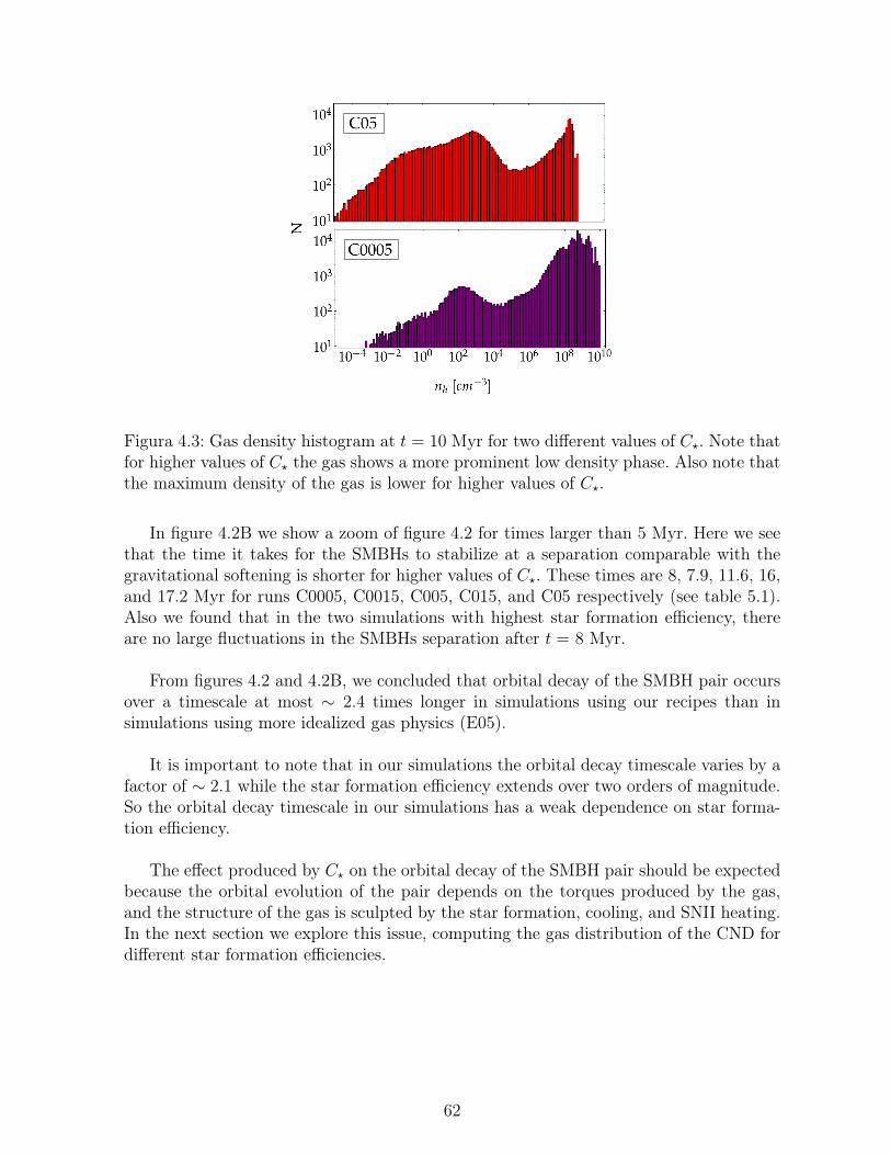
Figura 4.3: Gas density histogram at t = 10 Myr for two different values of C?. Note thatfor higher values of C? the gas shows a more prominent low density phase. Also note thatthe maximum density of the gas is lower for higher values of C?.

In figure 4.2B we show a zoom of figure 4.2 for times larger than 5 Myr. Here we seethat the time it takes for the SMBHs to stabilize at a separation comparable with thegravitational softening is shorter for higher values of C?. These times are 8, 7.9, 11.6, 16,and 17.2 Myr for runs C0005, C0015, C005, C015, and C05 respectively (see table 5.1).Also we found that in the two simulations with highest star formation efficiency, thereare no large fluctuations in the SMBHs separation after t = 8 Myr.

From figures 4.2 and 4.2B, we concluded that orbital decay of the SMBH pair occursover a timescale at most ∼ 2.4 times longer in simulations using our recipes than insimulations using more idealized gas physics (E05).

It is important to note that in our simulations the orbital decay timescale varies by afactor of ∼ 2.1 while the star formation efficiency extends over two orders of magnitude.So the orbital decay timescale in our simulations has a weak dependence on star forma-tion efficiency.

The effect produced by C? on the orbital decay of the SMBH pair should be expectedbecause the orbital evolution of the pair depends on the torques produced by the gas,and the structure of the gas is sculpted by the star formation, cooling, and SNII heating.In the next section we explore this issue, computing the gas distribution of the CND fordifferent star formation efficiencies.

62

4 6 8 10 12 14 16 18t [Myr]

−0.2

−0.1

0.0

0.1

0.2

Torq

ue

nH > 106 cm−3

C05C015C005C0015C0005

4 6 8 10 12 14 16 18t [Myr]

−0.2

−0.1

0.0

0.1

0.2

Torq

ue

nH < 106 cm−3

C05C015C005C0015C0005

Figura 4.4: Torque experienced by the SMBHs due to gas with density above 106 cm−3(left panel) a below 106 cm−3 (right panel). The lines of different colours represent si-mulations with for different values of C?. From this figure we see that practically all thegravitational torque is produced by gas with density higher than 106 cm−3.

4.3.2. Effect of the gas distribution on the orbital decay

In figure 4.3 we show the density distribution of the gas at t = 10 Myr for two differentvalues of C?. From this figure, we find that for higher values of C? a greater proportionof the gas has a low density and the maximum gas density is lower. This is because withmore vigorous star formation, high density gas is more efficiently converted into stars.With a greater number of stars, there is a greater number of supernovae explosions, whichheat the cold dense gas around the stars and drive the formation of a hot diffuse medium.

The torques the gas exerts on the SMBHs are density dependent, and we expect thatmost of the torque experienced by the SMBHs is due to high density gas. From figure4.3, we would expect that in simulations with smaller values of C?, where the portionof high density gas is greater, the torque of the gas on the SMBHs is more intense andthe in-spiral of the SMBHs faster. However, left panel of figure 4.4 shows that the torqueproduced by gas with a density greater than 106 cm−3 fluctuates repeatedly about zero,indicating that the high density gas does not always extract angular momentum from theSMBHs, but also deposits angular momentum into the SMBHs. This is consistent withthe large fluctuations that we observe on the separation of the SMBHs in figure 4.2. Forcompleteness, we plot in right panel of figure 4.4 the torque produced by gas less densethan 106 cm−3. It is clear from this figure that the effect of the low density gas on theorbits of the SMBHs is negligible.

The fluctuations of the torque exerted by the high density gas on the SMBHs may bethe result of the spatial distribution of this gas in the disk. To explore this, we show thedistribution of gas with densities greater than 106 cm−3 in the plane of the disk at t =

63

Figura 4.5: Distribution of gas in the plane of the disk at t = 10 Myr for C0005 (leftpanel) and C05 (right panel). We only show the gas with density greater than 106 cm−3.The green circles are the two black holes.

Tabla 4.2: Gas clumps number and densities.C? Ncl,t1 Ncl,t2 Ncl,t3 ∆ncl [cm−3] ncl [cm−3]0.005 86 44 38 106 − 108.7 107.6

0.015 84 39 25 106 − 109.3 107.9

0.05 87 32 19 106 − 108.6 107.7

0.15 70 27 15 106 − 108.8 107.9

0.5 37 16 9 106 − 108.0 107.1

Ncl,t1 corresponds to the number of clumps at t1 =5 Myr, Ncl,t2 corresponds to thenumber of clumps at t2 =10 Myr, and Ncl,t3 corresponds to the number of clumps att3 =15 Myr. ∆ncl corresponds to the range of densities of the clumps and ncl to the

mean density of the clumps.

10 Myr for run C0005 in figure 4.5 and for run C05 in figure 4.5B. From these figures, wefind that gas with density greater than 106 cm−3 is mainly concentrated in clumps, twoof which surround the two black holes. In this clumpy CND, the SMBHs have encoun-ters with these high density gaseous clumps, and depending on the characteristics of theencounter, they gain or lose angular momentum. This is reflected in the fluctuations ofthe gravitational torque produced by the high density gas on the SMBHs (figure 4.4).

From figures 4.5 and 4.5B, it seems that the main difference between run C0005 andrun C05 is the number of clumps formed. This difference may be the cause of the differentnumbers of fluctuations in the SMBHs’ separation seen in these runs, and the slightlydifferent migration timescale of the SMBHs. Simulations with lower SFR yield a greaternumber of gaseous clumps, so it is more probable for the SMBHs to closely interact withone or more clumps in these simulations.

64

In order to determine if the number of clumps depends on and C?, we compute thenumber of clumps (Ncl) as the number of groups of gas particles that are gravitationalbound with central density greater than 106 cm−3. We compute Ncl at three differenttimes– 5, 10, and 15 Myr– for each value of C? explored. We also compute the mean den-sity and the range of densities of these clumps. We summarize this information in table 2.

From table 2 we found that the number of clumps decreases as C? increases. Thisis consistent with figure 4.3, where we found that higher SFR correspond to a lowerproportion of high density gas. Therefore, in simulations with lower C?, the SMBHs areprone to interact with a higher number of gaseous clumps. This is reflected in the slightincrease in fluctuations of both the separation and the gravitational torque experiencedby the SMBHs that we observe in simulations with higher SFR.

Having explained in this section why the orbital decay timescale changes with C? insimulations using our recipe, in the next section we analyze why the orbital decay of theSMBHs in these simulations is faster than in simulation SDH05 and typically slower thanin simulation E05.

4.4. Gas physics and its effect on orbital decayBefore the SMBHs form a binary, the gas extracts angular momentum from the

SMBHs through dynamical friction, which leads to the in-spiral of the SMBHs towardthe center of the disk. As the intensity of the dynamical friction is proportional to thedensity of the gas, in a disk where the gas density is higher, the orbital decay of theSMBHs is faster (Chandrasekhar 1943; Ostriker 1999; Kim & Kim 2007).

In figure 4.6 we show the mean density of the gas around the SMBHs for the simula-tions E05, SDH05, and C005. The mean is taken over all gas particles within twice thegravitational influence radius (bound radius) of the SMBH: Rbound = 2GMBH/(c

2s + v2rel),

where cs is the sounds speed of the gas and vrel is its velocity relative to the SMBH. Wechoose this region around each SMBH because most of the torque experienced by theSMBH comes from gas particles in this region.

As seen in figure 4.6, our recipes yield far greater gas density than the recipes usedin simulation SDH05. This is because our recipes produce a greater density threshold forstar formation than the threshold of simulation SDH05. Additionally, the temperaturefloor for star formation is much lower using our recipes (25 K in ours, as compared to104 K in SDH05). As a result, the orbital decay of the SMBHs in simulations using ourrecipes is faster than in simulation SDH05.

Figure 4.6 also shows that the density of the gas in simulations with our recipes ismuch greater than in simulation E05. However, after t ∼ 6 Myr, in some of the simulationswith our recipes, the migration of the SMBHs slows. This is because in the simulationswith our recipes, the CND is fragmented in a few tens of high density gaseous clumpsand these gaseous clumps erratically perturb the orbits of the SMBHs. So even thoughin these simulations the density is higher than in simulation E05, the orbital decay of the

65

0 2 4 6 8 10 12 14 16 18Time [Myr]

103

104

105

106

107

108

109

1010

n H[c

m−

3 ]

E05SDH05C005

Figura 4.6: Mean density of the gas around the SMBHs as a function of time for simula-tions E05, SDH05, and C0005. The mean is taken over all gas particles within twice thegravitational influence radius of the SMBH.

SMBHs is, in some cases, delayed due to the interaction of the SMBHs with these gaseousclumps. The CND of simulation E05 is smoother than the CND in simulations with ourrecipes, and there are no high density gaseous clumps in it to perturb the SMBHs orbits.

In the next section we investigate whether these perturbations are likely to affect theevolution of SMBHs in real CNDs by comparing properties of the clumps in our simula-tions to observations.

4.5. Gaseous clumps

4.5.1. Density of the gaseous clumps.

As seen in section §3.2, the stochastic fluctuations of the SMBHs’ separation co-mes from gravitational interaction between the black holes and high density gas clumps(nh > 106cm−3). However, these fluctuations are unlikely to occur in real CNDs becauseintensity of the gravitational torques is density dependent, and the densities of the gasclumps in our simulations are higher than the densities of gas clumps in observed CNDs.For example, if we compare our clumps’ densities with the density of molecular clouds inisolated galaxies (Mathis 1990; Oka et al. 2001; Struve & Conway 2010) or ultra lumi-nous infrared galaxies (Downes & Solomon 1998; Schulz et al. 2007), which are typically∼ 102−105cm−3, we find that the density of the clumps in our simulations is at least twoorders of magnitude greater. Inside the molecular clouds, there are star forming regions(cold or hot cores) with densities comparable to the mean density of the clumps in our

66

simulations (< nh >∼ 107cm−3). However, they are one or two orders of magnitude lessdense than roughly half of the gas clumps in our simulations (nh ∼ 106 − 109.3cm−3).Even though one of the gas clumps that perturbs the SMBH orbits may have a densitycomparable with the density of these cores, the mass of these cores is on the order of∼ 103M� (Garay et al. 2004; Muñoz et al. 2007), which is at least two orders of magni-tude smaller than the mass of any of the clumps in our simulations.

The clumps in our simulations have these extremely high densities because our recipesdo not account for all of the physical processes that sculpt the clumps. For example, inour simulations we use a cooling that assumes that the gas is optically thin while theclumps in our simulations are optically thick (τ >> 1). Also, there is a large amountof energy that we are not considering in our simulations, such as the energy of photonsemitted by the stars and by the black hole’s accretion disk. The effects of turbulence,which is typically damped in SPH codes, are also omitted. All these physical processeswill prevent the further collapse of the clumps, promoting the formation of clumps withlower (and hence more realistic) densities.

4.5.2. Force resolution and the SMBH-clump interaction.

The high densities of the gaseous clumps can affect the orbits of the SMBHs in aspurious way. The gravitational pull at the edge of these clumps can be greater thanthe gravitational pull at the “edge” of the SMBHs in our simulations, where we defi-ne the edge of an SMBH to be its gravitational softening. We define the effective massdensity of our black holes (ρBH) to be the mass of the black hole (MBH) enclosed wit-hin a sphere of radius equal to the gravitational softening of the black holes (εBH), i.e.ρBH = 3MBH/(4πε

3BH). We can compare ρBH with the mass density of the gaseous clumps

(ρcl = mH ncl) to determine if, in our simulations, the clumps are more compact than theblack holes. For a gravitational softening of 4 pc, we find that ρBH = 3.8mH × 106cm−3.Hence, in our simulations the density of the gaseous clumps is greater than the effectivemass density of the black holes. This implies that the gravitational pull at the edge ofthe black holes (FBH(ε) ∝ ερBH) is typically smaller than the gravitational pull at theedge of the clumps (Fcl(Rcl) ∝ Rcl ρcl = 4− 5 ε ρcl). Indeed, considering a gravitationalsoftening of 4 pc, and the minimum and maximum densities of the gaseous clumps inour simulations, FBH(ε)/Fcl(Rcl) ∼ 0.04 - 10. Therefore, a black hole sees the clumps aspoint masses, and it is not able to disrupt them when it has a close encounter with oneof them, within a distance . 4 pc. Instead, in our simulations a close encounter withinthis distance will result in the scattering of the black hole.

If we decrease εBH, we would expect the higher resolution of the black hole’s gra-vitational force to allow the black hole to disrupt a clump in a close encounter, wherethe minimum distance is . 4 pc. To illustrate how decreasing εBH affects the outcomeof close encounters, we show how an encounter proceeds for different values of εBH inthe bottom two rows of figure 4.8. Snapshots farther right in this figure correspond tolater times. The first row of this figure shows a different encounter– one that illustratesscattering of the SMBH. In the middle row (run C0015_ε.004), we see that the SMBH’sgravitational potential disrupts the clump, and the SMBH does not scatter significantly.On the other hand, in the lower row (run C0015) where εBH is larger, the black hole is not

67

able to disrupt the clump. The orbit of the SMBH is perturbed and the gaseous clumpis scattered.

If these close encounters, where the minimum distance between the black hole andthe clump is . 4 pc, are the primary source of large fluctuations in the separation ofthe black holes, then we expect decreasing εBH sufficiently would cause these fluctua-tions to disappear. More precisely, we expect the large fluctuations to disappear onceFBH(ε)/Fcl(ε) > 1 for all clumps in the simulation.

In figures 4.8 we show the evolution of the SMBHs’ separation for different values ofεBH. The smallest value that we choose for εBH is still much greater than the Schwarzs-child radius of the black holes in our simulations (Rsch = 4.78× 10−6 pc). We note that,as we change εBH, the orbits of the black holes change. So, in simulations with the sameSFR but different εBH, the black holes don’t have close encounters with the same gaseousclumps. We found that in three of our simulations (runs C0015_ε.004, C005_ε.004, andC05_ε.004), making εBH smaller causes the large fluctuations to disappear. As expected,the better resolution of the gravitational force of the black holes in these simulationsallows them to disrupt the clumps in all close encounters. In contrast, we found that inthe runs C0005_ε.004 and C015_ε.004, some large fluctuations in the separation of thepair occurred (see peaks enclosed by red circles in figures 4.8 and 4.8D) that are evenlarger than the fluctuations observed in the simulations with the same SFR, but largerεBH (runs C0005 and C015). We analyzed each of these large fluctuations to determinewhy they are present even when the black hole’s gravitational force is resolved down toscales of 0.004 pc, where FBH(εBH) is larger.

In the case of run C0005_ε.004, we identify two large fluctuations (enclosed by redcircles in figure 4.8). In figure 4.9, we show the evolution of the orbits of the black holesduring these two large fluctuations. The upper row of figure 4.9 shows the orbits of theblack holes during the first of these large fluctuations, and the lower row of figure4.9shows the second of these large fluctuations. We found that these two large fluctuationsoccurred because the black holes follow orbits of different radius and eccentricity, butwith respect to nearly the same center, which is located close to the densest and mostmassive gas clump of the simulation (ncl = 7.4 × 108cm−3 and Mcl = 8.8 × 108 M�).Therefore, the large fluctuations in run C0005_ε.004 are not the result of close encoun-ters with high density clumps. Instead they are the result of the movement of the blackholes which, at the moment of these fluctuations, are not bound together.

Run C015_ε.004 also has two large fluctuations in the separation of the black holes(enclosed by red circles in figure 4.8D). We show the evolution of the orbit of the blackholes during these two large fluctuations in figure 4.10. From the upper row of figure 4.10,we found that the first large fluctuation is the result of scattering of one of the black ho-les due to gravitational interaction with a high density gas clump. This gas clump hadin turn been ejected from a past scattering with another high density gas clump. In thelower row of figure 4.10, we see that the second large fluctuation is the result of scatteringwith the same gas clump responsible of the first large fluctuation. Both of these closeencounters have a minimum distance which is greater than 10 pc, and therefore they arenot artificially produced by low resolution of the gravitational force of the black holes.

68

Figura 4.7: Distribution of gas in the plane of the disk. Time of the snapshots increasesfrom left to right. The figures show the interaction between one black hole and a clump forthree different simulations (upper, middle, and lower rows). The upper row correspondsto the run C0015, where εBH = 4 pc; the middle row correspond to the run C0015_ε.004,where εBH = 0.004 pc; and the lower row correspond to a run with εBH = 4 pc restartedfrom simulation C0015_ε.004 in order to follow the same close encounter that we show inthe middle row but with a higher gravitational softening. In all the panels the SMBH isrepresented as a green filled circle. In the upper and lower row we see that, where εBH = 4and thus the density of the black hole is comparable with the density of the gas, the closeencounter produces a slingshot effect on the black hole. In contrast, we see in the middlerow that, when εBH = 0.004, as the effective density of the black hole is greater than thedensity of the clumps, the clump is disrupted in the close encounter with the black hole.

69

Figura 4.8: Evolution of the SMBHs’ separation for simulations with different values ofthe gravitational softening of the black holes and different values of C∗. The continuousline correspond to simulations where ε 4 pc, the doted line to simulations where ε 0.04 pcand the dashed line to simulations where ε 0.004 pc. Each panel correspond to a differentvalues of the star formation efficiency: C? = 0.005 (left upper panel), C? = 0.015 (middleupper panel), C? = 0.05 (right upper panel), C? = 0.15 (left lower panel) and C? = 0.5(left middle panel).

70

However, the clump that produces these two large fluctuations in the separation of theblack holes is the most dense and massive clump in run C015_ε.004 (3.5× 108cm−3 and4× 108 M�). So this clump is the most extreme clump in our simulation and hence, thetwo scatterings produced by it are highly unlikely to happen in a real CND. We note thatshortly after the last scattering (∼ 2 Myr), this clump is disrupted by one of the blackholes, and after this disruption the orbital decay of the SMBH pair continues relativelysmoothly.

Intense, fluctuating gravitational torques experienced by SMBH pairs in a clumpymedium have also been observed in numerical simulations by other authors (Escala etal. 2004; Fiacconi et al. 2013; Roskar et al. 2014). To compare our results with the onesobtained by Fiacconi et al. (2013), we estimate the effective density of the black holesand the clumps of their simulations. Using figure 3 of Fiacconi et al. (2013), we estimatethat the density of their clumps range between 0.8 × 106cm−3 and 13 × 106cm−3. Thisestimate is a lower bound for the density, because we assume that the vertical size oftheir clumps is comparable to the thickness of their disk. If we compare this densityrange with the effective density of their black holes (which is ρBH = 7.9mH × 107cm−3),we find that ρBH is typically greater than the density of their clumps and therefore theirsimulations don’t suffer of a bad resolved black holes force. However, from our estimation,we found that the density of these gas clumps is greater, or equal, than the density of thedensest, observed molecular clouds. This means that in these simulations the stochasticgravitational torques experienced by the black holes due to the gravitational interactionwith the densest gas clumps can be overestimated.

4.6. ConclusionsWe studied the evolution of a pair of SMBHs embedded in a star forming CND to

explore how different SFR and gas physics can result in different timescales for the orbi-tal decay of the pair. For this purpose, we ran twenty three N-body/SPH simulations. Ineighteen of these simulations we used a modified version of the code Gadget-3 in whichwe implemented recipes for star formation, cooling and supernovae explosions that re-semble the ones used by other authors in the study of SMBH pairs (Callegari et al. 2011;Van Wassenhove et al. 2012; Roskar et al. 2014). The other two simulations used differentgas physics. In one of these simulations we used the hybrid multiphase model for starformation implemented in Gadget-3 Springel & Hernquist 2003; Springel et al. 2005a),where it is assumed that star formation is self regulated (simulation SDH05). In the otherone, the gas thermodynamics is simpler and there is no star formation (simulation E05).

Before the SMBH pair forms a binary, their orbital decay is driven by dynamicalfriction coming from their gaseous environment. As this dynamical friction is density de-pendent, we expect the orbital decay of the SMBHs to occur more quickly in simulationswhere the gas density of the CND is higher. The simulations we ran with our recipesresulted in a higher mean gas density around the SMBHs than simulation SDH05, andaccordingly we found the SMBHs’ orbital decay to be faster using our recipes. However,

71

Figura 4.9: Distribution of gas in the plane of the disk, from left to right the time of thesnapshots increases. The figures show the orbit of the black holes in the run C0005_ε.004.The upper row shows the evolution during the first large fluctuation in the SMBHs’separation (first red circle in figure 4.8). The lower row shows the evolution during thesecond large fluctuation on the SMBHs’ separation (second red circle in figure 4.8). Herewe can see that the two large fluctuations are the result of the changing separation of theblack holes as they orbit a common center, near the center of very dense and massive gasclump, with different orbital radii. The fluctuations are not the result of close encounterswith high density gas clumps.

Figura 4.10: Distribution of gas in the plane of the disk, from left to right the time of thesnapshots increases. The figures show the orbit of the black holes in the run C015_ε.004.The upper row shows the evolution during the first large fluctuation on the SMBHs’separation (first red circle in figure 4.8D). The lower row shows the evolution at themoment of the second large fluctuation on the SMBHs’ separation (second red circle infigure 4.8D).

72

in simulations with our recipes the orbital decay is sometimes slower than in simulationE05, even though the gas density in these simulations is higher than in simulation E05.This happen because in these simulations, the CND is fragmented in a few tens of highdensity (∼ 106 − 109 cm−3) gaseous clumps, which erratically perturb the orbits of theSMBHs, delaying their orbital decay.

The density of these gaseous clumps are extremely high compared to the observeddensity of molecular clouds in isolated galaxies (Mathis 1990; Struve & Conway 2010) orULIRGs (Downes & Solomon 1998; Schulz et al. 2007), which is typically on the order of∼ 102−105cm−3. The reason for this discrepancy is that we don’t include all the differentphysical process that sculpt the properties of the gas clumps. For example, to properlymodel the formation of gas clumps in the CND, we need to consider a more realisticcooling function which computes the effects of photons trapped inside the optically thickclumps, or follow the radiative transfer of these photons inside the clumps. Also, we haveto include heating due to the stars and the accretion disks of the SMBHs, which canhave an important effect on the temperatures and densities of the gas clumps. As the gasclumps are regions of vigorous star formation, we also expect that they will be highlyturbulent. This turbulence, which would sustain the gas clumps against gravitational co-llapse, is also a missing ingredient in our simulations since it is damped in SPH codeslike Gadget-3.

We also found that in simulations with our recipes, the density of the gas clumps iscomparable to or greater than the effective mass density of the SMBHs, which we defineas ρBH = 3MBH/(4πε

3BH) (for εBH = 4 pc, this density is ρBH = 3.8mH × 106cm−3).

We ran simulations where the gravitational softening of the SMBHs is smaller, and hencetheir effective mass density higher. With these simulations we show that the outcome of aclose encounter, within a distance comparable with the gravitational softening, dependson the force resolution of the SMBHs. If the force resolution (i.e. gravitational softening)is such that the effective density of the SMBHs is smaller than the density of the gasclumps, a close encounter results in the scattering of the SMBH. On the other hand, ifthe force resolution is such that the effective density of the SMBHs is higher than thedensity of the gas clumps, a close encounter results in the tidal disruption of the gasclump and the SMBH orbit is less affected.

Recently, it has been argued that the orbital evolution of a pair of SMBHs in a clumpyCND has a stochastic behavior, due to the gravitational interaction of the SMBHs withhigh density gaseous clumps (Fiacconi et al. 2013; Roskar et al. 2014). However, in thesimulations of these studies, as in our simulations, the densities of the denser gaseousclumps are higher than the densities of the observed, denser molecular clouds (Mathis1990; Oka et al 2001; Struve & Conway 2010). Thus, in these simulations the effect of thedenser gaseous clumps on the orbital evolution of the SMBHs, which is density depen-dent, can be overestimated. So the delay produced on the orbital decay of the SMBHs bythese gaseous clumps in real CNDs can be even smaller than the observed in simulations.

We emphasize that even though in our simulations the orbit-perturbing gravitationaltorques produced by these gaseous clumps are overestimated, the migration timescaleis still at most a factor three longer than the migration timescale in simulations with

73

simpler gas physics (Escala et al. 2005; Dotti et al. 2006). Even with this overestimation,gravitational interaction with the gas with the SMBHs produces a migration timescalewhich is much shorter than the typical migration timescale due to gravitational interac-tion with a background of stars. Interaction with gas yields a migration timescale on theorder of 107 yr, while migration timescale is on the order of one to ten Gyr in the case ofa triaxial distribution of stars (Berczik et al. 2006; Khan et al. 2011).

From our numerical study and previous studies of binaries embedded in gaseous cir-cumbinary disks (Escala et al. 2005; Dotti et al. 2006; Cuadra et al. 2009), we concludethat from the moment the SMBHs are separated by hundreds of parsecs until shortlyafter they form a binary, SFR has a much smaller effect on their orbits than cavityformation in the CND does. (This cavity formation is the result of inefficient viscousdissipation of angular momentum extracted from the binary (del Valle & Escala 2012,2014). Indeed, we show that for a two order of magnitude of difference on the SFR themigration timescale only change in a factor of two, and in comparison, the formation ofa cavity in the CND can extend the migration timescale by two orders of magnitude.However, since we are limited by the resolution of our simulations, we don’t explore fora sufficiently long period the effects of the star formation on the evolution of the SMBHsafter they form a binary. Amaro-Seoane et al. (2013) have made advances in this direc-tion by studying the evolution of an SMBH binary which resides inside the central cavityof a star-forming gaseous circumbinary disk. Their results indicate that star formationslows the orbital decay of the binary. However, they do not explore how star formationaffects the evolution of an SMBH binary when it is embedded in a circumbinary disk wit-hout a gap, a regime in which the gravitational torque of the gas on the binary is stronger.

As a future work, the effects of the star formation on the orbital evolution of anSMBH binary embedded in a circumbinary disk without a gap should be explored. Wealso need to model the gas around the binary more realistically. Ultimately, we wouldlike to determine if the gas can extract sufficient angular momentum from the SMBHbinary to drive its separation down to scales small enough for gravitational radiation totake over, ensuring coalescence of the SMBHs.

Acknowledgments. L del V’s research was supported by CONICYT-Chile throughGrant D-21090518 and a Redes (12-0021) grant, DAS Universidad de Chile and pro-yecto anillo de ciencia y tecnologÃa ACT1101. A.E. acknowledges partial support fromthe Center of Excellence in Astrophysics and Associated Technologies (PFB 06), FON-DECYT Regular Grant 1130458. J.C. acknowledges support from FONDECYT RegularGrant 1141175. The simulations were performed using the HPC clusters Markarian (FON-DECYT 11090216) from the DAS, Geryon(2) (PFB 06, QUIMAL 130008 and FondequipAIC-57 ) at the Center for Astro-Engineering UC and Damiana from the AEI. We usedsplash (Price 2007) for the SPH visualization in Figures 7, 8, 9, 15 and 16. We are gratefulto V. Springel for allowing us to use the Gadget-3 code.

74

Capítulo 5

Gap-opening criterion in simulations ofgalaxy mergers

In this chapter we apply our gap opening criterion to the SMBHB-disk systems thatare formed in the nuclear region of galaxy mergers. With this purpose we run differentsimulations of galaxy mergers. These simulations include recipes to model the star for-mation, the feedback of supernovas and radiative cooling of optically thin gas. We useour gap opening criterion to determine how likely the SMBH binaries formed in these ga-laxy mergers will experience a fast shrinking, and how far they are from a slow shrinkingregime.

5.1. IntroductionCentral SMBHs are found in practically every galaxy with a significant bulge (Ri-

chstone et al. 1998, Magorrian et al. 1998, Gultekin et al. 2009). Within the currentlyaccepted evolutionary model of the Universe the merger between galaxies is a commonevent (White & Frenk 1991, Springel et al. 2005). If the two galaxies involved in a mergerhost a SMBH we expect that both SMBHs will sink by dynamical friction to the inner-most region of the core of the merger remnant. When the mass enclosed by the orbit ofthese two SMBHs is smaller than the sum of their masses, then they will form a SMBHbinary (see chapter §1 for a more extended discussion of this picture).

Understand the further evolution of these SMBH binaries is crucial because if theyare able to shrink their separation down to aGW ∼ 10−3(MMBHs/106M�) pc, then thebinary becomes an intensive emitter of gravitational waves (GW) which allows the bi-nary to coalescence within 1010 yr (see chapter §1). Therefore, if we are able to determinewhat happens to SMBH binaries after galaxy mergers we will be able to determine theamount of sources of GW in the Universe and understand better the cosmic evolution ofthe population of SMBHs.

The problem is that after a galaxy merger the range of separations that has to becover by the SMBHs, in order to reach a separation comparable with aGW, is enormous(from ∼ 100 pc to 10−3 pc). This make the study of the fate of SMBHs after a galaxymerger very interesting but very challenging.

75

When the SMBHs binary in the nuclear region of the merger remnant is embeddedin a distribution of stars, the stars extract angular momentum from the binary drivingits in-spiral. If the stellar system is axisymmetric the migration timescale will be longerthan the age of the Universe (“last parsec problem”, Begelman, Blandford & Rees 1980).However, if the stellar distribution has some degree of triaxiality the shrinking timescalewill be of the order of 1− 10 Gyr (Khan et al. 2011; Vasiliev, Antonini & Merritt 2015),timescale that is comparable or longer than the time between galaxy mergers (see chapter§1 for a extended discussion of this picture).

However, if the galaxies involved in the merger have at least 1% of gas we expectthat a mass of the order of 10 to 100 times the mass of the SMBHs will sink to thecentral kiloparsec of the merger remnant (Barnes 2002; Mayer et al. 2010; Downes &Solomon 1998; Ueda et al. 2014). This gas can efficiently extract angular momentumfrom the binary making the shrinking timescale as short as 107 yr, down to a separationcomparable with aGW. However, if the gas does not redistribute efficiently the extractedangular momentum from the binary then it will be pushed away, generating a regionof low density or gap around the binary (Artymowicz & Lubow 1994). In this case, thebinary will enter a regime of slow migration in which, for a SMBH binary of mass ≥ 107

M�, the migration timescale can be as long as the age of the Universe (Cuadra et al. 2009).

In two previous publications (del Valle & Escala 2012, 2014) we derive and test againstSPH numerical simulation a gap-opening criterion that allow us to determine in whichconditions a binary that is embedded in a gaseous disk will excavate a gap. Therefore,this criterion allow us to determine when the binary experience a fast or slow shrinking.Motivated by the result of these publications we want to apply these criterion to determi-ne how likely is that the SMBHs binary/disk systems formed in situs in a galaxy mergerwill experience a fast shrinking.

In section §5.2 we present the gap opening criterion and how we will use this criterionto determine how likely the SMBHs binaries experience a fast shrinking. In section §5.3we present the numerical method and initial setup of the galaxy mergers. In section §5.4we apply our gap-opening criterion to the nuclear gaseous region of the merger remnant.In section §5.5 we estimate in which conditions the formation of a gap and the subsequentstalling of the fast shrinking occurs. Finally in section §5.6 we discuss and summarizeour main results. Additionally in the appendix we analyze the merger remnant, theirkinematics and characteristics of the nuclear region.

5.2. The position on the gap-opening criterion phasespace

In del Valle & Escala (2012, 2014) we derive an analytical criterion that allow us todetermine when a binary embedded in a gaseous disk opens a gap. When the binaryopens this cavity it enters a regimen of slow shrinking and therefore this gap-openingcriterion also allow us to determine when the binary experience a slow or fast shrinking.

76

The gap-opening criterion for an equal mass binary has the following form,

∆topen∆tclose

=1

0.33

(csv

) ( v

vbin

)2 (H

a

)≤ 1 , (5.1)

where v2bin = Gµ/a, v is the rotational velocity of the binary-disk system and a is thebinary separation (del Valle & Escala 2014).

The interesting thing is that this criterion can be used not only to determine if aparticular binary undergoes a fast shrinking but also can be used to determine how faris the binary from a slow shrinking regime. To illustrate this in figure 5.1 we present arepresentation of the gap opening criterion.

0.90 0.92 0.94 0.96 0.98 1.00(Vbin/V)2

0.5

1.0

1.5

2.0

(cs/V

)(H/a)

Early accretion

MBH ∼ 0.13%MRemnantr<2kp cs ∼ 150 km s−1

MBH ∼ 0.13%MRemnantr<2kp cs ∼ 30 km s−1

MBH ∼ 2%MRemnantr<2kp cs ∼ 150 km s−1

GapSlow shrinking

Distance to gap formation threshold

:

No GapFast shrinking

Figura 5.1: Representation of the gap-opening criterion in the space of parameters(cs/v) (H/a) vs (vbin/v). The black dashed curve represent the gap-opening criterionon equation 5.1. Below this curve there are the combination of parameters for which thebinary experience a slow shrinking and above the curve the combination of parametersfor which the binary experience a fast shrinking. We show three representative cases,two in the fast shrinking regime and one in the slow shrinking regime. The green dashedcurves represent the distance to the threshold line between the slow and fast shrinkingregime.

In figure 5.1 the gap-opening criterion (equation 5.1) is represented by the thick blackcurve. Here we show three representative cases, one below the curve in which the binary

77

opens a gap, and therefore experience a slow migration (Cuadra et al. 2009), and twoabove the curve that represent two cases where the binary experience a fast shrinking.However, we note that the case that is closer to the black thick threshold line is closerfrom the slow shrinking regime. Therefore, if there is a change on the parameters thatcontrol the gap-opening criterion, for example a decrease on cs, it is more probable thatthe binary/disk system that is closer to the threshold line will reach the slow migrationregime.

Therefore, from the position on the space of parameter of figure 5.1 we can determinehow far a binary/disk system is from a slow shrinking regime. This distance tells us howmuch have to change the parameters of binary/disk system in order to enter in a slowshrinking regime. We use this approach to study for the first time the likelihood of fastshrinking of SMBHs binaries in simulation of galaxy merger in terms of their position inthe space of parameters (cs/v) (H/a) vs (vbin/v), and not only by following the evolutionof their separation as is typically done (Callegari et al. 2011; Van Wassenhove et al.2014; Roskar et al. 2015). This will allow us to make more robust conclusions about theshrinking timescale of SMBH binaries because we will be able to determine how far theyare from a slow shrinking regime in the typical conditions of a galaxy merger. Also wewill be able to determine which conditions has to fulfill the nuclear region of the mergerremnant in order to make the SMBH binary experience a slow shrinking. We also exploreif the geometry of the galaxy merger has some influence on the position of the binary/disksystem on the phase space of the gap-opening criterion.

5.3. Initial conditions and numerical methodIn this section we present the different simulations of galaxy merger that we will use

in our study. All the simulations that we run consists of the merger of two equal-massdisk galaxies that collide on a parabolic orbit with pericentric distance Rmin = 8kpc. Inthe coordinate system that we use the orbital plane coincides with the x-y plane. We runfour mergers with different orientation of the disks of the galaxies relative to the planeof the parabolic orbit. We use the same geometry parameters defined by Barnes 2002:DIRect, RETrograde, POlar and INClined. In table 1 we present the different inclinationi between the galaxies and the orbital plane, and the pericentric argument ω, measuredin the orbital plane from the line of nodes to the y axis, for the mergers DIRect, RETro-grade, POlar and INClined.

Geometry i1 ω1 i2 ω2

DIRect 0 - -71 30RETrograde 180 - -109 30POlar 71 90 -109 90INClined 71 -30 -109 -30

Tabla 5.1: Geomerty parameters of galaxy mergers

The galaxies are initialized using the code GalactICS, in particular we use their “MilkyWay model” D (see Kuijken & Dubinski 1995 for details). In each galaxy model, we in-

78

clude a gaseous disk with the same exponential profile as the stellar component (Kuijken& Dubinski 1995) and with a total gas mass corresponding to 10% of the total stellardisk mass. In our simulations, we use the following units: [Mass]=5.8× 1011M�, [Distan-ce]=1.2 kpc and G=1. The total number of particles per galaxy is 420,000, 200,000 forsampling the gas, 120,000 for the dark matter halo, 80,000 for the disk component, and20,000 for the bulge. We also include a collisionless particle in the center of each galaxythat represent a SMBH.

For each merger setup (DIR, RET, PO or INC) we run two simulations where themass of the SMBHs is different. For one set of simulations the SMBH has a mass thatfollows the MSMBH−Mbulge relation in their host galaxies. This set of simulations permitus to explore the gap formation likelihood under the assumption that the mass accretionof the SMBHs occurs before they coalesce to form a single SMBH (“late accretion” model,see 5.2). In the second set of simulations we assume that the sum of the masses of theSMBHs is proportional to the mass on stars of the inner 2 kiloparsecs of the merger rem-nant. This set of simulations permit us to study the gap formation likelihood under theassumption that the mass accretion onto the SMBHs occurs before they form a boundbinary (“early accretion” model, see figure 5.2).

Accretion limits

MBH coalescence

Early accretion Late accretion

Figura 5.2: An scheme explaining the two accretion limits that we assume: The “earlyaccretion” limit where the accretion occurs before the coalescence of the SMBH binary(period indicated by the green dashed line) and the “late accretion” limit where theaccretion occurs after the coalescence of the binary (period indicated by the purple dashedline).

79

The gravitational softening of the dark matter halo particles and the initial stars is 50parsecs. For the gas, the stars formed during the simulation and the SMBHs the initialsoftening is 10 parsecs and then is reduced down to 1 parsec when the separation of theSMBHs is ∼ 500 parsecs.

We evolve the merging galaxies using the code Gadget-3 (Springel et al. 2001; Springel2005). This code evolves the system by computing gravitational forces with a hierarchicaltree algorithm, and it represents fluids by means of smoothed particle hydrodynamics(SPH; e.g.Monaghan1992) We used the recipes for cooling, stellar feedback and starformation included in the code Gadget-3. These recipes assume that the star formationis self-regulated and is parameterized only by the star formation timescale t0. We use thetypical value for this parameter, t0= 2.1, which provides a good fit to the Kennicutt law(Springel et al 2001)

5.4. The gap-opening criterion in remnants’ CNDIn this section we use the gap-opening criterion of equation 5.1 (del Valle & Escala

2014) to determine the position of the SMBH binaries, formed in situs in our simulationsof galaxy mergers, on the gap-opening criterion phase space. In this way we will deter-mine how likely is that SMBH binaries experience a fast shrinking (∼ 107 years). Alsowe will evaluate in which conditions these binaries can experience a slow shrinking.

5.4.1. Evaluating the gap-opening criterion

It was shown by Escala et al. 2005 that when the gravitational influence radius oftwo SMBHs embedded in a gaseous environment overlap they will generate a strongnon-axisymmetric density perturbation in the gas, which principal axis lags behind theprincipal axis that pass trough the two SMBHs. This is the process that can drive thefast shrinking of the SMBH binary if the binary does not excavate a gap on the disk.Therefore, is only valid to apply our gap-opening criterion in binary/disk systems wherethe gravitational influence radius of two SMBHs are overlapped. This means that to eva-luate our gap-opening criterion in our simulations of merging galaxies we need to knowat what scales this overlap occurs.

In figure 5.3 we show the evolution of the gravitational influence radius Rinf =2GMBH/(v

2BH + c2s) as a function of half the distance between the SMBHs. From this

figure we can see that Rinf becomes equal to the binary separation when the binary sepa-ration is approximately 35 pc. Therefore, for binary separations on the scale of 35 pc andless the gravitational influence sphere of each SMBH overlap, region that is properly re-solve by our simulations because our gravitational resolution for the gas and the SMBHsis ∼ 1 parsec. Also, we note that in this innermost region, below 100 parsecs, is wherethe conditions of the circum nuclear disks that are formed in our simulations match bet-ter the observations of ULIRGs (see the Appendix where we show the properties of themerger remnants).

80

100 101 102 103

R [pc]

100

101

102

103

Rin

f[p

c]

DIRRETPOINC

Figura 5.3: Gravitational influence radius Rinf = 2GMBH/(v2BH + c2s) of the SMBHs in

function of half the binary separation. The line represent the case when Rinf = R. Abovethis line Rinf > R and therefore the gravitational influence sphere of each SMBH overlap.

Now that we know at what separations of the SMBHs our gap-opening criterion isvalid, we will apply it to the SMBH binaries formed in our simulations of galaxy mergers.In figure 5.4 we plot the space parameter of the gap-opening criterion in an analogue wayas was done by del Valle & Escala 2014. The black curve is the threshold between theregion of the space of parameters where we expect that a gap will form (region below thecurve) and the region where the viscous diffusion of the gas is fast enough to maintainthe gap closed (region above the curve), as predict by our gap-opening criterion. Thisblack curve correspond to the cases where ∆topen = ∆tclose (see equation 5.1).

From the result of our four mergers with a “late accretion” model, squares in figure5.4, we see that they populate the region above the gap-opening threshold curve in theparameter space ((cs/v) (H/a), (vbin/v)) and therefore the formation of a gap on the diskin these simulations is unlikely. This is consistent with the evolution of the SMBH bina-ries that are formed in our simulations of galaxy mergers. All the SMBH binaries in thesefour simulations shrink their separation down to the gravitational resolution (softening∼ 1 pc), due to the extraction of angular momentum from the gas and background starson the remnant’s nuclear region, and they are never able to open a gap in this gaseousenvironment.

81

0.70 0.75 0.80 0.85 0.90 0.95 1.00(Vbin/V)2

0.5

1.0

1.5

2.0

2.5

3.0

3.5

4.0

(cs/

V)(

H/

a)

MBH ∝ MBulge

MBH ∝ MRemnantr<2kpc

DIRRETPOINC

Figura 5.4: The space of parameter of the gap-opening criterion: the ratio of the soundspeed of the gas and the velocity of the binary-disk system multiply by the ratio of thethickness of the disk and the binary separation (cs/v)(H/a), plotted against the quadraticratio between the rotational velocity of the isolated binary and the rotational velocityof the binary-disk system (vbin/v). The curve is the threshold between the region wherewe expect that a gap will form (region below the curve) and the region where no gapwill form (region above the curves), as predict by our gap-opening criterion (del Valle &Escala 2012,2014). The squares markers are the results from our simulations of merginggalaxies assuming the “late accretion” model. The stars markers are the results from oursimulations of merging galaxies assuming the “early accretion” model. The blue, red, greenand black colours design the different simulations DIR, RET, PO and INC respectively.All the square and star points are computed for the binary when it separation is smallerthan 35 pc, which is the distance in which the gravitational influence radius of the SMBHsoverlap.

From our simulations where the mass of the SMBHs is MBH = 0.0013 ∗MRemnantr<2kpc be-

fore the coalescence of the SMBH binary (star points on figure 5.4) we can see that theyare still well above the gap-opening threshold curve and therefore the SMBHs binaries inthese simulations are not able to excavate a gap on the circum nuclear disk.

Therefore, we can conclude from our gap opening-criterion that in the typical con-ditions on the central region of ULIRGs, and for a mass accretion that permits to theSMBHs fulfill theMBH−σ condition at the end of the merger, is unlikely that the SMBHbinary will excavate a gap on the gas, and therefore we expect that they will experience afast shrinking. Indeed, we can see that the position of the binary/disk systems formed inall the galaxy mergers is well above the threshold line, meaning that the SMBHs binaryare far away from the slow migration regime.

82

However, neither in our simulation nor estimations we include the effect of the blackhole accretion feedback. In principle this effect may push away the gas around the SMBHbinary, facilitating the formation of a gap, however, this feedback can also increase thesound speed of the gas around the binary, decreasing the viscous diffusion timescale andtherefore making more difficult the formation of a gap (see figure 5.4 to see how a changeon cs affects the likelihood of gap formation). Therefore the net effect of the AGN feed-back on the gap formation process is unclear.

5.4.2. Conditions needed to open a gap and further evolution

Now we explore the necessary conditions to open a gap in the gaseous circum-nucleardisk. As we see in the previous section if the sound speeds and thickness are comparablewith the values observed in ULIRGs and the SMBH binary ends with a mass that fulfillsthe M − σ relation in the merger remnant, for a “early accretion” or “late accretion”model, the formation of a gap is improbable.

From our gap opening criterion, equation 5.1, we know that ∆tclose/∆topen decreasewith c−1s , H−1 and MBH and therefore for colder thinner disks and more massive SMBHsthe formation of a gap is more probable. Therefore, we can evaluate for which values ofthese parameters the formation of a gap will occur.

We take the values from the simulation DIR (which is the one closer to the gap-opening threshold curve) as representative and we change the values of cs and MBH todetermine in which conditions a SMBH binary will excavate a gap reaching the slowshrinking regime.

From our gap opening criterion we know that a way to ensure gap formation is toreduce the sound speed of the gas, because this will reduce the speed with which the gascan fill a gap. We estimate that to ensure gap formation in the “late accretion” modelthe sound speed of the gas must be equal or smaller than 15 km s−1, which is muchsmaller than the turbulent velocity in interacting galaxies, such as ULIRGs (∼ 100 kms−1), or the turbulent velocity on high redshift star forming galaxies (∼ 50-80 km s−1,Cresci et al. , 2009; Dekel, Sari & Ceverino 2009 and references therein) and is similar tothe turbulent velocity in the inner region of local spirals (∼ 5-10 km s−1, Dickey et al. ,1990; Dib, Bell & Burkert 2006). We plot with blue triangles in figure 5.5 the position ofthe DIR “late accretion” simulation in the ((cs/v) (H/a),(vbin/v)) assuming that cs ∼ 15km s−1.

83

0.90 0.92 0.94 0.96 0.98 1.00(Vbin/V)2

0.5

1.0

1.5

2.0

(cs/

V)(

H/

a)

Late accretion

MBH ∼ 0.13% Mbulge cs ∼ 150 km s−1

MBH ∼ 0.13% Mbulge cs ∼ 15 km s−1

Figura 5.5: Same as figure 5.4. Here the different points represent the values on this spaceof parameters of the simulation DIR for different values of cs. The squares are the samefrom figure 5.4, the “late accretion” model in which we initialize the mass of the SMBHsas MBH ∼ 0.13 %Mbulge. The triangles are the values on this space of parameters of thesimulation DIR with the “late accretion” model assuming cs ∼ 15 km s−1.

In figure 5.6 we plot the values on the gap-opening space parameter ( (cs/v) (H/a),(vbin/v) ) for the simulation DIR, assuming the “early accretion” model. From this figurewe estimate that to ensure gap formation in typical conditions of a ULIRGs (H ∼100pc and cs ∼ 100 km/s) the black holes need to grow their mass to a mass comparablewith 2% the mass of the remnant’s bulge (MBH ∼ 2 %MRemnant(r < 2kpc)). This massgrowth will produce a SMBH with a mass one order of magnitude greater than the ex-pected from the observedMBH−Mbulge relation (Magorrian et al. 1998 ; Marconi & Hunt2003; Novak, Faber & Dekel 2006). Assuming that the SMBHs gain this mass over the∼ 100 Myr that pass from the beginning of the merger (where we assume the beginningof the merger as the moment when the separation between the dark matter halos of thegalaxies is comparable with the size of the dark matter halos) to the moment when thetwo SMBHs form a bound binary, the SMBHs need to accrete at a rate much greaterthan the typical accretion rate derived from observations (Di matteo et al. 2002; Dotti,Merloni & Montuori 2015 and references there in). Also, from figure 5.6 we estimate thatfor the “early accretion” model (assuming MBH ∼ 0.13 %MRemnant(r < 2kpc)) a soundspeed smaller than 30 km s−1 will ensure the formation of a gap. Then, for both accretionmodels the sound speed needed to form a gap is smaller than the typical turbulent velo-city observed in the inner region of ULIRGs which is of the order of 100 km s−1, thereforewe may expect that in typical conditions of ULIRGs such low turbulent velocity are notreached by the gas.

84

0.90 0.92 0.94 0.96 0.98 1.00(Vbin/V)2

0.5

1.0

1.5

2.0

(cs/

V)(

H/

a)

Early accretion

MBH ∼ 0.13% MRemnantr<2kp cs ∼ 150 km s−1

MBH ∼ 0.13% MRemnantr<2kp cs ∼ 30 km s−1

MBH ∼ 2% MRemnantr<2kp cs ∼ 150 km s−1

Figura 5.6: Same as figure 5.4. Here the different points represent the values on this spaceof parameters of the simulation DIR for different assumptions of MBH and cs. The starspoints are the same from figure 5.4, the “early accretion” model in which we initialize themass of the SMBHs asMBH ∼ 0.13 %MRemnant

r<2kpc . The triangles are the values on this spaceof parameters of the simulation DIR with the “early accretion” model assuming cs ∼ 30km s−1. The filled circles are the values on this space of parameters of the simulationDIR with the “early accretion” model assuming MBH ∼ 2 %MRemnant

r<2kpc .

5.5. Discussion and ConclusionsWe study the fate of SMBHs in simulations of galaxy mergers. If the galaxies involved

in these mergers have a gas fraction of at least 1% we expect that a massive gaseousdisk with a mass of ten to hundred times the mass of the SMBHs will be formed in thecentral kiloparsec of the merger remnant. The SMBHs in these nuclear region will forma SMBH binary which separation will experience a fast shrinking (in a timescale ∼ 107

years) mainly due to the gravitational torque produced by the gaseous disk. However, ifthe gas does not redistribute efficiently the extracted angular momentum from the binarya cavity of low density of gas will be formed around the binary and the shrinking of theSMBH binary will be dramatically delayed.

We use the gap-opening criterion derived in del Valle & Escala (2012, 2014), thatallow us to determine in which binary/disk system a gap is formed, to determine howlikely is that the SMBHs binaries formed in our galaxy mergers will experience a fast orslow shrinking. Using this approach we also determine how far are the SMBHs binariesfrom the slow shrinking regime by studying their positions on the phase space of thegap opening criterion. This allow us to determine how much the properties of the bi-nary/disk system (sound speed, ratio between the mass of binary and the disk, thickness

85

of the disk, velocity of the system) have to change in order to make the binary shift froma fast shrinking mode to a slow shrinking mode. From these estimations we make mo-re robust conclusion about the shrinking timescales of SMBHs binaries in galaxy mergers.

The simulations of galaxies mergers that we run correspond to the merger of equalmass “Milky way” type galaxies in a parabolic orbit. The inclination between the planeof the galaxies and the plane of the orbit differ between simulations, we explore fourdifferent geometries which we call RET, DIR, PO and INC following the nomenclatureof Barnes (2002). We evolve our galaxy merges using the SPH/N-body code Gadget-3which include recipes for star formation, radiative cooling and supernovae heating. Wefind that all our merger remnants have properties consistent with observation of inter-acting galaxies within the central 100 pc (Sanders & Mirabel 1996; Downes & Solomon1998; Medling et al. 2014; Ueda et al. 2014).

We find that the position of all SMBH binaries in the phase space of the gap openingcriterion are within the fast shrinking regime and very far from the slow shrinking regime.This means that the SMBH binaries in our simulations will very likely experience a fastshrinking and that the properties of the gas around them have to change very radicallyin order to pass from the fast shrinking regime into the slow shrinking regime. This is inconcordance with the actual evolution of the SMBHs in our galaxy merger simulations,where we observe that the SMBHs experience a fast migration until they reach a separa-tion comparable with the gravitational softening without forming a gap.

However, in our simulations the SMBHs do not experience mass accretion. For thisreason we run four additional simulations to estimate the gap-opening likelihood assu-ming that the mass of the SMBHs is proportional to the mass of the of the remnant’sbulge, in concordance with the MBH −Mbulge relation. We find that even if the SMBHsreach this higher masses before they form a bound binary the formation of a gap is unli-kely.

From our gap-opening criterion we find that the formation of a gap is more probablefor more massive SMBHs (del Valle & Escala 2012, 2014) or disks with smaller soundspeed. Hence we estimate the necessary SMBH’s mass to form a gap and the necessarysound speed of the disk to form a gap. We find that the SMBH binary has to reach a masscomparable with 2% the mass of the remnant’s bulge before they form a bound binaryin order to gap formation be possible. This condition can be translated to an accretionrate much higher than the typical accretion rate derived from observations (Di matteoet al. 2002; Dotti, Merloni & Montuori 2015 and references there in). We also find thatthe sound speed of the gas has to be smaller than 15 km s−1 to gap formation occur,sound speed that is much smaller than the typical turbulent velocity on the inner regionof ULIRGs which is of the order of 100 km s−1 and which is more similar to the turbulentvelocity in the inner region of a “Milky Way” type galaxy (∼ 5-10 km s−1, Dib, Bell &Burkert 2006).

We conclude that in standard conditions of the nuclear region of ULRIGs, and evenfor a relative high accretion rate, the formation of a gap is very unlikely to occur becausein these conditions the SMBHs binaries/gaseous disk system are very far from the slow sh-

86

rinking regime in the phase space of the gap-opening criterion. Thus, we expect that afterthe merger of galaxies with a gas fraction of at least 1 %−5 %, the SMBHs will experiencea fast shrinking (in a typical timescale of the order of 107 yr) down to the scales wheretheir final coalescence will be driving by the emission of gravitational waves (∼ 10−3 pc),unless other processes strongly affect the distribution of the gas nearby the SMBH binary.

One of these processes that can stop the fast shrinking of the SMBH binary is theeffect of the accretion luminosity of the SMBHs in the nearby gas. However, the effectof the accretion luminosity onto the gas is not clear, because some numerical works sug-gest that even for a super-Eddington regime the radiation is not strong enough to pushall the gas that is nearby the SMBHs away from the SMBHs (Krumholz & Thompson2012). Therefore we conclude that, if the accretion luminosity of the black holes doesnot push away a large portion of the gas nearby the SMBH binary, then the SMBHbinaries are very likely to experience a fast shrinking. However, to make this statementmore robust, further research of the characteristic of the gas in the nuclear region ofmerger remnants at sub parsec scales are needed. This research would allow us to putmore secure constraints on the rate of merging SMBHs in the universe, which is a crucialingredient in models of the evolution of the population of SMBHs in the Universe, and todetermine the amount of gravitational waves sources that we expect to observe with thefuture European Laser Interferometer Space Antenna (eLISA, Amaro-Seoane et al. 2013).

Acknowledgments. L del V’s research was supported by CONICYT-Chile throughGrant D-21090518 and a Redes (12-0021) grant, DAS Universidad de Chile and proyectoanillo de ciencia y tecnología ACT1101. A.E. acknowledges partial support from the Cen-ter of Excellence in Astrophysics and Associated Technologies (PFB 06), FONDECYTRegular Grant 1130458. The simulations were performed using the HPC clusters Doco-rozco (FONDECYT 1130458) from the DAS and Geryon(2) (PFB 06, QUIMAL 130008and Fondequip AIC-57 ) at the Center for Astro-Engineering UC. We are grateful to V.Springel for allowing us to use the Gadget-3 code.

87

Appendix: Structure of the merger remnant

Kinematics of the merger remnant

In this appendix we describe the dynamical structure of the mergers remnants for ourfour simulations of galaxy mergers.

In fig 5.7 we show the distribution and kinematics of the gas at the end of each simu-lation. These figures show the radial velocity vr of the gas particles as a function of theradius r for the four mergers that we simulate. We can see that the distribution of theparticles in these figures is nearly symmetric with respect to vr = 0 for radius smallerthan r ≈ 1−10 kpc. For larger radius all the simulations present narrow diagonal stripesthat are not symmetric with respect to vr = 0. These stripes are the tails of the mergerwhich are form from extracted material from the disk of the galaxy when the galaxiesexperience a pericentric passage. The amount of material in each of these tails and theirnumber depend on the orbital parameters of the merger. For example the merger INC infigure 5.7 (bottom right panel) shows more of these asymmetric features than the othermergers because, in this merger, there are two pairs of tails in different planes that co-exist simultaneously. Instead in simulation DIR (upper left panel) there are only a pairof tails and in simulation RET (upper right panel) there are only two big tails and athird smaller tail which is in the same plane of the bigger tails. The PO merger (bottomleft panel) shows only one of this asymmetric structures and in this case is not properlya tail but more an elongated puffier structure of gas.

The distribution of the gas that is nearby to vr = 0 represents particles with nearlycircular orbits and therefore are characteristic of the gas disc that is formed by the in-fallof material. The particles of gas with larger vr dispersion, symmetric respect to vr = 0,represent the gas that follows more elongated eccentric orbits in this disk. For example,the remnants of the DIR and RET mergers have large amounts of gas with narrower vrdistributions at radius smaller than 4 kpc and larger than 2.5 kpc. This narrower dis-tribution represent a disk structure and they are not found in simulations PO and INC.In simulation PO there is no disk structure at this radius and the remnant has a moreellipsoidal geometry. For the case of the simulation INC at this radius the material on thetails is still falling and, comparing with the evolution of the tails of the RET and DIRmergers, we expect that at these radius the tails will settled down in a disk structureafter a few Myr.

In radius smaller than 2.5 kpc we find the nuclear region which for simulations RET,DIR and INC has the shape of a disk. For the case of the RET and DIR simulationswe can see that this nuclear disk have a larger vr dispersion than the disk in the region2.5 kpc < r < 4 kpc and therefore they consist of gas with more elongated orbits. Thekinematics of the nuclear disk of the INC simulations its more difficult to recognizebecause its hidden by the gas tails. The simulation PO has a nuclear region that has amore ellipsoidal geometry with a larger vr dispersion however below 100 pc appears anarrower structure that can be identify as a disk.

88

Tails of the merger

Narrow distribution

Central disk

Ellipsoidal

Figura 5.7: Radial velocities and distribution of gas in all merger remnants. In each plot,the horizontal axis is the radius in logarithmic scale, while the vertical axis is vr. Thesefigures show the distribution and kinematics of the gas at the end of each simulation.

Properties of the nuclear region

In figure 5.8 we show the surface density of the gas in function of the radius (leftpanel) and the sound speed of the gas in function of the radius (right panel) for thenuclear region of our four simulations. In these two figures we compute the quantities onthe plane perpendicular to the angular momentum of the central kiloparsec of the mergerremnant. From these figures we can see that, although the exact form of the surface den-sity and sound speed profile of the nuclear region differs between different simulations,the general trend is similar for the four mergers that we simulate.

In all our simulations the nuclear region of the merger remnant have surface densi-ties that range between 1024 − 1025 cm−2 which is consistent with the observed averagesurface density of the nuclear region of ULIRGs (Hodge et al. 2014; Iono et al. 2014; Xuet al. 2014). The surface density profile, in the four merger’s remnant, roughly decay asr−0.5, and therefore is less steeper than a typical Mestel density profile (see figure 5.8)which is used to model circum-nuclear disks in more idealized simulations (Escala et al.2005, Dotti et al. 2006).

89

101 102 103

R [pc]

1023

1024

1025

1026

1027

Σ[c

m−

2 ]

DIRRETPOINC

r−1

r−0.5

101 102 103

R [pc]

102

103

c s[k

ms−

1 ]

DIRRETPOINC

Figura 5.8: Left Panel: Surface density in function of radius for our for simulations ofgalaxy mergers with different orbital parameters. This surface density is computed onthe plane perpendicular to the angular momentum of the central kiloparsec of the mergerremnant. Right Panel: Sound speed as a function of radius for our for simulations ofgalaxy mergers.

The sound speed of the central 2.5 kpc of the four merger remnants range between110 km s−1 and 1200 km s−1, however, in the innermost region (below 100 pc), which isthe region where we will study the evolution of SMBH binaries, the sound speed is of theorder of 100 km s−1 which is consistent with the turbulent velocity of the gas observedin the central kiloparsecs of ULIRGs (Downes & Solomon 1998; Ueda et al. 2014). Thehigher sound speeds that we observe in the central kiloparsec of our simulations are con-sequence of the high star formation rate in these regions and the subsequent heating bysupernova Type II explosion which typically heats the gas up to 108 K which correspondto a sound speed of the order of 1000 km s−1.

In the left panel of figure 5.9 we show the enclosed mass in function of the radius. Wecan see from this figure that the enclosed mass follow a similar trend with radius for thefour merger, also we can see that the enclosed mass inside 2.5 kpc is of the order of 1010

M� for the four mergers, which is consistent with the mass observed in the nuclear regionof interacting galaxies such as ULIRGs (Sanders & Mirabel 1996; Downes & Solomon1998; Engel et al. 2010; Medling et al. 2014; Ueda et al. 2014; Xu et al. 2014).

In all our mergers the total mass on gas of the two galaxies just before the first pas-sage is approximately 5.8× 1010 M�, therefore, from the left panel of figure 5.9 we foundthat the percent of this mass on gas that ends accumulated in the central 2.5 kpc ofthe remnants are 70%, 36%, 35% and 18%, for the merger DIR, INC, RET, and POrespectively. We note that these percents are smaller than the typical values that arefound in other simulations of galaxy mergers because in these works it is not consideredthe consumption of gas by star formation (Barnes & Hernquist 1996; Mihos & Hernquist

90

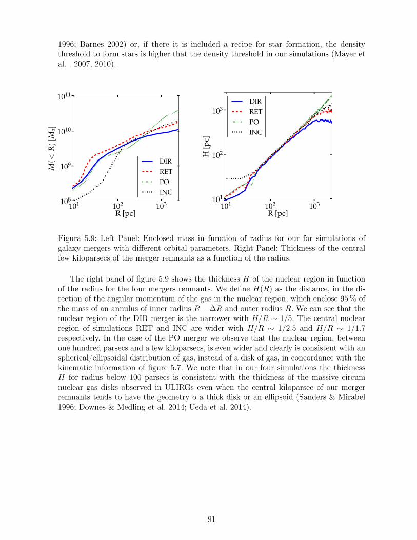
1996; Barnes 2002) or, if there it is included a recipe for star formation, the densitythreshold to form stars is higher that the density threshold in our simulations (Mayer etal. . 2007, 2010).

101 102 103

R [pc]

108

109

1010

1011

M(<

R)

[Mo]

DIRRETPOINC

101 102 103

R [pc]

101

102

103

H[p

c]

DIRRETPOINC

Figura 5.9: Left Panel: Enclosed mass in function of radius for our for simulations ofgalaxy mergers with different orbital parameters. Right Panel: Thickness of the centralfew kiloparsecs of the merger remnants as a function of the radius.

The right panel of figure 5.9 shows the thickness H of the nuclear region in functionof the radius for the four mergers remnants. We define H(R) as the distance, in the di-rection of the angular momentum of the gas in the nuclear region, which enclose 95% ofthe mass of an annulus of inner radius R−∆R and outer radius R. We can see that thenuclear region of the DIR merger is the narrower with H/R ∼ 1/5. The central nuclearregion of simulations RET and INC are wider with H/R ∼ 1/2.5 and H/R ∼ 1/1.7respectively. In the case of the PO merger we observe that the nuclear region, betweenone hundred parsecs and a few kiloparsecs, is even wider and clearly is consistent with anspherical/ellipsoidal distribution of gas, instead of a disk of gas, in concordance with thekinematic information of figure 5.7. We note that in our four simulations the thicknessH for radius below 100 parsecs is consistent with the thickness of the massive circumnuclear gas disks observed in ULIRGs even when the central kiloparsec of our mergerremnants tends to have the geometry o a thick disk or an ellipsoid (Sanders & Mirabel1996; Downes & Medling et al. 2014; Ueda et al. 2014).

91

Capítulo 6

Conclusions

In this thesis I study the evolution of SMBHs after a galaxy merger and how likely isthat the SMBHs of the galaxies will coalescence after the merger. Within the context ofhierarchical structure formation, where the merger between galaxies is a common event,and from the observational realization that a SMBH is harboured in the center of prac-tically every galaxy with a significant bulge, I overview how the formation and evolutionof SMBH binaries has become an established concept.

I discussed the standard theory of the evolution and merger of SMBH binaries ingalactic nuclei based in the study of the long-term evolution of a SMBH binary at thecenter of a dense stellar system. In this picture the SMBHs sink to the center of thedense stellar system due to the gravitational drag generated by the background starsonto the SMBHs and then the distance between the SMBHs becomes small enough toform a binary. This SMBH binary continues shrinking due to the transfer of energy ontothe stars, however this process kicks out stars of the system, depleting the number ofstars that are able to extract energy from the binary and drive the further shrinking ofthe SMBH binary. This depletion of stars stalls the shrinking of the binary and only inthe more favourable cases, were the closest regions of the binary are refilled with newstars, the coalescence of the SMBH binary is achieved in a timescale of the order of 1 Gyr.

I also review how the stars are not the only component of galaxies that can extractangular momentum from the SMBHs binary. Indeed, numerical simulations of merginggalaxies and observations of ultra luminous infrared galaxies (ULIRGs) have shown thatin galaxy mergers 60% to 90% of the total gas is driven to the central kilo parsec ofthe merger remnant forming a disk like structure (circum nuclear disk). Therefore, if thegalaxies involved in the merger have at least 1% of gas it is expected that the SMBHbinary will end embedded in a gaseous environment with a mass comparable to or muchgreater than its own mass, this will have an important effect on its orbital evolution.

Different studies have shown that this huge accumulation of gas can dramaticallyshorten the typical timescale of the coalescence of the SMBH binary. For example, Es-cala et al. (2005) showed that when the gravitational spheres of the SMBHs overlap, astrong non axisymmetric density perturbation is produced in the gas with a principalaxis that lags behind the principal axis of the binary. This offset produces a torque ontothe SMBHs that drives the transfer of angular momentum from the binary to the gas.

92

Under these conditions, if the extracted angular momentum is efficiently redistributed bythe gas, Escala etal. (2004, 2005) showed that the SMBH binary will experience a fastmigration that will allow the binary to coalesce in a timescale of the order of 10 Myr.However, if the gas does not efficiently redistribute the extracted angular momentumit will be pushed away from the binary forming a gap or cavity of low density. In theseconditions, numerical studies have shown that the gas will not be able to drive the SMBHbinary to coalescence in a timescale shorter than the age of the universe (Cuadra etal2009).

Therefore, the aim of this thesis is to derive a criterion to determine under which con-ditions the gas will be able to efficiently redistribute the extracted angular momentumfrom the binary (conditions for which a SMBH binary will experience a fast shrinking).Then, I use these criterion to determine how likely is that in real astrophysical systemsthe conditions that will permit the fast shrinking of SMBHs after a galaxy merger arefulfilled. These studies ultimately will allow us to set constraints to the likelihood ofcoalescence of SMBHs in the universe, will help us to reach a better understanding ofthe evolution of the population of SMBHs in the universe and will help us to determi-ne the amount of gravitational waves expected to be observed by the future EuropeanLaser Interferometer Space Antenna (eLISA, Amaro-Seoane et al. 2013) or by means ofmillisecond pulsar timing arrays.

6.1. Main resultsI derived an analytic criterion to determine when the gravitational torque exerted by

a SMBH binary in a massive gaseous disk will produce the formation of a gap. In diskswhere this gap or cavity does not form, we expect that the extraction of angular momen-tum from the binary will ensure the coalescence of the binary in a timescale of the orderof 107 yr. In comparison, in systems where the gap is formed the coalescence timescalemay be as long as 109 yr. We ran forty one SPH simulations of binaries embedded onisothermal gaseous disks to test our gap-opening criterion and we found concordance bet-ween the predictions of our gap-opening criterion and the gaps formed in our simulations.

To estimate the likelihood of formation of a gap, and therefore of the coalescence ofSMBHs in galaxy mergers, I run eight simulations of major merger with different orbitalparameter to apply the gap-opening criterion to the in situ disk-binary system formed inthese simulations. In the eight simulations of major galaxy mergers that I performed Ifound that more than 60% of the gas of the two galaxies ends in the central kilo parsec ofthe merger remnant and that the mass of the gas in this central region isMgas ≈ 1010 M�.Also, I found that in the central one hundred parsecs the conditions of the gas roughlymatches the condition observed on interacting galaxies such as ULIRGs.

I evaluated my gap-opening criterion on these eight simulations and I found that theformation of a gap is unlikely even if the SMBHs accrete all the mass necessary to fulfillthe MBH −Mbulge relation on the remnant galaxy before they form a bound binary.

93

Moreover, I estimate that gap formation would be possible only if the gas has a turbu-lent velocity of the order of 10 km s−1 , which is comparable with the turbulent velocity inthe inner region of local spiral galaxies. Also, the gap formation would be possible if theSMBHs accrete a mass that is of the order of 2% the mass of the bulge of the remnantgalaxy before they form a bound binary, mass that is one order of magnitude greaterthan the expected from the MBH −Mbulge relation. This implies that the SMBHs haveto accrete mass at a rate much greater than the derived from observations. Therefore,we may expect that in typical conditions of the central kilo parsec of ULIRGs SMBHbinaries will coalescence in a timescale of the order of 107 yr.

In addition, I studied the effect of star formation in the dynamical evolution of a pair ofSMBHs in the pre-binary epoch following the evolution of a pair of SMBHs with a initialdistance of 500 pc inside a star forming circum-nuclear disk (CND). For this purposeI implemented in the code Gadget-3 recipes of star formation, cooling and supernovaexplosions that allowed me to simulate the multiphase structure of the gas. I found thatthe orbits of the SMBHs are perturbed by the presence of high density gas clumps andthat the shrinking of the separation of the SMBHs from 500 pc down to 4 pc does notdepend strongly on the star formation efficiency. Indeed, I proved that for a difference ofa factor 20 in the star formation efficiency the migration timescale changes only in factora 2.

6.2. Open issuesImplemented recipes of SF, cooling and SN heating in galaxy mergers: In

chapter §2.2 I present my implementation of recipes for star formation, supernovae hea-ting and cooling in the code Gadget-3. In chapter §4 I use these recipes to study the effectof the star formation efficiency in the migration of a pair of SMBHs in a star-formingcircum nuclear disk. These recipes allow me to model in a better way the multiphasestructure of the gas than the recipes that are included in the code Gadget-3.

As a future work I will simulate the same galaxy mergers that I simulate in chapter§5 but with the recipes that I implemented. These simulations will have a more clumpyand realistic ISM which will allow me to evaluate the likelihood of coalescence of SMBHbinaries in the central region of interacting galaxies in a more realistic environment.

Gap-opening criterion in other astronomical systems: The gap-opening crite-rion that I derive in this thesis can be applied to other systems that are analogous tothe SMBH binary-disk system. For example: the evolution of proto-stellar binaries andcommon envelope events which are produced when one of the stars enter in a giant phase(Passy et al. 2012).

For proto-stellar binary system the proto-stars will shrink their separation until theyexcavate a gap on the gaseous environment, in analogue way as SMBH binaries do. The-refore my gap-opening criterion can be used to determine the final separation of starbinaries. Also knowing the timescale in which gap-formation occurs allows us to set cons-traints to the evolution of the gas-dust distribution around binary stars, constraints that

94

are crucial to models of planet formation around binary stars. For example some studiesshow that the dimensionless viscosity parameter (Shakura & Sunyaev 1973) of the gas ina proto-planetary disk is higher than the dimensionless viscosity parameter of the dust(Johansen & Klahr 2005), meaning that gap formation can occur first in the dust, pro-ducing a decoupling between gas and dust.

Viscous dissipation in the gap opening criterion: From the gap-opening crite-rion of chapter §3 we can see that in a gaseous disks where viscous dissipation is faster,it is harder for the binary to excavate a gap. This happens because with a faster viscousdissipation the gas is able to redistribute the extracted angular momentum from the bi-nary.

In my derivation of the gap-formation I used the dimensionless viscosity parameter αss

of Shakura & Sunyaev (1973) to parametrize the viscous dissipation (νvisc ∼ αss cs ), whichin my simulations is αss ≈ 0.008 − 0.016. However, the presence of magnetohydrodyna-mic stresses can significantly increase the viscous torques, with an effective dimensionlessviscosity parameter α ≥ 0.2 (Shi et al. 2012). Moreover, global instability of the gasin massive gaseous also increase the torques, leading to an effective αss of order unity(Krumholz et al. 2007, Escala et al. 2007).

From these estimates, we expect that the value of αss in real gas-rich astrophysicalsystems, like the nuclear disk in ULRIGs (Downes & Solomon 1998) and Sub-millimeterGalaxies (Chapman et al. 2003, 2005; Takoni et al. 2006; Swinbank et al. 2010), willbe one or two orders of magnitude greater than in my simulations. Therefore, from thegap-opening criterion we can conclude that in the nuclear region of the gas-rich merginggalaxies, it is more likely that a SMBH binary will not be able to excavate a gap on thegas, allowing the gravitational torques from the gas to shrink the SMBH binary separa-tion down to scales where gravitational wave emission can drive the final coalescence ofthe binary within a Hubble time. For this reason it will be very interesting to test thedependence between the gap-opening criterion and the strength of the viscous torques, inorder to determine if these important predictions of the gap-opening criterion are correct.

Black hole accretion luminosity: From a simple estimation we can compare theluminosity associated to an AGN with the luminosity produced by several supernovaexplosions in the vicinity of a SMBH binary. Assuming that the energy released by apopulation of stars per unit of mass is ∼ 7.65 × 1047 erg M−1

� (Stinson et al. 2006) andthat the typical timescale for supernova explosions is of the order of 106 years, we findthat the luminosity associated to supernova explosions in a stellar population of totalmass Mstars is ∼ 3× 1035 (Mstars/M�) erg s−1. Also, we can assume that at the beginningof the binary evolution a total mass of stars comparable with the mass of the SMBHsis inside the orbit of the binary. In this case, for a SMBH binary of mass ∼ 108 M� thesupernova luminosity associated to the stars, inside the orbit of the binary, is ∼ 3× 1043

erg s−1. On the other hand, a SMBH of mass ∼ 108 M� accreting at the Eddington limithas an accretion luminosity of the order ∼ 1046 erg s−1, which is much greater than theluminosity associated to the supernovas (note that the luminosity of AGNs range between1042− 1048 erg s−1, e.g: Hopkins, Richards & Hernquist 2007). Therefore, we can assumethat the effect of the black hole accretion luminosity in the gas around the SMBH binary

95

would be another important process worthy of being studied.

Although this process is typically included in some simulation of galaxy merger, therecipes used to model the AGN feedback assume that the gas is efficiently heated bythe radiation produced by the accretion onto the black holes. However, how coupled isthe gas to the AGN feedback is not clear. Indeed, some works suggest that even for asuper-Eddington regime the radiation is not strongly enough to push away the gas thatis near the SMBHs (Krumholz & Thompson 2012).

Determine the effect of the AGN feedback onto the gas around a SMBH binary iscrucial to determine if this feedback can make easier or more difficult the formation of acavity. In principle, if the gas is pushed away from the binary then we can think that theAGN feedback will make easier the formation of a gap, however, as the gas is also heatedby the AGN feedback, and the gap formation is more difficult in a hotter gas, it is notclear whether the AGN feedback will facilitate or not the formation of a gap. Therefore,an interesting subject to future research is to study the effect of AGN feedback in the like-lihood of gap formation and its consequence in the shrinking timescale of SMBH binaries.

The SMBHs coalescence likelihood in semi analytical models: Another in-teresting study would be use what we learn from detailed simulations of galaxy mergersin semi-analytical models of galaxy evolution. We can export the information of the li-kelihood of coalescence of SMBH and its dependence on the parameters of the galaxymerger to semi-analytical models. Using this information we can determine in a moreconsistent way the evolution on mass of the population of SMBHs. This information willalso permit us to compute the gravitational wave background on the universe that isexpected to be observed using millisecond pulsar timing arrays.

6.2.1. SMBHs in the context of hierarchical structure formation

In the ΛCDM cosmological model, the currently accepted evolutionary model for theuniverse, lower mass self-gravitating systems form first later, following a hierarchical pro-cess of mass accretion and mergers, more massive gravitationally bound systems appearin the Universe. In this evolutionary picture of the Universe the host galaxies of SMBHsexperience multiple mergers during their lifetime (Menou, Haiman & Narayanan 2001).In these mergers SMBHs will sink together with the core of each galaxy and ultimatelythey will form binary systems inside the core of the mergers remnants.

From the hierarchical structure formation model we may expect that, if the shrinkingof these binaries is not fast enough then SMBH binaries may be widespread in the Uni-verse and, as Volonteri, Haardt & Madau (2003) show, they may contribute up to 10%of the total population of SMBHs today and even more in the past. Indeed, if the binaryshrinks only due to the gravitational interaction with stars the shrinking timescales ists ∼ 1 − 10 Gyr, which is comparable to or greater than the timescale between galaxymergers. These means that triple SMBH interactions after a major merger are very likely,which will result in a population of massive SMBHs wandering in galaxy halos and inthe intergalactic medium at the present epoch (Volonteri, Haardt & Madau 2003).

96

The results that I present in this thesis naturally suppress these predictions becau-se they support that the shrinking timescale of SMBHs after a galaxy merger is of theorder of ts ∼ 10 Myr thanks to the presence of gas that extracts angular momentumfrom the binary in a efficient way. Indeed, I found that for higher redshifts where theamount of gas is greater and the turbulent velocity of the gas higher is more likely thatthe shrinking of the SMBH binary will be faster, making the existence of a high rateof triple SMBH interactions very unlikely at high redshifts. Therefore, we expect not toobserve this population of wandering SMBHs at redshift zero. A population of this typeis more likely made of a collection of recoiling SMBHs: black holes that are the result ofthe coalescence of two black holes (2 MBHs → 1 MBH) and that experience a velocitykick due to the anisotropies of the gravitational waves emitted in the coalescence event(Bonning, Shields & Salviander 2007).

In addition like the merger rate of galaxies is ∝ (1 + z)2−3 (Fakhouri & Ma 2008,Lotz et al. 2011), and for higher redshifts the conditions for a fast shrinking are morefavorable (higher gas fraction and more turbulence) thus, the results of my thesis suggestthat in most major galaxy mergers (z > 1) the SMBH binary will coalescence in atimescale much shorter than the time between mergers. Meaning that the number ofSMBHs binaries at this redshifts will be very low, setting important constraints to theevolution of the population of SMBHs and the expected number of SMBH binaries in theUniverse.

97

Capítulo 7

Bibliography

Amaro-Seoane P., Aoudia S., Babak S. et al. , 2013, GW Notes, 6, 4

Amaro-Seoane P., Brem P., Cuadra J., 2013, ApJ, 764, 14

Armitage, P., Natarajan, P. 2002, ApJ, 567L, 9

Armitage, P., & Rice, W. K. M. 2005, Proc. of the STScI May Symp. 2005: ADecade Of Extrasolar Planets Around Normal Stars p 66 , vol 19, Livio et al. (NewYork: Cambrige University Press), astro-ph/0507492

Artymowicz, P., Lubow, S.H. 1994, ApJ, 421, 651

Artymowicz, P., Lubow, S.H. 1996, ApJ, 467L, 77

Barnes, J. E. 2002, MNRAS, 333, 481

Barnes, J., Hernquist, L. 1996, ApJ, 471, 115

Barnes, J., Hernquist, L. 1992, ARA&A, 30, 705

Baruteau C. & Masset F., 2013. Recent developments in planet migration theory. InTides in Astronomy and Astrophysics (pp. 201-253). Springer Berlin Heidelberg.

Bate, M. R. & Bonnell, I. A. 1997, MNRAS, 285, 33

Bate, M. R., Lubow, S.H., Ogilvie G. I., & Miller K. A., 2003, MNRAS, 341, 213

Begelman M. C., Blandford R. D. & Rees M. J., 1980, Nature, 287, 307

Berczik P., Merritt D., Spurzem R., Bischof H.-P., 2006, ApJL, 642, L21

Binney J. & Tremaine S., 1987, Galactic Dynamics, Princeton Univ.Press, NewJersey, USA.

Boehm, C., Schewtschenko, J. A., Wilkinson, R. J., Baugh, C. M., & Pascoli, S.,2014 MNRASLetters, 445, L31

Boyle B.J., Shanks, T. et al. , 2000, MNRAS, 317, 1014

Bon E., Jovanovic P., Marziani P. et al. , 2012, ApJ, 759, 118

98

Boroson, T.A. & Lauer T.R., 2009, Narure, 458, 53

Bromm V., Coppi P.S. & Larson R.B., 2002, ApJ, 564, 23

Callegari S., Kazantzidis S., Mayer L., Colpi M., Bellovary J. M., Quinn T., WadsleyJ., 2011, ApJ, 729, 85

Ceverino D. & Klypin A., 2009, ApJ, 695, 292

Chapman S. C., Blain A. W., Ivison R. J. & Smail I. R., 2003, Nature, 422, 695

Chapman S. C., Blain A. W., Smail I. R. & Ivison R. J., 2005, ApJ, 622, 772

Chandrasekhar S., 1943, ApJ, 97, 255

Christensen C. R., Quinn, T., Stinson G., Bellovary J. et al. , 2010, ApJ, 717, 121

Cresci G., Hicks E. K. S., Genzel R., Förster-Schreiber N. M., Davies R., et al.2009 ,ApJ, 697, 115

Cuadra J., Armitage P. J., Alexander R. D., et al. , 2009, MNRAS, 393, 1423

Comerford J., Gerke B., Stern D., Cooper M., & Weiner, B., Newman J., Madsen,K., & Barrows, R. 2012, ApJ, 753, 42

Chapman S. C., Blain A. W., Ivison R. J., & Smail Ian R., 2003, Nature, 422, 695

Chapman S. C., Blain A. W., Smail Ian R. & Ivison R. J., 2005, ApJ, 622, 772

Chapon D., Mayer L. & Teyssier R. 2011, submitted eprint arXiv:1110.6086

Dekel A., Sari R. & Ceverino D., 2009, ApJ, 703, 801

del Valle L., Escala A., 2012, ApJ, 761, 31

del Valle L., Escala A., 2014, ApJ, 780, 84

Dib, S., Bell, E., & Burkert, A. 2006, ApJ, 638, 797

Dickey J. M., Hanson M. M. & Helou G., 1990, ApJ, 352, 522

Di Matteo T., Allen S. W., Fabian A. C. et al. , 2002, in Lighthouses of the Universe:The Most Luminous Celestial Objects and Their Use for Cosmology, Gilfanov M.,Sunyeav R., Churazov E., eds., p. 443

Dotti M., Colpi M., & Haardt, F. 2006, MNRAS, 367, 103

Dotti M., Sesana A. & Decarli R. 2011, Advances in Astronomy Volume 2012,Article ID 940568,

Dotti M., Merloni A. & Montuori C., 2015, MNRAS, 448, 3603

Downes D., Solomon P. M., 1998, ApJ, 507, 615

Eracleous, M., Boroson, T.A., Halpern, J.P. & Liu J., 2011, arXiv:1106.2952

99

Escala A., Larson R. B., Coppi P. S., Mardones D., 2004, ApJ, 607, 765

Escala A., Larson R. B., Coppi P. S., Mardones D., 2005, ApJ, 630, 152

Escala, A., 2007 ApJ, 671, 1264

Evans II, P. J., 1999, ARA&A, 37, 311

Fabian A. C., Wilman R. J., & Crawford C. S., 2002, MNRAS, 329, L18

Fabbiano G., Wang J., Elvis M. & Risaliti G., 2011, Nature, 477, 431

Fakhouri O. & Ma C., 2008, MNRAS, 386, 577

Farris B. D., Duffell P., MacFadyen A. I., Haiman Z., 2014, ApJ, 783, 134

Ferrarese L. & Merritt D. A, 2000, ApJ, 539, 12

Ferrarese L. & Ford H, 2005, Space Science Reviews, 116, 523

Fiacconi D., Mayer L., Roskar R., Colpi M., 2013, ApJL, 777, L14

Foreman, G., Volonteri, M. & Dotti, M., 2009, ApJ, 693, 1554

Garay G. et al., 2004, ApJ, 610, 313

Gerritsen J. P. E & Icke V., 1997, aap, 325, 972

Gingold R. A. & Monaghan J. J., 1977, MNRAS, 181, 375

Goldreich P., Tremaine S. 1980, ApJ, 241, 425

Goldreich P., Tremaine S. 1982, ARA&A, 20, 249

Gold R., Paschalidis V., Etienne Z. B., Shapiro S. L., & Pfeiffer H. P., 2013, ar-Xiv:1312.0600.

Goodman J. & Tan J. C., 2004, ApJ, 608, 108

Gould A. & Rix H.W, 2000, ApJ, 532, L29

Guedes J., Callegari S., Madau P. & Mayer L., 2011, 742, 76

Gultekin et al., 2009, ApJ, 698, 198

Gunther, R., & Kley, W. 2002, A&A, 387, 550

Hayasaki, K., Mineshige, S., & Sudou, H. 2006, arXiv preprint astro-ph/0609144.

Hayasaki K., Saito H. & Mineshige S., 2013, pasj, 65, 4

Heckman T. & Best P., 2014, Annu. Rev. Astron. Astrophys., 52, 589

Hodge J. A., D. Riechers D., R. Decarli R., et al. , 2014, ApJ, 748, L18

Hopkins P., Richards P. & Hernquist L. 2007, ApJ, 654, 753

100

Hopkins P. F. & Quataert E., 2010, MNRAS, 407, 1529

Hoyle F., & Fowler, W. 1963, MNRAS, 125, 169

Iono D., Wilson C.D., Takakuwa S., et al. , 2007, 659, 283

Ivanov P. B., Papaloizou J. C. B., & Polnarev A. G., 1999, MNRAS, 307, 79

Johansen A. & Klahr H., 2005, ApJ, 634, 1353

Kaspi, S., Smith, P. S., Netzer, H., et al. , 2000,ApJ, 533, 631

Katz N., Weinberg D. H., Hernquist L., 1996, apjs, 105, 19

Kazantzidis, S., et al. 2005, ApJ, 623L, 67

Kennicutt Jr. R. C., 1998, ApJ, 498, 541

Khan F. M., Just A., Merritt D., 2011, ApJ, 732, 89

Kazantzidis S., Mayer L., Colpi M., Madau P., Debattista V. P„ Wadsley J., StadelJ., Quinn T., and Moore B. ApJ, 623, 67

Khan F. M., Preto M., Berczik P., Berentzen I., Just A., & Spurzem. R., 2012, ApJ,749, 147

Kim H., Kim W.-T., 2007, ApJ, 665, 432

Kormendy J., Ho L. C., 2013, araa, 51, 511

Komossa S., Burwitz V., Hasinger G., Predehl P., Kaastra J. S. & Ikebe Y., 2003,ApJL, 582, L15

Kocsis B., Haiman Z. & Loeb A., 2012a, MNRAS, 427, 2680

Kocsis B., Haiman Z. & Loeb A., 2012b, MNRAS, 427, 2660

Komosa S., Zhou H. & Lu H., 2008, ApJ, 678, 81

Krumholz M., Klein R. & McKee C., 2007, ApJ, 656, 959

Krumholz, M. & Thompson T., 2012, ApJ, 760, 155

La Franca F., Fiore F., Comastri A., et al. , ApJ, 2005, 635, 854

Lehto H. & Valtonen M., 1996, ApJ, 460, 207

Levin Y., 2007, MNRAS374, 515

Liu X., Greene J., Shen Y. & Strauss A., 2010, ApJL, 715, 1

Liu X., Greene J., Shen Y. & Strauss A., 2011, ApJL, 737, 2

Lin, D. N. C., Papaloizou, J. 1979, MNRAS, 186, 799

101

Lin, D. N. C., Papaloizou, J. 1986, ApJ, 309, 846

Lodato, G., & Price, D. J. 2010, MNRAS, 405, 1212

Lodato G., Nayakshin S., King A. R., Pringle J. E., 2009, MNRAS, 398, 1392

Lucia G. & Blaizot J., 2007, MNRASsoc, 375, 2

Lucy L. B., 1977, ApJ, 82, 1013

Lupi A., Haardt F., Dotti M., 2015, MNRAS, 446, 1765

Lodato G., & Price D. J., 2010, MNRAS, 405, 1212

Lotz J. M, Jonsson P., Cox T.J., Croton D., 2011, ApJ, 742, 103

Lynden-Bell D. 1969, Nature, 223, 690

Lynden-Bell D. & M.J. Rees, 1971 MNRAS152, 461

Lynden-Bell D., 1978, Physica Scripta, 17, 185

MacFadyen A. I. & Milosavljevic M., 2008, ApJ, 672, 83

Madau P. & Rees M. J., 2001, ApJLet. 551, L27

Magorrian J., Tremaine S., Richstone D. et al. , 1998, ApJ, 115, 2285.

Mathis J. S., 1990, araa, 28, 37

Marconi A. & Hunt L. K, 2003, ApJ, 589, L21

Mayer L., Kazantzidis S., Madau P., Colpi M., Quinn T., & Wadsley J. 2007,Science, 316, 1874

Makino J., Funato Y., 2004, ApJ, 602, 93

Mashchenko S., Wadsley J. & Couchman H. M. P., 2008, Science, 319, 174

Mayer L., Kazantzidis S., Escala A., Callegari S., 2010, Nature, 466, 1082

Mayer L. et al., 2007, Science, 316, 1874

McKee C. F. & Ostriker J. P., 1977, ApJ, 218, 148

McKee C .F. & Ostriker E. C., 2007, ARA&A, 45, 565

Medling A. M., U V., Guedes J., Max C. E. et al. , 2014, ApJ, 784, 70

Menou K., Haiman Z. & Narayanan V. K., 2001, ApJ, 558, 535

Merloni A., 2004, MNRAS, 353, 1035

Merloni A. & Heinz S., 2008, MNRAS, 388, 1011

Mestel, L. 1963, MNRAS, 126, 553

102

Mihos J. C., Hernquist L., 1996, ApJ, 464, 641

Milosavljevic M., & Phinney E. S., 2005, ApJ, 622, L93

Miralda-Escude J., Kollmeier J. A., 2005, ApJ, 619, 30

Miller G. E. & Scalo J. M., 1979, apjs, 41, 513

Monaghan J. J., 1992, ARA&A, 30, 543

Murray, J. R. 1996, MNRAS, 279, 402

Muñoz D. J. et al., 2007, ApJ, 668, 906

Myers A. D et al. , 2007, ApJ, 658, 99

Myers A. D et al. , 2008, ApJ, 678, 635

Netzer, H., 2003, ApJLetters, 583,

Novak G. S., Faber S. M. & Dekel A., 2006, ApJ, 637, 96

Oka, T., Hasegawa, T., Sato, F., et al. 2001, ApJ, 562, 348

Ostriker E. C., 1999, ApJ, 513, 252

Ozel F., Psaltis D., Narayan D., & McClintock J., 2010, ApJ, 725, 1918

Passy JC., De Marco O., Fryer C. L., Herwig F. et al. , 2012, ApJ, 744, 52

Peters P. C. & Mathews J., 1963, Phys. Rev. 131, 435

Peters P. C., 1964, Phys. Rev.,136, 1224

Plummer, H. C. 1911, MNRAS, 71, 460

Preto M., Berentzen I., Berczik P. & Spurzem, R., 2011, ApJL, 732, L26

Price D. J., 2007, pasa, 24, 159

Raiteri C. M., Villata M., Navarro J. F., 1996, aap, 315, 105

Richstone D. et al., 1998, Nature, 395, A14

Richards G.T., Strauss M. A. & Fan, 2006, ApJ, 131, 2766

Rodriguez C., Taylor G. B., Zavala R. T. et al. , 2006, ApJ, 649, 49

Roedig C., Dotti M., Sesana A., Cuadra J., & Colpi M., 2011, MNRAS, 415, 3033

Roedig, C., Sesana, A., Dotti, M., Cuadra, J., Amaro-Seoane, P. & Haardt F., 2012,å, 545, 127

Roskar R. et al., 2014, ArXiv e-prints

Salpeter, E. E., 1964, ApJ140, 796

103

Sanders D. B., Mirabel I. F., 1996, araa, 34, 749

Saitoh T. R. et al. , 2008, pasj, 60, 667

Saitoh T. R. et al., 2010, in Astronomical Society of the Pacific Conference Se-ries, Vol. 423, Galaxy Wars: Stellar Populations and Star Formation in InteractingGalaxies, Smith B., Higdon J., Higdon S., Bastian N., eds., p. 185

Scannapieco, C., White, S., Springel, V. & Tissera, P., 2009,MNRAS, 396, 696

Schulz A. et al., 2007, aap, 466, 46

Shakura, N. 1., & Sunyaev, RA., 1973, A&A, 24, 337

Shaver P. A., Wall J. V.,Kellerman K. I. et al. 1996, Nature, 384, 439

Shu F. H., Adams F. C. & Lizano S., 1987, ARA&A, 25, 23

Shi J., Krolik J., Lubow S., & Hawley J., 2012, ApJ, 749, 118

Sillanpaa A., Haarala S., Valtonen M. J. et al. , 1988, ApJ, 325, 628

Soltan A., 1982, MNRAS, 200, 115

Springel V., Yoshida N. & White S. D. M., 2001, NewA, 6, 79

Springel V., Hernquist L., 2003, MNRAS, 339, 289

Springel V., Di Matteo T. & Hernquist L., 2005, MNRAS, 361, 776

Springel V., 2005, MNRAS, 364, 1105

Springel V. et al., 2005b, Nature, 435, 629

Stinson G. et al. , 2006, MNRAS, 373, 1074

Struve C., Conway J. E., 2010, aap, 513, A10

Swinbank, A., Smail, I., Longmore, S., Harris, A., Baker, A., De Breuck C., Richard,J., Edge, A., Ivison, R., Blundell, R., Coppin, K., Cox, P., Gurwell, M., Hainline,L., Krips, M., Lundgren, A., Neri, R., Siana, B., Siringo, G., Stark, D., Wilner, D.,& Younger, J., 2010, Nature, 464, 733

Takeuchi, T. & Lin, D. N. C., 2002, ApJ, 581, 1344

Takoni, L., Neri, R., Chapman S., Genzel R., Smali, I., Ivison, R., Bertoldi, F,. BlinA., Cox P., Greve T. & Omont A., 2006, ApJ, 640, 228

Tasker E.J. & Bryan G.L., 2006 ,ApJ, 641, 878

Taylor, P. & Miller J., 2011, arXiv:1112.5120v3 [astro-ph.IM]

Tzalmantza, P., Decarli, R., Dotti, M, & Hogg D.W., 2011, ApJ, 738, 20

Ueda J., Iono D., Yun M. S., Crocker A. F. et al., 2014, apjs, 214, 1

104

Valtonen, M., Lehto J. H., Nilsson K., et al. , 2008, Nature, 452, 851

Van Wassenhove S., Volonteri M., Mayer L. & Dotti M.,2012, ApJL, 748, L7

Vasiliev E., Antonini F. & Merritt D., 2014, ApJ, 785, 163

Vasiliev E., Antonini F. & Merritt D., 2015, ApJ, 810, 49

Volonteri M., Haardt F. & Madau P., 2003, ApJ, 582, 559

Wada K. & Norman C., 2000, ApJ, 547, 172

Wadsley J. W., Stadel J., Quinn T., 2004, Nature, 9, 137

Ward, W. R, & Hourigan, K. 1989, ApJ, 347, 490

Ward, W. R. 1997, Icarus, 126, 261

White, S. D., & Frenk, C. S., 1991, ApJ, 379, 52

Xu C. K., Cao C., Lu N., et al. , 2014, ApJ, 787, 48

Yu Q. & Tremaine S., 2002, MNRAS, 335,4 965

ZelDovich, Y. B. & Novikov, I. D., 1964, Soviet Physics Doklady, 9, 246

105