New Astronomy 9 (2003) 137–158

www.elsevier.com/locate/newast

Gasoline: a flexible, parallel implementation of TreeSPH

J.W. Wadsley a,*, J. Stadel b, T. Quinn c

a Department of Physics and Astronomy, McMaster University, Hamilton, Canadab Institute for Theoretical Physics, University of Zurich, Switzerland

c Astronomy Department, University of Washington, Seattle, Washington, USA

Received 20 March 2003; received in revised form 20 August 2003; accepted 26 August 2003

Communicated by L.E. Hernquist

Abstract

The key features of the Gasoline code for parallel hydrodynamics with self-gravity are described. Gasoline is an

extension of the efficient Pkdgrav parallel N-body code using smoothed particle hydrodynamics. Accuracy measure-

ments, performance analysis and tests of the code are presented. Recent successful Gasoline applications are sum-

marized. These cover a diverse set of areas in astrophysics including galaxy clusters, galaxy formation and gas-giant

planets. Future directions for gasdynamical simulations in astrophysics and code development strategies for tackling

cutting edge problems are discussed.

� 2003 Elsevier B.V. All rights reserved.

PACS: 02.60.Cb; 95.30.Lz; 95.35.+d

Keywords: Hydrodynamics; Methods: numerical; Methods: n-body simulations; Dark matter

1. Introduction

We present Gasoline, a parallel N -body and

gasdynamics code, which has enabled new light tobe shed on a range of complex astrophysical sys-

tems. Gasoline is highly flexible in the sense that it

has been ported to many systems and its modular

design has allowed the code to be simultaneously

applied to a wide range of problems using a single,

centrally maintained version of the source code.We

* Corresponding author.

E-mail addresses: wadsley@mcmaster.ca (J.W. Wadsley),

stadel@physil.unizh.ch (J. Stadel), trq@astro.washington.edu

(T. Quinn).

1384-1076/$ - see front matter � 2003 Elsevier B.V. All rights reserv

doi:10.1016/j.newast.2003.08.004

discuss the current code in the context of future

directions in numerical simulations in astrophysics,

including fundamental limitations in serial and

parallel.Astrophysicists have always been keen to exploit

technology to better understand the universe.

N -body simulations predate the use of digital

computers with the use of light bulbs and light in-

tensity measurements as an analog of gravity for

manual simulations of a many-body self-gravitat-

ing system (Holmberg, 1947). Astrophysical objects

from planets, individual stars, interstellar clouds,star clusters, galaxies, accretion disks, clusters of

galaxies through to large scale structure have all the

ed.

138 J.W. Wadsley et al. / New Astronomy 9 (2003) 137–158

been the subject of numerical investigations.

The most challenging extreme is probably the

simulation of the evolution of space–time itself

in computational general relativistic simulations

of colliding neutron stars and black holes. Since

the advent of digital computers, improvements instorage and processing power have dramatically

increased the scale of achievable simulations.

This, in turn, has driven remarkable progress in

algorithm development. Increasing problem sizes

have forced simulators who were once content

with OðN 2Þ algorithms to pursue more complex

OðN logNÞ and, with limitations, even OðNÞ algo-rithms and adaptivity in space and time.

Gasoline evolved from the Pkdgrav parallel

N -body tree code designed by Stadel (2001). In

Section 2 we summarize the essential gravity code

design incorporated into the current Gasoline

version, including the parallel data structures and

the details of the tree code as applied to calculating

gravitational forces. We complete the section with a

brief examination of the gravitational force accu-racy. The initial modular design of Pkdgrav and a

collaborative programming model using CVS for

source code management has facilitated several si-

multaneous developments from the Pkdgrav code

base. These include inelastic collisions (e.g. plane-

tesimal dynamics, Richardson et al., 2000), gas

dynamics (Gasoline) and star formation.

In Section 3 we examine aspects of hydro-dynamics in astrophysical systems to motivate

smoothed particle hydrodynamics (SPH) as our

choice of fluid dynamics method for Gasoline. We

describe our SPH implementation including

neighbour-finding algorithms and cooling.

Interesting astrophysical systems usually exhibit

a large range of time scales. Tree codes are very

adaptable in space; however, time adaptivity hasbecome important for leading edge numerical

simulations. In Section 4 we describe our hierar-

chical timestepping scheme.

In Section 5 we examine the performance of

Gasoline when applied to challenging numerical

simulations of real astrophysical systems. In par-

ticular, we examine the current and potential

benefits of multiple timesteps for time adaptivityin areas such as galaxy and planet formation.

We present astrophysically oriented tests used to

validate Gasoline in Section 6. We conclude by

summarizing current and proposed applications

for Gasoline.

2. Gravity

Gravity is the key driving force in most astro-

physical systems. With assumptions of axisymme-

try or perturbative approaches an impressive

amount of progress has been made with analytical

methods, particularly in the areas of solar system

dynamics, stability of disks, stellar dynamics and

quasi-linear aspects of the growth of large scalestructure in the universe. In many systems of

interest, however, non-linear interactions play a

vital role. This ultimately requires the use of self-

gravitating N -body simulations.

Fundamentally, solving gravity means solving

Poisson�s equation for the gravitational potential,

/, given a mass density, q: r2/ ¼ 4pGq where G is

the Newtonian gravitational constant. In a simu-lation with discrete bodies it is common to start

from the explicit expression for the acceleration,

ai ¼ r/ on a given body, i, in terms of the sum

of the influence of all other bodies, ai ¼Pi6¼j GMj=ðri � rjÞ2 where the rj and Mj are the

position and masses of the bodies, respectively.

When attempting to model collisionless systems,

these same equations model the characteristics ofthe collisionless Boltzmann equation, and the bo-

dies can be thought of as samples of the distribution

function. In practical work it is essential to soften

the gravitational force on some scale r < � to avoid

problems with the integration and to minimize two-

body effects in cases where the bodies represent a

collisionless system.

Early N -body work such as studies of relativelysmall stellar systems were approached using a direct

summation of the forces on each body due to every

other body in the system (Aarseth and Lecar, 1975).

This direct OðN 2Þ approach is impractical for large

numbers of bodies, N , but has enjoyed a revival due

to incredible throughput of special purpose hard-

ware such asGRAPE (Hut andMakino, 1999). The

GRAPE hardware performs the mutual force cal-culation for sets of bodies entirely in hardware and

remains competitive with other methods on more

J.W. Wadsley et al. / New Astronomy 9 (2003) 137–158 139

standard floating point hardware up to N �100; 000.

A popular scheme for larger N is the particle–

mesh (PM) method which has long been used in

electrostatics and plasma physics. The adoption of

PM was strongly related to the realization of theexistence of the OðN logNÞ fast Fourier transform(FFT) in the 1960s. The FFT is used to solve for the

gravitational potential from the density distribution

interpolated onto a regular mesh. In astrophysics

sub-mesh resolution is often desired, in which case

the force can be corrected on sub-mesh scales with

local direct sums as in the particle–particle particle–

mesh (P3M) method. PM is popular in stellar diskdynamics, and P3M has been widely adopted in

cosmology (e.g. Efstathiou et al., 1985). PM codes

have similarities with iterative schemes such as

multigrid (e.g. Press et al., 1995). In both cases the

particles masses must be interpolated onto a mesh,

the Poisson equation is solved on the mesh, and the

forces are interpolated back to the particles. How-

ever, FFTs are significantly faster than iterativemethods for solving the Poisson equation on the

mesh.Working in Fourier space also allows efficient

force error control through optimization of the

Green�s function and smoothing. Fourier methods

are widely recognized as ideal for large, fairly ho-

mogeneous, periodic gravitating simulations. Mul-

tigrid has some advantages in parallel due to the

local nature of the iterations. The particle–particlecorrection can get expensive when particles cluster

in a few cells. Both multigrid (e.g. Fryxell et al.,

2000, Kravtsov et al., 1997) and P3M (AP3M:

Couchman, 1991) can adapt to address this via a

hierarchy of sub-meshes. With this approach the

serial slow down due to heavy clustering tends to-

ward a fixed multiple of the unclustered run speed.

In applications such as galactic dynamics wherehigh resolution in phase space is desirable and

particle noise is problematic, the smoothed gravi-

tational potentials provided by an expansion in

modes is useful. PM does this with Fourier modes;

however, a more elegant approach is the self-

consistent field method (SCF) (Hernquist and

Ostriker, 1992, Weinberg, 1999). Using a basis set

closely matched to the evolving system dramati-cally reduces the number of modes to be modeled;

however, the system must remain close to axisym-

metric and similar to the basis. SCF parallelizes

well and is also used to generate initial conditions

such as stable individual galaxies that might be used

for merger simulations.

A current popular choice is to use tree algo-

rithms which are inherently OðN logNÞ. This ap-proach recognizes that details of the remote mass

distribution become less important for accurate

gravity with increasing distance. Thus the remote

mass distribution can be expanded in multipoles

on the different size scales set by a tree-node hi-

erarchy. The appropriate scale to use is set by the

opening angle subtended by the tree-node bounds

relative to the point where the force is being cal-culated. The original Barnes–Hut (Barnes and

Hut, 1986) method employed oct-trees but this is

not especially advantageous, and other trees also

work well (Jernigan and Porter, 1989). The tree

approach can adapt to any topology, and thus the

speed of the method is somewhat insensitive to the

degree of clustering. Once a tree is built it can also

be re-used as an efficient search method for otherphysics such as particle-based hydrodynamics.

A particularly useful property of tree codes is the

ability to efficiently calculate forces for a subset of

the bodies. This is critical if there is a large range of

time-scales in a simulation and multiple indepen-

dent timesteps are employed. At the cost of force

calculations no longer being synchronized among

the particles substantial gains in time-to-solutionmay be realized. Multiple timesteps are particularly

important for current astrophysical applications

where the interest and thus resolution tends to be

focused on small regions such as individual galax-

ies, stars or planets within large simulated envi-

ronments. Dynamical times can become very short

for small numbers of particles. Adaptive P3M codes

are faster for full force calculations but are difficultto adapt to calculate a subset of the forces.

In order to treat periodic boundaries with tree

codes it is necessary to effectively infinitely replicate

the simulation volume. This may be approximated

with an Ewald summation (Hernquist et al., 1991).

An efficient alternative which is seeing increasing

use is to use trees in place of the direct particle–

particle correction with a periodic particle–meshcode, often called Tree-PM (Bagla, 2002; Bode

et al., 2000; Wadsley, 1998).

140 J.W. Wadsley et al. / New Astronomy 9 (2003) 137–158

The fast multipole method (FMM) recognizes

that the applied force as well as the mass distribu-

tion may be treated through expansions. This leads

to a force calculation step that is OðNÞ as each tree

node interacts with a similar number of nodes

independent of N and the number of nodes isproportional to the number of bodies. Building the

tree is still OðN logNÞ but this is a small cost for

simulations up to N � 107 (Dehnen, 2000). The

Greengard and Rokhlin (1987) FMM used spher-

ical harmonic expansions where the desired accu-

racy is achieved solely by changing the order of the

expansions. For the majority of astrophysical ap-

plications the allowable force accuracies make itmuch more efficient to use fixed order Cartesian

expansions and an opening angle criterion similar

to standard tree codes (Dehnen, 2000; Salmon and

Warren, 1994). This approach has the nice prop-

erty of explicitly conserving momentum (as do PM

and P3M codes). The prefactor for Cartesian FMM

is quite small so that it can outperform tree codes

even for small N (Dehnen, 2000). It is a signifi-cantly more complex algorithm to implement,

particularly in parallel. One reason widespread

adoption has not occurred is that the speed benefit

over a tree code is significantly reduced when small

subsets of the particles are having forces calculated

(e.g. for multiple timesteps).

2.1. Solving gravity in Gasoline

2.1.1. Design

Gasoline is built on the Pkdgrav framework

and thus uses the same gravity algorithms. The

Pkdgrav parallel N -body code was designed by

Stadel (Stadel, 2001) and developed in conjunction

with Quinn beginning in the early 1990s.

Gasoline is fundamentally a tree code. It uses avariant on the K–D tree (see below) for the purpose

of calculating gravity, dividing work in parallel and

searching. Stadel (2001) designed Pkdgrav from the

start as a parallel code. There are four layers in the

code. The Master layer is essentially serial code

that orchestrates overall progress of the simulation.

The processor set tree (PST) layer distributes work

and collects feedback on parallel operations inan architecture-independent way using MDL. The

machine-dependent layer (MDL) is a relatively

short section of code that implements remote pro-

cedure calls, effective memory sharing and parallel

diagnostics. MDL has been implemented in MPI,

PVM, pthreads, shmem and CHARM. Localizing

the communication in the MDL layer has made it

fairly easy to port the code. It has been run on theCRAY T3D/T3E, SGI Origin, KSR, Intel IA32

and IA64, AMD (32 and 64 bit) and Alpha

(Quadrics and Ethernet).

All processors other than the master loop in

the PST level waiting for directions from the

single process executing the Master level. Direc-

tions are passed down the PST in a tree based

Oðlog2 NP Þ procedure, where NP is the number ofprocessors, that ends with access to the funda-

mental bulk particle data on every node at the

PKD level. The parallel K–D (PKD) layer is al-

most entirely serial but for a few calls to MDL to

access remote data. The PKD layer manages local

trees for gravity and particle data and is where the

physics is implemented. This modular design en-

ables new physics to be coded at the PKD levelwithout requiring detailed knowledge of the

parallel framework.

2.1.2. Mass moments

Pkdgrav departed significantly from the original

N -body tree code design of Barnes and Hut (1986)

by using fourth (hexadecapole) rather than second

(quadrupole) order multipole moments to repre-sent the mass distribution in cells at each level of

the tree. This results in less computation for the

same level of accuracy: better pipelining, smaller

interaction lists for each particle and reduced

communication demands in parallel. Higher order

cartesian multipoles have also been employed by

Salmon and Warren. The number of terms for

higher order moments increases rapidly. Reducedmultipole moments require only nþ 1 terms rather

than ðnþ 1Þðnþ 2Þ=2 to be stored for the nth mo-

ment. Reduced multipole moments rely on the fact

that Green�s function is harmonic, reducing the

number of independent terms in the expression to

the minimum number which is naturally identical

to the number required to specify the spherical

harmonic of the same order. Appendix B of Sal-mon and Warren (1994) includes expressions for

the moment terms up to fourth-order including the

J.W. Wadsley et al. / New Astronomy 9 (2003) 137–158 141

definition of reduced multipole moments. Salmon

and Warren (1994) showed that the choice of the

order of the expansion that minimizes the compu-

tational work increases as greater accuracy is de-

sired. This relationship has been shown to hold in

practice for Gasoline for a range of test caseselaborated Stadel (Stadel, 2001). Fig. 1 summarizes

the results comparing quadrupoles against hexa-

decapole expansions. In all cases tested the hexa-

decapole approach was substantially more efficient.

The test cases shown are taken from Stadel (2001).

Test 1 is an unclustered periodic initial condition

with 32,768 particles. Test 2 is the same simulation

in a heavily clustered state at the final time. Test 4 isa heavily clustered simulation with 116,985 parti-

cles of differing masses so that the mass resolution

is very high in the most clustered region.

2.1.3. The tree

The original K–D tree (Bentley, 1979) was a

balanced binary tree where each pair of children

contains the same number of particles (up to a

Fig. 1. Relative costs of evaluating gravity interactions as a function o

multipole expansion order. The rms error was varied by changing the o

three test cases described in the text.

single particle difference). This results in a tree of

minimum depth. Gasoline divides the simulation

in a similar way using recursive partitioning. At

the PST level this is parallel domain decomposi-

tion and the division occurs on the longest axis to

recursively divide the work among the remainingprocessors. Each particle is assigned an amount of

work based on the size of its interaction list and

the work in any partition is estimated as a the sum

over the particles contained. Even divisions occur

only when an even number of processors remains.

Otherwise the work is split in proportion to the

number of processors on each side of the division.

Thus, Gasoline may use arbitrary numbers ofprocessors and is efficient for flat problem topol-

ogies without adjustment. At the bottom of the

PST level there is a single processor responsible for

a local rectangular domain. From this stage the

tree is constructed differently to take into account

the accuracy of gravity and efficiency of other

search operations such as neighbour finding re-

quired for SPH.

f the rms relative force errors for hexadecapole and quadrupole

pening angle (as defined in Section 2.1.4) in the range 0.4–0.9 for

B

CM

BucketCell

maxBB 21

ropen

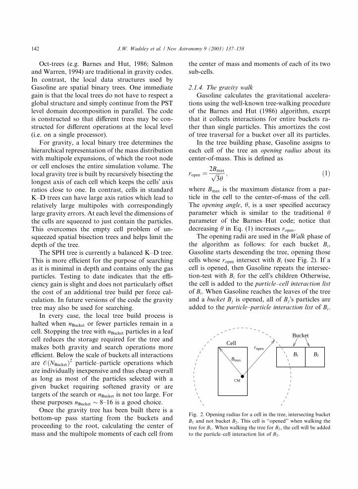
Fig. 2. Opening radius for a cell in the tree, intersecting bucket

B1 and not bucket B2. This cell is ‘‘opened’’ when walking the

tree for B1. When walking the tree for B2, the cell will be added

to the particle–cell interaction list of B2.

142 J.W. Wadsley et al. / New Astronomy 9 (2003) 137–158

Oct-trees (e.g. Barnes and Hut, 1986; Salmon

and Warren, 1994) are traditional in gravity codes.

In contrast, the local data structures used by

Gasoline are spatial binary trees. One immediate

gain is that the local trees do not have to respect a

global structure and simply continue from the PSTlevel domain decomposition in parallel. The code

is constructed so that different trees may be con-

structed for different operations at the local level

(i.e. on a single processor).

For gravity, a local binary tree determines the

hierarchical representation of the mass distribution

with multipole expansions, of which the root node

or cell encloses the entire simulation volume. Thelocal gravity tree is built by recursively bisecting the

longest axis of each cell which keeps the cells� axisratios close to one. In contrast, cells in standard

K–D trees can have large axis ratios which lead to

relatively large multipoles with correspondingly

large gravity errors. At each level the dimensions of

the cells are squeezed to just contain the particles.

This overcomes the empty cell problem of un-squeezed spatial bisection trees and helps limit the

depth of the tree.

The SPH tree is currently a balanced K–D tree.

This is more efficient for the purpose of searching

as it is minimal in depth and contains only the gas

particles. Testing to date indicates that the effi-

ciency gain is slight and does not particularly offset

the cost of an additional tree build per force cal-culation. In future versions of the code the gravity

tree may also be used for searching.

In every case, the local tree build process is

halted when nBucket or fewer particles remain in a

cell. Stopping the tree with nBucket particles in a leaf

cell reduces the storage required for the tree and

makes both gravity and search operations more

efficient. Below the scale of buckets all interactionsare OðNBucketÞ2 particle–particle operations which

are individually inexpensive and thus cheap overall

as long as most of the particles selected with a

given bucket requiring softened gravity or are

targets of the search or nBucket is not too large. For

these purposes nBucket � 8–16 is a good choice.

Once the gravity tree has been built there is a

bottom-up pass starting from the buckets andproceeding to the root, calculating the center of

mass and the multipole moments of each cell from

the center of mass and moments of each of its two

sub-cells.

2.1.4. The gravity walk

Gasoline calculates the gravitational accelera-

tions using the well-known tree-walking procedureof the Barnes and Hut (1986) algorithm, except

that it collects interactions for entire buckets ra-

ther than single particles. This amortizes the cost

of tree traversal for a bucket over all its particles.

In the tree building phase, Gasoline assigns to

each cell of the tree an opening radius about its

center-of-mass. This is defined as

ropen ¼2Bmaxffiffiffi

3p

h; ð1Þ

where Bmax is the maximum distance from a par-

ticle in the cell to the center-of-mass of the cell.

The opening angle, h, is a user specified accuracy

parameter which is similar to the traditional hparameter of the Barnes–Hut code; notice that

decreasing h in Eq. (1) increases ropen.The opening radii are used in the Walk phase of

the algorithm as follows: for each bucket Bi,

Gasoline starts descending the tree, opening those

cells whose ropen intersect with Bi (see Fig. 2). If a

cell is opened, then Gasoline repeats the intersec-

tion-test with Bi for the cell�s children Otherwise,

the cell is added to the particle–cell interaction list

of Bi. When Gasoline reaches the leaves of the treeand a bucket Bj is opened, all of Bj�s particles areadded to the particle–particle interaction list of Bi.

J.W. Wadsley et al. / New Astronomy 9 (2003) 137–158 143

Once the tree has been traversed in this manner

we can calculate the gravitational acceleration for

each particle of Bi by evaluating the interactions

specified in the two lists. Gasoline uses the hexa-

decapole multipole expansion to calculate parti-

cle–cell interactions.

2.1.5. Softening

The particle–particle interactions are softened

to lessen two-body effects that compromise the

attempt to model continuous fluids, including

the collisionless dark matter fluid. In Gasoline the

particle masses are effectively smoothed in space

using the same spline form employed for SPH inSection 3.1. This results in gravitational forces

that vanish at zero separation and return to

Newtonian 1=r2 at a separation of �i þ �j where �iis the gravitational softening associated with each

particle. In this sense the gravitational forces are

well matched to the SPH forces. The softening

can be kept constant in physical or comoving

coordinates.

2.1.6. Periodicity

A disadvantage of tree codes is that they must

deal explicitly with periodic boundary conditions

(as are usually required for cosmological simula-

tions). Gasoline incorporates periodic boundaries

via the Ewald summation technique (e.g. Hern-

quist et al., 1991) where the Greens function forthe case with infinite periodic replicas is divided

into short and long range components that can be

solved efficiently in real and Fourier space, re-

spectively. Hernquist et al. (1991) used the Ewald

summation to generate a table that stored the

correct periodic forces for a given vector separa-

tion in the simulation volume. Gasoline uses a

technique similar to that used by Ding et al.(1992). Non-periodic forces for each interaction

are calculated using the tree method (including

interactions down to the particle–particle level

with the 26 nearest replicas of the box). This force

is corrected to give the correct periodic solution

via an Ewald sum over the infinite periodic repli-

cas. To be efficient this sum uses a reduced repre-

sentation of the whole simulation box. Ding et al.used a set of 35 massive particles with masses and

positions chosen so that they have the same low-

order multipole expansion as the entire simulation

box for this task. Gasoline uses the hexadecapole

moment expansion of the fundamental cube di-

rectly in the Ewald sum (Stadel, 2001). This dra-

matically reduces the work. For example, in the

example discussed in Section 5.2, the Ewald workis 10 s of the 84 s of gravity work in a single global

step and a much smaller fraction for substeps. For

each particle the computations are local and fixed,

and thus the algorithm scales exceedingly well in

parallel. There is still substantial additional work

in periodic simulations because particles interact

with cells and particles in nearby replicas of the

fundamental cube.

2.1.7. Force accuracy

The tree opening criteria places a bound on the

relative error due to a single particle–cell interac-

tion. As Gasoline uses hexadecapoles the error

bound improves rapidly as the opening angle, h, islowered. The relationship between the typical (e.g.

rms) relative force error and opening angle is not astraight-forward power-law in h because the net

gravitational forces on each particle result from

the cancellation of many opposing forces. In Fig. 3,

we show a histogram of the relative acceleration

errors for a cosmological Gasoline simulation at

two different epochs for a range of opening angles.

We have plotted the error curves as cumulative

fractions to emphasize the limited tails to higherror values. For typical Gasoline simulations we

commonly use h ¼ 0:7 which gives an rms relative

error of 0.0039 for the clustered final state referred

to by the left panel of Fig. 3. The errors relative to

the mean acceleration (Fig. 4) are larger (rms

0.0083) but of less importance for highly clustered

cases.

When the density in a periodic simulation isfairly uniform the net gravitational accelerations

are small. This is the case in cosmology at early

times when the perturbations ultimately leading to

cosmological structures are still small. In a tree

code the small forces result from the cancellation

of large opposing forces. In this situation it is es-

sential to tighten the cell-opening criterion to in-

crease the relative accuracy so that the netaccelerations are sufficiently accurate. For exam-

ple, in the right hand panels of Figs. 3 and 4 the

Fig. 3. Gasoline relative errors, for various opening angles h. The distributions are all for a 323, 64 Mpc box where the left panel

represents the clustered final state and the right an initial condition (redshift z ¼ 19). Typical values of h ¼ 0:5 and 0.7 are shown as

thick lines. The solid curves compare to exact forces and thus have a minimum error set by the parameters of the Ewald summation

whereas the dotted curves compare to the h ¼ 0:1 case. The Ewald summation errors only become noticeable for h < 0:4. Relative

errors are best for clustered objects but over-emphasize errors for low acceleration particles that are common in cosmological initial

conditions.

Fig. 4. Gasoline errors relative to the mean for the same cases as Fig. 3. The errors are measured compared to the mean acceleration

(magnitude) averaged over all the particles. Errors relative to the mean are more appropriate to judge accuracy for small accelerations

resulting from force cancellation in a nearly homogeneous medium.

144 J.W. Wadsley et al. / New Astronomy 9 (2003) 137–158

errors are larger, and at z ¼ 19, the rms relative

error is 0.041 for h ¼ 0:7. However, here the ab-

solute errors are lower by nearly a factor of two in

rms (0.026) as shown in Fig. 4. At early times,

when the medium is fairly homogeneous, the net

accelerations are small due to a high degree of

force cancellation. In this case, acceleration errors

normalized to a mean acceleration provide the

better measure of accuracy as large relative errors

are meaningless for accelerations close to zero. At

later times the cancellation among forces is much

less severe and relative errors become a better

measure of the quality of the integration. To en-

sure accurate integrations we switch to a value

such as h ¼ 0:5 before z ¼ 2, giving an rms rela-

tive error of 0.0077 and an rms error of 0.0045

J.W. Wadsley et al. / New Astronomy 9 (2003) 137–158 145

normalized to the mean absolute acceleration for

the z ¼ 19 distribution (a reasonable start time for

a cosmological simulation on this scale). In prin-

ciple h could be changed in a more continuous

fashion for optimal performance.

3. Gasdynamics

Astrophysical systems are predominantly at

very low physical densities and experience wide-

ranging temperature variations. Most of the ma-

terial is in a highly compressible gaseous phase. In

general this means that a perfect adiabatic gasis an excellent approximation for the system.

Microscopic physical processes such as shear vis-

cosity and diffusion can usually be neglected. High-

energy processes and the action of gravity tend to

create large velocities so that flows are both tur-

bulent and supersonic: strong shocks and very high

Mach numbers are common. Radiative cooling

processes can also be important; however, thetimescales can often be much longer or shorter than

dynamical timescales. In the latter case isothermal

gas is often assumed for simplicity. In many areas

of computational astrophysics, particularly cos-

mology, gravity tends to be the dominating force

that drives the evolution of the system. Visible

matter, usually in the form of radiating gas, pro-

vides the essential link to observations. Radiativetransfer is always present but may not significantly

affect the energy and thus pressure of the gas during

the simulation.

Fluid dynamics solvers can be broadly classified

into Eulerian or Lagrangian methods. Eulerian

methods use a fixed computational mesh through

which the fluid flows via explicit advection terms.

Regular meshes provide for ease of analysis andthus high-order methods such as PPM (Woodward

and Collela, 1984) and TVD schemes (e.g. Harten

et al., 1987; Kurganov and Tadmor, 2000) have

been developed. The inner loops of mesh methods

can often be pipelined for high performance. La-

grangian methods follow the evolution of fluid

parcels via the full (comoving) derivatives. This

requires a deforming mesh or a mesh-less methodsuch as smoothed particle hydrodynamics (SPH)

(Monaghan, 1992). Data management is more

complex in these methods; however, advection is

handled implicitly and the simulation naturally

adapts to follow density contrasts.

Large variations in physical length scales in

astrophysics have limited the usefulness of Eule-

rian grid codes. Adaptive mesh refinement (AMR)(Bryan and Norman, 1997; Fryxell et al., 2000)

overcomes this at the cost of data management

overheads and increased code complexity. In the

cosmological context there is the added compli-

cation of dark matter. There is more dark matter

than gas in the universe so it dominates the grav-

itational potential. Perturbations present on all

scales in the dark matter guide the formation ofgaseous structures including galaxies and the first

stars. A fundamental limit to AMR in computa-

tional cosmology is matching the AMR resolution

to the underlying dark matter resolution. Particle

based Lagrangian methods such as SPH are well

matched to this constraint. A useful feature of

Lagrangian simulations is that bulk flows (which

can be highly supersonic in the simulation frame)do not limit the timesteps. Particle methods are

also well suited to rapidly rotating systems such as

astrophysical disks where arbitrarily many rota-

tion periods may have to be simulated (e.g. SPH

explicitly conserves angular momentum). A key

concern for all methods is correct angular mo-

mentum transport.

3.1. Smoothed particle hydrodynamics in Gasoline

Smoothed particle hydrodynamics is an ap-

proach to hydrodynamical modeling developed by

Lucy (1977) and Gingold and Monaghan (1977). It

is a particle method that does not refer to grids for

the calculation of hydrodynamical quantities: all

forces and fluid properties are found on movingparticles eliminating numerically diffusive advec-

tive terms. The use of SPH for cosmological sim-

ulations required the development of variable

smoothing to handle huge dynamic ranges (Hern-

quist and Katz, 1989). SPH is a natural partner for

particle based gravity. SPH has been combined

with P3M (Evrard, 1988), Adaptive P3M (HY-

DRA, Couchman et al., 1995) GRAPE (Steinmetz,1996) and tree gravity (Hernquist and Katz, 1989).

Parallel codes using SPH include Hydra MPI,

146 J.W. Wadsley et al. / New Astronomy 9 (2003) 137–158

Parallel TreeSPH (Dave et al., 1997) and the

GADGET tree code (Springel et al., 2001).

The basis of the SPH method is the represen-

tation and evolution of smoothly varying fluid

quantities whose value is only known at disordered

discrete points in space occupied by particles.Particles are the fundamental resolution elements

comparable to cells in a mesh. SPH functions

through local summation operations over particles

weighted with a smoothing kernel, W , that ap-

proximates a local integral. The smoothing oper-

ation provides a basis from which to obtain

derivatives. Thus, estimates of density related

physical quantities and gradients are generated.The summation aspect led to SPH being described

as a Monte Carlo type method (with Oð1=ffiffiffiffiN

pÞ

errors) however it was shown by Monaghan (1985)

that the method is more closely related to inter-

polation theory with errors OððlnNÞd=NÞ, where dis the number of dimensions.

A general smoothed estimate for some quantity

f at particle i given particles j at positions~rrj takesthe form

fi;smoothed ¼Xnj¼1

fjWijð~rri �~rrj; hi; hjÞ; ð2Þ

where Wij is a kernel function and hj is a smoothing

length indicative of the range of interaction of par-

ticle j. It is common to convert this particle-weigh-

ted sum to volume weighting using fjmj=qj in place

of fj where themj and qj are the particle masses and

densities, respectively. For momentum and energy

conservation in the force terms, a symmetric kernel,

Wij ¼ Wji, is required. We use the kernel-averagefirst suggested by Hernquist and Katz (1989)

Wij ¼1

2wðj~rri �~rrjj=hiÞ þ

1

2wðj~rri �~rrjj=hjÞ: ð3Þ

For wðxÞ we use the standard spline form with

compact support where w ¼ 0 if x > 2 (Monaghan,

1992).We employ a fairly standard implementation of

the hydrodynamics equations of motion for SPH

(Monaghan, 1992). Density is calculated from a

sum over particle masses mj,

qi ¼Xnj¼1

mjWij: ð4Þ

The momentum equation is expressed

d~vvidt

¼ �Xnj¼1

mjPiq2iþ Pjq2jþPij

!riWij; ð5Þ

where Pj is pressure, ~vvi velocity and the artificialviscosity term Pij is given by

Pij ¼�a 1

2ðci þ cjÞlij þ bl2

ij12ðqi þ qjÞ for ~vvij �~rrij < 0;

0 otherwise;

8<:

ð6Þ

where lij ¼hð~vvij �~rrijÞ

~rr2ij þ 0:01ðhi þ hjÞ2; ð7Þ

where~rrij ¼~rri �~rrj,~vvij ¼~vvi �~vvj and cj is the soundspeed. a ¼ 1 and b ¼ 2 are coefficients we use

for the terms representing shear and Von Neu-

mann-Richtmyer (high Mach number) viscosities

respectively. When simulating strongly rotating

systems we use the multiplicative Balsara (1995)

switch, jr �~vvj=ðjr �~vvj þ jr �~vvjÞ, to suppress the

viscosity in non-shocking, shearing environments.

The pressure averaged energy equation (analo-gous to Eq. (5)) conserves energy exactly in the

limit of infinitesimal timesteps but may produce

negative energies due to the Pj term if significant

local variations in pressure occur. We employ the

following equation (advocated by Evrard, 1988,

Benz, 1989) which also conserves energy exactly in

each pairwise exchange but is dependent only on

the local particle pressure

duidt

¼ Piq2i

Xnj¼1

mj~vvij � riWij; ð8Þ

where ui is the internal energy of particle i, which isequal to 1=ðc� 1ÞPi=qi for an ideal gas. This for-

mulation does not suffer from numerical negative

energy problems. Entropy is also better conserved

because the expression is closely tied to the particle

evolution. It may be compared to entropy formu-

lations where the energy is calculated using

ui ¼ Aiqc�1i =ðc� 1Þ, based on the local particle

density, qi and entropy function AiðsÞ. If qc�1 in theentropy formulation were to be integrated using

the continuity equation rather than calculated us-

ing an SPH sum the result is equivalent to Eq. (8).

By comparison, SPH energy equation formulations

J.W. Wadsley et al. / New Astronomy 9 (2003) 137–158 147

that use symmetrized adiabatic work (such as the

geometric and arithmetic averages) do not have a

direct relationship to an entropy based expression.

For cosmological simulations, the cosmological

expansion rate is known exactly. We take advan-tage of this to add the appropriate amount to the

divergence term in Eq. (8) directly and use co-

moving velocities rather than physical velocities in

the SPH divergence term. This results in a more

accurate thermal energy integration.

Springel and Hernquist (2002) compared Eq. (8)

(which they labelled ‘‘energy, asymmetric’’) to

various energy and entropy formulations of SPH.In the tests where asymmetric energy was included

it performed very well. For example, in the point

blast test shown in their Fig. 3 it performed simi-

larly to the entropy formulations which are col-

lectively a lot better than the symmetrized work

formulations. Springel and Hernquist (2002) did

not try the asymmetric formulation in all their

tests which led to these tests being attempted in-dependently with Gasoline. The strong disconti-

nuity test looks very similar to the ‘‘energy,

standard’’ result in their Fig. 8. In the cosmologi-

cal box test (their Fig. 9) Gasoline gives results

intermediate between the geometric results and the

entropy results. It is difficult to argue which an-

swer is more correct given that cosmological tests

with cooling are strongly resolution dependent.We conclude that the treatment of energy in

Gasoline is more than adequate. Gasoline�s SPH

implementation predates the new entropy equation

proposed by Springel and Hernquist (2002) and

significant additional coding would be required to

try the approach. It may appear as part of future

developments.

3.1.1. Neighbor finding

Finding neighbors of particles is a useful oper-

ation. A neighbor list is essential to SPH, but it can

also be a basis for other local estimates, such as a

dark matter density and as a first step in finding

potential colliders or interactors via a short range

force. Stadel developed an efficient search algo-

rithm using priority queues and a K–D tree ball-search to locate the k-nearest neighbors for each

particle (freely available as the Smooth utility at

http://www-hpcc.astro.washington.edu). For Gas-

oline we use a parallel version of the algorithm

that caches non-local neighbors via MDL. The

SPH interaction distance 2hi is set equal to the kthneighbor distance from particle i. We use an exact

number of neighbors. The number is set to a value

such as 32 or 64 at start-up. We have also imple-mented a minimum smoothing length which is

usually set to be comparable to the gravitational

softening.

To calculate the fluid accelerations using SPH

we perform two smoothing operations. First we

sum densities and then forces using the density

estimates. To get a kernel-averaged sum for every

particle (Eqs. (2) and (3)) it is sufficient to performa gather operation over all particles within 2hi ofevery particle i. If only a subset of the particles are

active and require new forces, all particles for

which the active set are neighbors must also per-

form a gather so that they can scatter their con-

tribution to the active set. Finding these scatter

neighbors requires solving the k-inverse nearest

neighbor problem, an active research area incomputer science (e.g. Anderson and Tjaden,

2001). Fortunately, during a simulation the change

per step in h for each particle typically less than

2–3 percent, so it is sufficient to find scatter neigh-

bors, j for which some active particles is within

2hj;OLDð1þ eÞ. We use a tree search where the

nodes contain SPH interaction bounds for their

particles estimated with e ¼ 0:1. This correspondsto limiting the change in h over a step to be no

more than a 10% increase. In practice this re-

striction rarely needs to be applied. A similar

scheme has been employed by Springel et al.

(2001). For the forces sum the inactive neighbors

need density values which can be estimated using

the continuity equation or calculated exactly with

a second inverse neighbor search.

3.2. Cooling

In astrophysical systems the cooling timescale is

usually short compared to dynamical timescales

which often results in temperatures that are close to

an equilibrium set by competing heating and

cooling processes. We have implemented a range ofcases including: adiabatic (no cooling), isothermal

(instant cooling), and implicit energy integration.

148 J.W. Wadsley et al. / New Astronomy 9 (2003) 137–158

Hydrogen and helium cooling processes have been

incorporated. Ionization fractions are calculated

assuming equilibrium for a given temperature,

density and photo-ionizing background to avoid

the cost of integrating the equations for the ion

fractions. Gasoline can optionally add heating dueto feedback from star formation, an uniform UV

background or user defined functions.

The implicit integration uses a stiff equation

solver assuming that the hydrodynamic work and

density are constant across the step. The second-

order nature of the particle integration is main-

tained using an implicit predictor step when

needed. Internal energy is required on every stepto calculate pressure forces on the active parti-

cles. The energy integration is OðNÞ but reason-

ably expensive. To avoid integrating energy for

every particle on the smallest timestep we ex-

trapolate each particle forward on its individual

dynamical timestep and use linear interpolation

to estimate internal energy at intermediate times

as required.

4. Integration: multiple timesteps

The range of physical scales in astrophysical

systems is large. For example current galaxy for-

mation simulations contain 9 orders of magnitude

variation in density. The dynamical timescale forgravity scales as q�1=2 and for gas it scales as

q�1=3T�1=2. For an adiabatic gas the local dynam-

ical time scales as q�2=3. With gas cooling (or the

isothermal assumption) simulations can achieve

very high gas densities. In most cases gas sets the

Full Step: Kick Drift Kick

Rung 0 (Base time step)

Rung 1

Rung 2

Fig. 5. Illustration of multiple timestepping: the linear sections repres

axis. The vertical bars represent kicks changing the velocity. In KDK

force evaluation) which is why there are two bars interior of the KDK

shortest dynamical timescales, and thus gas simu-

lations are much more demanding (many more

steps to completion) than corresponding gravity

only simulations. Time adaptivity can be very

effective in this regime.

Gasoline incorporates the timestep scheme de-scribed as Kick–Drift–Kick (KDK) in Quinn et al.

(1997). The scheme uses a fixed timestep. Starting

with all quantities synchronized, velocities and

energies are updated to the half-step (half-Kick),

followed by a full step position update (Drift). The

positions alone are sufficient to calculate gravity

at the end of the step; however, for SPH, veloci-

ties and thermal energies are also required andobtained with a predictor step using the old ac-

celerations. Finally another half-Kick is applied

synchronizing all the variables. Without gas forces

this is a symplectic leap-frog integration. The leap-

frog scheme requires only one force evaluation and

minimum storage. It can be argued that symplectic

integration is not essential for cosmological col-

lapses where the number of dynamical times issmall. However, it is critical in solar system inte-

grations and in galaxy formation where systems

must be integrated stably for many dynamical

times.

To adapt the timestep size an arbitrary number

of sub-stepping rungs factors of two smaller may

be used as shown in Fig. 5. The scheme is no

longer strictly symplectic if particles change rungsduring the integration which they generally must

do to satisfy their individual timestep criteria.

After overheads, tree-based force calculation

scales approximately with the number of active

particles so large speed-ups may be realized in

Full Step: Drift Kick Drift

Rung 0 (Base time step)

Rung 1

Rung 2

ent particle positions during a drift step with time along the x-

, the accelerations are applied as two half-kicks (from only one

case. At the end of each full step all variables are synchronized.

J.W. Wadsley et al. / New Astronomy 9 (2003) 137–158 149

comparison to single stepping (see Section 5).

Fig. 5 compares KDK with DKD, also discussed

in Quinn et al. (1997). For KDK the force calcu-

lations for different rungs are synchronized. In the

limit of many rungs this results in half as many

force calculation times with their associated treebuilds compared to DKD. KDK also gives sig-

nificantly better momentum and energy conserva-

tion for the same choice of timestep criteria.

We use standard timestep criteria based on the

particle acceleration, and for gas particles, the

Courant condition and the expansion cooling rate.

dtAccel 6 gAccel

ffiffiffia�

r;

dtCourant 6 gCouranth

ð1þ aÞcþ blMAX

;

dtExpand 6 gExpandu

du=dtif du=dt < 0:

ð9Þ

gAccel, gCourant, and gExpand are accuracy parameters

typically chosen to be 0.3, 0.4, and 0.25, respec-

tively. lMAX is the maximum value of jlijj (fromEq. (7)) over interactions between pairs of SPH

particles.For cosmology in place of the comoving ve-

locity ~vv, we use the momentum ~pp ¼ a2~vv which is

canonical to the comoving position, ~xx. As de-

scribed in detail in Appendix A of Quinn et al.

(1997), this results in a separable Hamiltonian

which may be integrated straightforwardly using

the Drift and Kick operators

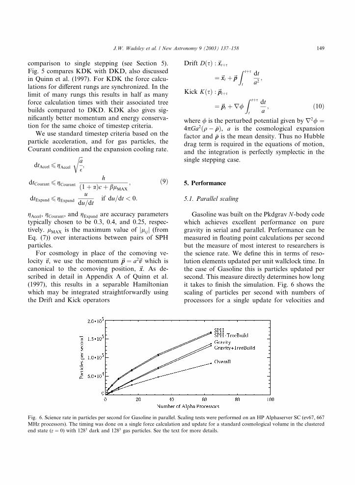
Fig. 6. Science rate in particles per second for Gasoline in parallel. Sc

MHz processors). The timing was done on a single force calculation a

end state (z ¼ 0) with 1283 dark and 1283 gas particles. See the text f

Drift DðsÞ :~xxtþs

¼~xxt þ~ppZ tþs

t

dta2

;

Kick KðsÞ :~pptþs

¼~ppt þr/Z tþs

t

dta; ð10Þ

where / is the perturbed potential given by r2/ ¼4pGa2ðq� �qqÞ, a is the cosmological expansion

factor and �qq is the mean density. Thus no Hubble

drag term is required in the equations of motion,

and the integration is perfectly symplectic in the

single stepping case.

5. Performance

5.1. Parallel scaling

Gasoline was built on the Pkdgrav N -body code

which achieves excellent performance on pure

gravity in serial and parallel. Performance can be

measured in floating point calculations per secondbut the measure of most interest to researchers is

the science rate. We define this in terms of reso-

lution elements updated per unit wallclock time. In

the case of Gasoline this is particles updated per

second. This measure directly determines how long

it takes to finish the simulation. Fig. 6 shows the

scaling of particles per second with numbers of

processors for a single update for velocities and

aling tests were performed on an HP Alphaserver SC (ev67, 667

nd update for a standard cosmological volume in the clustered

or more details.

150 J.W. Wadsley et al. / New Astronomy 9 (2003) 137–158

positions for all particles. This requires gravita-

tional forces for all particles and SPH for the gas

particles (half the total). The simulation used is a

1283 gas and 1283 dark matter particle, purely

adiabatic cosmological simulation (ACDM) in a

200 Mpc box at the final time (redshift, z ¼ 0). Atthis time the simulation is highly clustered locally

but material is still well distributed throughout the

volume. Thus, it is still possible to partition the

volume to achieve even work balancing among a

fair number of processors. As a rule of thumb we

aim to have around 100,000 particles per proces-

sor. As seen in the figure, the gravity scales very

well. For pure gravity around 80% scaling effi-ciency can be achieved out to 64 processors. The

cache based design has small memory overheads

and uses the large amounts of gravity work to hide

the communication overheads associated with

filling the cache with remote particle and cell data.

With gas the efficiency is lowered because the data

structures to be passed are larger and there is less

work per data element to hide the communicationcosts. Thus the computation to communication

ratio is substantially lowered with more proces-

sors. Fixed costs such as the treebuilds for gravity

and SPH scale well, but the gas-only costs peel

away from the more efficient gravity scaling. When

the overall rate is considered, Gasoline is still

making substantial improvements in the time to

solution going from 32 to 64 processors (lowestcurve in the figure). The overall rate includes costs

for domain decomposition and OðNÞ updates of

the particle information such as updating the po-

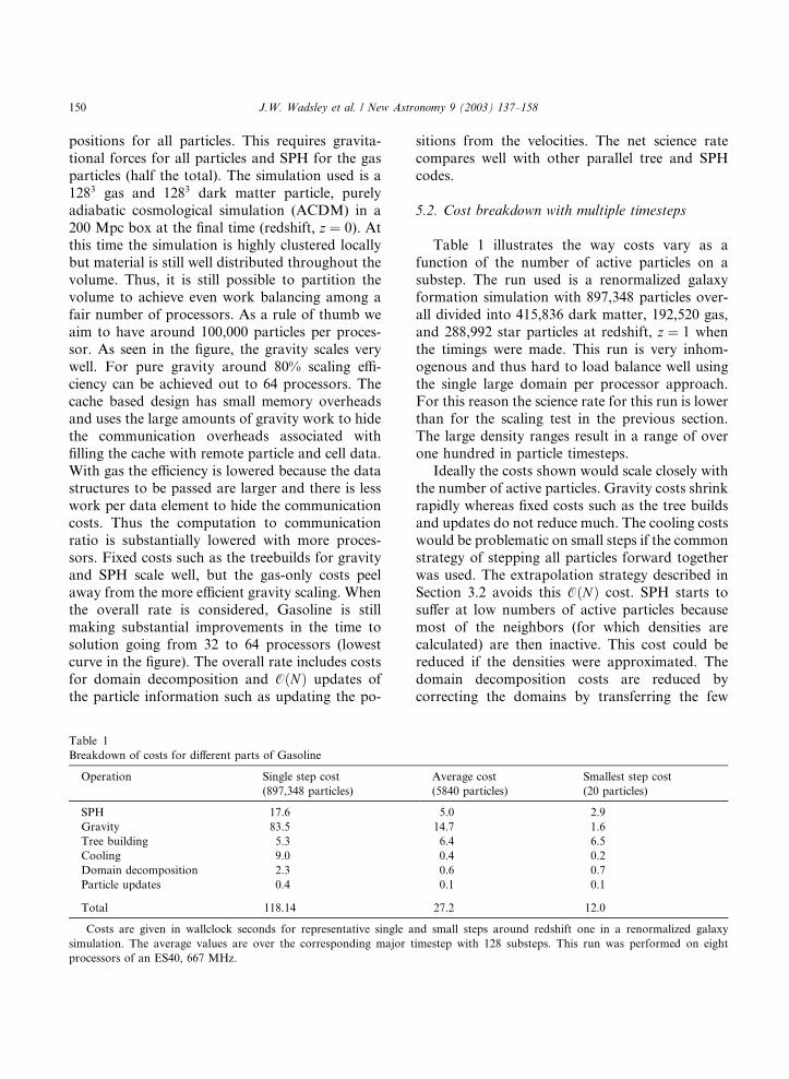
Table 1

Breakdown of costs for different parts of Gasoline

Operation Single step cost

(897,348 particles)

SPH 17.6

Gravity 83.5

Tree building 5.3

Cooling 9.0

Domain decomposition 2.3

Particle updates 0.4

Total 118.14

Costs are given in wallclock seconds for representative single a

simulation. The average values are over the corresponding major t

processors of an ES40, 667 MHz.

sitions from the velocities. The net science rate

compares well with other parallel tree and SPH

codes.

5.2. Cost breakdown with multiple timesteps

Table 1 illustrates the way costs vary as a

function of the number of active particles on a

substep. The run used is a renormalized galaxy

formation simulation with 897,348 particles over-

all divided into 415,836 dark matter, 192,520 gas,

and 288,992 star particles at redshift, z ¼ 1 when

the timings were made. This run is very inhom-

ogenous and thus hard to load balance well usingthe single large domain per processor approach.

For this reason the science rate for this run is lower

than for the scaling test in the previous section.

The large density ranges result in a range of over

one hundred in particle timesteps.

Ideally the costs shown would scale closely with

the number of active particles. Gravity costs shrink

rapidly whereas fixed costs such as the tree buildsand updates do not reduce much. The cooling costs

would be problematic on small steps if the common

strategy of stepping all particles forward together

was used. The extrapolation strategy described in

Section 3.2 avoids this OðNÞ cost. SPH starts to

suffer at low numbers of active particles because

most of the neighbors (for which densities are

calculated) are then inactive. This cost could bereduced if the densities were approximated. The

domain decomposition costs are reduced by

correcting the domains by transferring the few

Average cost

(5840 particles)

Smallest step cost

(20 particles)

5.0 2.9

14.7 1.6

6.4 6.5

0.4 0.2

0.6 0.7

0.1 0.1

27.2 12.0

nd small steps around redshift one in a renormalized galaxy

imestep with 128 substeps. This run was performed on eight

J.W. Wadsley et al. / New Astronomy 9 (2003) 137–158 151

particles that have moved over domain boundaries

rather than finding new domains every step.

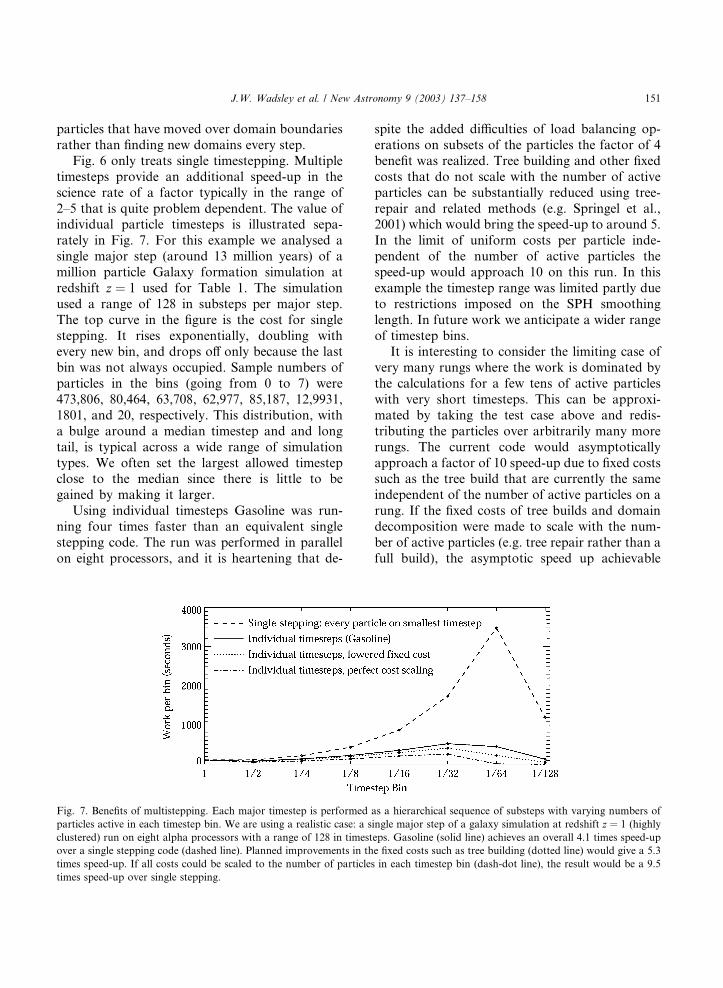
Fig. 6 only treats single timestepping. Multiple

timesteps provide an additional speed-up in the

science rate of a factor typically in the range of

2–5 that is quite problem dependent. The value ofindividual particle timesteps is illustrated sepa-

rately in Fig. 7. For this example we analysed a

single major step (around 13 million years) of a

million particle Galaxy formation simulation at

redshift z ¼ 1 used for Table 1. The simulation

used a range of 128 in substeps per major step.

The top curve in the figure is the cost for single

stepping. It rises exponentially, doubling withevery new bin, and drops off only because the last

bin was not always occupied. Sample numbers of

particles in the bins (going from 0 to 7) were

473,806, 80,464, 63,708, 62,977, 85,187, 12,9931,

1801, and 20, respectively. This distribution, with

a bulge around a median timestep and and long

tail, is typical across a wide range of simulation

types. We often set the largest allowed timestepclose to the median since there is little to be

gained by making it larger.

Using individual timesteps Gasoline was run-

ning four times faster than an equivalent single

stepping code. The run was performed in parallel

on eight processors, and it is heartening that de-

Fig. 7. Benefits of multistepping. Each major timestep is performed

particles active in each timestep bin. We are using a realistic case: a s

clustered) run on eight alpha processors with a range of 128 in timest

over a single stepping code (dashed line). Planned improvements in th

times speed-up. If all costs could be scaled to the number of particles

times speed-up over single stepping.

spite the added difficulties of load balancing op-

erations on subsets of the particles the factor of 4

benefit was realized. Tree building and other fixed

costs that do not scale with the number of active

particles can be substantially reduced using tree-

repair and related methods (e.g. Springel et al.,2001) which would bring the speed-up to around 5.

In the limit of uniform costs per particle inde-

pendent of the number of active particles the

speed-up would approach 10 on this run. In this

example the timestep range was limited partly due

to restrictions imposed on the SPH smoothing

length. In future work we anticipate a wider range

of timestep bins.It is interesting to consider the limiting case of

very many rungs where the work is dominated by

the calculations for a few tens of active particles

with very short timesteps. This can be approxi-

mated by taking the test case above and redis-

tributing the particles over arbitrarily many more

rungs. The current code would asymptotically

approach a factor of 10 speed-up due to fixed costssuch as the tree build that are currently the same

independent of the number of active particles on a

rung. If the fixed costs of tree builds and domain

decomposition were made to scale with the num-

ber of active particles (e.g. tree repair rather than a

full build), the asymptotic speed up achievable

as a hierarchical sequence of substeps with varying numbers of

ingle major step of a galaxy simulation at redshift z ¼ 1 (highly

eps. Gasoline (solid line) achieves an overall 4.1 times speed-up

e fixed costs such as tree building (dotted line) would give a 5.3

in each timestep bin (dash-dot line), the result would be a 9.5

152 J.W. Wadsley et al. / New Astronomy 9 (2003) 137–158

with Gasoline would be 24 times. This limit is due

to updates and local and parallel data accessing

overheads that would be shared among a large

number of particles when many are active (e.g.

through re-use of data in the MDL software ca-

ches). For the ideal code where all costs scale withthe number of active particles the speed-up versus

a single stepping code approaches the ratio of the

median timestep to the smallest timestep. This

ratio can be in the hundreds for foreseeable runs

with large dynamic range.

In parallel, communication costs and load bal-

ancing are the dominant obstacles to large multi-

stepping gains. For small runs, such as the galaxyformation example used here, the low numbers of

the particles on the shortest timesteps make load

balancing difficult. If more than 16 processors are

used with the current code on this run there will be

idle processors for a noticeable fraction of the

time. Though the time to solution is reduced with

more processors, it is an inefficient use of com-

puting resources. The ongoing challenge is to see ifbetter load balancing through more complex work

division offsets increases in communication and

other parallel overheads.

6. Tests

6.1. Shocks: spherical adiabatic collapse

There are three key points to keep in mind when

evaluating the performance of SPH on highly

symmetric tests. The first is that the natural par-

ticle configuration is a semi-regular three-dimen-

sional glass rather than a regular mesh. The second

is that individual particle velocities are smoothed

before they affect the dynamics so that the lowlevel noise in individual particle velocities is not

particularly important. The dispersion in individ-

ual velocities is related to continuous settling of

the irregular particle distribution. This is particu-

larly evident after large density changes. Thirdly,

the SPH density is a smoothed estimate. Any sharp

step in the number density of particles translates

into a density estimate that is smooth on the scaleof �2–3 particle separations. When relaxed irreg-

ular particle distributions are used, SPH resolves

density discontinuities close to this limit. As a

Lagrangian method SPH can also resolve contact

discontinuities just as tightly without the advective

spreading of some Eulerian methods.

We have performed standard Sod (1978) shock

tube tests used for the original TreeSPH (Hern-quist and Katz, 1989). We find the best results

with the pairwise viscosity of Eq. (7) which is

marginally better than the bulk viscosity formu-

lation for this test. The one-dimensional tests

often shown do not properly represent the ability

of SPH to model shocks on more realistic prob-

lems. The results of Fig. 8 demonstrate that SPH

can resolve discontinuities in a shock tube verywell when the problem is set up to be comparable

to the environment in a typical three-dimensional

simulation.

The shocks of the previous example have a

fairly low Mach number compared to astrophysi-

cal shocks found in collapse problems. (Evrard,

1988) first introduced a spherical adiabatic col-

lapse as a test of gasdynamics with gravity. Thistest is nearly equivalent to the self-similar collapse

of Navarro and White (1993) and has comparable

shock strengths. We compare Gasoline results on

this problem with a very high resolution 1D La-

grangian mesh solution in Fig. 9. We used a three-

dimensional glass initial condition. The solution is

excellent with two particle spacings required to

model the shock. The deviation at the inner radii isa combination of the minimum smoothing length

(0.01) and earlier slight over-production of en-

tropy at a less resolved stage of the collapse. The

pre-shock entropy generation (bottom left panel of

Fig. 9) occurs in any strongly collapsing flow and

is present for both the pairwise (Eq. (7)) and di-

vergence based artificial viscosity formulations.

The post-shock entropy values are correct.

6.2. Rotating isothermal cloud collapse

The rotating isothermal cloud test examines the

angular momentum transport in an analogue of a

typical astrophysical collapse with cooling. Grid

methods must explicitly advect material across cell

boundaries which leads to small but systematicangular momentum non-conservation and trans-

port errors. SPH conserves angular momentum

Fig. 8. Sod (1978) shock tube test results with Gasoline for density (left) and velocity (right). This a three-dimensional test using glass

initial conditions similar to the conditions in a typical simulation. The diamonds represent averages in bins separated by the local

particle spacing: the effective fluid element width. Discontinuities are resolved in three to four particle spacings which is much fewer

than in the one dimensional results shown in Hernquist and Katz (1989).

Fig. 9. Adiabatic collapse test from Evrard (1988) with 28,000 particles, shown at time t ¼ 0:8 (this is the same as t ¼ 0:88 in Hernquist

and Katz (1989) whose time scaling is slightly different). The results shown as diamonds are binned at the particle spacing with actual

particle values shown as points. The solid line is a high resolution 1D PPM solution provided by Steinmetz.

J.W. Wadsley et al. / New Astronomy 9 (2003) 137–158 153

very well, limited only by the accuracy of the timeintegration of the particle trajectories. However,

the SPH artificial viscosity that is required to

handle shocks has an unwanted side-effect in the

form of viscous transport away from shocks. Themagnitude of this effect scales with the typical

particle spacing, and it can be combatted effec-

tively with increased resolution. The Balsara

154 J.W. Wadsley et al. / New Astronomy 9 (2003) 137–158

(1995) switch detects shearing regions so that the

viscosity can be reduced where strong compression

is not also present.

We modeled the collapse of a rotating, isother-

mal gas cloud. This test is similar to a tests per-

formed by Navarro and White (1993) and Thackeret al. (2000) except that we have simplified the

problem in the manner of Navarro and Steinmetz

(1997). We use a fixed NFW (Navarro et al., 1995)

(concentration c ¼ 11, mass¼ 2� 1012M�) poten-

tial without self-gravity to avoid coarse gravita-

tional clumping with the associated angular

momentum transport. This results in a disk with a

circular velocity of 220 km/s at 10 kpc. The initial4� 1010M�, 100 kpc gas cloud was constructed

with particle locations evolved into a uniform

density glass initial condition and set in solid body

rotation (~vv ¼ 0:407 km/s/pc eez �~rr) correspondingto a rotation parameter k � 0:1. The gas was kept

isothermal at 10,000 K rather than using a cooling

function to make the test more reproducible. The

corresponding sound speed of 10 km/s impliessubstantial shocking during the collapse.

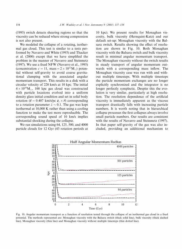
We ran simulations using 64, 125, 500, and 4000

particle clouds for 12 Gyr (43 rotation periods at

Fig. 10. Angular momentum transport as a function of resolution te

potential. The methods represented are: Monaghan viscosity with th

line), Monaghan viscosity (thin line) and Monaghan viscosity withou

10 kpc). We present results for Monaghan vis-

cosity, bulk viscosity (Hernquist-Katz) and our

default set-up: Monaghan viscosity with the Bal-

sara switch. Results showing the effect of resolu-

tion are shown in Fig. 10. Both Monaghan

viscosity with the Balsara switch and bulk viscosityresult in minimal angular momentum transport.

The Monaghan viscosity without the switch results

in steady transport of angular momentum out-

wards with a corresponding mass inflow. The

Monaghan viscosity case was run with and with-

out multiple timesteps. With multiple timesteps

the particle momentum exchanges are no longer

explicitly synchronized and the integrator is nolonger perfectly symplectic. Despite this the evo-

lution is very similar, particularly at high resolu-

tion. The resolution dependence of the artificial

viscosity is immediately apparent as the viscous

transport drastically falls with increasing particle

numbers. It is worth noting that in hierarchical

collapse processes the first collapses always involve

small particle numbers. Our results are consistentwith the results of Navarro and Steinmetz (1997).

In that paper self-gravity of the gas was also in-

cluded, providing an additional mechanism to

sted through the collapse of an isothermal gas cloud in a fixed

e Balsara switch (thick solid line), bulk viscosity (thick dashed

t multiple timesteps (thin dotted line).

J.W. Wadsley et al. / New Astronomy 9 (2003) 137–158 155

transport angular momentum due to mass clump-

ing. As a result, their disks show a gradual trans-

port of angular momentum even with the Balsara

switch; however, this transport was readily re-

duced with increased particle numbers.

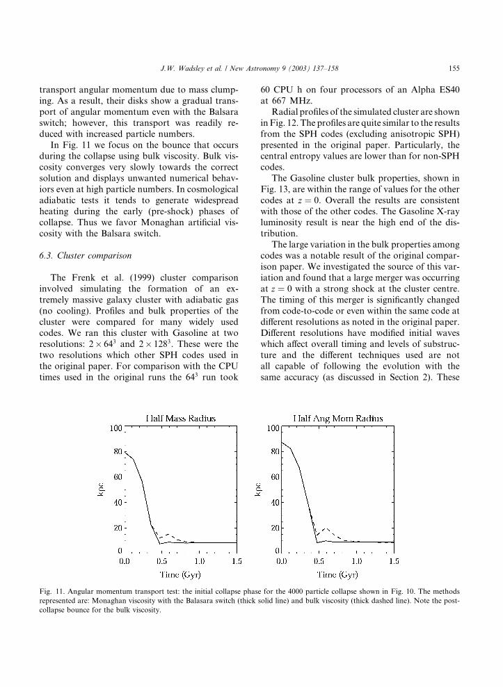
In Fig. 11 we focus on the bounce that occursduring the collapse using bulk viscosity. Bulk vis-

cosity converges very slowly towards the correct

solution and displays unwanted numerical behav-

iors even at high particle numbers. In cosmological

adiabatic tests it tends to generate widespread

heating during the early (pre-shock) phases of

collapse. Thus we favor Monaghan artificial vis-

cosity with the Balsara switch.

6.3. Cluster comparison

The Frenk et al. (1999) cluster comparison

involved simulating the formation of an ex-

tremely massive galaxy cluster with adiabatic gas

(no cooling). Profiles and bulk properties of the

cluster were compared for many widely usedcodes. We ran this cluster with Gasoline at two

resolutions: 2� 643 and 2� 1283. These were the

two resolutions which other SPH codes used in

the original paper. For comparison with the CPU

times used in the original runs the 643 run took

Fig. 11. Angular momentum transport test: the initial collapse phase

represented are: Monaghan viscosity with the Balasara switch (thick s

collapse bounce for the bulk viscosity.

60 CPU h on four processors of an Alpha ES40

at 667 MHz.

Radial profiles of the simulated cluster are shown

inFig. 12. The profiles are quite similar to the results

from the SPH codes (excluding anisotropic SPH)

presented in the original paper. Particularly, thecentral entropy values are lower than for non-SPH

codes.

The Gasoline cluster bulk properties, shown in

Fig. 13, are within the range of values for the other

codes at z ¼ 0. Overall the results are consistent

with those of the other codes. The Gasoline X-ray

luminosity result is near the high end of the dis-

tribution.The large variation in the bulk properties among

codes was a notable result of the original compar-

ison paper. We investigated the source of this var-

iation and found that a large merger was occurring

at z ¼ 0 with a strong shock at the cluster centre.

The timing of this merger is significantly changed

from code-to-code or even within the same code at

different resolutions as noted in the original paper.Different resolutions have modified initial waves

which affect overall timing and levels of substruc-

ture and the different techniques used are not

all capable of following the evolution with the

same accuracy (as discussed in Section 2). These

for the 4000 particle collapse shown in Fig. 10. The methods

olid line) and bulk viscosity (thick dashed line). Note the post-

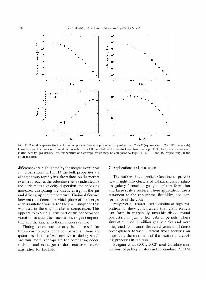
Fig. 12. Radial properties for the cluster comparison. We have plotted radial profiles for a 2� 643 (squares) and a 2� 1283 (diamonds)

Gasoline run. The innermost bin shown is indicative of the resolution. Taken clockwise from the top left the four panels show dark

matter density, gas density, gas temperature and entropy which may be compared to Figs. 10, 12, 17, and 18, respectively, in the

original paper.

156 J.W. Wadsley et al. / New Astronomy 9 (2003) 137–158

differences are highlighted by the merger event near

z ¼ 0. As shown in Fig. 13 the bulk properties are

changing very rapidly in a short time. As the merger

event approaches the velocities rise (as indicated by

the dark matter velocity dispersion and shocking

increases, dissipating the kinetic energy in the gas

and driving up the temperature. Timing difference

between runs determine which phase of the mergereach simulation was in for the z ¼ 0 snapshot that

was used in the original cluster comparison. This

appears to explain a large part of the code-to-code

variation in quantities such as mean gas tempera-

ture and the kinetic to thermal energy ratio.

Timing issues must clearly be addressed for

future cosmological code comparisons. There are

quantities that are less sensitive to timing whichare thus more appropriate for comparing codes,

such as total mass, gas to dark matter ratio and

axis ratios for the halo.

7. Applications and discussion

The authors have applied Gasoline to provide

new insight into clusters of galaxies, dwarf galax-

ies, galaxy formation, gas-giant planet formation

and large scale structure. These applications are a

testament to the robustness, flexibility, and per-

formance of the code.Mayer et al. (2002) used Gasoline at high res-

olution to show convincingly that giant planets

can form in marginally unstable disks around

protostars in just a few orbital periods. These

simulation used 1 million gas particles and were

integrated for around thousand years until dense

proto-planets formed. Current work focusses on

improving the treatment of the heating and cool-ing processes in the disk.

Borgani et al. (2001, 2002) used Gasoline sim-

ulations of galaxy clusters in the standard ACDM

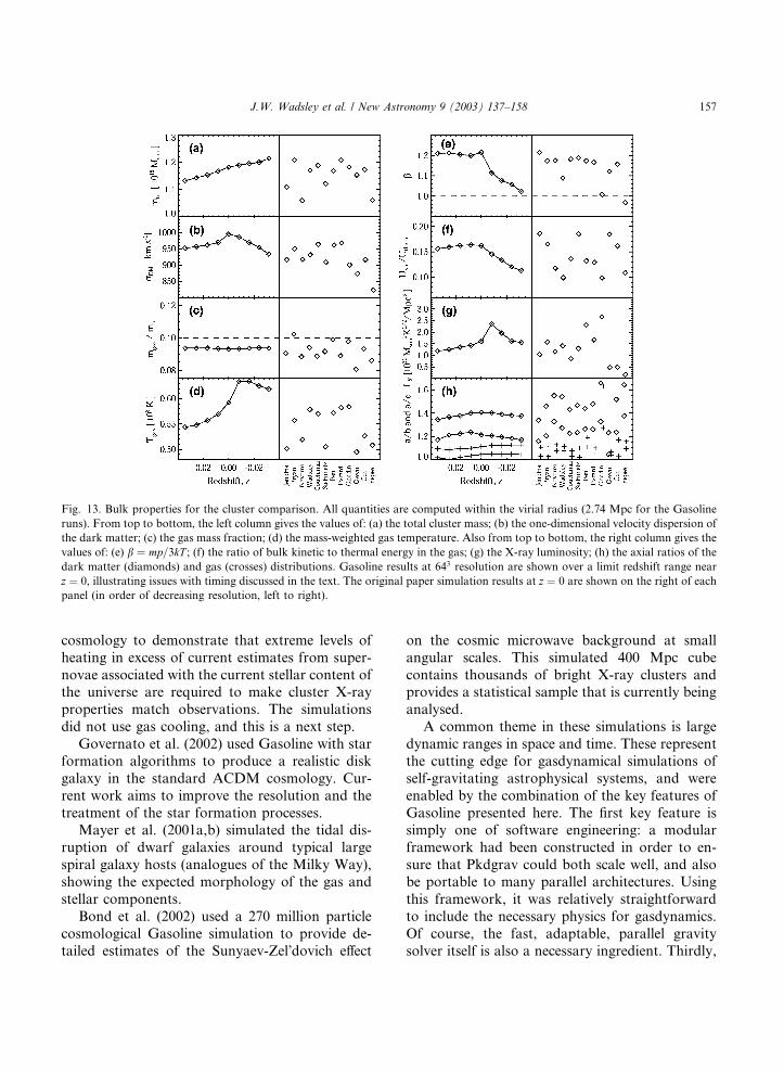
Fig. 13. Bulk properties for the cluster comparison. All quantities are computed within the virial radius (2.74 Mpc for the Gasoline

runs). From top to bottom, the left column gives the values of: (a) the total cluster mass; (b) the one-dimensional velocity dispersion of

the dark matter; (c) the gas mass fraction; (d) the mass-weighted gas temperature. Also from top to bottom, the right column gives the

values of: (e) b ¼ mp=3kT ; (f) the ratio of bulk kinetic to thermal energy in the gas; (g) the X-ray luminosity; (h) the axial ratios of the

dark matter (diamonds) and gas (crosses) distributions. Gasoline results at 643 resolution are shown over a limit redshift range near

z ¼ 0, illustrating issues with timing discussed in the text. The original paper simulation results at z ¼ 0 are shown on the right of each

panel (in order of decreasing resolution, left to right).

J.W. Wadsley et al. / New Astronomy 9 (2003) 137–158 157

cosmology to demonstrate that extreme levels of

heating in excess of current estimates from super-

novae associated with the current stellar content ofthe universe are required to make cluster X-ray

properties match observations. The simulations

did not use gas cooling, and this is a next step.

Governato et al. (2002) used Gasoline with star

formation algorithms to produce a realistic disk

galaxy in the standard ACDM cosmology. Cur-

rent work aims to improve the resolution and the

treatment of the star formation processes.Mayer et al. (2001a,b) simulated the tidal dis-

ruption of dwarf galaxies around typical large

spiral galaxy hosts (analogues of the Milky Way),

showing the expected morphology of the gas and

stellar components.

Bond et al. (2002) used a 270 million particle

cosmological Gasoline simulation to provide de-

tailed estimates of the Sunyaev-Zel�dovich effect

on the cosmic microwave background at small

angular scales. This simulated 400 Mpc cube

contains thousands of bright X-ray clusters andprovides a statistical sample that is currently being

analysed.

A common theme in these simulations is large

dynamic ranges in space and time. These represent

the cutting edge for gasdynamical simulations of

self-gravitating astrophysical systems, and were

enabled by the combination of the key features of

Gasoline presented here. The first key feature issimply one of software engineering: a modular

framework had been constructed in order to en-

sure that Pkdgrav could both scale well, and also

be portable to many parallel architectures. Using

this framework, it was relatively straightforward

to include the necessary physics for gasdynamics.

Of course, the fast, adaptable, parallel gravity

solver itself is also a necessary ingredient. Thirdly,

158 J.W. Wadsley et al. / New Astronomy 9 (2003) 137–158

the gasdynamical implementation is state-of-the-

art and tested on a number of standard problems.

Lastly, significant effort has gone into making the

code adaptable to a large range in timescales. In-

creasing the efficiency with which such problems

can be handled will continue be a area of devel-opment with contributions from computer science

and applied mathematics.

Acknowledgements

The authors would like to thank Carlos Frenk

for providing the cluster comparison results andMatthias Steinmetz for providing high resolution

numerical solutions for the adiabatic spherical

collapse. Development of Pkdgrav and Gasoline

was supported by grants from the NASA HPCC/

ESS program.

References

Aarseth, S., Lecar, M., 1975. ARA&A 13, 1.

Anderson, R., Tjaden, B., 2001. The inverse nearest neighbor

problem with astrophysical applications. Proceedings of the

Twelfth Annual ACM-SIAM Symposium on Discrete

Algorithms (SODA), Washington, DC, January 2001.

Bagla, J.S., 2002. JApA 23, 185.

Balsara, D.S., 1995. J. Comput. Phys. 121 (2), 357.

Barnes, J., Hut, P., 1986. Nature 324, 446.

Benz, W., 1989. Numerical Modeling of Stellar Pulsation.

NATO Workshop, Les Arcs, France.

Bentley, J.L., 1979. IEEE Transactions on Software Engineer-

ing SE-5 (4), 333.

Bode, P., Ostriker, J.P., Xu, G., 2000. ApJS 128, 561.

Bond, J., Contaldi, C., Pen, U.-L., et al., 2002. ApJ (submitted),

astro-ph/0205386.

Borgani, S., Governato, F., Wadsley, J., Menci, N., Tozzi, P.,

Quinn, T., Stadel, J., Lake, G., 2002. MNRAS 336, 409.

Borgani, S., Governato, F., Wadsley, J., Menci, N., Tozzi, P.,

Lake, G., Quinn, T., Stadel, J., 2001. ApJ 559, 71.

Bryan, G., Norman, M., 1997. In: Clarke, D., West, M. (Eds.),

Computational Astrophysics. Proc. 12th Kingston Confer-

ence, Halifax, October 1996, PASP, p. 363.

Couchman, H.M.P., 1991. ApJL 368, 23.

Couchman, H.M.P., Thomas, P.A., Pearce, F.R., 1995. ApJ

452, 797.

Dave, R., Dubinksi, J., Hernquist, L., 1997. NewA. 2, 277.

Dehnen, W., 2000. ApJ 536, 39.

Ding, H., Karasawa, N., Goddard III, W., 1992. Chem. Phys.

Lett. 196, 6.

Efstathiou, G., Davis, M., Frenk, C.S., White, S.D.M., 1985.

ApJS 57, 241.

Evrard, A.E., 1988. MNRAS 235, 911.

Fryxell, B., Olson, K., Ricker, P., Timmes, F.X., Zingale, M.,

Lamb, D.Q., MacNeice, P., Rosner, R., Truran, J.W., Tufo,

H., 2000. ApJS 131, 273. Available from http://flash.uchi-

cago.edu.

Frenk, C., White, S., Bryan, G., et al., 1999. ApJ. 525, 554.

Gingold, R.A., Monaghan, J.J., 1977. MNRAS 181, 375.

Governato, F., Mayer, L., Wadsley, J., Gardner, J.P., Willman,

B., Hayashi, E., Quinn, T., Stadel, J., Lake, G., 2002. ApJ

(submitted), astro-ph/0207044.

Greengard, L., Rokhlin, V., 1987. J. Comput. Phys. 73, 325.

Harten, A., Enquist, B., Osher, S., Charkravarthy, S., 1987.

J. Comput. Phys. 71, 231.

Hernquist, L., Katz, N., 1989. ApJS 70, 419.

Hernquist, L., Ostriker, J., 1992. ApJ 386, 375.

Hernquist, L., Bouchet, F., Suto, Y., 1991. ApJS 75, 231.

Holmberg, E., 1947. ApJ 94, 385.

Hut, P., Makino, J., 1999. Science 283, 501.

Jernigan, J.G., Porter, D.H., 1989. ApJS 71, 871.

Kravtsov, A.V., Klypin, A.A., Khokhlov, A.M.J., 1997. ApJS

111, 73.

Kurganov, A., Tadmor, E., 2000. J. Comput. Phys. 160, 241.

Lucy, L., 1977. AJ 82, 1013.

Mayer, L., Quinn, T., Wadsley, J., Stadel, J., 2002. Science 298,

1756.

Mayer, L., Governato, F., Colpi, M., Moore, B., Quinn, T.,

Wadsley, J., Stadel, J., Lake, G., 2001a. ApJ 559, 754.

Mayer, L., Governato, F., Colpi, M., Moore, B., Quinn, T.,

Wadsley, J., Stadel, J., Lake, G., 2001b. ApJ 547, 123.

Monaghan, J.J., 1985. Comput. Phys. Rep. 3, 71.

Monaghan, J.J., 1992. ARA&A 30, 543.

Navarro, J.F., Steinmetz, M., 1997. ApJ 478, 13.

Navarro, J.F., White, S.D.M., 1993. MNRAS 265, 271.

Navarro, J.F., Frenk, C., White, S.D.M., 1995. MNRAS 275,

720.

Press, W.H., Teukolsky, S.A., Vetterling, W.T., Flannery, B.P.,

1995. Numerical Recipies in C. Cambridge University Press,

Cambridge.

Quinn, T., Katz, N., Stadel, J., Lake, G., 1997. ApJ (submit-

ted), astro-ph/9710043.

Richardson, D.C., Quinn, T., Stadel, J., Lake, G., 2000. Icarus

143, 45–59.

Salmon, J., Warren, M., 1994. J. Comput. Phys. 111, 136.

Sod, G.A., 1978. J. Comput. Phys. 27, 1.

Springel, V., Hernquist, L., 2002. MNRAS 333, 649.

Springel, V., Yoshida, N., White, S.D.M., 2001. NewA. 6, 79.

Stadel, J., 2001. Ph.D. Thesis, University of Washington,

Seattle, WA.

Steinmetz, M., 1996. MNRAS 278, 1005.

Thacker, R., Tittley, E., Pearce, F., Couchman, H., Thomas, P.,

2000. MNRAS 319, 619.

Wadsley, J.W., 1998. Ph.D. Thesis, University of Toronto.

Weinberg, M., 1999. AJ 117, 629.

Woodward, P., Collela, P., 1984. J. Comput. Phys. 54, 115.