gasoline-related air pollutants in california - trends … · – do not cite gasoline-related air...
TRANSCRIPT

– DO NOT CITE
GASOLINE-RELATED AIR POLLUTANTS IN CALIFORNIA TRENDS IN EXPOSURE AND HEALTH RISK 1996 TO 2014 January 2018
Safer Alternatives Assessment and Biomonitoring Section Reproductive and Cancer Hazard Assessment Branch Office of Environmental Health Hazard Assessment California Environmental Protection Agency

Gasoline-Related Air Pollutants i January 2018 OEHHA
List of Contributors
Office of Environmental Health Hazard Assessment (OEHHA) Report Authors Daniel Sultana Sara Hoover
OEHHA Reviewers
Lauren Zeise Allan Hirsch Melanie Marty Dave Siegel Martha Sandy Ken Kloc
We thank the following additional contributors: Staff of the California Air Resources Board Former OEHHA staff
George Alexeeff Elinor Fanning Kate MacGregor

Gasoline-Related Air Pollutants ii January 2018 OEHHA
Table of Contents
List of Appendices ...................................................................................................................... iii
List of Selected Acronyms .......................................................................................................... iv
Glossary of Selected Terms ........................................................................................................ v
Preface ...................................................................................................................................... vi
Executive Summary ................................................................................................................... 1
Introduction ................................................................................................................................ 9
I. Gasoline-Related Sources of Air Pollution ..............................................................................13
II. Hazard Identification for Gasoline-Related Chemicals ...........................................................20
III. Exposure Assessment for Gasoline-Related Chemicals .......................................................42
IV. Screening Cancer and Non-Cancer Risk Assessment .........................................................65
V. Challenges and Limitations ...................................................................................................76
VI. Highlights of Key Findings ...................................................................................................79
VII. Recommended Future Research ........................................................................................82
VIII. Chemical Profiles ...............................................................................................................85
References ............................................................................................................................. 325
Appendices ............................................................................................................................. 336

Gasoline-Related Air Pollutants iii January 2018 OEHHA
List of Appendices
Brief History of CARB’s Regulation of Gasoline Formulation .............................. 336
Fuel-Related Research Conducted by OEHHA .................................................. 338
Primary Emissions Rankings ............................................................................. 341
Calculation of Population-Weighted Ambient Air Concentrations ....................... 358
Method for Determining Gasoline-Attributable Fractions .................................... 382
Summary of Research Results from Interagency Agreement with UC Riverside 389
Screening Health Risk Assessment Methods For VOCs and PAHs ................... 394
Gasoline-Related PAHs and Related Compounds ............................................. 400
List of Tables ..................................................................................................... 403
List of Figures .................................................................................................... 408

Gasoline-Related Air Pollutants iv January 2018 OEHHA
List of Selected Acronyms and Definitions
List of Acronyms CAAQS California Ambient Air Quality Standard CalEnviroScreen California Communities Environmental Health Screening Tool CalEPA California Environmental Protection Agency CARB California Air Resources Board CASRN Chemical Abstracts Services Registry Number cREL Chronic reference exposure level
MATES III Multiple Air Toxics Exposure Study III (monitoring and evaluation study conducted in the South Coast Air Basin)
MTBE Methyl t-butyl ether NAAQS National Ambient Air Quality Standards NATTS National Air Toxics Trends Stations NMOC Non-methane organic compound OEHHA Office of Environmental Health Hazard Assessment PAH Polycyclic aromatic hydrocarbon PAMS Photochemical Assessment Monitoring Stations PEF Potency equivalency factor PM10 Particulate matter with diameter less than 10 microns PM2.5 Particulate matter with diameter less than 2.5 microns ppbC Parts per billion on a carbon basis ppmC Parts per million on a carbon basis ppbV Parts per billion by volume RfC Reference concentration ROG Reactive organic gases SC South Coast Air Basin SCOS Southern California Ozone Study SCAQMD South Coast Air Quality Management District SD San Diego Air Basin SFB San Francisco Bay Area Air Basin SJV San Joaquin Valley Air Basin SLAMS State and Local Air Monitoring Stations SOA Secondary organic aerosol SV Sacramento Valley Air Basin SWRCB State Water Resources Control Board TAC Toxic Air Contaminant TOG Total organic gases US EPA United States Environmental Protection Agency VOCs Volatile organic compounds

Gasoline-Related Air Pollutants v January 2018 OEHHA
Glossary of Selected Terms (as used in this report) Cancer risk Estimated excess risk of cancer in a
population assuming a lifetime exposure to a specific ambient air concentration of a chemical. A cancer risk of 5 in 1 million, which can also be expressed as 5x10⁻⁶ (the format used in this report), means that 5 excess cancer cases are estimated for a population of 1 million people exposed for life to the chemical at that concentration.
Gasoline-attributable fraction Fraction of a chemical’s emissions from gasoline-related sources, out of the total emissions from all sources
Hazard quotient Ratio of the gasoline-attributable ambient air concentration to a health benchmark for non-cancer health effects (such as a chronic Reference Exposure Level). A hazard quotient above one indicates a potential health concern.
Population-weighted annual average ambient air concentration
Annual average ambient air concentration calculated for an air basin, using annual average concentrations in each census tract and weighting by census tract population over air basin population
Gasoline-attributable population-weighted annual average ambient air concentration (also referred to in this report as “gasoline-attributable concentration”)
Product of the gasoline-attributable fraction multiplied by the population-weighted annual average ambient air concentration

Gasoline-Related Air Pollutants vi January 2018 OEHHA
Preface
The Office of Environmental Health Hazard Assessment (OEHHA), along with other boards and departments in the California Environmental Protection Agency (CalEPA), helps evaluate human health and environmental risks associated with the use of gasoline and other fuels. OEHHA’s activities in this area include:
• Characterization of potential health concerns associated with the hundreds of components in the current gasoline formulation.
• Evaluation of new fuel components for their potential to cause adverse impacts on human and environmental health, prior to their widespread introduction into the fuel supply.
• Investigation of the impacts of traffic-related air pollution on human health, particularly in sensitive individuals such as children.
This report describes OEHHA’s evaluation of trends in exposure and health risk for gasoline-related pollutants in California over the period 1996 to 2014. We applied screening approaches to broadly assess average exposures to gasoline-related pollutants and associated health risks for the general public in five major air basins and statewide. We carried out the analysis by using existing emissions and ambient air-monitoring data, basic exposure modeling methods, and well-established screening risk assessment approaches. Evaluating peak exposures and exposures in heavily impacted areas, such as those near major roadways, was beyond the scope of the current project. CalEPA efforts that are focusing on assessing cumulative exposures to air pollutants at the community scale include the new Community Air Protection Program established under AB 617 (C. Garcia, Chapter 136, Statutes of 2017). The primary purpose of the current analysis is to establish a baseline “report card” for gasoline-related exposures and associated health risks, which can be used in later evaluations of new fuel formulations. We also flag potential concerns for further evaluation, and recommend follow-up research to help fill identified data gaps.

Gasoline-Related Air Pollutants 1 January 2018 OEHHA
Executive Summary
Motor vehicles have long been recognized as a major source of air pollution, particularly in urban areas with high population density. Gasoline-related air pollutants, as defined in this report, arise from the following processes:
• Evaporation of liquid gasoline • Emission of exhaust from gasoline-powered engines • Formation of atmospheric transformation products
Many chemicals emitted from gasoline-related sources, which include on- and off-road vehicles and gasoline-powered equipment, are known to be potentially harmful to human health. This report describes OEHHA’s evaluation of trends in exposure and health risk for gasoline-related pollutants in California from 1996 to 2014. We used available emissions and ambient air monitoring data to estimate average exposures across air basins and statewide, and conducted a screening-level health risk assessment for selected gasoline-related air pollutants. The specific aims of the project were to: • Develop a comprehensive list of gasoline-related air pollutants, including those that are
directly emitted or formed in the atmosphere • Identify gasoline-related pollutants of concern in terms of widespread exposure and/or
toxicity • For gasoline-related pollutants selected based on exposure potential and/or toxicity and with
adequate data: o Estimate average exposures for the general population, based on ambient air
monitoring data in five air basins and statewide o Estimate the proportion of the ambient air concentrations attributable to gasoline use o Conduct a screening-level cancer and non-cancer risk assessment
• Examine time trends in exposure and health risk for gasoline-related pollutants
The assessment was conducted using data from 1996 to 20141, which spans the time before and after the removal of methyl t-butyl ether (MTBE) from gasoline. Beginning in 1996, MTBE was used as an oxygenate to improve the combustion efficiency of gasoline and reduce smog-forming and toxic emissions. After significant environmental concerns were identified, MTBE was voluntarily phased out between 2000 and 2003, and was banned from California gasoline beginning in 2004. Ethanol replaced MTBE as the oxygenate of choice in 2004. By evaluating the period 1996 to 2014 in this report, we were able to track the changing chemical exposures
1 Not all chemicals had ambient air monitoring data available for every year, and this is noted where relevant. We used data from the California Air Resources Board (CARB) Emission Inventory for the source apportionment; these data were available through 2012.

Executive Summary
Gasoline-Related Air Pollutants 2 January 2018 OEHHA
and potential health concerns associated with the changing gasoline formulation. The results of our analysis can be used as a baseline against which future changes in gasoline formulations, and associated exposures and health concerns, can be tracked. Major findings are highlighted below.
Emissions from Gasoline-Related Sources
• Estimated emissions of total organic gases2 from gasoline-related sources have declined by nearly 70% statewide since 1996 (see Figure 1). This significant reduction is attributable primarily to the decline in on-road mobile source emissions, which occurred even while gasoline sales remained steady and California’s population continued to grow.
Figure 1. Statewide trends in gasoline-related emissions and gasoline use
Data from CARB Emission Inventory and State Board of Equalization. Mobile source emissions estimates not available for 2009. • By 2012, emissions from on-road motor vehicles had decreased so substantially that they
were approaching levels similar to emissions from other gasoline-related mobile sources, which include lawn and garden equipment, recreational boats and off-road vehicles. Less apparent in Figure 1 is the decline in emissions from these other mobile sources, dropping almost in half since 1999.
2“Total organic gases” (TOG) include gaseous and lower volatility organic compounds emitted to the atmosphere. TOG excludes carbon monoxide, carbon dioxide and some other carbon compounds (for more details, see http://www.arb.ca.gov/ei/speciate/factsheets_model_ei_speciation_tog_8_00.pdf).

Executive Summary
Gasoline-Related Air Pollutants 3 January 2018 OEHHA
Gasoline-Related VOCs
• There are over 350 volatile organic compounds (VOCs) emitted from gasoline-related sources. Ninety-five of the top 100 VOCs emitted from these sources had lower primary emissions in 2012 compared to 1996, with reductions of between 20 and 90%. Ethanol was the only VOC with substantially increased gasoline-related emissions, which were 17-fold higher in 2012 compared to 1996. This increase was expected because ethanol replaced methyl t-butyl ether (MTBE) as a fuel oxygenate.
• The most highly emitted gasoline-related VOCs with known toxicity concerns were (in order
of highest to lowest primary emissions): toluene, m-xylene, propylene, benzene, n-hexane, formaldehyde, ethylbenzene, isobutene, 1,2,4-trimethylbenzene, and 1,3-butadiene. After accounting for secondary atmospheric formation, two additional gasoline-related VOCs with toxicity concerns - acetaldehyde and propionaldehyde - were found to be emitted at comparably high levels.
• Emissions of gasoline-related VOCs identified as having the most significant health
concerns have been steadily declining in California. Figure 2 plots the data for benzene, illustrating the substantial reductions in gasoline-related emissions and population-weighted ambient air concentrations since 1996. Figure 2 also shows that benzene emissions from non-gasoline-related sources were relatively constant over the same time period, and lower than gasoline-related emissions.
Figure 2. Trends in statewide benzene emissions and ambient air concentrations
Emission Inventory data available through 2012; mobile source data not available for 2009.
0.00
0.20
0.40
0.60
0.80
1.00
1.20
0
10
20
30
40
50
60Be
nzen
e (p
pb)
Benz
ene
(ton
s pe
r day
)
Year
Benzene emissions from gasoline-related sources
Benzene emissions from non-gasoline-related sources
Statewide population-weighted annual average ambient air concentration of benzene

Executive Summary
Gasoline-Related Air Pollutants 4 January 2018 OEHHA
• VOCs emitted from gasoline-related sources can react with other chemicals in the atmosphere to produce a range of potentially toxic transformation products, including carbonyls (e.g., many types of aldehydes, including aromatic aldehydes), dicarbonyls (e.g., diacetyl), peroxynitrates (e.g., PAN), and phenols. With the notable exceptions of formaldehyde, acetaldehyde and acrolein, gasoline-related atmospheric transformation products that we identified are generally not routinely monitored in ambient air.
Screening Assessment of Cancer and Noncancer Risks
• The combined statewide annual average gasoline-attributable exposures to acetaldehyde, benzene, 1,3-butadiene and formaldehyde were estimated to result in about 500 excess cancer cases in 1 million exposed people in 1996, dropping to 80 excess cancer cases in 1 million in 2014. The statewide gasoline-attributable cancer risk3 for exposures to benzene or 1,3-butadiene each still exceeded 1 in 1 million in 2014 (about 50 and 20 excess cancer cases in 1 million, respectively). Figure 3 plots the combined gasoline-attributable cancer risk for these four carcinogens and for benzene and 1,3-butadiene individually. The screening calculations in this report account for early-in-life sensitivity to carcinogens.
Figure 3. Statewide cancer risks for selected VOCs based on gasoline-attributable population-weighted annual average ambient air concentrations
• Polycyclic aromatic hydrocarbons (PAHs) can be found in gasoline and are also formed
during combustion. Naphthalene was the most abundant gasoline-related PAH identified in
3 See the glossary (on page v) for a definition of cancer risk and how to interpret these values.

Executive Summary
Gasoline-Related Air Pollutants 5 January 2018 OEHHA
ambient air in the South Coast Air Basin. Gasoline-attributable exposures to naphthalene in the South Coast Air Basin in 1996 were estimated to result in approximately 50 excess cancer cases in 1 million exposed people, dropping by an order of magnitude to about 5 excess cancer cases in 1 million in 2014.
• The combined cancer risks based on 2014 data from two sites in the South Coast Air Basin
for other gasoline-related PAHs, including benzo(a)pyrene and six additional particle-bound PAHs, were estimated to be at least an order of magnitude lower than the cancer risks associated with naphthalene exposure (i.e., less than 1 excess cancer case in 1 million exposed people).
• Gasoline-attributable hazard quotients4 for non-cancer health effects, including chronic respiratory toxicity and neurotoxicity, were generally below one (indicating a lack of health concern) for annual average exposures in the South Coast Air Basin and across the state. This was the case over the entire study period (1996 to 2014) for all of the toxicants we were able to evaluate, except acrolein (discussed in the next bullet) and benzene. For benzene, the hazard quotient for hematologic effects was slightly elevated at 1.1 in 1996, dropping to 0.21 by 2014.
• Hazard quotients for respiratory toxicity were elevated for gasoline-related exposures to
acrolein, based on 2014 data from the South Coast Air Basin and statewide. There are some known technical issues with measuring acrolein in ambient air, so this respiratory risk estimate is uncertain. However, our finding is consistent with previous studies that have flagged ambient concentrations of acrolein as a concern for respiratory toxicity (Morello-Frosch et al., 2000; Woodruff et al., 2007).
• We could not assess the cancer and non-cancer risks for a number of gasoline-related VOCs that we flagged as having toxicity concerns, such as benzaldehyde, malonaldehyde, and peroxyacetyl nitrate [PAN], due to insufficient ambient air data and/or lack of health reference levels.
PM2.5 and Nitrogen Dioxide Exposures
• Fine particulate matter (PM2.5) is directly emitted from a range of primary sources (e.g., vehicle tailpipes), and also formed via highly complex secondary atmospheric reactions. OEHHA roughly approximated gasoline-attributable fractions for PM2.5 based on available primary emissions data and proxies for secondary PM2.5 components, a method that had substantial uncertainties. The estimated gasoline-attributable fractions were higher for the South Coast Air Basin compared to those for the San Francisco Bay Area, San Joaquin Valley and Sacramento Valley Air Basins, and generally decreased with time across the state.
4 See the glossary (on page v) for a definition of hazard quotient and how to interpret these values.

Executive Summary
Gasoline-Related Air Pollutants 6 January 2018 OEHHA
• Ambient air concentrations of PM2.5 dropped by about 50% statewide from 1999 to 2013.
The estimated fractions of PM2.5 attributable to gasoline-related sources dropped over this same period, and varied by geographic region. Gasoline-related sources contributed most significantly to PM2.5 in the South Coast Air Basin, with an estimated gasoline-attributable fraction of about 20% in 2012 (the date of the most recent Emission Inventory available at the time this report was written), compared to only about 10% for the San Joaquin Valley Air Basin in the same year. However, the method used to estimate these fractions has a number of limitations, and does not fully capture spatial and seasonal variability in the components of PM2.5. Gasoline-related PM2.5 remains a potential health concern, particularly in urban areas with heavy traffic. Continued research on the contribution of gasoline sources to PM2.5 exposures and associated health impacts in California is warranted.
• Ambient air concentrations of nitrogen dioxide have dropped significantly since 1996, as has
the fraction of nitrogen dioxide from gasoline-attributable sources. In the South Coast Air Basin in 1996, the population-weighted annual average ambient air concentration of nitrogen dioxide exceeded the annual average California Ambient Air Quality Standard (CAAQS) of 0.03 ppm, with an estimated 47% of emissions coming from gasoline-related sources (based on primary emissions of nitrogen oxides). By 2013, the population-weighted ambient air concentration in the South Coast Air Basin dropped below the CAAQS, with the fraction from gasoline-related sources dropping to 29% by 2012.
Recommended Future Research
While this report documents substantial declines in air pollution from gasoline-related sources, it also shows that an ongoing commitment to air quality improvements is essential in California. Below we describe follow-up research that would help fill some data gaps identified in this report, advance our understanding of the overall impact of gasoline-related pollution, and inform future risk reduction measures. Better understanding of the universe of gasoline-related air pollutants and associated health risks: New analytical methods that can more broadly screen for chemicals in the ambient air (so-called “non-targeted analyses”) could be carried out to more fully elucidate the universe of gasoline-related VOCs and their associated atmospheric transformation products. Such research could help identify new chemicals of concern, and focus resources for monitoring and health risk assessment on the most abundant gasoline-related VOCs. Additionally, a number of chemicals with high emissions were not evaluated in the screening assessment in this report because they did not have adequate toxicity information, such as Reference Exposure Levels or cancer potency values. Novel toxicity “read-across” approaches that rely on structure-activity analyses and non-conventional toxicology data sets could potentially be applied to help evaluate the toxicity of gasoline-related chemicals that have not been well studied. Closer examination of neighborhoods and communities for gasoline-related impacts: We applied screening methods to estimate average exposure and health risk for broad regions of the state,
Executive Summary
Gasoline-Related Air Pollutants 7 January 2018 OEHHA
and this approach does not examine the higher levels of gasoline-related air pollution in neighborhoods near highways and other heavily trafficked roads. We recommend further work to quantify the potentially much higher exposures in these locations, by building on previous California projects that have mapped air pollution and health effects in heavily impacted communities. For example, gasoline-related air pollution could be studied in communities identified by OEHHA’s California Communities Environmental Health Screening Tool (CalEnviroScreen) as already burdened by a disproportionate share of environmental pollution, and faced with socioeconomic and health challenges. One way to do this would be to design a targeted biomonitoring study to measure indicators for gasoline-related chemicals in the blood and urine of people living in areas heavily impacted by vehicle traffic. Pending resources, we could potentially extend our current biomonitoring study of diesel emissions in San Francisco Bay Area communities by measuring stable urinary metabolites or DNA or protein adducts in blood of selected VOCs linked to gasoline use. This potential research could aid in the understanding of cumulative exposure to air pollutants in impacted communities and complement CARB’s newly launched Community Air Protection Program, established under AB 617 (C. Garcia, Chapter 136, Statutes of 2017). Expanded monitoring of gasoline-related atmospheric transformation products: Atmospheric transformation products are less widely monitored in ambient air in general, with a few important exceptions (e.g., acetaldehyde and formaldehyde). A short-term pilot study to monitor additional transformation products of concern, such as PAN, could be carried out to examine current ambient air levels and help determine if long-term monitoring would be warranted. Acrolein is also recommended for further monitoring based on our screening results that showed elevated exposures associated with respiratory health risks. CARB recently acquired several new analyzers to measure ambient air levels of selected VOCs, including acrolein. After testing and evaluating these devices, CARB plans to use them to measure VOCs of concern in communities impacted by air pollution. We also recommend research on chemicals in blood or urine that are reliable indicators of exposure to acrolein and related compounds. Further research on gasoline-related contributions to particulate matter: Exposures to particulate matter remain a significant health concern. CARB is already sponsoring research in this area, including a study on the association between ultrafine particle exposures and premature death. Additional research is recommended to better characterize the contributions of gasoline-related sources to ambient particulate matter, particularly the ultrafine and secondary components. Analysis of health effects associated with exposure to gasoline-related criteria air pollutants: Epidemiological studies in California indicate that elevated PM2.5 and nitrogen dioxide concentrations are associated with increased mortality and other health effects. A quantitative assessment of health impacts associated with exposure to gasoline-related criteria air pollutants was beyond the scope of this report, and would be worth pursuing in a future project. California's continued dependence on gasoline-fueled transportation means the State will need to maintain its efforts to address public health issues associated with vehicle-related air pollution. CARB has already established a broad mobile source strategy, which includes

Executive Summary
Gasoline-Related Air Pollutants 8 January 2018 OEHHA
initiatives to promote zero-emission technologies and further tightening of emission standards for small off-road engines, such as those used in lawn and garden equipment. California’s strong commitment to innovative scientific research and ongoing regulatory efforts will build on the impressive reductions in toxicants already achieved and help ensure clean air for future generations of Californians.

Gasoline-Related Air Pollutants 9 January 2018 OEHHA
Introduction
Emissions from cars have declined over the past 30 years due to improved vehicle emission controls and cleaner burning gasoline. In spite of these improvements, traffic-related air pollution remains a public health problem. A large number of studies, including some funded by OEHHA and CARB, have linked exposure to traffic and traffic-related air pollution to negative health outcomes in California. Children in the San Francisco Bay Area that lived in close proximity to major roadways had double the odds of current asthma compared to children who lived further away (Kim et al., 2008) while children in Southern California that lived or studied in areas with more traffic had an increased risk of new-onset asthma (McConnell et al., 2010). Decreased lung function in Northern California adults with asthma was associated with traffic exposure (Balmes et al., 2009). The California Children’s Health Study found that exposures to traffic-related pollutants are associated with increased asthma prevalence, new-onset asthma, risk of bronchitis and wheezing, deficits of lung function growth, and airway inflammation (Chen et al., 2015). Delfino et al. (2016) found emergency room visits / hospital admissions for asthma increased as traffic-related air pollution increased and that the relationship was stronger in neighborhoods with heavy traffic density. Wilhelm et al. (2011) reported that prenatal exposures to elevated levels of traffic-related air pollutants, such as benzene, naphthalene and PM2.5, were associated with increased risk of pre-term birth in a study in Southern California. Results from a study in the San Joaquin Valley suggested that prenatal exposure to traffic-related pollutants adversely affected the birth weight of full-term babies (Padula et al., 2012). Coker et al. (2016) investigated the relationship between term low term birth weight and concentrations of traffic-related air pollutants (nitrogen dioxide, nitrogen oxide, and PM2.5) in Southern California by creating clusters of census blocks with similar levels of air pollution. They found that the clusters with the highest risk of term low birth weight had the shortest maternal distance to highways. The population of California is increasing and more vehicles will be on the road. The public health impact of motor vehicle use will continue to be an important factor in setting state air pollution policies and in community and use planning, such as siting of schools and hospitals away from heavily trafficked roadways (CARB, 2005). California has invested enormous effort and resources to meet ambient air quality standards, and identify and implement strategies to reduce air pollutant exposures (see for example, CARB, 2016; 2017). This includes ongoing regulation of vehicle emissions and fuel composition. The composition of California’s gasoline is subject to both federal and state regulations. The California Clean Air Act of 1988 mandated that standards for vehicle emissions and fuel formulations in the state be equivalent to or more stringent than those required under federal law. Regulations promulgated by the California Air Resources Board (CARB) allow flexibility in the precise composition of gasoline, and refiners may choose their preferred fuel formulas as long as they meet specified standards. For a brief history of the changes in the California gasoline formulation since the 1990s, including the phase-out of MTBE and the addition of ethanol as the replacement oxygenate, see Appendix A.

Introduction
Gasoline-Related Air Pollutants 10 January 2018 OEHHA
In view of the changing fuel formulations together with anticipated changes in vehicle technologies and fleet composition, the California Legislature recognized the need to track potential health impacts attributable to the use of gasoline in the state. With other boards and departments in CalEPA, the Office of Environmental Health Hazard Assessment (OEHHA) works to proactively evaluate the human and environmental health impacts of motor vehicle fuels, with particular attention to children’s health. The ultimate goal of CalEPA’s proactive research is to allow state regulators to take timely action to mitigate or avert predicted adverse impacts and avoid a repetition of the 1990s experience with MTBE, a fuel additive widely used in that decade to reduce vehicle emissions that was banned after it was found to be a pervasive groundwater contaminant. OEHHA has undertaken a number of activities to fulfill our particular responsibilities for conducting fuels research, including preparing the current report to evaluate trends in exposures and health risks associated with gasoline-related pollution in California. See Appendix B for a listing of additional related OEHHA research activities. Other state and regional agencies have carried out exposure and health evaluations of gasoline-related air pollutants in California. For example, CARB regularly issues an Almanac of Emissions and Air Quality5 that summarizes data on emissions and ambient air concentrations for monitored air pollutants, including some gasoline-related chemicals (CARB, 2013). The 2009 Almanac included estimates of the fraction of total emissions that came from gasoline mobile sources for selected Toxic Air Contaminants (TACs) and also reported estimates of statewide cancer risks for carcinogenic TACs. The 2013 version of the Almanac included estimates of aggregate volatile organic compound (VOC) emissions from gasoline-related motor vehicles. Propper et al. (2015) analyzed trends in selected TAC emissions and ambient air concentrations and discussed the impact that regulations, such as cleaner fuels and vehicle regulations, have had on these trends. The South Coast Air Quality Management District (SCAQMD) conducted a series of studies known as the Multiple Air Toxics Exposure Studies6 (MATES), which included a number of gasoline-related chemicals of concern (SCAQMD, 2008; 2015). The MATES reports summarized emissions and ambient air concentrations of selected air pollutants in the South Coast Air Basin, and provided associated cancer risk estimates. In the current report, we applied screening approaches to broadly assess average exposures to and health risks associated with gasoline-related pollutants for the general public across five air basins and statewide. The purpose of this analysis is to establish a baseline understanding of the impacts of gasoline use, track trends in exposure to gasoline-related pollutants and associated health risks over time, and identify priorities for future research. Some of the key elements of this work include the following:
• Compilation of a comprehensive list of gasoline-related VOCs ranked by emissions. • Identification of other gasoline-related chemicals of concern, including criteria air
pollutants, particulate PAHs, and atmospheric transformation products.
5 http://www.arb.ca.gov/aqd/almanac/almanac.htm 6 http://www.aqmd.gov/home/library/air-quality-data-studies/health-studies

Introduction
Gasoline-Related Air Pollutants 11 January 2018 OEHHA
• Estimation of the fraction of emissions attributable to gasoline-related sources, on a statewide basis and at the air basin level, for pollutants with adequate data.
• Calculation of gasoline-attributable population-weighted annual average ambient air concentrations (also referred to as “gasoline-related concentrations”) for chemicals of potential health concern that had adequate air monitoring data.
• Evaluation of potential cancer and non-cancer risks associated with exposures to gasoline-related chemicals in California.
• Tracking of time trends in exposures to gasoline-related pollutants and associated health risks in California over the period 1996 to 2014.
This report is organized as follows: I. Gasoline-Related Sources of Air Pollution (p. 13) This section compares emissions for major categories of pollutants (e.g., VOCs, criteria air pollutants) from gasoline and non-gasoline-related sources.
II. Hazard Identification for Gasoline-Related Chemicals (p. 20) This section identifies compounds emitted by gasoline-related sources that have toxicological concerns associated primarily with chronic exposures (e.g., cancer and chronic respiratory toxicity). We conducted the hazard identification on the following categories of gasoline-related chemicals: VOCs, criteria air pollutants, PAHs, and atmospheric transformation products. Section II describes the results of our hazard evaluation and provides a complete list of those chemicals with sufficient data available for a detailed exposure analysis and screening-level risk assessment. III. Exposure Assessment for Gasoline-Related Chemicals (p. 42) This section provides an overview of the methods and results from our exposure assessment for a subset of gasoline-related compounds, selected based on results from our hazard identification and data availability. We focused on annual average exposures and did not evaluate short-term or peak exposures. Exposure assessment results discussed in this section include:
• Fractions of emissions attributable to gasoline-related sources for selected compounds. • Population-weighted annual average ambient air concentrations for selected gasoline-
related compounds in California based on data from 1996 to 2014. • Gasoline-attributable population-weighted annual average ambient air concentrations of
selected compounds (i.e., the product of the above two factors; also referred to as the “gasoline-attributable concentration”).
Complete exposure assessment methods and results are described in the Chemical Profiles and Appendices D and E.

Introduction
Gasoline-Related Air Pollutants 12 January 2018 OEHHA
IV. Screening Cancer and Non-Cancer Risk Assessment (p. 65) This section presents an overview of our methods and results from the screening-level assessment of cancer risks and non-cancer hazard quotients based on annual average exposures for selected gasoline-related chemicals with sufficient data (i.e., available health reference values and adequate data to generate a gasoline-attributable concentration). Complete details on the risk assessment methods and results are provided in the Chemical Profiles and Appendix G.
V. Challenges and Limitations (p. 76) Here we discuss some key challenges and limitations we encountered while conducting our analysis of trends in exposure and risk for gasoline-related chemicals. VI. Highlights of Key Findings (p. 79) This section summarizes the main results of the report, compares this report to other related reports and suggests future research that would advance our understanding of gasoline-related pollution. VIII. Chemical Profiles (p. 85) This section contains the results of the source apportionment, exposure analysis, and screening risk assessment for each gasoline-related chemical we were able to evaluate in detail.

Gasoline-Related Air Pollutants 13 January 2018 OEHHA
I. Gasoline-Related Sources of Air Pollution
Gasoline-related air pollutants arise from a number of processes, including evaporation of liquid gasoline, emission of gasoline combustion products, and formation of atmospheric transformation products. The pollutants can be volatile, semi-volatile or particle-bound. Some of the pollutants are emitted directly from the source (primary emissions) while others are formed in secondary atmospheric reactions. This report addresses three major categories of gasoline-related chemicals of potential concern:
• Volatile organic compounds (VOCs), which are directly emitted and/or formed through secondary atmospheric reactions
• Polycyclic aromatic hydrocarbons (PAHs) • Criteria air pollutants
This section illustrates the relative importance of emission sources, based on analyses of data from the CARB Emission Inventories for 1996 through 2012. The Emission Inventory is described in the box below. Description of the CARB Emission Inventory • Catalogs air pollution sources in California, with estimated tonnage of primary emissions from
each source. Emissions resulting from secondary atmospheric reactions are not addressed. • Includes tonnage of total organic gases (TOG), reactive organic gases (ROG), carbon
monoxide, nitrogen oxides, sulfur oxides and particulate matter from each air pollution source. o Total organic gases (TOG) include VOCs and lower volatility organic compounds emitted to
the atmosphere. TOG excludes carbon monoxide, carbon dioxide and some other carbon compounds (for more details, see: http://www.arb.ca.gov/ei/speciate/factsheets_model_ei_speciation_tog_8_00.pdf).
o Reactive organic gases (ROG) are defined as TOG minus "exempt" VOCs, which have been determined to have negligible photochemical reactivity. Exempt VOCs include methane, ethane, and chlorofluorocarbons (CFCs) (complete list available at: http://www.arb.ca.gov/ei/speciate/voc_rog_dfn_1_09.pdf).
• Tabulates a range of air pollution sources, including mobile sources (e.g., cars), stationary sources (e.g., power plants), area-wide sources (e.g., fireplaces and farming activities) and natural sources (e.g., plants, trees and wildfires).
• Splits out gasoline and non-gasoline-related sources of pollution. • Links each source to a “speciation profile.” The speciation profile provides estimates of the
chemical composition of the primary emissions from each source. The profile includes the identity of the constituent chemicals and the estimated percentages of the source TOG attributable to each constituent.
For more details on CARB’s methods for constructing the Emission Inventory, visit this link: http://www.arb.ca.gov/ei/documentation.htm

Section I Gasoline-Related Sources of Air Pollution
Gasoline-Related Air Pollutants 14 January 2018 OEHHA
Comparison of Gasoline-Related Emissions to Other Sources
Figure 4 shows the 2012 percentages of total primary7 emissions for various types of pollutants from gasoline-related, non-gasoline-related and natural sources, including the following: primary reactive organic gases (ROG), total organic gases (TOG), carbon monoxide (CO), nitrogen oxides (NOx), sulfur oxides (SOx), particulate matter up to 2.5 µm (PM2.5), and particulate matter up to 10 µm (PM10). Figure 5 displays the total tonnages emitted instead of percentages. See the box above for a description of ROG and TOG. Figures 4 and 5 capture only primary emissions, because secondary atmospheric formation of pollutants is not accounted for in the Emission Inventory. This could particularly impact the interpretation of the PM2.5 data displayed in these figures, as a large proportion is known to be formed through secondary reactions (see the Chemical Profile on particulate matter in Section VIII for more details on this complex issue).
7 Primary emissions are chemicals directly emitted from a source as opposed to secondary reaction products which are formed through atmospheric reactions.

Section I Gasoline-Related Sources of Air Pollution
Gasoline-Related Air Pollutants 15 January 2018 OEHHA
Figure 4. Estimated 2012 percentages of statewide primary8 emissions for organic gases and selected criteria air pollutants from gasoline- and non-gasoline-related sources (data from CARB Emission Inventory).
Figure 5. Estimated 2012 statewide primary8 emission tonnage from gasoline-related sources and other sources (data from CARB Emission Inventory). Note: Vertical axis is a log scale.
8 Figures 4 and 5 do not account for secondary formation of pollutants.
59%
34%40%
1%
18%25%
49%
25%
57%
14%
78%
78%
75%
50%
17%9%
46%
21%
4% 0% 2%
0%
10%
20%
30%
40%
50%
60%
70%
80%
90%
100%
ROG TOG CO NOx SOx PM10 PM2.5
Natural sources Other sources Gasoline-related sources
-
1,000
2,000
3,000
4,000
5,000
6,000
ROG TOG CO NOx SOx PM10 PM2.5
Tons
per
day
Natural sources Other sources Gasoline-related sources

Section I Gasoline-Related Sources of Air Pollution
Gasoline-Related Air Pollutants 16 January 2018 OEHHA
Emissions of Total Organic Gases (TOG): Characteristics and Trends
Figures 6, 7 and 8 display estimated TOG emissions from primary sources over time, using data from CARB’s Emission Inventory. TOG includes VOCs and lower volatility organic compounds emitted to the atmosphere (see the description of TOG in the box on p. 13). Figure 6 illustrates the trends in TOG emissions from gasoline-related and other sources from 1996 through 2012. There was a steady reduction in estimated TOG from gasoline-related sources after 1999 through 2012, with a total drop of more than 55%. Over the same period, the estimated TOG emissions from non-gasoline-related anthropogenic sources were more constant, with an increase apparent after 2010. Figure 6. Time course of estimated daily primary TOG emissions from gasoline-related and non-gasoline-related sources (data from CARB Emission Inventory; mobile source data not available for 2009).
Figure 7 shows the trend in TOG emissions from gasoline-related sources from 1996 to 2012 in more detail, with the major sub-categories of on-road mobile vehicles, other mobile sources, and other sources (primarily petroleum storage and delivery) split out. The box below Figure 7 provides examples of sources included in each of these major sub-categories. The substantial reduction over time in gasoline-related TOG emissions illustrated in Figure 6 and 7 is attributable primarily to declines in on-road mobile source emissions, linked to the introduction of cleaner burning fuel and fleet turnover. These reductions are even more impressive given that gasoline sales were roughly the same in
0
1000
2000
3000
4000
5000
6000
1996 1997 1998 1999 2000 2001 2002 2003 2004 2005 2006 2007 2008 2009 2010 2011 2012
Tota
l Org
anic
Gas
Em
issi
ons (
tons
per
day
)
Gasoline-related sources Non-gasoline-related anthropogenic sources Natural source
Increase due to change in estimated natural source emissions

Section I Gasoline-Related Sources of Air Pollution
Gasoline-Related Air Pollutants 17 January 2018 OEHHA
2000 and 2012 (also shown in Figure 7) and motor vehicle registrations declined by less than 5% between 2001 and 2012.9 Figure 7. Trends in gasoline-related TOG emissions and gasoline sales
Note: Data from CARB Emission Inventory and State Board of Equalization. Example sources for Figure 6 sub-categories 2012 Emissions
(tons per day) Gasoline-related on-road mobile sources
Passenger vehicles 151 Light duty trucks 110 Heavy duty work trucks 99 Motorcycles 39 Other vehicles, including motorhomes and buses 5
Gasoline-related other mobile sources Recreational boats 113 Off-road equipment including lawn and garden 112 Off-road recreational vehicles including motorcycles and ATVs 37 Agricultural equipment and fuel storage 22
Other gasoline-related sources Petroleum production and distribution 66
9 The total number of registered private and commercial vehicles in California was about 30 million in 2001 and 29 million in 2012. (see https://www.rita.dot.gov/bts/publications/state_transportation_statistics).

Section I Gasoline-Related Sources of Air Pollution
Gasoline-Related Air Pollutants 18 January 2018 OEHHA
By 2012, emissions from on-road mobile sources had decreased so substantially that they were approaching levels similar to emissions from other gasoline-related mobile sources, which include lawn and garden equipment, recreational boats and off-road vehicles. Less apparent in Figure 7 is the decline in emissions from these other mobile sources, dropping almost in half since 1999. Figure 8 shows how parts of the driving cycle contributed to TOG emissions from gasoline-related on-road vehicles. About 55% of the TOG emissions came out of the tailpipe, which includes emissions when the car starts, while the car is driving (known as “hot stabilized exhaust”), and while the car is idling. The remaining 45% of TOG came from evaporation of gasoline from various processes, including evaporative losses while the car is running, during the first hour after engine shutdown (known as “hot soak emissions”) and from daytime heating of the fuel delivery systems in the vehicle (known as “diurnal emissions”). Figure 8. Estimated fraction of TOG emissions from different parts of the driving cycle10 for gasoline-related on-road motor vehicles in 2012 (data from CARB Emission Inventory).
10 “Resting loss” emissions occur during periods of constant or decreasing temperature. “Start” emissions occur in the first few minutes of engine operation. “Hot soak” emissions occur during the first hour after engine shutdown. “Diurnal” emissions occur during daytime heating of fuel delivery systems (Scott et al., 1999).
Hot stabilized exhaust, 33%
Evaporative running losses, 28%
Starts, 23%
Hot soak, 9%
Diurnal, 4%
Evaporative resting losses, 3%
Idle exhaust, 0.2%

Section I Gasoline-Related Sources of Air Pollution
Gasoline-Related Air Pollutants 19 January 2018 OEHHA
Emissions of Criteria Air Pollutants and PAHs from Gasoline-related Sources
Primary emissions of the criteria air pollutants carbon monoxide, nitrogen oxides (or NOx) and sulfur oxides from gasoline-related sources declined by 74%, 72% and 60%, respectively, between 1996 and 2012. Estimated primary emissions of PM2.5 from gasoline-related sources ranged from 19 to 26 tons per day during 1996 through 2008, decreasing to 12 to 13 tons per day for the period of 2010 to 2012. Almost all of this reduction was associated with lower estimated emissions of PM2.5 from on-road mobile sources starting in 2010. Gasoline-related PM2.5 primary emissions are relatively low compared to emissions from other sources (see Figure 4). The volatile PAHs naphthalene, 1-methylnaphthalene and 2-methylnaphthalene are included in the Emission Inventory. In 2012, 33% of estimated statewide emissions of naphthalene came from gasoline-related sources; the comparable percentages for 1- and 2-methylnaphthalene were 99% and 21% respectively. A large number of semi-volatile and particle bound PAHs have been detected in gasoline-vehicle exhaust as well (Schauer et al., 2002; Zielinska et al., 2004; Riddle et al., 2007). These types of PAHs are not captured in the Emission Inventory, so we examined other options for quantifying the relative contribution of gasoline-related emissions compared to other sources. We were not able to find a reliable method to estimate the gasoline-attributable fraction, so applied a conservative fraction of 1 in the screening risk assessment. Appendix H provides a list of gasoline-related PAHs and other polycyclic organic compounds identified by these studies. Additional discussion of PAHs can be found in the Chemical Profiles section of this report.
Gasoline-Related Air Pollutants 20 January 2018 OEHHA
II. Hazard Identification for Gasoline-Related Chemicals
Gasoline-related mixtures include liquid fuel, gasoline vapors, and engine exhaust. OEHHA convened two workshops on possible approaches for evaluating human health effects from exposure to these complex mixtures (OEHHA, 2000). We also reviewed available toxicology literature on gasoline exhaust emissions (see for example, McDonald et al., 2007; International Agency for Research on Cancer [IARC], 2014; Mauderly et al., 2014). IARC (2014) concluded that gasoline engine exhaust is possibly carcinogenic to humans (Group 2B). Mauderly et al. (2014) studied the non-cancer health effects in rodents exposed to gasoline exhaust, reporting lung cytotoxicity, suppressed oxidant production by alveolar macrophages, and induced oxidant stress and pro-atherosclerotic responses in aorta. However, these findings are not directly applicable for evaluating the particular gasoline formulation used in California. Further, and more broadly, assessing exposure to and risks from complex mixtures is an ongoing area of research and poses many unresolved scientific challenges (see for example, Carlin et al., 2013; Dominici et al., 2010; OEHHA, 2000). Therefore, the remainder of the report focuses on evaluating individual gasoline-related chemicals of concern. This section describes how gasoline-related chemicals were evaluated for potential health concerns and selected for further assessment. Categories examined were VOCs, PAHs, criteria air pollutants, and atmospheric transformation products.

Section II Hazard Identification for Gasoline-Related Chemicals
Gasoline-Related Air Pollutants 21 January 2018 OEHHA
Hazard Identification Results for Gasoline-Related VOCs
The first step in evaluating potential hazards of gasoline-related VOCs was to construct a list of these chemicals. CARB advised OEHHA that gasoline-related air pollution sources have the materials description code 1100 in the Emission Inventory. We used this code to identify gasoline-related sources in the Inventory and the VOCs emitted by these sources. We then ranked the gasoline-related VOCs by primary emissions for the years 1996 and 2012 (see Appendix E for more details on the methods). Appendix C provides the complete list of gasoline-related VOCs and ranks for 1996 and 2012. Ranking by emissions was one way to prioritize the chemicals by exposure potential, an important factor in identifying VOCs for in-depth hazard research. Figure 9 illustrates the breakdown of gasoline-related primary VOC emissions into component chemicals for 2012. The top 25 most emitted VOCs in 2012 are listed in Table 1; the rank in 1996 is provided for comparison. These top 25 VOCs made up 74% of the primary emission tonnage from gasoline-related sources.

Section II Hazard Identification for Gasoline-Related Chemicals
Gasoline-Related Air Pollutants 22 January 2018 OEHHA
Figure 9. Breakdown of gasoline-related VOCs based on 2012 primary emissions (data from CARB Emission Inventory).
Isopentane
Ethanol
Toluene
Methane
Ethylene
2-Methylpentane
n-Pentane
2,2,4-Trimethylpentanem-Xylene
n-Butane3-MethylpentaneMethylcyclopentane
Propylene
2,3-Dimethylpentane
Benzene
3-Methylhexane
Acetylene
n-Hexane2,3-Dimethylbutane
2-MethylhexaneFormaldehyde
o-Xylene
Ethylbenzene
2,4-Dimethylpentane
Isobutene
Remaining 337 chemicals

Section II Hazard Identification for Gasoline-Related Chemicals
Gasoline-Related Air Pollutants 23 January 2018 OEHHA
Table 1. Top 25 Gasoline-related VOCs ranked by 2012 primary emissions from gasoline-related sources (data from CARB Emission Inventory; 1996 emissions rank included for comparison)
Chemical Name CASRN 2012
Emissions Rank
1996 Emissions
Rank11 Isopentane 78-78-4 1 1 Ethanol 64-17-5 2 89 Toluene 108-88-3 3 4 Methane 74-82-8 4 2 Ethylene 74-85-1 5 5 2-Methylpentane 107-83-5 6 8 n-Pentane 109-66-0 7 7 2,2,4-Trimethylpentane 540-84-1 8 16 m-Xylene 108-38-3 9 9 n-Butane 106-97-8 10 6 3-Methylpentane 96-14-0 11 15 Methylcyclopentane 96-37-7 12 12 Propylene 115-07-1 13 10 2,3-Dimethylpentane 565-59-3 14 20 Benzene 71-43-2 15 13 3-Methylhexane 589-34-4 16 26 Acetylene 74-86-2 17 14 n-Hexane 110-54-3 18 17 2,3-Dimethylbutane 79-29-8 19 22 2-Methylhexane 591-76-4 20 58 Formaldehyde 50-00-0 21 18 o-Xylene 95-47-6 22 21 Ethylbenzene 100-41-4 23 23 2,4-Dimethylpentane 108-08-7 24 35 Isobutene 115-11-7 25 11
11 MTBE was rank 362 in 2012 (down from rank 3 in 1996); it therefore does not appear in Table 1, which tabulates only the top 25 gasoline-related VOCs in 2012.

Section II Hazard Identification for Gasoline-Related Chemicals
Gasoline-Related Air Pollutants 24 January 2018 OEHHA
We screened the complete list of gasoline-related VOCs (see Appendix C) for chemicals with toxicity concerns. We focused primarily on identifying toxicants with chronic health effects, particularly carcinogens and chronic respiratory toxicants. Chronic effects are amenable to screening-level risk assessment based on annual average exposures. We also identified known reproductive and developmental toxicants and searched for information on other toxicological endpoints, such as neurotoxicity. We did not address potential additional health effects from short-term peak exposures, other types of chemical hazards like explosivity and flammability, or potential for climate change impacts (such as from methane emissions). Carcinogens were identified based on the following sources:
• Proposition 65 list of chemicals known to the state to cause cancer: http://oehha.ca.gov/proposition-65/proposition-65-list
• TACs identified as carcinogenic: http://oehha.ca.gov/air/toxic-air-contaminants • International Agency for Research on Cancer (IARC), 1, 2A or 2B carcinogens:
http://monographs.iarc.fr/ENG/Classification/ • National Toxicology Program Technical Reports:
https://ntp.niehs.nih.gov/results/pubs/longterm/reports/longterm/index.html We used the following sources to identify gasoline-related VOCs with non-cancer health effects, including chronic respiratory toxicity, neurotoxicity, and reproductive and/or developmental toxicity:
• OEHHA chronic Reference Exposure Level (cREL) documents: https://oehha.ca.gov/air/general-info/oehha-acute-8-hour-and-chronic-reference-exposure-level-rel-summary
• Proposition 65 listed chemicals known to the state to cause reproductive toxicity (including male and female reproductive toxicity and developmental toxicity): http://oehha.ca.gov/proposition-65/proposition-65-list
• US EPA Integrated Risk Information System (IRIS): http://www.epa.gov/IRIS/ Table 2 lists gasoline-related VOCs that we identified as having known or suspected toxicological concerns based on the above secondary sources and a high-level literature review. Table 2 also notes whether adequate ambient air data were available. All VOCs identified as having toxicity concerns that also had at least some ambient air data were retained for exposure analysis and screening risk assessment. Ethanol was also retained for further evaluation, as requested by CARB because of its wide use as a fuel oxygenate. However, OEHHA (1999) found that toxicity concerns are not likely to be significant for ethanol at expected ambient air levels.

Section II Hazard Identification for Gasoline-Related Chemicals
Gasoline-Related Air Pollutants 25 January 2018 OEHHA
Table 2. Gasoline-related VOCs of potential health concern A check mark () indicates that the chemical is a known carcinogen or chronic respiratory toxicant (see page 24 for explanation). For suspected carcinogens or chronic respiratory toxicants, supporting information is provided in a footnote. Selected toxicity concerns other than carcinogenicity and respiratory toxicity are also noted. Gasoline-related VOC Emissions rank Carcinogen Chronic
respiratory toxicant
Selected other toxicity concerns
Ambient air monitoring
data available
1996 2012
Acetaldehyde 45 47 Acrolein 86 94 Benzaldehyde 59 62 Suspected
carcinogenicity1 Suspected respiratory
toxicity2
Limited data
Benzene 13 15 Proposition 65 developmental and male reproductive
toxicant
Other target organs/systems3:
Hematologic
1,3-Butadiene 38 45 Proposition 65 developmental, female and male reproductive
toxicant
n-Butanal (butyraldehyde) 139 161 Suspected respiratory
toxicity4
Limited data

Section II Hazard Identification for Gasoline-Related Chemicals
Gasoline-Related Air Pollutants 26 January 2018 OEHHA
Gasoline-related VOC Emissions rank Carcinogen Chronic respiratory
toxicant
Selected other toxicity concerns
Ambient air monitoring
data available
1996 2012
2-Butenal (crotonaldehyde) 114 128 Suspected respiratory
toxicity4
Limited data
Cumene (isopropylbenzene) 133 140 US EPA (1997) developed reference concentration; targets
of toxicity include: endocrine and urinary
systems
Limited data
Ethylbenzene 23 23 Other target
organs/systems: Alimentary;
reproductive/ development;
endocrine; kidney
Formaldehyde 18 21 Hexaldehyde 143 177 Suspected
respiratory toxicity4
Limited data
n-Hexane 17 18 Other target
organs/systems: Nervous
Isobutene (isobutylene) 11 25 Suspected respiratory
toxicity5

Section II Hazard Identification for Gasoline-Related Chemicals
Gasoline-Related Air Pollutants 27 January 2018 OEHHA
Gasoline-related VOC Emissions rank Carcinogen Chronic respiratory
toxicant
Selected other toxicity concerns
Ambient air monitoring
data available
1996 2012
Isoprene 79 91 Limited data Methanol 34 75 Proposition 65
developmental toxicant
No data
3-Methylbutanal (isovaleraldehyde)
125 149 Suspected respiratory
toxicity4
Minimal data6
Methyl t-butyl ether (MTBE) 3 362 Other target
organs/systems: alimentary; eye;
kidney
Naphthalene7 107 95 Limited data Propionaldehyde 111 124 Suspected
respiratory toxicity4
Limited data
Propylene 10 13 Styrene 85 93 Other
target organs/systems:
nervous
m-Tolualdehyde 57 63 Suspected respiratory
toxicity4
No data

Section II Hazard Identification for Gasoline-Related Chemicals
Gasoline-Related Air Pollutants 28 January 2018 OEHHA
Gasoline-related VOC Emissions rank Carcinogen Chronic respiratory
toxicant
Selected other toxicity concerns
Ambient air monitoring
data available
1996 2012
Toluene 4 3 Proposition 65 developmental and female reproductive
toxicant
Other target organs/systems:
nervous
1,2,3-Trimethylbenzene 69 71 US EPA (2016b) developed reference concentrations based
on decreased pain sensitivity; targets of
toxicity include nervous, respiratory,
and hematologic systems
1,2,4-Trimethylbenzene 25 27
1,3,5-Trimethylbenzene 44 46

Section II Hazard Identification for Gasoline-Related Chemicals
Gasoline-Related Air Pollutants 29 January 2018 OEHHA
Gasoline-related VOC Emissions rank Carcinogen Chronic respiratory
toxicant
Selected other toxicity concerns
Ambient air monitoring
data available
1996 2012
m-Xylene 9 9
Other target
organs/systems: eye; nervous
o-Xylene 21 22
p-Xylene 146 54
Table 2 footnotes
1. NTP (1990) found some evidence of carcinogenicity in male and female mice. 2. Subchronic study identified goblet cell metaplasia in the nasal septum of rats (Laham et al., 1991). 3. “Other target organs/systems” are those identified by OEHHA (2015) as toxicity targets for the cRELs. Note that the
respiratory system as a target is captured in the “chronic respiratory toxicant” column. 4. Based on comparison to known respiratory toxicants. 5. Draft health protective concentration based on respiratory toxicity (OEHHA, 1999). 6. Isovaleraldehyde had 3-hour measurements from one monitoring site, which were not sufficient data for the exposure
analysis. 7. Naphthalene is also discussed in the section on PAHs below (p. 30).

Section II Hazard Identification for Gasoline-Related Chemicals
Gasoline-Related Air Pollutants 30 January 2018 OEHHA
Hazard Identification Results for Gasoline-Related PAHs
Polycyclic aromatic hydrocarbons (PAHs) are present in gasoline and can be formed when gasoline is burned. PAHs can be volatile, semi-volatile or particle-bound. Gas-phase PAHs can react further to form atmospheric transformation products such as nitro-PAHs (OEHHA, 2006). Polycyclic organic matter, which includes PAHs, is identified as a TAC in California. Many PAHs are known carcinogens. PAH exposures may also contribute to asthma, bronchitis, and other respiratory problems, may affect the developing fetus, and may reduce fertility. The main sources used to identify gasoline-related PAHs were: four automobile exhaust speciation studies (Schauer et al., 2002; Zielinska et al., 2004; Riddle et al., 2007); the Department of Energy National Renewable Energy Laboratory’s (DOE NREL) Gasoline/Diesel PM Split Study12); and CARB’s Emission Inventory (which includes data for the volatile PAHs naphthalene, 1-methylnaphthalene, and 2-methylnaphthalene). In addition, we reviewed speciation profiles of gasoline vehicles in the US Environmental Protection Agency’s (US EPA) database of speciation profiles13 (hereafter referred to as US EPA’s Speciate database). We also consulted the following references:
• Fraser et al. (1998a), who collected ambient air samples from a tunnel in Los Angeles in 1993 and determined emission rates for many PAHs.
• Miguel et al. (1998), who collected ambient air samples of particle-bound PAHs from a tunnel in the San Francisco Bay Area in summer 1996. One bore of the tunnel had diesel truck traffic and light duty traffic while another bore had primarily light duty traffic. They compared the concentrations of ten particle-bound PAHs in the two bores.
• Marr et al. (1999), who collected gasoline and diesel fuel samples in 1997. They measured the amount of 16 PAHs in the fuel samples and found that naphthalene made up 97% of those PAHs. They also measured ambient air concentrations of 10 PAHs in a tunnel in the San Francisco Bay Area.
We reviewed availability of ambient air data and health reference levels (typically cancer potency factors) for the PAHs, nitro-PAHs, oxo-PAHs (e.g., ketones and quinones derived from PAHs) and selected other polycyclic matter (e.g., methylbiphenyls) identified in the speciation studies and databases noted above (see Appendix H). Table 3 lists the PAHs that were retained for exposure analysis and screening-level risk assessment. Cancer potency equivalency factors were available for the gasoline-related PAHs
12 See for example, Lough et al. 2007 and Fujita et al. 2007. A summary of the Gasoline/Diesel PM Split Study is available at http://www.arb.ca.gov/research/seminars/doe/doe.htm. Archived results from Gasoline/Diesel PM Split Study are available at http://web.archive.org/web/20121010113724/http://www.nrel.gov/vehiclesandfuels/nfti/feat_split_study.html. 13 https://www.epa.gov/air-emissions-modeling/speciate-version-45-through-32

Section II Hazard Identification for Gasoline-Related Chemicals
Gasoline-Related Air Pollutants 31 January 2018 OEHHA
benzo[j]fluoranthene, 5-methylchrysene and 1-nitropyrene, but these lacked ambient air monitoring data and could not be assessed further. Table 3. Gasoline-related PAHs retained for further analysis
CASRN Chemical name
56-55-3 Benz[a]anthracene1,4 50-32-8 Benzo[a]pyrene1,4 205-99-2 Benzo[b]fluoranthene1,4 207-08-9 Benzo[k]fluoranthene1,4 218-01-9 Chrysene1,4 53-70-3 Dibenz[ah]anthracene1,4 193-39-5 Indeno[1,2,3-cd]pyrene1,4 91-20-3 Naphthalene1,2,3,4,5 90-12-0 1-Methylnaphthalene3 91-57-6 2-Methylnaphthalene3
1. Potency or potency equivalency factor available (OEHHA, 2015) 2. Chronic Reference Exposure Level (cREL) available (OEHHA, 2015) 3. Gasoline-attributable fraction calculated 4. Ambient air data available 5. Also discussed in the section above on gasoline-related VOCs The following gasoline-related PAHs are frequently detected in the South Coast Air Basin, but were not retained for further analysis because no health reference values are available: acenaphthene, acenaphthylene, anthracene, fluoranthene, fluorene, phenanthrene and pyrene.

Section II Hazard Identification for Gasoline-Related Chemicals
Gasoline-Related Air Pollutants 32 January 2018 OEHHA
Hazard Identification Results for Gasoline-Related Criteria Air Pollutants
California has established ambient air quality standards for six criteria air pollutants (carbon monoxide, nitrogen dioxide, sulfur dioxide, ozone, lead and particulate matter). The current standards are available on-line here: https://www.arb.ca.gov/research/aaqs/caaqs/caaqs.htm. Related reports by CARB and OEHHA can be accessed from the same link. All criteria air pollutants have been associated with current and/or historical gasoline use. Lead has been banned from gasoline14 and was not considered further. The focus of our hazard identification for the remaining criteria air pollutants was on health effects from chronic exposures. Criteria air pollutants are well known to be associated with a range of health effects, as described in detail in reports by CARB and OEHHA (see for example, CARB and OEHHA, 2002, 2005, 2007; CARB, 2008, 2010), and US EPA (see for example, US EPA, 2009, 2010, 2013, 2016a). In the San Joaquin Valley, prenatal and early life exposures to carbon monoxide, nitrogen dioxide and PM10 were associated with decreased pulmonary function in subgroups of asthmatic children (Mortimer et al., 2008). Basu et al. (2017) found that ambient PM2.5 was associated with increased risk of preterm delivery in California. Ammonium, nitrate and bromine in PM2.5, which are constituents linked to traffic and biomass combustion, showed the strongest association. Ritz et al. (2006) found that elevated average outdoor concentrations of nitrogen dioxide in the South Coast Air Basin were associated with increased risk of infant death from all causes and SIDS while elevated particulate matter concentrations were associated with increased risk of infant death from all causes and respiratory causes. A study of New Jersey birth records from 1998 through 2004 found that elevated average ambient air levels of nitrogen dioxide, sulfur dioxide and carbon monoxide increased the odds of stillbirth (Faiz et al., 2012). In a study of nine California counties, elevated PM2.5 levels were associated with increased mortality in California (Ostro et al., 2006). Jerrett et al. (2013) reported that nitrogen dioxide concentrations were associated with all-cause mortality, and mortality from cardiovascular disease, ischemic heart disease, stroke, and lung cancer. Based on a metanalysis, Faustini et al. (2014) concluded that there was evidence for an independent effect of nitrogen dioxide on mortality that may be as great as that of PM2.5. Ostro et al. (2015) reported significant positive associations between ischemic heart disease mortality and specific sources and types of species of fine and ultrafine particles in a cohort of California teachers. Green et al. (2016) found that prior year exposures to PM2.5 and ozone in California were associated with adverse cardiovascular outcomes in women. The health effects from peak exposures to criteria air pollutants are also important and well documented (some relevant reports include CARB and OEHHA, 2005; US EPA, 2010; 2013). For example, researchers have found increased hospital visits due to asthma attacks and
14 Lead is still allowed in some specialty aircraft fuels (https://www.scientificamerican.com/article/lead-in-aviation-fuel/).

Section II Hazard Identification for Gasoline-Related Chemicals
Gasoline-Related Air Pollutants 33 January 2018 OEHHA
cardiovascular complications like heart attacks during peak criteria air pollutant episodes (see Dominici et al., 2006 and Ostro et al., 2006, which relate short-term increases in PM2.5 levels to increases in hospitalizations and mortality). Evaluating potential health concerns from peak exposures to criteria air pollutants was beyond the scope of the current assessment. Chronic exposure to ozone can affect lung function (see for example, Tager et al., 2005). CAAQS for ozone are available for exposures averaged over 1 hour and daily exposures averaged over 8 hours. Ozone is not directly emitted, but rather is an atmospheric product of NOx and many hydrocarbon precursors. Modeling of ozone attributable to gasoline emissions is a complex undertaking and was beyond the scope of this report. Measurements of sulfur dioxide in California are generally well below ambient air standards, in part because the current gasoline formulation is low in sulfur. Thus, sulfur dioxide was not addressed in the current assessment. The criteria air pollutant carbon monoxide is emitted from gasoline-powered engines and poses health concerns. It is regulated in California under 1-hour and 8-hour standards. An annual average standard is not set, so this pollutant was not amenable to the type of assessment conducted in the current report. We retained the gasoline-related criteria air pollutants PM and nitrogen dioxide for assessment. Table 4 summarizes selected health effects and lists the CAAQS for PM and nitrogen dioxide. For PM2.5, the CAAQS of 12 µg/m3 (annual average) was derived based on studies showing that higher levels of ambient particulate matter are linked to increased mortality. Because PM2.5 is a greater health concern than PM10, as reflected in the relative annual average standards, we evaluated PM2.5 in more detail in this report.
The CAAQS for nitrogen dioxide of 0.030 ppm (annual average) is based on protecting lung development and preventing exacerbation of existing diseases in compromised individuals such as those with asthma and heart disease. Refer to the Chemical Profiles on particulate matter and nitrogen dioxide for additional information.

Section II Hazard Identification for Gasoline-Related Chemicals
Gasoline-Related Air Pollutants 34 January 2018 OEHHA
Table 4. Criteria air pollutants addressed in this assessment Criteria air pollutant
Selected health effects
California Ambient Air Quality Standards 1 hour 8 hour 24 hour Annual
arithmetic mean
Nitrogen dioxide1 Respiratory effects: irritation, bronchitis, aggravation of asthma, decreased lung function in patients with lung disease
0.18 ppm -- -- 0.030 ppm
Particulate matter2 (PM2.5, PM10)
Respiratory effects: irritation, decreased lung function, aggravation of asthma, chronic bronchitis. Cardiovascular effects: irregular heartbeat, nonfatal heart attacks. Premature death in people with heart or lung disease.
-- -- PM10: 50 µg/m3
PM2.5: 12 µg/m3
PM10: 20 µg/m3
Table notes: 1. The CAAQS for nitrogen dioxide was reviewed in 2007 (CARB and OEHHA, 2007). 2. CARB and OEHHA (2002) summarized the health effects of PM2.5 as part of a review of the
CAAQS. More recently, CARB (2008, 2010) estimated premature deaths associated with exposure to PM2.5.

Section II Hazard Identification for Gasoline-Related Chemicals
Gasoline-Related Air Pollutants 35 January 2018 OEHHA
Hazard Identification Results for Atmospheric Transformation Products of Gasoline-Related Chemicals
This section reviews atmospheric transformation products of gasoline-related chemicals, briefly summarizes earlier research sponsored by OEHHA, and describes the additional analyses we were able to conduct on selected chemicals of concern.
Summary of Previous Research on Atmospheric Chemistry for Gasoline-Related Compounds
Drs. Roger Atkinson and Janet Arey of the University of California Riverside (UCR) reviewed and summarized the atmospheric chemistry of the 25 most highly emitted gasoline-related VOCs (excluding methane) in 1998 and several less highly emitted compounds of toxicological concern (OEHHA, 2006). Some gasoline-related chemicals that are formed only via atmospheric transformation (such as PAN, furan, and phenol), and selected gasoline-related PAHs (such as naphthalene), were also included in their review. As described in OEHHA (2006), categories of atmospheric transformation products related to gasoline emissions include:
• Carbonyls, such as formaldehyde, acetaldehyde and acetone • Dicarbonyls, such as diacetyl, glyoxal and 3-hexene-2,5-dione • Hydroxycarbonyls, such as 4-hydroxypentanal • Hydroperoxides, such as ethyl hydroperoxide • Organic nitrates, including alkyl nitrates and hydroxynitrates, such as pentyl nitrate and
2-hydroxy-1-propyl nitrate • Peroxynitrates (including peroxyacyl nitrates, [RC(O)OONO2] and peroxyalkyl nitrates
[ROONO2]), such as peroxyacetyl nitrate (PAN) • Phenolic compounds, such as phenol, cresols and nitrophenols • Ozone • Nitrogen oxides • Secondary organic aerosol (SOA)
As a follow up to the 2006 report, OEHHA entered into an Interagency Agreement with UCR from 2006 to 2008 to determine the presence and concentration in ambient air of selected atmospheric transformation products of gasoline-related emissions. The focus of this study was to measure in ambient air atmospheric products of potential concern, such as carbonyls, that were known or predicted to form from gasoline-related VOCs. Some of the chemicals measured in this study had never before been detected in ambient air. This work was published in Arey et al. (2009) and Obermeyer et al. (2009) (for more details see Appendix F). OEHHA sponsored research by Dr. Judith Charles’ group at UC Davis to measure acrolein and other carbonyls identified as potential toxicity concerns in ambient air in the San Francisco Bay

Section II Hazard Identification for Gasoline-Related Chemicals
Gasoline-Related Air Pollutants 36 January 2018 OEHHA
Area. The results of the study were published in Destaillats et al. (2002). Three ambient air samples were collected at the toll plaza of the San Francisco-Oakland Bay Bridge, two in the evening rush hour and one in the morning rush hour. Thirty-six carbonyls were identified in the samples, including 14 saturated aliphatic carbonyls, six unsaturated carbonyls, four aromatic carbonyls, six dicarbonyls, and six hydroxyl carbonyls. The authors highlighted their identification of malonaldehyde as the first report of this chemical in ambient air. Malonaldehyde (sodium salt) was listed as known to the state to cause cancer under Proposition 65 in 2011. Destaillats et al. also quantified the ambient air concentrations of acrolein, methacrolein, crotonaldehyde, p-tolualdehyde, methylglyoxal, benzaldehyde, hydroxyacetone, and glycolaldehyde. They found that levels of acrolein measured during rush hour exceeded the cREL of 0.06 µg/m3 in effect at that time.15 See the Chemical Profile for acrolein for a further discussion of these results. OEHHA also funded the development of formation potentials for selected transformation products by Dr. William Carter of UCR (Carter, 2001; see Appendix E for details).
Further Evaluation of Atmospheric Transformation Products in the Current Report
Table 5 lists gasoline-related atmospheric transformation products reviewed in the current assessment. The Table notes potential toxicity concerns, possible VOC precursors (i.e., parent compounds), and whether we retained the transformation products for further evaluation. We estimated gasoline-attributable ambient air concentrations for the few atmospheric transformation products that are also found in primary emissions and have adequate ambient air monitoring data (i.e., acetaldehyde, acrolein, and formaldehyde). We also carried out that analysis for benzaldehyde, which had limited ambient air monitoring data. For transformation products that had available formation potentials from Carter (2001) but inadequate ambient air monitoring data, OEHHA estimated only gasoline-attributable fractions (determined by applying formation potentials to the Emission Inventory; see the list below and Appendix E for more details). The atmospheric transformation products retained for exposure assessment and the specific types of calculations carried out for each one are summarized below. Gasoline-attributable ambient air concentrations were estimated for:
• Acetaldehyde • Acrolein • Aromatic aldehydes, as represented by benzaldehyde, which had limited ambient air
monitoring data. • Formaldehyde
15 The current cREL for acrolein is 0.35 µg/m3; see the Chemical Profile for more information.

Section II Hazard Identification for Gasoline-Related Chemicals
Gasoline-Related Air Pollutants 37 January 2018 OEHHA
Gasoline-attributable fractions were estimated for:
• Alkyl nitrates • n-Butanal (butyraldehyde) and propionaldehyde, as selected higher aldehydes • Cresols • Nitrophenols and similar aromatic nitro compounds • PAN and PAN analogues • Peroxybenzoyl nitrate and other aromatic PAN analogues

Section II Hazard Identification for Gasoline-Related Chemicals
Gasoline-Related Air Pollutants 38 January 2018 OEHHA
Table 5. Selected atmospheric transformation products of potential concern Selected atmospheric transformation products of potential concern
Selected toxicity concerns1 Possible VOC precursors (OEHHA, 2006; Carter, 2001)
Retained for
further analysis2
Simple aldehydes Acetaldehyde3,4,5 Carcinogenicity, respiratory toxicity Isopentane, ethanol, propylene, 2,3,4-trimethylpentane Formaldehyde3,4,5 Carcinogenicity, respiratory toxicity Acetaldehyde, acrolein, 1,3-butadiene isobutene, MTBE,
PAN, propylene, styrene
Higher aldehydes5 n-Butanal (butyraldehyde) 3
Respiratory toxicity
n-Butane
Hexanal (hexaldehyde)3 1-Octene7
2-Methypropanal (isobutyraldehyde) 3
2-Methylpropane (isobutane)
Propionaldehyde (propanal)6
2-Methylpentane, n-pentane
Unsaturated aldehydes Acrolein (propenal) 3,4,5 Respiratory toxicity 1,3-Butadiene Crotonaldehyde (2-butenal)3
Respiratory toxicity
Aromatic aldehydes5 Benzaldehyde3 Respiratory toxicity Toluene, ethylbenzene o-Tolualdehyde3
Respiratory toxicity, neurotoxicity o-Xylene
m-Tolualdehyde3 m-Xylene p-Tolualdehyde3 p-Xylene 1,2-Dicarbonyls Diacetyl3 Chemical in butter flavor, associated with
bronchiolitis obliterans o-Xylene, trimethylbenzenes

Section II Hazard Identification for Gasoline-Related Chemicals
Gasoline-Related Air Pollutants 39 January 2018 OEHHA
Selected atmospheric transformation products of potential concern
Selected toxicity concerns1 Possible VOC precursors (OEHHA, 2006; Carter, 2001)
Retained for
further analysis2
Glyoxal3 Mutagenicity Aromatics, such as benzaldehyde toluene, trimethylbenzenes and xylenes. Other VOCs, such as acetylene (17th most highly emitted in 2012) and acrolein
Methylglyoxal3 Mutagenicity, neurotoxicity potential cardiovascular injury; mitochondrial dysfunction
Aromatics, such as toluene, trimethylbenzenes and xylenes
Ethylglyoxal3 Genotoxicity Ethylbenzene, ethyltoluenes Unsaturated 1,4-dicarbonyls 2-Butenedial2 Carbonyl structure poses toxicity concerns
Toluene, ethylbenzene, o-xylene, o-ethyltoluene
3-Hexene-2,5-dione2 p-Xylene, 1,2,4-trimethylbenzene Other dicarbonyls Malonaldehyde3 Mutagenicity, carcinogenicity Acrolein, n-butane 3-Oxo-butanal3 Carbonyl structure poses toxicity concerns n-Pentane 1,4-Butanedial3 Respiratory toxicity n-Butane Phenols Cresols (o-, m-, p-)2 Neurotoxicants, possible carcinogens Toluene Phenol Respiratory toxicity Benzene Heterocyclic aromatics Furan Carcinogen 1,3-Butadiene Nitrates Alkyl nitrates2 Respiratory irritation, possible central
nervous system effects Alkanes, alkenes and other compounds

Section II Hazard Identification for Gasoline-Related Chemicals
Gasoline-Related Air Pollutants 40 January 2018 OEHHA
Selected atmospheric transformation products of potential concern
Selected toxicity concerns1 Possible VOC precursors (OEHHA, 2006; Carter, 2001)
Retained for
further analysis2
Peroxyacetyl nitrate (PAN) and PAN analogues2
Respiratory toxicity PAN: Acetaldehyde, methyl-substituted alkenes, methylbenzenes Higher saturated PAN analogues: Alkyl-substituted alkenes, alkylbenzenes Unsaturated PAN analogues: Acrolein, methacrolein, 1,3-butadiene, crotonaldehyde, isoprene
Peroxybenzoyl nitrate and aromatic PAN analogues2
Eye irritation, evidence of mutagenicity, respiratory toxicity Benzaldehyde and other aromatic aldehydes
Nitroaromatics2 Nitrophenols Methemoglobinemia, some evidence of
mutagenicity Benzaldehyde, phenol
3-Nitrotoluene Methemoglobinemia Toluene Selected products of PAHs 2-Formylcinnam- aldehyde
Carbonyl structure poses toxicity concerns Naphthalene
Naphthols (1- and 2-) Respiratory toxicity Naphthalene Quinones, such as 1,4-Naphthoquinone
Electrophilic, redox-agents capable of modifying DNA and proteins Naphthalene and other PAHs
Nitro-PAHs 1-Nitronaphthalene Respiratory toxicity, mutagenicity
Naphthalene
2-Nitronaphthalene Mutagenicity Naphthalene 3-Nitrobiphenyl Structurally related to 4-nitrobiphenyl, a
Proposition 65 carcinogen Biphenyl

Section II Hazard Identification for Gasoline-Related Chemicals
Gasoline-Related Air Pollutants 41 January 2018 OEHHA
Table 5 notes: 1. Based on secondary sources and a limited literature review, as well as consideration of structural features potentially associated with
toxicity concerns. 2. Gasoline-attributable fraction developed and, if possible, ambient air concentration reported. 3. Detected in ambient air in Riverside by UCR and/or in SF Bay Area by Destaillats et al. (2002). Findings from UCR studies were published
in Arey et al., 2009 and Obermeyer et al., 2009. 4. Regularly monitored by CARB in ambient air in California. 5. Formation potential developed (Carter, 2001). 6. Limited data from CARB. 7. Koppmann (2008), p. 304.

Gasoline-Related Air Pollutants 42 January 2018 OEHHA
III. Exposure Assessment for Gasoline-Related Chemicals
We conducted an exposure assessment for selected gasoline-related chemicals, which involved the following elements:
• Source apportionment to determine the gasoline-attributable fraction of emissions and compare emissions from gasoline and non-gasoline-related sources.
• Estimation of population-weighted annual average ambient air concentrations • Estimation of the gasoline-attributable portion of the population-weighted ambient air
concentrations. This is the product of the gasoline-attributable fraction and the population-weighted ambient air concentration for a particular chemical. It is also referred to in this report as the “gasoline-attributable concentration.”
In this section, we tabulate the chemicals retained for assessment, provide an overview of the methods applied, and briefly describe the results. For complete details on exposure assessment methods and results, refer to Appendices D and E, and the Chemical Profiles. Some chemicals have partial results due to data limitations, which are noted in this section of the report and described in more detail in the Chemical Profiles.
Chemical Retained for Exposure Assessment
Table 6 lists the chemicals retained for exposure assessment and whether the chemical is found in primary emissions, formed in secondary reactions, or both. Table 6 also lists the air basins for which population-weighted annual average ambient air concentrations could be calculated.

Section III Exposure Assessment for Gasoline-Related Chemicals
Gasoline-Related Air Pollutants 43 January 2018 OEHHA
Table 6. Gasoline-related chemicals retained for exposure assessment Gasoline-related chemical
Type of emissions used to estimate gasoline-attributable fractions
Locations for which population-weighted annual
average ambient air concentrations were
calculated
Comments
VOCs that are directly emitted Benzene Primary SC, SD, SF, SJV, SV1, State 1,3-Butadiene Primary SC, SD, SF, SJV, SV, State Cumene Primary SC Ethanol Primary SF (2012-2015) Ethylbenzene Primary SC n-Hexane Primary SC Isobutene Primary SC Isoprene Primary None Annual averages available from selected sites
in SC Methanol Primary None MTBE Primary SC, SD, SF, SJV, SV, State Ambient air monitoring data were available for
1996 to 2004 due to the phase-out of MTBE; data from 2003 and 2004 included many non-detects
Propylene Primary SC Styrene Primary SC Toluene Primary SC, SD, SF, SJV, SV, State Trimethylbenzenes2 Primary SC Xylenes3 Primary SC, SD, SF, SJV, SV, State

Section III Exposure Assessment for Gasoline-Related Chemicals
Gasoline-Related Air Pollutants 44 January 2018 OEHHA
Gasoline-related chemical
Type of emissions used to estimate gasoline-attributable fractions
Locations for which population-weighted annual
average ambient air concentrations were
calculated
Comments
VOCs that are both directly emitted and formed through secondary atmospheric reactions Acetaldehyde Primary + secondary SC, SD, SF, SJV, SV, State Acrolein Primary + secondary SC, SD, SF, SJV, SV, State Benzaldehyde Primary + secondary (for
aromatic aldehydes as a group)
SC Ambient air data from DRI (Zielinska et al., 1999) Additional measurements for comparison from Fresno, Kern and Sacramento Counties (US EPA Air Data)
Butyraldehyde Primary + secondary (for higher aldehydes as a
group)
None Ambient air measurements from Fresno, Kern and Sacramento Counties (US EPA Air Data )
Formaldehyde Primary + secondary SC, SD, SF, SJV, SV, State Hexaldehyde Primary + secondary (for
higher aldehydes as a group)
None Ambient air measurements from Sacramento County (US EPA Air Data )
Propionaldehyde Primary + secondary (for higher aldehydes as a
group)
None Ambient air measurements from Fresno, Kern and Sacramento Counties (US EPA Air Data )

Section III Exposure Assessment for Gasoline-Related Chemicals
Gasoline-Related Air Pollutants 45 January 2018 OEHHA
Gasoline-related chemical
Type of emissions used to estimate gasoline-attributable fractions
Locations for which population-weighted annual
average ambient air concentrations were
calculated
Comments
VOCs formed mostly through secondary atmospheric reactions Cresols Primary + secondary None Cresols were measured in ambient air in a Los
Angeles tunnel study (Fraser et al., 1998a). Nitrophenols and aromatic nitro-compounds
Primary + secondary None
Alkyl nitrates Secondary None Peroxynitrates4 Secondary None PAN measured during Southern California
Ozone Study (SCOS) Criteria air pollutants Nitrogen dioxide Primary5 SC, SD, SF, SJV, SV, State Particulate matter Primary and estimate of
secondary6 SC, SD, SF, SJV, SV, State

Section III Exposure Assessment for Gasoline-Related Chemicals
Gasoline-Related Air Pollutants 46 January 2018 OEHHA
Gasoline-related chemical
Type of emissions used to estimate gasoline-attributable fractions
Locations for which population-weighted annual
average ambient air concentrations were
calculated
Comments
PAHs Volatile PAHs included in Emission Inventory Naphthalene Primary SC7 Ambient air data from DRI (Zielinska et al.,
1999) and US EPA NATTS Additional measurements from other studies included for comparison (see Chemical Profile for details)
1-Methylnaphthalene Primary None No ambient air data available 2-Methylnaphthalene Other PAHs Benzo[a]pyrene Not calculated because
these PAHs are not in the Emission Inventory8
SC (1996-2004)9
Additional ambient air data from other studies also included (see Chemical Profile for details) Benzo[b]fluoranthene
Benzo[k]fluoranthene Dibenz[ah]anthracene Indeno[1,2,3-cd]pyrene

Section III Exposure Assessment for Gasoline-Related Chemicals
Gasoline-Related Air Pollutants 47 January 2018 OEHHA
Gasoline-related chemical
Type of emissions used to estimate gasoline-attributable fractions
Locations for which population-weighted annual
average ambient air concentrations were
calculated
Comments
Other PAHs (continued) Acenaphthene Not calculated because
these PAHs are not in the Emission Inventory8
None Ambient air monitoring data from US EPA NATTS) and some short-term studies. Acenaphthylene
Anthracene Benzo[a]anthracene Benzo[e]pyrene Benzo[ghi]perylene Chrysene Coronene Cyclopenta[cd]pyrene Fluoranthene Fluorene Fluorenone Perylene Phenanthrene Pyrene Retene

Section III Exposure Assessment for Gasoline-Related Chemicals
Gasoline-Related Air Pollutants 48 January 2018 OEHHA
Table 6 notes 1. South Coast, San Diego, San Francisco Bay Area, San Joaquin Valley and Sacramento Valley Air Basins. 2. 1,2,3-Trimethylbenzene, 1,2,4-trimethylbenzene, 1,3,5-trimethylbenzene are analyzed separately. 3. Separate gasoline-attributable fractions were calculated for m-xylene, p-xylene and o-xylene. Ambient air concentrations were
calculated for m- and p-xylene together (because these are reported together in ambient air measurements) and o-xylene separately.
4. Peroxyacetyl nitrate (PAN), PAN analogues, peroxybenzoyl nitrate, and other aromatic PAN analogues. 5. Based on NOx. 6. Separate estimates for PM2.5 and PM10. It is known that significant fractions of ambient particulate matter form through
secondary atmospheric reactions. Estimates of the contribution of gasoline-related sources to total PM2.5 (primary and secondary) were made using various approaches described in the Chemical Profile.
7. Two models of naphthalene ambient air concentrations were developed. The first model was based on 1996 data collected by DRI (published in Zielinska et al., 1999). The second model was based on data collected by US EPA NATTS from 2007 to 2014. Estimated values were compared to many other studies of naphthalene.
8. Although speciation profiles were available in the US EPA Speciate database, it was not possible to calculate gasoline-attributable fractions for PAHs (other than naphthalene) due to uncertainty in linking CARB Emission Inventory emission tonnage to US EPA speciation profiles. For these PAHs, the gasoline-attributable fractions were assumed to be 1 in the screening risk assessment.
9. Population-weighted average concentrations of PAHs in the South Coast Air Basin were based on California Toxic Monitoring Network dataset. CARB stopped analyzing PAHs identified as TACs in February 2005. There were a large number of non-detects in the data (see Chemical Profiles for details).

Section III Exposure Assessment for Gasoline-Related Chemicals
Gasoline-Related Air Pollutants 49 January 2018 OEHHA
Exposure Assessment Methods
Methods for Calculating Gasoline-Attributable Fractions
This section gives a brief overview of the methods used to estimate the gasoline-attributable fractions in the five most populated air basins (South Coast, San Diego, San Francisco Bay Area, San Joaquin Valley and Sacramento) and statewide from 1996 to 2012. Detailed descriptions of the methods are in Appendix E; later in the main report, we go over limitations of the methods.
The gasoline-attributable fractions were estimated as the fraction of the chemical’s total emissions that came from gasoline-related sources. Estimates of the gasoline-attributable fractions were calculated as follows:
Gasoline-attributable fraction = tons of chemical from gasoline-related sources
tons of chemical from all sources
The CARB Emission Inventory was used to calculate the tons of each chemical released directly from all pollution sources and gasoline-related sources. Gasoline-related sources were identified as sources having Emission Inventory material code 1100. For some chemicals like acetaldehyde, acrolein and formaldehyde, substantial portions of their ambient air concentration were formed through secondary atmospheric reactions. Carter (2001) modeled these secondary reactions and provided factors, called direct formation potentials, that were used in conjunction with the CARB Emission Inventory to estimate the tons of the chemicals formed through these secondary reactions. Direct formation potentials were calculated for: formaldehyde, acetaldehyde, aromatic aldehydes (like benzaldehyde), higher aldehydes (like propionaldehyde), acrolein, cresols, nitrophenols and aromatic nitro-compounds, alkyl nitrates, peroxyacetyl nitrate, higher saturated acyl peroxynitrates, aromatic peroxynitrates (like peroxybenzoyl nitrate) and unsaturated PAN analogues (such as that formed from methacrolein). See Appendix E for more details. If the chemical had a significant portion of its ambient air concentration produced through secondary atmospheric reactions, then the gasoline-attributable fraction was calculated as:
Gasoline-attributable fraction = tons of chemical from gasoline-related sources and secondary reactions
tons of chemical from all sources and secondary reactions
If the chemical was formed solely through secondary atmospheric reactions, then the gasoline-attributable fraction was calculated as:
Gasoline-attributable fraction = tons of chemical from gasoline-related secondary reactions
tons of chemical from all secondary reactions
Section III Exposure Assessment for Gasoline-Related Chemicals
Gasoline-Related Air Pollutants 50 January 2018 OEHHA
We used data from the Emission Inventory to estimate the contribution of gasoline-related sources to primary PM2.5. To examine the contribution of gasoline-related sources to secondary PM2.5, we applied gasoline-attributable fractions for NOx, SOx, and ROG, as proxies for ammonium nitrate, ammonium sulfate, and SOA, respectively. More details on the approach we applied to approximate gasoline-attributable fractions for total PM2.5 are provided in the Chemical Profile. The Emission Inventory includes emission estimates for volatile PAHs (i.e., naphthalene, and 1- and 2-methylnaphthalene), but not for particle-bound PAHs (e.g., benzo[a]pyrene). We reviewed published studies on PAH source apportionment (see for example, Ravindra et al., 2008), but did not locate sufficient data to estimate gasoline-related fractions for PAHs not included in the Emission Inventory. Therefore, we made the very conservative assumption that 100% of these PAHs came from gasoline-related sources (i.e., a gasoline-attributable fraction of 1) when calculating health risks. Emission Inventory estimates were available for the years 1996 to 2012. Mobile source emissions were not available for 2009 so gasoline-attributable fractions were not calculated for this year. Natural source emission estimates were available for 1996 to 2008 and 2012. The 2008 natural source emission estimates were applied to 2010 and 2011.

Section III Exposure Assessment for Gasoline-Related Chemicals
Gasoline-Related Air Pollutants 51 January 2018 OEHHA
Methods for Calculating Population-Weighted Annual Average Ambient Air Concentrations for Selected Chemicals
This section provides an overview of our approach for estimating population-weighted average concentrations. For complete details, see Appendix D.
The three steps for estimating population-weighted average concentration of a chemical in an air basin were:
• Estimate the annual average concentration of a chemical at as many monitoring sites as possible within the air basin.
• Estimate the annual average at each census tract in the air basin by interpolating the annual averages from nearby monitoring sites.
• Create a population-weighted average of the census tract annual average concentrations that gives more weight to the concentrations in locations where more people live.
CARB compiles data on ambient air concentrations of many chemicals at monitoring sites throughout the State of California. The extent of monitoring sites and frequency of measurements depend on the program for which the measurements were taken. The different programs include, for example, monitoring TACs (California Toxic Monitoring Network); VOCs that contribute to ozone formation (Photochemical Assessment Monitoring Stations [PAMS]); and criteria air pollutants (State and Local Air Monitoring Stations [SLAMS]). Appendix D describes the various data files that were used in this study. Other sources of ambient air data included the US EPA’s AirData website, from which data on various PAHs, ethanol, and some aldehydes were obtained. Additional measurements of PAHs were extracted from published articles. We estimated population-weighted annual averages based on measured ambient air concentrations, supplemented with modeled ambient air values using carbon monoxide as a surrogate to account for spatial and temporal variation (CARB, OEHHA and SWRCB, 1999; Parrish et al., 2002; Von Schneidemesser et al., 2010). More sophisticated modeling approaches are being developed (see for example, US EPA’s Hazardous Air Pollutant Exposure Model16), but applying these more complex estimation methods was beyond the scope of this report. The California Toxic Monitoring Network has only a few monitoring sites in some air basins, so using modeled values in addition to measured data produced more robust population-weighted annual averages. The table below illustrates this point for benzene in 2014.
16 See https://www.epa.gov/fera/human-exposure-modeling-hazardous-air-pollutant-exposure-model-hapem.

Section III Exposure Assessment for Gasoline-Related Chemicals
Gasoline-Related Air Pollutants 52 January 2018 OEHHA
Analysis approach Percentage of basin population included in the population-weighted annual average of
benzene in 2014 SC17 SD SFB SJV SV
Measured data only 77% 65% 67% 22% 54% Measured data supplemented with modeled values 99% 98% 93% 60% 71%
PAMS collected 24-hour average data at some monitoring sites in selected years only. Thus, using only the measured data often led to averages that changed dramatically from year to year because of missing data. By supplementing with modeled values, variability due to missing data was reduced. The results for individual chemicals are provided in the Chemical Profiles section, with plots showing the range of the measured data and the population-weighted averages based on measured data and modeled values. For isoprene, propionaldehyde, butyraldehyde, and a number of PAHs, it was not possible to calculate population-weighted annual average ambient air concentrations due to insufficient data. In these cases, annual averages were calculated for individual monitoring sites. The percentage of non-detects was reviewed for the gasoline-related pollutants prior to modeling and calculating population-weighted annual averages (see Appendix D). In cases with a significant percentage of non-detects, a sensitivity analysis was conducted by changing the value substituted for non-detects from half the level of detection (LOD) to the LOD and recalculating the model and population-weighted annual averages. These results are provided where relevant in the Chemical Profiles (starting on page 85).
Methods for Obtaining Gasoline-Attributable Ambient Air Concentrations
The gasoline-attributable population-weighted annual average ambient air concentration (referred to as the “gasoline-attributable concentration”) is the ambient concentration of a chemical estimated to come from gasoline-related sources. This was calculated simply by multiplying the population-weighted average ambient air concentration of a chemical by the gasoline-attributable fraction for that chemical.
17 South Coast (SC), San Diego (SD), San Francisco Bay Area (SFB), San Joaquin Valley (SJV) and Sacramento Valley Air Basins (SV)

Section III Exposure Assessment for Gasoline-Related Chemicals
Gasoline-Related Air Pollutants 53 January 2018 OEHHA
Exposure Assessment Results
This section provides an overview of results from the exposure assessment for gasoline-related VOCs (including some volatile PAHs) and criteria air pollutants. The Chemical Profiles provide detailed exposure assessment results for the full set of gasoline-related chemicals we were able to evaluate (see list in Table 6).
Exposure Assessment Results – VOCs
General Trends in Ambient Air Concentrations - VOCs This section provides a brief description of general trends in overall population-weighted annual average ambient air concentrations for selected gasoline-related VOCs statewide and in the South Coast Air Basin. The population-weighted averages are based on measured ambient air concentrations and include some modeled values. Unlike the gasoline-attributable concentrations discussed below, these values reflect both gasoline and non-gasoline-related sources. To examine statewide trends, we had adequate data to estimate average concentrations only for gasoline-related VOCs that are identified as TACs, because TACs are measured in a more extensive monitoring network compared to other VOCs. Between 1996 and 2014, declines in the statewide population-weighted annual average ambient air concentrations of benzene, 1,3-butadiene, m- and p-xylene, o-xylene and toluene were substantial, ranging between 68% and 81%. The declines for acetaldehyde and formaldehyde were 37% and 28%, respectively during the same time period. Because the annual averages for acetaldehyde and formaldehyde were highly variable, a five-year moving average was also calculated. The declines based on the five-year moving averages were somewhat lower, at 24% and 20% for acetaldehyde and formaldehyde, respectively, between 1996 and 2014. We were able to assess additional VOCs in the South Coast Air Basin, which has a more extensive monitoring system. Table 7 shows the percentage declines (as ranges) in population-weighted annual average ambient air concentrations observed in the South Coast Air Basin. For more detailed results on these and other gasoline-related VOCs, see the Chemical Profiles.

Section III Exposure Assessment for Gasoline-Related Chemicals
Gasoline-Related Air Pollutants 54 January 2018 OEHHA
Table 7. Summary of changes in population-weighted annual average ambient air concentrations of gasoline-related VOCs in the South Coast Air Basin between 1996 and 2014 (unless otherwise noted). Chemicals are grouped by ranges noted in the first column.
Percentage decline in population-weighted
ambient air concentration
Chemicals
30-39% Formaldehydec 40-49% Acetaldehydec 50-59% -- 60-69% Benzaldehydea, isobutenea 70 -79% Benzene, n-hexaneb, propyleneb, styreneb,
m- and p-xylene, o-xylene 80-89% 1,3-Butadiene, cumeneb, ethylbenzeneb,
toluene, 1,3,5-trimethylbenzeneb 90-99% Naphthalenea, 1,2,3-trimethylbenzeneb,
1,2,4-trimethylbenzeneb a. Benzaldehyde, isobutene, naphthalene concentrations were modeled for 1996 and 2014 b. For chemicals monitored by PAMS network 2014 population-weighted annual averages were
extrapolated from 1996-2011 data c. The population-weighed annual average ambient air concentrations of acetaldehyde and
formaldehyde were highly variable. The percent decreases based on a five-year moving average were lower, at 35% and 27% for acetaldehyde and formaldehyde respectively.
Gasoline-Related Emissions - VOCs Consistent with the observed trends in ambient air concentrations outlined above, gasoline-related sources emitted fewer tons of VOCs in 2012 compared to 1996. Figure 10 shows the dramatic decline in aggregate primary emissions from gasoline-related sources for the top 100 gasoline-related VOCs over this time period. Ninety-five of the top 100 had lower emissions in 2012 compared to 1996. For almost all of the VOCs retained for our detailed exposure analysis, the observed decline was between 60 and 80%. Reductions in emissions from on-road gasoline-powered mobile sources (cars and trucks) accounted for the bulk of the decline. The striking drops in emissions also occurred for the VOCs with the most significant health concerns, including benzene and 1,3-butadiene (see Figure 11 for the example of 1,3-butadiene).

Section III Exposure Assessment for Gasoline-Related Chemicals
Gasoline-Related Air Pollutants 55 January 2018 OEHHA
Figure 10. Trend in aggregate primary emissions for the top 100 gasoline-related VOCs
Figure 11. Time course of 1,3-butadiene primary emissions from gasoline-related sources
Note: Mobile source data were not available for 2009. Of the top 100 most highly emitted gasoline-related VOCs, the five that showed increased emissions between 1996 and 2012 were (approximate increase noted in parenthetical): ethanol (17-fold), 2-methylhexane (1.5-fold), 2,3,3-trimethylpentane (4-fold), p-xylene (4-fold) and trans-1,2-dimethylcyclopentane (4-fold). The increased emissions of ethanol were expected due to its use as a replacement oxygenate for MTBE. The increases in emissions for the other four
0
500
1000
1500
2000
2500
Emiss
ions
for
the
top
100
gaso
line-
rela
ted
VOCs
(t
ons
per d
ay)
Year
Mobile source data were not available for 2009
-
2
4
6
8
10
12
1,3-
Buta
dien
e (t
ons
per
day
)
Year
1,3-Butadiene from gasoline-related sources

Section III Exposure Assessment for Gasoline-Related Chemicals
Gasoline-Related Air Pollutants 56 January 2018 OEHHA
VOCs were associated with adjustments in Emission Inventory source profiles due to fuel formulation changes. Of these five VOCs, we evaluated ethanol and p-xylene in detail (see Hazard Identification section and Chemical Profiles for more information). The VOCs we evaluated in detail in this report with the top 10 highest primary emissions from gasoline-related sources in 2012 were (in order of highest to lowest emissions): ethanol, toluene, m-xylene, propylene, benzene, n-hexane, formaldehyde, o-xylene, ethylbenzene, and isobutene. When we accounted for both primary emissions and secondary formation (from atmospheric reactions) in 2012, the top 10 most highly emitted gasoline-related chemicals that we were able to evaluate in detail were (in order of highest to lowest emissions): PAN, ethanol, formaldehyde, toluene, alkyl nitrates18, acetaldehyde, higher PAN analogues, m-xylene, propylene, and benzene (see Table 8 below). Table 8. Top 10 chemicals evaluated in detail in this report that were emitted and/or formed from gasoline-related sources. Chemicals are sorted by descending total emissions.
Chemical
2012 Primary
emissions rank
2012 Emissions from gasoline-related sources (tons per day)
Primary emissions
Secondary formation Total
PAN -- - 46.7 46.7 Ethanol 2 39.0 - 39.0
Formaldehyde 21 8.8 30.1 38.9 Toluene 3 38.3 - 38.3
Alkyl nitrates -- - 36.1 36.1 Acetaldehyde 47 2.8 31.6 34.4 Higher PAN analogues
-- - 24.3 24.3
m-Xylene 9 22.3 - 22.3 Propylene 13 16.2 - 16.2 Benzene 15 13.9 - 13.9
Naphthalene and 1- and 2-methylnaphthalene are the only PAHs included in the Emission Inventory, because they are also VOCs. Gasoline-related emissions of naphthalene decreased by 57% between 1996 and 2012 to 0.6 tons per day in 2012. In contrast, gasoline-related emissions of 1- and 2-methylnaphthalene increased five-fold during this same period. However, 2012 emissions of 1- and 2-methylnaphthalene were still low at 0.1 and 0.2 tons per day and ranks of 206 and 167, respectively.
18 The category “alkyl nitrates” is used primarily to represent the nitrate formation products that result when higher molecular weight peroxy radicals react with nitrogen oxide (Carter, 2001). These products include hydroxynitrates and other oxygen-containing nitrates.
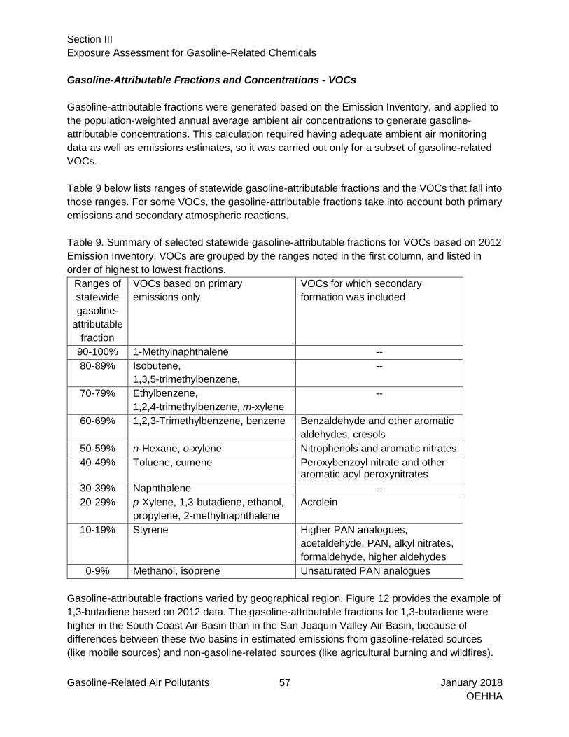
Section III Exposure Assessment for Gasoline-Related Chemicals
Gasoline-Related Air Pollutants 57 January 2018 OEHHA
Gasoline-Attributable Fractions and Concentrations - VOCs Gasoline-attributable fractions were generated based on the Emission Inventory, and applied to the population-weighted annual average ambient air concentrations to generate gasoline-attributable concentrations. This calculation required having adequate ambient air monitoring data as well as emissions estimates, so it was carried out only for a subset of gasoline-related VOCs. Table 9 below lists ranges of statewide gasoline-attributable fractions and the VOCs that fall into those ranges. For some VOCs, the gasoline-attributable fractions take into account both primary emissions and secondary atmospheric reactions. Table 9. Summary of selected statewide gasoline-attributable fractions for VOCs based on 2012 Emission Inventory. VOCs are grouped by the ranges noted in the first column, and listed in order of highest to lowest fractions.
Ranges of statewide gasoline-
attributable fraction
VOCs based on primary emissions only
VOCs for which secondary formation was included
90-100% 1-Methylnaphthalene -- 80-89% Isobutene,
1,3,5-trimethylbenzene, --
70-79% Ethylbenzene, 1,2,4-trimethylbenzene, m-xylene
--
60-69% 1,2,3-Trimethylbenzene, benzene Benzaldehyde and other aromatic aldehydes, cresols
50-59% n-Hexane, o-xylene Nitrophenols and aromatic nitrates 40-49% Toluene, cumene Peroxybenzoyl nitrate and other
aromatic acyl peroxynitrates 30-39% Naphthalene -- 20-29% p-Xylene, 1,3-butadiene, ethanol,
propylene, 2-methylnaphthalene Acrolein
10-19% Styrene Higher PAN analogues, acetaldehyde, PAN, alkyl nitrates, formaldehyde, higher aldehydes
0-9% Methanol, isoprene Unsaturated PAN analogues Gasoline-attributable fractions varied by geographical region. Figure 12 provides the example of 1,3-butadiene based on 2012 data. The gasoline-attributable fractions for 1,3-butadiene were higher in the South Coast Air Basin than in the San Joaquin Valley Air Basin, because of differences between these two basins in estimated emissions from gasoline-related sources (like mobile sources) and non-gasoline-related sources (like agricultural burning and wildfires).

Section III Exposure Assessment for Gasoline-Related Chemicals
Gasoline-Related Air Pollutants 58 January 2018 OEHHA
Gasoline-attributable fractions were also higher for chemicals in the South Coast Air Basin than statewide (illustrated for 1,3-butadiene in Figure 12). The chemicals with the largest differences between the South Coast Air Basin and statewide gasoline-attributable fractions included many that had substantial contributions from secondary emissions (acrolein, higher PAN analogues, alkyl nitrates, PAN, acetaldehyde, formaldehyde, and higher aldehydes) and a few others that were largely in primary emissions (propylene, naphthalene, 1,3-butadiene and benzene). Figure 12. 1,3-Butadiene gasoline-attributable fractions in 2012
There were some notable changes in gasoline-attributable fractions immediately after 2003, when MTBE was banned. Most of the differences in gasoline-attributable fractions from 2003 to 2004 could be linked to changes made by CARB to source profiles19, which were adjusted to reflect the changes in California gasoline that occurred in 2004. With the MTBE phase-out, its gasoline-attributable fraction dropped from almost 100% in 2003 to near 0% in 2004. Over the same period, statewide gasoline-attributable fractions for ethanol increased from 2% to 39%, as expected with its increased use as an oxygenate. Other chemicals with marked increases in statewide gasoline-attributable fractions between 2003 to 2004 included p-xylene, 1-methylnaphthalene and 2-methylnaphthalene. For p-xylene, the fraction increased from 6% in 2003 to 37% in 2004 (see Chemical Profiles for details). These increases were associated with adjustments to gasoline-related source profiles due to fuel formulation changes. The statewide gasoline-attributable fractions increased less dramatically (by about 6 to 7%) from 2003 to 2004 for a number of other chemicals, including naphthalene, toluene and o-xylene.
19 Source profiles are part of the CARB Emission Inventory and are described on p. 13.
47%
33%
58%
24%19%
26%
0%
10%
20%
30%
40%
50%
60%
70%
80%
90%
100%
South Coast AirBasin
San Diego AirBasin
San FranciscoBay Area Air
Basin
San JoaquinValley Air Basin
SacramentoValley Air Basin
State

Section III Exposure Assessment for Gasoline-Related Chemicals
Gasoline-Related Air Pollutants 59 January 2018 OEHHA
Styrene, isobutene, methanol and n-hexane gasoline-attributable fractions declined by up to 7% between 2003 and 2004. However, a general decline in gasoline-attributable fractions over a longer time period was also observed for these and other chemicals, so these particular reductions from 2003 to 2004 may not be traceable only to the fuel formulation change. Gasoline-attributable fractions of criteria air pollutants also declined between 1996 and 2012. Statewide gasoline-attributable fractions of NOx declined from 39% (1996) to 21% (2012) due to reduced estimated emissions from gasoline-related on-road mobile sources and increased estimated emissions from non-gasoline-related on-road and other mobile sources. Gasoline-attributable fractions for NOx in the South Coast and San Diego Air Basins were somewhat higher compared to the statewide value in both 1996 and 2012 (by about 10%). In the South Coast Air Basin, for which the most data were available, the gasoline-attributable ambient air concentrations declined by 50 to 90% between 1996 and 2014 for the VOCs we could assess in detail. Table 10 summarizes changes in the 2012 South Coast Air Basin gasoline-attributable concentrations for these VOCs. Table 10. Percent decrease in gasoline-attributable concentrations of VOCs between 1996 and 2014 for the South Coast Air Basin Percent decrease VOCs 90-100 1,2,4-Trimethylbenzene, 1,3-butadiene, styrene 80-90 Ethylbenzene, toluene, propylene, 1,3,5-trimethylbenzene
1,2,3-trimethylbenzene 70-80 Isobutene, n-hexane, m- and p-xylene, o-xylene, cumene, benzene 60-70 Acetaldehyde, formaldehyde
Figure 13 illustrates the decline over time for benzene, and also shows that gasoline-related emissions are the dominant source (>75%) of this toxicant in the South Coast Air Basin. Other VOCs with emissions similarly dominated by gasoline-related sources include isobutene, ethylbenzene and trimethylbenzenes. These air pollutants also showed a significant drop in ambient air in the South Coast region over this time period (see individual Chemical Profiles for details).

Section III Exposure Assessment for Gasoline-Related Chemicals
Gasoline-Related Air Pollutants 60 January 2018 OEHHA
Figure 13. South Coast Air Basin population-weighted annual average ambient air concentration and gasoline-attributable concentration for benzene
A comparison of gasoline-attributable concentrations across air basins was possible only for VOCs identified as TACs because they had sufficient ambient air monitoring. The highest gasoline-attributable concentrations of TACs were observed in the South Coast Air Basin in 1996. The gasoline-attributable concentrations generally declined over time across all of the basins and the differences between air basins became less pronounced. However, the 2014 acetaldehyde and formaldehyde gasoline-attributable concentrations in the South Coast Air Basin were still considerably higher than in other air basins and statewide (see Figure 14 for the example of formaldehyde).
0.00
0.20
0.40
0.60
0.80
1.00
1.20
1.40
Benz
ene
(ppb
v)
YearPopulation-weighted annual average ambient air concentrationGasoline-attributable concentration

Section III Exposure Assessment for Gasoline-Related Chemicals
Gasoline-Related Air Pollutants 61 January 2018 OEHHA
Figure 14. Gasoline-attributable population-weighted annual average ambient air concentrations for formaldehyde

Section III Exposure Assessment for Gasoline-Related Chemicals
Gasoline-Related Air Pollutants 62 January 2018 OEHHA
Exposure Assessment Results – Criteria Air Pollutants
General Trends in Ambient Air Concentrations – Criteria Air Pollutants We assessed two gasoline-related criteria air pollutants: PM2.5 and nitrogen dioxide. Figure 15 shows the overall population-weighted annual average ambient air concentrations of PM2.5, which reflect emissions from both gasoline-related and non-gasoline sources. The Figure covers 1999 to 2013, which are the years for which PM2.5 monitoring data were available. Over this time period, annual average concentrations of all-source PM2.5 declined by 47% statewide and by 53% in the South Coast Air Basin. By 2013, all basins except the San Joaquin Valley Air Basin had population-weighted annual average ambient air concentrations for PM2.5 below the current CAAQS of 12 µg/m3 (annual average, adopted in 2002). The major sources of 2012 emissions of primary PM2.5 in the San Joaquin Valley were wildfires (35%) and miscellaneous sources (44%; including farming operations [14%] and fugitive windblown dust [8%]). Figure 15. Trends in population-weighted annual average ambient air concentrations for PM2.5
Note: The CAAQS of 12 µg/m3 shown in Figure 15 became effective in 2002. Figure 16 shows the trends in the overall population-weighted annual average ambient air concentrations of nitrogen dioxide, which reflect emissions from both gasoline-related and non-gasoline sources. In the South Coast Air Basin and statewide, concentrations of nitrogen dioxide declined by 50% and 46%, respectively, between 1996 and 2013 (the most recent year with data).
0
5
10
15
20
25
1998 2000 2002 2004 2006 2008 2010 2012 2014
PM
2.5
popu
latio
n-w
eigh
ted
annu
al a
vera
ge
ambi
ent
air c
once
ntra
tions
(μg
/m3 )
South Coast Air Basin San Diego Air BasinSan Francisco Bay Area Air Basin San Joaquin Valley Air BasinSacramento Valley Air Basin State
CAAQS for PM2.5 (12 µg/m3, annual average)

Section III Exposure Assessment for Gasoline-Related Chemicals
Gasoline-Related Air Pollutants 63 January 2018 OEHHA
Figure 16. Trends in population-weighted annual average ambient air concentrations for nitrogen dioxide
Gasoline-Attributable Emissions, Fractions and Concentrations – Criteria Air Pollutants
PM2.5
For PM2.5, the Emission Inventory includes information on primary emissions of PM2.5. Primary PM2.5 emissions from gasoline-related sources decreased in the South Coast Air Basin and statewide by 45% and 37%, respectively, from 1996 to 2012. We used Emission Inventory data to calculate gasoline-attributable fractions for primary PM2.5. To estimate these fractions for secondary PM2.5, we used the fractions for NOx, SOx, and ROG as proxies for ammonium nitrate, ammonium sulfate, and SOA, respectively (see the Chemical Profile for details on the method and a discussion of the substantial uncertainties with this approach). The estimated gasoline-attributable fractions for the South Coast Air Basin declined from about 30% in 1996 to about 20% in 2012. Other air basins had lower gasoline-attributable fractions compared to the South Coast, and these also declined over the same time period. Population-weighted ambient air concentrations of PM2.5 dropped by 53%, 42%, 44%, 28%, 47% and 47% in the South Coast, San Diego, San Francisco Bay Area, San Joaquin Valley and Sacramento Valley Air Basins and statewide, respectively, over the period 1999 to 2013. Gasoline-attributable concentrations of PM2.5 declined even more substantially, reflective of the declines in gasoline-attributable fractions described above. For example, the estimated South Coast Air Basin gasoline-attributable concentrations declined by about 70% during this period.
0.000
0.005
0.010
0.015
0.020
0.025
0.030
0.035
0.040
1996 1998 2000 2002 2004 2006 2008 2010 2012 2014
Nitr
ogen
dio
xide
pop
ulat
ion-
wei
ghte
d an
nual
ave
rage
am
bien
t air
conc
ontr
atio
n (p
pm)
South Coast Air Basin San Diego Air BasinSan Francisco Bay Area Air Basin San Joaquin Valley Air BasinSacramento Valley Air Basin State
CAAQS for NO2 (0.03 ppm, annual average)

Section III Exposure Assessment for Gasoline-Related Chemicals
Gasoline-Related Air Pollutants 64 January 2018 OEHHA
Nitrogen Dioxide Consistent with the observed trend in ambient air concentrations of nitrogen dioxide (see Figure 16 above), the estimated statewide emissions of NOx from gasoline-related sources decreased dramatically, by 72% between 1996 and 2012. Similar declines in emissions of NOx from gasoline-related sources over the same time period were observed in the five air basins studied: South Coast (77%), San Diego (74%), San Francisco Bay Area (65%), San Joaquin (76%), and Sacramento Valley (70%). Based on the Emission Inventory data for NOx, we generated gasoline-attributable fractions and examined the results over time and by region (for complete results see the Chemical Profile). In the South Coast Air Basin, the fraction attributable to gasoline-related sources declined from 47% to 29% between 1996 and 2012. During the same time period, the statewide gasoline-attributable fractions for NOx declined from 39% to 21%. The gasoline-attributable fraction for NOx was applied to population-weighted concentrations for nitrogen dioxide. As expected, the resulting gasoline-attributable concentrations for nitrogen dioxide decreased substantially from 1996 to 2013, mirroring the trends in emissions and measured air concentrations. In the South Coast Air Basin and statewide, the gasoline-attributable nitrogen dioxide concentration declined by about 70% over this time period.

Gasoline-Related Air Pollutants 65 January 2018 OEHHA
IV. Screening Cancer and Non-Cancer Risk Assessment
A screening cancer and non-cancer risk assessment was carried out for selected gasoline-related chemicals. Chemicals were retained for risk assessment based on availability of an exposure measure (i.e., gasoline-attributable concentration; see page 52 in the Exposure Assessment Section) and a health reference value (e.g., cancer potency value or chronic reference exposure level). The following pages contain a summary of the results of the screening cancer and non-cancer risk assessment. There were four main results:
• Estimated cancer risks for selected gasoline-related VOCs • Estimated cancer risks for selected gasoline-related PAHs • Estimated non-cancer hazard quotients for selected gasoline-related VOCs
Screening Risk Assessment Methods
A brief description of methods used in the screening risk assessment is provided below. Additional details are provided in Appendix G.
Methods for Estimating Cancer Risks for Gasoline-Related VOCs
Cancer risks were estimated for the South Coast Air Basin and statewide for gasoline-related VOCs (including the volatile PAH naphthalene) that were known carcinogens and had available potency values. The reason for selecting the South Coast Air Basin to highlight is that ambient air monitoring data were available for more chemicals in this basin compared to other air basins. In addition, the South Coast Air Basin is known to have more gasoline-related mobile sources, so the health risk results would represent a worst-case scenario. Cancer risks were estimated based on gasoline-attributable population-weighted annual average ambient air concentrations. The calculation also took into account early-in-life sensitivity using a method developed by OEHHA. This method incorporates age sensitivity factors and 95th percentiles of age-specific breathing rates. For further details and an example calculation, see Appendix G.
Methods for Estimating Cancer Risks from Selected PAHs, Other than Naphthalene
Naphthalene is a volatile PAH that is included in the Emission Inventory, and cancer risks were assessed using the methods for VOCs as noted in the previous section. We identified additional PAHs that had available air monitoring data in California (see Chemical Profiles for details), as well as cancer potency values or potency equivalency factors, and retained these for screening risk assessment (see Table 3 on page 31). We used potency values developed by OEHHA (2015) for California’s Air Toxics Hot Spots Program (for specific values, refer to Appendix G). It was not possible to calculate gasoline-attributable fractions for these PAHs, because they are

Section IV Screening Cancer and Non-Cancer Risk Assessment
Gasoline-Related Air Pollutants 66 January 2018 OEHHA
not in the Emission Inventory, so cancer risks were conservatively calculated by assuming that 100% of the ambient air concentrations are attributable to gasoline-related sources. The sources used for PAH ambient air data were:
• California Toxic Monitoring Network • South Coast Air Basin ambient air study of PAHs (Eiguren-Fernandez et al., 2004) • Multiple Air Toxics Exposure Study III (SCAQMD, 2008) • National Air Toxics Trends Stations, available at the US EPA AQS Data Mart database
website (https://aqs.epa.gov/api) Many of these PAH data sets had a large number of non-detects. Non-detects were set equal to half the limit of detection prior to calculating the annual average. The ambient air concentrations of these PAHs were highest in the fall and winter with most of the non-detects occurring in the spring and summer months.
Methods for Estimating Non-Cancer Hazard Quotients for Selected Gasoline-Related VOCs
Non-cancer hazard quotients were calculated for gasoline-related chemicals with a chronic Reference Exposure Level (cREL) developed by OEHHA for the Air Toxics Hot Spots Program (OEHHA, 2015; https://oehha.ca.gov/air/general-info/oehha-acute-8-hour-and-chronic-reference-exposure-level-rel-summary). We carried out these calculations in the South Coast Air Basin, which has the most complete set of ambient air data on pollutants with cRELs (data available for all but methanol). Non-cancer hazard quotients were also calculated on a statewide basis for the few chemicals with adequate ambient air monitoring data across all air basins. The hazard quotient for a chemical was calculated as follows:
Gasoline-attributable hazard quotient = (Gasoline-attributable concentration of chemical)/(CREL) For each cREL, OEHHA identifies “hazard index target organs”. Hazard indices (i.e., sums of hazard quotients) were examined for the respiratory system and the nervous system.

Section IV Screening Cancer and Non-Cancer Risk Assessment
Gasoline-Related Air Pollutants 67 January 2018 OEHHA
Screening Risk Assessment Results
Cancer Risks for Selected Gasoline-Related VOCs
Gasoline-attributable cancer risks for the South Coast Air Basin are plotted over time in Figure 17 (benzene and 1,3-butadiene) and Figure 18 (acetaldehyde, ethylbenzene, formaldehyde, naphthalene, MTBE and styrene). The estimated combined cancer risks for these carcinogens20 dropped by almost a factor of seven (from 9.4x10⁻⁴ in 1996 to 1.4x10⁻⁴ in 2014). This is equivalent to an estimated reduction of 797 cancer cases per 1 million people. The statewide gasoline-attributable cancer risks are shown in Figure 19 (benzene and 1,3-butadiene) and Figure 20 (acetaldehyde, formaldehyde and MTBE). The set of carcinogenic VOCs evaluated statewide is smaller due to more limited availability of ambient air monitoring data. The statewide combined cancer risk20 for acetaldehyde, benzene, 1,3-butadiene and formaldehyde dropped by about a factor of six (from 4.9x10⁻⁴ based on 1996 data to 8.2x10⁻⁵ based on 2014 data). Note that the combined 2014 estimated cancer risks for these four chemicals in the South Coast Air Basin was almost a factor of two higher (1.3X10⁻⁴) compared to statewide. For both the South Coast Basin and statewide, the majority of the drop in estimated cancer risk from 1996 to 2014 was driven by reductions in the ambient air concentrations of benzene and 1,3-butadiene. In 2014, these two carcinogens were still the major contributors to the estimated cancer risk for the South Coast Air Basin and statewide. Though less apparent from Figure 17, the gasoline-attributable cancer risk of the other VOCs declined as well. In the South Coast Air Basin, the gasoline-attributable cancer risks of formaldehyde, acetaldehyde and ethylbenzene decreased by 65%, 63% and 81% between 1996 and 2014.
20 MTBE was excluded from the calculation of combined cancer risks because ambient air monitoring data were not available in 2014.

Section IV Screening Cancer and Non-Cancer Risk Assessment
Gasoline-Related Air Pollutants 68 January 2018 OEHHA
Figure 17. Cancer risks for benzene and 1,3-butadiene in the South Coast Air Basin based on gasoline-attributable population-weighted annual average ambient air concentrations
Figure 18. Cancer risks for other carcinogenic VOCs in the South Coast Air Basin based on gasoline-attributable population-weighted annual average ambient air concentrations
0
1.0E-04
2.0E-04
3.0E-04
4.0E-04
5.0E-04
Gaso
line-
attr
ibut
able
can
cer r
isk
in th
e So
uth
Coas
t Air
Basin
Year
Benzene 1,3-Butadiene

Section IV Screening Cancer and Non-Cancer Risk Assessment
Gasoline-Related Air Pollutants 69 January 2018 OEHHA
Figure 19. Statewide cancer risks for benzene and 1,3-butadiene based on gasoline-attributable population-weighted annual average ambient air concentrations
Figure 20. Statewide cancer risks for acetaldehyde, formaldehyde and MTBE based on gasoline-attributable population-weighted annual average ambient air concentrations
0
1.0E-04
2.0E-04
3.0E-04
4.0E-04
5.0E-04
Stat
ewid
e ga
solin
e-at
trib
utab
le c
ance
r risk
Year
Benzene 1,3-Butadiene

Section IV Screening Cancer and Non-Cancer Risk Assessment
Gasoline-Related Air Pollutants 70 January 2018 OEHHA
Cancer Risks for Selected Gasoline-Related PAHs (Other than Naphthalene)
The following gasoline-related PAHs had a cancer potency value or a potency equivalency factor and ambient air monitoring data:
• Benz[a]anthracene • Benzo[a]pyrene • Benzo[b]fluoranthene • Benzo[k]fluoranthene • Chrysene • Dibenz[ah]anthracene • Indeno[1,2,3-cd]pyrene
We had insufficient data to determine gasoline-attributable fractions for these PAHs, which are not included in the Emission Inventory. Therefore, cancer risks were estimated based on the highly conservative assumption that 100% of the ambient air concentrations of these PAHs were from gasoline-related sources. This section provides an overview of results from the screening cancer risk assessment for PAHs other than naphthalene; for more details, see the Chemical Profiles on PAHs. Figure 21 plots the cancer risks based on annual average concentrations of benzo[a]pyrene (BaP) calculated based on measurements at selected monitoring sites across California. The highest BaP cancer risks statewide were estimated for California Toxic Monitoring Network sites in Chico, Fresno, Burbank, and North Long Beach (the last site is not included in Figure 21). Two other sites in the California Toxic Monitoring Network, Rubidoux and Central Los Angeles, had measurements for a longer time period and so are also included in Figure 21. The California Toxic Monitoring Network stopped measuring BaP in early 2005. We used data from MATES III (SCAQMD, 2008) and US EPA NATTS (https://aqs.epa.gov/api) studies to extend the timeframe of BaP measurements for the Rubidoux and Central Los Angeles sites. Figure 21 also graphs BaP cancer risks estimated based on data from Eiguren-Fernandez et al. (2004) (abbreviated “EF” in Figure 21 below). Eiguren-Fernandez et al. measured ambient air PAHs at six sites in 2001 and 2002, including four near Los Angeles (San Dimas, Upland, Mira Loma and Riverside).

Section IV Screening Cancer and Non-Cancer Risk Assessment
Gasoline-Related Air Pollutants 71 January 2018 OEHHA
Figure 21. Benzo[a]pyrene cancer risk based on annual average ambient air concentrations at selected sites
Benzo[b]fluoranthene, benzo[k]fluoranthene, dibenz[ah]anthracene and indeno[cd]pyrene were also monitored by the California Toxic Monitoring Network. Figure 22 shows the estimated cancer risks associated with exposure to these four PAHs and BaP based on measurements at 1st St. in Fresno, which was one of the two sites with the highest concentrations in the state (similar concentrations were found at Chico; data not shown). Figure 23 plots population-weighted cancer risks calculated for the South Coast Air Basin, which had PAH data for many more sites. For additional information, refer to the Chemical Profiles on PAHs. We estimated combined cancer risks in 2014 for seven PAHs (the five listed above, plus benz[a]anthracene and chrysene) based on data from two sites in the South Coast Air Basin (North Main St. in Los Angeles and Rubidoux in Riverside) and assuming a gasoline-attributable fraction of 1. Combined cancer risks for these seven PAHs were 4.8x10⁻⁷ and 5.1x10⁻⁷, respectively, or about an order of magnitude lower than the estimated gasoline-attributable population-weighted cancer risk for naphthalene in the South Coast Air Basin in 2014.
0.0E+00
5.0E-07
1.0E-06
1.5E-06
2.0E-06
2.5E-06
3.0E-06
Benz
o[a]
pyre
ne c
ance
r risk
at
sel
ecte
d sit
es in
Cal
iforn
ia
YearCalif. Toxics - Fresno-1st Street EF - Riverside, Riverside CountyCalif. Toxics - Chico-Manzanita Avenue EF - Upland, San Bernardino CountyCalif. Toxics - Rubidoux MATES III - N. Long BeachCalif. Toxics - Central Los Angeles MATES III - RubidouxCalif. Toxics - Burbank-W Palm Avenue MATES III - Central L.A.South Coast population-weighted annual average US EPA NATTS - Central L.A.EF - Mira Loma, Riverside County US EPA NATTS - San JoseEF - San Dimas, Los Angeles County US EPA NATTS - Rubidoux, Riverside County

Section IV Screening Cancer and Non-Cancer Risk Assessment
Gasoline-Related Air Pollutants 72 January 2018 OEHHA
Figure 22. Cancer risk for selected PAHs based on annual average ambient air concentrations at 1st St. Fresno21
Figure 23. Cancer risk for selected PAHs based on population-weighted annual average ambient air concentrations in the South Coast Air Basin21
21 Figure design is based on MATES III report.
0.0E+00
5.0E-07
1.0E-06
1.5E-06
2.0E-06
2.5E-06
3.0E-06
3.5E-06
4.0E-06
1996 1997 1998 1999 2000 2001 2002 2003 2004
Canc
er ri
sk
Year
Benzo[a]pyrene Benzo[b]fluoranthene Benzo[k]fluoranthene
Dibenz[ah]anthracene Indeno[cd]pyrene
0.0E+00
5.0E-07
1.0E-06
1.5E-06
2.0E-06
2.5E-06
3.0E-06
3.5E-06
4.0E-06
1996 1997 1998 1999 2000 2001 2002 2003 2004
Canc
er ri
sk
Year
Benzo[a]pyrene Benzo[b]fluoranthene Benzo[k]fluoranthene
Dibenz[ah]anthracene Indeno[cd]pyrene

Section IV Screening Cancer and Non-Cancer Risk Assessment
Gasoline-Related Air Pollutants 73 January 2018 OEHHA
Non-Cancer Hazard Quotients for Selected Gasoline-Related VOCs
Gasoline-attributable hazard quotients were calculated for respiratory toxicants with health reference values and adequate ambient air monitoring data in the South Coast Air Basin (see Figure 24) and statewide. Statewide hazard quotients were all lower than the corresponding South Coast Air Basin values. Acrolein and formaldehyde had the highest gasoline-attributable hazard quotients in the South Coast Air Basin in 2014 (3 and 0.1 respectively). The statewide gasoline-attributable hazard quotient for acrolein was also slightly elevated (1.2) in 2014. There are challenges in accurately measuring acrolein in ambient air, so more work is needed to evaluate the potential risks for respiratory toxicity (see the Chemical Profile for acrolein for details). We identified other suspected respiratory toxicants, including a number of carbonyls (e.g., benzaldehyde, hexaldehyde, propionaldehyde and butyraldehyde), that could not be assessed because chronic reference exposure levels were not available and ambient air monitoring data were limited. Figure 25 shows hazard quotients for nervous system toxicants, with available health reference values, calculated based on gasoline-attributable population-weighted annual average ambient air concentrations for the South Coast Air Basin. These gasoline-attributable hazard quotients are all well below one, as was the overall hazard index. However, this is not a comprehensive list of gasoline-related nervous system toxicants. For example, OEHHA set a chronic reference exposure level for cresol mixtures of 600 µg/m3 based on adverse effects to the nervous system but ambient air data are not available for cresols. Statewide nervous system hazard quotients were also calculated for chemicals with adequate data (toluene and combined xylenes) and were all lower than the corresponding South Coast Air Basin values.

Section IV Screening Cancer and Non-Cancer Risk Assessment
Gasoline-Related Air Pollutants 74 January 2018 OEHHA
Figure 24. Gasoline-attributable hazard quotients for chronic respiratory toxicants based on estimated annual average exposures in the South Coast Air Basin (vertical axis is log-scale)
Figure 25. Gasoline-attributable hazard quotients for nervous system toxicants based on estimated annual average exposures in the South Coast Air Basin (vertical axis is log-scale)
Notes on Figures 24 and 25 1. Acetaldehyde, acrolein and formaldehyde include primary emissions and secondary formation 2. Acrolein ambient air monitoring started in 2004. 3. Two models were developed for naphthalene air concentrations based on limited data from 1996 and 2007-2014. 4. Hazard quotients for trimethylbenzenes and xylenes were based on the sum of the ambient air concentrations for the individual isomers.
0.00001
0.0001
0.001
0.01
0.1
Gaso
line-
attr
ibut
able
ner
vous
sys
tem
ha
zard
quo
tient
s in
the
Sout
h Co
ast A
ir Ba
sin
YearTrimethylbenzenes Toluene Xylenes n-Hexane Styrene

Section IV Screening Cancer and Non-Cancer Risk Assessment
Gasoline-Related Air Pollutants 75 January 2018 OEHHA
We also reviewed available non-cancer health reference values for other endpoints. Figure 26 shows the hazard quotients for benzene, 1,3-butadiene, MTBE and ethylbenzene based on various non-cancer effects. The hazard quotient for hematologic effects of benzene was 1.1 in 1996; by 2014 it had dropped to 0.21. The hazard quotient for reproductive effects of 1,3-butadiene dropped by twelve-fold from 1996 to 2014. For MTBE, the hazard quotient in 1996 was well below 1, and by 2004, ambient air levels had mostly dropped below the limit of detection. Statewide hazard quotients for these other endpoints were calculated for chemicals with adequate data (benzene, 1,3-butadiene and MTBE) and were all lower than the corresponding South Coast Air Basin values. Figure 26. Gasoline-attributable hazard quotients for target organs other than respiratory system based on estimated annual average exposures in the South Coast Air Basin (vertical axis is log-scale)
Note: MTBE ambient air data were no longer collected after 2004. In 2004, most measurements were below the limit of detection (0.3 ppb).
0.0001
0.001
0.01
0.1
1
10
Gaso
line-
attr
ibut
able
haz
ard
quot
ient
s fo
r oth
er t
arge
t org
ans
YearBenzene (hematologic system)1,3-Butadiene (reproductive system)MTBE (kidney, eyes, liver)Ethylbenzene (liver, kidney, endocrine system, development)Cumene (endocrine system, kidney)

Gasoline-Related Air Pollutants 76 January 2018 OEHHA
V. Challenges and Limitations
In this section, we describe some of the challenges and data limitations we encountered as we carried out the screening assessment described in this report.
Limitations in Hazard Identification
In carrying out hazard identification for gasoline-related pollutants, we focused primarily on VOCs (i.e., those present in liquid fuel, exhaust, and/or evaporative emissions, or as secondary transformation products). This approach was driven by data availability. Gasoline-related particle phase pollutants are less well elucidated, so we examined gasoline-related PM (unspeciated) and a few individual particle-phase PAHs. Assessing other pollutants arising from processes associated with gasoline vehicle operation, such as releases of metals and other particulate matter from engine, tire and brake wear (Grigoratos 2015; Dahl et al., 2006), was beyond the scope of this report. The hazard identification for gasoline-related atmospheric transformation products was limited in several ways. First, detailed atmospheric chemistry was examined for the top 25 most highly emitted gaseous pollutants, accounting for 77% of non-methane gasoline-related emissions in 1998, and a few other toxicologically important compounds. However, the universe of potential atmospheric transformation products associated with gasoline use is greater than described in this report. Second, in general, only first-generation products were identified, and second or third generation products were not characterized. Our screening for toxicologically important compounds among the entire set of gasoline-related substances we identified was limited by gaps in toxicological data. For the most highly emitted gasoline-related VOCs in primary exhaust, toxicity concerns have been relatively well characterized, but this was not the case for other VOCs or atmospheric transformation products.
Limitations in the Calculation of Population-Weighted Annual Average Ambient Air Concentrations
For many of the chemicals studied, ambient air data were spatially or temporally limited. Often, data were collected at a few sites in each air basin and the data from a single monitoring site were available for most but not all of the years between 1996 and 2014. We supplemented measured ambient air levels with modeled concentrations, based on carbon monoxide levels at additional locations and for missing time points, where possible. This approach has significant uncertainty because it assumes a constant relationship between carbon monoxide and the air pollutant over time and space. There are more sophisticated modeling approaches being developed, which could be applied in future work assessing exposure to mobile source pollutants. For example, US EPA’s Hazardous Air Pollutant Exposure Model (HAPEM) no

Section V Challenges and Limitations
Gasoline-Related Air Pollutants 77 January 2018 OEHHA
longer uses carbon monoxide as a tracer. The updated and improved HAPEM applies ambient air concentration data, population data, and human activity pattern data to estimate inhalation exposure concentrations for various air toxics. It addresses exposures in microenvironments, and includes adjustments for proximity to major roadways. We calculated annual average ambient air concentrations across entire air basins, and this approach does not address potentially highly elevated exposures in specific communities, such as those next to a major roadway. We also did not address intermittent peak excursions in exposures that can occur during poor air quality episodes or the elevated exposures drivers and passengers routinely experience while commuting (Ham et al., 2017).
Limitations in Evaluation of Gasoline-Attributable Emissions
We used CARB’s Emission Inventory, which compiles data for over 3,000 sources, to study trends in gasoline-related emissions and to calculate gasoline-attributable fractions. A major limitation of this approach was that we calculated gasoline-attributable fractions on a basin-wide basis, and could not address the known issue of locally elevated impacts from gasoline-related sources. Complete Emission Inventory data extracts were available for 1996-2008 and 2012. We used the available data to extrapolate to missing years (i.e., 2009, 2013, and 2014) and to fill in missing natural source emissions for 2010 and 2011. The Emission Inventory is updated periodically by CARB, and some of these changes had large impacts on the gasoline-attributable fractions. In particular, the approach for estimating natural source emissions was updated in 2002, which dramatically affected the calculated fractions. For PAHs, we were able to determine gasoline-attributable fractions only for naphthalene and 1- and 2-methylnaphthalene, because these volatile compounds are included in the Emission Inventory. For particle phase PAHs, a highly conservative assumption that 100% of emissions were attributable to gasoline-related sources was applied for the screening risk assessment. For PM2.5, the approach we applied to estimate the gasoline-attributable fractions included a number of simplifying assumptions that introduced substantial uncertainties. First, we used proxies for the gasoline-attributable fractions of the main secondary PM2.5 components - NOx as a proxy for ammonium nitrate, SOx as a proxy for ammonium sulfate, and ROG as a proxy for SOA. However, the relationship between NOx and nitrate is complex and likely does not follow a simple linear relationship. Further, the formation of SOA depends on a number of factors, such as the composition of VOCs emitted and atmospheric conditions. These complexities were not incorporated into the method for approximating PM2.5 gasoline-attributable fractions. For more details on the approach applied and additional limitations, see the Chemical Profile for PM2.5.

Section V Challenges and Limitations
Gasoline-Related Air Pollutants 78 January 2018 OEHHA
Limitations in Evaluating Contributions from Secondary Atmospheric Formation from VOC Emissions
For a small subset of 12 VOCs, including acrolein, acetaldehyde, formaldehyde, aromatic aldehydes, higher aldehydes, and PAN, we estimated contributions from secondary atmospheric formation based on a report by Dr. William Carter (2001), which was commissioned by OEHHA. A number of simplifying assumptions were applied in the development of formation potentials. For example, the atmospheric reactions of many VOCs were approximated using those of better-studied model species. Assumptions were made about atmospheric conditions, which affected reaction yields. Some secondary reaction products such as aromatic aldehydes and higher aldehydes could only be modeled as groups. A more sophisticated modeling system, US EPA’s Community Multiscale Air Quality (CMAQ) Modeling System, could be considered for future work on secondary transformation products. US EPA (2017) describes CMAQ as bringing together “meteorological models, to represent atmospheric and weather activities, emission models to represent man-made and naturally-occurring contributions to the atmosphere, and an air chemistry-transport model to predict the atmospheric fate of air pollutants under varying conditions.”
Limitations in Health Risk Calculations
We focused primarily on reviewing health effects associated with chronic exposures (e.g., cancer and chronic respiratory toxicity) to individual gasoline-related pollutants. We did not evaluate health effects associated with acute exposures, other types of chemical hazards like explosivity or flammability, or potential impacts on climate from gasoline-related emissions. For a number of chemicals identified as a potential health hazard, health reference values were not available. For example, cumene is a known carcinogen but lacked a cancer potency value; aldehydes such as butyraldehyde and hexaldehyde were flagged as suspected respiratory toxicants but did not have established cREL values. For the screening risk assessment calculations, we used point estimates for all parameters and did not examine distributions in exposure or potential interindividual differences in responses to toxic substances. Our screening assessment evaluated potential health risks for individual gasoline-related air pollutants. We were not able to evaluate health risks associated with exposure to gasoline-related complex mixtures because of insufficient data and lack of an accepted methodology. It is well known that concurrent exposure to multiple pollutants can have a synergistic toxic effect (Mauderly and Samet, 2009; Carlin et al., 2013). Dominici et al. (2010) recommend a multipollutant approach to controlling air pollution, while acknowledging that this is a challenging task.

Gasoline-Related Air Pollutants 79 January 2018 OEHHA
VI. Highlights of Key Findings
Emissions from Gasoline-Related Sources
Estimated emissions of TOG from gasoline-related sources have declined by nearly 70% statewide since 1996. This significant reduction is attributable primarily to the decline in on-road mobile source emissions, which occurred even while gasoline sales remained steady and California’s population continued to grow. By 2012, emissions from on-road motor vehicles had decreased so substantially that they were approaching levels similar to emissions from other gasoline-related mobile sources, which include lawn and garden equipment, recreational boats and off-road vehicles. Emissions from these other mobile sources also declined over the same period, dropping almost in half since 1999. CARB (2016) has a broad strategy in place to seek additional reductions in mobile source emissions, which includes initiatives to promote zero-emission technologies and further tightening of standards for small-off road engines.
Gasoline-Related VOCs
We identified close to 300 VOCs in primary emissions from gasoline-related sources based on 1996 data. By 2012, this number increased to more than 350. Isopentane has consistently been the most highly emitted chemical from gasoline-related sources, but was not assessed in detail in this report because of low toxicity. Between 1996 and 2003, the second most highly emitted gasoline-related VOC was MTBE. In 2004, MTBE was phased out and MTBE emissions dropped to nearly zero. Ethanol replaced MTBE as the oxygenate of choice and became the fifth most highly emitted gasoline-related VOC in 2004. By 2012, ethanol was the second most highly emitted gasoline-related VOC. Methane, an important greenhouse gas, was the fourth most highly emitted VOC from gasoline-related sources in 2012. However, only about 1% of total methane emissions came from gasoline-related sources. Among the top 25 most highly emitted VOCs from gasoline-related sources (primary emissions) in 1996 and 2012, toluene, m- and o-xylene, propylene, benzene, n-hexane, formaldehyde, ethylbenzene and isobutene were identified as having both health concerns and available health reference values. The primary emission tonnage of these highly emitted chemicals of particular concern declined by about 65 to 85% between 1996 and 2012. The findings above are based on primary emissions only, drawn from the Emission Inventory data. When we accounted for secondary emissions, based on Carter’s formation potentials (Carter, 2001; see Appendix E in the current report for more details), we identified acetaldehyde and propionaldehyde (a higher aldehyde) as additional highly emitted gasoline-related VOCs that we were able to evaluate in our screening health risk assessment. Total emissions (primary and secondary) of acetaldehyde and higher aldehydes declined by 65 and 67%, respectively, between 1996 and 2012.

Section VI Highlights of Key Findings
Gasoline-Related Air Pollutants 80 January 2018 OEHHA
Similar to the patterns we observed for estimated emissions, population-weighted ambient air concentrations for gasoline-related VOCs generally declined between 1996 and 2014. Based on data from the South Coast Air Basin, which has ambient air measurements on the largest number of chemicals and a more extensive monitoring network than other basins, concentrations of acetaldehyde and formaldehyde declined by 47% and 37%, respectively, when comparing 1996 and 2014. However, the annual average aldehyde concentrations were quite variable over this entire time period and a 5-year moving average in the South Coast Air Basin showed less dramatic declines (24% for acetaldehyde and 20% for formaldehyde). Concentrations for most other VOCs declined even more substantially (by between 67% for benzaldehyde to 92% for 1,2,4-trimethylbenzene). Acrolein was an exception, with ambient air concentrations fluctuating between 2004 and 2014 (the years with available data). We compared our findings on VOCs in this report with the conclusions of the earlier assessment of ethanol as a replacement oxygenate for MTBE (CARB, OEHHA and SWRCB, 1999). In that 1999 report, acetaldehyde and PAN were predicted to be the major products of potential concern from combustion of ethanol-containing fuel. We found that gasoline-related emissions of acetaldehyde and PAN increased slightly between 2003 and 2004, but declined overall between 1996 and 2014. The longer- term decline of these VOCs reflected overall reductions in emissions from newer cars. We also found that the population-weighted annual average ambient air concentrations of acetaldehyde in the South Coast Air Basin and statewide declined by 47% and 37% between 1996 and 2014. PAN is not monitored in ambient air, so possible changes in concentrations over time cannot be assessed for this chemical. Despite the overall observed declines in emissions and ambient air concentrations of gasoline-related VOCs that we document in this report, potential health concerns associated with some VOCs still remain:
• Estimated gasoline-attributable cancer cases for benzene and 1,3-butadiene still exceeded 1 in 1 million exposed individuals in 2014, at 53 and 19 cases, respectively. Estimated cancer cases per 1 million were even higher in the South Coast Air Basin in 2014: 68 for benzene and 36 for 1,3-butadiene. Continued efforts to reduce gasoline-related emissions of carcinogenic VOCs will be necessary as an ongoing investment in public health in California.
• The gasoline-attributable concentration of acrolein in the South Coast Air Basin exceeded the cREL based on respiratory toxicity by a factor of 3 in 2014, while the hazard quotient statewide was 1.2 (see discussion in the Chemical Profile). Further research is warranted on acrolein exposures in California and associated respiratory health risks.
Gasoline-Related PAHs
Based on available ambient air data, naphthalene was the dominant gasoline-related PAH with the highest measured concentrations over the time period assessed. Gasoline-related

Section VI Highlights of Key Findings
Gasoline-Related Air Pollutants 81 January 2018 OEHHA
emissions of naphthalene decreased by 57% between 1996 and 2012, to 0.6 tons per day in 2012 (rank 95). The gasoline-attributable cancer risk for naphthalene in 2014 was 4.8x10⁻⁶. This is about an order of magnitude higher than was estimated for other gasoline-related PAHs (see the Screening Risk Assessment Results section for more details). We based our evaluation of naphthalene on modeled concentrations developed from limited ambient air studies. Additional ambient air monitoring of naphthalene in areas impacted by gasoline-related pollution should be considered to better understand potential exposures and health risks.
Particulate Matter
Ambient air concentrations of PM2.5 substantially declined across the state from 1999 to 2013, with even greater drops predicted for gasoline-attributable concentrations. Gasoline-attributable fractions for PM2.5 were higher in the South Coast Air Basin than in other basins, and generally declined across the state over time. Gasoline-related sources remain an important source of urban PM2.5 and ultrafine particles, with particular concerns for communities heavily impacted by traffic (Zhu et al., 2002; Health Effects Institute, 2013). CARB is currently funding a study that is investigating potential associations between exposures to ultrafine particles and premature death (Kleeman, 2014). Additional research into the contribution of gasoline sources to ambient particulate matter and associated health risks in California is warranted.
Nitrogen Dioxide
Nitrogen dioxide concentrations fell by 46% from 1996 to 2013, but exposures to nitrogen dioxide remain a concern. A number of studies have shown a significant relationship between elevated nitrogen dioxide concentrations and adverse health outcomes such as term low birth weight and increased mortality rates in infants and adults in California. Future work to quantify the health impacts of gasoline-related nitrogen dioxide exposure in California is warranted.
Atmospheric Transformation Products
In general, we were very limited in our ability to assess exposure potential and health concerns for the majority of the gasoline-related atmospheric transformation products (see Table 5 for more details). We developed a list of gasoline-related atmospheric transformation products of potential concern based on our previous report (OEHHA, 2006). We were able to estimate the extent of secondary formation for a subset of these by applying formation potentials developed by Carter (2001) to the Emission Inventory. Our analysis predicted that some of these atmospheric transformation products, including PAN and PAN analogues, alkyl nitrates, and a number of carbonyls, are among the most highly emitted (via secondary formation) gasoline-related chemicals.

Gasoline-Related Air Pollutants 82 January 2018 OEHHA
VII. Recommended Future Research
This report documents substantial declines in air pollution from gasoline-related sources, but also shows that an ongoing commitment to air quality improvements is essential in California. The following areas of research would help fill some data gaps identified in this report, advance our understanding of the overall impact of gasoline-related pollution, and inform future risk reduction measures. Better understanding of the universe of gasoline-related air pollutants and associated health risks: New analytical methods that can more broadly screen for chemicals in the ambient air (so-called “non-targeted analyses”) could be carried out to more fully elucidate the universe of gasoline-related VOCs and their associated atmospheric transformation products. Such research could help identify new chemicals of concern, and focus resources for monitoring and health risk assessment on the most abundant gasoline-related VOCs. Additionally, a number of chemicals with high emissions were not evaluated in the screening assessment in this report because they did not have adequate toxicity information, such as Reference Exposure Levels or cancer potency values. Novel toxicity “read-across” approaches that rely on structure-activity analyses and non-conventional toxicology data sets could potentially be applied to help evaluate the toxicity of gasoline-related chemicals that have not been well studied. Closer examination of neighborhoods and communities for gasoline-related impacts: We applied screening methods to estimate average exposure and health risk for broad regions of the state, and this approach does not examine the higher levels of gasoline-related air pollution in neighborhoods near highways and other heavily trafficked roads. We recommend further work to quantify the exposures associated with gasoline-related sources in these locations, by building on previous projects that have mapped air pollution and health effects in heavily impacted communities (see for example, Ostro and Kim, 2004; Health Effects Institute, 2010; Delfino et al., 2015). Gasoline-related air pollution could be studied in communities identified by CalEnviroScreen as already burdened by a disproportionate share of environmental pollution, and faced with socioeconomic and health challenges (OEHHA, 2017; Cushing et al., 2015). One way to do this would be to design a targeted biomonitoring study of selected gasoline-related chemicals in areas heavily impacted by vehicle traffic. OEHHA is launching a collaborative study with UC Berkeley and the University of Washington of diesel exhaust exposures in the San Francisco Bay Area, using 1-nitropyrene as a biomarker (see, for example, Miller-Schulze et al., 2013). Pending adequate resources, we could potentially extend this study by measuring gasoline-related VOCs, using urinary metabolites or DNA or protein adducts in blood as biomarkers (Alwis et al., 2012; Rudel et al., 2014). For example, ethylbenzene and benzene both have relatively high gasoline-attributable fractions and could be considered for possible biomonitoring. Another approach would be to carry out a more detailed modeling approach of gasoline-related exposures in impacted communities, for example by

Section VII Recommended Future Research
Gasoline-Related Air Pollutants 83 January 2018 OEHHA
using US EPA’s HAPEM to account for time spent in microenvironments and adjust for proximity to busy roadways. AB 617 (C. Garcia, Chapter 136, Statutes of 2017) is aimed at addressing high cumulative exposure to toxic air contaminants and criteria air pollutants in communities across California. CARB has established the Office of Community Air Protection to implement the new mandates under the law, which include developing a statewide strategy to reduce emissions impacting communities, deploying community level air monitoring, and engaging with communities to design and implement emission reduction plans. A targeted biomonitoring study of selected VOCs could aid in the understanding of cumulative air pollutant exposures in communities impacted by gasoline-related sources and other emissions, and complement the work being carried out by CARB under AB 617. California’s programs aimed at reducing greenhouse gas emissions include the implementation of the low carbon fuel standard, and the addition of more zero-emission vehicles to California’s fleet. Analyzing the effects of these activities on gasoline-related pollutants would be worthwhile as one aspect of assessing changes in community exposures resulting from these programs. Expanded monitoring of gasoline-related atmospheric transformation products: Atmospheric transformation products are less widely monitored in ambient air in general, with a few important exceptions (e.g., acetaldehyde and formaldehyde). A short-term pilot study to monitor additional transformation products of concern, such as PAN, could be carried out to examine current ambient air levels and help determine if long-term monitoring would be warranted. Acrolein is recommended for more in-depth study based on our screening results that showed elevated exposures associated with respiratory health risks. CARB recently acquired several analyzers that employ gas chromatography, mass spectrometry, and Fourier Transform Infrared Reference spectroscopy to measure ambient air levels of selected VOCs, including acrolein. After testing and evaluation of the devices, CARB plans to use them to measure VOCs of concern in communities impacted by air pollution. We also recommend investigation of potential biomarkers for acrolein and related compounds that could be used to estimate human exposure directly (see for example, Li et al., 2004). Further research on gasoline-related criteria air pollutant exposures and health impacts: Studies in California have shown that elevated PM2.5 and nitrogen dioxide concentrations are linked to higher mortality and other health effects (Basu et al., 2017; Ostro et al., 2015; Jerrett et al., 2013; Lipsett et al., 2011; Mortimer et al., 2008; Ritz et al., 2006). Additional research on gasoline-related contributions to these pollutants is warranted. Further work could include refining the estimates of the gasoline-attributable fraction of ambient particulate concentrations, particularly the portion arising from secondary reactions in the atmosphere. Research on ultrafine particles (less than 0.1 μm in size) is also important, and new work is underway (see for example, Kleeman, 2014). Estimating mortality and other health impacts associated with gasoline-related PM2.5 and nitrogen dioxide exposures would be another useful extension of the

Section VII Recommended Future Research
Gasoline-Related Air Pollutants 84 January 2018 OEHHA
current report. Such an analysis could build on existing reports by CARB and other agencies (see for example, CARB, 2010; European Environment Agency, 2017). California's dependence on gasoline-fueled transportation means the state will need to maintain its efforts to address public health impacts from vehicle-related pollution. CARB (2016) has already adopted a broad mobile source strategy, which includes initiatives to promote zero-emission technologies for vehicles and other equipment. Additional gains are being sought through further tightening of evaporative emission and exhaust standards for small off-road engines, including those used in lawn and garden equipment. California’s continued commitment to both scientific research and regulatory efforts will build on the already impressive reductions in pollutants demonstrated in this report, and help ensure clean air for future generations of Californians.

Gasoline-Related Air Pollutants 85 January 2018 OEHHA
VIII. Chemical Profiles
The Chemical Profiles summarize results from the exposure assessment and screening risk assessment for the gasoline-related chemicals that we were able to review in detail (see the Hazard Identification Section for more information). The exposure assessment results include:
• Gasoline-attributable fractions and other source apportionment information • Population-weighted annual average concentrations • Gasoline-attributable concentrations (product of the above two factors) • Trends in chemical emissions from gasoline and non-gasoline sources
Screening risk assessment results include:
• Gasoline-attributable cancer risks for the South Coast Air Basin and statewide in 1996 and 2014
• Gasoline-attributable hazard quotients for the South Coast Air Basin and statewide in 1996 and 2014
The results presented for each chemical depended on data availability, so not all chemicals have the complete set of information outlined above.
Guide to Exposure Assessment Results for Gasoline-Related Chemicals
The following figures are presented in the Chemical Profiles, depending on data availability:
• Statewide annual emissions of the chemical from gasoline-related sources and non-gasoline-related sources between 1996 and 2012. These plots are based on estimated emissions from the CARB Emission Inventory; for some chemicals the plots also take into account estimated secondary atmospheric reaction tonnage. Mobile source emission data were not available for 2009, so there are gaps in the plots as a result.
• Gasoline-related and non-gasoline-related sources of chemicals. These plots are based on CARB’s 2012 Emission Inventory (the latest year for which emission estimates were available). A guide to interpreting these plots is provided on the next few pages using acetaldehyde as an example.
• Gasoline-attributable fractions in the state and five air basins (South Coast, San Diego, San Francisco Bay Area, San Joaquin Valley and Sacramento Valley) between 1996 and 2012. As noted above, mobile source emission data were not available for 2009.
• Estimated population-weighted annual average ambient air concentrations and gasoline-attributable population-weighted annual average ambient air concentration (or “gasoline-attributable concentrations”) of the chemical in the South Coast Air Basin between 1996 and 2014.

Section VIII Chemical Profiles
Gasoline-Related Air Pollutants 86 January 2018 OEHHA
• Comparison of estimated population-weighted annual average ambient air concentrations to available ambient air measurements in the South Coast Air Basin. This was a visual check on the robustness of modeled values included in the estimated averages.
The figures are reduced in size for space considerations. Readers can use the zoom feature in Adobe Reader to expand the figures. Due to data limitations, some chemicals have only partial results. For example, it was not possible to calculate population-weighted values for isoprene, propionaldehyde, butyraldehyde and many PAHs. For these chemicals, summaries of available ambient air data are presented instead. Any limitations are noted in the introductory text in each Chemical Profile. For more information on the exposure assessment methods see Appendix D and Appendix E.
Guide to Reading Emission Source Plots
This guide uses acetaldehyde as an example (the full Chemical Profile on acetaldehyde starts on p. 190). The emission source plot for acetaldehyde is shown in Figure 113 on p. 192 and reproduced below. It shows the tons of acetaldehyde emitted from different sources. The plot is based on CARB’s 2012 Emission Inventory.
• The vertical axis shows the tons of chemical emitted in the five most populated air basins: South Coast (SC), San Diego (SD), San Francisco Bay (SF), San Joaquin Valley (SJV) and Sacramento Valley (SV). The tonnage is broken into gasoline-related and non-gasoline-related sources; these are labeled as (G) and (NG) respectively on the plots.
• The tonnage is further broken down into seven emission categories from the Emission Inventory: cleaning and surface coatings, fuel combustion, industrial processes, miscellaneous processes, natural sources, on-road motor vehicles, other mobile sources, petroleum production, solvent evaporation, and waste disposal. These categories are described briefly in Table 11 below. Refer to CARB’s website for a complete description of the Emission Inventory categories (http://www.arb.ca.gov/ei/ei.htm).
• The vertical axis label for acetaldehyde indicates that the tonnage is from primary emissions and secondary atmospheric reactions. Each plot has a similar label indicating if the emissions were primary, secondary, or both.
• The table immediately below each plot contains the tonnage values for the different emission categories. For acetaldehyde, gasoline-related on-road mobile sources contributed 5.58 tons per day in the South Coast Air Basin through primary emissions and secondary reactions in 2012.
• The bubble captions on the plot are example sources from the emission category. For example, for acetaldehyde, “biogenic sources” are example natural sources in the South

Section VIII Chemical Profiles
Gasoline-Related Air Pollutants 87 January 2018 OEHHA
Coast Air Basin. The sources highlighted in this way are significant contributors to emissions from the category but are not the only sources in the category. Example plot: Acetaldehyde (also shown on p. 192 as Figure 113)
Table 11. Emissions categories Emissions Category Examples
Cleaning and surface coatings
• Dry cleaning • Emissions resulting from the use of solvents in degreasing
operations in the manufacturing and maintenance industries • Coatings and related solvents (e.g., auto refinishing, plastic
parts, industrial coatings, aircraft coatings) • Emissions from solvents contained in adhesives and sealants
used for the following industries: construction, transportation and other
Fuel combustion
• Internal combustion engines, boilers and process heaters used in electricity generation, oil and gas production and manufacturing.
• Other areas like commercial natural gas burning
Industrial processes • Plastic production • Fiberglass production

Section VIII Chemical Profiles
Gasoline-Related Air Pollutants 88 January 2018 OEHHA
Emissions Category Examples
Miscellaneous processes
• Livestock • Woodstoves • Forest management (burning) • Agricultural burning
Natural sources
• Biological and geological sources • Wildfires • Windblown dust • Biogenic emissions from plants and trees
On-road motor vehicles
• Passenger cars • Light, medium and heavy duty trucks • Buses • Motorcycles • Motorhomes
Other mobile sources
• Aircraft • Boats • Trains • Farm equipment • Lawn and garden equipment
Petroleum production and marketing
• Natural gas transmission losses • Fugitive emissions from valves and fittings during oil and gas
production • Spills during vehicle refueling
Solvent evaporation
• Consumer products (a consumer product is any chemically formulated product used by household and institutional consumers, e.g., detergents, home and garden products, cosmetics, aerosol paints)
• Architectural coatings like non-aerosol paint and paint thinner • Pesticides and fertilizers • Asphalt paving and roofing
Waste disposal • Landfills • Composting • Sewage treatment

Section VIII Chemical Profiles
Gasoline-Related Air Pollutants 89 January 2018 OEHHA
Index to Chemical Profiles
Table 12. Index to Chemical Profiles Acenaphthene……………………………………. p. 259 Acenaphthylene…………………………………. p. 190 Acetaldehyde……………………………………. p. 190 Acrolein…………………………………………... p. 196 Alkyl nitrates…………………………………….. p. 230 Anthracene……………………………………… p. 263 Benzaldehyde…………………………………… p. 203 Benzene…………………………………………. p. 91 Benzo[a]anthracene……………………………. p. 265 Benzo[a]pyrene…………………………………. p. 279 Benzo[b]fluoranthene………………………….. p. 268 Benzo[e]pyrene………………………………… p. 268 Benzo[ghi]perylene…………………………… p. 276 Benzo[k]fluoranthene…………………………... p. 272 1,3-Butadiene…………………………………… p. 98 Butyraldehyde…………………………………… p. 214 Chrysene………………………………………… p. 286 Coronene………………………………………… p. 289 Cresols…………………………………………… p. 223 Cyclopenta[cd]pyrene………………………….. p. 290 Dibenz[ah]anthracene……………………….. p. 291 Ethanol…………………………………………... p. 110 Ethylbenzene…………………………………… p. 115 Fluoranthene……………………………………. p. 291 Fluorene…………………………………………. p. 297 Fluorenone……………………………………… p. 299 Formaldehyde………………………………….. p. 208 Indeno[1,2,3-cd]pyrene………………………... p. 301 Isobutene……………………………………….. p. 126 Isoprene……………….………………………… p. 131 Methanol…………….…………………………… p. 135 Methyl t- butyl ether (MTBE)…….……… p. 138 1-Methylnaphthalene…………………………… p. 256 2-Methylnaphthalene…………………………… p. 256 Naphthalene…………………………………….. p. 248 n-Hexane………………………………………… p. 121 Nitrogen dioxide………………………………… p. 312 Nitrophenols and aromatic nitro-compounds ... p. 227 Particulate matter……………………………….. p. 317 Peroxynitrates………………………………… p. 234

Section VIII Chemical Profiles
Gasoline-Related Air Pollutants 90 January 2018 OEHHA
Perylene……………………………………….. p. 301 Phenanthrene…………………………………. p. 306 Propionaldehyde……………………………… p. 214 Propylene……………………………………… p. 141 Pyrene…………………………………………. p. 308 Retene…………………………………………. p. 310 Styrene………………………………………… p. 146 Toluene……………………………………….. p. 152 Trimethylbenzenes...…………………………. p.157 Xylenes…..……………………………………. p. 173

Section VIII Chemical Profiles
Gasoline-Related Air Pollutants 91 January 2018 OEHHA
Chemical Profiles: Gasoline-Related VOCs Based on Primary Emissions Only
This section reviews exposure assessment results for chemicals with ambient air concentrations primarily resulting from direct emissions. Source apportionment results are presented for all gasoline-related chemicals we assessed. Population-weighted gasoline-attributable ambient air concentrations could only be calculated for some chemicals. Emission Inventory estimates were not available for 2009, 2013 or 2014. Gasoline-attributable fractions for those years were taken from 2008, 2012 and 2012, respectively.
Benzene: Exposure and Screening Risk Assessment Results
Benzene is a carcinogen and had the 15th highest primary emissions from gasoline-related sources in 2012 among all gasoline-related VOCs. Estimated emissions of benzene from gasoline-related sources declined between 1996 and 2012 (Figure 27). Statewide, in 2012, gasoline-related sources, including cars, trucks, motorcycles, off-road equipment and boats, were the dominant contributor to benzene emissions, accounting for 63% of the total. Examples of non-gasoline-related sources of benzene include waste disposal and other mobile sources like airplanes and construction equipment (Figure 28). Table 13 and Figure 29 show the gasoline-attributable fractions for benzene in the various air basins between 1996 and 2012. The gap in the graph is due to lack of mobile source data for 2009. The fractions are lower in the San Joaquin Valley Air Basin because benzene emissions from waste disposal (a non-gasoline-related source) made up a larger part of total benzene tonnage compared to other air basins. The population-weighted annual average ambient air concentrations were based on measurements from the California Toxic Monitoring Network and were supplemented with modeled values to produce more robust estimates. The model was based on data22 from 1996-2014 (see Appendix D). The five most populated air basins (South Coast, San Diego, San Francisco Bay Area, San Joaquin Valley and Sacramento Valley Air Basins) had between two and six monitoring stations active annually between 1996 and 2014. The South Coast Air Basin had the most monitoring stations with five to six stations collecting data at any time. Table 14 provides the population-weighted annual average ambient air concentrations for the South Coast, San Diego, San Francisco Bay Area, San Joaquin Valley and Sacramento Valley Air Basins and statewide. Figures 30 and 31 compare the population-weighted annual average ambient air concentrations of benzene in the South Coast Air Basin to actual ambient air measurements from the California Toxic Monitoring Network and PAMS monitoring network for sites within the basin.
22 CARB adjusted the benzene data from California Toxics Monitoring Network from 1996-1999 for consistency with an improved measurement technique used in later years (ftp://ftp.arb.ca.gov/aqd/aqdcd/web2011/BzButAdj.pdf).

Section VIII Chemical Profiles
Gasoline-Related Air Pollutants 92 January 2018 OEHHA
Table 15 tabulates the gasoline-attributable population-weighted annual average ambient air concentrations (referred to as gasoline-attributable concentrations). Figure 32 shows that the gasoline-attributable concentrations of benzene declined by 80% between 1996 and 2014 in the South Coast Air Basin. Cancer risks and non-cancer hazard quotients were calculated based on gasoline-attributable concentrations (see Appendix G for details). The gasoline-attributable cancer risk for annual average exposures to benzene in the South Coast Air Basin declined from 3.4x10⁻⁴ in 1996 to 6.8x10⁻⁵ in 2014, corresponding to a reduction of an estimated 271 cancer cases per 1 million people. In comparison, the statewide gasoline-attributable cancer risk for benzene declined from 2.6x10⁻⁴ in 1996 to 5.3x10⁻⁵ in 2014, or a reduction of about 200 cancer cases per 1 million people. The gasoline-attributable hazard quotient for benzene, based on hematologic toxicity, declined from 1.1 in 1996 to 0.21 in the South Coast Air Basin in 2014. The statewide gasoline-attributable hazard quotient declined from 0.81 in 1996 to 0.17 in 2014.
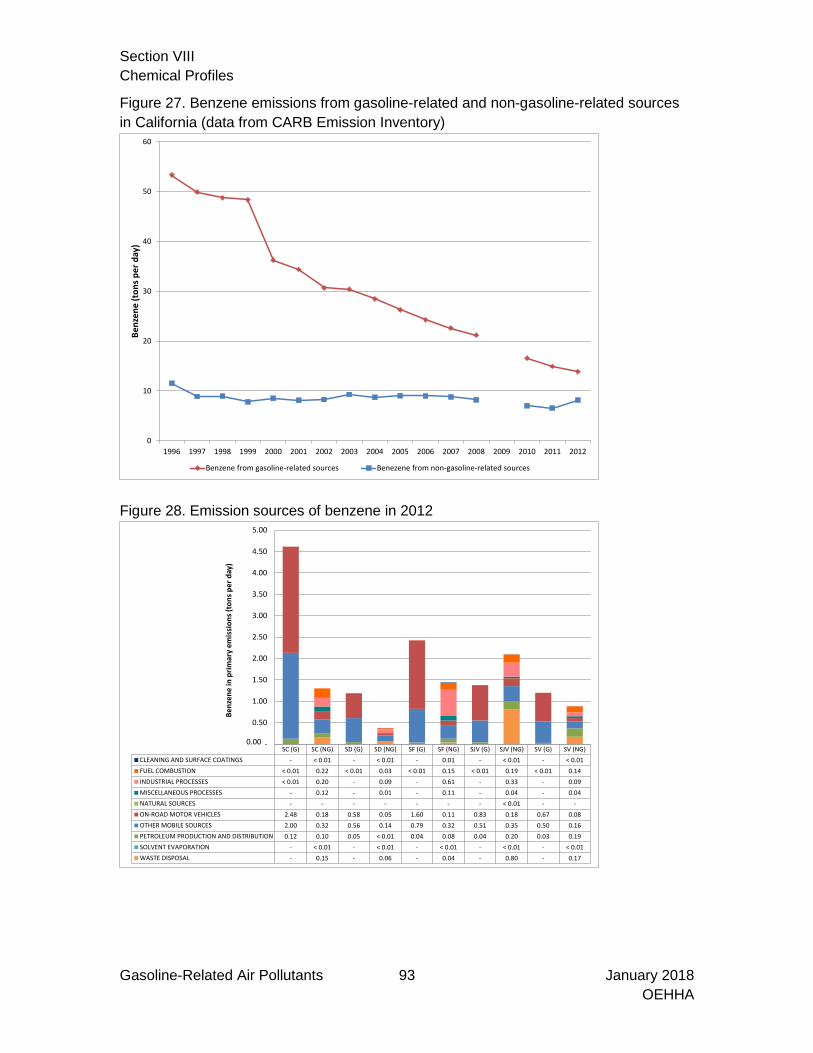
Section VIII Chemical Profiles
Gasoline-Related Air Pollutants 93 January 2018 OEHHA
Figure 27. Benzene emissions from gasoline-related and non-gasoline-related sources in California (data from CARB Emission Inventory)
Figure 28. Emission sources of benzene in 2012
0
10
20
30
40
50
60
1996 1997 1998 1999 2000 2001 2002 2003 2004 2005 2006 2007 2008 2009 2010 2011 2012
Benz
ene
(ton
s per
day
)
Benzene from gasoline-related sources Benezene from non-gasoline-related sources
SC (G) SC (NG) SD (G) SD (NG) SF (G) SF (NG) SJV (G) SJV (NG) SV (G) SV (NG)CLEANING AND SURFACE COATINGS - < 0.01 - < 0.01 - 0.01 - < 0.01 - < 0.01FUEL COMBUSTION < 0.01 0.22 < 0.01 0.03 < 0.01 0.15 < 0.01 0.19 < 0.01 0.14INDUSTRIAL PROCESSES < 0.01 0.20 - 0.09 - 0.61 - 0.33 - 0.09MISCELLANEOUS PROCESSES - 0.12 - 0.01 - 0.11 - 0.04 - 0.04NATURAL SOURCES - - - - - - - < 0.01 - -ON-ROAD MOTOR VEHICLES 2.48 0.18 0.58 0.05 1.60 0.11 0.83 0.18 0.67 0.08OTHER MOBILE SOURCES 2.00 0.32 0.56 0.14 0.79 0.32 0.51 0.35 0.50 0.16PETROLEUM PRODUCTION AND DISTRIBUTION 0.12 0.10 0.05 < 0.01 0.04 0.08 0.04 0.20 0.03 0.19SOLVENT EVAPORATION - < 0.01 - < 0.01 - < 0.01 - < 0.01 - < 0.01WASTE DISPOSAL - 0.15 - 0.06 - 0.04 - 0.80 - 0.17
-
0.50
1.00
1.50
2.00
2.50
3.00
3.50
4.00
4.50
5.00
Benz
ene
in p
rimar
y em
issi
ons (
tons
per
day
)
0.00

Section VIII Chemical Profiles
Gasoline-Related Air Pollutants 94 January 2018 OEHHA
Table 13. Benzene gasoline-attributable fractions
Year South
Coast Air Basin
San Diego
Air Basin
San Francisco Bay Area Air Basin
San Joaquin Valley
Air Basin
Sacramento Valley Air
Basin State
1996 81% 92% 84% 70% 86% 82% 1997 89% 90% 83% 70% 85% 85% 1998 89% 90% 83% 70% 85% 84% 1999 89% 90% 84% 79% 86% 86% 2000 84% 86% 80% 67% 83% 81% 2001 81% 86% 81% 72% 80% 81% 2002 84% 83% 78% 65% 77% 79% 2003 83% 83% 78% 62% 75% 77% 2004 83% 82% 76% 60% 74% 77% 2005 82% 80% 76% 53% 72% 74% 2006 82% 80% 74% 50% 70% 73% 2007 80% 79% 73% 50% 70% 72% 2008 78% 79% 72% 56% 70% 72% 2009 -- -- -- -- -- -- 2010 78% 79% 68% 54% 66% 70% 2011 80% 77% 65% 56% 63% 69% 2012 78% 76% 63% 40% 58% 63%
Note: Mobile source emissions were unavailable for 2009. Figure 29. Benzene gasoline-attributable fractions
0%
10%
20%
30%
40%
50%
60%
70%
80%
90%
100%
1996 1997 1998 1999 2000 2001 2002 2003 2004 2005 2006 2007 2008 2009 2010 2011 2012
Benz
ene
gaso
line-
attr
ibut
able
frac
tions
South Coast Air Basin San Diego Air Basin San Francisco Bay Area Air Basin
San Joaquin Valley Air Basin Sacramento Valley Air Basin State

Section VIII Chemical Profiles
Gasoline-Related Air Pollutants 95 January 2018 OEHHA
Table 14. Benzene population-weighted annual average ambient air concentrations (ppbv) Year South Coast
Air Basin San Diego Air Basin
San Francisco Bay Area Air Basin
San Joaquin Valley Air Basin
Sacramento Valley Air Basin
State
1996 1.3 0.89 0.77 0.65 0.60 0.99 1997 1.2 0.88 0.72 0.62 0.58 0.92 1998 1.2 0.87 0.78 0.70 0.58 0.94 1999 1.1 1.0 0.70 0.64 0.58 0.89 2000 0.96 0.83 0.61 0.60 0.47 0.76 2001 0.80 0.70 0.48 0.49 0.38 0.63 2002 0.73 0.67 0.48 0.49 0.45 0.60 2003 0.69 0.63 0.47 0.44 0.45 0.57 2004 0.57 0.55 0.41 0.36 0.39 0.48 2005 0.50 0.62 0.36 0.36 0.36 0.44 2006 0.46 0.54 0.34 0.36 0.37 0.41 2007 0.41 0.46 0.30 0.32 0.33 0.37 2008 0.38 0.43 0.25 0.29 0.34 0.33 2009 0.34 0.38 0.24 0.27 0.30 0.31 2010 0.36 0.38 0.25 0.25 0.27 0.31 2011 0.33 0.35 0.29 0.27 0.29 0.31 2012 0.33 0.35 0.28 0.27 0.27 0.31 2013 0.30 0.30 0.28 0.26 0.27 0.28 2014 0.27 0.28 0.25 0.26 0.22 0.26
Note: Non-detects were replaced by half the limit of detection.
Table 15. Benzene gasoline-attributable concentrations (ppbv) Year South Coast
Air Basin San Diego Air Basin
San Francisco Bay Area Air Basin
San Joaquin Valley Air Basin
Sacramento Valley Air Basin
State
1996 1.1 0.81 0.65 0.45 0.51 0.81 1997 1.1 0.79 0.60 0.44 0.49 0.78 1998 1.1 0.78 0.64 0.49 0.49 0.79 1999 1.00 0.92 0.59 0.50 0.50 0.77 2000 0.81 0.71 0.49 0.40 0.40 0.62 2001 0.65 0.60 0.39 0.35 0.30 0.51 2002 0.61 0.56 0.38 0.32 0.35 0.47 2003 0.57 0.52 0.37 0.28 0.34 0.43 2004 0.48 0.45 0.31 0.22 0.29 0.37 2005 0.41 0.49 0.27 0.19 0.26 0.33 2006 0.38 0.43 0.25 0.18 0.26 0.30 2007 0.33 0.36 0.22 0.16 0.23 0.26 2008 0.29 0.34 0.18 0.16 0.23 0.24 2009 0.26 0.30 0.17 0.15 0.21 0.22 2010 0.28 0.30 0.17 0.13 0.18 0.22 2011 0.26 0.27 0.19 0.15 0.18 0.22 2012 0.26 0.27 0.17 0.11 0.16 0.19 2013 0.23 0.22 0.17 0.10 0.15 0.18 2014 0.21 0.21 0.16 0.10 0.13 0.17
Note: The 2009 gasoline-attributable concentrations were calculated with the 2008 gasoline-attributable fractions and the 2013 and 2014 gasoline-attributable concentrations were calculated with the 2012 gasoline-attributable fractions.

Section VIII Chemical Profiles
Gasoline-Related Air Pollutants 96 January 2018 OEHHA
Figure 30. Population-weighted annual average ambient air concentration of benzene in the South Coast Air Basin compared to California Toxic Monitoring Network data23
Figure 31. Population-weighted annual average ambient air concentration of benzene in the South Coast Air Basin compared to data from PAMS data23
23 The first quartile, median and third quartile are plotted for sites/years with ≥10 months of data.
0
0.5
1
1.5
2
2.5
3
1996 1998 2000 2002 2004 2006 2008 2010 2012 2014
Benz
ene
(ppb
v)
Fontana-Arrow Highway North Long Beach
Azusa Upland
Burbank-W Palm Avenue Riverside-Rubidoux
Los Angeles-North Main Street Population_weighted annual average ambient air concentration
0
0.5
1
1.5
2
2.5
1996 1998 2000 2002 2004 2006 2008 2010 2012 2014
Benz
ene
(ppb
v)
Hawthorne Pico Rivera
Azusa Upland
Burbank-W Palm Avenue Riverside-Rubidoux
Los Angeles-North Main Street Banning Airport
Santa Clarita Los Angeles-Westchester Parkway
Pico Rivera-4144 San Gabriel Population_weighted annual average ambient air concentration

Section VIII Chemical Profiles
Gasoline-Related Air Pollutants 97 January 2018 OEHHA
Figure 32. South Coast population-weighted annual average ambient air concentration and gasoline-attributable concentration of benzene
0.0
0.2
0.4
0.6
0.8
1.0
1.2
1.4
1996 1997 1998 1999 2000 2001 2002 2003 2004 2005 2006 2007 2008 2009 2010 2011 2012 2013 2014
Benz
ene
(ppb
v)
Population-weighted annual average ambient air concentrationGasoline-attributable concentration

Section VIII Chemical Profiles
Gasoline-Related Air Pollutants 98 January 2018 OEHHA
1,3-Butadiene: Exposure and Screening Risk Assessment Results
1,3-Butadiene is a carcinogen and had the 45th highest primary emissions from gasoline-related sources in 2012 among all gasoline-related VOCs. Figure 33 shows that statewide emissions of 1,3-butadiene from gasoline-related sources declined between 1996 and 2012. Figure 34 shows the emission sources of 1,3-butadiene. Statewide, in 2012, 47% of 1,3-butadiene came from gasoline-related sources, including cars, trucks, motorcycles, off-road equipment and recreational boats. Aircraft and plastics manufacturing were non-gasoline-related sources of 1,3-butadiene. Table 16 and Figure 35 show the gasoline-attributable fractions of 1,3-butadiene. The gasoline-attributable fractions were higher in the South Coast, San Diego and San Francisco Bay Area Air Basins. In the San Joaquin Valley and Sacramento Valley Air Basins, wildfires and controlled burning (agricultural burning and forest management) contributed to 1,3-butadiene emissions and caused the gasoline-attributable fractions to be lower in these two basins. In the Emission Inventory, estimated natural source emissions were allowed to vary more prior to 2002 than afterwards. Since natural sources, such as wildfires, were significant 1,3-butadiene sources, 1,3-butadiene emission tonnage fluctuated during these earlier years also and affected the gasoline-attributable fractions. In the San Francisco Bay Area Air Basin, the estimated emissions of 1,3-butadiene from natural sources dropped in 2002 and subsequent years, which caused the gasoline-attributable fractions to increase. Between 2004 and 2012, the gasoline-attributable fractions varied by air basin primarily because of differences in 1,3-butadiene emissions from natural sources. The ambient air data used to calculate the population-weighted annual average ambient air concentrations came from the California Toxic Monitoring Network and were supplemented with modeled values at additional locations. A detailed description of the model is in Appendix D. The model was based on data24 from 1996-2014. By supplementing measured values with modeled values, we produced more robust estimates of population-weighted averages. The five most populated air basins (South Coast, San Diego, San Francisco Bay Area, San Joaquin Valley and Sacramento Valley Air Basins) had between two and six monitoring stations active annually between 1996 and 2014. The South Coast Air Basin had the most monitoring stations with five to six stations collecting data at any time. Population-weighted averages were calculated for the South Coast, San Diego, San Francisco Bay Area, San Joaquin Valley and Sacramento Valley Air Basins and
24 The 1,3-butadiene data from California Toxic Monitoring Network from 1996-1999 were adjusted by CARB to make earlier measurements consistent with an improved measurement technique that was used in later years (ftp://ftp.arb.ca.gov/aqd/aqdcd/web2011/BzButAdj.pdf).

Section VIII Chemical Profiles
Gasoline-Related Air Pollutants 99 January 2018 OEHHA
statewide (see Table 17). Half the limit of detection was substituted for non-detects. Figure 36 compares the population-weighted annual average ambient air concentrations of 1,3-butadiene in the South Coast Air Basin to actual ambient air measurements from monitoring sites within the basin. Table 18 tabulates the gasoline-attributable population-weighted annual average ambient air concentrations (referred to as gasoline-attributable concentrations) for all air basins. Figure 37 shows that the gasoline-attributable concentration of 1,3-butadiene in the South Coast Air Basin declined by 89% between 1996 and 2014. The number of non-detects in the California Toxic Monitoring Network data increased from 11% in 2000 to 63% in 2014. The population-weighted average was calculated with half the limit of detection substituted for non-detects. For comparison, Table 19 contains population-weighted annual average concentrations of 1,3-butadiene calculated with the limit of detection substituted for non-detects. In 2014, the statewide population-weighted annual average was 25% higher (0.070 versus 0.056 ppbv) when the limit of detection was substituted for non-detects than when half the limit of detection was substituted. The discrepancy was lower in previous years. Cancer risks and hazard quotients for non-cancer health effects were calculated based on gasoline-attributable ambient air concentrations (see Appendix G for details). The cancer risk for 1,3-butadiene in the South Coast Air Basin declined from 4.4x10⁻⁴ in 1996 to 3.6 x10⁻⁵ in 2014, corresponding to a reduction of about 400 cancer cases per 1 million people. The statewide cancer risk for 1,3-butadiene declined from 1.8 x10⁻⁴ in 1996 to 1.9 x10⁻⁵ in 2014, or a reduction of 160 cancer cases per 1 million people. The gasoline-attributable hazard quotient for 1,3-butadiene, based on reproductive toxicity, declined from 0.33 in 1996 to 0.027 in the South Coast Air Basin in 2014. The statewide gasoline-attributable hazard quotient declined from 0.14 in 1996 to 0.015 in 2014.

Section VIII Chemical Profiles
Gasoline-Related Air Pollutants 100 January 2018 OEHHA
Figure 33. 1,3-Butadiene emissions from gasoline-related and non-gasoline-related sources in California (data from CARB Emission Inventory)
Figure 34. Emission sources of 1,3-butadiene in 2012
-
2
4
6
8
10
12
14
16
18
1996 1997 1998 1999 2000 2001 2002 2003 2004 2005 2006 2007 2008 2009 2010 2011 2012
1,3-
Buta
dien
e (t
ons
per d
ay)
1,3-Butadiene from non-gasoline-related sources 1,3-Butadiene from gasoline-related sources
Apparent fluctuations in 1996-2002 and 2012 non-gasoline-related 1,3-butadiene emissions are due to variations in estimated natural source emissions. The increase between 2008 and 2010 is due to a change in estimated 1,3-butadiene emissions from plastic product manufacturing.
SC (G) SC (NG) SD (G) SD (NG) SF (G) SF (NG) SJV (G) SJV (NG) SV (G) SV (NG)CLEANING AND SURFACE COATINGS - - - - - < 0.01 - - - -FUEL COMBUSTION < 0.01 < 0.01 < 0.01 < 0.01 < 0.01 < 0.01 < 0.01 < 0.01 < 0.01 < 0.01INDUSTRIAL PROCESSES - 0.56 - 0.13 - 0.14 - 0.22 - 0.34MISCELLANEOUS PROCESSES - 0.02 - < 0.01 - 0.01 - 0.05 - 0.06NATURAL SOURCES - 0.35 - 0.28 - 0.04 - 0.51 - 0.62ON-ROAD MOTOR VEHICLES 0.48 0.02 0.12 < 0.01 0.32 0.01 0.17 0.02 0.14 < 0.01OTHER MOBILE SOURCES 0.45 0.09 0.13 0.07 0.18 0.16 0.11 0.11 0.11 0.06PETROLEUM PRODUCTION AND DISTRIBUTION - < 0.01 - - - < 0.01 - < 0.01 - < 0.01SOLVENT EVAPORATION - - - - - - - - - -WASTE DISPOSAL - - - - - - - < 0.01 - < 0.01
-
0.20
0.40
0.60
0.80
1.00
1.20
1,3-
Buta
dien
e in
prim
ary
emis
sion
s (to
ns p
er d
ay)
Wildfires
Plastics
0.00

Section VIII Chemical Profiles
Gasoline-Related Air Pollutants 101 January 2018 OEHHA
Table 16. 1,3-Butadiene gasoline-attributable fractions
Year
South Coast
Air Basin
San Diego
Air Basin
San Francisco Bay Area Air Basin
San Joaquin Valley
Air Basin
Sacramento Valley Air
Basin State
1996 85% 84% 25% 63% 72% 45% 1997 84% 88% 24% 72% 70% 49% 1998 85% 87% 24% 76% 69% 50% 1999 84% 83% 23% 80% 27% 38% 2000 79% 81% 20% 53% 65% 39% 2001 78% 79% 20% 68% 39% 37% 2002 71% 62% 79% 18% 62% 51% 2003 64% 34% 79% 37% 56% 51% 2004 74% 66% 76% 28% 43% 51% 2005 72% 64% 75% 32% 41% 51% 2006 70% 63% 74% 33% 39% 50% 2007 68% 61% 72% 32% 39% 48% 2008 67% 60% 71% 32% 38% 47% 2009 -- -- -- -- -- -- 2010 54% 45% 62% 24% 24% 38% 2011 51% 42% 60% 22% 23% 35% 2012 47% 33% 58% 24% 19% 26%
Note: Mobile source emissions were not available for 2009. Figure 35. 1,3-Butadiene gasoline-attributable fractions
Note: Gasoline-attributable fractions fluctuate prior to 2002 because natural source emissions were estimated differently (see Figure 33).
0%
10%
20%
30%
40%
50%
60%
70%
80%
90%
100%
1996 1997 1998 1999 2000 2001 2002 2003 2004 2005 2006 2007 2008 2009 2010 2011 2012
1,3-
Buta
dien
e ga
solin
e-at
trib
utab
le fr
actio
ns
South Coast Air Basin San Diego Air Basin San Francisco Bay Area Air Basin
San Joaquin Valley Air Basin Sacramento Valley Air Basin State

Section VIII Chemical Profiles
Gasoline-Related Air Pollutants 102 January 2018 OEHHA
Table 17. Population-weighted annual average ambient air concentrations of 1,3-butadiene (ppbv)
Year South Coast Air Basin
San Diego Air Basin
San Francisco Bay Area Air Basin
San Joaquin Valley Air Basin
Sacramento Valley Air Basin State
1996 0.39 0.27 0.24 0.20 0.18 0.30 1997 0.35 0.25 0.22 0.18 0.16 0.27 1998 0.35 0.25 0.23 0.21 0.17 0.28 1999 0.31 0.27 0.19 0.16 0.14 0.24 2000 0.26 0.22 0.16 0.15 0.12 0.20 2001 0.23 0.20 0.14 0.14 0.11 0.18 2002 0.20 0.18 0.13 0.13 0.12 0.16 2003 0.15 0.13 0.096 0.088 0.094 0.12 2004 0.14 0.13 0.096 0.079 0.087 0.11 2005 0.11 0.14 0.082 0.079 0.078 0.099 2006 0.10 0.12 0.072 0.073 0.078 0.090 2007 0.10 0.11 0.068 0.070 0.074 0.087 2008 0.085 0.097 0.052 0.059 0.071 0.073 2009 0.079 0.093 0.055 0.062 0.068 0.071 2010 0.078 0.082 0.054 0.047 0.054 0.067 2011 0.074 0.078 0.067 0.058 0.063 0.069 2012 0.059 0.066 0.048 0.044 0.046 0.054 2013 0.065 0.067 0.063 0.059 0.057 0.062 2014 0.057 0.059 0.054 0.057 0.045 0.056
Note: half the limit of detection substituted for non-detects
Table 18. Gasoline-attributable concentrations of 1,3-butadiene (ppbv) Year South Coast
Air Basin San Diego Air Basin
San Francisco Bay Area Air Basin
San Joaquin Valley Air Basin
Sacramento Valley Air Basin State
1996 0.33 0.23 0.061 0.13 0.13 0.14 1997 0.30 0.22 0.052 0.13 0.11 0.13 1998 0.30 0.22 0.055 0.16 0.12 0.14 1999 0.26 0.23 0.043 0.13 0.039 0.092 2000 0.20 0.17 0.033 0.080 0.077 0.078 2001 0.18 0.16 0.029 0.094 0.041 0.068 2002 0.14 0.11 0.10 0.024 0.072 0.083 2003 0.095 0.046 0.076 0.033 0.052 0.061 2004 0.10 0.087 0.073 0.022 0.038 0.059 2005 0.082 0.091 0.061 0.025 0.032 0.050 2006 0.072 0.076 0.053 0.024 0.030 0.045 2007 0.069 0.066 0.049 0.023 0.029 0.042 2008 0.057 0.058 0.037 0.019 0.027 0.034 2009 0.053 0.056 0.039 0.020 0.026 0.034 2010 0.043 0.037 0.033 0.011 0.013 0.025 2011 0.037 0.033 0.040 0.013 0.014 0.024 2012 0.028 0.022 0.028 0.010 0.0086 0.014 2013 0.031 0.022 0.037 0.014 0.0107 0.016 2014 0.027 0.020 0.031 0.013 0.0084 0.015
Note: The 2009 gasoline-attributable concentrations were calculated with the 2008 gasoline-attributable fractions and the 2013 and 2014 gasoline-attributable concentrations were calculated with the 2012 gasoline-attributable fractions.

Section VIII Chemical Profiles
Gasoline-Related Air Pollutants 103 January 2018 OEHHA
Figure 36. Population-weighted annual average ambient air concentration of 1,3-butadiene in the South Coast Air Basin
Note: Vertical bars show the first quartile, median and third quartile of daily average concentrations for sites with ≥10 months of data. Figure 37. South Coast population-weighted annual average ambient air concentration and gasoline-attributable concentration of 1,3-butadiene
0
0.1
0.2
0.3
0.4
0.5
0.6
0.7
0.8
1996 1998 2000 2002 2004 2006 2008 2010 2012 2014
1,3-
Buta
dien
e (p
pbv)
Fontana-Arrow Highway North Long Beach
Azusa Upland
Burbank-W Palm Avenue Riverside-Rubidoux
Los Angeles-North Main Street Population_weighted annual average ambient air concentration
0.00
0.05
0.10
0.15
0.20
0.25
0.30
0.35
0.40
0.45
1996 1997 1998 1999 2000 2001 2002 2003 2004 2005 2006 2007 2008 2009 2010 2011 2012 2013 2014
1,3-
Buta
dien
e (p
pbv)
Population-weighted annual average ambient air concentration Gasoline attributable concentration

Section VIII Chemical Profiles
Gasoline-Related Air Pollutants 104 January 2018 OEHHA
Table 19. Population-weighted average concentrations of 1,3-butadiene with limit of detection substituted for non-detects (ppbv)
Year
South Coast
Air Basin
San Diego
Air Basin
San Francisco Bay Area Air Basin
San Joaquin Valley
Air Basin
Sacramento Valley Air
Basin State
1996 0.39 0.27 0.24 0.20 0.18 0.30 1997 0.35 0.25 0.22 0.18 0.17 0.27 1998 0.35 0.25 0.23 0.21 0.17 0.27 1999 0.30 0.27 0.19 0.17 0.15 0.24 2000 0.26 0.22 0.16 0.16 0.12 0.20 2001 0.23 0.20 0.15 0.14 0.11 0.19 2002 0.21 0.18 0.13 0.14 0.12 0.17 2003 0.15 0.14 0.10 0.10 0.10 0.13 2004 0.15 0.14 0.11 0.088 0.10 0.12 2005 0.12 0.15 0.092 0.088 0.089 0.11 2006 0.11 0.13 0.082 0.083 0.088 0.10 2007 0.11 0.12 0.078 0.081 0.087 0.10 2008 0.094 0.11 0.064 0.070 0.083 0.083 2009 0.087 0.10 0.065 0.072 0.080 0.081 2010 0.087 0.093 0.064 0.058 0.066 0.077 2011 0.082 0.089 0.077 0.068 0.074 0.079 2012 0.072 0.080 0.063 0.059 0.062 0.068 2013 0.076 0.080 0.076 0.072 0.071 0.074 2014 0.071 0.074 0.068 0.072 0.060 0.070

Section VIII Chemical Profiles
Gasoline-Related Air Pollutants 105 January 2018 OEHHA
Cumene: Exposure and Screening Risk Assessment Results
Cumene (isopropylbenzene) is a carcinogen and had the 140th highest primary emissions from gasoline-related sources in 2012 among all gasoline-related VOCs. Estimated emissions of cumene have declined between 1996 and 2012 (see Figure 38). Figure 39 displays the breakdown of gasoline-related and non-gasoline-related sources for cumene in each air basin. Between 1996 and 2012, gasoline-attributable fractions ranged from 38% to 57% across the air basins. In 2012, a little less than half of ambient cumene came from gasoline-related sources statewide (see Table 20 and Figure 40). Population-weighted annual average concentrations were calculated for the South Coast Air Basin. The ambient air data used to calculate the population-weighted annual average ambient air concentrations came from PAMS and was supplemented with modeled values at additional locations (see Table 21). Figure 41 shows the population-weighted annual average concentration along with measured data from South Coast Air Basin monitoring sites. Figure 42 shows that the gasoline-attributable concentration of cumene declined by 80% between 1996 and 2014 in the South Coast Air Basin. A cancer risk assessment was not carried out for cumene because a cancer potency value has not been developed. US EPA (2007) developed a chronic reference concentration (RfC) of 0.4 mg/m3 (80 ppb) for cumene, with the endocrine and urinary systems as targets for toxicity. Hazard quotients based on gasoline-attributable concentrations in the South Coast Air Basin were all well below 1, decreasing from 6.3x10⁻⁴ in 1996 to 1.3x10⁻⁴ in 2014. There were inadequate data to calculate a statewide hazard quotient for cumene.
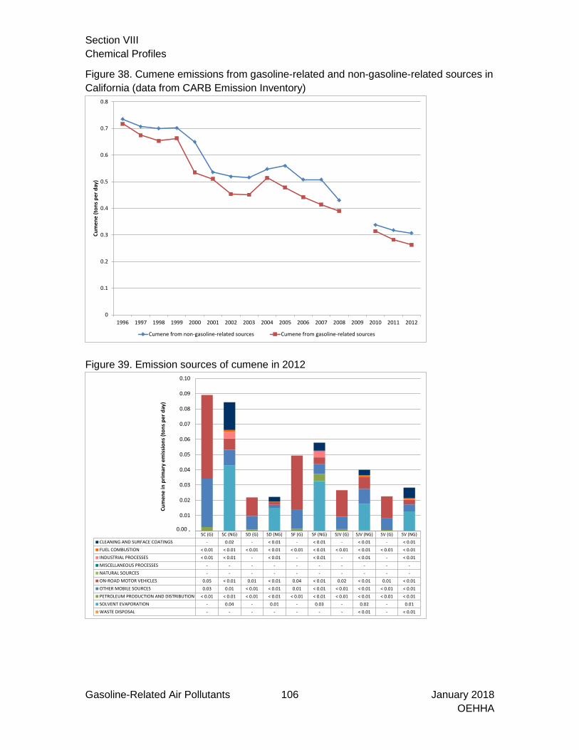
Section VIII Chemical Profiles
Gasoline-Related Air Pollutants 106 January 2018 OEHHA
Figure 38. Cumene emissions from gasoline-related and non-gasoline-related sources in California (data from CARB Emission Inventory)
Figure 39. Emission sources of cumene in 2012
0
0.1
0.2
0.3
0.4
0.5
0.6
0.7
0.8
1996 1997 1998 1999 2000 2001 2002 2003 2004 2005 2006 2007 2008 2009 2010 2011 2012
Cum
ene
(ton
s per
day
)
Cumene from non-gasoline-related sources Cumene from gasoline-related sources
SC (G) SC (NG) SD (G) SD (NG) SF (G) SF (NG) SJV (G) SJV (NG) SV (G) SV (NG)CLEANING AND SURFACE COATINGS - 0.02 - < 0.01 - < 0.01 - < 0.01 - < 0.01FUEL COMBUSTION < 0.01 < 0.01 < 0.01 < 0.01 < 0.01 < 0.01 < 0.01 < 0.01 < 0.01 < 0.01INDUSTRIAL PROCESSES < 0.01 < 0.01 - < 0.01 - < 0.01 - < 0.01 - < 0.01MISCELLANEOUS PROCESSES - - - - - - - - - -NATURAL SOURCES - - - - - - - - - -ON-ROAD MOTOR VEHICLES 0.05 < 0.01 0.01 < 0.01 0.04 < 0.01 0.02 < 0.01 0.01 < 0.01OTHER MOBILE SOURCES 0.03 0.01 < 0.01 < 0.01 0.01 < 0.01 < 0.01 < 0.01 < 0.01 < 0.01PETROLEUM PRODUCTION AND DISTRIBUTION < 0.01 < 0.01 < 0.01 < 0.01 < 0.01 < 0.01 < 0.01 < 0.01 < 0.01 < 0.01SOLVENT EVAPORATION - 0.04 - 0.01 - 0.03 - 0.02 - 0.01WASTE DISPOSAL - - - - - - - < 0.01 - < 0.01
-
0.01
0.02
0.03
0.04
0.05
0.06
0.07
0.08
0.09
0.10
Cum
ene
in p
rimar
y em
issi
ons (
tons
per
day
)
0.00

Section VIII Chemical Profiles
Gasoline-Related Air Pollutants 107 January 2018 OEHHA
Table 20. Cumene gasoline-attributable fractions
Year South
Coast Air Basin
San Diego Air Basin
San Francisco Bay Area Air Basin
San Joaquin
Valley Air Basin
Sacramento Valley Air
Basin State
1996 45% 51% 46% 48% 57% 49% 1997 45% 57% 44% 47% 55% 49% 1998 43% 57% 44% 46% 56% 48% 1999 43% 57% 48% 45% 55% 49% 2000 40% 57% 41% 41% 53% 45% 2001 49% 57% 40% 43% 55% 49% 2002 45% 52% 45% 39% 49% 47% 2003 46% 54% 43% 41% 49% 47% 2004 48% 54% 44% 44% 52% 48% 2005 46% 53% 39% 42% 50% 46% 2006 48% 53% 41% 40% 48% 47% 2007 46% 50% 38% 39% 47% 45% 2008 47% 54% 43% 41% 50% 48% 2009 -- -- -- -- -- -- 2010 51% 54% 48% 40% 47% 48% 2011 50% 51% 47% 41% 46% 47% 2012 51% 50% 46% 40% 44% 46%
Note: Mobile source emissions were not available for 2009.
Figure 40. Cumene gasoline-attributable fractions
0%
10%
20%
30%
40%
50%
60%
70%
80%
90%
100%
1996 1997 1998 1999 2000 2001 2002 2003 2004 2005 2006 2007 2008 2009 2010 2011 2012
Cum
ene
gaso
line-
attr
ibut
able
frac
tions
South Coast Air Basin San Diego Air Basin San Francisco Bay Area Air Basin
San Joaquin Valley Air Basin Sacramento Valley Air Basin State

Section VIII Chemical Profiles
Gasoline-Related Air Pollutants 108 January 2018 OEHHA
Table 21. Cumene results for the South Coast Air Basin
Year
Population-weighted average concentration of cumene (ppbv)
Gasoline-attributable
fraction
Gasoline-attributable
concentration (ppbv)
1996 0.11 45% 0.050 1997 0.10 45% 0.045 1998 0.094 43% 0.041 1999 0.093 43% 0.040 2000 0.088 40% 0.035 2001 0.067 49% 0.033 2002 0.064 45% 0.029 2003 0.058 46% 0.027 2004 0.050 48% 0.024 2005 0.045 46% 0.021 2006 0.043 48% 0.020 2007 0.039 46% 0.018 2008 0.032 47% 0.015 2009 0.030 47% 0.014 2010 0.027 51% 0.014 2011 0.024 50% 0.012 2012 0.023 51% 0.012 2013 0.022 51% 0.011 2014 0.020 51% 0.010
Note: The 2009 gasoline-attributable concentrations were calculated with the 2008 gasoline-attributable fractions. The 2012 - 2014 population-weighted averages were based completely on modeled values (see Figure 41). The 2013 and 2014 gasoline-attributable concentrations were calculated with the 2012 gasoline-attributable fractions.

Section VIII Chemical Profiles
Gasoline-Related Air Pollutants 109 January 2018 OEHHA
Figure 41. Population-weighted annual average ambient air concentration of cumene in the South Coast Air Basin
Note: Vertical bars show the quartiles for sites with ≥10 months of data.
Figure 42. South Coast population-weighted annual average ambient air concentration and gasoline-attributable concentration of cumene
0
0.05
0.1
0.15
0.2
0.25
0.3
0.35
0.4
1996 1998 2000 2002 2004 2006 2008 2010 2012 2014
Cum
ene
(ppb
v)
Hawthorne Pico RiveraAzusa UplandBurbank-W Palm Avenue Riverside-RubidouxLos Angeles-North Main Street Banning AirportSanta Clarita Los Angeles-Westchester ParkwayPico Rivera-4144 San Gabriel Population_weighted annual average ambient air concentration
0.00
0.02
0.04
0.06
0.08
0.10
0.12
1996 1997 1998 1999 2000 2001 2002 2003 2004 2005 2006 2007 2008 2009 2010 2011 2012 2013 2014
Cum
ene
(ppb
v)
Population-weighted annual average ambient air concentration Gasoline-attributable concentration

Section VIII Chemical Profiles
Gasoline-Related Air Pollutants 110 January 2018 OEHHA
Ethanol: Exposure Assessment Results
Ethanol had the 2nd highest primary emissions from gasoline-related sources in 2012 among all gasoline-related VOCs. Gasoline-attributable fractions of ethanol increased in 2004 due to its use as a replacement for the oxygenate MTBE. In 2004, California gasoline contained about 5.7% added ethanol by volume but that percentage increased over time to the maximum allowed percentage of 10%. Figure 43 shows that the estimated statewide daily emissions of ethanol from gasoline-related sources increased from 3 tons in 2003 to 62 tons in 2004. Fifty-four percent of this increase came from on-road mobile sources, 36% came from other mobile sources, and 10% came from petroleum production and distribution. Figure 44 shows the components of the driving cycle of on-road mobile sources that contributed to the increase, with 35% coming from changes in emissions during engine starts and hot stabilized exhaust and the remaining 65% coming from changes in evaporative emissions. In 2012, less ethanol was emitted from gasoline-related sources than from non-gasoline-related sources, such as livestock and consumer products (see Figure 45). Gasoline-attributable fractions are shown in Table 22 and Figure 46. The gasoline-attributable fraction for ethanol in the San Joaquin Valley Air Basin is substantially lower than in other basins because of the extensive emissions from livestock, consumer products and industrial processes (e.g., winemaking). A number of studies have researched changes over time in pollutant emissions associated with the use of reformulated gasoline in California (see for example, Harley et al, 2006; Kirchstetter et al., 1999), including the impact of adding ethanol. In a study of seven vehicles, Karavalakis et al. (2011) found that NOx emissions increased with increasing ethanol content in gasoline burned by older vehicles but was roughly constant in newer vehicles. These authors also found that acetaldehyde emissions increased with increasing ethanol content in two vehicles (one older and one newer), as predicted in the CARB, OEHHA and SWRCB (1999) study. Other VOC emissions either declined or remained roughly constant with increasing ethanol content. In the CARB, OEHHA and SWRCB (1999) study of the use of ethanol as an oxygenate in California gasoline, ambient air concentrations of ethanol under different fuel formulation scenarios were estimated for the South Coast Air Basin (see Table 4.8 on page 36 of volume 3 of that report). Based on the use of fuel, which was 10% by volume (3.5% oxygen by weight), the estimated maximum daily average air concentration was between 75 and 81 ppb and the estimated population-weighted annual average air concentration was 8.8 ppb. We looked for ambient air measurements of ethanol to compare with the predictions made in the CARB, OEHHA and SWRCB (1999) study. The measurements that were available came from sites in the San Francisco Bay Area Air Basin from 2012 to 2015 (see Table 23). When these measurements were made, California gasoline was 10%

Section VIII Chemical Profiles
Gasoline-Related Air Pollutants 111 January 2018 OEHHA
ethanol as in the study model. The measured maximum concentrations rarely exceeded the maximums predicted in the study for the South Coast Air Basin. The maximum daily average ethanol concentrations exceeded the maximum estimate of 75 ppb at 5 of 18 sites in 2012, 2 of 19 sites in 2013, 1 of 21 sites in 2014 and 0 of 19 sites in 2015. The population-weighted annual averages could be compared to the annual average predicted in the model. The population-weighted annual average ambient air concentrations of ethanol for the San Francisco Bay Area Air Basin were 20, 9.0, 8.0 and 7.9 ppb in 2012 to 2015. When two sites with large outliers were excluded from the dataset for this air basin, the population-weighted annual average ambient air concentrations of ethanol were 16, 8.0, 7.0 and 7.0 ppb between 2012 and 2015. These values are in the same range as the projected value of 8.8 ppb for 2003 in the South Coast Air Basin. Figure 43. Ethanol emissions from gasoline-related and non-gasoline-related sources in California (data from CARB Emission Inventory)
0
20
40
60
80
100
120
140
160
180
1996 1997 1998 1999 2000 2001 2002 2003 2004 2005 2006 2007 2008 2009 2010 2011 2012
Etha
nol (
tons
per
day
)
Ethanol from non-gasoline-related sources Ethanol from gasoline-related sources
Ethanol tonnage increased when gasoline changed
71% of the increase in ethanol emissions between 2008 and 2010 is due to an increase in estimated emissions from livestock husbandry and the bulk of the remaining increase is due to increased emissions from solvent evaporation.

Section VIII Chemical Profiles
Gasoline-Related Air Pollutants 112 January 2018 OEHHA
Figure 44. Components of the driving cycle of gasoline-related on-road mobile sources that contributed to the increase in ethanol emissions between 2003 and 2004.25
Figure 45. Emission sources of ethanol in 2012
25 “Resting loss” emissions occur during periods of constant or decreasing temperature. “Start” emissions occur in the first few minutes of engine operation. “Hot soak” emissions occur during the first hour after engine shutdown. “Diurnal” emissions occur during daytime heating of fuel delivery systems (Scott et al., 1999).
CATALYST EVAPORATIVE RUNNING LOSSES
27%
NON-CATALYST EVAPORATIVE RUNNING LOSSES
12%
CATALYST EVAPORATIVE RESTING LOSSES
5%NON-CATALYST EVAPORATIVE RESTING LOSSES
2%
CATALYST HOT SOAK
6%
NON-CATALYST HOT SOAK2%
CATALYST DIURNAL9%
NON-CATALYST DIURNAL2%
CATALYST STARTS16%
NON-CATALYST STARTS4%
CATALYST HOT STABILIZED EXHAUST
7%
NON-CATALYST HOT STABILIZED EXHAUST
8%
SC (G) SC (NG) SD (G) SD (NG) SF (G) SF (NG) SJV (G) SJV (NG) SV (G) SV (NG)CLEANING AND SURFACE COATINGS - 1.05 - 0.96 - 1.01 - 1.09 - 0.41FUEL COMBUSTION < 0.01 0.08 < 0.01 < 0.01 < 0.01 < 0.01 < 0.01 < 0.01 < 0.01 < 0.01INDUSTRIAL PROCESSES < 0.01 1.24 - 0.06 - 1.67 - 10.93 - 0.53MISCELLANEOUS PROCESSES - 0.60 - 0.32 - 0.80 - 39.35 - 2.66NATURAL SOURCES - - - - - - - - - -ON-ROAD MOTOR VEHICLES 5.83 < 0.01 1.22 < 0.01 3.45 < 0.01 1.79 < 0.01 1.41 < 0.01OTHER MOBILE SOURCES 6.03 < 0.01 1.60 < 0.01 2.38 < 0.01 1.61 < 0.01 1.43 < 0.01PETROLEUM PRODUCTION AND DISTRIBUTION 2.38 0.02 0.78 < 0.01 0.77 0.14 0.55 < 0.01 0.49 < 0.01SOLVENT EVAPORATION - 24.41 - 5.03 - 11.09 - 6.02 - 4.31WASTE DISPOSAL - 0.43 - 0.09 - 0.22 - 3.51 - 0.13
-
10.00
20.00
30.00
40.00
50.00
60.00
70.00
Etha
nol i
n pr
imar
y em
issi
ons (
tons
per
day
)
Consumer products
Winemaking
Livestock husbandry
0.00

Section VIII Chemical Profiles
Gasoline-Related Air Pollutants 113 January 2018 OEHHA
Table 22. Ethanol gasoline-attributable fractions
Year South
Coast Air Basin
San Diego
Air Basin
San Francisco Bay Area Air Basin
San Joaquin
Valley Air Basin
Sacramento Valley Air
Basin State
1996 2% 2% 2% 1% 3% 2% 1997 4% 4% 4% 1% 4% 3% 1998 3% 4% 4% 1% 4% 3% 1999 3% 4% 4% 1% 3% 3% 2000 3% 4% 4% 1% 3% 3% 2001 4% 4% 4% 1% 3% 3% 2002 4% 4% 4% 1% 3% 3% 2003 3% 3% 3% 1% 2% 2% 2004 46% 50% 45% 17% 46% 39% 2005 45% 49% 43% 16% 45% 38% 2006 43% 46% 40% 14% 43% 36% 2007 41% 47% 39% 14% 43% 35% 2008 40% 46% 38% 15% 42% 35% 2009 -- -- -- -- -- -- 2010 34% 39% 33% 5% 34% 22% 2011 35% 37% 32% 5% 34% 21% 2012 34% 36% 31% 6% 29% 22%
Note: Mobile source emissions were not available for 2009.
Figure 46. Ethanol gasoline-attributable fractions
0%
10%
20%
30%
40%
50%
60%
70%
80%
90%
100%
1996 1997 1998 1999 2000 2001 2002 2003 2004 2005 2006 2007 2008 2009 2010 2011 2012
Etha
nol g
asol
ine-
attr
ibut
able
frac
tions
South Coast Air Basin San Diego Air Basin San Francisco Bay Area Air Basin
San Joaquin Valley Air Basin Sacramento Valley Air Basin State

Section VIII Chemical Profiles
Gasoline-Related Air Pollutants 114 January 2018 OEHHA
Table 23. Ethanol ambient air measurements from San Francisco Bay Area Air Basin (ppbv)
County Name
Site Name Year N
Mea
n
Stan
dard
devi
atio
n
Min
imum
Fris
t qu
artil
e
Med
ian
Third
qu
artil
e
95th
pe
rcen
tile
Max
imum
Alameda
Fremont-Chapel Way
2008 19 17.1 19.8 5.1 6.1 9.8 16.5 90.0 90.0
Livermore-793 Rincon Avenue
2012 28 12.4 11.8 2.2 5.5 8.3 14.6 33.8 58.5 2013 31 7.3 6.9 1.1 2.5 5.0 8.0 22.5 31.1 2014 29 4.8 3.0 1.5 3.0 3.8 5.1 12.2 13.5 2015 24 5.7 7.8 0.9 2.3 3.5 6.5 11.9 40.0
Oakland-9925 International Blvd
2012 30 22.1 17.1 7.2 10.0 17.8 28.6 61.2 83.8 2013 31 9.7 7.5 3.2 5.1 8.6 11.7 32.7 35.4 2014 30 5.4 1.9 2.5 4.2 5.3 6.3 8.8 9.1 2015 25 5.4 3.1 1.8 3.3 4.3 6.6 10.4 14.5
Oakland-9925 International Blvd #11
2012 30 15.0 17.8 3.6 6.4 9.3 13.6 40.2 96.2 2013 31 8.8 15.3 1.1 2.7 4.5 8.9 38.8 82.3 2014 29 4.0 3.0 1.2 2.0 3.0 5.5 7.2 16.2 2015 25 3.4 3.2 0.6 1.2 1.9 4.2 9.2 14.1
Oakland-Laney College
2014 28 3.4 2.0 1.0 2.2 3.0 4.1 6.7 10.8 2015 25 3.1 2.0 0.9 1.7 2.4 5.0 6.2 7.9
Contra Costa
Bethel Island Road
2012 30 10.0 6.8 3.9 5.3 7.6 11.3 22.1 35.2 2013 22 4.0 3.0 1.4 1.8 3.4 4.6 9.4 14.1 2014 29 3.3 2.2 1.1 1.9 2.4 3.9 7.9 9.4 2015 25 4.2 3.4 0.7 1.6 3.0 5.5 11.6 12.6
Concord-2975 Treat Blvd
2012 30 9.5 8.4 2.4 4.6 5.7 13.9 28.3 38.8 2013 31 4.0 3.0 0.9 1.8 2.8 6.0 12.4 13.1 2014 30 2.6 1.4 0.1 1.8 2.2 3.1 5.6 7.0 2015 25 2.0 1.1 0.6 1.1 1.7 3.1 3.7 4.0
Crockett-Kendall Avenue
2012 29 4.9 5.4 0.1 1.7 3.3 5.4 13.3 26.3 2013 29 2.8 2.3 0.4 1.1 2.0 4.0 7.9 9.7 2014 30 1.7 2.4 0.5 0.8 1.1 1.5 4.5 13.3 2015 25 1.3 0.7 0.3 0.7 1.1 1.5 2.5 2.8
Martinez-Jones Street
2012 30 8.6 8.3 2.9 4.4 6.3 9.8 36.1 39.2 2013 30 4.2 3.2 0.8 1.8 3.1 5.5 11.4 14.1 2014 29 2.7 1.4 1.1 1.6 2.4 3.2 5.8 6.5 2015 25 2.2 1.4 0.6 1.0 1.7 3.7 4.2 4.9
Richmond-7th Street
2012 29 9.9 7.0 3.6 5.2 7.9 12.0 18.0 38.7 2013 30 5.9 5.0 0.9 2.3 4.1 7.7 18.1 19.1 2014 30 2.5 1.5 0.7 1.7 2.2 2.8 5.3 6.8 2015 24 2.1 1.7 0.3 0.8 1.4 3.1 5.1 7.3
San Pablo-Rumrill Blvd
2012 30 10.3 6.3 4.2 6.7 8.4 11.6 29.5 29.8
San Pablo-Rumrill Blvd
2013 31 4.9 3.1 0.9 2.7 4.0 6.7 9.4 16.2 2014 30 3.3 1.5 1.4 2.3 2.8 3.6 6.7 7.6 2015 24 2.7 1.1 1.2 1.8 2.4 3.5 4.4 5.4
Marin
Fort Cronkhite
2012 30 0.7 0.7 0.1 0.1 0.6 0.9 1.6 3.6 2013 29 0.3 0.3 0.1 0.1 0.3 0.4 0.8 1.5 2014 29 1.8 3.0 0.1 0.2 0.5 2.6 5.5 15.1 2015 25 1.7 0.5 1.1 1.3 1.7 2.0 2.8 3.0
San Rafael
2012 30 20.9 19.5 4.0 6.4 13.8 26.1 69.5 74.3 2013 30 7.6 12.1 1.5 2.9 4.7 6.6 37.5 61.9 2014 28 5.5 5.4 1.8 2.8 4.0 6.8 10.7 29.7 2015 24 3.6 1.7 1.1 2.1 3.4 5.0 6.2 7.2

Section VIII Chemical Profiles
Gasoline-Related Air Pollutants 115 January 2018 OEHHA
County Name
Site Name Year N
Mea
n
Stan
dard
devi
atio
n
Min
imum
Fris
t qu
artil
e
Med
ian
Third
qu
artil
e
95th
pe
rcen
tile
Max
imum
Napa Napa-Jefferson Avenue
2012 28 78.6 72.8 10.8 28.4 51.4 110.7 244.0 334.3 2013 28 37.1 51.4 9.3 15.7 21.7 36.0 166.0 253.3 2014 29 18.4 10.6 0.1 8.8 18.6 25.6 35.6 38.0 2015 24 13.1 9.6 0.3 6.1 12.7 18.7 32.1 33.2
San Francisco
San Francisco-Arkansas Street
2012 30 26.8 42.4 7.2 10.2 13.9 19.4 90.9 227.4 2013 33 10.5 11.1 2.6 3.7 7.2 12.7 36.4 57.7 2014 34 8.0 6.4 2.0 3.8 5.9 9.5 25.4 26.0 2015 27 6.5 4.9 1.6 3.2 5.2 7.2 16.6 22.8
San Mateo
Redwood City 2012 29 23.5 12.6 11.1 13.8 17.7 33.6 46.6 58.3 2013 30 9.7 6.6 2.5 5.2 8.8 12.8 27.6 29.9 2014 28 14.4 15.7 4.8 6.4 8.3 15.8 51.2 77.9 2015 24 10.8 5.5 3.8 6.8 9.4 12.0 20.1 25.7
Santa Clara
Cupertino-Monte Vista Park
2012 61 11.4 7.0 2.7 6.4 10.0 14.9 23.9 37.7 2013 59 4.0 2.6 1.0 2.4 3.6 5.0 10.0 17.1
San Jose-Jackson Street
2008 59 27.3 14.0 0.3 18.7 25.9 31.8 58.0 69.2 2009 52 15.9 13.4 4.5 8.6 11.9 16.9 51.1 70.6 2010 61 11.6 4.3 4.0 8.2 11.1 14.3 18.2 22.7 2011 60 12.3 5.7 3.7 8.1 11.7 16.1 22.9 25.9 2012 59 27.1 17.2 3.3 15.8 22.6 35.4 53.3 115.1 2013 60 12.0 10.8 2.3 5.9 9.3 15.1 23.8 61.6 2014 60 11.6 6.9 1.1 6.2 9.8 15.1 26.5 32.7 2015 50 15.1 5.7 7.0 10.2 13.4 18.4 26.8 28.8
San Jose-Knox Avenue
2014 13 5.6 2.8 2.8 3.6 5.2 6.6 12.4 12.4 2015 23 4.1 2.7 1.0 2.3 3.5 5.8 9.5 11.8
Solano Vallejo-304 Tuolumne Street
2012 30 8.7 12.5 1.6 3.4 5.0 8.5 23.5 69.6 2013 28 5.6 5.6 0.9 1.2 4.1 8.2 14.2 25.4 2014 28 3.4 2.7 0.9 1.7 2.3 4.3 7.8 12.7 2015 25 2.3 1.5 0.6 1.1 1.7 3.2 4.9 5.9
Sonoma Santa Rosa-5th Street
2012 28 5.9 4.4 2.0 3.1 4.7 7.2 13.0 23.4 2013 28 5.5 4.5 0.9 2.6 4.2 6.9 14.9 19.6
Sebastopol 2014 28 4.5 3.4 1.7 2.8 3.4 5.0 13.1 16.2 2015 25 3.1 2.1 1.0 1.7 2.4 4.1 6.8 9.7
Note: Summary statistics for 2015 measurements were based on data from January to October.

Section VIII Chemical Profiles
Gasoline-Related Air Pollutants 116 January 2018 OEHHA
Ethylbenzene: Exposure and Screening Risk Assessment Results
Ethylbenzene is a carcinogen and had the 23rd highest primary emissions from gasoline-related sources in 2012 among all gasoline-related VOCs. Figure 47 shows the decline of estimated ethylbenzene emissions from gasoline-related sources between 1996 and 2012. Gasoline-related sources of ethylbenzene included light duty passenger cars and trucks (see Figure 48). Table 24 and Figure 49 show that the gasoline-attributable fractions for ethylbenzene remained close to 80% between 1996 and 2012. The apparent increases in gasoline-attributable fractions from the San Francisco Bay Area and statewide in 2002 were due to an adjustment by CARB of natural source emissions in the Emission Inventory. In particular, "non-agricultural biogenic sources", a component of "natural sources" was removed from San Francisco Bay Area Emission Inventory causing the ethylbenzene gasoline-attributable fractions to increase in 2002. Population-weighted annual average concentrations were calculated for the South Coast Air Basin (see Table 25). The ambient air data used to calculate the population-weighted annual average ambient air concentrations came from PAMS and was supplemented with modeled values at additional locations to produce more robust estimates. Figure 50 shows the population-weighted annual average concentration along with the quartiles of measured data from South Coast Air Basin monitoring sites. Figure 51 shows that gasoline-attributable concentrations of ethylbenzene declined by 81% between 1996 and 2014. Cancer risks were calculated based on gasoline-attributable ambient air concentrations (see Appendix G for details). The gasoline-attributable cancer risk for ethylbenzene in the South Coast Air Basin declined from 1.8x10⁻⁵ in 1996 to 3.3x10⁻⁶ in 2014, corresponding to a reduction of an estimated 14 cancer cases per 1 million people. There were inadequate data to calculate a statewide cancer risk for ethylbenzene.

Section VIII Chemical Profiles
Gasoline-Related Air Pollutants 117 January 2018 OEHHA
Figure 47. Ethylbenzene emissions from gasoline and non-gasoline-related sources in California (data from CARB Emission Inventory)
Figure 48. Emission sources of ethylbenzene in 2012
SC (G) SC (NG) SD (G) SD (NG) SF (G) SF (NG) SJV (G) SJV (NG) SV (G) SV (NG)CLEANING AND SURFACE COATINGS - 0.09 - 0.04 - 0.10 - 0.08 - 0.03FUEL COMBUSTION < 0.01 < 0.01 < 0.01 < 0.01 < 0.01 < 0.01 < 0.01 < 0.01 < 0.01 < 0.01INDUSTRIAL PROCESSES < 0.01 0.01 - < 0.01 - 0.04 - 0.02 - < 0.01MISCELLANEOUS PROCESSES - < 0.01 - < 0.01 - < 0.01 - < 0.01 - < 0.01NATURAL SOURCES - - - - - - - - - -ON-ROAD MOTOR VEHICLES 1.87 0.03 0.42 < 0.01 1.21 0.02 0.60 0.03 0.48 0.01OTHER MOBILE SOURCES 0.89 0.05 0.25 0.02 0.35 0.05 0.23 0.06 0.22 0.02PETROLEUM PRODUCTION AND DISTRIBUTION 0.05 < 0.01 0.02 < 0.01 0.02 < 0.01 0.02 < 0.01 0.01 < 0.01SOLVENT EVAPORATION - 0.29 - 0.08 - 0.17 - 0.09 - 0.12WASTE DISPOSAL - 0.06 - 0.03 - 0.02 - 0.08 - 0.02
-
0.50
1.00
1.50
2.00
2.50
3.00
Ethy
lben
zene
in p
rimar
y em
issi
ons (
tons
per
day
)
0.00

Section VIII Chemical Profiles
Gasoline-Related Air Pollutants 118 January 2018 OEHHA
Table 24. Ethylbenzene gasoline-attributable fractions
Year
South Coast
Air Basin
San Diego
Air Basin
San Francisco Bay Area Air Basin
San Joaquin
Valley Air Basin
Sacramento Valley Air
Basin State
1996 86% 85% 40% 86% 84% 65% 1997 88% 86% 37% 86% 83% 64% 1998 88% 87% 36% 86% 83% 63% 1999 88% 86% 38% 86% 87% 64% 2000 84% 82% 36% 82% 80% 57% 2001 86% 82% 35% 82% 83% 57% 2002 85% 84% 82% 80% 81% 83% 2003 85% 79% 81% 78% 80% 81% 2004 88% 86% 83% 82% 83% 85% 2005 87% 85% 82% 81% 82% 83% 2006 87% 85% 81% 79% 81% 83% 2007 86% 83% 80% 78% 80% 82% 2008 86% 84% 81% 79% 81% 82% 2009 -- -- -- -- -- -- 2010 85% 82% 81% 75% 77% 80% 2011 84% 80% 80% 75% 76% 79% 2012 84% 78% 80% 70% 77% 78%
Note: Mobile source emissions were not available for 2009. Figure 49. Ethylbenzene gasoline-attributable fractions

Section VIII Chemical Profiles
Gasoline-Related Air Pollutants 119 January 2018 OEHHA
Table 25. Ethylbenzene results for the South Coast Air Basin
Year
Population-weighted annual average ambient
air concentration of ethylbenzene (ppbv)
Gasoline-attributable
fraction
Gasoline-attributable
concentration (ppbv)
1996 0.54 86% 0.46 1997 0.50 88% 0.44 1998 0.48 88% 0.42 1999 0.45 88% 0.40 2000 0.40 84% 0.34 2001 0.35 86% 0.30 2002 0.34 85% 0.29 2003 0.31 85% 0.26 2004 0.27 88% 0.23 2005 0.24 87% 0.21 2006 0.21 87% 0.18 2007 0.16 86% 0.14 2008 0.16 86% 0.13 2009 0.15 86% 0.13 2010 0.14 85% 0.12 2011 0.12 84% 0.10 2012 0.12 84% 0.10 2013 0.12 84% 0.097 2014 0.10 84% 0.087
Note: The 2009 gasoline-attributable concentration was calculated with the 2008 gasoline-attributable fraction. The 2012 - 2014 population-weighted averages were based completely on modeled values (see Figure 50). The 2013 and 2014 gasoline-attributable concentrations were calculated with the 2012 gasoline-attributable fraction.

Section VIII Chemical Profiles
Gasoline-Related Air Pollutants 120 January 2018 OEHHA
Figure 50. Population-weighted annual average ambient air concentration of ethylbenzene in the South Coast Air Basin
Note: Vertical bars show the quartiles for sites with ≥10 months of data. Figure 51. South Coast population-weighted annual average ambient air concentration and gasoline-attributable concentration of ethylbenzene
0
0.1
0.2
0.3
0.4
0.5
0.6
0.7
0.8
0.9
1
1996 1998 2000 2002 2004 2006 2008 2010 2012 2014
Ethy
lben
zene
(ppb
v)
Hawthorne Pico Rivera
Azusa Upland
Burbank-W Palm Avenue Riverside-Rubidoux
Los Angeles-North Main Street Banning Airport
Santa Clarita Los Angeles-Westchester Parkway
Pico Rivera-4144 San Gabriel Population_weighted annual average ambient air concentration

Section VIII Chemical Profiles
Gasoline-Related Air Pollutants 121 January 2018 OEHHA
n-Hexane: Exposure and Screening Risk Assessment Results
n-Hexane is a neurotoxicant and had the 18th highest primary emissions from gasoline-related sources in 2012 among all gasoline-related VOCs. Figure 52 shows the decline in estimated gasoline-related n-hexane emissions in California between 1996 and 2012. Figure 53 displays n-hexane emission sources. Table 26 and Figure 54 show n-hexane gasoline-attributable fractions. Statewide, in 2012, 63% of total n-hexane emissions came from gasoline-related sources. In the South Coast and San Diego Air Basins, about two-thirds of n-hexane emissions came from gasoline-related sources. In the San Francisco Bay Area, Sacramento Valley and San Joaquin Valley Air Basins roughly equal amounts of n-hexane were produced by gasoline and non-gasoline-related sources. There were many substantial non-gasoline-related sources of n-hexane, with examples including: consumer products (all air basins); fugitive losses from oil and gas production (San Joaquin Valley and Sacramento Valley Air Basins); plastic manufacturing (South Coast, San Diego, San Joaquin and Sacramento Air Basins); fiberglass manufacturing (South Coast and San Diego Air Basins); wastewater treatment during petroleum refining (San Francisco Bay Area Air Basin); and auto refinishing (San Francisco Bay Area Air Basin). Population-weighted annual average ambient air concentrations were calculated for the South Coast Air Basin (see Table 27). The ambient air data used to calculate the population-weighted annual average ambient air concentrations came from PAMS and was supplemented with modeled values at additional locations. The reason for including modeled values was that some years lacked sufficient data, different years had data from different sites leading to inconsistent results, and adding modeled values produced a more robust estimate of the population-weighted average. Figure 55 shows the population-weighted annual average concentration along with a summary of measured data from South Coast Air Basin monitoring sites. Figure 56 shows that the gasoline-attributable ambient air concentrations of n-hexane in the South Coast Air Basin declined by 77% between 1996 and 2014. Hazard quotients for non-cancer health effects were calculated based on gasoline-attributable concentrations (see Appendix G for details). The gasoline-attributable hazard quotient for n-hexane, based on neurotoxicity, declined from 3.3x10⁻⁴ in 1996 to 7.7x10⁻⁵ in 2014 in the South Coast Air Basin. There were inadequate data to calculate a statewide hazard quotient for n-hexane.

Section VIII Chemical Profiles
Gasoline-Related Air Pollutants 122 January 2018 OEHHA
Figure 52. n-Hexane emissions from gasoline and non-gasoline-related sources in California (data from CARB Emission Inventory)
Figure 53. Emission sources of n-hexane in 2012
0
5
10
15
20
25
30
35
40
1996 1997 1998 1999 2000 2001 2002 2003 2004 2005 2006 2007 2008 2009 2010 2011 2012
n-He
xane
(ton
s per
day
)
n-Hexane from gasoline-related sources n-Hexane from non-gasoline-related sources
SC (G) SC (NG) SD (G) SD (NG) SF (G) SF (NG) SJV (G) SJV (NG) SV (G) SV (NG)CLEANING AND SURFACE COATINGS - 0.07 - 0.02 - 0.33 - 0.18 - 0.02FUEL COMBUSTION < 0.01 0.01 < 0.01 0.01 < 0.01 0.01 < 0.01 0.02 < 0.01 < 0.01INDUSTRIAL PROCESSES < 0.01 0.47 - 0.10 - 0.20 - 0.21 - 0.30MISCELLANEOUS PROCESSES - < 0.01 - < 0.01 - 0.10 - 0.02 - 0.10NATURAL SOURCES - - - - - -ON-ROAD MOTOR VEHICLES 1.82 0.06 0.41 0.02 1.12 0.04 0.59 0.06 0.47 0.03OTHER MOBILE SOURCES 1.45 0.08 0.40 0.02 0.57 0.06 0.38 0.09 0.35 0.04PETROLEUM PRODUCTION AND DISTRIBUTION 0.50 0.28 0.17 < 0.01 0.14 0.30 0.14 0.42 0.11 0.39SOLVENT EVAPORATION - 1.18 - 0.24 - 0.57 - 0.30 - 0.22WASTE DISPOSAL - 0.10 - 0.04 - 0.03 - 0.04 - 0.06
-
0.50
1.00
1.50
2.00
2.50
3.00
3.50
4.00
n-He
xane
in p
rimar
y em
issi
ons (
tons
per
day
)
0.00
Consumer products

Section VIII Chemical Profiles
Gasoline-Related Air Pollutants 123 January 2018 OEHHA
Table 26. Gasoline-attributable fractions of n-hexane
Year
South Coast
Air Basin
San Diego
Air Basin
San Francisco Bay Area Air Basin
San Joaquin Valley
Air Basin
Sacramento Valley Air
Basin State
1996 71% 77% 62% 50% 69% 67% 1997 77% 78% 65% 52% 69% 70% 1998 75% 78% 61% 51% 68% 68% 1999 76% 78% 63% 62% 73% 71% 2000 68% 72% 55% 53% 65% 64% 2001 65% 72% 61% 52% 61% 64% 2002 70% 68% 57% 51% 60% 63% 2003 71% 70% 58% 49% 61% 64% 2004 71% 68% 54% 42% 58% 61% 2005 69% 67% 55% 43% 56% 60% 2006 68% 64% 55% 42% 54% 59% 2007 65% 64% 53% 41% 53% 58% 2008 64% 64% 52% 42% 49% 57% 2009 -- -- -- -- -- -- 2010 59% 71% 55% 42% 47% 56% 2011 62% 69% 54% 46% 46% 57% 2012 63% 69% 53% 46% 45% 57%
Note: Mobile source emissions were not available for 2009. Figure 54. n-Hexane gasoline-attributable fractions
0%
10%
20%
30%
40%
50%
60%
70%
80%
90%
100%
1996 1997 1998 1999 2000 2001 2002 2003 2004 2005 2006 2007 2008 2009 2010 2011 2012
n-He
xane
Gas
olin
e At
trib
utab
le F
ract
ions
South Coast Air Basin San Diego Air Basin
San Francisco Bay Area Air Basin San Joaquin Valley Air Basin
Sacramento Valley Air Basin Statewide

Section VIII Chemical Profiles
Gasoline-Related Air Pollutants 124 January 2018 OEHHA
Table 27. n-Hexane results in the South Coast Air Basin
Year
Population-weighted annual average ambient
air concentration of n-hexane (ppbv)
Gasoline-attributable
fraction
Gasoline-attributable
concentration (ppbv)
1996 0.93 71% 0.66 1997 0.87 77% 0.67 1998 0.85 75% 0.63 1999 0.81 76% 0.62 2000 0.73 68% 0.50 2001 0.63 65% 0.41 2002 0.58 70% 0.41 2003 0.56 71% 0.40 2004 0.46 71% 0.32 2005 0.44 69% 0.30 2006 0.40 68% 0.27 2007 0.36 65% 0.24 2008 0.33 64% 0.21 2009 0.31 64% 0.19 2010 0.29 59% 0.17 2011 0.27 62% 0.17 2012 0.27 63% 0.17 2013 0.26 63% 0.16 2014 0.25 63% 0.15
Note: The 2009 gasoline-attributable concentration was calculated with the 2008 gasoline-attributable fraction. The 2012 - 2014 population-weighted averages were based completely on modeled values (see Figure 55). The 2013 and 2014 gasoline-attributable concentrations were calculated with the 2012 gasoline-attributable fraction

Section VIII Chemical Profiles
Gasoline-Related Air Pollutants 125 January 2018 OEHHA
Figure 55. Population-weighted annual average ambient air concentration of n-hexane in the South Coast Air Basin
Note: The vertical bars show the quartiles from South Coast Air Basin monitoring sites with 10 or more months of data. Figure 56. South Coast population-weighted annual average ambient air concentration and gasoline-attributable concentration of n-hexane
0
0.2
0.4
0.6
0.8
1
1.2
1.4
1.6
1.8
2
1996 1998 2000 2002 2004 2006 2008 2010 2012 2014
n-He
xane
(ppb
v)
Hawthorne Pico Rivera
Azusa Upland
Burbank-W Palm Avenue Riverside-Rubidoux
Los Angeles-North Main Street Banning Airport
Santa Clarita San Jacinto - Young Street
Los Angeles-Westchester Parkway Pico Rivera-4144 San Gabriel
Population_weighted annual average ambient air concentration
0.00
0.10
0.20
0.30
0.40
0.50
0.60
0.70
0.80
0.90
1.00
1996 1997 1998 1999 2000 2001 2002 2003 2004 2005 2006 2007 2008 2009 2010 2011 2012 2013 2014
n-He
xane
(ppb
v)
Population-weighted annual average ambient air concentration Gasoline attributable concentration

Section VIII Chemical Profiles
Gasoline-Related Air Pollutants 126 January 2018 OEHHA
Isobutene: Exposure and Screening Risk Assessment Results
Isobutene is a respiratory toxicant and had the 25th highest primary emissions from gasoline-related sources in 2012 among all gasoline-related VOCs. Estimated annual emissions of isobutene from gasoline-related sources in California declined between 1996 and 2012. Figure 57 shows that the change in fuel blend that occurred between 2003 and 2004 resulted in a 50% decrease in isobutene emissions from gasoline-related sources. Isobutene is a byproduct of MTBE combustion (CARB, OEHHA and SWRCB, 1999). Emissions of isobutene declined by 86% between 1996 and 2012 due to the phaseout of MTBE and reduced emissions from newer vehicles. Plots of emission sources and gasoline-attributable fractions are in Figures 58 and 59. The gasoline-attributable fractions are also shown in Table 28. The plots show that isobutene is emitted primarily by gasoline-related sources. Statewide, in 2012, 86% of isobutene came from gasoline-related sources including cars, gasoline trucks, buses and motorcycles. Non-gasoline-related sources included construction, mining and farming equipment. Gasoline-attributable fractions dropped off in all basins between 2003 and 2004. A review of emissions from the South Coast Air Basin showed that one of the major sources of the change was the decline in isobutene from catalyst-stabilized exhaust. Isobutene ambient air monitoring data were only available from summer months. A model was developed using data from PAMS in the South Coast Air Basin to estimate isobutene concentrations as described in Appendix D. The model was used to estimate isobutene concentrations in other seasons and years. The data came from 1996 to 2002 but the bulk of the measurements were from 2001 and 2002. Because of the need to use a model based primarily on 2001 and 2002 data, isobutene results for other years should be interpreted cautiously. Table 29 contains the gasoline-attributable population-weighted annual average ambient air concentration (also referred to as gasoline-attributable concentration). Figure 60 graphs the gasoline-attributable ambient air concentrations of isobutene in the South Coast Air Basin, which declined by 68% between 1996 and 2014. Figure 61 compares the estimated population-weighted annual average ambient air concentration of isobutene in the South Coast Air Basin to the first and third quartiles from monitoring sites in the South Coast and San Diego Air Basins. Figure 61 shows that the modeled values in the South Coast Air Basin were higher than the ambient air concentrations of isobutene in the San Diego Air Basin. Ambient air measurements from the South Coast Air Basin were not available from these later years (i.e., 2003 - 2014). A draft health protective concentration of 1100 ppb was developed for isobutene by OEHHA (1999). The average concentration for isobutene in 2014 was over 1000-fold lower than this health protective concentration. There were inadequate data to calculate a statewide hazard quotient for isobutene.

Section VIII Chemical Profiles
Gasoline-Related Air Pollutants 127 January 2018 OEHHA
Figure 57. Isobutene emissions from gasoline and non-gasoline-related sources in California (data from CARB Emission Inventory)
Figure 58. Emission sources of isobutene in 2012
0.0
10.0
20.0
30.0
40.0
50.0
60.0
70.0
1996 1997 1998 1999 2000 2001 2002 2003 2004 2005 2006 2007 2008 2009 2010 2011 2012
Isob
uten
e (t
ons p
er d
ay)
Isobutene from non-gasoline-related sources Isobutene from gasoline-related sources
SC (G) SC (NG) SD (G) SD (NG) SF (G) SF (NG) SJV (G) SJV (NG) SV (G) SV (NG)CLEANING AND SURFACE COATINGS - - - - - - - - - -FUEL COMBUSTION < 0.01 0.02 < 0.01 < 0.01 < 0.01 < 0.01 < 0.01 0.02 < 0.01 < 0.01INDUSTRIAL PROCESSES < 0.01 < 0.01 - - - < 0.01 - < 0.01 - < 0.01MISCELLANEOUS PROCESSES - 0.01 - < 0.01 - < 0.01 - 0.08 - < 0.01NATURAL SOURCES - - - - - - - - - -ON-ROAD MOTOR VEHICLES 1.26 0.08 0.30 0.02 0.79 0.05 0.43 0.09 0.35 0.03OTHER MOBILE SOURCES 1.25 0.11 0.35 0.03 0.49 0.08 0.32 0.12 0.31 0.05PETROLEUM PRODUCTION AND DISTRIBUTION 0.02 0.06 < 0.01 < 0.01 < 0.01 < 0.01 < 0.01 < 0.01 < 0.01 < 0.01SOLVENT EVAPORATION - < 0.01 - < 0.01 - < 0.01 - < 0.01 - < 0.01WASTE DISPOSAL - - - - - - - - - -
-
0.50
1.00
1.50
2.00
2.50
3.00
Isob
uten
e in
prim
ary
emis
sion
s (to
ns p
er d
ay)
0.00

Section VIII Chemical Profiles
Gasoline-Related Air Pollutants 128 January 2018 OEHHA
Table 28. Isobutene gasoline-attributable fractions
Year
South Coast
Air Basin
San Diego
Air Basin
San Francisco Bay Area Air Basin
San Joaquin
Valley Air Basin
Sacramento Valley Air
Basin State
1996 98% 98% 97% 96% 97% 97% 1997 98% 98% 97% 95% 97% 97% 1998 98% 98% 97% 96% 97% 97% 1999 98% 98% 97% 95% 97% 97% 2000 97% 97% 96% 94% 96% 96% 2001 97% 97% 96% 93% 96% 96% 2002 95% 95% 94% 91% 94% 94% 2003 95% 96% 95% 87% 93% 94% 2004 90% 91% 89% 78% 87% 88% 2005 90% 91% 89% 77% 87% 87% 2006 89% 91% 88% 74% 85% 87% 2007 89% 90% 88% 74% 85% 86% 2008 88% 90% 87% 74% 85% 86% 2009 -- -- -- -- -- -- 2010 90% 93% 91% 72% 87% 87% 2011 89% 92% 90% 71% 86% 87% 2012 90% 92% 90% 72% 86% 86%
Note: Mobile source emissions were not available for 2009. Figure 59. Isobutene gasoline-attributable fractions
0%
10%
20%
30%
40%
50%
60%
70%
80%
90%
100%
1996 1997 1998 1999 2000 2001 2002 2003 2004 2005 2006 2007 2008 2009 2010 2011 2012
Isob
uten
e g
asol
ine-
attr
ibut
able
frac
tions
South Coast Air Basin San Diego Air Basin
San Francisco Bay Area Air Basin San Joaquin Valley Air Basin
Sacramento Valley Air Basin State

Section VIII Chemical Profiles
Gasoline-Related Air Pollutants 129 January 2018 OEHHA
Table 29. Isobutene results for the South Coast Air Basin
Year Population-weighted
average concentration of isobutene (ppbv)
Gasoline-attributable
fraction
Gasoline-attributable concentration (ppb)
1996 0.96 98% 0.94 1997 0.87 98% 0.85 1998 0.86 98% 0.84 1999 0.82 98% 0.80 2000 0.72 97% 0.70 2001 0.65 97% 0.63 2002 0.60 95% 0.57 2003 0.58 95% 0.55 2004 0.50 90% 0.45 2005 0.44 90% 0.40 2006 0.42 89% 0.37 2007 0.38 89% 0.34 2008 0.34 88% 0.30 2009 0.32 88% 0.28 2010 0.32 90% 0.29 2011 0.30 89% 0.27 2012 0.31 90% 0.28 2013 0.30 90% 0.27 2014 0.30 90% 0.27
Note: The 2009 gasoline-attributable concentration was calculated with 2008 gasoline-attributable fraction. The 2013 and 2014 gasoline-attributable concentrations were calculated with the 2012 gasoline-attributable fraction

Section VIII Chemical Profiles
Gasoline-Related Air Pollutants 130 January 2018 OEHHA
Figure 60. Modeled population-weighted isobutene ambient air concentration in the South Coast Air Basin
Figure 61. Population-weighted annual average ambient air concentration of isobutene in the South Coast Air Basin.
Note: The vertical bars show the quartiles of data from monitoring sites in the South Coast and San Diego Air Basins. The data were 3-hour samples collected by DRI during the summer months of 1995 and 1996 (Zielinska et al., 1999)

Section VIII Chemical Profiles
Gasoline-Related Air Pollutants 131 January 2018 OEHHA
Isoprene: Exposure and Screening Risk Assessment Results
Isoprene is a carcinogen and had the 91st highest primary emissions from gasoline-related sources in 2012 among all gasoline-related VOCs. Figure 62 shows that isoprene came almost entirely from natural sources in 2012. The gasoline-attributable fractions of isoprene were close to zero in 2012. Isoprene ambient air concentrations were available from a few monitoring stations in the South Coast Air Basin. Tables 30 and 31 contain the annual average ambient air concentrations from these stations and the gasoline-attributable fractions of isoprene. The annual average concentrations of isoprene from these stations were roughly constant between 1996 and 2011. There were insufficient isoprene data to calculate population-weighted annual average ambient air concentrations. In the South Coast Air Basin, the gasoline-attributable concentration of isoprene is 99%-100% between 1996 and 2001. Between 2002 and 2008, the gasoline-attributable fraction falls to 1%-2%. The reason for the decline is that the estimated tonnage of isoprene from natural sources increased in 2002 and onward. The same thing happened in San Diego, San Joaquin Valley and Sacramento Valley Air Basins. The San Francisco Bay Area Air Basin had biogenic sources included prior to 2002 and so did not see the large changes in isoprene tonnage. Haney et al. (2015) derived a unit risk value for isoprene of 6.2x10⁻⁸ per ppb. The highest observed ambient air concentration for isoprene in 2011 was 0.25 ppb (Table 30). A rough estimate of the cancer risk associated with lifetime exposure to 0.25 ppb is 1.6x10⁻⁸ or about 2 additional cancer cases per 100 million people. Less than 1% of this risk is gasoline-related.

Section VIII Chemical Profiles
Gasoline-Related Air Pollutants 132 January 2018 OEHHA
Figure 62. Emission sources of isoprene in 2012
SC (G) SC (NG) SD (G) SD (NG) SF (G) SF (NG) SJV (G) SJV (NG) SV (G) SV (NG)CLEANING AND SURFACE COATINGS - - - - - - - - - -FUEL COMBUSTION < 0.01 < 0.01 < 0.01 < 0.01 < 0.01 - < 0.01 < 0.01 < 0.01 < 0.01INDUSTRIAL PROCESSES < 0.01 < 0.01 - - - < 0.01 - < 0.01 - < 0.01MISCELLANEOUS PROCESSES - < 0.01 - < 0.01 - < 0.01 - < 0.01 - < 0.01NATURAL SOURCES - 33.40 - 33.88 - 57.31 - 74.10 - 144.17ON-ROAD MOTOR VEHICLES 0.13 - 0.03 - 0.09 - 0.04 - 0.04 -OTHER MOBILE SOURCES 0.08 - 0.02 - 0.03 - 0.02 - 0.02 -PETROLEUM PRODUCTION AND DISTRIBUTION < 0.01 < 0.01 < 0.01 < 0.01 < 0.01 < 0.01 < 0.01 < 0.01 < 0.01 < 0.01SOLVENT EVAPORATION - - - - - - - - - -WASTE DISPOSAL - - - - - - - - - < 0.01
-
20.00
40.00
60.00
80.00
100.00
120.00
140.00
160.00
Isop
rene
in p
rimar
y em
issi
ons (
tons
per
day
)
0.00

Section VIII Chemical Profiles
Gasoline-Related Air Pollutants 133 January 2018 OEHHA
Table 30. Annual average concentrations of isoprene (ppb) in South Coast Air Basin
Year Az
usa
Bann
ing
Airp
ort
Burb
ank-
W
Palm
Ave
nue
Haw
thor
ne
Los
Ange
les-
Nor
th M
ain
Stre
et
Los
Ange
les-
Wes
tche
ster
Pa
rkw
ay
Pico
Riv
era
Pico
Riv
era-
4144
San
G
abrie
l R
iver
side
-R
ubid
oux
Sant
a C
larit
a
Upl
and
1996 0.16
0.38 1997
1998
1999
0.25
0.39 2000 0.23
0.21
2001 0.16 0.06 0.24 0.12
0.21
0.37 2002 0.16
0.31 0.13
0.22 0.31
2003 0.36 0.11
0.13
0.22
0.40 2004 0.20 0.08 0.24
0.18
0.25 0.30
2005 0.15 0.08 0.23
0.10
0.25 0.30 2006 0.25 0.10
0.10
0.27 0.36
2007 0.27 0.09
0.09
0.25 0.34 2008 0.17 0.06 0.29
0.08
0.17
0.30 0.30
2009 0.13
0.24
0.05
0.14
0.28
2010 0.11
0.18
0.11 0.05
0.12 0.15 0.24
2011 0.16
0.21
0.12 0.05
0.15 0.15 0.25
Note: monitoring sites in the South Coast Air Basin with 12 months of data

Section VIII Chemical Profiles
Gasoline-Related Air Pollutants 134 January 2018 OEHHA
Table 31. Isoprene gasoline-attributable fractions
Year
South Coast
Air Basin
San Diego
Air Basin
San Francisco Bay Area Air Basin
San Joaquin
Valley Air Basin
Sacramento Valley Air
Basin State
1996 >99% >99% 1% >99% >99% 3% 1997 >99% >99% 1% >99% >99% 3% 1998 >99% >99% 1% >99% >99% 3% 1999 >99% >99% 1% >99% >99% 3% 2000 99% >99% 1% 99% 99% 2% 2001 99% 99% 1% 99% 99% 2% 2002 2% <1% 1% <1% <1% <1% 2003 2% <1% <1% <1% <1% <1% 2004 1% <1% <1% <1% <1% <1% 2005 1% <1% <1% <1% <1% <1% 2006 1% <1% <1% <1% <1% <1% 2007 1% <1% <1% <1% <1% <1% 2008 1% <1% <1% <1% <1% <1% 2009 -- -- -- -- -- -- 2010 < 1% < 1% < 1% < 1% < 1% < 1% 2011 < 1% < 1% < 1% < 1% < 1% < 1% 2012 < 1% < 1% < 1% < 1% < 1% < 1%
Note: Gasoline-attributable fractions from 2001 and earlier in the South Coast, San Diego, San Joaquin Valley and Sacramento Valley did not include natural sources, and so are too large. The statewide estimates from 1996-2001 are inflated for the same reason. Mobile source emissions were unavailable for 2009.

Section VIII Chemical Profiles
Gasoline-Related Air Pollutants 135 January 2018 OEHHA
Methanol: Exposure and Screening Risk Assessment Results
Methanol is a developmental toxicant and had the 75th highest primary emissions from gasoline-related sources in 2012 among all gasoline-related VOCs. Figure 63 shows that in 2012 methanol came primarily from non-gasoline-related sources, with the main source being biogenic. Figures 64 and 65 show the emission sources and gasoline-attributable fractions of methanol. The gasoline-attributable fractions are also provided in Table 32. Gasoline-attributable fractions of methanol declined in 2002 due to a large increase in estimated emissions from natural sources, which was an adjustment made by CARB to the Emission Inventory. Estimated emissions of methanol from gasoline-related sources declined in 2004, but this was a small change relative to CARB’s adjustment to natural source emissions. Ambient air monitoring data were not available for methanol so population-weighted annual average ambient air concentrations and gasoline-attributable concentrations of the chemical could not be calculated. Methanol has a cREL of 4 mg/m3, based on developmental toxicity. A hazard quotient for methanol was not calculated due to lack of ambient air data.

Section VIII Chemical Profiles
Gasoline-Related Air Pollutants 136 January 2018 OEHHA
Figure 63. Emissions of methanol from gasoline and non-gasoline-related sources in California (data from CARB Emission Inventory)
Figure 64. Emission sources of methanol in 2012
SC (G) SC (NG) SD (G) SD (NG) SF (G) SF (NG) SJV (G) SJV (NG) SV (G) SV (NG)CLEANING AND SURFACE COATINGS - 0.52 - 0.03 - 0.16 - 0.07 - 0.05FUEL COMBUSTION < 0.01 < 0.01 < 0.01 < 0.01 < 0.01 < 0.01 < 0.01 < 0.01 < 0.01 < 0.01INDUSTRIAL PROCESSES - 0.03 - 0.02 - 0.18 - 0.09 - < 0.01MISCELLANEOUS PROCESSES - - - - - - - - - -NATURAL SOURCES - 9.00 - 6.46 - 7.40 - 21.25 - 20.64ON-ROAD MOTOR VEHICLES 0.17 < 0.01 0.04 < 0.01 0.12 < 0.01 0.06 < 0.01 0.05 < 0.01OTHER MOBILE SOURCES 0.19 < 0.01 0.05 < 0.01 0.07 < 0.01 0.05 < 0.01 0.05 < 0.01PETROLEUM PRODUCTION AND DISTRIBUTION - < 0.01 - - - < 0.01 - < 0.01 - -SOLVENT EVAPORATION - 2.04 - 0.48 - 1.01 - 0.55 - 0.40WASTE DISPOSAL - < 0.01 - < 0.01 - < 0.01 - 0.26 - 0.05
-
5.00
10.00
15.00
20.00
25.00
Met
hano
l in
prim
ary
emis
sion
s (to
ns p
er d
ay)
0.00

Section VIII Chemical Profiles
Gasoline-Related Air Pollutants 137 January 2018 OEHHA
Table 32. Methanol gasoline-attributable fractions
Year
South Coast
Air Basin
San Diego
Air Basin
San Francisco Bay Area Air Basin
San Joaquin
Valley Air Basin
Sacramento Valley Air
Basin State
1996 38% 40% 36% 48% 51% 42% 1997 38% 40% 35% 47% 48% 41% 1998 36% 41% 36% 48% 50% 41% 1999 36% 37% 36% 44% 46% 40% 2000 27% 31% 29% 36% 40% 32% 2001 29% 30% 29% 34% 38% 32% 2002 15% 7% 12% 3% 3% 5% 2003 17% 8% 13% 3% 3% 5% 2004 6% 3% 4% 1% 1% 1% 2005 5% 2% 4% 1% 1% 1% 2006 5% 2% 3% 1% 1% 1% 2007 4% 2% 3% 1% 1% 1% 2008 4% 2% 3% 1% 1% 1% 2009 -- -- -- -- -- -- 2010 4% 2% 2% 1% 1% 1% 2011 3% 1% 2% 1% < 1% 1% 2012 3% 1% 2% < 1% < 1% 1%
Note: Mobile source emissions were unavailable for 2009. Figure 65. Methanol gasoline-attributable fractions
0%
10%
20%
30%
40%
50%
60%
70%
80%
90%
100%
1996 1997 1998 1999 2000 2001 2002 2003 2004 2005 2006 2007 2008 2009 2010 2011 2012
Met
hano
l Gas
olin
e At
trib
utab
le F
ract
ions
South Coast Air Basin San Diego Air Basin
San Francisco Bay Area Air Basin San Joaquin Valley Air Basin
Sacramento Valley Air Basin State

Section VIII Chemical Profiles
Gasoline-Related Air Pollutants 138 January 2018 OEHHA
Methyl t-Butyl Ether (MTBE): Exposure and Screening Risk Assessment Results
Between 1996 and 2003, almost all MTBE primary emissions in California came from gasoline-related sources. Due to the phase out of MTBE, the gasoline-attributable fractions of MTBE fell to zero in 2004 (see Table 34). The ambient air concentrations of MTBE also fell dramatically, as expected. In 2003, more than 50% of the ambient air measurements of MTBE were below the limit of detection; the percentage of non-detects rose to 97% in 2004. Population-weighted annual average ambient air concentrations of MTBE were estimated for the South Coast, San Diego, San Francisco Bay Area, Sacramento Valley and San Joaquin Valley Air Basins and state for the years 1996 to 2002 (see Table 33). The ambient air data used to calculate the population-weighted annual average ambient air concentrations came from the California Toxic Monitoring Network and was supplemented with modeled values at additional locations to produce more robust estimates. Figure 66 shows the population-weighted annual average ambient air concentrations of MTBE in the South Coast Air Basin between 1996 and 2002 along with the quartiles of measured values from South Coast monitoring sites. In Figure 67, the gasoline-attributable concentration and ambient air concentration essentially overlap for all years shown (up to 2002), because the MTBE gasoline-attributable fraction was close to 100%. Tables 33 and 35 contain the population-weighted annual average ambient air concentration and gasoline-attributable concentrations of MTBE in the other air basins. Cancer risks and non-cancer hazard quotients were calculated based on gasoline-attributable ambient air concentrations (see Appendix G for details). The gasoline-attributable cancer risk for MTBE in 1996 was 2.1x10⁻⁵ in the South Coast Air Basin and 1.6x10⁻⁵ statewide. The 1996 gasoline-attributable hazard quotient for MTBE, based on toxicity to the kidney, eyes and alimentary system, was only 0.0016 in the South Coast Air Basin and 0.0013 statewide. In 2004, when ambient air monitoring of MTBE ceased, nearly all of the measurements were below the detection limit, and similarly negligible MTBE exposures would be expected in 2014.

Section VIII Chemical Profiles
Gasoline-Related Air Pollutants 139 January 2018 OEHHA
Table 33. Population-weighted annual average concentration of MTBE (ppbv)
Year
South Coast
Air Basin
San Diego
Air Basin
San Francisco Bay Area Air Basin
San Joaquin Valley
Air Basin
Sacramento Valley Air
Basin State
1996 3.2 2.4 2.0 1.8 1.7 2.5 1997 3.2 2.4 1.9 1.8 1.6 2.5 1998 2.6 1.9 1.5 1.6 1.3 2.0 1999 2.6 2.3 1.5 1.5 1.3 2.1 2000 2.2 1.9 1.3 1.3 1.1 1.7 2001 1.8 1.6 1.0 1.1 0.87 1.4 2002 1.6 1.5 1.0 1.1 1.0 1.3
Note: Half the limit of detection substituted for non-detects Table 34. Gasoline-attributable fractions of MTBE
Year
South Coast
Air Basin
San Diego
Air Basin
San Francisco Bay Area Air Basin
San Joaquin
Valley Air Basin
Sacramento Valley Air
Basin State
1996-2003 >99% >99% >99% >99% >99% >99%
2004-2008 0% 0% 0% 0% 0% 0% Table 35. Gasoline-attributable concentrations of MTBE (ppbv)
Year
South Coast
Air Basin
San Diego
Air Basin
San Francisco Bay Area Air Basin
San Joaquin Valley
Air Basin
Sacramento Valley Air
Basin State
1996 3.2 2.4 2.0 1.8 1.7 2.5 1997 3.2 2.4 1.9 1.8 1.6 2.5 1998 2.6 1.9 1.5 1.5 1.3 2.0 1999 2.6 2.3 1.5 1.5 1.3 2.1 2000 2.2 1.9 1.3 1.3 1.1 1.7 2001 1.8 1.6 0.98 1.1 0.86 1.4 2002 1.6 1.5 0.97 1.1 0.98 1.3

Section VIII Chemical Profiles
Gasoline-Related Air Pollutants 140 January 2018 OEHHA
Figure 66. Population-weighted annual average ambient air concentration of MTBE in the South Coast Air Basin
Note: The vertical bars show the quartiles of measurements at South Coast Air Basin monitoring sites with 10 or more months of data. Figure 67. South Coast population-weighted annual average ambient air concentration and gasoline-attributable concentration of MTBE
0
1
2
3
4
5
6
7
8
1996 1997 1998 1999 2000 2001 2002 2003 2004
MTB
E (p
pbv)
Fontana-Arrow Highway North Long Beach
Azusa Burbank-W Palm Avenue
Riverside-Rubidoux Los Angeles-North Main Street
Population_weighted annual average ambient air concentration
0.0
0.5
1.0
1.5
2.0
2.5
3.0
3.5
1996 1997 1998 1999 2000 2001 2002
MTB
E (p
pbv)
Population-weighted annual average ambient air concentration Gasoline-attributable concentration
Population-weighted annual average ambient air concentration and gasoline-attributable concentration coincide.

Section VIII Chemical Profiles
Gasoline-Related Air Pollutants 141 January 2018 OEHHA
Propylene: Exposure and Screening Risk Assessment Results
Propylene is a respiratory toxicant and had the 13th highest primary emissions from gasoline-related sources in 2012 among all gasoline-related VOCs. The estimated annual emissions of propylene from gasoline-related sources declined between 1996 and 2012 (see Figure 68). Figure 69 displays the emissions sources of propylene in 2012. Statewide, in 2012, 22% of propylene emissions came from gasoline-related sources. Some non-gasoline-related sources of propylene include wildfires (San Diego, San Joaquin Valley and Sacramento Valley Air Basins), agricultural burning (San Joaquin Valley and Sacramento Valley Air Basins), emissions from aircraft, emissions from construction and mining equipment, and emissions from petroleum refining and manufacturing industries. Table 36 and Figure 70 show that the gasoline-attributable fractions varied by air basin, with lower percentages of propylene from gasoline-related sources in the San Joaquin and Sacramento Valley Air Basins. The fractions vary between 1996 and 2002 and between 2011 and 2012 for some basins due to fluctuations in the emissions estimates from natural sources (e.g., emissions from wildfires). Between 2003 and 2011, estimated emissions from natural source were roughly constant, leading to more stable gasoline-attributable fractions for propylene during those years. Population-weighted annual average concentrations were calculated for the South Coast Air Basin (see Table 37). The ambient air data used to calculate the population-weighted annual average ambient air concentrations came from PAMS and was supplemented with modeled values at additional locations to produce more robust estimates. Figure 71 shows the population-weighted annual average along with the quartiles of measured data from South Coast Air Basin monitoring sites. Figure 72 shows that the gasoline-attributable ambient air concentration of propylene in the South Coast Air Basin declined by 84% between 1996 and 2014. Hazard quotients for non-cancer health effects were calculated based on gasoline-attributable concentrations (see Appendix G for details). The gasoline-attributable hazard quotient for propylene, based on respiratory toxicity, declined from 7.5x10⁻⁴ in 1996 to 1.2 x10⁻⁴ in 2014 in the South Coast Air Basin. There were inadequate data to calculate a statewide hazard quotient for propylene.

Section VIII Chemical Profiles
Gasoline-Related Air Pollutants 142 January 2018 OEHHA
Figure 68. Emissions of propylene from gasoline and non-gasoline-related sources in California (data from CARB Emission Inventory)
Figure 69. Emission sources of propylene in 2012
0
10
20
30
40
50
60
70
80
1996 1997 1998 1999 2000 2001 2002 2003 2004 2005 2006 2007 2008 2009 2010 2011 2012
Prop
ylen
e (t
ons p
er d
ay)
Propylene from non-gasoline-related sources Propylene from gasoline-related sources
Apparent variation in non-gasoline tonnage due to variation in estimates of naturalsource emissions prior to 2004 and in 2012
SC (G) SC (NG) SD (G) SD (NG) SF (G) SF (NG) SJV (G) SJV (NG) SV (G) SV (NG)CLEANING AND SURFACE COATINGS - < 0.01 - - - < 0.01 - - - < 0.01FUEL COMBUSTION < 0.01 1.63 < 0.01 0.07 < 0.01 0.60 < 0.01 0.31 < 0.01 0.19INDUSTRIAL PROCESSES - 0.03 - 0.02 - 0.20 - 0.09 - 0.01MISCELLANEOUS PROCESSES - 0.26 - 0.10 - 0.16 - 0.46 - 0.80NATURAL SOURCES - 2.75 - 2.17 - 0.45 - 4.16 - 4.96ON-ROAD MOTOR VEHICLES 2.57 0.23 0.62 0.06 1.67 0.14 0.89 0.24 0.72 0.10OTHER MOBILE SOURCES 2.73 0.53 0.77 0.28 1.07 0.62 0.69 0.58 0.68 0.28PETROLEUM PRODUCTION AND DISTRIBUTION - 0.05 - - - < 0.01 - < 0.01 - < 0.01SOLVENT EVAPORATION - 0.04 - < 0.01 - 0.03 - 0.01 - 0.01WASTE DISPOSAL - < 0.01 - < 0.01 - < 0.01 - 0.24 - 0.04
-
1.00
2.00
3.00
4.00
5.00
6.00
7.00
Prop
ylen
e in
prim
ary
emis
sion
s (to
ns p
er d
ay)
0.00
Wildfires
Petroleumrefining

Section VIII Chemical Profiles
Gasoline-Related Air Pollutants 143 January 2018 OEHHA
Table 36. Gasoline-attributable fractions of propylene
Year
South Coast
Air Basin
San Diego
Air Basin
San Francisco Bay Area Air Basin
San Joaquin
Valley Air Basin
Sacramento Valley Air
Basin State
1996 80% 80% 82% 57% 62% 59% 1997 82% 85% 81% 67% 59% 72% 1998 83% 86% 81% 73% 59% 73% 1999 82% 80% 68% 70% 22% 46% 2000 77% 77% 73% 46% 56% 57% 2001 75% 77% 77% 60% 32% 53% 2002 68% 55% 74% 14% 55% 43% 2003 60% 29% 73% 32% 45% 44% 2004 73% 60% 66% 31% 35% 46% 2005 70% 58% 67% 30% 33% 44% 2006 68% 56% 66% 29% 32% 42% 2007 66% 54% 65% 28% 30% 41% 2008 64% 53% 60% 27% 29% 39% 2009 -- -- -- -- -- -- 2010 61% 50% 59% 22% 25% 35% 2011 58% 47% 56% 20% 23% 32% 2012 49% 34% 55% 21% 18% 22%
Note: Mobile source emissions were unavailable for 2009. Figure 70. Propylene gasoline-attributable fractions
0%
10%
20%
30%
40%
50%
60%
70%
80%
90%
100%
1996 1997 1998 1999 2000 2001 2002 2003 2004 2005 2006 2007 2008 2009 2010 2011 2012
Prop
ylen
e G
asol
ine
Attr
ibut
able
Fra
ctio
n
South Coast Air Basin San Diego Air Basin San Francisco Bay Area Air Basin
San Joaquin Valley Air Basin Sacramento Valley Air Basin State

Section VIII Chemical Profiles
Gasoline-Related Air Pollutants 144 January 2018 OEHHA
Table 37. Propylene results for the South Coast Air Basin
Year
Population-weighted average
concentration of propylene (ppbv)
Gasoline-attributable
fraction
Gasoline-attributable
concentration (ppbv)
1996 1.9 80% 1.5 1997 1.7 82% 1.4 1998 1.7 83% 1.4 1999 1.6 82% 1.3 2000 1.5 77% 1.1 2001 1.3 75% 0.95 2002 1.2 68% 0.79 2003 1.1 60% 0.67 2004 0.91 73% 0.66 2005 0.88 70% 0.61 2006 0.80 68% 0.55 2007 0.72 66% 0.48 2008 0.65 64% 0.42 2009 0.61 64% 0.39 2010 0.58 61% 0.36 2011 0.54 58% 0.31 2012 0.53 49% 0.26 2013 0.52 49% 0.25 2014 0.49 49% 0.24
Note: The 2009 gasoline-attributable concentration was calculated with the 2008 gasoline-attributable fraction. The 2012-2014 population-weighted annual average ambient air concentrations were based completely on modeled values. The 2013 and 2014 gasoline-attributable concentrations were calculated with the 2012 gasoline-attributable fraction.

Section VIII Chemical Profiles
Gasoline-Related Air Pollutants 145 January 2018 OEHHA
Figure 71. Population-weighted annual average ambient air concentration of propylene in the South Coast Air Basin
Note: The vertical bars show the quartiles of measurements of propylene from South Coast Air Basin monitoring sites with 10 or more months of data. Figure 72. South Coast population-weighted annual average ambient air concentration and gasoline-attributable concentration of propylene
0
0.5
1
1.5
2
2.5
3
3.5
4
4.5
1996 1998 2000 2002 2004 2006 2008 2010 2012 2014
Prop
ylen
e (p
pbv)
Hawthorne Pico Rivera
Azusa Upland
Burbank-W Palm Avenue Riverside-Rubidoux
Los Angeles-North Main Street Banning Airport
Santa Clarita San Jacinto - Young Street
Los Angeles-Westchester Parkway Pico Rivera-4144 San Gabriel
Population_weighted annual average ambient air concentration
0.0
0.2
0.4
0.6
0.8
1.0
1.2
1.4
1.6
1.8
2.0
1996 1997 1998 1999 2000 2001 2002 2003 2004 2005 2006 2007 2008 2009 2010 2011 2012 2013 2014
Prop
ylen
e (p
pbv)
Population-weighted annual average ambient air concentration Gasoline attributable concentration

Section VIII Chemical Profiles
Gasoline-Related Air Pollutants 146 January 2018 OEHHA
Styrene: Exposure and Screening Risk Assessment Results
Styrene is a carcinogen and neurotoxicant and had the 93rd highest primary emissions from gasoline-related sources in 2012 among all gasoline-related VOCs. Figure 73 shows that the emissions of styrene from gasoline-related sources have declined between 1996 and 2012. Figure 74 shows the emission sources. Table 38 and Figure 75 show gasoline-attributable fractions of styrene. Statewide, in 2012, 12% of styrene emissions came from gasoline-related sources. The gasoline-attributable fractions varied by air basin. In the South Coast, San Francisco Bay Area and San Joaquin Valley Air Basins, more styrene emissions came from non-gasoline-related sources than from gasoline-related sources. Plastic and fiberglass manufacturing made up a large part of these non-gasoline emissions. In the San Joaquin Valley and Sacramento Valley Air Basins, the gasoline-attributable fractions of styrene varied dramatically over the years due to variation in emission estimates from fiberglass manufacturing. Population-weighted annual average ambient air concentrations were calculated for the South Coast Air Basin (see Table 39). The ambient air data used to calculate the population-weighted annual average ambient air concentrations came from PAMS, included the years 1996-2011 and was supplemented with modeled values at additional locations to produce more robust estimates. Figure 76 shows the population-weighted annual average along with the quartiles of measured data from PAMS in the South Coast Air Basin. The data from the California Toxic Monitoring Network had a large percentage of non-detects and are shown in Figure 77 for comparison. Figure 78 shows that the gasoline-attributable ambient air concentration of propylene in the South Coast Air Basin declined by 94% between 1996 and 2014. Cancer risks and non-cancer hazard quotients were calculated based on gasoline-attributable ambient air concentrations (see Appendix G for details). The gasoline-attributable cancer risk for styrene in the South Coast Air Basin declined from 1.2x10⁻⁵ in 1996 to 7.3x10⁻⁷ in 2014, corresponding to a reduction of an estimated 11 cancer cases per 1 million people. The gasoline-attributable hazard quotient for styrene, based on neurotoxicity, declined from 5.4x10⁻⁴ in 1996 to 3.3x10⁻⁵ in 2014 in the South Coast Air Basin. There were inadequate data to calculate a statewide cancer risk or non-cancer hazard quotient for styrene.

Section VIII Chemical Profiles
Gasoline-Related Air Pollutants 147 January 2018 OEHHA
Figure 73. Emissions of styrene from gasoline and non-gasoline-related sources in California (data from CARB Emission Inventory)
Figure 74. Emission sources of styrene in 2012
0.0
1.0
2.0
3.0
4.0
5.0
6.0
1996 1997 1998 1999 2000 2001 2002 2003 2004 2005 2006 2007 2008 2009 2010 2011 2012
Styr
ene
(ton
s per
day
)
Styrene from non-gasoline-related sources Styrene from gasoline-related sources
Apparent fluctuations in non-gasoline-related emissions of styrene are due to changes in estimatedemissions from fiberglass manufacturing.
SC (G) SC (NG) SD (G) SD (NG) SF (G) SF (NG) SJV (G) SJV (NG) SV (G) SV (NG)CLEANING AND SURFACE COATINGS - < 0.01 - < 0.01 - < 0.01 - < 0.01 - < 0.01FUEL COMBUSTION < 0.01 < 0.01 < 0.01 < 0.01 < 0.01 < 0.01 < 0.01 < 0.01 < 0.01 < 0.01INDUSTRIAL PROCESSES - 1.10 - 1.38 - 0.34 - 0.33 - 0.42MISCELLANEOUS PROCESSES - - - - - - - 0.01 - < 0.01NATURAL SOURCES - - - - - - - - - -ON-ROAD MOTOR VEHICLES 0.13 < 0.01 0.03 < 0.01 0.08 < 0.01 0.04 < 0.01 0.03 < 0.01OTHER MOBILE SOURCES 0.07 0.02 0.02 0.02 0.03 0.04 0.02 0.03 0.02 0.01PETROLEUM PRODUCTION AND DISTRIBUTION - < 0.01 - - - < 0.01 - < 0.01 - -SOLVENT EVAPORATION - < 0.01 - < 0.01 - < 0.01 - < 0.01 - < 0.01WASTE DISPOSAL - < 0.01 - < 0.01 - < 0.01 - 0.35 - 0.06
-
0.20
0.40
0.60
0.80
1.00
1.20
1.40
1.60
Styr
ene
in p
rimar
y em
issi
ons (
tons
per
day
)
0.00
Fiberglass and plasticmanufacturing

Section VIII Chemical Profiles
Gasoline-Related Air Pollutants 148 January 2018 OEHHA
Table 38. Styrene gasoline-attributable fractions
Year
South Coast
Air Basin
San Diego
Air Basin
San Francisco
Bay Area Air Basin
San Joaquin
Valley Air Basin
Sacramento Valley Air
Basin State
1996 57% 60% 59% 61% 11% 45% 1997 21% 71% 56% 59% 11% 29% 1998 26% 77% 55% 57% 10% 32% 1999 20% 75% 48% 58% 23% 32% 2000 15% 71% 45% 28% 10% 24% 2001 32% 69% 47% 39% 24% 41% 2002 36% 67% 45% 38% 57% 46% 2003 36% 67% 48% 30% 69% 45% 2004 34% 63% 46% 15% 52% 38% 2005 41% 60% 45% 21% 48% 43% 2006 42% 59% 43% 25% 48% 44% 2007 40% 58% 43% 26% 53% 43% 2008 32% 62% 43% 27% 56% 41% 2009 -- -- -- -- -- -- 2010 20% 4% 26% 14% 12% 16% 2011 19% 4% 23% 16% 12% 15% 2012 15% 3% 22% 8% 9% 12%
Note: Mobile source emissions were unavailable for 2009. Figure 75. Styrene gasoline-attributable fractions
0%
10%
20%
30%
40%
50%
60%
70%
80%
90%
100%
1996 1997 1998 1999 2000 2001 2002 2003 2004 2005 2006 2007 2008 2009 2010 2011 2012
Styr
ene
Gas
olin
e At
trib
utab
le F
ract
ions
South Coast Air Basin San Diego Air Basin
San Francisco Bay Area Air Basin San Joaquin Valley Air Basin
Sacramento Valley Air Basin State
Apparent decline in styrene gasoline-attributable fractions between 2008 and 2010 is due to change in estimated emissions from fiberglass manufacturing.

Section VIII Chemical Profiles
Gasoline-Related Air Pollutants 149 January 2018 OEHHA
Table 39. Styrene exposure results for the South Coast Air Basin
Year
Population-weighted average concentration of styrene (ppbv)
Gasoline-attributable
fractions
Gasoline-attributable
concentration (ppbv)
1996 0.19 57% 0.11 1997 0.17 21% 0.036 1998 0.18 26% 0.046 1999 0.17 20% 0.035 2000 0.140 15% 0.021 2001 0.125 32% 0.040 2002 0.117 36% 0.042 2003 0.115 36% 0.041 2004 0.102 34% 0.035 2005 0.090 41% 0.037 2006 0.080 42% 0.034 2007 0.074 40% 0.030 2008 0.071 32% 0.023 2009 0.061 32% 0.020 2010 0.060 20% 0.012 2011 0.053 19% 0.010 2012 0.049 15% 0.0074 2013 0.047 15% 0.0071 2014 0.044 15% 0.0066
Note: The 2009 gasoline-attributable concentration was calculated with the 2008 gasoline-attributable fraction. The 2012 - 2014 population-weighted annual average ambient air concentrations were based completely on modeled values. The 2013 and 2014 gasoline-attributable concentrations were calculated with the 2012 gasoline-attributable fraction.

Section VIII Chemical Profiles
Gasoline-Related Air Pollutants 150 January 2018 OEHHA
Figure 76. Population-weighted annual average ambient air concentration of styrene in the South Coast Air Basin compared to styrene measurements from PAMS data
Note: The vertical bars show the quartiles of measurements from South Coast Air Basin monitoring sites with 10 or more months of data. Figure 77. Population-weighted annual average ambient air concentration of styrene in the South Coast Air Basin compared to styrene measurements from the California Toxic Monitoring Network
Note: The vertical bars show the quartiles of measurements from South Coast Air Basin monitoring sites with 10 or more months of data.
0
0.1
0.2
0.3
0.4
0.5
0.6
1996 1998 2000 2002 2004 2006 2008 2010 2012 2014
Styr
ene
(ppb
v)
Hawthorne Pico Rivera
Azusa Upland
Burbank-W Palm Avenue Riverside-Rubidoux
Los Angeles-North Main Street Banning Airport
Santa Clarita Los Angeles-Westchester Parkway
Pico Rivera-4144 San Gabriel Population_weighted annual average ambient air concentration
0
0.05
0.1
0.15
0.2
0.25
0.3
0.35
1996 1998 2000 2002 2004 2006 2008 2010 2012 2014
Styr
ene
(ppb
v)
North Long Beach Azusa
Upland Burbank-W Palm Avenue
Riverside-Rubidoux Los Angeles-North Main Street
Population_weighted annual average ambient air concentration

Section VIII Chemical Profiles
Gasoline-Related Air Pollutants 151 January 2018 OEHHA
Figure 78. South Coast population-weighted annual average ambient air concentration and gasoline-attributable concentration of styrene
0.00
0.02
0.04
0.06
0.08
0.10
0.12
0.14
0.16
0.18
0.20
1996 1997 1998 1999 2000 2001 2002 2003 2004 2005 2006 2007 2008 2009 2010 2011 2012 2013 2014
Styr
ene
(ppb
v)
Population-weighted annual average ambient air concentration
Gasoline-attributable concentration

Section VIII Chemical Profiles
Gasoline-Related Air Pollutants 152 January 2018 OEHHA
Toluene: Exposure and Screening Risk Assessment Results
Toluene is a respiratory toxicant, neurotoxicant, and developmental and reproductive toxicant. It had the third highest primary emissions from gasoline-related sources in 2012 among all gasoline-related VOCs. Figure 79 shows that emissions of toluene from gasoline-related sources declined between 1996 and 2012. Figure 80 shows the emission sources of toluene. Table 40 and Figure 81 show the gasoline-attributable fractions of toluene. Statewide, in 2012, 48% of toluene emissions came from gasoline-related sources. Non-gasoline-related sources of toluene included landfills, paints and consumer products. Population-weighted annual average ambient air concentrations of toluene were estimated for the South Coast, San Diego, San Francisco Bay Area, Sacramento Valley and San Joaquin Valley Air Basins and statewide for the years 1996 to 2014 (see Table 41). The ambient air data used to calculate the population-weighted annual average ambient air concentrations came from the California Toxic Monitoring Network and was supplemented with modeled values at additional locations to produce more robust estimates. Figure 82 compares the population-weighted annual average ambient air concentrations of toluene in the South Coast Air Basin to actual ambient air measurements from monitoring sites within the basin. Table 42 tabulates the gasoline-attributable population-weighted annual average ambient air concentrations (referred to as gasoline-attributable concentrations) for all air basins. Figure 83 shows that the gasoline-attributable concentrations of toluene declined by 80% between 1996 and 2014 in the South Coast Air Basin. The results for the other air basins are tabulated in Table 42. Hazard quotients for non-cancer health effects were calculated based on gasoline-attributable concentrations (see Appendix G for details). The gasoline-attributable hazard quotient for toluene in the South Coast Air Basin declined from 0.026 in 1996 to 0.0045 in 2014. The statewide gasoline-attributable hazard quotient declined from 0.020 in 1996 to 0.0039 in 2014.

Section VIII Chemical Profiles
Gasoline-Related Air Pollutants 153 January 2018 OEHHA
Figure 79. Emissions of toluene from gasoline and non-gasoline-related sources in California (data from CARB Emission Inventory)
Figure 80. Emission sources of toluene in 2012
0
20
40
60
80
100
120
140
1996 1997 1998 1999 2000 2001 2002 2003 2004 2005 2006 2007 2008 2009 2010 2011 2012
Tolu
ene
(ton
s per
day
)
Toluene from gasoline-related sources Toluene from non-gasoline-related sources
SC (G) SC (NG) SD (G) SD (NG) SF (G) SF (NG) SJV (G) SJV (NG) SV (G) SV (NG)CLEANING AND SURFACE COATINGS - 5.43 - 2.57 - 2.72 - 2.45 - 1.30FUEL COMBUSTION < 0.01 0.12 < 0.01 0.02 < 0.01 0.09 < 0.01 0.12 < 0.01 0.09INDUSTRIAL PROCESSES < 0.01 0.24 - 0.02 - 0.23 - 0.19 - 0.14MISCELLANEOUS PROCESSES - 0.27 - 0.07 - 0.37 - 0.17 - 0.42NATURAL SOURCES - - - - - - - < 0.01 - -ON-ROAD MOTOR VEHICLES 7.88 0.23 1.78 0.06 5.07 0.14 2.55 0.24 2.06 0.10OTHER MOBILE SOURCES 4.61 0.35 1.29 0.11 1.81 0.28 1.18 0.40 1.14 0.16PETROLEUM PRODUCTION AND DISTRIBUTION 0.44 0.06 0.14 < 0.01 0.16 0.06 0.13 0.11 0.09 0.11SOLVENT EVAPORATION - 3.42 - 0.82 - 1.86 - 0.97 - 0.86WASTE DISPOSAL - 2.33 - 1.09 - 0.72 - 1.05 - 0.64
-
2.00
4.00
6.00
8.00
10.00
12.00
14.00
Tolu
ene
in p
rimar
y em
issi
ons (
tons
per
day
)
0.00
Coatings (e.g., auto-refinishing paint)

Section VIII Chemical Profiles
Gasoline-Related Air Pollutants 154 January 2018 OEHHA
Table 40. Toluene gasoline-attributable fractions
Year
South Coast
Air Basin
San Diego
Air Basin
San Francisco Bay Area Air Basin
San Joaquin
Valley Air Basin
Sacramento Valley Air
Basin State
1996 56% 52% 50% 54% 57% 55% 1997 64% 50% 49% 54% 55% 57% 1998 62% 48% 48% 55% 56% 56% 1999 62% 46% 51% 61% 63% 57% 2000 54% 39% 45% 53% 48% 50% 2001 56% 37% 45% 52% 53% 50% 2002 61% 51% 55% 51% 60% 58% 2003 61% 33% 55% 46% 50% 51% 2004 62% 51% 55% 51% 60% 58% 2005 61% 49% 51% 48% 59% 56% 2006 63% 49% 49% 46% 56% 56% 2007 58% 47% 47% 45% 55% 53% 2008 58% 46% 46% 46% 53% 53% 2009 -- -- -- -- -- -- 2010 54% 45% 55% 43% 48% 51% 2011 52% 42% 54% 43% 47% 49% 2012 51% 40% 52% 40% 46% 48%
Note: Mobile source emissions were unavailable for 2009. Figure 81. Toluene gasoline-attributable fractions
0%
10%
20%
30%
40%
50%
60%
70%
80%
90%
100%
1996 1997 1998 1999 2000 2001 2002 2003 2004 2005 2006 2007 2008 2009 2010 2011 2012
Tolu
ene
Gas
olin
e At
trib
utab
le F
ract
ions
South Coast Air Basin San Diego Air Basin
San Francisco Bay Area Air Basin San Joaquin Valley Air Basin
Sacramento Valley Air Basin State

Section VIII Chemical Profiles
Gasoline-Related Air Pollutants 155 January 2018 OEHHA
Table 41. Population-weighted average concentration of toluene (ppbv)
Year South Coast Air Basin
San Diego Air Basin
San Francisco Bay Area Air Basin
San Joaquin Valley Air Basin
Sacramento Valley Air Basin State
1996 3.3 2.3 2.0 1.6 1.5 2.5 1997 3.0 2.1 2.0 1.5 1.4 2.3 1998 2.7 2.0 1.7 1.5 1.2 2.1 1999 2.4 2.2 1.5 1.3 1.2 1.9 2000 2.6 2.1 1.6 1.5 1.2 2.0 2001 2.3 1.9 1.3 1.4 1.0 1.8 2002 2.1 1.9 1.4 1.4 1.3 1.7 2003 2.0 1.7 1.3 1.2 1.2 1.6 2004 1.6 1.5 1.2 0.98 1.3 1.4 2005 1.5 1.8 1.03 1.03 1.05 1.3 2006 1.4 1.5 0.91 0.98 0.98 1.2 2007 1.2 1.2 0.85 0.87 0.88 1.0 2008 1.0 1.2 0.64 0.74 0.81 0.89 2009 0.91 0.99 0.63 0.70 0.73 0.81 2010 0.94 1.0 0.66 0.64 0.64 0.82 2011 0.75 0.77 0.65 0.59 0.60 0.69 2012 0.82 0.81 0.61 0.61 0.59 0.72 2013 0.72 0.68 0.65 0.61 0.58 0.66 2014 0.62 0.58 0.52 0.55 0.44 0.57
Table 42. Gasoline-attributable concentration of toluene (ppbv)
Year South Coast Air Basin
San Diego Air Basin
San Francisco Bay Area Air Basin
San Joaquin Valley Air Basin
Sacramento Valley Air Basin State
1996 1.8 1.2 1.00 0.86 0.86 1.4 1997 1.9 1.0 0.96 0.82 0.75 1.3 1998 1.7 1.0 0.81 0.83 0.70 1.2 1999 1.5 1.0 0.79 0.78 0.74 1.1 2000 1.4 0.82 0.73 0.82 0.58 1.01 2001 1.3 0.70 0.59 0.71 0.56 0.90 2002 1.3 0.98 0.78 0.72 0.76 1.00 2003 1.2 0.57 0.74 0.57 0.61 0.83 2004 1.0 0.76 0.63 0.50 0.78 0.79 2005 0.90 0.89 0.52 0.49 0.61 0.72 2006 0.90 0.72 0.45 0.45 0.55 0.67 2007 0.68 0.57 0.40 0.39 0.48 0.54 2008 0.60 0.55 0.30 0.35 0.43 0.47 2009 0.53 0.46 0.29 0.33 0.39 0.42 2010 0.51 0.45 0.36 0.27 0.31 0.42 2011 0.39 0.32 0.35 0.26 0.28 0.34 2012 0.42 0.33 0.32 0.25 0.27 0.34 2013 0.37 0.27 0.34 0.25 0.27 0.32 2014 0.31 0.23 0.27 0.22 0.20 0.27
Note: The 2009 gasoline-attributable concentration was calculated with the 2008 gasoline-attributable fraction. The 2013 and 2014 gasoline-attributable concentrations were calculated with the 2012 gasoline-attributable fraction.

Section VIII Chemical Profiles
Gasoline-Related Air Pollutants 156 January 2018 OEHHA
Figure 82. Population-weighted annual average ambient air concentration of toluene in the South Coast Air Basin
Note: The vertical bars show the quartiles of 24-hour measurements from South Coast Air Basin monitoring sites. Figure 83. South Coast population-weighted annual average ambient air concentration and gasoline-attributable concentration of toluene
0
1
2
3
4
5
6
7
1996 1998 2000 2002 2004 2006 2008 2010 2012 2014
Tolu
ene
(ppb
v)
Fontana-Arrow Highway North Long Beach
Azusa Upland
Burbank-W Palm Avenue Riverside-Rubidoux
Los Angeles-North Main Street Population_weighted annual average ambient air concentration
0.0
0.5
1.0
1.5
2.0
2.5
3.0
3.5
1996 1997 1998 1999 2000 2001 2002 2003 2004 2005 2006 2007 2008 2009 2010 2011 2012 2013 2014
Tolu
ene
(ppb
v)
Population-weighted average Gasoline attributable concentration

Section VIII Chemical Profiles
Gasoline-Related Air Pollutants 157 January 2018 OEHHA
Trimethylbenzenes: Exposure and Screening Risk Assessment Results
In this Chemical Profile, the exposure assessment results are presented for the individual trimethylbenzene isomers, and the screening risk assessment results for the group are presented after that.
1,2,3-Trimethylbenzene: Exposure Assessment Results 1,2,3-Trimethylbenzene had the 71st highest primary emissions from gasoline-related sources in 2012 among all gasoline-related VOCs. Figure 84 shows that the emissions of 1,2,3-trimethylbenzene from gasoline-related sources declined between 1996 and 2012. Figure 85 shows the emission sources of 1,2,3-trimethylbenzene. Table 43 and Figure 86 show the gasoline-attributable fractions of 1,2,3-trimethylbenzene. Statewide, in 2012, 64% of 1,2,3-trimethylbenzene emissions came from gasoline-related sources. Non-gasoline-related sources included consumer products, other mobile sources (like construction and mining equipment), and very heavy diesel trucks. Population-weighted annual average ambient air concentrations of 1,2,3-trimethylbenzene were calculated for the South Coast Air Basin (see Table 44). The ambient air data used to calculate the population-weighted annual average ambient air concentrations came from PAMS and was supplemented with modeled values at additional locations to produce more robust estimates. Figure 87 shows the population-weighted average along with the quartiles of measured data from South Coast Air Basin monitoring. Figure 88 shows that the gasoline-attributable concentration of 1,2,3-trimethylbenzene declined by 90% in the South Coast Air Basin between 1996 and 2014.

Section VIII Chemical Profiles
Gasoline-Related Air Pollutants 158 January 2018 OEHHA
Figure 84. Emissions of 1,2,3-trimethylbenzene from gasoline and non-gasoline-related sources in California (data from CARB Emission Inventory)
Figure 85. Emission sources of 1,2,3-trimethylbenzene in 2012
0
0.5
1
1.5
2
2.5
3
3.5
4
4.5
1996 1997 1998 1999 2000 2001 2002 2003 2004 2005 2006 2007 2008 2009 2010 2011 2012
1,2,
3-Tr
imet
hylb
enze
ne (t
ons p
er d
ay)
1,2,3-Trimethylbenzene from gasoline-related sources
1,2,3-Trimethylbenzene from non-gasoline-related sources
SC (G) SC (NG) SD (G) SD (NG) SF (G) SF (NG) SJV (G) SJV (NG) SV (G) SV (NG)CLEANING AND SURFACE COATINGS - 0.05 - < 0.01 - 0.01 - < 0.01 - 0.02FUEL COMBUSTION < 0.01 < 0.01 < 0.01 < 0.01 < 0.01 < 0.01 < 0.01 < 0.01 < 0.01 < 0.01INDUSTRIAL PROCESSES < 0.01 0.01 - < 0.01 - < 0.01 - < 0.01 - < 0.01MISCELLANEOUS PROCESSES - - - - - - - - - -NATURAL SOURCES - - - - - - - - - -ON-ROAD MOTOR VEHICLES 0.30 0.02 0.07 < 0.01 0.19 < 0.01 0.10 0.02 0.08 < 0.01OTHER MOBILE SOURCES 0.14 0.02 0.04 < 0.01 0.05 0.02 0.03 0.03 0.03 0.01PETROLEUM PRODUCTION AND DISTRIBUTION < 0.01 < 0.01 < 0.01 < 0.01 < 0.01 < 0.01 < 0.01 < 0.01 < 0.01 < 0.01SOLVENT EVAPORATION - 0.11 - 0.04 - 0.08 - 0.04 - 0.03WASTE DISPOSAL - - - - - - - < 0.01 - < 0.01
-
0.05
0.10
0.15
0.20
0.25
0.30
0.35
0.40
0.45
0.50
1,2,
3-Tr
imet
hylb
enze
ne in
prim
ary
emis
sion
s (to
ns p
er d
ay)
0.00

Section VIII Chemical Profiles
Gasoline-Related Air Pollutants 159 January 2018 OEHHA
Table 43. 1,2,3-Trimethylbenzene gasoline-attributable fractions
Year
South Coast
Air Basin
San Diego Air
Basin
San Francisco Bay Area Air Basin
San Joaquin Valley Air
Basin
Sacramento Valley Air
Basin State
1996 65% 70% 65% 68% 74% 68% 1997 64% 75% 62% 66% 73% 68% 1998 63% 76% 63% 66% 74% 67% 1999 63% 74% 72% 64% 73% 68% 2000 59% 75% 65% 61% 71% 65% 2001 68% 75% 63% 62% 72% 68% 2002 65% 71% 70% 58% 67% 67% 2003 65% 72% 70% 60% 68% 67% 2004 66% 71% 68% 62% 69% 67% 2005 64% 70% 67% 60% 67% 65% 2006 65% 70% 65% 58% 65% 65% 2007 63% 67% 64% 57% 64% 64% 2008 64% 70% 67% 58% 66% 65% 2009 -- -- -- -- -- -- 2010 68% 70% 69% 60% 65% 66% 2011 67% 67% 68% 58% 63% 65% 2012 67% 66% 67% 57% 62% 64%
Note: Mobile source emissions were unavailable for 2009. Figure 86. 1,2,3-Trimethylbenzene gasoline-attributable fractions
0%
10%
20%
30%
40%
50%
60%
70%
80%
90%
100%
1996 1997 1998 1999 2000 2001 2002 2003 2004 2005 2006 2007 2008 2009 2010 2011 2012
1,2,
3-Tr
imet
hylb
enze
ne g
asol
ine-
attr
ibut
able
frac
tions
South Coast Air Basin San Diego Air Basin
San Francisco Bay Area Air Basin San Joaquin Valley Air Basin
Sacramento Valley Air Basin State

Section VIII Chemical Profiles
Gasoline-Related Air Pollutants 160 January 2018 OEHHA
Table 44. 1,2,3-Trimethylbenzene results for South Coast Air Basin
Year
Population-weighted average concentration
of 1,2,3-trimethylbenzene
Gasoline-attributable
fraction
Gasoline-attributable
concentration (ppbv)
1996 0.21 65% 0.14 1997 0.20 64% 0.13 1998 0.19 63% 0.12 1999 0.18 63% 0.11 2000 0.16 59% 0.096 2001 0.14 68% 0.094 2002 0.13 65% 0.082 2003 0.11 65% 0.073 2004 0.094 66% 0.062 2005 0.083 64% 0.053 2006 0.071 65% 0.046 2007 0.056 63% 0.036 2008 0.043 64% 0.028 2009 0.037 64% 0.024 2010 0.033 68% 0.022 2011 0.029 67% 0.020 2012 0.025 67% 0.017 2013 0.022 67% 0.015 2014 0.020 67% 0.014
Note: The 2009 gasoline-attributable concentration was calculated with the 2008 gasoline-attributable fraction. The 2012-2014 population-weighted annual average ambient air concentrations were based completely on modeled values. The 2013 and 2014 gasoline-attributable concentrations were calculated with the 2012 gasoline-attributable fraction.

Section VIII Chemical Profiles
Gasoline-Related Air Pollutants 161 January 2018 OEHHA
Figure 87. Population-weighted annual average ambient air concentration of 1,2,3-trimethylbenzene in the South Coast Air Basin
Note: The vertical bars show the quartiles of measurements from South Coast Air Basin monitoring sites with 10 or more months of data. Note that the vertical axis was truncated to show the results more clearly. Figure 88. South Coast population-weighted annual average ambient air concentration and gasoline-attributable concentration of 1,2,3-trimethylbenzene
0
0.05
0.1
0.15
0.2
0.25
0.3
1996 1998 2000 2002 2004 2006 2008 2010 2012 2014
1,2,
3-Tr
imet
hylb
enze
ne (p
pbv)
Site Hawthorne Site Pico Rivera
Site Azusa Site Upland
Site Burbank-W Palm Avenue Site Riverside-Rubidoux
Site Los Angeles-North Main Street Site Banning Airport
Site Santa Clarita Site Los Angeles-Westchester Parkway
Site Pico Rivera-4144 San Gabriel Population_weighted annual average ambient air concentration
0.00
0.05
0.10
0.15
0.20
0.25
1996 1997 1998 1999 2000 2001 2002 2003 2004 2005 2006 2007 2008 2009 2010 2011 2012 2013 2014
1,2,
3-Tr
imet
hylb
enze
ne (
ppbv
)
Population-weighted annual average ambient air concentration
Gasoline-attributable concentration

Section VIII Chemical Profiles
Gasoline-Related Air Pollutants 162 January 2018 OEHHA
1,2,4-Trimethylbenzene: Exposure Assessment Results 1,2,4-Trimethylbenzene had the 27th highest primary emissions from gasoline-related sources in 2012 among all gasoline-related VOCs. The statewide emissions of 1,2,4-trimethylbenzene from gasoline-related sources declined between 1996 and 2012 (see Figure 89). Figure 90 shows the emission sources of 1,2,4-trimethylbenzene. Table 45 and Figure 91 show the gasoline-attributable fractions of 1,2,4-trimethylbenzene. Depending on the air basin, 71-81% of 1,2,4-trimethylbenzene came from gasoline-related sources in 2012. Non-gasoline-related sources of 1,2,4-trimethylbenzene included cold cleaning (a process used to remove grease from metal parts), heavy diesel trucks, construction and mining equipment and consumer products. Population-weighted annual average ambient air concentrations were calculated for the South Coast Air Basin (see Table 46). The ambient air data used to calculate the population-weighted annual average ambient air concentrations came from PAMS and was supplemented with modeled values at additional locations to produce more robust estimates. Figure 92 shows the population-weighted average along with the quartiles of measured data from South Coast Air Basin monitoring sites. Figure 93 shows that the gasoline-attributable concentration of 1,2,4-trimethylbenzene declined by 92% in the South Coast Air Basin between 1996 and 2014.

Section VIII Chemical Profiles
Gasoline-Related Air Pollutants 163 January 2018 OEHHA
Figure 89. Emissions of 1,2,4-trimethylbenzene from gasoline and non-gasoline-related sources in California (data from CARB Emission Inventory)
Figure 90. Emission sources of 1,2,4-trimethylbenzene in 2012
0
5
10
15
20
25
1996 1997 1998 1999 2000 2001 2002 2003 2004 2005 2006 2007 2008 2009 2010 2011 2012
1,2,
4-Tr
imet
hylb
enze
ne (t
ons p
er d
ay)
1,2,4-Trimethylbenzene from gasoline-attributable sources
1,2,4-Trimethylbenzene from non-gasoline-attributable sources
SC (G) SC (NG) SD (G) SD (NG) SF (G) SF (NG) SJV (G) SJV (NG) SV (G) SV (NG)CLEANING AND SURFACE COATINGS - 0.11 - 0.02 - 0.03 - 0.02 - 0.04FUEL COMBUSTION < 0.01 < 0.01 < 0.01 < 0.01 < 0.01 < 0.01 < 0.01 < 0.01 < 0.01 < 0.01INDUSTRIAL PROCESSES < 0.01 0.03 - < 0.01 - < 0.01 - < 0.01 - < 0.01MISCELLANEOUS PROCESSES - < 0.01 - < 0.01 - < 0.01 - < 0.01 - < 0.01NATURAL SOURCES - - - - - - - - - -ON-ROAD MOTOR VEHICLES 1.66 0.05 0.37 0.01 1.08 0.03 0.53 0.05 0.43 0.02OTHER MOBILE SOURCES 0.70 0.08 0.20 0.02 0.28 0.06 0.18 0.09 0.18 0.03PETROLEUM PRODUCTION AND DISTRIBUTION 0.03 < 0.01 0.01 < 0.01 0.02 < 0.01 0.02 < 0.01 < 0.01 < 0.01SOLVENT EVAPORATION - 0.31 - 0.12 - 0.24 - 0.13 - 0.10WASTE DISPOSAL - - - - - - - < 0.01 - < 0.01
-
0.50
1.00
1.50
2.00
2.50
3.00
1,2,
4-tr
imet
hylb
enze
ne in
prim
ary
emis
sion
s (to
ns p
er d
ay)
0.00

Section VIII Chemical Profiles
Gasoline-Related Air Pollutants 164 January 2018 OEHHA
Table 45. 1,2,4-Trimethylbenzene gasoline-attributable fractions
Year
South Coast
Air Basin
San Diego
Air Basin
San Francisco Bay Area Air Basin
San Joaquin
Valley Air Basin
Sacramento Valley Air
Basin State
1996 79% 83% 79% 81% 85% 81% 1997 79% 85% 77% 80% 84% 81% 1998 78% 85% 77% 79% 85% 81% 1999 78% 85% 83% 78% 84% 81% 2000 74% 83% 78% 74% 81% 78% 2001 79% 83% 77% 75% 82% 80% 2002 76% 80% 79% 71% 78% 78% 2003 77% 81% 79% 71% 78% 78% 2004 79% 82% 80% 74% 81% 80% 2005 78% 81% 79% 73% 80% 78% 2006 79% 81% 78% 71% 78% 78% 2007 77% 79% 77% 70% 77% 77% 2008 79% 83% 81% 73% 80% 80% 2009 -- -- -- -- -- -- 2010 81% 80% 79% 71% 77% 78% 2011 80% 78% 80% 71% 76% 77% 2012 81% 77% 79% 71% 75% 77%
Note: Mobile source emissions were unavailable for 2009. Figure 91. 1,2,4-Trimethylbenzene gasoline-attributable fractions
0%
10%
20%
30%
40%
50%
60%
70%
80%
90%
100%
1996 1997 1998 1999 2000 2001 2002 2003 2004 2005 2006 2007 2008 2009 2010 2011 2012
1,2,
4-Tr
imet
hylb
enze
ne G
asol
ine
Attr
ibut
able
Fra
ctio
ns
South Coast Air Basin San Diego Air Basin
San Francisco Bay Area Air Basin San Joaquin Valley Air Basin
Sacramento Valley Air Basin State

Section VIII Chemical Profiles
Gasoline-Related Air Pollutants 165 January 2018 OEHHA
Table 46. 1,2,4-Trimethylbenzene results for the South Coast Air Basin
Year
Population-weighted average concentration of 1,2,4-trimethylbenzene
(ppbv)
Gasoline-attributable
fraction
Gasoline-attributable
concentration (ppbv)
1996 0.61 79% 0.48 1997 0.56 79% 0.44 1998 0.54 78% 0.43 1999 0.51 78% 0.40 2000 0.44 74% 0.32 2001 0.39 79% 0.31 2002 0.35 76% 0.27 2003 0.31 77% 0.24 2004 0.25 79% 0.20 2005 0.22 78% 0.17 2006 0.18 79% 0.14 2007 0.14 77% 0.11 2008 0.11 79% 0.087 2009 0.094 79% 0.074 2010 0.089 81% 0.072 2011 0.074 80% 0.059 2012 0.062 81% 0.050 2013 0.056 81% 0.045 2014 0.050 81% 0.041
Note: The 2009 gasoline-attributable concentration was calculated with the 2008 gasoline-attributable fraction. The 2012-2014 population-weighted annual average ambient air concentrations were based completely on modeled values. The 2013 and 2014 gasoline-attributable concentrations were calculated with the 2012 gasoline-attributable fraction.

Section VIII Chemical Profiles
Gasoline-Related Air Pollutants 166 January 2018 OEHHA
Figure 92. Population-weighted annual average ambient air concentration of 1,2,4-trimethylbenzene in the South Coast Air Basin
Figure 93. South Coast population-weighted annual average ambient air concentration and gasoline-attributable concentration of 1,2,4-trimethylbenzene
-0.1
0.1
0.3
0.5
0.7
0.9
1.1
1.3
1.5
1996 1998 2000 2002 2004 2006 2008 2010 2012 2014
1,2,
4-Tr
imet
hylb
enze
ne (p
pbv)
Hawthorne Pico Rivera
Azusa Upland
Burbank-W Palm Avenue Riverside-Rubidoux
Los Angeles-North Main Street Banning Airport
Santa Clarita Los Angeles-Westchester Parkway
Pico Rivera-4144 San Gabriel Population_weighted annual average ambient air concentration
0.00
0.10
0.20
0.30
0.40
0.50
0.60
0.70
1996 1997 1998 1999 2000 2001 2002 2003 2004 2005 2006 2007 2008 2009 2010 2011 2012 2013 2014
1,2,
4-Tr
imet
hylb
enze
ne (p
pbv)
Population-weighted annual average ambient air concentration Gasoline-attributable concentration

Section VIII Chemical Profiles
Gasoline-Related Air Pollutants 167 January 2018 OEHHA
1,3,5-Trimethylbenzene: Exposure Assessment Results 1,3,5-Trimethylbenzene had the 46th highest primary emissions from gasoline-related sources in 2012 among all gasoline-related VOCs. Statewide emissions of 1,3,5-trimethylbenzene from gasoline-related sources declined between 1996 and 2012 (see Figure 94). Figure 95 shows the emission sources of 1,3,5-trimethylbenzene. Table 47 and Figure 96 show gasoline-related sources of 1,3,5-trimethylbenzene. Depending on the air basin, 78-90% of 1,3,5-trimethylbenzene came from gasoline-related sources in 2012. Non-gasoline-related sources of 1,3,5-trimethylbenzene were primarily mobile sources such as very heavy diesel trucks, construction and mining equipment, farm equipment and aircraft. Gasoline-attributable fractions of 1,3,5-trimethylbenzene in the San Francisco Bay Area Air Basin increased in 2002 due to a change in estimated emissions from natural sources. This Emission Inventory adjustment also affected the statewide gasoline-attributable fraction. Population-weighted annual average ambient air concentrations were calculated for the South Coast Air Basin (see Table 48). The ambient air data used to calculate the population-weighted annual average ambient air concentrations came from the PAMS and was supplemented with modeled values at additional locations to produce more robust estimates. Figure 97 shows the population-weighted average along with the quartiles of measurements from monitoring sites in the South Coast Air Basin. Figure 98 shows that the gasoline-attributable concentration of 1,3,5-trimethylbenzene was 88% lower in 2014 than in 1996.

Section VIII Chemical Profiles
Gasoline-Related Air Pollutants 168 January 2018 OEHHA
Figure 94. Emissions of 1,3,5-trimethylbenzene from gasoline and non-gasoline-related sources in California (data from CARB Emission Inventory)
Figure 95. Emission sources of 1,3,5-trimethylbenzene in 2012
0
2
4
6
8
10
12
1996 1997 1998 1999 2000 2001 2002 2003 2004 2005 2006 2007 2008 2009 2010 2011 2012
1,3,
5-Tr
imet
hylb
enze
ne (t
ons p
er d
ay)
1,3,5-Trimethylbenzene from non-gasoline-related sources
1,3,5-Trimethylbenzene from gasoline-related sources
Apparent decline in 1,3,5-trimethylbenzene due to CARB adjustment ofemissions from natural sources
SC (G) SC (NG) SD (G) SD (NG) SF (G) SF (NG) SJV (G) SJV (NG) SV (G) SV (NG)CLEANING AND SURFACE COATINGS - < 0.01 - < 0.01 - < 0.01 - < 0.01 - < 0.01FUEL COMBUSTION < 0.01 < 0.01 < 0.01 < 0.01 < 0.01 < 0.01 < 0.01 < 0.01 < 0.01 < 0.01INDUSTRIAL PROCESSES < 0.01 < 0.01 - < 0.01 - < 0.01 - < 0.01 - < 0.01MISCELLANEOUS PROCESSES - - - - - - - - - -NATURAL SOURCES - - - - - - - - - -ON-ROAD MOTOR VEHICLES 0.64 0.02 0.14 < 0.01 0.42 0.01 0.21 0.02 0.17 < 0.01OTHER MOBILE SOURCES 0.28 0.03 0.08 < 0.01 0.11 0.02 0.07 0.04 0.07 0.01PETROLEUM PRODUCTION AND DISTRIBUTION 0.01 < 0.01 < 0.01 < 0.01 < 0.01 < 0.01 < 0.01 < 0.01 < 0.01 < 0.01SOLVENT EVAPORATION - 0.03 - 0.01 - 0.03 - 0.01 - 0.01WASTE DISPOSAL - - - - - - - < 0.01 - < 0.01
-
0.10
0.20
0.30
0.40
0.50
0.60
0.70
0.80
0.90
1.00
1,3,
5-tr
imet
hylb
enze
ne in
prim
ary
emis
sion
s (to
ns p
er d
ay)
0.00

Section VIII Chemical Profiles
Gasoline-Related Air Pollutants 169 January 2018 OEHHA
Table 47. 1,3,5-Trimethylbenzene gasoline-attributable fractions
Year
South Coast
Air Basin
San Diego
Air Basin
San Francisco Bay Area Air Basin
San Joaquin
Valley Air Basin
Sacramento Valley Air
Basin State
1996 91% 92% 20% 88% 92% 46% 1997 91% 92% 18% 88% 92% 44% 1998 91% 93% 18% 88% 92% 43% 1999 90% 93% 19% 87% 92% 43% 2000 88% 91% 18% 84% 90% 37% 2001 89% 91% 17% 84% 90% 36% 2002 87% 88% 87% 80% 86% 86% 2003 87% 89% 88% 76% 85% 86% 2004 89% 90% 88% 79% 87% 87% 2005 88% 89% 87% 78% 86% 86% 2006 87% 89% 87% 76% 85% 86% 2007 87% 87% 86% 76% 84% 85% 2008 87% 90% 88% 76% 85% 86% 2009 -- -- -- -- -- -- 2010 90% 90% 89% 78% 86% 87% 2011 89% 89% 89% 77% 85% 86% 2012 90% 88% 89% 78% 85% 86%
Note: Mobile source emissions were unavailable for 2009. Figure 96. 1,3,5-Trimethylbenzene gasoline-attributable fractions
0%
10%
20%
30%
40%
50%
60%
70%
80%
90%
100%
1996 1997 1998 1999 2000 2001 2002 2003 2004 2005 2006 2007 2008 2009 2010 2011 2012
1,3,
5-Tr
imet
hylb
enze
ne g
asol
ine-
attr
ibut
able
frac
tions
South Coast Air Basin San Diego Air Basin
San Francisco Bay Area Air Basin San Joaquin Valley Air Basin
Sacramento Valley Air Basin State
Apparent increases in gasoline-attributable fractions are due to an adjustment to natural source emissions in the San Francisco Bay Area Air Basin

Section VIII Chemical Profiles
Gasoline-Related Air Pollutants 170 January 2018 OEHHA
Table 48. 1,3,5-Trimethylbenzene results from the South Coast Air Basin
Year
Population-weighted average concentration
of 1,3,5-trimethylbenzene (ppbv)
Gasoline-attributable
fraction
Gasoline-attributable
concentration (ppbv)
1996 0.25 91% 0.23 1997 0.23 91% 0.21 1998 0.23 91% 0.20 1999 0.22 90% 0.20 2000 0.18 88% 0.16 2001 0.16 89% 0.15 2002 0.15 87% 0.13 2003 0.13 87% 0.12 2004 0.11 89% 0.098 2005 0.096 88% 0.084 2006 0.080 87% 0.070 2007 0.067 87% 0.058 2008 0.054 87% 0.047 2009 0.048 87% 0.042 2010 0.047 90% 0.042 2011 0.040 89% 0.035 2012 0.036 90% 0.032 2013 0.034 90% 0.030 2014 0.031 90% 0.028
Note: The 2009 gasoline-attributable concentration was calculated with the 2008 gasoline-attributable fraction. The 2012-2014 population-weighted annual average ambient air concentrations were based completely on modeled values. The 2013 and 2014 gasoline-attributable concentrations were calculated with the 2012 gasoline-attributable fraction.

Section VIII Chemical Profiles
Gasoline-Related Air Pollutants 171 January 2018 OEHHA
Figure 97. Population-weighted annual average ambient air concentration of 1,3,5-trimethylbenzene in the South Coast Air Basin
Note: The vertical bars show the quartiles from monitoring sites in the South Coast Air Basin with 10 or more months of data. Figure 98. South Coast population-weighted annual average ambient air concentration and gasoline-attributable concentration of 1,3,5-trimethylbenzene
0
0.05
0.1
0.15
0.2
0.25
0.3
0.35
0.4
1996 1998 2000 2002 2004 2006 2008 2010 2012 2014
1,3,
5-Tr
imet
hylb
enze
ne (p
pbv)
Hawthorne Pico Rivera
Azusa Upland
Burbank-W Palm Avenue Riverside-Rubidoux
Los Angeles-North Main Street Banning Airport
Santa Clarita Los Angeles-Westchester Parkway
Pico Rivera-4144 San Gabriel Population_weighted annual average ambient air concentration
0.00
0.05
0.10
0.15
0.20
0.25
0.30
1996 1997 1998 1999 2000 2001 2002 2003 2004 2005 2006 2007 2008 2009 2010 2011 2012 2013 2014
1,3,
5-Tr
imet
hylb
enze
ne (p
pbv)
Population-weighted annual average ambient air concentration Gasoline attributable concentration

Section VIII Chemical Profiles
Gasoline-Related Air Pollutants 172 January 2018 OEHHA
Trimethylbenzenes: Screening Risk Assessment Results US EPA (2016b) developed an RfC of 6x10⁻² mg/m3 (12 ppb) for trimethylbenzenes, based on decreased pain sensitivity (a neurological effect). Hazard quotients were calculated using the sum of the gasoline-attributable concentrations for the individual trimethylbenzene isomers in the South Coast Air Basin. The hazard quotients for total trimethylbenzenes were all well below 1, decreasing from 0.07 in 1996 to 0.007 in 2014. There were inadequate data to calculate a statewide hazard quotient for total trimethylbenzenes.

Section VIII Chemical Profiles
Gasoline-Related Air Pollutants 173 January 2018 OEHHA
Xylenes: Exposure and Screening Risk Assessment Results
In this Chemical Profile, the exposure assessment results are presented for the xylene isomers (m-/p-, followed by o-), and the screening risk assessment results for the group are presented after that.
m- and p-Xylene: Exposure Assessment Results Ambient air monitoring data are reported for m-xylene and p-xylene together, and the exposure results are therefore presented in this section for the two isomers combined. m-Xylene and p-xylene are respiratory toxicants and neurotoxicants and had the 9th and 54th highest primary emissions from gasoline-related sources in 2012 among all gasoline-related VOCs. Figure 99 shows that the statewide emissions of m-xylene from gasoline-related sources declined between 1996 and 2012. Figure 101 shows that the estimated statewide emissions of p-xylene from gasoline-related sources increased in 2004 and then decreased through 2012. The increase was primarily due to a new emission profile for light duty passenger vehicles that burn reformulated gasoline. Figures 100 and 102 show the emission sources of m-xylene and p-xylene. Table 49, Figure 103, Table 50 and Figure 104 show the gasoline-attributable fractions of m-xylene and p-xylene. Statewide, in 2012, 76% of m-xylene came from gasoline-related sources. The remaining 21% came primarily from consumer products and surface coatings (like auto refinishing). The breakdown of m-xylene emissions by source category was similar for the five air basins considered. Statewide, in 2012, 29% of p-xylene came from gasoline-related sources. Non-gasoline sources of p-xylene included paint (e.g., auto refinishing) and consumer products. While it was possible to separate out m-xylene from p-xylene in the Emission Inventory, ambient air concentrations of m- and p-xylene were measured together. A combined m- and p-xylene gasoline-attributable fraction was calculated by combining the emission tonnage of the two chemicals from the Emission Inventory (Table 51). This combined fraction was used to determine the gasoline-attributable concentration of m- and p-xylene. Population-weighted annual average ambient air concentrations of m- and p-xylene were estimated for the South Coast, San Diego, San Francisco Bay Area, Sacramento Valley and San Joaquin Valley Air Basins and statewide for the years 1996 to 2014 (see Table 52). The ambient air data used to calculate the population-weighted annual average ambient air concentrations came from the California Toxic Monitoring Network and was supplemented with modeled values at additional locations to produce more robust estimates. Figure 105 compares the population-weighted annual average ambient air concentrations of m- and p-xylene in the South Coast Air Basin to actual ambient air measurements from monitoring sites within the basin. Table 53 tabulates the gasoline-attributable population-weighted annual average ambient air concentrations (referred to as gasoline-attributable concentrations) for all air

Section VIII Chemical Profiles
Gasoline-Related Air Pollutants 174 January 2018 OEHHA
basins. Figure 106 shows that the gasoline-attributable concentration of m- and p-xylene in the South Coast Air Basin declined by 78% between 1996 and 2012. Table 54 contains population-weighted annual average ambient air concentrations calculated with the limit of detection substituted for non-detects; they are provided for comparison with Table 52.

Section VIII Chemical Profiles
Gasoline-Related Air Pollutants 175 January 2018 OEHHA
Figure 99. Emissions of m-xylene from gasoline and non-gasoline-related sources in California (data from CARB Emission Inventory)
Figure 100. Emission sources of m-xylene in 2012
-
10
20
30
40
50
60
70
80
90
1996 1997 1998 1999 2000 2001 2002 2003 2004 2005 2006 2007 2008 2009 2010 2011 2012
m-X
ylen
e (t
ons p
er d
ay)
m-Xylene from gasoline-related sources m-Xylene from non-gasoline-related sources
SC (G) SC (NG) SD (G) SD (NG) SF (G) SF (NG) SJV (G) SJV (NG) SV (G) SV (NG)CLEANING AND SURFACE COATINGS - 0.96 - 0.26 - 0.28 - 0.28 - 0.19FUEL COMBUSTION < 0.01 0.01 < 0.01 < 0.01 < 0.01 < 0.01 < 0.01 0.01 < 0.01 < 0.01INDUSTRIAL PROCESSES < 0.01 0.05 - < 0.01 - 0.04 - 0.01 - < 0.01MISCELLANEOUS PROCESSES - 0.04 - 0.01 - 0.02 - 0.04 - 0.08NATURAL SOURCES - - - - - - - - - -ON-ROAD MOTOR VEHICLES 4.69 0.05 1.07 0.01 3.05 0.03 1.53 0.06 1.24 0.02OTHER MOBILE SOURCES 2.64 0.08 0.74 0.03 1.03 0.07 0.67 0.10 0.66 0.04PETROLEUM PRODUCTION AND DISTRIBUTION 0.11 < 0.01 0.04 < 0.01 0.05 0.01 0.04 < 0.01 0.02 < 0.01SOLVENT EVAPORATION - 0.94 - 0.25 - 0.53 - 0.28 - 0.28WASTE DISPOSAL - 0.10 - 0.04 - 0.03 - 0.04 - 0.06
-
1.00
2.00
3.00
4.00
5.00
6.00
7.00
8.00
m-X
ylen
e in
prim
ary
emis
sion
s (to
ns p
er d
ay)
0.00

Section VIII Chemical Profiles
Gasoline-Related Air Pollutants 176 January 2018 OEHHA
Figure 101. Emissions of p-xylene from gasoline and non-gasoline-related sources in California (data from CARB Emission Inventory)
Figure 102. Emission sources of p-xylene in 2012
-
2
4
6
8
10
12
14
16
1996 1997 1998 1999 2000 2001 2002 2003 2004 2005 2006 2007 2008 2009 2010 2011 2012
p-Xy
lene
(ton
s per
day
)
p-Xylene from non-gasoline-related sources p-Xylene from gasoline-related sources
SC (G) SC (NG) SD (G) SD (NG) SF (G) SF (NG) SJV (G) SJV (NG) SV (G) SV (NG)CLEANING AND SURFACE COATINGS - 0.90 - 0.19 - 0.21 - 0.21 - 0.16FUEL COMBUSTION - < 0.01 - < 0.01 - < 0.01 - < 0.01 - < 0.01INDUSTRIAL PROCESSES < 0.01 0.03 - < 0.01 - 0.03 - 0.01 - < 0.01MISCELLANEOUS PROCESSES - 0.04 - 0.01 - 0.02 - 0.04 - 0.08NATURAL SOURCES - - - - - - - - - -ON-ROAD MOTOR VEHICLES 0.75 < 0.01 0.15 < 0.01 0.48 < 0.01 0.22 < 0.01 0.18 < 0.01OTHER MOBILE SOURCES 0.05 0.02 0.01 0.02 0.02 0.04 0.01 0.05 0.01 0.01PETROLEUM PRODUCTION AND DISTRIBUTION 0.04 < 0.01 0.02 < 0.01 0.02 < 0.01 0.02 < 0.01 < 0.01 < 0.01SOLVENT EVAPORATION - 0.80 - 0.21 - 0.43 - 0.22 - 0.24WASTE DISPOSAL - 0.10 - 0.04 - 0.03 - 0.04 - 0.07
-
0.50
1.00
1.50
2.00
2.50
p-Xy
lene
in p
rimar
y em
issi
ons (
tons
per
day
)
0.00

Section VIII Chemical Profiles
Gasoline-Related Air Pollutants 177 January 2018 OEHHA
Table 49. m-Xylene gasoline-attributable fractions
Year
South Coast
Air Basin
San Diego
Air Basin
San Francisco Bay Area Air Basin
San Joaquin
Valley Air Basin
Sacramento Valley Air
Basin State
1996 86% 85% 75% 88% 85% 83% 1997 86% 87% 73% 87% 83% 83% 1998 86% 86% 73% 87% 86% 83% 1999 86% 85% 77% 87% 87% 83% 2000 82% 83% 74% 84% 82% 80% 2001 84% 82% 72% 83% 84% 80% 2002 83% 84% 85% 81% 83% 84% 2003 84% 81% 86% 81% 82% 83% 2004 82% 83% 84% 80% 82% 83% 2005 81% 84% 81% 79% 81% 81% 2006 81% 82% 80% 79% 80% 81% 2007 79% 80% 78% 77% 79% 79% 2008 80% 81% 79% 77% 80% 80% 2009 -- -- -- -- -- -- 2010 79% 79% 78% 69% 73% 77% 2011 77% 76% 81% 74% 72% 77% 2012 77% 75% 80% 73% 73% 76%
Note: Mobile source emissions were unavailable for 2009. Figure 103. m-Xylene gasoline-attributable fractions
0%
10%
20%
30%
40%
50%
60%
70%
80%
90%
100%
1996 1997 1998 1999 2000 2001 2002 2003 2004 2005 2006 2007 2008 2009 2010 2011 2012
m-X
ylen
e ga
solin
e-at
trib
utab
le fr
actio
ns
South Coast Air Basin San Diego Air Basin San Francisco Bay Area Air Basin
San Joaquin Valley Air Basin Sacramento Valley Air Basin State

Section VIII Chemical Profiles
Gasoline-Related Air Pollutants 178 January 2018 OEHHA
Table 50. p-Xylene gasoline-attributable fractions
Year
South Coast
Air Basin
San Diego
Air Basin
San Francisco Bay Area Air Basin
San Joaquin
Valley Air Basin
Sacramento Valley Air
Basin State
1996 3% 3% 7% 3% 2% 4% 1997 6% 5% 2% 4% 3% 3% 1998 4% 3% 2% 3% 3% 2% 1999 6% 5% 7% 5% 4% 5% 2000 5% 5% 15% 5% 3% 7% 2001 5% 4% 13% 4% 4% 7% 2002 5% 7% 13% 4% 5% 6% 2003 5% 5% 13% 5% 5% 6% 2004 37% 38% 45% 36% 37% 37% 2005 35% 39% 38% 35% 35% 35% 2006 34% 36% 36% 34% 32% 34% 2007 31% 34% 34% 32% 31% 32% 2008 34% 35% 35% 33% 32% 33% 2009 -- -- -- -- -- -- 2010 34% 32% 35% 24% 25% 30% 2011 31% 29% 40% 31% 24% 30% 2012 31% 28% 40% 30% 26% 29%
Note: Mobile source emissions were unavailable for 2009. Figure 104. p-Xylene gasoline-attributable fractions
0%
10%
20%
30%
40%
50%
60%
70%
80%
90%
100%
1996 1997 1998 1999 2000 2001 2002 2003 2004 2005 2006 2007 2008 2009 2010 2011 2012
p-Xy
lene
gas
olin
e-at
trib
utab
le fr
actio
ns
South Coast Air Basin San Diego Air Basin San Francisco Bay Area Air Basin
San Joaquin Valley Air Basin Sacramento Valley Air Basin State

Section VIII Chemical Profiles
Gasoline-Related Air Pollutants 179 January 2018 OEHHA
Table 51. Gasoline-attributable fraction of m- and p-xylene
Year
South Coast
Air Basin
San Diego
Air Basin
San Francisco Bay Area Air Basin
San Joaquin Valley
Air Basin
Sacramento Valley Air
Basin State
1996 78% 76% 62% 81% 75% 73% 1997 79% 79% 60% 80% 73% 73% 1998 78% 78% 60% 80% 77% 73% 1999 78% 77% 64% 80% 79% 73% 2000 73% 74% 62% 76% 71% 69% 2001 75% 71% 60% 74% 75% 69% 2002 74% 76% 77% 72% 74% 75% 2003 76% 70% 78% 72% 72% 74% 2004 74% 76% 77% 73% 75% 75% 2005 73% 77% 73% 72% 73% 73% 2006 72% 74% 71% 71% 71% 72% 2007 70% 72% 69% 69% 70% 70% 2008 72% 73% 70% 69% 71% 71% 2009 -- -- -- -- -- -- 2010 70% 70% 69% 58% 62% 67% 2011 67% 67% 73% 65% 61% 67% 2012 67% 65% 72% 64% 63% 66%
Note: Mobile source emissions were unavailable for 2009.

Section VIII Chemical Profiles
Gasoline-Related Air Pollutants 180 January 2018 OEHHA
Table 52. m- and p-Xylene population-weighted annual average concentrations (ppbv)
Year
South Coast
Air Basin
San Diego
Air Basin
San Francisco Bay Area Air Basin
San Joaquin Valley
Air Basin
Sacramento Valley Air
Basin State
1996 1.5 0.98 0.91 0.71 0.65 1.1 1997 1.4 0.94 0.80 0.61 0.60 1.0 1998 1.3 0.90 0.74 0.67 0.59 0.97 1999 1.3 1.1 0.77 0.66 0.62 0.99 2000 1.21 0.99 0.81 0.75 0.55 0.96 2001 1.2 0.95 0.74 0.71 0.50 0.92 2002 1.0 0.90 0.66 0.70 0.57 0.83 2003 0.92 0.80 0.67 0.61 0.56 0.76 2004 0.78 0.72 0.57 0.50 0.52 0.65 2005 0.69 0.80 0.50 0.49 0.47 0.60 2006 0.63 0.69 0.45 0.46 0.47 0.55 2007 0.57 0.59 0.43 0.43 0.42 0.50 2008 0.55 0.58 0.34 0.38 0.42 0.47 2009 0.48 0.52 0.35 0.37 0.39 0.43 2010 0.47 0.47 0.35 0.33 0.32 0.41 2011 0.43 0.43 0.39 0.35 0.34 0.40 2012 0.43 0.44 0.35 0.33 0.32 0.39 2013 0.43 0.40 0.41 0.36 0.35 0.40 2014 0.40 0.36 0.33 0.35 0.29 0.37
Note: half the limit of detection substituted for non-detects Table 53. Gasoline-attributable concentrations of m- and p-xylene
Year
South Coast
Air Basin
San Diego
Air Basin
San Francisco Bay Area Air Basin
San Joaquin Valley
Air Basin
Sacramento Valley Air
Basin State
1996 1.2 0.75 0.57 0.57 0.49 0.83 1997 1.1 0.74 0.48 0.49 0.44 0.74 1998 1.0 0.70 0.44 0.53 0.46 0.70 1999 0.97 0.84 0.50 0.53 0.49 0.72 2000 0.88 0.73 0.50 0.57 0.39 0.66 2001 0.89 0.68 0.45 0.53 0.38 0.64 2002 0.76 0.68 0.51 0.51 0.42 0.62 2003 0.70 0.56 0.53 0.44 0.40 0.57 2004 0.58 0.54 0.44 0.36 0.39 0.49 2005 0.50 0.61 0.36 0.35 0.35 0.44 2006 0.45 0.51 0.32 0.32 0.34 0.40 2007 0.39 0.43 0.30 0.30 0.30 0.35 2008 0.40 0.42 0.24 0.26 0.30 0.33 2009 0.34 0.38 0.24 0.26 0.28 0.30 2010 0.33 0.33 0.24 0.19 0.20 0.28 2011 0.29 0.29 0.28 0.23 0.21 0.27 2012 0.29 0.29 0.25 0.21 0.20 0.26 2013 0.29 0.26 0.29 0.23 0.22 0.26 2014 0.27 0.24 0.24 0.22 0.18 0.24
Note: The 2009 gasoline-attributable concentration was calculated with the 2008 gasoline-attributable fraction. The 2013 and 2014 gasoline-attributable concentrations were calculated with the 2012 gasoline-attributable fraction.

Section VIII Chemical Profiles
Gasoline-Related Air Pollutants 181 January 2018 OEHHA
Figure 105. Population-weighted annual average ambient air concentration of m- and p-xylene in the South Coast Air Basin
Note: The vertical bars show the quartiles of measurements from monitoring stations in the South Coast Air Basin with 10 or more months of data. Figure 106. South Coast population-weighted annual average ambient air concentration and gasoline-attributable concentration of m- and p-xylene
0
0.5
1
1.5
2
2.5
3
1996 1998 2000 2002 2004 2006 2008 2010 2012 2014
m,p
-Xyl
ene
(ppb
v)
Fontana-Arrow Highway North Long Beach
Azusa Upland
Burbank-W Palm Avenue Riverside-Rubidoux
Los Angeles-North Main Street Population_weighted annual average ambient air concentration
0.0
0.2
0.4
0.6
0.8
1.0
1.2
1.4
1.6
1996 1997 1998 1999 2000 2001 2002 2003 2004 2005 2006 2007 2008 2009 2010 2011 2012 2013 2014
m,p
-Xyl
ene
(ppb
v)
Population-weighted annual average ambient air concentration Gasoline attributable concentration

Section VIII Chemical Profiles
Gasoline-Related Air Pollutants 182 January 2018 OEHHA
Table 54. m- and p-Xylene population-weighted annual average concentrations (ppbv) with limit of detection substituted for non-detects
Year South
Coast Air Basin
San Diego
Air Basin
San Francisco Bay Area Air Basin
San Joaquin
Valley Air Basin
Sacramento Valley Air
Basin State
1996 1.5 0.98 0.91 0.71 0.65 1.1 1997 1.4 0.94 0.80 0.61 0.60 1.0 1998 1.3 0.90 0.74 0.67 0.59 0.97 1999 1.3 1.1 0.77 0.66 0.62 0.99 2000 1.2 0.99 0.81 0.75 0.55 0.96 2001 1.2 0.95 0.74 0.71 0.50 0.92 2002 1.0 0.90 0.66 0.70 0.57 0.83 2003 0.92 0.80 0.67 0.61 0.56 0.76 2004 0.78 0.72 0.57 0.50 0.52 0.65 2005 0.69 0.80 0.50 0.49 0.47 0.60 2006 0.63 0.69 0.45 0.46 0.47 0.55 2007 0.57 0.59 0.43 0.43 0.42 0.50 2008 0.55 0.58 0.34 0.38 0.42 0.47 2009 0.48 0.52 0.35 0.37 0.39 0.43 2010 0.47 0.47 0.35 0.33 0.32 0.41 2011 0.43 0.43 0.39 0.35 0.34 0.40 2012 0.43 0.44 0.35 0.33 0.32 0.39 2013 0.43 0.40 0.41 0.36 0.35 0.40 2014 0.40 0.36 0.33 0.35 0.29 0.37

Section VIII Chemical Profiles
Gasoline-Related Air Pollutants 183 January 2018 OEHHA
o-Xylene: Exposure Assessment Results o-Xylene is a respiratory toxicant and neurotoxicant and had the 22nd highest primary emissions from gasoline-related sources in 2012 among all gasoline-related VOCs. Figure 107 shows that the emissions of o-xylene from gasoline-related sources declined between 1996 and 2012. Figure 108 displays the emission sources of o-xylene. Table 55 and Figure 109 show the gasoline-attributable fractions of o-xylene. Statewide, in 2012, 52% of o-xylene came from gasoline-related sources. A significant non-gasoline-related source of o-xylene was paint (e.g., auto refinishing) and consumer products. Population-weighted annual average ambient air concentrations of o-xylene were estimated for the South Coast, San Diego, San Francisco Bay Area, Sacramento Valley and San Joaquin Valley Air Basins and statewide for the years 1996 to 2014 (see Table 56). The ambient air data used to calculate the population-weighted annual average ambient air concentrations came from the California Toxic Monitoring Network and was supplemented with modeled values at additional locations to produce more robust estimates. Figure 110 compares the population-weighted annual average ambient air concentrations of o-xylene in the South Coast Air Basin to ambient air measurements from monitoring sites within the basin. Table 57 tabulates the gasoline-attributable population-weighted annual average ambient air concentrations (referred to as gasoline-attributable concentrations) for all air basins. Figure 111 shows that the gasoline-attributable concentration of o-xylene in the South Coast Air Basin declined by 78% between 1996 and 2014. The results for the other air basins are tabulated in Table 57. Table 58 contains population-weighted annual average ambient air concentrations calculated with the limit of detection substituted for non-detects; they are provided for comparison with Table 56.

Section VIII Chemical Profiles
Gasoline-Related Air Pollutants 184 January 2018 OEHHA
Figure 107. Emissions of o-xylene from gasoline and non-gasoline-related sources in California (data from CARB Emission Inventory)
Figure 108. Emission sources of o-xylene in 2012
0.0
5.0
10.0
15.0
20.0
25.0
30.0
1996 1997 1998 1999 2000 2001 2002 2003 2004 2005 2006 2007 2008 2009 2010 2011 2012
o-Xy
lene
(ton
s per
day
)
o-Xylene from non-gasoline-related sources o-Xylene from gasoline-related sources
SC (G) SC (NG) SD (G) SD (NG) SF (G) SF (NG) SJV (G) SJV (NG) SV (G) SV (NG)CLEANING AND SURFACE COATINGS - 1.34 - 0.49 - 0.49 - 0.50 - 0.28FUEL COMBUSTION < 0.01 < 0.01 < 0.01 < 0.01 < 0.01 < 0.01 < 0.01 < 0.01 < 0.01 < 0.01INDUSTRIAL PROCESSES < 0.01 0.03 - < 0.01 - 0.05 - 0.02 - < 0.01MISCELLANEOUS PROCESSES - 0.04 - 0.01 - 0.02 - 0.03 - 0.08NATURAL SOURCES - - - - - - - - - -ON-ROAD MOTOR VEHICLES 1.98 0.03 0.45 < 0.01 1.28 0.02 0.63 0.03 0.51 0.01OTHER MOBILE SOURCES 0.93 0.05 0.26 0.02 0.36 0.05 0.23 0.07 0.23 0.02PETROLEUM PRODUCTION AND DISTRIBUTION 0.05 < 0.01 0.02 < 0.01 0.02 < 0.01 0.02 < 0.01 0.01 < 0.01SOLVENT EVAPORATION - 0.80 - 0.21 - 0.42 - 0.22 - 0.33WASTE DISPOSAL - 0.10 - 0.04 - 0.03 - 0.05 - 0.07
-
0.50
1.00
1.50
2.00
2.50
3.00
3.50
o-Xy
lene
in p
rimar
y em
issi
ons (
tons
per
day
)
0.00
Coatings (e.g. auto refinishing)
Consumer products

Section VIII Chemical Profiles
Gasoline-Related Air Pollutants 185 January 2018 OEHHA
Table 55. o-Xylene gasoline-attributable fractions
Year
South Coast
Air Basin
San Diego
Air Basin
San Francisco Bay Area Air Basin
San Joaquin Valley
Air Basin
Sacramento Valley Air
Basin State
1996 62% 58% 53% 67% 57% 59% 1997 69% 58% 50% 66% 55% 60% 1998 67% 57% 50% 66% 57% 59% 1999 67% 54% 54% 70% 64% 61% 2000 60% 48% 51% 65% 49% 54% 2001 63% 46% 50% 62% 56% 55% 2002 64% 61% 65% 61% 60% 63% 2003 66% 42% 66% 57% 53% 58% 2004 66% 62% 67% 62% 62% 64% 2005 64% 62% 62% 61% 60% 62% 2006 65% 61% 60% 60% 58% 61% 2007 60% 58% 57% 58% 56% 58% 2008 62% 58% 57% 58% 56% 59% 2009 -- -- -- -- -- -- 2010 59% 53% 58% 46% 47% 54% 2011 56% 50% 62% 51% 46% 53% 2012 55% 48% 61% 49% 48% 52%
Note: Mobile source emissions were unavailable for 2009. Figure 109. o-Xylene gasoline-attributable fractions
+
0%
10%
20%
30%
40%
50%
60%
70%
80%
90%
100%
1996 1997 1998 1999 2000 2001 2002 2003 2004 2005 2006 2007 2008 2009 2010 2011 2012
o-Xy
lene
gas
olin
e at
trib
utab
le fr
actio
ns
South Coast Air Basin San Diego Air Basin
San Francisco Bay Area Air Basin San Joaquin Valley Air Basin
Sacramento Valley Air Basin State

Section VIII Chemical Profiles
Gasoline-Related Air Pollutants 186 January 2018 OEHHA
Table 56. o-Xylene population-weighted average concentration
Year South Coast Air Basin
San Diego Air Basin
San Francisco Bay Area Air Basin
San Joaquin Valley Air Basin
Sacramento Valley Air Basin State
1996 0.54 0.36 0.32 0.25 0.23 0.40 1997 0.44 0.30 0.26 0.19 0.18 0.33 1998 0.38 0.26 0.21 0.19 0.14 0.28 1999 0.43 0.38 0.26 0.22 0.19 0.33 2000 0.39 0.32 0.25 0.23 0.17 0.31 2001 0.37 0.31 0.23 0.21 0.16 0.29 2002 0.40 0.36 0.27 0.27 0.24 0.33 2003 0.35 0.31 0.25 0.23 0.22 0.29 2004 0.29 0.27 0.21 0.18 0.19 0.24 2005 0.23 0.27 0.16 0.16 0.16 0.20 2006 0.22 0.23 0.15 0.16 0.16 0.19 2007 0.20 0.20 0.15 0.15 0.15 0.17 2008 0.19 0.20 0.12 0.13 0.15 0.16 2009 0.18 0.19 0.13 0.14 0.15 0.16 2010 0.19 0.19 0.14 0.13 0.13 0.16 2011 0.15 0.15 0.13 0.12 0.12 0.14 2012 0.17 0.17 0.13 0.13 0.13 0.15 2013 0.16 0.14 0.15 0.13 0.13 0.15 2014 0.13 0.12 0.11 0.12 0.098 0.12
Note: There were a large number of non-detects; half the limit of detection was substituted.
Table 57. Gasoline-attributable concentrations of o-xylene (ppbv)
Year South Coast Air Basin
San Diego Air Basin
San Francisco Bay Area Air Basin
San Joaquin Valley Air Basin
Sacramento Valley Air Basin State
1996 0.34 0.21 0.17 0.17 0.13 0.24 1997 0.30 0.17 0.13 0.13 0.097 0.19 1998 0.25 0.14 0.11 0.13 0.082 0.17 1999 0.29 0.21 0.14 0.15 0.12 0.20 2000 0.24 0.16 0.13 0.15 0.086 0.17 2001 0.23 0.14 0.11 0.13 0.088 0.16 2002 0.25 0.22 0.17 0.16 0.14 0.20 2003 0.23 0.13 0.17 0.13 0.12 0.17 2004 0.19 0.17 0.14 0.11 0.12 0.15 2005 0.15 0.17 0.10 0.098 0.094 0.12 2006 0.14 0.14 0.090 0.094 0.093 0.11 2007 0.12 0.12 0.085 0.086 0.082 0.10 2008 0.12 0.12 0.067 0.077 0.085 0.096 2009 0.11 0.11 0.074 0.079 0.082 0.093 2010 0.11 0.10 0.079 0.058 0.063 0.088 2011 0.083 0.075 0.082 0.063 0.053 0.072 2012 0.094 0.083 0.081 0.063 0.063 0.079 2013 0.087 0.069 0.089 0.065 0.063 0.075 2014 0.074 0.060 0.069 0.058 0.047 0.064
Note: The 2009 gasoline-attributable concentration was calculated with the 2008 gasoline-attributable fraction. The 2013 and 2014 gasoline-attributable concentrations were calculated with the 2012 gasoline-attributable fraction.

Section VIII Chemical Profiles
Gasoline-Related Air Pollutants 187 January 2018 OEHHA
Figure 110. Population-weighted annual average ambient air concentration of o-xylene in the South Coast Air Basin
Note: The vertical bars show the quartiles of the data from monitoring sites in the South Coast Air Basin with 10 or more months of data per year. Figure 111. South Coast population-weighted annual average ambient air concentration and gasoline-attributable concentration of o-xylene
0
0.1
0.2
0.3
0.4
0.5
0.6
0.7
0.8
0.9
1
1996 1998 2000 2002 2004 2006 2008 2010 2012 2014
o-Xy
lene
(ppb
v)
Fontana-Arrow Highway North Long Beach
Azusa Upland
Burbank-W Palm Avenue Riverside-Rubidoux
Los Angeles-North Main Street Population_weighted annual average ambient air concentration
0.00
0.10
0.20
0.30
0.40
0.50
0.60
1996 1997 1998 1999 2000 2001 2002 2003 2004 2005 2006 2007 2008 2009 2010 2011 2012 2013 2014
o-Xy
lene
(pp
bv)
Population-weighted annual average ambient air concentration Gasoline-attributable concentration
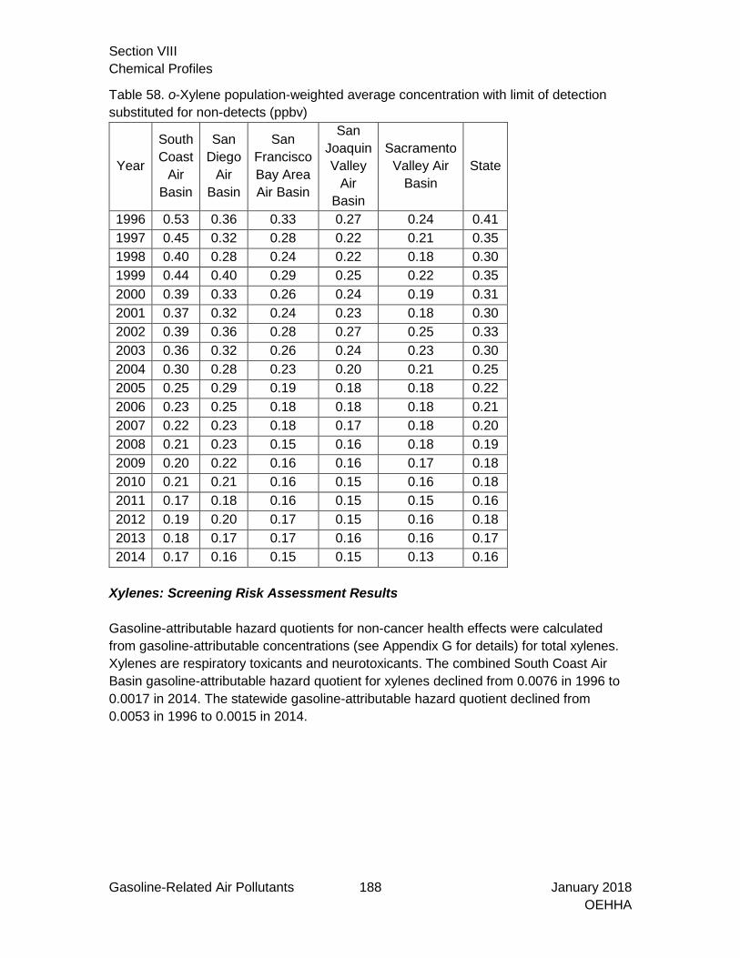
Section VIII Chemical Profiles
Gasoline-Related Air Pollutants 188 January 2018 OEHHA
Table 58. o-Xylene population-weighted average concentration with limit of detection substituted for non-detects (ppbv)
Year
South Coast
Air Basin
San Diego
Air Basin
San Francisco Bay Area Air Basin
San Joaquin Valley
Air Basin
Sacramento Valley Air
Basin State
1996 0.53 0.36 0.33 0.27 0.24 0.41 1997 0.45 0.32 0.28 0.22 0.21 0.35 1998 0.40 0.28 0.24 0.22 0.18 0.30 1999 0.44 0.40 0.29 0.25 0.22 0.35 2000 0.39 0.33 0.26 0.24 0.19 0.31 2001 0.37 0.32 0.24 0.23 0.18 0.30 2002 0.39 0.36 0.28 0.27 0.25 0.33 2003 0.36 0.32 0.26 0.24 0.23 0.30 2004 0.30 0.28 0.23 0.20 0.21 0.25 2005 0.25 0.29 0.19 0.18 0.18 0.22 2006 0.23 0.25 0.18 0.18 0.18 0.21 2007 0.22 0.23 0.18 0.17 0.18 0.20 2008 0.21 0.23 0.15 0.16 0.18 0.19 2009 0.20 0.22 0.16 0.16 0.17 0.18 2010 0.21 0.21 0.16 0.15 0.16 0.18 2011 0.17 0.18 0.16 0.15 0.15 0.16 2012 0.19 0.20 0.17 0.15 0.16 0.18 2013 0.18 0.17 0.17 0.16 0.16 0.17 2014 0.17 0.16 0.15 0.15 0.13 0.16
Xylenes: Screening Risk Assessment Results Gasoline-attributable hazard quotients for non-cancer health effects were calculated from gasoline-attributable concentrations (see Appendix G for details) for total xylenes. Xylenes are respiratory toxicants and neurotoxicants. The combined South Coast Air Basin gasoline-attributable hazard quotient for xylenes declined from 0.0076 in 1996 to 0.0017 in 2014. The statewide gasoline-attributable hazard quotient declined from 0.0053 in 1996 to 0.0015 in 2014.

Section VIII Chemical Profiles
Gasoline-Related Air Pollutants 189 January 2018 OEHHA
Chemical Profiles: Gasoline-related VOCs Based on Primary Emissions and Secondary Atmospheric Formation
The gasoline-related VOCs in this section are emitted from both primary sources and are also formed via secondary atmospheric reactions. The emission tonnage for these chemicals includes primary emissions from the Emission Inventory and estimated tonnage from secondary atmospheric reactions. The combined primary emissions and estimated tonnage from secondary formation were used to calculate the gasoline-attributable fractions for these gasoline-related VOCs.

Section VIII Chemical Profiles
Gasoline-Related Air Pollutants 190 January 2018 OEHHA
Acetaldehyde: Exposure and Screening Risk Assessment Results
Acetaldehyde is a carcinogen and a respiratory toxicant and had the 47th highest primary emissions from gasoline-related sources in 2012 among all gasoline-related VOCs. Acetaldehyde is also formed through secondary atmospheric reactions. Secondary reaction tonnage was calculated using formation potentials as described in Appendix E. An estimated 81% of total acetaldehyde tonnage was formed through secondary reactions statewide in 2012. Figure 112 shows that the statewide tons of acetaldehyde emitted from gasoline-related sources (primary and secondary combined) declined between 1996 and 2012. After the Emission Inventory update in 2002, the estimated acetaldehyde emissions from non-gasoline related sources remained roughly constant. Figure 113 and Figure 114 show the sources and gasoline-attributable fractions of acetaldehyde based on primary emissions and secondary reactions. Statewide, in 2012, 18% of all acetaldehyde tonnage (primary emissions plus secondary formation) came from gasoline-related sources. Table 59 shows that gasoline-attributable fractions of acetaldehyde varied greatly by air basin. Non-gasoline-related sources included biogenic sources (all basins), livestock (San Joaquin Valley, Sacramento Valley and San Francisco Bay Area Air Basins), aircraft and construction and mining equipment. The large drop in gasoline-attributable fractions in 2002 and subsequent years was due to an update of natural sources in the Emission Inventory. Population-weighted annual average ambient air concentrations of acetaldehyde were estimated for the South Coast, San Diego, San Francisco Bay Area, Sacramento Valley and San Joaquin Valley Air Basins and statewide for the years 1996 to 2014 (see Table 60). The ambient air data used to calculate the population-weighted annual average ambient air concentrations came from the California Toxic Monitoring Network and was supplemented with modeled values at additional locations to produce more robust estimates. Figure 115 compares the population-weighted annual average ambient air concentrations of acetaldehyde in the South Coast Air Basin to ambient air measurements from monitoring sites within the basin. Table 61 tabulates the gasoline-attributable population-weighted annual average ambient air concentrations (referred to as gasoline-attributable concentrations) for all air basins. Figure 116 shows that the gasoline-attributable concentration in the South Coast Air Basin declined by 63% between 1996 and 2012. Cancer risks and non-cancer hazard quotients were calculated based on gasoline-attributable ambient air concentrations (see Appendix G for details). The gasoline-attributable cancer risk for acetaldehyde in the South Coast Air Basin declined from 1.9x10⁻⁵ in 1996 to 7.1x10⁻⁶ in 2014, corresponding to an estimated reduction of 12 cancer cases per 1 million people. The statewide gasoline-attributable cancer risk for acetaldehyde declined from 1.2x10⁻⁵ in 1996 to 2.1x10⁻⁶ in 2014, or a reduction of about 10 cancer cases per 1 million people. The gasoline-attributable hazard quotient, based

Section VIII Chemical Profiles
Gasoline-Related Air Pollutants 191 January 2018 OEHHA
on respiratory toxicity, declined in the South Coast Air Basin from 0.013 in 1996 to 0.0050 in 2014. The statewide gasoline-attributable hazard quotient declined from 0.0086 in 1996 to 0.0020 in 2014.

Section VIII Chemical Profiles
Gasoline-Related Air Pollutants 192 January 2018 OEHHA
Figure 112. Emissions of acetaldehyde from gasoline and non-gasoline-related sources in California (data from CARB Emission Inventory)
Figure 113. Primary emission sources and sources of secondary formation of acetaldehyde in 2012

Section VIII Chemical Profiles
Gasoline-Related Air Pollutants 193 January 2018 OEHHA
Table 59. Acetaldehyde gasoline-attributable fractions based on primary emissions and secondary atmospheric reactions
Year South
Coast Air Basin
San Diego Air
Basin
San Francisco Bay Area Air Basin
San Joaquin Valley
Air Basin
Sacramento Valley Air
Basin State
1996 61% 62% 48% 38% 54% 49% 1997 66% 64% 48% 40% 54% 54% 1998 63% 62% 46% 39% 53% 52% 1999 64% 62% 47% 41% 35% 46% 2000 57% 56% 42% 32% 46% 44% 2001 58% 56% 42% 33% 38% 43% 2002 50% 36% 40% 13% 13% 21% 2003 47% 29% 39% 15% 13% 21% 2004 52% 39% 39% 16% 13% 22% 2005 50% 37% 37% 15% 12% 21% 2006 49% 35% 35% 14% 12% 20% 2007 47% 35% 34% 14% 11% 19% 2008 46% 34% 33% 13% 11% 18% 2009 -- -- -- -- -- -- 2010 45% 31% 33% 8% 9% 15% 2011 44% 29% 32% 8% 8% 14% 2012 43% 27% 31% 8% 8% 13%
Note: Mobile source emissions unavailable in 2009. Figure 114. Acetaldehyde gasoline-attributable fractions

Section VIII Chemical Profiles
Gasoline-Related Air Pollutants 194 January 2018 OEHHA
Table 60. Population-weighted annual average ambient air concentrations of acetaldehyde (ppbv)
Year South Coast Air Basin
San Diego Air Basin
San Francisco Bay Area Air Basin
San Joaquin Valley Air Basin
Sacramento Valley Air Basin State
1996 1.7 1.3 1.1 1.2 1.0 1.4 1997 1.6 1.2 1.0 1.1 0.97 1.3 1998 1.4 1.1 0.83 1.0 0.86 1.1 1999 1.5 1.3 0.98 1.2 1.0 1.3 2000 1.2 1.0 0.78 0.91 0.74 0.97 2001 1.2 1.1 0.81 0.93 0.70 1.0 2002 1.2 1.1 0.85 1.0 0.93 1.0 2003 1.3 1.1 0.89 1.1 0.97 1.1 2004 1.2 1.1 0.90 1.0 0.98 1.1 2005 1.3 1.3 0.94 1.2 1.1 1.2 2006 1.0 1.1 0.75 1.1 0.91 0.93 2007 1.0 0.99 0.72 1.0 0.92 0.90 2008 0.90 0.94 0.64 0.90 0.86 0.83 2009 0.89 0.96 0.70 0.94 0.85 0.85 2010 1.0 0.95 0.76 1.0 0.84 0.90 2011 0.91 0.96 0.82 1.1 0.83 0.89 2012 1.0 1.0 0.81 1.0 0.87 0.94 2013 1.0 0.93 0.90 1.0 0.92 0.95 2014 0.92 0.85 0.81 0.98 0.79 0.88
Note: Half the limit of detection substituted for non-detects
Table 61. Gasoline-attributable concentrations of acetaldehyde (ppbv)
Year South Coast Air Basin
San Diego Air Basin
San Francisco Bay Area Air Basin
San Joaquin Valley Air Basin
Sacramento Valley Air Basin State
1996 1.1 0.8 0.51 0.44 0.56 0.69 1997 1 0.79 0.48 0.43 0.52 0.69 1998 0.87 0.67 0.38 0.39 0.45 0.58 1999 0.95 0.83 0.46 0.51 0.35 0.58 2000 0.66 0.58 0.33 0.29 0.34 0.43 2001 0.71 0.61 0.34 0.31 0.27 0.44 2002 0.59 0.41 0.34 0.14 0.12 0.22 2003 0.59 0.33 0.35 0.16 0.12 0.23 2004 0.63 0.44 0.35 0.16 0.13 0.24 2005 0.65 0.49 0.35 0.18 0.13 0.24 2006 0.49 0.37 0.27 0.15 0.11 0.18 2007 0.45 0.34 0.24 0.14 0.1 0.17 2008 0.42 0.32 0.22 0.12 0.093 0.15 2009 0.41 0.33 0.23 0.12 0.092 0.15 2010 0.43 0.3 0.25 0.085 0.073 0.14 2011 0.4 0.28 0.26 0.083 0.07 0.13 2012 0.42 0.27 0.25 0.089 0.067 0.13 2013 0.43 0.25 0.27 0.089 0.071 0.13 2014 0.39 0.23 0.25 0.083 0.061 0.12
Note: The 2009 gasoline-attributable concentration was calculated with the 2008 gasoline-attributable fraction. The 2013 and 2014 gasoline-attributable concentrations were calculated with the 2012 gasoline-attributable fraction.

Section VIII Chemical Profiles
Gasoline-Related Air Pollutants 195 January 2018 OEHHA
Figure 115. Population-weighted annual average ambient air concentration of acetaldehyde in the South Coast Air Basin
Note: The vertical bars show the quartiles of acetaldehyde at South Coast Air Basin monitoring sites. Figure 116. South Coast population-weighted annual average ambient air concentration and gasoline-attributable concentration of acetaldehyde
0
0.5
1
1.5
2
2.5
3
3.5
4
1996 1998 2000 2002 2004 2006 2008 2010 2012 2014
Acet
alde
hyde
(ppb
v)
Fontana-Arrow Highway North Long Beach
Azusa Upland
Burbank-W Palm Avenue Riverside-Rubidoux
Los Angeles-North Main Street Population_weighted annual average ambient air concentration

Section VIII Chemical Profiles
Gasoline-Related Air Pollutants 196 January 2018 OEHHA
Acrolein: Exposure and Screening Risk Assessment Results
Acrolein is a respiratory toxicant and had the 94th highest primary emissions from gasoline-related sources in 2012 among all gasoline-related VOCs. Acrolein is also formed through secondary atmospheric reactions, so the true emissions rank is likely higher. 1,3-Butadiene is the main precursor chemical for acrolein (OEHHA, 2006). Secondary reaction tonnage was calculated using formation potentials as described in Appendix E. Based on these calculations using 2012 data, 39% of total emissions of acrolein were formed through these secondary reactions statewide. Figure 117 shows that the statewide tons of acrolein emitted from gasoline-related sources (primary and secondary combined) declined between 1996 and 2012. Figure 117 also shows that acrolein emissions from non-gasoline related sources increased in 2012, which was attributable primarily to a higher estimate of emissions from waste disposal. Figure 118 displays the emissions sources of acrolein. Table 62 and Figure 119 show the gasoline-attributable fractions of acrolein based on primary emissions and secondary formation. Statewide, in 2012, 28% of total emissions of acrolein came from gasoline-related sources including cars, light duty trucks, boats and off-road equipment. Non-gasoline-related sources included aircraft, agricultural pesticides, wildfires and industrial processes including plastics manufacturing. The apparent increase in the gasoline-attributable fractions in the San Francisco Bay Air Basin in 2002 and later was due to a reduction in estimated emissions from natural sources of acrolein precursor chemicals (i.e., the denominator decreased, so the gasoline-attributable fraction increased). The California Toxic Monitoring Network began measuring ambient air concentrations of acrolein in 2004. Ambient air samples are collected in passivated stainless steel containers and then analyzed using gas chromatography mass spectrometry (GC/MS). The method is similar to that recommended by US EPA for analyzing ambient air concentrations of acrolein. US EPA studied the reliability of this method and found some potential issues.26 First, acrolein concentrations can increase over time in containers that have been previously cleaned and stored. Second, the accuracy of acrolein gas standards used to calibrate GC/MS equipment varied by laboratory. CARB recently acquired several analyzers that employ gas chromatography, mass spectrometry, and Fourier Transform Infrared Reference spectroscopy to measure ambient air levels of selected VOCs, including acrolein. After testing and evaluating the devices, CARB plans to use them to measure VOCs of concern in communities impacted by air pollution. A study funded by OEHHA and carried out by Dr. Judith Charles’ group at UC Davis measured concentrations of acrolein and other carbonyls at the San Francisco-Oakland Bay Bridge Toll Plaza in 2001 using a new method for acrolein measurements
26 http://www3.epa.gov/ttnamti1/files/ambient/airtox/20101217acroleindataqualityeval.pdf

Section VIII Chemical Profiles
Gasoline-Related Air Pollutants 197 January 2018 OEHHA
(Destaillats et al., 2002). Destaillats et al. collected three samples during one morning and two evening periods of rush hour traffic. Each sample was collected over four hours. The estimated mean acrolein concentrations were 0.100 µg/m3 during the morning rush hour period, and 0.032 and 0.058 µg/m3 for the two evening rush hour periods. They noted that the morning commute concentration exceeded the OEHHA cREL at that time of 0.06 µg/m3 (the cREL was subsequently increased by OEHHA to 0.35 µg/m3). However, Destaillats et al. also noted that the acrolein concentrations they measured were lower than mean values predicted for Alameda County (0.154 µg/m3) and San Francisco County (0.272 µg/m3) by an earlier US EPA analysis based on 1996 data (Morello-Frosch et al. 2000). The means reported by Destaillats et al. were also about an order of magnitude lower than the population-weighted annual average ambient air concentration of 1.15 µg/m3 (reported as 0.5 ppb in Table 63 below) that we calculated for the San Francisco Bay Air Basin for 2004 (the earliest year for which data were available for our analysis). More recently, Cahill (2014) measured concentrations of acrolein in remote, rural, and urban areas in California between September and October 2013. He reported a median below the method detection limit (MDL) in the remote areas. In the rural and urban areas, the median measurements were 0.068 and 0.165 µg/m3 (0.030 and 0.080 ppb). These medians were about an order of magnitude lower than the population-weighted annual averages we estimated based on 2013 data across the state (see Table 63 below). He also compared his ambient outdoor acrolein measurements to those from previous studies and found a wide range of values that depended on location of measurement and method used to make the measurement. Population-weighted annual average concentrations of acrolein were calculated for the years 2004 through 2014 using ambient air measurements of acrolein collected by the California Toxic Monitoring Network (see Table 63). Figure 120 compares the estimated population-weighted annual average concentrations to actual ambient air measurements in the South Coast Air Basin. During this time period, ambient air concentrations of acrolein increased, gasoline-attributable fractions fell and gasoline-attributable concentrations of acrolein remained roughly constant (see Table 64 and Figure 121). Hazard quotients for non-cancer health effects were calculated based on gasoline-attributable ambient air concentrations (see Appendix G for details). Acrolein is a respiratory toxicant, with a gasoline-attributable hazard quotient of 3 in the South Coast Air Basin in 2014. The statewide gasoline-attributable hazard quotient was 1.2 in 2014. As noted above, there are some uncertainties about the methods used to measure acrolein ambient air concentrations, and there have been discrepancies in measured concentrations versus predicted means. However, acrolein has been consistently flagged as a potential respiratory health concern in ambient air by previous authors (Destaillats et al., 2002; Woodruff et al., 2007; Logue et al., 2010), and our work supports that concern. Further research is warranted to better evaluate the respiratory health risks of acrolein in California. This could include work to refine sample collection

Section VIII Chemical Profiles
Gasoline-Related Air Pollutants 198 January 2018 OEHHA
and analytical methods for measuring acrolein in ambient air; and investigation of an appropriate biomarker for acrolein (see for example, Li et al., 2004) to more directly evaluate potential exposure in humans.

Section VIII Chemical Profiles
Gasoline-Related Air Pollutants 199 January 2018 OEHHA
Figure 117. Emissions of acrolein from gasoline and non-gasoline-related sources in California (data from CARB Emission Inventory)
Figure 118. Primary emission sources and sources of secondary formation of acrolein in 2012
0
0.5
1
1.5
2
2.5
3
3.5
4
1996 1997 1998 1999 2000 2001 2002 2003 2004 2005 2006 2007 2008 2009 2010 2011 2012
Acro
lein
(ton
s per
day
)(in
clud
es p
rimar
y em
issi
ons a
nd se
cond
ary
reac
tion
prod
ucts
)
Acrolein from gasoline-related sources Acrolein from non-gasoline-related sources
SC (G) SC (NG) SD (G) SD (NG) SF (G) SF (NG) SJV (G) SJV (NG) SV (G) SV (NG)CLEANING AND SURFACE COATINGS - - - - - < 0.01 - - - -FUEL COMBUSTION < 0.01 < 0.01 < 0.01 < 0.01 < 0.01 < 0.01 < 0.01 < 0.01 < 0.01 < 0.01INDUSTRIAL PROCESSES - 0.08 - 0.03 - 0.12 - 0.08 - 0.04MISCELLANEOUS PROCESSES - < 0.01 - < 0.01 - < 0.01 - 0.02 - < 0.01NATURAL SOURCES - 0.04 - 0.03 - < 0.01 - 0.06 - 0.07ON-ROAD MOTOR VEHICLES 0.15 < 0.01 0.04 < 0.01 0.10 < 0.01 0.05 < 0.01 0.04 < 0.01OTHER MOBILE SOURCES 0.15 0.09 0.04 0.09 0.06 0.20 0.04 0.12 0.04 0.07PETROLEUM PRODUCTION AND DISTRIBUTION - < 0.01 - - - < 0.01 - < 0.01 - < 0.01SOLVENT EVAPORATION - < 0.01 - < 0.01 - < 0.01 - 0.10 - 0.02WASTE DISPOSAL - - - - - - - 0.16 - 0.03
-
0.10
0.20
0.30
0.40
0.50
0.60
Acro
lein
in p
rimar
y em
issi
ons a
nd se
cond
ary
form
atio
n(t
ons p
er d
ay)
0.00
Pesticides
Plastics manufacturing

Section VIII Chemical Profiles
Gasoline-Related Air Pollutants 200 January 2018 OEHHA
Table 62. Acrolein gasoline-attributable fractions from primary and secondary reactions
Year
South Coast
Air Basin
San Diego
Air Basin
San Francisco Bay Area Air Basin
San Joaquin
Valley Air Basin
Sacramento Valley Air
Basin State
1996 75% 72% 38% 42% 65% 52% 1997 79% 72% 36% 41% 63% 54% 1998 88% 71% 36% 43% 65% 56% 1999 79% 69% 34% 49% 43% 49% 2000 72% 63% 30% 39% 62% 46% 2001 71% 62% 30% 43% 51% 45% 2002 70% 55% 59% 24% 57% 51% 2003 66% 44% 58% 31% 53% 50% 2004 71% 55% 56% 27% 50% 49% 2005 69% 53% 53% 28% 48% 48% 2006 67% 52% 52% 27% 46% 47% 2007 65% 50% 49% 26% 45% 46% 2008 60% 49% 48% 28% 45% 44% 2009 -- -- -- -- -- -- 2010 64% 40% 38% 23% 33% 38% 2011 61% 37% 35% 21% 31% 35% 2012 58% 33% 32% 14% 25% 28%
Note: Mobile source emissions were not available for 2009 Figure 119. Acrolein gasoline-attributable fractions
0%
10%
20%
30%
40%
50%
60%
70%
80%
90%
100%
1996 1997 1998 1999 2000 2001 2002 2003 2004 2005 2006 2007 2008 2009 2010 2011 2012
Acto
lein
gas
olin
e-at
trib
utab
le fr
actio
ns(p
rimar
y em
issi
ons a
nd se
cond
ary
reac
tion
prod
ucts
)
South Coast Air Basin San Diego Air Basin San Francisco Bay Area Air Basin
San Joaquin Valley Air Basin Sacramento Valley Air Basin State

Section VIII Chemical Profiles
Gasoline-Related Air Pollutants 201 January 2018 OEHHA
Table 63. Population-weighted annual average ambient air concentrations of acrolein (ppb)
Year South Coast
Air Basin
San Diego
Air Basin
San Francisco Bay Area Air Basin
San Joaquin Valley
Air Basin
Sacramento Valley Air
Basin
State
2004 0.54 0.51 0.50 0.49 0.51 0.51 2005 0.59 0.59 0.53 0.50 0.51 0.56 2006 0.57 0.56 0.55 0.58 0.54 0.56 2007 0.60 0.60 0.52 0.54 0.56 0.57 2008 0.67 0.67 0.61 0.61 0.65 0.65 2009 0.71 0.71 0.64 0.68 0.68 0.69 2010 0.66 0.66 0.62 0.62 0.62 0.64 2011 0.87 0.85 0.87 0.87 0.81 0.86 2012 0.73 0.74 0.70 0.71 0.73 0.72 2013 0.69 0.73 0.72 0.69 0.66 0.70 2014 0.68 0.64 0.65 0.62 0.64 0.66
Note: half the limit of detection substituted for non-detects Table 64. Gasoline-attributable concentrations of acrolein (ppb)
Year South Coast
Air Basin
San Diego
Air Basin
San Francisco Bay Area Air Basin
San Joaquin Valley
Air Basin
Sacramento Valley Air
Basin
State
2004 0.38 0.28 0.28 0.13 0.25 0.25 2005 0.41 0.31 0.28 0.14 0.24 0.27 2006 0.38 0.29 0.28 0.16 0.25 0.26 2007 0.39 0.30 0.25 0.14 0.25 0.26 2008 0.40 0.33 0.29 0.17 0.29 0.29 2009 0.42 0.35 0.30 0.19 0.31 0.30 2010 0.42 0.27 0.23 0.14 0.21 0.24 2011 0.53 0.32 0.30 0.18 0.25 0.30 2012 0.42 0.25 0.22 0.10 0.18 0.20 2013 0.40 0.24 0.23 0.10 0.16 0.19 2014 0.39 0.21 0.21 0.09 0.16 0.18
Note: The 2009 gasoline-attributable concentration was calculated with the 2008 gasoline-attributable fraction. The 2013 and 2014 gasoline-attributable concentrations were calculated with the 2012 gasoline-attributable fraction.

Section VIII Chemical Profiles
Gasoline-Related Air Pollutants 202 January 2018 OEHHA
Figure 120. South Coast Air Basin population-weighted annual average ambient air concentration compared to quartiles of acrolein measurements
Figure 121. South Coast population-weighted annual average ambient air concentration and gasoline-attributable concentration of acrolein
0
0.2
0.4
0.6
0.8
1
1.2
1.4
2003 2005 2007 2009 2011 2013 2015
Acro
lein
(ppb
v)
North Long Beach Azusa
Burbank-W Palm Avenue Riverside-Rubidoux
Los Angeles-North Main Street Population_weighted annual average ambient air concentration
0.00
0.10
0.20
0.30
0.40
0.50
0.60
0.70
0.80
0.90
1.00
2004 2005 2006 2007 2008 2009 2010 2011 2012 2013 2014
Acro
lein
(ppb
v)
Population-weighted annual average ambient air concentration Gasoline attributable concentration

Section VIII Chemical Profiles
Gasoline-Related Air Pollutants 203 January 2018 OEHHA
Benzaldehyde: Exposure and Screening Risk Assessment Results
Benzaldehyde is an aromatic aldehyde that is carcinogenic in mice and has evidence of respiratory toxicity in rats. It had the 62nd highest primary emissions from gasoline-related sources in 2012 among all gasoline-related VOCs. Benzaldehyde is also formed through secondary atmospheric reactions. Carter (2001) provided formation potentials for aromatic aldehydes, including benzaldehyde, as a group. These formation potentials were used to estimate tons of aromatic aldehydes formed through secondary atmospheric reactions as a group, and we used that information to estimate the gasoline-attributable fraction for benzaldehyde. In 2012, about 46% of the overall emissions of aromatic aldehydes were formed through secondary reactions. Figure 122 shows that total emissions of aromatic aldehydes declined between 1996 and 2012. Figure 123 shows the emission sources of aromatic aldehydes. Table 65 and Figure 124 show the gasoline-attributable fractions of aromatic aldehydes. Statewide in 2012, 68% of aromatic aldehyde emissions came from gasoline-related sources including cars and light duty trucks. The main non-gasoline-related sources included heavy-duty diesel trucks, off-road equipment and aircraft. Figure 124 shows that gasoline-attributable fractions in the San Joaquin air basin dropped between 2001 and 2003, because estimated emissions from diesel farm equipment, a source of aromatic aldehydes, increased in 2003. Data collected by the Desert Research Institute (DRI) in the summer of 1996 were used to create a model for estimating ambient air concentrations of benzaldehyde (see Appendix D for details). Table 66 lists the population-weighted annual average ambient air concentrations for the South Coast Air Basin. Figure 125 compares the estimated population-weighted annual average ambient air concentrations of benzaldehyde in the South Coast Air Basin to the DRI data and to benzaldehyde measurements from other studies. It was assumed that the gasoline-attributable fraction of aromatic aldehydes could be used for benzaldehyde. Figure 126 shows that the gasoline-attributable ambient air concentration of benzaldehyde in the South Coast Air Basin declined by 80% between 1996 and 2012. We located a few studies that could be used to check the estimated population-weighted annual average ambient air concentrations for benzaldehyde. A study funded by OEHHA and conducted at the San Francisco-Oakland Bay Bridge Toll Plaza in April 2001 found benzaldehyde air levels in the range of 0.02-0.04 ppb (Destaillats et al., 2002). The US EPA AirData website had 3-hour measurements taken during summer months in Sacramento County, Fresno County and Kern County. CARB NMOC/PAMS benzaldehyde data came from two monitoring sites in the San Joaquin Air Basin. Figure 125 compares our modeled population-weighted ambient air concentrations of benzaldehyde in the South Coast Air Basin to ambient air measurements taken at sites in California.

Section VIII Chemical Profiles
Gasoline-Related Air Pollutants 204 January 2018 OEHHA
We could not estimate cancer risk or a non-cancer hazard quotient for benzaldehyde, because we did not locate a cancer potency or other health reference value. Figure 122. Emissions of aromatic aldehydes from gasoline and non-gasoline-related sources in California (data from CARB Emission Inventory)
Figure 123. Primary emission sources and sources of secondary formation of aromatic aldehydes in 2012
SC (G) SC (NG) SD (G) SD (NG) SF (G) SF (NG) SJV (G) SJV (NG) SV (G) SV (NG)CLEANING AND SURFACE COATINGS - 0.09 - 0.04 - 0.04 - 0.04 - 0.02FUEL COMBUSTION < 0.01 < 0.01 < 0.01 < 0.01 < 0.01 < 0.01 < 0.01 0.01 < 0.01 < 0.01INDUSTRIAL PROCESSES < 0.01 0.23 - 0.29 - 0.08 - 0.07 - 0.09MISCELLANEOUS PROCESSES - < 0.01 - < 0.01 - < 0.01 - 0.04 - < 0.01NATURAL SOURCES - - - - - - - < 0.01 - -ON-ROAD MOTOR VEHICLES 0.78 0.07 0.19 0.02 0.52 0.04 0.27 0.07 0.22 0.03OTHER MOBILE SOURCES 1.01 0.12 0.29 0.05 0.40 0.11 0.25 0.12 0.25 0.06PETROLEUM PRODUCTION AND DISTRIBUTION < 0.01 < 0.01 < 0.01 < 0.01 < 0.01 < 0.01 < 0.01 < 0.01 < 0.01 < 0.01SOLVENT EVAPORATION - 0.07 - 0.02 - 0.04 - 0.02 - 0.02WASTE DISPOSAL - 0.03 - 0.01 - < 0.01 - 0.09 - 0.02
-
0.20
0.40
0.60
0.80
1.00
1.20
1.40
1.60
1.80
2.00
Benz
alde
hyde
and
oth
er a
rom
atic
ald
ehyd
es
from
prim
ary
emis
sion
s and
seco
ndar
y at
mos
pher
ic re
actio
ns
(ton
s per
day
)
0.00

Section VIII Chemical Profiles
Gasoline-Related Air Pollutants 205 January 2018 OEHHA
Table 65. Gasoline-attributable fractions of aromatic aldehydes (including benzaldehyde) from primary and secondary atmospheric reactions
Year
South Coast
Air Basin
San Diego
Air Basin
San Francisco Bay Area Air Basin
San Joaquin
Valley Air Basin
Sacramento Valley Air
Basin State
1996 85% 84% 79% 81% 74% 83% 1997 81% 84% 78% 80% 72% 81% 1998 83% 84% 77% 80% 72% 82% 1999 81% 84% 79% 82% 82% 82% 2000 74% 79% 73% 75% 70% 76% 2001 81% 79% 73% 76% 79% 79% 2002 80% 80% 78% 71% 80% 79% 2003 79% 76% 79% 66% 77% 77% 2004 79% 80% 78% 63% 79% 78% 2005 79% 79% 76% 64% 77% 77% 2006 79% 79% 75% 62% 76% 76% 2007 78% 77% 74% 62% 76% 75% 2008 76% 78% 74% 63% 75% 75% 2009a -- -- -- -- -- -- 2010 78% 57% 76% 58% 68% 71% 2011 76% 55% 74% 58% 67% 70% 2012 74% 53% 74% 53% 64% 68%
Note: Mobile source emissions were unavailable for 2009. Figure 124. Gasoline-attributable fractions of aromatic aldehydes
0%
10%
20%
30%
40%
50%
60%
70%
80%
90%
100%
1996 1997 1998 1999 2000 2001 2002 2003 2004 2005 2006 2007 2008 2009 2010 2011 2012
Arom
atic
ald
ehyd
es g
asol
ine-
attr
ibut
able
frac
tions
base
d on
prim
ary
emis
sion
s and
seco
ndar
y at
mos
pher
ic re
actio
ns
South Coast Air Basin San Diego Air Basin San Francisco Bay Area Air Basin
San Joaquin Valley Air Basin Sacramento Valley Air Basin State

Section VIII Chemical Profiles
Gasoline-Related Air Pollutants 206 January 2018 OEHHA
Table 66. Benzaldehyde in the South Coast Air Basin Year Population-weighted
annual average ambient air
concentration (ppbv)
Gasoline-attributable
fraction
Gasoline-attributable
concentration (ppbv)
1996 0.18 85% 0.15 1997 0.17 81% 0.14 1998 0.17 83% 0.14 1999 0.16 81% 0.13 2000 0.14 74% 0.10 2001 0.13 81% 0.10 2002 0.12 80% 0.095 2003 0.11 79% 0.091 2004 0.098 79% 0.078 2005 0.087 79% 0.069 2006 0.083 79% 0.066 2007 0.078 78% 0.060 2008 0.069 76% 0.053 2009 0.065 76% 0.050 2010 0.067 78% 0.052 2011 0.063 76% 0.048 2012 0.064 74% 0.048 2013 0.063 74% 0.047 2014 0.061 74% 0.045
Note: The 2009 gasoline-attributable concentration was calculated with the 2008 gasoline-attributable fraction. The 2013 and 2014 gasoline-attributable concentrations were calculated with the 2012 gasoline-attributable fraction.

Section VIII Chemical Profiles
Gasoline-Related Air Pollutants 207 January 2018 OEHHA
Figure 125. Comparison of modeled population-weighted ambient air concentration of benzaldehyde in the South Coast Air Basin to measurements from other sites in California.
Note: The plot shows the first quartile, median, and third quartile from each site and year. The data used to calculate the summary statistics were 3-hour samples from summer months. Figure 126. South Coast population-weighted annual average ambient air concentration and gasoline-attributable concentration of benzaldehyde
0
0.05
0.1
0.15
0.2
0.25
0.3
0.35
1995 1997 1999 2001 2003 2005 2007 2009 2011 2013 2015
Benz
alde
hyde
(ppb
v)
DRI - Azusa DRI - Burbank
DRI - North Main US EPA - Bakersfield-Golden State Highway
US EPA - Clovis-N Villa Avenue US EPA - Sacramento-Del Paso Manor
SC Population_weighted annual average ambient air concentration
0
0.02
0.04
0.06
0.08
0.1
0.12
0.14
0.16
0.18
0.2
1996 1997 1998 1999 2000 2001 2002 2003 2004 2005 2006 2007 2008 2009 2010 2011 2012 2013 2014
Benz
alde
hyde
(ppb
v)
Population-weighted annual average ambient air concentration Gasoline-attributable concentration
Gasoline-attributable concentration calculated using gasoline-attributable fraction of aromatic aldehydes

Section VIII Chemical Profiles
Gasoline-Related Air Pollutants 208 January 2018 OEHHA
Formaldehyde: Exposure and Screening Risk Assessment Results
Formaldehyde is a carcinogen and respiratory toxicant and had the 21st highest primary emissions from gasoline-related sources in 2012 among all gasoline-related VOCs. Formaldehyde is also formed through secondary atmospheric reactions. Secondary emissions were estimated by applying the formation potential to data from the Emission Inventory (see Appendix E). In 2012, 89% of formaldehyde emissions was formed through these secondary reactions. Figure 127 shows that the overall formaldehyde emissions declined between 1996 and 2012. Figure 128 shows the emission sources of formaldehyde. Table 67 and Figure 129 show the gasoline-attributable fractions of formaldehyde. Statewide, in 2012, 11% of formaldehyde emissions came from gasoline-related sources. Biogenic sources, wildfires, aircraft, residential combustion and construction and mining equipment were some of the main non-gasoline-related sources of formaldehyde. The gasoline-attributable fractions varied by air basin. In the San Joaquin and Sacramento Valley Air Basins, controlled burning contributed a substantial part of formaldehyde emissions and caused the gasoline-attributable fractions in these two basins to be lower. Gasoline-attributable fractions dropped in San Diego, Sacramento and San Joaquin Valley air basins in 2002, because of an increase in estimated emissions from natural sources. Population-weighted annual average ambient air concentrations of formaldehyde were estimated for the South Coast, San Diego, San Francisco Bay Area, Sacramento Valley and San Joaquin Valley Air Basins and statewide for the years 1996 to 2014 (see Table 68). The ambient air data used to calculate the population-weighted annual average ambient air concentrations came from the California Toxic Monitoring Network and was supplemented with modeled values at additional locations to produce more robust estimates. Table 69 tabulates the gasoline-attributable population-weighted annual average ambient air concentrations (referred to as gasoline-attributable concentrations) for all air basins. Figure 130 compares the population-weighted annual average ambient air concentrations of formaldehyde in the South Coast Air Basin to ambient air measurements from monitoring sites within the basin. Figure 131 shows that the gasoline-attributable concentrations of formaldehyde in the South Coast Air Basin declined by 65% between 1996 and 2014. Cancer risks and hazard quotients for non-cancer health effects were calculated from gasoline-attributable concentrations (see Appendix G for details). The gasoline-attributable cancer risk for formaldehyde in the South Coast Air Basin declined from 6.5x10⁻⁵ in 1996 to 2.3 x10⁻⁵ in 2014, corresponding to a reduction of 42 estimated cancer cases per 1 million people. The statewide gasoline-attributable cancer risk of formaldehyde declined from 3.9x10⁻⁵ in 1996 to 6.8x10⁻⁶ in 2014, or 33 cancer cases per 1 million people.

Section VIII Chemical Profiles
Gasoline-Related Air Pollutants 209 January 2018 OEHHA
The gasoline-attributable hazard quotient for formaldehyde, based on respiratory toxicity, declined from 0.36 in 1996 to 0.13 in 2014 in the South Coast Air Basin. The statewide gasoline-attributable hazard quotient declined from 0.22 in 1996 to 0.042 in 2014.

Section VIII Chemical Profiles
Gasoline-Related Air Pollutants 210 January 2018 OEHHA
Figure 127. Emissions of formaldehyde from gasoline and non-gasoline-related sources in California (data from CARB Emission Inventory)
Figure 128. Primary emission sources and sources of secondary formation of formaldehyde in 2012

Section VIII Chemical Profiles
Gasoline-Related Air Pollutants 211 January 2018 OEHHA
Table 67. Formaldehyde gasoline-attributable fractions
Year South
Coast Air Basin
San Diego Air
Basin
San Francisco Bay Area Air Basin
San Joaquin
Valley Air Basin
Sacramento Valley Air
Basin State
1996 63% 63% 41% 39% 52% 45% 1997 66% 64% 40% 42% 50% 51% 1998 67% 64% 39% 43% 50% 50% 1999 66% 62% 36% 45% 24% 39% 2000 59% 56% 34% 31% 44% 40% 2001 57% 56% 34% 36% 31% 38% 2002 46% 31% 35% 11% 13% 20% 2003 43% 22% 35% 15% 13% 20% 2004 46% 31% 33% 14% 11% 19% 2005 44% 30% 30% 13% 11% 18% 2006 42% 28% 29% 12% 10% 17% 2007 40% 27% 28% 12% 10% 16% 2008 39% 27% 27% 12% 9% 16% 2009 2010 40% 24% 26% 9% 7% 13% 2011 38% 22% 25% 9% 7% 12% 2012 35% 19% 23% 9% 6% 11%
Note: Mobile source emissions were unavailable for 2009. Figure 129. Formaldehyde gasoline-attributable fractions

Section VIII Chemical Profiles
Gasoline-Related Air Pollutants 212 January 2018 OEHHA
Table 68. Population-weighted average concentrations of formaldehyde (ppbv) with half the limit of detection substituted for non-detects
Year South Coast Air Basin
San Diego Air Basin
San Francisco Bay Area Air Basin
San Joaquin Valley Air Basin
Sacramento Valley Air Basin State
1996 4.0 3.1 2.8 2.9 2.7 3.4 1997 3.7 3.0 2.5 2.6 2.5 3.1 1998 3.3 2.7 2.2 2.5 2.3 2.8 1999 3.5 3.2 2.6 3.0 2.8 3.1 2000 2.8 2.5 2.1 2.3 2.1 2.4 2001 3.2 2.9 2.3 2.5 2.2 2.8 2002 3.5 3.3 2.9 2.8 3.0 3.2 2003 3.3 3.0 2.6 2.7 2.9 3.0 2004 3.0 2.6 2.2 2.3 2.4 2.6 2005 3.0 2.8 2.0 2.3 2.4 2.6 2006 2.9 2.6 2.0 2.4 2.5 2.5 2007 2.8 2.6 1.9 2.4 2.6 2.5 2008 2.9 2.5 1.8 2.3 2.4 2.5 2009 2.2 2.2 1.7 2.1 2.1 2.0 2010 2.5 2.3 1.9 2.4 2.3 2.3 2011 2.5 2.4 2.1 2.4 2.3 2.3 2012 2.5 2.4 1.9 2.3 2.3 2.3 2013 2.6 2.4 2.3 2.4 2.5 2.5 2014 2.5 2.4 2.2 2.5 2.4 2.4
Table 69. Gasoline-attributable concentrations of formaldehyde (ppbv)
Year South Coast Air Basin
San Diego Air Basin
San Francisco Bay Area Air Basin
San Joaquin Valley Air Basin
Sacramento Valley Air Basin State
1996 2.5 2.0 1.1 1.1 1.4 1.5 1997 2.4 1.9 1.0 1.1 1.3 1.6 1998 2.2 1.7 0.85 1.1 1.2 1.4 1999 2.3 2.0 0.95 1.4 0.68 1.2 2000 1.6 1.4 0.70 0.71 0.93 0.98 2001 1.8 1.6 0.78 0.89 0.68 1.1 2002 1.6 1.01 1.0 0.31 0.40 0.64 2003 1.4 0.67 0.92 0.40 0.37 0.58 2004 1.4 0.80 0.71 0.32 0.27 0.50 2005 1.3 0.82 0.61 0.30 0.25 0.47 2006 1.2 0.73 0.57 0.30 0.25 0.43 2007 1.1 0.70 0.54 0.29 0.25 0.41 2008 1.1 0.67 0.49 0.27 0.23 0.39 2009 0.86 0.59 0.44 0.24 0.20 0.32 2010 1.0 0.56 0.48 0.21 0.17 0.31 2011 0.94 0.53 0.51 0.21 0.16 0.29 2012 0.86 0.47 0.45 0.20 0.15 0.25 2013 0.92 0.47 0.53 0.21 0.16 0.27 2014 0.89 0.46 0.52 0.21 0.15 0.26
Note: The 2009 gasoline-attributable concentration was calculated with the 2008 gasoline-attributable fraction. The 2013 and 2014 gasoline-attributable concentrations were calculated with the 2012 gasoline-attributable fraction.

Section VIII Chemical Profiles
Gasoline-Related Air Pollutants 213 January 2018 OEHHA
Figure 130. Population-weighted annual average ambient air concentration of formaldehyde in the South Coast Air Basin
Note: The vertical bars show the annual quartiles at South Coast Air Basin monitoring sites. Figure 131. South Coast population-weighted annual average ambient air concentration and gasoline-attributable concentration of formaldehyde
0
1
2
3
4
5
6
7
8
9
10
1996 1998 2000 2002 2004 2006 2008 2010 2012 2014
Form
alde
hyde
(ppb
v)
Fontana-Arrow Highway North Long BeachAzusa UplandBurbank-W Palm Avenue Riverside-RubidouxLos Angeles-North Main Street Population_weighted annual average ambient air concentration

Section VIII Chemical Profiles
Gasoline-Related Air Pollutants 214 January 2018 OEHHA
Propionaldehyde, Butyraldehyde, and Other Higher Aldehydes: Exposure and Screening Risk Assessment Results
Higher aldehydes are saturated aldehydes with three or more carbon atoms, such as propionaldehyde, butyraldehyde and hexaldehyde. Propionaldehyde, butyraldehyde and hexaldehyde are suspected respiratory toxicants and had the 124th, 161st and 177th highest primary emissions from gasoline-related sources in 2012 among all gasoline-related VOCs. These aldehydes are also formed through secondary atmospheric reactions. We used direct formation potentials provided by Dr. Carter and data from the Emission Inventory to calculate the secondary atmospheric formation of higher aldehydes as a group (see Appendix E). Statewide, in 2012, we estimated that 82% of higher aldehyde emissions came from these secondary atmospheric reactions. Figure 132 shows that the tons of higher aldehydes emitted from gasoline-related sources or with gasoline-related sources of secondary formation declined between 1996 and 2012. Figure 133 shows the emission sources of higher aldehydes. Table 70 and Figure 134 show the gasoline-attributable fractions of higher aldehydes. Statewide, in 2012, 11% of higher aldehydes came from gasoline-related sources. Propionaldehyde, butyraldehyde and hexaldehyde were the most common directly emitted higher aldehydes in the Emission Inventory in 2012. Table 71 and Figure 135 display ambient air measurements of propionaldehyde. Ambient air measurements of butyraldehyde are shown in Table 72 and Figure 136. Ambient air measurements of hexaldehyde are shown in Table 73 and Figure 137. US EPA developed an RfC for propionaldehyde equal to 0.008 mg/m3 (or 3 ppb). Ambient air measurements of propionaldehyde were taken over 3-hour intervals during summer months. For each year, the average of these measurements was calculated. These averages were all below 0.3 ppb, a factor of 10 lower than the RfC. Hazard quotients were not calculated for butyraldehyde or hexaldehyde due to sparse ambient air monitoring and lack of health reference values.

Section VIII Chemical Profiles
Gasoline-Related Air Pollutants 215 January 2018 OEHHA
Figure 132. Emissions of higher aldehydes from gasoline and non-gasoline-related sources in California (data from CARB Emission Inventory)
Figure 133. Primary emission sources and sources of secondary formation of higher aldehydes in 2012

Section VIII Chemical Profiles
Gasoline-Related Air Pollutants 216 January 2018 OEHHA
Table 70. Gasoline-attributable fractions of higher aldehydes
Year South Coast Air
Basin
San Diego Air Basin
San Francisco Bay Area Air
Basin
San Joaquin Valley Air
Basin
Sacramento Valley Air
Basin
State
1996 52% 51% 33% 34% 43% 40% 1997 58% 53% 32% 34% 42% 42% 1998 55% 51% 30% 34% 41% 40% 1999 57% 51% 32% 36% 35% 39% 2000 49% 45% 28% 29% 35% 34% 2001 51% 45% 28% 29% 33% 34% 2002 40% 28% 30% 13% 13% 18% 2003 38% 25% 30% 13% 12% 17% 2004 41% 28% 29% 14% 13% 18% 2005 39% 27% 28% 13% 12% 17% 2006 38% 26% 26% 12% 11% 16% 2007 36% 25% 25% 12% 11% 15% 2008 35% 25% 25% 11% 10% 15% 2009 -- -- -- -- -- -- 2010 35% 22% 26% 8% 8% 13% 2011 34% 20% 25% 8% 8% 12% 2012 33% 19% 24% 8% 7% 11%
Note: Mobile source emissions were unavailable for 2009. Figure 134. Gasoline-attributable fractions of higher aldehydes
0%
10%
20%
30%
40%
50%
60%
70%
80%
90%
100%
1996 1997 1998 1999 2000 2001 2002 2003 2004 2005 2006 2007 2008 2009 2010 2011 2012
High
er a
ldeh
ydes
gas
olin
e-at
trib
utab
le fr
actio
ns
South Coast Air Basin San Diego Air Basin San Francisco Bay Area Air Basin
San Joaquin Valley Air Basin Sacramento Valley Air Basin State
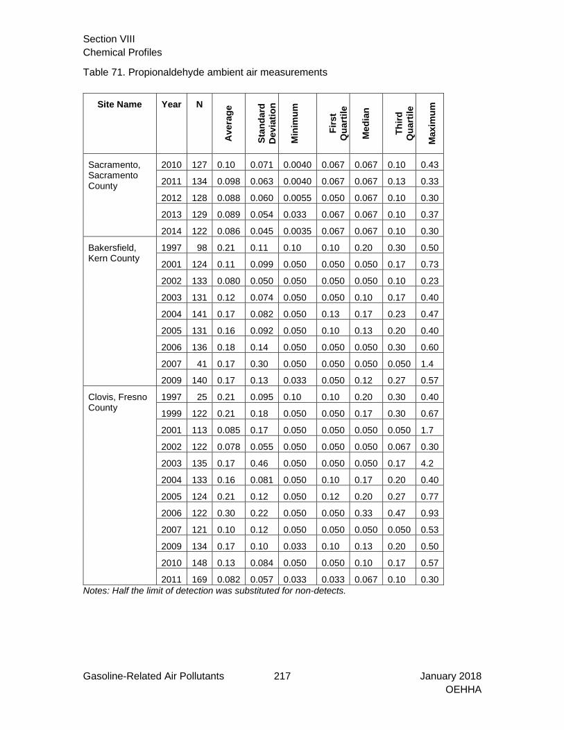
Section VIII Chemical Profiles
Gasoline-Related Air Pollutants 217 January 2018 OEHHA
Table 71. Propionaldehyde ambient air measurements
Site Name Year N
Ave
rage
Stan
dard
D
evia
tion
Min
imum
Firs
t Q
uart
ile
Med
ian
Third
Q
uart
ile
Max
imum
Sacramento, Sacramento County
2010 127 0.10 0.071 0.0040 0.067 0.067 0.10 0.43
2011 134 0.098 0.063 0.0040 0.067 0.067 0.13 0.33
2012 128 0.088 0.060 0.0055 0.050 0.067 0.10 0.30
2013 129 0.089 0.054 0.033 0.067 0.067 0.10 0.37
2014 122 0.086 0.045 0.0035 0.067 0.067 0.10 0.30
Bakersfield, Kern County
1997 98 0.21 0.11 0.10 0.10 0.20 0.30 0.50
2001 124 0.11 0.099 0.050 0.050 0.050 0.17 0.73
2002 133 0.080 0.050 0.050 0.050 0.050 0.10 0.23
2003 131 0.12 0.074 0.050 0.050 0.10 0.17 0.40
2004 141 0.17 0.082 0.050 0.13 0.17 0.23 0.47
2005 131 0.16 0.092 0.050 0.10 0.13 0.20 0.40
2006 136 0.18 0.14 0.050 0.050 0.050 0.30 0.60
2007 41 0.17 0.30 0.050 0.050 0.050 0.050 1.4
2009 140 0.17 0.13 0.033 0.050 0.12 0.27 0.57
Clovis, Fresno County
1997 25 0.21 0.095 0.10 0.10 0.20 0.30 0.40
1999 122 0.21 0.18 0.050 0.050 0.17 0.30 0.67
2001 113 0.085 0.17 0.050 0.050 0.050 0.050 1.7
2002 122 0.078 0.055 0.050 0.050 0.050 0.067 0.30
2003 135 0.17 0.46 0.050 0.050 0.050 0.17 4.2
2004 133 0.16 0.081 0.050 0.10 0.17 0.20 0.40
2005 124 0.21 0.12 0.050 0.12 0.20 0.27 0.77
2006 122 0.30 0.22 0.050 0.050 0.33 0.47 0.93
2007 121 0.10 0.12 0.050 0.050 0.050 0.050 0.53
2009 134 0.17 0.10 0.033 0.10 0.13 0.20 0.50
2010 148 0.13 0.084 0.050 0.050 0.10 0.17 0.57
2011 169 0.082 0.057 0.033 0.033 0.067 0.10 0.30 Notes: Half the limit of detection was substituted for non-detects.

Section VIII Chemical Profiles
Gasoline-Related Air Pollutants 218 January 2018 OEHHA
Figure 135. Propionaldehyde ambient air measurements
Data are 3-hour measurements from summer months. Vertical bars show the quartiles from each site and year.
0
0.05
0.1
0.15
0.2
0.25
0.3
0.35
0.4
0.45
0.5
1996 1998 2000 2002 2004 2006 2008 2010 2012 2014
Prop
iona
ldeh
yde
(ppb
v)
US EPA AirData Sacramento County US EPA AirData Kern County US EPA AirData Fresno County

Section VIII Chemical Profiles
Gasoline-Related Air Pollutants 219 January 2018 OEHHA
Table 72. Ambient air measurements of butyraldehyde
Site Name Year N
Ave
rage
Stan
dard
D
evia
tion
Min
imum
Firs
t Q
uart
ile
Med
ian
Third
Q
uart
ile
Max
imum
Sacramento, Sacramento County
2010 127 0.10 0.071 0.0040 0.067 0.067 0.10 0.43 2011 134 0.098 0.063 0.0040 0.067 0.067 0.13 0.33 2012 128 0.088 0.060 0.0055 0.050 0.067 0.10 0.30 2013 129 0.089 0.054 0.033 0.067 0.067 0.10 0.37 2014 122 0.086 0.045 0.0035 0.067 0.067 0.10 0.30
Bakersfield, Kern County
1997 98 0.21 0.11 0.10 0.10 0.20 0.30 0.50 2001 124 0.11 0.099 0.050 0.050 0.050 0.17 0.73 2002 133 0.080 0.050 0.050 0.050 0.050 0.10 0.23 2003 131 0.12 0.074 0.050 0.050 0.10 0.17 0.40 2004 141 0.17 0.082 0.050 0.13 0.17 0.23 0.47 2005 131 0.16 0.092 0.050 0.10 0.13 0.20 0.40 2006 136 0.18 0.14 0.050 0.050 0.050 0.30 0.60 2007 41 0.17 0.30 0.050 0.050 0.050 0.050 1.4 2009 140 0.17 0.13 0.033 0.050 0.12 0.27 0.57
Clovis, Fresno County
1997 25 0.21 0.095 0.10 0.10 0.20 0.30 0.40 1999 122 0.21 0.18 0.050 0.050 0.17 0.30 0.67 2001 113 0.085 0.17 0.050 0.050 0.050 0.050 1.7 2002 122 0.078 0.055 0.050 0.050 0.050 0.067 0.30 2003 135 0.17 0.46 0.050 0.050 0.050 0.17 4.2 2004 133 0.16 0.081 0.050 0.10 0.17 0.20 0.40 2005 124 0.21 0.12 0.050 0.12 0.20 0.27 0.77 2006 122 0.30 0.22 0.050 0.050 0.33 0.47 0.93 2007 121 0.10 0.12 0.050 0.050 0.050 0.050 0.53 2009 134 0.17 0.10 0.033 0.10 0.13 0.20 0.50 2010 148 0.13 0.084 0.050 0.050 0.10 0.17 0.57 2011 169 0.082 0.057 0.033 0.033 0.067 0.10 0.30
Note: Half the limit of detection was substituted for non-detects.

Section VIII Chemical Profiles
Gasoline-Related Air Pollutants 220 January 2018 OEHHA
Figure 136. Ambient air measurements of butyraldehyde
Note: Data are 3-hour measurements from summer months. Vertical bars show the quartiles from each site and year. Table 73. Hexaldehyde ambient air measurements (ppbv)
Site Name Year N
Ave
rage
Stan
dard
de
viat
ion
Min
imum
Firs
t qu
artil
e
Med
ian
Third
qu
artil
e
Max
imum
Sacramento
- Del Paso Manor
2010 127 0.27 0.16 0.072 0.17 0.23 0.31 1.1 2011 133 0.22 0.15 0.018 0.15 0.17 0.26 0.85 2012 126 0.19 0.29 0.021 0.021 0.13 0.22 2.2 2013 129 0.20 0.16 0.021 0.11 0.17 0.23 1.3 2014 121 0.18 0.12 0.012 0.096 0.16 0.24 0.73
Note: Data are from summer months.
0
0.05
0.1
0.15
0.2
0.25
0.3
0.35
0.4
0.45
0.5
1996 1998 2000 2002 2004 2006 2008 2010 2012 2014
Buty
rald
ehyd
e (p
pbv)
Bakersfield Clovis Sacramento

Section VIII Chemical Profiles
Gasoline-Related Air Pollutants 221 January 2018 OEHHA
Figure 137. Hexaldehyde ambient air measurements
Note: Vertical lines show first quartile, median and third quartile of hexaldehyde from summer months
0
0.05
0.1
0.15
0.2
0.25
0.3
0.35
2009 2010 2011 2012 2013 2014
Hexa
ldeh
yde
(ppb
v)
Sacramento - Del Paso Manor

Section VIII Chemical Profiles
Gasoline-Related Air Pollutants 222 January 2018 OEHHA
Chemical Profiles: Atmospheric Transformation Products of Gasoline-related Chemicals
The chemicals described in this section are formed primarily through secondary atmospheric reactions of precursor chemicals. The secondary emission tonnage was calculated using the Emission Inventory and formation potentials (Carter, 2001). There were inadequate data to estimate ambient air concentrations or conduct a screening risk assessment for these atmospheric transformation products, so the Chemical Profiles below primarily discuss the estimates for gasoline-attributable fractions.

Section VIII Chemical Profiles
Gasoline-Related Air Pollutants 223 January 2018 OEHHA
Cresols: Exposure Assessment Results
Aromatic compounds, such as toluene, are precursors for secondary formation of cresols in the atmosphere (Carter 2001; OEHHA 2006). Cresols are also directly emitted from some non-gasoline-related sources (e.g., solvent evaporation). Secondary reaction tonnage for cresols was calculated using formation potentials as described in Appendix E. Based on our analysis of the 2012 Emission Inventory, more than 99% of total emissions of cresols statewide were formed through secondary atmospheric reactions. The gasoline-related precursor chemicals that contributed most to the formation of cresols were toluene, m-xylene, o-xylene, 1,2,4-trimethylbenzene, p-xylene and ethylbenzene. The tons of cresols emitted from gasoline-related sources or with gasoline-related sources of secondary formation declined statewide between 1996 and 2012 (Figure 138). Figure 139 displays the gasoline and non-gasoline-related sources of cresols. Cresols formed from gasoline-related on-road motor vehicle emissions exceeded cresols derived from non-gasoline source emissions statewide and in all five air basins analyzed. In 2012, 60% of cresol emissions statewide came from gasoline-related sources (Table 74 and Figure 140). We did not locate adequate ambient air data for cresols to support the analyses conducted in this report; however, we did identify some literature studies on cresols. Fraser et al. (1998a) collected samples of air from a Los Angeles tunnel in 1993 and detected m- and p-cresol and o-cresol. They noted that cresols are often excluded from profiles of vehicle exhaust in photochemical airshed models. In a separate paper, Fraser et al. (1998b) discussed that the spatial distribution of cresols in ambient air around Los Angeles suggests that a large fraction of cresols are directly emitted. Their conclusion is inconsistent with the results of our analysis that 99% of cresols came from secondary reactions. The work of Fraser et al. prompted OEHHA to investigate which speciation profiles included cresols. None of the gasoline vehicle profiles in the US EPA Speciate database or CARB Emission Inventory included cresols. A profile for diesel exhaust from medium duty diesel trucks in the US EPA’s Speciate database27 contained cresols as did speciation profiles for petroleum refining, cigarette smoke, wood burning and pulp and paper mills. Non-gasoline related sources of cresols in the CARB Emission Inventory included solid waste disposal, petroleum marketing (losses from tank trucks and barge loading), and consumer products (e.g., degreasers). Therefore, it appears that cresols are not typically included in primary emissions speciation profiles, particularly those relevant to gasoline-related sources. This suggests that direct
27 Profile number 5295 in the US EPA’s Speciate database based on the paper “Comparison of Emissions for Medium-Duty Diesel Trucks Operated on California In-Use Diesel, ARCO’s EC-Diesel, and ARCO EC-Diesel with a Diesel Particulate Filter,” by Durbin & Norbeck for DOE NREL under Contract # ACL-1-30110-01, 2002.

Section VIII Chemical Profiles
Gasoline-Related Air Pollutants 224 January 2018 OEHHA
emissions are not being captured in the Emission Inventory, and that our estimate that 99% of cresols comes from secondary formation is an overestimate.

Section VIII Chemical Profiles
Gasoline-Related Air Pollutants 225 January 2018 OEHHA
Figure 138. Statewide annual tons of cresols that were directly emitted or formed through secondary atmospheric reactions (data from CARB Emission Inventory)
Figure 139. Primary emission sources and sources of secondary formation of cresols in 2012.
0.0
0.5
1.0
1.5
2.0
2.5
3.0
3.5
4.0
4.5
5.0
1996 1997 1998 1999 2000 2001 2002 2003 2004 2005 2006 2007 2008 2009 2010 2011 2012
Cres
ols f
rom
prim
ary
emis
sion
s an
d se
cond
ary
atm
osph
eric
reac
tions
(ton
s per
day
)
Cresols from gasoline-related sources Cresols from non-gasoline-related sources
SC (G) SC (NG) SD (G) SD (NG) SF (G) SF (NG) SJV (G) SJV (NG) SV (G) SV (NG)CLEANING AND SURFACE COATINGS - 0.10 - 0.04 - 0.04 - 0.04 - 0.02FUEL COMBUSTION < 0.01 < 0.01 < 0.01 < 0.01 < 0.01 < 0.01 < 0.01 < 0.01 < 0.01 < 0.01INDUSTRIAL PROCESSES < 0.01 < 0.01 - < 0.01 - < 0.01 - < 0.01 - < 0.01MISCELLANEOUS PROCESSES - < 0.01 - < 0.01 - < 0.01 - < 0.01 - < 0.01NATURAL SOURCES - - - - - - - < 0.01 - -ON-ROAD MOTOR VEHICLES 0.29 < 0.01 0.07 < 0.01 0.19 < 0.01 0.09 < 0.01 0.08 < 0.01OTHER MOBILE SOURCES 0.15 0.01 0.04 < 0.01 0.06 < 0.01 0.04 0.01 0.04 < 0.01PETROLEUM PRODUCTION AND DISTRIBUTION < 0.01 < 0.01 < 0.01 < 0.01 < 0.01 < 0.01 < 0.01 < 0.01 < 0.01 < 0.01SOLVENT EVAPORATION - 0.09 - 0.03 - 0.05 - 0.03 - 0.03WASTE DISPOSAL - 0.03 - 0.01 - < 0.01 - 0.01 - < 0.01
-
0.05
0.10
0.15
0.20
0.25
0.30
0.35
0.40
0.45
0.50
Cres
ols f
rom
prim
ary
emis
sion
s an
d se
cond
ary
atm
osph
eric
reac
tions
(ton
s per
day
)
0.00

Section VIII Chemical Profiles
Gasoline-Related Air Pollutants 226 January 2018 OEHHA
Table 74. Gasoline-attributable fractions of cresols based on primary emission tonnage and secondary reaction tonnage
Year South
Coast Air Basin
San Diego Air Basin
San Francisco Bay Area Air Basin
San Joaquin
Valley Air Basin
Sacramento Valley Air
Basin State
1996 69% 67% 51% 70% 68% 64% 1997 73% 67% 49% 69% 66% 64% 1998 72% 66% 48% 69% 68% 63% 1999 72% 64% 51% 72% 72% 64% 2000 66% 58% 47% 66% 61% 58% 2001 69% 56% 46% 66% 66% 58% 2002 70% 66% 67% 64% 67% 68% 2003 71% 52% 66% 61% 62% 65% 2004 72% 67% 67% 65% 68% 69% 2005 71% 66% 62% 63% 67% 67% 2006 71% 65% 62% 61% 65% 66% 2007 68% 63% 60% 60% 64% 64% 2008 69% 63% 61% 61% 63% 65% 2009a -- -- -- -- -- -- 2010 68% 61% 66% 56% 58% 63% 2011 66% 58% 66% 58% 56% 62% 2012 65% 56% 65% 55% 57% 60%
Note: Mobile source emissions were unavailable for 2009. Figure 140. Gasoline-attributable fractions of cresols
0%
10%
20%
30%
40%
50%
60%
70%
80%
90%
100%
1996 1997 1998 1999 2000 2001 2002 2003 2004 2005 2006 2007 2008 2009 2010 2011 2012
Cres
ols g
asol
ine-
attr
ibut
able
frac
tions
bas
ed o
n pr
imar
y em
issi
ons
and
seco
ndar
y at
mos
pher
ic re
actio
ns
South Coast Air Basin San Diego Air Basin San Francisco Bay Area Air Basin
San Joaquin Valley Air Basin Sacramento Valley Air Basin State

Section VIII Chemical Profiles
Gasoline-Related Air Pollutants 227 January 2018 OEHHA
Nitrophenols and Aromatic Nitro-compounds: Exposure Assessment Results
Nitrophenols and aromatic nitro-compounds are formed in the atmosphere from aromatic compounds (Carter, 2001; OEHHA, 2006). Fraser et al. (1998a) detected nitrobenzene in ambient air samples collected in 1993 from a Los Angeles tunnel. The tons of nitrophenols and aromatic nitro-compounds formed from secondary reactions were calculated using formation potentials, as described in Appendix E. Based on these calculations, more than 99% of nitrophenols and aromatic nitro-compounds were formed through secondary atmospheric reactions statewide in 2012. Based on the application of formation potentials to the Emission Inventory, the gasoline-related precursor chemicals that contributed most to the formation of nitrophenols and aromatic nitro-compounds statewide in 2012 included toluene, m-xylene, benzaldehyde, tolualdehyde and o-xylene. Figure 141 shows that tons of nitrophenols and aromatic nitro-compounds directly emitted or formed through secondary atmospheric reactions declined between 1996 and 2012. Figure 142 contains the emissions sources of nitrophenols and aromatic nitro-compounds. Table 75 and Figure 143 show the gasoline-attributable fractions of nitrophenols and aromatic nitro-compounds. Statewide, in 2012, 53% of nitrophenols and aromatic nitro-compounds came from gasoline-related sources.

Section VIII Chemical Profiles
Gasoline-Related Air Pollutants 228 January 2018 OEHHA
Figure 141. Statewide annual tons of nitrophenols and aromatic nitro-compounds that were directly emitted or formed through secondary atmospheric reactions (data from CARB Emission Inventory)
Figure 142. Primary emission sources and sources of secondary of formation of nitrophenols and aromatic nitro-compounds in 2012
0.0
2.0
4.0
6.0
8.0
10.0
12.0
14.0
16.0
1996 1997 1998 1999 2000 2001 2002 2003 2004 2005 2006 2007 2008 2009 2010 2011 2012
Nitr
ophe
nols
and
aro
mat
ic n
itro-
com
poun
ds (t
ons p
er d
ay)
Nitrophenols and aromatic nitro- compounds from gasoline-related sources
Nitrophenols and aromatic nitro- compounds from non-gasoline-related sources
SC (G) SC (NG) SD (G) SD (NG) SF (G) SF (NG) SJV (G) SJV (NG) SV (G) SV (NG)CLEANING AND SURFACE COATINGS - 0.33 - 0.13 - 0.15 - 0.26 - 0.08FUEL COMBUSTION < 0.01 < 0.01 < 0.01 < 0.01 < 0.01 < 0.01 < 0.01 0.01 < 0.01 < 0.01INDUSTRIAL PROCESSES < 0.01 0.19 - 0.19 - 0.11 - 0.08 - 0.07MISCELLANEOUS PROCESSES - 0.01 - < 0.01 - 0.02 - 0.02 - 0.02NATURAL SOURCES - - - - - - - < 0.01 - -ON-ROAD MOTOR VEHICLES 0.89 0.03 0.20 < 0.01 0.58 0.02 0.29 0.03 0.23 0.01OTHER MOBILE SOURCES 0.54 0.06 0.15 0.02 0.21 0.05 0.14 0.06 0.14 0.03PETROLEUM PRODUCTION AND DISTRIBUTION 0.03 < 0.01 < 0.01 < 0.01 0.01 < 0.01 0.01 < 0.01 < 0.01 < 0.01SOLVENT EVAPORATION - 0.27 - 0.08 - 0.15 - 0.08 - 0.09WASTE DISPOSAL - 0.09 - 0.04 - 0.03 - 0.12 - 0.04
-
0.20
0.40
0.60
0.80
1.00
1.20
1.40
1.60
Nitr
ophe
nols
and
aro
mat
ic n
itro
com
poun
dsfr
om p
rimar
y em
issi
ons a
nd se
cond
ary
atm
osph
eric
reac
tions
(t
ons p
er d
ay)
0.00

Section VIII Chemical Profiles
Gasoline-Related Air Pollutants 229 January 2018 OEHHA
Table 75. Gasoline-attributable fractions of nitrophenols and aromatic nitro-compounds are based on primary emission tonnage and secondary reaction tonnage.
Year
South Coast
Air Basin
San Diego
Air Basin
San Francisco Bay Area Air Basin
San Joaquin
Valley Air Basin
Sacramento Valley Air
Basin State
1996 69% 67% 54% 68% 62% 64% 1997 69% 66% 52% 67% 60% 63% 1998 69% 65% 51% 68% 60% 63% 1999 68% 64% 55% 71% 69% 64% 2000 61% 58% 51% 63% 56% 58% 2001 67% 56% 50% 63% 64% 60% 2002 68% 65% 66% 61% 67% 67% 2003 68% 52% 67% 57% 62% 63% 2004 69% 65% 67% 58% 68% 67% 2005 68% 64% 64% 58% 66% 66% 2006 69% 64% 62% 56% 64% 65% 2007 66% 62% 60% 55% 63% 63% 2008 66% 62% 60% 56% 62% 63% 2009 -- -- -- -- -- -- 2010 64% 49% 63% 51% 54% 59% 2011 61% 45% 62% 45% 52% 56% 2012 60% 44% 60% 40% 51% 53%
Note: Mobile source emissions were unavailable for 2009. Figure 143. Gasoline-attributable fractions of nitrophenols and aromatic nitro-compounds
0%
10%
20%
30%
40%
50%
60%
70%
80%
90%
100%
1996 1997 1998 1999 2000 2001 2002 2003 2004 2005 2006 2007 2008 2009 2010 2011 2012
Nitr
ophe
nol g
asol
ine-
attr
ibut
able
frac
tions
bas
ed o
n pr
imar
y em
issi
ons
and
seco
ndar
y at
mos
pher
ic re
actio
ns
South Coast Air Basin San Diego Air Basin San Francisco Bay Area Air Basin
San Joaquin Valley Air Basin Sacramento Valley Air Basin State

Section VIII Chemical Profiles
Gasoline-Related Air Pollutants 230 January 2018 OEHHA
Alkyl Nitrates: Exposure Assessment Results
Gasoline-related precursors of alkyl nitrates include 2,2,4-trimethylpentane and 2,3,4-trimethylpentane (OEHHA, 2006). Based on the Emission Inventory, direct emissions of alkyl nitrates were zero. Tons of alkyl nitrates formed through secondary atmospheric reactions were calculated using formation potentials as described in Appendix E. Based on these calculations, the gasoline-related precursor chemicals that contributed most to the formation of alkyl nitrates statewide in 2012 included isopentane, 2-methylpentane, methylcyclopentane, n-pentane and 2,2,4-trimethylpentane. Figure 144 shows that the tons of alkyl nitrates emitted from gasoline-related sources or with gasoline-related sources of secondary formation declined between 1996 and 2012. Figure 145 shows the emission sources of alkyl nitrates. Table 76 and Figure 146 show the gasoline-attributable fractions of alkyl nitrates. Statewide, in 2012, 15% of alkyl nitrates came from gasoline-related sources. The gasoline-attributable fractions declined in 2002 due to an adjustment by CARB to natural source emissions.

Section VIII Chemical Profiles
Gasoline-Related Air Pollutants 231 January 2018 OEHHA
Figure 144. Statewide annual tons of alkyl nitrates that were directly emitted or formed through secondary atmospheric reactions (data from CARB Emission Inventory)
Figure 145. Sources of secondary formation of alkyl nitrates in 2012

Section VIII Chemical Profiles
Gasoline-Related Air Pollutants 232 January 2018 OEHHA
Table 76. Gasoline-attributable fractions of alkyl nitrates based on secondary reaction tonnage only.
Year
South Coast
Air Basin
San Diego
Air Basin
San Francisco Bay Area Air Basin
San Joaquin
Valley Air Basin
Sacramento Valley Air
Basin State
1996 59% 61% 39% 54% 59% 51% 1997 63% 65% 39% 55% 59% 53% 1998 59% 62% 37% 53% 57% 50% 1999 61% 61% 41% 56% 58% 51% 2000 53% 57% 35% 49% 53% 45% 2001 60% 56% 35% 50% 55% 47% 2002 50% 32% 37% 18% 12% 20% 2003 49% 29% 36% 19% 12% 19% 2004 52% 33% 38% 19% 13% 21% 2005 50% 32% 36% 19% 12% 19% 2006 50% 30% 34% 18% 11% 18% 2007 47% 29% 33% 17% 11% 17% 2008 47% 29% 32% 16% 10% 17% 2009 2010 44% 26% 30% 14% 8% 14% 2011 43% 24% 29% 13% 8% 13% 2012 43% 23% 28% 13% 8% 13%
Note: Mobile source emissions were unavailable for 2009.

Section VIII Chemical Profiles
Gasoline-Related Air Pollutants 233 January 2018 OEHHA
Figure 146. Gasoline-attributable fractions of alkyl nitrates

Section VIII Chemical Profiles
Gasoline-Related Air Pollutants 234 January 2018 OEHHA
Peroxyacetyl Nitrate (PAN): Exposure Assessment Results
PAN, a respiratory toxicant, is formed through secondary atmospheric reactions of hydrocarbons with oxygen and nitrogen dioxide in the presence of light. PAN does not appear in the Emission Inventory and its primary emission tonnage was estimated to be zero. Secondary atmospheric reaction tonnage of PAN was calculated using formation potentials as described in Appendix E. Secondary gasoline-related PAN emissions declined by 65% between 1996 and 2012 (see Figure 147). The 10 main precursors of PAN were isoprene, ethanol, propylene, ethylene, acetaldehyde, isopentane, ethane, d-limonene, a-pinene and carene (based on all sources in 2012 Emission Inventory and formation potentials). These 10 chemicals react to form 73% of PAN, with 39% formed from isoprene. The estimated tonnage from secondary atmospheric reactions was used to investigate the sources of PAN. Figure 148 shows the sources of PAN in 2012. In the South Coast Air Basin, in 2012, 45% of PAN were derived from gasoline-related emissions. In the other air basins, a smaller fraction of PAN was derived from gasoline-related sources. In all basins, biogenic sources (e.g., plants) contributed to PAN formation. The gasoline-related precursor chemicals that contributed most to the formation of PAN statewide in 2012 included isopentane, ethanol, propylene, m-xylene and toluene. The secondary tonnage was used to calculate the gasoline-attributable fractions of PAN shown in Figure 149 and Table 77. Statewide, in 2012, 17% of PAN was derived from gasoline-related emissions. We were not able to estimate ambient air concentrations for PAN, due to lack of adequate data, but did locate some relevant literature. Ambient air measurements of PAN were taken during the 1997 Southern California Ozone Study. The maximum PAN concentrations were 4.8 and 3.0 ppb at Azusa and Simi Valley, respectively (Grosjean et al., 2001). In a review of PAN studies from 1960 to 1997, Grosjean (2003) found that peak concentrations fell from 60-70 ppb to 5-10 ppb in Southern California. He attributed the downward trend to reductions in emissions of NOx and VOCs that act as ozone precursors. Draft health protective concentrations of 0.6 ppb (annual average) and 1.8 ppb (1 hour) for PAN were previously developed by OEHHA (1999). These values have not been finalized, but do suggest a potential health concern based on PAN concentrations reported in Grosjean’s publications.

Section VIII Chemical Profiles
Gasoline-Related Air Pollutants 235 January 2018 OEHHA
Figure 147. Statewide annual tons of PAN formed through secondary atmospheric reactions (data from CARB Emission Inventory)
Figure 148. Sources of secondary formation of PAN in 2012

Section VIII Chemical Profiles
Gasoline-Related Air Pollutants 236 January 2018 OEHHA
Table 77. Gasoline-attributable fractions of PAN based on secondary reaction tonnage only.
Year
South Coast
Air Basin
San Diego
Air Basin
San Francisco Bay Area Air Basin
San Joaquin
Valley Air Basin
Sacramento Valley Air
Basin State
1996 64% 65% 44% 42% 60% 51% 1997 68% 68% 44% 44% 59% 55% 1998 66% 66% 42% 43% 59% 53% 1999 67% 65% 44% 45% 39% 48% 2000 60% 60% 39% 36% 52% 46% 2001 62% 59% 39% 37% 44% 45% 2002 53% 36% 41% 15% 13% 22% 2003 51% 29% 40% 17% 13% 21% 2004 55% 38% 40% 18% 13% 23% 2005 54% 36% 38% 17% 12% 22% 2006 53% 34% 36% 16% 12% 20% 2007 50% 34% 34% 15% 11% 19% 2008 50% 33% 34% 14% 11% 19% 2009 -- -- -- -- -- -- 2010 46% 30% 32% 10% 9% 16% 2011 46% 28% 31% 10% 8% 15% 2012 44% 26% 29% 10% 8% 14%
Note: Mobile source emissions were unavailable for 2009. Figure 149. Gasoline-attributable fractions of PAN

Section VIII Chemical Profiles
Gasoline-Related Air Pollutants 237 January 2018 OEHHA
Higher PAN Analogues (Higher Saturated Acyl Peroxynitrates): Exposure Assessment Results
Carter (2001) noted that precursor chemicals of higher PAN analogues include, for example, alkyl-substituted alkenes and alkylbenzenes. Primary emission tonnage of higher PAN analogues was estimated to be zero because they did not appear in the Emission Inventory. Secondary atmospheric reaction tonnage of higher PAN analogues was calculated using formation potentials as described in Appendix E. Based on the Emission Inventory and formation potentials, the gasoline-related precursor chemicals that contributed most to the formation of higher PAN analogues statewide in 2012 included 2-methylpentane, toluene, n-pentane, isopentane, methylcyclopentane. Figure 150 shows that the statewide gasoline-related tonnage of higher PAN analogues declined between 1996 and 2012. Figure 151 shows the sources of secondary formation of higher PAN analogues. Table 78 and Figure 152 show the gasoline-attributable fractions of higher PAN analogues. Statewide, in 2012, 19% of higher PAN analogues tonnage was formed from gasoline-related emissions.

Section VIII Chemical Profiles
Gasoline-Related Air Pollutants 238 January 2018 OEHHA
Figure 150. Statewide annual tons of higher PAN analogues formed through secondary atmospheric reactions (data from CARB Emission Inventory)
Figure 151. Sources of secondary formation of higher PAN analogues in 2012

Section VIII Chemical Profiles
Gasoline-Related Air Pollutants 239 January 2018 OEHHA
Table 78. Gasoline-attributable fractions of higher PAN analogues based on secondary reaction tonnage
Year
South Coast
Air Basin
San Diego
Air Basin
San Francisco Bay Area Air Basin
San Joaquin
Valley Air Basin
Sacramento Valley Air
Basin State
1996 62% 63% 43% 46% 60% 52% 1997 66% 65% 42% 47% 59% 54% 1998 63% 63% 40% 46% 58% 52% 1999 65% 62% 43% 50% 51% 51% 2000 58% 57% 38% 41% 52% 46% 2001 61% 56% 38% 42% 50% 46% 2002 54% 38% 42% 19% 15% 24% 2003 53% 33% 41% 20% 15% 23% 2004 56% 40% 42% 21% 15% 25% 2005 54% 38% 40% 20% 15% 24% 2006 54% 36% 38% 19% 14% 22% 2007 51% 35% 37% 18% 13% 21% 2008 51% 35% 36% 17% 13% 21% 2009 -- -- -- -- -- -- 2010 48% 32% 35% 13% 10% 18% 2011 48% 30% 34% 13% 10% 17% 2012 47% 29% 33% 13% 9% 16%
Note: Mobile source emissions were unavailable for 2009.
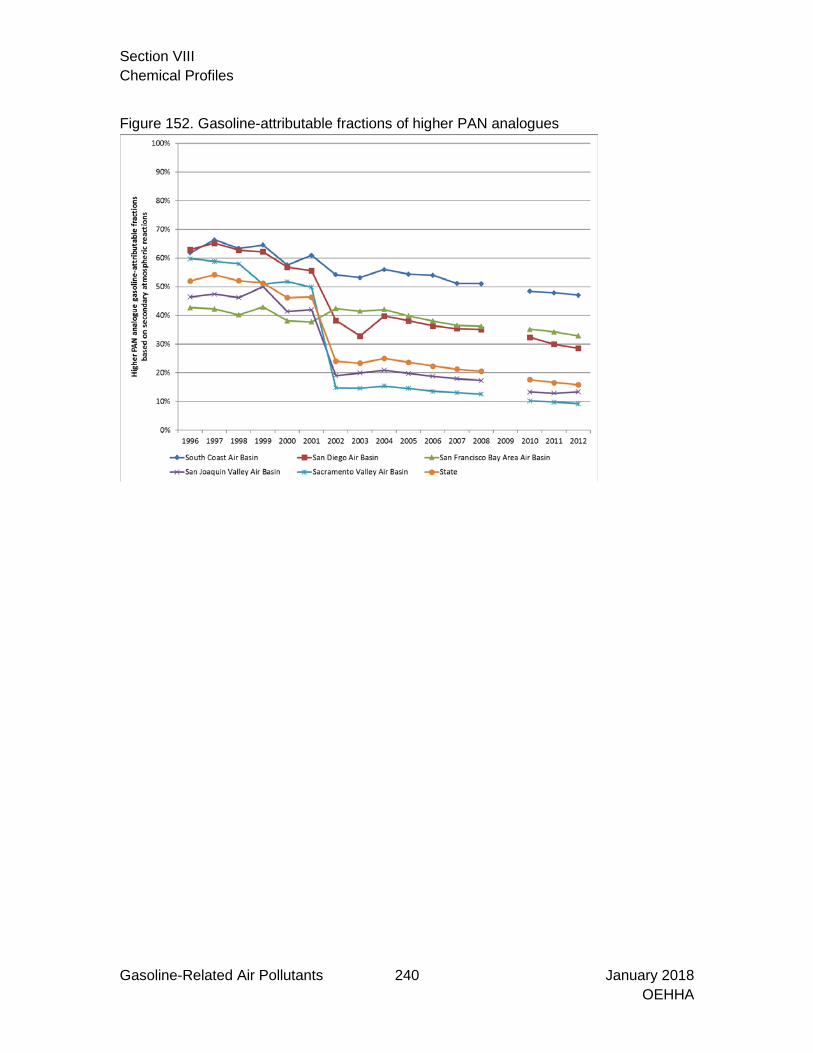
Section VIII Chemical Profiles
Gasoline-Related Air Pollutants 240 January 2018 OEHHA
Figure 152. Gasoline-attributable fractions of higher PAN analogues

Section VIII Chemical Profiles
Gasoline-Related Air Pollutants 241 January 2018 OEHHA
Unsaturated PAN Analogues: Exposure Assessment Results
Secondary atmospheric reaction tonnage of unsaturated PAN analogues was calculated by applying formation potentials to Emission Inventory data, as described in Appendix E. In 2012, 9% of the estimated total tonnage of unsaturated PAN analogues in the South Coast Air Basin was formed from gasoline-related emissions, with other air basins having lower percentages. Precursor chemicals of unsaturated PAN analogues include acrolein and methacrolein, for example (Carter, 2001). The gasoline-related precursor chemicals that contributed most to the formation of unsaturated PAN analogues statewide in 2008 included (listed in order of highest contribution): 1,3-butadiene, acrolein, 2-methyl-2-propenal (methacrolein), crotonaldehyde and isoprene. Figure 153 shows that estimated statewide tonnage of unsaturated PAN analogues formed from gasoline-related sources declined from 2 tons per day in 1996 to 0.5 tons per day in 2012. Figure 154 illustrates the sources of secondary formation of unsaturated PAN analogues. Table 79 and Figure 155 show the gasoline-attributable fractions of unsaturated PAN analogues.

Section VIII Chemical Profiles
Gasoline-Related Air Pollutants 242 January 2018 OEHHA
Figure 153. Statewide annual tons of unsaturated PAN analogues formed through secondary atmospheric reactions (data from CARB Emission Inventory)
Figure 154. Sources that contributed to secondary formation of unsaturated PAN analogues in 2012
0
5
10
15
20
25
30
35
40
45
1996 1997 1998 1999 2000 2001 2002 2003 2004 2005 2006 2007 2008 2009 2010 2011 2012
Uns
atur
ated
PAN
ana
logu
es
from
seco
ndar
y at
mos
pher
ic re
actio
ns (t
ons p
er d
ay)
Tons of unsaturated PAN analogues from non-gasoline-related sources
Tons of unsaturated PAN analogues from gasoline-related sources
Apparent increase in tonnage is due to a CARB adjustment of natural source emissions in 2002
SC (G) SC (NG) SD (G) SD (NG) SF (G) SF (NG) SJV (G) SJV (NG) SV (G) SV (NG)CLEANING AND SURFACE COATINGS - - - - - < 0.01 - - - -FUEL COMBUSTION < 0.01 < 0.01 < 0.01 < 0.01 < 0.01 < 0.01 < 0.01 < 0.01 < 0.01 < 0.01INDUSTRIAL PROCESSES < 0.01 0.06 - 0.02 - 0.03 - 0.03 - 0.03MISCELLANEOUS PROCESSES - < 0.01 - 0.01 - < 0.01 - 0.01 - < 0.01NATURAL SOURCES - 1.67 - 1.69 - 2.81 - 3.68 - 7.12ON-ROAD MOTOR VEHICLES 0.08 < 0.01 0.02 < 0.01 0.06 < 0.01 0.03 < 0.01 0.02 < 0.01OTHER MOBILE SOURCES 0.08 0.03 0.02 0.03 0.03 0.07 0.02 0.04 0.02 0.02PETROLEUM PRODUCTION AND DISTRIBUTION < 0.01 < 0.01 < 0.01 < 0.01 < 0.01 < 0.01 < 0.01 < 0.01 < 0.01 < 0.01SOLVENT EVAPORATION - < 0.01 - < 0.01 - < 0.01 - 0.02 - < 0.01WASTE DISPOSAL - - - - - - - 0.03 - < 0.01
-
1.00
2.00
3.00
4.00
5.00
6.00
7.00
8.00
Uns
atur
ated
PAN
ana
logu
esfr
om se
cond
ary
atm
osph
eric
reac
tions
(t
ons p
er d
ay)
0.00

Section VIII Chemical Profiles
Gasoline-Related Air Pollutants 243 January 2018 OEHHA
Table 79. Gasoline-attributable fractions of unsaturated PAN analogues based on secondary reaction tonnage.
Year
South Coast
Air Basin
San Diego Air
Basin
San Francisco Bay Area Air Basin
San Joaquin
Valley Air Basin
Sacramento Valley Air
Basin State
1996 80% 79% 8% 54% 72% 25% 1997 83% 79% 8% 55% 70% 25% 1998 89% 79% 8% 57% 70% 25% 1999 83% 77% 8% 65% 38% 23% 2000 77% 72% 6% 49% 68% 19% 2001 76% 71% 6% 56% 49% 18% 2002 18% 5% 7% 3% 1% 3% 2003 18% 5% 6% 3% 1% 3% 2004 18% 5% 6% 3% 1% 3% 2005 17% 5% 5% 3% 1% 3% 2006 15% 4% 5% 2% 1% 2% 2007 14% 4% 5% 2% 1% 2% 2008 13% 4% 4% 2% 1% 2% 2009 -- -- -- -- -- -- 2010 11% 3% 3% 2% 1% 2% 2011 9% 3% 3% 1% 1% 1% 2012 9% 2% 3% 1% 1% 1%
Note: Mobile source emissions were unavailable for 2009. Figure 155. Gasoline-attributable fractions of unsaturated PAN analogues
0%
10%
20%
30%
40%
50%
60%
70%
80%
90%
100%
1996 1997 1998 1999 2000 2001 2002 2003 2004 2005 2006 2007 2008 2009 2010 2011 2012
Uns
atur
ated
PAN
ana
logu
es g
asol
ine-
attr
ibut
able
frac
tions
s ba
sed
on se
cond
ary
atm
osph
eric
reac
tions
South Coast Air Basin San Diego Air Basin San Francisco Bay Area Air Basin
San Joaquin Valley Air Basin Sacramento Valley Air Basin State
Apparent decline in gasoline-attributable fractions of unsaturated PAN analogues is due to CARB adjustment of natural source emissions. More specifically, estimated isoprene from natural sources increased dramatically in 2002.

Section VIII Chemical Profiles
Gasoline-Related Air Pollutants 244 January 2018 OEHHA
Peroxybenzoyl Nitrate and Other Aromatic PAN analogues (Aromatic Acyl Peroxynitrates): Exposure Assessment Results
Carter (2001) identified alkylbenzenes as precursor chemicals for atmospheric formation of aromatic peroxynitrates. The top five gasoline-related precursor chemicals that contributed to the formation of aromatic peroxynitrates statewide in 2012 were toluene, benzaldehyde, tolualdehyde, m-xylene and styrene. Secondary atmospheric reaction tonnage of aromatic peroxynitrates was calculated using formation potentials applied to Emission Inventory data as described in Appendix E. Figure 156 plots secondary formation tonnage of aromatic peroxynitrates from gasoline-related sources, which declined between 1996 and 2012. Figure 157 summarizes the sources of secondary formation of aromatic peroxynitrates. Table 80 and Figure 158 show the gasoline-attributable fractions of aromatic peroxynitrates. Statewide, in 2012, 49% of secondary formation emission tonnage of aromatic peroxynitrates came from gasoline-related sources.

Section VIII Chemical Profiles
Gasoline-Related Air Pollutants 245 January 2018 OEHHA
Figure 156. Statewide annual tons of aromatic acyl peroxynitrates formed through secondary atmospheric reactions (data from CARB Emission Inventory)
Figure 157. Sources of secondary formation of aromatic acyl peroxynitrates in 2012
-
0.5
1.0
1.5
2.0
2.5
3.0
3.5
4.0
4.5
5.0
1996 1997 1998 1999 2000 2001 2002 2003 2004 2005 2006 2007 2008 2009 2010 2011 2012
Arom
atic
acy
l per
oxyn
itrat
es
from
seco
ndar
y at
mos
pher
ic re
actio
ns (t
ons p
er d
ay)
Tons of aromatic acyl peroxynitrates from non-gasoline-related sources
Tons of aromatic acyl peroxynitrates from gasoline-related sources
SC (G) SC (NG) SD (G) SD (NG) SF (G) SF (NG) SJV (G) SJV (NG) SV (G) SV (NG)CLEANING AND SURFACE COATINGS - 0.09 - 0.04 - 0.04 - 0.04 - 0.02FUEL COMBUSTION < 0.01 < 0.01 < 0.01 < 0.01 < 0.01 < 0.01 < 0.01 < 0.01 < 0.01 < 0.01INDUSTRIAL PROCESSES < 0.01 0.14 - 0.18 - 0.05 - 0.04 - 0.06MISCELLANEOUS PROCESSES - < 0.01 - < 0.01 - < 0.01 - < 0.01 - < 0.01NATURAL SOURCES - - - - - - - < 0.01 - -ON-ROAD MOTOR VEHICLES 0.25 0.01 0.06 < 0.01 0.16 < 0.01 0.08 0.01 0.07 < 0.01OTHER MOBILE SOURCES 0.19 0.02 0.05 < 0.01 0.07 0.02 0.05 0.03 0.05 0.01PETROLEUM PRODUCTION AND DISTRIBUTION < 0.01 < 0.01 < 0.01 < 0.01 < 0.01 < 0.01 < 0.01 < 0.01 < 0.01 < 0.01SOLVENT EVAPORATION - 0.07 - 0.02 - 0.04 - 0.02 - 0.02WASTE DISPOSAL - 0.03 - 0.01 - < 0.01 - 0.06 - 0.02
-
0.05
0.10
0.15
0.20
0.25
0.30
0.35
0.40
0.45
0.50
Arom
atic
acy
l per
oxyn
itrat
es
from
seco
ndar
y at
mos
pher
ic re
actio
ns
(ton
s per
day
)
0.00

Section VIII Chemical Profiles
Gasoline-Related Air Pollutants 246 January 2018 OEHHA
Table 80. Gasoline-attributable fractions of peroxybenzoyl nitrate and other aromatic acyl peroxynitrates are based on secondary reaction tonnage only.
Year South
Coast Air Basin
San Diego Air Basin
San Francisco
Bay Area Air Basin
San Joaquin
Valley Air Basin
Sacramento Valley Air
Basin State
1996 69% 67% 60% 68% 52% 65% 1997 63% 67% 58% 67% 50% 62% 1998 65% 66% 57% 67% 50% 63% 1999 62% 64% 60% 70% 64% 64% 2000 54% 58% 55% 60% 47% 56% 2001 64% 57% 54% 62% 60% 61% 2002 66% 66% 65% 59% 68% 66% 2003 66% 52% 66% 54% 63% 63% 2004 67% 65% 66% 51% 67% 65% 2005 67% 64% 62% 53% 66% 64% 2006 68% 64% 61% 52% 64% 64% 2007 64% 62% 59% 51% 63% 62% 2008 63% 62% 59% 52% 63% 62% 2009 -- -- -- -- -- -- 2010 59% 35% 60% 45% 49% 54% 2011 57% 32% 59% 47% 47% 52% 2012 54% 30% 58% 38% 45% 49%
Note: Mobile source emissions were unavailable for 2009. Figure 158. Gasoline-attributable fractions of peroxybenzoyl nitrate and other aromatic acyl peroxynitrates
0%
10%
20%
30%
40%
50%
60%
70%
80%
90%
100%
1996 1997 1998 1999 2000 2001 2002 2003 2004 2005 2006 2007 2008
Gas
olin
e-at
trib
utab
le fr
actio
ns o
f pe
roxy
benz
oyl n
itrat
e a
nd o
ther
ar
omat
ic a
cyl p
erox
ynitr
ates
South Coast Air Basin San Diego Air Basin San Francisco Bay Area Air BasinSan Joaquin Valley Air Basin Sacramento Valley Air Basin State

Section VIII Chemical Profiles
Gasoline-Related Air Pollutants 247 January 2018 OEHHA
Chemical Profiles: Gasoline-Related PAHs This section presents exposure and screening risk assessment results for selected gasoline-related PAHs. We present summary graphs and tables of available ambient air measurements. Population-weighted annual average ambient air concentrations were also calculated for the South Coast Air Basin for selected PAHs. Sources of ambient air PAH measurements that we located are described below: • US EPA NATTS measured ambient air concentrations of PAHs from 3 monitoring sites in
California: San Jose in Santa Clara County, Rubidoux in Riverside County and Main Street in Los Angeles between 2008 and 2014. The samples were collected over 24-hour periods at six-day intervals throughout the year.
• California Air Toxic Monitoring Network monitored the following particle-bound PAHs: benzo[a]pyrene, benzo[b]fluoranthene, benzo[ghi]perylene, benzo[k]fluoranthene, dibenz[ah]anthracene, and indeno[1,2,3-cd]pyrene. Monitoring of these ended in February 2005 because the calculated health risks were low.
• Multiple Air Toxics Exposure Study III (MATES III) measured ambient air concentrations of 16 PAHs at three sites in Southern California between Dec 2004 and March 2005. The monitoring sites are listed in the following table.
Site Address City County Air Basin Central Los Angeles 1630 N. Main St. Los Angeles Los Angeles South Coast Riverside (Rubidoux) 5888 Mission Blvd. Riverside Riverside South Coast North Long Beach 3648 N. Long Beach Blvd. Long Beach Los Angeles South Coast
• Eiguren-Fernandez et al. (2004) measured ambient air concentrations of PAHs at six
schools in Southern California between 2001 and 2002. Particle-bound and vapor phase PAHs were measured. In the tables below, the particle-bound and vapor-phase concentrations are tabulated separately. In the plots of ambient air concentrations that appear in the main report, the particle-bound and vapor-phase concentrations were added. The schools where samples were collected were located in the cities listed in the table below.
City County Atascadero San Luis Obispo Lompoc Santa Barbara San Dimas Los Angeles Upland San Bernardino Mira Loma Riverside Riverside Riverside
Additional data sources were available for naphthalene, and are described in the
naphthalene section below.

Section VIII Chemical Profiles
Gasoline-Related Air Pollutants 248 January 2018 OEHHA
Gasoline-Related PAHs in the Emission Inventory
Naphthalene: Exposure and Screening Risk Assessment Results Naphthalene is a carcinogen and a respiratory toxicant and had the 95th highest primary emissions from gasoline-related sources in 2012 among all gasoline-related VOCs. Figure 159 shows that the statewide emissions of naphthalene from gasoline-related sources declined between 1996 and 2012. Estimated naphthalene emissions from gasoline-related sources appeared to increase between 2003 and 2004 when the Emission Inventory was changed to account for the phase out of MTBE, but then declined again over the next eight years. Schifter et al. (2013) examined emissions from high emitting vehicles powered by different gasoline-blends and found that changing from MTBE to ethanol had no impact on naphthalene emissions from high emitting vehicles. Figure 160 and Figure 161 show the emission sources and gasoline-attributable fractions of naphthalene (see Table 81 also). Statewide, in 2012, 33% of naphthalene emissions came from gasoline-related sources including cars, trucks, motorcycles, lawn and garden equipment and recreational boats. Non-gasoline-related sources of naphthalene included aircraft, construction and mining equipment, consumer products, asphalt paving and concrete production. Gasoline-attributable fractions increased between 2003 and 2004 because mobile source emissions were estimated to contain more naphthalene. The gasoline-attributable fractions for naphthalene in the South Coast and San Francisco Bay Area Air Basins increased between 2008 and 2010 because of a decrease in the modeled naphthalene emissions from solvent evaporation. In a study of 15 US EPA priority PAHs in Southern California ambient air, Eiguren-Fernandez et al. (2004) found that vapor phase PAHs accounted for more than 99.9% of measured PAH mass and that naphthalene made up 91% of PAH mass. Naphthalene is not routinely monitored in California, so we searched for available studies that included ambient air measurements of this PAH. We found nine relevant studies, although none of these studies spanned the entire time period of interest for the current report (1996 to 2014). We used two sets of data from the South Coast Air Basin as the basis for modeling naphthalene air concentrations over time, and used the other studies we located for validation. The first model was based on data collected during the summer of 1996 by the Desert Research Institute (DRI) (Zielinska et al., 1999; complete dataset obtained from those authors). The second model was based on data from 2007 to 2014 collected by the NATTS (https://www3.epa.gov/ttnamti1/natts.html). The models are described in Appendix D. The population-weighted annual average ambient air concentrations were calculated based on modeled values (Tables 82 and 83). The model based on 1996 DRI data produced population-weighted annual average concentrations that ranged from 0.15 ppb in 1996 to 0.077 ppb in 2014. The model based on 2007-2014 NATTS data gave population-weighted annual averages that ranged from 0.048 ppb in 1996 to 0.014 ppb in 2014. Other measurements of ambient air naphthalene concentrations have been made in and around the South Coast Air Basin, and we used those to compare with our model results (Figure 162). The 1996 model produced

Section VIII Chemical Profiles
Gasoline-Related Air Pollutants 249 January 2018 OEHHA
estimates that are higher than the measured values from more recent studies. The 2007-2014 model seems to underestimate the 1996 ambient air concentrations. Naphthalene annual average concentrations appear to range from about 0.15 ppb in 1996 to 0.016 ppb in 2014. Cancer risks were calculated based on gasoline-attributable ambient air concentrations (see Appendix G for details). Based on the 1996 modeled values, the gasoline-attributable cancer risk of naphthalene in the South Coast Air Basin was 4.4x10⁻⁵ in 1996. Based on the 2007-2014 modeled values, the gasoline-attributable cancer risk of naphthalene in the South Coast Air Basin was 4.8x10⁻⁶ in 2014. Our estimates indicate an approximate reduction of 40 estimated cancer cases per 1 million people between 1996 and 2014 in the South Coast region. There were inadequate data to calculate a statewide hazard quotient for naphthalene.

Section VIII Chemical Profiles
Gasoline-Related Air Pollutants 250 January 2018 OEHHA
Figure 159. Annual naphthalene emissions from gasoline and non-gasoline-related sources in California (data from CARB Emission Inventory)
Figure 160. Emission sources of naphthalene in 2012
0.0
0.5
1.0
1.5
2.0
2.5
1996 1997 1998 1999 2000 2001 2002 2003 2004 2005 2006 2007 2008 2009 2010 2011 2012
Nap
htha
lene
(ton
s per
day
)
Naphthalene from gasoline-related sources Naphthalene from non-gasoline-related sources
Apparent decline in non-gasoline-related naphthalene was due to a change in the EmissionInventory's solvent evaporation category
SC (G) SC (NG) SD (G) SD (NG) SF (G) SF (NG) SJV (G) SJV (NG) SV (G) SV (NG)CLEANING AND SURFACE COATINGS - 0.02 - 0.01 - 0.01 - 0.01 - < 0.01FUEL COMBUSTION < 0.01 < 0.01 < 0.01 < 0.01 < 0.01 < 0.01 < 0.01 < 0.01 < 0.01 < 0.01INDUSTRIAL PROCESSES < 0.01 0.02 - 0.01 - 0.02 - 0.01 - 0.03MISCELLANEOUS PROCESSES - < 0.01 - < 0.01 - < 0.01 - < 0.01 - < 0.01NATURAL SOURCES - - - - - - - - - -ON-ROAD MOTOR VEHICLES 0.13 < 0.01 0.03 < 0.01 0.08 < 0.01 0.04 < 0.01 0.03 < 0.01OTHER MOBILE SOURCES 0.07 0.03 0.02 0.02 0.03 0.05 0.02 0.04 0.02 0.02PETROLEUM PRODUCTION AND DISTRIBUTION < 0.01 < 0.01 < 0.01 < 0.01 < 0.01 < 0.01 < 0.01 < 0.01 < 0.01 < 0.01SOLVENT EVAPORATION - 0.08 - 0.10 - 0.05 - 0.06 - 0.11WASTE DISPOSAL - - - - - - < 0.01 - < 0.01
-
0.05
0.10
0.15
0.20
0.25
Nap
htha
lene
in p
rimar
y em
issi
ons (
tons
per
day
)
0.00
Consumer products and asphalt paving

Section VIII Chemical Profiles
Gasoline-Related Air Pollutants 251 January 2018 OEHHA
Table 81. Naphthalene gasoline-attributable fractions
Year
South Coast
Air Basin
San Diego
Air Basin
San Francisco Bay Area Air Basin
San Joaquin Valley
Air Basin
Sacramento Valley
Air Basin State
1996 46% 36% 42% 36% 31% 40% 1997 45% 34% 38% 34% 28% 37% 1998 47% 35% 38% 33% 29% 38% 1999 45% 35% 44% 35% 29% 38% 2000 38% 30% 41% 29% 24% 33% 2001 43% 29% 39% 29% 25% 34% 2002 40% 26% 38% 25% 20% 31% 2003 41% 27% 38% 26% 20% 32% 2004 48% 33% 45% 32% 26% 38% 2005 46% 31% 43% 31% 25% 37% 2006 45% 29% 41% 29% 23% 35% 2007 42% 28% 39% 28% 22% 33% 2008 41% 27% 39% 28% 22% 33% 2009 -- -- -- -- -- -- 2010 58% 27% 46% 33% 19% 35% 2011 57% 24% 45% 32% 18% 33% 2012 56% 23% 43% 31% 22% 33%
Note: Mobile source emissions were not available for 2009. Figure 161. Naphthalene gasoline-attributable fractions
0%
10%
20%
30%
40%
50%
60%
70%
80%
90%
100%
1996 1997 1998 1999 2000 2001 2002 2003 2004 2005 2006 2007 2008 2009 2010 2011 2012
Nap
htha
lene
gas
olin
e-at
trib
utab
le fr
actio
ns
South Coast Air Basin San Diego Air Basin
San Francisco Bay Area Air Basin San Joaquin Valley Air Basin
Sacramento Valley Air Basin State

Section VIII Chemical Profiles
Gasoline-Related Air Pollutants 252 January 2018 OEHHA
Table 82. Results for naphthalene in the South Coast Air Basin based on 1996 model
Year
Population-weighted average concentration of
naphthalene (ng/m3)
Population-weighted average concentration of
naphthalene (ppbv)
Gasoline-attributable
fraction
Gasoline-attributable
concentration (ppbv)
1996 812 0.15 46% 0.071 1997 778 0.15 45% 0.067 1998 760 0.14 47% 0.068 1999 729 0.14 45% 0.062 2000 680 0.13 38% 0.049 2001 640 0.12 43% 0.052 2002 611 0.12 40% 0.047 2003 596 0.11 41% 0.046 2004 538 0.10 48% 0.050 2005 495 0.094 46% 0.044 2006 482 0.092 45% 0.042 2007 464 0.089 42% 0.038 2008 434 0.083 41% 0.034 2009 418 0.080 41% 0.033 2010 428 0.082 58% 0.047 2011 412 0.079 57% 0.045 2012 418 0.080 56% 0.044 2013 412 0.079 56% 0.044 2014 403 0.077 56% 0.043
Notes: The 2009 gasoline-attributable concentration was calculated with the 2008 gasoline-attributable fraction. The 2013 and 2014 gasoline-attributable concentrations were calculated with the 2012 gasoline-attributable fraction.

Section VIII Chemical Profiles
Gasoline-Related Air Pollutants 253 January 2018 OEHHA
Table 83. Results for naphthalene in the South Coast Air Basin based on 2007-2014 model
Year
Population-weighted average concentration of
naphthalene (ng/m3)
Population-weighted average concentration of
naphthalene (ppbv)
Gasoline-attributable
fraction
Gasoline-attributable
concentration (ppbv)
1996 251 0.048 46% 0.022 1997 234 0.045 45% 0.020 1998 227 0.043 47% 0.020 1999 214 0.041 45% 0.018 2000 191 0.036 38% 0.014 2001 172 0.033 43% 0.014 2002 159 0.030 40% 0.012 2003 152 0.029 41% 0.012 2004 129 0.025 48% 0.012 2005 113 0.022 46% 0.0100 2006 107 0.020 45% 0.0093 2007 99 0.019 42% 0.0080 2008 89 0.017 41% 0.0070 2009 86 0.016 41% 0.0068 2010 85 0.016 58% 0.0094 2011 80 0.015 57% 0.0086 2012 85 0.016 56% 0.0091 2013 79 0.015 56% 0.0083 2014 72 0.014 56% 0.0076
Notes: The 2009 gasoline-attributable concentration was calculated with the 2008 gasoline-attributable fraction. The 2013 and 2014 gasoline-attributable concentrations were calculated with the 2012 gasoline-attributable fraction.

Section VIII Chemical Profiles
Gasoline-Related Air Pollutants 254 January 2018 OEHHA
Figure 162. Comparison of modeled annual average naphthalene concentration to naphthalene measurements from other studies
0.1
1
10
100
1000
10000
100000
1992 1994 1996 1998 2000 2002 2004 2006 2008 2010 2012 2014 2016
Nap
htha
lene
(ng/
m3 )
Fraser Gupta DRI Azusa DRI Burbank DRI Los Angeles
SCOS97 Azusa SCOS97 Banning SCOS97 Los Angeles SCOS97 Riverside EF Riverside
EF San Dimas EF Mira Loma EF Upland EF Long Beach Reisen Los Angeles
Reisen Riverside Reisen Los Angeles Reisen Riverside MATES III Los Angeles MATES III Rubidoux
MATES III Wilmington Nishino Upland NATTS Rubidoux NATTS Los Angeles Pop. Wt. Ann. Avg DRI
Pop. Wt. Ann. Avg. NATTS
1996 Model
2007 - 2014 Model

Section VIII Chemical Profiles
Gasoline-Related Air Pollutants 255 January 2018 OEHHA
Notes for Figure 162: 1. Vertical lines range from minimum to maximum value in the study. 2. The 1996 model is based on naphthalene data collected by the Desert Research Institute
(DRI) in 1996 (Zielinska et al., 1999). 3. The 2007-2014 model is based on data collected from the NATTS between 2007 and 2014. 4. References:
a. Fraser et al. (1998b) collected naphthalene samples during a smog episode Sept 8-9, 1993
b. Gupta et al. (1996) collected 12 naphthalene samples in Oct. 1994 c. DRI collected naphthalene samples during summer months of 1995 and 1996 (Zielinska
et al., 1999) d. SCOS97 - data collected by Arey as part of Southern California Ozone Study e. EF - data described in Eiguren-Fernandez et al. (2004), summary statistics reported in
Lu et al. (2005) f. Reisen - summary statistics from Lu et al. (2005), based on data in Reisen (2003) and
Reisen and Arey (2005) g. MATES III – Multiple Air Toxics Exposure Study in the South Coast Air Basin h. Nishino et al. (2008) i. NATTS – Naphthalene (total suspended particulate) data downloaded from
https://aqs.epa.gov/api

Section VIII Chemical Profiles
Gasoline-Related Air Pollutants 256 January 2018 OEHHA
1-Methylnaphthalene: Exposure Assessment Results The estimated gasoline-related primary emissions of 1-methylnaphthalene increased in 2004, which was associated with the replacement of MTBE with ethanol and reflected in revised speciation profiles in the Emission Inventory. The estimated statewide gasoline-attributable fraction for 1-methylnaphthalene was at its lowest in 2002-2003 (41%), rising to 98% in 2004 and staying at or above that value since then (Table 84). We did not locate ambient air measurements for 1-methylnaphthalene in the sources we consulted for ambient air PAH data (see the beginning of the PAH Chemical Profiles for a description of these sources). Table 84. Statewide tonnage and gasoline-attributable fractions of 1-methylnaphthalene
Year Gasoline-attributable emissions
(tons per day)
Total emissions
(tons per day)
Gasoline-attributable
fraction 1996 0.012 0.012 100% 1997 0.0047 0.0047 100% 1998 0.0049 0.0049 100% 1999 0.010 0.010 100% 2000 0.021 0.032 66% 2001 0.019 0.030 63% 2002 0.0071 0.018 41% 2003 0.0066 0.016 41% 2004 0.13 0.13 98% 2005 0.12 0.12 98% 2006 0.11 0.11 98% 2007 0.10 0.10 97% 2008 0.095 0.095 100% 2009 -- -- -- 2010 0.093 0.093 99% 2011 0.082 0.083 99% 2012 0.078 0.078 99%
Note: Mobile source emissions were unavailable for 2009.
2-Methylnaphthalene: Exposure Assessment Results The estimated gasoline-related primary emissions of 2-methylnaphthalene increased in 2004 as was true for 1-methylnaphthalene. The increases were associated with the replacement of MTBE with ethanol and reflected in adjustments to speciation profiles in the Emission Inventory. The estimated statewide gasoline-attributable fractions of 2-methylnaphthalene were about 5% or less until 2004, increasing to close to 20-30% in 2004 and later (Table 85). The fractions are lower for 2-methylnaphthalene compared to 1-methylnaphthalene, because

Section VIII Chemical Profiles
Gasoline-Related Air Pollutants 257 January 2018 OEHHA
2-methylnaphthalene is also part of the mixture “naphtha”, which is emitted by some non-gasoline-related sources. We did not locate ambient air measurements for 2-methylnaphthalene. Table 85. Statewide tonnage and gasoline-attributable fractions of 2-methylnaphthalene
Year Gasoline-attributable emissions
(tons per day)
Total emissions
(tons per day)
Gasoline-attributable
fraction
1996 0.029 0.838 3% 1997 0.011 0.851 1% 1998 0.011 0.838 1% 1999 0.024 0.862 3% 2000 0.049 0.860 6% 2001 0.043 0.808 5% 2002 0.017 0.749 2% 2003 0.016 0.753 2% 2004 0.306 1.057 29% 2005 0.278 1.033 27% 2006 0.252 1.007 25% 2007 0.233 0.993 23% 2008 0.221 0.965 23% 2009 -- -- -- 2010 0.206 0.896 23% 2011 0.183 0.856 21% 2012 0.172 0.802 21%
Note: Mobile source emissions were unavailable for 2009.

Section VIII Chemical Profiles
Gasoline-Related Air Pollutants 258 January 2018 OEHHA
Other Gasoline-Related PAHs with Some Ambient Air Data
PAHs measured by the California Toxic Monitoring Network were benzo[a]pyrene, benzo[b]fluoranthene, benzo[k]fluoranthene, benzo[ghi]perylene, indeno[1,2,3-cd]pyrene and dibenz[ah]anthracene. We used these measurements to estimate population-weighted annual average ambient air concentrations for the South Coast Air Basin. Measurements from other studies are also included in the discussion below for comparison. We also report cancer risk estimates where possible. For PAHs not included in the California Toxic Monitoring Network, we located some ambient air measurements and these data are summarized in the relevant sections below.

Section VIII Chemical Profiles
Gasoline-Related Air Pollutants 259 January 2018 OEHHA
Acenaphthene: Summary of Ambient Air Measurements A few studies have measured acenaphthene in ambient air. Descriptions of these studies are on page 247. Figure 163 contains a plot of the first quartile, median and third quartile of these measurements. The data used to create the plot are tabulated below. The annual average and standard deviation from the Eiguren-Fernandez et al. and MATES III studies were used to estimate the quartiles for the plot by assuming the data came from a lognormal distribution. Figure 163. Acenaphthene ambient air measurements
Note: Vertical bars show first quartile, median and third quartile
0.00
2.00
4.00
6.00
8.00
10.00
12.00
14.00
16.00
2000 2002 2004 2006 2008 2010 2012 2014 2016
Acen
apht
hene
(ng/
m3 )
Eiguren-Fernandez et al. - San Dimas , Los Angeles County Eiguren-Fernandez et al. - Upland , San Bernardino County
Eiguren-Fernandez et al. - Mira Loma , Riverside County Eiguren-Fernandez et al. - Riverside , Riverside County
MATES III - Central Los Angeles MATES III - Riverside
MATES III - Long Beach US EPA NATTS North Long Beach
US EPA NATTS Los Angeles-North Main Street US EPA NATTS Riverside-Rubidoux
US EPA NATTS San Jose-Jackson Street

Section VIII Chemical Profiles
Gasoline-Related Air Pollutants 260 January 2018 OEHHA
The following box provides further details on acenaphthene ambient air measurements displayed in Figure 163.
Eiguren-Fernandez et al. (2004) Site Time Particle phase (pg/m3) Vapor phase (ng/m3)
Average SD Average SD Atascadero May 2001-July 2002 2.09 3.61 2.51 2.18 Lompoc May 2001-July 2002 2.56 2.46 2.16 1.39 San Dimas May 2001-July 2002 3.17 5.49 5.83 2.39 Upland May 2001-July 2002 0.39 0.67 10.6 6.78 Mira Loma May 2001-July 2002 0.76 1.31 12.9 3.55 Riverside May 2001-July 2002 1.32 2.29 4.58 2
MATES III (ng/m3)
Site Year Average SD Central Los Angeles 2005 7.61 4.76 Riverside 2005 4.65 2.92 North Long Beach 2005 8.49 6.70
US EPA NATTS (ng/m3)
Site Year N Percent
non-detect
Minimum First Quartile Median Third
Quartile Maximum Average S D
Los Angeles-North Main Street
2007 39 13% 0.035 1.6 2.4 3.4 9.5 2.7 2008 61 0% 1.4 2.4 3.4 5.6 17 4.7 2009 60 2% 0.034 3.7 6.1 8 44 7 2010 59 0% 0.53 3.1 4.9 8 25 6.1 2011 59 0% 0.76 2.7 4.3 6.3 15 4.9 2012 60 0% 1.3 3.2 4.8 7.1 12 5.4 2013 58 0% 0.63 2.9 3.9 5.3 12 4.3 2014 56 0% 0.79 2.8 4.1 5.8 9.5 4.4 2015 39 0% 0.86 1.9 3.2 5.3 7.2 3.7
North Long Beach
2012 26 0% 0.87 1.6 2.4 2.8 3.5 2.2 2013 29 0% 0.31 0.91 1.4 2.3 4.4 1.7
Riverside-Rubidoux
2007 55 4% 0.055 1.1 1.8 2.6 5.7 2 2008 71 1% 0.031 1.2 2 2.6 5.6 2.1 2009 64 2% 0.021 1.4 1.9 2.9 6.3 2.4 2010 65 2% 0.032 1.1 1.7 2.7 5.8 2.1 2011 67 0% 0.18 1.1 2.1 3.4 7.8 2.6 2012 67 0% 0.61 1.6 2.1 3.5 8.2 2.6 2013 64 0% 0.39 1.4 2.1 3 7.2 2.4 2014 65 2% 0.048 1.4 2 3.6 6.2 2.5 2015 48 33% 0.033 0.035 1 1.5 4.1 1.1
San Jose-Jackson Street
2008 40 0% 0.56 1 1.3 1.8 3 1.5 2009 61 2% 0.028 0.73 1.1 1.7 4.8 1.3 2010 59 0% 0.44 0.85 1.2 1.6 3.9 1.3 2011 61 0% 0.41 0.72 1.4 2.2 5.3 1.5 2012 59 0% 0.35 0.85 1.2 1.5 3.2 1.3 2013 59 0% 0.61 1.2 1.6 2.4 4.1 1.8 2014 59 2% 0.074 1.2 1.8 2.3 23 2.1 2015 43 33% 0.054 0.055 0.86 1.1 1.9 0.75
Note: Half the limit of detection substituted for non-detects

Section VIII Chemical Profiles
Gasoline-Related Air Pollutants 261 January 2018 OEHHA
Acenaphthylene: Summary of Ambient Air Measurements A few studies have measured acenaphthylene in ambient air. Descriptions of these studies are on page 247. Figure 164 contains a plot of the first quartile, median and third quartile of these measurements. The data used to create the plot are tabulated below. The annual average and standard deviation from the Eiguren-Fernandez et al. and MATES III studies were used to estimate the quartiles for the plot by assuming the data came from a lognormal distribution. Figure 164. Acenaphthylene ambient air measurements
Note: Vertical bars show first quartile, median and third quartile
0.00
1.00
2.00
3.00
4.00
5.00
6.00
7.00
2004 2006 2008 2010 2012 2014 2016
Acen
apht
hyle
ne (n
g/m
3 )
MATES III - Central Los Angeles MATES III - Riverside MATES III - North Long Beach Los Angeles-North Main Street
North Long Beach Riverside-Rubidoux San Jose-Jackson Street

Section VIII Chemical Profiles
Gasoline-Related Air Pollutants 262 January 2018 OEHHA
The following box provides further details on acenaphthylene ambient air measurements displayed in Figure 164. MATES III (2005) (ng/m3)
Average SD Central Los Angeles 5.08 4.05 Riverside 4.4 4.5 North Long Beach 5.23 5.38
US EPA (ng/m3)
Site Year N P
erce
nt
non-
dete
ct
Min
imum
Firs
t Q
uarti
le
Med
ian
Third
Q
uarti
le
Max
imum
Ave
rage
Sta
ndar
d D
evia
tion
Los Angeles-North Main Street
2007 39 41% 0.025 0.03 0.18 0.84 5.2 0.8 1.4 2008 61 26% 0.019 0.033 1.1 2.2 6.6 1.5 1.6 2009 60 45% 0.026 0.035 0.38 2.4 11 1.4 2.2 2010 59 53% 0.016 0.027 0.04 1.7 5.1 0.93 1.3 2011 59 44% 0.016 0.021 0.51 1.5 7.3 1.2 1.7 2012 60 53% 0.011 0.014 0.02 1.1 4.2 0.67 1 2013 58 60% 0.016 0.019 0.024 1.1 5.3 0.78 1.3 2014 56 64% 0.007 0.0071 0.0089 0.71 4 0.43 0.77 2015 39 74% 0.026 0.028 0.028 0.32 2.3 0.32 0.57
North Long Beach
2012 26 62% 0.013 0.015 0.021 0.37 4.9 0.45 1 2013 29 66% 0.018 0.021 0.023 0.49 5.4 0.7 1.3
Riverside-Rubidoux
2007 55 51% 0.025 0.03 0.06 0.8 8.4 1 1.9 2008 71 34% 0.016 0.022 0.4 1.1 3.9 0.82 0.97 2009 64 55% 0.021 0.027 0.035 0.67 9 0.84 1.8 2010 65 60% 0.016 0.022 0.028 0.51 7.8 0.58 1.3 2011 67 64% 0.018 0.023 0.031 0.61 7.5 0.48 1.1 2012 67 51% 0.014 0.019 0.028 0.53 4 0.5 0.92 2013 64 55% 0.019 0.023 0.029 0.75 6.2 0.62 1.1 2014 65 60% 0.0069 0.0084 0.011 0.55 4.4 0.48 0.89 2015 48 77% 0.027 0.028 0.028 0.032 1.5 0.14 0.29
San Jose-Jackson Street
2008 40 33% 0.025 0.026 0.44 1.4 6.1 1.1 1.5 2009 61 48% 0.03 0.032 0.17 0.98 7.2 1.1 1.9 2010 59 51% 0.024 0.025 0.026 0.79 8.3 0.69 1.4 2011 61 56% 0.02 0.021 0.022 0.88 13 1.2 2.6 2012 59 47% 0.016 0.017 0.13 0.55 7.7 0.86 1.8 2013 59 51% 0.025 0.026 0.028 1.6 11 1.3 2.3 2014 59 51% 0.01 0.011 0.012 0.52 8.8 0.81 1.7 2015 43 74% 0.042 0.044 0.045 0.14 3.4 0.41 0.89
Note: Half the limit of detection substituted for non-detects

Section VIII Chemical Profiles
Gasoline-Related Air Pollutants 263 January 2018 OEHHA
Anthracene: Summary of Ambient Air Measurements A few studies have measured anthracene in ambient air. Descriptions of these studies are on page 247. Figure 165 contains a plot of the first quartile, median and third quartile of these measurements. The data used to create the plot are tabulated below. The annual average and standard deviation from the Eiguren-Fernandez et al. and MATES III studies were used to estimate the quartiles for the plot by assuming the data came from a lognormal distribution. Figure 165. Anthracene ambient air measurements
Note: Vertical bars show first quartile, median and third quartile
0.00
0.20
0.40
0.60
0.80
1.00
1.20
1.40
1.60
1.80
2.00
2000 2002 2004 2006 2008 2010 2012 2014 2016
Anth
race
ne (n
g/m
3 )
Eiguren-Fernandez et al. - San Dimas Eiguren-Fernandez et al. - Upland
Eiguren-Fernandez et al. - Mira Loma Eiguren-Fernandez et al. - Riverside
MATES III - Central Los Angeles MATES III - Riverside
MATES III - North Long Beach US EPA NATTS Los Angeles-North Main Street
US EPA NATTS North Long Beach US EPA NATTS Riverside-Rubidoux
US EPA NATTS San Jose-Jackson Street

Section VIII Chemical Profiles
Gasoline-Related Air Pollutants 264 January 2018 OEHHA
Box below provides more details on ambient air measurements of anthracene in Figure 165 Eiguren-Fernandez et al. (2004)
Site Time Particle phase (pg/m3) Vapor phase (ng/m3) Average SD Average SD
Atascadero May 2001-July 2002 0.16 0.15 0.73 0.29 Lompoc May 2001-July 2002 2.05 2.62 0.13 0.15 San Dimas May 2001-July 2002 3.18 3.45 1.4 1.07 Upland May 2001-July 2002 1.87 1.85 0.36 0.19 Mira Loma May 2001-July 2002 2.77 4.8 0.59 0.4 Riverside May 2001-July 2002 2.3 2.6 1.1 0.87
MATES III (2005) (ng/m3)
Site Average SD Central Los Angeles 1.19 3.07 Riverside 0.72 1.62 North Long Beach 1.07 2.53
US EPA National Air Toxics Trend Stations (ng/m3)
Site Year N
Per
cent
no
n-de
tect
Min
imum
Firs
t Q
uarti
le
Med
ian
Third
Q
uarti
le
Max
imum
Ave
rage
Sta
ndar
d D
evia
tion
Los Angeles-North Main Street
2007 39 51% 0.03 0.045 0.072 0.37 1.2 0.23 0.28 2008 61 56% 0.015 0.02 0.026 0.55 2.1 0.35 0.48 2009 60 37% 0.028 0.042 0.41 0.92 4 0.63 0.8 2010 59 27% 0.018 0.036 0.42 0.79 13 0.72 1.7 2011 59 15% 0.019 0.18 0.36 0.64 1.6 0.46 0.38 2012 60 5% 0.019 0.36 0.49 0.78 1.5 0.54 0.29 2013 58 14% 0.012 0.24 0.38 0.57 0.98 0.43 0.27 2014 56 13% 0.023 0.27 0.4 0.52 0.94 0.39 0.23 2015 39 21% 0.028 0.12 0.2 0.36 0.67 0.24 0.18
North Long Beach
2012 26 23% 0.017 0.1 0.2 0.25 0.98 0.23 0.22 2013 29 21% 0.014 0.12 0.18 0.29 1.2 0.27 0.28
Riverside-Rubidoux
2007 55 60% 0.035 0.04 0.065 0.39 4.5 0.38 0.83 2008 71 63% 0.014 0.016 0.021 0.31 4.1 0.26 0.65 2009 64 55% 0.022 0.029 0.038 0.37 4.4 0.32 0.69 2010 65 31% 0.018 0.031 0.23 0.47 1.6 0.32 0.32 2011 67 31% 0.018 0.04 0.21 0.32 1.1 0.24 0.24 2012 67 31% 0.021 0.026 0.22 0.4 6.4 0.38 0.82 2013 64 38% 0.015 0.018 0.17 0.3 1.3 0.22 0.24 2014 65 49% 0.023 0.027 0.095 0.33 1.3 0.21 0.26 2015 48 71% 0.028 0.03 0.03 0.086 0.54 0.075 0.1
San Jose-Jackson Street
2008 40 58% 0.021 0.022 0.022 0.28 0.92 0.18 0.24 2009 61 46% 0.034 0.035 0.11 0.35 2.9 0.32 0.54 2010 59 25% 0.027 0.028 0.22 0.4 2.8 0.32 0.43 2011 61 10% 0.027 0.13 0.2 0.35 1.3 0.3 0.29 2012 59 3% 0.022 0.15 0.22 0.36 1 0.29 0.21 2013 59 7% 0.018 0.2 0.28 0.42 1.4 0.36 0.28 2014 59 2% 0.037 0.28 0.33 0.56 1.5 0.45 0.28 2015 43 53% 0.046 0.048 0.049 0.13 0.78 0.16 0.21
Note: Half the limit of detection substituted for non-detects

Section VIII Chemical Profiles
Gasoline-Related Air Pollutants 265 January 2018 OEHHA
Benz[a]anthracene: Summary of Ambient Air Measurements We located a few studies that measured benz[a]anthracene in ambient air (see page 247 for study descriptions). Figure 166 plots the first quartile, median and third quartile of these measurements. The annual average and standard deviation from the Eiguren-Fernandez et al. and MATES III studies were used to estimate the quartiles for the plot by assuming the data came from a lognormal distribution. Table 86 contains cancer risk estimates based on the average measurement from each site and year. Risks were all well below 1x10⁻⁶. Figure 166. Benz[a]anthracene ambient air measurements
Note: Vertical bars show first quartile, median and third quartile
0.00
0.02
0.04
0.06
0.08
0.10
0.12
0.14
0.16
0.18
0.20
2000 2002 2004 2006 2008 2010 2012 2014 2016
Benz
[a]n
thra
cene
(ng/
m3 )
Eiguren-Fernandez et al. - San Dimas , Los Angeles County Eiguren-Fernandez et al. - Upland , San Bernardino County
Eiguren-Fernandez et al. - Mira Loma , Riverside County Eiguren-Fernandez et al. - Riverside , Riverside County
MATES III - Central Los Angeles MATES III - Riverside
MATES III - North Long Beach US EPA NATTS Los Angeles-North Main Street
US EPA NATTS North Long Beach US EPA NATTS Riverside-Rubidoux
US EPA NATTS San Jose-Jackson Street

Section VIII Chemical Profiles
Gasoline-Related Air Pollutants 266 January 2018 OEHHA
Box gives more details on ambient air measurements of benz[a]anthracene shown in Figure 166 Eiguren-Fernandez et al. (2004)
Site Time Particle phase (pg/m3) Vapor phase (ng/m3) Average SD Average SD
Atascadero May 2001-July 2002 24.2 38.1 0.24 0.12 Lompoc May 2001-July 2002 6.26 8.19 - - San Dimas May 2001-July 2002 29.8 39.5 0.07 0.1 Upland May 2001-July 2002 24.4 23.3 0.03 0.05 Mira Loma May 2001-July 2002 41.2 58 - - Riverside May 2001-July 2002 19.6 27.4 0.07 0.08
MATES III (2005) (ng/m3)
Site Average SD Central Los Angeles 0.1 0.08 Riverside 0.12 0.12 North Long Beach 0.14 0.13
US EPA National Air Toxics Trend Stations (ng/m3)
Site Year N
Per
cent
no
n-de
tect
Min
imum
Firs
t Q
uarti
le
Med
ian
Third
Q
uarti
le
Max
imum
Ave
rage
Sta
ndar
d D
evia
tion
Los Angeles-North Main Street
2007 39 82% 0.03 0.04 0.045 0.06 0.41 0.075 0.076 2008 61 72% 0.031 0.04 0.05 0.072 0.39 0.084 0.081 2009 60 72% 0.033 0.041 0.05 0.1 1.3 0.1 0.17 2010 59 71% 0.018 0.029 0.033 0.097 0.67 0.076 0.11 2011 59 69% 0.028 0.036 0.041 0.089 0.29 0.074 0.064 2012 60 55% 0.018 0.023 0.034 0.08 0.31 0.058 0.052 2013 58 74% 0.031 0.038 0.041 0.075 0.77 0.083 0.12 2014 56 32% 0.0093 0.013 0.031 0.067 1.4 0.076 0.19 2015 39 85% 0.032 0.034 0.034 0.035 1.1 0.077 0.17
North Long Beach 2012 26 77% 0.021 0.023 0.029 0.041 2 0.12 0.38 2013 29 76% 0.035 0.038 0.043 0.05 0.33 0.076 0.08
Riverside-Rubidoux
2007 55 76% 0.035 0.04 0.05 0.09 0.58 0.095 0.11 2008 71 69% 0.027 0.03 0.039 0.094 0.76 0.091 0.14 2009 64 72% 0.027 0.032 0.04 0.088 1.6 0.1 0.21 2010 65 69% 0.019 0.024 0.03 0.059 0.52 0.063 0.082 2011 67 88% 0.021 0.04 0.046 0.058 0.34 0.062 0.049 2012 67 60% 0.023 0.03 0.035 0.096 0.68 0.075 0.095 2013 64 83% 0.038 0.043 0.05 0.062 1.7 0.097 0.22 2014 65 34% 0.0095 0.015 0.034 0.085 0.66 0.075 0.11 2015 48 85% 0.032 0.034 0.034 0.036 0.73 0.06 0.1
San Jose-Jackson Street
2008 40 75% 0.041 0.043 0.043 0.067 0.48 0.076 0.08 2009 61 79% 0.039 0.042 0.043 0.044 1.8 0.11 0.24 2010 59 85% 0.027 0.027 0.028 0.028 0.26 0.045 0.049 2011 61 80% 0.037 0.04 0.04 0.042 0.64 0.085 0.12 2012 59 75% 0.026 0.028 0.028 0.053 1.2 0.074 0.16 2013 59 81% 0.049 0.05 0.051 0.051 0.61 0.092 0.11 2014 59 47% 0.014 0.015 0.031 0.059 2 0.12 0.31 2015 43 91% 0.052 0.054 0.055 0.055 0.28 0.072 0.056
Note: Half the limit of detection substituted for non-detects

Section VIII Chemical Profiles
Gasoline-Related Air Pollutants 267 January 2018 OEHHA
Table 86. Benz[a]anthracene cancer risk based on various studies Eiguren-Fernandez et al. (2004) 2001 Mira Loma, Riverside County 1.6E-08 Riverside, Riverside County 3.5E-08 San Dimas, Los Angeles County 3.9E-08 Upland, San Bernardino County 2.1E-08
MATES III 2005 Central Los Angeles, Los Angeles County 3.9E-08 N. Long Beach, Los Angeles County 5.4E-08 Rubidoux, Riverside County 4.7E-08
US EPA NATTS 2008 2009 2010 2011 2012 2013 2014 Central Los Angeles, Los Angeles County 3.3E-08 3.9E-08 3.0E-08 2.9E-08 2.3E-08 3.2E-08 3.0E-08 Rubidoux, Riverside County 3.5E-08 3.9E-08 2.5E-08 2.4E-08 2.9E-08 3.8E-08 2.9E-08 San Jose, Santa Clara County 3.0E-08 4.3E-08 1.8E-08 3.3E-08 2.9E-08 3.6E-08 4.7E-08

Section VIII Chemical Profiles
Gasoline-Related Air Pollutants 268 January 2018 OEHHA
Benzo[b]fluoranthene: Exposure and Screening Risk Assessment Results Data from the California Toxic Monitoring Network were used to estimate the population-weighted annual average ambient air concentrations of benzo[b]fluoranthene in the South Coast Air Basin from 1996-2004, the years with data. These results are displayed in Figure 167 and Table 87. Table 87 shows that between 1996 and 2004 the percentage of non-detects increased from 15 to 40%. By default, non-detects were replaced with half the limit of detection. Figure 168 compares the population-weighted annual average to ambient air data collected from other monitoring studies. For Eiguren-Fernandez et al. and MATES III studies, the quartiles were calculated from the reported averages and standard deviations by assuming the data came from a lognormal distribution. Summaries from these studies are presented in tables below. Descriptions of these studies are on page 247. Table 88 contains cancer risk estimates for benzo[b]fluoranthene based on averages for each site and year. The maximum cancer risk across all sites in the California Toxic Monitoring Network is provided for comparison with the cancer risk based on the South Coast Air Basin population-weighted average. Figure 167. Benzo[b]fluoranthene population-weighted annual average ambient air concentration in the South Coast Air Basin
Note: The vertical bars show the quartiles of benzo[b]fluoranthene measurements from South Coast Air Basin monitoring sites in the California Toxic Monitoring Network with 10 or more months of data. Due to the large percentage of non-detects the estimated first quartile and median are the same at some sites.
0
0.05
0.1
0.15
0.2
0.25
0.3
0.35
0.4
0.45
1995 1996 1997 1998 1999 2000 2001 2002 2003 2004 2005
Benz
o[b]
fluor
anth
ene
(ng/
m3 )
Fontana-Arrow Highway North Long Beach
Azusa Burbank-W Palm Avenue
Riverside-Rubidoux Los Angeles-North Main Street
Population-weighted annual average ambient air concentration

Section VIII Chemical Profiles
Gasoline-Related Air Pollutants 269 January 2018 OEHHA
Table 87. Population-weighted annual average ambient air concentration of benzo[b]fluoranthene in the South Coast Air Basin
Year Benzo[b]fluoranthene population-weighted annual
average ambient air concentration (ng/m3)
Percent of measurements that are non-
detects 1996 0.18 15% 1997 0.19 19% 1998 0.20 21% 1999 0.18 21% 2000 0.15 34% 2001 0.13 38% 2002 0.13 36% 2003 0.085 41% 2004 0.11 40%
Figure 168. Additional benzo[b]fluoranthene ambient air measurements
Note: The vertical bars show the quartiles of benzo[b]fluoranthene measurements from additional monitoring sites
0
0.05
0.1
0.15
0.2
0.25
1996 1998 2000 2002 2004 2006 2008 2010 2012 2014
Benz
o[b]
fluor
anth
ene
(ng/
m3 )
Eiguren-Fernandez et al. - San Dimas Eiguren-Fernandez et al. - Upland
Eiguren-Fernandez et al. - Mira Loma Eiguren-Fernandez et al. - Riverside
MATES III - Central LA (North Main St) MATES III - Rubidoux
MATES III - North Long Beach US EPA NATTS - North Long Beach
US EPA NATTS - Riverside-Rubidoux US EPA NATTS - Los Angeles-North Main Street
US EPA NATTS - San Jose-Jackson Street Population-weighted annual average ambient air concentration

Section VIII Chemical Profiles
Gasoline-Related Air Pollutants 270 January 2018 OEHHA
The following box provides further details on benzo[b]fluoranthene ambient air measurements displayed in Figure 168.
Eiguren-Fernandez et al. (2004) particle phase PAHs (pg/m3) Site Time Average SD Atascadero May 2001-July 2002 64.8 94.7 Lompoc May 2001-July 2002 11.7 15.3 San Dimas May 2001-July 2002 79 79.7 Upland May 2001-July 2002 53 36 Mira Loma May 2001-July 2002 99.1 114 Riverside May 2001-July 2002 55.5 60.4
MATES III (2005) (ng/m3)
Site Average1 SD2 Central Los Angeles 0.11 0.15 Riverside 0.13 0.21 North Long Beach 0.13 0.21
Notes: Average of benzo[b]fluoranthene was calculated by taking the average of benzo[b+j+k]fluoranthene and dividing by 3. SD of benzo[b]fluoranthene was calculated by taking the SD of benzo[b+j+k]fluoranthene and dividing by √3. US EPA National Air Toxics Trend Stations (ng/m3)
Site Year N
Per
cent
no
n-
Min
imum
Firs
t Q
uarti
le
Med
ian
Third
Q
uarti
le
Max
Ave
rage
Sta
ndar
d D
evia
tion
Los Angeles-North Main Street
2007 39 77% 0.035 0.045 0.055 0.075 0.55 0.1 0.12 2008 61 59% 0.043 0.057 0.076 0.19 0.72 0.15 0.15 2009 60 35% 0.031 0.049 0.10 0.22 2.8 0.21 0.37 2010 59 46% 0.024 0.042 0.078 0.2 0.72 0.14 0.15 2011 59 14% 0.017 0.062 0.095 0.19 0.6 0.15 0.14 2012 60 23% 0.017 0.042 0.074 0.15 0.43 0.11 0.089 2013 58 29% 0.020 0.03 0.061 0.18 0.9 0.14 0.17 2014 56 5% 0.017 0.048 0.073 0.17 1.8 0.14 0.24
North Long Beach
2012 26 58% 0.020 0.023 0.035 0.076 2.5 0.18 0.49 2013 29 55% 0.018 0.022 0.025 0.14 0.75 0.13 0.2
Riverside-Rubidoux
2007 55 67% 0.035 0.045 0.055 0.17 1.0 0.15 0.2 2008 71 63% 0.039 0.043 0.061 0.14 0.74 0.12 0.14 2009 64 45% 0.025 0.034 0.069 0.16 2.9 0.19 0.41 2010 65 43% 0.025 0.038 0.07 0.16 1.1 0.12 0.16 2011 67 31% 0.017 0.031 0.081 0.14 0.71 0.11 0.12 2012 67 36% 0.022 0.03 0.081 0.17 0.74 0.12 0.13 2013 64 34% 0.022 0.027 0.080 0.18 2.0 0.16 0.26 2014 65 18% 0.015 0.039 0.067 0.18 0.88 0.15 0.19
San Jose-Jackson Street
2008 40 73% 0.058 0.061 0.062 0.15 1.4 0.15 0.23 2009 61 57% 0.036 0.039 0.040 0.19 3.2 0.23 0.46 2010 59 59% 0.036 0.037 0.038 0.12 0.59 0.12 0.15 2011 61 34% 0.020 0.021 0.053 0.15 1.5 0.18 0.31 2012 59 58% 0.024 0.026 0.026 0.12 1.4 0.13 0.24 2013 59 54% 0.026 0.027 0.027 0.20 1.4 0.2 0.32 2014 59 34% 0.019 0.021 0.052 0.16 2.5 0.22 0.44
Note: Half the detection limit substituted for non-detects

Section VIII Chemical Profiles
Gasoline-Related Air Pollutants 271 January 2018 OEHHA
Table 88. Benzo[b]fluoranthene cancer risk CARB TAC 1996 1997 1998 1999 2000 2001 2002 2003 2004 Maximum risk across all CARB sites 1.9E-07 2.6E-07 2.7E-07 2.2E-07 2.1E-07 2.5E-07 1.9E-07 1.7E-07 2.2E-07 South Coast Air Basin population-weighted average
7.0E-08
7.5E-08
7.9E-08
7.2E-08
5.8E-08
5.2E-08
4.9E-08
3.3E-08
4.2E-08
Eiguren-Fernandez et al. (2004) 2001-2002 Mira Loma, Riverside County 3.9E-08 Riverside, Riverside County 2.2E-08 San Dimas, Los Angeles County 3.1E-08 Upland, San Bernardino County 2.1E-08
MATES III 2005 Central Los Angeles, Los Angeles County 4.4E-08 N. Long Beach, Los Angeles County 5.1E-08 Rubidoux, Riverside County 5.2E-08
US EPA NATTS 2008 2009 2010 2011 2012 2013 2014 Central Los Angeles, Los Angeles County 5.8E-08 8.2E-08 5.4E-08 5.8E-08 4.3E-08 5.4E-08 5.4E-08 Rubidoux, Riverside County 4.7E-08 7.4E-08 4.7E-08 4.3E-08 4.7E-08 6.2E-08 5.8E-08 San Jose, Santa Clara County 5.8E-08 8.9E-08 4.7E-08 7.0E-08 5.1E-08 7.8E-08 8.6E-08

Section VIII Chemical Profiles
Gasoline-Related Air Pollutants 272 January 2018 OEHHA
Benzo[k]fluoranthene: Exposure and Screening Risk Assessment Results Data from the California Toxic Monitoring Network were used to estimate the population-weighted annual average ambient air concentration of benzo[k]fluoranthene in the South Coast Air Basin from 1996-2004, the years with data. These results are presented in Figure 169 and displayed in Table 89. During this time period, the percent of non-detects varied between 50 and 78% in the South Coast Air Basin. By default, these non-detects were replaced with half the limit of detection. Figure 170 compares the population-weighted annual average ambient air concentration to measurements from other ambient air monitoring studies. For Eiguren-Fernandez et al. and MATES III studies, the quartiles were calculated from the reported averages and standard deviations by assuming the data came from a lognormal distribution. Summaries from these studies are presented in tables below. Descriptions of these studies are on page 247. Table 90 contains benzo[k]fluoranthene cancer risk estimates. The maximum cancer risk across all California Toxic Monitoring Network sites is provided for comparison with the cancer risk based on the South Coast Air Basin population-weighted average. Figure 169. Benzo[k]fluoranthene population-weighted annual average ambient air concentration in the South Coast Air Basin
Note: The vertical bars show the quartiles of benzo[k]fluoranthene measurements from South Coast Air Basin monitoring sites in the California Toxic Monitoring Network with 10 or more months of data. Due to the large percentage of non-detects the estimated first quartile and median are the same at some sites.
0
0.02
0.04
0.06
0.08
0.1
0.12
0.14
0.16
1995 1996 1997 1998 1999 2000 2001 2002 2003 2004 2005
Benz
o[k]
fluor
anth
ene
(ng/
m3 )
Fontana-Arrow Highway North Long Beach
Azusa Burbank-W Palm Avenue
Riverside-Rubidoux Los Angeles-North Main Street
Population-weighted annual average ambient air concentration

Section VIII Chemical Profiles
Gasoline-Related Air Pollutants 273 January 2018 OEHHA
Table 89. Population-weighted annual average ambient air concentration of benzo[k]fluoranthene in the South Coast Air Basin Year Benzo[k]fluoranthene population-
weighted annual average ambient air concentration (ng/m3)
Percent of measurements that
are non-detects 1996 0.067 52% 1997 0.077 54% 1998 0.081 50% 1999 0.073 57% 2000 0.059 75% 2001 0.058 72% 2002 0.054 65% 2003 0.039 78% 2004 0.047 74%
Figure 170. Additional benzo[k]fluoranthene ambient air measurements
Note: The vertical bars show the quartiles of benzo[k]fluoranthene measurements from additional monitoring sites.
0
0.02
0.04
0.06
0.08
0.1
0.12
0.14
0.16
1996 1998 2000 2002 2004 2006 2008 2010 2012 2014
Benz
o[k]
fluor
anth
ene
(ng/
m3 )
Eiguren-Fernandez et al. - San Dimas Eiguren-Fernandez et al. - Upland
Eiguren-Fernandez et al. - Mira Loma Eiguren-Fernandez et al. - Riverside
MATES III - Central LA (North Main St) MATES III - Rubidoux
MATES III - North Long Beach US EPA NATTS - North Long Beach
US EPA NATTS - Riverside-Rubidoux US EPA NATTS - Los Angeles-North Main Street
US EPA NATTS - San Jose-Jackson Street Population-weighted annual average ambient air concentration

Section VIII Chemical Profiles
Gasoline-Related Air Pollutants 274 January 2018 OEHHA
The following box provides further details on benzo[k]fluoranthene ambient air measurements displayed in Figure 170.
Eiguren-Fernandez et al. (2004) particle phase PAHs (pg/m3) Site Time Average SD Atascadero May 2001-July 2002 46.1 68.4 Lompoc May 2001-July 2002 5.8 7.65 San Dimas May 2001-July 2002 36.9 36 Upland May 2001-July 2002 22.7 20.5 Mira Loma May 2001-July 2002 52.8 53.5 Riverside May 2001-July 2002 26.8 28
MATES III (2005) (ng/m3)
Site Average1 SD2 Central Los Angeles 0.11 0.15 Riverside 0.13 0.21 North Long Beach 0.13 0.21
Note: Average of benzo[k]fluoranthene was calculated by taking the average of benzo[b+j+k]fluoranthene and dividing by 3. SD of benzo[k]fluoranthene was calculated by taking the SD of benzo[b+j+k]fluoranthene and dividing by √3.
US EPA National Air Toxics Trend Stations (ng/m3)
Site Year N
Per
cent
no
n-de
tect
Min
imum
Firs
t Q
uarti
le
Med
ian
Third
Q
uarti
le
Max
Ave
rage
Sta
ndar
d D
evia
tion
Los Angeles-North Main Street
2007 39 82% 0.035 0.045 0.05 0.065 0.43 0.082 0.091 2008 61 77% 0.024 0.032 0.039 0.045 0.47 0.062 0.073 2009 60 80% 0.031 0.037 0.043 0.07 0.65 0.071 0.085 2010 59 85% 0.016 0.024 0.028 0.035 0.18 0.041 0.034 2011 59 69% 0.02 0.025 0.029 0.056 0.15 0.046 0.034 2012 60 92% 0.022 0.026 0.028 0.033 0.23 0.035 0.028 2013 58 79% 0.02 0.025 0.027 0.038 0.29 0.044 0.047 2014 56 71% 0.014 0.014 0.017 0.044 0.61 0.042 0.084 2015 39 95% 0.039 0.04 0.041 0.041 0.43 0.062 0.085
North Long Beach
2012 26 88% 0.026 0.027 0.03 0.042 0.78 0.068 0.15 2013 29 83% 0.023 0.025 0.028 0.032 0.18 0.042 0.039
Riverside-Rubidoux
2007 55 80% 0.035 0.04 0.055 0.075 0.63 0.098 0.12 2008 71 73% 0.022 0.024 0.03 0.059 0.34 0.059 0.07 2009 64 80% 0.025 0.029 0.036 0.044 0.77 0.063 0.1 2010 65 82% 0.016 0.02 0.025 0.031 0.25 0.035 0.034 2011 67 91% 0.019 0.028 0.032 0.041 0.17 0.04 0.026 2012 67 91% 0.024 0.033 0.038 0.042 0.25 0.043 0.03 2013 64 83% 0.025 0.029 0.033 0.041 0.7 0.054 0.086 2014 65 72% 0.014 0.017 0.021 0.037 0.36 0.047 0.066 2015 48 96% 0.039 0.04 0.041 0.042 0.35 0.049 0.047
San Jose-Jackson Street
2008 40 85% 0.028 0.034 0.035 0.035 0.31 0.05 0.05 2009 61 79% 0.037 0.039 0.04 0.041 0.98 0.083 0.13 2010 59 85% 0.024 0.025 0.025 0.026 0.32 0.041 0.049 2011 61 77% 0.026 0.028 0.029 0.036 0.41 0.06 0.08 2012 59 85% 0.032 0.033 0.034 0.035 0.54 0.056 0.076 2013 59 83% 0.032 0.033 0.034 0.034 0.44 0.064 0.076 2014 59 76% 0.021 0.022 0.023 0.024 0.89 0.073 0.14 2015 43 93% 0.062 0.064 0.065 0.066 0.21 0.074 0.032
Note: Half the limit of detection substituted for non-detects

Section VIII Chemical Profiles
Gasoline-Related Air Pollutants 275 January 2018 OEHHA
Table 90. Benzo[k]fluoranthene cancer risk California Toxic Monitoring Network 1996 1997 1998 1999 2000 2001 2002 2003 2004 Maximum risk across all California sites 8.2E-08 1.0E-07 1.2E-07 9.4E-08 8.8E-08 1.1E-07 8.7E-08 8.1E-08 9.9E-08 South Coast Air Basin population-weighted average
2.6E-08 3.0E-08 3.2E-08 2.8E-08 2.3E-08 2.2E-08 2.1E-08 1.5E-08 1.8E-08
Eiguren-Fernandez et al. (2004) 2001-2002 Mira Loma, Riverside County 2.1E-08 Riverside, Riverside County 1.0E-08 San Dimas, Los Angeles County 1.4E-08 Upland, San Bernardino County 8.8E-09
MATES III 2005 Central Los Angeles, Los Angeles County 4.4E-08 N. Long Beach, Los Angeles County 5.1E-08 Rubidoux, Riverside County 5.2E-08
US EPA NATTS 2008 2009 2010 2011 2012 2013 2014 Central Los Angeles, Los Angeles County 2.4E-08 2.8E-08 1.6E-08 1.8E-08 1.4E-08 1.7E-08 1.6E-08 Rubidoux, Riverside County 2.3E-08 2.5E-08 1.4E-08 1.6E-08 1.7E-08 2.1E-08 1.8E-08 San Jose, Santa Clara County 1.9E-08 3.2E-08 1.6E-08 2.3E-08 2.2E-08 2.5E-08 2.8E-08

Section VIII Chemical Profiles
Gasoline-Related Air Pollutants 276 January 2018 OEHHA
Benzo[ghi]perylene: Summary of Ambient Air Measurements Data from the California Toxic Monitoring Network were used to estimate the population-weighted annual average ambient air concentration of benzo[ghi]perylene in the South Coast Air Basin from 1996-2004, the years with data. These results are presented in Table 91 and displayed in Figure 171. Between 1% and 13% of the measurements were non-detects in the South Coast Air Basin during this time period. By default, non-detects were replaced with half the limit of detection. Ambient air measurements from other studies are shown in Figure 172. Summaries from these other ambient air monitoring studies are presented in tables below. Descriptions of these studies are on page 247. Figure 171. Benzo[ghi]perylene population-weighted annual average ambient air concentration in the South Coast Air Basin
Note: The vertical bars show the quartiles of benzo[ghi]perylene measurements from South Coast Air Basin monitoring sites in the California Toxic Monitoring Network with 10 or more months of data. Due to the large percentage of non-detects the estimated first quartile and median are the same at some sites.
0
0.2
0.4
0.6
0.8
1
1.2
1.4
1.6
1995 1996 1997 1998 1999 2000 2001 2002 2003 2004 2005
Benz
o[gh
i]per
ylen
e (n
g/m
3 )
Azusa Burbank-W Palm Avenue
Fontana-Arrow Highway Los Angeles-North Main Street
North Long Beach Riverside-Rubidoux
Population-weighted annual average ambient air concentration

Section VIII Chemical Profiles
Gasoline-Related Air Pollutants 277 January 2018 OEHHA
Table 91. Population-weighted annual average of benzo[ghi]perylene in the South Coast Air Basin
Year Benzo[ghi]fluoranthene population-weighted
annual average ambient air concentration (ng/m3)
Percent of measurements that are non-
detects
1996 0.60 1% 1997 0.63 2% 1998 0.63 2% 1999 0.56 5% 2000 0.47 5% 2001 0.36 6% 2002 0.35 12% 2003 0.24 13% 2004 0.34 11%
Figure 172. Additional benzo[ghi]perylene ambient air measurements
Note: The vertical bars show the quartiles of benzo[ghi]perylene measurements from other studies.
0
0.1
0.2
0.3
0.4
0.5
0.6
0.7
1996 1998 2000 2002 2004 2006 2008 2010 2012 2014
Benz
o[gh
i]per
ylen
e (n
g/m
3 )
Eiguren-Fernandez et al. - San Dimas Eiguren-Fernandez et al. - Upland
Eiguren-Fernandez et al. - Mira Loma Eiguren-Fernandez et al. - Riverside
MATES III - Central LA (North Main St) MATES III - Rubidoux
MATES III - North Long Beach US EPA NATTS - Felton Elementary School
US EPA NATTS - Los Angeles-North Main Street US EPA NATTS - North Long Beach
US EPA NATTS - Riverside-Rubidoux US EPA NATTS - San Jose-Jackson Street
Population-weighted annual average ambient air concentration

Section VIII Chemical Profiles
Gasoline-Related Air Pollutants 278 January 2018 OEHHA
Box below gives further details on benzo[ghi]perylene ambient air measurements in Figure 172. Eiguren-Fernandez et al. (2004) particle phase PAHs (pg/m3)
Site Time Average SD Atascadero May 2001-July 2002 107 128 Lompoc May 2001-July 2002 23.3 30.5 San Dimas May 2001-July 2002 174 147 Upland May 2001-July 2002 94.3 71 Mira Loma May 2001-July 2002 193 187 Riverside May 2001-July 2002 112 99.6
MATES III (2005) (ng/m3) Site Average SD Central Los Angeles 0.35 0.24 Riverside 0.33 0.31 North Long Beach 0.4 0.36
US EPA National Air Toxics Trend Stations (ng/m3) Site Year N
Perc
ent
non-
dete
ct
Min
imum
Firs
t Q
uarti
le
Med
ian
Third
Q
uarti
le
Max
imum
Aver
age
Stan
dard
D
evia
tion
Los Angeles-North Main Street
2007 39 51% 0.03 0.045 0.065 0.14 0.75 0.13 0.15 2008 61 52% 0.05 0.071 0.089 0.22 0.62 0.17 0.14 2009 60 5% 0.025 0.084 0.12 0.25 1.6 0.21 0.24 2010 59 10% 0.016 0.06 0.1 0.22 0.56 0.15 0.13 2011 59 29% 0.026 0.04 0.1 0.16 0.5 0.14 0.12 2012 60 27% 0.02 0.036 0.087 0.15 1.3 0.12 0.17 2013 58 19% 0.018 0.042 0.064 0.17 0.39 0.11 0.1 2014 56 5% 0.016 0.055 0.082 0.15 0.6 0.12 0.11
North Long Beach 2012 26 62% 0.022 0.026 0.037 0.07 0.79 0.09 0.16 2013 29 52% 0.017 0.02 0.023 0.11 0.68 0.12 0.18
Riverside-Rubidoux
2007 55 65% 0.03 0.04 0.06 0.12 0.74 0.13 0.16 2008 71 63% 0.044 0.049 0.069 0.16 0.41 0.12 0.096 2009 64 27% 0.015 0.026 0.064 0.15 1.2 0.14 0.19 2010 65 25% 0.015 0.028 0.07 0.12 0.68 0.09 0.098 2011 67 61% 0.029 0.039 0.05 0.099 0.61 0.085 0.093 2012 67 60% 0.024 0.032 0.037 0.11 0.33 0.074 0.068 2013 64 38% 0.019 0.023 0.056 0.14 0.67 0.1 0.11 2014 65 23% 0.014 0.032 0.068 0.17 0.43 0.11 0.12
San Jose-Jackson Street
2008 40 75% 0.067 0.07 0.07 0.11 0.87 0.14 0.15 2009 61 28% 0.022 0.023 0.065 0.16 1.8 0.16 0.27 2010 59 36% 0.018 0.018 0.053 0.1 0.53 0.089 0.11 2011 61 64% 0.033 0.034 0.035 0.11 0.93 0.13 0.2 2012 59 66% 0.027 0.029 0.029 0.092 0.71 0.095 0.14 2013 59 51% 0.023 0.024 0.026 0.19 0.7 0.14 0.2 2014 59 29% 0.018 0.02 0.05 0.14 0.94 0.14 0.21
Note: Half the limit of detection substituted for non-detects

Section VIII Chemical Profiles
Gasoline-Related Air Pollutants 279 January 2018 OEHHA
Benzo[a]pyrene: Exposure and Screening Risk Assessment Results We estimated population-weighted annual average ambient air concentrations of benzo[a]pyrene in the South Coast Air Basin from 1996 to 2004, the years with data from the California Toxic Monitoring Network. Results are shown in Figure 173 and Table 92. Figure 174 compares the population-weighted annual average to ambient air data collected from other monitoring studies. Summaries from these other studies are presented in tables below. Descriptions of these studies are on page 247. Table 93 contains cancer risk estimates based on the average concentrations of benzo[a]pyrene for each monitoring site and year. The maximum cancer risk based on the highest average measurements across all California Toxic Monitoring Network sites is provided for comparison with the cancer risk based on the South Coast Air Basin population-weighted average. The cancer risk based on the highest observed annual average was slightly elevated with values between 1.6x10⁻⁶ to 2.7x10⁻⁶ during the years 1996 to 2004.

Section VIII Chemical Profiles
Gasoline-Related Air Pollutants 280 January 2018 OEHHA
Figure 173. Benzo[a]pyrene population-weighted annual average ambient air concentration in the South Coast Air Basin
Note: The vertical bars show the quartiles of benzo[a]pyrene measurements from South Coast Air Basin monitoring sites in the California Toxic Monitoring Network with 10 or more months of data. Due to the large percentage of non-detects the estimated first quartile and median are the same at some sites. Table 92. Population-weighted annual average ambient air concentration of benzo[a]pyrene in the South Coast Air Basin
Year Benzo[a]pyrene population-weighted annual average ambient air concentration
(ng/m3)
Percent non-detects
1996 0.12 55% 1997 0.15 54% 1998 0.16 49% 1999 0.12 55% 2000 0.11 61% 2001 0.10 62% 2002 0.078 61% 2003 0.067 65% 2004 0.088 66%
Note: Half the limit of detection was substituted for non-detects.
0
0.05
0.1
0.15
0.2
0.25
0.3
0.35
1995 1996 1997 1998 1999 2000 2001 2002 2003 2004 2005
Benz
o[a]
pyre
ne (n
g/m
3 )
Fontana-Arrow Highway North Long Beach Azusa
Burbank-W Palm Avenue Riverside-Rubidoux Los Angeles-North Main Street
Population_weighted annual average

Section VIII Chemical Profiles
Gasoline-Related Air Pollutants 281 January 2018 OEHHA
Figure 174. Additional benzo[a]pyrene ambient air measurements
Note: The vertical bars show the quartiles of benzo[a]pyrene measurements from additional monitoring studies. For Eiguren-Fernandez et al. and MATES III studies, the quartiles were calculated from the reported averages and standard deviations by assuming the data came from a lognormal distribution.
0
0.05
0.1
0.15
0.2
0.25
0.3
0.35
1996 1998 2000 2002 2004 2006 2008 2010 2012 2014 2016
Benz
o[a]
pyre
ne (n
g/m
3 )
Eiguren-Fernandez et al. - Mira Loma , Riverside County Eiguren-Fernandez et al. - Riverside , Riverside County
Eiguren-Fernandez et al. - San Dimas , Los Angeles County Eiguren-Fernandez et al. - Upland , San Bernardino County
MATES III - Central Los Angeles MATES III - North Long Beach
MATES III - Riverside US EPA NATTS - Los Angeles-North Main Street
US EPA NATTS - North Long Beach US EPA NATTS - Riverside-Rubidoux
US EPA NATTS - San Jose-Jackson Street Population-weighted annual average

Section VIII Chemical Profiles
Gasoline-Related Air Pollutants 282 January 2018 OEHHA
The following box provides further details on benzo[a]pyrene ambient air measurements displayed in Figure 174
Eiguren-Fernandez et al. (2004) particle phase PAHs (pg/m3) Site Time Average SD Atascadero May 2001-July 2002 88.1 130 Lompoc May 2001-July 2002 9.01 11.9 San Dimas May 2001-July 2002 76.2 93.2 Upland May 2001-July 2002 37.4 42.9 Mira Loma May 2001-July 2002 99.9 131 Riverside May 2001-July 2002 46.8 54.2
MATES III (2005) (ng/m3)
Site Average SD Central Los Angeles 0.12 0.10 Riverside 0.14 0.15 North Long Beach 0.18 0.17
US EPA NATTS (ng/m3)
Site Year N
Per
cent
no
n-de
tect
M
inim
um
Firs
t Q
uarti
le
Med
ian
Third
Q
uarti
le
Max
Ave
rage
Sta
ndar
d D
evia
tion
Los Angeles-North Main Street
2007 78 21% 0.035 0.097 0.16 0.26 0.47 0.18 0.11 2008 122 82% 0.035 0.044 0.055 0.063 0.37 0.082 0.078 2009 120 75% 0.032 0.038 0.044 0.098 1.3 0.1 0.17 2010 118 75% 0.017 0.026 0.03 0.073 0.99 0.086 0.18 2011 118 71% 0.028 0.034 0.04 0.068 0.31 0.067 0.06 2012 120 78% 0.023 0.026 0.031 0.05 0.46 0.054 0.067 2013 116 69% 0.02 0.025 0.029 0.073 0.63 0.07 0.1 2014 112 52% 0.013 0.014 0.025 0.064 1.1 0.067 0.15
North Long Beach
2012 52 88% 0.026 0.028 0.03 0.043 1.4 0.092 0.27 2013 58 76% 0.023 0.025 0.029 0.033 0.39 0.067 0.09
Riverside-Rubidoux
2007 110 29% 0.030 0.055 0.21 0.31 0.62 0.21 0.14 2008 142 73% 0.029 0.034 0.04 0.085 0.34 0.069 0.058 2009 128 75% 0.025 0.03 0.037 0.059 1.5 0.093 0.2 2010 130 72% 0.018 0.021 0.027 0.052 0.6 0.05 0.076 2011 134 94% 0.018 0.038 0.044 0.055 0.44 0.056 0.055 2012 134 81% 0.029 0.035 0.039 0.046 0.52 0.056 0.063 2013 128 75% 0.025 0.03 0.035 0.062 1.3 0.078 0.17 2014 130 54% 0.013 0.019 0.026 0.075 0.5 0.071 0.10
San Jose-Jackson Street
2008 80 88% 0.040 0.049 0.049 0.05 0.55 0.073 0.086 2009 122 79% 0.038 0.04 0.041 0.042 0.83 0.092 0.13 2010 118 86% 0.025 0.025 0.025 0.026 0.3 0.043 0.055 2011 122 80% 0.036 0.039 0.04 0.041 0.99 0.099 0.17 2012 118 85% 0.033 0.034 0.035 0.036 0.92 0.078 0.14 2013 118 78% 0.033 0.033 0.034 0.035 0.71 0.092 0.14 2014 118 66% 0.020 0.021 0.022 0.055 1.8 0.12 0.28
Note: Half the limit of detection substituted for non-detects.

Section VIII Chemical Profiles
Gasoline-Related Air Pollutants 283 January 2018 OEHHA
Table 93. Benzo[a]pyrene cancer risk California Toxic Monitoring Network 1996 1997 1998 1999 2000 2001 2002 2003 2004 Maximum risk across all California sites 2.0E-06 2.4E-06 2.7E-06 2.0E-06 1.8E-06 2.6E-06 1.8E-06 1.6E-06 2.1E-06 South Coast Air Basin population-weighted average 4.6E-07 5.7E-07 6.3E-07 4.6E-07 4.4E-07 3.9E-07 3.1E-07 2.6E-07 3.4E-07
Eiguren-Fernandez et al. (2004) 2001-2002 Mira Loma, Riverside County 3.9E-07 Riverside, Riverside County 1.8E-07 San Dimas, Los Angeles County 3.0E-07 Upland, San Bernardino County 1.5E-07
MATES III 2005 Central Los Angeles, Los Angeles County 4.7E-07 N. Long Beach, Los Angeles County 7.0E-07 Rubidoux, Riverside County 5.4E-07
US EPA NATTS 2008 2009 2010 2011 2012 2013 2014 Central Los Angeles, Los Angeles County 3.2E-07 3.9E-07 3.3E-07 2.6E-07 2.1E-07 2.7E-07 2.6E-07 Rubidoux, Riverside County 2.7E-07 3.6E-07 1.9E-07 2.2E-07 2.2E-07 3.0E-07 2.8E-07 San Jose, Santa Clara County 2.8E-07 3.6E-07 1.7E-07 3.9E-07 3.0E-07 3.6E-07 4.7E-07

Section VIII Chemical Profiles
Gasoline-Related Air Pollutants 284 January 2018 OEHHA
Benzo[e]pyrene: Summary of Ambient Air Measurements US EPA National Air Toxics Trend Stations measured benzo[e]pyrene in ambient air. A description of this program is on page 247. Figure 175 contains a plot of these measurements. The data used to create the plot are tabulated below. Figure 175. Benzo[e]pyrene ambient air measurements
Note: Vertical bars show first quartile, median and third quartile
0
0.02
0.04
0.06
0.08
0.1
0.12
0.14
0.16
0.18
2006 2007 2008 2009 2010 2011 2012 2013 2014 2015 2016
Benz
o[e]
pyre
ne (n
g/m
3 )
US EPA NATTS Los Angeles-North Main Street US EPA NATTS North Long Beach
US EPA NATTS Riverside-Rubidoux US EPA NATTS San Jose-Jackson Street

Section VIII Chemical Profiles
Gasoline-Related Air Pollutants 285 January 2018 OEHHA
Benzo[e]pyrene measurements from US EPA National Air Toxics Trend Stations (ng/m3)
Site Year N
Perc
ent
non-
dete
ct
Min
imum
Firs
t Q
uarti
le
Med
ian
Third
Q
uarti
le
Max
imum
Aver
age
Stan
dard
D
evia
tion
Los Angeles-North Main Street
2007 78 74% 0.035 0.04 0.05 0.075 0.44 0.084 0.083 2008 122 79% 0.054 0.069 0.085 0.099 0.47 0.12 0.1 2009 120 45% 0.026 0.036 0.073 0.15 1.4 0.13 0.19 2010 118 53% 0.019 0.031 0.057 0.13 0.76 0.1 0.14 2011 118 20% 0.016 0.04 0.068 0.12 0.31 0.093 0.079 2012 120 45% 0.02 0.026 0.068 0.13 2 0.11 0.25 2013 116 57% 0.021 0.026 0.034 0.1 0.41 0.08 0.083 2014 112 14% 0.013 0.037 0.054 0.11 0.81 0.092 0.12 2015 78 79% 0.038 0.04 0.04 0.041 0.5 0.08 0.1
North Long Beach
2012 52 65% 0.023 0.027 0.038 0.059 1.1 0.098 0.22
2013 58 66% 0.024 0.027 0.03 0.082 0.42 0.089 0.11 Riverside-Rubidoux
2007 110 73% 0.035 0.04 0.055 0.12 0.52 0.1 0.11 2008 142 72% 0.048 0.053 0.067 0.14 0.37 0.11 0.086 2009 128 55% 0.021 0.027 0.036 0.1 1.4 0.11 0.2 2010 130 54% 0.02 0.027 0.037 0.087 0.57 0.071 0.081 2011 134 51% 0.017 0.027 0.039 0.077 0.4 0.064 0.067 2012 134 64% 0.026 0.033 0.038 0.087 0.34 0.067 0.059 2013 128 63% 0.026 0.03 0.037 0.1 0.86 0.083 0.12 2014 130 31% 0.015 0.024 0.048 0.14 0.62 0.096 0.12 2015 96 85% 0.038 0.04 0.04 0.042 0.45 0.061 0.069
San Jose-Jackson Street
2008 80 83% 0.073 0.075 0.076 0.077 0.68 0.11 0.11 2009 122 70% 0.031 0.033 0.033 0.11 1.6 0.12 0.22 2010 118 69% 0.027 0.028 0.029 0.081 0.34 0.07 0.082 2011 122 59% 0.019 0.02 0.021 0.089 0.8 0.098 0.16 2012 118 73% 0.029 0.031 0.031 0.071 0.62 0.079 0.11 2013 118 63% 0.033 0.034 0.035 0.11 0.58 0.11 0.14 2014 118 54% 0.019 0.021 0.021 0.11 1.2 0.12 0.22 2015 86 86% 0.061 0.063 0.064 0.065 0.39 0.094 0.085
Note: half the limit of detection substituted for non-detects

Section VIII Chemical Profiles
Gasoline-Related Air Pollutants 286 January 2018 OEHHA
Chrysene: Summary of Ambient Air Measurements A few studies have measured chrysene in ambient air. Descriptions of these studies are on page 247. Figure 176 contains a plot of the first quartile, median and third quartile of these measurements. The data used to create the plot are tabulated below. The annual average and standard deviation from the Eiguren-Fernandez et al. and MATES III studies were used to estimate the quartiles for the plot by assuming the data came from a lognormal distribution. Chrysene cancer risks are presented in Table 94. Figure 176. Chrysene ambient air measurements
Note: Vertical bars show first quartile, median and third quartile
0.00
0.10
0.20
0.30
0.40
0.50
0.60
2000 2002 2004 2006 2008 2010 2012 2014 2016
Chry
sene
(ng/
m3 )
Eiguren-Fernandez et al. - San Dimas Eiguren-Fernandez et al. - UplandEiguren-Fernandez et al. - Mira Loma Eiguren-Fernandez et al. - RiversideMATES III - Riverside MATES III - Central Los AngelesMATES III - North Long Beach US EPA NATTS Los Angeles-North Main StreetUS EPA NATTS North Long Beach US EPA NATTS Riverside-RubidouxUS EPA NATTS San Jose-Jackson Street

Section VIII Chemical Profiles
Gasoline-Related Air Pollutants 287 January 2018 OEHHA
Box provides more details on ambient air measurements of chrysene shown in Figure 176 Eiguren-Fernandez et al. (2004)
Site Time Particle phase (pg/m3) Vapor phase (ng/m3) Average SD Average SD
Atascadero May 2001-July 2002 21.4 25.8 0.38 0.18 Lompoc May 2001-July 2002 7.98 10.4 - - San Dimas May 2001-July 2002 46.4 40.6 0.3 0.35 Upland May 2001-July 2002 39.5 26.8 0.12 0.2 Mira Loma May 2001-July 2002 56.7 66.7 - - Riverside May 2001-July 2002 32 32.9 0.26 0.13
MATES III (2005) (ng/m3)
Site Average SD Central Los Angeles 0.32 0.19 Riverside 0.35 0.29 North Long Beach 0.43 0.31
US EPA (ng/m3)
Site Year N
Per
cent
no
n-de
tect
Min
imum
Firs
t Q
uarti
le
Med
ian
Third
Q
uarti
le
Max
imum
Ave
rage
Sta
ndar
d D
evia
tion
Los Angeles-North Main Street
2007 78 23% 0.035 0.083 0.14 0.19 0.63 0.16 0.12 2008 122 5% 0.037 0.11 0.17 0.25 0.71 0.21 0.14 2009 120 2% 0.03 0.11 0.17 0.26 2.1 0.23 0.27 2010 118 5% 0.026 0.092 0.14 0.2 0.95 0.18 0.17 2011 118 2% 0.018 0.1 0.13 0.21 0.56 0.17 0.11 2012 120 3% 0.021 0.11 0.14 0.19 1.6 0.18 0.2 2013 116 2% 0.018 0.069 0.098 0.19 0.81 0.15 0.13 2014 112 0% 0.04 0.087 0.12 0.17 1.5 0.17 0.21 2015 78 8% 0.028 0.072 0.12 0.16 1.2 0.15 0.18
North Long Beach
2012 52 19% 0.019 0.068 0.094 0.14 2 0.18 0.38 2013 58 0% 0.028 0.047 0.068 0.15 0.62 0.14 0.16
Riverside-Rubidoux
2007 110 36% 0.03 0.06 0.11 0.21 1 0.17 0.2 2008 142 34% 0.028 0.046 0.076 0.18 1.1 0.15 0.2 2009 128 13% 0.018 0.072 0.1 0.2 2.3 0.19 0.31 2010 130 3% 0.019 0.075 0.1 0.17 0.74 0.15 0.12 2011 134 9% 0.015 0.082 0.12 0.15 0.53 0.13 0.091 2012 134 6% 0.024 0.082 0.12 0.2 1.1 0.16 0.16 2013 128 5% 0.016 0.067 0.099 0.18 1.8 0.15 0.22 2014 130 2% 0.018 0.069 0.094 0.19 0.96 0.15 0.16 2015 96 29% 0.027 0.029 0.084 0.11 0.82 0.11 0.12
San Jose-Jackson Street
2008 80 33% 0.043 0.044 0.1 0.17 0.9 0.15 0.15 2009 122 15% 0.026 0.062 0.096 0.16 2.2 0.18 0.3 2010 118 5% 0.021 0.056 0.077 0.14 0.46 0.11 0.087 2011 122 2% 0.018 0.061 0.084 0.15 1 0.16 0.19 2012 118 19% 0.024 0.054 0.082 0.13 1.4 0.14 0.2 2013 118 0% 0.035 0.061 0.089 0.17 0.86 0.16 0.18 2014 118 0% 0.039 0.07 0.094 0.15 2.2 0.2 0.33 2015 86 56% 0.044 0.046 0.047 0.13 0.42 0.11 0.1
Note: Half the limit of detection substituted for non-detects

Section VIII Chemical Profiles
Gasoline-Related Air Pollutants 288 January 2018 OEHHA
Table 94. Chrysene cancer risk Eiguren-Fernandez et al. (2004) 2001 Mira Loma, Riverside County 2.2E-09 Riverside, Riverside County 1.1E-08 San Dimas, Los Angeles County 1.3E-08 Upland, San Bernardino County 6.2E-09
MATES III 2005 Central Los Angeles, Los Angeles County 1.2E-08 N. Long Beach, Los Angeles County 1.7E-08 Rubidoux, Riverside County 1.4E-08
US EPA NATTS 2008 2009 2010 2011 2012 2013 2014 Central Los Angeles, Los Angeles County 8.2E-09 8.9E-09 7.0E-09 6.6E-09 7.0E-09 5.8E-09 6.6E-09 Rubidoux, Riverside County 5.8E-09 7.4E-09 5.8E-09 5.1E-09 6.2E-09 5.8E-09 5.8E-09 San Jose, Santa Clara County 5.8E-09 7.0E-09 4.3E-09 6.2E-09 5.4E-09 6.2E-09 7.8E-09

Section VIII Chemical Profiles
Gasoline-Related Air Pollutants 289 January 2018 OEHHA
Coronene: Summary of Ambient Air Measurements The US EPA National Toxic Trend Stations measured coronene in ambient air. A description of this program is on page 247. A summary of the data is presented below. A plot was not produced due to the large percentage of non-detects. Coronene ambient air measurements from US EPA National Air Toxics Trend Stations (ng/m3) Site Year N
Perc
ent
non-
dete
ct
Min
imum
Firs
t Q
uarti
le
Med
ian
Third
Q
uarti
le
Max
imu
m
Aver
age
Stan
dard
D
evia
tion
Los Angeles-North Main Street
2007 39 62% 0.03 0.035 0.05 0.085 0.3 0.071 0.057 2008 61 80% 0.06 0.074 0.094 0.11 0.37 0.11 0.066 2009 60 28% 0.023 0.058 0.096 0.18 0.77 0.13 0.12 2010 59 14% 0.012 0.04 0.065 0.12 0.28 0.084 0.063 2011 59 63% 0.027 0.035 0.041 0.086 0.27 0.071 0.057 2012 60 62% 0.021 0.025 0.032 0.07 0.22 0.053 0.041 2013 58 59% 0.02 0.025 0.032 0.087 0.18 0.057 0.043 2014 56 9% 0.012 0.043 0.063 0.11 0.24 0.078 0.05 2015 39 82% 0.038 0.039 0.039 0.04 0.4 0.067 0.07
North Long Beach
2012 26 88% 0.024 0.026 0.028 0.04 0.16 0.042 0.036 2013 29 69% 0.023 0.027 0.029 0.051 0.25 0.062 0.067
Riverside-Rubidoux
2007 55 78% 0.03 0.035 0.045 0.06 0.34 0.068 0.065 2008 71 86% 0.053 0.058 0.069 0.087 0.3 0.085 0.046 2009 64 45% 0.018 0.026 0.049 0.096 0.48 0.082 0.092 2010 65 35% 0.011 0.017 0.039 0.074 0.26 0.051 0.044 2011 67 90% 0.01 0.037 0.044 0.055 0.29 0.054 0.038 2012 67 87% 0.027 0.031 0.036 0.041 0.15 0.041 0.019 2013 64 73% 0.025 0.029 0.034 0.065 0.2 0.051 0.036 2014 65 32% 0.012 0.019 0.046 0.11 0.25 0.068 0.059 2015 48 90% 0.037 0.039 0.04 0.041 0.17 0.048 0.026
San Jose-Jackson Street
2008 40 88% 0.08 0.083 0.084 0.085 0.42 0.1 0.062 2009 61 69% 0.027 0.029 0.03 0.083 0.98 0.092 0.15 2010 59 42% 0.015 0.015 0.041 0.063 0.31 0.056 0.061 2011 61 79% 0.035 0.038 0.039 0.041 0.44 0.078 0.095 2012 59 81% 0.03 0.032 0.032 0.033 0.32 0.053 0.055 2013 59 64% 0.032 0.033 0.033 0.089 0.32 0.078 0.079 2014 59 51% 0.018 0.019 0.02 0.097 0.33 0.073 0.085 2015 43 91% 0.061 0.063 0.063 0.064 0.32 0.082 0.061
Note: Half the limit of detection substituted for non-detects

Section VIII Chemical Profiles
Gasoline-Related Air Pollutants 290 January 2018 OEHHA
Cyclopenta[cd]pyrene: Summary of Ambient Air Measurements Ambient air concentration data for cyclopenta[cd]pyrene were only available in the US EPA NATTS data set. Ninety percent of the data were less than the limit of detection. A plot was not produced for cyclopenta[cd]pyrene due to the large percentage of non-detects and lack of other data sets for comparison. The table below contains summary statistics based on substituting half the limit of detection for non-detects. US EPA National Air Toxics Trend Stations (ng/m3)
Site Year N Pe
rcen
t no
n-de
tect
Min
imum
Firs
t Q
uarti
le
Med
ian
Third
Q
uarti
le
Max
imum
Aver
age
Stan
dard
D
evia
tion
Los Angeles-North Main Street
2008 55 95% 0.063 0.078 0.093 0.11 0.39 0.1 0.057 2009 60 87% 0.034 0.04 0.045 0.059 0.44 0.074 0.077 2010 59 90% 0.02 0.027 0.033 0.039 0.22 0.045 0.038 2011 59 83% 0.022 0.027 0.032 0.038 0.25 0.047 0.044 2012 60 95% 0.028 0.032 0.035 0.041 0.29 0.043 0.036 2013 58 81% 0.014 0.019 0.019 0.026 0.2 0.034 0.037 2014 56 84% 0.016 0.017 0.018 0.024 0.14 0.027 0.022 2015 39 92% 0.049 0.051 0.051 0.053 0.53 0.069 0.077
North Long Beach
2012 26 96% 0.032 0.034 0.038 0.049 0.59 0.062 0.11 2013 29 86% 0.018 0.019 0.021 0.023 0.22 0.034 0.041
Riverside-Rubidoux
2008 59 95% 0.056 0.06 0.066 0.08 0.32 0.08 0.047 2009 64 86% 0.021 0.032 0.037 0.044 0.44 0.058 0.07 2010 65 91% 0.019 0.024 0.028 0.034 0.28 0.037 0.037 2011 67 96% 0.025 0.031 0.036 0.044 0.43 0.047 0.052 2012 67 99% 0.028 0.041 0.046 0.051 0.17 0.048 0.017 2013 64 89% 0.019 0.022 0.025 0.03 0.34 0.036 0.043 2014 65 83% 0.016 0.02 0.023 0.03 0.2 0.037 0.036 2015 48 100% 0.049 0.051 0.052 0.053 0.063 0.052 0.0021
San Jose-Jackson Street
2008 40 100% 0.072 0.088 0.088 0.089 0.091 0.088 0.003 2009 61 89% 0.04 0.043 0.043 0.044 0.52 0.065 0.077 2010 59 95% 0.029 0.03 0.03 0.031 0.15 0.034 0.017 2011 61 84% 0.03 0.031 0.032 0.033 0.45 0.055 0.067 2012 59 95% 0.04 0.042 0.043 0.043 0.26 0.053 0.043 2013 59 83% 0.024 0.025 0.025 0.026 0.32 0.048 0.064 2014 59 92% 0.025 0.026 0.027 0.027 0.29 0.036 0.038 2015 43 95% 0.079 0.082 0.083 0.084 0.26 0.089 0.03
Note: Half the limit of detection substituted for non-detects

Section VIII Chemical Profiles
Gasoline-Related Air Pollutants 291 January 2018 OEHHA
Dibenz[ah]anthracene: Exposure and Screening Risk Assessment Results Ambient air measurements of dibenz[ah]anthracene were available from 4 sources: the California Toxic Monitoring Network, a study by Eiguren-Fernandez et al., the Multiple Air Toxics Exposure Study (MATES III), and the National Air Toxics Trends monitoring stations (NATTS). About 90% of the data from California Toxic Monitoring Network were non-detects where the detection limit was 0.05 ng/m3. The NATTS data had a similarly large fraction of non-detects. Summaries from these ambient air monitoring studies are presented in tables below. Detailed descriptions of the studies are on page 247. Table 95 summarizes cancer risk estimates based on average concentrations of dibenz[ah]anthracene for each site and year.

Section VIII Chemical Profiles
Gasoline-Related Air Pollutants 292 January 2018 OEHHA
California Toxic Monitoring Network stations – South Coast Air Basin - dibenz[ah]anthracene (ng/m3)
Site Year N
Perc
ent
non-
dete
ct
Third
Q
uarti
le
Max
imu
m
Aver
age
Stan
dar
d Dev
iatio
Azusa 2004 30 100% 0.025 0.025 0.025 0 Burbank-W Palm Avenue
1996 24 88% 0.025 0.11 0.031 0.018 1997 31 94% 0.025 0.06 0.027 0.0087 1998 30 80% 0.025 0.2 0.046 0.052 1999 30 90% 0.025 0.57 0.046 0.1 2000 31 90% 0.025 0.1 0.032 0.022 2001 30 83% 0.025 0.09 0.033 0.018 2002 31 87% 0.025 0.08 0.03 0.013 2003 27 93% 0.025 0.16 0.032 0.027 2004 31 97% 0.025 0.06 0.026 0.0063
Fontana-Arrow Highway
1999 30 100% 0.025 0.025 0.025 0 2000 31 100% 0.025 0.025 0.025 0 2001 29 97% 0.025 0.07 0.027 0.0084 2002 31 100% 0.025 0.025 0.025 0 2003 29 100% 0.025 0.025 0.025 0
Los Angeles-North Main Street
1996 24 96% 0.025 0.06 0.026 0.0071 1997 30 100% 0.025 0.025 0.025 0 1998 30 97% 0.025 0.05 0.026 0.0046 1999 30 100% 0.025 0.025 0.025 0 2000 31 90% 0.025 0.07 0.029 0.013 2001 30 93% 0.025 0.08 0.028 0.012 2002 31 94% 0.025 0.06 0.027 0.0076 2003 31 100% 0.025 0.025 0.025 0 2004 31 100% 0.025 0.025 0.025 0
North Long Beach
1996 20 95% 0.025 0.05 0.026 0.0056 1997 31 94% 0.025 0.09 0.028 0.012 1998 30 87% 0.025 0.14 0.034 0.027 1999 30 97% 0.025 0.07 0.027 0.0082 2000 31 94% 0.025 0.13 0.03 0.02 2001 28 82% 0.025 0.12 0.036 0.026 2002 31 94% 0.025 0.07 0.028 0.01 2003 31 97% 0.025 0.05 0.026 0.0045 2004 31 94% 0.025 0.18 0.031 0.028
Riverside-Rubidoux
1996 24 88% 0.025 0.05 0.028 0.0085 1997 29 100% 0.025 0.025 0.025 0 1998 29 93% 0.025 0.29 0.036 0.05 1999 30 100% 0.025 0.025 0.025 0 2000 31 97% 0.025 0.06 0.026 0.0063 2001 30 90% 0.025 0.08 0.029 0.012 2002 31 87% 0.025 0.07 0.029 0.011 2003 31 97% 0.025 0.06 0.026 0.0063 2004 31 100% 0.025 0.025 0.025 0

Section VIII Chemical Profiles
Gasoline-Related Air Pollutants 293 January 2018 OEHHA
Eiguren-Fernandez et al. (2004) particle phase PAHs (pg/m3) Site Time Average SD Atascadero May 2001-July 2002 11.1 18.4 Lompoc May 2001-July 2002 2.09 2.79 San Dimas May 2001-July 2002 7.74 10.4 Upland May 2001-July 2002 5.67 5.63 Mira Loma May 2001-July 2002 12.1 13.8 Riverside May 2001-July 2002 5.54 8.73
MATES III (2005) - dibenz[ah]anthracene (ng/m3)
Site Average SD Central Los Angeles 0.03 0.02 Riverside 0.04 0.05 North Long Beach 0.06 0.06
US EPA National Air Toxics Trend Stations, (ng/m3)
Site Year N Percent non-detect
Minimum First Quartile
Median Third Quartile
Max Average Standard Deviation
Los Angeles- North Main Street
2007 39 100% 0.03 0.04 0.045 0.05 0.075 0.048 0.0099 2008 61 97% 0.043 0.051 0.062 0.071 0.12 0.063 0.015 2009 60 97% 0.026 0.029 0.034 0.041 0.21 0.04 0.026 2010 59 95% 0.014 0.019 0.023 0.027 0.15 0.029 0.025 2011 59 100% 0.019 0.027 0.031 0.036 0.056 0.033 0.0068 2012 60 98% 0.018 0.022 0.024 0.027 0.22 0.03 0.033 2013 58 93% 0.015 0.018 0.018 0.022 0.085 0.022 0.011 2014 56 95% 0.012 0.012 0.013 0.016 0.15 0.018 0.02 2015 39 97% 0.035 0.037 0.037 0.037 0.37 0.047 0.055
North Long Beach
2012 26 96% 0.022 0.023 0.025 0.033 0.22 0.035 0.038 2013 29 93% 0.017 0.018 0.02 0.022 0.053 0.022 0.0084
Riverside-Rubidoux
2007 55 100% 0.035 0.04 0.05 0.065 0.09 0.053 0.013 2008 71 99% 0.035 0.041 0.045 0.055 0.11 0.051 0.014 2009 64 97% 0.016 0.024 0.027 0.032 0.18 0.031 0.021 2010 65 98% 0.014 0.017 0.02 0.023 0.075 0.021 0.0082 2011 67 100% 0.014 0.034 0.038 0.047 0.1 0.041 0.012 2012 67 99% 0.019 0.027 0.031 0.034 0.052 0.032 0.0062 2013 64 98% 0.018 0.021 0.023 0.027 0.18 0.026 0.019 2014 65 91% 0.012 0.015 0.017 0.021 0.1 0.021 0.015 2015 48 98% 0.035 0.037 0.037 0.038 0.081 0.038 0.0065
San Jose-Jackson Street
2008 40 98% 0.049 0.06 0.061 0.061 0.13 0.062 0.012 2009 61 98% 0.03 0.032 0.033 0.033 0.28 0.038 0.032 2010 59 97% 0.021 0.021 0.021 0.022 0.054 0.023 0.0055 2011 61 93% 0.019 0.035 0.035 0.036 0.095 0.039 0.013 2012 59 97% 0.027 0.029 0.029 0.029 0.11 0.031 0.011 2013 59 88% 0.023 0.024 0.024 0.025 0.069 0.028 0.012 2014 59 88% 0.018 0.019 0.02 0.02 0.27 0.032 0.042 2015 43 100% 0.057 0.058 0.06 0.06 0.061 0.059 0.001
Note: Half the limit of detection substituted for non-detects

Section VIII Chemical Profiles
Gasoline-Related Air Pollutants 294 January 2018 OEHHA
Table 95. Dibenz[ah]anthracene cancer risk CARB TAC 1996 1997 1998 1999 2000 2001 2002 2003 2004 Maximum risk across all California sites 1.9E-07 2.5E-07 2.6E-07 3.2E-07 2.9E-07 3.9E-07 3.4E-07 3.4E-07 3.8E-07 South Coast Air Basin population-weighted average
1.1E-07 1.1E-07 1.4E-07 1.2E-07 1.2E-07 1.3E-07 1.1E-07 1.1E-07 1.1E-07
Eiguren-Fernandez et al. (2004) 2001 Mira Loma, Riverside County 4.9E-08 Riverside, Riverside County 2.3E-08 San Dimas, Los Angeles County 3.2E-08 Upland, San Bernardino County 2.3E-08
MATES III 2005 Central Los Angeles, Los Angeles County 1.2E-07 N. Long Beach, Los Angeles County 2.5E-07 Rubidoux, Riverside County 1.6E-07
US EPA NATTS 2008 2009 2010 2011 2012 2013 2014 Central Los Angeles, Los Angeles County 2.58E-07 1.64E-07 1.19E-07 1.35E-07 1.23E-07 9.00E-08 7.36E-08 Rubidoux, Riverside County 2.09E-07 1.27E-07 8.59E-08 1.68E-07 1.31E-07 1.06E-07 8.59E-08 San Jose, Santa Clara County 2.54E-07 1.55E-07 9.41E-08 1.6E-07 1.27E-07 1.15E-07 1.31E-07
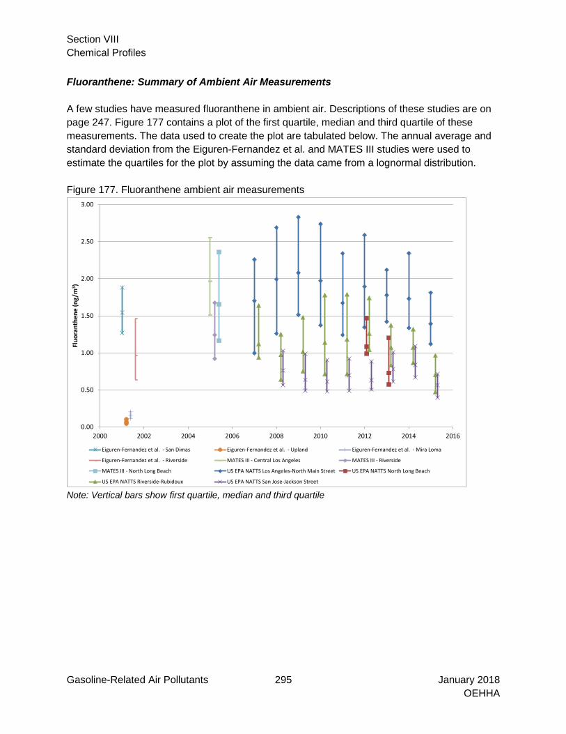
Section VIII Chemical Profiles
Gasoline-Related Air Pollutants 295 January 2018 OEHHA
Fluoranthene: Summary of Ambient Air Measurements A few studies have measured fluoranthene in ambient air. Descriptions of these studies are on page 247. Figure 177 contains a plot of the first quartile, median and third quartile of these measurements. The data used to create the plot are tabulated below. The annual average and standard deviation from the Eiguren-Fernandez et al. and MATES III studies were used to estimate the quartiles for the plot by assuming the data came from a lognormal distribution. Figure 177. Fluoranthene ambient air measurements
Note: Vertical bars show first quartile, median and third quartile
0.00
0.50
1.00
1.50
2.00
2.50
3.00
2000 2002 2004 2006 2008 2010 2012 2014 2016
Fluo
rant
hene
(ng/
m3 )
Eiguren-Fernandez et al. - San Dimas Eiguren-Fernandez et al. - Upland Eiguren-Fernandez et al. - Mira Loma
Eiguren-Fernandez et al. - Riverside MATES III - Central Los Angeles MATES III - Riverside
MATES III - North Long Beach US EPA NATTS Los Angeles-North Main Street US EPA NATTS North Long Beach
US EPA NATTS Riverside-Rubidoux US EPA NATTS San Jose-Jackson Street

Section VIII Chemical Profiles
Gasoline-Related Air Pollutants 296 January 2018 OEHHA
Box below gives more details on fluoranthene ambient air data show in Figure 177 Eiguren-Fernandez et al. (2004)
Site Time Particle phase (pg/m3) Vapor phase (ng/m3) Average SD Average SD
Atascadero May 2001-July 2002 6.11 13.7 0.82 2.14 Lompoc May 2001-July 2002 4.51 7.29 b b San Dimas May 2001-July 2002 31.1 41.7 1.58 0.48 Upland May 2001-July 2002 40.8 16.7 0.04 0.05 Mira Loma May 2001-July 2002 47.9 70.2 0.12 0.02 Riverside May 2001-July 2002 24.3 35.4 1.14 0.79
MATES III (2005) (ng/m3)
Site Average SD Min Max Central Los Angeles 2.12 0.86 0.48 4.37 Riverside 1.37 0.64 0.33 3.09 North Long Beach 1.9 1.07 0.54 4.84
US EPA National Air Toxics Trend Stations (ng/m3)
Site Year N
Per
cent
no
n-de
tect
Min
imum
Firs
t Q
uarti
le
Med
ian
Third
Q
uarti
le
Max
imum
Ave
rage
Sta
ndar
d D
evia
tion
Los Angeles-North Main Street 2007 39 13% 0.025 1 1.7 2.3 3 1.6 0.88 2008 61 0% 0.06 1.3 2 2.7 4.9 2 1 2009 60 0% 0.51 1.5 2.1 2.8 6.2 2.4 1.3 2010 59 0% 0.34 1.4 2 2.7 5.4 2.3 1.2 2011 59 0% 0.48 1.2 1.7 2.3 5.1 1.9 0.95 2012 60 0% 0.67 1.3 1.9 2.6 4.6 2 0.88 2013 58 0% 0.3 1.4 1.8 2.1 4.6 1.8 0.83 2014 56 0% 0.43 1.3 1.7 2.3 6.5 1.9 0.94 2015 39 3% 0.41 1.1 1.4 1.8 3.5 1.6 0.74
North Long Beach 2012 26 0% 0.61 0.99 1.1 1.5 5.7 1.3 0.96 2013 29 0% 0.35 0.57 0.73 1.2 2.3 0.93 0.56
Riverside-Rubidoux
2007 55 4% 0.04 0.94 1.1 1.6 2.8 1.2 0.55 2008 71 0% 0.081 0.64 0.97 1.2 11 1.2 1.5 2009 64 2% 0.023 0.75 1 1.5 5.4 1.2 0.75 2010 65 2% 0.019 0.71 1.1 1.8 3.2 1.3 0.7 2011 67 0% 0.17 0.71 1.2 1.8 3.6 1.3 0.77 2012 67 0% 0.25 1 1.3 1.7 4.3 1.4 0.74 2013 64 0% 0.32 0.83 1.1 1.4 4.2 1.2 0.57 2014 65 0% 0.4 0.86 1.1 1.3 2.3 1.1 0.37 2015 48 0% 0.29 0.47 0.7 0.96 2 0.78 0.38
San Jose-Jackson Street
2008 40 0% 0.37 0.56 0.76 1 1.6 0.81 0.32 2009 61 0% 0.28 0.49 0.64 0.99 4.3 0.85 0.61 2010 59 0% 0.31 0.48 0.61 0.9 1.9 0.72 0.35 2011 61 0% 0.23 0.49 0.7 0.92 2.3 0.78 0.39 2012 59 0% 0.29 0.5 0.63 0.88 3.5 0.77 0.48 2013 59 0% 0.31 0.61 0.78 1 2.4 0.86 0.4 2014 59 0% 0.39 0.66 0.83 1.1 9 1.1 1.3 2015 43 0% 0.29 0.39 0.56 0.71 1.3 0.61 0.27
Note: Half the limit of detection substituted for non-detects

Section VIII Chemical Profiles
Gasoline-Related Air Pollutants 297 January 2018 OEHHA
Fluorene: Summary of Ambient Air Measurements A few studies have measured fluorene in ambient air. Descriptions of these studies are on page 247. Figure 178 contains a plot of the first quartile, median and third quartile of these measurements. The data used to create the plot are tabulated below. The annual average and standard deviation from the Eiguren-Fernandez et al. and MATES III studies were used to estimate the quartiles for the plot by assuming the data came from a lognormal distribution. Figure 178. Fluorene ambient air measurements
Note: Vertical bars show first quartile, median and third quartile
0.00
0.50
1.00
1.50
2.00
2.50
3.00
2000 2002 2004 2006 2008 2010 2012 2014 2016
Fluo
rene
(ng/
m3 )
Eiguren-Fernandez et al. - San Dimas Eiguren-Fernandez et al. - Upland Eiguren-Fernandez et al. - Mira Loma
Eiguren-Fernandez et al. - Riverside MATES III - Central Los Angeles MATES III - Riverside
MATES III - North Long Beach US EPA NATTS Los Angeles-North Main Street US EPA NATTS North Long Beach
US EPA NATTS Riverside-Rubidoux US EPA NATTS San Jose-Jackson Street

Section VIII Chemical Profiles
Gasoline-Related Air Pollutants 298 January 2018 OEHHA
Box below gives more details on fluorene ambient air data displayed in Figure 178 Eiguren-Fernandez et al. (2004)
Particle phase (pg/m3) Vapor phase (ng/m3) Site Time Average SD Average SD Atascadero May 2001-July 2002 5.91 10.2 3.03 2.37 Lompoc May 2001-July 2002 8.39 11.2 4.04 4.52 San Dimas May 2001-July 2002 9.85 14.8 4.02 3.79 Upland May 2001-July 2002 4.89 4.55 21.4 21.1 Mira Loma May 2001-July 2002 2.35 4.07 22.8 20.7 Riverside May 2001-July 2002 7.68 10.2 5.45 1.43
MATES III (ng/m3)
Site Time Average SD Central LA (North Main St) 2005 2.12 0.86 Rubidoux 2005 1.37 0.64 North Long Beach 2005 1.9 1.07
US EPA National Air Toxics Trend Stations (ng/m3)
Site Year N
Per
cent
no
n-de
tect
Min
imum
Firs
t Q
uarti
le
Med
ian
Third
Q
uarti
le
Max
imum
Ave
rage
Sta
ndar
d D
evia
tion
Los Angeles-North Main Street
2007 39 8% 0.04 2.2 3.4 4.6 8.3 3.4 2 2008 61 0% 2.2 3.2 4.8 6.8 16 5.5 3 2009 60 0% 2.1 4.6 6.2 8.5 37 7.5 5.3 2010 59 0% 0.98 4.1 6 8.8 24 6.9 4.3 2011 59 0% 1.3 3.9 5 6.9 14 5.6 2.7 2012 60 0% 2.1 4.3 6.7 10 19 7.7 4.2 2013 58 2% 0.026 4.8 5.8 6.7 13 5.7 2.2 2014 56 7% 0.036 3.4 5.4 6.5 11 5 2.4 2015 39 5% 0.077 3 3.9 6 8.2 4.3 1.8
North Long Beach 2012 26 0% 1.7 2.3 3.5 3.8 5 3.3 1 2013 29 10% 0.026 1.2 2.1 3.7 5.4 2.4 1.6
Riverside-Rubidoux
2007 55 4% 0.06 2.2 3.3 4.7 7.2 3.4 1.6 2008 71 1% 0.04 2.1 3.3 4.2 7.1 3.3 1.7 2009 64 3% 0.019 2.5 3.6 4.5 9.4 3.6 1.9 2010 65 0% 0.078 2.2 3.7 5.1 8.3 3.7 1.9 2011 67 0% 0.5 2.1 4 5.5 9.5 4.1 2.2 2012 67 0% 0.79 3.1 4.1 5.4 9 4.4 1.9 2013 64 17% 0.028 2 3.5 4.5 10 3.2 2.1 2014 65 25% 0.037 1.3 3 4.1 7.8 2.9 2 2015 48 15% 0.075 1.1 2.1 2.8 5.4 2.1 1.3
San Jose-Jackson Street
2008 40 0% 1 1.7 2 2.9 4.7 2.4 0.95 2009 61 0% 0.7 1.3 1.8 2.9 7.6 2.3 1.3 2010 59 0% 0.82 1.5 2 2.8 6 2.3 1.1 2011 61 0% 0.98 1.6 2.3 3.5 5.9 2.6 1.3 2012 59 0% 0.86 1.4 1.9 2.9 6.1 2.3 1.2 2013 59 17% 0.034 1.4 2.4 3.3 6.2 2.4 1.6 2014 59 24% 0.056 1 2.8 3.7 18 2.8 2.8 2015 43 40% 0.12 0.13 1.5 2.4 3.9 1.4 1.2
Note: Half the limit of detection substituted for non-detects

Section VIII Chemical Profiles
Gasoline-Related Air Pollutants 299 January 2018 OEHHA
Fluorenone: Summary of Ambient Air Measurements US EPA National Air Toxics Trend Stations measured fluorenone in ambient air. A description of this program is on page 247. Figure 179 contains a plot of these measurements. The data used to create the plot are tabulated below. Figure 179. Fluorenone ambient air measurements
Note: Vertical bars show first quartile, median and third quartile
0
0.5
1
1.5
2
2.5
3
3.5
4
4.5
5
2007 2008 2009 2010 2011 2012 2013 2014 2015 2016
Fluo
reno
ne (n
g/m
3 )
Los Angeles-North Main Street North Long Beach Riverside-Rubidoux San Jose-Jackson Street

Section VIII Chemical Profiles
Gasoline-Related Air Pollutants 300 January 2018 OEHHA
Fluorenone ambient air measurements from US EPA National Air Toxics Trend Stations (ng/m3)
Site Year N
Perc
ent
non-
dete
ct
Min
imum
Firs
t Q
uarti
le
Med
ian
Third
Q
uarti
le
Max
imum
Aver
age
Stan
dard
D
evia
tion
Los Angeles-North Main Street
2008 55 18% 0.028 1.1 2.7 4.6 9.7 2.9 2.4 2009 60 0% 0.46 1.9 2.8 4.4 29 3.8 3.9 2010 59 0% 0.5 1.8 2.6 4 9.3 3.2 1.9 2011 59 0% 0.46 1.5 2.1 2.8 7.2 2.4 1.4 2012 60 0% 0.61 1.8 2.7 3.8 8.1 3 1.6 2013 58 0% 0.33 1.6 2.1 2.6 5.6 2.2 1.1 2014 56 0% 0.51 1.6 2.2 3 6.8 2.5 1.3 2015 39 3% 0.56 1.3 2 2.9 5.5 2.2 1.2
North Long Beach
2012 26 0% 0.67 0.99 1.4 1.8 2.8 1.5 0.59
2013 29 0% 0.34 0.7 0.88 1.4 3.3 1.2 0.81 Riverside-Rubidoux
2008 59 14% 0.025 0.84 1.9 2.8 4.8 1.9 1.3 2009 64 2% 0.023 1.2 1.9 2.6 7.1 2 1.2 2010 65 3% 0.027 0.92 1.5 2.6 7.5 1.9 1.3 2011 67 0% 0.15 0.88 1.7 2.5 5.2 1.8 1.1 2012 67 0% 0.21 1.4 1.9 2.7 4.6 2.1 0.99 2013 64 0% 0.32 1.1 1.6 2.2 4.9 1.7 0.81 2014 65 0% 0.49 1.3 1.6 2.2 4 1.8 0.77 2015 48 0% 0.29 0.73 1.2 1.8 4.1 1.4 0.78
San Jose-Jackson Street
2008 40 23% 0.037 0.59 1 1.5 2.5 1 0.71 2009 61 0% 0.28 0.65 0.88 1.6 5.1 1.2 0.83 2010 59 2% 0.031 0.69 0.91 1.3 4 1.1 0.69 2011 61 0% 0.28 0.66 0.92 1.6 3.3 1.2 0.67 2012 59 0% 0.36 0.6 0.79 1.3 2.8 1 0.56 2013 59 0% 0.45 0.78 1 1.6 4.6 1.3 0.8 2014 59 0% 0.45 0.76 1.1 1.4 3.6 1.2 0.68 2015 43 0% 0.42 0.67 1 1.5 3.8 1.2 0.68
Note: Half the limit of detection substituted for non-detects

Section VIII Chemical Profiles
Gasoline-Related Air Pollutants 301 January 2018 OEHHA
Indeno[1,2,3-cd]pyrene: Exposure and Screening Risk Assessment Results Data from the California Toxic Monitoring Network were used to estimate of the population-weighted annual average ambient air concentration of indeno[1,2,3-cd]pyrene in the South Coast Air Basin from 1996-2004, the years with data. These results are displayed in Figure 180 and Table 96 below. Between 1996 and 2004, the percentage of non-detects increased from 2% to 40% in the South Coast Air Basin. By default, non-detects were replaced with half the limit of detection. Figure 181 compares measurements from other ambient air monitoring studies to the population-weighted annual average. Summaries from these other ambient air monitoring studies are presented in tables below. Descriptions of these studies are on page 247. Table 97 contains indeno[cd]pyrene cancer risk estimates based on averages for each site and year. Figure 180. Indeno[1,2,3-cd]pyrene population-weighted annual average ambient air concentration in the South Coast Air Basin
Note: The vertical bars show the quartiles of indeno[1,2,3-cd]pyrene measurements from South Coast Air Basin monitoring sites in the California Toxic Monitoring Network with 10 or more months of data. Due to the large percentage of non-detects the estimated first quartile and median are the same at some sites.
0
0.1
0.2
0.3
0.4
0.5
0.6
0.7
1995 1996 1997 1998 1999 2000 2001 2002 2003 2004 2005
Inde
no[1
,2,3
-cd]
pyre
ne (n
g/m
3 )
Azusa Burbank-W Palm Avenue
Fontana-Arrow Highway Los Angeles-North Main Street
North Long Beach Riverside-Rubidoux
Population-weighted annual average ambient air concentration

Section VIII Chemical Profiles
Gasoline-Related Air Pollutants 302 January 2018 OEHHA
Table 96. Indeno[1,2,3-cd]pyrene population-weighted annual average ambient air concentration in the South Coast Air Basin
Year Indeno[1,2,3-cd]pyrene population-weighted
annual average ambient air concentration
(ng/m3)
Percent of measurements that are non-
detects
1996 0.27 2% 1997 0.27 11% 1998 0.30 14% 1999 0.27 15% 2000 0.23 23% 2001 0.19 31% 2002 0.17 33% 2003 0.11 38% 2004 0.12 42%
Figure 181. Additional indeno[1,2,3-cd]pyrene ambient air measurements
Note: The vertical bars show the quartiles of indeno[1,2,3-cd]pyrene measurements from additional monitoring sites
0
0.05
0.1
0.15
0.2
0.25
0.3
0.35
1996 1998 2000 2002 2004 2006 2008 2010 2012 2014
Inde
no[1
,2,3
-cd]
pyre
ne (n
g/m
3 )
Eiguren-Fernandez et al. - San DimasEiguren-Fernandez et al. - UplandEiguren-Fernandez et al. - Mira LomaEiguren-Fernandez et al. - RiversideMATES III - Central LA (North Main St)MATES III - RubidouxMATES III - North Long BeachUS EPA NATTS Los Angeles-North Main StreetUS EPA NATTS North Long BeachUS EPA NATTS Riverside-Rubidoux

Section VIII Chemical Profiles
Gasoline-Related Air Pollutants 303 January 2018 OEHHA
Box below provides more details on data used in Figure 171. Eiguren-Fernandez et al. (2004) particle phase PAHs (pg/m3)
Site Time Average SD Atascadero May 2001-July 2002 86.5 129 Lompoc May 2001-July 2002 12.3 15.9 San Dimas May 2001-July 2002 78.8 91.9 Upland May 2001-July 2002 49.1 37 Mira Loma May 2001-July 2002 100 105 Riverside May 2001-July 2002 52.4 64.4
MATES III (2005) (ng/m3)
Site Average SD Central Los Angeles 0.17 0.12 Riverside 0.18 0.16 North Long Beach 0.18 0.17
US EPA National Air Toxics Trend Stations (ng/m3)
Site Year N Percent non-detect
Minimum First Quartile
Median Third Quartile
Max Average Standard Deviation
Los Angeles-North Main Street
2007 39 77% 0.035 0.04 0.05 0.065 0.49 0.084 0.1 2008 61 79% 0.046 0.058 0.074 0.084 0.4 0.11 0.093 2009 60 43% 0.021 0.032 0.061 0.15 1.6 0.13 0.21 2010 59 47% 0.011 0.021 0.036 0.11 0.39 0.076 0.085 2011 59 56% 0.023 0.031 0.04 0.11 0.32 0.085 0.08 2012 60 60% 0.022 0.027 0.034 0.081 0.34 0.062 0.057 2013 58 47% 0.013 0.018 0.036 0.1 0.46 0.074 0.09 2014 56 21% 0.013 0.03 0.053 0.12 0.88 0.093 0.13 2015 39 79% 0.033 0.034 0.035 0.036 0.42 0.07 0.089
North Long Beach
2012 26 81% 0.025 0.028 0.033 0.046 0.97 0.087 0.19 2013 29 59% 0.015 0.018 0.02 0.07 0.44 0.075 0.11
Riverside-Rubidoux
2007 55 75% 0.035 0.04 0.05 0.079 0.55 0.094 0.11 2008 71 76% 0.041 0.045 0.055 0.098 0.41 0.086 0.072 2009 64 56% 0.017 0.022 0.029 0.098 1.3 0.1 0.19 2010 65 42% 0.013 0.018 0.042 0.082 0.63 0.065 0.085 2011 67 70% 0.014 0.035 0.046 0.076 0.38 0.066 0.058 2012 67 72% 0.028 0.035 0.039 0.068 0.32 0.061 0.051 2013 64 53% 0.018 0.02 0.025 0.092 0.94 0.078 0.12 2014 65 37% 0.014 0.021 0.051 0.14 0.49 0.098 0.12 2015 48 85% 0.033 0.034 0.035 0.036 0.39 0.054 0.064
San Jose-Jackson Street
2008 40 78% 0.063 0.065 0.066 0.067 0.76 0.11 0.13 2009 61 67% 0.025 0.027 0.027 0.092 1.9 0.12 0.26 2010 59 58% 0.017 0.017 0.018 0.062 0.38 0.062 0.088 2011 61 74% 0.031 0.033 0.034 0.074 0.74 0.11 0.17 2012 59 80% 0.032 0.033 0.034 0.035 0.54 0.079 0.11 2013 59 58% 0.021 0.022 0.022 0.11 0.74 0.11 0.17 2014 59 56% 0.02 0.022 0.022 0.11 1.3 0.14 0.26 2015 43 84% 0.053 0.055 0.056 0.057 0.41 0.087 0.086
Note: Half the limit of detection substituted for non-detects

Section VIII Chemical Profiles
Gasoline-Related Air Pollutants 304 January 2018 OEHHA
Table 97. Indeno[1,2,3-cd]pyrene cancer risk California Toxic Monitoring Network 1996 1997 1998 1999 2000 2001 2002 2003 2004 Maximum across all CARB sites 2.0E-07 2.6E-07 3.0E-07 2.3E-07 2.2E-07 2.6E-07 2.0E-07 1.7E-07 2.0E-07 South Coast Air Basin population-weighted annual average
1.0E-07 1.0E-07 1.2E-07 1.1E-07 8.9E-08 7.5E-08 6.5E-08 4.2E-08 4.6E-08
Eiguren-Fernandez et al. (2004) 2001 Mira Loma, Riverside County 3.9E-08 Riverside, Riverside County 2.0E-08 San Dimas, Los Angeles County 3.1E-08 Upland, San Bernardino County 1.9E-08
MATES III 2005 Central Los Angeles, Los Angeles County 6.6E-08 N. Long Beach, Los Angeles County 7.0E-08 Rubidoux, Riverside County 7.0E-08
US EPA NATTS 2008 2009 2010 2011 2012 2013 2014 Central Los Angeles, Los Angeles County 4.3E-08 5.1E-08 3.0E-08 3.3E-08 2.4E-08 2.9E-08 3.6E-08 Rubidoux, Riverside County 3.3E-08 3.9E-08 2.5E-08 2.6E-08 2.4E-08 3.0E-08 3.8E-08 San Jose, Santa Clara County 4.3E-08 4.7E-08 2.4E-08 4.3E-08 3.1E-08 4.3E-08 5.4E-08
Note: The maximum cancer risk across all sites in the California Toxic Monitoring Network is provided for comparison with the South Coast Air Basin cancer risk.

Section VIII Chemical Profiles
Gasoline-Related Air Pollutants 305 January 2018 OEHHA
Perylene: Summary of Ambient Air Measurements US EPA National Air Toxics Trend Stations measured perylene in ambient air. A description of this program is on page 247. A summary of the data is presented below. A plot was not created due to the large fraction of non-detects. Perylene ambient air measurements from US EPA National Air Toxics Trend Stations (ng/m3)
Site Year N
Perc
ent
non-
dete
ct
Min
imum
Firs
t Q
uarti
le
Med
ian
Third
Q
uarti
le
Max
imum
Aver
age
Stan
dard
D
evia
tion
Los Angeles-North Main
Street
2007 39 100% 0.035 0.04 0.045 0.055 0.075 0.049 0.0099 2008 61 97% 0.038 0.047 0.055 0.065 0.24 0.06 0.03 2009 60 75% 0.015 0.018 0.022 0.042 0.21 0.037 0.038 2010 59 78% 0.014 0.019 0.023 0.033 0.52 0.075 0.12 2011 59 98% 0.021 0.03 0.035 0.039 0.078 0.036 0.0091 2012 60 92% 0.022 0.026 0.028 0.034 0.23 0.038 0.033 2013 58 93% 0.015 0.018 0.018 0.022 0.17 0.024 0.022 2014 56 96% 0.016 0.016 0.017 0.021 0.29 0.024 0.037 2015 39 97% 0.026 0.027 0.027 0.027 0.27 0.037 0.044
North Long Beach
2012 26 96% 0.026 0.028 0.03 0.039 0.39 0.047 0.07 2013 29 90% 0.017 0.018 0.02 0.022 0.066 0.024 0.012
Riverside-Rubidoux
2007 55 100% 0.035 0.04 0.05 0.065 0.095 0.054 0.014 2008 71 100% 0.032 0.038 0.041 0.05 0.082 0.046 0.01 2009 64 77% 0.012 0.014 0.018 0.022 0.25 0.034 0.042 2010 65 80% 0.013 0.017 0.02 0.025 0.42 0.059 0.1 2011 67 99% 0.016 0.036 0.042 0.051 0.11 0.046 0.015 2012 67 99% 0.023 0.033 0.037 0.041 0.11 0.038 0.011 2013 64 97% 0.018 0.021 0.023 0.027 0.35 0.029 0.041 2014 65 94% 0.016 0.019 0.023 0.027 0.13 0.026 0.016 2015 48 98% 0.026 0.027 0.027 0.028 0.13 0.03 0.015
San Jose-Jackson Street
2008 40 98% 0.045 0.055 0.055 0.056 0.11 0.056 0.0092 2009 61 84% 0.018 0.019 0.019 0.02 0.21 0.034 0.037 2010 59 75% 0.021 0.021 0.021 0.043 0.4 0.058 0.083 2011 61 93% 0.021 0.038 0.038 0.039 0.17 0.044 0.024 2012 59 95% 0.033 0.034 0.034 0.035 0.18 0.039 0.022 2013 59 90% 0.023 0.024 0.024 0.025 0.14 0.03 0.021 2014 59 88% 0.024 0.026 0.026 0.026 0.42 0.042 0.06 2015 43 100% 0.042 0.043 0.044 0.044 0.045 0.043 0.0008
Note: Half the limit of detection substituted for non-detects
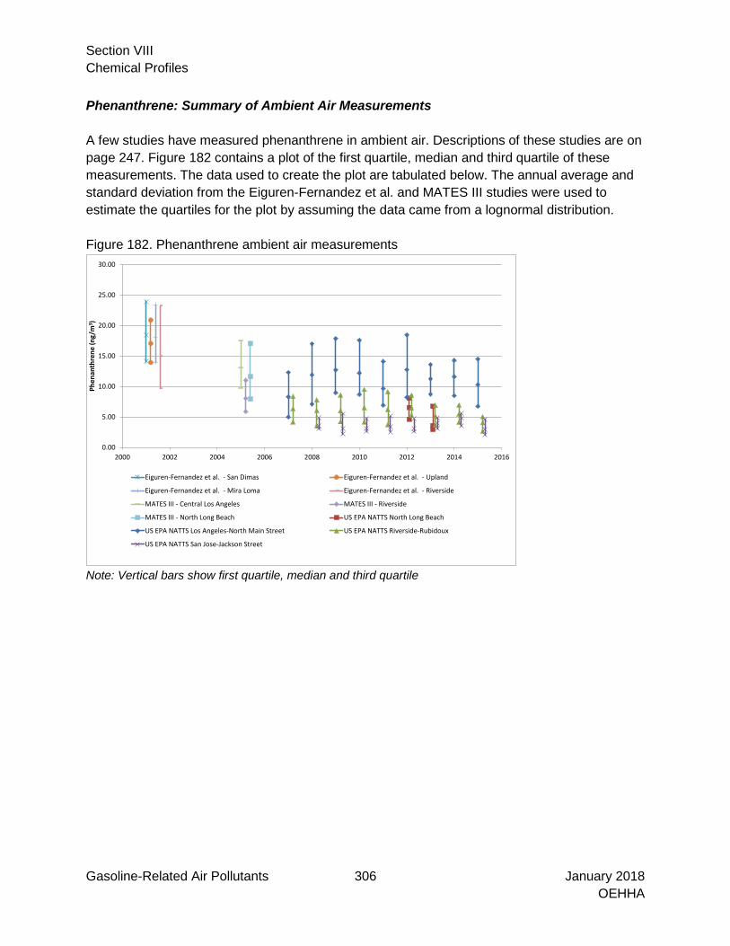
Section VIII Chemical Profiles
Gasoline-Related Air Pollutants 306 January 2018 OEHHA
Phenanthrene: Summary of Ambient Air Measurements A few studies have measured phenanthrene in ambient air. Descriptions of these studies are on page 247. Figure 182 contains a plot of the first quartile, median and third quartile of these measurements. The data used to create the plot are tabulated below. The annual average and standard deviation from the Eiguren-Fernandez et al. and MATES III studies were used to estimate the quartiles for the plot by assuming the data came from a lognormal distribution. Figure 182. Phenanthrene ambient air measurements
Note: Vertical bars show first quartile, median and third quartile
0.00
5.00
10.00
15.00
20.00
25.00
30.00
2000 2002 2004 2006 2008 2010 2012 2014 2016
Phen
anth
rene
(ng/
m3 )
Eiguren-Fernandez et al. - San Dimas Eiguren-Fernandez et al. - Upland
Eiguren-Fernandez et al. - Mira Loma Eiguren-Fernandez et al. - Riverside
MATES III - Central Los Angeles MATES III - Riverside
MATES III - North Long Beach US EPA NATTS North Long Beach
US EPA NATTS Los Angeles-North Main Street US EPA NATTS Riverside-Rubidoux
US EPA NATTS San Jose-Jackson Street

Section VIII Chemical Profiles
Gasoline-Related Air Pollutants 307 January 2018 OEHHA
Eiguren-Fernandez et al. (2004) Particle phase (pg/m3) Vapor phase (ng/m3) Site Time Average SD Average SD Atascadero May 2001-July 2002 4.63 6.83 11.4 3.43 Lompoc May 2001-July 2002 1.46 1.86 7.32 1.75 San Dimas May 2001-July 2002 23.8 14.7 19.8 8.07 Upland May 2001-July 2002 32.6 25.5 17.8 5.48 Mira Loma May 2001-July 2002 36.5 29 19.4 7.69 Riverside May 2001-July 2002 27.3 21.9 18.5 13.4
MATES III (2005) (ng/m3)
Site Average SD Central Los Angeles 14.35 6.52 Riverside 8.96 4.39 North Long Beach 13.65 8.4
US EPA National Air Toxics Trend Stations (ng/m3)
Site Year N
Perc
ent
non-
M
inim
um
Firs
t Q
uarti
le
Med
ian
Third
Q
uarti
le
Max
imum
Aver
age
Stan
dard
D
evia
tion
Los Angeles-North Main Street
2007 39 13% 0.045 5 8.3 12 29 8.8 6 2008 61 0% 3.9 7.1 12 17 36 13 7.4 2009 60 0% 3.6 9 13 18 63 16 10 2010 59 0% 2 8.7 12 18 45 15 8.7 2011 59 0% 2.5 6.9 9.6 14 31 11 6.2 2012 60 0% 2.7 8.2 13 18 36 15 7.8 2013 58 0% 2.2 8.7 11 14 28 11 5.1 2014 56 0% 2.4 8.5 12 14 28 12 4.9 2015 39 0% 2.7 6.7 10 14 27 11 5.6
North Long Beach 2012 26 0% 3.4 4.6 6.6 8.1 14 6.7 2.4 2013 29 0% 1.6 2.9 3.6 6.7 11 4.8 2.8
Riverside-Rubidoux
2007 55 4% 0.08 4.2 6.3 8.4 18 6.6 3.4 2008 71 1% 0.074 3.6 6.1 7.8 32 6.7 5 2009 64 0% 0.084 4.2 6 8.6 23 6.7 3.9 2010 65 0% 0.16 4.2 6.5 9.5 18 6.9 3.8 2011 67 0% 0.71 3.7 6.2 9.1 18 6.9 3.9 2012 67 0% 1.3 5.3 6.5 8.6 15 7.1 3.2 2013 64 0% 1.4 3.7 5.1 6.9 14 5.5 2.4 2014 65 0% 1.8 4.1 5.5 7 10 5.7 2.1 2015 48 0% 1.2 2.7 4.1 5.1 13 4.4 2.7
San Jose-Jackson Street
2008 40 0% 1.8 3 3.5 4.9 8.3 4.1 1.6 2009 61 0% 1.2 2.2 3.2 5.5 20 4 2.8 2010 59 0% 1.5 2.6 3.1 4.8 9.4 3.9 1.9 2011 61 0% 1.6 2.6 3.4 5.2 9.7 4 2 2012 59 0% 1.5 2.6 3.1 4.7 9.9 3.7 1.7 2013 59 0% 1.5 3.1 4 4.8 11 4.2 1.8 2014 59 0% 2 3.5 4.8 5.6 37 5.2 4.5 2015 43 0% 1.2 2 3 4.6 8 3.4 1.7
Note: Half the limit of detection substituted for non-detects

Section VIII Chemical Profiles
Gasoline-Related Air Pollutants 308 January 2018 OEHHA
Pyrene: Summary of Ambient Air Measurements A few studies have measured pyrene in ambient air. Descriptions of these studies are on page 247. Figure 183 contains a plot of the first quartile, median and third quartile of these measurements. The data used to create the plot are tabulated below. The annual average and standard deviation from the Eiguren-Fernandez et al. and MATES III studies were used to estimate the quartiles for the plot by assuming the data came from a lognormal distribution. Figure 183. Pyrene ambient air measurements
Note: Vertical bars show first quartile, median and third quartile
0.00
0.50
1.00
1.50
2.00
2.50
2000 2002 2004 2006 2008 2010 2012 2014 2016
Pyre
ne (n
g/m
3 )
Eiguren-Fernandez et al. - San Dimas Eiguren-Fernandez et al. - Upland
Eiguren-Fernandez et al. - Mira Loma Eiguren-Fernandez et al. - Riverside
MATES III - Central Los Angeles MATES III - Riverside
MATES III - North Long Beach US EPA NATTS Los Angeles-North Main Street
US EPA NATTS North Long Beach US EPA NATTS Riverside-Rubidoux
US EPA NATTS San Jose-Jackson Street

Section VIII Chemical Profiles
Gasoline-Related Air Pollutants 309 January 2018 OEHHA
Box below gives more details on pyrene ambient air measurements displayed in Figure 183 Eiguren-Fernandez et al. (2004)
Site Time Particle phase (pg/m3) Vapor phase (ng/m3) Average SD Average SD
Atascadero May 2001-July 2002 17.3 1.26 1.68 0.44 Lompoc May 2001-July 2002 5.51 5.6 - - San Dimas May 2001-July 2002 48 21.1 0.61 0.56 Upland May 2001-July 2002 54.2 11.2 0.32 0.08 Mira Loma May 2001-July 2002 69.5 50.1 0.35 0.14 Riverside May 2001-July 2002 37.7 21.3 0.79 0.54
MATES III (2005) (ng/m3)
Site Average SD Central Los Angeles 1.67 0.73 Riverside 1.19 0.7 North Long Beach 1.68 1.01
US EPA National Air Toxics Trend Stations (ng/m3)
Site Year N
Per
cent
no
n-de
tect
Min
imum
Firs
t Q
uarti
le
Med
ian
Third
Q
uarti
le
Max
imum
Ave
rage
Sta
ndar
d D
evia
tion
Los Angeles-North Main Street
2007 39 13% 0.03 0.78 1.1 1.5 2.6 1.1 0.64 2008 61 0% 0.36 0.93 1.3 1.6 3.2 1.3 0.61 2009 60 0% 0.35 0.96 1.3 2 4.8 1.6 0.89 2010 59 0% 0.24 0.89 1.4 1.8 3 1.4 0.69 2011 59 0% 0.25 0.8 1.1 1.5 2.7 1.2 0.56 2012 60 0% 0.45 0.83 1.1 1.7 4.6 1.3 0.65 2013 58 0% 0.21 0.79 1 1.4 2.4 1.1 0.49 2014 56 0% 0.28 0.82 1 1.3 4 1.1 0.54 2015 39 3% 0.27 0.58 0.77 1.1 2 0.85 0.4
North Long Beach 2012 26 0% 0.37 0.61 0.78 0.91 3.7 0.88 0.63 2013 29 0% 0.24 0.37 0.52 0.7 2.6 0.78 0.68
Riverside-Rubidoux
2007 55 4% 0.045 0.53 0.74 1 2.5 0.85 0.47 2008 71 3% 0.033 0.36 0.57 0.89 6.8 0.81 1 2009 64 2% 0.03 0.44 0.58 1.1 4.1 0.83 0.68 2010 65 2% 0.019 0.48 0.75 1.1 2.3 0.86 0.48 2011 67 0% 0.11 0.45 0.75 1.1 2.2 0.81 0.45 2012 67 0% 0.14 0.59 0.8 1 2.8 0.9 0.5 2013 64 0% 0.21 0.5 0.7 0.94 3.2 0.77 0.43 2014 65 0% 0.24 0.51 0.66 0.88 1.9 0.72 0.31 2015 48 0% 0.15 0.28 0.41 0.52 1.4 0.44 0.24
San Jose-Jackson Street
2008 40 0% 0.25 0.41 0.58 0.86 1.6 0.68 0.33 2009 61 0% 0.23 0.41 0.54 0.93 4 0.75 0.6 2010 59 0% 0.29 0.37 0.48 0.81 1.8 0.62 0.33 2011 61 0% 0.18 0.42 0.55 0.78 2.3 0.68 0.41 2012 59 0% 0.2 0.41 0.52 0.78 2.6 0.64 0.4 2013 59 0% 0.24 0.45 0.69 0.92 1.9 0.77 0.4 2014 59 0% 0.31 0.49 0.63 0.88 4.5 0.85 0.74 2015 43 0% 0.26 0.33 0.42 0.57 1.3 0.51 0.26
Note: Half the limit of detection substituted for non-detects

Section VIII Chemical Profiles
Gasoline-Related Air Pollutants 310 January 2018 OEHHA
Retene: Summary of Ambient Air Measurements US EPA National Air Toxics Trend Stations measured retene in ambient air. A description of this study is on page 247. Figure 184 contains a plot of these measurements. The data used to create the plot are tabulated below. Figure 184. Retene ambient air measurements
Note: Vertical bars show first quartile, median and third quartile
0
0.2
0.4
0.6
0.8
1
1.2
2007 2008 2009 2010 2011 2012 2013 2014 2015 2016
Rete
ne (n
g/m
3 )
US EPA NATTS Los Angeles-North Main Street US EPA NATTS North Long BeachUS EPA NATTS Riverside-Rubidoux US EPA NATTS San Jose-Jackson Street

Section VIII Chemical Profiles
Gasoline-Related Air Pollutants 311 January 2018 OEHHA
Retene ambient air measurements from US EPA National Air Toxics Trend Stations (ng/m3)
Site Year N Percent
non-detect M
inim
um
Firs
t Q
uarti
le
Med
ian
Third
Q
uarti
le
Max
imum
Aver
age
Stan
dard
D
evia
tion
Los Angeles-North Main Street
2008 55 5% 0.032 0.12 0.23 0.37 3.1 0.37 0.52 2009 60 7% 0.034 0.14 0.22 0.71 8.5 0.59 1.2 2010 59 36% 0.058 0.082 0.2 0.47 1.6 0.36 0.39 2011 59 2% 0.022 0.13 0.23 0.46 2.1 0.39 0.39 2012 60 28% 0.053 0.086 0.2 0.37 1.4 0.29 0.29 2013 58 47% 0.038 0.048 0.1 0.28 1.7 0.26 0.36 2014 56 2% 0.01 0.082 0.12 0.29 1.5 0.24 0.3 2015 39 18% 0.039 0.086 0.13 0.2 1 0.19 0.21
North Long Beach
2012 26 27% 0.061 0.12 0.31 0.6 5.2 0.67 1.1 2013 29 45% 0.044 0.056 0.17 0.4 4.3 0.54 0.97
Riverside-Rubidoux
2008 59 29% 0.026 0.036 0.11 0.23 2.7 0.24 0.42 2009 64 8% 0.025 0.1 0.16 0.27 4 0.33 0.58 2010 65 17% 0.044 0.16 0.21 0.36 1.5 0.29 0.26 2011 67 1% 0.023 0.14 0.28 0.47 3 0.39 0.44 2012 67 31% 0.07 0.094 0.27 0.42 1.6 0.36 0.34 2013 64 25% 0.051 0.11 0.16 0.27 0.89 0.22 0.17 2014 65 0% 0.055 0.12 0.18 0.35 2 0.28 0.29 2015 48 17% 0.037 0.1 0.15 0.22 1.7 0.21 0.26
San Jose-Jackson Street
2008 40 10% 0.039 0.15 0.22 0.58 8.3 0.82 1.6 2009 61 8% 0.038 0.14 0.23 0.88 9 0.79 1.4 2010 59 29% 0.066 0.068 0.24 0.65 3.8 0.55 0.72 2011 61 0% 0.07 0.16 0.31 0.99 4.4 0.69 0.88 2012 59 49% 0.077 0.08 0.17 0.5 2.7 0.36 0.48 2013 59 32% 0.061 0.064 0.21 0.66 2 0.48 0.58 2014 59 3% 0.014 0.13 0.17 0.7 2.5 0.49 0.61 2015 43 9% 0.062 0.16 0.21 0.32 1.6 0.35 0.37
Note: Half the limit of detection substituted for non-detects

Section VIII Chemical Profiles
Gasoline-Related Air Pollutants 312 January 2018 OEHHA
Chemical Profiles: Gasoline-Related Criteria Air Pollutants
Nitrogen Dioxide: Exposure
Nitrogen oxides (NOx) are formed during combustion and are emitted by on-road vehicles, other mobile sources and stationary sources (like manufacturing and industrial plants, oil and gas production facilities and electric utilities). Nitrogen oxides react to form nitric acid, which contributes to secondary PM formation (Shepherd, 2003). They also contribute to the formation of ground-level ozone (US EPA, 2016a; CARB, 1997). The Emission Inventory had estimates for NOx. These data were used to identify sources of NOx and to calculate the gasoline-attributable fractions. Sources of NOx were identified in CARB’s 2012 Emission Inventory and are summarized in Table 98 below. A substantial portion (about 19%) of NOx came from gasoline-related on-road mobile sources. Non-gasoline-related sources of NOx include large diesel trucks, ocean-going vessels and construction and mining equipment. Figure 185 shows that gasoline-attributable fractions of NOx declined between 1996 and 2012. There is an apparent increase in gasoline-attributable fractions between 2008 and 2010 because the 2010 Emission Inventory had lower estimates of NOx emissions from non-gasoline-related on-road mobile sources and other mobile sources. Gasoline-attributable fractions for NOx differed among air basins, ranging in 2012 from 14% in the San Joaquin Valley Air Basin to about 30% in the South Coast and San Diego Air Basins (see Table 99). Ambient air monitoring data of nitrogen dioxide was available from 1996 to 2013. Population-weighted annual average ambient air concentrations for nitrogen dioxide declined during this time period (see Table 100). Gasoline-attributable fractions for NOx were applied to calculate the gasoline-attributable concentrations of nitrogen dioxide. In the South Coast Air Basin and statewide, the gasoline-attributable nitrogen dioxide concentration declined by about 70% over this time period (see Table 101 and Figure 186). Despite declines in ambient concentrations, nitrogen dioxide levels still pose health concerns in California, as demonstrated by a number of studies (see for example, Coker et al., 2016; Jerrett et al., 2013; Ritz et al., 2006).

Section VIII Chemical Profiles
Gasoline-Related Air Pollutants 313 January 2018 OEHHA
Table 98. Statewide sources of NOx in 2012
Source Category
Percentage of NOx (by
weight) from gasoline-related sources
Percentage of NOx (by
weight) from non-
gasoline-related sources
On-Road Motor Vehicles 18.8% 29.9% Other Mobile Sources 2.2% 31.6% Fuel Combustion < 0.1% 9.9% Miscellaneous Processes - 3.2% Industrial Processes - 2.6% Natural Sources - 1.3% Petroleum Production And Marketing < 0.1% 0.3% Waste Disposal - 0.2% Cleaning And Surface Coatings - < 0.1% Solvent Evaporation - - Total 21.0% 79.0%

Section VIII Chemical Profiles
Gasoline-Related Air Pollutants 314 January 2018 OEHHA
Table 99. Gasoline-attributable fractions of nitrogen oxides.
Year
South Coast
Air Basin
San Diego
Air Basin
San Francisco Bay Area Air Basin
San Joaquin
Valley Air Basin
Sacramento Valley Air
Basin State
1996 47% 50% 37% 30% 41% 39% 1997 48% 49% 36% 29% 39% 39% 1998 48% 49% 36% 30% 39% 39% 1999 48% 49% 36% 31% 31% 38% 2000 38% 42% 33% 22% 29% 32% 2001 37% 43% 33% 23% 27% 31% 2002 34% 39% 33% 20% 27% 28% 2003 35% 37% 34% 15% 25% 26% 2004 35% 38% 31% 15% 24% 25% 2005 33% 36% 29% 14% 22% 23% 2006 31% 35% 27% 12% 20% 21% 2007 29% 32% 26% 12% 20% 20% 2008 28% 33% 25% 12% 19% 20% 2009 -- -- -- -- -- -- 2010 32% 34% 27% 15% 21% 23% 2011 30% 32% 26% 14% 20% 21% 2012 29% 31% 25% 14% 20% 21%
Note: Mobile source emissions were not available for 2009. Note that these fractions are based on emissions of NOx not nitrogen dioxide
Figure 185. NOx gasoline-attributable fractions
0%
10%
20%
30%
40%
50%
60%
70%
80%
90%
100%
1996 1997 1998 1999 2000 2001 2002 2003 2004 2005 2006 2007 2008 2009 2010 2011 2012
Nitr
ogen
Oxi
des g
asol
ine-
attr
ibut
able
frac
tions
South Coast Air Basin San Diego Air Basin San Francisco Bay Area Air Basin
San Joaquin Valley Air Basin Sacramento Valley Air Basin State

Section VIII Chemical Profiles
Gasoline-Related Air Pollutants 315 January 2018 OEHHA
Table 100. Population-weighted average concentration of nitrogen dioxide (ppmv)
Year
South Coast
Air Basin
San Diego
Air Basin
San Francisco Bay Area Air Basin
San Joaquin
Valley Air Basin
Sacramento Valley Air
Basin State
1996 0.033 0.022 0.020 0.019 0.015 0.025 1997 0.032 0.022 0.019 0.018 0.013 0.024 1998 0.032 0.021 0.019 0.018 0.014 0.024 1999 0.034 0.024 0.020 0.020 0.015 0.026 2000 0.031 0.022 0.018 0.018 0.015 0.024 2001 0.030 0.020 0.018 0.017 0.014 0.022 2002 0.028 0.020 0.017 0.018 0.014 0.022 2003 0.027 0.020 0.015 0.017 0.013 0.021 2004 0.025 0.018 0.014 0.015 0.013 0.019 2005 0.023 0.017 0.014 0.015 0.012 0.018 2006 0.023 0.018 0.014 0.015 0.012 0.018 2007 0.022 0.016 0.014 0.014 0.012 0.017 2008 0.021 0.016 0.013 0.014 0.011 0.017 2009 0.021 0.015 0.013 0.013 0.010 0.016 2010 0.018 0.014 0.012 0.011 0.008 0.014 2011 0.017 0.013 0.013 0.011 0.009 0.014 2012 0.016 0.013 0.012 0.012 0.009 0.013 2013 0.016 0.013 0.013 0.012 0.009 0.014
Table 101. Gasoline-attributable concentration of nitrogen dioxide (ppmv)
Year
South Coast
Air Basin
San Diego
Air Basin
San Francisco Bay Area Air Basin
San Joaquin Valley
Air Basin
Sacramento Valley Air
Basin State
1996 0.015 0.011 0.0073 0.0058 0.0062 0.0097 1997 0.016 0.011 0.0068 0.0054 0.0052 0.0096 1998 0.015 0.0100 0.0068 0.0054 0.0056 0.0095 1999 0.016 0.012 0.0072 0.0063 0.0046 0.0096 2000 0.012 0.0093 0.0061 0.0040 0.0044 0.0076 2001 0.011 0.0087 0.0059 0.0040 0.0037 0.0070 2002 0.0097 0.0078 0.0055 0.0035 0.0038 0.0061 2003 0.0096 0.0073 0.0052 0.0024 0.0033 0.0053 2004 0.0089 0.0069 0.0045 0.0022 0.0030 0.0048 2005 0.0075 0.0062 0.0042 0.0021 0.0026 0.0042 2006 0.0070 0.0062 0.0039 0.0018 0.0024 0.0038 2007 0.0065 0.0052 0.0035 0.0017 0.0023 0.0035 2008 0.0060 0.0055 0.0033 0.0017 0.0021 0.0033 2009 0.0058 0.0051 0.0032 0.0016 0.0019 0.0031 2010 0.0058 0.0047 0.0033 0.0017 0.0018 0.0032 2011 0.0052 0.0041 0.0033 0.0017 0.0018 0.0030 2012 0.0047 0.0039 0.0029 0.0017 0.0018 0.0028 2013 0.0048 0.0039 0.0032 0.0017 0.0019 0.0028
Note: calculated with NOx gasoline-attributable fractions.

Section VIII Chemical Profiles
Gasoline-Related Air Pollutants 316 January 2018 OEHHA
Figure 186. Ambient air concentrations of nitrogen dioxide in the South Coast Air Basin
0.000
0.005
0.010
0.015
0.020
0.025
0.030
0.035
0.040
1996 1997 1998 1999 2000 2001 2002 2003 2004 2005 2006 2007 2008 2009 2010 2011 2012 2013
Nitr
ogen
Dio
xide
in th
e So
uth
Coas
t Air
Basi
n (p
pm)
Population weighted ambient air concentration of NOx Gasoline-attributable concentration of NOx

Section VIII Chemical Profiles
Gasoline-Related Air Pollutants 317 January 2018 OEHHA
PM2.5: Exposure Assessment Results
Particulate matter (PM) can be emitted directly from a variety of sources (primary PM) and can also be formed from gas-phase chemicals (secondary PM). Particulate matter up to 2.5 µm in diameter is known as PM2.5, which is the form addressed in this Chemical Profile. Based on the 2012 statewide Emission Inventory, more than 98% of primary PM2.5 comes from non-gasoline-related sources such as burning (woodstoves, fireplaces, agricultural burning, wildfires), road dust, farming operations, and exhaust from diesel engines. Exhaust from gasoline vehicles makes only a small contribution to primary PM2.5. Table 102 shows the fractions by weight of primary PM2.5 that came from non-gasoline-related sources and gasoline-related sources in 2012.
Table 102. Statewide sources for primary PM2.5 in 2012
Source category Percentage of primary PM2.5
(by weight) from non-gasoline-related sources
Percentage of primary PM2.5 (by weight) from
gasoline-related sources Miscellaneous processes
Residential fuel combustion 6.4% -- Fugitive windblown dust 6.1% -- Managed burning and disposal 3.8% -- Cooking 3.3% -- Unpaved road dust 3.2% -- Paved road dust 3.1% -- Farming operations 3.0% -- Construction and demolition 1.9% -- Fires 0.1% -- Other (miscellaneous processes) < 0.05% --
Natural sources (wildfires) 48.9% -- On-road motor vehicles 5.2%1 0.4% Other mobile sources 4.2% 1.1% Industrial processes 4.8% -- Fuel combustion 3.4% < 0.05% Waste disposal 0.4% -- Cleaning and surface coatings 0.3% -- Petroleum production and marketing
0.3% < 0.05%
Solvent evaporation < 0.05% -- Total 98.4% 1.6%
1. This is primarily from brake wear, a non-gasoline-related source associated with motor vehicles. We researched possible approaches for estimating the fraction of total PM2.5 (i.e., primary plus secondary) attributable to gasoline-related sources. One aspect of this calculation is understanding the proportion of total PM2.5 coming from primary sources versus secondary
Section VIII Chemical Profiles
Gasoline-Related Air Pollutants 318 January 2018 OEHHA
formation. Another consideration is the composition of secondary PM2.5, which is known to include sulfate, nitrate, ammonium and secondary organic aerosols (SOA). A number of studies have examined the estimated contributions to ambient PM2.5 from gasoline-related sources, the proportion of PM2.5 attributable to primary sources versus secondary formation, and the composition of secondary PM2.5 (see for example, Rogge et al., 1993; Schauer et al., 1996; Watson et al., 1998; Gertler et al. 2000; Held et al., 2005; Fine et al., 2008; Ying and Kleeman, 2006; Hu et al., 2014a,b, 2015). Some of this work is briefly discussed below. Based on preliminary results from a simulation study of PM2.5, Hu et al. (2014b, 2015) reported that primary PM2.5 accounted for about 70% of total PM2.5 in Los Angeles and Fresno, suggesting that secondary formation could account for about 30%. However, there are shortcomings with models of secondary PM2.5, and this proportion is likely to vary by region, meteorological parameters, proximity to sources, and other factors. Calculations based on California data from the Chemical Speciation Network indicate higher percentages of secondary PM2.5 (see Table 104 below). Gasoline-related aromatic VOCs like toluene, xylenes and trimethylbenzenes are important precursors of SOA (Fine et al. 2008, Pandis 2003). Ensberg et al. (2014) noted that current atmospheric models tend to underpredict SOA levels in urban areas. They concluded that either vehicle emissions are not the main contributors to SOA formation, or that the models of SOA formation from vehicle emissions are inadequate. Jathar et al. (2014) found that 10% to 20% of emissions from gasoline exhaust, diesel exhaust and biomass burning are not adequately characterized, and the failure to account for them in emission inventories significantly hinders studies of SOA formation. There are also conflicting results on the relative contributions of gasoline versus diesel vehicles to ambient particulate matter (Gertler et al., 2005), and to the formation of SOA. For example, Bahreini et al. (2012) estimated that very little ambient SOA was derived from diesel combustion and recommend focusing on reducing emissions from gasoline vehicles in order to reduce SOA. However, Gentner et al. (2012) found that diesel emissions were responsible for 65 to 90% of vehicle-derived SOA. Gasoline-related sources emit NOx and, to a lesser extent, SOx and ammonia, which are also precursors of PM2.5. Rogge et al. (1993) found that ammonium, nitrate, and sulfate made up 40% and 50% of total PM2.5 at two sites in the South Coast Air Basin. In a review of findings from a PM research program (the “Supersites Program”) and related studies, Fine et al. (2008) reported that ammonium, nitrate, and sulfate typically make up 50% of total PM2.5 mass, and that the percentage can increase to 70% in the winter in the western US. These studies are useful, but cover a limited geographic region and do not capture short-term variability in the percentages. A few studies have modeled the estimated contributions from various sources, including gasoline-related sources, to total PM2.5 and its components in California. Held et al. (2005) estimated that gasoline-engines used in transportation contributed about 10% to 20% to total PM2.5 based on a three-day simulation study in 1993 for four sites in the South Coast Air Basin. Ying and Kleeman (2006) estimated that about 30% of nitrate and about 20% of ammonium in

Section VIII Chemical Profiles
Gasoline-Related Air Pollutants 319 January 2018 OEHHA
secondary PM2.5 came from gasoline engines used in transportation, based on a a simulation for a three-day period in 1996 in the South Coast Air Basin. Given the limited information available in the literature, we settled on a method for estimating gasoline-attributable fractions for PM2.5 that relies on data from the Emission Inventory and the Chemical Speciation Network28. The approach, described in the section below, involves calculating gasoline-attributable fractions for primary PM2.5, and using proxies to estimate the gasoline-attributable fractions for components of secondary PM2.5 (NOx as a proxy for ammonium nitrate; SOx as a proxy for ammonium sulfate, and ROG as a proxy for SOA). There are a number of uncertainties and limitations to this approach, which are also summarized below.
Gasoline-Attributable Fractions for PM2.5 Using the methods described in Appendix E and data from the Emission Inventory we first estimated the gasoline-attributable fractions for primary PM2.5 (shown in Table 103). The fractions range from 0.6% to 8.4% for PM2.5 depending on the year and air basin. Table 103. Gasoline-attributable fractions for primary PM2.5 based on the Emission Inventory
Year South
Coast Air Basin
San Diego Air Basin
San Francisco Bay Area Air Basin
San Joaquin Valley Air
Basin
Sacramento Valley Air
Basin State
1996 4.5% 3.8% 3.3% 1.3% 1.6% 1.8% 1997 6.6% 4.2% 3.5% 1.4% 1.6% 2.4% 1998 6.9% 4.5% 3.7% 1.6% 1.7% 2.5% 1999 8.0% 4.8% 3.3% 2.4% 0.7% 1.8% 2000 5.8% 3.7% 3.6% 1.0% 1.5% 1.1% 2001 5.7% 3.8% 3.9% 1.5% 1.0% 1.8% 2002 6.0% 3.9% 4.0% 0.6% 1.9% 2.0% 2003 2.1% 1.9% 4.1% 1.2% 2.0% 1.7% 2004 7.8% 5.0% 4.2% 1.5% 1.8% 2.5% 2005 8.0% 5.1% 3.0% 1.6% 1.9% 2.5% 2006 8.4% 5.4% 4.5% 1.7% 1.9% 2.8% 2007 8.1% 5.3% 4.5% 1.7% 2.0% 2.8% 2008 8.2% 5.7% 4.7% 1.8% 2.1% 2.9% 2009 -- -- -- -- -- -- 2010 5.9% 3.6% 4.3% 1.0% 1.4% 2.0% 2011 5.7% 3.8% 4.1% 1.0% 1.4% 1.9% 2012 4.7% 2.8% 4.4% 1.1% 1.2% 1.6%
Note: Mobile source emissions were unavailable for 2009.
28 See https://www.arb.ca.gov/aqd/pm25/pmfmon.htm for a description of the PM2.5 monitoring and speciation network in California. PM2.5 speciation data are available from CARB.

Section VIII Chemical Profiles
Gasoline-Related Air Pollutants 320 January 2018 OEHHA
Data from the Chemical Speciation Network were used to estimate the average proportions of PM2.5 components by air basin over the period 2000 to 2014. These percentages are shown in Table 104 below. Note that the PM2.5 speciation data are from only a small number of sites in each air basin, and the results may not represent the air quality over the entire region. Table 104. Average percentages of PM2.5 components based on data from Chemical Speciation Network (2000-2014).
Air Basin Primary PM2.5 (%)
Secondary PM2.5 components
Ammonium sulfate (%)
Ammonium nitrate (%)
SOA (%)
South Coast 26.7% 16.8% 43.6% 12.9% San Diego 32.3% 21.9% 26.7% 19.1% San Francisco Bay Area 39.6% 14.1% 24.1% 22.2% San Joaquin Valley 34.5% 11.1% 37.6% 16.8% Sacramento Valley 46.0% 10.6% 20.0% 23.3%
Table Notes: Speciation data for PM2.5 samples collected at sites within the Network were obtained for 2000 to 2014. The calculation of the percentages uses data on the total mass of the PM2.5 sample, and the speciated masses of organics, sulfate and nitrate. Nitrate and sulfate are assumed to be fully neutralized by ammonium (Buzcu-Guven et al., 2007), and half the organics are attributed to secondary formation (Fine et al., 2008). The values shown in the Table represent averages for each basin over the full time period. We then applied the following equation to estimate gasoline-attributable fractions for total PM2.5,
accounting for both primary and secondary components: PM2.5GAF(y, AB) = (a%)PrimaryPM2.5GAF(y, AB) + (𝑏𝑏%)SOxGAF(y, AB) + (c%)NOxGAF(y, AB) + (d%)ROGGAF(y, AB)
Where:
PM2.5 GAF (y, AB) = Gasoline-attributable fraction for PM2.5 in year y and air basin AB
a% = Fraction of total PM2.5 from primary sources
PrimaryPM2.5GAF(y,AB) = Gasoline-attributable fraction of primary PM2.5 based on the Emission Inventory for year y and air basin AB
b% = Fraction of total PM2.5 assumed to be ammonium sulfate
SOxGAF(y,AB) = Gasoline-attributable fraction of SOx used as a proxy for the gasoline-attributable fraction for ammonium sulfate
c% = Fraction of total PM2.5 assumed to be ammonium nitrate
NOxGAF(y,AB) = Gasoline-attributable fraction of NOx used as a proxy for the gasoline-attributable fraction for ammonium nitrate
d% = Fraction of total PM2.5 assumed to be SOA
ROGGAF(y,AB) = Gasoline-attributable fraction of ROG used as a proxy for the gasoline-attributable fraction for SOA

Section VIII Chemical Profiles
Gasoline-Related Air Pollutants 321 January 2018 OEHHA
The estimated gasoline-attributable fractions for total PM2.5 based on the above equation are shown in Table 105 on the next page. There are many limitations to the approach we applied, including the following: Using gasoline-attributable fractions for NOx, SOx and ROG as proxies for the gasoline-
attributable fractions of ammonium nitrate, ammonium sulfate and SOA is inherently uncertain. For example, the relationship between NOx and nitrate is complex and likely does not follow the linear relationship assumed in the above equation (Mysliwiec et al., 2002). Also, the formation of SOA depends on a number of factors, such as the composition of VOCs emitted and atmospheric conditions, and is not well understood (Lurmann et al., 2006). To estimate the percentages in Table 104 above, a 50/50 split between primary and secondary organic aerosol was assumed (Fine et al., 2008). The actual ratio will vary by season and location. These complexities have not been incorporated into the method for approximating PM2.5 gasoline-attributable fractions.
The average percentages of the secondary components presented in Table 104 were estimated over the period 2000 to 2014, but these percentages likely vary seasonally and over time. Further, the data used to calculate these values came from a few monitoring sites in each air basin, which were located in areas with poor air quality as required under the State Implementation Plan29 for California. For example, there are only two PM2.5 speciation monitoring sites (downtown Los Angeles and Riverside) in the South Coast Air Basin. Therefore, the PM2.5 speciation data used to calculate the percentages in Table 104 are likely not representative of the overall air quality in each air basin.
29 A State Implementation Plan is a comprehensive plan that describes how an area will attain National Ambient Air Quality Standards. For more information, see https://www.arb.ca.gov/planning/sip/background.htm.

Section VIII Chemical Profiles
Gasoline-Related Air Pollutants 322 January 2018 OEHHA
Table 105. Estimated PM2.5 gasoline-attributable fractions Year South Coast
Air Basin San Diego Air Basin
San Francisco Bay Area Air Basin
San Joaquin
Valley Air Basin
Sacramento Valley Air
Basin
1996 31% 28% 21% 19% 23% 1997 33% 29% 21% 19% 23% 1998 33% 28% 21% 19% 22% 1999 33% 30% 21% 21% 21% 2000 26% 24% 19% 15% 19% 2001 26% 25% 19% 16% 16% 2002 24% 22% 20% 11% 11% 2003 23% 18% 20% 10% 11% 2004 25% 22% 19% 10% 10% 2005 24% 21% 17% 9% 10% 2006 23% 21% 17% 8% 9% 2007 22% 19% 16% 8% 9% 2008 21% 20% 16% 8% 9% 2009 -- -- -- -- -- 2010 23% 20% 16% 8% 8% 2011 22% 19% 16% 8% 8% 2012 21% 17% 16% 8% 8%
Note: Mobile source emissions were unavailable for 2009.

Section VIII Chemical Profiles
Gasoline-Related Air Pollutants 323 January 2018 OEHHA
Population-Weighted and Gasoline-Attributable Air Concentrations of PM2.5 PM2.5 ambient air concentration data were available from 1999 through 2013. Population-weighted annual average ambient air concentrations of PM2.5 are shown in Table 106. To produce the gasoline-attributable concentrations, the estimated fractions (see Table 105) were multiplied by the population-weighted annual average ambient air concentrations. The results are provided in Table 107 below. Table 106. Population-weighted annual average concentrations of PM2.5 (µg/m3)
Year South
Coast Air Basin
San Diego Air Basin
San Francisco Bay Area Air
Basin
San Joaquin Valley Air
Basin
Sacramento Valley Air
Basin State
1999 23 17 16 23 16 19
2000 21 15 13 19 12 17
2001 22 17 13 18 12 18
2002 21 15 14 21 14 17
2003 19 14 10 17 11 15
2004 18 13 11 16 11 15
2005 16 12 10 16 11 13
2006 15 12 10 17 12 13
2007 15 13 9.7 17 11 13
2008 14 13 9.7 17 12 12
2009 13 11 8.3 15 8.9 11
2010 11 9.8 7.7 13 7 9.5
2011 11 10 8.8 14 9.1 10
2012 11 10 7.4 14 7.2 9.7
2013 11 9.9 9.2 16 8.6 10

Section VIII Chemical Profiles
Gasoline-Related Air Pollutants 324 January 2018 OEHHA
Table 107. PM2.5 Gasoline-attributable concentrations (µg/m3)
Year South
Coast Air Basin
San Diego Air
Basin
San Francisco Bay Area Air
Basin
San Joaquin Valley Air
Basin
Sacramento Valley Air
Basin 1999 7.6 5.0 3.4 4.7 3.4
2000 5.4 3.7 2.4 2.8 2.2
2001 5.8 4.2 2.4 2.8 1.9
2002 5.2 3.3 2.7 2.2 1.6
2003 4.4 2.5 2.0 1.6 1.2
2004 4.5 2.9 2.1 1.5 1.2
2005 3.8 2.4 1.7 1.5 1.1
2006 3.5 2.5 1.7 1.4 1.1
2007 3.4 2.4 1.6 1.4 0.96
2008 2.9 2.5 1.5 1.4 1.0
2009 2.7 2.2 1.3 1.2 0.78
2010 2.5 1.9 1.3 1.1 0.57
2011 2.5 1.9 1.4 1.2 0.71
2012 2.3 1.8 1.2 1.2 0.56
2013 2.3 1.7 1.4 1.4 0.67

Gasoline-Related Air Pollutants 325 January 2018 OEHHA
References
This list includes references cited in the main report and Chemical Profiles. Alwis KU, Blount BC, Britt AS, Patel D, Ashley DL (2012). Simultaneous analysis of 28 urinary VOC metabolites using ultra high performance liquid chromatography coupled with electrospray ionization tandem mass spectrometry (UPLC-ESI/MSMS). Anal Chim Acta 750:152-160. Arey J, Obermeyer G, Aschmann SM, Chattopadhyay S, Cusick RD, Atkinson R (2009). Dicarbonyl products of the OH radical-initiated reaction of a series of aromatic hydrocarbons. Environ Sci Technol 43(3):683-689. Bahreini R, Middlebrook AM, Gouw JD, Warneke C, Trainer M, Brock CA, Stark H, Brown SS, Dube WP, Gilman JB, Hall K (2012). Gasoline emissions dominate over diesel in formation of secondary organic aerosol mass. Geophys Res Lett 39(6): L06805. Balmes JR, Earnest G, Katz PP, Yelin EH, Eisner MD, Chen H, Trupin L, Lurmann F, Blanc PD (2009). Exposure to traffic: lung function and health status in adults with asthma. J Allergy Clin Immunol 123(3):626-631. Basu R, Pearson D, Ebisu K, Malig B (2017). Association between PM2.5 and PM2.5 constituents and preterm delivery in California, 2000–2006. Paediatr Perinat Epidemiol 31(5):424-434. Buzcu-Guven B, Brown SG, Frankel A, Hafner HR, Roberts PT (2007). Analysis and apportionment of organic carbon and fine particulate matter sources at multiple sites in the midwestern United States. J Air Waste Manag Assoc 57(5):606-619. Cahill TM (2014). Ambient acrolein concentrations in coastal, remote, and urban regions in California. Environ Sci Technol 48(15):8507-8513. CARB (1997). Sources and Control of Oxides of Nitrogen Emissions. Available at: http://www.arb.ca.gov/mandrpts/noxdoc/noxdoc.pdf CARB (2005). Air Quality and Land Use Handbook: A Community Health Perspective. Available at: https://www.arb.ca.gov/ch/handbook.pdf CARB (2008). Methodology for Estimating Premature Deaths Associated with Long-term Exposure to Fine Airborne Particulate Matter in California. Available at: https://www.arb.ca.gov/research/health/pm-mort/PMmortalityreportFINALR10-24-08.pdf CARB (2010). Estimate of Premature Deaths Associated with Fine Particle Pollution (PM2.5) in California Using a U.S. Environmental Protection Agency Methodology. Available at https://www.arb.ca.gov/research/health/pm-mort/pm-report_2010.pdf

References
Gasoline-Related Air Pollutants 326 January 2018 OEHHA
CARB (2013). California Almanac of Emissions and Air Quality. 2013 Edition. https://www.arb.ca.gov/aqd/almanac/almanac13/almanac2013all.pdf CARB (2016). Mobile Source Strategy. Available at: https://www.arb.ca.gov/planning/sip/2016sip/2016mobsrc.pdf CARB (2017). Strategies to Reduce Air Pollution Exposure Near High-Volume Roadways. Available at: https://www.arb.ca.gov/ch/rd_technical_advisory_final.PDF CARB and OEHHA (2002). Public Hearing to Consider Amendments to the Ambient Air Quality Standards for Particulate Matter and Sulfates. Available at: http://www.arb.ca.gov/research/aaqs/std-rs/pm-final/pm-final.htm CARB and OEHHA (2005). Review of the California Ambient Air Quality Standard for Ozone. Available at: http://www.arb.ca.gov/research/aaqs/ozone-rs/ozone-final/ozone-final.htm CARB and OEHHA (2007). Review of the California Ambient Air Quality Standard for Nitrogen Dioxide. Available at: http://www.arb.ca.gov/research/aaqs/no2-rs/no2tech.pdf CARB, OEHHA, and SWRCB (1999). Health and Environmental Assessment of the Use of Ethanol as a Fuel Oxygenate. Report to the California Environmental Policy Council in Response to Executive Order D-5-99. Health effects volume available at: http://oehha.ca.gov/air/crnr/potential-health-risks-ethanol-gasoline Carlin DJ, Rider CV, Woychik R, Birnbaum LS (2013). Unraveling the health effects of environmental mixtures: an NIEHS priority. Environ Health Perspect 121(1):A6. Carter WP (2001). Determination of Aldehyde and PAN Formation Potentials for Volatile Organic Compounds. Air Pollution Research Center University of California, Riverside. Prepared under contract with OEHHA. Chen Z, Salam MT, Eckel SP, Breton CV, Gilliland FD (2015). Chronic effects of air pollution on respiratory health in Southern California children: findings from the Southern California Children’s Health Study. J Thorac Dis 7(1):46-58. Claeys M, Graham B, Vas G, Wang W, Vermeylen R, Pashynska V, Cafmeyer J, Guyon P, Andreae MO, Artaxo P, Maenhaut W (2004). Formation of secondary organic aerosols through photooxidation of isoprene. Science 303(5661):1173-1176. Coker E, Liverani S, Ghosh JK, Jerrett M, Beckerman B, Li A, Ritz B, Molitor J (2016). Multi-pollutant exposure profiles associated with term low birth weight in Los Angeles County. Environ Int 91:1-13.

References
Gasoline-Related Air Pollutants 327 January 2018 OEHHA
Cushing L, Faust J, August LM, Cendak R, Wieland W, Alexeeff G (2015). Racial/ethnic disparities in cumulative environmental health impacts in California: evidence from a statewide environmental justice screening tool (CalEnviroScreen 1.1). Am J Public Health 105(11):2341-2348. Dahl A, Gharibi A, Swietlicki E, Gudmundsson A, Bohgard M, Ljungman A, Blomqvist G, Gustafsson M (2006). Traffic-generated emissions of ultrafine particles from pavement–tire interface. Atmos Environ 40(7):1314-1323. Delfino RJ, Kleeman MJ, Gillen D, Wu J, Nickerson B (2015). Risk of Pediatric Asthma Morbidity from Multipollutant Exposures. Prepared under contract with CARB. Available at: https://www.arb.ca.gov/research/apr/past/10-319.pdf Destaillats H, Spaulding RS, Charles MJ (2002). Ambient air measurement of acrolein and other carbonyls at the Oakland-San Francisco Bay Bridge toll plaza. Environ Sci Technol 36(10):2227-2235. Dominici F, Peng RD, Bell ML, Pham L, McDermott A, Zeger SL, Samet JM (2006). Fine particulate air pollution and hospital admission for cardiovascular and respiratory diseases. JAMA 295(10):1127-1134. Dominici F, Peng RD, Barr CD, Bell ML (2010). Protecting human health from air pollution: shifting from a single-pollutant to a multi-pollutant approach. Epidemiology 21(2):187-194. Eiguren-Fernandez A, Miguel AH, Froines JR, Thurairatnam S, Avol EL (2004). Seasonal and spatial variation of polycyclic aromatic hydrocarbons in vapor-phase and PM2.5 in Southern California urban and rural communities. Aerosol Sci Technol 38(5):447-455. Ensberg JJ, Hayes PL, Jimenez JL, Gilman JB, Kuster WC, De Gouw JA, Holloway JS, Gordon TD, Jathar S, Robinson AL, Seinfeld JH (2014). Emission factor ratios, SOA mass yields, and the impact of vehicular emissions on SOA formation. Atmos Chem Phys 14(5):2383-2397. European Environment Agency (2017). Air Quality in Europe — 2017 Report. Available at: https://www.eea.europa.eu//publications/air-quality-in-europe-2017 Faiz AS, Rhoads GG, Demissie K, Kruse L, Lin Y, Rich DQ (2012). Ambient air pollution and the risk of stillbirth. Am J Epidemiol 176(4):308-316. Faustini A, Rapp R, Forastiere F (2014). Nitrogen dioxide and mortality: review and meta-analysis of long-term studies. Eur Respir J 44(3):744-753. Fine PM, Sioutas C, Solomon PA (2008). Secondary particulate matter in the United States: insights from the particulate matter Supersites Program and related studies. J Air Waste Manag Assoc 58(2):234-253.

References
Gasoline-Related Air Pollutants 328 January 2018 OEHHA
Fraser MP, Cass GR, Simoneit BR (1998a). Gas-phase and particle-phase organic compounds emitted from motor vehicle traffic in a Los Angeles roadway tunnel. Environ Sci Technol 32(14):2051-2060. Fraser MP, Cass GR, Simoneit BR, Rasmussen RA (1998b). Air quality model evaluation data for organics. 5. C6-C22 nonpolar and semipolar aromatic compounds. Environ Sci Technol 32(12):1760-1770. Fujita EM, Zielinska B, Campbell DE, Arnott WP, Sagebiel JC, Mazzoleni L, Chow JC, Gabele PA, Crews W, Snow R, Clark NN. (2007). Variations in speciated emissions from spark-ignition and compression-ignition motor vehicles in California’s South Coast Air Basin. J Air Waste Manag Assoc 57(6):705-720. Gentner DR, Isaacman G, Worton DR, Chan AW, Dallmann TR, Davis L, Liu S, Day DA, Russell LM, Wilson KR, Weber R (2012). Elucidating secondary organic aerosol from diesel and gasoline vehicles through detailed characterization of organic carbon emissions. Proc Natl Acad Sci USA 109(45):18318-18323. Gertler AW, Gillies JA, Pierson WR. (2000). An assessment of the mobile source contribution to PM10 and PM2.5 in the United States. Water Air Soil Poll 123(1-4):203-214. Gertler AW (2005). Diesel vs. gasoline emissions: Does PM from diesel or gasoline vehicles dominate in the US? Atmos Environ 39(13):2349-2355. Green R, Broadwin R, Malig B, Basu R, Gold EB, Qi L, Sternfeld B, Bromberger JT, Greendale GA, Kravitz HM, Tomey K. (2016). Long-and short-term exposure to air pollution and inflammatory/hemostatic markers in midlife women. Epidemiology 27(2):211-220. Grigoratos T, Martini G (2015). Brake wear particle emissions: a review. Environ Sci Pollut R. 22(4):2491-2504. Grosjean E, Grosjean D, Woodhouse LF (2001). Peroxyacetyl nitrate and peroxypropionyl nitrate during SCOS 97-NARSTO. Environ Sci Technol 35(20):4007-4014. Grosjean D (2003). Ambient PAN and PPN in southern California from 1960 to the SCOS97-NARSTO. Atmos Environ 37(Suppl 2):221-238. Gupta P, Harger WP, Arey J (1996). The contribution of nitro-and methylnitronaphthalenes to the vapor-phase mutagenicity of ambient air samples. Atmos Environ 30(18):3157-3166. Ham W, Vijayan A, Schulte N, Herner JD (2017). Commuter exposure to PM2.5, BC, and UFP in six common transport microenvironments in Sacramento, California. Atmos Environ 167:335-345.

References
Gasoline-Related Air Pollutants 329 January 2018 OEHHA
Haney JT, Phillips T, Sielken RL, Valdez-Flores C (2015). Development of an inhalation unit risk factor for isoprene. Regul Toxicol Pharmacol 73(3):712-725. Harley RA, Hooper DS, Kean AJ, Kirchstetter TW, Hesson JM, Balberan NT, Kendall GR (2006). Effects of reformulated gasoline and motor vehicle fleet turnover on emissions and ambient concentrations of benzene. Environ Sci Technol 40(16):5084-88. Health Effects Institute (2010). Traffic-related Air Pollution: A Critical Review of the Literature on Emissions, Exposure, and Health Effects. Available at: https://www.healtheffects.org/publication/traffic-related-air-pollution-critical-review-literature-emissions-exposure-and-health Health Effects Institute (2013). Understanding the Health Effects of Ambient Ultrafine Particles. Available at: https://www.healtheffects.org/publication/understanding-health-effects-ambient-ultrafine-particles Held T, Ying Q, Kleeman MJ, Schauer JJ, Fraser MP (2005). A comparison of the UCD/CIT air quality model and the CMB source–receptor model for primary airborne particulate matter. Atmos Environ 39(12):2281-2297. Hu J, Zhang H, Chen SH, Wiedinmyer C, Vandenberghe F, Ying Q, Kleeman MJ (2014a). Predicting primary PM2.5 and PM10 trace composition for epidemiological studies in California. Environ Sci Technol 48(9):4971-4979. Hu J, Zhang H, Chen S, Ying Q, Wiedinmyer C, Vandenberghe F, Kleeman MJ (2014b). Identifying PM2.5 and PM10 sources for epidemiological studies in California. Environ Sci Technol 48(9):4980-90. Hu J, Zhang H, Ying Q, Chen SH, Vandenberghe F, Kleeman MJ (2015). Long-term particulate matter modeling for health effects studies in California-Part 1: Model performance on temporal and spatial variations. Atmos Chem Phys 15:3445-3461. International Agency for Research on Cancer (IARC) (2014). Diesel and Gasoline Engine Exhausts and Some Nitroarenes. Volume 105. IARC Monographs on the Evaluation of Carcinogenic Risks to Humans. World Health Organization. Lyon, France. Jathar SH, Gordon TD, Hennigan CJ, Pye HO, Pouliot G, Adams PJ, Donahue NM, Robinson AL (2014). Unspeciated organic emissions from combustion sources and their influence on the secondary organic aerosol budget in the United States. Proc Natl Acad Sci USA 111(29):10473-10478.

References
Gasoline-Related Air Pollutants 330 January 2018 OEHHA
Jerrett M, Burnett RT, Beckerman BS, Turner MC, Krewski D, Thurston G, Martin RV, van Donkelaar A, Hughes E, Shi Y, Gapstur SM (2013). Spatial analysis of air pollution and mortality in California. Am J Respir Crit Care Med 188(5):593-599. Karavalakis G, Durbin TD, Shrivastava M, Zheng Z, Villela M, Jung H (2011). Impacts of ethanol fuel level on emissions of regulated and unregulated pollutants from a fleet of gasoline light-duty vehicles. Fuel 93(1):549-558. Kim JJ, Huen K, Adams S, Smorodinsky S, Hoats A, Malig B, Ostro B (2008). Residential traffic and children’s respiratory health. Environ Health Perspect 116(9):1274-1279. Kirchstetter TW, Singer BC, Harley RA, Kendall GR, Traverse M (1999). Impact of California reformulated gasoline on motor vehicle emissions. 1. Mass emission rates. Environ Sci Technol 33(2):318-328. Kleeman, M (2014). Association between long-term ultrafine particulate matter exposure and premature death. Research project funded by California Air Resources Board. Contract Number 14-314. Project status: Active. Abstract available at: https://www.arb.ca.gov/research/single-project.php?row_id=65238 Koppmann, R (2008). Volatile Organic Compounds in the Atmosphere. Ames, Iowa: Blackwell Publishing. Laham S, Broxup B, Robinet M, Potvin M, Schrader K (1991). Subacute inhalation toxicity of benzaldehyde in the Sprague-Dawley rat. Am Ind Hyg Assoc J 52(12):503-510. Li H, Wang J, Kaphalia BS, Ansari GA, Khan MF (2004). Quantitation of acrolein–protein adducts: potential biomarker of acrolein exposure. J Toxicol Environ Health A 67(6):513-524. Lipsett MJ, Ostro BD, Reynolds P, Goldberg D, Hertz A, Jerrett M, Smith DF, Garcia C, Chang ET, Bernstein L (2011). Long-term exposure to air pollution and cardiorespiratory disease in the California teachers study cohort. Am J Respir Crit Care Med 184(7):828-835. Logue JM, Small MJ, Stern D, Maranche J, Robinson AL (2010). Spatial variation in ambient air toxics concentrations and health risks between industrial-influenced, urban, and rural sites. J Air Waste Manag Assoc 60(3):271-286. Lough GC, Christensen CG, Schauer JJ, Tortorelli J, Mani E, Lawson DR, Clark NN, Gabele PA. (2007). Development of molecular marker source profiles for emissions from on-road gasoline and diesel vehicle fleets. J Air Waste Manag Assoc 57(10):1190-1199. Lu R, Wu J, Turco RP, Winer AM, Atkinson R, Arey J, Paulson SE, Lurmann FW, Miguel AH, Eiguren-Fernandez A (2005). Naphthalene distributions and human exposure in Southern California. Atmos Environ 39(3):489-507.
References
Gasoline-Related Air Pollutants 331 January 2018 OEHHA
Lurmann FW, Brown SG, McCarthy MC, Roberts PT (2006). Processes influencing secondary aerosol formation in the San Joaquin Valley during winter. J Air Waste Manag Assoc 56(12):1679-93. Marr LC, Kirchstetter TW, Harley RA, Miguel AH, Hering SV, Hammond SK (1999). Characterization of polycyclic aromatic hydrocarbons in motor vehicle fuels and exhaust emissions. Environ Sci Technol 33(18):3091-3099. Mauderly JL, Samet JM (2009). Is there evidence for synergy among air pollutants in causing health effects? Environ Health Perspect 117(1):1-6. Mauderly JL, Barrett EG, Day KC, Gigliotti AP, McDonald JD, Harrod KS, Lund AK, Reed MD, Seagrave JC, Campen MJ, Seilkop SK (2014). The National Environmental Respiratory Center (NERC) experiment in multi-pollutant air quality health research: II. Comparison of responses to diesel and gasoline engine exhausts, hardwood smoke and simulated downwind coal emissions. Inhal Toxicol 26(11):651-667. McConnell R, Islam T, Shankardass K, Jerrett M, Lurmann F, Gilliland F, Gauderman J, Avol E, Künzli N, Yao L, Peters J (2010). Childhood incident asthma and traffic-related air pollution at home and school. Environ Health Perspect 118(7):1021-1026. McDonald JD, Reed MD, Campen MJ, Barrett EG, Seagrave J, Mauderly JL (2007). Health effects of inhaled gasoline engine emissions. Inhalation Toxicol 19(Suppl 1):107-116. Miguel AH, Kirchstetter TW, Harley RA, Hering SV (1998). On-road emissions of particulate polycyclic aromatic hydrocarbons and black carbon from gasoline and diesel vehicles. Environ Sci Technol 32(4):450-5. Miller-Schulze JP, Paulsen M, Kameda T, Toriba A, Tang N, Tamura K, Dong L, Zhang X, Hayakawa K, Yost MG, Simpson CD (2013). Evaluation of urinary metabolites of 1-nitropyrene as biomarkers for exposure to diesel exhaust in taxi drivers of Shenyang, China. J Expo Sci Environ Epidemiol 23:170-175. Morello‐Frosch RA, Woodruff TJ, Axelrad DA, Caldwell JC (2000). Air toxics and health risks in California: the public health implications of outdoor concentrations. Risk Anal 20(2):273-292. Mortimer K, Neugebauer R, Lurmann F, Alcorn S, Balmes J, Tager I (2008). Air pollution and pulmonary function in asthmatic children: effects of prenatal and lifetime exposures. Epidemiology 19(4) 550-557. Mysliwiec MJ, Kleeman MJ (2002). Source apportionment of secondary airborne particulate matter in a polluted atmosphere. Environ Sci Technol 36(24):5376-5384.

References
Gasoline-Related Air Pollutants 332 January 2018 OEHHA
Nishino N, Atkinson R, Arey J (2008). Formation of nitro products from the gas-phase OH radical-initiated reactions of toluene, naphthalene, and biphenyl: effect of NO2 concentration. Environ Sci Technol 42(24):9203-9209. Obermeyer G, Aschmann SM, Atkinson R, Arey J (2009). Carbonyl atmospheric reaction products of aromatic hydrocarbons in ambient air. Atmos Environ 43(24) 3736-3744. OEHHA (1999). Potential Health Risks of Ethanol in Gasoline. Volume 5 of Health and Environmental Assessment of the Use of Ethanol as a Fuel Oxygenate. Available at: https://oehha.ca.gov/media/downloads/crnr/etohr3.pdf OEHHA (2000). Summary of Scientific Meeting Held June, 2000 on Approaches to Assessing Health Impacts of Gasoline-Related Exposures in California. Available at: https://oehha.ca.gov/media/downloads/air/document/gasoehha.pdf OEHHA (2006). Atmospheric Chemistry of Gasoline-Related Emissions: Formation of Pollutants of Potential Concern. Reproductive and Cancer Hazard Assessment Section, OEHHA, CalEPA. Available at: https://oehha.ca.gov/media/downloads/air/document/atmoschemgas.pdf OEHHA (2015). Air Toxics Hot Spots Program Guidance Manual for the Preparation of Risk Assessments. Available at: http://oehha.ca.gov/air/crnr/notice-adoption-air-toxics-hot-spots-program-guidance-manual-preparation-health-risk-0 OEHHA (2017). California Communities Environmental Health Screening Tool, Version 3 (CalEnviroScreen 3.0). Available at: http://oehha.ca.gov/calenviroscreen/report/calenviroscreen-30 Ostro B, Kim J (2004). Traffic Pollution and Children’s Health: Refining estimates of exposure for the East Bay Children’s Respiratory Health Study. Prepared by OEHHA for CARB and CalEPA. Available at: https://www.arb.ca.gov/research/apr/past/03-327.pdf Ostro B, Broadwin R, Green S, Feng WY, Lipsett M (2006). Fine particulate air pollution and mortality in nine California counties: results from CALFINE. Environ Health Perspect 114(1): 29-33. Ostro B, Feng WY, Broadwin R, Green S, Lipsett M (2007). The effects of components of fine particulate air pollution on mortality in California: results from CALFINE. Environ Health Perspect 115(1):13-19. Ostro B, Roth LA, Malig B, Marty M (2009). The effects of fine particle components on respiratory hospital admissions in children. Environ Health Perspect 117(3):475-480

References
Gasoline-Related Air Pollutants 333 January 2018 OEHHA
Ostro B, Hu J, Goldberg D, Reynolds P, Hertz A, Bernstein L, Kleeman MJ (2015). Associations of mortality with long-term exposures to fine and ultrafine particles, species and sources: results from the California teachers study cohort. Environ Health Perspect 123(6):549-556. Padula AM, Mortimer K, Hubbard A, Lurmann F, Jerrett M, Tager IB (2012). Exposure to traffic-related air pollution during pregnancy and term low birth weight: estimation of causal associations in a semiparametric model. Am J Epidemiol 176(9) 815-824. Pandis S (2003). Atmospheric Aerosol Processes. In: Particulate Matter Science for Policy Makers: A NARSTO Assessment (McMurry PH, Shepherd MF, Vickery JS, eds). Cambridge, UK: Cambridge University Press. Parrish DD, Trainer M, Hereid D, Williams EJ, Olszyna KJ, Harley RA, Meagher JF, Fehsenfeld FC (2002). Decadal change in carbon monoxide to nitrogen oxide ratio in US vehicular emissions. J Geophys Res-Atmos 107(D12). Propper R, Wong P, Bui S, Austin J, Vance W, Alvarado Á, Croes B, Luo D (2015). Ambient and emission trends of toxic air contaminants in California. Environ Sci Technol 49(19):11329-11339. Ravindra K, Sokhi R, Van Grieken R (2008). Atmospheric polycyclic aromatic hydrocarbons: source attribution, emission factors and regulation. Atmos Environ 42(13):2895-2921. Reisen F (2003). Atmospheric chemistry and measurements of vehicle-derived polycyclic aromatic compounds. Ph.D. Thesis, University of California, Riverside. Reisen F, Arey J (2005). Atmospheric reactions influence seasonal PAH and nitro-PAH concentrations in the Los Angeles basin. Environ Sci Technol 39(1):64-73. Riddle SG, Jakober CA, Robert MA, Cahill TM, Charles MJ, Kleeman MJ (2007). Large PAHs detected in fine particulate matter emitted from light-duty gasoline vehicles. Atmos Environ 41(38):8658-8668. Ritz B, Wilhelm M, Zhao Y (2006). Air pollution and infant death in southern California, 1989-2000. Pediatrics 118(2):493-502. Rogge WF, Mazurek MA, Hildemann LM, Cass GR, Simoneit BR (1993). Quantification of urban organic aerosols at a molecular level: identification, abundance and seasonal variation. Atmos Environ. Part A. General Topics 27(8):1309-1330. Rudel RA, Ackerman JM, Attfield KR, Brody JG (2014). New exposure biomarkers as tools for breast cancer epidemiology, biomonitoring, and prevention: a systematic approach based on animal evidence. Environ Health Perspect 122(9):881-895.

References
Gasoline-Related Air Pollutants 334 January 2018 OEHHA
Schauer JJ, Rogge WF, Hildemann LM, Mazurek MA, Cass GR, Simoneit BR (1996). Source apportionment of airborne particulate matter using organic compounds as tracers. Atmos Environ 30(22):3837-3855. Schauer JJ, Kleeman MJ, Cass GR, Simoneit BR (2002). Measurement of emissions from air pollution sources. 5. C1-C32 organic compounds from gasoline-powered motor vehicles. Environ Sci Technol 36(6):1169-1180. Schifter I, Díaz L, González U (2013). Impact of reformulated ethanol–gasoline blends on high-emitting vehicles. Environ Technol 34(7):911-922. Scott KI, Simpson JR, McPherson EG (1999). Effects of tree cover on parking lot microclimate and vehicle emissions. J Arboric 25(3) 129-142. Shepherd M (2003). Perspective for Managing PM. In: Particulate Matter Science for Policy Makers: A NARSTO Assessment (McMurry PH, Shepherd MF, Vickery JS, eds). Cambridge, UK: Cambridge University Press. South Coast Air Quality Management District (SCAQMD) (2008). MATES III: Multiple Air Toxics Exposure Study in the South Coast Air Basin. Available at: http://www.aqmd.gov/home/library/air-quality-data-studies/health-studies/mates-iii/mates-iii-final-report SCAQMD (2015). MATES IV: Multiple Air Toxics Exposure Study in the South Coast Air Basin. Available at: http://www.aqmd.gov/home/library/air-quality-data-studies/health-studies/mates-iv Tager IB, Balmes J, Lurmann F, Ngo L, Alcorn S, Künzli N (2005). Chronic exposure to ambient ozone and lung function in young adults. Epidemiology 16(6):751-759. US EPA (1997). Toxicological Review of Cumene. Available at: https://cfpub.epa.gov/ncea/iris/iris_documents/documents/toxreviews/0306tr.pdf US EPA (2009). Integrated Science Assessment (ISA) for Particulate Matter (Final Report, Dec 2009). Available at: http://ofmpub.epa.gov/eims/eimscomm.getfile?p_download_id=494959 US EPA (2010). Quantitative Health Risk Assessment for Particulate Matter - Final Report. Available at: https://www3.epa.gov/ttn/naaqs/standards/pm/data/PM_RA_FINAL_June_2010.pdf US EPA (2013). Integrated Science Assessment (ISA) of Ozone and Related Photochemical Oxidants. Available at: https://www.epa.gov/isa/integrated-science-assessment-isa-ozone-and-related-photochemical-oxidants

References
Gasoline-Related Air Pollutants 335 January 2018 OEHHA
US EPA (2016a). Integrated Science Assessment (ISA) for Oxides of Nitrogen – Health Criteria (Final Report, 2016). Available at: http://ofmpub.epa.gov/eims/eimscomm.getfile?p_download_id=526855 US EPA (2016b). Toxicological Review of Trimethylbenzenes (Final Report). Available at: https://cfpub.epa.gov/ncea/iris/iris_documents/documents/toxreviews/1037tr.pdf US EPA (2017). Community Multiscale Air Quality Modeling System (CMAQ) Fact Sheet. Available at: https://www.epa.gov/sites/production/files/2016-10/documents/community_multi-scale_air_quality_model_fact_sheet.pdf Von Schneidemesser E, Monks PS, Plass-Duelmer C (2010). Global comparison of VOC and CO observations in urban areas. Atmos Environ 44(39):5053-5064. Watson JG, Fujita EM, Chow JC, Zielinska B, Richards LW, Neff W, Dietrich D (1998). Northern Front Range Air Quality Study Final Report. Desert Research Institute, Reno, NV. Prepared for Colorado State University and Energy Power Research Institute. Wilhelm M, Ghosh JK, Su J, Cockburn M, Jerrett M, Ritz B (2011). Traffic-related air toxics and preterm birth: a population-based case-control study in Los Angeles County, California. Environ Health 10(1):89. Woodruff TJ, Wells EM, Holt EW, Burgin DE, Axelrad DA (2007). Estimating risk from ambient concentrations of acrolein across the United States. Environ Health Perspect 115(3): 410-415. Ying Q, Kleeman MJ (2006). Source contributions to the regional distribution of secondary particulate matter in California. Atmos Environ 40(4):736-752. Zielinska B, Sagebiel J, Harshfield G, Fujita E (1999). Air Monitoring Program for Determination of the Impacts of the Introduction of California’s Phase 2 Reformulated Gasoline on Ambient Air Quality in the South Coast Air Basin. Final report (No. PB-99-175523/XAB). Desert Research Inst., Energy and Environmental Engineering Center, Reno, NV (United States). Prepared under contract with CARB, Research Division, Sacramento, CA (United States). Zielinska B, Sagebiel J, McDonald JD, Whitney K, Lawson DR (2004). Emission rates and comparative chemical composition from selected in-use diesel and gasoline-fueled vehicles. J Air Waste Manag Assoc 54(9):1138-1150. Zhu Y, Hinds WC, Kim S, Sioutas C (2002). Concentration and size distribution of ultrafine particles near a major highway. J Air Waste Manag Assoc 52(9):1032-1042.

Gasoline-Related Air Pollutants 336 January 2018 OEHHA
Brief History of CARB’s Regulation of Gasoline Formulation
Phase I California Cleaner Burning Gasoline (CBG), sold beginning in 1992, reduced volatility, phased out lead, and required additives to prevent engine deposits. Phase II CBG, also known as California Reformulated Gasoline 2 (CaRFG2), was introduced for year-round use in California in 1996. In comparison to the reformulated gasoline mandated under federal regulations, CaRFG2 had a lower vapor pressure, lower aromatic content, reduced olefin content, substantially lower sulfur content, and reduced distillation temperature. Neither federal nor state law mandated the use of a particular oxygenate to meet the oxygen content requirements for fuel. In formulating CaRFG2, refiners favored methyl t- butyl ether (MTBE) based on its ability to meet performance and regulatory requirements at the lowest cost. In the late 1990s, mounting evidence that MTBE was contaminating groundwater and surface water in California and other states prompted debate over its continued use as a fuel oxygenate. In March 1999, California Governor Gray Davis issued Executive Order D-5-99, which required removal of MTBE from California’s gasoline by December 31, 2002 (the deadline was later extended to December 31, 2003). The Executive Order directed state agencies to facilitate the phase out of MTBE without reducing the emissions benefits of the existing CaRFG2 program. The Governor also requested that CARB and the State Water Resources Control Board (SWRCB) conduct an environmental fate and transport analysis of gasoline containing ethanol, a likely substitute for MTBE. OEHHA was directed to prepare an analysis of the health risks or benefits posed by substituting ethanol for MTBE in gasoline. CARB, SWRCB and OEHHA completed the report entitled “Health and Environmental Assessment of the Use of Ethanol as a Fuel Oxygenate” in December of 1999 (CARB, OEHHA and SWRCB, 1999). CARB approved Phase 3 reformulated gasoline (CaRFG3) regulations in 1999, to take effect December 31, 2002 (Board Resolution 99-39). The new gasoline was designed to maintain the air quality benefits of CaRFG2 without the use of MTBE. By 2004, most California gasoline contained 5.7% ethanol by weight, replacing MTBE. The Federal Renewable Fuels Standard prompted refiners to add more ethanol to gasoline, and most California gasoline now contains 10% ethanol by weight, the maximum allowed under CaRFG3. More recently, CARB has begun to address climate change impacts of transportation fuels, as required by the California Global Warming Solutions Act of 2006 (AB 32). In 2009, CARB adopted the Low Carbon Fuel Standard with the purpose of reducing the carbon intensity of fuels by 10% by 2020.

Appendix A. Brief History of CARB’s Regulation of Gasoline Formulation
Gasoline-Related Air Pollutants 337 January 2018 OEHHA
Appendix A References CARB, OEHHA, and SWRCB (1999). Health and Environmental Assessment of the Use of Ethanol as a Fuel Oxygenate. Report to the California Environmental Policy Council in Response to Executive Order D-5-99. Health effects section available at: http://oehha.ca.gov/air/crnr/potential-health-risks-ethanol-gasoline

Gasoline-Related Air Pollutants 338 January 2018 OEHHA
Fuel-Related Research Conducted by OEHHA As noted in the Introduction to this report, OEHHA was charged with proactively evaluating the human and environmental health impacts of motor vehicle fuels. We have undertaken a number of activities and written several reports to fulfill our responsibilities for conducting fuels research, including:
• Developed the “Health and Environmental Assessment of the Use of Ethanol as a Fuel Oxygenate” (one section in the California Air Resources Board 1999 report).
• Convened a scientific meeting in 2000 on “Approaches to Assessing Health Impacts of Gasoline-Related Exposures in California” and wrote a meeting summary report (OEHHA, 2000).
• Convened a scientific meeting in 2001 on “Issues in the Assessment of Health Impacts of Gasoline Emissions in California” at the University of California, Los Angeles.
• Sponsored research by Drs. Roger Atkinson and Janet Arey at UC Riverside to identify atmospheric transformation products, and developed a report on “Atmospheric Chemistry of Gasoline-Related Emissions: Formation of Pollutants of Potential Concern” (OEHHA, 2006).
• Funded a follow-up Interagency Agreement with UC Riverside to measure selected atmospheric transformation products of potential concern in chamber studies and ambient air (findings reported in Arey et al., 2009, Nishino et al., 2008, Obermeyer et al., 2009).
• Contracted with Dr. William Carter at UC Riverside to develop formation potentials for selected atmospheric transformation products (Carter, 2001).
• Contracted with Dr. Judith Charles at UC Davis to develop an improved method for analyzing acrolein in ambient air and to measure selected carbonyls in ambient air (Destaillats et al., 2002).
• Published papers on the respiratory health of children attending schools located near busy roads including:
o Proximity of California public schools to busy roads (Green et al., 2004) o Residential traffic and children’s respiratory health (Kim et al., 2008)
• Developed fact sheets about the impact of traffic-related air pollution on children’s health:
o Air Pollution from Nearby Traffic and Children’s Health: Information for Schools (OEHHA, 2004)
o Air Pollution from Nearby Traffic and Children’s Health Information for Parents (OEHHA, 2004)
• Participates in the Fuels Multimedia Working Group (MMWG), within the California Environmental Protection Agency. The MMWG reviews the potential multimedia impacts of new fuel formulations. For example, an evaluation of PuriNOx was conducted in 2004 (CARB, DTSC, OEHHA and SWRCB, 2004).

Appendix B Fuel-Related Research Conducted by OEHHA
Gasoline-Related Air Pollutants 339 January 2018 OEHHA
• Identified constituents of potential concern in biogas and developed health protective standards for those constituents as part of a joint analysis with CARB (CARB and OEHHA, 2013) for the California Public Utilities Commission.
• Assisted the California Council on Science and Technology with portions of the Senate Bill 4 study related to human and environmental risk, including: identification of well stimulation treatment chemical hazards; definition of possible exposure pathways; and development of quantitative screening criteria for ranking these hazards. OEHHA also coordinated public participation activities.
• Preparing to assist CARB in a project to monitor neighborhood air quality near oil and gas facilities by:
o Identifying chemical hazards and potential risks to California communities from oil and gas production activities and from unanticipated events, such as the natural gas leak at Aliso Canyon.
o Advising on the use of CalEnviroScreen to inform selection of monitoring sites. o Assessing chemicals lacking current RELs and providing input on additional
chemicals that should be monitored. Appendix B References Arey J, Obermeyer G, Aschmann SM, Chattopadhyay S, Cusick RD, Atkinson R (2009). Dicarbonyl products of the OH radical-initiated reaction of a series of aromatic hydrocarbons. Environ Sci Technol 43(3):683-689. CARB, DTSC, OEHHA, and SWRCB (2004). Multi-Media Assessment of Lubrizol's PuriNOx Water/Diesel Emulsion. Available at: https://www.arb.ca.gov/fuels/multimedia/033004altdslrpt.pdf CARB, OEHHA, and SWRCB (1999). Health and Environmental Assessment of the Use of Ethanol as a Fuel Oxygenate. Report to the California Environmental Policy Council in Response to Executive Order D-5-99. Health effects section available at: http://oehha.ca.gov/air/crnr/potential-health-risks-ethanol-gasoline CARB and OEHHA (2013). Recommendations to the California Public Utilities Commission Regarding Health Protective Standards for the Injection of Biomethane into the Common Carrier Pipeline. Available at: http://www.arb.ca.gov/energy/biogas/documents/FINAL_AB_1900_Staff_Report_&_Appendices_%20051513.pdf Carter WP (2001). Determination of Aldehyde and PAN Formation Potentials for Volatile Organic Compounds. Air Pollution Research Center University of California, Riverside. Prepared under contract with OEHHA.

Appendix B Fuel-Related Research Conducted by OEHHA
Gasoline-Related Air Pollutants 340 January 2018 OEHHA
Destaillats H, Spaulding RS, Charles MJ (2002). Ambient air measurement of acrolein and other carbonyls at the Oakland-San Francisco Bay Bridge toll plaza. Environ Sci Technol 36(10):2227-2235. Green RS, Smorodinsky S, Kim JJ, McLaughlin R, Ostro B (2004). Proximity of California public schools to busy roads. Environ Health Perspect 112(1):61-66. Kim JJ, Huen K, Adams S, Smorodinsky S, Hoats A, Malig B, Ostro B (2008). Residential traffic and children’s respiratory health. Environ Health Perspect 116(9):1274-1279. Nishino N, Atkinson R, Arey J (2008). Formation of nitro products from the gas-phase OH radical-initiated reactions of toluene, naphthalene, and biphenyl: Effect of NO2 concentration. Environ Sci Technol 42:9203-9209. Obermeyer G, Aschmann SM, Atkinson R, Arey J (2009). Carbonyl atmospheric reaction products of aromatic hydrocarbons in ambient air. Atmos Environ 43:3736-3744. OEHHA (2000). Summary of Scientific Meeting Held June, 2000 on Approaches to Assessing Health Impacts of Gasoline-Related Exposures in California. Available at: https://oehha.ca.gov/media/downloads/air/document/gasoehha.pdf OEHHA (2004). Air Pollution from Nearby Traffic and Children’s Health: Information for Schools. Available at: http://oehha.ca.gov/media/downloads/faqs/factsheetschools_0.pdf OEHHA (2004). Air Pollution from Nearby Traffic and Children’s Health: Information for Parents. Available at: http://oehha.ca.gov/media/downloads/faqs/factsheetparent_0.pdf OEHHA (2006). Atmospheric Chemistry of Gasoline-Related Emissions: Formation of Pollutants of Potential Concern. Reproductive and Cancer Hazard Assessment Section, OEHHA, California Environmental Protection Agency. Available at: https://oehha.ca.gov/media/downloads/air/document/atmoschemgas.pdf
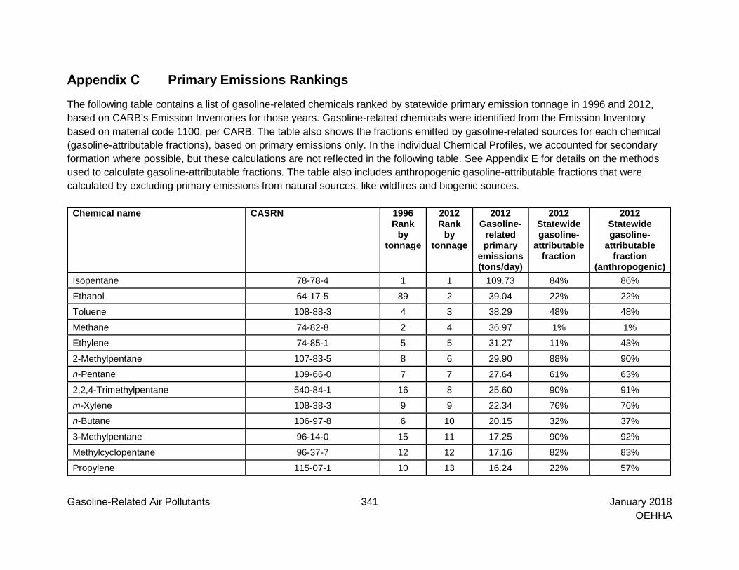
Gasoline-Related Air Pollutants 341 January 2018 OEHHA
Primary Emissions Rankings
The following table contains a list of gasoline-related chemicals ranked by statewide primary emission tonnage in 1996 and 2012, based on CARB’s Emission Inventories for those years. Gasoline-related chemicals were identified from the Emission Inventory based on material code 1100, per CARB. The table also shows the fractions emitted by gasoline-related sources for each chemical (gasoline-attributable fractions), based on primary emissions only. In the individual Chemical Profiles, we accounted for secondary formation where possible, but these calculations are not reflected in the following table. See Appendix E for details on the methods used to calculate gasoline-attributable fractions. The table also includes anthropogenic gasoline-attributable fractions that were calculated by excluding primary emissions from natural sources, like wildfires and biogenic sources.
Chemical name CASRN 1996 Rank
by tonnage
2012 Rank
by tonnage
2012 Gasoline-
related primary
emissions (tons/day)
2012 Statewide gasoline-
attributable fraction
2012 Statewide gasoline-
attributable fraction
(anthropogenic) Isopentane 78-78-4 1 1 109.73 84% 86%
Ethanol 64-17-5 89 2 39.04 22% 22%
Toluene 108-88-3 4 3 38.29 48% 48%
Methane 74-82-8 2 4 36.97 1% 1%
Ethylene 74-85-1 5 5 31.27 11% 43%
2-Methylpentane 107-83-5 8 6 29.90 88% 90%
n-Pentane 109-66-0 7 7 27.64 61% 63%
2,2,4-Trimethylpentane 540-84-1 16 8 25.60 90% 91%
m-Xylene 108-38-3 9 9 22.34 76% 76% n-Butane 106-97-8 6 10 20.15 32% 37%
3-Methylpentane 96-14-0 15 11 17.25 90% 92%
Methylcyclopentane 96-37-7 12 12 17.16 82% 83%
Propylene 115-07-1 10 13 16.24 22% 57%

Appendix C Primary Emissions Rankings
Gasoline-Related Air Pollutants 342 January 2018 OEHHA
Chemical name CASRN 1996 Rank
by tonnage
2012 Rank
by tonnage
2012 Gasoline-
related primary
emissions (tons/day)
2012 Statewide gasoline-
attributable fraction
2012 Statewide gasoline-
attributable fraction
(anthropogenic) 2,3-Dimethylpentane 565-59-3 20 14 15.36 55% 57%
Benzene 71-43-2 13 15 13.88 63% 63%
3-Methylhexane 589-34-4 26 16 12.90 61% 63%
Acetylene 74-86-2 14 17 12.10 11% 50%
Hexane 110-54-3 17 18 10.85 57% 57%
2,3-Dimethylbutane 79-29-8 22 19 9.59 92% 94%
2-Methylhexane 591-76-4 58 20 9.58 77% 77%
Formaldehyde 50-00-0 18 21 8.84 22% 22%
o-Xylene 95-47-6 21 22 8.82 52% 52%
Ethyl benzene 100-41-4 23 23 8.35 78% 78%
2,4-Dimethylpentane 108-08-7 35 24 8.17 58% 59%
Isobutene 115-11-7 11 25 7.67 86% 86%
2,3,4-Trimethylpentane 565-75-3 33 26 7.20 95% 96%
1,2,4-Trimethylbenzene 95-63-6 25 27 7.16 77% 77%
2,2-Dimethylbutane 75-83-2 29 28 6.02 92% 93%
1-Methyl-3-ethylbenzene 620-14-4 27 29 5.78 83% 83%
Ethane 74-84-0 24 30 5.77 1% 2%
n-Heptane 142-82-5 36 31 5.74 39% 39%
Methylcyclohexane 108-87-2 32 32 5.43 31% 31%
Cyclopentane 287-92-3 39 33 5.24 68% 70%
2-Methyl-2-butene 513-35-9 30 34 4.91 97% 97%
3-Methylheptane 589-81-1 37 35 4.84 77% 77%
Cyclohexane 110-82-7 31 36 4.31 60% 61%

Appendix C Primary Emissions Rankings
Gasoline-Related Air Pollutants 343 January 2018 OEHHA
Chemical name CASRN 1996 Rank
by tonnage
2012 Rank
by tonnage
2012 Gasoline-
related primary
emissions (tons/day)
2012 Statewide gasoline-
attributable fraction
2012 Statewide gasoline-
attributable fraction
(anthropogenic) 2,4-Dimethylhexane 589-43-5 52 37 3.88 53% 54%
2-Methylheptane 592-27-8 49 38 3.69 64% 64%
2,2,5-Trimethylhexane 3522-94-9 53 39 3.67 79% 83%
Isobutane 75-28-5 19 40 3.58 11% 12%
2,5-Dimethylhexane 592-13-2 50 41 3.43 95% 96%
2,3,3-Trimethylpentane 560-21-4 136 42 3.36 99% 99%
trans-2-Pentene 646-04-8 41 43 3.19 97% 97%
2,3-Dimethylhexane 584-94-1 60 44 2.92 88% 89%
1,3-Butadiene 106-99-0 38 45 2.87 26% 52%
1,3,5-Trimethylbenzene 108-67-8 44 46 2.78 86% 86%
Acetaldehyde 75-07-0 45 47 2.78 6% 12%
n-Octane 111-65-9 48 48 2.63 34% 34%
1-Butene 106-98-9 40 49 2.56 11% 44%
trans-2-Butene 624-64-6 42 50 2.50 81% 81% trans-1,3-Dimethylcyclopentane 1759-58-6 56 51 2.48 73% 73%
1-Methyl-4-ethylbenzene 622-96-8 46 52 2.47 84% 84% cis-1,3-Dimethylcyclopentane 2532-58-3 61 53 2.44 76% 76%
p-Xylene 106-42-3 146 54 2.37 29% 29%
3-Methyloctane 2216-33-3 51 55 2.36 67% 71%
2-Methyl-1-butene 563-46-2 43 56 2.15 99% 99%
3-Ethylpentane 617-78-7 54 57 1.94 54% 56%
1-Methyl-2-ethylbenzene 611-14-3 55 58 1.90 76% 76%
cis-2-Butene 590-18-1 47 59 1.82 84% 84%

Appendix C Primary Emissions Rankings
Gasoline-Related Air Pollutants 344 January 2018 OEHHA
Chemical name CASRN 1996 Rank
by tonnage
2012 Rank
by tonnage
2012 Gasoline-
related primary
emissions (tons/day)
2012 Statewide gasoline-
attributable fraction
2012 Statewide gasoline-
attributable fraction
(anthropogenic) 4-Methylheptane 589-53-7 73 60 1.73 75% 75%
3-Methyl-1-butene 563-45-1 66 61 1.72 47% 93%
Benzaldehyde 100-52-7 59 62 1.70 64% 64%
m-Tolualdehyde 620-23-5 57 63 1.70 100% 100% n-Propylbenzene 103-65-1 64 64 1.61 83% 83%
cis-2-Pentene 627-20-3 65 65 1.52 97% 97%
Acetone 67-64-1 63 66 1.45 1% 2%
1-Propyne 74-99-7 62 67 1.43 24% 84%
4-Methyloctane 2216-34-4 68 68 1.41 60% 64%
1-Pentene 109-67-1 67 69 1.32 48% 48%
Propane 74-98-6 28 70 1.32 2% 3%
1,2,3-Trimethylbenzene 526-73-8 69 71 1.32 64% 64%
Ethylcyclopentane 1640-89-7 76 72 1.30 61% 61%
1-Methyl-3n-propylbenzene 1074-43-7 72 73 1.23 98% 98% cis-1,trans-2,3-Trimethylcyclopentane 15890-40-1 109 74 1.12 94% 95%
Methanol 67-56-1 34 75 1.12 1% 14% trans-1,2-Dimethylcyclopentane 822-50-4 168 76 1.11 99% 99%
Cyclopentene 142-29-0 70 77 1.11 98% 98%
n-Nonane 111-84-2 74 78 1.08 22% 22%
1,2-Propadiene 463-49-0 71 79 1.07 69% 69%
2-Methyl-2-pentene 625-27-4 81 80 9.43E-01 99% 99%
1,2-Dimethyl-4-ethylbenzene 934-80-5 83 81 9.19E-01 75% 75%
1,3-Dimethyl-5-ethylbenzene 934-74-7 82 82 8.80E-01 80% 80%

Appendix C Primary Emissions Rankings
Gasoline-Related Air Pollutants 345 January 2018 OEHHA
Chemical name CASRN 1996 Rank
by tonnage
2012 Rank
by tonnage
2012 Gasoline-
related primary
emissions (tons/day)
2012 Statewide gasoline-
attributable fraction
2012 Statewide gasoline-
attributable fraction
(anthropogenic) trans-2-Hexene 4050-45-7 77 83 8.76E-01 99% 99%
2,6-Dimethylheptane 1072-05-5 75 84 8.45E-01 44% 46%
2-Methyloctane 3221-61-2 132 85 7.78E-01 57% 59%
1-Hexene 592-41-6 105 86 7.52E-01 72% 72%
2,2-Dimethylhexane 590-73-8 102 87 7.28E-01 96% 97%
3,5-Dimethylheptane 926-82-9 78 88 7.27E-01 69% 74%
2-Methylnonane 871-83-0 84 89 6.57E-01 42% 42%
Indan 496-11-7 90 90 6.56E-01 64% 64%
Isoprene 78-79-5 79 91 6.54E-01 0% 98%
2-Methyl-2-propenal 78-85-3 88 92 6.06E-01 95% 95%
Styrene 100-42-5 85 93 6.04E-01 12% 12%
Acrolein 107-02-8 86 94 5.97E-01 29% 29%
Naphthalene 91-20-3 107 95 5.94E-01 33% 33%
1,2,4-Trimethylcyclopentene 2815-58-9 80 96 5.86E-01 92% 94%
1,3-Dimethyl-4-ethylbenzene 874-41-9 98 97 5.80E-01 82% 82%
1,4-Dimethyl-2-ethylbenzene 1758-88-9 100 98 5.50E-01 75% 75% n-Decane 124-18-5 87 99 5.48E-01 7% 7%
4-Methyl-trans-2-pentene 674-76-0 101 100 5.16E-01 99% 99%
trans-1,4-Dimethylcyclohexane 9/8/7942 110 101 5.13E-01 38% 38% trans-1-Methyl-3-ethylcyclopentane 2613-65-2 91 102 5.04E-01 81% 83%
trans-1,3-Dimethylcyclohexane 8/28/7942 116 103 4.99E-01 15% 16% cis-1,3-Dimethylcyclohexane 638-04-0 92 104 4.90E-01 18% 18%
3,3-Dimethylpentane 562-49-2 159 105 4.85E-01 88% 88%

Appendix C Primary Emissions Rankings
Gasoline-Related Air Pollutants 346 January 2018 OEHHA
Chemical name CASRN 1996 Rank
by tonnage
2012 Rank
by tonnage
2012 Gasoline-
related primary
emissions (tons/day)
2012 Statewide gasoline-
attributable fraction
2012 Statewide gasoline-
attributable fraction
(anthropogenic) 1,3-Diethylbenzene (meta) 141-93-5 115 106 4.53E-01 88% 88%
cis-1,trans-2,4-Trimethylcyclopentane 200 107 4.50E-01 100% 100% cis-1,2-Dimethylcyclopentane 1192-18-3 201 108 4.48E-01 100% 100%
2-Methyl-1-pentene 763-29-1 99 109 4.40E-01 95% 95%
1,2,3,5-Tetramethylbenzene 527-53-7 120 110 4.37E-01 63% 63%
Vinylacetylene 689-97-4 97 111 4.25E-01 100% 100%
1,4-Diethylbenzene (para) 105-05-5 96 112 4.24E-01 87% 87%
2,2,3-Trimethylpentane 564-02-3 192 113 4.20E-01 97% 97%
2,2,4-Trimethylhexane 16747-26-5 108 114 4.17E-01 72% 77%
2,5-Dimethylheptane 2216-30-0 205 115 4.16E-01 51% 52%
2,2,5-Triethylheptane 20291-95-6 94 116 4.14E-01 33% 33%
cis-2-Hexene 7688-21-3 118 117 4.13E-01 99% 99%
2-Methylindan 824-63-5 121 118 4.08E-01 100% 100%
2,3,5-Trimethylhexane 1069-53-0 134 119 3.92E-01 83% 86%
3-Methylcyclopentene 1120-62-3 95 120 3.90E-01 99% 99%
2,4-Dimethylheptane 2213-23-2 104 121 3.84E-01 52% 54%
3-Methyl-1-pentene 760-20-3 93 122 3.80E-01 99% 99%
Isobutylcyclopentane 3788-32-7 208 123 3.73E-01 99% 99%
Propionaldehyde 123-38-6 111 124 3.67E-01 4% 4%
3,4-Dimethylheptane 922-28-1 127 125 3.66E-01 78% 82%
5-Methylindan 874-35-1 124 126 3.66E-01 45% 45%
1-Methyl-2-isopropylbenzene 527-84-4 113 127 3.63E-01 96% 96%
Crotonaldehyde 4170-30-3 114 128 3.52E-01 24% 24%

Appendix C Primary Emissions Rankings
Gasoline-Related Air Pollutants 347 January 2018 OEHHA
Chemical name CASRN 1996 Rank
by tonnage
2012 Rank
by tonnage
2012 Gasoline-
related primary
emissions (tons/day)
2012 Statewide gasoline-
attributable fraction
2012 Statewide gasoline-
attributable fraction
(anthropogenic) trans-3-Hexene 13269-52-8 112 129 3.46E-01 99% 99%
1,3,5-Trimethylcyclohexane 1839-63-0 106 130 3.43E-01 52% 52% cis-1-Methyl-3-ethylcyclopentane 2613-66-3 117 131 3.35E-01 81% 82%
1,2,4,5-Tetramethylbenzene 95-93-2 130 132 3.22E-01 62% 62%
Cyclohexene 110-83-8 103 133 3.20E-01 100% 100%
Ethylcyclohexane 1678-91-7 149 134 3.07E-01 16% 16%
trans-3-Heptene 14686-14-7 119 135 3.05E-01 100% 100%
2-Methyl-3-ethylpentane 609-26-7 182 136 2.99E-01 78% 79%
2,3,4-Trimethylhexane 921-47-1 213 137 2.84E-01 100% 100%
1,1,4-Trimethylcyclohexane 7094-27-1 214 138 2.71E-01 66% 66%
3,3-Dimethyloctane 4110-44-5 123 139 2.69E-01 37% 41%
Cumene 98-82-8 133 140 2.63E-01 46% 46%
4-Methyl-1-pentene 691-37-2 138 141 2.63E-01 100% 100%
2,2,4-Trimethylheptane 14720-74-2 122 142 2.59E-01 35% 39% 3-Methyl-cis-2-hexene 10574-36-4 135 143 2.56E-01 100% 100%
2,6-Dimethyloctane 2051-30-1 126 144 2.49E-01 20% 22%
2,3-Dimethylheptane 3074-71-3 185 145 2.48E-01 85% 86%
2,4-Dimethyloctane 4032-94-4 128 146 2.41E-01 9% 10%
trans-1,cis-2,3-Trimethylecyclopentane -- 147 2.39E-01 100% 100%
2,5-Dimethyloctane 15869-89-3 137 148 2.37E-01 38% 42%
Isovaleraldehyde 590-86-3 125 149 2.30E-01 71% 71% 3-Methyl-cis-2-pentene 922-62-3 196 150 2.27E-01 98% 98%
3-Methyl-3-ethylpentane 1067-08-9 216 151 2.15E-01 100% 100%

Appendix C Primary Emissions Rankings
Gasoline-Related Air Pollutants 348 January 2018 OEHHA
Chemical name CASRN 1996 Rank
by tonnage
2012 Rank
by tonnage
2012 Gasoline-
related primary
emissions (tons/day)
2012 Statewide gasoline-
attributable fraction
2012 Statewide gasoline-
attributable fraction
(anthropogenic) 2,2,3-Trimethylbutane 464-06-2 156 152 2.10E-01 68% 69%
3,4-Dimethylhexane 583-48-2 176 153 2.10E-01 62% 62%
3-Ethylhexane 619-99-8 223 154 2.06E-01 43% 43%
Methyl ethyl ketone {2-butanone} 78-93-3 131 155 2.06E-01 2% 2% n-Undecane 1120-21-4 142 156 1.99E-01 4% 4%
1,2-Dimethyl-3-ethylbenzene 933-98-2 155 157 1.91E-01 98% 98%
3,3-Dimethylhexane 563-16-6 184 158 1.89E-01 98% 99% cis-1,2-Dimethylcyclohexane 8/6/7942 157 159 1.87E-01 63% 63%
2,4-Dimethyl-2-pentene 625-65-0 129 160 1.87E-01 100% 100%
Butyraldehyde 123-72-8 139 161 1.81E-01 6% 6%
trans-1,2-Dimethylcyclohexane 6876-23-9 218 162 1.80E-01 75% 75%
2,2,3,Trimethylhexane 16747-25-4 219 163 1.80E-01 100% 100% cis-1,cis-2,3-Trimethylcyclopentane 2613-69-6 220 164 1.79E-01 100% 100%
2-Methyl-trans-3-hexene 692-24-0 141 165 1.77E-01 100% 100%
3,3-Dimethyl-1-pentene 3404-73-7 199 166 1.72E-01 100% 100%
2-Methyl naphthalene 91-57-6 208 167 1.72E-01 21% 21%
1-Methyl-2n-propylbenzene 1074-17-5 140 168 1.69E-01 91% 91%
trans-2-Heptene 14686-13-6 153 169 1.69E-01 99% 99%
cis-2-Heptene 6443-92-1 154 170 1.66E-01 99% 99%
1,2,3,4-Tetramethylbenzene 488-23-3 144 171 1.66E-01 93% 93%
trans-2-Ethylmethylcyclopentane 224 172 1.64E-01 100% 100%
Dimethylcyclopentane 28729-52-4 225 173 1.64E-01 87% 87%
1-Methylcyclopentene 693-89-0 201 174 1.58E-01 100% 100%

Appendix C Primary Emissions Rankings
Gasoline-Related Air Pollutants 349 January 2018 OEHHA
Chemical name CASRN 1996 Rank
by tonnage
2012 Rank
by tonnage
2012 Gasoline-
related primary
emissions (tons/day)
2012 Statewide gasoline-
attributable fraction
2012 Statewide gasoline-
attributable fraction
(anthropogenic) 1-Methyl-4n-propylbenzene 1074-55-1 212 175 1.49E-01 26% 26%
3-Methyl-trans-2-pentene 616-12-6 169 176 1.49E-01 99% 99%
Hexaldehyde 66-25-1 143 177 1.47E-01 2% 3%
1-Methyl-4-ethylcyclohexane 6236-88-0 145 178 1.46E-01 54% 54%
1,2-Butadiene {methylallene} 590-19-2 150 179 1.41E-01 94% 94%
1-Methyl-3-isopropylbenzene 535-77-3 148 180 1.40E-01 28% 28%
2,3-Dimethyloctane 7146-60-3 147 181 1.39E-01 15% 16%
3-Ethylheptane 15869-80-4 228 182 1.38E-01 49% 49%
1,3-Dipropylbenzene 17171-72-1 163 183 1.38E-01 100% 100%
3,3-Dimethylheptane 4032-86-4 229 184 1.34E-01 100% 100%
trans-1,3-Pentadiene 2004-70-8 151 185 1.30E-01 100% 100%
2,2-Dimethylpentane 590-35-2 190 186 1.29E-01 79% 80% 3-Methyl-trans-2-hexene 20710-38-7 208 187 1.22E-01 100% 100%
cis-3-Hexene 7642093 193 188 1.12E-01 99% 99%
3-Methylnonane 5911046 221 189 1.09E-01 24% 24%
1-Nonene 124-11-8 161 190 1.08E-01 55% 55% n-Pentylbenzene 538-68-1 160 191 1.08E-01 98% 98%
Propylcyclopentane 2040-96-2 232 192 1.05E-01 60% 60%
4-Methylindan 824-22-6 170 193 1.05E-01 58% 58%
1-Ethyl-2n-propylbenzene 16021-20-8 179 194 1.03E-01 81% 81%
2,2-Dimethyloctane 15869-87-1 158 195 1.03E-01 38% 42%
(2-Methylpropyl)benzene 538-93-2 175 196 9.47E-02 41% 41%
n-Dodecane 112-40-3 177 197 9.20E-02 3% 3%

Appendix C Primary Emissions Rankings
Gasoline-Related Air Pollutants 350 January 2018 OEHHA
Chemical name CASRN 1996 Rank
by tonnage
2012 Rank
by tonnage
2012 Gasoline-
related primary
emissions (tons/day)
2012 Statewide gasoline-
attributable fraction
2012 Statewide gasoline-
attributable fraction
(anthropogenic) 1,3-Dimethyl-2-ethylbenzene 11/28/9757 165 198 8.67E-02 28% 28%
4-Methyl-trans-2-hexene 3683-22-5 162 199 8.50E-02 99% 99% 1-Methyl-2-n-butylbenzene 1595-68-1 166 200 8.20E-02 87% 87%
1,2,4-Triethylbenzene 887-44-1 197 201 8.18E-02 99% 99%
2-Methyl-2-hexene 2738-19-4 152 202 8.02E-02 100% 100%
1-Methyl-1-ethylcyclohexane 4926-90-3 236 203 7.96E-02 99% 99%
n-Butylbenzene 104-51-8 225 204 7.80E-02 86% 86% 3-Methyl-trans-3-hexene 3899-36-3 180 205 7.77E-02 98% 98%
1-Methylnaphthalene 90-12-0 225 206 7.76E-02 99% 99% 1-(1,1-Dimethylethyl)-3,5-dimethylbenzene 98-19-1 167 207 7.62E-02 98% 98%
cis-1,cis-3,5-Trimethylcyclohexane 1795-27-3 236 208 7.47E-02 10% 10%
4,4-Dimethylheptane 1069-19-5 235 209 7.46E-02 100% 100%
2,3-Dimethyl-1-butene 563-78-0 174 210 7.37E-02 70% 70%
1,2-Diethylbenzene (ortho) 135-01-3 188 211 6.92E-02 30% 30%
2,4,4-Trimethylhexane 16747-30-1 171 212 6.91E-02 82% 85%
1,1,2-Trimethylcyclopentane 4259-00-1 244 213 6.16E-02 24% 24%
n-Butylcyclopentane 2040-95-1 245 214 5.97E-02 99% 99%
4,4-Dimethyl-2-pentene 690-08-4 221 215 5.97E-02 100% 100% cis-1,trans-2,trans-4-Trimethylcyclohexane 7667-60-9 245 215 5.97E-02 100% 100%
1-Methyl-4-isopropylbenzene 99-87-6 178 217 5.41E-02 49% 49%
4-Methyl-cis-2-pentene 691-38-3 206 218 5.19E-02 95% 95%
1,3,5-Triethylbenzene 102-25-0 203 219 4.86E-02 99% 99%

Appendix C Primary Emissions Rankings
Gasoline-Related Air Pollutants 351 January 2018 OEHHA
Chemical name CASRN 1996 Rank
by tonnage
2012 Rank
by tonnage
2012 Gasoline-
related primary
emissions (tons/day)
2012 Statewide gasoline-
attributable fraction
2012 Statewide gasoline-
attributable fraction
(anthropogenic) 1,4-Isodipropylbenzene 577-55-9 230 220 4.77E-02 100% 100%
1-Methyl-4-n-pentylbenzene 230 220 4.77E-02 100% 100%
5-Methylnonane 15869-85-9 236 222 4.76E-02 97% 97%
n-Propyl alcohol 71-23-8 245 223 4.72E-02 3% 3% cis-2-Octene 7642048 181 224 4.41E-02 99% 99%
2,4-Dimethyl-1-pentene 2213-32-3 189 224 4.41E-02 50% 50%
2,2-Dimethylpropane 463-82-1 164 226 4.22E-02 41% 41% trans-2-Octene 13389-42-9 191 227 4.17E-02 96% 96%
1,3-Butadiyne 460-12-8 186 228 4.00E-02 100% 100%
2,3-Dimethyl-2-pentene 10574-37-5 186 228 4.00E-02 100% 100%
3,3-Dimethyl-1-butene 558-37-2 183 230 3.72E-02 1% 1%
1-Methyl-4-t-butylbenzene 98-51-1 243 231 3.58E-02 75% 75%
1,1,3-Trimethylcyclohexane 3073-66-3 253 232 3.32E-02 5% 5%
2-Ethyl-1-butene 760-21-4 206 233 3.30E-02 99% 99% 3-n-Dipropylbenzene 234 234 3.28E-02 100% 100%
3-Methyl-cis-3-hexene 4914-89-0 233 235 3.25E-02 100% 100%
1,1-Dimethylcyclohexane 590-66-9 252 236 3.21E-02 12% 12%
2,4-Dimethylnonane 17302-24-8 -- 237 3.20E-02 25% 26%
Isopropylcyclohexane 696-29-7 253 238 3.12E-02 2% 2%
Pentamethylbenzene 700-12-9 245 239 3.11E-02 100% 100%
3-Ethyl-2-pentene 816-79-5 211 240 3.09E-02 100% 100%
1,1-Methylethylcyclopentane 16747-50-5 172 241 3.05E-02 33% 33%
1,1,2-Trimethylcyclohexane 7094-26-0 253 242 2.98E-02 31% 31%

Appendix C Primary Emissions Rankings
Gasoline-Related Air Pollutants 352 January 2018 OEHHA
Chemical name CASRN 1996 Rank
by tonnage
2012 Rank
by tonnage
2012 Gasoline-
related primary
emissions (tons/day)
2012 Statewide gasoline-
attributable fraction
2012 Statewide gasoline-
attributable fraction
(anthropogenic) (1-Methylpropyl)benzene 135-98-8 236 243 2.98E-02 17% 17%
s-Pentylbenzene 29316-05-0 236 243 2.98E-02 100% 100%
Trimethylcyclohexane 30498-63-6 253 243 2.98E-02 4% 4%
1-Octene 111-66-0 173 246 2.56E-02 20% 20%
2-Butyne 503-17-3 195 247 2.12E-02 84% 84%
5-Methyl-1-hexene 3524-73-0 253 248 2.01E-02 100% 100%
trans-3-Nonene 20063-92-7 253 249 1.76E-02 100% 100%
3,4-Dimethyl-2-pentene 24910-63-2 245 250 1.68E-02 100% 100%
tert-Amyl methyl ether (TAME) 994-05-8 217 251 1.65E-02 99% 99%
3-Ethyloctane 5881-17-4 253 252 1.63E-02 12% 13%
Butylcyclohexane 1678-93-9 253 253 1.62E-02 2% 2%
2-Methyl-1-octene 4588-18-5 253 254 1.60E-02 100% 100%
3-Ethylnonane 17302-11-3 253 255 1.56E-02 98% 99%
cis-3-Nonene 20237-46-1 245 256 1.51E-02 100% 100%
4-Methyl-1-hexene 3769-23-1 245 257 1.50E-02 100% 100%
trans-4-Octene 14850-23-8 253 258 1.49E-02 100% 100%
Dihydronaphthalene 253 258 1.49E-02 100% 100%
1,3-Cyclopentadiene 542-92-7 253 258 1.49E-02 100% 100%
5-Methyl-cis-2-hexene 3404-62-4 253 258 1.49E-02 100% 100%
3,6-Dimethyloctane 15869-94-0 253 258 1.49E-02 10% 10%
2,3-Dimethyl-2-octene 19781-18-1 253 258 1.49E-02 100% 100% n-Hexylbenzene 1077-16-3 253 258 1.49E-02 100% 100%
Ethylindan -- 265 1.41E-02 100% 100%

Appendix C Primary Emissions Rankings
Gasoline-Related Air Pollutants 353 January 2018 OEHHA
Chemical name CASRN 1996 Rank
by tonnage
2012 Rank
by tonnage
2012 Gasoline-
related primary
emissions (tons/day)
2012 Statewide gasoline-
attributable fraction
2012 Statewide gasoline-
attributable fraction
(anthropogenic) 2,2-Dimethylheptane 1071-26-7 285 266 1.30E-02 4% 4%
trans-1,2-cis-4-Trimethylcyclopentane 4850-28-6 280 267 1.28E-02 77% 79%
Unidentified 99-99-9 -- 268 1.25E-02 0% 0%
1,1,3-Trimethylcyclopentane 4516-69-2 275 269 1.16E-02 2% 2%
1,2,4-Trimethylcyclopentane 99-07-3 273 270 1.15E-02 1% 1%
3,4-Dimethyl-1-pentene 7385-78-6 194 271 1.08E-02 100% 100%
2-Methyldecane 6975-98-0 -- 272 9.57E-03 1% 1% cis-1-Ethyl-3-methylcyclopentane 99-07-1 289 273 9.24E-03 35% 35%
1-Methyl-2-tert-butylbenzene 1074-92-6 198 274 8.01E-03 100% 100% trans-1,3-Diethylcyclopentane -- 275 7.47E-03 100% 100%
c11-Aromatics -- 276 7.39E-03 91% 91%
3,3-Diethylpentane 1067-20-5 -- 277 7.29E-03 99% 99%
c10-Olefins -- 278 7.26E-03 4% 4%
Dimethylheptanes 98-09-1 241 279 7.01E-03 4% 5%
1,2-Isodipropylbenzene 100-18-5 276 280 6.51E-03 100% 100%
1-Ethyl-4-isopropylbenzene 4218-48-8 271 281 6.33E-03 4% 4% trans-1-Ethyl-3-methylcyclopentane 99-08-5 289 282 6.24E-03 26% 26%
1,2,3-Trimethylcyclopentane 99-07-4 274 283 5.86E-03 1% 1%
2-Methyl-1-hexene 6094026 -- 284 5.66E-03 100% 100%
Indene 95-13-6 -- 285 5.44E-03 14% 14%
1-Methyl-3-butylbenzene 99-08-4 270 286 5.07E-03 12% 12%
4-Methylnonane 17301-94-9 -- 287 4.96E-03 1% 1%
1-Ethyl-2-isopropylbenzene 271 288 4.95E-03 29% 29%

Appendix C Primary Emissions Rankings
Gasoline-Related Air Pollutants 354 January 2018 OEHHA
Chemical name CASRN 1996 Rank
by tonnage
2012 Rank
by tonnage
2012 Gasoline-
related primary
emissions (tons/day)
2012 Statewide gasoline-
attributable fraction
2012 Statewide gasoline-
attributable fraction
(anthropogenic) trans-1-Methyl-2-propylcyclopentane 932-44-5 -- 289 4.63E-03 100% 100%
Trimethylcyclopentane 30498-64-7 278 290 4.56E-03 9% 9%
tert-Pentylbenzene 2049-95-8 -- 291 4.32E-03 100% 100%
3-Ethyl-3-methylheptane 17302-01-1 -- 292 4.19E-03 100% 100%
t-Butylbenzene 98-06-6 -- 293 3.83E-03 0% 0%
2-Ethyl-1-pentene 3404-71-5 -- 294 3.68E-03 100% 100%
cis-1-Ethyl-2-methylcyclopentane 930-89-2 288 295 3.52E-03 9% 9%
2,3,3-Trimethyl-1-butene 594-56-9 -- 296 3.07E-03 98% 98%
trans-3-Octene 14919-01-8 -- 297 2.99E-03 100% 100%
t-1-Butyl-4-ethylbenzene 276 298 2.98E-03 100% 100%
3-Methyl-5-ethylheptane -- 299 2.96E-03 100% 100%
1-Methyl-4-(1-methylpropyl)benzene 1595-16-0 -- 300 2.79E-03 100% 100%
Dimethylcyclopentene -- 301 2.54E-03 18% 18%
cis-3-Heptene 7642106 -- 302 2.52E-03 100% 100% trans,trans-1,2,4-Trimethylcyclohexane 2234-75-5 -- 303 2.23E-03 0% 0%
Isopropylcyclopentane 3875-51-2 -- 304 2.20E-03 98% 98%
2,7-Dimethyloctane 1072-16-8 -- 305 2.19E-03 3% 3%
cis-1,trans-2,cis-4-Trimethylcyclohexane -- 306 2.15E-03 100% 100%
trans-1-Ethyl-4-methylcyclohexane 99-08-2 -- 307 1.90E-03 1% 1%
Trimethylindan 36541-18-1 -- 308 1.80E-03 100% 100%
1-Methyl-4-isobutylbenzene -- 309 1.75E-03 3% 3%
2-Methyl-2-octene 16993-86-5 -- 310 1.70E-03 5% 5%
1-Ethyl-3-methylcyclopentane 99-04-8 281 311 1.47E-03 1% 1%

Appendix C Primary Emissions Rankings
Gasoline-Related Air Pollutants 355 January 2018 OEHHA
Chemical name CASRN 1996 Rank
by tonnage
2012 Rank
by tonnage
2012 Gasoline-
related primary
emissions (tons/day)
2012 Statewide gasoline-
attributable fraction
2012 Statewide gasoline-
attributable fraction
(anthropogenic) 1-Ethyl-2-methylcyclopentane 99-08-3 281 311 1.47E-03 1% 1%
2,6-Dimethylnaphthalene 581-42-0 -- 313 1.44E-03 100% 100% 2-Methyl-cis-3-hexene 15840-60-5 -- 314 1.39E-03 100% 100%
cis-1,4-Dimethylcyclohexane 624-29-3 283 315 1.38E-03 1% 1% n-Tridecane 629-50-5 -- 316 1.16E-03 0% 0%
2-Methylundecane 7045-71-8 -- 317 7.82E-04 0% 0%
1-Heptene 592-76-7 -- 318 7.22E-04 0% 0%
Unidentified (SAROAD 43381) -- 319 5.72E-04 100% 100%
Unidentified (SAROAD 43384) -- 320 5.58E-04 100% 100%
Unidentified (SAROAD 43382) -- 321 5.35E-04 100% 100%
2,3-Dimethyl-1-hexene 16746-86-4 -- 322 4.36E-04 100% 100%
cis-Bicyclo[3.3.0]octane 694-72-4 287 323 4.29E-04 1% 1%
Dimethylindene -- 324 4.16E-04 100% 100%
Ethylmethylcyclohexanes 90-08-3 -- 325 4.11E-04 0% 0%
2-Undecene, (e)- 693-61-8 -- 326 4.10E-04 100% 100%
3-Ethyl-3-hexene 16789-51-8 -- 327 3.31E-04 100% 100%
3-Methyl-1-hexene 3404-61-3 -- 328 2.52E-04 30% 30%
n-Tetradecane 629-59-4 -- 329 2.48E-04 0% 0%
trans-1,cis-2,3-Trimethylcyclopentane 215 330 2.01E-04 29% 30%
2,3-Dimethyl-2-heptene 3074-64-4 -- 331 1.83E-04 100% 100%
Ethylmethylhexane 90-08-2 279 332 1.67E-04 1% 1%
Isobutylcyclohexane 1678-98-4 -- 333 1.52E-04 0% 0%
Unidentified (SAROAD 43383) -- 334 1.26E-04 100% 100%

Appendix C Primary Emissions Rankings
Gasoline-Related Air Pollutants 356 January 2018 OEHHA
Chemical name CASRN 1996 Rank
by tonnage
2012 Rank
by tonnage
2012 Gasoline-
related primary
emissions (tons/day)
2012 Statewide gasoline-
attributable fraction
2012 Statewide gasoline-
attributable fraction
(anthropogenic) 1,4-Dimethyl-1-cyclohexene 70688-47-0 -- 335 1.26E-04 100% 100%
trans-4-Nonene 10405-85-3 -- 336 8.90E-05 100% 100%
2,2,3,3-Tetramethylpentane 7154-79-2 284 337 7.61E-05 0% 0%
Propenylcyclohexane 90-10-5 -- 338 7.43E-05 0% 0%
Propylcyclohexane 1678-92-8 -- 339 6.57E-05 0% 0%
trans,cis-1,2,4-Trimethylcyclohexane 99-07-5 -- 340 6.32E-05 0% 0%
Methylheptyne -- 341 6.29E-05 100% 100% trans,trans-1,3,5-Trimethylcyclohexane 99-07-6 -- 342 5.94E-05 0% 0%
Methyl biphenyl 28652-72-4 -- 343 5.79E-05 100% 100%
Tetramethylcyclopentane 90-09-8 -- 344 5.35E-05 0% 0%
Unidentified (SAROAD 43385) -- 345 4.72E-05 100% 100%
cis-1-Ethyl-3-methylcyclohexane 19489-10-2 -- 346 4.15E-05 0% 0%
1,2,3-Trimethylcyclohexane 1678-97-3 -- 347 3.77E-05 0% 0%
trans-2-Nonene 6434-78-2 -- 348 3.14E-05 100% 100% cis,trans-1,2,4-Trimethylcyclohexane 99-07-9 -- 349 2.64E-05 0% 0%
trans-1-Ethyl-3-methylcyclohexane 99-08-0 -- 350 2.17E-05 0% 0% n-Pentadecane 629-62-9 -- 351 2.09E-05 0% 0%
1,2-Dimethylcyclopentane 2452-99-5 -- 352 1.43E-05 0% 0%
cis-Bicyclo[4.3.0]nonane 4551-51-3 -- 353 1.41E-05 0% 0% cis,cis-1,2,4-Trimethylcyclohexane 99-05-4 -- 354 1.23E-05 0% 0%
trans-1-Ethyl-2-methylcyclohexane 4923-78-8 -- 354 1.23E-05 0% 0% cis,trans-1,2,3-Trimethylcyclohexane 20348-72-5 -- 356 8.51E-06 0% 0%
Ethylhexane 90-08-1 286 357 4.78E-06 0% 0%

Appendix C Primary Emissions Rankings
Gasoline-Related Air Pollutants 357 January 2018 OEHHA
Chemical name CASRN 1996 Rank
by tonnage
2012 Rank
by tonnage
2012 Gasoline-
related primary
emissions (tons/day)
2012 Statewide gasoline-
attributable fraction
2012 Statewide gasoline-
attributable fraction
(anthropogenic) cis-1-Ethyl-4-methylcyclohexane 3728-56-1 -- 358 4.69E-06 0% 0%
cis-1-Ethyl-2-methylcyclohexane 4923-77-7 -- 358 4.69E-06 0% 0%
1,1-Dimethylcyclopentane 1638-26-2 -- 360 1.24E-06 0% 0%
4-Ethyldecane 99-04-9 291 361 1.14E-06 0% 0% Methyl t-butyl ether (MTBE) 1634-04-4 3 362 1.04E-06 0% 0%
1-Methyl-2-n-butylbenzene 1595-11-5 204 -- -- -- --
2,4,4-Trimethyl-2-pentene 107-40-4 242 -- -- -- --

Gasoline-Related Air Pollutants 358 January 2018 OEHHA
Calculation of Population-Weighted Ambient Air Concentrations
This appendix describes how California ambient air monitoring data and census data were used to estimate population-weighted ambient air concentrations for selected pollutants. The first step was to calculate the annual average concentration of the pollutant at monitoring sites. When there were enough sites with data, these averages were combined to calculate a population-weighted annual average ambient air concentration. The following sections describe:
• The ambient air monitoring data sources • How annual averages were calculated and/or modeled at monitoring sites • How monitoring site averages were interpolated to census tracts • How census tract estimates were combined to get population-weighted annual averages
for an air basin and state • How decennial census tract values were interpolated
Sources of Ambient Air Monitoring Data
Ambient Air Monitoring Data from California Air Resources Board CARB collects ambient air measurements from monitoring stations throughout California. The data for this analysis were primarily taken from CARB’s 2015 Air Quality Data DVD. Additional data were available on the CARB website for download. A brief description of each data file follows.
• Carbon monoxide (CO) data were taken from the dlygas_csv.txt data file, which was downloaded from the CARB website. It contained data on criteria pollutants by monitoring station from 1995-2011. There were data from throughout the state and from nearly each day in each year. For 2012 to 2014, hourly data were converted to daily averages and appended to the daily data. The data file co20102014.txt, from the CARB website, was used for 2012 and 2013 data and “2014 AQMIS Extraction 20150310.accdb” from the DVD was used for 2014.
• Nitrogen dioxide daily averages came from the Access database “AQDVD2015_Daily Data.accdb” on the DVD. The 2014 NO2 data was incomplete and not used.
• The California Toxic Monitoring Network data file (DailyToxcis_3-6-2014.accdb) contained the daily average concentrations of TACs for the years 1990-2014. There were data from two or three days in each month. The detectors used to measure the concentrations of chemicals in the air have minimum levels of detection. When the actual concentration fell below this limit of detection, CARB put one-half the limit of detection in the data file.
• The PAMS hourly data file (NMOC_PAMS 3-hr data 1994-2014.accdb) contained data on non-methane organic compounds collected by the Photochemical Assessment Monitoring Station (PAMS) monitoring network. It included hourly concentrations of non-methane organic compounds by monitoring station 1994-2014. The data were from July through October of each year. There were 0 to 8 measurements per day.

Appendix D Calculation of Population-Weighted Ambient Air Concentrations
Gasoline-Related Air Pollutants 359 January 2018 OEHHA
• The PAMS 24 hour data set (NMOC 24 Hour.accdb) contained data on non-methane organic compounds collected by the Photochemical Assessment Monitoring Stations (PAMS). It included 24-hour average concentrations of non-methane organic compounds by monitoring station from the years 1994-2014. The data were from throughout the year. The number of data points varied by site and year. Many sites had 50 to 60 data points per year. The South Coast Air Basin data from 2012 to 2014 was very limited.
• The PM10 data file (PM10StdDaily20150302.xlsx) contained the daily average concentration of PM10 from 1996 to 2014. The 2014 data were incomplete and not used. For many sites data were collected every sixth day resulting in 50 to 60 measurements annually. The data in the file were at standard temperature and pressure. There was a separate data file with measurements recorded at local conditions. The local conditions data file was not used because data were either missing or very sparse for 1998 and earlier.
• The PM2.5 data file (PM25Daily20150302.xlsx) contained daily average concentrations of PM2.5 from 1998 to 2014. The data from1998 and 2014 were incomplete and not used. Measurements were recorded at local conditions.
• The location data file (location.dat) contained monitoring station information such as name, air basin, county, address, latitude and longitude.
DRI Ambient Air Measurements The DRI data file (dri_rfg9596.xls) was created by Desert Research Institute (DRI) (Zielinska et al., 1999).It contained ambient air measurements from summer months in 1995 and 1996. There were two readings per day and the samples were collected over a 3-hour period. The data came from four monitoring stations in Southern California but the bulk of the data are from three of these sites: Azusa, Burbank and Los Angeles.
US EPA AirData
• PAH data collected by three California monitoring stations in the National Air Toxics Trend Stations (NATTS) system were downloaded from the US EPA AirData website30.
• Benzaldehyde, butyraldehyde, ethanol and propionaldehyde data were downloaded from the US EPA AirData website.
30 https://ofmext.epa.gov/AQDMRS/aqdmrs.html

Appendix D Calculation of Population-Weighted Ambient Air Concentrations
Gasoline-Related Air Pollutants 360 January 2018 OEHHA
Methods for Estimating the Annual Average Concentration at Each Monitoring Site
Introduction This section describes how air quality monitoring data was used to calculate the annual average ambient air concentrations of chemicals at sites within an air quality monitoring network. The method used depended on the amount of data available for the chemical. The general procedures used are described in the sections immediately below. Details for individual chemicals are provided after the general methods. Data sources were described in the previous section. The annual average from each monitoring site was used at a later stage to calculate the population-weighted average of the chemical; this procedure is explained in detail later in this appendix. The estimated population-weighted annual averages are presented in the Chemical Profiles section beginning on page 85.
Method 1 – Dense Monitoring Networks
This method was used for nitrogen dioxide and particulate matter (PM2.5 and PM10). The annual average concentration at a monitoring station was calculated as the average of the observed daily average concentrations from one year. The site had to have 10 or more months of data to be included. Details about nitrogen dioxide and particulate matter are provided below in individual sections
Method 2 – California Toxic Monitoring Network The California Toxic Monitoring Network collected ambient air data from multiple air basins. Data from 1996 through 2014 were used. The five most populated air basins (SC, SD, SFB, SJV, and SV) had between two and six monitoring stations active annually between 1996 and 2014. The South Coast Air Basin had the most monitoring stations with five to six stations collecting data at any time. The annual average was calculated at each site from daily average data. The annual averages were retained provided they were based on 10 or more months of data. These observed annual averages were supplemented with modeled annual averages at additional locations. The observed and modeled annual averages were then used to calculate the population-weighted averages for the five basins and for the state. The model for the concentration of a toxic contaminant took into account the year the measurement was made and the level of carbon monoxide at the site:
𝑆𝑆𝑆𝑆𝑆𝑆𝑖𝑖𝑖𝑖 = 𝐼𝐼𝐼𝐼𝐼𝐼𝐼𝐼𝐼𝐼𝐼𝐼𝐼𝐼𝐼𝐼𝐼𝐼 + 𝛽𝛽1996 𝑌𝑌𝐼𝐼𝑌𝑌𝐼𝐼1996 + ⋯+ 𝛽𝛽2013 𝑌𝑌𝐼𝐼𝑌𝑌𝐼𝐼2013 +
𝛽𝛽𝑆𝑆𝑆𝑆𝑆𝑆𝑆𝑆 𝑆𝑆𝑆𝑆𝑆𝑆𝑆𝑆𝑖𝑖𝑖𝑖 + 𝑆𝑆𝑆𝑆𝐼𝐼𝐼𝐼𝑖𝑖 + 𝐸𝐸𝐼𝐼𝐼𝐼𝐸𝐸𝐼𝐼𝑖𝑖𝑖𝑖
Where • SqCik is the square root of the kth daily average ambient air concentration of the TAC
from site i. • Year1995+j is an indicator function that indicates if the measurement was made in the year
1995+j. For example, Year1996 equals 1 if the measurement was taken in year 1996 and

Appendix D Calculation of Population-Weighted Ambient Air Concentrations
Gasoline-Related Air Pollutants 361 January 2018 OEHHA
equals zero otherwise. There were 18 indicator variables Year1 to Year18, one for each year between 1996 and 2013. 2014 was the reference year.
• SqCoik is the square root of the kth daily average carbon monoxide concentration at site i. • Sitei is a random effect for site i. Sitei is assumed to have a normal distribution with
mean zero and standard deviation σSite. Sitei and Sitej are assumed to be independent when i ≠ j.
• Errorik is the error term that is assumed to have a normal distribution with mean zero and standard deviation σerror. Errorik is assumed to be independent of Sitej for all j and independent of Errori’k’ unless i=i' and k=k’.
The model accounts for annual changes in TAC levels and uses observed levels of carbon monoxide to account for spatial and temporal differences within a year. Random effects are included to account for the repeated measurements made at the monitoring sites. A square root transformation was used in order reduce uneven spread about the average response. A log transformation was not used because some of the measurements were near zero and a log transformation introduced uneven spread at these small values. When the ambient air concentration of the chemical fell below the device’s limit of detection, one-half the limit of detection was put in the data file as a placeholder by CARB. The handling of non-detects is discussed separately for each chemical below. A model for predicting the annual average of a chemical from the annual average of carbon monoxide was considered but ultimately rejected since, for some chemicals, large numbers of non-detects in the data made calculating the annual averages directly from the data questionable. A data file containing the annual traffic volume near each monitoring site was obtained from Environmental Health Investigations Branch of the California Department of Public Health. An attempt was made to include the traffic volume as an additional predictor of benzene. Traffic volume did not significantly contribute to the model (i.e., carbon monoxide tended to be higher in areas with more traffic), and was excluded from the final models that were used. A data file was obtained that contained a land use description of each monitoring site. The data file was obtained from the US EPA web site. An attempt was made to include land use code as an additional predictor of benzene ambient air concentration. Land use codes did not significantly contribute to the model and were excluded from the final models. Once the model was fit, the best linear unbiased predictor of the square root of the daily average concentration of the toxic chemical was found using the square root of the daily average concentration of carbon monoxide at sites in California. These values were squared to get an estimate of the daily average concentration of the chemical. The daily averages from a site were combined to get an annual average for the monitoring site. A modeled annual average was retained provided it was based on 300 or more daily average estimates. When possible, the

Appendix D Calculation of Population-Weighted Ambient Air Concentrations
Gasoline-Related Air Pollutants 362 January 2018 OEHHA
measured annual average concentration from a monitoring site was used instead of the modeled concentration. The criterion for using the observed annual average from a monitoring site instead of the modeled annual average concentration was that there needed to be 10 or more months of data used to calculate the observed annual average.
Method 3 – Photochemical Assessment Monitoring Stations (PAMS) 24 hour data file The Photochemical Assessment Monitoring Stations (PAMS) had daily average concentrations from nine sites in the South Coast Air Basin from 1996 to 2011. Data were collected every sixth day. However, the number of daily averages available throughout the year varied by monitoring site and year. Seven of these sites also had carbon monoxide data. The model for the concentration of a PAMS chemical included an annual trend term and the observed level of carbon monoxide:
𝑆𝑆𝑆𝑆𝑆𝑆𝑖𝑖𝑖𝑖 = 𝐼𝐼𝐼𝐼𝐼𝐼𝐼𝐼𝐼𝐼𝐼𝐼𝐼𝐼𝐼𝐼𝐼𝐼 + 𝛽𝛽𝑇𝑇𝑇𝑇𝑇𝑇𝑇𝑇𝑇𝑇𝑇𝑇𝐼𝐼𝐼𝐼𝐼𝐼𝑇𝑇 + 𝛽𝛽𝑆𝑆𝑆𝑆𝑆𝑆𝑆𝑆𝑆𝑆𝑆𝑆𝑆𝑆𝑆𝑆𝑖𝑖𝑖𝑖 + 𝑆𝑆𝑆𝑆𝐼𝐼𝐼𝐼𝑖𝑖 + 𝐸𝐸𝐼𝐼𝐼𝐼𝐸𝐸𝐼𝐼𝑖𝑖𝑖𝑖 Where
• SqCik is the square root of the kth daily average ambient air concentration of the chemical from site i.
• Trend is the value of a third degree polynomial with slope set to zero in the years 1996 and 2014. More precisely, let ‘year’ be the year the measurement was made and y=year-1995, then Trend = y3 - 30*y2 + 57.
• Let SqCOik be the square root of the kth daily average carbon monoxide concentration at site i.
• Let Sitei be a random effect for site i, which is assumed to have a normal distribution with mean zero and standard deviation σSite. Sitei and Sitej are assumed to be independent when i ≠ j.
• Let Errorik be the error term, which is assumed to have a normal distribution with mean zero and standard deviation σError. Errorik is assumed to be independent of Sitei for all i and independent of Errori’k’ unless i=i' and k=k’.
The reasons for modeling the annual trend this way included: (1) Some years had sparse data which led to erratic estimates when a separate intercept was included for each year (as was done for the California Toxic Monitoring Network data); (2) The South Coast PAMS data ended in 2011 and OEHHA wanted to extrapolate to 2014; and (3) A review of the PAMS data sets indicated that the annual trend in concentrations between 1996 and 2011 had roughly a backward S shape that could be modeled by this type of polynomial. The appropriateness of the model was checked for each chemical by comparing the estimated population-weighted averages to the observed values (see plots in the Chemical Profiles section of this report). The model was used to calculate the best linear unbiased predictors of the square root of the daily average chemical concentrations at each monitoring site in the South Coast Air Basin with carbon monoxide data. The square root values were squared to get estimates of the daily average concentrations. These daily averages were combined into annual averages. An

Appendix D Calculation of Population-Weighted Ambient Air Concentrations
Gasoline-Related Air Pollutants 363 January 2018 OEHHA
estimated annual average was retained provided it was based on 300 or more daily average estimates. The annual average concentration of the chemical at a site was calculated directly from the PAMS data instead of from the modeled values provided there were at least 10 months of data available from the monitoring site.
Method 4 – Three Hour Data Files The hourly PAMS data file and DRI data file are described above. Both of these files contained measurements of ambient air concentrations of chemicals collected for 3-hour periods during the summer months. Data from these files were used to estimate chemical concentrations in the South Coast Air Basin using the model described below. The model for the three-hour average concentration of a chemical was
𝑆𝑆𝑆𝑆𝑆𝑆𝑖𝑖𝑖𝑖 = 𝐼𝐼𝐼𝐼𝐼𝐼𝐼𝐼𝐼𝐼𝐼𝐼𝐼𝐼𝐼𝐼𝐼𝐼 + 𝛽𝛽1 𝑆𝑆𝑆𝑆𝑆𝑆𝑆𝑆𝑖𝑖𝑖𝑖 + 𝑆𝑆𝑆𝑆𝐼𝐼𝐼𝐼𝑖𝑖 + 𝐸𝐸𝐼𝐼𝐼𝐼𝐸𝐸𝐼𝐼𝑖𝑖𝑖𝑖 Where
• 𝑆𝑆𝑆𝑆𝑆𝑆𝑖𝑖𝑖𝑖 is the square root of the kth three-hour average concentration of the chemical from site i
• 𝑆𝑆𝑆𝑆𝑆𝑆𝑆𝑆𝑖𝑖𝑖𝑖 is the square root of the kth three-hour average concentration of carbon monoxide from site i.
• 𝑆𝑆𝑆𝑆𝐼𝐼𝐼𝐼𝑖𝑖 is a random effect for the ith monitoring site. It is assumed to follow a normal distribution with mean 0 and standard deviation σSite. Random effects are included to account for the repeated measurements made at the monitoring sites. Sitei and Sitej are independent.
• 𝐸𝐸𝐼𝐼𝐼𝐼𝐸𝐸𝐼𝐼𝑖𝑖𝑖𝑖 is random error. Sitej and Errorik are independent for all j. Errorik and Errori’k’ are independent unless i=i' and t=t’.
The model was used to calculate the best linear unbiased predictors of the square root of the daily average chemical concentrations at each monitoring site in the South Coast Air Basin with carbon monoxide data. These hourly predictions were combined into daily averages and then annual averages for the monitoring site. The annual averages from the monitoring sites were used to create a population-weighted average for the whole air basin.
Acetaldehyde Acetaldehyde data was extracted from the California Toxic Monitoring Network data. The limit of detection for acetaldehyde was 0.1 ppb from 1990 through 2014. There were very few non-detects in the data set. Between 1996 and 2014, the highest percentage of non-detects (2.5%) occurred in 1999. In the data set, ARB substituted non-detects with 0.05 ppbv (one-half the limit of detection). These substituted values were left in for model fitting and the calculation of annual averages. Acetaldehyde measurements were taken two or three times a month at monitoring stations located in each air basin. The exact number of monitoring stations in an air basin depended on the year. Between 1996 and 2014, the South Coast Air Basin had four to five monitoring stations while other air basins had fewer. A model was developed for estimating the

Appendix D Calculation of Population-Weighted Ambient Air Concentrations
Gasoline-Related Air Pollutants 364 January 2018 OEHHA
daily average concentration of acetaldehyde from the carbon monoxide daily average as described in Method 2 – above. The parameter estimates are shown below.
Covariance Parameter Estimate σSite 0.02409 σError 0.07402
Parameter Estimate Standard
Error DF t Value Pr > |t|
Intercept 0.5033 0.03539 25 14.22 <.0001 β1996 -0.0603 0.02162 7998 -2.79 0.0053 β1997 -0.0838 0.0218 7998 -3.84 0.0001 β1998 -0.1534 0.02151 7998 -7.13 <.0001 β1999 -0.0821 0.02178 7998 -3.77 0.0002 β2000 -0.1819 0.02187 7998 -8.32 <.0001 β2001 -0.1366 0.0217 7998 -6.29 <.0001 β2002 -0.1029 0.02185 7998 -4.71 <.0001 β2003 -0.0626 0.02135 7998 -2.93 0.0034 β2004 -0.035 0.02152 7998 -1.63 0.1035 β2005 0.02223 0.02146 7998 1.04 0.3003 β2006 -0.0663 0.02212 7998 -3 0.0027 β2007 -0.0547 0.02192 7998 -2.49 0.0127 β2008 -0.0802 0.02189 7998 -3.66 0.0003 β2009 -0.0503 0.02191 7998 -2.3 0.0217 β2010 -0.014 0.02317 7998 -0.6 0.5459 β2011 -0.0183 0.02239 7998 -0.82 0.4137 β2012 0.01412 0.02199 7998 0.64 0.5208 β2013 0.01647 0.02154 7998 0.76 0.4443 βSqCO 0.7351 0.01295 7998 56.76 <.0001
A previous report found that the 1996 South Coast Air Basin population-weighted concentration of acetaldehyde was 1.75 ppbv based on the TAC data and using a different estimation method (CARB, 1999). The method described in this section gave a population-weighted average of 1.7 ppbv for the South Coast.
Acrolein Acrolein data were extracted from the California Toxic Monitoring Network data. Acrolein was measured from July 2003 onwards. The limit of detection was 0.3 ppbv. The annual percentage of non-detects from all monitoring site were 6%,12%,17%, 13%, 14%, 3%, 2%, 3%, 3%, 4%, 9% and 4% % in the years 2003 to 2014.The percentage of non-detects dropped dramatically in 2008. When the data from individual monitoring sites were reviewed by year, sites with 3-5 non-detects in 2007 tended to have zero non-detects in 2008 reducing the percent of non-detects. A model was developed for estimating the daily average concentration of acrolein based on the year of observation and the carbon monoxide daily average (see Method 2 – California Toxic

Appendix D Calculation of Population-Weighted Ambient Air Concentrations
Gasoline-Related Air Pollutants 365 January 2018 OEHHA
Monitoring Network) above. When a measurement fell below the limit of detection, the original data set had one-half the limit of detection as a placeholder. No adjustment was made to these values. Only partial data were available from 2003 so the Chemical Profiles section only has results for 2004 through 2014. The parameter estimates are shown below:
Covariance Parameter Estimate σSite 0.00208 σError 0.06006
Parameter Estimate Standard
Error DF t Value Pr > |t|
Intercept 0.7171 0.021 19 34.15 <.0001 β2003 -0.0116 0.02335 4178 -0.5 0.6202 β2004 -0.1274 0.01989 4178 -6.4 <.0001 β2005 -0.106 0.01973 4178 -5.37 <.0001 β2006 -0.0944 0.0203 4178 -4.65 <.0001 β2007 -0.0839 0.02018 4178 -4.16 <.0001 β2008 -0.0166 0.0199 4178 -0.83 0.4038 β2009 0.00533 0.01999 4178 0.27 0.7898 β2010 -0.0117 0.02087 4178 -0.56 0.5741 β2011 0.1009 0.02017 4178 5 <.0001 β2012 0.03414 0.02005 4178 1.7 0.0887 β2013 0.01512 0.02031 4178 0.74 0.4567 βSqCO 0.1612 0.01853 4178 8.7 <.0001
Benzaldehyde Benzaldehyde data were extracted from the DRI data file. The data had units ppbv so no conversion was necessary. The data were collected at four monitoring sites in the summers of 1995 and 1996 although most of the data came from only three of the sites. Only the 1996 data were used. The hourly concentration of benzaldehyde was positively correlated with the hourly concentration of carbon monoxide. A model was developed for estimating the square root of the hourly concentration of benzaldehyde from the square root of the hourly concentration of carbon monoxide as described in Method 4 above. The parameter estimates are shown below. Covariance Parameter
Estimate
σSite 0.00164 σError 0.00785
Parameter Estimate Standard
Error DF t Value Pr > |t|
Intercept 0.04967 0.02892 3 1.72 0.1844 βSqCO 0.3227 0.01862 226 17.33 <.0001

Appendix D Calculation of Population-Weighted Ambient Air Concentrations
Gasoline-Related Air Pollutants 366 January 2018 OEHHA
The fixed effects from the model were used to estimate the level of benzaldehyde in the South Coast from 1996 through 2014.The results for benzaldehyde were based on this model and should be interpreted with care due to the extrapolation of results from 1996 to later years. Figure 125 on page 207 compares the estimated population-weighted annual average concentration of benzaldehyde in the South Coast to measurements from around California.
Benzene Benzene concentration measurements were extracted from the California Toxic Monitoring Network data. CARB adjusted the pre-1999 benzene and 1,3-butadiene data to account for a change in the methodology used to measure benzene and 1,3-butadiene. The limit of detection changed over time. From 1/2/1990 – 12/29/1996 the benzene limit of detection was 0.5 ppb. In 1996, nearly half of the measurements were non-detects. From 1/4/1997-4/19/2001, the limit of detection was 0.2 ppb. After that, the limit of detection was 0.05 ppb. Between 1997 and 2000, the annual percent of non-detects was 21%, 15%, 6% and 8%. The higher percentage of non-detects in 1997 and 1998 compared to 1999 and 2000 seemed to indicate that the adjustment made to pre-1999 data introduced an overabundance of non-detects; this speculation was not investigated further. After 2001, the annual percent of non-detects was 0% to 2%. Non-detects were left equal to half the limit of detection. The annual average benzene concentrations at monitoring sites were estimated using method 2, which was described above. The parameter estimates from the model are shown below.
Covariance Parameter Estimate σSite 0.00435 σError 0.02257
Parameter Estimate Standard Error DF t Value Pr > |t| Intercept -0.0517 0.01642 25 -3.15 0.0042
β1996 0.07685 0.01191 8132 6.45 <.0001 β1997 0.08307 0.01207 8132 6.88 <.0001 β1998 0.0908 0.01196 8132 7.59 <.0001 β1999 0.07751 0.0121 8132 6.41 <.0001 β2000 0.05934 0.01202 8132 4.94 <.0001 β2001 0.0186 0.01209 8132 1.54 0.1239 β2002 0.03217 0.01228 8132 2.62 0.0088 β2003 0.02638 0.01196 8132 2.21 0.0275 β2004 0.01854 0.01199 8132 1.55 0.1222 β2005 0.00366 0.01197 8132 0.31 0.7598 β2006 0.01073 0.01231 8132 0.87 0.3834 β2007 0.00443 0.01235 8132 0.36 0.7195 β2008 0.00181 0.01221 8132 0.15 0.8823 β2009 0.00489 0.01229 8132 0.4 0.6911 β2010 0.02995 0.01267 8132 2.36 0.0181 β2011 0.01275 0.01238 8132 1.03 0.3033 β2012 0.02721 0.01229 8132 2.21 0.0269 β2013 -0.0091 0.01208 8132 -0.75 0.4532 βSqCO 0.9381 0.00701 8132 133.85 <.0001

Appendix D Calculation of Population-Weighted Ambient Air Concentrations
Gasoline-Related Air Pollutants 367 January 2018 OEHHA
1,3-Butadiene 1,3-Butadiene concentrations were extracted from the California Toxic Monitoring Network data. CARB changed to a more accurate method for determining the concentration of 1,3-butadiene and benzene in 1999. The benzene and 1,3-butadiene data from 1998 and earlier were adjusted by CARB to account for the discrepancy resulting from the change in methodology. The limit of detection for 1,3-butadiene was 0.04 ppb. The percentage of non-detects increased steadily from 6% in 1996 to 64% in 2014. A model was developed to estimate the concentration of 1,3-butadiene at additional locations. Non-detects were left equal to half the limit of detection when developing the model. Method 2, described above, was used to estimate the concentration of 1,3-butadiene at monitoring sites with carbon monoxide data. Parameter estimates from the model are shown below.
Covariance Parameter
Estimate
σSite 0.00138 σError 0.00846
Effect Estimate Standard
Error DF t Value Pr > |t|
Intercept -0.0943 0.00957 25 -9.85 <.0001 β1996 0.08591 0.0073 8135 11.77 <.0001 β1997 0.07542 0.00738 8135 10.22 <.0001 β1998 0.08207 0.00732 8135 11.21 <.0001 β1999 0.04984 0.00741 8135 6.73 <.0001 β2000 0.03801 0.00736 8135 5.16 <.0001 β2001 0.04112 0.0074 8135 5.56 <.0001 β2002 0.03496 0.00752 8135 4.65 <.0001 β2003 -0.0152 0.00733 8135 -2.07 0.0385 β2004 0.00741 0.00734 8135 1.01 0.3133 β2005 -0.0078 0.00733 8135 -1.06 0.289 β2006 -0.0055 0.00754 8135 -0.73 0.4652 β2007 0.00625 0.00756 8135 0.83 0.4085 β2008 -0.002 0.00748 8135 -0.27 0.7849 β2009 0.01037 0.0075 8135 1.38 0.1668 β2010 0.01259 0.00776 8135 1.62 0.1046 β2011 0.0099 0.00758 8135 1.31 0.1916 β2012 -0.0116 0.00754 8135 -1.54 0.1236 β2013 -0.0022 0.0074 8135 -0.29 0.7702 βSqCO 0.5408 0.0043 8135 125.9 <.0001

Appendix D Calculation of Population-Weighted Ambient Air Concentrations
Gasoline-Related Air Pollutants 368 January 2018 OEHHA
Since there were a large number of non-detects in the original data file, a sensitivity analysis was conducted to determine the effect of the non-detect values on the estimated population-weighted average concentrations. A data file with non-detects set equal to the limit of detection was created and the model was fit to this data set The estimated population-weighted averages based on both data sets are presented in the Chemical Profiles section for comparison.
Butyraldehyde The butyraldehyde data were downloaded from US EPA AirData website. The data had units ppbC and were converted to ppbv by dividing by 4 (the number of carbon atoms in butyraldehyde). The data were 3-hour measurements from summer months. Half the limit of detection was substituted for non-detects. For each year and site, summary statistics were calculated and reported in the Chemical Profile for butyraldehyde.
Cumene (isopropylbenzene) Cumene data were taken from the PAMS 24-hour data file. The data were in ppbC and were converted to ppbV by dividing each ppbC measurement by 9. Method 3 was used to estimate the annual average of cumene at monitoring sites in the South Coast Air Basin. The estimated parameters from the model are shown below.
Covariance Parameter
Estimate
σSite 0.00018 σError 0.00832
Effect Estimate Standard
Error DF t Value Pr > |t|
Intercept 0.1219 0.00848 9 14.37 <.0001 βTrend 2.2 x10⁻⁵ 1.94 x10⁻⁶ 4129 11.11 <.0001 βSqCO 0.1694 0.00604 4129 28.06 <.0001
Ethylbenzene Ethylbenzene data were taken from the PAMS 24-hour data file. The California Toxic Monitoring Network data also had ethylbenzene data but most of the values were non-detects and so it was not used. The data were in ppbC and were converted to ppbv by dividing each ppbC measurement by 8. Method 3 was used to estimate the annual average of ethylbenzene at monitoring sites in the South Coast Air Basin. The estimated parameters from the model are shown below.

Appendix D Calculation of Population-Weighted Ambient Air Concentrations
Gasoline-Related Air Pollutants 369 January 2018 OEHHA
Covariance Parameters Covariance Parameter
Estimate
σSite 0.00191 σError 0.01469
Solution for Fixed Effects Effect Estimate Standard
Error DF t Value Pr > |t|
Intercept 0.1343 0.01674 9 8.02 <.0001 βTrend 3.3 x10⁻⁵ 2.51 x10⁻⁶ 4315 13.21 <.0001 βSqCO 0.5174 0.00779 4315 66.41 <.0001
Formaldehyde Formaldehyde data were extracted from the California Toxic Monitoring Network data. The limit of detection was 0.1 ppbv. Between 1996 and 2008 the annual percentage of non-detects was less than 1%. In the data file, non-detects were replaced with half the limit of detection. These values were not changed or excluded during model fitting. The annual average of formaldehyde was estimated at monitoring sites with carbon monoxide data using Method 2 (described above). The estimated model parameters are shown below. Covariance Parameter
Estimate
σSite 0.04856 σError 0.1971
Effect Estimate Standard
Error DF t Value Pr > |t|
Intercept 1.1275 0.0523 25 21.56 <.0001 β1996 -0.0545 0.03522 7998 -1.55 0.1217 β1997 -0.1035 0.03553 7998 -2.91 0.0036 β1998 -0.1932 0.03505 7998 -5.51 <.0001 β1999 -0.0637 0.0355 7998 -1.79 0.0729 β2000 -0.233 0.03564 7998 -6.54 <.0001 β2001 -0.1192 0.03537 7998 -3.37 0.0008 β2002 0.0123 0.03561 7998 0.35 0.7297 β2003 -0.025 0.03479 7998 -0.72 0.4721 β2004 -0.1214 0.03507 7998 -3.46 0.0005 β2005 -0.1056 0.03499 7998 -3.02 0.0026 β2006 -0.0929 0.03606 7998 -2.58 0.01 β2007 -0.0661 0.03574 7998 -1.85 0.0643 β2008 -0.0767 0.03569 7998 -2.15 0.0317
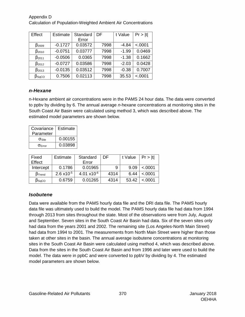
Appendix D Calculation of Population-Weighted Ambient Air Concentrations
Gasoline-Related Air Pollutants 370 January 2018 OEHHA
Effect Estimate Standard Error
DF t Value Pr > |t|
β2009 -0.1727 0.03572 7998 -4.84 <.0001 β2010 -0.0751 0.03777 7998 -1.99 0.0469 β2011 -0.0506 0.0365 7998 -1.38 0.1662 β2012 -0.0727 0.03586 7998 -2.03 0.0428 β2013 -0.0135 0.03512 7998 -0.38 0.7007 βSqCO 0.7506 0.02113 7998 35.53 <.0001
n-Hexane n-Hexane ambient air concentrations were in the PAMS 24 hour data. The data were converted to ppbv by dividing by 6. The annual average n-hexane concentrations at monitoring sites in the South Coast Air Basin were calculated using method 3, which was described above. The estimated model parameters are shown below. Covariance Parameter
Estimate
σSite 0.00155 σError 0.03898
Fixed Effect
Estimate Standard Error
DF t Value Pr > |t|
Intercept 0.1786 0.01965 9 9.09 <.0001 βTrend 2.6 x10⁻⁵ 4.01 x10⁻⁶ 4314 6.44 <.0001 βSqCO 0.6759 0.01265 4314 53.42 <.0001
Isobutene Data were available from the PAMS hourly data file and the DRI data file. The PAMS hourly data file was ultimately used to build the model. The PAMS hourly data file had data from 1994 through 2013 from sites throughout the state. Most of the observations were from July, August and September. Seven sites in the South Coast Air Basin had data. Six of the seven sites only had data from the years 2001 and 2002. The remaining site (Los Angeles-North Main Street) had data from 1994 to 2001. The measurements from North Main Street were higher than those taken at other sites in the basin. The annual average isobutene concentrations at monitoring sites in the South Coast Air Basin were calculated using method 4, which was described above. Data from the sites in the South Coast Air Basin and from 1996 and later were used to build the model. The data were in ppbC and were converted to ppbV by dividing by 4. The estimated model parameters are shown below.

Appendix D Calculation of Population-Weighted Ambient Air Concentrations
Gasoline-Related Air Pollutants 371 January 2018 OEHHA
Covariance Parameter
Estimate
σSite 0.02842 σError 0.02488
Effect Estimate Standard
Error DF t Value Pr > |t|
Intercept 0.01161 0.07051 5 0.16 0.8757 βSqCO 0.8236 0.01695 1687 48.58 <.0001
Isobutene data were also extracted from the DRI data file. The data were collected at four monitoring sites in the summers of 1995 and 1996 although most of the data came from only three of the sites. Only the 1996 data were used. The annual average isobutene concentrations at monitoring sites in the South Coast Air Basin were calculated using method 4, which was described above. The population-weighted annual average ambient air concentrations of isobutene were very similar to those estimated from the PAMS data set. The PAMS hourly data was used because it had data from more sites and a large portion of the measurements came from 2001 and 2002 and not just 1996.
Isoprene
Isoprene data were extracted from the PAMS 24-hour data file. Data were available from 1996 to 2011. A model was not developed for isoprene because an annual temporal trend was not apparent and a model based on carbon monoxide levels was not plausible since most isoprene comes from natural sources. Annual monitoring site averages are reported in the Chemical Profiles section for sites with 12 months of data instead of population-weighted annual averages.
Methyl t-Butyl Ether (MTBE) Data on MTBE was extracted from the California Toxic Monitoring Network data. The limit of detection was 0.3 ppbv. Between 1996 and 2002 the percent of non-detects ranged from 0% to 4%. In 2003 and 2004, MTBE was phased out and the measured levels of MTBE in the ambient air dropped. The percent of non-detects in 2003 and 2004 was 52% and 99%, respectively. The annual average concentration of MTBE was estimated at sites throughout the state using method 2, which was described at the beginning of this section. Only data from 1996 through 2002 were used to fit the model. Non-detects were left equal to half the limit of detection when fitting the model. The parameter estimates from the model are given below where 2002 is the reference year.

Appendix D Calculation of Population-Weighted Ambient Air Concentrations
Gasoline-Related Air Pollutants 372 January 2018 OEHHA
Covariance Parameter
Estimate
σSite 0.02702 σError 0.05622
Effect Year Estimate Standard
Error DF t Value Pr > |t|
Intercept
0.06859 0.03971 21 1.73 0.0988 β1996 1996 0.2335 0.0241 2720 9.69 <.0001 β1997 1997 0.2592 0.02026 2720 12.79 <.0001 β1998 1998 0.09375 0.01611 2720 5.82 <.0001 β1999 1999 0.1041 0.0167 2720 6.23 <.0001 β2000 2000 0.06273 0.01601 2720 3.92 <.0001 β2001 2001 0.0006 0.01625 2720 0.04 0.9706 βSqCO
1.2632 0.01678 2720 75.28 <.0001
Naphthalene Naphthalene data were extracted from the DRI data file. The data were collected during July, August and September of 1995 and 1996 at four sites in the South Coast Air Basin. Only the data from 1996 were used for modeling since the gasoline formulation changed that year. The samples were collected over a 3-hour period twice a day. One of the sites only had a few measurements; the model is essentially based on measurements from three sites. The data were in ppbC and were converted to ppbV by dividing by 10. Hourly naphthalene concentrations were positively correlated with carbon monoxide. Method 4 (described above) was used to model the 3-hour average concentrations of naphthalene from the 3-hour average concentrations of carbon monoxide. The parameter estimates from the model are given below. Covariance Parameters Estimate
σSite 0.001775 σError 0.01768
Effect Estimate Standard Error DF t Value Pr > |t|
Intercept 0.1515 0.03595 3 4.21 0.0244 βSqCO 0.2137 0.02639 247 8.1 <.0001
Naphthalene measurements were also available from the National Air Toxics Trends Stations (NATTS). These measurements were 24-hour averages and had units ng/m3. The model for the concentration of naphthalene from the NATTS network was similar to Method 4 but used 24-hour averages instead of 3-hour averages:
𝑆𝑆𝑆𝑆𝑆𝑆𝑖𝑖𝑖𝑖 = 𝐼𝐼𝐼𝐼𝐼𝐼𝐼𝐼𝐼𝐼𝐼𝐼𝐼𝐼𝐼𝐼𝐼𝐼 + 𝛽𝛽𝑆𝑆𝑆𝑆𝑆𝑆𝑆𝑆𝑆𝑆𝑆𝑆𝑆𝑆𝑆𝑆𝑖𝑖𝑖𝑖 + 𝑆𝑆𝑆𝑆𝐼𝐼𝐼𝐼𝑖𝑖 + 𝐸𝐸𝐼𝐼𝐼𝐼𝐸𝐸𝐼𝐼𝑖𝑖𝑖𝑖

Appendix D Calculation of Population-Weighted Ambient Air Concentrations
Gasoline-Related Air Pollutants 373 January 2018 OEHHA
Where • 𝑆𝑆𝑆𝑆𝑆𝑆𝑖𝑖𝑖𝑖 is the square root of the kth daily average ambient air concentration of the chemical
from site i. • 𝑆𝑆𝑆𝑆𝑆𝑆𝑆𝑆𝑖𝑖𝑖𝑖 is the square root of the kth daily average carbon monoxide concentration at site
i. • Let Sitei be a random effect for site i, which is assumed to have a normal distribution with
mean zero and standard deviation σSite. Sitei and Sitej are assumed to be independent when i ≠ j.
• Let Errorik be the error term, which is assumed to have a normal distribution with mean zero and standard deviation σError. Errorik is assumed to be independent of Sitei for all i and j and independent of εi’j’k’ unless i=i', j=j’ and k=k’.
The parameter estimates from this model are shown below.
Covariance Parameter
Estimate
σSite 0.7421 σError 5.3756
Effect Estimate Standard
Error DF t Value Pr > |t|
Intercept 0.7122 0.4889 3 1.46 0.241 βSqCO 12.7946 0.3353 1409 38.15 <.0001
Nitrogen Dioxide Nitrogen dioxide data were extracted from the database AQDVD2015_Daily Data.accdb, which is available on CARB’s 2015 Air Quality Data DVD. The data were average concentrations based on samples collected over 24-hour periods. Annual averages at each monitoring site were calculated using Method 1 above. The average was retained provided it was based on at least 10 months of data. The data from 2014 appeared to be incomplete (about half the sites had 10 or more months of data) and was not used. Between 1996 and 2013, there were 92 to 116 monitoring sites each year with at least 10 months of data. Each site had about 330 measurements per year. The annual averages from each site were used to calculate the population-weighted averages.
Other PAHs PAHs measured by California Toxic Air Contaminant Network The California Toxic Monitoring Network data file contained the daily average concentrations of particle-bound TAC PAHs from 1990 through February 2005. There were data from two or three days in each month. When the actual concentration fell below the limit of detection, CARB put one-half the limit of detection in the data file (and we did not adjust these values). The annual

Appendix D Calculation of Population-Weighted Ambient Air Concentrations
Gasoline-Related Air Pollutants 374 January 2018 OEHHA
average was calculated by averaging the measurements at each site (i.e., no modelling was done at other locations). PAHs measured by NATTS US EPA NATTS measured ambient air concentrations of PAHs from 3 monitoring sites in California: San Jose in Santa Clara County, Rubidoux in Riverside County and Main Street in Los Angeles between 2008 and 2014. The samples were collected over 24-hour periods at six-day intervals throughout the year. In the data files, we replaced non-detects with half the level of detection. The annual average was calculated by averaging the measurements at each site i.e., no modelling was done at other locations.
PM10 PM10 data were taken from the data file PM10StdDaily20150302.xlsx. The annual average at each monitoring site was calculated as described in Method 1 above. The averages were retained provided they were based on 10 or more months of data. There were between 108 and 163 sites with 10 or more months of data between 1996 and 2013. Each site had about 85 measurements per year. These averages were used to determine the population-weighted averages.
PM2.5 PM2.5 data was extracted from the file PM25Daily20150302.xlsx available on CARB’s 2015 Air Quality Data DVD. The data were available starting in 1998. The 1998 and 2014 data were incomplete and were not used. Method 1 was used to find monitoring site annual averages for 1999 through 2013. The averages were retained provided they were based on 10 or more months of data. There were 70 to 101 sites with 10 or more months of data each year between 1999 and 2013. Each site had about 150 measurements per year. These averages were used to find the population-weighted averages.
Propionaldehyde Propionaldehyde data were downloaded from US EPA AirData website. Propionaldehyde data had units ppbC and were converted to ppbv by dividing by 3 (the number of carbon atoms in propionaldehyde). The data were 3-hour measurements from summer months. Half the limit of detection was substituted for non-detects. For each year and site, summary statistics were calculated with the data and reported in the Chemical Profile for propionaldehyde.
Propylene Propylene data were extracted from the PAMS 24-hour data file. The data came from monitoring sites in the South Coast Air Basin. The data were positively correlated with carbon monoxide. Method 3 was used to estimate the annual average concentration of propylene. The parameter estimates from the model are shown below.

Appendix D Calculation of Population-Weighted Ambient Air Concentrations
Gasoline-Related Air Pollutants 375 January 2018 OEHHA
Covariance parameter
Estimate
σSite 0.0031 σError 0.07795
Effect Estimate Standard
Error DF t Value Pr > |t|
Intercept 0.2526 0.02778 9 9.09 <.0001 βTrend 3.6 x10⁻⁵ 5.67 x10⁻⁶ 4314 6.44 <.0001 βSqCO 0.9558 0.01789 4314 53.42 <.0001
Styrene The styrene data in the California Toxic Monitoring Network data had too many non-detects to be useful (more than 70% of the measurements were non-detects for many years). The styrene data from the nmoc24 data file were used instead. This data file only had data from the South Coast Air Basin. Measurements were available from 1996 to 2011. The data were in ppbC and were converted to ppbV by dividing by 8. Method 3 was used to estimate the annual average of styrene at monitoring sites in the South Coast Air Basin. The estimated model parameters are shown below. Covariance parameter
Estimate
σSite 0.00015 σError 0.01565
Effect Estimate Standard
Error DF t Value Pr > |t|
Intercept 0.2074 0.0104 9 19.95 <.0001 βTrend 2.7 x10⁻⁵ 2.51 x10⁻⁶ 4160 10.92 <.0001 βSqCO 0.1854 0.00815 4160 22.75 <.0001
Toluene Toluene data were extracted from the California Toxic Monitoring Network data file. The limit of detection was 0.2 ppbv from 1996 to 2014. The number of non-detects increased from 1% to 26% between 1996 to 2014. Method 2, which was described above, was used to estimate the annual average concentration of toluene at monitoring sites. Non-detects were set to half the limit of detection. The estimated model parameters are given below. Covariance parameter
Estimate
σSite 0.01895 σError 0.1021

Appendix D Calculation of Population-Weighted Ambient Air Concentrations
Gasoline-Related Air Pollutants 376 January 2018 OEHHA
Effect Estimate Standard
Error DF t Value Pr > |t|
Intercept -0.1112 0.03482 25 -3.19 0.0038 β1996 0.2229 0.0258 7878 8.64 <.0001 β1997 0.2037 0.02622 7878 7.77 <.0001 β1998 0.1561 0.02665 7878 5.86 <.0001 β1999 0.09627 0.02666 7878 3.61 0.0003 β2000 0.2096 0.02626 7878 7.98 <.0001 β2001 0.1868 0.02611 7878 7.15 <.0001 β2002 0.2153 0.02652 7878 8.12 <.0001 β2003 0.1915 0.02583 7878 7.41 <.0001 β2004 0.1677 0.02589 7878 6.48 <.0001 β2005 0.1561 0.02585 7878 6.04 <.0001 β2006 0.1484 0.02655 7878 5.59 <.0001 β2007 0.1298 0.02663 7878 4.87 <.0001 β2008 0.0918 0.02633 7878 3.49 0.0005 β2009 0.08497 0.02641 7878 3.22 0.0013 β2010 0.1198 0.0273 7878 4.39 <.0001 β2011 0.02933 0.0267 7878 1.1 0.272 β2012 0.07524 0.02652 7878 2.84 0.0046 β2013 0.01956 0.02605 7878 0.75 0.4528 βSqCO 1.4201 0.01522 7878 93.31 <.0001
1,2,3-Trimethylbenzene 1,2,3-Trimethylbenzene data were extracted from the PAMS 24-hour data file. We converted the data, originally in units of ppbC, to ppbV by dividing by 9. There were seven monitoring sites with 1,2,3-trimethylbenzene and carbon monoxide data. Most of the data were from 2001 and later. Data from two sites (2166 and 2492) were excluded due to possible errors prior to 2007 per SCAQMD. Method 3 was used to estimate the levels of 1,2,3-trimethylbenzene from the more densely monitored carbon monoxide. The estimated model parameters are shown below. Covariance parameter
Estimate
σSite 0.00023 σError 0.00669
Effect Estimate Standard
Error DF t Value Pr > |t|
Intercept 0.2559 0.00947 7 27.02 <.0001 βTrend 5.7 x10⁻⁵ 2.07 x10⁻⁶ 2940 27.48 <.0001 βSqCO 0.1786 0.00677 2940 26.4 <.0001

Appendix D Calculation of Population-Weighted Ambient Air Concentrations
Gasoline-Related Air Pollutants 377 January 2018 OEHHA
1,2,4-Trimethylbenzene 1,2,4-Trimethylbenzene data were extracted from the PAMS 24-hour data file. The data were converted from ppbC to ppbV by dividing by 9. Data from two sites (2166 and 2492) were excluded due to possible errors prior to 2007 per SCAQMD. Model 3 was used to estimate the annual average concentrations of 1,2,4-trimethylbenzene at monitoring sites in the South Coast Air Basin where carbon monoxide data were available. The model parameter estimates are given below. Covariance Parameter
Estimate
σSite 0.00077 σError 0.01384
Effect Estimate Standard
Error DF t Value Pr > |t|
Intercept 0.3292 0.01458 7 22.58 <.0001 βTrend 0.00009 2.84 x10⁻⁶ 3011 31.8 <.0001 βSqCO 0.3915 0.00949 3011 41.24 <.0001
1,3,5-Trimethylbenzene
1,3,5-Trimethylbenzene data were extracted from the PAMS 24-hour data file. The data were converted from ppbC to ppbV by dividing by 9. Data from two sites (2166 and 2492) were excluded due to possible errors prior to 2007 per SCAQMD. Method 3 was used to estimate the annual average concentration of 1,3,5-trimethylbenzene at sites with carbon monoxide data. The estimated model parameters are given below. Covariance Parameter
Estimate
σSite 0.00053 σError 0.0057
Effect Estimate Standard
Error DF t Value Pr > |t|
Intercept 0.1665 0.01073 7 15.52 <.0001 βTrend 4.5 x10⁻⁵ 1.85 x10⁻⁶ 2999 24.38 <.0001 βSqCO 0.2897 0.00613 2999 47.23 <.0001

Appendix D Calculation of Population-Weighted Ambient Air Concentrations
Gasoline-Related Air Pollutants 378 January 2018 OEHHA
m- & p-Xylene m- & p-Xylene data were extracted from the California Toxic Monitoring Network data file. The limit of detection was 0.6 ppbv between 1996 and early 2001. After that, the limit of detection was 0.2 ppbv. Between 1996 and 2000, the annual fraction of measurements that fell below the limit of detection ranged from 42% to 63%. Between 2001 and 2014, the annual percent of non-detects increased from 2% to 49%. When the concentration fell below the limit of detection, CARB put one-half the limit of detection into the data set as a placeholder. These values were left in the data set for modeling. Three large outliers were dropped from the data set. Method 2 was initially used to calculate the annual average of m- & p-xylene at monitoring sites but the resulting population-weighted averages fluctuated too much. Instead, Method 3 was used to estimate the annual average concentration of m- & p-xylene at monitoring sites. The parameter estimates for the model are shown below. Covariance Parameter
Estimate
σSite 0.0078 σError 0.05363
Effect Estimate Standard
Error DF t Value Pr > |t|
Intercept -0.0551 0.02058 25 -2.68 0.0129 βTrend -1.28 x10⁻⁶ 2.50 x10⁻⁶ 7815 -0.51 0.607 βSqCO 1.0819 0.01102 7815 98.22 <.0001
Since some years of data had a large number of non-detects, a sensitivity analysis was carried out to determine whether the non-detects would have a substantial effect on the estimated population-weighted average concentration of m- & p-xylene. A data set was created with the limit of detection, which varied by year, put in for the non-detect values. There were noticeable differences between the analyses done with the two data sets. The population-weighted average results from the two analyses are included in Chemical Profiles for comparison.
o-Xylene
o-Xylene data were extracted from the California Toxic Monitoring Network data file. The limit of detection was 0.1 ppb. Each year between 15% and 43% of the measurements were non-detects; these were recorded as 0.05 ppb. Method 2 was used to estimate the annual average at monitoring sites. The estimated model parameters are in the tables below. Covariance Parameter
Estimate
σSite 0.00255 σError 0.01754

Appendix D Calculation of Population-Weighted Ambient Air Concentrations
Gasoline-Related Air Pollutants 379 January 2018 OEHHA
Effect Estimate Standard Error
DF t Value Pr > |t|
Intercept -0.0399 0.01366 25 -2.92 0.0073 β1996 0.01221 0.01096 7769 1.11 0.2652 β1997 -0.0389 0.01113 7769 -3.49 0.0005 β1998 -0.0767 0.01137 7769 -6.75 <.0001 β1999 -0.0227 0.0114 7769 -1.99 0.0463 β2000 -0.006 0.01115 7769 -0.53 0.5927 β2001 0.00148 0.01108 7769 0.13 0.8937 β2002 0.06567 0.01125 7769 5.84 <.0001 β2003 0.0435 0.01097 7769 3.97 <.0001 β2004 0.02853 0.01099 7769 2.6 0.0095 β2005 -0.0051 0.01098 7769 -0.46 0.6448 β2006 -0.0013 0.01126 7769 -0.12 0.9069 β2007 0.00386 0.01129 7769 0.34 0.7321 β2008 0.00954 0.01117 7769 0.85 0.3932 β2009 0.02045 0.01121 7769 1.83 0.068 β2010 0.04414 0.01157 7769 3.82 0.0001 β2011 -0.0032 0.01132 7769 -0.28 0.7779 β2012 0.034 0.0114 7769 2.98 0.0029 β2013 0.01557 0.01121 7769 1.39 0.1649 βSqCO 0.642 0.0063 7769 101.96 <.0001
A sensitivity analysis was conducted to determine the effect of the non-detect values on the estimated population-weighted average concentrations. A data set was formed with non-detect values set to 0.1. The same model was fit to the data set and the population-weighted average concentrations were calculated. The estimated population-weighted average concentrations calculated from the data set is included in the Chemical Profiles section of o-xylene for comparison.
Method for Estimating the Annual Average Concentration at Each Census Tract The annual average concentration of a compound at each census tract was estimated by combining the annual average concentrations from nearby monitoring stations (where nearby is defined to be less than 30 km). The formula for estimating the concentration at the jth census tract from the data from nearby monitoring stations was:
𝐼𝐼𝑗𝑗 = �𝑏𝑏𝑖𝑖/𝑇𝑇𝑖𝑖𝑗𝑗2
∑ 1/𝑇𝑇𝑖𝑖𝑗𝑗2𝑇𝑇𝑗𝑗𝑖𝑖=1
𝑇𝑇𝑗𝑗
𝑖𝑖=1
Where:
nj = number of monitoring stations within 30 km of the jth census tract bi = annual average concentration at the ith monitoring station dij = distance from the ith monitoring station to the jth census tract

Appendix D Calculation of Population-Weighted Ambient Air Concentrations
Gasoline-Related Air Pollutants 380 January 2018 OEHHA
The distance squared weighting was used in a previous report (CARB, 1999). If there were no observations within 30 km of the census tract, then no estimate was made for the population in that census tract. The distances from the monitoring stations to the census tract centroids were calculated according to the formula below. The formula assumes that the earth is spherical. D = R*arccos(sin(L1) sin(L2) + cos(L1) cos(L2) cos(DG)) Where:
R = 6371 km is the average radius of the earth L1 = latitude at the first point L2 = latitude at the second point DG = longitude of the second point minus longitude of the first point D = computed distance (km) arccos in radians
Method for Calculating the Population-Weighted Annual Average Concentrations The annual average concentration of a chemical was estimated at monitoring sites throughout an air basin (p. 360). These annual averages were used to estimate the concentration of the chemical at census tracts in the air basin by using an inverse distance squared weighting scheme to combine the monitoring site averages (p. 379). A weighted average of the census tract chemical concentration estimates was found using the census tract populations as weights. The air basin population-weighted annual average concentration was calculated according to the formula:
∑i=1
m [(pi ci)/ ∑
i=1
m pi]
Where:
ci = annual average concentration at each census tract pi = population in the census tract m = number of census tracts (with concentration estimates) in the air basin
Each monitoring station was assigned an air basin in CARB’s “location” data file. Census tracts were assigned to air basins by determining which monitoring station the census tract was closest to and assigning the monitoring station’s air basin to the census tract. Where possible a statewide population-weighted average concentration was estimated. The method used depended on the data available.

Appendix D Calculation of Population-Weighted Ambient Air Concentrations
Gasoline-Related Air Pollutants 381 January 2018 OEHHA
Methods for Estimating the Census Tract Populations Every ten years, when the decennial census is done, the boundaries of some census tracts are altered (e.g., a census tract may be split into two separate tracts due to a large population increase). The impact on this study is that some of the 1990 and 2000 and 2010 census tracts do not match up. The US census bureau provides files that map 2000 census results into the 1990 census tracts and 2010 results into 2000 census tracts. The files for mapping 2000 census results to 1990 census tracts and 2010 census results to 2000 census tracts were capop19902000.txt and capop20002010.txt; they were downloaded from the US census website http://www.census.gov. The California Department of Finance carried out this mapping for census 2000 and provided the results on their website in the file “1970-1980-1990-2000 comparability file.xls”. The file contained the latitude, longitude, 1990 population and 2000 population of each 1990 census tract. The 2010 populations of the 2010 census tracts were obtained from the US census website. The mapping files were used to add the 2010 populations of the 1990 census tracts to the comparability file. Estimates of the census tract populations for the years 1996 to 2000 were obtained by linearly interpolating between the 1990 and 2000 populations as follows pyear,i=p1990,i+(p2000,i-p1990,i) /10 x (year -1990) where pyear,i is the population from census tract i for year. A similar method was used to interpolate the 2000 and 2010 census tract populations. A different approach was used to estimate the census tract populations for 2011 to 2015. The California Department of Finance provides a data file with annual estimates of the California county populations for 2011 to 2015 (E-42015InternetVersion.xls). The 2010 census tract and county populations were used to determine the ratio of each census tract population to its county population. These ratios were then applied to the 2011 county populations to estimate the census tract populations in 2011. The same approach was used to get the 2012-2015 census tract populations.

Gasoline-Related Air Pollutants 382 January 2018 OEHHA
Method for Determining Gasoline-Attributable Fractions
Introduction
The gasoline-attributable fraction of a chemical is the fraction of the ambient air concentration of a chemical that came from gasoline-related sources. It was estimated as the ratio of emission tonnage from gasoline-related sources divided by emission tonnage from all sources:
Gasoline-attributable fraction = tons of chemical from gasoline-related sources
tons of chemical from all sources
If the chemical had a significant portion of its ambient air concentration coming from secondary atmospheric reactions, then the previous formula was modified as follows: Gasoline-attributable fraction = tons of chemical from gasoline-related sources and secondary reactions
tons of chemical from all sources and secondary reactions
If the chemical had all of its ambient air concentration coming from secondary atmospheric reactions, then the previous formula was modified as follows: Gasoline-attributable fraction = tons of chemical from gasoline-related secondary reactions
tons of chemical from all secondary reactions
The emission tonnage information came from the CARB’s Emission Inventory. Based on input from CARB, all sources with material code equal to 1100 were identified as gasoline-related sources. Some chemicals were emitted directly from the sources. and referred to as primary emission products. The tonnage of these chemicals was derived directly from the Emission Inventory. Other chemicals were formed in significant proportions as both primary emission products and as products of secondary atmospheric reactions. The tonnage from these secondary reactions was calculated using the Emission Inventory and direct formation potential values provided by Carter (2001). A detailed description of how the direct formation potential was used is provided below.
Data Source: Emission Inventory Extracts
A description of CARB’s Emission Inventory is available at https://www.arb.ca.gov/ei/ei.htm. CARB provided to OEHHA Emission Inventory extracts, which include estimates of the amount of pollutants discharged into the atmosphere by source categories, for each air basin, and within a specified time span. The extracts covered the following years: 1996 to 2006 (data file received in August 2008); 2007 (data file received in August 2009); 2008 (data file received in August 2010); and 2010 to 2012 (data file received in October 2015). Some additional notes on the Emission Inventory extracts are provided below:
• CARB’s approach for estimating ROG and TOG emissions from natural sources was changed in 2002, and this affected gasoline-attributable fractions for chemicals like

Appendix E Method for Determining Gasoline-Attributable Fractions
Gasoline-Related Air Pollutants 383 January 2018 OEHHA
1,3-butadiene and acetaldehyde that had large natural source components. These changes are noted where relevant in the Chemical Profiles.
• Natural source emission estimates were not available for 2009 to 2011, so the 2008 values were used for those years. The statewide ROG and TOG emissions attributed to natural sources differed by about 10% between 2008 and 2012.
• Mobile source emissions were not available for 2009, so gasoline-attributable fractions could not be calculated for that year. Estimates for 2008 were applied as a proxy.
Primary Emission Tonnage This section describes how the primary emission tonnage of a chemical was calculated. CARB provided data files that contained the estimated annual tons of total organic gases (TOG) (i.e., gaseous organic compounds including both reactive organic gases and the relatively unreactive organic gases such as methane) emitted by sources throughout California. The data were extracted from CARB’s Emission Inventory and covered the years 1996 to 2012. The TOG of an emission source included all the chemicals released as primary emissions from the source. The TOG of each emission source was separated into component primary emission chemicals using the source’s chemical speciation profile. These data were aggregated into two lists: The first list had the primary emissions weight of each chemical by air basin and year for all sources. The second list had the primary emissions weight of each chemical by air basin and year for gasoline-related sources only.
Calculating Tonnage of Secondary Formation Products This section describes how the tonnage of a chemical from secondary atmospheric reactions was calculated. A formation potential is the percentage of each primary emission chemical that reacts to form another chemical. Under contract with OEHHA, Dr. William Carter determined formation potentials for twelve reaction products: formaldehyde, acetaldehyde, lumped higher aldehydes, benzaldehyde and other aromatic aldehydes, acrolein, cresols, nitrophenols and aromatic nitro-compounds, lumped alkyl nitrates, peroxyacetyl nitrate (PAN), higher saturated acyl peroxynitrates, peroxybenzoyl nitrate and other aromatic acyl peroxynitrates (PBzN) and unsaturated PAN analogues such as that formed from methacrolein. The formation potentials were used to determine secondary formation for selected pollutants, described in detail below. The tons of a secondary product were calculated by finding the amount of secondary product formed from each primary emission product and then adding them up. The rest of this section explains this calculation in detail. Let Ai and Ci be the primary emissions weight of the ith chemical from gasoline-related sources and all sources, respectively. The weight of secondary product j from all sources is referred to here as “Dj”. Dj was calculated by multiplying the primary emissions weight of each chemical Ci by the direct formation potential of the secondary product (fij) and summing over all chemicals, as follows

Appendix E Method for Determining Gasoline-Attributable Fractions
Gasoline-Related Air Pollutants 384 January 2018 OEHHA
𝐷𝐷𝑗𝑗 = �𝑆𝑆𝑖𝑖𝑓𝑓𝑖𝑖𝑗𝑗
𝑇𝑇
𝑖𝑖=1
where n is the number of distinct primary emission chemicals from all sources. The weight of secondary product j from gasoline-related sources is referred to here as “Bj”. It was calculated as
𝐵𝐵𝑗𝑗 = � 𝐴𝐴𝑖𝑖𝑓𝑓𝑖𝑖𝑗𝑗𝑇𝑇
𝑖𝑖=1
There were direct formation potentials for some chemicals to themselves (e.g., formaldehyde to formaldehyde). These direct formation potentials, where fjj>0, were not used. Chemicals of interest falling in this group included: formaldehyde, higher aldehydes, acetaldehyde, cresol, acrolein and benzaldehyde.
Calculating Gasoline-Attributable Fractions
For chemical i: Ai = weight of chemical from primary emissions from gasoline-related sources Bi = weight of chemical formed from secondary reactions for which the input chemicals were emitted from gasoline-related sources Ci = weight of chemical from primary emissions from all sources
Di = weight of chemical formed from secondary reactions for which the input chemicals were emitted from all sources The gasoline-attributable fraction for primary emissions only was calculated as 𝐴𝐴𝑖𝑖/𝑆𝑆𝑖𝑖. The gasoline-attributable fraction for chemicals in primary emissions products and also formed through secondary reactions was calculated as (𝐴𝐴𝑖𝑖 + 𝐵𝐵𝑖𝑖)/(𝑆𝑆𝑖𝑖 + 𝐷𝐷𝑖𝑖). Acetaldehyde, acrolein, aromatic aldehydes (e.g., benzaldehyde), formaldehyde and higher aldehydes (i.e., propionaldehyde) fell in this category. Cresols, nitrophenols and aromatic nitrates, lumped alkyl nitrates, peroxyacetyl nitrate (PAN), higher saturated acyl nitrates, aromatic acyl peroxynitrates (e.g., peroxybenzoyl nitrate) and unsaturated PAN analogues are mostly produced through secondary reactions. Their gasoline-attributable fractions were calculated as 𝐵𝐵𝑖𝑖/𝐷𝐷𝑖𝑖.
Air Basin and Year Specific Gasoline-Attributable Fractions
The Emission Inventory included the air basin where the emissions source was located and the year the emissions occurred. Based on this information, separate gasoline-attributable fractions were calculated for the five most populated air basins by year. The air basins were the South

Appendix E Method for Determining Gasoline-Attributable Fractions
Gasoline-Related Air Pollutants 385 January 2018 OEHHA
Coast Air Basin, San Diego, San Francisco Bay Area, San Joaquin Valley and Sacramento Valley Air Basins. Statewide gasoline-attributable fractions were also calculated using Emission Inventory data from all the air basins.
Some Notes on Calculating Gasoline-Attributable Fractions for Specific Chemicals
• Formation potentials were only available for aromatic aldehydes as a group. The Emission Inventory included two aromatic aldehydes: benzaldehyde and tolualdehyde. The primary emission tonnage of “aromatic aldehydes” was calculated by adding the primary emission tonnage of benzaldehyde and tolualdehyde.
• Formation potentials were only available for higher aldehydes as a group. The Emission Inventory included a number of higher aldehydes (hexaldehyde, propionaldehyde, butyraldehyde, isovaleraldehyde, glutaraldehyde, isobutyraldehyde and decanal). The primary emission tonnage of “higher aldehydes” was calculated by adding the primary emission tonnage of these higher aldehydes together.
• Gasoline-attributable fractions were calculated for nitrogen oxides. The ambient air monitoring data were for nitrogen dioxide. It was assumed that the gasoline-attributable fractions for NOx could be applied to nitrogen dioxide.
• The Emission Inventory did not include secondary formation of particulate matter. Gasoline-attributable fractions of PM2.5 were estimated from source attribution studies of PM2.5 which included both primary emissions and secondary formation of PM2.5. These estimates are described in the Chemical Profile for PM
• Gasoline-attributable fractions of PM10 were based on the primary emissions data from the Emission Inventory. Secondary formation of PM10 was not included.
• In the Emission Inventory, the emission tonnages of NOx, PM2.5 and PM10 are stored separately from the TOG and so the step (mentioned above) of splitting the TOG into component chemicals based on speciation profiles was not required here.
• Directly emitted cresols in the Emission Inventory came from non-gasoline-related sources and included o-cresol and cresylic acid.
• Nitrophenols do not appear in the Emission Inventory. Some aromatic nitro-compounds do appear in the Emission Inventory including nitrobenzene, 2,2-dichloronitroaniline, bromodinitroaniline (2,4-dinitro-6-bromoaniline) and bromodinitrobenzene. These directly emitted aromatic nitro-compounds came from non-gasoline sources that were linked to speciation profiles for industrial processes, mineral products, textile products and organic chemical storage.
• Alkyl nitrates do not appear in the Emission Inventory so direct emissions of alkyl nitrates were estimated to be zero.
• PAN does not appear in the Emission Inventory and its primary emission tonnage was estimated to be zero.

Appendix E Method for Determining Gasoline-Attributable Fractions
Gasoline-Related Air Pollutants 386 January 2018 OEHHA
• Primary emission tonnage of higher saturated acyl peroxynitrates was estimated to be zero because they did not appear in the Emission Inventory.
• Primary emissions of aromatic acyl peroxynitrates were estimated to be zero because they do not appear in the Emission Inventory.
• Primary emissions of unsaturated PAN analogues were estimated to be zero because they were not in the Emission Inventory.
Gasoline-Attributable Annual Average Concentration The gasoline-attributable annual average concentration of a chemical was calculated by multiplying the estimated population-weighted annual average concentration of an air basin by the appropriate gasoline-attributable fraction.
Example Calculation Based on Primary Emissions Only – Benzene
The estimated gasoline-attributable fraction of benzene in the South Coast in 1996 was 0.81, based on primary emissions. The details of this calculation are shown below.
Primary emissions weight of benzene from gasoline-related sources (tons per year)
7,304
Primary emissions weight of benzene from all sources (tons per year) 9,023 Gasoline-attributable fraction for benzene 7,304/9,023 or 0.81
Example Calculation Based on Primary and Secondary Emissions – Formaldehyde Formaldehyde is found in primary emissions and formed in secondary atmospheric reactions. The estimated gasoline-attributable fraction of formaldehyde in the South Coast in 1996 was 0.63, based on both primary and secondary emissions. The details of this calculation are shown below.
Primary emissions weight of formaldehyde from gasoline-related sources (tons per year) (“A”)
4,817
Weight of formaldehyde from secondary reactions from gasoline-related sources (tons per year) (“B”)
14,256
Primary emissions weight of formaldehyde from all sources (tons per year) (“C”)
9,591
Weight of formaldehyde from secondary reactions from all sources (tons per year) (“D”)
20,826
Gasoline-attributable fraction for formaldehyde (A+B)/(C+D) = 0.63

Appendix E Method for Determining Gasoline-Attributable Fractions
Gasoline-Related Air Pollutants 387 January 2018 OEHHA
The partial calculation of “B” (defined above) is shown below:
Year Air basin Primary emitted VOCs
Tons from gasoline sources (Ai)
Direct formation potential (fij) of formaldehyde
Formaldehyde secondary product weight
1996 SC 2,2,3-Trimethylbutane 55.0 0.028653846 1.6 1996 SC Methane 20,725.5 0.000508882 10.5 1996 SC Ethane 3,210.6 0.005376256 17.3 1996 SC Ethylene 16,764.9 0.251697436 4,219.7 1996 SC Propane 2,157.3 0.003547051 7.7 Additional rows for all gasoline-related VOCs - table is truncated for space reasons Total formaldehyde from secondary reactions from gasoline-related sources (tons per year)
14,256
The partial calculation of “D” (defined above) is shown below:
Year Air basin Primary emitted VOC
Tons from all sources (Ci)
Direct formation potential (fij) of formaldehyde
Formaldehyde secondary product weight
1996 SC 2,2,3-Trimethylbutane 62.5 0.028653846 1.8
1996 SC Methane 155,157.7 0.000508882 79.0
1996 SC Ethane 21,388.3 0.005376256 115.0 1996 SC Ethylene 24,660.7 0.251697436 6,207.0 1996 SC Propane 8,588.6 0.003547051 30.5 Table is truncated to save space Total formaldehyde from secondary reactions from all sources (tons per year)
20,826
Additional Comments on Gasoline-Attributable Fractions The source apportionment procedure relied heavily on values tabulated in CARB’s Emission Inventory. Possible problems that could affect the calculated gasoline-attributable fractions include missing sources, inaccurate estimates of pollution tonnage and inaccurate source profiles. The Emission Inventory tabulated primary emissions only. The chemical profiles include explanations for why the gasoline-attributable fractions of specific chemicals change dramatically. One reason was that the total organic gas (TOG) from a source was updated over time to a much different value. Another reason was that the source was linked to a new source profile. These two changes could cause large changes in the estimated tonnage of a chemical released into the air. In turn, this caused large changes in the estimated

Appendix E Method for Determining Gasoline-Attributable Fractions
Gasoline-Related Air Pollutants 388 January 2018 OEHHA
gasoline-attributable fraction of the chemical from one year to the next. For example, the tons emitted from natural sources, including wildfires and other biogenic sources were revised in 2002 as part of Western Regional Air Partnership (WRAP) so that estimates in different regions were similar. The revision had a dramatic effect on the gasoline-attributable fraction of many chemicals. After that year, the tonnage was kept constant for many natural sources in the Emission Inventory. Another example is the introduction of new source profiles following the prohibition of MTBE from gasoline. Appendix F References Carter WP (2001). Determination of Aldehyde and PAN Formation Potentials for Volatile Organic Compounds. Air Pollution Research Center University of California, Riverside. Prepared under contract with OEHHA.

Gasoline-Related Air Pollutants 389 January 2018 OEHHA
Summary of Research Results from Interagency Agreement with UC Riverside
OEHHA entered into an Interagency Agreement with the University of California Riverside (UCR) from 2006 to 2008 to determine the presence and concentrations of atmospheric reaction products of gasoline-related emissions in ambient air (OEHHA agreement number 06-E0016). Dr. Janet Arey was the principal investigator. The project involved both laboratory methods development work and ambient air analyses. The focus of the work was on measuring atmospheric products of gasoline-related volatile aromatic compounds (such as benzene, ethylbenzene) and PAHs. Arey and colleagues published two papers describing results of the project (Obermeyer et al., 2009; Arey et al., 2009). Research reported in a third paper (Nishino et al., 2008) was partially supported by this agreement. The project arose out of earlier OEHHA-supported work to describe the atmospheric chemistry of gasoline-related compounds. Atkinson and Arey summarized the known or predicted atmospheric products of gasoline-related VOCs, PAHs and nitro-PAHs or classes of compounds (OEHHA, 2006). The research described in this Appendix was primarily undertaken to determine whether certain toxic products that were predicted to occur from gasoline-related emissions could be measured in ambient air. Arey et al. (2009) carried out chamber studies to investigate the dicarbonyl reaction products of toluene, xylenes and trimethylbenzenes, all of which are emitted from gasoline-powered vehicles. The dicarbonyls were chosen because of the known and suspected toxicity of these types of compounds. Arey et al. observed glyoxal, methylglyoxal and diacetyl, which are 1,2-dicarbonyls. They also identified 1,4-dicarbonyls such as 1,4-butenedial and 3-hexene-2,5-dione. The 1,4-dicarbonyls were generally observed in lower yield than the 1,2-dicarbonyls. Obermeyer et al. (2009) reported on ambient air measurements of the carbonyl atmospheric reaction products of aromatic hydrocarbons and other VOCs. They collected ambient air samples in Riverside in 2008. The table below summarizes the carbonyls and dicarbonyls that were identified in the ambient air samples, along with the possible VOC precursors of those atmospheric reaction products.

Appendix F Summary of Research Results Interagency Agreement with UC Riverside
Gasoline-Related Air Pollutants 390 January 2018 OEHHA
Carbonyls and dicarbonyls identified in ambient air from Riverside, California, November 18-19 2008 (adapted from Obermeyer et al., 2009) Carbonyl Structure Possible VOC precursors Aromatic carbonyls Benzaldehyde C6H5CHO Toluene, ethylbenzene o-Tolualdehyde o-CH3C6H4CHO o-Xylene m-Tolualdehyde m-CH3C6H4CHO m-Xylene p-Tolualdehyde p-CH3C6H4CHO p-Xylene Acetophenone C6H5C(O)CH3 Ethylbenzene 1,2-dicarbonyls Glyoxal (CHO)2 Aromatics and other VOCs Methylglyoxal CH3C(O)CHO Aromatics and other VOCs Diacetyl CH3C(O)C(O)CH3 o-Xylene, 1,2,3-trimethylbenzene, 1,2,4-
trimethylbenzene Ethylglyoxala CH3CH2C(O)CHO Ethylbenzene, ethyltoluenes Unsaturated 1,4-dicarbonyls 2-Butenedial (unsaturated form of 1,4-butanedial)
HC(O)CH=CHCHO Toluene, ethylbenzene, o-xylene, o-ethyltoluene
3-Hexene-2,5-dionea CH3C(O)CH=CHC(O)CH3 p-Xylene, 1,2,4-trimethylbenzene Other dicarbonyls Malonaldehyde HC(O)CH2CHO n-Butane 3-Oxo-butanala CH3C(O)CH2CHO n-Pentane 1,4-Butanediala HC(O)CH2CH2CHO n-Butane
aObermeyer et al. (2009) noted that, to their knowledge, these were the first reported observations in ambient air of these compounds.

Appendix F Summary of Research Results Interagency Agreement with UC Riverside
Gasoline-Related Air Pollutants 391 January 2018 OEHHA
Nishino et al. (2008) measured formation yields of nitro products from the atmospheric reactions of toluene, naphthalene and biphenyl, and examined the effect of the nitrogen dioxide concentration. The researchers also measured ambient air concentrations of selected aromatic hydrocarbons and nitrated aromatic hydrocarbons in Upland, California, the location of a South Coast Air Quality Management District (SCAQMD) monitoring station. A key conclusion of this work is that, for nitrogen dioxide concentrations found in urban areas, nitro-PAH formation from atmospheric OH radical-initiated reactions will occur. This conclusion was supported both by the laboratory investigations and the ambient analyses. The table below summarizes the ambient air measurements taken in 2006 and 2007.

Appendix F Summary of Research Results Interagency Agreement with UC Riverside
Gasoline-Related Air Pollutants 392 January 2018 OEHHA
Ambient aromatic, nitroaromatic, and nitrogen dioxide concentrations in Upland, CA in 2006 and 2007 (adapted from Nishino et al., 2008). Date 10/22/06 10/23/06 10/24/06 10/28/06 9/12/07 9/18/07 9/26/07 10/25/07 Toluene and PAH (ng m-3) Toluene 4400 5890 8980 4510 6276 3643 4956 9404 Naphthalene 60.7 101.1 139.5 100.3 159.3 70.9 104.1 265.5 Biphenyl 6.9 10.2 13.6 8.5 13.8 7.5 9.9 22.3 Nitroaromatics (pg m-3) 3-Nitrotoluene 695 753 1723 407 1005 780 488 995 1-Nitronaphthalene 58.3 84.6 78.6 108.3 101.9 38.9 42.9 94.3 2-Nitronaphthalene 71.4 88.7 79.2 91.3 69.5 25.5 39.9 78.7 3-Nitrobiphenyl 22.5 42.8 39.6 21.2 45.0 9.5 23.5 50.9 Nitrogen dioxide (ppbv) Nitrogen dioxide 12 24 28 26 20 17 17a 33a
a. Data not available from Upland, CA. Value given is from Fontana, CA, the nearest downwind SQAQMD monitoring station.

Appendix F Summary of Research Results Interagency Agreement with UC Riverside
Gasoline-Related Air Pollutants 393 January 2018 OEHHA
Appendix F References Arey J, Obermeyer G, Aschmann SM, Chattopadhyay S, Cusick RD, Atkinson R (2009). Dicarbonyl products of the OH radical-initiated reaction of a series of aromatic hydrocarbons. Environ Sci Technol 43:683-689. Nishino N, Atkinson R, Arey J (2008). Formation of nitro products from the gas-phase OH radical-initiated reactions of toluene, naphthalene, and biphenyl: Effect of NO2 concentration. Environ Sci Technol 42:9203-9209. Obermeyer G, Aschmann SM, Atkinson R, Arey J (2009). Carbonyl atmospheric reaction products of aromatic hydrocarbons in ambient air. Atmos Environ 43:3736-3744. Office of Environmental Health Hazard Assessment (OEHHA, 2006). Atmospheric Chemistry of Gasoline-Related Emissions: Formation of Pollutants of Potential Concern. Reproductive and Cancer Hazard Assessment Section, OEHHA, California Environmental Protection Agency. Available at: https://oehha.ca.gov/media/downloads/air/document/atmoschemgas.pdf

Gasoline-Related Air Pollutants 394 January 2018 OEHHA
Screening Health Risk Assessment Methods For VOCs and PAHs
This Appendix provides additional details on the screening risk assessment used for gasoline-related VOCs and PAHs.
Methods for Estimating Cancer Risks for Gasoline-Related VOCs Gasoline-attributable cancer risks for gasoline-related VOCs, including naphthalene, were estimated for the South Coast Air Basin and statewide, based on the five most populous air basins (South Coast, San Diego, San Francisco Bay Area, San Joaquin Valley and Sacramento Valley). These five air basins account for approximately 80% of the total California population. The cancer risk calculations take into account early-in-life sensitivity using the method described in OEHHA (2015). The method for estimating the cancer risk is explained using acetaldehyde as an example. The cancer risk is based on the gasoline-attributable population-weighted annual average ambient air concentration of acetaldehyde (also referred to as gasoline-attributable concentration). The gasoline-attributable concentration of acetaldehyde in the South Coast Air Basin in 1996 was estimated to be 1.1 ppb, which was converted to 1.98x10⁻³ mg/m3 using the conversion factor from Table 108 below. The concentration had to be converted to match the units of the cancer potency values. Table 108. Conversion factors and cancer potency values for selected VOCs
Chemical Conversion factor1 at 25 ° C and 1 atm
Cancer potency value2
(mg/kg-day)-1 Acetaldehyde 1 ppm = 1.8 mg/m3 1.0x10⁻²
Benzene 1 ppm = 3.2 mg/ m3 1.0 x10⁻¹ 1,3-Butadiene 1 ppm = 2.21 mg/ m3 6.0 x10⁻¹ Ethyl benzene 1 ppm = 4.35 mg/ m3 8.7 x10⁻³ Formaldehyde 1 ppm = 1.24 mg/ m3 2.1 x10⁻²
Methyl t-butyl ether (MTBE) 1 ppm = 3.6 mg/ m3 1.8 x10⁻³ Naphthalene 1 ppm = 5.24 mg/ m3 1.2 x10⁻¹
Styrene 1 ppm = 4.26 mg/m3 2.6 x10⁻² Notes:
1. Conversion factors for all chemicals except naphthalene came from Appendix B of the report “Air Toxics Hot Spots Risk Assessment Guidelines Part II: Technical Support Document for Cancer Potency Factors” (OEHHA, 2009). The conversion factor for naphthalene came from the NIOSH Pocket Guide to Chemical Hazards.
2. Cancer potency values were obtained from OEHHA (2015).

Appendix G Screening Health Risk Assessment Calculations
Gasoline-Related Air Pollutants 395 January 2018 OEHHA
The average daily dose (ADD) for each age range was calculated using the formula: ADDage range = (Air concentration) x (Body weight adjusted breathing rateage range) The body weight adjusted breathing rates are presented in Table 109. Table 109. Inhalation rates and age sensitivity factors
Age Range 95th Percentile Inhalation Rate1
(L/kg-day)
Age Sensitivity
Factor2 3rd Trimester 361 10
0<2 years 1090 10 2<16 years 745 3
16<70 years 290 1 Notes:
1. OEHHA (2015) Table I-2 2. OEHHA (2015) Table I-4
The calculation of the average daily dose for each lifestage is shown in Table 110 below: Table 110. Example calculation of average daily dose for acetaldehyde in the South Coast Air Basin in 1996.
Age range Concentration (mg/m3)
95th Percentile body weight
adjusted breathing rate
(L/kg-day)
Average daily dose
(mg/kg-day)
3rd trimester 0.00198 361 7.15 x10⁻⁴ 0<2 years 0.00198 1090 2.16 x10⁻³ 2<16 years 0.00198 745 1.48 x10⁻³ 16<70 years 0.00198 290 5.74 x10⁻⁴
The cancer risk was calculated using the following formula Cancer risk =∑age range [ (ADDage range X CPF x ASFage range X [fraction of lifetime)] where ADDage range is the average daily dose for the age range, CPF is the cancer potency factor, ASFage range is the age sensitivity factor, and fraction of lifetime is calculated as length of age range divided by 70.

Appendix G Screening Health Risk Assessment Calculations
Gasoline-Related Air Pollutants 396 January 2018 OEHHA
The gasoline-attributable cancer risk from exposure to an ambient air concentration of 1.1 ppb acetaldehyde was calculated to be 2.0 x10⁻⁵ as shown in Table 111 below. Table 111. Example calculation of cancer risk from exposure to acetaldehyde in the ambient air in the South Coast Air Basin in 1996
Age Range Average daily dose
(mg/kg-day)
Cancer Potency Factor
ASF Duration (years)
Cancer Risk
3rd Trimester 7.15 x10⁻⁴ 0.01 10 0.3 3.1 x10⁻⁷ 0<2 years 2.16 x10⁻³ 0.01 10 2 6.2 x10⁻⁶
2<16 years 1.48 x10⁻³ 0.01 3 14 8.9 x10⁻⁶ 16<70 years 5.74 x10⁻⁴ 0.01 1 54 4.4 x10⁻⁶
Sum 2.0 x10⁻⁵
Methods for Estimating Cancer Risks For Selected PAHs
This section discusses methods for PAHs other than naphthalene, which is addressed as a VOC in the previous section. A list of PAHs with cancer potency factors or potency equivalency factors was compiled and refined to include only those PAHs with monitoring data in the South Coast Air Basin (see Table 3 on p. 31). It was not possible to calculate gasoline-attributable fractions for these PAHs because, unlike the volatile PAH naphthalene, they are not included in the CARB Emission Inventory. Therefore, we conservatively assumed a gasoline-attributable fraction of 1 and cancer risks were calculated using the total ambient air concentrations. Cancer potency factors and potency equivalency factors (PEF) were obtained from OEHHA (2015) and are listed in Table 112. To determine a cancer potency factor based on a PEF, the benzo[a]pyrene inhalation cancer potency factor was multiplied by the PEF (see Table 116). For details on the cancer risk calculation, see the previous section. Table 112. Inhalation cancer potency factors for gasoline-related PAHs with ambient air data (OEHHA, 2015)
Chemical
Inhalation cancer
potency factor
(mg/kg-day)-1
PEF
Benz[a]anthracene1 3.9 E-1 0.1 Benzo[a]pyrene 3.9 -- Benzo[b]fluoranthene1 3.9 E-1 0.1 Benzo[k]fluoranthene1 3.9 E-1 0.1 Chrysene1 3.9 E-2 0.01 Dibenz[ah]anthracene 4.1 -- Indeno[1,2,3-cd]pyrene1 3.9 E-1 0.1
Notes: 1. Cancer potency estimated from benzo[a]pyrene potency

Appendix G Screening Health Risk Assessment Calculations
Gasoline-Related Air Pollutants 397 January 2018 OEHHA
The sources used for PAH ambient air data are listed below and described on p. 247. Abbreviation Data source Calif. Toxics CARB’s CaliforniaToxic Monitoring Network Eiguren-Fernandez et. al South Coast Air Basin ambient air study of
PAHs (Eiguren-Fernandez et al., 2004) MATES III Multiple Air Toxics Exposure Study in the South
Coast Air Basin (South Coast Air Quality Management District, 2008)
US EPA NATTS Ambient air data from the National Air Toxics Trends Network downloaded from the US EPA AirData website (https://aqs.epa.gov/api)
Many of these PAH data sets had a large number of non-detects. Non-detects were set equal to half the limit of detection prior to calculating the annual average.
Methods for Estimating Non-Cancer Hazard Quotients Gasoline related chemicals were included if a gasoline-attributable concentration was calculated for the South Coast Air Basin and a chronic reference exposure level (cREL) was available. Statewide hazard quotients were not calculated for respiratory toxicants because it was not possible to estimate a statewide population-weighted average concentration for acrolein, naphthalene, or propylene. The hazard quotients for the South Coast Air Basin should be conservative estimates since the gasoline-attributable concentrations in the South Coast Air Basin are typically higher than those statewide. For example, the average acrolein ambient air concentrations and the gasoline-attributable fractions for acrolein tended to be higher in the South Coast Air Basin compared to other air basins. Similarly, statewide hazard quotients were not calculated for nervous system toxicants because of data limitations. For two of the neurotoxicants, n-hexane and styrene, data were inadequate to estimate statewide gasoline-attributable concentrations. For the remaining neurotoxicants, benzene, toluene, and xylenes, the hazard quotients for the South Coast Air Basin will be conservative estimates, because the ambient air concentrations of these chemicals are higher in the South Coast compared to statewide values. Chronic RELs were obtained from OEHHA (2015). The hazard quotient for a chemical was calculated according to the equation below.
Gasoline-attributable hazard quotient =Gasoline-attributable concentration of chemical
cREL
Table 113 lists the cRELs used in this report and the associated hazard index target organs or systems (OEHHA, 2015).

Appendix G Screening Health Risk Assessment Calculations
Gasoline-Related Air Pollutants 398 January 2018 OEHHA
Table 113. List of cRELs Chemical cREL (ppb) Target Organs/Systems Acetaldehyde 80 Respiratory Acrolein 0.15 Respiratory Benzene 1 Hematologic 1,3-Butadiene 1 Reproductive/development Ethylbenzene
400 Alimentary;
reproductive/development; endocrine; kidney
Formaldehyde 7 Respiratory system Methyl t-butyl ether (MTBE) 2000 Alimentary; eye; kidney Naphthalene 2 Respiratory n-Hexane 2000 Nervous Propylene 2000 Respiratory Styrene 200 Nervous Toluene 70 Reproductive/development; nervous;
respiratory m-, o- and p-Xylene 200 Eye; nervous; respiratory
US EPA (2016) developed an RfC of 6x10⁻² mg/m3 (12 ppb) for trimethylbenzenes based on increased pain sensitivity. US EPA (1997) also developed an RfC for cumene of 0.4 mg/m3 (80 ppb) based on toxicity to endocrine and urinary systems.

Appendix G Screening Health Risk Assessment Calculations
Gasoline-Related Air Pollutants 399 January 2018 OEHHA
References for Appendix G Eiguren-Fernandez A, Miguel AH, Froines JR, Thurairatnam S, Avol EL (2004). Seasonal and spatial variation of polycyclic aromatic hydrocarbons in vapor-phase and PM2.5 in Southern California urban and rural communities. Aerosol Sci Technol 38(5):447-455. OEHHA (2009). Technical Support Document for Cancer Potency Factors: Methodologies for derivation, listing of available values, and adjustments to allow for early life stage exposures. Available at: https://oehha.ca.gov/air/crnr/technical-support-document-cancer-potency-factors-2009 OEHHA (2015). Air Toxics Hot Spots Program Guidance Manual for the Preparation of Risk Assessments. Available at: http://oehha.ca.gov/air/crnr/notice-adoption-air-toxics-hot-spots-program-guidance-manual-preparation-health-risk-0 South Coast Air Quality Management District (SCAQMD) (2008). MATES III: Multiple Air Toxics Exposure Study in the South Coast Air Basin. Available at: http://www.aqmd.gov/home/library/air-quality-data-studies/health-studies/mates-iii/mates-iii-final-report US EPA (1997). Toxicological Review of Cumene. Available at: https://cfpub.epa.gov/ncea/iris/iris_documents/documents/toxreviews/0306tr.pdf US EPA (2016). Toxicological Review of Trimethylbenzenes (Final Report). Available at: https://cfpub.epa.gov/ncea/iris/iris_documents/documents/toxreviews/1037tr.pdf

Gasoline-Related Air Pollutants 400 January 2018 OEHHA
Gasoline-Related PAHs and Related Compounds The following table contains a list of PAHs, nitro-PAHs, oxo-PAHs and selected other polycyclic matter that were determined to be gasoline-related. The chemicals are sorted by molecular weight. The footnotes indicate if a cancer potency value (used for calculating cancer risk) has been developed, if a chronic reference exposure level (cREL) has been developed, if a gasoline-attributable fraction was calculated and if ambient air data were available. The main sources used to identify gasoline-related PAHs included: CARB’s Emission Inventory and four recent automobile exhaust speciation studies (Schauer et al. 2002, Zielinska et al. 2004, Riddle et al. 2007, and the Department of Energy National Renewable Energy Laboratory Gasoline/Diesel PM Split Study31).
CASRN Chemical name Molecular weight
91-20-3 Naphthalene1,2,3,4 128 Dihydronaphthalenes 130
83-33-0 1-Indanone 132 90-12-0 1-Methylnaphthalene3 142 91-57-6 2-Methylnaphthalene3 142 208-96-8 Acenaphthylene4 152 83-32-9 Acenaphthene4 154
1&2-Ethylnaphthalene 156 Dimethylnaphthalenes 156
86-73-7 Fluorene4 166 Methylbiphenyls 168 C3-Naphthalenes including trimethylnaphthalenes, 1-ethyl-2-methylnaphthalene, 2-ethyl-1-methylnaphthalene
170
86-57-7 1-Nitronaphthalene 173 120-12-7 Anthracene4 178 85-01-8 Phenanthrene4 178 486-25-9 9-Fluorenone4 180 548-39-0 Perinaphthenone; 1H-phenalen-1-one 180
Methylfluorenes 180
31 See for example, Lough et al. 2007 and Fujita et al. 2007. A summary of the Gasoline/Diesel PM Split Study is available at http://www.arb.ca.gov/research/seminars/doe/doe.htm. Archived results from Gasoline/Diesel PM Split Study are available at: http://web.archive.org/web/20121010113724/http://www.nrel.gov/vehiclesandfuels/nfti/feat_split_study.html.

Appendix H Gasoline-Related PAHs and Related Compounds
Gasoline-Related Air Pollutants 401 January 2018 OEHHA
CASRN Chemical name Molecular weight
82-86-0 Acenaphthenequinone 182 132-65-0 Dibenzothiophene 184
C4-Naphthalenes 184 Methyl nitronaphthalenes 187 Methylanthracenes 192 Methylphenanthrenes 192
90-44-8 Anthrone 194 90-47-1 Xanthone 196
C2-Fluorenes 196 129-00-0 Pyrene4 202 201-06-9 Acephenanthrylene 202 206-44-0 Fluoranthene4 202
Dimethylphenanthrenes 206 84-65-1 Anthraquinone 208
Methylpyrene / methylfluoranthene 216
602-60-8 9-Nitroanthracene 223 203-12-3 Benzo[ghi]fluoranthene 226
Benzo[bjk]fluoranthene 226 195-19-7 Benzo(c)phenanthrene 228 218-01-9 Chrysene1,4 228 217-59-4 Triphenylene 228 27208-37-3 Cyclopenta[cd]pyrene4 228 56-55-3 Benz(a)anthracene1,4 228 61523-34-0 Benzonaphthothiophene 234 483-65-8 Retene4 234
5-Methylchrysene1 242 6-Methylchrysene 242 2541-69-7 7-Methylbenz(a)anthracene 242 892-21-7 3-Nitrofluoranthene 247 5522-43-0 1-Nitropyrene1 247 192-97-2 Benzo[e]pyrene (BeP)4 252 198-55-0 Perylene4 252 205-99-2 Benzo[b]fluoranthene1,4 252 50-32-8 Benzo[a]pyrene (BaP)1,4 252 207-08-9 Benzo[k]fluoranthene1.4 252 205-82-3 Benzo[j]fluoranthene1 252 2498-66-0 Benz(a)anthracene-7,12-dione 258 500024-84-0 7-Methylbenzo(a)pyrene 266 20268-51-3 7-Nitrobenzo[a]anthracene 273

Appendix H Gasoline-Related PAHs and Related Compounds
Gasoline-Related Air Pollutants 402 January 2018 OEHHA
CASRN Chemical name Molecular weight
7496-02-8 6-Nitrochrysene 273 191-24-2 Benzo(ghi)perylene4 276 193-39-5 Indeno[1,2,3-cd]pyrene1,4 276 193-43-1 Indeno[1,2,3-cd]fluoranthene 276 215-58-7 Dibenz(ac)anthracene 278 53-70-3 Dibenz(ah)anthracene1,4 278 63041-90-7 6-Nitrobenzo[a]pyrene 297 191-07-1 Coronene4 300
PAH MW 3025 302 PAH MW 3265 326 PAH MW 3505 350 PAH MW 3745 374
1. Cancer potency factor or potency equivalency factor available 2. cREL available 3. Gasoline-attributable fraction calculated 4. Ambient air data available 5. Riddle et al. (2007) did not specify more than the molecular weights of these PAHs
Appendix H References Riddle SG, Jakober CA, Robert MA, Cahill TM, Charles MJ, Kleeman MJ. (2007). Large PAHs detected in fine particulate matter emitted from light-duty gasoline vehicles. Atmos Environ, 41(38), 8658-8668. Schauer JJ, Kleeman MJ, Cass GR, Simoneit BR. (2002). Measurement of emissions from air pollution sources. 5. C1-C32 organic compounds from gasoline-powered motor vehicles. Environ Sci Technol, 36(6), 1169-1180. Zielinska B, Sagebiel J, McDonald JD, Whitney K, Lawson DR. (2004). Emission rates and comparative chemical composition from selected in-use diesel and gasoline-fueled vehicles. J Air Waste Manag Assoc, 54(9), 1138-1150.

Gasoline-Related Air Pollutants 403 January 2018 OEHHA
List of Tables Table 1. Top 25 Gasoline-related VOCs ranked by 2012 primary emissions from gasoline-related sources (data from CARB Emission Inventory; 1996 emissions rank included for comparison) ........................... 23
Table 2. Gasoline-related VOCs of potential health concern .................................................................. 25
Table 3. Gasoline-related PAHs retained for further analysis ................................................................. 31
Table 4. Criteria air pollutants addressed in this assessment ................................................................. 34
Table 5. Selected atmospheric transformation products of potential concern ......................................... 38
Table 6. Gasoline-related chemicals retained for exposure assessment ................................................ 43
Table 7. Summary of changes in population-weighted annual average ambient air concentrations of gasoline-related VOCs in the South Coast Air Basin between 1996 and 2014 (unless otherwise noted). Chemicals are grouped by ranges noted in the first column. .................................................................. 54
Table 8. Top 10 chemicals evaluated in detail in this report that were emitted and/or formed from gasoline-related sources. Chemicals are sorted by descending total emissions. .................................................. 56
Table 9. Summary of selected statewide gasoline-attributable fractions for VOCs based on 2012 Emission Inventory. VOCs are grouped by the ranges noted in the first column, and listed in order of highest to lowest fractions. ..................................................................................................................................... 57
Table 10. Percent decrease in gasoline-attributable concentrations of VOCs between 1996 and 2014 for the South Coast Air Basin ...................................................................................................................... 59
Table 11. Emissions categories ............................................................................................................. 87
Table 12. Index to Chemical Profiles ...................................................................................................... 89
Table 13. Benzene gasoline-attributable fractions .................................................................................. 94
Table 14. Benzene population-weighted annual average ambient air concentrations (ppbv) .................. 95
Table 15. Benzene gasoline-attributable concentrations (ppbv) ............................................................. 95
Table 16. 1,3-Butadiene gasoline-attributable fractions ........................................................................ 101
Table 17. Population-weighted annual average ambient air concentrations of 1,3-butadiene (ppbv) .... 102
Table 18. Gasoline-attributable concentrations of 1,3-butadiene (ppbv) ............................................... 102
Table 19. Population-weighted average concentrations of 1,3-butadiene with limit of detection substituted for non-detects (ppbv) .......................................................................................................................... 104
Table 20. Cumene gasoline-attributable fractions ................................................................................ 107
Table 21. Cumene results for the South Coast Air Basin...................................................................... 108
Table 22. Ethanol gasoline-attributable fractions .................................................................................. 113
Table 23. Ethanol ambient air measurements from San Francisco Bay Area Air Basin (ppbv) ............. 114

Appendix I List of Tables
Gasoline-Related Air Pollutants 404 January 2018 OEHHA
Table 24. Ethylbenzene gasoline-attributable fractions ........................................................................ 118
Table 25. Ethylbenzene results for the South Coast Air Basin ............................................................. 119
Table 26. Gasoline-attributable fractions of n-hexane .......................................................................... 123
Table 27. n-Hexane results in the South Coast Air Basin ..................................................................... 124
Table 28. Isobutene gasoline-attributable fractions .............................................................................. 128
Table 29. Isobutene results for the South Coast Air Basin ................................................................... 129
Table 30. Annual average concentrations of isoprene (ppb) in South Coast Air Basin ......................... 133
Table 31. Isoprene gasoline-attributable fractions ................................................................................ 134
Table 32. Methanol gasoline-attributable fractions ............................................................................... 137
Table 33. Population-weighted annual average concentration of MTBE (ppbv) .................................... 139
Table 34. Gasoline-attributable fractions of MTBE ............................................................................... 139
Table 35. Gasoline-attributable concentrations of MTBE (ppbv) ........................................................... 139
Table 36. Gasoline-attributable fractions of propylene ......................................................................... 143
Table 37. Propylene results for the South Coast Air Basin ................................................................... 144
Table 38. Styrene gasoline-attributable fractions ................................................................................. 148
Table 39. Styrene exposure results for the South Coast Air Basin ....................................................... 149
Table 40. Toluene gasoline-attributable fractions ................................................................................. 154
Table 41. Population-weighted average concentration of toluene (ppbv) ............................................. 155
Table 42. Gasoline-attributable concentration of toluene (ppbv)........................................................... 155
Table 43. 1,2,3-Trimethylbenzene gasoline-attributable fractions ......................................................... 159
Table 44. 1,2,3-Trimethylbenzene results for South Coast Air Basin .................................................... 160
Table 45. 1,2,4-Trimethylbenzene gasoline-attributable fractions ......................................................... 164
Table 46. 1,2,4-Trimethylbenzene results for the South Coast Air Basin .............................................. 165
Table 47. 1,3,5-Trimethylbenzene gasoline-attributable fractions ......................................................... 169
Table 48. 1,3,5-Trimethylbenzene results from the South Coast Air Basin ........................................... 170
Table 49. m-Xylene gasoline-attributable fractions ............................................................................... 177
Table 50. p-Xylene gasoline-attributable fractions ................................................................................ 178
Table 51. Gasoline-attributable fraction of m- and p-xylene ................................................................. 179
Table 52. m- and p-Xylene population-weighted annual average concentrations (ppbv) ...................... 180
Table 53. Gasoline-attributable concentrations of m- and p-xylene ...................................................... 180

Appendix I List of Tables
Gasoline-Related Air Pollutants 405 January 2018 OEHHA
Table 54. m- and p-Xylene population-weighted annual average concentrations (ppbv) with limit of detection substituted for non-detects.................................................................................................... 182
Table 55. o-Xylene gasoline-attributable fractions ................................................................................ 185
Table 56. o-Xylene population-weighted average concentration .......................................................... 186
Table 57. Gasoline-attributable concentrations of o-xylene (ppbv) ....................................................... 186
Table 58. o-Xylene population-weighted average concentration with limit of detection substituted for non-detects (ppbv) ...................................................................................................................................... 188
Table 59. Acetaldehyde gasoline-attributable fractions based on primary emissions and secondary atmospheric reactions .......................................................................................................................... 193
Table 60. Population-weighted annual average ambient air concentrations of acetaldehyde (ppbv) .... 194
Table 61. Gasoline-attributable concentrations of acetaldehyde (ppbv) ............................................... 194
Table 62. Acrolein gasoline-attributable fractions from primary and secondary reactions ..................... 200
Table 63. Population-weighted annual average ambient air concentrations of acrolein (ppb) ............... 201
Table 64. Gasoline-attributable concentrations of acrolein (ppb) .......................................................... 201
Table 65. Gasoline-attributable fractions of aromatic aldehydes (including benzaldehyde) from primary and secondary atmospheric reactions ......................................................................................................... 205
Table 66. Benzaldehyde in the South Coast Air Basin ......................................................................... 206
Table 67. Formaldehyde gasoline-attributable fractions ....................................................................... 211
Table 68. Population-weighted average concentrations of formaldehyde (ppbv) with half the limit of detection substituted for non-detects.................................................................................................... 212
Table 69. Gasoline-attributable concentrations of formaldehyde (ppbv) ............................................... 212
Table 70. Gasoline-attributable fractions of higher aldehydes .............................................................. 216
Table 71. Propionaldehyde ambient air measurements ....................................................................... 217
Table 72. Ambient air measurements of butyraldehyde........................................................................ 219
Table 73. Hexaldehyde ambient air measurements (ppbv) .................................................................. 220
Table 74. Gasoline-attributable fractions of cresols based on primary emission tonnage and secondary reaction tonnage .................................................................................................................................. 226
Table 75. Gasoline-attributable fractions of nitrophenols and aromatic nitro-compounds are based on primary emission tonnage and secondary reaction tonnage. ................................................................ 229
Table 76. Gasoline-attributable fractions of alkyl nitrates based on secondary reaction tonnage only. . 232
Table 77. Gasoline-attributable fractions of PAN based on secondary reaction tonnage only. ............. 236
Table 78. Gasoline-attributable fractions of higher PAN analogues based on secondary reaction tonnage ............................................................................................................................................................ 239

Appendix I List of Tables
Gasoline-Related Air Pollutants 406 January 2018 OEHHA
Table 79. Gasoline-attributable fractions of unsaturated PAN analogues based on secondary reaction tonnage. ............................................................................................................................................... 243
Table 80. Gasoline-attributable fractions of peroxybenzoyl nitrate and other aromatic acyl peroxynitrates are based on secondary reaction tonnage only. ................................................................................... 246
Table 81. Naphthalene gasoline-attributable fractions .......................................................................... 251
Table 82. Results for naphthalene in the South Coast Air Basin based on 1996 model ....................... 252
Table 83. Results for naphthalene in the South Coast Air Basin based on 2007-2014 model .............. 253
Table 84. Statewide tonnage and gasoline-attributable fractions of 1-methylnaphthalene .................... 256
Table 85. Statewide tonnage and gasoline-attributable fractions of 2-methylnaphthalene .................... 257
Table 86. Benz[a]anthracene cancer risk based on various studies ..................................................... 267
Table 87. Population-weighted annual average ambient air concentration of benzo[b]fluoranthene in the South Coast Air Basin .......................................................................................................................... 269
Table 88. Benzo[b]fluoranthene cancer risk ......................................................................................... 271
Table 89. Population-weighted annual average ambient air concentration of benzo[k]fluoranthene in the South Coast Air Basin .......................................................................................................................... 273
Table 90. Benzo[k]fluoranthene cancer risk ......................................................................................... 275
Table 91. Population-weighted annual average of benzo[ghi]perylene in the South Coast Air Basin .... 277
Table 92. Population-weighted annual average ambient air concentration of benzo[a]pyrene in the South Coast Air Basin .................................................................................................................................... 280
Table 93. Benzo[a]pyrene cancer risk .................................................................................................. 283
Table 94. Chrysene cancer risk ............................................................................................................ 288
Table 95. Dibenz[ah]anthracene cancer risk ........................................................................................ 294
Table 96. Indeno[1,2,3-cd]pyrene population-weighted annual average ambient air concentration in the South Coast Air Basin .......................................................................................................................... 302
Table 97. Indeno[1,2,3-cd]pyrene cancer risk ...................................................................................... 304
Table 98. Statewide sources of NOx in 2012 ........................................................................................ 313
Table 99. Gasoline-attributable fractions of nitrogen oxides. ................................................................ 314
Table 100. Population-weighted average concentration of nitrogen dioxide (ppmv) ............................. 315
Table 101. Gasoline-attributable concentration of nitrogen dioxide (ppmv) .......................................... 315
Table 102. Statewide sources for primary PM2.5 in 2012....................................................................... 317
Table 103. Gasoline-attributable fractions for primary PM2.5 based on the Emission Inventory ............. 319
Table 104. Average percentages of PM2.5 components based on data from Chemical Speciation Network (2000-2014). ........................................................................................................................................ 320

Appendix I List of Tables
Gasoline-Related Air Pollutants 407 January 2018 OEHHA
Table 105. Estimated PM2.5 gasoline-attributable fractions ................................................................... 322
Table 106. Population-weighted annual average concentrations of PM2.5 (µg/m3) ................................ 323
Table 107. PM2.5 Gasoline-attributable concentrations (µg/m3) ............................................................ 324
Table 108. Conversion factors and cancer potency values for selected VOCs ..................................... 394
Table 109. Inhalation rates and age sensitivity factors ......................................................................... 395
Table 110. Example calculation of average daily dose for acetaldehyde in the South Coast Air Basin in 1996. .................................................................................................................................................... 395
Table 111. Example calculation of cancer risk from exposure to acetaldehyde in the ambient air in the South Coast Air Basin in 1996 ............................................................................................................. 396
Table 112. Inhalation cancer potency factors for gasoline-related PAHs with ambient air data (OEHHA, 2015) ................................................................................................................................................... 396
Table 113. List of cRELs ...................................................................................................................... 398

Gasoline-Related Air Pollutants 408 January 2018 OEHHA
List of Figures Figure 1. Statewide trends in gasoline-related emissions and gasoline use ............................................. 2
Figure 2. Trends in statewide benzene emissions and ambient air concentrations................................... 3
Figure 3. Statewide cancer risks for selected VOCs based on gasoline-attributable population-weighted annual average ambient air concentrations .............................................................................................. 4
Figure 4. Estimated 2012 percentages of statewide primary emissions for organic gases and selected criteria air pollutants from gasoline- and non-gasoline-related sources (data from CARB Emission Inventory). .............................................................................................................................................. 15
Figure 5. Estimated 2012 statewide primary8 emission tonnage from gasoline-related sources and other sources (data from CARB Emission Inventory). ..................................................................................... 15
Figure 6. Time course of estimated daily primary TOG emissions from gasoline-related and non-gasoline-related sources (data from CARB Emission Inventory; mobile source data not available for 2009). ....... 16
Figure 7. Trends in gasoline-related TOG emissions and gasoline sales ............................................... 17
Figure 8. Estimated fraction of TOG emissions from different parts of the driving cycle for gasoline-related on-road motor vehicles in 2012 (data from CARB Emission Inventory). ................................................. 18
Figure 9. Breakdown of gasoline-related VOCs based on 2012 primary emissions (data from CARB Emission Inventory). .............................................................................................................................. 22
Figure 10. Trend in aggregate primary emissions for the top 100 gasoline-related VOCs ...................... 55
Figure 11. Time course of 1,3-butadiene primary emissions from gasoline-related sources ................... 55
Figure 12. 1,3-Butadiene gasoline-attributable fractions in 2012 ............................................................ 58
Figure 13. South Coast Air Basin population-weighted annual average ambient air concentration and gasoline-attributable concentration for benzene ..................................................................................... 60
Figure 14. Gasoline-attributable population-weighted annual average ambient air concentrations for formaldehyde ......................................................................................................................................... 61
Figure 15. Trends in population-weighted annual average ambient air concentrations for PM2.5 ............ 62
Figure 16. Trends in population-weighted annual average ambient air concentrations for nitrogen dioxide .............................................................................................................................................................. 63
Figure 17. Cancer risks for benzene and 1,3-butadiene in the South Coast Air Basin based on gasoline-attributable population-weighted annual average ambient air concentrations ......................................... 68
Figure 18. Cancer risks for other carcinogenic VOCs in the South Coast Air Basin based on gasoline-attributable population-weighted annual average ambient air concentrations ......................................... 68
Figure 19. Statewide cancer risks for benzene and 1,3-butadiene based on gasoline-attributable population-weighted annual average ambient air concentrations ........................................................... 69

Appendix J List of Figures
Gasoline-Related Air Pollutants 409 January 2018 OEHHA
Figure 20. Statewide cancer risks for acetaldehyde, formaldehyde and MTBE based on gasoline-attributable population-weighted annual average ambient air concentrations ......................................... 69
Figure 21. Benzo[a]pyrene cancer risk based on annual average ambient air concentrations at selected sites ....................................................................................................................................................... 71
Figure 22. Cancer risk for selected PAHs based on annual average ambient air concentrations at 1st St. Fresno ................................................................................................................................................... 72
Figure 23. Cancer risk for selected PAHs based on population-weighted annual average ambient air concentrations in the South Coast Air Basin21 ........................................................................................ 72
Figure 24. Gasoline-attributable hazard quotients for chronic respiratory toxicants based on estimated annual average exposures in the South Coast Air Basin (vertical axis is log-scale) ............................... 74
Figure 25. Gasoline-attributable hazard quotients for nervous system toxicants based on estimated annual average exposures in the South Coast Air Basin (vertical axis is log-scale) ........................................... 74
Figure 26. Gasoline-attributable hazard quotients for target organs other than respiratory system based on estimated annual average exposures in the South Coast Air Basin (vertical axis is log-scale) ............... 75
Figure 27. Benzene emissions from gasoline-related and non-gasoline-related sources in California (data from CARB Emission Inventory) ............................................................................................................. 93
Figure 28. Emission sources of benzene in 2012 ................................................................................... 93
Figure 29. Benzene gasoline-attributable fractions ................................................................................. 94
Figure 30. Population-weighted annual average ambient air concentration of benzene in the South Coast Air Basin compared to California Toxic Monitoring Network data ........................................................... 96
Figure 31. Population-weighted annual average ambient air concentration of benzene in the South Coast Air Basin compared to data from PAMS data23....................................................................................... 96
Figure 32. South Coast population-weighted annual average ambient air concentration and gasoline-attributable concentration of benzene .................................................................................................... 97
Figure 33. 1,3-Butadiene emissions from gasoline-related and non-gasoline-related sources in California (data from CARB Emission Inventory) .................................................................................................. 100
Figure 34. Emission sources of 1,3-butadiene in 2012 ......................................................................... 100
Figure 35. 1,3-Butadiene gasoline-attributable fractions....................................................................... 101
Figure 36. Population-weighted annual average ambient air concentration of 1,3-butadiene in the South Coast Air Basin .................................................................................................................................... 103
Figure 37. South Coast population-weighted annual average ambient air concentration and gasoline-attributable concentration of 1,3-butadiene .......................................................................................... 103
Figure 38. Cumene emissions from gasoline-related and non-gasoline-related sources in California (data from CARB Emission Inventory) ........................................................................................................... 106
Figure 39. Emission sources of cumene in 2012 .................................................................................. 106

Appendix J List of Figures
Gasoline-Related Air Pollutants 410 January 2018 OEHHA
Figure 40. Cumene gasoline-attributable fractions ............................................................................... 107
Figure 41. Population-weighted annual average ambient air concentration of cumene in the South Coast Air Basin .............................................................................................................................................. 109
Figure 42. South Coast population-weighted annual average ambient air concentration and gasoline-attributable concentration of cumene ................................................................................................... 109
Figure 43. Ethanol emissions from gasoline-related and non-gasoline-related sources in California (data from CARB Emission Inventory) ........................................................................................................... 111
Figure 44. Components of the driving cycle of gasoline-related on-road mobile sources that contributed to the increase in ethanol emissions between 2003 and 2004. ................................................................ 112
Figure 45. Emission sources of ethanol in 2012 ................................................................................... 112
Figure 46. Ethanol gasoline-attributable fractions................................................................................. 113
Figure 47. Ethylbenzene emissions from gasoline and non-gasoline-related sources in California (data from CARB Emission Inventory) ........................................................................................................... 117
Figure 48. Emission sources of ethylbenzene in 2012 ......................................................................... 117
Figure 49. Ethylbenzene gasoline-attributable fractions ....................................................................... 118
Figure 50. Population-weighted annual average ambient air concentration of ethylbenzene in the South Coast Air Basin .................................................................................................................................... 120
Figure 51. South Coast population-weighted annual average ambient air concentration and gasoline-attributable concentration of ethylbenzene ........................................................................................... 120
Figure 52. n-Hexane emissions from gasoline and non-gasoline-related sources in California (data from CARB Emission Inventory) ................................................................................................................... 122
Figure 53. Emission sources of n-hexane in 2012 ................................................................................ 122
Figure 54. n-Hexane gasoline-attributable fractions ............................................................................. 123
Figure 55. Population-weighted annual average ambient air concentration of n-hexane in the South Coast Air Basin .............................................................................................................................................. 125
Figure 56. South Coast population-weighted annual average ambient air concentration and gasoline-attributable concentration of n-hexane ................................................................................................. 125
Figure 57. Isobutene emissions from gasoline and non-gasoline-related sources in California (data from CARB Emission Inventory) ................................................................................................................... 127
Figure 58. Emission sources of isobutene in 2012 ............................................................................... 127
Figure 59. Isobutene gasoline-attributable fractions ............................................................................. 128
Figure 60. Modeled population-weighted isobutene ambient air concentration in the South Coast Air Basin ............................................................................................................................................................ 130
Figure 61. Population-weighted annual average ambient air concentration of isobutene in the South Coast Air Basin. ............................................................................................................................................. 130

Appendix J List of Figures
Gasoline-Related Air Pollutants 411 January 2018 OEHHA
Figure 62. Emission sources of isoprene in 2012 ................................................................................. 132
Figure 63. Emissions of methanol from gasoline and non-gasoline-related sources in California (data from CARB Emission Inventory) ................................................................................................................... 136
Figure 64. Emission sources of methanol in 2012 ................................................................................ 136
Figure 65. Methanol gasoline-attributable fractions .............................................................................. 137
Figure 66. Population-weighted annual average ambient air concentration of MTBE in the South Coast Air Basin .................................................................................................................................................... 140
Figure 67. South Coast population-weighted annual average ambient air concentration and gasoline-attributable concentration of MTBE ...................................................................................................... 140
Figure 68. Emissions of propylene from gasoline and non-gasoline-related sources in California (data from CARB Emission Inventory) ................................................................................................................... 142
Figure 69. Emission sources of propylene in 2012 ............................................................................... 142
Figure 70. Propylene gasoline-attributable fractions ............................................................................. 143
Figure 71. Population-weighted annual average ambient air concentration of propylene in the South Coast Air Basin .............................................................................................................................................. 145
Figure 72. South Coast population-weighted annual average ambient air concentration and gasoline-attributable concentration of propylene ................................................................................................ 145
Figure 73. Emissions of styrene from gasoline and non-gasoline-related sources in California (data from CARB Emission Inventory) ................................................................................................................... 147
Figure 74. Emission sources of styrene in 2012 ................................................................................... 147
Figure 75. Styrene gasoline-attributable fractions ................................................................................ 148
Figure 76. Population-weighted annual average ambient air concentration of styrene in the South Coast Air Basin compared to styrene measurements from PAMS data .......................................................... 150
Figure 77. Population-weighted annual average ambient air concentration of styrene in the South Coast Air Basin compared to styrene measurements from the California Toxic Monitoring Network .............. 150
Figure 78. South Coast population-weighted annual average ambient air concentration and gasoline-attributable concentration of styrene .................................................................................................... 151
Figure 79. Emissions of toluene from gasoline and non-gasoline-related sources in California (data from CARB Emission Inventory) ................................................................................................................... 153
Figure 80. Emission sources of toluene in 2012 ................................................................................... 153
Figure 81. Toluene gasoline-attributable fractions ................................................................................ 154
Figure 82. Population-weighted annual average ambient air concentration of toluene in the South Coast Air Basin .............................................................................................................................................. 156
Figure 83. South Coast population-weighted annual average ambient air concentration and gasoline-attributable concentration of toluene .................................................................................................... 156

Appendix J List of Figures
Gasoline-Related Air Pollutants 412 January 2018 OEHHA
Figure 84. Emissions of 1,2,3-trimethylbenzene from gasoline and non-gasoline-related sources in California (data from CARB Emission Inventory) .................................................................................. 158
Figure 85. Emission sources of 1,2,3-trimethylbenzene in 2012 ........................................................... 158
Figure 86. 1,2,3-Trimethylbenzene gasoline-attributable fractions ....................................................... 159
Figure 87. Population-weighted annual average ambient air concentration of 1,2,3-trimethylbenzene in the South Coast Air Basin .......................................................................................................................... 161
Figure 88. South Coast population-weighted annual average ambient air concentration and gasoline-attributable concentration of 1,2,3-trimethylbenzene ............................................................................ 161
Figure 89. Emissions of 1,2,4-trimethylbenzene from gasoline and non-gasoline-related sources in California (data from CARB Emission Inventory) .................................................................................. 163
Figure 90. Emission sources of 1,2,4-trimethylbenzene in 2012 ........................................................... 163
Figure 91. 1,2,4-Trimethylbenzene gasoline-attributable fractions ....................................................... 164
Figure 92. Population-weighted annual average ambient air concentration of 1,2,4-trimethylbenzene in the South Coast Air Basin .......................................................................................................................... 166
Figure 93. South Coast population-weighted annual average ambient air concentration and gasoline-attributable concentration of 1,2,4-trimethylbenzene ............................................................................ 166
Figure 94. Emissions of 1,3,5-trimethylbenzene from gasoline and non-gasoline-related sources in California (data from CARB Emission Inventory) .................................................................................. 168
Figure 95. Emission sources of 1,3,5-trimethylbenzene in 2012 ........................................................... 168
Figure 96. 1,3,5-Trimethylbenzene gasoline-attributable fractions ....................................................... 169
Figure 97. Population-weighted annual average ambient air concentration of 1,3,5-trimethylbenzene in the South Coast Air Basin .......................................................................................................................... 171
Figure 98. South Coast population-weighted annual average ambient air concentration and gasoline-attributable concentration of 1,3,5-trimethylbenzene ............................................................................ 171
Figure 99. Emissions of m-xylene from gasoline and non-gasoline-related sources in California (data from CARB Emission Inventory) ................................................................................................................... 175
Figure 100. Emission sources of m-xylene in 2012 .............................................................................. 175
Figure 101. Emissions of p-xylene from gasoline and non-gasoline-related sources in California (data from CARB Emission Inventory) ................................................................................................................... 176
Figure 102. Emission sources of p-xylene in 2012 ............................................................................... 176
Figure 103. m-Xylene gasoline-attributable fractions ............................................................................ 177
Figure 104. p-Xylene gasoline-attributable fractions ............................................................................. 178
Figure 105. Population-weighted annual average ambient air concentration of m- and p-xylene in the South Coast Air Basin .................................................................................................................................... 181

Appendix J List of Figures
Gasoline-Related Air Pollutants 413 January 2018 OEHHA
Figure 106. South Coast population-weighted annual average ambient air concentration and gasoline-attributable concentration of m- and p-xylene ....................................................................................... 181
Figure 107. Emissions of o-xylene from gasoline and non-gasoline-related sources in California (data from CARB Emission Inventory) ................................................................................................................... 184
Figure 108. Emission sources of o-xylene in 2012 ............................................................................... 184
Figure 109. o-Xylene gasoline-attributable fractions ............................................................................. 185
Figure 110. Population-weighted annual average ambient air concentration of o-xylene in the South Coast Air Basin .............................................................................................................................................. 187
Figure 111. South Coast population-weighted annual average ambient air concentration and gasoline-attributable concentration of o-xylene ................................................................................................... 187
Figure 112. Emissions of acetaldehyde from gasoline and non-gasoline-related sources in California (data from CARB Emission Inventory) ........................................................................................................... 192
Figure 113. Primary emission sources and sources of secondary formation of acetaldehyde in 2012 .. 192
Figure 114. Acetaldehyde gasoline-attributable fractions ..................................................................... 193
Figure 115. Population-weighted annual average ambient air concentration of acetaldehyde in the South Coast Air Basin .................................................................................................................................... 195
Figure 116. South Coast population-weighted annual average ambient air concentration and gasoline-attributable concentration of acetaldehyde ........................................................................................... 195
Figure 117. Emissions of acrolein from gasoline and non-gasoline-related sources in California (data from CARB Emission Inventory) ................................................................................................................... 199
Figure 118. Primary emission sources and sources of secondary formation of acrolein in 2012 .......... 199
Figure 119. Acrolein gasoline-attributable fractions .............................................................................. 200
Figure 120. South Coast Air Basin population-weighted annual average ambient air concentration compared to quartiles of acrolein measurements ................................................................................. 202
Figure 121. South Coast population-weighted annual average ambient air concentration and gasoline-attributable concentration of acrolein .................................................................................................... 202
Figure 122. Emissions of aromatic aldehydes from gasoline and non-gasoline-related sources in California (data from CARB Emission Inventory) .................................................................................................. 204
Figure 123. Primary emission sources and sources of secondary formation of aromatic aldehydes in 2012 ............................................................................................................................................................ 204
Figure 124. Gasoline-attributable fractions of aromatic aldehydes ....................................................... 205
Figure 125. Comparison of modeled population-weighted ambient air concentration of benzaldehyde in the South Coast Air Basin to measurements from other sites in California. ................................................ 207
Figure 126. South Coast population-weighted annual average ambient air concentration and gasoline-attributable concentration of benzaldehyde .......................................................................................... 207

Appendix J List of Figures
Gasoline-Related Air Pollutants 414 January 2018 OEHHA
Figure 127. Emissions of formaldehyde from gasoline and non-gasoline-related sources in California (data from CARB Emission Inventory) ........................................................................................................... 210
Figure 128. Primary emission sources and sources of secondary formation of formaldehyde in 2012 . 210
Figure 129. Formaldehyde gasoline-attributable fractions .................................................................... 211
Figure 130. Population-weighted annual average ambient air concentration of formaldehyde in the South Coast Air Basin .................................................................................................................................... 213
Figure 131. South Coast population-weighted annual average ambient air concentration and gasoline-attributable concentration of formaldehyde........................................................................................... 213
Figure 132. Emissions of higher aldehydes from gasoline and non-gasoline-related sources in California (data from CARB Emission Inventory) .................................................................................................. 215
Figure 133. Primary emission sources and sources of secondary formation of higher aldehydes in 2012 ............................................................................................................................................................ 215
Figure 134. Gasoline-attributable fractions of higher aldehydes ........................................................... 216
Figure 135. Propionaldehyde ambient air measurements .................................................................... 218
Figure 136. Ambient air measurements of butyraldehyde .................................................................... 220
Figure 137. Hexaldehyde ambient air measurements .......................................................................... 221
Figure 138. Statewide annual tons of cresols that were directly emitted or formed through secondary atmospheric reactions (data from CARB Emission Inventory) .............................................................. 225
Figure 139. Primary emission sources and sources of secondary formation of cresols in 2012. ........... 225
Figure 140. Gasoline-attributable fractions of cresols ........................................................................... 226
Figure 141. Statewide annual tons of nitrophenols and aromatic nitro-compounds that were directly emitted or formed through secondary atmospheric reactions (data from CARB Emission Inventory) ................ 228
Figure 142. Primary emission sources and sources of secondary of formation of nitrophenols and aromatic nitro-compounds in 2012 ...................................................................................................................... 228
Figure 143. Gasoline-attributable fractions of nitrophenols and aromatic nitro-compounds .................. 229
Figure 144. Statewide annual tons of alkyl nitrates that were directly emitted or formed through secondary atmospheric reactions (data from CARB Emission Inventory) .............................................................. 231
Figure 145. Sources of secondary formation of alkyl nitrates in 2012 ................................................... 231
Figure 146. Gasoline-attributable fractions of alkyl nitrates .................................................................. 233
Figure 147. Statewide annual tons of PAN formed through secondary atmospheric reactions (data from CARB Emission Inventory) ................................................................................................................... 235
Figure 148. Sources of secondary formation of PAN in 2012 ............................................................... 235
Figure 149. Gasoline-attributable fractions of PAN ............................................................................... 236

Appendix J List of Figures
Gasoline-Related Air Pollutants 415 January 2018 OEHHA
Figure 150. Statewide annual tons of higher PAN analogues formed through secondary atmospheric reactions (data from CARB Emission Inventory) .................................................................................. 238
Figure 151. Sources of secondary formation of higher PAN analogues in 2012 ................................... 238
Figure 152. Gasoline-attributable fractions of higher PAN analogues................................................... 240
Figure 153. Statewide annual tons of unsaturated PAN analogues formed through secondary atmospheric reactions (data from CARB Emission Inventory) .................................................................................. 242
Figure 154. Sources that contributed to secondary formation of unsaturated PAN analogues in 2012 . 242
Figure 155. Gasoline-attributable fractions of unsaturated PAN analogues .......................................... 243
Figure 156. Statewide annual tons of aromatic acyl peroxynitrates formed through secondary atmospheric reactions (data from CARB Emission Inventory) .................................................................................. 245
Figure 157. Sources of secondary formation of aromatic acyl peroxynitrates in 2012 .......................... 245
Figure 158. Gasoline-attributable fractions of peroxybenzoyl nitrate and other aromatic acyl peroxynitrates ............................................................................................................................................................ 246
Figure 159. Annual naphthalene emissions from gasoline and non-gasoline-related sources in California (data from CARB Emission Inventory) .................................................................................................. 250
Figure 160. Emission sources of naphthalene in 2012 ......................................................................... 250
Figure 161. Naphthalene gasoline-attributable fractions....................................................................... 251
Figure 162. Comparison of modeled annual average naphthalene concentration to naphthalene measurements from other studies ........................................................................................................ 254
Figure 163. Acenaphthene ambient air measurements ........................................................................ 259
Figure 164. Acenaphthylene ambient air measurements...................................................................... 261
Figure 165. Anthracene ambient air measurements ............................................................................. 263
Figure 166. Benz[a]anthracene ambient air measurements ................................................................. 265
Figure 167. Benzo[b]fluoranthene population-weighted annual average ambient air concentration in the South Coast Air Basin .......................................................................................................................... 268
Figure 168. Additional benzo[b]fluoranthene ambient air measurements ............................................. 269
Figure 169. Benzo[k]fluoranthene population-weighted annual average ambient air concentration in the South Coast Air Basin .......................................................................................................................... 272
Figure 170. Additional benzo[k]fluoranthene ambient air measurements ............................................. 273
Figure 171. Benzo[ghi]perylene population-weighted annual average ambient air concentration in the South Coast Air Basin .......................................................................................................................... 276
Figure 172. Additional benzo[ghi]perylene ambient air measurements ................................................. 277
Figure 173. Benzo[a]pyrene population-weighted annual average ambient air concentration in the South Coast Air Basin .................................................................................................................................... 280

Appendix J List of Figures
Gasoline-Related Air Pollutants 416 January 2018 OEHHA
Figure 174. Additional benzo[a]pyrene ambient air measurements ...................................................... 281
Figure 175. Benzo[e]pyrene ambient air measurements ...................................................................... 284
Figure 176. Chrysene ambient air measurements ................................................................................ 286
Figure 177. Fluoranthene ambient air measurements .......................................................................... 295
Figure 178. Fluorene ambient air measurements ................................................................................. 297
Figure 179. Fluorenone ambient air measurements ............................................................................. 299
Figure 180. Indeno[1,2,3-cd]pyrene population-weighted annual average ambient air concentration in the South Coast Air Basin .......................................................................................................................... 301
Figure 181. Additional indeno[1,2,3-cd]pyrene ambient air measurements .......................................... 302
Figure 182. Phenanthrene ambient air measurements ......................................................................... 306
Figure 183. Pyrene ambient air measurements .................................................................................... 308
Figure 184. Retene ambient air measurements ................................................................................... 310
Figure 185. NOx gasoline-attributable fractions .................................................................................... 314
Figure 186. Ambient air concentrations of nitrogen dioxide in the South Coast Air Basin ..................... 316