gaussian beam summation for diffraction in inhomogeneous media

$: Gaussian Beam Summation for Diffraction in Inhomogeneous Media$
Commun. Comput. Phys.doi: 10.4208/cicp.190809.090210a

Vol. 8, No. 4, pp. 758-796October 2010

Gaussian Beam Summation for Diffraction in

Inhomogeneous Media Based on the Grid Based

Particle Method

Shingyu Leung1,∗ and Hongkai Zhao2

1 Department of Mathematics, Hong Kong University of Science and Technology,Clear Water Bay, Hong Kong.2 Department of Mathematics, University of California at Irvine, Irvine,CA 92697-3875, USA.

Received 19 August 2009; Accepted (in revised version) 9 February 2010

Available online 17 May 2010

Abstract. We develop an efficient numerical method to compute single slit or dou-ble slit diffraction patterns from high frequency wave in inhomogeneous media. Weapproximate the high frequency asymptotic solution to the Helmholtz equation usingthe Eulerian Gaussian beam summation proposed in [20, 21]. The emitted rays froma slit are embedded in the phase space using an open segment. The evolution of thisopen curve is accurately computed using the recently developed Grid Based ParticleMethod [24] which results in a very efficient computational algorithm. Following thegrid based particle method we proposed in [23, 24], we represent the open curve orthe open surface by meshless Lagrangian particles sampled according to an under-lying fixed Eulerian mesh. The end-points of the open curve are tracked explicitlyand consistently with interior particles. To construct the overall wavefield, each ofthese sampling particles also carry necessary quantities that are obtained by solvingadvection-reaction equations. Numerical experiments show that the resulting methodcan model diffraction patterns in inhomogeneous media accurately, even in the occur-rence of caustics.

AMS subject classifications: 34E05, 78A05, 78A45

Key words: Dynamic interface, Gaussian beams, diffraction, high frequency asymptotic solution.

1 Introduction

Diffraction is one of the most commonly seen phenomena in wave propagation. When-ever an incident wave encounters an obstacle, it bends itself around such a small obstacle

∗Corresponding author. Email addresses: [email protected] (S. Leung), [email protected] (H. Zhao)

http://www.global-sci.com/ 758 c©2010 Global-Science Press

S. Leung and H. Zhao / Commun. Comput. Phys., 8 (2010), pp. 758-796 759

(a) (b)

Figure 1: Setup for (a) single slit diffraction and (b) double dlit diffraction.

or it spreads itself out through small openings. In this paper, we concentrate on the sec-ond case and we will consider the single slit diffraction or the double slit diffraction. Thesetup of the problem is shown in Fig. 1. In both of these experiments, we for simplicityconsider only that the incident wave has a plane wavefront when it hits the slit(s). Thiscan be done by, for example, assuming that a point source is placed far away from theslit(s). We let b be the width of a slit. In double slit diffraction, we further let a be thedistance between two slits. The incident wave has an incident wavelength 2π/ω≪b.

Mathematically, such behavior cannot be predicted by solving the wave equation us-ing the usual geometrical optics method. This high frequency asymptotic method com-putes wavefield only along ray trajectories which are governed by the Fremat’s principle.In shadow region where no ray is reaching, the method fails to explain for the spreadingof diffraction wave. There is no mechanism in usual geometrical optics to explain for thebending of ray near an obstacle.

Various methods were proposed to include the diffraction phenomenon in the highfrequency asymptotic solution. One of the first attempts was the geometrical theory ofdiffraction (GTD) [17, 26, 32, 33]. The idea was to introduce diffracted rays in additionto the typical geometrical optics rays. These extra rays added correction to the asymp-totic expansion by geometrical optics. Different types of diffracted rays were introducedto account for various kinds of scatterer surfaces [25]. However, similar to geometri-cal optics, typical GTD fails near caustics and special treatment has to be introducedto extend the usual GTD to compute the wavefield near these transition regions [18].Another approach was the (ray-based) complex geometrical optics (CGO) which dealtwith complex rays instead of usual real rays as in the original geometrical optics [9–11].Diffraction of an initial beam of the Gaussian form was correctly calculated even in someinhomogeneous media [3, 4, 10, 19]. Relating to the CGO, the Gaussian beam summationmethod can also provide a powerful framework for constructing uniform asymptotic so-

760 S. Leung and H. Zhao / Commun. Comput. Phys., 8 (2010), pp. 758-796

lutions systematically even at caustics. The idea underlying Gaussian beams is simply tobuild asymptotic solutions to partial differential equations concentrated on a single curvethrough the domain; this single curve is nothing but a ray as shown in [31]. The existenceof such solutions has been known to the pure mathematics community since sometimein the 1960s [1], and these solutions have been used to obtain results on propagation ofsingularities in hyperbolic PDEs [16,31]. An integral superposition of these solutions canbe used to define a more general solution that is not necessarily concentrated on a sin-gle curve. Gaussian beams can also be used to treat pseudo-differential equations in anatural way, including the Helmholtz equation and the Schrodinger equation.

In geophysical applications, Gaussian beam superpositions have been used for seis-mic wave modeling [7] and for seismic wave migration [15]. The numerical implemen-tations in these works were based on ray-centered coordinates which proved to be com-putationally inefficient. More recently, based on [31, 40], we proposed a purely Euleriancomputational approach in [21] and [20] which overcomes some of these difficulties. Theidea is to first follow the ansatz proposed in [31, 40] to construct Gaussian beams to theHelmholtz equation along central rays. Mathematically, this ansatz constructs an ap-proximate phase function with an imaginary part as a Taylor expansion around a centralray by using phase derivatives on the central ray. To have a corresponding Eulerian for-mulation capturing multi-valued phases and caustics, [20, 21] have applied the EulerianGaussian beam approach. The Eulerian method proposed in [20,21] is based on level setsand paraxial Liouville equations [22,29,30] and is designed to solve Helmholtz equationsin the high frequency regime.

In this paper, we will apply the Gaussian beam summation method to compute diffrac-tion patterns in both homogeneous and inhomogeneous media. Even though we are lim-iting our discussion to only the single slit and the double slit diffraction, the proposedalgorithm can be naturally applied to diffraction patterns due to multiple slits (of anyapertures and locations). One main idea in this paper is to implicitly represent all beamscoming out from a slit in the phase space using an open curve. This open segment will bemoved according to the characteristics of an Liouville equation.

In this work, we will apply the method we have recently introduced in [23,24] whichcan naturally model various motions of an open curve or an open surface in two dimen-sions and three dimensions. When we are constructing the wavefield, we also need tosolve Liouville equations along with the interface motion. We will extend the approachin [24] to solve advection-reaction equations. The approach is to first solve the reactionpart along the characteristic using high order ODE solver at each time step and then toapproximate the quantity using least square fitting at the new sampling locations.

The advantages of this approach are multi-folded. Just like the Eulerian methods wedeveloped in [20,21], the framework in this paper gives a quasi-uniform resolution of raydistribution so that the resulting Gaussian beam summation will as well have a uniformresolution. On the other hand, unlike the Eulerian Gaussian beam approaches based onthe level set method, the current formulation does not require interpolation of variousquantities on the underlying mesh in order to construct the overall wavefield. Moreover,


the ability to accurately deal with the motion of an open curve and surfaces with highco-dimensionality makes the proposed algorithm computationally accurate and efficient.

The rest of the paper will be organized as follows. We will first describe in Section 2the construction of the high frequency asymptotic solution to the paraxial wave equationusing the Eulerian Gaussian beams summations. In Section 3, we will introduce a newnumerical method for solving the necessary partial differential equations for the summa-tion process. Various examples will be given in Section 4 to demonstrate diffractions ofthe wave equation in different apertures and media.

2 Gaussian beams (GB)

2.1 Construction of Lagrangian Gaussian beams

We construct an asymptotically valid solution Ψ(x,z;ω) for the Helmholtz wave equationconcentrated on a single curve γ. Namely, |Ψ(x,z;ω)| is small away from γ, and it willsatisfy the Helmholtz equation up to O(ω−M) for some fixed positive number M undersome appropriate norm [31, 39]. Here we are interested in constructing the lowest-orderGaussian beam so that the Helmholtz equation will be satisfied up to O(ω−1/2) in the L2

sense.

To construct such Gaussian beams for the Helmholtz equation

∇2U+ω2

c2(x,z)U =0, x∈Ω⊂R

2, (2.1)

we follow [20, 21, 31, 40] and start with the WKBJ ansatz

U(x,z)≈A(x,z)exp(

iωτ(x,z))

. (2.2)

The functions A(x,z) and τ(x,z) are both assumed to be smooth, and these requirementsare feasible because the beam solution is constructed to be concentrated on a single curve;this is the essential difference between traditional WKBJ asymptotic solutions and Gaus-sian beam solutions. As a result, the requirements on the phase function τ are slightlydifferent from those of traditional WKBJ asymptotics. We will require that τ is real val-ued on γ, but away from this curve γ, τ can be complex valued with the restriction thatthe imaginary part of the second-order derivative τxx is positive definite.

Substituting this ansatz into (2.1) and equating the terms of leading order, we obtainthe eikonal equation for the traveltime τ and the transport equation for the amplitude A

|∇τ|2 =1

c2, (2.3a)

∇τ ·∇A+1

2A∇2τ =0. (2.3b)


In many applications, let z be vertically up, we will assume that the wave will travel onlyin the positive z-direction and therefore the traveltime field satisfies

∂τ

∂z>0, (2.4)

i.e., rays are subhorizontal. In this case, we introduce the following Hamiltonian for theHelmholtz equation

H(x,p)=−√

1

c2(x,z)−p2, (2.5)

where p=τx.According to the Gaussian beam theory [31], the ray γ is nothing but the x-projection

of bicharacteristics (x(z),θ(z)) satisfying the following Hamiltonian system

x=dx

dz= tanθ, (2.6a)

θ =dθ

dz=

1

c(cz tanθ−cx), (2.6b)

where θ is the angle between the ray direction and the positive z-axis and the phase vari-able p relates to this ray angle through the relationship p= sinθ/c(x,z). Along bicharac-teristics, the phase function satisfies

τ =dτ

dz=

1

ccosθ. (2.7)

To determine the second order derivative τxx along bicharacteristics, we solve thefollowing variational system for matrix-valued solutions B(z) and C(z):

B=−HTxpB−HxxC, B|z=0 = B0, (2.8a)

C= HppB+HxpC, C|z=0 =C0, (2.8b)

where the derivative is the material derivative along the characteristics, I is the identitymatrix, the matrix B0 is chosen to take into account the initial phase function and to havean imaginary part which is positive definite. In two dimension, we have

Hxx =cos2θ(ccxx−3c2

x)+c2x

c3cos3 θ, (2.9a)

Hxp =cx tanθ

ccos2 θ, Hpp =

c

cos3θ. (2.9b)

Here B=B(z;x0,θ0) and C=C(z;x0,θ0) are taken to be the variations of p= p(z;x0,θ0) andx= x(z;x0,θ0) along the bi-characteristics with respect to the initial point x0 =α,

B(z;x0,θ0)=∂p

∂α, C(z;x0,θ0)=

∂x

∂α. (2.10)


We notice that BC−1 yields the Hessian of the phase function τ along the bi-characteristics.Solution to the above equations exists on any interval t∈ [0,T]. Moreover, we have thefollowing lemma on the bound of the solution [31, 40].

Lemma 2.1. Under the above assumptions, C(z) is non-singular for any z, and Im(BC−1) ispositive definite.

Since p(z)=τx(z) along bicharacteristics, we can use the following second-order Tay-lor expansion to define a smooth global approximate phase function

τ(x,z;x0,θ0)=τ(z;x0,θ0)+p(z;x0,θ0)·(

x−x(z;x0,θ0))

+1

2

(

x−x(z;x0,θ0))T

(BC−1)(

x−x(z;x0,θ0))

. (2.11)

Next we need to determine the amplitude function A. According to the beam theory,the amplitude function A satisfies the transport equation

A=−1

2trace(BC−1)A, A|z=0 =A0(x0,θ0), (2.12)

with A= A√

cosθ/c. To reduce the number of equations, we introduce M = BC−1 andsimplify Eqs. (2.8b) and (2.12) to the following Ricatti equation

M=−(Hxx+2HxpM+HppM2), (2.13a)

A=−1

2tr(M)A. (2.13b)

Numerically, it is hard to guarantee the condition in Lemma 2.1 by solving the equa-tion of M using typical integrators such as TVD-RK3. Accumulation of numerical errorcould drive the imaginary part of M to be negative and therefore the magnitude of thebeam solution will blow up as

|x−x(z;x0,θ0)|→∞.

To better impose the positivity of Im(BC−1) in Lemma 2.1, we modify the imaginary partof M= Mr+iMi by introducing M= Mr +iMi and Mi = logMi, so that (2.13b) becomes

Mr =−(

Hxx+2HxpMr+Hpp(M2r −exp(2Mi))

)

, (2.14a)

Mi =−2(Hxp+HppMr), (2.14b)

A=−1

2

(

Mr+iexp(Mi))

A. (2.14c)

To obtain a smooth global approximate amplitude function, we simply use the exten-sion

A(x,z;x0,θ0)=A(z;x0,θ0). (2.15)


It is possible to construct a higher order approximation to the amplitude function [39].However, without taking into account of a higher order Taylors approximation of thephase function, such a high order approximation will not result in a high order construc-tion of the overall wavefield. In practice, we can obtain good asymptotic solution alreadyusing only the zeroth-order approximation to the amplitude function with a second-orderTaylor approximation to the phase function.

Inserting (2.11) and (2.15) into the WKBJ ansatz yields an asymptotically valid solu-tion

Ψ(x,z;x0,θ0)= A(x,z;x0,θ0)exp[

iωτ(x,z;x0,θ0)]

, (2.16)

concentrated on a single smooth curve γ which is the x-projection of the bicharacteristicemanating from (x0,θ0) at z= z0 =0.

The asymptotic solution of the overall wavefield is obtained by integrating all thebeams parametrized by the initial point (x0,θ0)

U(x,z)=d(ǫ,ω,n)∫

θ0

∫

x0

Ψ(x,z;x0,θ0)dx0dθ0, (2.17)

for some normalization constant d(ǫ,ω,n).

2.2 Initializing Gaussian beams

If A0(x) and τ0(x) are given in specific expressions, then we may use the following strat-egy to initialize beam propagation

x|z=0 = x0, (2.18a)

θ|z=0 = θ0 =sin−1(

c(x0,0)∂τ0

∂x(x0)

)

, (2.18b)

τ|z=0 = τ0(x0), (2.18c)

M|z=0 = M0 =∂2τ0

∂x2(x0)cosθ0+iǫcos2θ0, (2.18d)

A|z=0 =A0(x0). (2.18e)

Consequently, the resulting beam ingredients are functions of x0 only, and the approxi-mate functions

τ(x,z;x0,θ0)=τ(x,z;x0) and A(x,z;x0,θ0)=A(x,z;x0).

Furthermore, the beam summation formula will be modified to be the following:


x0

Ψ(x,z;x0)dx0, (2.19)


where

Ψ(x,z;x0)= A(x,z;x0)exp(

iωτ(x,z;x0))

, A(x,z;x0)= A(z;x0), (2.20a)

τ(x,z;x0)=τ(z;x0)+p(z;x0)·(

x−x(z;x0))

+1

2

(

x−x(z;x0))T

M(

x−x(z;x0))

. (2.20b)

The following lemma proved in [39] holds in terms of recovering the initial data bythe initial beam summation:

Lemma 2.2. Let φ0∈C∞(Rn) be a real-valued function and a0 ∈C∞

0 (Rn). Define

u(x)= a0(x)exp[iωφ0(x)], (2.21a)

v(x;y)=( ǫω

2π

)n2a0(y)exp

iω[

φ0(y)+φ′0(y)(x−y)

]

+ω

2[iφ′′

0 (y)−ǫ](x−y)2

. (2.21b)

Then∥

∥

∥u(x)−

∫

Rnv(x;y)dy

∥

∥

∥

L2≤C

( 1

ǫω

)1/2, (2.22)

for some constant C.

The parameter ǫ in the beam decomposition controls the initial beam width since theamplitude of the beam decays away from the center in the order of

O(

exp[−ǫω

2(x−y)2

])

. (2.23)

Theoretically, this parameter will not affect the asymptotic order as ω →∞ if it is inde-pendent of ω and therefore we can arbitrarily pick this width. One simple way is to pickunity for ǫ. In this case, as seen from the estimate, the initial condition of this particularasymptotic decomposition converges to the exact initial profile in the order of O(ω−1/2).

In numerical implementation, on the other hand, numerical quadrature for the beamintegral will introduce errors as well. Suppose that we shoot out rays parameterizedby y with a uniform spacing ∆x, and we approximate the integral by a simple mid-point quadrature. Then the overall error in approximating the initial wavefield will beO

(

(ǫω)−1/2+∆x2)

. If ǫ=1, then the error is O(

ω−1/2+∆x2)

; in other words, if ω is fixedand we increase the number of beams by letting ∆x→0, then the approximation error inthe initial wavefield is still in the order of ω−1/2, which is undesirable.

In [20], we have proposed to choose the initial beam width ǫ according to ω and ∆x sothat the error in the decomposition is O(∆x) which converges to zero as we increase thenumber of beams. Consider one Gaussian centered at zero in the form of exp(−ǫωy2/2),which has the standard deviation of σ = 1/

√ǫω. Since this Gaussian decays to almost

zero 3σ away from the center, we have proposed to resolve this Gaussian using a fixednumber of grid points. Numerically, we use three grid points to resolve 3σ, which givesǫ=1/ω∆x2.


This particular choice of ǫ, however, depends explicitly on ω. This might affect theasymptotic order as ω→∞. To simplify the analysis in the order of convergence of theasymptotic solution, we take

∆x=O(ω−1/2),

which givesǫ=1/ω∆x2 =O(1).

So the typical Gaussian beam theory [31, 40] (which uses ǫ = 1) follows which gives theasymptotic solution of order O(ω−1/2).

Other type of initial beam decomposition is possible. In [20], we have proposed andhave systematically studied various way to initialize each Gaussian beams components.We refer interested reader to that paper for a more detailed description.

2.3 Eulerian Gaussian beams (EGB)

By the level set methodology we embed the ray tracing system into the Liouville equationin phase space. Let

φ(x,θ,z)∈R, ψ(x,θ,z)∈R, and T(x,θ,z)∈R.

We have the following level set equations and the phase equation

φz+u·φx+v·φθ =0, φ(x,θ,0)= x, (2.24a)

ψz+u·ψx +v·ψθ =0, ψ(x,θ,0)= θ, (2.24b)

Tz+u·Tx +v·Tθ =1

ccosθ, T(x,θ,0)=τ0(x), (2.24c)

where u= x and v= θ. Similarly we have the equations for A and M,

Az+u·Ax+v·Aθ =−1

2MA, (2.25a)

Mz+u·Mx +v·Mθ =−(

Hxx+2HxpM+HppM2)

, (2.25b)

with the initial conditions

A|z=0 =A0(x,θ), (2.26a)

M|z=0 = M0(x,θ). (2.26b)

In the previous subsection, we have described the way to initialize the beam in the La-grangian framework. Here, on the other hand, the function A and M are defined in thewhole phase space even though all necessary components to construct the wavefield arerequired on the level set

Γ0 =

sin(ψ)/

c(φ,0)− τ′0(φ)=0

. (2.27)


Figure 2: Eulerian Gaussian Beam with the initial wavefunction decomposed using the asymptotic decomposition.The set of sampling points Γ in [20, 21] are shown in blue dots. The useful level set is plotted using a blacksolid line.

There is no unique way how to embed the initial condition for A and M and extend themfrom the level set Γ0 to the entire phase space. One simple possibility is to set

A0(x,θ)= A0(x) and M0(x,θ)=∂2τ0

∂x2(x)cosθ+iǫcos2 θ.

Another way is to extend the quantities orthogonally away from the zero level set as inthe usual level set method [27, 41].

Now we have all ingredients for constructing Eulerian Gaussian beams solution forz >0. The first step is to extract the necessary information by looking into the zero levelset defined by

Γ(z)=

(x,θ) :sin

(

ψ(x,θ,z))

c− ∂τ0[φ(x,θ,z)]

∂x=0

. (2.28)

Then the wavefield can be computed by


x′,θ′Ψ(x,z;x′,θ′)δ[Γ(z)]dx′dθ′

=d(ǫ,ω,n)∫

Γ(0)Ψ(x,z;x′,θ′(x′))dx′. (2.29)

Numerically, however, the implementation of the δ-function could be tricky. One has tosmooth it across several grid size and to replace it by a discrete δ∆x-function. Anotherapproach described in [20, 21] is to first explicitly determine the set of points on the zerolevel set which intersect with the grid lines. Then one interpolates all necessary com-ponents at these locations and then integrates them to get the wavefunction, as shownin Fig. 2. We refer interested readers to those references for further explanations on thisapproach.

In the next section, we will describe a new grid-based particle method which does notrequire any extension from the necessary level set to the whole computational domain


and also does not need any extraction of the Γ(z) level set in the summation process. Wewill further address this issue in Section 2.4.

2.4 Eulerian Gaussian beams for single/double slit diffraction

2.4.1 Representation using open curves

Up to this point, we have introduced the Eulerian Gaussian beams approach to constructthe high frequency asymptotic solution to the Helmholtz equation. However, the aboveconstruction requires that the initial wavefield is given for all x∈R. This is numericallyvery inefficient. Since the solution to the transport equation (2.12) is

A(z)=A0(x0,θ0)

√

det(C(z;x0,θ0)), (2.30)

all beams with A0=0 contributes nothing to the overall wavefield for any z. More impor-tantly, when we are modeling the diffraction from a slit, the initial wavefield is definedonly for x ∈ Ωslit ⊂ R, where Ωslit is the slit locations. For example, in the single slitdiffraction as shown in Fig. 1, the initial wavefield is defined for the b-width region. Inthe Eulerian formulation, this implies that we are given and are interested only on onesegment (single slit) or several segments (multiple slits) of the level set in the phase spacegiven by

Γslit(z)=

(x,θ) :sin(ψ(x,θ,z))

c(x,z)− ∂τ0[φ(x,θ,z)]

∂x=0, and φ(x,θ,z)∈Ωslit

. (2.31)

The summation formula to construct the wavefield can be further simplified to


x′,θ′Ψ(x,z;x′,θ′)δ[Γslit(z)]dx′dθ′

=d(ǫ,ω,n)∫

Γslit(0)Ψ(x,z;x′,θ′(x′))dx′. (2.32)

One can definitely follow the same approach as in [20,21] by first obtaining all neces-sary components on the computational mesh and then interpolating the solutions at thesome sampling locations on the zero level set, as shown in Fig. 2. To initialize these func-tions in the original Eulerian framework, we have mentioned in the previous subsectionthat one has to somehow extend the initial conditions from one particular level set to theentire phase space. It is not trivial if the initial curve is an open segment as in the currentcase. One simple fix is to first extend the set Γslit to Γ and then initialize these componentsaccordingly. For instance, one can extend A to the whole phase space by defining A =0for x /∈Ωslit. The description in the previous subsection can then be extended naturally.We can solve the same Liouville systems for the level set functions φ (2.24c) and ψ (2.24c),the traveltime function T (2.24c), the amplitude function A (2.25b) and also the HessianM (2.25b).


The main concern in applying this approach is the accuracy in solving the Liouvilleequation for the amplitude function. It is numerically challenging to maintain an accuratesolution for z > 0. For example, if one is solving (2.25b) using WENO-TVDRK methodsas in typical level set methods, it could be difficult to maintain the shape discontinuityof A along the level set Γ. If one is solving A(x,z) for z > 0, using the semi-Lagrangianmethod as in [20–22] to trace back along the characteristics, it could be tricky to accuratelyinterpolate A on the initial mesh.

Moreover, in modeling propagation from only a small slit, this approach is not com-putationally efficient since the useful level set Γslit consists of only one or several smallsegment(s) in the whole phase space. It is therefore more desirable to apply a numericalscheme which can naturally and directly model the motion of open segment(s).

2.4.2 Initial wavefield decomposition

In this section, we will discuss the accuracy in recovering the incident wavefield at theslit using the Gaussian beam decomposition we described in the previous section. With-out loss of generality, we consider a single slit centered at x = 0 with width b and thedomain is x∈ [−xmax,xmax] with xmax > b/2. With the formulation we described above,we decompose the initial wavefield into the sum of Gaussian profiles

U(x,0)=χΩslit

≃(ǫω

2π

)1/2∫

Ωslit

exp[

− ǫω

2(x−y)2

]

dy (2.33a)

≃(ǫω

2π

)1/2∆x

M

∑i=−M

exp[

− ǫω

2(x−xi)

2]

, (2.33b)

where ǫ=1/ω∆x2, χΩslitis the characteristic function which equals 1 if x∈Ωslit=[−b/2,b/2]

and 0 otherwise, xi for i =−M,··· ,M is a uniform discretization of the interval Ωslit and∆x=b/2M.

This discretized decomposition (2.33b) is slightly different from the decomposition inthe radial basis function approximation [5], in which one computes the projection of theinitial function into the space spanned by some radial basis functions. For instance, onedetermines the coordinates/weights λi for i=−N,··· ,N by minimizing

minλi

∣

∣

∣χΩslit

−N

∑i=−N

λiexp[

− ǫω

2(x−xi)

2]∣

∣

∣

2, (2.34)

with x±N =±xmax. For this discontinuous initial profile, the interpolant

N

∑i=−N

λi exp[

− ǫω

2(x−xi)

2]

, (2.35)

unfortunately shows undesired oscillations near the discontinuity which does not decayto zero as N→∞. This Gibbs phenomenon has recently been carefully studies [12].


On the other hand, our approximation uses only (2M+1) beams centered at x−M =−b/2,··· ,xM =b/2, rather than (2N+1) basis as in the radial basis function interpolation.Since the weight for each of these Gaussian profiles is positive, the resulting approxima-tion (2.33b) does not show spurious oscillations nears the boundaries x=±xmax as in theGibbs phenomenon.

Indeed, the approximation (2.33b) will always generate non-zero incident wavefieldfor |x|> b/2. However, since each beams decays to almost zero when x is 3σ away fromthe center with σ = 1/ǫω = ∆x is the standard deviation of the Gaussian, the recoveredwavefield (2.33b) is well-approximated by zero for

∣

∣|x|−b/2∣

∣>3σ.

In this sense, the support of the recovered incident field converges to the exact initialwavefield in the order of O(∆x).

For other choice of ǫ, the parameter (ǫω) places a very important role in the error fromthe initial condition decomposition. Using the terminology in the radial basis functioninterpolation, this parameter is also called the shape parameter which also controls howwell-condition is the projection we discussed above. In the continuum limit (2.33a), wehave

(ǫω

2π

)1/2∫ b/2

−b/2exp

[

− ǫω

2(x−y)2

]

dy

=1

2

Erf[ 1√

2σ

(

x+b

2

)]

−Erf[ 1√

2σ

(

x− b

2

)]

, (2.36)

where Erf(x) is the (Gauss) error function given by

Erf(x)=2

π

∫ x

0exp(−t2)dt. (2.37)

This decomposition also converges to χΩslit, as σ→0.

2.4.3 Numerical approaches

Even though it is more computationally efficient to model the incident wavefield usingan open curve in the phase space, it is numerically more challenging to compute its evo-lution in the Eulerian framework.

One simple method is to directly apply the level set method, [2] in the content ofimage analysis implicitly represented the open curves using the centerline of a level setfunction, i.e., the curve of interest is the zero level set. Numerically this is challengingsince the level set function gives almost no zero value. To overcome this issue of numer-ical difficulties, the authors considered the µ-level set instead. But then the curve cannever be recovered and there is always an O(µ) smoothed zone near the interface.

A second approach was the work of [35] for modeling spiral crystal growth. The ideawas based on the level set method [28] where the author used the intersection of two level


set functions to represent the codimension-two boundary of the open curve/surface. Thecurve/surface of interest was implicitly defined as the zero level set of one signed dis-tance function at which the other one was positive, i.e.,

S=

x : φ(x)=0 and ψ(x)>0

.

However, one had to define velocities for not only the level set function φ which repre-sented the curve/surface of interest, but also the level set functions ψ which was usedsolely to define the codimension-two boundary. Moreover, the method proposed in [35]worked only for fixed-end curve and it is not clear how to define the velocity for ψ sothat the evolution of the boundary satisfied certain given motion law. A generalization tothis approach was proposed in [36] for constructing open surfaces from point cloud data.The method incorporated the method proposed in [6,8] to allow motion of the boundary.Computationally, all these methods were not efficient since one has to solve not only oneto get the implicit representation of the open curve/surface, but the number of PDEs, i.e.,the number of the level set functions, equaled to the codimension of the object.

Another approach was the vector distance function method [14] which extended thesigned distance function of the level set method. The vector distance function was de-fined as

φ(x)=x−y,

with y the closest point from the grid point x to the interface. Therefore, this vectorvalued function embedded not only the distance and the inside/outside information,but also the normal vector. Unfortunately, this representation required solving the samenumber of PDE’s to the dimension of the space where the object is living, independent ofthe codimension of the object. In particular, the method required solving two PDEs formodeling open/closed curves/surfaces in R

2.

Based on the grid based particle method we have introduced in [24], we have intro-duced a new numerical technique in [23] which can naturally model various motionsof an open curve or an open surface in two dimensions and three dimensions. We willsummarize the method in the next section.

3 The grid-based particle method (GBPM)

In this section, we introduce a newly developed numerical method which can naturallymodel evolution of open curves and can also solve these Liouville equations along withthe motion. We will first summarize the method in Section 3.1 and then we will explainhow the open curves motion can be taken care of in Section 3.2 and how this method cannaturally solve the Liouville equation in Section 3.3.


3.1 The method

In this section, we give a general recipe of the grid based particle method. For a completedescription of the algorithm, we refer the readers to [24].

In [24] and also in this paper, we represent the interface by meshless particles whichare associated to an underlying Eulerian mesh. In our current algorithm, each samplingparticle on the interface is chosen to be the closest point from each underlying grid pointin a small neighborhood of the interface. This one to one correspondence gives eachparticle an Eulerian reference during the evolution. The closest point to a grid point, x,and the corresponding shortest distance can be found in different ways depending on theform in which the interface is given.

At the first step, we define an initial computational tube for active grid points anduse their corresponding closest points as the sampling particles for the interface. A gridpoint p is called active if its distance to the interface is smaller than a given tube radius,ǫ, and we label the set containing all active grids Υ. To each of these active grid points,we associate the corresponding closest point on the interface, and denote this point by y.This particle is called the foot-point associated to this active grid point. This link betweenthe active grid points and its foot-points is kept during the evolution. Furthermore, wecan also compute and store certain Lagrangian information of the interface at the foot-points, including normal, curvature and parametrization, which will be useful in variousapplications.

As a result of the interface sampling, the density of particles on the interface willbe roughly inversely proportional to the local grid size. This relation provides an easyadaptive approach in the current grid based particle method. In some regions where onewants to resolve the interface better by putting more marker particles, one might simplylocally refine the underlying Eulerian grid and add the new foot-points accordingly.

This initial set-up is illustrated in Fig. 3(a). We plot the underlying mesh in solid line,all active grids using small circles and their associated foot-points using squares. On theleft most sub-figure, we show the initial set-up after the initialization. To each grid pointnear the interface (blue circles), we associate a foot-point on the interface (red squares).The relationship of each of these pairs is shown by a solid line link. In practice, we donot necessary use such a thick computational tube. Since the thicker the tube, the moreover-sampling of the interface. Usually, we use ǫ =1.1h which already gives a relativelygood sampling.

To track the motion of the interface, we move all the sampling particles according toa given motion law. This motion law can be very general, but in this paper, we will onlyconcentrate on the motion under an external velocity field given by

u=u(y).

Since we have a collection of particles on the interface, we simply move these points justlike all other particle-based methods, which is simple and computationally efficient. We


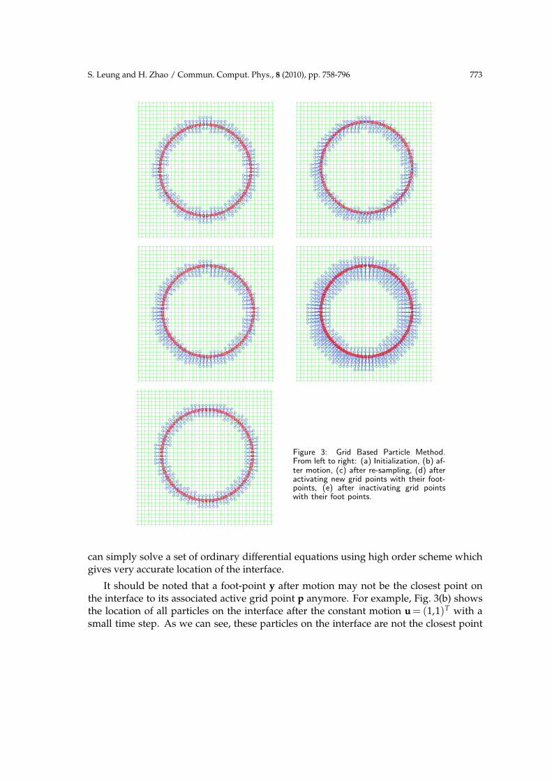
Figure 3: Grid Based Particle Method.From left to right: (a) Initialization, (b) af-ter motion, (c) after re-sampling, (d) afteractivating new grid points with their foot-points, (e) after inactivating grid pointswith their foot points.

can simply solve a set of ordinary differential equations using high order scheme whichgives very accurate location of the interface.

It should be noted that a foot-point y after motion may not be the closest point onthe interface to its associated active grid point p anymore. For example, Fig. 3(b) showsthe location of all particles on the interface after the constant motion u = (1,1)T with asmall time step. As we can see, these particles on the interface are not the closest point


from these active grid points to the interface anymore. More importantly, the motionmay cause those original foot-points to become unevenly distributed along the interface.This may introduce both stiffness, when particles are getting together, and large error,when particles are getting apart. To maintain a quasi-uniform distribution of particles,we need to resample the interface by recomputing the foot-points and updating the set ofactive grid points (Υ) during the evolution. During this resampling process, we locally re-construct the interface, which involves communications among different particles on theinterface. This local reconstruction also provides geometric and Lagrangian informationat the recomputed foot-points on the interface.

The key step in the method is a least square approximation of the interface usingpolynomials at each particle in a local coordinate system, (n′)⊥,n′, with y as the origin,Fig. 4(a). Using this local reconstruction, we find the closest point from this active gridpoint to the local approximation of the interface, Fig. 4(b). This gives the new foot-pointlocation. Further, we also compute and update any necessary geometric and Lagrangianinformation, such as normal, curvature, and also possibly an updated parametrization ofthe interface at this new foot-point. For a detail description, we refer interested readersto [24].

3.2 The GBPM for open curves evolutions

In this section, we will briefly summarized [24] and discuss how our algorithm can modelthe motion of an open curve (in 2 dimensions). The main idea is to explicitly keep trackof the motion of the end-points of the open curve, and then to enforce this condition onthe boundary locations in the local reconstruction step of the grid-based particle methodwe described in the previous subsection.

3.2.1 Representation

As defined before, any grid point which is in a ǫ-neighborhood of the interface is calledactive grid point. In Fig. 5, we demonstrate a typical scenario near an end-point of anopen curve. Given an open curve, we first collect active grid points which are withinthe ǫ-neighborhood. Then, for each of these active grid points we find the correspondingclosest points on the open curve.

Away from the boundary point (green sun-symbol), the set-up is exactly the sameas before. If an active grid point has a distance greater than ǫ away from the boundary(green sun-symbol), we simply project the grid point (red square) onto the surface locallyreconstructed by the least square fitting. This gives the associated foot-point (red circle)on the surface.

For a grid point within the ǫ-neighborhood of the boundary, we assign it with two

foot-points. One is the closest point from the grid point to the open surface, while thesecond one is the closest point from the active grid point to the closed boundary and wewill call this second foot-point the boundary-point. In two dimensions, the second foot-point is just the end-point itself, as shown in Fig. 5.


(a) (b)

Figure 4: (a) Definition of a local coordinates. (b) Local reconstruction of the interface using the foot-points(green squares). The new foot-point (red triangle) associated to the active grid point (blue circle) is obtainedby least square fitting a polynomial.

Figure 5: Representation of the open surface and the boundary in the Grid-Based Particle Method. Away fromthe boundary-point (the green sun-symbol), the representation is the same as in [24]. Each active grid point (reddiamonds) is associated to its closest point on the interface (red circles). Near the boundary-point, each activegrid point (blue triangles and green squares) is associated to its closest point (red circles or green sun-symbol)and also the closest boundary point (green sun-symbol).

Note that these two foot-points could be the same or could be different. In Fig. 5, weplot these special grid points using blue triangles or green squares. Consider the bluetriangles, one of their associated foot-points is still obtained by local least square approx-imation of the interface, which is plotted using red circles. Since these blue triangle activegrid points are within ǫ from the end point (green sun-symbol), their second foot-pointsare also activated which are the closest boundary points (the connectivity is plotted usinga dotted line). In Fig. 5, we plot this type of active grid points using green squares and theconnectivity between the active grid points and their foot-points using a dashed-dottedline.


3.2.2 Motion and resampling

Now we discuss how our algorithm incorporates this boundary information in the evo-lution step and the resampling step. As before, the motion phase of the algorithm is rela-tively straight-forward. We simply move all sampling points (including both the closestpoints and the boundary-points) as in the usual Lagrangian type methods. The motionlaw of the closest-points can be very general. We can naturally deal with the motion byan external velocity field or geometrical motions such as motion by the mean or the Gaus-sian curvature. The motion law imposed on boundary-points can be explicitly given orcan be determined by local geometry of the boundary such as the curvature or the torsion,which can be easily computed from local reconstruction of the boundary as described inthe previous section.

For two dimensional cases, there is no need to resample end-points of the open curvesince they are just explicitly tracked points. The resampling of the open surface near theboundary requires more care. Away from the boundary, the resembling step follows theprocedures in standard grid based particle method. However, near the boundary, weneed to take into account the boundary of the open surface.

The local reconstruction phase of the algorithm is similar as before. For each of theactive grid point p, we consider its neighboring active grids and collect a set of their cor-responding closest points and, if any, also a separate set of their corresponding boundary-points. If p is close to the boundary of the open surface, its neighboring active grid pointmight be assigned two foot-points which might or might not be the same (the blue trian-gles and the green squares in Fig. 5, respectively). We will distinguish these two types offoot-points in this local reconstruction step.

If the set of boundary-points is empty, we will simply use the set of closest pointsfor local reconstruction, as in the original algorithm in [24]. Otherwise, we will form aset of sampling points for local reconstruction using both the set of closest points andalso the set of boundary-points. These sampling points have to satisfy the following twoconditions. The first criteria is the same as what we have proposed in [24] that any twosampling points should be at least of O(h) away, where h is the local mesh size. Thisremoves any redundant information in the sampling points. The second constraint isthat boundary-points in the sampling set should define at least parts of the boundary ofΩ, where Ω is the convex hull formed by the projection of the sampling points on thetangent plane. This is the first place where we incorporate the boundary information inthe local reconstruction.

In two dimensions, here is the way to construct this sampling set from both the closestpoints and the boundary-points. The set of the sampling point starts with the set of theclosest points, for which by default any two of these particles are of at least O(h) awayfrom each other. Then for each boundary-point, we check if it is O(h) away from allof the sampling points or not. If not, then we will reject that particular boundary-pointand then repeat the procedure with the next boundary-point. Otherwise, in the localcoordinates system (n′)⊥,n′ where we denote the boundary-point by (x,y) and the set


(a) (b)

Figure 6: (a) In the original algorithm [24], any potential new foot-point (red triangle) will be rejected ifx∗ /∈ [xmin,xmax] = [min(xj),max(xj)]. (b) In the new algorithm, we associate the new closest point to theclosest boundary-point if the corresponding active grid point is close to the boundary. In this plot, we associatethe active grid point (blue circle) to the particle corresponding to xmin (red triangle) assuming it is a boundary-point.

of the accepted sampling points by (xj,yj), we check if x∈ [min(xj),max(xj)]. If not, thenwe will add this boundary-point to the list of the sampling point. Otherwise, we willuse this boundary-point to replace the sampling point corresponding to either min(xj) ormax(xj), whichever closer to x.

Now, with these sampling points, we construct a local least square fitting and we de-note it by y= f (x). To determine the new closest point, we minimize the distance from thegrid point p to the function y= f (x). If the minimum is attained at x∗∈[min(xi),max(xi)],we follow the same procedure as in [24] and determine the new closest point (x∗, f (x∗)),accordingly. In the previous algorithm, we deactivated any grid point if this new foot-point leads to an extrapolation, i.e., if x∗ /∈ [min(xi),max(xi)], Fig. 6(a). For active pointsnear the boundary, we again enforce the boundary information at this step of the algo-rithm. We now go back and check if the set of boundary-points is non-empty, i.e., if anyof the active grid points in the neighborhood is of the blue triangle or the green squaretype as in Fig. 5. If so, we will assign x∗ to this boundary-point, for example x∗ = xmin

as shown in Fig. 6(b). If none of the neighboring active grid points is associated to aboundary-point, we will simply deactivate this active grid point as in [24].

All other steps in our algorithm will be the same as described in [24]. We approximateany Lagrangian information associated to this particle using the local reconstruction ofthe surface. For example, the normal vector at this new foot-point is approximated by thenormal vector of the local reconstruction at x∗. The curvature and the global parametriza-tion can also be updated accordingly.

3.3 The GBPM for solving Liouville equations

In this section, we consider f : Σ(t)→R defined on the surface Σ(t) represented by ourquasi-uniformly distributed but unorganized particles. Considering the following Liou-


ville equation, we have the following ODE defined along each characteristic

D f(

y(t))

Dt= g

(

t,y(t), f (y(t)))

, (3.1)

where D/Dt=∂/∂t+u·∇ is the material derivative along any trajectory of a particle y(t)on the interface, and g is the source term defined only on the surface. For instance, if f isone of the level set functions φ or ψ, then the source term g is simply zero and this impliesthat the quantity f in this case should be preserved along any particle trajectory. If f isone of T, A and M, the source term g will be modified according to (2.24c) and (2.25b).

There are two main steps in using the GBPM for solving the advection-reaction equa-tion. We first solve the advection-reaction equation along with the particle trajectory inthe motion phase. Then for each sampling particle in the resampling step, we use againleast square fitting polynomials to approximate f at new foot-point locations. In the re-maining subsections, we will discuss these two main steps in details.

3.3.1 Motion phase

Solving this Liouville equation is relatively straight-forward in the motion phase of ourformulation. Since we are representing the interface Σ(t) using Lagrangian particles,we can simply solve a system of ODE’s to update the function value f carried by eachparticle. Denoting yi(tn) the location of the foot-point associated to an active grid pointxi at the time t= tn. According to the motion u=u(yi), we solve the following system ofODE

dy(t)

dt=u(y(t)), (3.2a)

D f (y(t))

Dt= g

(

t,y(t), f (y(t)))

, (3.2b)

for one timestep from tn to tn+1 with the initial conditions

y(tn)=yi(tn) and f (y(tn))= f (yi(tn)).

This system can be solved easily using any ODE integrator such as the TVD-RK method[34]. To improve the stability, we can also apply any implicit schemes in a straight-forward way if the source term does not depend on the local geometry of the surface.We will study and develop implicit schemes for solving geometry-depending PDE on anevolving surface in a later paper.

These new particle locations indeed sample the surface Σ(tn+1) at tn+1. Note howeverthat since these particles are in general not the closest points from their associated activegrid points, we denote these solutions at tn+1 by y∗

i (tn+1) and f (y∗i (tn+1)), rather than

yi(tn+1) and f (yi(tn+1)).


3.3.2 Resampling phase

The next step in the algorithm is to resample the surface by recomputing the closest pointfrom an active grid point to the interface by locally reconstructing the surface using leastsquare fitting. For solving the Liouville equation, we have to update the function valueat the new foot-point location yi(tn+1) using the function values at y∗

j (tn+1). This is es-

sentially an approximation problem. Given

f (y∗j (tn+1)), for j=1,··· ,m,

we need to approximate f (yi(tn+1)). In this paper, we consider the local coordinates aty∗

i (tn+1) and approximate the function value on the tangent plane. As an example, wehere discuss in details the two dimensional formulation. Higher dimensions extension isrelatively simple. In the local coordinate (n′)⊥,n′ with n′ the normal vector associatedto the foot-point yi(tn), we express the function f in terms of this local coordinates (x,y).This gives

f (x,y)= f(

x,y(x))

= f (x), (3.3)

where y(x) is the least square polynomial we used to locally approximate the interface.Let x∗ be the minimizer which leads to the location for the new foot-point, Fig. 7(a), wehave the following approximation problem. Given m data points (xj, f (xj)) for j=1,··· ,m,we want to approximate f (x∗). Various interpolation or approximation methods could beused. In the current formulation, we again use the least square technique and determinea polynomial approximation f to the function f according to the data points. Then thefunction value at the new foot-point is given by f (x∗) as shown in Fig. 7(b), i.e.,

f(

yi(tn+1))

= f (x∗). (3.4)

3.4 Gaussian beam summation

Once we have obtained all necessary components at the foot-points, we can construct theresulting wavefield generated by these sampling beams.

On the right subplot in Fig. 8, we have demonstrated a typical sampling scenario ob-tained by the grid based particle method. In Fig. 2, the sampling particles are obtainedby finding the zero’s of the level set function at each xi using linear interpolations. In thegrid base particle method, these sampling particles are closest points from the underly-ing uniform mesh. There is a fundamental difference between these two solutions. Usingthe pure Eulerian formulation as in Fig. 2, we immediately obtain for any grid point xi

all arrival-angle(s) θ(xi), and also the corresponding arrival-time(s) and other necessarycomponents for constructing the induced wavefield. In the grid based particle method,on the other hand, the sampling is only quasi-uniform. The sampling locations dependon not only the underlying mesh size ∆x, but also the geometry of the curve. To computeall arrival-angles and their corresponding arrival-times at a particular receiver location


(a) (b)

Figure 7: (a) Local reconstruction of the interface using the foot-points (green squares). The new foot-point(red triangle) associated to the active grid point (blue circle) is obtained by least square fitting a polynomial.

(b) Approximating f (x∗) (red triangle) by least square fitting a polynomial using f (xj) (green squares).

Figure 8: The sampling particles (blue dots) of the level set in the grid based particle method. Note thedifference on the sampling from Fig. 2.

xi, we need to further interpolate all sampling foot-points. However, we will not fur-ther study the implication of this difference in the sampling since we can still eventuallyobtain the overall wavefield on a uniform mesh in the real space.

For each of the foot-points (xi,θi) on the open curve at a given z, we first compute thewavefield Ψ induced by this particular arrival beam using (2.20b). One could definitelyspeed up the computations by looking at only a small neighborhood of the central beamsince the magnitude of the wavefield decays exponentially away from each of these beamanyway [39]. But in this current implementation, we do not study the relationship ofapplying such a mask function with the accuracy of the final solution, and we simplydetermine the induced wavefield everywhere in the computational domain.

The next step is to sum up all these contributions according to the initial parametriza-tion of all arrival beams, i.e., summing up these beams according to (2.32). Associated to


all foot-points, we have the level set function φ which acts as a natural parameterizationin the case since the incident rays can be parametrized by their incident location x′ as in(2.32). As shown in the left subplot in Fig. 8, the function value of φ essentially providesthe takeoff location of the arrival beam.

Approximating the integral (2.32), we need to determine the weight for the wave-field induced by each arrival beam. We first sort these φi at these foot-points (xi,θi) fori=1,··· , I. It is possible that several foot-points might have the same φi. For example, con-sidering the initial setup where we consider a horizontal curve. Active grid points fromabove and below the interested segment will coincide to the same points, giving the sameφi for multiple foot-points. In this case, we first eliminate the redundant foot-points inthis summation process and average all carrying function values among these redundantparticles. Then, the weight for each of these distinct arrival beams will be computed bythe average of the distances between the two neighboring φi’s. Mathematically, assumingφi is sorted, we have

wj =∆φj =1

2

∣

∣φj+1−φj−1

∣

∣.

3.5 Algorithm

To end this section, we first summarize the whole algorithm in obtaining diffraction pat-terns using Eulerian Gaussian beams and the grid based particle method. Then we willdiscuss the computational complexity of the proposed algorithm and will compare itwith different approaches.

Algorithm 3.1: Diffraction pattern using EGB and GBPM

1. Initialization. Collect all grid points in a small neighborhood of the open curve. From each of thesegrid points, compute the closest point on the interface. Initialize φ, ψ, A, M and T according to(2.18e) and (2.24c).

2. Motion. Move all foot-points according to a given motion law given by (2.6b).

3. Updating necessary components. Update φ, ψ, A, M and T according to (2.24c) and (2.25b) alongthe motion trajectories as described in Section 3.3.1.

4. Re-Sampling. For each active grid point, re-compute the closest point to the interface reconstructedlocally by those particles after the motion in step 2. Approximate φ, ψ, A, M and T at all newfoot-points using least square fitting as described in Section 3.3.2.

5. Updating the computational tube.

6. Construct individual wavefields. For each foot-point, compute the induced wavefield using (2.20b).

7. Construct overall wavefield. Determine the weight for each individual wavefield as described inSection 3.4.

8. Iteration. Repeat steps 2-7 until the final computational time.

Let N be the number of grid points in each direction in the phase space. The opencurve in the GBPM can be represented by O(N) points. This significantly drops the


order from O(N2) comparing to the approach in [20, 21] as described near the end ofSection 2.4.1. The motion step according to (2.6b) and the evolution step according to(2.24c) and (2.25b) involves only ODE solvers. For O(N) points in the phase space, theoverall computational complexity is still O(N) for these two phases for one ∆z step. Tocompute these quantities up to a fixed final level z f , the overall computational complex-

ity is O(N2). To determine the overall wavefield for each given z, we first constructthe individual wavefield according to (2.20b) and then sum up all individual wavefieldaccording to (2.32). The computational complexity is O(N) for each beam and thereforeO(N·N)=O(N2) for all O(N) beams. If the wavefield is necessary only on the final levelz f , one might skip steps 6 and 7 in the above algorithm for all intermediate steps and so

the overall computational complexity is of only O(N2). If the wavefield is necessary forall z-level, the computational complexity is O(N3). Even with ∆x=O(ω−1/2), the overallcomputational complexity is of only O(ω3/2), which is still significantly better than usualfinite difference methods.

4 Examples

4.1 Accuracy in solving PDE on an evolving surface

In this first example, we will study the accuracy and the convergence of solving anadvection-reaction equation using the grid based particle method. We consider solving

D f

Dt=[4πcos(4πt)] f , (4.1a)

f (0,θ)=sin(2θ), (4.1b)

tanθ =y−0.25

x−0.25, (4.1c)

on an evolving circle under the velocity field (u,v)=(1,1). The circle is initially centeredat (0.25,0.25) with radius 0.2. We compute the solution of f at t=0.5 and compare it withthe exact solution on the circle finally centered at (0.75,0.75) with the same radius 0.2

fexact(t,θ)=sin(2θ)exp[sin(4πt)], (4.2a)

tanθ =y−0.25−t

x−0.25−t. (4.2b)

All quadratures are done using the TVD-RK3 method.In Fig. 9, we plot the errors in the solution using the following two- and infinity-

norms.

E∆x,2 =

√

∫

θ| f (0.5,θ)− fexact(0.5,θ)|2dθ, (4.3a)

E∆x,∞ =maxθ

| f (0.5,θ)− fexact(0.5,θ)|, (4.3b)


(a)10−2

10−3

10−2

Rate=1.8517

∆ x

E∆

x

(b)10−2

10−3

10−2

Rate=2.0657

∆ x

E∆

x

Figure 9: Convergence of solving a PDE on an evolving surface using (a) E∆x,2 and (b) E∆x,∞.

for different ∆x. For each active grid point, we first compute the exact value of f atthe exact closest point from the grid location to the circle. We then compare it with thecomputed function value at the foot-point. To calculate the overall error, we sum thesepointwise errors using the Trapezoidal integration.

The error consists of the following two parts. The first part is the error we made incalculating the foot-point location. Numerically, the foot-point only approximates theclosest point locations since there is error we made in the local reconstruction. However,as studied in [24], such error is of O(∆x3) when using a local quadratic approximation.The second contribution is the error we made in solving the ODE and approximating thefunction on the interface in the resampling step. Since we are using the TVD-RK3 whichis third order accurate for each time step, the overall accuracy at a fixed final time is there-fore O(∆x3 ·∆t) =O(∆x3 ·∆x−1) =O(∆x2). This explains the second order convergence(1.85, 2.06) in Fig. 9.

4.2 Single or double slit diffraction in homogeneous medium

In this example, we consider diffraction patterns in a homogeneous medium. These arerelatively simple cases where good analytical explicit approximations are available. Thefirst example is the single slit diffraction with the aperture centered at x = 0 having sizeequals to b = 0.1. We assume that the incident wave is a plane wave with the frequencyω=256π. Since the Liouville equation has u=v=0 in the phase space, we concentrate ourcomputations on the domain x∈ [−0.1,0.1] and θ∈ [−1.5,1.5] using a uniform underlyingmesh of 257 grids in each direction.

For these simple cases, the motion law (2.6b) is reduced to x = tanθ and θ = 0. Forθ(z=0)=0 (corresponding to the plane wave passing through the slit), we have x(z)=x0

and θ(z)=0. This means that an open segment stays the same open segment in the phasespace. When projected onto the physical space, the open segment just translates in thez-direction without any stretching/folding in the x-direction.


(a)

−1.5 −1 −0.5 0 0.5 1 1.50

0.5

1

1.5

2

2.5

3

0

0.2

0.4

0.6

0.8

1

1.2

1.4

1.6

1.8

(b)−1.5 −1 −0.5 0 0.5 1 1.5

0

0.1

0.2

0.3

0.4

0.5

0.6

0.7

0.8

0.9

1

x

I/I(0

)

ComputedTheory (Fresnel)Theory (Fraunhofer)

(c)−1.5 −1 −0.5 0 0.5 1 1.5

10−6

10−5

10−4

10−3

10−2

10−1

100

x

I/I(0

)

ComputedTheory (Fraunhofer)

(d)−1.5 −1 −0.5 0 0.5 1 1.5

10−6

10−5

10−4

10−3

10−2

10−1

100

x

I/I(0

)

ComputedTheory (Fresnel)

(e)−1.5 −1 −0.5 0 0.5 1 1.5

10−7

10−6

10−5

10−4

10−3

10−2

x

Abs

olut

e E

rror

Figure 10: Single slit diffraction in homogeneousmedium. The aperture is b=0.1 with an incidentplane wave frequency ω =256π. (a) The inten-sity field using Eulerian Gaussian beams summa-tion. (b) The intensity at z = z f = 3≫ b = 0.1.

(c) Comparison with the Fraunhofer’s solution(dashed line) in the log-scale. These two solu-tions acceptably match with each other for themiddle region where |x| is small. (d) Compari-son with the Fresnel’s solution (dashed line) inthe log-scale. (e) The absolute difference be-tween the computed intensity and that from theFresnel approximation.

In Fig. 10(a), we show our computed intensity field defined as I = |U|2 for z up to3. We have compared our solution at z = z f = 3 with some well-known approximationsto this single slit diffraction problem [13]. In Fig. 10(b), we plot the intensity at z = z f

together with the Fraunhofer diffraction formula given by

I(θ)≃ I(0)( sinβ

β

)2, (4.4)

where tanθ = x/z f , λ = 2π/ω, and β = πbsinθ/λ. This approximation is obtained byconsidering the asymptotic solution to the Fresnel-Kirchhoff formula as z f →∞ with the


(a)0 0.5 1 1.5

−0.2

−0.1

0

0.1

0.2

0.3

0.4

0.5

0.6

0.7

x

Re(

U)

ComputedFresnel

(b)0 0.5 1 1.5

−0.5

−0.4

−0.3

−0.2

−0.1

0

0.1

0.2

0.3

0.4

0.5

x

Im(U

)

ComputedFresnel

(c)0 0.5 1 1.5

10−5

10−4

10−3

10−2

10−1

x

Abs

olut

e E

rror

in R

e(U

)

(d)0 0.5 1 1.5

10−5

10−4

10−3

10−2

10−1

x

Abs

olut

e E

rror

in Im

(U)

Figure 11: Single slit diffraction in homogeneous medium. The aperture is b=0.1 with an incident plane wavefrequency ω = 256π. (a) The real part of the wavefield on z = 3 and 0 < x < 1.5. (b) The imaginary part ofthe wavefield on z = 3 and 0< x < 1.5. (c) The absolute difference between the solution in (a) and that fromthe Fresnel approximation. (d) The absolute difference between the solution in (b) and that from the Fresnelapproximation.

small |x|, approximation. To better compare the Eulerian Gaussian beams solution withthe Fraunhofer solution, we have also plotted the intensity in the log-scale, Fig. 10(c). Ourcomputed solution matches well with this analytical intensity in the middle portion. Forlarger |x|, our computed solution starts to deviate from the approximation given in (4.4).The locations of the first few maxima and minima match very accurately. However, thecorresponding intensity at these minima are quite different. Theoretically, the Fraunhoferdiffraction gives zero intensity at these minima which is accurate only asymptotically asz f →∞.

A better approximation is obtained by considering the Fresnel approximation whichsimplifies the Fresnel-Kirchhoff formula and gives

I(x)≃ I(0)|C(x)+iS(x)|2, (4.5)

where C(x) and S(x) are the Fresnel integrals given by

C(x)=∫ v(x)

0cos

(πw2

2

)

dw, (4.6a)


(a)

−1.5 −1 −0.5 0 0.5 1 1.50

0.5

1

1.5

2

2.5

3

0

0.2

0.4

0.6

0.8

1

1.2

1.4

1.6

1.8

(b)−1.5 −1 −0.5 0 0.5 1 1.5

0

0.1

0.2

0.3

0.4

0.5

0.6

0.7

0.8

0.9

1

x

I/I(0

)

ComputedTheory (Fresnel)Theory (Fraunhofer)

(c)−1.5 −1 −0.5 0 0.5 1 1.5

10−6

10−5

10−4

10−3

10−2

10−1

100

x

I/I(0

)

ComputedTheory (Fraunhofer)

(d)−1.5 −1 −0.5 0 0.5 1 1.5

10−6

10−5

10−4

10−3

10−2

10−1

100

x

I/I(0

)

ComputedTheory (Fresnel)

(e)−1.5 −1 −0.5 0 0.5 1 1.5

10−7

10−6

10−5

10−4

10−3

10−2

x

Abs

olut

e E

rror

Figure 12: Double slit diffraction in homoge-neous medium. The distance between two slitsis a=0.1 and the aperture of each slit is b=0.05with an incident plane wave frequency ω=256π.(a) The intensity field using Eulerian Gaussianbeams summation. (b) The intensity at z=z f =3. (c) Comparison with the Fraunhofer’s solu-tion (dashed line) in the log-scale. These twosolutions acceptably match with each other forthe middle region where |x| is small. (d) Com-parison with the Fresnel’s solution (dashed line)in the log-scale Our solution matches extremelywell with the Fresnel’s solution. (e) The abso-lute difference between the computed intensityand that from the Fresnel approximation.

S(x)=∫ v(x)

0sin

(πw2

2

)

dw, (4.6b)

v(x)=√

2/λz f

( b

2−x

)

. (4.6c)

This solution more accurately approximates the Fresnel-Kirchhoff formula than the Fraun-hofer’s approximation for finite z f ≪∞. The Fraunhofer formula predicts that the solu-tion has zero intensity at minima when β = mπ for m = 0,±1,±2,··· . For finite z f , thisobservation is not true and has to be corrected using the Fresnel diffraction. As seen


(a) 0 0.5 1 1.5

−0.4

−0.2

0

0.2

0.4

0.6

x

Re(

U)

ComputedFresnel

(b) 0 0.5 1 1.5−0.5

−0.4

−0.3

−0.2

−0.1

0

0.1

0.2

0.3

0.4

0.5

x

Im(U

)

ComputedFresnel

(c) 0 0.5 1 1.5

10−4

10−3

10−2

10−1

x

Abs

olut

e E

rror

in R

e(U

)

(d) 0 0.5 1 1.5

10−5

10−4

10−3

10−2

10−1

x

Abs

olut

e E

rror

in Im

(U)

Figure 13: Double slit diffraction in homogeneous medium. The aperture is b=0.1 with an incident plane wavefrequency ω = 256π. (a) The real part of the wavefield on z = 3 and 0 < x < 1.5. (b) The imaginary part ofthe wavefield on z = 3 and 0< x < 1.5. (c) The absolute difference between the solution in (a) and that fromthe Fresnel approximation. (d) The absolute difference between the solution in (b) and that from the Fresnelapproximation.

in Fig. 10(d), our solution not only locates similar maxima/minima locations, but alsogives similar nonzero intensity at these maxima/minima as obtained by the Fresnel so-lution (4.5), as shown in Fig. 10(e). In Fig. 11, we have directly compared the computedwavefield on z=3 to that from the Fresnel approximation given by

U(x,y)=−3i

4exp

( iπ

4+

2πiz f

λ

)

[

C(x)+iS(x)]

. (4.7)

These two solutions match very well.A slight more complicated situation is the double slit diffraction. In this example, we

have used a=0.1 and b=0.05. To resolve the incident wave from each slit using the samenumber of Gaussian beams, we have doubled the number of grid to 513 in each directionof the phase space. We use the same frequency ω=256π and compute the solution at thesame z f =3.

Fig. 12 shows our computed solution together with the Fraunhofer diffraction for-mula and the Fresnel approximation. Similar to the single slit diffraction, our solutionmatches well with the Fraunhofer approximation for small |x| and matches extremely


well with the Fresnel solution, as shown in Fig. 12(e). We have also compared our com-puted wavefield on z = 3 with that from the Fresnel approximation in Fig. 13. Thesesolutions match well as in the single diffraction case.

4.3 Gaussian beam diffraction in lens-like medium

We study the diffraction of a Gaussian beam in a parabolic lens-like medium with thevelocity given by

c(x,z)=1√

1−x2. (4.8)

This example has been widely studied in various articles [3, 4, 10, 19]. Considering aninitial Gaussian wave profile given by

U(x,0)=exp(

− x2

2σ20

)

, (4.9)

with σ0 =0.01, we compute the solution to the Helmholtz equation with ω =64π.

−0.1 −0.08 −0.06 −0.04 −0.02 0 0.02 0.04 0.06 0.08 0.1−0.1

−0.08

−0.06

−0.04

−0.02

0

0.02

0.04

0.06

0.08

0.1

x

θ

−0.1 −0.08 −0.06 −0.04 −0.02 0 0.02 0.04 0.06 0.08 0.1−0.1

−0.08

−0.06

−0.04

−0.02

0

0.02

0.04

0.06

0.08

0.1

x

θ

−0.1 −0.08 −0.06 −0.04 −0.02 0 0.02 0.04 0.06 0.08 0.1−0.1

−0.08

−0.06

−0.04

−0.02

0

0.02

0.04

0.06

0.08

0.1

x

θ

−0.1 −0.08 −0.06 −0.04 −0.02 0 0.02 0.04 0.06 0.08 0.1−0.1

−0.08

−0.06

−0.04

−0.02

0

0.02

0.04

0.06

0.08

0.1

x

θ

−0.1 −0.08 −0.06 −0.04 −0.02 0 0.02 0.04 0.06 0.08 0.1−0.1

−0.08

−0.06

−0.04

−0.02

0

0.02

0.04

0.06

0.08

0.1

x

θ

−0.1 −0.08 −0.06 −0.04 −0.02 0 0.02 0.04 0.06 0.08 0.1−0.1

−0.08

−0.06

−0.04

−0.02

0

0.02

0.04

0.06

0.08

0.1

x

θ

−0.1 −0.08 −0.06 −0.04 −0.02 0 0.02 0.04 0.06 0.08 0.1−0.1

−0.08

−0.06

−0.04

−0.02

0

0.02

0.04

0.06

0.08

0.1

x

θ

−0.1 −0.08 −0.06 −0.04 −0.02 0 0.02 0.04 0.06 0.08 0.1−0.1

−0.08

−0.06

−0.04

−0.02

0

0.02

0.04

0.06

0.08

0.1

x

θ

−0.1 −0.08 −0.06 −0.04 −0.02 0 0.02 0.04 0.06 0.08 0.1−0.1

−0.08

−0.06

−0.04

−0.02

0

0.02

0.04

0.06

0.08

0.1

x

θ

Figure 14: Diffraction of a Gaussian in a parabolic medium. We show the evolution of the open level curve inthe x-θ phase space. Caustics are clearly observed at the third and the seventh subplot.


z

x

0 1 2 3 4 5 6

−0.5

0

0.5 00.20.40.60.8

Figure 15: Diffraction of a Gaussian in a parabolic medium. The intensity I(x,z).

0 1 2 3 4 5 60

0.1

0.2

0.3

0.4

0.5

0.6

0.7

0.8

0.9

1

z

I

ComputedExact

0 1 2 3 4 5 60

0.01

0.02

0.03

0.04

0.05

0.06

0.07

0.08

0.09

z

Abs

olut

e E

rror

Figure 16: Diffraction of a Gaussian in a parabolic medium. (a) The intensity along x = 0, I(0,z). The re-focusing effect is clearly seen at z= π and 2π. (b) The absolute difference between the computed solution in(a) and that from the small-angle approximation.

0 1 2 3 4 5 6−0.1

−0.08

−0.06

−0.04

−0.02

0

0.02

0.04

0.06

0.08

0.1

z

x

Figure 17: Diffraction of a Gaussian in aparabolic medium. The central beam locationby ray tracing.

We initialize the level set Γ(0) by

(x,θ) : |x|≤0.05, θ =0

.

Unlike in the previous example where the level set stays unmoved (u = v = 0), the seg-ment in this example will roughly rotate about the origin. Fig. 14 shows the evolutionof this segment. Our algorithm can give a nice quasi-uniform sampling of the evolvingcurve. In the phase space, caustic is defined as locations where the level set overturns,i.e., ∂x/∂φ=0 along the level set or the x-projection of the level set will change the num-


−0.1 −0.08 −0.06 −0.04 −0.02 0 0.02 0.04 0.06 0.08 0.10

1

2

3

4

5

6

7

x

T

−0.1 −0.08 −0.06 −0.04 −0.02 0 0.02 0.04 0.06 0.08 0.10

1

2

3

4

5

6

7

x

T

−0.1 −0.08 −0.06 −0.04 −0.02 0 0.02 0.04 0.06 0.08 0.10

1

2

3

4

5

6

7

x

T

−0.1 −0.08 −0.06 −0.04 −0.02 0 0.02 0.04 0.06 0.08 0.10

1

2

3

4

5

6

7

x

T

−0.1 −0.08 −0.06 −0.04 −0.02 0 0.02 0.04 0.06 0.08 0.10

1

2

3

4

5

6

7

x

T

−0.1 −0.08 −0.06 −0.04 −0.02 0 0.02 0.04 0.06 0.08 0.10

1

2

3

4

5

6

7

x

T

−0.1 −0.08 −0.06 −0.04 −0.02 0 0.02 0.04 0.06 0.08 0.10

1

2

3

4

5

6

7

x

T

−0.1 −0.08 −0.06 −0.04 −0.02 0 0.02 0.04 0.06 0.08 0.10

1

2

3

4

5

6

7

x

T

−0.1 −0.08 −0.06 −0.04 −0.02 0 0.02 0.04 0.06 0.08 0.10

1

2

3

4

5

6

7

x

T

Figure 18: Diffraction of a Gaussian in a parabolic medium. We show arrivaltimes at various z’s correspondingto that in figure 14. Multiple arrivals are observed at (x,z) = (0,π/2) and (0,3π/2) which corresponds toapproximately the second and the seventh subplots.

ber of arrivals. In the third and the seventh subplots in Fig. 14, we can see the overturnof the level set which clearly show the existence of caustics in the solution. Geometricaloptics solution cannot correctly compute the results wavefield since this asymptotic ap-proximation wrongly predicts that the amplitude will blow up at these caustic locations.

As discussed in those above cited references, the intensity of the wavefield can bewell approximated by the following Gaussian profile for small slit |x| or small angle θ

I(x,z)=σ0

σ(z)exp

(

− x2

σ2(z)

)

, (4.10a)

σ(z)=σ0

√

1+[( 1

ωσ20

)2−1

]

sin2(z). (4.10b)

We have shown the computed wavefield in Fig. 15. The refocusing effect of this parabolicmedium is clearly seen at around z=π and z=2π. To compare these two solutions clearly,in Fig. 16 we plot the computed intensity with the exact values along x = 0. These twosolutions match well.

In Fig. 17, we have also plotted the ray tracing solution of the central beams. TheseLagrangian beams are shotted from z = 0 with takeoff angles equal zero and takeoff lo-cations uniformly distributed along the x-direction. As seen clearly, all these rays collide


and form caustics at z=π/2 and z=3π/2. Since we have all rays converging to a singlepoint at these z-levels, the geometrical optics solution is not able to produce the rightdiffraction behavior in the wavefield. Our solution can capture the right behavior of thewave propagation even at caustics. In Fig. 18, we have shown the arrivaltimes at differentz’s. In the third and the seventh subplots, we have multiple arrivals that all rays almostconverge to a single point.

4.4 Diffraction in inhomogeneous media

In this section, we will consider the diffraction pattern by a single slit in a sinusoidalmedium with the velocity given by

c(x,z)=1+0.2sin[3π(x+0.55)]sin(πz

2

)

. (4.11)

The slit is placed at z = 0 centered at x = 0 with size b = 0.1. The incident wave is aplane wave with frequency ω = 64π. We have shown a contour plot of the underlyingvelocity model in Fig. 19. This velocity model has been used widely to test the abilityof a numerical method to obtain a nice representation of the multivalued arrivaltimesolution [29, 30, 37, 38].

z

x

0 0.5 1 1.5 2 2.5 3 3.5 4−0.4

−0.2

0

0.2

0.4

0.6

0.8

0.9

1

1.1

Figure 19: Diffraction of a plane wave in a sinusoidal medium. The contour plot of the underlying velocitymodel.

In Fig. 20, we plot the evolution of the open level curve in the x−θ phase space atdifferent z’s. At one end location with x0=−0.05 and θ0=0, the velocities are (u,v)|(x0 ,θ0)=(0,0). This implies that this end point is kept fixed in z. The other endpoint of the segmentwill move around according to the motion law, as shown in Fig. 21. Unlike the previousexample, the open curve in this example is extensively stretched as it evolves in z. UsualLagrangian type method will not be able to nicely sample this curve. As shown in Fig. 20,our numerical method can obtain a nice quasi-uniform sampling of this open level setwhile the end points are accurately tracked.

We shown in Fig. 22 the corresponding arrivaltimes of each arrival rays. As shownclearly in the last two subplots from both Figs. 20 and 22, we have two arrivals for z


−0.2 −0.1 0 0.1 0.2 0.3 0.4 0.5 0.6 0.7 0.8−0.8

−0.6

−0.4

−0.2

0

0.2

0.4

0.6

0.8

x

θ

−0.2 −0.1 0 0.1 0.2 0.3 0.4 0.5 0.6 0.7 0.8−0.8

−0.6

−0.4

−0.2

0

0.2

0.4

0.6

0.8

x

θ

−0.2 −0.1 0 0.1 0.2 0.3 0.4 0.5 0.6 0.7 0.8−0.8

−0.6

−0.4

−0.2

0

0.2

0.4

0.6

0.8

x

θ

−0.2 −0.1 0 0.1 0.2 0.3 0.4 0.5 0.6 0.7 0.8−0.8

−0.6

−0.4

−0.2

0

0.2

0.4

0.6

0.8

x

θ

−0.2 −0.1 0 0.1 0.2 0.3 0.4 0.5 0.6 0.7 0.8−0.8

−0.6

−0.4

−0.2

0

0.2

0.4

0.6

0.8

x

θ

−0.2 −0.1 0 0.1 0.2 0.3 0.4 0.5 0.6 0.7 0.8−0.8

−0.6

−0.4

−0.2

0

0.2

0.4

0.6

0.8

x

θ

−0.2 −0.1 0 0.1 0.2 0.3 0.4 0.5 0.6 0.7 0.8−0.8

−0.6

−0.4

−0.2

0

0.2

0.4

0.6

0.8

x

θ

−0.2 −0.1 0 0.1 0.2 0.3 0.4 0.5 0.6 0.7 0.8−0.8

−0.6

−0.4

−0.2

0

0.2

0.4

0.6

0.8

x

θ

−0.2 −0.1 0 0.1 0.2 0.3 0.4 0.5 0.6 0.7 0.8−0.8

−0.6

−0.4

−0.2

0

0.2

0.4

0.6

0.8

x

θ

Figure 20: Diffraction of a plane wave in a sinusoidal medium. We show the evolution of the open level curvein the x-θ phase space at various z’s. The multiple arrivals are clearly seen at the last two subplots.

−0.2 −0.1 0 0.1 0.2 0.3 0.4 0.5 0.6 0.7 0.8−0.8

−0.6

−0.4

−0.2

0

0.2

0.4

0.6

0.8

x

θ

Figure 21: Diffraction of a plane wave in asinusoidal medium. The end points of the openlevel set for all z. Since u and v are both zeroat (x,θ) = (−0.05,0), one of the end-point iskept fixed.

approximately greater than 3. For instance in the last subplot which corresponds to z=4,we have a caustic at around x = 0.77. Same as in the previous example, the classicalgeometrical optics approximation fails to predict the amplitude at these locations. Butthe Gaussian beam approach can give finite amplitude solution as shown in the intensityplot of the wavefield in Fig. 23 (a). We show also the real and the imaginary parts of thewavefield in (b) and (c), respectively.

As an even more challenging example, we consider also the double slit diffractionpattern in this sinusoidal media. We use the same set-up as in Section 4.2 where we placestwo slits at z = 0 which are separated by a = 0.1 and with the width b = 0.05. To resolve


−0.2 −0.1 0 0.1 0.2 0.3 0.4 0.5 0.6 0.7 0.80

0.5

1

1.5

2

2.5

3

3.5

4

4.5

5

x

T

−0.2 −0.1 0 0.1 0.2 0.3 0.4 0.5 0.6 0.7 0.80

0.5

1

1.5

2

2.5

3

3.5

4

4.5

5

x

T

−0.2 −0.1 0 0.1 0.2 0.3 0.4 0.5 0.6 0.7 0.80

0.5

1

1.5

2

2.5

3

3.5

4

4.5

5

x

T

−0.2 −0.1 0 0.1 0.2 0.3 0.4 0.5 0.6 0.7 0.80

0.5

1

1.5

2

2.5

3

3.5

4

4.5

5

x

T

−0.2 −0.1 0 0.1 0.2 0.3 0.4 0.5 0.6 0.7 0.80

0.5

1

1.5

2

2.5

3

3.5

4

4.5

5

x

T

−0.2 −0.1 0 0.1 0.2 0.3 0.4 0.5 0.6 0.7 0.80

0.5

1

1.5

2

2.5

3

3.5

4

4.5

5

x

T−0.2 −0.1 0 0.1 0.2 0.3 0.4 0.5 0.6 0.7 0.80

0.5

1

1.5

2

2.5

3

3.5

4

4.5

5

x

T

−0.2 −0.1 0 0.1 0.2 0.3 0.4 0.5 0.6 0.7 0.80

0.5

1

1.5

2

2.5

3

3.5

4

4.5

5

x

T

−0.2 −0.1 0 0.1 0.2 0.3 0.4 0.5 0.6 0.7 0.80

0.5

1

1.5

2

2.5

3

3.5

4

4.5

5

x

T

Figure 22: Diffraction of a plane wave in a sinusoidal medium. We show the arrivaltimes at various z’s. Twoarrivals are clearly seen at the last two subplots.

−1 −0.5 0 0.5 10

0.5

1

1.5

2

2.5

3

3.5

4

0

0.5

1

1.5

2

2.5

3

3.5

4

4.5

−1 −0.5 0 0.5 10

0.5

1

1.5

2

2.5

3

3.5

4

−2

−1.5

−1

−0.5

0

0.5

1

1.5

2

−1 −0.5 0 0.5 10

0.5

1

1.5

2

2.5

3

3.5

4

−1.5

−1

−0.5

0

0.5

1

1.5

2

Figure 23: Diffraction of a plane wave in a sinusoidal medium. (a) The intensity of the wavefield. (b) The realpart of the wavefield. (c) The imaginary part of the wavefield.

each slit using the same number of beams, we have doubled the number of mesh in eachdirection in the phase space. We have shown the evolution of the two segments in Fig. 24.The left segment is vigorously stretched under the velocity field but still our algorithm


−1 −0.8 −0.6 −0.4 −0.2 0 0.2 0.4 0.6 0.8−1

−0.8

−0.6

−0.4

−0.2

0

0.2

0.4

0.6

0.8

1

x

θ

−1 −0.8 −0.6 −0.4 −0.2 0 0.2 0.4 0.6 0.8−1

−0.8

−0.6

−0.4

−0.2

0

0.2

0.4

0.6

0.8

1

x

θ

−1 −0.8 −0.6 −0.4 −0.2 0 0.2 0.4 0.6 0.8−1

−0.8

−0.6

−0.4

−0.2

0

0.2

0.4

0.6

0.8

1

x

θ

−1 −0.8 −0.6 −0.4 −0.2 0 0.2 0.4 0.6 0.8−1

−0.8

−0.6

−0.4

−0.2

0

0.2

0.4

0.6

0.8

1

x

θ

−1 −0.8 −0.6 −0.4 −0.2 0 0.2 0.4 0.6 0.8−1

−0.8

−0.6

−0.4

−0.2

0

0.2

0.4

0.6

0.8

1

x

θ

−1 −0.8 −0.6 −0.4 −0.2 0 0.2 0.4 0.6 0.8−1

−0.8

−0.6

−0.4

−0.2

0

0.2

0.4

0.6

0.8

1

x

θ

−1 −0.8 −0.6 −0.4 −0.2 0 0.2 0.4 0.6 0.8−1

−0.8

−0.6

−0.4

−0.2

0

0.2

0.4

0.6

0.8

1

x

θ

−1 −0.8 −0.6 −0.4 −0.2 0 0.2 0.4 0.6 0.8−1

−0.8

−0.6

−0.4

−0.2

0

0.2

0.4

0.6

0.8

1

x

θ

−1 −0.8 −0.6 −0.4 −0.2 0 0.2 0.4 0.6 0.8−1

−0.8

−0.6

−0.4

−0.2

0

0.2

0.4

0.6

0.8

1

x

θ

Figure 24: Diffraction of a plane wave in a sinusoidal medium. We show the evolution of the open level curvein the x-θ phase space at various z’s. The multiple arrivals are clearly seen at the last two subplots.

−1 −0.5 0 0.5 10

0.5

1

1.5

2

2.5

3

3.5

4

0

0.2

0.4

0.6

0.8

1

1.2

−1 −0.5 0 0.5 10

0.5

1

1.5

2

2.5

3

3.5

−0.8

−0.6

−0.4

−0.2

0

0.2

0.4

0.6

0.8

1

−1 −0.5 0 0.5 10

0.5

1

1.5

2

2.5

3

3.5

−1

−0.8

−0.6

−0.4

−0.2

0

0.2

0.4

0.6

0.8

1

Figure 25: Diffraction of a plane wave in a sinusoidal medium. (a) The intensity of the wavefield. (b) The realpart of the wavefield. (c) The imaginary part of the wavefield.

can nicely maintain a quasi-uniform sampling of the level curve and can accurately keeptrack of the end points in the evolution. Again, as in the single slit case, caustics areclearly observed in the last subplot. The overall wavefield, together with the real and theimaginary parts, are plotted in Fig. 25.


Acknowledgments

The work of Leung was supported in part by the RGC under Grant DAG09/10.SC02. Thework of Zhao was supported in part by the ONR grant N00014-02-1-0090 and also in partby the NSF grant DMS0811254.

References

[1] V. M. Babich and V. S. Buldyrev, Asymptotic Methods in Short Wave Diffraction Problems(in Russian), Nauka, Moscow, 1972.

[2] S. Basu, D. P. Mukherjee and S. T. Acton, Implicit evolution of open ended curves, IEEE.Image. Proc., 1 (2007), 261–264.

[3] P. Berczynski, Y. A. Kravtsov and G. Zeglinski, Gaussian beam diffraction in inhomogeneousand nonlinear media: analytical and numerical solutions by complex geometrical optics,Cent. Eur. J. Phys., 6 (2008), 603–611.

[4] M. Bornatici and O. Maj, Wave beam propagation in a weakly inhomogeneous isotropicmedium: paraxial approximation and beyond, Plasma. Phys. Control. Fusion., 45 (2003),707–719.

[5] M. D. Buhmann, Radial Basis Functions, Cambridge University Press, 2003.[6] P. Burchard, L.-T. Cheng, B. Merriman and S. Osher, Motion of curves in three spatial di-

mensions using a level set approach, J. Comput. Phys., 170(2) (2001), 720–741.[7] V. Cerveny, M. M. Popov and I. Psencik, Computation of wave fieds in inhomogeneous

media – Gaussian beam approach, Geophys. J. R. Astr. Soc., 70 (1982), 109–128.[8] L.-T. Cheng, P. Burchard, B. Merriman and S. Osher, Motion of curves constrained on sur-

faces using a level-set approach, J. Comput. Phys., 175 (2002), 604–644.[9] S. Choudhary and L. B. Felsen, Asymptotic theory for inhomogeneous waves, IEEE. T. An-

tenn. Propag., 21 (1973), 827–842.[10] S. Choudhary and L. B. Felsen, Analysis of Gaussian beam propagation and diffraction by

inhomogeneous wave tracking, Proc. IEEE., 62 (1974), 1530–1541.[11] R. A. Egorchenkov and Y. A. Kravtsov, Complex ray-tracing algorithms with application to

optical problems, J. Opt. Soc. Am. A., 18 (2001), 650–656.[12] B. Fornberg and N. Flyer, The gibbs phenomenon for radial basis functions, In A. Jerri, editor,

The Gibbs Phenomenon in Various Representations and Applications, Potsdam, 2007.[13] G. R. Fowles, Introduction to Modern Optics, Dover, 1989.[14] J. Gomes and O. Faugeras, Using the vector distance functions to evolve manifolds of arbi-

trary codimension, Lect. Notes. Comput. Sc., 2106 (2001), 1–13.[15] N. R. Hill, Gaussian beam migration, Geophysics., 55 (1990), 1416–1428.[16] L. Hormander, On the existence and the regularity of solutions of linear pseudo-differential

equations, L’Enseignement Mathematique, 17 (1971), 99–163.[17] J. B. Keller, Geometrical theory of diffraction, J. Opt. Soc., 52 (1962), 116–130.[18] R. G. Kouyoumjian, Self-Focusing: Past and Present, Chapter 6 The Geometrical Theory of

Diffraction and its Application, pages 165–215, Springer, 2006.[19] Y. A. Kravtsov and P. Berczyski, Gaussian beams in inhomogeneous media: a review, Stud.

Geophys. Geod., 51 (2007), 1–36.[20] S. Leung and J. Qian, Eulerian Gaussian beams for schrodinger equations in the semi-

classical regime, J. Comput. Phys., 228 (2009), 2951–2977.


[21] S. Leung, J. Qian and R. Burridge, Eulerian Gaussian beams for high frequency wave prop-agation, Geophysics, 72 (2007), SM61–SM76.

[22] S. Leung, J. Qian and S. Osher, A level set method for three-dimensional paraxial geometricaloptics with multiple sources, Commun. Math. Sci., 2(4) (2004), 643–672.

[23] S. Leung and H. K. Zhao, A grid-based particle method for evolution of open curves andsurfaces, J. Comput. Phys., 228 (2009), 7706–7728.

[24] S. Leung and H. K. Zhao, A grid based particle method for moving interface problems, J.Comput. Phys., 228 (2009), 2993–3024.

[25] M. Motamed and O. Runborg, A fast phase space method for computing creeping rays, J.Comput. Phys., 219 (2006), 276–295.

[26] Y. I. Orlov and S. K. Tropkin, Penumbral diffraction fields in inhomogeneous media, Radio-phys. Quantum. El., 24 (1981), 233–240.

[27] S. Osher and R. P. Fedkiw, Level Set Methods and Dynamic Implicit Surfaces, Springer-Verlag, New York, 2003.

[28] S. J. Osher and J. A. Sethian, Fronts propagating with curvature dependent speed: algo-rithms based on Hamilton-Jacobi formulations, J. Comput. Phys., 79 (1988), 12–49.

[29] J. Qian and S. Leung, A level set based eulerian method for paraxial multivalued traveltimes,J. Comput. Phys., 197 (2004), 711–736.

[30] J. Qian and S. Leung, A local level set method for paraxial multivalued geometric optics,SIAM J. Sci. Comput., 28 (2006), 206–223.

[31] J. Ralston, Gaussian beams and the propagation of singularities, Studies in Partial Pifferen-tial Equations, 23 (1983), 206–248.

[32] B. D. Seckler and J. B. Keller, Asymptotic theory of diffraction in inhomogeneous media, J.Acoust. Soc. Am., 31 (1959), 206–216.

[33] B. D. Seckler and J. B. Keller, Geometrical theory of diffraction in inhomogeneous media, J.Acoust. Soc. Am., 31 (1959), 192–205.

[34] C. W. Shu and S. J. Osher, Efficient implementation of essentially non-oscillatory shock cap-turing schemes, J. Comput. Phys., 77 (1988), 439–471.

[35] P. Smereka, Spiral crystal growth, Phys. D., 138 (2000), 282–301.[36] J. E. Solem and A. Heyden, Reconstructing open surfaces from image data, Int. J. Comput.

Vision., 69 (2006), 267–275.[37] W. W. Symes, A slowness matching finite difference method for traveltimes beyond trans-

mission caustics, In 68th Ann. Internat. Mtg., Soc. Expl. Geophys., Expanded Abstracts,pages 1945–1948. Soc. Expl. Geophys., 1998.

[38] W. W. Symes and J. Qian, A slowness matching Eulerian method for multivalued solutionsof eikonal equations, J. Sci. Comp., 19 (2003), 501–526.

[39] N. Tanushev, Superpositions and higher order Gaussian beams, Commun. Math. Sci., 6(2008), 449–475.

[40] N. Tanushev, J. Qian and J. Ralston, Mountain waves and Gaussian beams, SIAM J. Multi.Model. & Simul., 6 (2007), 688–709.

[41] H.-K. Zhao, T. Chan, B. Merriman and S. J. Osher, A variational level set approach for mul-tiphase motion, J. Comput. Phys., 127 (1996), 179–195.

gaussian beam summation for diffraction in inhomogeneous media

Documents