gaussian-binary restricted boltzmann machines on modeling ... · gaussian-binary restricted...
TRANSCRIPT

arX
iv:1
401.
5900
v1 [
cs.N
E]
23 J
an 2
014
Gaussian-binary Restricted Boltzmann Machines onModeling Natural Image Statistics
Nan WangInstitut fur NeuroinformatikRuhr-Universitat BochumBochum, 44780, [email protected]
Jan MelchiorInstitut fur NeuroinformatikRuhr-Universitat BochumBochum, 44780, Germany
Laurenz WiskottInstitut fur NeuroinformatikRuhr-Universitat BochumBochum, 44780, Germany
Abstract
We present a theoretical analysis of Gaussian-binary restricted Boltzmann ma-chines (GRBMs) from the perspective of density models. The key aspect of thisanalysis is to show that GRBMs can be formulated as a constrained mixture ofGaussians, which gives a much better insight into the model’s capabilities andlimitations. We show that GRBMs are capable of learning meaningful featuresboth in a two-dimensional blind source separation task and in modeling naturalimages. Further, we show that reported difficulties in training GRBMs are dueto the failure of the training algorithm rather than the model itself. Based on ouranalysis we are able to propose several training recipes, which allowed success-ful and fast training in our experiments. Finally, we discuss the relationship ofGRBMs to several modifications that have been proposed to improve the model.
1 Introduction
Inspired by the hierarchical structure of the visual cortex, recent studies on proba-bilistic models used deep hierarchical architectures to learn high order statistics of thedata [Karklin and Lewicki(2009), Koster and Hyvarinen(2010)]. One widely used architecture isa deep believe network (DBN), which is usually trained as stacked restricted Boltzmann ma-chines (RBMs) [Hinton and Salakhutdinov(2006), Bengio et al.(2006), Erhan et al.(2010)]. Sincethe original formulation of RBMs assumes binary input values, the model needs to be modi-fied in order to handle continuous input values. One common way is to replace the binary in-put units by linear units with independent Gaussian noise, which is known as Gaussian-binaryrestricted Boltzmann machines (GRBMs) or Gaussian-Bernoulli restricted Boltzmann machines[Krizhevsky(2009), Cho et al.(2011)] first proposed by [Welling et al.(2004)].
The training of GRBMs is known to be difficult, so that severalmodifications have been pro-posed to improve the training. [Lee et al.(2007)] used a sparse penalty during training, which al-lowed them to learn meaningful features from natural image patches. [Krizhevsky(2009)] trainedGRBMs on natural images and concluded that the difficulties are mainly due to the existence ofhigh-frequency noise in the images, which further preventsthe model from learning the importantstructures. [Theis et al.(2011)] illustrated that in termsof likelihood estimation GRBMs are alreadyoutperformed by simple mixture models. Other researchers focused on improving the model in the
1

view of generative models [Ranzato et al.(2010), Ranzato and Hinton(2010), Courville et al.(2011),Le Roux et al.(2011)Le Roux, Heess, Shotton, and Winn]. [Choet al.(2011)] suggested that thefailure of GRBMs is due to the training algorithm and proposed some modifications to overcomethe difficulties encountered in training GRBMs.
The studies above have shown the failures of GRBMs empirically, but to our knowledge there isno analysis of GRBMs apart from our preliminary work [Wang etal.(2012)], which accounts thereasons behind these failures. In this paper, we extend our work in which we consider GRBMs fromthe perspective of density models, i.e. how well the model learns the distribution of the data. Weshow that a GRBM can be regarded as a mixture of Gaussians, which has already been mentionedbriefly in previous studies [Bengio(2009), Theis et al.(2011), Courville et al.(2011)] but has goneunheeded. This formulation makes clear that GRBMs are quitelimited in the way they can representdata. However we argue that this fact does not necessarily prevent the model from learning thestatistical structure in the data. We present successful training of GRBMs both on a two-dimensionalblind source separation problem and natural image patches,and that the results are comparable tothat of independent component analysis (ICA). Based on our analysis we propose several trainingrecipes, which allowed successful and fast training in our experiments. Finally, we discuss therelationship between GRBMs and above mentioned modifications of the model.
2 Gaussian-binary restricted Boltzmann machines (GRBMs)
2.1 The model
A Boltzmann Machine (BM) is a Markov Random Field with stochastic visible andhiddenunits[Smolensky(1986)], which are denoted asX := (X1, . . . , XM )
T andH := (H1, . . . , HN )T , re-
spectively. In general, we use bold letters denote vectors and matrices.
The joint probability distribution is defined as
P (X,H) :=1
Ze−
1T0
E(X,H), (1)
Z :=
∫ ∫
e−1T0
E(x,h)dxdh (2)
whereE (X,H) denotes anenergy functionas known from statistical physics, which defines thedependence betweenX andH. The temperature parameterT0 is usually ignored by setting its valueto one, but it can play an important role in inference of BMs [Desjardins et al.(2010)]. ThepartitionfunctionZ normalizes the probability distribution by integrating over all possible values ofX andH, which is intractable in most cases. So that in training BMs using gradient descent the partitionfunction is usually estimated using sampling methods. However, even sampling in BMs remainsdifficult due to the dependencies between all variables.
An RBM is a special case of a BM where the energy function contains no terms combining twodifferent hidden or two different visible units. Viewed as agraphical model, there are no lateralconnections within the visible or hidden layer, which results in a bipartite graph. This impliesthat the hidden units are conditionally independent given the visibles and vice versa, which allowsefficient sampling.
The values of the visible and hidden units are usually assumed to be binary, i.e.Xm, Hn ∈ {0, 1}.The most common way to extend an RBM to continuous data is a GRBM, which assumes con-tinuous values for the visible units and binary values for the hidden units. Its energy function[Cho et al.(2011), Wang et al.(2012)] is defined as
E (X,H) : =
M∑
i
(Xi − bi)2
2σ2−
N∑
j
cjHj −M,N∑
i,j
XiwijHj
σ2(3)
=||X− b||2
2σ2− c
TH− X
TWH
σ2, (4)
where ||u|| denotes the Euclidean norm ofu. In GRBMs the visible units given the hid-den values are Gaussian distributed with standard deviation σ. Notice that some authors
2

[Krizhevsky(2009), Cho et al.(2011), Melchior(2012)] usean independent standard deviation foreach visible unit, which comes into account if the data is notwhitened [Melchior(2012)].
The conditional probability distribution of the visible given the hidden units is given by
P (X|h) =P (X,h)
∫P (x,h) dx
(5)
(1,4)=
ecTh
M∏
i
eXiw
Ti∗h
σ2 − ||Xi−bi||22σ2
∫ecT h
M∏
i
exiw
Ti∗h
σ2 − ||xi−bi||22σ2 dx
(6)
=
M∏
i
eXiw
Ti∗h
σ2 − ||Xi−bi||2
2σ2
∫e
xiwTi∗h
σ2 − ||xi−bi||22σ2 dxi
(7)
(11)=
M∏
i
e−||Xi−bi−w
Ti∗h||2
2σ2
∫e−
||xi−bi−wTi∗h||2
2σ2 dxi
(8)
=
M∏
i
N(Xi; bi +w
Ti∗h, σ
2)
︸ ︷︷ ︸
=P (Xi|h)
(9)
= N(X;b+Wh, σ2
), (10)
wherewi∗ andw∗j denote theith row and thejth column of the weight matrix, respectively.N(x;µ, σ2
)denotes a Gaussian distribution with meanµ and varianceσ2. And N
(X;µ, σ2
)
denotes an isotropic multivariate Gaussian distribution centered at vectorµ with varianceσ2 in alldirections. From (7) to (8) we used the relation
ax
σ2− (x− b)
2
2σ2=
−x2 + 2bx+ 2ax− b2
2σ2
=−x2 + 2bx+ 2ax− b2 + a2 − a2 + 2ab− 2ab
2σ2
=−(x− a− b)2 + a2 + 2ab
2σ2. (11)
The conditional probability distribution of the hidden units given the visibles can be derived asfollows
P (H|x) =P (x,H)∑
h
P (x,h)(12)
(1,4)=
e−||x−b||2
2σ2
N∏
j
e
(
cj+xT
w∗jσ2
)
Hj
∑
h
e−||x−b||2
2σ2
N∏
j
e
(
cj+xT w∗j
σ2
)
hj
(13)
=
N∏
j
e
(
cj+xT
w∗jσ2
)
Hj
∑
hj
e
(
cj+xT w∗j
σ2
)
hj
︸ ︷︷ ︸
=P (Hj |x)
. (14)
=⇒ P (Hj = 1|x) =1
1 + e−(
cj+xT w∗j
σ2
) (15)
3

P (H|x) turns out to be a product of independent sigmoid functions, which is a frequently usednon-linear activation function in artificial neural networks.
2.2 Maximium likelihood estimation
Maximum likelihood estimation (MLE) is a frequently used technique for training probabilisticmodels like BMs. In MLE we have a data setX = {x1, . . . , xL} where the observationsxl areassumed to be independent and identically distributed (i.i.d.). The goal is to find the optimal pa-rametersΘ that maximize the likelihood of the data, i.e. maximize the probability that the data isgenerated by the model [Bishop(2006)]. For practical reasons one often considers the logarithm ofthe likelihood, which has the same maximum as the likelihoodsince it is a monotonic function. Thelog-likelihood is defined as
lnP (X ;Θ) = ln
L∏
l=1
P (xl;Θ) =
L∑
l=1
lnP (xl;Θ). (16)
We use the average log-likelihood per training case denotedby ℓ. For RBMs it is defined as
ℓ :=⟨
lnP (X ;Θ)⟩
x
=
⟨
ln
(∑
h
e−E(x,h)
)⟩
x
− lnZ, (17)
wherex ∈ X . And 〈f(u)〉u denotes the expectation of the functionf(u) with respect to variableu.
The gradient of theℓ turns out to be the difference between the expectations of the energies gradientunder the data and model distribution, which is given by
∂ℓ
∂θ
(17,2)=
⟨∑
h
e−E(x,h)
Z∑
h′
e−E(x,h′)
Z
(
−∂E (x,h)
∂θ
)⟩
x
− 1
Z
∑
h
∑
x
e−E(x,h)
(
−∂E (x,h)
∂θ
)
(18)
(1)= −
⟨∑
h
P (h|x) ∂E (x,h)
∂θ
⟩
x
+
⟨∑
h
P (h|x) ∂E (x,h)
∂θ
⟩
x
. (19)
In practice, a finite set of i.i.d. samples can be used to approximate the expectations in (19). Whilewe can use the training data to estimate the first term, we do not have any i.i.d. samples fromthe unknown model distribution to estimate the second term.Since we are able to compute theconditional probabilities in RBMs efficiently, Gibbs sampling can be used to generate those samples.But Gibbs-sampling only guarantees to generate samples from the model distribution if we run itinfinite long. As this is impossible, a finite number ofk sampling steps are used instead. Thisprocedure is known as Contrastive Divergence -k (CD-k) algorithm, in which evenk = 1 showsgood results [Hinton(2002)]. The CD-gradient approximation is given by
∂ℓ
∂θ≈ −
⟨∑
h
P (h|x) ∂E (x,h)
∂θ
⟩
x
+
⟨∑
h
P (h|xk)∂E(x(k),h
)
∂θ
⟩
x(k)
, (20)
wherex(k) denotes the samples afterk steps of Gibbs sampling. The derivatives of the GRBM’senergy function with respect to the parameters are given by
∂E (X,H)
∂b= −X− b
σ2, (21)
∂E (X,H)
∂c= −H, (22)
∂E (X,H)
∂W= −XH
T
σ2, (23)
∂E (X,H)
∂ σ= −||X− b||2
σ3+
2XTWH
σ3, (24)
4

and the corresponding gradient approximations (20) become
∂ℓ
∂b≈
⟨x− b
σ2
⟩
x
−⟨x(k) − b
σ2
⟩
x(k)
, (25)
∂ℓ
∂c≈ 〈P (h = 1|x)〉
x−⟨
P(
h = 1|x(k))⟩
x(k), (26)
∂ℓ
∂w≈
⟨
xP (h = 1|x)Tσ2
⟩
x
−⟨
x(k)P
(h = 1|x(k)
)T
σ2
⟩
x(k)
, (27)
∂ℓ
∂ σ≈
⟨ ||x− b||2 − 2 xTWP (h = 1|x)
σ3
⟩
x
(28)
−⟨
||x(k) − b||2 − 2x(k)TWP
(h = 1|x(k)
)
σ3
⟩
x(k)
,
whereP (h = 1|x) := (P (h1 = 1|x) , · · · , P (hN = 1|x))T , i.e. P (h = 1|x) denotes a vector ofprobabilities.
2.3 The marginal probability distribution of the visible units
From the perspective of density estimation, the performance of the model can be assessed by exam-ining how well the model estimates the data distribution. Wetherefore take a look at the model’smarginal probability distribution of the visible units, which can be formalized as a product of experts(PoE) or as a mixture of Gaussians (MoG))1.
2.3.1 In the Form of Product of Experts
We derive the marginal probability distribution of the visible unitsP (X) by factorizing the jointprobability distribution over the hidden units.
P (X) =∑
h
P (X,h) (29)
(1,4)=
1
Ze−
||X−b||22σ2
N∏
j
∑
hj
ecj+X
Tw∗j
σ2 hj (30)
hj∈{0,1}=
1
Z
N∏
j
(
e−||X−b||2
2Nσ2 + ecj+X
Tw∗j
σ2 − ||X−b||22Nσ2
)
(31)
(11)=
1
Z
N∏
j
(
e−||X−b||2
2Nσ2 + e||b+Nw∗j||2−||b||2
2Nσ2 +cj−||X−b−Nw∗j||2
2Nσ2
)
(32)
=1
Z
N∏
j
(√2πNσ2
)M[
N(X;b, Nσ2
)
+e||b+Nw∗j||2−||b||2
2Nσ2 +cjN(X;b+Nw∗j, Nσ2
) ]
(33)
=:1
Z
N∏
j
pj (X). (34)
Equation (34) illustrates thatP (X) can be written as a product ofN factors, referred to as a productof experts [Hinton(2002)]. Each expertpj(X) consists of two isotropic Gaussians with the samevarianceNσ2. The first Gaussian is placed at the visible biasb. The second Gaussian is shifted
1Some part of this analysis has been previously reported by [Freund & Haussler(1992)]. Thanks to theanonymous reviewer for pointing out this coincidence.
5

relative to the first one byN times the weight vectorw∗j and scaled by a factor that depends onw∗jandb. Every hidden unit leads to one expert, each mode of which corresponds to one state of thecorresponding hidden unit. Figure 1 (a) and (b) illustrateP (X) of a GRBM-2-2 viewed as a PoE,where GRBM-M -N denotes a GRBM withM visible andN hidden units.
Figure 1: Illustration of a GRBM-2-2 as a PoE and MoG, in whicharrows indicate the roles of thevisible bias vector and the weight vectors. (a) and (b) visualize the two experts of the GRBM. Thered (dotted) and blue (dashed) circles indicate the center of the two Gaussians in each expert. (c) vi-sualizes the components in the GRBM. Denoted by the green (filled) circles, the four componentsare the results of the product of the two experts. Notice how each component sits right between ared (dotted) and a blue (dashed) circle.
2.3.2 In the Form of Mixture of Gaussians
Using Bayes’theorem, the marginal probaility ofX can also be formalized as:
P (X) =∑
h
P (X|h)P (h) (35)
=∑
h
N(X;b+Wh, σ2
)
(√2πσ2
)M
Zec
Th+ ||b+Wh||2−||b||2
2σ2 (36)
=
(√2πσ2
)M
Z︸ ︷︷ ︸
P (h:h∈H0)
N(X;b, σ2
)
+
N∑
j=1
(√2πσ2
)M
Ze
||b+w∗j||2−||b||2
2σ2 +cj
︸ ︷︷ ︸
P (hj :hj∈H1)
N(X;b+w∗j , σ
2)
+
N−1∑
j=1
N∑
k>j
(√2πσ2
)M
Ze
||b+w∗j+w∗k||2−||b||2
2σ2 +cj+ck
︸ ︷︷ ︸
P (hjk:hjk∈H2)
N(X;b+w∗j +w∗k, σ
2)
+ . . . , (37)
whereHk denotes the set of all possible binary vectors with exactlyk ones andM − k zerosrespectively. As an example,
∑N−1j=1
∑N
k>j P (hjk : hjk ∈ H2) =∑
h∈H2P (h) sums over the
probabilities of all binary vectors having exactly two entries set to one.P (H) in (36) is derived as
6

follows
P (H) =
∫
P (x,H) dx (38)
(1,4)=
1
Z
∫
ecTH
M∏
i
exiw
Ti∗H
σ2 − ||xi−bi||2
2σ2 dx (39)
=ec
TH
Z
M∏
i
∫
exiw
Ti∗H
σ2 − ||xi−bi||2
2σ2 dxi (40)
(11)=
ecTH
Z
M∏
i
(
e(bi+wT
i∗H)2−b2i
2σ2
∫
e||xi−bi−w
Ti∗H||2
2σ2 dxi
)
(41)
=ec
TH
Z
(√2πσ2
)M
e
M∑
i
(bi+wTi∗H)2−b2
i
2σ2
(42)
=
(√2πσ2
)M
Zec
TH+ ||b+WH||2−||b||2
2σ2 (43)
Since the form in (37) is similar to a mixture of isotropic Gaussians, we follow its naming conven-tion. Each Gaussian distribution is called acomponentof the model distribution, which is exactlythe conditional probability of the visible units given a particular state of the hidden units. As wellas in MoGs, each component has amixing coefficient, which is the marginal probability of thecorresponding state and can also be viewed as the prior probability of picking the correspondingcomponent. The total number of components in a GRBM is2N , which is exponential in the numberof hidden units, see Figure 1 (c) for an example.
The locations of the components in a GRBM are not independentof each other as it is the case inMoGs. They are centered atb+Wh, which is the vector sum of the visible bias and selected weightvectors. The selection is done by the corresponding entriesin h taking the value one. This impliesthat only theM +1 components that sum over exactly one or zero weights can be placed and scaledindependently. We name them first order components and the anchor component respectively. All2N −M−1 higher order components are then determined by the choice ofthe anchor and first ordercomponents. This indicates that GRBMs are constrained MoGswith isotropic components.
3 Experiments
3.1 Two-dimensional blind source separation
The general presumption in the analysis of natural images isthat they can be consid-ered as a mixture of independent super-Gaussian sources [Bell and Sejnowski(1997)], but see[Zetzsche and Rohrbein(2001)] for an analysis of remainingdependencies. In order to be able tovisualize how GRBMs model natural image statistics, we use amixture of two independent Lapla-cian distributions as a toy example.
The independent sourcess = (s1, s2)T are mixed by a random mixing matrixA yielding
x′ = As, (44)
wherep (si) = e−√
2|si|√2
. It is common to whiten the data (see Section 4.1), resultingin
x = Vx′ = VAs, (45)
whereV =⟨
x′x′T⟩− 1
2
is the whitening matrix calculated with principle component analysis
(PCA). Through all this paper, we used the whitened data.
In order to assess the performance of GRBMs in modeling the data distribution, we ran the ex-periments for200 times and calculated theℓ for test data analytically. For comparision, we also
7

calculated theℓ over the test data for ICA2, an isotropic two-dimensional Gaussian distributionand the true data distribution3. The results are presented in Table 1, which confirm the conclusionof [Theis et al.(2011)] that GRBMs are not as good as ICA in terms of ℓ.
Table 1: Comparision ofℓ between different models
ℓ ± std
Gaussian −2.8367± 0.0086GRBM −2.8072± 0.0088
ICA −2.7382± 0.0091data distribution −2.6923± 0.0092
To illustrate how GRBMs model the statistical structure of the data, we looked at the probabilitydistributions of the 200 trained GRBMs. About half of them (110 out of 200) recovered the in-dependent components, see Figure 2 (a) as an example. This can be further illustrated by plottingthe Amari errors4 between the true unmixing matrixA−1 and estimated model matrices, i.e. theunmixing matrix of ICA and the weight matrix of the GRBM, as shown in Figure 3. One can seethat these 110 GRBMs estimated the unmixing matrix quite well, although GRBMs are not as goodas ICA. This is due to the fact that the weight vectors in GRBMsare not restricted to be orthogonalas in ICA.
For the remaining 90 GRBMs, the two weight vectors pointed tothe opposite direction as shownin Figure 2 (b). Accordingly, these GRBMs failed to estimatethe unmixing matrix, but in terms ofdensity estimation these solutions have the same quality asthe orthogonal ones. Thus all the 200GRBMs were able to learn the statistical structures in the data and model the data distribution prettywell.
For comparison, we plotted the probability distribution ofa learned GRBM with four hidden units,see Figure 2 (c), in which GRBMs can always find the two independent components correctly.
To further show how the components contribute to the model distribution, we randomly chose one ofthe 110 GRBMs and calculated the mixing coefficients of the anchor and the first order components ,as shown in Table 2. The large mixing coefficient for the anchor component indicates that the modelwill most likely reach hidden states in which none of the hidden units are activated. In general, themore activated hidden units a state has, the less likely it will be reached, which leads naturally to asparse representation of the data.
Table 2: The mixing coefficients of a successfully-trained GRBM-2-2, GRBM-2-4 and an MoG-3.∑
h∈H0
P (h)∑
h∈H1
P (h)∑
h∈H2
P (h)∑
h∈H3
P (h)∑
h∈H4
P (h)
GRBM-2-2 0.9811 0.0188 7.8856e-05 – –GRBM-2-4 0.9645 0.0352 3.4366e-04 1.2403e-10 6.9977e-18
MoG-3 0.9785 0.0215 – – –
2For the fast ICA algorithm [Hyvarinen(1999)] we used for training, theℓ for super Gaussian sources can
also be assessed analytically byℓ = −⟨ N∑
j=1
ln 2 cosh2w
T∗j xl
⟩
xl
+ ln |detW|.3As we know the true data distribution, the exactℓ can be calculated by
ℓ = −√2⟨
|u1∗xl|+ |u2∗xl|⟩
xl
− ln 2 + ln |detU|, whereU = (VA)−1.4The Amari error [Bach and Jordan(2002)] between two matrices A and B is defined as:
12N
(
N∑
i=1
N∑
j=1
|(AB−1)ij |
maxk |(AB−1)ik|+
|(AB−1)ij |
maxk |(AB−1)kj |
)
− 1.
8
−4 −2 0 2 4x1
−4
−2
0
2
4
x2
(a) GRBM-2-2
(a)
−4 −2 0 2 4x1
−4
−2
0
2
4
x2
(b) GRBM-2-2
(b)
−4 −2 0 2 4x1
−4
−2
0
2
4
x2
(c) GRBM-2-4
(c)
−4 −2 0 2 4x1
−4
−2
0
2
4
x2
(d) MoG-2-3
(d)
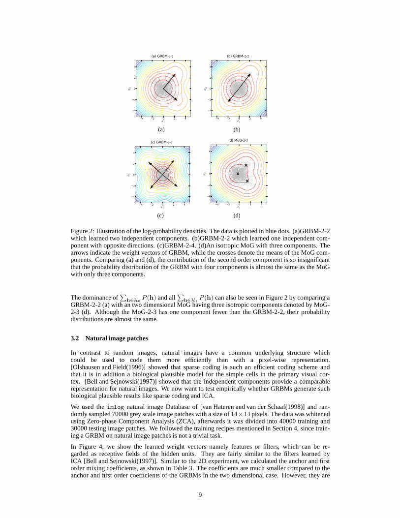
Figure 2: Illustration of the log-probability densities. The data is plotted in blue dots. (a)GRBM-2-2which learned two independent components. (b)GRBM-2-2 which learned one independent com-ponent with opposite directions. (c)GRBM-2-4. (d)An isotropic MoG with three components. Thearrows indicate the weight vectors of GRBM, while the crosses denote the means of the MoG com-ponents. Comparing (a) and (d), the contribution of the second order component is so insignificantthat the probability distribution of the GRBM with four components is almost the same as the MoGwith only three components.
The dominance of∑
h∈H0P (h) and all
∑
h∈H1P (h) can also be seen in Figure 2 by comparing a
GRBM-2-2 (a) with an two dimensional MoG having three isotropic components denoted by MoG-2-3 (d). Although the MoG-2-3 has one component fewer than the GRBM-2-2, their probabilitydistributions are almost the same.
3.2 Natural image patches
In contrast to random images, natural images have a common underlying structure whichcould be used to code them more efficiently than with a pixel-wise representation.[Olshausen and Field(1996)] showed that sparse coding is such an efficient coding scheme andthat it is in addition a biological plausible model for the simple cells in the primary visual cor-tex. [Bell and Sejnowski(1997)] showed that the independent components provide a comparablerepresentation for natural images. We now want to test empirically whether GRBMs generate suchbiological plausible results like sparse coding and ICA.
We used theimlog natural image Database of [van Hateren and van der Schaaf(1998)] and ran-domly sampled 70000 grey scale image patches with a size of14×14 pixels. The data was whitenedusing Zero-phase Component Analysis (ZCA), afterwards it was divided into 40000 training and30000 testing image patches. We followed the training recipes mentioned in Section 4, since train-ing a GRBM on natural image patches is not a trivial task.
In Figure 4, we show the learned weight vectors namely features or filters, which can be re-garded as receptive fields of the hidden units. They are fairly similar to the filters learned byICA [Bell and Sejnowski(1997)]. Similar to the 2D experiment, we calculated the anchor and firstorder mixing coefficients, as shown in Table 3. The coefficients are much smaller compared to theanchor and first order coefficients of the GRBMs in the two dimensional case. However, they are
9

ICA GRBM Random matrix0.0
0.1
0.2
0.3
0.4
0.5
0.6
0.7
0.8
0.9
1.0
Amari e
rror
Figure 3: The Amari errors between the real unmixing matrix and the estimations from ICA andthe 110 GRBMs. The box extends from the lower to the upper quantile values of the data, with aline at the median. The whiskers extend from the box to show the range of the reliable data points.The outlier points are marked by “+”. As a base line, the amarierrors between the real unmixingmatrices and random matrices are provided.
Figure 4: Illustration of 196 learned filters of a GRBM-196-196. The plot has been ordered fromleft to right and from top to bottom by the increasing averageactivation level of the correspondinghidden units.
still significantly large, considering that the total number of components in this case is2196. Similarto the two-dimensional experiments, the more activated hidden units a state has, the less likely it willbe reached, which leads naturally to a sparse representation. To support this statement, we plottedthe histogram of the number of activated hidden units per training sample, as shown in Figure 5.
Table 3: The mixing coefficients of GRBMs-196-196 per component (the Partition function wasestimated using AIS).
∑
h∈H0
P (h)∑
h∈H1
P (h)∑
h∈H\{H0∪H1}P (h)
GRBM-196-196 0.04565 0.00070 0.95365
We also examined the results of GRBMs in the over-complete case, i.e. GRBM-196-588. Thereis no prominent difference of the filters compared to the complete case shown in Figure 4. Tofurther compare the filters in the complete and over-complete case, we estimated the spatial fre-quency, location and orientation for all filters in the spatial and frequency domains, see Fig-ure 6 and Figure 7 respectively. This is achieved by fitting a Gabor function of the form used
10

28 56 84 112 140 168 196The # of activated hidden units
0.00
0.05
0.10
0.15
0.20
0.25
frequ
ency
Figure 5: The histogram of the number of activated hidden units per training sample. The histogramsbefore and after training are plotted in blue (dotted) and ingreen (solid), respectively.
by [Lewicki and Olshausen(1999)]. Note that the additionalfilters in the over-complete case in-crease the variety of spatial frequency, location and orientation.
(a) GRBM−196−196 (b) GRBM−196−588
Figure 6: The spatial layout and size of the filters, which aredescribed by the position and size ofthe bars. Each bar denotes the center position and the orientation of a fitted Gabor function within14×14 grid. The thickness and length of each bar are propotional toits spatial-frequency bandwidth.
4 Successful Training of GRBMs on Natural Images
The training of GRBMs has been reported to be difficult [Krizhevsky(2009), Cho et al.(2011)].Based on our analysis we are able to propose some recipes which should improve the success andspeed of training GRBMs on natural image patches. Some of them do not depend on the data distri-bution and should therefore improve the training in general.
4.1 Preprocessing of the Data
The preprocessing of the data is important especially if themodel is highly restricted like GRBMs.Whitening is a common preprocessing step for natural images. It removes the first and second orderstatistics from the data, so that it has zero mean and unit variance in all directions. This allows train-
11

0 0.5 1
fy
fx
(a) GRBM−196−196
0 0.5 1
fy
fx
(b) GRBM−196−588
Figure 7: A polar plot of frequency tuning and orientation ofthe learned filters. The crosshairsdescribe the selectivity of the filters, which is given by the1/16-bandwidth in spatial-frequency andorientation, [Lewicki and Olshausen(1999)].
ing algorithms to focus on higher order statistics like kurtosis, which is assumed to play an importantrole in natural image representations [Olshausen and Field(1996), Hyvarinen et al.(2001)].
The components of GRBMs are isotropic Gaussians, so that themodel would use several compo-nents for modeling covariances. But the whitened data has a spherical covariance matrix so that thedistribution can be modelled already fairly well by a singlecomponent. The other components canthen be used to model higher order statistics, so that we claim that whitening is also an importantpreprocessing step for GRBMs.
4.2 Parameter Initialization
The initial choice of model parameters is important for optimization process. Using prior knowledgeabout the optimization problem can help to derive an initialization, which can improve the speed andsuccess of the training.
For GRBMs we know from the analysis above that the anchor component, which is placed at thevisible bias, represents most of the whitened data. Therefore it is reasonable in practice to set thevisible bias to the data’s mean.
Learning the right scaling is usually very slow since the weights and biases determine both the po-sition and scaling of the components. In the final stage of training GRBMs on whitened naturalimages, the first components are scaled down extremely compared to the anchor component. There-fore, it will usually speed up the training process if we initialize the parameters so that the first orderscaling factors are already very small. Considering equation (37), we are able to set a specific firstorder scaling factor by initializing the hidden bias to
cj = −||b+w∗j ||2 − ||b||22σ2
+ ln τj , (46)
so that the scaling is determined byτj , which should ideally be chosen close to the unknown finalscaling factors. In practice, the choice of0.01 showed good performance in most cases. The learningrate for the hidden bias can then be set much smaller than the learning rate for the weights.
According to [Bengio(2010)], the weights should be initialized towij ∼ U(
−√6√
N+M,
√6√
N+M
)
,
whereU(a, b) is the uniform distribution in the interval [a, b]. In our experience, this works betterthan the commonly used initialization to small Gaussian-distributed random values.
4.3 Gradient Restriction and Choices of the Hyperparameters
The choice of the hyper-parameters has an significant impacton the speed and success of trainingGRBMs. For successful training in an acceptable number of updates, the learning rate needs to besufficiently big. Otherwise the learning process becomes too slow or the algorithm converges to alocal optimum where all components are placed in the data’s mean. But if the learning rate is chosentoo big, the gradient can easily diverge resulting in a number overflow of the weights. This effect
12

Method Time per epoch in sCD-1 2.1190PCD-1 2.1348CD-10 10.8052PCD-10 10.8303PT-10 21.4855
Table 4: Comparison of the CPU time for training a GRBM with different methods.
becomes even more crucial as the model dimensionality increases, so that a GRBM with 196 visibleand 1000 hidden units diverges already for a learning rate of0.001.
We therefore propose restricting the weight gradient column norms∇w:j to a meaningful size toprevent divergence. Since we know that the components are placed in the region of data, there is noneed for a weight norm to be bigger than twice the maximal datanorm. Consequently, this naturalbound also holds for the gradient and can in practice be chosen even smaller. It allows to choose biglearning rates even for very large models and therefore enables fast and stable training. In practice,one should restrict the norm of the update matrix rather thanthe gradient matrix to also restrict theeffects of the momentum term and etc.
Since the components are placed on the data they are naturally restricted, which makes the use of aweight decay useless or even counter productive since we want the weights to grow up to a certainnorm. Thus we do recommend not to use a weight decay regularization.
A momentum term adds a percentage of the old gradient to the current gradient which leads to amore robust behavior especially for small batch-sizes. In the early stage of training the gradientusually varies a lot, a large momentum can therefore be used to prevent the weights from convergingto zero. In the late stage however, it can also prevent convergence so that in practice a momentumof 0.9 that will be reduced to zero in the final stage of training is recommended.
4.4 Training Method
Using the gradient approximation, RBMs are usually trainedas described in Section 2.2. The qual-ity of the approximation highly depends on the set of samplesused for estimating the model ex-pectation, which should ideally be i.i.d. But Gibbs sampling usually has a low mixing rate, whichmeans that the samples tend to stay close to the previously presented samples. Therefore, a fewsteps of Gibbs sampling commonly leads to a biased approximation of the gradient. In order toincrease the mixing rate [Tieleman(2008)] suggested to usea persistent Markov chain for drawingsamples from the model distribution, which is referred as persistent Contrastive Divergence (PCD).[Desjardins et al.(2010)] proposed to use parallel tempering (PT), which selects samples from a per-sistent Markov chain with a different scaling of the energy function. In particular, [Cho et al.(2011)]analyzed PT algorithm for training GRBMs and proposed a modified version of PT.
In our experiments all methods above lead to meaningful features and comparableℓ, but dif-fer in convergence speed as shown in Figure 8. As for PT, we used original algorithm[Desjardins et al.(2010)] together with weight restrictions and temperatures from 0.1 to 1 with step-size 0.1. Although, PT has a better performance than CD, it has also a much higher computationalcost as shown in Table 4.
5 Discussion
The difficulties of using GRBMs for modeling natural images have been reported by several au-thors [Krizhevsky(2009), Bengio et al.(2006)] and variousmodifications have been proposed to ad-dress this problem.
[Ranzato and Hinton(2010)] analyzed the problem from the view of generative models and arguedthat the failure of GRBMs is due to the model’s focus on predicting the mean intensity of each pixelrather than the dependence between pixels. To model the covariance matrices at the same time, theyproposed the mean-covariance RBM (mcRBM). In addition to the conventional hidden unitshm,
13

20 40 60 80 100
Epoch
-277.85
-277.75
-277.65
-277.55
-277.45
-277.35
Log Likelih
ood
CD-1PCD-1CD-10PCD-10PT-10
Figure 8: Evolution of theℓ of a GRBM 196-16 on the whitened natural image dataset for CD,PCDusing ak of 1, 10 each and PT with 10 temperatures. The learning curves are theaverage over 40trials. The learning rate was 0.1, an initial momentum term of 0.9 was multiplied with 0.9 after eachfifth epoch, the gradient was restricted to one hundredth of the maximal data norm (0.48), no weightdecay was used.
there is a group of hidden unitshc dedicated to model the covariance between the visible units.From the view of density models, mcRBMs can be regarded as improved GRBMs such that theadditional hidden units are used to depict the covariances.The conditional probabilities of mcRBMare given by
P (X|hm,hc) = N (X;ΣWhm,Σ) , (47)
whereΣ =(C diag(Ph
c)CT)−1
[Ranzato and Hinton(2010)]. By comparing (47) and (9), it canbe seen that the components of mcRBM can have a covariance matrix that is not restricted to bediagonal as it is the case for GRBMs.
From the view of generative models another explanation for the failure of GRBMs is providedby [Courville et al.(2011)]. Although they agree with the poor ability of GRBMs in modeling co-variances, [Courville et al.(2011)] argue that the deficiency is due to the binary nature of the hiddenunits. In order to overcome this limitation, they developedthe spike-and-slab RBM (ssRBM), whichsplits each binary hidden unit into a binary spike variablehj and a real valued slab variablesj . Theconditional probability of visible units is given by
P (X|s,h, ||X||2 < R) =1
BN
X;Λ−1N∑
j=1
w∗jsjhj,Λ−1
, (48)
where Λ is a diagonal matrix andB is determined by integrating the GaussianN (X;Λ−1∑N
j=1 w∗jsjhj ,Λ−1) over the ball||X||2 < R [Courville et al.(2011)]. In contrast
to the conditional probability of GRBMs (9),w∗j in (48) is scaled by the continuous variablesj ,which implies that the components can be shifted along theirweight vectors.
We have shown that GRBMs are capable of modeling natural image patches and that the reportedfailures are due to the training procedure. [Lee et al.(2007)] showed also that GRBMs could learnmeaningful filters by using a sparse penalty. But this penalty changes the objective function andintroduced a new hyper-parameter.
[Cho et al.(2011)] addressed these training difficulties, by proposing a modification of PT and anadaptive learning rate. However, we claim that the reporteddifficulties of training GRBMs with PT
14

are due to the mentioned gradient divergence problem. With gradient restriction we were able toovercome the problem and train GRBMs with normal PT successfully.
6 Conclusion
In this paper, we provide a theoretical analysis of GRBM and showed that its product of expertsformulation can be rewritten as a constrained mixture of Gaussians. This representation gives amuch better insight into the capabilities and limitations of the model. We use two-dimensional blindsource separation task as a toy problem to demonstrate how GRBMs model the data distribution. Inour experiments, GRBMs were capable of learning meaningfulfeatures both in the toy problem andin modeling natural images.
In both cases, the results are comparable to that of ICA. But in contrast to ICA the features are notrestricted to be orthogonal and can form an over-complete representation. However, the success oftraining GRBMs highly depends on the training setup, for which we proposed several recipes basedon the theoretical analysis. Some of them can be further generalized to other datasets or directlyapplied like the gradient restriction.
In our experience, maximizing theℓ does not imply good features and vice versa. Prior knowledgeabout the data distribution will be beneficial in the modeling process. For instance, our recipes arebased on the prior knowledge of the natural image statistics, which is center peaked and has heavytails. It will be an interesting topic to integrate prior knowledge of the data distribution into themodel rather than starting modeling from scratch.
Considering the simplicity and easiness of training with our proposed recipe, we believe thatGRBMs provide a possible way for modeling natural images. Since GRBMs are usually used asfirst layer in deep belief networks, the successful trainingof GRBMs should therefore improve theperformance of the whole network.
15

References
[Bach and Jordan(2002)] F. R. Bach and M. I. Jordan. Kernel independent component analysis.Journal of Machine Learning Research, 3:1–48, 2002.
[Bell and Sejnowski(1997)] A. Bell and T. Sejnowski. The “independent components” of naturalscenes are edge filters.Vision Research, 37(23):3327–3338, 12 1997. ISSN 00426989.
[Bengio(2010)] X. Glorot Bengio. Understanding the difficulty of training deep feedforward neu-ralnetworks.AISTATS, 2010.
[Bengio(2009)] Y. Bengio. Learning deep architectures forAI. Foundation and Trends in MachineLearning., 2(1):1–127, 2009. Also published as a book. Now Publishers, 2009.
[Bengio et al.(2006)] Y. Bengio, P. Lamblin, D. Popovici, and H. Larochelle. Greedy layer-wisetraining of deep networks. InProceedings of the Conference on Neural Information ProcessingSystems, pages 153–160, 2006.
[Bishop(2006)] C. M. Bishop.Pattern Recognition and Machine Learning, chapter 8, pages 359–422. Springer, Secaucus, NJ, USA, 2006. ISBN 0387310738.
[Cho et al.(2011)] K. Cho, A. Ilin, and T. Raiko. Improved learning of gaussian-bernoulli restrictedboltzmann machines. InProceedings of the International Conference on Artificial NeuralNetworks, 10–17, 2011.
[Courville et al.(2011)] A. C. Courville, J. Bergstra, and Y. Bengio. A spike and slab restrictedboltzmann machine.Journal of Machine Learning Research, 15:233–241, 2011.
[Desjardins et al.(2010)] G. Desjardins, A. Courville, Y. Bengio, P. Vincent, and O. Delalleau. Par-allel tempering for training of restricted boltzmann machines. InProceedings of the Interna-tional conference on Artificial Intelligence and Statistics, 2010.
[Erhan et al.(2010)] D. Erhan, Y. Bengio, A. C. Courville, P.Manzagol, P. Vincent, and Y. Ben-gio. Why does unsupervised pre-training help deep learning? Journal of Machine LearningResearch, 11:625–660, 2010.
[Freund & Haussler(1992)] Y. Freund, and D. Haussler(1992)Unsupervised learning of distribu-tions of binary vectors using two layer networks.Proceedings of the Conference on NeuralInformation Processing Systems, 912 – 919.
[Hinton and Salakhutdinov(2006)] G. E. Hinton and R. Salakhutdinov. Reducing the dimensional-ity of data with neural networks.Science, 313(5786):504–507, 7 2006.
[Hinton(2002)] G. E. Hinton. Training products of experts by minimizing contrastive divergence.Neural Computation, 14:1771–1800, 8 2002. ISSN 0899-7667.
[Hyvarinen(1999)] A. Hyvarinen. Fast and robust fixed-point algorithms for independent compo-nent analysis.IEEE Transactions on Neural Networks, 10(3):626–634, 1999.
[Hyvarinen et al.(2001)] A. Hyvarinen, J. Karhunen, and E. Oja. Independent component analysis.John Wiley & Sons, USA, 2001. ISBN 0-471-40540-X.
[Karklin and Lewicki(2009)] Y. Karklin and M.S. Lewicki. Emergence of complex cell propertiesby learning to generalize in natural scenes.Nature, 457:83–86, 1 2009.
[Koster and Hyvarinen(2010)] U. Koster and A. Hyvarinen. A two-layer model of natural stimuliestimated with score matching.Neural Computation, 22(9):2308–2333, 2010.
[Krizhevsky(2009)] A. Krizhevsky. Learning multiple layers of features from tiny images. Master’sthesis, University of Toronto, Toronto, 4 2009.
[Le Roux et al.(2011)Le Roux, Heess, Shotton, and Winn] N. LeRoux, N. Heess, J. Shotton, andJ. Winn. Learning a generative model of images by factoring appearance and shape.NeuralComputation, 23(3):593–650, 12 2011.
[Lee et al.(2007)] H. Lee, C. Ekanadham, and A. Y.Ng. Sparse deep belief net model for visual areav2. In Proceedings of the 20th Conference on Neural Information Processing Systems. MITPress, 2007.
[Lewicki and Olshausen(1999)] M. S. Lewicki and B. A. Olshausen. Probabilistic framework forthe adaptation and comparison of image codes.Journal of teh Optical Society of America, 16(7):1587–1601, 7 1999.
16

[Melchior(2012)] J. Melchior. Learning natural image statistics with gaussian-binary restrictedboltzmann machines. Master’s thesis, ET-IT Dept., Univ. ofBochum, Germany, 2012.
[Olshausen and Field(1996)] B. A. Olshausen and D. J. Field.Natural image statistics and efficientcoding.Networks, 7(2):333–339, 5 1996. ISSN 0954-898X.
[Ranzato and Hinton(2010)] M. Ranzato and G. E. Hinton. Modeling pixel means and covariancesusing factorized third-order boltzmann machines. InProceedings of the IEEE Computer Soci-ety Conference on Computer Vision and Pattern Recognition, pages 2551–2558, 2010.
[Ranzato et al.(2010)] M. Ranzato, A. Krizhevsky, and G. E. Hinton. Factored 3-way restrictedboltzmann machines for modeling natural images.Journal of Machine Learning Research, 9:621–628, 2010.
[Smolensky(1986)] P. Smolensky. Information processing in dynamical systems: foundations ofharmony theory. InParallel distributed processing: explorations in the microstructure of cog-nition, pages 194–281. MIT Press, Cambridge, MA, USA, 1986. ISBN 0-262-68053-X.
[Theis et al.(2011)] L. Theis, S. Gerwinn, F. Sinz, and M. Bethge. In all likelihood, deep belief isnot enough.Journal of Machine Learning Research, 12:3071–3096, 11 2011.
[Tieleman(2008)] T. Tieleman. Training restricted boltzmann machines using approximations to thelikelihood gradient. InProceedings of the 25th Annual International Conference onMachineLearning, pages 1064–1071, New York, NY, USA, 2008. ACM. ISBN 978-1-60558-205-4.
[van Hateren and van der Schaaf(1998)] J. H. van Hateren and A. van der Schaaf. Independentcomponent filters of natural images compared with simple cells in primary visual cortex.Pro-ceedings of the Royal Society, 265(1394):359–366, 1998. PMC1688904.
[Wang et al.(2012)] N. Wang, J. Melchior, and L. Wiskott. An analysis of gaussian-binary restrictedboltzmann machines for natural image. In Michel Verleysen,editor,Proceedings of the 20thEuropean Symposium on Artificial Neural Networks, Computational Intelligence and MachineLearning, pages 287–292, Bruges, Belgium, Arpil 2012.
[Welling et al.(2004)] M. Welling, M. Rosen-Zvi, and G. E. Hinton. Exponential family harmoni-ums with an application to information retrieval. InProceedings of the 17th Conference onNeural Information Processing Systems. MIT Press, 12 2004.
[Zetzsche and Rohrbein(2001)] C. Zetzsche and F. Rohrbein.Nonlinear and extra-classical recep-tive field properties and the statistics of natural scenes.Network Comp Neural Sys, 12:331–350,Aug 2001.
17