gdce 2010 dx11
TRANSCRIPT

Group execution

Advanced DirectX® 11 technology: DirectCompute by Example
Jason Yang and Lee Howes
August 18, 2010
DirectX 11 Basics
New API from Microsoft®
– Released alongside Windows® 7
– Runs on Windows Vista® as well
Supports downlevel hardware
– DirectX9, DirectX10, DirectX11-class HW supported
– Exposed features depend on GPU
Allows the use of the same API for multiple generations of GPUs
– However Windows Vista/Windows 7 required
Lots of new features…
What is DirectCompute?
DirectCompute brings GPGPU to DirectX
DirectCompute is both separate from and integrated with the DirectX graphics pipeline
– Compute Shader
– Compute features in Pixel Shader
Potential applications
– Physics
– AI
– Image processing

DirectCompute – part of DirectX 11
DirectX 11 helps efficiently combine Compute work with graphics
– Sharing of buffers is trivial
– Work graph is scheduled efficiently by the driver
Input
Assembler
Vertex
Shader Tesselation
Geometry
Shader Rasterizer
Pixel
Shader
Compute
Shader
Graphics pipeline
DirectCompute Features
Scattered writes
Atomic operations
Append/consume buffer
Shared memory (local data share)
Structured buffers
Double precision (if supported)
DirectCompute by Example
Order Independent Transparency (OIT)
– Atomic operations
– Scattered writes
– Append buffer feature
Bullet Cloth Simulation
– Shared memory
– Shared compute and graphics buffers

Order Independent Transparency
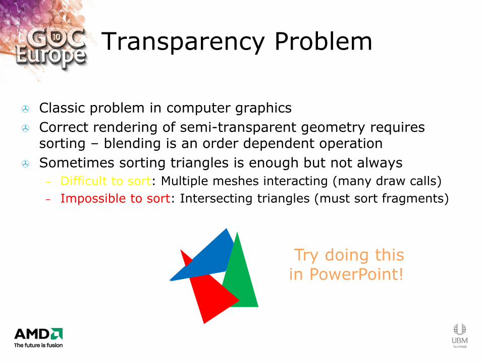
Transparency Problem
Classic problem in computer graphics
Correct rendering of semi-transparent geometry requires sorting – blending is an order dependent operation
Sometimes sorting triangles is enough but not always
– Difficult to sort: Multiple meshes interacting (many draw calls)
– Impossible to sort: Intersecting triangles (must sort fragments)
Try doing this in PowerPoint!
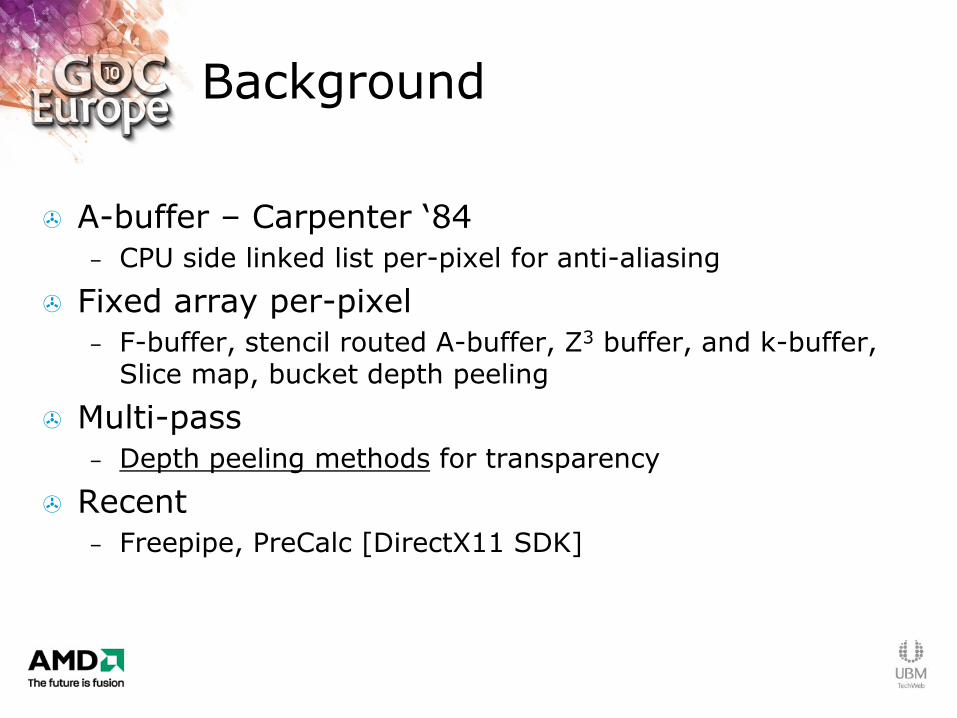
Background
A-buffer – Carpenter „84
– CPU side linked list per-pixel for anti-aliasing
Fixed array per-pixel
– F-buffer, stencil routed A-buffer, Z3 buffer, and k-buffer, Slice map, bucket depth peeling
Multi-pass
– Depth peeling methods for transparency
Recent
– Freepipe, PreCalc [DirectX11 SDK]
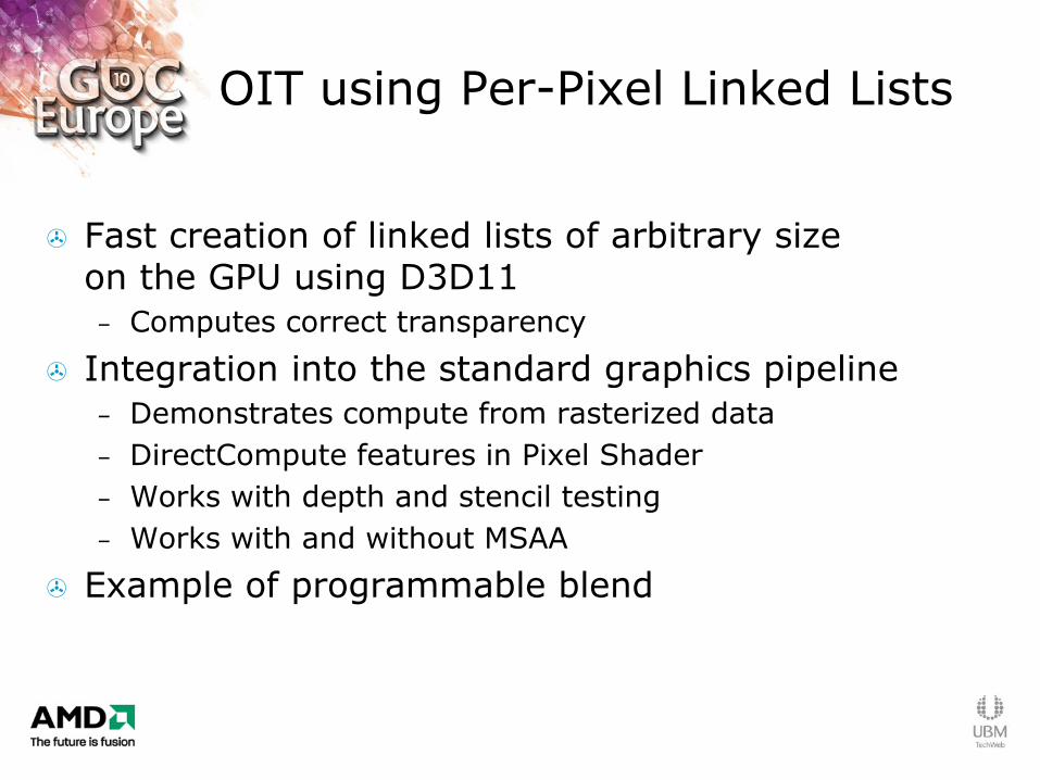
OIT using Per-Pixel Linked Lists
Fast creation of linked lists of arbitrary size on the GPU using D3D11
– Computes correct transparency
Integration into the standard graphics pipeline
– Demonstrates compute from rasterized data
– DirectCompute features in Pixel Shader
– Works with depth and stencil testing
– Works with and without MSAA
Example of programmable blend

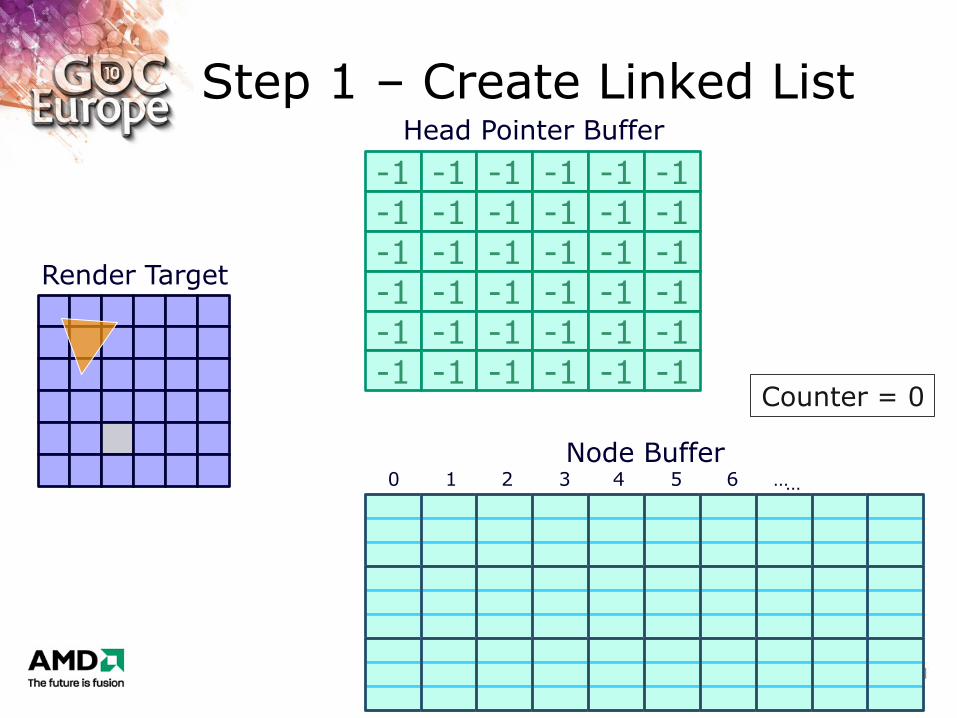
Linked List Construction
Two Buffers
– Head pointer buffer
addresses/offsets
Initialized to end-of-list (EOL) value (e.g., -1)
– Node buffer
arbitrary payload data + “next pointer”
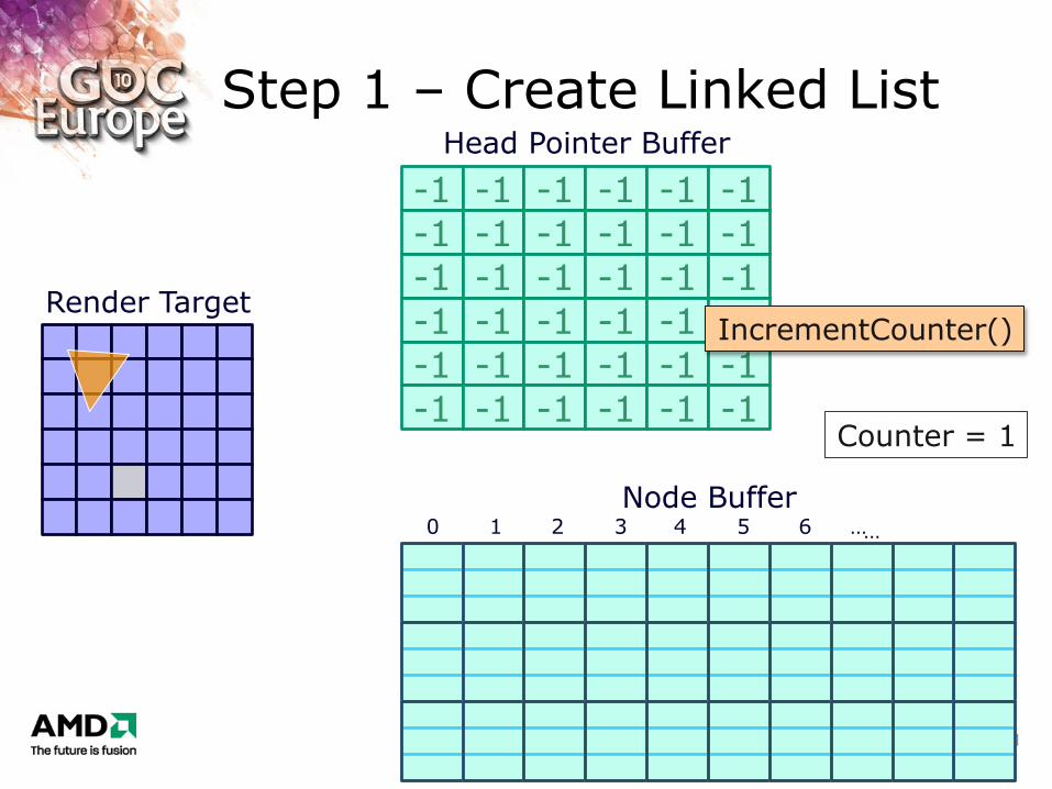
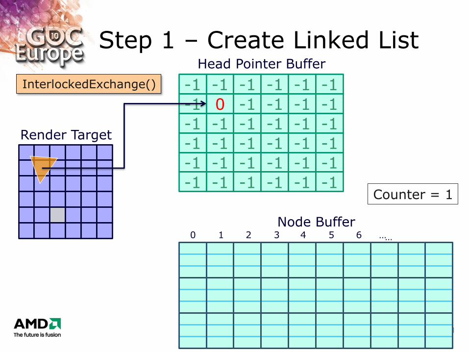
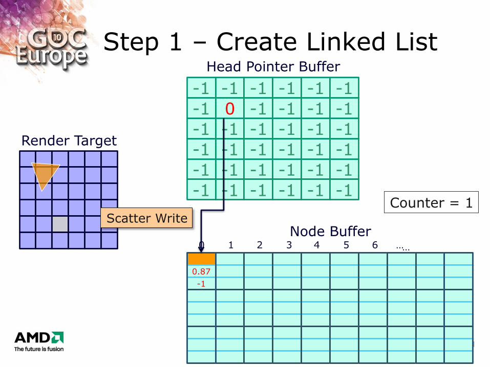
Each shader thread
1. Retrieve and increment global counter value
2. Atomic exchange into head pointer buffer
3. Add new entry into the node buffer at location from step 1

Algorithm Overview
0. Render opaque scene objects
1. Render transparent scene objects
2. Screen quad resolves and composites fragment lists

Step 0 – Render Opaque
Render all opaque geometry normally
Render Target
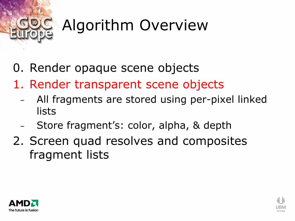
Algorithm Overview
0. Render opaque scene objects
1. Render transparent scene objects
– All fragments are stored using per-pixel linked lists
– Store fragment‟s: color, alpha, & depth
2. Screen quad resolves and composites fragment lists

Setup
Two buffers
– Screen sized head pointer buffer
– Node buffer – large enough to handle all fragments
Render as usual
Disable render target writes
Insert render target data into linked list

Step 1 – Create Linked List
-1 -1 -1 -1 -1 -1
-1 -1 -1 -1 -1 -1
-1 -1 -1 -1 -1 -1
Head Pointer Buffer
-1 -1 -1 -1 -1 -1
-1 -1 -1 -1 -1 -1
-1 -1 -1 -1 -1 -1
Node Buffer 0 1 2 3 4 5 6 …
Counter = 0
Render Target
Step 1 – Create Linked List
-1 -1 -1 -1 -1 -1
-1 -1 -1 -1 -1 -1
-1 -1 -1 -1 -1 -1
-1 -1 -1 -1 -1 -1
-1 -1 -1 -1 -1 -1
-1 -1 -1 -1 -1 -1
…
Render Target
Head Pointer Buffer
Node Buffer 0 1 2 3 4 5 6 …
Counter = 0
Step 1 – Create Linked List
-1 -1 -1 -1 -1 -1
-1 -1 -1 -1 -1 -1
-1 -1 -1 -1 -1 -1
-1 -1 -1 -1 -1 -1
-1 -1 -1 -1 -1 -1
-1 -1 -1 -1 -1 -1
…
Render Target
Head Pointer Buffer
Node Buffer 0 1 2 3 4 5 6 …
Counter = 1
IncrementCounter()
Step 1 – Create Linked List
-1 -1 -1 -1 -1 -1
-1 0 -1 -1 -1 -1
-1 -1 -1 -1 -1 -1
-1 -1 -1 -1 -1 -1
-1 -1 -1 -1 -1 -1
-1 -1 -1 -1 -1 -1
…
Render Target
Head Pointer Buffer
Node Buffer 0 1 2 3 4 5 6 …
Counter = 1
InterlockedExchange()
Step 1 – Create Linked List
-1 -1 -1 -1 -1 -1
-1 0 -1 -1 -1 -1
-1 -1 -1 -1 -1 -1
0.87
-1
-1 -1 -1 -1 -1 -1
-1 -1 -1 -1 -1 -1
-1 -1 -1 -1 -1 -1
…
Render Target
Head Pointer Buffer
Node Buffer 0 1 2 3 4 5 6 …
Counter = 1 Scatter Write
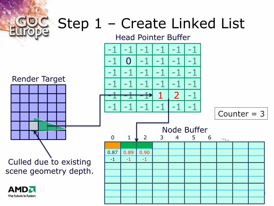
Step 1 – Create Linked List
-1 -1 -1 -1 -1 -1
-1 0 -1 -1 -1 -1
-1 -1 -1 -1 -1 -1
0.87
-1
0.89
-1
0.90
-1
-1 -1 -1 -1 -1 -1
-1 -1 -1 1 2 -1
-1 -1 -1 -1 -1 -1
…
Culled due to existing scene geometry depth.
Render Target
Head Pointer Buffer
Node Buffer 0 1 2 3 4 5 6 …
Counter = 3

Node Buffer 0 1 2 3 4 5 6 …
Step 1 – Create Linked List
-1 -1 -1 -1 -1 -1
-1 3 4 -1 -1 -1
-1 -1 -1 -1 -1 -1
0.87
-1
0.89
-1
0.90
-1
0.65
0
0.65
-1
-1 -1 -1 -1 -1 -1
-1 -1 -1 1 2 -1
-1 -1 -1 -1 -1 -1
…
Render Target
Head Pointer Buffer
Counter = 5
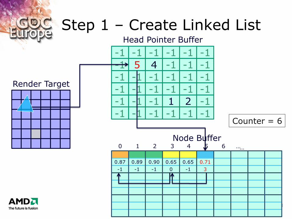
Step 1 – Create Linked List
-1 -1 -1 -1 -1 -1
-1 5 4 -1 -1 -1
-1 -1 -1 -1 -1 -1
0.87
-1
0.89
-1
0.90
-1
0.65
0
0.65
-1
0.71
3
-1 -1 -1 -1 -1 -1
-1 -1 -1 1 2 -1
-1 -1 -1 -1 -1 -1
…
Render Target
Head Pointer Buffer
Node Buffer 0 1 2 3 4 5 6 …
Counter = 6
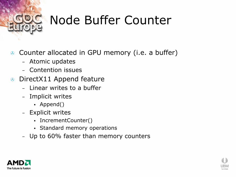
Node Buffer Counter
Counter allocated in GPU memory (i.e. a buffer)
– Atomic updates
– Contention issues
DirectX11 Append feature
– Linear writes to a buffer
– Implicit writes
Append()
– Explicit writes
IncrementCounter()
Standard memory operations
– Up to 60% faster than memory counters
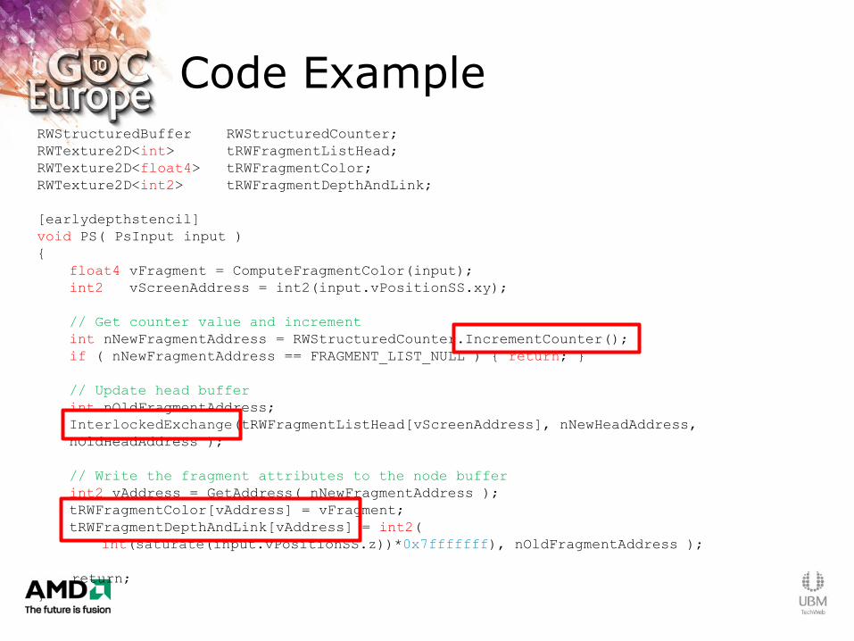
Code Example RWStructuredBuffer RWStructuredCounter;
RWTexture2D<int> tRWFragmentListHead;
RWTexture2D<float4> tRWFragmentColor;
RWTexture2D<int2> tRWFragmentDepthAndLink;
[earlydepthstencil]
void PS( PsInput input )
{
float4 vFragment = ComputeFragmentColor(input);
int2 vScreenAddress = int2(input.vPositionSS.xy);
// Get counter value and increment
int nNewFragmentAddress = RWStructuredCounter.IncrementCounter();
if ( nNewFragmentAddress == FRAGMENT_LIST_NULL ) { return; }
// Update head buffer
int nOldFragmentAddress;
InterlockedExchange(tRWFragmentListHead[vScreenAddress], nNewHeadAddress,
nOldHeadAddress );
// Write the fragment attributes to the node buffer
int2 vAddress = GetAddress( nNewFragmentAddress );
tRWFragmentColor[vAddress] = vFragment;
tRWFragmentDepthAndLink[vAddress] = int2(
int(saturate(input.vPositionSS.z))*0x7fffffff), nOldFragmentAddress );
return;
}
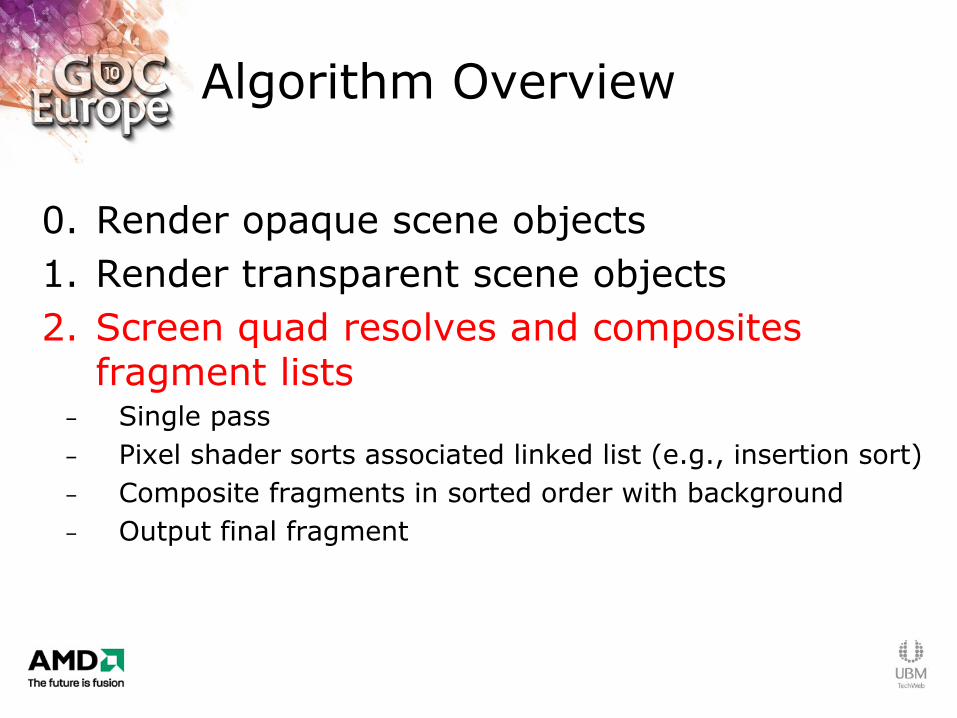
Algorithm Overview
0. Render opaque scene objects
1. Render transparent scene objects
2. Screen quad resolves and composites fragment lists
– Single pass
– Pixel shader sorts associated linked list (e.g., insertion sort)
– Composite fragments in sorted order with background
– Output final fragment
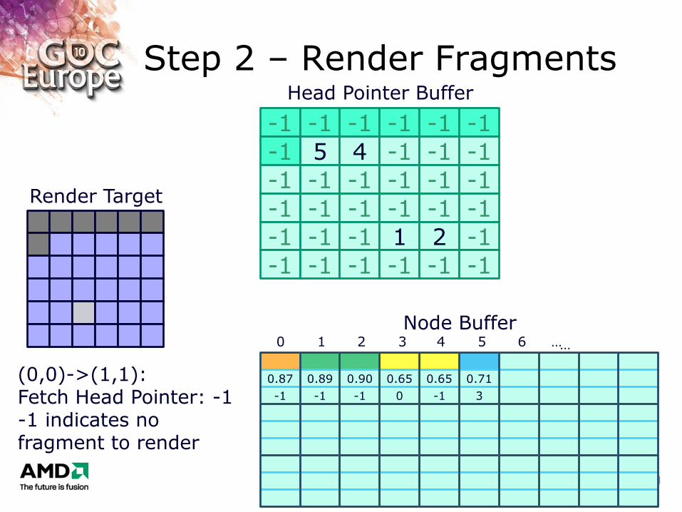
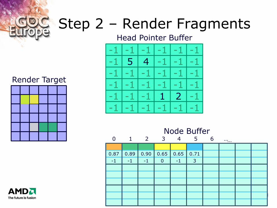
Step 2 – Render Fragments
-1 -1 -1 -1 -1 -1
-1 5 4 -1 -1 -1
-1 -1 -1 -1 -1 -1
0.87
-1
0.89
-1
0.90
-1
0.65
0
0.65
-1
0.71
3
-1 -1 -1 -1 -1 -1
-1 -1 -1 1 2 -1
-1 -1 -1 -1 -1 -1
…
(0,0)->(1,1): Fetch Head Pointer: -1 -1 indicates no fragment to render
Render Target
Head Pointer Buffer
Node Buffer 0 1 2 3 4 5 6 …
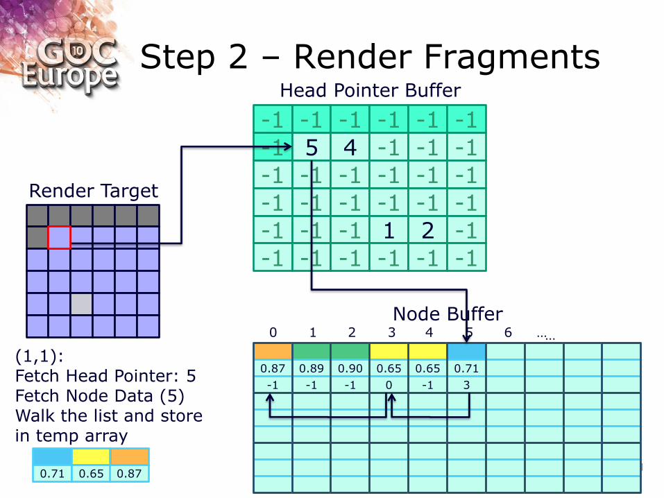
Step 2 – Render Fragments
-1 -1 -1 -1 -1 -1
-1 5 4 -1 -1 -1
-1 -1 -1 -1 -1 -1
0.87
-1
0.89
-1
0.90
-1
0.65
0
0.65
-1
0.71
3
-1 -1 -1 -1 -1 -1
-1 -1 -1 1 2 -1
-1 -1 -1 -1 -1 -1
…
(1,1): Fetch Head Pointer: 5 Fetch Node Data (5) Walk the list and store in temp array
0.71 0.65 0.87
Render Target
Head Pointer Buffer
Node Buffer 0 1 2 3 4 5 6 …
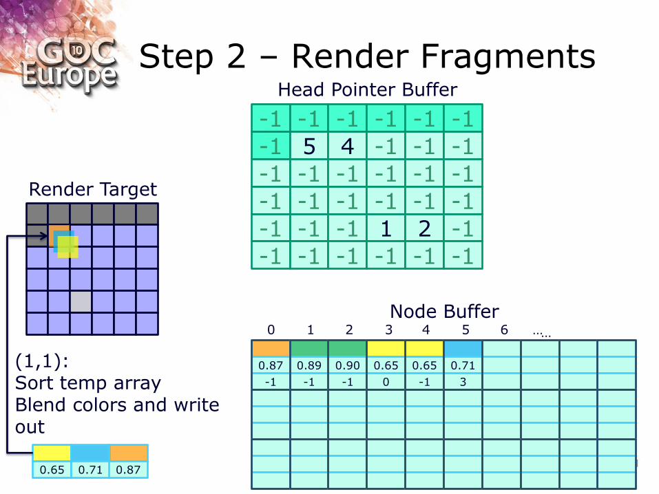
Step 2 – Render Fragments
-1 -1 -1 -1 -1 -1
-1 5 4 -1 -1 -1
-1 -1 -1 -1 -1 -1
0.87
-1
0.89
-1
0.90
-1
0.65
0
0.65
-1
0.71
3
-1 -1 -1 -1 -1 -1
-1 -1 -1 1 2 -1
-1 -1 -1 -1 -1 -1
…
(1,1): Sort temp array Blend colors and write out
0.65 0.71 0.87
Render Target
Head Pointer Buffer
Node Buffer 0 1 2 3 4 5 6 …
Step 2 – Render Fragments
-1 -1 -1 -1 -1 -1
-1 5 4 -1 -1 -1
-1 -1 -1 -1 -1 -1
0.87
-1
0.89
-1
0.90
-1
0.65
0
0.65
-1
0.71
3
-1 -1 -1 -1 -1 -1
-1 -1 -1 1 2 -1
-1 -1 -1 -1 -1 -1
…
Render Target
Head Pointer Buffer
Node Buffer 0 1 2 3 4 5 6 …
Anti-Aliasing
Store coverage information in the linked list
Resolve per-sample
– Execute a shader at each sample location
– Use MSAA hardware
Resolve per-pixel
– Execute a shader at each pixel location
– Average all sample contributions within the shader
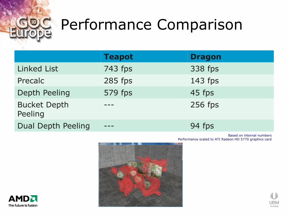
Performance Comparison
Teapot Dragon
Linked List 743 fps 338 fps
Precalc 285 fps 143 fps
Depth Peeling 579 fps 45 fps
Bucket Depth Peeling
--- 256 fps
Dual Depth Peeling --- 94 fps Based on internal numbers
Performance scaled to ATI Radeon HD 5770 graphics card
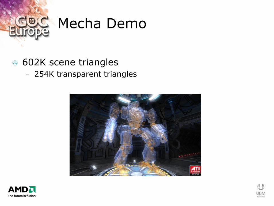
Mecha Demo
602K scene triangles
– 254K transparent triangles
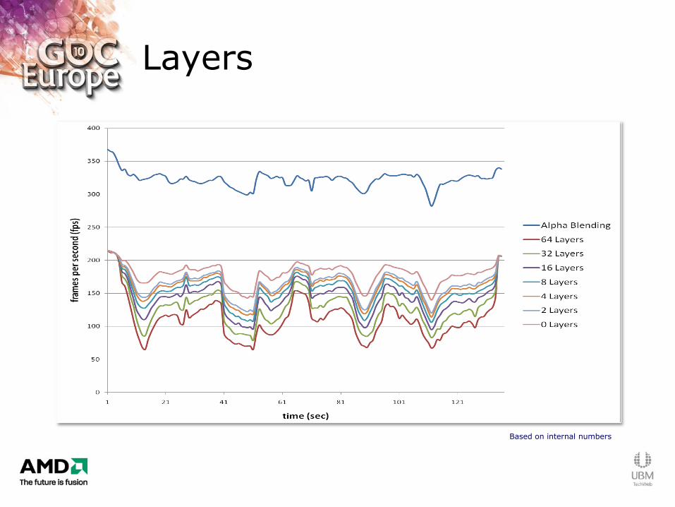
Layers
Based on internal numbers
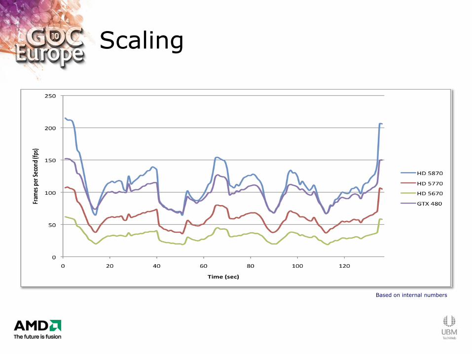
Scaling
Based on internal numbers
Future Work
Memory allocation
Sort on insert
Other linked list applications
– Indirect illumination
– Motion blur
– Shadows
More complex data structures
Bullet Cloth Simulation
DirectCompute for physics
DirectCompute in the Bullet physics SDK
– An introduction to cloth simulation
– Some tips for implementation in DirectCompute
– A demonstration of the current state of development
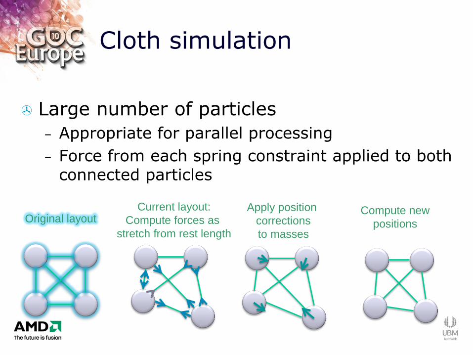
Cloth simulation
Large number of particles
– Appropriate for parallel processing
– Force from each spring constraint applied to both connected particles
Original layout Current layout:
Compute forces as
stretch from rest length
Compute new
positions
Apply position
corrections
to masses
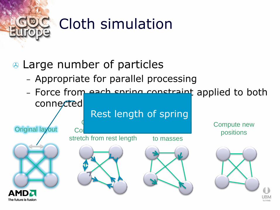
Cloth simulation
Large number of particles
– Appropriate for parallel processing
– Force from each spring constraint applied to both connected particles
Original layout Current layout:
Compute forces as
stretch from rest length
Compute new
positions
Apply position
corrections
to masses
Rest length of spring
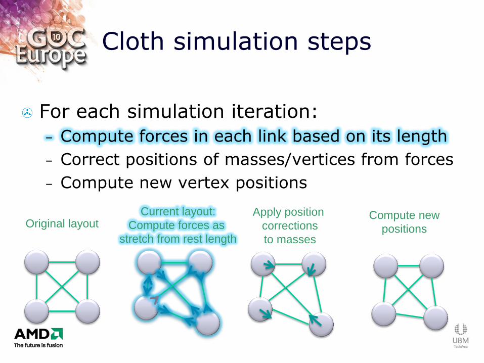
Cloth simulation steps
For each simulation iteration:
– Compute forces in each link based on its length
– Correct positions of masses/vertices from forces
– Compute new vertex positions
Original layout Current layout:
Compute forces as
stretch from rest length
Compute new
positions
Apply position
corrections
to masses
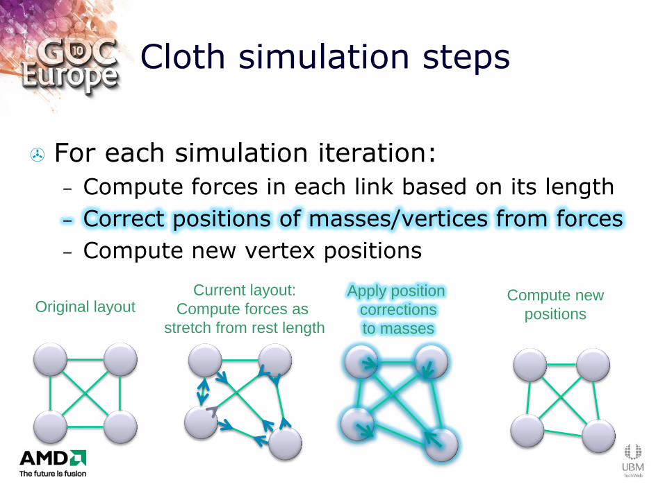
Cloth simulation steps
For each simulation iteration:
– Compute forces in each link based on its length
– Correct positions of masses/vertices from forces
– Compute new vertex positions
Original layout Current layout:
Compute forces as
stretch from rest length
Apply position
corrections
to masses
Compute new
positions
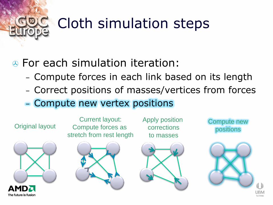
Cloth simulation steps
For each simulation iteration:
– Compute forces in each link based on its length
– Correct positions of masses/vertices from forces
– Compute new vertex positions
Original layout Current layout:
Compute forces as
stretch from rest length
Compute new
positions
Apply position
corrections
to masses

Springs and masses
Two or three main types of springs
– Structural/shearing
– Bending

Springs and masses
Two or three main types of springs
– Structural/shearing
– Bending
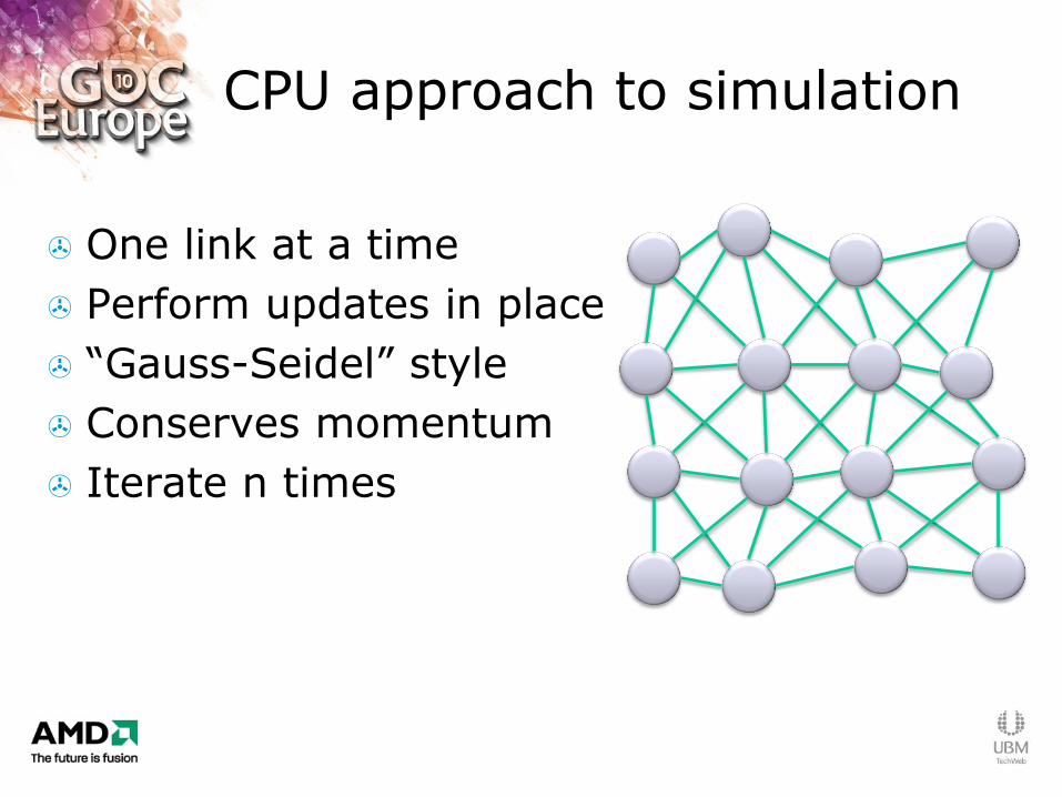
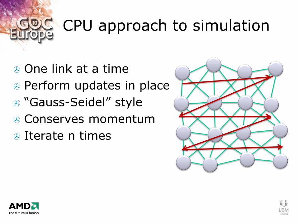
CPU approach to simulation
One link at a time
Perform updates in place
“Gauss-Seidel” style
Conserves momentum
Iterate n times

CPU approach to simulation
One link at a time
Perform updates in place
“Gauss-Seidel” style
Conserves momentum
Iterate n times
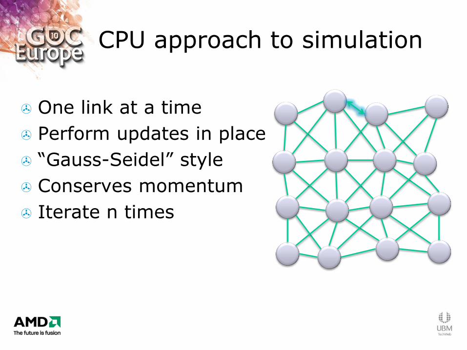
CPU approach to simulation
One link at a time
Perform updates in place
“Gauss-Seidel” style
Conserves momentum
Iterate n times

CPU approach to simulation
One link at a time
Perform updates in place
“Gauss-Seidel” style
Conserves momentum
Iterate n times
CPU approach to simulation
One link at a time
Perform updates in place
“Gauss-Seidel” style
Conserves momentum
Iterate n times
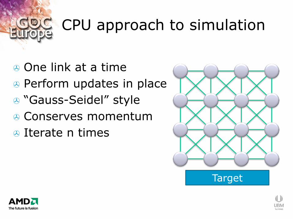
CPU approach to simulation
One link at a time
Perform updates in place
“Gauss-Seidel” style
Conserves momentum
Iterate n times
Target
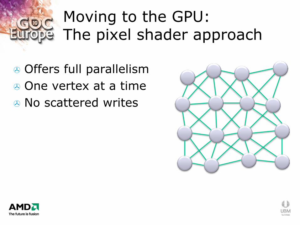
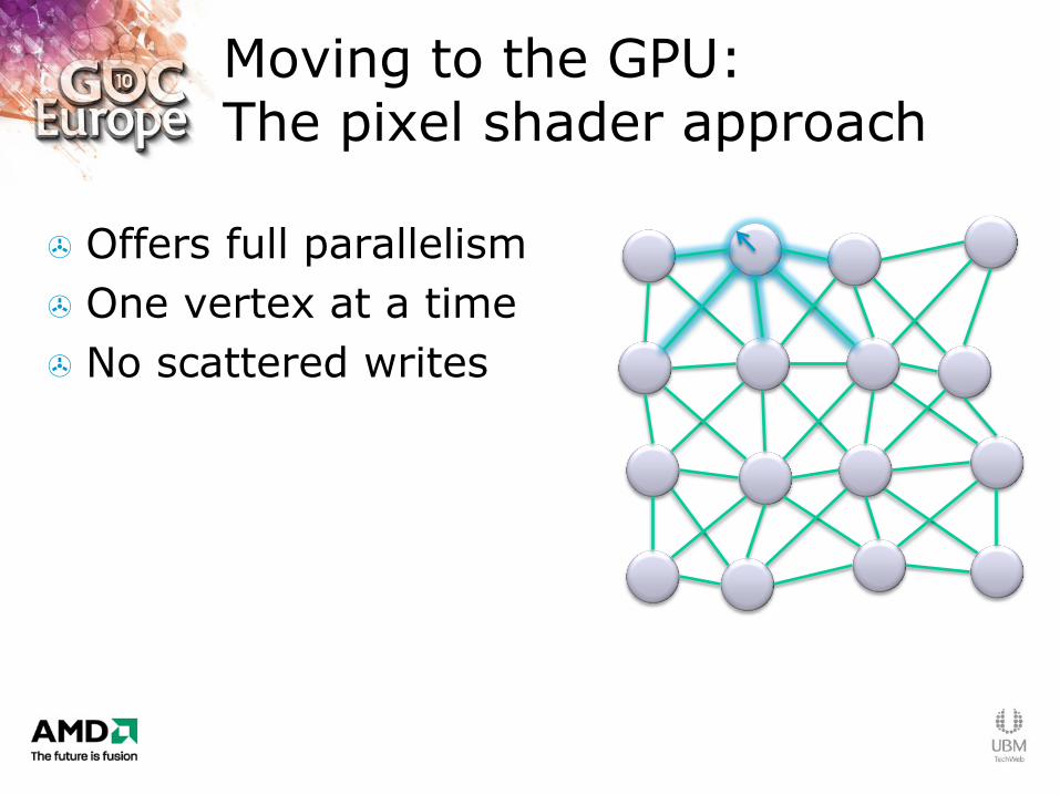
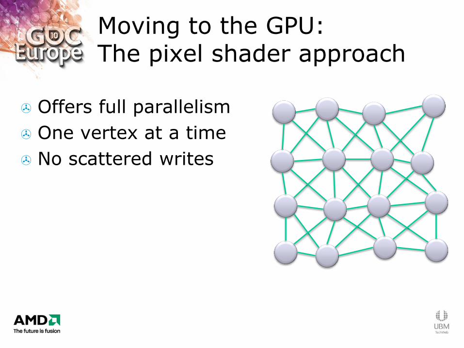
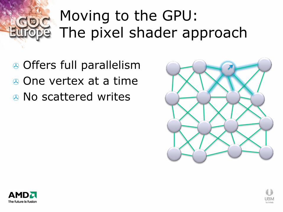
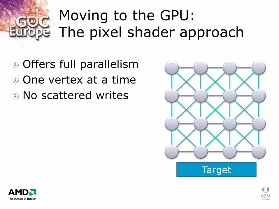
Moving to the GPU: The pixel shader approach
Offers full parallelism
One vertex at a time
No scattered writes
Moving to the GPU: The pixel shader approach
Offers full parallelism
One vertex at a time
No scattered writes

Moving to the GPU: The pixel shader approach
Offers full parallelism
One vertex at a time
No scattered writes
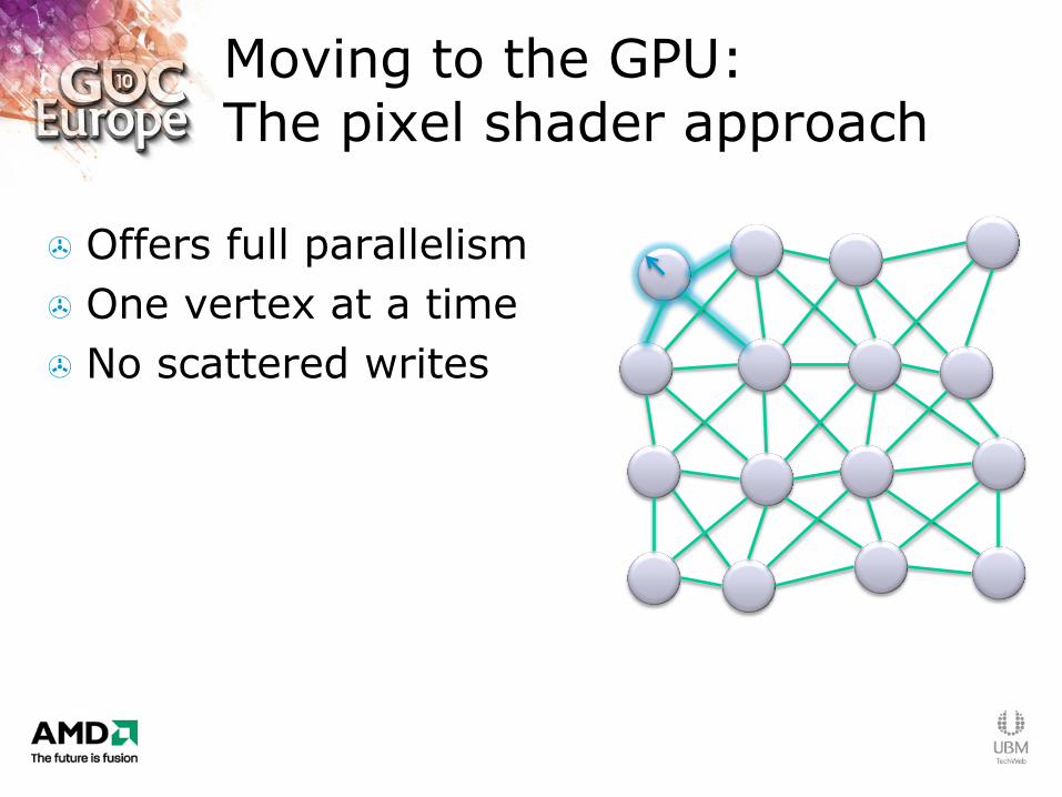
Moving to the GPU: The pixel shader approach
Offers full parallelism
One vertex at a time
No scattered writes
Moving to the GPU: The pixel shader approach
Offers full parallelism
One vertex at a time
No scattered writes
Moving to the GPU: The pixel shader approach
Offers full parallelism
One vertex at a time
No scattered writes
Moving to the GPU: The pixel shader approach
Offers full parallelism
One vertex at a time
No scattered writes
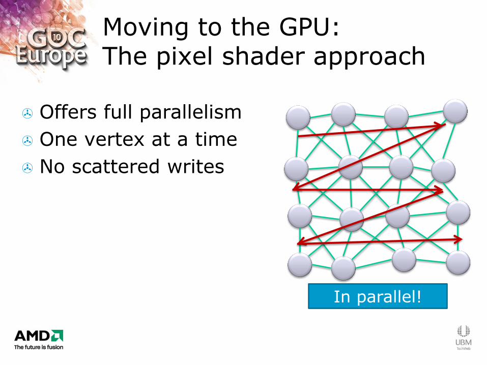
In parallel!
Moving to the GPU: The pixel shader approach
Offers full parallelism
One vertex at a time
No scattered writes
Target
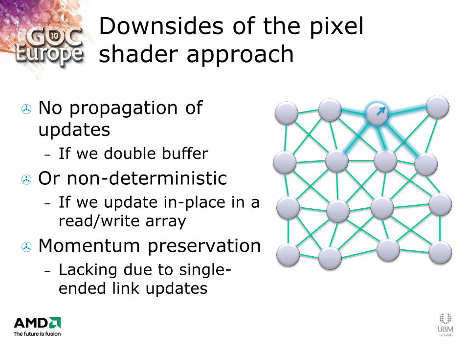
Downsides of the pixel shader approach
No propagation of updates
– If we double buffer
Or non-deterministic
– If we update in-place in a read/write array
Momentum preservation
– Lacking due to single-ended link updates

Can DirectCompute help?
Offers scattered writes as a feature as we saw earlier
The GPU implementation could be more like the CPU
– Solver per-link rather than per-vertex
– Leads to races between links that update the same vertex
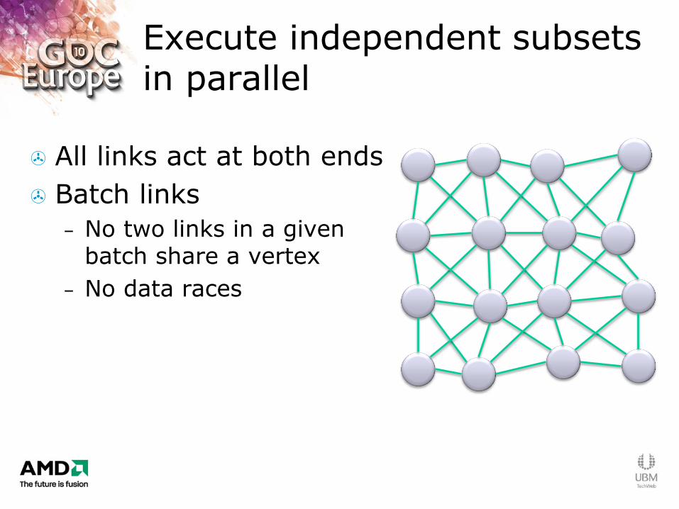
Execute independent subsets in parallel
All links act at both ends
Batch links
– No two links in a given batch share a vertex
– No data races

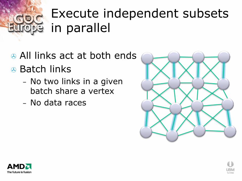
Execute independent subsets in parallel
All links act at both ends
Batch links
– No two links in a given batch share a vertex
– No data races

Execute independent subsets in parallel
All links act at both ends
Batch links
– No two links in a given batch share a vertex
– No data races

Execute independent subsets in parallel
All links act at both ends
Batch links
– No two links in a given batch share a vertex
– No data races
Execute independent subsets in parallel
All links act at both ends
Batch links
– No two links in a given batch share a vertex
– No data races
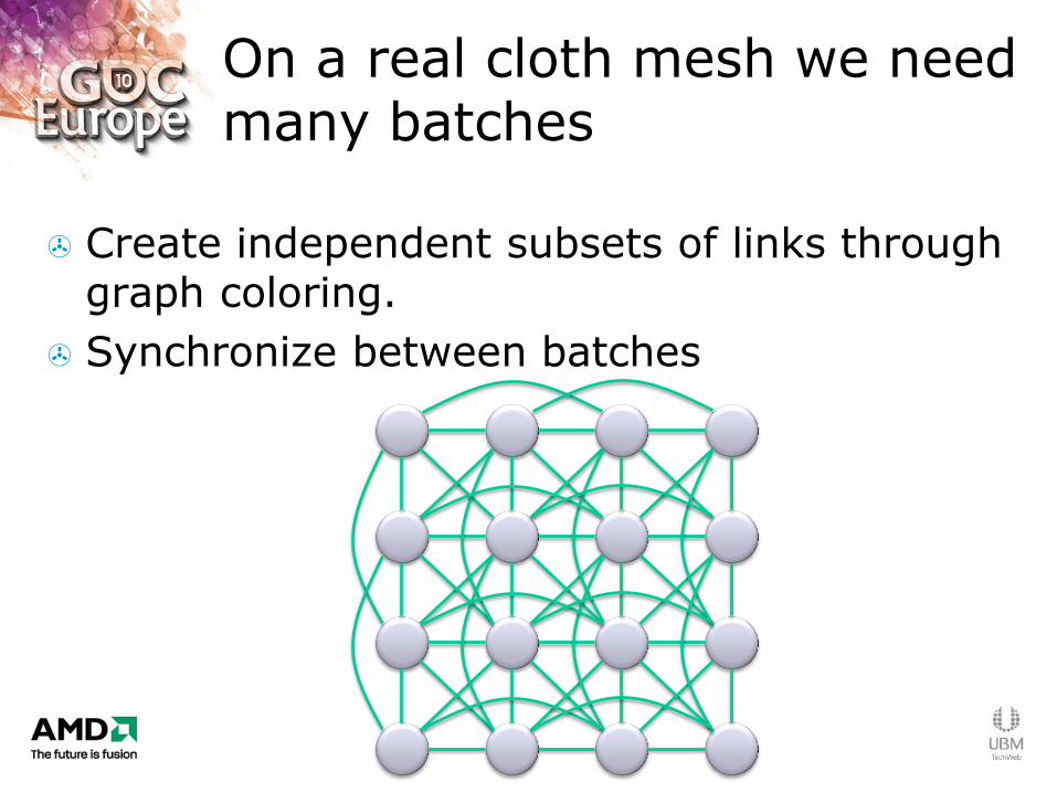
On a real cloth mesh we need many batches
Create independent subsets of links through graph coloring.
Synchronize between batches
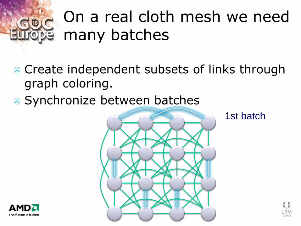
On a real cloth mesh we need many batches
Create independent subsets of links through graph coloring.
Synchronize between batches
1st batch

On a real cloth mesh we need many batches
Create independent subsets of links through graph coloring.
Synchronize between batches
2nd batch
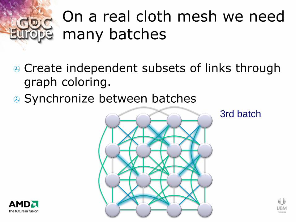
On a real cloth mesh we need many batches
Create independent subsets of links through graph coloring.
Synchronize between batches
3rd batch
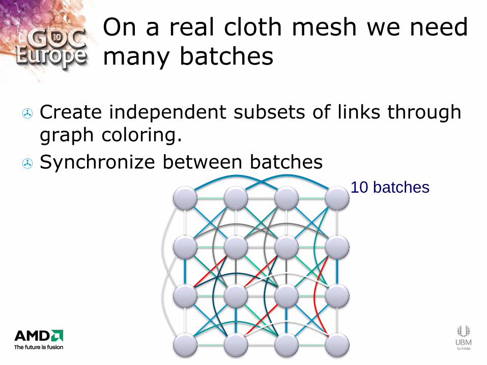
On a real cloth mesh we need many batches
Create independent subsets of links through graph coloring.
Synchronize between batches
10 batches
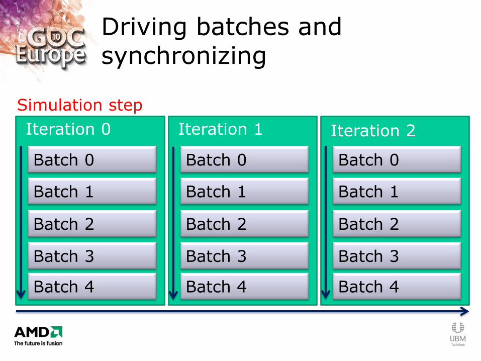
Driving batches and synchronizing
Iteration 0 Iteration 1 Iteration 2
Simulation step
Batch 0
Batch 1
Batch 2
Batch 3
Batch 0
Batch 1
Batch 2
Batch 3
Batch 0
Batch 1
Batch 2
Batch 3
Batch 4 Batch 4 Batch 4
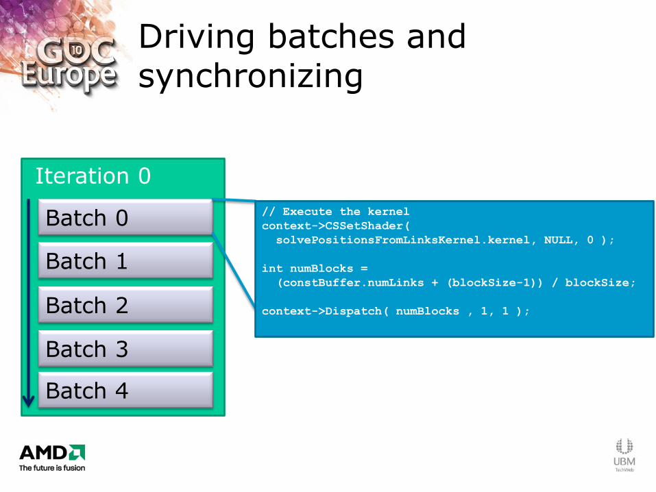
Driving batches and synchronizing
Iteration 0
Batch 0
Batch 1
Batch 2
Batch 3
Batch 4
// Execute the kernel
context->CSSetShader(
solvePositionsFromLinksKernel.kernel, NULL, 0 );
int numBlocks =
(constBuffer.numLinks + (blockSize-1)) / blockSize;
context->Dispatch( numBlocks , 1, 1 );
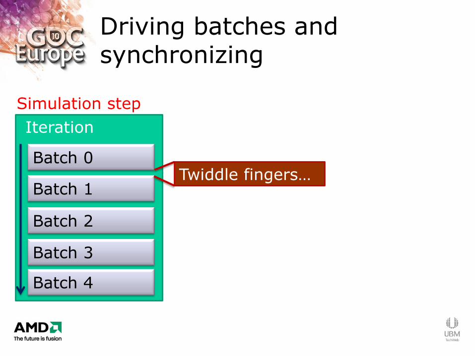
Driving batches and synchronizing
Iteration
Simulation step
Batch 0
Batch 1
Batch 2
Batch 3
Batch 4
Twiddle fingers…
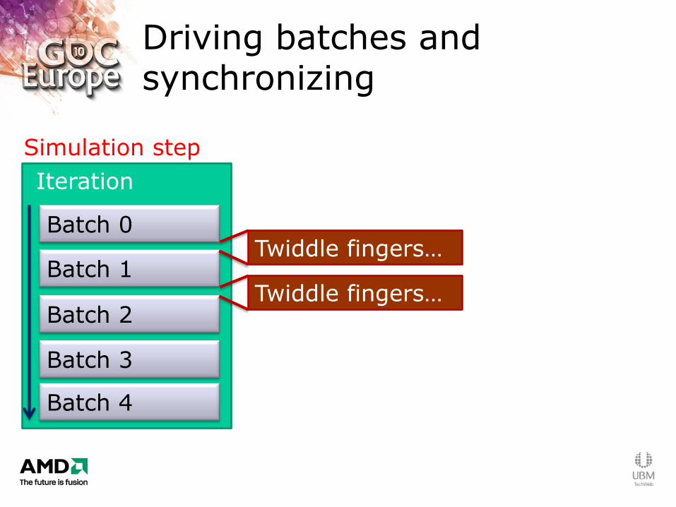
Driving batches and synchronizing
Iteration
Simulation step
Batch 0
Batch 1
Batch 2
Batch 3
Batch 4
Twiddle fingers…
Twiddle fingers…

Driving batches and synchronizing
Iteration
Simulation step
Batch 0
Batch 1
Batch 2
Batch 3
Batch 4
Twiddle fingers…
Twiddle fingers…
Twiddle fingers…
Remember, 10 batches!
Twiddle fingers…
Twiddle fingers…
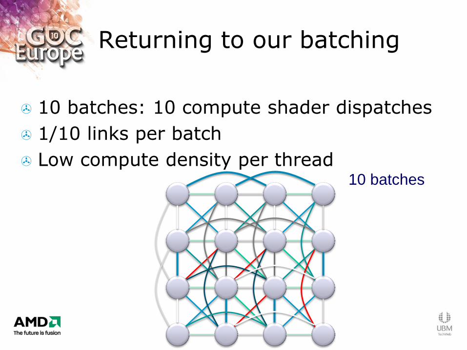
Returning to our batching
10 batches: 10 compute shader dispatches
1/10 links per batch
Low compute density per thread 10 batches
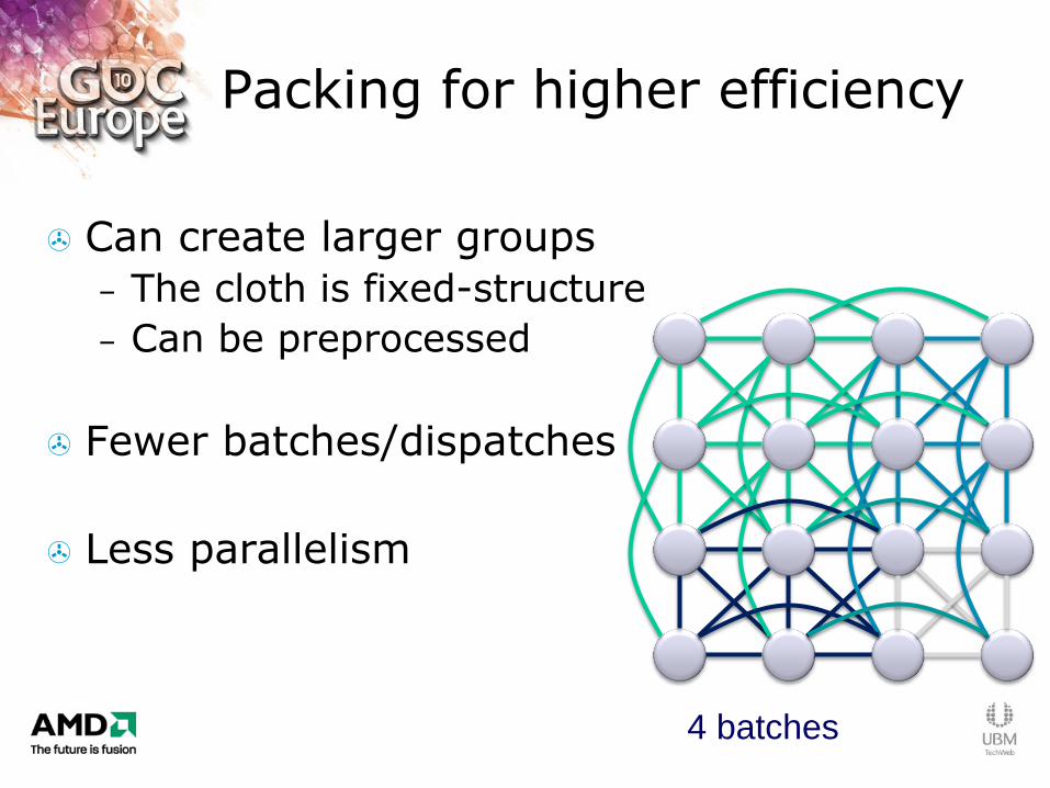
Packing for higher efficiency
Can create larger groups
– The cloth is fixed-structure
– Can be preprocessed
Fewer batches/dispatches
Less parallelism
4 batches
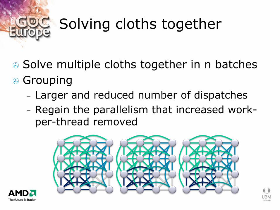
Solving cloths together
Solve multiple cloths together in n batches
Grouping
– Larger and reduced number of dispatches
– Regain the parallelism that increased work-per-thread removed
4 batches

Shared memory
We‟ve made use of scattered writes
The next feature of DirectCompute: shared memory
– Load data at the start of a block
– Compute over multiple links together
– Write data out again
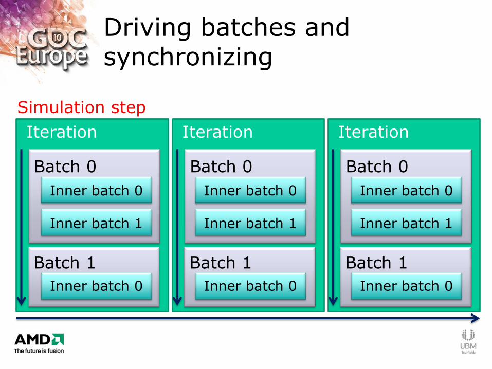
Driving batches and synchronizing
Iteration
Simulation step
Batch 0
Batch 1
Inner batch 0
Inner batch 1
Inner batch 0
Iteration
Batch 0
Batch 1
Iteration
Batch 0
Batch 1
Inner batch 0
Inner batch 1
Inner batch 0
Inner batch 0
Inner batch 1
Inner batch 0
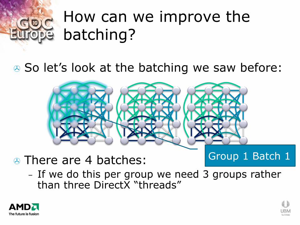
So let‟s look at the batching we saw before:
There are 4 batches: – If we do this per group we need 3 groups rather
than three DirectX “threads”
How can we improve the batching?
Group 1 Batch 1
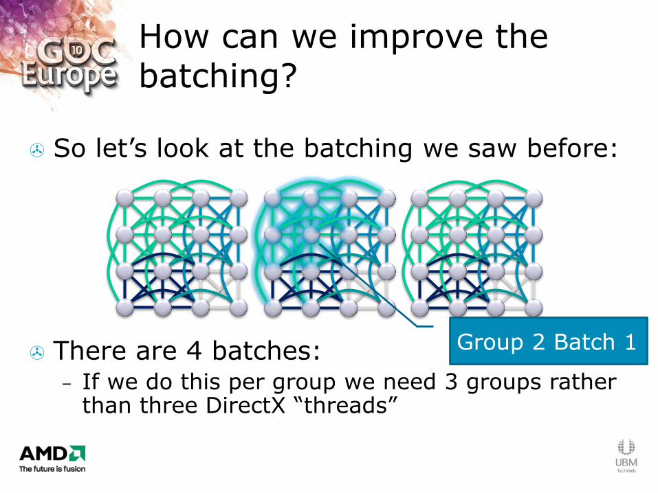
So let‟s look at the batching we saw before:
There are 4 batches: – If we do this per group we need 3 groups rather
than three DirectX “threads”
How can we improve the batching?
Group 2 Batch 1
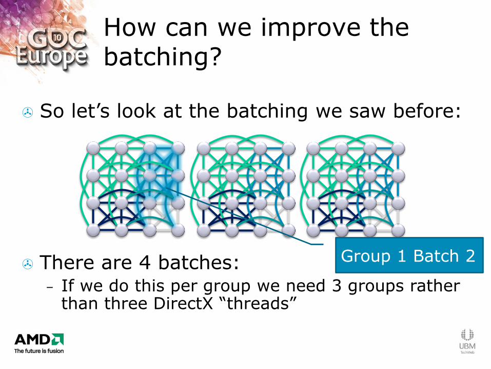
So let‟s look at the batching we saw before:
There are 4 batches: – If we do this per group we need 3 groups rather
than three DirectX “threads”
How can we improve the batching?
Group 1 Batch 2
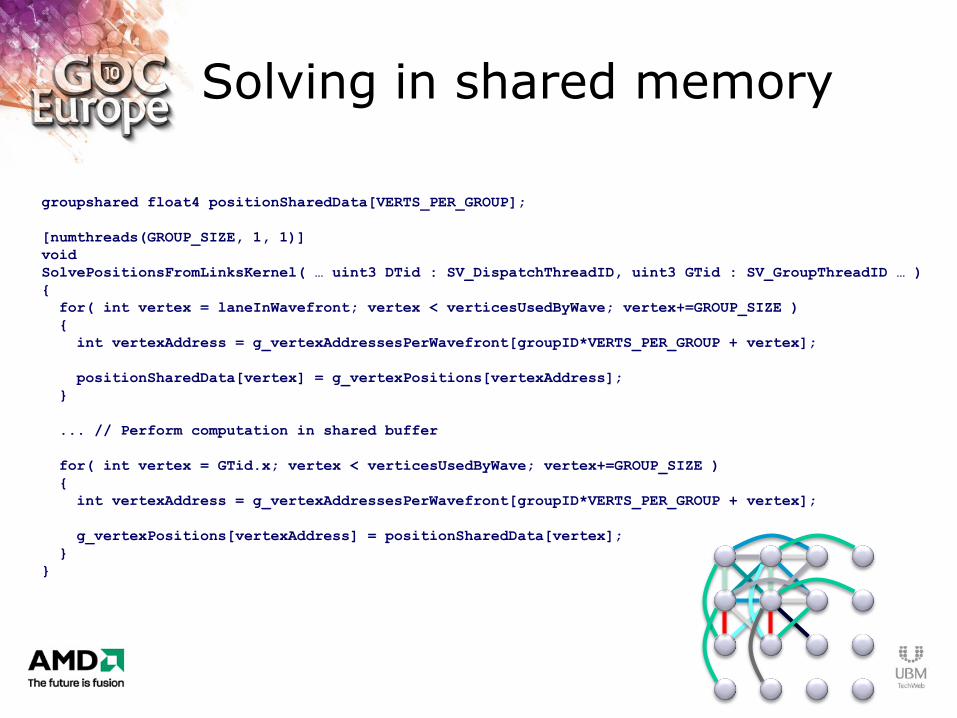
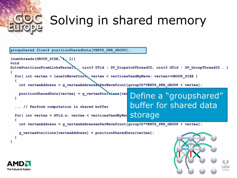
Solving in shared memory
groupshared float4 positionSharedData[VERTS_PER_GROUP];
[numthreads(GROUP_SIZE, 1, 1)]
void
SolvePositionsFromLinksKernel( … uint3 DTid : SV_DispatchThreadID, uint3 GTid : SV_GroupThreadID … )
{
for( int vertex = laneInWavefront; vertex < verticesUsedByWave; vertex+=GROUP_SIZE )
{
int vertexAddress = g_vertexAddressesPerWavefront[groupID*VERTS_PER_GROUP + vertex];
positionSharedData[vertex] = g_vertexPositions[vertexAddress];
}
... // Perform computation in shared buffer
for( int vertex = GTid.x; vertex < verticesUsedByWave; vertex+=GROUP_SIZE )
{
int vertexAddress = g_vertexAddressesPerWavefront[groupID*VERTS_PER_GROUP + vertex];
g_vertexPositions[vertexAddress] = positionSharedData[vertex];
}
}
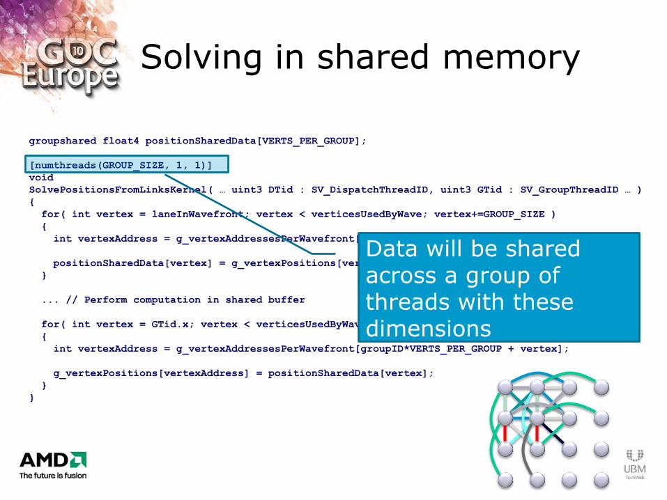
Define a “groupshared” buffer for shared data storage
Solving in shared memory
groupshared float4 positionSharedData[VERTS_PER_GROUP];
[numthreads(GROUP_SIZE, 1, 1)]
void
SolvePositionsFromLinksKernel( … uint3 DTid : SV_DispatchThreadID, uint3 GTid : SV_GroupThreadID … )
{
for( int vertex = laneInWavefront; vertex < verticesUsedByWave; vertex+=GROUP_SIZE )
{
int vertexAddress = g_vertexAddressesPerWavefront[groupID*VERTS_PER_GROUP + vertex];
positionSharedData[vertex] = g_vertexPositions[vertexAddress];
}
... // Perform computation in shared buffer
for( int vertex = GTid.x; vertex < verticesUsedByWave; vertex+=GROUP_SIZE )
{
int vertexAddress = g_vertexAddressesPerWavefront[groupID*VERTS_PER_GROUP + vertex];
g_vertexPositions[vertexAddress] = positionSharedData[vertex];
}
}
Data will be shared across a group of threads with these dimensions
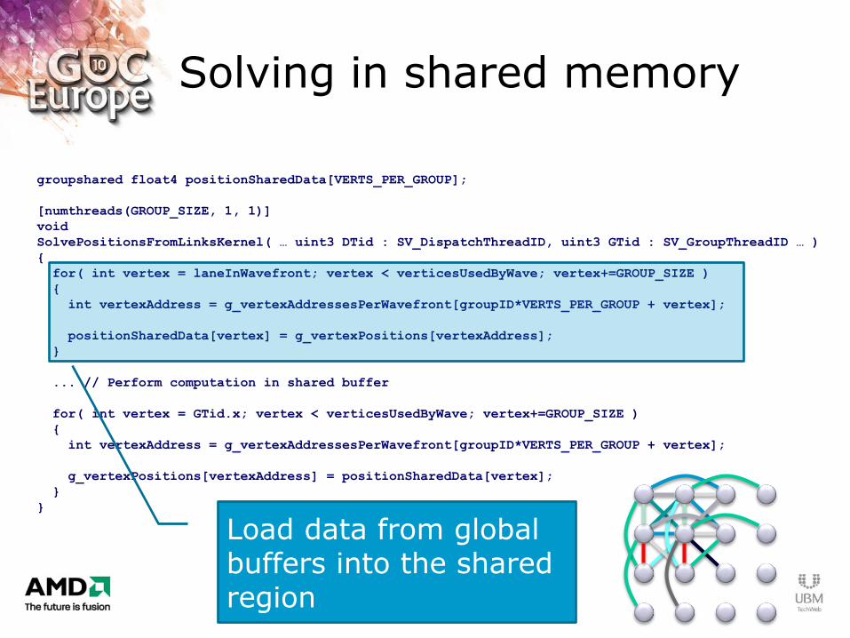
Solving in shared memory
groupshared float4 positionSharedData[VERTS_PER_GROUP];
[numthreads(GROUP_SIZE, 1, 1)]
void
SolvePositionsFromLinksKernel( … uint3 DTid : SV_DispatchThreadID, uint3 GTid : SV_GroupThreadID … )
{
for( int vertex = laneInWavefront; vertex < verticesUsedByWave; vertex+=GROUP_SIZE )
{
int vertexAddress = g_vertexAddressesPerWavefront[groupID*VERTS_PER_GROUP + vertex];
positionSharedData[vertex] = g_vertexPositions[vertexAddress];
}
... // Perform computation in shared buffer
for( int vertex = GTid.x; vertex < verticesUsedByWave; vertex+=GROUP_SIZE )
{
int vertexAddress = g_vertexAddressesPerWavefront[groupID*VERTS_PER_GROUP + vertex];
g_vertexPositions[vertexAddress] = positionSharedData[vertex];
}
}
Load data from global buffers into the shared region
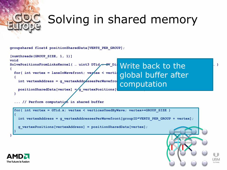
Solving in shared memory
groupshared float4 positionSharedData[VERTS_PER_GROUP];
[numthreads(GROUP_SIZE, 1, 1)]
void
SolvePositionsFromLinksKernel( … uint3 DTid : SV_DispatchThreadID, uint3 GTid : SV_GroupThreadID … )
{
for( int vertex = laneInWavefront; vertex < verticesUsedByWave; vertex+=GROUP_SIZE )
{
int vertexAddress = g_vertexAddressesPerWavefront[groupID*VERTS_PER_GROUP + vertex];
positionSharedData[vertex] = g_vertexPositions[vertexAddress];
}
... // Perform computation in shared buffer
for( int vertex = GTid.x; vertex < verticesUsedByWave; vertex+=GROUP_SIZE )
{
int vertexAddress = g_vertexAddressesPerWavefront[groupID*VERTS_PER_GROUP + vertex];
g_vertexPositions[vertexAddress] = positionSharedData[vertex];
}
}
Write back to the global buffer after computation
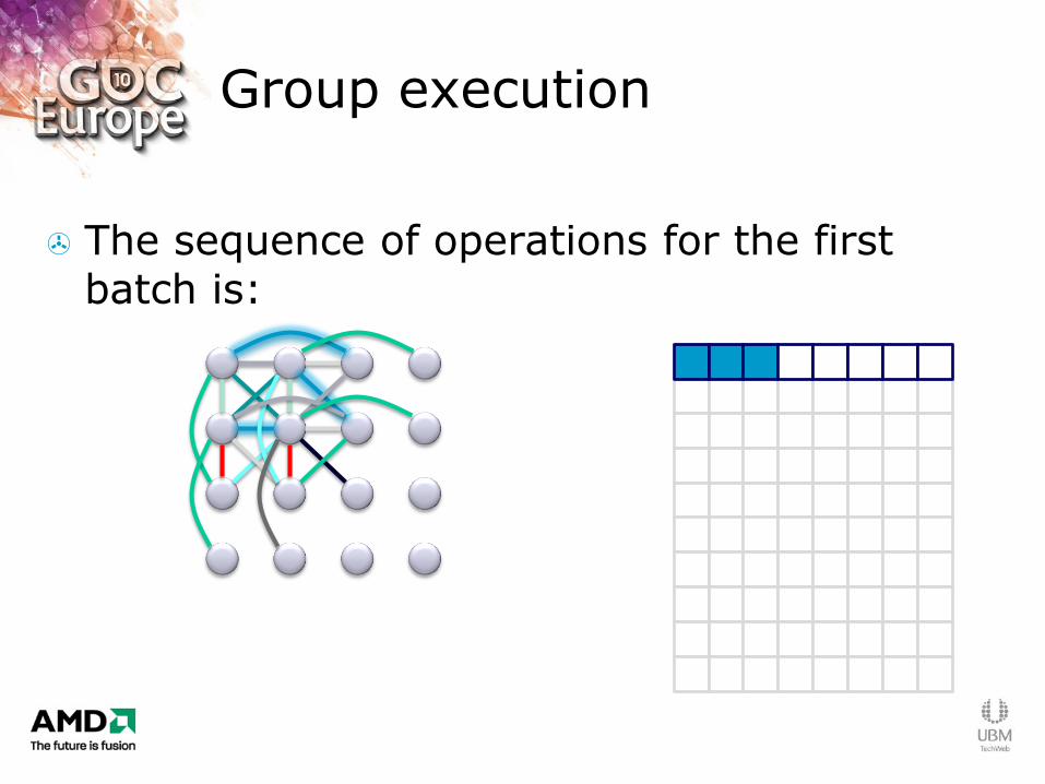
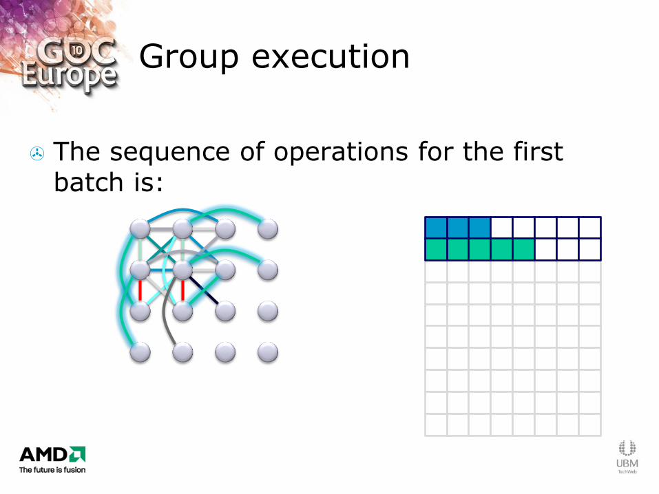
Group execution
The sequence of operations for the first batch is:
Group execution
The sequence of operations for the first batch is:
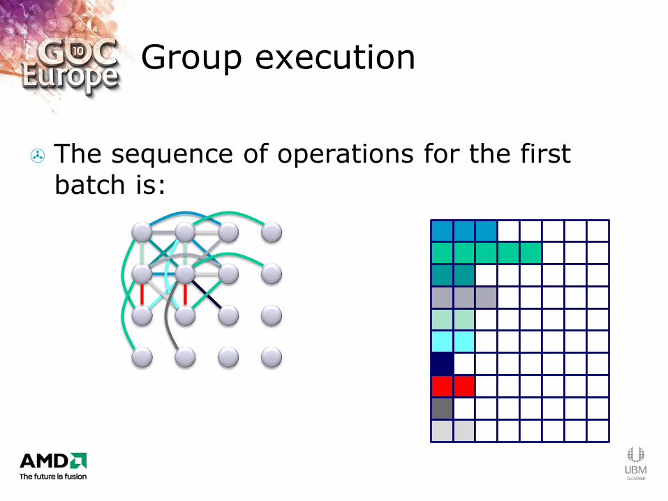
Group execution
The sequence of operations for the first batch is:
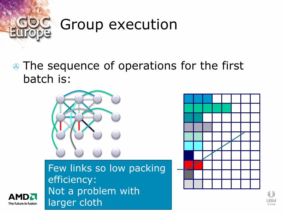
Group execution
The sequence of operations for the first batch is:
Few links so low packing efficiency: Not a problem with larger cloth
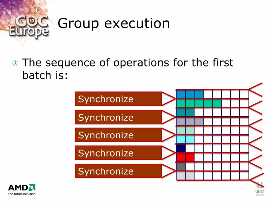
Group execution
The sequence of operations for the first batch is:
Synchronize
Synchronize
Synchronize
Synchronize
Synchronize
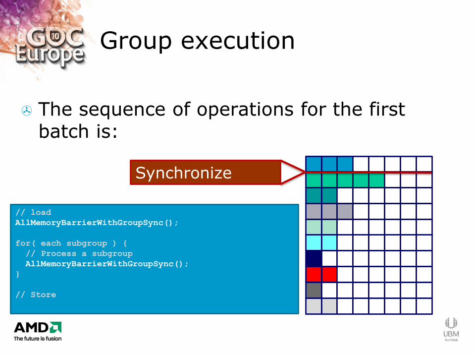
Group execution
The sequence of operations for the first batch is:
// load
AllMemoryBarrierWithGroupSync();
for( each subgroup ) {
// Process a subgroup
AllMemoryBarrierWithGroupSync();
}
// Store
Synchronize

Why is this an improvement?
So we still need 10*4 batches. What have we gained?
– The batches within a group chunk are in-shader loops
– Only 4 shader dispatches, each with significant overhead
The barriers will still hit performance
– We are no longer dispatch bound, but we are likely to be on-chip synchronization bound
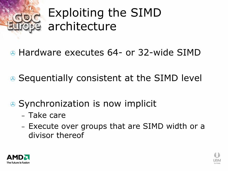
Exploiting the SIMD architecture
Hardware executes 64- or 32-wide SIMD
Sequentially consistent at the SIMD level
Synchronization is now implicit
– Take care
– Execute over groups that are SIMD width or a divisor thereof
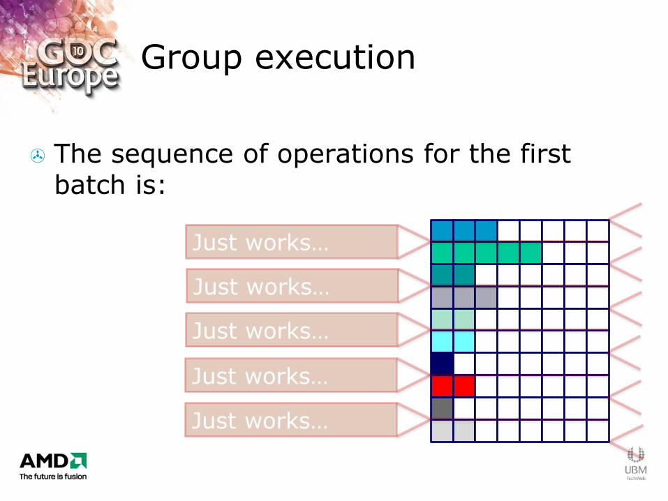
Group execution
The sequence of operations for the first batch is:
Just works…
Just works…
Just works…
Just works…
Just works…
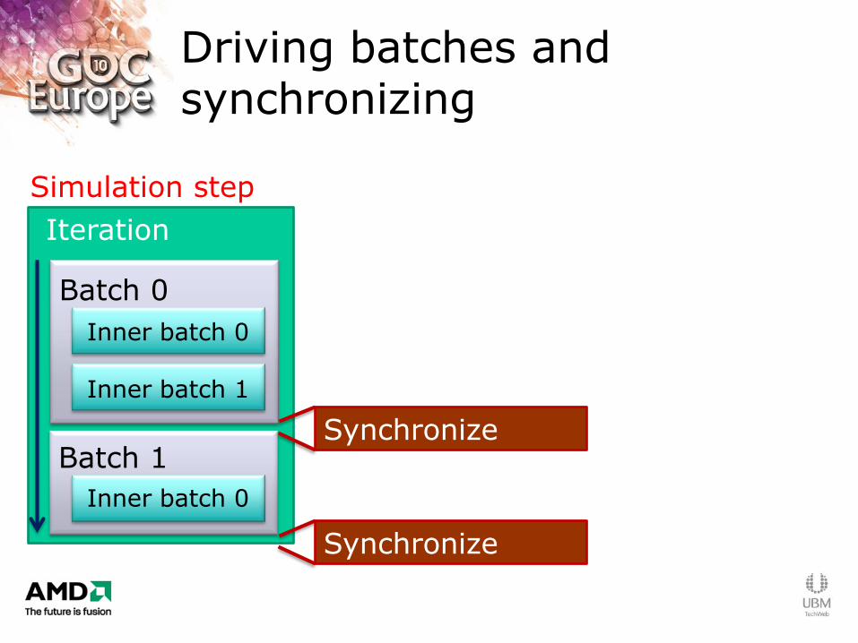
Driving batches and synchronizing
Iteration
Simulation step
Batch 0
Batch 1
Inner batch 0
Inner batch 1
Inner batch 0
Synchronize
Synchronize

Performance gains
For 90,000 links:
– No solver running in 2.98 ms/frame
– Fully batched link solver in 3.84 ms/frame
– SIMD batched solver 3.22 ms/frame
– CPU solver 16.24 ms/frame
3.5x improvement in solver alone
(67x improvement CPU solver)
Based on internal numbers
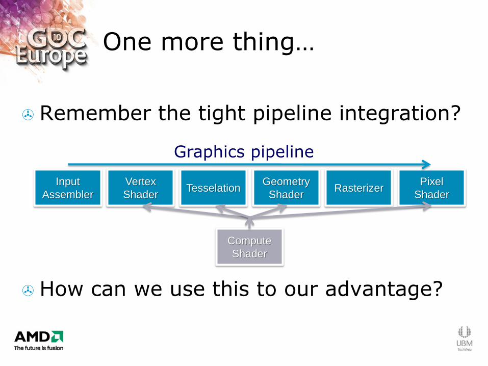
One more thing…
Remember the tight pipeline integration?
How can we use this to our advantage?
Input
Assembler
Vertex
Shader Tesselation
Geometry
Shader Rasterizer
Pixel
Shader
Compute
Shader
Graphics pipeline
Efficiently output vertex data
Cloth simulation updates vertex positions
– Generated on the GPU
– Need to be used on the GPU for rendering
– Why not keep them there?
Large amount of data to update
– Many vertices in fine simulation meshes
– Normals and other information present
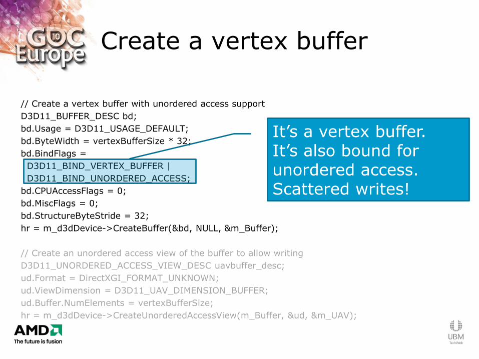
Create a vertex buffer
// Create a vertex buffer with unordered access support
D3D11_BUFFER_DESC bd;
bd.Usage = D3D11_USAGE_DEFAULT;
bd.ByteWidth = vertexBufferSize * 32;
bd.BindFlags =
D3D11_BIND_VERTEX_BUFFER |
D3D11_BIND_UNORDERED_ACCESS;
bd.CPUAccessFlags = 0;
bd.MiscFlags = 0;
bd.StructureByteStride = 32;
hr = m_d3dDevice->CreateBuffer(&bd, NULL, &m_Buffer);
// Create an unordered access view of the buffer to allow writing
D3D11_UNORDERED_ACCESS_VIEW_DESC uavbuffer_desc;
ud.Format = DirectXGI_FORMAT_UNKNOWN;
ud.ViewDimension = D3D11_UAV_DIMENSION_BUFFER;
ud.Buffer.NumElements = vertexBufferSize;
hr = m_d3dDevice->CreateUnorderedAccessView(m_Buffer, &ud, &m_UAV);
It‟s a vertex buffer. It‟s also bound for unordered access. Scattered writes!
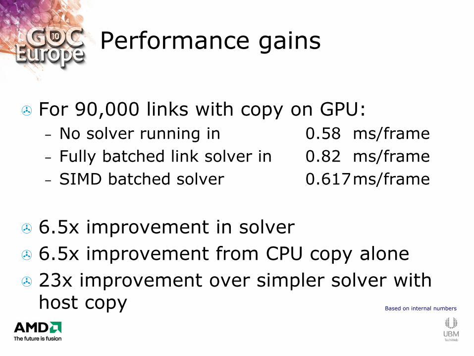
Performance gains
For 90,000 links with copy on GPU:
– No solver running in 0.58 ms/frame
– Fully batched link solver in 0.82 ms/frame
– SIMD batched solver 0.617 ms/frame
6.5x improvement in solver
6.5x improvement from CPU copy alone
23x improvement over simpler solver with host copy Based on internal numbers

Thanks
Justin Hensley
Holger Grün
Nicholas Thibieroz
Erwin Coumans
References
Yang J., Hensley J., Grün H., Thibieroz N.: Real-Time Concurrent Linked List Construction on the GPU. In Rendering Techniques 2010: Eurographics Symposium on Rendering (2010), vol. 29, Eurographics.
Grün H., Thibieroz N.: OIT and Indirect Illumination using DirectX11 Linked Lists. In Proceedings of Game Developers Conference 2010 (Mar. 2010). http://developer.amd.com/gpu_assets/OIT%20and%20Indirect%20Illumination%20using%20DirectX11%20Linked%20Lists_forweb.ppsx
http://developer.amd.com/samples/demos/pages/ATIRadeonHD5800SeriesRealTimeDemos.aspx
http://bulletphysics.org
Trademark Attribution
AMD, the AMD Arrow logo, ATI, the ATI logo, Radeon and combinations thereof are trademarks of Advanced Micro Devices, Inc. in the United States and/or other jurisdictions. Microsoft, Windows, Windows Vista, Windows 7 and DirectX are registered trademarks of Microsoft Corporation in the U.S. and/or other juristictions. Other names used in this presentation are for identification purposes only and may be trademarks of their respective owners.
©2010 Advanced Micro Devices, Inc. All rights reserved.