Pressure Measurements using an Airborne Differential

Absorption Lidar. Part I" Analysis of the systematic

error sources

Cyrille N. Flamant 1

University of Maryland, College Park, Maryland

Geary K. Schwemmer 2, C. Laurence Korb

Laboratory' for Atmospheres

NASA Goddard Space Flight Center, Greenbelt, Maryland

Keith D. Evans

Joint Center for Earth Systems Technology

University of Maryland Baltimore County, Baltimore, Maryland

Stephen P. Palm

Science Systems and Applications Inc., Seabrook, Maryland

1Current affiliation: Service d'A_ronomie du CNRS, Universit_ Pierre et Marie Curie,

Paris, France

-'Corresponding author address: .NASA Goddard Space flight Center, Code 912, Green-

belt, Maryland 20771.

https://ntrs.nasa.gov/search.jsp?R=19990025236 2019-02-02T02:28:42+00:00Z

Abstract

Remote airborne measurements of the vertical and horizontal struc-

ture of the atmospheric pressure field in the lower troposphere are

made with an oxygen differential absorption lidar (DIAL)..4. detailed

analysis of this measurement technique is provided which includes cor-

rections for imprecise knowledge of the detector background level, the

oxygen absorption line parameters, and variations in the laser output

energy. In addition, we analyze other possible sources of systematic

errors including spectral effects related to aerosol and molecular scat-

tering, interference by rotational Raman scattering and interference

by isotopic oxygen lines.

Key words: Differential Absorption Lidar, Pressure, Raman, Oxygen Iso-

topic Line

1. Introduction

Measurement of atmospheric pressure field is desirable for improving weather

forecasting in the mid-latitudes, since the location of high and low pressure

areas determine the weather patterns. Furthermore, the storm regime and

fronts are an important weather phenomena and produce significant air-sea

interaction and planetary boundary layer (PBL) fluxes (Brown and Levy,

19S6). The frontal location and mesoscale dynamics of midlatitude storm

systems are difficult to define with conventional analysis, partly because of

mesoscale variability in both the atmosphere and ocean, which is generally

observed to be very large. Bond and Feagle (1985) suggested that atmo-

spheric dynamics take place on scales that are not practically resolvable with

conventional methods.

Better determination of the winds, stress, sea surface temperature and

frontal location are essential for progress in these mesoscale modeling efforts.

Nuss and Brown (1987) have shown that the primary limitation on the ac-

curacy of the models was the sparsity of the input data. Remote sensing

instruments are likely candidates to supplement the existing observational

network with additional data at a density usable for routine synoptic-scale

analyses.

Experiments incorporating scatterometer wind data in the European Cen-

ter for Medium Range Weather Forcasts forecasting model have shown great

potential for improved forcasting skills in the Southern Hemisphere (Ander-

son et aI., 1987). In order to relate this data to conventional analysis a good

representation of the stress, roughness, stratification, PBL winds and upper

level flow with corresponding pressure fields must be established. Levy and

Brown (1991) tested the existing method of integrating the Seasat-A Satel-

lite Scatterometer (SASS) wind data to provide surface-pressure analyses in

the Southern Hemisphere and compared the results with standard opera-

tional analysis products. SASS-derived winds were input in a PBL model to

construct surface-pressure fields (Brown and Levy, 1986). Their fields were

found in good agreement (within 1-2 hPa) with the National Meteorological

Center analyses in the Northern Hemisphere. In addition, the comparisons

also revealed some sub-synoptic-scale variability that was not shown in the

National Meteorological Center analyses.

Differential absorption lidar (DIAL) providesthe only direct remotemea-

surementof atmosphericpressurewith high spatial resolution and precision.

The theory of using the DIAL techniqueto measureatmosphericpressurehas

been describedby Korb and Weng (198:3).The lidar system usedin these

measurementshas been describedby Schwemmeret al. (1957), and earlier

measurements from ground and aircraft reported have been by Korb et al.

(1989) and Start et al. (1992). We describe here the detailed analysis of the

various potential systematic error sources to DIAL pressure measurements.

In a companion paper (hereon referred to as Part II) we describe the devel-

opment and application of the correction techniques as applied to a series of

measurements made from an aircraft off the east coast of the United States

during June and July of 1989.

High spectral resolution DIAL is a particularly complicated technique,

both from an instrumental perspective and from an analysis perspective. The

pressure measurement is usually more forgiving than DIAL measurements of

temperature and specific humidity that operate with a laser centered on

narrow absorption lines, This is because the pressure measurement is made

in the much broader, flatter absorption trough between lines. There are still,

however, many opportunities for systematic errors to enter the data. Thus,

we have attempted to evaluate as many sources of error as possible within

this study before applying corrections to the data collected from the flight

experiments.

The instrument typically must include one or more tunable high spectral

resolution lasers, preferably single frequency with very high spectral purity,

i.e. very low broadband emission or out of band frequencies. One laser, the

on-line laser, is tuned to the oxygenspectral absorption feature of interest,

while the second,off-line laser is tuned to a nearby unabsorbed frequency.

The lasersare fired nearly simultaneouslyand the resulting two return sig-

nals must be accurately superimposedin order to be able to ratio them to

determine the atmospheric transmissionas a function of rangeor altitude.

Since the data is digitally sampledat discrete time intervals, the time (or

range)of any givensamplein onelaser return must accurately correspondto

the time (or range)of the correspondingsamplein the other laserreturn sig-

nal. Backscatterby moleculesis double doppler broadened,and hasa width

equal to twice the doppler width of the absorption lines. On the other hand,

the backscatterfrom aerosolsis very narrow and is spectrally identical to

the outgoing laser emission (ignoring any doppler shift causedby the bulk

motion of aerosols,which is negligiblecomparedto the width of the oxygen

absorption lines). Effects due to this complexity have been discussed by Korb

and Weng (1982) for temperature measurements, and by Ansmann (1985) as

well as Ansmann and Bosenberg (1987) with respect to water vapor measure-

ments. Accordingly, a measurement of the aerosol to molecular backscatter

ratio must be derived from the off-line (or reference) return signal. In addi-

tion, oxygen and nitrogen rotational Raman scattering contribute a signal,

which is over 3% of the molecular backscatter, if not filtered out, as is the

case with the measurements discussed in Part II. Since rotational Raman

backscatter is spectrally spread out over tens of wavenumbers from the laser

frequency, it is only weakly absorbed on the return path to the lidar receiver,

and can dominate the on-line return signal from large distances. These and

other systematic effects are carefully evaluated in the following analysis.

5

In Section2 we describe the data acquisition equipment. Section 3 de-

scribes instrumental effects and Section 4 atmospheric effects. The error

sourcesare discussedfrom the perspectiveof having observedanomalously

high pressureretrievals in regionsof high aerosolbackscatter.

2. Description of the data acquisition

Nighttime measurementsweremade with a dual alexandrite laser lidar sys-

tem mountedin a nadir pointing position in the NASA Electra aircraft. The

laser beamshad a divergenceof about 2.5 mrad. Pressurewasderived from

measurementsof the atmospherictransmission in the trough regionbetween

the RR13and RQ14lines of the oxygenA-band, at a vacuum wavenumberof

13,152.3Scm -1, or 760.32 nm wavelength in surface pressure air. The off-line

or reference laser wavelength was 757.49 nm. The receiver contained a red

pass filter, blocking wavelengths below 720 nm. The detector, a multialkali

photomultiplier tube (PMT) had a gain of approximately 2x104 and was

followed by a transimpedence amplifier with a gain of 3,000 volts/amp. The

PMT was gated on a few microseconds after the laser pulse, and kept on for

about 100/,s. The amplifier output signal was fed through a 2 MHz single

pole low pass filter to a transient recorder with a 12 bit A/D converter sam-

pling at a 5 MHz rate, which corresponds to 30 m altitude intervals. Five

hundred samples were stored in the transient recorder memory, correspond-

ing to the time the PMT was gated on to the time it was gated off. The

digitizer clock was rephased with each laser pulse to a measured accuracy

of better than 1 ns. The on-line laser was fired first, then 300 #s latter the

6

off-line laser was fired, the digitizer clock was again rephased,and another

500 samplescontaining the off-line return signal werestored. A few millisec-

ondsbeforethe next pulsepair, the data acquisition system wastriggered to

makea backgroundmeasurementwhich wassubtracted from the set of laser

return signalsthat followed.The entire sequencewas repeatedevery100ms,

and all data wererecorded.

Sincethe aircraft was flown at an altitude between3600m and 4200m,

the return signals include the strong surface reflection and about 75 /as of

data after that, which contains information on the behavior of the PMT in

response to strong signals. We used a notch in the gating pulse to reduce

the amplitude of the electrical impulse associated with the surface return. A

second photomultiplier was used as an altimeter. It was connected to a time

to digital converter which counted 80 MHz clock pulses from the rephased

master clock from which the digitizer clock was derived. By counting the

number of clock pulses from the time the laser fired to the time the surface

reflection arrived at this PMT, we measured the aircraft altitude to a reso-

lution of 1.9 m. The altimeter was calibrated to an absolute accuracy at this

resolution by ranging to a hard target while the aircraft was situated on the

ground and comparing the result to a second, calibrated laser ranger. Having

the altimeter measurement made simultaneously with the pressure measure-

ment is important for establishing an absolute calibration to the pressure

measurements, we note that the pressure drops about 1 hPa for every 10 m

increase in altitude near the surface.

In addition to the lidar system, a Navigation and Environmental Measure-

ments System (NEMS) collected data from a Loran navigation instrument,

aircraft pitch and roll from gyroscopes,cabin pressure,outside air temper-

ature, dew point, and static pressure.Radiosondeballoons were launched

from Wallops Island at the beginning of eachflight and hourly thereafter.

The balloons were tracked by radar to determine their geometric altitude

and the wind vector as they ascended.

3. Instrumental error sources

a. Ambient light background and Iidar signal baseline subtraction

Five milliseconds prior to firing the laser, the data system acquires the back-

ground of ambient atmospheric light scattered in the direction of the tele-

scope. The background signal is then subtracted from the subsequent lidar

return signals in real time and the signal minus background was recorded

on tape. The gain of the PMT changes during the transient however, so we

routinely exclude at least the first microsecond of data from analysis. An

error in the measurement and subtraction of the background signal will have

the same effect as an error in the lidar signal baseline discussed next.

PMTs typically exhibit an elevated dark current for some time after ex-

posure to a bright light source, even to some extent if the PMT was off when

exposed. Lidar return signal data is recorded between the altitude of the air-

craft to the equivalent of 11 km below the surface. In previous work by Korb

et al. (19S9) and Starr et al. (1992), the return signal below the surface was

used to define a baseline reference for each shot to correct for this signal in-

duced bias. Strong backscatter signal is usually received from the near-field

backscatter, from clouds and the surface return. Near-field blinding of the

PMT is eliminated by setting to zero the voltage between the photocath-

ode and the first dynode for a few microseconds.Then the digitization gates

were open 100 _s, long enoughfor the saturated signal to decay to a suit-

able baselinevalue. Previously,Korb et al. (1989) would average 100 values

along the tail end of the signal, then subtract from the near field return a

value equal to this tail value and assume it is constant throughout the signal,

which is not strictly true. An improved PMT (Hamamatsu R1017) was used

for the data discussed here and was tested in the laboratory prior to its use

in the field. Lee et al. (1989) have measured the response function of this

PMT, which after the first 10 tLs, decays exponentially with a ? #s time con-

stant. They found that an unsaturated pulse peak should have a negligible

baseline value (close to zero). Therefore, we applied no such extra baseline

subtraction to the data discussed here. Verification of the background sub-

traction and baseline assumption was made by introducing a baseline shift to

our measured signals, reprocessing the data to retrieve 12.'5 pressure profiles

along one flight track. The mean of the differences between the radiosonde

and the lidar pressures, and the variance at each altitude in the lidar data

are a minimum without any baseline shift. Shifts of 4-10 counts (,_2% of

the median signal level) induces an average 3 hPa bias, unevenly distributed

with altitude and peaking at about 6 hPa at an altitude of 1.500 m. It also in-

creases the standard deviation along the flight track from 4.0 hPa to 4.:3 hPa.

The standard deviations were taken at each altitude using the 125 pressure

profiles along the flight track, not from the 100 signal average used to make

each pressure retrieval, so they include atmospheric variance. The latter had

standard deviations of 1 to :2 hPa.

b. Laser blocked data and off-line�off-line lidar data

To test for possible ground loops in the signals, we looked at in-flight acquired

data in which the laser beams were blocked from exiting the aircraft. We also

took data with both lasers tuned to the same off-line frequency, which we

call off-off data, to check the signal altitude registration and the background

subtraction.

For blocked data measurements, the regular background and return sig-

nal recording sequence takes place without the laser beam going out to the

atmosphere so that the signal detected for both acquisitions should be pro-

portional to the atmospheric background. In the case where no ground loop

exists and without the background subtraction, the ratio of the on-line to the

off-line should be equal to unity and not vary with range but should be noisy

because of the small quantities being ratioed. In the case of a ground loop,

the strong flash lamp current pulse (_ 100 A) will perturb the potential of

the local ground which manifests itself as a signal in single ended inputs if

there is a ground current path for this pulse through the detection system.

The receiver will register an output signal added to the background, and the

ratio of the on-line to off-line signal will not be unity or constant with range.

Ground loops are eliminated by careful design of the electronics and data ac-

quisition system, and through testing, ensuring there is only a single ground

path from the detector to earth ground, and that no part of it includes laser

electronics. This was tested with an Ohmmeter and a floating oscilloscope

set to a gain of 100# volts/div. Other than the small transient due to the

switching of the gate voltage, there was no evidence of a ground loop on the

10

receiversignalsat the l0 _¢\' limiting resolution, which correspondsto 0.04

counts. Nor was ground loop interference found to affect the recorded data

(Figure 1).

Off-off measurements are made in-flight by tuning both lasers to the same

wavelength, corresponding in this case to the off-line wavelength. If the lasers

sample the same atmospheric layer at the same time, the return signal on

both channels should be proportional and their ratio should be constant

with altitude. If one channel starts recording before the other, aerosol fea-

tures will not be registered at the same altitude and large oscillations in the

ratio of the two signals will be generated. Except for some near-field discrep-

ancies which are due to slightly different divergence characteristics of the two

lasers, the signal ratio yields a constant with altitude. Note that a relatively

large (8 tared) telescope field of view (FOV) creates an overlap function that

quickly converges to unity, at about 50 meters distance.

c. Aircraft pitch, roll and altitude corrections

The nadir direction for the outgoing laser beam is calculated so as to account

for the nominal in-flight aircraft pitch angle of +2 ° (nose up). On the ground,

the airplane pitch angle is -2 ° , so the laser beam is aligned toward the back

of the aircraft at a 4 ° angle from the vertical when on the ground. In flight.

the beam is pointing straight down.

Both pitch and roll are measured using gyros, and the data is recorded on

the NEMS acquisition computer. In the post-experiment analysis, we gener-

ate 100-shot averaged lidar profiles, and add the NEMS data to the records

and use the roll and pitch information to correct the altitudes of the backscat-

11

tered signalsand the optical depths.

The altitude of the aircraft is measuredfrom the signal reflected off the

surfaceand is correctedfor the pitch and roll anglesand an 18m calibration

offset. Neglecting the aircraft displacementduring the lasepulseround-trip

time (.3mm at a 4 km altitude for a speedof 120ms-l), weassumethat the

laser beamround-trip is achievedon the samepath. If the surfacereflection

signal is not abovethe altimeter discriminator threshold, an erroneousalti-

tude retrieval results. Thoseshotswere filtered out (on the order of 10 per

flight leg).

d. Laser energy normalization and calibration of atmospheric transmission

versus pressure

The return signal intensity for both the on-line and off-line signals are range-

squared corrected as well as laser energy corrected. The latter correction

is clone using energy monitor values, made with a photoconductive silicon

photodiode and a charged integrating digitizer that integrates over the 100 ns

laser pulse. Corrections are made according to:

1 [.S';;(z] __ -- i

: \ E,j x E, ,.here = Eu, (1)

where i can be read as on-line or off-line, j is the shot number, N is number

of shots, E is the energy monitor value and 5' is the lidar signal value.

The optical power received goes through the detection chain and the

output signal, S(z), is given as a number of counts per unit time, related to

the optical power, P(z), by:

S(z) - P(z) ae- R.D (2)huc

12

where h is Plank's constant, u is the laser off-line or on-line wavenumber,

G is the gain of the P*[T dynode chain, e- is the charge of an electron, D

is the volts to counts (analog to digital) conversion factor, c is the speed of

light and R, is the equivalent resistance of the transimpedence amplifier.

Since both on-line and off-line signals are made with a single detector

and both energy monitor signals are made with a single detector, then in cal-

culating the transmission, all constants will factor out and the transmission

profile, r(z), is given as:

Po::(')x (a)

\ Eo_ ] '

where Po,_ and Poll are the detected optical power for the on-line and off-line

channel (ignoring any molecular broadening), respectively given by:

ATo c

and

ATo c

- (z o: - ,7Eo:: (&,o:i(z) + Zm,oIi(z))

exp -2 (c_p,o//(r) + e_m,oH(r)) dr (4b)re]

where r/ is the detector quantum efficiency at 760 nm a, To is the receiver

optical throughput (or one way transmission), A is the surface area of the

3Our on-line and off-line wavelengths are separated by 3 nm. Using the manufacturer's

nominal curves, we calculated a change in q from the on-line to the off-line wavelength of

about 1 part in 1000, which is small compared to our other corrections and is equivalent

to an error in the energy monitor ratio, which is explicitly corrected for. Similarly, any

errors in To will be implicitly corrected for with the energy monitor correction.

13

telescope, Eo,_ and E off are the on-line and off-line laser output energies, c_p

and a,, the aerosol (particulate) and Rayleigh (molecular) extinction coef-

ficients, 3p and 3= the aerosol and Rayleigh backscatter coefficients, K the

oxygen resonant absorption coefficient which is essentially zero at the off-line

frequency we selected for the pressure measurements, z is the altitude, zr,f

is the aircraft altitude. The normal DIAL simplyfing assumption of ignoring

any wavelength dependence of all variables except K is made for the moment

to effect a solution for pressure. The wavelength dependence of the extinction

and backscatter coefficients will be treated in the next section on atmospheric

effects. Introducing equations (4a) and (4b) in equation (3), we find:

¢.) ~

The measured transmission for each altitude is computed from the lidar

return signals using equation (:3), in the region between the gating turn-on

transient and the surface return. Korb and Weng (19S3) states that the one

way oxygen absorption optical depth is:

[= K(r)dr = C Ip2(z)- p2(z,,1) l, (6)-!

where p(z) and p(zr,l) are the pressure at altitudes z and z,,y and C is an

experimentally determined calibration constant. Higher order terms can be

neglected for the limited range of altitudes encountered in our experimental

measurements. Solving for p(z),

1 In r(zr_y,z)P(-) = 9 C 1/2+ (r)

p(zT,f) is acquired with the NEMS on the aircraft and z_,f is measured with

the altimeter channel of the lidar system, r(zT,f,z) is the lidar measured

14

atmospheric transmissionwith a correction applied for systematicerrors in

the measurementof the ratio of the laser energies.Next we describe the

method usedto find the calibration constant C and the laser energy ratio

correction to the measured transmissions.

It was observed that the transmission calculated from equation (:3) and

extrapolated back to the altitude of the aircraft was not unity (Figure 1). We

attribute this to an error in the measurement of the relative energ2y in each

laser pulse based on a laboratory assessment using two similar photodiode

detectors. A systematic correction was developed, as part of the absolute

calibration, based on the lidar data and balloon sounding in order to force

the transmission to one at the aircraft altitude. Let us consider two regions

of the atmosphere sampled by the lidar: the near field and the far field.

Let 7m(ZreI, Z) be the lidar measured transmission between the aircraft and

altitude z. If both the transmission measured in the far field and in the

near field are in error bv the same factor then we can determine the correct

transmission for the atmospheric path between the near and far fields by the

ratio of the two measured transmissions:

- K(r) .

Using equation (S) in equation (6) we solve for the calibration constant C:

1 zi r)C =-._ln /]p2(zj_)-p2(z,,,_r) [. (9)-

Values of p(zi_,r) and p(zne_,.) are accurately estimated from the balloon

sounding. Radar tracking of the target trailing the meteorological package

provides us with the exact balloon altitude at all times. A parabola is fit to

15

these independent measurements of pressure (from radiosonde) and altitude

(from radar) for the first 3000 m. The parabola is then used to interpolate

between radiosonde data points to get the pressure at z/_ and z,,_. In order

to minimize the calibration error due to noise in the measurements, values

of the lidar measured transmissions are averaged over 180 m in altitude in

the near and far fields. We calculate a value of C for the transmission profile

taken nearest in time and space to a radiosonde profile.

To correct the measured transmission for the energy monitor error we

first calculate the corrected transmission profile in the near field 7o(z,_,r),

using equations (5), (6) and (9):

Tc(Zr_l,Z,_e,.,) = exp (-20 [ p2(z,_e:,) - p_(z_:)[). (10)

The correction factor T¢(zr_l, z,_,,,.)/rm(z,.,/, z,,,,.,.) is then applied to the

entire transmission profile. Finally, we have to account for the pitch and

roll angles as they increase the path over which the absorption coefficient

is calculated, while our relationship between optical depth and pressure is

based on a vertical path. The corrected vertical transmission profile is given

by:

= (...(z.°:,z) )x cos Opcos OF. (11)rm ( zr_ / , z,_r )

Figure 2 shows an uncorrected and a corrected transmission profile made

from measured lidar signals.

4. Atmospheric systematic effects on measured transmission

In this section we consider the effects of rotational Raman scattering, wave-

length dependence of the aerosol backscatter coefficient, and Doppler broad-

16

ening in the presenceof an isotopicoxygen line. All theseprocessesrequire

a knowledgeof the relative contributions of Rayleigh and Mie scattering to

the lidar signals.Therefore we first discussthe retrieval of the backscatter

ratio R from the off-line signal, where we define R as:

3R(_) = ,,oI:(-) + 9m,o¢:(_)

,&,o::(_) (12)

For the off-line channel, the received optical power at the PMT may be

written as:

)Po::(_)-(=..:__)___Eo::::&::(.=)exp-2 ; _o::(_)dr, (::3)

where ,3of:and ao:S represent the total (Rayleigh + Mie) backscatter and

extinction coefficients. We solve equations (13) and (2) for the attenuated

backscatter coefficient in terms of the off-line measured signal:

where C" is the lumped constant, and (z_,f-z) 2 Soff(z) is the range-squared,

energy normalized signal.

If we assume for the moment that the total (aerosol plus molecular)

backscatter to extinction ratio, ¢off(z) = floff(z)/aoff(z) is constant with

altitude, we may then write:

,3o::(z) exp 9oj(:) /3osl(r)dr =C'(z_es-z)2Sojj(z) (1.5)..I

that may be integrated from z,_S to : :

["Jz,,,/3°H(r') exp J_z,_, 13°':(r) dr dr' :

20o..,._ ( :.:.o...,.)). ,10)17

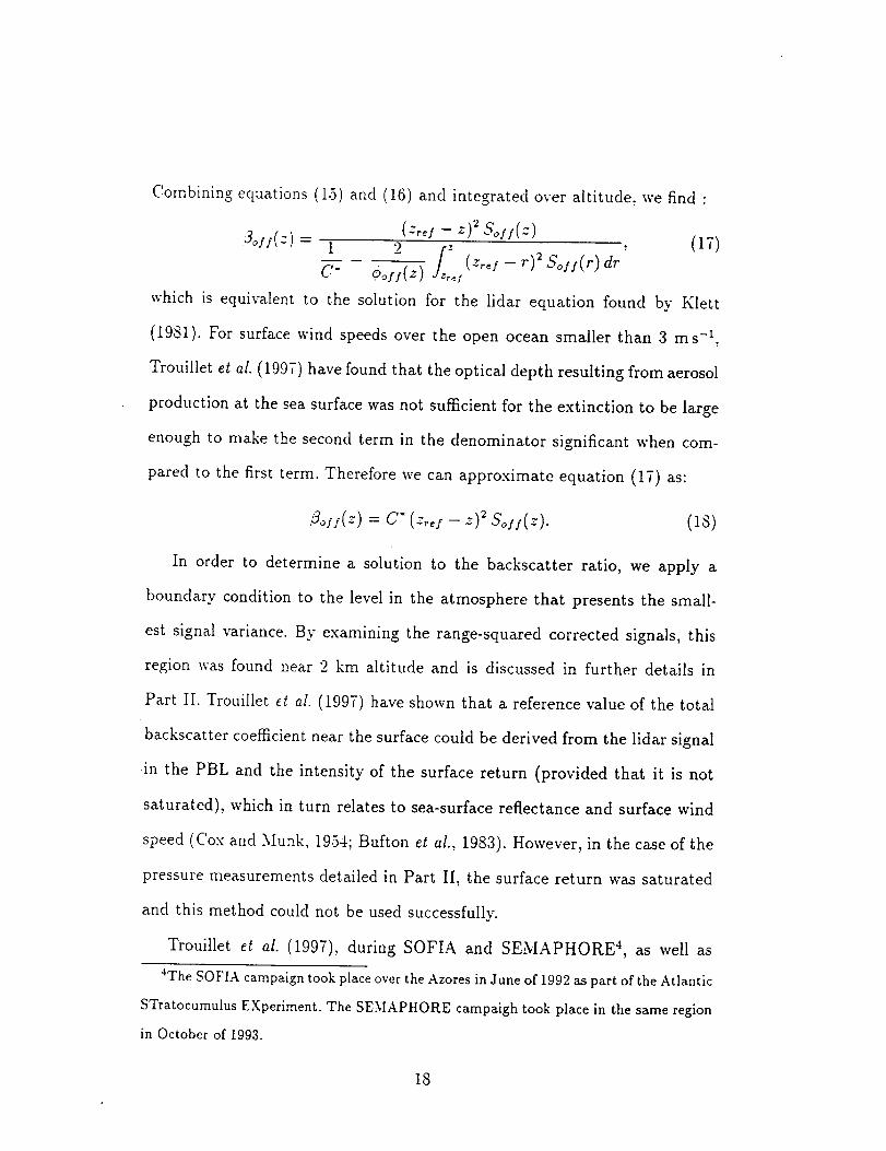
Combining equations (1.5) and 16) and integrated over altitude, we find :

(-'r_: - _)_Sos:(:)

Zl3o:s(-) = i 2 (-'to: - _)_SoH(_)a_ (17)C" oo::(.-).:

which is equivalent to the solution for the lidar equation found by KIett

(19SI). For surface wind speeds over the open ocean smaller than 3 ms -_.

Trouillet et al. (1997) have found that the optical depth resulting from aerosol

production at the sea surface was not sufficient for the extinction to be large

enough to make the second term in the denominator significant when com-

pared to the first term. Therefore we can approximate equation (17) as:

,So::(_)= c"(-_,:- _)_Sos:(._). (is)

In order to determine a solution to the backscatter ratio, we apply a

boundary condition to the level in the atmosphere that presents the small-

est signal variance. By examining the range-squared corrected signals, this

region was found near 2 km altitude and is discussed in further details in

Part II. Trouillet et al. (1997) have shown that a reference value of the total

backscatter coefficient near the surface could be derived from the lidar signal

.in the PBL and the intensity of the surface return (provided that it is not

saturated), which in turn relates to sea-surface reflectance and surface wind

speed (Cox and Munk: 1954; Bufton et al., 1983). However, in the case of the

pressure measurements detailed in Part II, the surface return was saturated

and this method could not be used successfully.

Trouillet et al. (1997), during SOFIA and SEMAPHORE 4, as well as

4The SOFIA campaign took place over the Azores in June of 1992 as part of the Atlantic

STratocumu!.us EXperiment. The SEMAPHORE ¢ampaigh took place in the same region

in October of 1993.

18

Flamant and Pelon (1996), during PYREX '5, have reported values of the

scattering ratio of R=I.5 at an altitude of 2 km above the Atlantic and

the .Mediterraneam respectively. These values were obtained from extinction

measurements made around 0.5 lLm by a nephelometer carried onboard an

aircr£ft. At a wavelength of 760 nm, the value of this ratio is expected to

be larger, although values of R=l.2 have been observed (Sasano and Brow-

ell, 1989). In order to estimate the errors on the pressure retrievals caused

bv rotational Raman scattering, the wavelength dependence of the aerosol

backscatter coefficient, and Doppler broadening in the presence of an isotopic

oxygen line, the boundary condition of R=1.5+0.3 at 2 km is taken in the

following sections.

The ratio of the off-line lidar signal in the PBL to the off-line lidar signal in

the free troposphere varies between 2 and 3, on average. The backscatter ratio

in the PBL will then range from 2.4 to 5.4, if we assume the transmission to be

small. On figure 3 we show representative backscatter ratio profile calculated

from our data in nearly neutral stratification conditions with R equal to 1.2,

1.5 and 1.8. In slightly unstable condition, this ratio is expected to be larger.

a. Rotational Raman scattering

The measurements under consideration in Part II were taken at night with

a broadband optical filter in the receiver which failed to exclude rotational

Raman scattering from the lidar signals. VV%need to account for rotational

Raman scattering by oxygen and nitrogen since most of this light will be

5The PYREX campaign was deployed in the Pyr6n6es region at the French-Spanish

border in October and November of 1990.

19

unabsorbedby oxygenoil its way back to the receiver.The total amount of

Raman scattering from these two moleculesis on the order of 3.5% of the

Ravleigh scattering (Korb et al., 1995). We may neglect vibration-rotation

Raman scattering as it is another two orders of magnitude smaller than this.

Use of a 1 nm bandpass filter would exclude rotational Raman scattering

from the measured signals. This would require an off-line wavelength closer

to the on-line wavelength.

To account for Raman scattering in the lidar detected optical power for

the on-line signal, we separate the measured 02 transmission into its partic-

ulate and molecular backscatter components including a term to account for

the Raman backscatter as

r(z)"_s= [('3"(z) +/3m(z))r°2(z)+O'O3'5'8_(z)T°2(z) ]_p(z)+_m(z)+O.O35_,_(z). (19)

In equation (19), to2 and To2 are the 2-way and 1-way 02 transmission

respectively, and 0.035 x ,3m is the Raman backscatter coefficient. The Ra-

man component of the signal has only the one-way 02 absorption imposed

on the laser light on the outgoing path from the lidar. There is essentially

no oxygen resonant extinction for the Raman backscattered signal because

of the frequency shift, except for any coincidences between 02 absorption

and rotational Raman lines which we have calculated to be an insignificant

fraction of the total Raman signal. The fraction of the on-line signal due to

Raman scattering will decrease as the aerosol scattering component increases,

so that this effect will be important in relatively aerosol-free atmospheres.

We can evaluate the extent of this effect on the measured 02 transmission

by using the scattering ratio estimated from the off-line signals.

2O

If Or/r is the fractional difference in the measured transmission and

the desired (non-Raman contaminated) transmission, it follows from equa-

tion (19) that:

0_(-) _m_o,(-)- To2(-)T(.:) ,-o_(z)

__i. -R--(..7¥5.sg j -

Differentiating equation (7) with the 2-way transmission, we get:

(20)

1 O_-(z)Op(.:)- ._Cp(.:) -,-(.:)" (21)

Combining equations (20) and (21) :

1 ([R(:) + °°35 / T°'(-')] - 1) (22)Op(z) - 4Cp(z) R(z) + 0.035 "

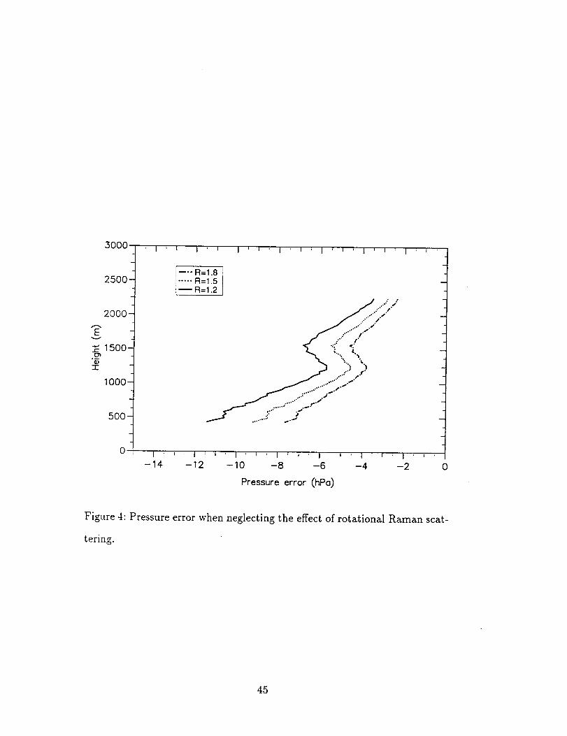
Figure 4 shows the error in the retrieved pressure field from neglecting the

effect of the rotational Raman scattering. This was calculated from equation

(22) using the data from Figures 2 and :3. The error increases with range in

the free troposphere, since the backscattered signal is more strongly absorbed

and a larger fraction of the measured total signal is contributed by Raman

scattering. The error temporarily drops as the beam penetrates the mixed

layer due to the sudden increase in aerosol backscatter, then continues as

the absorption increases. The Raman signal component causes a maximum

error of about -10 hPa near the surface. The constant slope of this error will

be, in large part, removed by the calibration procedure described in Section

3.d, leaving the residual error caused by aerosol gradients. From Figure 4,

one can see that when the signal goes from relatively clear air into a region

of high aerosol content, a jump in pressure will be observed in the retrieval

(between 1600 m and 1300 m).

21

b. Elastic scattering spectral considerations

The two main scattering phenomena in the atmosphere are Mie scattering

for aerosols and Rayleigh scattering for molecules. For Rayleigh scattering,

the laser line shape will be broadened by the Brownian motion of the molecu-

lar scatterers. Aerosol scattering is not affected by Doppler broadening. The

dial technique for pressure measurements uses the existence of an absorp-

tion trough, the region of minimum absorption between two closely spaced

strongly absorbed oxygen lines. The trough is formed by the wings of the

nearest collision broadened lines where the absorption is pressure sensitive.

The lines are selected so that the resultant measurement will be temperature

insensitive. The on- line frequency was taken in the trough region between

13150 cm -1 and 13154 cm -1, and the off- line frequency in a nearby location

with minimal resonant absorption but nearly identical attenuation due to

scattering and continuum absorption. For the off-line detected optical power,

we use a simplified form of the lidar equation that uses spectrally integrated

quantities:

To A rl c c 2

Po::(':)- (z.: - _.)_Eo:: : (T_:/(z)) [:3,,,o::(z)+ 9m,o/:(z)], (23a)

and for the on-line detected power, we write :

To ,4 7] c

_

[,_p,on(2) T:n(z ) rLn(z) + _m,on(Z)T;m(z)rLn(z)] , (23b)

where T_(z) is the one way transmission due to scattering and continuum

absorption effects, TL(z) is the one way transmission of the laser initial line

22

shape due to resonant absorption effectsand T_(z) isthe resonant one way

transmission on the return path for the Mie scattering. T_(z) and T_(z) are

nearly identical since the signal is elastically scattered by aerosols, with no

change in the shape of the initial spectrum other than the modification it un-

dergoes as a result of the spectral structure of the absorption trough. Ty(z)

is the resonant one way transmission experienced by the Doppler broadened

Rayleigh backscatter on the return path. Even though the 02 trough is signif-

icantly broader (1.5 cm -1) than the initial laser line (0.015 cm -1 at FWHM)

and the double Doppler broadened backscattered line shape (_0.06 cm -1

at FWHM), the fact that it is not flat will affect the measurements: the

larger the line width, the larger the f IC(_,)dr associated with the line shape

on the return path. Using equations (23a) and (23b) in equation (.'3), and

implementing the usual DIAL assumption that the continuum backscatter

coefficient and transmission are equal at the two closely spaced on-line and

off-line wavelengths, the overall optical depth between the reference altitude

and altitude z can be expressed as:

m(Z)dr, (24)+

where f/C;(L,, r) dr is the optical depth associated with Mie particle scatter-

ing and f IC_(v, r) dr is the optical depth associated with Rayleigh molecular

scattering. Aerosols will increase the aerosol to total backscatter ratio (the

first term on the right-hand side of the equation), therefore reducing the over-

all value of f l((v,r)dr because f l(v(v,r) dr is smaller than f I(_(v,r)dr.

Note that this is the opposite effect observed in 1-120 DIAL measurements

23

(Ansmann. 198.5) and 02 temperature DIAL measurements (Theopold and

Bosenberg, 1993) since we operate at an absorption local minimum rather

than a local maximum. This effect is minor however when compared to the

effects described in the next two sections.

c. Aero.sol extinction and backscatter coefficients wavelength dependence

The transmission expressed in equation (5) assumes the attenuation due to

scattering and continuum absorption to be nearly identical for the on-line

and off-line wavelengths. We now drop that assumption to investigate the

impact of the wavelength dependence of the extinction and backscatter co-

efficients (between the on-line and the off-line wavelengths) on the pressure

measurements. We still consider these coefficients to have minimal change

over the small spectral intervals covered by the backscatter line shapes, how-

ever. From equations ('_3a) and (23b), equation (:3) can be rewritten as:

T( Z )raeas

= { 9,,o.(Z)+

The first part of the right hand side can be considered as a correction to

transmission as calculated assuming the aerosol extinction and backscatter

coefficients to be insensitive to wavelength (i.e. the r(z) of equation (5)).

If OT/7 is the fractional difference in the measured transmission and the

desired transmission, equation (25) can be used:

Or(z) r(-_)_o,- r(z)

T(z)

= (T:n(z) _ _3p,o,_(z)+ _m,o,,(z) _ 1

\Tcoll(z)] 13p,ol.r(z) +/3,,,oil(z)

24

(26)

In order to get the error induced in the pressure retrieval, we combine

equations (21) and (26):

1 1) ,27,Op(z)= 4Cp(z) T_f(z) t3p,off(z)+_3,,,off(z)

The impact of the aerosol wavelength dependence for DIAL measurements

made over the Atlantic (Part II) was tested using the maritime aerosol model

described by Trouillet et al. (1997). Based on the works of Voltz (1973), Shet-

tle and Fenn (1979) and d'Almeida et al. (1991), the model assumes a lognor-

real size distribution for the combination of sulfate and sea-salt aerosols in

the lower troposphere. Since lidar signal intensity is very sensitive to relative

humidity (Dupont et al., 1994), the aerosol refractive index dependence on

relative humidity is also introduced and modeled according to relationships

previously proposed by H_inel (1971; 1972) and d'Almeida et al. (1991). The

relative fractional occupation rate of the two modal radii depends on the sur-

face wind speed. This rate is assumed constant in the PBL for a given wind

speed. Aloft, in order to account for the decreasing sea-salt aerosol concen-

tration, a 2 km height scale (Blanchard and Woodcock, 1980) is introduced.

A Mie model is used to calculate the backscatter and extinction coeffi-

cients for the sulfate and sea-salt aerosols at 757 nm (corresponding to the

off-line wavelength of the DIAL system). The maritime particulate mixture

phase function profile is then deduced from a relative humidity profile and

the fractional concentration of sea-salt dependence with height. The sulfate

and sea-salt aerosol backscatter and extinction coefficients wavelength de-

25

pendenceare calculated accordingto:

c_ = in(a(A2)/a(A_))

ln(A2/A1)

and

for A2 _ A1 (28a)

In(3(A2)/3(,\_)) for A2 > ,\1 (28b)c_3 = In(A2/,\1)

where ,\_, = 757 nm and A1 = 532 nm. The ,_,ngstrom coefficients _5,_ and

6a calculated from equations (28a) and (28b) will be used to estimate the

difference in transmission between the on-line and off-line wavelength given

by equation (26). However, _5_and c5,_also depend on relative humidity. Since

we expect typical values to be quite different in the free troposphere and in

the boundary layer, the humidity profile measured at Wallops was used to

calculate these coefficients throughtout the lower troposphere. Table 1 sum-

marizes the value of the ,_,ngstrom coefficients for extinction and backscatter

for relative humidities of 10% and .50%, representative of the free troposphere

and the boundary layer, respectively.

Because wind measurements were taken only at Wallops and not above

the ocean, we show the resulting error for a surface wind speed ranging from

3 to 7 m s -1 (Figure 5). The error induced by this uncertainty is negligible, in

comparison to the error resulting from the vertical aerosol distribution. The

latter effect induces an error that is largest in the free troposphere. This is

caused by (i) the large wavelength dependence of molecular extinction and

backscatter coefficients (6 _ -4) and (ii) the fact that sulfate aerosols dom-

inate the particulate scattering in a region where their scattering properties

strongly depend on wavelength (for low values of the relative humidity, see

Table 1). In the PBL, sea-salt aerosols control the particle scattering but

26

their hydroscopicproperties preventsanv strong wavelengthdepende.nceof

the extinction and backscattercoefficients.This will result in a pressuredis-

continuity at the top of the PBL becauseof the strong aerosolgradient. Note

that the error doesnot depend on the value of scattering ratio chosenas a

boundary condition (equation (27)).

d. Isotopic oxygen lines

Isotopic lines have been observed in the 02 spectrum in long-path atmo-

spheric spectroscopic measurements by Babcock and Herzberg (1948). From

their measurements one expects to observe an 016 - O is line in the center of

the trough we used for pressure measurements. Figure 6 shows a calculated

absorption spectrum near the 1(}00 hPa level assuming a line strength equal

to the strength of the same transition in 016 - 016. We attempted to locate

this line with the lidar in flight by tuning the laser across the absorption

trough while observing a real-time display" of atmospheric transmission in-

tegrated over a portion of the path below the aircraft. We failed to observe

the isotopic line due to inadequate signal to noise over reasonable integration

times of a few seconds. Alternatively, we located the laser frequency where we

thought it should be to avoid the isotopic line by interpolating between the

sides of the 016 - 016 lines as measured on the real-time display. However.

this technique may also be of questionable accuracy for the same reason we

failed to observe the isotopic line. Therefore, we studied what would happen

if the laser were actually located on the isotopic line.

To help visualize the spectral processes, refer to figure 6, where we have

plotted the 02 spectrum in the boundary layer with and without the isotopic

27

line. the laser output spectrum, and the 1Rayleighbroadenedcomponentof

the laserbackscatter.The isotopic line adds about .30%to the trough absorp-

tion at the line center. Note that the collision broadenedline profile central

absorption is altitude independentsince the decreasein absorption due to a

redistribution of the molecular population into the wings of the profile due

to increasingpressureis exactly offsetby the increasein density (Korb and

Weng, 1982).Thereforethis additional absorption, to first order, is pressure

independentin the center,gradually changingover to a p2 dependence as the

frequency moves further from line center. The laser spectrum was measured

by Korb et al. (199.5) to consist of three nearly equally spaced modes sepa-

rated by 0.007 cm -1, the two outer modes being half as intense as the central

mode. The laser spectrum envelope can be approximated by a Gaussian pro-

file with a half width equal to the mode spacing.

For a description of the mathematical representation of the lidar formula-

tion which includes the frequency dependence of the laser light and Rayleigh

scattering, we refer the reader to Ansmann and Bosenberg (1987).

For the purposes of modeling the effect of the isotopic line absorption

on the Rayleigh broadened and aerosol backscatter, we use three modeled

atmospheres having backscatter profiles similar to our data, represented in

Figure 7. \Ve calculated lidar signals using our system parameters, with the

on-line signals as a function of frequency. Figure 8 represents the on-line

return signal spectra at 4 altitude levels in an atmosphere characterized by

a backscatter ratio of .5 in the PBL and 1.2 in the free troposphere. The

outgoing laser energy is concentrated within the isotopic absorption line,

hence experiences a stronger absorption coefficient. The backscattered energy

a

28

is distributed into the wings of the isotopic line and experiencesa smaller

spectrally integrated absorption coefficient.With the laser centeredon the

isotopic line, the immediate effect of the aerosolsis to force more of the

backscatter into the isotopic absorption line. therefore increasing the net

absorption. As the laserbeampropagatesdownthrough the atmosphere,its

spectral shapechanges,broadeningif centeredon the isotopic line, or if off-

center, becoming asymmetric. This effect is minor compared to the variation

in aerosol scattering, however. The net 30% offset in the absorption baseline

due to the presence of the isotopic line is not a source of error since it acts

as a net change to the 016 - O la line strength, which is accounted for in the

calibration procedure discussed in the section on instrumental errors.

To evaluate the error in the retrieved pressure profiles caused by ignoring

the effect of Rayleigh broadening in the presence of the isotopic line, we ana-

lyze the oxygen transmission calculated for combined aerosol and molecular

scattering and compare it to the oxygen transmission calculated for molec-

ular scattering only. We could compare it to aerosol only scattering which

would more closely conform to the lidar assumption of monochromicity, but

chose pure Rayleigh scattering for consistency with our other corrections and

the more realistic limit of having zero aerosols as opposed to zero molecules.

We define a correction factor, r', to be applied to the measured transmission,

that will yield the transmission we should get in the absence of aerosols, r,,,:

Trneas

r" - (29)Tm

where r._s can be found from the optical depth (equation 24):

• + m(z)

29

and

× exp \ , J (30)

rm = exp (-2_",,I K,,(r) dr), (31)

where we have integrated the absorption coefficients I(p and K,n over the

spectrum. Taking the ratio of r,,,=, to rm and expressing the backscatter

coefficient in terms of scattering ratio R(z):

r'(z, : exp [-2 (1 R_z))(_:_/(p(r) dr- _, K=(r)dr)]

= .r_. (32)

The oxygen transmission for the molecular scattered light and particulate

scattered light are calculated using laboratory line parameters measured by

Burch and Gryvnak (1969), and line frequencies measured by Babcock and

Herzberg (1948), in a voigt line shape algorithm. Using equations 21, 26, and

32, we find the error induced in the pressure retrieval:

1

?)p(z) = -4Cp(z) (r'(z)- 1). (33)

Using the modeled lidar backscatter profiles from Figure 7, we estimate

the errors in the pressure profile caused by not accounting for isotopic absorp-

tion using equations (32) and (33), plotting the results in Figure 9. Because

aerosol scattering is concentrated at the line center, the effective absorption

coefficient is larger for aerosol backscatter than for molecular backscatter.

Hence. the model with greater aerosol scattering in the free troposphere shows

larger pressure errors. The increased aerosol backscatter from the PBL causes

even higher errors. From this figure, one can see that any aerosol structure

3O

will create a correlated false structure in the retreived pressurefield. But

what happenswhen the laserfrequencyis somewhereelsein relation to the

isotopic line? This is illustrated in Figure 10,wherewehave plotted the er-

rors for the worst casemodel, and having the laser located at one, two, and

three half-widths from the isotopic line center, as well as on line center. At

one half-width, the laser is centeredon a linear region on the side of the

line profile. Refer back to Figure 6 to help visualize this. If one spectrally

integratesover the molecular backscatter lineshape,the effectiveabsorption

coefficientis about the sameasthat for the aerosolline shape,sinceenergy

on the higher absorbingside of the lasercenter frequencyis compensatedfor

by lower absorption on the oppositeside.This is why the errors arecloseto

zero at all altitudes. When the laser is located at two half-widths from the

isotopic line center, the molecular backscatter contains a larger portion of

energyin the isotopic line than doesthe aerosolbackscatter.Hencethe spec-

trally integratedabsorption coefficientis larger for molecularthan for aerosol

backscatter,and the errors are negative instead of positive. As the laser is

located evenfurther from line center, the errors will decreasein magnitude,

as doesthe curve for three half-widths awayin Figure 10.

5. Summary and conclusion

We have analyzed the sensitivity of differential absorption lidar measure-

ments of the atmosphericpressureprofiles to instrumental and atmospheric

systematicerror sources.The errorsareevaluatedfor airborne lidar measure-

mentsmadeoff the mid-atlantic coast of the United States in 1989, as if they

31

were uncorrectedfor. They aresummarizedin Table 2. Large errors can re-

sult by ignoring the effects of Raman scattering, the wavelength dependence

of extinction and backscatter coefficients, and interference by isotopic oxygen

lines in the oxygen spectrum. All of these errors are strongly correlated with

structure in the aerosol backscatter profiles and systematically add. They can

introduce large pressure gradients on the horizontal since the lidar signal is

highly sensitive to aerosol content and relative humidity which in turn relate,

at small scales, to convective activity in the PBL, and, at larger scales, to

stratification and coastal influence in terms of aerosol population. Account-

ing for their effects is also important on the vertical since pressure errors

can be large in the free troposphere, a region where DIAL measurements are

generally calibrated with respect to balloon data (see section g.d).

A correction scheme is derived for each effect. These will be applied to

pressure profile retrievals from the 1989 flight experiments in a companion

paper, Part II, and the accuracy to which the retrievals are made will be

evaluated.

Acknowledgements. Support for this work was provided by Dr. John

Theon and Dr. Ramesh Kakar of NASA Headquarters; direction of Cyrille

Flamant's grant by Pr. Thomas D. Wilkerson, technical support by Dr. Coorg

Prasad. presently with Science and Engineering Services, Inc., Burtonsville,

MD, and Mr. Joseph Famiglietti, NASA GSFC. The authors would also like

to thank Dr. Patrick Chazette of CEA and Drs. Jacques Pelon, Pierre H.

Flamant and Vincent Trouillet of CNRS for many helpful discussions.

32

References

[1] d'Almeida, G. A., P. Koepke, and E. P. Shettle, 1991: Atmospheric

aerosols, global climatologg and radiative characteristics. Adarsh

Deepak Publishing, 124 pp.

[2] Anderson D., A. Hollingsworth, S. Uppala, and P. Woiceshyn, 1987:

A study of the feasability of using sea and wind information from

ERS-1 satellite. Part I: Wind scatterometer data. European Center for

.Medium Range Weather Forcasts contract report 6297/86/HGE-I(SC),

121 pp.

[3] Ansmann, A., 1985: Errors in ground-based water-vapor DIAL mea-

surements due to Doppler- broadened Rayleigh backscatter. Appl. Opt.,

24, 3476 3480.

[4J Ansmann, A.. and J. Bosenberg, 1987: Correction scheme for spec-

tral broadening by Rayleigh scattering in differential absorption lidar

measurements of water vapor in the troposphere. Appl. Opt., 26, 3026

3032.

[5] Babcock, H. D., and L. Herzberg, 1948: Fine structure of the red system

of atmospheric oxygen bands. Astrophys. J., 108, 167 190.

[6] Blanchard, C. D., and A. H. Woodcock, 1980: The production, concen-

tration, and vertical distribution of the sea-salt aerosol. Annals N. Y.

Academy of Sciences, 330 347.

33

[7] Bond, N. A., and R. G. Feagle,198.5:Structure of a cold front over the

ocean. Quart. J. Roll. Meteor. Soc., 111,739 759.

[8] Brown R. A., and G. Levy', 1986: Ocean surface pressure fields from

satellite-sensed winds. Mon. Wea. Rev., 114, 2197 2206.

[9] Burch, D. E., and D. A. Gryvnak, 1969: Strengths, widths, and shapes

of the oxygen lines near 13,100 cm -1 (7620 A). Appl. Opt., 8, 1493

1499.

[10] Bufton, J. L., F. E. Hodge, and R. N. Swift, 1983: Airborne measure-

ments of laser backscatter from the ocean surface. Appl. Opt., 22, 2603

2618.

[11] Cox, C., and W. Munk, 1983: Measurements of roughness of the sea

surface from photographs of the sun's glitter. J. Opt. Soc. Am., 44,

8:38 8.50.

[12] Dupont, E., J. Pelon, and C. Flamant, 1994: Study of the moist con-

vective boundary layer structure by backscatter lidar. Bound.-Laller

Meteor., 69, 1 25..

[13] FIamant, C., and J. Pelon, 1996: Atmospheric boundary-layer structure

over the Mediterranean during a Tramontane event. Quart. J. Roll.

Meteor. Soc., 122, 1741 1778.

[14] Flamant, C. N., G. K. Schwemmer, C.L. Korb, S. P. Palm, and K. D.

Evans: Pressure measurements using an airborne differential absorption

34

lidar. Part II: Resultsfrom the 1989PressureField Experiment.To be

submitted to g. ,4tmos. Ocean. Tech.

[15] H/inel, G., 1971: New results concerning of visibility on relative Hu-

midity and their Significance in Model for Visibility Forecast. Bei'trage

zur des Atmosphiire, 44, 137 167.

[16] H/inel, G., 1972: Computation of extinction of visible radiation by at-

mospheric aerosol particles as a function of the relative humidity based

upon measured properties. Aerosol science, 3, 377:3S6.

[17] Klett, J. D., 1981: Stable analytical inversion solution for processing

lidar return. Appl. Opt., 20, 211 220.

[18] Korb, C. L., and C. Y. Weng, 1982: A theoretical study of a two wave-

length lidar technique for the measurement of atmospheric temperature

profiles. J. Appl. Meteor., 21, 1:346 1355.

[19] Korb, C. L., and C. Y. Weng, 1983: Differential absorption lidar tech-

nique for measurement of the atmospheric pressure profile. Appl. Opt.,

22, 3759 3770.

[20] Korb, C. L., G. K. Schwemmer, M. Dombrowski, and C. Y. V_ng. 1989:

Airborne and ground based lidar measurements of the atmospheric

pressure profile. Appl. Opt., 28, 3015 3020.

[21] Korb, C. L., G. K. Schwemmer, J. Famiglietti, H. Walden, and C.

Prasad, 1995: Differential absorption lidars for remote sensing of the

35

atmospheric pressureand temperature profiles: Final report. NASA

Tech. Memo. 104618,249 pp.

[22] Lee, H. S., G. K. Schwemmer, C. L. Korb, M. Dombrowski, and

C. Prasad, 1989: Gated photomultiplier response characterization for

DIAL measurements. Appl. Opt.,29, 3303 3315.

[23] Levy, G., and R. A. Brown, 1991: Southern hemisphere synoptic

weather from a satellite scatterometer. :lion. Wea. Rev., 119, 2803

2813.

[24] Nuss, W., and R. A. Brown, 1987: Evaluation of surface winds and

flux analysis in mid-latitude marine cyclones. J. Dynamics of Atmo-

spheres/Oceans, 10, 291 315.

[2.51Sasano, Y., and E. V. Browell, 1989: Light scattering characteristics of

various aerosol types derived from multiple wavelength lidar observa-

tions. Appl. Opt., 28, 1670 1679.

[26] Schwemmer, G. K., M. Dombrowski, C. L. Korb, J. Milrod, H. Walden,

and R. H. Kagann, 1987: A lidar system for measuring atmospheric

pressure and temperature profiles. Rev. Sci. Instr., 58, 2226 2237.

[27] Shettle, E. P., and R. W. Fenn, 1979: Models for aerosols of the lower

atmosphere and the effects of humidity variations on their optical prop-

erties. Air Force Geophysics Laboratory Environment Research Papers,

No 678, 94 pp. [AFGL-TR-79-0214.]

36

[2s] Starr. D. O'C., C. L. Korb, G. K. Schwemmer, and C. Y. Weng, 1992:

Observations of height- dependent pressure perturbation structure of

a strong mesoscale gravity wave. Mon. Wea. Rev., 120, 2808 2820.

[29] Theopold, F., and J. Bosenberg, 1993: Differential absorption lidar

measurements of atmospheric temperature profiles: Theory and exper-

iment. J. Atmos. Ocea. Tech., 10, 165 179.

[30] Trouillet, V., J. Pelon, P. Chazette, and C. Flamant, 1997: Wind speed

dependence of the atmospheric boundary layer optical properties and

ocean surface reflectance as observed by airborne backscatter lidar.

Submitted to J. .4tmos. Ocea. Tech.

[31] Volz, F. E., 1973: Infrared optical constants of ammonium sulfate, sa-

hara dust, volcanic pumice, and flyash. Appl. Opt., 12,564 568.

37

Table 1: Wavelengthdependenceof the sea-saltand sulfate aerosolsextinc-

tion and backscattercoefficientsbetween532 nm and 7.57nm.

Relative humidity

/_ngstrom coefficient

Extinction (6_) Backscatter ($_)

Sea-salt Sulfate Sea-salt Sulfate

10

50

0.24 -1.34 -0.24 -1.38

1.03 0.13 0.82 0.26

38

Table 2: Systematicerror on pressureretrievals causedby instrumental and

atmosphericeffects (in hPa).

Atmosphericeffects

Rotational Wavelength Isotopic

Raman dependence lines

Instrumental effects

Baseline

subtraction

Free troposphere

R=l.2

R=l.8

-7 to -4 1.0 to 3 -0.3 to 0.7

-4 to -2 1.0 to 3 -0.8 to 2

0. to 4-0.15

0. to +0.15

Boundary layer

R=2

R=5

-12 to -6 0. to 1 -1.2 to 3 0. to +0.3

-6 to -3 0. to 1 -2 to 5 0. to +0.3

39

List

3

4

5

of Figures

Ratio of the on-line to the off-line signal in the case where

the laser beam is prevented from going out to the atmosphere.

In the event that no ground loop affects the data, the signal

detected for both acquisitions should be proportional to the

atmospheric background, and the ratio of the on-line to the off-

line should be equal to unity and constant with range. Noise

in the data results from the small quantities being ratioed... 42

Oxygen transmission profile before (dashed line) and after

(solid line) calibration using a pressure sounding. Note that

only the corrected transmission profile goes through unity at

the height of the aircraft (3800 m in this case) .......... 43

Scattering ratio profile derived from lidar measurements, made

at 760 nm, during the 1989 Pressure Experiment. Profiles are

given for three values of the scattering ratio boundary condi-

tion applied to the lidar signal profile at 2000 m ......... 44

Pressure error when neglecting the effect of rotational Raman

scattering .............................. 45

Pressure error when neglecting the effect of aerosol backscatter

and extinction coefficients wavelength dependence ........ 46

4O

9

10

Calculatedtransmissionspectrum(solid line) for 02 in the re-

gion of the DIAL measurements, with and without the isotopic

lines. Superimposed is the laser output spectrum (dotted line)

and Rayleigh broadened backscatter (dashed line) relative to

the O_ absorption spectrum .................... 47

Backscatter ratio models used to calculate the effect of Rayleigh

broadening in isotopic line effects. Two models use R=l.2 in

the free troposphere with R=5 (solid line) and R=2 (dashed

line) in the PBL. The third model (dotted line) uses R=1.8 in

the free troposhere and R=5 in the PBL ............. 48

The on-line return signal spectra at various altitude levels,

100 m (solid line), 800 m (short-dashed line), 1500 m (long-

dashed line) and 2200 m (short-and-long-dashed line), in an

atmosphere characterized by' a backscatter ratio of .5 in the

boundary-layer ........................... 49

Errors in the retrieved pressure profile due to isotopic line

interference. The line styles correspond to those representing

their respective scattering models in Figure 7".......... 50

Pressure errors for the worst case aerosol model (R=l.8 in free

troposphere and R=5 in PBL) due to the laser being on the

isotopic line and the errors for the laser being one, two and

three half-widths off the isotopic line ............... 51

41

3000 _-_1600

2OO

-1200

-2600

Ev

-4000

<-5400

-6800

-9600

-11000 I I I I I I I I I

0 2 4 6 8 10 12 14 16 18 20

Intensi_ Ratio(on-line/off-line)

Figure 1: Ratio of the on-line to the off-line signal in the case where the laser

beam is prevented from going out to the atmosphere. In the event that no

ground loop affects the data, the signal detected for both acquisitions should

be proportional to the atmospheric background, and the ratio of the on-line

to the off-line should be equal to unity and constant with range. Noise in the

. data results from the small quantities being ratioed.

42

4000 4

.

._.2500E

_-'2000._

I 1500 Z

1000 2

0.0

I I I ' I

/./'/ i/`'./

.'/':/ "

_ I I I.."-' I ' .

//" ../_-

/./ .-1" -i. 4" .

j/' ,.,

j,- /,,"

I I I ' I _ I _ I I I I '

O.1 0.2 0.,5 0.4- 0.5 0.6 0.7 0.8 0.9

Transmission

1.0

Figure 2: Oxygen transmission profile before (dashed line) and after (solid

line) calibration using a pressure sounding. Note that only the corrected

transmission profile goes through unity at the height of the aircraft (3800 m

in this case).

43

3000

2500-

2000-

E

1500-.m

I

1000-

500-

!..

f.s'"

%

(",_°

--'" R=1.8..... R=1.5

R=1.2

i ' I ' ' I = I I I I ,1.5 2.0 2.5 ,..3.0 ,.3.5 4.0

Backscatter ratio

Figure 3: Scattering ratio profile derived from lidar measurements, made at

760 nm, during the 1989 Pressure Experiment. Profiles are given for three

values of the scattering ratio boundary condition applied to the lidar signal

profile at 2000 m.

44

3000

2500-

2000

E

15002

I

10001

500"

O,

I ' i I ' I I ' i I _ i _ I ' I , I ' i , I _ i

--'- R=I 8..... R=I 5m R=1.2

f

.." i

4"" .f"

...."' t,. /

...-" ._,"...°" j.

..' f

d" ¢"•:: _"

• .. ._

%.. "_,.

..................;i

I

-14I i I i I l I i , I i I

- 12 - 10 -8 -6 -4 -2 0

Pressure error (hPo)

Figure 4: Pressure error when neglecting the effect of rotational Raman scat-

tering.

45

4OOO

3500-

3000 /

2500 2

2000 £

1500 Z

1000

0.0

I , 1 I , I a I l , I t I ' I ,

Surface wind sp .--- 7 m/s..... 5 rams

3 m_/s

,,,0.5 1.0 1.5 2.0 2.5 3.0

Pressure error (hPo)

Figure 5: Pressure error when neglecting the effect of aerosol backscatter and

extinction coefficients wavelength dependence.

46

Ev

O(.9

cO

°_

¢M

O

<

0.25

0.20

0.15

0.10

0.05

0.00

15152.0

jl Fi_ _ 1.0

I

I I

I I

I _ 0.8I I

I I

0.6!

I

I

I

: t

: I

i i i I i , J" - 1 i

13152.2 13152.4

Wovenumber (cm")

o

0.4 "_

n,'

0.2

0.0

Figure 6: Calculated transmission spectrum (solid line) for O2 in the region

of the DIAL measurements, with and without the isotopic lines. Superim-

posed is the laser output spectrum (dotted line) and Rayleigh broadened

backscatter (dashed line) relative to the 02 absorption spectrum.

47

v

a),-j

3000 L .........I

F

L

I

2000 _

I

[LL

1000

FE

LI

L0

0 I 2 3

Aerosol scattering ratio

Figure 7: Backscatter ratio models used to calculate the effect of Rayleigh

broadening in isotopic line effects. Two models use R=1.2 in the free tropo-

sphere with R=5 (solid line) and R=2 (dashed line) in the PBL. The third

model (dotted line) uses R=1.8 in the free troposhere and R=5 in the PBL.

48

0.020!

FF1

0.015 F-

; Li

0 -

o. ,..

-_.0.010--o

_ -

0.005 --

?-

0.000 ,

1.315245

I I I I 1

./'

• -,

1.315250 1.315255 1.315260 1.315265 1.315270

Wavenumber, 10,000. (cm-1)

Figure 8: The on-line return signal spectra at various altitude levels, 100 m

(solid line), 800 m (short-dashed line), 1500 m (long-dashed line) and 2200 m

(short-and-long-dashed line), in an atmosphere characterized by a backscat-

ter ratio of 5 in the boundary-layer.

49

_CO0_'_ ....... i ......... _ ......... , ......... , ......... , .........

LU_E_" " ,,,,,,

2000 -- \ \ \ \

,2_ ,,

.-: X

O. , ....... ,I.,, ,,,,,. I ......... t i'. .............

0 1 2 3 4 5 6

Pressure errors (hPo)

Figure 9: Errors in the retrieved pressure profile due to isotopic line interfer-

ence. The line styles correspond to those representing their respective scat-

tering models in Figure 7.

5O

E

_J

-1._

3000_E

tkFE

2000 --

10001

f

I

I

I

I

I

I

I

I

_I

4O,

-2

d\' , ' ' ' , '

,_i\ - on isotopic ne/;:_ ....... I haif-w[dth away

/ / _ .... 2 half-wldths away

i i _ ..... 3 ha!f-wrd:hs away

/ i

/ !

i !I I

/

I I/ " ./I

,: , I ., , , I , , , I , \

0 2 4

Pressure errors (hPo)

r

5

Figure 10: Pressure errors for the worst case aerosol model (R=l.8 in free

troposphere and R=5 in PBL) due to the laser being on the isotopic line and

the errors for the laser being one, two and three half-widths off the isotopic

line.

51