gekoppelte simulationen von cfdgekoppelte simulationen von ... · pdf filegekoppelte...

Gekoppelte Simulationen von CFDGekoppelte Simulationen von CFDund EMAG zur Berechnung von

thermischen Effekten in elektrischenAnlagenAnlagen

Pascal Bayrasyasca ay asy

Mohammadali Salari

Klaus Wolf

© Fraunhofer SCAI 1Fraunhofer Institut SCAI

MpCCI – The Independent Code Coupling Interface

Neutral and vendor independent solution for

Fluid-Structure Interaction

Thermal & Radiation Couplingp g

Acoustics

Magneto-Hydro Dynamics Magneto-Hydro Dynamics

Thermo-Electrical coupling

1D S t C d d 3D CFD li 1D System Code and 3D CFD coupling

© Fraunhofer SCAI 2

MpCCI CouplingEnvironment



Dimensions of Simulation Models and Coupling Regions

surface coupling 3D surface coupling2D surface coupling

and volume coupling3D volume coupling2D volume coupling 3D volume coupling

and 1D-3D cross dimension


MpCCI Workflow1. Preparation of

Model Filesmodel file

Code Amodel file

Code Amodel file

Code Bmodel file

Code Bscanscan2. Definition of

CouplingProcess

MpCCI GUICodesCoupling RegionsQuantitiesOptions

userinput

scanscan

3. Running theCoupled Simulation Code A

Adapter

Code B

Adapter

MpCCIServer

readread start

Adapter Adapter

MpCCI Monitor

data

4. Post-Processing ResultsResultsCode A

ResultsResultsCode BTracefile

Post-ProcessingA

Post-ProcessingB

MpCCIVisualizer


A BVisualizer

MpCCI – Independent CoSimulation Interface

Open interface through APIOpen interface through API Coupled Simulations as Platform independent Computing Coupling of parallel codes

li f d d d l i li i Coupling of <n> codes and models in one application

Running on distributed and heterogeneous hardware

Generic coupling concept Flexible mapping workflow

Ramping and under-relaxation

Support for dynamic remeshing in code

H dli f h d d Handling for orphaned nodes

Flexible coupling schemes Asynchronous buffered communication

b l Subcycling support

Coupling on demand

Support for ‘iterative explicit’ coupling


MpCCI – Independent CoSimulation InterfaceMpCCI 4.1.1 MpCCI 4.2.1 MpCCI 4.3May 2011 April 2012 April 2013

Abaqus 6.10, 6.11 6.12‐1 6.13Ansys 11.0,12.x, 13.0 11.0, 12.x, 13.0, 14.0 11.0, 12.x, 13.0, 14.0Flowmaster 7.6, 7.7 7.6, 7.7, 7.8, 8.0, 8.1, 8.2 7.6, 7.7, 7.8, 8.0, 8.1, 8.2Fluent 6.3.26, 12.x, 13.0 12.x, 13.0, 14.0 12.x, 13.0, 14.0Flux 10.2, 10.3 10.2, 10.3 10.2, 10.3

/FINE/Hexa 2.11‐0 2.10‐4 2.10‐4FINE/Open ‐ 2.11‐x, 2.12‐x 2.11‐x, 2.12‐xFINE/Turbo ‐ 8.9‐1 8.9‐x, 8.10‐x 8.9‐x, 8.10‐xICEPAK 4.4.x, 13 13.0, 14.0 13.0, 14.0JMAG ‐ 11.0, 11.1 11.0, 11.1MatLab ‐ R2007b, R2009b R2007b, R2009bMapleSim ‐ ‐ under developmentMSC.Adams ‐ 2010, 2011, 2012 2010, 2011, 2012MSC.Marc 2007, 2008, 2010 2007, 2008, 2010, 2011 2008, 2010, 2011, 2012MD.Nastran 2010.1 2010.1, 2011.1, 2012.1 2010.1, 2011.1, 2012.1,m2012.2OpenFOAM 1.5, 1.6, 1.7 1.5, 1.6, 1.7 1.5, 1.6, 1.7, 2.0, 2.1RadTherm 9.1, 9.2, 9.3, 10.0 10.0, 10.1, 10.2 10.0, 10.1, 10.2, 10.4

d d lSIMPACK ‐ ‐ under developmentSTAR‐CD 4.[06..14] 4.[06..16] 4.[06..16]STAR‐CCM+ 5.[02..06],6.02 6.[02..06], 7.02 6.[02..06], 7.02, 7.04



Code Adapter APICode Adapter API

provides an environment to realize compatible code adapters

Used to couple commercial codes with inhouse FEM/CFD

Onera, Snecma, SNPE

Dassault Aviation, aerospace comp.

PowerAlstom

turbine manufacturersturbine manufacturers

Various Universities

Software vendors


FSI-Mapping PlugIn for EnSight Postprocessor

Fully Interactive Mapping

For all file formats supported by EnSight

FSI and Thermal Coupling


MpCCI – Licensed End Users

Some of our MpCCI/Mapping CustomersSome of our MpCCI/Mapping Customers Electrical Engineering: ABB, Eaton Moeller, Jiangnan Electromechanical Inst, some

Japanese Companies

Aircraft/Space: Airbus BAE Systems China Commercial Aircraft Dassault Aviation Aircraft/Space: Airbus, BAE Systems, China Commercial Aircraft, Dassault Aviation, Goodrich Aerospace, Lockheed Martin, NASA Ames, Shanghai Academy of Space Flight, Space Research Centre Poland

Propulsion: Snecma Propulsion, Snecma Moteurs, SNPE, ONERA, CENAERO, Power Alstomp p , , , , ,

Energy: BechtelBettis, Knoll Atomic Labs, CEA Cesta / Valduc, CNES, Fortum, VTT

Consumer:, Daya Great Information, Estech Corp, Jiaxipera Compressor, some Japanese Companiesp

Oil: Exxon Mobile, Halliburton

Automotive Supplier: Dana Corp, Stress Engineering Services, Borgwarner

Automotive OEM: Audi Deutz AG Daimler Ford General Motors IFP Moteurs Nissan Automotive OEM: Audi, Deutz AG, Daimler, Ford, General Motors, IFP Moteurs, Nissan Motor, Toyota Motor Corp, VW

Heavy Industry: IHI Heavy Industries, TÜV Nord, TKSE, Benteler

Universities: Various sites using their own code combinations


Universities: Various sites using their own code combinations

Example: Thermal Management for Automotive Vehicles


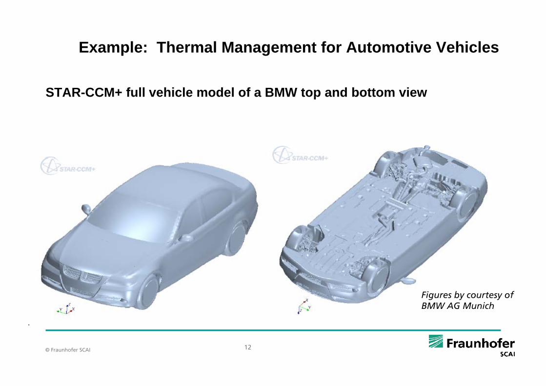
Example: Thermal Management for Automotive Vehicles

STAR-CCM+ full vehicle model of a BMW top and bottom view

Figures by courtesy of BMW AG Munich


Thermal Management for Automotive Vehicles

RadTherm full vehicle model of a BMW top and bottom view




Fluent RadTherm

TFilmHTCoeff

Fluent,

STAR-CCM+

OpenFOAM

RadTherm

TWall

Starting with flow field Tw=const.



User frontend



Wall temperature in STAR-CCM+ of BMW vehicle top and bottom view




Coupled full vehicle model of a BMW• Computed on 42+6 CPUs

• Neighborhood calculation is done online

• Steady state simulation takes ~1-2 days


Coupled Thermal Simulation of a three-phase transformer


Coupled Thermal Simulation of a three-phase transformer

Source: Nelu- Cristian Chereches, Contribution à l’optimisation de circuits thermoconvectifs, 7 Feb. 2006, PhD Thesis Université de Reims Champagne Ardenne


Thesis, Université de Reims Champagne-Ardenne

Why coupling?

In modern engineering we need to be more precise, so we have to take the different

physical aspects of problem into account and this could be done by coupling different

simulators.

By coupled simulation we could solve numerous interesting new problems in engineering

How JMAG-MpCCI-Fluent coupling works?

JMAG does the electromagnetic analysis but not CFD analysis.

Fluent does the CFD analysis but not electromagnetic analysis.

Fluent and JMAG could communicate each other through MpCCI.

Through MpCCI we can couple Maxwell´s equations with fluid flow and thermal equations in order to solve the whole system of partial differential equations.q y p q

Analysis Objective

Transformers are made to be used long-term: design policy to control r nning costs from lossesrunning costs from losses.

Losses include copper loss in the coil and iron loss in the core.

Heat is produced and standards required heat resistant design for Heat is produced and standards required heat resistant design for safety.

Losses and heat prediction is a vital component for transformer design

Use a coupled approach to obtain losses in a transformer and use them to evaluate the temperature distribution in tranformer.


Analysis Model

Magnetic field analysis handles the phenomena that produce magnetic fl and edd c rrents in transformer’s core hen c rrentmagnetic flux and eddy currents in transformer’s core when current flows through the coil. Transient response magnetic field analysis is adopted.g y Loss evaluation for a single excitation frequency

Heat generation is handled in a thermal analysis Heat generation is handled in a thermal analysis Steady state analysis of a transformer with oil coolant

Losses distribution are used as heat source terms for each part (core and coils)


Magnetic Frequency Response Analysis

Voltage (V) 141.42Excitation Three-phase AC

Frequency (Hz) 60

Power supply

Frequency (Hz) 60

Phase difference

With reference to U-phase,

V-phase:+120 (deg),W-phase: 120 (deg)phase:-120 (deg)

Connection pattern (transformer side) delta-delta-connection

Connection pattern (load side) Y-connection

Primary coil

Number of turns (turn/phase) 50

Coil Resistance (ohm/phase) 0.031

Secondary coil

Number of turns (turn/phase) 5

Coil Resistance (ohm/phase) 0.00156

External load resistance (ohm/phase) 0.06

Materials are temperature dependent for electric conductivity


electric conductivity

JMAG Copper Electric Properties Definition


JMAG Solver Settings

Set the frequency control One Step

Single frequency

Activate Coupling• Allow bidirectional coupled analysis


Thermal Fluid Analysis

Material n-heptane liquidDensity 684 kg/m3

Fluid properties:“Oil coolant”

y gSpecific heat 2219 j/kg.K

Thermal conductivity 0.14 W/m.K

Viscosity 4 09e-4 kg/m sViscosity 4.09e 4 kg/m.s

Viscous model Laminar flow

S lid tiMaterial steelD it 8030 k / 3Solid properties:

“Core”Density 8030 kg/m3

Specific heat 502.48 j/kg.KThermal conductivity 16.27 W/m.K

Solid properties:“Coils”

Material copperDensity 8978 kg/m3Coils Density 8978 kg/m3

Specific heat 381 j/kg.KThermal conductivity 387.6 W/m.K

Boundary conditions: Velocity 0.001 m/sBoundary conditions:Inlet

yTemperature 293.15 K

Boundary conditions:Outlet Temperature 293.15 K


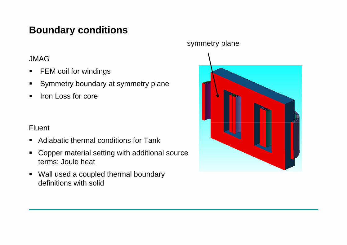
Boundary conditions

JMAG

symmetry plane

FEM coil for windings

Symmetry boundary at symmetry plane

Iron Loss for core Iron Loss for core

Fluent

Adiabatic thermal conditions for Tank

C t i l tti ith dditi l Copper material setting with additional source terms: Joule heat

Wall used a coupled thermal boundary ydefinitions with solid

Mesh element size

JMAG

Elements NodesFluent

Cells Nodes 87434 16344 768176 165747

Exchange of variables between JMAG and Fluent

Fluent

Joule Heat

JMAG

Temperature

Number of iterations

JMAG:

10 analysis steps

FLUENT:

20 sub-iterations

200 iterations

MpCCI:

10 data exchanges

Steady state coupled simulation

• Use staggered communication scheme:

• Convergence acceleration options:Convergence acceleration options: Use initial solution

Use subcycling

Use relaxation

FLUENTi=40 i=60 i=200i=20i=0

JMAGi=2 i=4 i=10i=3i=0


Cooling effect on Joule loss distribution (Logarithmic view)Without CFD coolingMax Joule loss density=1.28e8

With CFD cooling analysis Max Joule loss density=2.22e4


Cooling effect on magnetic flux density

Without CFD cooling analysis With CFD cooling analysis

Max Magnetic Flux density: 2.82 T Max Magnetic Flux density: 1.27 T


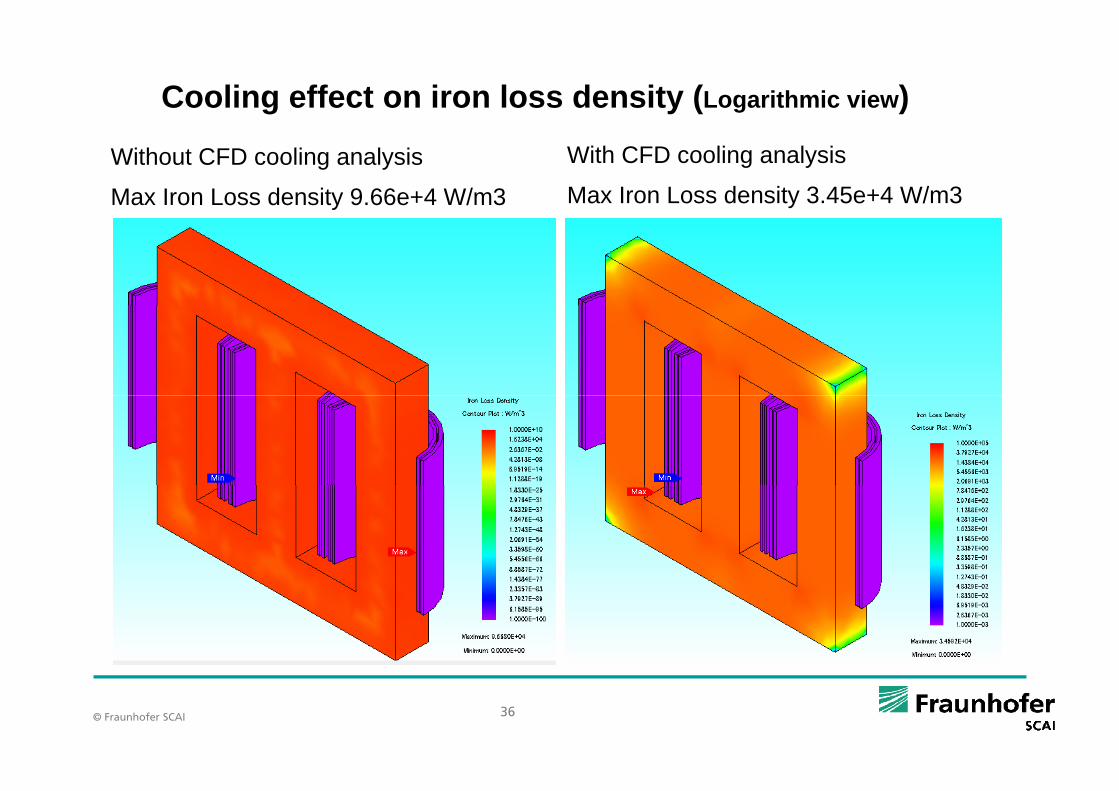
Cooling effect on iron loss density (Logarithmic view)With CFD cooling analysis

Max Iron Loss density 3.45e+4 W/m3Without CFD cooling analysis

Max Iron Loss density 9.66e+4 W/m3


Temperature Distribution in Coils

Max temperature 318.7 K


Velocity streamlines with temperature distribution


Fluid temperature on plane section


Conclusion

Thermal Effects in electrical ComponentsThermal Effects in electrical Components

Co-simulation provides much better and detailed insight into ‘hot spots’Co simulation provides much better and detailed insight into hot spots

Demand request for standardised interfaces for co-simulation

End-users want to be open in the choice of their codes


Contact

Klaus WolfKlaus Wolf

Fraunhofer Institut SCAI

Schloss BirlinghovenSchloss Birlinghoven

53754 Sankt Augustin

Tel: 02241 / 14 2557

Email: [email protected]

Web: http://www.mpcci.de


gekoppelte simulationen von cfdgekoppelte simulationen von ... · pdf filegekoppelte...

Documents