gender bias in standardized tests: evidence from a
TRANSCRIPT

Gender Bias in Standardized Tests: Evidence from aCentralized College Admissions System ∗
Perihan Ozge Saygin†
January 16, 2018
Abstract
Debate regarding student assessment methods, which also concerns the gendergap, has critiqued the use of standardized tests to select and/or assign students tocolleges, given that high school grades are found to be better predictors of collegeperformance. This paper aims to analyze the gender gap in educational outcomesfrom different student assessment methods using Turkish administrative data anda college application setting in which the centralized admission system allocatesstudents based on a composite score, which is a weighted average of high schoolgrade point average and a standardized test score. I find that females significantlyoutperform males in high school grade point average in every subject, and not onlyon average but also at all quintiles. Yet the situation is reversed when it comes tostandardized test scores: Males outperform females in all subjects and almost allquintiles, with the largest magnitude of the difference in quantitative subjects andhighest quintiles.
JEL Classification: I21, I24, I25Keywords: gender gap, standardized test, college admissions, centralized admissions
∗The author declares that she has no relevant or material financial interests that relate to the researchdescribed in this paper. Some of the results presented in this paper are from my PhD dissertation. Anearlier version of this paper was a working paper titled “Do Girls Really Outperform Boys in EducationalOutcomes?”. I am indebted to David Card and Francesca Lotti for their advice and encouragement, andto the Student Selection and Placement Center (OSYM in Turkish) in Turkey for sharing data. I wouldalso like to thank Scott Kostyshak, Andrea Weber, Richard Romano, and anonymous referees for theirinsightful comments. Any errors are my own.†University of Florida, Department of Economics, e-mail: [email protected]

1 Introduction
Standardized tests are commonly used in college applications around the world, millions of
senior high school students annually take a standardized test, as these are the most widely
used college entrance exams. Ideally, the results of the standardized tests are indicative
of a student’s college performance. Yet the debate is twofold: Advocates of standardized
testing argue that the tests offer fair placement by treating everyone equally; their critics
argue that such tests are a poor measure of ability, and that high school grades are found
to be better predictors of college performance (Easton et al. 2017).
In countries with centralized college application systems1, standardized tests remain
the sole determinant of student admissions. In some cases, a student’s high school grade
point average is also considered, and may be combined with a standardized test score to
produce a composite score used for admission decisions; in some decentralized systems,
other required application materials are also considered.
Some studies concerning the gender bias have criticized the use of standardized tests
to select and/or assign students to schools or colleges (Connor and Vargyas (1992);
Medina and Neill (1990); Rosser (1989)). Since the 1970s, for instance, in the United
States the gender gap in SAT takers has averaged 45 points each year. This gender gap
persists despite the reverse in the gender gap in college attendance, and females generally
achieving better freshman year grades than males with the same SAT scores2. As for the
gender gap, the debate on standardized tests has several additional dimensions that may
be relevant. First, most of these standardized tests are associated with a large number
of applicants, which generates higher levels of competition on college entrance exams.
In the case of standardized tests associated with centralized admissions, test scores are
the main determinant of admission, which imposes extra pressure to succeed. Second,
they are usually one-shot tests given annually, and being fast is a comparative advantage.
Given the high-stakes nature of the tests, this creates additional pressure that might affect
the outcome differently if people differ in their performance under pressure. Finally, the
outcomes of standardized tests with multiple-choice questions are presumed to be affected
by willingness to take risks and self-confidence (Ben-Shakhar and Sinai (1991); Badilga
1In some countries, the admission process is centrally coordinated (i.e., examinations are overseen bya central authority, which also determines student placements) or the university system as a whole iscentrally planned, including determination of the number of seats available in each university.
2See The College Board (2012).
1

(2013)).
The literature on gender differences in social preferences and attitudes toward competi-
tion provides consistent evidence that females underperform in competitive environments
(Gneezy et al. (2003); Paserman (2010); Niederle and Vesterlund (2007)). These
findings motivated other studies to explain gender differences in labor markets and edu-
cational outcomes (Croson and Gneezy (2009); Niederle and Vesterlund (2011); Buser
et al. (2014)). For instance, Shurchkov (2012), Ors et al. (2013), and Azmat et al.
(2014) show that the competitive nature of evaluations explains a significant part of the
gender gap in academic examinations. Niederle and Vesterlund (2010) show that the
persistent gender gap in mathematics performance at high percentiles may in part be
explained by the differential manner in which men and women respond to competitive
test-taking environments. In the latest Programme for International Student Assessment
(PISA), Organisation for Economic Co-operation and Development (OECD) also reports
this notable gender difference: In every country tested, girls had much higher levels of
schoolwork- and test-related anxiety than boys. On average across OECD countries, girls
were 17 percentage points more likely to feel ”very anxious” before a test, even if they
were well prepared (OECD, 2017).
Given that there is convincing evidence on significant gender differences in all of these
factors that are relevant to gender bias in a one-shot standardized test, it is possible that
the gender gap might be different in educational outcomes measured by standardized tests
than the gender gap in educational achievement (i.e., grades obtained) during high school
or later in college. If found, a varying gender gap in high school grades compared to stan-
dardized tests is concerning, particularly in countries with centralized college admission
systems in which standardized tests alone determine admissions.
The aim of this paper is to provide an overview of the difference between gender gaps
in educational attainment assessed with different methods and highlight the importance of
this bias in a college application setting, which affects students’ lifetime earnings. Using
administrative data from the centralized university entrance examination in Turkey, I
investigate whether the gender gap in high school GPA differs from the gender gap in
standardized test scores. Focusing on Turkey’s particular institutional setting in Turkey
allows me to compare the gender gap for the same student sample evaluated under diffe-
rent assessment methods, where the combination of these outcomes determines students’
2

college admissions in a centralized system. Due to data limitations, this paper does not
focus on alternative channels through which standardized tests might create a gender
bias, yet it provides evidence for differences in the gender gap under different student
assessment methods, which has important policy implications for designing a university
entrance system.
In addition to demonstrating the advantages of using administrative data on high
school GPA and standardized test scores for the same sample of students3, the Turkish
case is an interesting context studying the potential gender bias in standardized tests
for two reasons. First, the institutional setting in Turkey is a relevant example, and
helps to identify potential bias that could be due to the assessment method. In Turkey,
similar to several other countries in the world4, access to a university education5 is only
possible through a nationwide university entrance exam. Universities have no say in
admissions, and students are allocated by a centralized algorithm based on their scores
and choices. The algorithm assigns applicants according to their final admission score,
which is calculated for each applicant as a weighted sum of the standardized test score
and high school GPA, where the latter has a small weight. The high school GPA is
calculated based on the weighted averages of the grades of every exam during the 4
years of high school education. While most of these are essay or short-answer exams,
the standardized test is a 3-hour multiple-choice test conducted on a national level only
once a year. Moreover, the number of applicants far exceeds the capacity of Turkish
universities; therefore, college applicants compete fiercely for high-return majors in top
universities, with an increasing number of retakers every year. Since the standardized test
is combined with a centralized placement system in Turkey, the test outcome becomes
even more crucial in college admissions. Comparing the gender gap in high school GPA
to the one in standardized test scores in the Turkish college admissions system provides
3The advantage of studying the Turkish case is that high school GPA and standardized multiple-choice test scores are used together to evaluate students for college admissions. Since I observe the samestudents’ high school GPAs and test scores and compare the gender gap in the two different measures ofachievement that are relevant for college admissions, I can argue that the positive selection of females inthe sample of university applicants would be the same for both gender gap estimations.
4United States (SAT and ACT), Sweden (Swedish Scholastic Aptitude Test, abbreviation SweSAT,Hogskoleprovet in Swedish), France (Baccalaureat (or le bac)), Colombia (SABER 11 Exam), Chile (Pru-eba de Seleccion Universitaria or PSU), Brazil (Vestibular or ENEM), and National College EntranceExamination (gaokao) in China. For a summary of worldwide university admission systems and policyissues, see the World Bank report by Helms (2008)
5Both public and private universities accept students through the centralized system; access to privateuniversities is less competitive.
3

a natural setting to investigate potential bias generated by a standardized test applied
in a centralized system, with fierce competition for an outcome as potentially critical as
college admissions.
Second, Turkey is a case that is worth studying because recent reports have yielded
interesting results for the gender gap in educational outcomes in Turkey. While the gender
gap in average educational achievements or in selection into science seems to be compara-
ble to OECD averages, the gender gap in completion rates at all levels of education seems
to be persistent in Turkey. According to PISA 2009 (OECD 2010), although Turkey does
not rank very high in general, gender differences in reading performance favor girls (43
points) and exceed the OECD average, which is 39 points. The gender gap in math per-
formance favors boys by 11 points, but is slightly lower than the OECD average, which is
12 points. Girls outperform boys in science by 17 points, while the OECD average gender
gap was zero. On the other hand, similar to most developing countries, a sizable gap
remains in overall schooling levels in Turkey. In 2014, the percentages of adults who had
attained at least a high school degree in Turkey were 40% for men and 31% for women,
while the OECD averages were 77% and 76%, respectively. As for higher education over-
all (including all vocational, bachelor’s, master’s, and PhD degrees), the percentages of
adults who had attained a higher education degree were 18% for men and 15% for women,
while the OECD averages were 32% and 35%, respectively.
Putting together the OECD reports and PISA findings, it seems that the gender gap
is diminishing or reversing in favor of females in educational outcomes, while the gap in
college enrollment and completion6 remains significant. Although the data in hand do not
allow us to link the gender gap in college enrollment to the potential gender bias due to
standardized tests in a centralized college system, it helps us to shed light on the sources
of the gender gap among college applicants7.
In this paper, I document the gender gap in educational outcomes obtained based on
two different evaluation methods, using a sample of the Student Selection and Placement
System (OSYS in Turkish) for college admissions in Turkey in 2008. After a descriptive
6The gender gap in admissions to top-ranked universities is also found to be persistent Saygin (2016).7This is particularly important in Turkey, because Turkey has one of the highest earnings premiums for
tertiary education among OECD countries. In 2013, tertiary-educated adults earned 88% more on averagethan adults with upper secondary education (the OECD average proportion was 60%). The returns toschooling are found to be even more significant for females in Turkey: In 2013, tertiary-educated womenaged 25-64 years earned 111% more than those with an upper secondary education while the OECDaverage was 63% (OECD 2015).
4
analysis of data and a graphical analysis of gender differences, I estimate the average
gender gap, as well as at different quantiles of the test score and high school GPA dis-
tributions. First, I explore the gender gap in high school GPAs in different high school
tracks and find a significant and large gender gap in favor of female students at all quan-
tiles of high school GPAs in all high school tracks. Second, I analyze the gender gap in
standardized test scores in different subjects, and find that females’ superior performance
reverses when it comes to standardized test scores. Conditional on high school GPA, I
find a significant gender gap in favor of males, with the largest magnitude in quantitative
subjects and highest quintiles.
These findings are important not only because this is a comprehensive study that
compares the gender gap under different assessment methods using administrative data,
but it also provides evidence on variations in the gender gap under different evaluation
methods. Although it is difficult to disentangle the different channels that can create the
difference in gender gap under the two student assessment methods, this paper’s findings
are consistent with the literature on gender differences in attitude toward competition
and pressure8. The fact that female students outperform males in terms of high school
grades but are not as successful on standardized tests raises the question of whether the
competitive nature and pressure of a 3-hour exam for such a critical matter might have a
negative effect on females, especially at the higher ends of test score distributions - i.e.,
the range that results in top-ranked university placements.
The structure of the paper is as follows. In the next section, I describe the instituti-
onal setting, which is relevant for the gender gap analysis. Section 3 describes the data
and presents a detailed descriptive analysis of the sample and the gender gap in various
outcomes. I present the main empirical analysis and results in Section 4, and Section 5
concludes with discussion of the interpretation of the findings and further channels to be
explored.
2 College Admissions in Turkey
Admission to both public and private universities has been conducted using a centralized
system since 1974. Access to any kind of higher education program is provided only
through a standardized test called the Student Selection Test (OSS in Turkish) that
8I provide a brief discussion of interpretation of results in the concluding section.
5
is administered at the national level annually around June — i.e., at the end of the
academic year— by a central authority (Student Selection and Placement Center; OSYM
in Turkish). After taking the test and receiving their scores, applicants submit a list of
higher education programs in order of preference, and OSYM assigns students to each
university program (major) according to the preferences and test scores9, and given each
program’s limited capacities. In other words, each applicant gets one or no assignment as
an outcome of the allocation mechanism, in which universities and/or departments have
no say.
Looking more closely at college applications, every year approximately 90% of senior
high school students take the test, along with retakers who did not get a desirable assign-
ment in previous years. In 2008, about 1.6 million applicants took the university entrance
examination; about 20% were high school graduates who were taking the exam for the
first time, and the rest were retakers. Given the limited capacities of university programs,
there is significant excess demand. Only 51% of applicants10 are assigned to a university
program, which leads to a growing number of retakers every year. This creates fierce
competition for a seat at a high-quality university and a major with high and secured
returns on the labor market. Those who do not get an assignment must wait a year to
try again. Given these numbers, college admissions is clearly a very competitive matter,
which starts influencing students’ lives much earlier than the actual application period;
students and their families face more extreme pressure during the last year of high school.
In terms of the gender gap, it seems that female students are less likely to take the
test for university entrance. In 2008, 44% of high school graduates eligible to apply for
the university entrance test were female, while only 38% of applicants (including retakers)
were female. Another significant gender gap seems to be present in retaking ratios: 55%
of females and 66% of males are retakers, while for those who end up being assigned to
a university program, 76% of females and 84% of males have taken the test at least once
before.
The formal education system in Turkey consists of primary education, high school
education, and university. Allocation of primary school graduates to high schools is
also conducted by a centralized system with a standardized test. Depending on their
9See Balinski and Sonmez (1999) for further information about the allocation algorithm.10Out of 1.6 million applicants, only 16% were assigned to four-year university programs, 15% were
assigned to two-year programs, and 20% were assigned to distance-education programs.
6

test scores, all students are sorted into different type of high schools in line with their
preferences11. After entering high school, another important decision students face in their
second year is the choice of a subject track: Sciences, Social sciences, Equally-Weighted12,
foreign languages, or arts. This specialization results in different subject curricula.
The OSS test consists of two main parts, a quantitative and a qualitative section13, and
there are two sets of these sections, in which questions for Quantitative-I and Qualitative-
I are less sophisticated than those for Quantitative-II and Qualitative-II. All applicants,
regardless of their high school track, are expected to answer the questions in Quantitative-
I and Qualitative-I, while Quantitative-II and Qualitative-II are required only for certain
university major applications. For instance, the Qualitative-II section is irrelevant for a
student with a science high school specialization subject who aims to obtain an engineering
major, and the Quantitative-II section is the most relevant. Similarly, a student who
followed a social science track in high school does not need to focus on the Quantitative-
II section, but she must maximize her correct answers on Qualitative-II. These scores are
calculated for different categories, in which differing weights are given across sections of
the test14.
High school GPA is also part of the evaluation for university entrance, even though it
has a rather small impact. First, three types of high school GPA scores are calculated that
consider grades in social science, science, and equally weighted subject tracks15. These are
calculated by taking high school track subjects into account to give, for instance, students
who chose science as their track a bonus when calculating the science GPA score. These
weighted high school GPA scores are then added to OSS test scores in their correspon-
ding subjects to calculate the final admission score for assignments16. Each university
program puts emphasis on one of these admission score types. For instance, a student
11This examination is called the Secondary School Examination (OKS in Turkish) and is administeredby the Ministry of Education. The aim of this examination is to restrict access to top-ranked high schoolsthat are expected to provide a higher standard of education. Those types include Anatolian High Schools,Scientific High Schools, Foreign Language High Schools, and some private high schools. There are alsogeneral type high schools as well as vocational high schools that are open to every student, regardlessof their test scores on the OKS. OKS test scores, therefore, are only important for students who aim toattend one of these top-ranked high schools.
12This track focus on Turkish and mathematics and give equal weight to both and relatively less weightto science
13There is also an additional foreign language section.14A higher weight is given to the math and science sections when calculating quantitative test scores.15Equally weighted high school GPA scores are calculated considering the grades in math and Turkish
subjects equally and give lower importance to science.16These weights lead to a situation in which students are strongly encouraged to apply to university
programs that fit their high school specialization tracks.
7

can be assigned to an engineering major according to the Quantitative-II admission score,
which is calculated as a weighted sum of the OSS test score in Quantitative-II and the
quantitative-weighted high school GPA.
The empirical analysis of the gender gap in test scores and high school GPA will be
performed by considering different type of test scores, high school GPA, and high school
tracks.
3 Data, Descriptive Statistics, and Sample Selection
The dataset employed in this study was obtained by merging the 2008 OSS dataset and
the 2008 Survey of OSS Applicants and Higher Education Programs dataset. The OSS
dataset provides administrative individual information on test scores, high school GPA,
submitted choice list of university programs, and assignment outcome for 1,646,376 ap-
plicants. In contrast, the Survey of OSS applicants conducted by OSYM asks applicants
about the socioeconomic characteristics of their household, their high school achievements,
expenditures on private tutorials, and their views on high school education. The survey
is conducted online, and 62,775 applicants answered the survey questions in 2008. I have
access to only a random sample of about 16%, with 9,983 observations17.
Table 1 provides summary statistics for the sample of 9,983 applicants in the 2008
OSS dataset. It is clear that on average, females have higher high school GPAs and test
scores, and a lower rate for retaking the test than males. Similar characteristics hold
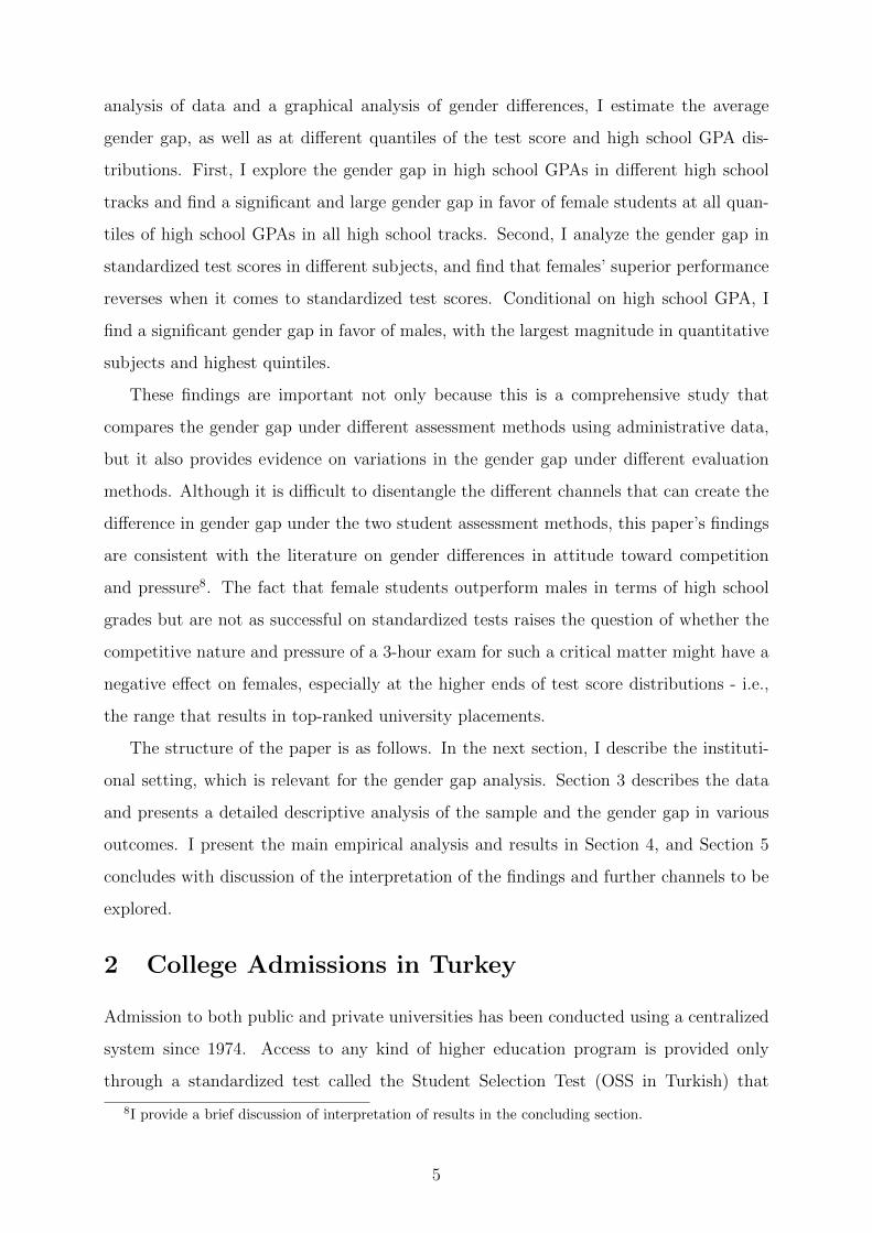
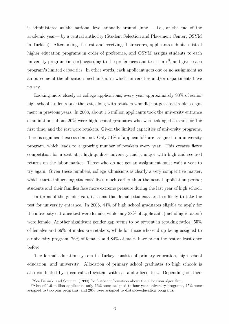
when only first-taker applicants are considered. On closer examination, Figure 1 shows
cumulative distribution functions of high school GPA and weighted GPA scores, and there
is visible female outperformance in all GPA distributions. On the other hand, looking at
Figure 2, in which standardized test score distributions are shown, female outperformance
is less clear —especially at the highest ends of the distributions— and disappears once I
condition on high school GPA, as shown at Figure 3.
As our sample consists only of university entrance test applicants who are senior high
school students and those who already graduated from high school, we do not observe
those who either drop out or graduate from high school but do not apply for university.
Although the gender gap in terms of university applications is not as severe as seen in
17I provide more information on sample selection in the appendix. Also, OSYM provided a report toshow that the sample that answered the survey is representative of the whole population of universityapplicants in 2008; this report is available on their website: http://osym.gov.tr/belge/1-10386/2008-ogrenci-secme-ve-yerlestirmesistemi-osys-2008-osy-.html.
8

earlier levels of education, still 44% of high school graduates were girls, while only 38% of
applicants (including retakers) were girls. As girls are less likely to obtain a high school
degree and take the university entrance test, this might create a positive selection bias.
Hence, the estimates of gender gap in high school GPA and test scores could be biased in
favor of girls due to positive selection. Indeed, it seems that females have better financial
support and their parents are relatively better educated with respect to boys. Table 2
shows parental education and family support indicators by gender, and that the mean
differences in parental education levels are positive and significant. Female applicants not
only have better educated parents, but they are also significantly more likely to attend
private tutoring centers. Additionally, it seems that their parents are more likely to be
willing to pay a private university tuition, which is considerably higher than the tuition
at public universities. Looking at sample descriptive statistics, selection could be an
issue for precise estimate of the gender gap. On the other hand, this paper aims to
detect a significant difference in gender gap estimates in student outcomes assessed under
different methods (high school GPAs vs standardized test scores) for the same exact
sample. Therefore, it is possible to argue that selection bias would be the same for both
gender gap estimations. There is no reason to expect that positive selection of females
would bias the gender gap in high school GPA more than the gender gap in test scores,
since they are both relevant for university applications and all students in my sample are
university applicants.
Although selection is not expected to confound the results of interest, to reduce the
selection bias I use a rich set of control variables as well as high school type, track, and
city fixed effects. Controlling for high-school-related fixed effects is crucial to control for
unobserved heterogeneity, as selection into high schools is also based on a national exam
with a high level of competition for the best high schools. Table 3 shows high school type
and track subjects by gender for both the first-taker sample and the whole sample. In
the following section, the gender gap is estimated for several subsamples to ensure that
selection into retaking, high school type, and tracks do not substantially affect the results.
4 Empirical Design
In this section, to determine whether there is a difference in gender gap in high school
GPA compared to the gender gap in test scores in a more comprehensive empirical setting,
9

I analyze the gender gap in high school GPA and weighted high school GPA scores and
OSS test scores. I compare gender differences in different subjects and compare them on
different samples, taking into account selection into high school tracks in the empirical
design explained below. The variable of interest, M , is an indicator variable taking the
value of 1 for male applicants and 0 otherwise. Let the educational outcome Y (high
school GPAs and OSS test scores) of applicant i, graduating or graduated from high
school school type h, with track t be denoted by Yiht, then the model is given by:
Yiht = δMi + x′iβ + µh + µt + εiht (1)
where i = 1, ...N , h = 1, ...H, t = 1, ..., T , and εiht is a random error term.
The goal is to identify whether the estimate of δ is different when the outcome is high
school GPA as opposed to the outcome of test scores. I separately estimate this model for
both high school GPA and test scores in different track subjects18 in order to elaborate
on the differences in gender gap in different subjects.
Further, I test whether the estimates of δ change when the model is estimated on
different subsamples of applicants, such as only first-time takers, only first- and second-
time takers19, and subsamples of different high school types and tracks. The dataset
described in the previous section allows the use of a rich set of control variables20, high
school type, and high school city fixed effects, as well as high school track-subject fixed
effects with robust standard errors. As explained in Section 2, the process for transition
to high schools in Turkey is based on a similar centralized standardized-test-based system,
and therefore students are already sorted into different types of high schools based on their
observed and unobserved characteristics. This feature helps to control for unobserved
individual characteristics once I control for high-school-related fixed effects.
18The types of scores are Equally Weighted-I, Equally Weighted-II, Qualitative-II, Qualitative-II,Quantitative-I, and Quantitative-II.
19This analysis is necessary not only because retaking status could be a crucial determinant of success,but it is also important because selection into retaking is not equal across gender. As mentioned earlier,when we consider the full sample of applicants including retakers, female applicants’ share drops to 38%,while among new high school graduate applicants, this share is 44%.
20I introduce indicator variables for working status and attending private tutoring. Household controlsinclude mother and father education categorical variables, as well as an index of availability of opportu-nities in the household in which the applicant lives. This index is created based on access to internet,own room in the house, buying a daily newspaper, number of books, etc.
10

4.1 The Gender Gap in High School GPA
Estimation results for high school GPA are reported in Table 4, in which high school type,
track subject, and city fixed effects are included, as well as controls for other individual
characteristics such as retaking, private tutoring, and working status, and household
controls. The gender gap in high school GPA is around 5 points, where the average high
school GPA of the sample is 73.63 with a standard deviation of 11.65. The following
columns of Table 4 report results for, respectively, the sample of only first- and second-
time takers, only first-time takers, and finally only applicants with one of the three main
high school subjects, which excludes technical and vocational high school types.
High school GPA is used as an input to calculate the weighted high school GPA
scores to be combined with standardized test scores to calculate the assignment score
for university entrance. These weighted high school GPA scores are calculated in three
different categories: Quantitative High School GPA Score, Qualitative High School GPA
Score, and Equally Weighted High School GPA Score. I estimated the gender gap in these
high school GPA scores separately, and results are reported in Tables 5–7, which provide
evidence for a statistically significant gender gap in favor of females in all tracks.
Results for Equally Weighted High School GPA Scores are reported in Table 5. The
first column represents the whole sample and reports a gender gap of 3.02 points in favor
of females. The gender gap remains almost the same when we exclude retakers who had
taken the OSS test more than once before. On the other hand, the gender gap among
first-time takers reported in column 3 seems to be relatively smaller than the gender gap in
the whole sample. Column 4 represents applicants with one of the three main high school
subjects, while column 5 also excludes science background students21. Similar results
are obtained for Qualitative and Quantitative High School GPA scores, and results are
reported in Tables 6 and 7, respectively. It seems that the magnitudes of the gender gap
in favor of females is similar for Equally Weighted and Quantitative High School GPAs
while female outperformance is slightly smaller for Qualitative High School GPA.
After confirming that females outperform, on average, on high school GPA in all high
school tracks, I estimated the gender gap in high school GPA using a quantile estimation
method. Results are reported for overall high school GPA and subject weighted GPA
scores in Table 8. While the overall high school GPA is estimated on the full sample, the
21Column 5 includes applicants with equally-weighted and social science tracks.
11

gender gap in subject-weighted high school GPA scores is estimated on the subsample
of students in corresponding high school tracks. The first columns in Table 8 show OLS
results with robust standard errors and the following columns show quantile regression
results for the 10th, 25th, 50th, 75th, and 90th percentiles, respectively. I find a significant
gender gap in favor of females at all percentiles, with slight changes in magnitude, but
are mostly comparable to their OLS estimates. Female outperformance is highest at the
75th percentile in Equally Weighted and Qualitative High School GPA Scores, while it
is highest at the 25th percentile for Quantitative Weighted GPA Score and gets smaller,
but remains significant, at the 90th percentile. I do not find a significant difference in
the gender gap when I run the estimation on only the subsample of first-time takers or
first- and second-time takers. In all types of GPA estimations, there is a slight increase
in magnitude of the gender gap in favor of females when I consider the subsample of
first-time takers compared to the sample of all 9,983 applicants22.
4.2 The Gender Gap in Standardized Test Scores
OSS test scores in the different subjects are calculated based on the number of correct
and incorrect answers in relevant sections of the test for each category23. The three main
test scores —Quantitative-I, Qualitative-I, and Equally Weighted-I— are calculated based
on the four main sections of the test: Turkish-I, Social Science-I, Math-I, and Science-I.
These sections are relevant for all applicants regardless of their high school track subject,
and the three test scores are calculated for all applicants, no matter which major they are
interested in.
There are also subject-specific test scores: Quantitative-II, Qualitative-II, and Equally
Weighted-II. These scores are calculated based on performance on the second part of the
test, which is designed to be more sophisticated. For instance, for the Quantitative-II
test scores, the number of correct answers in the Math-II and Science-II sections would
be particularly important while for those who want to maximize the Qualitative-II test
score, the Social Science-II and Turkish-II sections are the most important.
First, I estimate the gender gap for the three main test scores, which are calculated
for all applicants, so that gender gap estimates will not be exposed to any bias due to
sorting into high school track subjects. Estimation results are reported in Table 9, where
22Results are available upon request.23Every four incorrect answers cancels out one correct answer.
12

high school type, track subject, and city fixed effects are included, controlling for other
individual characteristics such as retaking, private tutoring, and working status as well
as parents’ education status. The first three columns report results for the whole sample,
where the dependent variables are Equally Weighted-I, Quantitative-I, and Qualitative-I
test scores, respectively. A significant gender gap in favor of females is found for Equally
Weighted-I and Qualitative-I test scores by 1.66 and 3.19 points, respectively, while males
outperform, on average, on Quantitative-I test scores by 2.39 points. Once I estimate
the gender gap by excluding retakers who had taken the test more than once before, the
gender gap in favor of females for Qualitative-I and Equally Weighted-I becomes larger
in magnitude, and male outperformance on Quantitative-I loses significance.
On the other hand, the gender gap in test scores reverses once it is estimated condi-
tional on high school GPA. Table 10 shows the same specifications as Table 9, in which
the only difference is the addition of high school GPA as a control in the estimations.
There is a significant gender gap in all test scores in favor of males, with particularly high
magnitude in quantitative scores, and results do not seem to change significantly on the
subsample of first-time takers.
Second, I estimate the gender gap in subject-specific test scores and report the results
in Table 11. The first three columns report results for the sample of applicants with their
corresponding high school tracks, while the last three columns consider only first- and
second-time takers of these samples. Similar to the main subject test scores, I find a
significant gender gap in favor of females for Qualitative-II and Equally Weighted-II test
scores, while there is no significant difference in Quantitative-II test scores. The gender
gap in favor of females is 6.52 and 5.97 points in Equally-Weighted-II and Qualitative-II
test scores, respectively, where male outperformance is not significantly different from
zero, as indicated by the positive and insignificant coefficient. Again, once I exclude the
retakers who took the OSS test more than once before, the significant gender gap estimates
in favor of females become slightly larger in magnitude, but this difference seems to be
negligible.
The gender gap in subject-specific test scores is also found to be reversing once I
condition on high school GPA. Table 12 shows the same specifications as Table 11, with the
addition of high school GPA in the control variables. Once high school GPA is controlled
for, the gender gap in subject-specific test scores favors males and is significant in all
13

subjects, with a particularly high gap in magnitude in the Quantitative-II score. Once
retakers are excluded, male outperformance loses significance for the Qualitative-II and
Equally Weighted-II scores, but the gap in the Quantitative-II score remains significant
and the magnitude remains unaffected.
It seems that there is clearly significant male outperformance in both main and subject-
specific test scores in all subjects, and the magnitude of the gap is especially large when
it comes to quantitative scores.
I also used a quantile estimation method for the main test scores on the full sample
and for the subject-specific test scores on the subsamples of applicants with relevant high
school tracks. Results are reported in Tables 13 and 14, respectively. As for the gender
gap in main test scores, I find a significant gap in favor of males for all quantiles, with
an increasing gap at higher quantiles of the test score distributions. The highest gap
is found to be 9.48 points in the highest quintile of the quantitative test scores, while
the lowest significant gap is 2.04 points in the lowest quartile of the qualitative score
distribution24. Table 14 shows that the gap in subject-specific test scores exhibits similar
patterns, with an even larger magnitude in quantitative scores. It is also important to
underline that these subject-specific assignment scores are the relevant scores for top
majors, such as medical school, law school, engineering, economics, sciences, etc. For
instance, the Quantitative-II test score is obtained from the more sophisticated sections of
the test, compared to the Quantitative-I test score —and is the relevant score for medical
school admission— while the Quantitative-I test score is required for 2-year vocational
programs or 4-year majors associated with lower paying jobs. This implies that the gap
in standardized test scores is not only larger at higher quintiles, but also higher in scores
that are relevant for highly ranked majors.
5 Interpretation of Results and Conclusion
In this paper, I compare the gender differences in educational outcomes based on different
student assessment methods. High school GPAs and standardized test scores are used
jointly to evaluate students in a centralized college admissions system in Turkey. Using
administrative data, I show that female students outperform male students in terms of
high school GPA, both on average and at all quantiles of the distributions. I also estimate
24The gap is not significant in the lowest quintile of the Qualitative-I and Equally Weighted-I scoresdistributions.
14

the gender gap in standardized test scores in different subjects, both on average and at
different quantiles of the test score distribution. Conditional on high school GPA, I find
that the gender gap in favor of females reverses in test scores and becomes especially
large in the higher quantiles of the quantitative score distribution, while I find mostly
absolute female outperformance on high school GPA across the distribution. Comparing
these findings, I argue that the gender gap is affected by the student assessment method
used in a centralized system of college admissions.
With careful analysis of the gender gap using administrative data, these results provide
evidence for potential gender bias in the use of standardized tests as an assessment met-
hod. This evidence is crucial, given previous findings suggesting that high school GPAs
are better predictors of college performance than standardized test scores (Easton et al.
2017). The findings of this paper are also consistent with the literature on gender differen-
ces in social preferences and attitudes toward competition. Female students outperform
males strongly in terms of high school GPA, which is an average of all grades obtained
during high school education from mostly essay-type exams, while they fall behind when
it comes to a 3-hour standardized test taken under the pressure of losing an entire year
if they do not score high enough. This evidence is consistent with findings from previous
literature suggesting that females might underperform when the assessment is conducted
under pressure and characterized by high competition, especially in quantitative subjects.
Given previous findings showing that standardized tests are less predictive of college
success, this difference in gender gap in high school GPA and test scores could create
inefficiencies. Moreover, since centralized college admissions in Turkey place a dispro-
portionate weight on standardized test scores compared to high school GPA, this seems
to penalize females, who have a tendency to perform worse under pressure, by creating
unequal opportunities to access highly ranked majors and universities. Looking at these
findings, it is possible to argue that standardized tests might be responsible for part of
the gender gap due to their competitive nature combined with the pressure of the centra-
lized system. On the other hand, it is possible to propose other channels that might be
consistent with these findings, in particular female outperformance on high school GPA.
One possibility is that high school GPA is less objective than standardized tests and
there might be a gender bias in favor of female students, especially in male-dominated
subjects (Breda and Ly, 2015). Duckworth and Seligman (2005) show that self-discipline
15

predicts academic performance in school. If female students are more self-disciplined,
and self-discipline is rewarded by teachers on GPA more than the positive effect of self-
discipline on test performance, GPA could possibly advantage females. Another potential
explanation for the lower GPA of males could be an economic model in which individuals
derive utility from both academic performance and popularity among peers, the latter
being more negatively correlated with academic performance for males (the social stigma
of being a “nerd”, or “masculinity” being negatively associated with GPA) (DiPrete and
Buchmann, 2013)25. Yet it is difficult to argue that these alternative channels could drive
these results, considering the significantly large magnitude of female outperformance on
high school GPA that reverses to become a gender gap in favor of males in even larger
magnitude.
While distinguishing between the different hypotheses is important, it is not possible
to test these alternative hypotheses in this study. Rather, this paper is a step toward
understanding the potential gender bias driven by standardized tests in a centralized
system. Given that decentralized admissions in college applications have been increasingly
replaced by centralized admissions in many countries, empirical evidence on topics that
are usually understudied, such as gender bias, becomes particularly vital26. Standardized
test scores in decentralized systems27 are not the only determinant of college admissions,
and therefore the lesser importance of standardized test scores might be associated with
a lower or reversing gender gap in college enrollment. Studying the case of Turkey as an
extreme example also opens channels for further investigation of whether the gender bias
would have less impact on college enrollment in decentralized systems.
25In Turkey, students know that high school GPA, even if with a low weight, will impact collegeadmissions, and therefore it is possible to argue that the impact of popularity’s being negatively correlatedwith performance could be relatively lower.
26Machado and Szerman (2016) study transition in the Brazilian higher education market and investi-gate the impacts on student sorting, migration, and enrollment. Hafalir et al. (2017) provide a theoreticalcomparison of centralized college admissions to decentralized ones in terms of the efficiency of allocationof abilities.
27In the United States, students not only take centralized exams like the Scholastic Aptitude Test(SAT), but also complete college-specific requirements such as essays.
16

References
Azmat, C. Calsamiglia and N. Iriberri 2014. Gender differences in response to big stakes. CEP DiscussionPapers, CEPDP1314. Centre for Economic Performance, London School of Economics and PoliticalScience, London, UK.
Baldiga, K. 2013. Gender Differences in Willingness to Guess, Management Science 60(2), 434 - 448.
Balinski M. and T. Sonmez, 1999. A Tale of Two Mechanisms: Student Placement, Journal of EconomicTheory 84(1), 73-94.
Ben-Shakhar, G. and Y. Sinai, 1991. Gender Differences in Multiple-Choice Tests: The Role of DifferentialGuessing Tendencies, Journal of Educational Measurement 28(1), 23-35.
Breda, T. and Ly, S. T., 2015. Professors in Core Science Fields Are Not Always Biased against Women:Evidence from France, American Economic Journal: Applied Economics 7(4): 53-75.
Buser, T., M. Niederle, and H. Oosterbeek, 2014. Gender, Competitiveness and Career Choices, TheQuarterly Journal of Economics, 1409-1447.
Connor K. and E. Vargyas, 1992. The Legal Implications of Gender Bias in Standardized Testing, BerkeleyWomen’s Law Journal.
Croson, R, and Gneezy, U., 2009. Gender Differences in Preferences, Journal of Economic Literature47(2): 448-474.
DiPrete T. A. and Buchmann C., 2013. Rise of Women, The: The Growing Gender Gap in Educationand What it Means for American Schools, Russell Sage Foundation.
Duckworth A. L., Seligman M. E. P., 2005. Self-discipline outdoes IQ in predicting academic performanceof adolescents. Psychological Science, 16: 939-944.
Easton, J.Q., Johnson, E., and Sartain, L. 2017. The predictive power of ninth-grade GPA. Chicago, IL:University of Chicago Consortium on School Research.
Gneezy, U., M. Niederle, and A. Rustichini, 2003. Performance in Competitive Environments: GenderDifferences, Quarterly Journal of Economics 118(3), 1049-1074.
Hafalir, Isa E., R. Hakimov, D. Kbler, and M. Kurino, 2017. College Admissions with Entrance Exams:Centralized versus Decentralized, Unpublished manuscript.
Helms R. M., 2008. University Admissions Worldwide, World Bank, Education Working Paper SeriesNumber 15
Machado C. and C. Szerman, 2016. Centralized Admission and the Student-College Match, Unpublishedmanuscript.
N. Medina, and D. Neill., 1990. Fallout From the Testing Explosion, National Center for Fair and OpenTesting.
Niederle, M., and L.Vesterlund, 2007. Do Women Shy away from Competition? Do Men Compete tooMuch?, Quarterly Journal of Economics 122(3), 1067-1101.
Niederle, M., and L.Vesterlund, 2010. Explaining the Gender Gap in Math Test Scores: The Role ofCompetition, Journal of Economic Perspectives, 24(2), 129-144.
Niederle, M., and L.Vesterlund, 2011. Gender and Competition, Annual Review in Economics, 3, 601-630.
OECD, 2010. PISA 2009 at a Glance, OECD Publishing, Paris.
OECD, 2015. Education at a Glance 2015: OECD Indicators, OECD Publishing, Paris.
17

OECD, 2017. Schoolwork-related anxiety, in PISA 2015 Results (Volume III): Students’ Well-Being,OECD Publishing, Paris.
Ors, E., F. Palomino, E.A. Peyrache, 2013. Performance Gender-Gap: Does Competition Matter?, Jour-nal of Labor Economics 31(3), 443-499.
Paserman, M. D., 2010. Gender Differences in Performance in Competitive Environments: Evidence fromProfessional Tennis Players, Mimeo, Boston University and Hebrew University.
Rosser, P., 1989. The SAT the gender gap: Identifying the Causes, Center for Women Policy Studies.
The College Board, 2012. SAT Report on College & Career Readiness.
Saygin, P.O. 2016. Gender Differences in Preferences for Taking Risk in College Applications, Economicsof Education Review, 52, 120-133.
Shurchkov, O., 2012. Under Pressure: Gender Differences in Output Quality and Quantity Under Com-petition and Time Constraints, Journal of the European Economic Association 10(5): 1189-1213.
18

A Figures and Tables
Figure 1: Cumulative Distribution Functions: High School GPA
Note: The top left graph shows the cumulative distribution functions of high school GPA of femaleand male applicants. The top right graph shows the cumulative distribution functions of the EquallyWeighted Type (EW) of weighted high school GPA scores of female and male applicants. The bottomleft graph shows the cumulative distribution functions of the Qualitative Type (QL) of weighted highschool GPA scores of female and male applicants. The bottom right graph shows the cumulative distri-bution functions of the Quantitative Type (QT) of weighted high school GPA scores of female and maleapplicants.
19

Figure 2: Cumulative Distribution Functions: Test Scores
Note: All graphs show the cumulative distribution functions of standardized test scores for femaleand male applicants in different subjects. EW, QT, and QL indicate Equally Weighted, Quantitative,and Qualitative, respectively. EW1, QT1, and QL1 are the types of test scores calculated based onachievement on less sophisticated sections of the test, while EW2, QT2, and QL2 indicate the types oftest scores for more advanced sections.
20

Figure 3: Cumulative Distribution Functions: Test Scores Conditional on GPA
Note: All graphs show the cumulative distribution functions of standardized test scores for female andmale applicants in different subjects conditional on high school GPA. EW, QT, and QL indicate EquallyWeighted, Quantitative, and Qualitative, respectively. EW1, QT1, and QL1 are the types of test scorescalculated based on achievement on less sophisticated sections of the test, while EW2, QT2, and QL2indicate the types of test scores for more advanced sections.
21

Table 1: Achievements by Gender on 2008 University Entrance Tests
Female Male All sample FT Female FT Male All FT
High School GPA 76.53 72.03 73.63 78.85 72.44 75.19(11.21) (11.58) (11.65) (12.66) (13.61) (13.58)
QT Weighted GPA Score 82.44 78.53 79.92 87.12 82.58 84.53(9.63) (10.26) (10.22) (10.06) (11.84) (11.34)
QL Weighted GPA Score 85.89 82.23 83.53 90.00 85.90 87.65(7.89) (8.68) (8.59) (7.96) (9.90) (9.34)
EW Weighted GPA Score 84.69 80.89 82.24 89.24 84.96 86.80(8.69) (9.44) (9.36) (8.82) (10.83) (10.24)
Test Score EW 1 212.55 206.03 208.34 226.25 215.98 220.38(35.90) (42.80) (40.60) (37.92) (50.79) (45.99)
Test Score EW 2 153.68 145.22 148.22 160.89 150.27 154.82(83.63) (86.58) (85.64) (92.75) (95.40) (94.40)
Test Score QT-1 188.20 188.75 188.55 204.08 201.86 202.82(38.71) (45.26) (43.04) (41.82) (53.99) (49.15)
Test Score QL-1 219.11 209.58 212.96 230.16 217.15 222.72(34.24) (42.05) (39.72) (35.38) (48.30) (43.70)
Test Score QT-2 111.46 106.15 108.04 133.93 127.82 130.44(98.32) (100.30) (99.63) (104.54) (109.53) (107.43)
Test Score QL-2 111.57 96.25 101.69 93.62 71.46 80.96(101.90) (101.46) (101.87) (107.29) (99.37) (103.39)
Birth year 1988.23 1987.68 1987.88 1989.77 1989.65 1989.70(2.55) (2.99) (2.85) (1.14) (1.36) (1.27)
OSS exam retake 0.78 0.84 0.82(0.41) (0.37) (0.38)
Previously Assigned Retaker 0.24 0.32 0.29(0.43) (0.47) (0.46)
Assigned to College 0.63 0.62 0.62 0.67 0.61 0.64(0.48) (0.49) (0.49) (0.47) (0.49) (0.48)
Source: OSYM08 Administrative Dataset, own calculations.Note: EW, QT, and QL indicate Equally Weighted, Quantitative, and Qualitative, respectively. Columns 4 to 6 showdescriptive statistics for first-time taker (FT) subsamples.
22

Table 2: Family Characteristics of OSS 2008 Applicants by Gender
Female Male All sample
If working 0.19 0.34 0.29(0.40) (0.47) (0.45)
House Index 7.29 6.92 7.05(1.21) (1.45) (1.38)
Adult Support Index 2.62 2.57 2.59(0.85) (0.81) (0.82)
Mother Education Not Reported 0.00 0.01 0.01(0.06) (0.09) (0.08)
Mother No School 0.11 0.23 0.19(0.32) (0.42) (0.39)
Mother Primary School 0.47 0.43 0.44(0.50) (0.49) (0.50)
Mother Middle School 0.12 0.11 0.11(0.32) (0.31) (0.32)
Mother High School 0.20 0.15 0.17(0.40) (0.36) (0.37)
Mother College or Beyond 0.10 0.07 0.08(0.29) (0.25) (0.27)
Father Education Not Reported 0.02 0.03 0.02(0.14) (0.16) (0.16)
Father No School 0.03 0.07 0.06(0.18) (0.26) (0.23)
Father Primary School 0.29 0.32 0.31(0.45) (0.46) (0.46)
Father Middle School 0.16 0.14 0.15(0.37) (0.35) (0.36)
Father High School 0.27 0.25 0.26(0.45) (0.43) (0.44)
Father College or Beyond 0.22 0.19 0.20(0.42) (0.39) (0.40)
23

Table 3: High School Type and Subject by Gender
Female Male All sample FT Female FT Male All FT
HS Type
Anatolian HS 0.12 0.11 0.11 0.30 0.27 0.28(0.32) (0.31) (0.31) (0.46) (0.45) (0.45)
Scientific HS 0.01 0.01 0.01 0.02 0.03 0.02(0.10) (0.11) (0.10) (0.13) (0.17) (0.15)
General HS 0.45 0.49 0.48 0.08 0.16 0.12(0.50) (0.50) (0.50) (0.27) (0.36) (0.33)
Foreign Language HS 0.15 0.08 0.11 0.32 0.19 0.24(0.36) (0.27) (0.31) (0.46) (0.39) (0.43)
Vocational HS 0.24 0.27 0.26 0.25 0.31 0.28(0.43) (0.45) (0.44) (0.43) (0.46) (0.45)
HS Subject
Science 0.29 0.34 0.32 0.36 0.41 0.39(0.45) (0.47) (0.47) (0.48) (0.49) (0.49)
Social 0.12 0.14 0.13 0.10 0.11 0.10(0.32) (0.35) (0.34) (0.30) (0.31) (0.31)
Math and Social Sciences 0.36 0.28 0.31 0.31 0.23 0.26(0.48) (0.45) (0.46) (0.46) (0.42) (0.44)
Others 0.23 0.23 0.23 0.23 0.25 0.24(0.42) (0.42) (0.42) (0.42) (0.43) (0.43)
Source: OSYM08 Administrative Dataset, own calculations.Note: HS indicates high school. Columns 4 to 6 show descriptive statistics for first-time taker (FT) subsamples.
Table 4: High School GPA Estimations
(1) (2) (3) (4)
Male -4.76 -5.60 -5.26 -5.75(.25)∗∗∗ (.37)∗∗∗ (.63)∗∗∗ (.38)∗∗∗
Second Takers .04 1.13 .72(.24) (.40)∗∗∗ (.43)∗
Enrollment in Private Tutoring Instituion 2.79 3.72 4.45 3.35(.27)∗∗∗ (.46)∗∗∗ (1.00)∗∗∗ (.52)∗∗∗
Taking One-to-One Private Tutoring -2.24 -2.76 -3.37 -2.72(.29)∗∗∗ (.41)∗∗∗ (.72)∗∗∗ (.43)∗∗∗
If working -2.02 -2.29 -1.61 -2.28(.26)∗∗∗ (.46)∗∗∗ (.92)∗ (.52)∗∗∗
Obs. 9983 4991 1792 3966
F statistic 6.9 5.44 4.37 8.41
Source: OSYM08 Administrative Dataset, own calculations.Note: The dependent variable is high school GPA in all columns. *,**,*** indicate significance at the 10%, 5%, and1% level, respectively. Robust standard errors are in parentheses. All estimations include high school type, subjectof track, and city fixed effects as well as a rich covariate set. I introduce indicator variables for working status andattending private tutoring. Household controls include mother and father education categorical variables as well asan index of the availability of opportunities in the applicant’s household. This index is created based on access tothe internet, one’s own room in the house, buying a daily newspaper, number of books, etc. The first column reportsresults from the full sample of 9,983 applicants. The second column excludes retakers who had taken the exam morethan once before. The third column includes only first-time taker applicants. The last column considers applicantsonly from the three main high school track subjects, excluding also retakers who had taken the exam more than oncebefore.
24

Table 5: Equally Weighted High School GPA Estimations
(1) (2) (3) (4) (5)
Male -3.02 -3.15 -2.40 -3.16 -3.66(.17)∗∗∗ (.23)∗∗∗ (.36)∗∗∗ (.23)∗∗∗ (.26)∗∗∗
Second Takers .99 1.54 1.30 1.17(.17)∗∗∗ (.26)∗∗∗ (.26)∗∗∗ (.26)∗∗∗
Enrollment in Private Tutoring Instituion 2.30 2.97 2.92 2.70 1.80(.19)∗∗∗ (.29)∗∗∗ (.56)∗∗∗ (.31)∗∗∗ (.30)∗∗∗
Taking One-to-One Private Tutoring -1.30 -1.51 -1.47 -1.36 -1.18(.20)∗∗∗ (.26)∗∗∗ (.41)∗∗∗ (.26)∗∗∗ (.30)∗∗∗
If working -1.59 -1.66 -1.31 -1.56 -1.64(.18)∗∗∗ (.29)∗∗∗ (.52)∗∗ (.31)∗∗∗ (.30)∗∗∗
Obs. 9983 4991 1792 3966 3118
F statistic 21.78 18.37 14.53 34.83 70.33
Source: OSYM08 Administrative Dataset, own calculations.Note: The dependent variable is Equally Weighted type of high school GPA score in all columns. *,**,*** indicatesignificance at the 10%, 5%, and 1% level, respectively. Robust standard errors are in parentheses. All estimationsinclude high school type, subject of track, and city fixed effects as well as the rich covariate set described in Table 4.The first column reports the results from the full sample of 9,983 applicants. The second column excludes retakerswho had taken the exam more than once before. The third column takes only first-time taker applicants. The fourthcolumn takes applicants only from the three main high school track subjects excluding also retakers who had takenthe exam more than once before. The last column has all applicants in Equally-Weighted subject track.
Table 6: Quantitative High School GPA Estimations
(1) (2) (3) (4) (5)
Male -3.43 -3.65 -2.82 -3.68 -2.56(.19)∗∗∗ (.27)∗∗∗ (.42)∗∗∗ (.27)∗∗∗ (.31)∗∗∗
Second Takers .66 1.41 1.13 .61(.19)∗∗∗ (.29)∗∗∗ (.30)∗∗∗ (.30)∗∗
Enrollment in Private Tutoring Instituion 2.48 3.25 3.26 2.95 3.58(.21)∗∗∗ (.33)∗∗∗ (.66)∗∗∗ (.36)∗∗∗ (.44)∗∗∗
Taking One-to-One Private Tutoring -1.51 -1.76 -1.75 -1.60 -1.53(.22)∗∗∗ (.30)∗∗∗ (.47)∗∗∗ (.30)∗∗∗ (.35)∗∗∗
If working -1.74 -1.85 -1.46 -1.74 -2.08(.20)∗∗∗ (.34)∗∗∗ (.61)∗∗ (.36)∗∗∗ (.37)∗∗∗
Obs. 9983 4991 1792 3966 3227
F statistic 19.05 16.21 12.31 30.98 17.87
Source: OSYM08 Administrative Dataset, own calculations.Note: The dependent variable is Quantitative type of high school GPA score in all columns. *,**,*** indicate signifi-cance at the 10%, 5%, and 1% level, respectively. Robust standard errors are in parentheses. All estimations includehigh school type, subject of track, and city fixed effects as well as the rich covariate set described in Table 4. The firstcolumn reports the results from the full sample of 9,983 applicants. The second column excludes retakers who hadtaken the exam more than once before. The third column takes only first-time taker applicants. The fourth columntakes applicants only from the three main high school track subjects excluding also retakers who had taken the exammore than once before. The last column has all applicants in Quantitative (Science and Math) subject track.
25

Table 7: Qualitative High School GPA Estimations
(1) (2) (3) (4) (5)
Male -2.83 -2.98 -2.29 -2.98 -2.18(.16)∗∗∗ (.22)∗∗∗ (.33)∗∗∗ (.21)∗∗∗ (.42)∗∗∗
Second Takers .52 1.19 .95 .31(.15)∗∗∗ (.24)∗∗∗ (.24)∗∗∗ (.40)
Enrollment in Private Tutoring Instituion 2.14 2.80 2.75 2.54 1.05(.18)∗∗∗ (.27)∗∗∗ (.52)∗∗∗ (.29)∗∗∗ (.40)∗∗∗
Taking One-to-One Private Tutoring -1.21 -1.42 -1.38 -1.29 -.86(.19)∗∗∗ (.25)∗∗∗ (.38)∗∗∗ (.24)∗∗∗ (.54)
If working -1.42 -1.56 -1.22 -1.48 -1.11(.17)∗∗∗ (.28)∗∗∗ (.48)∗∗ (.29)∗∗∗ (.41)∗∗∗
Obs. 9983 4991 1792 3966 1332
F statistic 20.24 17.59 13.8 32.47 4.54
Source: OSYM08 Administrative Dataset, own calculations.Note: The dependent variable is Qualitative type of high school GPA score in all columns. *,**,*** indicate significanceat the 10%, 5%, and 1% level, respectively. Robust standard errors are in parentheses. All estimations include highschool type, subject of track, and city fixed effects as well as the rich covariate set described in Table 4. The firstcolumn reports the results from the full sample of 9,983 applicants. The second column excludes retakers who hadtaken the exam more than once before. The third column takes only first-time taker applicants. The fourth columntakes applicants only from the three main high school track subjects excluding also retakers who had taken the exammore than once before. The last column has all applicants in Qualitative (Social Sciences) subject track.
26

Table 8: High School GPA: OLS and Quantile Regression with High School Type andCity Fixed Effects
Overall High School GPA
OLS Q(0.10) Q(0.25) Q(0.50) Q(0.75) Q(0.90)
Male -4.766∗∗∗ -4.361∗∗∗ -4.850∗∗∗ -5.470∗∗∗ -5.031∗∗∗ -4.015∗∗∗
(-19.14) (-13.56) (-15.51) (-16.14) (-14.06) (-9.47)
N 9983 9983 9983 9983 9983 9983
Equally Weighted High School GPA
OLS Q(0.10) Q(0.25) Q(0.50) Q(0.75) Q(0.90)
Male -3.683∗∗∗ -3.276∗∗∗ -3.364∗∗∗ -3.905∗∗∗ -4.170∗∗∗ -3.251∗∗∗
(-14.31) (-8.99) (-11.07) (-12.11) (-11.48) (-7.65)
N 3118 3118 3118 3118 3118 3118
Quantitative High School GPA
OLS Q(0.10) Q(0.25) Q(0.50) Q(0.75) Q(0.90)
Male -2.563∗∗∗ -2.051∗∗∗ -3.053∗∗∗ -2.865∗∗∗ -2.465∗∗∗ -2.228∗∗∗
(-8.17) (-4.84) (-7.05) (-7.26) (-6.05) (-5.41)
N 3227 3227 3227 3227 3227 3227
Qualitative High School GPA
OLS Q(0.10) Q(0.25) Q(0.50) Q(0.75) Q(0.90)
Male -3.280∗∗∗ -3.289∗∗∗ -2.956∗∗∗ -3.242∗∗∗ -3.485∗∗∗ -3.271∗∗∗
(-16.10) (-10.13) (-12.15) (-12.00) (-11.25) (-8.07)
N 4450 4450 4450 4450 4450 4450
Source: OSYM08 Administrative Dataset, own calculations.Note: The first column shows the OLS results with robust standard errors and the following columnsshows the quantile regressions results for corresponding quantiles. *,**,*** indicate significance atthe 10%, 5%, and 1% level, respectively. t statistics are in parentheses. All estimations include highschool type, subject of track, and city fixed effects as well as the rich covariate set described in Table4. High school GPA is estimated on the full sample, while subject-weighted GPA scores are estimatedon the sample of students with corresponding high school subject tracks, respectively.
27

Table 9: Main Subjects Test Score Estimations
EW1 QT1 QL1 EW1 QT1 QL1
Male -1.66 2.39 -3.19 -2.96 1.02 -4.14(.75)∗∗ (.70)∗∗∗ (.78)∗∗∗ (.95)∗∗∗ (.90) (1.00)∗∗∗
Second Takers 4.53 3.79 4.68 8.92 7.94 8.94(1.06)∗∗∗ (.99)∗∗∗ (1.10)∗∗∗ (1.04)∗∗∗ (.98)∗∗∗ (1.09)∗∗∗
Third Takers 7.05 4.83 7.57(1.09)∗∗∗ (1.02)∗∗∗ (1.14)∗∗∗
Fourth Takers 6.55 2.60 7.81(1.41)∗∗∗ (1.32)∗∗ (1.47)∗∗∗
Enrollment in Private Tutoring Instituion 9.07 8.62 7.77 14.05 12.56 12.47(.82)∗∗∗ (.76)∗∗∗ (.85)∗∗∗ (1.18)∗∗∗ (1.12)∗∗∗ (1.24)∗∗∗
Taking One-to-One Private Tutoring -6.90 -6.72 -6.69 -7.46 -7.09 -7.80(.87)∗∗∗ (.81)∗∗∗ (.90)∗∗∗ (1.08)∗∗∗ (1.02)∗∗∗ (1.13)∗∗∗
If working -12.28 -11.33 -11.67 -11.18 -9.90 -11.14(.81)∗∗∗ (.76)∗∗∗ (.84)∗∗∗ (1.20)∗∗∗ (1.14)∗∗∗ (1.26)∗∗∗
Obs. 9983 9983 9983 4991 4991 4991
F statistic 22.11 38.33 15.27 22.69 36.14 15.69
Source: OSYM08 Administrative Dataset, own calculations.Note: *,**,*** indicate significance at the 10%, 5%, and 1% level, respectively. Robust standard errors are in parent-heses. All estimations include high school type, subject of track, and city fixed effects as well as the rich covariate setdescribed in Table 4. The first three columns include test scores estimations for the three main category of test scores.Dependent variables are Equally Weighted 1 (EW1) test scores, Quantitative 1 (QT1) test scores, and Qualitative1 (QL1) test scores, respectively, for the full sample of 9,983 applicants. The last three columns repeat the sameestimations, but exclude the retakers who had taken the exam more than once before.
28

Table 10: Main Subjects Test Score Estimations Conditional on High School GPA
EW1 QT1 QL1 EW1 QT1 QL1
Male 4.00 7.95 2.00 4.23 8.07 2.57(.70)∗∗∗ (.65)∗∗∗ (.74)∗∗∗ (.85)∗∗∗ (.79)∗∗∗ (.92)∗∗∗
High School GPA 1.18 1.16 1.08 1.28 1.26 1.20(.03)∗∗∗ (.03)∗∗∗ (.03)∗∗∗ (.03)∗∗∗ (.03)∗∗∗ (.04)∗∗∗
Second Takers 4.22 3.49 4.40 7.47 6.51 7.58(.97)∗∗∗ (.90)∗∗∗ (1.04)∗∗∗ (.91)∗∗∗ (.85)∗∗∗ (.98)∗∗∗
Third Takers 6.17 3.97 6.77(1.00)∗∗∗ (.93)∗∗∗ (1.07)∗∗∗
Fourth Takers 8.25 4.27 9.38(1.29)∗∗∗ (1.20)∗∗∗ (1.37)∗∗∗
Enrollment in Private Tutoring Instituion 5.80 5.40 4.77 9.28 7.88 8.02(.75)∗∗∗ (.70)∗∗∗ (.80)∗∗∗ (1.04)∗∗∗ (.97)∗∗∗ (1.12)∗∗∗
Taking One-to-One Private Tutoring -4.24 -4.10 -4.25 -3.92 -3.61 -4.50(.80)∗∗∗ (.74)∗∗∗ (.85)∗∗∗ (.94)∗∗∗ (.88)∗∗∗ (1.02)∗∗∗
If working -10.19 -9.27 -9.75 -8.23 -7.01 -8.39(.74)∗∗∗ (.69)∗∗∗ (.79)∗∗∗ (1.05)∗∗∗ (.98)∗∗∗ (1.13)∗∗∗
Obs. 9983 9983 9983 4991 4991 4991
F statistic 32.56 53.38 22.11 36.67 56.34 24.44
Source: OSYM08 Administrative Dataset, own calculations.Note: *,**,*** indicate significance at the 10%, 5%, and 1% level, respectively. Robust standard errors are in parent-heses. All estimations include high school type, subject of track, and city fixed effects as well as the rich covariateset described in Table 4. All estimations are conditioned on high school GPA. The first three columns include testscores estimations for the three main categories of test scores. Dependent variables are Equally Weighted 1 (EW1) testscores, Quantitative 1 (QT1) test scores, and Qualitative 1 (QL1) test scores, respectively, for the full sample of 9,983applicants. The last three columns repeat the same estimations, but exclude retakers who had taken the exam morethan once before.
29

Table 11: Subject-Weighted Test Scores
EW2 QT2 QL2 EW2 QT2 QL2
Male -6.52 3.50 -5.97 -10.46 1.77 -10.24(1.81)∗∗∗ (2.38) (1.92)∗∗∗ (2.33)∗∗∗ (2.53) (2.44)∗∗∗
Second Takers 7.61 .14 8.78 11.98 6.98 12.60(2.85)∗∗∗ (3.20) (3.02)∗∗∗ (2.77)∗∗∗ (2.76)∗∗ (2.90)∗∗∗
Third Takers 6.03 -12.43 8.89(2.95)∗∗ (3.35)∗∗∗ (3.13)∗∗∗
Fourth Takers -.67 -30.14 .91(3.84) (4.66)∗∗∗ (4.08)
Enrollment in Private Tutoring Instituion 10.25 14.25 10.88 19.01 24.75 19.42(1.96)∗∗∗ (3.35)∗∗∗ (2.08)∗∗∗ (2.76)∗∗∗ (4.80)∗∗∗ (2.88)∗∗∗
Taking One-to-One Private Tutoring -6.04 -3.82 -6.03 -3.59 -6.80 -4.13(2.13)∗∗∗ (2.69) (2.26)∗∗∗ (2.68) (2.87)∗∗ (2.79)
If working -18.08 -19.54 -18.81 -12.36 -15.00 -11.99(2.01)∗∗∗ (2.90)∗∗∗ (2.14)∗∗∗ (3.04)∗∗∗ (3.72)∗∗∗ (3.17)∗∗∗
Obs. 4450 3227 4450 2198 1768 2198
F statistic 7.31 9.87 5.24 7.53 8.74 5.15
Source: OSYM08 Administrative Dataset, own calculations.Note: *,**,*** indicate significance at the 10%, 5%, and 1% level, respectively. Robust standard errors are in parent-heses. All estimations include high school type, subject, and city fixed effects as well as the rich covariate set describedin Table 4. The first three columns include test scores estimations for the three advanced categories of test scores.Dependent variables are Equally Weighted 2 (EW2) test scores, Quantitative 2 (QT2) test scores, and Qualitative2 (QL2) test scores, respectively, for the full sample of 9,983 applicants. The last three columns repeat the sameestimations on the subsample of applicants with the corresponding highs school track subject excluding the retakerswho had taken the exam more than once before.
30

Table 12: Subject-Weighted Test Scores Conditional on GPA
EW2 QT2 QL2 EW2 QT2 QL2
Male 3.27 11.32 3.37 2.04 11.10 1.25(1.75)∗ (2.25)∗∗∗ (1.88)∗ (2.22) (2.29)∗∗∗ (2.37)
High School GPA 1.90 1.90 1.81 1.93 1.91 1.78(.08)∗∗∗ (.09)∗∗∗ (.09)∗∗∗ (.10)∗∗∗ (.09)∗∗∗ (.10)∗∗∗
Second Takers 5.10 2.97 6.39 7.89 8.47 8.85(2.68)∗ (2.99) (2.88)∗∗ (2.55)∗∗∗ (2.45)∗∗∗ (2.72)∗∗∗
Third Takers 2.89 -9.44 5.89(2.78) (3.13)∗∗∗ (2.98)∗∗
Fourth Takers -.08 -26.05 1.48(3.61) (4.35)∗∗∗ (3.88)
Enrollment in Private Tutoring Instituion 6.98 6.55 7.77 14.06 15.90 14.86(1.85)∗∗∗ (3.15)∗∗ (1.98)∗∗∗ (2.54)∗∗∗ (4.27)∗∗∗ (2.71)∗∗∗
Taking One-to-One Private Tutoring -2.57 1.12 -2.72 .07 .37 -.76(2.01) (2.52) (2.16) (2.45) (2.57) (2.62)
If working -14.89 -15.09 -15.77 -9.03 -9.80 -8.93(1.90)∗∗∗ (2.72)∗∗∗ (2.04)∗∗∗ (2.78)∗∗∗ (3.31)∗∗∗ (2.97)∗∗∗
Obs. 4450 3227 4450 2198 1768 2198
F statistic 13.23 15.41 9.7 12.73 15.22 8.67
Source: OSYM08 Administrative Dataset, own calculations.Note: *,**,*** indicate significance at the 10%, 5%, and 1% level, respectively. Robust standard errors are in parent-heses. All estimations include high school type, subject of track, and city fixed effects as well as the rich covariate setdescribed in Table 4. All estimations are conditioned on high school GPA. The first three columns include test scoreestimations for the three advanced categories of test scores. Dependent variables are Equally Weighted 2 (EW2) testscores, Quantitative 2 (QT2) test scores, and Qualitative 2 (QL2) test scores, respectively, for the full sample of 9,983applicants. The last three columns repeat the same estimations on the subsample of applicants with the correspondinghighs school track subject excluding the retakers who had taken the exam more than once before.
31

Table 13: Main Test Scores: OLS and Quantile Regression Conditional on GPA
EW1 Test Score
OLS Q(0.10) Q(0.25) Q(0.50) Q(0.75) Q(0.90)
Male 4.006∗∗∗ 1.828 3.194∗∗∗ 4.570∗∗∗ 5.410∗∗∗ 5.699∗∗∗
(6.37) (1.59) (3.93) (7.11) (8.11) (6.68)
N 9983 9983 9983 9983 9983 9983
QT1 Test Score
OLS Q(0.10) Q(0.25) Q(0.50) Q(0.75) Q(0.90)
Male 7.960∗∗∗ 5.480∗∗∗ 6.753∗∗∗ 7.762∗∗∗ 8.679∗∗∗ 9.483∗∗∗
(13.63) (5.97) (10.31) (12.46) (12.62) (12.06)
N 9983 9983 9983 9983 9983 9983
QL1 Test Score
OLS Q(0.10) Q(0.25) Q(0.50) Q(0.75) Q(0.90)
Male 2.005∗∗ -0.595 2.045∗ 3.614∗∗∗ 4.225∗∗∗ 3.411∗∗∗
(2.99) (-0.50) (2.33) (4.97) (6.24) (4.64)
N 9983 9983 9983 9983 9983 9983
Source: OSYM08 Administrative Dataset, own calculations.Note: The first column shows the OLS results with robust standard errors and the following columnsshow the quantile regressions results for corresponding quantiles. *,**,*** indicate significance atthe 10%, 5%, and 1% level, respectively. The t statistics are in parentheses. All estimations includehigh school type, subject of track, and city fixed effects as well as the rich covariate set described inTable 4. Dependent variables are Equally Weighted 1 (EW1) test scores, Quantitative 1 (QT1) testscores, and Qualitative 1 (QL1) test scores, respectively, for the full sample of 9,983 applicants.
32

Table 14: Subject-Specific Test Scores: OLS and Quantile Regression Conditional onGPA
EW2 Test Score
OLS Q(0.25) Q(0.50) Q(0.75)
Male 3.294∗ 5.147∗∗∗ 5.805∗∗∗ 6.978∗∗∗
(1.94) (3.57) (6.26) (7.77)
N 4450 4450 4450 4450
QT2 Test Score
OLS Q(0.25) Q(0.50) Q(0.75)
Male 10.16∗∗∗ 9.027∗∗∗ 9.433∗∗∗ 12.36∗∗∗
(3.43) (3.31) (6.85) (7.83)
N 3118 3227 3227 3227
QL2 Test Score
OLS Q(0.25) Q(0.50) Q(0.75)
Male 3.389∗ 6.066∗∗∗ 6.724∗∗∗ 6.839∗∗∗
(1.86) (4.04) (6.31) (7.07)
N 4450 4450 4450 4450
Source: OSYM08 Administrative Dataset, own calculations.Note: The first column shows the OLS results with robust standard errors and the following columnsshow the quantile regressions results for corresponding quantiles. *,**,*** indicate significance atthe 10%, 5%, and 1% level, respectively. The t statistics are in parentheses. All estimations includehigh school type, subject of track, and city fixed effects as well as the rich covariate set described inTable 4. Dependent variables are Equally Weighted 2 (EW2) test scores, Quantitative 2 (QT2) testscores, and Qualitative 2 (QL2) test scores, respectively, for the subsamples of applicants from thecorresponding high school tracks.
33

A Appendix
A.1 Sample Selection
The dataset employed in this study was obtained from a merge of the 2008 OSS (Stu-
dent Selection Examination) dataset and the 2008 Survey of OSS Applicants and Higher
Education Programs dataset. The OSS dataset provides administrative individual in-
formation for 1,646,376 applicants, while the Survey of OSS Applicants is conducted by
OSYM and asks applicants about the socioeconomic characteristics of their household,
their high school achievements, expenditures on private tutorials, and their views on high
school education and private tutorials. The survey is conducted online, and 62,775 appli-
cants answered survey questions in 2008. I have access to only a random sample of about
16%, with 9,983 observations.
OSYM has a report showing that the sample that answered the survey is representative
of the whole population of university applicants in 2008; this report is only available
upon request from OSYM. Therefore, I present here some descriptive statistics from the
subsample studied in this paper and the 2008 OSYM statistics published online28. In the
reports that are available online, we have access to the number of applicants, retaking
status, passing threshold29, and placement outcome. In Table A.1, I provide the share of
applicants by these characteristics in order to compare the sample to the population of
OSS applicants in 2008 in Turkey.
The share of applicants that obtained a test score that satisfied the threshold for at
least one of the test scores is around 93% for our subsample, while the population share
seems to be slightly higher. Out of the total 1,646,376 applicants, 950,802 applicants
have been assigned to a university program, according to the report published by OSYM
in 200830. Therefore the share of assigned students does not seem to be substantially
different in the subsample with respect to the population. Also, the share of first-time
takers in the subsample seems to be equal to the share in the population. Finally, it also
seems that the shares of applicants who are honor graduates from their high schools are
similar for the subsample and the population.
28http://osym.gov.tr/belge/1-10386/2008-ogrenci-secme-ve-yerlestirme-sistemi-osys-2008-osy-.html29Applicants are required to achieve certain test score to be eligible to submit a choice list for a
placement.30See the table at http://osym.gov.tr/dosya/1-48259/h/ozet1.pdf
34

Table A.1: Sample Selection
Sample Population
Number of observations (Applicants) 9,983 1,646,376
Passed threshold 0.927 0.957
Placed 0.619 0.578
First taker 0.18 0.174
Honor degree student 0.004 0.003
Note: Own calculations from numbers published by OSYM.
35