NBER WORKING PAPER SERIES

GENDER-TARGETED JOB ADS IN THE RECRUITMENT PROCESS:EVIDENCE FROM CHINA

Peter KuhnKailing ShenShuo Zhang

Working Paper 25365http://www.nber.org/papers/w25365

NATIONAL BUREAU OF ECONOMIC RESEARCH1050 Massachusetts Avenue

Cambridge, MA 02138December 2018

This research is supported by the National Natural Science Foundation of China through Grant No.71203188, "Impacts of Hukou, Education and Wage on Job Search and Match: Evidence Based onOnline Job Board Microdata". We thank Austin Jones for careful research assistance. This paper benefitedfrom many helpful comments from seminar and conference participants. Special thanks are due toEliza Forsythe, Lisa Kahn, Marianna Kudlyak, Michael A. Kuhn, Ioana Marinescu and Benjamin Villena-Roldan.The authors have no competing interests in this research. The views expressed herein are those ofthe authors and do not necessarily reflect the views of the National Bureau of Economic Research.

NBER working papers are circulated for discussion and comment purposes. They have not been peer-reviewed or been subject to the review by the NBER Board of Directors that accompanies officialNBER publications.

© 2018 by Peter Kuhn, Kailing Shen, and Shuo Zhang. All rights reserved. Short sections of text,not to exceed two paragraphs, may be quoted without explicit permission provided that full credit,including © notice, is given to the source.

Gender-Targeted Job Ads in the Recruitment Process: Evidence from China Peter Kuhn, Kailing Shen, and Shuo ZhangNBER Working Paper No. 25365December 2018, Revised August 2019JEL No. J16,J63,J71

ABSTRACT

We document how explicit employer requests for applicants of a particular gender enter the recruitmentprocess on a Chinese job board. Overall, we find that 19 out of 20 callbacks to jobs requesting a particulargender are of the requested gender. Mostly, this is because application pools to those jobs are highlysegregated, but men and women who apply to jobs requesting the ‘other’ gender also experience lowercallback rates than other applicants. Regressions that control for job title-by-firm fixed effects suggestthat explicit requests for men in a job ad reduce the female share of applicants by 15 percentage points,while explicit requests for women raise it by 25 percentage points. Regressions that control for workerand job title fixed effects suggest that applying to a gender-mismatched job reduces men’s callbackprobability by 24 percent and women’s by 43 percent. Together, these findings suggest that explicitgender requests direct where workers send their applications and predict how an application will betreated by the employer, if it is made.

Peter KuhnDepartment of EconomicsUniversity of California, Santa Barbara2127 North HallSanta Barbara, CA 93106and NBERpjkuhn@econ.ucsb.edu

Kailing ShenResearch School of EconomicsANU College of Business & EconomicsHW Arndt Building (25a)The Australian National UniversityCanberra ACT 0200Australiakailing.shen@gmail.com

Shuo Zhang701 Bolton Walk Apt 101GoletaGoleta, Cali 93117United Statesshuo_zhang@ucsb.edu

1

Statements in a job ad that either men or women are preferred by the employer are widely used in developing-economy labor markets, and have been studied by economists (Kuhn and Shen (KS) 2013; Delgado Helleseter, Kuhn and Shen (DKS) forthcoming).1 These studies use samples of job ads to document how gendered ads are used. For example, they show that gendered job ads are much more common in jobs requiring low levels of skill compared to higher levels, and that the gender requested in a job ad is more closely tied to the job’s duties than to the identity of the firm posting the ad. Gendered ads also tend to reinforce, rather than counteract existing stereotypes of male and female work, with requests for men most common in jobs like construction, driving and security services, while requests for women dominate in jobs like receptionists, clerks and customer service assistants. In addition, there is a strong interaction between employers’ stated age and gender preferences; part of this is connected to frequent employer searches for young, physically attractive women in helping or customer-contact positions, and for older men in managerial positions. Among other implications, these facts provide support for models of recruiting that incorporate application processing costs, and for explanations of gender wage gaps in which employers’ tastes or productivity assessments depend on the interaction between a worker’s gender and age.

While these papers provide new information about when employers post gendered job ads, to our knowledge no research has yet studied how these ads enter the recruitment process after they are posted. In particular, economists still lack answers to two key questions: First, how do workers respond to gender-targeted job ads? Do these ads direct workers’ search toward jobs that request the worker’s gender, and away from jobs that request the opposite gender? Second, how ‘serious’ are employers when they make a gender request in a job ad? At one extreme, advertised gender requests could be hard requirements in the sense that gender-mismatched applications are always rejected, or are successful only when no workers of the requested gender apply. At the other extreme, advertised gender requests could just be soft suggestions that a particular gender is preferred, or even that a particular gender might prefer working in that job (for example due to the presence of same-sex co-workers or a flexible work schedule). Knowing which of these two scenarios is closer to the truth sheds light on the extent to which gendered job ads limit men’s and women’s choices in the labor market, and how they contribute to aggregate outcomes like gender segregation in employment.

To address these questions, this paper uses internal data from a Chinese job board (XMRC.com) to establish a first set of basic facts about how explicit gender requests in job ads 1 Appendix 1 provides examples of explicitly gendered job ads from the ten most populous countries served by

Indeed.com (“the world’s #1 job site”), representing 57 percent of the world’s population. With the exception of the United States, gendered ads were easy to find on all the remaining platforms. A similar search on Computrabajo.com (which serves 20 Spanish-speaking countries) quickly detected explicit gender requests on all the larger platforms -- including Colombia, Mexico, Argentina, Peru and Venezuela -- with the exception of Spain and Chile.

2

enter the recruitment process. A key advantage of our data is that -- in addition to knowing the characteristics of all the ads (including the requested gender, if any) -- we know the gender and qualifications of every person who applied to each ad, and (for a subset of the ads) the gender and qualifications of the persons who were called back to the ad. We establish four facts about aggregate patterns, and document two partial correlations that suggest causal effects of explicit gender requests on application and callback behavior.

First, as a summary indicator of the extent to which employers’ eventual personnel selection decisions reflect their initial gender requests in the job ad, we ask the following question: If a job ad requests a particular gender, what share of successful applicants to that job (in our case, callbacks) are of that gender? This statistic, which we refer to as gender matching -- is 94 percent in jobs requesting women, 96 percent in jobs requesting men, and 95 percent overall. Thus, 19 in 20 callbacks to gendered job ads are of the requested gender. Second, a key source of this high gender matching rate is self-selection by workers: 92.5 percent of applications to gendered job ads are of the requested gender; this number -- which we refer to as workers’ compliance with employers’ gender requests -- is very similar for jobs requesting men versus women. Notably, these matching and compliance statistics for employers’ gender requests are higher than the corresponding statistics for employers’ age, education and experience requests, suggesting that employer’s gender requests play a particularly important role in the matching process.2

Third, both men and women who apply to jobs that request the opposite gender experience lower callback rates than workers who apply to non-gendered jobs, or to jobs requesting their own gender. In other words, at least in the aggregate statistics, employers appear to enforce their own gender requests by penalizing gender-mismatched applicants. This enforcement is far from lexicographic, however. For example, among applicants to jobs requesting women, men are 80 percent as likely to get a callback as women. Among applicants to jobs requesting men, women are only 45 percent as likely to be called back as men, a difference which is highly statistically significant. Thus, at least in the aggregate statistics, women who apply to ‘men’s’ jobs succeed much less frequently than men applying to ‘women’s’ jobs.

Fourth, decomposing the total amount of gender matching in the aggregate data into components associated with compliance, enforcement and their interaction, we find that these components account for 74, 6, and 20 percent respectively. Intuitively, the dominant role of compliance reflects the fact that applicant pools to explicitly male and female jobs are highly gender-segregated. Thus, if these application patterns are (hypothetically) held fixed, the

2 See Section 2 for our exact definitions of matching on these dimensions. For example, in the case of age we use

the share of callbacks that fall into the age range that is explicitly requested in the job ad.

3

gender mix of callback pools would strongly match employers’ requests even if hiring from applicant pools was gender neutral in all job types.3

Fifth -- and turning now to partial correlations -- , the high level of workers’ apparent compliance in the aggregate statistics is not just an artifact of the tendency for, say, women to apply to stereotypically female jobs (which request women more frequently in our data). To demonstrate this, we regress the female share of applications to a job ad on indicators for whether the ad requests for men or women, with controls that include firm-by-job-title fixed effects. Thus, even when comparing job ads posted by the same firm for the same job title, we estimate that adding an explicit request for men to a job ad reduces the female share of applicants by 15 percentage points; a request for women raises the female share by 25 percentage points.4 Importantly, Marinescu and Wolthoff (2016) show that job titles are more detailed and more predictive of wages and application decisions than are six-digit SOC codes.

To shed additional light on how employers’ explicit gender requests interact with job titles in influencing workers’ application decisions, we use a Bayesian machine learning approach (McCallum and Nigam 1998) to identify job ads whose gender preferences can be clearly predicted from the job title, and those that cannot. Consistent with the hypothesis that prospective applicants try to infer their hiring prospects from all the information contained in the ad, we find that explicit gender labels have the largest effects on applicant gender mix in jobs whose title does not suggest a clear gender preference on the employer’s part.5 Further, we find that men and women respond differently to this ambiguity: essentially, men are not deterred from applying to ‘gender-ambiguous’ jobs, while women tend to apply only when their gender is explicitly requested. This pattern -- which echoes existing findings that female job searchers are more ambiguity-averse, and more responsive to affirmative action statements than men (Gee 2018, Ibanez and Reinter 2018) -- accounts for the larger effect of female than male labels on the gender mix of applicants.

Finally, we show that the substantial apparent enforcement by employers of their own gender requests in the aggregate statistics is not an artifact of how workers of different ability levels self-select into making gender-mismatched applications. To demonstrate this, we regress an indicator of whether an application received a callback on indicators for the six possible matches between worker types (men and women) and job types (male, female, and no gender

3 We emphasize the descriptive nature of this decomposition because high self-sorting could be caused by high

enforcement. 4 Consistent with KS’s (2013) model of the effects of advertised employer preferences, requesting either male or

female applicants has a cost on XMRC: it reduces the total number of applications received. Effects of gender requests on the observed quality and match of applications (on dimensions other than gender) are robustly zero, however.

5 Some common job titles with this feature are “international trade person” and “accountant”.

4

request), with fixed effects for job titles and for individual workers. Also included are detailed controls for firm and job characteristics, and for the match between the job’s requirements and the worker’s qualifications. Thus, even when comparing applications made by the same worker to the same job title, to which the worker is identically matched according to education, experience, and age requirements, we estimate that gender-mismatched applications experience a substantial callback penalty.6

Specifically, we estimate that a man’s callback probability falls by 2.2 percentage points (or 24 percent) if he applies to an identical, explicitly female job compared to a nongendered job. Women’s callback chances fall by a greater amount (3.7 percentage points or 43 percent) when applying to an explicitly male job compared to a nongendered job. While highly statistically significant, both these effects are smaller in magnitude than the corresponding regression-unadjusted differentials, a fact that sheds light on the nature of selection into gender-mismatched applications. For example, women who apply to jobs requesting men might do so primarily because feel they are better qualified according to some other characteristic -- such as education or experience -- that compensates for being of the ‘wrong’ gender. If so, selection into gender-mismatched jobs would be positive, and controlling for resume fixed effects would increase the size of the estimated mismatch penalty. Instead, we find that the estimated penalty falls, implying negative selection. This suggests that workers who apply to gender mismatched jobs are of lower ability, or apply for jobs more indiscriminately than other workers.

Finally, to illustrate the implications of our estimated effects for aggregate labor market outcomes, we simulate the effects of a gendered-ad ban (like the bans that occurred in the United States in 1974 and Austria in 2004) on gender segregation using a simple urn-ball matching model. Under our baseline assumptions, banning explicit gender requests would reduce gender segregation across jobs, firms and occupations by about 28, 27 and 19 percent respectively. These findings are quite robust to alternative assumptions about employers treat applications to previously-gendered jobs after a ban (a situation for which we have no data), in part because our estimates suggest that many workers -- due to gender differences in preferences and training -- would continue to apply to gender-typical jobs even after a ban. Importantly, however, these effects could be larger if banning gendered ads had long-run effects on men’s and women’s investments in gender-stereotyped skills, and could be smaller if employers succeed in communicating their gender preferences to applicants using code words and other signals after a ban.

6 We also control for the relationship between the applicant’s current (or most recent) wage and the wage

advertised in the job ad.

5

Our paper contributes to a number of literatures, the first of which uses the contents of job ads to study labor markets. These studies include Hershbein and Kahn (2018) and Modestino, Shoag and Balance (2015), both of which ask whether employers request higher qualifications for the same jobs when local labor market conditions make workers “easier to get”. Brencic and Norris (2009, 2010, 2012), and Brencic (2010, 2012) use the same type of data to study aspects of employers’ recruiting strategies, including whether to post a wage and whether to adjust ad contents during the course of recruitment. Relative to this literature, a key advance of our paper is the use of internal job board data to see whether and how such changes in ad content actually matter: do they direct workers’ search, and do they inform potential applicants of how employers will respond when workers who do not meet the advertised criteria apply?

Second, our paper relates to a large literature that studies racial, gender, and other differentials in callback rates using resume audit methods (Bertrand and Mullainathan 2004, Kroft et al. 2013, Neumark et al. 2015). While our estimates of callback differentials are not experimentally based, a key advantage of our job-board-based approach is that it lets us study callbacks to the entire population of jobs on offer, which vary dramatically in their gender preferences. For example, even though a roughly equal number of jobs on XMRC request women and men, 85 percent of ads for front desk personnel explicitly request women, and 88 percent of ads for security personnel explicitly request men (DKS, forthcoming). This extreme heterogeneity poses a challenge for audit studies, which typically elicit an average race or gender preference in a relatively narrow set of jobs, often selected to be approximately race- or gender-neutral.7 In contrast, a key parameter in our approach is this heterogeneity, as captured by our mismatch penalty parameter: how does, say, a woman’s callback probability change when she redirects her application from a nongendered to an equivalent female job? As already noted, our estimates of the mismatch penalty control for unobserved worker quality by using worker fixed effects, since we can observe the same worker applying to different types of jobs.

Another related literature is a rapidly growing group of empirical papers that study where jobseekers decide to send their applications. Motivated in part by an older theoretical literature on directed search in labor markets (e.g. Albrecht and Vroman 2006), these papers include Marinescu and Wolthoff (2016); Belot, Kircher and Muller (2017); and Banfi and Villena-Roldan (2019), all of whom study the effects of the posted wage on the number and quality of applications a firm receives. Marinescu and Rathelot (2015) study the geographic scope of

7 In addition to cost, a key reason for this narrow focus is the difficulty of constructing plausible resumes for a large

variety of jobs, many of which are highly specialized. Thus, for example, both Bertrand and Mullainathan (2004) and Kroft et al. (2013) restrict their attention to four occupations: sales, administrative support, clerical, and customer service. Carlsson and Rooth’s (2007) study is noteworthy for studying the heterogeneity in discrimination across 13 occupations.

6

workers’ search, and Kudlyak, Lkhagvasuren and Sysuyev (2013) study how workers re-direct their search over the course of a search spell. Ibanez and Reinter (2018) and Leibbrandt and List (2019) study the effects of affirmative action statements on application decisions, while Flory, Leibbrandt and List (2015) and Mas and Pallais (2017) study how workers’ application decisions respond to competitive work environments and non-wage job attributes respectively.8 Our paper differs from these in at least two key ways: it is the first to focus on the effects of explicit gender requests in ads, and -- instead of focusing on a very particular subset of jobs -- it studies application and callback decisions in the entire population of ads on this job board.

Finally, there is a large literature on gender differentials in labor markets, but very little of it has focused on the explicit gender profiling of jobs in emerging economy labor markets like the one we study here. Understanding this practice would seem to be an essential component of understanding gender differentials in labor markets in much of the world. We hope that this paper, which establishes a first set of basic facts about how gendered ads enter the recruitment process, will stimulate additional research on this under-researched phenomenon.

Section 1 of the paper describes our data source. Section 2 presents aggregate estimates of gender matching, compliance and enforcement. Sections 3 and 4 conduct regression analyses of compliance and enforcement respectively, and Section 5 illustrates the magnitude of these estimated effects by calculating their implications for gender segregation. Section 6 discusses avenues for further research on gender-targeted job ads.

1. Data

As noted, our data consist of internal records of XMRC.com, an Internet job board serving the city of Xiamen. XMRC is a private firm, commissioned by the local government to serve private-sector employers seeking relatively skilled workers.9 Its job board has a traditional structure, with posted ads and resumes, on-line job applications and a facility for employers to contact workers via the site. XMRC went online in early 2000; it is nationally recognized as

8 An emerging concern in this regard derives from the increasing capacity to micro-target all types of online ads.

For example, Verizon recently placed a job ad that was set to run “on the Facebook feeds of users 25 to 36 years old who lived in the nation’s capital, or had recently visited there, and had demonstrated an interest in finance” (Angwin, Scheiber and Tobindec, 2017). In contrast to the Chinese case that we study -- where all applicants can view all ads -- in the Facebook case non-targeted workers were not even aware of the ad’s existence.

9 The other major local job site, XMZYJS, is operated directly by the local government. It serves private sector firms seeking production and low-level service workers. Unlike XMRC, XMZYJS does not host resumes or provide a service for workers and firms to contact each other through the site.

7

dominant in Xiamen, possibly due to its close links with the local government and social security bureau.10

To document how gendered job ads enter the recruiting process on XMRC, we began with the universe of ads that received their first application between May 1 and October 30, 2010. We then matched those ads to all the resumes that applied to them, creating a complete set of applications. Finally, for the subset of ads that used XMRC’s internal messaging system to contact applicants, we have indicators for which applicants were contacted after the application was submitted. This indicator serves as our measure of callbacks. Our primary dataset for the paper is this subset of ads where both application and callback information is available, which comprises 3,637/42,744 = 8.5 percent of all ads. Summary statistics for this sample are very similar to the universe of ads, shown in Appendix Table A4.1. In Section 3, however -- where we focus only on application behavior—we use the full sample of 42,744 job ads. This analysis is replicated on the smaller sample in Appendix Table A4.4, with very similar results.

Aside from being the only integrated dataset of ads, resumes, applications and callbacks we are aware of -- especially in an environment that permits gendered job ads -- , an important advantage of our 2010 XMRC sample is its simple and unambiguous indicator of employers’ gender requests. On many job boards (both in China and elsewhere), employers’ gender requests must be inferred by parsing the text of the ad, a process which requires a number of judgment calls.11 On XMRC, in contrast, when creating a profile for each new job that is advertised, employers were given the option to specify a desired gender. This datum was then displayed in the job’s online description, together with (and in the same format as) more standard desiderata like education and experience requirements, which are collected in the same way. Thus, our measure of whether the employer states a gender preference is simple and standardized across all job ads.

A second advantage of our setting is the relatively simple nature of the search technology on the site: In 2010, XMRC’s site largely emulated printed job ads, where workers peruse ads using simple search filters to decide where to apply. More recently (and coming soon to XMRC), many job boards use machine learning to display suggested job matches to individual workers based on the worker’s location, qualifications, employment history and recent searches. In these cases, the jobs a worker applies to are jointly determined by the jobs

10 XMRCs offices are in the same building as complementary local government offices (e.g. for social security and

payroll taxation), offering employers the advantage of ‘one-stop shopping’ for employment-related services. 11 For example, in Spanish one must decide whether “abogada” and “abogado” as job titles are explicit gender

requests; in Chinese one must decide whether the adjective ‘beautiful’ can describe both men and women.

8

that are suggested to her by the board’s algorithms and her choices from that set.12 This joint determination does not apply to our data.

Third, the environment in Xiamen in 2010 was remarkably free of legal impediments to posting a gendered job ad, and free of stigma attached to employers posting such ads. While China’s constitution has formally given women equal rights since 1982, these principles had few practical consequences for labor markets until July 2012, when the first lawsuit claiming gender discrimination in employment was filed. The first regulations that appear to have constrained firms’ ability to post gendered job ads on online job boards appeared in May 2016, when China’s Ministry of Industry and Information Technology clearly specified fines for both job boards and employers posting such ads.13 Since then, some Chinese job boards (especially some prominent national boards) responded by eliminating -- or at least making it hard to find -- overtly discriminatory job ads on their sites. Smaller and regional job boards continued to post explicit gender requests after 2016, but enforcement has been increasing; XMRC finally removed explicit gender requests in March 2019.14 That said, as described in Appendix 3, even boards that have eliminated gendered ads continue to allow indirect signals of their employers’ desired gender, such as “gentleman” (绅士), “beautiful face” (面容姣好), and “little brother/sister” (小哥哥) which refers to attractive young men and women. Perhaps more importantly, many sites still allow recruiters to filter applications and resumes by gender, making it easy to restrict their attention to only male or female applicants.

In sum, while gendered recruitment by employers is still present in China’s new legal environment, it is now less overt, more varied in form and harder to detect. XMRC in 2010 thus provides a picture of how employers would choose to advertise jobs when unconstrained, and of how employers treat applications that do not match a measure of gender preferences that employers have few incentives to misrepresent. Arguably, our XMRC data may also provide insights for how gendered job ads work in countries where they remain largely unregulated.

In all, our primary dataset comprises 229,616 applications made by 79,697 workers (resumes) to 3,637 ads, placed by 1,614 firms, resulting in 19,245 callbacks. Thus there was an average of 63 applications per ad and 5.3 callbacks per ad. One in twelve applications received a callback, while one in four resumes received a callback. Descriptive statistics are provided in Tables 1 and 2 for ads and applications respectively. Table 1 shows that 867/3,637 = 24 percent of ads requested female applicants, 18 percent requested male applicants and the remaining 58

12 We do not observe which ads were viewed by workers; thus our estimated effects should be interpreted as

incorporating workers’ decisions regarding which types of jobs to search for. See Horton (2017) for a recent analysis of the effects of algorithmic recommendations in the labor market.

13 See Appendix 2 for additional details on China’s labor laws as they apply to gender profiling in job ads. 14 See Appendix 3 for a recent survey of gender targeting on Chinese job boards.

9

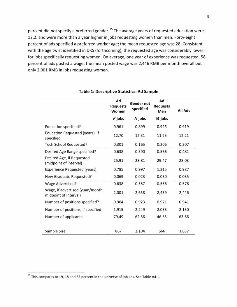
percent did not specify a preferred gender.15 The average years of requested education were 12.2, and were more than a year higher in jobs requesting women than men. Forty-eight percent of ads specified a preferred worker age; the mean requested age was 28. Consistent with the age twist identified in DKS (forthcoming), the requested age was considerably lower for jobs specifically requesting women. On average, one year of experience was requested. 58 percent of ads posted a wage; the mean posted wage was 2,446 RMB per month overall but only 2,001 RMB in jobs requesting women.

Table 1: Descriptive Statistics: Ad Sample

Ad

Requests Women

Gender not specified

Ad Requests

Men All Ads

𝑭 jobs 𝑵 jobs 𝑴 jobs

Education specified? 0.961 0.899 0.925 0.919 Education Requested (years), if specified 12.70 12.31 11.25 12.21

Tech School Requested? 0.301 0.165 0.206 0.207

Desired Age Range specified? 0.638 0.390 0.566 0.481 Desired Age, if Requested (midpoint of interval) 25.91 28.81 29.47 28.03

Experience Requested (years) 0.785 0.997 1.215 0.987

New Graduate Requested? 0.069 0.023 0.030 0.035

Wage Advertised? 0.638 0.557 0.556 0.576 Wage, if advertised (yuan/month, midpoint of interval) 2,001 2,658 2,439 2,446

Number of positions specified? 0.964 0.923 0.971 0.941

Number of positions, if specified 1.915 2.249 2.033 2.130

Number of applicants 79.49 62.56 46.55 63.66

Sample Size 867 2,104 666 3,637

15 This compares to 19, 18 and 63 percent in the universe of job ads. See Table A4.1.

10

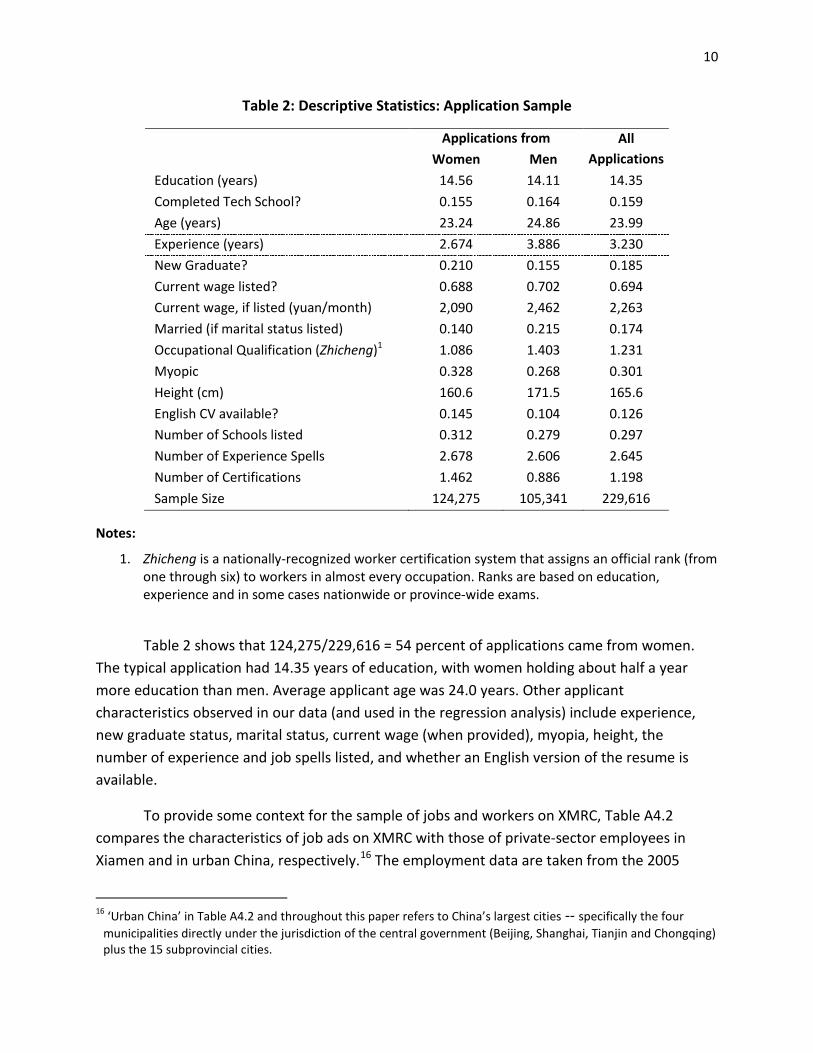
Table 2: Descriptive Statistics: Application Sample

Applications from All Applications Women Men

Education (years) 14.56 14.11 14.35 Completed Tech School? 0.155 0.164 0.159 Age (years) 23.24 24.86 23.99 Experience (years) 2.674 3.886 3.230 New Graduate? 0.210 0.155 0.185 Current wage listed? 0.688 0.702 0.694 Current wage, if listed (yuan/month) 2,090 2,462 2,263 Married (if marital status listed) 0.140 0.215 0.174 Occupational Qualification (Zhicheng)1 1.086 1.403 1.231 Myopic 0.328 0.268 0.301 Height (cm) 160.6 171.5 165.6 English CV available? 0.145 0.104 0.126 Number of Schools listed 0.312 0.279 0.297 Number of Experience Spells 2.678 2.606 2.645 Number of Certifications 1.462 0.886 1.198 Sample Size 124,275 105,341 229,616

Notes:

1. Zhicheng is a nationally-recognized worker certification system that assigns an official rank (from one through six) to workers in almost every occupation. Ranks are based on education, experience and in some cases nationwide or province-wide exams.

Table 2 shows that 124,275/229,616 = 54 percent of applications came from women. The typical application had 14.35 years of education, with women holding about half a year more education than men. Average applicant age was 24.0 years. Other applicant characteristics observed in our data (and used in the regression analysis) include experience, new graduate status, marital status, current wage (when provided), myopia, height, the number of experience and job spells listed, and whether an English version of the resume is available.

To provide some context for the sample of jobs and workers on XMRC, Table A4.2 compares the characteristics of job ads on XMRC with those of private-sector employees in Xiamen and in urban China, respectively.16 The employment data are taken from the 2005

16 ‘Urban China’ in Table A4.2 and throughout this paper refers to China’s largest cities -- specifically the four

municipalities directly under the jurisdiction of the central government (Beijing, Shanghai, Tianjin and Chongqing) plus the 15 subprovincial cities.

11

Chinese Census 1% microdata sample. Clearly, the ads on XMRC seek workers who are considerably younger, better educated, better paid, and more female than the employed population of Xiamen, or of a typical large Chinese city. This is as we might expect, for three reasons. The first is XMRC’s explicit niche in the local labor market: to serve relatively skilled workers. Second, due to a massive recent expansion of China’s higher education system, younger cohorts are much better educated than their parents. Thus, any job board seeking skilled workers will be disproportionately seeking young workers.17 Third, as on any job board, the ads and resumes on XMRC represent vacancies and jobseekers, not employed workers. Thus we would expect new labor market entrants (who are all looking for work) and young workers (who turn over more frequently than other workers) to be substantially overrepresented relative to the currently employed population.

Finally, the bottom panel of Table A4.2 attempts to compare the broad occupation distributions of XMRC ads to China’s and Xiamen’s urban labor force. This is challenging because of the occupational classification system used by XMRC, which uses 37 categories that were created by the website; mapping these into Census categories is a fairly subjective exercise. With these cautions in mind, Table A4.2 indicates that jobs in production, construction and manufacturing are under-represented on XMRC, while professional and technical jobs are highly over-represented. Again, this is consistent with XMRC’s focus on skilled workers, a population we know is less subject to gender profiling than less-skilled workers.

2. Gender Matching, Compliance and Enforcement: Aggregate Statistics

Aggregate statistics on applications and callbacks are shown in Table 3, broken down by the three job types in our data: jobs requesting women (F jobs), jobs requesting men (M jobs) and jobs that do not state a gender preference (N jobs). Turning first to total gender matching, row 1 shows the share of callbacks that are female (𝛿) by job type. These statistics indicate a high congruence of the callback pool with employers’ stated requests. Specifically, 94.0 percent of callbacks to F jobs are female and 100 − 3.7 = 96.3 percent of callbacks to M jobs are male. Combining F and M jobs, 94.8 percent of callbacks to gendered job ads are of the requested gender. Row 2 shows the share of applications to the three job types that are female (𝛼). It suggests that applicants’ compliance with employers’ gender requests plays a substantial role in accounting for this high level of gender matching, since applicant pools are almost as highly sorted by gender as callback pools. Specifically, 92.6 percent of applications to F jobs are female and 100− 7.9 = 92.1 percent of applications to M jobs are male. Combining F and M jobs, 92.5 percent of applications to gendered job ads are of the requested gender.

17 Rapid educational upgrading since the 2005 Census also implies that Table A4.2 is likely to overstate the

education gap between the XMRC ads and Xiamen’s 2010 labor force.

12

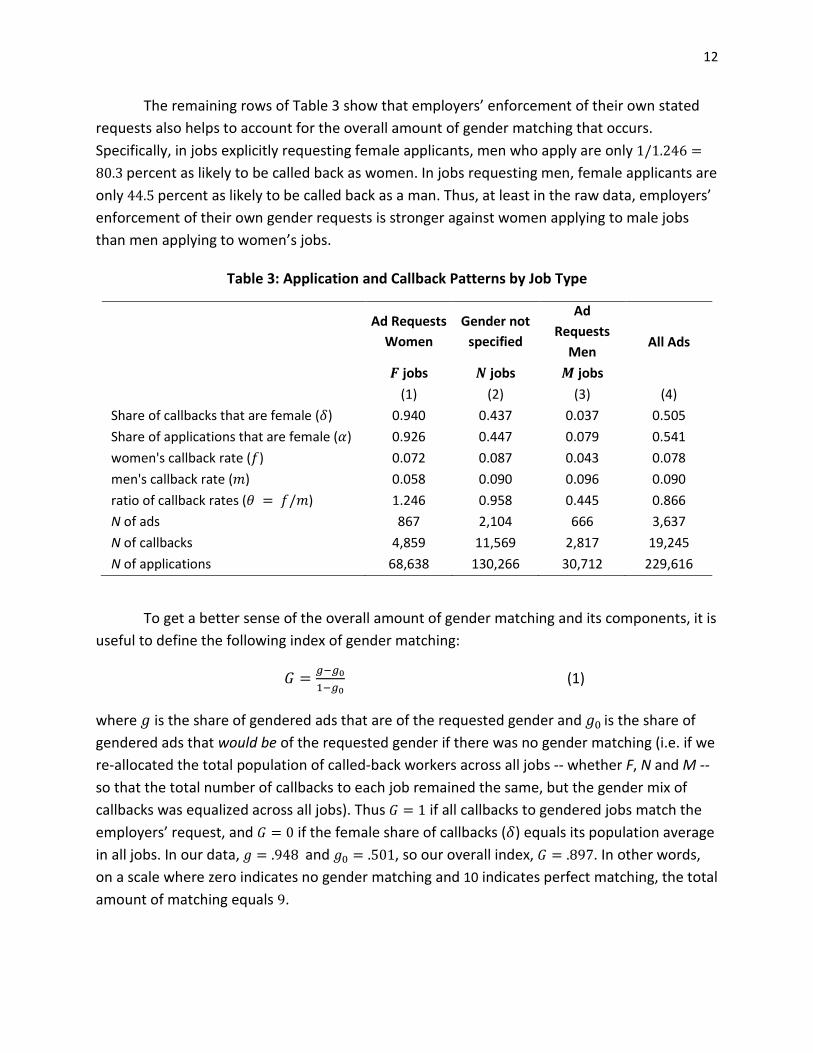
The remaining rows of Table 3 show that employers’ enforcement of their own stated requests also helps to account for the overall amount of gender matching that occurs. Specifically, in jobs explicitly requesting female applicants, men who apply are only 1/1.246 =80.3 percent as likely to be called back as women. In jobs requesting men, female applicants are only 44.5 percent as likely to be called back as a man. Thus, at least in the raw data, employers’ enforcement of their own gender requests is stronger against women applying to male jobs than men applying to women’s jobs.

Table 3: Application and Callback Patterns by Job Type

Ad Requests Women

Gender not specified

Ad Requests

Men All Ads

𝑭 jobs 𝑵 jobs 𝑴 jobs (1) (2) (3) (4)

Share of callbacks that are female (𝛿) 0.940 0.437 0.037 0.505 Share of applications that are female (𝛼) 0.926 0.447 0.079 0.541 women's callback rate (𝑓) 0.072 0.087 0.043 0.078 men's callback rate (𝑚) 0.058 0.090 0.096 0.090 ratio of callback rates (𝜃 = 𝑓/𝑚) 1.246 0.958 0.445 0.866 N of ads 867 2,104 666 3,637 N of callbacks 4,859 11,569 2,817 19,245 N of applications 68,638 130,266 30,712 229,616

To get a better sense of the overall amount of gender matching and its components, it is useful to define the following index of gender matching:

𝐺 = 𝑔−𝑔01−𝑔0

(1)

where 𝑔 is the share of gendered ads that are of the requested gender and 𝑔0 is the share of gendered ads that would be of the requested gender if there was no gender matching (i.e. if we re-allocated the total population of called-back workers across all jobs -- whether F, N and M -- so that the total number of callbacks to each job remained the same, but the gender mix of callbacks was equalized across all jobs). Thus 𝐺 = 1 if all callbacks to gendered jobs match the employers’ request, and 𝐺 = 0 if the female share of callbacks (𝛿) equals its population average in all jobs. In our data, 𝑔 = .948 and 𝑔0 = .501, so our overall index, 𝐺 = .897. In other words, on a scale where zero indicates no gender matching and 10 indicates perfect matching, the total amount of matching equals 9.

13

With this index in hand, we can assess the relative contributions of compliance and enforcement to gender matching, G, using the accounting identity:

𝛿𝐽 = 𝜃𝐽𝛼𝐽

𝜃𝐽𝛼𝐽 + (1−𝛼𝐽) (2)

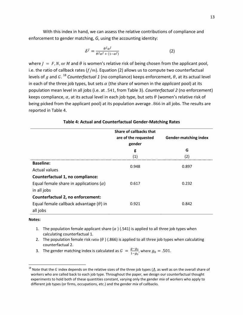
where 𝐽 = 𝐹,𝑁, or 𝑀 and 𝜃 is women’s relative risk of being chosen from the applicant pool, i.e. the ratio of callback rates (𝑓/𝑚). Equation (2) allows us to compute two counterfactual levels of 𝑔 and 𝐺. 18 Counterfactual 1 (no compliance) keeps enforcement, 𝜃, at its actual level in each of the three job types, but sets 𝛼 (the share of women in the applicant pool) at its population mean level in all jobs (i.e. at . 541, from Table 3). Counterfactual 2 (no enforcement) keeps compliance, 𝛼, at its actual level in each job type, but sets 𝜃 (women’s relative risk of being picked from the applicant pool) at its population average . 866 in all jobs. The results are reported in Table 4.

Table 4: Actual and Counterfactual Gender-Matching Rates

Share of callbacks that are of the requested

gender Gender-matching index

g G (1) (2)

Baseline: Actual values

0.948 0.897

Counterfactual 1, no compliance: Equal female share in applications (𝛼) in all jobs

0.617 0.232

Counterfactual 2, no enforcement: Equal female callback advantage (𝜃) in all jobs

0.921 0.842

Notes:

1. The population female applicant share (𝛼 ) (.541) is applied to all three job types when calculating counterfactual 1.

2. The population female risk ratio (𝜃 ) (.866) is applied to all three job types when calculating counterfactual 2.

3. The gender matching index is calculated as 𝐺 = 𝑔−𝑔01−𝑔0

, where 𝑔0 = .501.

18 Note that the 𝐺 index depends on the relative sizes of the three job types (J), as well as on the overall share of

workers who are called back to each job type. Throughout the paper, we design our counterfactual thought experiments to hold both of these quantities constant, varying only the gender mix of workers who apply to different job types (or firms, occupations, etc.) and the gender mix of callbacks.

14

According to row 2 of Table 4, eliminating worker compliance while maintaining actual levels of enforcement would reduce the share of callbacks that are of the requested gender, 𝑔, from .948 to . 617. The corresponding decline in the gender matching index, 𝐺, is from .897 to .232. Thus, workers’ compliance with employers’ gender requests accounts for 0.897−0.232

0.897= 74

percent of the gender matching in our data. According to row 3, eliminating employers’ enforcement while maintaining actual levels of worker compliance would have a much smaller impact, reducing 𝑔 from .948 to .921 and 𝐺 from .897 to .842. Thus, active enforcement by employers of their own gender requests accounts for only .897−.842

.897= 6 percent of the gender

matching in our data. Because the decomposition in equation (2) is exact but nonlinear, the remaining 20 percent of gender matching is due to the interaction between compliance and enforcement.19 We conclude that compliance, i.e. applicants’ self-sorting according to employers’ gender requests in job ads, accounts for the vast majority of gender matching in gendered ads. The intuition is straightforward: Because applicant pools are so highly gender-segregated, even completely equal treatment of male and female applicants in all job types would have only a small impact on the gender mix of callbacks to each job if application patterns are held fixed.

To put our estimates of gender-matching, compliance and enforcement in context, Table A4.3 presents comparable measures of those three quantities for employers’ gender, age, education and experience requests, as well as for the match between the posted wage and the applicant’s current wage (when reported). Thus, for example, row 2 shows the share of called-back workers whose age is within the ad’s requested age range (e.g. 24-28), the share of applications whose age is in the requested range, and the share of age-mismatched applications that are rejected.20 Interestingly, compliance, enforcement and total matching are all greater for gender than for these other four characteristics. While these differences are particularly dramatic on the worker self-selection side, substantial enforcement differences are also present: The shares of age-, education-, experience-. or wage-mismatched applicants that are called back all exceed 25.2 percent, compared to 5.2 percent of gender-mismatched applicants. Together, these statistics suggest an especially important role for gender, relative to these other characteristics, in determining what employers and employees consider to be a good match.

19 By ‘exact’ we mean that eliminating both compliance and enforcement would reduce 𝐺 to zero. 20 Mismatch in education, experience and wages is measured by the indicators used in Table 6’s callback

regressions, which are based on broad categories. For example, education is measured using five categories (primary, middle, technical school, post-secondary and university) and a match occurs when the job’s request and the employee’s actual education fall into the same category. Additional details are provided in Table A4.3.

15

3. Regression Analysis—Compliance

Section 2’s aggregate statistics exhibit a high apparent level of worker compliance with employers’ explicit gender requests: according to Table 3, 𝐹, 𝑁 and 𝑀 job ads attract applicant pools that are 92.6, 44.7 and 7.9 percent female respectively. Depending on which types of jobs explicitly request men and women, these large differences could over- or understate the causal effect of attaching an explicit gender label to a typical ad. For example, if gender requests are primarily used as a type of affirmative action (i.e. to attract workers to jobs in which their gender is underrepresented), these raw gaps would underestimate the causal effects of explicit labels on application behavior. DKS (forthcoming), however, show that explicit gender labels mostly reinforce prevailing stereotypes; thus Table 3’s raw statistics could substantially overstate the causal effect of attaching a gender request to a job ad.

To adjust for these confounding factors, this Section takes two complementary approaches. In the first, we regress the female share of applicants to an ad on explicit gender requests, with controls for a detailed list of skill requirements and other desiderata, plus firm and job title fixed effects. Job titles are the main heading in every job ad. They provide a brief description of the job and can run up to 18 words on XMRC. For example, here is a random sample of ten (translated) job titles on the XMRC website: front desk administration assistant, project engineer, quality control, shift leader, customer service maintenance specialist, administration, ME product engineer, experienced two-dimension designer, customer service engineer, and front desk clerk. Job titles provide considerably more relevant information about the type of work than even the most granular standardized occupational classification systems. For example, Marinescu and Wolthoff (2016) found that job titles on Careerbuilder.com were much more predictive of advertised wages than 6-digit SOC codes, and were essential controls for identifying the effect of advertised wages on the number and quality of applications an ad received. Thus, in this approach we will be comparing the gender mix of applications to observationally identical ads for a very narrowly defined type of work, holding constant the identity of the firm advertising the job.

In our second approach, we replace the job title fixed effects in the above analysis by indicators of the predicted, or implicit ‘maleness’ or ‘femaleness’ of the job derived from a machine learning analysis of the words in the titles. Essentially, we use the words in the title to predict whether a person reading it can infer whether the job is likely to request men, or to request women. While these two predicted probabilities (𝑀𝑝 and 𝐹𝑝, respectively) absorb less variation in job characteristics than the full set of title fixed effects, they provide a simple structure that helps us identify the types of jobs where inserting a gender label into a job ad has the largest estimated impact on application behavior. Notably, in both our estimation approaches in this Section, we use the entire sample of job ads available to us, not just the

16

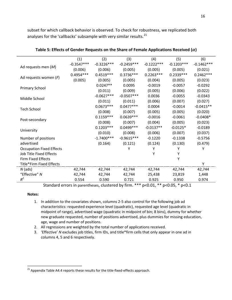
subset for which callback behavior is observed. To check for robustness, we replicated both analyses for the ‘callbacks’ subsample with very similar results.21

Table 5: Effects of Gender Requests on the Share of Female Applications Received (𝜶)

(1) (2) (3) (4) (5) (6)

Ad requests men (M) -0.3547*** -0.3226*** -0.2459*** -0.1222*** -0.1203*** -0.1462***

(0.006) (0.006) (0.005) (0.005) (0.005) (0.021)

Ad requests women (F) 0.4954*** 0.4519*** 0.3736*** 0.2263*** 0.2339*** 0.2462*** (0.005) (0.005) (0.005) (0.004) (0.005) (0.023)

Primary School 0.0247** 0.0095 -0.0019 -0.0057 -0.0292 (0.011) (0.009) (0.005) (0.006) (0.022)

Middle School -0.0627*** -0.0507*** 0.0036 -0.0055 -0.0343 (0.011) (0.011) (0.006) (0.007) (0.027)

Tech School 0.0673*** 0.0477*** 0.0004 -0.0014 -0.0415** (0.008) (0.007) (0.005) (0.005) (0.020)

Post-secondary 0.1159*** 0.0639*** -0.0016 -0.0061 -0.0408* (0.008) (0.007) (0.004) (0.005) (0.023)

University 0.1203*** 0.0499*** -0.0137** -0.0125* -0.0189 (0.010) (0.008) (0.006) (0.007) (0.037)

Number of positions advertised

-1.7400*** -0.9615*** -0.1220 -0.1338 -0.5756 (0.164) (0.121) (0.124) (0.130) (0.479)

Occupation Fixed Effects Y Y Y Y Job Title Fixed Effects Y Y Firm Fixed Effects Y Title*Firm Fixed Effects Y N (ads) 42,744 42,744 42,744 42,744 42,744 42,744 “Effective” N 42,744 42,744 42,744 25,438 23,819 1,448 R2 0.554 0.590 0.721 0.925 0.950 0.974

Standard errors in parentheses, clustered by firm. *** p<0.01, ** p<0.05, * p<0.1

Notes:

1. In addition to the covariates shown, columns 2-5 also control for the following job ad characteristics: requested experience level (quadratic), requested age level (quadratic in midpoint of range), advertised wage (quadratic in midpoint of bin; 8 bins), dummy for whether new graduate requested, number of positions advertised, plus dummies for missing education, age, wage and number of positions.

2. All regressions are weighted by the total number of applications received. 3. ‘Effective’ N excludes job titles, firm IDs, and title*firm cells that only appear in one ad in

columns 4, 5 and 6 respectively.

21 Appendix Table A4.4 reports these results for the title-fixed-effects approach.

17

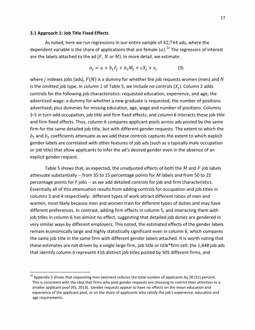
3.1 Approach 1: Job Title Fixed Effects

As noted, here we run regressions in our entire sample of 42,744 ads, where the dependent variable is the share of applications that are female (𝛼).22 The regressors of interest are the labels attached to the ad (𝐹, 𝑁 or 𝑀). In more detail, we estimate:

𝛼𝑗 = 𝑎 + 𝑏1𝐹𝑗 + 𝑏2𝑀𝑗 + 𝑐𝑋𝑗 + 𝑒𝑗 (3)

where 𝑗 indexes jobs (ads), 𝐹(𝑀) is a dummy for whether the job requests women (men) and 𝑁 is the omitted job type. In column 1 of Table 5, we include no controls (𝑋𝑗). Column 2 adds controls for the following job characteristics: requested education, experience, and age; the advertised wage; a dummy for whether a new graduate is requested; the number of positions advertised; plus dummies for missing education, age, wage and number of positions. Columns 3-5 in turn add occupation, job title and firm fixed effects, and column 6 interacts these job title and firm fixed effects. Thus, column 6 compares applicant pools across ads posted by the same firm for the same detailed job title, but with different gender requests. The extent to which the 𝑏1 and 𝑏2 coefficients attenuate as we add these controls captures the extent to which explicit gender labels are correlated with other features of job ads (such as a typically male occupation or job title) that allow applicants to infer the ad’s desired gender even in the absence of an explicit gender request.

Table 5 shows that, as expected, the unadjusted effects of both the 𝑀 and 𝐹 job labels attenuate substantially -- from 35 to 15 percentage points for M labels and from 50 to 25 percentage points for F jobs -- as we add detailed controls for job and firm characteristics. Essentially all of this attenuation results from adding controls for occupation and job titles in columns 3 and 4 respectively: different types of work attract different ratios of men and women, most likely because men and women train for different types of duties and may have different preferences. In contrast, adding firm effects in column 5, and interacting them with job titles in column 6 has almost no effect, suggesting that detailed job duties are gendered in very similar ways by different employers. This noted, the estimated effects of the gender labels remain economically large and highly statistically significant even in column 6, which compares the same job title in the same firm with different gender labels attached. It is worth noting that these estimates are not driven by a single large firm, job title or title*firm cell: the 1,448 job ads that identify column 6 represent 416 distinct job titles posted by 505 different firms, and

22 Appendix 5 shows that requesting men (women) reduces the total number of applicants by 28 (31) percent.

This is consistent with the idea that firms who post gender requests are choosing to restrict their attention to a smaller applicant pool (KS, 2013). Gender requests appear to have no effects on the mean education and experience of the applicant pool, or on the share of applicants who satisfy the job’s experience, education and age requirements.

18

comprise 686 title*firm cells.23 In addition, estimates of column 6 that leave out one job title at a time are all very close to the full-sample estimates.24 Together, these patterns suggest that adding an explicit gender request to a job ad has substantial causal effects on the gender mix of applications it will receive. In other words, employers’ gender requests appear to direct workers’ applications.

3.2 Approach 2 -- Implicit Maleness and Femaleness

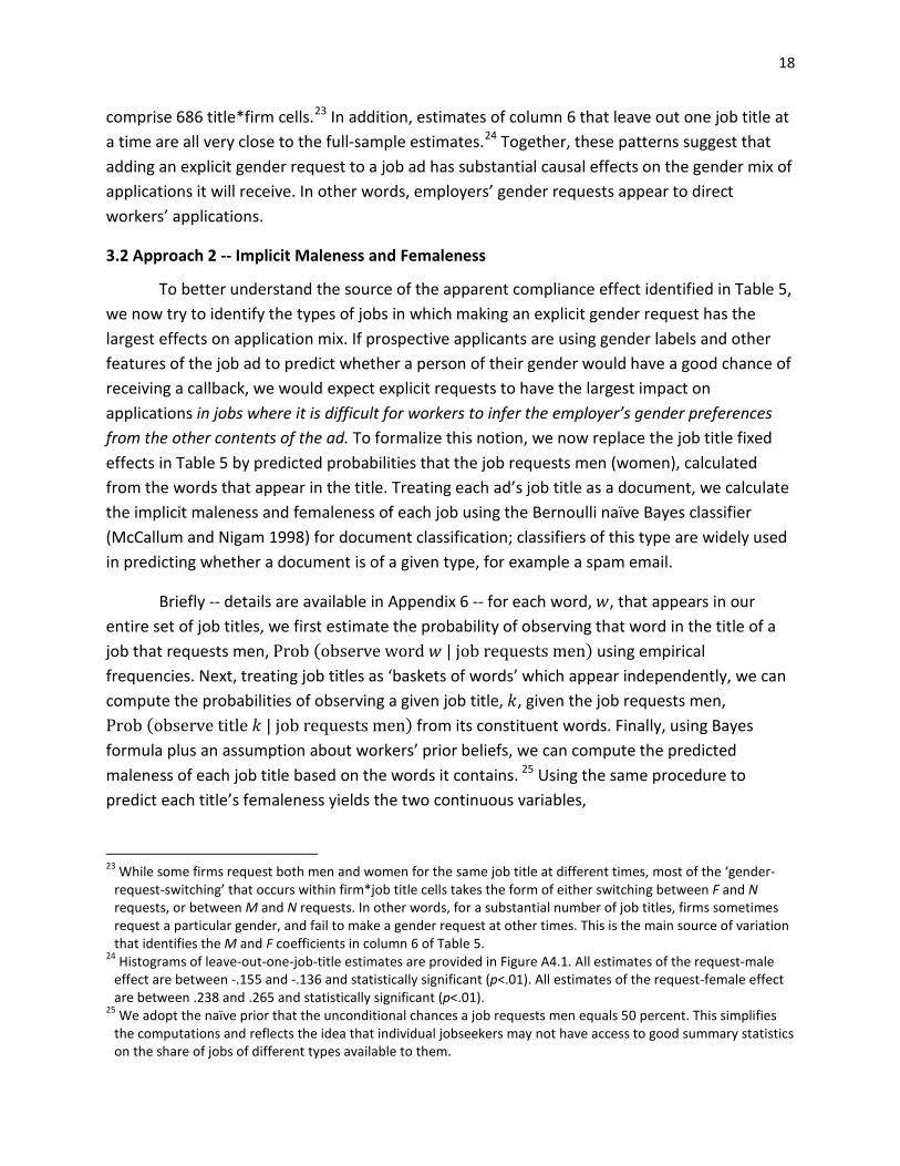
To better understand the source of the apparent compliance effect identified in Table 5, we now try to identify the types of jobs in which making an explicit gender request has the largest effects on application mix. If prospective applicants are using gender labels and other features of the job ad to predict whether a person of their gender would have a good chance of receiving a callback, we would expect explicit requests to have the largest impact on applications in jobs where it is difficult for workers to infer the employer’s gender preferences from the other contents of the ad. To formalize this notion, we now replace the job title fixed effects in Table 5 by predicted probabilities that the job requests men (women), calculated from the words that appear in the title. Treating each ad’s job title as a document, we calculate the implicit maleness and femaleness of each job using the Bernoulli naïve Bayes classifier (McCallum and Nigam 1998) for document classification; classifiers of this type are widely used in predicting whether a document is of a given type, for example a spam email.

Briefly -- details are available in Appendix 6 -- for each word, 𝑤, that appears in our entire set of job titles, we first estimate the probability of observing that word in the title of a job that requests men, Prob (observe word 𝑤 | job requests men) using empirical frequencies. Next, treating job titles as ‘baskets of words’ which appear independently, we can compute the probabilities of observing a given job title, 𝑘, given the job requests men, Prob (observe title 𝑘 | job requests men) from its constituent words. Finally, using Bayes formula plus an assumption about workers’ prior beliefs, we can compute the predicted maleness of each job title based on the words it contains. 25 Using the same procedure to predict each title’s femaleness yields the two continuous variables,

23 While some firms request both men and women for the same job title at different times, most of the ‘gender-

request-switching’ that occurs within firm*job title cells takes the form of either switching between F and N requests, or between M and N requests. In other words, for a substantial number of job titles, firms sometimes request a particular gender, and fail to make a gender request at other times. This is the main source of variation that identifies the M and F coefficients in column 6 of Table 5.

24 Histograms of leave-out-one-job-title estimates are provided in Figure A4.1. All estimates of the request-male effect are between -.155 and -.136 and statistically significant (p<.01). All estimates of the request-female effect are between .238 and .265 and statistically significant (p<.01).

25 We adopt the naïve prior that the unconditional chances a job requests men equals 50 percent. This simplifies the computations and reflects the idea that individual jobseekers may not have access to good summary statistics on the share of jobs of different types available to them.

19

𝑀𝑝 ≡ 𝑃𝑃𝑃𝑏(job explicitly requests men| job title 𝑘) (4)

𝐹𝑝 ≡ 𝑃𝑃𝑃𝑏(job explicitly requests women| job title 𝑘) (5)

which we use in our empirical analysis to represent the information contained in the job title about whether the job is likely to request men or women. Overall, 𝑀𝑝 and 𝐹𝑝 are quite predictive of employers’ actual requests, with correlations of .411 and .402 with actual requests for men and women (which are binary variables) respectively. As we might expect, 𝑀𝑝 and 𝐹𝑝 identify what we might think of as stereotypically male and female jobs: the five ‘most female’ job titles (starting with the highest) are “front office desk staff”, “administration office staff”, “office staff”, “cashier” and “administration assistant”. The five ‘most male’ are “driver”, “technician”, “warehouse managing staff”, “warehouse manager”, and “production manager”.26 These indices of implicit maleness or femaleness allow us to estimate the effect on application behavior of adding an explicit gender request to jobs that ‘look the same’ to workers in terms of an employer’s likely gender preference, and to see in which types of jobs the effect of explicit requests on application behavior is the greatest.

More specifically, we now regress the female share of applicants to a job, 𝛼𝑗, on employers’ explicit gender requests (F and M), plus all the control variables used in column 5 of Table 5 (other than the job title fixed effects) plus quartics in the implicit maleness or femaleness of the job that workers could infer from the job’s title (𝑀𝑝 and 𝐹𝑝). In addition, each of these quartics is interacted with the three explicit job types, 𝐹, 𝑁 and 𝑀. These interactions allow, for example, the effect of an explicit request for women to differ in jobs that are stereotypically male (based on the words that appear in the job title) from jobs whose titles do not convey an obvious gender preference.

Predicted male and female applicant shares from these regressions are shown in Figure 1. Part (a) of the Figure shows the predicted female applicant share as a function of the predicted femaleness of the job based on the words in the job title, separately for the three types of jobs (𝐹, 𝑁 and 𝑀). Predicted maleness is held fixed at its mean. Part (b) is the corresponding figure for male applicant shares as a function of perceived maleness, holding predicted femaleness at its mean. Finally, part (c) shows the estimated effects of encountering a request for a particular gender (relative to a non-gendered job) on the share of that gender in the applicant pool, with 95 percent confidence bands. These are the distances between the top two curves in parts (a) and (b).

26 Additional examples of job titles at different levels of 𝐹𝑝 and 𝑀𝑝 are provided in Figure A4.3.

20

Figure 1: Effects of Gender Requests and Implicit Gender of the Job Ads on the Gender Composition of Applications Received

21

Notes:

1. Figures represent predicted values of the female/male share of applicants (α) from a specification identical to column 5 in Table 5, where the job title fixed effects are replaced by quartics in Fp and Mp, each interacted with explicit job type (F, N and M).

2. Predictions in part (a), which shows the effect of implicit femaleness (Fp), hold Mp at its mean. Predictions in part (b), which depicts the implicit maleness (Mp), hold Fp at its mean. All other characteristics are set at their means. The regression is weighted by the number of applications to each ad, and standard errors are clustered at the firm level.

3. Part (c) shows the predicted effects of attaching an explicit male (female) label to a job ad (relative to an N label) at different levels of implicit maleness (femaleness), with 95 percent confidence bands. Notably, both effects are larger in jobs whose title does not convey a clear preference for the applicant’s gender. In addition, the effects of explicit requests for women on application behavior are significantly larger (both economically and statistically) than the effects of explicit requests for men.

4. Predictions for values of Fp or Mp greater than 0.9 are imprecise and not shown; only 2,462 ads have values in this range, comprising .0377 and .0330 of the sample respectively.

Figure 1 shows, first of all, that explicit requests for male and female applicants have stronger effects on the gender mix of applications when the words in the job title do not send clear signals about whether the employer is likely to prefer men or women (i.e. when 𝑀𝑝 and 𝐹𝑝 are low). For example, when 𝐹𝑝 is near zero, the predicted effect on the female applicant share of inserting an explicit request for women into an N job is about 53 percentage points. This effect diminishes to about 26 percentage points when 𝐹𝑝 equals 0.7. A similar pattern is present for men, though it is less pronounced.

Second, there is a subtle but interesting gender difference regarding when explicit requests matter. In ‘not-obviously-female’ (low 𝐹𝑝) jobs, women comprise a relatively large share of applicants only when the job explicitly requests women. In ‘not-obviously-male’ (low 𝑀𝑝) jobs, men comprise a relatively large share of applicants both when men are explicitly requested, and when the ad does not make a gender request. Together these patterns help us understand the much larger impact of 𝐹 labels than 𝑀 labels on the applicant mix in Table 5. Essentially, the main gender difference in application behavior occurs in jobs that -- based on their title -- are neither stereotypically male nor female. If we think of applying for jobs as entering a competition to get hired, these patterns are evocative of well-known gender

22

differences in entry into competition (Niederle and Vesterlund 2007), and of gender gaps in the propensity to apply for jobs in the presence of ambiguity (Gee, 2018).27

We conclude our discussion of compliance effects with a reminder that our substantial estimated compliance effects are consistent with at two very different underlying mechanisms. One is that job labels communicate information about a worker’s chances of getting a callback; in this view, women avoid male jobs because they know they have a lower chance of getting those jobs if they apply. The second mechanism is that -- much like labels on men’s and women’s clothing—job labels communicate information about whether the worker is likely to want the job, without conveying any reluctance by the firm to transact with the worker. In this mechanism, women avoid male jobs because women dislike certain job attributes -- perhaps competitive pay policies, long and inflexible hours, or even the absence of female co-workers -- associated with those jobs. Assessing the relative importance of these two mechanisms requires an analysis of how gender-mismatched applications are treated when they are made, which is our goal in the next Section.

4. Regression Analysis—Enforcement

Section 2’s aggregate statistics suggest a substantial amount of apparent enforcement by employers of their own explicit gender requests: according to Table 3, conditional on applying, women’s callback rate in explicitly male jobs is 4.3 percent, compared to 8.7 percent in non-gendered jobs -- a mismatch penalty of 4.4 percentage points, or 51 percent. Men’s callback penalty from applying to explicitly female jobs, defined analogously, equals 9.0 - 5.8 = 3.2 percentage points, or 36 percent. Depending on which types of workers decide to apply to gender-mismatched jobs, however, these differences could over- or understate the change in callback chances that a representative worker would experience if she redirected her application from a non-gendered job to an identical job that requested the opposite gender.

To see this, imagine first that (say) women who apply to jobs requesting men are better qualified on dimensions like education, experience, and unobserved ability that the applicants hope will compensate for being of the ‘wrong’ gender. For the same reason, women may restrict their applications to jobs that fit their qualifications more closely when applying to explicitly male jobs. In both these cases, workers who make gender-mismatched applications will be positively selected on unobservables, and Table 3’s raw mismatch penalties will underestimate the adverse effects of gender mismatch on the callback rate (because the

27 To probe robustness to functional form, Figure A4.2 forces predicted applicant shares to be between zero and

one by changing the dependent variable from 𝛼 (the female share) to 𝑙𝑃𝑔 � 𝛼1−𝛼

�, and replacing the quartics in 𝐹𝑝

and 𝑀𝑝 by linear terms (still interacted with 𝐹, 𝑁 and 𝑀). In both cases, our main conclusions -- including the larger effects of 𝐹 labels than 𝑀 labels on applicant mix -- continue to hold.

23

people who choose to cross-apply are better-qualified and better matched than those who do not).

Alternatively, selection into mismatch can be negative, for example, if the women who apply to jobs requesting men are less able, or apply to jobs more indiscriminately. This could happen because those workers have low application costs, are highly motivated to find a job, or are simply careless. In this case, Table 3’s 4.4 percentage point mismatch penalty for women will overestimate the adverse effects of gender mismatch on the callback rate. Adding controls for worker qualifications and job-worker match should attenuate the magnitude of the estimated penalty towards its true, smaller value.

To distinguish between these scenarios -- and thereby measure just how ‘hard’ or ‘soft’ employers’ explicit gender requests are -- , we run linear probability regressions in a sample of applications, where the dependent variable is an indicator for whether the worker received a callback. In doing so, we control as tightly as possible for other aspects of match and worker quality that might affect callback rates. Of particular note, we control for unobserved worker ability by using worker fixed effects -- i.e. we will compare the callback rates of the same worker who sends her resume to two observationally-identical jobs that differ only in their explicit gender label. We control for the detailed type of work using job title fixed effects. To account for the fact that people who apply to gender-mismatched jobs might be better or worse matched to the job on dimensions other than gender, we also include detailed controls for matching on a variety of characteristics.

In more detail, we estimate the following linear probability model:

Callback𝑖 = 𝛼 + 𝛽1FtoF𝑖 + 𝛽2FtoM𝑖 + 𝛽3MtoF𝑖 + 𝛽4MtoM𝑖

+𝛿FWorker𝑖 + 𝜑𝑋𝑖 + 𝜀𝑖 (6)

where 𝑖 indexes applications. Of the six possible application types, women applying to nongendered jobs (FtoN) is the omitted type. In this specification, 𝛽1 and 𝛽2 give the effect on women of applying to M and F jobs (relative to nongendered jobs), while 𝛽3 and 𝛽4 give the effect on men of applying to M and F jobs (again, relative to nongendered jobs). The parameter 𝛿 gives the callback gap between men and women applying to nongendered jobs. Our main focus will be on the gender mismatch penalties associated with applying to a job that is targeted at the ‘other’ gender, 𝛽2 and 𝛽3.

24 Table 6: Effects of Gender Requests on Callback Rates

(1) (2) (3) (4) (5) (6)

Female Worker * Female Job -0.0149 -0.0105*** -0.0101*** -0.0098*** -0.0136*** -0.0153*** (0.009) (0.002) (0.002) (0.002) (0.002) (0.003)

Female Worker * Male Job -0.0440*** -0.0425*** -0.0423*** -0.0410*** -0.0326*** -0.0371***

(0.013) (0.004) (0.004) (0.004) (0.006) (0.008)

Male Worker * Female Job -0.0328*** -0.0271*** -0.0272*** -0.0208*** -0.0215*** -0.0216***

(0.010) (0.003) (0.003) (0.003) (0.004) (0.005)

Male Worker * Male Job 0.0054 0.0016 0.0017 0.0038* -0.0055 -0.0155*** (0.009) (0.002) (0.002) (0.002) (0.004) (0.005)

Male Worker 0.0038 0.0004 -0.0029 -0.0065*** -0.0173*** (0.006) (0.002) (0.002) (0.002) (0.002)

Education less than requested -0.0055** -0.0047* -0.0070*** -0.0081*** -0.0095*** (0.002) (0.003) (0.003) (0.002) (0.004)

Education more than requested

-0.0048*** -0.0084*** -0.0069*** -0.0014 0.0020 (0.001) (0.002) (0.002) (0.002) (0.003)

Age less than requested -0.0005 -0.0018 -0.0020 -0.0036* -0.0020 (0.002) (0.002) (0.002) (0.002) (0.002)

Age more than requested -0.0330*** -0.0309*** -0.0284*** -0.0205*** -0.0215*** (0.003) (0.003) (0.003) (0.003) (0.004)

Experience less than requested

-0.0062*** -0.0066*** -0.0080*** -0.0094*** -0.0070*** (0.002) (0.002) (0.002) (0.002) (0.003)

Experience more than requested

0.0004 0.0020 0.0012 -0.0013 0.0013 (0.002) (0.002) (0.002) (0.002) (0.004)

Wage below advertised -0.0010 -0.0008 -0.0020 -0.0001 -0.0015 (0.002) (0.002) (0.002) (0.002) (0.003)

Wage above advertised 0.0009 0.0007 0.0002 -0.0060*** -0.0045 (0.002) (0.002) (0.002) (0.002) (0.003)

Detailed CV controls Y Y Y Occupation Fixed Effects Y Y Y Competition Controls Y Y Job Title Fixed Effects Y Y Worker Fixed Effects Y N applications 229,616 229,616 229,616 229,616 229,616 229,616 ‘Effective’ N 229,616 229,616 229,616 229,616 229,590 192,681 R2 0.001 0.005 0.005 0.016 0.198 0.388

Standard errors in parentheses, clustered by worker. *** p<0.01, ** p<0.05, * p<0.1

Notes:

1. In addition to the covariates shown, columns 2-6 include the following controls for ad characteristics: requested education (5 categories), experience (quadratic), age (quadratic), the advertised wage (quadratic in midpoint of bin; 8 bins) and a dummy for whether a new graduate is requested. Columns 2-6 also include a dummy for whether the applicant’s new graduate status matches the requested status, plus indicators for missing age and wage information for either the ad or the worker.

2. “Detailed CV controls” (used in columns 3-6) are an indicator for attending technical school; the applicant’s zhicheng rank (6 categories); an English CV indicator; the number of schools attended, job experience spells and certifications reported; and the following characteristics interacted with gender: height, myopia, and marital status (interacted with applicant gender)

3. Occupation fixed effects control for the 37 categories used on the XMRC website. 4. ‘Effective’ N excludes job titles and worker IDs that only appear in one ad in columns 5 and 6

respectively.

25

Column 1 of Table 6 estimates equation 6 without controls, replicating the unadjusted gaps in Table 3. Column 2 adds controls for the job’s requested level of education, experience and age; the advertised wage; and an indicator for whether a new graduate is requested. Also included are indicators of the match between the applicant’s characteristics and those requirements, including indicators for whether the applicant’s education, age and experience are below or above the requested level, the match between the advertised wage and the applicant’s current or previous wage, and the match between requested and actual new-graduate status. Column 3 adds controls for the following worker (CV) characteristics: whether he/she attended a technical school; the applicant’s zhicheng rank; whether an English CV is available; the number of schools attended, experience spells and certifications reported.28 Indicators for applicant height, myopia and marital status are also included, all interacted with the applicant’s gender.29

Column 4 adds fixed effects for the occupation of the advertised job, using XMRC’s occupational categories. Column 5 adds job title fixed effects plus two indicators of the amount of competition for the job: the number of positions advertised and the number of persons who applied to the ad.30 Our most saturated specification is column 6, which adds a full set of worker fixed effects. In this case, the effects of fixed applicant characteristics (“detailed cv controls” and the main gender effect) are no longer identified, but our main coefficients of interest -- which are interactions between job and applicant gender -- can still be estimated. In effect, column 6 compares the outcomes of the same worker who has applied to observationally identical jobs that differ only according to the gender label (𝐹, 𝑁 or 𝑀) attached to the job, while allowing for this effect to differ according to the applicant’s gender.

Before discussing our main coefficients of interest, it is worth noting that whenever they are statistically significant, observable indicators of the match between worker qualifications and job requirements are of the expected signs in Table 6: workers who have less education or experience than requested, or are older than requested are less likely to be called back. Finally, the job competition controls (not shown) are always highly statistically significant, indicating that these highly localized measures of labor market tightness have strong effects on the chances of being called back. Also of some interest, workers with more education than the job

28 Zhicheng is a nationally-recognized worker certification system that assigns an official rank (from one through

six) to workers in almost every occupation. Ranks are based on education, experience and in some cases nationwide or province-wide exams.

29 These ‘detailed CV controls’ introduced in column 3 are not requested in job ads very often, so it is not practical to construct variables summarizing their match with the job’s requirements.

30 These ‘queue length’ or ‘submarket tightness’ controls account for the possibility that overall competition for callbacks might be systematically stiffer in some job types than others. For example, callback rates in jobs that request women might be lower for all applicants if women ‘crowd into’ those jobs more than men crowd into jobs that request men (Sorensen 1990).

26

requests also experience a statistically significant callback penalty in all specifications but one (Shen and Kuhn 2013).

Turning to the mismatch penalties, both men’s and women’s penalties attenuate somewhat as we add covariates in Table 6. As discussed, this consistent pattern suggests that gender mismatched applicants are negatively, rather than positively selected, perhaps because they are less discriminating in where they send their applications. Despite this moderate attenuation, however, the estimated mismatch penalty remains both economically and statistically significant in the presence of worker fixed effects (column 6). For a woman, applying to a job requesting men reduces her callback chances by 3.7 percentage points, only a little less than the unadjusted effect (4.4 percentage points). For men, the attenuation is more pronounced – from 3.3 to 2.2 percentage points -- suggesting a greater amount of negative self-selection into gender-mismatched applications among men.

In sum, our preferred estimates in Table 6 (column 6) imply that both men and women face substantial callback penalties when they apply to jobs that request the ‘other’ gender. While our estimates do not support the hypothesis that being of the requested gender is an essential requirement to get a callback, they do imply that applicants who choose to apply to gender-mismatched jobs pay a price in terms of a lower chance of getting a callback. Notably, this price (at 3.7 percentage points, or 43 percent) is higher for women than men (2.2 percentage points, or 24 percent), a difference which is highly statistically significant.

Two potential concerns with the above estimates are the possibility of gender misclassification and the effects of luck in the application process. Concerning gender misclassification, if some workers’ genders are miscoded in their XMRC profiles our estimates of mismatch penalties would likely be underestimates, since some apparently gender-mismatched applications might be revealed as gender-matched on closer inspection by the employer. To check for this, we searched our data for individual workers who apply to an unusually large number of apparently gender-mismatched jobs, and excluded them from our sample. Appendix 7 shows that excluding workers who direct more than half of their applications to opposite-gender jobs has almost no effect on the results.31

Concerning luck, our results could overstate employers’ openness to gender-mismatched applicants if a significant number of mismatched applicants are called back only because no candidates of the preferred gender applied to the job (Lang, Manove and Dickens 2005; Lazear, Shaw and Stanton 2018). While our job competition controls capture some of

31 Miscoding of the requested gender is not a concern since our data are the exact record of requested gender that

workers observe on the job board when deciding where to apply. See Appendix 7 for additional discussion of how gender is coded on the job board and on how we construct our “gender misclassification-robust” subsample of applications.

27

these effects, a more direct test is to look directly at applicant pools containing zero applicants of the requested gender. As it happens, none of the 666 male jobs in our dataset received zero male applicants. We did find five female jobs that received no female applicants, and these jobs did call back some men. However, these jobs constitute less than 0.6 percent of the 867 female jobs in our sample.

We conclude this Section with two important caveats regarding the interpretation of our enforcement estimates. The first is that the our estimated mismatch penalties in callback rates do not in themselves constitute evidence for any particular form of discrimination, such as taste-based or statistical discrimination. Indeed, mismatch penalties are consistent with a number of underlying processes, including gender differences in productivity (both real and imagined) and the tastes of employers, recruiters, co-workers and customers, with the important proviso that any such productivity or taste differences must be highly job-specific to explain the patterns in our data: men need to be strongly preferred in some jobs, and women in others. To distinguish among these possible sources of mismatch penalties, research needs to examine the precise types of jobs in which they occur. For example, to assess the role of job-specific productivity differences one could look at tasks where there is established evidence of gender differentials in performance (Baker and Cornelson 2016, Cook et al, 2017). Customer tastes could be isolated by looking at jobs involving customer contact, and at employers’ requests for applicant beauty. Indeed, DKS (forthcoming) find some support for a customer-tastes explanation of a significant share of explicit gender requests. Specifically, they find a large group of ads requesting young, attractive women in customer-contact jobs.

A second caveat concerns treatment effect heterogeneity. Specifically, while we have a number of controls for the quality of the match between the worker and the job, it is important to remember that our estimates still represent treatment-on-the-treated effects on the sample of applications people choose to make to gender-mismatched jobs. If workers disproportionately apply to the gender-mismatched jobs where they know their personal gender mismatch penalty (i.e. their personal treatment effect) is small, our estimates in Table 6 will underestimate the callback penalty associated with a randomly-selected gender-mismatched application.

5. Implications for Gender Segregation

While our estimates suggest that advertised gender requests have substantial effects on where workers send their applications and on how those applications are treated, it is not clear what these effects might imply for aggregate outcomes like the gender wage gap, gender differences in career advancement, or gender segregation in employment. To explore these implications, this Section focuses on one particular outcome -- gender segregation -- and

28

calculates predicted changes in that outcome if gendered job ads were prohibited, as the United States and Austria did in 1974 and 2004 respectively.32 Our goal is to illustrate the mechanisms via which a gendered-ad ban might affect labor market segregation, and to illustrate the implications of our estimated effects for the size of those effects.

Our approach is based on the idea that prohibiting explicit gender requests removes a piece of information that directs workers’ applications away from jobs requesting the other gender; thus a gendered-ad ban will result in more gender-mismatched applications.33 The effects of a gendered ad ban therefore depend on (a) the number of applications that are redirected, and (b) how those redirected applications are treated by employers. We calculate (a) using our regression estimates of female applicant shares (𝛼) from column 6 of Table 5, and -- in our baseline calculations -- we assume (b) is unchanged by a gendered ad ban. In other words, if (for example) female applicants to explicitly male jobs were 44.5 percent as likely to get a callback as men when gendered ads were allowed (𝜃 = .445 in Table 3), we assume those same jobs (which are no longer explicitly labeled as male) will continue to call back women and men in the same proportion after such ads are banned.

We proceed in four stages. First, we estimate the total amount of gender segregation among successful applications, (i.e. among called-back workers) at three different levels: the job (i.e. the ad), the firm, and the occupation. Next, we decompose these segregation measures into segregation within versus between the three job types defined by the explicit labels (F, N and M), and assume that within-label segregation is not affected by an ad ban: removing, say, the female label does not have any obvious effects on how workers will choose among the jobs that were formerly labeled as female. Third, we simulate between-label segregation after a ban using regression estimates of the extent to which explicit gender requests direct workers’ applications between the three job types, from Table 5. Adding this counterfactual between-label segregation to within-label segregation gives us total segregation after a ban. Finally, we assess the robustness of our calculations to changes in assumptions. Details of all these procedures are provided in Appendix 8.

32 In 1973, gendered job ads were prohibited by the U.S. Supreme Court. (Pittsburgh Press Co. v. Pittsburgh

Commission on Human Relations et al). In 2004, the Austrian government instituted a 360 Euro per-ad fine on gendered job ads as part of the Austrian Equal Treatment Act. See Walsh et al. (1975, chapter 5) for a fascinating study of gendered job ads in the United States prior to the 1973 prohibition.

33 In all these exercises, we classify jobs according to their gender request before the ban. For simplicity, our approach holds constant the total number of applications and callbacks made at every job; only their gender composition is changed. If workers compensate for the frictions introduced by the ban by raising the total number of applications they send, those frictions will take the form of increased search costs rather than fewer jobs found.

29

5.1 Measuring Segregation

To measure segregation, we use Duncan and Duncan’s (1955) segregation index, applied to the set of successful applicants (i.e. callbacks) in a unit (job ad, firm, or occupation). In our context, this index gives the share of men (or women) who would have to be reassigned to a different unit in order for men and women to be distributed identically across units.34 Because some of the units used in our analysis are small, however, we need to adjust Duncan and Duncan’s measure for the effect of purely random variation in where workers send their resumes and in which resumes are picked from the application pool.35 To accomplish this, we extend the one-stage sample-shuffling approach developed by Carrington and Troske (1997) to reflect the fact that the allocation of workers to jobs is the outcome of two urn-ball processes: the allocation of applicants to jobs, and the selection of successful applicants from applicant pools.

Unadjusted (𝑆) and noise-adjusted (�̃�) Duncan segregation indices across jobs, firms and occupations are shown in columns 1 and 2 of Table 7. Interestingly, noise-adjusted segregation across jobs equals .607, which essentially coincides with Cutler et al.’s (1999) threshold of 0.6 for defining a U.S city as having a residential ghetto. Adjusted segregation across other units is lower (at .394 and .385 for firms and occupations respectively), and -- as expected -- adjusting for random matching has the greatest impact in the smallest units (jobs).

5.2 Decomposing Segregation

To decompose total gender segregation into between- versus within-job type components, we perform a counterfactual simulation exercise similar to our noise-adjustment procedure: we calculate between-label segregation as the amount that would exist if each of the three explicit job types had its own female applicant share (α) and its own relative callback risk (𝜃), given by the respective means in the data. The allocation of workers to jobs and callbacks to workers within each of these job types, on the other hand, is assumed to be result from random binomial processes.36 We find that between-label segregation across jobs equals .360, as column 3 of Table 7 shows; thus about 60 percent of gender segregation across jobs is associated with employers’ explicit gender requests. The remaining 40 percent of gender segregation that occurs within job types, in column 4 of the table, is assumed to be unaffected by the ban.

34 This property is independent of which group is being re-allocated and of the relative size of the two groups

(Zoloth 1976). Notably, however, the counterfactual reallocation of residents underlying this interpretation does not preserve the total populations of the units.

35 This is especially important when measuring segregation across individual job ads, whose callback pools contain an average of 5.3 workers. To see the issue, note that if each ad calls back only one worker, segregation will always be complete: every job’s callback pool will be entirely male or entirely female.

36 See Appendix A8.2 for details.

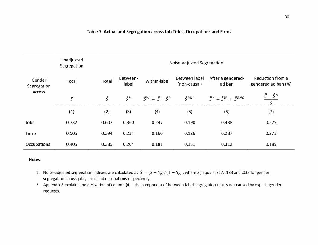
30

Table 7: Actual and Segregation across Job Titles, Occupations and Firms

Gender Segregation

across

Unadjusted Segregation

Noise-adjusted Segregation

Total

Total Between- label Within-label Between label

(non-causal) After a gendered-

ad ban Reduction from a

gendered ad ban (%)

𝑆

�̃� �̃�𝐵 �̃�𝑊 = �̃� − �̃�𝐵 �̃�𝐵𝐵𝐵 �̃�𝐴 = �̃�𝑊 + �̃�𝐵𝐵𝐵 �̃� − �̃�𝐴

�̃�

(1) (2) (3) (4) (5) (6) (7)

Jobs 0.732 0.607 0.360 0.247 0.190 0.438 0.279

Firms 0.505 0.394 0.234 0.160 0.126 0.287 0.273

Occupations 0.405 0.385 0.204 0.181 0.131 0.312 0.189

Notes:

1. Noise-adjusted segregation indexes are calculated as �̃� = (𝑆 − 𝑆0) (1 − 𝑆0)⁄ , where 𝑆0 equals .317, .183 and .033 for gender segregation across jobs, firms and occupations respectively.

2. Appendix 8 explains the derivation of column (4)—the component of between-label segregation that is not caused by explicit gender requests.

31

5.3 Baseline Effects of a Gendered-Ad Ban

To estimate between-label segregation after a ban, we first use the regression coefficients from column 6 of Table 5 to estimate the female applicant shares to F, N and M jobs that we would expect to see after a ban: these reflect only the differences in α across job types that are not caused by the ban. (Men and women will continue to apply to typically-male and -female jobs even after a ban, just not to the same extent as before.) Using these applicant shares, we simulate between-label segregation after a ban, reported in column 5 of Table 7, assuming -- in our baseline scenario -- that the additional applications to gender-mismatched jobs continue to be treated the same by employers (i.e. encounter the same 𝜃s) as they were before the ban. Finally, we add this counterfactual between-label segregation to within-label segregation to get our baseline estimate of segregation after a ban, reported in column 6 of Table 7.

Under these assumptions, column 7 of Table 7 states that banning explicit gender requests would reduce gender segregation across jobs, firms and occupations by 28, 27 and 19 percent respectively. Notably, the magnitude of these declines is constrained by two key features of our simulations: (a) we do not expect an ad ban to change the amount of within-label segregation; and (b) our Table 6 regressions indicate that many workers will continue to disproportionately apply to jobs that formerly requested their gender even after a ban, most likely because they have tastes and training that attach them to those types of work. Indeed, gender-specific training may help to explain why ad bans have a larger predicted effect at the job title and firm level than the occupation level: It may be easier to re-allocate one’s application to a different firm or different detailed job title in response to the removal of explicit gender requests than to change one’s occupation.37 This finding is also consistent with our result (in Section 3.2) that gender labels affect application behavior most strongly in jobs which are not clearly gender-stereotyped -- it is in these low-𝐹𝑝 and low-𝑀𝑝 jobs where we expect the desegregating effects of an ad ban to be the greatest.

Finally, we remind the reader that these predicted effects on gender segregation come at the cost of increased labor market frictions: because a ban directs a substantial number of workers’ applications into jobs that formerly requested the other gender --where by assumption they have a smaller chance of getting a callback-- fewer total callbacks will result from the same total number of applications. Stepping outside our simulations, after a ban, both

37 Mechanically, gender differences in occupation-specific training affect our simulation results via two channels: First, compared to job segregation, a larger share of occupational segregation is within the F, N, and M labels, and therefore not affected by a ban. In particular, the majority of jobs that are not explicitly gendered (N jobs) are highly gender segregated by occupation, and this segregation is unlikely to be changed by removing gender requests. Second, again compared to job segregation, a smaller share of between-label occupational segregation is caused by the labels.

32

men and women might need to submit more applications, search longer, or reduce their reservation wages to find an acceptable job.

5.4 Sensitivity and Caveats

Table A8.2 assesses the sensitivity of the preceding calculations to two alternative assumptions about the effect of a gendered ad ban on women’s relative callback chances (the 𝜃s). In one, the callback penalty associated with applying to a gender-mismatched job increases by 50 percent after a ban is imposed. We think this is unlikely, but it might occur if the gender-mismatched applicants created by the ban are of lower ability (or more poorly matched on dimensions like education, age and experience) than the workers who purposely cross-applied when gendered ads were present.38 In the second robustness test, we go to the opposite extreme by assuming that the gendered ad ban equates the gender gap in relative callback rates (𝜃) across all three job types. This might occur if the average quality or match of gender-mismatched applications rises, or if a gendered-ad ban signaled to employers that gender discrimination in the later stages of the hiring process will also be subject to increased legal scrutiny. In the longer term, such declines in expected hiring discrimination could also increase men’s and women’s investments in gender-atypical skills (like nursing for men and management for women), making workers more qualified for those jobs.

Interestingly, we find that both of these large changes in assumptions have relatively muted effects on the estimated impact of a gendered-ad ban. A 50 percent increase in the mismatch penalty after a ban reduces the predicted decline in segregation across jobs resulting from an ad ban from 28.0 to 21.5 percent; eliminating the mismatch penalty after a ban raises it from 28.0 to 35.0 percent. As already noted, these differences are small because within-label segregation is not directly affected by a ban, because we estimate that only about 60 percent of between-label segregation is caused by explicit gender requests, and because gender differentials in callback rates have small effects on outcomes when applicant pools are highly segregated (as they are in our simulations, even after a ban).

A final caveat regarding the above calculations is that they do not incorporate steps employers might take to circumvent a gendered ad ban by communicating the information formerly conveyed in explicit gender requests via other signals. For example, as discussed in Appendix 3, recent attempts to discourage gendered job ads in China have led some employers to use code words to communicate the same message.39 If such responses are common and

38 We think this is unlikely because Table 6 suggests that workers who voluntarily cross-apply when gendered ads

are allowed are on average negatively selected. Thus we would expect the ‘involuntary’ cross-applicants induced by a gendered-ad ban to be, on average, better selected.

39 Some job boards have also responded to ad bans by making it easier for recruiters filter resumes by gender, both within the applicant pool and when a recruiter is searching through resumes posted on the site. Note that,

33

effective, a gendered ad ban might reduce job segregation by much less than our baseline estimate of 28 percent.

6. Discussion

We believe that this is the first paper to study how workers respond to explicit gender requests in job ads, and how employers treat applicants to these types of ads. Our best estimates suggest that gendered job ads direct workers’ applications away from jobs requesting the ‘other’ gender, and that employers penalize workers who apply to gender-mismatched jobs (in the form of a lower callback probability). Our estimated mismatch penalty is substantially greater for women who apply to men’s jobs than for men who apply to women’s jobs. Finally, our baseline estimates suggest that banning explicit gender requests could reduce gender segregation in the labor market by amounts ranging from 19 to 28 percent. Intuitively, these predicted reductions are larger for segregation across firms and detailed job titles than occupations, because workers are tied to occupations by their previous human capital investments. Our regression results also suggest that an ad ban will have larger effects on segregation in job titles that are not highly gender-stereotyped, because it is there that gender labels most strongly direct workers’ application decisions. Finally, we note that actual reductions in segregation could be lower than these numbers if employers find ways to circumvent a ban using code words and other signals of their gender preferences, and higher than these numbers if workers alter their longer-term human capital investments in response to a ban.

Because our estimates are computed from a single job board, and because our estimates of causal connections are not based on random assignment, we view our analysis as the first rather than the last word on the effects of gendered job ads in labor markets. In our view, further analysis could profit from work in at least three different directions. First, it would be of interest to conduct a resume audit study of employers’ ‘enforcement’ decisions: how will employers respond when we send identical resumes of different genders to jobs that request male versus female applicants? We view such an analysis as complementary with our internal job-board-based approach, because resume audits typically achieve tighter identification at the expense of focusing on only a handful of jobs. This is a significant issue in an environment such as ours, where employers’ gender preferences vary dramatically across jobs.

Second, it would be useful to conduct a natural field experiment (a la Leibbrandt and List 2014 or Ibanez and Reinter 2018) on workers’ ‘compliance’ decisions: How, if at all, do workers’ application decisions change when they are exposed to identical job ads that differ

because workers will no longer know whether firms are engaged in this filtering, these tools will raise search frictions for workers compared to a labor market that allows gendered ads.

34

only in the presence or absence of a gender request? Again, such an approach would be complementary with a job-board-based approach because it provides a better-identified estimate, but for a small subset of jobs.

Finally, internal job-board data could be fruitfully used to study natural experiments associated with the sudden imposition of a gendered-ad ban. An appealing feature of this approach is that it would allow investigators to study the simultaneous changes in both worker (compliance) and firm (enforcement) behavior that result from such a ban. In addition, to the extent that a job board constitutes a local, occupational or national labor market, such a study would capture general equilibrium effects of the policy change, none of which are addressed by the preceding approaches.

35

References

Aaronson, Daniel, Daniel Hartley, and Bhashkar Mazumder. 2017. “The Effects of the 1930s HOLC ‘Redlining’ Maps.” Chicago Federal Reserve working paper no. 2017-12.

Albrecht, J., P. Gautier and S. Vroman. 2006. “Equilibrium Directed Search with Multiple Applications.” Review of Economic Studies, 73(4), 869-891.

Angwin, Julia, Noam Scheiber and Ariana Tobindec. 2017. “Facebook Job Ads Raise Concerns About Age Discrimination.” New York Times, December 20, 2017.

Banfi, Stefano, and Benjamin Villena-Roldan. 2019. “Do High-Wage Jobs Attract more Applicants? Directed Search Evidence from the Online Labor Market.” Journal of Labor Economics, 37(3), 715-746.

Baker, Michael and Kirsten Cornelson. 2016 “Gender Based Occupational Segregation and Sex Differences in Sensory, Motor and Spatial Aptitudes.” National Bureau of Economic Research, working paper no. 22248.

Belot, Michele, Philipp Kircher and Paul Muller. 2017. “How Wage Announcements Affect Job Search Behaviour - A Field Experimental Investigation.” European University Institute, working paper.

Bertrand, Marianne and Sendhil Mullainathan. 2004. “Are Emily and Greg More Employable Than Kakisha and Jamal? A Field Experiment on Labor Market Discrimination.” American Economic Review, 94(4), 991-1013.

Bielby, W. T., and J. N. Baron. 1984.‘‘A Woman’s Place Is with Other Women: Sex Segregation within Organizations.’’ in Sex Segregation in the Workplace: Trends, Explanations, Remedies, B. F. Reskin, ed. Washington, DC: National Academies Press.

Blau, Francine D., Brummund, Peter and Albert Yung-Hsu Liu. 2013. “Trends in Occupational Segregation by Gender 1970-2009: Adjusting for the Impact of Changes in the Occupational Coding System.” Demography, 50(2), 471-492.

Brenčič, Vera. 2010. “Do Employers Respond to the Costs of Continued Search?” Oxford Bulletin of Economics and Statistics, 72(2), 211-245.

Brenčič, Vera. 2012. “Wage Posting: Evidence from Job Ads.” Canadian Journal of Economics, 45(4), 1529-1559.

Brenčič, Vera and John B. Norris. 2009. “Employers’ Online Search: An Empirical Analysis.” Industrial Relations, 48(4), 684-709.

36

Brenčič, Vera and John B. Norris. 2012. “Employers’ Online Recruitment and Screening Practices.” Economic Inquiry, 50(1), 94-111.

Brenčič, Vera and John B. Norris. 2010. “Do Employers Change Job Offers in Their Online Job Ads to Facilitate Search?” Economics Letters, 108(1), 46-48.

Card, David, Ana Rute Cardoso, and Patrick Kline. 2016."Bargaining, Sorting, and the Gender Wage Gap: Quantifying the Impact of Firms on the Relative Pay of Women" Quarterly Journal of Economics, 131(2), 633-686.

Carlsson, Magnus and Rooth, Dan-Olof. 2007. “Evidence of Ethnic Discrimination in the Swedish Labor Market using Experimental Data.” Labour Economics, 14(4), 716-729.

Carrington, William J. and Kenneth R. Troske. 1997. “On Measuring Segregation in Samples With Small Units.” Journal of Business & Economic Statistics, 15(4), 402-409.

Cook, Cody, Rebecca Diamond, Jonathan Hall, John A. List, and Paul Oyer. 2017. “The Gender Earnings Gap in the Gig Economy: Evidence from over a Million Uber Drivers.“ unpublished paper, Stanford University, accessed December 20, 2017.

Cutler, David M., Edward L. Glaeser and Jacob L. Vigdor. 1999. “The Rise and Decline of the American Ghetto.” Journal of Political Economy, 107(3), 455-506.

Delgado Helleseter, Miguel, Peter Kuhn and Kailing Shen. forthcoming. “The Age Twist in Employers’ Gender Requests: Evidence from Four Job Boards”, Journal of Human Resources.

Duncan, Otis Dudley, and Beverly Duncan. 1955. “A Methodological Analysis of Segregation Indexes” American Sociological Review, 20(2), 210-217.

Federal Housing Administration. 1938. Underwriting Manual: Underwriting and Valuation Procedure Under Title II of the National Housing Act With Revisions to February, 1938 (Washington, D.C.), Part II, Section 9, Rating of Location. Available at: http://wbhsi.net/~wendyplotkin/DeedsWeb/fha38.html (visited May 10, 2016).

Flory, Jeffrey A., Andreas Leibbrandt and John A. List. 2015. “Do Competitive Workplaces Deter Female Workers? A Large-Scale Natural Field Experiment on Job Entry Decisions.” The Review of Economic Studies, 82(1), 122-155.

Gee, Laura. 2018. “The More You Know: Information Effects on Job Application Rates in a Large Field Experiment”, Management Science, 65(5), 2077-2094.

37

Hirschbein, Brad and Kahn, Lisa. 2018. “Do Recessions Accelerate Routine-Biased Technological Change? Evidence from Vacancy Postings.” American Economic Review, 108(7), 1737-1772.

Horton, John (2017) “The Effects of Algorithmic Labor Market Recommendations: Evidence from a Field Experiment”, Journal of Labor Economics, 35(2).

Human Rights Watch. 2018. “Only Men Need Apply: Gender Discrimination in Job Advertisements in China.”

Ibanez, Marcela and Gerhard Reinter. 2018. “Sorting through Affirmative Action: Three Field Experiments in Colombia.” Journal of Labor Economics, 36(2), 437-478.

Kroft, Kory, Fabian Lange and Matthew J. Notowidigdo. 2013. “Duration Dependence and Labor Market Conditions: Evidence from a Field Experiment.” Quarterly Journal of Economics, 128(3), 1123-1167.

Kuhn, Peter and Kailing Shen. 2013a. “Gender Discrimination in Job Ads: Evidence from China.” Quarterly Journal of Economics, 128(1), 287-366.

Kuhn, Peter and Kailing Shen. 2013b. “Do Chinese Employers Avoid Hiring Overqualified Workers? Evidence from an Internet Job Board.” Research in Labor Economics, 37, 1-30.

Kuhn, Peter and Kailing Shen. 2015. “Do Employers Prefer Migrant Workers? Evidence from a Chinese Job Board.” IZA Journal of Labor Economics 4:22.

Kuhn, Peter. “Employer Investments in Employee Assessment.” unpublished paper, UC Santa Barbara, March 2016.

Kudlyak, Marianna, Damba Lkhagvasuren and Roman Sysuyev. 2013. “Systematic Job Search: New Evidence from Individual Job Application Data.” FRB Richmond working paper no 12-03R.

Lang, Kevin, Michael Manove, and William T. Dickens. 2005. “Racial Discrimination in Labor Markets with Posted Wage Offers.” American Economic Review, 95(4), 1327-1340.

Lazear, Edward P., Kathryn L. Shaw, and Christopher T. Stanton. 2018. “Who Gets Hired? The Importance of Competition among Applicants” Journal of Labor Economics 36(S1).

Leibbrandt, A. and John A. List. 2014. “Do women avoid salary negotiations? Evidence from a large-scale natural field experiment.” Management Science, 61(9), 2016-2024.

38

Leibbrandt, A. and John. A. List. 2019. “Do Equal Employment Opportunity Statements Backfire? Evidence from a Natural Field Experiment on Job-Entry Decisions.” unpublished paper, University of Chicago.

Logan, John R., Brian J. Stults and Reynolds Farley. 2004.“Segregation of Minorities in The Metropolis: Two Decades of Change” Demography, 41(1), 1-22.

Makinen, Julie. 2014. “China's Women Begin to Confront Blatant Workplace Bias” February 28, 2014. Available at: http://www.latimes.com/world/asia/la-fg-china-women-work-20140228-story.html#page=1. Visited April 8, 2015.

Marinescu, Ioana and Roland Rathelot. 2015.“Mismatch Unemployment and the Geography of Job Search” unpublished paper, University of Chicago.

Marinescu, Ioana and Ronald Wolthoff. 2016. “Opening the Black Box of the Matching Function: the Power of Words.” National Bureau of Economic Research, working paper W22508.

Mas, Alexandre and Amanda Pallais. 2017. “Valuing Alternative Work Arrangements.” American Economic Review, 107(12), 3722-3759.

McCallum, Andrew and Kamal Nigam. 1998. “A Comparison of Event Models for Naive Bayes Text Classification.” AAAI-98 Workshop on Learning for Text Categorization. 752.

Modestino, Alicia Sasser, Daniel Shoag and Joshua Balance. “Upskilling: Do Employers Demand Greater Skill When Workers Are Plentiful?” unpublished paper, Northeastern University.

Neumark, David Ian Burn and Patrick Button. 2015. “Is It Harder for Older Workers to Find Jobs? New and Improved Evidence from a Field Experiment.” National Bureau of Economic Research, working paper W21669.

Niederle, Muriel, and Lise Vesterlund. 2007. “Do Women Shy Away from Competition? Do Men Compete Too Much?” Quarterly Journal of Economics, 122(3), 1067-1101.

Pittsburgh Press Co. vs Pittsburgh Commission on Human Relations et al., U.S. Supreme Court decision argued March 20. 1973, decided on June 21, 1973.

Shen, Kailing and Peter Kuhn. 2013. “Do Chinese Employers Avoid Hiring Overqualified Workers? Evidence from an Internet Job Board.” Research in Labor Economics, 37, 1-30.

Sorensen, Elaine. 1990. “The Crowding Hypothesis and Comparable Worth.” Journal of Human Resources, 25(1), pp. 55-89.

39

Walsh, John, Miriam Johnson and Marged Sugarman. 1975. “Help Wanted: Case Studies of Classified Ads.” Salt Lake City, Utah: Olympus Research Corporation (funded by U.S. Department of Labor research contract no. 2141-73-28).

Zoloth, B.S. 1976. “Alternative Measures of School Segregation.” Madison: Institute for Research on Poverty, University of Wisconsin.

40

Appendix—for online publication

1

Appendix 1: International Examples of Gendered Job Ads from Indeed.com

Accurate measures of the share of ads on a job site that are gender-targeted cannot be generated by conducting searches on the site’s public portals, for a number of reasons. First, the ads on the site at a point in time represent a stock sample with potentially many stale ads. Second, unless the job board has chosen to collect and to publicize an unambiguous indicator of the employer’s gender preference (as XMRC does), gender preferences can be expressed in many different ways, some of which are evasive, others of which are costly to detect.40 Third, jobseekers’ search results are often prioritized in ways that are opaque to the user. Finally, without a well-defined sample that has been drawn from the board’s internal database, researchers are forced to rely on denominators provided by the job board, which are not clearly defined and prone to exaggeration.41

With these cautions in mind, we can arguably get some indicators of at least the presence and typical form of explicit gender requests by conducting keyword searches for jobs through the worker portal on a site. In this document we present examples of the results of such searches on Indeed.com, which currently operates job search platforms in 63 countries. The ads reproduced in the following pages were collected from Indeed.com’s international portal: https://www.indeed.com/worldwide on November 12, 2018. In all cases, we searched for the terms “male” and “female” in the sites’ native languages (this was English in India and Pakistan), then -- where necessary -- used Google to translate the results. Since “male” and “female” can be used in several ways that do not request a specific gender for the job (including saying that both men and women are welcome), we manually searched through these search results ads till we found ads that expressed a preference for one gender. We never had to go beyond the first 50 search results to find such ads. Noting that Indeed, as a U.S.-owned company, may be more sensitive to stigma associated with posting gendered ads, and that its international sites tend to serve educated and disproportionately English-speaking workers, it seems likely that gendered ads would be even easier to find on locally-owned and operated sites.

In all cases the searches were done without creating an account on Indeed, and without specifying a type of work or location—the only search term was “male” or “female”. No other filtering or ordering of results was done. The countries searched are the ten countries represented by Indeed with the largest populations. Since Indeed serves ten of the eleven largest countries, our results are for the world’s 11 most populous countries with exception of Bangladesh, representing 57.4% of the world’s population. The ads are numbered by country population rank.

40 The use of gendered job titles (such as abogada and abogado in Spanish) is particularly burdensome to measure since

each title expresses gender in a different way. 41 Another emerging difficulty is the possibility that job boards are designing their worker-facing search algorithms to

make certain forms of explicit gender requests hard to find via a keyword search, even though these requests are still present in ads (that are found via other keywords). We report some suggestive evidence of this in Section 3.2.

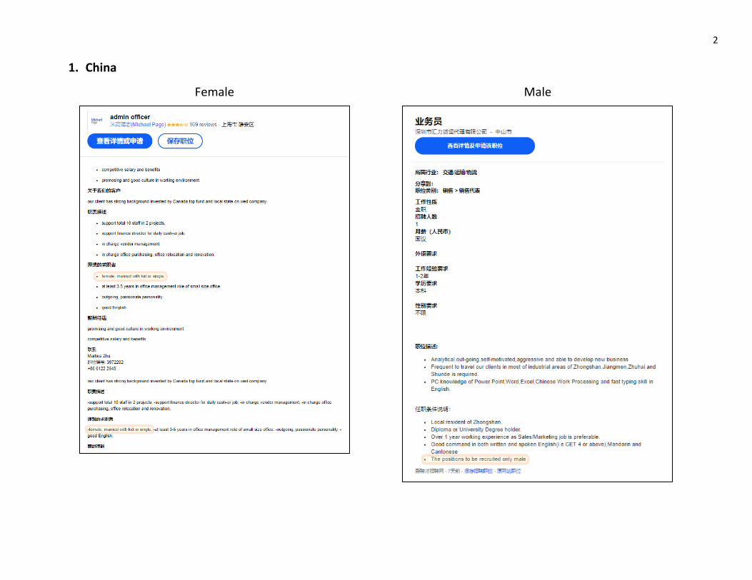
2

1. China

Female Male

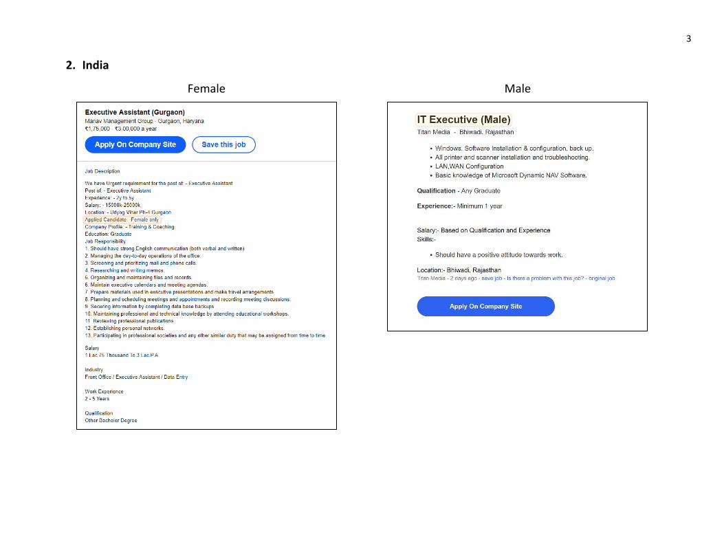
3

2. India

Female Male

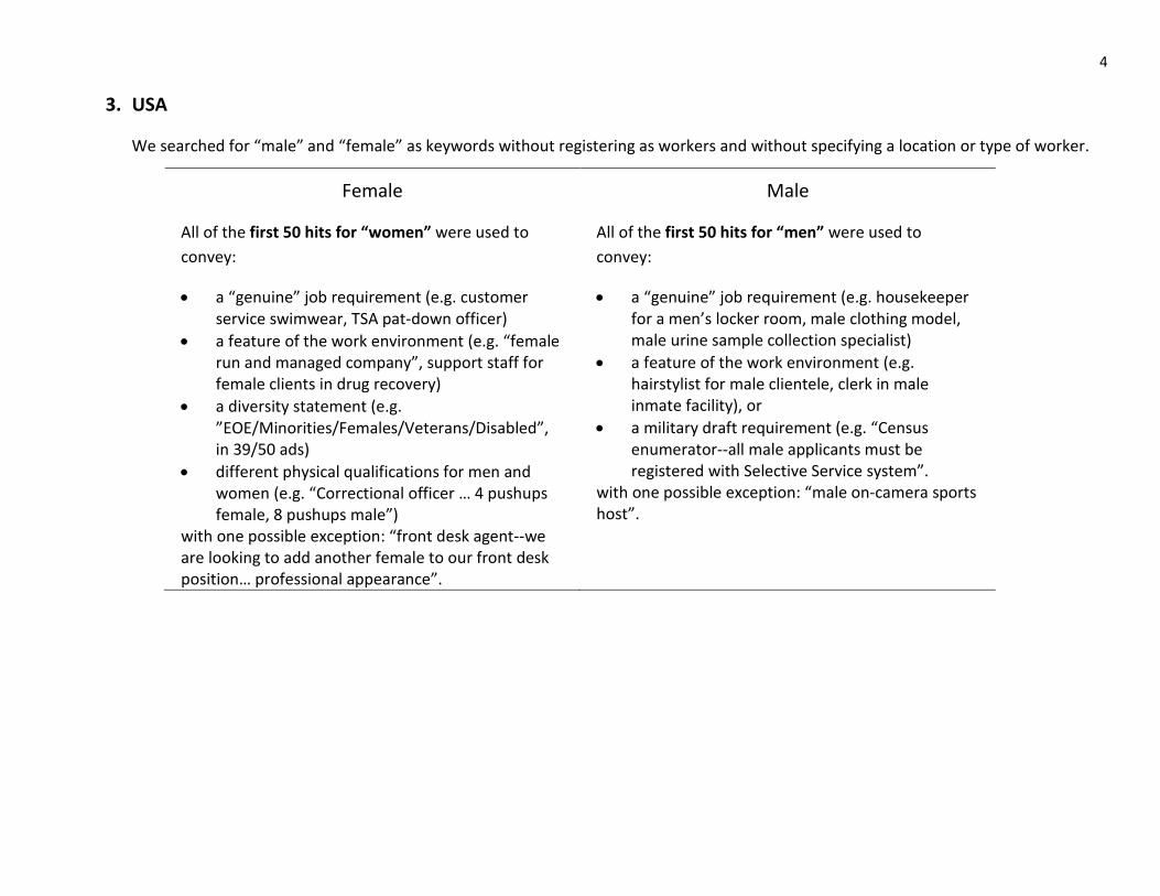
4

3. USA

We searched for “male” and “female” as keywords without registering as workers and without specifying a location or type of worker.

Female Male

All of the first 50 hits for “women” were used to convey:

• a “genuine” job requirement (e.g. customer service swimwear, TSA pat-down officer)

• a feature of the work environment (e.g. “female run and managed company”, support staff for female clients in drug recovery)

• a diversity statement (e.g. ”EOE/Minorities/Females/Veterans/Disabled”, in 39/50 ads)

• different physical qualifications for men and women (e.g. “Correctional officer … 4 pushups female, 8 pushups male”)

with one possible exception: “front desk agent--we are looking to add another female to our front desk position… professional appearance”.

All of the first 50 hits for “men” were used to convey:

• a “genuine” job requirement (e.g. housekeeper for a men’s locker room, male clothing model, male urine sample collection specialist)

• a feature of the work environment (e.g. hairstylist for male clientele, clerk in male inmate facility), or

• a military draft requirement (e.g. “Census enumerator--all male applicants must be registered with Selective Service system”.

with one possible exception: “male on-camera sports host”.

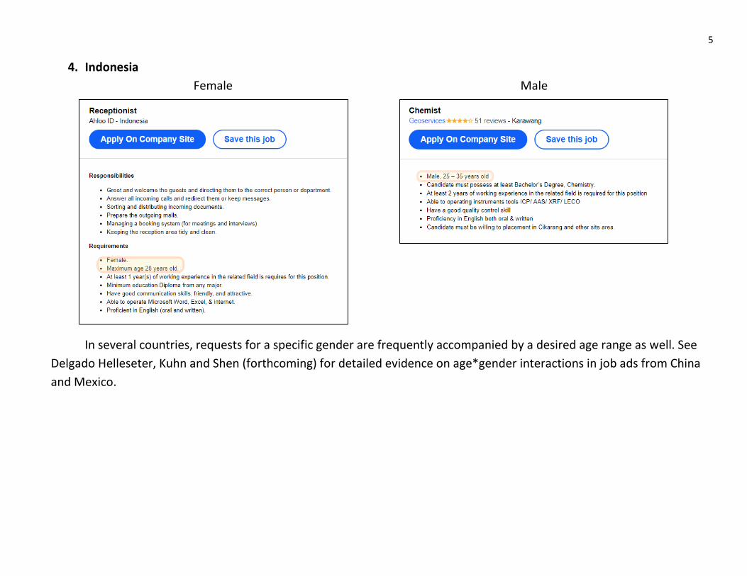
5

4. Indonesia Female Male

In several countries, requests for a specific gender are frequently accompanied by a desired age range as well. See Delgado Helleseter, Kuhn and Shen (forthcoming) for detailed evidence on age*gender interactions in job ads from China and Mexico.

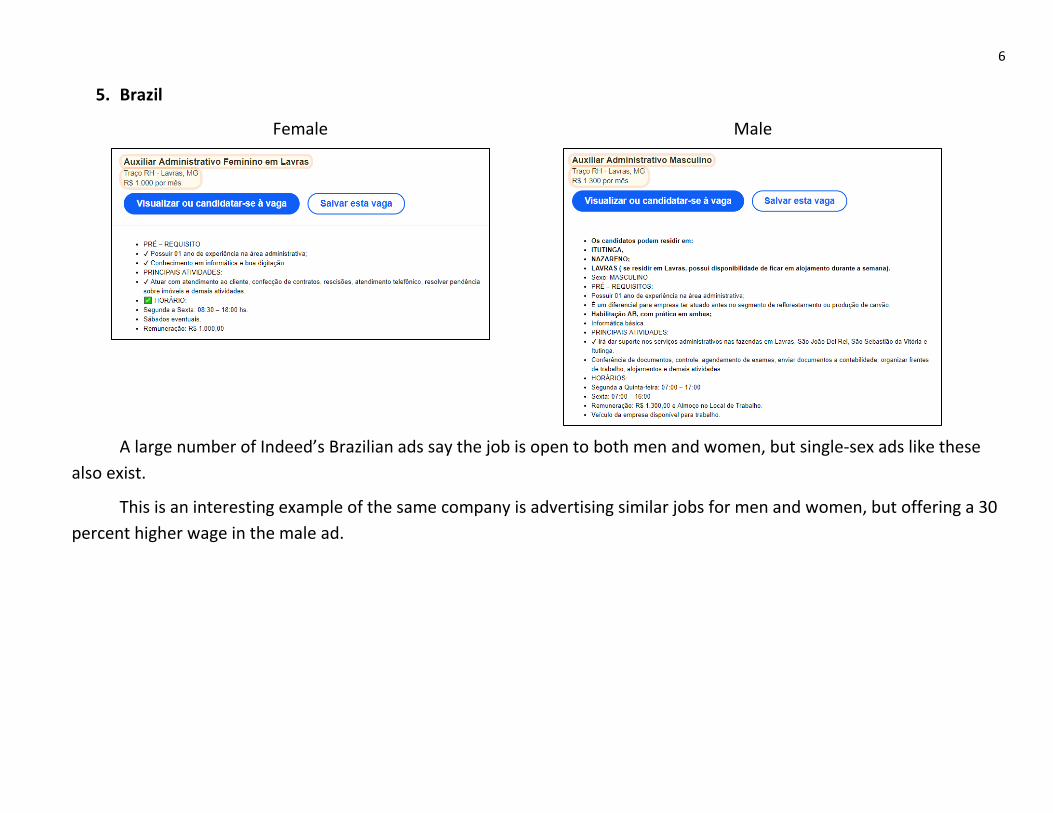
6

5. Brazil

Female Male

A large number of Indeed’s Brazilian ads say the job is open to both men and women, but single-sex ads like these

also exist.

This is an interesting example of the same company is advertising similar jobs for men and women, but offering a 30 percent higher wage in the male ad.

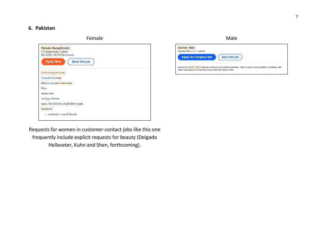
7

6. Pakistan

Female Male

Requests for women in customer-contact jobs like this one frequently include explicit requests for beauty (Delgado

Helleseter, Kuhn and Shen, forthcoming).

8

7. Nigeria

Female Male

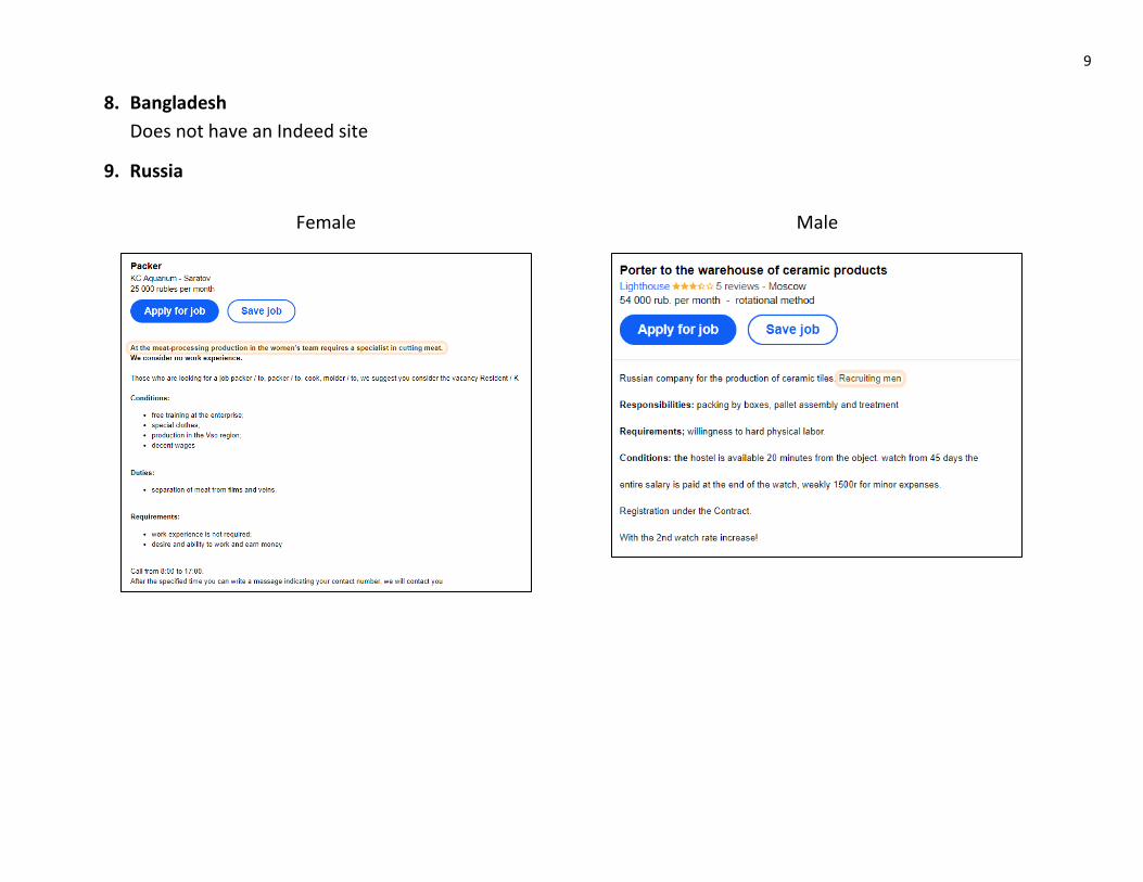
9

8. Bangladesh Does not have an Indeed site

9. Russia

Female Male

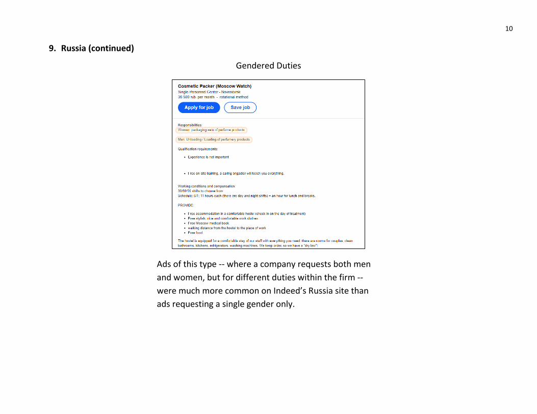
10

9. Russia (continued)

Gendered Duties

Ads of this type -- where a company requests both men and women, but for different duties within the firm -- were much more common on Indeed’s Russia site than ads requesting a single gender only.

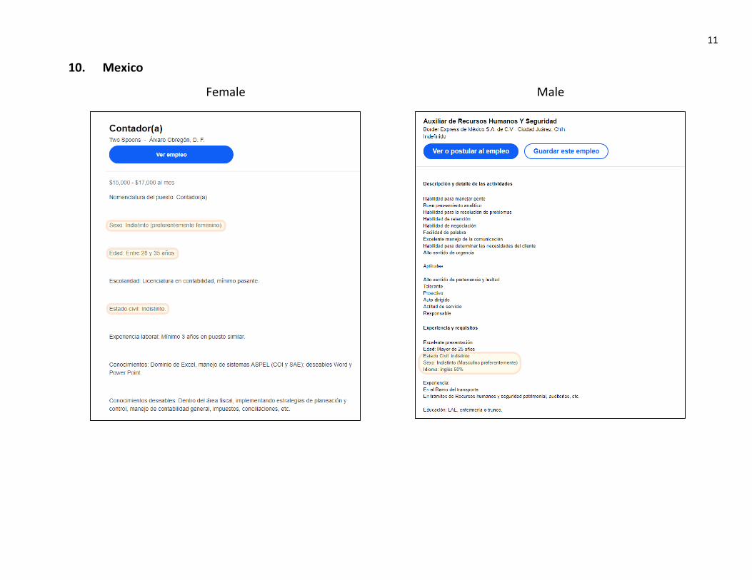
11

10. Mexico

Female Male

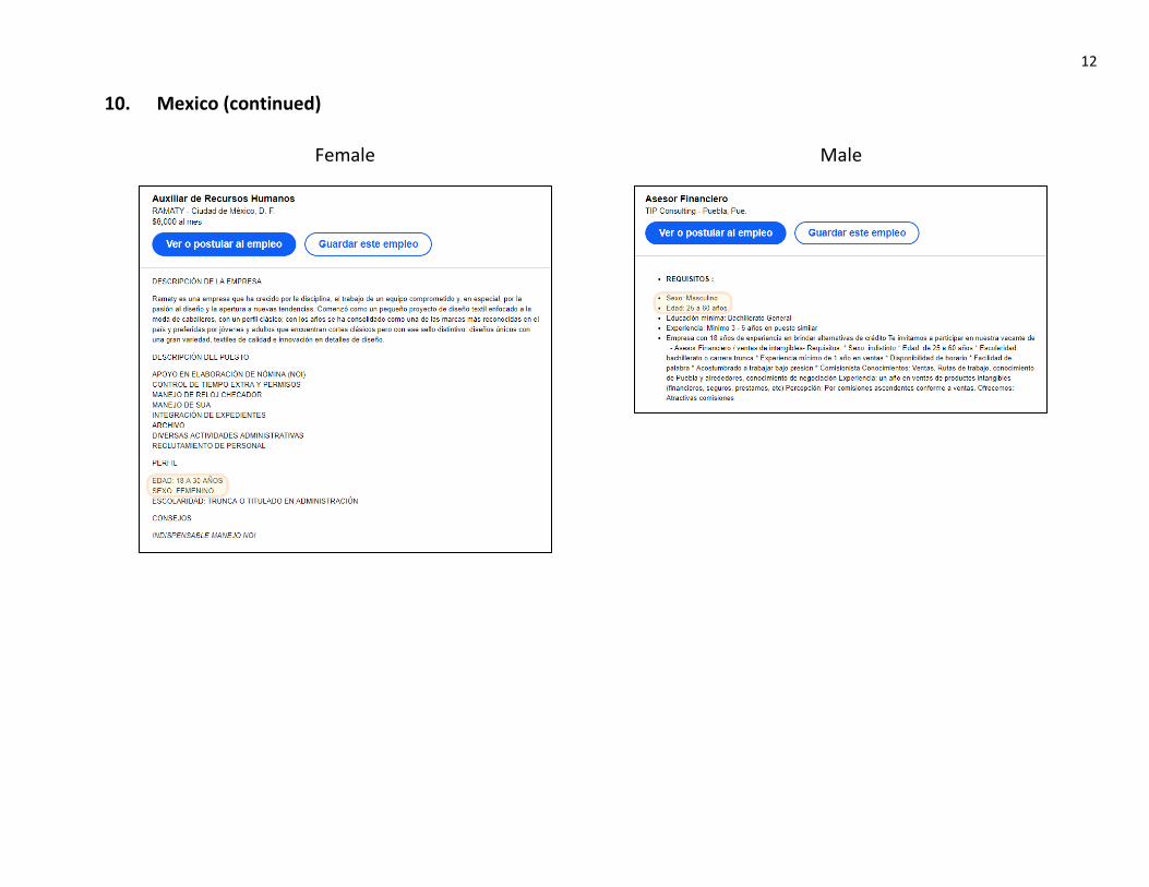
12

10. Mexico (continued)

Female Male

13

11. Japan

The Japanese Equal Employment Opportunity Law prohibits employers from saying that they prefer to hire men (women). However, job ads on Indeed’s Japan site frequently say that men (women) are playing “active roles”, or ‘thriving’ in these jobs or in the firm. The intent appears to be to signal that the jobs in question are suited to a particular gender.

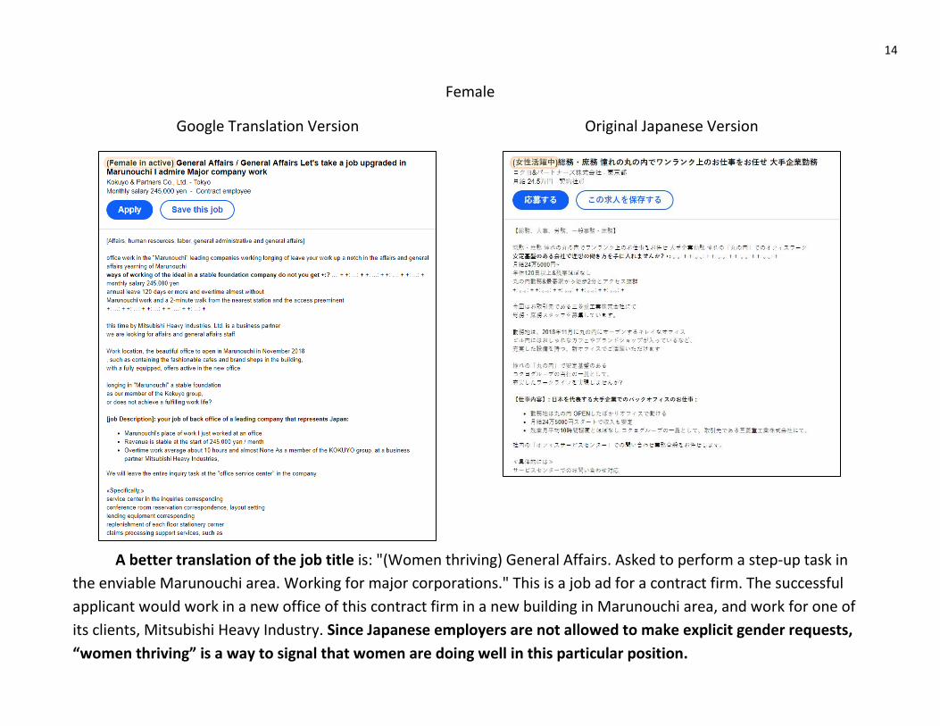
14

Female

Google Translation Version Original Japanese Version

A better translation of the job title is: "(Women thriving) General Affairs. Asked to perform a step-up task in the enviable Marunouchi area. Working for major corporations." This is a job ad for a contract firm. The successful applicant would work in a new office of this contract firm in a new building in Marunouchi area, and work for one of its clients, Mitsubishi Heavy Industry. Since Japanese employers are not allowed to make explicit gender requests, “women thriving” is a way to signal that women are doing well in this particular position.

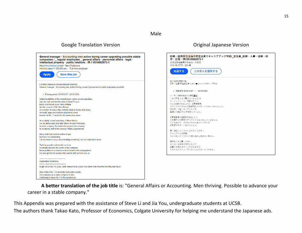
15

Male

Google Translation Version Original Japanese Version

A better translation of the job title is: "General Affairs or Accounting. Men thriving. Possible to advance your career in a stable company."

This Appendix was prepared with the assistance of Steve Li and Jia You, undergraduate students at UCSB. The authors thank Takao Kato, Professor of Economics, Colgate University for helping me understand the Japanese ads.

16

Appendix 2: Legislation Affecting Gender-Targeted Job Ads in China

A2.1 Early Laws and Regulations Concerning Gender Discrimination

China’s constitution and labor law have prohibited gender discrimination since at least 1982. For example, Article 48 of the Constitution of the People's Republic of China (1982) grants women “equal rights with men in all spheres of life, political, economic, cultural, social, and family life”, and affirms the principle of equal pay for equal work for men and women. With the exception of “types of work that are not suitable for females”, the Labor Law of the PRC (1994; Article 13) prohibits using sex as a pretext for excluding females from employment or for raising recruitment standards; similar provisions are found in the Law of the PRC on the Protection of Rights and Interests of Women (2005; Article 22), and the Law of the PRC on Promotion of Employment (2007, Articles 26 and 27.) The latter law also prohibits employment contracts that restrict female workers from getting married or bearing a child.

While a ban on ads (of any kind) that “carry any nationality, religious or sex discriminating information” has been in place since 1994 (Advertisement law of the PRC, Articles 7 and 39), the earliest regulations we are aware of that specifically prohibit gender discrimination by labor market intermediaries date from 2007. At that time, the Ministry of Labor and Social Security’s Regulations on Employment Service and Employment Management prohibited intermediaries from “releasing any information indicating employment discrimination” (Articles 58 and 74).

Enforcement of China’s anti-discrimination laws before 2012 however, is widely perceived to have been weak (Human Rights Watch 2018), and our previous studies of online job boards (Kuhn and Shen 2013; Delgado Helleseter, Kuhn and Shen forthcoming) suggest that these laws did not seriously constrain employers’ use of explicitly gendered job ads at that time.

A2.2 Court Cases

According to FlorCruz (2014), the first lawsuit claiming gender discrimination in China’s labor market was filed in July 2012. After graduating from a Beijing university, Ju Cao was told that she was not qualified for an administrative assistant job because “this was a position for men, we would not consider you although you are qualified”. As part of an out-of-court settlement, the firm made a public apology to Ms. Cao. In 2014, another new graduate, Guo Mou was rejected from a copywriting job at Hangzhou‘s prestigious New East Cuisine Education school, for the reason that “men are more qualified for this position”. The school was ordered to pay Ms. Guo 2,000 yuan for “spiritual injury” (CCTV.com, 2015). In China’s first lawsuit on gender discrimination against a state-owned enterprise (SOE), Hu Ma was rejected for a

17

delivery job with China Post. In response to her lawsuit, submitted on January 26,. 2015, China Post argued that delivery required workers to hold heavy objects, which met the legal exception of not being “suitable for females”. The Court of Beijing rejected China Post’s argument and ordered them to compensate Ms. Hu (Zhang, 2016).

Since the latter two lawsuits, the plaintiffs (Guo and Hu), have become activists against gender discrimination in employment. As part of their efforts, they have collected gender-targeted job ads on sites including Zhaopin.com, 51job.com, 58.com, Chinahr.com, and reported them to Ministry of Labor and Social Security.

A2.3 Responses of the Job Boards

In addition to the above court cases, a recent regulatory development seems to have prodded China’s largest job boards to actively discourage and remove gendered job ads from their sites. In May 2016, China’s Ministry of Industry and Information Technology issued a regulation aimed directly at gendered job ads on online job platforms. A key component of this regulation clarified the division of fines between the job board (30%) and the firm placing the ad (70%). This appears to have been at least partially effective: by October 2018, explicit requests for men or women ads were effectively absent from the two of largest privately operated job boards: 51 job and Zhaopin (see Appendix 3).

Some insight into how this change occurred is available from our conversations with officials at Liepin.com, a ‘high-end’ job board catering to executive-level positions. After receiving notice of the May 2016 regulation, Liepin sent a letter to all HR personnel using their website, stating that the HR personnel would not be allowed to post new job ads stating an explicit preference for one gender. Hiring managers were also asked to revise existing ads by removing any gender labels or other statements of gender preference.

At the same time, Liepin developed and improved its own filtering system to detect gendered job ads. Focusing first on newly-posted ads, Liepin tagged ads including statements like “male first”, or “only for women” “male engineer” etc. and asked HR personnel to change these ads. Starting in July 2016, Liepin actively revised previously-posted ads by removing the gender requests without changing anything else. All such ads were replaced by the end of August, 2016. Since then, in part due to increased scrutiny from applicants who are willing to report violations to the government, Liepin has improved its screening for words that may convey a preferred gender, using human screeners to examine jobs that are considered suspect by Liepin’s algorithms. Notably, throughout this process, Liepin continued to allow HR personnel to filter job applications by gender, so that the firm could choose to see only applications from one gender regardless of who applied. Thus, at least on Liepin, internal filters seem to have replaced public gender requests.

18

References

CCTV.com. 2015. “The Communist Party announced the top ten cases of labor violations: the first case of employment gender discrimination ranked first” CCTV News, February 02, 2015 (accessed November 18, 2018).

FlorCruz, Michelle. 2014. “Chinese Woman Wins Settlement In China's First Ever Gender Discrimination Lawsuit” International Business Times, February 2, 2014 (accessed November 18, 2018).

Zhang, Yuanyuan. 2016.“Ma Hu v. Beijing Post Employment Sex Discrimination Case Second Trial” China Women’s News, January 29, 2016 (accessed November 18, 2018).

19

Appendix 3: Gendered Job Ads in China, 2018

A3.1. Methods

As noted in Appendix 1, accurate measures of the share of ads on a job site that are gender-targeted cannot be generated by conducting searches on the site’s public portals. As we did in Appendix 1 for the international context, however, this Appendix attempts to document the presence and typical form of gender requests on various Chinese job sites by searching for jobs using gender-related keywords. Specifically, entering the sites via their jobseeker portals, we searched for words that might convey a gender preference by the employer. Then, we inspected the first page of results (usually 50 ads) to count the number of those hits in which the keyword was used to request a specific gender (as opposed to describing the product/service, or inviting both genders to apply). In performing these searches, we did not create a worker profile on the site or specify any worker characteristics, nor did we enter any search terms for the location and type of work sought. All searches were performed in October 2018. The only search terms we entered were the following (one at a time):

(1) Direct gender indicators: “man (男)” and “woman (女 )” (This includes “men” and “women” in Chinese).

(2) Transformed gender indicators: “nan” (the pronunciation for man, or 南 meaning south, which has the same pronunciation with man in Chinese), and “nv” (the pronunciation for woman; nv is the Chinese phonetic of women). These indicators have been used by employers to evade some recent enforcement activities (Human Rights Watch, 2018).

(3) Gendered adjectives: handsome (帅), gentleman (绅士), and “tall and strong” (高大健壮) for men; beautiful (美丽), lady (淑女), and “beautiful face” (面容姣好) for women.

(4) New “web words”: little brother (小哥哥 lad), little sister (小姐姐 lass). These new words refer in a polite way to someone who is young and good-looking. They are more widely used by young people, and in job ads aimed at younger workers, such as social media jobs.

In the rest of this Appendix, we provide a verbal overview of these search results. Tabular results with additional details and commentary are available from the authors.

A3.2. 51job.com and Zhaopin.com

51job and Zhaopin are China’s two largest job boards. Both are privately run and cater to private-sector firms and workers. Our searches of these sites revealed no uses of the ‘direct’ indicators “man (男)” and “woman (女)” to request a specific gender, and only a few uses of the transformed indicators “nan”, or “nv”. One likely reason is enforcement: these boards now face a risk of being fined if they post gendered jobs; in response, the boards seem to have improved the screening of sensitive words so they no longer appear in workers’ search results. In

20

addition, these boards now discourage recruiters from making gender requests in job ads.42 A second possible reason is that these boards cater to highly skilled workers; this may leave the boards more vulnerable to disapproval on social media if they post gendered ads. A third contributing factor may be the fact that employers’ demand for gender profiling was relatively low in highly skilled jobs to begin with, even when this practice was widely tolerated (Kuhn and Shen 2013; Delgado, Kuhn and Shen, forthcoming), thus reducing the cost of compliance with the new restrictions.

This being noted, our analysis also shows that these job boards still accept subtler gender signals in ads, such as the gendered adjectives and the new “web words” we examined. For example, even though searches for “woman” yielded no results, searches for compound words like “lady” = “gentle+woman” (two characters) yielded several pages of results (though most of these refer to the names, products or brand of the firms). In addition, the adjectives “handsome”, “gentleman”, and “tall and strong” were frequently used to request men in jobs that included fitness instructors, sales, and warehouse work. “Beautiful”, “lady”, and “beautiful face” were used to request women in jobs that included customer service, front desk and modeling. Finally, the new web words ”little brother” and “little sister” were also used to convey a clear gender preference. For example “little brother” was frequently used to request (young) men for (electric bicycle) delivery jobs, and “little sister” for camgirl jobs.43 Also of interest, both Zhaopin and 51job allow recruiters to select a filter that will only show the recruiter the applications from a particular gender. 44 Overall, prohibition of gendered job ads has pushed formerly overt discrimination into more hidden forms on these platforms.

A3.3 Chinahr.com

We conducted a comparable search of Chinahr.com, a national job board that caters more to blue collar workers than Zhaopin and 51job. Here, the terms “man” and “woman’ each yielded more than one page of search results.45 Inspecting the first page of these revealed that 17 (or 43%) of the uses of “man” were explicit gender requests, as were 15 (or 38%) of the uses of “woman”. Interestingly, here the transformed gender terms “nan” and “nv” were almost never used to request an applicant gender, perhaps because direct requests were still feasible. Perhaps for the same reason, gendered adjectives and new web words -- while present -- weren’t used much to request candidates of a specific gender either. We speculate that Chinahr

42 Zhaopin’s portal states “Please do not include words that have the meaning of gender discrimination”. Chinahr

says “To make sure the job ad can pass checking, please do not enter repeat or meaningless information, and do not enter discriminating information, such as ‘women first’, or ‘only for men’”.

43 The delivery jobs in question involve driving electric bicycles with packages or meals; pay is commission-based and the jobs are short term and relatively dangerous. Because most of the employees are young men, they are typically called “delivery little brother”.

44 The same is true for Liepin.com, a recruiting site focusing on higher managerial positions. 45 On Chinahr, a page of search results comprises 40 job ads.

21

is more tolerant of gender profiling by employers than 51job and Zhaopin because of its focus on blue collar jobs, where, as noted, employers’ demand for gender profiling appears to be much higher (Delgado, Kuhn and Shen, forthcoming; Kuhn and Shen 2013), and where both stigma and enforcement may be weaker.

A3.4 Local Internet Job Boards

Parallel to the private-sector boards discussed above, China has a system of government-run or government-sponsored job boards that operate at the city or province level. These boards’ names end in RC, GGZP or HR; XMRC is one of them. In general, these boards tend to serve lower skill levels than the national boards described previously. Like the national job boards, however, all of these boards serve private-sector employers and workers; recruiting for government jobs takes place via other channels. In a comprehensive web search -- also in November 2018 -- we were able to find 33 such boards of non-negligible size.46

When we examined the recruiter portals of these 33 sites, we found that 11 of them (including XMRC) asked employers to specify the gender of the worker they were seeking when the employer fills out a template for a job ad. Four of the sites (also including XMRC) allowed workers to filter job ads based on these employer requests. Keyword searches for “male” and “female” produced hits on all but two of these sites, and examination of the first 50 hits on each site revealed that these terms were frequently used to express a preference for male or female applicants. Code words like “nan” and “nv” turned up almost no results, perhaps because direct gender requests are still possible on these sites.

In sum, compared with private job boards, government-sponsored local job sites had a larger number of explicitly gendered job ads in late 2018. We can think of three possible reasons for this. First, these sites tend to be relatively small, so they may so far have escaped the attention of regulators. Second, these sites -- especially the pure job-posting services -- serve less-skilled jobs and workers, where employers’ demand for gender filters is considerably greater. Finally, in China, workers may be much less inclined to report government-sponsored sites for regulatory violations, compared to privately operated sites. Since November 2018, increasing enforcement appears, however, to have encroached on these job boards as well. In fact, XMRC was forced to abandon explicitly gendered ads in March 2019.

A3.5 Other Internet Job Boards

58.com is China’s largest online job board serving temporary and part time jobs. In contrast to the job sites discussed previously, employers on 58.com include a large number of individuals, not just firms. Most of the jobs posted have low skill requirements and are informal

46 We found 57 boards in total, but 24 of these claimed to host 1000 or fewer job ads.

22

in nature (in the sense that they do not participate in the social insurance system). A search of 58.com, parallel to those of 51job, Zhaopin and Chinahr, indicated that both the words “man” and “woman” and their transformations are frequently used to request workers of a particular gender.47 This may be due, in part, to workers’ unwillingness to report individuals (as opposed to firms) for discrimination, and the small stakes involved in doing so. And again, demand for gendered ads may be higher due to the less-skilled nature of these jobs.

Finally, Yingjiesheng.com is a website that aggregates information about job openings for new university graduates from a number of sources, including the job boards described above. In addition to referring applicants to those job postings, Yingjiesheng provides information about the recruitment plans of firms attending campus job fairs, and about the recruitment plans posted by firms on their own websites. These plans frequently include explicit gender preferences, which can often vary within firms. For example, a firm’s official, posted recruitment plan might say, “We are hiring 5 men for position A, 10 men for position B, and 5 women for position C”.

This Appendix was prepared with the assistance of Naijia Wu, an undergraduate student at UCSB.

47 Notably, this is despite the fact that 58’s employer portal asks job posters, “Please do not include special symbols or any gender discriminating information”.

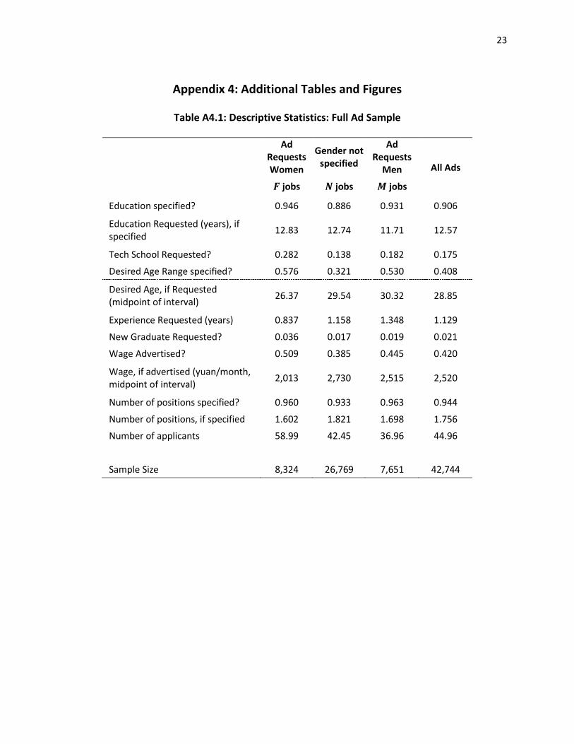
23

Appendix 4: Additional Tables and Figures

Table A4.1: Descriptive Statistics: Full Ad Sample

Ad

Requests Women

Gender not specified

Ad Requests

Men All Ads

𝑭 jobs 𝑵 jobs 𝑴 jobs

Education specified? 0.946 0.886 0.931 0.906

Education Requested (years), if specified 12.83 12.74 11.71 12.57

Tech School Requested? 0.282 0.138 0.182 0.175

Desired Age Range specified? 0.576 0.321 0.530 0.408

Desired Age, if Requested (midpoint of interval) 26.37 29.54 30.32 28.85

Experience Requested (years) 0.837 1.158 1.348 1.129

New Graduate Requested? 0.036 0.017 0.019 0.021

Wage Advertised? 0.509 0.385 0.445 0.420

Wage, if advertised (yuan/month, midpoint of interval) 2,013 2,730 2,515 2,520

Number of positions specified? 0.960 0.933 0.963 0.944

Number of positions, if specified 1.602 1.821 1.698 1.756

Number of applicants 58.99 42.45 36.96 44.96

Sample Size 8,324 26,769 7,651 42,744

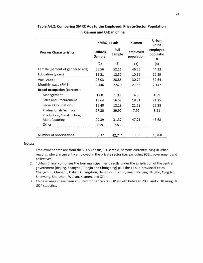
24

Table A4.2: Comparing XMRC Ads to the Employed, Private-Sector Population in Xiamen and Urban China

Worker Characteristics

XMRC job ads Xiamen Urban China

Callback Sample

Full Sample employed

population

employed populatio

n (1) (2) (3) (4)

Female (percent of gendered ads) 56.56 52.11 46.75 44.23 Education (years) 12.21 12.57 10.56 10.59 Age (years) 28.03 28.85 30.77 32.64 Monthly wage (RMB) 2,446 2,520 2,185 2,147 Broad occupation (percent):

Management 1.68 1.99 4.3 4.59 Sales and Procurement 18.64 16.59 18.31 21.25 Service Occupations 15.40 12.29 21.68 22.28 Professional/Technical 27.30 29.92 7.99 8.21 Production, Construction, Manufacturing 29.39 31.37 47.71 43.68 Other 7.59 7.83 -- --

Number of observations 3,637 42,744 1,163 99,768

Notes:

1. Employment data are from the 2005 Census, 1% sample, persons currently living in urban regions, who are currently employed in the private sector (i.e. excluding SOEs, government and collectives).

2. “Urban China” comprises the four municipalities directly under the jurisdiction of the central government (Beijing, Shanghai, Tianjin and Chongqing) plus the 15 sub-provincial cities: Changchun, Chengdu, Dalian, Guangzhou, Hangzhou, Harbin, Jinan, Nanjing, Ningbo, Qingdao, Shenyang, Shenzhen, Wuhan, Xiamen, and Xi’an.

3. Chinese wages have been adjusted for per capita GDP growth between 2005 and 2010 using IMF GDP statistics.

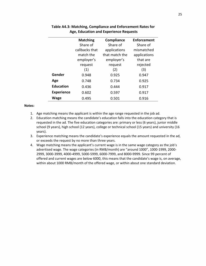
25

Table A4.3: Matching, Compliance and Enforcement Rates for Age, Education and Experience Requests

Matching Compliance Enforcement

Share of callbacks that

match the employer’s

request

Share of applications

that match the employer’s

request

Share of mismatched applications

that are rejected

(1) (2) (3) Gender 0.948 0.925 0.947 Age 0.748 0.734 0.925 Education 0.436 0.444 0.917 Experience 0.602 0.597 0.917 Wage 0.495 0.501 0.916

Notes:

1. Age matching means the applicant is within the age range requested in the job ad. 2. Education matching means the candidate’s education falls into the education category that is

requested in the ad. The five education categories are: primary or less (6 years), junior middle school (9 years), high school (12 years), college or technical school (15 years) and university (16 years).

3. Experience matching means the candidate’s experience equals the amount requested in the ad, or exceeds the request by no more than three years.

4. Wage matching means the applicant’s current wage is in the same wage category as the job’s advertised wage. The wage categories (in RMB/month) are “around 1000”, 1000-1999, 2000-2999, 3000-3999, 4000-4999, 5000-5999, 6000-7999, and 8000-9999. Since 99 percent of offered and current wages are below 6000, this means that the candidate’s wage is, on average, within about 1000 RMB/month of the offered wage, or within about one standard deviation.

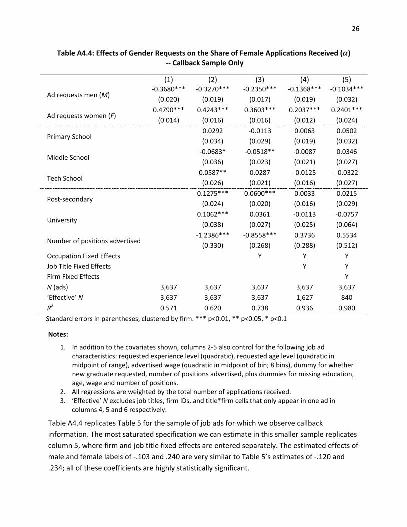
26

Table A4.4: Effects of Gender Requests on the Share of Female Applications Received (𝜶) -- Callback Sample Only

(1) (2) (3) (4) (5)

Ad requests men (M) -0.3680*** -0.3270*** -0.2350*** -0.1368*** -0.1034***

(0.020) (0.019) (0.017) (0.019) (0.032)

Ad requests women (F) 0.4790*** 0.4243*** 0.3603*** 0.2037*** 0.2401***

(0.014) (0.016) (0.016) (0.012) (0.024)

Primary School 0.0292 -0.0113 0.0063 0.0502 (0.034) (0.029) (0.019) (0.032)

Middle School -0.0683* -0.0518** -0.0087 0.0346 (0.036) (0.023) (0.021) (0.027)

Tech School 0.0587** 0.0287 -0.0125 -0.0322 (0.026) (0.021) (0.016) (0.027)

Post-secondary 0.1275*** 0.0600*** 0.0033 0.0215 (0.024) (0.020) (0.016) (0.029)

University 0.1062*** 0.0361 -0.0113 -0.0757 (0.038) (0.027) (0.025) (0.064)

Number of positions advertised -1.2386*** -0.8558*** 0.3736 0.5534 (0.330) (0.268) (0.288) (0.512)

Occupation Fixed Effects Y Y Y Job Title Fixed Effects Y Y Firm Fixed Effects Y N (ads) 3,637 3,637 3,637 3,637 3,637 ‘Effective’ N 3,637 3,637 3,637 1,627 840 R2 0.571 0.620 0.738 0.936 0.980 Standard errors in parentheses, clustered by firm. *** p<0.01, ** p<0.05, * p<0.1

Notes:

1. In addition to the covariates shown, columns 2-5 also control for the following job ad characteristics: requested experience level (quadratic), requested age level (quadratic in midpoint of range), advertised wage (quadratic in midpoint of bin; 8 bins), dummy for whether new graduate requested, number of positions advertised, plus dummies for missing education, age, wage and number of positions.

2. All regressions are weighted by the total number of applications received. 3. ‘Effective’ N excludes job titles, firm IDs, and title*firm cells that only appear in one ad in

columns 4, 5 and 6 respectively.

Table A4.4 replicates Table 5 for the sample of job ads for which we observe callback information. The most saturated specification we can estimate in this smaller sample replicates column 5, where firm and job title fixed effects are entered separately. The estimated effects of male and female labels of -.103 and .240 are very similar to Table 5’s estimates of -.120 and .234; all of these coefficients are highly statistically significant.

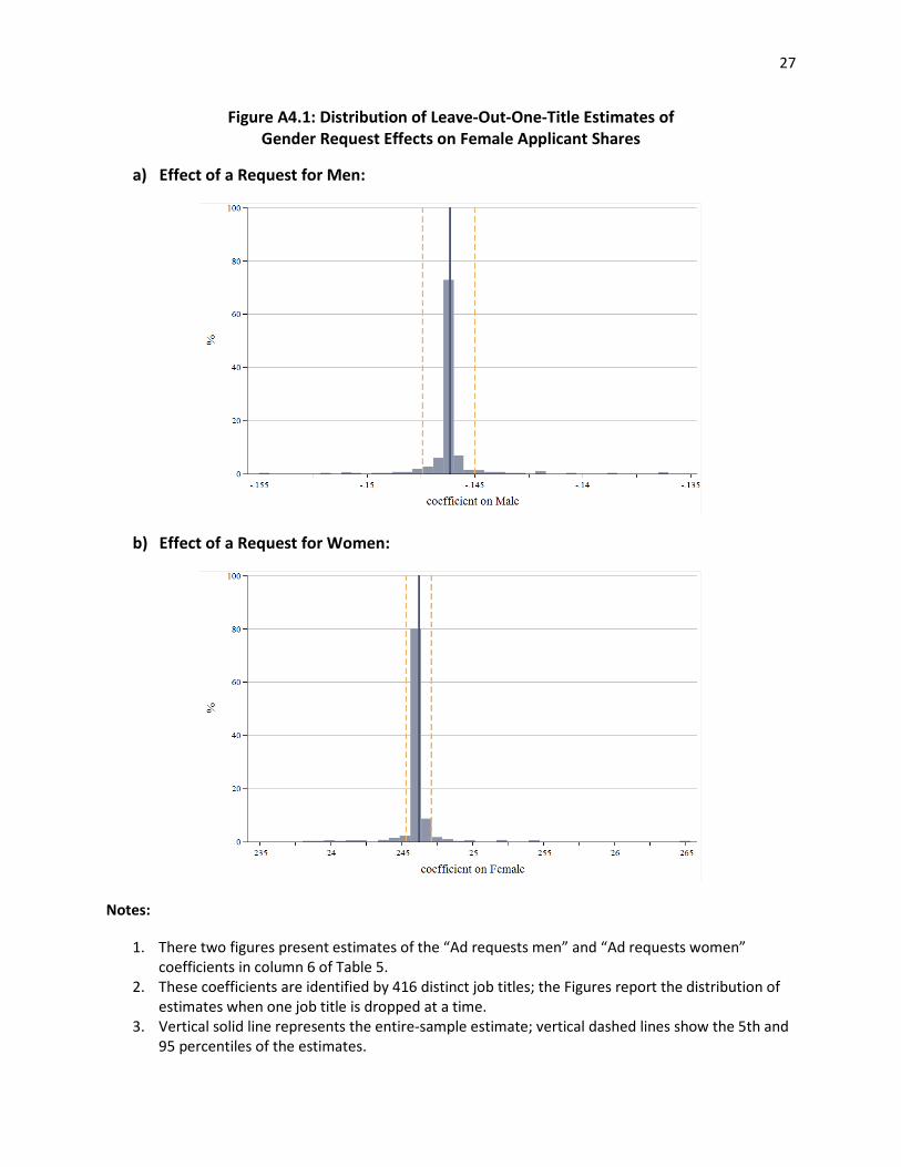
27

Figure A4.1: Distribution of Leave-Out-One-Title Estimates of Gender Request Effects on Female Applicant Shares

a) Effect of a Request for Men:

b) Effect of a Request for Women:

Notes:

1. There two figures present estimates of the “Ad requests men” and “Ad requests women” coefficients in column 6 of Table 5.

2. These coefficients are identified by 416 distinct job titles; the Figures report the distribution of estimates when one job title is dropped at a time.

3. Vertical solid line represents the entire-sample estimate; vertical dashed lines show the 5th and 95 percentiles of the estimates.

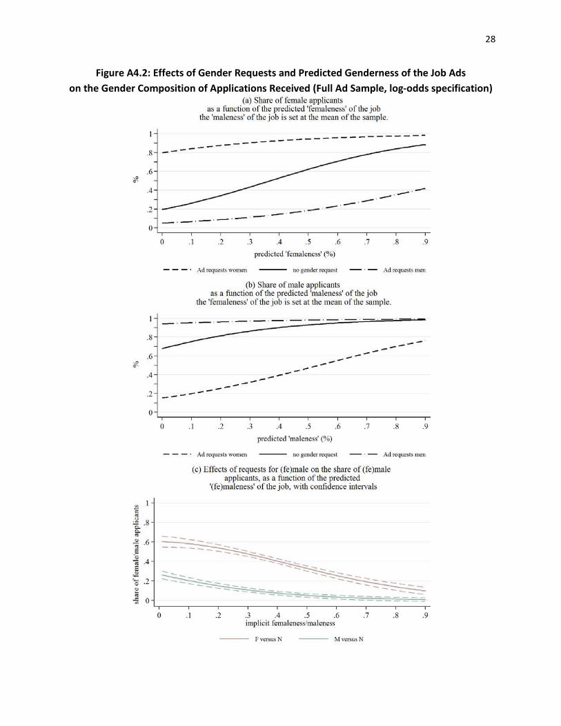
28

Figure A4.2: Effects of Gender Requests and Predicted Genderness of the Job Ads on the Gender Composition of Applications Received (Full Ad Sample, log-odds specification)

29

Notes:

1. Figures represent predicted values of the female share of applicants (𝛼) from a specification identical to Figure 1, with the following changes:

a. The dependent variable 𝛼, is now 𝑙𝑃𝑔 𝛼1−𝛼

. ‘Corner’ values of 𝛼 are accommodated by

setting 𝛼 = 0.5𝐴

when 𝛼 = 0 and setting 𝛼 = 𝐴−0.5𝐴

when 𝛼 = 1, where 𝐴 is the total

number of applications to the ad. b. the quartics in 𝐹𝑝 and 𝑀𝑝 (each interacted with 𝐹, 𝑁 and 𝑀) are replaced by linear

terms (again interacted with 𝐹, 𝑁 and 𝑀 ). 2. As in Figure 1, predictions in part (a) hold 𝑀𝑝 at its mean, and predictions in part (b) hold 𝐹𝑝 at

its mean. All other characteristics are set at their means. 3. The regression is weighted by the number of applications to each ad, and standard errors are

clustered at the firm level.

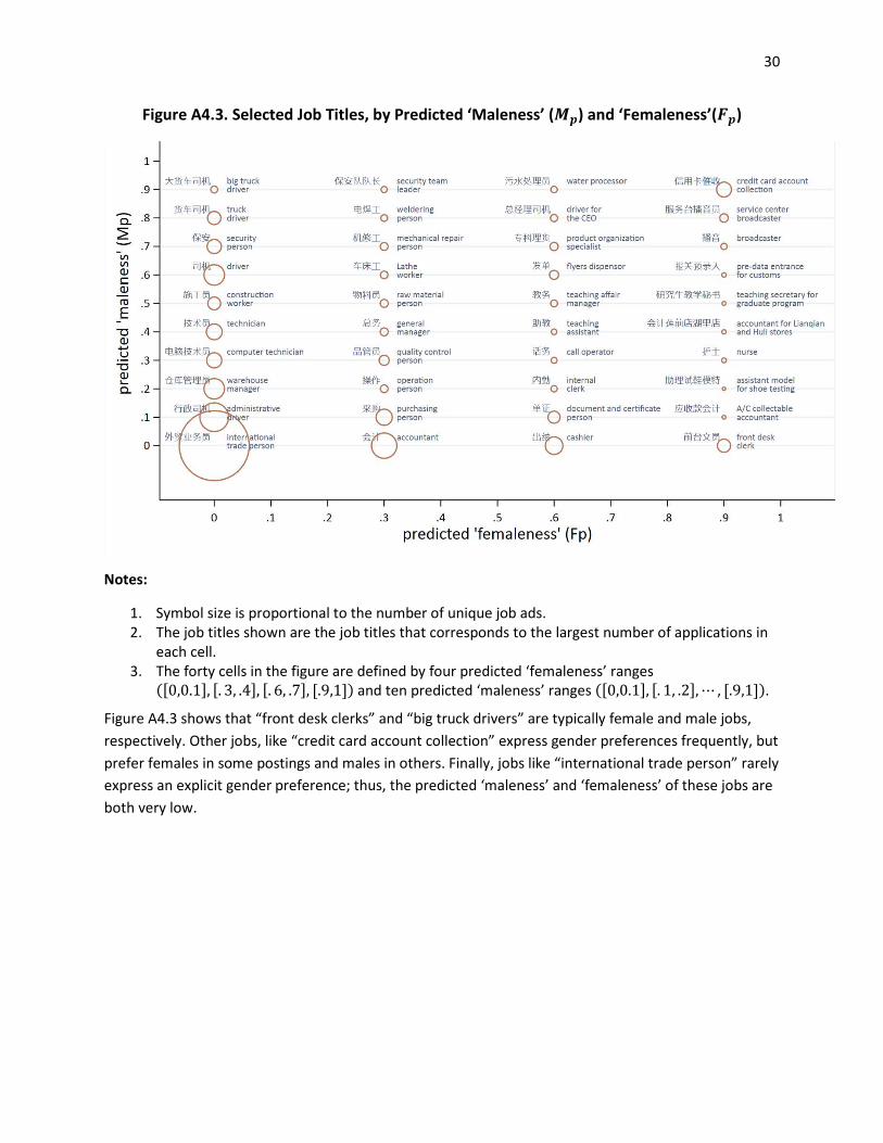
30

Figure A4.3. Selected Job Titles, by Predicted ‘Maleness’ (𝑴𝒑) and ‘Femaleness’(𝑭𝒑)

Notes:

1. Symbol size is proportional to the number of unique job ads. 2. The job titles shown are the job titles that corresponds to the largest number of applications in

each cell. 3. The forty cells in the figure are defined by four predicted ‘femaleness’ ranges

([0,0.1], [. 3, .4], [. 6, .7], [.9,1]) and ten predicted ‘maleness’ ranges ([0,0.1], [. 1, .2],⋯ , [.9,1]).

Figure A4.3 shows that “front desk clerks” and “big truck drivers” are typically female and male jobs, respectively. Other jobs, like “credit card account collection” express gender preferences frequently, but prefer females in some postings and males in others. Finally, jobs like “international trade person” rarely express an explicit gender preference; thus, the predicted ‘maleness’ and ‘femaleness’ of these jobs are both very low.

31

Appendix 5: Effects of Explicit Gender Requests on the Number and Quality of Applications

Table A5.1 replicates Table 5, using the total number of applications received as the outcome variable. Tables A5.2-A5.7 do the same for a variety of measures of the average quality of the applicant pool.

In some of the uncontrolled regressions of column 1, a number of effects are estimated, which confirm known features of the data: there are more female jobseekers than men on the board; gendered job ads are more common in unskilled positions, and men tend to have more experience than women.

Once job titles are controlled for, however (columns 5 and 6),

-there is some evidence that employers pay a price in applicant numbers when they advertise a gender preference (though the estimates are imprecise in column 6)

-there is no detectable effect of gender requests on mean applicant education and experience (Tables A5.2 and A5.3)

-all the estimated effects of gender requests on match quality (Tables A5.4-A5.7) are small and statistically insignificant

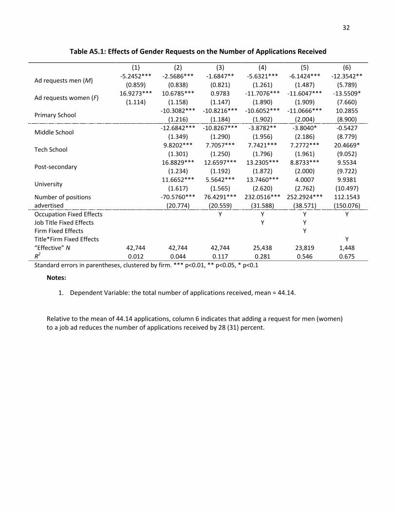
32

Table A5.1: Effects of Gender Requests on the Number of Applications Received

(1) (2) (3) (4) (5) (6)

Ad requests men (M) -5.2452*** -2.5686*** -1.6847** -5.6321*** -6.1424*** -12.3542** (0.859) (0.838) (0.821) (1.261) (1.487) (5.789)

Ad requests women (F) 16.9273*** 10.6785*** 0.9783 -11.7076*** -11.6047*** -13.5509* (1.114) (1.158) (1.147) (1.890) (1.909) (7.660)

Primary School -10.3082*** -10.8216*** -10.6052*** -11.0666*** 10.2855 (1.216) (1.184) (1.902) (2.004) (8.900)

Middle School -12.6842*** -10.8267*** -3.8782** -3.8040* -0.5427 (1.349) (1.290) (1.956) (2.186) (8.779)

Tech School 9.8202*** 7.7057*** 7.7421*** 7.2772*** 20.4669* (1.301) (1.250) (1.796) (1.961) (9.052)

Post-secondary 16.8829*** 12.6597*** 13.2305*** 8.8733*** 9.5534 (1.234) (1.192) (1.872) (2.000) (9.722)

University 11.6652*** 5.5642*** 13.7460*** 4.0007 9.9381 (1.617) (1.565) (2.620) (2.762) (10.497)

Number of positions advertised

-70.5760*** 76.4291*** 232.0516*** 252.2924*** 112.1543 (20.774) (20.559) (31.588) (38.571) (150.076)

Occupation Fixed Effects Y Y Y Y Job Title Fixed Effects Y Y Firm Fixed Effects Y Title*Firm Fixed Effects Y “Effective” N 42,744 42,744 42,744 25,438 23,819 1,448 R2 0.012 0.044 0.117 0.281 0.546 0.675 Standard errors in parentheses, clustered by firm. *** p<0.01, ** p<0.05, * p<0.1

Notes:

1. Dependent Variable: the total number of applications received, mean = 44.14.

Relative to the mean of 44.14 applications, column 6 indicates that adding a request for men (women) to a job ad reduces the number of applications received by 28 (31) percent.

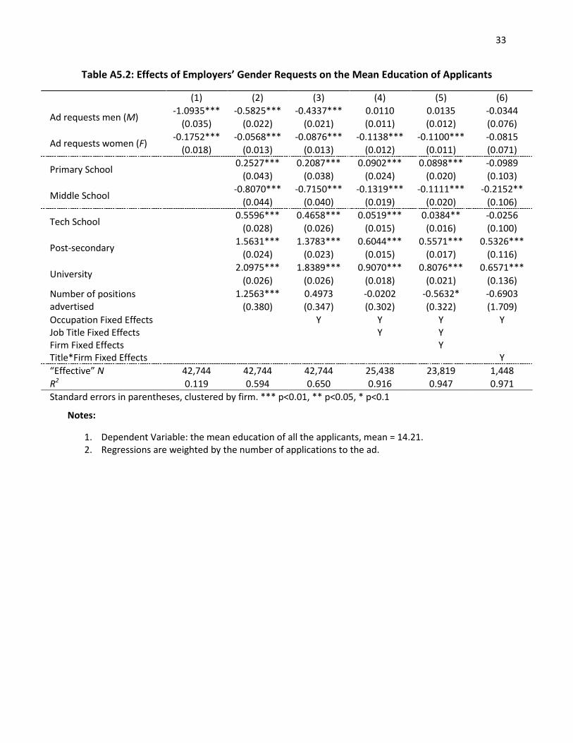
33

Table A5.2: Effects of Employers’ Gender Requests on the Mean Education of Applicants

(1) (2) (3) (4) (5) (6)

Ad requests men (M) -1.0935*** -0.5825*** -0.4337*** 0.0110 0.0135 -0.0344 (0.035) (0.022) (0.021) (0.011) (0.012) (0.076)

Ad requests women (F) -0.1752*** -0.0568*** -0.0876*** -0.1138*** -0.1100*** -0.0815 (0.018) (0.013) (0.013) (0.012) (0.011) (0.071)

Primary School 0.2527*** 0.2087*** 0.0902*** 0.0898*** -0.0989 (0.043) (0.038) (0.024) (0.020) (0.103)

Middle School -0.8070*** -0.7150*** -0.1319*** -0.1111*** -0.2152** (0.044) (0.040) (0.019) (0.020) (0.106)

Tech School 0.5596*** 0.4658*** 0.0519*** 0.0384** -0.0256 (0.028) (0.026) (0.015) (0.016) (0.100)

Post-secondary 1.5631*** 1.3783*** 0.6044*** 0.5571*** 0.5326*** (0.024) (0.023) (0.015) (0.017) (0.116)

University 2.0975*** 1.8389*** 0.9070*** 0.8076*** 0.6571*** (0.026) (0.026) (0.018) (0.021) (0.136)

Number of positions advertised

1.2563*** 0.4973 -0.0202 -0.5632* -0.6903 (0.380) (0.347) (0.302) (0.322) (1.709)

Occupation Fixed Effects Y Y Y Y Job Title Fixed Effects Y Y Firm Fixed Effects Y Title*Firm Fixed Effects Y “Effective” N 42,744 42,744 42,744 25,438 23,819 1,448 R2 0.119 0.594 0.650 0.916 0.947 0.971 Standard errors in parentheses, clustered by firm. *** p<0.01, ** p<0.05, * p<0.1

Notes:

1. Dependent Variable: the mean education of all the applicants, mean = 14.21. 2. Regressions are weighted by the number of applications to the ad.

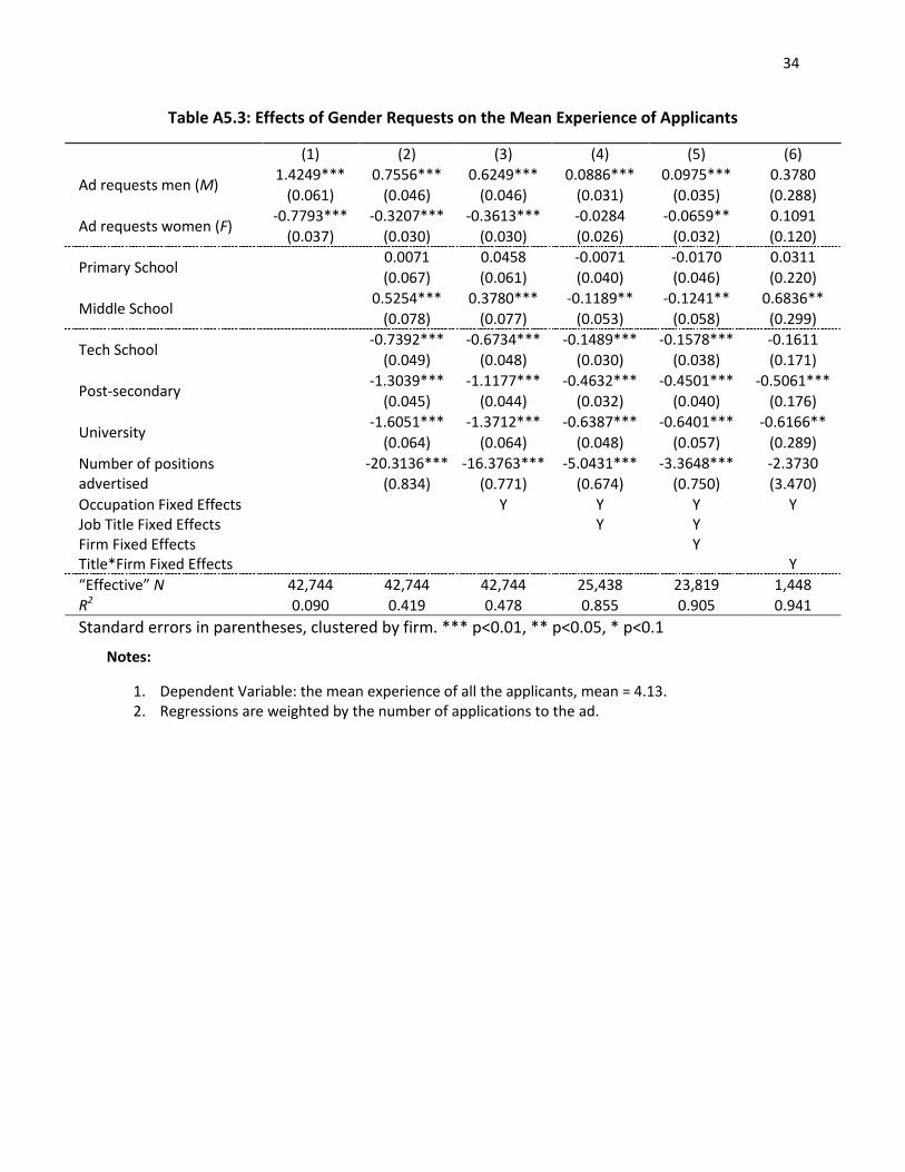
34

Table A5.3: Effects of Gender Requests on the Mean Experience of Applicants

(1) (2) (3) (4) (5) (6)

Ad requests men (M) 1.4249*** 0.7556*** 0.6249*** 0.0886*** 0.0975*** 0.3780 (0.061) (0.046) (0.046) (0.031) (0.035) (0.288)

Ad requests women (F) -0.7793*** -0.3207*** -0.3613*** -0.0284 -0.0659** 0.1091 (0.037) (0.030) (0.030) (0.026) (0.032) (0.120)

Primary School 0.0071 0.0458 -0.0071 -0.0170 0.0311 (0.067) (0.061) (0.040) (0.046) (0.220)

Middle School 0.5254*** 0.3780*** -0.1189** -0.1241** 0.6836** (0.078) (0.077) (0.053) (0.058) (0.299)

Tech School -0.7392*** -0.6734*** -0.1489*** -0.1578*** -0.1611 (0.049) (0.048) (0.030) (0.038) (0.171)

Post-secondary -1.3039*** -1.1177*** -0.4632*** -0.4501*** -0.5061*** (0.045) (0.044) (0.032) (0.040) (0.176)

University -1.6051*** -1.3712*** -0.6387*** -0.6401*** -0.6166** (0.064) (0.064) (0.048) (0.057) (0.289)

Number of positions advertised

-20.3136*** -16.3763*** -5.0431*** -3.3648*** -2.3730 (0.834) (0.771) (0.674) (0.750) (3.470)

Occupation Fixed Effects Y Y Y Y Job Title Fixed Effects Y Y Firm Fixed Effects Y Title*Firm Fixed Effects Y “Effective” N 42,744 42,744 42,744 25,438 23,819 1,448 R2 0.090 0.419 0.478 0.855 0.905 0.941 Standard errors in parentheses, clustered by firm. *** p<0.01, ** p<0.05, * p<0.1

Notes:

1. Dependent Variable: the mean experience of all the applicants, mean = 4.13. 2. Regressions are weighted by the number of applications to the ad.

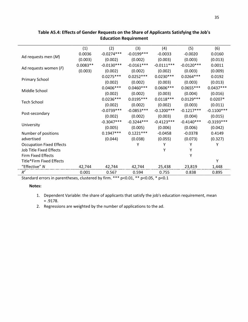
35

Table A5.4: Effects of Gender Requests on the Share of Applicants Satisfying the Job's Education Requirement

(1) (2) (3) (4) (5) (6)

Ad requests men (M) 0.0036 -0.0274*** -0.0199*** -0.0033 -0.0020 0.0160 (0.003) (0.002) (0.002) (0.003) (0.003) (0.013)

Ad requests women (F) 0.0083** -0.0130*** -0.0161*** -0.0111*** -0.0120*** 0.0011 (0.003) (0.002) (0.002) (0.002) (0.003) (0.009)

Primary School 0.0275*** 0.0252*** 0.0230*** 0.0264*** 0.0192 (0.002) (0.002) (0.003) (0.003) (0.013)

Middle School 0.0406*** 0.0460*** 0.0606*** 0.0655*** 0.0437*** (0.002) (0.002) (0.003) (0.004) (0.016)

Tech School 0.0236*** 0.0195*** 0.0118*** 0.0129*** 0.0207* (0.002) (0.002) (0.002) (0.003) (0.011)

Post-secondary -0.0739*** -0.0853*** -0.1200*** -0.1217*** -0.1100*** (0.002) (0.002) (0.003) (0.004) (0.015)

University -0.3047*** -0.3244*** -0.4123*** -0.4140*** -0.3193*** (0.005) (0.005) (0.006) (0.006) (0.042)

Number of positions advertised

0.1947*** 0.1221*** -0.0458 -0.0378 0.4149 (0.044) (0.038) (0.055) (0.073) (0.327)

Occupation Fixed Effects Y Y Y Y Job Title Fixed Effects Y Y Firm Fixed Effects Y Title*Firm Fixed Effects Y “Effective” N 42,744 42,744 42,744 25,438 23,819 1,448 R2 0.001 0.567 0.594 0.755 0.838 0.895 Standard errors in parentheses, clustered by firm. *** p<0.01, ** p<0.05, * p<0.1

Notes:

1. Dependent Variable: the share of applicants that satisfy the job's education requirement, mean = .9178.

2. Regressions are weighted by the number of applications to the ad.

36

Table A5.5: Effects of Gender Requests on the Share of Applicants Satisfying the Job's Experience Requirement

(1) (2) (3) (4) (5) (6)

Ad requests men (M) 0.0292*** 0.0317*** 0.0278*** 0.0155*** 0.0158*** 0.0263 (0.004) (0.003) (0.003) (0.004) (0.004) (0.039)

Ad requests women (F) -0.0077* -0.0135*** -0.0145*** -0.0016 -0.0006 0.0015 (0.004) (0.003) (0.003) (0.003) (0.004) (0.017)

Primary School -0.0197*** -0.0169*** -0.0142*** -0.0154*** -0.0142 (0.003) (0.003) (0.005) (0.005) (0.020)

Middle School 0.0183*** 0.0143*** 0.0033 -0.0004 -0.0074 (0.005) (0.005) (0.007) (0.007) (0.021)

Tech School -0.0395*** -0.0365*** -0.0185*** -0.0191*** -0.0339* (0.004) (0.004) (0.004) (0.004) (0.019)

Post-secondary -0.0685*** -0.0598*** -0.0347*** -0.0389*** -0.0564*** (0.003) (0.003) (0.004) (0.004) (0.019)

University -0.0797*** -0.0690*** -0.0418*** -0.0495*** -0.0644 (0.005) (0.005) (0.006) (0.007) (0.042)

Number of positions advertised

-0.5309*** -0.3733*** -0.0715 -0.1033 0.4454 (0.066) (0.065) (0.087) (0.100) (0.574)

Occupation Fixed Effects Y Y Y Y Job Title Fixed Effects Y Y Firm Fixed Effects Y Title*Firm Fixed Effects Y “Effective” N 42,744 42,744 42,744 25,438 23,819 1,448 R2 0.004 0.590 0.606 0.748 0.836 0.908

Standard errors in parentheses, clustered by firm. *** p<0.01, ** p<0.05, * p<0.1

Notes:

1. Dependent Variable: the share of applicants that satisfy the job's experience requirement, mean = .8741.

2. Regressions are weighted by the number of applications to the ad.

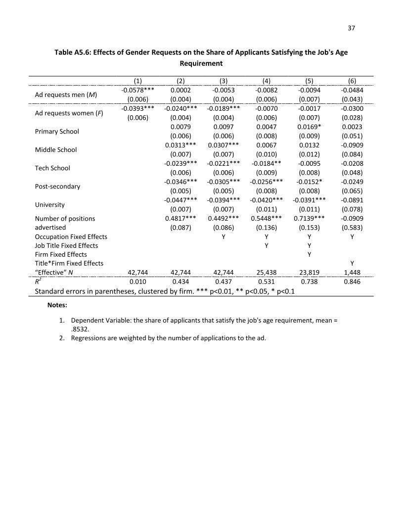
37

Table A5.6: Effects of Gender Requests on the Share of Applicants Satisfying the Job's Age Requirement

(1) (2) (3) (4) (5) (6)

Ad requests men (M) -0.0578*** 0.0002 -0.0053 -0.0082 -0.0094 -0.0484 (0.006) (0.004) (0.004) (0.006) (0.007) (0.043)

Ad requests women (F) -0.0393*** -0.0240*** -0.0189*** -0.0070 -0.0017 -0.0300 (0.006) (0.004) (0.004) (0.006) (0.007) (0.028)

Primary School 0.0079 0.0097 0.0047 0.0169* 0.0023 (0.006) (0.006) (0.008) (0.009) (0.051)

Middle School 0.0313*** 0.0307*** 0.0067 0.0132 -0.0909 (0.007) (0.007) (0.010) (0.012) (0.084)

Tech School -0.0239*** -0.0221*** -0.0184** -0.0095 -0.0208 (0.006) (0.006) (0.009) (0.008) (0.048)

Post-secondary -0.0346*** -0.0305*** -0.0256*** -0.0152* -0.0249 (0.005) (0.005) (0.008) (0.008) (0.065)

University -0.0447*** -0.0394*** -0.0420*** -0.0391*** -0.0891 (0.007) (0.007) (0.011) (0.011) (0.078)

Number of positions advertised

0.4817*** 0.4492*** 0.5448*** 0.7139*** -0.0909 (0.087) (0.086) (0.136) (0.153) (0.583)

Occupation Fixed Effects Y Y Y Y Job Title Fixed Effects Y Y Firm Fixed Effects Y Title*Firm Fixed Effects Y “Effective” N 42,744 42,744 42,744 25,438 23,819 1,448 R2 0.010 0.434 0.437 0.531 0.738 0.846 Standard errors in parentheses, clustered by firm. *** p<0.01, ** p<0.05, * p<0.1

Notes:

1. Dependent Variable: the share of applicants that satisfy the job's age requirement, mean = .8532.

2. Regressions are weighted by the number of applications to the ad.

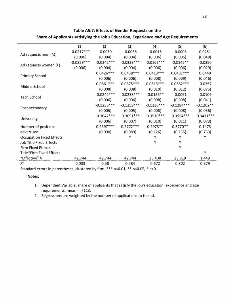
38

Table A5.7: Effects of Gender Requests on the Share of Applicants satisfying the Job's Education, Experience and Age Requirements

(1) (2) (3) (4) (5) (6)

Ad requests men (M) -0.0217*** -0.0059 -0.0056 -0.0015 -0.0003 0.0251 (0.006) (0.004) (0.004) (0.006) (0.006) (0.048)

Ad requests women (F) -0.0329*** -0.0342*** -0.0339*** -0.0162*** -0.0145** -0.0256 (0.006) (0.004) (0.004) (0.006) (0.006) (0.029)

Primary School 0.0426*** 0.0438*** 0.0413*** 0.0481*** 0.0440 (0.006) (0.006) (0.008) (0.009) (0.046)

Middle School 0.0661*** 0.0675*** 0.0513*** 0.0582*** -0.0357 (0.008) (0.008) (0.010) (0.012) (0.075)

Tech School -0.0242*** -0.0238*** -0.0156** -0.0091 -0.0109 (0.006) (0.006) (0.008) (0.008) (0.041)

Post-secondary -0.1256*** -0.1259*** -0.1336*** -0.1284*** -0.1262** (0.005) (0.005) (0.008) (0.008) (0.056)

University -0.3042*** -0.3091*** -0.3510*** -0.3554*** -0.3411*** (0.006) (0.007) (0.010) (0.011) (0.073)

Number of positions advertised

0.2597*** 0.2772*** 0.2973** 0.3770** 0.1473 (0.090) (0.089) (0.126) (0.155) (0.753)

Occupation Fixed Effects Y Y Y Y Job Title Fixed Effects Y Y Firm Fixed Effects Y Title*Firm Fixed Effects Y “Effective” N 42,744 42,744 42,744 25,438 23,819 1,448 R2 0.003 0.58 0.584 0.672 0.802 0.879 Standard errors in parentheses, clustered by firm. *** p<0.01, ** p<0.05, * p<0.1

Notes:

1. Dependent Variable: share of applicants that satisfy the job's education, experience and age requirements, mean = .7113.

2. Regressions are weighted by the number of applications to the ad.

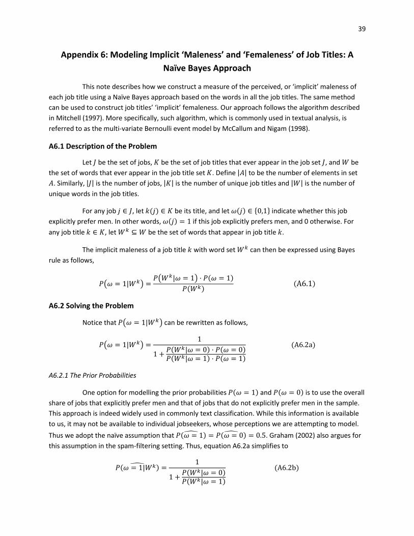
39

Appendix 6: Modeling Implicit ‘Maleness’ and ‘Femaleness’ of Job Titles: A Naïve Bayes Approach

This note describes how we construct a measure of the perceived, or ‘implicit’ maleness of each job title using a Naïve Bayes approach based on the words in all the job titles. The same method can be used to construct job titles’ ‘implicit’ femaleness. Our approach follows the algorithm described in Mitchell (1997). More specifically, such algorithm, which is commonly used in textual analysis, is referred to as the multi-variate Bernoulli event model by McCallum and Nigam (1998).

A6.1 Description of the Problem

Let 𝐽 be the set of jobs, 𝐾 be the set of job titles that ever appear in the job set 𝐽, and 𝑊 be the set of words that ever appear in the job title set 𝐾. Define |𝐴| to be the number of elements in set 𝐴. Similarly, |𝐽| is the number of jobs, |𝐾| is the number of unique job titles and |𝑊| is the number of unique words in the job titles.

For any job 𝑗 ∈ 𝐽, let 𝑘(𝑗) ∈ 𝐾 be its title, and let 𝜔(𝑗) ∈ {0,1} indicate whether this job explicitly prefer men. In other words, 𝜔(𝑗) = 1 if this job explicitly prefers men, and 0 otherwise. For any job title 𝑘 ∈ 𝐾, let 𝑊𝑘 ⊆ 𝑊 be the set of words that appear in job title 𝑘.

The implicit maleness of a job title 𝑘 with word set 𝑊𝑘 can then be expressed using Bayes rule as follows,

𝑃�𝜔 = 1|𝑊𝑘� =𝑃�𝑊𝑘|𝜔 = 1� ⋅ 𝑃(𝜔 = 1)

𝑃(𝑊𝑘) (A6.1)

A6.2 Solving the Problem

Notice that 𝑃�𝜔 = 1|𝑊𝑘� can be rewritten as follows,

𝑃�𝜔 = 1|𝑊𝑘� =1

1 + 𝑃(𝑊𝑘|𝜔 = 0) ⋅ 𝑃(𝜔 = 0)𝑃(𝑊𝑘|𝜔 = 1) ⋅ 𝑃(𝜔 = 1)

(A6.2a)

A6.2.1 The Prior Probabilities

One option for modelling the prior probabilities 𝑃(𝜔 = 1) and 𝑃(𝜔 = 0) is to use the overall share of jobs that explicitly prefer men and that of jobs that do not explicitly prefer men in the sample. This approach is indeed widely used in commonly text classification. While this information is available to us, it may not be available to individual jobseekers, whose perceptions we are attempting to model. Thus we adopt the naïve assumption that 𝑃(𝜔 = 1)� = 𝑃(𝜔 = 0)� = 0.5. Graham (2002) also argues for this assumption in the spam-filtering setting. Thus, equation A6.2a simplifies to

𝑃(𝜔 = 1|𝑊𝑘)� =1

1 + 𝑃(𝑊𝑘|𝜔 = 0)𝑃(𝑊𝑘|𝜔 = 1)

(A6.2b)

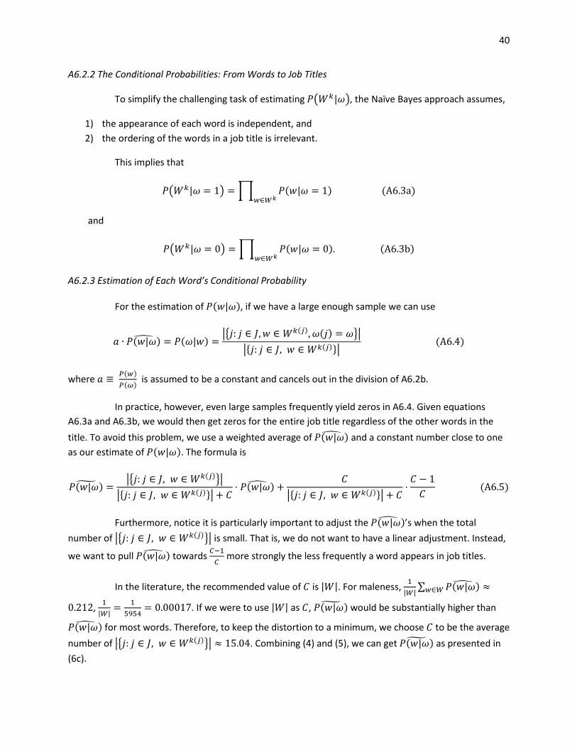
40

A6.2.2 The Conditional Probabilities: From Words to Job Titles

To simplify the challenging task of estimating 𝑃�𝑊𝑘|𝜔�, the Naïve Bayes approach assumes,

1) the appearance of each word is independent, and 2) the ordering of the words in a job title is irrelevant.

This implies that

𝑃�𝑊𝑘|𝜔 = 1� = � 𝑃(𝑤|𝜔 = 1)𝑤∈𝑊𝑘

(A6.3a)

and

𝑃�𝑊𝑘|𝜔 = 0� = � 𝑃(𝑤|𝜔 = 0).𝑤∈𝑊𝑘

(A6.3b)

A6.2.3 Estimation of Each Word’s Conditional Probability

For the estimation of 𝑃(𝑤|𝜔), if we have a large enough sample we can use

𝑎 ∙ 𝑃(𝑤|𝜔)� = 𝑃(𝜔|𝑤) =��𝑗: 𝑗 ∈ 𝐽,𝑤 ∈ 𝑊𝑘(𝑗),𝜔(𝑗) = 𝜔��

�{𝑗: 𝑗 ∈ 𝐽, 𝑤 ∈ 𝑊𝑘(𝑗)}� (A6.4)

where 𝑎 ≡ 𝑃(𝑤)𝑃(𝜔) is assumed to be a constant and cancels out in the division of A6.2b.

In practice, however, even large samples frequently yield zeros in A6.4. Given equations A6.3a and A6.3b, we would then get zeros for the entire job title regardless of the other words in the title. To avoid this problem, we use a weighted average of 𝑃(𝑤|𝜔)� and a constant number close to one as our estimate of 𝑃(𝑤|𝜔). The formula is

𝑃(𝑤|𝜔)� =��𝑗: 𝑗 ∈ 𝐽, 𝑤 ∈ 𝑊𝑘(𝑗)��

�{𝑗: 𝑗 ∈ 𝐽, 𝑤 ∈ 𝑊𝑘(𝑗)}�+ 𝐶⋅ 𝑃(𝑤|𝜔)� +

𝐶�{𝑗: 𝑗 ∈ 𝐽, 𝑤 ∈ 𝑊𝑘(𝑗)}�+ 𝐶

⋅𝐶 − 1𝐶

(A6.5)

Furthermore, notice it is particularly important to adjust the 𝑃(𝑤|𝜔)� ’s when the total number of ��𝑗: 𝑗 ∈ 𝐽, 𝑤 ∈ 𝑊𝑘(𝑗)�� is small. That is, we do not want to have a linear adjustment. Instead,

we want to pull 𝑃(𝑤|𝜔)� towards 𝐵−1𝐵

more strongly the less frequently a word appears in job titles.

In the literature, the recommended value of 𝐶 is |𝑊|. For maleness, 1|𝑊|∑ 𝑃(𝑤|𝜔)�𝑤∈𝑊 ≈

0.212, 1|𝑊| = 15954

= 0.00017. If we were to use |𝑊| as 𝐶, 𝑃(𝑤|𝜔)� would be substantially higher than

𝑃(𝑤|𝜔)� for most words. Therefore, to keep the distortion to a minimum, we choose 𝐶 to be the average number of ��𝑗: 𝑗 ∈ 𝐽, 𝑤 ∈ 𝑊𝑘(𝑗)�� ≈ 15.04. Combining (4) and (5), we can get 𝑃(𝑤|𝜔)� as presented in (6c).

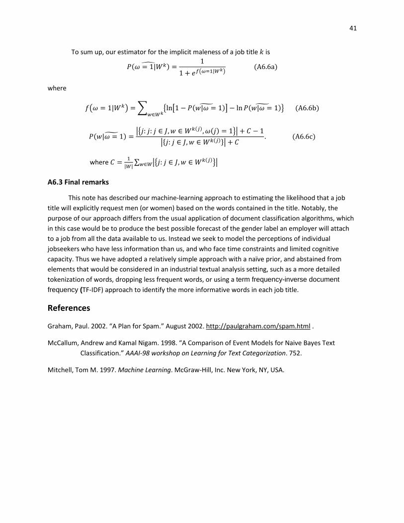
41

To sum up, our estimator for the implicit maleness of a job title 𝑘 is

𝑃(𝜔 = 1|𝑊𝑘)� =1

1 + 𝑒𝑓�𝜔=1|𝑊𝑘� (A6.6a)

where

𝑓�𝜔 = 1|𝑊𝑘� = � �ln�1 − 𝑃(𝑤|𝜔 = 1)� �− ln𝑃(𝑤|𝜔 = 1)� � (A6.6b)𝑤∈𝑊𝑘

𝑃(𝑤|𝜔 = 1) =� ��𝑗: 𝑗: 𝑗 ∈ 𝐽,𝑤 ∈ 𝑊𝑘(𝑗),𝜔(𝑗) = 1��+ 𝐶 − 1�{𝑗: 𝑗 ∈ 𝐽,𝑤 ∈ 𝑊𝑘(𝑗)}�+ 𝐶

. (A6.6c)

where 𝐶 = 1|𝑊|

∑ ��𝑗: 𝑗 ∈ 𝐽,𝑤 ∈ 𝑊𝑘(𝑗)��𝑤∈𝑊

A6.3 Final remarks

This note has described our machine-learning approach to estimating the likelihood that a job title will explicitly request men (or women) based on the words contained in the title. Notably, the purpose of our approach differs from the usual application of document classification algorithms, which in this case would be to produce the best possible forecast of the gender label an employer will attach to a job from all the data available to us. Instead we seek to model the perceptions of individual jobseekers who have less information than us, and who face time constraints and limited cognitive capacity. Thus we have adopted a relatively simple approach with a naïve prior, and abstained from elements that would be considered in an industrial textual analysis setting, such as a more detailed tokenization of words, dropping less frequent words, or using a term frequency-inverse document frequency (TF-IDF) approach to identify the more informative words in each job title.

References

Graham, Paul. 2002. “A Plan for Spam.” August 2002. http://paulgraham.com/spam.html .

McCallum, Andrew and Kamal Nigam. 1998. “A Comparison of Event Models for Naive Bayes Text Classification.” AAAI-98 workshop on Learning for Text Categorization. 752.

Mitchell, Tom M. 1997. Machine Learning. McGraw-Hill, Inc. New York, NY, USA.

42

Appendix 7: Gender Misclassification

Miscoding of the requested gender is not a concern for our application analysis, since our data are the exact record of requested gender that workers observe on the job board when deciding where to apply. Miscoding of the requested gender could account for the relatively high success rates of gender-mismatched applicants if employers sometimes specify a gender requirement without intending to. If so, advertised gender requirements would be de facto rather soft. We view this as a possible interpretation of the relatively weak mismatch penalty in callbacks in our data.

Another possibility is that workers miscode their own gender when using the drop-down menu in the application process. The very high compliance rates we observe suggest that this is not a major concern. Nevertheless, we checked to see if miscoded applicant gender could account for the relatively weak enforcement in our data by re-running the main analysis on a restricted subsample for whom we are confident we have the right gender.48

To construct this sample, we first use the universe of applications, with no restrictions, to calculate the share of applications each CV in the sample sends to jobs which request the opposite gender. We then drop all the CVs in our sample for whom this share is 0.5 or higher. We also drop all CVs who submit fewer than 5 applications in the unrestricted data, because we may not have enough observations on them to reliably assess their application behavior. These restrictions only drop approximately 15,000 applications, leaving a sample size of 213,719.

We then re-run the application-level regressions from Table 5, and the results are very similar to those presented in the main analysis, which gives us confidence that the results are not being driven by misreported gender. They are reported in Table A7.1. Results for other cutoffs are not materially different.

48 Note that miscoded applicant gender cannot explain weak enforcement if firms use resume-processing software

to pre-screen resumes based on coded gender: such screens would eliminate both actual and false gender mismatches from consideration, generating a high level of measured enforcement. Miscoded applicant gender can only explain low compliance if employers can see that some apparently mismatched applicants are in fact of the requested gender (for example from the photo, name or other features of the resume.

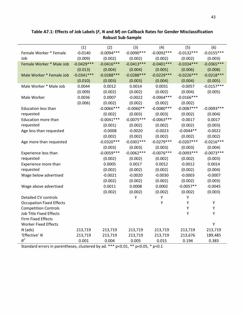
43

Table A7.1: Effects of Job Labels (F, N and M) on Callback Rates for Gender Misclassification Robust Sub-Sample

(1) (2) (3) (4) (5) (6) Female Worker * Female Job

-0.0140 -0.0094*** -0.0090*** -0.0092*** -0.0132*** -0.0155*** (0.009) (0.002) (0.002) (0.002) (0.002) (0.003)

Female Worker * Male Job -0.0429*** -0.0416*** -0.0413*** -0.0401*** -0.0334*** -0.0365*** (0.013) (0.004) (0.004) (0.005) (0.006) (0.008)

Male Worker * Female Job -0.0341*** -0.0288*** -0.0288*** -0.0229*** -0.0226*** -0.0218*** (0.010) (0.003) (0.003) (0.004) (0.004) (0.005)

Male Worker * Male Job 0.0044 0.0012 0.0014 0.0031 -0.0057 -0.0157*** (0.009) (0.002) (0.002) (0.002) (0.004) (0.005)

Male Worker 0.0036 0.0007 -0.0022 -0.0064*** -0.0166*** (0.006) (0.002) (0.002) (0.002) (0.002)

Education less than requested

-0.0066*** -0.0060** -0.0080*** -0.0087*** -0.0093*** (0.002) (0.003) (0.003) (0.002) (0.004)

Education more than requested

-0.0041*** -0.0075*** -0.0063*** -0.0017 0.0017 (0.001) (0.002) (0.002) (0.002) (0.003)

Age less than requested -0.0008 -0.0020 -0.0023 -0.0044** -0.0022 (0.002) (0.002) (0.002) (0.002) (0.002)

Age more than requested -0.0320*** -0.0301*** -0.0279*** -0.0207*** -0.0216*** (0.003) (0.003) (0.003) (0.003) (0.004)

Experience less than requested

-0.0059*** -0.0062*** -0.0076*** -0.0093*** -0.0073*** (0.002) (0.002) (0.002) (0.002) (0.003)

Experience more than requested

0.0005 0.0017 0.0012 -0.0012 0.0014 (0.002) (0.002) (0.002) (0.002) (0.004)

Wage below advertised -0.0021 -0.0020 -0.0030 -0.0003 -0.0007 (0.002) (0.002) (0.002) (0.002) (0.003)

Wage above advertised 0.0011 0.0008 0.0002 -0.0057** -0.0045 (0.002) (0.002) (0.002) (0.002) (0.003)

Detailed CV controls Y Y Y Occupation Fixed Effects Y Y Y Competition Controls Y Y Job Title Fixed Effects Y Y Firm Fixed Effects Worker Fixed Effects Y N (ads) 213,719 213,719 213,719 213,719 213,719 213,719 ‘Effective’ N 213,719 213,719 213,719 213,719 213,676 189,485 R2 0.001 0.004 0.005 0.015 0.194 0.383 Standard errors in parentheses, clustered by ad. *** p<0.01, ** p<0.05, * p<0.1

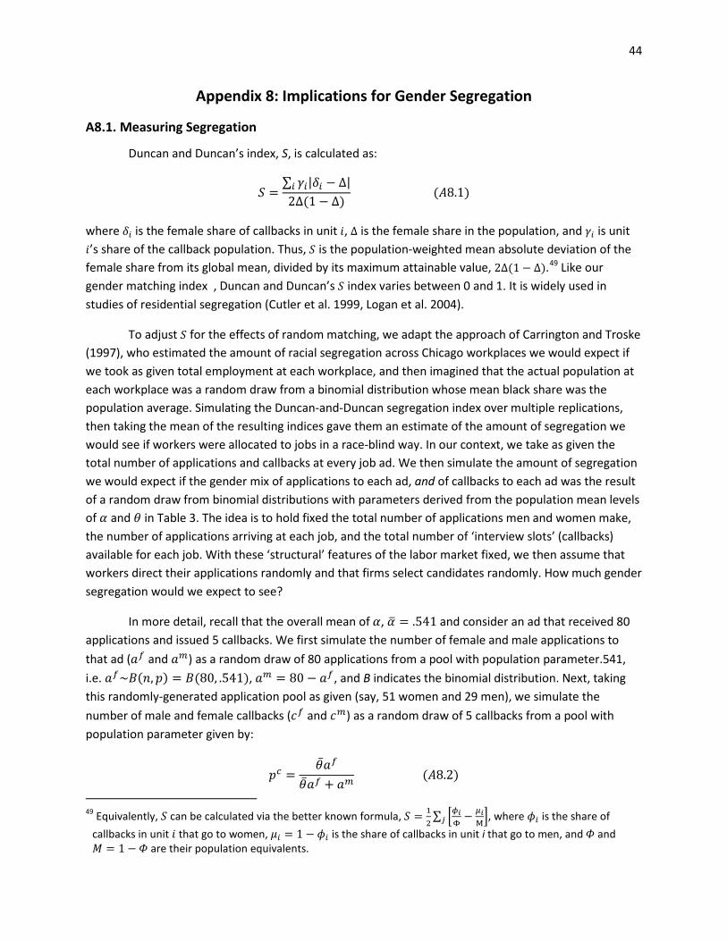
44

Appendix 8: Implications for Gender Segregation

A8.1. Measuring Segregation

Duncan and Duncan’s index, S, is calculated as:

𝑆 =∑ 𝛾𝑖|𝛿𝑖 − ∆|𝑖

2∆(1 − ∆) (𝐴8.1)

where 𝛿𝑖 is the female share of callbacks in unit 𝑖, Δ is the female share in the population, and 𝛾𝑖 is unit 𝑖’s share of the callback population. Thus, 𝑆 is the population-weighted mean absolute deviation of the female share from its global mean, divided by its maximum attainable value, 2Δ(1 − Δ).49 Like our gender matching index , Duncan and Duncan’s 𝑆 index varies between 0 and 1. It is widely used in studies of residential segregation (Cutler et al. 1999, Logan et al. 2004).

To adjust 𝑆 for the effects of random matching, we adapt the approach of Carrington and Troske (1997), who estimated the amount of racial segregation across Chicago workplaces we would expect if we took as given total employment at each workplace, and then imagined that the actual population at each workplace was a random draw from a binomial distribution whose mean black share was the population average. Simulating the Duncan-and-Duncan segregation index over multiple replications, then taking the mean of the resulting indices gave them an estimate of the amount of segregation we would see if workers were allocated to jobs in a race-blind way. In our context, we take as given the total number of applications and callbacks at every job ad. We then simulate the amount of segregation we would expect if the gender mix of applications to each ad, and of callbacks to each ad was the result of a random draw from binomial distributions with parameters derived from the population mean levels of 𝛼 and 𝜃 in Table 3. The idea is to hold fixed the total number of applications men and women make, the number of applications arriving at each job, and the total number of ‘interview slots’ (callbacks) available for each job. With these ‘structural’ features of the labor market fixed, we then assume that workers direct their applications randomly and that firms select candidates randomly. How much gender segregation would we expect to see?

In more detail, recall that the overall mean of 𝛼, 𝛼� = .541 and consider an ad that received 80 applications and issued 5 callbacks. We first simulate the number of female and male applications to that ad (𝑎𝑓 and 𝑎𝑚) as a random draw of 80 applications from a pool with population parameter.541, i.e. 𝑎𝑓~𝐵(𝑛,𝑝) = 𝐵(80, .541), 𝑎𝑚 = 80 − 𝑎𝑓, and B indicates the binomial distribution. Next, taking this randomly-generated application pool as given (say, 51 women and 29 men), we simulate the number of male and female callbacks (𝑐𝑓 and 𝑐𝑚) as a random draw of 5 callbacks from a pool with population parameter given by:

𝑝𝑐 =�̅�𝑎𝑓

�̅�𝑎𝑓 + 𝑎𝑚 (𝐴8.2)

49 Equivalently, 𝑆 can be calculated via the better known formula, 𝑆 = 1

2∑ �𝜙𝑖

Φ− 𝜇𝑖

Μ�𝑗 , where 𝜙𝑖 is the share of

callbacks in unit 𝑖 that go to women, 𝜇𝑖 = 1 − 𝜙𝑖 is the share of callbacks in unit i that go to men, and 𝛷 and 𝛭 = 1 − 𝛷 are their population equivalents.

45

where �̅� = .866 is the overall mean of women’s relative callback risk. Thus, 𝑐𝑓~𝐵(𝑛,𝑝) = 𝐵(5,𝑝𝑐); 𝑐𝑚 = 5 − 𝑐𝑓. Doing this for every job, then calculating the realized segregation index, 𝑆, completes a single iteration.

Figure A8.1 plots the distribution of realized 𝑆 values from 1000 iterations in this baseline scenario where there is no systematic variation across jobs in either application or callback behavior. It shows a surprisingly concentrated distribution with a mean of .317 and all values falling between .30 and .34. Thus, while random matching can generate a high level of measured segregation, the amount of segregation it generates is tightly constrained by the distribution of applicant pool sizes and callback pool sizes and the overall share of men and women in the population.

Figure A8.1: Simulated Segregation Indices with Random Allocation of Applications to Jobs, and Random Selection of Callbacks from All Applicant Pools

Finally, to remove the effects of this randomness, we follow Carrington-Troske by defining a noise-adjusted segregation measure, �̃�, as:

�̃� =𝑆 − 𝑆01 − 𝑆0

(A8.3)

where 𝑆 is the unadjusted segregation index from equation (A8.1) and 𝑆0 = .317 is the mean level of segregation expected from noise in matching. Since 𝑆 = .732, the noise-adjusted index of gender segregation across jobs in our data is given by �̃� = .732− .317

1− .317= .607.

A8.2 Decomposing Segregation

We begin by noting that a substantial amount of the gender segregation among successful applicants occurs within groups of jobs that have a specific gender label (𝐹, 𝑁 or 𝑀) attached to them;

0

2

4

6

8

10

Den

sity

.3 .305 .31 .315 .32 .325 .33 .335

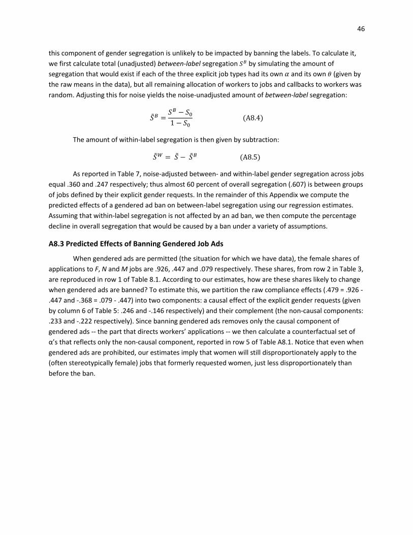
46

this component of gender segregation is unlikely to be impacted by banning the labels. To calculate it, we first calculate total (unadjusted) between-label segregation 𝑆𝐵 by simulating the amount of segregation that would exist if each of the three explicit job types had its own 𝛼 and its own 𝜃 (given by the raw means in the data), but all remaining allocation of workers to jobs and callbacks to workers was random. Adjusting this for noise yields the noise-unadjusted amount of between-label segregation:

�̃�𝐵 =𝑆𝐵 − 𝑆01 − 𝑆0

(A8.4)

The amount of within-label segregation is then given by subtraction:

�̃�𝑊 = �̃� − �̃�𝐵 (A8.5)

As reported in Table 7, noise-adjusted between- and within-label gender segregation across jobs equal .360 and .247 respectively; thus almost 60 percent of overall segregation (.607) is between groups of jobs defined by their explicit gender requests. In the remainder of this Appendix we compute the predicted effects of a gendered ad ban on between-label segregation using our regression estimates. Assuming that within-label segregation is not affected by an ad ban, we then compute the percentage decline in overall segregation that would be caused by a ban under a variety of assumptions.

A8.3 Predicted Effects of Banning Gendered Job Ads

When gendered ads are permitted (the situation for which we have data), the female shares of applications to F, N and M jobs are .926, .447 and .079 respectively. These shares, from row 2 in Table 3, are reproduced in row 1 of Table 8.1. According to our estimates, how are these shares likely to change when gendered ads are banned? To estimate this, we partition the raw compliance effects (.479 = .926 - .447 and -.368 = .079 - .447) into two components: a causal effect of the explicit gender requests (given by column 6 of Table 5: .246 and -.146 respectively) and their complement (the non-causal components: .233 and -.222 respectively). Since banning gendered ads removes only the causal component of gendered ads -- the part that directs workers’ applications -- we then calculate a counterfactual set of α’s that reflects only the non-causal component, reported in row 5 of Table A8.1. Notice that even when gendered ads are prohibited, our estimates imply that women will still disproportionately apply to the (often stereotypically female) jobs that formerly requested women, just less disproportionately than before the ban.

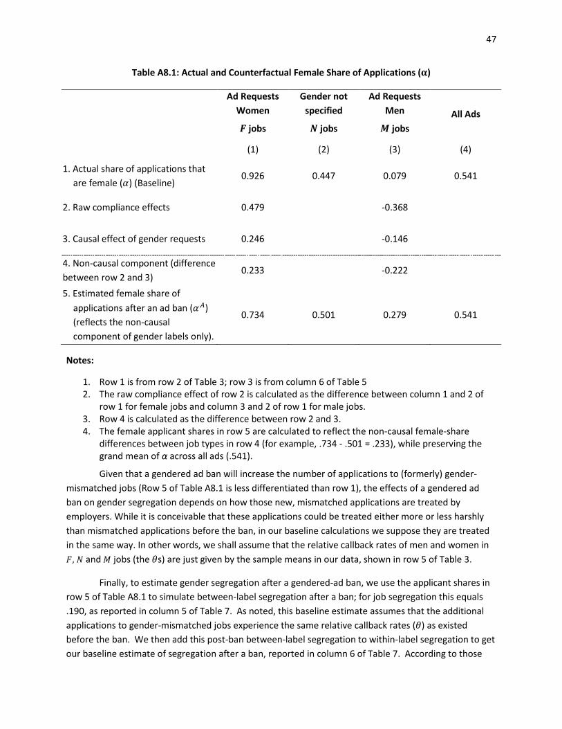
47

Table A8.1: Actual and Counterfactual Female Share of Applications (𝛂)

Ad Requests

Women Gender not

specified Ad Requests

Men All Ads 𝑭 jobs 𝑵 jobs 𝑴 jobs

(1) (2) (3) (4)

1. Actual share of applications that are female (𝛼) (Baseline)

0.926 0.447 0.079 0.541

2. Raw compliance effects 0.479 -0.368

3. Causal effect of gender requests 0.246 -0.146

4. Non-causal component (difference between row 2 and 3)

0.233 -0.222

5. Estimated female share of applications after an ad ban (𝛼𝐴) (reflects the non-causal component of gender labels only).

0.734 0.501 0.279 0.541

Notes:

1. Row 1 is from row 2 of Table 3; row 3 is from column 6 of Table 5 2. The raw compliance effect of row 2 is calculated as the difference between column 1 and 2 of

row 1 for female jobs and column 3 and 2 of row 1 for male jobs. 3. Row 4 is calculated as the difference between row 2 and 3. 4. The female applicant shares in row 5 are calculated to reflect the non-causal female-share

differences between job types in row 4 (for example, .734 - .501 = .233), while preserving the grand mean of α across all ads (.541).

Given that a gendered ad ban will increase the number of applications to (formerly) gender-mismatched jobs (Row 5 of Table A8.1 is less differentiated than row 1), the effects of a gendered ad ban on gender segregation depends on how those new, mismatched applications are treated by employers. While it is conceivable that these applications could be treated either more or less harshly than mismatched applications before the ban, in our baseline calculations we suppose they are treated in the same way. In other words, we shall assume that the relative callback rates of men and women in 𝐹, 𝑁 and 𝑀 jobs (the 𝜃s) are just given by the sample means in our data, shown in row 5 of Table 3.

Finally, to estimate gender segregation after a gendered-ad ban, we use the applicant shares in row 5 of Table A8.1 to simulate between-label segregation after a ban; for job segregation this equals .190, as reported in column 5 of Table 7. As noted, this baseline estimate assumes that the additional applications to gender-mismatched jobs experience the same relative callback rates (𝜃) as existed before the ban. We then add this post-ban between-label segregation to within-label segregation to get our baseline estimate of segregation after a ban, reported in column 6 of Table 7. According to those

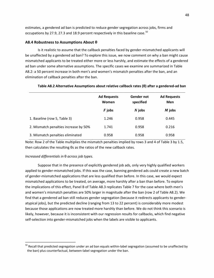
48

estimates, a gendered ad ban is predicted to reduce gender segregation across jobs, firms and occupations by 27.9, 27.3 and 18.9 percent respectively in this baseline case.50

A8.4 Robustness to Assumptions About 𝛉

Is it realistic to assume that the callback penalties faced by gender-mismatched applicants will be unaffected by a gendered ad ban? To explore this issue, we now comment on why a ban might cause mismatched applicants to be treated either more or less harshly, and estimate the effects of a gendered ad ban under some alternative assumptions. The specific cases we examine are summarized in Table A8.2: a 50 percent increase in both men’s and women’s mismatch penalties after the ban, and an elimination of callback penalties after the ban.

Table A8.2 Alternative Assumptions about relative callback rates (θ) after a gendered-ad ban

Ad Requests

Women Gender not

specified Ad Requests

Men

𝑭 jobs 𝑵 jobs 𝑴 jobs

1. Baseline (row 5, Table 3) 1.246 0.958 0.445

2. Mismatch penalties increase by 50% 1.741 0.958 0.216

3. Mismatch penalties eliminated 0.958 0.958 0.958

Note: Row 2 of the Table multiplies the mismatch penalties implied by rows 3 and 4 of Table 3 by 1.5, then calculates the resulting θs as the ratios of the new callback rates.

Increased differentials in θ across job types.

Suppose that in the presence of explicitly gendered job ads, only very highly qualified workers applied to gender-mismatched jobs. If this was the case, banning gendered ads could create a new batch of gender-mismatched applications that are less qualified than before. In this case, we would expect mismatched applications to be treated, on average, more harshly after a ban than before. To explore the implications of this effect, Panel B of Table A8.3 replicates Table 7 for the case where both men’s and women’s mismatch penalties are 50% larger in magnitude after the ban (row 2 of Table A8.2). We find that a gendered ad ban still reduces gender segregation (because it redirects applicants to gender-atypical jobs), but the predicted decline (ranging from 13 to 22 percent) is considerably more modest because those applications are now treated more harshly than before. We do not think this scenario is likely, however, because it is inconsistent with our regression results for callbacks, which find negative self-selection into gender-mismatched jobs when the labels are visible to applicants.

50 Recall that predicted segregation under an ad ban equals within-label segregation (assumed to be unaffected by

the ban) plus counterfactual, between-label segregation under the ban.

49

Diminished differentials in θ across job types.

There are at least two reasons why a gendered-ad ban might cause gender-mismatched applicants to jobs that were formerly explicitly gendered to be treated less harshly than before. One is the possibility that these new applicants are more positively selected than before (because before the ban, mismatched applicants were negatively selected). Second, a gendered-ad ban could signal to employers that public policy has become less tolerant of gender discrimination in the applicant selection process as well as the advertising process. To explore this scenario, panel C of Table A8.3 explores the extreme case where a gendered ad ban eliminates gender mismatch penalties for both men and women (row 3 of Table A8.2). Here the predicted declines in segregation are larger than in the baseline case, but not dramatically so, ranging from 26 to 35 percent. This modest effect of completely eliminating gender discrimination in employers’ callback decisions process underscores the dominant role of workers’ self-selection decisions in accounting for gender-matching in labor markets, already noted in our discussion of the aggregate statistics.

Table A8.3 Simulated Effects of a Gendered Ad Ban under alternative assumptions about the effects of a ban on θ

Segregation across

Noise-adjusted segregation (𝑺�)

Estimated noise-adjusted segregation after a gendered-ad

ban

Percentage reduction in noise-adjusted

segregation from a gendered ad ban

�̃� �̃�𝐴 �̃� − �̃�𝐴

�̃�

(1) (2) (3)

A. Baseline: θ is unaffected by a gendered ad ban

Jobs 0.607 0.438 0.279 Firms 0.395 0.287 0.273 Occupations 0.385 0.312 0.189

B. Gender-Mismatch Penalties Increase by 50%

Jobs 0.607 0.476 0.216 Firms 0.395 0.313 0.208 Occupations 0.385 0.335 0.131

C. Gender-Mismatch Penalties fall to zero

Jobs 0.607 0.395 0.349 Firms 0.395 0.260 0.341 Occupations 0.385 0.285 0.259