gene co-expression networks across many microarrays

Gene Co-expression Networks Across Many

Microarrays

by

Michael Bankston

B.S., University of Colorado, Colorado Springs, 2007

A thesis submitted to the Graduate Faculty of the

University of Colorado at Colorado Springs

in partial fulfillment of the

requirements for the degree of

Master of Science

Department of Computer Science

2013

c� Copyright By Michael Bankston 2013

All Rights Reserved

This thesis for Master of Science degree by

Michael Bankston

has been approved for the

Department of Computer Science

by

Dr. Jugal Kalita, Chair

Dr. Lisa Hines

Dr. Rory Lewis

Date

iii

Bankston, Michael

M.S., Computer Science

Thesis directed by Dr. Jugal Kalita

Dedicated to my wife, Lacey

v

Acknowledgments

First, I would like to acknowledge my thesis advisor, Dr. Jugal Kalita, who originally

inspired me to go down the research path of microarray meta-analysis and and field of

bioinformatics in general, and who was always available for questions and feedback on such

short notice. Also, to the two graduate students, Connor Clark for his contributions to the

graph comparison algorithm implementations and literature review, and Tri Doan for his

thorough research into the many possible routes of future work to extend the results of this

thesis.

And lastly, I would like to acknowledge my wife, Lacey Bankston, whose knowledge

of biology I relied on to strengthen the relevancy of the work, and to her incredible patience

in allowing me the time I required to finish this work under a very short timeline.

TABLE OF CONTENTS

1 Introduction 1

1.1 Objective . . . . . . . . . . . . . . . . . . . . . . . . . . . . . . . . . . . . . 2

1.2 Accomplishments . . . . . . . . . . . . . . . . . . . . . . . . . . . . . . . . . 3

1.3 Outline of Thesis . . . . . . . . . . . . . . . . . . . . . . . . . . . . . . . . . 4

2 Biological Background 6

2.1 Trp53 Example . . . . . . . . . . . . . . . . . . . . . . . . . . . . . . . . . . 7

3 Microarray Combination 8

3.1 Background . . . . . . . . . . . . . . . . . . . . . . . . . . . . . . . . . . . . 8

3.2 Approach . . . . . . . . . . . . . . . . . . . . . . . . . . . . . . . . . . . . . 10

3.2.1 Normalizing Value Ranges . . . . . . . . . . . . . . . . . . . . . . . . 10

3.2.2 Combining Platforms . . . . . . . . . . . . . . . . . . . . . . . . . . 11

4 Gene Regulatory Network Modeling 16

4.1 Background . . . . . . . . . . . . . . . . . . . . . . . . . . . . . . . . . . . . 16

4.2 Approach . . . . . . . . . . . . . . . . . . . . . . . . . . . . . . . . . . . . . 16

4.2.1 Static Bayesian Networks . . . . . . . . . . . . . . . . . . . . . . . . 17

4.2.1.1 Experiment Introduction . . . . . . . . . . . . . . . . . . . 21

4.2.1.2 Escherichia coli Experiment . . . . . . . . . . . . . . . . . 21

4.2.1.3 Large-Scale Human Microarray Experiment . . . . . . . . . 23

4.2.2 Dynamic Bayesian Networks . . . . . . . . . . . . . . . . . . . . . . 27

4.2.2.1 Time Series Interpolation . . . . . . . . . . . . . . . . . . . 28

4.2.2.2 Escherichia coli Experiment . . . . . . . . . . . . . . . . . 33

vii

4.3 Conclusion . . . . . . . . . . . . . . . . . . . . . . . . . . . . . . . . . . . . 35

5 Gene Network Graph Comparison 37

5.1 Background . . . . . . . . . . . . . . . . . . . . . . . . . . . . . . . . . . . . 37

5.2 Approach . . . . . . . . . . . . . . . . . . . . . . . . . . . . . . . . . . . . . 38

5.2.1 Frequent Subgraphs Experiment . . . . . . . . . . . . . . . . . . . . 39

5.2.2 Graphlet Degree Similarity Experiment . . . . . . . . . . . . . . . . 40

6 Microarray Meta-Analysis Tool 42

6.1 Introduction . . . . . . . . . . . . . . . . . . . . . . . . . . . . . . . . . . . . 42

6.2 Demo Walkthrough . . . . . . . . . . . . . . . . . . . . . . . . . . . . . . . . 43

6.3 Conclusion . . . . . . . . . . . . . . . . . . . . . . . . . . . . . . . . . . . . 50

7 Conclusion 51

7.1 Future Work . . . . . . . . . . . . . . . . . . . . . . . . . . . . . . . . . . . 52

7.1.1 Microarray Combination . . . . . . . . . . . . . . . . . . . . . . . . . 52

7.1.2 Gene Regulatory Networks . . . . . . . . . . . . . . . . . . . . . . . 54

7.1.3 Time Series Combination . . . . . . . . . . . . . . . . . . . . . . . . 55

References 57

Appendix A Software Packages and Versions 61

Appendix B All Sub-Graphs 62

TABLES

3.1 Platform Summary . . . . . . . . . . . . . . . . . . . . . . . . . . . . . . . . 15

3.2 Platform Combination Comparison . . . . . . . . . . . . . . . . . . . . . . . 15

4.1 Large-Scale Microarray Summary . . . . . . . . . . . . . . . . . . . . . . . . 27

5.1 Intra-species Graphlet Degree Scores . . . . . . . . . . . . . . . . . . . . . . 41

FIGURES

2.1 TF Family p53 in Mouse . . . . . . . . . . . . . . . . . . . . . . . . . . . . . 7

4.1 SOS Regulation . . . . . . . . . . . . . . . . . . . . . . . . . . . . . . . . . . 22

4.2 SOS Regulation Run 1 . . . . . . . . . . . . . . . . . . . . . . . . . . . . . . 24



4.5 Dynamic SOS Regulation Run . . . . . . . . . . . . . . . . . . . . . . . . . 36

5.1 Frequent Subgraph 1 . . . . . . . . . . . . . . . . . . . . . . . . . . . . . . . 40

5.2 Frequent Subgraph 2 . . . . . . . . . . . . . . . . . . . . . . . . . . . . . . . 40

6.1 Opening Screen . . . . . . . . . . . . . . . . . . . . . . . . . . . . . . . . . . 43

6.2 New Project . . . . . . . . . . . . . . . . . . . . . . . . . . . . . . . . . . . . 44

6.3 New Experiment . . . . . . . . . . . . . . . . . . . . . . . . . . . . . . . . . 45

6.4 Add Platforms and Microarrays . . . . . . . . . . . . . . . . . . . . . . . . . 46

6.5 Probe Selection . . . . . . . . . . . . . . . . . . . . . . . . . . . . . . . . . . 47

6.6 Running the Experiment . . . . . . . . . . . . . . . . . . . . . . . . . . . . . 48

6.7 Graph View . . . . . . . . . . . . . . . . . . . . . . . . . . . . . . . . . . . . 49

x

B.1 All Sub-Graphs . . . . . . . . . . . . . . . . . . . . . . . . . . . . . . . . . . 62

CHAPTER 1

INTRODUCTION

Gene expression analysis is a very important topic in biological studies. In humans,

there are between 20,000 and 23,000 genes [43], each of which is mapped to one or more

gene products. When genes express themselves, the gene products are usually proteins, but

can also include functional RNA (fRNA). In the presence of certain gene products, genes

can also alter the expression levels of other genes.

Since the expression level of one gene may determine the expression level of another,

the relationship between two or more genes is called co-expression. It is possible to record

levels of co-expression in individual cells at various points in time. One method to do this

is through the use of a DNA microarray, which will contain relative expression levels from

one or more genes over multiple time points.

If gene co-expression levels are accurately determined for a given function, then a

Gene Regulatory Network (GRN) can be inferred for that function. Accurate GRNs are

extraordinarily important in understanding the methods of how genes interact with each

other in both normal organic processes and in the development of disease. This knowledge

and understanding can help to predict possible disease susceptibility in individuals or help

in the research of new pharmaceutical drugs.

Although GRNs can sometimes be deduced through other experimental means, a

popular method is through the analysis of DNAmicroarrays by using data mining techniques

to determine the correlations between the expression levels of various genes. There are

many techniques in computational biology for inferring GRNs from this correlation data,

2

but a common problem is the very specific nature of an individual microarray. Even if

a correlation is found in a single microarray, it is still very unlikely that correlation will

continue to be found when compared to a selection of other microarrays; as low as a 2.2%

chance [27]. A typical gene expression microarray dataset consists of relatively few time

points (often <20) in comparison to the number of genes, generally in the thousands. This

scarcity of time-course data is the so-called dimensionality problem, making the problem of

determining GRN structure from a single microarray an ill-posed problem [55].

With the rapid increase in publicly available microarray data, such as the Gene Ex-

pression Omnibus (GEO) [3] and ArrayExpress [37] archives, there is an abundance of data

covering many di↵erent experiments. Although these microarrays can be developed with

di↵erent goals in mind, there is a great overlap in gene co-expression data from microar-

ray to microarray, so that confidence and robustness in determining expression correlations

between genes can be greatly increased through finding similar correlations across multiple

datasets. However, combining microarray datasets is not a straightforward process, as ex-

periments are commonly conducted in di↵erent laboratories with di↵erent equipment can

lead to inherent biases in the data that are not always removed in processing the data [51].

Finding methods to predict accurate and robust gene co-expression networks from

multiple microarrays is currently an important topic in bioinformatics with much work still

ahead of it.

1.1 Objective

The overall objectives of this research is to find and compare microarray meta-analysis

techniques, then use these sets of combined gene expression levels to infer Gene Regulatory

Networks. Static networks will be generated on very large sets of disparate combined ex-

3

periments with no regard to time, while dynamic networks will be generated using smaller

time series microarray experiments combined using both microarray meta-analysis tech-

niques and interpolated time points to fill in time gaps created after combination. A small,

simple GUI tool will be built for configuring and running these experiments to allow for

easier microarray meta-analysis for non-computer experts, since the need for such a tool is

great.

1.2 Accomplishments

The accomplishments presented in this thesis lays the groundwork for a great deal of

future work by solving various problems in the course of producing and comparing GRN

graphs and implementing a large library of useful functions and GUI tools designed for

microarray meta-analysis.

Microarray combination is accomplished by creating parsers to ingest both individual

microarray samples and microarray matrix files in SOFT format. Microarray platform

files, also in SOFT format, is used to map probes to genes. An algorithm developed for

combining platforms together using metadata analysis allows for probe mapping across

microarrays from di↵erent platforms. Then, gene expression value normalization runs across

these microarrays to make them comparable against each other, even if originating from

di↵erent experiments and/or platforms.

Using combined microarray data as observations, Bayesian networks are inferred

through a learning algorithm and tested for sparseness, with several experiments run and

compared. Time series microarrays are also combined into time-based observations through

another algorithm developed to fill in gaps in time through interpolation. All time series

microarray experiments are then used as training observations for a dynamic Bayesian net-

4

work learning algorithm after interpolated to have the same time step size. An example

experiment to test this process is shown with results.

Two graph comparison algorithms are implemented for the use of inter-species and

intra-species GRN graph comparison. The first, to find sub-graphs in two graphs from the

same species, is tested with some human GRNs under di↵erent conditions. The second,

to find a graph similarity measure, uses combinations of several di↵erent species and the

results are tallied.

The Microarray Meta-Analysis Tool (MMAT), developed during the course of this

work, is intended for use by non-computer expert scientists to use in custom microarray

meta-analysis experiments. Several screenshots and instructions are given.

Since a very large literature review was done in the course of this work, a very sub-

stantial future work section is included to help give ideas to others on how to extend upon

this work.

1.3 Outline of Thesis

Chapter 2 presents the biological background for gene expressions and the use of

microarrays for measuring them. Chapter 3 explains the di�culty of and various possible

solutions to the problem of combining disparate microarray experiments for the use in mi-

croarray meta-analysis. It also outlines the exact methods used for microarray meta-anaylsis

in later chapters. Chapter 4 describes the process of inferring Gene Regulatory Networks

from a meta-analysis of many disparate microarray data sets. Here, it is shown how a static

Bayesian network can model a gene co-expression network, while using a Dynamic Bayesian

Network (DBN) extends a static Bayesian network to model gene expression cycles and feed-

back loops from multiple time series data. In Chapter 5, the comparison of the graphs built

5

from static Bayesian networks is shown using two di↵erent graph comparison algorithms.

First, an algorithm for finding subgraphs in two graphs with identical labels, and second,

an algorithm that compares only the structure of two graphs giving a similarity measure.

The first algorithm is run for inter-species graphs, while the second is run against graphs

for multiple species. The Microarray Meta-Analysis Tool (MMAT) GUI is introduced in

Chapter 6, with a brief example of how to use it. Chapter 7 concludes the work with a

summary and substantial future work section.

CHAPTER 2

BIOLOGICAL BACKGROUND

A gene is a string of genomic information written in the DNA of an organism that

encodes for possible gene products. These products include proteins (from protein coding

regions), and functional RNA, such as ribosomal RNA (rRNA) and transfer RNA (tRNA),

that are used for many basic biological purposes. When a gene expresses itself, the possible

products of the gene are produced, which can have a wide variety of e↵ects both on the

organism’s state and on other genes. This process, called gene expression, is the fundamental

level where genotype propagates to the phenotype.

When genes express together, called gene co-expression, the changes made to the

biological processes of an organism are commonly di↵erent than if only one of the gene

expresses individually. More interestingly, two or more genes expressing together can bring

about biological e↵ects that cannot be determined by treating the gene products generated

by both as independent. New proteins, functional RNA, and sudden changes in other gene

expressions, both downward and upward, can be caused by two or more genes co-expressing.

The co-expression of genes also hints at a deeper regulation network that genes employ

to control the products of other genes. One or more genes strongly expressing can cause

other genes to express more strongly, up-regulation, or more weakly, down-regulation. These

regulatory e↵ects on genes, in turn, combined with other environmental situations in the cell

and the expression levels of yet more genes, can then a↵ect more expression levels of other

genes. These regulatory processes of gene a↵ecting gene gives rise to a entire regulation

7

Figure 2.1: TF Family p53 in Mouse

network where genes work, not as independent units, but as part of an entire connected

system.

This regulation network, commonly called a Gene Regulatory Network (GRN), de-

scribes many of the mechanics at work in a cell of an organism, and is key to understanding

both healthy processes and an organism’s response to disease, chemical stressors, di↵erent

environments, and many other events, both internal and external.

2.1 Trp53 Example

An example of a real mouse GRN is shown in Figure 2.11. The gene Trp53 encodes

tumor protein p53, which responds to diverse cellular stresses to regulate target genes

that induce cell cycle arrest, apoptosis, senescence, DNA repair, or changes in metabolism.

Mice deficient for this gene are developmentally normal but are susceptible to spontaneous

tumors [12]. The yellow hexagon represents a gene cluster of 108 other genes.

1Figure retrieved from: http://rulai.cshl.edu/TRED/GRN/p53.htm

CHAPTER 3

MICROARRAY COMBINATION

3.1 Background

A DNA microarray, also commonly known as a DNA chip or biochip, is used to mea-

sure the expression levels of many genes at once. Individual DNA microarray experiments

are used to monitor and record gene expression levels at various key points in an organism’s

state. Some common uses for microarray experiments include showing the di↵erence in

healthy and diseased states of an organism, such as cancerous versus non-cancerous, the

e↵ect of various treatments of medical conditions versus a control, and using a time series

of microarrays to follow gene expression as it changes in time in a particular environment.

Microarray experiments are usually done as a series of measurements with a common

platform. A microarray platform consists of probes, which can number in the tens of thou-

sands, where the purpose of each is to bind to a particular strand of cDNA or RNA. In this

way, each probe can measure the density or rate of specific strands within a cell or other

biological environment. These measurements can help to determine the level of expression

of a gene at a particular point in time by tracing back a gene product to its original source.

These expression levels are usually measured as log ratio floating point values, but the range

of values are determined by the type and specific bias of the experiment and the platform

used.

An entire microarray experiment that results in a series can then be thought of as a

large matrix, where rows are genes (either canonical or alternatively spliced), and columns

are individual measurements. When trying to determine when two or more gene co-express

9

together using various machine learning algorithms, each column can be treated as a sepa-

rate observation when using supervised and unsupervised learning approaches.

A microarray series usually consists of two or more, possibly hundreds, of individual

measurements, or samples. However, the number of gene products measured can easily

reach to 20,000 or more with popular platforms. This discrepancy between dimensions in

microarray series data, the dimensionality problem [55], makes determining co-expression

links an ill-posed problem with so few observations.

One method to solve the dimensionality problem is to merge multiple microarray

experiment series into a single matrix, thereby greatly increasing the number of observations.

This method, called microarray meta-analysis, is an integrative data analysis method is

traditionally defined as a synthesis of results from datasets that are independent but related

[35]. Not only can many microarray experiment series be combined through meta-analysis,

but even intersecting genes from di↵erent microarray platforms can be combined.

Many researchers have embraced microarray technology in recent years, and due to

their extensive use, there has been an explosion in publicly available datasets online. Sev-

eral Internet repositories have been set up for the public with anonymous downloading for

research use. Examples of such repositories include the Gene Expression Omnibus (GEO,

http://www.ncbi.nlm. nih.gov/geo/) [3], ArrayExpress (http://www.ebi.ac.uk/microarray-

as/ae/) [37], and the Stanford Microarray Database (SMD, http://genome-www5.stanford.edu/)

[16]. Literally tens of thousands of datasets are free to download, and such a deluge of

information makes this a golden opportunity for new techniques in meta-analysis to be

developed.

10

3.2 Approach

The ultimate goal of the research described in this thesis is to use as many microarray

datasets as possible in the attempt to infer Gene Regulatory Networks. With this in mind, a

dataset aggregation meta-analysis strategy is needed that can scale to thousands of microar-

ray samples or more. The two main obstacles to microarray combination are: expression

value ranges and biases between datasets and the use of di↵erent microarray platforms.

An overall strategy for combining microarrays that solves both problems is needed before

processing all the data.

3.2.1 Normalizing Value Ranges

Value ranges on individual gene expression within a microarray sample can vary a

great deal from dataset to dataset due to systematic variations arising from variation in

the technology rather than biological variations. The scale di↵erences between microarray

experiments can di↵er substantially from reasons such as a changes in the photomultiplier

tube settings of the scanner and others [50].

Scale-normalization is a commonly used method for the simple scaling of the log ratios

from a series of arrays so that each array has the same median absolute deviation [36]. This

method has been shown to be quite e↵ective as an aggregation strategy when used for

the purposes of determining Gene Regulatory Network structures in the past [51]. The

scale-normalization formula used to transform each log ratio value is as follows:

M0ij =

Mij �mediani

MADi(3.1)

11

where Mij is the log ratio of the jth gene in the ith array and the median absolute de-

viation MADi is defined as the median absolute deviations from the median: MADi =

mediani(|Mij �mediani|).

Scale-normalization not only has the advantage of preparing microarray samples for

comparison within datasets, but also theoretically allows arrays between datasets to be

comparable as well. Therefore, this method can be used to combine many microarrays

together, which can be treated as a single dataset [51]. The drawback is that bias and

artifacts may still be present in the data after scale-normalization. However, this variance

due to experimental bias and error, in theory, could be interpreted as observational noise

that can be statistically canceled out when scaling up to thousands of microarray samples.

3.2.2 Combining Platforms

Microarray platforms, such as the A↵ymetrix Human Genome U133A Array and the

Agilent-014850 Whole Human Genome Microarray, are both designed to measure expression

levels of the entire human genome as it is understood today, but have completely di↵erent

probe structures. The challenge is to match up di↵erent platforms such as these so that

microarray samples that use one or another can be combined.

Probe ID’s from platform to platform generally have no correlation to each other

whatsoever, so that when analyzing a single microarray sample that uses these probe ID’s,

it is unknown which probe ID matches one platform or another. However, platform de-

scription files, such as platform SOFT (Simple Omnibus Format in Text) files from the

Gene Expression Omnibus repository, do contain metadata associated with each probe. In

theory, it should be possible to mine this metadata to match one probe from one platform

12

to another probe in another platform so as to create a mapping data structure that can be

referenced when ingesting microarray samples.

The algorithm for matching platform probes to other platform probes relies on the

existence of one or more pieces of metadata that can each be recorded and compared to

every other probe on another platform. If metadata matches in some manner between two

probes from two platforms, then a multi-platform that forms a union of probes from both

platforms can be built.

More formally, given platform A with I probes and platform B with J probes, let pAi

be a probe in A and let pBj be a probe in B. Each probe has one or more metadata mn

that can be compared. Multi-platform X has probe pXk if and only if pAi(mn) = pBj (mn)

for some subset of n and some measure of equality between metadata. This means that

multi-platform probe count K I, J . Once a multi-platform is built from two platforms,

it can be treated as a single platform to join with another platform.

An algorithm for producing a multi-platform map that can recognize microarrays from

any platform in the mapping and trace it back to a single gene was originally developed in

the course of this work. This algorithm to determine a multi-platform from N platforms is

shown in Algorithm 1.

There are many types of metadata that is possible, including, but not limited to:

• Probe name

• Primary gene label

• Alternate gene synonyms

• Chromosome number

• Nucleotide sequence begin/end

13

Algorithm 1: BuildMultiPlatformData: I platforms PI , each with n probes and m metadata; metadata equality score

threshold E

Result: Multi-platform X with k n probes

X � ;;

foreach platform P do

if P is first platform then

add all probes along with metadata to X;

else

foreach probe p in P do

foreach probe x in X do

e � metadataEqualityScore(p(m), x(m));

if e � E then

add name key and all metadata from p to x;

break;

foreach probe x in X do

if P does not contain x then

remove x from X ;

14

• Sequence type

• Free text gene description

• Free text biological process/molecular function description

• ID’s from various gene/transcript databases.

Each piece of metadata, when compared to others, must be treated and scored di↵er-

ently. The metadataEqualityScore() function in Algorithm 1 will return a di↵erent score

depending on what metadata is being processed and score combination strategy. For the

purposes of producing Gene Regulatory Network structures in later chapters, only Primary

gene label and Alternate gene synonyms were used when combining platforms1. Popular

microarray platforms containing these two metadata fields were chosen specifically to test

this algorithm.

Given platforms A and B, the return value of metadataEqualityScore() was 1 if Pri-

mary gene label of a probe in A matched with either the Primary gene label or any of

the Alternate gene synonyms of a probe in B, and 0 otherwise. Metadata equality score

threshold E was set to 1.

The three platforms used for testing included three popular whole genome platforms

where probes were tied to specific genes. Statistics on all three platforms are shown in Table

3.1. The results of combining three platforms all four combinations are shown in Table

3.2. GEO ID’s are the accession numbers given to the platforms on the Gene Expression

Omnibus.

1The ability to expand to other pieces of metadata is available, and is described in the Future Work

section of Chapter 7.

15

Table 3.1: Platform Summary

Platform GEO ID Full Platform Name Probe Count

GPL96 A↵ymetrix Human Genome U133A Array 20,967

GPL8490 Illumina Human Methylation27 BeadChip 27,551

GPL6480 Agilent-014850 Whole Human Genome Microarray 30,936

Table 3.2: Platform Combination Comparison

Platform GEO IDs Retained Probes

GPL96 + GPL8490 9,730

GPL96 + GPL6480 12,436

GPL8490 + GPL6480 11914

GPL96 + GPL8490 + GPL6480 9581

CHAPTER 4

GENE REGULATORY NETWORK MODELING

4.1 Background

A Gene Regulatory Network (GRN) describes a series of interactions in a cell between

genes (or DNA segments) through indirect means, such as RNA and protein expression prod-

ucts. These interactions control gene product expression levels either upward or downward,

which, in turn, can change the expression levels of other gene products. These gene to gene

interactions can be thought of as a casual network which describes each gene a↵ecting one

or more other genes. The attempt to model this interaction network with enough fidelity

to be useful has been a long time research challenge.

4.2 Approach

The use of as many microarrays as possible to infer GRNs is one of the primary goals

of this research, and the methods of combining microarray studies in mass as described

in Chapter 3 are used to produce gene expression observations. From these observations,

machine learning techniques can be used to learn from the data and find gene to gene

connections. The two machine learning techniques used in this thesis for building the

GRN casual network are static and dynamic Bayesian networks, which have some distinct

advantages over other techniques.

Gene expression is an inherently stochastic process since they directly or indirectly

depend on probabilistic collisions between molecules [40]. Even if the underlying systems

was deterministic, it may appear to be stochastic because of our inability to perfectly mea-

17

sure all of the variables. Because of this, the variables measured in microarray experiments

are not expected to be perfectly accurate, but instead quite noisy. Finding the most probable

model should be the goal, since even if a GRN were a perfect Boolean network in reality,

the inherent di�culty in measuring all variables in the system makes it impossible to model

with perfect certainty [31].

Since the landmark work of Friedman et al. [19], Bayesian networks have been popular

for modeling many di↵erent biological processes due to their ability to describe complex

stochastic processes and because they provide a clear methodology for learning from noisy

observations. They are part of a family of models called probabilistic graphical models and

are well suited for describing any abritrary combinatorial gene regulation because they are

not limited to pair-wise or linear interactions between genes. Since they describe interactions

in a probabilistic manner, Bayesian networks are robust to noisy data, cleanly handle missing

data, and allow for unobserved factors to be represented by latent variables [22].

4.2.1 Static Bayesian Networks

A Bayesian network is a representation of a joint probability distribution consisting

of two components. The first component, G, is a directed acyclic graph (DAG) where its

nodes correspond to the set of random variables � = X1, ..., Xn. Each variable Xi can take

values from a finite set, V al(Xi). The second component, ✓, are the links of the graph that

correspond to direct influence from one variable to another. A directed link from variable

Xi to variable Xj defines variable Xi as a parent of variable Xj . Every node of the DAG

corresponds to a conditional probability distribution (CPD) that represents p(Xi|Pa(Xi))

where Pa(Xi) designates the parents of Xi in G.

18

The graph G represents a conditional independence assumption, also known as the

Markov Assumption: every variable Xi is independent of its non-descendants, given its

parents in G. Therefore, there is a unique joint probability distribution over X from G:

p(X1, ..., Xn) =nY

i=1

(p(Xi PaG(Xi))). (4.1)

For modeling GRNs, it makes sense to interpret a Bayesian network as a causal

network where all the links from parent to child variables denote that each parent causally

influences the values of the child variables. In this way, each gene can be represented by a

random variable of the DAG, with every link representing the probability of influence of one

gene on another [19]. Since GRNs are to be inferred from microarray data, the Bayesian

network must be learned rather than constructed by expert knowledge. It is certainly

possible to do both simultaneously, but for the purposes of this research, the goal is to use

as many microarrays as possible to learn a Bayesian network modeled GRN from scratch1.

The problem of learning a Bayesian network involves finding a network B = hG, ✓i,

when given a training set D = x1, ..., xN of independent instances of �, that best matches D.

However, the task of finding Bayesian network structure that describes the observed data

the most is proven to be an NP-hard problem [9]. For this reason heuristic algorithms are

used for learning structure, and there are many di↵erent approaches. Of these techniques,

greedy-hill climbing and simulated annealing are the most popular to use with biological

data. For this research approach, simulated annealing was chosen for its past success in

GRN Bayesian model searches [22].

1A possible method for combining expert knowledge with learning is outlined in the Future Work section

of Chapter 7.

19

The task of inferring the structure of a Bayesian network is typically expressed using

Bayes’ rule, where the posterior probability of a given network structure G after having

observed data D is given by:

P (G|D) =P (D|G)P (G)

P (D). (4.2)

During Bayesian network learning, a scoring function will evaluate how accurately

a given network G matches the data D. So, with a particular scoring function, the best

Bayesian network is the one that maximizes this scoring function. Many choices exist,

such as the Maximum Likelihood (ML), Bayesian Information Criterion (BIC) [47], Akaike

Information Criterion (AIC) [1], and Bayesian metric with Dirichlet priors and equivalence

(BDe) [23].

Empirical data indicates that biological gene networks are sparsely connected, with

the average number of regulators acting on genes is less than two [26]. With this in mind,

a scoring function that minimizes network complexity is needed. Maximum Likelihood

scoring does not penalize network complexity, but the other scoring functions do. For the

purposes of the experiments in this thesis, the BDe metric was chosen due to its common

use in the existing literature on learning GRNs. However, BIC, along with the very similar

AIC, have also been successfully used, and would be good choices for future comparison

work 2.

Each value in a microarray is a measurement of expression, and a continuous value.

Although algorithms for learning Bayesian networks for continuous variables exist, for the

purposes of learning GRNs, discretization of the values prior to learning is the usual method

practiced in the literature. This has the advantage of reducing the dimensionality of the

2The extra scoring function options are mentioned in the Future Work section of Chapter 7.

20

problem, and as argued in Hartemink’s Ph.D dissertation [20], gene transcriptional regula-

tion can be thought of as being in a limited number of states, such as none-low-high. As

he argues in his dissertation, there seems to be no added benefit of increasing the number

of degrees of freedom in learning continuous variables due, in part, to the noise inherent in

microarray analysis.

Two simpler discretization methods include quantile and interval discretization. For

the tests in this thesis, quantile discretization was chosen due to the fact that under quantile

discretization, the number of observations corresponding to the each discretization level is

guaranteed to be equal. In contrast, interval discretization can produce vectors where many

discretization levels may be represented too frequently, while others may not be represented

at all [20].

In quantile discretization, N sorted observations are divided into D discretization

levels by placing an equal number of observations into each of the D discretization levels.

Obviously, this has to mean that D N . The observation with index i is discretized as

level j if and only if:

bjNDc < i b(j + 1)N

Dc. (4.3)

For all the tests in this thesis, quantile discretization levels of 3 and 5 were both tried

with very similar results for all networks learned. Presumably, when combining enormous

numbers of microarray probe values, increasing the number of discretization levels from 3

to 5 does little to change the underlying structure in the data. However, exploring other

discretization values, along with other discretization methods could be valuable future work

in microarray combination3.

3As outlined in the Future Work section of Chapter 7.

21

4.2.1.1 Experiment Introduction

Static Bayesian networks model causality without regard to time, so they are better

suited for learning gene co-expression links from hundreds, or thousands, of disparate mi-

croarray experiments whether they are part of a time series, treatment versus control, or

other type. With this in mind, two experiments were devised for determining links from

many microarrays.

The first experiment attempts to infer a particular known regulatory network and

find its accuracy using a certain number of microarrays. The second experiment uses as

many microarrays as possible, using only the most active genes to find which connections

stand out over a very large number of microarrays.

For both experiments, the Banjo Bayesian network learning software was used4. Banjo

is a Java library designed and implemented by Hartemink, a professor of Computer Science

at Duke university, and is able to learn both static and dynamic Bayesian networks. One

of its original purposes was to learn from biological data, and it has been used in other

research before in the inference of GRNs [28] [21].

4.2.1.2 Escherichia coli Experiment

The first experiment devised for learning a GRN from many microarrays involves

attempting to learn and model the SOS response gene regulatory pathway in Escherichia

coli (E. coli) bacteria. SOS response is a global response to DNA damage where a protein

produced from the RecA gene, inactivates a repressor enzyme produced from the LexA gene.

This repressor enzyme reduces the expression levels of at least six other genes, sulA, unmC,

unmD, uvrA, uvrB, and uvrD [4]. In this experiment, di↵erent combinations of microarray

4Banjo homepage: http://www.cs.duke.edu/ amink/software/banjo/

22

Figure 4.1: SOS Regulation

experiments are combined in the attempt to model this process. The measure of success was

in the networks’ accuracy in modeling the RecA gene a↵ecting the LexA gene, with LexA

enzyme product a↵ecting every other gene. A graphical representation of this regulatory

network is show in Figure 4.1.

Microarray data was gleaned from the GEO database, and the two most popular

platforms for measuring gene expression in E. coli bacteria: A↵ymetrix E. coli Antisense

Genome Array (GEO Accession GPL199) and the A↵ymetrix E. coli Genome 2.0 Array

(GEO Accession GPL3154). Between these two platforms, a total of 1614 microarrays were

used for gene expression observational data.

Three runs were performed in the attempt to infer a gene expression network that

gave links in a biologically realistic manner. Each run was allowed 1 hour for a simulated

annealing search, although in each run, the top scoring network was found within the first

10 minutes. Interestingly, the RecA to LexA connection was found in every run quickly

and existed in the top ten scoring networks every time. It is assumed this means that this

connection was likely very common and easy to find in the data.

23

For the first run, only microarrays from the GPL3154 platform, totaling 676, were

used. The resulting highest scoring Bayesian network is shown in Figure 4.2. The biologi-

cally realistic connection of RecA a↵ecting LexA was found during this run, but many other

spurious connections were found as well, and RecA is not at the top.

For the second run, 938 microarrays from the GPL199 platform were used. The

resulting highest scoring Bayesian network is shown in Figure 4.3. Again, the connection of

RecA a↵ecting LexA was found, but like the first run, many other connections were found.

As in the first run, RecA is not at the top, and is near the bottom instead.

After the first two runs, it was obvious that the connection between RecA and LexA

was easy to find in the data, but not the influence of LexA on the rest. The third run

attempted to use an enormous number of microarrays, 1614 in total, to find a more accurate

network model. All microarrays from both of the first two runs were combined using the

multi-platform algorithm in Chapter 3. The highest scoring network found is shown in

Figure 4.4. This is an obvious improvement over the first two runs, as it not only shows the

link between RecA and LexA, but also showing the regulatory process with RecA as the top

parent variable, as it should be [4]. Other connections were also found between the other

genes, but it is unknown whether these links exist or not in the true network [51].

4.2.1.3 Large-Scale Human Microarray Experiment

The second experiment was devised to use as many microarrays as possible for finding

gene to gene connections. Microarrays from three di↵erent platforms were used: A↵ymetrix

Human Genome U133A Array, Illumina Human Methylation27 BeadChip, Agilent-014850

Whole Human Genome Microarray. However, the total number of genes in common on all

three platforms was still at 9,581, far too high for learning on any available computer due

24

Figure 4.2: SOS Regulation Run 1


25


to space requirements. Memory requirements for learning Bayesian networks uses O(n2n)

space by the number of variables, but only O(n) by the number of observations5, so a

method to reduce the number of genes was needed.

Most genes are very inactive in most microarray experiments. Some genes only express

strongly under very rare circumstances, or never express strongly at all. It would be more

interesting to look at only the most active genes over a large number of microarrays. With

this goal in mind, a total of 574 genes with the largest ranges in values over the entire

5Memory requirements using Banjo. There are other learning methods that may reduce this memory

requirement [29].

26

microarray dataset were used in every test. The memory requirements for even this number

of genes approached 5 gigabytes for the largest dataset.

The goal of this test was to create networks that had real biological significance.

Leclerc et al., found that the average number of transcriptional regulators per gene to be

1.5 � 2.0 [26] in most organisms, so a sparse network would be preferred over a dense one

in theoretical results.

In this experiment, gene regulatory Bayesian networks were learned from three di↵er-

ent sizes of micorarray multi-datasets, 489, 881, and 2509. The chosen datasets represented

a variety of experiments to try to capture both common and uncommon gene regulation

events. This includes cancer studies, treatment and control of various conditions, specific

tissue studies, and several time-series experiments. Since the search space for these net-

works is intractably large, the Time to Learn metric was defined as when a better network

was not found in the time it took for the best network so far to be found. In other words,

if a best scoring network takes t time to learn, the search is stopped at 2t.

The results of all three runs are shown in Table 4.1. It is obvious from the results that

as the number of samples goes up, so does the number of gene connections. However, it

does not appear to be a linear relationship, and could be reaching an asymptote as samples

rise, but more data and longer tests would be needed to verify. The largest dataset in this

test was the limit to what could be done on hardware available. However, the largest test’s

number of average arcs per gene is within the 1.5� 2.0 range, giving a promising result. Of

course, with only a subset of the most active genes, some connections could not be made to

non-included genes, and some of the connections that do exist could possibly be spurious.

27

Table 4.1: Large-Scale Microarray Summary

Samples Total Connections Average Connections Per Gene Time to Learn (h:m)

489 568 ⇠0.99 3:03

881 644 ⇠1.12 3:57

2509 949 ⇠1.65 8:01

4.2.2 Dynamic Bayesian Networks

An extension of Bayesian networks, known as Dynamic Bayesian networks (DBNs),

add a time component to the network model, allowing for modeling time delay between gene

expression values. The use of dynamic Bayesian networks for modeling Gene Regulatory

Networks has been an extremely popular method in past research [32] [53] [24] [19] [42].

The advantage Dynamic Bayesian networks have over static networks is in their ability to

model possible feedback loops in gene regulation where the up or down regulation of a target

gene by a regulatory gene may mean another up or down regulation from the target gene

back to the regulatory gene. These feedback loops are a common and essential part of any

biological system, including GRNs [33].

Like a static Bayesian network, a DBN has a set of random variables � = X1, ..., Xn,

but each variable is assigned a time index t, where the number of time points is dependent on

the Markov lag chosen. In a first-order Markov model, a variable Xt+1 is directly dependent

on the previous time point Xt, but not on earlier time points. This is the first-order Markov

property, which states that the future is independent of the past given the present.

28

In modeling GRNs, DBNs are well-suited for learning from microarray time series

data, where an experiment will track a particular organism’s gene expression levels over a

series of time points. In theory, it should be possible to infer dependencies of the expression

level of one gene from another gene earlier in time. DBNs have the added benefit of

modeling the transcription lag inherent in gene expression, since instant gene regulation

is biologically unrealistic. Additionally, DBNs can model gene regulation feedback loops

through variable arcs that cycle in time. As an example, if modeling two variables, A and

B, a conditional dependency can exist between At�1 and Bt followed by another conditional

dependency from Bt to At+1. A influences B, which in turn influences A, completing the

cycle. The DBN model of cyclic gene regulation can also model arbitrarily more complex

gene regulation cycles between three or more genes.

4.2.2.1 Time Series Interpolation

A challenge in using time series microarray data is that time lag between data points

need not be uniform. For example, one experiment may measure gene expression at 0

minutes, 30 minutes, 1.5 hours, and 3 hours. The assumption made in learning a DBN from

time series data is that each observation has the same time lag from the previous observation.

This irregular sampling rate is very prevalent across time series microarray experiments,

and a solution is needed before constructing DBNs from the data. The approach taken

in this thesis is to use B-spline interpolation to produce gene-expression points at regular

intervals from non-uniform time series microarrays.

B-splines are a type of piecewise polynomial that generalize linear interpolation so that

reconstructed data can consist of quadratic, cubic, or higher-order curves [15]. B-splines

also have the added benefit of acting as a filter, eliminating extremes in reconstructed

29

data which can result from using noisy data as input [45]. B-splines have already been

successfully used for gene regulation modeling from time series microarray experiments in

previous work [2], and was chose due to their advantages over other interpolation methods

when considering the specific problem of noisy microarray data.

When working in two dimensional space of time series gene expression values, there

is the independent variable t, representing time and the dependent variable x, representing

expression value. The spline is a weighted sum of a set of basis splines, which are a set of

curves defined by two parameters: the order k of the splines, and a vector ~⌧ of points of

discontinuity in the t dimension, called knots. All values of t are bounded by the first and

last knot values:

⌧1 t ⌧|~⌧ |. (4.4)

The B-spline contains n bases, where:

n = |~⌧ |� k. (4.5)

The basis splines are formally defined from the Cox-de Boor regression formulas [15]:

bi,1(t) =

8>><

>>:

1 if ⌧i t ⌧i+1

0 otherwise

(4.6)

bi,k(t) =t� ⌧i

⌧i+k�1 � ⌧ibi,k�1(t) +

⌧i+k � t

⌧i+k � ⌧i+1bi+1,k�1(t) (4.7)

where bi,k is the ith basis of order k.

The choice of knots in the t time dimension will have a large e↵ect on the interpo-

lating B-spline calculated. In the work done by Bar-Joseph et al. [2], knots were assumed

to be uniform before fitting the splines. However, in Smith’s Ph.D dissertation [49], he

argues that with microarray gene expression values, the splines can oscillate too much while

trying to fit the observations and can lead to unsolvable equations when data is too sparse.

30

Instead, he argues that knots should be chosen on the actual time points of the expression

measurements, so this is the method implemented by the work in this thesis.

According to Smith’s dissertation, a large di↵erence in accuracy is seen when increas-

ing the order k from 2 to 3 but little di↵erence in accuracy is seen when increasing the order

beyond 3, and was sometimes worse [49]. A k value of 3 is known as a quadratic spline, and

is the value used for all interpolating runs.

Using math functions available in the Apache Commons Math Java library6, a B-

spline interpolation algorithm is used to fill in missing observations at key points in time.

These extra observations between real observation points are referred to as pseudo-observations,

and are used to simulate a regular sampling rate for a given microarray sample. The rate

of sampling, T , is an adjustable parameter that will determine at what points in time and

how many pseudo-observations will be added to the DBN learning data.

For example, given a microarray time series with sampling time points 0 minutes,

30 minutes, 1.5 hours, and 3 hours, with T = 30m, and interpolation knot ⌧1 set to 0, all

four real observations are used, plus psuedo-observations at 1 hour, 2 hours, and 2.5 hours

interpolated from the data. This gives a total of 7 observations for a learning set from this

microarray time series: |~⌧ | = 7.

The algorithm for producing and building a data structure for all these observations

given a particular time series microarray experiment is shown in Algorithm 2.

Because of the goal of using as many microarray experiments as possible for use as

training data, combining time series microarrays from separate experiments is needed. Now

that all the building blocks are in place, fusion of multiple time series microarrays into one

large observational set is possible.

6Found at http://commons.apache.org/proper/commons-math/

31

Algorithm 2: UniformObservationsBSplineInterpolationData: Microarray time series S with p1, ..., pP probes and N observations ordered by

time; Time step step

Result: Microarray time series R with � N observations ordered by time with

uniform time distance step between time points

first � first time point in S;

last � last time point in S;

totalCount = floor( last�firstT ) + 1;

foreach pi 2 S do

T � set of N times in S;

G � {S(pi, T1), . . . , S(pi, TN )};

polynomialSplineFunction() � bSplineInterpolate(T,G);

for time = first ; time last ; time = time+ step do

R(pi, time) � polynomialSplineFunction(time);

The process of preparing the observational data is as follows:

1. If multiple platforms are used, a multi-platform probe mapping is calculated using

Algorithm 1 from Chapter 3.

2. All microarray samples that will be used for observations are value-normalized against

each other as explained in Chapter 3.

3. A time-step is chosen (one that will intersect with the maximum number of real

observations to minimize interpolation error is a good choice).

32

4. Each microarray time series is transformed by Algorithm 2 so that every time series

has the same number of observations with the same time lag between values.

5. Combine all observations by lining up equal time points from each time series

In theory, this method would allow for an arbitrary number of microarray time series

to be combined to be used as a learning data set for a DBN. As far as the author knows,

there is no other existing method of combining multiple time series microarray experiments

together into one observational dataset, making this a first of its kind. It should be kept

in mind that di↵erent experiments do have di↵erent biases, environmental conditions, test

assumptions, etc, that may add extra error to the end result. Any experiment set up using

these methods would need to take into account any special considerations of the particular

microarray datasets used and adjust/interpret accordingly.

One possible problem with this method of microarray combination is the use of ex-

periments with very di↵erent time ranges. Ideally, all time series datasets used would have

the same start and end time, but this is commonly not the case. In combining one time

series with another, there may be time points available for one dataset that’s not available

for another. There are two basic ways to handle this situation: only use time points from

every time series dataset that are in common (truncate), or attempt to predict missing time

points outside of the time window available. The approach taken in this research was the

former, but interesting future research could try to find a new method of prediction that

makes sense for time series microarrays since this problem is still unexplored in the existing

literature7.7As explained in the Future Work section of 7.

33

4.2.2.2 Escherichia coli Experiment

As an experiment for combining multiple time series microarrays, the E. coli experi-

ment using static Bayesian networks is revisited, but with only time series data. Again, the

goal is to re-construct the SOS response gene regulatory pathway where 8 gene products

are involved. In the static Bayesian network experiment, over 1600 microarrays were used

since there was no restriction on the type of microarray dataset samples used. However, in

this experiment, only time series microarrays are allowed, and there are far fewer available

in public repositories.

The ability to combine multiple platforms was very helpful in finding more data, since

there was no restriction to use only a single platform. All microarray datasets were found

in the GEO database, using the two most popular platforms for measuring gene expression

in E. coli bacteria: A↵ymetrix E. coli Antisense Genome Array (GEO Accession GPL199)

and the A↵ymetrix E. coli Genome 2.0 Array (GEO Accession GPL3154). In total, 16 time

series datasets, from either one or the other platform, were combined into a single training

set.

There is no standard method in which researchers annotate time series datasets with

time points, so it was necessary to interpret the description of each dataset separately and

hand-label every sample within a time series with a time. Some datasets are so badly

annotated and described, it is necessary to go back to the original research paper associated

with the time series to find the time values. Also, only time series that had time steps

similar to each other made sense to use. Some were too short (< 5 minutes) while some

were too long (> 24 hours). Ultimately, only datasets with time point lags of around 30-60

minutes were used since there were a larger number of them available.

34

A T value of 30 minutes was used, and since the dataset with the smallest time range

was 3.5 hours, all others were truncated down to this range (the maximum was 6 hours). At

30 minute increments, every dataset contained 8 temporal observations, interpolated where

needed. This means a total of 16 ⇥ 8 = 128 observations are used for a DBN training set.

This is still a small number of observations, so great results with such noisy data is not

expected. However, the goal was to pull something biologically relevant from the data.

For learning DBN structure, it was decided to use a minimum Markov lag of 1 and

a maximum Markov lag of 2. The rationale behind this is that the transcription lag under

realistic biological settings would never include a gene regulating another instantly in time.

It’s certainly possible that two genes could co-express at the same time, but there should

be no casual link between the two, since it would be assumed that some other, unknown

variable actually caused both to co-express at some earlier point. A Markov lag of 1 under

this experiment means a temporal casual link of 30 minutes, while a Markov lag of 2 means

a casual link of 1 hour.

The search for the best fitting DBN to the data was run for about 10 minutes, but

seemed to converge to a best solution within a minute. Presumably, this is because of the

extremely small variable and microarray size. The results are shown as a three time slice

graph in Figure 4.5.

The results are good, since they only show biologically validated connections. LexA

is casually a↵ecting two gene products in the second time slice, and one more in the third

time slice. LexA is known to a↵ect the regulation of these genes [4]. RecA is shown to

connect to uvrD in the next time slice, which simply skips a step. RecA a↵ects LexA which

then a↵ects uvrD, but with 30 minute time slices, the RecA to LexA regulation may simply

be between time slices too many times to show up in the observations. The full SOS gene

35

regulation network may not be inferrable from a dataset of this size and/or type. This is

expected when working with smaller observational datasets with a lot of noise.

4.3 Conclusion

Using microarray scale-normalization and multi-platform techniques introduced in

Chapter 3, both static and dynamic Bayesian networks were used to infer GRNs under

several di↵erent circumstances. It was shown that not only is it possible to scale up a very

large number of genes and microarrays for large experiments, but experiments to find low

level regulation networks between only a small number of genes is also possible.

36

Figure 4.5: Dynamic SOS Regulation Run

CHAPTER 5

GENE NETWORK GRAPH COMPARISON

5.1 Background

Comparing gene network graphs can be a very useful tool for discovering similarities

and di↵erences in both inter-species and intra-species gene networks. The considerations for

the comparison of networks from the same species versus multiple species are very di↵erent.

For graphs from the same species, gene names are the same and certain assumptions can be

made about their function in each of the graphs can be made. However, graph comparison

between species requires a di↵erent set of assumptions due to genes named di↵erently, and

commonly no direct one-to-one relationship between genes from one species to the other.

Inter-species comparison of biological networks has the potential to discover simi-

larities in the functionality and organization of genes across species. Comparing the gene

coexpression network of a well understood organism to a poorly understood organism could

allow the discovery of analogous coexpression behavior in di↵erent species, and suggest the

function of previously uncharacterized genes. For this reason, it is advantageous to explore

methods to compare the gene coexpression networks that are produced.

To compare gene networks across species, several hurdles must be overcome. First of

all, there is no obvious one-to-one mapping from genes in one species to genes in another–

if there were, interspecies comparison would be unnecessary. While some orthological infor-

mation is available, it is incomplete, and may not be available for some pairings of species.

Therefore, gene orthology cannot be relied on to map one network to another. Instead, find-

ing similarities in the topologies of the networks is the primary goal. This rules out some

38

alignment techniques previously used on protein-protein interaction networks. The second

problem is that finding an accurate injective mapping from the genes of one network to the

genes of another is computationally di�cult. This is the subgraph isomorphism problem,

which is NP-hard [13].

When comparing gene networks generated from the same species, it is common that

all networks have nodes corresponding to genes with the same labels. In this case, exactly

comparing graphs becomes computationally tractable. A simple and e↵ective algorithm has

been published by Koyuturk et al. for finding frequent common subgraphs in graphs with

labeled nodes [25]. This algorithm could be employed to compare results from di↵erent

experiments, or perhaps be used to combine several gene networks into a single network of

high confidence interactions.

5.2 Approach

Two di↵erent gene network graph comparison algorithms were used on a variety of

learned graphs. The first, a frequent subgraph algorithm, finds smaller subgraphs common

to two graphs, but only works over graphs with the same node labels. The second, a graphlet

degree similarity algorithm, is used to compare topology only between two graphs. A few

experiments were devised to show how di↵erent learned gene networks compared with each

other.

Koyuturk, et al.’s frequent subgraph algorithm is the approach taken for comparing

within species. It relies on nodes in two graphs being compared to be labeled identically,

which will be true for two gene networks of the same species that model the same genes. To

find these subgraphs, it uses a mining approach that starts with candidate edgesets, which

are only the single edges between individual nodes in the beginning, and attempts to extend

39

these candidates out by one edge at a time. If the extended edgeset is common to both

graphs, it is kept and edges are added once again. Once an edgeset cannot be extended

further, the algorithm stops extending it. All edgesets remaining from both input graphs

are the output, and are called frequent subgraphs.

The graphlet degree similarity algorithm used was developed by Przulj [44], and is

useful for comparing topology of graphs developed for two di↵erent species since it does not

rely on node labels. This algorithm uses a greedy seed and extend approach that computes

the pairwise similarity of nodes in two graphs, aligns the most similar pair of nodes first, and

then works outward to the neighbors of nodes that have already been aligned. Similarity

between two nodes is computed by comparing their graphlet degrees. Graphlet degree is a

generalization of the standard graph theoretic concept of node degree. It counts, for a given

small graph called a graphlet and a given node in the network being compared with, how

many unique subgraphs of the network are isomorphic to the given graphlet and contain the

given node. Computing the graphlet degree of each node for many di↵erent graphlets gives

a highly discriminative characterization of the topology around a given node. The graphlet

degrees for each node are combined into an aggregate score called the Graphlet Degree

Distribution (GDD) between 0 and 1, where 0 is no similarity and 1 is perfect similarity.

5.2.1 Frequent Subgraphs Experiment

To test the implementation of Koyuturk, et al.’s frequent subgraph algorithm, two

large cancer-related microarray datasets were used. The first dataset contained 10 di↵erent

microarray series dealing with leukemia patients totaling over 700 separate microarrays. The

second dataset was from 26 di↵erent microarray series from Breast cancer studies containing

just over 1000 microarrays. A large-scale static Bayesian network graph with 574 genes was

40

Figure 5.1: Frequent Subgraph 1

Figure 5.2: Frequent Subgraph 2

created for both, using methods explained in Chapter 4. Tests were run to compare the gene

regulation connections present in both graphs to find their similarity. Since the datasets

were both cancer related, but from two di↵erent cancers, they are expected to be similar,

but not identical.

After running this algorithm on the two datasets, 29 distinct subgraphs were found

with 1-4 connections each. Two examples of the discovered frequent subgraphs are shown

in Figure 5.1 and Figure 5.2. All subgraphs can be found in Appendix B.

5.2.2 Graphlet Degree Similarity Experiment

The experiment for comparing gene networks of di↵erent species uses Przulj’s graphlet

degree similarity algorithm. Four di↵erent species, homo sapien (human), Mus musculus

(Mouse), Escherichia coli (E. coli), and Saccharomyces cerevisiae (Yeast) are compared.

41

Table 5.1: Intra-species Graphlet Degree Scores

Human Mouse E. coli Yeast

Human 1.0 0.6921 0.7068 0.6956

Mouse 1.0 0.8498 0.8442

E. coli 1.0 0.8131

Yeast 1.0

The gene networks for all four species are generated using the methods explained in

Chapter 4, using from 600-1000 microarrays for each. Each network search is run for 4

hours to converge to a high-scoring network. The results of all six one-to-one comparisons

are shown in Table 5.1.

CHAPTER 6

MICROARRAY META-ANALYSIS TOOL

6.1 Introduction

During the course of this work, a Graphical User Interface (GUI) was implemented

to facilitate microarray meta-analysis without the need for programming skills or di�cult

to use command line interfaces. Instead, a user can create and manage projects made of

multiple experiments all with a simple, friendly visual interface.

This tool, the Microarray Meta-Analysis Tool (MMAT)1, was made in response to

a need of the existence of such tools in the computational biology world. According to

one very recent (2012) meta-analysis survey paper, “existing meta-analysis packages are

relatively primitive and di�cult to use” [52]. The design of MMAT is such that meta-

analysis workflow is much more obvious and intuitive. It forms a good basis for a possible

future expansion of features.

MMAT is a Java Swing project that utilizes the libraries written for the other work

in this thesis. The only two requirements for running MMAT is an installation of GraphViz

for the graphing visualization tool, and Java 7.

1Available for download at http://sourceforge.net/projects/mmatmicroarraymetaanalysistool/

43

Figure 6.1: Opening Screen

6.2 Demo Walkthrough

This section gives a brief walkthrough of the various features built into MMAT, and

its overall design. Although in a very alpha state, it is stable and can already be used for a

variety of experiments. MMAT is distributed in a single folder, and is run by executing the

RunMMAT.bat file. The opening window displayed to the user is shown in Figure 6.1.

44

Figure 6.2: New Project

The first step to starting is to first create a new project. Either right-click on the No

Project node in the Project Explorer or under the File menu and select New Project.

Name your new project in the popup dialog window, and it will appear in the Project

Explorer along with empty Experiment and Platforms nodes. This step with a new

project named “E coli” is shown in Figure 6.2.

45

Figure 6.3: New Experiment

Next, start a new experiment by right-clicking the Experiments node or selecting

from the File menu and choose either New Static Experiment or New Time Series

Experiment and naming your new experiment in the popup dialog window. The screen

after making a new static experiment named ”E coli 50” is shown in Figure 6.3.

46

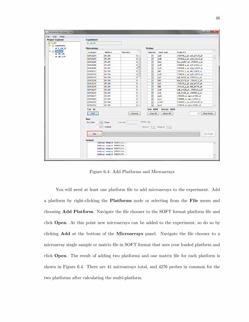
Figure 6.4: Add Platforms and Microarrays

You will need at least one platform file to add microarrays to the experiment. Add

a platform by right-clicking the Platforms node or selecting from the File menu and

choosing Add Platform. Navigate the file chooser to the SOFT format platform file and

click Open. At this point new microarrays can be added to the experiment, so do so by

clicking Add at the bottom of the Microarrays panel. Navigate the file chooser to a

microarray single sample or matrix file in SOFT format that uses your loaded platform and

click Open. The result of adding two platforms and one matrix file for each platform is

shown in Figure 6.4. There are 41 microarrays total, and 4276 probes in common for the

two platforms after calculating the multi-platform.

47

Figure 6.5: Probe Selection

Since 4276 probes is a very large number of total genes, this number can be manually

reduced by checking and unchecking probes in the Selected column of the Probes table on

the right side. The Clear All and Select All buttons below the table can help with this.

Also, probes can be automatically chosen by activity by entering a number in the text field

to the left of the Most Active button and clicking the button. This will automatically

select only the specified number of probes that have the largest expression ranges in the

currently loaded microarrays. The result of choosing 50 probes and calculating the new

probe selection is shown in Figure 6.5.

48

Figure 6.6: Running the Experiment

The experiment is now ready to be run. Click the Run button outlined in red in the

Run panel. A new Banjo Bayesian network learning job will start in the background. The

best network will be searched for the amount of time chosen in the hours and minutes

spinners in the Run panel (default 1 minute). A progress bar will update as the experiment

run continues.

49

Figure 6.7: Graph View

Once the run finishes, the View Graph button on the right side of the progress bar

becomes usable. Click this button and the best network found is converted to dot format

and GraphViz will produce a graph image. This is done automatically, and an image viewer

pops up to show the new graph image. You can pan this image by dragging the left mouse

button and zoom in and out with the mouse wheel.

50

6.3 Conclusion

The MMAT tool should prove useful for running various microarray meta-analysis

experiments and producing gene networks. Although it is only a simple tool now, its

design allows for a great deal of expansion of features, such as extra run options, complete

time series microarray dynamic network support, more probe selection assistance tools, and

more.

CHAPTER 7

CONCLUSION

In this thesis, each goal accomplished led to the next.

First, a method of multi-platform microarray combination was necessary for every-

thing else that followed. An algorithm for combining platforms together into multi-platform

mappings and a normalization calculation that made micorarrays from across experiments

and platforms comparable were developed towards this end.

Once many microarrays could be combined, gene coexpression networks using Bayesian

networks were developed after using a learning algorithm that used each microarray as an

observation, and each gene as a variable. Very large scale graphs were developed using

more microarrays than any other known experiment the current research, along with the

rediscovery of the E. coli SOS gene regulatory pathway as a test.

Building on methods developed and lessons learned from creating gene coexpression

networks, dynamic Bayesian networks from combined time series microarray experiments

was next. This required the development of a novel interpolation and combination algo-

rithm to align multiple time series experiments into comparable observational sets. These

calculated time-based observations were used to build dynamic gene regulatory network

graphs where genes could be modeled a↵ecting each other in time. Once again the E. coli

SOS gene regulatory pathway was modeled, but with a time component.

Now that large-scale gene networks had been produced, the next step was in compar-

ing these graphs using two di↵erent graph comparison algorithms. Both inter-species and

intra-species tests were done that showed how comparable they were.

52

With the entire library of methods and programming work done, a graphical user

interface tool called the Microarray Meta-Analysis Tool (MMAT) was developed to help

other researchers to their own experiments in a user-friendly manner that did not require

any programming or command line skills.

7.1 Future Work

A great deal of future work could be accomplished that would extend all of the subjects

explored in this thesis. The areas of microarray combination with multiple platforms,

modeling Gene Regulatory Networks, combination of time series microarray datasets, and

network comparison could all be explored on their own. There is no shortage of research

paths that could branch o↵ the work done within this thesis.

7.1.1 Microarray Combination

The work described in Chapter 3 dealt with the normalization of many microarrays

so that their values could be directly compared. The method used, scale-normalization, is

one of many possible methods. Also, more work could be done with platform combination

that would tie more probes together with more accuracy.

• The metadataEqualityScore() function given in Algorithm 1 could be extended to

scoring gene location data, free description text, utilizing multiple gene databases to

compare ID’s, DNA nucleotide strings, and others. Many of the platforms have a

great deal of metadata available, and much more could be used to tie one probe from

one platform to another.

• Better handling of gene transcripts. The method used in this thesis does not handle

alternate gene transcripts well. The most common gene products are used to represent

53

a gene, but this means throwing out some extra probes when combining platforms. A

better platform combining algorithm would recognize multiple probes relating to the

same gene and re-label the probe with some kind of transcript ID. This way, alternative

gene transcript probes in common with each other from multiple platforms could be

tied together accurately.

• Some platforms use a single probe to measure multiple products where another plat-

form will use multiple probes for the same task. A better combination algorithm could

tie probes together in a one-to-many manner to take care of this situation. However,

several problems would need to be overcome, such as handling multiple probe values

from one platform being equivalent to a single probe value from another, and probe

measurement overlap. As an example of overlap, probe a from platform A may be

tied to probes x and y from platform B. However, probe b from platform A may

be tied to probes x and z from platform B, so probe x is overlapped. A method to

overcome this overlap would be needed.

• Rather than using metadata, statistics based methods could be used to find equivalent

probes between two microarrays. The idea would be to find large numbers of microar-

rays from two or more di↵erent platforms, and use the statistical data that may be

available from the experiments themselves, and statistics calculated from the values

of the microarray data. The theory is that probe values that behave statistically

similar should be tied together for microarray meta-analysis with multiple platforms.

Some example algorithms that could perform this analysis include, Fisher’s inverse

chi-square [18], GeneMeta [11], metaArray [38] [39], RankProd [5], DEDS [54], and

54

mDEDS [7]. Campain and Yang’s 2010 paper compares all these methods against

each other on several datasets [7].

7.1.2 Gene Regulatory Networks

This thesis work described using static and dynamic Bayesian networks to model

Gene Regulatory Networks, but there are many other models available. Other future work

could also include di↵erent network scoring criteria and learning method, network sparsifi-

cation (since GRN’s are biologically expected to be sparse), post-aggregation of networks,

gene-transcript aware networks, starting from an expert knowledge base network, and gene

clustering.

• Several other models have been used successfully for the modeling of a GRN be-

sides Bayesian networks such as ordinary di↵erential equations (ODE’s), probabilistic

Boolean networks [48], Hybrid Petri nets (HPN’s) [30], and other various hybrid ap-

proaches. One recent hybrid approach, DELDBN, looks to have great promise in

combining the best of ODE’s and dynamic Bayesian network’s [28].

• Other scoring criteria for Bayesian network structures besides the BDe metric used in

this thesis could be used instead. Bayesian Information Criterion (BIC) [47], Akaike

Information Criteria [1], Mutual Information Tests (MIT) [8], K2 [14], and BDeu [6].

• Use a di↵erent, and possibly improved, learning method for Bayesian networks, such

as Annealed Importance Sampling [34].

• Network sparsification could be useful due to the expectation of sparse connection

in a real GRN [26]. A flood-based information flow analysis network sparsification

method has been successfully used on GRN’s very recently [41].

55

• It has been shown that a combination of pre-aggregation of similar microarray datasets

and post-aggregation of networks learned from those datasets can be more accurate

than pre-aggregation alone [51].

• Extending GRN models so that they show the transcriptional regulation of both the

canonical and alternative splicing transcripts of various genes. Either they can be

separate nodes, or edges can be annotated with the particular transcript that caused

the regulation.

• Beginning from an already expert hand-built smaller GRN and building on it through

learning methods may be more fruitful at learning very large and complicated GRN’s

than starting from scratch.

• Clustering of gene in microarrays is a very popular topic in bioinformatics [10] [46],

and could be used to separate genes into functional groups before learning GRN’s.

This would have the benefit of reducing dimensionality of data making it simpler to

learn structure, and have more interpretable results.

7.1.3 Time Series Combination

Combining time series microarray experiments together into a meta-analysis study

for time-aware GRN’s is an extremely cutting edge research topic. In fact, the methods

outlined in this thesis are the only multi-platform multi-time series aggregation methods

known by the author at the time of writing. Much could be done to improve on this work.

• Other interpolation methods could be used, including attempting smoothing on the

B-spline interpolator.

56

• The method taken to combine time series with di↵erent time windows in this thesis

was to truncate to the time series with the smallest time window. Another method

which interpolates points outside of its beginning and end times could be explored to

prevent truncation.

• Although it could be useful for any kind of GRN inference, but discretization of val-

ues is especially important in time series data. Other methods of discretization of

values could be beneficial in combining time series data, and two recent methods

include Information-preserving Discretization (IPD) [22] and Short Series Discretiza-

tion (SSD) [17]. Also, switching to continuous variables in DBN learning could be

beneficial as well [32].

• Time lag estimation for transcriptional regulatory events has been e↵ective in past

research at finding gene regulation outside of any arbitrarily chosen time per Markov

lag in DBN’s [56].

REFERENCES

[1] H. Akaike. On entropy maximization principle. Applications of Statistics, pages 27–41,1977.

[2] Z. Bar-Joseph, G. Gerber, D. Gi↵ord, T. Jaakkola, and I. Simon. Continuous repre-sentations of time-series expression data. Journal of Computational Biology, 10, 2003.

[3] T. Barrett, S. E. Wilhite, P. Ledoux, et al. NCBI GEO: archive for functional genomicsdata sets – update. Nucleic Acids Research, 41:D991–D995, 2013.

[4] M. Benedicte. After 30 Years of Study, the Bacterial SOS Response Still Surprises Us.PLOS Biology, 3:e255, 2005.

[5] R. Breitling, P. Armengaud, A. Amtmann, and P. Herzyk. Rank products: a simple, yetpowerful, new method to detect di↵erentially regulated genes in replicated microarrayexperiments. FEBS Letters, 573:83–92, 2004.

[6] W. Buntine. Theory refinement of Bayesian networks. In Proceedings of the SeventhConference on Uncertainty in Artificial Intelligence, pages 52–60, Los Angeles, CA,1991.

[7] A. Campain and Y. H. Yang. Comparison study of microarray meta-analysis methods.BMC Bioinformatics, 11:408, 2010.

[8] L. Campos. A Scoring Function for Learning Bayesian Networks based on Mutual Infor-mation and Conditional Independence Tests. Journal of Machine Learning Research,7:2149–2187, 2006.

[9] D. M. Chickering. Learning Bayesian networks is NP-complete. AI and STAT, 5:121–130, 1996.

[10] H. Chipman, T. Hastie, and R. Tibshriani. Clustering Microarray Data. Boca Raton,Florida, 2003.

[11] J. Choi, U. Yu, S. Kim, and O. Yoo. Combining multiple microarray studies andmodeling interstudy variation. Bioinformatics, 19:84–90, 2003. Suppl 1.

[12] A. U. Contreras. Deacetylation of p53 induces autophagy by suppressing Bmf expres-sion. Journal of Cell Biology, 201:427–437, 2013.

[13] S. A. Cook. The complexity of theorem-proving procedures. Proceedings of the 3rdACM Symposium on Theory of Computing, pages 151–158, 1971.

[14] G. F. Cooper and E. Herskovits. A Bayesian method for the induction of probabilisticnetworks from data. Machine Learning, 9:309–348, 1992.

[15] C. de Boor. On calculating with B-splines. Journal of Approximation Theory, 6:50–62,1972.

58

[16] J. Demeter, C. Beauheim, J. Gollub, et al. The Stanford Microarray Database: im-plementation of new analysis tools and open source release of software. Nucleic AcidsResearch, 35:D766–D770, 2007.

[17] E. Dimitrova, M. Licona, and R. Laubenbacher. Discretization of Time Series Data.Journal of Computational Biology, 17:853–868, 2010.

[18] R. Fisher. Statistical methods for research workers, volume 11. Oliver and Boyd,Edinburgh, 1950.

[19] N. Friedman, M. Linial, I. Nachman, and D. Pe’er. Using Bayesian Networks to AnalyzeExpression Data. Journal of Computation Biology, 7, 2000.

[20] A. Hartemink. Principled Computational Methods for the Validation and Discovery ofGenetic Regulatory Networks. PhD thesis, Massachusetts Institute Of Technology, Sep2001.

[21] A. Hartemink. Bayesian Networks and Informative Priors: Transcriptional RegulatoryNetwork Models. Bayesian Inference for Gene Expression and Proteomics, pages 401–424, 2006.

[22] A. Hartemink, D. Gi↵ord, T. Jaakkola, and R. Young. Bayesian Methods for Elu-cidating Genetic Regulatory Networks. IEEE Intelligent Systems, Special Issue onIntelligent Systems in Biology, 17, 2002.

[23] D. Heckerman, D. Geiger, and D. Chickering. Learning Bayesian networks: The com-bination of knowledge and statistical data. Machine Learning, 20:197–243, 1995.

[24] D. Husmeier. Studying the conditions for learning dynamic Bayesian networks todiscover genetic regulatory networks. Bioinformatics, 19:2271–2282, 2003.

[25] M. Koyuturk, A. Grama, and W. Szpankowski. An e�cient algorithm for detectingfrequent subgraphs in biological networks. Bioinformatics, 20:i200–i207, 2004.

[26] R. Leclerc. Survival of the sparsest: robust gene networks are parsimonious. MolecularSystems Biology, 4:213, 2008.

[27] H. Lee, A. Hsu, J. Sajdak, et al. Coexpression Analysis of Human Genes Across ManyMicroarray Data Sets. Genome Research, 2004.

[28] Z. Li, P. Li, A. Krishnan, and J. Liu. Large-scale dynamic gene regulatory networkinference combining di↵erential equation models with local dynamic Bayesian networkanalysis. Bioinformatics, 27:2686–2691, 2011.

[29] B. Malone, C. Yuan, and E. Hansen. Memory-E�cient Dynamic Programming forLearning Optimal Bayesian Networks. Association for the Advancement of ArtificialIntelligence, 2011.

[30] H. Matsuno and A. Doi. Hybrid Petri Net Representation of Gene Regulatory Network.Pacific Symposium on Biocomputing, 5:338–349, 2000.

[31] H. H. McAdams and A. Arkin. Stochastic mechanisms in gene expression. Proceedingsof the National Academy of Science, 94:814–819, 1997.

59

[32] K. Murphy and S. Mian. Modeling gene expression data using dynamic Bayesian net-works. Technical report, Computer Science Division, University of California, Berkeley,CA, 1999.

[33] C. J. Needham, J. R. Bradford, A. J. Bulpitt, et al. A Primer on Learning in BayesianNetworks for Computational Biology. PLOS Computional Biology, 3:e129, 2007.

[34] T. Niinimaki and M. Koivisto. Annealed importance sampling for structure learningin Bayesian networks. IJCAI, 2013.

[35] S. L. Normand. Meta-analysis: formulating, evaluating, combining, and reporting.Statistics in Medicine, 18:321–359, 1999.

[36] D. Park and X. Wang. Toward a general framework for microarray data comparison.Proceedings of the 6th IEEE International Conference on Computer and InformationTechnology, page 212, 2006.

[37] H. Parkinson, U. Sarkans, N. Kolesnikov, et al. ArrayExpress update–an archive ofmicroarray and high-throughput sequencing-based functional genomics experiments.Nucleic Acids Research, 39:D1002–D1004, 2011.

[38] G. Parmigiani, E. S. Garrett, R. Anbazhagan, and E. Gabrielson. A statistical frame-work for expression-based molecular classification in cancer. Journal of the RoyalStatistical Society: Series B Statistics Methodology, 64:717–736, 2002.

[39] G. Parmigiani, E. S. Garrett, R. Anbazhagan, and E. Gabrielson. A cross-study com-parison of gene expression studies for the molecular classification of lung cancer. ClinicalCancer Research, 10:2922–2927, 2004.

[40] J. Paulsson. Models of stochastic gene expression. Physics of Life Reviews, 2:157–175,2005.

[41] A. Pavlogiannis, V. Mozhayskiy, and I. Tagkopoulos. A flood-based information flowanalysis and network minimization method for gene regulatory networks. BMC Bioin-formatics, 14:137, 2013.

[42] D. Peer, A. Regev, G. Elidan, and N. Friedman. Inferring subnetworks from perturbedexpression profiles. Bioinformatics, 1:1–9, 2001.

[43] M. Pertea and S. Salzberg. Between a chicken and a grape: estimating the number ofhuman genes. Genome Biology, page 206, 2010.

[44] N. Przulj. Biological Network Comparison Using Graphlet Degree Distribution. Bioin-formatics, 23:e177–e183, 2007.

[45] D. Rogers and J. Adams. Mathematical Elements for Computer Graphics. McGraw-Hill, 1989.

[46] S. Roy, D. K. Bhattacharyya, and J. K. Kalita. CoBi:Pattern Based Co-RegulatedBiclustering of Gene Expression Data. Pattern Recognition Letters, 2013.

[47] G. Schwarz. Estimating the dimension of a model. Annals of Statistics, 6:461–464,1978.

60

[48] I. Shmulevich, E. Dougherty, S. Kim, and W. Zhang. Probabilistic Boolean networks:a rule-based uncertainty model for gene regulatory networks. Bioinformatics, 18:261–274, 2002.

[49] A. Smith. Classification and Alignment of Gene-Expression Time-Series Data. PhDthesis, University of Wisconsin-Madison, 2009.

[50] G. Smyth and T. Speed. Normalization of cDNA microarray data. Methods, 31:265–273, 2003.

[51] E. Steele and A. Tucker. Consensus and Meta-analysis regulatory networks for combin-ing multiple microarray gene expression datasets. Journal of Biomedical Informatics,41:914–926, 2007.

[52] G. Tseng, D. Ghosh, and E. Feingold. Comprehensive literature review and statisticalconsiderations for microarray meta-analysis. Nucleic Acids Research, 40:3785–3799,2012.

[53] R. J. van Berlo, E. P. van Someren, and M. J. Reinders. Studying the conditions forlearning dynamic Bayesian networks to discover genetic regulatory networks. Simula-tion, 79:12, 2003.

[54] Y. H. Yang, Y. Xiao, and M. R. Segal. Identifying di↵erentially expressed genes frommicroarray experiments via statistic synthesis. Bioinformatics, 21:1084–1093, 2005.

[55] D. Zak, G. E. Gonye, J. S. Schwaber, and F. J. Doyle. Importance of input pertur-bations and stochastic gene expression in the reverse engineering of genetic regulatorynetworks: insights from an identifiability analysis of an in silico network. GenomeResearch, page 2396–2405, 2003.

[56] M. Zou and S. Conzen. A new dynamic Bayesian network (DBN) approach for iden-tifying gene regulatory networks from time course microarray data. Bioinformatics,21:71–79, 2004.

Appendix A

SOFTWARE PACKAGES AND VERSIONS

• Banjo 2.1.0 – http://www.cs.duke.edu/

~

amink/software/banjo/

• GraphViz 2.2.2 – http://www.graphviz.org/

• Java SE Development Kit 7 – http://www.oracle.com/technetwork/java/javase/downloads/jdk7-downloads-1880260.html

• The Apache Commons Mathematics Library 3.2 – http://commons.apache.org/

proper/commons-math/

• The Apache Commons I/O Library 2.4 – http://commons.apache.org/proper/

commons-io/

• The Apache Commons Exec Library 1.1 – http://commons.apache.org/proper/

commons-exec/

• SwingX 1.6.5 – http://weblogs.java.net/blog/kschaefe/archive/2013/01/29/

swingx-165-released/

Appendix B

ALL SUB-GRAPHS

Figure B.1: All Sub-Graphs

gene co-expression networks across many microarrays

Documents