gene prediction - univerzita karlovamraz/bioinf/bioalg10-9.pdf · 2011-01-04 · an introduction to...

www.bioalgorithms.infoAn Introduction to Bioinformatics Algorithms

Gene Prediction

Bioinformatics Algorithms

• Gene: A sequence of nucleotides coding for protein• Gene Prediction Problem: Determine the beginning and end

positions of genes in a genome

• atgcatgcggctatgctaatgcatgcggctatgctaagctgggatccgatgacaatgcatgcggctatgctaatgcatgcggctatgcaagctgggatccgatgactatgctaagctgggatccgatgacaatgcatgcggctatgctaatgaatggtcttgggatttaccttggaatgctaagctgggatccgatgacaatgcatgcggctatgctaatgaatggtcttgggatttaccttggaatatgctaatgcatgcggctatgctaagctgggatccgatgacaatgcatgcggctatgctaatgcatgcggctatgcaagctgggatccgatgactatgctaagctgcggctatgctaatgcatgcggctatgctaagctgggatccgatgacaatgcatgcggctatgctaatgcatgcggctatgcaagctgggatcctgcggctatgctaatgaatggtcttgggatttaccttggaatgctaagctgggatccgatgacaatgcatgcggctatgctaatgaatggtcttgggatttaccttggaatatgctaatgcatgcggctatgctaagctgggaatgcatgcggctatgctaagctgggatccgatgacaatgcatgcggctatgctaatgcatgcggctatgcaagctgggatccgatgactatgctaagctgcggctatgctaatgcatgcggctatgctaagctcatgcggctatgctaagctgggaatgcatgcggctatgctaagctgggatccgatgacaatgcatgcggctatgctaatgcatgcggctatgcaagctgggatccgatgactatgctaagctgcggctatgctaatgcatgcggctatgctaagctcggctatgctaatgaatggtcttgggatttaccttggaatgctaagctgggatccgatgacaatgcatgcggctatgctaatgaatggtcttgggatttaccttggaatatgctaatgcatgcggctatgctaagctgggaatgcatgcggctatgctaagctgggatccgatgacaatgcatgcggctatgctaatgcatgcggctatgcaagctgggatccgatgactatgctaagctgcggctatgctaatgcatgcggctatgctaagct

Introduction


• Gene: A sequence of nucleotides coding for protein• Gene Prediction Problem: Determine the beginning and end

positions of genes in a genome

• atgcatgcggctatgctaatgcatgcggctatgctaagctgggatccgatgacaatgcatgcggctatgctaatgcatgcggctatgcaagctgggatccgatgactatgctaagctgggatccgatgacaatgcatgcggctatgctaatgaatggtcttgggatttaccttggaatgctaagctgggatccgatgacaatgcatgcggctatgctaatgaatggtcttgggatttaccttggaatatgctaatgcatgcggctatgctaagctgggatccgatgacaatgcatgcggctatgctaatgcatgcggctatgcaagctgggatccgatgactatgctaagctgcggctatgctaatgcatgcggctatgctaagctgggatccgatgacaatgcatgcggctatgctaatgcatgcggctatgcaagctgggatcctgcggctatgctaatgaatggtcttgggatttaccttggaatgctaagctgggatccgatgacaatgcatgcggctatgctaatgaatggtcttgggatttaccttggaatatgctaatgcatgcggctatgctaagctgggaatgcatgcggctatgctaagctgggatccgatgacaatgcatgcggctatgctaatgcatgcggctatgcaagctgggatccgatgactatgctaagctgcggctatgctaatgcatgcggctatgctaagctcatgcggctatgctaagctgggaatgcatgcggctatgctaagctgggatccgatgacaatgcatgcggctatgctaatgcatgcggctatgcaagctgggatccgatgactatgctaagctgcggctatgctaatgcatgcggctatgctaagctcggctatgctaatgaatggtcttgggatttaccttggaatgctaagctgggatccgatgacaatgcatgcggctatgctaatgaatggtcttgggatttaccttggaatatgctaatgcatgcggctatgctaagctgggaatgcatgcggctatgctaagctgggatccgatgacaatgcatgcggctatgctaatgcatgcggctatgcaagctgggatccgatgactatgctaagctgcggctatgctaatgcatgcggctatgctaagct

Gene!

Introduction


• In 1960’s it was discovered that the sequence of codons in a gene determines the sequence of amino acids in a protein

an incorrect assumption: the triplets encoding for amino acid sequences form contiguous strips of information.

• A paradox: genome size of many eukaryotes does not correspond to “genetic complexity”, for example, the salamander genome is 10 times the size of that of human.

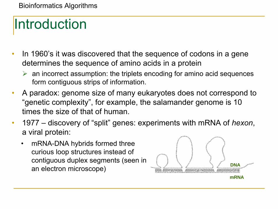
• 1977 – discovery of “split” genes: experiments with mRNA of hexon, a viral protein:

Introduction

• mRNA-DNA hybrids formed three curious loop structures instead of contiguous duplex segments (seen in an electron microscope) DNA

mRNA


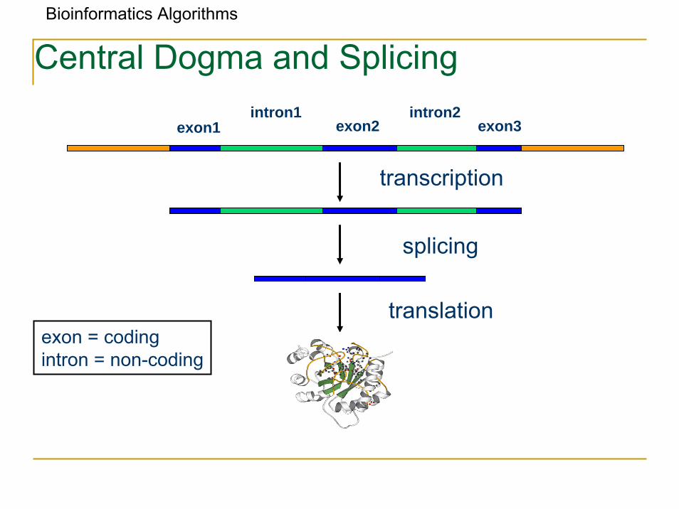
Central Dogma and Splicing

exon1 exon2 exon3intron1 intron2

transcription

translation

splicing

exon = codingintron = non-coding


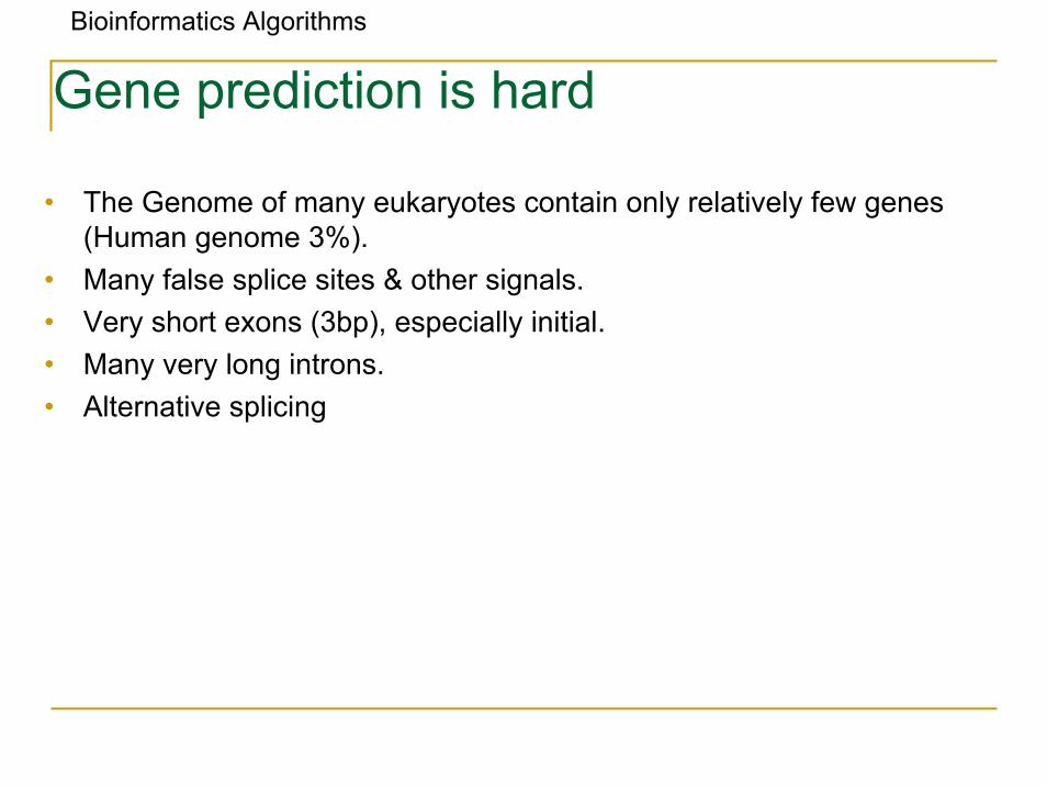
• The Genome of many eukaryotes contain only relatively few genes (Human genome 3%).

• Many false splice sites & other signals.• Very short exons (3bp), especially initial.• Many very long introns.• Alternative splicing

Gene prediction is hard


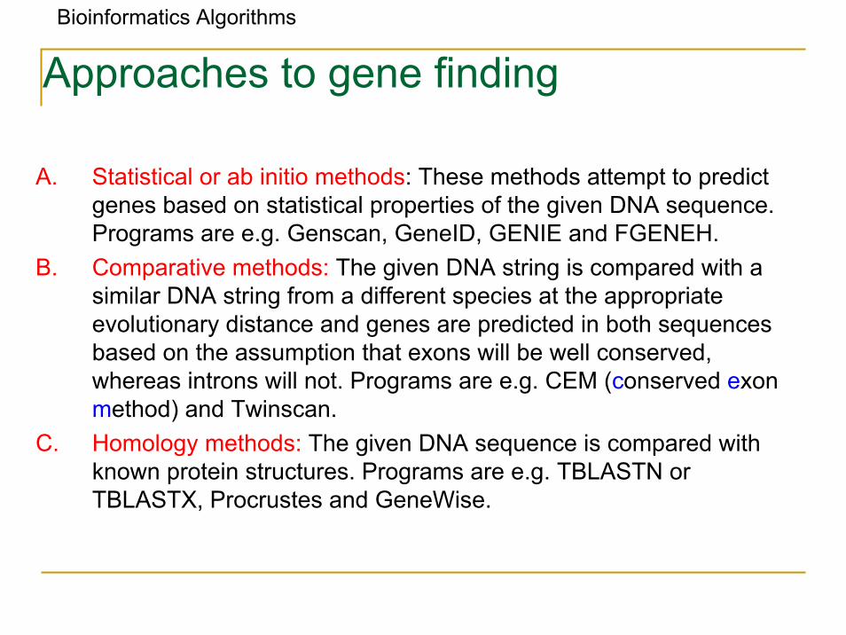
A. Statistical or ab initio methods: These methods attempt to predict genes based on statistical properties of the given DNA sequence.Programs are e.g. Genscan, GeneID, GENIE and FGENEH.

B. Comparative methods: The given DNA string is compared with a similar DNA string from a different species at the appropriate evolutionary distance and genes are predicted in both sequences based on the assumption that exons will be well conserved, whereas introns will not. Programs are e.g. CEM (conserved exonmethod) and Twinscan.

C. Homology methods: The given DNA sequence is compared with known protein structures. Programs are e.g. TBLASTN or TBLASTX, Procrustes and GeneWise.

Approaches to gene finding


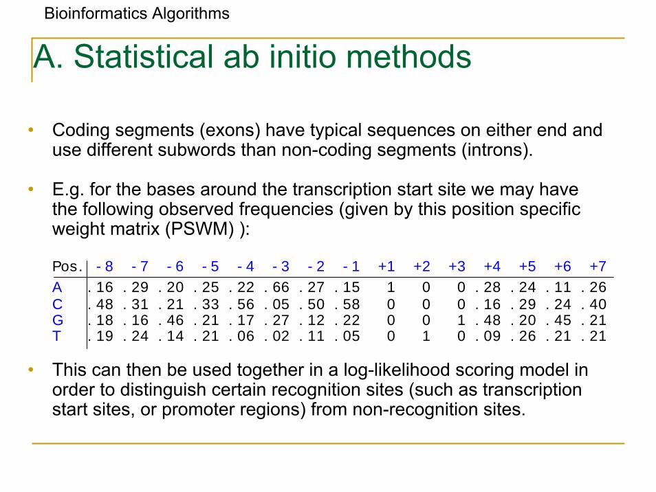
• Coding segments (exons) have typical sequences on either end anduse different subwords than non-coding segments (introns).

• E.g. for the bases around the transcription start site we may have the following observed frequencies (given by this position specific weight matrix (PSWM) ):

Pos. -8 -7 -6 -5 -4 -3 -2 -1 +1 +2 +3 +4 +5 +6 +7

A .16 .29 .20 .25 .22 .66 .27 .15 1 0 0 .28 .24 .11 .26C .48 .31 .21 .33 .56 .05 .50 .58 0 0 0 .16 .29 .24 .40G .18 .16 .46 .21 .17 .27 .12 .22 0 0 1 .48 .20 .45 .21T .19 .24 .14 .21 .06 .02 .11 .05 0 1 0 .09 .26 .21 .21

• This can then be used together in a log-likelihood scoring model in order to distinguish certain recognition sites (such as transcription start sites, or promoter regions) from non-recognition sites.

A. Statistical ab initio methods


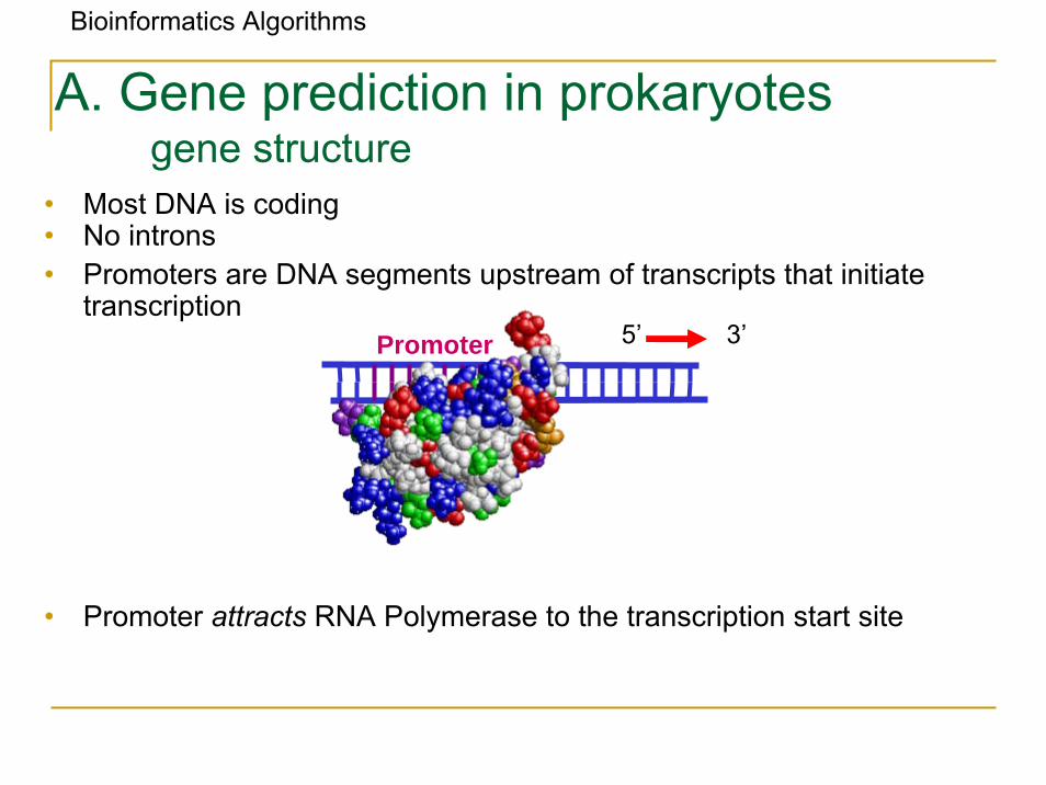
• Most DNA is coding • No introns• Promoters are DNA segments upstream of transcripts that initiate

transcription

• Promoter attracts RNA Polymerase to the transcription start site

A. Gene prediction in prokaryotesgene structure

5’Promoter 3’

http://www.biochemistry.bham.ac.uk/sjwb/alpharot.gif


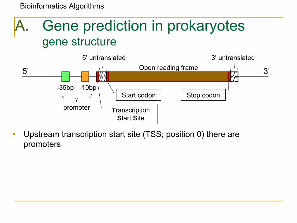
• Upstream transcription start site (TSS; position 0) there are promoters

A. Gene prediction in prokaryotesgene structure

5’ 3’

5’ untranslated 3’ untranslatedOpen reading frame

-35bp -10bp

promoter

Start codon

Transcription Start Site

Stop codon


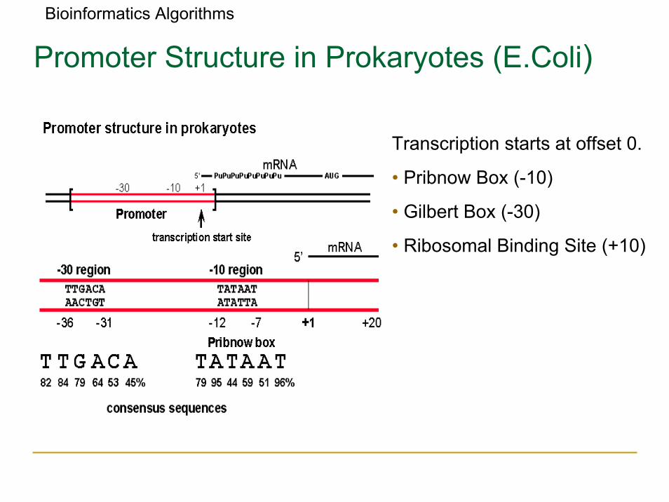
Promoter Structure in Prokaryotes (E.Coli)

Transcription starts at offset 0.

• Pribnow Box (-10)

• Gilbert Box (-30)

• Ribosomal Binding Site (+10)


• Detect potential coding regions by looking at ORFs– A genome of length n is comprised of (n/3) codons– Stop codons (TAA, TAG or TGA) break genome into segments

between consecutive Stop codons– The subsegments of these that start from the Start codon (ATG) are

ORFs• ORFs in different frames may overlap

Genomic Sequence

Open reading frame

ATG TGA

Open Reading Frames (ORFs)


Six Frames in a DNA Sequence

• stop codons – TAA, TAG, TGA

• start codons – ATG

GACGTCTGCTTTGGAGAACTACATCAACCGGACTGTGGCTGTTATTACTTCTGATGGCAGAATGATTGTG

CTGCAGACGAAACCTCTTGATGTAGTTGGCCTGACACCGACAATAATGAAGACTACCGTCTTACTAACAC

GACGTCTGCTTTGGAGAACTACATCAACCGGACTGTGGCTGTTATTACTTCTGATGGCAGAATGATTGTGGACGTCTGCTTTGGAGAACTACATCAACCGGACTGTGGCTGTTATTACTTCTGATGGCAGAATGATTGTGGACGTCTGCTTTGGAGAACTACATCAACCGGACTGTGGCTGTTATTACTTCTGATGGCAGAATGATTGTG

CTGCAGACGAAACCTCTTGATGTAGTTGGCCTGACACCGACAATAATGAAGACTACCGTCTTACTAACACCTGCAGACGAAACCTCTTGATGTAGTTGGCCTGACACCGACAATAATGAAGACTACCGTCTTACTAACACCTGCAGACGAAACCTCTTGATGTAGTTGGCCTGACACCGACAATAATGAAGACTACCGTCTTACTAACAC


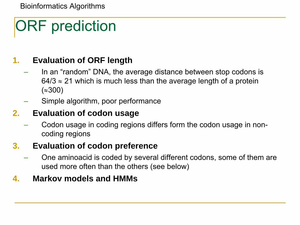
1. Evaluation of ORF length– In an “random” DNA, the average distance between stop codons is

64/3 ≈ 21 which is much less than the average length of a protein (≈300)

– Simple algorithm, poor performance2. Evaluation of codon usage

– Codon usage in coding regions differs form the codon usage in non-coding regions

3. Evaluation of codon preference– One aminoacid is coded by several different codons, some of them are

used more often than the others (see below)4. Markov models and HMMs

ORF prediction


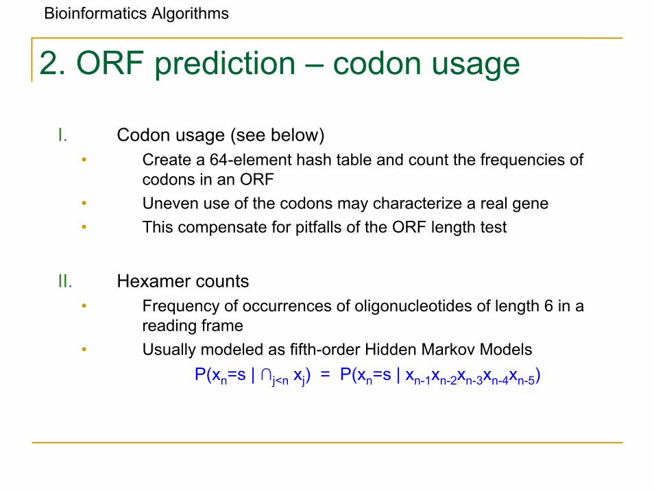
2. ORF prediction – codon usage

I. Codon usage (see below)• Create a 64-element hash table and count the frequencies of

codons in an ORF• Uneven use of the codons may characterize a real gene• This compensate for pitfalls of the ORF length test

II. Hexamer counts • Frequency of occurrences of oligonucleotides of length 6 in a

reading frame• Usually modeled as fifth-order Hidden Markov Models

P(xn=s | ∩j<n xj) = P(xn=s | xn-1xn-2xn-3xn-4xn-5)


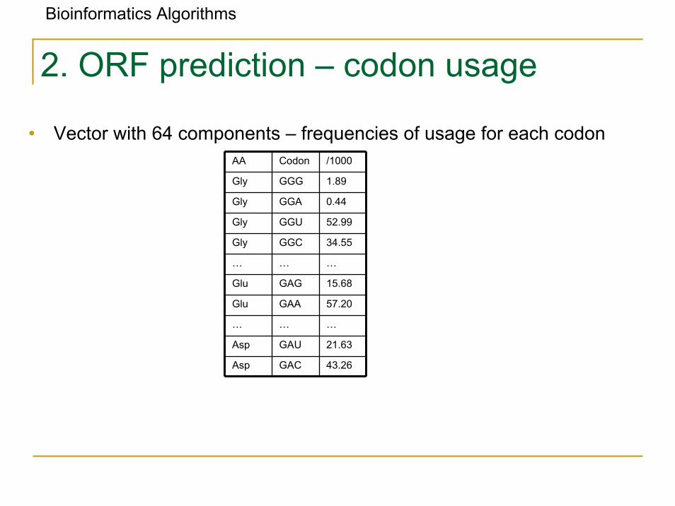
• Vector with 64 components – frequencies of usage for each codon

2. ORF prediction – codon usage

AA Codon /1000

Gly GGG 1.89

Gly GGA 0.44

Gly GGU 52.99

Gly GGC 34.55

… … …

Glu GAG 15.68

Glu GAA 57.20

… … …

Asp GAU 21.63

Asp GAC 43.26


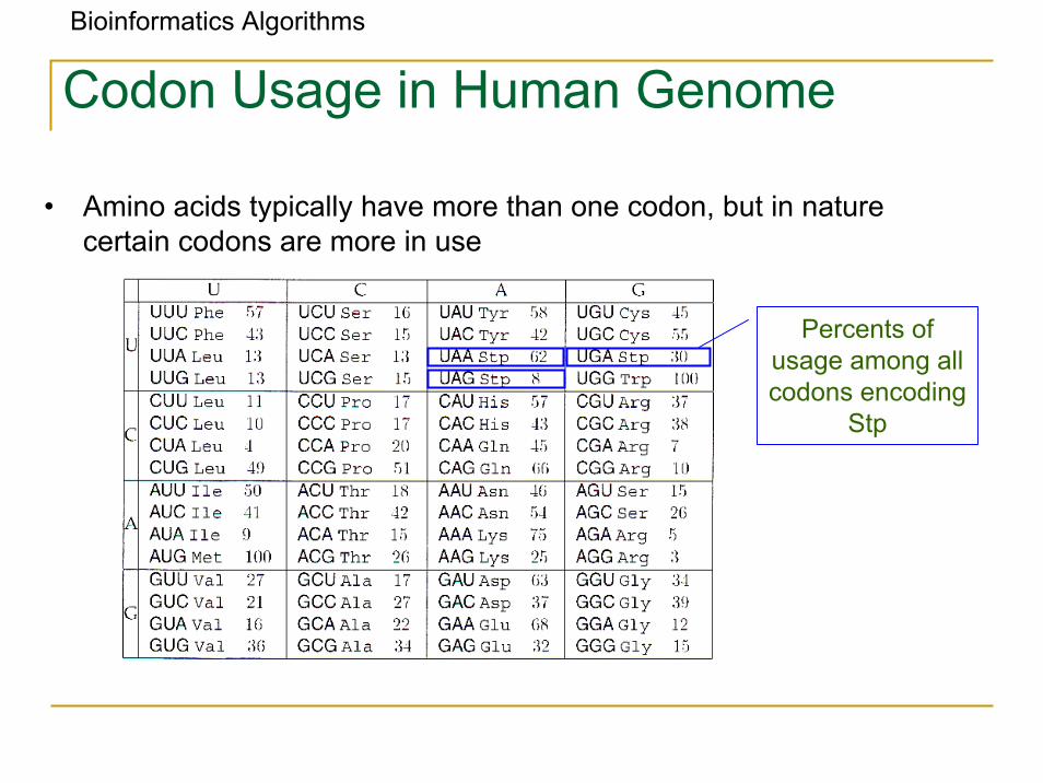
Codon Usage in Human Genome

• Amino acids typically have more than one codon, but in nature certain codons are more in use

Percents ofusage among allcodons encoding

Stp


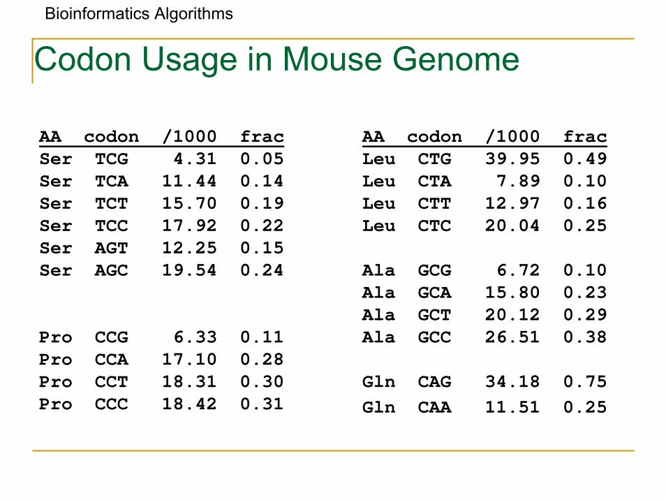
AA codon /1000 fracSer TCG 4.31 0.05Ser TCA 11.44 0.14Ser TCT 15.70 0.19Ser TCC 17.92 0.22Ser AGT 12.25 0.15Ser AGC 19.54 0.24

Pro CCG 6.33 0.11Pro CCA 17.10 0.28Pro CCT 18.31 0.30Pro CCC 18.42 0.31

AA codon /1000 fracLeu CTG 39.95 0.49Leu CTA 7.89 0.10Leu CTT 12.97 0.16Leu CTC 20.04 0.25

Ala GCG 6.72 0.10Ala GCA 15.80 0.23Ala GCT 20.12 0.29Ala GCC 26.51 0.38

Gln CAG 34.18 0.75Gln CAA 11.51 0.25

Codon Usage in Mouse Genome


• For each reading frame a codon preference statistics at each position is computed. The statistic is calculated over a window of length lw (lw is usually between 25 and 50), where the window is moved along the sequence in increments of three bases, maintaining the reading frame. The magnitude of the codon preference statistic is a measure of the likeness of a particular window of codons to a predetermined preferred usage.

• The statistic is based on the concept of synonymous codons. Synonymous codons are those codons specifying the same amino acid.

3. ORF prediction – codon preference


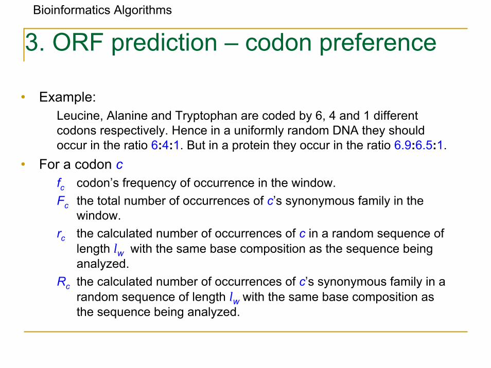
• Example:Leucine, Alanine and Tryptophan are coded by 6, 4 and 1 different codons respectively. Hence in a uniformly random DNA they shouldoccur in the ratio 6:4:1. But in a protein they occur in the ratio 6.9:6.5:1.

• For a codon cfc codon’s frequency of occurrence in the window.Fc the total number of occurrences of c’s synonymous family in the

window.rc the calculated number of occurrences of c in a random sequence of

length lw with the same base composition as the sequence being analyzed.

Rc the calculated number of occurrences of c’s synonymous family in a random sequence of length lw with the same base composition as the sequence being analyzed.



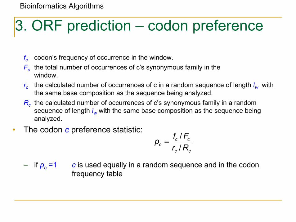
fc codon’s frequency of occurrence in the window.Fc the total number of occurrences of c’s synonymous family in the

window.rc the calculated number of occurrences of c in a random sequence of length lw with

the same base composition as the sequence being analyzed.Rc the calculated number of occurrences of c’s synonymous family in a random

sequence of length lw with the same base composition as the sequence being analyzed.

• The codon c preference statistic:

– if pc =1 c is used equally in a random sequence and in the codon frequency table


cc

ccc Rr

Ffp//

=


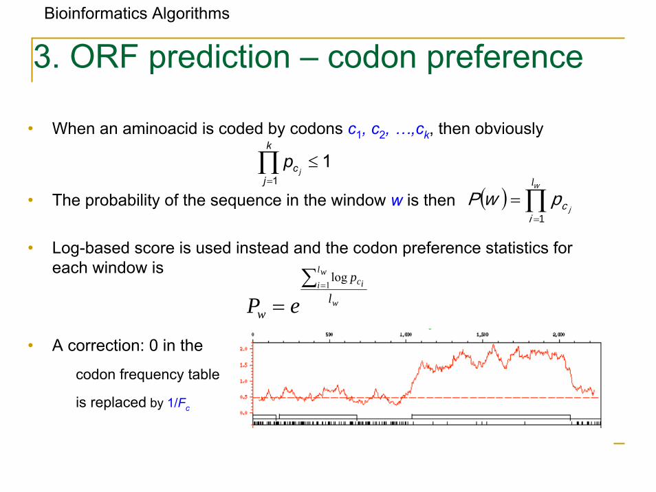
• When an aminoacid is coded by codons c1, c2, …,ck, then obviously

• The probability of the sequence in the window w is then

• Log-based score is used instead and the codon preference statistics for each window is

• A correction: 0 in the

codon frequency table

is replaced by 1/Fc

11

≤∏=

k

jc j

p

( ) ∏=

=w

ji

cpwPl

1


w

wl

i ic

l

p

w eP∑

==1log


4. ORF prediction – using Markov models and HMM

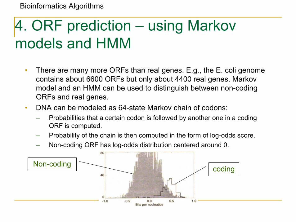
• There are many more ORFs than real genes. E.g., the E. coli genome contains about 6600 ORFs but only about 4400 real genes. Markov model and an HMM can be used to distinguish between non-coding ORFs and real genes.

• DNA can be modeled as 64-state Markov chain of codons:– Probabilities that a certain codon is followed by another one in a coding

ORF is computed.– Probability of the chain is then computed in the form of log-odds score.– Non-coding ORF has log-odds distribution centered around 0.

Non-codingcoding


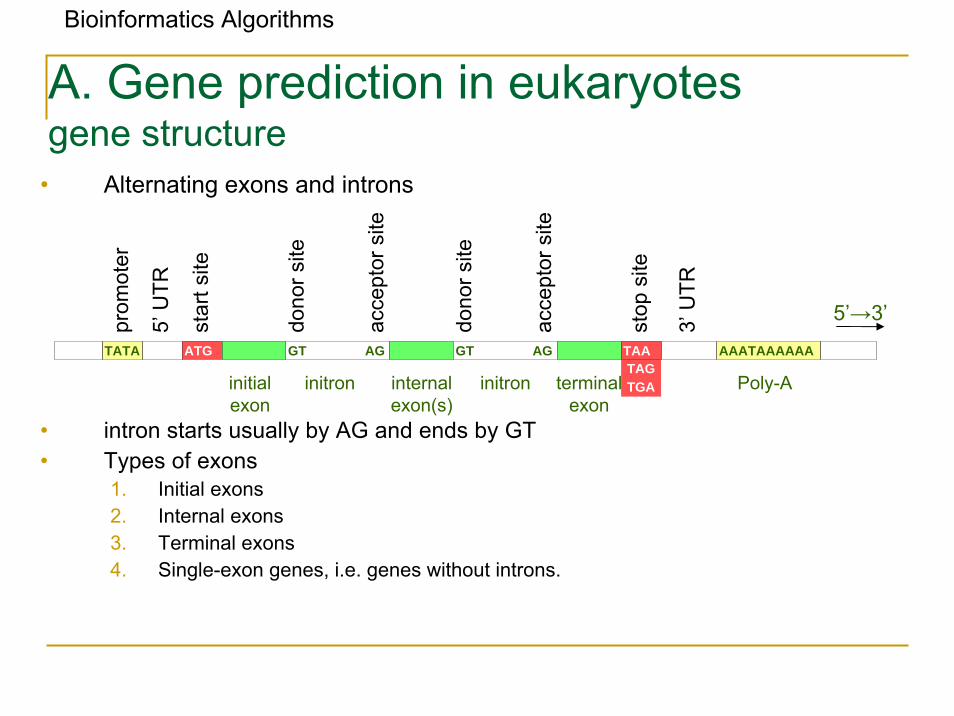
• Alternating exons and introns

• intron starts usually by AG and ends by GT• Types of exons

1. Initial exons2. Internal exons3. Terminal exons4. Single-exon genes, i.e. genes without introns.

A. Gene prediction in eukaryotesgene structure

TATA ATG GT AG GT AG AAATAAAAAA

prom

oter

5’U

TR

star

t site

dono

r site

initial exon

dono

r site

acce

ptor

site

acce

ptor

site

internal exon(s)

terminal exon

stop

site

3’U

TR

5’→3’

initron initronTAGTGA Poly-A

TAA


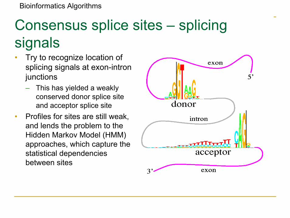
Consensus splice sites – splicingsignals• Try to recognize location of

splicing signals at exon-intronjunctions– This has yielded a weakly

conserved donor splice site and acceptor splice site

• Profiles for sites are still weak, and lends the problem to the Hidden Markov Model (HMM) approaches, which capture the statistical dependencies between sites


Splice site detection

5’ 3’Donor site

Position% -8 … -2 -1 0 1 2 … 17A 26 … 60 9 0 1 54 … 21C 26 … 15 5 0 1 2 … 27G 25 … 12 78 99 0 41 … 27T 23 … 13 8 1 98 3 … 25

• In the exon-intron junctions there is a large similarity to the consensus sequence → algorithms based on position specific weight matrices.

• However, this is far too simple, since it does not use all the information encoded in a gene. Thus more integrated approaches are sought. This naturally leads us to Hidden Markov Models.


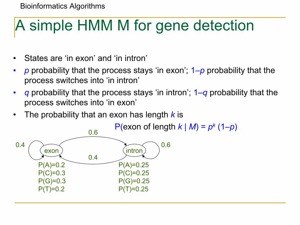
A simple HMM M for gene detection

• States are ‘in exon’ and ‘in intron’• p probability that the process stays ‘in exon’; 1–p probability that the

process switches into ‘in intron’• q probability that the process stays ‘in intron’; 1–q probability that the

process switches into ‘in exon’• The probability that an exon has length k is

P(exon of length k | M) = pk (1–p)

exon intron0.4 0.6

0.6

0.4P(A)=0.2P(C)=0.3P(G)=0.3P(T)=0.2

P(A)=0.25P(C)=0.25 P(G)=0.25 P(T)=0.25



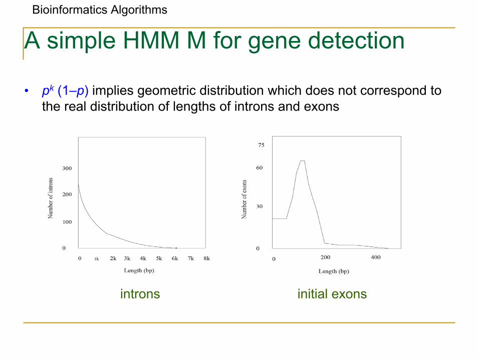
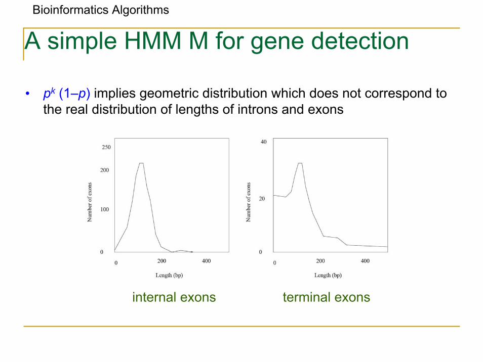
• pk (1–p) implies geometric distribution which does not correspond to the real distribution of lengths of introns and exons

introns initial exons



• pk (1–p) implies geometric distribution which does not correspond to the real distribution of lengths of introns and exons

internal exons terminal exons



• If an exon is too short (under 50bp), the spliceosome (enzyme that performs the splicing) has not enough room.

• Exons that are longer than 300 bp are difficult to locate. • Typical numbers for vertebrates:

• mean gene length ≈ 30kb, • mean coding region length ≈ 1−2kb.

• we need other models that can model biological exon lengths


Ribosomal Binding Site


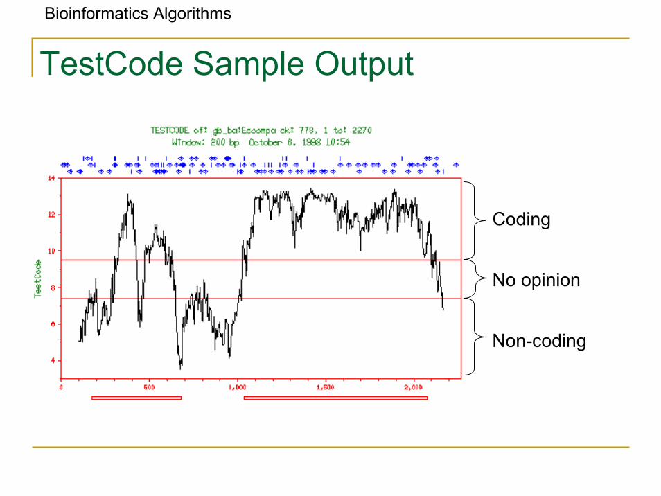
TestCode

• Statistical test described by James Fickett in 1982: tendency for nucleotides in coding regions to be repeated with periodicity of 3– Judges randomness instead of codon frequency.– Finds “putative” coding regions, not introns, exons, or splice sites.

• TestCode finds ORFs based on compositional bias with a periodicity of three.


TestCode Statistics

• Define a window size no less than 200 bp, slide the window along the sequence down 3 bases. In each window:– Calculate for each base {A, T, G, C}

• max (n3k+1, n3k+2, n3k) / min ( n3k+1, n3k+2, n3k)

• Use these values to obtain a probability from a lookup table (which was a previously defined and determined experimentally with known coding and noncoding sequences

• Probabilities can be classified as indicative of " coding” or “noncoding” regions, or “no opinion” when it is unclear what level of randomization tolerance a sequence carries

• The resulting sequence of probabilities can be plotted


TestCode Sample Output

Coding

No opinion

Non-coding


Popular Gene Prediction Algorithms

• GENSCAN: uses modified Hidden Markov Models (HMMs) –semi-Markov model – based on statistical methods and on data from an annotated training set

• TWINSCAN – Uses both HMM and similarity (e.g., between human and

mouse genomes)


B. Comparative gene finding• Idea: the level of sequence conservation between two species

depends on the function of the DNA, e.g. coding sequence is moreconserved than intergenic sequence.

• Program Rosetta:– first computes a global alignment of two homologous sequences– and then attempts to predict genes in both sequences simultaneously.

• A conserved exon method: that uses local conservation.• Orthologous Genes: homologous genes in two species that have a

common ancestor.


Using Known Genes to Predict New Genes

• Some genomes may be very well-studied, with many genes having been experimentally verified.

• Closely-related organisms may have similar genes.• Unknown genes in one species may be compared to genes in some

closely-related species.• Most human genes have mouse orthologs:

– 95% of coding exons are in a one-to-one correspondence between the two genomes.

– 75% of orthologous coding exons have equal length, and – 95% have equal length modulo 3. – Intron lengths differ by an average of 50%. – The coding sequence similarity between the two organisms is around 85%,– the intron sequence similarity is around 35%, – 5’ UTRs and 3’ UTRs around 68%.


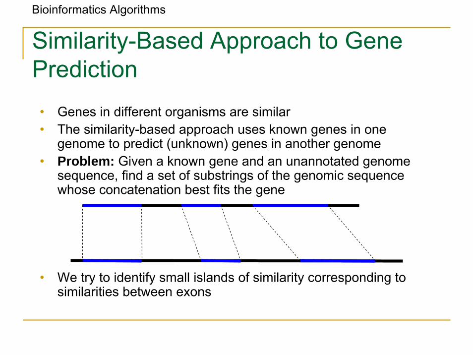
Similarity-Based Approach to Gene Prediction

• Genes in different organisms are similar• The similarity-based approach uses known genes in one

genome to predict (unknown) genes in another genome• Problem: Given a known gene and an unannotated genome

sequence, find a set of substrings of the genomic sequence whose concatenation best fits the gene

• We try to identify small islands of similarity corresponding to similarities between exons


Reverse Translation

• Given a known protein, find a gene in the genome which codes for it.• One might infer the coding DNA of the given protein by reversing the

translation process– Inexact: amino acids map to > 1 codon.– This problem is essentially reduced to an alignment problem.

• This reverse translation problem can be modeled as traveling in Manhattan grid with free horizontal jumps– Complexity of Manhattan is n3

• Every horizontal jump models an insertion of an intron• Problem with this approach: would match nucleotides pointwise and

use horizontal jumps at every opportunity


Comparing Genomic DNA Against mRNA

Portion of genome

mRN

A

(codon sequence)

exon3exon1 exon2intron1 intron2


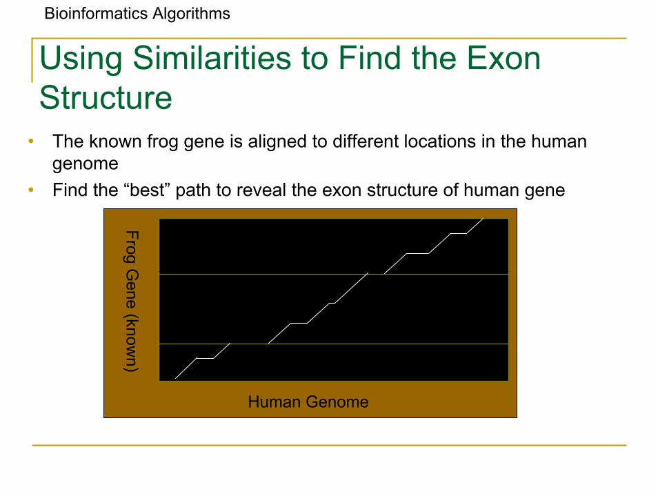
Using Similarities to Find the ExonStructure

• The known frog gene is aligned to different locations in the human genome

• Find the “best” path to reveal the exon structure of human gene

Frog Gene (know

n)

Human Genome


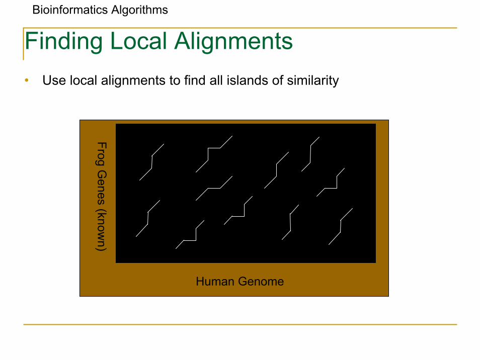
Finding Local Alignments• Use local alignments to find all islands of similarity

Human Genome

Frog Genes (know

n)


Chaining Local Alignments

• Find substrings that match a given gene sequence (candidate exons)

• Define a candidate exons as (l, r, w)

(left, right, weight defined as score of local alignment)• Look for a maximum chain of substrings

– Chain: a set of non-overlapping nonadjacent intervals.


Exon Chaining Problem

• Locate the beginning and end of each interval (2n points)• Find the “best” path

34

119

155

5

0 2 3 5 6 11 13 16 20 25 27 28 30 32


Exon Chaining Problem: Formulation

• Exon Chaining Problem: Given a set of putative exons, find a maximum set of non-overlapping putative exons.

• Input: a set of weighted intervals (putative exons).

• Output: A maximum chain of intervals from this set.


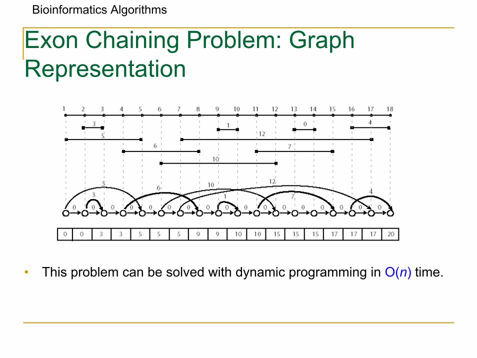
Exon Chaining Problem: Graph Representation

• This problem can be solved with dynamic programming in O(n) time.


Exon Chaining Algorithm

ExonChaining (G, n ) //Graph, number of intervalsfor i ← to 2n

si ← 0for i ← 1 to 2n

if vertex vi in G corresponds to right end of the interval Ij ← index of vertex for the left end of the interval Iw ← weight of the interval Isj ← max {sj + w, si -1}

elsesi ← si-1

return s2n


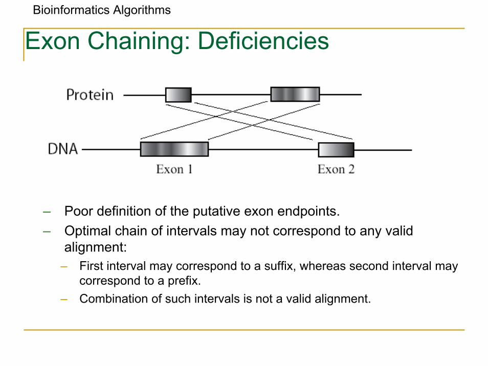
Exon Chaining: Deficiencies

– Poor definition of the putative exon endpoints.– Optimal chain of intervals may not correspond to any valid

alignment:– First interval may correspond to a suffix, whereas second interval may

correspond to a prefix.– Combination of such intervals is not a valid alignment.


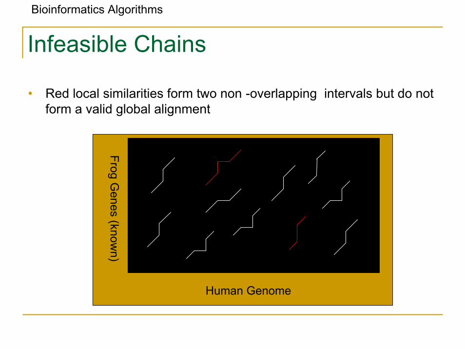
Infeasible Chains

• Red local similarities form two non -overlapping intervals but do not form a valid global alignment

Human Genome

Frog Genes (know

n)


Spliced Alignment

• Mikhail Gelfand and colleagues proposed a spliced alignmentapproach of using a protein within one genome to reconstruct theexon-intron structure of a (related) gene in another genome. – Begins by selecting either all putative exons between potential acceptor

and donor sites or by finding all substrings similar to the target protein (as in the Exon Chaining Problem).

– This set is further filtered in such way that attempts to retain all true exons, with some false ones.


Spliced Alignment Problem: Formulation

• Goal: Find a chain of blocks in a genomic sequence that best fits a target sequence

• Input: Genomic sequences G, target sequence T, and a set of candidate exons B.

• Output: A chain of exons Γ such that the global alignment score between Γ* and T is maximum among all chains of blocks from B.

Γ* – the concatenation of all exons from chain Γ


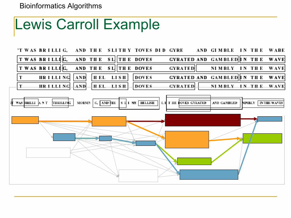
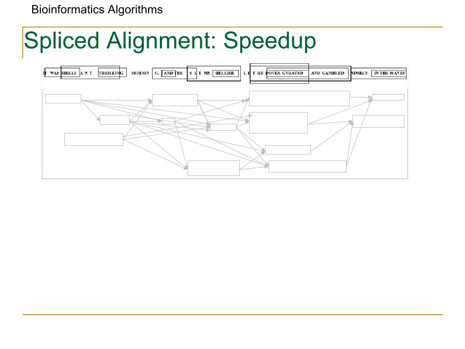
Lewis Carroll Example


Spliced Alignment: Idea

• Compute the best alignment between i-prefix of genomic sequence G and j-prefix of target T:

S(i,j)

• But what is “i-prefix” of G?• There may be a few i-prefixes of G depending on which block B we

are in.


Spliced Alignment: Idea

• Compute the best alignment between i-prefix of genomic sequence G and j-prefix of target T:

S(i,j)

• But what is “i-prefix” of G?• There may be a few i-prefixes of G depending on which block B we

are in.• Compute the best alignment between i-prefix of genomic sequence

G and j-prefix of target T under the assumption that the alignment uses the block B at position i

S(i,j,B)


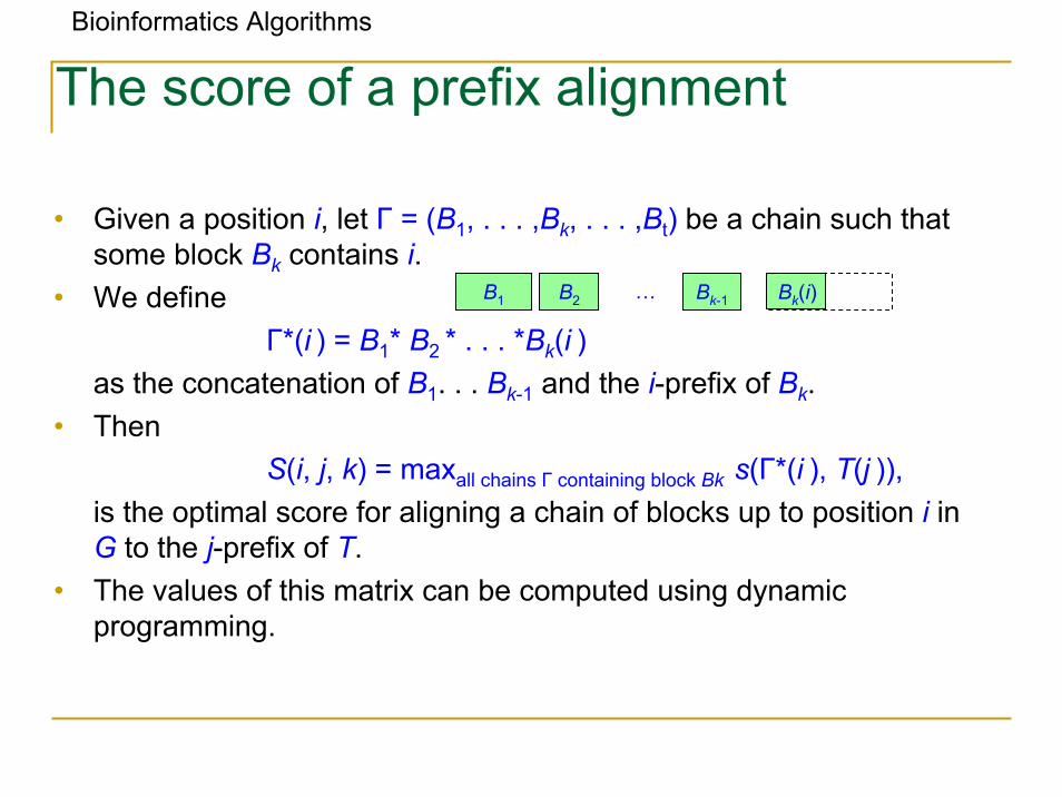
• Given a position i, let Γ = (B1, . . . ,Bk, . . . ,Bt) be a chain such that some block Bk contains i.

• We defineΓ*(i ) = B1* B2 * . . . *Bk(i )

as the concatenation of B1. . . Bk-1 and the i-prefix of Bk.• Then

S(i, j, k) = maxall chains Γ containing block Bk s(Γ*(i ), T(j )),is the optimal score for aligning a chain of blocks up to position i in G to the j-prefix of T.

• The values of this matrix can be computed using dynamic programming.

Bk(i)

The score of a prefix alignment

B1 B2 Bk-1…


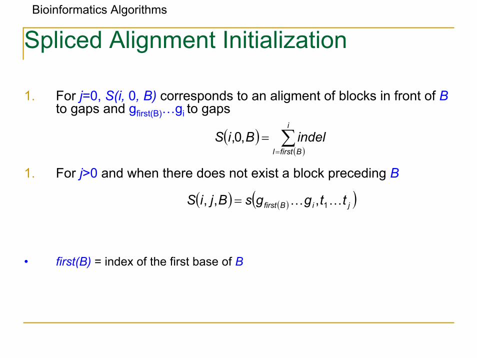
Spliced Alignment Initialization

1. For j=0, S(i, 0, B) corresponds to an aligment of blocks in front of Bto gaps and gfirst(B)…gi to gaps

1. For j>0 and when there does not exist a block preceding B

• first(B) = index of the first base of B

( )( )

∑=

=i

BfirstlindelBiS ,0,

( ) ( )( )jiBfirst ttggsBjiS KK 1,,, =


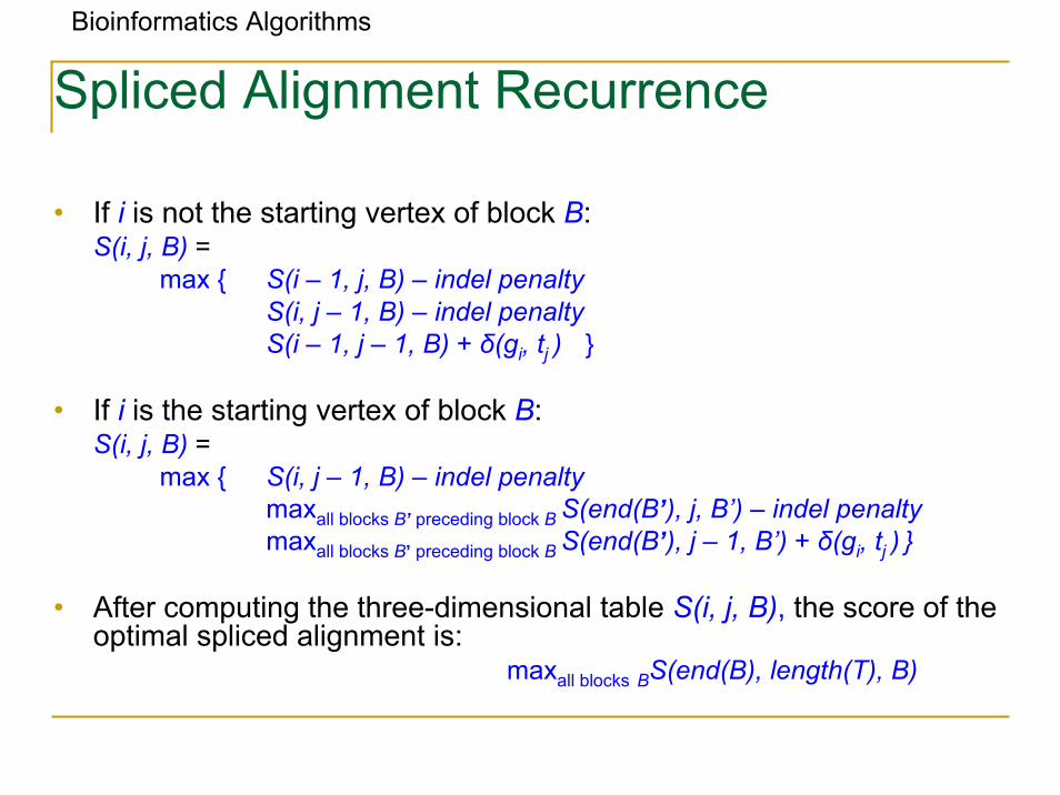
Spliced Alignment Recurrence

• If i is not the starting vertex of block B:S(i, j, B) =

max { S(i – 1, j, B) – indel penaltyS(i, j – 1, B) – indel penaltyS(i – 1, j – 1, B) + δ(gi, tj ) }

• If i is the starting vertex of block B:S(i, j, B) =

max { S(i, j – 1, B) – indel penaltymaxall blocks B’ preceding block B S(end(B’), j, B’) – indel penalty maxall blocks B’ preceding block B S(end(B’), j – 1, B’) + δ(gi, tj ) }

• After computing the three-dimensional table S(i, j, B), the score of the optimal spliced alignment is:

maxall blocks BS(end(B), length(T), B)


Spliced Alignment: Complications

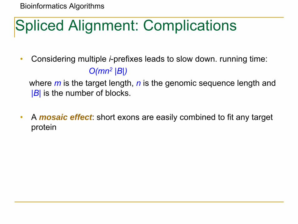
• Considering multiple i-prefixes leads to slow down. running time: O(mn2 |B|)

where m is the target length, n is the genomic sequence length and|B| is the number of blocks.

• A mosaic effect: short exons are easily combined to fit any target protein


Spliced Alignment: Speedup


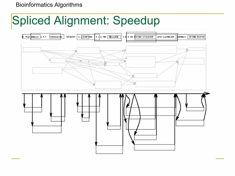
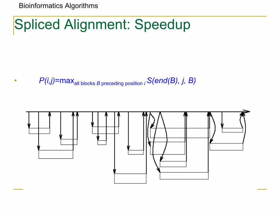
Spliced Alignment: Speedup

• P(i,j)=maxall blocks B preceding position i S(end(B), j, B)


Exon Chaining vs Spliced Alignment

• In Spliced Alignment, every path spells out string obtained by concatenation of labels of its edges. The weight of the path is defined as optimal alignment score between concatenated labels (blocks) and target sequence

– Defines weight of entire path in graph, but not the weights for individual edges.

• Exon Chaining assumes the positions and weights of exons are pre-defined.


Gene Prediction: Aligning Genome vs. Genome

• Align entire human and mouse genomes.

• Predict genes in both sequences simultaneously as chains of aligned blocks (exons).

• This approach does not assume any annotation of either human or mouse genes.


Gene Prediction Tools

• GENSCAN/Genome Scan• TwinScan• Glimmer• GenMark


The GENSCAN Algorithm• Algorithm is based on probabilistic model of gene structure similar to

Hidden Markov Models (HMMs).• GENSCAN uses a training set in order to estimate the HMM

parameters, then the algorithm returns the exon structure using maximum likelihood approach standard to many HMM algorithms (Viterbi algorithm). – Biological input: Codon bias in coding regions, gene structure (start and

stop codons, typical exon and intron length, presence of promoters, presence of genes on both strands, etc)

– Covers cases where input sequence contains no gene, partial gene, complete gene, multiple genes.

• GENSCAN limitations:– Does not use similarity search to predict genes. – Does not address alternative splicing. – Could combine two exons from consecutive genes together


• Incorporates similarity information into GENSCAN: predicts gene structure which corresponds to maximum probability conditional on similarity information

• Algorithm is a combination of two sources of information– Probabilistic models of exons-introns– Sequence similarity information

GenomeScan


TwinScan

• Aligns two sequences and marks each base as gap ( - ), mismatch (:), match (|), resulting in a new alphabet of 12 letters: Σ = {A-, A:, A |, C-, C:, C |, G-, G:, G |, T-, T:, T|}.

• Run Viterbi algorithm using emissions ek(b) where b ∈ Σ, k.• The emission probabilities are estimated from human/mouse

gene pairs. – Ex. eI(x|) < eE(x|) since matches are favored in exons, and

eI(x-) > eE(x-)since gaps (as well as mismatches) are favored in introns.

– Compensates for dominant occurrence of poly-A region in introns

http://www.standford.edu/class/cs262/Spring2003/Notes/ln10.pdf


Glimmer

• Gene Locator and Interpolated Markov ModelER• Finds genes in bacterial DNA• Uses interpolated Markov Models• Made of 2 programs

– BuildIMM• Takes sequences as input and outputs the Interpolated Markov Models

(IMMs)– Glimmer

• Takes IMMs and outputs all candidate genes• Automatically resolves overlapping genes by choosing one, hence limited• Marks “suspected to truly overlap” genes for closer inspection by user


GenMark

• Based on non-stationary Markov chain models

• Results displayed graphically with coding vs. noncoding probability dependent on position in nucleotide sequence

gene prediction - univerzita karlovamraz/bioinf/bioalg10-9.pdf · 2011-01-04 · an introduction to...

Documents