general utility lattice program - curtin university · chapter 1 introduction & background the...
TRANSCRIPT

General Utility Lattice Programverion 3.0
Julian D. Gale
Nanochemistry Research Institute,Department of Applied Chemistry,Curtin University of Technology,
P.O. Box U1987, Perth 6845,Western Australia
email: [email protected]

Contents
1 Introduction & background 41.1 Overview of program . . . . . . . . . . . . . . . . . . . . . . . . . . . . . . . 41.2 Introduction . . . . . . . . . . . . . . . . . . . . . . . . . . . . . . . . . . . . 111.3 Methods . . . . . . . . . . . . . . . . . . . . . . . . . . . . . . . . . . . . . . 12
1.3.1 Coulomb interaction . . . . . . . . . . . . . . . . . . . . . . . . . . . 131.3.2 Dispersion interactions . . . . . . . . . . . . . . . . . . . . . . . . . . 191.3.3 Two-body short-range interactions . . . . . . . . . . . . . . . . . . . . 201.3.4 Polarisability . . . . . . . . . . . . . . . . . . . . . . . . . . . . . . . 201.3.5 Radial interactions . . . . . . . . . . . . . . . . . . . . . . . . . . . . 231.3.6 Three-body interactions . . . . . . . . . . . . . . . . . . . . . . . . . 231.3.7 Four-body interactions . . . . . . . . . . . . . . . . . . . . . . . . . . 251.3.8 Many-body interactions . . . . . . . . . . . . . . . . . . . . . . . . . 25
1.3.8.1 The Embedded Atom Method . . . . . . . . . . . . . . . . . 251.3.8.2 Bond Order Potentials . . . . . . . . . . . . . . . . . . . . . 27
1.3.9 One-body interactions . . . . . . . . . . . . . . . . . . . . . . . . . . 281.3.10 Potential truncation . . . . . . . . . . . . . . . . . . . . . . . . . . . . 29
1.3.10.1 Radial truncation . . . . . . . . . . . . . . . . . . . . . . . 291.3.10.2 Cut and shift . . . . . . . . . . . . . . . . . . . . . . . . . . 301.3.10.3 Tapering . . . . . . . . . . . . . . . . . . . . . . . . . . . . 301.3.10.4 Molecular mechanics . . . . . . . . . . . . . . . . . . . . . 30
1.3.11 Partial occupancy . . . . . . . . . . . . . . . . . . . . . . . . . . . . . 311.3.12 Structural optimisation . . . . . . . . . . . . . . . . . . . . . . . . . . 321.3.13 Genetic algorithms . . . . . . . . . . . . . . . . . . . . . . . . . . . . 381.3.14 Calculation of bulk properties . . . . . . . . . . . . . . . . . . . . . . 40
1.3.14.1 Elastic constants . . . . . . . . . . . . . . . . . . . . . . . . 401.3.14.2 Bulk and shear moduli . . . . . . . . . . . . . . . . . . . . . 411.3.14.3 Young’s moduli . . . . . . . . . . . . . . . . . . . . . . . . 411.3.14.4 Poisson’s ratio . . . . . . . . . . . . . . . . . . . . . . . . . 421.3.14.5 Acoustic velocities . . . . . . . . . . . . . . . . . . . . . . . 421.3.14.6 Static and high frequency dielectric constants . . . . . . . . 43
1

1.3.14.7 Refractive indices . . . . . . . . . . . . . . . . . . . . . . . 431.3.14.8 Piezoelectric constants . . . . . . . . . . . . . . . . . . . . . 441.3.14.9 Electrostatic potential, electric field and electric field gradients 441.3.14.10 Born effective charges . . . . . . . . . . . . . . . . . . . . . 451.3.14.11 Phonons . . . . . . . . . . . . . . . . . . . . . . . . . . . . 461.3.14.12 Vibrational partition function . . . . . . . . . . . . . . . . . 481.3.14.13 Frequency-dependent dielectric constants and reflectivity . . 50
1.3.15 Calculation of surface properties . . . . . . . . . . . . . . . . . . . . . 511.3.15.1 Surface energy . . . . . . . . . . . . . . . . . . . . . . . . . 531.3.15.2 Attachment energy . . . . . . . . . . . . . . . . . . . . . . . 561.3.15.3 Morphology . . . . . . . . . . . . . . . . . . . . . . . . . . 561.3.15.4 Surface phonons . . . . . . . . . . . . . . . . . . . . . . . . 57
1.3.16 Free energy minimisation . . . . . . . . . . . . . . . . . . . . . . . . 571.3.17 Monte Carlo . . . . . . . . . . . . . . . . . . . . . . . . . . . . . . . 601.3.18 Defect calculations . . . . . . . . . . . . . . . . . . . . . . . . . . . . 611.3.19 Derivation of interatomic potentials . . . . . . . . . . . . . . . . . . . 651.3.20 Calculation of derivatives . . . . . . . . . . . . . . . . . . . . . . . . . 691.3.21 Crystal symmetry . . . . . . . . . . . . . . . . . . . . . . . . . . . . . 711.3.22 Code details . . . . . . . . . . . . . . . . . . . . . . . . . . . . . . . . 73
2 Results 752.0.23 Mechanical properties . . . . . . . . . . . . . . . . . . . . . . . . . . 752.0.24 Born effective charges . . . . . . . . . . . . . . . . . . . . . . . . . . 782.0.25 Frequency-dependent optical properties . . . . . . . . . . . . . . . . . 782.0.26 Surface calculations . . . . . . . . . . . . . . . . . . . . . . . . . . . 792.0.27 Bond-order potentials . . . . . . . . . . . . . . . . . . . . . . . . . . . 81
3 Further background 853.0.27.1 Cut-offs and molecules . . . . . . . . . . . . . . . . . . . . 853.0.27.2 Combination rules . . . . . . . . . . . . . . . . . . . . . . . 893.0.27.3 Mean field theory . . . . . . . . . . . . . . . . . . . . . . . 903.0.27.4 Algorithms for energy and derivative evaluations . . . . . . . 91
3.0.28 Phonons . . . . . . . . . . . . . . . . . . . . . . . . . . . . . . . . . . 923.0.28.1 Phonon density of states . . . . . . . . . . . . . . . . . . . . 923.0.28.2 Infra-red phonon intensities . . . . . . . . . . . . . . . . . . 933.0.28.3 Thermodynamic quantities from phonons . . . . . . . . . . . 93
3.0.29 Free energies . . . . . . . . . . . . . . . . . . . . . . . . . . . . . . . 943.0.30 Defects . . . . . . . . . . . . . . . . . . . . . . . . . . . . . . . . . . 95
3.0.30.1 The Mott-Littleton method . . . . . . . . . . . . . . . . . . 953.0.30.2 Displacements in region 2a . . . . . . . . . . . . . . . . . . 973.0.30.3 Region 2b energy . . . . . . . . . . . . . . . . . . . . . . . 98
2

3.0.31 Fitting . . . . . . . . . . . . . . . . . . . . . . . . . . . . . . . . . . . 983.0.31.1 Fundamentals of fitting . . . . . . . . . . . . . . . . . . . . 983.0.31.2 Fitting energy surfaces . . . . . . . . . . . . . . . . . . . . . 993.0.31.3 Empirical fitting . . . . . . . . . . . . . . . . . . . . . . . . 1003.0.31.4 Simultaneous fitting . . . . . . . . . . . . . . . . . . . . . . 1013.0.31.5 Relax fitting . . . . . . . . . . . . . . . . . . . . . . . . . . 101
3.0.32 Genetic algorithms . . . . . . . . . . . . . . . . . . . . . . . . . . . . 1023.1 Getting started . . . . . . . . . . . . . . . . . . . . . . . . . . . . . . . . . . . 104
3.1.1 Running GULP . . . . . . . . . . . . . . . . . . . . . . . . . . . . . . 1043.1.2 Getting on-line help . . . . . . . . . . . . . . . . . . . . . . . . . . . 1043.1.3 Example input files . . . . . . . . . . . . . . . . . . . . . . . . . . . . 105
3.2 Guide to input . . . . . . . . . . . . . . . . . . . . . . . . . . . . . . . . . . . 1063.2.1 Format of input files . . . . . . . . . . . . . . . . . . . . . . . . . . . 1063.2.2 Atom names . . . . . . . . . . . . . . . . . . . . . . . . . . . . . . . 1083.2.3 Input of structures . . . . . . . . . . . . . . . . . . . . . . . . . . . . 1093.2.4 Species / libraries . . . . . . . . . . . . . . . . . . . . . . . . . . . . . 1123.2.5 Input of potentials . . . . . . . . . . . . . . . . . . . . . . . . . . . . 1133.2.6 Defects . . . . . . . . . . . . . . . . . . . . . . . . . . . . . . . . . . 1143.2.7 Restarting jobs . . . . . . . . . . . . . . . . . . . . . . . . . . . . . . 1183.2.8 Memory management . . . . . . . . . . . . . . . . . . . . . . . . . . 1193.2.9 Summary of keywords . . . . . . . . . . . . . . . . . . . . . . . . . . 120
3.2.9.1 Groups of keywords by use . . . . . . . . . . . . . . . . . . 1223.2.9.2 Summary of options . . . . . . . . . . . . . . . . . . . . . . 123
3.3 Guide to output . . . . . . . . . . . . . . . . . . . . . . . . . . . . . . . . . . 1273.3.1 Main output . . . . . . . . . . . . . . . . . . . . . . . . . . . . . . . . 1273.3.2 Files for graphical display . . . . . . . . . . . . . . . . . . . . . . . . 1293.3.3 Input files for other programs . . . . . . . . . . . . . . . . . . . . . . 1293.3.4 Temporary files . . . . . . . . . . . . . . . . . . . . . . . . . . . . . . 130
3.4 Guide to installation . . . . . . . . . . . . . . . . . . . . . . . . . . . . . . . . 130
3

Chapter 1
Introduction & background
The General Utility Lattice Program (GULP) is designed to perform a variety of tasks basedon force field methods. The original code was written to facilitate the fitting of interatomicpotentials to both energy surfaces and empirical data. However, it has expanded now to bea general purpose code for the modelling of condensed phase problems. While version 1.0focussed on solids, clusters and embedded defects, the latest version is also capable of handlingsurfaces, interfaces, and polymers.
As with any large computer program (and GULP currently runs to about 310,000 lines) thereis always the possibility of bugs. While every attempt is made to ensure that there aren’t any andto trap incorrect input there can be no guarantee that a user won’t find some way of breaking theprogram. So it is important to be vigilant and to think about your answers - remember GIGO!Immature optimising compilers can also be a common source of grief. As with most programs,the author accepts no liability for any errors but will attempt to correct any that are reported.
1.1 Overview of programThe following is intended to act as a brief summary of the capabilities of GULP to enable you todecide whether your required task can be performed without having to read the whole manual.Alternatively it may suggest some new possibilities for calculations!
System types
• 0-D (clusters and embedded defects)
• 1-D (polymers)
• 2-D (slabs and surfaces)
• 3-D (bulk materials)
4

Energy minimisation
• constant pressure / constant volume / unit cell only / isotropic
• thermal/optical calculations
• application of external pressure
• user specification of degrees of freedom for relaxation
• relaxation of spherical region about a given ion or point
• symmetry constrained relaxation
• unconstrained relaxation
• constraints for fractional coordinates and cell strains
• Newton/Raphson, conjugate gradients or Rational Function optimisers
• BFGS or DFP updating of hessian
• limited memory variant of BFGS for large systems
• search for minima by genetic algorithms with simulated annealing
• free energy minimisation with analytic first derivatives
• choice of regular or domain decomposition algorithms for first derivative calculations
Transition states
• location of n-th order stationary points
• mode following
Crystal properties
• elastic constants
• bulk modulus (Reuss/Voight/Hill conventions)
• shear modulus (Reuss/Voight/Hill conventions)
• Youngs modulus
• Poisson ratios
5

• compressibility
• piezoelectric stress and strain constants
• static dielectric constants
• high frequency dielectric constants
• frequency dependent dielectric constants
• static refractive indices
• high frequency refractive indices
• phonon frequencies
• phonon densities of states (total and projected)
• phonon dispersion curves
• Born effective charges
• zero point vibrational energies
• heat capacity (constant volume)
• entropy (constant volume)
• Helmholtz free energy
Defect calculations
• vacancies, interstitials and impurities can be treated
• explicit relaxation of region 1
• implicit relaxation energy for region 2
• energy minimisation and transition state calculations are possible
• defect frequencies can be calculated (assuming no coupling with 2a)
6

Surface calculations
• calculation of surface and attachment energies
• multiple regions allowed with control over rigid or unconstrained movement
• can be used to simulate grain boundaries
• calculation of phonons allowed for region 1
Fitting
• empirical fitting to structures, energies and most crystal properties
• fit to multiple structures simultaneously
• simultaneous relaxation of shell coordinates during fitting
• fit to structures by either minimising gradients or displacements
• variation of potential parameters, charges and core/shell charge splits
• constraints available for fitted parameters
• generate initial parameter sets by the genetic algorithm for subsequent refinement
• fit to quantum mechanically derived energy hypersurfaces
Structure analysis
• calculate bond lengths/distances
• calculate bond angles
• calculate torsion angles
• calculate out of plane distances
• calculation of the density and cell volume
• electrostatic site potentials
• electric field gradients
7

Structure manipulation
• convert centred cell to primitive form
• creation of supercells
Electronegativity equalisation method
• use EEM to calculate charges for systems containing H, C, N, O, F, Al, Si, P
• use QEq to calculate charges for any element
• new modified scheme for hydrogen within QEq that has correct forces
Generation of input files for other programs
• GDIS (.gin/.res)
• THBREL/THBPHON/CASCADE (.thb)
• MARVIN (.mvn)
• Insight (.xtl file)
• Insight (.arc/.car files)
• G-Vis (.xr)
• Cerius2 (.arc/.xtl/.cssr)
• Materials Studio
• SIESTA (.fdf)
• Molden (.xyz)
• QMPOT (.frc)
• General (.cif/.xml)
• DLV (.str)
8

Interatomic potentials available
• Buckingham
• Four-range Buckingham
• Lennard-Jones (with input as A and B)
• Lennard-Jones (with input in ε and σ format)
• Lennard-Jones (with ESFF combination rules)
• Morse potential (with or without Coulomb subtract)
• Harmonic (with or without Coulomb subtract)
• General potential (Del Re) with energy and gradient shifts
• Spline
• Spring (core-shell)
• Spring with cosh functional form
• Coulomb subtract
• Coulomb with erfc
• Coulomb with short range taper
• Inverse Gaussian
• Damped dispersion (Tang-Toennies)
• Rydberg potential
• Covalent exponential form
• Breathing shell harmonic
• Breathing shell exponential
• Coulomb with complementary error function
• Coulomb with short range taper
• Covalent-exponential
• Fermi-Dirac form
9

• Three body potentials - harmonic with or without exponential decay
• Exponential three-body potential
• Urey-Bradley three-body potential
• Stillinger-Weber two- and three-body potentials
• Stillinger-Weber with charge softening
• Axilrod-Teller potential
• Four-body torsional potential
• Ryckaert-Bellemans cosine expansion for torsional potential
• Out of plane distance potential
• Tsuneyuki Coulomb correction potential
• Squared harmonic
• Embedded atom method for metals (Sutton-Chen potentials and others)
• Two-body potentials can be intra- or inter-molecular, or both
• Two-body potentials can be tapered to zero using cosine, polynomial or Voter forms
Coulomb summations• Ewald sum for 3-D
• Parry sum for 2-D
• Saunders et al sum for 1-D
• Cell multipole method for 0-D
• Wolf et al sum for 0-,1-,2-, & 3-D
Molecular dynamics• Shell model (dipolar and breathing) molecular dynamics
• Finite mass or adiabatic algorithms
• Forward extrapolation of shells added for adiabatic algorithms
• NVE or NVT (Nose-Hoover) or NPT (Variable cell shape)
10

Monte Carlo
• Rigid molecules allowed for
• Displacement or rotation of species
• NVT or Grand Canonical ensembles allowed
1.2 IntroductionThe simulation of ionic materials has a long history going back over most of the last century.It began with lattice energy calculations based on experimental crystal structures through theuse of Madelung’s constant [1]. This was then expanded through the inclusion of short-rangerepulsive interactions, as found in the work of Born-Lande and Born-Mayer [2], in order that thecrystal structure be a minimum with respect to isotropic expansion or compression. For manysimple ionic materials a reasonable estimate of the lattice energy may even be obtained withoutknowledge of the structure, as demonstrated by the work of Kapustinskii [3]. Over the last fewdecades atomistic simulation, in which we are only concerned with atoms, rather than electronsand sub-atomic particles, has developed significantly with the widespread use of computers.Correspondingly the field has evolved from one that was initially concerned with reproducingexperimental numbers, to one where predictions are being made, and insight is being offered.
The widespread use of atomistic simulation for solid state materials clearly resulted fromthe availability of computer programs for the task, just as much as the advent of the hardwareto run the calculations. In the early days of solid state forcefield simulation for ionic materialsmuch of the work in the UK was centred around the Atomic Energy Authority at Harwell.Consequently a number of computer codes arose from this work, such as HADES [4], MIDAS[5], PLUTO [6], METAPOCS and CASCADE [7]. Eventually these migrated into the academicdomain, leading to the THB suite of codes, including THBREL, THBFIT and THBPHON fromLeslie. Further development of these programs led to the PARAPOCS code from Parker andco-workers [8], for free energy minimisation of solids using numerical derivatives, and theDMAREL code from the group of Price for the simulation of molecular crystals through theuse of distributed multipoles [9]. There were also several other prominent codes developedcontemporaneously to the above family, in particular the WMIN code of Busing [10], the PCKseries of programs from Williams [11], and the UNISOFT program of Eckold et al [12]. Whilethe codes mentioned above focus specifically on static lattice and quasiharmonic approachesto simulation, it should not be forgotten that there was a much larger, parallel, development offorcefield software for performing molecular dynamics simulation leading to programs such asGROMOS [13], AMBER [14], CHARMM [15], and DLPOLY [16, 17], to name but a few.
This article focuses on the General Utility Lattice Program which began development in theearly 90’s, and is therefore subsequent to much of the aforemention software, but implementsmany of the same ideas. However, there are increasingly many new, and unique, developments
11
as well. The key philosophy was to try to bring together many of the facilities required for solidstate simulation, with particular emphasis on static lattice/lattice dynamical methods, in a singlepackage, and to try to make it as easy to use as possible. Of course, this is an aim and the degreeof success depends on the perspective of the end user! It is important to also mention here theprograms METADISE from Parker and co-workers[18], and SHELL from the group of Allan[19], which are also contemporary simulation codes sharing some of the same ideas.
In this work, the specific aim is to document the very latest version of GULP, 3.0, which in-cludes many new features over previous versions, as well as having been considerably rewritten.Given that the previous release was version 1.3, the above use of 3.0 may come as a suprise.However, there was a development version of GULP that included periodic semi-empiricalquantum mechanical methods from the MINDO and MNDO family, and this was nominallyreferred to as version 2.0 [20]. Hence the extra increment to avoid any possible confusion.Firstly, we detail the background theory to the underlying methods, some of which is not read-ily available in the literature. Secondly, we present a brief review of the utilisation of the codeto date, in order to highlight the scope of its previous application. Finally, we present someresults illustrating the new capabilities of the latest version.
1.3 MethodsThe starting point for the majority simulation techniques is the calculation of the energy, and sowill it be for this article. Most methods are based around the initial determination of the internalenergy, with subsequent treatment of the nuclear degrees of freedom in order to determine theappropriate free energy to the ensemble of interest. In principle, the internal energy of a solidis a manybody quantity that explicitly depends upon the positions and momenta of all electronsand nuclei. However, this is an intractable problem to solve at any level of theory, and thusapproximations must be made to simplify the situation. To tackle this we assume that the effectof the electrons will largely be subsumed into an effective atom, and that the energy can bedecomposed into an expansion in terms of interactions between different subsets of the totalnumber of atoms, N :
U =N∑
i=1
Ui +1
2
N∑
i=1
N∑
j=1
Uij +1
6
N∑
i=1
N∑
j=1
N∑
k=1
Uijk + ....
where the first term represents the self energies of the atoms, the second the pairwise inter-action, etc. This decomposition is exact if performed to a high enough order. However, weknow that the contribution from higher order terms becomes progressively smaller for mostsystems, and so we choose to neglect the terms beyond a certain point and introduce a degreeof parameterisation of the remaining terms to compensate. Justification for this is forthcomingfrom quantum mechanics. It is well known that the Hartree-Fock method is a reasonable firstapproximation for the description of many systems, albeit with a systematic quantitative error
12
for most observables. Here the highest term included is a four-centre integral, which indicatesthat including up to four-body terms should be reasonable approach, which is indeed found tobe the case for most organic systems, for example. Furthermore, it is intuitively obvious thatthe further apart two atoms are, the weaker their interaction will be. Thus the introduction ofdistance cut-offs is a natural way to simplify the computational task.
The form of the explicit interaction between atoms is usually chosen based on physicalinsights as to the nature of the forces between the particles. For instance, if considering acovalent diatomic molecule the natural representation of the potential energy surface would bea Morse potential since this is harmonic at the minimum and leads to dissociation at large bondlengths, in accord with spectroscopic observation. In the following sections we will reviewsome of the common types of potential that are widely used, as well as some novel approacheswhich point towards the future of forcefield methods.
1.3.1 Coulomb interactionWhen considering ionic materials, the Coulomb interaction is by far the dominant term and canrepresent, typically, up to 90% of the total energy. Despite having the simplist form, just beinggiven by Coulomb’s law;
UCoulombij =
qiqj
4πε0rij
it is in fact the most complicated to evaluate for periodic systems (subsequently atomic unitswill be employed and the factor of 4πε0 will be omitted). This is because the Coulomb energy isgiven by a conditionally convergent series, i.e. the Coulomb energy is ill-defined for an infinite3-D material unless certain additional conditions are specified. The reason for this can be readilyunderstood - the interaction between ions decays as the inverse power of r, but the number ofinteracting ions increases with the surface area of a sphere, which is given by 4πr2. Hence,the energy density of interaction increases with distance, rather than decaying. One solution tothe problem, proposed by Evjen [21], is to sum over charge-neutral groups of atoms. However,by far the most widely employed approach is the method of Ewald [22] for three-dimensionalmaterials. Here the conditions of charge neutrality and zero dipole moment are imposed toyield a convergent series with a well-defined limit. To accelerate the evaluation, the Coulombterm is subjected to a Laplace transformation and then separated into two components, oneof which is rapidly convergent in real space, and a second which decays quickly in reciprocalspace. Conceptually, this approach can be viewed as adding and subtracting a Gaussian chargedistribution centred about each ion [23]. The resulting expressions for real and reciprocal space,as well as the self-energy of the ion, are given below:
U real =1
2
N∑
i=1
N∑
j=1
qiqj
rijerfc
(
η1
2 rij
)
13

U recip =1
2
N∑
i=1
N∑
j=1
∑
G
4π
Vqiqj exp (iG.rij)
exp(
−G2
4η
)
G2
U self = −N∑
i=1
q2i
(
η
π
) 1
2
U electrostatic = U real + U recip + U self
Here q is the charge on an ion, G is a reciprocal lattice vector (where the special case G = 0is excluded), V is the volume of the unit cell, and η is a parameter that controls the divisionof work between real and reciprocal space. It should also be noted that although the reciprocalspace term is written as a two-body interaction over pairs of atoms, it can be rewritten as a singlesum over ions for more efficient evaluation. The above still leaves open the choice of cut-offradii for real and reciprocal space. One approach to defining these in a consistent fashion is tominimise the total number of terms to be evaluated in both series for a given specified accuracy,A [24]. This leads to the following expressions:
ηopt =
(
Nwπ3
V
)1
3
rmax =
(
− ln (A)
η
) 1
2
Gmax = 2η1
2 (− ln (A))1
2
Note that the above expressions contain one difference from the original derivation, in that aweight parameter, w, has been included that represents the relative computational expense ofcalculating a term in real and reciprocal space. Tuning of this parameter can lead to significantbenefits for large systems. There have been several modifications proposed for the basic Ewaldsummation that accelerate its evaluation for large systems, most notably the particle-mesh [25],and fast multipole methods [26, 27]. Furthermore, there are competitive approaches that operatepurely in real space for large unit cells and that scale linearly with increasing size, such as thehierarchical fast multipole methods, though care must be taken to obtain the same limitingresult by imposing the zero dipole requirement. This latter approach can also be applied toaccelerating the calculation of the Coulomb energy of finite clusters.
In principle, it is possible to calculate the Coulomb energy of a system with a net dipole, µ,as well. The nature of the correction to the Ewald energy can be determined as a function of theshape of the crystal, and the formula below can also be employed [28]:
Udipole =2π
3Vµ2
However, the complication of using the above correction is that it depends on the macroscopicdipole of the crystal, and even on any compensating electric field due to the environment sur-rounding the particle. Hence the dipole moment is usually ill-defined, since it depends on the
14
surfaces, as well as the bulk material. Even if we neglect surface effects, the definition ofthe dipole moment is ambiguous since the operator is not invariant under translation of atomicimages by a lattice vector. Consequently, we will take the Ewald result as being definitive.
Similarly, it is possible to relax the charge neutrality constraint, and to perform calculationson charged supercells [29], provided care is taken when constructing thermodynamic cycles.This is often used when probing defect energetics as an alternative to the Mott-Littleton method.Here the net charge, Q (Q =
∑
qi) is neutralised by a uniform background charge, leading toan energy correction of:
U background = − π
2V ηQ2
So far we have only considered how to handle infinite 3-D solids, but the same issues existfor lower dimensionalities. Again for a 2-D slab, the Coulomb sum is only conditionally con-vergent and so an analogous approach to the Ewald sum is usually taken, originally devised byParry [30, 31]. Here the slab, or surface, is taken so as to be oriented with the surface vectorsin the xy plane and with the surface normal lying parallel to z. The energy contributions in realand reciprocal space are given by:
U real =1
2
N∑
i=1
N∑
j=1
qiqj
rij
erfc(
η1
2 rij
)
U recip1 =
1
2
N∑
i=1
N∑
j=1
∑
G
π
A
qiqj exp (iG.rij)
|G|
[
exp (|G| zij) erfc
(
|G|2η
1
2
+ η1
2 zij
)
+
exp (− |G| zij) erfc
(
|G|2η
1
2
− η1
2 zij
)]
U recip2 = −1
2
N∑
i=1
N∑
j=1
2πqiqj
A
zij.erf(
η1
2 zij
)
+exp
(
−ηz2ij
)
(πη)1
2
U self = −N∑
i=1
q2i
(
η
π
) 1
2
Note, there are now two terms in reciprocal space involving the 2-D reciprocal lattice vector,G, and here A is the surface area of the repeat unit, while zij is the component of the distancebetween two ions parallel to the surface normal. Again it is possible to relax the dipolar andcharge neutrality constraints within the repeat directions. However, the approach to correctingthe energy is far more uncertain, and it is necessary to make approximations [32]. As per the3-D case, the optimum value of the convergence parameter can also be determined [33]:
ηopt =πw
A
15

Recently, another approach has been proposed for the calculation of the 2-D Coulomb sum,which is reported to be faster than the Parry method for all cases, and especially beneficial asthe number of atoms increases [34].
Lowering the dimensionality further, we arrive at 1-D periodic systems which represents asingle polymer strand, for example. At this dimensionality the Coulomb sum becomes abso-lutely convergent, though at a very slow rate when performed directly in real space. Summingover charge neutral units accelerates the process, though convergence is still somewhat tardy.While there have been several proposed approaches to accelerating the Coulomb sum, we findthat the method proposed by Saunders et al [35], in which a neutralising background charge isapplied, is effective. Here there are three contributions to the energy given by:
U real1 =
1
2
+M∑
m=−M
N∑
i=1
N∑
j=1
qiqj
rij + ma
U real2 = −1
2
N∑
i=1
N∑
j=1
qiqj
a
[
ln(√
(u + x)2 + y2 + z2 + u + x)
+
ln(√
(u − x)2 + y2 + z2 + u − x)
− 2 ln a]
U real3 =
1
2
N∑
i=1
N∑
j=1
qiqj [ξ (M, rij) + ξ (M,−rij)]
where the first term is summed over all images of i and j in the unit cells from −M to M , ais the 1-D repeat parameter in the x direction, and the remaining variables and functions aredefined as below:
u = a(
M +1
2
)
ξ (M, rij) = −M∑
i=1
Eia2i−1W2i−1
(
u + x, y2 + z2)
Wn (u + x, α) =
(
∂
∂u
)n(
(u + x)2 + α)− 1
2
Although the required extent of the summations, given by M , to achieve a given precision isnot known a priori, the method can be implemented in an iterative fashion so that the degree ofconvergence is tested as the number of lattice repeats is increased.
One alternative approach to the above methods for performing the Coulomb sum in anydimensionality is that due to Wolf et al [36]. Their approach involves a purely real space sum-mation that is asymptotic to the Ewald limit given a suitable choice of convergence parameters.It is based around the concept of ensuring that the sum of the charges of all ions within a spher-ical cut-off region is equal to zero and that the potential goes smoothly to zero at that cut-off.
16
This is achieved by placing an image of every ion that a given atom interacts with at the cut-off boundary, but in the diametrically opposite direction. While this approach can be applieddirectly to the Coulomb potential, convergence is slow. Better results are obtained by using adamped form of the potential, which is chosen to be equivalent to the real space component ofthe Ewald sum, with subtraction of the associated self-energy of the corresponding Gaussian.In this form the expression for the energy is:
UWolf =1
2
∑
i
∑
j
qiqj
(
erfc (αrij)
rij
− limrij→rcut
erfc (αrij)
rij
)
−
∑
i
q2i
erfc (αrcut)
2rcut
+α
π1
2
where α is the convergence parameter, closely related to the factor η in the Ewald sum, and rcut
is the cut-off radius. There is a trade-off to be made in the choice of parameters within this sum.The smaller the value of α, the closer the converged value will be to the Ewald limit. However,the cut-off radius required to achieve convergence is also increased. This summation methodhas been implemented within GULP for 1-D, 2-D and 3-D calculations, though by default theterm due to the limit of the distance approaching the cut-off is omitted from the derivatives inorder to keep them analytically correct at the expense of the loss of smoothing.
Before leaving the topic of how Coulomb interactions are evaluated, it is important to notethe special case of molecular mechanics forcefields. Here the Coulomb interaction, and usuallythe dispersion one too, is subtracted for interactions which are between neighbours (i.e. bondedor 1-2) and next nearest neighbours (i.e. which have a common bonded atom, 1-3) accordingto the connectivity. This is done so that the parameters in the two- and three-body potentialscan be directly equated with experimentally observable quantities, such as force constants fromspectroscopy. Furthermore, long-range interactions for atoms that are 1-4 connected are oftenscaled, usually by 1
2.
So far we have discussed the methods for evaluating Coulomb sums. However, we have yetto comment on how the atomic charges are determined. In most simulations, the charges onions are fixed (i.e. independent of geometry) for simplicity and their magnitude is determinedparametrically along with other forcefield parameters, or extracted from quantum mechanicalinformation. In the later situation there is the question as to what is the appropriate charge totake since it depends on how the density matrix is partitioned. Although Mulliken analysis [37]is commonly used as a standard, this is not necessarily the optimum charge definition for usein a forcefield. Arguably a better choice would be to employ the Born effective charges [38]that describe the response of the ions to an electric field, about which more will be said later. Ifthe charges are purely regarded as parameters then the use of formal charges is convenient as itremoves a degree of freedom and maximises the transferability of the forcefield, especially tocharged defects.
An alternative to using fixed charges is to allow the charges to be determined as a functionof the geometry. It is well documented that this environment dependance of the charge is very
17

important in some cases. For example, the binding energy of water in ice is much greater thanthat in the water dimer. This arises due to the increased ionicity of the O-H bond in the solidstate and cannot be described correctly by a simple two-body model. In order to implement avariable charge scheme, a simple Hamiltonian is needed that is practical for forcefield simula-tions. Consequently most approaches to geometry-dependent charges have been based aroundthe concept of electronegativity equalisation [39]. Here the energy of an atom is expanded withrespect to the charge, q, where the first derivative of the energy with respect to charge is theelectronegativity, χ, and the second is the hardness, µ:
Ui = U0i + χ0
i qi +1
2µ0
i q2i +
1
2qiVi
The final term in the above expression is the interaction with the Coulomb potential due to otheratoms within the system. By solving the coupled set of equations for all atoms simultaneously,this leads to a set of charges that balance the chemical potential of the system. There are twovariants of this method in general use. In the first, typified by the work of Mortier and co-workers [40], the Coulomb interaction, J , is described by a simple 1
rform. The alternative, as
used by Rappe and Goddard in their QEq method [41], is to use a damped Coulomb potentialthat allows for the fact that at short distances the interaction arises from the overlap of electrondensity, rather than from just simple point ions. Hence, in QEq the potential is calculated basedon the interaction of s orbitals with appropriate exponents. A further variant tries to encapsulatethe short range damping of the Coulomb interaction in a mathematically more efficient form[42];
Jij =1
(
r3ij + γ−3
ij
) 1
3
where the pairwise terms γij are typically determined according to combination rules in orderto minimise the number of free parameters:
γij =√
γiγj
In the case of hydrogen, the variation of charge is so extreme between the hydride and protonlimits that it was necessary to make the electronegativity a function of the charge itself in theoriginal QEq scheme. As a result, the solution for the charges now requires an iterative self-consistent process. Here we propose a modified formulation from that of Rappe and Goddardthat drastically simplifies the calculation of analytic derivatives:
UH = U0H + χ0
HqH +1
2J0
HH
(
1 +2qH
3ζ0H
)
q2H +
1
2qHVH
The reason for the simplification is based on the Hellmann-Feynman theorem and can be un-derstood as follows. If we consider the Cartesian first derivatives of the variable charge energywe arrive at:
(
dU
dα
)
=
(
∂U
∂α
)
q
+
(
∂U
∂q
)
α
(
∂q
∂α
)
18

where the first term represents the conventional fixed charge derivative, and the second term isthe contribution from the variation in charge as a function of structure. However, if the chargesat each geometry are chosen so as to minimise the total energy of the system, then the firstderivative of the internal energy with respect to charge is zero and so the correction disappears.Consequently it only becomes necessary to evaluate the first derivatives of the charges withrespect to position when calculating the second derivative matrix.
1.3.2 Dispersion interactionsAfter the Coulomb energy, the most long-ranged of the energy contributions is usually thedispersion term. From quantum theory we know that the form of the interaction is a series ofterms in increasing inverse powers of the interatomic distance, where even powers are usuallythe most significant:
Udispersionij = −C6
r6ij
− C8
r8ij
− C10
r10ij
− .....
The first term represents the instanteous dipole - instanteous dipole interaction energy, and thesubsequent terms correspond to interactions between higher order fluctuating moments. Oftenin simulations only the first term, C6
r6 , is considered as the dominant contribution. Again, thedispersion term can cause difficulties due to the slow convergence with respect to a radial cut-off. Although the series is absolutely convergent, unlike the Coulomb sum, the fact that allcontributions are attractive implies that there is no cancellation between shells of atoms. Theproblem can be remedied by using an Ewald-style summation [43] to accelerate convergencefor materials where the dispersion term is large:
U recipC6 = −1
2
N∑
i=1
N∑
j=1
Cij
π3
2
12V
∑
G
exp (iG.rij) G3
[
π1
2 erfc
(
G
2η1
2
)
+
4η3
2
G3− 2η
1
2
G
exp
(
−G2
4η
)
U realC6 = −1
2
N∑
i=1
N∑
j=1
Cij
r6
(
1 + ηr2ij +
η2r4ij
2
)
exp(
−ηr2ij
)
U selfC6 =
1
2
N∑
i=1
N∑
j=1
−Cij
3V(πη)
3
2 +N∑
i=1
Ciiη3
6
There can also be problems with the dispersion energy at short-range since it tends to neg-ative infinity faster than some expressions for the repulsion between atoms, thus leading tocollapse of the system. This can be resolved by recognising that the above expansion for thedispersion energy is only valid for non-overlapping systems, and that at short-range the contri-bution decays to zero as it becomes part of the intrinsic correlation energy of the atom. To allow
19

for this, Tang and Toennies [44] proposed that the dispersion energy is exponentially dampedas the distance tends to zero according to the function:
f2n (rij) = 1 −
2n∑
k=0
(brij)k
k!
exp (−brij)
1.3.3 Two-body short-range interactionsContributions to the energy must be included that represent the interaction between atoms whenthey are bonded, or ions when they are in the immediate coordination shells. For the ioniccase, a repulsive potential is usually adequate, with the most common choices being either apositive term which varies inversely with distance, or an exponential form. These lead to theLennard-Jones and Buckingham potentials, respectively, when combined with the attractive C6
term:UBuckingham
ij = A exp
(
−rij
ρ
)
− C6
r6ij
ULennard−Jonesij =
Cm
rmij
− C6
r6ij
The Buckingham potential is easier to justify from a theoretical perspective since the repul-sion between overlapping electron densities, due to the Pauli principle, which take an exponen-tial form at reasonable distances. However, the Lennard-Jones potential, where the exponent istypically 9-12, is more robust since the repulsion increases faster with decreasing distance thanthe attractive dispersion term.
For covalently bonded atoms, it is often preferable to Coulomb subtract the interaction andto describe it with either a harmonic or Morse potential. In doing so, the result is a potentialwhere the parameters have physical significance. For instance, in the case of the Morse potentialthe parameters become the dissociation energy of the diatomic species, the equilibrium bondlength and a third term, which coupled with the dissociation energy, is related to the vibrationalfrequency for the stretching mode.
This does not represent an exhaustive list of the forms used to describe short-range interac-tions, but most other forms are closely related to the above functional forms, with the exceptionof the use of a spline function, which consists of a tabulation of function values versus distance.A full list of the two-body potential functional forms presently available is given in Table 1.1.
1.3.4 PolarisabilityThe Coulomb interaction introduced previously is just the first term of an expansion involvingmoments of the charge density of an atom which includes the monopole, dipole, quadrupole,etc. Unlike the monopole term, it is generally unreasonable to assume that the dipole moment of
20
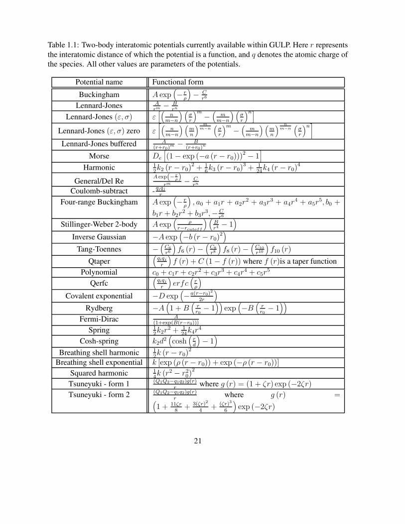
Table 1.1: Two-body interatomic potentials currently available within GULP. Here r representsthe interatomic distance of which the potential is a function, and q denotes the atomic charge ofthe species. All other values are parameters of the potentials.
Potential name Functional formBuckingham A exp
(
− rρ
)
− Cr6
Lennard-Jones Arm − B
rn
Lennard-Jones (ε, σ) ε[(
nm−n
) (
σr
)m −(
mm−n
) (
σr
)n]
Lennard-Jones (ε, σ) zero ε[
(
nm−n
) (
mn
) mm−n
(
σr
)m −(
mm−n
) (
mn
) nm−n
(
σr
)n]
Lennard-Jones buffered A(r+r0)
m − B(r+r0)
n
Morse De
[
(1 − exp (−a (r − r0)))2 − 1
]
Harmonic 12k2 (r − r0)
2 + 16k3 (r − r0)
3 + 124
k4 (r − r0)4
General/Del Re A exp(− rρ)
rm − Crn
Coulomb-subtract - qiqj
r
Four-range Buckingham A exp(
− rρ
)
, a0 + a1r + a2r2 + a3r
3 + a4r4 + a5r
5, b0 +
b1r + b2r2 + b3r
3,− Cr6
Stillinger-Weber 2-body A exp(
ρr−rcutoff
) (
Br4 − 1
)
Inverse Gaussian −A exp(
−b (r − r0)2)
Tang-Toennes −(
C6
r6
)
f6 (r) −(
C8
r8
)
f8 (r) −(
C10
r10
)
f10 (r)
Qtaper(
qiqj
r
)
f (r) + C (1 − f (r)) where f (r)is a taper functionPolynomial c0 + c1r + c2r
2 + c3r3 + c4r
4 + c5r5
Qerfc(
qiqj
r
)
erfc(
rρ
)
Covalent exponential −D exp(
−a(r−r0)2
2r
)
Rydberg −A(
1 + B(
rr0− 1
))
exp(
−B(
rr0− 1
))
Fermi-Dirac A(1+exp(B(r−r0)))
Spring 12k2r
2 + 124
k4r4
Cosh-spring k2d2(
cosh(
rd
)
− 1)
Breathing shell harmonic 12k (r − r0)
2
Breathing shell exponential k [exp (ρ (r − r0)) + exp (−ρ (r − r0))]
Squared harmonic 14k (r2 − r2
0)2
Tsuneyuki - form 1 (Q1Q2−q1q2)g(r)r
where g (r) = (1 + ζr) exp (−2ζr)
Tsuneyuki - form 2 (Q1Q2−q1q2)g(r)r
where g (r) =(
1 + 11ζr8
+ 3(ζr)2
4+ (ζr)3
6
)
exp (−2ζr)
21
an atom is fixed, since both the magnitude and direction readily alter within the crystalline en-vironment according to the polarisability of the species. There are two approaches to modellingthe polarisability that have been widely used, which we will now introduce.
The first, and most intuitive model is to use a point ion dipolar polarisability, α, which, in thepresence of an electric field, Vf , will give rise to a dipole moment, µ, and energy of interactionas given below:
µ = αVf
Upolarisation = −1
2αV 2
f
This approach has the advantage that it is readily extended to higher order polarisabilities, suchas quadrupolar, etc [45]. It has been applied both in the area of molecular crystals, thoughoften fixed moments are sufficient here [46], and, more recently, to ionic materials by Wilson,Madden and co-workers [47]. The only disadvantage of this approach is that the polarisabilityis independent of the environment, which implies that it is undamped at extreme electric fieldsand can lead to a polarisation catastrophy. It is well documented that the polarisability of theoxide ion is very sensitive to its location, since in the gas phase the second electron is unboundand only associates in the solid state due to the Madelung potential [48]. A further complicationis that the scheme must involve a self-consistency cycle if the induced multipoles on one atomiccentre are allowed to interact with those on another, though in some approaches this is neglectedfor simplicity.
The second approach to the inclusion of dipolar polarisability is via the shell model firstintroduced by Dick and Overhauser [49]. Here a simple mechanical model is used, wherebyan ion is divided into a core, which represents the nucleus and inner electrons of the ion andtherefore has all of the mass associated with it, and a shell, which mimics the valence electrons.Although it is convenient to think in terms of this physical picture, it should not be taken tooliterally as in some situations the shell can carry a positive charge, particularly for metal cations.The core and shell are Coulombically screened from each other, but coupled by a harmonicspring of force constant kcs. If the shell charge is qs, then the polarisability of the ion in vacu isgiven by;
α =q2s
kcs
By convention, the short-range forces are specified to act on the shell, while the Coulombpotential acts on both. Hence, the short-range forces act to damp the polarisability by effec-tively increasing the spring constant, and thus the polarisability is now environment dependent.The shell model has been widely adopted within the ionic materials community, particularlywithin the UK. Although the same issue exists as for point ion polarisabilities, namely thatself-consistency has to be achieved for the interaction of the dipoles due to the positions ofthe shells, the problem is transformed into a coordinate optimisation one. This can be solvedconcurrently with the optimisation of the atomic core positions. The main disadvantage of thisapproach is that is not naturally extensible to higher order moments, though some attempts have
22
been made, such as the spherical and elliptical breathing shell models. Furthermore, when per-forming molecular dynamics special treatment of the shells must be made by either using anadiabatic approach, in which the shells are optimised at every timestep, or by using a techniqueanaloguous to the Car-Parrinello method [50], in which a fictious mass is assigned to the shell[51].
As a final note on the topic of polarisability, it is impossible to distinguish from a phe-nomenological point of view between on site ion polarisation and charge transfer between ions.This may explain why the combination of formal charges with the shell model has been sosuccessful for modelling materials that are quite covalent, such as silica polymorphs. Providedthe crystal symmetry is low enough, the shell model could be viewed as representing chargetransfer/covalency.
1.3.5 Radial interactionsThere is a refinement to the conventional point particle shell model, which is the so-calledbreathing shell model, that introduces non-central ion forces [52]. Here the ion is assigned afinite radius, R0, and then all the short-range repulsion potentials act upon the radius of the ion,rather than the nuclear position. A radial constraining potential is then added which representsthe self-energy of the ion. Two functional forms are most commonly used:
UBSM−Harmonici =
1
2KBSM (Ri − R0)
2
UBSM−Exponentiali = K
′
BSM (exp (ρ (Ri − R0)) + exp (−ρ (Ri − R0)))
This model has two important consequences. Firstly, it allows the change of radius betweentwo different coordination environments to be modelled - for example, octahedral versus tetra-hedral. This represents an alternative to using different repulsive parameters in the Buckinghampotential by scaling the A term according to exp (−ρtet/ρoct) to correct for this effect. Secondly,the coupling of the repulsive interactions via a common shell radius creates a many-body effectthat is able to describe the Cauchy violation (C12 6= C44) for rock salt structured materials.
1.3.6 Three-body interactionsThere are two physical interpretations for the introduction of three-body terms, depending onwhether you take a covalent or ionic perspective. Within the former view, as adopted by molec-ular mechanics, the three-body potential represents the repulsion between bond pairs, or evenoccasionally lone pairs. Hence, the form chosen is usually a harmonic one that penalises devi-ation from the expected angle for the coordination environment, such 120ofor a trigonal planarcarbon atom:
Uijk =1
2k2 (θ − θ0)
2
23

Table 1.2: Three-body interatomic potentials currently available in GULP. For potentials witha unique pivot atom, this atom is taken to be atom 1 and θ is the angle between the vectors r12
and r13. All terms other than θ, θ123, θ231, θ312, r12, r13, r23 are parameters of the potential.
Potential name Functional formThree (harmonic) 1
2k2 (θ − θ0)
2 +16k3 (θ − θ0)
3 + 124
k4 (θ − θ0)4
Three (exponential-harmonic) 12k2 (θ − θ0)
2 exp(
− r12
ρ12
)
exp(
− r13
ρ13
)
Three (exponential) k exp(
− r12
ρ12
)
exp(
− r13
ρ13
)
exp(
− r23
ρ23
)
Axilrod-Teller k (1+3 cos(θ123) cos(θ231) cos(θ312))r3
12r3
13r3
23
Stillinger-Weber 3-body k exp(
ρ12
r12−rcutoff12
+ ρ13
r13−rcutoff13
)
(cos (θ) − cos (θ0))2
Bcross k (r12 − r012) (r13 − r0
13)
Urey-Bradley 12k2 (r23 − r0
23)2
Vessal k2((θ0−π)2−(θ−π)2)2
8(θ0−π)2exp
(
− r12
ρ12
)
exp(
− r13
ρ13
)
Cosine-harmonic 12k2 (cos (θ) − cos (θ0))
2
Murrell-Mottram k exp (−ρQ1) fMM (Q1, Q2, Q3)fMM = c0 + c1Q1 + c2Q
21 + c3 (Q2
2 + Q23) + c4Q
31 +
c5Q1 (Q22 + Q2
3) + (c6 + c10Q1) (Q33 − 3Q3Q
22) + c7Q
41 +
c8Q21 (Q2
2 + Q23) + c9 (Q2
2 + Q23)
2
Q1 = R1+R2+R3√3
,Q2 = R2−R3√2
,Q3 = 2R1−R2−R3√6
R1 =r12−r0
12
r0
12
,R2 =r13−r0
13
r0
13
,R3 =r23−r0
23
r0
23
BAcross (k12 (r12 − r012) + k13 (r13 − r0
13)) (θ − θ0)Linear-three-body k (1 ± cos (nθ))
Bcoscross k (1 + b cosm (nθ)) (r12 − r012) (r13 − r0
13)
At the other end of the spectrum, ionic materials possess three-body forces due to the three-centre dispersion contribution, particularly between the more polarisable anions. This is typi-cally modelled by the Axilrod-Teller potential [53]:
Uijk = k(1 + 3 cos (θijk) cos (θjki) cos (θkij))
r3ijr
3jkr
3ik
As with two-body potentials, there are many variations on the above themes, such as couplingthe three-body potential to the interatomic distances, but the physical reasoning is often thesame. A full tabulation of the three-body potentials is given in Table 1.2.
24
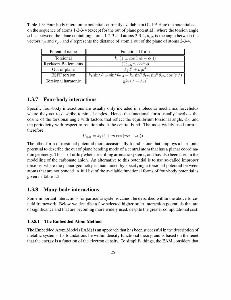
Table 1.3: Four-body interatomic potentials currently available in GULP. Here the potential actson the sequence of atoms 1-2-3-4 (except for the out of plane potential), where the torsion angleφ lies between the plane containing atoms 1-2-3 and atoms 2-3-4, θijk is the angle between thevectors rji and rjk, and d represents the distance of atom 1 out of the plane of atoms 2-3-4.
Potential name Functional formTorsional k4 (1 ± cos (nφ − φ0))
Ryckaert-Bellemanns ∑5n=0 cn cosn φ
Out of plane k2d2 + k4d
4
ESFF torsion k1 sin2 θ123 sin2 θ234 + k2 sinn θ123 sinn θ234 cos (nφ)
Torsional harmonic 12k2 (φ − φ0)
2
1.3.7 Four-body interactionsSpecific four-body interactions are usually only included in molecular mechanics forcefieldswhere they act to describe torsional angles. Hence the functional form usually involves thecosine of the torsional angle with factors that reflect the equilibrium torsional angle, φ0, andthe periodicity with respect to rotation about the central bond. The most widely used form istherefore:
Uijkl = k4 (1 + m cos (nφ − φ0))
The other form of torsional potential more occasionally found is one that employs a harmonicpotential to describe the out of plane bending mode of a central atom that has a planar coordina-tion geometry. This is of utility when describing aromatic systems, and has also been used in themodelling of the carbonate anion. An alternative to this potential is to use so-called impropertorsions, where the planar geometry is maintained by specifying a torsional potential betweenatoms that are not bonded. A full list of the available functional forms of four-body potential isgiven in Table 1.3.
1.3.8 Many-body interactionsSome important interactions for particular systems cannot be described within the above force-field framework. Below we describe a few selected higher order interaction potentials that areof significance and that are becoming more widely used, despite the greater computational cost.
1.3.8.1 The Embedded Atom Method
The Embedded Atom Model (EAM) is an approach that has been successful in the description ofmetallic systems. Its foundations lie within density functional theory, and is based on the tenetthat the energy is a function of the electron density. To simplify things, the EAM considers that
25

Table 1.4: Density functionals available within the Embedded Atom Method.
Functional Functional formPower law f (ρ) = ρ
1
n
Banerjea and Smith [54] f (ρ) = c0
(
1 − 1n
ln(
ρρ0
)) (
ρρ0
) 1
n + c1
(
ρρ0
)
Numerical splined data from data file
Table 1.5: Functional forms for the distance dependence of the atomic density available withinthe Embedded Atom Method.
Density Functional formPower law ρij = cr−n
ij
Exponential ρij = crnij exp (−d (rij − r0))
Gaussian ρij = crnij exp
(
−d (rij − r0)2)
Cubic ρij = c (rij − r0)3for rij < r0
Quadratic ρij = c (rij − r0)2for rij < r0
Quartic ρij = c (rij − r0)4for rij < r0
Voter-Chen cr6ij (exp (−βrij) + 29 exp (−2βrij))
the electron density is a superposition of the atomic densities, and that instead of integrating thedensity across all space it is sufficient just to express the energy as a function of the density atthe nucleus of an atom, summed over all particles:
UEAM = −N∑
i=1
f (ρi)
The above equations encapsulate the idea that the interaction between any given pair of atomsis dependent on the number of other atoms within the coordination sphere. Within this genericscheme there are a number of variations, based around different functionals of the density (Table1.4) and different representations of how the density varies with distance (Table 1.5).
In the original work of Sutton and Chen [55], which developed and extended the ideas ofFinnis and Sinclair [56], a square root was used as the density functional, while the density itselfwas represented as an inverse power of the interatomic distance. The densities from the paperof Finnis and Sinclair, both the quadratic and combined quadratic-cubic form, can both alsobe used. One of the beauties of the EAM is that, in principle, once the metal is parameterisedit can be studied in other environments, such as alloys, without further modification. On thedownside, the prediction of the relative stability of phases can be sensitive to the cut-off radius
26

chosen, though if care is taken this problem can be surmounted [57].
1.3.8.2 Bond Order Potentials
Related in many ways to the embedded atom method, but with a more sophisticated formalism,are so-called bond order potentials. It was recognised by Abell [58] that the local binding energycould be expressed as follows:
UBO =N∑
i=2
i−1∑
j=1
[
U repulsive (rij) − BijUattractive (rij)
]
where Bij is the bond order between the atoms i and j. The bond order is dependent on thelocal environment of both atoms and thereby converts an apparent two-body interaction into amany-body one. Several different formulations have been proposed, most notably by Tersoff[59, 60], and also more recently by Pettifor and co-workers [61], where the latter use a moreextensive analysis of the contributions to the bond order and appeal to first principles methodsto extract the parameters. One particular model has had an enormous impact in recent yearsdue to its applicability to carbon polymorphs and hydrocarbon systems, that due to Brenner andco-workers [62]. Unsurprisingly, it has been extensively applied to fullerenes, nanotubes anddiamond, as systems of topical interest. One of the other reasons for the popularity of the modelis the fact that Brenner makes his code freely available. An independent implementation of theBrenner model has been made within GULP, since the capabilities of the program require thatanalytic derivatives to at least second order, and preferably third, are present, which is not thecase for the existing code. To date, there exist three published variants of the Brenner potentials,but we have implemented just the latest of these models since it superceeds the previous two[63].
The terms in the expression for the energy in the Brenner model are expressed as follows:
U repulsive (r) = Af c (r)(
1 +Q
r
)
exp (−αr)
Uattractive (r) = f c (r)3∑
n=1
Bn exp (−βnr)
where A, Q, α, B1−3, and β1−3 are parameterised constants that depend on the atomic species, Cor H, involved and f c (r) is a cosine tapering function to ensure that the potential goes smoothlyto zero of the form:
1 r < rmin
f c (r) = 12
[
1 + cos(
(r−rmin)(rmax−rmin)
π)]
rmin < r < rmax
0 r > rmax
27

The bond order term itself is composed of several terms;
Bij =1
2
(
bσ−πij + bσ−π
ji
)
+1
2
(
ΠRCij + bDH
ij
)
Note that the above expression for Bij differs from the one given in the defining manuscript dueto the factor of a half for the second term, but is required to obtain results that agree with thosequoted. The first two terms in the above equation represent the influence of local bond lengthsand angles about the atoms i and j, respectively, while the third term is a correction for radicalcharacter, and the fourth one for the influence of dihedral angles. Both of the last two terms arerelated to the degree of conjugation present. Full defining equations for these terms, along withthe parameters, can be found in the original reference and the subsequent errata.
In the above many-body contributions to the bond order, bicubic and tricubic splines areused to interpolate parameter values. For the distributed Brenner potential code, the spline co-efficients are precomputed and supplied as data files. In the present implementation the splinesare performed internally on the fly. This has two advantages in that it both avoids possibletranscription errors, as well as loss of precision through I/O, and allows for the possibility ofparameter fitting to be readily implemented.
Because of the short-ranged nature of the Brenner potential we have implemented two dif-ferent algorithms for the evaluation of the interactions. The first involves a conventional searchover all atoms to find neighbours with a non-zero interaction. The second uses a spatial decom-position of the system into cubes of side length equal to the maximum range of the potential.Consequently only atoms within neighbouring cubes can possibly interact. This leads to a linearscaling algorithm that is far more efficient for large systems. A comparison is presented in theresults section.
While the Brenner model does have many strengths, such as its ability to describe bonddissociation, there are also a few limitations. Perhaps the most significant is the difficulty indescribing long-range forces. For instance, there is no bonding between the sheets for graphite.There have been a number of remedies proposed, including adding on two-body potentials todescribe these effects, either only between different molecules, or with a tapering that removesthe interaction at short-range so as not to invalidate the parameterisation. However, there arelimitations to these approaches, though a more sophisticated expression for removing the con-tribution of long-range forces where the existing interactions due to the Brenner potential aresignificant shows promise [64]. As yet, this is still to be implemented.
1.3.9 One-body interactionsGoing to the other extreme of complexity from many-body interactions, we have the simplistpossible atomistic model, namely the Einstein model [65]. This approach deviates from thosethat have gone before in that there is no interaction between particles and all atoms are simply
28

tethered to their lattice site by harmonic springs:
UEinstein =1
2
N∑
i=1
ki
(
(
xi − x0i
)2+(
yi − y0i
)2+(
zi − z0i
)2)
This model acts as a reference state since all interactions are purely harmonic and consequentlythe phonon density of states, and also the structure, are independent of temperature. This impliesthat all the quantities that can be derived from the vibrational partition function can be analyt-ically determined for any temperature without approximation, unlike other potential models.Even a structure that consistents of atoms coupled together by a series of harmonic potentialshas implied anharmonicity that arises from the derivatives of the transformation matrix from thebond-oriented pairwise frame of reference to the Cartesian one.
Given that the results of the Einstein model can be derived without recourse to a structuraldescription, there is no need to employ an atomistic simulation program in order to calculatethe required quantities. However, it can be useful to combine the Einstein model with a conven-tional, more accurate, representation of the interactions for use in thermodynamic integration[66]. Since the free energy of the Einstein crystal is known under any conditions, it is possibleto extract free energies from molecular dynamics via a series of perturbative runs in which theEinstein model is introduced to an anharmonic potential in a series of steps, as a function of aswitching parameter, λ, in order to obtain the difference relative to the known value.
It is worth highlighting the differences between the Einstein model and all others within theprogram. Because of the lack of interatomic interactions, there can be no optimisation of thestructure and no strain related properties calculated. For the same reason, there is no phonondispersion across the Brillouin zone. Finally, because the particles are tethered to lattice sitesthere is no translational invariance, and consequently all vibrational frequencies are positive andnon-zero (assuming all force constants are specified to be likewise).
1.3.10 Potential truncationAs previously mentioned, all potentials must have a finite range in order to be calculable. How-ever, there are a range of conditions for a potential to act between two species, as well as variousmethods for handling the truncation of potentials. Hence, it is appropriate to describe a few ofthese issues here.
1.3.10.1 Radial truncation
The natural way to truncate a potential is through the use of a spherical cut-off radius. It is alsopossible to specify a minimum radius from which the potential should act too. Hence, it is pos-sible to create multiple distance ranges within a potential with different forcefield parameters,as well as to overlay different potentials. Of course, where there is a cut-off boundary, there willbe a discontinuity in the energy for most interaction terms, unless the potential smoothly tends
29

to zero at that distance by design. This can lead to problems during energy minimisation, sincethe point of lowest energy may not be a point of zero force anymore, and in other simulationtechniques, such as molecular dynamics, where energy conservation will be affected by discon-tinuities. Other than increasing the cut-off radius, there are several approaches to minimisingthese difficulties as described briefly in the subsequent subsections.
1.3.10.2 Cut and shift
To avoid a discontinuity in the energy at the potential cut-off, a constant shift can be added tothe potential so that the energy at the cut-off boundary becomes zero:
U shiftedij (rij) = Uij (rij) − Uij (rcut)
where rcut is the cut-off radius. However, the gradient is still discontinuous at the cut-off dis-tance, so the procedure can be extended by adding a linear term in the distance such that thegradient is also zero at this point. While in principle this method can be applied to make anyorder of derivative go exactly to zero at the boundary by construction, the increasing powersof distance lead to the correction terms modifying the variation of the potential with distancemore strongly as the order rises. This characteristic, that the potential is modified away fromthe point of cut-off, makes this method of smoothing less desirable than some.
1.3.10.3 Tapering
In this approach, the potential is multiplied by a smooth taper function that goes to zero, bothfor its value and its derivatives typically up to second order. This is usually applied over a shortrange from an inner radius, rtaper, to the cut-off distance:
Uij (rij) rij < rtaper
Uij (rij) f taper (rij) rtaper < rij < rcut
0 rij > rcut
Hence, within rtaper the potential is unchanged. There are numerous possible functionalforms that satisfy the required criteria for a taper function. Perhaps the two most commonly usedare a fifth order polynomial or a cosine function with a half a wavelength equal to rcut − rtaper.Both of these are available within GULP as part of the overall two-body potential cut-off.
1.3.10.4 Molecular mechanics
In the simulation of molecular systems, it is often preferable to use a molecular mechanicsforcefield. This implies that certain cut-offs are determined by connectivity, rather than bydistance alone. For example, particular potentials may only act between those atoms that are
30

bonded, such as a harmonic force constant, whereas others may specifically only act betweenthose that aren’t covalently linked. Fundamental to this is the notion of a bond between atoms.Within GULP these can either be determined automatically by comparing distances betweenpairs of atoms with the sum of the covalent radii, multiplied by a suitable tolerance factor, oralternatively the connectivity can be user specified. From this information, it is possible forthe program to determine the number of molecules and, in the case of periodic systems, theirdimensionality.
A number of options are possible that control how both the potentials and the Coulombterms act, as described below:
• Bonded: A potential may act only between atoms that are bonded (1-2).
• Exclude 1-2: The case of bonded atoms is specifically omitted from the allowed interac-tions.
• Exclude 1-3: Interactions between bonded atoms and those with a common bonded atomare excluded.
• Only 1-4: A potentials only act between atoms that are three bonds apart. This can beuseful in the description of torsional interactions.
• Intramolecular: Only interactions within a given molecule are permitted for the potential.
• Intermolecular: Only interactions between atoms of different molecules are allowed.
• Molecular Coulomb subtraction: All electrostatic interactions between atoms within thesame molecule are excluded. This implies that the charges on the atoms within a moleculepurely serve to describe its interaction with other molecules.
• Molecular mechanics Coulomb treatment: This implies that Coulomb terms are excludedfor all 1-2 and 1-3 interactions. In addition, it is sometimes desirable to remove, or scaledown, 1-4 electrostatic interactions too. The benefit of this is that the parameters of theintramolecular potentials then have a direct correspondance with the equilibrium bondlengths, bond angles and localised vibrational frequencies. It should be noted that two-body potentials can also be scaled for the 1-4 interaction, if so desired.
1.3.11 Partial occupancyMany materials have complex structures which include disorder of one form or another. Thiscan typically consist of partial occupancy where there are more symmetry degenerate sites thanthere are ions to occupy them, or where there are mixtures of ions that share the same structuralposition. In principle, the only way to accurately model such systems is to construct a supercellof the material containing a composition consistent with the required stoichiometry and then to
31

search through configuration space for the most stable local minima, assuming the system is inthermodynamic equilibrium (which may not always be the case). This includes allowing for thecontribution from the configurational entropy to the relative stability. While this approach hasbeen taken for several situations, most notably some of the disordered polymorphs of alumina[67, 68], it is demanding because of the shear number of possibilities which increases with afactorial dependance.
There is an approximate approach to the handling of disorder, which is to introduce a mean-field approach. Here all atoms are assigned an occupancy factor, oi, where 0 ≤ oi ≤ 1, and allinteractions are then scaled by the product of the relevant occupancies:
Um−fij = oiojUij
Um−fijk = oiojokUijk
and so on for high order terms. This approach can be utilised in any atomistic simulationprogram by scaling all the relevant potential parameters according to the above rules. However,for complex forcefields this can be tedious, and it also precludes fitting to multiple structureswhere the occupancies of ions of the same species are different. Hence, the inclusion of partialoccupancies has been automated in GULP so that only the site occupancies have to be specifiedand everything else is handled by the program. This includes the adding of constraints so thatatoms that share the same site move together as a single particle, as well as checking that the sumof the occupancies at any given site do not exceed one. It should be noted that the handling ofpartial occupancies requires particular care in determining phonons where the matrix elementsfor all coupled species must be condensed in order to obtain the correct number of modes.
The use of a mean field model is clearly an approximation. For structures, it can often workquite well, since crystallography returns an average anyway. However, for other quantities,such as thermodynamic data it has limitations. For example, the excess enthalpy of mixingof two phases is typically overestimated since the stabilisation that arises from local structuraldistortions to accommodate particular species is omitted [69].
1.3.12 Structural optimisationHaving defined the internal energy of a system, the first task to be performed is to find theminimum energy structure for the present material. To be more precise, this will typically bea local minimum on the global potential energy surface that the starting coordinates lie closestto. Trying to locate the global energy minimum is a far more challenging task and one that hasno guarantee of success, except for the simplist possible cases. There are several approaches tosearching for global minima, including simulated annealing [70], via either the Monte Carlo ormolecular dynamics methods, and genetic algorithms [71, 72]. Here we will focus the quest fora local minimum.
32

At any given point in configuration space, the internal energy may be expanded as a Taylorseries:
U (x + δx) = U (x) +∂U
∂xδx +
1
2!
∂2U
∂x2(δx)2 + ...
where the first derivatives can be collectively written as the gradient vector, g, and the secondderivative matrix is referred to as the Hessian matrix, H . This expansion is usually truncated ateither first or second order, since close to the minimum energy configuration we know that thesystem will behave harmonically.
If the expansion is truncated at first order then the minimisation just involves calculating theenergy and first derivatives, where the latter are used to determine the direction of movementand a line search is used to determine the magnitude of the step length. In the method ofsteepest descents this process is then repeated until convergence. However, this is known to bean inefficient strategy since all the previous information gained about the energy hypersurfaceis ignored. Hence it is far more efficient to use the so-called conjugate gradients algorithm [73]where subsequent steps are made orthogonal to the previous search vectors. For a quadraticenergy surface, this will converge to the minimum in a number of steps equal to the number ofvariables, N .
If we expand the energy to second order, and there by use a Newton-Raphson procedure,then the displacement vector, ∆x, from the current position to the minimum is given by theexpression:
∆x = −H−1g
which is exact for a harmonic energy surface (i.e. if we know the inverse Hessian matrix andgradient vector at any given point then we can go to the minimum in one step). For a realisticenergy surface, and starting away from the region close to the minimum, then the above ex-pression becomes increasingly approximate. Furthermore, there is the danger that if the energysurface is close to some other stationary point, such as a transition state, then simply applyingthis formula iteratively may lead to a maximum, rather than the minimum. Consequently, theexpression is modifed to be
∆x = −αH−1g
where α is a scalar quantity which is determined by performing a line search along the searchdirection to find the one-dimensional minimum and the procedure becomes iterative again, asper conjugate gradients.
By far, the most expensive step of the Newton-Raphson method, particularly once the sizeof the system increases, is the inversion of the Hessian. Furthermore, the Hessian may only varyslowly from one step to the next. It is therefore wasteful and undesirable to invert the this matrixat every step of the optimisation. This can be avoided through the use of updating formulae thatuse the change in the gradient and variables between cycles to modify the inverse Hessian suchthat it approaches the exact matrix. Two of the most widely employed updating schemes arethose due to Davidon-Fletcher-Powell (DFP) [74] and Broyden-Fletcher-Goldfarb-Shanno [75],
33

which are given below:
HDFPi+1 = HDFP
i +∆x ⊗ ∆x
∆x.∆g−(
HDFPi .∆g
)
⊗(
HDFPi .∆g
)
∆g.HDFPi .∆g
HBFGSi+1 = HBFGS
i +∆x ⊗ ∆x
∆x.∆g−(
HBFGSi .∆g
)
⊗(
HBFGSi .∆g
)
∆g.HBFGSi .∆g
+
[
∆g.HBFGSi .∆g
]
v ⊗ v
v =∆x
∆x.∆g− HBFGS
i .∆g
∆g.HBFGSi ∆g
The BFGS algorithm is generally recognised as the more efficient one and so is the defaultoptimiser. However, if performing a transition state search then DFP is preferred due to thedifferent tendances of the updates with regard to targetting a positive definite character for theHessian. The practical approach taken in a BFGS optimisation is to initialise the Hessian byperforming an exact inversion of the second derivatives and then subsequently updating for anumber of cycles. Occassionally it is necessary to calculate the exact inverse Hessian again.This is triggered by one of a number of possible situations:
• The maximum number of cycles for updating is exceeded
• The angle between the gradient vector and the search vector exceeds a given threshold
• The energy has dropped by more than a certain threshold in one cycle, so the curvature islikely to have altered
• The energy cannot be lowered by line minimisation along the current search vector
There is one variation upon the BFGS strategy above, in which, rather than calculating theexact second derivative matrix and inverting it, the Hessian is initialised approximately andthen updated such that it tends to the true Hessian. Two possible starting approximations tothe Hessian are either to use a unit matrix or to perform a finite difference estimate of theon-diagonal elements only in order to achieve better preconditioning. By taking this approachthe cost is similar to conjugate gradients, though with a higher memory requirement, but theconvergence is typically twice as fast since more information from previous energy/gradientevaluations is retained.
The choice of appropriate algorithm for minimisation depends on the size of the systemand number of variables. For small systems, the Newton-Raphson methods that use secondderivatives will be far more efficient. As the size of system increases, the computational costof building and inverting the Hessian matrix will ultimately grow as N 3 while the memoryrequirements also increase as N (N + 1) /2 for lower-half triangular storage. Hence, ultimately
34

it will become necessary to use first the unit Hessian approach and then ultimately the conjugategradients method as N continues to increase. This balance may also be influenced by the useof symmetry, where possible, as will be discussed later. A further issue is that for minimisationwhere the initial structure lies outside the harmonic region, Newton-Raphson methods may notbe particularly advantageous, whereas they will be as convergence is approached. Hence GULPincludes the facility to change the minimiser from, for example, conjugate gradients, to BFGSwhen a criterion is met, such as the gradient norm falling below a specified threshold.
Aside from the minimisation algorithm itself, something should be said about the criteriafor convergence of an optimisation. Typically some or all of the following can be checked forconvergence:
• the gradient norm (root mean square gradient per variable)
• the maximum individual gradient component
• the norm of the estimated displacement vector
• the change in the function (energy, enthalpy or free energy) between successive cycles
• the change in the variables between successive cycles
Normally all of these quantities are well converged (and often excessively so - i.e. well be-yond chemical accuracy) with Newton-Raphson optimisation for a forcefield. Occassionallyconvergence is not achieved, which is nearly always indicative of a significant discontinuity inthe energy surface, such as that caused by interatomic potential cut-offs. Ideally all potentialsshould be tapered so that their value, first and second derivatives go smoothly to zero at thecut-off radius. In practice, most repulsive potentials are negligibly small by a typical cut-offdistance of 10 Angstroms and so it is usually the attractive potentials that mimic dispersionthat are responsible. The other common cause are discontinuities in bonding - i.e. an atom isdisplaced beyond a bond cut-off during minimisation and so the whole nature of the interactionpotential changes. While this can be overcome by maintaining a fixed connectivity list, the realissue is that the forcefield is inadequate for the system being modelled.
All of the above discussion has related to the search for a local minimum where the firstderivatives are zero and the second derivative matrix is positive definite. However, there aremany instances in which it is necessary to locate other stationary points on the potential energysurface, and in particular transition states, such as for ion diffusion. There are a number ofalgorithms available for locating transition states, of which the most widely used class in solidstate optimisations tend to be constrained minimisations. Here the reaction path is discretised insome way and the system minimised so that the variable changes are orthogonal to the directionof the pathway. Arguably the most successful and widely used approach is the Nudged ElasticBand method [76]. However, the disadvantage of these constrained techniques is that someassumption usually has to be made about the nature of the mechanism before the calculations are
35
performed. In contrast, there are algorithms which use Newton-Raphson techniques in order tolocate stationary points with an arbitrary number of negative eigenvalues for the Hessian (wherea transition state is the special case of a single negative eigenvalue). In the case of GULP, themethod implemented is so-called Rational Functional Optimisation (RFO) [77].
In the RFO method, the inverse Hessian matrix is diagonalised to obtain the eigenvalues andeigenvectors. From the eigenvalues it is possible to examine whether the matrix has the requiredcharacteristics for the stationary point being sought. If the number of negative eigenvalues isincorrect, then the spectrum is level-shifted to correct this and the search direction constructedappropriately. By default, the Hessian modes with the smallest eigenvalues are followed towardsthe corresponding stationary point. However, eigenvector following can also be performedin which different modes from the spectrum are selected. Hence the RFO optimiser will, inprinciple, locate various possible transition states starting from a given position. There are afew provisos though, most notably that there must be a non-zero projection of the gradientvector in the search direction leading to the stationary point. Furthermore, the step size mustbe quite small in order to ensure convergence to a transition state. Since the line search canno longer be used, the optimisation relies on a fixed proportion of the search vector to achieveconvergence. In the implementation in GULP, this step magnitude is correlated to the gradientnorm, so that as the calculation approaches convergence, and therefore enters the harmonicregion, the proportion of the search vector used approaches 100%. Hessian updating can alsobe applied while optimising towards a transition state. However, because the rate of convergencedepends more critically on the inverse Hessian being accurate, more frequent exact calculationsare usually required. RFO can also be used to accelerate optimisations to minima once theharmonic region is approached, since it is able to better handle soft modes. In extreme cases,the number of cycles is reduced by an order of magnitude by use of RFO towards the end ofan optimisation, as well confirming that the Hessian has the required structure. A final note ofcaution is that this method does not guarantee that a local minimum has been achieved, even ifthe Hessian is confirmed as having all positive eigenvalues. This is because the Hessian onlyspans the space of the allowed optimisation variables and there may be directions of negativecurvature with respect to constrained degrees of freedom. Hence, a Γ-point phonon calculationshould always be used as a final validation.
Often it is desirable to apply external forces to a system when performing a minimisation.The most common example is the application of an isotropic external pressure, such as used inthe determination of the equation of state for a material. This situation can be straightforwardlyhandled by making the objective function for minimisation the enthalpy instead of the internalenergy:
H = U + pV
More complex is the case when an external force is to be applied to individual atoms. Thisarises when the program is being coupled to a separate quantum mechanical calculation as partof a QM/MM method (i.e. a quantum mechanics/molecular mechanics coupled calculation).Here the forces on the forcefield atoms arise from the quantum mechanical region, which is not
36

explicitly considered in the present calculation. Adding the negative of the external forces tothe internal derivatives is simple to implement. However, for minimisation the internal energyis no longer a well-behaved objective function (i.e. the minimum of the internal energy doesnot correspond to a configuration of zero gradients). One solution to this would be to minimisethe gradient norm instead, but this requires either one order higher of energy derivatives or thatconjugate gradients are used to minimise, which is less efficient.
The approach implemented within GULP to handle the application of external forces is todefine a new additional term in the internal energy, which is the work due to the external force:
U external = −∫ final
initialF external.α
where α represents the vector of atomic coordinates and F external is the vector of external forces.With this correction to the internal energy, the minimum coincides with force balance and sothe full range of standard minimisers are applicable. However, the final energy is an arbitraryquantity unless taken with respect to a standard reference set of atomic positions.
The framework of structural optimisation in GULP is designed to be flexible and to allow theuser as much freedom as possible to control the degrees of freedom. Intrinsically, there are fourmain classes of variables possible within the forcefield models available, namely, atomic coor-dinates, the unit cell periodicity (for polymers, surfaces, and bulk materials), shell coordinates,and breathing shell radii. Each variable can be controlled by optionally specifying a binary flagthat indicates whether it is to be varied or held fixed. Alternatively there are keywords that selectdefault settings of the flags, such that those quantities not constrained by symmetry are allowedto vary. In particular, the defaults automatically handle the fact that one atom must be fixed inorder to remove the three translational degrees of freedom. For bulk systems, the first atom isusually the one chosen to be fixed, since the choice is arbitrary. In the case of slab calculations,the atom nearest the centre of the slab is fixed since this is the one least likely to move by asubstantial amount. When there is a centre of symmetry in the space group, then there is noneed to fix any atoms since the origin is already immoveable. The default optimisation optionsalso automatically construct the constraints necessary to preserve the space group symmetry asthe atoms are displaced.
When minimising periodic systems there are a couple of choices that have to be made. Thefirst concerns the representation of the unit cell. This can be achieved through either the unitcell parameters, a, b, c, α, β, γ, or via the Cartesian cell vectors as a (3x3) matrix. Correspondly,when optimising the unit cell this can be done with respect to the cell parameters directly, theCartesian cell vectors or by using a strain tensor. Here we chose to use the Voight strain tensorto scale the Cartesian lattice vectors:
1 + ε112ε6
12ε5
12ε6 1 + ε2
12ε4
12ε5
12ε4 1 + ε3
37
Through using the six Voight strains as the variables, we have the same advantage as work-ing with the unit cell parameters in that cell rotation is eliminated by construction. However, aswill be demonstrated later, the derivatives with respect to strain are closely related to the Carte-sian internal derivatives and therefore readily calculated at almost no extra cost. We should notethat when strain derivatives are taken, they are done so with respect to infinitesimal strain aboutthe current configuration, rather than with respect to a single constant reference cell. For 2-Dsystems, the strain tensor is correspondingly reduced to a (2x2) matrix and for polymers thereis a single scalar strain value. At this point we should also comment on the absolute spatialorientation of systems, since this a matter of convention, rather than an absolute choice. For3-D systems, GULP orients the a cell vector along the x-axis, the b cell vector in the xy-plane,and then the orientation of the c cell vector is fixed, except for an issue of chirality, which isresolved by selecting the orientation that has a positive dot product with the z-axis. For 2-Dsystems, the same two conventions are followed for the surface vectors, which leaves the sur-face normal parallel to the z-axis. Finally, for 1-D systems, the repeat direction is taken to liealong the x-axis.
1.3.13 Genetic algorithmsThe approach to minimisation of a structure has already been discussed when considering thecase of a local stationary point. Now we turn to consider the quest for a global minimum.In order to do this, a technique is required that allows barriers to be overcome in some way.While hyperdynamic [78]and basin-filling approaches are becoming increasingly useful, themore traditional approach has been to employ methods that incorporate random changes in thestructure with a tendancy to minimise a so-called cost function. Here the cost function is aquantity that represents a measure of the quality of the structure. In the most obvious case, thismight be just the total energy of the system. However, because stochastic processes requiremany moves, it is often convenient to use a more computationally efficient cost function. Forexample, one form that has previously been successfully used for oxides is a combination ofbond-valence sum rules with a short-ranged Coulomb penalty that prevents ions of like chargeapproaching each other [79].
There are two main approaches to the global optimisation of structures via a random walk- the Monte Carlo method [80] and Genetic Algorithms (GAs) [71, 79]. Although both are inprinciple equally capable of performing the task, it could be argued that genetic algorithms aremore naturally suited to coarse grained global optimisation, while the Monte Carlo technique isalso able to yield an integration within the phase space of a statistical ensemble. Here we willconcentrate on the use of GAs.
In the genetic algorithm, each optimisation variable is discretised within a specified range.This is particularly well suited to fractional coordinates where there are natural bounds of 0 and1. Then all that need be specified is the number of allowed intervals within the range. If a coarsegrid of points is specified then configuration space will be rapidly searched, but the solution willbe very approximate and the global minimum may not be resolvable with the level of resolution
38
available. Conversely, if a fine grid is utilised then the search is capable of locating a moreaccurate estimate of the global minimum. However, because of the large number of possibleconfigurations, the optimal state may never be visited. Clearly a hierarchical approach may beideal, where a coarse discretisation is initially used and then refined as the process progresses.The state of each configuration is represented by a binary number which is a concatination ofthe binary representations of the grid point numbers for each individual variable.
The fundamental idea behind genetic algorithms is to perform a process that mimics naturalselection through survival of the fittest. Here the concept of fitness equates to the value of thechosen cost function. Each cycle of the GA begins with an even number of so-called parents.In the first step these are typically randomly chosen initial configurations. These parents thenare randomly paired up in order to breed to produce two children in order to maintain the sizeof the population. This is the tournament phase, in which a probability is set for the parent withthe lower cost function to go through to the next generation and to form the children. A randomnumber is chosen and compared to this probability in order to make the decision. Choosingthis probability threshold is a balance between wanting to ensure that the better configurationssurvive against trying to maintain diversity in the population during the initial stages. Moresophisticated tournament procedures have also been proposed where an exponential weightingis used in favour of the fitter candidates. Usually the number of children is set equal to thenumber of parents in order to maintain a stable population size.
Apart from the tournament phase, there are two other processes that can occur, which aremutation and crossover. In the mutation phase, a number of binary digits are changed from 0to 1 or vice versa. Again the chance of this occuring is determined by comparison of a randomnumber to the mutation probability. During crossover, two configurations are selected, thebinary strings split at a random point, and the two parts switched between configurations. Bothmutation and crossover represent genetic defects that are designed to introduce randomnesswith the aim of exploring configuration space.
The above three genetic algorithm steps are applied repeatedly with the aim of graduallyreducing the cost functions of the population down and focussing in on the global minimum.When the procedure is stopped after the specified number of steps, then hopefully the config-uration with the lowest cost function will be the global minimum, though this can never beenknown for certain for complex systems. If the cost function used was an approximation to thetotal energy that is ultimately desired to be the criterion for selection, then a selection of the bestconfigurations can be subsequently minimised according to the total energy and hopefully theglobal minimum will lie amongst this set, even though it is not the structure with the absolutelylowest cost function.
There are several possible refinements to the genetic algorithm procedure, which, somewhatappropriately, is itself still evolving. However, the above basic formulation is capable of cor-rectly predicting the atomic coordinates of binary, and even some ternary oxides, given the unitcell. Indeed, the method had an early success through assisting in the solution of the previouslyunknown structure of Li3RuO4 [72]. More details of the background to, and application of, the
39
genetic algorithm for solid state structural optimisation can be found elsewhere [79].
1.3.14 Calculation of bulk propertiesHaving determined the optimised structure for a material it is then possible to calculate a widerange of physical properties based on the curvature of the energy surface about the minimum.These include both mechanical properties, such as the bulk modulus and elastic constants, aswell as dielectric properties. The expressions used for the calculation of the individual proper-ties that may be determined routinely from the second derivative matrix are detailed below.
1.3.14.1 Elastic constants
The elastic constants represent the second derivatives of the energy density with respect tostrain:
Cij =1
V
(
∂2U
∂εi∂εj
)
thereby describing the mechanical hardness of the material with respect to deformation. Sincethere are 6 possible strains within the notation scheme we employ, the elastic constant tensor isa 6 x 6 symmetric matrix. The 21 potentially independent matrix elements are usually reducedconsiderably by symmetry [81]. For example, for a cubic material the only unique elements areC11, C12, and C44. The calculation of elastic constants is potentially very useful, since the fulltensor has only been measured experimentally for a very small percentage of all known solids.This is primarily because the practical determination typically requires single crystals with asize of a few micrometres at least.
In calculating the second derivatives of the energy with respect to strain it is important toallow for the response of all internal degrees of freedom of the crystal to the perturbation. If weintroduce the following notation for the second derivative matrices:
Dεε =
(
∂2U
∂ε∂ε
)
internal
Dεi =
(
∂2U
∂ε∂αi
)
ε
Dij =
(
∂2U
∂αi∂βj
)
ε
then the full expression for the elastic constant tensor can be written as:
C =1
V
(
Dεε − DεiD−1ij Djε
)
The elastic compliances, S, can be readily calculated from the above expression by invertingthe matrix (i.e. S = C−1). The above expressions are valid for adiabatic conditions and at zero
40

pressure. The adiabatic elastic constants can be extended to the case of finite external pressureaccording to the corrections:
Cαβγζ =1
V
(
∂2U
∂εαβ∂εγζ
)
+p
2(2δαβδγζ − δαζδβγ − δαγδβζ)
Here the strains are expressed directly in terms of the Cartesian components, as opposed to inthe Voight notation, so as to make the corrections more transparent.
Under isothermal conditions the expressions for the elastic constant tensor are analogus,except for the fact that the differentials are with respect to the Helmholtz free energy, ratherthan the internal energy. Because the evaluation of the isothermal elastic constants requires thefourth derivative of the internal energy with respect to internal coordinates and strains, this isnot presently implemented within GULP analytically. However, finite differences may be usedin combination with free energy minimisation in order to determine this tensor.
1.3.14.2 Bulk and shear moduli
Like the elastic constant tensor, the bulk (K) and shear (G) moduli contain information regard-ing the hardness of a material with respect to various types of deformation. Experimentally abulk modulus is much more facile to determine than the elastic constant tensor. If the struc-ture of a material is studied as a function of applied isotropic pressure, then a plot of pressureversus volume can be fitted to an equation of state where the bulk modulus is one of the curveparameters. Typically a third or fourth order Birch-Murgnahan equation of state is utilised.Alternatively, the bulk and shear moduli are also clearly related to the elements of the elasticconstant. However, there is no unique definition of this transformation. Here we give threedifferent definitions due to Reuss, Voight and Hill [81]. Below are the equations for the Reussand Voight definitions, while the Hill values are defined as the average of the other two:
KV oight =1
9(C11 + C22 + C33 + 2 (C12 + C13 + C23))
KReuss = (S11 + S22 + S33 + 2 (S12 + S13 + S23))−1
GV oight =1
15(C11 + C22 + C33 + 3 (C44 + C55 + C66) − C12 − C13 − C23)
GReuss =15
4 (S11 + S22 + S33 − S12 − S13 − S23) + 3 (S44 + S55 + S66)
1.3.14.3 Young’s moduli
When a uniaxial tension is applied to a material then the lengthening of the material is measuredaccording to the strain. The ratio of stress to strain defines the value of the Young’s modulus forthat axis:
Yα =σαα
εαα
41

Since a material will always increase in length under tension, the value of this quantity shouldalways be positive. The Young’s moduli in each of the Cartesian directions can be calculatedfrom the elastic compliances:
Yx = S−111
Yy = S−122
Yz = S−133
1.3.14.4 Poisson’s ratio
Complementary to Young’s modulus is the Poisson ratio, which measures the change in a ma-terial at right angles to the uniaxial stress. Formally it is defined as the ratio of lateral to longi-tudinal strain under a uniform, uniaxial stress. The expression used to calculate this property,assuming an isotropic medium, is given below [81]:
σα (β) = −SααββYβ
Because most materials naturally shrink orthogonal to an applied tension this leads to positivevalues for Poisson’s ratio, with a theoretical maximum of 0.5. Typical values for many materialslie in the range 0.2-0.3, though negative values are also known. For an isotropic material thisquantity can also be related to the bulk modulus:
K =1
3
Y
(1 − 2σ)
1.3.14.5 Acoustic velocities
The acoustic velocities are key quantities in the interpretation of seismic data. The polycrys-talline averages of these acoustic velocities in a solid can be derived from the bulk and shearmoduli of the material, as well as the density, ρ. There are two values, that for a transversewave, Vs, and that for a longitudinal wave, Vp, which are given by:
Vs =
√
G
ρ
Vp =
√
4G + 3K
3ρ
As to be expected, there is some degree of variability in the calculated values according to thedefinition of the bulk and shear moduli employed.
42

1.3.14.6 Static and high frequency dielectric constants
The dielectric properties of a material are of crucial importance in many contexts, includingthose beyond the strictly bulk properties. For example, the response of a solid to a chargeddefect depends on the inverse of the dielectric constant. The actual value of the dielectricconstant varies according to the frequency of the electromagnetic field applied. Commonlytwo extreme values are quoted, namely the static and high frequency dielectric constants. Inthe static limit all degrees of freedom of the crystal, both nuclear and electronic, are able torespond to the electric field and therefore to provide screening. At the high frequency limitthe oscillation is greater than the maximum vibrational frequency of the material and thereforeonly the electrons are able to respond to the perturbation fast enough. Here we describe howto calculate these extremal values, while the case of intermediate frequencies will be presentedlater.
The static dielectric constant (3 x 3) tensor can be determined from the Cartesian secondderivative matrix of all particles, Dαβ , and the vector, q, containing the charges of all particles:
ε0αβ = δαβ +
4π
V
(
qD−1αβq
)
The expression for the high frequency dielectric constant is identical to that for the static equiva-lent, except that the second derivative matrix, Dαβ, now only includes the Cartesian componentsfor any shells present within the model. If a core only model is being used then the high fre-quency dielectric tensor is just a unit matrix. Hence information regarding the high frequencydielectric constants is particularly useful in determining the parameters of a shell model due tothe relatively direct correlation.
Because the dielectric constant tensor depends on the inverse second derivative matrix, ithas many of the characteristics of the Hessian matrix and is therefore quite a sensitive indicatorof whether a potential model is sensible. Extreme values, particularly negative ones, instantlypoint to the fact that the potential model is inadequate or that the system wishes to undergo asymmetry change.
1.3.14.7 Refractive indices
The refractive indices of a material, n, are simply related to the dielectric constant by:
n =√
ε
For orthorhombic, tetragonal or cubic unit cells, in the standard orientation, this represents atrivial mapping since the dielectric constant tensor is a diagonal matrix and so the square rootscan be taken directly. For other crystal systems it is necessary to diagonalise the tensor first andthen find the refractive indices in this new axis eigensystem.
43

1.3.14.8 Piezoelectric constants
The piezoelectric constants are key quantities in many technological applications, since theygovern the correlation between strain in a material and applied electric field for non-centrosymmetricmaterials (centrosymmetric materials necessarily have zero for all piezoelectric constants).There are several different types of piezoelectric constant too, depending on whether it is thepolarisation being induced by a given strain that it is being considered or the stress/strain in-duced by an applied electric field. In GULP, both the piezoelectric stress constants, d, and thepiezoelectric strain constants, e, are calculated:
dαi =∂Pα
∂σi
eαi =∂Pα
∂εi
The two sets are related by a transformation involving either the elastic constant, or the elasticcompliance tensor, depending on the direction. The piezoelectric strain constants are calculatedfrom the Cartesian second derivative matrices according to:
eαi = −N−1∑
k=1
4π
Vqk
(
∂2U
∂α∂β
)−1 (∂2U
∂β∂εi
)
The above piezoelectric strain constants can be readily transformed into piezoelectric stressconstants by multiplication by the elastic compliance tensor.
1.3.14.9 Electrostatic potential, electric field and electric field gradients
The electrostatic site potential is a measure of the Coulomb interaction per unit charge experi-enced by an ion at a given position in space. This can be formally defined by;
Vi =N∑
j=1
qj
rij
where the summation explicitly excludes the case where i = j. Clearly this is closely definedto the definition of the electrostatic energy, the two simply being related by;
U electrostatic =1
2
N∑
i=1
qiVi
Similar considerations also apply with regard to periodic systems (i.e. an appropriate chargesummation technique must be utilised with a net charge and dipole of zero).
The electrostatic potential is a useful quantity for qualitative predictions as to certain prop-erties of a material. For instance, if a structure contains several distinct oxygen sites one might
44

expect that there would be a correlation between site potential and basicity. However, the limi-tations of the point ion, or dipolar shell, model must be kept in mind. Certainly the absolute sitepotential will be totally dependent on the choice of charges in the potential model, and thereforewill be arbitrary, so at best only trends should be considered.
Based on the calculation of the site potential, the electric field, and the electric field gradientmay also be determined as the first and second derivatives, respectively, of this quantity, whileagain excluding the case where i = j;
∂Vi
∂α=
N∑
j=1
− qj
r3ij
αij
∂2Vi
∂α∂β=
N∑
j=1
(
3αijβij − r2ijδαβ
)
r5ij
The electric field gradient tensor is perhaps the most useful quantity since it may be transformedinto the so-called asymmetry parameter, η, which can be important in the interpretation of solidstate NMR data [82]. If we represent the tensorial components of the electric field gradient asVαβ, then first the (3x3) matrix can be diagonalised to yield the three principal axis components,Vxx, Vyy, and Vzz. If the components are labelled V1, V2, and V3, such that |V3|¿|V2|¿|V1|, thenthe asymmetry parameter is defined as;
η =|V2| − |V1|
|V3|
which ensures that the values lie in the range 0-1. A high symmetry site, such as one of Oh
point group where all components are equal, would therefore have an asymmetry of zero.
1.3.14.10 Born effective charges
The quantification of the charges associated with atoms/ions is one of the most problematictasks in theoretical chemistry. Given that the atomic charge is not a direct quantum mechanicalobservable, it is therefore an artificial quantity, but one that is nonetheless useful in the devel-opment of understanding from quantitative results. Not surprisingly there are many differentdefinitions of charge, the most famous of which is that due to Mulliken [37], where overlapdensity is apportioned equally to both nuclear centres. More recently, there has been consider-able interest in Bader analysis [83] as a means of partitioning electron density. Both of theseaforementioned schemes are based on the analysis of the density matrix, or the density itself.However, there is another family of charge definitions which define the atomic charges in termsof the response of the dipole moment of the system with respect to perturbations. Since thedipole is a genuine observable, such charge definitions are particularly attractive for forcefieldsas they describe the charges that are consistent with the response of the material to atomicdisplacements.
45

The most widely used definition in this second category is the Born effective charge:
qBorni =
∂µα
∂βi
Here the charge of an atom is now a symmetric (3x3) tensorial quantity since it describes thederivative of the three Cartesian components of the dipole moment with respect to the threeCartesian atomic displacements. While the definition of the dipole moment is complicated bythe choice of the particular images of each ion, this complication doesn’t affect the derivativesof the dipole moment within the present model. Differentiation of the dipole moment leads tothe following expression for the Born effective charge;
qBorni = qcore
i δαβ −(
Dcore−shellD−1shell−shellq
shell)
i
where the first term on the right-hand side is the core charge of the ion, and the second termis the corresponding component of the product of the core-shell second derivative matrix withthe inverse of the shell-shell second derivative matrix, scaled by the vector of shell charges,qshell. Physically, the second term corresponds to the response of all the shells present to theatomic displacement of atom i, or in other words, the electronic contribution. Hence for a rigidion model, the Born effective charge tensor is equal to a diagonal matrix with all the diagonalelements equal to the core charge. Increasingly the Born effective charges are being determinedfrom ab initio calculations, thus creating a new avenue for determining shell model parametersbeyond the fitting of dielectric constants. Beyond this, the Born effective charges are alsoespecially important in the determination of Γ-point phonon frequencies, as will be discussedin the next section.
1.3.14.11 Phonons
Atoms must constantly be in motion as a consequence of the Heisenberg uncertainty principleand this is achieved through vibrations. At low temperatures the vibrations correspond to simpleharmonic motion about the position of minimum energy, while as the temperature increasesthey become increasingly anharmonic. For a molecule, there will be 3N − 6 vibrational modes(or 3N − 5 for a linear system). In the case of an infinitely perfect 3D solid, there will bea corresponding infinite number of phonons. These phonons are described by calculating theirvalues at points in reciprocal space, usually within the first Brillouin zone. Hence we will obtain3N phonons per k-point. The lowest three modes represent the so-called acoustic branch whichtend to values of zero at the centre of the Brillouin zone (k = 0, 0, 0), known as the Γ-point. Atthis point, the acoustic modes correspond to the pure translation of the crystal lattice, and thusthey are modes of zero frequency. A plot of the vibrational frequencies versus k gives rise tophonon dispersion curves.
To calculate the vibrations or phonons of a system, the starting point is the force constantmatrix, given by the second derivatives with respect to the atoms in Cartesian space. In the case
46

of a solid, the terms must be multiplied by the corresponding phase factor, exp (ik.r). Thus theforce constant matrix, F , between two atoms i and j is given by;
Fiαjβ (k) =∑
R
(
∂2U
∂α∂β
)
exp (ik (rij + R))
The summation over R represents the sum over lattice vectors within the cut-off radius. Thismatrix of force constants is then converted to the dynamical matrix, D, by multiplying by theinverse square root masses of the ions:
Diαjβ (k) =1
(mimj)1
2
Fiαjβ (k)
The origin of the three acoustic phonons at the Γ-point for a solid, or in the regular vibra-tional spectrum for a molecule, arises from the sum rules that govern the energy derivatives.Firstly, the sum of all first derivatives, or alternatively forces, must be equal to zero in theabsence of an external force:
N∑
i=1
(
∂U
∂αi
)
= 0
Secondly, by further differentiating the above expression, it can be shown that the on-diagonalelements of the force constant matrix are equal to the negative sum of the off-diagonal elements:
(
∂2U
∂αi∂βi
)
= −∑
′Nj=1
(
∂2U
∂αi∂βj
)
where the summation now excludes the case when i = j. It should be noted that if a phononcalculation is performed for a surface using a two-region strategy, as will be discussed later,then there will no longer be three modes of zero frequency at the zone-centre. This is becausethe influence of region 2 acts as an external force, which breaks the translational invariance.
In forming the dynamical matrix from the force constant matrix there are a number of issuesrelating to particular forcefields and system types. The most common issue relates to the useof the shell model, in which the shells have zero mass. Since the number of vibrational modesis strictly given by three times the number of atoms, which in this case also corresponds thenumber of cores, then the shell co-ordinates cannot appear directly in the dynamical matrix.Instead the shell contributions are factored into the force constants of the cores according to theexpression:
F totalcc = Fcc − FcsF
−1ss Fsc
where Fcc, Fss, and Fsc are the core-core, shell-shell and shell-core force constant matrices,respectively, and Fcs is just the transpose of Fsc. In the case of the breathing shell model, theshell index is extended to run over the shell radius, as well as its Cartesian co-ordinates.
47

At the Γ-point there is an extra complication in the calculation of the phonons. In materialswhere the atoms possess a charge, the degeneracy of the Transverse Optical (TO) and Longitu-dinal (LO) Optical modes is broken due to the electric field that is generated during vibration.This effect is not allowed for in the usual analytic evaluation of the dynamical matrix. Further-more, the precise splitting that occurs also depends on the direction of approach to the Γ-pointin reciprocal space, kΓ(i.e. the LO and TO modes are likely to be discontinuous at this point inphonon dispersion plots). If the Born effective charges are known then this non-analytic term[84] can be corrected for by adding a correction to the dynamical matrix [38]:
Dnaiαjβ =
4π
V (mimj)1
2
(
kΓ.qborni
)
α
(
kΓ.qbornj
)
β
(kΓε∞kΓ)αβ
where terms have the meanings as previously defined. As to be expected, the influence ofthe charges on the splitting is mediated in inverse proportion to the high frequency dielectricconstant tensor.
Two scenarios arise with regard to the calculation of the Γ-point phonons. If the value for aspecific direction of approach is required, such as in the case of a phonon dispersion curve, thenthe value of kΓmay be explicitly specified. The direction of approach is automatically set equalto the direction of the phonon dispersion curve when the Γ-point is part of one in GULP. Alter-natively, if the intention is to compute the infra-red spectrum as a polycrystalline average, thenthe phonons at this point should be a spherical average over all possible orientations. To allowfor this last possibility, there is the possibility within GULP to perform a numerical integrationby sampling the phonon modes as a function of θ and φ in spherical polar coordinates and thenaveraging the resulting frequencies.
1.3.14.12 Vibrational partition function
Statistical mechanics allows the connection to be made between microscopic quantum energylevels and macroscopic thermodynamic observables [85]. Pivotal to this process is the partitionfunction, Z tot, for the system. In order to determine this quantity we make the assumptionthat all forms of energy are independent and therefore that the total energy is just the sumof contributions from translation, rotation, vibration and the electronic state. In the case of asolid, we can neglect the translational and rotational components, and furthermore since weare considering forcefield methods the electronic energy is not directly calculated. Hence, theproblem reduces down to one of determining the vibration energy levels, and subsequently thecorresponding partition function.
The vibrational energy levels for a harmonic oscillator for the mth mode are simply givenby;
Uvibm (n, k) =
(
n +1
2
)
hω (m, k)
48

if the frequency is specified in Hz. By summing over all energy levels it is possible to show thatthe vibrational partition function is equal to;
Zvib =∑
m
∑
k
exp(
− hω2kBT
)
(
1 − exp(
− hωkBT
))
Here, and subsequently, the explicit dependance of the frequency on mode and k-point hasbeen dropped for brevity. Substituting this expression into the various statistical mechanicalexpressions fors thermodynamic quantities, we obtain the following relationships:
Uvib =∑
m
∑
k
wk
1
2hω +
hω(
exp(
− hωkBT
)
− 1)
Avib =∑
m
∑
k
wk
(
1
2hω + kBT ln
(
1 − exp
(
− hω
kBT
)))
Cvibv =
∑
m
∑
k
wkkB
(
hω
kBT
)2 exp(
− hωkBT
)
(
exp(
− hωkBT
)
− 1)2
Note that the first term in the internal energy is just the zero point vibrational energy. In theabove equations a sum over points in the Brillouin zone is included and the term wk representsthe weight of that particular point, such that the sum of all weights is equal to one. Formallyspeaking, this sum should be an integration over the phonon density of states. In practice, adiscrete sum of points is typically used to numerically integrate the quantities.
There are a number of different choices possible for the set of points in the Brillouin zonefor integration of the thermodynamic properties, just as there are for integration of the bandstructure in an electronic calculation. For high symmetry materials there are occasionally spe-cial point(s), such as those due to Baldereschi [86], and Chadi and Cohen [87]. However, themost appropriate in general is usually the Monkhorst-Pack scheme [88]. This involves an evenlyspaced mesh of k-points, given by three so-called shrinking factors, one along each axis of theBrillouin zone. This still leaves the issue of the translational position of the mesh relative to theorigin. The optimal choice is to maximise the distance of all points from the origin along eachaxis by using an offset of half a mesh spacing from there to the first mesh point. The benefitsof this choice are that it increases the rate of convergence as a function of increasing shrinkingfactor, as well as avoiding the issue of the non-analytic correction to the LO/TO splitting at theΓ-point.
If the space group symmetry has been specified for the material, then it is possible to deter-mine the Patterson group, which is the equivalent of the space group in reciprocal space. Notethat all systems have at least inversion symmetry (also known as time-reversal symmetry) in theBrillouin zone - a fact that is always used to accelerate the Ewald sum. By using the Pattersongroup, it is only necessary to sum over k-points that lie within the asymmetric wedge of the
49

Brillouin zone, with appropriate weighting of points situated on the boundary [89]. This canlead to substantial computational savings for systems with small unit cells (and therefore highshrinking factors) and high symmetry.
When calculating thermodynamic quantities it is important to ensure convergence to thedesired precision with respect to the shrinking factors. Because the mesh is in reciprocal space,the shrinking factor required for a given precision is inversely proportional to the unit cell lengthalong that axis.
1.3.14.13 Frequency-dependent dielectric constants and reflectivity
We have already seen that the limiting dielectric properties in the static and high-frequencylimits can be readily calculated for a system. However, the dielectric constant may also becalculated as an explicit function of the frequency of applied field, ωf . In order to determinethis, first it is necessary to calculate the oscillator strength, Ω, for each vibrational mode basedon the Born effective charges and the eigenvector, e, for that mode:
Ωαβ =
N∑
i=1
qBorniαγ eiγ
m1
2
i
N∑
i=1
qBorniβγ eiγ
m1
2
i
The dielectric constant at the applied field is then given by:
εαβ (ωf) = εαβ (∞) +4π
V
modes∑
m=1
Ωmαβ
(
ω2m − ω2
f
)
From the form of the above relationship, it can be readily seen that there is a singularity in thedielectric constant when the applied frequency exactly matches that of one of the vibrationalmodes of the system. The limiting behaviour of the above expression is such that the results areequivalent to the previously calculated values for the dielectric constant as the frequency of theapplied field tends to both zero and infinity.
One further property can be readily extracted from the above data, which is the bulk reflec-tivity. This measures the ratio of the reflected to absorbed power at a given frequency. While thefrequency-dependent dielectric constant is a tensor, the reflectivity, R, has a value for each spe-cific direction of incidence, kin, and reflection, kout, typically specified as vectors in reciprocalspace:
R (ωf) =
√
ε (ωf) − 1√
ε (ωf) + 1
2
ε (ωf) = kinε (ωf) kout
50
1.3.15 Calculation of surface propertiesThe properties of the surfaces of materials are every bit as important as the bulk properties,since they control the interaction between the substance and the external environment. At themost obvious level, the very shape of the particles or crystallites formed is determined by theproperties of the surface relative to the bulk, while catalysis and reactions of the material alsopredominantly occur at the surface. From the earlier discussion of electrostatics, it is apparentthat the surface structure is a key factor in determining the bulk polarisation and net dipole ofthe material, which has consequences even for the bulk region.
Due to the interest in surface phenomena, the history of modelling surfaces using atomisticsimulation is also a long one spanning a number of different computer codes. Of the recent era,the dominant computer code for surface simulation of ionic materials has been MARVIN [90],which has been developed alongside GULP for many years. However, to ensure the maximumintegration of functionality between bulk and surface simulations, both in terms of forcefieldmodels, as well as accessible properties, it was decided to incorporate much of the functionalityof MARVIN into GULP to produce a single code capable of simulating systems with any typeof boundary condition from 0-D, through to 3-D. Here we describe the methodology employedfor surface calculations.
There are two phases to any surface calculation, namely the creation of the surface fromthe bulk material and the subsequent calculation of its optimised structure and properties. Eachsurface is specified by at least two pieces of information. Firstly, there are the Miller indices(hkl) of the plane that defines the orientation of the bulk cleavage. Secondly, there is the so-called shift - i.e. the displacement of the plane relative to the unit cell origin. For simplecases, such as the (001) surface of a rock salt structure there is only one unique choice ofshift. However, for more complex cases there may be several shifts for a given plane that leadto distinct surfaces. When cleaving surfaces there are also other important considerations totake into account, in particular the type of surface. As illustrated in Figure 1.1, there are threebasic types of surface. In type 1, the atomic structure consists of charge neutral sheets of ionsparallel to the surface plane and thus all shifts are guaranteed to yield a surface with no dipolemoment in the direction of the surface normal. For type 2 surfaces, there are combinations oflayers of cations and anions that possess zero net dipole in the appropriate direction. Hencefor well chosen values of the shift a non-dipolar surface can be obtained. Finally, for type 3,all cleavage planes result in a dipolar surface, which is therefore likely to be less stable. Whiledipolar surfaces can exist, this normally leads to twinning of crystals or strong solvation in orderto anul the dipole. Alternatively, the surfaces can reconstruct in order to remove the dipole.This typically involves the creation of cation or anion vacancies at the surface or chemicalmodification. When an ion is conceptually removed, in practice it is moved to the bottom of thesurface slab in a calculation in order to maintain charge neutrality [91]. Real examples of thethree types of surface are presented for polymorphs of calcium carbonate in Figure 1.2.
From the above, it can be seen that often the creation of the surface is a significant taskin its own right and can be a complex process. In previous programs for surface calculations,
51

Figure 1.1: The three types of surface as categorised by Tasker (a) type I, where each layerconsists of coplanar anions and cations, and all planar cuts lead to a nonpolar surface; (b) typeIIa, where the anions and cations comprising the layers are not coplanar, but which allows forsome surface cuts to split the layers in such a way as to produce no dipole; (c) type IIb, whichis as per type IIa, except that some ions must be moved from the surface to the bottom of region2 in order to achieve zero dipole; and (d) type III, where there are alternating layers of cationsand anions, and all possible planar cuts result in a surface with a dipole moment.
(a) (b)
(c) (d)
52
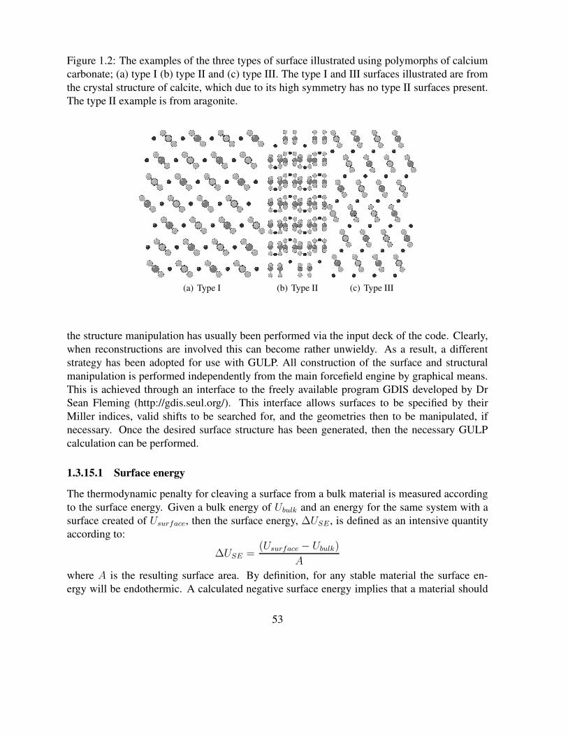
Figure 1.2: The examples of the three types of surface illustrated using polymorphs of calciumcarbonate; (a) type I (b) type II and (c) type III. The type I and III surfaces illustrated are fromthe crystal structure of calcite, which due to its high symmetry has no type II surfaces present.The type II example is from aragonite.
(a) Type I (b) Type II (c) Type III
the structure manipulation has usually been performed via the input deck of the code. Clearly,when reconstructions are involved this can become rather unwieldy. As a result, a differentstrategy has been adopted for use with GULP. All construction of the surface and structuralmanipulation is performed independently from the main forcefield engine by graphical means.This is achieved through an interface to the freely available program GDIS developed by DrSean Fleming (http://gdis.seul.org/). This interface allows surfaces to be specified by theirMiller indices, valid shifts to be searched for, and the geometries then to be manipulated, ifnecessary. Once the desired surface structure has been generated, then the necessary GULPcalculation can be performed.
1.3.15.1 Surface energy
The thermodynamic penalty for cleaving a surface from a bulk material is measured accordingto the surface energy. Given a bulk energy of Ubulk and an energy for the same system with asurface created of Usurface, then the surface energy, ∆USE , is defined as an intensive quantityaccording to:
∆USE =(Usurface − Ubulk)
A
where A is the resulting surface area. By definition, for any stable material the surface en-ergy will be endothermic. A calculated negative surface energy implies that a material should
53

dissociate, i.e. the crystal should disperse into the surrounding medium.There are two practical approaches that are widely used to determine the surface energy by
computational means. In the first, a two-dimensional slab of material is created from the bulk,thus creating two surfaces overall. This method has the advantage that it can be used withinprograms that only allow for three-dimensional boundary conditions through the introductionof a sufficently large vacuum gap between the images, such that the surfaces don’t interactacross the vacuum. In addition, it becomes necessary to assess whether the slab is also thickenough since the properties must converge to those of the bulk at the centre of the slab. In thesecond method, a single surface is created by employing a two region strategy, as shown inFigure 1.3. Here the solid is divided into region 1, which contains the surface and all layersof atoms below it that exhibit a significant atomic relaxation, and region 2, which contains therest of the bulk material where it is assumed that no displacements from the three-dimensionalcrystal structure are induced. In practice, only the atoms of region 2 that have an interactionwith region 1 need be explicitly considered, and so the depth of region 2 is controlled by thecut-offs of the forcefield and the Parry sum used for the electrostatics. This second method is themost efficient and precise for atomistic techniques. However, it is considerably harder to extendto quantum mechanical methods since the electronic perturbations may extend further into thebulk and embedding, typically via Green’s functions, is required to determine the influence ofthe electronic structure of region 2 on region 1. Through the GDIS interface, it is possible toautomatically estimate the required region 1 and 2 sizes needed to converge the surface energy(with a default tolerance of 0.001J/m2) based on the unrelaxed surface energies. However, ifthere are strong relaxations of the surface, it may be necessary to further verify that the relaxedsurface energy is sufficiently converged.
The total energy for a surface calculation comprising two regions can be written in terms ofthe interaction energies within, and between, the different regions:
Utot = U11 + U12 + U22
The energy of region 2 with itself, U22, is not particularly meaningful, since the region 2 is justa partial representation of the effectively infinite bulk material below, and any given particlewithin this region will not experience the full set of interactions that it should. However, thisterm is just an additive constant that is unaltered on energy minimisation, or any other displace-ment of region 1. Consequently it can be ignored in calculations. In the two region model, theenergy required to determine the surface energy is given by:
Usurface = U11 +1
2U12
Note that while the above energy only includes half of the region 1-region 2 interaction energy,the objective quantity for energy minimisation is the total energy, which includes the full valueof U12. This is because the energy change of region 2 must be allowed for when optimising.
54

Figure 1.3: The two region surface simulation cell viewed at right angles to the surface normal,where solid vertical lines denote the boundaries between two-dimensional periodic images ofthe cell and the dash line indicates the boundary between region 1 and the frozen region 2.
55

1.3.15.2 Attachment energy
The surface energy, described above, provides a measure of the thermodynamic stability of acleavage plane. However, there is a widely used alternative criterion which is the attachmentenergy. This is the energy associated with the addition of a stoichiometric layer of material onto the surface cut:
Uattachment = Un+1tot − Un
tot − U1tot
where Untot represents the total internal energy of a surface model consisting of n growth layers,
and U1tot is the energy of the growth layer alone. For any stable material, this implies that the
attachment energy must be an exothermic quantity. In practice, the calculation of the attachmentenergy is obtained from the energy of interaction of the growth layer at the surface with therest of the underlying material. This benefits from the fact that the attachment energy can beobtained from a single calculation, just as is the case for the surface energy, rather than byperforming the actual addition of a layer as part of a multistage process.
Although the attachment energy is also a strictly thermodynamic quantity, it is often re-garded as representing the kinetics of crystal growth because of the conceptual link between theease of the addition of a growth layer and the rate at which a surface is added to. Consequently,those faces where the attachment energy is most exothermic will tend to grow most rapidly.
1.3.15.3 Morphology
The morphology of a crystal is the macroscopic shape that it adopts. Because this can be readilyobserved for nearly all materials, either under an electron microscope or, in the case of manynaturally occuring minerals, by visual inspection with the naked eye, it should provide a readymeans to test the validity of a simulation model. Of course, the reality is rather more complex,since the morphology is sensitive to the presence of impurities, the nature of the solvent used asthe growth medium, and many other factors relating to the sample preparation. Consequentlythere are materials where many different morphologies can be observed for the same compound.A classic example, is that of calcite (CaCO3), where there are both several different polymorphsof the bulk material and several hundred different known morphologies. Many of these varia-tions result from biomineralisation by different species. Despite this, for many pure inorganicmaterials morphological prediction using atomistic techniques is surprisingly successful.
Crystal morphologies can be calculated based on either the surface energy or attachmentenergy, which are typically taken to represent growth under conditions of thermodynamic andkinetic control, respectively. In order to do this, it is first necessary to determine the objectivequantity for all significant faces. Given that dipolar faces are usually unstable, the number oflikely cleavage planes for most materials is actually considerably smaller than initially mightbe conceived of based on permutations of the Miller indices. Furthermore, where there is spacegroup symmetry present for the bulk, many surface planes are equivalent, thus reducing thenumber of unique faces. Finally, only those faces with the largest interplanar spacings are likelyto appear in the morphology [92]. The actual morphology is generated as a three-dimensional
56

Wulff plot [93]. Here the ratio of the surface normal distances of all planes from the centre ofthe polyhedron are determined according to the either the surface or attachment energy. Thefinal shape of the polyhedron is then determined by the intersection of the cleavage planes.Unstable surfaces lie outside the polyhedron and never intersect. Morphological plots can alsobe produced through the GDIS interface to GULP.
In the equilibrium morphology approach, the contribution of a given plane to the totalsurface area is inversely proportional to its surface energy [94]. For the growth morphologymethodology [95], the surface area contribution is again inversely proportional, but now to thenegative of the attachment energy. This is because surfaces with a highly exothermic attachmentenergy will rapidly grow out of the morphology to leave the slow growing bounding faces.
1.3.15.4 Surface phonons
The calculation of the phonons of a 2-D slab is exactly analogous to that for the three dimen-sional case, except that the Brillouin zone is also now two dimensional leading to dispersiononly in the xy-plane (taking z to be the direction of the surface normal).
Turning to consider the standard two region surface model, there are some important issuesto consider. Because region 2 is quasi-infinite, it is only possible to determine the phononsfor the particles in region 1. Therefore, the dynamical matrix is constructed based on region 1alone, but with contributions to the on-diagonal matrix blocks from the potential experienceddue to a rigid, non-vibrating region 2. Consequently it is assumed that the vibrations of thetwo regions are completely decoupled. Since this is an approximation, the frequencies nearthe interface of the regions will be slightly in error, particularly in the low frequency regimewhere coupling is generally strongest. However, the surface modes, which are usually the onesof primary interest, will be less affected. As always, it is essential to monitor the convergenceof all quantities with respect to increasing the region 1 depth. Finally, because region 1 isvibrating under the influence of an external potential, the first three frequencies at the Γ-pointwill no longer be zero, though they typically will be small.
1.3.16 Free energy minimisationOne of the most important issues in solid state modelling is the variation of materials proper-ties with the applied conditions. While isotropic external pressure is trivial to incorporate, ashas already been shown, inclusion of the effect of temperature is more complex. This processis exacerbated by the fact that the majority of potentials have been derived through the use ofsome empirical (i.e. experimental) data which has been measured under a given set of condi-tions. Hence the forcefield itself can often already contain an implicit temperature, or worse,if multiple pieces of experimental data have been employed that were measured at differentconditions, it can be a convolution of several temperatures. One solution to this is to extractforcefields from quantum mechanical methods so that everything is obtained explicitly at ab-solute zero. For now, we will assume that the forcefield has been derived so as to be free of
57

implicit temperature effects, by whatever means.There are several distinct approaches to the inclusion of temperature into simulations. Which
one is most appropriate depends on the particular temperature and nature of the system. In thelow temperature regime, the atoms of the crystal structure just execute vibrations about theirlattice sites, which in the limit of absolute zero will be purely harmonic. This situation is bestdescribed through the use of lattice dynamics, which is the quasi-static approach to treating avibrating lattice. As the temperature increases, the motions will become increasingly anhar-monic. In principle, this can be handled, to a point, through the use of anharmonic correctionsto the harmonic lattice dynamics, in order to allow for weak phonon-phonon coupling. How-ever, when the temperature becomes sufficiently high that diffusion can occur it is necessary toswitch to an alternative approach. Typically one of two approaches can then be employed. Ifdetailed information is required concerning the atomic motions and related properties, then themethod of choice is molecular dynamics [96]. This propagates Newton’s equations of motionthrough time using a finite difference formalism. Hence it retains time correlation functions andthe trajectories of all atoms. Its strength is that anharmonic effects are fully included. However,since it regards nuclei as classical particles, it is invalid at low temperatures due to the neglectof the quantisation of vibration and zero point motion, unless the Path-Integral formalism isemployed. It can be seen therefore that lattice dynamics and molecular dynamics are largelycomplementary in their regions of applicability. Although GULP also includes the capabilityto perform molecular dynamics, this topic will not be discussed here since this area, in regardto other codes, has been discussed elsewhere [16], and the more unique, static, features willbe focussed on here. Likewise, the effect of temperature can also be explored through MonteCarlo simulation [80], if the focus is integration over phase space, with no regard to timescaleor kinetic factors, but this topic will not be discussed further because it is not one of the morenovel features of GULP.
Concentrating now on the use of lattice dynamics for examining the temperature dependanceof crystal properties, the dominant effect is the change in the crystal structure. When heated,most materials undergo thermal expansion which correspondingly leads to softening of manyof the mechanical properties. There are a few celebrated examples of materials that actuallycontract on heating, through the rotation of quasi-rigid polyhedra, which is technologicallyvery important in the quest for zero thermal expansion composites.
It has already been shown that it is possible to calculate the Helmholtz free energy for agiven structure as a function of temperature through the determination of the vibrational par-tition function from the phonon density of states. Hence, a natural approach to determine thedependance of structure on temperature is through free energy minimisation. Here the key foun-dation is the quasi-harmonic approximation, which assumes that the vibrational frequencies canbe determined as if the atoms are vibrating purely harmonically while the cell parameters areadjusted to minimise the free energy. Previous studies have indicated that this is a reasonableapproximation until a temperature of approximately half the melting point has been reached.
The major barrier to free energy minimisation is that we have already seen that efficient
58
optimisation requires at least the first derivatives of the quantity with respect to the structuralvariables. Hence a number of approaches evolved for tackling this problem. LeSar et al [97] de-veloped a method whereby the atoms where represented as Gaussian distributions, whose widthrepresented the vibrational motion. The Gaussian exponent was then regarded as a variationalparameter that minimised the free energy. Hence the free energy could be obtained withoutdirect recourse to a phonon density of states, making derivatives straight forward. While thisapproach is easy to apply to metals, the extension to a more complex ionic systems is moredemanding. A method that approximated the phonon density of states was introduced by Sut-ton [98], which involved taking moments of the dynamical matrix, as pioneered by Montroll[99] several decades earlier, and in the spirit of tight binding theory. This approach has the ad-vantage that the derivatives are taken of the dynamical matrix elements, rather than of phononfrequencies, which are the product of a matrix diagonalisation.
In the field of ionic materials, Parker and Price [8] pioneered the use of free energy min-imisation through the use of numerical derivatives. Here central finite differences were takenwith respect to the cell strains, with the internal degrees of freedom being formally optimisedat every point. This approach had the advantage over the other methods that no approximationwas being introduced beyond the quasiharmonic one. However, because this requires (2N + 1)optimisations and phonon evaluations per energy/gradient evaluation with respect to the freeenergy, the minimisation was restricted to the strains alone in order to reduce the number ofvariables, N , to a maximum of six.
More recently, Kantorovich [100] has derived expressions for the analytical derivatives ofthe free energy, which were implemented contemporaneously in the program SHELL of Allanand co-workers [101], and in GULP [102]. If we consider the differential with respect to strain,though the expressions would be identical for any degree of freedom, then the first derivative ofthe free energy is given by:
(
∂A
∂ε
)
=
(
∂Ustatic
∂ε
)
+∑
k
∑
m
h
2ω
1
2+
1
exp(
hωkBT
)
− 1
(
∂ω2
∂ε
)
where the expression is written in terms of the derivatives of the square of the frequencies,since these values represent the eigenvalues of the dynamical matrix. Their derivatives can becalculated through the application of perturbation theory and expressed as the derivatives of thedynamical matrix projected onto the corresponding eigenvectors:
(
∂ω (k, m)2
∂ε
)
= e∗m (k)
(
∂D (k)
∂ε
)
em (k)
In order to determine the derivatives of the phonon frequencies, we therefore require the phasedthird derivatives of the energy with respect to either three Cartesian coordinates, or two Carte-sian coordinates and one strain. for internal and external variables, respectively.
For the most efficient optimisers, based on Newton-Raphson techniques, we strictly need thesecond derivatives with respect to the free energy, which corresponds to the fourth derivatives of
59
the internal energy. However, this is considerably more expensive and complex, so the Hessianmatrix is usually approximated by the conventional internal energy Hessian by assuming thatthe free energy contribution to the curvature is small. Furthermore, the use of updating formulaewill ultimately correct for the discrepancy given sufficient optimisation steps.
With the advent of analytical derivatives, it is now possible to consider two types of free en-ergy minimisation. The first has been christened the Zero Static Internal Stress Approximation(ZSISA) by Allan and co-workers [103], which resembles the approach taken with numericalfirst derivatives (i.e. the unit cell is minimised with respect to the free energy, while maintain-ing the internal degrees of freedom at a minimum with respect to the internal energy). Whenworking within this formalism there is an additional contribution to the strain derivatives, whichcorrects for the fact that internal degrees of freedom are not at a minimum with respect to thefree energy:
(
∂A
∂ε
)
ZSISA
=
(
∂A
∂ε
)
−(
∂2A
∂ε∂α
)(
∂2A
∂α∂β
)−1 (∂A
∂β
)
Here the approximation is again made that the second derivative matrices can be approximatedby neglecting the free energy contribution; an approximation that should be enhanced by thecancelation that results from taking a ratio. The second type of optimisation can be called fullfree energy minimisation (FFEM), in which the internal degrees of freedom are also minimisedwith respect to the free energy. This is potentially appealing since sometimes it is the details ofthe internal changes that might be of interest, for example, the nature of an adsorption complexwithin a microporous material.
Results for silicate materials show a number of interesting features regarding the merits ofboth approaches. Firstly, in the case of α-quartz where accurate experimental data is avail-able for comparison, it appears that the ZSISA approach underestimates the thermal expansion,while the FFEM method is more accurate, though of course this is subject to the limitations ofthe specific potential model chosen [102]. However, for all silicates tried so far the full min-imisation approach goes catasrophically wrong at about ambient conditions. This is illustrativeof a general problem with this approach which tends to drive systems to instability. This canbe readily understood, since the free energy is minimised by creating phonons that tend to zerofrequency and hence the structure is motivated to create soft modes. This behaviour does nottend to happen in the ZSISA approach where only the cell strains are directly coupled to thefree energy and thus the relaxations tend to lead only to a scaling of modes, rather than moreindividual changes. Hence the use of ZSISA is far more robust and generally recommended formost purposes.
1.3.17 Monte CarloAn alternative approach to including temperature into results, if one is not interested in thetime correlation properties, just the ensemble averages, is Monte Carlo simulation. Here thedistribution of positions according to a Boltzmann distribution is determined numerically for
60

a specified temperature and conditions. Under the Metropolis importance sampling scheme,if a randomly chosen move for the system leads to a lowering in the energy then the move isaccepted and the system evolves to the new state. If the energy increases, then the move isaccepted with a probability given by:
P = exp(
− ∆U
kBT
)
where ∆U is the energy change associated with the move. There are several types of moveavailable for a system as listed below:
• Translation - this allows atoms or molecules to move in x, y or z, according to the flagsset
• Rotation - for rigid molecules, this allows the molecule to sample the rotational distribu-tion
• Creation/destruction - in the Grand Canonical ensemble, molecules can be inserted orremoved to a reservoir of molecules whose chemical potential is specified
1.3.18 Defect calculationsWhile the simulation of bulk material properties is important, just as crucial is the study of bothintrinsic and extrinsic defects. Many of the key applications of solid state systems, such ascatalysis, electronic and ionic conductivity, ion exchange and waste immobilisation, criticallydepend on the utlisation of the characteristics of defect centres. Consequently, from the earlydays of the field of atomistic simulation defect studied have been one of the most vigorouslypursued topics.
There are two widely used approaches for performing defect calculations on solids; the su-percell and the cluster methods, with or without embedding in the latter case. Both approacheshave their merits and demerits. Putting computational implementation factors aside, the useof embedded clusters is ideal for the infinitely dilute limit, while the supercell method is moreappropriate for high concentrations of defects where there exists significant defect-defect inter-action. In practice, the nature of the computational method often biases the method of choice.However, with atomistic techniques both approaches are feasible. Since the supercell methodis simply the extension of a bulk calculation, we will focus here on the embedded cluster ap-proach. In this particular context, the technique is generally referred to as the Mott-Littletonmethod [104], after the authors of the pioneering work in the field, though the implementationaldetails differ a little from their original work.
The basis of the Mott-Littleton method is the so-called two region strategy. Here a pointcalled the defect centre is defined, which typically lies at a point concentric with the initialdefect site, or, where there is more than one defect, at the mid-point of the ensemble of point
61

defects. The crystal around the defect centre is divided into two spherical regions, with the innersphere being labelled region 1, and the outer spherical shell of ions being region 2a. Atomsoutside of these spheres belong to region 2b, which then extends to infinity. The dimensions ofthese regions are typically specified either by their radii or the number of ions contained withinthem. The ions in region 1 are assumed to be strongly perturbed by the defect and therefore arerelaxed explicitly with respect to their Cartesian coordinates. In contrast, the ions in region 2 areassumed to be weakly perturbed and therefore their displacements, with the associated energyof relaxation, can be approximated in some way. Clearly, as the region 1 radius is increasedthese approximations will become increasingly valid, and thus an important stage of a defectcalculation is to ensure that the defect energy is sufficiently converged with respect to the regionradii. In some cases the convergence of the absolute defect energy can be slow, in which case itmay be sufficent to monitor the convergence of relative defect energies instead. As a guideline,the radius of region 1 and the difference of the radii of regions 1 and 2 should be both be greaterthan the short-range potential cut-off to achieve convergence, though for charged defects thismay not be adequate.
Within the Mott-Littleton scheme, we can express the total energy of the two region systemas the sum of contributions from the energies within the regions and between them:
Utot (x, ξ) = U11 (x) + U12 (x, ξ) + U22 (ξ)
where U11 (x) represents the energy of region 1 as a function of the Cartesian coordinates,x, U22 (ξ) represents the energy of region 2 as a function of the Cartesian displacements, ξ,and U12 (x, ξ) is the energy of interaction between the two regions. At this stage we do notdistinguish between regions 2a and 2b. If the forces acting on region 2 are small, then we canassume that the response of the atoms in this region will be purely harmonic. Hence, the energyof region 2 can be written as:
U22 (ξ) =1
2ξT H22ξ
where H22 is the Hessian matrix for region 2. If we now apply the condition that the displace-ments in region 2 will be the equilibrium values this yields the following condition:
(
∂Utot (x, ξ)
∂ξ
)
x
=
(
∂U12 (x, ξ)
∂ξ
)
x
+ H22ξ = 0
Combining this equation, and the previous one, it is possible to eliminate the energy of region 2from the total energy without direct recourse to the Hessian matrix (which would be of infinitedimension):
Utot (x, ξ) = U11 (x) + U12 (x, ξ) − 1
2
(
∂U12 (x, ξ)
∂ξ
)
x
ξ
Thus the problem of calculating the energy of region 1 in the potential of region 2 has beenreduced to evaluating the energy of region 1 and its interaction with region 2, without having
62
to evaluate the self energy of region 2. Furthermore, in order to lead to partial cancellation ofterms, the quantity calculated is the defect energy - i.e. the difference between the energy of theperfect region 1 and 2, U p
tot, and the defective case, U dtot, rather than the individual contributions:
Udefect (x, ξ) = Udtot (x, ξ) − Up
tot (x, ξ)
It should be noted that it is assumed that the energy of any species removed or added during theformation of the defect has an energy of zero at infinite separation. If this is not the case, thenthe defect energy must be corrected a posteriori for this. However, such corrections have noinfluence on the outcome of the defect calculation itself.
There is one important consequence of the above formulation of the total defect energy, inthat it becomes necessary to find the optimised energy with respect to the Cartesian coordinatesof region 1 by force balance, rather than by energy minimisation. The point at which the forcestend to zero is usually only slightly different from the minimum in the internal energy, depend-ing on the degree of perturbation of region 2. Hence, during an optimisation of the defect energyGULP initially minimises the energy, as per a conventional Newton-Raphson procedure. Oncethe gradient norm falls below a specified tolerance, and region 1 lies within the harmonic region,then the harmonic displacements according to the Hessian and gradients are applied without theuse of a line search until the forces drop below the specified tolerance.
A further important point relates to the state of the bulk crystal when performing defectcalculations. Because of the use of displacements in region 2, it is crucial that the bulk structureis at an energy minimium with respect to the internal coordinates before performing a defectcalculation. Hence the bulk crystal must be relaxed to equilibrium at least at constant volume,if not at constant pressure. Furthermore, it is also important that there are no imaginary phononmodes within the Brillouin zone otherwise the displacements in region 2 may correspond tounstable harmonic equilibrium. The presence of such modes is the most common cause of un-physical results, for instance obtaining negative defect energies for intrinsic defects. Becausethe presence of defects lowers the symmetry, a Mott-Littleton calculation may encounter insta-bilities not apparent for the bulk material.
Now it is necessary to consider the treatment of region 2 in more detail, and in particularthe difference between regions 2a and 2b. In region 2a, the forces on the individual ions due toshort-range interatomic potentials and the Coulomb term are explicitly calculated and the localdisplacement evaluated. While the forces on region 2a are technically due to all ions in region1, a commonly used approximation is to evaluate the forces due to defect species only. This isthe approach taken in the default calculation method for compatability with earlier results.
In contrast to the above situation for region 2a, for region 2b the energy of relaxation mustbe determined implicitly since this region extends to infinity. It is assumed that in region 2bthe only force acting is that due to the Coulomb potential in order to simplify the problem. Bychoosing the radius of region 2a to always be greater than that of region 1 by the short-rangepotential cut-off this can always be arranged to be valid. Even having retained only the Coulombinteraction in the perturbation of region 2b, this still leaves many interactions to consider. To
63
simplify the problem, the electrostatic potential due to defects in region 1 can be representedby the multipole moments of the deformation situated at the defect centre. If region 2a issufficiently large, then the only significant term will be the monopole moment of the defect(i.e. the net charge). Hence, the energy of region 2b is evaluated as the induced relaxationenergy due to the net charge of the defect situated at the specified defect centre. While thisis a significant approximation, it usually works well in practice and again becomes valid withincreasing region sizes. In the original Mott-Littleton method, the interaction with region 2bwas described by a continuum approximation. However, in subsequent implementations a sumof the induced polarisation energy is performed over the atomic sites. For the general case ofan anisotropic dielectric constant tensor [105], the energy of region 2b is calculated as:
U2b = −1
2Q2
∑
i∈2b
∑
αβ
Mαβi rα
cirβci
r6ci
where Q is the net charge of the defect, rci is the distance of the ith atom from the defect centre,and Mαβ
i is a 3 x 3 matrix for each atomic site, in the Cartesian frame, that represents the on-sitepolarisability. The quantitative definition of the matrix elements Mαβ
i is [4]:
Mαβi =
∑
γ
((
D−1)αγ
q)
i
(
ε−1)γβ
where D−1i represents the on-diagonal block of a modified inverse second derivative matrix
and ε is the static dielectric constant tensor. Note that the inverse of the second derivativematrix is singular and therefore a further approximation must be made. Physically, this problemcorresponds to the division of the polarisation between the sublattices being arbitrary. The usualsolution taken is to assume that the polarisation is divided equally between the cation and anionsublattices, with the second derivative matrix being modified correspondingly. In the specialcase of a cubic crystal, the expression for the region 2b energy can be simplified to:
U2b = −1
2Q2
∑
i∈2b
mi
r4ci
where mi is the average of the diagonal elements of the matrix M (for the cubic case these willall be equal, but if the isotropic formula were to be applied in a non-cubic case this would notbe so).
Because the expression for the region 2b energy is not particularly short-ranged, it is ap-propriate to evaluate it using lattice summation techniques analogous to those applied to themonopole-monopole term. Hence the term is summed to convergence based on a perfect in-finite lattice and then the contributions from ions in regions 1 and 2a are subtracted off. Thedistance dependent factor within the expression for the energy can be rewritten as:
rαrβ
r6=
1
8
∂2(
1r4
)
∂rα∂rβ
+δαβ
4
(
1
r4
)
64

Hence, by evaluating the equivalent of the Ewald summation for the inverse fourth power ofdistance, and its second derivatives with respect to Cartesian displacements, it is possible toachieve a rapidly convergent expression for the energy of region 2b.
Having described how defect energies are calculated in theory, we mention a few practicalpoints. There are three types of defect that can be specified within GULP:
• Vacancy
• Interstitial
• Impurity
The last one of these three is clearly the combination of a vacancy and an interstitial at the sameatomic position in the structure. The location of a vacancy or an impurity can be specified byreference to either a spatial position or an atom position by referencing the site. An interstitial,by its very nature, must be specified by coordinates. When an atom is designated to be vacant,then both the core and shell will be removed automatically since it would not be sensible toleave one or the other present in the system. It is also possible to specify that a whole moleculebe removed from the system, when the connectivity has been defined.
Most types of calculation, that are logically applicable, can also be applied to defect runs,such as optimisation to a minimum or a transition state. In the case of vibrations, the frequenciesare calculated for a dynamical matrix based on region 1. In must be noted that this is a largeapproximation, since any modes that are coupled between regions 1 and 2 will not be properlydescribed. Only localised modes relating to atoms near the centre of region 1 will be correctlypredicted. Consequently such calculations of vibrations must be interpreted cautiously.
Finally, a degree of point group symmetry may be utilised during defect calculations. An au-tomatic search for common symmetry elements is performed about the defect centre, includingmirror planes and C2 axes that are aligned with, or between, the Cartesian axes. Such symmetryis used to reduce the number of region 1 and region 2 atoms stored, thereby reducing the num-ber of degrees of freedom for optimisation, as well as taking advantage of symmetry adaptedalgorithms to accelerate the calculation of the energy and its derivatives.
1.3.19 Derivation of interatomic potentialsOne of the major challenges facing anyone wishing to use forcefield methods is to determine thefunctional form and parameters required to calculate the energy and properties. In the field oforganic chemistry and biomolecules, there are a number of well-established forcefields, such asMM3 [106], and those associated with the programs AMBER [14], and CHARMM [15], whichare, in principle, capable of handling most elements typically found in these systems (C, H, O,N, S, P, etc) in their common hybridisation states. These are constructed around the molecularmechanics approach where the forcefield is connectivity driven and interactions are described
65

in terms of two-, three-, and four-body bonding terms, plus long-range Coulomb and non-bonded interactions. While there have been several attempts to generate general forcefields thatcover the entire periodic table, such as UFF [107], ESFF [108], etc, none have been completelysuccessful. Because of the enormity of the amount of data required when spanning the wholerange of elements, it is impractical to determine such a universal forcefield by empirical fitting.Instead general rules must be used to predict parameters based on extrapolations and intrinsicproperties of the element that are known - for instance the electronegativity. Not surprisingly,this leads to limitations in the quality of the results. For most inorganic systems it is usuallynecessary to derive a forcefield for the specific material, or family of materials, of interest.
There are two means by which a forcefield can generally be derived, if we exclude rule basedextrapolations. Firstly, it is possible to obtain parameters by fitting to a potential energy surfaceobtained from a non-empirical theoretical method. This would typically consist of results fromab initio calculations, ideally on the periodic solid [109], or perhaps on a gas phase cluster, oreven better, both of the aforementioned sources. The potential energy surface can be fitted eitheras a sequence of geometries with their corresponding energies, or derivatives of the energy couldalso be included to maximise the amount of information from each higher level calculation.Many of the early forcefields for ionic materials were determined using electron gas methods[110], in which the energies of interaction between pairs of ions were determined by a densityfunctional calculation using the overlapping ionic electron densities, where the anion is confinedin an appropriate potential well. Secondly, parameters can be obtained by empirical fitting inwhich the normal process of using a forcefield to determine the properties of a material isinverted. This approach depends on the availability of a range of experimental data. Knowledgeof the crystal structure is a definite prerequisite for this method, but is insufficient alone sinceinformation is required as to the curvature of the energy surface about the minimum. This laterdata may come from quantities such as elastic constants, bulk moduli, piezoelectric constants,dielectric constants, or phonon frequencies.
In order to perform a fit, first it is necessary to define a quantity that measures the quality ofthe results, known as the sum of squares;
F =Nobs∑
i=1
wi
(
f obsi − f calc
i
)2
where Nobs is the number of observables, f obsi and f calc
i are the fitted and calculated values ofthe observable, respectively, and wi is the weighting factor for the given observable. Because ofthe weighting factor, there are an infinite number of possible solutions all of which are equallyvalid. Hence, one of the most important skills is knowing how to choose appropriate and sen-sible weighting factors. There are several criteria that can be used for guidance though. Firstly,if fitting experimental data, the weighting factor should be inversely proportional to the uncer-tainty in the measured value. Obviously trusted, precise values should be given more prioritythan data where there are large error bars. Secondly, the weight factor should be inversely pro-portional to the magnitude of the observable squared. This ensures that all values are fitted on an
66

equal footing, regardless of units. For example, fitted vibrational frequencies in wavenumbersare typically two to three orders of magnitude larger than structural variables.
The fitting process itself involves minimising the above function F . To do this, the defaultapproach is similar to that used in optimisation. For many terms, the evaluation of the deriva-tives of the sum of squares with respect to the variables is complex, and in some of the fittingalgorithms that will be discussed subsequently it is even impossible. As a result, numericalderivatives are employed during fitting since it greatly simplifies the process. Because of this,the default optimiser is to use a BFGS update of an initial on-diagonal only Hessian, obtainedby finite differences, in a Newton-Raphson process. However, for particularly difficult cases,where correlation between variables is strong, there is the option to use a full Hessian matrix,again obtained by finite differences.
Now we turn to specifically consider the fitting methodology for the case of empirical data.Traditionally, the experimental structure is fitted by varying the potential parameters so as tominimise the forces at this configuration, and this is the default strategy. Other observables, suchas elastic constants etc, are then calculated at the experimental structure too. When workingwith the shell model, either dipole or breathing shell, there is an additional complication thoughin that while the cores are fully specified since they are equated with the nuclei of the ions,the positions/radii of the shells are undefined. One approach is to fit with the shells positionedto be concentric with the cores. However, this is unphysical since it implies that there is noionic polarisation, which defeats the object of including the model in the first place. A secondapproach might be to place the shell according to specified ion dipoles, but this information isalmost impossible to come by. Only data about the total polarisation of the unit cell is typicallyavailable and a unique atomic decomposition is not possible. In order to handle this issue,the simultaneous relaxation of shells approach was introduced into GULP [111]. Here theshells are allowed to move during fitting. Formally, the most correct approach is to allow theshells to be energy minimised at every evaluation of the fitting function. However, a simplerapproach has been implemented in which the shell forces are added as observables and theshell positions become fitting variables. In this way, the shells are minimised directly withinthe fitting procedure. In the absence of any observables other than the structure, this is exactlyequivalent to minimising the shells at every step of fitting. When observables are present therewill be small differences, but these are usually an acceptable price to pay for the greater ease ofimplementation.
There is actually a more fundamental flaw with the approach of fitting forces at the exper-imental geometry as a method of fitting. Often we judge the quality of a fit by the percentageerror in the structural variables rather than the forces. Although lowering the forces during a fitgenerally improves the optimised structure with respect to experiment, this is not guaranteed tobe the case (and indeed we have found examples where it is not). This can be understood bymaking a harmonic estimate of the atomic displacements, x, based on the forces, f :
x = H−1f
It can be readily seen that the magnitude of the displacements also depends on the inverse
67
of the Hessian matrix. Thus if the forces improve, but the description of the curvature aboutthe minimum deteriorates, then the errors can potentially increase. If curvature informationis included in the fit, then this can tend to reduce this problem. However, there is a furtherdifficulty here. Formally speaking, the expressions for the elastic constants and other propertiesare defined about a position of zero stress and zero internal derivative. Therefore, calculating theproperties at the experimental structure when the forces are non-zero leads to errors also. Thesolution to both of these dilemas is to use the so-called relax fitting methodology [111] in whichthe structure is fully optimised at every evaluation of the fitting function and the propertiescalculated at the optimised configuration. Obviously this is a far more expensive procedure, butdoes yield the most reliable results. Also there is the requirement that the initial potential set isreasonable enough to actually give a valid minimisation of the structure.
Having obtained an apparently successful fit, it is important to assess the quality of theresults, since there are plenty of pitfalls and so convergence shouldn’t be taken to represent agood quality solution. Firstly, the potential model should be tested for all reasonable properties,not just those used in the fit. It could easily be the case that a forcefield reproduces a highsymmetry structure and, say, a single curvature observable, such as the bulk modulus. However,examination of the full elastic constant tensor, dielectric properties and phonons might revealthat the system is unstable with respect to a lowering of symmetry which wouldn’t show upin the fit. Secondly, the forcefield could be transferred to a different material, not used inthe original fit, to test whether the results are sensible. Finally, it is important to look at thepotential parameters and assess whether the numbers are physically sensible. For instance, it isnot uncommon for dispersion terms to become extremely large if allowed to fit unconstrained.While this might have improved the sum of squares for one particular system, it means all hopeof transferability has been lost. Similarly, there can often be problems with fitting A and ρof a Buckingham potential concurrently due to the strong correlation coefficent between theparameters.
The focus above has been primarily on empirical derivation of interatomic potentials. How-ever, with the increasing ability to perform periodic ab initio calculations on solids an attractivealternative is to derive forcefields that attempt to reproduce the results of such methods. Thereare several reasons to take this approach. Firstly, by fitting the outcomes of a single Hamiltonianit is possible to guarantee that the training set is fully consistent (i.e. there are no differences intemperature, pressure, sample quality, or variable uncertainities in the observables). Secondly,data can be obtained for materials were no experimental information exists or at geometries thatare significantly perturbed from the equilibrium one. Thirdly, the data from quantum mechan-ical methods is free of statistical mechanical effects, such as thermal vibrations and zero pointmotion. Hence, if the aim is to perform free energy minimisation then the interatomic potentialswill represent a proper starting point for the inclusion of these quantities.
Fitting of quantum mechanical data can be performed in one of two ways, either by pro-ceeding in the same fashion as for empirical derivation, or by use of an energy hypersurface.In the latter case, this is achieved by specifying a series of structures with their corresponding
68
energies, and optionally first derivatives. Typically the structures would include the equilibriumconfiguration and as many distinct distortions about this point in order to probe as many differ-ent interatomic distances between atoms as possible. Perhaps the most difficult decision is howto weight the configurations. Unless the forcefield is able to reproduce the ab initio data veryaccurately, then it is usually desirable to weight the fit in favour of configurations nearer theequilibrium structure. One approach that has been taken is to use a Boltzmann factor weight-ing based on the energy difference to the minimum energy configuration, with an appropriatechoice of temperature to the task ultimately to be performed [112]. However, there are manyother possible choices too. A further issue concerns the fitting of quantum mechanical ener-gies. Unless these values have been converted to a binding or lattice energy with reference tothe dissociated state of the species within the system then it is inappropriate to fit the absolutevalues of the energies. Consequently, the easiest solution is to include an additive energy shiftparameter in the fit, such that only relative energies are actually fitted.
Finally, the option exists within GULP to perform fitting using genetic algorithms as well asvia least squares techniques. This may be potentially useful in cases where a complex systemis being fitted when there is no reasonable starting approximation to the forcefield available orwhere there may be multiple local minima in the parameter space. However, to date we have yetto encounter a situation where this approach has proved beneficial over the more conventionalmethodology. This emphasizes that there is no substitute for making physically sensible choicesfor the functional form of the forcefield and the initial parameters.
1.3.20 Calculation of derivativesIn order to be able to optimise structures efficiently and to calculate many properties requiresthe availability of derivatives. While finite difference methods can be used to determine these,this is both inefficient and inaccurate for forcefields, since numerical errors can cause problems,especially when potentials do not go exactly to zero at the cut-off distance. Consequently allderivatives are determined analytically in GULP. All functional forms for the energy have upto analytic second derivatives available, while two-, three- and four-body interactions includethird derivatives. In addition, analytic third derivatives can be calculated for the embedded atommethod, but currently not for any other many-body potential functions.
Because the determination of derivatives is central to many quantities, a brief descriptionof the approach to their calculation is given here, while fuller details can be found in both theoriginal Harwell Report [113], and the subsequent publication of many of these details[114].Ultimately two types of derivative are required - those with respect to atomic degrees of freedomand those with respect to the unit cell. In GULP, all atomic coordinate derivatives are calculatedin the Cartesian frame of reference and then transformed to the fractional coordinate derivatives,when appropriate to the periodicity. For the unit cell, strain derivatives are taken as previouslydescribed.
Both the Cartesian and strain derivatives can be related to a set of pivotal quantities, which
69

are the first derivatives with respect to the interatomic distances, divided by the distance:
∂U
∂α=
(
1
r
∂U
∂r
)
α
∂U
∂ε=
(
1
r
∂U
∂r
)
αβ
where, in the expression for the strain derivative, the components α and β are the appropriateCartesian directions for the given strain (e.g. ε4 implies α = y and β = z). It is implicitthat all quantities are subscripted with ij to indicate that the terms refer to a specific pairwiseinteraction. Let us introduce the shorthand:
U1 =
(
1
r
∂U
∂r
)
U2 =
(
1
r
∂
∂r
(
1
r
∂U
∂r
))
U3 =
(
1
r
∂
∂r
(
1
r
∂
∂r
(
1
r
∂U
∂r
)))
The second derivatives can then be obtained by differentiating the above expressions once moreand written as:
∂2U
∂α∂β= U2αβ + U1δαβ
∂2U
∂α∂ε= U2αβγ + U1 (βδαγ + γδαβ)
∂2U
∂εαβ∂εγζ
= U2αβγζ + U1 (δαβδγζ) +1
4U1 (δαγβζ + δαζβγ + δβγαζ + δβζαγ)
Likewise, the third derivatives can be obtained by further differentiation:
∂3U
∂α∂β∂γ= U3αβγ + U2 (αδβγ + βδαγ + γδαβ)
∂3U
∂α∂β∂εγζ= U3αβγζ + U2 (α (γδβζ + ζδβγ) + β (γδαζ + ζδαγ) + γζδαβ)
+U1 (δαγδβζ + δαζδβγ)
Note that for free energy minimisation, which is were the third derivatives are required, onlythe derivatives with respect to two Cartesian coordinates and one strain, or three Cartesiancoordinates are needed.
70

In both three-body and four-body terms there exist derivatives with respect to either a trig-nometric function of an angle, or the angle itself. These derivatives can be converted into theabove forms through the use of the cosine rule:
cos (θ) =r212 + r2
13 − r223
2r12r13
where θ is the angle at the pivot atom 1, lying between the vectors r12 and r13. Derviatives withrespect to angles are therefore obtained through the expression:
∂θ
∂r= − 1
sin (θ)
∂ cos (θ)
∂r
Care must be taken in handling the limit as θ tends to either 0o or 180o.
1.3.21 Crystal symmetryAn important topic, particularly in the context of optimisation, is crystal symmetry. For periodiccrystals, there is the option to specify the solid via the asymmetric unit atoms, the space groupnumber/symbol, and the origin setting. It should be noted that the use of space group symbolsis preferable since it distinguishes between different settings of the same space group. Apartfrom the building of the full unit cell from the asymmetric unit, the symmetry can be utilisedto greatly accelerate the structural optimisation through several different means. The first ben-efit of symmetry is that it lowers the number of independent geometric variables, since manyatomic coordinates are related via a roto-translation operation. Furthermore, the existance ofspecial positions implies that some coordinates are not allow to vary, typically for sites such as(
12, 1
2, 1
2
)
, and that in other cases coordinates are not independent and must be related by con-straints. Even larger reductions in scale can be achieved by using unit cell centring to reduce thecentred-cell down to the primitive representation, thereby reducing the number of atoms by afactor or between 2 and 4. All of these factors reduce the number of variables, and since the rateof convergence is usually correlated to the number of independent variables, depending on thealgorithm, this can lead to fewer optimisation steps being required. Furthermore, the amount ofmemory to store the Hessian matrix is reduced, as well as there being a large improvement inthe cost of inverting this matrix.
The second gain from the use of symmetry is that it is possible to use new algorithms tocalculate the energy and its derivatives that involve fewer computations, provided the symmetryis high enough [115]. Considering a two-body potential model, instead of looping over allpossible pairs of atoms in order to compute the energy, when symmetry is present it is sufficientto only calculate the interactions between the atoms of the asymmetric unit and all other atoms.For a system of N fatoms in the full unit cell and N a atoms in the asymmetric unit, then theexecution times for the algorithms, T f and T a, respectively, will be given by:
T f ∝ 1
2Nf
(
Nf + 1)
71
T a ∝ NaNf
It can therefore be seen that provided the number of atoms in the asymmetric unit is roughly lessthan half the number in the full unit cell then the symmetry adapted algorithm will be faster.The extension of symmetry to other types of potential is also straightforward. For example,for a three-body angular potential it is only necessary to calculate the terms that arise when anasymmetric unit atom lies within a valid triad of species.
While the symmetry-adapted evaluation of the energy is trivial, more care is required for thederivatives since these are vector/tensorial properties. For the first derivatives with respect toatomic positions, it is sufficient to again only evaluate the derivatives with respect to the asym-metric unit atoms and then to scale these terms by the number of symmetry-equivalent atoms inthe full cell. Conversely, the first derivatives with respect to cell strain are more complex, sincealthough the interaction of the asymmetric unit with all other atoms spans all possible uniquederivatives, the orientation of the terms now matters. In short, the strain derivatives will violatethe crystal symmetry if the terms are evaluated for the asymmetric unit interacting with the restof the crystal alone. However, given that the crystal symmetry is specified and that the sumof the terms is correct, when again scaled by the site multiplicities, it is possible to obtain thecorrect first strain derivatives by appropriate averaging.
Turning now to the second derivatives, the symmetry-adapted generation of the Hessianmatrix is more complex. Considering the process by which the Hessian is generated in theabsence of symmetry, there are three steps. Firstly, the Cartesian derivatives that are initiallygenerated have to be transformed into fractional space by multiplying each 3 x 3 block by theunit cell vector matrix and its transpose. This generates the matrix Dff , where the subscript fsignifies a dimension equal to number of atomic coordinates in the full unit cell. Secondly, Dff
is reduced to the smaller matrix Daa, where the subscript a now signifies that the dimension isequal to the number of atomic coordinates in the asymmetric unit. This is achieved using thetransformation matrix, Tfa, and its transpose:
Daa = TafDffTfa
The transformation matrix is sparse and contains 3 x 3 blocks between each asymmetric unitatom and its symmetry equivalent images, which are just the rotation matrices, R, that createdthose images. The third, and final, step is to reduce the matrix Daa according to any constraintsthat are present between coordinates. It is possible to combine the second and third steps intoone by pre-multiplying the transformation matrix by the constraint matrix.
All the symmetry unique information concerning the second derivatives is contained withinthe columns between the asymmetric unit and the full cell. Hence, it is more efficient justto calculate the sub-matrix Dfa instead. This can then by transformed to the required matrixaccording to:
Daa = SafDfa
This not only reduces the computational effort in calculating the second derivatives, but alsoreduces the memory required and lowers the number of matrix multiplications required to form
72
the Hessian. The 3 x 3 blocks of the required transformation matrix are given by:
Saf =1
Naeqv
Naeqv∑
n=1
R−1n Rf ′
where Naeqv is the number of symmetry equivalent atoms to the asymmetric unit atom a, and
f ′ is the atom to which the atom f maps under the transformation R−1n . Again the second
derivatives with respect to strain-strain and strain-internal are more complex since they areinitially generated such that symmetry is violated. However, resymmetrisation by averagingsymmetry related matrix elements solves this problem.
The use of crystal symmetry in reciprocal space is even more straightforward than in realspace. Because the Ewald sum can be written to be a sum over one-centred terms in reciprocalspace, instead of a pairwise expression, the only change necessary is to restrict the sum to theasymmetric unit with appropriate weighting for site multiplicity. The same strategy is used inthe symmetrisation of other one-centre terms in real space, such as the Einstein model. Crystalsymmetry is also exploited in the calculation of charges via the electronegativity equalisationmethod, which is thereby accelerated, especially through the reduction of the size of the matrixto be inverted.
1.3.22 Code detailsThe original version of GULP [115] was written in Fortran 77 since the more recent standardshad yet to be released. This implied that memory was statically allocated via a series of param-eters. Subsequently, non-standard extensions were introduced to allow the second derivativearrays to be dynamically declared, since they represented the dominant use of memory. For thecurrent version Fortran 90 has now been adopted leading to full use of dynamic memory.
The program has been compiled and tested for most Unix-style operating systems, includingLinux and Apple-Macintosh OSX, using most Fortran 90 compilers. While compilation underMS-DOS is in principle possible, this operating system is not supported since it is the onlyoperating system that cannot be automatically catered for within a single standard Makefile.
The code has also been parallelised for the evaluation of the energy and first derivatives usingMPI, based upon a replicated data paradigm. When performing calculations on sufficiently largesystems that require the use of parallel computers, then the most appropriate types of calculationare usually either conjugate gradient optimisation or molecular dynamics. Hence, the absenceof second derivatives is less critical. However, a distributed data algorithm for the secondderivatives and using Scalapack for matrix diagonalisation/inversion would be feasible and maybe implemented in the future. Because GULP is currently targetted primarily at crystallinesystems, where unit cells are typically small, the distribution of parallel work does not usea spatial decomposition. Instead the Brode-Ahlrichs algorithm [116] is used for the pairwiseloops in real space in order to try to ensure load balancing over the processors. A similarapproach is used for the four-body potentials based on the first two atoms of the sequence of
73

four. In the case of three-body potentials, the work is divided by a straight distribution of pivotatoms over the nodes. Parallelisation in reciprocal space is achieved by a equal division ofreciprocal lattice vectors over nodes. Given that the number of operations per k-vector is equal,this should guarantee load balancing as long as the number of reciprocal lattice vectors is largecompared with the number of processors (which is almost always the case).
74

Chapter 2
Results
In this section we present a few illustrations of the application of the new functionality withinGULP, including validation studies to compare with previous implementations.
2.0.23 Mechanical propertiesThe range of mechanical, and related, properties computed by GULP has been significantlyextended for the present version. Since no article on simulations of ionic materials would becomplete without a mention of the ubiquitous and evergreen perennial MgO, we choose to takethis well-studied system as an example.
Magnesium oxide adopted the cubic rock salt structure and possesses the well-known char-acteristic of exhibiting a Cauchy violation in the elastic constants (i.e. C12 6= C44). No simpletwo-body forcefield is capable of reproducing this many body effect. Consequently, it is neces-sary to use a breathing shell model to describe this material accurately. While there have beenprevious breathing shell models for MgO [117], we choose to fit a new set of potentials herethat reproduce the structure, elastic constants, and high and low frequency dielectric constantsunder ambient conditions. The resulting potential model is described in Table 2.1, while thecalculated properties are given in Table 2.2.
The calculated properties for magnesium oxide can be seen to be in excellent agreementwith experiment under ambient conditions, with the exception of the Poisson ratio. Of course,this agreement is a consequence of fitting a model with the correct essential physics to a subsetof the experimental data. The disagreement in the Poisson ratios is because the values arecalculated using different expressions. If the Poisson ratio is evaluated based on the soundvelocities according to:
σ =
(
Vp
Vs
)2 − 2
2[
(
Vp
Vs
)2 − 1]
then our calculated value becomes 0.182 in good agreement with the determination of Zha et al
75

Table 2.1: Breathing shell model for magnesium oxide. Here “shel” denotes a potential thatacts on the central position of the shell, while “bshel” denotes an interaction that acts on theradius of the shell which was fixed at 1.2A. The charge on Mg is +2, while the core and shellcharges for O are +0.8 and −2.8, respectively.
Species 1 Species 2 A(eV) ρ(A) C6(eVA6) kcs(eVA−2) kBSM (eVA−2)Mg core O bshel 28.7374 0.3092 0.0 - -O shel O shel 0.0 0.3 54.038 - -O core O shel - - - 46.1524 -O shel O bshel - - - - 351.439
Table 2.2: Calculated and experimental properties for magnesium oxide under ambient con-ditions. All experimental elastic properties are taken from reference [118]. Note, for the cal-culated bulk (K) and shear (G) moduli the Hill value is taken, though the variation betweendefinitions is small.
Properties Experiment Calculateda(A) 4.212 4.2123
C11 (GPa) 297.0 297.1C12 (GPa) 95.2 95.1C44 (GPa) 155.7 155.7
ε0 9.86 9.89ε∞ 2.96 2.94
K (GPa) 162.5 162.4G (GPa) 130.4 130.9Vs (km/s) 6.06 6.05Vp (km/s) 9.68 9.70
σ 0.18 0.24
76

Figure 2.1: The variation of the elastic constants of magnesium oxide with applied pressure asdetermined by breathing shell model calculation. C11, C12, and C44 are presented by a solid,dashed and dot-dashed line, respectively.
[118].To provide a test of the model, it is possible to calculate the variation of the elastic properties
of magnesium oxide as a function of applied pressure. The variation of the elastic constants upto 60 GPa is shown in Figure 2.1.
When compared to the experimental results of Zha et al, the calculated trend in the valueof C11 is in good agreement in that it consistently increases under pressure and approximatelydoubles in magnitude by the time that 60 GPa is reached. Unfortunately, the trends for the otherelastic constants are not so good, since the curve for C12 flattens with increasing pressure, ratherthan becoming steeper, and the curve for C44 passes through a maximum which is not observedin the experimental data from the aforementioned group. However, the calculated trends domatch the extrapolated behaviour based upon the results of ultrasonic measurements [119].
77
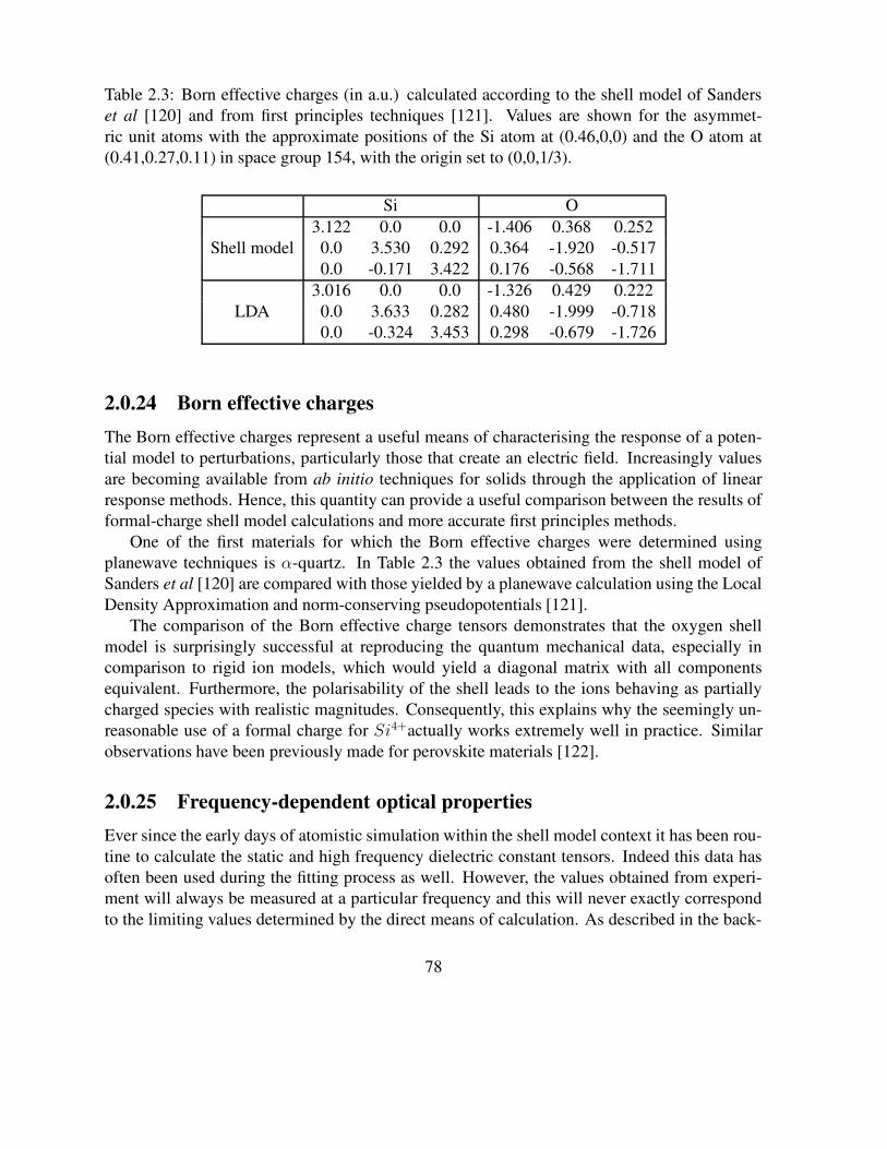
Table 2.3: Born effective charges (in a.u.) calculated according to the shell model of Sanderset al [120] and from first principles techniques [121]. Values are shown for the asymmet-ric unit atoms with the approximate positions of the Si atom at (0.46,0,0) and the O atom at(0.41,0.27,0.11) in space group 154, with the origin set to (0,0,1/3).
Si O3.122 0.0 0.0 -1.406 0.368 0.252
Shell model 0.0 3.530 0.292 0.364 -1.920 -0.5170.0 -0.171 3.422 0.176 -0.568 -1.711
3.016 0.0 0.0 -1.326 0.429 0.222LDA 0.0 3.633 0.282 0.480 -1.999 -0.718
0.0 -0.324 3.453 0.298 -0.679 -1.726
2.0.24 Born effective chargesThe Born effective charges represent a useful means of characterising the response of a poten-tial model to perturbations, particularly those that create an electric field. Increasingly valuesare becoming available from ab initio techniques for solids through the application of linearresponse methods. Hence, this quantity can provide a useful comparison between the results offormal-charge shell model calculations and more accurate first principles methods.
One of the first materials for which the Born effective charges were determined usingplanewave techniques is α-quartz. In Table 2.3 the values obtained from the shell model ofSanders et al [120] are compared with those yielded by a planewave calculation using the LocalDensity Approximation and norm-conserving pseudopotentials [121].
The comparison of the Born effective charge tensors demonstrates that the oxygen shellmodel is surprisingly successful at reproducing the quantum mechanical data, especially incomparison to rigid ion models, which would yield a diagonal matrix with all componentsequivalent. Furthermore, the polarisability of the shell leads to the ions behaving as partiallycharged species with realistic magnitudes. Consequently, this explains why the seemingly un-reasonable use of a formal charge for Si4+actually works extremely well in practice. Similarobservations have been previously made for perovskite materials [122].
2.0.25 Frequency-dependent optical propertiesEver since the early days of atomistic simulation within the shell model context it has been rou-tine to calculate the static and high frequency dielectric constant tensors. Indeed this data hasoften been used during the fitting process as well. However, the values obtained from experi-ment will always be measured at a particular frequency and this will never exactly correspondto the limiting values determined by the direct means of calculation. As described in the back-
78

ground theory section, it is possible to evaluate the dielectric properties and refractive indicesas a function of radiation frequency for the gamma point.
Here we present results for the frequency variation of the dielectric constant tensor of quartz,shown in Figure 2.2, as calculated using the previously mentioned shell model potential ofSanders et al [120]. Note that the limiting values are the same as the ones obtained withoutreference to the phonon frequencies.
In accord with experiment, the dielectric constant decreases slowly with the frequency ofmeasurement until the highest phonon mode of quartz - the Si-O stretch - is approached. Atfrequencies below this the curve contains considerable variation caused by the discontinuitieswhen a lattice phonon mode is reached. For simplicity, the curve shown is for the dielectricconstant in the ab plane only. The corresponding curve for the principal tensor componentparallel to the 001 direction is almost identical, except that the limiting values are slightlydifferent and the positions of the discontinuities due to coincidence with phonons are displacedto higher frequency.
While the qualitative agreement with experimental data is good, there is a quantitative dis-crepancy in the dielectric constant variation. This is a result of the imperfection of the original fitto the dielectric data for quartz, though there are also issues concerning the variation with tem-perature since the calculations are formally performed at absolute zero, while the experimentdata was measured at 293 K. However, the use of empirical fitting implies that the interatomicpotentials do partially account for the temperature difference already. At the lowest measuredfrequency, the calculated values are an almost perfect match due to the faster rate of decreaseof the dielectric constant in the experiment data.
2.0.26 Surface calculationsBefore applying GULP to surfaces problems that were previously not possible, it must first bevalidated. Firstly, we focus on comparing our results to MARVIN, starting with the simple in-organic salt, corundum. In the original MARVIN paper [90], the twelve faces with the lowestinterplanar spacings were identified and their surfaces relaxed using several different potentialmodels. The calculations utilising the QM5 model were repeated using both MARVIN withthe BFGS minimiser and the same surfaces generated using GDIS and minimised in GULPusing its BFGS minimiser. The unrelaxed surface and attachment energies were compared andboth sets of calculations agreed to better than 0.0001Jm−2 for the surface energies and within0.0001eV mol−1 for the attachment energies. This indicates that the 2-D Ewald sum incorpo-rated into GULP is correct. Next the relaxed surface and attachment energies were compared.Except for the (310) face, all the GULP calculations returned the same relaxed surface energyas the corresponding MARVIN run to within 0.0001Jm−2. The relaxed attachment energiesagreed to within 0.003eV mol−1. Excluding the (310) face, the MARVIN calculations took 138s on a 1133MHz Intel Pentium III CPU Linux system, whilst the GULP calculations took just108 s. This difference is timing is primarily due to the faster energy calculation time in GULPsince the MARVIN minimiser is based on the GULP algorithm and consequently the number of
79
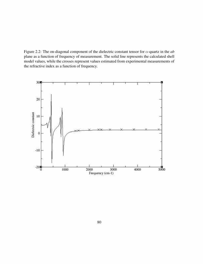
Figure 2.2: The on-diagonal component of the dielectric constant tensor for α-quartz in the abplane as a function of frequency of measurement. The solid line represents the calculated shellmodel values, while the crosses represent values estimated from experimental measurements ofthe refractive index as a function of frequency.
80
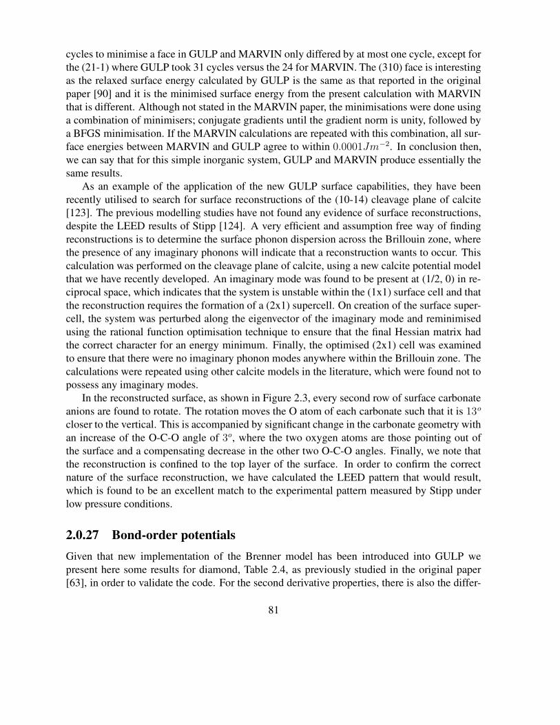
cycles to minimise a face in GULP and MARVIN only differed by at most one cycle, except forthe (21-1) where GULP took 31 cycles versus the 24 for MARVIN. The (310) face is interestingas the relaxed surface energy calculated by GULP is the same as that reported in the originalpaper [90] and it is the minimised surface energy from the present calculation with MARVINthat is different. Although not stated in the MARVIN paper, the minimisations were done usinga combination of minimisers; conjugate gradients until the gradient norm is unity, followed bya BFGS minimisation. If the MARVIN calculations are repeated with this combination, all sur-face energies between MARVIN and GULP agree to within 0.0001Jm−2. In conclusion then,we can say that for this simple inorganic system, GULP and MARVIN produce essentially thesame results.
As an example of the application of the new GULP surface capabilities, they have beenrecently utilised to search for surface reconstructions of the (10-14) cleavage plane of calcite[123]. The previous modelling studies have not found any evidence of surface reconstructions,despite the LEED results of Stipp [124]. A very efficient and assumption free way of findingreconstructions is to determine the surface phonon dispersion across the Brillouin zone, wherethe presence of any imaginary phonons will indicate that a reconstruction wants to occur. Thiscalculation was performed on the cleavage plane of calcite, using a new calcite potential modelthat we have recently developed. An imaginary mode was found to be present at (1/2, 0) in re-ciprocal space, which indicates that the system is unstable within the (1x1) surface cell and thatthe reconstruction requires the formation of a (2x1) supercell. On creation of the surface super-cell, the system was perturbed along the eigenvector of the imaginary mode and reminimisedusing the rational function optimisation technique to ensure that the final Hessian matrix hadthe correct character for an energy minimum. Finally, the optimised (2x1) cell was examinedto ensure that there were no imaginary phonon modes anywhere within the Brillouin zone. Thecalculations were repeated using other calcite models in the literature, which were found not topossess any imaginary modes.
In the reconstructed surface, as shown in Figure 2.3, every second row of surface carbonateanions are found to rotate. The rotation moves the O atom of each carbonate such that it is 13o
closer to the vertical. This is accompanied by significant change in the carbonate geometry withan increase of the O-C-O angle of 3o, where the two oxygen atoms are those pointing out ofthe surface and a compensating decrease in the other two O-C-O angles. Finally, we note thatthe reconstruction is confined to the top layer of the surface. In order to confirm the correctnature of the surface reconstruction, we have calculated the LEED pattern that would result,which is found to be an excellent match to the experimental pattern measured by Stipp underlow pressure conditions.
2.0.27 Bond-order potentialsGiven that new implementation of the Brenner model has been introduced into GULP wepresent here some results for diamond, Table 2.4, as previously studied in the original paper[63], in order to validate the code. For the second derivative properties, there is also the differ-
81
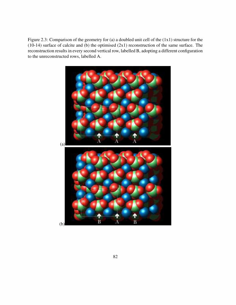
Figure 2.3: Comparison of the geometry for (a) a doubled unit cell of the (1x1) structure for the(10-14) surface of calcite and (b) the optimised (2x1) reconstruction of the same surface. Thereconstruction results in every second vertical row, labelled B, adopting a different configurationto the unreconstructed rows, labelled A.
(a)
(b)
82

Table 2.4: Calculated properties of diamond based on the model of Brenner et al [63]. Note thatthe calculated values for the bond length and energy are not quoted in the original reference.However, since the experimental values were part of the fitted data, we take these values to beequal to the observed ones.
Property Experiment Original value GULP valueBond length(A) 1.54 1.54 1.5441
Bond energy (eV) 3.68 3.68 3.684C11(GPa) 10.8 10.7 10.75C12(GPa) 1.3 1.0 1.26C44(GPa) 5.8 6.8 7.21
ence that the values obtained here are fully analytic whereas the published values are obtainedvia finite differences. This may explain the small discrepancies in the elastic constants.
As stated in the background section, two algorithms have been implemented for the evalua-tion of the Brenner potential based on either pairwise atom looping or a spatial decompositionin order to determine the neighbour list. The computational cost of the two approaches forincreasing supercells of diamond are illustrated in Figure 2.4. The linear scaling behaviour ofthe spatial decomposition can clearly be seen, as can the fact that this algorithm is effectivelysuperior in performance for systems containing beyond a 100 atoms. Obviously this trade offpoint is dependent on the density of the system, though there are few cases for hydrocarbonswhere the density is greater than that of diamond. For systems much below a 100 atoms thecost of evaluating the Brenner potential is so negligible in comparison to other tasks, such as amatrix inversion for property calculation, that the choice of algorithm is irrelevant.
83
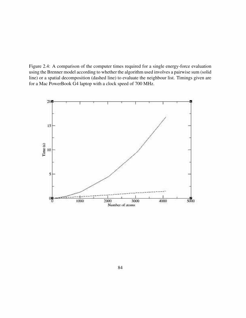
Figure 2.4: A comparison of the computer times required for a single energy-force evaluationusing the Brenner model according to whether the algorithm used involves a pairwise sum (solidline) or a spatial decomposition (dashed line) to evaluate the neighbour list. Timings given arefor a Mac PowerBook G4 laptop with a clock speed of 700 MHz.
84

Chapter 3
Further background
In this section some of the theory behind GULP is explained and references are supplied forthose who require a more detailed description of the methods involved.
3.0.27.1 Cut-offs and molecules
All short-ranged two-, three- and four-bodied potentials have finite cut-offs in real space whichmust be set by the user in some way. Unless the cut-off chosen is so large that convergenceis genuinely achieved then it effectively becomes a parameter of the potential. Hence whenpublishing new potentials it is good practice to publish the cut-offs. Similarly, if you are tryingto reproduce the results of previously published potentials make sure you use the same cut-offs.
The main effect of finite cut-offs is to introduce discontinuities into the energy surface asatoms move across the boundary. Generally speaking, the energy minimisation procedure inGULP is not too sensitive to these because of the use of analytical second derivatives. However,if working with only first derivatives or particularly short cut-offs this can be the reason for aminimisation failing to satisfy the required convergence criteria.
An important difference between GULP and some other programs is that it is perfectly al-lowable for potentials to overlap, i.e. two or more potentials can act between the same species atthe same distance. Hence, there are no resulting restrictions for the cut-offs and complex poten-tial functions can be built by combining several potentials together. Conversely, it is importantnot to duplicate potentials when not intended.
For some types of potential the cut-offs may correspond to chemical criteria such as bondlengths or they may only need to act between molecules or conversely only within them. Insuch cases it is best not to use distance cut-offs to achieve the correct effect, but instead to usethe molecule handling facilities within GULP. There are three keywords which when specifiedactivate the molecule facility within the program - molecule, molq and molmec. If anyof these words are present then a search will be performed to locate any molecules within thestructures input. This is done by searching for bonds based on the sum of the covalent radii plus
85

Table 3.1: Common functional forms for two-body interatomic potentials incorporated intoGULP (where r represents the distance between two atoms i and j). For full documentation seehelp.txt.
Potential Name Formula Units for inputBuckingham A exp(−r/ρ) − Cr−6 A in eV, ρ in A, C in eVA6
Lennard-Jones† Ar−m − Br−n A in eVAm, B in eVAn
orε(c1(
σr)m − c2(
σr)n) ε in eV, σ in A
c1 = (n/(m − n))(m/n)(m/(m−n))
c2 = (m/(m − n))(m/n)(n/(m−n))
Harmonic? 12k2(r−r0)
2+ 16k3(r−r0)
3+ 112
k4(r−r0)4 k2in eVA−2, r0 in A
k3 in eVA−3, k4 in eVA−4
Morse D[1 − exp(−a(r − r0))]2 − 1 D in eV, a in A−2, r0 in A
Spring (core-shell) 12k2r
2 + 124
k4r4 k2 in eVA−2, k4 in eVA−4
General A exp(−r/ρ)r−m − Cr−n A in eVAm, ρ in A,C in eVAn
Stillinger-Weber A exp(ρ/(r − rmax))(Br−4 − 1) A in eV, ρ in A, B in A4
(sw2)† combination rules permitted? k3, k4 are optional
86

Table 3.2: Common functional forms for three-body potentials incorporated into GULP (wherer represents the distance between two atoms i and j, θijk represents the angle between the twointeratomic vectors i-j and j-k). For full documentation of all the functional forms availablesee help.txt.
Potential Name Formula Units for inputStillinger-Weber K exp(ρ/(r12 − rmax) + ρ/(r13 −
rmax))(cos(θ213) − cos(θ0))2
K in eV,
(sw3) ρ in A
Three-body † 12k2(θ − θ0)
2 + 16k3(θ − θ0)
3 + 112
k4(θ − θ0)4 θ0 in
k2 in eVrad−2,k3 in eVrad−3,k4 in eVrad−4
Three-body? 12k2(θ213 − θ0)
2 exp(−r12/ρ) exp(−r13/ρ) k2 in eVrad−2,θ0 in , ρ in A
Axilrod-Teller K(1 + 3 cos θ213 cos θ123 cos θ132)/(r12r13r23)3 K in eVA9
Exponential A exp(−r12/ρ) exp(−r13/ρ) exp(−r23/rho) A in eV, r in A
Urey-Bradley 12k(r23 − r0)
2 k in eVA−2,r0 in A
Cosine-harmonic 12k2 (cos θ − cos θ0)
2 k2in eV
Bond-angle cross(
k1
(
rij − r0ij
)
+ k2
(
rjk − r0jk
))
(θ − θ0) k1& k2in eV A−1deg−1
(bacross)
† harmonic, keyword three? harmonic + exponential, keyword three expo
87

Table 3.3: Common functional forms for four-body potentials incorporated into GULP (whereφijkl is the torsional angle between the planes ijk and jkl). For full documentation see the filehelp.txt.
Potential Name Formula Units for inputFour-body k(1 + cos(nφ − φ0)) k in eV, φ0 in
Ryckaert-Bellemans ∑
kn(cos φ)n kn in eV
Out of plane kd ∗ ∗2 k in eVA−2
a percentage tolerance factor. For most common compounds the default covalent radii will besufficient to locate all the bonds - if this is not the case then it is possible for the user to eitherincrease the tolerance factor or to adjust the covalent radii using the covalent option fromthe element group of commands.
An alternative scenario is that atoms become bonded which shouldn’t be. For example,metal atoms often can become bonded in ionic compounds because the covalent radii is nolonger relevant for a positively charged ion. These bonds can be removed either by manuallysetting the radii of the element to zero or by using the nobond option to exclude the formationof certain bond types. Whether the correct molecules have been located or not can be seen fromthe molecule print out in the output file. The three molecule-based keywords mentioned abovediffer in what they imply for the treatment of intramolecular electrostatics:
molecule ⇒ exclude all Coulomb interactions within the moleculemolq ⇒ retain all Coulomb interactions within the moleculemolmec ⇒ exclude all Coulomb interactions between atom which are
bonded (1-2) or two bonds away (1-3)
The specification of molmec does not automatically imply that all potentials will be treatedin a molecular mechanics fashion, only the electrostatic terms. Providing one of the above thereterms is present then optional words may be added to a potential specification line which controlaspects of the potential cut-offs. Below is a list of the words that are available and whether it isnecessary to still give any cut-offs on the potential parameter line:
88
Option Effect Cut-offs?intra only act within a molecule yesinter only act between molecules yesbond only act between bonded atoms nox12 do not act between bonded atoms yesx13 do not act between 1-2 and 1-3 atoms yes
Although with some options it is necessary to still specify a cut-off for generality, the valuemay not be important any more. For example, if an O-H potential for water is specified as beingintramolecular then as long as the maximum distance cut-off is greater than about 1.0 A thenit doesn’t matter particularly what it is. Similarly for a potential which is given as being x12then it doesn’t matter if the minimum cut-off distance is zero - the potential won’t act betweenbonded atoms.
By default, GULP dynamically calculates the molecular connectivity during a calculation.The reason for this is that it ensures that the restart file will yield the same answer as the point inthe calculation where it left off. However, sometimes difficulties occur because a bond becomestoo long and the molecule breaks into two. When this happens GULP will stop with an errormessage as this often indicates that the potential model is not working well for the systemunder study. If the user wants to proceed regardless then there is a keyword fix which tells theprogram to fix the connectivity as that at the starting geometry and not to update it. This meansthat the program will never stop with this error, but it does mean that a restart may not give thesame answer as the initial run if atoms have moved too far.
In the case of ionic materials where the user would like to try to remove some of the nu-merical problems associated with cut-offs then there are some other options. The normal wayof doing this is with a cut-and-shifted potential. In this approach the potential is forced to go tozero at the cut-off by adding a constant to the energy. This makes the energy continuous, butthe gradient still has a discontinuity. Again this can be resolved by adding a second term whichshifts the gradient to be zero at the cut-off. In GULP this takes the form of a linear term inthe distance which, provided the cut-off isn’t very short, will have minimal effect in the regionof the potential minimum. These corrections are activated using the potential options energyor gradient after the potential type, but are only currently applicable to certain two-bodypotentials where it is appropriate. It should be noted that some potential functions go to zero byconstruction at the cut-off, for example the Stillinger-Weber two- and three-body potentials.
3.0.27.2 Combination rules
When using Lennard-Jones potentials it is common to use combination rules to determine theinteraction parameters between two species. This means that the parameters for the interac-tion are determined from one-centre only parameters by some form of averaging. The mainadvantage of this approach is that it reduces the number of parameters to be determined and
89

aids transferability of potentials. Conversely, the resulting potentials may not be as accurate forany one given system. There are two types of combination rule used, depending on whether thepotential is being used in the ε/σ or A/B format (see Table 2 for details). If the potentials arebeing used in the A/B form then the average is taken using a geometric mean:
Aij =√
AiAj
Bij =√
BiBj
However, if the ε/σ form is being employed then a more complex relationship is needed:
εij =2(εiεj)
1
2 (σ3i σ
3j )
(σ6i + σ6
j )
σij =
(
σ6i + σ6
j
2
)1
6
Within GULP it is possible to specify the parameters by species, rather than by pairs ofspecies, using the atomab or epsilon options. If the word combine is added to the spec-ification of a lennard-type potential then the parameters can be omitted from the input andthey will be generated using the appropriate combination rules. In turn this makes it possible tofit potentials based on combination rules without having to do this via a series of constraints.
3.0.27.3 Mean field theory
One of the biggest problems that can face someone attempting to simulate complex materialsis the fact that often they can be partly disordered or involve partial occupancies of sites. Oneapproach to treating such systems is to generate a supercell so that lots of permutations canbe examined. However, the number of possibilities is usually too large to examine each oneindividually to locate the most stable configuration. Furthermore, this process may alter thesymmetry of crystal. Fitting potentials to such structures also becomes rather difficult.
An alternative approach to handling partial occupancies is to use mean field theory. Theeffect of this is that each site experiences a potential which is the mean of all possible configu-rations on the disordered positions. In doing so we are assuming that all possible configurationsare equally as likely, i.e. the less stable configurations are equally as likely as the more stableones. This may apply to materials were there is little energetic difference between configu-rations or to ones which were formed under kinetic rather than thermodynamic control andhaven’t had chance to achieve a Boltzmann distribution. It must be decided for any given mate-rial whether it is therefore appropriate to use this approach.
The practical upshot of the mean field method is that all interactions just become scaled bythe site occupancies of both atoms. This has been implemented in GULP such that the usercan specify the site occupancy in addition to the coordinates (see the later section on the input
90

for further details) and the program will automatically handle most aspects of the mean fieldapproach. This includes ensuring the total occupancy on a site does not exceed unity and wheretwo different ions share a site with partial occupancy they are constrained to move as a singleion in optimisations.
One important word of warning - it is important that the user thinks through interactionscarefully when using the partial occupancy feature to ensure that everything is handled properly.The biggest danger comes in systems where there are two partially occupied sites very close toeach other such that in the real system their occupancy would be mutually exclusive. When thishappens it is often necessary to specifically exclude potentials between these atoms to obtainthe correct behaviour.
3.0.27.4 Algorithms for energy and derivative evaluations
GULP actually contains several different algorithms for calculating the energy and its first andsecond derivatives. By default the program will try to choose the most efficient for any givensystem, excluding possibilities such as the cell multipole method which would actually lead toslight changes in the answer. Normally the user will need to know nothing about what algorithmis being used, so this section is really for the curious.
Usually real-space interactions are calculated in a lower-half triangular fashion to avoid dou-ble counting of interactions which would give rise to loops of the form shown below:
do i = 2, numatdo j = 1, i-1
[Calculate interaction between i and j]enddo
enddo
If there is the possibility of self-terms or interactions between periodic replications of thesame atom then the i = j term would not be excluded, though it may be more efficient to handlethis case in a separate loop. For solids where there is significant space group symmetry then adifferent algorithm may be more efficient:
do i = 1, nasymdo j = 1, numat
[Calculate interaction between i and j]enddo
enddo
where nasym is the number of species in the asymmetric unit and numat is the number ofatoms in the full unit cell. Both the symmetry adapted and standard algorithms are present inGULP with selection being made based on the amount of symmetry in the crystal. The use of
91

symmetry can result in up to an order of magnitude speed-up in favourable cases and thereforeis well worth using. More details concerning the use of symmetry, in particular with respect tothe calculation of derivatives, can be found elsewhere [115].
The second algorithmic aspect to mention applies to the situation when a constant volumeoptimisation is being performed and some atoms are held fixed. Typical cases where this occursare in an optical calculation, in which only shells are relaxed, or where a molecule is dockedwithin a rigid microporous material. In this case the energy of interaction between certainatoms is a constant term and the forces on them are ignored. When this happens these atomsare excluded or frozen out of the energy calculation after the first point to save computationalexpense.
3.0.28 Phonons3.0.28.1 Phonon density of states
We may also be interested in the phonon density of states for a solid as the number of fre-quencies versus frequency value becomes a continuous function when integrated across theBrillouin zone. While full analytical integration across the Brillouin zone is not readily carriedout, this integral can be approximated by a numerical integration. We can imagine calculatingthe phonons at a grid of points across the Brillouin zone and summing the values at each pointmultiplied by the appropriate weight (which for a simple regular grid is just the inverse of thenumber of grid points). As the grid spacing goes to zero the result of this summation tends totowards the true result.
For performing these integrations GULP uses a standard scheme developed by Monkhorstand Pack [88] for choosing the grid points. This is based around three so-called shrinkingfactors, n1, n2 and n3 - one for each reciprocal lattice vector. These specify the number ofuniformly spaced grid points along each direction. The only remaining choice is the offset ofthe grid relative to the origin. This is chosen so as to maximise the distance of the grid from anyspecial points, such as the gamma point as this gives more rapid convergence.
In many cases it is not necessary to utilise large numbers of points to achieve reasonableaccuracy in the integration of properties, such as phonons, across the Brillouin zone. For highsymmetry systems several schemes have been devised to reduce the number of points to aminimum by utilising special points in k space. However, because GULP is designed to begeneral the Monkhorst-Pack scheme is used. The user can input special points instead, if knownfor the system of interest.
Often it is not necessary to integrate across the full Brillouin zone due to the presenceof symmetry. By using the Patterson group (the space group of the reciprocal lattice) GULPreduces the integration region to that of the asymmetric wedge which may only be 1/48-th ofthe size of the full volume [89].
When producing plots of the phonon density of states the critical factor, apart from theresolution of the integration grid, is the ‘box’ size. The continuous density of states curve has
92

to be approximated by a series of finite regions of frequency or boxes. Each phonon mode ateach point in k space is assigned to the box whose frequency region it falls into. The smaller thebox size the better the resolution of the plot. However, more points will be needed to maintaina smooth variation of number density.
3.0.28.2 Infra-red phonon intensities
In order to make comparison between theoretically calculated phonon spectra and experimentit is important to know something about the intensity of the vibrational modes. Of course theintensity depends on the technique being used to determine the frequency as different methodshave different selection rules. While Raman intensities are not readily calculable from mostpotential models, due normally to the absence of polarisabilities higher than dipolar ones, ap-proximate values for infra-red spectra can be determined [125]:
IIR ∝ (∑
all speciesqd)2
where q is the charge on each species and d is the Cartesian displacement associated withthe normalised eigenvector.
3.0.28.3 Thermodynamic quantities from phonons
There are a range of quantities that can be readily calculated from the phonon density of states.The accuracy with which they are determined though clearly depends on the k points or shrink-ing factors selected for the Brillouin zone integration. For systems with large unit cells a smallnumber of k points, perhaps even the Γ-point alone, will be sufficient. However, for those sys-tems with small to medium unit cells it is important to examine how converged the propertiescalculated are with respect to the grid size.
If a phonon calculation is performed then GULP will automatically print out the relevantthermodynamical quantities. This output depends partly on whether a temperature has beenspecified for the given structure. If the calculation is set for zero Kelvin then only the zero pointenergy is output:
ZPE =∑
k−pointswk
∑
all modes
1
2hν
where wk is the weight associated with the given k point. In principal, the zero point energyshould be added to the lattice energy when determining the relative stability of two differentstructures. However, because the derivatives of the zero point energy are non-trivial it is nor-mally neglected in an energy minimisation.
For temperatures above absolute zero we can calculate the vibrational partition function,which in turn can be readily used to calculate three further properties:
93
Vibrational partition function:
Zvib =∑
k−pointswk
∑
all modes
(
1 − exp
(
− hν
kT
))−1
Vibrational entropy:
Svib = R ln Zvib + RT
(
∂ ln Zvib∂T
)
Helmholtz free energy:A = U − TSvib
whereU = Ulattice energy + Uvibrational energy
Heat capacity at constant volume:
Cv = RT
(
2
(
∂ ln Zvib∂T
)
+ T
(
∂2 ln Zvib∂T 2
))
3.0.29 Free energiesAlthough the most common methods for studying the properties of materials as a function oftemperature are molecular dynamics and Monte Carlo simulations, there is an alternative basedon static methods within the quasi-harmonic approximation. This is to directly minimise thefree energy of the system at a given temperature, where the free energy is calculated from thelattice energy combined with contributions from the phonons including the entropy and zeropoint energy.
The advantages of working with free energy minimisation are that MD simulations are quiteexpensive due to the need to reduce the uncertainty by sampling large amounts of phase space.Molecular dynamics and free energy minimisation are in fact complementary techniques. Thelater approach breaks down at high temperatures as anharmonic effects become important -typically it works at temperatures up to half the melting point as a rough guide. Conversely,molecular dynamics is not strictly valid at low temperatures because the zero point motions andquantum nature of the vibrational levels is ignored.
Although in principle it is possible to analytically fully minimise the free energy of a solid,in practice this is extremely difficult as it requires the fourth derivatives of the energy withrespect to the Cartesian coordinates. Hence, a number of approximations are normally made -the main one being that the principal effect of temperature is to expand or contract the unit celland the effect on internal degrees of freedom is less important.
When changing unit cell parameters we are concerned with the Gibbs free energy as thisis appropriate to a constant pressure calculation. This quantity is related to the Helmholtz free
94

energy, whose relationship to the vibrational entropy has already been given previously, by theexpression;
G = A + PV
withP = Pext − Pint
where P is the pressure. The pressure has two components - any external applied pressure plusthe internal phonon pressure coming from the vibrations. The phonon pressure is given by:
Pint = −∂A
∂V
In order to calculate the Gibbs free energy it is therefore necessary to calculate the derivativeof the Helmholtz free energy with respect to the unit cell volume. This can be done numericallyby finite differences. Central differencing is more expensive than using forward differences.However, it is generally necessary to determine the phonon pressure with sufficient accuracy.In turn each calculation of the Helmholtz free energy requires a constant volume minimisationfor the given set of unit cell parameters, followed by a phonon calculation.
Once the Gibbs free energy has been calculated then the next stage of a free energy minimi-sation is to isotropically expand or contract the unit cell until the external pressure balances theinternal pressure. Having done this then the derivatives of the Gibbs free energy can be evalu-ated numerically by finite differences and the unit cell optimised with respect to this quantity.
Because of the three levels of optimisation plus phonon calculations involved, free energyminimisations are rather expensive and shouldn’t be undertaken lightly! Due to the numericalnature of several of the derivatives it may be necessary for the user to adjust the finite differ-encing interval for a calculation to work optimally. Also the calculations are very sensitive tothe quality of the underlying energy surface. Potentials with short cutoffs, leading to disconti-nuities, and soft modes can cause difficulties for the method, so always check your model wellbefore starting.
Free energy minimisation can be used in conjunction with fitting to allow a series of struc-tures at different temperatures to be fitted with inclusion of the thermal effects, though againthis is an expensive procedure. It is important to note that a free energy minimisation at 0 Kis not the same as an ordinary static calculation. This is due to the presence of the zero pointenergy in the former method.
3.0.30 Defects3.0.30.1 The Mott-Littleton method
The calculation of defect energies is more difficult and approximate than the calculation of bulkproperties. In theory, a defect can cause very long range perturbations, particularly if it is notcharge-neutral. Consequently the user must always check the convergence of the approxima-tions made.
95

The simplification in the modelling of defects is to divide the crystal that surrounds thedefect into three spherical regions known as regions 1, 2a and 2b [126, 127, 104]. In region1 all interactions are treated exactly at an atomistic level and the ions are explicitly allowed torelax in response to the defect. Except in the case of very short-ranged defects it is not generallypossible to achieve the desired degree of convergence by increasing region 1 before running outof computer resources. Consequently, in region 2a some allowance is made for the relaxationof ions but in a way that is more economical.
In region 2a the ions are assumed to be situated in an harmonic well and they subsequentlyrespond to the force of the defect accordingly [114]. This approximation is only thus valid forsmall perturbations and also requires that the bulk lattice has been optimised prior to the defectcalculation. For region 2a individual ion displacements are still considered, whereas for region2b only the implicit polarisation of sub-lattices, rather than specific ions, is considered.
If the vector x represents the positions of ions in region 1, while ζ represents the displace-ments of ions in region 2a, then the total energy of the system may be written as:
E = E1(x) + E12(x, ζ) + E2(ζ)
where E1 and E2 are the energies of regions 1 and 2 respectively, and E12 is the energy ofinteraction between them. We now assume that the energy of region 2 is a quadratic function ofthe displacements:
E2(ζ) =1
2ζTWζ
We also know that we wish to obtain the displacements in region 2 for which the energy isa minimum:
∂E
∂ζ= 0 =
∂E12(x, ζ)
∂ζ+ Wζ
This expression can be used to eliminate E2 from the total energy, leaving it purely in termsof E1 and E12:
E = E1(x) + E12(x, ζ) − 1
2
∂E12(x, ζ)
∂ζζ
The displacements in region 2 are formally a function of x for region 1 which makes theminimisation of the total energy with respect to both the positions of region 1 and the displace-ments of region 2 potentially complicated. This problem can be avoided by using force balancein region 1 as the criteria for convergence (i.e. all forces on ions in region 1 must be zero), ratherthan purely minimising the energy. The two approaches are equivalent provided that region 2 isat equilibrium also. This will be achieved provided that the displacements in region 2 are smallenough that they are genuinely quadratic.
In terms of the minimisation procedure employed for defect calculations the force bal-ance process leads to a slightly different approach to the bulk optimisation. Initially the sameNewton-Raphson procedure with BFGS hessian updating and line searches is employed to avoidconvergence to stationary points which are not minima. After at least one cycle of the above and
96

when the gradient norm falls below a certain threshold the minimiser abandons the line searchprocedure and aims purely to reduce the gradients to zero, regardless of the energy. In practicepositive changes in the energy near convergence are only ever small.
The defect energy is now the difference in the total energies for the defective and perfectlattice, Ed and Ep respectively, with corrections due to the energy of any interstitial or vacancyspecies at infinite separation from the lattice, E∞:
Edefect = Ed − Ep + E∞
Two final aspects must be dealt with in order to obtain the final working equations for thedefect energy. Firstly, due to the slow convergence of electrostatic terms in real space alone wecannot evaluate the region 1 - region 2 energy directly. Instead we must calculate the energy ofregion 1 interacting with the perfect lattice to infinity and then explicitly subtract and add backthe terms due to ions which are no longer on their perfect lattice sites. Secondly, because thedisplacements in region 2 depend on the force acting on a given ion, which in turn is a functionof other region 2 ions, there is in fact a linear dependency of the energy on ζ . By suitablemanipulation of the energy terms this may be removed to leave the following expression for thedefect energy:
Edefect = E11(dd) − E11(dp) + E1∞(dp) − E1∞(pp)
+E12a(dd) − E12a(dp) + E12a(pp) − E12a(pd)
−∑
(
∂E12a(dd)
∂r− ∂E12a(pd)
∂r
)
where the general symbol Eij(kl) denotes the energy of interaction summed over all ions inregion i interacting with ions in region j where i and j can be 1, 2a or ∞ (signifying a sum over1, 2a and 2b out to infinity). The letters k and l indicate whether the energy is for the perfect ordefective coordinates in regions i and j respectively, depending on whether they are p or d.
3.0.30.2 Displacements in region 2a
Expanding the energy as a Taylor series and truncating at second order gives the Newton-Raphson estimate of the vector from the current ion position to the energy minimum position interms of the force, g, acting on the ion:
ζ = −W−1g
Hence if we know the local second derivative matrix and the force acting on the ion we cancalculate its displacement. There are a number of possible ways of calculating the force actingon the ions in region 2a. The most common approach is to use the electrostatic force due to onlythe defect species - i.e. the force due to any interstitial species based on their current positions,
97

less the force due to any vacancies at the position of the original vacant site. In this way region2a responds to the change in the multipole moments of the defect species in region 1, but notthe influence of other forces. Hence for this approximation to strictly hold the distance betweenany defects and the boundary of region 2a should be greater than the short-range cutoff.
3.0.30.3 Region 2b energy
Region 2b is assumed to be sufficiently far from the defects that the ions only respond bypolarising according to the electrostatic field resulting from the total defect charge placed at thecentre of region 1. This can be written for cubic systems as follows:
E2b = −1
2Q2
∑
i6=1,2a
qimi
R4i
Because this expression is just dependant on the distance and a couple of lattice site re-lated parameters the region 2b energy can be evaluated using a method analogous to the Ewaldsum and then subtracting off the contribution from ions in regions 1 and 2a. An alternativemore general, but still not completely general, expression is the following where the lattice sitedependant property is now an anisotropic tensor, rather than a scalar [105]:
E2b = −1
2Q2
∑
i6=1,2a
∑
αβ
qiMαβi Rα
i Rβi
R6i
This can again be calculated by partial reciprocal space transformation based on the secondderivatives of the R−4 lattice sum.
3.0.31 Fitting3.0.31.1 Fundamentals of fitting
Before any production runs can be performed with an interatomic potential program it is neces-sary to obtain the potential parameters. If you are lucky there may be good parameters for yoursystem of interest already published in the literature so you can just type them in and get goingstraight away. Unfortunately most people are not so lucky! The fitting facility within GULP[128] allows you to derive interatomic potentials in either of two possible ways. Firstly, you candetermine the parameters by fitting to data from some higher quality calculation, such as an abinitio one, normally by attempting to reproduce an energy hypersurface. Secondly, you couldattempt to derive empirical potentials by trying to reproduce experimental data.
Regardless of which method of fitting you are using the key quantity is the ’sum of squares’which measures how good your fit is. Ideally this should be zero at the end of a fit - in practicethis will only happen for trivial cases where the potentials can be guaranteed to completelyreproduce the data (for example fitting a Morse potential to a bond length, dissociation energy
98

and frequency for a diatomic should always work perfectly). The sum of squares, F , is definedas follows:
F =∑
all observablesw(fcalc − fobs)
2
where fcalc and fobs are the calculated and observed quantities and w is a weighting factor.There is no such thing as a unique fit as there are an infinite number of possible fits dependingon the choice of the weighting factors. The choice of weighting factor for each observabledepends on several factors such as the relative magnitude of the quantities and the reliability ofthe data (for instance a crystal structure will generally be more reliable than an elastic constantmeasurement).
The aim of a fit is to minimise the sum of squares by varying the potential parameters. Thereare several standard techniques for solving least squares problems. At the moment GULP usesa Newton-Raphson functional minimisation approach to solving the problem, rather than themore conventional methods. This is because it avoids storing the co-variance matrix. Thedownside is that near-redundant variables are not eliminated. Currently the minimisation of thesum of squares is performed using numerical first derivatives. The reason for using numericalderivatives is because many of the properties, particularly those derived from second deriva-tives, are rather difficult to implement analytical derivatives for. Consequently the value of thegradient norm output during fitting should only be taken as a rough guide to convergence.
The choice of which potential parameters to fit belongs to the user and is controlled by aseries of flags on the potential input line (0 ⇒ fix, 1 ⇒ vary). There are also options containedwithin the variables sub-section for allowing more general parameters to fit, such as chargedistributions. Note that when fitting charges at least two charges must be varied to have anyeffect as the program eliminates one variable due the charge neutrality constraint. There is alsothe option to vary the charge split between a core and shell while maintaining a constantoverall charge on the ion. The user may also impose their own constraints on fitting variablesthrough the constrain fit option.
It is generally recommended that a small number of parameters are fitted initially and thenumber gradually increased in subsequent restarts. Often if all parameters are allowed to varyfrom the start unphysical parameters may result. Dispersion terms of Buckingham or Lennard-Jones potentials are particularly prone to poor behaviour during fitting, as they tend to go tozero or become exceedingly large. It is generally recommended that such terms are set equalto a physically sensible value (based on quantum mechanical estimates or polarisability-basedformulae) and held fixed until everything else is refined.
A final check that the program looks for is that the total number of variables being fitted isless than the total number of observables!
3.0.31.2 Fitting energy surfaces
To fit an energy surface it is basically necessary to input all the structures and the energiesthat correspond to them. To do this it is just a matter of putting one structure after another in
99

the input file (within the limit of the maximum number of structures for which the program isdimensioned). It is possible to fit the gradients acting on the atoms as well the energy of eachstructure, though often just the energies are fitted. If the latter is the case, then the easiest wayto turn off the fitting of the gradients is to specify noflag as a keyword to prevent the programfor looking for gradient flags in the absence of a keyword to specify them.
Perhaps the only unique feature of fitting an energy surface is the need to include an energyshift in some cases. This is a single additive energy term which is the same for all structures andjust moves the energy scale up and down. The justification for this is that often it is impossibleto calculate the energy that corresponds exactly to the interatomic potential one from a quantummechanical calculation [109]. Most commonly this arises where the potential model has partialcharges in which case there is an unknown term in the lattice energy due to ionisation potentialsand electron affinities for fractions of an electron.
To simplify the specification of this shift value in the input, if you give the shift optionafter the first structure then this value will apply to all subsequent structures until a differentvalue is input. Similarly, its magnitude can be altered by using the variables sub-section tospecify the shift as a variable and this will apply to all structures. It is generally recommendedthat the shift is fitted first and allowed to fit through out the procedure.
3.0.31.3 Empirical fitting
An alternative to fitting quantum mechanical data to derive an interatomic potential is to actuallyfit experimental data. In this case the procedure serves two purposes. Firstly, the degree to whichall the data can be reproduced may serve as some guide as to the physical correctness of themodel used. Secondly, it provides a means of extrapolation of experimental data for one systemto a different one where the data may not be known, or alternatively to unknown properties ofthe same material.
Any of the properties that can be calculated for the bulk solid or gas phase molecule canalso be used in reverse to fit a potential to. Obviously the essential ingredient in the fit is theexperimental structure, without which you won’t get very far! The conventional way to fit thestructure is by requiring that the forces on the atoms are zero. This is clearly not a perfectstrategy as it could be satisfied by a transition state rather than a minimum, though in practiceit is rare, except when symmetry constraints are imposed.
Normally a good fit requires some second derivative information as well as the structure. Forvery high symmetry systems, such as rock salt, the structural data alone is completely inade-quate. If we imagine a potential as being a binomial expansion about the experimental geometry,then unless the first and second derivatives are reasonably well reproduced by our model thenthe range of applicability will be almost zero. Typical sources of second derivative informationare elastic, dielectric and piezoelectric (where applicable) constants. Also vibrational frequen-cies contain far more information than any of the above. However, the fitting of frequencies isnot straightforward. To fit the frequency magnitudes is certainly possible, however, you haveno guarantee that the correct mode has been fitted to the correct eigenvalue. Hence, frequency
100

fitting only tends to be useful from empirical data for special cases, such as O-H stretchingmodes which are well separated from other modes and for diatomics where there is no problemin assignment!
One other case where frequency fitting can be useful is at the lower end of the spectrum. Foran isolated molecule or a solid at its Γ point the first three modes should have zero frequency asthey are just translations. In some cases there may be imaginary modes due the potentials notcorrectly reproducing the true symmetry. Hence by fitting the first three modes to be zero it ispossible to encourage the potentials to yield the correct symmetry.
3.0.31.4 Simultaneous fitting
There is one main difficulty in the conventional scheme for fitting in which the forces on theatoms are minimised by variation of the potential parameters which arises when using a shellmodel. Normally we don’t know what the shell coordinates are at the outset unless the ions aresited at centres of symmetry. In the past people have tried fitting with the shells placed on topof the cores. However, this means that the potentials are tuned to minimise the polarisation inthe system and leads to the shell model having only a small beneficial effect. It also doubles thenumber of observables connected with gradients, but only introduces a small number of extravariables thus making it harder to get a good fit.
The solution to this problem is allow the shell positions to evolve in some way during the fit.There are two possibilities - either we can minimise the shell positions at every point during thefit or we can added the shell coordinates as fitting parameters. In the case where only structuraldata is being fitted the two methods are equivalent except in the way that they evolve towards theanswer. When other properties are included the second approach is not strictly correct, thoughthe difference is usually small.
After experimenting with several test cases it was found that the second scheme in which theshell coordinates become fitted variables was far more stable in convergence and more efficient.Hence this is the scheme that has been adopted and is referred to as ’simultaneous’ fitting due tothe concurrent fitting of shell positions. Whenever working with shell models it is recommendedthat the keyword simultaneous is added during conventional fitting - it can improve the sumof squares by several orders of magnitude! Not only does this scheme apply to the coordinatesof shells, but also to the radii of breathing shells as well.
3.0.31.5 Relax fitting
It has been observed that sometimes in conventional fitting getting an improved sum of squaresdoesn’t always get you what is considered to be a better quality fit. This is because peopleoften use different criteria to make their judgement to the ones input into the fitting process. Inparticular they look at the difference between the optimised structural parameters and those fromexperiment, rather than looking at the forces. The reason why the forces can be lower, but leadto a worse structure is because in a harmonic approximation the displacements in the structure
101
are given by the gradient vector multiplied by the inverse hessian. Hence, if the gradients getsmaller but the inverse hessian gets much larger then the situation may get worse.
The solution to this problem is to fit according to the criteria by which the structures arejudged - this is what relax fitting does. This means that at every point in the fit the structure isoptimised and the displacements of the structural parameters calculated instead of the gradients.In this approach the shell model is naturally handled correctly and so there is no need forsimultaneous fitting. The downside is that it is much more expensive in computer time thanconventional fitting. Also you can only start a relax fit once you have a reasonable set ofpotential parameters - i.e. one which will give you a valid minimisation. Hence a conventionalfit is often a prerequisite for a relax fit.
There is a further benefit to using relax fitting. In a conventional fit the properties arecalculated at the experimental structure normally with non-zero gradients which is not strictlycorrect. In a relax fit the properties are calculated for the optimised structure where they arevalid.
3.0.32 Genetic algorithmsConventional minimisation techniques based upon methods such as Newton-Raphson are excel-lent ways of locating local minima. However, they are of limited use in finding global minima.For example, if we know the chemical composition of a compound and its unit cell, but don’tknow the structure then we would want to locate the most stable arrangement for placing theatoms within the unit cell. To search systematically for a reasonable set of atomic coordinatesmay take a very long time by hand. Genetic algorithms [129] are a method by which we cansearch for global minima rather than local minima, though there can never be an guarantee offinding a global minimum. In many respects it resembles Monte Carlo methods for minimasearching, though is regarded by some as being more efficient.
The concept behind the method, as the name might suggest, is to carry out a ’natural se-lection’ procedure within the program in the same way that nature does this in real life. Westart off with an even numbered sample of randomly chosen configurations. This is our trial setwhich is allowed to evolve according to a number of principles described below. Before we cando this we need to consider how to represent our data for each configuration. To do this we en-code each number as a binary string by dividing the range between the maximum and minimumpossible values (for example 1 and 0 for fractional coordinates) into a series of intervals wherethe number of such intervals is an integer power of 2. Given this data representation the systemnow evolves according to the following steps:
(a) Reproduction (tournament) - pairs of configurations are chosen at random and the param-eters which measure the relative quality of the two are compared (this is the energy for geneticoptimisation or the sum of squares for genetic fitting). The best configuration goes forwardto the next iteration, except that there is a small probability, which can be set, for the weakerconfiguration to win the tournament. This process is repeated as many times as there are con-
102
figurations so that the total number remains constant.
(b) Crossover - a random point is chosen at which to split two binary strings, after which thetwo segments are swapped over.
(c) Mutation - a random binary digit is switched to simulate genetic mutations. This can helpto search for alternative local minima.
The default output from a genetic algorithm run is a given number of the final configurations,where the ones with the best fitness criteria are selected. However, unless the run smoothlyprogresses to the region of a single minimum it may be more interesting to look at a sampleof the best configurations from the entire run. This can be done with GULP using the bestoption.
Genetic algorithms can only locate minima to within the resolution allowed by the discreti-sation used in the binary representation. Also they are very slow to converge within the regionof a minimum. Hence, the genetic algorithm should be used to coarsely locate the regions asso-ciated with minima on the global surface, after which conventional Newton-Raphson methodswill most efficiently pin-point the precise minimum in each case.
103

3.1 Getting started3.1.1 Running GULPUnder UNIX:To run GULP on a machine with the UNIX operating system simply type:
<directory>gulp < inputfile
where <directory> is the path name for the location of gulp on your machine, or if theexecutable is in your current directory or lies in your path then this may be omitted. In this casethe output will come to your terminal. If you wish to save it to an output file then type
<directory>gulp < inputfile > outputfile
You may like to try using one of the example input files (called exampleN, where N is a number)to see what happens! Input may also be typed directly into the program line by line if no inputfile is specified. Having finished typing all the required input just type ‘start’ to commence therun.
Under VMS/DCL:The easiest approach to running GULP on a VAX is to create a file called GULP.COM contain-ing the following:
ASSIGN ’P1’.GLP FOR005ASSIGN ’P1’.OUT FOR006RUN GULPDEASSIGN FOR005DEASSIGN FOR006
To run a job then type:
@GULP <Inputfile>
which will use <Inputfile>.GLP as an input file and write <Inputfile>.OUT as anoutput file.
3.1.2 Getting on-line helpTo obtain on-line help on GULP type
104

<directory>gulp <CR>help <CR>
A list of all the possible help topics can then be accessed by typing topics or alternativelyjust type the particular keyword or option that you require help on. Only sufficient charactersto specify a unique topic are required. To finish with help type stop if you wish to exit theprogram or quit if you want to return to interactive use.
If the help command fails to work it means that the path for the location of the file help.txt(which is an ordinary ASCII text file containing all the help information) has not been set atcompile time and that the file is not in the present directory either.
An alternative, and better, way of accessing help is to use the on-line help text from theGULP web site.
3.1.3 Example input filesWith the program you should have received a number of sample input files which illustratehow GULP works for a number of particular run types. They also serve as a test to ensure thatthe program works correctly on your machine type. Please note that the interatomic potentialsshould not be taken as correct for general use - some are made up for the purposes of demon-stration only! Below is a brief description of what each example file is doing. Note that morefiles may be added and available on-line at the web site.
Table 3.4: List of examples provided
example1 optimises the structure of alumina to constant pressure and then calculates theproperties at the final point
example2 simultaneous fit of a shell model potential to the structure of α-quartz, fol-lowed by an optimisation with the fitted potentials - the general potential isused with energy and gradient shifts for the Si-O instead of the usual Buck-ingham potential
example3 an electronegativity equalisation calculation is used to derive partial chargesfor quartz and are then used to calculate the electrostatic potential and electricfield gradients at each site - bond lengths are also calculated
example4 simultaneous fit of a shell model potential to La2O3 using an Ewald-style sumto evaluate the C6 terms, followed by an optimisation with the production ofa table comparing the initial and final structures at the end
example5 calculation of a phonon dispersion curve for MgO from 0,0,0 to 1/2,1/2,1/2- note that normally the structure should be optimised first and that althougha phonon density of states curve is produced this may not be accurate due torestricted sampling of k space.
105

example6 calculation of the defect energy for replacing a Mg2+ ion in MgO by a Li+ion to create a negatively charged defect
example7a location of the transition state for a magnesium cation migrating to a vacantcation site in MgO in a defect calculation
example7b this shows an alternative way of obtaining the same result as in 7a by start-ing the magnesium in a special position and using the resulting symmetryconstraints to allow a ordinary minimisation to the saddle point
example8 a molecular defect calculation in which a sulphate anion is removed fromBaSO4 - note that the use of the mole keyword to Coulomb subtract withinthe sulphate anion.
example9 an example of how to use a breathing shell model for MgO - including fittingthe model, optimising the structure and calculating the properties
example10 optimisation of urea showing how to handle intermolecular potentialsexample11 an example of how to map out the potential energy surface for the migration
of a sodium cation parallel to the c axis through a crystal of quartz with analuminium defect using the translate option
example12 optimisation of two structures within the same input file - also illustrates theuse of the name option
example13 shows how to use a library to access potentials for an optimisation of corun-dum
example14 relaxed fit to structure and propertiesexample15 simple NVE molecular dynamicsexample16 example of constant pressure shell model MDexample17 Sutton-Chen calculation for bulk Niexample18 example of shell model MD in NVT ensembleexample19 shell model MD run for a zeolite with finite massexample20 shell model MD run for a zeolite with adiabatic algorithmexample21 charged defect optimisation in a supercellexample22 energy surface fit for a molecular crystalexample23 evaluation of the cost function for a particular structureexample24 example of structure prediction for polymorphs of TiO2example25 free energy minimisation of quartz within the ZSISA approximation
3.2 Guide to input3.2.1 Format of input filesOn the whole it is only necessary to use up to the first four letters of any word, unless this failsto specify a unique word, and the input is not case sensitive as all characters are converted tolower case on being read in.
106
The first line of the input is the only special line and is referred to as the keyword line.Keywords should all be given on this line. These consist of control words which require no fur-ther parameters and generally specify the tasks to be performed by the program. For example atypical keyword line would look like:
optimise conp properties phonon
or in abbreviated form:
opti conp prop phon
This combination of words tells GULP to do a constant pressure optimisation and then tocalculate the lattice properties and phonons at the optimised geometry. The order of wordswithin the keyword line is not significant.
All subsequent lines can be given in any order unless that line relates to a previous pieceof input. Such lines contain ‘options’ which generally also require the specification of furtherinformation. This information can normally follow on the same line or on the subsequent line.For example the pressure to be applied to a structure could be input as either
pressure 10.0 or pressure10.0
In many cases the units may also be specified if you don’t wish to use the default:
pressure 1000 kbar
Any lines beginning with a ‘#’ and anything that follows a ‘#’ part way through a line istreated as a comment and as such is ignored by the program.
When performing runs with multiple structures any structure dependent options are assumedto apply to the last structure given, or the first structure if no structure has yet been speci-fied. Some options should be specified as sub sections of a particular option. For example,elastic, sdlc, hfdlc, piezo, energy and gradients all are sub sections ofthe observables command and should appear as follows:
observableselastic 21 1 54.23 3 49.8hfdlc1 1 2.9
107
end
Provided there is no ambiguity, GULP will accept these options even if observables isomitted, however, it makes the input more readable if the section heading is included.
GULP reads only the first 80 characters on a line in an input file. Should an input line betwo long to fit within this limit then the line can be continued on a second or further lines byadding the continuation character ‘&’ to the end of the line.
3.2.2 Atom namesMany parts of the input to GULP require the specification of atom names, be it when givingtheir coordinates or when specifying potential parameters. The convention adopted in GULP isthat an atom should be referred to by its element symbol, optionally followed by a number todistinguish different occurrences of the same element. Numbers between 1 and 999 are validnumbers. Hence examples of valid atom specifiers are Si, Si12, O3 and H387. Somethinglike Si4+ would not be a valid symbol. The reason for using the element symbol is becauseseveral calculations use elemental properties such as the mass or covalent radii in dynamical ormolecular runs, respectively.
Sometimes it is desirable to label all the atoms in the structure with numbers to identifythem, but with the same interatomic potential acting on them. To avoid having to input the po-tential multiple times for each symbol there is a convention within GULP which it is importantto know. Any reference to just an atomic symbol applies to all occurrences of that element,whereas any reference to an atom type with a number only applies to that specific species. Forexample a Buckingham potential specified as follows:
buckSi core O core 1283.0 0.299 10.66 0.0 12.0
would apply to all Si atoms, regardless of whether they are called Si or Si1 etc. However, thefollowing potential:
buckSi1 core O core 1283.0 0.299 10.66 0.0 12.0
would only act on Si1. It is important to remember this as people have labelled one atom Siand the Si1 in the past and put potentials for both which resulted in twice the potential actingon Si1 as there should have been. If the potential had been specified as just acting on Si thenthe correct answer would be obtained as it would act on both atoms once.
In addition to the atom label there is optionally a species type specifier which should be oneof the following:
108

core - represents the main part of an atom including all its massshel - represents the mass-less component in a shell modelbcor - a core, but with a spherical breathing radiusbshe - a shell, but with a spherical breathing radius
If not given, then core is the default type. Note that the bcor and bshe types only needto be used in the structure specification. There after they can be treated as an ordinary core orshell in the potential specification and the program will select whether the potential should acton the radius or the centre of the species.
3.2.3 Input of structuresThe structure for a three-dimensional solid requires the input of three main sets of information- the unit cell, the fractional coordinates and types of the atoms, and finally the space groupsymmetry. Taking these in order, the unit cell can be input either as the cell parameters:
cell4.212 4.212 4.212 90.0 90.0 90.0
or as the cell vectors:
vectors4.212 0.000 0.0000.000 4.212 0.0000.000 0.000 4.212
Normally it is easiest to use the cell parameter form and this is recommended. The mainreason why you might chose to use the cell vectors is because you want to calculate the proper-ties in a non-standard reference frame (given that quantities such as the elastic constants dependon the unit cell orientation relative to the Cartesian frame). If the cell parameters are input, thenthe a cell vector is aligned along the x axis, the b cell vector in the xy plane and the c cell vectorin the general xyz direction.
When GULP transposes a system between the primitive and centred unit cells the orien-tation of the atoms is preserved so that any properties calculated will be the same regardlessof the cell used. It is recommend that the cell parameters be used for input where possible asthis ensures that symmetry can be used to accelerate optimisations. Turning now to the internalcoordinates of the atoms, these can again be given either in fractional or Cartesian form, thoughthe former is the more natural for a periodic system. Each line of input must contain at least theatom label followed by the coordinates, in which ever units. For example for the case of MgO:
109

fractionalMg core 0.0 0.0 0.0O core 0.5 0.5 0.5
Note that if the space group symmetry is to be given then it is only necessary to specifythe atoms of the asymmetric unit. Furthermore in any cases where a fractional coordinate is arecurring decimal, such as 1/3, then it is necessary to specify this value to six decimal placesto be sure of it being recognised correctly as a special position. If we were to include a shellmodel for oxygen then the input of coordinates would now look like the following:
fractionalMg core 0.0 0.0 0.0O core 0.5 0.5 0.5O shel 0.5 0.5 0.5
There is no need to specify the number of atoms to be input or to terminate the section asthis is automatically done when the program finds something which is not an element symbolor a special character at the start of a line.
In addition to the coordinates, there are a number of optional parameters which can followthe z coordinate on the line. These are, in order, the charge, the site occupancy (which defaultsto 1.0), the ion radius for a breathing shell model (which defaults to 0.0) and 3 flags to identifygeometric variables (1 ⇒ vary, 0 ⇒ fix). Note that the flags will only be read if there is nokeyword to specify the geometric variables (e.g. conp or conv). Hence in full the input forMgO could look as follows:
fractionalMg core 0.0 0.0 0.0 2.00000 1.0 0.0 0 0 0O core 0.5 0.5 0.5 0.86902 1.0 0.0 0 0 0O shel 0.5 0.5 0.5 -2.86902 1.0 0.0 0 0 0
In the case of MgO all the flags can be set to 0 as there are no geometric variables withinthe unit cell by symmetry.
If we wanted to run a breathing shell calculation for MgO then the input might look like thefollowing for a constant pressure run:
fractionalMg core 0.0 0.0 0.0 2.00000 1.0 0.0O core 0.5 0.5 0.5 0.86902 1.0 0.0O bshe 0.5 0.5 0.5 -2.86902 1.0 1.2
110

or for a mean field calculation of the energy of a 40/60 MgO/CaO material:
fractionalMg core 0.0 0.0 0.0 2.00000 0.4 0.0Ca core 0.0 0.0 0.0 2.00000 0.6 0.0O core 0.5 0.5 0.5 0.86902 1.0 0.0O shel 0.5 0.5 0.5 -2.86902 1.0 0.0
The space group symmetry can be specified either through the space group number orthrough the standard Hermann-Mauguin symbol. Again for MgO, either of the following wouldbe valid:
space225
or spaceF M 3 M
In general it is better to use the symbol rather than the number as the structure may be ina non-standard setting. The help file contains a full list of the standard symbols for each spacegroup to illustrate how the symbol should be written in the input, though further non-standardsettings will be accepted. The space option is not compulsory in the input of a structure andif it is absent then GULP will assume that the structure is in P 1 (i.e. no symmetry).
Related to the space option is the origin option which allows non-standard origins tobe handled. The input for this option can take the form of a single integer (1 or 2) if you wantto select one of the standard alternative origin settings. Alternatively if three floating pointnumbers are input then they are taken to be an origin shift in fractional coordinates, or if threeinteger numbers are input then they are divided by 24 to obtain the shift.
The structural input for a molecular system is just the Cartesian coordinates. Currentlythe use of point group symmetry is unavailable for isolated systems so there is no equivalentcommand to space for molecules. There is unlikely to be much benefit from the additionof point group symmetry as most molecular calculations are much faster than their solid stateanalogues.
Multiple structures can be included in the same file by placing one after another, includingmixtures of solid and molecular compounds. A useful option for keeping track of differentstructures is the name option. This must precede the structure and allows the user to give a oneword name to the compound which will then be used as a label in the output file. Using this thestructural input for a file containing both corundum and quartz might look as follows:
name corundumcell4.7602 4.7602 12.9933 90.0 90.0 120.0frac
111

Al core 0.00000 0.0 0.35216O core 0.30624 0.0 0.00000space167name quartzcell4.91485 4.91485 5.40629 90.0 90.0 120.0fracSi core 0.4682 0.0000 0.333333O core 0.4131 0.2661 0.213100space152
3.2.4 Species / librariesIn the input for the coordinates there was the option to input the species charge for each individ-ual atom in the asymmetric unit or even the full cell. Normally this is unnecessary as all atomsof the same type have the same charge. In this latter case the charges can be assigned by thespecies option. So for a zeolite structure, for example, where there may be lots of different Siand O sites we could assign charges as follows:
speciesSi core 4.00000O core 0.86902O shel -2.86902
The species command can also serve another purpose which is to assign potential librarysymbols to each atom type. Quite often we may simulate a whole series of materials witha standard set of potentials. Rather than typing them in every time we can call a library.GULP at present comes with two libraries - one for zeolite and aluminophosphate type sys-tems [24, 130, 131] and one for metal oxides from the work of Bush et al [132]. All we needto do to call these potentials is to assign the potential types to the types in the library files. Inthe case of bush.lib, there is no need to do anything as the symbols are just the metal elementsymbols. For the zeolitic materials there is more than one kind of some atom types and so anassignment is needed. Using this our input would look like:
speciesSi core SiO core O O2-O shel O O2-
112

library catlow.lib
3.2.5 Input of potentialsThe various types of potentials available in GULP have been tabulated earlier and detaileddescriptions of the input format for each one can be found in the on-line help. This section willtherefore just contain some general pointers as to how to input potentials.
Let us take the example of a Buckingham potential which acts between magnesium coresand oxygen shells with the parameters A=1280.0eV, ρ=0.300A, C=4.5 eVA6 and acts over therange of 0 to 12 A. The input for this would look as follows for an optimisation run:
buckMg core O shel 1280.0 0.3 4.5 0.0 12.0
If we want to perform a fitting run then it is also necessary to specify the flags which indi-cate which parameters are to be variables (1) and which ones are not (0). There is one flag foreach potential parameter and the order of the flags matches that of the parameters. Hence a fitin which we want to vary A only would look as follows:
buckMg core O shel 1280.0 0.3 4.5 0.0 12.0 1 0 0
It would not matter if we had put the flags on the end of the line in the input for an opti-misation run - they would have just been ignored. For most potential types some parametersare optional and can be omitted, normally when they are zero. There is always a hierarchy tothe order of omission of values. For example, for most two-body potentials if one number ismissing then this is assumed to be the minimum cut-off radius and this value is zero (as it quitecommonly is). For a Buckingham potential, if a second number is omitted then this is assumedto be the C term which again is often zero. If you are going to omit values it is important toremove the flags when not needed from the input as this may confuse matters. If in doubt giveall values!
The number of input parameters can also vary according to any options specified after thepotential type. For example, if we wanted the above potential to only act between atoms whichare bonded then the input would be:
buck bondMg core O shel 1280.0 0.3 4.5
No potential cut-offs are needed as these are set by the fact that the atoms must be bonded.Similarly for a Lennard-Jones potential when given as lennard combine then no potential
113

parameters will appear on the input line as these are determined by combination rules.More than one potential can be specified for each occurrence of the potential type. Hence
the following would be perfectly valid:
buckMg core O shel 1280.0 0.3 4.5 0.0 12.0Ca core O shel 1420.0 0.3 6.3 0.0 10.0
If the input for one potential is too long to fit on one line then it may be continued on to thenext line by using the continuation character ‘&’ at the end of the line.
For two-body potentials there is no ambiguity about the order of the atoms as both are equiv-alent. For some three-body potentials and all four-body potentials it is important to be awareof the convention regarding the order of input. For a three-body potential which has a uniquepivot atom, typically at which the angle is measured, then this pivot atom must be given firstand then the two terminal atoms in any order. Hence the O-Si-O angle bending term widelyused for zeolites is input as:
threeSi core O shel O shel 2.09 109.5 1.9 1.9 3.6
In the case of four-body terms there is no unique pivot and so the atoms are input in theorder which they are connected. A piece of good advice is that three- and four-body terms areoften most readily dealt with using connectivity based cut-offs as part of the molecule set ofoptions.
3.2.6 DefectsIn this section we shall cover the basic input required to perform a Mott-Littleton calculationfor an isolated defect in an otherwise perfect solid, as activated by the presence of the keyworddefect. The main run type that we will be concerned with for defects is optimisation as wenormally wish to obtain the defect energy and structure. We may also wish to locate transitionstates for the migration of defects - this follows the same approach as an optimisation, but withthe keyword trans rather than opti. There is currently no facility to fit to defect quantities.
The first issue to consider is the bulk calculation that must precede a defect calculation. Fora correct calculation the bulk structure must be optimised at least to constant volume otherwisenegative defect energies may result from the removal of bulk forces, rather than defect relatedones. If you intend to perform several defect calculations and the bulk unit cell is a reasonablesize it is sensible to optimise the bulk as a first job and then use the restart file for the defectcalculations to avoid wasted effort. There are also other reasons for optimising the bulk sepa-rately. Firstly, if you want to perform a transition state run then the trans keyword will tryto be applied to the bulk as well as the defect with strange results (this can avoid by using the
114

bulk noopt keyword). Secondly, when creating defects it is important to know where thebulk atoms are so that they can be placed correctly.
At the end of the bulk calculation a property evaluation must be performed as the secondderivatives and dielectric constants are needed for the response tensors of region 2. This isautomatically invoked and there is no need to add the keyword property. Again for somematerials the calculation of the properties can be expensive. Hence, if multiple defect calcu-lations are to be performed then this step can be minimised by adding the keyword save tothe first run (which will write out a temporary file fort.44 which contains the quantities neededfor future runs in a binary form to save space) and the keyword restore to subsequent runs(which will cause them to read in the information from fort.44 rather than re-calculating it).
Having dealt with the preliminaries, we are now ready to consider how to input the detailsof the defect calculation. Remember, the following commands should appear after the structureto which they refer. Firstly, we need to determine the defect centre around which the regionsare based. This is given using the option centre (center will also work for the benefit ofthose of you who are American-minded!). The defect centre is normally placed at the sameposition as the defect, in the case of a single defect site, or at the middle of a series of defectsso as to maximise the distance between any defect and the region 1 boundary. Symmetry is notexplicitly input by the user for a defect calculation, however, the program will automatically tryto search for any simple symmetry elements. These can then be used to accelerate the calcula-tion. In order to do this it requires that the defect centre is chosen so as to maximise the pointgroup symmetry about itself. This is worth keeping in mind when choosing the location of thedefect centre. A general feature of the centre option, and those which specify the positionsof defect species, is that there are a number of alternative methods for specifying the location:
(a) Atom symbol : this is the label for a species within the unit cell. It is best to use a uniquespecifier (by changing the type number of one atom if necessary) - if there is ambiguity theprogram will normally chose the first occurrence of the symbol.
centre Mg2 core
This will place the defect centre at the final bulk position of the Mg2 core.
(b) Atom number : here the position is given by the number of the atom in the asymmetric unitas input.
centre 3
This will place the defect centre at the final bulk position of the third atom in the asymmetricunit.
115

(c) Fractional coordinates : here the position is explicitly given in fractional units - the fracoption in the following command is optional as it is the default:
centre frac 0.25 0.25 0.25
(d) Cartesian coordinates: here the position is explicitly given in Cartesian coordinates, theorigin of the unit cell being at 0,0,0:
centre cart 1.5 2.4 0.8
(e) Molecule number: this places the defect centre at the middle of the molecule whose num-ber is given (which corresponds to that in the output):
centre mol 2
Having located the defect centre the next thing we need to do is to specify the region 1 andregion 2a radii. This is done with the size command:
size 4.0 10.0
would result in a region 1 radius of 4.0 A and a region 2a radius of 10.0 A. It is important tocheck how sensitive the defect energy is to these values and to increase them until satisfactoryconvergence is achieved. One way of doing this while minimising computational expense is byusing the restart file. If we wanted to restart a defect calculation run with the above radii, butwith region 1 increased to 6.0 A and region 2a to 12.0 A then we would just need to edit therestart file to contain the new values, plus the old region 1 size (needed for correct restarting) atthe end of the line:
size 6.0 12.0 4.0
We now have specified the regions - next we need to create some defects. There are threeoptions for this:
vacancy - removes an ion from the structure to infinityinterstitial - inserts an ion into the structure from infinityimpurity - replaces one ion with a different one
The last one, an impurity, is obviously just a short-cut combination of the other two. The actualinput for each option for specifying the ion(s) involved follows that for centre in that the atomlabel, atom number, fractional or Cartesian coordinates can be used. The molecule number canalso be used with the vacancy option, in which case it removes all the atoms of the molecule
116

from the structure (see example8). Note that when molecules are removed and inserted it isimportant to correct the defect energy for the molecule at infinity, if this is not zero, as this isnot done automatically.
An important part of the interstitial and impurity commands is to specify the type of speciesto be inserted. For example, the impurity command to replace O2 with S would be:
impurity S O2
The key thing to note is that the inserting species is always specified first. To make life easyshells are handled automatically in most cases. So if both O2 and S were specified as shellmodel atoms then the above command would remove both the O2 core and shell, and also insertthe S core and shell (initially at the same position). It becomes important when introducingspecies with a type different to any of the bulk species that all the necessary properties of theinserting ion are given in the species option otherwise the atom will be assumed to have nocharge and no shell.
There is one further option when introducing an interstitial to make life easier. For exam-ple, imagine we want to protonate an oxygen (typically in a zeolite framework) to generate ahydroxyl group at O2. This can be readily achieved using the bond option:
interstitial H bond O2
this will place the H into the structure at the sum of the covalent radii from O2. To determinethe direction for the bond the program maximises the angles to any other atoms to which O2has bonds.
Putting all these keywords together, we shall illustrate how a lithium impurity could becreated in magnesium oxide to generate a negatively charged defect. For the purposes of thisexample we will work with the full unit cell structure as given by the following:
opti conp defectcell4.212 4.212 4.212 90.0 90.0 90.0fracMg core 0.0 0.0 0.0Mg core 0.0 0.5 0.5Mg1 core 0.5 0.0 0.5Mg core 0.5 0.5 0.0O core 0.5 0.5 0.5O core 0.5 0.0 0.0O core 0.0 0.5 0.0O core 0.0 0.0 0.5
117

speciesMg core 2.0O core -2.0Li core 1.0
Based on the above basic input (+ interatomic potentials) all the following would be validways of creating the defect:
(a)centre Mg1size 6.0 12.0vacancy Mg1interstitial Li 0.5 0.0 0.5
(b)centre Mg1size 6.0 12.0impurity Li Mg1
(c)centre 0.5 0.0 0.5size 6 12impurity Li 0.5 0.0 0.5
(d)centre 3size 6 12impurity Li cart 2.106 0.0 2.106
There are more permutations than this, but hopefully it gives you the general idea.
3.2.7 Restarting jobsBecause on the whole GULP doesn’t require very much CPU time per step (the exceptionsnormally being second derivative calculations on large systems) it doesn’t maintain a binarydumpfile with all the details for a restart from exactly where it left off. Instead there is theoption to dump out a restart file which is just a copy of the original input (slightly rearranged!)but with any coordinates or potential parameters updated as the run progresses. The frequencywith which this is written out can be controlled by the user. If the following is specified:
118

dump every 4 gulp.res
then a restart file will be written after every 4 cycles. If the ‘4’ is omitted then it defaults tobeing one - i.e. a dumpfile is written after every cycle. As the cost of writing out this file isnormally small compared to the cost of a cycle this is the usual choice. If the every option isomitted then the restart file is written just at the end of the run.
3.2.8 Memory managementUnlike previous versions of GULP, the code is now written in Fortran90 and therefore prettymuch all memory is dynamically allocated. Hence there should rarely be any need to alter thecode to increase a parameter. The only main parameter in the code is the number of elements,which is set to 107 by default. In the event that you wish to study elements further downthe periodic table than this, you need to edit this value, add the appropriate element data andrecompile.
Even though the code is fully dynamic, you can still exhaust the memory of your computerunder certain circumstances. Remember that any runs that require the analytic second deriva-tives, such as phonons or Newton-Raphson optimisation, will cause a memory requirement ofroughly 5
2(3N + 6)2double precision words. Hence if you run out of memory or the machine
starts swapping you should first of all try to reduce the memory demands by using an optimi-sation algorithm that doesn’t require full second derivatives, such as unit-Hessian based BFGS,limited memory BFGS or conjugate gradients.
119

3.2.9 Summary of keywordsThe following is a concise summary of all the valid keywords available in GULP - for moredetail consult the on-line help.
Table 3.5: Valid keywords in GULP
angle calculate valid three body anglesanneal perform simulated annealingaverage output average bond lengthsbond calculate valid bond lengths based on covalent radiibreathe only calculate gradients for breathing shell radiibroaden dos apply Lorenzian broadening to density of states databulk noopt fix bulk structure prior to a defect calculationc6 calculate C6 terms using lattice sum methodcartesian output Cartesian coordinates for initial structurecellonly only calculate gradients for and optimise cell parameterscmm calculate cluster electrostatics using cell multipole methodcompare produce a table comparing the initial and final geometriesconjugate use conjugate gradientsconp perform constant pressure calculation - cell to varyconv perform constant volume calculation - hold cell fixedcost perform cost function calculationdcharge output the first derivatives of the atomic chargesdefect perform a defect calculation after bulk calculationdfp use Davidon-Fletcher-Powell update rather than BFGSdipole add the dipole correction energy for the unit celldistance calculate interatomic distanceseem calculate charges using electronegativity equalisationefg calculate the electric field gradientseigenvectors write out eigenvectors for phonons/frequenciesfit perform a fitting runfix molecule fix connectivity for molecules at start and do not updatefree energy perform a free energy instead of internal energy calcfrequency calculate defect frequenciesfull write out structure as full rather than primitive cellgear use the Gear fifth order algorithm for molecular dynamicsgenetic perform a genetic algorithm runglobal after global optimisation, dump out restart file before optgradients perform a single point calculation of energy and gradientshessian output hessian matrix
120

hexagonal write out structure as hexagonal rather than rhombohedralintensity calculate IR intensities for phonon/vibrational modesisotropic allow cell parameters to vary isotropicallylinmin output details of line minimisationlower sym try to lower the symmetry using imaginary modesmd perform a molecular dynamics runminimum image use the minimum image convention during MDmolecule locate molecules and coulomb subtract within themmolmec locate molecules and coulomb subtract 1-2 and 1-3molq locate molecules for intramolecular potentials onlynoanisotropic use isotropic formula for region 2b energynobreathe freeze breathing shell radii during optimisationnod2sym do not use symmetry for second derivativesnodpsym do not use symmetry for defect potential calculationnoelectrostatics turns off Ewald sum even when charges are presentnoenergy do not calculate the energy - useful for debugging datasetsnoexclude do not use atom freezing algorithm during optimisationnodensity do not output density of state plot after phonon calculationnodsymmetry do not use symmetry during a defect calculationnofirst point skip first point in a translate runnoflags no variable flags are present and all variables to be excludednofrequency do not print out frequencies at each k pointnokpoints do not print out k point listnoksymmetry do not use Patterson symmetry in Brillouin zonenolist md do not use list method for 3- and 4-body terms in MDnoreal exclude all real space two-body interactionsnorecip exclude all reciprocal space two-body interactionsnorepulsive do not use truncate repulsive terms based on Ewald accuracynosderv do not use symmetry for gradient calculationsnosymmetry turn after symmetry once unit cell has been generatednozeropt exclude zero point energy from free energy calculationnumdiag estimate on-diagonal hessian elements numericallyoperators print out listing of symmetry operators usedoptimise minimise the energy with respect to geometrical variablesoutcon output constraints in restart filephonon calculate the lattice phonon modes and cluster frequenciespositive force hessian to remain positive on the diagonalpot calculate the electrostatic potential at the atomic sitespotgrid calculate the electrostatic potential over a gridpredict perform structure prediction calculation
121

property calculate the bulk lattice propertiesqeq calculate charges using the QEq scheme of Rappe and Goddardqok its OK to run with a non-charge neutral unit cellregi before output region 1 coordinates before defect calculationrelax use relax fittingrestore read in defect calculation restart info and skip property calcnrfo use the rational function optimisation methodsave write out defect calculation restart informationshell only calculate gradients for and optimise shell positionssimultaneous simultaneously optimise shells while fittingsingle perform a single point calculation of the energystatic first perform a static optimisation before a free energy onetorsion calculate valid four body torsion anglestransition state optimise using RFO to first order transition stateunit use a unit matrix as the initial hessian for optimisationverlet use the Verlet algorithm for molecular dynamicszsisa use the ZSISA approximation in a free energy minimisation
3.2.9.1 Groups of keywords by use
(a) Control of calculation typeangle, bond, cost, defect, distance, eem, efg, fit,free energy, genetic, gradients, md, montecarlo, noenergy,optimise, pot, predict, property, phonon, qeq, single, sm,static first, torsion, transition state
(b) Geometric variable specificationbreathe, bulk noopt, cellonly, conp, conv, isotropic, nobreathe,noflags, shell
(c) Algorithmc6, dipole, fbfgs, fix molecule, full, hill, kfull, marvinSE,minimum image, molecule, molmec, molq, newda, noanisotropic 2b,nod2sym, nodsymmetry, noelectrostatics, noexclude, nofcentral,nofirst point, noksymmetry, nolist md, nonanal, noquicksearch,noreal, norecip, norepulsive, nosderv, nozeropt, qok, spatial,storevectors, nomolecularinternalke, voight, zsisa
(d) Optimisation methodconjugate, dfp, lbfgs, numdiag, positive, rfo, unit
122

(e) Output controlaverage, broaden dos, cartesian, compare, conserved, dcharge,eigenvectors, global, hessian, hexagonal, intensity, linmin,nodensity out, nodpsym, nofirst point, nofrequency, nokpoints,operators, outcon, regi before, restore, save, terse
(f) Structure controlfull, hexagonal, lower symmetry, nosymmetry
(g) Miscellaneousnomodcoord, oldunits, zeropotential
3.2.9.2 Summary of options
The following is a concise summary of all the valid options available in GULP - for more detailconsult the on-line help.
Table 3.6: Valid options in GULP
14 scale specifies the 1-4 scaling factor for molecular mechanicsaccuracy specifies the accuracy of the Ewald summationatomab specifies the one-centre A and B terms for combination rulesaxilrod-teller specifies an Axilrod-Teller three-body potentialbest output best N configurations from genetic algorithm runbcross specifies a bond-bond cross term three-body potentialboth all subsequent potentials are both inter- and intra-molecularbox specify box size/number for dispersion and DOS plotsbroaden dos alters the default DOS broadening factorbsm specifies radial parameters for a breathing shell modelbuck4 specifies a four range Buckingham potentialbuckingham specifies a Buckingham potentialbulk modulus gives the experimental bulk modulus for fitting (cubic only)cartesian input crystal structure using Cartesian coordinatescell input unit cell as a, b, c, alpha, beta, gammacentre specifies location of defect centrecharge vary specified atomic charges during fittingcmm selects cell multipole method for Coulomb terms and orderconfigurations controls the number of configurations in genetic algorithmconstrain input constraints between variables (fitting and optimisation)
123

contents specifies the unit cell contents for structure predictioncost set the parameters for the cost functioncoulomb specifies a coulomb subtraction potentialcovalent specifies the covalent radii for an elementcovexp specifies the covalent-exponential potentialcrossover specifies the crossover probability in the genetic algorithmcutd cutoff for distance calculationcutp overall interatomic potential cutoffcuts core-shell cutoff distancecv specifies the constant volume heat capacity for fittingdamped dispersion C6 and C8 potentials with short range dampingdeflist input defect species list for restartdelf maximum energy change before hessian is recalculateddelta specifies the differencing interval for numerical gradientsdiscrete specifies the discretisation interval for the genetic algorithmdispersion produces phonon dispersion curvesdump write out a dumpfile for restartseam density specifies the form and parameters for the Embedded Atom densityeam functional specifies the functional form of the Embedded Atom Methodelastic specifies elastic constant values for fittingelectroneg input new parameters for electronegativity equalisationelement opens the element parameter options sectionenergy specifies the lattice energy for fittingensemble selects either the NVE or NVT ensemble for MDentropy specifies the entropy for fittingepsilon/sigma specifies the one-centre ε/σ for combination rulesequilibriation length of equilibriation period in a molecular dynamics runexponential specifies an exponential three-body potentialfactor temperature reduction factor for simulated annealingfinite use finite differences to evaluate numerical derivativesfractional input crystal structure using fractional coordinatesftol specifies the function tolerance for optimisationsgdcrit controls change from energy to force balance in defect calculationgeneral specifies a general interatomic potentialgenetic general option for genetic algorithm sub-optionsgexp specifies expotential weights for genetic algorithmsgradients specifies gradients that are to be used in fittinggrid specifies the grid for genetic algorithmsgtol specifies the gradient tolerance for optimisationsharmonic specifies an harmonic potential
124

hfdlc specifies high frequency dielectric constants for fittinghfrefractive specifies the high frequency refractive index for fittingignore tells the program to ignore input until ”erongi” is foundimpurity replace one ion by another for a defect calculationintegrator specifies MD integrator algorithm to useintermolecular all subsequent potentials are intermolecular onlyinterstitial insert an interstitial for a defect calculationintramolecular all subsequent potentials are intramolecular onlyionic specifies the ionic radii for an elementiterations specifies that the number of cycles of shell optimisation in MDkeyword allows the input of keywords on any linekpoints specify explicit k points for phonon calculationlennard specifies a Lennard-Jones potentiallibrary specifies a file containing a library of interatomic potentialslin3 specifies parameters for the ESFF linear three-body potentialline maximum number of points in a line minimisationlowest mode sets the lowest and highest modes to be included in the free energymanybody specifies that a manybody potential should act between two atomsmarvin input commands to be passed through to a Marvin runmass specifies the atomic mass for an elementmaxcyc specifies the maximum number of cyclesmaximum upper bound for genetic algorithm parametersmaxone limits size of second derivative arrays for dynamic memorymdarchive specifies the name for an MD archive fileminimum lower bound for genetic algorithm parametersmode2a allows the user to chose how region 2a is treatedmorse specifies a Morse potentialmove 2a to 1 after a defect calc region 2a ions are moved to region 1murrell-mottram species parameters for the Murrell-Mottram 3-body potentialmutation specifies the mutation probability in the genetic algorithmname give a one-word name to a structurenobond excludes bond formation between species in molecule runobservables opens the observables option sectionoutofplane out of plane distance four-body potentialorigin gives the origin setting number or explicit originoutput creates dumpfiles for input to other programspiezo specifies the piezoelectric constants for fittingpolynomial specifies a polynomial potentialpotential inputs electrostatic potential at a point for fittingpotgrid specifies a grid of points at which to calculate the potential
125

pressure specifies the applied external pressureproduction controls the length of the production time for MD runproject dos generate projected densities of statesqeqiter specifies maximum number of iterations for QEq chargesqeqradius sets the radius at which two-centre integrals switch to 1/rqeqtol tolerance for convergance of QEq charges for Hqerfc specifies that an erfc screened Coulomb terms should be usedqtaper tapers Coulomb term at short range to a constant valueregion 1 explicit specification of region ions for defect calculationreldef maps defect region 1 atoms to perfect ones for restartingrspeed controls the balance between real and reciprocal spacertol specifies the bond length tolerance for molecule generationrydberg specifies the parameters for a Rydberg potentialryckaert specifies a Ryckaert-Bellemans four-body potentialsample controls sampling frequency during an MD runscale specifies scaling factor for vectors and Cartesian coordinatesscmaxsearch sets maximum search range for many body potentials in FEMsdlc specifies static dielectric constants for fittingseed specifies seed for random number generatorshear modulus specifies the shear modulus for fitting (cubic case only)shellmass specifies the proportion of atoms mass for the shell in MDshift adds an offset to the energy for fitting energy hypersurfacesshrink specify shrinking factors for Brillouin zone integrationsize specifies the sizes of regions 1 and 2a for a defect calculationspacegroup gives either the space group number or symbolspecies specifies the charges for all atomic speciesspline specifies spline potential and splining datasplit vary specified core-shell charge split during fittingspring specifies core-shell spring constantsrefractive specifies the static refractive index for fittingstart tells the program to ignore the remaining input and to beginstepmx controls the maximum step during a minimisationstop tells the program to stop executing immediatelysupercell creates a supercellsw2 specifies a Stillinger-Weber two-body potentialsw3 specifies a Stillinger-Weber three-body potentialswitch minim changes the minimiser according to a given criteriasymbol changes element symbol from those in eledatatemperature specifies temperature for thermodynamic properties and MDthree specifies a three-body potential
126

time places a limit on the run time for the jobtimestep controls the timestep in a molecular dynamics runtitle inputs title lines for a jobtorsion specifies a four-body potentialtournament defines the tournament probability for the genetic algorithmtpxo species two point crossover in genetic algorithmstranslate scans a potential energy surface by translating atomstscale controls the temperature scaling in a molecular dynamics runttol specifies minimum temperature for simulated annealingunfreeze sets optimisation flags to 1 within a spherical regionunique sets cost function difference for structures to be uniqueupdate sets the maximum number of hessian updatesurey-bradley specifies a Urey-Bradley three-body potentialvacancy creates a vacancy for a defect calculationvariables opens the variables option sectionvectors input lattice vectors to define unit cellweight changes the weights of observables in fittingwrite controls the frequency of writing for the MD dumpfilextol controls the parameter tolerance in optimisation
3.3 Guide to output3.3.1 Main outputHopefully, if you understand what has gone into the input for the calculation the output will belargely self-explanatory! Hence this section will give only a few brief pointers as to the natureof the output. Many pieces of the output are specific to particular options. The following is aguide to the order which things will appear in the output file, which in turn mirrors the order inwhich runtypes are executed:
Banner gives the version number of the programKeywords the program echoes the keywords it has found in the input with
the exception of some debugging keywords which only affect themore verbose pieces of output
Title if input by the user
127

Structural output for each configuration (structure) in turn the program will echo thestructural information that was input and any derived quantities inthe following order:
• Formula for compound (excluding shells)
• Number of species in the asymmetric unit
• Total number of species in the primitive cell
• Dimensionality of system
• For 3-D systems only
– Symmetry information– Cell vectors for primitive cell– Cell parameters for primitive and full cell– Cell volume
• Temperature
• Pressure
• Coordinates (fractional for 3-D / mixed fractional Cartesianfor 2-D and 1-D / Cartesian for 0-D), including the site oc-cupancy and charge. Where applicable, coordinates whichare free to vary are indicated by an asterisk following them
• Molecule listing (if requested)
• Geometry analysis output (if requested)
Species output contains all species/element specific dataElectrostatic accuracyparameterTime limit for runInteratomic potentialsFitting output fitting involves all structures and precedes all other calculation
types so that they can use the optimised parametersTranslate output as translate performs the runtype for each point along the specified
path it precedes the run type output
128

Runtype output the output appears for each configuration in the following ordersubject to the runtype having been requested by the user:
• Electronegativity equalisation
• Optimisation / energy / gradient calculation - for non-primitive unit cells values are given for the primitive cellunless specified otherwise
• Property calculation
• Phonon calculations
• Electrostatic potential and derivatives
• Molecular dynamics
• Defect calculation
Timing informationFile output information
3.3.2 Files for graphical displayBoth phonon dispersion and phonon density of states calculations produce information whichis suitable for graphic display. Although there is a crude picture generated in the GULP outputit is rather limited by the text nature of the output file. The command output phononcan be used to dump the data generated by GULP to two files with the extensions ‘.dens’ and‘.disp’ which can then be exported into a graph plotting program (after suitable modification)to produce proper plots.
3.3.3 Input files for other programsThe output option allows the user to generate input files for a number of other programs,both for displaying crystal structures and for other types of run. The file types available aresummarised below:
129
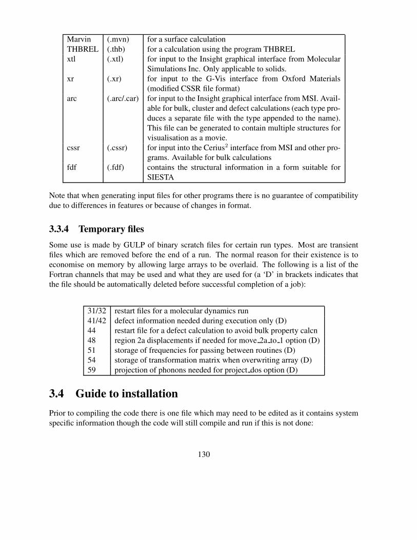
Marvin (.mvn) for a surface calculationTHBREL (.thb) for a calculation using the program THBRELxtl (.xtl) for input to the Insight graphical interface from Molecular
Simulations Inc. Only applicable to solids.xr (.xr) for input to the G-Vis interface from Oxford Materials
(modified CSSR file format)arc (.arc/.car) for input to the Insight graphical interface from MSI. Avail-
able for bulk, cluster and defect calculations (each type pro-duces a separate file with the type appended to the name).This file can be generated to contain multiple structures forvisualisation as a movie.
cssr (.cssr) for input into the Cerius2 interface from MSI and other pro-grams. Available for bulk calculations
fdf (.fdf) contains the structural information in a form suitable forSIESTA
Note that when generating input files for other programs there is no guarantee of compatibilitydue to differences in features or because of changes in format.
3.3.4 Temporary filesSome use is made by GULP of binary scratch files for certain run types. Most are transientfiles which are removed before the end of a run. The normal reason for their existence is toeconomise on memory by allowing large arrays to be overlaid. The following is a list of theFortran channels that may be used and what they are used for (a ‘D’ in brackets indicates thatthe file should be automatically deleted before successful completion of a job):
31/32 restart files for a molecular dynamics run41/42 defect information needed during execution only (D)44 restart file for a defect calculation to avoid bulk property calcn48 region 2a displacements if needed for move 2a to 1 option (D)51 storage of frequencies for passing between routines (D)54 storage of transformation matrix when overwriting array (D)59 projection of phonons needed for project dos option (D)
3.4 Guide to installationPrior to compiling the code there is one file which may need to be edited as it contains systemspecific information though the code will still compile and run if this is not done:
130

local.F : This file contains two strings which specify where the files eledata and help.txt canbe found on your system should they not be present in the execution directory. There is also adefault library directory pointer. You need to change the path to point to the directory wherethese files will reside on your machine. If GULP cannot find the element information file onyour machine then the default values will be set.
After this all you need to do on most Unix machines is type ”make”.
If you wish to run the program in parallel using MPI then you will need to alter the file ”get-machine” accordingly. The usual changes would be to add the ”-DMPI” option and in somecases change the compiler name (for example to mpif90) or include the MPI libraries in the linkstage.
131

Bibliography
[1] E. Madelung. Das elektrische feld in systemen von regelmaessig angeordneten punkt-ladungen. Phys. Z., 19:524–532, 1918.
[2] M. Born and J.E. Mayer. Zur gittertheorie der ionenkristalle. Z. Physik, 75:1–18, 1932.
[3] A.F. Kapustinskii. Lattice energy of ionic crystals. Quart. Rev. Chem. Soc., 10:283–294,1956.
[4] M.J. Norgett. A user’s guide to hades. Technical Report AERE-R7015, AERE HarwellLaboratory, 1972.
[5] J.H. Harding. A guide to midas. Technical Report AERE-R13127, AERE Harwell Lab-oratory, 1988.
[6] J.H. Harding. A guide to the harwell pluto program. Technical Report AERE-R10546,AERE Harwell Laboratory, 1982.
[7] M. Leslie. Cascade. Technical Report DLSCITM36T, Daresbury Laboratory, 1984.
[8] S.C. Parker and G.D. Price. Computer modelling of phase transitions in minerals. Adv.Solid State Chem., 1:295–327, 1989.
[9] D.J. Willock, S.L. Price, M. Leslie, and C.R.A. Catlow. The relaxation of molecularcrystal structures using a distributed multipole electrostatic model. J. Comp. Chem.,16:628–647, 1995.
[10] W.R. Busing. Wmin, a computer program to model molecules and crystals in terms ofpotential energy functions. Technical Report ORNL-5747, Oak Ridge National Labora-tory, 1981.
[11] D.E. Williams. Molecular packing analysis. Acta Cryst. A, 28:629–635, 1972.
[12] G. Eckold, M. Stein-Arsic, and H.J. Weber. Unisoft - a program package for latticedynamical calculations. J. Appl. Cryst., 20:134–139, 1987.
132

[13] W.F. van Gunsteren and H.J.C. Berendsen. Groningen molecular simulation (gromos)library manual. Technical report, Biomos, Groningen, 1987.
[14] D.A. Pearlman, D.A. Case, J.W. Caldwell, W.S. Ross, T.E. Cheatham III, S. DeBolt,D. Ferguson, G. Seibel, and P. Kollman. Amber, a package of computer programs for ap-plying molecular mechanics, normal mode analysis, molecular dynamics and free energycalculations to simulate the structural and energetic properties of molecules. Comput.Phys. Commun., 91:1–41, 1995.
[15] B.R. Brooks, R.E. Bruccoleri, B.D. Olfson, D.J. States, S. Swaminathan, and M. Karplus.Charmm: A program for macromolecular energy, minimization, and dynamics calcula-tions. J. Comp. Chem., 4:187–217, 1983.
[16] W. Smith and T.R. Forester. Dl poly 2.0: A general purpose parallel molecular dynamicssimulation package. J. Mol. Graphics, 14:136–141, 1996.
[17] W. Smith, C.W. Yong, and P.M. Rodger. Dl poly: application to molecular simulation.Mol. Simul., 28:385–471, 2002.
[18] G. Watson, E.T. Kelsey, N.H. de Leeuw, D.J. Harris, and S.C. Parker. Atomistic sim-ulation of dislocations, surfaces and interfaces in mgo. J. Chem. Soc., Faraday Trans.,92:433–438, 1996.
[19] M.B. Taylor, G.D. Barrera, N.L. Allan, T.H.K. Barron, and W.C. Mackrodt. Shell: Acode for lattice dynamics and structure optimisation of ionic crystals. Comp. Phys. Com-mun., 109:135–143, 1998.
[20] J.D. Gale. Semi-empirical methods as a tool in solid state chemistry. Faraday Discuss.,106:219–232, 1997.
[21] H.M. Evjen. On the stability of certain heteropolar crystals. Phys. Rev., 39:675–687,1932.
[22] P.P. Ewald. Die berechnung optischer und elektrostatisher gitterpotentiale. Ann. Phys.,64:253–287, 1921.
[23] M.P. Tosi. Cohesion of ionic solids in the born model. Solid State Phys., 16:1–120, 1964.
[24] R.A. Jackson and C.R.A. Catlow. Computer simulation studies of zeolite structure. Mol.Simul., 1:207–224, 1988.
[25] U. Essmann, L. Perera, M.L. Berkowitz, T. Darden, H. Lee, and L.G. Pedersen. A smoothparticle mesh ewald method. J. Chem. Phys., 103:8577–8595, 1995.
133

[26] L. Greengard and V. Rokhlin. A fast algorithm for particle simulations. J. Comput. Phys.,73:325–348, 1987.
[27] H.G. Petersen, D. Soelvason, J.W. Perram, and Smith E.R. A very fast multipole method.J. Chem. Phys., 101:8870–8876, 1994.
[28] S.W. de Leeuw, J.W. Perram, and E.R. Smith. Simulation of electrostatic systems in peri-odic boundary conditions. i. lattice sums and dielectric constants. Proc. R. Soc. London,Ser. A, 373:27–56, 1980.
[29] M. Leslie and M.J. Gillan. The energy and elastic dipole tensor of defects in ionic-crystals calculated by the supercell method. J. Phys. C, Solid State Phys., 18:973–982,1985.
[30] D.E. Parry. The electrostatic potential in the surface region of an ionic crystal. Surf. Sci.,49:433–440, 1975.
[31] D.E. Parry. Errata: The electrostatic potential in the surface region of an ionic crystal.Surf. Sci., 54:195–195, 1976.
[32] E. Wasserman, J.R. Rustad, and A.R. Felmy. Molecular modeling of the surface chargingof hematite i. the calculation of proton affinities and acidites on a surface. Surf. Sci.,424:19–27, 1999.
[33] J.H. Harding. A guide to midas. Technical Report AERE R-13127, AERE HarwellLaboratory, 1988.
[34] A. Arnold and C. Holm. A novel method for calculating electrostatic interactions in 2dperiodic slab geometries. Chem. Phys. Lett., 354:324–330, 2002.
[35] V.R. Saunders, C. Freyia-Fava, R. Dovesi, and C. Roetti. On the electrostatic potential inlinear periodic polymers. Comp. Phys. Commun., 84:156–172, 1994.
[36] D. Wolf, P. Keblinski, S.R. Philpot, and J. Eggebrecht. Exact method for the simulationof coulombic systems by spherically truncated, pairwise r−1 summation. J. Chem. Phys.,110:8254–8282, 1999.
[37] R.S. Mulliken. Electronic population analysis on lcao-mo molecular wave functions. i.J. Chem. Phys., 23:1833–1840, 1955.
[38] S. Baroni, S. de Gironcoli, A. Dal Corso, and P. Giannozzi. Phonons and related crystalproperties from density-functional perturbation theory. Rev. Mod. Phys., 73:515–562,2001.
134

[39] R.T. Sanderson. An interpretation of bond lengths and a classification of bonds. Science,114:670–672, 1951.
[40] K.A. van Genechten, W.J. Mortier, and P. Geerlings. Intrinsic framework electronegativ-ity: A novel concept in solid state chemistry. J. Chem. Phys., 86:5063–5071, 1987.
[41] A.K. Rappe and W.A. Goddard III. Charge equilibration for molecular dynamics simu-lations. J. Phys. Chem., 95:3358–3363, 1991.
[42] S.L. Njo, J.F. Fan, and B. van de Graaf. Extending and simplifying the electronegativityequalization method. J. Mol. Catal. A, 134:79–88, 1998.
[43] D.E. Williams. Accelerated convergence treatment of r−n lattice sums. Cryst. Rev.,2:3–25, 1989.
[44] K.T. Tang and J.P. Toennies. An improved simple-model for the van der waals potentialbased on universal damping functions for the dispersion coefficients. J. Chem. Phys.,80:3726–3741, 1984.
[45] J. Applequist. A multipole interaction theory of electric polarization of atomic andmolecular assemblies. J. Chem. Phys., 83:809–826, 1985.
[46] T. Beyer, G.M. Day, and S.L. Price. The prediction, morphology, and mechanical prop-erties of the polymorphs of paracetamol. J. Am. Chem. Soc., 123:5086–5094, 2001.
[47] P.A. Madden and M. Wilson. ’covalent’ effects in ’ionic’ systems. Chem. Soc. Rev.,pages 339–350, 1996.
[48] J.H. Harding and N.C. Pyper. The meaning of the oxygen 2nd-electron affinity and oxidepotential models. Phil. Mag. Lett., 71:113–121, 1995.
[49] B.G. Dick and A.W. Overhauser. Theory of the dielectric constants of alkali halide crys-tals. Phys. Rev., 112:90–103, 1958.
[50] R. Car and M. Parinello. Unified approach for molecular-dynamics and density-functional theory. Phys. Rev. Lett., 55:2471–2474, 1985.
[51] P.J.D. Lindan and M.J. Gillan. Shell-model molecular-dynamics simulation of superionicconduction in caf2. J. Phys. Condens. Matter, 5:1019–1030, 1993.
[52] U. Schroeder. A new model for lattice dynamics (breathing shell model). Solid StateCommun., 4:347–349, 1966.
[53] P.M. Axilrod and E. Teller. Interaction of the van der waals type between three atoms. J.Chem. Phys., 11:299–300, 1943.
135

[54] A. Banerjea and J.R. Smith. Origins of the universal binding-energy relation. Phys. Rev.B, 37:6632–6645, 1988.
[55] A.P. Sutton and J. Chen. Long-range finnis-sinclair potentials. Phil. Mag. Lett., 61:139–146, 1990.
[56] M.W. Finnis and J.E. Sinclair. A simple empirical n-body potential for transition metals.Phil. Mag. A, 50:45–55, 1984.
[57] J. Cai and Y.Y. Ye. Simple analytical embedded-atom-potential model including a long-range force for fcc metals and their alloys. Phys. Rev. B, 54:8398–8410, 1996.
[58] G.C. Abell. Empirical chemical pseudopotential theory of molecular and metallic bond-ing. Phys. Rev. B, 31:6184–6196, 1985.
[59] J. Tersoff. New empirical-model for the structural-properties of silicon. Phys. Rev. Lett.,56:632–635, 1986.
[60] J. Tersoff. New empirical-approach for the structure and energy of covalent systems.Phys. Rev. B, 37:6991–7000, 1988.
[61] D.G. Pettifor, I.I. Oleinik, D. Nguyen-Manh, and V. Vitek. Bond-order potentials: bridg-ing the electronic to atomistic modelling hierarchies. Comp. Mater. Sci., 23:33–37, 2002.
[62] D.W. Brenner. Empirical potential for hydrocarbons for use in simulating the chemicalvapor deposition of diamond films. Phys. Rev. B, 42:9458–9471, 1990.
[63] D.W. Brenner, O.A. Shenderova, J.A. Harrison, S.J. Stuart, B. Ni, and S.B. Sinnott. Asecond-generation reactive empirical bond order (rebo) potential energy expression forhydrocarbons. J. Phys.: Condens. Matter, 14:783–802, 2002.
[64] J. Che, T. Cagin, and W.A. Goddard III. Generalized extended empirical bond-orderdependent force fields including nonbond interactions. Theor. Chem. Acc., 102:346–354,1999.
[65] A. Einstein. Die plancksche theorie der strahlung und die theorie der spezifischenwaerme. Ann. Phys., 22:180–190, 1907.
[66] D. Frenkel and A.J.C. Ladd. New monte carlo method to compute the free energy ofarbitrary solids. application to the fcc and hcp phases of hard spheres. J. Chem. Phys.,81:3188–3193, 1981.
[67] G. Paglia, A.L. Rohl, C.E. Buckley, and J.D. Gale. A computational investigation ofthe structure of κ-alumina using interatomic potentials. J. Mater. Chem., 11:3310–3316,2001.
136

[68] G.W. Watson and D.J. Willock. The enumeration of structures for γ -alumina based on adefective spinel structure. Chem. Commun., pages 1076–1077, 2001.
[69] N.L. Allan, G.D. Barrera, M.Y. Lavrentiev, I.T. Todorov, and J.A. Purton. Ab initiocalculation of phase diagrams of ceramics and minerals. J. Mater. Chem., 11:63–68,2001.
[70] P.J.M. van Laarhoven and E.H.L. Aarts. Simulated annealing: Theory and applications.Reidel, 1987.
[71] J.H. Holland. Adaption in natural and artificial systems. The University of MichiganPress, 1975.
[72] T.S. Bush, C.R.A. Catlow, and P.D. Battle. Evolutionary programming techniques forpredicting inorganic crystal-structures. J. Mater. Chem., 5:1269–1272, 1995.
[73] W.H. Press, S.A. Teukolsky, W.T. Vetterling, and B.P. Flannery. Numerical recipes inFortran: The art of scientific computing. Cambridge University Press, 1986.
[74] R. Fletcher and M.J.D. Powell. A rapidly convergent descent method for minimization.Comput. J., 6:163–168, 1964.
[75] D.F. Shanno. Conditioning of quasi-newton methods for function minimization. Math.Comput., 24:647–656, 1970.
[76] G. Mills, H. Jonsson, and G.K. Schenter. Reversible work transition-state theory - appli-cation to dissociative adsorption of hydrogen. Surf. Sci., 324:305–337, 1995.
[77] A. Banerjee, N. Adams, J. Simons, and R. Shepard. Search for stationary points onsurfaces. J. Phys. Chem., 89:52–57, 1985.
[78] A.F. Voter, F. Montalenti, and T.C. Germann. Extending the time scale in atomisticsimulation of materials. Ann. Rev. Materials Research, 32:321–346, 2002.
[79] S.M. Woodley, P.D. Battle, J.D. Gale, and C.R.A. Catlow. The prediction of inorganiccrystal structures using a genetic algorithm and energy minimisation. Phys. Chem. Chem.Phys., 1:2535–2542, 1999.
[80] D. Frenkel and B. Smit. Understanding molecular simulation: from algorithms to appli-cations. Academic Press, 2001.
[81] J.F. Nye. Physical properties of crystals. Oxford University Press, 1957.
[82] J.W. Akitt. NMR and chemistry. Chapman and Hall, 1983.
137
[83] R.F.W. Bader, T.T. Nguyendang, and Y. Tal. A topological theory of molecular-structure.Rep. Prog. Phys., 44:893–948, 1981.
[84] W. Cochran and R.A. Cowley. Dielectric constants and lattice vibrations. J. Phys. Chem.Solids, 23:447–450, 1962.
[85] J.M. Seddon and J.D. Gale. Thermodynamics and statistical mechanics. Royal Societyof Chemistry, 2002.
[86] A. Baldereschi. Mean-value point in the brillouin zone. Phys. Rev. B, 7:5212–5215,1973.
[87] D.J. Chadi and M.L. Cohen. Special points in the brillouin zone. Phys. Rev. B, 8:5747–5753, 1973.
[88] H.J. Monkhorst and J.D. Pack. Special points for brillouin-zone integrations. Phys. Rev.B, 13:5188–5192, 1976.
[89] R. Ramirez and M.C. Boehm. The use of symmetry in reciprocal space integrations- asymmetric units and weighting factors for numerical-integration procedures in anycrystal symmetry. Int. J. Quantum Chem., 34:571–594, 1988.
[90] D.H. Gay and A.L. Rohl. Marvin: A new computer code for studying surfaces andinterfaces and its application to calculating the crystal morphologies of corundum andzircon. J. Chem. Soc., Faraday Trans., 91:926–936, 1995.
[91] P.W. Tasker. The stability of ionic crystal surfaces. J. Phys. C, 12:4977–4984, 1979.
[92] J.D.H. Donnay and D. Harker. A new law of crystal morphology extending the law ofbravais. Am. Miner., 22:446–467, 1937.
[93] G. Wulff. Zur frage der geschwindigkeitb des wachsthums und der auflosung der krys-tallflachen. Z. Kryst., 34:449–530, 1901.
[94] J.W. Gibbs. Collected works. New York, Longman, 1928.
[95] P. Hartman and P. Bennema. The attachment energy as a habit controlling factor 1.theoretical considerations. J. Crystal Growth, 49:145–156, 1980.
[96] M.P. Allen and D.J. Tildesley. Computer simulation of liquids. Oxford University Press,1987.
[97] R. LeSar, R. Najafabati, and D.J. Srolovitz. Thermodynamics of solid and liquidembedded-atom-method metals - a variational study. J. Chem. Phys., 94:5090–5097,1991.
138

[98] A.P. Sutton. Direct free-energy minimization methods - application to grain-boundaries.Phil. Trans. R. Soc. London A, 341:233–245, 1992.
[99] E.W. Montroll. Frequency spectrum of crystalline solids. J. Chem. Phys., 10:218–229,1942.
[100] L.N. Kantorovich. Thermoelastic properties of perfect crystals with nonprimitive lattices.1. general-theory. Phys. Rev. B, 51:3520–3534, 1995.
[101] M.B. Taylor, G.D. Barrera, N.L. Allan, and T.H.K. Barron. Free-energy derivatives andstructure optimization with quasiharmonic lattice dynamics. Phys. Rev. B, 56:14380–14390, 1997.
[102] J.D. Gale. Analytical free energy minimization of silica polymorphs. J. Phys. Chem. B,102:5423–5431, 1998.
[103] N.L. Allan, T.H.K. Barron, and J.A.O. Bruno. The zero static internal stress approxi-mation in lattice dynamics, and the calculation of isotope effects on molar volumes. J.Chem. Phys., 105:8300–8303, 1996.
[104] N.F. Mott and M.J. Littleton. Conduction in polar crystals. i. electrolytic conduction insolid salts. Trans. Faraday Soc., 34:485–499, 1938.
[105] C.R.A. Catlow, R. James, W.C. Mackrodt, and R.F. Stewart. Defect energetics in α −al2o3 and rutile tio2. Phys. Rev. B, 25:1006–1026, 1982.
[106] N.L. Allinger, X.F. Zhou, and J. Bergsma. Molecular mechanics parameters. J. Mol.Struct. (Theochem), 118:69–83, 1994.
[107] A.K. Rappe, C.J. Casewit, K.S. Colwell, W.A. Goddard III, and W.M. Skiff. Uff, a fullperiodic table force field for molecular mechanics and molecular dynamics simulations.J. Am. Chem. Soc., 114:10024–10035, 1992.
[108] S. Barlow, A.L. Rohl, S.G. Shi, C.M. Freeman, and D. O’Hare. Molecular mechanicsstudy of oligomeric models for poly(ferro cenylsilanes) using the extensible systematicforcefield (esff). J. Am. Chem. Soc., 118:7578–7592, 1996.
[109] J.D. Gale, C.R.A. Catlow, and W.C. Mackrodt. Periodic ab initio determination of inter-atomic potentials for alumina. Modelling Simul. Mater. Sci. Eng., 1:73–81, 1992.
[110] R.G. Gordon and Y.S. Kim. Theory for the forces between closed-shell atoms andmolecules. J. Chem. Phys., 56:3122–3133, 1972.
[111] J.D. Gale. Empirical potential derivation for ionic materials. Phil. Mag. B, 73:3–19,1996.
139

[112] T.J. Grey, J.D. Gale, and D. Nicholson. Parameterization of a potential function forthe ca2+ − ne and ca2+ − n2 interactions using high-level ab initio data. Mol. Phys.,98:1565–1573, 2000.
[113] C.R.A. Catlow and M.J. Norgett. Lattice structure and stability of ionic materials. Tech-nical Report AERE-M2936, AERE Harwell Laboratory, 1976.
[114] C.R.A. Catlow and W.C. Mackrodt. Theory of simulation methods for lattice and defectenergy calculations in crystals. Lecture Notes in Physics, 166:3–20, 1982.
[115] J.D. Gale. Gulp: A computer program for the symmetry-adapted simulation of solids. J.Chem. Soc., Faraday Trans., 1:629–637, 1997.
[116] S. Brode and R. Ahlrichs. An optimized md program for the vector computer cyber-205.Comp. Phys. Commun., 42:51–57, 1986.
[117] C.R.A. Catlow, I.D. Faux, and M.J. Norgett. Shell and breathing shell model calculationsfor defect formation energies and volumes in magnesium oxide. J. Phys. C: Solid StatePhys., 9:419–429, 1976.
[118] C.-S. Zha, H.-K. Mao, and R.J. Hemley. Elasticity of mgo and a primary pressure scaleto 55 gpa. Proc. Natl. Acad. Sci., 97:13494–13499, 2000.
[119] I. Jackson and H. Niesler. In High pressure research in geophysics. Center for AcademicPublishing, Tokyo, 1982.
[120] M.J. Sanders, M. Leslie, and C.R.A. Catlow. Interatomic potentials for sio2. J. Chem.Soc. Chem. Commun., pages 1271–1273, 1984.
[121] X. Gonze, D.C. Allan, and M.P. Teter. Dielectric tensor, effective charges, and phonons inα-quartz by variational density-functional perturbation theory. Phys. Rev. Lett., 68:3603–3606, 1992.
[122] Ph. Ghosez, J.-P. Michenaud, and X. Gonze. Dynamical atomic charges: The case ofabo3 compounds. Phys. Rev. B, 58:6224–6240, 1998.
[123] A.L. Rohl, K. Wright, and J.D. Gale. Evidence from surface phonons for the (2x1)reconstruction of the (10-14) surface of calcite from computer simulation. Am. Miner.,page in press, 2003.
[124] S.L.S. Stipp. Toward a conceptual model of the calcite surface: Hydration, hydrolysis,and surface potential. Geochimica Cosmochimica Acta, 63:3121–3131, 1999.
[125] E. Dowty. Phys. Chem. Miner., 14:67, 1987.
140

[126] C.R.A. Catlow. J. Chem. Soc., Faraday Trans. 2, 85:335, 1989.
[127] A.B. Lidiard. J. Chem. Soc., Faraday Trans. 2, 85:341, 1989.
[128] J.D. Gale. Phil. Mag. B, 73:3, 1996.
[129] K. Gallagher, M Sambridge, and G. Drijkoningen. Geophys. Res. Lett., 18:2177, 1991.
[130] K.-P Schroder, J. Sauer, M. Leslie, C.R.A Catlow, and J.M. Thomas. Chem. Phys. Lett.,188:320, 1992.
[131] J.D. Gale and N.J. Henson. J. Chem. Soc., Faraday Trans., 90:3175, 1994.
[132] T.S. Bush, J.D. Gale, C.R.A. Catlow, and P.D. Battle. J. Mater. Chem., 4:831, 1994.
141