generalized algebraic modeling system (gams) m. b. abaee

Generalized Algebraic Modeling System

(GAMS)

M. B. Abaee [email protected]

M. S. Ghazizadeh [email protected]

PWUT – Spring 2010

CONTENTS 1. INTRODUCTION

2/138

1.1. The Most Important Features of GAMS 1.2. Using GAMSIDE 1.2.1. Install GAMS and IDE 1.2.2. Open the IDE through the icon 1.2.3. Create a Project

1.2.4. Define a Project name and location 1.2.5. Create or open an existing file of GAMS instructions 1.2.6. Prepare the file so you think it is ready for execution 1.2.7. Run the file with GAMS by punching the run button 1.2.8. Open and navigate around the output 1.2.9. Fixing Compilation Errors 1.2.11. Accessing documentation on GAMS through the IDE

CONTENTS 2. INTRODUCTORY INFORMATION

3/138

2.1. Model Structure 2.2. Comments in Models 2.3. Terms, Symbols and Reserved Words 2.3.1. Characters 2.3.2. Reserved Words 2.3.3. Operators 2.4. Common mathematical functions 2.4.1. Abs 2.4.2. Exp 2.4.3. Log, Log10 2.4.4. Max , Min 2.4.5. Prod 2.4.6. Round

CONTENTS

4/138

2.4.7. Smin , Smax 2.4.8. Sqr 2.4.9. Sqrt 2.4.10. Sum 2.4.11. Other Mathematical functions 2.5. SET 2.5.1. Set Naming and Declaration 2.5.2. Subsets 2.5.3. Multi-dimensional Sets 2.5.4. The Alias Statement: Multiple Names for a Set 2.5.5. SET Operations 2.6. DATA 2.6.1. SCALAR 2.6.2. PARAMETER

CONTENTS

5/138

2.6.3. TABLE 2.6.4. Data Entry Through Computation 2.7. VARIABLE 2.7.1. Variable Declaration 2.7.2. Type of Defining Variables 2.7.3. Suffix of Variables 2.7.4. Example 2.8. EQUATION 2.8.1. Declaration of Equations 2.8.2. Definition of Equations 2.9. MODEL, SOLVE 2.9.1. Assembling a Model 2.9.2. Solving a Model 2.9.3. Solution Procedure

CONTENTS

6/138

2.10. OUTPUT

CONTENTS 3. SPECIAL ORDERS GAMS

7/138

3.1. Programming Flow Control Features 3.1.1. The Loop Statement 3.1.2. The If-Elseif-Else Statement 3.1.3. The While Statement 3.1.4. The For Statement 3.1.5. The Repeat Statement 3.1.6. Numerical Relationship Operators 3.1.7. Logical Operators 3.1.8. Mixed Logical Conditions 3.2. Ordered Sets 3.2.1. ORD Operator 3.2.2. CARD Operator 3.2.3. SAMEAS Operator

CONTENTS

8/138

3.2.4. DIAG Operator 3.2.5. Lag and Lead Operator 3.3. .. 3.3.1. …

CONTENTS 4. GAMS and Other Applications

9/138

4.1. GAMS/Excel 4.1.1. Converting Data to GAMS 4.1.2. Import Data from Excel 4.1.3. Export Data to Excel 4.1.4. Executing GAMS from Excel 4.2. GAMS/MATLAB 4.2.1. Installation 4.2.2. Returning Values to MATLAB 4.2.3. Modifying Parameters 4.2.4. Advanced Use 4.3. …

CONTENTS 7. BASIC MODELS FOR ECONOMICS OF ELECTRICITY

10/138

7.1. Power Transit 7.2. Economic Dispatch 7.2.1. Basic Economic Dispatch 7.2.2. Economic Dispatch with Elastic Demand 7.2.3. Economic Dispatch with Losses 7.2.4. First Project 7.3. Optimal Power Flow 7.3.1. DC Load Power 7.3.2. Optimal DC Power Flow Formulation 7.3.3. Economic Dispatch Including a Line with Limited Transmission Capacity 7.3.4. Economic Dispatch with Bilateral Contracts 7.3.5. AC Load Power Formulation 7.3.6. Optimal AC Power

CONTENTS

11/138

7.4. UNIT COMMITMENT 7.4.1. Unit Commitment Formulation 7.4.2. Multi Period Unit Commitment 7.5. AUCTION 7.5.1. Single-Period Auction 7.5.2. Multi-Period Auction 7.5.3. Network-Constrained Multi-Period Auction 7.6. PRODUCER SELF-SCHEDULING AND OFFER STRATEGIES 7.6.1. Price Taker Producer 7.6.2. Price Taker Hydroelectric Producer 7.6.3. Price Maker Producer 7.7. CONSUMER AND RETAILER 7.7.1. Retailer 7.7.2. …

CONTENTS 8. SOLOTION OF BASIC MODELS FOR ECONOMICS OF

ELECTRICITY

12/138

8.1. Power Transit 8.2. Economic Dispatch 8.2.1. Basic Economic Dispatch 8.2.2. Economic Dispatch with Elastic Demand 8.2.3. Economic Dispatch with Losses 8.2.4. First Project 8.3. Optimal Power Flow 8.3.1. Economic Dispatch Including a Line with Limited Transmission Capacity 8.3.2. Economic Dispatch with Bilateral Contracts 8.3.3. Optimal AC Power

CONTENTS

13/138

8.3.6. Optimal AC Power Flow 8.4. UNIT COMMITMENT 8.4.1. Multi Period Unit Commitment 8.4.2. … 8.5. AUCTION 8.5.1. Single-Period Auction 8.5.2. Multi-Period Auction 8.5.3. Network-Constrained Multi-Period Auction 8.6. PRODUCER SELF-SCHEDULING AND OFFER STRATEGIES 8.6.1. Price Taker Producer 8.6.2. Price Taker Hydroelectric Producer 8.6.3. Price Maker Producer 8.7. CONSUMER AND RETAILER 8.7.1. Retailer

1. INTRODUCTION 1.1. The Most Important Features of GAMS Capability to solve from small scale to large scale problems with small

code by means of the use of index to write blocks of similar constraints from only one constraint.

The model is independent from the solution method, and it can be solved by different solutions methods by only changing the solver.

The translation from the mathematical model to GAMS is almost transparent since GAMS has been built to resemble mathematical programming models.

GAMS also uses common English words, thus is easy to understand it’s statements.

14/138

1. INTRODUCTION 1.2. Using GAMSIDE 1.2.1. Install GAMS and IDE

15/138

The GAMSIDE is automatically installed when GAMS is installed.

1.2.2. Open the IDE through the icon

1.2.3. Create a Project

by going to the File menu. Select to New Project (Later you will use your previous projects).

1. INTRODUCTION 1.2. Using GAMSIDE …

What is a Project?

16/138

The GAMSIDE employs a “Project” file for two purposes: First, the project location determines where all saved files are

placed (to place files elsewhere use the save as dialogue) and where GAMS looks for files when executing.

Second the project saves file names and program options associated with the effort.

We recommend that you define a new project every time you wish to change the file storage directory.

1. INTRODUCTION

1.2.4. Define a Project name and location

17/138

Put it in a directory you want to use. All files associated with this project will be saved in that directory.

In the “File name” area type in a name for the project file you wish to use. If I was doing this, I would go to a suitable subdirectory and create a subdirectory called Projdir and put in the name useide. In turn, your project name will be called useide.gpr where gpr stands for GAMS project.

1.2. Using GAMSIDE …

1. INTRODUCTION

1.2.5. Create or open an existing file of GAMS instructions

18/138

Several cases are possible: a) Create a new file b) Open an existing file


1. INTRODUCTION

19/138

c) Open a model library file (the simplest at this stage and the one we will use)

Select a model like transportation

It will be automatically saved in your project file


1. INTRODUCTION

1.2.6. Prepare the file so you think it is ready for execution

20/138

When using model library transport.gms should now appear as part of your IDE screen.

The IDE contains a full featured editor. Go through the file and change what you want.


1. INTRODUCTION

1.2.7. Run the file with GAMS by punching the run button

21/138

The so called process window will then appear which gives a log of the steps GAMS goes through in running the model and your model will run.


1. INTRODUCTION

1.2.8. Open and navigate around the output

22/138

By double clicking on lines in the process window you can access program output both in general and at particular locations. The positioning of your access is determined by the color of the line you click on.


1. INTRODUCTION

23/138

Color of Line in Process Window Function and Destination When Double Clicked

Blue line Opens LST file and jumps to line in LST file corresponding to bolded line in Process file

Non bolded black line Opens LST file and jumps to location of nearest Bolded Line

Red line Identifies errors in source file. Cursor Jumps to Source (GMS) file location of error. Error description text in process window and in LST file which is not automatically opened.


1. INTRODUCTION

1.2.9. Fixing Compilation Errors

24/138

No one is perfect, errors occur in everyone’s GAMS coding. The IDE can help you in finding and fixing those errors. The red lines mark errors. To see where the errors occurred double-click on the top one.

A double-click takes you to the place in the source where the error was made. The tip here is always start at the top of the process file when doing this.


1. INTRODUCTION

1.2.10. Matching Parentheses

25/138

The IDE provides you with a way of checking on how the parentheses match up in your GAMS code. This involves usage of the symbol from the menu bar coupled with appropriate cursor positioning. Suppose we have a line of GAMS code like:


1. INTRODUCTION

1.2.11. Accessing documentation on GAMS through the IDE

26/138

The GAMSIDE has a tie in to documentation. In particular suppose we wish to know about a particular item and there happens to be a file on that item.


2. INTRODUCTORY INFORMATION 2.1. Model Structure The parts of a GAMS Model or Program are defined in the table below:

27/138

1. SETS Structures consisting of a complex of indices or names

2. DATA PARAMETERS, TABLES, SCALARS Determination of values of input parameters

3. VARIABLES Variables or arrays of variables Declaration with assigning a type of variable Declaration of limits for possible changes, initial level

4. EQUATIONS Equations or complexes and arrays of equations Declaration with assigning a name Recording of equations in the GAMS language

5. MODEL, SOLVE Model and methods of solution

6. OUTPUT Output of information into a separate file

2. INTRODUCTORY INFORMATION 2.2. Comments in Models

There are two main methods of introducing comments and elucidation's in the body of a GAMS model.

28/138

a) If a line begins with the “ * ”symbol, the contents of the line are treated as a comment. For example:

*plants (plants)

2. INTRODUCTORY INFORMATION 2.2. Comments in Models …

29/138

b) A program section beginning with the line $ONTEXT and ending with the line $OFFTEXT is a comment. The above functional words begin with the first symbol of the line.

$ONTEXT - - - - - - - - - - This guide is for a scientist who knows the Persian language. + + + + + + + + + + $OFFTEXT

2. INTRODUCTORY INFORMATION 2.3. Terms, Symbols and Reserved Words

30/138

2.3.1. Characters A to Z Alphabet a to z Alphabet 0 to 9 numerals & Ampersand " double quote # pound sign * multiply = equal ? question mark @ at > greater than ; semicolon \ back slash < less than ‘ single quote : colon - minus / slash , comma ( ) parenthesis space $ dollar [ ] square brackets _ underscore . dot { } braces ! exclamation mark + plus % percent ^ Circumflex


31/138

2.3.2. Reserved Words Abort acronym Acronyms Alias all And

assign binary Card Display eps Eq

equation equations Ge Gt Inf Integer

Le Loop Lt Maximizing Minimizing Model

models Na Ne Negative Not

options Or Ord Parameter Sets Positive

Prod Scalar Scalars Set System Smax

Smin Sos1 Sos2 Sum Yes Table

Using variable Variables Or Else Repeat

Until While If Then put Semicont

semiint File Files Putpage free

No option Solve for


32/138

2.3.3. Operators

Premiership Operator Example

(1) ** x ** y (x > 0) (2) * x * y

(3) / x / y

(4) - , + x ± y

2. INTRODUCTORY INFORMATION 2.4. Common mathematical functions

33/138

2.4.1. Abs

X=abs(t); X=abs(y+2); Eq1.. z=e=abs(yy);

2

It's use in .. equations in terms that involve variables requires the model type be NLP.

Expressions can contain a function that calculates the absolute value of an expression or term.

2. INTRODUCTORY INFORMATION 2.4. Common mathematical functions …

34/138

2.4.2. Exp


Expressions can contain a function that calculates the exponentiation of an expression or term.

X=exp(t); X=exp(y+2); Eq2.. z=e=exp(yy);


35/138

2.4.3. Log, Log10


Expressions can contain a function that calculates the natural logarithm or logarithm base 10 of an expression or term.

X=log(t); X=log(y+2); Eq3..z=e=log(yy); X=log10(tt); X=log10(y+2); Eq4..z=e=log10(yy);

2

log log 2 log


36/138

2.4.4. Max , Min

Expressions can contain a function that calculates the maximum or minimum of a set of expressions or term.

It's use in .. equations in terms that involve variables requires the model type be DNLP.

X=min(y+2,t,r); Eq.. z=e=max(yy,t);

2, , ,


37/138

2.4.5. Prod


Expressions can contain a function that calculates the product of set indexed expressions or terms.

X=prod(i, a(i)*2);

2


38/138

2.4.6. Round

This function may be used on data during GAMS calculations. It cannot be used in models

Data calculation expressions can contain a function that rounds the numerical result of an expression or term. There are 2 variants of the rounding function. The first, Rounds the result to the nearest integer value. X=round(12.432); 12

The second, rounds the result to the number of decimal points specified by the second argument. X=round(12.432,2); 12.430


39/138

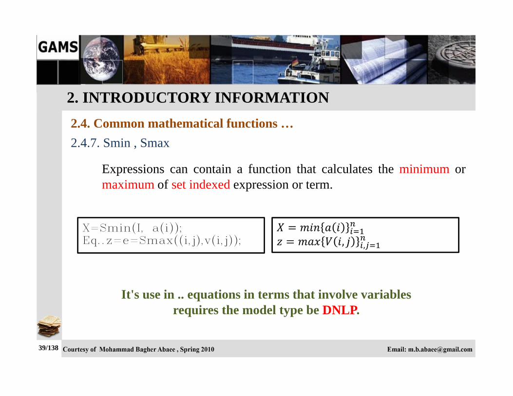
2.4.7. Smin , Smax

Expressions can contain a function that calculates the minimum or maximum of set indexed expression or term.

X=Smin(I, a(i)); Eq..z=e=Smax((i,j),v(i,j));

, ,

It's use in .. equations in terms that involve variables requires the model type be DNLP.


40/138

2.4.8. Sqr

Expressions can contain a function that calculates the square of an expression or term.


X= sqr (y+2); Eq10.. z=e= sqr (yy);

2


41/138

2.4.9. Sqrt

Expressions can contain a function that calculates the square root of an expression or term.


X= sqrt (y+2); Eq10.. z=e= sqrt (yy);

2


42/138

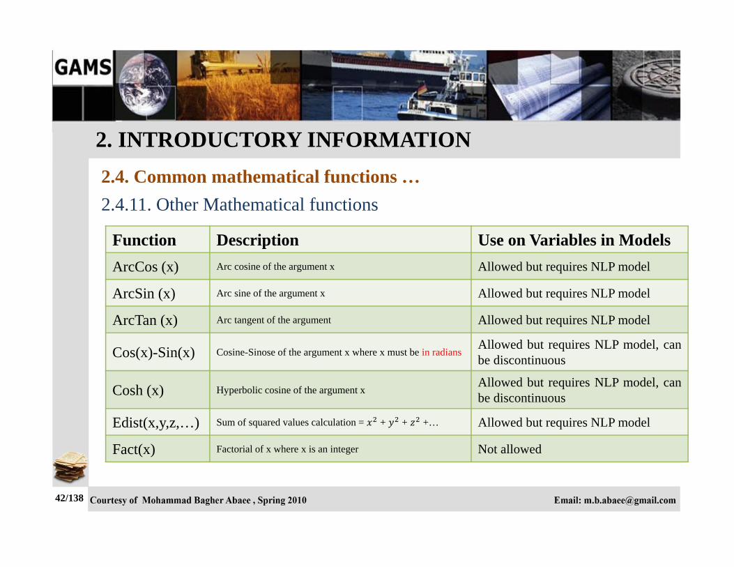
2.4.11. Other Mathematical functions

Function Description Use on Variables in Models ArcCos (x) Arc cosine of the argument x Allowed but requires NLP model

ArcSin (x) Arc sine of the argument x Allowed but requires NLP model

ArcTan (x) Arc tangent of the argument Allowed but requires NLP model

Cos(x)-Sin(x) Cosine-Sinose of the argument x where x must be in radians Allowed but requires NLP model, can be discontinuous

Cosh (x) Hyperbolic cosine of the argument x Allowed but requires NLP model, can be discontinuous

Edist(x,y,z,…) Sum of squared values calculation = + + +… Allowed but requires NLP model

Fact(x) Factorial of x where x is an integer Not allowed


43/138

2.4.10. Sum

Expressions can contain a function that calculates the sum of set indexed expressions or term.

This function is linear. It can be used on data during GAMS calculation or in models on variables or parameters.

X=Sum(i, a(i)); Eq..z=e=Sum((i,j),B(i,j));

,


44/138

2.4.11. Other Mathematical functions …

Function Description Use on Variables in Models Floor (x) Largest integer that is less than or equal to x Not allowed

Normal(x,y) Random number normally distributed with mean x and standard deviation y Not allowed

Uniform(x,y) Random number with uniform distribution between x and y Not allowed

Uniformint(x,y) Integer random number with uniform distribution between x and y Not allowed

Pi Value of Pi 3.141716… Allowed

Power(x,y) x raised to an integer power. , where y must be an integer Allowed but requires NLP model

Sign(x) Sign of x. Returns 1 if x > 0, -1 if x < 0, and 0 if x = 0 Allowed but requires DNLP model

2. INTRODUCTORY INFORMATION 2.5. SET

45/138

2.5.1. Set Naming and Declaration

SETS are the equivalent of indices in a typical programming language.

In GAMS, indices have names, written through a combination of letters and digits, without spaces.

A set name must begin with a letter, but the next symbol can be a letter, digit or the marks “+” and “-”. For example:

Jlobest 1999 1972-138 GenCo D6H83 Navruz-99

2. INTRODUCTORY INFORMATION 2.5. SET …

46/138

2.5.1. Set Naming and Declaration …

The set declaration contains: • the set name • a list of elements in the set (up to 63 characters long spaces etc

allowed in quotes) • optional labels describing the whole set • optional labels defining individual set elements

The general format for a set statement is: SET setname optional defining text

/ firstsetelementname optional defining text secondsetelementname optional defining text ... /;


47/138

2.5.1. Set Naming and Declaration …

SET PROCESS PRODUCTION PROCESSES /X1,X2,X3/; SET Consumers Cities / Tokyo City1 London ”$ City2” Moscow / Year /1990*2010/ b /a1b*a20b/ a /a1a*a20b/ ;


48/138

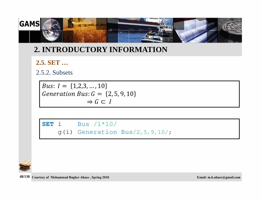
2.5.2. Subsets

: 1,2,3, … , 10 : 2, 5, 9, 10

SET i Bus /1*10/ g(i) Generation Bus/2,5,9,10/;


49/138

2.5.3. Multi-dimensional Sets

SET i /a, b/ j /c, d, e/

ij1(i,j) /a.c, a.d/ or /a.(c,d)/ ij2(i,j) /a.c, b.c/ ij3(i,j) /a.c, b.c, a.d, b.d/or/(a,b).(c,d)/ ;

GAMS allows sets with up to 20 dimensions.


50/138

2.5.4. The Alias Statement: Multiple Names for a Set

There are occasions when one may wish to address a single set more than once in a statement. In GAMS this is done by giving the set another name through the ALIAS command as follows:

ALIAS(knownset,newset1,newset2,...);

SET i Bus /1*10/ ; ALIAS(i, j, k);


51/138

2.5.5. SET Operations

Operations can be performed on sets using the symbols:

+ - * Not

s3(n) = s1(n) + s2(n);

Symbol “ + ” performs the set union operation

3 1 2

s3(n) = s1(n) - s2(n);

Symbol “ - ” performs the operation of difference of sets. This set consists of elements, which belong to set A but not set B

3 1 1 2


52/138

2.5.5. SET Operations …

s3(n) = s1(n) * s2(n); s3(n) = s1(n) And s2(n);

Operator “ * ” performs the set intersection operation; only the elements included in both set A and set B belong to the intersection of the sets A and B

3 1 2

s3(n) = Not s1(n);

The symbol “ Not” performs the set complement operation

3 1

2. INTRODUCTORY INFORMATION 2.6. DATA

53/138

Digital data are contained in arrays (zero, scalar, or multidimensional matrices called parameters in GAMS). The SETs, described in section 2.5, can play the role of indices for these arrays. To declare an array to contain data values GAMS provides for three forms:

SCALAR (zero-dimensional) PARAMETER (one-dimensional) TABLE (multidimensional)

Scalar entry is for scalars, Parameter generally for vectors and Table for matrices.

2. INTRODUCTORY INFORMATION 2.6. DATA …

54/138

2.6.1. SCALAR

A scalar is regarded as a parameter that has no domain. Should define value for SCALAR. SCALAR format is used to enter items that are not defined with

respect to SETs. The SCALAR declaration contains:

• the set itemname • numerical value • optional labeling text

The general format for a set statement is: SCALAR itemname optional labeling text / NumericalValue /;


55/138

2.6.1. SCALAR …

SCALAR V / 0.005 /; SCALAR Price Energy Price($/MWh) /40/ Load /350/;

0.005 40 350


56/138

2.6.2. PARAMETER

Generally parameter format is used with data items that are one-dimensional (vectors) although multidimensional cases can be entered.

Zero is the default value for all parameters. Therefore, you only need to include the nonzero entries in the element-value list, and these can be entered in any order.

PARAMETER format is used to enter items defined with respect to SETs.


57/138

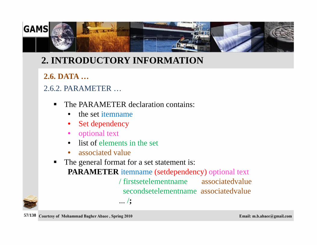
2.6.2. PARAMETER …

The PARAMETER declaration contains: • the set itemname • Set dependency • optional text • list of elements in the set • associated value

The general format for a set statement is: PARAMETER itemname (setdependency) optional text

/ firstsetelementname associatedvalue secondsetelementname associatedvalue ... /;


58/138


SET t / H1*H3 /; PARAMETER Tem(t) temperature /H1 3 H2 H3 -2.5 / ;

Temperature 1 3 Temperature 2 0 Temperature 3 2.5


59/138


SET t / H1*H3 /; SET day / day1,day2 /; PARAMETER Tem1(t, day) /H1.day1 3 H1.day2 3.5 H3.day1 -1 H3.day2 -2 / ;

Temperature 1, 1 3 Temperature 1, 2 3.5 Temperature 2, 1 0 Temperature 2, 2 0 Temperature 3, 1 1 Temperature 3, 2 2


60/138

2.6.3. TABLE

Generally table format is used with data items that are multidimensional (matrix).

Zero is the default value for all element of table. Therefore, you only need to include the nonzero entries in the element-value, and these can be entered in any order.

Items in tables must be defined with respect to at least 2 sets and can be defined over up to 20 sets. When more than two dimensional items are entered, as in the equilibrium example, periods(.) set off the element names set1elementname.set2elementname.set3elementname etc.


61/138

2.6.3. TABLE …

The TABLE declaration contains: • the set itemname • Sets • descriptive text • associated value

The general format for a set statement is: TABLE itemname (set1,set2,…) descriptive text

set_2_element_1 set_2_element_2 … set_1_element_1 value11 value12 set_1_element_2 value21 value22 … ;


62/138

2.6.3. TABLE …

SET t / H1*H3 / day / day1,day2 /;

TABLE Tem1(t, day) / day1 day2 H1 3 3.5 H2 0 H3 -1 -2 / ;

Temperature 1, 1 3 Temperature 1, 2 3.5 Temperature 2, 1 0 Temperature 2, 2 0 Temperature 3, 1 1 Temperature 3, 2 2


63/138

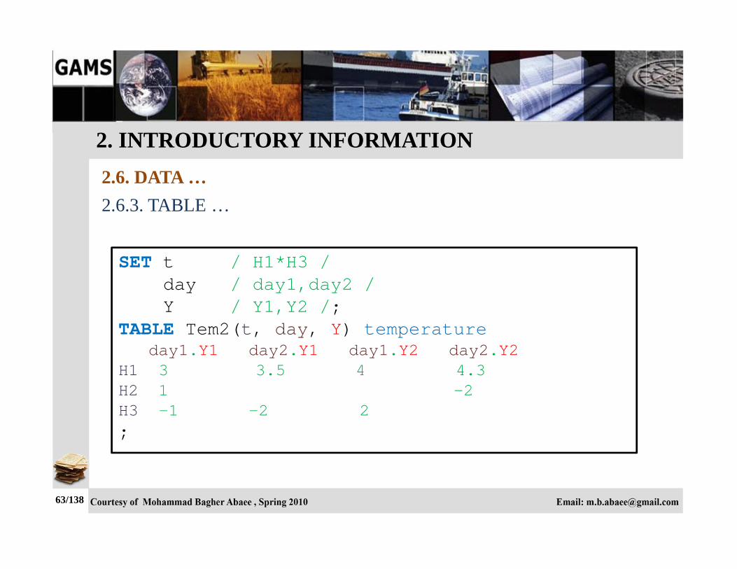
2.6.3. TABLE …

SET t / H1*H3 / day / day1,day2 /

Y / Y1,Y2 /; TABLE Tem2(t, day, Y) temperature day1.Y1 day2.Y1 day1.Y2 day2.Y2 H1 3 3.5 4 4.3 H2 1 -2 H3 -1 -2 2 ;


64/138

2.6.3. TABLE …

SET t / H1*H3 / day / day1,day2 /

Y / Y1,Y2 /; TABLE Tem2(t, day, Y) temperature Y1 Y2 H1.day1 3 4 H2.day1 1 H3.day1 -1 2 H1.day2 3.5 4.3 H2.day2 -2 H3.day2 -2 ;


65/138

2.6.4. Data Entry Through Computation

After declaration, parameter values may be computed later in the model. Determination of data through direct computation or assignment following the initial definition is possible and sometimes useful.


66/138

2.6.4. Data Entry Through Computation

PARAMETER A B C(t) D(t,day) E(t,day,Y); A = tem(‘H1’); C(t) = SUM(day,tem1(t,day)); D(t,day) = tem1(t,day) * abs(tem2(t,day,‘Y1’)); E(t,day,Y) = 54 * tem2(t,day,Y);

2. INTRODUCTORY INFORMATION 2.7. VARIABLE

67/138

The decision variables (or endogenous variables) of a GAMS-

expressed model must be declared with a Variables statement.

Named variables can be defined over from 0 up to 20 sets and thus one

variable name may be associated with a single case or numerous

individual variables, each associated with a specific simultaneous

collection of set elements for each of the named sets.

2. INTRODUCTORY INFORMATION 2.7. VARIABLE

68/138

The general syntax for VARIABLE declaration is: VARIABLE firstvariablename optional text /optional value for attribute/ secondvarname (setdependency) optional text /optional values for attributes/ ... ;

2.7.1. Variable Declaration

2. INTRODUCTORY INFORMATION 2.7. VARIABLE …

69/138

2.7.2. Type of Defining Variables

Variable Type Allowed Range of Variable Free ∞ ∞

Positive ∞ Negative ∞ Binary Integer 0; 1; … ; 100 default

The variable that serves as the quantity to be optimized must be a scalar and must be of the free type.


70/138

2.7.3. Suffix of Variables

Suffix Description .L Value (level) .LO Lower boundary .UP Upper boundary .FX Fixed value .m Dual value


71/138

2.7.4. Example

VARIABLE obj objective value P(i) Product of Generator(i) Flow(i,j) Line Flow ;

POSITIVE VARIABLE P(i); BINARY VARIABLE Rn(i,t);

Rn.fx(i,‘H0’) = 0; P.up(‘2’) = 300;

2. INTRODUCTORY INFORMATION 2.8. EQUATION

72/138

2.8.1. Declaration of Equations

Declaration of equation names is similar to the declaration of SETs or PARAMETERs. The similarity is in the fact that a list and comments are allowed and recommended.

The general syntax for EQUATION declaration is: EQUATION firstequationname optional text secondeqname (setdependency) optional text ... ;

2. INTRODUCTORY INFORMATION 2.8. EQUATION …

73/138

2.8.1. Declaration of Equations …

EQUATION is a keyword which must appear before the name of each equation if there is semicolon at the end of the line.

Commas separate different names of equations in a row or one row is assigned for each name.

Equations can be defined over from 0 up to 20 sets. The name can include two parts:

o an identifier of the name of the equation, and o indices in parentheses.

The identifier (name) of an equation may include no more than 10 symbols and must always begin with a letter.


74/138

2.8.1. Declaration of Equations …

EQUATION Eq1(i), Eq2(i,j), Objective; OR EQUATION Objective objective function Eq1(i) Equation1(i) Eq2(i,j) Equation2(i,j) ;


75/138

2.8.2. Definition of Equations

The definition of equation structures is a mathematical peculiarity in the GAMS language.

The syntax for defining equations in GAMS is as follows :

equationname(setdependency)$optional logical condition . . lhs_equation_terms equation_type rhs_equation_terms ;

= G = right part is less than or equal to the left hand side = E = right hand side is equal to the left hand side = L = right hand side is greater than or equal to the left hand side


76/138

2.8.2. Definition of Equations …

EQUATION Eq1(i), Eq2(i,j), Objective ; Objective.. obj =E= (k1-k2)*(k1-k2); Eq1(i) .. Y1(i) + SUM(j,Y2(i,j))=E=5*x(i)*x(i); Eq2(i,j) .. Y2(i,j) =G= -10*x(i)+100*q(i,j);

2. INTRODUCTORY INFORMATION 2.9. MODEL, SOLVE

77/138

MODEL One first model /all/ Two second model /obj,Eq1/ Three third model /Two,Eq2/;

Models are objects that GAMS solves. They are collections of the specified equations and contain variables

along with the upper and lower bound attributes of the variables. The basic form of the model statement is:

MODEL ModelName1 Optional Text /Model Contents / ModelName2 Optional Text /Model Contents /;

2.9.1. Assembling a Model

2. INTRODUCTORY INFORMATION 2.9. MODEL, SOLVE …

78/138

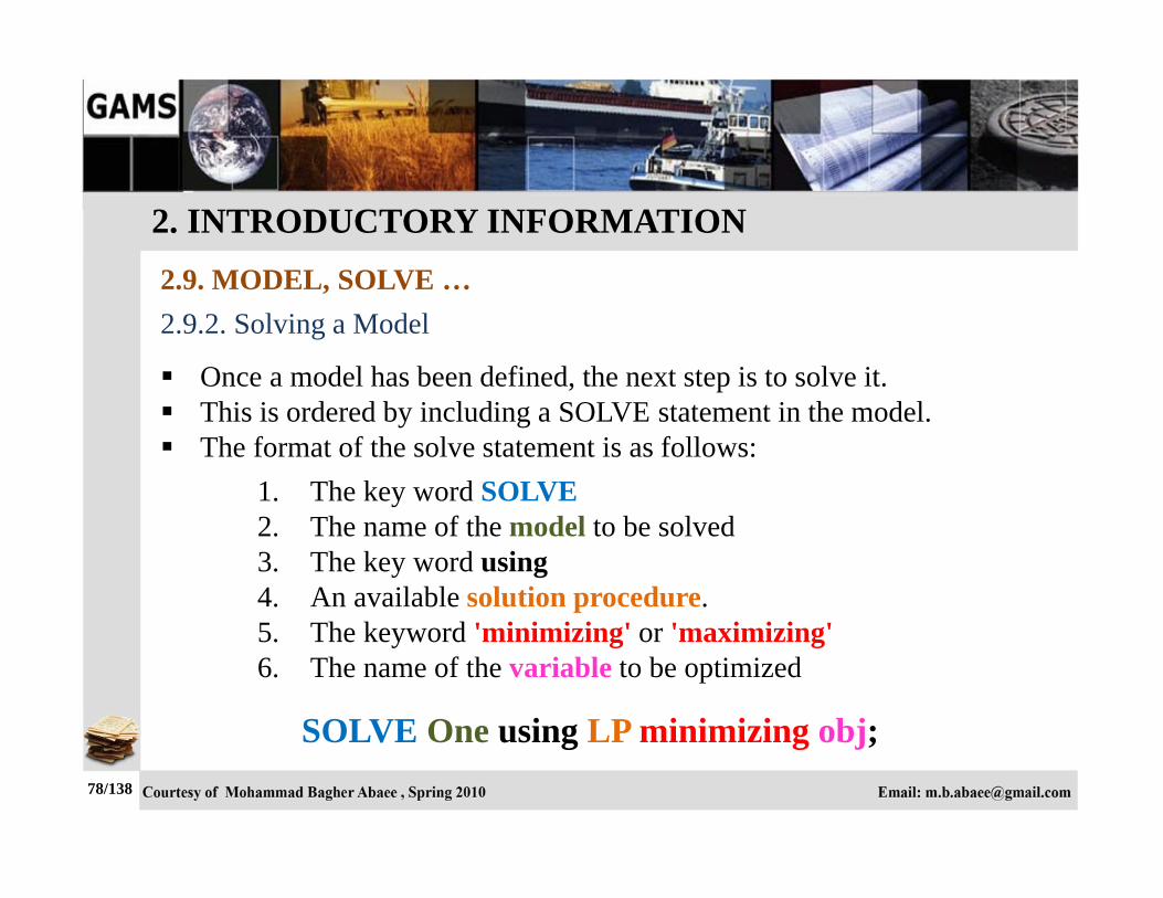
Once a model has been defined, the next step is to solve it. This is ordered by including a SOLVE statement in the model. The format of the solve statement is as follows:

2.9.2. Solving a Model

1. The key word SOLVE 2. The name of the model to be solved 3. The key word using 4. An available solution procedure. 5. The keyword 'minimizing' or 'maximizing' 6. The name of the variable to be optimized

SOLVE One using LP minimizing obj;

2. INTRODUCTORY INFORMATION 2.9. MODEL, SOLVE …

79/138

2.9.3. Solution Procedure Solution

Procedure Description

LP Linear programming. The model cannot contain nonlinear or discrete (binary and integer) variables.

NLP Nonlinear programming. In the model, nonlinear forms must be continuous functions and the model may not contain discrete variables.

MIP Mixed integer programming. Similar to RMIP, but the requirements of discreteness of variables and equations are stringent. Discrete variables must take discrete values within boundaries.

MINLP Mixed integer nonlinear programming. The same characteristics as for RMINLP, but the requirements of discreteness are very stringent.

DNLP for nonlinear programming with discontinuous derivatives

2. INTRODUCTORY INFORMATION 2.10. OUTPUT

80/138

3. SPECIAL ORDERS GAMS 3.1. Programming Flow Control Features

81/138

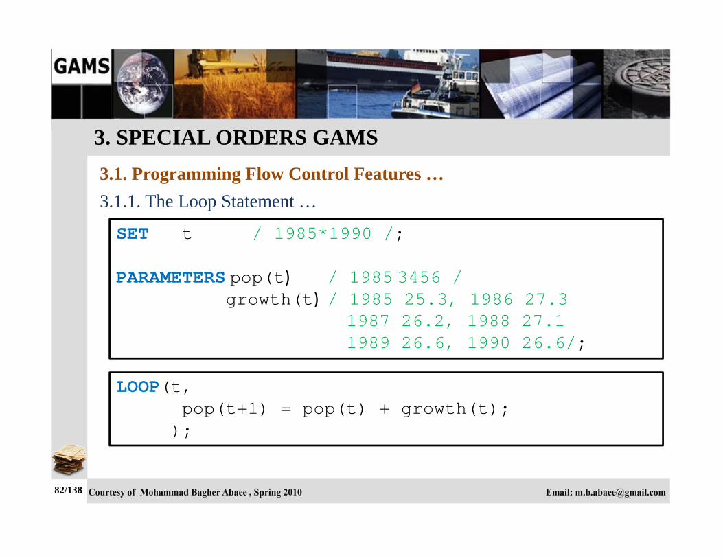
3.1.1. The Loop Statement

The Loop statement allows one to execute a group of statements for each element of a set. The syntax of the Loop statement is: LOOP ( (set1,set2,…) [$(condition)], Statement or Statements to Execute; );

One cannot place GAMS set, acronym, for, scalar, parameter, table, variable, equation or model

statements inside the Loop statement.

3. SPECIAL ORDERS GAMS 3.1. Programming Flow Control Features …

82/138

3.1.1. The Loop Statement …

SET t / 1985*1990 /; PARAMETERS pop(t) / 1985 3456 / growth(t) / 1985 25.3, 1986 27.3 1987 26.2, 1988 27.1 1989 26.6, 1990 26.6/;

LOOP(t, pop(t+1) = pop(t) + growth(t); );


83/138

3.1.2. The If-Elseif-Else Statement

The IF-ELSE operator is useful for transferring from one operator to another. In some cases, it can be written down as a set of $ conditions. The following syntax is for the "IF-THEN-ELSE" operator:

IF ( Condition, Statements; {ElseIf Condition , Statements; } [Else Statements;] );

One cannot place GAMS set, acronym, for, scalar, parameter,

table, variable, equation or model statements inside the If statement.


84/138

3.1.2. The If-Elseif-Else Statement …

IF (f <= 0, p(i) = -1 ; q(j) = -1 ; ElseIf ((f > 0) and (f < 1)), p(i) = p(i)**2 ; q(j) = q(j)**2 ; Else p(i) = p(i)**3 ; q(j) = q(j)**3 ; );


85/138

3.1.3. The While Statement

The While statement allows one to repeatedly execute a block of statements until a logical condition is satisfied. Ordinarily, the syntax of the While statement is: WHILE (Condition, Statement or Statements to Execute; );


statements inside the While statement.


86/138

3.1.3. The While Statement …

WHILE (x<10, x=x+0.01; ); OR $Onend WHILE x<10 do x=x+0.01; EndWhile;


87/138

3.1.4. The For Statement

The For statement allows one to repeatedly execute a block of statements over a successively varied values of a scalar.

The syntax of the For statement is: FOR (Scalarq = Startval To (Downto) Endval by Increment,

Statement or Statements to Execute; );

• Scalarq: is a scalar • Startval: is the constant or scalar giving the value where scalarq will

begin • To: indicates that GAMS will add increment until scalarq gets equal to

or larger than end


88/138

3.1.4. The For Statement …

The syntax of the For statement is: FOR (Scalarq = Startval To (Downto) Endval by Increment,

Statement or Statements to Execute; );

• Downto: indicates that GAMS will subtract increment until scalarq gets equal to or smaller than end.

• Endval: is a constant or scalar giving the value that will result in statement termination when scalarq equals or passes it.

• Increment: is a positive constant or scalar which is optional and defaults to one.

One cannot place GAMS set, acronym, for, scalar, parameter, table, variable, equation or model statements inside the For statement.


89/138

3.1.4. The For Statement …

FOR (x=12 downto 1 by 2, data(i)=x; ); OR $Onend FOR x=12 downto 1 by 2 do data(i)=x; EndFor;


90/138

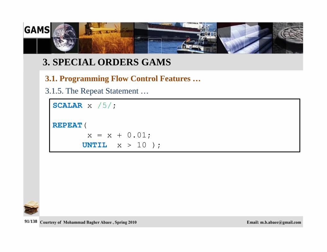
3.1.5. The Repeat Statement

The Repeat statement causes one to execute a block of statements over and over until a logical condition is satisfied.

The syntax of the Repeat statement is: REPEAT ( Statement or Statements to Execute; UNTIL logical condition is true );


statements inside the Repeat statement.


91/138

3.1.5. The Repeat Statement …

SCALAR x /5/; REPEAT( x = x + 0.01; UNTIL x > 10 );


92/138

Operator Meaning

Lt < Strictly less than Le <= Less than-or-equal to Eq = Equal to Ne < > Not equal to Ge >= Greater than or equal to Gt > Strictly greater than

3.1.6. Numerical Relationship Operators


93/138

Operator Meaning

Not Not And And Or Inclusive or

Xor Exclusive or . .

3.1.7. Logical Operators


94/138

Operands Results

a b a and b a or b a xor b not a 0 0 0 0 0 1 0 non-zero 0 1 1 1

non-zero 0 0 1 1 0 non-zero non-zero 1 1 0 0

3.1.7. Logical Operators …


95/138

3.1.7. Mixed Logical Conditions

Logical Condition Numerical Value Logical Value

1 2 3 4 2 True 2 1 3 4 0 False 4 5 3 10/8 17.125 True 4 5 3 10 8 1 True 4 5 2 3 6 2 True 4 0 2 3 6 0 False

3. SPECIAL ORDERS GAMS 3.2. Ordered Sets

96/138

3.2.1. ORD Operator

The ORD returns an ordinal number equal to the index position in a set.

SET t time periods / 2000*2010 /; PARAMETER val(t); val(t) = ORD(t);

v 2000 1 v 2001 2

… v 2010 11

3. SPECIAL ORDERS GAMS 3.2. Ordered Sets …

97/138

3.2.2. CARD Operator

The CARD operator returns an ordinal number equal to the number of elements in a set.

SET t time periods / 2000*2010 /; PARAMETER S; S = CARD(t);

11


98/138

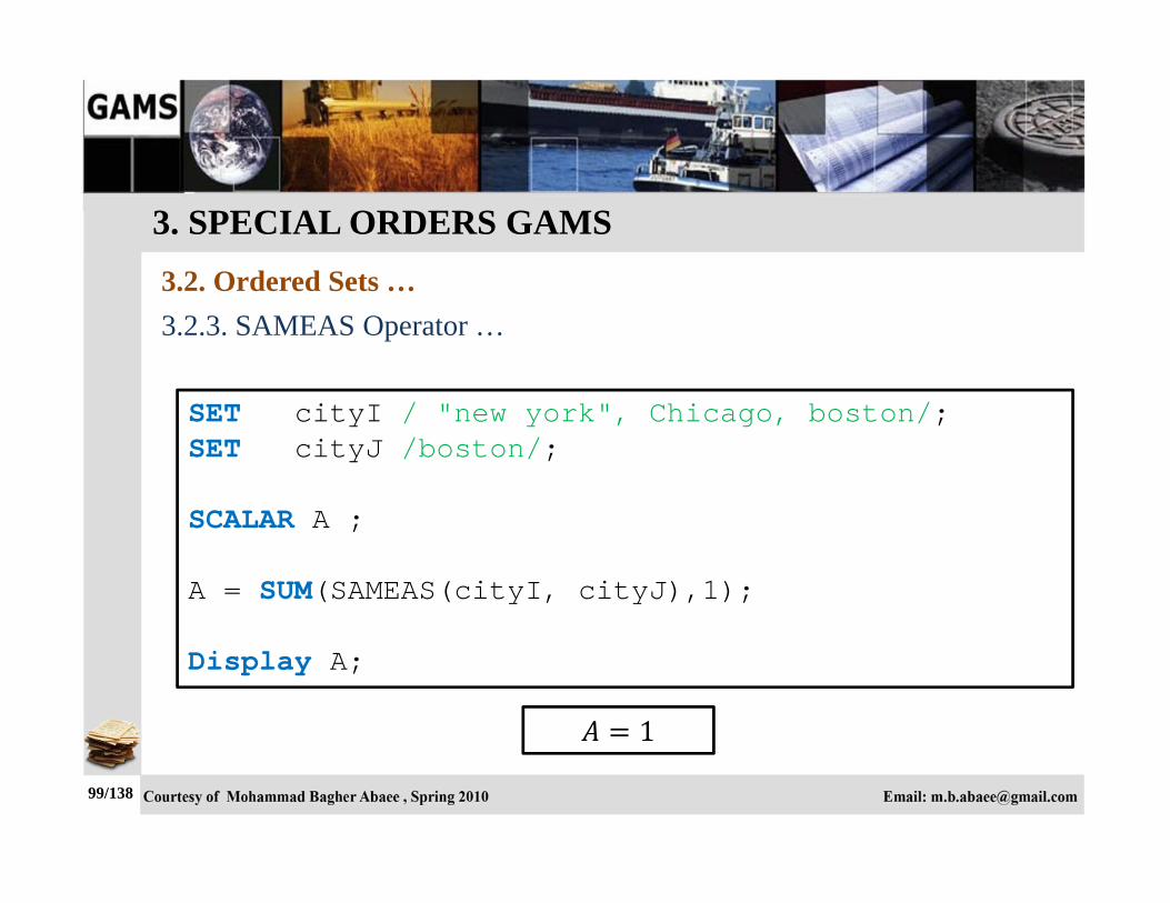
3.2.3. SAMEAS Operator

One may wish to do conditional processing dependent upon the text defining a name of a set element matching the text for a particular text string or matching up with the text for a name of a set element inset.

SAMEAS(SetElement, OtherSetElement) or SAMEAS(aSetElement, "text") returns an indicator that is true if the text giving the name of Etelement is the same as the text for OtherSetElement and a false otherwise.


99/138

3.2.3. SAMEAS Operator …

SET cityI / "new york", Chicago, boston/; SET cityJ /boston/; SCALAR A ; A = SUM(SAMEAS(cityI, cityJ),1); Display A;

1


100/138

3.2.4. DIAG Operator

DIAG(setelement, othersetelement) or diag(asetelement, "text") returns a number that is one if the text giving the name of setelement is the same as the text for othersetelement and a zero otherwise.

SET cityI / "new york", Chicago, boston/; SET cityJ /boston/; SCALAR A ; A = SUM((cityI, cityJ), DIAG(cityI, cityJ)); Display A;

1


101/138

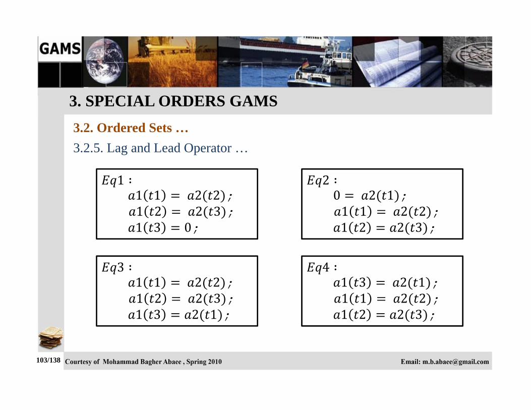
3.2.5. Lag and Lead Operator

Operators LAG and LEAD are used for correlating an element of a set with the next or preceding element of the set. GAMS has two variants of LAG and LEAD operators:

Linear LAG and LEAD operators (+, -) Circular LAG and LEAD operators (++, --).

The difference between these two types of operators is in the method of processing at the initial and final points of the sequence. In circular operators, after the final element of the sequence, there comes the first, while in linear operators sets are broken.


102/138

3.2.5. Lag and Lead Operator …

SET t /t1*t3/; VARIABLE a1(t),a2(t) ; EQUATION Eq1(t),Eq2(t),Eq3(t),Eq4(t) ; Eq1(t) .. a1(t) =e= a2(t+1); Eq2(t) .. a1(t-1) =e= a2(t); Eq3(t) .. a1(t) =e= a2(t++1); Eq4(t) .. a1(t--1) =e= a2(t);


103/138

3.2.5. Lag and Lead Operator …

1 1 1 2 2 ; 1 2 2 3 ; 1 3 0;

2 0 2 1 ; 1 1 2 2 ; 1 2 2 3 ;

3 1 1 2 2 ; 1 2 2 3 ; 1 3 2 1 ;

4 1 3 2 1 ; 1 1 2 2 ; 1 2 2 3 ;

4. GAMS and Other Applications 4.1. GAMS/Excel

104/138

4.1.1. Converting Data to GAMS

From wherever your gams system directory is, run “XLS2GMS.exe”. For GAMSIDE users, this may be: C:\Program Files\GAMS

4. GAMS and Other Applications 4.1. GAMS/Excel …

105/138

4.1.1. Converting Data to GAMS … Input file (*.XLS)

Range

Output GAMS Include file (*.txt

or *.inc)


106/138

4.1.1. Converting Data to GAMS …

TABLE d(i, j) $include data.txt ;


107/138

4.1.2. Import Data from Excel

When calling XLS2GMS directly from GAMS we want to specify all command and options directly from the command line or from a command file.

Command is: $call = xls2gms I=“C:\test.xls” O=“C:\data.txt” R=Sheet1!B1:E10 • Command Statement • I=inputfilename • I=inputfilename • Sheet of excel • Range of sheet


108/138

4.1.2. Import Data from Excel … SET i / $call = xls2gms I=Book1.xlsx O=setI.txt R=Sheet2!A1:A3 $include setI.txt / j / $call = xls2gms I=Book1.xlsx O=setJ.txt R=Sheet2!B1:B3 $include setJ.txt /; TABLE d(i, j) $call = xls2gms I=Book1.xlsx O=Data.txt R=Sheet1!B2:E4 $include data.txt ;

4. GAMS and Other Applications 4.2. GAMS/MATLAB

109/138

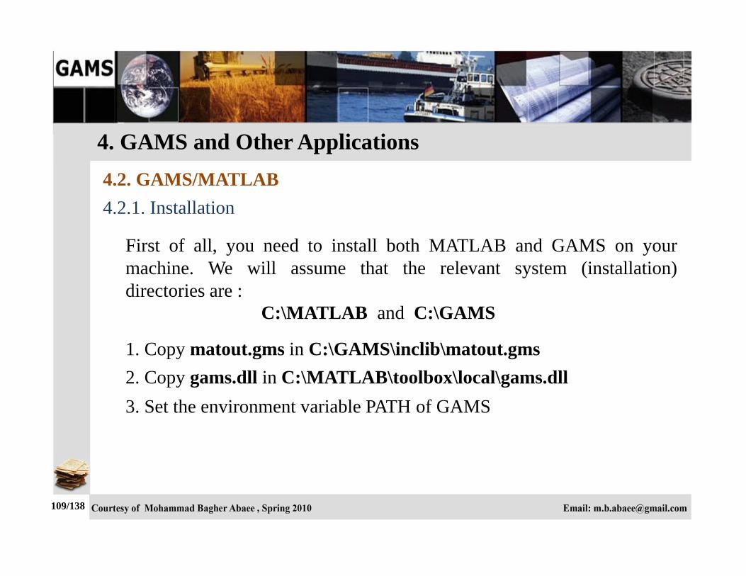
4.2.1. Installation

First of all, you need to install both MATLAB and GAMS on your machine. We will assume that the relevant system (installation) directories are : C:\MATLAB and C:\GAMS

1. Copy matout.gms in C:\GAMS\inclib\matout.gms 2. Copy gams.dll in C:\MATLAB\toolbox\local\gams.dll 3. Set the environment variable PATH of GAMS

4. GAMS and Other Applications 4.2. GAMS/MATLAB …

110/138

4.2.1. Installation …

To test the installation, carry out the following steps:

1. Start up MATLAB 2. In the MATLAB command window, change directories to the

examples directory provided as part of the distribution. (This directory contains at least two files, testinst.m and testinst.gms that are required for this test.)

3. Run the example “testinst” that is found in the examples directory of the distribution. At the MATLAB prompt you just type: >> testinst


111/138

4.2.1. Installation …

The resulting output will depend on the platform on which you run this from. It should include the output given below: Q = name: ’Q’ val: [3x3 double] ans = 1 0 0 0 1 0 0 0 1 Q = 2 0 0 0 2 0 0 0 2 J = ’1’ ’2’ ’3’ ….

Q = name: ’Q’ val: [3x3 double] J = name: ’J’ val: {3x1 cell} Q = name: ’Q’ val: [3x3 double] J = name: ’J’ val: {3x1 cell} A = name: ’A’ val: [2x3 double] ….

ans = 3 0 0 0 3 0 0 0 3 ans = ’1’ ’2’ ’3’ ans = 0 2 -5 2 0 2


112/138

4.2.2. Returning Values to MATLAB

In order to run the same model within MATLAB and return the solution vector variable of x(i) and parameter of d(i, j) back into the MATLAB workspace, one change is required to the GAMS file, namely to add the below line after the SOLVE statement:

$libinclude matout x.l i $libinclude matout d i j

This just writes out the level values of the solution to a file that can be read back into MATLAB. In MATLAB, you just execute the following statement: [x d] = gams(’NameGamsFile’);

7. BASIC MODELS FOR ECONOMICS OF ELECTRICITY

7.1. Power Transit

113/138

Figure 7.1.1 shows a 6-Bus system. There are two Power Plants at Bus1 and Bus2 and three Steel Factory at Bus3, Bus4 and Bus5. Power Plants can contract bilateral. markets for a single commodity, and we are given the unit costs of shipping the commodity from plants to markets. The economic question is: how much shipment should there be between each plant and each market so as to minimize total transport cost?


7.2. Economic Dispatch

114/138

To appreciate the advantages of dispatching a power system according to the solution of the ED problem, consider the case where a power plant supplies 10,000MW during 1 h at an average cost of $0.05/kWh; if the consumers buy this energy at the rate of $0.06/kWh, this arrangement results in a net profit to the supplier of $100,000/h. In this case an improvement in supply efficiency of just 1% through the use of ED would result in a profit increment of $5000/h or $43.8 million in one year.


7.2. Economic Dispatch …

115/138

7.2.1. Basic Economic Dispatch

Consider two generating units supplying the system demand . The quadratic unit cost functions are characterized by the parameters provided in the table as follows:

Unit $⁄ $⁄ $⁄

G1 100 20 0.05 0 400 G2 200 25 0.10 0 300



116/138

7.2.1. Basic Economic Dispatch …

For the specific system demand levels of 40, 250, 300, and 600MW, calculate and analysis: A. No generation limits 1) ED generation levels 2) Cost of generation each unit 3) Incremental cost B. With generation limits 1) ED generation levels 2) Cost of generation each unit 3) Incremental cost



117/138

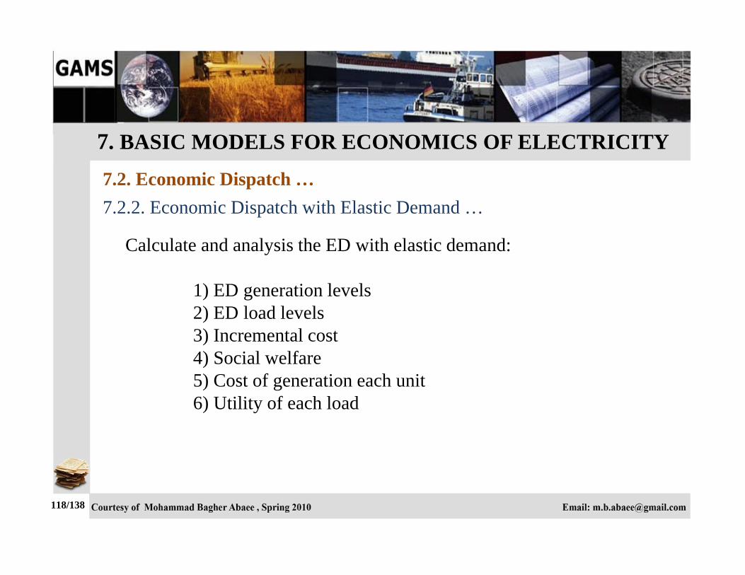
7.2.2. Economic Dispatch with Elastic Demand

The generating units of example 7.2.1 as well as the elastic demands characterized below are considered in this example:

Load $⁄ $⁄

L1 55 -0.2 0 300 L2 50 -0.1 0 350



118/138

7.2.2. Economic Dispatch with Elastic Demand …

Calculate and analysis the ED with elastic demand: 1) ED generation levels 2) ED load levels 3) Incremental cost 4) Social welfare 5) Cost of generation each unit 6) Utility of each load



119/138

7.2.3. Economic Dispatch with Losses

In the generating units of example 7.2.1 as well as consider sensitivity coefficients of the losses with respect to the generation levels. Sensitivity coefficients of the losses provided in the table as follows:

Unit

G1 0.00047 G2 0.00023



120/138

7.2.4. First Project …

In example 7.2.1, suppose that quadratic cost functions are piecewise linear cost functions. Piecewise linear functions are illustrated in below figures for both generators.


7.2. Economic Dispatch

121/138

7.2.4. First Project …

Now, calculate, analysis and compare with results of section 7.2.1 at the specific system demand levels of 40, 250, 300, and 600MW: A. No generation limits 1) ED generation levels 2) Cost of generation each unit 3) Incremental cost B. With generation limits 1) ED generation levels 2) Cost of generation each unit 3) Incremental cost


7.3. Optimal Power Flow

122/138

7.3.1. DC Load Power Formulation

…

…


7.3. Optimal Power Flow …

123/138

7.3.2. Optimal DC Power Flow Formulation

,

Quadratic Cost Function

:

,

,



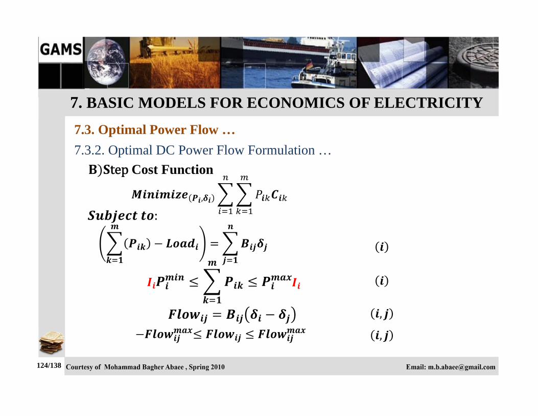
124/138

7.3.2. Optimal DC Power Flow Formulation …

,

tep Cost Function

:

,

,



125/138

7.3.3. Economic Dispatch Including a Line with Limited Transmission Capacity

Consider the three-bus, three-line network characterized in the table and depicted in below figure (shut susceptances neglected).

Reactance

1 2 0.1 unlimited 1 3 0.1 140 2 3 0.1 unlimited



126/138

7.3.3. Economic Dispatch Including a Line with Limited Transmission …

Buses 1 and 2 include the two units characterized in Section 7.2.1. Voltage magnitudes are constant and equal to 1. A base of 100 kV and 200MVA is considered.

Now, calculate, analysis and compare with results of section 7.2.1 at the specific system demand levels of 250 and 300MW with and without transmission limit and generation limits in line 1–3: 1) ED generation levels 2) Cost of generation each unit 3) LMPs



127/138

7.3.4. Economic Dispatch with Bilateral Contracts

Considering the units with the cost functions of Section 7.2.1, suppose that the generating unit 2 and the load engage in a bilateral contract of 50MW at $31.5/MWh.

Now, for the specific system demand levels of 50, 250, 300, and 600MW, calculate and analysis: 1) ED generation levels 2) Cost of generation each unit 3) Profit of each unit 4) Incremental cost



128/138

7.3.5. AC Load Power Formulation

Polar Equations



129/138

7.3.5. AC Load Power Formulation …

Cartesian Equations



130/138

7.3.5. AC Load Power Formulation …

Cartesian Equations



131/138

7.3.6. Optimal AC Power

Consider the three-bus, three-line network that is depicted in below figure.



132/138

7.3.6. Optimal AC Power …

Base of 100MVA is considered.

Calculate: 1) Generations 2) magnitude and angle of Voltages 3) Active and reactive loss 4) LMPs 5) Current and power flow of lines While objective is: A. Minimum Cost B. Minimum Network Loss



133/138

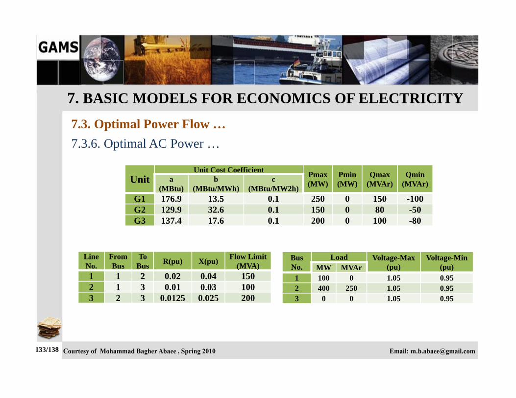
7.3.6. Optimal AC Power …

Unit Unit Cost Coefficient Pmax

(MW) Pmin (MW)

Qmax (MVAr)

Qmin (MVAr) a

(MBtu) b

(MBtu/MWh) c

(MBtu/MW2h) G1 176.9 13.5 0.1 250 0 150 -100 G2 129.9 32.6 0.1 150 0 80 -50 G3 137.4 17.6 0.1 200 0 100 -80

Line No.

From Bus

To Bus R(pu) X(pu) Flow Limit

(MVA) 1 1 2 0.02 0.04 150 2 1 3 0.01 0.03 100 3 2 3 0.0125 0.025 200

Bus No.

Load Voltage-Max (pu)

Voltage-Min (pu) MW MVAr

1 100 0 1.05 0.95 2 400 250 1.05 0.95 3 0 0 1.05 0.95


7.4. UNIT COMMITMENT

134/138

In formulating the ED, we consider that all generating units are online and ready to produce.

The unit commitment problem is solved over a particular time period T; in the day-ahead market, the time period is usually 24 hours.

UC is the problem of determining the schedule of generating units within a power system subject to device and operating constraints.

The decision process selects units to be ON or OFF, the type of fuel, the power generation for each unit, the fuel mixture applicable, and the reserve margins.

Mathematically, UC is a Non-convex, non-linear, large-scale, mixed-integer optimization problem with a great number of 0-1 variables, and a series of prevailing equality constraints.


7.4. UNIT COMMITMENT …

135/138

StartupCost

O Function:

:

• Area Constraints o System Load Balance o System Spinning and Operating Reserve Constraints

• Zonal Constraints o System Spinning and Operating Reserve Constraints

• Security Constraints • Unit Constraints

o Minimum and Maximum Generation limits



136/138

o System Spinning and Operating Reserve Constraints o Reserve limits o Minimum Up/Down times o Hours up/down at start of study o Must run schedules o Pre-scheduled generation schedules o Ramp Rates o Hot, Intermediate, & Cold startup costs o Maximum starts per day and per week o Maximum Energy per day and per study length



137/138

7.4.1. Unit Commitment Formulation

, , ,

O Function

:

Power Balance: ,

Min Generation: , , ,

Max Generation: , , ,



138/138

7.4.1. Unit Commitment Formulation …

Ramp-up limit: , , ,

Ramp-down limit: , , ,

Minimum up time: , , , ,

Minimum down time: , , , ,

Synchronal Reserve ,

generalized algebraic modeling system (gams) m. b. abaee

Documents