generalized fokker–planck theory for electron and photon transport

Generalized Fokker–Planck theory for electron and photon transportin biological tissues: application to radiotherapy

Edgar Olbrant* and Martin Frank

Department of Mathematics, Center for Computational Engineering Science, RWTH AachenUniversity, Schinkelstrasse 2, D-52062 Aachen, Germany

(Received 9 December 2009; final version received 21 April 2010)

In this paper, we study a deterministic method for particle transport in biologicaltissues. The method is specifically developed for dose calculations in cancer therapyand for radiological imaging. Generalized Fokker–Planck (GFP) theory [Leakeas andLarsen, Nucl. Sci. Eng. 137 (2001), pp. 236–250] has been developed to improve theFokker–Planck (FP) equation in cases where scattering is forward-peaked and wherethere is a sufficient amount of large-angle scattering. We compare grid-basednumerical solutions to FP and GFP in realistic medical applications. First, electron dosecalculations in heterogeneous parts of the human body are performed. Therefore,accurate electron scattering cross sections are included and their incorporation into ourmodel is extensively described. Second, we solve GFP approximations of the radiativetransport equation to investigate reflectance and transmittance of light in biologicaltissues. All results are compared with either Monte Carlo or discrete-ordinates transportsolutions.

Keywords: generalized Fokker–Planck; deterministic method; radiotherapy; particletransport; Boltzmann equation; Monte Carlo

AMS Subject Classification: 35Q20; 35Q84; 65C05; 62P10; 78A35; 85A25

1. Introduction

The numerical solution of the Boltzmann transport equation (BTE) [7,20] remains a

difficult and important challenge in electron and photon transport. To contribute to this

field of research, we study selected approximations of the transport equation for electrons

and photons, and present numerical results in different geometries.

Nowadays, cancer patients often undergo therapies with high energy ionizing

radiation. In external radiotherapy, photon beams dominate in clinical use – less patients

receive electron therapy. Treatments are also performed by using heavy-charged particles

such as ions or protons. These have higher costs for their particle accelerators, but gain

more and more importance due to first high-intensity laser systems for protons [47].

To aid the recovery of patients, it is important to deposit a sufficient amount of energy

in the tumour. Simultaneously, the ambient healthy tissue should not be damaged.

Therefore, the success of such radiation treatments strongly depends on the correct dose

distribution. It is recommended that uncertainties in dose distributions should be less than

2% to get an overall desired accuracy of 3% in the delivered dose to a volume [43].

ISSN 1748-670X print/ISSN 1748-6718 online

q 2010 Taylor & Francis

DOI: 10.1080/1748670X.2010.491828

http://www.informaworld.com

*Corresponding author. Email: [email protected]

Computational and Mathematical Methods in Medicine

Vol. 11, No. 4, December 2010, 313–339

Additionally, thresholds have been developed to compare dose results computed by

different algorithms. A suggested tolerance in homogeneous geometries is the 2% (relative

pointwise difference) or 2mm (absolute distance to agreement) criterion. However, in

heterogeneities this limit increases to 3% or 3mm [53].

Up to now, many clinical dose calculation algorithms rely on pencil beam models.

Originally developed for cosmic ray showers, Fermi ([16], cited by [45]) and Eyges [15]

introduced a small-angle scattering theory which was later applied to electrons. This

theory was used by Hogstrom et al. to propose the pencil-beam model. Their algorithm

includes experimental data, taken from dose measurements in a water phantom, to

compute the central-axis dose [26]. Although it was the first clinically applicable model,

its accuracy deep in the irradiated material or in heterogeneities is poor. This is basically

due to the small-angle approximation in Fermi–Eyges theory. It is true that single electron

collisions show small deviations. However, after multiple scattering events, they

accumulate to big angle changes in large penetration depths. Besides, crude

approximations such as small deviations of particles throughout their whole path through

the tissue [37], geometric structures, transverse to the beam direction, are assumed to be

infinite. Although many improvements of Fermi–Eyges theory were performed, e.g. by

including additional correction factors [2,32,33,48], they still suffer from the small angle

and the homogeneity assumption. Comparisons with experimental data showed

disadvantages in inhomogeneous phantoms [40].

A statistical simulation method for radiation transport problems is the Monte Carlo

(MC) method [4]. It performs direct simulations of individual particle tracks which result

from a random sequence of free flights and interaction events. In this way random histories

are generated. If their number is large enough, macroscopic quantities can be obtained by

averaging over the simulated histories. MC tools model physical processes very precisely

and can handle arbitrary geometries without losing accuracy. Although they rank among

the most accurate methods for predicting absorbed dose distributions, their high-

computation times limit their use in clinics. Due to the increase in computing power and

decrease in hardware costs, MC techniques have recently become a growing field in

radiotherapy [50]. Not only general-purpose MC codes are now publicly available, but

also commercial MC treatment planning systems [11,49]. However, they have not yet

gained widespread clinical use.

A different approach in the solution of radiation transport problems is deterministic

calculations solving the linear BTE. In principle, its solution will give very accurate dose

distributions comparable to that of MC simulations. The BTE can be analytically solved

only in very simplified geometries, which is insufficient for clinical applications.

Additionally, numerical solutions to the BTE require deterministic methods coping with a

6D phase space. Because of this and their simpler implementation, MC techniques have so

far prevailed in the medical-physics community. Nevertheless, Borgers [7] argued that on

certain accuracy conditions, deterministic methods could compete with MC calculations.

In this paper, we describe electron and photon transport in media by solving the

generalized Fokker–Planck (GFP) approximation of the linear BTE [38]. For electron

transport, this is an extension of the Fokker–Planck (FP) model, formulated in [24], to

higher-order approximations in angle scattering. It should be stressed that this approach

brings about several advantages: the BTE does not require any assumption on the

geometry so that arbitrary heterogeneities are possible. Furthermore, we benefit from

mathematical and physical approximation ansatze because they can be directly included in

the differential equation. This avoids heuristic assumptions. In contrast to MC simulation,

deterministic solutions do not suffer from statistical noise, and their resolution does not

E. Olbrant and M. Frank314

depend on the number of particles traversing a certain region. Moreover, the treatment

planning problem can be formulated as a PDE-constrained optimization problem. This

structure can be used to obtain additional information to speed-up the optimization

[18,19]. This is hard to achieve by MC techniques.

Previous studies in deterministic methods for radiotherapy primarily concentrated on a

combination of rigorous-analytic solutions and laboratory measurements (see pencil beam

models above). Without explicitly using experimental data in their model, Huizenga and

Storchi [27] presented the phase space evolution (PSE) model for electrons and

subsequently applied it to multi-layered geometries [41]. Various improvements and

extension to 3D beam dose calculations were performed [30,31]. However, 3D dose

calculations showed disadvantages in computation times [34]. Moreover, PSE models

used first-order discretizations in space which cannot compete with MC techniques [7]. By

contrast, our access focuses on the continuous model of the Boltzmann equation

discretized with high-order schemes.

First studies for deterministic dose calculations in charged-particle transport came

from well-known procedures for numerical solutions to the transport equation of neutrons

or photons. Several approximative models to the BTE have been developed. Each of these

methods has its advantages and drawbacks [8]. Multi-group methods are sometimes used

to discretize the energy domain [12]. This leads to a number of monoenergetic equations to

be separately discretized in space and angle. Although discretizations in space are usually

done by finite difference and finite element (FE) methods, the remaining angle domain is

discretized by discrete ordinates [5,14]. Such an approach is implemented in the solver

Attila [22]. Recently, 3D dose calculations for real clinical test cases were performed with

Attila [53]. Results with similar accuracy as MC calculations were achieved in promising

computation times.

Less frequent are angular FE approaches [11] seeking to reduce ray effects. Tervo et al.

[51] extended FE discretizations to all variables in spatial, angular and energy domains so

that no group cross sections were needed. Moreover, a detailed description of three

coupled BTEs with FE discretizations of all variables was proposed in [6].

In this paper, the BTE is approximated by the continuous slowing down (CSD) method

[36,39]. Scattering processes are modelled by GFP approximations [38] and compared to

classical FP [44] solutions. Leakeas and Larsen [38] showed that scattering kernels with a

sufficient amount of large-angle scattering yield inaccurate FP results. As an extension of

the work in [38], we perform deterministic GFP simulations and investigate their

behaviour in real applications. It is well known that electron scattering is dominantly

forward peaked. Hence, many electron transport simulations used the classical FP

approximation [13,17,24]. However, up to now, no comparisons to GFP dose

computations have been done including realistic physical scattering cross sections. In

our case, the latter are extracted from ICRU libraries [28]. We describe in detail how

transport coefficients in the BTE can be computed from these scattering cross sections and

compute GFP electron dose profiles in inhomogeneous geometries.

Even more challenging for GFP theory are scattering kernels including large angle

scattering. We therefore investigate transport of photons in biological tissues with

forward-peaked and large-angle scattering. Using test cases from [23] the radiative

transport equation for GFP approximations up to order five is solved to determine

reflectance and transmittance of light in biological tissues.

In the remaining paper, the following structure is presented: a short discussion of basic

electron interactions with matter is given at the beginning. We describe a model for

electron transport and review crucial steps of the GFP theory. In addition, we derive

Computational and Mathematical Methods in Medicine 315

transport coefficients for the GFP equations from databases for electron scattering cross

sections. In Section 3, a deterministic model for light propagation together with different

scattering kernels is introduced. Discretization methods used in our GFP equations are

studied in Section 4. In Section 5, we compute FP, GFP and discrete-ordinates’ results for

transmittance and reflectance of light by a slab. Moreover, we numerically compare FP,

GFP and MC solutions for 5 and 10MeV electrons in homogeneous and heterogenous slab

geometries. Section 6 gives the conclusions and outlooks. Appendix A contains explicit

formulae for high-order polynomial operators. In Appendix B, we present the equations to

be solved for the GFP coefficients.

2. Deterministic model for electron transport

2.1 Physical interactions

Electron beams are nowadays a widely spread tool in cancer therapy. Typical electron

beams, provided by high-energy linear accelerators, range from 1 to 25MeV. During

irradiation of human tissue, electrons interact with matter through several competing

mechanisms.

1. Elastic scattering. This is usually a non-radiative interaction between electrons and

the atomic shell. Projectiles experience small deflections and lose little energy.

High-energy electrons can also penetrate through atomic shells and are afterwards

scattered at the bare nucleus without any energy loss. With kinetic energies above

1 keV, elastic scattering in water dominantly occurs in the forward direction [37].

2. Soft inelastic e 2–e 2 scattering. Electrons interact with other electrons of the outer

atomic shell which usually leads to excitation or ionization of the target particle.

Here binding energies are only a few electron volts so that projectile electrons

transfer little energy and are hardly deflected.

3. Hard inelastic e 2–e 2 scattering. These collisions are determined by large transfer

energies to the target electron. What ‘large’ exactly means is specified in MC codes

by cutoff energies. In PENELOPE [46], for example, the default value of this

simulation parameter is set to 1% of the maximum energy of all particles. As a

consequence, the target electrons are ejected with larger scattering angles and

higher kinetic energies (delta rays). They act as an additional source in the transport

equation.

4. Bremsstrahlung. Owing to the electrostatic field of atoms, electrons are decelerated

and hence emit bremsstrahlung photons. However, for energies below 1MeV this

phenomenon can be neglected. Bremsstrahlung photons are not mainly emitted in

the forward direction. The lower their kinetic energy the more isotropic their angle

distribution becomes [35].

Evidently, there are more interaction processes such as ejection of Auger electrons or

characteristic X-ray photons. But they are very unlikely in the energy range considered.

Although inelastic collisions are decisive for the energy transfer, the radiation damage

in the patient strongly depends on the spatial distribution of electrons in their passage

through matter. They dominantly undergo multiple scattering events with small

deviations. However, single backward scattering events also occur frequently which

leads to tortuous trajectories of electrons. To a big extent, such trajectories are due to

elastic collisions. We therefore focus on very accurate and realistic simulation of elastic

processes in our model. This is achieved by transport coefficients extracted from the ICRU

77 database [28]. Inelastic transport coefficients are obtained in the same way.


Elastic and soft inelastic events lead to small energy loss. With kinetic energies above

1 keV, electrons are assumed to lose their energy continuously [21]. Because of this, we

implement the CSD approximation to model energy loss by electrons. Hence, we neglect

large energy loss fluctuations caused by hard inelastic collisions.

Bremsstrahlung effects are considered in our model in a very restricted way: only

energy transfer of electrons after soft bremsstrahlung collisions is simulated by means of

the radiative stopping power. However, the effect of hard photon emission as well as the

transport of photons is disregarded so far.

2.2 The GFP approximation for electrons

The motion of particles can be described by a 6D phase space ðr;E;VÞ [ ðV £ I £ S2Þ

with

spatial variable r ¼ ðx1; x2; x3Þ [ V , R3 open and bounded;

energy variable E [ I ¼ ½Emin;Emax� , R;

direction variable V ¼ ðV1;V2;V3Þ [ S2 , R3 unit sphere

¼ ðffiffiffiffiffiffiffiffiffiffiffiffiffiffiffi12 m2

pcosðfÞ;

ffiffiffiffiffiffiffiffiffiffiffiffiffiffiffi12 m2

psinðfÞ;mÞ; m ¼ cosðuÞ:

If particle transport takes place in an isotropic and homogeneous medium in which

interaction processes are Markovian and particles do not interact with themselves, their

distribution can be described by the unique solution of the time-dependent linear BTE. For

practical applications in radiotherapy, we are faced with issues such as distributions of the

deposited energy in biological tissues or penetration depths of the beam. For many

purposes it is, therefore, sufficient to know the steady solution:

saCðr;E;VÞ þV�7Cðr;E;VÞ ¼ LBCðr;E;VÞ ð1Þ

with

Cðr;E;VÞ ¼ Cbðr;E;VÞ for all r [ ›V;V�n , 0;E [ I;

where Cðr;E;VÞ is called angular flux and denotes the distribution of particles travelling

in direction V. Boundary conditions (BC) are imposed on the angular flux depending on

the incident beam. Absorption of particles is described by the absorption cross section sa.

The right-hand-side

LBCðr;E;VÞ :¼

ð10

ð4p

ssðE0;E;V�V0ÞCðr;E0;V0Þ dV0 dE0 2 SsðEÞCðr;E;VÞ

is known as linear Boltzmann Operatorwhich describes scattering. Its integral contains the

differential scattering cross section (DSCS) ssðE0;E;V�V0Þ characterizing interaction

mechanisms in which particles are deflected. The dot product V�V0 ¼ cosðu0Þ ¼ m0

indicates that the scattering probability only depends on the scattering angle. This implies

that the deflection of scattered particles is axially symmetrical around the direction of

incidence V0. Integrating the scattering kernel ssðE0;E;V�V0Þ over all angles and


energies, one gets the total DSCS (TDSCS)

SsðEÞ ¼ 2p

ð10

ð121

ssðE0;E;m0Þ dm0 dE

0: ð2Þ

The angle and energy integral in the Boltzmann operator is the main difficulty in its

numerical solution. That is why an important aim is to develop accurate approximations.

However, up to now, there is no predominant method used for all types of particles. In fact,

depending on specific particle properties, one has to choose an appropriate approximation.

One crucial property of elastic DSCSs in water is a sharp peak in the forward direction

[29]. To express this mathematically, we define the positive nth scattering transport

coefficient (STC)

jnðEÞ :¼ 2p

ð10

ð121

ð12 m0Þn ssðE

0;E;m0Þ dm0 dE0; for all n $ 0; ð3Þ

and assume that as n increases, the coefficients jn fall off sufficiently fast, i.e.

jnþ1ðEÞp jnðEÞ; for all n $ 0 andE [ I: ð4Þ

Additionally, elastic scattering often entails a small energy loss. Therefore, the first

approximation is the expansion of the scattering kernel around m0 ¼ 1 and E ¼ E0. In this

way, Pomraning [44] showed that the already known FP operator is the lowest-order

asymptotic limit of the integral operator LB. In [39], this FP operator is derived as a first

order angle approximation to LB:

FP operator LFP :¼ ðj1=2ÞL; ð5Þ

where

LBCðVÞ ¼ LFPCðVÞ þOð1Þ; for 1p 1:

As the spherical Laplace–Beltrami operator

L ¼›

›mð12 m2Þ

›

›mþ

1

12 m2

›2

›f2

� �; withm ¼ cosðuÞ;

is differential in angle, the non-local integral Boltzmann operator LB is now approximated

by a local differential operator. The crucial point is that an integro-differential equation is

transformed into a partial differential equation. Although discretizations of differential

equations often lead to large linear systems, their numerical effort turns out to be much

lower. This is due to the local character of differential equations, which bring along much

sparser matrices.

Pomraning’s resulting FP equation for particle transport in an isotropic medium yields

saCðr;E;VÞ þV�7Cðr;E;VÞ ¼j1ðEÞ

2LCðr;E;VÞ þ

›ðSðr;EÞCðr;E;VÞÞ

›E; ð6Þ


where Sðr; 1Þ is called stopping power defined by

Sðr;EÞ ¼

ð10

ð4p

ðE2 E0ÞssðE0;E;V�V0Þ dV dE0: ð7Þ

The standard FP approximation is a frequently used method to describe transport processes

in media with highly forward-peaked scattering. Comparisons to real data, however, reveal

that many scattering processes of interest contain a small but sufficient amount of large-

angle scattering. To gain higher-order asymptotic approximations to LB, one could expand

LB to a

Polynomial operator LPn :¼Xn

m¼1an;mL

m;

with

an;m [ OðjmÞ ¼ Oð1m21Þ and LBCðVÞ ¼ LPnCðVÞ þOð1nÞ; for all n $ 1:

However, Leakeas and Larsen [39] showed that eigenvalues of LPn might become positive

so that the angular flux could become infinite. This served as a motivation for them to

develop asymptotically equivalent operators to LPn, which remain stable and preserve

certain eigenvalues of LB. We have summarized the details of the computation in the

appendix. We end up with GFP equations which incorporate large-angle scattering and

are, therefore, more accurate than the conventional FP equation:

saCðr;E;VÞ þV�7Cðr;E;VÞ ¼ LGFPnCðr;E;VÞ þ›ðSðr;EÞCðr;E;VÞÞ

›E: ð8Þ

For positive coefficients aiðEÞ;biðEÞ and m [ N, the GFP operators are defined by

LGFP2m :¼Xmi¼1

aiðEÞLðI 2 biðEÞLÞ21 and LGFP2mþ1

:¼ LGFP2m þ amþ1ðEÞL:

2.3 Determination of physical quantities

The fundamental part in GFP theory is based on the assumption of forward-peakedness

(Equation (1)). Its expected accuracy strongly depends on the behaviour of transport

coefficients jnðEÞ, which are different for the various projectiles and materials. The ICRU

Report 77 provides differential cross sections for elastic and inelastic scattering of electrons

and positrons for different materials and energies between 50 and 100MeV [28]. To obtain

transport coefficients jnðEÞ, we use these cross sections and proceed in the following way:

(a) The ELSEPA code system, distributed with the report, calculates elastic and

inelastic angular differential cross sections for a fixed energy E,

s el;inelðE;m0Þ ¼

ð10

sel;inels ðE0;E;m0Þ dE

0;

in tabulated form for discrete m0 and s el;inelðE;m0Þ. For a predetermined set of

energy values between 50 and 100MeV, data for s el;inelðE;m0Þ are extracted from

these files.


(b) With this we calculate the nth transport coefficient for a fixed energy E,

jel;ineln ðEÞ ¼ 2pNð121

ð12 m0Þns el;inelðE;m0Þ dm0; with m0 ¼ cosðu0Þ;

via numerical integration of the tabulated cross sections s el;inelðE;m0Þ by means of

the trapezodial rule. Additionally, wemultiply the result by themolecular density of

the transmitted matter

N ¼ NA

r

A;

where NA is Avogadro’s number, r the mass density of the material and A its molar

mass.

(c) Again, all computed results of jel;ineln ðEÞ are stored and used as a look-up table. To

obtain the nth transport coefficient at the desired energy E, these tabulated data are

linear interpolated.

Finally, we use the following transport coefficient in our equation:

jnðEÞ :¼ 2pNð121

ð12 m0Þnðs elðE;m0Þ þ s inelðE;m0ÞÞ dm0:

Figure 1 illustrates the electron transport coefficients of different order in liquid water.

Except for the 0th coefficient, every other coefficient is strictly monotonically decreasing.

For E $ 1023, j1 is always bigger than j2 but, as E decreases, their deviation reduces more

Figure 1. Comparison of STC in liquid water for energies between 50 and 100MeV.


and more. Unfortunately, for increasing n $ 2 the difference between two consecutive jnis so small that the assumption of forward-peakedness is not fulfilled. The inelastic

transport coefficients are much smaller than elastic transport coefficients for n $ 1. The

higher the order of the transport coefficient, the larger is the difference between elastic and

inelastic ones.

Our stopping power in Equation (7) is equivalent to the physical total stopping power

as the sum of collision and radiative stopping powers. For different materials both are

directly included in the files of the ICRU database. Hence, we do a linear interpolation to

get the stopping power S(E) at the desired energy E.

3. Deterministic model for light propagation

3.1 The GFP equation for grey photons

Many medical applications such as cancer treatment or optical imaging of tumours make

use of propagation of laser light in biological tissues. Its behaviour is determined by the

solution of the steady grey radiative transport equation

saCðr;VÞ þV�7Cðr;VÞ ¼ ms

ð4p

ssðV�V0ÞCðr;VÞ dV0 2Cðr;VÞ

� �; ð9Þ

with

Cðr;VÞ ¼ Cbðr;VÞ; for all r [ ›V ; V�n , 0:

Similar to 2.2, one can derive GFP approximations to the radiative transport equation in a

straightforward way. The intensity Cðr;VÞ describes the radiation power flowing in

direction V which is influenced by scattering and absorption coefficients sa and ms. More

important is the scattering kernel ssðV�V0Þ. It is also characteristic for biological tissues

that this kernel has a sharp peak at V�V0 ¼ 1. For its simulation, mathematically simple

scattering kernels with a free parameter are used.

3.2 Models for scattering kernels

One often cited scattering kernel is the (single) Henyey–Greenstein (HG) kernel [25]

defined by

sHGs ðm0Þ ¼

SHGs

2pfHGðm0Þ; ð10Þ

where

fHGðm0Þ :¼12 g2

2ð12 2gm0 þ g2Þ3=2; for g [ ð21; 1Þ;

is the corresponding phase function, and SHGs the TDSCS. The single parameter g

determines the amount of small- and large-angle scattering. If g < 1, sHGs is not only

strongly forward peaked but also includes large-angle scattering. Its value depends on the

irradiated tissue. For biological tissues, typical values for g are around 0.9 (human blood:

g ¼ 0:99, human dermis: g ¼ 0:81 [9]). Expanding fHGðm0Þ in Legendre polynomials


gives expressions for jn depending only on g:

j1 ¼ 12 g; ð11Þ

j2 ¼4

32 2gþ

2

3g2; ð12Þ

j3 ¼ 2218

5gþ 2g2 2

2

5g3; ð13Þ

j4 ¼16

52

32

5gþ

32

7g2 2

8

5g3 þ

8

35g4; ð14Þ

j5 ¼16

32

80

7gþ

200

21g2 2

40

9g3 þ

8

7g4 2

8

63g5: ð15Þ

This is all we need in order to calculate ai and bi for GFP2–GFP5. It turns out that they

remain positive, without exception.

To control large-angle and forward-peaked scattering, a linear combination of forward

and backward HG phase functions was introduced [23]. For real constants g1 [ð21; 0�; g2 [ ½0; 1Þ; b [ ½0; 1� and the phase function

fDHGðm0Þ :¼ bfHGðm0; g1Þ þ ð12 bÞfHGðm0; g2Þ; ð16Þ

the double HG scattering kernel is defined by

sDHGs ðm0Þ ¼

SDHGs

2pfDHGðm0Þ: ð17Þ

An indicator for the amount of forward or backward scattering is the constant b. Setting

b ¼ 0, the backward scattering phase function fHGðm0; g1Þ vanishes, whereas b ¼ 1

reduces fDHGðm0Þ to the single HG phase function fHGðm0; g1Þ. This provides an

opportunity to adapt it to the material of interest.

Analogous to the above procedure for the single HG phase function, one can conclude

that

ssn ¼ bðgn1 2 gn2Þ þ gn2;

from which all STCs jn can be calculated.

4. Numerics for GFP

4.1 Discretization of differential GFP equations

Replacing the right-hand-side of the Boltzmann equation by the GFP2 approximation

operator yields

Sðr;EÞ›Cðr;E;VÞ

›Eþ saCðr;E;VÞ þV�7Cðr;E;VÞ

¼ aðEÞLðI 2 bðEÞLÞ21Cðr;E;VÞ þCðr;E;VÞ›Sðr;EÞ

›E: ð18Þ


To solve Equation (18), we restate it by setting

Cð0Þ ¼ Cðr;E;VÞ and Cð1Þ ¼ ðI 2 bðEÞLÞ21Cð0Þ;

so that it becomes

Sðr;EÞ›Cð0Þðr;E;VÞ

›Eþ saC

ð0Þðr;E;VÞ þV�7Cð0Þðr;E;VÞ

¼ aðEÞLCð1Þðr;E;VÞ þCð0Þðr;E;VÞ›Sðr;EÞ

›E; ð19Þ

ðI 2 bðEÞLÞCð1Þðr;E;VÞ ¼ Cð0Þðr;E;VÞ: ð20Þ

These equations form a coupled system of second-order differential equations with the

angular momentum operator L. Solving this system requires differencing schemes for the

space and angle variable. Initial and BC are imposed on C(0).

The asymptotic GFP analysis transformed the original BTE into a new type of equation

which requires an additional condition to the energy variable:

Cð0Þðr;E1;VÞ ¼ 0; ð21Þ

where E1 denotes a large cutoff energy. In the numerical simulations, it should be bigger

than the energy of all particles from the incoming beam.

A simplified model to be studied is that of a plate which is infinitely extended in x- and

y-direction with a thickness d in z-direction. Owing to symmetry reasons

. the angular flux is independent of x- and y-direction and

. its direction of motion V only depends on u.

That is why the initial 6D problem has now been reduced to a 3D one. Although it seems

that we only describe a 1D object in space, one should not forget the fact that our slab still

remains 3D. From the mathematical point of view, the symmetry of this model, however,

leads to a 1D problem in space which decreases computational costs.

In slab geometry, the aforementioned system reduces to

Sðr;EÞ›Cð0Þðz;E;mÞ

›E¼ aðEÞLmC

ð1Þðz;E;mÞ þCð0Þðr;E;VÞ›Sðr;EÞ

›E

2 saCð0Þðz;E;mÞ2

›Cð0Þðz;E;mÞ

›z�m; ð22Þ

ðI 2 bðEÞLmÞCð1Þðz;E;mÞ ¼ Cð0Þðz;E;mÞ; ð23Þ

where the 1D angular momentum operator Lm is defined by

Lm :¼›

›mð12 m2Þ

›

›m

� �: ð24Þ

We solve this system in two steps:

(1) to obtain the solution Cð1Þðz;E;mÞ to Equation (23),

(2) to plug Cð1Þðz;E;mÞ in Equation (22) and solve the resulting differential equation.


To achieve accurate results and lower computation times, a high-order scheme was

implemented [42]:

~LmCð1ÞðmjÞ ¼

1

wj

Djþ1=2

Cð1Þjþ1 2C

ð1Þj

mjþ1 2 mj

2 Dj21=2

Cð1Þj 2C

ð1Þj21

mj 2 mj21

" #; ð25Þ

Djþ1=2 ¼ Dj21=2 2 2mjwj;

with

D1=2 ¼ 0 ¼ DMþ1=2;

where mj are abscissas for a Gauss–Legendre quadrature rule with weights wj.

With knowledge of the already calculated explicit values Cð1Þi;j , the right-hand-side of

Equation (22) reduces to a single C(0) dependence. The resulting partial differential

equation is discretized with finite differences in the z-direction. Hence, we end up with an

ordinary differential equation in the energy variable E. Its solution is obtained by the

embedded 2nd/3rd order Runge–Kutta MATLAB solver ode23 solving from the initial

condition in Equation (21) backward in energy to E ¼ 0. The remaining discretizations are

of first order in z and of second order in m.

Higher-order GFP equations are discretized and solved analogously. However, due to

more frequent occurrence of Lm and ðI 2 bðEÞLmÞ, the right-hand-side of Equation (22)

becomes more involved and more systems have to be solved.

5. Numerical results

5.1 Slab geometry: HG kernel

First, we neglect absorption and start with a simpler form of the GFP equation

V�7Cðr;VÞ ¼ LGFPnCðr;VÞ: ð26Þ

This is solved in slab geometry with the HG scattering kernel from Equation (10) for

selected values of the anisotropy factor g. Symmetry properties mentioned above yield the

following boundary value problem (exemplarily stated for GFP2):

m›Cð0Þðz;mÞ

›z¼ aLmC

ð1Þðz;mÞ ðI 2 bLmÞCð1Þðz;mÞ ¼ Cð0Þðz;mÞ; ð27Þ

with BC

Cð0Þð0;mÞ ¼ 105�e210ð12mÞ2 ; 1 $ m . 0; and Cð0Þðd;mÞ ¼ 0;21 # m , 0:

For g ¼ 0.8 and 0.95, results were computed by time marching with an adaptive Runge–

Kutta solver until a steady state was reached. Incoming photons moving in positive

z-direction at z ¼ 0 are simulated by narrow Gaussian peaks around m ¼ 1. Corresponding

graphs illustrate steady solutions and use penetration depth in centimetres as x- andÐ 121Cðz;mÞ dm in 1/(J cm2 s) as y-axis. The latter quantity is sometimes called energy

density and is related to the dose. Discretization parameters in z (110 points) and in m (64

points) directions were chosen large enough to reach convergence. Figures 2 and 3


additionally show converged transport solutions generated by a discrete ordinates method

(DOM); which we use as benchmark in the following.

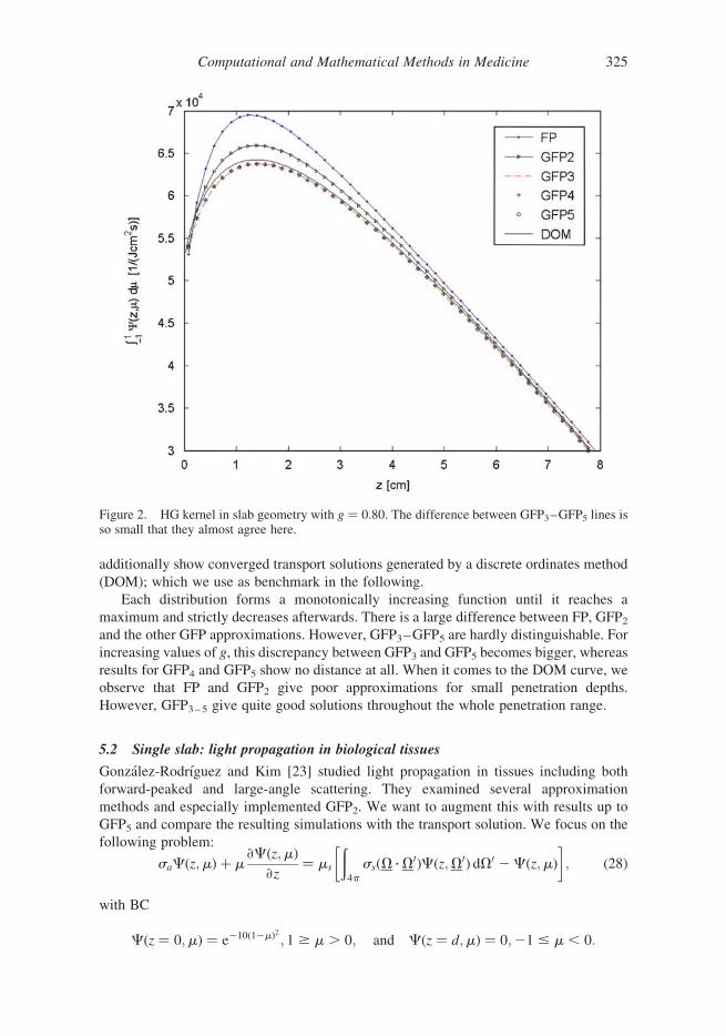
Each distribution forms a monotonically increasing function until it reaches a

maximum and strictly decreases afterwards. There is a large difference between FP, GFP2and the other GFP approximations. However, GFP3–GFP5 are hardly distinguishable. For

increasing values of g, this discrepancy between GFP3 and GFP5 becomes bigger, whereas

results for GFP4 and GFP5 show no distance at all. When it comes to the DOM curve, we

observe that FP and GFP2 give poor approximations for small penetration depths.

However, GFP3–5 give quite good solutions throughout the whole penetration range.

5.2 Single slab: light propagation in biological tissues

Gonzalez-Rodrıguez and Kim [23] studied light propagation in tissues including both

forward-peaked and large-angle scattering. They examined several approximation

methods and especially implemented GFP2. We want to augment this with results up to

GFP5 and compare the resulting simulations with the transport solution. We focus on the

following problem:

saCðz;mÞ þ m›Cðz;mÞ

›z¼ ms

ð4p

ssðV�V0ÞCðz;V0Þ dV0 2Cðz;mÞ

� �; ð28Þ

with BC

Cðz ¼ 0;mÞ ¼ e210ð12mÞ2 ; 1 $ m . 0; and Cðz ¼ d;mÞ ¼ 0;21 # m , 0:

Figure 2. HG kernel in slab geometry with g ¼ 0.80. The difference between GFP3–GFP5 lines isso small that they almost agree here.


It is a slab geometry with a thickness of d ¼ 2mm disregarding any time dependence. Its

solution enables to compute reflectance R(m) and transmittance T(m) defined by

RðmÞ :¼ Cðm; 0Þ 2 1 # m , 0 TðmÞ :¼ Cðm; dÞ 1 $ m . 0:

5.2.1 Single Henyey–Greenstein kernel

In the first run, Equation (28) was solved with discretizations of 64 points in angle and 80

points in space using GFP approximations with the HG DSCS ss ¼ sHGs . Further constants

were set to

g ¼ 0:98; sa ¼ 0:01mm21; ms ¼ 50mm21:

Reflectance. Starting at Rð21Þ < 0:23, the reflectance slightly increases and attains its

maximum at m < 20:5 (Figure 4). Although in this interval GFP data show discrepancies

among each other, their results are accurate and GFP3 gives the best approximation. For

m . 20:5, the transport solution DOM hunches down more than GFP functions and

hence, the error increases rapidly. Surprisingly, for m * 20:25, GFP3-reflectance values

are closer to DOM than those of GFP5. Throughout the whole interval, FP values give a

very poor approximation.

Transmittance. It is almost a straight line, only bending for small m. In contrast to the

reflectance, a more or less constant distance to the transport solution is always sustained.

To the eye, there are no differences between all GFP simulations in a wide range. Only for

Figure 3. HG kernel in slab geometry with g ¼ 0.95. Solutions for GFP3–GFP5 already overlap.


Figure 4. Single HG with g ¼ 0.98: reflectance and transmittance of liver tissue arising from a slabgeometry with thickness d ¼ 2mm and conditions as in Equation (28). Transmittance is plotted in asemi-logarithmic scale.


small m, the functions start to deviate and GFP3 data give best results, whereas FP is

inaccurate again.

5.2.2 Double Henyey–Greenstein kernel

Taking the amount of large-angle scattering in biological tissues into account, Gonzalez-

Rodrıguez and Kim applied the double HG DSCS to simulate transmittance and

reflectance in liver tissue. The following fit parameters were used:

g1 ¼ 0:85; g2 ¼ 20:34; b ¼ 0:86;

where g1 ¼ 0:85 provides a forward peak which is not very sharp. In addition, the

combination of g2 ¼ 20:34 and b ¼ 0:86 contains a significant amount of large-angle

scattering which leads to increasing STCs:

j1 ¼ 0:3166; j2 ¼ 0:3916; j3 ¼ 0:6058; j4 ¼ 1:0075; j5 ¼ 1:7388:

In this case, our fundamental assumption is not valid which could negatively affect our

approximations. Moreover, it is important to emphasize that simulations for GFP3–GFP5ran with some negative coefficients ai, bi. Nevertheless, our code gave reasonable results

plotted in Figure 5 for discretization parameters of 64 points in m and 70 points in

z-direction.

Reflectance. Figure 5 shows ‘bump head’ functions similarly shaped to those of the

single HG kernel. The x-coordinates of their maxima are, however, shifted to the right.

Moreover, for large m, different GFP approximations do not match as well as they do in

Figure 4. In contrast to the single HG kernel, GFP3 data give a poor approximation,

whereas GFP5 is the best one among all shown here. Only for m < 0, GFP2 is not able to

match GFP5. As expected, FP gives even worse results than for the single HG kernel.

Transmittance. This time our transport solution DOM is more peaked at m < 1.

Nevertheless, GFP gives more accurate results than in Figure 4. A comparison between the

two best approximations GFP3 and GFP5 yields small differences which enlarge near

m < 0. However, the classical FP deviates from our benchmark to a big extent.

Owing to the contribution of large-angle scattering, numerical computations with the

double HG kernel are more challenging and, in fact, give GFP coefficients which

contradict our assumptions. Nevertheless, the GFP results plotted above approximate the

transport solution very well and are much more precise than those of the FP calculations.

5.3 Slab geometry: electron propagation in biological tissues

For dose calculations, the following GFP equation is to be solved (examplarily stated for

GFP2):

saCð0Þðz;E;mÞ þ

›Cð0Þðz;E;mÞ

›z�m ¼ aLmC

ð1Þðz;E;mÞ þ›ðSðz;EÞCð0Þðz;E;mÞÞ

›E

ðI 2 bLmÞCð1Þðz;m; sÞ ¼ Cð0Þðz;E;mÞ

ð29Þ

BC : Cð0Þð0;E;mÞ ¼ 105�e2200ð12mÞ2 e250ðE02EÞ2 1 $ m . 0;E [ I

Cð0Þðd;E;mÞ ¼ 0 21 # m , 0;E [ I:


Figure 5. Double HG with g1 ¼ 0:85, g2 ¼ 20:34: GFP approximations for reflectance andtransmittance of liver tissue. Transmittance is plotted in a semi-logarithmic scale.


The initial boundary value problem in Equation (29) describes the propagation of

electrons through matter with a monoenergetic pencil beam of energy E0 irradiated

orthogonally to the boundary surface of the material. This is modelled by a product of two

narrow Gaussian functions around m ¼ 1 and E ¼ E0. After computing the solution, one

can calculate the absorbed dose via

DðrÞ ¼2pT

rðrÞ

ð10

ð121

Sðr;E0ÞCð0Þðr;m;E0Þ dm dE0;

where T is the duration of the irradiation of the patient and r the mass density of the

irradiated tissue, so that DðrÞ leads to SI unit J/kg or Gy.

Several test cases were implemented for 5 and 10-MeV beams. As benchmark we used

solutions of the MC code systems GEANT4 (standard physics package) [1,3] and

PENELOPE [46]. However, it should be stressed that all physical models were obtained

independently. The following criteria are generally employed to quantify the accuracy of a

dose curve [53]: 2%/2mm (pointwise difference within 2% or 2mm horizontal distance-

to-agreement) in homogeneous and 3%/3mm in inhomogeneous geometries.

5.3.1 Homogeneous geometry

Characteristic electron dose profiles in a semi-infinite water phantom are shown in

Figures 6 and 7. First they provide a high surface dose, increase to a maximum at a certain

depth and drop off with a steep slope afterwards. Solutions for GFP4 and GFP5 are omitted

because they overlap with GFP3 in our plot. Except for GFP2, computations were

performed according to Equation (25) (32 points in m, 350 points in z). Owing to better

results, we applied upwind finite difference discretizations for GFP2, equidistant in z (400

points) and m (200 points). All approximations are close to each other because GFP

transport coefficients jnðEÞ for water do not fall off highly enough within our energy

interval. All in all, the calculated results agree well with PENELOPE and GEANT4. All

dose profiles for a 5-MeV beam satisfy the 2%/2mm criterion. As we neglect

bremsstrahlung, the difference to MC computations becomes bigger for 10MeV. In fact,

the largest FP and GFP2 distance to PENELOPE and GEANT4 becomes 3mm at z < 5 cm

and hence, they do not meet the criterion.

5.3.2 Inhomogeneous geometries

Dose calculation is more challenging in parts of the body where materials of strongly

varying densities meet. Here, large dosimetric differences between experiments and

predictions exist [40]. As deviations of already 5% in the deposited dose may result in a

20–30% impact on complication rates [44], it is of big importance to compute the dose

accurately in such transition regions.

Possible clinical applications for electron beams are, for example, irradiation of the

chest wall or the vertebral column. To simulate dose curves on the central beam, we

assume that 10-MeV electrons pass three different materials: muscle (0–1.5 cm), bone

(1.5–3 cm) and lung (3–9 cm). For all results, parameters for Morel’s discretization [42]

were set to 32 points in m and 400 points in z. Figure 8 illustrates approximations up to

order three because higher-order results overlap with the latter on that scale. The

agreement with the MC dose profile is very satisfactory although bigger differences occur


Figure 7. 10-MeV electron beam: normalized dose in liquid water.

Figure 6. Normalized dose in liquid water for a 5-MeV electron beam.


for small penetration depths. The dose differences between PENELOPE and FP exceed the

3%/3mm limit only at the boundary z ¼ 0.

Radiotherapy gains in importance not least because surgical interventions can be

avoided. Especially sensitive body areas such as the brain, coated by cerebral membranes,

are of big interest. There are many voids between those membranes, which means that

scattering and absorption properties change abruptly. Therefore, we consider an air cavity

irradiated by a 10-MeV electron beam first penetrating water (0–4 cm), then air (4–6 cm)

and later water (6–9 cm) again. Similar to pure water, GFP2 calculations yield better

solutions for equidistant upwind discretizations (200 points in m and 300 points in z).

Remaining curves were obtained by Morel’s scheme (m-direction: 32 points, z-direction:

350 points). Except for small penetration depths, all deterministic solutions are very close

to each other and demonstrate good agreement with PENELOPE (Figure 9). Again FP and

GFP2 results show the best approximations. Larger, but still comparably small, differences

between them occur in the air region. Except for the boundary value (z ¼ 0), the FP and

GFP2 curves fulfill the 3%/3mm criterion.

6. Conclusions

Practical applications of GFP approximations have been at the centre of interest in this

paper. Hereby, numerical examples of GFP solutions for the HG kernel in slab geometry

showed more accurate approximations than FP calculations. Further test cases for

reflectance and transmittance in liver tissue by means of single and double HG kernels also

revealed GFP3- and GFP5-results closest to the transport solution.

We derived an ab initio model from the ICRU database for electron transport. This

model was compared to publicly available MC codes (PENELOPE and GEANT4) which

in turn has been benchmarked against experiments. We extracted the stopping power,

elastic and inelastic cross sections from the ICRU database and transformed them into

Figure 8. Normalized dose curves of 10-MeV electrons irradiated on the back of the body.


transport coefficients needed for GFP computations. Dose distributions for electron beams

were performed without additional coupling to photons and positrons. We are aware that

our physical model neglects important interactions such as energy straggling and hard

radiative events with emission of photons. They are inevitable for accurate dose

calculations with high-energy electrons. However, in our energy range, they are less

frequent and regarded as extensions for improved models in future. And in fact,

comparisons of GFP approximations with MC calculations reveal dose profiles, which are

close to each other in both homogeneous and inhomogeneous geometries.

Several tasks for further examination remain:

(i) The first step towards real dose calculations from CT data is an extension to two

space dimensions. As the GFP theory was derived for angular fluxes in 3D space, this

should only be a challenge to the numerical and programming approach.

(ii) Owing to a rising demand for proton therapy facilities, the adaption of the GFP

theory to protons is certainly an interesting subject of further study.

(iii) To improve computational results, it is necessary to include more physical

phenomena. Especially for high-energy electron beams, it is inevitable to simulate

the transport of bremsstrahlung quanta.

Acknowledgements

The authors would like to thank Bruno Dubroca from Universite Bordeaux not only for providing hiscode for the DOM but also for his support and advice. We also acknowledge support from theGerman Research Foundation DFG under grant KL 1105/14/2 and the German Academic ExchangeService DAAD Program D/07/07534.

Figure 9. 10-MeV electron beam: normalized dose in liquid water with air cavity.


References

[1] S. Agostinelli, J. Allison, K. Amako, J. Apostolakis, et al., Geant4-a simulation toolkit, Nucl.Instrum. Methods B 506 (2003), pp. 250–303.

[2] A. Ahnesjo, M. Saxner, and A. Trepp, A pencil beam model for photon dose calculation, Med.Phys. 19 (1992), pp. 263–273.

[3] J. Allison, et al., Geant4 developments and applications, IEEE Trans. Nucl. Sci. 53 (2006),pp. 270–278.

[4] P. Andreo, Monte Carlo techniques in medical radiation physics, Phys. Med. Biol. 36 (1991),pp. 861–920.

[5] D. Balsara, Fast and accurate discrete ordinates methods for multidimensional radiativetransfer. Part I, basic methods, J. Quant. Spectrosc. Radiat. Transfer 69 (2001), pp. 671–707.

[6] E. Boman, J. Tervo, and M. Vauhkonen,Modelling the transport of ionizing radiation using thefinite element method, Phys. Med. Biol. 50 (2005), pp. 265–280.

[7] C. Borgers, Complexity of Monte Carlo and deterministic dose calculation methods, Phys.Med. Biol. 43 (1998), pp. 517–528.

[8] T.A. Brunner, Forms of application radiation transport. Sandia Report, sand2002-1778,Sandia National Laboratories, Albuquerque, 2002.

[9] W. Cheong, S.A. Prahl, and A.J. Welch, A review of the optical properties of biological tissues,IEEE J. Quant. Electron. 26 (1990), pp. 2166–2185.

[10] G.G.M. Coppa and P. Ravetto, Quasi-singular angular finite element methods in neutrontransport problems, Trans. Theory Stat. Phys. 24 (1995), pp. 155–172.

[11] J. Cygler, et al., Clinical use of a commercial Monte Carlo treatment planning system forelectron beams, Phys. Med. Biol. 50 (2005), pp. 1029–1034.

[12] R.P. Datta, et al., Computational model for coupled electron–photon transport in twodimensions, Phys. Rev. E 53 (1996), pp. 6514–6522.

[13] R. Duclous, et al., Reduced multi-scale kinetic model for the relativistic electron transport insolid targets: Effects related to secondary electrons, Laser Particle Beams 28(1) (2010),pp. 165–177.

[14] P. Edstrom, A fast and stable solution method for the radiative transfer problem, SIAMRev. 47(2005), pp. 447–468.

[15] L. Eyges, Multiple scattering with energy loss, Phys. Rev. 74 (1948), pp. 1534–1535.[16] E. Fermi, The ionization loss of energy in gases and in condensed materials, Phys. Rev. 57

(1940), pp. 485–493.[17] M. Frank, H. Hensel, and A. Klar, A fast and accurate moment method for the Fokker–Planck

equation and applications to electron radiotherapy, SIAM J. Appl. Math. 67 (2007),pp. 582–603.

[18] M. Frank, M. Herty, and A.N. Sandjo, Optimal treatment planning governed by kineticequations, to appear in Math. Mod. Meth. Appl. Sci. Available at http://www.worldscinet.com/m3as/00/forthcoming.shtml (preprint 2009).

[19] M. Frank, M. Herty, and M. Schafer, Optimal treatment planning in radiotherapy based onBoltzmann transport calculations, Math. Mod. Meth. Appl. Sci. 18 (2008), pp. 573–592.

[20] J.C. Garth, Electron/photon transport – a key technology to radiation physics? A review,Trans. Amer. Nucl. Soc. 90 (2004), pp. 289–291.

[21] J.C. Garth, Electron/photon transport and its applications, The Monte Carlo Method:Versatility Unbounded in a Dynamic Computing World, Chattanooga, Tennessee, 17–21April, 2005.

[22] K.A. Gifford, et al., Comparison of a finite-element multigroup discrete-ordinates code withMonte Carlo for radiotherapy calculations, Phys. Med. Biol. 51 (2006), pp. 2253–2265.

[23] P. Gonzalez-Rodrıguez and A.D. Kim, Light propagation in tissues with forward-peaked andlarge-angle scattering, Appl. Opt. 47 (2008), pp. 2599–2609.

[24] H. Hensel, R. Iza-Teran, and N. Siedow, Deterministic model for dose calculation in photonradiotherapy, Phys. Med. Biol. 51 (2006), pp. 675–693.

[25] L.G. Henyey and J.L. Greenstein, Diffuse radiation in the galaxy, Astrophys. J. 93 (1941),pp. 70–83.

[26] K.R. Hogstrom, M.D. Mills, and P.R. Almond, Electron beam dose calculations, Phys. Med.Biol. 26 (1981), pp. 445–459.

[27] H. Huizenga and P. Storchi, Numerical calculation of energy deposition by broad high-energyelectron beams, Phys. Med. Biol. 34 (1989), pp. 1371–1396.


[28] M.J. Berger, A. Jablonski, I.K. Bronic, C.J. Powell, F. Salvat, and L. Sanche, Elastic scatteringof electrons and positrons, report 77, J. ICRU 7 (2007).

[29] Y. Itikawa and N. Mason, Cross sections for electron collisions with water molecules, J. Phys.Chem. Ref. Data 34(1) (2005), pp. 1–22.

[30] J. Janssen, et al., Numerical calculation of energy deposition by high-energy electron beams:III. Three-dimensional heterogeneous media, Phys. Med. Biol. 39 (1994), pp. 1351–1366.

[31] J. Janssen, et al., Numerical calculation of energy deposition by high-energy electron beams:III-B. Improvements to the 6D phase space evolution model, Phys. Med. Biol. 42 (1997),pp. 1441–1449.

[32] D. Jette, Electron dose calculation using multiple-scattering theory. A. Gaussian multiple-scattering theory, Med. Phys. 15 (1988), pp. 123–137.

[33] D. Jette and A. Bielajew, Electron dose calculation using multiple-scattering theory: Second-order multiple-scattering theory, Med. Phys. 16 (1989), pp. 698–711.

[34] E. Korevaar, et al., Accuracy of the phase space evolution dose calculation model for clinical25MeV electron beams, Phys. Med. Biol. 45 (2000), pp. 2931–2945.

[35] H. Krieger, Grundlagen der Strahlungsphysik und des Strahlenschutzes, 2nd ed., TeubnerVerlag, Wiesbaden, 2007.

[36] E. Larsen, et al., Electron dose calculations using the method of moments, Med. Phys. 24(1997), pp. 111–125.

[37] J.A. LaVerne and S.M. Pimblott, Effect of elastic collisions on energy deposition by electronsin water, J. Phys. Chem. A 101 (1997), pp. 4504–4510.

[38] C.L. Leakeas and E.W. Larsen, Generalized Fokker–Planck approximations of particletransport with highly forward-peaked scattering, Nucl. Sci. Eng. 137 (2001), pp. 236–250.

[39] H.W. Lewis, Multiple scattering in an infinite medium, Phys. Rev. 78 (1950), pp. 526–529.[40] C. Martens, et al., Underdosage of the upper-airway mucosa for small fields as used in

intensity-modulated radiation therapy: A comparison between radiochromic film measure-ments, Monte Carlo simulations, and collapsed cone convolution calculations, Med. Phys. 29(2002), pp. 1528–1535.

[41] M. Morawska-Kaczynska and H. Huizenga, Numerical calculation of energy deposition bybroad high-energy electron beams: II. Multi-layered geometry, Phys. Med. Biol. 37 (1992),pp. 2103–2116.

[42] J.E. Morel, An improved Fokker–Planck angular differencing scheme, Nucl. Sci. Eng. 89(1985), pp. 131–136.

[43] N. Papanikolau, et al., Tissue inhomogeneity corrections for megavoltage photon beams,Medical Physics Publishing, Madison, AAPM Report No. 85 (2004).

[44] G.C. Pomraning, The Fokker–Planck operator as an asymptotic limit, Math. Models MethodsAppl. Sci. 2(1) (1992), pp. 21–36.

[45] B. Rossi and K. Greisen, Cosmic-ray theory, Rev. Med. Phys. 13 (1941), pp. 240–309.[46] F. Salvat, J.M. Fernandez-Varea, and J. Sempau, PENELOPE-2008: A Code System for Monte

Carlo Simulation of Electron and Photon Transport, OECD, 2009.[47] H. Schwoerer, et al., Laser-plasma acceleration of quasi-monoenergetic protons from

microstructured targets, Nature 439 (2006), pp. 445–448.[48] A.S. Shiu and K.R. Hogstrom, Pencil-beam redefinition algorithm for electron dose

distributions, Med. Phys. 18 (1991), pp. 7–18.[49] C. Siantar, et al., Description and dosimetric verification of the peregrine Monte Carlo dose

calculation system for photon beams incident on a water phantom, Med. Phys. 28 (2001),pp. 1322–1337.

[50] E. Spezi and G. Lewis, An overview of Monte Carlo treatment planning for radiotherapy,Radiat. Prot. Dos. 131 (2008), pp. 123–129.

[51] J. Tervo, et al., A finite-element model of electron transport in radiation therapy and a relatedinverse problem, Inverse Probl. 15 (1999), pp. 1345–1361.

[52] O.N. Vassiliev, et al., Feasibility of a multigroup deterministic solution method for 3Dradiotherapy dose calculations, Int. J. Radiat. Oncol. Biol. Phys. 72 (2008), pp. 220–227.

[53] J. Venselaar, H. Welleweerd, and B. Mijnheer, Tolerances for the accuracy of photon beamdose calculations of treatment planning systems, Radiother. Oncol. 60 (2001), pp. 191–201.


Appendix A. Polynomial operators

LP2 ¼j1

2þ

j2

8

� �Lþ

j2

16

� �L 2 ðA1Þ

LP3 ¼j1

2þ

j2

8þ

j3

24

� �Lþ

j2

16þ

j3

36

� �L 2 þ

j3

288

� �L 3 ðA2Þ

LP4 ¼j1

2þj2

8þ

j3

24þ

j4

64

� �Lþ

j2

16þ

j3

36þ

3j4

256

� �L 2 þ

j3

288þ

5j4

2304

� �L 3 þ

j4

9216

� �L 4 ðA3Þ

LP5 ¼j1

2þj2

8þ

j3

24þ

j4

64þ

j5

160

� �Lþ

j2

16þ

j3

36þ

3j4

256þ

j5

200

� �L 2

þj3

288þ

5j4

2304þ

127j5

115200

� �L 3 þ

j4

9216þ

j5

11520

� �L 4 þ

j5

460800L 5 ðA4Þ

Appendix B. Derivation of GFP operators

GFP2

If lBn denotes one eigenvalue of LB for n $ 0 and a, b are two positive constants, the GFP operatordefined by

LP2 þOð1 2Þ ¼ LGFP2 :¼ aLðI 2 bLÞ21;¼ aLþ abL 2 þOðab 2Þ; ðB1Þ

will have to satisfy three properties to substitute LP2 in the favoured way:

(1) Eigenvalue preservation:

2anðnþ 1Þ

1þ bnðnþ 1Þ¼ lGFP2n ¼

!lBn ¼ 2san for n ¼ 1; 2:

Multiplying the above equation by ð1þ bnðnþ 1ÞÞ – 0 and dividing by nðnþ 1Þ; weconclude

ða2 bsanÞ ¼san

nðnþ 1Þn ¼ 1; 2 ,

1 2sa1

1 2sa2

" #�

a

b

" #¼

sa1=2

sa2=6

" #

(2) Order: Oðab 2Þ¼! Oð1 2Þ

(3) Equivalence:

aLþ abL 2 ¼!LP2 þOð1 2Þ ¼

j1

2þ

j2

8

� �Lþ

j2

16L 2 þOð1 2Þ;


where san is a quantity which can be expressed in terms of jn:

sa0 ¼ 0; ðB2Þ

sa1 ¼ j1; ðB3Þ

sa2 ¼ 3j1 23

2j2; ðB4Þ

sa3 ¼ 6j1 215

2j2 þ

5

2j3; ðB5Þ

sa4 ¼ 10j1 245

2j2 þ

35

2j3 2

35

8j4; ðB6Þ

sa5 ¼ 15j1 2105

2j2 þ 70j3 2

315

8j4 þ

63

8j5: ðB7Þ

In the following, item (1) is first transformed to a system of linear equations and thereafter solvedfor the desired GFP coefficients (here a and b). However, the final equations to be solved arenon-linear for GFP operators of order n $ 3. In this case of order n ¼ 2, Equations (B3) and (B4)yield

a ¼j1

2þj2

8and b ¼

j2

8j1:

Going on with item (2), it is to be checked

ab 2 ¼j1

2þj2

8

� �j2

8j1

� �2

¼j1

2þ

j2

8

� �|fflfflfflfflfflfflffl{zfflfflfflfflfflfflffl}

[Oð1Þ

j22

64j21

!|fflfflfflffl{zfflfflfflffl}[Oð1 2Þ

[ Oð1 2Þ:

As equivalence condition follows straight forward, it has been shown that the operator LGFP2 isan Oð1 2Þ approximation to LB whose first three eigenvalues agree. Now it is quite intuitive toapply a similar procedure to higher-order operators. We determined explicit solutions for GFP2–GFP5 coefficients and performed verifications for items (1)–(3). According to GFP3 all itemswere checked without computer support. The asymptotic behaviour of GFP operators of orderfour and five was, however, checked by means of a symbolic toolbox. To keep our followingdescription short, we confine ourselves to final results.

GFP3

LP3 þOð1 3Þ ¼ LGFP3 :¼ a1LðI 2 b1LÞ21 þ a2L

¼ ða1 þ a2ÞLþ a1b1L2 þ a1b

21L

3 þOða1b31Þ ðB8Þ



ða1 þ a2Þ2 sanb1 þ nðnþ 1Þb1a2 ¼san

nðnþ 1Þn ¼ 1; 2; 3 ðB9Þ

) a1 ¼j2ð27j

22 þ 5j23 2 24j2j3Þ

8j3ð3j2 2 2j3ÞðB10Þ

b1 ¼j3

6ð3j2 2 2j3ÞðB11Þ

a2 ¼j1

22

9j228j3

þ3j2

8: ðB12Þ

(2) Equivalence: To guarantee that LGFP3 ¼ LP3 þOð1 3Þ, all coefficients of L i in Equations

(B8) and (A2) must coincide. Let a1,b1,a2 be the defining positive coefficients of LGFP3 as

stated in Equations (B10)–(B12), then one can show that they satisfy

I: a1 þ a2 ¼j1

2þ

j2

8þ

j3

24þOð1 3Þ

II: a1b1 ¼j2

16þ

j3

36þOð1 3Þ

III: a1b21 ¼

j3

288þOð1 3Þ:

GFP4

LP4 þOð1 4Þ ¼ LGFP4 :¼ a1LðI 2 b1LÞ21 þ a2LðI 2 b2LÞ

21

¼ ða1 þ a2ÞLþ ða1b1 þ a2b2ÞL2 þ ða1b

21 þ a2b

22ÞL

3 þ ða1b31 þ a2b

32ÞL

4

þOða1b41Þ þOða2b

42Þ ðB13Þ


ða1 þ a2Þ2 sanðb1 þ b2Þ2 sannðnþ 1Þb1b2 þ nðnþ 1Þða1b2 þ a2b1Þ

¼san

nðnþ 1Þn ¼ 1; 2; 3; 4

ðB14Þ

(2) Equivalence:

I: a1 þ a2 ¼j1

2þ

j2

8þ

j3

24þ

j4

64þOð1 4Þ

II: a1b1 þ a2b2 ¼j2

16þ

j3

36þ

3j4

256þOð1 4Þ

III: a1b21 þ a2b

22 ¼

j3

288þ

5j4

2304þOð1 4Þ

IV: a1b31 þ a2b

32 ¼

j4

9216þOð1 4Þ


GFP5

LP5 þOð1 5Þ ¼ LGFP5 :¼ a1LðI 2 b1LÞ21 þ a2LðI 2 b2LÞ

21 þ a3L

¼ ða1 þ a2 þ a3ÞLþ ða1b1 þ a2b2ÞL2 þ ða1b

21 þ a2b

22ÞL

3 þ ða1b31 þ a2b

32ÞL

4

þ ða1b41 þ a2b

42ÞL

5 þOða1b51Þ þOða2b

52Þ

ðB15Þ


ða1 þ a2 þ a3Þ2 sanðb1 þ b2Þ2 sannðnþ 1Þb1b2

þ nðnþ 1Þ½b2ða1 þ a3Þ þ b1ða2 þ a3Þ� þ a3b1b2½nðnþ 1Þ�2 ¼san

nðnþ 1Þ

n ¼ 1; 2; 3; 4; 5

ðB16Þ

(2) Equivalence:

I: a1 þ a2 þ a3 ¼j1

2þ

j2

8þ

j3

24þ

j4

64þ

j5

160þOð1 5Þ

II: a1b1 þ a2b2 ¼j2

16þ

j3

36þ

3j4

256þ

j5

200þOð1 5Þ

III: a1b21 þ a2b

22 ¼

j3

288þ

5j4

2304þ

127j5

115200þOð1 5Þ

IV: a1b31 þ a2b

32 ¼

j4

9216þ

j5

11520þOð1 5Þ

V: a1b41 þ a2b

42 ¼

j5

460800þOð1 5Þ

All linear and nonlinear equations stated above lead to explicit solutions for ai and bi. Equationsposed for GFP2 and GFP3 actually deliver uniquely determined constants, whereas for higher GFPoperators there is no guarantee for unique or even real-valued ai and bi. Nevertheless, it is importantto emphasize that the resulting values of ai and bi must be positive. Otherwise, eigenvalues lGFPkn ofa GFPk operator could become negative.


generalized fokker–planck theory for electron and photon transport

Documents